Mining Frequent Itemsets in a Stream

Toon CaldersEindhoven University of Technology

Nele DextersUniversity of Antwerp

Bart GoethalsUniversity of Antwerp

Abstract

We study the problem of finding frequent itemsets in acontinuous stream of transactions. The current frequency ofan itemset in a stream is defined as its maximal frequencyover all possible windows in the stream from any point inthe past until the current state that satisfy a minimal lengthconstraint. Properties of this new measure are studied andan incremental algorithm that allows, at any time, to im-mediately produce the current frequencies of all frequentitemsets is proposed. Experimental and theoretical analy-sis show that the space requirements for the algorithm areextremely small for many realistic data distributions.

1. Introduction

Mining frequent sets over streams of itemsets presentsinteresting new challenges over traditional mining in staticdatabases. Due to the speed of new arriving data, it is as-sumed that the history of the stream can not be revisited,unless it is stored. Storing large parts of a stream, however,is impossible as the amount of data is typically huge.

Most previous work on mining frequently occurringitemsets over data streams either focusses on (1) the slidingwindow model, (2) the time-fading model, or (3) the land-mark model. Each of these models requires a fixed windowlength or decay factor, given by the user. In many applica-tions, however, choosing such parameters that are most ap-propriate for every itemset at every timepoint in an evolvingstream is almost impossible. For example, consider a largeretail chain of which sales can be considered as a stream.Then, in order to find frequent sets to do market basketanalysis, it is very difficult to choose in which period of thecollected data you are interested. For many products, theamount of them sold depends highly on the period of theyear. In summer time, e.g., sales of ice cream increase andduring the soccer world cup, sales of beer increase. Suchseasonal behavior of a specific item or combination of itemscan only be discovered when choosing the correct windowsize for that item(set). This size, however, can hide a similarbehavior of other item(set)s in another window.

Therefore, we propose to consider for each itemset thewindow in which it has the highest frequency. More specif-ically, we define the current frequency of an itemset as themaximum over all windows from the past until the currentstate that satisfy a minimal size constraint. Notice that thisis an extension of the max-frequency measure defined be-fore for items [1]. Hence, when the stream evolves, thelength of the window containing the highest frequency fora given itemset can change continuously. This new streammeasure turns out to be very suitable to early detect sud-den bursts of occurrences of itemsets, while still taking intoaccount the history of the itemset. This behavior might beparticularly useful in applications where hot topics, or pop-ular combinations of topics need to be tracked. Examplesof such applications include, e.g., identifying stocks with astrong growth or tracking popular search terms on the inter-net. In these applications it is of vital importance to identifysudden bursts quickly, while still taking into account thehistory.

Concretely, our contributions are the following. First,(1) the max-frequency measure [1] is extended to itemsetsand minimal window length, and (2) a detailed study of itsbehavior is performed, taking into account minimal win-dow length and minimal frequency thresholds, resulting inseveral important properties. (3) An efficient algorithm forcomputing the exact frequencies for all frequent itemsets atany time is proposed; this in contrast to the often only ap-proximate algorithms for other methods. Finally, (4) a the-oretical and empirical evaluation of our proposed method isgiven.

The organization of the paper is as follows. In Section 2,the new measure is defined and the central problem state-ment is formally introduced. Section 3 gives several prop-erties of the max-frequency and states the main theorem, onwhich the incremental algorithm in Section 4 is based. InSection 5, a theoretical analysis for the worst case is done.Experimental results in Section 6 show that the memory re-quirements for the algorithm are extremely small for manyreal-life data distributions. In Section 7, the relation be-tween our measure and existing related work is explored,and Section 8 concludes the paper.

2. Problem Statement

2.1. Streams and Max-Frequency

A stream 〈I1 I2 . . . In〉 is a sequence of itemsets, de-noted S, where n = |S| is the length of the stream. I1 isconsidered the first and oldest itemset in the stream, and In

the latest and most recent. We assume that the items in thestream come from a finite set of items I.

The number of sets in a stream S that con-tain itemset I is denoted count(I, S). For example,count(a, 〈ab c adf〉) = 2 and count(af, 〈ab c adf〉) =1. The frequency of I in S is defined as

freq(I, S) :=count(I, S)

|S| .

For example, freq(a, 〈ab c adf〉) = 2/3 andfreq(af, 〈ab c adf〉) = 1/3.

Let S1 be 〈I11 . . . I1

n1〉, S2 be 〈I2

1 . . . I2n2〉, . . . and

Sm be 〈Im1 . . . Im

nm〉. The concatenation of the streams

S1, . . . , Sm, denoted S1 · S2 · . . . · Sm, is

〈 I11 . . . I1

n1I21 . . . I2

n2. . . Im

1 . . . Imnm

〉 .

Let S = 〈I1 I2 . . . In〉. Then, S[s, t] denotes the sub-stream or window 〈Is Is+1 . . . It〉. The sub-stream of S

consisting of the last k items of S, denoted last(k, S), is

last(k, S) := S[|S| − k + 1, |S|] .

We are now ready to define our new frequency measure:

Definition 1 Given a minimal window size mwl , the max-frequency mfreqmwl(I, S) of itemset I in a stream S is de-fined as the maximum of the frequencies of I over all win-dows, of size at least mwl , extending from the end of thestream; that is:

mfreqmwl(I, S) := maxk=mwl,...,|S|

(freq(I, last(k, S))) .

If the length of the stream is less than mwl , the max-frequency is defined to be 0.

The longest window in which the maximum frequencyis reached is called the maximal window for I in S, andits starting point is denoted startmaxmwl(I, S). That is,startmaxmwl(I, S) is the smallest index such that

mfreqmwl(I, S) = freq(I, S[startmaxmwl(I, S), |S|]) .

mwl wil be omitted when clear from the context.

Example 1 Let mwl = 3.

mfreqmwl(a, 〈a b a a a b〉) = 3/4 .

mfreqmwl(a, 〈b c d a b c d a〉) = 2/5 .

0.1

0.15

0.2

0.25

0.3

0.35

bacbccbacbbcbcbbabcbbcbaccbbcccbbacbccbacbbcbcbbabcbbcbaccbbcccba

mwl=3mwl=5

mwl=10

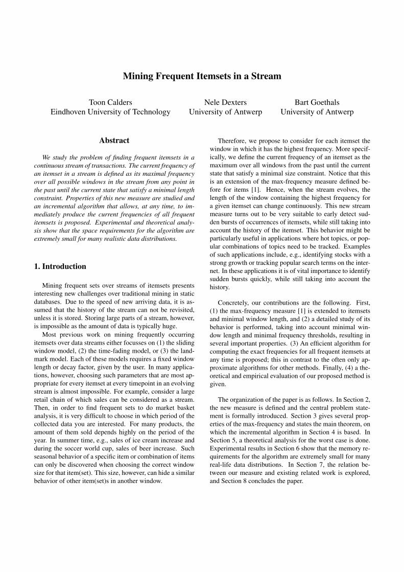
Figure 1. Max-frequency for minimal windowlengths 1, 3, and 10.

In the definition of the max-frequency, an explicit lowerbound is given on the size of the windows in which the fre-quencies are considered. This lower bound is given to re-lieve the undesirable effect of having a frequency of 100%in a window of length 1, every time the target item arrives inthe stream. The effect of the minimal window length mwlis illustrated in Figure 1. It is clear that for longer mini-mal window lengths, there are still jumps in the frequency,but they are less pronounced. Hence, setting an appropriateminimal window length effectively resolves the instabilityof the max-frequency measure.

2.2. Evolving Streams

A stream was defined as a statical object. In reality, how-ever, a stream is an evolving object that is essentially un-bounded. When processing a stream, it is to be assumedthat only a small part of it can be kept in memory.

St will denote the stream S up to timestamp t; that is, thepart of the stream that already passed at time t, St = S[1, t].For simplicity, we assume that the first itemset arrives attimestamp 1, and since then, at every timestamp a new item-set is inserted into the stream.

The main problem we study in this paper is the fol-lowing: Given a minimal frequency threshold and a min-imal window length, for an evolving stream S, main-tain a small summary of the stream in time, such that,at any timepoint t, all current frequent itemsets can beproduced instantly from this summary. More formally,we will introduce a concise summary, summary(St), andefficient procedures Update , and Get mfreq , such thatUpdate(summary(St), I) equals summary(St · 〈I〉), andGet mfreq(summary(St+1)) equals mfreqmwl(A, St+1).

Because Update has to be executed every time a newitemset arrives, it has to be extremely efficient in order to befinished before the next itemset arrives. Similarly, becausethe stream continuously grows, the summary must be inde-pendent of the number of items seen so far, or, at least grow

very slowly as the stream evolves. The method we developwill indeed meet these criteria, as the theoretical analysis inSection 5, and the experiments in Section 6 show.

For ease of presentation, we present our solution in amodular way; first we present how a summary can be main-tained that allows for one itemset A, to produce its max-frequency at any point in time, for the case no minimal win-dow length has been set. Notice that no minimal windowlength actually corresponds to having a minimal windowlength of 1. We denote the max-frequency of A in S with-out minimal window length simply as mfreq1(A, S). Then,we extend the method to work with minimal window lengthand minimal frequency, but still for only one target itemsetA. Finally, we show how to combine everything into onesolution for mining all frequent itemsets at once, withouthaving to maintain a separate summary for every itemset.

3. Properties of Max-Frequency

In this section, we show some properties of max-frequency for one itemset A without a minimal windowlength constraint. These properties will be crucial for theincremental algorithm that maintains the summary of thestream for A.

Obviously, checking all possible windows to find themaximal one is infeasible algorithmically, given the con-straints of stream problems. Fortunately, not every point inthe stream needs to be checked. The theoretical results fromthis section show exactly which points need to be inspected.These points will be called the borders in the stream. Thesummary of the stream will consist exactly of the recordingof these borders, and the corresponding frequency of thetarget itemset.

Definition 2 Timestamp q is called a border for set A in S ifthere exists a stream B such that q = startmax (A, S · B) .

Thus, a border is a point in the stream that can still becomethe starting point of the maximal window. Based on the nexttheorem, it is possible to give an exact syntactic characteri-zation of the borders.

Theorem 1 Let S be a stream of length L, and let S[q, L]be the maximal window for the itemset A. Then, for any p,r with p < q ≤ r: freq(A, S[p, q − 1]) < freq(A, S[q, r]).

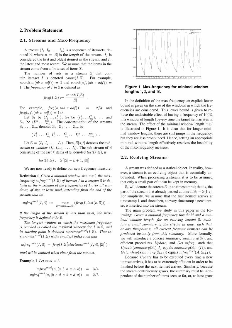
Proof 1 Let B1 denote S[p, q − 1], B2 denote S[q, r], andB3 denote S[r + 1, L]. Because B2 · B3 is the maximalwindow for A in S, it holds that the frequency of A inB2 · B3 is strictly higher than in B1 · B2 · B3 and it is atleast as high as in B3 (remember that in the case of multi-ple windows with maximal frequency the largest one is se-lected). Now, let l1 = |B1|, l2 = |B2|, and l3 = |B3|,

and let a1 = count(A, B1), a2 = count(A, B2), anda3 = count(A, B3), as depicted in:

B1︷ ︸︸ ︷a1/l1

B2︷ ︸︸ ︷a2/l2

B3︷ ︸︸ ︷a3/l3

.

Then, the conditions on the frequency translate into:

a2 + a3

l2 + l3>

a1 + a2 + a3

l1 + l2 + l3and

a2 + a3

l2 + l3≥ a3

l3.

From these conditions, it can be derived that

freq(A, B1) =a1

l1<

a2

l2= freq(A, B2) .

Corollary 1 Let S be a stream of length L, and let 1 ≤ q ≤L. Position q is a border for target itemset A in S if andonly if for all indices j, k with 1 ≤ j < q and q ≤ k ≤ L, itholds that freq(A, S[j, q − 1]) < freq(A, S[q, k]) .

Proof 2 Only if: Follows directly from Theorem 1.If: We need to show that there exists a continuation S

′ ofstream S (resulting in stream S ·S′) in which q is the startingpoint of the maximal window. We consider two cases: eitherq is the rightmost border in S, or not. If q is the rightmostborder, then q is the maximal border in S, because for anyother border p < q, freq(A, S[p, q − 1]) < freq(A, S[q, L])which implies freq(A, S[p, L]) < freq(A, S[q, L]), andhence the Corollary holds.

In the other case, we will show that it is always possibleto continue S in such a way that the rightmost border disap-pears, while all other borders remain and no new bordersare introduced. By consecutively applying this procedure,any border will eventually become the rightmost border atone point, and hence become the starting point of the maxi-mal window.

Let q < q′ be the two largest borders in S. Since, becauseof the only-if part of this theorem,

freq(A, S[q, q′ − 1]) ≤ freq(A, S[q′, L])

=count(A, S[q′, L])

L − q′ + 1,

we can always find positive integers x ≤ y such that:

freq(A, S[q, q′ − 1]) =count(A, S[q′, L]) + x

L − q′ + 1 + y.

Then, the following continuation of S has exactly the sameborders as S, except from q′, which is no longer a border:

S · 〈x×︷ ︸︸ ︷

A A · · · A

y−x×︷ ︸︸ ︷∅ ∅ · · · ∅〉 .

4/9 4/10 2/3 1/2〈 a a a b b b a b b

∖a b a b a b a b b b b a a b

∖a b b a 〉

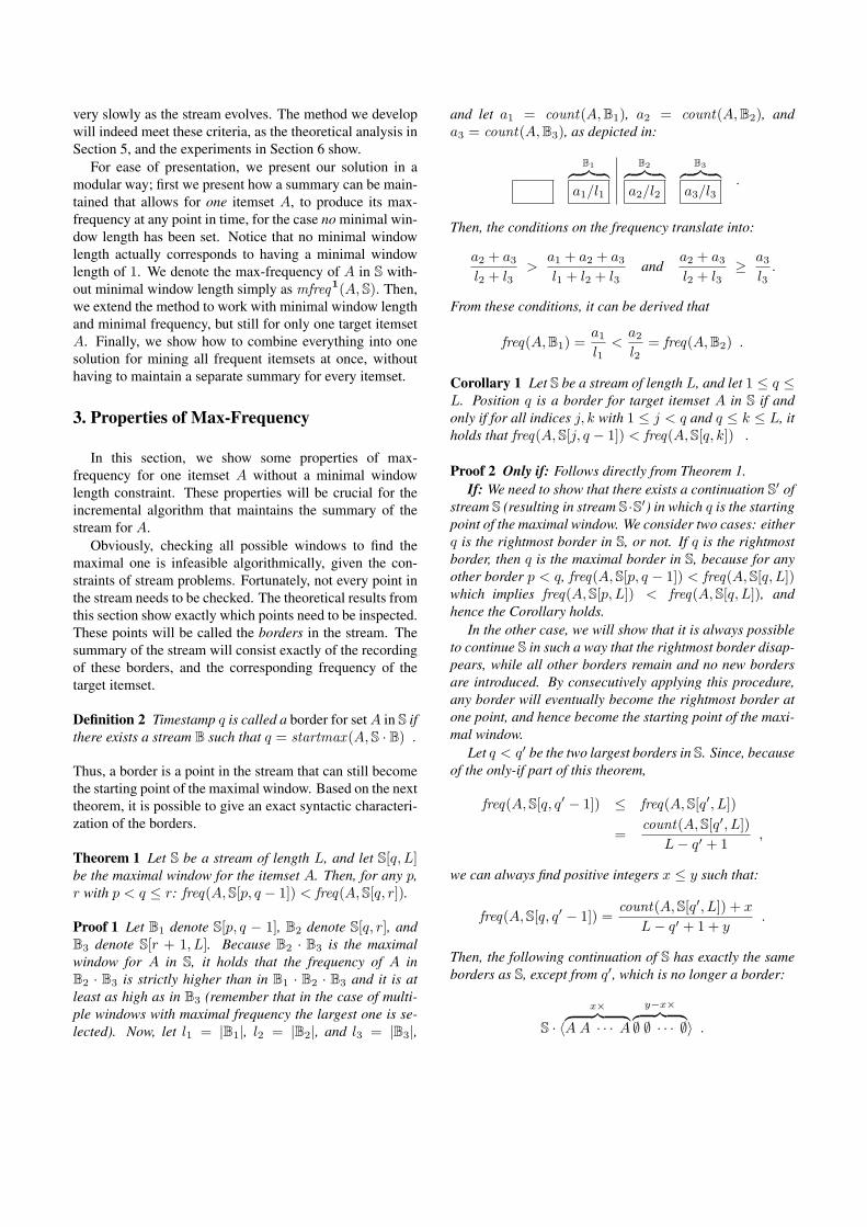
Figure 2. Example of dropping borders.

Example 2 Assume we have the stream S27, given in Fig-ure 2 and we focus on target {a}. In this stream, two posi-tions have been marked with a backslash. Both these pointsdo not meet the criteria to be a border given in Corollary 1.Indeed, for both positions, a block before and after it is in-dicated such that the frequency in the before-block is higherthan in the after-block. The only positions that do meet therequirement are indicated by vertical bars.

4. Algorithm

Based on the results of Section 3, we present an incre-mental algorithm to efficiently maintain the summary forone itemset A allowing us to produce the current max-frequency (without minimal window length constraint) ofan itemset instantly at any time.

4.1. The Summary

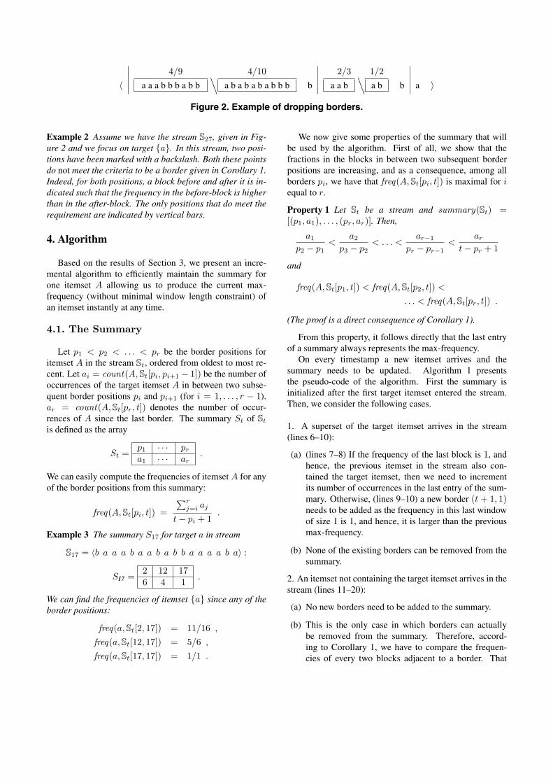
Let p1 < p2 < . . . < pr be the border positions foritemset A in the stream St, ordered from oldest to most re-cent. Let ai = count(A, St[pi, pi+1 − 1]) be the number ofoccurrences of the target itemset A in between two subse-quent border positions pi and pi+1 (for i = 1, . . . , r − 1).ar = count(A, St[pr, t]) denotes the number of occur-rences of A since the last border. The summary St of St

is defined as the array

St =p1 · · · pr

a1 · · · ar.

We can easily compute the frequencies of itemset A for anyof the border positions from this summary:

freq(A, St[pi, t]) =

∑rj=i aj

t − pi + 1.

Example 3 The summary S17 for target a in stream

S17 = 〈b a a a b a a b a b b a a a a b a〉 :

S17 =2 12 176 4 1

.

We can find the frequencies of itemset {a} since any of theborder positions:

freq(a, St[2, 17]) = 11/16 ,

freq(a, St[12, 17]) = 5/6 ,

freq(a, St[17, 17]) = 1/1 .

We now give some properties of the summary that willbe used by the algorithm. First of all, we show that thefractions in the blocks in between two subsequent borderpositions are increasing, and as a consequence, among allborders pi, we have that freq(A, St[pi, t]) is maximal for iequal to r.

Property 1 Let St be a stream and summary(St) =[(p1, a1), . . . , (pr, ar)]. Then,

a1

p2 − p1<

a2

p3 − p2< . . . <

ar−1

pr − pr−1<

ar

t − pr + 1

and

freq(A, St[p1, t]) < freq(A, St[p2, t]) <

. . . < freq(A, St[pr, t]) .

(The proof is a direct consequence of Corollary 1).

From this property, it follows directly that the last entryof a summary always represents the max-frequency.

On every timestamp a new itemset arrives and thesummary needs to be updated. Algorithm 1 presentsthe pseudo-code of the algorithm. First the summary isinitialized after the first target itemset entered the stream.Then, we consider the following cases.

1. A superset of the target itemset arrives in the stream(lines 6–10):

(a) (lines 7–8) If the frequency of the last block is 1, andhence, the previous itemset in the stream also con-tained the target itemset, then we need to incrementits number of occurrences in the last entry of the sum-mary. Otherwise, (lines 9–10) a new border (t + 1, 1)needs to be added as the frequency in this last windowof size 1 is 1, and hence, it is larger than the previousmax-frequency.

(b) None of the existing borders can be removed from thesummary.

2. An itemset not containing the target itemset arrives in thestream (lines 11–20):

(a) No new borders need to be added to the summary.

(b) This is the only case in which borders can actuallybe removed from the summary. Therefore, accord-ing to Corollary 1, we have to compare the frequen-cies of every two blocks adjacent to a border. That

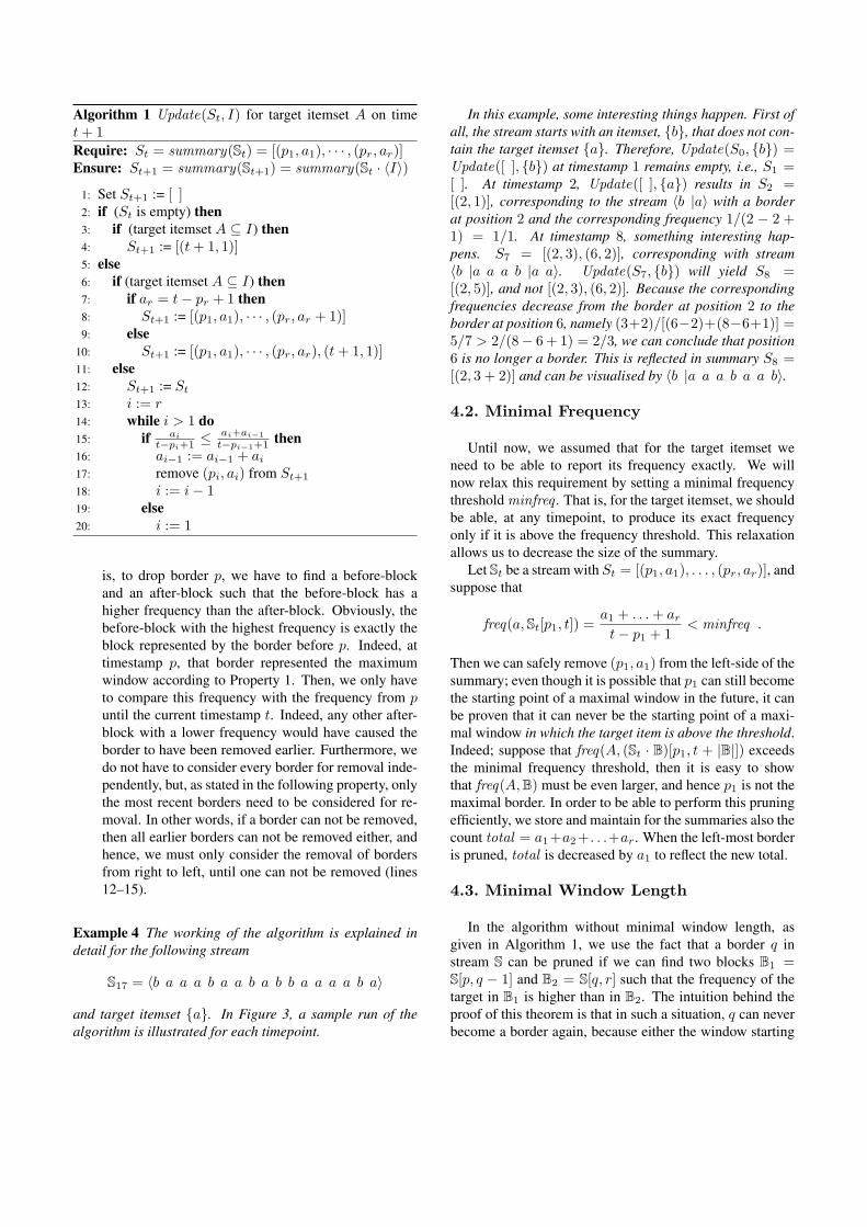
Algorithm 1 Update(St, I) for target itemset A on timet + 1Require: St = summary(St) = [(p1, a1), · · · , (pr, ar)]Ensure: St+1 = summary(St+1) = summary(St · 〈I〉)

1: Set St+1 := [ ]2: if (St is empty) then3: if (target itemset A ⊆ I) then4: St+1 := [(t + 1, 1)]5: else6: if (target itemset A ⊆ I) then7: if ar = t − pr + 1 then8: St+1 := [(p1, a1), · · · , (pr, ar + 1)]9: else

10: St+1 := [(p1, a1), · · · , (pr, ar), (t + 1, 1)]11: else12: St+1 := St

13: i := r14: while i > 1 do15: if ai

t−pi+1 ≤ ai+ai−1t−pi−1+1 then

16: ai−1 := ai−1 + ai

17: remove (pi, ai) from St+1

18: i := i − 119: else20: i := 1

is, to drop border p, we have to find a before-blockand an after-block such that the before-block has ahigher frequency than the after-block. Obviously, thebefore-block with the highest frequency is exactly theblock represented by the border before p. Indeed, attimestamp p, that border represented the maximumwindow according to Property 1. Then, we only haveto compare this frequency with the frequency from puntil the current timestamp t. Indeed, any other after-block with a lower frequency would have caused theborder to have been removed earlier. Furthermore, wedo not have to consider every border for removal inde-pendently, but, as stated in the following property, onlythe most recent borders need to be considered for re-moval. In other words, if a border can not be removed,then all earlier borders can not be removed either, andhence, we must only consider the removal of bordersfrom right to left, until one can not be removed (lines12–15).

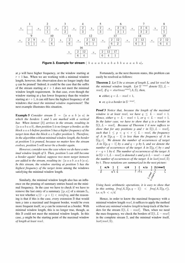
Example 4 The working of the algorithm is explained indetail for the following stream

S17 = 〈b a a a b a a b a b b a a a a b a〉

and target itemset {a}. In Figure 3, a sample run of thealgorithm is illustrated for each timepoint.

In this example, some interesting things happen. First ofall, the stream starts with an itemset, {b}, that does not con-tain the target itemset {a}. Therefore, Update(S0, {b}) =Update([ ], {b}) at timestamp 1 remains empty, i.e., S1 =[ ]. At timestamp 2, Update([ ], {a}) results in S2 =[(2, 1)], corresponding to the stream 〈b |a〉 with a borderat position 2 and the corresponding frequency 1/(2 − 2 +1) = 1/1. At timestamp 8, something interesting hap-pens. S7 = [(2, 3), (6, 2)], corresponding with stream〈b |a a a b |a a〉. Update(S7, {b}) will yield S8 =[(2, 5)], and not [(2, 3), (6, 2)]. Because the correspondingfrequencies decrease from the border at position 2 to theborder at position 6, namely (3+2)/[(6−2)+(8−6+1)] =5/7 > 2/(8− 6 + 1) = 2/3, we can conclude that position6 is no longer a border. This is reflected in summary S8 =[(2, 3 + 2)] and can be visualised by 〈b |a a a b a a b〉.

4.2. Minimal Frequency

Until now, we assumed that for the target itemset weneed to be able to report its frequency exactly. We willnow relax this requirement by setting a minimal frequencythreshold minfreq . That is, for the target itemset, we shouldbe able, at any timepoint, to produce its exact frequencyonly if it is above the frequency threshold. This relaxationallows us to decrease the size of the summary.

Let St be a stream with St = [(p1, a1), . . . , (pr, ar)], andsuppose that

freq(a, St[p1, t]) =a1 + . . . + ar

t − p1 + 1< minfreq .

Then we can safely remove (p1, a1) from the left-side of thesummary; even though it is possible that p1 can still becomethe starting point of a maximal window in the future, it canbe proven that it can never be the starting point of a maxi-mal window in which the target item is above the threshold.Indeed; suppose that freq(A, (St · B)[p1, t + |B|]) exceedsthe minimal frequency threshold, then it is easy to showthat freq(A, B) must be even larger, and hence p1 is not themaximal border. In order to be able to perform this pruningefficiently, we store and maintain for the summaries also thecount total = a1+a2+. . .+ar. When the left-most borderis pruned, total is decreased by a1 to reflect the new total.

4.3. Minimal Window Length

In the algorithm without minimal window length, asgiven in Algorithm 1, we use the fact that a border q instream S can be pruned if we can find two blocks B1 =S[p, q − 1] and B2 = S[q, r] such that the frequency of thetarget in B1 is higher than in B2. The intuition behind theproof of this theorem is that in such a situation, q can neverbecome a border again, because either the window starting

1 2 3 4 5 6 7 8b−→ a−→ 2

1a−→ 2

2a−→ 2

3b−→ 2

3a−→ 2 6

3 1a−→ 2 6

3 2b−→ 2

59 10 11 12 13 14 15

a−→ 2 95 1

b−→ 26

b−→ 26

a−→ 2 126 1

a−→ 2 126 2

a−→ 2 126 3

a−→ 2 126 4

16 17b−→ 2 12

6 4a−→ 2 12 17

6 4 1

Figure 3. Example for stream 〈 b a a a b a a b a b b a a a a b a〉.

at p will have higher frequency, or the window starting atr + 1 has. When we are working with a minimal windowlength, however, this observation does no longer imply thatq can be pruned! Indeed; it could be the case that the suffixof the stream starting at r + 1 does not meet the minimalwindow length requirement. In that case, even though thewindow starting at q has lower frequency than the windowstarting at r+1, it can still have the highest frequency of allwindows that meet the minimal window requirement! Thenext example illustrates this situation.

Example 5 Consider stream S = 〈|a a a b |a a〉 inwhich the borders 1 and 5 are marked with a verticalbar. When itemset {b} arrives in the stream, resulting in〈|a a a b a a b〉, then position 5 is no longer a border, as theblock a a a b before position 5 has a higher frequency of thetarget item than the block a a b after position 5. Therefore,in the algorithm without minimal window length, the borderat position 5 is pruned, because no matter how the streamevolves, position 5 will never be a border again.

However, consider now the case where we do have a min-imal window length of 3. Then, position 5 can still becomea border again! Indeed, suppose two more target itemsetsare added to the stream, resulting in: 〈|a a a b .a a b |a a〉.In this stream, the window starting at position 5 has thehighest frequency of the target items among the windowssatisfying the minimal window length.

Similarly, the minimal window length also has an influ-ence on the pruning of summary entries based on the mini-mal frequency. In the case we have to check if we have toremove the last entry of a summary [(p, a)] of a stream St,we test whether a/(t − p + 1) < minfreq , and the reason-ing is that if this is the case, every extension B that wouldturn p into a maximal and frequent border, would be evenmore frequent itself, so p can be removed as a border. Withminimal window length, this is no longer true, though, asthis B could not meet the minimal window length. In thiscase, p might be the starting point of the maximal windowof length at least mwl .

Fortunately, as the next theorem states, this problem caneasily be resolved as follows:

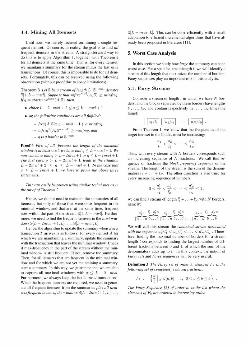
Theorem 2 Let S be a stream of length L, and let mwl bethe minimal window length. Let S

−mwl denote S[1, L −mwl ]. If q = startmaxmwl(A, S), then,

• either, q = L − mwl + 1,

• or, q is a border in S−mwl .

Proof 3 Notice that, because the length of the maximalwindow is at least mwl , we have q ≤ L − mwl + 1.Hence, either q = L − mwl + 1, or q < L − mwl + 1.In the latter case, we have to show that q is a border inS[1, L − mwl ]. Because of Theorem 1 it now suffices toshow that for any positions p and r in S[1, L − mwl ],such that 1 ≤ p < q < r ≤ L − mwl , the frequencyof A in S[p, q − 1] is less than the frequency of A inS[q, r]. We denote the number of occurrences of targetA in S[p, q − 1] by a and q − p by b, and we denote thenumber of occurrences of the target A in S[q, r] by c andr − q + 1 by d. The number of occurrences of the target Ain S[r+1, L−mwl ] is denoted x and y is L−mwl −r andthe number of occurrences of the target A in last(mwl , S)by t. These notations are summarized in the next picture:

Using basic arithmetic operations, it is easy to show thatin this setting, freq(A, S[p, q − 1]) < freq(A, S[q, r]),i.e. a/b < c/d.

Hence, in order to know the maximal frequency with aminimal window length mwl , it suffices to apply the methodwithout any minimal window length to keep track of the bor-ders for the stream S[1, L − mwl]. Then, when we needthe max-frequency, we check the borders of S[1, L − mwl]in the complete stream S, and the minimal window itself,last(mwl , S).

4.4. Mining All Itemsets

Until now, we merely focused on mining a single fre-quent itemset. Of course, in reality, the goal is to find allfrequent itemsets in the stream. A straightforward way todo this is to apply Algorithm 1, together with Theorem 2for all itemsets at the same time. That is, for every itemset,we maintain a summary for the stream minus the last mwltransactions. Of course, this is impossible to do for all item-sets. Fortunately, this can be resolved using the followingobservation (without proof due to space limitations).

Theorem 3 Let S be a stream of length L. S−mwl denotes

S[1, L − mwl ]. Suppose that mfreqmwl(A, S) ≥ minfreq .If q = startmaxmwl(A, S), then,

• either L − 2 · mwl + 2 ≤ q ≤ L − mwl + 1

• or, the following conditions are all fulfilled:

– freq(A, S[q, q + mwl − 1]) ≥ minfreq ,

– mfreq1(A, S−mwl) ≥ minfreq , and

– q is a border in S−mwl .

Proof 4 First of all, because the length of the maximalwindow is at least mwl , we have that q ≤ L−mwl +1. Wenow can have that q > L−2mwl +1 or q ≤ L−2mwl +1.The first case, q > L − 2mwl + 1, leads to the situationL − 2mwl + 2 ≤ q ≤ L − mwl + 1. In the case thatq ≤ L − 2mwl + 1, we have to prove the above threestatements.

This can easily be proven using similar techniques as inthe proof of Theorem 2.

Hence, we do not need to maintain the summaries of allitemsets, but only of those that were once frequent in theminimal window, and that are, at the same time, frequentnow within the part of the stream S[1, L − mwl ]. Further-more, we need to find the frequent itemsets in the mwl win-dows S[L − 2mwl + 1, L], . . ., S[L − mwl, L].

Hence, the algorithm to update the summary when a newtransaction T arrives is as follows: for every itemset A forwhich we are maintaining a summary, update the summarywith the transaction that leaves the minimal window. Checkif max-frequency in the part of the stream without the min-imal window is still frequent. If not, remove the summary.Then, for all itemsets that are frequent in the minimal win-dow and for which we are not yet maintaining a summary,start a summary. In this way, we guarantee that we are ableto capture all maximal windows with q ≤ L − 2 · mwl .Furthermore, we always keep the last 2 · mwl transactions.When the frequent itemsets are required, we need to gener-ate all frequent itemsets from the summaries plus all item-sets frequent in one of the windows S[L−2mwl+1, L], . . .,

S[L − mwl, L]. This can be done efficiently with a smalladaptation to efficient incremental algorithms that have al-ready been proposed in literature [11].

5. Worst Case Analysis

In this section we study how large the summary can be inworst case. For a specific streamlength l, we will identify astream of this length that maximizes the number of borders.Farey sequences play an important role in this analysis.

5.1. Farey Streams

Consider a stream of length l in which we have N bor-ders, and the blocks separated by these borders have lengthsl1, . . . , lN , and contain respectively a1, . . . , aN times thetarget:

a1/l1 a2/l2 · · · aN/lN .

From Theorem 1, we know that the frequencies of thetarget itemset in the blocks must be increasing:

a1

l1<

a2

l2< · · · <

aN

lN.

Thus, with every stream with N borders corresponds suchan increasing sequence of N fractions. We call this se-quence of fractions the block frequency sequence of thestream. The length of the stream is the sum of the denom-inators l1 + . . . + lN . The other direction is also true: forevery increasing sequence of numbers

0 <a′1

l′1<

a′2

l′2< · · · <

a′N

l′N≤ 1 ,

we can find a stream of length l′1 + . . .+ l′N with N borders,namely:

|a′1×︷ ︸︸ ︷

a . . . a

l′1−a′1×︷ ︸︸ ︷

b . . . b |a′2×︷ ︸︸ ︷

a . . . a

l′2−a′2×︷ ︸︸ ︷

b . . . b | . . . |a′

N×︷ ︸︸ ︷a . . . a

l′N−a′N×︷ ︸︸ ︷

b . . . b

We will call this stream the canonical stream associatedwith the sequence a′

1/l′1 < a′2/l′2 < . . . < a′

N/l′N . There-fore, finding the maximal number of borders for a streamlength l corresponds to finding the largest number of dif-ferent fractions between 0 and 1, of which the sum of thedenominators adds up to l. In this context, the notion ofFarey sets and Farey sequences will be very useful.

Definition 3 The Farey set of order k, denoted Fk is thefollowing set of completely reduced fractions:

Fk :={a

b

∣∣∣ gcd(a, b) = 1, 0 < a ≤ b ≤ k}

.

The Farey Sequence [2] of order k, is the list where theelements of Fk are ordered in increasing order.

Just like any other increasing sequence of fractions, alsothe Farey sequence Fk can be associated with its canonicalstream Fk, which has |Fk| borders, and a length that equalsthe sum of the denominators of the elements in Fk. Forexample, consider the Farey sequence of the fifth order:

F5 =15

<14

<13

<25

<12

<35

<23

<34

<45

<11.

The corresponding Farey stream of the fifth order, F5, isgiven in Figure 4. This stream has |F5| = 10 borders and atotal length of 5 + 4 + 3 + 5 + 2 + 5 + 3 + 4 + 5 + 1 = 37.

We will now show that the Farey streams have the maxi-mal number of borders; that is, for every stream S of lengthequal to the length of Fk, the number of borders in S is lessthan or equal to the number of borders in Fk = |Fk|. Thisresult is based on the following straightforward observation.Let dsum({a1/l1, . . . , aN/lN}) =

∑Ni=1 li, i.e., dsum(S)

is the sum of the denominators of the elements in S.

Lemma 1 Let S = {a1/l1, . . . , aN/lN} be a set of N dif-ferent fractions, with 0 < ai < li, for all i = 1 . . . N . Let kbe such that |S| > |Fk|, then

dsum(S) > dsum(Fk) .

Theorem 4 Let S be a stream with L = |Fk|. Then, thenumber of borders in S is at most the number of borders inFk.

Corollary 2 Let l = dsum(Fk), and N = |Fk|, for a fixedk. A stream of length l has maximally N borders.

5.2. Bounds

For a Farey stream Fk the number of borders in it equals|Fk| and the length equals dsum(Fk). This representationdoes, however, not reveal the actual ratio between the sizeand the number of borders of a stream. Therefore, the as-ymptotic behavior of these quantities has been worked out,based on known results in number theory.

k∑i=1

φ(i) =3k2

π2+ O(k log k) ,

k∑i=1

i · φ(i) =2k3

π2+ O(k2 log k) .

This leads to the observation that, asymptotically, the num-ber of borders N and the length of the stream L in worstcase are related as follows:

N =(

π2L

2

)2/3 3π2

.

Experiments for Farey streams up to length 107 has shownthis approximation to be extremely accurate.

2

4

6

8

10

12

14

16

18

20

22

0 100 5 103 1 104 2 104 2 104 2 104 3 104 4 104 4 104 5 104

# bo

rder

s

stream size

maximumaverage

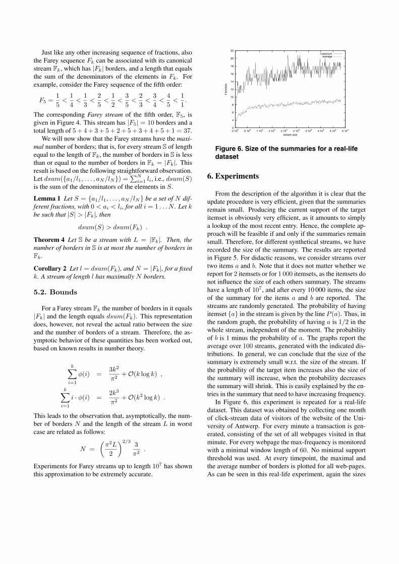
Figure 6. Size of the summaries for a real-lifedataset

6. Experiments

From the description of the algorithm it is clear that theupdate procedure is very efficient, given that the summariesremain small. Producing the current support of the targetitemset is obviously very efficient, as it amounts to simplya lookup of the most recent entry. Hence, the complete ap-proach will be feasible if and only if the summaries remainsmall. Therefore, for different synthetical streams, we haverecorded the size of the summary. The results are reportedin Figure 5. For didactic reasons, we consider streams overtwo items a and b. Note that it does not matter whether wereport for 2 itemsets or for 1 000 itemsets, as the itemsets donot influence the size of each others summary. The streamshave a length of 107, and after every 10 000 items, the sizeof the summary for the items a and b are reported. Thestreams are randomly generated. The probability of havingitemset {a} in the stream is given by the line P (a). Thus, inthe random graph, the probability of having a is 1/2 in thewhole stream, independent of the moment. The probabilityof b is 1 minus the probability of a. The graphs report theaverage over 100 streams, generated with the indicated dis-tributions. In general, we can conclude that the size of thesummary is extremely small w.r.t. the size of the stream. Ifthe probability of the target item increases also the size ofthe summary will increase, when the probability decreasesthe summary will shrink. This is easily explained by the en-tries in the summary that need to have increasing frequency.

In Figure 6, this experiment is repeated for a real-lifedataset. This dataset was obtained by collecting one monthof click-stream data of visitors of the website of the Uni-versity of Antwerp. For every minute a transaction is gen-erated, consisting of the set of all webpages visited in thatminute. For every webpage the max-frequency is monitoredwith a minimal window length of 60. No minimal supportthreshold was used. At every timepoint, the maximal andthe average number of borders is plotted for all web-pages.As can be seen in this real-life experiment, again the sizes

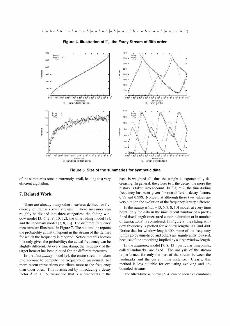
〈 |a b b b b |a b b b |a b b |a a b b b |a b |a a a b b |a a b |a a a b |a a a a b |a〉

Figure 4. Illustration of F5, the Farey Stream of fifth order.

0

100

200

300

400

500

600

0 100 1 106 2 106 3 106 4 106 5 106 6 106 7 106 8 106 9 106 1 107

# bo

rder

s

stream size

item aitem b

P(a)

(a) linear distribution

0

50

100

150

200

250

300

350

400

0 100 1 106 2 106 3 106 4 106 5 106 6 106 7 106 8 106 9 106 1 107

# bo

rder

s

stream size

item aitem b

P(a)

(b) twin peaks

10

11

12

13

14

15

16

0 100 1 106 2 106 3 106 4 106 5 106 6 106 7 106 8 106 9 106 1 107

# bo

rder

s

stream size

item aitem b

P(a)

(c) random distribution

0

20

40

60

80

100

120

140

0 100 1 106 2 106 3 106 4 106 5 106 6 106 7 106 8 106 9 106 1 107

# bo

rder

s

stream size

item aitem b

P(a)

(d) sinus distribution

Figure 5. Size of the summaries for synthetic data

of the summaries remain extremely small, leading to a veryefficient algorithm.

7. Related Work

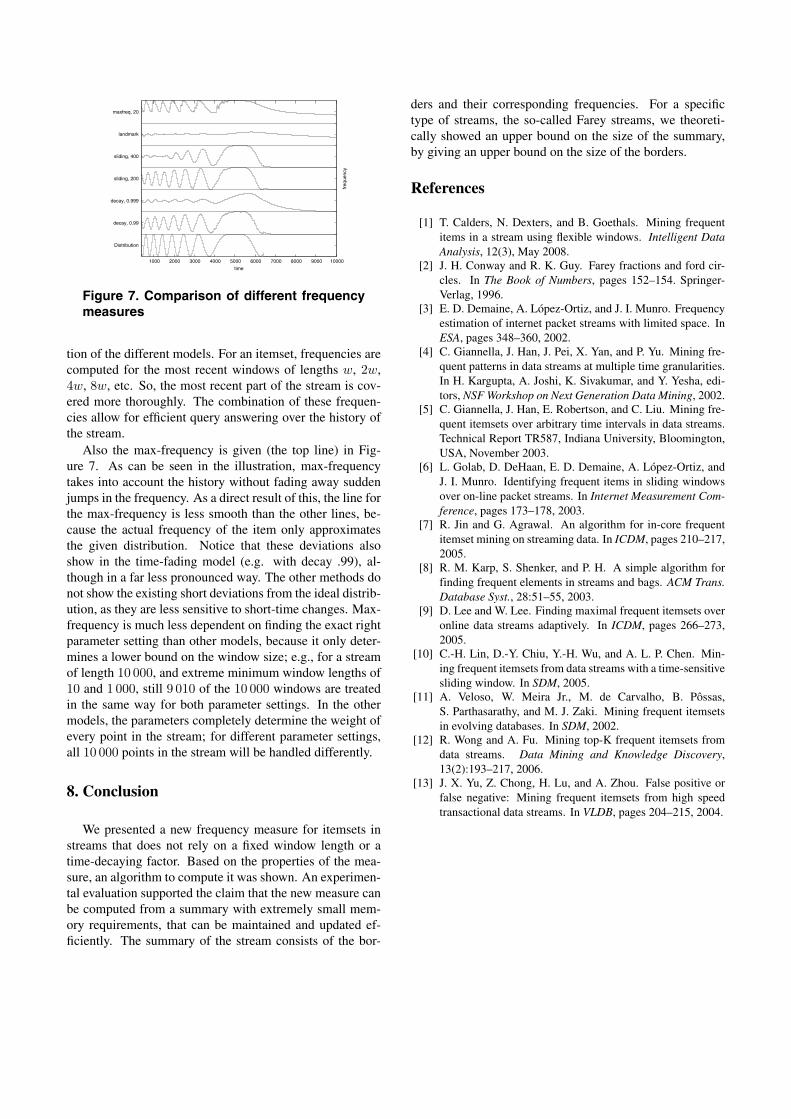
There are already many other measures defined for fre-quency of itemsets over streams. These measures canroughly be divided into three categories: the sliding win-dow model [3, 6, 7, 8, 10, 12], the time fading model [9],and the landmark model [7, 8, 13]. The different frequencymeasures are illustrated in Figure 7. The bottom line reportsthe probability at that timepoint in the stream of the itemsetfor which the frequency is reported. Notice that this bottomline only gives the probability; the actual frequency can beslightly different. At every timestamp, the frequency of thetarget itemset has been plotted for the different measures.

In the time-fading model [9], the entire stream is takeninto account to compute the frequency of an itemset, butmore recent transactions contribute more to the frequencythan older ones. This is achieved by introducing a decayfactor d < 1. A transaction that is n timepoints in the

past, is weighted dn, thus the weight is exponentially de-creasing. In general, the closer to 1 the decay, the more thehistory is taken into account. In Figure 7, the time-fadingfrequency has been given for two different decay factors,0.99 and 0.999. Notice that although these two values arevery similar, the evolution of the frequency is very different.

In the sliding window [3, 6, 7, 8, 10] model, at every timepoint, only the data in the most recent window of a prede-fined fixed length (measured either in duration or in numberof transactions) is considered. In Figure 7, the sliding win-dow frequency is plotted for window lengths 200 and 400.Notice that for window length 400, some of the frequencyjumps go by unnoticed and others are significantly lowered,because of the smoothing implied by a large window length.

In the landmark model [7, 8, 13], particular timepoints,called landmarks, are fixed. The analysis of the streamis performed for only the part of the stream between thelandmarks and the current time instance. Clearly, thismethod is less suitable for evaluating evolving and un-bounded streams.

The tilted-time windows [5, 4] can be seen as a combina-

maxfreq, 20

landmark

sliding, 400

sliding, 200

decay, 0.999

decay, 0.99

Distribution

1000 2000 3000 4000 5000 6000 7000 8000 9000 10000

freq

uenc

y

time

Figure 7. Comparison of different frequencymeasures

tion of the different models. For an itemset, frequencies arecomputed for the most recent windows of lengths w, 2w,4w, 8w, etc. So, the most recent part of the stream is cov-ered more thoroughly. The combination of these frequen-cies allow for efficient query answering over the history ofthe stream.

Also the max-frequency is given (the top line) in Fig-ure 7. As can be seen in the illustration, max-frequencytakes into account the history without fading away suddenjumps in the frequency. As a direct result of this, the line forthe max-frequency is less smooth than the other lines, be-cause the actual frequency of the item only approximatesthe given distribution. Notice that these deviations alsoshow in the time-fading model (e.g. with decay .99), al-though in a far less pronounced way. The other methods donot show the existing short deviations from the ideal distrib-ution, as they are less sensitive to short-time changes. Max-frequency is much less dependent on finding the exact rightparameter setting than other models, because it only deter-mines a lower bound on the window size; e.g., for a streamof length 10 000, and extreme minimum window lengths of10 and 1 000, still 9 010 of the 10 000 windows are treatedin the same way for both parameter settings. In the othermodels, the parameters completely determine the weight ofevery point in the stream; for different parameter settings,all 10 000 points in the stream will be handled differently.

8. Conclusion

We presented a new frequency measure for itemsets instreams that does not rely on a fixed window length or atime-decaying factor. Based on the properties of the mea-sure, an algorithm to compute it was shown. An experimen-tal evaluation supported the claim that the new measure canbe computed from a summary with extremely small mem-ory requirements, that can be maintained and updated ef-ficiently. The summary of the stream consists of the bor-

ders and their corresponding frequencies. For a specifictype of streams, the so-called Farey streams, we theoreti-cally showed an upper bound on the size of the summary,by giving an upper bound on the size of the borders.

References

[1] T. Calders, N. Dexters, and B. Goethals. Mining frequentitems in a stream using flexible windows. Intelligent DataAnalysis, 12(3), May 2008.

[2] J. H. Conway and R. K. Guy. Farey fractions and ford cir-cles. In The Book of Numbers, pages 152–154. Springer-Verlag, 1996.

[3] E. D. Demaine, A. Lopez-Ortiz, and J. I. Munro. Frequencyestimation of internet packet streams with limited space. InESA, pages 348–360, 2002.

[4] C. Giannella, J. Han, J. Pei, X. Yan, and P. Yu. Mining fre-quent patterns in data streams at multiple time granularities.In H. Kargupta, A. Joshi, K. Sivakumar, and Y. Yesha, edi-tors, NSF Workshop on Next Generation Data Mining, 2002.

[5] C. Giannella, J. Han, E. Robertson, and C. Liu. Mining fre-quent itemsets over arbitrary time intervals in data streams.Technical Report TR587, Indiana University, Bloomington,USA, November 2003.

[6] L. Golab, D. DeHaan, E. D. Demaine, A. Lopez-Ortiz, andJ. I. Munro. Identifying frequent items in sliding windowsover on-line packet streams. In Internet Measurement Com-ference, pages 173–178, 2003.

[7] R. Jin and G. Agrawal. An algorithm for in-core frequentitemset mining on streaming data. In ICDM, pages 210–217,2005.

[8] R. M. Karp, S. Shenker, and P. H. A simple algorithm forfinding frequent elements in streams and bags. ACM Trans.Database Syst., 28:51–55, 2003.

[9] D. Lee and W. Lee. Finding maximal frequent itemsets overonline data streams adaptively. In ICDM, pages 266–273,2005.

[10] C.-H. Lin, D.-Y. Chiu, Y.-H. Wu, and A. L. P. Chen. Min-ing frequent itemsets from data streams with a time-sensitivesliding window. In SDM, 2005.

[11] A. Veloso, W. Meira Jr., M. de Carvalho, B. Possas,S. Parthasarathy, and M. J. Zaki. Mining frequent itemsetsin evolving databases. In SDM, 2002.

[12] R. Wong and A. Fu. Mining top-K frequent itemsets fromdata streams. Data Mining and Knowledge Discovery,13(2):193–217, 2006.

[13] J. X. Yu, Z. Chong, H. Lu, and A. Zhou. False positive orfalse negative: Mining frequent itemsets from high speedtransactional data streams. In VLDB, pages 204–215, 2004.