microeconometrics using stata - colin cameron
TRANSCRIPT

Microeconometrics Using Stata
Second Edition
A. COLIN CAMERONDepartment of EconomicsUniversity of California, Davis, CAandSchool of EconomicsUniversity of Sydney, Sydney, Australia
PRAVIN K. TRIVEDISchool of EconomicsUniversity of Queensland, Brisbane, AustraliaandDepartment of EconomicsIndiana University, Bloomington, IN
A Stata Press PublicationStataCorp LPCollege Station, Texas
CHAPTER 28 DRAFT

28 Machine learning for prediction andinference
28.1 Introduction
Microeconometrics studies tend to focus on estimation of one or more regression modelparameters β, and subsequent statistical inference on β or relevant marginal effects thatare a function of β.
A quite different purpose of statistical analysis is prediction. For example, we maywish to predict the probability of twelve-month survival following hip or knee replace-ment surgery. In that case we are interested in obtaining a good prediction y of thedependent variable y.
In principle nonparametric methods such as kernel regression can provide a flexibleway to obtain predictions. But these methods suffer from the curse of dimensionalityif there are many potential regressors. The machine learning literature has proposed awide range of alternative techniques for prediction, where the term machine learning isused as the machine, here the computer, selects the best predictor using only the dataat hand, rather than via a model specified by the researcher who has detailed knowledgeof the specific application.
Machine learning entails data mining that can lead to overfitting the sample athand. To guard against overfitting, models are assessed on the basis of out-of-sampleprediction using cross validation or by penalizing model complexity using informationcriteria or other penalty measures. We begin by presenting cross validation and penaltymeasures.
We then present various techniques for prediction that are used in the machinelearning literature. We focus on shrinkage estimators, notably the LASSO. Additionallya brief review is provided of principal components for dimension reduction, and neuralnetworks, regression trees and random forests for flexible nonlinear models. There isno universal best method for prediction, though for some specific data types, such asimages or text, one method may work particularly well. Often an ensemble predictionthat is a weighted average of predictions from different methods performs best.
The machine learning literature has focused on prediction of y. The recent econo-metrics literature has developed methods that use machine learning methods as an in-termediate input to the ultimate goal of estimating and performing inference on modelparameter(s) of interest. This is a very active area of research.
1263

1264 Chapter 28 Machine learning for prediction and inference
A leading inference example of machine learning methods is inference on α in thepartial linear model y = d′α + x′γ + u where machine learning methods are usedto determine the best set of controls x. A second leading example is instrumentalvariables estimation with many potential instruments and/or controls. Then we wishto select only a few variables to avoid the weak instrument problems that can arise withmany instruments. These and related examples cover many applied microeconometricsapplications and the development of methods for valid inference with machine learningas an input promises to be revolutionary.
The econometrics inference literature to date has emphasized use of the LASSO, andStata 16 has introduced a suite of commands for prediction and inference using theLASSO. For these reasons we emphasize the LASSO. We expect that additional methods,notably random forests and neural nets, will be increasingly used in microeconometricstudies.
28.2 Measuring the predictive ability of a model
There are several ways to measure the predictive ability of a model. Ideally such mea-sures penalize model complexity and control for in-sample overfitting.
Traditionally econometricians have used penalty measures such as in-sample adjustedR2 and in-sample information criteria. The machine learning literature instead empha-sizes out-of-sample predictive ability using cross validation. An introductory treatmentis given in James, Witten, Hastie, and Tibshirani (2013, chaps. 5, 6.1).
28.2.1 Generated data example
The example used in much of this chapter is one where the continuous dependent variabley is regressed on three correlated normally distributed regressors, denoted x1, x2 andx3. The actual data generating process for y is a linear model with an intercept andx1 alone. Many of the methods can be adapted for other types of data such as binaryoutcomes and counts.
The data are generated using commands presented in chapter 5, notably the drawnormcommand to generate correlated normally distributed regressors with correlation 0.5 andthe rnormal() function to obtain normally distributed errors. The DGP for y is a linearmodel with intercept 2 and slope coefficient 1 for variable x1. We have
. * Generate three correlated variables (rho = 0.5) and y linear only in x1
. qui set obs 40
. set seed 12345
. matrix MU = (0,0,0)
. scalar rho = 0.5
. matrix SIGMA = (1,rho,rho \ rho,1,rho \ rho,rho,1)
. drawnorm x1 x2 x3, means(MU) cov(SIGMA)
. generate y = 2 + 1*x1 + rnormal(0,3)

28.2.2 Mean squared error 1265
Summary statistics and correlations for the variables are
. * Summarize data
. summarize
Variable Obs Mean Std. dev. Min Max
x1 40 .3337951 .8986718 -1.099225 2.754746x2 40 .1257017 .9422221 -2.081086 2.770161x3 40 .0712341 1.034616 -1.676141 2.931045y 40 3.107987 3.400129 -3.542646 10.60979
. correlate(obs=40)
x1 x2 x3 y
x1 1.0000x2 0.5077 1.0000x3 0.4281 0.2786 1.0000y 0.4740 0.3370 0.2046 1.0000
OLS estimation of y on x1, x2 and x3 yields the following
. * OLS regression of y on x1-x3
. regress y x1 x2 x3, vce(robust)
Linear regression Number of obs = 40F(3, 36) = 4.91Prob > F = 0.0058R-squared = 0.2373Root MSE = 3.0907
Robusty Coefficient std. err. t P>|t| [95% conf. interval]
x1 1.555582 .5006152 3.11 0.004 .5402873 2.570877x2 .4707111 .5251826 0.90 0.376 -.5944086 1.535831x3 -.0256025 .6009393 -0.04 0.966 -1.244364 1.193159
_cons 2.531396 .5377607 4.71 0.000 1.440766 3.622025
Only variable x1 is statistically significant at level 0.05. This is very likely given the DGP
depends on only x1, but it is by no means certain. Due to randomness we expect thatvariable x2, or variable x3, will be statistically significant at level 0.05 in five percent ofsimilarly generated datasets.
28.2.2 Mean squared error
In general we predict at point x0 using y0 = g(x0), where for OLS y0 = x′0β. We wish
to estimate the expected prediction error E{(y0 − y0)2}.
The standard criterion used for continuous dependent variable is minimization of

1266 Chapter 28 Machine learning for prediction and inference
the mean squared error (MSE) of the predictor
MSE = 1N
∑N
i=1(yi − yi)
2. (28.1)
If the MSE is computed in sample, it under-estimates the true prediction error. Oneway to see this under-estimation is that with N independent regressors including theintercept, OLS necessarily produces a perfect fit with R2 = 1 and MSE = 0. By contrast,the true prediction error will generally be greater than zero.
A second way to see this under-estimation is to note that if y = Xβ + u thenthe OLS residual vector u = y − Xβ = (I − M)u where M = X(X′X)−1X. Since(I−M) < I in the matrix sense it follows that on average |ui| < |ui| so the OLS residualon average is smaller than the true unknown error. For similar reasons with independenthomoskedastic errors the unbiased estimator of σ2 is s2 = 1
N−K
∑Ni=1(yi − yi)2 and not
the smaller 1N
∑Ni=1(yi − yi)2.
Several methods seek to adjust MSE for model size. These include information cri-teria that penalize MSE for model size, and cross-validation measures that estimate themodel on a subsample and compute MSE for the remainder of the sample.
We focus on using MSE as the measure of predictive ability. For continuous dataother measures can be used such as the mean absolute error 1
N
∑Ni=1|yi − yi|. For
likelihood-based models the log-likelihood may be used. For generalized linear modelsthe deviance may be used. For binary outcomes the number of incorrect classifications iscommonly used if interest lies in predicting the actual outcome y, rather than Pr(y = 1).
28.2.3 Information criteria and related penalty measures
Two standard measures that penalize model fit for model size are Akaike’s informationcriterion (AIC) and the Bayesian information criterion (BIC). The general formulas forthese measures were presented in section 13.8.2.
Specializing to the classical linear regression model under i.i.d. normal errors, thefitted log-likelihood equals N ln 2π + N + ln MSE, leading to
AIC = N ln 2π + N + ln MSE + 2K
BIC = N ln 2π + N + ln MSE + (ln N) × K,
where K is the number of regressors including the intercept. Models with smaller AIC
and BIC are preferred, so AIC and BIC are penalized measures of MSE. BIC has a largerpenalty for model size than AIC, so BIC leads to smaller models and might be preferredwhen more parsimonious models are desired.
A related information measure is Mallow’s Cp measure
Cp = (N × MSE/σ2) − N + 2K,

28.2.3 Information criteria and related penalty measures 1267
where σ2 =∑N
i=1(yi − yi)2/(N − p) and yi is the OLS prediction from the largest modelunder consideration that has p regressors including the intercept. Models with smallerCp are preferred. Selecting a model on the basis of minimum Cp is asymptoticallyequivalent to minimizing AIC.
Another penalty measure that is often used is adjusted R2, denoted R2, which can
be expressed as
R2
= 1 −MSE × N/(N − K)
TSS/(N − 1),
where TSS =∑N
i=1(yi − yi)2. Again MSE is penalized for model size since R2
is adecreasing function of K. However, this penalty is relatively small. In the classicallinear regression model with homoskedastic normally distributed errors it can be shownthat, for nested models, choosing the larger model if it has higher R
2is equivalent to
choosing the larger model if the F -statistic for testing joint significance of the additionalregressors exceeds one. The usual critical values used in such a test are substantiallygreater than one.
To enable comparison of all eight possible models that are linear in parameters andregressors we first define the regressor lists for each model.
. * Regressor lists for all possible models
. global xlist1
. global xlist2 x1
. global xlist3 x2
. global xlist4 x3
. global xlist5 x1 x2
. global xlist6 x2 x3
. global xlist7 x1 x3
. global xlist8 x1 x2 x3
The following code provides a loop that estimates each model and computes thevarious penalized fit measures. Note that the global macro defining the kth regressorlist needs to be referenced as ${xlist‘k’} rather than simply $xlist‘k’. We have
. * Full sample estimates with AIC, BIC, Cp, R2adj penalties
. qui regress y $xlist8
. scalar s2full = e(rmse)^2 // Needed for Mallows Cp
. forvalues k = 1/8 {2. qui regress y ${xlist`k´}3. scalar mse`k´ = e(rss)/e(N)4. scalar r2adj`k´ = e(r2_a)5. scalar aic`k´ = -2*e(ll) + 2*e(rank)6. scalar bic`k´ = -2*e(ll) + e(rank)*ln(e(N))7. scalar cp`k´ = e(rss)/s2full - e(N) + 2*e(rank)8. display "Model " "${xlist`k´}" _col(15) " MSE=" %6.3f mse`k´ ///
> " R2adj=" %6.3f r2adj`k´ " AIC=" %7.2f aic`k´ ///> " BIC=" %7.2f bic`k´ " Cp=" %6.3f cp`k´
9. }Model MSE=11.272 R2adj= 0.000 AIC= 212.41 BIC= 214.10 Cp= 9.199
1268 Chapter 28 Machine learning for prediction and inference
Model x1 MSE= 8.739 R2adj= 0.204 AIC= 204.23 BIC= 207.60 Cp= 0.593Model x2 MSE= 9.992 R2adj= 0.090 AIC= 209.58 BIC= 212.96 Cp= 5.838Model x3 MSE=10.800 R2adj= 0.017 AIC= 212.70 BIC= 216.08 Cp= 9.224Model x1 x2 MSE= 8.598 R2adj= 0.196 AIC= 205.58 BIC= 210.64 Cp= 2.002Model x2 x3 MSE= 9.842 R2adj= 0.080 AIC= 210.98 BIC= 216.05 Cp= 7.211Model x1 x3 MSE= 8.739 R2adj= 0.183 AIC= 206.23 BIC= 211.29 Cp= 2.592Model x1 x2 x3 MSE= 8.597 R2adj= 0.174 AIC= 207.57 BIC= 214.33 Cp= 4.000
The MSE, which does not penalize for model size, is smallest for the largest model withall three regressors. The penalized measures all favor the model with an intercept andx1 as the only regressors. More generally different penalties may favor different models.
28.2.4 splitsample command
The preceding example used the same sample for both estimation and measurement ofmodel fit. Cross validation instead estimates the model on one sample, called a trainingsample, and measures predictive ability based on a different sample, called a test sampleor holdout sample or validation sample. This approach can be applied to a range ofmodels, and to loss functions other than mean-squared error.
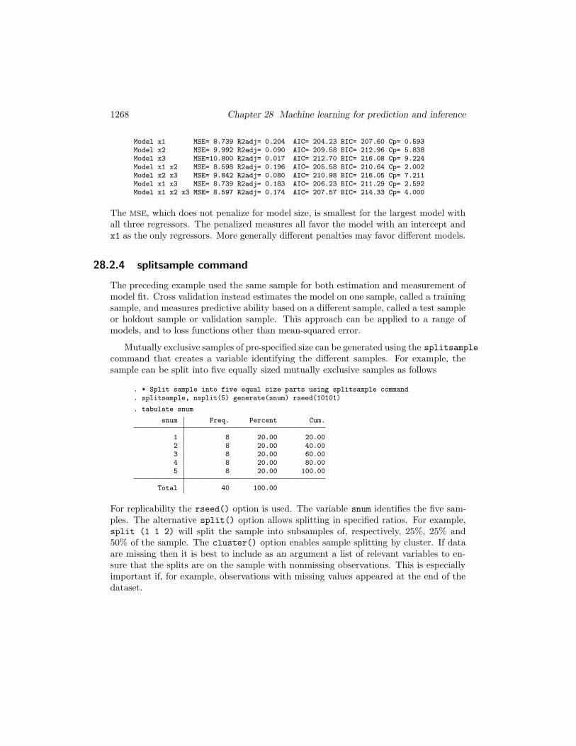
Mutually exclusive samples of pre-specified size can be generated using the splitsamplecommand that creates a variable identifying the different samples. For example, thesample can be split into five equally sized mutually exclusive samples as follows
. * Split sample into five equal size parts using splitsample command
. splitsample, nsplit(5) generate(snum) rseed(10101)
. tabulate snum
snum Freq. Percent Cum.
1 8 20.00 20.002 8 20.00 40.003 8 20.00 60.004 8 20.00 80.005 8 20.00 100.00
Total 40 100.00
For replicability the rseed() option is used. The variable snum identifies the five sam-ples. The alternative split() option allows splitting in specified ratios. For example,split (1 1 2) will split the sample into subsamples of, respectively, 25%, 25% and50% of the sample. The cluster() option enables sample splitting by cluster. If dataare missing then it is best to include as an argument a list of relevant variables to en-sure that the splits are on the sample with nonmissing observations. This is especiallyimportant if, for example, observations with missing values appeared at the end of thedataset.

28.2.5 Single split cross validation 1269
28.2.5 Single split cross validation
We begin with the simplest approach of single split validation. We randomly divide theoriginal sample into two parts: a training sample on which the model will be fitted anda test sample which will be used to assess the fit of the model.
It is common to use a larger part of the original sample for estimation and a smallerpart for assessing predictive ability. The following code creates an indicator variable fora training sample of 80% of the data (dtrain==1) and a test sample of 20% of the data(dtrain==0).
. * Form indicator for training data (80% of sample) and test data (20%)
. splitsample, split(1 4) values(0 1) generate(dtrain) rseed(10101)
. tabulate dtrain
dtrain Freq. Percent Cum.
0 8 20.00 20.001 32 80.00 100.00
Total 40 100.00
We fit each of the eight potential regression models on the 32 observations in thetraining sample, and compute the MSE separately for the 32 observations in the trainingsample (an in-sample MSE) and for the 8 observations in the test sample (an out–of-sample MSE).
. * Single split validation - training and test MSE for the 8 possible models
. forvalues k = 1/8 {2. qui reg y ${xlist`k´} if dtrain==13. qui predict y`k´hat4. qui gen y`k´errorsq = (y`k´hat - y)^25. qui sum y`k´errorsq if dtrain == 16. scalar mse`k´train = r(mean)7. qui sum y`k´errorsq if dtrain == 08. qui scalar mse`k´test = r(mean)9. display "Model " "${xlist`k´}" _col(16) ///
> " Training MSE = " %7.3f mse`k´train " Test MSE = " %7.3f mse`k´test10. }
Model Training MSE = 10.124 Test MSE = 16.280Model x1 Training MSE = 7.478 Test MSE = 13.871Model x2 Training MSE = 8.840 Test MSE = 14.803Model x3 Training MSE = 9.658 Test MSE = 15.565Model x1 x2 Training MSE = 7.288 Test MSE = 13.973Model x2 x3 Training MSE = 8.668 Test MSE = 14.674Model x1 x3 Training MSE = 7.474 Test MSE = 13.892Model x1 x2 x3 Training MSE = 7.288 Test MSE = 13.980
. drop y*hat y*errorsq
As expected, the in-sample MSE (where we normalize by N) decreases as regressors areadded, and is minimized at 7.288 when all three regressors are included.
But when we instead consider the out-of-sample MSE we find that this is minimizedat 13.871 when only x1 is a regressor. Indeed the model with all three regressors has

1270 Chapter 28 Machine learning for prediction and inference
the fifth highest out-of-sample MSE, due to in-sample overfitting.
28.2.6 K-fold cross validation
The results from single-split validation depend on how the sample is split. For example,in the current example different sample splits due to different seeds can lead to out-of-sample MSE being minimized by models other than that with x1 alone as regressor.K-fold cross validation (CV) reduces this limitation by forming more than one split ofthe full sample.
Specifically the sample is randomly divided into K groups or folds of approximatelyequal size. In turn one of the K folds is used as the test dataset while the remainingK − 1 folds are used as the training set. Thus when fold 1 is the test dataset the modelis fit on folds 2 to K, when fold 2 is the test dataset the model is fit on fold 1 and folds3 to K, and so on. The following shows the case K = 5
Fit on folds Test on foldj = 1 2,3,4,5 1j = 2 1,3,4,5 2j = 3 1,2,4,5 3j = 4 1,2,3,5 4j = 5 1,2,3,4 5
Then the cross-validation measure is the average of the K MSEs
CVK = 1K
∑K
j=1MSE(j), (28.2)
where MSE(j) is the MSE for fold j based on OLS estimates obtained by regression usingall data except fold j.
As the number of folds increases the training set size increases so bias decreases.At the same time the fitted models overlap so test set predictions are more highlycorrelated leading to greater variance in the estimate of the expected prediction errorE{(y0− y0)2}. The consensus is that K = 5 or K = 10 provides a good balance betweenbias and variance; most common is to set K = 10.
With so few observations we use K = 5 and obtain the MSE for each fold.
. * Five-fold cross validation example for model with all regressors
. splitsample, nsplit(5) generate(foldnum) rseed(10101)
. matrix allmses = J(5,1,.)
. forvalues i = 1/5 {2. qui reg y x1 x2 x3 if foldnum != `i´3. qui predict y`i´hat4. qui gen y`i´errorsq = (y`i´hat - y)^25. qui sum y`i´errorsq if foldnum ==`i´6. matrix allmses[`i´,1] = r(mean)

28.2.6 K-fold cross validation 1271
7. }
. matrix list allmses
allmses[5,1]c1
r1 13.980321r2 6.4997357r3 9.3623792r4 6.413401r5 12.23958
To obtain the CV5 measure we convert the matrix allmses to a variable and obtainits mean.
. * Compute the average MSE over the five folds and standard deviation
. svmat allmses, names(vallmses)
. qui sum vallmses1
. display "CV5 = " %5.3f r(mean) " with st. dev. = " %5.3f r(sd)CV5 = 9.699 with st. dev. = 3.389
The resulting CV5 measure is 9.699. The MSE’s do vary considerably over the five foldswith standard deviation 3.389 that is large relative to the average.
The user-written crossfold command (Daniels 2012) performs K-fold cross valida-tion. Applying this to all eight potential models, using K = 5 and the same split foreach model we obtain
. * Five-fold cross validation measure for all possible models
. forvalues k = 1/8 {2. set seed 101013. qui crossfold regress y ${xlist`k´}, k(5)4. matrix RMSEs`k´ = r(est)5. svmat RMSEs`k´, names(rmse`k´)6. qui generate mse`k´ = rmse`k´^27. qui sum mse`k´8. scalar cv`k´ = r(mean)9. scalar sdcv`k´ = r(sd)
10. display "Model " "${xlist`k´}" _col(16) " CV5 = " %7.3f cv`k´ ///> " with st. dev. = " %7.3f sdcv`k´11. }
Model CV5 = 11.960 with st. dev. = 3.561Model x1 CV5 = 9.138 with st. dev. = 3.069Model x2 CV5 = 10.407 with st. dev. = 4.139Model x3 CV5 = 11.776 with st. dev. = 3.272Model x1 x2 CV5 = 9.173 with st. dev. = 3.367Model x2 x3 CV5 = 10.872 with st. dev. = 4.221Model x1 x3 CV5 = 9.639 with st. dev. = 2.985Model x1 x2 x3 CV5 = 9.699 with st. dev. = 3.389
The crossfold command reports for each fold RMSE, the square root of the mean-squared error, rather than MSE. To compute the CV5 measure we retrieve the RMSE’sstored in matrix r(est) and calculate the average of the squares of the RMSE’s.
The cross validation measure is lowest for the model with x1 the only regressor.However, it is only slightly higher in the model with both x1 and x2 included. Recall

1272 Chapter 28 Machine learning for prediction and inference
that the folds are randomly chosen, so that with different seed we would obtain differentfolds, different CV values, and hence might find that, for example, the model with bothx1 and x2 included has the minimum CV.
Due to the randomness in K-fold cross validation, some studies use a one standarderror rule that chooses the smallest model with CV within one standard deviation ofthe model with minimum CV. Applying that rule in this particular example favors(marginally) an intercept-only model since 9.138 + 3.069 = 12.207 > 11.960.
Once the preferred model is obtained by cross validation it is fit using the entiresample. Note that the data-mining to obtain a preferred model introduces issues similarto those raised by pre-test bias; see section 11.3.8. Section 28.8 provides examples ofspecial settings, methods and assumptions for which it is possible to ignore the datamining.
Cross validation is easily adapted to estimators other than OLS, and to other lossfunctions such as mean absolute error 1
N
∑Ni=1|yi− yi|. Information criteria have the ad-
vantage of being less computationally demanding and can yield results not too dissimilarfrom those obtained using cross validation.
28.2.7 Leave-one-out cross validation
Leave-one-out cross validation (LOOCV) is the special case of K-fold cross-validationwith K = N . Then N models are estimated, in each model (N − 1) observations areused in training and the remaining observation is used for validation. So we drop eachobservation in turn, estimating a model without that observation and then using thefitted model to predict the dropped observation.
The user-written loocv command (Barron 2014) implements LOOCV. Note, however,that it is quite slow as it is written to apply to any Stata estimation command and doesnot take advantage of the great computational savings that are possible in the specialcase of OLS.
For the model with x1 the only regressor we obtain
. * Leave-one-out cross validation
. loocv regress y x1
Leave-One-Out Cross-Validation Results
Method Value
Root Mean Squared Errors 3.0989007Mean Absolute Errors 2.5242994Pseudo-R2 .15585569
. display "LOOCV MSE = " r(rmse)^2LOOCV MSE = 9.6031853
The MSE from LOOCV is 3.09892 = 9.603, similar to the CV5 measure of 9.699.

28.2.8 Best subsets selection and stepwise selection 1273
LOOCV is not as good for measuring global fit as the N folds are highly correlatedwith each other, leading to higher variance than if K = 5 or K = 10. LOOCV is usedespecially for nonparametric regression where concern is with local fit; see section 27.2.4.Assuming a correctly specified likelihood model, model selection on the basis of LOOCV
is asymptotically equivalent to using AIC.
28.2.8 Best subsets selection and stepwise selection
The best subsets method sequentially determines the best fitting model for models withone regressor, with two regressors, and so on up to all p potential regressors. ThenK-fold cross-validated MSE or a penalty measure such as AIC or BIC is computed forthese p best fitting models of different sizes. In theory there are 2p models to estimate,but this is greatly reduced by using a method called the leaps-and-bounds algorithm.
Stepwise selection methods, introduced in section 11.3.7, entail less computationthan the best subsets method. For example, with p potential regressors the stepwiseforwards procedure requires p + (p − 1) + ∙ ∙ ∙ + 1 = p(p + 1)/2 regressions.
The user-written vselect command (Lindsey and Sheather 2010) implements bestsubsets and stepwise selection methods for OLS regression with predictive ability mea-sured using any of adjusted R2, AIC, BIC or AICC where AICC is a bias-corrected versionof AIC that equals AIC+2(K+1)(K+2)/(N−K−2). The vselect command, however,does not cover K-fold cross validated MSE.
The default for the vselect command is to use the best subsets method. We obtain
. * Best subset selection with community-contributed add-on vselect
. vselect y x1 x2 x3, best
Response : ySelected predictors: x1 x2 x3
Optimal models:
# Preds R2ADJ C AIC AICC BIC1 .2043123 .5925225 204.2265 204.8932 207.60422 .1959877 2.002325 205.5761 206.7189 210.64273 .1737073 4 207.5735 209.3382 214.329
predictors for each model:
1 : x12 : x1 x23 : x1 x2 x3
For models of a given size all measures reduce to minimizing MSE, while the variousmodels give different penalties for increased model size. The best fitting model withone, two and three regressors are those with, respectively, regressors x1, (x1,x2), and(x1,x2,x3). All the penalized measures favor the model with just x1 and an interceptas regressor.
The forwards (or backwards) option of the vselect command implements forwards(or backwards) selection. Then one additionally needs to specify which of the variouspenalty measures is used as model selection criterion. The fix option of the vselect

1274 Chapter 28 Machine learning for prediction and inference
command enables specifying regressors that should be included in all models, and thecommand permits weighted regression.
The user-written gvselect command (Lindsey and Sheather 2015) implements bestsubsets selection for any Stata command that reports a fitted log-likelihood. Then thebest fitting model of a given size is that with the highest fitted log-likelihood, and thebest model overall is that with the smallest AIC or BIC.
28.3 Shrinkage Estimators
The linear model can be made quite flexible by including as regressors transformationsof underlying variables such as polynomials and interactions. Nonetheless the machinelearning literature has introduced other models and other estimation methods that canpredict better than OLS.
In this section we present shrinkage estimators, most notably the LASSO, that shrinkparameter estimates towards zero. The resultant reduction in variability may be suffi-ciently large enough to offset the induced bias leading to lower MSE.
To see this potential gain, consider a scalar unbiased estimator θ with E(θ) = θ
and Var(θ) = v. Then MSE(θ) = v since the mean squared error equals variance plussquared bias
E{(θ − θ)2} = E[{θ − E(θ)}2] + {E(θ) − θ}2 (28.3)
Now define the shrinkage estimator θ = aθ where 0 ≤ a ≤ 1. Then Var(θ) = Var(aθ) =a2v and Bias(θ) = E(θ)− θ = (a− 1)θ, so MSE(θ) = a2v + (a− 1)2θ2. In the case thatθ shrinks all the way to zero (a = 0), θ has lower MSE than θ if θ2 < v. And if θ = 0.9θ
then θ has lower MSE than θ for θ2 < 19v. The potential reduction in MSE of θ carriesover directly to the predictor y = x0θ.
Shrinkage methods are also called penalized or regularized methods. Many shrinkageestimators can also be interpreted in a Bayesian framework as weighted sums of aspecified prior and sample maximum likelihood estimator. In some other cases theshrinkage estimator may be a limiting form of such an estimator.
We focus on shrinkage for linear regression with MSE loss. But shrinkage estimatorscan be applied to other settings with different loss functions, such as ML estimation forthe logit model.
We present the leading shrinkage estimators: ridge regression shrinks all parameterstowards zero, the LASSO sets some parameters to zero while other parameters are shrunktowards zero, and the elastic net combines ridge regression and LASSO. An introductorytreatment is given in James et al. (2013, chap. 6.2).

28.3.1 Ridge regression 1275
28.3.1 Ridge regression
The ridge estimator of Hoerl and Kennard (1970), also known as Tikhonov regulariza-tion, is a biased estimator that reduces MSE by retaining all regressors but shrinkingparameter estimates towards zero.
The ridge estimator βλ of β minimizes
Qλ(β) = 1N
∑N
i=1(yi − x′
iβ)2 + λ∑p
j=1κjβ
2j (28.4)
where λ ≥ 0 is a tuning parameter that needs to be provided and p is the number ofregressors. Different values of the penalty parameter λ lead to different ridge estimators.The regressors x are standardized and some simpler methods set κj = 1 for all j.
The first term in the objective function is the sum of squared residuals minimizedby the OLS estimator. The second term is a penalty that for given λ is likely to increasewith the number of regressors p.
The resulting ridge estimator when all κj = 1 can be expressed as
βλ= (X′X + λNIp)
−1X′y (28.5)
where p is the number of regressors. This estimator is a shrinkage estimator as itshrinks the OLS estimator β = (X′X)−1X′y, the special case λ = 0, towards 0. In thesimplest case that the regressor matrix X is orthonormalized so that X′X = Ip, the OLS
estimator is X′y and the ridge estimator is X′y/(1 + λ) which shrinks all coefficientstowards zero by the same multiplicative factor. For a given specification a shrinkagefactor that would lower the mean square error of the prediction can be shown to exist;the practical task is to estimate it.
When the basic ridge regression is used it is customary to standardize the regressorsto have zero mean and unit variance. Some references and ridge regression programsassume that the dependent variable has been standardized to have zero mean. In thatcase yi is replaced with yi − y and, without loss of generality, the intercept can bedropped. The following code standardizes the regressors and demeans the dependentvariable.
. * Standardize regressors and demean y
. foreach var of varlist x1 x2 x3 {2. qui egen double z`var´ = std(`var´)3. }
. qui summarize y
. qui generate double ydemeaned = y - r(mean)
. summarize ydemeaned z*
Variable Obs Mean Std. dev. Min Max
ydemeaned 40 -3.33e-17 3.400129 -6.650633 7.501798zx1 40 2.63e-17 1 -1.594598 2.693921zx2 40 2.62e-17 1 -2.34211 2.80662zx3 40 -2.98e-17 1 -1.688912 2.764129
1276 Chapter 28 Machine learning for prediction and inference
The Stata commands presented below for shrinkage estimation automatically standard-ize regressors. Then the preceding code is unnecessary.
There are several ways to choose the value of the penalty parameter λ. It can bedetermined by cross-validation, and algorithms exist to quickly compute βλ for manyvalues of λ. Alternatively penalty measures such as AIC may be used. Then the penaltybased on the number of regressors p may be replaced by the effective degrees of freedomwhich for ridge regression can be shown to equal
∑pj=1λj/(λj + λ) where λj are the
eigenvalues of X′X.
28.3.2 Least absolute shrinkage and selection operator (LASSO)
The least absolute shrinkage and selection operator (LASSO) estimator, due to Tibshirani(1999), reduces MSE by setting some coefficients to zero. Additionally the coefficientsof retained variables are shrunk towards zero. Unlike ridge regression, the LASSO canbe used for variable selection.
The LASSO estimator βλ of β minimizes
Qλ(β) = 1N
∑N
i=1(yi − x′
iβ)2 + λ∑p
j=1κj |βj | (28.6)
where λ ≥ 0 is a tuning parameter that needs to be provided and p is the number ofpotential regressors. Different values of the penalty parameter λ lead to different LASSO
estimators. The regressors x are standardized and some simpler implementations setκj = 1 for all j,
The first term in the objective function is the sum of squared residuals minimized bythe OLS estimator. The second term is a penalty measure based on the absolute valueof the parameters, unlike the ridge estimator which uses the square of the parameters.
There is no explicit solution for the resulting LASSO estimator. It can be shownthat the LASSO estimator sets all but k ≤ p of the βj coefficients to zero, where k is adecreasing function of λ, while also shrinking non-zero coefficients towards zero.
To see that some βj may equal zero, suppose there are two regressors. The combi-nations of β1 and β2 for which the sum of squared residuals
∑Ni=1(yi−β1x1i−β2x2i)2 is
constant defines an ellipse. Different values of the sum of squared residuals correspondto different ellipses, given in figure 28.1 and the OLS estimator is the centroid of theellipses. In general the LASSO can be shown to equivalently minimize
∑Ni=1(yi − x′
iβ)2
subject to the constraint that∑p
j=1κj |βj | ≤ s, where higher values of s correspondto lower values of λ. Specializing to the case p = 2, and letting κ1 = κ2 = 1, theLASSO constraint |β1| + |β2| ≤ s defines the diamond-shaped region in the left panel offigure 28.1 and we are likely to wind up at one of the corners where β1 = 0 or β2 = 0.By contrast the ridge estimator constraint β2
1 + β22 ≤ s defines a circle and a corner
solution is very unlikely.
It is very important to note that LASSO picks the best fitting linear combination x′βsubject to the LASSO constraint, rather than the best variables x. This is especially

28.3.3 Elastic net 1277
Figure 28.1. Lasso versus ridge
the case when variables are correlated, such as when potential regressors include powersand interactions of underlying variables. Thus the exact variables selected will vary inrepeated samples or if there is a different partition of the data into K folds.
For prediction, LASSO works best when a few of the potential regressors have βj 6= 0while most βj = 0. By comparison, ridge regression works best when many predictorsare important and have coefficients of standardized regressors that are of similar size.The LASSO is suited to variable selection, whereas ridge regression is not.
Hastie, Tibshirani, and Friedman (2009, chap. 3.8) discuss several penalized orregularized estimators that can be viewed as variations of the LASSO, including thegrouped LASSO, the smoothly clipped absolute deviation SCAD penalty and the Dantzigselector. The LASSO estimator is a special case of a more general method called least-angle regression. The user-written lars command Mander (2014) implements least-angle regression; the a(lasso) option obtains LASSO estimates.
A thresholded or relaxed LASSO performs an additional modified LASSO using onlythose variables chosen by the initial LASSO. The adaptive LASSO presented in sec-tion 28.4.4 is an example.
28.3.3 Elastic net
In many applications variables can be highly correlated with each other. The LASSO
penalty will drop many of these correlated variables, while the ridge penalty shrinks thecoefficients of correlated variables towards each other.
The elastic net combines ridge regression and LASSO. This can improve the MSE, but
1278 Chapter 28 Machine learning for prediction and inference
will retain more variables than the LASSO. The elastic net has objective function
Qλ,α(β) = 12N
∑N
i=1(yi − x′
iβ)2 + λ∑p
j=1κj{α|βj | +
(1−α)2 β2
j } (28.7)
The ridge penalty averages correlated variables while the LASSO penalty leads to spar-sity. Ridge is the special case α = 0 and LASSO is the special case α = 1.
28.3.4 Finite sample distribution of LASSO-related estimators
A model selection method is consistent if asymptotically it correctly selects the correctmodel from a selection of candidate models. A model selection method is conservative ifasymptotically it always selects a model that nests the correct model. Selecting a modelon the basis of minimum BIC is a consistent model selection procedure, while selectinga model on the basis of minimum AIC is conservative (Leeb and Potscher 2005).
A statistical model selection and estimation method is said to have an oracle propertyif it leads to consistent model selection and a subsequent estimator that is asymptoticallyequivalent to the estimator that could be obtained if the true model was known so thatmodel selection was unnecessary.
For example, suppose yi = αx1i + βx2i + ui and the true model is one with eitherβ = 0 or β 6= 0. A consistent model selection method correctly determines whetheror not β = 0. Let α be the estimator of α that first uses a model selection methodto determine whether or not β = 0 and then estimates whichever model is selected.Then α has the oracle property if its asymptotic distribution is the same as that for theinfeasible estimator of α that directly fits the true model without initial model selection.
The LASSO is a consistent model selection procedure, but does not have the oracleproperty due to its bias. The adaptive LASSO presented in section 28.4.4 is one of severalvariations of LASSO that does have the oracle property.
Unfortunately the oracle property is an asymptotic property that while potentiallyuseful in some settings such as recognizing numbers on a license plate, does not carry overto the finite sample settings that economists encounter. Our models do not fit perfectlyand we expect that with more observations it is possible to detect more variables thatpredict the outcome of interest. Leeb and Potscher (2005), for example, consider thepreceding example where β is of order O(1/
√N). Then even though asymptotically
the oracle property may still hold, α has a complicated finite sample distribution thatis affected by the first stage determination of whether or not β = 0. In fact α hasMSE that can be very large and even larger than that if we simply estimated both αand β without first determining whether or not β = 0. Mathematically this differencebetween finite sample and asymptotic performance is a consequence of the asymptoticconvergence not being uniform with respect to parameters.
As a result we cannot perform standard inference on LASSO or post-LASSO OLS
coefficient estimates. Instead if inference on parameters is desired some model structureis required and more complicated estimation methods need to be used. These are

28.4.1 The lasso command 1279
presented in sections 28.8 and 28.9.
28.4 Prediction using LASSO, ridge and elasticnet
We present an application of prediction for linear models using the LASSO and therelated shrinkage estimators – ridge and elastic net. These methods can be adapted tobinary outcome models (logit and probit) and exponential mean models (Poisson), andwe provide a logit example.
28.4.1 The lasso command
LASSO estimates can be obtained using the lasso command that has syntax
lasso model depvar [(alwaysvars)] othervars [if ] [in] [weight], options
The model is one of linear, logit, probit, or poisson. The variables alwaysvarsare variables to be always included while the LASSO selects among the othervars vari-ables. The penalty λ can be determined by cross validation (option cv), adaptive crossvalidation (option adaptive), BIC (option bic), or by a plug-in formula (option plugin).For cross validation the options include folds(#) for the number of folds. The plug-in methods are intended for non-prediction use of the LASSO; see section 28.8. Otheroptions set tolerances for optimization.
For clustered data the option cluster(clustervar ) defines the objective function tobe the average over clusters of the within-cluster sums of squared residuals. So (12.6)becomes
Qλ(β) =1G
∑G
g=1
{1
Ng
∑Ng
i=1(yig − x′
igβ)2}
+ λ∑Ng
j=1κj |βj |
Cross validation then selects folds at the cluster level, which requires a considerablenumber of clusters.
The lasso command output focuses on determination of the penalty λ. Postestima-tion commands lassoinfo, lassoknots, lassoselect, cvplot, lassocoef, coefpath,lassogof, and bicplot provide additional information. These commands are illustratedbelow.
The elasticnet command has syntax, options and postestimation commands sim-ilar to those for the lasso command. Ridge estimates can be obtained using theelasticnet command with option alpha(0). Stata also includes a sqrtlasso com-mand which is seldom used and is not covered here.

1280 Chapter 28 Machine learning for prediction and inference
28.4.2 Lasso linear regression example
We apply the lasso linear command to the current data example. Since there areonly 40 observations we use 5-fold cross validation rather than the default of 10 folds.The five folds are determined by a random number generator, so for replicability weneed to set the seed.
. * Lasso using 5-fold cross validation
. lasso linear y x1 x2 x3, selection(cv) folds(5) rseed(10101)
5-fold cross-validation with 100 lambdas ...Grid value 1: lambda = 1.591525 no. of nonzero coef. = 0Folds: 1...5 CVF = 11.85738Grid value 2: lambda = 1.450138 no. of nonzero coef. = 1Folds: 1...5 CVF = 11.60145Grid value 3: lambda = 1.321312 no. of nonzero coef. = 1Folds: 1...5 CVF = 11.2296
(output omitted )Grid value 10: lambda = .688933 no. of nonzero coef. = 1Folds: 1...5 CVF = 9.829713Grid value 11: lambda = .6277301 no. of nonzero coef. = 2Folds: 1...5 CVF = 9.739804
(output omitted )Grid value 20: lambda = .2717294 no. of nonzero coef. = 2Folds: 1...5 CVF = 9.393794Grid value 21: lambda = .2475897 no. of nonzero coef. = 2Folds: 1...5 CVF = 9.393523Grid value 22: lambda = .2255945 no. of nonzero coef. = 2Folds: 1...5 CVF = 9.40661Grid value 23: lambda = .2055533 no. of nonzero coef. = 2Folds: 1...5 CVF = 9.420332Grid value 24: lambda = .1872925 no. of nonzero coef. = 2Folds: 1...5 CVF = 9.434326... cross-validation complete ... minimum found
Lasso linear model No. of obs = 40No. of covariates = 3
Selection: Cross-validation No. of CV folds = 5
--------------------------------------------------------------------------| No. of Out-of- CV mean| nonzero sample prediction
ID | Description lambda coef. R-squared error---------+----------------------------------------------------------------
1 | first lambda 1.591525 0 0.0519 11.8573820 | lambda before .2717294 2 0.1666 9.393794
* 21 | selected lambda .2475897 2 0.1666 9.39352322 | lambda after .2255945 2 0.1655 9.4066124 | last lambda .1872925 2 0.1630 9.434326
--------------------------------------------------------------------------* lambda selected by cross-validation.
The default grid for λ is a decreasing logarithmic grid of 100 values with λj =λ1 × 10⁻⁴(j−1)/99, j = 2, ..., 100, where λ1 is the smallest value at which no variablesare selected. Here λ1 = 1.591525 and, for example, λ2 = λ1 × 10⁻⁴/99 = 1.591525 ×.97700996 = 1.450138.
28.4.3 Lasso post estimation commands example 1281
The output shows that reducing the penalty to λ2 = 1.450 led to the inclusion ofa regressor, and reducing the penalty to λ11 = 0.628 led to the inclusion of a secondregressor. The CV objective function continued to decline to a minimum value of 9.394at λ21 = 0.248. The results are only listed to the 24th largest grid value of λ, ratherthan all 100 grid point values, as the minimum CV value has already been attained bythen.
28.4.3 Lasso post estimation commands example
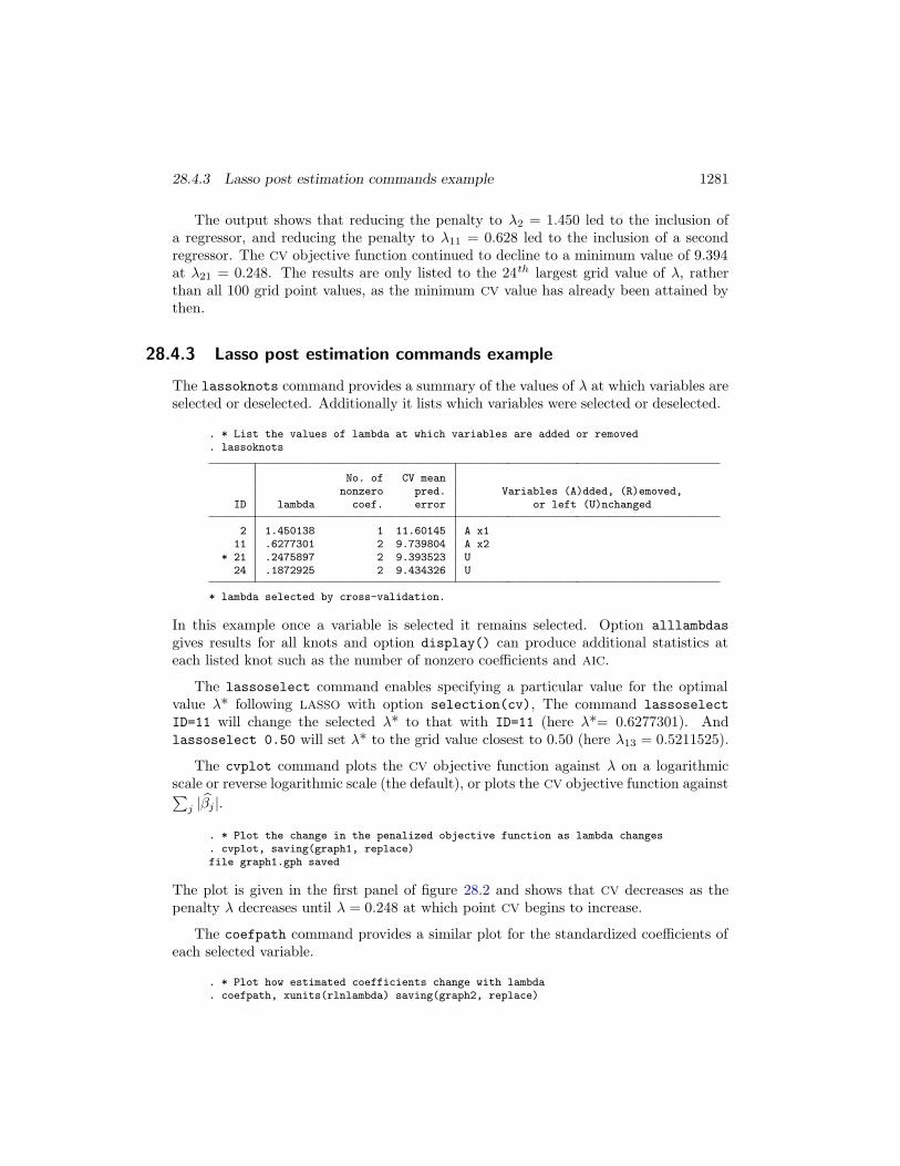
The lassoknots command provides a summary of the values of λ at which variables areselected or deselected. Additionally it lists which variables were selected or deselected.
. * List the values of lambda at which variables are added or removed
. lassoknots
No. of CV meannonzero pred. Variables (A)dded, (R)emoved,
ID lambda coef. error or left (U)nchanged
2 1.450138 1 11.60145 A x111 .6277301 2 9.739804 A x2
* 21 .2475897 2 9.393523 U24 .1872925 2 9.434326 U
* lambda selected by cross-validation.
In this example once a variable is selected it remains selected. Option alllambdasgives results for all knots and option display() can produce additional statistics ateach listed knot such as the number of nonzero coefficients and AIC.
The lassoselect command enables specifying a particular value for the optimalvalue λ* following LASSO with option selection(cv), The command lassoselectID=11 will change the selected λ* to that with ID=11 (here λ*= 0.6277301). Andlassoselect 0.50 will set λ* to the grid value closest to 0.50 (here λ13 = 0.5211525).
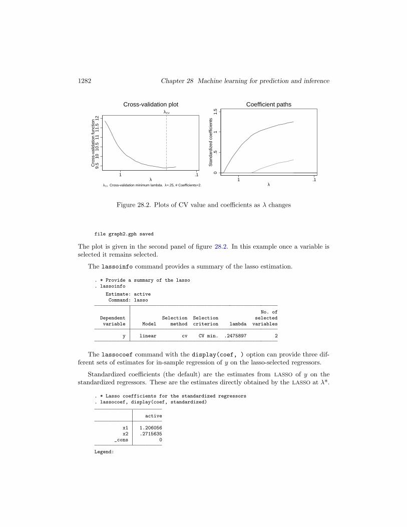
The cvplot command plots the CV objective function against λ on a logarithmicscale or reverse logarithmic scale (the default), or plots the CV objective function against∑
j |βj |.
. * Plot the change in the penalized objective function as lambda changes
. cvplot, saving(graph1, replace)file graph1.gph saved
The plot is given in the first panel of figure 28.2 and shows that CV decreases as thepenalty λ decreases until λ = 0.248 at which point CV begins to increase.
The coefpath command provides a similar plot for the standardized coefficients ofeach selected variable.
. * Plot how estimated coefficients change with lambda
. coefpath, xunits(rlnlambda) saving(graph2, replace)
1282 Chapter 28 Machine learning for prediction and inference
9.5
1010
.511
11.5
12C
ross
-val
idat
ion
func
tion
λCV
.11λ
λCV Cross-validation minimum lambda. λ=.25, # Coefficients=2.
Cross-validation plot
0.5
11.
5S
tand
ardi
zed
coef
ficie
nts
.11λ
Coefficient paths
Figure 28.2. Plots of CV value and coefficients as λ changes
file graph2.gph saved
The plot is given in the second panel of figure 28.2. In this example once a variable isselected it remains selected.
The lassoinfo command provides a summary of the lasso estimation.
. * Provide a summary of the lasso
. lassoinfo
Estimate: activeCommand: lasso
No. ofDependent Selection Selection selectedvariable Model method criterion lambda variables
y linear cv CV min. .2475897 2
The lassocoef command with the display(coef, ) option can provide three dif-ferent sets of estimates for in-sample regression of y on the lasso-selected regressors.
Standardized coefficients (the default) are the estimates from LASSO of y on thestandardized regressors. These are the estimates directly obtained by the LASSO at λ*.
. * Lasso coefficients for the standardized regressors
. lassocoef, display(coef, standardized)
active
x1 1.206056x2 .2715635
_cons 0
Legend:
28.4.3 Lasso post estimation commands example 1283
b - base levele - empty cello - omitted
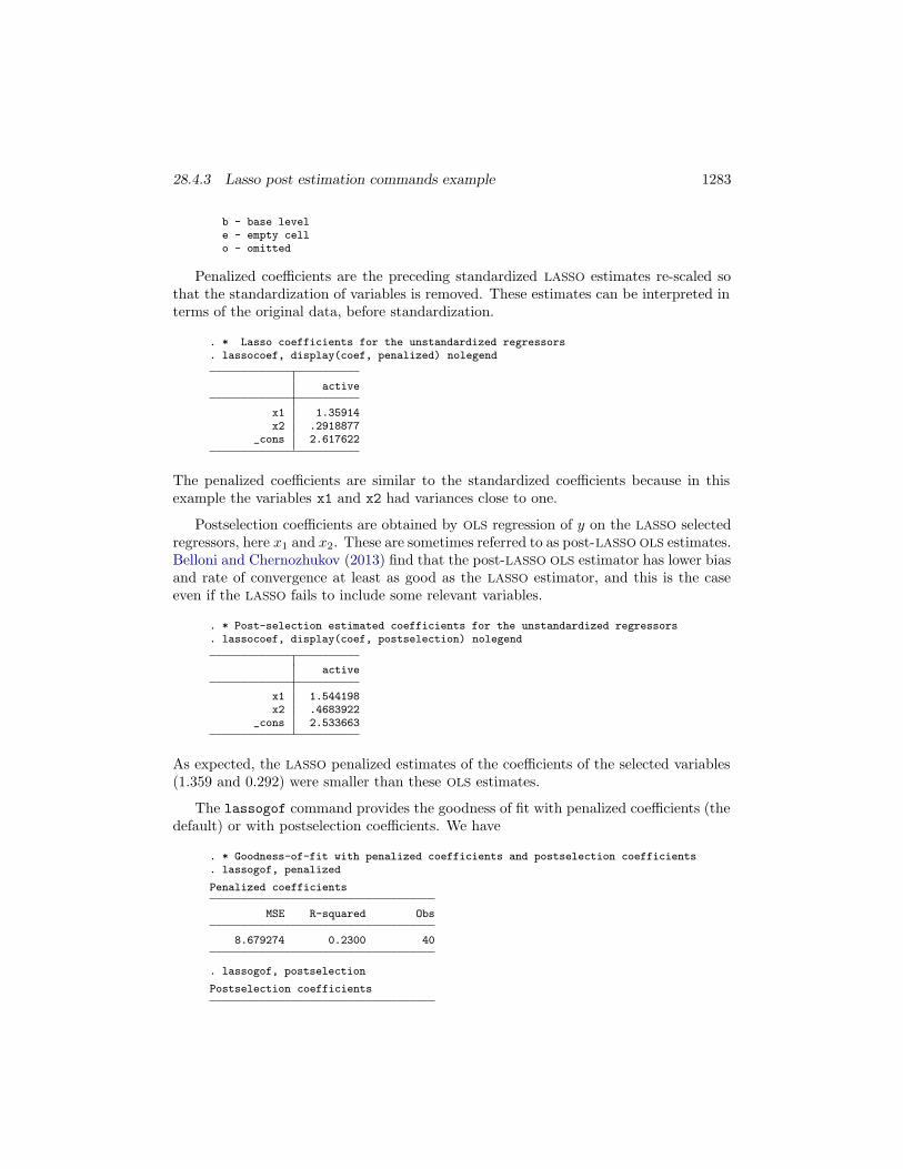
Penalized coefficients are the preceding standardized LASSO estimates re-scaled sothat the standardization of variables is removed. These estimates can be interpreted interms of the original data, before standardization.
. * Lasso coefficients for the unstandardized regressors
. lassocoef, display(coef, penalized) nolegend
active
x1 1.35914x2 .2918877
_cons 2.617622
The penalized coefficients are similar to the standardized coefficients because in thisexample the variables x1 and x2 had variances close to one.
Postselection coefficients are obtained by OLS regression of y on the LASSO selectedregressors, here x1 and x2. These are sometimes referred to as post-LASSO OLS estimates.Belloni and Chernozhukov (2013) find that the post-LASSO OLS estimator has lower biasand rate of convergence at least as good as the LASSO estimator, and this is the caseeven if the LASSO fails to include some relevant variables.
. * Post-selection estimated coefficients for the unstandardized regressors
. lassocoef, display(coef, postselection) nolegend
active
x1 1.544198x2 .4683922
_cons 2.533663
As expected, the LASSO penalized estimates of the coefficients of the selected variables(1.359 and 0.292) were smaller than these OLS estimates.
The lassogof command provides the goodness of fit with penalized coefficients (thedefault) or with postselection coefficients. We have
. * Goodness-of-fit with penalized coefficients and postselection coefficients
. lassogof, penalized
Penalized coefficients
MSE R-squared Obs
8.679274 0.2300 40
. lassogof, postselection
Postselection coefficients

1284 Chapter 28 Machine learning for prediction and inference
MSE R-squared Obs
8.597958 0.2372 40
The postselection estimator is OLS which maximizes R2 since it minimizes the sum ofsquared residuals. The lasso added a penalty which necessarily leads to smaller in-sample R2. The difference here between 0.2372 and 0.2300 is not great.
Finally we verify that the postselection estimates are indeed obtained by OLS of yon the lasso-selected variables.
. * Compare to OLS with the lasso selected regressors
. regress y x1 x2, noheader
y Coefficient Std. err. t P>|t| [95% conf. interval]
x1 1.544198 .6305617 2.45 0.019 .2665582 2.821837x2 .4683922 .6014166 0.78 0.441 -.7501936 1.686978
_cons 2.533663 .5159805 4.91 0.000 1.488188 3.579139
28.4.4 Adaptive lasso
The adaptive LASSO (Zou 2006) is a multi-step LASSO method that usually leads tofewer variables being selected compared to the basic CV method.
The preceding analysis set κj = 1 in (28.6). Adaptive LASSO also begins with regularCV LASSO (or CV Ridge) with κj = 1. Adaptive LASSO then does a second LASSO thatexcludes variables with βj = 0 and for the remainder sets κj = 1/|βj |δ with defaultδ = 1 which favors variables with a larger coefficient as they receive a smaller penalty.The default is to have one adaptive step but additional adaptive steps can be requested.
For the current example with one adaptive step we obtain
. * Lasso linear using 5-fold adaptive cross validation
. qui lasso linear y x1 x2 x3, selection(adaptive) folds(5) rseed(10101)
. lassoknots
No. of CV meannonzero pred. Variables (A)dded, (R)emoved,
ID lambda coef. error or left (U)nchanged
26 3.945214 1 11.60145 A x1* 52 .3512089 1 9.160539 U
57 .2205694 2 9.210699 A x295 .0064297 2 9.172378 U
* lambda selected by cross-validation in final adaptive step.
Now the optimal choice of λ leads to only x1 being selected.
The selection(none) option fits at each value of λ on the grid but does not select
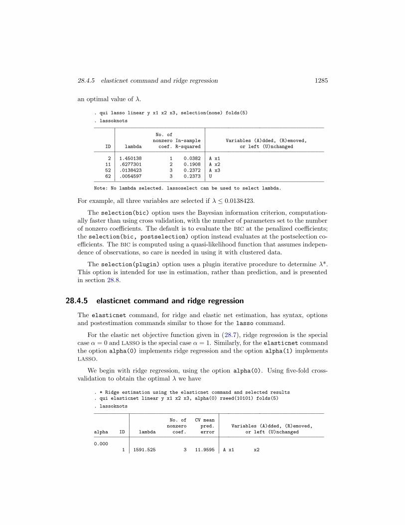
28.4.5 elasticnet command and ridge regression 1285
an optimal value of λ.
. qui lasso linear y x1 x2 x3, selection(none) folds(5)
. lassoknots
No. ofnonzero In-sample Variables (A)dded, (R)emoved,
ID lambda coef. R-squared or left (U)nchanged
2 1.450138 1 0.0382 A x111 .6277301 2 0.1908 A x252 .0138423 3 0.2372 A x362 .0054597 3 0.2373 U
Note: No lambda selected. lassoselect can be used to select lambda.
For example, all three variables are selected if λ ≤ 0.0138423.
The selection(bic) option uses the Bayesian information criterion, computation-ally faster than using cross validation, with the number of parameters set to the numberof nonzero coefficients. The default is to evaluate the BIC at the penalized coefficients;the selection(bic, postselection) option instead evaluates at the postselection co-efficients. The BIC is computed using a quasi-likelihood function that assumes indepen-dence of observations, so care is needed in using it with clustered data.
The selection(plugin) option uses a plugin iterative procedure to determine λ*.This option is intended for use in estimation, rather than prediction, and is presentedin section 28.8.
28.4.5 elasticnet command and ridge regression
The elasticnet command, for ridge and elastic net estimation, has syntax, optionsand postestimation commands similar to those for the lasso command.
For the elastic net objective function given in (28.7), ridge regression is the specialcase α = 0 and LASSO is the special case α = 1. Similarly, for the elasticnet commandthe option alpha(0) implements ridge regression and the option alpha(1) implementsLASSO.
We begin with ridge regression, using the option alpha(0). Using five-fold cross-validation to obtain the optimal λ we have
. * Ridge estimation using the elasticnet command and selected results
. qui elasticnet linear y x1 x2 x3, alpha(0) rseed(10101) folds(5)
. lassoknots
No. of CV meannonzero pred. Variables (A)dded, (R)emoved,
alpha ID lambda coef. error or left (U)nchanged
0.0001 1591.525 3 11.9595 A x1 x2

1286 Chapter 28 Machine learning for prediction and inference
x3* 93 .3052401 3 9.54017 U100 .1591525 3 9.566065 U
* alpha and lambda selected by cross-validation.
. lassocoef, display(coef, penalized) nolegend
active
x1 1.139476x2 .4865453x3 .0958546
_cons 2.659647
. lassogof, penalized
Penalized coefficients
MSE R-squared Obs
8.70562 0.2277 40
The ridge coefficient estimates are on average shrunken towards zero compared to theOLS slope estimates of, respectively, 1.555, 0.471 and -0.026, given in section 28.2. AndR2 has fallen from 0.2373 to 0.2277.
For elastic net regression the elasticnet command performs a two-dimensional gridsearch over both λ and α. The default for λ is the same logarithmic grid with 100 pointsas used by lasso, while α = 0.5, 0.7, 1.0. For this example the defaults led to α = 1 soelastic net reduced to LASSO. We specify a narrower grid that leads to α = 0.95.
. * Elastic net estimation and selected results
. qui elasticnet linear y x1 x2 x3, alpha(0.9(0.05)1) rseed(10101) folds(5)
. lassoknots
No. of CV meannonzero pred. Variables (A)dded, (R)emoved,
alpha ID lambda coef. error or left (U)nchanged
1.0004 1.450138 1 11.60145 A x1
13 .6277301 2 9.739804 A x226 .1872925 2 9.434326 U
0.95029 1.591525 1 11.73019 A x138 .688933 2 9.81611 A x2
* 48 .2717294 2 9.3884 U51 .2055533 2 9.425887 U
0.90053 1.675289 1 11.74015 A x162 .7561031 2 9.900317 A x276 .2055533 2 9.431641 U
* alpha and lambda selected by cross-validation.

28.4.6 Comparison of shrinkage estimators 1287
. lassocoef, display(coef, penalized) nolegend
active
x1 1.329744x2 .2908281
_cons 2.627567
. lassogof, penalized
Penalized coefficients
MSE R-squared Obs
8.693386 0.2288 40
The optimal values of α = 0.95 and λ = .2717 lead to selection of x1 and x2. Thepenalized coefficient estimates and MSE are close to the lasso estimates, the case α = 1.In real-life examples with many more regressors we expect a bigger difference.
28.4.6 Comparison of shrinkage estimators
The results across several shrinkage model estimates can be compared using the postes-timation commands lassocoef, lassogof, and lassoinfo.
First. save model results using the estimates store command.
. * Fit various models and store results
. qui regress y x1 x2 x3
. estimates store OLS
. qui lasso linear y x1 x2 x3, selection(cv) folds(5) rseed(10101)
. estimates store LASCV
. qui lasso linear y x1 x2 x3, selection(adaptive) folds(5) rseed(10101)
. estimates store LASADAPT
. qui lasso linear y x1 x2 x3, selection(plugin) folds(5)
. estimates store LASPLUG
. qui elasticnet linear y x1 x2 x3, alpha(0) selection(cv) folds(5) rseed(10101)
. estimates store RIDGECV
. qui elasticnet linear y x1 x2 x3, alpha(0.9(0.05)1) rseed(10101) folds(5)
. estimates store ELASTIC
We compare in-sample model fit and the specific variables selected. The comparisonbelow uses penalized coefficient estimates for standardized variables. For unpenalizedpostselection estimates of unstandardized variables use lassogof option postselectionand lassocoef option display(coef, postselection).
. * Compare in-sample fit and selected coefficients of various models
. lassogof OLS LASCV LASADAPT LASPLUG RIDGECV ELASTIC
Penalized coefficients

1288 Chapter 28 Machine learning for prediction and inference
Name MSE R-squared Obs
OLS 8.597403 0.2373 40LASCV 8.679274 0.2300 40
LASADAPT 8.755573 0.2232 40LASPLUG 10.23264 0.0922 40RIDGECV 8.70562 0.2277 40ELASTIC 8.693386 0.2288 40
. lassocoef OLS LASCV LASADAPT LASPLUG RIDGECV ELASTIC, display(coef) nolegend
OLS LASCV LASADAPT LASPLUG RIDGECV ELASTIC
x1 1.555582 1.206056 1.462431 .3693423 1.011134 1.179972x2 .4707111 .2715635 .452667 .2705777x3 -.0256025 .0979251
_cons 2.531396 0 0 0 0 0
CV LASSO selects x1 and x2, while adaptive LASSO which provides a bigger penalty thanCV LASSO selects only x1. Ridge by construction retains all variables, while the elasticnet in this example selected x1 and x2.
All methods have similar in-sample MSE and R2, aside from plugin LASSO. The pluginLASSO, see section 28.8.5, is designed to select the variables that best approximate thosein the true model and is expected to predict well out of sample. The plugin LASSO didindeed pick only x1, the model for the DGP of this example.
28.4.7 Shrinkage for logit, probit and Poisson models
In principle the LASSO, ridge and elastic net penalties can be applied to objective func-tions other than the sum of squared residuals used for linear regression.
In particular, for generalized linear models the objective function uses the sum ofsquared deviance residuals, defined in section 13.8.3, rather than the sum of squaredresiduals. The lasso and elasticnet commands can also be applied to logit, probitand Poisson models.
The squared residual (yi−x′iβ)2 in (28.4), (28.6) and (28.7) is replaced by the squared
deviance residual. For logit this term is 2[yi lnΛ(x′iβ) + (1− yi) ln{1−Λ(x′
iβ)}], whereΛ(z) = ez/(1 + ez). For probit we use 2[yi lnΦ(x′
iβ) + (1 − yi) ln{1 − Φ(x′iβ)}] where
Φ(∙) is the standard normal c.d.f. For Poisson we use 2{yix′iβ − exp(x′
iβ) − vi}, wherevi = 0 if yi = 0 and vi = yi ln(yi) − yi otherwise.
The related Stata commands in the case of LASSO are, respectively, lasso logit,lasso probit and lasso poisson,
To illustrate the method for a binary variable, we convert y to a variable dy thattakes value 1 if y > 3, and implement LASSO for a logit model with λ determined byfive-fold CV.

28.5 Dimension reduction 1289
. * Lasso for logit example
. qui generate dy = y > 3
. qui lasso logit dy x1 x2 x3, rseed(10101) folds(5)
. lassoknots
No. ofnonzero CV mean Variables (A)dded, (R)emoved,
ID lambda coef. deviance or left (U)nchanged
2 .2065674 1 1.407613 A x1* 24 .0266792 1 1.192646 U
26 .0221495 2 1.192865 A x230 .0152668 3 1.194545 A x331 .0139106 3 1.195055 U
* lambda selected by cross-validation.
The optimal λ leads to selection of only x1.
For a count example we create a Poisson variable ycount that takes values between0 and 7 and whose mean depends on only x1. LASSO with five-fold CV yields
. * Lasso for count data example
. qui generate ycount = rpoisson(exp(-1 + x1))
. qui lasso poisson ycount x1 x2 x3, rseed(10101) folds(5)
. lassoknots
No. ofnonzero CV mean Variables (A)dded, (R)emoved,
ID lambda coef. deviance or left (U)nchanged
2 1.012329 1 2.191141 A x1* 25 .119132 1 .8257619 U
29 .0821131 2 .8334985 A x3
* lambda selected by cross-validation.
Again the optimal λ leads to selection of only x1.
28.5 Dimension reduction
Dimension reduction methods reduce the number of regressors from p to m < p linearcombinations of regressors. Thus given initial model y = β0 + Xβ + u, where X isN × p, we form matrix Z = XA, where A is p×m and Z is N ×m. Then we estimatethe model y = γ0 + Zγ + v.
Here we present principal components, a long-standing method that uses only Xto form A (unsupervised learning). A related method is partial least squares, whichadditionally uses the relationship between y and X to form A (supervised learning).Principal components is the method most often used in econometrics studies and canbe used in a very wide range of applications.

1290 Chapter 28 Machine learning for prediction and inference
28.5.1 Principal components
The principal components method selects the linear combinations of regressors, calledprincipal components, as follows. The first principal component has the largest samplevariance among all normalized linear combinations of the columns of X. The secondprincipal component has the largest sample variance subject to being orthogonal to thefirst, and so on. More formally the jth principal component is the N × 1 vector Xhj
where hj is the eigenvector corresponding to λj , the jth largest eigenvalue of X′X.
The principal components are not invariant to the scaling of X and it is commonpractice to apply principal components to data that has been standardized to have meanzero and variance one. Let X∗ denote the regressor matrix after this standardization.The Stata pca command computes the principal components. The default option is thecorrelation option that is equivalent to automatically standardizing the data beforeanalysis. So with this default option there is no need to first standardize the regressors.We obtain
. * Principal components using default option that first standardizes the data
. pca x1 x2 x3
Principal components/correlation Number of obs = 40Number of comp. = 3Trace = 3
Rotation: (unrotated = principal) Rho = 1.0000
Component Eigenvalue Difference Proportion Cumulative
Comp1 1.81668 1.08919 0.6056 0.6056Comp2 .727486 .27165 0.2425 0.8481Comp3 .455836 . 0.1519 1.0000
Principal components (eigenvectors)
Variable Comp1 Comp2 Comp3 Unexplained
x1 0.6306 -0.1063 -0.7688 0x2 0.5712 -0.6070 0.5525 0x3 0.5254 0.7876 0.3220 0
The output includes the three eigenvalues and three eigenvectors. The data are stan-dardized automatically so each of the three variables has variance one and the sum ofthe variances is three. The variance of each principal component equals the correspond-ing eigenvalue, so the first principal component has variance 1.81668 and explains afraction 1.81668/3 = 0.6056 of the total variance.
Note that the same results are obtained if we use the previously standardized vari-ables zx1-zx3 and the covariance option, specifically command pca zx1 zx2 zx3,covariance.
The post-estimation predict command constructs variables equal to the three prin-cipal components. We obtain

28.5.1 Principal components 1291
. * Compute the 3 principal components and their means, st.devs., correlations
. predict pc1 pc2 pc3(score assumed)
Scoring coefficientssum of squares(column-loading) = 1
Variable Comp1 Comp2 Comp3
zx1 0.6306 -0.1063 -0.7688zx2 0.5712 -0.6070 0.5525zx3 0.5254 0.7876 0.3220
. summarize pc1 pc2 pc3
Variable Obs Mean Std. dev. Min Max
pc1 40 -3.35e-09 1.347842 -2.52927 2.925341pc2 40 -3.63e-09 .8529281 -1.854475 1.98207pc3 40 2.08e-09 .6751564 -1.504279 1.520466
. correlate pc1 pc2 pc3(obs=40)
pc1 pc2 pc3
pc1 1.0000pc2 0.0000 1.0000pc3 -0.0000 -0.0000 1.0000
The principal components have mean zero, standard deviation equal to the square rootof the corresponding eigenvalue, for example
√1.81668 = 1.3478, and are uncorrelated.
The principal components are computed applying the relevant eigenvectors to thestandardized variables. For example, the first principal component is computed asfollows
. * Manually compute the first principal component and compare to pc1
. generate double pc1manual = 0.6306*zx1 + 0.5712*zx2 + 0.5254*zx3
. summarize pc1 pc1manual
Variable Obs Mean Std. dev. Min Max
pc1 40 -3.35e-09 1.347842 -2.52927 2.925341pc1manual 40 -9.02e-18 1.347822 -2.529204 2.925356
The principal components are obtained without any consideration of regression ona variable y. If we regress y on all p principal components we necessarily get the samepredicted values of y and the same R2 as if we regress y on all of the original p regressors.The hope is that if we regress y on just, say, the first m < p principal components thenwe obtain fit better than that obtained by arbitrarily picking m regressors and not muchworse than if we used all p regressors. There is no guarantee this will happen, but inpractice it often does.
The following example gives correlations of the dependent variable with fitted valuesfrom regression on, respectively, all three regressors, the first principal component, x1,x2, and x3. Recall that the square of these correlations equals R2 from the corresponding

1292 Chapter 28 Machine learning for prediction and inference
OLS regression.
. * Compare R from OLS on all three regressors, on pc1, on x1, on x2, on x3
. qui regress y x1 x2 x3
. predict yhat(option xb assumed; fitted values)
. correlate y yhat pc1 x1 x2 x3(obs=40)
y yhat pc1 x1 x2 x3
y 1.0000yhat 0.4871 1.0000pc1 0.4444 0.9122 1.0000x1 0.4740 0.9732 0.8499 1.0000x2 0.3370 0.6919 0.7700 0.5077 1.0000x3 0.2046 0.4200 0.7082 0.4281 0.2786 1.0000
There is some loss in fit due to using only the first principal component. The correlationhas fallen from 0.4871 to 0.4444, corresponding to a fall in R2 from 0.237 to 0.197. Re-gression on x1 alone has better fit, as expected since the DGP in this example dependedon x1 alone, while regressions on x2 alone and on x3 alone do not fit nearly as well asregression on the first principal component.
28.6 Machine learning methods for prediction
The term machine learning is used as the machine, here the computer, selects the bestpredictor using only the data at hand, rather than via a model specified by the researcherwho has detailed knowledge of the specific application. The terms machine learning,statistical learning and data science are to some extent interchangeable.
The LASSO and other shrinkage estimators are leading examples of methods used inmachine learning. In this section we present additional machine learning methods.
The machine learning literature distinguishes between supervised learning, where anoutcome variable y is observed, and unsupervised learning, where no outcome variable isobserved. Within supervised learning distinction is made between an outcome measuredon a cardinal scale, most often continuous, and an outcome that is categorical. The lattercase is referred to as classification.
Machine learning methods are often applied to big data, where the term big datacan mean either many observations or many variables. It includes the case where thenumber of variables exceeds the number of observations, even if there are relatively fewobservations.
By allowing potential regressors to include powers and interactions of underlyingvariables, a linear (in parameters) model used by shrinkage estimators such as the LASSO
may actually explain the outcome sufficiently well. Other machine learning methods,such as neural networks and regression trees, do not transform the underlying variablesbut instead fit models that can be very nonlinear in these underlying variables.

28.6.2 Neural networks 1293
The following overview summarizes some additional methods for prediction, manyfrom the machine learning literature. Some of these methods are illustrated in thesubsequent application section. The presentation is very dense and more advanced thanmuch of the other material in this book. Little detail is provided on these methods,such as determination of necessary tuning parameters akin to λ for the LASSO, thoughsee chapter 27 for nonparametric and semiparametric methods. For more details see,for example, James et al. (2013) or Hastie et al. (2009).
28.6.1 Supervised learning for continuous outcome
We have continuous outcome y that, given predictors x, is predicted by function g(x).OLS uses g(x) = x′β, or more precisely g(x) = z′β where the regressors z are speci-fied functions of x such as transformations and interactions. For simplicity we do notdistinguish between the underlying variables x and the regressors z formed from x.
A quite general model for g(x) is a fully nonparametric model such as kernel re-gression or local polynomial regression, with the function g(∙) unspecified. Such modelscan be estimated using the npregress command; see section 27.2.5. But this yieldsimprecise estimate of g(∙) for high-dimensional x, a problem referred to as the curse ofdimensionality, and the method is not suited to prediction outside the domain of x.
The econometrics literature has sought to overcome the curse of dimensionality byfitting semiparametric models that reduce the dimensionality of the nonparametric com-ponent, enabling estimation and inference on the parametric component. The leadingexamples – partial linear, single-index and generalized additive models – were presentedin sections 27.6-27.8. These semiparametric models are used to obtain estimates of pa-rameters or partial effects, rather than for prediction per se. In section 28.8 we presentestimation of key parameters in a partial linear model using LASSO to select controlvariables.
28.6.2 Neural networks
Neural networks lead to quite flexible nonlinear models for g(x). These models introducea series of hidden layers between the outcome y and the regressors x. Deep learningmethods use neural networks.
For example, a neural network with two layers introduces an intermediate layerbetween input variables x and the output y. The intermediate layer is composed ofM intermediate units or hidden variables zm,m = 1, ...,M , that are each a nonlineartransformation of a linear combination of the inputs x, so zm = g(α0m + x′αm) forspecified function g(∙).
Initial research often used the sigmoid function g(v) = 1/(1+ e−v). More recently itis common to use rectified linear units with g(v) = max(0, v). The output is then a linearcombination of the M hidden units, or a transformation of this linear combination, soE(y|x) = h(t) where t = β0 + z′β and usually h(t) = t. Given g(v) = 1/(1 + e−v)

1294 Chapter 28 Machine learning for prediction and inference
and h(t) = t a two-layer neural network reduces to the nonlinear model E(y|x) =β0 +
∑Mm=1 βj/{1 + e−(α0m+x′αm)}. If MSE is the loss function then estimation of the
various α and β parameters is a nonlinear least squares problem.
More complicated neural net models add additional hidden layers. There is a ten-dency to overfit and a ridge regression type penalty may be used. There is an art toestimation of neural network models as they entail several tuning parameters – thenumber of layers, the number of hidden variables in each layer, the function g(∙), and apenalty term for overfitting.
28.6.3 Regression trees
Regression trees sequentially split regressors x into regions that best predict y. Theprediction of y at a given value x0 that falls in a region R* is then the average of yacross all observations for which x ∈ R*. This is equivalent to regression of y on a setof mutually exclusive indicator variables where each indicator variable corresponds to agiven region of x values.
Suppose we first split on the jth variable xj at point s. Defining regions R1(j, s) ={x|xj < s} and R2(j, s) = {x|xj ≥ s}, the MSE is 1
N
∑Ni:xi∈R1(j,s)(yi − yR1)2 +
1N
∑i:xi∈R2(j,s)(yi − yR2)2. The first split is based on a search over regressors xj , j =
1, ..., p and split points s to obtain (j, s) that minimizes this MSE. We then next searchover possible splits of R1 and R2, with possible split on any of the p regressors, andchoose the additional split that minimizes MSE, and so on.
After K splits the MSE is 1N
∑Kk=1
∑i:xi∈Rk(yi − yRk)2 where Rk denotes the kth
terminal node. The prediction for x0 ∈ Rk is then the average of y over all xi ∈ Rk.So g(x0) = {
∑Kk=1
∑i:xi∈Rk 1(x ∈ Rk)yi}/{
∑Kk=1
∑i:xi∈Rk 1(xi ∈ Rk)}, where 1(A)
is an indicator function equal to one if event A occurs and equal to zero otherwise.
Implementation requires specification of the depth of the tree and the minimumnumber of observations in the terminal nodes of the tree. The method takes a so-calledgreedy approach that determines the best split at each step without looking ahead andpicking a split that could lead to a better tree in some future step. As a result changesin the residual sum of squares is not used as a stopping criteria as better splits may stillbe possible. Instead it is best to overfit with more splits than may be ideal, and thenprune back using a penalty function such as λ|T | where |T | is the number of terminalnodes.
Simple regression trees have the advantage of interpretability if there are few re-gressors. However, predictions from a single regression tree have high variance. Forexample, splitting the sample into two can lead to two quite different trees.
28.6.6 Boosting 1295
28.6.4 Bagging
Bagging and boosting are general methods for improving prediction that work especiallywell for regression trees.
Bagging, a shortening of “bootstrap aggregating”, reduces prediction variance byobtaining predictions for several different samples and averaging these predictions. Thedifferent samples are obtained by bootstrap that randomly chooses N observations withreplacement from the original sample of N observations.
Specifically, for each of the b = 1, ..., B bootstrap samples we obtain a large tree andprediction gb(x), and then use the average prediction gbag(x) = 1
B
∑Bb=1 gb(x). Since
sampling is with replacement, some observations will appear in the bootstrap multipletimes while others will not appear at all. The observations not in a bootstrap samplecan be used as a test sample – this replaces cross-validation.
28.6.5 Random forests
The B bagging estimates will be correlated since the bootstrap samples have consid-erable overlap. This is especially the case for regression trees since if a regressor isespecially important it will appear near the top of the tree in every bootstrap sample.
A random forest adjusts bagging for regression trees as follows: within each bootstrapsample each time a split is considered only a random sample of m < p predictors is usedin deciding the next split. Compared to a single regression tree this adds m as anadditional tuning parameter; often m is set to the first integer greater than
√p.
Random forests are related to kernel and k-nearest neighbors as they use a weightedaverage of nearby observations. Random forests can predict better as they have a data-driven way of determining which nearby observations get weight; see Lin and Jeon(2012).
28.6.6 Boosting
Boosting methods construct multiple predictions from reweighted data using the originalsample, rather than by bootstrap resampling, and use as predictor a combination ofthese predictions. There are many boosting algorithms.
A common boosting method for regression trees for continuous outcomes sequentiallyupdates the initial tree by applying a regression tree to residuals obtained from theprevious stage. Specifically, given the bth stage model with predictions gb(x), fit adecision tree hb(x) to residuals rb, defined below, rather than to the outcome y. Thenupdate gb+1(x) = gb(x) + λhb(x), where λ is a penalty parameter, and update theresiduals rb+1 = rb − λhb(x). The boosted prediction is gboost(x) = 1
B
∑Bb=1 gb(x).

1296 Chapter 28 Machine learning for prediction and inference
28.6.7 Supervised learning for categorical outcome (classification)
Digital license plate recognition provides an example of categorical classification. Givena digital image of a number or letter we aim to correctly categorize it.
With K categories let y take values 1, 2, ...,K . The standard loss function used isthe error rate that counts up the number of wrong classifications. Then
Error rate = 1N
∑Ni=11(yi 6= yi), (28.8)
where the indicator function 1(A) = 1 if event A happens and equals 0 otherwise.
One method to predict y is to apply a standard parametric model for categoricaldata such as binary logit in the case of two categories, or more generally multinomiallogit, that yields predicted probabilities of being in each category. Then allocate the ith
observation to the category with the highest predicted probability. In the case of binarylogit with outcome y taking values 1 or 2 we let yi = 2 if the predicted probabilityP (yi = 2) > 0.5 and let yi = 1 otherwise.
The following methods are felt to lead to classification with lower error rate thanmethods based on directly modelling Pr(y = k|x).
Discriminant analysis specifies a joint distribution for (y,x). For linear discriminantanalysis with K categories, in the kth category we suppose x|y = k ∼ N(μk,Σ) anddefine πk = Pr(y = k). Then obtain an expression for Pr(y = k|x) from Bayes theorem,evaluate this at sample estimates for μk,Σ, and πk, k = 1, 2, ...,K , and assign the ith
observation to category k with the largest estimated Pr(yi = k|xi). The procedure iscalled linear discriminant analysis because the resulting classification rule can be shownto be a linear function of x.
Quadratic discriminant analysis amends linear discriminant analysis by supposingx|y = k ∼ N(μk,Σk), so additionally the variance of x varies across categories. Theprocedure is called quadratic discriminant analysis because the resulting classificationrule can be shown to be a quadratic function of x.
The preceding classifiers are restrictive as they define a boundary that is linear orquadratic. For example if K = 2 then a linear classifier predicts y = 2 according towhether or not x′a > b for model determined coefficients a and b. This rules out moreflexible classifiers such as predicting y = 2 if x lies in a closed region and predictingy = 1 if x lies outside this closed region. A support vector machine allows such nonlinearboundaries; leading examples use what is called a polynomial kernel or a radial kernel.
The discrim command includes linear, quadratic and k-nearest neighbors discrimi-nant analysis. For support vector machines see the user-written svmachines command(Guenther and Schonlau 2016).

28.7.1 Training and holdout samples 1297
28.6.8 Unsupervised learning (cluster analysis)
In unsupervised learning there is no observed outcome y, only predictors x. The goalis to form one or more groups or clusters for which the predictors x take similar values.An example is determining several types of individual personality on the basis of a rangeof psychometric measures.
Principal components, introduced in section 28.5.1, provides one method. Then thefirst principal component defines the first group, the second principal component definesthe second group, and so on.
K-means clustering forms K distinct clusters for which the sum of within clus-ter variation is minimized. A common measure of variation is Euclidean distance inwhich case we choose clusters C1, ..., CK to minimize
∑Kk=1 W (Ck) where W (Ck) =
1Nk
∑i,i′∈Ck
∑pj=1(xij − xi′j)2, and Nk is the number of observations in cluster Ck.
Hierarchical clustering methods are sequential methods that start with many clustersthat are combined to form fewer clusters, or that start with one cluster and then splitclusters to form more clusters, until an optimal number of clusters is obtained.
The cluster kmeans command implements K-means clustering for continuous, bi-nary and mixed data using many different measures of distance.
28.7 Prediction application
We compare various methods of prediction using the chapter 3 data on natural logarithmof health expenditures. Several of the methods illustrated employ with little explanationuser-written programs whose use requires additional reading.
28.7.1 Training and holdout samples
The sample is split into two parts. A training sample is used to select and estimate thepreferred predictor within a class of predictors, such as LASSO. A test sample or hold-out sample of the remaining observations is then used to compare the out-of-samplepredictive ability of these various predictors.
The basic variables are 5 continuous variables and 14 binary variables. From these wecan create 188 interacted variables - 20 from continuous variables and their own second-order interactions, 28 from the 14 binary variables, and 140 from the interactions of thebinary and continuous variables.
. * Data for prediction example: 5 continuous and 14 binary variables
. qui use mus203mepsmedexp, clear
. keep if ltotexp != .(109 observations deleted)
. global xlist income educyr age famsze totchr
. global dlist suppins female white hisp marry northe mwest south ///

1298 Chapter 28 Machine learning for prediction and inference
> msa phylim actlim injury priolist hvgg
. global rlist c.($xlist)##c.($xlist) i.($dlist) c.($xlist)#i.($dlist)
The sample is split into a training and fitting sample that uses 80% of the observa-tions (train==1) and a holdout sample of 20% of the observations (train==0).
. splitsample ltotexp, generate(train) split(1 4) values(0 1) rseed(10101)
. tabulate train
train Freq. Percent Cum.
0 591 20.00 20.001 2,364 80.00 100.00
Total 2,955 100.00
Note that here the sample is completely observed, as a preceding command droppedobservations with missing values of ltotexp, the only variable with missing values. Soincluding a list of variables such as ltotexp in the splitcommand is actually unnecessary.
28.7.2 Various predictors
We obtain estimates using only the training sample (train==1). The subsequentpredict command provides predictions for the entire sample, so it provides predictionsfor both train==1 and train==0.
The first predictor is obtained by OLS regression of ltotexp on the 19 basic variablesusing the training sample. Most variables are statistically significant at the 5% level.
. * OLS with 19 regressors
. regress ltotexp $xlist $dlist if train==1, noheader vce(robust)
Robustltotexp Coefficient std. err. t P>|t| [95% conf. interval]
income .0010653 .0010664 1.00 0.318 -.0010259 .0031565educyr .0431495 .0081645 5.29 0.000 .027139 .0591599
age .0025177 .0040582 0.62 0.535 -.0054403 .0104757famsze -.0635828 .0285771 -2.22 0.026 -.1196218 -.0075437totchr .3220218 .0208646 15.43 0.000 .2811068 .3629368
suppins .1547863 .0523682 2.96 0.003 .0520934 .2574791female -.0643839 .052321 -1.23 0.219 -.1669842 .0382164white .1773761 .1474569 1.20 0.229 -.1117833 .4665356hisp -.1031283 .1030525 -1.00 0.317 -.3052118 .0989552
marry .1491644 .0571793 2.61 0.009 .0370372 .2612917northe .2805731 .0794206 3.53 0.000 .1248312 .436315mwest .3296948 .0760097 4.34 0.000 .1806417 .478748south .1997139 .0670176 2.98 0.003 .068294 .3311338
msa .0677191 .0572256 1.18 0.237 -.044499 .1799372phylim .2661041 .0627222 4.24 0.000 .1431074 .3891008actlim .39576 .0698797 5.66 0.000 .2587277 .5327924injury .1305469 .0607895 2.15 0.032 .0113402 .2497537
priolist .3835745 .077633 4.94 0.000 .2313381 .535811hvgg -.0965534 .0505962 -1.91 0.056 -.1957713 .0026646

28.7.2 Various predictors 1299
_cons 5.823748 .3754025 15.51 0.000 5.087593 6.559903
. qui predict y_small
A second predictor fits an OLS regression on the full set of 188 interacted variables.
. * OLS with 188 potential regressors and 104 estimated
. qui regress ltotexp $rlist if train==1
. qui predict y_full
From suppressed output the coefficients of 104 of the 188 variables are identified.
The third and fourth predictors we consider are penalized and postselection estimatesof the coefficients from a LASSO with tuning parameter λ determined by adaptive 10-fold cross-validation. Note that for each of the ten folds this uses 90% of the 2,364observations in the training sample for fitting and the remaining 10% for determiningthe best value of λ based on predictive ability.
. * LASSO with 188 potential regressors leads to 32 selected
. qui lasso linear ltotexp $rlist if train==1, selection(adaptive) ///> rseed(10101) nolog
. lassoknots
No. of CV meannonzero pred. Variables (A)dded, (R)emoved,
ID lambda coef. error or left (U)nchanged
51 17.76327 1 1.76889 A totchr59 8.438993 2 1.55272 A 0.actlim66 4.400098 3 1.473914 A 1.priolist#c.educyr71 2.76339 4 1.430335 A 0.phylim#c.famsze73 2.294215 6 1.415289 A 1.marry#c.educyr
1.suppins#c.age78 1.440834 7 1.386716 A 0.hvgg#c.totchr80 1.196205 9 1.380092 A 1.mwest#c.totchr
1.injury#c.educyr84 .824498 10 1.369338 A 1.mwest#c.famsze85 .7512519 11 1.367485 A 0.female#c.totchr87 .6237025 12 1.364392 A 0.priolist#c.totchr89 .5178088 13 1.361144 A 0.marry#c.totchr90 .4718081 14 1.359738 A 1.northe#c.educyr91 .4298939 15 1.35839 A 0.actlim#c.totchr92 .3917033 16 1.356668 A 0.priolist#c.famsze95 .2963092 17 1.352067 A 1.south#c.educyr96 .2699859 18 1.350489 A 0.white#c.famsze99 .2042345 20 1.346719 A 1.female#c.income
1.phylim#c.educyr100 .1860908 21 1.346044 A 0.actlim#c.famsze101 .169559 23 1.345632 A 1.actlim#c.famsze
1.northe#c.totchr103 .1407709 25 1.344879 A 0.south#c.famsze
0.injury#c.totchr104 .1282652 26 1.344431 A 0.suppins#c.income105 .1168705 27 1.344094 A 1.hvgg#c.educyr106 .106488 28 1.343763 A 0.priolist107 .0970279 29 1.343447 A 1.hisp#c.income

1300 Chapter 28 Machine learning for prediction and inference
108 .0884082 30 1.343113 A 0.suppins#c.totchr110 .0733981 31 1.342763 A 1.mwest#c.income112 .0609364 32 1.341704 A 1.msa#c.educyr
* 120 .0289497 32 1.339496 U121 .0263779 33 1.339525 A 1.hvgg#c.famsze128 .0137535 34 1.340677 A 0.suppins#c.famsze130 .0114184 35 1.341051 A 1.actlim#c.income132 .0094797 36 1.341602 A 0.msa135 .0071711 38 1.342449 A 1.hisp#c.age
1.south#c.totchr136 .006534 37 1.342685 R 1.msa#c.educyr138 .0054246 36 1.343111 R 0.actlim#c.famsze139 .0049427 37 1.343368 A 1.mwest#c.age143 .0034068 39 1.34451 A 1.msa#c.educyr
1.northe#c.income144 .0031042 38 1.344751 R totchr145 .0028284 39 1.344983 A 0.actlim#c.famsze147 .0023482 40 1.345372 A totchr149 .0019495 40 1.345694 U
* lambda selected by cross-validation in final adaptive step.
. qui predict y_laspen // use penalized coefficients
. qui predict y_laspost, postselection // use post selection OLS coeffs
The adaptive LASSO leads to 32 selected variables. Many are interactions such as0.actlim#c.totchr, the number of chronic conditions for individuals without an activ-ity limitation. We then calculate two predictors. The first uses the penalized coefficientswhich are the LASSO coefficient estimates. The second uses coefficients obtained by OLS
regression on the 32 regressors selected by the LASSO.
By comparison the option selection(cv) leads to 42 selected variables and theoption selection(bic) leads to 17 selected variables.
As a clustered example, for illustrative purposes we add the option cluster(age).Then cross validation selects 46 variables, adaptive lasso selects 34 variables and BIC
selects zero variables.
A fifth predictor regresses ltotexp on the first five principal components of the 19underlying variables.
. * Principal components using the first 5 principal components of 19 variables
. qui pca $xlist $dlist if train==1
. qui predict pc*
. qui regress ltotexp pc1-pc5 if train==1
. qui predict y_pca
A sixth predictor is a neural network on the 19 underlying variables, computedusing the user-written brain command (Doherr 2018). The option hidden(10 10), forexample, specifies two hidden layers with 10 hidden units in each layer. We fit a neuralnetwork with just one hidden layer and 10 units in that layer. Using program defaultswe obtain
. * Neural network with 19 variables and two hidden layers each with 10 units

28.7.3 Comparison of predictors 1301
. brain define, input($xlist $dlist) output(ltotexp) hidden(10)Defined matrices:
input[4,19]output[4,1]neuron[1,30]layer[1,3]brain[1,211]
. qui brain train if train==1, iter(500) eta(2)
. brain think y_neural
A seventh predictor is a random forest. The user-written rforest command (Schon-lau and Zou 2020) estimates random forests for regression and classification. Thetype(reg) option specifies that the tree is for regression and not for classification, thedepth(10) option limits the depth of the tree to be no more than 10 and the lsize(5)option sets the minimum number of observations per leaf to 5. Other options are set attheir default values. This includes setting numvars, the number of variables randomlyselected for each tree, to the square root of the number of predictors; here 5 as it is thefirst integer to exceed
√19.
. * Random forest with 19 variables
. qui rforest ltotexp $xlist $dlist if train==1, ///> type(reg) iter(200) depth(10) lsize(5)
. qui predict y_ranfor
Finally, the user-written boost command (Schonlau 2005) accommodates boostingand bagging regression trees for linear, logistic and Poisson regression. The commandis a C++ plugin that must first be loaded into Stata. For details on the method andprogram see Schonlau (2005).
We use the program defaults for boosted regression trees
. * Boosting linear regression with 19 variables
. program boost_plugin, plugin using("C:\users\ccameron\ado\plus\b\boost64.dll")
. qui boost ltotexp $xlist $dlist if train==1, ///> distribution(normal) trainfraction(0.8) maxiter(100) predict(y_boost)
28.7.3 Comparison of predictors
We compare the prediction performance of the various predictors both in sample andout of sample.
. * Training MSE and test MSE for the various methods
. qui regress ltotexp
. qui predict y_noreg
. foreach var of varlist y_noreg y_small y_full y_laspen y_laspost y_pca ///> y_neural y_ranfor y_boost {
2. qui gen `var´errorsq = (`var´ - ltotexp)^23. qui sum `var´errorsq if train == 14. scalar mse`var´train = r(mean)5. qui sum `var´errorsq if train == 06. qui scalar mse`var´test = r(mean)
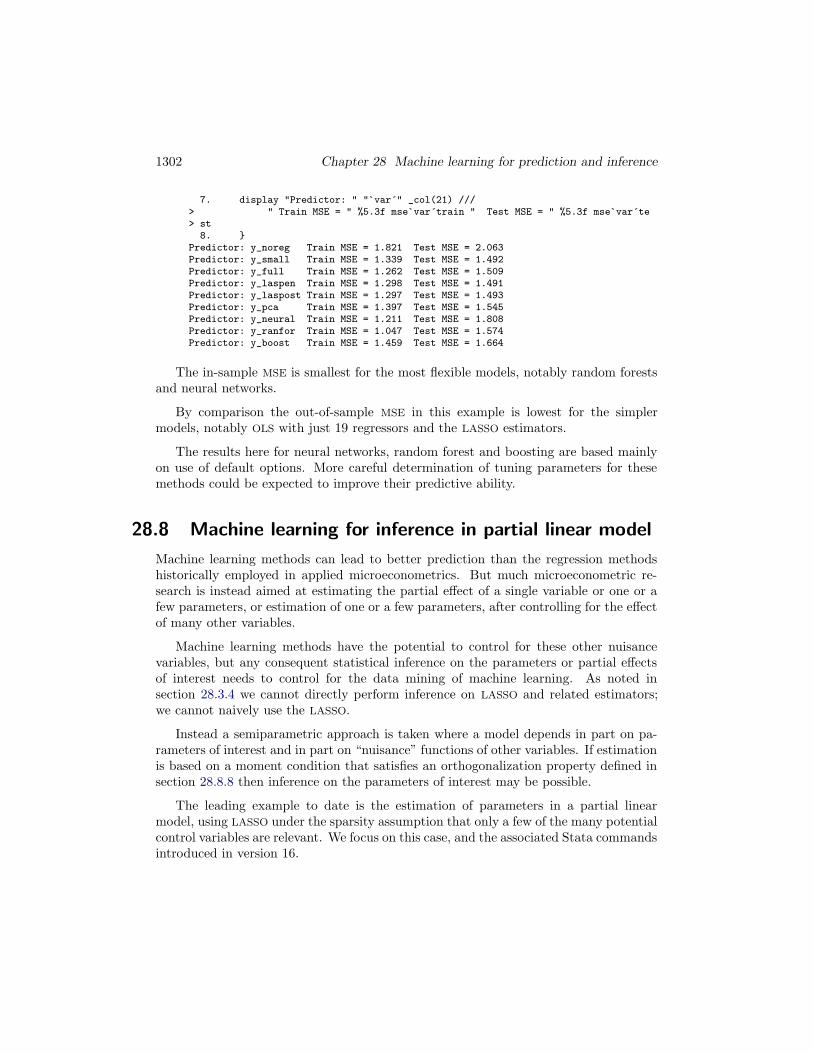
1302 Chapter 28 Machine learning for prediction and inference
7. display "Predictor: " "`var´" _col(21) ///> " Train MSE = " %5.3f mse`var´train " Test MSE = " %5.3f mse`var´te> st
8. }Predictor: y_noreg Train MSE = 1.821 Test MSE = 2.063Predictor: y_small Train MSE = 1.339 Test MSE = 1.492Predictor: y_full Train MSE = 1.262 Test MSE = 1.509Predictor: y_laspen Train MSE = 1.298 Test MSE = 1.491Predictor: y_laspost Train MSE = 1.297 Test MSE = 1.493Predictor: y_pca Train MSE = 1.397 Test MSE = 1.545Predictor: y_neural Train MSE = 1.211 Test MSE = 1.808Predictor: y_ranfor Train MSE = 1.047 Test MSE = 1.574Predictor: y_boost Train MSE = 1.459 Test MSE = 1.664
The in-sample MSE is smallest for the most flexible models, notably random forestsand neural networks.
By comparison the out-of-sample MSE in this example is lowest for the simplermodels, notably OLS with just 19 regressors and the LASSO estimators.
The results here for neural networks, random forest and boosting are based mainlyon use of default options. More careful determination of tuning parameters for thesemethods could be expected to improve their predictive ability.
28.8 Machine learning for inference in partial linear model
Machine learning methods can lead to better prediction than the regression methodshistorically employed in applied microeconometrics. But much microeconometric re-search is instead aimed at estimating the partial effect of a single variable or one or afew parameters, or estimation of one or a few parameters, after controlling for the effectof many other variables.
Machine learning methods have the potential to control for these other nuisancevariables, but any consequent statistical inference on the parameters or partial effectsof interest needs to control for the data mining of machine learning. As noted insection 28.3.4 we cannot directly perform inference on LASSO and related estimators;we cannot naively use the LASSO.
Instead a semiparametric approach is taken where a model depends in part on pa-rameters of interest and in part on “nuisance” functions of other variables. If estimationis based on a moment condition that satisfies an orthogonalization property defined insection 28.8.8 then inference on the parameters of interest may be possible.
The leading example to date is the estimation of parameters in a partial linearmodel, using LASSO under the sparsity assumption that only a few of the many potentialcontrol variables are relevant. We focus on this case, and the associated Stata commandsintroduced in version 16.

28.8.2 Partial linear model application 1303
28.8.1 Partial effects in the partial linear model
We consider a setting where interest lies in measuring the partial effect on y of a changein variable(s) d, controlling for additional control variables.
A partial linear model for linear regression specifies
y = d′α + g(xc) + u (28.9)
where xc denotes selected control variables and g(∙) is a flexible function of xc. Theparameter α can be given a causal interpretation with the selection-on-observables-only assumption that E(u|d,xc) = 0. The goal is to obtain a root-N consistent andasymptotically normal estimator of the partial effect α.
The partial linear model was introduced in section 27.6. There g(∙) was unspecifiedand estimation was by semiparametric methods that required that there be few controlsxc in order to avoid the curse of dimensionality.
LASSO methods due to Belloni, Chernozhukov, and Hansen (2014) and related papersinstead allow for complexity in g(∙) by specifying g(xc) ' x′γ + r, where x consists ofxc and flexible transformations of xc such as polynomials and interactions and r is anapproximation error. The starting point is then that
y = d′α + x′γ + r + u. (28.10)
The LASSO is used in creative ways, detailed in this section, to select a subset ofthe few variables in the high-dimensional x, and to construct regressors in a consequentregression that yields an estimate of α that is root-N consistent and asymptoticallynormal, despite the data mining.
The estimate of α is often called a causal estimate, because if the model is wellspecified with a good set of controls then an assumption of selection on observables onlymay be reasonable. But the method is also applicable without a causal interpretation.
A key assumption, called the sparsity assumption, is that only a small fraction ofthe x variables are relevant. Let p be the number of potential control variables (x)and s be the number of variables in the true model, where p and s may grow withN though at rates considerably less than N . The precise sparsity assumption varieswith the model and estimation method. For the partialing-out estimator, for example,the sparsity assumption is that s/(
√N/ ln p) is small. Additionally, the approximation
error r is assumed to satisfy√
1N
∑Ni=1 r2
i ≤ c√
sN for some c > 0.
In this section we present Stata commands that yield three different LASSO-basedestimators of α.
28.8.2 Partial linear model application
We consider the same example as in section 28.7, with the change that we are interestedin estimating the partial effect of having supplementary health insurance, so d in (28.10)

1304 Chapter 28 Machine learning for prediction and inference
is the single binary variable suppins.
. * Data for inference on suppins example: 5 continuous and 13 binary variables
. qui use mus203mepsmedexp, clear
. keep if ltotexp != .(109 observations deleted)
. global xlist2 income educyr age famsze totchr
. global dlist2 female white hisp marry northe mwest south ///> msa phylim actlim injury priolist hvgg
. global rlist2 c.($xlist2)##c.($xlist2) i.($dlist2) c.($xlist2)#i.($dlist2)
For later comparison we fit by OLS models without and with all the interactionsterms.
. * OLS on small model and full model
. qui regress ltotexp suppins $xlist2 $dlist2, vce(robust)
. estimates store OLSSMALL
. qui regress ltotexp suppins $rlist2, vce(robust)
. estimates store OLSFULL
. estimates table OLSSMALL OLSFULL, keep(suppins) b(%9.4f) se stats(N df_m r2)
Variable OLSSMALL OLSFULL
suppins 0.1706 0.18680.0469 0.0478
N 2955 2955df_m 19.0000 99.0000
r2 0.2682 0.3028
Legend: b/se
In this example there is little change in the coefficient of suppins going from a modelwith 19 regressors to a model with 99 identified regressors, and the gain in R2 is modest.Supplementary insurance is associated with a 17%-19% increase in health spending andthe estimates are highly statistically significant.
28.8.3 Partialing-out estimator
The partialing-out method is obtained in several steps. First, for scalar regressor dperform a LASSO of d on x and obtain a residual ud from OLS regression of d on theselected variables. Second, perform a LASSO of y on x, and obtain a residual uy fromOLS regression of y on the selected variables. Finally, obtain α by OLS regression of uy
on ud.
More generally if there are K key regressors of interest then perform K separateLASSOs of each dk on x, and K subsequent OLS regressions on the selected variables toobtain K separate residuals. The estimates α1,...,αK are obtained by OLS regression ofuy on all K residuals.

28.8.5 Plugin penalty parameter 1305
The partialing-out method is qualitatively similar to the Robinson differencing esti-mator presented in section 27.6 that instead used residuals from kernel regression. Themethod here requires a sparsity assumption that the number of nonzero coefficients inthe true model is small relative to the sample size N and grows at rate no more than√
N . More precisely s/(√
N/ ln p) should be small where p is the number of potentialcontrol variables and s is the number of variables in the true model.
The partialing-out estimator does not extend to nonlinear models. Instead the semioption provides a variation, termed semipartialing-out. First, ud is obtained as forpartialing out. Second, perform a LASSO of y on d and x and obtain a residual uy fromOLS regression of y on d and the selected x variables. Finally, obtain α by IV regressionof uy on d with instruments ud. For further details see [LASSO] poregress methods andformulas.
28.8.4 The poregress command and related commands
Partialing-out LASSO estimates can be obtained using the poregress command thathas syntax
poregress depvar varsofinterest [if ] [in], options
The control variables are specified with option controls([(alwaysvars)] othervars) wherealwaysvars are controls to always be included and othervars are variables selected or de-selected by the lasso. The penalty λ can be determined by a plug-in formula (the defaultoption selection(plugin)), by cross validation (option selection(cv)), by adaptivecross validation (option selection(adaptive)), or by BIC (option selection(bic)).For cross validation methods the rseed(#) option should be used.
The vce(cluster) option provides cluster-robust standard errors. Additionally ifthe selection(cv) or selection(adaptive) options are used then the cross validationdetermines folds at the cluster level and the LASSO objective functions use the averageof within-cluster averages.
The related commands xporegress and dsregress for the linear model; pologit,xpologit, and dslogit for binary outcomes; popoisson, xpopoisson, and dspoisson,for count data; and poivregress and xpoivregress for IV estimation in the linearmodel have similar syntax.
Postestimation commands lassoinfo, lassoknots, cvplot, lassocoef, and coefpathprovide additional information on the fitted models.
28.8.5 Plugin penalty parameter
The default is to use the plug-in formula for λ, developed for use of the LASSO in thecurrent inference setting, rather than for prediction. The plug-in value of λ leads toselection of fewer variables than the other methods. A good exposition of the plug-informula, and relevant references, is given in (Ahrens, Hansen, and Schaffer 2018).

1306 Chapter 28 Machine learning for prediction and inference
For the linear model with independent heteroskedastic errors Stata sets the penaltyparameter λ = c
√NΦ(1 − γ
2p ) where c = 1.1 and γ = 0.1/ ln{max(p,N)}. Severalstudies find that these are good values for c and γ. The individual loadings for each
regressor are κj =√
1N
∑Ni=1(xij εi)2 where xj has been normalized to have mean 0
and variance 1, and εi is a residual obtained by a sequence of first-stage LASSOs thatis detailed in the Stata documentation. These settings are based on linear regressionwith heteroskedastic errors. The option selection(plugin, homoskedastic) is usedfor homoskedastic errors.
If option vce(cluster) is used then the plugin value is the same as for heteroskedas-tic errors.
28.8.6 Partialing-out application
In the current application the partialing-out LASSO selects 21 variables and yields coef-ficient and standard error of suppins quite similar to the OLS results.
. * Partialing-out partial linear model using default plugin lambda
. poregress ltotexp suppins, controls($rlist2)
Estimating lasso for ltotexp using pluginEstimating lasso for suppins using plugin
Partialing-out linear model Number of obs = 2,955Number of controls = 176Number of selected controls = 21Wald chi2(1) = 15.43Prob > chi2 = 0.0001
Robustltotexp Coefficient std. err. z P>|z| [95% conf. interval]
suppins .1839193 .0468223 3.93 0.000 .0921493 .2756892
Note: Chi-squared test is a Wald test of the coefficients of the variablesof interest jointly equal to zero. Lassos select controls for modelestimation. Type lassoinfo to see number of selected variables in eachlasso.
The lassoinfo command lists the number of variables selected by the separateLASSOs for the dependent variable and the single regressor of interest.
. * Lasso information
. lassoinfo
Estimate: activeCommand: poregress
No. ofSelection selected
Variable Model method lambda variables
ltotexp linear plugin .080387 12suppins linear plugin .080387 9

28.8.7 Clustered errors application 1307
In total 21 variables were selected and this exactly equals the sum of variables selectedby the two distinct LASSOs (12 + 9 = 21). So this example is unusual in that the twosets of selected variables are disjoint.
Since the LASSO is applied to more than one variable, several of the post esti-mation commands need to name the variable of interest. For the LASSO for the de-pendent variable relevant commands are lassoknots, for(ltotexp); lassocoef (.,for(ltotexp)); cvplot, for(ltotexp); and coefpath, for(ltotexp). The last twocommands are only applicable if selection is by CV. For variable suppins use insteadfor(suppins).
The partialing-out estimated coefficient of suppins can also be obtained by manuallyperforming each step of the algorithm. We have
. * Partialing out done manually
. qui lasso linear suppins $rlist2, selection(plugin)
. qui predict suppins_lasso, postselection
. qui generate u_suppins = suppins - suppins_lasso
. qui lasso linear ltotexp $rlist2, selection(plugin)
. qui predict ltotexp_lasso, postselection
. qui generate u_ltotexp = ltotexp - ltotexp_lasso
. regress u_ltotexp u_suppins, vce(robust) noconstant noheader
Robustu_ltotexp Coefficient std. err. t P>|t| [95% conf. interval]
u_suppins .1839193 .0468223 3.93 0.000 .0921117 .2757268
The postselection option of the LASSO post-estimation predict command is usedhere as it predicts by OLS regression on the variables selected by the preceding lassocommand.
28.8.7 Clustered errors application
As an example of clustered data we re-estimated the previous model with option vce(clusterage). Using the default plugin method to determine the penalty we obtain
. * Cluster-robust partialing-out partial linear model using default plugin lambda
. poregress ltotexp suppins, controls($rlist2) vce(cluster age)
Estimating lasso for ltotexp using pluginEstimating lasso for suppins using plugin
Partialing-out linear model Number of obs = 2,955Number of controls = 176Number of selected controls = 15Wald chi2(1) = 8.57Prob > chi2 = 0.0034
(Std. err. adjusted for 26 clusters in age)
Robustltotexp Coefficient std. err. z P>|z| [95% conf. interval]
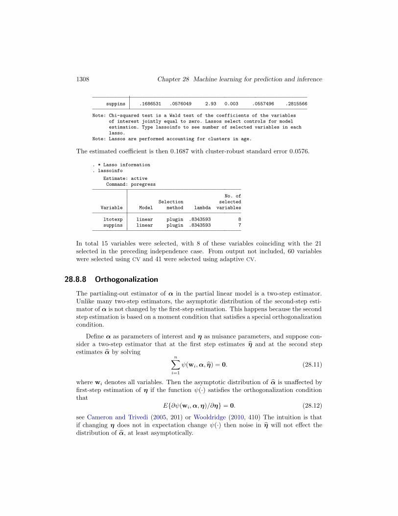
1308 Chapter 28 Machine learning for prediction and inference
suppins .1686531 .0576049 2.93 0.003 .0557496 .2815566
Note: Chi-squared test is a Wald test of the coefficients of the variablesof interest jointly equal to zero. Lassos select controls for modelestimation. Type lassoinfo to see number of selected variables in eachlasso.
Note: Lassos are performed accounting for clusters in age.
The estimated coefficient is then 0.1687 with cluster-robust standard error 0.0576.
. * Lasso information
. lassoinfo
Estimate: activeCommand: poregress
No. ofSelection selected
Variable Model method lambda variables
ltotexp linear plugin .8343593 8suppins linear plugin .8343593 7
In total 15 variables were selected, with 8 of these variables coinciding with the 21selected in the preceding independence case. From output not included, 60 variableswere selected using CV and 41 were selected using adaptive CV.
28.8.8 Orthogonalization
The partialing-out estimator of α in the partial linear model is a two-step estimator.Unlike many two-step estimators, the asymptotic distribution of the second-step esti-mator of α is not changed by the first-step estimation. This happens because the secondstep estimation is based on a moment condition that satisfies a special orthogonalizationcondition.
Define α as parameters of interest and η as nuisance parameters, and suppose con-sider a two-step estimator that at the first step estimates η and at the second stepestimates α by solving
n∑
i=1
ψ(wi, α, η) = 0. (28.11)
where wi denotes all variables. Then the asymptotic distribution of α is unaffected byfirst-step estimation of η if the function ψ(∙) satisfies the orthogonalization conditionthat
E{∂ψ(wi, α, η)/∂η} = 0. (28.12)
see Cameron and Trivedi (2005, 201) or Wooldridge (2010, 410) The intuition is thatif changing η does not in expectation change ψ(∙) then noise in η will not effect thedistribution of α, at least asymptotically.
28.8.9 Cross-fit partialing-out estimator 1309
Now consider the partial linear model y = αd + g(x) + u, and define η1 = E(d|x)and η2 = E(y|x). Estimates η1 (and η2) are obtained by OLS regression of d (andy) on the components of x selected by the LASSO. The partialing-out estimator ofα is then obtained by OLS regression of (y − η2) on (d − η1). This corresponds tosolving the population moment condition E{ψ(w, α, η1, η2)} = 0 where ψ(w, α, η1, η2) =(d − η1){(y − η2) − α(d − η1)}. To see this, recall that the OLS estimator for regressionof y on scalar x solves
∑i xiui =
∑i xi(yi − βxi) = 0 with corresponding population
moment condition E{x(y − βx)} = 0.
The orthogonalization condition (28.12) is satisfied since
E{∂ψ(w, α, η1, η2)/∂η1} = E{−(y − η2) + 2α(d − η1)}
E{∂ψ(w, α, η1, η2)/∂η2} = E{−(d − η1)}
and these expectations equal zero using η1 = E(d|x) and η2 = E(y|x).
The orthogonalization result is extraordinarily powerful. The two-step partialing-outapproach can in principle be applied for any two-step estimator satisfying the orthog-onalization condition, also called Neyman orthogonalization, and in principle the firststep may use machine learners other than the LASSO.
28.8.9 Cross-fit partialing-out estimator
The cross-fit partialing-out estimator is an adaptation of the partialing-out methodthat reduces bias by separating the sample used for LASSO predictions of y and thecomponents of d from the sample used for subsequent estimation of α. The combinationof an orthogonalized moment and cross-fitting is called double machine learning ordebiased machine learning and leads to methods requiring weaker assumptions.
The sample is split into a larger part for the estimation of nuisance components anda smaller part for estimation of the parameters of interest. For simplicity consider scalard and α. The larger sample is used for LASSO of components of d on x (and y on x),and for subsequent post-selection OLS regression of d (and y) on the selected variablesthat yields predictions d = x′πd (and y = x′πy). The smaller sample is then used tocompute residuals ud = d − x′πd and uy = y − x′πy, and subsequent OLS regression ofuy on ud yields estimate α.
This method reduces the complications of data mining by using one sample to obtainthe coefficients for πd and πy and using a separate sample for estimating α. Suchsample splitting leads to a more relaxed sparsity assumption that the number of nonzerocoefficients grows at rate no more than N rather than
√N . More precisely s/(N/ ln p)
should be small where p is the number of potential control variables and s is the numberor variables in the true model.
The preceding algorithm leads to efficiency loss as only part of the original sample isused at the second step to estimate α. So K-fold cross validation is used. For clarity setK = 10. Then for each k = 1, ..., 10 we obtain estimates πd,k and πy.k using 90% of the

1310 Chapter 28 Machine learning for prediction and inference
data and apply these estimates to the remaining 10% of the sample to form residuals ud,k
and uy,k. This yields ten sets of residuals, each using 10% of the sample. The defaultmethod for the xporegress command stacks these residuals to form N residuals ud anduy for the full sample; subsequent OLS regression of uy on ud yields estimate α. Theoption technique(dml1) leads to an alternative estimator α =
∑10k=1 αk where αk is
obtained by regression of uy,k on ud,k in the kth fold.
The xporegress command for cross-fit partialing-out has similar syntax to theporegress command. We obtain
. * Crossfit partialing out (double/debiased) using default plugin
. xporegress ltotexp suppins, controls($rlist2) rseed(10101) nolog
Cross-fit partialing-out Number of obs = 2,955linear model Number of controls = 176
Number of selected controls = 31Number of folds in cross-fit = 10Number of resamples = 1Wald chi2(1) = 15.66Prob > chi2 = 0.0001
Robustltotexp Coefficient std. err. z P>|z| [95% conf. interval]
suppins .1856171 .0469096 3.96 0.000 .093676 .2775582
Note: Chi-squared test is a Wald test of the coefficients of the variablesof interest jointly equal to zero. Lassos select controls for modelestimation. Type lassoinfo to see number of selected variables in eachlasso.
Across the ten folds the number of selected variables ranged from 11 to 14 forltotexp and from 7 to 11 for suppins.
. * Summarize the number of selected variables across the ten folds
. lassoinfo
Estimate: activeCommand: xporegress
No. of selected variablesSelection
Variable Model method min median max
ltotexp linear plugin 11 13 14suppins linear plugin 7 9 11
28.8.10 Double selection estimator
The double selection method performs a LASSO of y on x and separate LASSOs of eachcomponent of d on x. Then α is the coefficient of d from OLS regression of y on d andthe union of all components of x selected by the various LASSOs.
The method has the advantage of simplicity. It requires a similar sparsity assump-

28.9.1 Estimators for exponential conditional mean models 1311
tion to that for the partialing-out estimator, and it is asymptotically equivalent to thepartialing-out estimator.
The dsregress command for double selection estimation has similar syntax to thexporegress command. We obtain
. * Double selection partial linear model using default plugin
. dsregress ltotexp suppins, controls($rlist2)
Estimating lasso for ltotexp using pluginEstimating lasso for suppins using plugin
Double-selection linear model Number of obs = 2,955Number of controls = 176Number of selected controls = 21Wald chi2(1) = 15.30Prob > chi2 = 0.0001
Robustltotexp Coefficient std. err. z P>|z| [95% conf. interval]
suppins .1836224 .0469429 3.91 0.000 .091616 .2756289
Note: Chi-squared test is a Wald test of the coefficients of the variablesof interest jointly equal to zero. Lassos select controls for modelestimation. Type lassoinfo to see number of selected variables in eachlasso.
The coefficient of 0.1836 is very close to the partialing-out estimate of 0.1839.
28.9 Machine learning for inference in other models
Belloni, Chernozhukov, and Wei (2016) extend the methods for the partial linear modelextend to a generalized partial linear model, in which case (28.10) becomes
E(y|d,x) = f(d′α + x′γ) (28.13)
where the function f(∙) is specified. Now the partial effect of a change in d is morecomplicated, being α× f ′(d′α + x′γ). Partial effects in this single index model can beinterpreted as in section 13.7.3. In the special case that f(∙) = exp(∙) the partial effectscan be interpreted as semi-elasticities, and for a logit model with f(z) = ez/(1+ ez) thepartial effects can be interpreted in terms of the log-odds ratio; see section 10.5.
In this section we illustrate these extensions. Additionally we present an extensionof the partial linear model to the case where the regressor(s) d are endogenous.
28.9.1 Estimators for exponential conditional mean models
An exponential conditional mean variant of the partial linear model specifies E(y|d,x) =exp(d′α+x′γ). Because only α is consistently estimated we cannot compute a marginaleffect of a component of d changing but, given the exponential conditional mean speci-fication, we can interpret each component of α as a semi-elasticity; see section 13.7.3.

1312 Chapter 28 Machine learning for prediction and inference
Commands popoisson, xpopoisson and dspoisson extend the methods for thelinear model to the exponential model and have similar syntax to command poregress.
These commands are applicable to any nonnegative dependent variable with expo-nential conditional mean, and are not restricted to count data. So we could apply thismethod with dependent variable totexp, the level of health expenditures.
Nonetheless we illustrate the method for a count, converting totexp to a count thattakes values between 0 and 15. We compare standard Poisson regression estimates withthe partialing-out estimate. We obtain
. * Exponential variant of partial linear model and partialing-out estimator
. generate ycount = floor(sqrt(totexp/500))
. summarize ycount
Variable Obs Mean Std. dev. Min Max
ycount 2,955 2.633841 2.202957 0 15
. qui poisson ycount suppins $xlist2 $dlist2, vce(robust)
. estimates store PSMALL
. qui poisson ycount suppins $rlist2, vce(robust)
. estimates store PFULL
. qui popoisson ycount suppins, controls($rlist2) coef
. estimates store PPOLASSO
. estimates table PSMALL PFULL PPOLASSO, keep(suppins) b(%9.4f) se ///> stats(N df_m k_controls_sel)
Variable PSMALL PFULL PPOLASSO
suppins 0.0602 0.0645 0.06660.0298 0.0299 0.0304
N 2955 2955 2955df_m 19.0000 99.0000
k_controls~l 22.0000
Legend: b/se
The partialing-out estimator with option coef yields α = 0.0666, so private insurance isassociated with 6.66% higher outcome y. The default is to instead report exponentiatedcoefficients such as exp(0.0666) = 1.0689 in which case y is viewed as 1.0689 timeshigher.
28.9.2 Estimators for the logit model
A logistic variant of the partial linear model specifies E(y|d,x) = Λ(d′α + x′γ) whereΛ(z) = ez/(1 + ez). Because only α is consistently estimated we cannot compute amarginal effect of a component of d changing but, given the logistic specification, wecan interpret each component of α as the impact on the log-odds ratio, or equivalentlyeach exponentiated component of α as the impact on the odds ratio; see section 10.5.

28.9.3 Partialing-out for instrumental variables estimation 1313
Commands pologit, xpologit and dslogit extend the methods for the linearmodel to the exponential model and have similar syntax to command poregress.
These commands are applicable to any dependent variable that takes value betweenzero and one. To illustrate the method for a binary variable, we convert totexp to avariable that takes value 1 if expenditures exceed $4,000. The standard logit regressionestimates for the odds ratio (option or) are compared to the partialing-out estimate.We obtain
. * Logit variant of partial linear model and partialing-out estimator
. generate dy = totexp > 4000
. tabulate dy
dy Freq. Percent Cum.
0 1,661 56.21 56.211 1,294 43.79 100.00
Total 2,955 100.00
. qui logit dy suppins $xlist2 $dlist2, or vce(robust)
. estimates store LSMALL
. qui logit dy suppins $rlist2, or vce(robust)
. estimates store LFULL
. qui dslogit dy suppins, controls($rlist2) coef
. estimates store LPOLLASSO
. estimates table LSMALL LFULL LPOLLASSO, keep(suppins) b(%9.4f) se ///> stats(N df_m k_controls_sel)
Variable LSMALL LFULL LPOLLASSO
suppins 0.2498 0.2792 0.26800.0898 0.0936 0.0892
N 2955 2955 2955df_m 19.0000 99.0000
k_controls~l 19.0000
Legend: b/se
The partialing-out estimator with default option or yields estimate exp(α) = 0.2680, sothe odds ratio Pr(y = 1|d,x)]/ Pr(y = 0|d,x)] of having medical expenditures exceed-ing $4,000 is 26.8% higher for those with supplementary insurance compared to thosewithout supplementary insurance.
28.9.3 Partialing-out for instrumental variables estimation
For IV estimation the most efficient estimator uses all available instruments accordingto standard asymptotic theory. But in practice this asymptotic theory can fail in typicalsample sizes when there are too many instruments. This many instruments problem canarise when a model is considerably over-identified, with many more instruments thanendogenous regressors. But it can also arise in a just-identified model if there are many

1314 Chapter 28 Machine learning for prediction and inference
controls that lead to a low first-stage F -statistic because the marginal contribution ofthe instrument(s) becomes slight after inclusion of the many controls.
Chernozhukov, Hansen, and Spindler (2015) extend the partialing-out estimator toinstrumental variables estimation of the linear model with selection of a subset of controlvariables from a large number of controls and/or a subset of instruments from a largenumber of instruments.
The poivregress command provides partialing-out estimates of α and δ in themodel
y = d′α + w′δ + x′γ + v (28.14)
where d are endogenous variables, w are exogenous variables to always be included, andx are exogenous control variables that may potentially be included. Additionally thereare instruments z with dim[z] ≥ dim[d].
The poivregress command has syntax
poivregress depvar[exovars
]endovars=instrumvars
[if] [
in]
,
controls([alwaysvars
]othervars
[options
]
For simplicity, consider the case of scalar endogenous regressor d and δ = 0. Thepartialing-out algorithm is the following.
1. Calculate a partialled-out independent variable as the residual uyi from OLS re-gression of y on xy, where xy denotes the selected variables from a LASSO of y onx.
2. Calculate a scalar instrument udi as follows. Perform a LASSO of d on x and z anddenote the selected variables as, respectively, xd and zd. Then obtain a predictiond from OLS regression of d on xd and zd. Then calculate the residual udi andthe coefficients β from OLS regression of d on xd, where xd denotes the selected
variables from a LASSO of d on x.
3. Calculate a partialled out endogenous regressor udi =di − x′di
β).
4. Compute α by IV regression of uyi on udi with udi as the instrument.
As an example we consider a variant of the analysis of Belloni, Chen, Chernozhukov,and Hansen (2012) based on Acemoglu, Johnson, and Robinson (2001). In this examplethe model is just-identified, but there are only 64 observations and 24 potential controlsthat could lead to a weak instrument problem.
The goal is to use a cross-section sample of countries to measure the causal effecton per capita income (logpgp95) of protection against expropriation risk dependent(avexpr). The mortality rate of early settlers (logem4) is used as an instrument foravexpr. The global macro x2list includes 24 possible control variables which includemeasures of country latitude, temperature, humidity, soil types and natural resources.

28.9.3 Partialing-out for instrumental variables estimation 1315
. * Read in Acemoglu-Johnson-Robinson data and define globals
. qui use mus228ajr, clear
. global xlist lat_abst edes1975 avelf temp* humid* steplow deslow ///> stepmid desmid drystep drywint goldm iron silv zinc oilres landlock
. describe logpgp95 avexpr logem4
Variable Storage Display Valuename type format label Variable label
logpgp95 float %9.0g log PPP GDP pc in 1995, World Bankavexpr float %9.0g average protection against
expropriation risklogem4 float %9.0g log settler mortality
. summarize logpgp95 avexpr logem4, sep(0)
Variable Obs Mean Std. dev. Min Max
logpgp95 64 8.062237 1.043359 6.109248 10.21574avexpr 64 6.515625 1.468647 3.5 10logem4 64 4.657031 1.257984 2.145931 7.986165
We use command poivregress with plugin bandwidth for the homoskedastic case.
. * Partialling-out IV using plugin for lambda
. poivregress logpgp95 (avexpr=logem4), controls($xlist) selection(plugin, hom)
Estimating lasso for logpgp95 using pluginEstimating lasso for avexpr using pluginEstimating lasso for pred(avexpr) using plugin
Partialing-out IV linear model Number of obs = 64Number of controls = 24Number of instruments = 1Number of selected controls = 5Number of selected instruments = 1Wald chi2(1) = 8.74Prob > chi2 = 0.0031
Robustlogpgp95 Coefficient std. err. z P>|z| [95% conf. interval]
avexpr .8798503 .2976286 2.96 0.003 .296509 1.463192
Endogenous: avexprNote: Chi-squared test is a Wald test of the coefficients of the variables
of interest jointly equal to zero. Lassos select controls for modelestimation. Type lassoinfo to see number of selected variables in eachlasso.
Only five controls are selected. From postestimation command lassocoef(.,for(avexpr))the first LASSO selected logem4, edes1975 and zinc; from lassocoef(.,for(logpgp95))the second LASSO selected edes1975 and avelf; and from lassocoef(.,for(pred(avexpr)))the third LASSO selected edes1975, avelf, temp2, iron and zinc.
From output not given, when all 24 controls are used the regular IV estimate ofavexpr is 0.713 with standard error 0.147. The reason for the smaller standard error ofregular IV is that regular IV used an additional 19 controls that greatly improved modelfit. At the same time, reducing the number of controls in the first-stage estimation led

1316 Chapter 28 Machine learning for prediction and inference
to more precise estimation of the first-stage coefficient of the instrument logem4.
The following code manually implements the partialing-out IV estimator for thisexample.
. * poivregress estimator in just-identified model obtained manually
. gen y = logpgp95
. gen d = avexpr
. global zlist logem4
. qui lasso linear y $xlist, selection(plugin, hom) // lasso of y on x
. qui predict yhat, postselection
. generate yresid = y - yhat // generate y residual
. qui lasso linear d $xlist $zlist, selection(plugin, hom) // lasso d on x,z
. qui predict dhat, postselection // generate dhat
. qui lasso linear dhat $xlist, selection(plugin, hom) // lasso dhat on x
. predict dhat_hat, postselection(option xb assumed; linear prediction with postselection coefficients)
. generate dhatresid = dhat - dhat_hat // generate dhat residual
. generate dresid = d - dhat_hat // generate d "residual"
. ivregress 2sls yresid (dresid = dhatresid), noconstant vce(robust)
Instrumental variables 2SLS regression Number of obs = 64Wald chi2(1) = .Prob > chi2 = .R-squared = .Root MSE = .81396
Robustyresid Coefficient std. err. z P>|z| [95% conf. interval]
dresid .8798503 .2952943 2.98 0.003 .3010841 1.458617
Instrumented: dresidInstruments: dhatresid
The estimate equals that from poivregress, while the slight difference in the standarderror is due to different degrees of freedom correction.
Care is needed in using the poivregress command as it is possible that the LASSO
of d on x and z may lead to too few instruments being selected, in which case themodel becomes unidentified. Indeed this happened in the current example when thedefault heteroskedastic variant of the plugin value of lambda was used, as then thesingle instrument logem4 in this just-identified example was not selected.
Such selection of too few instruments is even more likely to occur with the cross-fitting xpoivregress command as the variable selection then occurs K times. Theremedy is to use a larger value of the LASSO penalty λ.

28.9.4 Further discussion 1317
28.9.4 Further discussion
The methods illustrated have been restricted to the partial linear model and generalizedpartial linear model using LASSO under the assumption of sparsity. These examples canbe extended to the use of other machine learners and to application in other models.
Farrell (2015) applies the LASSO to the doubly-robust AIPW estimator of ATE fora binary treatment presented in section 24.6.5. The telasso command, introduced inStata 17, implements this estimator. The command syntax, similar to that for teffectscommands, is
telasso ipwra (ovar omvarlist[, omodel om options
])
(tvar tmvarlist[, tmodel tm options
])[if] [
in] [
weight] [
, stat options]
where om options and tm options include options for the LASSO and determination ofthe LASSO penalty parameter in, respectively, the outcome model and the treatmentmodel. The outcome model can be linear, logit, probit or Poisson, the binary treatmentmodel can be logit or probit, and the command can compute ATE, ATET and potentialoutcome means. For details on the implementation of the LASSO see especially the lassocommand in section 28.4.1. The telasso command option vce(cluster clustervar)provides cluster-robust standard errors. It is important to note that in that case theLASSO is one that gives equal weight to each cluster rather than to each observation.
Farrell, Liang, and Misra (2019) establish theory suitable for use of deep nets forcausal inference and provide an application using the AIPW treatment effects estimator.
Many of these methods will use orthogonalized moment conditions, see section 28.8.8,and cross fitting, see section 28.8.9. The paper by Chernozhukov, Chetverikov, Demirer,Duflo, Hansen, Newey, and Robins (2018) provides an excellent overview, theory, andapplications that use a variety of machine learners (LASSO), regression tree, randomforest, boosting, and neural network to estimate ATE and LATE for a binary treatment,and for IV estimation in a partial linear model. The machine learner needs to approxi-mate well the nuisance part of the model. Appropriate assumptions to ensure this willvary with the setting and will not necessarily require a sparsity assumption.
This is an exceptionally active area of current econometric research, and we antici-pate an explosion of new methods that will be implementable in Stata using one’s owncoding, as user-written Stata programs and ultimately in some cases as official Stataprograms.
In a separate important strand of research that is not covered here, Wager and Athey(2018) use random forests to estimate the ATE for a binary treatment for subgroups ofthe population, and to identify groups with the greatest treatment effect. They providenonstandard asymptotic results that yield pointwise confidence intervals. Their methodincludes the use of “honest trees”, qualitatively similar to cross-fitting.

1318 Chapter 28 Machine learning for prediction and inference
28.10 Additional resources
Machine learning methods have only recently been used in microeconometrics. Ref-erences that are written from a statistics perspective include a Masters level text byJames et al. (2013), and more advanced texts by Hastie et al. (2009) and Efron andHastie (2016). Varian (2014) provides an early summary for economists of machinelearning approaches and some of the software packages developed to handle massivedatasets. Mullainathan and Spiess (2017) provide a detailed application of machinelearning methods for prediction in economics, and cite many applications. Athey andImbens (2019) provide a more recent overview.
Initial research on use of machine learning for statistical inference has used theLASSO; see Belloni, Chernozhukov, and Hansen (2014) for an accessible summary andillustration. Drukker (2020) provides a more recent account. Stata 16 introduced com-mands for LASSO and elastic net for both prediction and statistical inference that aredetailed in [LASSO] Stata Lasso Reference Manual.
The user-written lassopack package (Ahrens, Hansen, and Schaffer 2019) overlapsconsiderably with the Stata LASSO commands for prediction. The accompanying articleis well worth reading as it provides details on the background theory. The user-writtenpdslasso and ivlasso commands (Ahrens, Hansen, and Schaffer 2018) overlap consid-erably with the Stata commands for inference in the partial linear model and includesome additional features such as inference with clustered errors.
Other machine learning methods may be used, both for prediction and for statis-tical inference. The important innovation of double/debiased machine learning withorthogonalized moment conditions and cross fitting is presented in Chernozhukov et al.(2018). Wager and Athey (2018) and related articles use random forests to estimateheterogeneous treatment effects.
The user-written pylearn package (Droste 2020) provides Stata functions that im-plement popular python functions for regression trees, random forests, neural networks,adaptive boosting and gradient boosting.
28.11 Exercises
1. Suppose we have a sample of eight observations for which y takes values 1, 2, 3,4, 5, 6, 7, and 8. We wish to predict y using the sample mean. Compute MSE
using all the data. Now suppose we choose as training dataset the first, third,fifth and seventh observations, and the remaining four observations are the testdata. Compute the test MSE. Now suppose we use four-fold CV where the first foldhas the first and fifth observation, the second fold the second and sixth, the thirdfold the third and seventh and the fourth fold the fourth and eighth observation.Compute MSE for each fold. Hence compute CV4 and the standard error of CV4.
2. Repeat the analysis of section 28.4.6 with regressors x1, x2 and x3 augmented bytheir products and cross products, again using rseed(10101). Comment on the

28.11 Exercises 1319
differences between the various estimates.3. Generate a sample of 10,000 observations using the following code.
set obs 10000
set seed 10101
matrix MU = (0,0,0)
scalar rho = 0.95
matrix SIGMA = (1,rho,rho \ rho,1,rho \ rho,rho,1)
drawnorm x1 x2 x3, means(MU) cov(SIGMA)
scalar rho = 0.2
matrix SIGMA = (1, rho, rho \ rho, 1, rho \ rho, rho, 1)
drawnorm x4 x5 x6, means(MU) cov(SIGMA)
generate y = 1 + 2*x1 + 3*x2 + 2*x1*x2 + 2*x4 + 3*x5 + 2*x4*x5 + rnormal(0,10)
The potential regressors are x1-x6 and their products and cross products. Performadaptive LASSO with option rseed(101010) on the full sample, on the first 1,000observations, and on the first 100 observations. Comment on the ability of LASSO
to detect the true model as the sample sizes changes. (This comparison is easierfollowing the example in section 28.4.6.) Similarly perform OLS of y on all potentialregressors. Suppose we select only those regressors that are statistically significantat 5%. Comment on the ability of OLS to detect the true model as the samplesizes changes. (This comparison is simpler using the star option of estimatestable).
4. Perform an analysis with training and test samples qualitatively similar to that insection 28.7 using the same generated data as in section 28.2. Specifically split thedata into a training sample of 30 observations and a test sample of 10 observations,using command
splitsample y, generate(train) split(1 3) values(0 1) rseed(10101)
Use OLS and LASSO with five-fold cross-validation to obtain predictions. In thecase of LASSO obtain predictions from both penalized coefficients and postselectioncoefficients. Which method predicts best in the training sample? Which methodpredicts best in the holdout sample?
5. Use the same data as in section 28.7 but use only the continuous regressors, so theregressor list is c.($xlist)##c.($xlist). Give the same splitsample commandas in question 4 above. Using the training dataset perform 10-fold CV LASSO, adap-tive LASSO, Ridge and elasticnet regression with option rseed(101010). Comparethe coefficients selected and their penalized values, training sample fit and testsample fit across the estimates.
6. Repeat the previous question but using an exponential conditional mean modelrather than a log-linear model. The dependent variable is totexp, the level of ex-penditure, the sample should now include observations with totexp = 0, the lassopoisson and elasticnet poisson commands are used, and selected variables arecompared to Poisson estimates with heteroskedastic-robust standard errors thatare statistically significant at 5%.

1320 Chapter 28 Machine learning for prediction and inference
7. Estimate a partial linear model using the same generated sample as that in ques-tion 3. The single regressor of interest is x1 and the potential controls are allother variables and interactions, including interactions with x1. The list of poten-tial controls can be set up using commands
global xlist2 x2 x3 x4 x5 x6
global x1interact c.x1#c.($xlist2)
global rlist2 $x1interact c.($xlist2)##c.($xlist2)
Use command poregress with default options on the full sample, on the first1,000 observations, and on the first 100 observations. Compare the estimatedcoefficient of x1 to the DGP value as the sample size changes. Comment on thecontrols chosen for y and x1 as the sample size changes. Estimate by OLS themodel with all potential regressors included and compare the coefficient of x1 (andits heteroskedastic-robust standard error) to the poregress estimates. Estimateusing command xporegress with default options and compare to the poregressestimates.
8. Use the same data as in section 28.8, regress ltotexp on suppins and on con-trols that are only the continuous regressors, so the controls regressor list isc.($xlist2)##c.($xlist2). Regress ltotexp on suppins and potential con-trols using commands poregress, xporegress and dsregress with default op-tions, and by OLS. Compare the fitted coefficients and their heteroskedastic-robuststandard errors across these methods.