methodology of evaluation of abrasive tool wear with the use of laser scanning microscopy
TRANSCRIPT

Methodology of Evaluation of Abrasive Tool Wear with the Use of LaserScanning Microscopy
DARIUSZ LIPIŃSKI, WOJCIECH KACALAK, AND ROBERT TOMKOWSKI
Department of Mechanical Engineering, Koszalin University of Technology, Koszalin, Poland
Summary: Grinding is one of the basic precise materialremoval methods. Abrasive and shape wear, as well assmearing of the tools’ active surface handicap theprocessing results. The loss of cutting capacity inabrasive tools or alteration of their shape influencesthe surface quality and precision of the workpiecedimensions and its shape. Evaluation of the abrasive toolsurface is the basic criterion of forecasting the tools’durability and the process results. The applied method oflaser scanning made determination of the surfacecoordinates and subsequently of its geometric featureswith micrometric accuracy possible. Using the informa-tion on the abrasive tool surface geometric structure, amethodology of evaluation of the level of changes ingeometric features of the tool during the grinding processwas developed. Criteria for evaluation of the level ofabrasive grains attritious wear, the degree of smearing ofthe abrasive tool surface and evaluation of the cuttingcapability of the abrasive tools were determined. Thedeveloped method allowed for evaluation of the level ofabrasive tools’ wear, and subsequently formed founda-tions for assessment of the influence of the grindingparameters on the durability of abrasive tools, evaluationof the influence of the parameters of the process ofshaping the abrasive tools’ active surfaces on theirgeometric characteristics and evaluation of the level ofcorrelation between the monitored process parametersand the degree of the abrasive tools’ wear. SCANNING36: 53–63, 2014. © 2013 Wiley Periodicals, Inc.
Key words: grinding, wear, abrasive tools, surfaceanalysis, monitoring
Introduction
Grinding is one of the basic precise material removalmethods. Attritious and shape wear of the abrasive tool,as well as smearing of its active surface handicap thegrinding results. The loss of cutting capacity in abrasivetools or alteration of their primary shape influencesthe surface quality and precision of the workpiecedimensions and its shape. Evaluation of the abrasive toolsurface is therefore the basic criterion in evaluation ofthe workpiece grindability, which, in consequence,influences the durability period of the abrasive tools.
The abrasive tool can be worn out as a result of thefollowing phenomena [Kacalak, ’89; Shaw, ’96]:
� The grains becoming blunt, which is manifested bygradual decrement in the abrasive grains, leading tocreation of wear surfaces on the blades’ apexes.
� Chipping and cracking of grains when the strainsoccurring in the grains exceed the interim or fatigueresistance of the abrasive material.
� The grains being pulled out as a result of exceeding theinterim or fatigue resistance of the bond bridges.
� Smearing of the active surface as a result of welding layerchipswhich are gradually accumulating in the chip space.
The issue of wear of abrasive tools becomes a crucialimportance in case of grinding hard‐to‐machine alloys,widely applied in aviation, defense and medicalindustries due to their durability and resistance to surfacedegradation. Physical and chemical properties of suchalloys hamper their machinability by significantlydecreasing the abrasive tools’ durability.
Increasing the abrasive tools’ durability periodrequires proper selection of grinding parameters andconditions. Selection of grinding parameters and con-ditions is one of the fundamental tasks of systemssupervising grinding processes. Monitoring changes ofthe abrasive tools’ cutting capacity during the grindingprocess forms the basis for the above selection.
Themost often used [Inasaki, ’91; Comes deOlicerira
and Dornfeld, ’94; Mokbel and Maksoud, 2000;
Furutani et al., 2002; Lipiski andKacalak, 2007]method
Contract grant sponsor: The National Science Center in Poland (NCN).
Address for reprints: Dariusz Lipiński, Department of MechanicalEngineering, Koszalin University of Technology, ul. Racławicka 15‐17,75‐620 Koszalin, Poland E‐mail: [email protected]
Received 14 June 2012; revised 7 December 2012; Accepted withrevision 15 February 2013
DOI: 10.1002/sca.21088Published online 16 April 2013 in Wiley Online Library(wileyonlinelibrary.com).
SCANNING VOL. 36, 53–63 (2014)© Wiley Periodicals, Inc.

of evaluating the abrasive tools wear degree are indirect
methods using the correlation of the abrasive tool active
surfaces wear degree and the monitored variables of the
grinding process (i.e., components of the cutting force,
acoustic emission, machining system oscillations, etc).
Determining those correlations entails application ofmeasurement methods that allow for as precise evaluationof the abrasive tool’s wear during the grinding process aspossible, and subsequently relating it to the monitoredsignals. One of the advantages of application of indirectmethods is the possibility to monitor the condition of theabrasive tool during the grinding process.
Another group consists of the direct methods, bothcontact and non‐contact techniques are used in directmeasurements of abrasive tool’s topography.
The realized research [Calabrese and Murray, ’89;Lachance et al., 2004] proves high effectiveness of
evaluation of the abrasive tools surface wear performed
on basis of images obtained using the scanning electron
microscope (SEM). The application of SEM is,
however, of little practical importance mostly due to
the limitations concerning the sizes of the analyzed
surfaces and the difficulties imposed by their application
in automatic evaluation of the abrasive tools condition.
Application of profilometers for measuring the abrasivetool enables the analysis of its topography in 3D system.The conducted research is related both to the influence ofthe parameters of shaping the abrasive tool’s active surfaceon its topography [Xie et al., 2011], as well as evaluationof the tools cutting capacity on basis of analysis of surface
geometrical parameters [Nguyen and Butler, 2008].
At present numerous researchers [Kurada andBradley, ’97; Fan et al., 2002; Su and Tarng, 2006;
Kassim et al., 2007; Nadolny et al., 2011] focus on
visual systems, mostly due to the possibility of using
such systems in fast evaluation of the condition of the
tool directly on the work station. The basis of operation
of such systems are processing and analysis of a signal
that is proportional to the amount of light reflected from
the abrasive tools active surface.
The authors of the work developed a methodology ofevaluation of the abrasive tool’s conditions on basis ofanalysis of the abrasive tool’s measurement results, usingthe scanning system. The applied measurement systemfacilitated measurement of the whole surface of theabrasive tool directly on the work station with micro-metric accuracy. Using information on the abrasive tool’stopography, a method of detecting the flat areas wasoffered; then their statistical features were analyzed andthe level of changes that occurred during the grindingprocess was evaluated.
Methodology of Evaluation of the Degree of theWear of Abrasive Tools
The geometric features of abrasive tools are, on onehand, influenced by their characteristics, i.e. the abrasive
grains size, structure, volume participation of theabrasive tool and the bonding material, as well as itstype, and on the other hand by the process of shaping itsactive surface.
The geometric features of abrasive tools are modifiedduring the grinding process under the influence of theforces and cutting temperature that occur in the cuttingprocess. Modification of the grinding wheel topographyis caused mainly by attritious and fracture wear of theabrasive grains, as well as smearing of its active surfaceby chips [Kacalak, ’89; Shaw, ’96].
Evaluation of the degree of wear of abrasive toolsforms the basis for the monitoring and optimization ofgrinding processes (Fig. 1). It is also the foundation onwhich decisions concerning renewal of the abrasive toolactive surface are made.
In case of production processes the scanning systemsare most often used in digitalization of large objects forthe purpose of comparison and evaluation of the realobject with its model using computer tools. What wasalso used in the work was advanced topometric sensorsystem (ATOS), which allows for fast and easydigitalization of the measured object with high resolutionand local precision.
The system uses the triangulation method in whicheach single point measured in 3D space is registered bytwo different quasi‐triangulating measurement methods.During the measurement, the systems projects thestructural light in the form of bands on the measuredobject. The thus obtained structural image is grabbed bytwo camcorders. It takes a few seconds to perform thesingle measurement.
Fig 1. The diagram illustrating the procedures undertaken inevaluation of the condition of the abrasive tool’s active surface.
54 SCANNING VOL. 36, 1 (2014)

For every single measurement the software checks thecondition of the system calibration, possible dislocationof themeasured object and alteration of the lighting in thesurroundings in order to guarantee precise measurementresults even in relation to nonuniform materials, whichthe abrasive tools are.
The 3D image of the abrasive tool’s surface obtainedas a result of the measurement allows evaluation ofchanges of its surfaces correlated with the condition ofwear of the abrasive tool. The proposed methodologyof evaluation of the degree of wear of abrasive tools andthe degree of smearing of its active surface includes thefollowing steps:
� Measuring the ordinates of the abrasive tool’s Z(x, y).The measurement is performed using non‐contactmethods whose precision is a few (5–7) times higherthan the size of the abrasive grain.
� Detection of flat areas for the assumed flatness criteria.The detection is performed using the logical filterevaluating the degree of changeability of the ordinatesof the analysis window central point and the adjacentpoints. The threshold value used in the above detectionis related to the characteristic geometrical featuresof abrasive grains. This allows for application of detec-tion methods in analysis of the surfaces of abrasivetools with various characteristics.
� Determining the statistical parameters of the areasdeclared flat. The determined parameters allow forevaluation of the changes in the abrasive tool’scondition over time.
� Classification of the flat areas into the followingcategories: abrasions of the abrasive grains summits,smearing of the active surface.
� Determining the synthetic indicators evaluating theabrasive tool’s wear. The synthetic indicators facilitatemaking the decision concerning renewal of theabrasive tool’s surface by the systems of monitoringand optimizing the grinding processes. They can alsoform the basis for creating dependencies between themonitored variables of the grinding process (power,force, oscillations, acoustic emission) and the condi-tion of the abrasive tool’s surface, and as a resultbetween the dimensional and shape precision of thecreated elements and the geometric features of theworkpiece surface.
Measuring the Abrasive Tool’s Active Surface
A 3D scanner by GOM company named ATOS III SO(Fig. 2) was used for acquisition of the dimensionalimage of the grinding wheel’s active surface. The scanneruses structural light for measuring [Gupta et al., 2012,Sansoni et al., ’99]. The measured object is illuminated
by a series of blue light lines, thus creating a net of
specific thickness, i.e. the socalled raster, on the
measured surface. The distance between the lines in
the raster defines the number of data obtained during a
single measurement. The minimal range between the
lines used for measuring the abrasive tool for the CCD
3,296 � 2,572 matrix was 11.59 mm. The lines that
created the raster on the surface yield to the shape of the
measured object and are deformed.
Standards in the form of lined images are registered bytwo cameras, creating phase dislocations on basis of thesinusoidal distribution of intensity on the CCD detector.Independent 3D coordinates are automatically calculatedfor each pixel on basis of optical transformationequations.
As a result of the above operations a cloud of points isobtained and the number of points is mostly dependent
Fig 2. The diagram illustrated the measurement procedure of theabrasive tool’s active surface with use the laser scanning.
D. Lipiński et al.: Methodology of evaluation of abrasive tool wear with the use of laser scanning microscopy 55

on the camera resolution. The geometric configuration ofthe detector and the distortion parameters are calibratedusing photogrammetric methods.
The single images registered in this way are limitedin relation to the size of the field observed through thelenses (lenses with fields sizes 170 mm � 130 mm� 130 mmand38 mm � 29 mm � 15 mmwereused).
In the measurement of abrasive surface the problemare the dropouts, which result from the tool’s micro-fragments being blotted out and from the occurrence ofdeep intergranular spaces. In order to minimize thenumber of dropouts, a few (in this case 10)measurementsare made under various angles on the measured object’slocation in relation to the sensor.
This procedure allows for elimination of problem thatresult from the tool’s microfragments being blotted out.The deep intergranular space still remain partially non‐measured. In case of analysis of the abrasive tool activesurface wear condition, it is not an essential issues.Changes resulting from the wear process are observed inthe grain edges zone on the grinding tool’s active surface.
An exemplary result of the measurement of anabrasive tool is presented in Figure 3.
As a result of the measurements, after filtering off theabrasive tool’s shape, a matrix of Z ordinates describingthe abrasive tool’s geometric structure was obtained. Thematrix underwent subsequent transformations to deter-mine parameters for evaluation of the abrasive tool’swear during the grinding process. The first step of furtheranalysis was detection of the flat areas.
Detection of the Flat Areas
Flat areas present on the surface of the abrasive toolresult mainly from the attritious wear of grains andsmearing the grinding wheel’s surface with materialremoved during the grinding process. The proposedpattern of detecting the flat areas is presented in Figure 4.
The flat areas were detected using the slide analysiswindow sized 3 � 3. The difference of ordinates of theabrasive tool of the central element and the adjacentelements was determined in the analysis window. Four‐and eight‐field adjacency matrix H was adopted (Fig. 5).
For the thus defined analysis window and theadjacency term, transformations compliant with thebelow logical filter were performed on the mediummatrix Z’:
Z0 ðx; yÞ ¼ 1 if maxðGHÞ < e
0 elsewhere
�ð1Þ
where GH, vector of absolute differences g of surfaceordinates between the central element of the analysiswindow and the adjacent field, e, threshold value.
If the primary value of the analysis window laid on theborder of the data region, the data region was supple-mented with values in accordance with the mirror imagerule.
As a result, the medium matrix Z0 2 {0, 1} wasobtained. Next the binary medium matrix Z0 underwentdilation:
Z0 � S ¼ fpþ q : p 2 Z
0 ^ q 2 Sg ð2Þ
where:�, Minkowski’s total, S, structural element (S4 orS8) compliant with the previously defined adjacency (theprimary point was underlined):
Fig 3. Results of measurement of the abrasive tool’s surfaceusing the laser scanning method: (a) frontal surface of the abrasivetool; (b) a section of the tool’s surface.
Fig 4. The diagram for illustration of methodology of detectionof flat areas for a four‐field adjacency.
56 SCANNING VOL. 36, 1 (2014)

S4 ¼0 1 0
1 1 1
0 1 0
264
375;
S8 ¼1 1 1
1 1 1
1 1 1
264
375
ð3Þ
As a result of the above transformations, binaryresultant matrix Z″ is obtained, whose size is consistentwith the matrix of ordinates of the measured Z tool. Thevalue 1 of element of Z″ matrix means that thecorresponding element of Z matrix belongs to the areaidentified as flat (Fig. 4).
The flat areas on an abrasive tool’s surface can beproperly detected when the right threshold value e is set.The threshold value e was made dependent on thegeometric parameters of the grains. From the perspectiveof the abrasive tool’s cutting capacity, height h and widths of the abrasive grain over the bond surface weredeclared important (Fig. 6).
In accordance with the above assumptions, thethreshold value was formulated with the followingdependence:
e ¼ tanðkaÞlx ð4Þ
a ¼ arctan2h
s
� �ð5Þ
where lx, the horizontal distance between the primarypoint of analysis window and the adjacent field (verticaldiscretization step), k, coefficient determining themaximum slope angle of the flat surface in relation tothe slope angle of the abrasive grain a.
Obviously the minimal k coefficient value, and as aconsequence e, is dependent on the maximal verticalresolution of the measurement device.
Geometrical Features of the Flat Areas
Detection of the flat areas allowed for differentiationof objects on the abrasive tool that were interesting fromthe perspective of evaluation of the degree of abrasivetool’s wear. The determination of the statistical featuresof the flat areas was preceded by segmentation thatconsisted in separating particular (flat) objects from thebinary image and then by labeling.
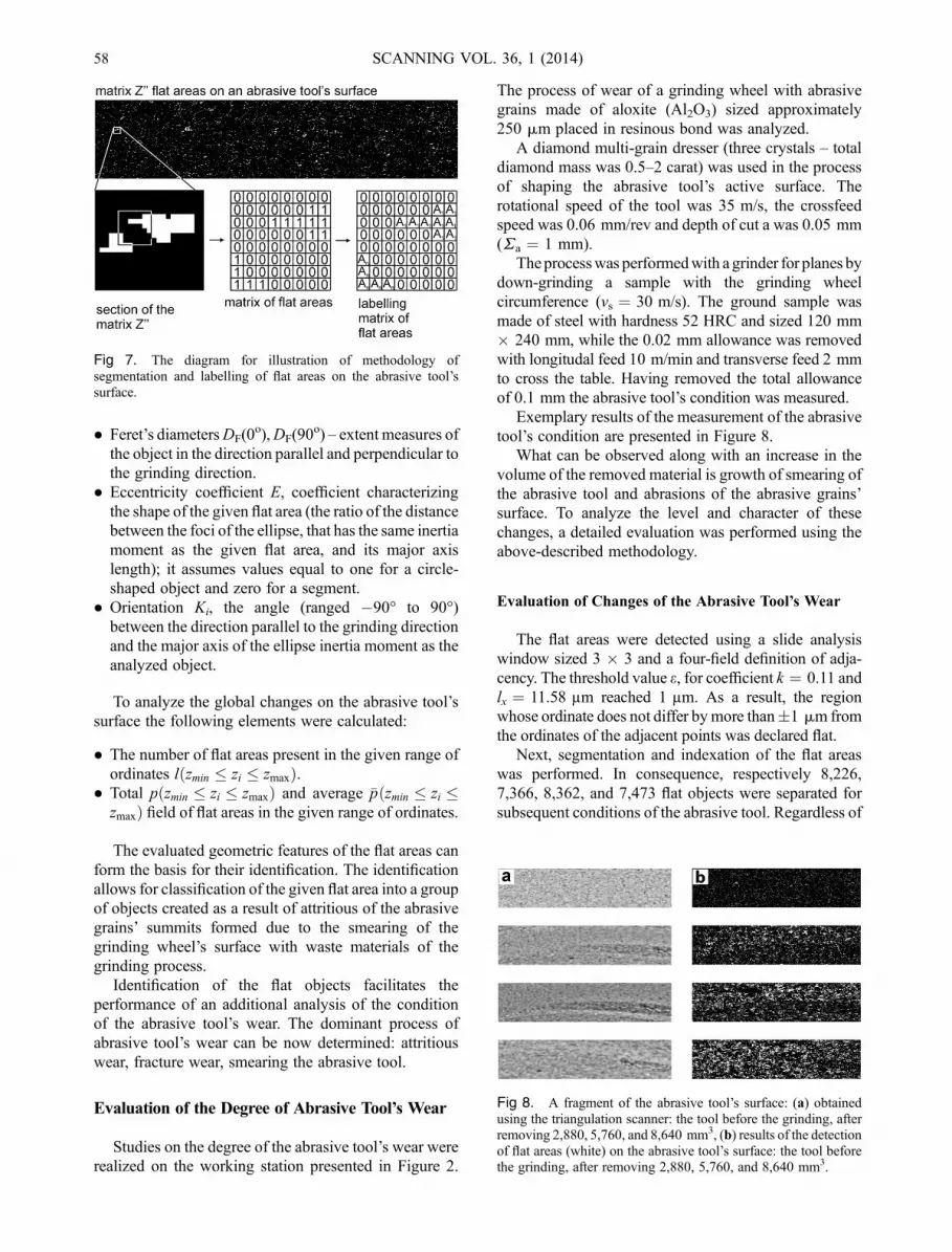
Segmentation through expansion of the region wasapplied. In this method the binary image is viewed lineby line until an element with value 1 is found. The value 1of any element in binary matrix Z″ means that thecorresponding element of matrix Z belongs to the areaidentified as flat. After the element is found it is labeledand then it is checked whether the adjacent elements areof the same value. If this is the case they are added, withthe same labels, to the created object, causing itsexpansion (Fig. 7).
Segmentation and labeling of the flat objects on theabrasive tool’s surface allowed for determination of thegeometric parameters and their statistical features.
The following local features of the flat areas weredetermined:
� field Pi, the number of elements belonging to the flatarea.
Fig 5. Graphic presentation of the rules of analysis of theabrasive tool’s surface in the vicinity of: (a) four fields, (b) eightfields.
kαkαgx
gy
gy-1
gx-1
lxlx
lxlx
h
s/2 sα
a) b) kα
kα
Fig 6. The diagram for illustration of evaluating the slope angle of the abrasive grain a (a), and threshold value e (b).
D. Lipiński et al.: Methodology of evaluation of abrasive tool wear with the use of laser scanning microscopy 57
� Feret’s diametersDF(0o),DF(90
o) – extent measures ofthe object in the direction parallel and perpendicular tothe grinding direction.
� Eccentricity coefficient E, coefficient characterizingthe shape of the given flat area (the ratio of the distancebetween the foci of the ellipse, that has the same inertiamoment as the given flat area, and its major axislength); it assumes values equal to one for a circle‐shaped object and zero for a segment.
� Orientation Ki, the angle (ranged �90° to 90°)between the direction parallel to the grinding directionand the major axis of the ellipse inertia moment as theanalyzed object.
To analyze the global changes on the abrasive tool’ssurface the following elements were calculated:
� The number of flat areas present in the given range ofordinates lðzmin � zi � zmaxÞ.
� Total pðzmin � zi � zmaxÞ and average �pðzmin � zi �zmaxÞ field of flat areas in the given range of ordinates.
The evaluated geometric features of the flat areas canform the basis for their identification. The identificationallows for classification of the given flat area into a groupof objects created as a result of attritious of the abrasivegrains’ summits formed due to the smearing of thegrinding wheel’s surface with waste materials of thegrinding process.
Identification of the flat objects facilitates theperformance of an additional analysis of the conditionof the abrasive tool’s wear. The dominant process ofabrasive tool’s wear can be now determined: attritiouswear, fracture wear, smearing the abrasive tool.
Evaluation of the Degree of Abrasive Tool’s Wear
Studies on the degree of the abrasive tool’s wear wererealized on the working station presented in Figure 2.
The process of wear of a grinding wheel with abrasivegrains made of aloxite (Al2O3) sized approximately250 mm placed in resinous bond was analyzed.
A diamond multi‐grain dresser (three crystals – totaldiamond mass was 0.5–2 carat) was used in the processof shaping the abrasive tool’s active surface. Therotational speed of the tool was 35 m/s, the crossfeedspeed was 0.06 mm/rev and depth of cut a was 0.05 mm(Sa ¼ 1 mm).
Theprocesswas performedwith a grinder for planes bydown‐grinding a sample with the grinding wheelcircumference (vs ¼ 30 m/s). The ground sample wasmade of steel with hardness 52 HRC and sized 120 mm� 240 mm, while the 0.02 mm allowance was removedwith longitudal feed 10 m/min and transverse feed 2 mmto cross the table. Having removed the total allowanceof 0.1 mm the abrasive tool’s condition was measured.
Exemplary results of the measurement of the abrasivetool’s condition are presented in Figure 8.
What can be observed along with an increase in thevolume of the removed material is growth of smearing ofthe abrasive tool and abrasions of the abrasive grains’surface. To analyze the level and character of thesechanges, a detailed evaluation was performed using theabove‐described methodology.
Evaluation of Changes of the Abrasive Tool’s Wear
The flat areas were detected using a slide analysiswindow sized 3 � 3 and a four‐field definition of adja-cency. The threshold value e, for coefficient k ¼ 0.11 andlx ¼ 11.58 µm reached 1 µm. As a result, the regionwhose ordinate does not differ bymore than�1 mm fromthe ordinates of the adjacent points was declared flat.
Next, segmentation and indexation of the flat areaswas performed. In consequence, respectively 8,226,7,366, 8,362, and 7,473 flat objects were separated forsubsequent conditions of the abrasive tool. Regardless of
Fig 7. The diagram for illustration of methodology ofsegmentation and labelling of flat areas on the abrasive tool’ssurface.
Fig 8. A fragment of the abrasive tool’s surface: (a) obtainedusing the triangulation scanner: the tool before the grinding, afterremoving 2,880, 5,760, and 8,640 mm3, (b) results of the detectionof flat areas (white) on the abrasive tool’s surface: the tool beforethe grinding, after removing 2,880, 5,760, and 8,640 mm3.
58 SCANNING VOL. 36, 1 (2014)

the condition of the tool (volume of the removedmaterial), the number of flat objects in the given range ofordinates did not increase.
To perform a detailed analysis of the changeability ofthe geometric features of the flat areas, the range ofabrasive tool’s ordinates was divided into N ¼ 25ranges. Flat areas included in each of the range ofordinates were identified.
However, as the working time of the tool increased,the value of the generic field of flat areas in the givenfield of ordinates grew. The generic field of the flat areaswas respectively 4.73%, 13.02%, 17.67%, and 22.17%of the abrasive tool’s surface. These changesare particularly visible in relation to the averagefield of the flat areas (Fig. 9). What is visible is anincrease of the average of the flat areas in the whole
−0.1 −0.05 0 0.05 0.1 0.150
200
400th
e av
erag
e fie
ld o
f the
flat
are
as, [
poin
ts]
z, [mm]−0.1 −0.05 0 0.05 0.1 0.15
0
200
400
z, [mm]
the
aver
age
field
of t
he fl
at a
reas
, [po
ints
]
−0.1 −0.05 0 0.05 0.1 0.150
200
400
z, [mm]−0.1 −0.05 0 0.05 0.1 0.15
0
200
400
z, [mm]
b
d
a
c
Fig 9. Average field of flat areas in the given range of ordinates: (a) the tool before the grinding, (b) after removing 2,880 mm3, (c)5,760 mm3, and (d) 8,640 mm3.
−0.1 −0.05 0 0.05 0.1 0.150
0.1
0.2
0.3
z, [mm]
DF
(0o ),
[mm
]
−0.1 −0.05 0 0.05 0.1 0.150
0.1
0.2
0.3
z, [mm]
DF
(0o ),
[mm
]
−0.1 −0.05 0 0.05 0.1 0.150
0.1
0.2
0.3
z, [mm]
DF
(0o ),
[mm
]
−0.1 −0.05 0 0.05 0.1 0.150
0.1
0.2
0.3
z, [mm]
DF
(0o ),
[mm
]
b
dc
a
Fig 10. Measurements of the average length of the flat areas in the given ordinates’ range in the parallel direction to the tool’s movement inrelation to the object: (a) the tool before the machining, (b) after removing 2,880 mm3, (c) 5,760 mm3, and (d) 8,640 mm3.
D. Lipiński et al.: Methodology of evaluation of abrasive tool wear with the use of laser scanning microscopy 59

range of ordinates, which, as the grinding time passed,started to increase both in the bottom and the top range ofthe ordinates.
An increase of the flat areas’ field occurs as a result ofa growth of the region’s extent both in the parallelDF(0
o)and perpendicular direction DF(90
o) in relation to thetool’s movement direction (Figs. 10 and 11).
Moreover, as the volume of the removed materialincreases, the centricity and directivity of the flat areasgrew (Figs. 12 and 13).
A detailed analysis of the average field of the flat areasshows that the main reason for changes in the analyzedabrasive tool’s condition is smearing of the intergranularspaces. The presence of smearings leads to an increase in
−0.1 −0.05 0 0.05 0.1 0.150
0.02
0.04
0.06
0.08
z, [mm]
DF
(90o ),
[mm
]
−0.1 −0.05 0 0.05 0.1 0.150
0.02
0.04
0.06
0.08
z, [mm]
DF
(90o ),
[mm
]
−0.1 −0.05 0 0.05 0.1 0.150
0.02
0.04
0.06
0.08
z, [mm]
DF
(90o ),
[mm
]
−0.1 −0.05 0 0.05 0.1 0.150
0.02
0.04
0.06
0.08
z, [mm]D
F(9
0o ), [m
m]
a b
dc
Fig 11. Measurements of the average length of the flat areas in the given ordinates’ range in the perpendicular direction to the tool’smovement in relation to the object: (a) the tool before the grinding, (b) after removing 2,880 mm3, (c) 5,760 mm3, and (d) 8,640 mm3.
0 0.2 0.4 0.6 0.8 10
1000
2000
3000
eccentricity
num
ber
of fi
elds
0 0.2 0.4 0.6 0.8 10
500
1000
1500
2000
2500
eccentricity
num
ber
of fi
elds
0 0.2 0.4 0.6 0.8 10
1000
2000
3000
eccentricity
num
ber
of fi
elds
0 0.2 0.4 0.6 0.8 10
1000
2000
3000
eccentricity
num
ber
of fi
elds
a b
dc
Fig 12. Distribution of the eccentricity coefficients of the flat areas: (a) the tool before the grinding, (b) after removing 2,880 mm3,(c) 5,760 mm3, and (d) 8,640 mm3.
60 SCANNING VOL. 36, 1 (2014)

the average flat areas’ field in the bottom range of theabrasive tool’s coefficients. An increase in this region isgreater than the increase of the average field in the toprange of the coordinates caused mainly by abrasions ofthe active abrasive grains.
The determined geometric sizes of the flat areasformed the basis for classification of the flat areas into the
following categories: attritious wear, smearing theintergranular spaces. The following features served asthe foundation for identification of the flat objects typicalof abrasions of the grains’ summits:
� Extent measures of the flat object DF(0o), DF(90
o) indirections parallel and perpendicular to the grinding
−100 −50 0 50 1000
1000
2000
3000
4000
5000
angle, [degrees]
num
ber
of fi
elds
−100 −50 0 50 1000
1000
2000
3000
4000
5000
angle, [degrees]
num
ber
of fi
elds
−100 −50 0 50 1000
1000
2000
3000
4000
5000
angle, [degrees]
num
ber
of fi
elds
−100 −50 0 50 1000
1000
2000
3000
4000
5000
angle, [degrees]nu
mbe
r of
fiel
ds
a b
dc
Fig 13. The distribution of directivity coefficients for flat areas: (a) the tool before the grinding, (b) after removing 2,880 mm3,(c) 5,760 mm3, and (d) 8,640 mm3.
−0.1 −0.05 0 0.05 0.1 0.150
0.01
0.02
0.03
0.04
z, [mm]
surf
ace
area
, [%
]
−0.1 −0.05 0 0.05 0.1 0.150
0.01
0.02
0.03
0.04
z, [mm]
surf
ace
area
, [%
]
−0.1 −0.05 0 0.05 0.1 0.150
0.01
0.02
0.03
0.04
z, [mm]
surf
ace
area
, [%
]
−0.1 −0.05 0 0.05 0.1 0.150
0.01
0.02
0.03
0.04
z, [mm]
surf
ace
area
, [%
]
a b
dc
Fig 14. Condition of the abrasion of abrasive grains in the given range of abrasive tool’s coefficients: (a) the tool before the grinding,(b) after removing 2,880 mm3, (c) 5,760 mm3, and (d) 8,640 mm3.
D. Lipiński et al.: Methodology of evaluation of abrasive tool wear with the use of laser scanning microscopy 61

direction no bigger than the maximal border abrasivegrain’s dimensions.
� Location of the flat object in relation to the maximalordinate of the abrasive tool no less than the doublevalue of the allowance.
� Eccentricity coefficient E – coefficient characterizingthe object shape in the range from 0 to 0.2, dependingon the abrasive tool’s shape.
The results of identification of the flat areas allowedfor detailed evaluation of the type of abrasive tool’s wear(Figs. 14 and 15).
The above analysis confirms the above‐formulatedstatements assuming that the main reason for changes ofthe analyzed abrasive tool’s condition are smearings ofits surface by waste materials of the grinding process.Smearing of the intergranular spaces results in progres-sive fracture wear of the abrasive grains and a decrease inthe abrasive tool’s cutting capacity.
Summary and Conclusions
Application of laser scanning systems in productionprocesses to digitalization of small objects with nonuni-form structure expands the range of their possibleapplications as an element of monitoring system ofgrinding processes.
The suggested methodology, based on analysis ofchanges in geometrical features of flat surfaces allowsfor fast evaluation of the tool condition (from a few to adozen seconds, depending on the computer’s power),
which combined with short time (a few seconds long)necessary for making one measurement, allows forapplication of such systems in on‐line mode.
The developed methodology of evaluation of thedegree of abrasive tool’s wear facilitates assessment ofchanges of the abrasive tool’s surface that occur duringthe grinding process. What was also developed werefoundations for identification of flat areas that allow fordetailed analysis of the forms of abrasive tool’s wear.
Flat areas occurring on the abrasive tool’s surfacewere used as basis for analysis of its condition. Anescalation of the abrasive tool’s wear entails an increaseof the surfaces of the flat areas. A detailed analysis ofchanges in the geometric features of the flat areas in thewhole range of ordinates of the abrasive tool facilitateddetermination of the dominant form of the abrasive tool’swear and offers the basis for evaluation of its cuttingcapacity.
The basic problem with assessing the condition of anabrasive tool’s wear is developing a set of parameters forevaluation of their geometric structure, forming acomplementary set, that guarantee high efficacy identi-fying the character of the abrasive tool’s wear andeasiness of the grade interpretation.
Development of synthetic indexes of evaluation of thecondition of an abrasive tool’s wear will allow forinclusion of the system of direct evaluation of theabrasive tool’s condition into the grinding processesmonitoring, optimization, and supervision systems. Italso forms the basis for developing models of correla-tions of grinding parameters, measured process featuresand monitoring the quality of the grinding process.
−0.1 −0.05 0 0.05 0.1 0.150
5
10
z, [mm]
surf
ace
area
, [%
]
−0.1 −0.05 0 0.05 0.1 0.150
5
10
z, [mm]
surf
ace
area
, [%
]
−0.1 −0.05 0 0.05 0.1 0.150
5
10
z, [mm]
surf
ace
area
, [%
]
−0.1 −0.05 0 0.05 0.1 0.150
2
4
6
8
10
12
z, [mm]
surf
ace
area
, [%
]
a b
dc
Fig 15. Smearings’ surface in the given range of ordinates of the abrasive tool : (a) the tool before the grinding, (b) after removing2,880 mm3, (c) 5,760 mm3, and (d) 8,640 mm3.
62 SCANNING VOL. 36, 1 (2014)

References
Calabrese SJ, Murray SF. 1989. SEM observations of slidingbehavior ofAl203 andCBNagainst steel. Scanning 11:231–236.
Comes de Olicerira JF, Dornfeld DA. 1994. Dimensionalcharacterization of grinding wheel surface through acousticemission. Annals CIRP 43:291–294.
Fan KC, Lee MZ, Mou JI. 2002. On‐line non‐contact system forgrinding wheel wear measurement. Int J Adv Manuf Technol19:14–22.
Furutani K, Ohguro N, Hieu NT, Nakamura T. 2002. Inprocessmeasurement of topography change of grinding wheelby hydrodynamic pressure. Int J Mach Tools Manuf42:1447–1453.
Gupta M, Agrawal A, Veeraraghavan A, Narasimhan SG. 2012. Apractical approach to 3D scanning in the presence ofinterreflections, subsurface scattering and defocus. Int JComput Vis 102:33–55.
Inasaki I. 1991. Monitoring and optimization of internal grindingprocess. Annals CIRP 41:359–362.
Kacalak W. 1989. Zużycie i trwałość ściernic diamentowych wprocesie zautomatyzowanego szlifowania elementów ceram-icznych, Monographs, Wydział Mechaniczny PolitechnikaKoszalińska (in Polish).
Kassim AA,MannanMA, ZhuM. 2007. Texture analysis methodsfor tool condition monitoring. J Image Vision Comput25:1080–1090.
Kurada S, Bradley C. 1997. A review of machine vision sensors fortool condition monitoring. J. Comput Ind 34:55–72.
Lachance S, Bauer R, Warkentin A. 2004. Application of regiongrowing method to evaluate the surface condition of grindingwheels. Int J Mach Tools Manuf 44:823–829.
Lipiński D, Kacalak W. 2007. Assessment of the accuracy of theprocess of ceramics grinding with the use of fuzzy interfer-ence, adaptive and natural computing algorithms, lecture notesin computer science. Berlin: Springer‐Verlag. p 596–603.
Mokbel AA, Maksoud TM. 2000. Monitoring of the condition ofdiamond grinding wheels using acoustic emission technique. JMater Process Technol 101:292–297.
Nadolny K, KapłonekW, Valicek J. 2011. Pneumatic method usedfor fast non‐contact measurements of axial contour of grindingwheel active surface. Measure Autom Monit 57:1071–1074.
Nguyen AT, Butler DL. 2008. Correlation of grinding wheeltopography and grinding performance: A study from aviewpoint of three‐dimensional surface characterization. IntJ Materals Process Technol 208:14–23.
Sansoni G, Carocci M, Rodella R. 1999. Three‐dimensional visionbased on a combination of gray‐code and phase‐shift lightprojection: Analysis and compensation of the systematicerrors. Appl Opt 38:6565–6573.
Shaw MC. 1996. Principles of abrasive processing. New York:Oxford University Press.
Su JC, Tarng YS. 2006. Measuring wear of the grinding wheelusing machine vision. Int J Adv Manuf Technol 31:50–60.
Xie J, Wei F, Zheng JH, Tamaki J, Kubo A. 2011. 3D laserinvestigation on micron‐scale grain protrusion topography oftruncated diamond grinding wheel for precision grindingperformance. Int J Mach Tools Manuf 51:411–419.
D. Lipiński et al.: Methodology of evaluation of abrasive tool wear with the use of laser scanning microscopy 63