Methodology For Evaluating Flying

Qualities From Desktop Simulator

Daniel Lindqvist

Space Engineering, master's level

2020

Luleå University of Technology

Department of Computer Science, Electrical and Space Engineering

Industrial SupervisorsPeter Jason, Marcus Back - SAAB

ExaminerJoel Sundstrom - Lulea University of Technology

Abstract

A modern fighter aircraft has an advanced flight control system which highly augmentsthe control inputs from the pilot. To verify a new iteration of the control system is a timeconsuming and expensive task. It is desired to find qualities that is not satisfactory to thepilot as early as possible in the verification process to reduce the cost for design changes.

The primary objective of this thesis is to develop methods that can be used for automaticalevaluation of aircraft flying qualities from the data provided by a desktop simulator. A desk-top simulator is cheap to use compared to flight tests and tests with a pilot in a simulator.Only fighter aircraft in the precision flight phase are studied however the methods developedcould easily be extended to include other types of aircraft and other phases of flight.

To evaluate the flying qualities two sets of criteria are used the MIL-F-8785C standardand the Gibson criteria. The MIL-F-8785C standard uses a second order linear system toevaluate the aircraft’s flying qualities. The linear system is estimated from the nonlineardata and evaluated against the MIL-F-8785C standard. The Gibson criteria studies the timeand frequency domain directly and are designed to work with highly augmented aircraft.The set of Gibson criteria used in this thesis primary evaluates data from the time domainhowever one criterion from the frequency domain is studied.

The methods developed to evaluate the flying qualities from the MIL-F-8785C standardonly works for a small part of the flight envelope furthermore they show a large differencefor what is considered acceptable flying qualities. Because of this the methods developed forthe MIL-F-8785C standard are considered not to be suited for evaluating flying qualities forhighly augmented aircraft. The methods developed to evaluate the flying qualities againstthe Gibson criteria works for a large part of the flight and also show a high accuracy. Thismakes the methods suited for evaluation of the flying qualities.

1

Acknowledgements

I would first and foremost like to thank my industrial supervisors Peter Jason and MarcusBack. Their advice and guidance have been invaluable to me while also giving me greatfreedom in selecting topics to research further. I would also like to thank my examiner JoelSundstrom at Lulea University of Technology for giving feedback and have been a greathelp with the logistics.

Another thanks goes to my colleges at SAAB who have made me feel very welcome andalso provided feedback to this thesis.

Finally but not least I would like to thank my friends at Lulea University of Technol-ogy who have made my time there something I will always look back on with a smile on myface.

2

Contents

1 Introduction 51.1 Motivation for research . . . . . . . . . . . . . . . . . . . . . . . . . . . . . . . 51.2 Goals . . . . . . . . . . . . . . . . . . . . . . . . . . . . . . . . . . . . . . . . 61.3 Scope . . . . . . . . . . . . . . . . . . . . . . . . . . . . . . . . . . . . . . . . 6

2 Theory 72.1 Handling and flying qualities . . . . . . . . . . . . . . . . . . . . . . . . . . . 72.2 Flying qualities rating system . . . . . . . . . . . . . . . . . . . . . . . . . . . 72.3 Aircraft longitudinal dynamics . . . . . . . . . . . . . . . . . . . . . . . . . . 82.4 Criteria for aircraft FQ . . . . . . . . . . . . . . . . . . . . . . . . . . . . . . . 10

2.4.1 MIL-F-8785C . . . . . . . . . . . . . . . . . . . . . . . . . . . . . . . . 102.4.2 Gibson criteria . . . . . . . . . . . . . . . . . . . . . . . . . . . . . . . 13

3 Method 173.1 Linear estimation and the MIL-F-8785C standard . . . . . . . . . . . . . . . . 173.2 Time domain and Gibson criteria . . . . . . . . . . . . . . . . . . . . . . . . . 17

3.2.1 Time to max q . . . . . . . . . . . . . . . . . . . . . . . . . . . . . . . 173.2.2 Finding steady state . . . . . . . . . . . . . . . . . . . . . . . . . . . . 183.2.3 The dropback criterion . . . . . . . . . . . . . . . . . . . . . . . . . . . 213.2.4 Flight path delay . . . . . . . . . . . . . . . . . . . . . . . . . . . . . . 233.2.5 Fluctuation in q . . . . . . . . . . . . . . . . . . . . . . . . . . . . . . 24

3.3 Bandwidth criterion . . . . . . . . . . . . . . . . . . . . . . . . . . . . . . . . 253.3.1 Evaluating LTI properties . . . . . . . . . . . . . . . . . . . . . . . . . 253.3.2 Calculating gain and phase . . . . . . . . . . . . . . . . . . . . . . . . 263.3.3 Calculating bandwidth and phase delay . . . . . . . . . . . . . . . . . 26

4 Validation of Methods 284.1 Linear estimation and the MIL-F-8785C standard . . . . . . . . . . . . . . . . 284.2 Time to max q . . . . . . . . . . . . . . . . . . . . . . . . . . . . . . . . . . . 304.3 Finding steady state . . . . . . . . . . . . . . . . . . . . . . . . . . . . . . . . 314.4 The dropback criterion . . . . . . . . . . . . . . . . . . . . . . . . . . . . . . . 334.5 Flight path delay . . . . . . . . . . . . . . . . . . . . . . . . . . . . . . . . . . 374.6 Fluctuations in q . . . . . . . . . . . . . . . . . . . . . . . . . . . . . . . . . . 394.7 Bandwidth criterion . . . . . . . . . . . . . . . . . . . . . . . . . . . . . . . . 39

5 Conclusion and Discussion 405.1 Linear estimation . . . . . . . . . . . . . . . . . . . . . . . . . . . . . . . . . . 405.2 Time to max q . . . . . . . . . . . . . . . . . . . . . . . . . . . . . . . . . . . 405.3 Finding steady state . . . . . . . . . . . . . . . . . . . . . . . . . . . . . . . . 405.4 The dropback criterion . . . . . . . . . . . . . . . . . . . . . . . . . . . . . . . 415.5 Flight path delay . . . . . . . . . . . . . . . . . . . . . . . . . . . . . . . . . . 415.6 Fluctuations in q . . . . . . . . . . . . . . . . . . . . . . . . . . . . . . . . . . 415.7 Bandwidth criterion . . . . . . . . . . . . . . . . . . . . . . . . . . . . . . . . 415.8 Concluding remarks . . . . . . . . . . . . . . . . . . . . . . . . . . . . . . . . 41

6 Future Research 42

7 Bibliography 43

3

Glossary

List of acronyms

DB Dropback

FBW Fly by wire

FCS Flight control system

FQ Flying qualities

FQL Flying quality level

HQ Handling qualities

LTI Linear time-invariant system

MSE Mean square error

PIO Pilot induced oscillations

List of symbols

Symbol Description Unit

α Angle of attack [rad]θ Pitch angle [rad]γ Flight path angle [rad]q Pitch rate [rad/s]nz Load factor -V Velocity [m/s]ωSP Short period natural frequency [rad/s]ζSP Dampening coefficient -kq Scaling constant -Tθ2 Time constant [s]η(s) Stick input in Laplace domain -CAP Control anticipation parameter [rad/s2/g]ϕ Phase [rad]τp Phase delay [s]ω Input frequency [rad/s]tss Time at steady state [s]

4

1 Introduction

When the Wright brothers first took to the skies with a powered aircraft in 1903 little wasunderstood about what makes an aircraft handle well. The flyer, as the aircraft was called,was in fact unstable and difficult to control. Aircraft performance saw a significant improve-ment during the First World War, but if the designs had good or bad handling qualities wasoften a matter of luck. No real understanding existed on what parameters were importantfor the pilot. During the 1930s an understanding on what aspects of the aircraft’s behaviorhad an influence on pilot opinion started to develop. During the 1940s and the Second WorldWar a standard set of criteria for good handling qualities began to develop. These criteriawere refined and expanded during the 1950s and 1960s with use of simulations and in flightexperiments.

Until the late 1960s there had always existed a direct mechanical link between the pilotand the control surfaces of the aircraft. Some aircraft used hydraulic actuators, feel springsor some other sort of augmentation to help the pilot control the aircraft but there still existeda mechanical link between the control stick and the control surfaces. This changed with theintroduction of fly by wire (FBW) aircraft where the pilot’s stick inputs were interpretedby a computer which then controls the actuators connected to the control surfaces. Thedynamics of the aircraft could be highly augmented by the FBW control system. An aero-dynamically unstable aircraft could be made stable with augmentation resulting in a moremaneuverable aircraft. Carefree maneuvering could be implemented which means that thepilot could use full stick defections in the entire flight envelope without the fear of exceedingthe maximum structural load or stalling the aircraft. The system is also lighter than me-chanical control systems and requires less maintenance. However, the augmentation of theFBW system has led to unforeseen problems. One of the most serious problems with earlyFBW aircraft is the high order pilot induced oscillation (PIO) which has led to a numberof accidents. Both the SAAB Gripen and the Lockheed YF-22 have suffered crashes due toPIO [2, page 12-18]. The handling problems of early FBW aircraft have also lead to newmethods for higher order aircraft and a wider understanding of what qualities give goodpilot feedback.

There exists no exact mathematical expression that can predict the pilot’s opinion on flyingqualities. One pilot may like the aircraft’s handling characteristics and the other may not.However there exist some qualities that most pilot will find satisfactory. In order to capturewhat qualities have correlation with pilot opinion different criteria have been developed. Inthis thesis two sets of criteria are studied in more detail, the MIL-F-8785C [10] standardand Gibson [4] criteria.

1.1 Motivation for research

To design a well functioning flight control system (FCS) that also has satisfactory handlingcharacteristics is a complex task. Testing the FCS in the real aircraft is expensive, time con-suming and requires much planing. In addition tests are sensitive to external factors, e.g.wind. If there exists a problem with the FCS, testing can also become dangerous quickly.Therefore it is important to test and verify the FCS in simulators before it is used in thereal aircraft.

A modern fighter aircraft has a large flight envelope and the flight characteristics changedepending on flight condition. To cover the entire flight envelope in a simulator with a pilotis both time consuming and expensive. This together with the multiple external loads amodern fighter aircraft can carry that also affect the handling makes it desirable to optimizethe process. A desktop simulator can quickly do a simulation of a specific maneuver and

5

replicate it over the entire flight envelope and for different aircraft configurations.

To manually look at the vast amount of simulated data for each point in the flight en-velope would be prone to error and time consuming. Therefore it is desired to developmethods that automatically study the nonlinear data and can find problematic areas of theflight envelope. If problematic areas of the flight envelope can be identified in advance morefocus can be put there during the pilot evaluation in the simulator.

1.2 Goals

This master’s thesis studies a generic delta canard fighter aircraft, however, most of thedeveloped methods can be applied to other types of aircraft as well. The goals of thismaster’s thesis are

• Investigate the relevance of some criteria in the MIL-F-8785C standard and Gibsoncriteria,

• develop methods to determine if the criteria are fulfilled or not from nonlinear data,and

• validate the methods to find where in the flight envelope they are relevant to use.

1.3 Scope

To ensure that the scope of this thesis does not becomes too large some limitations are set.These are:

• Only flying qualities in the longitudinal axis are studied i.e pure inputs with no feed-back from the pilot in the aircraft’s pitch axis, and

• only a light fighter in precision flight phase is studied.

6

2 Theory

This chapter will explain how a pilot evaluates an aircraft’s handling qualities, how anaircraft reacts to a stick input and also criteria that are used to evaluate an aircraft’s flyingqualities.

2.1 Handling and flying qualities

When a pilot is flying he or she usually have a task to preform, a task like holding a constantaltitude, landing or even air to air combat. The pilot sees, feels and hears what the aircraftis doing and can then change the input to the aircraft to complete the task. The nature towhich the aircraft responds to the pilot feedback is called handling qualities (HQ). The easeof which the task can be preformed is directly related to the aircraft’s HQ.

To better understand the dynamics of the aircraft inputs can be given with no pilot inthe control loop. The nature to which the aircraft responds to these inputs is called theaircraft’s flying qualities (FQ). Inputs can be step, pulse or a series of more complex inputs.Both FQ and HQ are dependent on each other and it is important to look at both whenevaluating a control system. Figure 1 shows the difference between FQ an HQ.

Figure 1: Illustration showing the difference between FQ and HQ.

2.2 Flying qualities rating system

The FQ are rated on a three-level scale where level 1 is the best result. The flying qualitylevel (FQL) is supposed to predict the pilot opinion on aircraft HQ. The FQL is determineddepending on how the aircraft preforms while evaluating a certain criterion. The definitionof level 1, 2 and 3 FQ is the following:

• Level 1 Flying qualities clearly adequate for the mission flight phase.

• Level 2 Flying qualities adequate to accomplish the mission flight phase, but someincrease in pilot workload or degradation in mission effectiveness, or both, exists.

• Level 3 Flying qualities such that the airplane can be controlled safely, but pilotworkload is excessive or mission effectiveness is inadequate, or both.

There exists prior research showing a correlation between FQL and pilot opinion [8, 9].

7

2.3 Aircraft longitudinal dynamics

When the pilot pulls the stick back or pushes the stick forward the aircraft changes attitudein pitch. How the aircraft responds to that input will determine the pilot’s opinion on theaircraft longitudinal FQ or HQ. It is therefore important to understand how an aircraftchanges its attitude.

The parameters that are primarily used to describe the aircraft’s longitudinal attitude isshown in Figure 2. A brief explanation on each parameter follows here:

• Pitch angle (θ) is the angle between the horizon and aircraft cord line. The cordline is a line running from the wings trailing edge to its leading edge and is essentiallywhere the aircraft’s nose is pointing.

• Pitch rate (q) is the rate the aircraft changes pitch angle, q = θ.

• Flight path angle (γ) is the angle between the horizon and the air-stream. It canalso be described as the angle between the horizon and the aircraft’s velocity vector.

• Angle of attack (α) is the angle between the air-stream and the wings cord line.

• Load factor (nz) is the ratio of lift (L) of the aircraft to its weight (W ), nz = L/W .It is dimensionless however, it is traditionally referred to as g.

Figure 2: Illustration of angles in pitch

From these parameters the equation

α = θ − γ (1)

is known per definition. When α increases the lift produced by the wing also increases untilα reaches a critical value and the wing stalls [6]. Stall will not be studied in this thesishowever it is important to know that an increase in α increases the lift prior to stall.

An aircraft movement through the air can be described as a rigid body with six degreesof freedom, three rotations and three translations. The equations of motion are complexand gives no direct way of measuring the FQ. Instead a second order equivalent system isoften used. The transfer function for q is defined as [1]

q(s) =kq(s+ (1/Tθ2))

s2 + 2ζSPωSP s+ ω2SP

η(s) (2)

where kq is a scaling constant, Tθ2 is the short period time constant, ζSP is the dampen-ing coefficient, ωSP is the short period natural frequency and η(s) is the stick input in theLaplace domain. This model assumes a constant speed and that the stick movement is theonly input to the system.

Figure 3 shows a linear model of a generic aircraft’s response to a pulse input. To pro-duce a pulse input the pilot pulls on the stick and holds it there for a specified amount oftime before releasing it. When the pilot pulls the stick the aircraft responds in the followingway:

8

1. The nose of the aircraft comes up, θ and q start to increase.

2. Due to the inertia of the aircraft θ is initially increasing faster than γ, resulting in anincrease in α.

3. An increase in α also increases the lift.

4. A increase in lift causes γ to increase faster until it increases with the same rate as θ.The time elapsed before γ shows a noticeable response is called the flight path delay(tγ).

5. The aircraft reaches a steady state where the difference between γ and θ is constantand the aircraft have a constant value of q.

The dynamics of how the aircraft responds when the stick is released works much in thesame way:

1. θ stops to increase and settles at a smaller value from which the stick is released. Thedifference in θ between when the stick is released and the value it settles at is calleddropback (DB).

2. Due to the inertia of the aircraft γ continues to increase, this leads to a decreaseddifference between γ and θ meaning α decreases.

3. A decrease in α also causes the lift to decrease.

4. Which in turn causes γ to stop increasing.

5. The aircraft reaches a steady state where the difference between γ and θ is constantand q = 0.

From this response some parameters can obtained. These parameters are shown in Figure3. From top to bottom the parameters are:

• qmax, maximum pitch acceleration.

• qmax, maximum pitch rate.

• qss, pitch rate at steady state.

• tss, time at which steady state have been reached.

• tq, time to reach maximum pitch rate.

• DB, Dropback.

• tγ , Flight path delay.

This thesis studies data from a nonlinear desktop simulator, however these linear conceptswill be extended to the nonlinear data.

9

Figure 3: Linear model of a generic aircraft response to a pulse input.

2.4 Criteria for aircraft FQ

To evaluate an aircraft’s FQ several different standards and criteria exists. In this thesistwo sets of criteria are used, the MIL-F-8785C standard [10] and Gibson criteria [4]. Bothare used widely in the industry. The two sets of criteria use a different philosophy. TheMIL-F-8785C standard uses a second order equivalent system. The Gibson criteria studythe time and frequency domains directly. The following two sections describe the criteria inmore detail.

2.4.1 MIL-F-8785C

The first iteration of the MIL-F-8785 standard appeared in 1948 and has since then beenimproved up until 1980 when the latest version of the standard was released, MIL-F-8785C.The standard is developed by the US military. The standard categorizes aircraft, flightphases and FQL, this way of categorizing is also used by other standards. Aircraft aredivided in to the following four classes:

• Class I Small light aircraft.

• Class II Medium weight, low to medium maneuverability aircraft.

• Class III Large heavy, low to medium maneuverability aircraft.

• Class IV High maneuverability aircraft.

The different phases of flight are divided into the following categories.

• Category A Flight phases that require rapid maneuvering, precision tracking, orprecise flight-path control e.g. formation flying or mid-air refueling.

• Category B Flight phases that are normally accomplished using gradual maneuversand without precision tracking e.g. climb, cruise or decent.

10

• Category C Terminal Flight Phases are normally accomplished using gradual ma-neuvers and usually require accurate flight-path control e.g. approach or landing.

How the standard defines FQL can be seen in Section 2.2. The standard has different re-quirements for longitudinal and lateral flying qualities but the important requirements forthis thesis are those for the longitudinal short-period characteristics. The long-period os-cillations that occur when the aircraft stabilizes airspeed is not relevant for FBW aircrafttherefore those criteria are not used.

To determine the FQL, limits are set on the short-period undamped natural frequency ωSPand the short-period damping ratio ζSP [10, page 13-14]. Both ωSP and ζSP are calculatedfrom a second order equivalent system like (2) on page 8. The limits for ζSP are shown inTable 1 and are constant regardless of where in the flight envelope the aircraft is. The limitsfor ωSP are shown in Figure 4 and depends on nz/α which is a constant for each point inthe flight envelope and assuming constant speed. The value of nz/α can be calculated fromthe second order equivalent system as

nz/α =V

gTθ2(3)

where g is the gravitational acceleration and V is the velocity. A full derivation can be foundin [1, page 243].

Category A and C Flight phases Category B Flight phasesLevel Min Max Min Max1 0.35 1.3 0.3 2.002 0.25 2.00 0.2 2.003 0.15 - 0.15 -

Table 1: Limits for ζSP

11

Figure 4: Short period frequency requirements for category A flight phase.

Figure ?? shows regions of ωSP and ζSP that produces FQL 1,2 and 3. The control antici-pation parameter (CAP ) is introduced on the y axis. CAP is a parameter used to estimatethe pilot’s ability to predict the flight path response and is defined as the ratio between qmaxand nz at steady state. CAP can also be approximated from a linear system as

CAP =qmaxnz≈ ω2

SP

nz/α(4)

where nz/α is calculated from (3). A full derivation can be found in [4, page 99].

12

Figure 5: Short period requirements for category A flight phase.

2.4.2 Gibson criteria

With the introduction of FBW aircraft the dynamics of the aircraft are highly augmentedby the FCS. Because of this the second order assumption used in the MIL-F-8785C standardis often not valid. There may exist several poles and zeros close to the frequency that isassociated to the aircraft’s unaugmented short period dynamics. This made it necessary todevelop new criteria for higher order aircraft.

John Campbell Gibson worked with FCS from 1956 to his retirement in 1992, having workedon the FCS of aircraft like the, Lightning Jaguar Tornado and Eurofighter. From the 1970she started to research FQ and HQ of highly augmented aircraft. This gave rise to a widerange of new criteria called the Gibson criteria. Gibson set specific goals for the criteria.These are lifted directly from [4, page 95].

• They would have to be expressed in both frequency and time domains as neither onits own give sufficiently complete design definition.

• They should in particular define limits on the shape of the response in these domainswithout reference to numerical mode parameters or mathematical formula, so that theycould be applied to any controlled response however high its order, and independentof type of model available, i.e. parametric or non-parametric.

• They should not depend on the assumption of any explicit pilot model parameters, asit is very difficult to apply these reliably.

• They should enable the control design engineer to synthesis directly the handlingcharacteristics desired for specific task as perceived visually or physically by pilots.

• Their meaning should be equally clear to both pilots and control design engineers.

The focus in this report are on the criteria specified in the time domain however someevaluation have been done in the frequency domain.

Time to max q A value of tq too small can cause the aircraft to feel abrupt and too largevalue can cause the aircraft to feel sluggish. The time to the maximum peak seen in Figure3 should be between 0.3 and 0.9 seconds [4, page 106].

13

Dropback criterion If the pilots stick input would be purely proportional to q the re-sulting θ response would be a straight line with a constant slope. The nose of the aircraftwould also stop immediately when the stick is released. This is expressed as the K/s linein the Laplace domain. A K/s like response is associated with comments like ”the nosefollows the stick” [4, page 62]. The K/s line can be seen in Figure 7. Due to the dynamicsexplained in Section 2.3 a pure K/s response is not possible. The nose of the aircraft willdropback or continue to rise for a small amount of time (negative dropback) when the stickis released. Excessive dropback can result in pilot complaints of abruptness and lack ofprecision in pitch control [7, page 41]. A higher dropback also result in less tolerance for apitch rate overshoot, qmax−qss. The relationship between dropback and pitch rate overshotcan be seen in in Figure 6. The maximum pitch rate and the dropback are normalized withqss so the criterion does not depend where in the flight envelope the aircraft is.

Assuming a linear model the dropback and dropback ratio can be calculated from botha step and a pulse input. The dynamics when the stick is pulled back is the same as whenthe stick is released resulting in the same dropback as seen in Figure 7.

Figure 6: Dropback criterion

14

Figure 7: How to calculate the dropback from both a pulse and a step input.

Flight path delay When the pilot pulls the stick the nose of the aircraft is raised. How-ever, there exist a time delay before the flight path γ, shows a noticeable response. This isthe flight path delay or tγ and is defined in Figure 3. Some tasks require precise flight pathcontrol like, air to air refueling or landing. It is therefore important that the flight path doesnot lag behind the nose too much. tγ should not exceed 1.5 seconds in the landing approachtask and 1 second for precision control task [8, page 27].

Bandwidth criterion The only criterion from the frequency domain studied in this reportis the bandwidth criterion [4, page 129]. The bandwidth criterion is a measurement on thespeed of the response the pilot can expect when tracking with rapid inputs. It is alsoa measurement on how tightly the pilot can close the loop before stability is threatened.The bandwidth is defined as the lower of the two frequencies ωBWphase

and ωBWgainwhere

ωBWphaseis the frequency with 45◦ phase margin and ωBWgain

is the frequency with 6 dBgain margin. These frequencies are shown in Figure 8. The bandwidth criterion consist oftwo parameters, the bandwidth and the phase delay τp. The phase delay is calculated with

τp =−(φ2ω(−180) + 180)

114.6ω−180=

∆◦

114.6ω−180(5)

where ω−180 is the frequency at −180◦ phase and φ2ω(−180) is the phase at 2ω−180. Thecalculated values for τp and ωBW are plotted in the graph shown in Figure 9.

15

Figure 8: Bode plot showing gain and phase margin.

(a) Category C. (b) Category A.

Figure 9: Bandwidth criterion

16

3 Method

Due to the fundamental differences between the MIL-F-8785C standard and the Gibsoncriteria it is necessary to develop two different methods to determine if the criteria arefulfilled or not.

3.1 Linear estimation and the MIL-F-8785C standard

To estimate a second order equivalent system the MATLAB function tfest [11] is used. Thefunction uses the instrument variable method that is described further in [5]. The functionoutputs an estimated transfer function with the help of the following inputs:

• Simulated data,

• input to the system and

• numbers of poles and numbers of zeros in the transfer function.

The simulated data is provided from the desktop simulator. The parameter estimated is qfrom t = 0 to where steady state is found. The method to find steady state is describedin Section 3.2.2. The input to the system (the stick input) is a step function. The stepinput is provided by a pilot model in the simulator. The input is not a perfect step, ittakes a couple of samples before the stick reaches maximum deflection. It is important toestimate the transfer function with the input from the simulator and not a perfect step in-put provided by MATLAB. If a perfect step is used the estimation will become less accurate.

The estimated transfer function have the same form as (2) on page 8. The values of ζSP andωSP are taken directly from the estimated transfer function. The values of CAP and nz/αare calculated with (3) and (4). The values are evaluated against the MIL-8785C standardto determine FQL 1, 2 or 3.

How good the second order estimation is vary over the flight envelope. To find where thelinear approximation is adequate, the Mean Square Error (MSE) between the approximationand the data from the simulation is used. The MSE is calculated with

MSE =1

n

n∑i=1

(Yi − Yi)2 (6)

where n is number of samples and (Yi− Yi) is the error between the two signals. The linearestimation is assumed to be better when the MSE is low.

3.2 Time domain and Gibson criteria

Compared to the MIL-F-8785C standard the Gibson criteria focus on what can be takendirectly from the time and frequency domain. The concepts explained in Section 2.4.2 arederived from a linear system. To use the Gibson criteria methods have to be developed toapply linear concepts to the nonlinear data.

3.2.1 Time to max q

As described in Section 2.4.2 on page 13, the time to max q from stick input should bebetween 0.3 and 0.9 seconds. The linear response shown in Figure 3, shows a smoothresponse to a step input with a clear peak for q. This is not always the case with thesimulated data, sometimes the global value of q is higher than the local peak directly afterthe step input. There also exists cases where two or more peaks exist. Figure 10a showsan example where the local maximum value of q directly after the stick input is lower than

17

the global maxima. Also two peaks exist in quick succession after the control input. Thetime to max q is a measurement of the aircraft’s initial response therefore the first peak isof interest. Furthermore, looking at q in Figure 10b it is clear that the initial accelerationis over at tq. To calculate tq , q is used. First the index iq is found with

iq = min(i) : q = 0, t > tstick. (7)

(a) (b)

Figure 10: tq is calculated with (7) and marked with a red circle

Figure 11a shows no clear peak for q. The value of q is equal to zero at the dashed line.Using only the previous described method would result in a value of tq that is too high.However, looking at q in Figure 11b the initial acceleration is for the most part at the localminimum after the initial stick input. To capture this behavior the index iq is found with

iq = i : q = 0, t > tqmax (8)

tq is then calculated as

tq = min(t(iq), t(iq)). (9)

(a) (b)

Figure 11: tq is calculated with (8) and marked with a red circle

3.2.2 Finding steady state

Steady state is where the derivative of a signal is equal to 0 until next input. Looking atthe nonlinear data no steady state exists. However, Figure 12 shows a clear steady state

18

like region in q. Finding where the simulated data reaches steady state like conditions isa critical part of evaluating the performance of the aircraft. The linear approximation,dropback criteria and flight path delay all rely on finding steady state. The two methodsdescribed in the two following paragraphs are used for finding steady state in both q andγ. However, these methods could be used for any signal x as long as it resembles a secondorder linear system.

Figure 12: Steady state like region marked with red.

Moving time window method The first method for finding tss looks for x that isbelow a specified limit for all samples of a specified time window. Figure 13 shows two timewindows. One marked as red where all samples are not below the specified limit. The othertime window is marked as green and all samples are below the specified limit and steadystate is found. The value x should be beneath is the average value of |x| for all samples, N .The time window Wn of length L is defined as

Wn =

{1, i = n, n+ 1, ...n+ L− 1

0, Otherwise(10)

Using this time window tss is calculated as

nss = min(n) : Wn · |x(i)| < ν1

N

N∑i=1

|x(I)| ∀ i ∈ [0, N ]. (11)

tss now becomes

tss = t(nss). (12)

ν is a scale factor on the mean value defining the limit q must be below. The values of νand L are determined by visually inspecting several graphs to find which values work best.

19

Figure 13: Illustration of moving time window method.

Moving boundary method The second method for finding tss looks for small changesin x over a short period of time. If a specified amount of samples from the signal lays withinthe boundary steady state is found. Figure 14 shows two sets of boundaries. Some sampleslay outside of the red boundary therefore no steady state exits at that point. All samplesare within the green boundary therefore steady state exits at that point. The boundary isset as a percentage to the maximum peak of x, xmax. Because xss ≈ 0 the ratio betweenxmax and xss is approximately the same for all cases. nss is calculates as

nss = min(n) :

∣∣∣∣ x(i)− x(i1)

xmax

∣∣∣∣ < ξ ∀ i ∈ [n,N + L− 1] (13)

where ξ is a percentage of xmax. The values of ξ and L are determined through trial anderror. The dashed lines in Figure 14 show the value nss must be in between. This is doneto make sure that xss is close to zero.

20

Figure 14: Illustration of moving boundary method.

3.2.3 The dropback criterion

The dropback criterion and the two ways of calculating the dropback ratio is describedin section 2.4.2 on page 14. The dropback criterion needs two parameters, qmax/qss andDB/qss.

DB/qss from pulse input The value of θ when the stick is released is recorded as θrealese.Steady state is search for after the stick is released. The dropback now becomes: DB =θstick − θss,q. Figure 15 shows an example of how the dropback is calculated. The dropbackratio is now calculated with

DB

qss=θrealese − θss,q

qss. (14)

21

Figure 15: Calculating DB/qss from a pulse input.

DB/qss from step input First the tangent of θ is calculated at tss,q. The dropback rationow becomes the time between where the tangent intercepts θ0 and tstick. Figure 16 showsthe dropback ratio marked with red. The tangent has the slope qss. The tangent interceptsthe y axis at θtangent. The dropback ratio now becomes

DB

qss= tstick −

θtangent − θ0qss

(15)

where tstick is the time at the stick input.

Figure 16: Calculating DB/qss from a step input.

Sensitivity of result The result is plotted with the dropback ratio on the x-axis andqmax/qss on the y-axis. Figure 17 shows one data point as a blue dot plotted in the drop-

22

back criterion. To determine how sensitive the result is a small time step ∆T is added orsubtracted from the original tss,q. The path the data point takes is shown as a dashed redline for tss −∆T and a solid red line for tss + ∆T . A result that is more sensitive to smallerrors in tss shows a longer path. The length of the path is measured between the twoextreme points. The distance to the boundary of acceptable dropback ratio is measured asavailable q overshoot as shown as a black line in Figure 17.

Figure 17: Example on how a data point moves in the dropback criterion when tss,q ischanged by a small amount.

3.2.4 Flight path delay

The definition of flight path delay (tγ) can be found in Figure 3 on page 10. To calculate tγthe tangent of γ is calculated at tss,γ . tγ now becomes the time elapsed between the stickinput and where the tangent intercepts the time axis. tγ now becomes

tγ =γsstss − γss

γss− tstick (16)

where tstick is the time at the stick input. Figure 18 shows an example how tγ is calculatedfrom the nonlinear data.

To determine how sensitive the result is ∆T is added or subtracted from tss,γ in the sameway as in the dropback criterion. How tγ changes is recorded.

23

Figure 18: Illustration of method used for calculating tγ .

3.2.5 Fluctuation in q

At some parts of the flight envelope q can fluctuate after the stick input. This is a conse-quence of a system with low dampening. A system with low dampening makes it hard tomaneuver with precision. The flight path vector moves up and down while also resultingin fluctuations in nz. To capture this behaviour a boundary is set on |q|. The number ofovershoots are counted as shown in Figure 19. A normal step response can produce one ortwo overshoots. One if there exits no clear peak in q and two if a clear peak exists. Threeovershoots can occur if there exists a clear peak in q followed by an undershoot before qreaches steady state like conditions. An example of this can be seen in Figure 14. Thisthird overshoot is normal in some parts of the flight envelope, however, the amplitude ofthe overshoot is low. If more than three overshoots are recorded it is conciderd unwantedfluctuations in q.

24

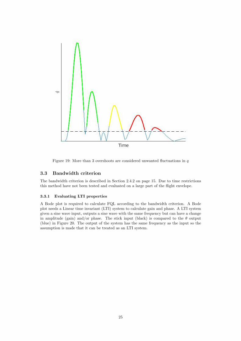
Figure 19: More than 3 overshoots are considered unwanted fluctuations in q

3.3 Bandwidth criterion

The bandwidth criterion is described in Section 2.4.2 on page 15. Due to time restrictionsthis method have not been tested and evaluated on a large part of the flight envelope.

3.3.1 Evaluating LTI properties

A Bode plot is required to calculate FQL according to the bandwidth criterion. A Bodeplot needs a Linear time invariant (LTI) system to calculate gain and phase. A LTI systemgiven a sine wave input, outputs a sine wave with the same frequency but can have a changein amplitude (gain) and/or phase. The stick input (black) is compared to the θ output(blue) in Figure 20. The output of the system has the same frequency as the input so theassumption is made that it can be treated as an LTI system.

25

Figure 20: Sine wave input (black) compared to the sine wave output (blue)

3.3.2 Calculating gain and phase

A sine wave is given as the stick input, the amplitude is set and the frequency is sweptover a selected frequency range. Both the gain and phase is calculated for each frequency.The gain is calculated by taking the average value of the peaks of θ and divide with theamplitude of the input sine wave and converting to decibels. The phase is calculated with

φ = 360◦ · tdiffω (17)

where φ is the phase, tdiff is the time between the input and output wave in seconds andω is the input frequency in Hz. The phase and gain is plotted in a Bode diagram shown inFigure 21.

3.3.3 Calculating bandwidth and phase delay

From the Bode diagram the bandwidth and time delay can be calculated. First the band-width is calculated by selecting the lowest of the two frequencies ωBWgain

or ωBWphase

explained is Section 2.4.2 on page 15. The phase delay is calculated with (5).

26

Figure 21: Bode diagram generated from frequency sweep.

27

4 Validation of Methods

In this section the methods described in the previous section are tested to determine howwell they work and what happens to the result when the methods don’t work as intended.

4.1 Linear estimation and the MIL-F-8785C standard

The values of ωSP , ζSP , nz/α and CAP are obtained from the estimated transfer function.The values are used to determine the FQL according to the MIL-F-8785C standard. Figure22 show three linear estimations and their corresponding data points in the ζSP − CAPgraph. The velocity increases but the altitude is constant. Figure 22a shows three differentlinear estimations as solid lines, the simulated data can be seen as dashed lines. FromFigure 22b it is clear that the dampening increases with airspeed while the value of CAPstay relatively constant. A constant value of CAP means that ωSP increases with an increasein velocity. This can be explained by looking at (5) on page 13. With increasing velocity,nz/α increases with increasing velocity due to the increase in nz. To keep (5) in balanceωSP needs to increase. An increase in ωSP results in a decrease in the overall response timein the time domain as seen in Figure 22a.

(a) (b)

Figure 22: Three different velocities at the same altitude is estimated. The correspondingdata points are plotted in the ζSP -CAP graph.

To get a visual representation of the boundary of FQL 1 according to the MIL-F-8785Cstandard Figure 23 is used. The original transfer function estimated from a specific flightcase is shown in blue. The values of ζSP and ωSP are changed to their maximum andminimum allowed value for FQL 1. Figure 23 shows the location of the data points in theζSP − CAP graph. Figure 23a show the corresponding transfer functions step response inthe time domain. It is clear that the region of level 1 FQL is generous and there exist caseswhere the Gibson criteria would not predict FQL 1.

28

(a) (b)

Figure 23: Illustration of the boundary of FQL 1 according to the MIL-F-8785C standardin the time domain and in the ζSP -CAP graph.

To find where the linear estimation is adequate the MSE between the estimated transferfunction and the simulated data is used. A lower value of MSE indicate a better estimation.Figure 24 shows two examples, one with a low MSE and one with a high MSE. For theestimation to be adequate there must exist a clear q overshoot followed by a relativelyconstant value of q as seen in Figure 24a. While the simulated value of q is slowly decreasingthe estimated value stays constant after the initial peak, this is due to the constant speedassumption used by the linear estimation. Figure 24b shows no clear constant value of qafter the initial peak which causes a high MSE. After visual comparison between the linearestimation and the simulated data the conclusion is made that there exists a correlationbetween the MSE and the quality of the estimation. However, the correlation is not perfect.Where no obvious q overshoot exists and the value stays relatively constant the estimatedtransfer function typically looks like what is shown in Figure 25. No overshoot exists in thelinear estimation resulting in a ζSP that is too large. This causes the estimation to showFQL 3 according to the MIL-F-8785C standard. However, the response fulfils all the Gibsoncriteria tested in this thesis.

(a) Low MSE (b) High MSE

Figure 24: Comparison between MSE of two linear estimations. Data from the simulator isshown as blue and the linear estimation is shown as red.

29

Figure 25: The linear estimation have a low MSE but is not a good estimation.

4.2 Time to max q

Over most parts of the flight envelope, there exists a peak in q after the initial stick input.When this is the case (9) on page 18 becomes tq = t(iq). However, there exists cases whentq = t(iq) gives a more appropriate value for tq. The first of the two following examples showwhere tq = t(iq) gives a more appropriate value of tq. The second example shows where themethod has not find an appropriate value of tq.

The initial peak in q can have a flat segment as shown in Figure 26. The red dot showswhere the first local minima in q is located and the black circle shows where q = 0. Hereit is clear that the first local minima in q gives a more appropriate value of tq. The valueof q does not change by a noticeable amount after the first local minima in q. If tq wasselected at the black circle the value of tq would be too large. This can also be noticedwhen compared to the neighbouring points in the flight envelope. If tq was only calculatedas the point where q = 0 there would exist points in the flight envelope where the valueof tq experience a large difference compared to it’s neighbouring points. The value of tq isexpected to change gradually over the flight envelope.

(a) (b)

Figure 26: Local minima in tq shown as red dot, q = 0 shown as black circle

Figure 27 shows an example of what happens if the first local minima in q is not located closeto 0. This causes the value of tq to be found too early. In this example a more appropriatevalue of tq would be where q = 0. This problem could potentially be fixed by setting aboundary on q that the found tq must be bellow a certain threshold. This is shown as adashed line in Figure 27b.

30

(a) (b)

Figure 27: Local minima in tq shown as red dot, q = 0 shown as black circle

4.3 Finding steady state

The two tested methods, moving time window and moving boundary method, generallyagree on where they find steady state as shown in Figure 28. Problematic areas for bothmethods is at the corner speed. Corner speed is the minimum speed at which the aircraftcan achieve its maximum allowable g [3]. Figure 29 shows a comparison between the twomethods at the corner speed. The combination of fluctuations in q after the initial stickinput and a subsequent drop makes it a challenging part of the flight envelope to find steadystate.

Figure 28: Both methods find tss,q at the same location.

The moving time window method uses the mean value of |q| to set the roof. The highvariability in |q| causes the roof to be set at a higher threshold than normal. This causes

31

the condition of steady state not to be strict enough which causes the method to find steadystate too early. Lowering the value of the weight ν in (11) can solve the problem but it mayalso cause problems with finding steady state at other parts of the flight envelope.

The moving boundary method looks at how much q changes over a specified amount oftime. Here the condition to find steady state becomes too strict. Changing ξ in (13) mightsolve the problem but can once again cause problems in other parts of the flight envelope.

Figure 29: Comparison between the two methods at the corner speed.

Both methods can also also find steady state too early if q rises slowly towards a steady statevalue after the initial peak. Figure 30 shows an example of this. Here, the moving boundarymethod have found steady state too early. However, both methods struggle when the datalooks like this. The reason both methods can struggle is because q rises slowly which givesa small constant value of q. A slowly changing q can be mistaken for steady state.

32

Figure 30: Comparison between the two methods when q slowly reaches steady state afterinitial peak.

4.4 The dropback criterion

The dropback criterion determines if the response have acceptable or unacceptable dropbackas seen in Figure 6 on page 14. To help visualize what acceptable or unacceptable dropbacklooks like the following two examples are used. The response in Figure 31 shows what isconsidered acceptable dropback. Figure 32 shows what is considered unacceptable dropback.Figure 31 actually shows a slightly negative dropback and dropback ratio. Because it is closeto the K/s line which is considered the optimal attitude response the decision has been madeto accept a small negative attitude dropback. Figure 32 shows a large q overshoot ratio andalso a high dropback and dropback ratio. The response is also far from the K/s line.

33

Figure 31: Low pitch rate overshoot and dropback ratio.

Figure 32: High pitch rate overshoot and dropback ratio.

34

When a data point have been calculated in the dropback criterion the selected tss,q is movedby ±∆T . This is to determine how sensitive the data point is to small errors in the selectedtss,q. Figure 33 shows a comparison between a tss,q that is sensitive to changes and onewhich is not. The dropback ratio is marked with a black dot. tss,q is moved with thesame amount of time in both examples. Figure 34 shows how the data points from the twoexamples move in the dropback criterion. The data point generally becomes more sensitiveto changes in tss,q with a combination of a long time to reach tss,q and q that reduces afterthe initial overshoot.

(a) Sensitive (b) Not sensitive

Figure 33: Comparison of how the dropback ratio is affected when tss is moved by ±∆T .

Figure 34: The two examples in Figure 33 and how their data points move in the dropbackcriterion when tss,q is moved by ±∆T .

The two methods to calculate steady state can have some variability in their estimated valueof tss,q. Both methods are plotted together in the dropback criterion as seen in Figure 35.The data points from the same place in the flight envelope is connected with a black line.The dropback ratio is calculated from a step input. Both methods show approximately thesame result for all flight cases tested except for corner speed where the moving boundarymethod fail to find an appropriate steady state.

35

Figure 35: Moving time window method shown as blue *, moving boundary shown as purplecircle.

The dropback ratio can be calculated from both a pulse and a step input. The result fromboth methods are plotted together in Figure 36. Cyan circle data points are calculated froma step and magenta square data points are calculated from a pulse. The data points laysufficiently close to each other to be considered to be within the margin of error. However,during slow flight the difference between the step and pulse response grow larger with reducedvelocity.

36

Figure 36: Dropback ratio from step is shown as cyan dot, pulse as magenta square.

4.5 Flight path delay

The method used to calculate tγ also relies on finding steady state. Both methods are tested,however, γ is used as input. The steady state like region is not as clear in γ as in q. Becauseof this there exists a larger spread in tss,γ over the flight envelope. Both Figure 37 and 38show a larger spread between the two methods. However, both methods to find steady statehave not been re tuned to find steady state in γ, if this is done the accuracy can be increasedin both methods.

37

Figure 37: Comparison between the two steady state methods when γ is used as input.

Figure 38: Comparison between the two steady state methods when γ is used as input.

38

The value of tss,γ is moved slightly in the same way as in the dropback criterion. Becauseγ shows less variability over time than q the result is less sensitive to changes in tss,γ . Thisalso becomes a measurement of flight path stability which is important when precision flightpath control is required, like air to air refuelling.

4.6 Fluctuations in q

Because of its simplicity the method used to find fluctuations never shows false positives.However, more evaluation is needed on where to put the boundary. The boundary have beenselected after studying an animation of the maneuver and deciding at what amplitude thefluctuations starts to become noticeable. Where to put the boundary should be investigatedfurther with a pilot in a simulator.

4.7 Bandwidth criterion

Due to time restrictions the bandwidth criterion has not been evaluated in as much detail ascompared to the other methods. For the velocities and altitudes tested the LTI assumptionseems to be valid. However at low frequencies nonlinear effects start to show up as shownin Figure 39a, this is not a problem though because the data obtained from the Bode plotis only taken from the higher frequencies. This also means that the frequency sweep can beshortened.

(a) Low frequency. (b) High frequency.

Figure 39: At low frequencies the output start to show non linear effects. Input is shown asblack and output as blue.

39

5 Conclusion and Discussion

In this section each method will be discussed, how good is the result and where are theyrelevant to use?

5.1 Linear estimation

The linear estimation only works well when the data already looks like a second order sys-tem. Furthermore the MIL-F-8785C standard that uses the linear estimation predicts FQL1 for FQ that would not pass some of the Gibson criteria. The combination of the methodonly working for data that already looks linear like and the standard showing a large vari-ation for FQL 1 makes the method developed not suitable for evaluating FQL for a highlyaugmented aircraft.

However, the method can be used to find areas in the flight envelope that show linearqualities. With linear like qualities the other methods developed, like finding tq or steadystate become more accurate. To find these areas the MSE is used. This method generallyworks well; however, it is not perfect. As shown in Section 4.1 there exits cases where theestimation is not good even though MSE is low. However these points can be identified bycomparing the MSE to surrounding points in the flight envelope. Points with low MSE buta bad linear estimation is usually surrounded by points which have a high MSE and is a badestimation.

The linear estimation might be better suited for non augmented aircraft where the aerody-namics is what primary determine the response of the aircraft.

5.2 Time to max q

The value of tq is expected to gradually change over the flight envelope. By using the lowerof the two time where q = 0 or the first local minima in q as described in (9) on 18 agradual change in tq can be observed. Sudden changes in tq can still occur at some points inthe flight envelope however this is due to the dynamics of the aircraft and not the methodfinding the wrong value of tq.

5.3 Finding steady state

The simulations done in this thesis have a fixed time interval and it is therefore possibleto fine tune the moving time window method to give an overall better accuracy. Howeverthis method can not be used if the simulation time is too long or too short. The movingboundary works for all time intervals as long there exists a clear initial peak in q. This havealways been the case for the simulations done in this thesis.

A question may arise when looking at the moving time window method, why not use afixed value as the limit? If fixed value is used problems may arise when the aircraft is car-rying heavy external stores. A limit that works well with a light aircraft may not be strictenough when the mass of the aircraft is increased. When the mean value is used insteadthe overall lower value of |q| of a heavy aircraft causes the limit to be lower and a moreappropriate steady state is found.

40

5.4 The dropback criterion

The parts where the result of the dropback criterion change the most when tss,q is movedwith ±∆T is usually where the linear estimation is good. A good linear estimation meansthe response resembles a second order linear system. When this is the case the methods thatfinds steady state becomes more accurate. This means that where the result is sensitive toerrors in the estimated tss,q is also where there exists a clear steady state. The parts of theenvelope where the response does not resemble a second order linear system the steady statelike region is not as clear. However, the result in the dropback criterion is usually not assensitive to changes in tss,q when this is the case. This combination makes the method quiteaccurate over all. Except for the corner speed, here the methods can miss the steady statewith a large amount resulting in a bad result. These data points can normally be foundbecause they do not follow the trend of the other data points.

Calculating the dropback ratio from a step or a pulse input show roughly the same re-sult. By calculating the dropback ratio from a step the velocity have not had as much timeto bleed of. This means that the FQ have not changed much from the initial flight condition.By calculating the dropback ratio from a pulse the velocity have reduced more. However,when pilots talk about dropback they refer to how much the attitude of the nose changeswhen the stick is released. So calculating the dropback ratio from a pulse is more accurateto what the pilot experiences.

5.5 Flight path delay

To find the flight path delay (tγ) steady state in γ also has to be found. The methods seemless accurate when finding steady state when γ is used as a input. However the result showsthat it is not sensitive to changes in the selected steady state. This is because γ does notvary much compared to q. This can be explained by the inertia of the aircraft that dampthe changes in γ. This mean that the accuracy of the method to find tγ is high even thoughit is harder to find steady state in γ. The accuracy can be increased further if the methodsthat finds steady state are tuned specifically for γ.

5.6 Fluctuations in q

The developed method can be used over the entire flight envelope. Fluctuations in q arenever a desired behaviour. This behaviour can occur when the aircraft is not sufficientlydamped. Generally a pilot like a well damped aircraft which allow for high precision attitudecontrol. Fluctuations in q also results in a less stable γ and nz response.

5.7 Bandwidth criterion

This criterion has only been tested for a small part of the flight envelope. For the partstested of the flight envelope the method works well. If the bandwidth criterion can be usedover a large part of the flight envelope it can be combined with the dropback criterion toincrease the accuracy of the predicted pilot opinion.

5.8 Concluding remarks

The main goal of this thesis was to develop methods to determine if the criteria used arefulfilled or not. This goal have largely been achieved. Parts of the MIL-F-8785C standardand the Gibson criteria from the time domain have been evaluated however, the bandwidthcriterion still needs more work. It is clear from this thesis that the methods developed toevaluate the Gibson criteria have a much higher accuracy than the method developed toevaluate the MIL-F-8785C standard. Furthermore the methods used to evaluate the Gibsoncriteria can be used for the majority of the flight envelope. Therefore the methods developedfor the Gibson criteria are better suited for evaluating FQL of a highly augmented fighteraircraft.

41

6 Future Research

The bandwidth criterion needs further testing and validation. Mainly what frequency sweepis sufficient for the necessary calculations. For example the frequency sweep could possiblybe shortened. The low frequencies does not contribute any significant information whencalculating FQL. Frequencies higher than ω−180 might also be ignored because the Bodediagram could be aproximated as a straight line beyond that point. The amplitude of thestick input also needs further investigation. Should full stick deflection be used or onlysmall deflections? Another that is worth exploring is to evaluate the possibility to estimatea transfer function from the Bode diagram. Does a transfer function obtained from thefrequency domain give a better estimation of the system than from the time domain?

This thesis have mainly studied the Gibson criteria from the time domain, however thereexists several criteria from the frequency domain like the phase rate criterion and the gainlimit criterion. The frequency domain can also give a better view of PIO triggering tenden-cies. To combine criteria from both the time and frequency domain can give a better picturewhen evaluating the aircraft’s FQ.

It would also be interesting to develop methods for evaluating the aircraft’s lateral move-ment. The longitudinal and lateral FQ are often treated separately with separate criteria.

The methods developed purpose is to find problematic areas in the flight envelope. Thereexits prior research showing a correlation between the Gibson criteria and pilot opinion.However there would be interesting to do further evaluation with a pilot in a simulator toget more feedback on their opinion on aircraft FQ and HQ at predicted problematic pointin the flight envelope.

42

7 Bibliography

References

[1] M.V. Cook. Flight Dynamics Principles. Elsevier Ltd, 2007. isbn: 978-0-7506-6927-6.

[2] Flight Control Design – Best Practices. North atlantic treaty organization, 2000.

[3] Flight training instruction. Basic maneuvering (BFM) advanced NFO T-45C/VMTS.Naval air training command, 2018.

[4] John Gibson. Development of design methodology for handling qualities excellence infly by wire aircraft. Delft University Press, 1999.

[5] Stephanie Glen. Instrumental Variable: Definition and Overview. 2016. url: www.

statisticshowto.datasciencecentral.com/instrumental-variable/.

[6] Snorri Gudmundsson. General Aviation Aircraft Design Applied Methods and Proce-dures. 2014.

[7] Handling Qualities of Unstable Highly Augmented Aircraft. North Atlantic Treaty Or-ganization, 1991.

[8] Richard A. Hyde. H∞ Aerospace Control Design. British Libary Cataloguing in Pub-lication Data. isbn: 9781447130499.

[9] David A. Kivioja. Comparison of the control anticipation parameter and the bandwidthcriterion during the landing task. Air force institute of technology, 1996.

[10] MILITARY SPECIFICATION FLYING QUALITIES OF PILOTED AIRPLANES.U.S. Military, 1980.

[11] tfest. 2019. url: www.mathworks.com/help/ident/ref/tfest.html.

43