method of frobenius | math 537 - ordinary differential equations
TRANSCRIPT
DefinitionsCauchy-Euler Equation
Method of Frobenius
Math 537 - Ordinary Differential EquationsLecture Notes – Method of Frobenius
Joseph M. Mahaffy,〈[email protected]〉
Department of Mathematics and StatisticsDynamical Systems Group
Computational Sciences Research Center
San Diego State UniversitySan Diego, CA 92182-7720
http://jmahaffy.sdsu.edu
Fall 2019
Joseph M. Mahaffy, 〈[email protected]〉Lecture Notes – Method of Frobenius —(1/53)
DefinitionsCauchy-Euler Equation
Method of Frobenius
Outline
1 DefinitionsLegendre’s Equation
2 Cauchy-Euler EquationDistinct RootsEqual RootsComplex Roots
3 Method of FrobeniusDistinct Roots, r1 − r2 6= NRepeated Roots, r1 = r2 = rRoots Differing by an Integer, r1 − r2 = N
Joseph M. Mahaffy, 〈[email protected]〉Lecture Notes – Method of Frobenius —(2/53)

DefinitionsCauchy-Euler Equation
Method of FrobeniusLegendre’s Equation
Definitions 1
Consider the 2nd order linear differential equation:
P (x)y ′′ +Q(x)y ′ +R(x)y = F (x). (1)
Definition (Ordinary and Singular Points)
x0 is an ordinary point of Eqn. (1) if P (x0) 6= 0 and Q(x)/P (x), R(x)/P (x), andF (x)/P (x) are analytic at x0.
x0 is a singular point of Eqn. (1) if x0 is not an ordinary point.
The previous ODEs solved by power series methods have centered aroundx0 = 0, when this is an ordinary point.
In an interval about a singular point, the solutions of Eqn. (1) can exhibitbehavior different from power series solutions for Eqn. (1) near an ordinarypoint.
If x0 = 0, then these solutions may behave like ln(x) or x−n near x0.
Joseph M. Mahaffy, 〈[email protected]〉Lecture Notes – Method of Frobenius —(3/53)
DefinitionsCauchy-Euler Equation
Method of FrobeniusLegendre’s Equation
Definitions 2
We concentrate on the homogeneous 2nd order linear differential equation tobetter understand behavior of the solution near a singular point:
P (x)y ′′ +Q(x)y ′ +R(x)y = 0. (2)
Definition (Regular and Irregular Singular Points)
If x0 is a singular point of Eqn. (2), then x0 is a regular singular point providedthe functions:
(x− x0)Q(x)
P (x)and (x− x0)2
R(x)
P (x)
are analytic at x0.
A singular point that is not regular is said to be an irregular singular point.
If Eqn. (2) has a regular singular point at x0, then it is possible that no powerseries solution exists of the form:
y(x) =
∞∑n=0
an(x− x0)n.
Joseph M. Mahaffy, 〈[email protected]〉Lecture Notes – Method of Frobenius —(4/53)
DefinitionsCauchy-Euler Equation
Method of FrobeniusLegendre’s Equation
Bessel’s Equation
Example: Consider Bessel’s equation of order ν:
x2y ′′ + xy ′ + (x2 − ν2)y = 0,
where P (x) = x2, Q(x) = x, and R(x) = x2 − ν2.
It is clear that x = 0 is a singular point.
We see that
limx→0
xQ(x)
P (x)= 1 and lim
x→0x2R(x)
P (x)= limx→0
(x2 − ν2) = −ν2,
which are both finite, so analytic.
It follows that x0 = 0 is a regular singular point.
Any other value of x0 for Bessel’s equation gives an ordinarypoint.
Joseph M. Mahaffy, 〈[email protected]〉Lecture Notes – Method of Frobenius —(5/53)
DefinitionsCauchy-Euler Equation
Method of FrobeniusLegendre’s Equation
Legendre’s Equation 1
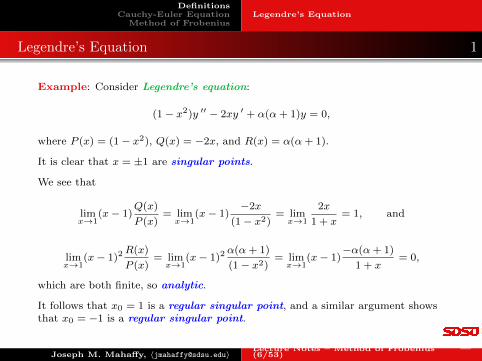
Example: Consider Legendre’s equation:
(1− x2)y ′′ − 2xy ′ + α(α+ 1)y = 0,
where P (x) = (1− x2), Q(x) = −2x, and R(x) = α(α+ 1).
It is clear that x = ±1 are singular points.
We see that
limx→1
(x− 1)Q(x)
P (x)= limx→1
(x− 1)−2x
(1− x2)= limx→1
2x
1 + x= 1, and
limx→1
(x− 1)2R(x)
P (x)= limx→1
(x− 1)2α(α+ 1)
(1− x2)= limx→1
(x− 1)−α(α+ 1)
1 + x= 0,
which are both finite, so analytic.
It follows that x0 = 1 is a regular singular point, and a similar argument showsthat x0 = −1 is a regular singular point.
Joseph M. Mahaffy, 〈[email protected]〉Lecture Notes – Method of Frobenius —(6/53)
DefinitionsCauchy-Euler Equation
Method of FrobeniusLegendre’s Equation
Legendre’s Equation 2
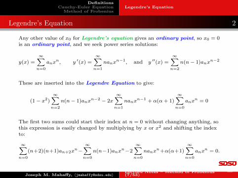
Any other value of x0 for Legendre’s equation gives an ordinary point, so x0 = 0is an ordinary point, and we seek power series solutions:
y(x) =∞∑n=0
anxn, y ′(x) =
∞∑n=1
nanxn−1, and y ′′(x) =
∞∑n=2
n(n− 1)anxn−2
These are inserted into the Legendre Equation to give:
(1− x2)
∞∑n=2
n(n− 1)anxn−2 − 2x
∞∑n=1
nanxn−1 + α(α+ 1)
∞∑n=0
anxn = 0
The first two sums could start their index at n = 0 without changing anything, sothis expression is easily changed by multiplying by x or x2 and shifting the indexto:
∞∑n=0
(n+2)(n+1)an+2xn−
∞∑n=0
n(n−1)anxn−2
∞∑n=0
nanxn+α(α+1)
∞∑n=0
anxn = 0.
Joseph M. Mahaffy, 〈[email protected]〉Lecture Notes – Method of Frobenius —(7/53)
DefinitionsCauchy-Euler Equation
Method of FrobeniusLegendre’s Equation
Legendre’s Equation 3
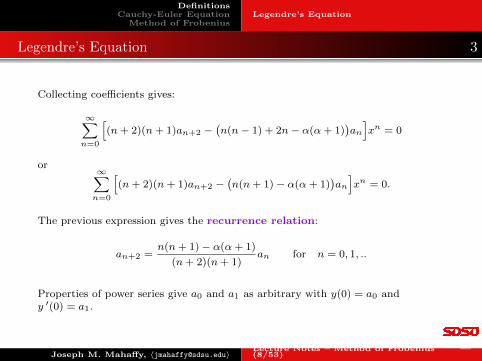
Collecting coefficients gives:
∞∑n=0
[(n+ 2)(n+ 1)an+2 −
(n(n− 1) + 2n− α(α+ 1)
)an]xn = 0
or∞∑n=0
[(n+ 2)(n+ 1)an+2 −
(n(n+ 1)− α(α+ 1)
)an]xn = 0.
The previous expression gives the recurrence relation:
an+2 =n(n+ 1)− α(α+ 1)
(n+ 2)(n+ 1)an for n = 0, 1, ..
Properties of power series give a0 and a1 as arbitrary with y(0) = a0 andy ′(0) = a1.
Joseph M. Mahaffy, 〈[email protected]〉Lecture Notes – Method of Frobenius —(8/53)
DefinitionsCauchy-Euler Equation
Method of FrobeniusLegendre’s Equation
Legendre’s Equation 4
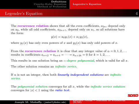
The recurrence relation shows that all the even coefficients, a2n, depend onlyon a0, while all odd coefficients, a2n+1, depend only on a1, so all solutions havethe form:
y(x) = a0y1(x) + a1y2(x),
where y1(x) has only even powers of x and y2(x) has only odd powers of x.
From the recurrence relation it is clear that any integer value of α = 0, 1, 2, . . .results in coefficients aα+2 = aα+4 = · · · = aα+2k = 0 for k = 1, 2, . . .
This results in one solution being an α-degree polynomial, which is valid for all x.
The other solution remains an infinite series.
If α is not an integer, then both linearly independent solutions are infiniteseries.
The polynomial solution converges for all x, while the infinite series solutionconverges for |x| < 1 using the ratio test.
Joseph M. Mahaffy, 〈[email protected]〉Lecture Notes – Method of Frobenius —(9/53)
DefinitionsCauchy-Euler Equation
Method of Frobenius
Distinct RootsEqual RootsComplex Roots
Cauchy-Euler Equation 1
Cauchy-Euler Equation (Also, Euler Equation): Consider the differentialequation:
L[y] = t2y ′′ + αty ′ + βy = 0,
where α and β are constants.
Assume t > 0 and attempt a solution of the form
y(t) = tr.
Note that tr may not be defined for t < 0.
The result is
L[tr] = t2(r(r − 1)tr−2) + αt(rtr−1) + βtr
= tr[r(r − 1) + αr + β] = 0.
Thus, obtain quadratic equation
F (r) = r(r − 1) + αr + β = 0.
Joseph M. Mahaffy, 〈[email protected]〉Lecture Notes – Method of Frobenius —(10/53)
DefinitionsCauchy-Euler Equation
Method of Frobenius
Distinct RootsEqual RootsComplex Roots
Cauchy-Euler Equation 2
Cauchy-Euler Equation: The quadratic equation
F (r) = r(r − 1) + αr + β = 0
has roots
r1, r2 =−(α− 1)±
√(α− 1)2 − 4β
2.
This is very similar to our constant coefficient homogeneous DE.
Real, Distinct Roots: If F (r) = 0 has real roots, r1 and r2, withr1 6= r2, then the general solution of
L[y] = t2y ′′ + αy ′ + βy = 0,
isy(t) = c1t
r1 + c2tr2 , t > 0.
Joseph M. Mahaffy, 〈[email protected]〉Lecture Notes – Method of Frobenius —(11/53)
DefinitionsCauchy-Euler Equation
Method of Frobenius
Distinct RootsEqual RootsComplex Roots
Cauchy-Euler Equation 3
Example: Consider the equation
2t2y ′′ + 3ty ′ − y = 0.
By substituting y(t) = tr, we have
tr[2r(r − 1) + 3r − 1] = tr(2r2 + r − 1) = tr(2r − 1)(r + 1) = 0.
This has the real roots r1 = −1 and r2 = 12 , giving the general
solutiony(t) = c1t
−1 + c2√t, t > 0.
Joseph M. Mahaffy, 〈[email protected]〉Lecture Notes – Method of Frobenius —(12/53)
DefinitionsCauchy-Euler Equation
Method of Frobenius
Distinct RootsEqual RootsComplex Roots
Cauchy-Euler Equation 4
Equal Roots: If F (r) = (r − r1)2 = 0 has r1 as a double root, there is onesolution, y1(t) = tr1 .
Need a second linearly independent solution.
Note that not only F (r1) = 0, but F ′(r1) = 0, so consider
∂
∂rL[tr] =
∂
∂r[trF (r)] =
∂
∂r[tr(r − r1)2]
= (r − r1)2tr ln(t) + 2(r − r1)tr.
Also,∂
∂rL[tr] = L
[∂
∂r(tr)
]= L[tr ln(t)].
Evaluating these at r = r1 gives
L[tr1 ln(t)] = 0.
Joseph M. Mahaffy, 〈[email protected]〉Lecture Notes – Method of Frobenius —(13/53)
DefinitionsCauchy-Euler Equation
Method of Frobenius
Distinct RootsEqual RootsComplex Roots
Cauchy-Euler Equation 5
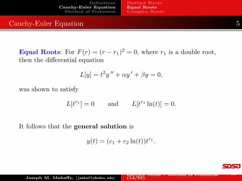
Equal Roots: For F (r) = (r − r1)2 = 0, where r1 is a double root,then the differential equation
L[y] = t2y ′′ + αy ′ + βy = 0,
was shown to satisfy
L[tr1 ] = 0 and L[tr1 ln(t)] = 0.
It follows that the general solution is
y(t) = (c1 + c2 ln(t))tr1 .
Joseph M. Mahaffy, 〈[email protected]〉Lecture Notes – Method of Frobenius —(14/53)

DefinitionsCauchy-Euler Equation
Method of Frobenius
Distinct RootsEqual RootsComplex Roots
Cauchy-Euler Equation 6
Example: Consider the equation
t2y ′′ + 5ty ′ + 4y = 0.
By substituting y(t) = tr, we have
tr[r(r − 1) + 5r + 4] = tr(r2 + 4r + 4) = tr(r + 2)2 = 0.
This only has the real root r1 = −2, which gives general solution
y(t) = (c1 + c2 ln(t))t−2, t > 0.
Joseph M. Mahaffy, 〈[email protected]〉Lecture Notes – Method of Frobenius —(15/53)
DefinitionsCauchy-Euler Equation
Method of Frobenius
Distinct RootsEqual RootsComplex Roots
Cauchy-Euler Equation 7
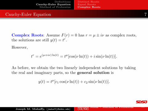
Complex Roots: Assume F (r) = 0 has r = µ± iν as complex roots,the solutions are still y(t) = tr.
However,
tr = e(µ+iν) ln(t) = tµ[cos(ν ln(t)) + i sin(ν ln(t))].
As before, we obtain the two linearly independent solutions by takingthe real and imaginary parts, so the general solution is
y(t) = tµ[c1 cos(ν ln(t)) + c2 sin(ν ln(t))].
Joseph M. Mahaffy, 〈[email protected]〉Lecture Notes – Method of Frobenius —(16/53)
DefinitionsCauchy-Euler Equation
Method of Frobenius
Distinct RootsEqual RootsComplex Roots
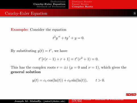
Cauchy-Euler Equation 8
Example: Consider the equation
t2y ′′ + ty ′ + y = 0.
By substituting y(t) = tr, we have
tr[r(r − 1) + r + 1] = tr(r2 + 1) = 0.
This has the complex roots r = ±i (µ = 0 and ν = 1), which gives thegeneral solution
y(t) = c1 cos(ln(t)) + c2 sin(ln(t)), t > 0.
Joseph M. Mahaffy, 〈[email protected]〉Lecture Notes – Method of Frobenius —(17/53)
DefinitionsCauchy-Euler Equation
Method of Frobenius
Distinct Roots, r1 − r2 6= NRepeated Roots, r1 = r2 = rRoots Differing by an Integer, r1 − r2 = N
Regular Singular Problem 1
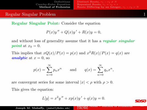
Regular Singular Point: Consider the equation
P (x)y ′′ +Q(x)y ′ +R(x)y = 0,
and without loss of generality assume that it has a regular singularpoint at x0 = 0.
This implies that xQ(x)/P (x) = p(x) and x2R(x)/P (x) = q(x) areanalytic at x = 0, so
p(x) =
∞∑n=0
pnxn and q(x) =
∞∑n=0
qnxn,
are convergent series for some interval |x| < ρ with ρ > 0.
This gives the equation:
L[y] = x2y ′′ + xp(x)y ′ + q(x)y = 0.
Joseph M. Mahaffy, 〈[email protected]〉Lecture Notes – Method of Frobenius —(18/53)
DefinitionsCauchy-Euler Equation
Method of Frobenius
Distinct Roots, r1 − r2 6= NRepeated Roots, r1 = r2 = rRoots Differing by an Integer, r1 − r2 = N
Regular Singular Problem 2
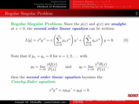
Regular Singular Problem: Since the p(x) and q(x) are analyticat x = 0, the second order linear equation can be written:
L[y] = x2y ′′ + x
( ∞∑n=0
pnxn
)y ′ +
( ∞∑n=0
qnxn
)y = 0. (3)
Note that if pn = qn = 0 for n = 1, 2, . . . with
p0 = limx→0
xQ(x)
P (x)and q0 = lim
x→0
x2R(x)
P (x),
then the second order linear equation becomes theCauchy-Euler equation:
x2y ′′ + xp0y′ + q0y = 0.
Joseph M. Mahaffy, 〈[email protected]〉Lecture Notes – Method of Frobenius —(19/53)
DefinitionsCauchy-Euler Equation
Method of Frobenius
Distinct Roots, r1 − r2 6= NRepeated Roots, r1 = r2 = rRoots Differing by an Integer, r1 − r2 = N
Method of Frobenius 1
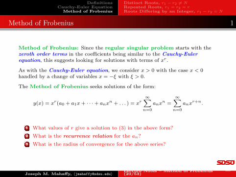
Method of Frobenius: Since the regular singular problem starts with thezeroth order terms in the coefficients being similar to the Cauchy-Eulerequation, this suggests looking for solutions with terms of xr.
As with the Cauchy-Euler equation, we consider x > 0 with the case x < 0handled by a change of variables x = −ξ with ξ > 0.
The Method of Frobenius seeks solutions of the form:
y(x) = xr(a0 + a1x+ · · ·+ anxn + . . . ) = xr
∞∑n=0
anxn =
∞∑n=0
anxr+n.
1 What values of r give a solution to (3) in the above form?
2 What is the recurrence relation for the an?
3 What is the radius of convergence for the above series?
Joseph M. Mahaffy, 〈[email protected]〉Lecture Notes – Method of Frobenius —(20/53)
DefinitionsCauchy-Euler Equation
Method of Frobenius
Distinct Roots, r1 − r2 6= NRepeated Roots, r1 = r2 = rRoots Differing by an Integer, r1 − r2 = N
Method of Frobenius 2
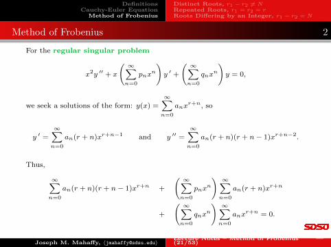
For the regular singular problem
x2y ′′ + x
( ∞∑n=0
pnxn
)y ′ +
( ∞∑n=0
qnxn
)y = 0,
we seek a solutions of the form: y(x) =∞∑n=0
anxr+n, so
y ′ =∞∑n=0
an(r + n)xr+n−1 and y ′′ =∞∑n=0
an(r + n)(r + n− 1)xr+n−2.
Thus,
∞∑n=0
an(r + n)(r + n− 1)xr+n +
( ∞∑n=0
pnxn
) ∞∑n=0
an(r + n)xr+n
+
( ∞∑n=0
qnxn
) ∞∑n=0
anxr+n = 0.
Joseph M. Mahaffy, 〈[email protected]〉Lecture Notes – Method of Frobenius —(21/53)
DefinitionsCauchy-Euler Equation
Method of Frobenius
Distinct Roots, r1 − r2 6= NRepeated Roots, r1 = r2 = rRoots Differing by an Integer, r1 − r2 = N
Method of Frobenius 3
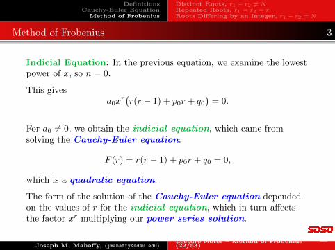
Indicial Equation: In the previous equation, we examine the lowestpower of x, so n = 0.
This givesa0x
r(r(r − 1) + p0r + q0
)= 0.
For a0 6= 0, we obtain the indicial equation, which came fromsolving the Cauchy-Euler equation:
F (r) = r(r − 1) + p0r + q0 = 0,
which is a quadratic equation.
The form of the solution of the Cauchy-Euler equation dependedon the values of r for the indicial equation, which in turn affectsthe factor xr multiplying our power series solution.
Joseph M. Mahaffy, 〈[email protected]〉Lecture Notes – Method of Frobenius —(22/53)
DefinitionsCauchy-Euler Equation
Method of Frobenius
Distinct Roots, r1 − r2 6= NRepeated Roots, r1 = r2 = rRoots Differing by an Integer, r1 − r2 = N
Distinct Roots, r1 − r2 6= N 1
The Method of Frobenius breaks into 3 cases, depending on theroots of the indicial equation.
Case 1. Distinct roots not differing by an integer, r1− r2 6= N .
For this case, a basis for the solution of the regular singularproblem satisfies:
y1(x) = xr1(a0 + a1x+ · · ·+ anxn + . . . ) = xr1
∞∑n=0
anxn
and
y2(x) = xr2(b0 + b1x+ · · ·+ bnxn + . . . ) = xr2
∞∑n=0
bnxn
with these solutions converging for at least |x| < ρ, where ρ is theradius of convergence for p(x) and q(x).
Joseph M. Mahaffy, 〈[email protected]〉Lecture Notes – Method of Frobenius —(23/53)
DefinitionsCauchy-Euler Equation
Method of Frobenius
Distinct Roots, r1 − r2 6= NRepeated Roots, r1 = r2 = rRoots Differing by an Integer, r1 − r2 = N
Distinct Roots, r1 − r2 6= N 2
Example: Consider the regular singular problem given by
4xy ′′ + 2y ′ + y = 0,
where x = 0 is a regular singular point.
From our definitions before we have p(x) = 12 and q(x) = x
4 , whichimplies that p0 = 1
2 and q0 = 0.
Since p and q have convergent power series for all x, the solutions willconverge for |x| <∞.
The indicial equation is given by:
r(r − 1) + 12r = r
(r − 1
2
)= 0,
so r1 = 0 and r2 = 12 .
Joseph M. Mahaffy, 〈[email protected]〉Lecture Notes – Method of Frobenius —(24/53)
DefinitionsCauchy-Euler Equation
Method of Frobenius
Distinct Roots, r1 − r2 6= NRepeated Roots, r1 = r2 = rRoots Differing by an Integer, r1 − r2 = N
Distinct Roots, r1 − r2 6= N 3
Example: We multiply our example by x and continue with
4x2y ′′ + 2xy ′ + xy = 0,
trying a solution of the form: y =∞∑n=0
anxn+r.
Differentiating y and entering into the equation gives:
4∞∑n=0
an(r + n)(r + n− 1)xr+n + 2∞∑n=0
an(r + n)xr+n +∞∑n=1
an−1xr+n = 0,
shifting the last index to match powers of x.
Note that when n = 0, we have
a0[4r(r − 1) + 2r
]= 2a0r(2r − 1) = 0,
which is an alternate way to obtain the indicial equation.
Joseph M. Mahaffy, 〈[email protected]〉Lecture Notes – Method of Frobenius —(25/53)
DefinitionsCauchy-Euler Equation
Method of Frobenius
Distinct Roots, r1 − r2 6= NRepeated Roots, r1 = r2 = rRoots Differing by an Integer, r1 − r2 = N
Distinct Roots, r1 − r2 6= N 4
Example: For n ≥ 1, we match powers of x, so[4(r + n)(r + n− 1) + 2(r + n)
]an + an−1 = 0.
From this we obtain the recurrence relation:
an+1 =−an
(2n+ 2r + 2)(2n+ 2r + 1), for n = 0, 1, . . .
First Solution: Let r = r1 = 0, then the recurrence relation becomes:
an+1 =−an
(2n+ 2)(2n+ 1), for n = 0, 1, . . . ,
soa1 = −
a0
2 · 1, a2 = −
a1
4 · 3=a0
4!, a3 = −
a2
6 · 5= −
a0
6!.
Thus,
an =(−1)n
(2n)!a0.
Joseph M. Mahaffy, 〈[email protected]〉Lecture Notes – Method of Frobenius —(26/53)
DefinitionsCauchy-Euler Equation
Method of Frobenius
Distinct Roots, r1 − r2 6= NRepeated Roots, r1 = r2 = rRoots Differing by an Integer, r1 − r2 = N
Distinct Roots, r1 − r2 6= N 5
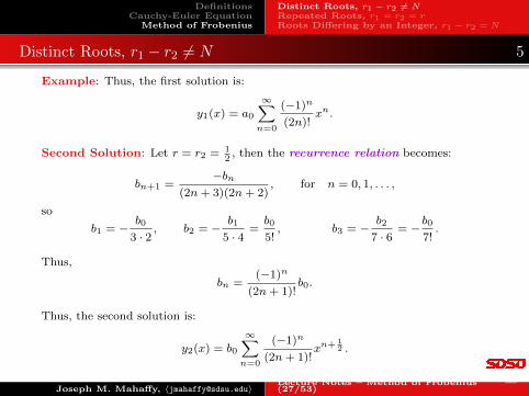
Example: Thus, the first solution is:
y1(x) = a0
∞∑n=0
(−1)n
(2n)!xn.
Second Solution: Let r = r2 = 12
, then the recurrence relation becomes:
bn+1 =−bn
(2n+ 3)(2n+ 2), for n = 0, 1, . . . ,
so
b1 = −b0
3 · 2, b2 = −
b1
5 · 4=b0
5!, b3 = −
b2
7 · 6= −
b0
7!.
Thus,
bn =(−1)n
(2n+ 1)!b0.
Thus, the second solution is:
y2(x) = b0
∞∑n=0
(−1)n
(2n+ 1)!xn+
12 .
Joseph M. Mahaffy, 〈[email protected]〉Lecture Notes – Method of Frobenius —(27/53)
DefinitionsCauchy-Euler Equation
Method of Frobenius
Distinct Roots, r1 − r2 6= NRepeated Roots, r1 = r2 = rRoots Differing by an Integer, r1 − r2 = N
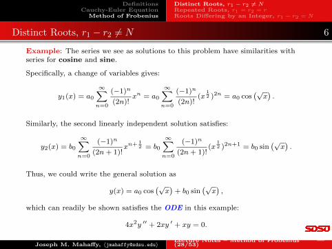
Distinct Roots, r1 − r2 6= N 6
Example: The series we see as solutions to this problem have similarities withseries for cosine and sine.
Specifically, a change of variables gives:
y1(x) = a0
∞∑n=0
(−1)n
(2n)!xn = a0
∞∑n=0
(−1)n
(2n)!(x
12 )2n = a0 cos
(√x).
Similarly, the second linearly independent solution satisfies:
y2(x) = b0
∞∑n=0
(−1)n
(2n+ 1)!xn+
12 = b0
∞∑n=0
(−1)n
(2n+ 1)!(x
12 )2n+1 = b0 sin
(√x).
Thus, we could write the general solution as
y(x) = a0 cos(√x)
+ b0 sin(√x),
which can readily be shown satisfies the ODE in this example:
4x2y ′′ + 2xy ′ + xy = 0.
Joseph M. Mahaffy, 〈[email protected]〉Lecture Notes – Method of Frobenius —(28/53)
DefinitionsCauchy-Euler Equation
Method of Frobenius
Distinct Roots, r1 − r2 6= NRepeated Roots, r1 = r2 = rRoots Differing by an Integer, r1 − r2 = N
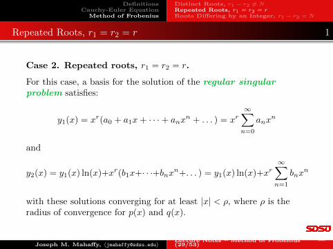
Repeated Roots, r1 = r2 = r 1
Case 2. Repeated roots, r1 = r2 = r.
For this case, a basis for the solution of the regular singularproblem satisfies:
y1(x) = xr(a0 + a1x+ · · ·+ anxn + . . . ) = xr
∞∑n=0
anxn
and
y2(x) = y1(x) ln(x)+xr(b1x+· · ·+bnxn+. . . ) = y1(x) ln(x)+xr∞∑n=1
bnxn
with these solutions converging for at least |x| < ρ, where ρ is theradius of convergence for p(x) and q(x).
Joseph M. Mahaffy, 〈[email protected]〉Lecture Notes – Method of Frobenius —(29/53)
DefinitionsCauchy-Euler Equation
Method of Frobenius
Distinct Roots, r1 − r2 6= NRepeated Roots, r1 = r2 = rRoots Differing by an Integer, r1 − r2 = N
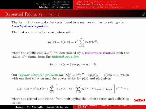
Repeated Roots, r1 = r2 = r 2
The form of the second solution is found in a manner similar to solving theCauchy-Euler equation.
The first solution is found as before with:
y1(x) = φ(r, x) = xr∞∑n=0
an(r)xn,
where the coefficients an(r) are determined by a recurrence relation with thevalues of r found from the indicial equation
F (r) = r(r − 1) + p0r + q0 = 0.
Our regular singular problem was L[y] = x2y ′′ + xp(x)y ′ + q(x)y = 0, whichwith our first solution and the power series for p(x) and q(x) gives
L[φ](r, x) = xra0F (r) +
∞∑n=1
anF (r + n) +
n−1∑k=0
ak[(r + k)pn−k + qn−k]
xr+n = 0,
where the second sum comes from multiplying the infinite series and collectingterms.
Joseph M. Mahaffy, 〈[email protected]〉Lecture Notes – Method of Frobenius —(30/53)
DefinitionsCauchy-Euler Equation
Method of Frobenius
Distinct Roots, r1 − r2 6= NRepeated Roots, r1 = r2 = rRoots Differing by an Integer, r1 − r2 = N
Repeated Roots, r1 = r2 = r 3
Assuming F (r + n) 6= 0, the recurrence relation for the coefficients as a functionof r satisfies:
an(r) = −∑n−1k=0 ak[(r + k)pn−k + qn−k]
F (r + n), n ≥ 1.
Selecting these coefficients reduces our power series solution to:
L[φ](r, x) = xra0F (r),
where F (r) = (r − r1)2 for our repeated root, so L[φ](r1, x) = 0, since our firstsolution is:
y1(x) = φ(r1, x) = xr1∞∑n=0
an(r1)xn,
Significantly, we have
L[∂φ∂r
](r1, x) = a0
∂∂r
[xr(r − r1)
2]∣∣∣r=r1
= a0 [(r − r1)2xrln(x) + 2(r − r1)x
r]∣∣∣r=r1
= 0,
so ∂φ∂r
(r1, x) is also a solution to our problem.
Joseph M. Mahaffy, 〈[email protected]〉Lecture Notes – Method of Frobenius —(31/53)
DefinitionsCauchy-Euler Equation
Method of Frobenius
Distinct Roots, r1 − r2 6= NRepeated Roots, r1 = r2 = rRoots Differing by an Integer, r1 − r2 = N
Repeated Roots, r1 = r2 = r 4
Since ∂φ∂r
(r1, x) is a solution and our first solution is:
y1(x) = φ(r1, x) = xr1∞∑n=0
an(r1)xn,
we obtain the second solution:
y2(x) =∂φ(r,x)∂r
∣∣∣r=r1
=∂
∂r
[xr∞∑n=0
an(r)xn
]∣∣∣∣∣r=r1
= (xr1 ln(x))∞∑n=0
an(r1)xn + xr1∞∑n=1
a′n(r1)xn
= y1(x) ln(x) + xr1∞∑n=1
a′n(r1)xn, x > 0,
where
an(r) = −∑n−1k=0 ak[(r + k)pn−k + qn−k]
F (r + n), n ≥ 1.
Joseph M. Mahaffy, 〈[email protected]〉Lecture Notes – Method of Frobenius —(32/53)
DefinitionsCauchy-Euler Equation
Method of Frobenius
Distinct Roots, r1 − r2 6= NRepeated Roots, r1 = r2 = rRoots Differing by an Integer, r1 − r2 = N
Bessel’s Equation Order Zero 1
Bessel’s Equation Order Zero satisfies:
x2y ′′ + xy ′ + x2y = 0,
where x = 0 is a regular singular point.
From our definitions before we have p(x) = 1 and q(x) = x2, whichimplies that p0 = 1 and q0 = 0.
Since p and q have convergent power series for all x, the solutions willconverge for |x| <∞.
The indicial equation is given by:
r(r − 1) + r = r2 = 0,
so r1 = r2 = 0, repeated root.
Joseph M. Mahaffy, 〈[email protected]〉Lecture Notes – Method of Frobenius —(33/53)
DefinitionsCauchy-Euler Equation
Method of Frobenius
Distinct Roots, r1 − r2 6= NRepeated Roots, r1 = r2 = rRoots Differing by an Integer, r1 − r2 = N
Bessel’s Equation Order Zero 2
With Bessel’s equation order zero,
x2y ′′ + xy ′ + x2y = 0,
we try a solution of the form: y =∞∑n=0
anxn+r.
Differentiating y and entering into the equation gives:
∞∑n=0
an(n+ r)(n+ r − 1)xn+r +∞∑n=0
an(n+ r)xn+r +∞∑n=2
an−2xn+r = 0,
shifting the last index to match powers of x.
From the same powers of x, (n+ r)2an + an−2 = 0, which for r = 0 gives therecurrence relation:
an =−an−2
n2, for n = 2, 3, 4, . . . ,
with a0 arbitrary and a1 = 0.
Joseph M. Mahaffy, 〈[email protected]〉Lecture Notes – Method of Frobenius —(34/53)
DefinitionsCauchy-Euler Equation
Method of Frobenius
Distinct Roots, r1 − r2 6= NRepeated Roots, r1 = r2 = rRoots Differing by an Integer, r1 − r2 = N
Bessel’s Equation Order Zero 3
The recurrence relation shows that the odd powers of x all vanish.
Letting n = 2m in the recurrence relation gives:
a2m =−a2m−2
(2m)2, for n = 1, 2, 3, . . . ,
so
a2 = −a0
22, a4 = −
a2
(2 · 2)2=
a0
24 · 22, a6 = −
a4
(2 · 3)2= −
a0
26(3 · 2)2, . . .
In general, we have
a2m =(−1)ma0
22m(m!)2, m = 1, 2, 3, . . .
The first solution becomes:
y1(x) = a0J0(x) = a0
∞∑m=0
(−1)mx2m
22m(m!)2.
Joseph M. Mahaffy, 〈[email protected]〉Lecture Notes – Method of Frobenius —(35/53)
DefinitionsCauchy-Euler Equation
Method of Frobenius
Distinct Roots, r1 − r2 6= NRepeated Roots, r1 = r2 = rRoots Differing by an Integer, r1 − r2 = N
Bessel’s Equation Order Zero 4
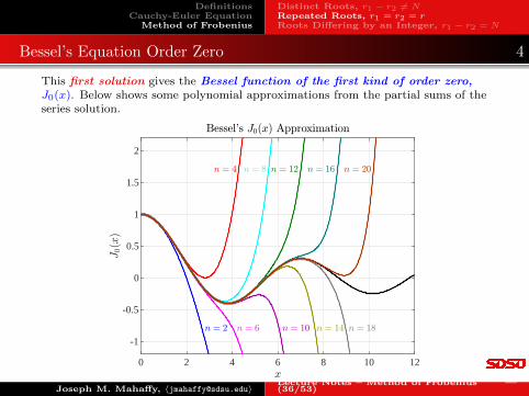
This first solution gives the Bessel function of the first kind of order zero,J0(x). Below shows some polynomial approximations from the partial sums of theseries solution.
0 2 4 6 8 10 12
-1
-0.5
0
0.5
1
1.5
2
Joseph M. Mahaffy, 〈[email protected]〉Lecture Notes – Method of Frobenius —(36/53)
DefinitionsCauchy-Euler Equation
Method of Frobenius
Distinct Roots, r1 − r2 6= NRepeated Roots, r1 = r2 = rRoots Differing by an Integer, r1 − r2 = N
Bessel’s Equation Order Zero 5
Since the Bessel’s equation order zero has only the repeated root r = 0 fromthe indicial equation, the second solution has the form:
y2(x) = y1(x) ln(x) + xr∞∑n=1
bnxn = ln(x)J0(x) +
∞∑n=1
bnxn.
One technique to solve for this second solution is to substitute into Bessel’sequation and solve for the coefficients, bn.
Alternately, we use our results in deriving this form of the second solution, wherewe found that the coefficients satisfied:
bn = a′n(r), where an(r) = −an−2(r)
(n+ r)2,
evaluated at r = 0 based on the recurrence relation for coefficients of the firstsolution.
Joseph M. Mahaffy, 〈[email protected]〉Lecture Notes – Method of Frobenius —(37/53)
DefinitionsCauchy-Euler Equation
Method of Frobenius
Distinct Roots, r1 − r2 6= NRepeated Roots, r1 = r2 = rRoots Differing by an Integer, r1 − r2 = N
Bessel’s Equation Order Zero 6
From the formula deriving the recurrence relation, we find (r + 1)2a1(r) = 0, sonot only a1(0) = 0, but a′1(0) = 0.
It follows from the recurrence relation that
a′3(0) = a′5(0) = · · · = a′2k+1(0) = · · · = 0.
The recurrence relation gives:
a2m(r) = −a2m−2(r)
(2m+ r)2, m = 1, 2, 3, . . .
Hence,
a2(r) = −a0
(2 + r)2,
a4(r) = −a2(r)
(4 + r)2=
a0
(4 + r)2(2 + r)2,
a6(r) = −a4(r)
(6 + r)2=
a0
(6 + r)2(4 + r)2(2 + r)2,
a2m(r) =(−1)ma0
(2m+ r)2(2m− 2 + r)2 · · · (4 + r)2(2 + r)2, m = 1, 2, 3, . . .
Joseph M. Mahaffy, 〈[email protected]〉Lecture Notes – Method of Frobenius —(38/53)
DefinitionsCauchy-Euler Equation
Method of Frobenius
Distinct Roots, r1 − r2 6= NRepeated Roots, r1 = r2 = rRoots Differing by an Integer, r1 − r2 = N
Bessel’s Equation Order Zero 7
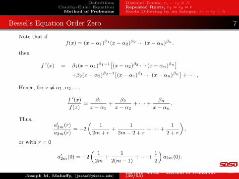
Note that iff(x) = (x− α1)β1 (x− α2)β2 · · · (x− αn)βn .
then
f ′(x) = β1(x− α1)β1−1[(x− α2)β2 · · · (x− αn)βn
]+β2(x− α2)β2−1
[(x− α1)β1 · · · (x− αn)βn
]+ · · · ,
Hence, for x 6= α1, α2, . . .
f ′(x)
f(x)=
β1
x− α1+
β2
x− α2+ · · ·+
βn
x− αn.
Thus,a′2m(r)
a2m(r)= −2
(1
2m+ r+
1
2m− 2 + r+ · · ·+
1
2 + r
),
or with r = 0
a′2m(0) = −2
(1
2m+
1
2(m− 1)+ · · ·+
1
2
)a2m(0).
Joseph M. Mahaffy, 〈[email protected]〉Lecture Notes – Method of Frobenius —(39/53)
DefinitionsCauchy-Euler Equation
Method of Frobenius
Distinct Roots, r1 − r2 6= NRepeated Roots, r1 = r2 = rRoots Differing by an Integer, r1 − r2 = N
Bessel’s Equation Order Zero 8
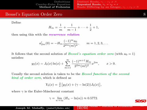
Define
Hm =1
m+
1
m− 1+ · · ·+
1
2+ 1,
then using this with the recurrence relation
a′2m(0) = −Hm(−1)ma0
22m(m!)2, m = 1, 2, 3, . . .
It follows that the second solution of Bessel’s equation order zero (with a0 = 1)satisfies:
y2(x) = J0(x) ln(x) +∞∑m=1
(−1)m+1Hm
22m(m!)2x2m, x > 0.
Usually the second solution is taken to be the Bessel function of the secondkind of order zero, which is defined as
Y0(x) = 2π
[y2(x) + (γ − ln(2))J0(x)
],
where γ is the Euler-Mascheroni constant
γ = limn→∞
(Hn − ln(n)) ≈ 0.5772.
Joseph M. Mahaffy, 〈[email protected]〉Lecture Notes – Method of Frobenius —(40/53)
DefinitionsCauchy-Euler Equation
Method of Frobenius
Distinct Roots, r1 − r2 6= NRepeated Roots, r1 = r2 = rRoots Differing by an Integer, r1 − r2 = N
Bessel’s Equation Order Zero 9
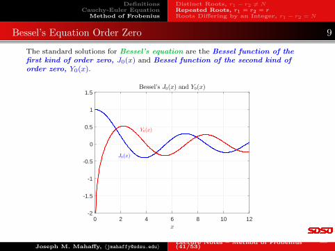
The standard solutions for Bessel’s equation are the Bessel function of thefirst kind of order zero, J0(x) and Bessel function of the second kind oforder zero, Y0(x).
0 2 4 6 8 10 12x
-2
-1.5
-1
-0.5
0
0.5
1
1.5Bessel’s J0(x) and Y0(x)
J0(x)
Y0(x)
Joseph M. Mahaffy, 〈[email protected]〉Lecture Notes – Method of Frobenius —(41/53)
DefinitionsCauchy-Euler Equation
Method of Frobenius
Distinct Roots, r1 − r2 6= NRepeated Roots, r1 = r2 = rRoots Differing by an Integer, r1 − r2 = N
Roots Differing by an Integer, r1 − r2 = N 1
Case 3. Roots Differing by an Integer, r1 − r2 = N , where N isa positive integer.
As before, one solution of the regular singular problem satisfies:
y1(x) = |x|r1∞∑n=0
anxn.
The second linearly independent solution has the form:
y2(x) = k y1(x) ln |x|+ |x|r2∞∑n=0
bnxn
with these solutions converging for at least |x| < ρ, where ρ is theradius of convergence for p(x) and q(x).
This case divides into two subcases, depending on whether or not thelogarithmic term appears, as k may be zero.
Joseph M. Mahaffy, 〈[email protected]〉Lecture Notes – Method of Frobenius —(42/53)
DefinitionsCauchy-Euler Equation
Method of Frobenius
Distinct Roots, r1 − r2 6= NRepeated Roots, r1 = r2 = rRoots Differing by an Integer, r1 − r2 = N
Roots Differing by an Integer, r1 − r2 = N 2
Case 3. Roots Differing by an Integer, r1 − r2 = N , where N isa positive integer.
This case is more complicated with the coefficients in the secondsolution satisfying:
bn(r2) = ddr [(r − r2)an(r)
∣∣r=r2
, n = 0, 1, 2, . . .
with a0 = r − r2 and
k = limr→r2
(r − r2)aN (r).
In practice the best way to determine if k = 0 is to compute an(r2)and see if one finds aN (r2).
If this is possible, then the second solution is readily found withoutthe logarithmic term; otherwise, the logarithmic term must beincluded.
Joseph M. Mahaffy, 〈[email protected]〉Lecture Notes – Method of Frobenius —(43/53)
DefinitionsCauchy-Euler Equation
Method of Frobenius
Distinct Roots, r1 − r2 6= NRepeated Roots, r1 = r2 = rRoots Differing by an Integer, r1 − r2 = N
Example: Roots, r1 − r2 = N 1
Example: Consider the ODE:
x2y ′′ + 3xy ′ + 4x4y = 0,
where x = 0 is a regular singular point.
We try a solution of the form: y1(x) =∞∑n=0
anxn+r.
Differentiating y and entering into the equation gives:
∞∑n=0
an(n+ r)(n+ r − 1)xn+r + 3∞∑n=0
an(n+ r)xn+r + 4∞∑n=4
an−4xn+r = 0,
shifting the last index to match powers of x.
Examining this equation with n = 0 gives the indicial equation:
F (r) = r(r − 1) + 3r = r(r + 2) = 0,
which has the roots r1 = 0 and r2 = −2 (r1 − r2 = 2).
Joseph M. Mahaffy, 〈[email protected]〉Lecture Notes – Method of Frobenius —(44/53)
DefinitionsCauchy-Euler Equation
Method of Frobenius
Distinct Roots, r1 − r2 6= NRepeated Roots, r1 = r2 = rRoots Differing by an Integer, r1 − r2 = N
Example: Roots, r1 − r2 = N 2
Example: The series above could be rearranged in the following form:
∞∑n=0
an(n+ r)(n+ r + 2)xn+r = −4∞∑n=4
an−4xn+r.
With r1 = 0, we obtain the recurrence relations:
a1(r1 +1)(r1 +3) = 3a1 = 0, a2(r1 +2)(r1 +4) = 8a2 = 0, a3(r1 +3)(r1 +5) = 15a3 = 0,
a1 = a2 = a3 = 0, and
an(r) = −4
(n+ r)(n+ r + 2)an−4(r) or an = −
4
n(n+ 2)an−4.
It follows that
a4 = −4
6 · 4a0 = −
a0
3 · 2, a8 = −
4
10 · 8a4 =
a0
5!, a12 = −
4
14 · 12a8 = −
a0
7!,
and a1 = a5 = ... = a4n+1 = 0, a2 = a6 = ... = a4n+2 = 0, anda3 = a7 = ... = a4n+3 = 0.
Joseph M. Mahaffy, 〈[email protected]〉Lecture Notes – Method of Frobenius —(45/53)
DefinitionsCauchy-Euler Equation
Method of Frobenius
Distinct Roots, r1 − r2 6= NRepeated Roots, r1 = r2 = rRoots Differing by an Integer, r1 − r2 = N
Example: Roots, r1 − r2 = N 3
Example: The results above are combined to give the 1st solution:
y1(x) = a0
∞∑m=0
(−1)m
(2m+ 1)!x4m.
To find the 2nd solution we need to know if the logarithmic term needs to beincluded.
This term is unnecessary if
limr→r2
aN (r) exists.
For this example, r2 = −2 and N = 2, so we examine
limr→−2
a2(r) =0
(r + 2)(r + 4)= 0,
which implies the second series may be computed directly with no logarithmicterm.
Thus, we try a solution of the form:
y2(x) =∞∑n=0
bnxn+r2 ,
with r2 = −2.Joseph M. Mahaffy, 〈[email protected]〉Lecture Notes – Method of Frobenius —(46/53)
DefinitionsCauchy-Euler Equation
Method of Frobenius
Distinct Roots, r1 − r2 6= NRepeated Roots, r1 = r2 = rRoots Differing by an Integer, r1 − r2 = N
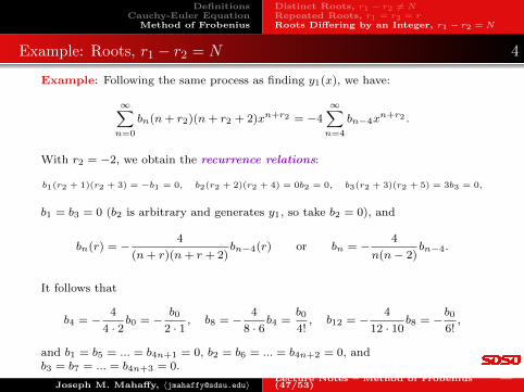
Example: Roots, r1 − r2 = N 4
Example: Following the same process as finding y1(x), we have:
∞∑n=0
bn(n+ r2)(n+ r2 + 2)xn+r2 = −4∞∑n=4
bn−4xn+r2 .
With r2 = −2, we obtain the recurrence relations:
b1(r2 + 1)(r2 + 3) = −b1 = 0, b2(r2 + 2)(r2 + 4) = 0b2 = 0, b3(r2 + 3)(r2 + 5) = 3b3 = 0,
b1 = b3 = 0 (b2 is arbitrary and generates y1, so take b2 = 0), and
bn(r) = −4
(n+ r)(n+ r + 2)bn−4(r) or bn = −
4
n(n− 2)bn−4.
It follows that
b4 = −4
4 · 2b0 = −
b0
2 · 1, b8 = −
4
8 · 6b4 =
b0
4!, b12 = −
4
12 · 10b8 = −
b0
6!,
and b1 = b5 = ... = b4n+1 = 0, b2 = b6 = ... = b4n+2 = 0, andb3 = b7 = ... = b4n+3 = 0.
Joseph M. Mahaffy, 〈[email protected]〉Lecture Notes – Method of Frobenius —(47/53)
DefinitionsCauchy-Euler Equation
Method of Frobenius
Distinct Roots, r1 − r2 6= NRepeated Roots, r1 = r2 = rRoots Differing by an Integer, r1 − r2 = N
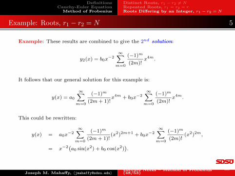
Example: Roots, r1 − r2 = N 5
Example: These results are combined to give the 2nd solution:
y2(x) = b0x−2
∞∑m=0
(−1)m
(2m)!x4m.
It follows that our general solution for this example is:
y(x) = a0
∞∑m=0
(−1)m
(2m+ 1)!x4m + b0x
−2∞∑m=0
(−1)m
(2m)!x4m.
This could be rewritten:
y(x) = a0x−2
∞∑m=0
(−1)m
(2m+ 1)!(x2)2m+1 + b0x
−2∞∑m=0
(−1)m
(2m)!(x2)2m,
= x−2(a0 sin(x2) + b0 cos(x2)
).
Joseph M. Mahaffy, 〈[email protected]〉Lecture Notes – Method of Frobenius —(48/53)
DefinitionsCauchy-Euler Equation
Method of Frobenius
Distinct Roots, r1 − r2 6= NRepeated Roots, r1 = r2 = rRoots Differing by an Integer, r1 − r2 = N
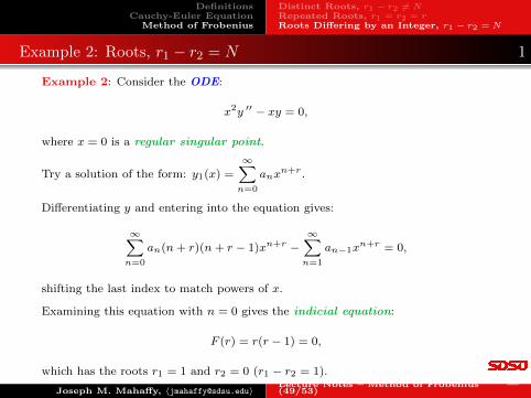
Example 2: Roots, r1 − r2 = N 1
Example 2: Consider the ODE:
x2y ′′ − xy = 0,
where x = 0 is a regular singular point.
Try a solution of the form: y1(x) =∞∑n=0
anxn+r.
Differentiating y and entering into the equation gives:
∞∑n=0
an(n+ r)(n+ r − 1)xn+r −∞∑n=1
an−1xn+r = 0,
shifting the last index to match powers of x.
Examining this equation with n = 0 gives the indicial equation:
F (r) = r(r − 1) = 0,
which has the roots r1 = 1 and r2 = 0 (r1 − r2 = 1).
Joseph M. Mahaffy, 〈[email protected]〉Lecture Notes – Method of Frobenius —(49/53)
DefinitionsCauchy-Euler Equation
Method of Frobenius
Distinct Roots, r1 − r2 6= NRepeated Roots, r1 = r2 = rRoots Differing by an Integer, r1 − r2 = N
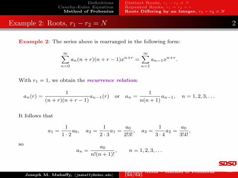
Example 2: Roots, r1 − r2 = N 2
Example 2: The series above is rearranged in the following form:
∞∑n=0
an(n+ r)(n+ r − 1)xn+r =∞∑n=1
an−1xn+r.
With r1 = 1, we obtain the recurrence relation:
an(r) =1
(n+ r)(n+ r − 1)an−1(r) or an =
1
n(n+ 1)an−1, n = 1, 2, 3, . . .
It follows that
a1 =1
1 · 2a0, a2 =
1
2 · 3a1 =
a0
2!3!, a3 =
1
3 · 4a2 =
a0
3!4!,
soan =
a0
n!(n+ 1)!, n = 1, 2, 3, . . .
Joseph M. Mahaffy, 〈[email protected]〉Lecture Notes – Method of Frobenius —(50/53)
DefinitionsCauchy-Euler Equation
Method of Frobenius
Distinct Roots, r1 − r2 6= NRepeated Roots, r1 = r2 = rRoots Differing by an Integer, r1 − r2 = N
Example 2: Roots, r1 − r2 = N 3
Example 2: The results above are combined to give the 1st solution:
y1(x) = a0
∞∑n=0
1
n!(n+ 1)!xn+1.
To find the 2nd solution we need to know if the logarithmic term needs to beincluded.
This term is necessary if
limr→r2
aN (r) fails to exist.
For this example, r2 = 0 and N = 1, so we examine
limr→0
a1(r) =a0(r)
(r + 1)r.
Since a0 is arbitrary (non-zero), this limit is undefined, so a second series solutionrequires the logarithmic term.
For r2 = 0, we try a solution of the form:
y2(x) = k y1(x) ln(x) +∞∑n=0
bnxn+r2 ,
Joseph M. Mahaffy, 〈[email protected]〉Lecture Notes – Method of Frobenius —(51/53)
DefinitionsCauchy-Euler Equation
Method of Frobenius
Distinct Roots, r1 − r2 6= NRepeated Roots, r1 = r2 = rRoots Differing by an Integer, r1 − r2 = N
Example 2: Roots, r1 − r2 = N 4
Example 2: Insert y2(x) = k y1(x) ln(x) +∞∑n=0
bnxn into the ODE, so
x2
[ky′′1 ln(x) + 2ky′1
1x− ky1 1
x2+∞∑n=2
n(n− 1)bnxn−2
]
−kxy1 ln(x)−∞∑n=0
bnxn+1 = 0.
Because y1(x) is a solution of the ODE, k ln(x)[x2y′′1 − xy1] = 0, which reducesthis expression to
2kxy′1 − ky1 +∞∑n=2
n(n− 1)bnxn −
∞∑n=0
bnxn+1 = 0.
Using the series solution for y1(x) with a0 = 1 and shifting indices, we obtain
∞∑n=0
(2k
(n!)2− kn!(n+1)!
)xn+1 +
∞∑n=1
bn+1(n+ 1)nxn+1 −∞∑n=0
bnxn+1 = 0.
Joseph M. Mahaffy, 〈[email protected]〉Lecture Notes – Method of Frobenius —(52/53)
DefinitionsCauchy-Euler Equation
Method of Frobenius
Distinct Roots, r1 − r2 6= NRepeated Roots, r1 = r2 = rRoots Differing by an Integer, r1 − r2 = N
Example 2: Roots, r1 − r2 = N 5
Example 2: From the series above our recurrence relation gives:
k − b0 = 0, or k = b0
and2k
(n!)2− kn!(n+1)!
+ n(n+ 1)bn+1 − bn = 0, n = 1, 2, 3, . . .
Equivalently,
bn+1 = 1n(n+1)
[bn − (2n+1)k
n!(n+1)!
], n = 1, 2, 3, . . .
For convenience we take a0 = 1 and b0 = k = 1.
The constant b1 is still arbitrary (as it would generate y1(x) again), so we selectb1 = 0 and find a particular 2nd solution using the recurrence relation:
y2(x) = y1(x) ln(x) + 1− 34x2 − 7
36x3 − 35
1728x4 − . . .
Joseph M. Mahaffy, 〈[email protected]〉Lecture Notes – Method of Frobenius —(53/53)