the method of frobenius - iit guwahati
TRANSCRIPT

The Method of Frobenius
Department of MathematicsIIT Guwahati
SU/KSK MA-102 (2018)
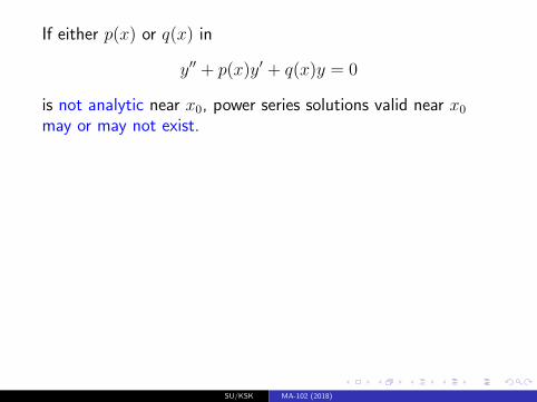
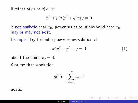
If either p(x) or q(x) in
y′′ + p(x)y′ + q(x)y = 0
is not analytic near x0, power series solutions valid near x0may or may not exist.
Example: Try to find a power series solution of
x2y′′ − y′ − y = 0 (1)
about the point x0 = 0.
Assume that a solution
y(x) =∞∑n=0
anxn
exists.
SU/KSK MA-102 (2018)
If either p(x) or q(x) in
y′′ + p(x)y′ + q(x)y = 0
is not analytic near x0, power series solutions valid near x0may or may not exist.
Example: Try to find a power series solution of
x2y′′ − y′ − y = 0 (1)
about the point x0 = 0.
Assume that a solution
y(x) =∞∑n=0
anxn
exists.
SU/KSK MA-102 (2018)
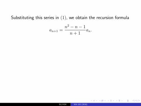
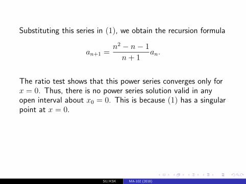
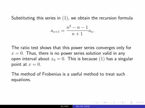
Substituting this series in (1), we obtain the recursion formula
an+1 =n2 − n− 1
n+ 1an.
The ratio test shows that this power series converges only forx = 0. Thus, there is no power series solution valid in anyopen interval about x0 = 0. This is because (1) has a singularpoint at x = 0.
The method of Frobenius is a useful method to treat suchequations.
SU/KSK MA-102 (2018)
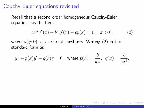
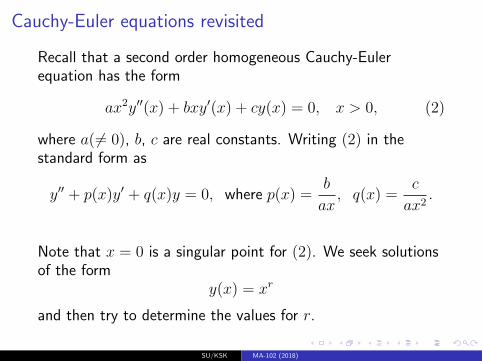
Cauchy-Euler equations revisited
Recall that a second order homogeneous Cauchy-Eulerequation has the form
ax2y′′(x) + bxy′(x) + cy(x) = 0, x > 0, (2)
where a(6= 0), b, c are real constants. Writing (2) in thestandard form as
y′′ + p(x)y′ + q(x)y = 0, where p(x) =b
ax, q(x) =
c
ax2.
Note that x = 0 is a singular point for (2). We seek solutionsof the form
y(x) = xr
and then try to determine the values for r.
SU/KSK MA-102 (2018)
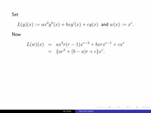
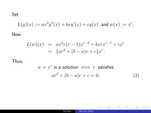
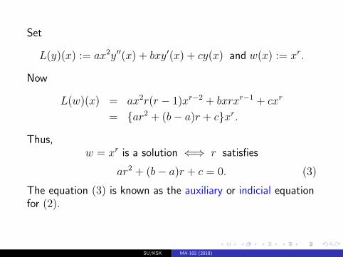
Set
L(y)(x) := ax2y′′(x) + bxy′(x) + cy(x) and w(x) := xr.
Now
L(w)(x) = ax2r(r − 1)xr−2 + bxrxr−1 + cxr
= {ar2 + (b− a)r + c}xr.
Thus,w = xr is a solution ⇐⇒ r satisfies
ar2 + (b− a)r + c = 0. (3)
The equation (3) is known as the auxiliary or indicial equationfor (2).
SU/KSK MA-102 (2018)
Set
L(y)(x) := ax2y′′(x) + bxy′(x) + cy(x) and w(x) := xr.
Now
L(w)(x) = ax2r(r − 1)xr−2 + bxrxr−1 + cxr
= {ar2 + (b− a)r + c}xr.
Thus,w = xr is a solution ⇐⇒ r satisfies
ar2 + (b− a)r + c = 0. (3)
The equation (3) is known as the auxiliary or indicial equationfor (2).
SU/KSK MA-102 (2018)
Set
L(y)(x) := ax2y′′(x) + bxy′(x) + cy(x) and w(x) := xr.
Now
L(w)(x) = ax2r(r − 1)xr−2 + bxrxr−1 + cxr
= {ar2 + (b− a)r + c}xr.
Thus,w = xr is a solution ⇐⇒ r satisfies
ar2 + (b− a)r + c = 0. (3)
The equation (3) is known as the auxiliary or indicial equationfor (2).
SU/KSK MA-102 (2018)
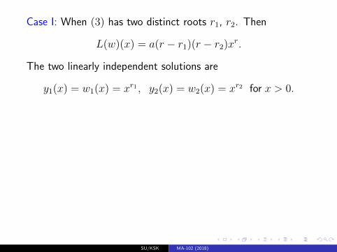
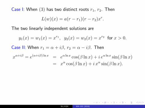
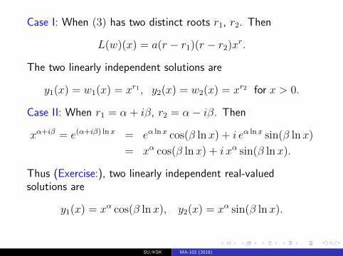
Case I: When (3) has two distinct roots r1, r2. Then
L(w)(x) = a(r − r1)(r − r2)xr.
The two linearly independent solutions are
y1(x) = w1(x) = xr1 , y2(x) = w2(x) = xr2 for x > 0.
Case II: When r1 = α + iβ, r2 = α− iβ. Then
xα+iβ = e(α+iβ) lnx = eα lnx cos(β lnx) + i eα lnx sin(β lnx)
= xα cos(β lnx) + i xα sin(β lnx).
Thus (Exercise:), two linearly independent real-valuedsolutions are
y1(x) = xα cos(β lnx), y2(x) = xα sin(β lnx).
SU/KSK MA-102 (2018)
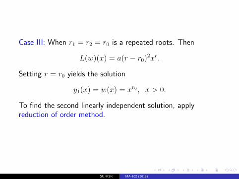
Case III: When r1 = r2 = r0 is a repeated roots. Then
L(w)(x) = a(r − r0)2xr.
Setting r = r0 yields the solution
y1(x) = w(x) = xr0 , x > 0.
To find the second linearly independent solution, applyreduction of order method.
SU/KSK MA-102 (2018)
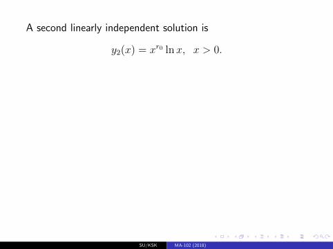
A second linearly independent solution is
y2(x) = xr0 lnx, x > 0.
Example: Find a general solution to
4x2y′′(x) + y(x) = 0, x > 0.
Note thatL(w)(x) = (4r2 − 4r + 1)xr.
The indicial equation has repeated roots r0 = 1/2. Thus, thegeneral solution is
y(x) = c1√x+ c2
√x lnx, x > 0.
SU/KSK MA-102 (2018)
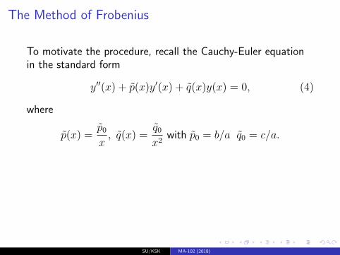
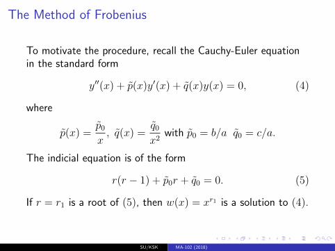
The Method of Frobenius
To motivate the procedure, recall the Cauchy-Euler equationin the standard form
y′′(x) + p̃(x)y′(x) + q̃(x)y(x) = 0, (4)
where
p̃(x) =p̃0x, q̃(x) =
q̃0x2
with p̃0 = b/a q̃0 = c/a.
The indicial equation is of the form
r(r − 1) + p̃0r + q̃0 = 0. (5)
If r = r1 is a root of (5), then w(x) = xr1 is a solution to (4).
SU/KSK MA-102 (2018)
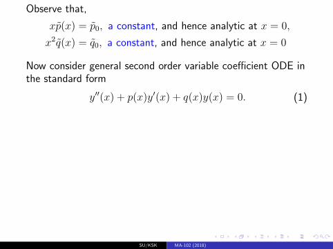
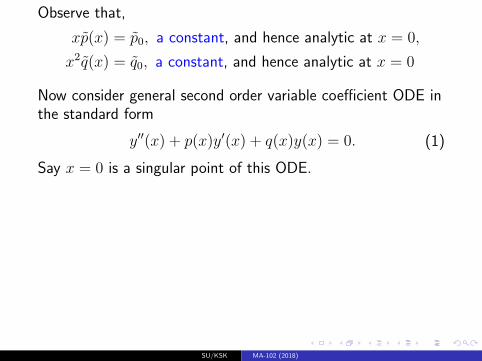
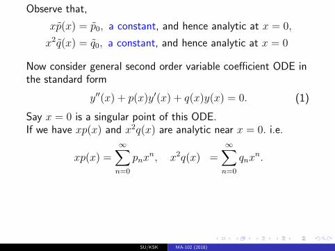
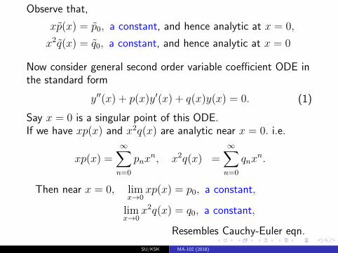
Observe that,
xp̃(x) = p̃0, a constant, and hence analytic at x = 0,
x2q̃(x) = q̃0, a constant, and hence analytic at x = 0
Now consider general second order variable coefficient ODE inthe standard form
y′′(x) + p(x)y′(x) + q(x)y(x) = 0. (1)
Say x = 0 is a singular point of this ODE.If we have xp(x) and x2q(x) are analytic near x = 0. i.e.
xp(x) =∞∑n=0
pnxn, x2q(x) =
∞∑n=0
qnxn.
Then near x = 0, limx→0
xp(x) = p0, a constant,
limx→0
x2q(x) = q0, a constant,
Resembles Cauchy-Euler eqn.
SU/KSK MA-102 (2018)
Observe that,
xp̃(x) = p̃0, a constant, and hence analytic at x = 0,
x2q̃(x) = q̃0, a constant, and hence analytic at x = 0
Now consider general second order variable coefficient ODE inthe standard form
y′′(x) + p(x)y′(x) + q(x)y(x) = 0. (1)
Say x = 0 is a singular point of this ODE.
If we have xp(x) and x2q(x) are analytic near x = 0. i.e.
xp(x) =∞∑n=0
pnxn, x2q(x) =
∞∑n=0
qnxn.
Then near x = 0, limx→0
xp(x) = p0, a constant,
limx→0
x2q(x) = q0, a constant,
Resembles Cauchy-Euler eqn.
SU/KSK MA-102 (2018)
Observe that,
xp̃(x) = p̃0, a constant, and hence analytic at x = 0,
x2q̃(x) = q̃0, a constant, and hence analytic at x = 0
Now consider general second order variable coefficient ODE inthe standard form
y′′(x) + p(x)y′(x) + q(x)y(x) = 0. (1)
Say x = 0 is a singular point of this ODE.If we have xp(x) and x2q(x) are analytic near x = 0. i.e.
xp(x) =∞∑n=0
pnxn, x2q(x) =
∞∑n=0
qnxn.
Then near x = 0, limx→0
xp(x) = p0, a constant,
limx→0
x2q(x) = q0, a constant,
Resembles Cauchy-Euler eqn.
SU/KSK MA-102 (2018)
Observe that,
xp̃(x) = p̃0, a constant, and hence analytic at x = 0,
x2q̃(x) = q̃0, a constant, and hence analytic at x = 0
Now consider general second order variable coefficient ODE inthe standard form
y′′(x) + p(x)y′(x) + q(x)y(x) = 0. (1)
Say x = 0 is a singular point of this ODE.If we have xp(x) and x2q(x) are analytic near x = 0. i.e.
xp(x) =∞∑n=0
pnxn, x2q(x) =
∞∑n=0
qnxn.
Then near x = 0, limx→0
xp(x) = p0, a constant,
limx→0
x2q(x) = q0, a constant,
Resembles Cauchy-Euler eqn.
SU/KSK MA-102 (2018)
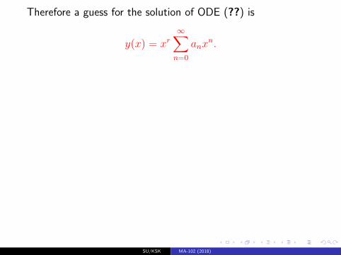
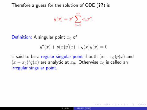
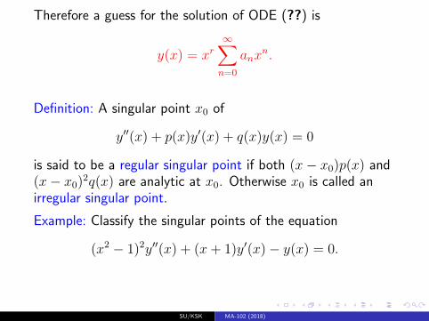
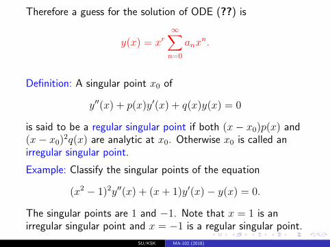
Therefore a guess for the solution of ODE (??) is
y(x) = xr∞∑n=0
anxn.
Definition: A singular point x0 of
y′′(x) + p(x)y′(x) + q(x)y(x) = 0
is said to be a regular singular point if both (x− x0)p(x) and(x− x0)2q(x) are analytic at x0. Otherwise x0 is called anirregular singular point.
Example: Classify the singular points of the equation
(x2 − 1)2y′′(x) + (x+ 1)y′(x)− y(x) = 0.
The singular points are 1 and −1. Note that x = 1 is anirregular singular point and x = −1 is a regular singular point.
SU/KSK MA-102 (2018)
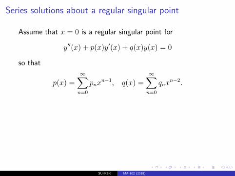
Series solutions about a regular singular point
Assume that x = 0 is a regular singular point for
y′′(x) + p(x)y′(x) + q(x)y(x) = 0
so that
p(x) =∞∑n=0
pnxn−1, q(x) =
∞∑n=0
qnxn−2.
In the method of Frobenius, we seek solutions of the form
w(x) = xr∞∑n=0
anxn =
∞∑n=0
anxn+r, x > 0.
Assume that a0 6= 0. We now determine r and an, n ≥ 1.
SU/KSK MA-102 (2018)
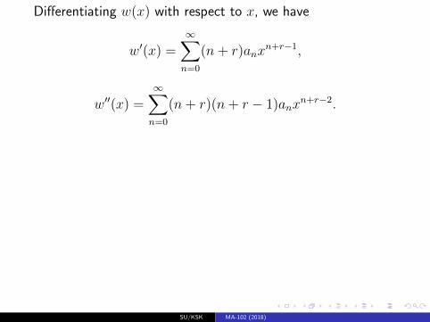
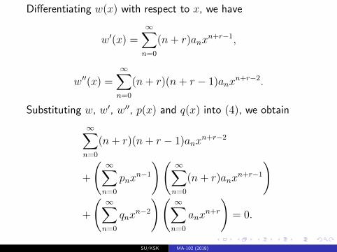
Differentiating w(x) with respect to x, we have
w′(x) =∞∑n=0
(n+ r)anxn+r−1,
w′′(x) =∞∑n=0
(n+ r)(n+ r − 1)anxn+r−2.
Substituting w, w′, w′′, p(x) and q(x) into (4), we obtain
∞∑n=0
(n+ r)(n+ r − 1)anxn+r−2
+
(∞∑n=0
pnxn−1
)(∞∑n=0
(n+ r)anxn+r−1
)
+
(∞∑n=0
qnxn−2
)(∞∑n=0
anxn+r
)= 0.
SU/KSK MA-102 (2018)
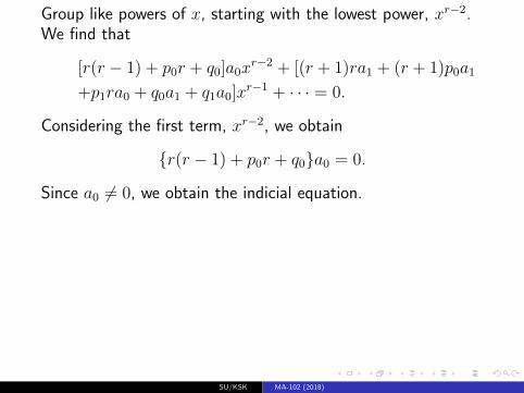
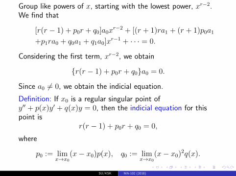
Group like powers of x, starting with the lowest power, xr−2.We find that
[r(r − 1) + p0r + q0]a0xr−2 + [(r + 1)ra1 + (r + 1)p0a1
+p1ra0 + q0a1 + q1a0]xr−1 + · · · = 0.
Considering the first term, xr−2, we obtain
{r(r − 1) + p0r + q0}a0 = 0.
Since a0 6= 0, we obtain the indicial equation.
Definition: If x0 is a regular singular point ofy′′ + p(x)y′ + q(x)y = 0, then the indicial equation for thispoint is
r(r − 1) + p0r + q0 = 0,
where
p0 := limx→x0
(x− x0)p(x), q0 := limx→x0
(x− x0)2q(x).
SU/KSK MA-102 (2018)
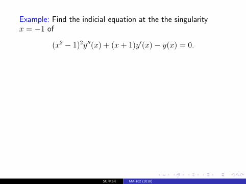
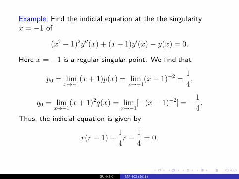
Example: Find the indicial equation at the the singularityx = −1 of
(x2 − 1)2y′′(x) + (x+ 1)y′(x)− y(x) = 0.
Here x = −1 is a regular singular point. We find that
p0 = limx→−1
(x+ 1)p(x) = limx→−1
(x− 1)−2 =1
4,
q0 = limx→−1
(x+ 1)2q(x) = limx→−1
[−(x− 1)−2] = −1
4.
Thus, the indicial equation is given by
r(r − 1) +1
4r − 1
4= 0.
SU/KSK MA-102 (2018)
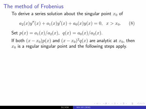
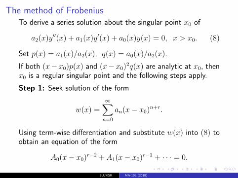
The method of FrobeniusTo derive a series solution about the singular point x0 of
a2(x)y′′(x) + a1(x)y
′(x) + a0(x)y(x) = 0, x > x0. (8)
Set p(x) = a1(x)/a2(x), q(x) = a0(x)/a2(x).
If both (x− x0)p(x) and (x− x0)2q(x) are analytic at x0, thenx0 is a regular singular point and the following steps apply.
Step 1: Seek solution of the form
w(x) =∞∑n=0
an(x− x0)n+r.
Using term-wise differentiation and substitute w(x) into (8) toobtain an equation of the form
A0(x− x0)r−2 + A1(x− x0)r−1 + · · · = 0.
SU/KSK MA-102 (2018)
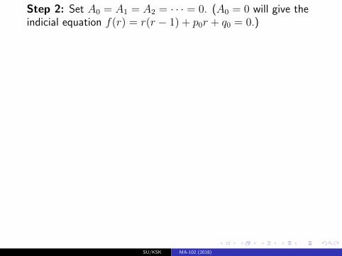
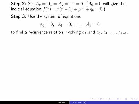
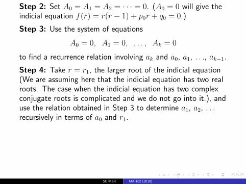
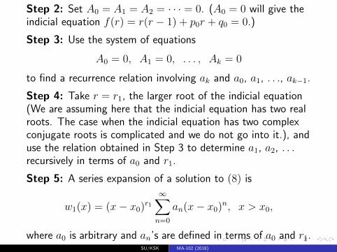
Step 2: Set A0 = A1 = A2 = · · · = 0. (A0 = 0 will give theindicial equation f(r) = r(r − 1) + p0r + q0 = 0.)
Step 3: Use the system of equations
A0 = 0, A1 = 0, . . . , Ak = 0
to find a recurrence relation involving ak and a0, a1, . . ., ak−1.
Step 4: Take r = r1, the larger root of the indicial equation(We are assuming here that the indicial equation has two realroots. The case when the indicial equation has two complexconjugate roots is complicated and we do not go into it.), anduse the relation obtained in Step 3 to determine a1, a2, . . .recursively in terms of a0 and r1.
Step 5: A series expansion of a solution to (8) is
w1(x) = (x− x0)r1∞∑n=0
an(x− x0)n, x > x0,
where a0 is arbitrary and an’s are defined in terms of a0 and r1.
SU/KSK MA-102 (2018)
Step 2: Set A0 = A1 = A2 = · · · = 0. (A0 = 0 will give theindicial equation f(r) = r(r − 1) + p0r + q0 = 0.)
Step 3: Use the system of equations
A0 = 0, A1 = 0, . . . , Ak = 0
to find a recurrence relation involving ak and a0, a1, . . ., ak−1.
Step 4: Take r = r1, the larger root of the indicial equation(We are assuming here that the indicial equation has two realroots. The case when the indicial equation has two complexconjugate roots is complicated and we do not go into it.), anduse the relation obtained in Step 3 to determine a1, a2, . . .recursively in terms of a0 and r1.
Step 5: A series expansion of a solution to (8) is
w1(x) = (x− x0)r1∞∑n=0
an(x− x0)n, x > x0,
where a0 is arbitrary and an’s are defined in terms of a0 and r1.SU/KSK MA-102 (2018)
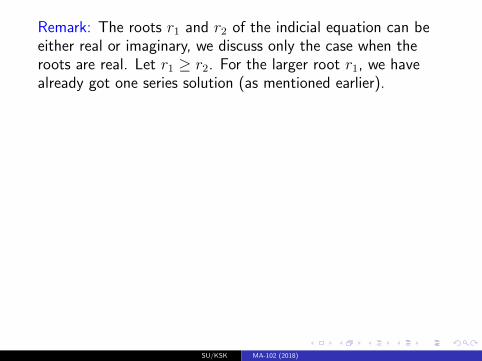
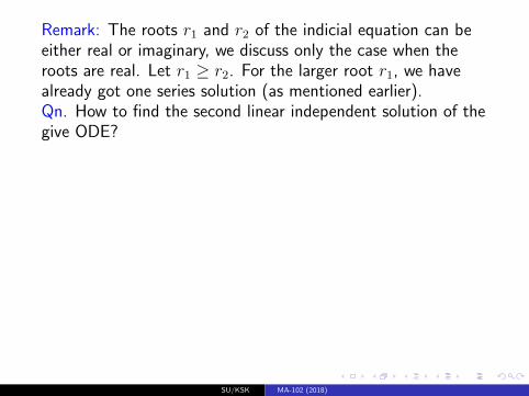
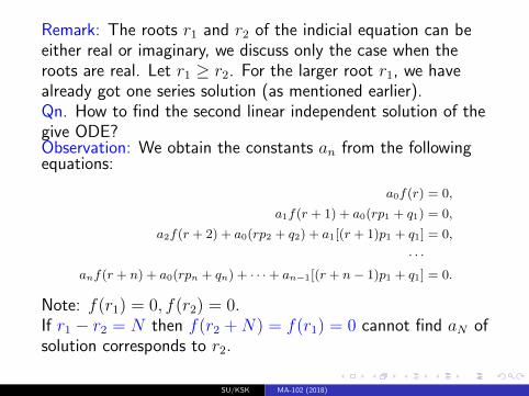
Remark: The roots r1 and r2 of the indicial equation can beeither real or imaginary, we discuss only the case when theroots are real. Let r1 ≥ r2. For the larger root r1, we havealready got one series solution (as mentioned earlier).
Qn. How to find the second linear independent solution of thegive ODE?Observation: We obtain the constants an from the followingequations:
a0f(r) = 0,
a1f(r + 1) + a0(rp1 + q1) = 0,
a2f(r + 2) + a0(rp2 + q2) + a1[(r + 1)p1 + q1] = 0,
· · ·anf(r + n) + a0(rpn + qn) + · · ·+ an−1[(r + n− 1)p1 + q1] = 0.
Note: f(r1) = 0, f(r2) = 0.If r1 − r2 = N then f(r2 +N) = f(r1) = 0 cannot find aN ofsolution corresponds to r2.
SU/KSK MA-102 (2018)
Remark: The roots r1 and r2 of the indicial equation can beeither real or imaginary, we discuss only the case when theroots are real. Let r1 ≥ r2. For the larger root r1, we havealready got one series solution (as mentioned earlier).Qn. How to find the second linear independent solution of thegive ODE?
Observation: We obtain the constants an from the followingequations:
a0f(r) = 0,
a1f(r + 1) + a0(rp1 + q1) = 0,
a2f(r + 2) + a0(rp2 + q2) + a1[(r + 1)p1 + q1] = 0,
· · ·anf(r + n) + a0(rpn + qn) + · · ·+ an−1[(r + n− 1)p1 + q1] = 0.
Note: f(r1) = 0, f(r2) = 0.If r1 − r2 = N then f(r2 +N) = f(r1) = 0 cannot find aN ofsolution corresponds to r2.
SU/KSK MA-102 (2018)

Remark: The roots r1 and r2 of the indicial equation can beeither real or imaginary, we discuss only the case when theroots are real. Let r1 ≥ r2. For the larger root r1, we havealready got one series solution (as mentioned earlier).Qn. How to find the second linear independent solution of thegive ODE?Observation: We obtain the constants an from the followingequations:
a0f(r) = 0,
a1f(r + 1) + a0(rp1 + q1) = 0,
a2f(r + 2) + a0(rp2 + q2) + a1[(r + 1)p1 + q1] = 0,
· · ·anf(r + n) + a0(rpn + qn) + · · ·+ an−1[(r + n− 1)p1 + q1] = 0.
Note: f(r1) = 0, f(r2) = 0.If r1 − r2 = N then f(r2 +N) = f(r1) = 0 cannot find aN ofsolution corresponds to r2.
SU/KSK MA-102 (2018)
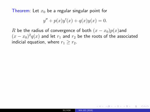
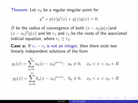
Theorem: Let x0 be a regular singular point for
y′′ + p(x)y′(x) + q(x)y(x) = 0.
R be the radius of convergence of both (x− x0)p(x)and(x− x0)2q(x) and let r1 and r2 be the roots of the associatedindicial equation, where r1 ≥ r2.
Case a: If r1 − r2 is not an integer, then there exist twolinearly independent solutions of the form
y1(x) =∞∑n=0
an(x− x0)n+r1 ; a0 6= 0, x0 < x < x0 +R
y2(x) =∞∑n=0
bn(x− x0)n+r2 , b0 6= 0, x0 < x < x0 +R
SU/KSK MA-102 (2018)
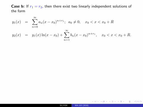
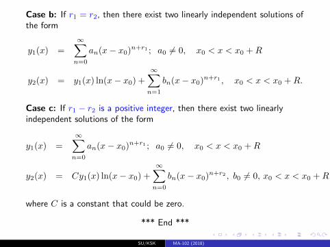
Case b: If r1 = r2, then there exist two linearly independent solutions ofthe form
y1(x) =
∞∑n=0
an(x− x0)n+r1 ; a0 6= 0, x0 < x < x0 +R
y2(x) = y1(x) ln(x− x0) +
∞∑n=1
bn(x− x0)n+r1 , x0 < x < x0 +R.
Case c: If r1 − r2 is a positive integer, then there exist two linearlyindependent solutions of the form
y1(x) =∞∑
n=0
an(x− x0)n+r1 ; a0 6= 0, x0 < x < x0 +R
y2(x) = Cy1(x) ln(x− x0) +
∞∑n=0
bn(x− x0)n+r2 , b0 6= 0, x0 < x < x0 +R
where C is a constant that could be zero.
*** End ***
SU/KSK MA-102 (2018)
Case b: If r1 = r2, then there exist two linearly independent solutions ofthe form
y1(x) =
∞∑n=0
an(x− x0)n+r1 ; a0 6= 0, x0 < x < x0 +R
y2(x) = y1(x) ln(x− x0) +
∞∑n=1
bn(x− x0)n+r1 , x0 < x < x0 +R.
Case c: If r1 − r2 is a positive integer, then there exist two linearlyindependent solutions of the form
y1(x) =
∞∑n=0
an(x− x0)n+r1 ; a0 6= 0, x0 < x < x0 +R
y2(x) = Cy1(x) ln(x− x0) +
∞∑n=0
bn(x− x0)n+r2 , b0 6= 0, x0 < x < x0 +R
where C is a constant that could be zero.
*** End ***
SU/KSK MA-102 (2018)