metals

Article

Metamodels’ Development for High Pressure Die Casting ofAluminum Alloy

Eva Anglada 1 , Fernando Boto 2 , Maider García de Cortazar 1 and Iñaki Garmendia 3,*

�����������������

Citation: Anglada, E.; Boto, F.;

García de Cortazar, M.; Garmendia, I.

Metamodels’ Development for High

Pressure Die Casting of Aluminum

Alloy. Metals 2021, 11, 1747. https://

doi.org/10.3390/met11111747

Academic Editor: Cristiano Fragassa

Received: 10 September 2021

Accepted: 26 October 2021

Published: 31 October 2021

Publisher’s Note: MDPI stays neutral

with regard to jurisdictional claims in

published maps and institutional affil-

iations.

Copyright: © 2021 by the authors.

Licensee MDPI, Basel, Switzerland.

This article is an open access article

distributed under the terms and

conditions of the Creative Commons

Attribution (CC BY) license (https://

creativecommons.org/licenses/by/

4.0/).

1 TECNALIA, Basque Research and Technology Alliance (BRTA), Mikeletegi Pasealekua 2,E-20009 Donostia-San Sebastián, Spain; eva.anglada@tecnalia.com (E.A.);maider.garciadecortazar@tecnalia.com (M.G.d.C.)

2 TECNALIA, Basque Research and Technology Alliance (BRTA), Mikeletegi Pasealekua 7,E-20009 Donostia-San Sebastián, Spain; fernando.boto@tecnalia.com

3 Mechanical Engineering Department, Engineering School of Gipuzkoa, University of the Basque CountryUPV/EHU, Plaza de Europa 1, E-20018 Donostia-San Sebastián, Spain

* Correspondence: inaki.garmendia@ehu.es

Abstract: Simulation is a very useful tool in the design of the part and process conditions of high-pressure die casting (HPDC), due to the intrinsic complexity of this manufacturing process. Usually,physics-based models solved by finite element or finite volume methods are used, but their maindrawback is the long calculation time. In order to apply optimization strategies in the design processor to implement online predictive systems, faster models are required. One solution is the use ofsurrogate models, also called metamodels or grey-box models. The novelty of the work presentedhere lies in the development of several metamodels for the HPDC process. These metamodels arebased on a gradient boosting regressor technique and derived from a physics-based finite elementmodel. The results show that the developed metamodels are able to predict with high accuracy thesecondary dendrite arm spacing (SDAS) of the cast parts and, with good accuracy, the misrun riskand the shrinkage level. Results obtained in the predictions of microporosity and macroporosity,eutectic percentage, and grain density were less accurate. The metamodels were very fast (less than1 s); therefore, they can be used for optimization activities or be integrated into online predictionsystems for the HPDC industry. The case study corresponds to several parts of aluminum cast alloys,used in the automotive industry, manufactured by high-pressure die casting in a multicavity mold.

Keywords: simulation; modeling; FEM; metamodel; gradient boosting; die casting; aluminum;HPDC; metal casting

1. Introduction

A large number of scientific and engineering fields study complex real-world phe-nomena or solve challenging design problems with simulation techniques [1–4]. However,in many cases, the computational cost of these simulations makes their use impossible forreal-time predictions and limits their application in optimization tasks. The use of machinelearning techniques such as neural networks or ensemble methods has become a usefulalternative to avoid these limitations.

In this paper, we take advantage of the metamodeling schema to have reliable and fastquality predictions for high-pressure die casting (HPDC). The metamodeling approach hasbeen used in many fields [5–7], but for the particular case of HPDC process, the numberof works is reduced. The work of Fiorese et al. in [8,9] was focused on the use of newpredictive variables derived from plunger movement and the prediction of the ultimatestrength of the cast parts. Krimpenis et al. [10] used neural nets and predicted the misrunrisks and the solidification time. Finally, Yao et al. [11] based their metamodel on a Gaussianprocess regression and predicted the temperature at the end of filling.

The novelty of this work is two-fold. From a computational point of view, the noveltylies in the application of a gradient boosting regressor technique to the HPDC process

Metals 2021, 11, 1747. https://doi.org/10.3390/met11111747 https://www.mdpi.com/journal/metals

Metals 2021, 11, 1747 2 of 19

modeling. From a metal casting point of view, the novelty lies in the possibility to predictin real time many aspects of interest for the quality of the manufactured parts, such as themisrun risk, the shrinkage defects, the microporosity and macroporosity, the grain density,the eutectic percentage, and the SDAS. These metamodels make it possible to implementan online predictive system in real time to be used during the manufacturing process andcan also be used as a basis for the optimization of the process parameters, shorting thesetup of the machine configuration.

Based on their underlying principles and data sources, there are three different typesof process modeling schemes:

• White-box models: These are rigorous models based on mass and energy balanceswith the process rate or kinetics equations. They give an almost exact image of thephysical laws and the behavior of the given real system. Complete knowledge of theway the system works is needed to develop the model;

• Black-box models: These are developed by measuring the inputs and outputs of thesystem and fitting a linear or nonlinear mathematical function to approximate theoperation of the system. In this case, since data from experiments on the real systemare used to build the model, we are not given any insight into or understanding ofhow the system works;

• Grey-box models: These are semi-empirical-based or experimentally adjusted mod-els. Grey-box models are developed using white-box models whose parametersare estimated using the measured system inputs and outputs. Some examples areneuro-fuzzy systems or semi-empirical models.

Metamodels, also called surrogate models or response surfaces, are within the “grey-box models” group. They are compact and inexpensive to evaluate and have provento be very useful for tasks such as optimization, design space exploration, prototyping,and sensitivity analysis. In this work, the development of certain metamodels for thehigh-pressure die casting process (HPDC), the most common process to cast automotiveparts, is presented.

A metamodel is an approximation of the relationship between the design variables(inputs) and the response functions (outputs), which is implied by an underlying simula-tion model.

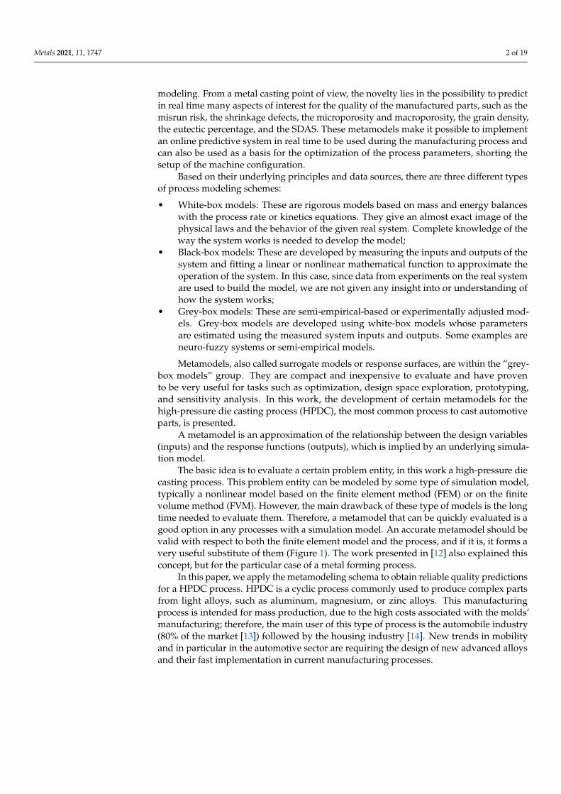
The basic idea is to evaluate a certain problem entity, in this work a high-pressure diecasting process. This problem entity can be modeled by some type of simulation model,typically a nonlinear model based on the finite element method (FEM) or on the finitevolume method (FVM). However, the main drawback of these type of models is the longtime needed to evaluate them. Therefore, a metamodel that can be quickly evaluated is agood option in any processes with a simulation model. An accurate metamodel should bevalid with respect to both the finite element model and the process, and if it is, it forms avery useful substitute of them (Figure 1). The work presented in [12] also explained thisconcept, but for the particular case of a metal forming process.

In this paper, we apply the metamodeling schema to obtain reliable quality predictionsfor a HPDC process. HPDC is a cyclic process commonly used to produce complex partsfrom light alloys, such as aluminum, magnesium, or zinc alloys. This manufacturingprocess is intended for mass production, due to the high costs associated with the molds’manufacturing; therefore, the main user of this type of process is the automobile industry(80% of the market [13]) followed by the housing industry [14]. New trends in mobilityand in particular in the automotive sector are requiring the design of new advanced alloysand their fast implementation in current manufacturing processes.

Metals 2021, 11, 1747 3 of 19

Figure 1. Metamodel schema.

This article is hereafter structured as follows: Section 2 gives some background aboutthe HPDC process and its simulation; Section 3 describes the basis of the methodologiesused (the variables’ selection, the design of experiments, the numerical simulation, andthe metamodeling); Section 4 explains how these methodologies were applied to this casestudy; Sections 5 and 6 show the results and their discussion, respectively; finally, Section 7compiles the conclusions of the work performed.

2. High-Pressure Die Casting Modeling

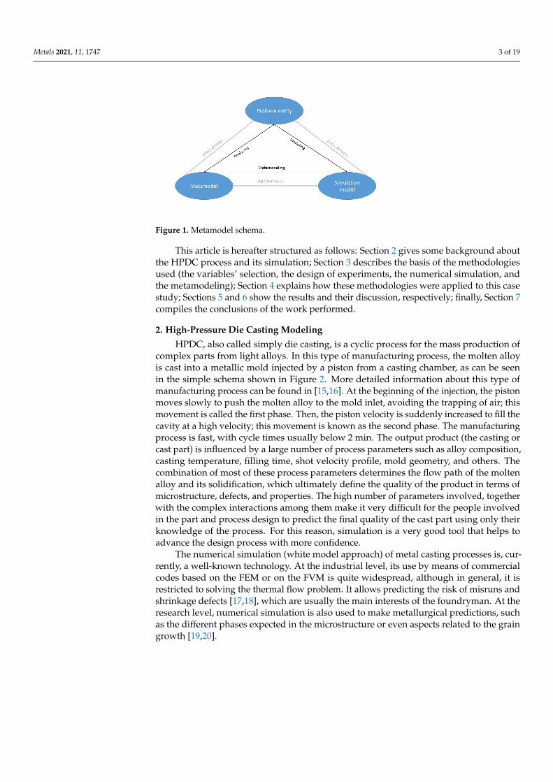
HPDC, also called simply die casting, is a cyclic process for the mass production ofcomplex parts from light alloys. In this type of manufacturing process, the molten alloyis cast into a metallic mold injected by a piston from a casting chamber, as can be seenin the simple schema shown in Figure 2. More detailed information about this type ofmanufacturing process can be found in [15,16]. At the beginning of the injection, the pistonmoves slowly to push the molten alloy to the mold inlet, avoiding the trapping of air; thismovement is called the first phase. Then, the piston velocity is suddenly increased to fill thecavity at a high velocity; this movement is known as the second phase. The manufacturingprocess is fast, with cycle times usually below 2 min. The output product (the casting orcast part) is influenced by a large number of process parameters such as alloy composition,casting temperature, filling time, shot velocity profile, mold geometry, and others. Thecombination of most of these process parameters determines the flow path of the moltenalloy and its solidification, which ultimately define the quality of the product in terms ofmicrostructure, defects, and properties. The high number of parameters involved, togetherwith the complex interactions among them make it very difficult for the people involvedin the part and process design to predict the final quality of the cast part using only theirknowledge of the process. For this reason, simulation is a very good tool that helps toadvance the design process with more confidence.

The numerical simulation (white model approach) of metal casting processes is, cur-rently, a well-known technology. At the industrial level, its use by means of commercialcodes based on the FEM or on the FVM is quite widespread, although in general, it isrestricted to solving the thermal flow problem. It allows predicting the risk of misruns andshrinkage defects [17,18], which are usually the main interests of the foundryman. At theresearch level, numerical simulation is also used to make metallurgical predictions, suchas the different phases expected in the microstructure or even aspects related to the graingrowth [19,20].

Metals 2021, 11, 1747 4 of 19

Figure 2. Cold-chamber high-pressure die casting schema.

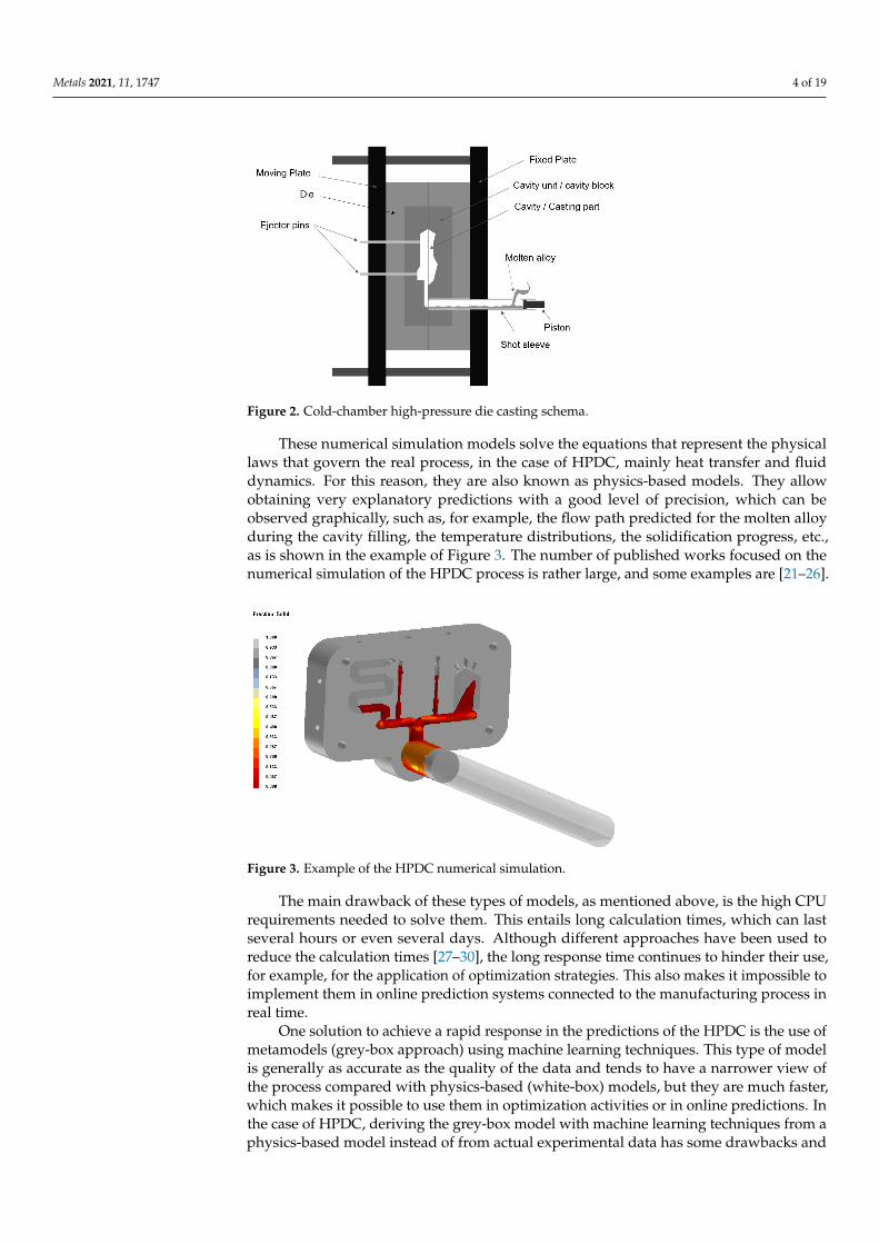
These numerical simulation models solve the equations that represent the physicallaws that govern the real process, in the case of HPDC, mainly heat transfer and fluiddynamics. For this reason, they are also known as physics-based models. They allowobtaining very explanatory predictions with a good level of precision, which can beobserved graphically, such as, for example, the flow path predicted for the molten alloyduring the cavity filling, the temperature distributions, the solidification progress, etc.,as is shown in the example of Figure 3. The number of published works focused on thenumerical simulation of the HPDC process is rather large, and some examples are [21–26].

Figure 3. Example of the HPDC numerical simulation.

The main drawback of these types of models, as mentioned above, is the high CPUrequirements needed to solve them. This entails long calculation times, which can lastseveral hours or even several days. Although different approaches have been used toreduce the calculation times [27–30], the long response time continues to hinder their use,for example, for the application of optimization strategies. This also makes it impossible toimplement them in online prediction systems connected to the manufacturing process inreal time.

One solution to achieve a rapid response in the predictions of the HPDC is the use ofmetamodels (grey-box approach) using machine learning techniques. This type of modelis generally as accurate as the quality of the data and tends to have a narrower view ofthe process compared with physics-based (white-box) models, but they are much faster,which makes it possible to use them in optimization activities or in online predictions. Inthe case of HPDC, deriving the grey-box model with machine learning techniques from aphysics-based model instead of from actual experimental data has some drawbacks and

Metals 2021, 11, 1747 5 of 19

advantages. The main drawback is the possible loss of accuracy. Whereas it is assumedthat the experimental data perfectly reflect the actual situation, the use of the simulationresults can imply a loss of accuracy, since the physics-based model will never be completelyaccurate [31]. The main advantage is the greater flexibility to select different input data ifthey are required during the grey-box model development. A supplementary advantage isa significant cost savings.

Considering these advantages, in the work presented here, we decided to develop ametamodel of the HPDC process, from a physics-based model. The methodology followedto develop this metamodel, capable of predicting the misrun risk, the shrinkage, theporosity level, the microstructure, and the grain density of the manufactured parts, isexplained together with the results obtained. The case study corresponds to several partsmanufactured in AlSi alloys in a multicavity mold.

3. Methodology

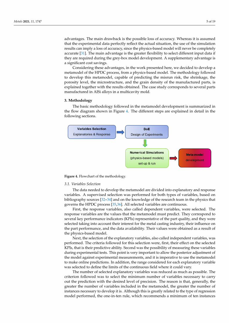
The basic methodology followed in the metamodel development is summarized inthe flow diagram shown in Figure 4. The different steps are explained in detail in thefollowing sections.

Figure 4. Flowchart of the methodology.

3.1. Variables Selection

The data needed to develop the metamodel are divided into explanatory and responsevariables. A supervised selection was performed for both types of variables, based onbibliography sources [32–34] and on the knowledge of the research team in the physics thatgoverns the HPDC process [35,36]. All selected variables are continuous.

First, the response variables, also called dependent variables, were selected. Theresponse variables are the values that the metamodel must predict. They correspond toseveral key performance indicators (KPIs) representative of the part quality, and they wereselected taking into account their interest for the metal casting industry, their influence onthe part performance, and the data availability. Their values were obtained as a result ofthe physics-based model.

Next, the selection of the explanatory variables, also called independent variables, wasperformed. The criteria followed for this selection were, first, their effect on the selectedKPIs, that is their predictive ability. Second was the possibility of measuring these variablesduring experimental tests. This point is very important to allow the posterior adjustment ofthe model against experimental measurements, and it is imperative to use the metamodelto make online predictions. In addition, the range considered for each explanatory variablewas selected to define the limits of the continuous field where it could vary.

The number of selected explanatory variables was reduced as much as possible. Thecriterion followed was to select the minimum number of variables necessary to carryout the prediction with the desired level of precision. The reason is that, generally, thegreater the number of variables included in the metamodel, the greater the number ofinstances necessary to develop it is. Although this is greatly related to the type of regressionmodel performed, the one-in-ten rule, which recommends a minimum of ten instances

Metals 2021, 11, 1747 6 of 19

for each independent variable, is commonly mentioned as a rule of thumb [37]. In thiscase, each instance is one simulation of the case study under different specific processconditions. Therefore, if the number of explanatory variables is very high, the number ofsimulations to be performed will be very large and the time required will be very long. Themain drawback of using a small number of explanatory variables is the risk of omittingsome variables whose effect is significant in the prediction. However, this also has someadditional advantages, such as requiring a smaller number of sensors if the metamodel isused in an online predictor.

3.2. Design of Experiments

Once having defined the limits of the continuous field, where the explanatory variablescan vary, the second step is to carry out a design of experiments to determine the test cases,that is the numerical simulations to be carried out. The idea is to have the minimumnumber of cases necessary to cover the whole field where the process conditions mayvary. As in this case, all the variables used are continuous, it is also necessary to define thenumber of levels for each variable, that is the points to study in the variable range.

Different techniques can be used to define the tests to be performed. In a completefactorial design, all possible combinations of the levels defined for the factors (variables)are studied. This type of design accentuates the factor effects, allows the estimation of theinteractions among them, and permits a good coverage of the whole field of the boundaryconditions. However, the drawback is that the resultant number of tests is high. Onealternative to the full factorial design is the use of reduced designs such as the centralcomposite design (CCD) or Box–Behnken designs. These approximations attempt to mapthe relationship between the response and the factor settings, minimizing the number oftrials. For more detailed information about these types of designs, Reference [38] can beconsulted.

3.3. Numerical Simulations: Obtaining the Data

The numerical simulations (physics-based models or white-box models) correspond-ing to each of the case studies identified in the DoE were set up and run.

The main governing equations of the physics involved in HPDC models at themacroscale level are the conservation of energy (1), the mass conservation or continu-ity Equation (2), and the Boussinesq form of the Navier–Stokes equation for incompressibleNewtonian fluids (3), where ρ represents density, h enthalpy, t time, ν velocity, k thermalconductivity, T temperature, Rq heat generation per unit mass, ρ0 density at the referencetemperature and pressure, p modified pressure, µl shear viscosity, g gravity, and βT thevolumetric thermal expansion coefficient. In addition, some additional equations wereused to calculate aspects related to the microstructure and specific algorithms for defectprediction . More detailed information about these topics can be found in [39,40].

ρ∂h∂t

+ ρν · ∇h = ∇ · (k∇T) + ρRq (1)

∂ρ

∂t+∇ · (ρν) = 0 (2)

ρ0

(∂ν

∂t+ ν · ∇ν

)= −∇ p + µl∇2ν− ρ0gβT(T − T0) (3)

These physics-based models were set up and solved with ProCAST, a finite elementsoftware specially focused on the simulation of metal casting processes. Actually, it usesa variation of the finite element method called the edge-based finite element method(EBFEM), which is a more robust discretization method for fluid flow problems. In addition,it uses a coupled finite element–cellular automaton model for the prediction of grainstructure solidification [41].

Metals 2021, 11, 1747 7 of 19

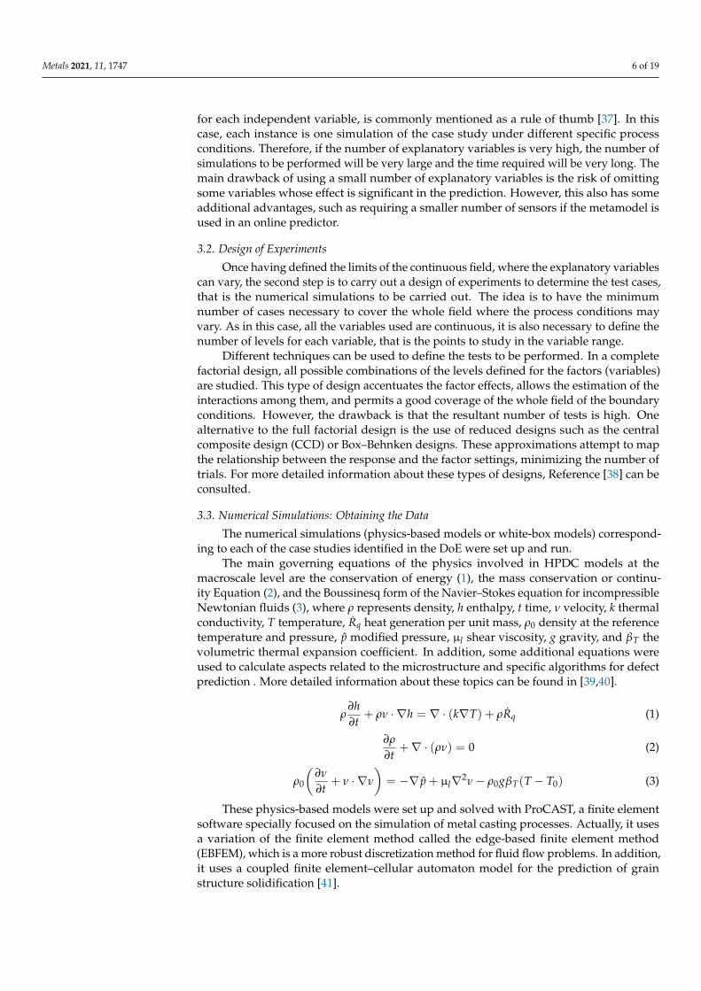
To set up the model, first, the mold geometry was drawn with a CAD system, then itwas discretized by means of a finite element mesh, and the material properties and bound-ary conditions were applied. Finally, the model was solved, as can be seen in Figure 5.

Figure 5. Physics-based model setup and running.

The numerical simulation of HPDC was very complex and very demanding in termsof the CPU. On the one hand, the flow velocity is very high during mold filling. In fact, thefilling time of the cavities is measured in milliseconds. Moreover, the alloy cooling ratesare also very high, easily exceeding values of 20 C/s. All this hinders the convergence ofthe numerical solution, requiring the use of short time steps that extend the CPU times. Onthe other hand, the manufacturing process is a continuous cycle procedure. Thus, the moldtemperature is not constant throughout the cycle, and the temperature distribution is notuniform throughout the mold, since it depends on the cavities’ geometry, the presence ofcooling or heating systems, and the cycle times. Therefore, the simulation of the thermalbehavior of the mold during several cycles until reaching the thermal stabilization isrequired before performing the simulation of the filling and solidification process.

Of course, when the simulation is not limited to the thermal flow problem, additionalcomplex calculations must be performed to obtain complementary results, such as themicrostructure, grain density, or porosity caused by air entrapment, which lengthen theCPU times even more.

These facts explain the interest in reducing the number of tests as much as possible.

3.4. Metamodel Development: Regression Model

There are many machine learning techniques commonly used in the literature toperform a supervised regression model, which is the underlying concept in a metamodelstrategy to predict any continuous variable. Some of those techniques are neural net-works [42], kriging or the Gaussian process [43], ensemble methods such as random forestor gradient boosting [44,45], etc.

For this study, we did not analyze all the strategies named before, but only the gradientboosting algorithm, which is a very competitive approach in terms of accuracy in this typeof regression problem, as pointed out in [46]. Two other reasons for selecting this techniqueare the power to prevent overfitting, which is very interesting in problems with a smallamount of data, and last, but not least, the setup of this approach is not so time consumingas in kriging or neural networks.

The main idea of the boosting method is to add models to the set sequentially. In eachiteration, a “weak” model (base learner) is trained with respect to the total error of the setgenerated up to that moment.

To overcome the overtraining problem of this type of algorithm, a statistical connectionwas established with the gradient descent formulation to find local minima.

In gradient boosting models (GBMs), the learning procedure is consecutively adjustedto new models to provide a more accurate estimate of the response variable. The main ideabehind this algorithm is to build the new base models so that they correlate as much aspossible to the negative gradient of the loss function, associated with the whole set. Theloss functions applied can be arbitrary, but to give better intuition, if the error functionis the classic quadratic error, the learning procedure would result in a consecutive error

Metals 2021, 11, 1747 8 of 19

adjustment. In general, the choice of the loss function depends on the problem, with a greatvariety of loss functions implemented up to now and with the possibility of implementinga specific one for the task. Normally, the choice of one of them is a consequence of trial anderror.

Therefore, the objective of this model is to minimize the loss function ψ(y, f ) shownin (4):

f = argmin f (x)(ψ(y, f (x))) (4)

With regard to the loss function, the minimum absolute error or L1 − loss is usu-ally used, considered one of the most robust, but also the minimum square error is alsoconsidered.

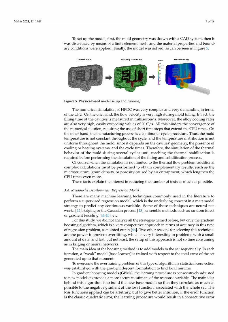
To summarize, the complete gradient boosting algorithm can be formulated as orig-inally proposed by Friedman [45]. A computationally flexible way of capturing the in-teractions among the variables in a GBM is based on the use of regression trees. Thesemodels usually have the tree depth and divisions as the parameters, but the most importantparameter in a GBM is the number of trees generated (learners). Therefore, an analysis ofthe number of learners for each case is needed to have the most reliable parametrization.In Figure 6, an analysis of the number of learners versus the error of the whole GBM isshown for the misrun prediction of Part Numbers 2, 3, and 4.

Figure 6. Number of learners (regression trees) vs. the error of the GB model for misrun prediction.Each line represents different test components in the casting. Part 1 and Part 2 are related to tensiletests in different locations. Part 3 is a flat plate component.

4. Design of the Tests and Implementation4.1. Case Study and Variables’ Selection

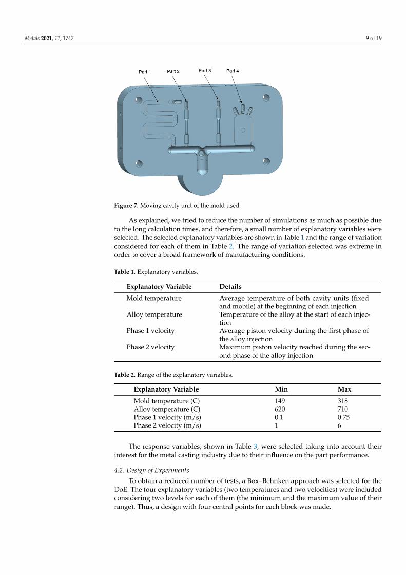
The case study corresponded to several parts cast in one multicavity mold by meansof the HPDC process. The mold has four cavities, as can be seen in Figure 7, to manufacturefour parts each time. The alloy used is an AlSi alloy, common in the HPDC manufacturingand for automotive structural components. Part Number 1 was designed to evaluate thecastability of the alloy, that is its ability to fill the entire cavity of the part; Part Numbers 2and 3 are specimens for tensile tests; and Part Number 4 is a flat plate designed to evaluatethe porosity level and the microstructure.

As introduced in previous sections, the CPU times needed to obtain the simulationresults were very long. In the tests conducted for this case study, the CPU times variedbetween 5 h and 37 h for each simulation. The reasons for these variations in CPU timeswere related to the convergence difficulties found for the different cases, due to the differentboundary conditions of each of them (mold and alloy temperatures and velocity values).

Metals 2021, 11, 1747 9 of 19

Figure 7. Moving cavity unit of the mold used.

As explained, we tried to reduce the number of simulations as much as possible dueto the long calculation times, and therefore, a small number of explanatory variables wereselected. The selected explanatory variables are shown in Table 1 and the range of variationconsidered for each of them in Table 2. The range of variation selected was extreme inorder to cover a broad framework of manufacturing conditions.

Table 1. Explanatory variables.

Explanatory Variable Details

Mold temperature Average temperature of both cavity units (fixedand mobile) at the beginning of each injection

Alloy temperature Temperature of the alloy at the start of each injec-tion

Phase 1 velocity Average piston velocity during the first phase ofthe alloy injection

Phase 2 velocity Maximum piston velocity reached during the sec-ond phase of the alloy injection

Table 2. Range of the explanatory variables.

Explanatory Variable Min Max

Mold temperature (C) 149 318Alloy temperature (C) 620 710Phase 1 velocity (m/s) 0.1 0.75Phase 2 velocity (m/s) 1 6

The response variables, shown in Table 3, were selected taking into account theirinterest for the metal casting industry due to their influence on the part performance.

4.2. Design of Experiments

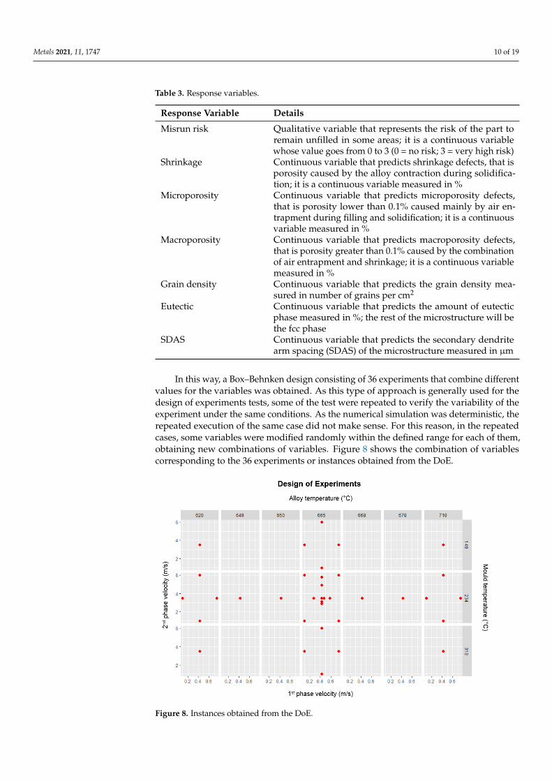
To obtain a reduced number of tests, a Box–Behnken approach was selected for theDoE. The four explanatory variables (two temperatures and two velocities) were includedconsidering two levels for each of them (the minimum and the maximum value of theirrange). Thus, a design with four central points for each block was made.

Metals 2021, 11, 1747 10 of 19

Table 3. Response variables.

Response Variable Details

Misrun risk Qualitative variable that represents the risk of the part toremain unfilled in some areas; it is a continuous variablewhose value goes from 0 to 3 (0 = no risk; 3 = very high risk)

Shrinkage Continuous variable that predicts shrinkage defects, that isporosity caused by the alloy contraction during solidifica-tion; it is a continuous variable measured in %

Microporosity Continuous variable that predicts microporosity defects,that is porosity lower than 0.1% caused mainly by air en-trapment during filling and solidification; it is a continuousvariable measured in %

Macroporosity Continuous variable that predicts macroporosity defects,that is porosity greater than 0.1% caused by the combinationof air entrapment and shrinkage; it is a continuous variablemeasured in %

Grain density Continuous variable that predicts the grain density mea-sured in number of grains per cm2

Eutectic Continuous variable that predicts the amount of eutecticphase measured in %; the rest of the microstructure will bethe fcc phase

SDAS Continuous variable that predicts the secondary dendritearm spacing (SDAS) of the microstructure measured in µm

In this way, a Box–Behnken design consisting of 36 experiments that combine differentvalues for the variables was obtained. As this type of approach is generally used for thedesign of experiments tests, some of the test were repeated to verify the variability of theexperiment under the same conditions. As the numerical simulation was deterministic, therepeated execution of the same case did not make sense. For this reason, in the repeatedcases, some variables were modified randomly within the defined range for each of them,obtaining new combinations of variables. Figure 8 shows the combination of variablescorresponding to the 36 experiments or instances obtained from the DoE.

Figure 8. Instances obtained from the DoE.

Metals 2021, 11, 1747 11 of 19

4.3. Numerical Simulation

The numerical simulations corresponding to each test case defined by the DoE werecarried out.

The two cavity units, located in the fixed and mobile plates, respectively, were drawnwith a CAD system together with the piston and its sleeve. This set was discretized with afinite element mesh formed by 468,436 nodes and 2,285,758 elements.

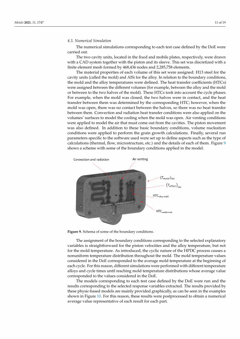
The material properties of each volume of this set were assigned: H13 steel for thecavity units (called the mold) and AlSi for the alloy. In relation to the boundary conditions,the mold and the alloy temperatures were defined. The heat transfer coefficients (HTCs)were assigned between the different volumes (for example, between the alloy and the moldor between to the two halves of the mold). These HTCs took into account the cycle phases.For example, when the mold was closed, the two halves were in contact, and the heattransfer between them was determined by the corresponding HTC; however, when themold was open, there was no contact between the halves, so there was no heat transferbetween them. Convection and radiation heat transfer conditions were also applied on thevolumes’ surfaces to model the cooling when the mold was open. Air venting conditionswere applied to model the air that must come out from the cavities. The piston movementwas also defined. In addition to these basic boundary conditions, volume nucleationconditions were applied to perform the grain growth calculations. Finally, several runparameters specific to the software used were set up to define aspects such as the type ofcalculations (thermal, flow, microstructure, etc.) and the details of each of them. Figure 9shows a scheme with some of the boundary conditions applied in the model.

Figure 9. Schema of some of the boundary conditions.

The assignment of the boundary conditions corresponding to the selected explanatoryvariables is straightforward for the piston velocities and the alloy temperature, but notfor the mold temperature. As introduced, the cyclic nature of the HPDC process causes anonuniform temperature distribution throughout the mold. The mold temperature valuesconsidered in the DoE corresponded to the average mold temperature at the beginning ofeach cycle. For this reason, different simulations were performed with different temperaturealloys and cycle times until reaching mold temperature distributions whose average valuecorresponded to the values considered in the DoE.

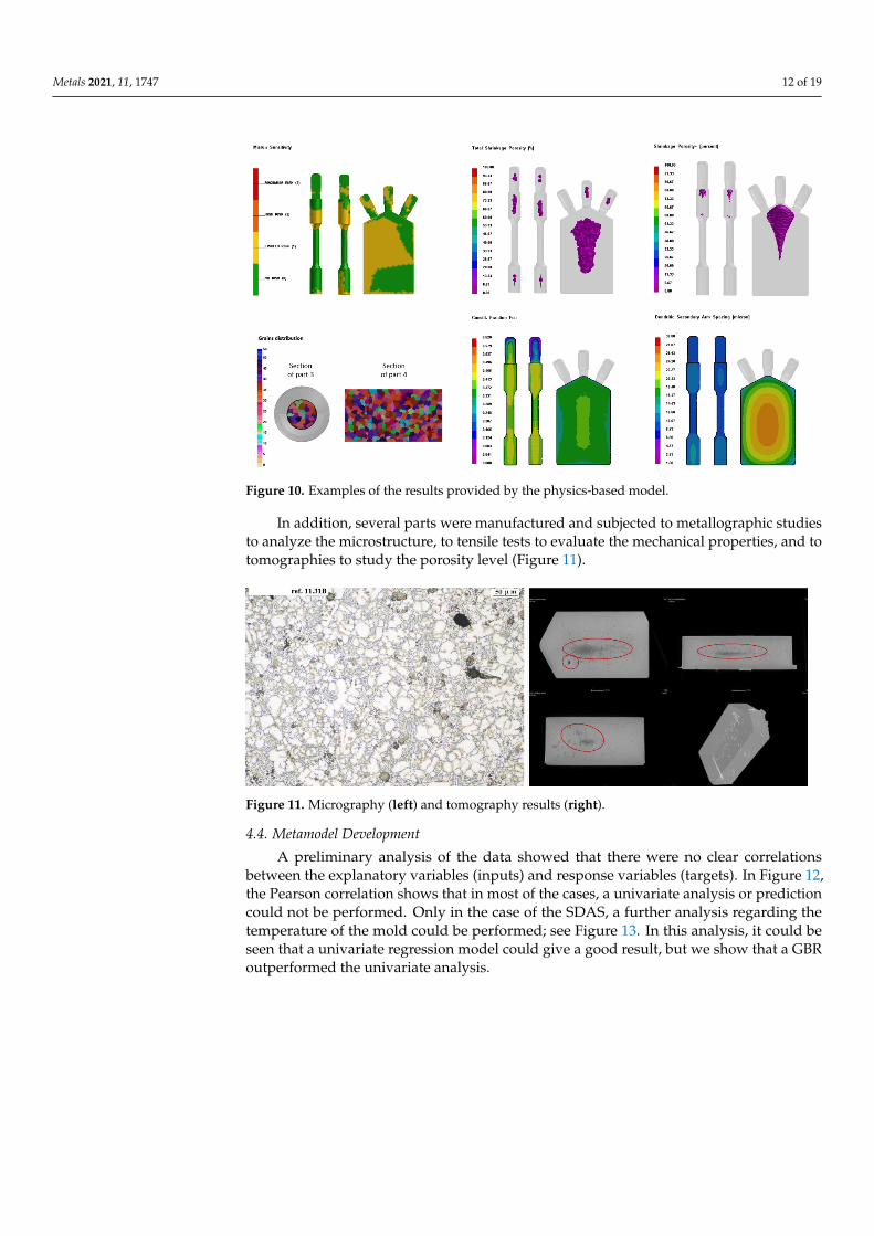
The models corresponding to each test case defined by the DoE were run and theresults corresponding to the selected response variables extracted. The results provided bythese physic-based models are mainly provided graphically, as can be seen in the examplesshown in Figure 10. For this reason, these results were postprocessed to obtain a numericalaverage value representative of each result for each part.

Metals 2021, 11, 1747 12 of 19

Figure 10. Examples of the results provided by the physics-based model.

In addition, several parts were manufactured and subjected to metallographic studiesto analyze the microstructure, to tensile tests to evaluate the mechanical properties, and totomographies to study the porosity level (Figure 11).

Figure 11. Micrography (left) and tomography results (right).

4.4. Metamodel Development

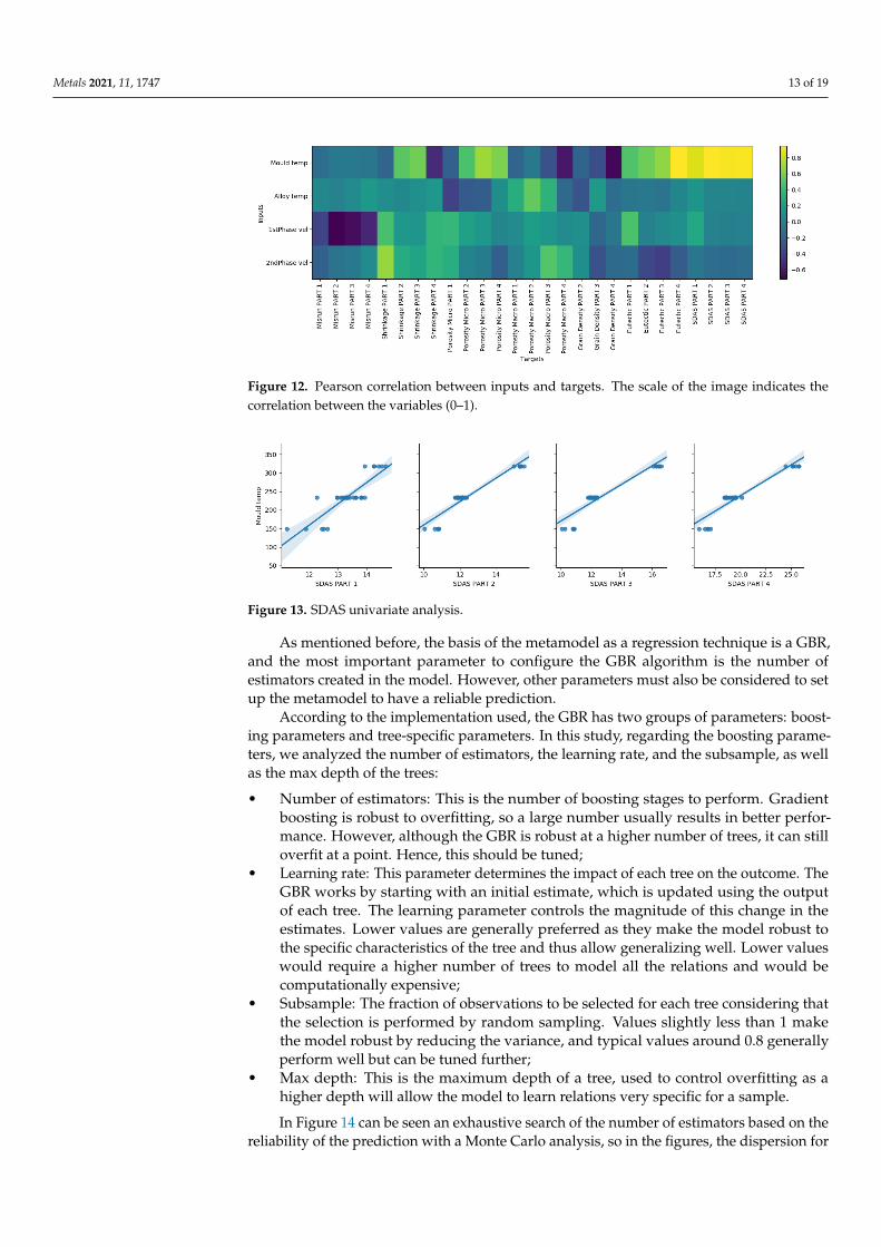
A preliminary analysis of the data showed that there were no clear correlationsbetween the explanatory variables (inputs) and response variables (targets). In Figure 12,the Pearson correlation shows that in most of the cases, a univariate analysis or predictioncould not be performed. Only in the case of the SDAS, a further analysis regarding thetemperature of the mold could be performed; see Figure 13. In this analysis, it could beseen that a univariate regression model could give a good result, but we show that a GBRoutperformed the univariate analysis.

Metals 2021, 11, 1747 13 of 19

Figure 12. Pearson correlation between inputs and targets. The scale of the image indicates thecorrelation between the variables (0–1).

Figure 13. SDAS univariate analysis.

As mentioned before, the basis of the metamodel as a regression technique is a GBR,and the most important parameter to configure the GBR algorithm is the number ofestimators created in the model. However, other parameters must also be considered to setup the metamodel to have a reliable prediction.

According to the implementation used, the GBR has two groups of parameters: boost-ing parameters and tree-specific parameters. In this study, regarding the boosting parame-ters, we analyzed the number of estimators, the learning rate, and the subsample, as wellas the max depth of the trees:

• Number of estimators: This is the number of boosting stages to perform. Gradientboosting is robust to overfitting, so a large number usually results in better perfor-mance. However, although the GBR is robust at a higher number of trees, it can stilloverfit at a point. Hence, this should be tuned;

• Learning rate: This parameter determines the impact of each tree on the outcome. TheGBR works by starting with an initial estimate, which is updated using the outputof each tree. The learning parameter controls the magnitude of this change in theestimates. Lower values are generally preferred as they make the model robust tothe specific characteristics of the tree and thus allow generalizing well. Lower valueswould require a higher number of trees to model all the relations and would becomputationally expensive;

• Subsample: The fraction of observations to be selected for each tree considering thatthe selection is performed by random sampling. Values slightly less than 1 makethe model robust by reducing the variance, and typical values around 0.8 generallyperform well but can be tuned further;

• Max depth: This is the maximum depth of a tree, used to control overfitting as ahigher depth will allow the model to learn relations very specific for a sample.

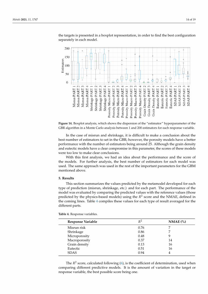
In Figure 14 can be seen an exhaustive search of the number of estimators based on thereliability of the prediction with a Monte Carlo analysis, so in the figures, the dispersion for

Metals 2021, 11, 1747 14 of 19

the targets is presented in a boxplot representation, in order to find the best configurationseparately in each model.

Figure 14. Boxplot analysis, which shows the dispersion of the “estimator” hyperparameter of theGBR algorithm in a Monte Carlo analysis between 1 and 200 estimators for each response variable.

In the case of misrun and shrinkage, it is difficult to make a conclusion about thebest number of estimators to set in the GBR; however, the porosity models have a betterperformance with the number of estimators being around 25. Although the grain densityand eutectic models have a clear compromise in this parameter, the scores of these modelswere too low to make clear conclusions.

With this first analysis, we had an idea about the performance and the score ofthe models. For further analysis, the best number of estimators for each model wasused. The same approach was used in the rest of the important parameters for the GBMmentioned above.

5. Results

This section summarizes the values predicted by the metamodel developed for eachtype of prediction (misrun, shrinkage, etc.) and for each part. The performance of themodel was evaluated by comparing the predicted values with the reference values (thosepredicted by the physics-based models) using the R2 score and the NMAE, defined inthe coming lines. Table 4 compiles these values for each type of result averaged for thedifferent parts.

Table 4. Response variables.

Response Variable R2 NMAE (%)

Misrun risk 0.76 7Shrinkage 0.86 7Microporosity 0.48 9Macroporosity 0.37 14Grain density 0.13 16Eutectic 0.51 16SDAS 0.94 4

The R2 score, calculated following (6), is the coefficient of determination, used whencomparing different predictive models. It is the amount of variation in the target orresponse variable, the best possible score being one.

Metals 2021, 11, 1747 15 of 19

The mean absolute error (MAE) is a measure of the prediction error. In this case, thenormalization of the error (NMAE), calculated following (5), is presented to also have acomparison criterion.

In both cases, N is the number of predictions, y the real measurements, y′ the predic-tions of the model where for each i, 1 ≤ i ≤ N, σy the standard deviation of a variable y,and ∆ is the range of the measured data.

NMAE =

(∑N

i (yi−y′i)N

)∆

(5)

R2 =

(1N∗ ∑N

i (yi − y) ∗(y′i − y′

)σy − σy′

)2

(6)

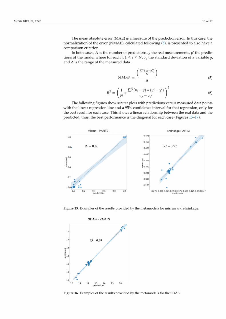
The following figures show scatter plots with predictions versus measured data pointswith the linear regression line and a 95% confidence interval for that regression, only forthe best result for each case. This shows a linear relationship between the real data and thepredicted; thus, the best performance is the diagonal for each case (Figures 15–17).

Figure 15. Examples of the results provided by the metamodels for misrun and shrinkage.

Figure 16. Examples of the results provided by the metamodels for the SDAS.

Metals 2021, 11, 1747 16 of 19

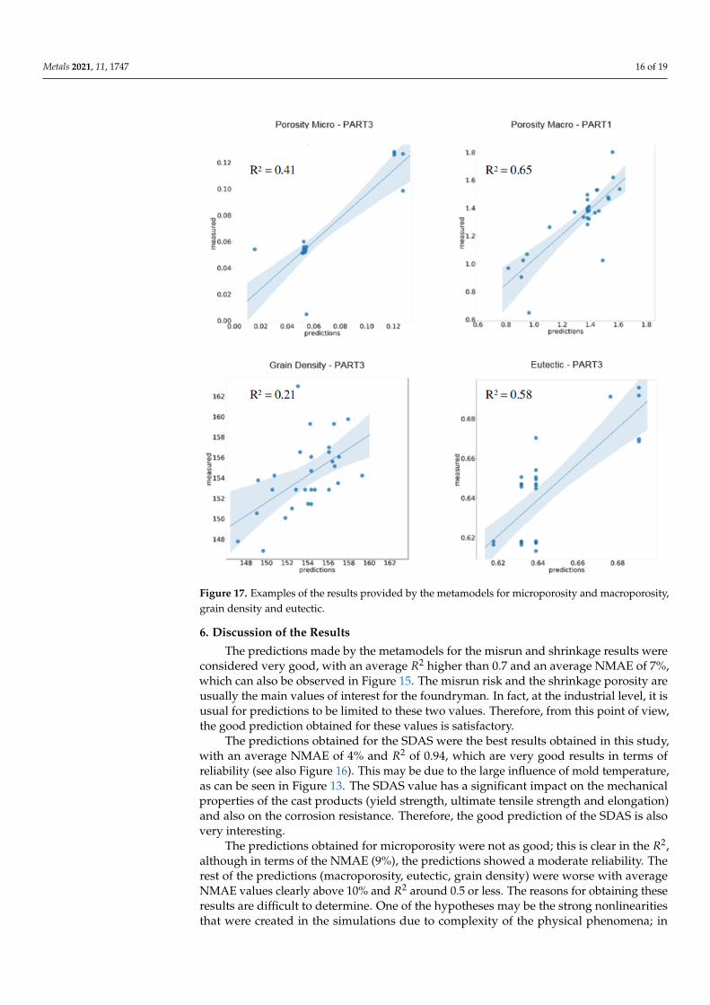
Figure 17. Examples of the results provided by the metamodels for microporosity and macroporosity,grain density and eutectic.

6. Discussion of the Results

The predictions made by the metamodels for the misrun and shrinkage results wereconsidered very good, with an average R2 higher than 0.7 and an average NMAE of 7%,which can also be observed in Figure 15. The misrun risk and the shrinkage porosity areusually the main values of interest for the foundryman. In fact, at the industrial level, it isusual for predictions to be limited to these two values. Therefore, from this point of view,the good prediction obtained for these values is satisfactory.

The predictions obtained for the SDAS were the best results obtained in this study,with an average NMAE of 4% and R2 of 0.94, which are very good results in terms ofreliability (see also Figure 16). This may be due to the large influence of mold temperature,as can be seen in Figure 13. The SDAS value has a significant impact on the mechanicalproperties of the cast products (yield strength, ultimate tensile strength and elongation)and also on the corrosion resistance. Therefore, the good prediction of the SDAS is alsovery interesting.

The predictions obtained for microporosity were not as good; this is clear in the R2,although in terms of the NMAE (9%), the predictions showed a moderate reliability. Therest of the predictions (macroporosity, eutectic, grain density) were worse with averageNMAE values clearly above 10% and R2 around 0.5 or less. The reasons for obtaining theseresults are difficult to determine. One of the hypotheses may be the strong nonlinearitiesthat were created in the simulations due to complexity of the physical phenomena; in

Metals 2021, 11, 1747 17 of 19

this way, the model was not able to identify the relationships. In fact, the microporosityand macroporosity, the eutectic percentage, and the grain density are aspects much lessstudied by simulation codes than the misrun or the shrinkage. It would be interesting to beable to improve the performance of the metamodels for these response variables in futureworks, although these types of results are generally simulated scientifically and not at theindustrial level. Taking into account the complexity of predicting some response variables,more data would be needed to establish a reliable relationship with the input parameters.In some of the regression models, other variables such as certain material properties couldalso be taken into account.

Compared with other alternatives, the approach taken in this work was very competi-tive [10]. It must be taken into account that there are few works that build metamodels, asmentioned in Section 1, for the HPDC process, and these works generate models that aredifficult to compare.

Finally, another important aspect besides reliability is the computational time, espe-cially compared with FEM simulations. The CPU time needed to make the predictions wasvery fast (milliseconds); therefore, it can be applied in optimization activities or to onlineprediction systems.

7. Conclusions

Different metamodels of the HPDC process of aluminum parts were successfullydeveloped based on a gradient boosting regressor. The best results were reached for theprediction of the SDAS, NMAE = 4%, R2 = 0.94, a microstructure parameter closely relatedto the mechanical properties of the cast products.

The metamodels predicted with good precision (NMAE = 7%, R2 = 0.7) the results ofgreatest interest for the metal casting industry, the misrun risk and the shrinkage level ofthe parts.

The rest of the predictions (microporosity and macroporosity, eutectic percentage andgrain density) were less precise.

The main highlight of the improved metamodel is its ability to reduce the time neededto obtain the predictions, without an important loss of accuracy compared with a moreconventional FEM simulation of the HPDC process. This implies that the metamodelapproximation may be a good solution to perform real-time predictions in this manufactur-ing process.

Author Contributions: Conceptualization, methodology, and investigation, E.A. and F.B.; writing, re-view and editing E.A., F.B., M.G.d.C., and I.G.; project administration, M.G.d.C.; funding acquisition,M.G.d.C. and I.G. All authors have read and agreed to the published version of the manuscript.

Funding: This work was supported by projects OASIS and SMAPRO. The OASIS project has receivedfunding from the European Union’s Horizon 2020 Research and Innovation Programme under GrantAgreement No 814581. The SMAPRO project has received funding from the Basque Governmentunder the ELKARTEK Program (KK-2017/00021).

Institutional Review Board Statement: Not applicable.

Informed Consent Statement: Not applicable.

Data Availability Statement: Not applicable.

Conflicts of Interest: The authors declare no conflict of interest.

References1. Gao, Y.; Liu, X.; Huang, H.; Xiang, J. A hybrid of FEM simulations and generative adversarial networks to classify faults in

rotor-bearing systems. ISA Trans. 2021, 108, 356–366. [CrossRef] [PubMed]2. Piltyay, S.; Bulashenko, A.; Herhil, Y.; Bulashenko, O. FDTD and FEM simulation of microwave waveguide polarizers. In

Proceedings of the 2020 IEEE 2nd International Conference on Advanced Trends in Information Theory (ATIT), Kyiv, Ukraine,25–27 November 2020; pp. 357–363.

3. Carlini, M.; McCormack, S.J.; Castellucci, S.; Ortega, A.; Rotondo, M.; Mennuni, A. Modeling and numerical simulation for aninnovative compound solar concentrator: Thermal analysis by FEM approach. Energies 2020, 13, 548. [CrossRef]

Metals 2021, 11, 1747 18 of 19

4. Gong, X.; Bustillo, J.; Blanc, L.; Gautier, G. FEM simulation on elastic parameters of porous silicon with different pore shapes. Int.J. Solids Struct. 2020, 190, 238–243. [CrossRef]

5. Forrester, A.I.; Keane, A.J. Recent advances in surrogate-based optimization. Prog. Aerosp. Sci. 2009, 45, 50–79. [CrossRef]6. Han, Z.H.; Zhang, K.S. Surrogate-based optimization. In Real-World Applications of Genetic Algorithms; InTech Open: Rijeka,

Croatia, 2012; pp. 343–362.7. Forrester, A.; Sobester, A.; Keane, A. Engineering Design via Surrogate Modeling: A Practical Guide; John Wiley and Sons: Hoboken,

NJ, USA, 2008.8. Fiorese, E.; Richiedei, D.; Bonollo, F. Analytical computation and experimental assessment of the effect of the plunger speed on

tensile properties in high-pressure die casting. Int. J. Adv. Manuf. Technol. 2017, 91, 463–476. [CrossRef]9. Fiorese, E.; Richiedei, D.; Bonollo, F. Improved metamodels for the optimization of high-pressure die casting process. Metall. Ital.

2016, 108, 21–24.10. Krimpenis, A.; Benardos, P.; Vosniakos, G.C.; Koukouvitaki, A. Simulation-based selection of optimum pressure die-casting

process parameters using neural nets and genetic algorithms. Int. J. Adv. Manuf. Technol. 2006, 27, 509–517. [CrossRef]11. Weixiong, Y.; Yi, Y.; Bin, Z. Novel methodology for casting process optimization using Gaussian process regression and genetic

algorithm. Res. Dev. 2009, 3, 12.12. Bonte, M.; van den Boogaard, A.H.; Huétink, J. A Metamodel Based Optimisation Algorithm for Metal Forming Processes; Springer:

Berlin/Heidelberg, Germany, 2007; pp. 55–72. [CrossRef]13. Seit, J. Trends and Challenges: The Die-Casting Industry on the Road to the Future. 2018. https://www.spotlightmetal.com/

trends-and-challenges-the-die-casting-industry-on-the-road-to-the-future-a-676717/ (accessed on: 10 September 2021).14. Udvardy, S.P. State of the Die Casting Industry. https://www.diecasting.org/wcm/Die_Casting/State_of_the_Industry/wcm/

Die_Casting/State_of_the_Industry.aspx?hkey=b50b590c-a1a6-4c65-8f04-3a6d38c821dc (accessed on: 10 September 2021).15. NADCA. Introduction to Die Casting; NADCA: Mt. Laurel, IL, USA, 2016.16. NADCA. Die casting handbook; NADCA: Mt. Laurel, IL, USA, 2015.17. Bazhenov, V.; Petrova, A.; Koltygin, A. Simulation of Fluidity and Misrun Prediction for the Casting of 356.0 Aluminium Alloy

into Sand Molds. Int. J. Met. 2018, 12, 514–522. [CrossRef]18. Gunasegaram, D.; Farnsworth, D.; Nguyen, T. Identification of critical factors affecting shrinkage porosity in permanent mold

casting using numerical simulations based on design of experiments. Int. J. Met. 2009, 209, 1209–1219. [CrossRef]19. Nastac, L. Numerical modeling of solidification morphologies and segregation patterns in cast dendritic alloys. Acta Mater. 1999,

47, 4253–4262. [CrossRef]20. Rappaz, M. Modeling of microstructure formation in solidification processes. Int. Mater. Rev. 1989, 34, 93–124. [CrossRef]21. Raffaeli, R.; Favi, C.; Mandorli, F. Virtual prototyping in the design process of optimized mold gating system for high pressure

die casting. Eng. Comput. 2015, 32, 102–128. [CrossRef]22. Chen, W. A Development Of Virtual Prototyping Manufacturing System For High Pressure Die Casting Processes. WIT Trans.

Built Environ. 2015, 67, 10.23. Ignaszak, Z. Validation Problems of Virtual Prototyping Systems Used in Foundry for Technology Optimization of Ductile

Iron Castings. In Advances in Integrated Design and Manufacturing in Mechanical Engineering II; Springer: Berlin, Germany, 2007.[CrossRef]

24. Chiang, K.; Liu, N.; Tsai, T. Modeling and analysis of the effects of processing parameters on the performance characteristics inthe high pressure die casting process of Al-Si alloys. Int. J. Adv. Manuf. Technol. 2009, 41, 1076–1084. [CrossRef]

25. Kwon, H.; Kwon, H. Computer aided engineering (CAE) simulation for the design optimization of gate system on high pressuredie casting (HPDC) process. Robot. -Comput.-Integr. Manuf. 2019, 55, 147–153. [CrossRef]

26. Cleary, P.; Ha, J.; Prakash, M.; Nguyen, T. Short shots and industrial case studies: Understanding fluid flow and solidification inhigh pressure die casting. Appl. Math. Model. 2012, 34, 2018–2033. [CrossRef]

27. Anglada, E.; Meléndez, A.; Vicario, I.; Arratibel, E.; Cangas, G. Simplified models for high pressure die casting simulation.Procedia Eng. 2015, 132, 974–981. [CrossRef]

28. Hong, C.; Umeda, T.; Kimura, Y. Numerical models for casting solidification:Part II. Application of the boundary element methodto solidification problems. Metall. Trans. B 1984, 15, 101–107. [CrossRef]

29. Hetu, J.; Gao, D.; Kabanemi, K.; Bergeron, S.; Nguyen, K.; Loong, C. Numerical modeling of casting processes. Adv. Perform.Mater. 1998, 5, 65–82. [CrossRef]

30. Snyder, D.; Waite, D.; Amin, A. Application of efficient parallel processing to finite element modeling of filling, solidification, anddefect prediction for ultra-large shape castings. In Light Metals: Proceedings of Sessions, TMS Annual Meeting; TMS: Pittsburgh, PA,USA, 1997; pp. 919–925.

31. Jauregui, R.; Silva, F. Numerical Validation Methods. In Numerical Analysis Theory and Application; Awrejcewicz., Ed.; IntechOpen:Rijeka, Croatia, 2011; Chapter 8, pp. 155–174.

32. NADCA. Die Casting Process Control; NADCA: Mt. Laurel, IL, USA,2015.33. Adamane, A.R.; Arnberg, L.; Fiorese, E.; Timelli, G.; Bonollo, F. Influence of injection parameters on the porosity and tensile

properties of high-pressure die cast Al-Si alloys: a review. Int. J. Met. 2015, 9, 43–53. [CrossRef]34. dos Santos, S.L.; Antunes, R.A.; Santos, S.F. Influence of injection temperature and pressure on the microstructure, mechanical

and corrosion properties of a AlSiCu alloy processed by HPDC. Mater. Des. 2015, 88, 1071–1081. [CrossRef]

Metals 2021, 11, 1747 19 of 19

35. Anglada, E.; Meléndez, A.; Vicario, I.; Arratibel, E.; Aguillo, I. Adjustment of a high pressure die casting simulation model againstexperimental data. Procedia Eng. 2015, 132, 966–973. [CrossRef]

36. Anglada, E.; Meléndez, A.; Vicario, I.; Idoiaga, J.K.; Mugarza, A.; Arratibel, E. Prediction and validation of shape distortions inthe simulation of high pressure die casting. J. Manuf. Process. 2018, 33, 228–237. [CrossRef]

37. Wynants, L.; Bouwmeester, W.; Moons, K.; Moerbeek, M.; Timmerman, D.; Van Huffel, S.; Van Calster, B.; Vergouwe, Y. Asimulation study of sample size demonstrated the importance of the number of events per variable to develop prediction modelsin clustered data. J. Clin. Epidemiol. 2015, 68, 1406–1414. [CrossRef] [PubMed]

38. Lawson, J. Design and Analysis of Experiments with R; Chapman and Hall/CRC: Boca Raton, FL, USA, 2014.39. Dantzig, J.A.; Rappaz, M. Solidification: -Revised & Expanded; EPFL Press: Lausanne, Switzerland, 2016.40. Lewis, R.; Ravindran, K. Finite element simulation of metal casting. Int. J. Numer. Methods Eng. 2000, 47, 29–59. [CrossRef]41. Gandin, C.A.; Desbiolles, J.L.; Rappaz, M.; Thevoz, P. A three-dimensional cellular automation-finite element model for the

prediction of solidification grain structures. Metall. Mater. Trans. A 1999, 30, 3153–3165. [CrossRef]42. Smith, M. Neural Networks for Statistical Modeling; Thomson Learning: Boston, MA, USA, 1993.43. Williams, C.K.; Rasmussen, C.E. Gaussian Processes for Machine Learning; MIT Press: Cambridge, MA, USA, 2006; Volume 2.44. Breiman, L. Random forests. Mach. Learn. 2001, 45, 5–32. [CrossRef]45. Friedman, J.H. Greedy function approximation: a gradient boosting machine. Ann. Stat. 2001, 29, 1189–1232.46. Orzechowski, P.; La Cava, W.; Moore, J.H. Where are we now? A large benchmark study of recent symbolic regression methods.

In Proceedings of the Genetic and Evolutionary Computation Conference, Kyoto, Japan, 15–19 July 2018; pp. 1183–1190.