mesoscale, seasonal and interannual variability in the mediterranean sea using a numerical ocean...
TRANSCRIPT

Progress in Oceanography 66 (2005) 321–340
Progress inOceanography
www.elsevier.com/locate/pocean
Mesoscale, seasonal and interannual variability inthe Mediterranean Sea using a numerical ocean model
Vicente Fernandez a,*, David E. Dietrich a, Robert L. Haney b, Joaquın Tintore a
a IMEDEA (CSIC-UIB), Instituto Mediterraneo de Estudios Avanzados, Spainb Department of Meteorology, Naval Postgraduate School, Monterey, CA, USA
Received 4 November 2002; received in revised form 17 February 2003; accepted 2 July 2004
Available online 10 May 2005
Abstract
In this paper, we present the results from a 1/8� horizontal resolution numerical simulation of the Mediterranean Sea
using an ocean model (DieCAST) that is stable with low general dissipation and that uses accurate control volume
fourth-order numerics with reduced numerical dispersion. The ocean model is forced using climatological monthly
mean winds and relaxation towards monthly climatological surface temperature and salinity. The variability of the cir-
culation obtained is assessed by computing the volume transport through certain sections and straits where comparison
with observations is possible. The seasonal variability of certain currents is reproduced in the model simulations. More
important, an interannual variability, manifested by changes in currents and water mass properties, is also found in the
results. This may indicate that the oceanic internal variability (not depending on external atmospheric forcing), is an
important component of the total variability of the Mediterranean circulation; variability that seems to be very signif-
icant and well documented by in situ and satellite data recovered in the Mediterranean Sea during the last decade.
� 2005 Elsevier Ltd. All rights reserved.
Keywords: Mediterranean sea; Ocean modelling; Interannual variability
1. Introduction
It is now well established that the Mediterranean Sea is a complex and variable ocean system in which
several temporal and spatial scales (basin, sub-basin and mesoscale) interact to form a highly variable gen-
eral circulation (see Robinson & Golnaraghi, 1994 for a review). After intensive experimental studies carried
out at local and basin scales in the western (La Violette, 1990) and eastern Mediterranean (POEM group
(1992)) and from recent satellite imagery studies covering all the Mediterranean Basin (e.g., Larnicol,
0079-6611/$ - see front matter � 2005 Elsevier Ltd. All rights reserved.
doi:10.1016/j.pocean.2004.07.010
* Corresponding author. Tel.: +34 9 71 611732; fax: +39 51 4151499.
E-mail address: [email protected] (V. Fernandez).
322 V. Fernandez et al. / Progress in Oceanography 66 (2005) 321–340
Ayoub, & Le Traon, 2002), it is clear that a wide range of space-time ocean variability is present in the Med-
iterranean Sea. An accurate representation of this observed variability of the Mediterranean Sea circulation
is a challenging problem in numerical ocean modelling. Several numerical attempts, using different ocean
general circulation models with different grid resolutions and forcing, have been made to reproduce and
understand the Mediterranean general circulation and its variability. Coarse resolution models (20–25 kmhorizontal grid spacing) driven by large scale climatological atmospheric forcing have succeeded to repro-
duce quite well some of the main features of the Mediterranean circulation and its seasonal cycle (Alvarez,
Tintore, Holloway, Eby, & Beckers, 1994; Beckers et al., 2002; Roussenov, Stanev, Artale, & Pinardi, 1995;
Wu & Haines, 1998; Zavatarelli & Mellor, 1995). Additional modelling efforts, involving coarse and also
high resolution models (<15 km horizontal grid spacing), have been carried out to assess the physical mech-
anisms generating mesoscale and interannual variability in the Mediterranean Sea (Demirov & Pinardi,
2002; Herbaut, Martel, & Crepon, 1997; Horton, Clifford, Schmitz, & Kantha, 1997; Korres, Pinardi, & Las-
caratos, 2000; Pinardi, Korres, Lascaratos, Roussenov, & Stanev, 1997).Interannual variability of the external atmospheric forcing is considered one of the main physical
mechanisms that generates interannual variability in the ocean. The fact that the atmospheric forcing
over the Mediterranean Sea shows a marked interannual variability (Garret, Outerbridge, & Thomson,
1993) has encouraged modelling studies in this direction. Therefore, the first attempts to reproduce in
numerical simulations the interannual variability of the circulation of the Mediterranean Sea were made
by forcing the ocean models with variable atmospheric forcing (Demirov & Pinardi, 2002; Herbaut et al.,
1997; Korres et al., 2000; Pinardi et al., 1997). Results from these studies have confirmed that the var-
iability of the external atmospheric forcing, more specifically anomalies in the winter wind stress and heatfluxes, can account for some of the large changes in the circulation observed from one year to another.
While some numerical studies have investigated that component of the Mediterranean Sea interannual
variability induced by external atmospheric forcing, little is known about the ocean variability generated
by the internal nonlinear dynamics of the mesoscale eddy field. Eddies can potentially interact with the
mean currents and the bottom topography producing long term responses in the ocean circulation.
Therefore, ocean mesoscale activity may be considered an important source of interannual variability
in the Mediterranean Sea, where a large number of narrow coastal currents, ocean fronts and eddies
are present (Larnicol et al., 2002). From the point of view of ocean modelling, coarse horizontal gridresolution (unable to resolve the radius of deformation) is a handicap to study this internally induced
interannual variability because the mesoscale eddy field can not be properly represented. Thus, only high
resolution modelling efforts (comparable to the radius of deformation) can address this issue as they are
able to show an important eddy field in the simulations. Except for the studies by Demirov and Pinardi
(2002), who use a horizontal resolution of 1/8� · 1/8� Horton et al. (1997), with a resolution of 10-km
horizontal grid, and the work of Herbaut et al. (1997), having a horizontal resolution of 1/8� · 1/10�in the western Mediterranean Basin, all other previously mentioned numerical studies were performed
with a coarse horizontal grid resolution (1/4�) and, to our knowledge, none of these previous studies havefocused on the potential effect of the mesoscale activity as a source of interannual variability in the Med-
iterranean Sea.
Besides an adequate grid resolution, the numerical dispersion and the physical and numerical dissi-
pation of an ocean model is an important factor that limits the capability to study the possible influ-
ence of eddies and ocean fronts on the interannual variability of the Mediterranean Sea. Low values of
horizontal viscosity and diffusivity are needed to permit baroclinic instability and to avoid damping of
temperature or salinity fronts that are created in the model. At the same time, it is also important to
minimize numerical dispersion and not to break up multi-scale features such as fronts, eddies andmeandering current systems. Moreover, the use of high-order accurate numerical approximations can
improve the accuracy of the numerical simulations in the Mediterranean Sea with little additional com-
puting cost (Sanderson & Brassington, 1998; Sanderson, 1998).
V. Fernandez et al. / Progress in Oceanography 66 (2005) 321–340 323
Herein, we implement the DieCAST model in the Mediterranean Sea with a horizontal grid resolu-
tion of 1/8� which resolves the deformation radius (10–20 km in the Mediterranean), and a perpetual
year monthly climatological atmospheric forcing (we do not introduce variability in the external forc-
ing). The first objective of the study is to address whether DieCAST can reproduce the main general
circulation features and seasonal cycle as reproduced by other models and measured in some places.
The second objective is to determine, if interannual variability induced by the realistic behaviour of nat-
ural fronts and eddies may be obtained in the model simulations and to discuss its relevance to the
observed variability in the Mediterranean Sea.
In the following section some details of the numerical characteristics of the DieCAST ocean model are
given. The model adaptation to the Mediterranean Sea is explained in Section 3. In Section 4, the spin up
of the model towards statistical equilibrium is described. Afterwards, in Section 5, the modelling results
and the variability of the model circulation at different time scales are presented, with special emphasis
on the western Mediterranean Basin. A general discussion of the results is presented in Section 6.
2. The DieCAST ocean model
The Dietrich/Center for Air-Sea Technology (DieCAST) is a primitive equation, z-level vertical coor-
dinate, finite difference ocean model. The model uses a rigid lid approximation, with a sea surface pres-
sure formulation, and the classical hydrostatic and Boussinesq approximations. The density is
determined from a nonlinear equation of state relating density to potential temperature, salinity and
pressure. All the significant numerical approximations of the most important terms of the primitiveequations, such as the advection and horizontal pressure gradient terms, are fourth-order-accurate (San-
derson & Brassington, 1998; Sanderson, 1998), except in zones adjacent to boundaries where conven-
tional second order accuracy is used. The model-predicted quantities are control volume averages of
momentum, temperature and salinity. All these control volumes are non-staggered or ‘‘collocated’’
(all the approximations are applied on the same control volume grid), avoiding the numerical dispersion
errors associated with the evaluation of the large Coriolis term on a staggered grid. When face-averaged
quantities are needed to evaluate fluxes across control volume faces, the conversions between the con-
trol volume averages and face averages are computed using a fourth-order accurate reduced dispersionscheme (Dietrich, 1997).
The DieCAST ocean model has been previously used in several studies and implemented and vali-
dated in several different regions including the Gulf of Mexico (Dietrich, 1997; Dietrich, Lin, Mes-
tas-Nunez, & Ko, 1997), the California Current (Haney, Hale, & Dietrich, 2001) and the Black Sea
(Staneva, Dietrich, Stanev, & Bowman, 2001). A more detailed description of the model equations
and the model numerical methods can be found in those references.
The fourth-order accurate approximation of the advection terms reduces the computational disper-
sion error to around 20% for the length scales of 4Dx, where Dx is the model grid size (see Table
5-1 of Haltiner & Williams, 1980). This gives an idea of the importance of using fourth-order accuracy
in the Mediterranean in order to resolve small scale structures that play a key role in understanding thegeneral circulation, and that would otherwise be broken up among the different wavelengths by exces-
sive numerical dispersion. The fact that DieCAST contains low total dissipation, and does not require
large dissipation for numerical stability, is important in order to create and maintain frontal regions
and coastal jets that are present in the Mediterranean. We see in the next section that the values of
eddy viscosity and diffusivity used in this study are lower than those used in previous modelling studies
of the Mediterranean.
324 V. Fernandez et al. / Progress in Oceanography 66 (2005) 321–340
3. Mediterranean model configuration
The model domain includes the entire Mediterranean Sea extending from 30�6 0N to 45�30 0N in latitude
and from 5�15 0E to 36�W in longitude. All lateral boundaries are closed except the Strait of Gibraltar,
where an open boundary is set to reproduce the observed inflow of Atlantic waters in the upper layersand the outflow of Mediterranean waters below (Baschcek, Send, Lafuente, & Candela, 2001; Send &
Baschek, 2001). The model horizontal mesh is the same in both the longitudinal (k) and the latitudinal
(u) directions, with Dk = 1/8� and u = Dkcos(u), thus making square horizontal control volume bound-
aries. Therefore, the maximum grid interval is DX = DY = 12 km in the southern latitude and the minimum
is 10 km in the north. This resolution is close to the Rossby radius of deformation in the Mediterranean
(10–20 km), and therefore may be enough to resolve mesoscale structures with a length scale of about
30 km (wavelength �120 km). In the vertical, the grid has 30 non-uniform vertical levels that vary in thick-
ness from about 10 m at the surface to 300 m at the bottom. The bathymetry on the model grid was derivedfrom ETOPO5 world database by a bilinear interpolation and it is truncated at 2750 m, but no filtering is
applied. This fact is important in the Mediterranean where the steep bottom topography in coastal areas
induces energetic coastal currents.
The model horizontal viscosity and diffusivity coefficients are constant and set to AH = AM = 10 m2s�1,
but increased by a factor of 2.5 in areas near the coastlines having only one model level. To check if our
model dissipation is low compared to other modelling studies, we use the non-dimensional cell Reynolds
and Peclet numbers. These numbers give an estimate of the importance of the nonlinear advective terms
compared to the viscosity and diffusivity terms, respectively, in the model equations. The larger these num-bers are, the less numerical dissipation present and, consequently, more short scale features are admitted in
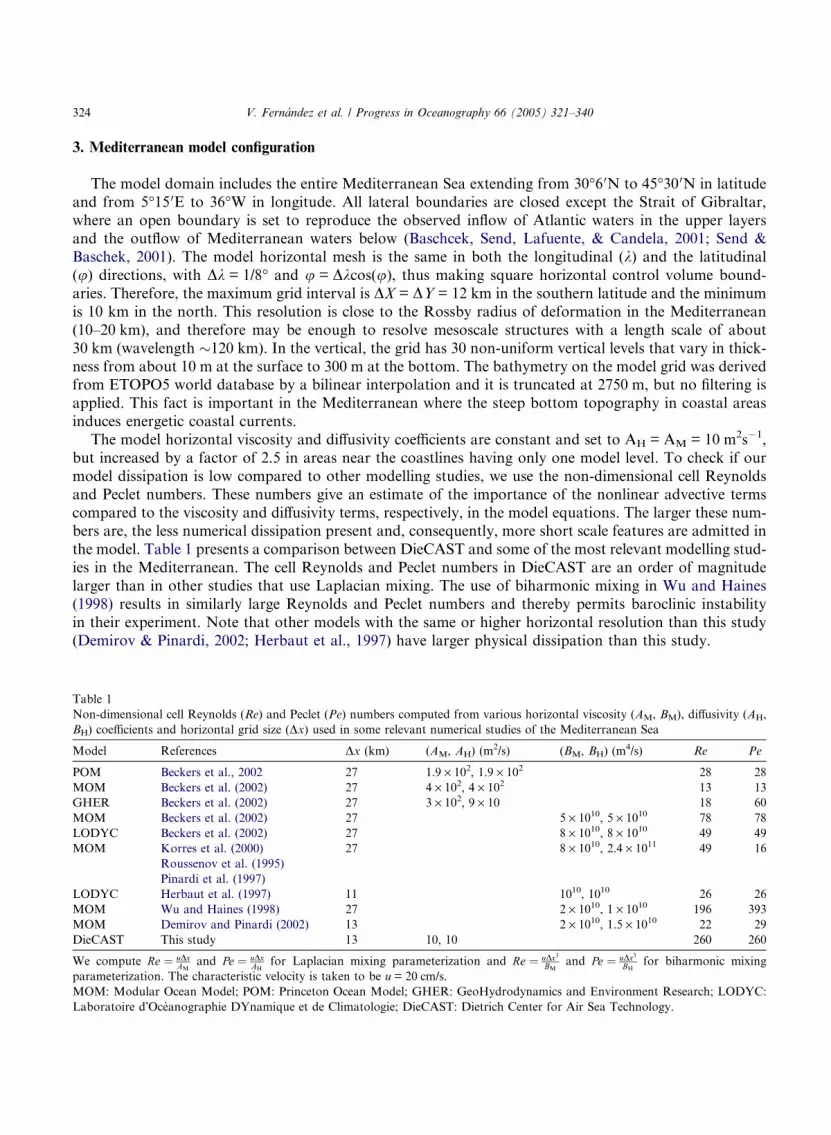
the model. Table 1 presents a comparison between DieCAST and some of the most relevant modelling stud-
ies in the Mediterranean. The cell Reynolds and Peclet numbers in DieCAST are an order of magnitude
larger than in other studies that use Laplacian mixing. The use of biharmonic mixing in Wu and Haines
(1998) results in similarly large Reynolds and Peclet numbers and thereby permits baroclinic instability
in their experiment. Note that other models with the same or higher horizontal resolution than this study
(Demirov & Pinardi, 2002; Herbaut et al., 1997) have larger physical dissipation than this study.
Table 1
Non-dimensional cell Reynolds (Re) and Peclet (Pe) numbers computed from various horizontal viscosity (AM, BM), diffusivity (AH,
BH) coefficients and horizontal grid size (Dx) used in some relevant numerical studies of the Mediterranean Sea
Model References Dx (km) (AM, AH) (m2/s) (BM, BH) (m
4/s) Re Pe
POM Beckers et al., 2002 27 1.9 · 102, 1.9 · 102 28 28
MOM Beckers et al. (2002) 27 4 · 102, 4 · 102 13 13
GHER Beckers et al. (2002) 27 3 · 102, 9 · 10 18 60
MOM Beckers et al. (2002) 27 5 · 1010, 5 · 1010 78 78
LODYC Beckers et al. (2002) 27 8 · 1010, 8 · 1010 49 49
MOM Korres et al. (2000) 27 8 · 1010, 2.4 · 1011 49 16
Roussenov et al. (1995)
Pinardi et al. (1997)
LODYC Herbaut et al. (1997) 11 1010, 1010 26 26
MOM Wu and Haines (1998) 27 2 · 1010, 1 · 1010 196 393
MOM Demirov and Pinardi (2002) 13 2 · 1010, 1.5 · 1010 22 29
DieCAST This study 13 10, 10 260 260
We compute Re ¼ uDxAM
and Pe ¼ uDxAH
for Laplacian mixing parameterization and Re ¼ uDx3BM
and Pe ¼ uDx3BH
for biharmonic mixing
parameterization. The characteristic velocity is taken to be u = 20 cm/s.
MOM: Modular Ocean Model; POM: Princeton Ocean Model; GHER: GeoHydrodynamics and Environment Research; LODYC:
Laboratoire d�Oceanographie DYnamique et de Climatologie; DieCAST: Dietrich Center for Air Sea Technology.

V. Fernandez et al. / Progress in Oceanography 66 (2005) 321–340 325
For the vertical viscosity and diffusivity, a variable formulation which includes the Richardson number is
used, as described and used in Staneva et al. (2001), with background values set at near-molecular values
(10�6 and 2 · 10�7 m2s�1 respectively). The bottom dissipation is represented by a conventional nonlinear
bottom drag with a coefficient of 0.002 and a zero flux condition for salinity and temperature. At all the
lateral walls of the domain with the exception of the open Strait of Gibraltar we assume free-slip boundaryconditions and zero flux of heat and salt.
The Strait of Gibraltar is represented by an open boundary, five grid points wide at the surface, located
at the western boundary of the model domain (5�25 0 longitude). The velocity, temperature and salinity pro-
file of the inflowing water can be specified in order to make it similar to the available observations. An
upper layer inflow of 1.14 Sv Atlantic water is specified in the upper 105 m. The inflow jet is two grid points
wide on the northern half of the strait with maximum velocities of 70 cm/s in the surface and decreasing
linearly with depth. Recent observations give a mean inflow of 0.85 ± 0.07 Sv in the upper 120–150 m, with
velocities up to 60 cm/s (Baschcek et al., 2001; Send & Baschek, 2001). The salinity and temperature of theinflow at the subsurface layers are constant in time and taken from the winter climatology. In the surface
layer, the values change each month based on the monthly climatology. The outflow takes place between
105 m and the model sill depth of 185 m. This outflow is model-determined using an upwind approxima-
tion, modified by a meridionally uniform increment each time step to maintain a net volume inflow equal
to zero, as required by incompressibility. This approach, which is consistent with the restoring boundary
conditions on the surface, is not correct for the real Mediterranean Sea in which the net inflow balances
the water loss through evaporation, but the effects of this error may be quite small, especially away from
the Strait of Gibraltar.The model surface momentum is directly forced by a monthly mean wind stress interpolated at each time
step. The source of the monthly wind stress is the daily 10-m wind data from 1986–1992 ECMWF reanal-
ysis as been prepared for the MEDMEX experiment (Beckers et al., 2002) and interpolated onto the 1/8�model grid using a bi-linear interpolation. We use MEDMEX stresses in order to facilitate a comparison of
our model results with those of other MEDMEX studies. The surface temperature and salinity fields in the
model are modified by a linear restoring towards monthly surface temperature and salinity climatologies
prepared from the MED4 climatological data base (Brasseur, Brankart, Schoenauen, & Beckers, 1996).
The restoring time scale is 5 days for both temperature and salinity. This fast restoring has been widely usedin modelling studies in the Mediterranean (Beckers et al., 2002) and has been adopted here, but we have to
note that it may damp surface transients and therefore inhibit some of the oceanic internal variability. The
model is initialized at a state of rest with winter mean temperature and salinity fields bilinearly interpolated
from the MODB seasonal climatology. The same initial conditions were used, for example, in the MED-
MEX experiment (Beckers et al., 2002). The model runs robustly with a time step of 15 min and requires
about 50 h for a one-year run on an Origin R200 SGI with four processors.
4. Model spin up and approach to equilibrium
Due to the mismatch between the initial winter hydrography and the monthly surface forcing fields,
the initial sub-surface values of temperature and salinity are modified during the model integration by
the annual cycle of the surface forcing. The changes in the surface temperature and salinity are mixed
downward from the beginning of the run until the annual mean profile reaches a stationary state, con-
sistent with the annual cycle of the surface forcing. According to Fig. 1, the annual average vertical
profile of temperature and salinity is stationary after 12 years of the simulation. Note that the averagetemperature in the first 500 m is increased from the initial winter value towards a yearly averaged pro-
file, while the salinity vertical profile is displaced towards lower values of salinity, although maintaining

3
Fig. 1. Time evolution of the annual average profile of temperature and salinity from the initial winter conditions (year 0) to the last
year of simulation (year 15).
326 V. Fernandez et al. / Progress in Oceanography 66 (2005) 321–340
a salinity maximum of 38.7 at intermediate levels (that corresponds to the average salinity of the Lev-
antine Intermediate Waters). These changes from the thermohaline initial conditions are a combined
effect of the surface restoring, the open Gibraltar condition and the vertical mixing.
A repeating seasonal cycle is obtained in the time series of the volume integrated kinetic energy
(.5(u2 + v2)), temperature and salinity (Fig. 2). The kinetic energy annual cycle has a maximum in winterand a minimum in summer. Note that the kinetic energy values are the same as, or bigger than, other MED-
MEX models (Beckers et al., 2002). Our KE is about half that of Demirov and Pinardi (2002) because our
wind stress forcing is about half as strong as theirs. The significance of this difference in forcing is addressed
in the Discussion section. Note also that at the end of the simulation we get almost no drift in the temper-
ature and salinity temporal evolution. As the model is fully conservative for temperature and salinity and
the bottom and lateral fluxes are set to zero, the small drift is caused by the combined effects of the heating
and freshening from Gibraltar and the surface relaxation. Another possible cause of the small drift is
round-off numerical errors, but this has been minimized after the use of double-precision variables in themodel.
5. Model results
We describe in this section the general circulation of the Mediterranean Sea obtained in the climatolog-
ical simulations. Throughout this paper, more attention will be put on the western Mediterranean, and,
therefore, a more detailed description of the circulation in this sub-basin will be given. We have selected
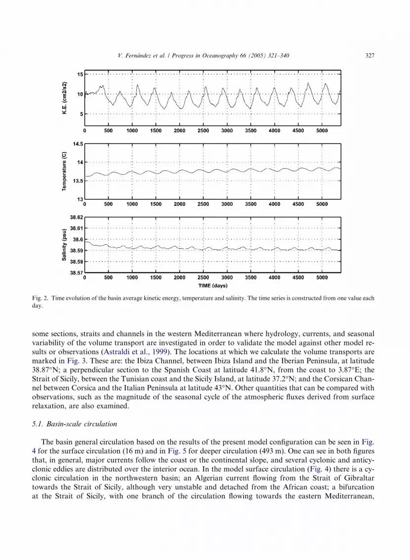
Fig. 2. Time evolution of the basin average kinetic energy, temperature and salinity. The time series is constructed from one value each
day.
V. Fernandez et al. / Progress in Oceanography 66 (2005) 321–340 327
some sections, straits and channels in the western Mediterranean where hydrology, currents, and seasonal
variability of the volume transport are investigated in order to validate the model against other model re-
sults or observations (Astraldi et al., 1999). The locations at which we calculate the volume transports are
marked in Fig. 3. These are: the Ibiza Channel, between Ibiza Island and the Iberian Peninsula, at latitude
38.87�N; a perpendicular section to the Spanish Coast at latitude 41.8�N, from the coast to 3.87�E; theStrait of Sicily, between the Tunisian coast and the Sicily Island, at latitude 37.2�N; and the Corsican Chan-
nel between Corsica and the Italian Peninsula at latitude 43�N. Other quantities that can be compared with
observations, such as the magnitude of the seasonal cycle of the atmospheric fluxes derived from surfacerelaxation, are also examined.
5.1. Basin-scale circulation
The basin general circulation based on the results of the present model configuration can be seen in Fig.
4 for the surface circulation (16 m) and in Fig. 5 for deeper circulation (493 m). One can see in both figures
that, in general, major currents follow the coast or the continental slope, and several cyclonic and anticy-
clonic eddies are distributed over the interior ocean. In the model surface circulation (Fig. 4) there is a cy-clonic circulation in the northwestern basin; an Algerian current flowing from the Strait of Gibraltar
towards the Strait of Sicily, although very unstable and detached from the African coast; a bifurcation
at the Strait of Sicily, with one branch of the circulation flowing towards the eastern Mediterranean,
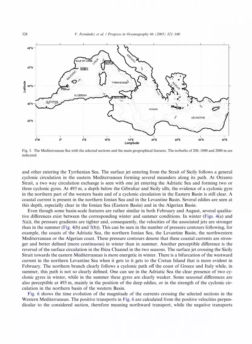
Fig. 3. The Mediterranean Sea with the selected sections and the main geographical features. The isobaths of 200, 1000 and 2000 m are
indicated.
328 V. Fernandez et al. / Progress in Oceanography 66 (2005) 321–340
and other entering the Tyrrhenian Sea. The surface jet entering from the Strait of Sicily follows a general
cyclonic circulation in the eastern Mediterranean forming several meanders along its path. At Otranto
Strait, a two way circulation exchange is seen with one jet entering the Adriatic Sea and forming two or
three cyclonic gyres. At 493 m, a depth below the Gibraltar and Sicily sills, the evidence of a cyclonic gyre
in the northern part of the western basin and of a cyclonic circulation in the Eastern Basin is still clear. A
coastal current is present in the northern Ionian Sea and in the Levantine Basin. Several eddies are seen at
this depth, especially clear in the Ionian Sea (Eastern Basin) and in the Algerian Basin.
Even though some basin-scale features are rather similar in both February and August, several qualita-tive differences exist between the corresponding winter and summer conditions. In winter (Figs. 4(a) and
5(a)), the pressure gradients are tighter and, consequently, the velocities of the associated jets are stronger
than in the summer (Fig. 4(b) and 5(b)). This can be seen in the number of pressure contours following, for
example, the coasts of the Adriatic Sea, the northern Ionian Sea, the Levantine Basin, the northwestern
Mediterranean or the Algerian coast. These pressure contours denote that these coastal currents are stron-
ger and better defined (more continuous) in winter than in summer. Another perceptible difference is the
reversal of the surface circulation in the Ibiza Channel in the two seasons. The surface jet crossing the Sicily
Strait towards the eastern Mediterranean is more energetic in winter. There is a bifurcation of the westwardcurrent in the northern Levantine Sea when it gets to it gets to the Cretan Island that is more evident in
February. The northern branch clearly follows a cyclonic path off the coast of Greece and Italy while, in
summer, this path is not so clearly defined. One can see in the Adriatic Sea the clear presence of two cy-
clonic gyres in winter, while in the summer these gyres are clearly weaker. Some seasonal differences are
also perceptible at 493 m, mainly in the position of the deep eddies, or in the strength of the cyclonic cir-
culation in the northern basin of the western Basin.
Fig. 6 shows the time evolution of the magnitude of the currents crossing the selected sections in the
Western Mediterranean. The positive transports in Fig. 6 are calculated from the positive velocities perpen-dicular to the considered section, therefore meaning northward transport, while the negative transports
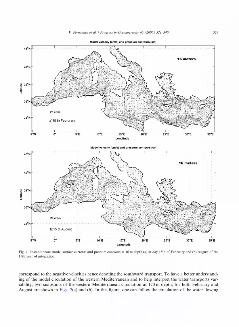
Fig. 4. Instantaneous model surface currents and pressure contours at 16 m depth (a) at day 15th of February and (b) August of the
15th year of integration.
V. Fernandez et al. / Progress in Oceanography 66 (2005) 321–340 329
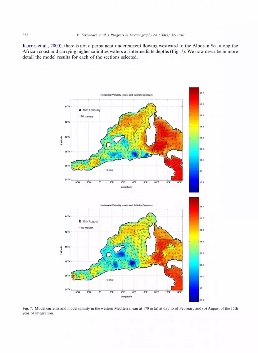
correspond to the negative velocities hence denoting the southward transport. To have a better understand-ing of the model circulation of the western Mediterranean and to help interpret the water transports var-
iability, two snapshots of the western Mediterranean circulation at 170 m depth, for both February and
August are shown in Figs. 7(a) and (b). In this figure, one can follow the circulation of the water flowing
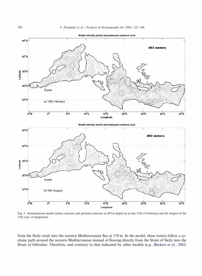
Fig. 5. Instantaneous model surface currents and pressure contours at 493 m depth (a) at day 15th of February and (b) August of the
15th year of integration.
330 V. Fernandez et al. / Progress in Oceanography 66 (2005) 321–340
from the Sicily strait into the western Mediterranean Sea at 170 m. In the model, these waters follow a cy-
clonic path around the western Mediterranean instead of flowing directly from the Strait of Sicily into the
Strait of Gibraltar. Therefore, and contrary to that indicated by other models (e.g., Beckers et al., 2002;
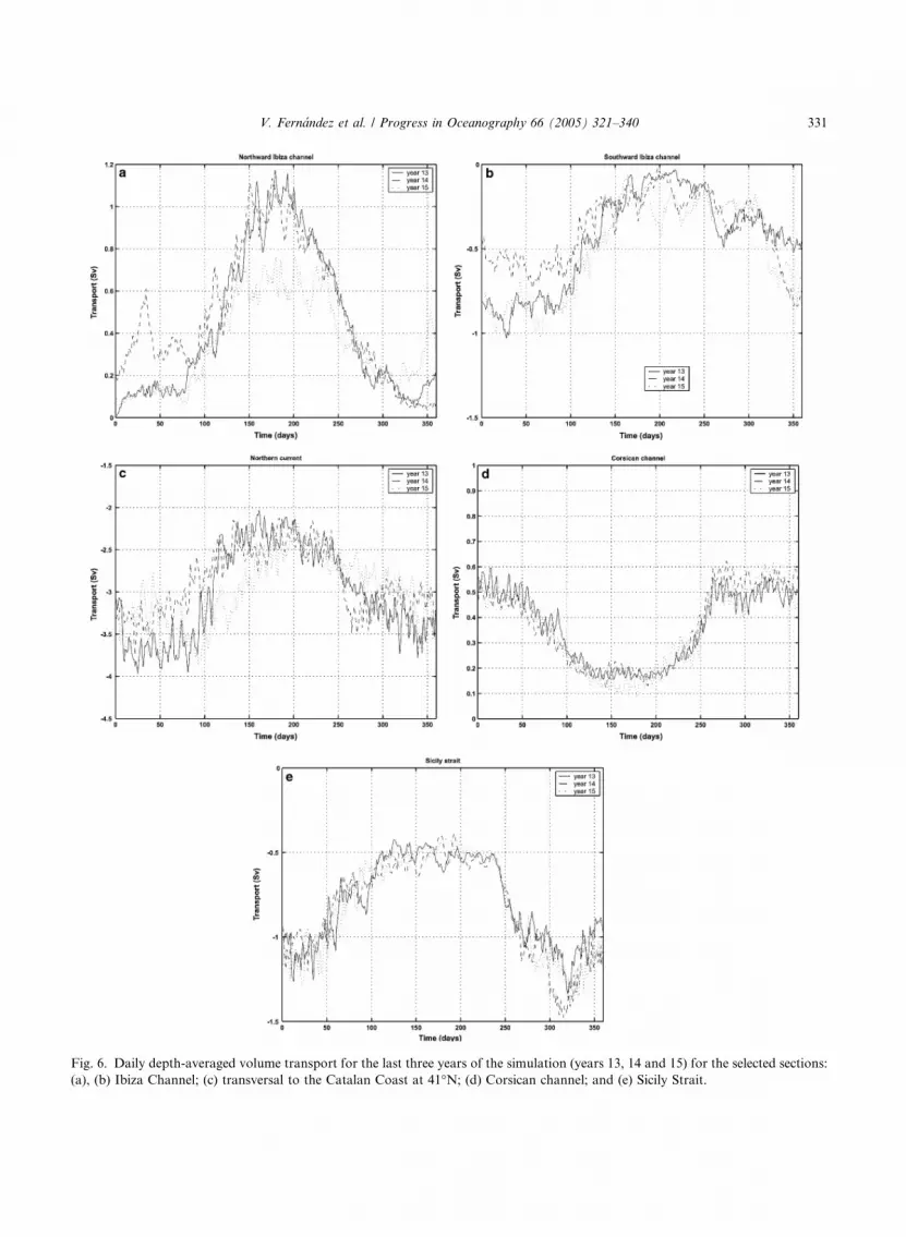
Fig. 6. Daily depth-averaged volume transport for the last three years of the simulation (years 13, 14 and 15) for the selected sections:
(a), (b) Ibiza Channel; (c) transversal to the Catalan Coast at 41�N; (d) Corsican channel; and (e) Sicily Strait.
V. Fernandez et al. / Progress in Oceanography 66 (2005) 321–340 331
332 V. Fernandez et al. / Progress in Oceanography 66 (2005) 321–340
Korres et al., 2000), there is not a permanent undercurrent flowing westward to the Alboran Sea along the
African coast and carrying higher salinities waters at intermediate depths (Fig. 7). We now describe in more
detail the model results for each of the sections selected.
Fig. 7. Model currents and model salinity in the western Mediterranean at 170 m (a) at day 15 of February and (b) August of the 15th
year of integration.

V. Fernandez et al. / Progress in Oceanography 66 (2005) 321–340 333
5.1.1. Northern current
The existence of a coastal current following the continental slope of the northwestern Mediterranean
Sea, flowing from the Corsican Channel towards the Balearic Sea, is a well known permanent feature of
the western Mediterranean circulation (Font, Garcia-Ladona, & Garcia-Gorriz, 1995). This current is
reproduced in the model simulation, fed by the current crossing the Corsica Channel, the west CorsicanCurrent transporting LIW from the Sicily strait and also by the recirculation of the same current when
it reaches the Ibiza Channel. We can see in Fig. 5 that this current reaches 500 m. Therefore, this current
carries surface waters, and also waters at intermediate depths. The depth-integrated transport of this cur-
rent at a latitude of 41�N in the model presents a seasonal cycle, being larger in winter than in summer. In
winter, the transport reaches a value of more than 3.8 Sv (southward) while in summer it decreases to
�2.3 Sv. These fluxes are larger than the geostrophic transports estimations of 1–1.5 Sv (Font et al.,
1995; Millot, 1999).
5.1.2. Ibiza Channel
This channel deserves special attention since it is, together with the Mallorca Channel, a passage where a
significant north–south water interchange in the western Mediterranean takes place. Mediterranean surface
and intermediate waters coming from the northern basin, after following a cyclonic path around the wes-
tern Mediterranean, reach these channels and can pursue south towards the Alboran Sea. At the same time,
northward intrusion of southern Atlantic waters (fresher and warmer) coming from the Algerian Basin is
observed through these channels with a marked seasonal and interannual variability (Lopez-Jurado, Garcıa
Lafuente, & Cano-Lucaya, 1995; Pinot, Lopez-Jurado, & Riera, 2002). It is important to note that the Bale-aric Basin is a place where few numerical models reproduce the northern inflow of Atlantic waters (Alvarez
et al., 1994).
The model southward transport through this channel is maximum in the winter months (January, Feb-
ruary and March) where it can be of 0.9 Sv in winter, with interannual variations, and it is very small in the
summer, from May to June (Fig. 6(b)). This variability of the southward transport crossing the Ibiza Chan-
nel is in phase with the strength of the northern current, which also presents a seasonal variability in the
model (Fig. 6(c)). As shown below, the northern current transport is much higher than the transport cross-
ing Ibiza indicating that only a small fraction of the northern current flows southward through the IbizaChannel, while most recirculates northward following the Balearic northern coast (Figs. 4, 5, 7). In the
observations, a clear seasonal signal is also seen in the transport of the northern current which ranges from
1 to 1.4 Sv in winter to <0.5 in summer (Pinot et al., 2002).
The northward transport in the model reproduces a seasonal variability in opposition to the southward
transport, being more intense in the summer, when the transport can be of �1 Sv (June, year 14th), and
being weaker in winter when it is only �0.1 Sv. The northern inflow of surface waters with salinity below
or equal to 37.5 is �0.4 Sv in June of year 14 and almost zero in winter, indicating that the northward trans-
port in the model is associated with the inflow of Atlantic waters from the Algerian Basin (fresher and war-mer) towards the northern basin. In observations, a northward transports from 0.2 to 0.7 Sv of southern
waters has been measured in the Ibiza Channel in summer (Pinot et al., 2002). The low salinity surface
waters coming from Gibraltar follow a more defined eastward path in winter while in summer they are
more spread to the north reaching the Ibiza Channel. This inflow of less modified Atlantic waters presents
also an interannual variability observed in in situ data and satellite imagery (Pinot et al., 2002), but the
physical mechanisms responsible for this variability are still unknown. It may be related to the oceano-
graphic conditions in the Algerian Basin and/or the atmospheric conditions in the northern basin.
5.1.3. Corsican Channel
This channel is a passage connecting the northern Tyrrhenian Sea with the northern basin. The model
circulation is such that water from the Tyrrhenian Sea enters the Northern basin, with a marked seasonality
334 V. Fernandez et al. / Progress in Oceanography 66 (2005) 321–340
in the transports. The model northward transport ranges from a maximum of �0.6 Sv in winter months to
a minimum of �0.2 Sv in the summer months, with few interannual variations (Fig. 6(d)). This northward
current crossing the Corsican Channel carries surface waters with relatively low salinity (S < 38), indicating
that almost no LIW crosses this channel in the model. Therefore, this suggests that the preferred path in the
model for LIW is through the Sardinian Channel (strait from Sardinia and Tunez) and not through theCorsica Channel towards the Gulf of Lyons (Fig. 7). These transport values and their seasonality, although
smaller, are in good agreement with observations, that indicate a seasonal variability ranging from 1.5 to
<0.5 Sv (Astraldi & Gasparini, 1992; Astraldi et al., 1999).
5.1.4. Strait of Sicily
The annual mean model transport crossing the Strait of Sicily, from the western towards the eastern
Mediterranean, is 0.6 Sv, with a seasonal cycle ranging from a maximum exchange of 1 Sv in the winter
months to a minimum transport of 0.4 Sv in the summer. Because there is no fresh water source/sink inthe model, an equivalent transport of waters flowing northward compensate for this southward transport,
since the net volume transport is equal to zero. This volume transport through Sicily is of the same order as
other numerical experiments (e.g., 0.6 Sv in Zavatarelli & Mellor, 1995). Observed transport estimates also
show seasonal variations and give a mean value for the westward transport of 1.1 Sv (Astraldi et al., 1999).
The eastward transport carries a large amount of surface modified Atlantic waters with S 6 37.5 close to
the Tunisian coast: 0.6 Sv in January and 0.1 Sv in July of year 15th. At the same time, the westward trans-
port consists mainly in LIW with a salinity around 38.5, that fills the whole bottom section of the Sicily
Strait. The transport of this LIW, with SP 38.5, is maximum in November (�0.6 Sv) and minimum in July(0.2 Sv) for year 15th. The typical value of LIW core salinity measured in the Sicily Strait, about 38.75, is a
bit higher than the model value, but this is justified by the reduced LIW water formation in the Eastern
Mediterranean due to the coarse climatological atmospheric forcing of the model.
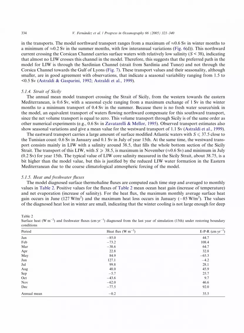
5.1.5. Heat and freshwater fluxes
The model diagnosed surface thermohaline fluxes are computed each time step and averaged to monthly
values in Table 2. Positive values for the fluxes of Table 2 mean ocean heat gain (increase of temperature)
and net evaporation (increase of salinity). For the heat flux, the maximum monthly average surface heatgain occurs in June (127 W/m2) and the maximum heat loss occurs in January (�85 W/m2). The values
of the diagnosed heat lost in winter are small, indicating that the winter cooling is not large enough for deep
Table 2
Surface heat (W m�2) and freshwater fluxes (cm yr�1) diagnosed from the last year of simulation (15th) under restoring boundary
conditions
Period Heat flux (W m�2) E-P-R (cm yr�1)
Jan �85.0 44.7
Feb �73.2 108.4
Mar �38.6 64.7
Apr 22.8 32.8
May 84.9 �65.3
Jun 127.1 �4.2
Jul 99.8 28.1
Aug 48.0 45.9
Sep �5.7 25.7
Oct �43.6 9.7
Nov �62.0 46.6
Dec �77.5 92.0
Annual mean �0.2 35.5

V. Fernandez et al. / Progress in Oceanography 66 (2005) 321–340 335
water formation, as expected when a model is forced with monthly climatological values. The annual mean
surface heat flux indicates a net slight cooling that is compensated by a heat inflow through Gibraltar to
give a very small model drift in temperature (Fig. 2). For the freshwater fluxes, in almost every month there
is a net evaporation, except May and June where precipitation and river runoff exceeds evaporation. The
net annual mean evaporation is compensated by the inflow of fresh waters through Gibraltar to give a smalldrift in salinity (Fig. 2). This range of diagnosed surface fluxes is consistent with the values reported by
other models (e.g., Table 1 in Myers & Haines, 2000).
As a conclusion of this section where we have shown some of the basic model results, it is clear that the
DieCAST model simulation with perpetual year climatological forcing reproduces the main features of the
large basin-scale circulation, as well as the seasonal variability of some sub-basin-scale currents and trans-
ports that are documented by observations in straits and channels.
5.2. Mesoscale and interannual variability
As the model results present numerous small scale features distributed over the whole basin, it is worthy
to analyse and discuss the mesoscale variability in the model, and more specifically, the model surface cir-
culation variability induced by the evolution of the model eddies. In order to do that, Fig. 8 shows the rms
variability of the sea surface pressure (in cm) over the 15th year at each grid point in space. This quantity is
computed from a 10-day sampling of the prognostic field, so fluctuations on shorter timescales are not in-
cluded. The model variability fluctuates around a mean value of 2.3 cm and ranges from 0.5 to 7 cm. These
values are smaller than the values obtained from satellite altimetry (e.g., Larnicol et al., 2002), which are inthe range from 4 to 16 cm. The smaller model variability may be due to the strong damping of surface tran-
sients by the 5-day restoring and the lack of directly forced synoptic variability in the model forcing. The
seasonal variability, representing the model linear response to the annual cycle of the buoyancy fluxes and
the wind stress applied at the surface, is responsible for some of the variability shown in Fig. 8. Shorter
Fig. 8. Root mean square (rms) variability of the sea surface pressure (in cm) computed over the 15th year of the simulation.
336 V. Fernandez et al. / Progress in Oceanography 66 (2005) 321–340
time-scale natural fronts and eddies in the model account for the largest rms variability (larger than 4 cm) in
sub-basins with high mesoscale variability in the model, as for example the Algerian Basin, the Tyrrhenian
Sea, the southern Ionian Sea and the southern coast of the Levantine Basin. This model result is in fair
agreement with observed fields computed from satellite data, where high values of rms reveal intense meso-
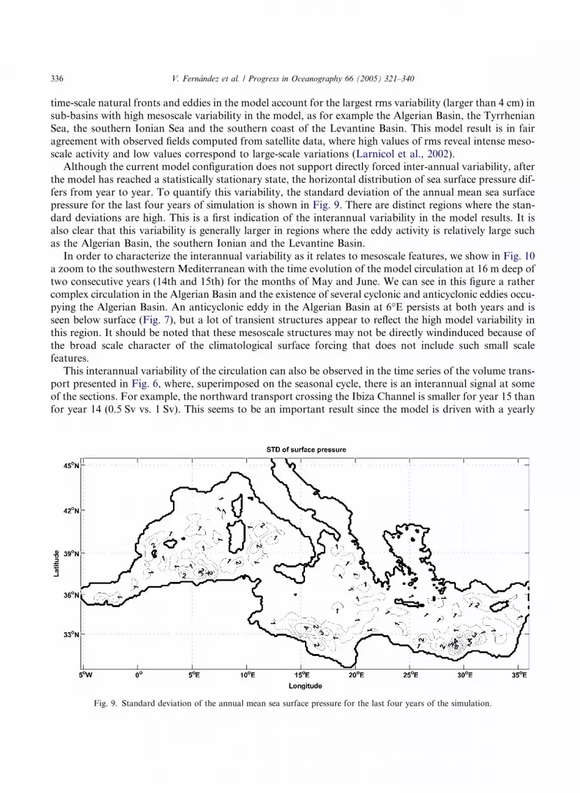
scale activity and low values correspond to large-scale variations (Larnicol et al., 2002).Although the current model configuration does not support directly forced inter-annual variability, after
the model has reached a statistically stationary state, the horizontal distribution of sea surface pressure dif-
fers from year to year. To quantify this variability, the standard deviation of the annual mean sea surface
pressure for the last four years of simulation is shown in Fig. 9. There are distinct regions where the stan-
dard deviations are high. This is a first indication of the interannual variability in the model results. It is
also clear that this variability is generally larger in regions where the eddy activity is relatively large such
as the Algerian Basin, the southern Ionian and the Levantine Basin.
In order to characterize the interannual variability as it relates to mesoscale features, we show in Fig. 10a zoom to the southwestern Mediterranean with the time evolution of the model circulation at 16 m deep of
two consecutive years (14th and 15th) for the months of May and June. We can see in this figure a rather
complex circulation in the Algerian Basin and the existence of several cyclonic and anticyclonic eddies occu-
pying the Algerian Basin. An anticyclonic eddy in the Algerian Basin at 6�E persists at both years and is
seen below surface (Fig. 7), but a lot of transient structures appear to reflect the high model variability in
this region. It should be noted that these mesoscale structures may not be directly windinduced because of
the broad scale character of the climatological surface forcing that does not include such small scale
features.This interannual variability of the circulation can also be observed in the time series of the volume trans-
port presented in Fig. 6, where, superimposed on the seasonal cycle, there is an interannual signal at some
of the sections. For example, the northward transport crossing the Ibiza Channel is smaller for year 15 than
for year 14 (0.5 Sv vs. 1 Sv). This seems to be an important result since the model is driven with a yearly
Fig. 9. Standard deviation of the annual mean sea surface pressure for the last four years of the simulation.
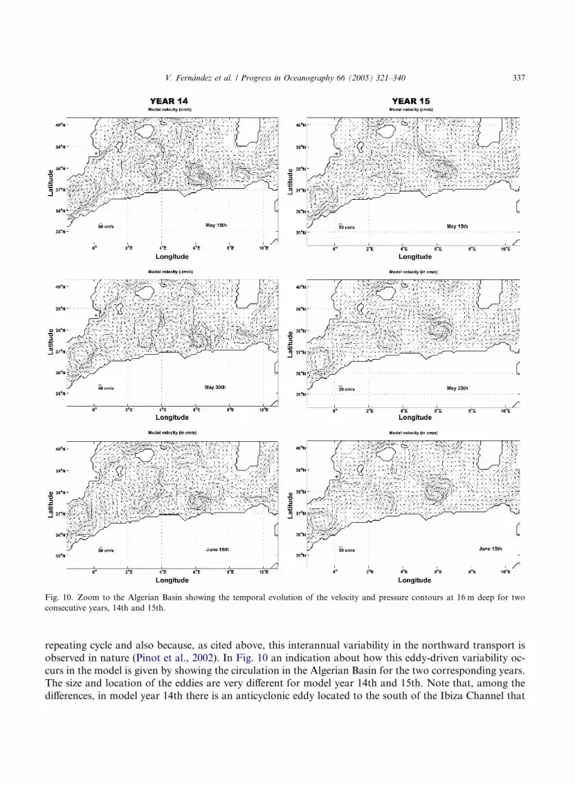
Fig. 10. Zoom to the Algerian Basin showing the temporal evolution of the velocity and pressure contours at 16 m deep for two
consecutive years, 14th and 15th.
V. Fernandez et al. / Progress in Oceanography 66 (2005) 321–340 337
repeating cycle and also because, as cited above, this interannual variability in the northward transport is
observed in nature (Pinot et al., 2002). In Fig. 10 an indication about how this eddy-driven variability oc-
curs in the model is given by showing the circulation in the Algerian Basin for the two corresponding years.The size and location of the eddies are very different for model year 14th and 15th. Note that, among the
differences, in model year 14th there is an anticyclonic eddy located to the south of the Ibiza Channel that
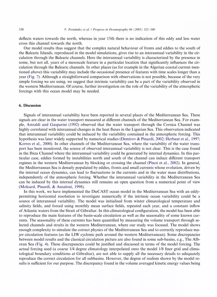
338 V. Fernandez et al. / Progress in Oceanography 66 (2005) 321–340
deflects waters towards the north, whereas in year 15th there is no indication of this eddy and less water
cross this channel towards the north.
Our model results thus suggest that the complex natural behaviour of fronts and eddies to the south of
the Balearic Islands, reproduced in the model simulations, gives rise to an interannual variability in the cir-
culation through the Balearic channels. Here the interannual variability is characterized by the presence insome, but not all, years of a mesoscale feature in a particular location that significantly influences the cir-
culation through the Balearic channels. In other places (as for example in the Algerian coastal current men-
tioned above) this variability may include the occasional presence of features with time scales longer than a
year (Fig. 7). Although a straightforward comparison with observations is not possible, because of the very
simple forcing we are using, we suggest that intrinsic variability can be a part of the variability observed in
the western Mediterranean. Of course, further investigation on the role of the variability of the atmospheric
forcings with this ocean model may be needed.
6. Discussion
Signals of interannual variability have been reported in several places of the Mediterranean Sea. These
signals are clear in the water transport measured at different channels of the Mediterranean Sea. For exam-
ple, Astraldi and Gasparini (1992) observed that the water transport through the Corsica Channel was
highly correlated with interannual changes in the heat fluxes in the Ligurian Sea. This observation indicated
that interannual variability could be induced by the variability contained in the atmospheric forcing. Thishypothesis was later widely supported by numerical studies (Demirov & Pinardi, 2002; Herbaut et al., 1997;
Korres et al., 2000). In other channels of the Mediterranean Sea, where the variability of the water trans-
port has been monitored, the source of observed interannual variability is not clear. This is the case found
in the Ibiza Channel where the interannual variability could be generated by internal dynamics. In this par-
ticular case, eddies formed by instabilities north and south of the channel can induce different transport
regimes in the western Mediterranean by blocking or crossing the channel (Pinot et al., 2002). In general,
the Mediterranean Sea is densely populated by eddies, fronts and small currents whose evolution, driven by
the internal ocean dynamics, can lead to fluctuations in the currents and in the water mass distributions,independently of the atmospheric forcing. Whether the interannual variability in the Mediterranean Sea
can be induced by this internal dynamics still remains an open question from a numerical point of view
(Molcard, Pinardi, & Ansaloni, 1998).
In this work, we have implemented the DieCAST ocean model in the Mediterranean Sea with an eddy-
permitting horizontal resolution to investigate numerically if the intrinsic ocean variability could be a
source of interannual variability. The model was initialised from winter climatological temperature and
salinity fields, and forced using monthly mean surface fields, repeated each year, and a constant inflow
of Atlantic waters from the Strait of Gibraltar. In this climatological configuration, the model has been ableto reproduce the main features of the basin-scale circulation as well as the seasonality of some known cur-
rents. The seasonality of these currents has been quantified by measuring the volume transport through se-
lected channels and straits in the western Mediterranean, where our study was focused. The model shows
enough complexity to simulate the correct physics of the Mediterranean Sea and to correctly reproduce ma-
jor circulation features (as the LIW cyclonic path around the western Mediterranean). Some discrepancies
between model results and the classical circulation picture are also found in some sub-basins, e.g., The Alb-
oran Sea (Fig. 4). These discrepancies could be justified and discussed in terms of the model forcing. The
actual forcing used (a coarse 1/4 degree climatology interpolated onto the model 1/8 finer grid and clima-tological boundary conditions at Gibraltar), are not able to supply all the necessary details to adequately
reproduce the correct circulation for all subbasins. However, the degree of realism shown by the model re-
sults is sufficient for our purpose. The discrepancy found in the volume averaged kinetic energy values being
V. Fernandez et al. / Progress in Oceanography 66 (2005) 321–340 339
about half that of Demirov and Pinardi (2002), can also be justified in terms of the model wind stress forc-
ing because in our study the surface averaged magnitude of the wind stress is about half of that in Demirov
and Pinardi (2002). The reason for this difference is the different bulk formulation used to compute the wind
stress forcing in both studies. We can also say that our wind stress forcing is smaller than other available
estimations of wind stress forcing. For example, the Southampton Oceanography Centre (SOC) wind stressclimatology gives a value of �0.032 N/m2 for the surface averaged annual mean wind stress, while this value
in our study is of �0.025 N/m2. Although a more complete evaluation of the role of the wind stress forcing
is out of the scope of this paper, it is not unrealistic to speculate that if a stronger wind stress were used to
force the model, the eddy-driven interannual variability could be even stronger than present results show.
As a main result of our study we have found the existence of a component of interannual variability
which is not associated with interannual changes in the external forcing which is only seasonally variable.
This interannual variability in the model results is related to the natural variability associated with the
realistic behaviour of ocean fronts and eddies (eddy driven interannual variability). The model resultsshow an important eddy field and numerous ocean fronts distributed all over the Mediterranean Sea.
Some of these features persist in the model during a period of time during which they move and evolve
slowly independently of the annual cycle of the atmospheric forcing. This process induces changes from
one year to another in the location of fronts and eddies that likewise imply anomalies in the circulation
patterns or in the water masses at specific locations. Importantly enough, these anomalies can happen not
only in the top layers but also in deeper layers, which are hardly related to the changes in the atmo-
spheric forcing. In agreement with observations, a key place where model results show interannual var-
iability in the water transports, induced by the eddy movements in the Algerian Basin, is the IbizaChannel.
Finally, we should note that the total observed interannual variability must be a combined effect of the
internal oceanic variability together with the variability induced by the external forcing. The amount of
variability accounted from nonlinearities and atmospheric forcing can differ from place to place in the
Mediterranean Sea. These issues need to be further investigated.
Acknowledgements
This study is a contribution to the Projects MAR1998-0840 and REN2001-3982. Partial support from
SOFT, EC funded project, EVK3-2000-00561 is also acknowledged. V. Fernandez acknowledges a FPI
grant from the Spanish Ministry for Science and Technology (PN1998 36125588). David E. Dietrich
acknowledges a grant from the Spanish ministry for Education and Culture (SAB1999-0037). A. Alvarez
read and kindly criticised the manuscript.
References
Alvarez, A., Tintore, J., Holloway, G., Eby & Beckers, J. M. (1994). Effects of topographic stress on circulation in the Western
Mediterranean. Journal of Geophysical Research, 101, 18167–18174.
Astraldi, M., & Gasparini, G. P. (1992). The seasonal characteristics of the circulation in the North Mediterranean Basin and their
relationship with the atmospheric-climatic conditions. Journal of Geophysical Research, 9, 867–888.
Astraldi, M., Balopoulos, S., Candela, J., Font, J., Gacic, M., Gasparini, G. P., Manca, B., Theocharis, A., & Tintore, J. (1999). The
role of straits and channels in understanding the characteristics of Mediterranean circulation. Progress in Oceanography, 44,
65–108.
Baschcek, B., Send, U., Lafuente, J. G., & Candela, J. (2001). Transport estimates in the Strait of Gibraltar with a tidal inverse model.
Journal of Geophysical Research, 106, 31017–31032.
Beckers, J. M., & MEDMEX (2002). Model intercomparison in the Mediterranean: MEDMEX simulations of the seasonal cycle.
Journal of Marine Systems, 33-34, 215–251.

340 V. Fernandez et al. / Progress in Oceanography 66 (2005) 321–340
Brasseur, P., Brankart, J., Schoenauen, R., & Beckers, J. M. (1996). Seasonal temperature and salinity fields in the Mediterranean Sea:
climatological analyses of an historical data set. Deep-Sea Research, 43, 59–192.
Demirov, E., & Pinardi, N. (2002). Simulation of the Mediterranean Sea circulation from 1979 to 1993: Part I. The interannual
variability. Journal of Marine Systems, 33–34, 23–50.
Dietrich, D. E. (1997). Application of a modified Arakawa ‘‘a’’ grid ocean model having reduced numerical dispersion to the Gulf of
Mexico circulation. Dynamics of Atmospheres and Oceans, 27, 201–217.
Dietrich, D. E., Lin, C. A., Mestas-Nunez, A., & Ko, D. S. (1997). A high resolution numerical study of Gulf Mexico Fronts and
Eddies. Meteorology and Atmospheric Physics, 64, 187–201.
Font, J., Garcia-Ladona, E., & Garcia-Gorriz, E. (1995). The seasonality of mesoscale motion in the Northern Current of the western
Mediterranean: several years of evidence. Oceanologica Acta, 18(2), 207–219.
Garret, C., Outerbridge, R., & Thomson, K. (1993). Interannual variability in Mediterranean heat and buoyancy fluxes. Journal of
Climate, 6, 900–910.
Haltiner, G. J., & Williams, R. T. (1980). Numerical prediction and dynamic meteorology. New York: Wiley.
Haney, R. L., Hale, R. A., & Dietrich, D. E. (2001). Offshore propagation of eddy kinetic energy in the California Current. Journal of
Geophysical Research, 106, 11709–11717.
Herbaut, C., Martel, F., & Crepon, M. (1997). A sensitivity study of the general circulation of the western Mediterranean Sea, Part II:
The response to atmospheric forcing. Journal of Physical Oceanography, 27, 2126–2145.
Horton, C., Clifford, M., Schmitz, J., & Kantha, L. (1997). A real-time oceanographic nowcast/forecast system for the Mediterranean
Sea. Journal of Geophysical Research, 102, 25123–25156.
Korres, G. N., Pinardi, N., & Lascaratos, A. (2000). The ocean response to low-frequency interannual atmospheric variability in the
Mediterranean Sea, Part I: Sensitivity experiments and energy analysis. Journal of Climate, 13, 705–731.
Larnicol, G., Ayoub, N., & Le Traon, P. Y. (2002). Major changes in Mediterranean Sea level variability from 7 years of TOPEX/
Poseidon and ERS-1/2 data. Journal of Marine Systems, 33–34, 63–89.
La Violette, A. (1990). The western Mediterranean circulation experiment (WMCE): introduction. Journal of Geophysical Research,
95(2), 1511–1514.
Lopez-Jurado, J. L., Garcıa Lafuente, J., & Cano-Lucaya, N. (1995). Hydrographic conditions of the Ibiza Channel during November
1990, March 1991 and July 1992. Oceanologica Acta, 18, 235–243.
Millot, C. (1999). Circulation in the Western Mediterranean Sea. Journal of Marine Systems, 20, 423–442.
Molcard, A. J., Pinardi, N., & Ansaloni, R. (1998). A spectral element ocean model on the Cray T3D: the interannual variability of the
Mediterranean Sea general circulation. Physics and Chemistry of the Earth, 23(5–6), 491–495.
Myers, P. G., & Haines, K. (2000). Seasonal and interannual variability in a model of the Mediterranean under derived flux forcing.
Journal of Physical Oceanography, 30, 1069–1082.
Pinardi, N., Korres, G., Lascaratos, A., Roussenov, V., & Stanev, E. (1997). Numerical simulation of the interannual variability of the
Mediterranean Sea upper circulation. Geophysical Research Letters, 24(4), 425–428.
Pinot, J. M., Lopez-Jurado, J. L., & Riera, M. (2002). The CANALES experiment (1996–1998). Interannual, seasonal, and mesoscale
variability of the circulation in the Balearic channels. Progress in Oceanography, 55, 335–370.
POEM Group (1992). General circulation of the eastern Mediterranean. Earth Science Reviews, 32, 285–309.
Robinson, A. R., & Golnaraghi, M. (1994). The physical and dynamical oceanography of the Mediterranean Sea. In Ocean processes in
climate dynamics: Global and Mediterranean examples (pp. 255–306). Norwell, MA: Kluewer Academy.
Roussenov, V., Stanev, E., Artale, V., & Pinardi, N. (1995). A seasonal model of the Mediterranean Sea general circulation. Journal of
Geophysical Research, 100, 13515–13538.
Sanderson, B. G., & Brassington, G. (1998). Accuracy in the context of a control-volume model. Atmosphere-Ocean, 36(4),
355–384.
Sanderson, B. G. (1998). Order and resolution for computational ocean dynamics. Journal of Physical Oceanography, 28, 1271–1286.
Send, U., & Baschek (2001). Intensive observations of the flow through the Strait of Gibraltar. Journal of Geophysical Research, 106,
31017–31032.
Staneva, J. V., Dietrich, D. E., Stanev, E., & Bowman, M. J. (2001). Rim current and coastal eddy mechanisms in an eddy-resolving
Black Sea general circulation model. Journal of Marine Systems, 31, 137–157.
Wu, P., & Haines, K. (1998). The general circulation of the Mediterranean Sea from a 100-years simulation. Journal of Geophysical
Research, 103(C1), 1121–1135.
Zavatarelli, M., &Mellor, G. L. (1995). A numerical study of the Mediterranean Sea circulation. Journal of Physical Oceanography, 25,
1384–1414.