İSTANBUL TECHNICAL UNIVERSITY ���� INSTITUTE OF SCIENCE AND TECHNOLOGY

M.Sc. Thesis by Umut UYSAL

Department : Mechanical Engineering

Programme : Automotive

JUNE 2010

OPTIMIZATION OF TIMING DRIVE SYSTEM DESIGN PARAMETERS FOR REDUCED ENGINE POWER LOSS

İSTANBUL TECHNICAL UNIVERSITY ���� INSTITUTE OF SCIENCE AND TECHNOLOGY

M.Sc. Thesis by Umut UYSAL (503071719)

Date of submission : 07 May 2010

Date of defence examination: 10 June 2010

Supervisor (Chairman) : Assis. Prof. Dr. Özgen AKALIN (ITU) Members of the Examining Committee : Prof. Dr. Metin ERGENEMAN (ITU)

Prof. Dr. İrfan YAVAŞLIOL (YTU)

JUNE 2010

OPTIMIZATION OF TIMING DRIVE SYSTEM DESIGN PARAMETERS FOR REDUCED ENGINE POWER LOSS

HAZİRAN 2010

İSTANBUL TEKNİK ÜNİVERSİTESİ ���� FEN BİLİMLERİ ENSTİTÜSÜ

YÜKSEK LİSANS TEZİ Umut UYSAL (503071719)

Tezin Enstitüye Verildiği Tarih : 07 Mayıs 2010

Tezin Savunulduğu Tarih : 10 Haziran 2010

Tez Danışmanı : Yrd. Doç. Dr. Özgen AKALIN (İTÜ) Diğer Jüri Üyeleri : Prof. Dr. Metin ERGENEMAN (İTÜ)

Prof. Dr. İrfan YAVAŞLIOL (YTÜ)

MOTOR GÜÇ KAYIPLARININ AZALTILMASI İÇİN ZAMANLAMA SİSTEMİ TASARIM PARAMETRELERİNİN OPTİMİZASYONU

v

FOREWORD

I would like to express my deep appreciation and thank my advisor Assis. Prof. Dr. Özgen AKALIN who made this thesis possible. This work could not have been completed without his support and invaluable advise.

I would like to thank my colleague Selçuk TABAK for his time and support during the simulations.

Last but not least, I would like to thank my family for their encouragement and assistance over my life.

May 2010

Umut Uysal

Mechanical Engineer

vi

vii

TABLE OF CONTENTS

Page

ABBREVIATIONS............................................................................................... ix LIST OF TABLES................................................................................................ xi LIST OF FIGURES............................................................................................ xiii LIST OF SYMBOLS ............................................................................................xv SUMMARY........................................................................................................ xvii ÖZET ...................................................................................................................xix 1. INTRODUCTION...............................................................................................1 2. TIMING DRIVE SYSTEMS IN INTERNAL COMBUSTION ENGINES......5

2.1 Types of Timing Drive System........................................................................5 2.1.1 Belt Drive System ....................................................................................5 2.1.2 Gear Drive System ...................................................................................6 2.1.3 Chain Drive System..................................................................................7

3. CHAIN DRIVE SIMULATION THEORY .....................................................11 3.1 Part Modelling...............................................................................................12

3.1.1 Chain Link Modeling .............................................................................12 3.1.2 Sprocket Modeling .................................................................................13 3.1.3 Guide and Tensioner Modeling...............................................................14

3.2 Chain Contact Kinematics .............................................................................15 3.2.1 Generalized Contact Kinematics.............................................................15 3.2.2 Time Derivatives ....................................................................................16 3.2.3 Roller-Sprocket Contact Kinematics.......................................................17 3.2.4 Link-Guide Contact Kinematics .............................................................19 3.2.5 Tensioner Guide Contact Kinematics......................................................20

3.3 Chain Contact Dynamics ...............................................................................20 3.4 Chain Initialization........................................................................................22

4. METHODOLOGY ...........................................................................................23 4.1 Engine Specification and Components...........................................................23 4.2 Simulation Parameters...................................................................................24 4.3 Chain Drive Simulation .................................................................................29

4.3.1 Solver Theory.........................................................................................29 4.4 Design of Experiment....................................................................................30 4.5 Statistical Analysis ........................................................................................31

4.5.1 Response Surface Methods.....................................................................31 4.5.2 Response Optimization...........................................................................31 4.5.3 Residual plot choices..............................................................................32 4.5.4 P-value ...................................................................................................33

5. RESULTS..........................................................................................................35 5.1 Component Level Friction Power Loss ..........................................................35 5.2 Friction Power Loss Distribution ...................................................................36 5.3 Optimisation of Friction Power Loss Results .................................................38

5.3.1 Data Consistency....................................................................................39

viii

5.3.2 Optimized Results.................................................................................. 39 5.3.3 Optimized Friction Power Loss Distribution .......................................... 41 5.3.4 Effect of Design Parameter Interaction................................................... 43

CONCLUSIONS AND RECOMMENDATIONS ............................................... 45 REFERENCES..................................................................................................... 47 APPENDICES ...................................................................................................... 49 CURRICULUM VITA ......................................................................................... 69

ix

ABBREVIATIONS

CA : Crank Angle CAE : Computer Aided Engineering CTF : Cam Sprocket Tooth Form CrTF : Crank Sprocket Tooth Form DfSS : Design for Six Sigma DoE : Design of Experiments DoF : Degree of Freedom DOHC : Double Over Head Camshaft FIP : Fuel Injection Pump FTF : FIP Sprocket Tooth Form GUI : Graphical User Interface NVH : Noise Vibration and Harshness OEM : Original Equipment Manufacturer OSP : Oil Supply Pressure SRR : Sprocket Root Runout TFR : Tensioner Flow Rate TSF : Tensioner Spring Force

xi

LIST OF TABLES

Page

Table 4.1: Specification of modelled engine...........................................................24 Table 4.2: Timing drive sub-component type and dimensions ................................24 Table 4.3: Crank Sprocket Tooth Profile Values ....................................................26 Table 4.4: Cam and FIP Sprocket Tooth Profile Values..........................................26 Table 4.5: Simulation input for seven design parameters ........................................28 Table 5.1 : Friction power loss results in Joule .......................................................38 Table 5.2 : Optimised design parameters ................................................................40 Table 5.3 : Calculated P-values ..............................................................................44 Table A.1 : DoE Matrix with seven design parameters ...........................................50 Table A.2 : Estimated regression coefficients.........................................................52

xiii

LIST OF FIGURES

Page

Figure 1.1 : Contribution of engine friction [3].........................................................2 Figure 2.1 : Components of belt drive systems [9]....................................................5 Figure 2.2 : Components of gear drive systems [9]...................................................6 Figure 2.3 : Components of chain drive system [9] ..................................................7 Figure 2.4 : Sub-components of timing chain [11]....................................................8 Figure 2.5 : Sub-components of bushing chain [12] .................................................9 Figure 2.6 : Sub-components of silent chain [12] .....................................................9 Figure 3.1 : Contact and connection forces in the chain simulation [13] .................12 Figure 3.2 : Representation of chain link [14] ........................................................13 Figure 3.3 : Chain link connectivity [14]................................................................13 Figure 3.4 : Sprocket geometry ..............................................................................14 Figure 3.5 : Guide and tensioning devices..............................................................15 Figure 3.6 : Generalized contact kinematics [14]....................................................15 Figure 3.7 : Roller and sprocket contact kinematics [14] ........................................17 Figure 3.8 : Illustrated roller and guide contact [14] ...............................................19 Figure 3.9 : Tensioner and guide contact kinematics [14].......................................20 Figure 3.10 : Chain link forces and link extension [15] ..........................................21 Figure 3.11 : Contact forces - Chain bush and sprocket or guide [15].....................21 Figure 4.1 : Chain drive layout...............................................................................23 Figure 4.2 : Minimum and maximum tooth form of crank sprocket [15] ................25 Figure 4.3 : Sprocket Tooth Profile Factors............................................................27 Figure 4.4 : Crank sprocket root run-out ................................................................27 Figure 4.5 : FIP and Cam sprocket root run-out......................................................28 Figure 5.1 : Total friction power loss – Base design ...............................................35 Figure 5.2 : Friction power loss distribution at 1000 rpm .......................................36 Figure 5.3 : Friction power loss distribution at 2000 rpm .......................................37 Figure 5.4 : Friction power loss distribution at 3000 rpm .......................................37 Figure 5.5 : Friction power loss distribution at 4000 rpm .......................................38 Figure 5.6 : Total friction power loss – Base design and Optimized desing ............39 Figure 5.7 : Improvement in total friction power loss .............................................40 Figure 5.8 : Optimisation plot – All design parameters...........................................41 Figure 5.9 : Optimized friction power loss distribution at 1000 rpm .......................41 Figure 5.10 : Optimized friction power loss distribution at 2000 rpm .....................42 Figure 5.11 : Optimized friction power loss distribution at 3000 rpm .....................42 Figure 5.12 : Optimized friction power loss distribution at 4000 rpm .....................43 Figure A.1 : Timing chain friction power loss – Base design..................................52 Figure A.2 : Sprockets’ Friction Power Loss – Base design....................................53 Figure A.3 : Guides’ friction power loss – Base design ..........................................53 Figure A.4 : Arm friction power loss – Base design ...............................................54 Figure A.5 : FIP guide friction power loss – Base design .......................................54

xiv

Figure A.6 : Crank guide friction power loss – Base design ................................... 55 Figure A.7 : Residual plots for total loss at 1000 rpm ............................................ 55 Figure A.8 : Residual plots for total loss at 2000 rpm ............................................ 56 Figure A.9 : Residual plots for total loss at 3000 rpm ............................................ 56 Figure A.10 : Residual plots for total loss at 4000 rpm .......................................... 57 Figure A.11 : Chain friction power loss – Base design and optimized design ......... 57 Figure A.12 : Sprocket friction power loss – Base design and optimized design .... 58 Figure A.13 : Guide friction power loss – Base design and optimized design......... 58 Figure A.14 : Arm friction power loss – Base design and optimized design ........... 59 Figure A.15 : FIP guide friction power loss – Base design and optimized design ... 59 Figure A.16 : Crank guide friction power loss – Base design and optimized design60 Figure A.17 : Surface plot of TFR versus OSP at 1000rpm.................................... 60 Figure A.18 : Surface plot of TSF versus CTF at 1000rpm .................................... 60 Figure A.19 : Surface plot of TSF versus OSP at 1000rpm .................................... 61 Figure A.20 : Surface plot of CrTF versus SRR at 1000rpm .................................. 61 Figure A.21 : Surface plot of FTF versus SRR at 1000rpm .................................... 61 Figure A.22 : Surface plot of FTF versus OSP at 1000rpm .................................... 62 Figure A.23 : Surface plot of CTF versus SRR at 1000rpm.................................... 62 Figure A.24 : Surface plot of TFR versus OSP at 2000rpm.................................... 62 Figure A.25 : Surface plot of TSF versus CrTF at 2000rpm ................................... 63 Figure A.26 : Surface plot of TSF versus OSP at 2000rpm .................................... 63 Figure A.27 : Surface plot of CrTF versus SRO at 2000rpm .................................. 63 Figure A.28 : Surface plot of FTF versus SRO at 2000rpm.................................... 64 Figure A.29 : Surface plot of CTF versus SRO at 2000rpm ................................... 64 Figure A.30 : Surface plot of TFR versus OSP at 3000rpm.................................... 64 Figure A.31 : Surface plot of TSF versus OSP at 3000rpm .................................... 65 Figure A.32 : Surface plot of FTF versus OSP at 3000rpm .................................... 65 Figure A.33 : Surface plot of CTF versus OSP at 3000rpm.................................... 65 Figure A.34 : Surface plot of TFR versus OSP at 4000rpm.................................... 66 Figure A.35 : Surface plot of TSF versus CTF at 4000rpm .................................... 66 Figure A.36 : Surface plot of TSF versus SRR at 4000rpm .................................... 66 Figure A.37 : Surface plot of TSF versus OSP at 4000rpm .................................... 67 Figure A.38 : Surface plot of CrTF versus SRR at 4000rpm .................................. 67 Figure A.39 : Surface plot of CrTF versus OSP at 4000rpm................................... 67 Figure A.40 : Surface plot of SRR versus OSP at 4000rpm.................................... 68

xv

LIST OF SYMBOLS

klink : Chain Link Stiffness Coefficient clink : Chain Link Damping Coefficient Flink : Chain Link Force ∆ : Chain Link Relative Displacement Rpitch : Pitch Radius Rroller : Roller Radius Rtooth : Tooth Radius Rout : Tip Radius Rguide : Guide Arc Radius Rlink : Chain Link Roller Radius Θcontact : Roller Contact Angle Fx, Fy : Sprocket Contact Force k : Camshaft Stiffness Coefficient c : Camshaft Damping Coefficient x, y : Relative Displacement of Sprocket Geometric Center Pk : Position Vector of Body K t : Tangent Vector n : Normal Vector q : Relative Minimum Distance Between Bodies a : Interference Between Profiles Vt : Tangential Relative Velocity Vc : Tangential Relative Velocity Between Centers δ : Distance Between Centers s : Position of Candidate Contact Points L : Chain Link Length D : Chain Link Clearance dij : Distance Between Two Adjacent Bush e : Link Extension A : Non-linear Stiffness Term re : Tooth Flank Radius ri : Tooth Root Radius α : Roller Sitting Angle da : Tip Diameter

xvii

OPTIMIZATION OF TIMING DRIVE SYSTEM DESIGN PARAMETERS FOR REDUCED ENGINE POWER LOSS

SUMMARY

Although power losses caused by the valve timing drive system is relatively lower compared to the power cylinder system losses, today’s high efficiency engine requirements necessitate the development of low friction timing drives more than ever. In this study, a design optimization methodology is presented that can be used to reduce the total friction power loss generated by the timing chain drive system of a four-cylinder diesel engine.

A timing drive model was developed based on computer-aided simulation methods and used to calculate the contribution of each system component to the overall timing drive friction loss at various engine operating conditions. This model enables to obtain the friction power loss distribution in component level by defining the friction losses on timing chain, drive sprockets and plastic guiding components individually. Using the analytical results and statistical methods, an optimization study was performed to calculate the ideal system design parameters, such as hydraulic tensioner spring force and flow rate, sprocket tooth profiles and circularity, and oil supply pressure. Additionally, a statistical study was accomplished in order to assess data consistency and parameter interactions by using surface plots with the most effective design parameters.

The simulation results revealed that while the plastic guide – timing chain friction is responsible for the most part of the frictional losses, the contribution of timing chain friction increase with increasing speed. In addition, the share of each guide and sprocket was identified. It was found that the tensioner guide is the key element in the guiding system causing frictional losses. Furthermore, tensioner spring force and engine oil pressure were identified as major design parameters that influence the efficiency of the timing drive. Consequently, the simulation results showed that 20% improvement can be generated in the overall timing drive friction power loss by simply optimizing the design parameters.

xviii

xix

MOTOR GÜÇ KAYIPLARININ AZALTILMASI İÇİN ZAMANLAMA SİSTEMİ TASARIM PARAMETRELERİNİN OPTİMİZASYONU

ÖZET

Supap tahrik sisteminin sebep olduğu güç kayıpları, piston-silindir sisteminin güç kayıplarına nazaran çok daha düşük olmasına rağmen, günümüzdeki yüksek verimli motor talebi düşük sürtünmeli supap zamanlama sistemlerinin geliştirilmesine her zamankinden daha fazla ihtiyaç duymaktadır. Bu çalışmada 4-zamanlı bir dizel motorun, zincir tahrik sistemi tarafından meydana getirilen toplam sürtünme güç kaybını azaltmada kullanılabilecek bir tasarım optimizasyon metodolojisi sunulmuştur.

Her bir sistem parçasının zamanlama sisteminin toplam sürtünme kaybındaki iştirakını çeşitli motor çalışma koşullarında hesaplamakta kullanılan ve bilgisayar destekli simulasyon metodlarına dayanan bir zamanlama sistemi modeli geliştirilmiştir. Bu model sürtünme güç kayıpları dağılımının parça seviyesinde; zamanlama zinciri, dişliler ve plastik klavuzlama elemanlarındaki sürtünme kayıplarını ayrı ayrı tanımlayarak, elde edilmesine olanak sağlar. İdeal sistem dizayn parametrelerinin; örneğin hidrolik gergi yay kuvveti ve debisinin, dişli profilleri ve ovalliğin ve yağ basıncının hesaplanması için analitik sonuçlar ve istatiksel metodlar kullanarak bir optimizasyon çalışması yapılmıştır. Ayrıca veri tutarlılığını ve parametrelerin etkileşimini değerlendirmek için en etkili parametrelerinin yüzey grafikleri kullanarak istatiksel bir çalışma tamamlanmıştır.

Simulasyon sonuçları plastik klavuz-zamanlama zinciri arasındaki sürtünmenin, sürtünme kayıplarının büyük bir kısmından sorumlu olduğunu ve zamanlama zinciri sürtünmesinin artan motor hızıyla arttığını ortaya çıkarmıştır. Ayrıca, her klavuz ve dişlinin sürtünmedeki payı tanımlanmıştır. Buna ek olarak gergi yay kuvveti ve motor yağ basıncının zamanlama sisteminin verimini etkileyen en baskın dizayn parametreleri olduğu belirtilmiştir. Sonuç olarak, toplam zincir tahrik sistemindeki sürtünme güç kayıplarının, dizayn parametrelerini basitçe optimize ederek %20 oranında geliştirilebileceği simülasyon sonuçlarıyla gösterilmiştir.

1

1. INTRODUCTION

Even though chain drives have been used on internal combustion engines for years,

there are not many published work available related to the quantitative analysis of the

efficiency and the assessment of the system loss of these kinds of drive trains. In

general, the design of the chain drives is fairly well understood. Owing to the variety

of applications and the range of operating conditions for chain drives, numerous

factors must be considered in specifying a chain drive. These factors include chain

length, load ratings, rotational forces, contact forces, chordal action and chain

vibration. Most of the design considerations center on assessing the load and power

transfer characteristics of the chain or relate to chain lifetime, robustness and

reliability. Chain drive efficiency is not a primary design consideration perhaps

owing to the non-critical nature of efficiency in many applications, although

automotive OEMs are under pressure to improve the fuel consumption and reduce

vehicle emissions with the new legislations. Therefore, decreasing the friction power

losses in timing drive system by optimizing the system design parameters can help to

achieve efficiency enhancement while reducing design and development time with

the minor design changes.

There are numerous studies focusing on the friction losses in the timing drive

systems but none of them investigated the possibility of improving the system

efficiency by using both CAE based analytical and statistical methodologies. It is

possible to optimize the system by changing the design parameters and investigate

their effect on system response regarding friction power loss.

Heywood (1998) named the friction loss as a great importance in engine design by

considering the large portion of the friction loss in the indicated work or power. That

portion of the friction work directly concerns the maximum brake torque and

minimum brake specific fuel consumption. He attracted attention to the formation of

the friction work, which results in the formation of heat, thus friction loss influence

the design of the cooling systems [1].

2

Similarly, Körfer and Lacy (2006) studied the friction losses of the belt driven and

timing chain driven systems by defining the friction loss as being the difference

between the area under the measured torque curve -average torque- in a drive and

zero. They clarified that the sliding friction is dominant for the friction power loss of

the chain systems [2].

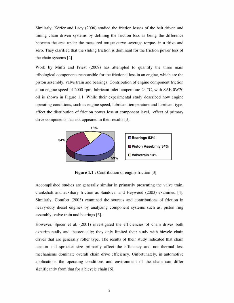
Work by Mufti and Priest (2009) has attempted to quantify the three main

tribological components responsible for the frictional loss in an engine, which are the

piston assembly, valve train and bearings. Contribution of engine component friction

at an engine speed of 2000 rpm, lubricant inlet temperature 24 °C, with SAE 0W20

oil is shown in Figure 1.1. While their experimental study described how engine

operating conditions, such as engine speed, lubricant temperature and lubricant type,

affect the distribution of friction power loss at component level, effect of primary

drive components has not appeared in their results [3].

34%

13%

53%

Bearings 53%

Piston Assebmly 34%

Valvetrain 13%

Figure 1.1 : Contribution of engine friction [3]

Accomplished studies are generally similar in primarily presenting the valve train,

crankshaft and auxiliary friction as Sandoval and Heywood (2003) examined [4].

Similarly, Comfort (2003) examined the sources and contributions of friction in

heavy-duty diesel engines by analyzing component systems such as, piston ring

assembly, valve train and bearings [5].

However, Spicer et al. (2001) investigated the efficiencies of chain drives both

experimentally and theoretically; they only limited their study with bicycle chain

drives that are generally roller type. The results of their study indicated that chain

tension and sprocket size primarily affect the efficiency and non-thermal loss

mechanisms dominate overall chain drive efficiency. Unfortunately, in automotive

applications the operating conditions and environment of the chain can differ

significantly from that for a bicycle chain [6].

3

However, Maile et al. (2009) developed a methodology for a cost effective and

reliable timing chain drive system based on Design for Six Sigma (DfSS) process,

the underlying assumptions regarding their expression for efficiency was not given.

They performed a theoretical study by applying a Design of Experiments (DoE)

methodology on a CAE model aiming to investigate significant factors that affect

chain load variability. Additionally, they considered that conventional timing chain

drive system design is very complex and time consuming, however time and money

can be saved by using new design tools and applying statistical methods [7]. They

pointed out the situation by giving the example of development steps of a four-

cylinder diesel engine, which faced twenty-one design changes from initial design

concept to the final design. These design changes resulted 40% cost increase in

component and 90% cost increase in the tooling from the original tooling design to

the actual production tooling cost.

The models developed by Kux and Parsche (2009) indicated that by using

appropriate optimization methods, it is possible to automate the computation of

possible compromises and to select suitable options from them. In respect of these

objectives, their aim was to develop chain drives by optimizing the parameters; such

as, position of the sprockets, the number of teeth and the initial positioning of rails

and tensioning elements. In their study, it has been reported that 21% reduction in

friction power was obtained, at the same time reducing the tensioner piston stroke,

lowering preload force by 60% and as a result decreasing the maximum chain force

by 37% with the optimized variant [8].

Consequently, published studies related to chain driven systems generally study the

design parameters by evaluating the robustness and reliability. Friction loss in the

system is not taken into consideration in initial design. Conventional timing drive

system design is very complex and time consuming that randomly tests components

on engines and then improves the design when and if failures occur. The increasing

complexity and cost of developing new engines means that this traditional design

approach is becoming uneconomical [7]. The opportunity of using CAE based design

tools to model the system by developing efficient models for the timing chain system

and statistical analysis methods, enables the reliability of the design to be established

before production commences. Moreover, most of the published works mainly assess

the engine components such as; piston assembly, valvetrain and bearings. These

4

studies consider engine operating conditions and lubricant effect, but they oversight

the possibility of decreasing the frictional loss by adjusting the design parameters.

The purpose of this study is to model the timing chain drive system of a four-cylinder

diesel engine and study the distribution of friction power loss individually on sub-

components of the system. In addition, effect of timing drive system design

parameters on friction power loss was investigated by creating design of experiments

that leads to decrease the engine friction loss by optimizing the design parameters for

varied engine speeds. As a result, improvement in friction power loss is

demonstrated by computer simulation and statistical analysis, meanwhile reducing

the design and development time.

5

2. TIMING DRIVE SYSTEMS IN INTERNAL COMBUSTION ENGINES

The main function of timing drive systems on internal combustion engines is to drive

the camshaft(s) synchronously with to the crankshaft to provide torque transfer.

Therefore, timing drive systems are subjected to loading of interactions from driven

systems like crank train and valve train systems. There are different types of timing

drive system technologies for the motion transfer for modern engine overhead

camshaft drives such as, belt drive systems, gear drive systems and chain drive

systems.

2.1 Types of Timing Drive System

There are mainly three technology used to transfer torque from crankshaft to

camshaft(s) which are belt drive, gear drive and chain drive. Selection for the type of

drive system depends on durability, package, NVH, efficiency and maintenance

costs.

2.1.1 Belt Drive System

Timing belts have teeth that fit into a matching toothed pulley. When correctly

tensioned, they do not slip and run at constant speed. Thus, they are often used to

transfer direct motion for indexing or timing purposes.

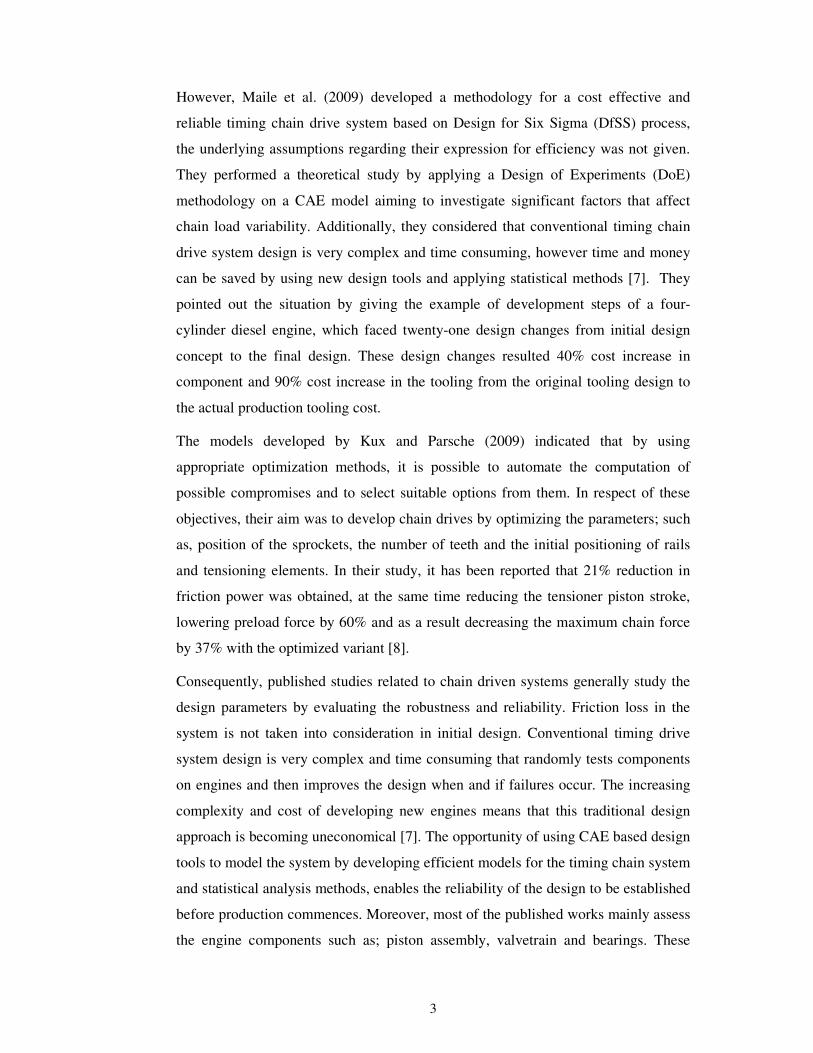
Figure 2.1 : Components of belt drive systems [9]

6

Belts are widely used on gasoline engines and relatively low volume diesel engines.

Toothed belt drive usage is a standard, as it provides no slip characteristics for belt

driven timing systems. An illustrated belt drive system is shown in Figure 2.1. Sub-

components are toothed belt, exhaust and intake cam pulley, crank pulley and a

mechanical tensioner.

Belt drives have comparably lower ultimate tensile strength and hence reduced

fatigue limits compared to chain drives. Due to this fact, they need frequent change

in maintenance periods. Belt width and thickness determine the fatigue strength of

the belt so design engineers perform application specific design optimizations. The

limited fatigue levels and frequent service replacement are the main reasons for

limited usage in diesel engines. In addition, belt systems should be protected from

ambient disturbers i.e. dust, water and belt covers are needed which increases the

package volume on engines. Belt drives are generally designed for dry environments,

but recent technological developments make possible belt drives running in engine

lubrication environment [10].

2.1.2 Gear Drive System

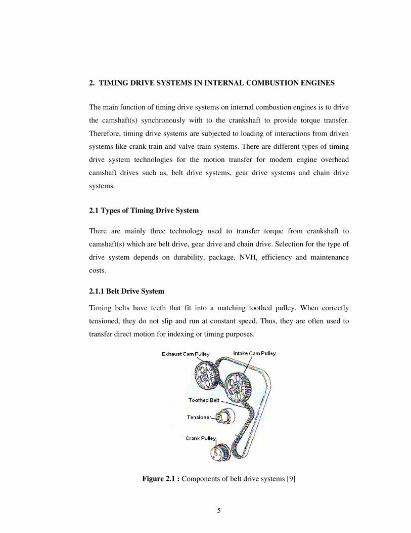
Gear drives have very high load carrying characteristics, therefore are almost a

standard for heavy-duty diesel engines. Their high tensile strength prioritizes usage

of gear drives under heavy loading conditions compared to the conventional drive

systems like chain or belt circuit.

Figure 2.2 : Components of gear drive systems [9]

7

A gear drive system consists of main gear(s) and an idler gear(s). Main gears are

used for the rotational motion transfer from crankshaft to camshaft(s) by the idler

gears and camshaft gears. Idler gears are used in the system just to transfer torque to

the matching gear. A representation of gear train systems can be seen on Figure 2.2.

The size and thickness determine the load carrying capabilities of the gears. The

shape and size of the gear contact area affects the gear wear properties. As gear

drives operate under almost boundary lubrication, gear lubricants need to have a

sufficient viscosity to withstand under heavy contact loads in order to reduce tooth

wear.

2.1.3 Chain Drive System

A chain is a reliable machine component, which transmits power by means of tensile

forces, and is used primarily for power transmission. Chain drives are commonly

used in commercial vehicle engines due to low maintenance costs. Special design

chains are always valid for specific applications but there are three main types of

chain drives available in today’s automotive market which are bush, roller and

inverted tooth chains which are also known as silent chains [11].

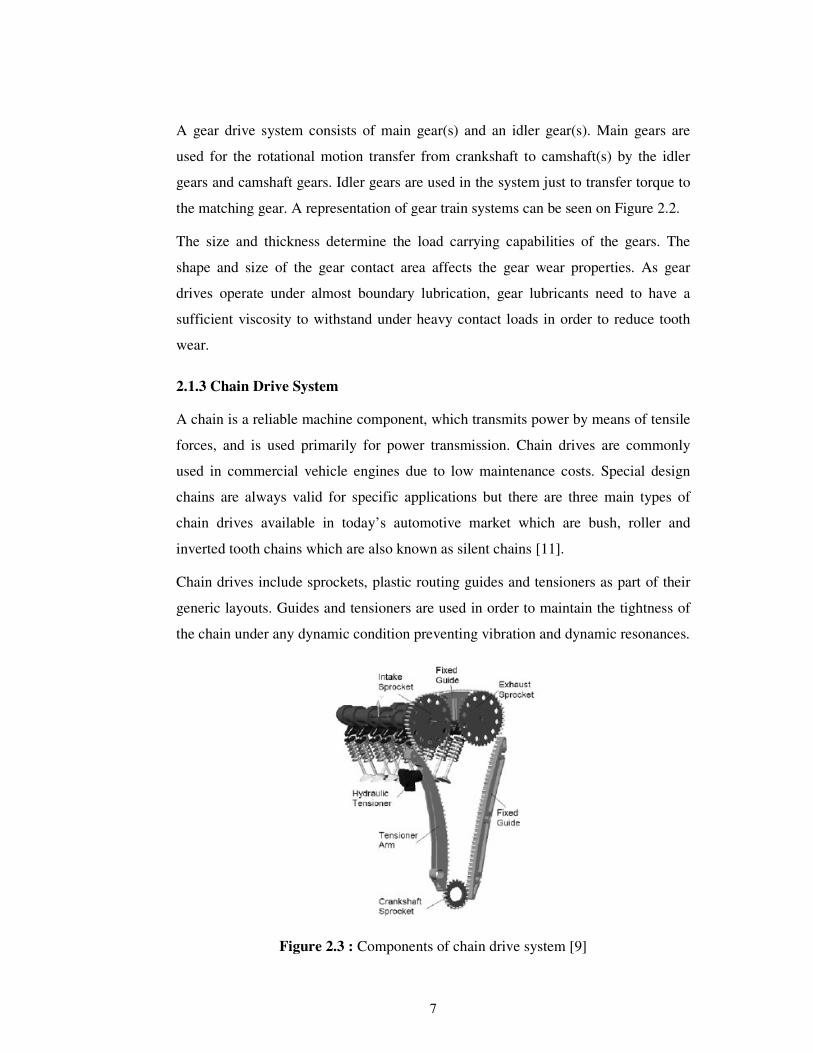
Chain drives include sprockets, plastic routing guides and tensioners as part of their

generic layouts. Guides and tensioners are used in order to maintain the tightness of

the chain under any dynamic condition preventing vibration and dynamic resonances.

Figure 2.3 : Components of chain drive system [9]

8

Torque is conveyed by the teeth of the sprocket meshing with the holes in the links

of the chain and hereby rotational motion input from crankshaft to camshafts and

other adjacent drive systems is transferred. Components of chain drive system are

shown in Figure 2.3. Basic system includes crankshaft sprocket, camshaft sprockets,

plastic guiding elements, and the tensioner. A fuel injection pump or a water pump

can be arbitrarily driven with the timing chain.

2.1.3.1 Timing Chain

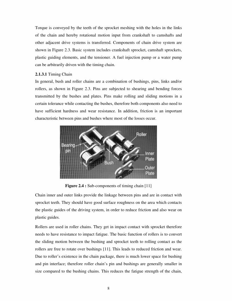
In general, bush and roller chains are a combination of bushings, pins, links and/or

rollers, as shown in Figure 2.3. Pins are subjected to shearing and bending forces

transmitted by the bushes and plates. Pins make rolling and sliding motions in a

certain tolerance while contacting the bushes, therefore both components also need to

have sufficient hardness and wear resistance. In addition, friction is an important

characteristic between pins and bushes where most of the losses occur.

Figure 2.4 : Sub-components of timing chain [11]

Chain inner and outer links provide the linkage between pins and are in contact with

sprocket teeth. They should have good surface roughness on the area which contacts

the plastic guides of the driving system, in order to reduce friction and also wear on

plastic guides.

Rollers are used in roller chains. They get in impact contact with sprocket therefore

needs to have resistance to impact fatigue. The basic function of rollers is to convert

the sliding motion between the bushing and sprocket teeth to rolling contact as the

rollers are free to rotate over bushings [11]. This leads to reduced friction and wear.

Due to roller’s existence in the chain package, there is much lower space for bushing

and pin interface; therefore roller chain’s pin and bushings are generally smaller in

size compared to the bushing chains. This reduces the fatigue strength of the chain,

9

hence roller types are mostly used in the applications subject to lower loads like

auxiliary drive systems on engines (e.g. oil pump drives). Small size pin and bush

reduces the contact area between pin and bushing increasing contact pressure

between components. Increase in contact force per unit area has a negative effect on

friction properties of timing chains.

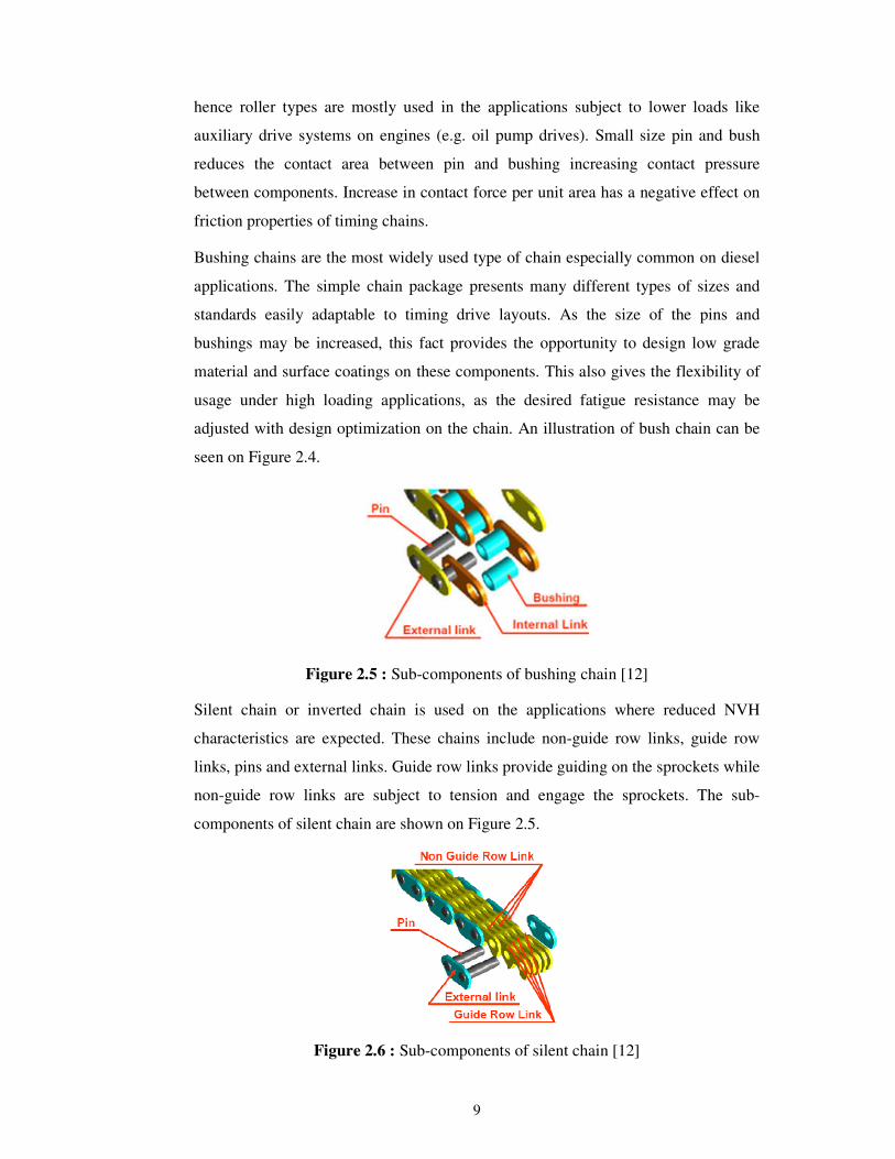
Bushing chains are the most widely used type of chain especially common on diesel

applications. The simple chain package presents many different types of sizes and

standards easily adaptable to timing drive layouts. As the size of the pins and

bushings may be increased, this fact provides the opportunity to design low grade

material and surface coatings on these components. This also gives the flexibility of

usage under high loading applications, as the desired fatigue resistance may be

adjusted with design optimization on the chain. An illustration of bush chain can be

seen on Figure 2.4.

Figure 2.5 : Sub-components of bushing chain [12]

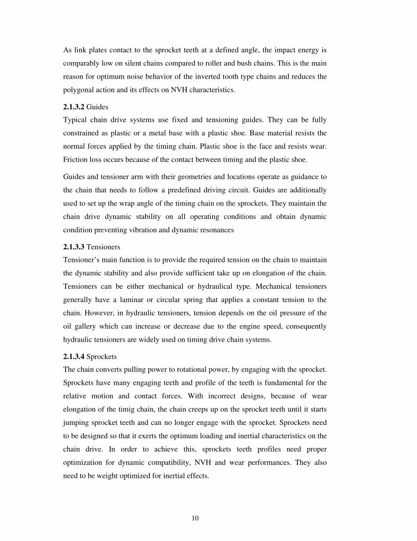
Silent chain or inverted chain is used on the applications where reduced NVH

characteristics are expected. These chains include non-guide row links, guide row

links, pins and external links. Guide row links provide guiding on the sprockets while

non-guide row links are subject to tension and engage the sprockets. The sub-

components of silent chain are shown on Figure 2.5.

Figure 2.6 : Sub-components of silent chain [12]

10

As link plates contact to the sprocket teeth at a defined angle, the impact energy is

comparably low on silent chains compared to roller and bush chains. This is the main

reason for optimum noise behavior of the inverted tooth type chains and reduces the

polygonal action and its effects on NVH characteristics.

2.1.3.2 Guides

Typical chain drive systems use fixed and tensioning guides. They can be fully

constrained as plastic or a metal base with a plastic shoe. Base material resists the

normal forces applied by the timing chain. Plastic shoe is the face and resists wear.

Friction loss occurs because of the contact between timing and the plastic shoe.

Guides and tensioner arm with their geometries and locations operate as guidance to

the chain that needs to follow a predefined driving circuit. Guides are additionally

used to set up the wrap angle of the timing chain on the sprockets. They maintain the

chain drive dynamic stability on all operating conditions and obtain dynamic

condition preventing vibration and dynamic resonances

2.1.3.3 Tensioners

Tensioner’s main function is to provide the required tension on the chain to maintain

the dynamic stability and also provide sufficient take up on elongation of the chain.

Tensioners can be either mechanical or hydraulical type. Mechanical tensioners

generally have a laminar or circular spring that applies a constant tension to the

chain. However, in hydraulic tensioners, tension depends on the oil pressure of the

oil gallery which can increase or decrease due to the engine speed, consequently

hydraulic tensioners are widely used on timing drive chain systems.

2.1.3.4 Sprockets

The chain converts pulling power to rotational power, by engaging with the sprocket.

Sprockets have many engaging teeth and profile of the teeth is fundamental for the

relative motion and contact forces. With incorrect designs, because of wear

elongation of the timig chain, the chain creeps up on the sprocket teeth until it starts

jumping sprocket teeth and can no longer engage with the sprocket. Sprockets need

to be designed so that it exerts the optimum loading and inertial characteristics on the

chain drive. In order to achieve this, sprockets teeth profiles need proper

optimization for dynamic compatibility, NVH and wear performances. They also

need to be weight optimized for inertial effects.

11

3. THEORY OF CHAIN DRIVE SIMULATION

In order to model the timing drive system Ricardo VALDYN simulation program

was used. The theory and equations discussed in this section covers the working

principle of VALDYN.

Valves have to be actuated synchronously by the camshafts concerning the piston’s

motion. Timing chain drives are intended to transfer motion from the engine’s

crankshaft to the camshaft with a constant ratio. Therefore, precisely two crankshaft

rotations are needed for a single camshaft rotation. Timing chain is the load carrying

part in a timing drive system and it has contact with sprockets, plastic guides, and the

parts creating the chain has contact in itself, as well. Friction loses are unavoidable

where a contact between two parts take place, even lubricants present in the engine

environment. Friction loss can be simulated in software thus simulation tools are

used extensively in the design of timing chain drives.

As the basic approach, each chain link is modeled by a single rigid body and

connected to the adjacent chain links with spring and damper elements. Then the

resulting multi-body system is simulated based on the Newton-Euler laws. The

displacement of the chain is computed only in the x-y plane. The motion on the z-

axis can be ignored without influencing the validity of the simulation. Therefore,

each chain link has three enabled DoFs (degrees of freedom); translations in x and y

directions and rotation around z-axis. Sprockets are modeled as generic mass

elements with only one DoF which is rotation about the z-axis. Similarly, plastic

guides are modeled as generic mass elements, exclusively fixed guides has no

rotational DoFs. Contact contours are defined to reflect the actual shape of the

sprockets and plastic guides. An exception for the chain links is the identification of

circles around the pins. The smaller circle defines the surface, which contacts the

sprocket, whereas the larger circle is the outer surface, which couples the chain links

and contacts the sprockets and guides [13].

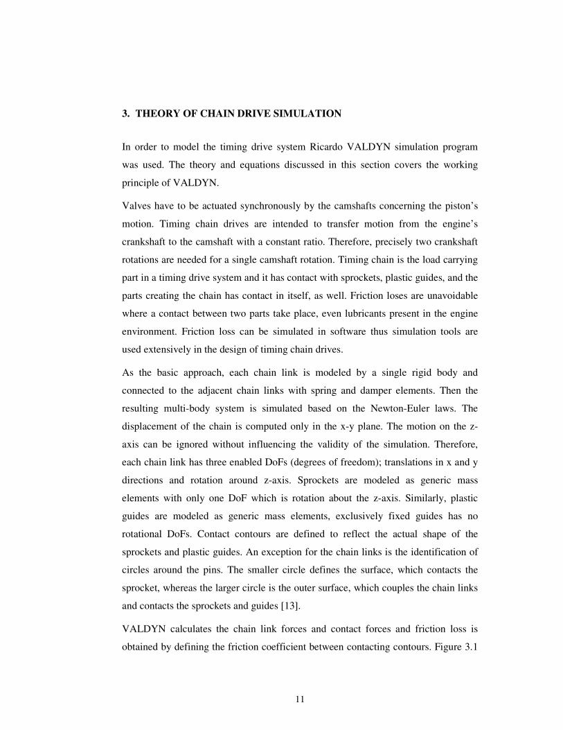
VALDYN calculates the chain link forces and contact forces and friction loss is

obtained by defining the friction coefficient between contacting contours. Figure 3.1

12

illustrates the contact forces between chain links and the sprockets or guides, and

link connection forces between adjacent chain links. The contact forces occur when a

link contacts a sprocket or guide. Contact forces can be computed by calculating the

intersecting area between the surface profiles of the concerned parts. Contact forces

depend on the stiffness of materials, the relative velocities and the damping

properties of the materials. The connection forces act between neighboring chain

links and are computed by defining the stiffness and damping elements as shown in

Figure 3.1.

Figure 3.1 : Contact and connection forces in the chain simulation [13]

3.1 Component Modelling

3.1.1 Chain Link Modeling

In modeling, the basic approach is to model each chain link as a single rigid body

connected to adjacent chain links by means of linear spring and dampers and

simulate the resulting multi-body system based on the Newton-Euler laws.

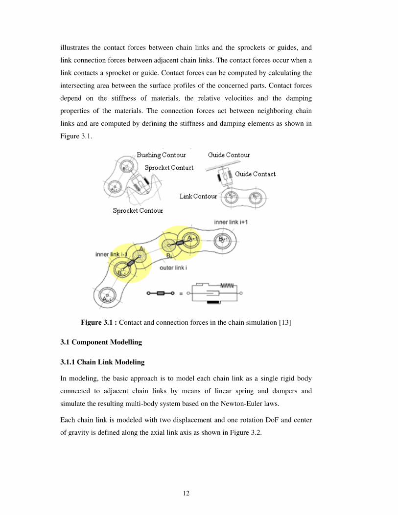
Each chain link is modeled with two displacement and one rotation DoF and center

of gravity is defined along the axial link axis as shown in Figure 3.2.

13

Figure 3.2 : Representation of chain link [14]

Connection between chain links can be gained by defining linear spring and damper

elements as shown in Figure 3.3, where klink and clink are the chain link stiffness and

damping coefficient, respectively. Location of chain pin centers are denoted by

points P1 and P2. Every Nth link is attached to the neighboring link, Nth+1, by

connecting the P2N and P1

N+1 by spring and damper elements. The force Flink

transmitted by each chain link spring and damper is

.

∆+∆= linklinklink ckF (3.1)

∆ is the relative displacement between the geometric centers of adjacent chain link

centers as shown in Figure 3.3 and (˙) denotes the derivative with respect to time.

Figure 3.3 : Chain link connectivity [14]

3.1.2 Sprocket Modeling

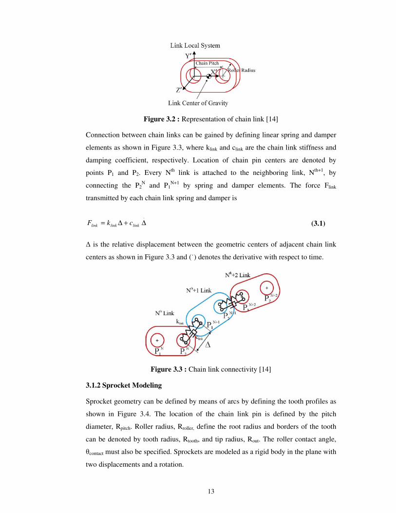
Sprocket geometry can be defined by means of arcs by defining the tooth profiles as

shown in Figure 3.4. The location of the chain link pin is defined by the pitch

diameter, Rpitch. Roller radius, Rroller, define the root radius and borders of the tooth

can be denoted by tooth radius, Rtooth, and tip radius, Rout. The roller contact angle,

θcontact must also be specified. Sprockets are modeled as a rigid body in the plane with

two displacements and a rotation.

14

Figure 3.4 : Sprocket geometry

Therefore, the connection between sprockets and camshafts is composed of stiffness

and damper elements. Consequently, forces, which occur in the X and Y directions

are:

.

xckxFx += (3.2)

.

yckyFy += (3.3)

where k and c represent the shaft stiffness and damping coefficient, respectively; x

and y are the relative displacements between the sprocket geometric center and the

ground in the X and Y directions, respectively.

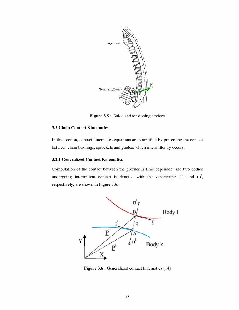
3.1.3 Guide and Tensioner Modeling

Guides are modeled similarly to the sprocket tooth profiles by means of arcs. Only

difference is the existence of tensioning devices as shown if Figure 3.5 on moving

guides. This type of guides generally known as arms and are modeled as rigid bodies

with a single DoF. With the force, which does not change its initial direction, applied

by the tensioning devices arm can rotate on the hinge point as shown in Figure 3.5

[14]. Additionally, fixed guides exist in the system that are modeled as a rigid body

to the associated curve.

15

Figure 3.5 : Guide and tensioning devices

3.2 Chain Contact Kinematics

In this section, contact kinematics equations are simplified by presenting the contact

between chain bushings, sprockets and guides, which intermittently occurs.

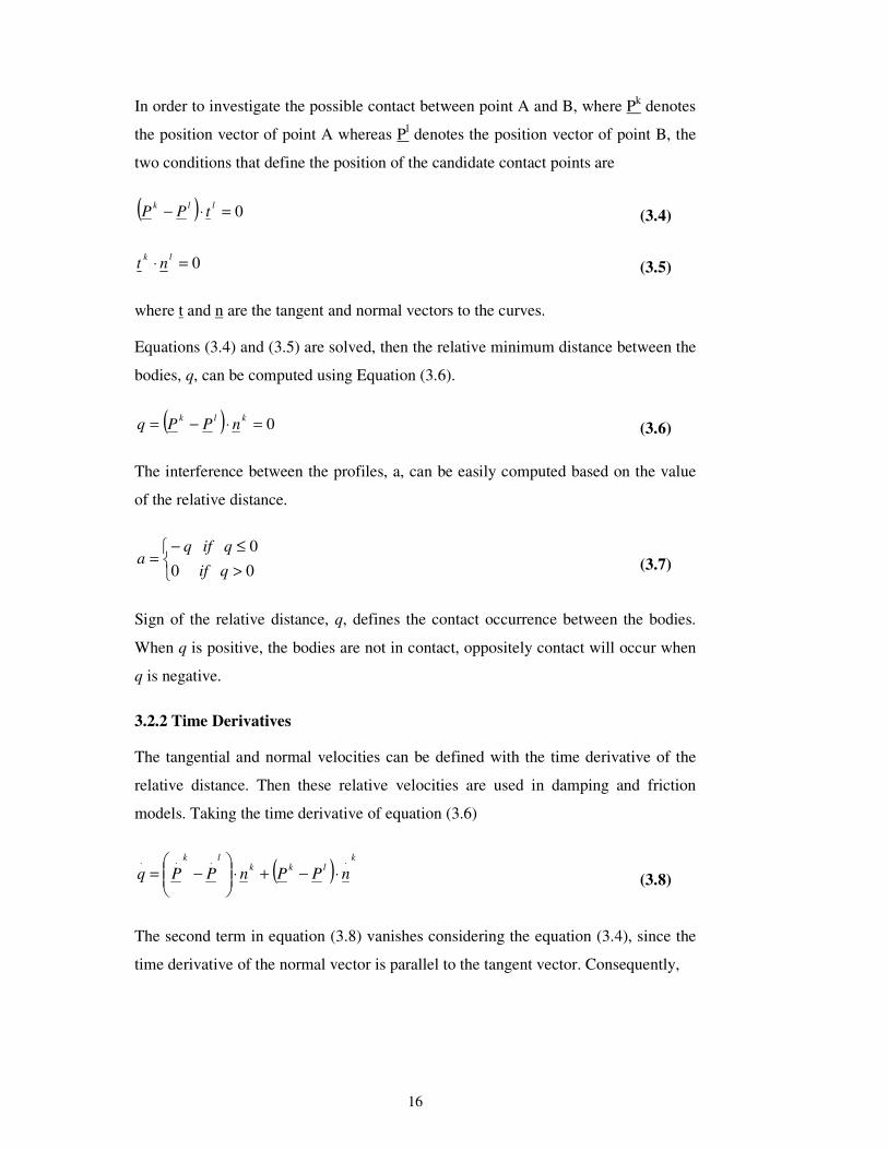
3.2.1 Generalized Contact Kinematics

Computation of the contact between the profiles is time dependent and two bodies

undergoing intermittent contact is denoted with the superscripts (.)k and (.)l,

respectively, are shown in Figure 3.6.

Figure 3.6 : Generalized contact kinematics [14]

16

In order to investigate the possible contact between point A and B, where Pk denotes

the position vector of point A whereas Pl denotes the position vector of point B, the

two conditions that define the position of the candidate contact points are

( ) 0=⋅−llk

tPP (3.4)

0=⋅lk

nt (3.5)

where t and n are the tangent and normal vectors to the curves.

Equations (3.4) and (3.5) are solved, then the relative minimum distance between the

bodies, q, can be computed using Equation (3.6).

( ) 0=⋅−=klk

nPPq (3.6)

The interference between the profiles, a, can be easily computed based on the value

of the relative distance.

>

≤−=

00

0

qif

qifqa (3.7)

Sign of the relative distance, q, defines the contact occurrence between the bodies.

When q is positive, the bodies are not in contact, oppositely contact will occur when

q is negative.

3.2.2 Time Derivatives

The tangential and normal velocities can be defined with the time derivative of the

relative distance. Then these relative velocities are used in damping and friction

models. Taking the time derivative of equation (3.6)

( )k

lkklk

nPPnPPq....

⋅−+⋅

−= (3.8)

The second term in equation (3.8) vanishes considering the equation (3.4), since the

time derivative of the normal vector is parallel to the tangent vector. Consequently,

17

klk

nPPq ⋅

−=

...

(3.9)

The time derivative of the relative distance is equal to the relative velocity in the

normal direction, of two body fixed points that coincide with the contact points.

Similarly, the relative velocity in the tangential direction, Vt is given by

klk

t tPPV ⋅

−=

..

(3.10)

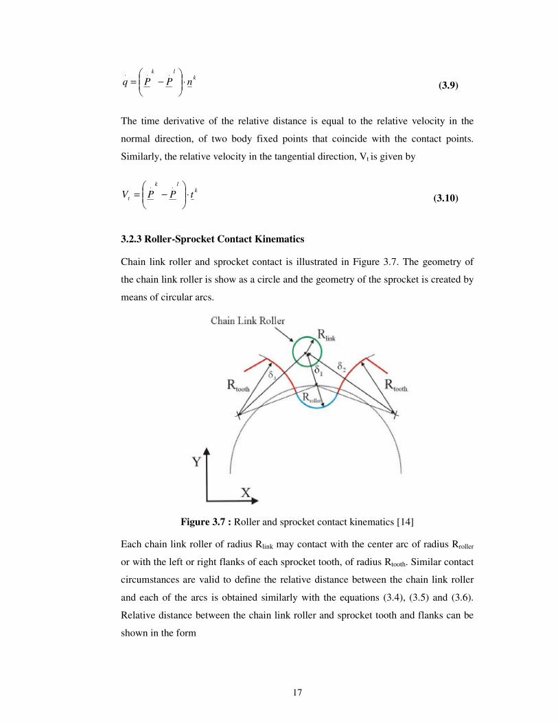
3.2.3 Roller-Sprocket Contact Kinematics

Chain link roller and sprocket contact is illustrated in Figure 3.7. The geometry of

the chain link roller is show as a circle and the geometry of the sprocket is created by

means of circular arcs.

Figure 3.7 : Roller and sprocket contact kinematics [14]

Each chain link roller of radius Rlink may contact with the center arc of radius Rroller

or with the left or right flanks of each sprocket tooth, of radius Rtooth. Similar contact

circumstances are valid to define the relative distance between the chain link roller

and each of the arcs is obtained similarly with the equations (3.4), (3.5) and (3.6).

Relative distance between the chain link roller and sprocket tooth and flanks can be

shown in the form

18

linkroller RRq −+= 11 δ (3.11)

linktooth RRq −−= 22 δ (3.12)

linktooth RRq −−= 33 δ (3.13)

where deltas (δ) are the distance between centers. Clearly, the roller can only contact

with only one of the curves, thus, the relative distance q is chosen as the minimum

one of the three shown in equations (3.11), (3.12) and (3.13).

{ }321 ,,min qqqq = (3.14)

Then the time derivative of the relative distance q is;

3

.

3

.

2

.

2

.

1

.

1

.

,, δδδ === qqq (3.15)

=

=

=

=

33

.

22

.

11

.

.

qqifq

qqifq

qqifq

q (3.16)

The tangential relative velocities are

..

11 θθ rollerlinklinkct RRVV ++= (3.17)

..

22 θθ toothlinklinkct RRVV ++= (3.18)

..

33 θθ toothlinklinkct RRVV ++= (3.19)

where Vc is the relative velocity between centers in the tangential direction, .

θlink

and .

θ are the link angular and sprocket angular velocities. The tangential relative

velocity Vt between link and sprocket is then

19

=

=

=

=

33

22

11

qqifV

qqifV

qqifV

V

t

t

t

t (3.20)

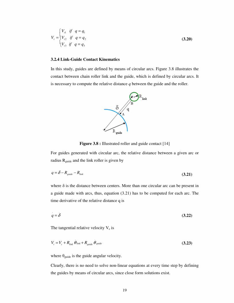
3.2.4 Link-Guide Contact Kinematics

In this study, guides are defined by means of circular arcs. Figure 3.8 illustrates the

contact between chain roller link and the guide, which is defined by circular arcs. It

is necessary to compute the relative distance q between the guide and the roller.

Figure 3.8 : Illustrated roller and guide contact [14]

For guides generated with circular arc, the relative distance between a given arc or

radius Rguide and the link roller is given by

guide linkq R Rδ= − − (3.21)

where δ is the distance between centers. More than one circular arc can be present in

a guide made with arcs, thus, equation (3.21) has to be computed for each arc. The

time derivative of the relative distance q is

. .

q δ= (3.22)

The tangential relative velocity Vc is

. .

link guidet c link guideV V R Rθ θ= + + (3.23)

where θguide is the guide angular velocity.

Clearly, there is no need to solve non-linear equations at every time step by defining

the guides by means of circular arcs, since close form solutions exist.

20

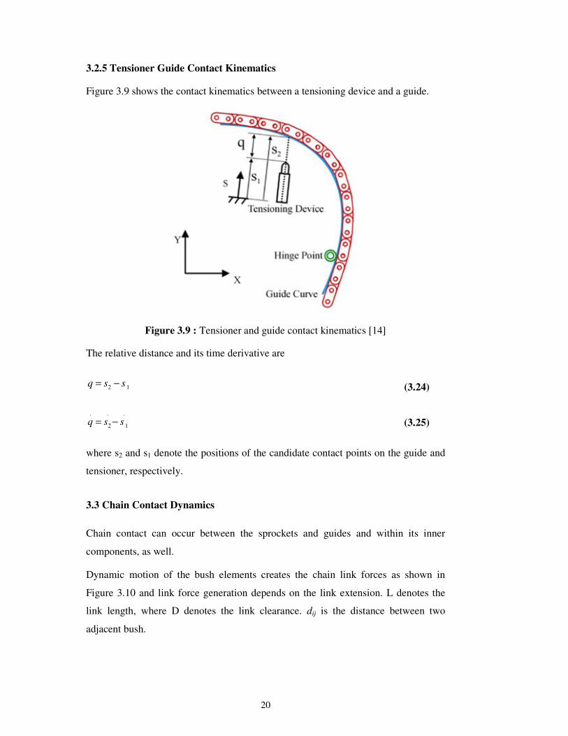
3.2.5 Tensioner Guide Contact Kinematics

Figure 3.9 shows the contact kinematics between a tensioning device and a guide.

Figure 3.9 : Tensioner and guide contact kinematics [14]

The relative distance and its time derivative are

2 1q s s= − (3.24)

. . .

2 1q s s= − (3.25)

where s2 and s1 denote the positions of the candidate contact points on the guide and

tensioner, respectively.

3.3 Chain Contact Dynamics

Chain contact can occur between the sprockets and guides and within its inner

components, as well.

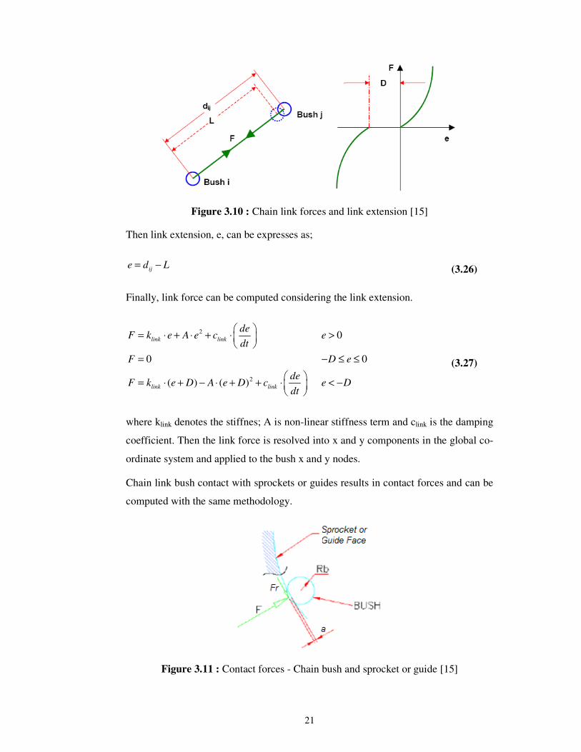
Dynamic motion of the bush elements creates the chain link forces as shown in

Figure 3.10 and link force generation depends on the link extension. L denotes the

link length, where D denotes the link clearance. dij is the distance between two

adjacent bush.

21

Figure 3.10 : Chain link forces and link extension [15]

Then link extension, e, can be expresses as;

ije d L= − (3.26)

Finally, link force can be computed considering the link extension.

2

2

0

0 0

( ) ( )

link link

link link

deF k e A e c e

dt

F D e

deF k e D A e D c e D

dt

= ⋅ + ⋅ + ⋅ >

= − ≤ ≤

= ⋅ + − ⋅ + + ⋅ < −

(3.27)

where klink denotes the stiffnes; A is non-linear stiffness term and clink is the damping

coefficient. Then the link force is resolved into x and y components in the global co-

ordinate system and applied to the bush x and y nodes.

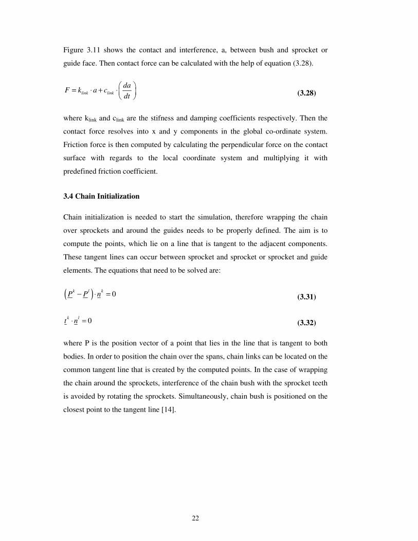
Chain link bush contact with sprockets or guides results in contact forces and can be

computed with the same methodology.

Figure 3.11 : Contact forces - Chain bush and sprocket or guide [15]

22

Figure 3.11 shows the contact and interference, a, between bush and sprocket or

guide face. Then contact force can be calculated with the help of equation (3.28).

link link

daF k a c

dt

= ⋅ + ⋅

(3.28)

where klink and clink are the stifness and damping coefficients respectively. Then the

contact force resolves into x and y components in the global co-ordinate system.

Friction force is then computed by calculating the perpendicular force on the contact

surface with regards to the local coordinate system and multiplying it with

predefined friction coefficient.

3.4 Chain Initialization

Chain initialization is needed to start the simulation, therefore wrapping the chain

over sprockets and around the guides needs to be properly defined. The aim is to

compute the points, which lie on a line that is tangent to the adjacent components.

These tangent lines can occur between sprocket and sprocket or sprocket and guide

elements. The equations that need to be solved are:

( ) 0k l k

P P n− ⋅ = (3.31)

0k lt n⋅ = (3.32)

where P is the position vector of a point that lies in the line that is tangent to both

bodies. In order to position the chain over the spans, chain links can be located on the

common tangent line that is created by the computed points. In the case of wrapping

the chain around the sprockets, interference of the chain bush with the sprocket teeth

is avoided by rotating the sprockets. Simultaneously, chain bush is positioned on the

closest point to the tangent line [14].

23

4. METHODOLOGY

4.1 Engine Specification and Components

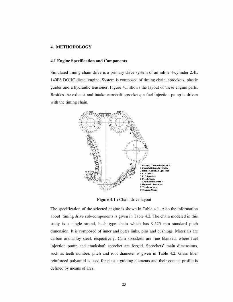
Simulated timing chain drive is a primary drive system of an inline 4-cylinder 2.4L

140PS DOHC diesel engine. System is composed of timing chain, sprockets, plastic

guides and a hydraulic tensioner. Figure 4.1 shows the layout of these engine parts.

Besides the exhaust and intake camshaft sprockets, a fuel injection pump is driven

with the timing chain.

Figure 4.1 : Chain drive layout

The specification of the selected engine is shown in Table 4.1. Also the information

about timing drive sub-components is given in Table 4.2. The chain modeled in this

study is a single strand, bush type chain which has 9,525 mm standard pitch

dimension. It is composed of inner and outer links, pins and bushings. Materials are

carbon and alloy steel, respectively. Cam sprockets are fine blanked, where fuel

injection pump and crankshaft sprocket are forged. Sprockets’ main dimensions,

such as teeth number, pitch and root diameter is given in Table 4.2. Glass fiber

reinforced polyamid is used for plastic guiding elements and their contact profile is

defined by means of arcs.

24

Item Unit Specification

Engine Type - 4-Cylinder Inline Diesel

Capacity Litres 2.4

Rated Speed rpm 4000

Max. Torque Nm 370

Power PS 140

Emission Level - Euro 4

Fuel Inj. System - Common Rail

Type Dimension

Timing Chain Single Strand, Bushing

Quenched and Tempered 9.525mm standart pitch

Hydraulic Tensioner

Oil fed and spring -

Cam Sprocket Fine Blanked 38 Teeth

Pitch Dia.: 115.34 mm Root Dia.: 108.87mm

FIP Sprocket Forged 38 Teeth

Pitch Dia.: 115.34 mm Root Dia.: 108.87mm

Crank Sprocket Forged 19 Teeth

Pitch Dia.: 57.87 mm Root Dia.: 51.45 mm

Plastic Guides Injection Molding Profile by means of arcs

4.2 Simulation Parameters

Design of Experiments (DoE) is a process of conducting and planning experiments in

order to extract the maximum amount of information from the collected data in the

fewest number of experimental runs. All relevant factors simultaneously is varied

over a set of planned experiments and the results are connected by means of a

mathematical model. This model is then used for optimization.

To do the work a DoE based investigation was conducted on seven factors, which

were:

• Tensioner Leak down (flow) rate

• Tensioner Spring Force

Table 4.1: Specification of modelled engine

Table 4.2: Timing drive sub-component type and dimensions

25

• Crank Sprocket Tooth Gap Form

• FIP Sprocket Tooth Gap Form

• Cam Sprocket Tooth Gap Form

• Sprocket Root Radius Run Out

• Oil Supply Pressure

These seven factors were derived based on the study completed by Plail et al. The

study highlights all the potential mechanisms of the chain drive and considers the

noise factors that exist for the system [16]. Each parameter was limited with lower

and upper values that are discussed as below, where “-1” indicates lower limit and

“+1” indicates upper limit.

1. Tensioner Leak down (flow) rate: It is defined by the diametrical clearance

between the hydraulic tensioner’s body and plunger. The minimum value is

set as 0.024mm and the maximum value set as 0.083mm, which are the

feasible manufacturing tolerances.

2. Tensioner Spring Force: The tensioner spring force value was set at the

minimum and maximum values of 80N and 120N.

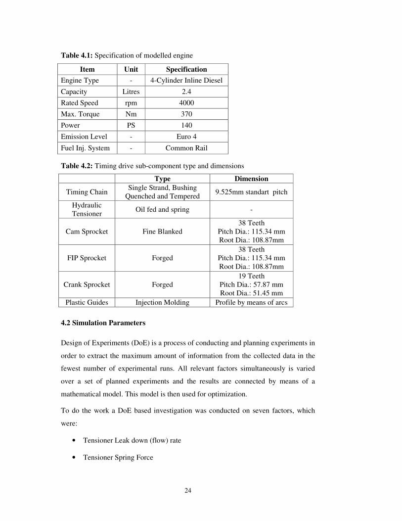
Requirements for the timing chains are specified and dimensions, tolerances, length

measurement, proof testing and minimum tensile strengths of the chains are covered

by ISO 606 standard. Maximum and minimum dimensions are specified to ensure

interchangeability of chain components produced by different chain makers [17].

ISO 606 represents the limits for dimensions, but they are not the manufacturing

tolerances.

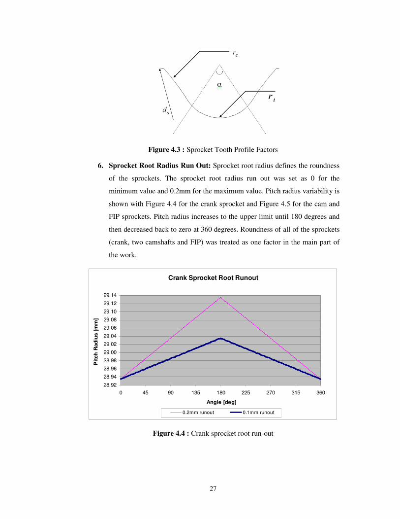
Figure 4.2 : Minimum and maximum tooth form of crank sprocket [15]

26

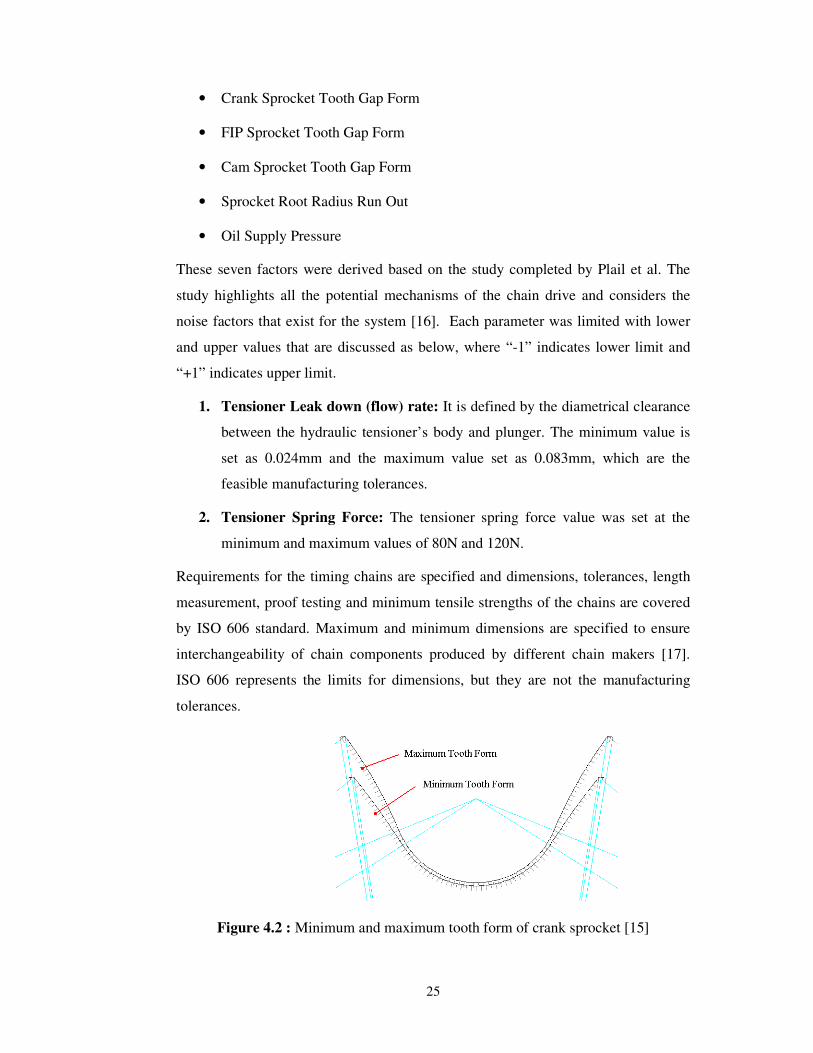
The minimum and maximum tooth gap forms determine the limits of the tooth form.

The tooth profile is defined in terms of flank radius (re), root radius (ri) and roller

sitting angle (α) subtended by the root radius as shown in Figure 4.3. Also height of

the teeth is limited by defining the tip diameter (da). Using these values gives

noticeable difference in the form of the tooth as illustrated in Figure 4.2. Calculated

values for each sprocket are shown in Table 4.1 and Table 4.2. Minimum and

maximum range for the sprocket tooth factors are indicated with “-1” and “+1”

respectively.

Factor “-1” Level “+1” Level

ri, roller seating radius(mm)

3.207 3.335

α, roller seating angle(degree)

135.26315 115.26315

re, tooth flank radius(mm) 16.002 27.4828

da, tip diameter(mm) 63.426 60.242

Factor “-1” Level “+1” Level

ri, roller seating radius(mm) 3.207 3.335

α, roller seating angle(degree)

137.6315 117.6315

re, tooth flank radius(mm) 30.48 82.4992

da, tip diameter(mm) 120.89 118.117

3. Crank Sprocket Tooth Form: ISO 606 defines the minimum and maximum

tooth profile as in Table 4.1.

4. FIP Sprocket Tooth Form: ISO 606 defines the minimum and maximum

tooth profile as in Table 4.2. Parameter sign shows the level used in DoE.

5. Cam Sprocket Tooth Form: Cam sprockets have the same teeth profile with

the FIP sprockets, so values in Table 4.2 is valid. Two cam sprockets tooth

form were treated as one factor in DoE.

Table 4.3: Crank Sprocket Tooth Profile Values

Table 4.4: Cam and FIP Sprocket Tooth Profile Values

27

Figure 4.3 : Sprocket Tooth Profile Factors

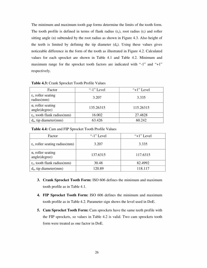
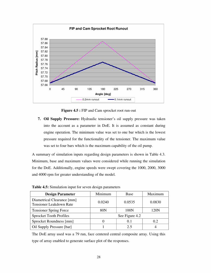
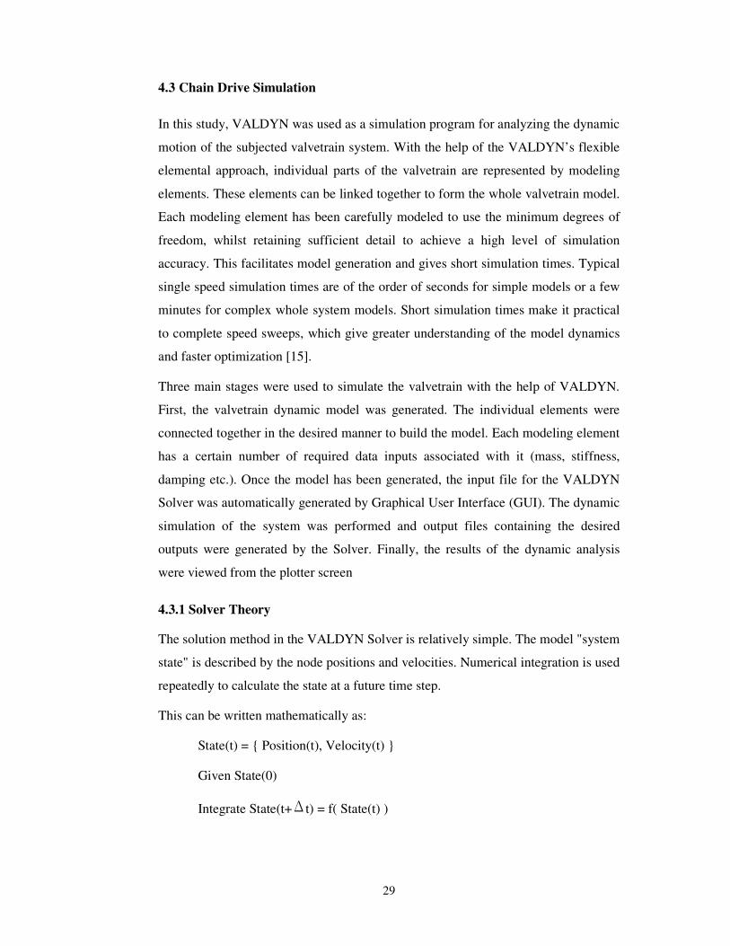
6. Sprocket Root Radius Run Out: Sprocket root radius defines the roundness

of the sprockets. The sprocket root radius run out was set as 0 for the

minimum value and 0.2mm for the maximum value. Pitch radius variability is

shown with Figure 4.4 for the crank sprocket and Figure 4.5 for the cam and

FIP sprockets. Pitch radius increases to the upper limit until 180 degrees and

then decreased back to zero at 360 degrees. Roundness of all of the sprockets

(crank, two camshafts and FIP) was treated as one factor in the main part of

the work.

Crank Sprocket Root Runout

28.92

28.94

28.96

28.98

29.00

29.02

29.04

29.06

29.08

29.10

29.12

29.14

0 45 90 135 180 225 270 315 360

Angle [deg]

Pit

ch

Rad

ius [

mm

]

0.2mm runout 0.1mm runout

Figure 4.4 : Crank sprocket root run-out

28

FIP and Cam Sprocket Root Runout

57.66

57.68

57.70

57.72

57.74

57.76

57.78

57.80

57.82

57.84

57.86

57.88

0 45 90 135 180 225 270 315 360

Angle [deg]

Pit

ch

Rad

ius [

mm

]

0.2mm runout 0.1mm runout

Figure 4.5 : FIP and Cam sprocket root run-out

7. Oil Supply Pressure: Hydraulic tensioner’s oil supply pressure was taken

into the account as a parameter in DoE. It is assumed as constant during

engine operation. The minimum value was set to one bar which is the lowest

pressure required for the functionality of the tensioner. The maximum value

was set to four bars which is the maximum capability of the oil pump.

A summary of simulation inputs regarding design parameters is shown in Table 4.3.

Minimum, base and maximum values were considered while running the simulation

for the DoE. Additionally, engine speeds were swept covering the 1000, 2000, 3000

and 4000 rpm for greater understanding of the model.

Design Parameter Minimum Base Maximum

Diametrical Clearance [mm] Tensioner Leakdown Rate

0.0240 0.0535 0.0830

Tensioner Spring Force 80N 100N 120N

Sprocket Tooth Profiles See Figure 4.2

Sprocket Roundness [mm] 0 0.1 0.2

Oil Supply Pressure [bar] 1 2.5 4

The DoE array used was a 79 run, face centered central composite array. Using this

type of array enabled to generate surface plot of the responses.

Table 4.5: Simulation input for seven design parameters

29

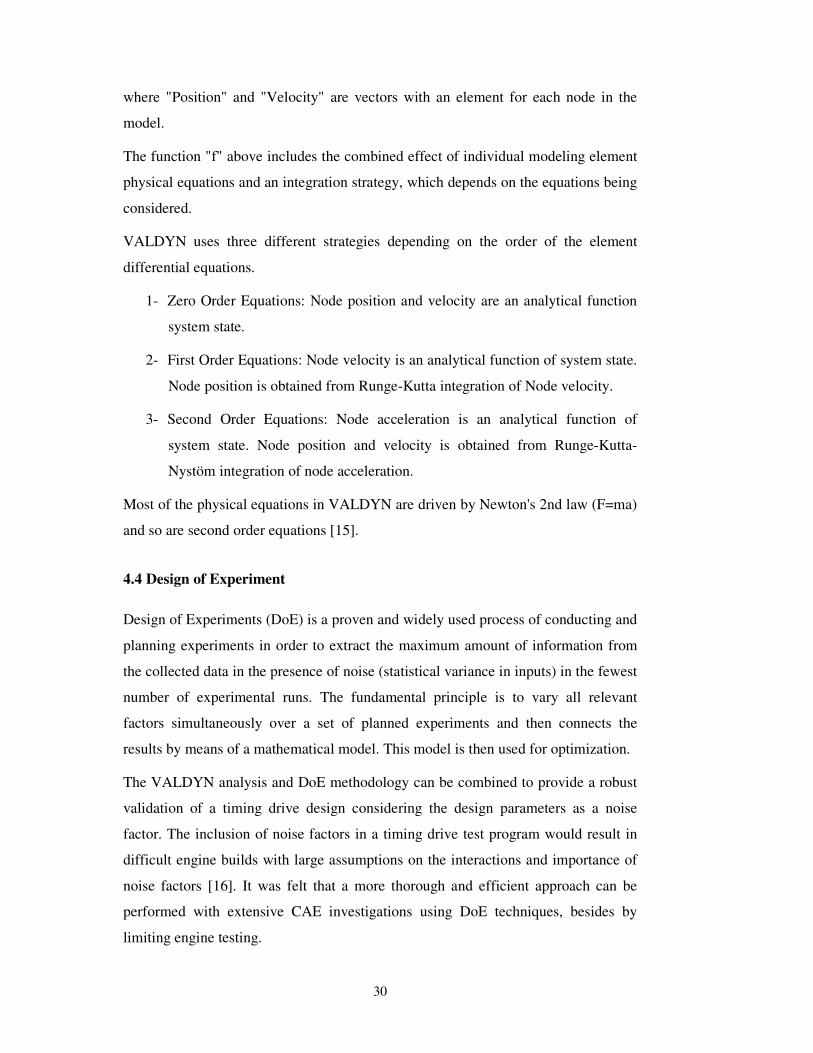
4.3 Chain Drive Simulation

In this study, VALDYN was used as a simulation program for analyzing the dynamic

motion of the subjected valvetrain system. With the help of the VALDYN’s flexible

elemental approach, individual parts of the valvetrain are represented by modeling

elements. These elements can be linked together to form the whole valvetrain model.

Each modeling element has been carefully modeled to use the minimum degrees of

freedom, whilst retaining sufficient detail to achieve a high level of simulation

accuracy. This facilitates model generation and gives short simulation times. Typical

single speed simulation times are of the order of seconds for simple models or a few

minutes for complex whole system models. Short simulation times make it practical

to complete speed sweeps, which give greater understanding of the model dynamics

and faster optimization [15].

Three main stages were used to simulate the valvetrain with the help of VALDYN.

First, the valvetrain dynamic model was generated. The individual elements were

connected together in the desired manner to build the model. Each modeling element

has a certain number of required data inputs associated with it (mass, stiffness,

damping etc.). Once the model has been generated, the input file for the VALDYN

Solver was automatically generated by Graphical User Interface (GUI). The dynamic

simulation of the system was performed and output files containing the desired

outputs were generated by the Solver. Finally, the results of the dynamic analysis

were viewed from the plotter screen

4.3.1 Solver Theory

The solution method in the VALDYN Solver is relatively simple. The model "system

state" is described by the node positions and velocities. Numerical integration is used

repeatedly to calculate the state at a future time step.

This can be written mathematically as:

State(t) = { Position(t), Velocity(t) }

Given State(0)

Integrate State(t+Δt) = f( State(t) )

30

where "Position" and "Velocity" are vectors with an element for each node in the

model.

The function "f" above includes the combined effect of individual modeling element

physical equations and an integration strategy, which depends on the equations being

considered.

VALDYN uses three different strategies depending on the order of the element

differential equations.

1- Zero Order Equations: Node position and velocity are an analytical function

system state.

2- First Order Equations: Node velocity is an analytical function of system state.

Node position is obtained from Runge-Kutta integration of Node velocity.

3- Second Order Equations: Node acceleration is an analytical function of

system state. Node position and velocity is obtained from Runge-Kutta-

Nystöm integration of node acceleration.

Most of the physical equations in VALDYN are driven by Newton's 2nd law (F=ma)

and so are second order equations [15].

4.4 Design of Experiment

Design of Experiments (DoE) is a proven and widely used process of conducting and

planning experiments in order to extract the maximum amount of information from

the collected data in the presence of noise (statistical variance in inputs) in the fewest

number of experimental runs. The fundamental principle is to vary all relevant

factors simultaneously over a set of planned experiments and then connects the

results by means of a mathematical model. This model is then used for optimization.

The VALDYN analysis and DoE methodology can be combined to provide a robust

validation of a timing drive design considering the design parameters as a noise

factor. The inclusion of noise factors in a timing drive test program would result in

difficult engine builds with large assumptions on the interactions and importance of

noise factors [16]. It was felt that a more thorough and efficient approach can be

performed with extensive CAE investigations using DoE techniques, besides by

limiting engine testing.

31

The DoE chosen was a 79-run face centered central composite array as shown in

Table A.1. Each run of the array was completed using the same simulation model

that had been used to evaluate the concept designs. The results from the DoE array

were processed using the statistical software package Minitab, and the regression

coefficients from the analysis were used to generate a transfer function for friction

power loss variability.

4.5 Statistical Analysis

Minitab is a statistical analysis program, in which advanced DoEs can be created and

analyzed. Design factors are screened to determine the most important one for

explaining process variation. After screening the factors, interactions between the

factors can be understood. Then the best factor settings can be produced for optimal

process performance.

4.5.1 Response Surface Methods

Response surface methods are used to examine the relationship between the response

variables, which appears as design parameters in this study. These methods are often

employed after identification of controllable factors and then optimized response is

found with the help of factor settings.

The design should be correctly chosen to ensure that the response surface is fit in the

most efficient manner. Central composite designs are often used when the design

plan calls for sequential experimentation because these designs can incorporate

information from a properly planned experiment. The design is built up into a central

composite design to fit a second-degree model by adding axial and center points in

order to allow efficient estimation of the quadratic terms in the second-order model

[18].

4.5.2 Response Optimization

The best value for the response can be produced by determining the optimal

conditions in many designed experiments. A combination of input variables is

searched by Minitab’s response optimizer that jointly optimizes a set of responses by

satisfying the requirements for each response in the set.

32

Firstly, an individual desirability for each response is obtained by using the goals and

boundaries that is provided. Three goals can be chosen:

• minimize the response (smaller is better)

• target the response (target is best)

• maximize the response (larger is better)

In our study considering the friction losses as negative values, loses were tried to be

maximized (aim is to approach zero).

4.5.3 Residual plot choices

Residual plots are generated by Minitab to examine the goodness of model fit.

4.5.3.1 Histogram of residuals

General characteristics of the data can be shown by histogram of residuals, including:

- Typical values, spread or variation, and shape

- Unusual values in the data

Skewness in the data is indicated by long tails in the plot. If one or two bars are far

from the others, those points may be outliers.

4.5.3.2 Normal plot of residuals

The points in this plot should generally form a straight line if the residuals are

normally distributed. If the points on the plot depart from a straight line, the

normality assumption may be invalid.

4.5.3.3 Residuals versus fits

This plot should show a random pattern of residuals on both sides of 0. If a point lies

far from the majority of points, it may be an outlier. Also, there should not be any

recognizable patterns in the residual plot. The following may indicate error that is not

random:

- a series of increasing or decreasing points

- a predominance of positive residuals, or a predominance of negative residuals

- patterns, such as increasing residuals with increasing fits

33

4.5.3.4 Residuals versus order

This is a plot of all residuals in the order that the data was collected and can be used

to find time-related effects. A positive correlation is indicated by a clustering of

residuals with the same sign. A negative correlation is indicated by rapid changes in

the signs of consecutive residuals.

4.5.4 P-value

Appropriateness of rejecting the null hypothesis in a hypothesis test is determined by

p-value. P-values range from 0 to 1. “The smaller the p-value, the smaller the

probability that rejecting the null hypothesis is a mistake” [18]. Before conducting

any analysis, alpha (α) level is determined. If the p-value of a test statistic is less than

the chosen alpha, the null hypothesis is rejected.

The p-value is calculated from the observed sample and represents the probability of

incorrectly rejecting the null hypothesis when it is actually true. If the p-value (P) of

a coefficient is less than the chosen α-level, the relationship between the predictor

and the response is statistically significant.

In our study p-value is used to define the most effective design parameter and then

effect of the interaction between the design parameters on total friction power loss is

graphed with surface plots.

35

5. RESULTS

An analytical study has been conducted on a 2.4L 4-cylinder diesel engine under four

speed points (1000, 2000, 3000, 4000rpm) with seven design parameters in order to

quantify the friction power loss on primary drive system parts. A DoE matrix was

created with 79 runs with face centered central composite array depending on seven

parameters. Each run was modeled with primary drive simulation program

VALDYN and power friction loss results obtained in terms of Watt. By considering

the engine speed in terms of time, power loss was translated into Joules and total loss

for four revolutions of crank was calculated. In the mean time primary drive

components’ –chain, sprockets and plastic guides- friction loss was obtained one by

one. With the help of the statistical analysis program Minitab, total primary drive

system friction power loss was optimized by adjusting the design parameters.

5.1 Component Level Friction Power Loss

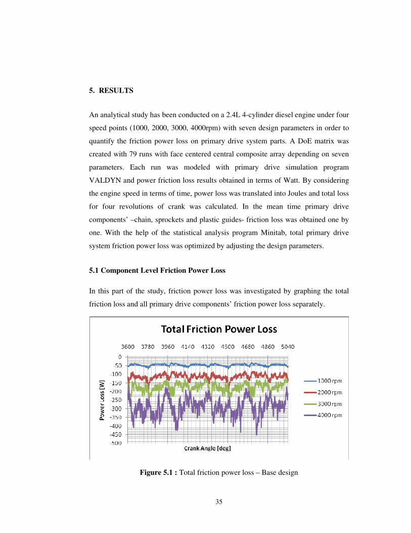
In this part of the study, friction power loss was investigated by graphing the total

friction loss and all primary drive components’ friction power loss separately.

Figure 5.1 : Total friction power loss – Base design

36

Figure 5.1 shows the total friction loss considering the base design parameters versus

the engine speed. It is clear that friction power loss increases as the engine speed

increases. Primary drive components’ friction power loss graphs considering the base

design parameters are shown separately in Figures A.1, A.2, A.3, A.4, A.5 and A.6.

Cam to cam guides friction power loss was not included, because this guide behaves

as a router only when chain vibrations increase. Therefore, chain is not always in

contact with this guide.

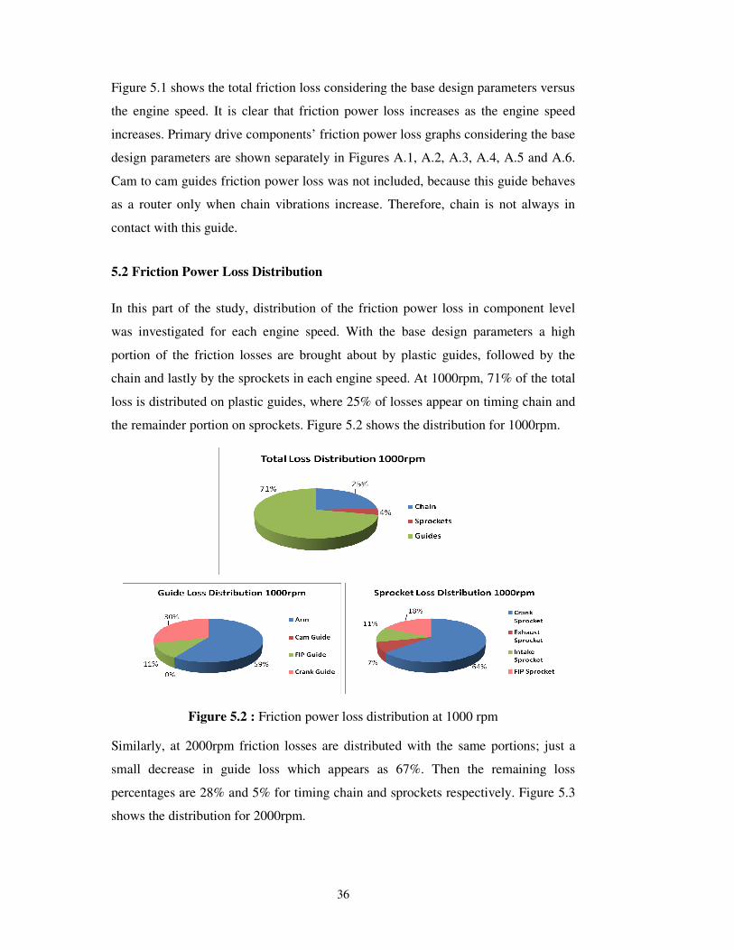
5.2 Friction Power Loss Distribution

In this part of the study, distribution of the friction power loss in component level

was investigated for each engine speed. With the base design parameters a high

portion of the friction losses are brought about by plastic guides, followed by the

chain and lastly by the sprockets in each engine speed. At 1000rpm, 71% of the total

loss is distributed on plastic guides, where 25% of losses appear on timing chain and

the remainder portion on sprockets. Figure 5.2 shows the distribution for 1000rpm.

Figure 5.2 : Friction power loss distribution at 1000 rpm

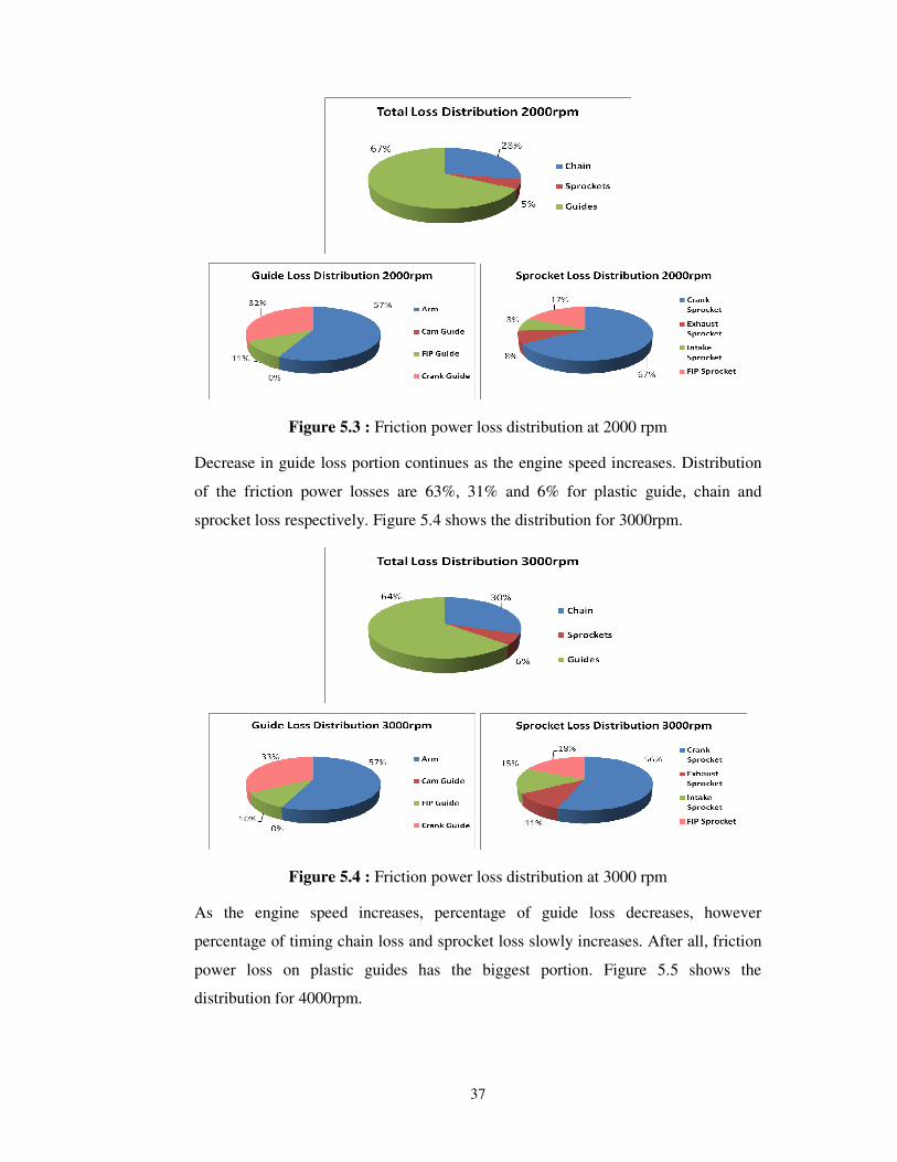
Similarly, at 2000rpm friction losses are distributed with the same portions; just a

small decrease in guide loss which appears as 67%. Then the remaining loss

percentages are 28% and 5% for timing chain and sprockets respectively. Figure 5.3

shows the distribution for 2000rpm.

37

Figure 5.3 : Friction power loss distribution at 2000 rpm

Decrease in guide loss portion continues as the engine speed increases. Distribution

of the friction power losses are 63%, 31% and 6% for plastic guide, chain and

sprocket loss respectively. Figure 5.4 shows the distribution for 3000rpm.

Figure 5.4 : Friction power loss distribution at 3000 rpm

As the engine speed increases, percentage of guide loss decreases, however

percentage of timing chain loss and sprocket loss slowly increases. After all, friction

power loss on plastic guides has the biggest portion. Figure 5.5 shows the

distribution for 4000rpm.

38

Figure 5.5 : Friction power loss distribution at 4000 rpm

5.3 Optimization of Friction Power Loss Results

In this part of the study, friction loss results that were obtained from VALDYN

simulations were converted from Watt into Joule for each 79 DoE runs between the

3600 CA° to 5040 CA°. Simulation results were taken into the account after 10

revolutions (3600 CA°) of the crank because primary drive system was stabilized

after a while from the start of the simulation. Crank angles were converted into

seconds depending on the engine speed. Then friction loss was calculated for the four

revolutions of the crankshaft. Table 5.1 summarizes the total friction power loss

regarding the base design, which is run order number 79 in DoE array as shown in

Table A.1.

Table 5.1 : Friction power loss results in Joule

Engine Speed @ 1000 rpm @ 2000 rpm @ 3000 rpm @ 4000 rpm

Total Loss [J] -11.053 -13.599 -13.922 -17.180

After creating the four total loss arrays for each engine speed (1000, 2000, 3000 and

4000 rpm), Minitab analyzer was used to optimize the friction losses. Table A.2

shows the estimated regression coefficients for the optimized results for each engine

speed. Then the Minitab optimizer was adjusted to maximize the friction power

losses. Maximizing was considered because power loss values were negative and

being closer to zero is better regarding the friction loss for a good design.

39

5.3.1 Data Consistency

Residual plots were generated to observe the goodness of the model. Histogram of

residuals, normal plot of residuals, residuals versus fits and residuals versus order

were assessed. Residual plots for total losses are shown in Figures A.7, A.8, A.9 and

A.10. In histogram of residuals, plots long tails were not observed which indicates

that the data was not skewed. Also the points in the normal probability plots have

formed a straight line which shows that the residuals are normally distributed.

Residuals versus fitted values have shown a random pattern on both sides of zero and

there were not any recognizable patterns in the plot where the points were clustered.

Therefore, it can be concluded that the distribution and the goodness of the collected

data from the simulation is consistent.

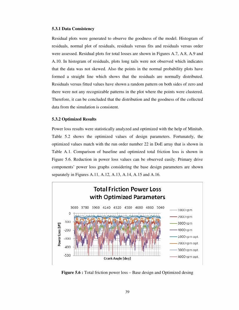
5.3.2 Optimized Results

Power loss results were statistically analyzed and optimized with the help of Minitab.

Table 5.2 shows the optimized values of design parameters. Fortunately, the

optimized values match with the run order number 22 in DoE array that is shown in

Table A.1. Comparison of baseline and optimized total friction loss is shown in

Figure 5.6. Reduction in power loss values can be observed easily. Primary drive

components’ power loss graphs considering the base design parameters are shown

separately in Figures A.11, A.12, A.13, A.14, A.15 and A.16.

Figure 5.6 : Total friction power loss – Base design and Optimized desing

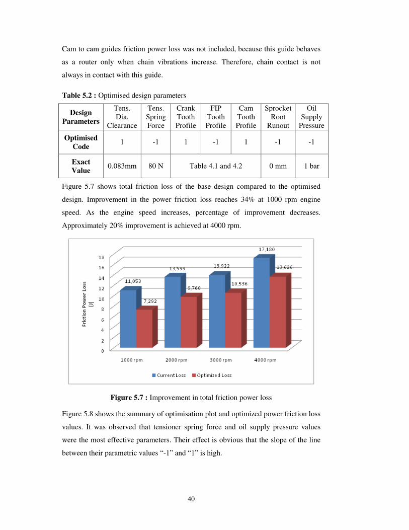
40

Cam to cam guides friction power loss was not included, because this guide behaves

as a router only when chain vibrations increase. Therefore, chain contact is not

always in contact with this guide.

Table 5.2 : Optimised design parameters

Design Parameters

Tens. Dia.

Clearance

Tens. Spring Force

Crank Tooth Profile

FIP Tooth Profile

Cam Tooth Profile

Sprocket Root

Runout

Oil Supply

Pressure

Optimised Code

1 -1 1 -1 1 -1 -1

Exact Value

0.083mm 80 N Table 4.1 and 4.2 0 mm 1 bar

Figure 5.7 shows total friction loss of the base design compared to the optimised

design. Improvement in the power friction loss reaches 34% at 1000 rpm engine

speed. As the engine speed increases, percentage of improvement decreases.

Approximately 20% improvement is achieved at 4000 rpm.

Figure 5.7 : Improvement in total friction power loss

Figure 5.8 shows the summary of optimisation plot and optimized power friction loss

values. It was observed that tensioner spring force and oil supply pressure values

were the most effective parameters. Their effect is obvious that the slope of the line

between their parametric values “-1” and “1” is high.

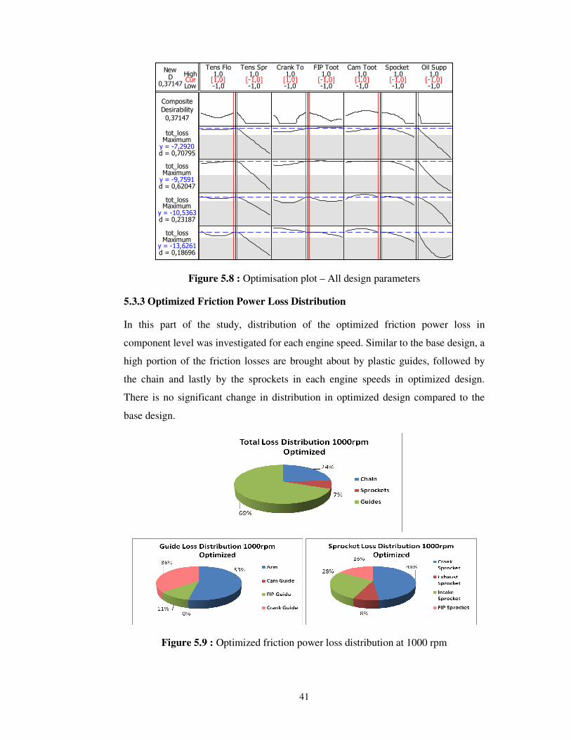
41

CurHigh

Low0,37147D

New

d = 0,70795

Maximumtot_loss

y = -7,2920

d = 0,62047

Maximumtot_loss

y = -9,7591

d = 0,23187

Maximumtot_loss

y = -10,5363

d = 0,18696

Maximumtot_loss

y = -13,6261

0,37147

Desirability

Composite

-1,0

1,0

-1,0

1,0

-1,0

1,0

-1,0

1,0

-1,0

1,0

-1,0

1,0

-1,0

1,0Tens Spr Crank To FIP Toot Cam Toot Spocket Oil SuppTens Flo

[1,0] [-1,0] [1,0] [-1,0] [1,0] [-1,0] [-1,0]

Figure 5.8 : Optimisation plot – All design parameters

5.3.3 Optimized Friction Power Loss Distribution

In this part of the study, distribution of the optimized friction power loss in

component level was investigated for each engine speed. Similar to the base design, a

high portion of the friction losses are brought about by plastic guides, followed by

the chain and lastly by the sprockets in each engine speeds in optimized design.

There is no significant change in distribution in optimized design compared to the

base design.

Figure 5.9 : Optimized friction power loss distribution at 1000 rpm

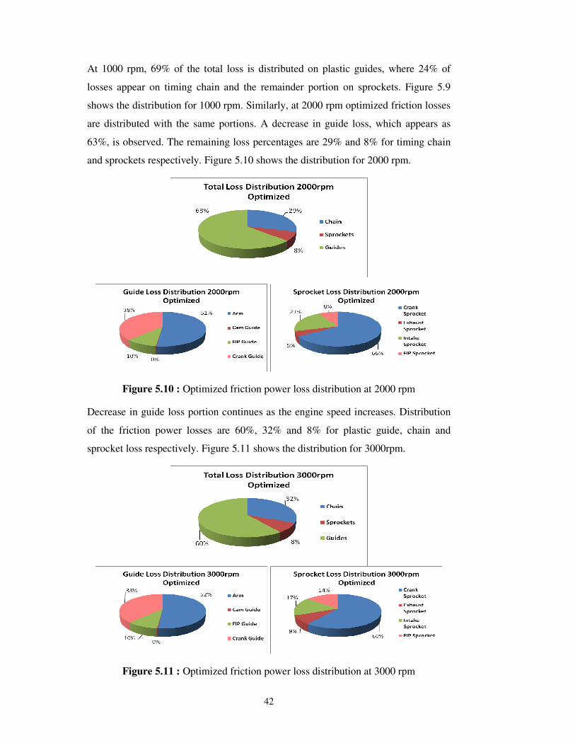
42

At 1000 rpm, 69% of the total loss is distributed on plastic guides, where 24% of

losses appear on timing chain and the remainder portion on sprockets. Figure 5.9

shows the distribution for 1000 rpm. Similarly, at 2000 rpm optimized friction losses

are distributed with the same portions. A decrease in guide loss, which appears as

63%, is observed. The remaining loss percentages are 29% and 8% for timing chain

and sprockets respectively. Figure 5.10 shows the distribution for 2000 rpm.

Figure 5.10 : Optimized friction power loss distribution at 2000 rpm

Decrease in guide loss portion continues as the engine speed increases. Distribution

of the friction power losses are 60%, 32% and 8% for plastic guide, chain and

sprocket loss respectively. Figure 5.11 shows the distribution for 3000rpm.

Figure 5.11 : Optimized friction power loss distribution at 3000 rpm

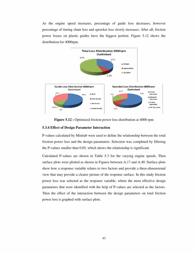
43

As the engine speed increases, percentage of guide loss decreases, however

percentage of timing chain loss and sprocket loss slowly increases. After all, friction

power losses on plastic guides have the biggest portion. Figure 5.12 shows the

distribution for 4000rpm.

Figure 5.12 : Optimized friction power loss distribution at 4000 rpm

5.3.4 Effect of Design Parameter Interaction

P-values calculated by Minitab were used to define the relationship between the total

friction power loss and the design parameters. Selection was completed by filtering

the P-values smaller than 0.05, which shows the relationship is significant.

Calculated P-values are shown in Table 5.3 for the varying engine speeds. Then

surface plots were plotted as shown in Figures between A.17 and A.40. Surface plots

show how a response variable relates to two factors and provide a three-dimensional

view that may provide a clearer picture of the response surface. In this study friction

power loss was selected as the response variable, where the most effective design

parameters that were identified with the help of P-values are selected as the factors.

Then the effect of the interaction between the design parameters on total friction

power loss is graphed with surface plots.

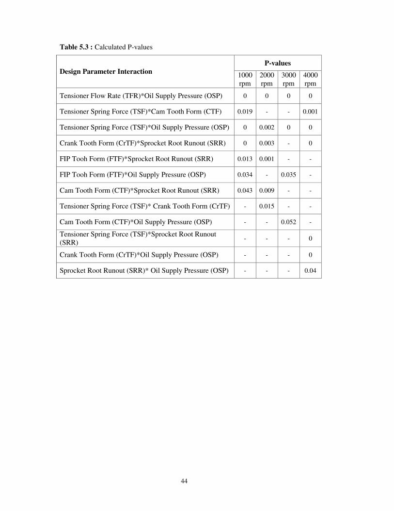
44

Table 5.3 : Calculated P-values

P-values Design Parameter Interaction 1000

rpm 2000rpm

3000rpm

4000rpm

Tensioner Flow Rate (TFR)*Oil Supply Pressure (OSP) 0 0 0 0

Tensioner Spring Force (TSF)*Cam Tooth Form (CTF) 0.019 - - 0.001

Tensioner Spring Force (TSF)*Oil Supply Pressure (OSP) 0 0.002 0 0

Crank Tooth Form (CrTF)*Sprocket Root Runout (SRR) 0 0.003 - 0

FIP Tooh Form (FTF)*Sprocket Root Runout (SRR) 0.013 0.001 - -

FIP Tooh Form (FTF)*Oil Supply Pressure (OSP) 0.034 - 0.035 -

Cam Tooth Form (CTF)*Sprocket Root Runout (SRR) 0.043 0.009 - -

Tensioner Spring Force (TSF)* Crank Tooth Form (CrTF) - 0.015 - -

Cam Tooth Form (CTF)*Oil Supply Pressure (OSP) - - 0.052 -

Tensioner Spring Force (TSF)*Sprocket Root Runout (SRR)

- - - 0

Crank Tooth Form (CrTF)*Oil Supply Pressure (OSP) - - - 0

Sprocket Root Runout (SRR)* Oil Supply Pressure (OSP) - - - 0.04

45

CONCLUSIONS AND RECOMMENDATIONS

An analytical study has been conducted to optimize the friction power loss of a

timing drive for a four-cylinder diesel engine by changing design parameters such as,

hydraulic tensioner diametrical clearance, spring force, sprockets’ teeth geometries,

sprocket circularity and engine oil pressure. From the results, the following

conclusions were derived.

• Timing drive absorbs approximately 0.3kW power by friction losses at 4000

rpm engine speed and this loss can be modeled and optimized by using

simulation tools. Friction power losses can be statistically analyzed and

optimized approximately decreasing by 20%.

• Tensioner spring force and oil supply pressure are the main factors affecting

the friction power loss.

• Plastic guide contact with timing chain has the biggest portion (70%) of the

friction loss in timing drive system, followed by the timing chain sub-

components (25%) and lastly by sprocket and timing chain contact (5%).

• Approximately half of the total guide friction loss occurs on the tensioner

arm. Crank guide brings about 40% of the total guide friction losses. FIP

guide causes the remaining portion.

• Cam to cam guide does not have an effect on friction power loss for the

investigated layout. Because, it only behaves as a router for the chain in the

subjected timing drive system and does not have contact with the timing

chain all the time.

• The crank sprocket has the biggest portion in friction power loss with

approximately 60% share, which is followed by FIP sprocket, exhaust and

intake camshaft sprockets respectively.

• The optimized timing drive design in order to minimize the friction loss

brings advances in engine efficiency. However, further improvements are

46

required to achieve lower targets by optimizing the design parameters for the

entire engine.

• In this study, multi-body systems were used to model the chain drive system

elements. Study can be completed with flexible modeling elements for

comparison in further investigations.

• Additionally, this methodology can be applied to valvetrain systems for a

better understanding of the whole system losses.

47

REFERENCES

[1] Heywood, J. B., 1998: Internal Combustion Engine Fundamentals, McGraw-Hill Book Company, New York.

[2] Körfer, W., Lacy, F., 2006: Timing Belt Drives and their Advantages Regarding Engine Efficiency and NVH Characteristics, MTZ 07-08 Volume 67.

[3] Mufti, R. A., Priest, M., 2009: Effect of Engin Operating Conditions and Lubricant Rheology on the Distribution of Losses in an Internal Combustion Engine, ASME, December Volume 131.

[4] Sandoval, D., Heywood, J. B., 2003: An Improved Friction Model for Spark-Ignition Engines, SAE Technical Paper Series, 2003-01-0725.

[5] Comfort, A., 2003: An Introduction to Heavy-Duty Diesel Engine Frictional Losses and Lubricant Properties Affecting Fuel Economy – Part I, SAE Technical Paper Series, 2003-01-3225.

[6] Spicer, J. B., Richardson, C. J. K., Ehrlich, M. J., Bernstein, J. R., Fukuda, M., Terada, M., 2001: Effects of Frictional Lose on Bicycle Chain Drive, ASME, December Volume 123.

[7] Maile, K., Campean, F., Day, A., 2009: Design for Reliability of an Engine Timing Chain, SAE Technical Paper Series, 2009-01-0206.

[8] Kux, S., Parsche, U., 2009: Effective Optimisation Methods for the Process of Designing Chain Drives, MTZ 01 Volume 70..

[9] Polat, Ö., 2008: Investigation of Lubrication Effect on Diesel Engine Timing Chain Wear, M. Sc. Thesis, Istanbul Technical University.

[10] Dayco - Markiv Automotive Products, 2008: R&D Products and Evolution Technical Presentation, Istanbul, Turkey.

[11] Url-1 <http://chain-guide.com/basics/index.html>, accessed at 20.11.2009.

[12] Morse TEC, 2008: Engine Chain Drive Technology Technical Presentation, Istanbul, Turkey.

[13] Konyha, Z., Matkovic, K., Gracanin, D., Duras, M., Juric, J., Hauser, H., 2007: Interactive Visual Analysis of a Timing Chain Drive Using Segmented Curve View and other Coordinated Views, IEEE

Computer Society.

[14] Rodriguez, J., Keribar, R., Fialek, G., 2005: A Comprehensive Drive Chain Model Applicable to Valvetrain System, SAE Technical Paper Series, 2005-01-1650.

[15] Valdyn, 2009: User’s Manual Version 4.3.

[16] Plail, J., Govett, H., Howell, T., 2003: Use of DoE Techniques with Valdyn for Design Verification of Chain Drive, Ricardo.

48

[17] ISO 606 International Standart, 1994: Short-pitch Transmission Precision Roller Chains and Chain Wheels.

[18] Minitab, 2003: Meet Minitab User Guide Release 14.

49

APPENDICES

APPENDIX A.1 : Tables and Graphs from VALDYN and MINITAB

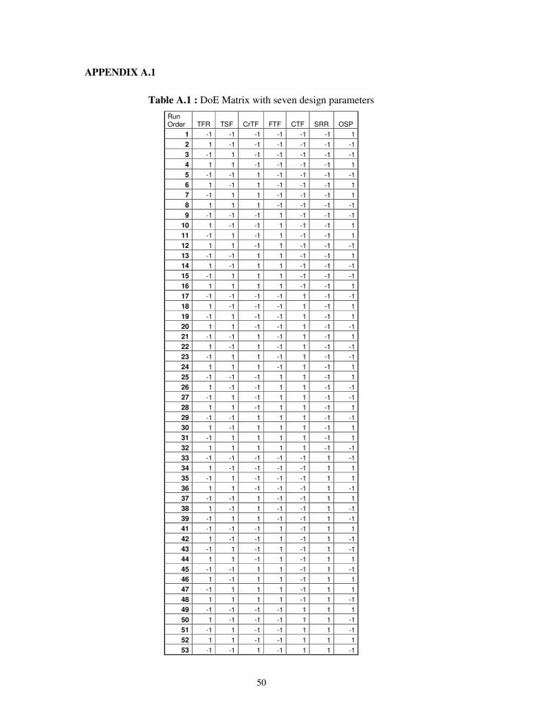
50

APPENDIX A.1

Table A.1 : DoE Matrix with seven design parameters

Run

Order TFR TSF CrTF FTF CTF SRR OSP

1 -1 -1 -1 -1 -1 -1 1

2 1 -1 -1 -1 -1 -1 -1

3 -1 1 -1 -1 -1 -1 -1

4 1 1 -1 -1 -1 -1 1

5 -1 -1 1 -1 -1 -1 -1

6 1 -1 1 -1 -1 -1 1

7 -1 1 1 -1 -1 -1 1

8 1 1 1 -1 -1 -1 -1

9 -1 -1 -1 1 -1 -1 -1

10 1 -1 -1 1 -1 -1 1

11 -1 1 -1 1 -1 -1 1

12 1 1 -1 1 -1 -1 -1

13 -1 -1 1 1 -1 -1 1

14 1 -1 1 1 -1 -1 -1

15 -1 1 1 1 -1 -1 -1

16 1 1 1 1 -1 -1 1

17 -1 -1 -1 -1 1 -1 -1

18 1 -1 -1 -1 1 -1 1

19 -1 1 -1 -1 1 -1 1

20 1 1 -1 -1 1 -1 -1

21 -1 -1 1 -1 1 -1 1

22 1 -1 1 -1 1 -1 -1

23 -1 1 1 -1 1 -1 -1

24 1 1 1 -1 1 -1 1

25 -1 -1 -1 1 1 -1 1

26 1 -1 -1 1 1 -1 -1

27 -1 1 -1 1 1 -1 -1

28 1 1 -1 1 1 -1 1

29 -1 -1 1 1 1 -1 -1

30 1 -1 1 1 1 -1 1

31 -1 1 1 1 1 -1 1

32 1 1 1 1 1 -1 -1

33 -1 -1 -1 -1 -1 1 -1

34 1 -1 -1 -1 -1 1 1

35 -1 1 -1 -1 -1 1 1

36 1 1 -1 -1 -1 1 -1

37 -1 -1 1 -1 -1 1 1

38 1 -1 1 -1 -1 1 -1

39 -1 1 1 -1 -1 1 -1

41 -1 -1 -1 1 -1 1 1

42 1 -1 -1 1 -1 1 -1

43 -1 1 -1 1 -1 1 -1

44 1 1 -1 1 -1 1 1

45 -1 -1 1 1 -1 1 -1

46 1 -1 1 1 -1 1 1

47 -1 1 1 1 -1 1 1

48 1 1 1 1 -1 1 -1

49 -1 -1 -1 -1 1 1 1

50 1 -1 -1 -1 1 1 -1

51 -1 1 -1 -1 1 1 -1

52 1 1 -1 -1 1 1 1

53 -1 -1 1 -1 1 1 -1

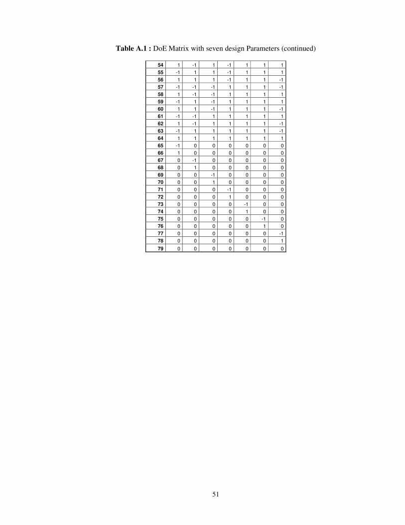
51

Table A.1 : DoE Matrix with seven design Parameters (continued)

54 1 -1 1 -1 1 1 1

55 -1 1 1 -1 1 1 1

56 1 1 1 -1 1 1 -1

57 -1 -1 -1 1 1 1 -1

58 1 -1 -1 1 1 1 1

59 -1 1 -1 1 1 1 1

60 1 1 -1 1 1 1 -1

61 -1 -1 1 1 1 1 1

62 1 -1 1 1 1 1 -1

63 -1 1 1 1 1 1 -1

64 1 1 1 1 1 1 1

65 -1 0 0 0 0 0 0

66 1 0 0 0 0 0 0

67 0 -1 0 0 0 0 0

68 0 1 0 0 0 0 0

69 0 0 -1 0 0 0 0

70 0 0 1 0 0 0 0

71 0 0 0 -1 0 0 0

72 0 0 0 1 0 0 0

73 0 0 0 0 -1 0 0

74 0 0 0 0 1 0 0

75 0 0 0 0 0 -1 0

76 0 0 0 0 0 1 0

77 0 0 0 0 0 0 -1

78 0 0 0 0 0 0 1

79 0 0 0 0 0 0 0

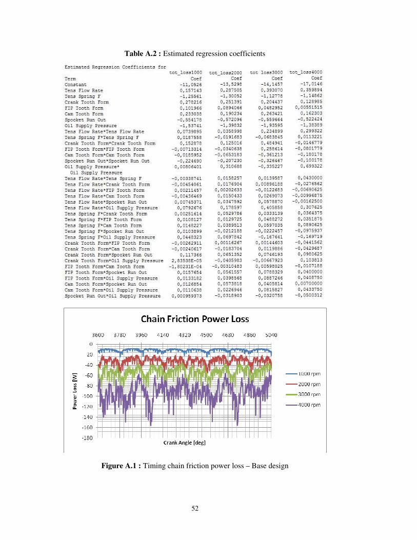
52

Table A.2 : Estimated regression coefficients

Figure A.1 : Timing chain friction power loss – Base design

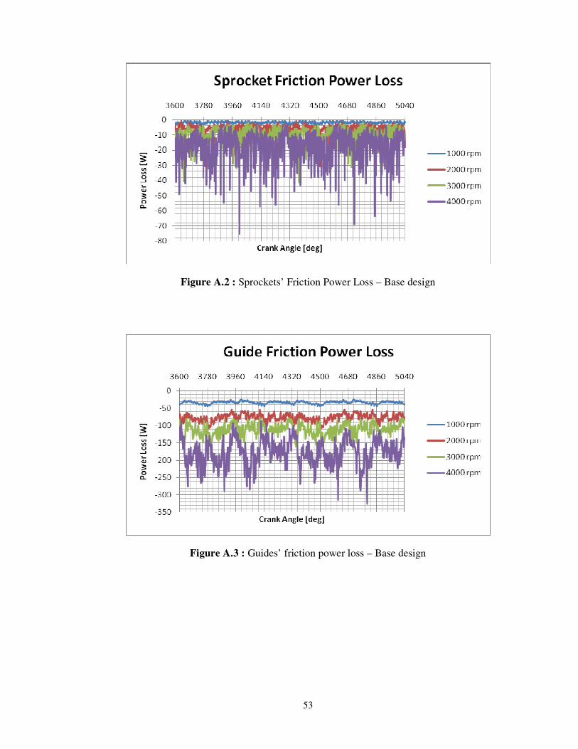
53

Figure A.2 : Sprockets’ Friction Power Loss – Base design

Figure A.3 : Guides’ friction power loss – Base design

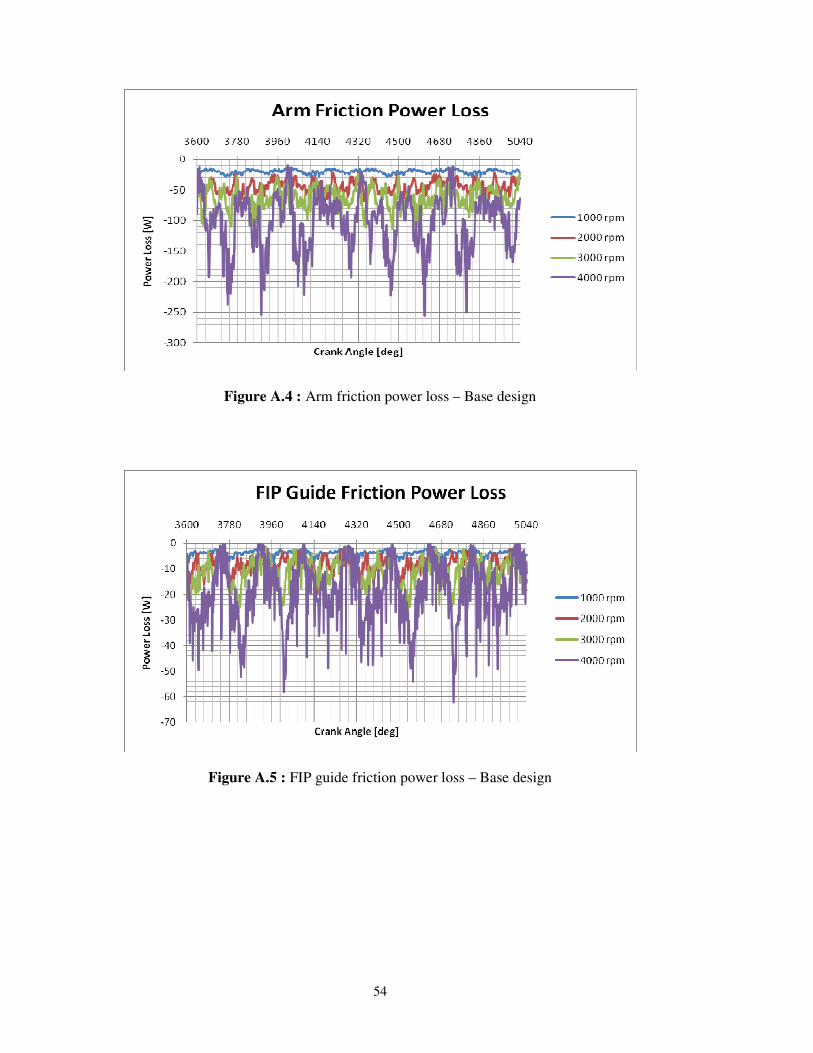
54

Figure A.4 : Arm friction power loss – Base design

Figure A.5 : FIP guide friction power loss – Base design

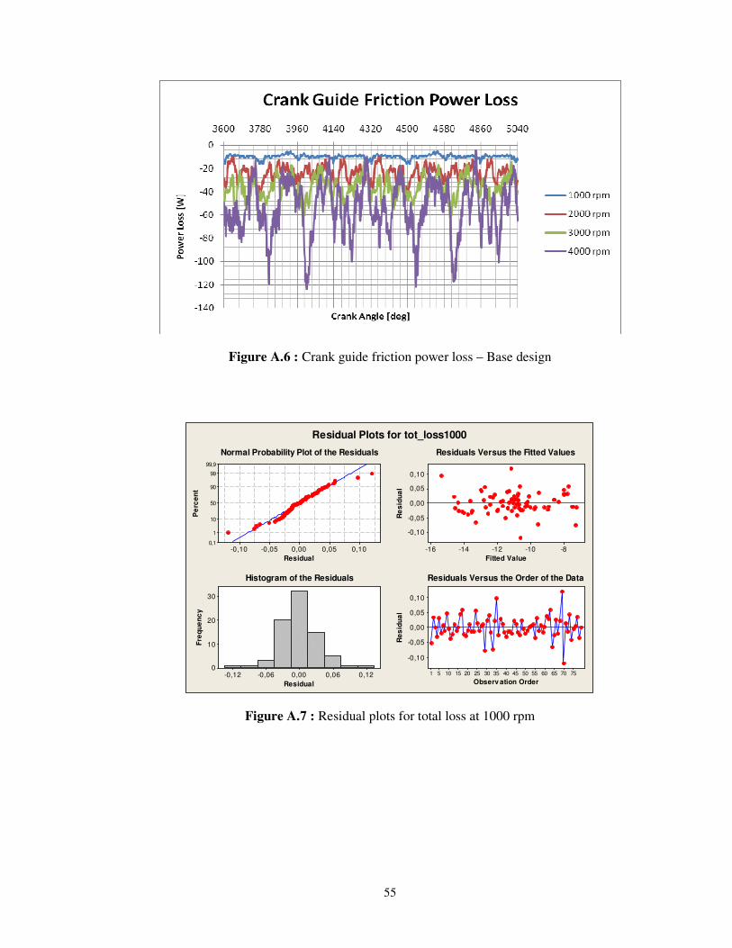
55

Figure A.6 : Crank guide friction power loss – Base design

Residual

Pe

rce

nt

0,100,050,00-0,05-0,10

99,9

99

90

50

10

1

0,1

Fitted Value

Re

sid

ua

l

-8-10-12-14-16

0,10

0,05

0,00

-0,05

-0,10

Residual

Fre

qu

en

cy

0,120,060,00-0,06-0,12

30

20

10

0

Observ ation Order

Re

sid

ua

l

757065605550454035302520151051

0,10

0,05

0,00

-0,05

-0,10

Normal Probability Plot of the Residuals Residuals Versus the Fitted Values

Histogram of the Residuals Residuals Versus the Order of the Data

Residual Plots for tot_loss1000

Figure A.7 : Residual plots for total loss at 1000 rpm

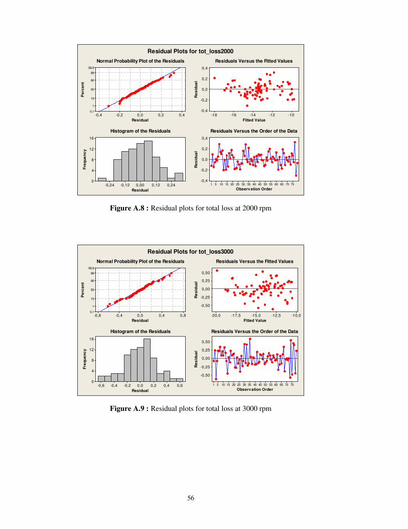
56

Residual

Pe

rce

nt

0,40,20,0-0,2-0,4

99,9

99

90

50

10

1

0,1

Fitted Value

Re

sid

ua

l

-10-12-14-16-18

0,4

0,2

0,0

-0,2

-0,4

Residual

Fre

qu

en

cy

0,240,120,00-0,12-0,24

16

12

8

4

0

Observation Order

Re

sid

ua

l

757065605550454035302520151051

0,4

0,2

0,0

-0,2

-0,4

Normal Probability Plot of the Residuals Residuals Versus the Fitted Values

Histogram of the Residuals Residuals Versus the Order of the Data

Residual Plots for tot_loss2000

Figure A.8 : Residual plots for total loss at 2000 rpm

Residual

Pe

rce

nt

0,80,40,0-0,4-0,8

99,9

99

90

50

10

1

0,1

Fitted Value

Re

sid

ua

l

-10,0-12,5-15,0-17,5-20,0

0,50

0,25

0,00

-0,25

-0,50

Residual

Fre

qu

en

cy

0,60,40,20,0-0,2-0,4-0,6

16

12

8

4

0

Observation Order

Re

sid

ua

l

757065605550454035302520151051

0,50

0,25

0,00

-0,25

-0,50

Normal Probability Plot of the Residuals Residuals Versus the Fitted Values

Histogram of the Residuals Residuals Versus the Order of the Data

Residual Plots for tot_loss3000

Figure A.9 : Residual plots for total loss at 3000 rpm

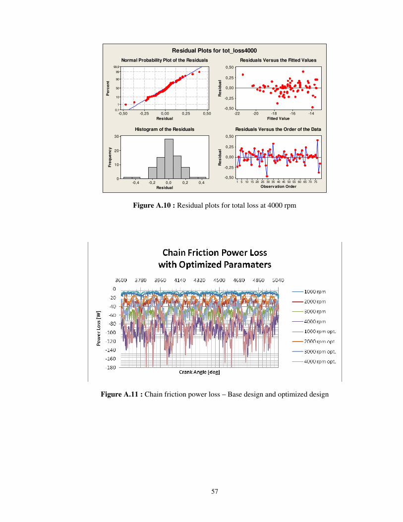
57

Residual

Pe

rce

nt

0,500,250,00-0,25-0,50

99,9

99

90

50

10

1

0,1

Fitted Value

Re

sid

ua

l

-14-16-18-20-22

0,50

0,25

0,00

-0,25

-0,50

Residual

Fre

qu

en

cy

0,40,20,0-0,2-0,4

30

20

10

0

Observation Order

Re

sid

ua

l

757065605550454035302520151051

0,50

0,25

0,00

-0,25

-0,50

Normal Probability Plot of the Residuals Residuals Versus the Fitted Values

Histogram of the Residuals Residuals Versus the Order of the Data

Residual Plots for tot_loss4000

Figure A.10 : Residual plots for total loss at 4000 rpm

Figure A.11 : Chain friction power loss – Base design and optimized design

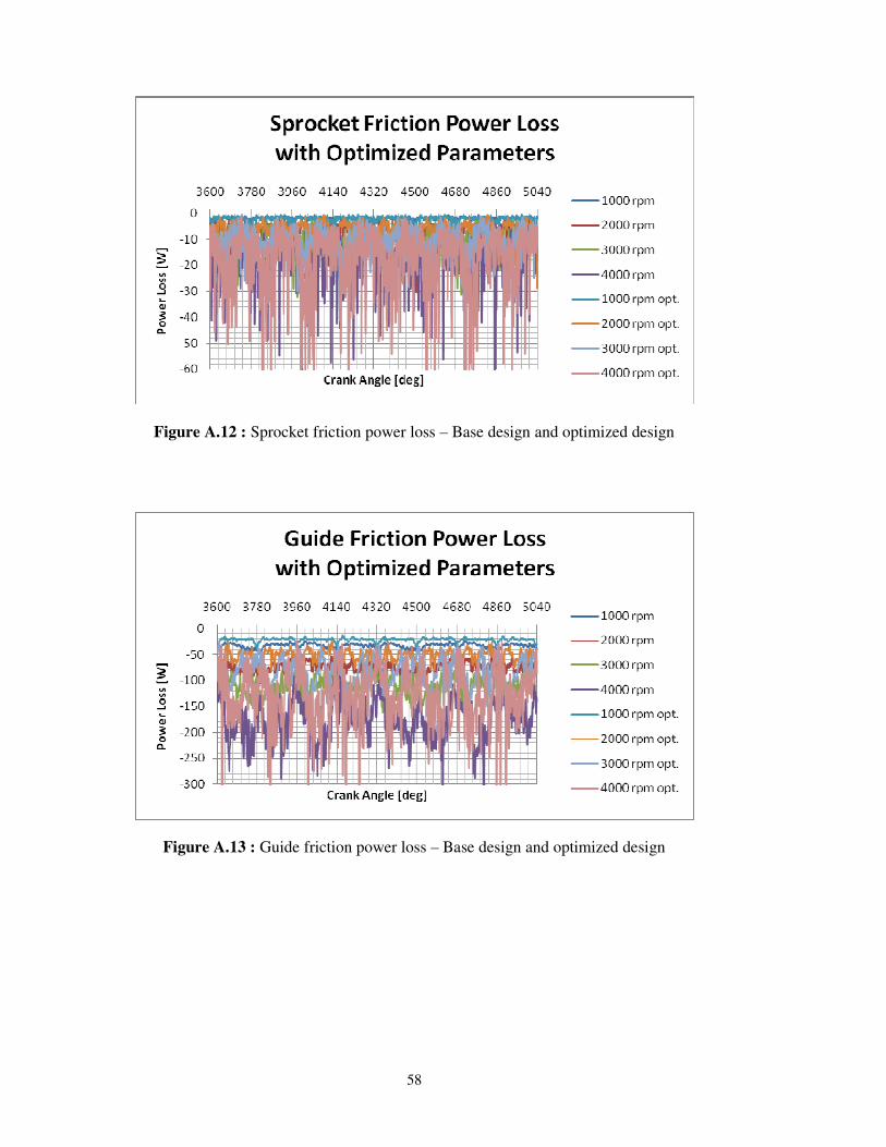
58

Figure A.12 : Sprocket friction power loss – Base design and optimized design

Figure A.13 : Guide friction power loss – Base design and optimized design

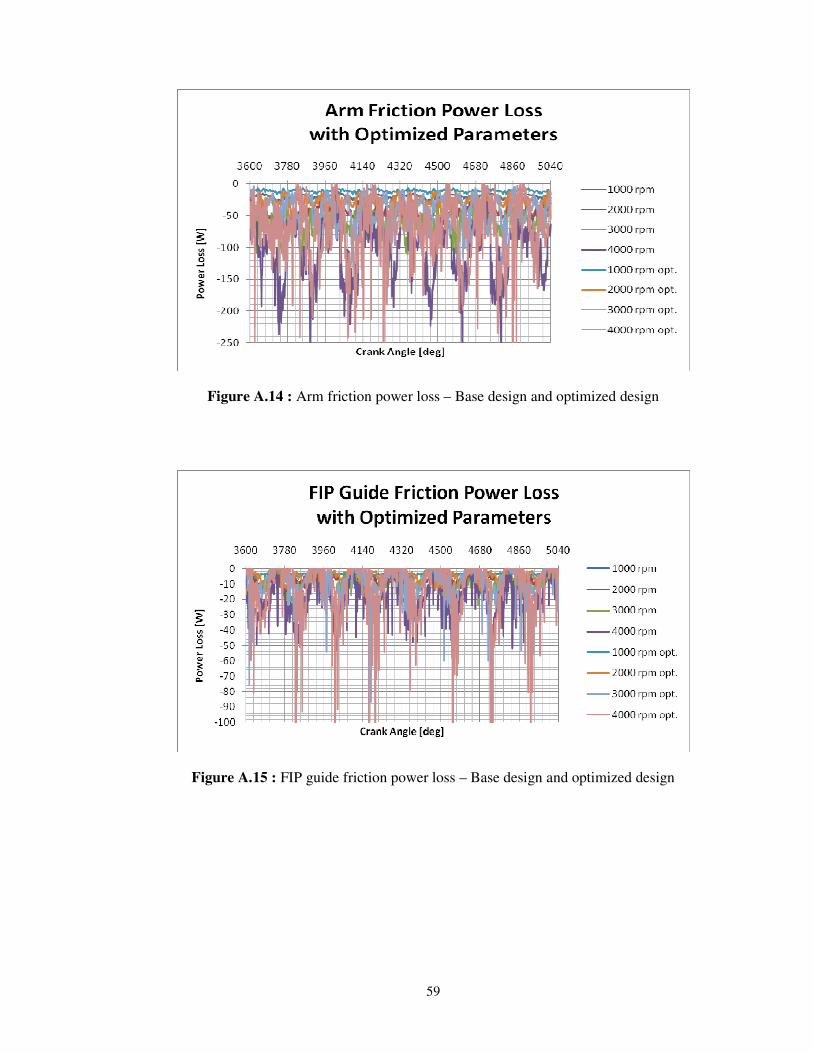
59

Figure A.14 : Arm friction power loss – Base design and optimized design

Figure A.15 : FIP guide friction power loss – Base design and optimized design

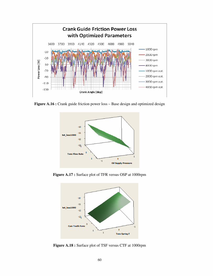
60

Figure A.16 : Crank guide friction power loss – Base design and optimized design

Figure A.17 : Surface plot of TFR versus OSP at 1000rpm

Figure A.18 : Surface plot of TSF versus CTF at 1000rpm

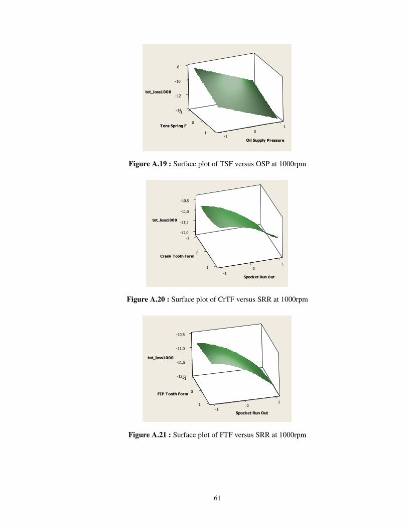
61

-14-1

-12

-10

-8

01

01-1

tot_loss1000

Tens Spring F

Oil Supply Pressure

Figure A.19 : Surface plot of TSF versus OSP at 1000rpm

-12,0

-1

-11,5

-11,0

-10,5

0

11 0

-1

tot_loss1000

Crank Tooth Form

Spocket Run Out

Figure A.20 : Surface plot of CrTF versus SRR at 1000rpm

-12,0-1

-11,5

-11,0

-10,5

0

11 0

-1

tot_loss1000

FIP Tooth Form

Spocket Run Out

Figure A.21 : Surface plot of FTF versus SRR at 1000rpm

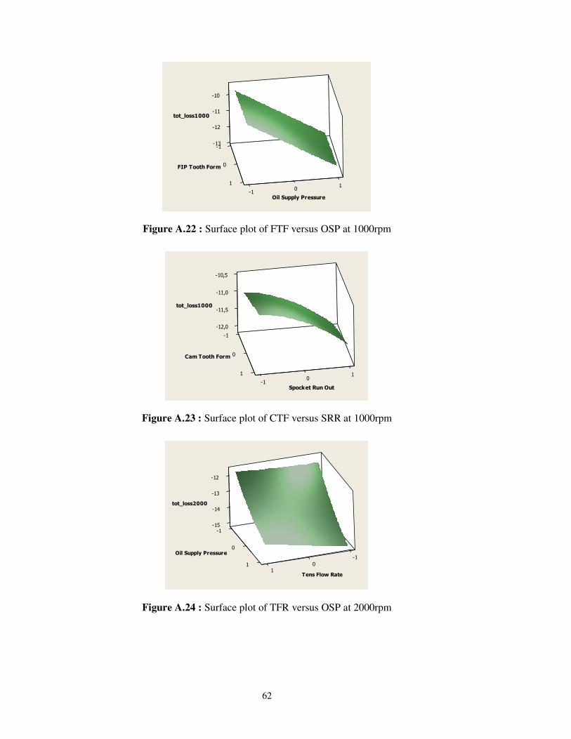
62

-13-1

-12

-11

-10

0

1 10

-1

tot_loss1000

FIP Tooth Form

Oil Supply Pressure

Figure A.22 : Surface plot of FTF versus OSP at 1000rpm

-12,0

-1

-11,5

-11,0

-10,5

0

1 10

-1

tot_loss1000

Cam Tooth Form

Spocket Run Out

Figure A.23 : Surface plot of CTF versus SRR at 1000rpm

-15-1

-14

-13

-12

0

-1

1 01

tot_loss2000

Oil Supply Pressure

Tens Flow Rate

Figure A.24 : Surface plot of TFR versus OSP at 2000rpm

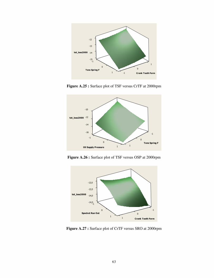
63

-15-1

-14

-13

-12

1

00

1 -1

tot_loss2000

Tens Spring F

Crank Tooth Form

Figure A.25 : Surface plot of TSF versus CrTF at 2000rpm

-16

-14

-1

-12

-1

-10

00

11

tot_loss2000

Tens Spring F

Oil Supply Pressure

Figure A.26 : Surface plot of TSF versus OSP at 2000rpm

-14,5-1

-14,0

-13,5

-13,0

0 -1

01

1

tot_loss2000

Spocket Run Out

Crank Tooth Form

Figure A.27 : Surface plot of CrTF versus SRO at 2000rpm

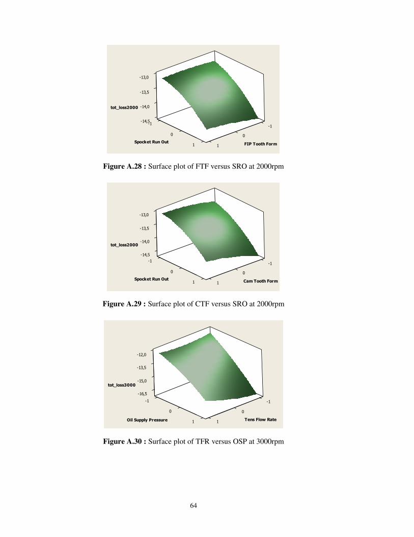
64

-14,5-1

-14,0

-1

-13,5

-13,0

0 0

1 1

tot_loss2000

Spocket Run OutFIP Tooth Form

Figure A.28 : Surface plot of FTF versus SRO at 2000rpm

-1

-14,5

-14,0

-1

-13,5

-13,0

0 0

1 1

tot_loss2000

Spocket Run OutCam Tooth Form

Figure A.29 : Surface plot of CTF versus SRO at 2000rpm

-1

-16,5

-1

-15,0

-13,5

-12,0

0 0

1 1

tot_loss3000

Oil Supply Pressure Tens Flow Rate

Figure A.30 : Surface plot of TFR versus OSP at 3000rpm

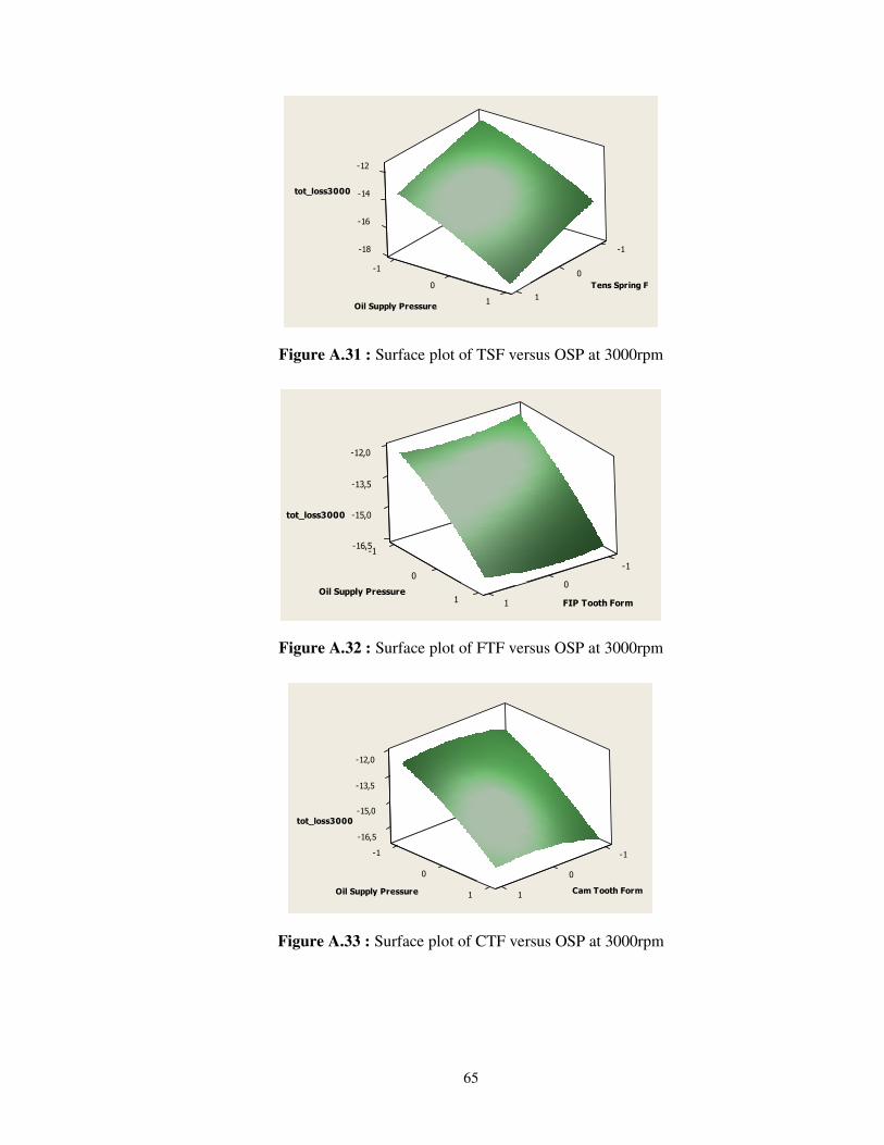
65

-18 -1

-16

-14

-12

-10

0

11

tot_loss3000

Tens Spring F

Oil Supply Pressure

Figure A.31 : Surface plot of TSF versus OSP at 3000rpm

-16,5-1

-15,0

-13,5

-12,0

-10

0

1 1

tot_loss3000

Oil Supply Pressure

FIP Tooth Form

Figure A.32 : Surface plot of FTF versus OSP at 3000rpm

-1

-16,5

-1

-15,0

-13,5

-12,0

0 0

1 1

tot_loss3000

Oil Supply Pressure Cam Tooth Form

Figure A.33 : Surface plot of CTF versus OSP at 3000rpm

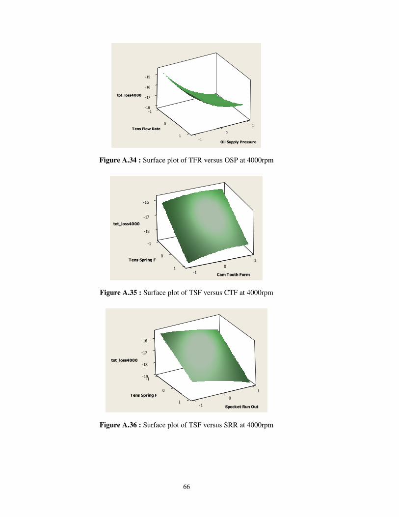
66

-18-1

-17

-16

-15

01

01

-1

tot_loss4000

Tens Flow Rate

Oil Supply Pressure

Figure A.34 : Surface plot of TFR versus OSP at 4000rpm

-1

-18

-17

-16

01

01

-1

tot_loss4000

Tens Spring F

Cam Tooth Form

Figure A.35 : Surface plot of TSF versus CTF at 4000rpm

-19-1

-18

-17

-16

0 1

01

-1

tot_loss4000

Tens Spring F

Spocket Run Out

Figure A.36 : Surface plot of TSF versus SRR at 4000rpm

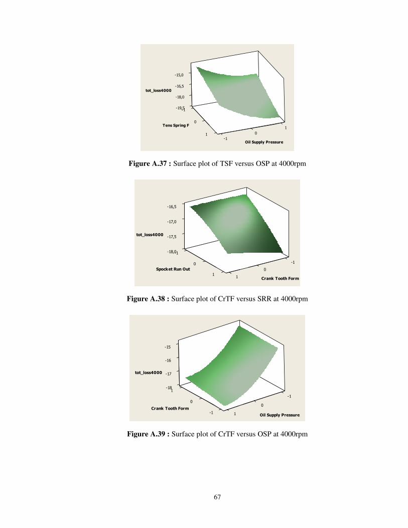
67

-19,5-1

-18,0

-16,5

-15,0

0

1

01-1

tot_loss4000

Tens Spring F

Oil Supply Pressure

Figure A.37 : Surface plot of TSF versus OSP at 4000rpm

-18,0-1

-17,5

-17,0

-16,5

-10

01

1

tot_loss4000

Spocket Run Out

Crank Tooth Form

Figure A.38 : Surface plot of CrTF versus SRR at 4000rpm

-181

-17

-16

-15

-1

00

-1 1

tot_loss4000

Crank Tooth Form

Oil Supply Pressure

Figure A.39 : Surface plot of CrTF versus OSP at 4000rpm

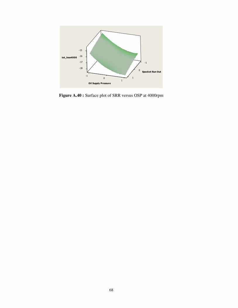
68

-1

0-18

-17

-16

-1

-15

0 11

tot_loss4000

Spocket Run Out

Oil Supply Pressure

Figure A.40 : Surface plot of SRR versus OSP at 4000rpm

69

CURRICULUM VITA

Candidate’s full name: Umut UYSAL

Place and date of birth: Bursa, 20.11.1985

Permanent Address: Doğu Mah. Dağ Sk. Park Apt. No:12 Daire:4 Pendik/İST

Universities and Colleges attended: Istanbul Technical University