matlab ® programming fundamentals r2014a
TRANSCRIPT

MATLAB®
Programming Fundamentals
R2014a

How to Contact MathWorks
www.mathworks.com Webcomp.soft-sys.matlab Newsgroupwww.mathworks.com/contact_TS.html Technical Support
[email protected] Product enhancement [email protected] Bug [email protected] Documentation error [email protected] Order status, license renewals, [email protected] Sales, pricing, and general information
508-647-7000 (Phone)
508-647-7001 (Fax)
The MathWorks, Inc.3 Apple Hill DriveNatick, MA 01760-2098For contact information about worldwide offices, see the MathWorks Web site.
MATLAB Programming Fundamentals
© COPYRIGHT 1984–2014 by The MathWorks, Inc.The software described in this document is furnished under a license agreement. The software may be usedor copied only under the terms of the license agreement. No part of this manual may be photocopied orreproduced in any form without prior written consent from The MathWorks, Inc.
FEDERAL ACQUISITION: This provision applies to all acquisitions of the Program and Documentationby, for, or through the federal government of the United States. By accepting delivery of the Programor Documentation, the government hereby agrees that this software or documentation qualifies ascommercial computer software or commercial computer software documentation as such terms are usedor defined in FAR 12.212, DFARS Part 227.72, and DFARS 252.227-7014. Accordingly, the terms andconditions of this Agreement and only those rights specified in this Agreement, shall pertain to and governthe use, modification, reproduction, release, performance, display, and disclosure of the Program andDocumentation by the federal government (or other entity acquiring for or through the federal government)and shall supersede any conflicting contractual terms or conditions. If this License fails to meet thegovernment’s needs or is inconsistent in any respect with federal procurement law, the government agreesto return the Program and Documentation, unused, to The MathWorks, Inc.
Trademarks
MATLAB and Simulink are registered trademarks of The MathWorks, Inc. Seewww.mathworks.com/trademarks for a list of additional trademarks. Other product or brandnames may be trademarks or registered trademarks of their respective holders.
Patents
MathWorks products are protected by one or more U.S. patents. Please seewww.mathworks.com/patents for more information.

Revision HistoryJune 2004 First printing New for MATLAB 7.0 (Release 14)October 2004 Online only Revised for MATLAB 7.0.1 (Release 14SP1)March 2005 Online only Revised for MATLAB 7.0.4 (Release 14SP2)June 2005 Second printing Minor revision for MATLAB 7.0.4September 2005 Online only Revised for MATLAB 7.1 (Release 14SP3)March 2006 Online only Revised for MATLAB 7.2 (Release 2006a)September 2006 Online only Revised for MATLAB 7.3 (Release 2006b)March 2007 Online only Revised for MATLAB 7.4 (Release 2007a)September 2007 Online only Revised for Version 7.5 (Release 2007b)March 2008 Online only Revised for Version 7.6 (Release 2008a)October 2008 Online only Revised for Version 7.7 (Release 2008b)March 2009 Online only Revised for Version 7.8 (Release 2009a)September 2009 Online only Revised for Version 7.9 (Release 2009b)March 2010 Online only Revised for Version 7.10 (Release 2010a)September 2010 Online only Revised for Version 7.11 (Release 2010b)April 2011 Online only Revised for Version 7.12 (Release 2011a)September 2011 Online only Revised for Version 7.13 (Release 2011b)March 2012 Online only Revised for Version 7.14 (Release 2012a)September 2012 Online only Revised for Version 8.0 (Release 2012b)March 2013 Online only Revised for Version 8.1 (Release 2013a)September 2013 Online only Revised for Version 8.2 (Release 2013b)March 2014 Online only Revised for Version 8.3 (Release 2014a)


Contents
Language
Syntax Basics
1Create Variables . . . . . . . . . . . . . . . . . . . . . . . . . . . . . . . . . . . 1-2
Create Numeric Arrays . . . . . . . . . . . . . . . . . . . . . . . . . . . . . 1-3
Continue Long Statements on Multiple Lines . . . . . . . . 1-5
Call Functions . . . . . . . . . . . . . . . . . . . . . . . . . . . . . . . . . . . . . 1-6
Ignore Function Outputs . . . . . . . . . . . . . . . . . . . . . . . . . . . 1-7
Variable Names . . . . . . . . . . . . . . . . . . . . . . . . . . . . . . . . . . . . 1-8Valid Names . . . . . . . . . . . . . . . . . . . . . . . . . . . . . . . . . . . . . 1-8Conflicts with Function Names . . . . . . . . . . . . . . . . . . . . . . 1-8
Case and Space Sensitivity . . . . . . . . . . . . . . . . . . . . . . . . . 1-10
Command vs. Function Syntax . . . . . . . . . . . . . . . . . . . . . . 1-12Command and Function Syntaxes . . . . . . . . . . . . . . . . . . . . 1-12Avoid Common Syntax Mistakes . . . . . . . . . . . . . . . . . . . . . 1-13How MATLAB Recognizes Command Syntax . . . . . . . . . . . 1-14
Common Errors When Calling Functions . . . . . . . . . . . . 1-16Conflicting Function and Variable Names . . . . . . . . . . . . . 1-16Undefined Functions or Variables . . . . . . . . . . . . . . . . . . . . 1-16
v

Program Components
2Array vs. Matrix Operations . . . . . . . . . . . . . . . . . . . . . . . . 2-2Introduction . . . . . . . . . . . . . . . . . . . . . . . . . . . . . . . . . . . . . . 2-2Array Operations . . . . . . . . . . . . . . . . . . . . . . . . . . . . . . . . . . 2-2Matrix Operations . . . . . . . . . . . . . . . . . . . . . . . . . . . . . . . . . 2-4
Relational Operators . . . . . . . . . . . . . . . . . . . . . . . . . . . . . . . 2-7Relational Operators and Arrays . . . . . . . . . . . . . . . . . . . . . 2-7Relational Operators and Empty Arrays . . . . . . . . . . . . . . . 2-8
Operator Precedence . . . . . . . . . . . . . . . . . . . . . . . . . . . . . . 2-9Precedence of AND and OR Operators . . . . . . . . . . . . . . . . 2-9Overriding Default Precedence . . . . . . . . . . . . . . . . . . . . . . 2-10
Special Values . . . . . . . . . . . . . . . . . . . . . . . . . . . . . . . . . . . . . 2-11
Conditional Statements . . . . . . . . . . . . . . . . . . . . . . . . . . . . 2-13
Loop Control Statements . . . . . . . . . . . . . . . . . . . . . . . . . . . 2-15
Represent Dates and Times in MATLAB . . . . . . . . . . . . . 2-17Date Strings . . . . . . . . . . . . . . . . . . . . . . . . . . . . . . . . . . . . . . 2-17Date Vectors . . . . . . . . . . . . . . . . . . . . . . . . . . . . . . . . . . . . . 2-18Serial Date Numbers . . . . . . . . . . . . . . . . . . . . . . . . . . . . . . 2-18
Compute Elapsed Time . . . . . . . . . . . . . . . . . . . . . . . . . . . . . 2-19Compute Elapsed Time . . . . . . . . . . . . . . . . . . . . . . . . . . . . . 2-19Compute Future Date . . . . . . . . . . . . . . . . . . . . . . . . . . . . . . 2-20
Carryover in Date Vectors and Strings . . . . . . . . . . . . . . 2-23
Troubleshooting: Converting Date Vector ReturnsUnexpected Output . . . . . . . . . . . . . . . . . . . . . . . . . . . . . . 2-24
Regular Expressions . . . . . . . . . . . . . . . . . . . . . . . . . . . . . . . 2-26What Is a Regular Expression? . . . . . . . . . . . . . . . . . . . . . . 2-26
vi Contents

Steps for Building Expressions . . . . . . . . . . . . . . . . . . . . . . 2-28Operators and Characters . . . . . . . . . . . . . . . . . . . . . . . . . . 2-31
Lookahead Assertions in Regular Expressions . . . . . . . 2-43Lookahead Assertions . . . . . . . . . . . . . . . . . . . . . . . . . . . . . . 2-43Overlapping Matches . . . . . . . . . . . . . . . . . . . . . . . . . . . . . . 2-44Logical AND Conditions . . . . . . . . . . . . . . . . . . . . . . . . . . . . 2-44
Tokens in Regular Expressions . . . . . . . . . . . . . . . . . . . . . 2-46Introduction . . . . . . . . . . . . . . . . . . . . . . . . . . . . . . . . . . . . . . 2-46Multiple Tokens . . . . . . . . . . . . . . . . . . . . . . . . . . . . . . . . . . 2-48Unmatched Tokens . . . . . . . . . . . . . . . . . . . . . . . . . . . . . . . . 2-48Tokens in Replacement Strings . . . . . . . . . . . . . . . . . . . . . . 2-50Named Capture . . . . . . . . . . . . . . . . . . . . . . . . . . . . . . . . . . . 2-50
Dynamic Regular Expressions . . . . . . . . . . . . . . . . . . . . . . 2-52Introduction . . . . . . . . . . . . . . . . . . . . . . . . . . . . . . . . . . . . . . 2-52Dynamic Match Expressions — (??expr) . . . . . . . . . . . . . . . 2-53Commands That Modify the Match Expression —(??@cmd) . . . . . . . . . . . . . . . . . . . . . . . . . . . . . . . . . . . . . . 2-54
Commands That Serve a Functional Purpose — (?@cmd) . . 2-55Commands in Replacement Expressions — ${cmd} . . . . . . 2-58
Comma-Separated Lists . . . . . . . . . . . . . . . . . . . . . . . . . . . . 2-61What Is a Comma-Separated List? . . . . . . . . . . . . . . . . . . . 2-61Generating a Comma-Separated List . . . . . . . . . . . . . . . . . 2-61Assigning Output from a Comma-Separated List . . . . . . . . 2-63Assigning to a Comma-Separated List . . . . . . . . . . . . . . . . 2-64How to Use the Comma-Separated Lists . . . . . . . . . . . . . . . 2-65Fast Fourier Transform Example . . . . . . . . . . . . . . . . . . . . 2-67
Alternatives to the eval Function . . . . . . . . . . . . . . . . . . . 2-69Why Avoid the eval Function? . . . . . . . . . . . . . . . . . . . . . . . 2-69Variables with Sequential Names . . . . . . . . . . . . . . . . . . . . 2-69Files with Sequential Names . . . . . . . . . . . . . . . . . . . . . . . . 2-70Function Names in Variables . . . . . . . . . . . . . . . . . . . . . . . . 2-71Field Names in Variables . . . . . . . . . . . . . . . . . . . . . . . . . . . 2-72Error Handling . . . . . . . . . . . . . . . . . . . . . . . . . . . . . . . . . . . 2-72
Shell Escape Functions . . . . . . . . . . . . . . . . . . . . . . . . . . . . 2-73
vii

Symbol Reference . . . . . . . . . . . . . . . . . . . . . . . . . . . . . . . . . 2-74Asterisk — * . . . . . . . . . . . . . . . . . . . . . . . . . . . . . . . . . . . . . 2-74At — @ . . . . . . . . . . . . . . . . . . . . . . . . . . . . . . . . . . . . . . . . . . 2-75Colon — : . . . . . . . . . . . . . . . . . . . . . . . . . . . . . . . . . . . . . . . . 2-76Comma — , . . . . . . . . . . . . . . . . . . . . . . . . . . . . . . . . . . . . . . 2-77Curly Braces — { } . . . . . . . . . . . . . . . . . . . . . . . . . . . . . . . . . 2-78Dot — . . . . . . . . . . . . . . . . . . . . . . . . . . . . . . . . . . . . . . . . . . . 2-78Dot-Dot — .. . . . . . . . . . . . . . . . . . . . . . . . . . . . . . . . . . . . . . . 2-79Dot-Dot-Dot (Ellipsis) — ... . . . . . . . . . . . . . . . . . . . . . . . . . . 2-79Dot-Parentheses — .( ) . . . . . . . . . . . . . . . . . . . . . . . . . . . . . 2-80Exclamation Point — ! . . . . . . . . . . . . . . . . . . . . . . . . . . . . . 2-81Parentheses — ( ) . . . . . . . . . . . . . . . . . . . . . . . . . . . . . . . . . 2-81Percent — % . . . . . . . . . . . . . . . . . . . . . . . . . . . . . . . . . . . . . 2-82Percent-Brace — %{ %} . . . . . . . . . . . . . . . . . . . . . . . . . . . . . 2-82Plus — + . . . . . . . . . . . . . . . . . . . . . . . . . . . . . . . . . . . . . . . . . 2-83Semicolon — ; . . . . . . . . . . . . . . . . . . . . . . . . . . . . . . . . . . . . 2-83Single Quotes — ’ ’ . . . . . . . . . . . . . . . . . . . . . . . . . . . . . . . . . 2-84Space Character . . . . . . . . . . . . . . . . . . . . . . . . . . . . . . . . . . 2-84Slash and Backslash — / \ . . . . . . . . . . . . . . . . . . . . . . . . . . 2-85Square Brackets — [ ] . . . . . . . . . . . . . . . . . . . . . . . . . . . . . . 2-85Tilde — ~ . . . . . . . . . . . . . . . . . . . . . . . . . . . . . . . . . . . . . . . . 2-86
Classes (Data Types)
Overview of MATLAB Classes
3Fundamental MATLAB Classes . . . . . . . . . . . . . . . . . . . . . 3-2
Numeric Classes
4Overview of Numeric Classes . . . . . . . . . . . . . . . . . . . . . . . 4-2
Integers . . . . . . . . . . . . . . . . . . . . . . . . . . . . . . . . . . . . . . . . . . 4-3Integer Classes . . . . . . . . . . . . . . . . . . . . . . . . . . . . . . . . . . . 4-3
viii Contents

Creating Integer Data . . . . . . . . . . . . . . . . . . . . . . . . . . . . . . 4-4Arithmetic Operations on Integer Classes . . . . . . . . . . . . . . 4-5Largest and Smallest Values for Integer Classes . . . . . . . . 4-6Integer Functions . . . . . . . . . . . . . . . . . . . . . . . . . . . . . . . . . 4-6
Floating-Point Numbers . . . . . . . . . . . . . . . . . . . . . . . . . . . . 4-7Double-Precision Floating Point . . . . . . . . . . . . . . . . . . . . . . 4-7Single-Precision Floating Point . . . . . . . . . . . . . . . . . . . . . . 4-8Creating Floating-Point Data . . . . . . . . . . . . . . . . . . . . . . . . 4-8Arithmetic Operations on Floating-Point Numbers . . . . . . 4-10Largest and Smallest Values for Floating-Point Classes . . 4-11Accuracy of Floating-Point Data . . . . . . . . . . . . . . . . . . . . . 4-12Avoiding Common Problems with Floating-PointArithmetic . . . . . . . . . . . . . . . . . . . . . . . . . . . . . . . . . . . . . 4-14
Floating-Point Functions . . . . . . . . . . . . . . . . . . . . . . . . . . . 4-16References . . . . . . . . . . . . . . . . . . . . . . . . . . . . . . . . . . . . . . . 4-16
Complex Numbers . . . . . . . . . . . . . . . . . . . . . . . . . . . . . . . . . 4-18Creating Complex Numbers . . . . . . . . . . . . . . . . . . . . . . . . . 4-18Complex Number Functions . . . . . . . . . . . . . . . . . . . . . . . . . 4-19
Infinity and NaN . . . . . . . . . . . . . . . . . . . . . . . . . . . . . . . . . . 4-20Infinity . . . . . . . . . . . . . . . . . . . . . . . . . . . . . . . . . . . . . . . . . . 4-20NaN . . . . . . . . . . . . . . . . . . . . . . . . . . . . . . . . . . . . . . . . . . . . 4-20Infinity and NaN Functions . . . . . . . . . . . . . . . . . . . . . . . . . 4-21
Identifying Numeric Classes . . . . . . . . . . . . . . . . . . . . . . . . 4-22
Display Format for Numeric Values . . . . . . . . . . . . . . . . . 4-23Default Display . . . . . . . . . . . . . . . . . . . . . . . . . . . . . . . . . . . 4-23Display Format Examples . . . . . . . . . . . . . . . . . . . . . . . . . . 4-23Setting Numeric Format in a Program . . . . . . . . . . . . . . . . 4-24
Function Summary . . . . . . . . . . . . . . . . . . . . . . . . . . . . . . . . 4-26
ix

The Logical Class
5Find Array Elements That Meet a Condition . . . . . . . . . 5-2Apply a Single Condition . . . . . . . . . . . . . . . . . . . . . . . . . . . 5-2Apply Multiple Conditions . . . . . . . . . . . . . . . . . . . . . . . . . . 5-4Replace Values that Meet a Condition . . . . . . . . . . . . . . . . . 5-5
Determine if Arrays Are Logical . . . . . . . . . . . . . . . . . . . . 5-8Identify Logical Matrix . . . . . . . . . . . . . . . . . . . . . . . . . . . . . 5-8Test an Entire Array . . . . . . . . . . . . . . . . . . . . . . . . . . . . . . . 5-9Test Each Array Element . . . . . . . . . . . . . . . . . . . . . . . . . . . 5-9Summary Table . . . . . . . . . . . . . . . . . . . . . . . . . . . . . . . . . . . 5-10
Reduce Logical Arrays to Single Value . . . . . . . . . . . . . . 5-12
Truth Table for Logical Operations . . . . . . . . . . . . . . . . . 5-15
Characters and Strings
6Creating Character Arrays . . . . . . . . . . . . . . . . . . . . . . . . . 6-2Creating a Character String . . . . . . . . . . . . . . . . . . . . . . . . . 6-2Creating a Rectangular Character Array . . . . . . . . . . . . . . 6-3Identifying Characters in a String . . . . . . . . . . . . . . . . . . . . 6-4Working with Space Characters . . . . . . . . . . . . . . . . . . . . . . 6-5Expanding Character Arrays . . . . . . . . . . . . . . . . . . . . . . . . 6-6
Cell Arrays of Strings . . . . . . . . . . . . . . . . . . . . . . . . . . . . . . 6-7Converting to a Cell Array of Strings . . . . . . . . . . . . . . . . . 6-7Functions for Cell Arrays of Strings . . . . . . . . . . . . . . . . . . 6-8
Formatting Strings . . . . . . . . . . . . . . . . . . . . . . . . . . . . . . . . 6-10Functions that Use Format Strings . . . . . . . . . . . . . . . . . . . 6-10The Format String . . . . . . . . . . . . . . . . . . . . . . . . . . . . . . . . 6-11Input Value Arguments . . . . . . . . . . . . . . . . . . . . . . . . . . . . 6-12The Formatting Operator . . . . . . . . . . . . . . . . . . . . . . . . . . . 6-13
x Contents

Constructing the Formatting Operator . . . . . . . . . . . . . . . . 6-14Setting Field Width and Precision . . . . . . . . . . . . . . . . . . . . 6-20Restrictions for Using Identifiers . . . . . . . . . . . . . . . . . . . . . 6-23
String Comparisons . . . . . . . . . . . . . . . . . . . . . . . . . . . . . . . . 6-25Comparing Strings for Equality . . . . . . . . . . . . . . . . . . . . . . 6-25Comparing for Equality Using Operators . . . . . . . . . . . . . . 6-26Categorizing Characters Within a String . . . . . . . . . . . . . . 6-27
Searching and Replacing . . . . . . . . . . . . . . . . . . . . . . . . . . . 6-28
Converting from Numeric to String . . . . . . . . . . . . . . . . . 6-30Function Summary . . . . . . . . . . . . . . . . . . . . . . . . . . . . . . . . 6-30Converting to a Character Equivalent . . . . . . . . . . . . . . . . . 6-31Converting to a String of Numbers . . . . . . . . . . . . . . . . . . . 6-31Converting to a Specific Radix . . . . . . . . . . . . . . . . . . . . . . . 6-31
Converting from String to Numeric . . . . . . . . . . . . . . . . . 6-32Function Summary . . . . . . . . . . . . . . . . . . . . . . . . . . . . . . . . 6-32Converting from a Character Equivalent . . . . . . . . . . . . . . 6-33Converting from a Numeric String . . . . . . . . . . . . . . . . . . . 6-33Converting from a Specific Radix . . . . . . . . . . . . . . . . . . . . . 6-34
Function Summary . . . . . . . . . . . . . . . . . . . . . . . . . . . . . . . . 6-35
Categorical Arrays
7Create Categorical Arrays . . . . . . . . . . . . . . . . . . . . . . . . . . 7-2
Convert Table Variables Containing Strings toCategorical . . . . . . . . . . . . . . . . . . . . . . . . . . . . . . . . . . . . . 7-7
Plot Categorical Data . . . . . . . . . . . . . . . . . . . . . . . . . . . . . . 7-13
Compare Categorical Array Elements . . . . . . . . . . . . . . . 7-20
xi

Combine Categorical Arrays . . . . . . . . . . . . . . . . . . . . . . . . 7-24
Access Data Using Categorical Arrays . . . . . . . . . . . . . . . 7-28Select Data By Category . . . . . . . . . . . . . . . . . . . . . . . . . . . . 7-28Common Ways to Access Data Using Categorical Arrays . . 7-28
Work with Protected Categorical Arrays . . . . . . . . . . . . . 7-35
Advantages of Using Categorical Arrays . . . . . . . . . . . . . 7-41Natural Representation of Categorical Data . . . . . . . . . . . . 7-41Mathematical Ordering for Strings . . . . . . . . . . . . . . . . . . . 7-41Reduce Memory Requirements . . . . . . . . . . . . . . . . . . . . . . . 7-42
Ordinal Categorical Arrays . . . . . . . . . . . . . . . . . . . . . . . . . 7-44Order of Categories . . . . . . . . . . . . . . . . . . . . . . . . . . . . . . . . 7-44How to Create Ordinal Categorical Arrays . . . . . . . . . . . . . 7-44Working with Ordinal Categorical Arrays . . . . . . . . . . . . . . 7-47
Other MATLAB Functions Supporting CategoricalArrays . . . . . . . . . . . . . . . . . . . . . . . . . . . . . . . . . . . . . . . . . . 7-48
Tables
8Create a Table . . . . . . . . . . . . . . . . . . . . . . . . . . . . . . . . . . . . . 8-2
Add and Delete Table Rows . . . . . . . . . . . . . . . . . . . . . . . . . 8-9
Add and Delete Table Variables . . . . . . . . . . . . . . . . . . . . . 8-13
Clean Messy and Missing Data in Tables . . . . . . . . . . . . . 8-18
Modify Units, Descriptions and Table VariableNames . . . . . . . . . . . . . . . . . . . . . . . . . . . . . . . . . . . . . . . . . . 8-25
Access Data in a Table . . . . . . . . . . . . . . . . . . . . . . . . . . . . . 8-29
xii Contents

Ways to Index into a Table . . . . . . . . . . . . . . . . . . . . . . . . . . 8-29Create Table from Subset of Larger Table . . . . . . . . . . . . . 8-30Create Array from the Contents of Table . . . . . . . . . . . . . . 8-34
Calculations on Tables . . . . . . . . . . . . . . . . . . . . . . . . . . . . . 8-38
Advantages of Using Tables . . . . . . . . . . . . . . . . . . . . . . . . . 8-43Conveniently Store Mixed-Type Data in SingleContainer . . . . . . . . . . . . . . . . . . . . . . . . . . . . . . . . . . . . . . 8-43
Access Data Using Numeric or Named Indexing . . . . . . . . 8-46Use Table Properties to Store Metadata . . . . . . . . . . . . . . . 8-48
Structures
9Create a Structure Array . . . . . . . . . . . . . . . . . . . . . . . . . . . 9-2
Access Data in a Structure Array . . . . . . . . . . . . . . . . . . . . 9-5
Concatenate Structures . . . . . . . . . . . . . . . . . . . . . . . . . . . . 9-9
Generate Field Names from Variables . . . . . . . . . . . . . . . 9-11
Access Data in Nested Structures . . . . . . . . . . . . . . . . . . . 9-12
Access Elements of a Nonscalar Struct Array . . . . . . . . . 9-14
Ways to Organize Data in Structure Arrays . . . . . . . . . . 9-16Plane Organization . . . . . . . . . . . . . . . . . . . . . . . . . . . . . . . . 9-16Element-by-Element Organization . . . . . . . . . . . . . . . . . . . 9-18
Memory Requirements for a Structure Array . . . . . . . . 9-20
xiii

Cell Arrays
10What Is a Cell Array? . . . . . . . . . . . . . . . . . . . . . . . . . . . . . . . 10-2
Create a Cell Array . . . . . . . . . . . . . . . . . . . . . . . . . . . . . . . . 10-3
Access Data in a Cell Array . . . . . . . . . . . . . . . . . . . . . . . . . 10-5
Add Cells to a Cell Array . . . . . . . . . . . . . . . . . . . . . . . . . . . 10-8
Delete Data from a Cell Array . . . . . . . . . . . . . . . . . . . . . . . 10-9
Combine Cell Arrays . . . . . . . . . . . . . . . . . . . . . . . . . . . . . . . 10-10
Pass Contents of Cell Arrays to Functions . . . . . . . . . . . 10-11
Preallocate Memory for a Cell Array . . . . . . . . . . . . . . . . 10-17
Cell vs. Struct Arrays . . . . . . . . . . . . . . . . . . . . . . . . . . . . . . 10-18
Multilevel Indexing to Access Parts of Cells . . . . . . . . . . 10-20
Function Handles
11What Is a Function Handle? . . . . . . . . . . . . . . . . . . . . . . . . 11-2
Creating a Function Handle . . . . . . . . . . . . . . . . . . . . . . . . 11-3Maximum Length of a Function Name . . . . . . . . . . . . . . . . 11-4The Role of Scope, Precedence, and Overloading WhenCreating a Function Handle . . . . . . . . . . . . . . . . . . . . . . . 11-4
Obtaining Permissions from Class Methods . . . . . . . . . . . . 11-5Using Function Handles for Anonymous Functions . . . . . . 11-6Arrays of Function Handles . . . . . . . . . . . . . . . . . . . . . . . . . 11-6
xiv Contents

Calling a Function Using Its Handle . . . . . . . . . . . . . . . . . 11-7Calling Syntax . . . . . . . . . . . . . . . . . . . . . . . . . . . . . . . . . . . . 11-7Calling a Function with Multiple Outputs . . . . . . . . . . . . . 11-8Returning a Handle for Use Outside of a Function File . . . 11-8Example — Using Function Handles in Optimization . . . . 11-9
Preserving Data from the Workspace . . . . . . . . . . . . . . . . 11-10Preserving Data with Anonymous Functions . . . . . . . . . . . 11-10Preserving Data with Nested Functions . . . . . . . . . . . . . . . 11-11
Applications of Function Handles . . . . . . . . . . . . . . . . . . . 11-13Example of Passing a Function Handle . . . . . . . . . . . . . . . . 11-13Pass a Function to Another Function . . . . . . . . . . . . . . . . . 11-13Capture Data Values For Later Use By a Function . . . . . . 11-15Call Functions Outside of Their Normal Scope . . . . . . . . . . 11-18Save the Handle in a MAT-File for Use in a Later MATLABSession . . . . . . . . . . . . . . . . . . . . . . . . . . . . . . . . . . . . . . . . 11-18
Saving and Loading Function Handles . . . . . . . . . . . . . . 11-19Invalid or Obsolete Function Handles . . . . . . . . . . . . . . . . . 11-19
Advanced Operations on Function Handles . . . . . . . . . . 11-20Examining a Function Handle . . . . . . . . . . . . . . . . . . . . . . . 11-20Converting to and from a String . . . . . . . . . . . . . . . . . . . . . 11-21Comparing Function Handles . . . . . . . . . . . . . . . . . . . . . . . 11-23
Functions That Operate on Function Handles . . . . . . . . 11-27
Map Containers
12Overview of the Map Data Structure . . . . . . . . . . . . . . . . 12-2
Description of the Map Class . . . . . . . . . . . . . . . . . . . . . . . 12-4Properties of the Map Class . . . . . . . . . . . . . . . . . . . . . . . . . 12-4Methods of the Map Class . . . . . . . . . . . . . . . . . . . . . . . . . . 12-5
xv

Creating a Map Object . . . . . . . . . . . . . . . . . . . . . . . . . . . . . 12-6Constructing an Empty Map Object . . . . . . . . . . . . . . . . . . . 12-6Constructing An Initialized Map Object . . . . . . . . . . . . . . . 12-7Combining Map Objects . . . . . . . . . . . . . . . . . . . . . . . . . . . . 12-8
Examining the Contents of the Map . . . . . . . . . . . . . . . . . 12-9
Reading and Writing Using a Key Index . . . . . . . . . . . . . 12-11Reading From the Map . . . . . . . . . . . . . . . . . . . . . . . . . . . . . 12-11Adding Key/Value Pairs . . . . . . . . . . . . . . . . . . . . . . . . . . . . 12-12Building a Map with Concatenation . . . . . . . . . . . . . . . . . . 12-13
Modifying Keys and Values in the Map . . . . . . . . . . . . . . 12-15Removing Keys and Values from the Map . . . . . . . . . . . . . . 12-15Modifying Values . . . . . . . . . . . . . . . . . . . . . . . . . . . . . . . . . . 12-15Modifying Keys . . . . . . . . . . . . . . . . . . . . . . . . . . . . . . . . . . . 12-16Modifying a Copy of the Map . . . . . . . . . . . . . . . . . . . . . . . . 12-16
Mapping to Different Value Types . . . . . . . . . . . . . . . . . . . 12-18Mapping to a Structure Array . . . . . . . . . . . . . . . . . . . . . . . 12-18Mapping to a Cell Array . . . . . . . . . . . . . . . . . . . . . . . . . . . . 12-19
Combining Unlike Classes
13Valid Combinations of Unlike Classes . . . . . . . . . . . . . . . 13-2
Combining Unlike Integer Types . . . . . . . . . . . . . . . . . . . . 13-3Overview . . . . . . . . . . . . . . . . . . . . . . . . . . . . . . . . . . . . . . . . 13-3Example of Combining Unlike Integer Sizes . . . . . . . . . . . . 13-4Example of Combining Signed with Unsigned . . . . . . . . . . 13-4
Combining Integer and Noninteger Data . . . . . . . . . . . . 13-6
Combining Cell Arrays with Non-Cell Arrays . . . . . . . . . 13-7
Empty Matrices . . . . . . . . . . . . . . . . . . . . . . . . . . . . . . . . . . . 13-8
xvi Contents

Concatenation Examples . . . . . . . . . . . . . . . . . . . . . . . . . . . 13-9Combining Single and Double Types . . . . . . . . . . . . . . . . . . 13-9Combining Integer and Double Types . . . . . . . . . . . . . . . . . 13-9Combining Character and Double Types . . . . . . . . . . . . . . . 13-10Combining Logical and Double Types . . . . . . . . . . . . . . . . . 13-10
Using Objects
14MATLAB Objects . . . . . . . . . . . . . . . . . . . . . . . . . . . . . . . . . . 14-2Getting Oriented . . . . . . . . . . . . . . . . . . . . . . . . . . . . . . . . . . 14-2What Are Objects and Why Use Them? . . . . . . . . . . . . . . . . 14-2Working with Objects . . . . . . . . . . . . . . . . . . . . . . . . . . . . . . 14-3Objects In the MATLAB Language . . . . . . . . . . . . . . . . . . . 14-3Other Kinds of Objects Used by MATLAB . . . . . . . . . . . . . 14-4
General Purpose Vs. Specialized Arrays . . . . . . . . . . . . . 14-5How They Differ . . . . . . . . . . . . . . . . . . . . . . . . . . . . . . . . . . 14-5Using General-Purpose Data Structures . . . . . . . . . . . . . . . 14-5Using Specialized Objects . . . . . . . . . . . . . . . . . . . . . . . . . . . 14-6
Key Object Concepts . . . . . . . . . . . . . . . . . . . . . . . . . . . . . . . 14-8Basic Concepts . . . . . . . . . . . . . . . . . . . . . . . . . . . . . . . . . . . . 14-8Classes Describe How to Create Objects . . . . . . . . . . . . . . . 14-8Properties Contain Data . . . . . . . . . . . . . . . . . . . . . . . . . . . . 14-9Methods Implement Operations . . . . . . . . . . . . . . . . . . . . . . 14-9Events are Notices Broadcast to Listening Objects . . . . . . 14-10
Creating Objects . . . . . . . . . . . . . . . . . . . . . . . . . . . . . . . . . . . 14-11Class Constructor . . . . . . . . . . . . . . . . . . . . . . . . . . . . . . . . . 14-11When to Use Package Names . . . . . . . . . . . . . . . . . . . . . . . . 14-11
Accessing Object Data . . . . . . . . . . . . . . . . . . . . . . . . . . . . . 14-14Listing Public Properties . . . . . . . . . . . . . . . . . . . . . . . . . . . 14-14Getting Property Values . . . . . . . . . . . . . . . . . . . . . . . . . . . . 14-14Setting Property Values . . . . . . . . . . . . . . . . . . . . . . . . . . . . 14-15
Calling Object Methods . . . . . . . . . . . . . . . . . . . . . . . . . . . . 14-16
xvii

What Operations Can You Perform . . . . . . . . . . . . . . . . . . . 14-16Method Syntax . . . . . . . . . . . . . . . . . . . . . . . . . . . . . . . . . . . 14-16Class of Objects Returned by Methods . . . . . . . . . . . . . . . . 14-18
Desktop Tools Are Object Aware . . . . . . . . . . . . . . . . . . . . 14-19Tab Completion Works with Objects . . . . . . . . . . . . . . . . . . 14-19Editing Objects with the Variables Editor . . . . . . . . . . . . . . 14-19
Getting Information About Objects . . . . . . . . . . . . . . . . . . 14-21The Class of Workspace Variables . . . . . . . . . . . . . . . . . . . . 14-21Information About Class Members . . . . . . . . . . . . . . . . . . . 14-23Logical Tests for Objects . . . . . . . . . . . . . . . . . . . . . . . . . . . . 14-24Displaying Objects . . . . . . . . . . . . . . . . . . . . . . . . . . . . . . . . 14-25Getting Help for MATLAB Objects . . . . . . . . . . . . . . . . . . . 14-25
Copying Objects . . . . . . . . . . . . . . . . . . . . . . . . . . . . . . . . . . . 14-27Two Copy Behaviors . . . . . . . . . . . . . . . . . . . . . . . . . . . . . . . 14-27Value Object Copy Behavior . . . . . . . . . . . . . . . . . . . . . . . . . 14-27Handle Object Copy Behavior . . . . . . . . . . . . . . . . . . . . . . . 14-28Testing for Handle or Value Class . . . . . . . . . . . . . . . . . . . . 14-32
Destroying Objects . . . . . . . . . . . . . . . . . . . . . . . . . . . . . . . . 14-34Object Lifecycle . . . . . . . . . . . . . . . . . . . . . . . . . . . . . . . . . . . 14-34Difference Between clear and delete . . . . . . . . . . . . . . . . . . 14-34
Defining Your Own Classes
15
Scripts and Functions
Scripts
16Create Scripts . . . . . . . . . . . . . . . . . . . . . . . . . . . . . . . . . . . . . 16-2
xviii Contents
Add Comments to Programs . . . . . . . . . . . . . . . . . . . . . . . . 16-4
Run Code Sections . . . . . . . . . . . . . . . . . . . . . . . . . . . . . . . . . 16-6Divide Your File into Code Sections . . . . . . . . . . . . . . . . . . . 16-6Evaluate Code Sections . . . . . . . . . . . . . . . . . . . . . . . . . . . . . 16-7Navigate Among Code Sections in a File . . . . . . . . . . . . . . . 16-8Example of Evaluating Code Sections . . . . . . . . . . . . . . . . . 16-9Change the Appearance of Code Sections . . . . . . . . . . . . . . 16-12Use Code Sections with Control Statements andFunctions . . . . . . . . . . . . . . . . . . . . . . . . . . . . . . . . . . . . . . 16-13
Scripts vs. Functions . . . . . . . . . . . . . . . . . . . . . . . . . . . . . . 16-16
Function Basics
17Create Functions in Files . . . . . . . . . . . . . . . . . . . . . . . . . . . 17-2
Add Help for Your Program . . . . . . . . . . . . . . . . . . . . . . . . 17-5
Run Functions in the Editor . . . . . . . . . . . . . . . . . . . . . . . . 17-7
Base and Function Workspaces . . . . . . . . . . . . . . . . . . . . . 17-9
Share Data Between Workspaces . . . . . . . . . . . . . . . . . . . . 17-10Introduction . . . . . . . . . . . . . . . . . . . . . . . . . . . . . . . . . . . . . . 17-10Best Practice: Passing Arguments . . . . . . . . . . . . . . . . . . . . 17-10Nested Functions . . . . . . . . . . . . . . . . . . . . . . . . . . . . . . . . . 17-11Persistent Variables . . . . . . . . . . . . . . . . . . . . . . . . . . . . . . . 17-12Global Variables . . . . . . . . . . . . . . . . . . . . . . . . . . . . . . . . . . 17-12Evaluating in Another Workspace . . . . . . . . . . . . . . . . . . . . 17-13
Check Variable Scope in Editor . . . . . . . . . . . . . . . . . . . . . 17-15Use Automatic Function and Variable Highlighting . . . . . 17-15Example of Using Automatic Function and VariableHighlighting . . . . . . . . . . . . . . . . . . . . . . . . . . . . . . . . . . . 17-16
xix

Types of Functions . . . . . . . . . . . . . . . . . . . . . . . . . . . . . . . . 17-19Local and Nested Functions in a File . . . . . . . . . . . . . . . . . 17-19Private Functions in a Subfolder . . . . . . . . . . . . . . . . . . . . . 17-20Anonymous Functions Without a File . . . . . . . . . . . . . . . . . 17-21
Anonymous Functions . . . . . . . . . . . . . . . . . . . . . . . . . . . . . 17-23What Are Anonymous Functions? . . . . . . . . . . . . . . . . . . . . 17-23Variables in the Expression . . . . . . . . . . . . . . . . . . . . . . . . . 17-24Multiple Anonymous Functions . . . . . . . . . . . . . . . . . . . . . . 17-25Functions with No Inputs . . . . . . . . . . . . . . . . . . . . . . . . . . . 17-26Functions with Multiple Inputs or Outputs . . . . . . . . . . . . 17-26Arrays of Anonymous Functions . . . . . . . . . . . . . . . . . . . . . 17-28
Local Functions . . . . . . . . . . . . . . . . . . . . . . . . . . . . . . . . . . . 17-30
Nested Functions . . . . . . . . . . . . . . . . . . . . . . . . . . . . . . . . . . 17-32What Are Nested Functions? . . . . . . . . . . . . . . . . . . . . . . . . 17-32Requirements for Nested Functions . . . . . . . . . . . . . . . . . . . 17-33Sharing Variables Between Parent and NestedFunctions . . . . . . . . . . . . . . . . . . . . . . . . . . . . . . . . . . . . . . 17-33
Using Handles to Store Function Parameters . . . . . . . . . . . 17-35Visibility of Nested Functions . . . . . . . . . . . . . . . . . . . . . . . 17-37
Variables in Nested and Anonymous Functions . . . . . . . 17-39
Private Functions . . . . . . . . . . . . . . . . . . . . . . . . . . . . . . . . . 17-41
Function Precedence Order . . . . . . . . . . . . . . . . . . . . . . . . 17-43
Function Arguments
18Find Number of Function Arguments . . . . . . . . . . . . . . . . 18-2
Support Variable Number of Inputs . . . . . . . . . . . . . . . . . 18-4
Support Variable Number of Outputs . . . . . . . . . . . . . . . . 18-6
xx Contents

Validate Number of Function Arguments . . . . . . . . . . . . 18-8
Argument Checking in Nested Functions . . . . . . . . . . . . 18-11
Ignore Function Inputs . . . . . . . . . . . . . . . . . . . . . . . . . . . . 18-13
Check Function Inputs with validateattributes . . . . . . . 18-14
Parse Function Inputs . . . . . . . . . . . . . . . . . . . . . . . . . . . . . 18-17
Input Parser Validation Functions . . . . . . . . . . . . . . . . . . 18-22
Debugging MATLAB Code
19Debugging Process and Features . . . . . . . . . . . . . . . . . . . . 19-2Ways to Debug MATLAB Files . . . . . . . . . . . . . . . . . . . . . . . 19-2Preparing for Debugging . . . . . . . . . . . . . . . . . . . . . . . . . . . 19-2Set Breakpoints . . . . . . . . . . . . . . . . . . . . . . . . . . . . . . . . . . . 19-5Run a File with Breakpoints . . . . . . . . . . . . . . . . . . . . . . . . 19-8Step Through a File . . . . . . . . . . . . . . . . . . . . . . . . . . . . . . . 19-10Examine Values . . . . . . . . . . . . . . . . . . . . . . . . . . . . . . . . . . 19-11Correct Problems and End Debugging . . . . . . . . . . . . . . . . . 19-17Conditional Breakpoints . . . . . . . . . . . . . . . . . . . . . . . . . . . . 19-24Breakpoints in Anonymous Functions . . . . . . . . . . . . . . . . . 19-26Breakpoints in Methods That Overload Functions . . . . . . . 19-27Error Breakpoints . . . . . . . . . . . . . . . . . . . . . . . . . . . . . . . . . 19-28
Presenting MATLAB Code
20Options for Presenting Your Code . . . . . . . . . . . . . . . . . . . 20-2
Document and Share Code Using Examples . . . . . . . . . . 20-4
xxi

Publishing MATLAB Code . . . . . . . . . . . . . . . . . . . . . . . . . . 20-6
Publishing Markup . . . . . . . . . . . . . . . . . . . . . . . . . . . . . . . . 20-8Markup Overview . . . . . . . . . . . . . . . . . . . . . . . . . . . . . . . . . 20-8Sections and Section Titles . . . . . . . . . . . . . . . . . . . . . . . . . . 20-11Text Formatting . . . . . . . . . . . . . . . . . . . . . . . . . . . . . . . . . . 20-13Bulleted and Numbered Lists . . . . . . . . . . . . . . . . . . . . . . . 20-14Text and Code Blocks . . . . . . . . . . . . . . . . . . . . . . . . . . . . . . 20-15External Graphics . . . . . . . . . . . . . . . . . . . . . . . . . . . . . . . . . 20-16Image Snapshot . . . . . . . . . . . . . . . . . . . . . . . . . . . . . . . . . . . 20-19LaTeX Equations . . . . . . . . . . . . . . . . . . . . . . . . . . . . . . . . . . 20-20Hyperlinks . . . . . . . . . . . . . . . . . . . . . . . . . . . . . . . . . . . . . . . 20-22HTML Markup . . . . . . . . . . . . . . . . . . . . . . . . . . . . . . . . . . . 20-25LaTeX Markup . . . . . . . . . . . . . . . . . . . . . . . . . . . . . . . . . . . 20-26
Output Preferences for Publishing . . . . . . . . . . . . . . . . . . 20-29How to Edit Publishing Options . . . . . . . . . . . . . . . . . . . . . . 20-29Specify Output File . . . . . . . . . . . . . . . . . . . . . . . . . . . . . . . . 20-30Run Code During Publishing . . . . . . . . . . . . . . . . . . . . . . . . 20-31Manipulate Graphics in Publishing Output . . . . . . . . . . . . 20-34Save a Publish Setting . . . . . . . . . . . . . . . . . . . . . . . . . . . . . 20-39Manage a Publish Configuration . . . . . . . . . . . . . . . . . . . . . 20-41
Create a MATLAB Notebook with Microsoft Word . . . . 20-45Getting Started with MATLAB Notebooks . . . . . . . . . . . . . 20-45Creating and Evaluating Cells in a MATLAB Notebook . . 20-47Formatting a MATLAB Notebook . . . . . . . . . . . . . . . . . . . . 20-53Tips for Using MATLAB Notebooks . . . . . . . . . . . . . . . . . . . 20-56Configuring the MATLAB Notebook Software . . . . . . . . . . 20-57
Coding and Productivity Tips
21Open and Save Files . . . . . . . . . . . . . . . . . . . . . . . . . . . . . . . 21-2Open Existing Files . . . . . . . . . . . . . . . . . . . . . . . . . . . . . . . . 21-2Save Files . . . . . . . . . . . . . . . . . . . . . . . . . . . . . . . . . . . . . . . . 21-4
Check Code for Errors and Warnings . . . . . . . . . . . . . . . . 21-7
xxii Contents

Automatically Check Code in the Editor — CodeAnalyzer . . . . . . . . . . . . . . . . . . . . . . . . . . . . . . . . . . . . . . 21-7
Create a Code Analyzer Message Report . . . . . . . . . . . . . . . 21-12Adjust Code Analyzer Message Indicators andMessages . . 21-13Understand Code Containing Suppressed Messages . . . . . 21-17Understand the Limitations of Code Analysis . . . . . . . . . . 21-18Enable MATLAB Compiler Deployment Messages . . . . . . . 21-22
Improve Code Readability . . . . . . . . . . . . . . . . . . . . . . . . . . 21-23Indenting Code . . . . . . . . . . . . . . . . . . . . . . . . . . . . . . . . . . . 21-23Right-Side Text Limit Indicator . . . . . . . . . . . . . . . . . . . . . . 21-25Code Folding — Expand and Collapse Code Constructs . . . 21-25
Find and Replace Text in Files . . . . . . . . . . . . . . . . . . . . . . 21-30Find Any Text in the Current File . . . . . . . . . . . . . . . . . . . . 21-30Find and Replace Functions or Variables in the CurrentFile . . . . . . . . . . . . . . . . . . . . . . . . . . . . . . . . . . . . . . . . . . . 21-30
Automatically Rename All Functions or Variables in aFile . . . . . . . . . . . . . . . . . . . . . . . . . . . . . . . . . . . . . . . . . . . 21-32
Find and Replace Any Text . . . . . . . . . . . . . . . . . . . . . . . . . 21-34Find Text in Multiple File Names or Files . . . . . . . . . . . . . 21-34Function Alternative for Finding Text . . . . . . . . . . . . . . . . . 21-34Perform an Incremental Search in the Editor . . . . . . . . . . . 21-34
Go To Location in File . . . . . . . . . . . . . . . . . . . . . . . . . . . . . 21-35Navigate to a Specific Location . . . . . . . . . . . . . . . . . . . . . . 21-35Set Bookmarks . . . . . . . . . . . . . . . . . . . . . . . . . . . . . . . . . . . 21-39Navigate Backward and Forward in Files . . . . . . . . . . . . . . 21-39Open a File or Variable from Within a File . . . . . . . . . . . . . 21-40
Display Two Parts of a File Simultaneously . . . . . . . . . . 21-42
Add Reminders to Files . . . . . . . . . . . . . . . . . . . . . . . . . . . . 21-45Working with TODO/FIXME Reports . . . . . . . . . . . . . . . . . 21-45
Colors in the MATLAB Editor . . . . . . . . . . . . . . . . . . . . . . . 21-49
Code Contains %#ok — What Does That Mean? . . . . . . . 21-51
MATLAB Code Analyzer Report . . . . . . . . . . . . . . . . . . . . . 21-52
xxiii

Running the Code Analyzer Report . . . . . . . . . . . . . . . . . . . 21-52Changing Code Based on Code Analyzer Messages . . . . . . 21-54Other Ways to Access Code Analyzer Messages . . . . . . . . . 21-55
Change Default Editor . . . . . . . . . . . . . . . . . . . . . . . . . . . . . 21-56Set Default Editor . . . . . . . . . . . . . . . . . . . . . . . . . . . . . . . . . 21-56Set Default Editor in '-nodisplay' mode . . . . . . . . . . . . . . . 21-56
Programming Utilities
22Identify Program Dependencies . . . . . . . . . . . . . . . . . . . . 22-2Simple Display of Program File Dependencies . . . . . . . . . . 22-2Detailed Display of Program File Dependencies . . . . . . . . . 22-2Dependencies Within a Folder . . . . . . . . . . . . . . . . . . . . . . . 22-3
Protect Your Source Code . . . . . . . . . . . . . . . . . . . . . . . . . . 22-9Building a Content Obscured Format with P-Code . . . . . . 22-9Building a Standalone Executable . . . . . . . . . . . . . . . . . . . . 22-11
Create Hyperlinks that Run Functions . . . . . . . . . . . . . . 22-12Run a Single Function . . . . . . . . . . . . . . . . . . . . . . . . . . . . . 22-13Run Multiple Functions . . . . . . . . . . . . . . . . . . . . . . . . . . . . 22-13Provide Command Options . . . . . . . . . . . . . . . . . . . . . . . . . . 22-14Include Special Characters . . . . . . . . . . . . . . . . . . . . . . . . . . 22-14
Software Development
Error Handling
23Exception Handling in a MATLAB Application . . . . . . . 23-2Overview . . . . . . . . . . . . . . . . . . . . . . . . . . . . . . . . . . . . . . . . 23-2Getting an Exception at the Command Line . . . . . . . . . . . . 23-2Getting an Exception in Your Program Code . . . . . . . . . . . 23-3
xxiv Contents

Generating a New Exception . . . . . . . . . . . . . . . . . . . . . . . . 23-4
Capture Information About Exceptions . . . . . . . . . . . . . . 23-5Overview . . . . . . . . . . . . . . . . . . . . . . . . . . . . . . . . . . . . . . . . 23-5The MException Class . . . . . . . . . . . . . . . . . . . . . . . . . . . . . 23-5Properties of the MException Class . . . . . . . . . . . . . . . . . . . 23-7Methods of the MException Class . . . . . . . . . . . . . . . . . . . . 23-14
Throw an Exception . . . . . . . . . . . . . . . . . . . . . . . . . . . . . . . 23-16
Respond to an Exception . . . . . . . . . . . . . . . . . . . . . . . . . . . 23-18Overview . . . . . . . . . . . . . . . . . . . . . . . . . . . . . . . . . . . . . . . . 23-18The try/catch Statement . . . . . . . . . . . . . . . . . . . . . . . . . . . . 23-18Suggestions on How to Handle an Exception . . . . . . . . . . . 23-20
Clean Up When Functions Complete . . . . . . . . . . . . . . . . . 23-23Overview . . . . . . . . . . . . . . . . . . . . . . . . . . . . . . . . . . . . . . . . 23-23Examples of Cleaning Up a Program Upon Exit . . . . . . . . . 23-25Retrieving Information About the Cleanup Routine . . . . . . 23-27Using onCleanup Versus try/catch . . . . . . . . . . . . . . . . . . . . 23-28onCleanup in Scripts . . . . . . . . . . . . . . . . . . . . . . . . . . . . . . . 23-28
Issue Warnings and Errors . . . . . . . . . . . . . . . . . . . . . . . . . 23-30Issue Warnings . . . . . . . . . . . . . . . . . . . . . . . . . . . . . . . . . . . 23-30Throw Errors . . . . . . . . . . . . . . . . . . . . . . . . . . . . . . . . . . . . . 23-30Add Run-Time Parameters to Your Warnings andErrors . . . . . . . . . . . . . . . . . . . . . . . . . . . . . . . . . . . . . . . . . 23-31
Add Identifiers to Warnings and Errors . . . . . . . . . . . . . . . 23-32
Suppress Warnings . . . . . . . . . . . . . . . . . . . . . . . . . . . . . . . . 23-34Turn Warnings On and Off . . . . . . . . . . . . . . . . . . . . . . . . . . 23-35
Restore Warnings . . . . . . . . . . . . . . . . . . . . . . . . . . . . . . . . . . 23-37Disable and Restore a Particular Warning . . . . . . . . . . . . . 23-37Disable and Restore Multiple Warnings . . . . . . . . . . . . . . . 23-38
Change How Warnings Display . . . . . . . . . . . . . . . . . . . . . 23-40Enable Verbose Warnings . . . . . . . . . . . . . . . . . . . . . . . . . . 23-40Display a Stack Trace on a Specific Warning . . . . . . . . . . . 23-41
xxv

Use try/catch to Handle Errors . . . . . . . . . . . . . . . . . . . . . . 23-42
Program Scheduling
24Use a MATLAB Timer Object . . . . . . . . . . . . . . . . . . . . . . . 24-2Overview . . . . . . . . . . . . . . . . . . . . . . . . . . . . . . . . . . . . . . . . 24-2Example: Displaying a Message . . . . . . . . . . . . . . . . . . . . . 24-3
Timer Callback Functions . . . . . . . . . . . . . . . . . . . . . . . . . . 24-5Associating Commands with Timer Object Events . . . . . . . 24-5Creating Callback Functions . . . . . . . . . . . . . . . . . . . . . . . . 24-6Specifying the Value of Callback Function Properties . . . . 24-8
Handling Timer Queuing Conflicts . . . . . . . . . . . . . . . . . . 24-10Drop Mode (Default) . . . . . . . . . . . . . . . . . . . . . . . . . . . . . . . 24-10Error Mode . . . . . . . . . . . . . . . . . . . . . . . . . . . . . . . . . . . . . . 24-12Queue Mode . . . . . . . . . . . . . . . . . . . . . . . . . . . . . . . . . . . . . . 24-13
Performance
25Analyzing Your Program’s Performance . . . . . . . . . . . . . 25-2Overview of Performance Timing Functions . . . . . . . . . . . . 25-2Time Functions . . . . . . . . . . . . . . . . . . . . . . . . . . . . . . . . . . . 25-2Time Portions of Code . . . . . . . . . . . . . . . . . . . . . . . . . . . . . . 25-2The cputime Function vs. tic/toc and timeit . . . . . . . . . . . . 25-3
Profiling for Improving Performance . . . . . . . . . . . . . . . . 25-4What Is Profiling? . . . . . . . . . . . . . . . . . . . . . . . . . . . . . . . . . 25-4Profiling Process and Guidelines . . . . . . . . . . . . . . . . . . . . . 25-5Using the Profiler . . . . . . . . . . . . . . . . . . . . . . . . . . . . . . . . . 25-6Profile Summary Report . . . . . . . . . . . . . . . . . . . . . . . . . . . . 25-12Profile Detail Report . . . . . . . . . . . . . . . . . . . . . . . . . . . . . . . 25-14The profile Function . . . . . . . . . . . . . . . . . . . . . . . . . . . . . . . 25-20
xxvi Contents

Determining Profiler Coverage . . . . . . . . . . . . . . . . . . . . . 25-27
Techniques for Improving Performance . . . . . . . . . . . . . 25-29Preallocating Arrays . . . . . . . . . . . . . . . . . . . . . . . . . . . . . . . 25-29Assigning Variables . . . . . . . . . . . . . . . . . . . . . . . . . . . . . . . 25-30Using Appropriate Logical Operators . . . . . . . . . . . . . . . . . 25-31Additional Tips on Improving Performance . . . . . . . . . . . . 25-31
Vectorization . . . . . . . . . . . . . . . . . . . . . . . . . . . . . . . . . . . . . . 25-33Using Vectorization . . . . . . . . . . . . . . . . . . . . . . . . . . . . . . . . 25-33Indexing Methods for Vectorization . . . . . . . . . . . . . . . . . . . 25-34Array Operations . . . . . . . . . . . . . . . . . . . . . . . . . . . . . . . . . . 25-37Logical Array Operations . . . . . . . . . . . . . . . . . . . . . . . . . . . 25-37Matrix Operations . . . . . . . . . . . . . . . . . . . . . . . . . . . . . . . . . 25-39Ordering, Setting, and Counting Operations . . . . . . . . . . . 25-41Functions Commonly Used in Vectorizing . . . . . . . . . . . . . . 25-43
Memory Usage
26Memory Allocation . . . . . . . . . . . . . . . . . . . . . . . . . . . . . . . . . 26-2Memory Allocation for Arrays . . . . . . . . . . . . . . . . . . . . . . . 26-2Data Structures and Memory . . . . . . . . . . . . . . . . . . . . . . . . 26-6
Memory Management Functions . . . . . . . . . . . . . . . . . . . . 26-12The whos Function . . . . . . . . . . . . . . . . . . . . . . . . . . . . . . . . 26-13
Strategies for Efficient Use of Memory . . . . . . . . . . . . . . 26-15Ways to Reduce the Amount of Memory Required . . . . . . . 26-15Using Appropriate Data Storage . . . . . . . . . . . . . . . . . . . . . 26-17How to Avoid Fragmenting Memory . . . . . . . . . . . . . . . . . . 26-20Reclaiming Used Memory . . . . . . . . . . . . . . . . . . . . . . . . . . . 26-21
Resolving “Out of Memory” Errors . . . . . . . . . . . . . . . . . . 26-23General Suggestions for Reclaiming Memory . . . . . . . . . . . 26-23Setting the Process Limit . . . . . . . . . . . . . . . . . . . . . . . . . . . 26-23Disabling Java VM on Startup . . . . . . . . . . . . . . . . . . . . . . . 26-25Increasing System Swap Space . . . . . . . . . . . . . . . . . . . . . . 26-25
xxvii

Using the 3GB Switch on Windows Systems . . . . . . . . . . . . 26-26Freeing Up System Resources on Windows Systems . . . . . 26-27
Custom Help and Documentation
27Create Help for Classes . . . . . . . . . . . . . . . . . . . . . . . . . . . . 27-2Help Text from the doc Command . . . . . . . . . . . . . . . . . . . . 27-2Custom Help Text . . . . . . . . . . . . . . . . . . . . . . . . . . . . . . . . . 27-3
Check Which Programs Have Help . . . . . . . . . . . . . . . . . . 27-10
Create Help Summary Files (Contents.m) . . . . . . . . . . . . 27-13What Is a Contents.m File? . . . . . . . . . . . . . . . . . . . . . . . . . 27-13Create a Contents.m File . . . . . . . . . . . . . . . . . . . . . . . . . . . 27-14Check an Existing Contents.m File . . . . . . . . . . . . . . . . . . . 27-14
Display Custom Documentation . . . . . . . . . . . . . . . . . . . . . 27-16Overview . . . . . . . . . . . . . . . . . . . . . . . . . . . . . . . . . . . . . . . . 27-16Identify Your Documentation (info.xml) . . . . . . . . . . . . . . . 27-17Create a Table of Contents (helptoc.xml) . . . . . . . . . . . . . . . 27-20Build a Search Database . . . . . . . . . . . . . . . . . . . . . . . . . . . 27-22Address Validation Errors for info.xml Files . . . . . . . . . . . . 27-23
Display Custom Examples . . . . . . . . . . . . . . . . . . . . . . . . . . 27-25How to Display Examples . . . . . . . . . . . . . . . . . . . . . . . . . . . 27-25Elements of the demos.xml File . . . . . . . . . . . . . . . . . . . . . . 27-28Thumbnail Images . . . . . . . . . . . . . . . . . . . . . . . . . . . . . . . . 27-29
Source Control Interface
28Source Control Interface on Microsoft Windows . . . . . . 28-2
Set Up Source Control (Microsoft Windows) . . . . . . . . . . 28-3
xxviii Contents

Create Projects in Source Control System . . . . . . . . . . . . . . 28-3Specify Source Control System with MATLAB Software . . 28-5Register Source Control Project with MATLAB Software . . 28-7Add Files to Source Control . . . . . . . . . . . . . . . . . . . . . . . . . 28-9
Check Files In and Out (Microsoft Windows) . . . . . . . . . 28-11Check Files Into Source Control . . . . . . . . . . . . . . . . . . . . . . 28-11Check Files Out of Source Control . . . . . . . . . . . . . . . . . . . . 28-11Undoing the Checkout . . . . . . . . . . . . . . . . . . . . . . . . . . . . . 28-12
Additional Source Control Actions (MicrosoftWindows) . . . . . . . . . . . . . . . . . . . . . . . . . . . . . . . . . . . . . . . 28-14Getting the Latest Version of Files for Viewing orCompiling . . . . . . . . . . . . . . . . . . . . . . . . . . . . . . . . . . . . . 28-14
Removing Files from the Source Control System . . . . . . . . 28-15Showing File History . . . . . . . . . . . . . . . . . . . . . . . . . . . . . . 28-16Comparing the Working Copy of a File to the Latest Versionin Source Control . . . . . . . . . . . . . . . . . . . . . . . . . . . . . . . 28-18
Viewing Source Control Properties of a File . . . . . . . . . . . . 28-20Starting the Source Control System . . . . . . . . . . . . . . . . . . 28-21
Access Source Control from Editors (MicrosoftWindows) . . . . . . . . . . . . . . . . . . . . . . . . . . . . . . . . . . . . . . . 28-23
Troubleshoot Source Control Problems (MicrosoftWindows) . . . . . . . . . . . . . . . . . . . . . . . . . . . . . . . . . . . . . . . 28-24Source Control Error: Provider Not Present or Not InstalledProperly . . . . . . . . . . . . . . . . . . . . . . . . . . . . . . . . . . . . . . . 28-24
Restriction Against @ Character . . . . . . . . . . . . . . . . . . . . . 28-25Add to Source Control Is the Only Action Available . . . . . . 28-25More Solutions for Source Control Problems . . . . . . . . . . . . 28-25
Source Control Interface on UNIX Platforms . . . . . . . . . 28-26
Specify Source Control System (UNIX Platforms) . . . . . 28-27MATLAB Desktop Alternative . . . . . . . . . . . . . . . . . . . . . . . 28-27Function Alternative . . . . . . . . . . . . . . . . . . . . . . . . . . . . . . . 28-28Setting a View and Checking Out a Folder with ClearCaseSoftware on UNIX Platforms . . . . . . . . . . . . . . . . . . . . . . 28-28
Check In Files (UNIX Platforms) . . . . . . . . . . . . . . . . . . . . 28-30
xxix
Checking In One or More Files Using the Current FolderBrowser . . . . . . . . . . . . . . . . . . . . . . . . . . . . . . . . . . . . . . . 28-30
Checking In One File Using the Editor, or the Simulink orStateflow Products . . . . . . . . . . . . . . . . . . . . . . . . . . . . . . 28-30
Function Alternative . . . . . . . . . . . . . . . . . . . . . . . . . . . . . . . 28-31
Check Out Files (UNIX Platforms) . . . . . . . . . . . . . . . . . . . 28-32Checking Out One or More Files Using the Current FolderBrowser . . . . . . . . . . . . . . . . . . . . . . . . . . . . . . . . . . . . . . . 28-32
Checking Out a Single File Using the Editor, or theSimulink or Stateflow Products . . . . . . . . . . . . . . . . . . . . 28-33
Function Alternative . . . . . . . . . . . . . . . . . . . . . . . . . . . . . . . 28-33
Undo the Checkout (UNIX Platforms) . . . . . . . . . . . . . . . 28-35Impact of Undoing a File Checkout . . . . . . . . . . . . . . . . . . . 28-35Undoing the Checkout for One or More Files Using theCurrent Folder Browser . . . . . . . . . . . . . . . . . . . . . . . . . . 28-35
Function Alternative . . . . . . . . . . . . . . . . . . . . . . . . . . . . . . . 28-35
Unit Testing
29Write Simple Test Case Using Classes . . . . . . . . . . . . . . . 29-2
Write Setup and Teardown Code Using Classes . . . . . . . 29-6Test Fixtures . . . . . . . . . . . . . . . . . . . . . . . . . . . . . . . . . . . . . 29-6Test Case with Method-Level Setup Code . . . . . . . . . . . . . . 29-6Test Case with Class-Level Setup Code . . . . . . . . . . . . . . . . 29-7
Types of Qualifications . . . . . . . . . . . . . . . . . . . . . . . . . . . . . 29-10
Write Tests Using Shared Fixtures . . . . . . . . . . . . . . . . . . 29-12
Create Basic Custom Fixture . . . . . . . . . . . . . . . . . . . . . . . 29-17
Create Advanced Custom Fixture . . . . . . . . . . . . . . . . . . . 29-20
xxx Contents

Create Basic Parameterized Test . . . . . . . . . . . . . . . . . . . . 29-28
Create Advanced Parameterized Test . . . . . . . . . . . . . . . 29-34
Create Simple Test Suites . . . . . . . . . . . . . . . . . . . . . . . . . . 29-43
Run Tests for Various Workflows . . . . . . . . . . . . . . . . . . . 29-46Set Up Example Tests . . . . . . . . . . . . . . . . . . . . . . . . . . . . . . 29-46Run All Tests in Class or Function . . . . . . . . . . . . . . . . . . . 29-46Run Single Test in Class or Function . . . . . . . . . . . . . . . . . 29-47Run Test Suites by Name . . . . . . . . . . . . . . . . . . . . . . . . . . . 29-48Run Test Suites from Test Array . . . . . . . . . . . . . . . . . . . . . 29-48Run Tests with Customized Test Runner . . . . . . . . . . . . . . 29-49
Add Plugin to Test Runner . . . . . . . . . . . . . . . . . . . . . . . . . 29-50
Write Plugins to Extend TestRunner . . . . . . . . . . . . . . . . 29-53Custom Plugins Overview . . . . . . . . . . . . . . . . . . . . . . . . . . 29-53Extending Test Level Plugin Methods . . . . . . . . . . . . . . . . . 29-54Extending Test Class Level Plugin Methods . . . . . . . . . . . . 29-54Extending Test Suite Level Plugin Methods . . . . . . . . . . . . 29-55
Create Custom Plugin . . . . . . . . . . . . . . . . . . . . . . . . . . . . . . 29-57
Analyze Test Case Results . . . . . . . . . . . . . . . . . . . . . . . . . . 29-64
Analyze Failed Test Results . . . . . . . . . . . . . . . . . . . . . . . . 29-67
Dynamically Filtered Tests . . . . . . . . . . . . . . . . . . . . . . . . . 29-70Test Methods . . . . . . . . . . . . . . . . . . . . . . . . . . . . . . . . . . . . . 29-70Method Setup and Teardown Code . . . . . . . . . . . . . . . . . . . 29-73Class Setup and Teardown Code . . . . . . . . . . . . . . . . . . . . . 29-75
Write Function-Based Unit Tests . . . . . . . . . . . . . . . . . . . . 29-78Create Test Function . . . . . . . . . . . . . . . . . . . . . . . . . . . . . . 29-78Run the Tests . . . . . . . . . . . . . . . . . . . . . . . . . . . . . . . . . . . . 29-81Analyze the Results . . . . . . . . . . . . . . . . . . . . . . . . . . . . . . . 29-82
Write Simple Test Case Using Functions . . . . . . . . . . . . . 29-83
xxxi

Write Test Using Setup and Teardown Functions . . . . . 29-88
xxxii Contents

Language
• Chapter 1, “Syntax Basics”
• Chapter 2, “Program Components”


1
Syntax Basics
• “Create Variables” on page 1-2
• “Create Numeric Arrays” on page 1-3
• “Continue Long Statements on Multiple Lines” on page 1-5
• “Call Functions” on page 1-6
• “Ignore Function Outputs” on page 1-7
• “Variable Names” on page 1-8
• “Case and Space Sensitivity” on page 1-10
• “Command vs. Function Syntax” on page 1-12
• “Common Errors When Calling Functions” on page 1-16

1 Syntax Basics
Create VariablesThis example shows several ways to assign a value to a variable.
x = 5.71;A = [1 2 3; 4 5 6; 7 8 9];I = besseli(x,A);
You do not have to declare variables before assigning values.
If you do not end an assignment statement with a semicolon (;), MATLAB®
displays the result in the Command Window. For example,
x = 5.71
displays
x =5.7100
If you do not explicitly assign the output of a command to a variable, MATLABgenerally assigns the result to the reserved word ans. For example,
5.71
returns
ans =5.7100
The value of ans changes with every command that returns an output valuethat is not assigned to a variable.
1-2

Create Numeric Arrays
Create Numeric ArraysThis example shows how to create a numeric variable. In the MATLABcomputing environment, all variables are arrays, and by default, numericvariables are of type double (that is, double-precision values). For example,create a scalar value.
A = 100;
Because scalar values are single element, 1-by-1 arrays,
whos A
returns
Name Size Bytes Class Attributes
A 1x1 8 double
To create a matrix (a two-dimensional, rectangular array of numbers), youcan use the [] operator.
B = [12, 62, 93, -8, 22; 16, 2, 87, 43, 91; -4, 17, -72, 95, 6]
When using this operator, separate columns with a comma or space, andseparate rows with a semicolon. All rows must have the same number ofelements. In this example, B is a 3-by-5 matrix (that is, B has three rowsand five columns).
B =12 62 93 -8 2216 2 87 43 91-4 17 -72 95 6
A matrix with only one row or column (that is, a 1-by-n or n-by-1 array) isa vector, such as
C = [1, 2, 3]
or
D = [10; 20; 30]
1-3

1 Syntax Basics
For more information, see:
• “Multidimensional Arrays”
• “Matrix Indexing”
1-4

Continue Long Statements on Multiple Lines
Continue Long Statements on Multiple LinesThis example shows how to continue a statement to the next line usingellipses (...).
s = 1 - 1/2 + 1/3 - 1/4 + 1/5 ...- 1/6 + 1/7 - 1/8 + 1/9;
Build a long character string by concatenating shorter strings together:
mystring = ['Accelerating the pace of ' ...'engineering and science'];
The start and end quotation marks for a string must appear on the sameline. For example, this code returns an error, because each line contains onlyone quotation mark:
mystring = 'Accelerating the pace of ...engineering and science'
An ellipses outside a quoted string is equivalent to a space. For example,
x = [1.23...4.56];
is the same as
x = [1.23 4.56];
1-5

1 Syntax Basics
Call FunctionsThese examples show how to call a MATLAB function. To run the examples,you must first create numeric arrays A and B, such as:
A = [1 3 5];B = [10 6 4];
Enclose inputs to functions in parentheses:
max(A)
Separate multiple inputs with commas:
max(A,B)
Store output from a function by assigning it to a variable:
maxA = max(A)
Enclose multiple outputs in square brackets:
[maxA, location] = max(A)
Call a function that does not require any inputs, and does not return anyoutputs, by typing only the function name:
clc
Enclose text string inputs in single quotation marks:
disp('hello world')
RelatedExamples
• “Ignore Function Outputs” on page 1-7
1-6

Ignore Function Outputs
Ignore Function OutputsThis example shows how to request specific outputs from a function.
Request all three possible outputs from the fileparts function.
helpFile = which('help');[helpPath,name,ext] = fileparts(helpFile);
The current workspace now contains three variables from fileparts:helpPath, name, and ext. In this case, the variables are small. However,some functions return results that use much more memory. If you do not needthose variables, they waste space on your system.
Request only the first output, ignoring the second and third.
helpPath = fileparts(helpFile);
For any function, you can request only the first outputs (where is lessthan or equal to the number of possible outputs) and ignore any remainingoutputs. If you request more than one output, enclose the variable names insquare brackets, [].
Ignore the first output using a tilde (~).
[~,name,ext] = fileparts(helpFile);
You can ignore any number of function outputs, in any position in theargument list. Separate consecutive tildes with a comma, such as
[~,~,ext] = fileparts(helpFile);
1-7

1 Syntax Basics
Variable Names
In this section...
“Valid Names” on page 1-8
“Conflicts with Function Names” on page 1-8
Valid NamesA valid variable name starts with a letter, followed by letters, digits, orunderscores. MATLAB is case sensitive, so A and a are not the same variable.The maximum length of a variable name is the value that the namelengthmaxcommand returns.
You cannot define variables with the same names as MATLAB keywords,such as if or end. For a complete list, run the iskeyword command.
Examples of valid names: Invalid names:
x6 6x
lastValue end
n_factorial n!
Conflicts with Function NamesAvoid creating variables with the same name as a function (such as i, j,mode, char, size, and path). In general, variable names take precedence overfunction names. If you create a variable that uses the name of a function, yousometimes get unexpected results.
Check whether a proposed name is already in use with the exist or whichfunction. exist returns 0 if there are no existing variables, functions, or otherartifacts with the proposed name. For example:
exist checkname
ans =0
1-8

Variable Names
If you inadvertently create a variable with a name conflict, remove thevariable from memory with the clear function.
Another potential source of name conflicts occurs when you define a functionthat calls load or eval (or similar functions) to add variables to theworkspace. In some cases, load or eval add variables that have the samenames as functions. Unless these variables are in the function workspacebefore the call to load or eval, the MATLAB parser interprets the variablenames as function names. For more information, see:
• “Loading Variables within a Function”
• “Alternatives to the eval Function” on page 2-69
See Also clear | exist | iskeyword | namelengthmax | which
1-9

1 Syntax Basics
Case and Space SensitivityMATLAB code is sensitive to casing, and insensitive to blank spaces exceptwhen defining arrays.
Uppercase and Lowercase
In MATLAB code, use an exact match with regard to case for variables, files,and functions. For example, if you have a variable, a, you cannot refer tothat variable as A. It is a best practice to use lowercase only when namingfunctions. This is especially useful when you use both Microsoft® Windows®
and UNIX®1 platforms because their file systems behave differently withregard to case.
When you use the help function, the help displays some function names in alluppercase, for example, PLOT, solely to distinguish the function name from therest of the text. Some functions for interfacing to Oracle® Java® software douse mixed case and the command-line help and the documentation accuratelyreflect that.
Spaces
Blank spaces around operators such as -, :, and ( ), are optional, but theycan improve readability. For example, MATLAB interprets the followingstatements the same way.
y = sin (3 * pi) / 2y=sin(3*pi)/2
However, blank spaces act as delimiters in horizontal concatenation. Whendefining row vectors, you can use spaces and commas interchangeably toseparate elements:
A = [1, 0 2, 3 3]
A =
1 0 2 3 3
1. UNIX is a registered trademark of The Open Group in the United States and othercountries.
1-10

Case and Space Sensitivity
Because of this flexibility, check to ensure that MATLAB stores the correctvalues. For example, the statement [1 sin (pi) 3] produces a muchdifferent result than [1 sin(pi) 3] does.
[1 sin (pi) 3]
Error using sinNot enough input arguments.
[1 sin(pi) 3]
ans =
1.0000 0.0000 3.0000
1-11

1 Syntax Basics
Command vs. Function Syntax
In this section...
“Command and Function Syntaxes” on page 1-12
“Avoid Common Syntax Mistakes” on page 1-13
“How MATLAB Recognizes Command Syntax” on page 1-14
Command and Function SyntaxesIn MATLAB, these statements are equivalent:
load durer.mat % Command syntaxload('durer.mat') % Function syntax
This equivalence is sometimes referred to as command-function duality.
All functions support this standard function syntax:
[output1, ..., outputM] = functionName(input1, ..., inputN)
If you do not require any outputs from the function, and all of the inputsare literal strings (that is, text enclosed in single quotation marks), you canuse this simpler command syntax:
functionName input1 ... inputN
With command syntax, you separate inputs with spaces rather than commas,and do not enclose input arguments in parentheses. Because all inputs areliteral strings, single quotation marks are optional, unless the input stringcontains spaces. For example:
disp 'hello world'
When a function input is a variable, you must use function syntax to pass thevalue to the function. Command syntax always passes inputs as literal textand cannot pass variable values. For example, create a variable and call thedisp function with function syntax to pass the value of the variable:
A = 123;disp(A)
1-12

Command vs. Function Syntax
This code returns the expected result,
123
You cannot use command syntax to pass the value of A, because this call
disp A
is equivalent to
disp('A')
and returns
A
Avoid Common Syntax MistakesSuppose that your workspace contains these variables:
filename = 'accounts.txt';A = int8(1:8);B = A;
The following table illustrates common misapplications of command syntax.
This Command... Is Equivalent to... Correct Syntax for PassingValue
open filename open('filename') open(filename)
isequal A B isequal('A','B') isequal(A,B)
strcmp class(A) int8 strcmp('class(A)','int8') strcmp(class(A),'int8')
cd matlabroot cd('matlabroot') cd(matlabroot)
isnumeric 500 isnumeric('500') isnumeric(500)
round 3.499 round('3.499'), same asround([51 46 52 57 57])
round(3.499)
Passing Variable NamesSome functions expect literal strings for variable names, such as save, load,clear, and whos. For example,
1-13

1 Syntax Basics
whos -file durer.mat X
requests information about variable X in the example file durer.mat. Thiscommand is equivalent to
whos('-file','durer.mat','X')
How MATLAB Recognizes Command SyntaxConsider the potentially ambiguous statement
ls ./d
This could be a call to the ls function with the folder ./d as its argument. Italso could request elementwise division on the array ls, using the variabled as the divisor.
If you issue such a statement at the command line, MATLAB can access thecurrent workspace and path to determine whether ls and d are functions orvariables. However, some components, such as the Code Analyzer and theEditor/Debugger, operate without reference to the path or workspace. In thosecases, MATLAB uses syntactic rules to determine whether an expression is afunction call using command syntax.
In general, when MATLAB recognizes an identifier (which might name afunction or a variable), it analyzes the characters that follow the identifier todetermine the type of expression, as follows:
• An equal sign (=) implies assignment. For example:
ls =d
• An open parenthesis after an identifier implies a function call. For example:
ls('./d')
• Space after an identifier, but not after a potential operator, implies afunction call using command syntax. For example:
ls ./d
1-14

Command vs. Function Syntax
• Spaces on both sides of a potential operator, or no spaces on either sideof the operator, imply an operation on variables. For example, thesestatements are equivalent:
ls ./ d
ls./d
Therefore, the potentially ambiguous statement ls ./d is a call to the lsfunction using command syntax.
The best practice is to avoid defining variable names that conflict withcommon functions, to prevent any ambiguity.
1-15

1 Syntax Basics
Common Errors When Calling Functions
In this section...
“Conflicting Function and Variable Names” on page 1-16
“Undefined Functions or Variables” on page 1-16
Conflicting Function and Variable NamesMATLAB throws an error if a variable and function have been given the samename and there is insufficient information available for MATLAB to resolvethe conflict. You may see an error message something like the following:
Error: <functionName> was previously used as a variable,conflicting with its use here as the name of a functionor command.
where <functionName> is the name of the function.
Certain uses of the eval and load functions can also result in a similarconflict between variable and function names. For more information, see:
• “Conflicts with Function Names” on page 1-8
• “Loading Variables within a Function”
• “Alternatives to the eval Function” on page 2-69
Undefined Functions or VariablesYou may encounter the following error message, or something similar, whileworking with functions or variables in MATLAB:
Undefined function or variable 'x'.
These errors usually indicate that MATLAB cannot find a particular variableor MATLAB program file in the current directory or on the search path. Theroot cause is likely to be one of the following:
• The name of the function has been misspelled.
1-16

Common Errors When Calling Functions
• The function name and name of the file containing the function are notthe same.
• The toolbox to which the function belongs is not installed.
• The search path to the function has been changed.
• The function is part of a toolbox that you do not have a license for.
Follow the steps described in this section to resolve this situation.
Verify the Spelling of the Function NameOne of the most common errors is misspelling the function name. Especiallywith longer function names or names containing similar characters (e.g., letterl and numeral one), it is easy to make an error that is not easily detected.
If you misspell a MATLAB function, a suggested function name appears inthe Command Window. For example, this command fails because it includesan uppercase letter in the function name:
accumArray
Undefined function or variable 'accumArray'.
Did you mean:>> accumarray
Press Enter to execute the suggested command or Esc to dismiss it.
Make Sure the Function Name Matches the File NameYou establish the name for a function when you write its function definitionline. This name should always match the name of the file you save it to. Forexample, if you create a function named curveplot,
function curveplot(xVal, yVal)- program code -
then you should name the file containing that function curveplot.m. If youcreate a pcode file for the function, then name that file curveplot.p. In thecase of conflicting function and file names, the file name overrides the namegiven to the function. In this example, if you save the curveplot function to a
1-17

1 Syntax Basics
file named curveplotfunction.m, then attempts to invoke the function usingthe function name will fail:
curveplotUndefined function or variable 'curveplot'.
If you encounter this problem, change either the function name or file nameso that they are the same. If you have difficulty locating the file that uses thisfunction, use the MATLAB Find Files utility as follows:
1 On the Home tab, in the File section, click Find Files.
2 Under Find files named: enter *.m
3 Under Find files containing text: enter the function name.
4 Click the Find button
1-18

Common Errors When Calling Functions
Make Sure the Toolbox Is InstalledIf you are unable to use a built-in function from MATLAB or its toolboxes,make sure that the function is installed.
If you do not know which toolbox supports the function you need, searchfor the function documentation at http://www.mathworks.com/help. Thetoolbox name appears at the top of the function reference page.
Once you know which toolbox the function belongs to, use the ver function tosee which toolboxes are installed on the system from which you run MATLAB.The ver function displays a list of all currently installed MathWorks®
products. If you can locate the toolbox you need in the output displayedby ver, then the toolbox is installed. For help with installing MathWorksproducts, see the Installation Guide documentation.
If you do not see the toolbox and you believe that it is installed, then perhapsthe MATLAB path has been set incorrectly. Go on to the next section.
Verify the Path Used to Access the FunctionThis step resets the path to the default. Because MATLAB stores the toolboxinformation in a cache file, you will need to first update this cache and thenreset the path. To do this,
1 On the Home tab, in the Environment section, click Preferences.
The Preference dialog box appears.
2 Under the MATLAB > General node, click the Update Toolbox PathCache button.
3 On the Home tab, in the Environment section, click Set Path....
The Set Path dialog box opens.
4 Click Default.
A small dialog box opens warning that you will lose your current pathsettings if you proceed. Click Yes if you decide to proceed.
1-19

1 Syntax Basics
(If you have added any custom paths to MATLAB, you will need to restorethose later)
Run ver again to see if the toolbox is installed. If not, you may need toreinstall this toolbox to use this function. See the Related Solution 1-1CBD3,"How do I install additional toolboxes into my existing MATLAB" for moreinformation about installing a toolbox.
Once ver shows your toolbox, run the following command to see if you canfind the function:
which -all <functionname>
replacing <functionname> with the name of the function. You should bepresented with the path(s) of the function file. If you get a message indicatingthat the function name was not found, you may need to reinstall that toolboxto make the function active.
Verify that Your License Covers The ToolboxIf you receive the error message “Has no license available”, there is alicensing related issue preventing you from using the function. To find theerror that is occurring, you can use the following command:
license checkout <toolbox_license_key_name>
replacing <toolbox_license_key_name> with the proper key name for thetoolbox that contains your function. To find the license key name, look atthe INCREMENT lines in your license file. For information on how to findyour license file see the related solution: 1-63ZIR6, "Where are the licensefiles for MATLAB located?”
The license key names of all the toolboxes are located after each INCREMENTtag in the license.dat file. For example:
INCREMENT MATLAB MLM 17 00-jan-0000 0 kB454554BADECED4258 \HOSTID=123456 SN=123456
If your license.dat file has no INCREMENT lines, refer to your licenseadministrator for them. For example, to test the licensing for Symbolic MathToolbox™, you would run the following command:
1-20

Common Errors When Calling Functions
license checkout Symbolic_Toolbox
A correct testing gives the result "ANS=1". An incorrect testing results in anerror from the license manager. You can either troubleshoot the error bylooking up the license manager error here:
http://www.mathworks.com/support/install.html
or you can contact the Installation Support Team with the error here:
http://www.mathworks.com/support/contact_us/index.html
When contacting support, provide your license number, your MATLABversion, the function you are using, and the license manager error (ifapplicable).
1-21

1 Syntax Basics
1-22

2
Program Components
• “Array vs. Matrix Operations” on page 2-2
• “Relational Operators” on page 2-7
• “Operator Precedence” on page 2-9
• “Special Values” on page 2-11
• “Conditional Statements” on page 2-13
• “Loop Control Statements” on page 2-15
• “Represent Dates and Times in MATLAB” on page 2-17
• “Compute Elapsed Time” on page 2-19
• “Carryover in Date Vectors and Strings” on page 2-23
• “Troubleshooting: Converting Date Vector Returns Unexpected Output”on page 2-24
• “Regular Expressions” on page 2-26
• “Lookahead Assertions in Regular Expressions” on page 2-43
• “Tokens in Regular Expressions” on page 2-46
• “Dynamic Regular Expressions” on page 2-52
• “Comma-Separated Lists” on page 2-61
• “Alternatives to the eval Function” on page 2-69
• “Shell Escape Functions” on page 2-73
• “Symbol Reference” on page 2-74

2 Program Components
Array vs. Matrix Operations
In this section...
“Introduction” on page 2-2
“Array Operations” on page 2-2
“Matrix Operations” on page 2-4
IntroductionMATLAB has two different types of arithmetic operations: array operationsand matrix operations. You can use these arithmetic operations to performnumeric computations, for example, adding two numbers, raising theelements of an array to a given power, or multiplying two matrices.
Matrix operations follow the rules of linear algebra. By contrast,array operations execute element by element operations and supportmultidimensional arrays. The period character (.) distinguishes the arrayoperations from the matrix operations. However, since the matrix and arrayoperations are the same for addition and subtraction, the character pairs.+ and .- are unnecessary.
Array OperationsArray operations work on corresponding elements of arrays with equaldimensions. For vectors, matrices, and multidimensional arrays, bothoperands must be the same size. Each element in the first input gets matchedup with a similarly located element from the second input. If the inputs aredifferent sizes, MATLAB cannot match the elements one-to-one.
As a simple example, you can add two vectors with the same length.
A = [1 1 1]
A =
1 1 1
B = 1:3
2-2

Array vs. Matrix Operations
B =
1 2 3
A+B
ans =
2 3 4
If the vectors are not the same size you get an error.
B = 1:4
B =
1 2 3 4
A+B
Error using +Matrix dimensions must agree.
If one operand is a scalar and the other is not, then MATLAB applies thescalar to every element of the other operand. This property is known as scalarexpansion because the scalar expands into an array of the same size as theother input, then the operation executes as it normally does with two arrays.
For example, the element-wise product of a scalar and a matrix uses scalarexpansion.
A = [1 0 2;3 1 4]
A =
1 0 23 1 4
3.*A
2-3

2 Program Components
ans =
3 0 69 3 12
The following table provides a summary of array arithmetic operators inMATLAB. For function-specific information, click the link to the functionreference page in the last column.
Operator Purpose Description ReferencePage
+ Addition A+B adds A and B. plus
+ Unary plus +A returns A. uplus
- Subtraction A-B subtracts B from A minus
- Unaryminus
-A negates the elements of A. uminus
.* Element-wisemultiplication
A.*B is the element-by-elementproduct of A and B.
times
.^ Element-wisepower
A.^B is the matrix with elementsA(i,j) to the B(i,j) power.
power
./ Right arraydivision
A./B is the matrix with elementsA(i,j)/B(i,j).
rdivide
.\ Left arraydivision
A.\B is the matrix with elementsB(i,j)/A(i,j).
ldivide
.' Arraytranspose
A.' is the array transpose of A. Forcomplex matrices, this does notinvolve conjugation.
transpose
Matrix OperationsMatrix operations follow the rules of linear algebra and are not compatiblewith multidimensional arrays. The required size and shape of the inputsin relation to one another depends on the operation. For nonscalar inputs,
2-4

Array vs. Matrix Operations
the matrix operators generally calculate different answers than their arrayoperator counterparts.
For example, if you use the matrix right division operator, /, to divide twomatrices, the matrices must have the same number of columns. But if youuse the matrix multiplication operator, *, to multiply two matrices, thenthe matrices must have a common inner dimension. That is, the numberof columns in the first input must be equal to the number of rows in thesecond input. The matrix multiplication operator calculates the product oftwo matrices with the formula,
C i j A i k B k jk
n( , ) ( , ) ( , ).
1
To see this, you can calculate the product of two matrices.
A = [1 3;2 4]
A =
1 32 4
B = [3 0;1 5]
B =
3 01 5
A*B
ans =
6 1510 20
The previous matrix product is not equal to the following element-wiseproduct.
2-5

2 Program Components
A.*B
ans =
3 02 20
The following table provides a summary of matrix arithmetic operators inMATLAB. For function-specific information, click the link to the functionreference page in the last column.
Operator Purpose Description ReferencePage
* Matrixmultiplication
C = A*B is the linear algebraicproduct of the matrices A and B. Thenumber of columns of A must equalthe number of rows of B.
mtimes
/ Matrixrightdivision
x = B/A is the solution to theequation xA = B. Matrices A andB must have the same number ofcolumns. In terms of the left divisionoperator, B/A = (A'\B')'.
mrdivide
\ Matrix leftdivision
x = A\B is the solution to theequation Ax = B. Matrices A and Bmust have the same number of rows.
mldivide
^ Matrixpower
A^B is A to the power B, if B is ascalar. For other values of B, thecalculation involves eigenvalues andeigenvectors.
mpower
' Complexconjugatetranspose
A' is the linear algebraic transposeof A. For complex matrices, this isthe complex conjugate transpose.
ctranspose
2-6

Relational Operators
Relational OperatorsRelational operators compare operands quantitatively, using operators like“less than” and “not equal to.” The following table provides a summary. Formore information, see the relational operators reference page.
Operator Description
< Less than
<= Less than or equal to
> Greater than
>= Greater than or equal to
== Equal to
~= Not equal to
Relational Operators and ArraysThe MATLAB relational operators compare corresponding elementsof arrays with equal dimensions. Relational operators always operateelement-by-element. In this example, the resulting matrix shows where anelement of A is equal to the corresponding element of B.
A = [2 7 6;9 0 5;3 0.5 6];B = [8 7 0;3 2 5;4 -1 7];
A == Bans =
0 1 00 0 10 0 0
For vectors and rectangular arrays, both operands must be the same sizeunless one is a scalar. For the case where one operand is a scalar and theother is not, MATLAB tests the scalar against every element of the otheroperand. Locations where the specified relation is true receive logical 1.Locations where the relation is false receive logical 0.
2-7

2 Program Components
Relational Operators and Empty ArraysThe relational operators work with arrays for which any dimension has sizezero, as long as both arrays are the same size or one is a scalar. However,expressions such as
A == []
return an error if A is not 0-by-0 or 1-by-1. This behavior is consistent withthat of all other binary operators, such as +, -, >, <, &, |, etc.
To test for empty arrays, use the function
isempty(A)
2-8

Operator Precedence
Operator PrecedenceYou can build expressions that use any combination of arithmetic, relational,and logical operators. Precedence levels determine the order in whichMATLAB evaluates an expression. Within each precedence level, operatorshave equal precedence and are evaluated from left to right. The precedencerules for MATLAB operators are shown in this list, ordered from highestprecedence level to lowest precedence level:
1 Parentheses ()
2 Transpose (.'), power (.^), complex conjugate transpose ('), matrix power(^)
3 Unary plus (+), unary minus (-), logical negation (~)
4 Multiplication (.*), right division (./), left division (.\), matrixmultiplication (*), matrix right division (/), matrix left division (\)
5 Addition (+), subtraction (-)
6 Colon operator (:)
7 Less than (<), less than or equal to (<=), greater than (>), greater than orequal to (>=), equal to (==), not equal to (~=)
8 Element-wise AND (&)
9 Element-wise OR (|)
10 Short-circuit AND (&&)
11 Short-circuit OR (||)
Precedence of AND and OR OperatorsMATLAB always gives the & operator precedence over the | operator.Although MATLAB typically evaluates expressions from left to right, theexpression a|b&c is evaluated as a|(b&c). It is a good idea to use parenthesesto explicitly specify the intended precedence of statements containingcombinations of & and |.
2-9

2 Program Components
The same precedence rule holds true for the && and || operators.
Overriding Default PrecedenceThe default precedence can be overridden using parentheses, as shown inthis example:
A = [3 9 5];B = [2 1 5];C = A./B.^2C =
0.7500 9.0000 0.2000
C = (A./B).^2C =
2.2500 81.0000 1.0000
2-10

Special Values
Special ValuesSeveral functions return important special values that you can use in yourown program files.
Function Return Value
ans Most recent answer (variable). If you do not assignan output variable to an expression, MATLABautomatically stores the result in ans.
eps Floating-point relative accuracy. This is thetolerance the MATLAB software uses in itscalculations.
intmax Largest 8-, 16-, 32-, or 64-bit integer your computercan represent.
intmin Smallest 8-, 16-, 32-, or 64-bit integer yourcomputer can represent.
realmax Largest floating-point number your computer canrepresent.
realmin Smallest positive floating-point number yourcomputer can represent.
pi 3.1415926535897...
i, j Imaginary unit.
inf Infinity. Calculations like n/0, where n is anynonzero real value, result in inf.
NaN Not a Number, an invalid numeric value.Expressions like 0/0 and inf/inf result in a NaN,as do arithmetic operations involving a NaN. Also, ifn is complex with a zero real part, then n/0 returnsa value with a NaN real part.
computer Computer type.
version MATLAB version string.
2-11

2 Program Components
Here are some examples that use these values in MATLAB expressions.
x = 2 * pix =
6.2832
A = [3+2i 7-8i]A =
3.0000 + 2.0000i 7.0000 - 8.0000i
tol = 3 * epstol =
6.6613e-016
intmax('uint64')ans =
18446744073709551615
2-12

Conditional Statements
Conditional StatementsConditional statements enable you to select at run time which block of code toexecute. The simplest conditional statement is an if statement. For example:
% Generate a random numbera = randi(100, 1);
% If it is even, divide by 2if rem(a, 2) == 0
disp('a is even')b = a/2;
end
if statements can include alternate choices, using the optional keywordselseif or else. For example:
a = randi(100, 1);
if a < 30disp('small')
elseif a < 80disp('medium')
elsedisp('large')
end
Alternatively, when you want to test for equality against a set of knownvalues, use a switch statement. For example:
[dayNum, dayString] = weekday(date, 'long', 'en_US');
switch dayStringcase 'Monday'
disp('Start of the work week')case 'Tuesday'
disp('Day 2')case 'Wednesday'
disp('Day 3')case 'Thursday'
disp('Day 4')
2-13

2 Program Components
case 'Friday'disp('Last day of the work week')
otherwisedisp('Weekend!')
end
For both if and switch, MATLAB executes the code corresponding to thefirst true condition, and then exits the code block. Each conditional statementrequires the end keyword.
In general, when you have many possible discrete, known values, switchstatements are easier to read than if statements. However, you cannot testfor inequality between switch and case values. For example, you cannotimplement this type of condition with a switch:
yourNumber = input('Enter a number: ');
if yourNumber < 0disp('Negative')
elseif yourNumber > 0disp('Positive')
elsedisp('Zero')
end
2-14

Loop Control Statements
Loop Control StatementsWith loop control statements, you can repeatedly execute a block of code.There are two types of loops:
• for statements loop a specific number of times, and keep track of eachiteration with an incrementing index variable.
For example, preallocate a 10-element vector, and calculate five values:
x = ones(1,10);for n = 2:6
x(n) = 2 * x(n - 1);end
• while statements loop as long as a condition remains true.
For example, find the first integer n for which factorial(n) is a 100-digitnumber:
n = 1;nFactorial = 1;while nFactorial < 1e100
n = n + 1;nFactorial = nFactorial * n;
end
Each loop requires the end keyword.
It is a good idea to indent the loops for readability, especially when they arenested (that is, when one loop contains another loop):
A = zeros(5,100);for m = 1:5
for n = 1:100A(m, n) = 1/(m + n - 1);
endend
You can programmatically exit a loop using a break statement, or skip tothe next iteration of a loop using a continue statement. For example, count
2-15

2 Program Components
the number of lines in the help for the magic function (that is, all commentlines until a blank line):
fid = fopen('magic.m','r');count = 0;while ~feof(fid)
line = fgetl(fid);if isempty(line)
breakelseif ~strncmp(line,'%',1)
continueendcount = count + 1;
endfprintf('%d lines in MAGIC help\n',count);fclose(fid);
Tip If you inadvertently create an infinite loop (a loop that never ends on itsown), stop execution of the loop by pressing Ctrl+C.
2-16

Represent Dates and Times in MATLAB®
Represent Dates and Times in MATLABMATLAB represents date and time information in any of three formats:
• Date String — A character string.
Example: Thursday, August 23, 2012 9:45:44.946 AM
• Date Vector — A 1-by-6 numeric vector containing the year, month, day,hour, minute, and second.
Example: [2012 8 23 9 45 44.946]
• Serial Date Number — A single number equal to the number of days sinceJanuary 0, 0000.
Example: 7.3510e+005
You can use any of these formats. If you work with more than one date andtime format, you can convert from one format to another using the datestr,datevec, and datenum functions.
Date StringsA date string is a character string composed of fields related to a specific dateand/or time. There are several ways to represent dates and times in characterstring format. For example, all of the following are date strings for August 23,2010 at 04:35:42 PM:
'23-Aug-2010 04:35:06 PM''Wednesday, August 23''08/23/10 16:35''Aug 23 16:35:42.946'
You can represent time in a date string using either a 12-hour or 24-hoursystem.
When you create a date string, include any characters you might need toseparate the fields, such as the hyphen, space, and colon used here:
d = '23-Aug-2010 16:35:42'
2-17

2 Program Components
Date VectorsA date vector is a 1-by-6 matrix of double-precision numbers. Elements of adate vector are integer valued, with the exception of the seconds element,which can be fractional. A date vector is arranged in the following order:
year month day hour minute second
The following date vector represents 10:45:07 AM on October 24, 2012:
[2012 10 24 10 45 07]
Date vectors must follow these guidelines:
• Date vectors have no separate field in which to specify milliseconds.However, the seconds field has a fractional part and accurately keepsthe milliseconds field.
• Time values are expressed in 24-hour notation. There is no AM or PMsetting.
Serial Date NumbersA serial date number represents a calendar date as the number of days thathas passed since a fixed base date. In MATLAB, serial date number 1 isJanuary 1, 0000.
MATLAB also uses serial time to represent fractions of days beginningat midnight; for example, 6 p.m. equals 0.75 serial days. So the string'31-Oct-2003, 6:00 PM' in MATLAB is date number 731885.75.
If you pass date vectors or date strings to a MATLAB function that acceptssuch inputs, MATLAB first converts the input to serial date numbers. If youare working with a large number of dates or doing extensive calculations withdates, use serial date numbers for better performance.
2-18

Compute Elapsed Time
Compute Elapsed Time
In this section...
“Compute Elapsed Time” on page 2-19
“Compute Future Date” on page 2-20
Compute Elapsed TimeCompute the time elapsed between a specific time and the current time, to0.01-second accuracy.
Define the initial date and time and convert to date vector form.
format shortgstr = 'March 28, 2012 11:51:00';t1 = datevec(str,'mmmm dd, yyyy HH:MM:SS')
t1 =
2012 3 28 11 51 0
Determine the current date and time.
t2 = clock
t2 =
2014 1 17 16 0 30.
The clock function returns the current date and time as a date vector.
Use etime to compute the number of seconds between t1 and t2.
e = etime(t2,t1)
2-19

2 Program Components
e =
5.7039e+07
Compute Future DateYou can compute future dates by adding to a date. This topic shows twoways to do this.
• “Add Days to a Serial Date Number” on page 2-20
• “Add Years, Months, Days, or Time to a Date” on page 2-21
Add Days to a Serial Date NumberThis example shows how to add a rational number of days to a serial datenumber.
The now function returns the current date in serial date number format. Youcan add a number to this date. For this example, add 50 days.
futuredate = now+50
futuredate =
7.3567e+05
Alternatively, the initial date might be in date string format. Convert thedate to a serial date number using the datenum function.
initialdate = datenum('21.03.2012 13:15','dd.mm.yyyy HH:MM');
Add a rational number of dates to the initial date. In this example, add 5.5days.
futuredate = initialdate + 5.5
2-20

Compute Elapsed Time
futuredate =
7.3496e+05
You can convert the future date to date string format.
datestr(futuredate,'dd.mm.yyyy HH:MM')
ans =
27.03.2012 01:15
Add Years, Months, Days, or Time to a DateThis example shows how to add a number of years, months, days, hours,minutes, seconds, or milliseconds to a date in serial date number format. Forexample, add 5 months to January 3, 2012:
Convert the date string to serial date number format.
initialdate = datenum('03/01/2012','dd/mm/yyyy');
Use the addtodate function to add 5 months to the initial date.
futuredate = addtodate(initialdate,5,'month')
futuredate =
735023
To convert the future date to a date string, use the datestr function.
datestr(futuredate, 'dddd, mmmm dd')
2-21

2 Program Components
ans =
Sunday, June 03
See Also addtodate | datenum | datestr | now
2-22

Carryover in Date Vectors and Strings
Carryover in Date Vectors and StringsIf an element falls outside the conventional range, MATLAB adjusts both thatdate vector element and the previous element. For example, if the minuteselement is 70, MATLAB adjusts the hours element by 1 and sets the minuteselement to 10. If the minutes element is -15, then MATLAB decreases thehours element by 1 and sets the minutes element to 45. Month values are anexception. MATLAB sets month values less than 1 to 1.
In the following example, the month element has a value of 22. MATLABincrements the year value to 2010 and sets the month to October.
datestr([2009 22 03 00 00 00])
ans =03-Oct-2010
The carrying forward of values also applies to time and day values in datestrings. For example, October 3, 2010 and September 33, 2010 are interpretedto be the same date, and correspond to the same serial date number.
datenum('03-Oct-2010')
ans =734414
datenum('33-Sep-2010')
ans =734414
The following example takes the input month (07, or July), finds the last dayof the previous month (June 30), and subtracts the number of days in the fieldspecifier (5 days) from that date to yield a return date of June 25, 2010.
datestr([2010 07 -05 00 00 00])
ans =25-Jun-2010
2-23

2 Program Components
Troubleshooting: Converting Date Vector ReturnsUnexpected Output
Because a date vector is a 1-by-6 vector of numbers, datestr might interpretyour input date vectors as vectors of serial date numbers, or vice versa, andreturn unexpected output.
Consider a date vector that includes the year 3000. This year is outside therange of years that datestr interprets as elements of date vectors. Therefore,the input is interpreted as a 1-by-6 vector of serial date numbers:
datestr([3000 11 05 10 32 56])
ans =
18-Mar-000811-Jan-000005-Jan-000010-Jan-000001-Feb-000025-Feb-0000
Here datestr interprets 3000 as a serial date number, and converts it to thedate string '18-Mar-0008'. Also, datestr converts the next five elements todate strings.
When converting such a date vector to a string, first convert it to a serial datenumber using datenum. Then, convert the date number to a string usingdatestr:
dn = datenum([3000 11 05 10 32 56]);ds = datestr(dn)
ds =
05-Nov-3000 10:32:56
When converting dates to strings, datestr interprets input as either datevectors or serial date numbers using a heuristic rule. Consider an m-by-6matrix. datestr interprets the matrix as m date vectors when:
2-24

Troubleshooting: Converting Date Vector Returns Unexpected Output
• The first five columns contain integers.
• The absolute value of the sum of each row is in the range 1500–2500.
If either condition is false, for any row, then datestr interprets the m-by-6matrix as m-by-6 serial date numbers.
Usually, dates with years in the range 1700–2300 are interpreted as datevectors. However, datestr might interpret rows with month, day, hour,minute, or second values outside their normal ranges as serial date numbers.For example, datestr correctly interprets the following date vector for theyear 2014:
datestr([2014 06 21 10 51 00])
ans =
21-Jun-2014 10:51:00
But given a day value outside the typical range (1–31), datestr returns adate for each element of the vector:
datestr([2014 06 2110 10 51 00])
ans =
06-Jul-000506-Jan-000010-Oct-000510-Jan-000020-Feb-000000-Jan-0000
When you have a matrix of date vectors that datestr might interpretincorrectly as serial date numbers, first convert the matrix to serial datenumbers using datenum. Then, use datestr to convert the date numbers.
When you have a matrix of serial date numbers that datestr might interpretas date vectors, first convert the matrix to a column vector. Then, use datestrto convert the column vector.
2-25

2 Program Components
Regular Expressions
In this section...
“What Is a Regular Expression?” on page 2-26
“Steps for Building Expressions” on page 2-28
“Operators and Characters” on page 2-31
What Is a Regular Expression?A regular expression is a string of characters that defines a certain pattern.You normally use a regular expression to search text for a group of wordsthat matches the pattern, for example, while parsing program input or whileprocessing a block of text.
The string 'Joh?n\w*' is an example of a regular expression. It defines apattern that starts with the letters Jo, is optionally followed by the letterh (indicated by 'h?'), is then followed by the letter n, and ends with anynumber of word characters, that is, characters that are alphabetic, numeric,or underscore (indicated by '\w*'). This pattern matches any of the following:
Jon, John, Jonathan, Johnny
Regular expressions provide a unique way to search a volume of text for aparticular subset of characters within that text. Instead of looking for anexact character match as you would do with a function like strfind, regularexpressions give you the ability to look for a particular pattern of characters.
For example, several ways of expressing a metric rate of speed are:
km/hkm/hrkm/hourkilometers/hourkilometers per hour
You could locate any of the above terms in your text by issuing five separatesearch commands:
strfind(text, 'km/h');
2-26

Regular Expressions
strfind(text, 'km/hour');% etc.
To be more efficient, however, you can build a single phrase that applies toall of these search strings:
Translate this phrase it into a regular expression (to be explained later inthis section) and you have:
pattern = 'k(ilo)?m(eters)?(/|\sper\s)h(r|our)?';
Now locate one or more of the strings using just a single command:
text = ['The high-speed train traveled at 250 ', ...'kilometers per hour alongside the automobile ', ...'travelling at 120 km/h.'];
regexp(text, pattern, 'match')
ans ='kilometers per hour' 'km/h'
There are four MATLAB functions that support searching and replacingcharacters using regular expressions. The first three are similar in the inputvalues they accept and the output values they return. For details, click thelinks to the function reference pages.
Function Description
regexp Match regular expression.
regexpi Match regular expression, ignoring case.
2-27

2 Program Components
Function Description
regexprep Replace part of string using regularexpression.
regexptranslate Translate string into regular expression.
When calling any of the first three functions, pass the string to be parsedand the regular expression in the first two input arguments. When callingregexprep, pass an additional input that is an expression that specifies apattern for the replacement string.
Steps for Building ExpressionsThere are three steps involved in using regular expressions to search textfor a particular string:
1 Identify unique patterns in the string
This entails breaking up the string you want to search for into groups of likecharacter types. These character types could be a series of lowercase letters,a dollar sign followed by three numbers and then a decimal point, etc.
2 Express each pattern as a regular expression
Use the metacharacters and operators described in this documentation toexpress each segment of your search string as a regular expression. Thencombine these expression segments into the single expression to use inthe search.
3 Call the appropriate search function
Pass the string you want to parse to one of the search functions, such asregexp or regexpi, or to the string replacement function, regexprep.
The example shown in this section searches a record containing contactinformation belonging to a group of five friends. This information includeseach person’s name, telephone number, place of residence, and email address.The goal is to extract specific information from one or more of the strings.
contacts = { ...
2-28

Regular Expressions
'Harry 287-625-7315 Columbus, OH [email protected]'; ...'Janice 529-882-1759 Fresno, CA [email protected]'; ...'Mike 793-136-0975 Richmond, VA [email protected]'; ...'Nadine 648-427-9947 Tampa, FL [email protected]'; ...'Jason 697-336-7728 Montrose, CO [email protected]'};
The first part of the example builds a regular expression that represents theformat of a standard email address. Using that expression, the example thensearches the information for the email address of one of the group of friends.Contact information for Janice is in row 2 of the contacts cell array:
contacts{2}
ans =Janice 529-882-1759 Fresno, CA [email protected]
Step 1 — Identify Unique Patterns in the StringA typical email address is made up of standard components: the user’saccount name, followed by an @ sign, the name of the user’s internet serviceprovider (ISP), a dot (period), and the domain to which the ISP belongs. Thetable below lists these components in the left column, and generalizes theformat of each component in the right column.
Unique patterns of an email address General description of each pattern
Start with the account namejan_stephens . . .
One or more lowercase letters and underscores
Add ’@’jan_stephens@ . . .
@ sign
Add the ISPjan_stephens@horizon . . .
One or more lowercase letters, no underscores
Add a dot (period)jan_stephens@horizon. . . .
Dot (period) character
Finish with the [email protected]
com or net
2-29

2 Program Components
Step 2 — Express Each Pattern as a Regular ExpressionIn this step, you translate the general formats derived in Step 1 into segmentsof a regular expression. You then add these segments together to form theentire expression.
The table below shows the generalized format descriptions of each characterpattern in the left-most column. (This was carried forward from the rightcolumn of the table in Step 1.) The second column shows the operators ormetacharacters that represent the character pattern.
Description of each segment Pattern
One or more lowercase letters and underscores [a-z_]+
@ sign @
One or more lowercase letters, no underscores [a-z]+
Dot (period) character \.
com or net (com|net)
Assembling these patterns into one string gives you the complete expression:
email = '[a-z_]+@[a-z]+\.(com|net)';
Step 3 — Call the Appropriate Search FunctionIn this step, you use the regular expression derived in Step 2 to match anemail address for one of the friends in the group. Use the regexp functionto perform the search.
Here is the list of contact information shown earlier in this section. Eachperson’s record occupies a row of the contacts cell array:
contacts = { ...'Harry 287-625-7315 Columbus, OH [email protected]'; ...'Janice 529-882-1759 Fresno, CA [email protected]'; ...'Mike 793-136-0975 Richmond, VA [email protected]'; ...'Nadine 648-427-9947 Tampa, FL [email protected]'; ...'Jason 697-336-7728 Montrose, CO [email protected]'};
2-30

Regular Expressions
This is the regular expression that represents an email address, as derivedin Step 2:
email = '[a-z_]+@[a-z]+\.(com|net)';
Call the regexp function, passing row 2 of the contacts cell array and theemail regular expression. This returns the email address for Janice.
regexp(contacts{2}, email, 'match')
ans ='[email protected]'
MATLAB parses a string from left to right, “consuming” the string as it goes.If matching characters are found, regexp records the location and resumesparsing the string, starting just after the end of the most recent match.
Make the same call, but this time for the fifth person in the list:
regexp(contacts{5}, email, 'match')
ans ='[email protected]'
You can also search for the email address of everyone in the list by using theentire cell array for the input string argument:
regexp(contacts, email, 'match');
Operators and CharactersRegular expressions can contain characters, metacharacters, operators,tokens, and flags that specify patterns to match, as described in these sections:
• “Metacharacters” on page 2-32
• “Character Representation” on page 2-33
• “Quantifiers” on page 2-34
• “Grouping Operators” on page 2-35
• “Anchors” on page 2-36
• “Lookaround Assertions” on page 2-36
2-31

2 Program Components
• “Logical and Conditional Operators” on page 2-37
• “Token Operators” on page 2-38
• “Dynamic Expressions” on page 2-40
• “Comments” on page 2-41
• “Search Flags” on page 2-41
MetacharactersMetacharacters represent letters, letter ranges, digits, and space characters.Use them to construct a generalized pattern of characters.
Metacharacter Description Example
. Any single character, includingwhite space
'..ain' matches sequences of fiveconsecutive characters that end with'ain'.
[c1c2c3] Any character contained within thebrackets. The following charactersare treated literally: $ | . * +? and - when not used to indicatea range.
'[rp.]ain' matches 'rain' or 'pain'or `.ain'.
[^c1c2c3] Any character not containedwithin the brackets. The followingcharacters are treated literally: $| . * + ? and - when not usedto indicate a range.
'[^*rp]ain' matches all four-lettersequences that end in 'ain', except'rain' and 'pain' and `*ain'. Forexample, it matches 'gain', 'lain', or'vain'.
[c1-c2] Any character in the range of c1through c2
'[A-G]' matches a single character inthe range of A through G.
\w Any alphabetic, numeric, orunderscore character. For Englishcharacter sets, \w is equivalent to[a-zA-Z_0-9]
'\w*' identifies a word.
2-32

Regular Expressions
Metacharacter Description Example
\W Any character that is notalphabetic, numeric, or underscore.For English character sets, \W isequivalent to [^a-zA-Z_0-9]
'\W*' identifies a substring that is nota word.
\s Any white-space character;equivalent to [ \f\n\r\t\v]
'\w*n\s' matches words that end withthe letter n, followed by a white-spacecharacter.
\S Any non-white-space character;equivalent to [^ \f\n\r\t\v]
'\d\S'matches a numeric digit followedby any non-white-space character.
\d Any numeric digit; equivalent to[0-9]
'\d*' matches any number ofconsecutive digits.
\D Any nondigit character; equivalentto [^0-9]
'\w*\D\>' matches words that do notend with a numeric digit.
\oN or \o{N} Character of octal value N '\o{40}' matches the space character,defined by octal 40.
\xN or \x{N} Character of hexadecimal value N '\x2C' matches the comma character,defined by hex 2C.
Character Representation
Operator Description
\a Alarm (beep)
\b Backspace
\f Form feed
\n New line
\r Carriage return
\t Horizontal tab
\v Vertical tab
\char Any character with special meaning in regular expressions that you want tomatch literally (for example, use \\ to match a single backslash)
2-33

2 Program Components
QuantifiersQuantifiers specify the number of times a string pattern must occur in thematching string.
QuantifierMatches the expression when itoccurs... Example
expr* 0 or more times consecutively. '\w*' matches a word of any length.
expr? 0 times or 1 time. '\w*(\.m)?' matches words thatoptionally end with the extension .m.
expr+ 1 or more times consecutively. '<img src="\w+\.gif">' matches an<img> HTML tag when the file namecontains one or more characters.
expr{m,n} At least m times, but no more than ntimes consecutively.
{0,1} is equivalent to ?.
'\S{4,8}' matches between four andeight non-white-space characters.
expr{m,} At least m times consecutively.
{0,} and {1,} are equivalent to *and +, respectively.
'<a href="\w{1,}\.html">' matchesan <a> HTML tag when the file namecontains one or more characters.
expr{n} Exactly n times consecutively.
Equivalent to {n,n}.
'\d{4}'matches four consecutive digits.
Quantifiers can appear in three modes, described in the following table. qrepresents any of the quantifiers in the previous table.
Mode Description Example
exprq Greedy expression: match as manycharacters as possible.
Given the string'<tr><td><p>text</p></td>', theexpression '</?t.*>' matches allcharacters between <tr and /td>:
'<tr><td><p>text</p></td>'
exprq? Lazy expression: match as fewcharacters as necessary.
Given the string'<tr><td><p>text</p></td>', theexpression '</?t.*?>' ends each
2-34

Regular Expressions
Mode Description Example
match at the first occurrence of theclosing bracket (>):
'<tr>' '<td>' '</td>'
exprq+ Possessive expression: match as muchas possible, but do not rescan anyportions of the string.
Given the string'<tr><td><p>text</p></td>', theexpression '</?t.*+>' does not returnany matches, because the closingbracket is captured using .*, and isnot rescanned.
Grouping OperatorsGrouping operators allow you to capture tokens, apply one operator tomultiple elements, or disable backtracking in a specific group.
GroupingOperator Description Example
(expr) Group elements of the expression andcapture tokens.
'Joh?n\s(\w*)' captures a token thatcontains the last name of any personwith the first name John or Jon.
(?:expr) Group, but do not capture tokens. '(?:[aeiou][^aeiou]){2}' matchestwo consecutive patterns of a vowelfollowed by a nonvowel, such as'anon'.
Without grouping,'[aeiou][^aeiou]{2}'matchesa vowel followed by two nonvowels.
2-35

2 Program Components
GroupingOperator Description Example
(?>expr) Group atomically. Do not backtrackwithin the group to complete thematch, and do not capture tokens.
'A(?>.*)Z' does not match 'AtoZ',although 'A(?:.*)Z' does. Using theatomic group, Z is captured using .*and is not rescanned.
(expr1|expr2) Match expression expr1 or expressionexpr2.
If there is a match with expr1, thenexpr2 is ignored.
You can include ?: or ?> after theopening parenthesis to suppresstokens or group atomically.
'(let|tel)\w+' matches words in astring that start with let or tel.
AnchorsAnchors in the expression match the beginning or end of the string or word.
Anchor Matches the... Example
^expr Beginning of the input string. '^M\w*' matches a word starting withM at the beginning of the string.
expr$ End of the input string. '\w*m$' matches words ending with mat the end of the string.
\<expr Beginning of a word. '\<n\w*' matches any words startingwith n.
expr\> End of a word. '\w*e\>' matches any words endingwith e.
Lookaround AssertionsLookaround assertions look for string patterns that immediately precede orfollow the intended match, but are not part of the match.
The pointer remains at the current location, and characters that correspondto the test expression are not captured or discarded. Therefore, lookaheadassertions can match overlapping character groups.
2-36

Regular Expressions
LookaroundAssertion Description Example
expr(?=test) Look ahead for characters that matchtest.
'\w*(?=ing)' matches strings thatare followed by ing, such as 'Fly' and'fall' in the input string 'Flying,not falling.'
expr(?!test) Look ahead for characters that do notmatch test.
'i(?!ng)' matches instances of theletter i that are not followed by ng.
(?<=test)expr Look behind for characters thatmatch test..
'(?<=re)\w*' matches strings thatfollow 're', such as 'new', 'use', and'cycle' in the input string 'renew,reuse, recycle'
(?<!test)expr Look behind for characters that donot match test.
'(?<!\d)(\d)(?!\d)' matchessingle-digit numbers (digits that donot precede or follow other digits).
If you specify a lookahead assertion before an expression, the operation isequivalent to a logical AND.
Operation Description Example
(?=test)expr Match both test and expr. '(?=[a-z])[^aeiou]' matchesconsonants.
(?!test)expr Match expr and do not match test. '(?![aeiou])[a-z]' matchesconsonants.
For more information, see “Lookahead Assertions in Regular Expressions”on page 2-43.
Logical and Conditional OperatorsLogical and conditional operators allow you to test the state of a givencondition, and then use the outcome to determine which string, if any, tomatch next. These operators support logical OR and if or if/else conditions.(For AND conditions, see “Lookaround Assertions” on page 2-36.)
2-37

2 Program Components
Conditions can be tokens, lookaround assertions, or dynamic expressions ofthe form (?@cmd). Dynamic expressions must return a logical or numericvalue.
Conditional Operator Description Example
expr1|expr2 Match expression expr1 orexpression expr2.
If there is a match with expr1,then expr2 is ignored.
'(let|tel)\w+' matches wordsin a string that start with let ortel.
(?(cond)expr) If condition cond is true, thenmatch expr.
'(?(?@ispc)[A-Z]:\\)' matchesa drive name, such as C:\, whenrun on a Windows system.
(?(cond)expr1|expr2) If condition cond is true, thenmatch expr1. Otherwise, matchexpr2.
'Mr(s?)\..*?(?(1)her|his)\w*' matches strings that includeher when the string begins withMrs, or that include his when thestring begins with Mr.
Token OperatorsTokens are portions of the matched text that you define by enclosing partof the regular expression in parentheses. You can refer to a token by itssequence in the string (an ordinal token), or assign names to tokens for easiercode maintenance and readable output.
Ordinal TokenOperator Description Example
(expr) Capture in a token the charactersthat match the enclosedexpression.
'Joh?n\s(\w*)' captures a tokenthat contains the last name of anyperson with the first name Johnor Jon.
\N Match the Nth token. '<(\w+).*>.*</\1>' capturestokens for HTML tags, such
2-38

Regular Expressions
Ordinal TokenOperator Description Example
as 'title' from the string'<title>Some text</title>'.
(?(N)expr1|expr2) If the Nth token is found, thenmatch expr1. Otherwise, matchexpr2.
'Mr(s?)\..*?(?(1)her|his)\w*' matches strings that includeher when the string begins withMrs, or that include his when thestring begins with Mr.
Named TokenOperator Description Example
(?<name>expr) Capture in a named tokenthe characters that match theenclosed expression.
'(?<month>\d+)-(?<day>\d+)-(?<yr>\d+)'creates named tokens for themonth, day, and year in an inputdate string of the form mm-dd-yy.
\k<name> Match the token referred to byname.
'<(?<tag>\w+).*>.*</\k<tag>>'captures tokens for HTML tags,such as 'title' from the string'<title>Some text</title>'.
(?(name)expr1|expr2) If the named token is found, thenmatch expr1. Otherwise, matchexpr2.
'Mr(?<sex>s?)\..*?(?(sex)her|his)\w*' matches strings that includeher when the string begins withMrs, or that include his when thestring begins with Mr.
Note If an expression has nested parentheses, MATLAB captures tokensthat correspond to the outermost set of parentheses. For example, given thesearch pattern '(and(y|rew))', MATLAB creates a token for 'andrew' butnot for 'y' or 'rew'.
For more information, see “Tokens in Regular Expressions” on page 2-46.
2-39

2 Program Components
Dynamic ExpressionsDynamic expressions allow you to execute a MATLAB command or a regularexpression to determine the text to match.
The parentheses that enclose dynamic expressions do not create a capturinggroup.
Operator Description Example
(??expr) Parse expr and include the resultingstring in the match expression.
When parsed, expr must correspondto a complete, valid regularexpression. Dynamic expressionsthat use the backslash escapecharacter (\) require twobackslashes: one for the initialparsing of expr, and one for thecomplete match.
'^(\d+)((??\\w{$1}))'determines how many charactersto match by reading a digit atthe beginning of the string. Thedynamic expression is enclosed ina second set of parentheses so thatthe resulting match is captured ina token. For instance, matching'5XXXXX' captures tokens for '5'and 'XXXXX'.
(??@cmd) Execute the MATLAB commandrepresented by cmd, and include thestring returned by the command inthe match expression.
'(.{2,}).?(??@fliplr($1))'finds palindromes that are atleast four characters long, such as'abba'.
(?@cmd) Execute the MATLAB commandrepresented by cmd, but discardany output the command returns.(Helpful for diagnosing regularexpressions.)
'\w*?(\w)(?@disp($1))\1\w*'matches words that include doubleletters (such as pp), and displaysintermediate results.
Within dynamic expressions, use the following operators to define replacementstrings.
Replacement StringOperator
Description
$& or $0 Portion of the input string that is currently a match
$` Portion of the input string that precedes the current match
2-40

Regular Expressions
Replacement StringOperator
Description
$' Portion of the input string that follows the current match (use $''to represent the string $')
$N Nth token
$<name> Named token
${cmd} String returned when MATLAB executes the command, cmd
For more information, see “Dynamic Regular Expressions” on page 2-52.
CommentsThe comment operator enables you to insert comments into your code to makeit more maintainable. The text of the comment is ignored by MATLAB whenmatching against the input string.
Characters Description Example
(?#comment) Insert a comment in the regularexpression. The comment text isignored when matching the inputstring.
'(?# Initial digit)\<\d\w+'includes a comment, and matcheswords that begin with a number.
Search FlagsSearch flags modify the behavior for matching expressions.
Flag Description
(?-i) Match letter case (default for regexp and regexprep).
(?i) Do not match letter case (default for regexpi).
(?s) Match dot (.) in the pattern string with any character (default).
(?-s) Match dot in the pattern with any character that is not a newlinecharacter.
2-41

2 Program Components
Flag Description
(?-m) Match the ^ and $ metacharacters at the beginning and end of a string(default).
(?m) Match the ^ and $ metacharacters at the beginning and end of a line.
(?-x) Include space characters and comments when matching (default).
(?x) Ignore space characters and comments when matching. Use '\ ' and'\#' to match space and # characters.
The expression that the flag modifies can appear either after the parentheses,such as
(?i)\w*
or inside the parentheses and separated from the flag with a colon (:), such as
(?i:\w*)
The latter syntax allows you to change the behavior for part of a largerexpression.
See Also regexp | regexpi | regexprep | regexptranslate
Concepts • “Lookahead Assertions in Regular Expressions” on page 2-43• “Tokens in Regular Expressions” on page 2-46• “Dynamic Regular Expressions” on page 2-52
2-42

Lookahead Assertions in Regular Expressions
Lookahead Assertions in Regular Expressions
In this section...
“Lookahead Assertions” on page 2-43
“Overlapping Matches” on page 2-44
“Logical AND Conditions” on page 2-44
Lookahead AssertionsThere are two types of lookaround assertions for regular expressions:lookahead and lookbehind. In both cases, the assertion is a condition thatmust be satisfied to return a match to the expression.
A lookahead assertion has the form (?=test) and can appear anywhere in aregular expression. MATLAB looks ahead of the current location in the stringfor the test condition. If MATLAB matches the test condition, it continuesprocessing the rest of the expression to find a match.
For example, look ahead in a path string to find the name of the folder thatcontains a program file (in this case, fileread.m).
str = which('fileread')
str =matlabroot\toolbox\matlab\iofun\fileread.m
regexp(str,'\w+(?=\\\w+\.[mp])','match')
ans ='iofun'
The match expression, \w+, searches for one or more alphanumeric orunderscore characters. Each time regexp finds a string that matches thiscondition, it looks ahead for a backslash (specified with two backslashes, \\),followed by a file name (\w+) with an .m or .p extension (\.[mp]). The regexpfunction returns the match that satisfies the lookahead condition, which isthe folder name iofun.
2-43

2 Program Components
Overlapping MatchesLookahead assertions do not consume any characters in the string. As aresult, you can use them to find overlapping character sequences.
For example, use lookahead to find every sequence of six nonwhitespacecharacters in a string by matching initial characters that precede fiveadditional characters:
string = 'Locate several 6-char. phrases';startIndex = regexpi(string,'\S(?=\S{5})')
startIndex =1 8 9 16 17 24 25
The starting indices correspond to these phrases:
Locate severa everal 6-char -char. phrase hrases
Without the lookahead operator, MATLAB parses a string from left to right,consuming the string as it goes. If matching characters are found, regexprecords the location and resumes parsing the string from the location of themost recent match. There is no overlapping of characters in this process.
string = 'Locate several 6-char. phrases';startIndex = regexpi(string,'\S{6}')
startIndex =1 8 16 24
The starting indices correspond to these phrases:
Locate severa 6-char phrase
Logical AND ConditionsAnother way to use a lookahead operation is to perform a logical AND betweentwo conditions. This example initially attempts to locate all lowercaseconsonants in a text string. The text string is the first 50 characters of thehelp for the normest function:
helptext = help('normest');str = helptext(1:50)
2-44

Lookahead Assertions in Regular Expressions
str =NORMEST Estimate the matrix 2-norm.
NORMEST(S
Merely searching for non-vowels ([^aeiou]) does not return the expectedanswer, as the output includes capital letters, space characters, andpunctuation:
c = regexp(str,'[^aeiou]','match')
c =Columns 1 through 14
' ' 'N' 'O' 'R' 'M' 'E' 'S' 'T' ' ''E' 's' 't' 'm' 't'
...
Try this again, using a lookahead operator to create the following ANDcondition:
(lowercase letter) AND (not a vowel)
This time, the result is correct:
c = regexp(str,'(?=[a-z])[^aeiou]','match')
c ='s' 't' 'm ' 't' 't' 'h' 'm' 't' 'r' 'x'
'n' 'r' 'm'
Note that when using a lookahead operator to perform an AND, you need toplace the match expression expr after the test expression test:
(?=test)expr or (?!test)expr
See Also regexp | regexpi | regexprep
Concepts • “Regular Expressions” on page 2-26
2-45

2 Program Components
Tokens in Regular Expressions
In this section...
“Introduction” on page 2-46
“Multiple Tokens” on page 2-48
“Unmatched Tokens” on page 2-48
“Tokens in Replacement Strings” on page 2-50
“Named Capture” on page 2-50
IntroductionParentheses used in a regular expression not only group elements of thatexpression together, but also designate any matches found for that group astokens. You can use tokens to match other parts of the same string. Oneadvantage of using tokens is that they remember what they matched, so youcan recall and reuse matched text in the process of searching or replacing.
Each token in the expression is assigned a number, starting from 1, goingfrom left to right. To make a reference to a token later in the expression,refer to it using a backslash followed by the token number. For example,when referencing a token generated by the third set of parentheses in theexpression, use \3.
As a simple example, if you wanted to search for identical sequential lettersin a string, you could capture the first letter as a token and then search for amatching character immediately afterwards. In the expression shown below,the (\S) phrase creates a token whenever regexpmatches any nonwhitespacecharacter in the string. The second part of the expression, '\1', looks for asecond instance of the same character immediately following the first:
poestr = ['While I nodded, nearly napping, ' ...'suddenly there came a tapping,'];
[mat,tok,ext] = regexp(poestr, '(\S)\1', 'match', ...'tokens', 'tokenExtents');
mat
2-46

Tokens in Regular Expressions
mat ='dd' 'pp' 'dd' 'pp'
The tokens returned in cell array tok are:
'd', 'p', 'd', 'p'
Starting and ending indices for each token in the input string poestr are:
11 11, 26 26, 35 35, 57 57
For another example, capture pairs of matching HTML tags (e.g., <a> and</a>) and the text between them. The expression used for this example is
expr = '<(\w+).*?>.*?</\1>';
The first part of the expression, '<(\w+)', matches an opening bracket (<)followed by one or more alphabetic, numeric, or underscore characters. Theenclosing parentheses capture token characters following the opening bracket.
The second part of the expression, '.*?>.*?', matches the remainder of thisHTML tag (characters up to the >), and any characters that may precede thenext opening bracket.
The last part, '</\1>', matches all characters in the ending HTML tag. Thistag is composed of the sequence </tag>, where tag is whatever characterswere captured as a token.
hstr = '<!comment><a name="752507"></a><b>Default</b><br>';expr = '<(\w+).*?>.*?</\1>';
[mat,tok] = regexp(hstr, expr, 'match', 'tokens');mat{:}
ans =<a name="752507"></a>
ans =<b>Default</b>
tok{:}
2-47

2 Program Components
ans ='a'
ans ='b'
Multiple TokensHere is an example of how tokens are assigned values. Suppose that youare going to search the following text:
andy ted bob jim andrew andy ted mark
You choose to search the above text with the following search pattern:
and(y|rew)|(t)e(d)
This pattern has three parenthetical expressions that generate tokens. Whenyou finally perform the search, the following tokens are generated for eachmatch.
Match Token 1 Token 2
andy y
ted t d
andrew rew
andy y
ted t d
Only the highest level parentheses are used. For example, if the searchpattern and(y|rew) finds the text andrew, token 1 is assigned the value rew.However, if the search pattern (and(y|rew)) is used, token 1 is assignedthe value andrew.
Unmatched TokensFor those tokens specified in the regular expression that have no match in thestring being evaluated, regexp and regexpi return an empty string ('') asthe token output, and an extent that marks the position in the string wherethe token was expected.
2-48

Tokens in Regular Expressions
The example shown here executes regexp on the path string str returnedfrom the MATLAB tempdir function. The regular expression expr includessix token specifiers, one for each piece of the path string. The third specifier[a-z]+ has no match in the string because this part of the path, Profiles,begins with an uppercase letter:
str = tempdir
str =C:\WINNT\Profiles\bpascal\LOCALS~1\Temp\
expr = ['([A-Z]:)\\(WINNT)\\([a-z]+)?.*\\' ...'([a-z]+)\\([A-Z]+~\d)\\(Temp)\\'];
[tok ext] = regexp(str, expr, 'tokens', 'tokenExtents');
When a token is not found in a string, MATLAB still returns a token stringand token extent. The returned token string is an empty character string(''). The first number of the extent is the string index that marks where thetoken was expected, and the second number of the extent is equal to oneless than the first.
In the case of this example, the empty token is the third specified in theexpression, so the third token string returned is empty:
tok{:}
ans ='C:' 'WINNT' '' 'bpascal' 'LOCALS~1' 'Temp'
The third token extent returned in the variable ext has the starting indexset to 10, which is where the nonmatching substring, Profiles, begins in thestring. The ending extent index is set to one less than the starting index, or 9:
ext{:}
ans =1 24 8
10 919 2527 34
2-49

2 Program Components
36 39
Tokens in Replacement StringsWhen using tokens in a replacement string, reference them using $1, $2, etc.instead of \1, \2, etc. This example captures two tokens and reverses theirorder. The first, $1, is 'Norma Jean' and the second, $2, is 'Baker'. Notethat regexprep returns the modified string, not a vector of starting indices.
regexprep('Norma Jean Baker', '(\w+\s\w+)\s(\w+)', '$2, $1')
ans =Baker, Norma Jean
Named CaptureIf you use a lot of tokens in your expressions, it may be helpful to assign themnames rather than having to keep track of which token number is assignedto which token.
When referencing a named token within the expression, use the syntax\k<name> instead of the numeric \1, \2, etc.:
poestr = ['While I nodded, nearly napping, ' ...'suddenly there came a tapping,'];
regexp(poestr, '(?<anychar>.)\k<anychar>', 'match')
ans ='dd' 'pp' 'dd' 'pp'
Named tokens can also be useful in labeling the output from the MATLABregular expression functions. This is especially true when you are processingnumerous strings.
For example, parse different pieces of street addresses from several strings. Ashort name is assigned to each token in the expression string:
str1 = '134 Main Street, Boulder, CO, 14923';str2 = '26 Walnut Road, Topeka, KA, 25384';str3 = '847 Industrial Drive, Elizabeth, NJ, 73548';
2-50

Tokens in Regular Expressions
p1 = '(?<adrs>\d+\s\S+\s(Road|Street|Avenue|Drive))';p2 = '(?<city>[A-Z][a-z]+)';p3 = '(?<state>[A-Z]{2})';p4 = '(?<zip>\d{5})';
expr = [p1 ', ' p2 ', ' p3 ', ' p4];
As the following results demonstrate, you can make your output easier towork with by using named tokens:
loc1 = regexp(str1, expr, 'names')
loc1 =adrs: '134 Main Street'city: 'Boulder'
state: 'CO'zip: '14923'
loc2 = regexp(str2, expr, 'names')
loc2 =adrs: '26 Walnut Road'city: 'Topeka'
state: 'KA'zip: '25384'
loc3 = regexp(str3, expr, 'names')
loc3 =adrs: '847 Industrial Drive'city: 'Elizabeth'
state: 'NJ'zip: '73548'
See Also regexp | regexpi | regexprep
Concepts • “Regular Expressions” on page 2-26
2-51

2 Program Components
Dynamic Regular Expressions
In this section...
“Introduction” on page 2-52
“Dynamic Match Expressions — (??expr)” on page 2-53
“Commands That Modify the Match Expression — (??@cmd)” on page 2-54
“Commands That Serve a Functional Purpose — (?@cmd)” on page 2-55
“Commands in Replacement Expressions — ${cmd}” on page 2-58
IntroductionIn a dynamic expression, you can make the pattern that you want regexp tomatch dependent on the content of the input string. In this way, you canmore closely match varying input patterns in the string being parsed. Youcan also use dynamic expressions in replacement strings for use with theregexprep function. This gives you the ability to adapt the replacement textto the parsed input.
You can include any number of dynamic expressions in the match_expr orreplace_expr arguments of these commands:
regexp(string, match_expr)regexpi(string, match_expr)regexprep(string, match_expr, replace_expr)
As an example of a dynamic expression, the following regexprep commandcorrectly replaces the term internationalization with its abbreviated form,i18n. However, to use it on a different term such as globalization, you haveto use a different replacement expression:
match_expr = '(^\w)(\w*)(\w$)';
replace_expr1 = '$118$3';regexprep('internationalization', match_expr, replace_expr1)
ans =i18n
2-52

Dynamic Regular Expressions
replace_expr2 = '$111$3';regexprep('globalization', match_expr, replace_expr2)
ans =g11n
Using a dynamic expression ${num2str(length($2))} enables you to basethe replacement expression on the input string so that you do not have tochange the expression each time. This example uses the dynamic replacementsyntax ${cmd}.
match_expr = '(^\w)(\w*)(\w$)';replace_expr = '$1${num2str(length($2))}$3';
regexprep('internationalization', match_expr, replace_expr)
ans =i18n
regexprep('globalization', match_expr, replace_expr)
ans =g11n
When parsed, a dynamic expression must correspond to a complete, validregular expression. In addition, dynamic match expressions that use thebackslash escape character (\) require two backslashes: one for the initialparsing of the expression, and one for the complete match. The parenthesesthat enclose dynamic expressions do not create a capturing group.
There are three forms of dynamic expressions that you can use in matchexpressions, and one form for replacement expressions, as described in thefollowing sections
Dynamic Match Expressions — (??expr)The (??expr) operator parses expression expr, and inserts the results backinto the match expression. MATLAB then evaluates the modified matchexpression.
2-53

2 Program Components
Here is an example of the type of expression that you can use with thisoperator:
str = {'5XXXXX', '8XXXXXXXX', '1X'};regexp(str, '^(\d+)(??X{$1})$', 'match', 'once');
The purpose of this particular command is to locate a series of X charactersin each of the strings stored in the input cell array. Note however that thenumber of Xs varies in each string. If the count did not vary, you could use theexpression X{n} to indicate that you want to match n of these characters. But,a constant value of n does not work in this case.
The solution used here is to capture the leading count number (e.g., the 5 inthe first string of the cell array) in a token, and then to use that count in adynamic expression. The dynamic expression in this example is (??X{$1}),where $1 is the value captured by the token \d+. The operator {$1} makes aquantifier of that token value. Because the expression is dynamic, the samepattern works on all three of the input strings in the cell array. With the firstinput string, regexp looks for five X characters; with the second, it looks foreight, and with the third, it looks for just one:
regexp(str, '^(\d+)(??X{$1})$', 'match', 'once')
ans ='5XXXXX' '8XXXXXXXX' '1X'
Commands That Modify the Match Expression —(??@cmd)MATLAB uses the (??@cmd) operator to include the results of a MATLABcommand in the match expression. This command must return a string thatcan be used within the match expression.
For example, use the dynamic expression (??@flilplr($1)) to locate apalindrome string, “Never Odd or Even”, that has been embedded into alarger string.
First, create the input string. Make sure that all letters are lowercase, andremove all nonword characters.
str = lower(...
2-54

Dynamic Regular Expressions
'Find the palindrome Never Odd or Even in this string');
str = regexprep(str, '\W*', '')
str =findthepalindromeneveroddoreveninthisstring
Locate the palindrome within the string using the dynamic expression:
palstr = regexp(str, '(.{3,}).?(??@fliplr($1))', 'match')
str ='neveroddoreven'
The dynamic expression reverses the order of the letters that make up thestring, and then attempts to match as much of the reversed-order string aspossible. This requires a dynamic expression because the value for $1 relieson the value of the token (.{3,}).
Dynamic expressions in MATLAB have access to the currently activeworkspace. This means that you can change any of the functions or variablesused in a dynamic expression just by changing variables in the workspace.Repeat the last command of the example above, but this time define thefunction to be called within the expression using a function handle stored inthe base workspace:
fun = @fliplr;
palstr = regexp(str, '(.{3,}).?(??@fun($1))', 'match')
palstr ='neveroddoreven'
Commands That Serve a Functional Purpose —(?@cmd)The (?@cmd) operator specifies a MATLAB command that regexp orregexprep is to run while parsing the overall match expression. Unlike theother dynamic expressions in MATLAB, this operator does not alter thecontents of the expression it is used in. Instead, you can use this functionalityto get MATLAB to report just what steps it is taking as it parses the contents
2-55

2 Program Components
of one of your regular expressions. This functionality can be useful indiagnosing your regular expressions.
The following example parses a word for zero or more characters followed bytwo identical characters followed again by zero or more characters:
regexp('mississippi', '\w*(\w)\1\w*', 'match')
ans ='mississippi'
To track the exact steps that MATLAB takes in determining the match, theexample inserts a short script (?@disp($1)) in the expression to displaythe characters that finally constitute the match. Because the example usesgreedy quantifiers, MATLAB attempts to match as much of the string aspossible. So, even though MATLAB finds a match toward the beginning of thestring, it continues to look for more matches until it arrives at the very end ofthe string. From there, it backs up through the letters i then p and the nextp, stopping at that point because the match is finally satisfied:
regexp('mississippi', '\w*(\w)(?@disp($1))\1\w*', 'match')
ipp
ans ='mississippi'
Now try the same example again, this time making the first quantifier lazy(*?). Again, MATLAB makes the same match:
regexp('mississippi', '\w*?(\w)\1\w*', 'match')
ans ='mississippi'
But by inserting a dynamic script, you can see that this time, MATLAB hasmatched the string quite differently. In this case, MATLAB uses the very firstmatch it can find, and does not even consider the rest of the string:
regexp('mississippi', '\w*?(\w)(?@disp($1))\1\w*', 'match')
2-56

Dynamic Regular Expressions
mis
ans ='mississippi'
To demonstrate how versatile this type of dynamic expression can be, considerthe next example that progressively assembles a cell array as MATLABiteratively parses the input string. The (?!) operator found at the end of theexpression is actually an empty lookahead operator, and forces a failure ateach iteration. This forced failure is necessary if you want to trace the stepsthat MATLAB is taking to resolve the expression.
MATLAB makes a number of passes through the input string, each timetrying another combination of letters to see if a fit better than last match canbe found. On any passes in which no matches are found, the test results inan empty string. The dynamic script (?@if(~isempty($&))) serves to omitthese strings from the matches cell array:
matches = {};expr = ['(Euler\s)?(Cauchy\s)?(Boole)?(?@if(~isempty($&)),' ...
'matches{end+1}=$&;end)(?!)'];
regexp('Euler Cauchy Boole', expr);
matches
matches ='Euler Cauchy Boole' 'Euler Cauchy ' 'Euler '
'Cauchy Boole' 'Cauchy ' 'Boole'
The operators $& (or the equivalent $0), $`, and $' refer to that part of theinput string that is currently a match, all characters that precede the currentmatch, and all characters to follow the current match, respectively. Theseoperators are sometimes useful when working with dynamic expressions,particularly those that employ the (?@cmd) operator.
This example parses the input string looking for the letter g. At each iterationthrough the string, regexp compares the current character with g, and not
2-57

2 Program Components
finding it, advances to the next character. The example tracks the progress ofscan through the string by marking the current location being parsed with a^ character.
(The $` and $· operators capture that part of the string that precedes andfollows the current parsing location. You need two single-quotation marks($'') to express the sequence $· when it appears within a string.)
str = 'abcdefghij';expr = '(?@disp(sprintf(''starting match: [%s^%s]'',$`,$'')))g';
regexp(str, expr, 'once');
starting match: [^abcdefghij]starting match: [a^bcdefghij]starting match: [ab^cdefghij]starting match: [abc^defghij]starting match: [abcd^efghij]starting match: [abcde^fghij]starting match: [abcdef^ghij]
Commands in Replacement Expressions — ${cmd}The ${cmd} operator modifies the contents of a regular expression replacementstring, making this string adaptable to parameters in the input string thatmight vary from one use to the next. As with the other dynamic expressionsused in MATLAB, you can include any number of these expressions withinthe overall replacement expression.
In the regexprep call shown here, the replacement string is'${convertMe($1,$2)}'. In this case, the entire replacement string is adynamic expression:
regexprep('This highway is 125 miles long', ...'(\d+\.?\d*)\W(\w+)', '${convertMe($1,$2)}');
The dynamic expression tells MATLAB to execute a function namedconvertMe using the two tokens (\d+\.?\d*) and (\w+), derived from thestring being matched, as input arguments in the call to convertMe. Thereplacement string requires a dynamic expression because the values of $1and $2 are generated at runtime.
2-58

Dynamic Regular Expressions
The following example defines the file named convertMe that convertsmeasurements from imperial units to metric.
function valout = convertMe(valin, units)switch(units)
case 'inches'fun = @(in)in .* 2.54; uout = 'centimeters';
case 'miles'fun = @(mi)mi .* 1.6093; uout = 'kilometers';
case 'pounds'fun = @(lb)lb .* 0.4536; uout = 'kilograms';
case 'pints'fun = @(pt)pt .* 0.4731; uout = 'litres';
case 'ounces'fun = @(oz)oz .* 28.35; uout = 'grams';
endval = fun(str2num(valin));valout = [num2str(val) ' ' uout];end
At the command line, call the convertMe function from regexprep, passing invalues for the quantity to be converted and name of the imperial unit:
regexprep('This highway is 125 miles long', ...'(\d+\.?\d*)\W(\w+)', '${convertMe($1,$2)}')
ans =This highway is 201.1625 kilometers long
regexprep('This pitcher holds 2.5 pints of water', ...'(\d+\.?\d*)\W(\w+)', '${convertMe($1,$2)}')
ans =This pitcher holds 1.1828 litres of water
regexprep('This stone weighs about 10 pounds', ...'(\d+\.?\d*)\W(\w+)', '${convertMe($1,$2)}')
ans =This stone weighs about 4.536 kilograms
2-59

2 Program Components
As with the (??@ ) operator discussed in an earlier section, the ${ } operatorhas access to variables in the currently active workspace. The followingregexprep command uses the array A defined in the base workspace:
A = magic(3)
A =8 1 63 5 74 9 2
regexprep('The columns of matrix _nam are _val', ...{'_nam', '_val'}, ...{'A', '${sprintf(''%d%d%d '', A)}'})
ans =The columns of matrix A are 834 159 672
See Also regexp | regexpi | regexprep
Concepts • “Regular Expressions” on page 2-26
2-60

Comma-Separated Lists
Comma-Separated Lists
In this section...
“What Is a Comma-Separated List?” on page 2-61
“Generating a Comma-Separated List” on page 2-61
“Assigning Output from a Comma-Separated List” on page 2-63
“Assigning to a Comma-Separated List” on page 2-64
“How to Use the Comma-Separated Lists” on page 2-65
“Fast Fourier Transform Example” on page 2-67
What Is a Comma-Separated List?Typing in a series of numbers separated by commas gives you what is called acomma-separated list. The MATLAB software returns each value individually:
1, 2, 3ans =
1ans =
2ans =
3
Such a list, by itself, is not very useful. But when used with large andmore complex data structures like MATLAB structures and cell arrays, thecomma-separated list can enable you to simplify your MATLAB code.
Generating a Comma-Separated ListThis section describes how to generate a comma-separated list from either acell array or a MATLAB structure.
Generating a List from a Cell ArrayExtracting multiple elements from a cell array yields a comma-separated list.Given a 4-by-6 cell array as shown here
2-61

2 Program Components
C = cell(4, 6);for k = 1:24, C{k} = k * 2; end
CC =
[2] [10] [18] [26] [34] [42][4] [12] [20] [28] [36] [44][6] [14] [22] [30] [38] [46][8] [16] [24] [32] [40] [48]
extracting the fifth column generates the following comma-separated list:
C{:, 5}ans =
34ans =
36ans =
38ans =
40
This is the same as explicitly typing
C{1, 5}, C{2, 5}, C{3, 5}, C{4, 5}
Generating a List from a StructureFor structures, extracting a field of the structure that exists across one of itsdimensions yields a comma-separated list.
Start by converting the cell array used above into a 4-by-1 MATLAB structurewith six fields: f1 through f6. Read field f5 for all rows and MATLAB returnsa comma-separated list:
S = cell2struct(C, {'f1', 'f2', 'f3', 'f4', 'f5', 'f6'}, 2);
S.f5ans =
34ans =
2-62

Comma-Separated Lists
36ans =
38ans =
40
This is the same as explicitly typing
S(1).f5, S(2).f5, S(3).f5, S(4).f5
Assigning Output from a Comma-Separated ListYou can assign any or all consecutive elements of a comma-separated list tovariables with a simple assignment statement. Using the cell array C fromthe previous section, assign the first row to variables c1 through c6:
C = cell(4, 6);for k = 1:24, C{k} = k * 2; end
[c1 c2 c3 c4 c5 c6] = C{1,1:6};
c5c5 =
34
If you specify fewer output variables than the number of outputs returned bythe expression, MATLAB assigns the first N outputs to those N variables, andthen discards any remaining outputs. In this next example, MATLAB assignsC{1,1:3} to the variables c1, c2, and c3, and then discards C{1,4:6}:
[c1 c2 c3] = C{1,1:6};
You can assign structure outputs in the same manner:
S = cell2struct(C, {'f1', 'f2', 'f3', 'f4', 'f5', 'f6'}, 2);
[sf1 sf2 sf3] = S.f5;
sf3sf3 =
38
2-63

2 Program Components
You also can use the deal function for this purpose.
Assigning to a Comma-Separated ListThe simplest way to assign multiple values to a comma-separated list is touse the deal function. This function distributes all of its input arguments tothe elements of a comma-separated list.
This example initializes a comma-separated list to a set of vectors in a cellarray, and then uses deal to overwrite each element in the list:
c{1} = [31 07]; c{2} = [03 78];
c{:}ans =
31 7ans =
3 78
[c{:}] = deal([10 20],[14 12]);
c{:}ans =
10 20ans =
14 12
This example does the same as the one above, but with a comma-separatedlist of vectors in a structure field:
s(1).field1 = [31 07]; s(2).field1 = [03 78];
s.field1ans =
31 7ans =
3 78
2-64

Comma-Separated Lists
[s.field1] = deal([10 20],[14 12]);
s.field1ans =
10 20ans =
14 12
How to Use the Comma-Separated ListsCommon uses for comma-separated lists are
• “Constructing Arrays” on page 2-65
• “Displaying Arrays” on page 2-66
• “Concatenation” on page 2-66
• “Function Call Arguments” on page 2-66
• “Function Return Values” on page 2-67
The following sections provide examples of using comma-separated lists withcell arrays. Each of these examples applies to MATLAB structures as well.
Constructing ArraysYou can use a comma-separated list to enter a series of elements whenconstructing a matrix or array. Note what happens when you insert a list ofelements as opposed to adding the cell itself.
When you specify a list of elements with C{:, 5}, MATLAB inserts the fourindividual elements:
A = {'Hello', C{:, 5}, magic(4)}A =
'Hello' [34] [36] [38] [40] [4x4 double]
When you specify the C cell itself, MATLAB inserts the entire cell array:
A = {'Hello', C, magic(4)}A =
'Hello' {4x6 cell} [4x4 double]
2-65

2 Program Components
Displaying ArraysUse a list to display all or part of a structure or cell array:
A{:}ans =
Helloans =
34ans =
36ans =
38...
ConcatenationPutting a comma-separated list inside square brackets extracts the specifiedelements from the list and concatenates them:
A = [C{:, 5:6}]A =
34 36 38 40 42 44 46 48
whos AName Size Bytes Class
A 1x8 64 double array
Function Call ArgumentsWhen writing the code for a function call, you enter the input arguments as alist with each argument separated by a comma. If you have these argumentsstored in a structure or cell array, then you can generate all or part of theargument list from the structure or cell array instead. This can be especiallyuseful when passing in variable numbers of arguments.
2-66

Comma-Separated Lists
This example passes several attribute-value arguments to the plot function:
X = -pi:pi/10:pi;Y = tan(sin(X)) - sin(tan(X));
C{1,1} = 'LineWidth'; C{2,1} = 2;C{1,2} = 'MarkerEdgeColor'; C{2,2} = 'k';C{1,3} = 'MarkerFaceColor'; C{2,3} = 'g';
plot(X, Y, '--rs', C{:})
Function Return ValuesMATLAB functions can also return more than one value to the caller. Thesevalues are returned in a list with each value separated by a comma. Insteadof listing each return value, you can use a comma-separated list with astructure or cell array. This becomes more useful for those functions thathave variable numbers of return values.
This example returns three values to a cell array:
C = cell(1, 3);[C{:}] = fileparts('work/mytests/strArrays.mat')C =
'work/mytests' 'strArrays' '.mat'
Fast Fourier Transform ExampleThe fftshift function swaps the left and right halves of each dimension ofan array. For a simple vector such as [0 2 4 6 8 10] the output would be[6 8 10 0 2 4]. For a multidimensional array, fftshift performs thisswap along each dimension.
fftshift uses vectors of indices to perform the swap. For the vector shownabove, the index [1 2 3 4 5 6] is rearranged to form a new index [4 5 6 12 3]. The function then uses this index vector to reposition the elements. Fora multidimensional array, fftshift must construct an index vector for eachdimension. A comma-separated list makes this task much simpler.
Here is the fftshift function:
function y = fftshift(x)
2-67

2 Program Components
numDims = ndims(x);idx = cell(1, numDims);
for k = 1:numDimsm = size(x, k);p = ceil(m/2);idx{k} = [p+1:m 1:p];end
y = x(idx{:});
The function stores the index vectors in cell array idx. Building this cell arrayis relatively simple. For each of the N dimensions, determine the size of thatdimension and find the integer index nearest the midpoint. Then, construct avector that swaps the two halves of that dimension.
By using a cell array to store the index vectors and a comma-separated listfor the indexing operation, fftshift shifts arrays of any dimension usingjust a single operation: y = x(idx{:}). If you were to use explicit indexing,you would need to write one if statement for each dimension you want thefunction to handle:
if ndims(x) == 1y = x(index1);
else if ndims(x) == 2y = x(index1, index2);
end
Another way to handle this without a comma-separated list would be to loopover each dimension, converting one dimension at a time and moving dataeach time. With a comma-separated list, you move the data just once. Acomma-separated list makes it very easy to generalize the swapping operationto an arbitrary number of dimensions.
2-68

Alternatives to the eval Function
Alternatives to the eval Function
In this section...
“Why Avoid the eval Function?” on page 2-69
“Variables with Sequential Names” on page 2-69
“Files with Sequential Names” on page 2-70
“Function Names in Variables” on page 2-71
“Field Names in Variables” on page 2-72
“Error Handling” on page 2-72
Why Avoid the eval Function?Although the eval function is very powerful and flexible, it not always thebest solution to a programming problem. Code that calls eval is often lessefficient and more difficult to read and debug than code that uses otherfunctions or language constructs. For example:
• MATLAB compiles code the first time you run it to enhance performancefor future runs. However, because code in an eval statement can change atrun time, it is not compiled.
• Code within an eval statement can unexpectedly create or assign to avariable already in the current workspace, overwriting existing data.
• Concatenating strings within an eval statement is often difficult to read.Other language constructs can simplify the syntax in your code.
For many common uses of eval, there are preferred alternate approaches,as shown in the following examples.
Variables with Sequential NamesA frequent use of the eval function is to create sets of variables such as A1,A2, ..., An, but this approach does not use the array processing power ofMATLAB and is not recommended. The preferred method is to store relateddata in a single array. If the data sets are of different types or sizes, use astructure or cell array.
2-69

2 Program Components
For example, create a cell array that contains 10 elements, where eachelement is a numeric array:
numArrays = 10;A = cell(numArrays,1);for n = 1:numArrays
A{n} = magic(n);end
Access the data in the cell array by indexing with curly braces. For example,display the fifth element of A:
A{5}
ans =17 24 1 8 1523 5 7 14 164 6 13 20 22
10 12 19 21 311 18 25 2 9
The assignment statement A{n} = magic(n) is more elegant and efficientthan this call to eval:
eval(['A', int2str(n),' = magic(n)']) % Not recommended
For more information, see:
• “Create a Cell Array” on page 10-3
• “Create a Structure Array” on page 9-2
Files with Sequential NamesRelated data files often have a common root name with an integer index, suchas myfile1.mat through myfileN.mat. A common (but not recommended) useof the eval function is to construct and pass each file name to a functionusing command syntax, such as
eval(['save myfile',int2str(n),'.mat']) % Not recommended
The best practice is to use function syntax, which allows you to pass variablesas inputs. For example:
2-70

Alternatives to the eval Function
currentFile = 'myfile1.mat';save(currentFile)
You can construct file names within a loop using the sprintf function (whichis usually more efficient than int2str), and then call the save functionwithout eval. This code creates 10 files in the current folder:
numFiles = 10;for n = 1:numFiles
randomData = rand(n);currentFile = sprintf('myfile%d.mat',n);save(currentFile,'randomData')
end
For more information, see:
• “Command vs. Function Syntax” on page 1-12
• “Import or Export a Sequence of Files”
Function Names in VariablesA common use of eval is to execute a function when the name of the functionis in a variable string. There are two ways to evaluate functions fromvariables that are more efficient than using eval:
• Create function handles with the @ symbol or with the str2func function.For example, run a function from a list stored in a cell array:
examples = {@odedemo,@sunspots,@fitdemo};n = input('Select an example (1, 2, or 3): ');examples{n}()
• Use the feval function. For example, call a plot function (such as plot,bar, or pie) with data that you specify at run time:
plotFunction = input('Specify a plotting function: ','s');data = input('Enter data to plot: ');feval(plotFunction,data)
2-71

2 Program Components
Field Names in VariablesAccess data in a structure with a variable field name by enclosing theexpression for the field in parentheses. For example:
myData.height = [67, 72, 58];myData.weight = [140, 205, 90];
fieldName = input('Select data (height or weight): ','s');dataToUse = myData.(fieldName);
If you enter weight at the input prompt, then you can find the minimumweight value with the following command.
min(dataToUse)
ans =90
For an additional example, see “Generate Field Names from Variables” onpage 9-11.
Error HandlingThe preferred method for error handling in MATLAB is to use a try, catchstatement. For example:
tryB = A;
catch exceptiondisp('A is undefined')
end
If your workspace does not contain variable A, then this code returns:
A is undefined
Previous versions of the documentation for the eval function include thesyntax eval(expression,catch_expr). If evaluating the expression inputreturns an error, then eval evaluates catch_expr. However, an explicittry/catch is significantly clearer than an implicit catch in an eval statement.Using the implicit catch is not recommended.
2-72

Shell Escape Functions
Shell Escape FunctionsIt is sometimes useful to access your own C or Fortran programs using shellescape functions. Shell escape functions use the shell escape command ! tomake external stand-alone programs act like new MATLAB functions.
For example, the following function, garfield.m, uses an external function,gareqn, to find the solution to Garfield’s equation.
function y = garfield(a,b,q,r)save gardata a b q r!gareqnload gardata
This function:
1 Saves the input arguments a, b, q, and r to a MAT-file in the workspaceusing the save command.
2 Uses the shell escape operator to access a C or Fortran program calledgareqn that uses the workspace variables to perform its computation.gareqn writes its results to the gardata MAT-file.
3 Loads the gardata MAT-file to obtain the results.
For more information, see “Run External Commands, Scripts, and Programs”.
2-73

2 Program Components
Symbol Reference
In this section...
“Asterisk — *” on page 2-74
“At — @” on page 2-75
“Colon — :” on page 2-76
“Comma — ,” on page 2-77
“Curly Braces — { }” on page 2-78
“Dot — .” on page 2-78
“Dot-Dot — ..” on page 2-79
“Dot-Dot-Dot (Ellipsis) — ...” on page 2-79
“Dot-Parentheses — .( )” on page 2-80
“Exclamation Point — !” on page 2-81
“Parentheses — ( )” on page 2-81
“Percent — %” on page 2-82
“Percent-Brace — %{ %}” on page 2-82
“Plus — +” on page 2-83
“Semicolon — ;” on page 2-83
“Single Quotes — ’ ’” on page 2-84
“Space Character” on page 2-84
“Slash and Backslash — / \” on page 2-85
“Square Brackets — [ ]” on page 2-85
“Tilde — ~” on page 2-86
Asterisk — *An asterisk in a filename specification is used as a wildcard specifier, asdescribed below.
2-74

Symbol Reference
Filename WildcardWildcards are generally used in file operations that act on multiple filesor folders. They usually appear in the string containing the file or folderspecification. MATLAB matches all characters in the name exactly except forthe wildcard character *, which can match any one or more characters.
To locate all files with names that start with 'january_' and have a matfile extension, use
dir('january_*.mat')
You can also use wildcards with the who and whos functions. To getinformation on all variables with names starting with 'image' and endingwith 'Offset', use
whos image*Offset
At — @The @ sign signifies either a function handle constructor or a folder thatsupports a MATLAB class.
Function Handle ConstructorThe @ operator forms a handle to either the named function that follows the @sign, or to the anonymous function that follows the @ sign.
Function Handles in General. Function handles are commonly used inpassing functions as arguments to other functions. Construct a functionhandle by preceding the function name with an @ sign:
fhandle = @myfun
For more information, see function_handle.
Handles to Anonymous Functions. Anonymous functions give you a quickmeans of creating simple functions without having to create your function ina file each time. You can construct an anonymous function and a handle tothat function using the syntax
fhandle = @(arglist) body
2-75

2 Program Components
where body defines the body of the function and arglist is the list ofarguments you can pass to the function.
See “Anonymous Functions” on page 17-23 for more information.
Class Folder DesignatorAn @ sign can indicate the name of a class folder, such as
\@myclass\get.m
See the documentation on “Options for Class Folders” for more information.
Colon — :The colon operator generates a sequence of numbers that you can use increating or indexing into arrays. See“Generating a Numeric Sequence” formore information on using the colon operator.
Numeric Sequence RangeGenerate a sequential series of regularly spaced numbers from first to lastusing the syntax first:last. For an incremental sequence from 6 to 17, use
N = 6:17
Numeric Sequence StepGenerate a sequential series of numbers, each number separated by a stepvalue, using the syntax first:step:last. For a sequence from 2 through 38,stepping by 4 between each entry, use
N = 2:4:38
Indexing Range SpecifierIndex into multiple rows or columns of a matrix using the colon operatorto specify a range of indices:
2-76

Symbol Reference
B = A(7, 1:5); % Read columns 1-5 of row 7.B = A(4:2:8, 1:5); % Read columns 1-5 of rows 4, 6, and 8.B = A(:, 1:5); % Read columns 1-5 of all rows.
Conversion to Column VectorConvert a matrix or array to a column vector using the colon operator as asingle index:
A = rand(3,4);B = A(:);
Preserving Array Shape on AssignmentUsing the colon operator on the left side of an assignment statement, you canassign new values to array elements without changing the shape of the array:
A = rand(3,4);A(:) = 1:12;
Comma — ,A comma is used to separate the following types of elements.
Row Element SeparatorWhen constructing an array, use a comma to separate elements that belongin the same row:
A = [5.92, 8.13, 3.53]
Array Index SeparatorWhen indexing into an array, use a comma to separate the indices into eachdimension:
X = A(2, 7, 4)
2-77

2 Program Components
Function Input and Output SeparatorWhen calling a function, use a comma to separate output and inputarguments:
function [data, text] = xlsread(file, sheet, range, mode)
Command or Statement SeparatorTo enter more than one MATLAB command or statement on the same line,separate each command or statement with a comma:
for k = 1:10, sum(A(k)), end
Curly Braces — { }Use curly braces to construct or get the contents of cell arrays.
Cell Array ConstructorTo construct a cell array, enclose all elements of the array in curly braces:
C = {[2.6 4.7 3.9], rand(8)*6, 'C. Coolidge'}
Cell Array IndexingIndex to a specific cell array element by enclosing all indices in curly braces:
A = C{4,7,2}
For more information, see “Cell Arrays”
Dot — .The single dot operator has the following different uses in MATLAB.
Decimal PointMATLAB uses a period to separate the integral and fractional parts of anumber.
2-78

Symbol Reference
Structure Field DefinitionAdd fields to a MATLAB structure by following the structure name with adot and then a field name:
funds(5,2).bondtype = 'Corporate';
For more information, see “Structures”
Object Method SpecifierSpecify the properties of an instance of a MATLAB class using the objectname followed by a dot, and then the property name:
val = asset.current_value
Dot-Dot — ..Two dots in sequence refer to the parent of the current folder.
Parent FolderSpecify the folder immediately above your current folder using two dots. Forexample, to go up two levels in the folder tree and down into the test folder,use
cd ..\..\test
Dot-Dot-Dot (Ellipsis) — ...A series of three consecutive periods (...) is the line continuation operator inMATLAB. This is often referred to as an ellipsis, but it should be noted thatthe line continuation operator is a three-character operator and is differentfrom the single-character ellipsis represented in ASCII by the hexadecimalnumber 2026.
Line ContinuationContinue any MATLAB command or expression by placing an ellipsis at theend of the line to be continued:
sprintf('The current value of %s is %d', ...vname, value)
2-79
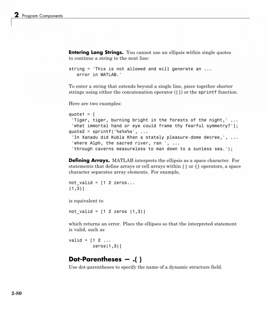
2 Program Components
Entering Long Strings. You cannot use an ellipsis within single quotesto continue a string to the next line:
string = 'This is not allowed and will generate an ...error in MATLAB.'
To enter a string that extends beyond a single line, piece together shorterstrings using either the concatenation operator ([]) or the sprintf function.
Here are two examples:
quote1 = ['Tiger, tiger, burning bright in the forests of the night,' ...'what immortal hand or eye could frame thy fearful symmetry?'];
quote2 = sprintf('%s%s%s', ...'In Xanadu did Kubla Khan a stately pleasure-dome decree,', ...'where Alph, the sacred river, ran ', ...'through caverns measureless to man down to a sunless sea.');
Defining Arrays. MATLAB interprets the ellipsis as a space character. Forstatements that define arrays or cell arrays within [] or {} operators, a spacecharacter separates array elements. For example,
not_valid = [1 2 zeros...(1,3)]
is equivalent to
not_valid = [1 2 zeros (1,3)]
which returns an error. Place the ellipses so that the interpreted statementis valid, such as
valid = [1 2 ...zeros(1,3)]
Dot-Parentheses — .( )Use dot-parentheses to specify the name of a dynamic structure field.
2-80

Symbol Reference
Dynamic Structure FieldsSometimes it is useful to reference structures with field names that canvary. For example, the referenced field might be passed as an argument to afunction. Dynamic field names specify a variable name for a structure field.
The variable fundtype shown here is a dynamic field name:
type = funds(5,2).(fundtype);
See “Generate Field Names from Variables” on page 9-11 for more information.
Exclamation Point — !The exclamation point precedes operating system commands that you want toexecute from within MATLAB.
Shell EscapeThe exclamation point initiates a shell escape function. Such a function is tobe performed directly by the operating system:
!rmdir oldtests
See “Shell Escape Functions” on page 2-73 for more information.
Parentheses — ( )Parentheses are used mostly for indexing into elements of an array or forspecifying arguments passed to a called function. Parenthesis also control theorder of operations, and can group a vector visually (such as x = (1:10))without calling a concatenation function.
Array IndexingWhen parentheses appear to the right of a variable name, they are indicesinto the array stored in that variable:
A(2, 7, 4)
2-81

2 Program Components
Function Input ArgumentsWhen parentheses follow a function name in a function declaration or call, theenclosed list contains input arguments used by the function:
function sendmail(to, subject, message, attachments)
Percent — %The percent sign is most commonly used to indicate nonexecutable text withinthe body of a program. This text is normally used to include comments in yourcode. Two percent signs, %%, serve as a cell delimiter described in “Run CodeSections” on page 16-6. Some functions also interpret the percent sign as aconversion specifier.
Single Line CommentsPrecede any one-line comments in your code with a percent sign. MATLABdoes not execute anything that follows a percent sign (that is, unless thesign is quoted, '%'):
% The purpose of this routine is to compute% the value of ...
See “Add Comments to Programs” on page 16-4 for more information.
Conversion SpecifiersSome functions, like sscanf and sprintf, precede conversion specifiers withthe percent sign:
sprintf('%s = %d', name, value)
Percent-Brace — %{ %}The %{ and %} symbols enclose a block of comments that extend beyond oneline.
Block CommentsEnclose any multiline comments with percent followed by an opening orclosing brace.
2-82

Symbol Reference
%{The purpose of this routine is to computethe value of ...%}
Note With the exception of whitespace characters, the %{ and %} operatorsmust appear alone on the lines that immediately precede and follow the blockof help text. Do not include any other text on these lines.
Plus — +The + sign appears most frequently as an arithmetic operator, but is alsoused to designate the names of package folders. For more information, see“Packages Create Namespaces”.
Semicolon — ;The semicolon can be used to construct arrays, suppress output from aMATLAB command, or to separate commands entered on the same line.
Array Row SeparatorWhen used within square brackets to create a new array or concatenateexisting arrays, the semicolon creates a new row in the array:
A = [5, 8; 3, 4]A =
5 83 4
Output SuppressionWhen placed at the end of a command, the semicolon tells MATLAB not todisplay any output from that command. In this example, MATLAB does notdisplay the resulting 100-by-100 matrix:
A = ones(100, 100);
2-83

2 Program Components
Command or Statement SeparatorLike the comma operator, you can enter more than one MATLAB commandon a line by separating each command with a semicolon. MATLAB suppressesoutput for those commands terminated with a semicolon, and displays theoutput for commands terminated with a comma.
In this example, assignments to variables A and C are terminated witha semicolon, and thus do not display. Because the assignment to B iscomma-terminated, the output of this one command is displayed:
A = 12.5; B = 42.7, C = 1.25;B =
42.7000
Single Quotes — ’ ’Single quotes are the constructor symbol for MATLAB character arrays.
Character and String ConstructorMATLAB constructs a character array from all characters enclosed in singlequotes. If only one character is in quotes, then MATLAB constructs a 1-by-1array:
S = 'Hello World'
For more information, see “Characters and Strings”
Space CharacterThe space character serves a purpose similar to the comma in that it can beused to separate row elements in an array constructor, or the values returnedby a function.
Row Element SeparatorYou have the option of using either commas or spaces to delimit the rowelements of an array when constructing the array. To create a 1-by-3 array,use
A = [5.92 8.13 3.53]
2-84

Symbol Reference
A =5.9200 8.1300 3.5300
When indexing into an array, you must always use commas to reference eachdimension of the array.
Function Output SeparatorSpaces are allowed when specifying a list of values to be returned by afunction. You can use spaces to separate return values in both functiondeclarations and function calls:
function [data text] = xlsread(file, sheet, range, mode)
Slash and Backslash — / \The slash (/) and backslash (\) characters separate the elements of a path orfolder string. On Microsoft Windows-based systems, both slash and backslashhave the same effect. On The Open Group UNIX-based systems, you mustuse slash only.
On a Windows system, you can use either backslash or slash:
dir([matlabroot '\toolbox\matlab\elmat\shiftdim.m'])dir([matlabroot '/toolbox/matlab/elmat/shiftdim.m'])
On a UNIX system, use only the forward slash:
dir([matlabroot '/toolbox/matlab/elmat/shiftdim.m'])
Square Brackets — [ ]Square brackets are used in array construction and concatenation, and also indeclaring and capturing values returned by a function.
Array ConstructorTo construct a matrix or array, enclose all elements of the array in squarebrackets:
A = [5.7, 9.8, 7.3; 9.2, 4.5, 6.4]
2-85

2 Program Components
ConcatenationTo combine two or more arrays into a new array through concatenation,enclose all array elements in square brackets:
A = [B, eye(6), diag([0:2:10])]
Function Declarations and CallsWhen declaring or calling a function that returns more than one output,enclose each return value that you need in square brackets:
[data, text] = xlsread(file, sheet, range, mode)
Tilde — ~The tilde character is used in comparing arrays for unequal values, findingthe logical NOT of an array, and as a placeholder for an input or outputargument you want to omit from a function call.
Not Equal toTo test for inequality values of elements in arrays a and b for inequality,use a~=b:
a = primes(29); b = [2 4 6 7 11 13 20 22 23 29];not_prime = b(a~=b)not_prime =
4 6 20 22
Logical NOTTo find those elements of an array that are zero, use:
a = [35 42 0 18 0 0 0 16 34 0];~aans =
0 0 1 0 1 1 1 0 0 1
2-86

Symbol Reference
Argument PlaceholderTo have the fileparts function return its third output value and skip thefirst two, replace arguments one and two with a tilde character:
[~, ~, filenameExt] = fileparts(fileSpec);
See “Ignore Function Inputs” on page 18-13 in the MATLAB Programmingdocumentation for more information.
2-87

2 Program Components
2-88

Classes (Data Types)
• Chapter 3, “Overview of MATLAB Classes”
• Chapter 4, “Numeric Classes”
• Chapter 5, “The Logical Class”
• Chapter 6, “Characters and Strings”
• Chapter 7, “Categorical Arrays”
• Chapter 8, “Tables”
• Chapter 9, “Structures”
• Chapter 10, “Cell Arrays”
• Chapter 11, “Function Handles”
• Chapter 12, “Map Containers”
• Chapter 13, “Combining Unlike Classes”
• Chapter 14, “Using Objects”
• Chapter 15, “Defining Your Own Classes”


3
Overview of MATLABClasses

3 Overview of MATLAB® Classes
Fundamental MATLAB ClassesThere are many different data types, or classes, that you can work with inthe MATLAB software. You can build matrices and arrays of floating-pointand integer data, characters and strings, and logical true and false states.Function handles connect your code with any MATLAB function regardless ofthe current scope. Tables, structures, and cell arrays provide a way to storedissimilar types of data in the same container.
There are 16 fundamental classes in MATLAB. Each of these classes is in theform of a matrix or array. With the exception of function handles, this matrixor array is a minimum of 0-by-0 in size and can grow to an n-dimensionalarray of any size. A function handle is always scalar (1-by-1).
All of the fundamental MATLAB classes are shown in the diagram below:
Numeric classes in the MATLAB software include signed and unsignedintegers, and single- and double-precision floating-point numbers. Bydefault, MATLAB stores all numeric values as double-precision floatingpoint. (You cannot change the default type and precision.) You can chooseto store any number, or array of numbers, as integers or as single-precision.Integer and single-precision arrays offer more memory-efficient storage thandouble-precision.
3-2

Fundamental MATLAB® Classes
All numeric types support basic array operations, such as subscripting,reshaping, and mathematical operations.
You can create two-dimensional double and logical matrices using one oftwo storage formats: full or sparse. For matrices with mostly zero-valuedelements, a sparse matrix requires a fraction of the storage space requiredfor an equivalent full matrix. Sparse matrices invoke methods especiallytailored to solve sparse problems
These classes require different amounts of storage, the smallest being alogical value or 8-bit integer which requires only 1 byte. It is important tokeep this minimum size in mind if you work on data in files that were writtenusing a precision smaller than 8 bits.
The following table describes the fundamental classes in more detail.
Class Name Documentation Intended Use
double, single Floating-PointNumbers
• Required for fractional numeric data.
• Double and Single precision.
• Use realmin and realmax to show range of values.
• Two-dimensional arrays can be sparse.
• Default numeric type in MATLAB.
int8, uint8,int16,uint16,int32,uint32,int64, uint64
Integers • Use for signed and unsigned whole numbers.
• More efficient use of memory.
• Use intmin and intmax to show range of values.
• Choose from 4 sizes (8, 16, 32, and 64 bits).
3-3

3 Overview of MATLAB® Classes
Class Name Documentation Intended Use
char “Characters andStrings”
• Data type for text.
• Native or Unicode®.
• Converts to/from numeric.
• Use with regular expressions.
• For multiple strings, use cell arrays.
logical “LogicalOperations”
• Use in relational conditions or to test state.
• Can have one of two values: true or false.
• Also useful in array indexing.
• Two-dimensional arrays can be sparse.
function_handle “FunctionHandles”
• Pointer to a function.
• Enables passing a function to another function
• Can also call functions outside usual scope.
• Useful in Handle Graphics callbacks.
• Save to MAT-file and restore later.
3-4

Fundamental MATLAB® Classes
Class Name Documentation Intended Use
table “Tables” • Rectangular container for mixed-type, column-orienteddata.
• Row and variable names identify contents.
• Use Table Properties to store metadata such asvariable units.
• Manipulation of elements similar to numeric or logicalarrays.
• Access data by numeric or named index.
• Can select a subset of data and preserve the tablecontainer or can extract the data from a table.
struct “Structures” • Fields store arrays of varying classes and sizes.
• Access one or all fields/indices in single operation.
• Field names identify contents.
• Method of passing function arguments.
• Use in comma-separated lists.
• More memory required for overhead
cell “Cell Arrays” • Cells store arrays of varying classes and sizes.
• Allows freedom to package data as you want.
• Manipulation of elements is similar to numeric orlogical arrays.
• Method of passing function arguments.
• Use in comma-separated lists.
• More memory required for overhead
Concepts • “Valid Combinations of Unlike Classes” on page 13-2
3-5

3 Overview of MATLAB® Classes
3-6

4
Numeric Classes
• “Overview of Numeric Classes” on page 4-2
• “Integers” on page 4-3
• “Floating-Point Numbers” on page 4-7
• “Complex Numbers” on page 4-18
• “Infinity and NaN” on page 4-20
• “Identifying Numeric Classes” on page 4-22
• “Display Format for Numeric Values” on page 4-23
• “Function Summary” on page 4-26

4 Numeric Classes
Overview of Numeric ClassesNumeric classes in the MATLAB software include signed and unsignedintegers, and single- and double-precision floating-point numbers. Bydefault, MATLAB stores all numeric values as double-precision floatingpoint. (You cannot change the default type and precision.) You can chooseto store any number, or array of numbers, as integers or as single-precision.Integer and single-precision arrays offer more memory-efficient storage thandouble-precision.
All numeric types support basic array operations, such as subscripting,reshaping, and mathematical operations.
4-2

Integers
Integers
In this section...
“Integer Classes” on page 4-3
“Creating Integer Data” on page 4-4
“Arithmetic Operations on Integer Classes” on page 4-5
“Largest and Smallest Values for Integer Classes” on page 4-6
“Integer Functions” on page 4-6
Integer ClassesMATLAB has four signed and four unsigned integer classes. Signed typesenable you to work with negative integers as well as positive, but cannotrepresent as wide a range of numbers as the unsigned types because one bitis used to designate a positive or negative sign for the number. Unsignedtypes give you a wider range of numbers, but these numbers can only bezero or positive.
MATLAB supports 1-, 2-, 4-, and 8-byte storage for integer data. You cansave memory and execution time for your programs if you use the smallestinteger type that accommodates your data. For example, you do not need a32-bit integer to store the value 100.
Here are the eight integer classes, the range of values you can store with eachtype, and the MATLAB conversion function required to create that type:
Class Range of Values Conversion Function
Signed 8-bit integer -27 to 27-1 int8
Signed 16-bit integer -215 to 215-1 int16
Signed 32-bit integer -231 to 231-1 int32
Signed 64-bit integer -263 to 263-1 int64
Unsigned 8-bit integer 0 to 28-1 uint8
Unsigned 16-bit integer 0 to 216-1 uint16
4-3

4 Numeric Classes
Class Range of Values Conversion Function
Unsigned 32-bit integer 0 to 232-1 uint32
Unsigned 64-bit integer 0 to 264-1 uint64
Creating Integer DataMATLAB stores numeric data as double-precision floating point (double)by default. To store data as an integer, you need to convert from double tothe desired integer type. Use one of the conversion functions shown in thetable above.
For example, to store 325 as a 16-bit signed integer assigned to variable x, type
x = int16(325);
If the number being converted to an integer has a fractional part, MATLABrounds to the nearest integer. If the fractional part is exactly 0.5, then fromthe two equally nearby integers, MATLAB chooses the one for which theabsolute value is larger in magnitude:
x = 325.499; x = x + .001;
int16(x) int16(x)ans = ans =
325 326
If you need to round a number using a rounding scheme other than thedefault, MATLAB provides four rounding functions: round, fix, floor, andceil. The fix function enables you to override the default and round towardszero when there is a nonzero fractional part:
x = 325.9;
int16(fix(x))ans =
325
Arithmetic operations that involve both integers and floating-point alwaysresult in an integer data type. MATLAB rounds the result, when necessary,
4-4

Integers
according to the default rounding algorithm. The example below yields anexact answer of 1426.75 which MATLAB then rounds to the next highestinteger:
int16(325) * 4.39ans =
1427
The integer conversion functions are also useful when converting otherclasses, such as strings, to integers:
str = 'Hello World';
int8(str)ans =
72 101 108 108 111 32 87 111 114 108 100
Arithmetic Operations on Integer ClassesMATLAB can perform integer arithmetic on the following types of data:
• Integers or integer arrays of the same integer data type. This yields aresult that has the same data type as the operands:
x = uint32([132 347 528]) .* uint32(75);class(x)ans =
uint32
• Integers or integer arrays and scalar double-precision floating-pointnumbers. This yields a result that has the same data type as the integeroperands:
x = uint32([132 347 528]) .* 75.49;class(x)ans =
uint32
For all binary operations in which one operand is an array of integer datatype (except 64-bit integers) and the other is a scalar double, MATLABcomputes the operation using elementwise double-precision arithmetic, andthen converts the result back to the original integer data type. For binary
4-5

4 Numeric Classes
operations involving a 64-bit integer array and a scalar double, MATLABcomputes the operation as if 80-bit extended-precision arithmetic were used,to prevent loss of precision.
Largest and Smallest Values for Integer ClassesFor each integer data type, there is a largest and smallest number that youcan represent with that type. The table shown under “Integers” on page 4-3lists the largest and smallest values for each integer data type in the “Rangeof Values” column.
You can also obtain these values with the intmax and intmin functions:
intmax('int8') intmin('int8')ans = ans =
127 -128
If you convert a number that is larger than the maximum value of an integerdata type to that type, MATLAB sets it to the maximum value. Similarly, ifyou convert a number that is smaller than the minimum value of the integerdata type, MATLAB sets it to the minimum value. For example,
x = int8(300) x = int8(-300)x = x =
127 -128
Also, when the result of an arithmetic operation involving integers exceedsthe maximum (or minimum) value of the data type, MATLAB sets it to themaximum (or minimum) value:
x = int8(100) * 3 x = int8(-100) * 3x = x =
127 -128
Integer FunctionsSee Integer Functions on page 4-26 for a list of functions most commonly usedwith integers in MATLAB.
4-6

Floating-Point Numbers
Floating-Point Numbers
In this section...
“Double-Precision Floating Point” on page 4-7
“Single-Precision Floating Point” on page 4-8
“Creating Floating-Point Data” on page 4-8
“Arithmetic Operations on Floating-Point Numbers” on page 4-10
“Largest and Smallest Values for Floating-Point Classes” on page 4-11
“Accuracy of Floating-Point Data” on page 4-12
“Avoiding Common Problems with Floating-Point Arithmetic” on page 4-14
“Floating-Point Functions” on page 4-16
“References” on page 4-16
MATLAB represents floating-point numbers in either double-precision orsingle-precision format. The default is double precision, but you can makeany number single precision with a simple conversion function.
Double-Precision Floating PointMATLAB constructs the double-precision (or double) data type accordingto IEEE® Standard 754 for double precision. Any value stored as a doublerequires 64 bits, formatted as shown in the table below:
Bits Usage
63 Sign (0 = positive, 1 = negative)
62 to 52 Exponent, biased by 1023
51 to 0 Fraction f of the number 1.f
4-7

4 Numeric Classes
Single-Precision Floating PointMATLAB constructs the single-precision (or single) data type accordingto IEEE Standard 754 for single precision. Any value stored as a singlerequires 32 bits, formatted as shown in the table below:
Bits Usage
31 Sign (0 = positive, 1 = negative)
30 to 23 Exponent, biased by 127
22 to 0 Fraction f of the number 1.f
Because MATLAB stores numbers of type single using 32 bits, they requireless memory than numbers of type double, which use 64 bits. However,because they are stored with fewer bits, numbers of type single arerepresented to less precision than numbers of type double.
Creating Floating-Point DataUse double-precision to store values greater than approximately 3.4 x 1038
or less than approximately -3.4 x 1038. For numbers that lie between thesetwo limits, you can use either double- or single-precision, but single requiresless memory.
Creating Double-Precision DataBecause the default numeric type for MATLAB is double, you can create adouble with a simple assignment statement:
x = 25.783;
The whos function shows that MATLAB has created a 1-by-1 array of typedouble for the value you just stored in x:
whos xName Size Bytes Class
x 1x1 8 double
4-8

Floating-Point Numbers
Use isfloat if you just want to verify that x is a floating-point number. Thisfunction returns logical 1 (true) if the input is a floating-point number, andlogical 0 (false) otherwise:
isfloat(x)ans =
1
You can convert other numeric data, characters or strings, and logical data todouble precision using the MATLAB function, double. This example convertsa signed integer to double-precision floating point:
y = int64(-589324077574); % Create a 64-bit integer
x = double(y) % Convert to doublex =
-5.8932e+11
Creating Single-Precision DataBecause MATLAB stores numeric data as a double by default, you need touse the single conversion function to create a single-precision number:
x = single(25.783);
The whos function returns the attributes of variable x in a structure. Thebytes field of this structure shows that when x is stored as a single, it requiresjust 4 bytes compared with the 8 bytes to store it as a double:
xAttrib = whos('x');xAttrib.bytesans =
4
You can convert other numeric data, characters or strings, and logical data tosingle precision using the single function. This example converts a signedinteger to single-precision floating point:
y = int64(-589324077574); % Create a 64-bit integer
x = single(y) % Convert to single
4-9

4 Numeric Classes
x =-5.8932e+11
Arithmetic Operations on Floating-Point NumbersThis section describes which classes you can use in arithmetic operationswith floating-point numbers.
Double-Precision OperationsYou can perform basic arithmetic operations with double and any of thefollowing other classes. When one or more operands is an integer (scalar orarray), the double operand must be a scalar. The result is of type double,except where noted otherwise:
• single — The result is of type single
• double
• int* or uint*— The result has the same data type as the integer operand
• char
• logical
This example performs arithmetic on data of types char and double. Theresult is of type double:
c = 'uppercase' - 32;
class(c)ans =
double
char(c)ans =
UPPERCASE
Single-Precision OperationsYou can perform basic arithmetic operations with single and any of thefollowing other classes. The result is always single:
4-10

Floating-Point Numbers
• single
• double
• char
• logical
In this example, 7.5 defaults to type double, and the result is of type single:
x = single([1.32 3.47 5.28]) .* 7.5;
class(x)ans =
single
Largest and Smallest Values for Floating-PointClassesFor the double and single classes, there is a largest and smallest numberthat you can represent with that type.
Largest and Smallest Double-Precision ValuesThe MATLAB functions realmax and realmin return the maximum andminimum values that you can represent with the double data type:
str = 'The range for double is:\n\t%g to %g and\n\t %g to %g';sprintf(str, -realmax, -realmin, realmin, realmax)
ans =The range for double is:
-1.79769e+308 to -2.22507e-308 and2.22507e-308 to 1.79769e+308
Numbers larger than realmax or smaller than -realmax are assigned thevalues of positive and negative infinity, respectively:
realmax + .0001e+308ans =
Inf
-realmax - .0001e+308
4-11

4 Numeric Classes
ans =-Inf
Largest and Smallest Single-Precision ValuesThe MATLAB functions realmax and realmin, when called with theargument 'single', return the maximum and minimum values that you canrepresent with the single data type:
str = 'The range for single is:\n\t%g to %g and\n\t %g to %g';sprintf(str, -realmax('single'), -realmin('single'), ...
realmin('single'), realmax('single'))
ans =The range for single is:-3.40282e+38 to -1.17549e-38 and1.17549e-38 to 3.40282e+38
Numbers larger than realmax('single') or smaller than-realmax('single') are assigned the values of positive and negativeinfinity, respectively:
realmax('single') + .0001e+038ans =
Inf
-realmax('single') - .0001e+038ans =
-Inf
Accuracy of Floating-Point DataIf the result of a floating-point arithmetic computation is not as precise asyou had expected, it is likely caused by the limitations of your computer’shardware. Probably, your result was a little less exact because the hardwarehad insufficient bits to represent the result with perfect accuracy; therefore, ittruncated the resulting value.
4-12

Floating-Point Numbers
Double-Precision AccuracyBecause there are only a finite number of double-precision numbers, youcannot represent all numbers in double-precision storage. On any computer,there is a small gap between each double-precision number and the next largerdouble-precision number. You can determine the size of this gap, which limitsthe precision of your results, using the eps function. For example, to find thedistance between 5 and the next larger double-precision number, enter
format long
eps(5)ans =
8.881784197001252e-16
This tells you that there are no double-precision numbers between 5 and5 + eps(5). If a double-precision computation returns the answer 5, theresult is only accurate to within eps(5).
The value of eps(x) depends on x. This example shows that, as x gets larger,so does eps(x):
eps(50)ans =
7.105427357601002e-15
If you enter eps with no input argument, MATLAB returns the value ofeps(1), the distance from 1 to the next larger double-precision number.
Single-Precision AccuracySimilarly, there are gaps between any two single-precision numbers. If xhas type single, eps(x) returns the distance between x and the next largersingle-precision number. For example,
x = single(5);eps(x)
returns
ans =4.7684e-07
4-13

4 Numeric Classes
Note that this result is larger than eps(5). Because there are fewersingle-precision numbers than double-precision numbers, the gapsbetween the single-precision numbers are larger than the gaps betweendouble-precision numbers. This means that results in single-precisionarithmetic are less precise than in double-precision arithmetic.
For a number x of type double, eps(single(x)) gives you an upper boundfor the amount that x is rounded when you convert it from double to single.For example, when you convert the double-precision number 3.14 to single,it is rounded by
double(single(3.14) - 3.14)ans =
1.0490e-07
The amount that 3.14 is rounded is less than
eps(single(3.14))ans =
2.3842e-07
Avoiding Common Problems with Floating-PointArithmeticAlmost all operations in MATLAB are performed in double-precisionarithmetic conforming to the IEEE standard 754. Because computers onlyrepresent numbers to a finite precision (double precision calls for 52 mantissabits), computations sometimes yield mathematically nonintuitive results. It isimportant to note that these results are not bugs in MATLAB.
Use the following examples to help you identify these cases:
Example 1 — Round-Off or What You Get Is Not What YouExpectThe decimal number 4/3 is not exactly representable as a binary fraction. Forthis reason, the following calculation does not give zero, but rather revealsthe quantity eps.
e = 1 - 3*(4/3 - 1)
4-14

Floating-Point Numbers
e =2.2204e-16
Similarly, 0.1 is not exactly representable as a binary number. Thus, you getthe following nonintuitive behavior:
a = 0.0;for i = 1:10
a = a + 0.1;enda == 1
ans =0
Note that the order of operations can matter in the computation:
b = 1e-16 + 1 - 1e-16;c = 1e-16 - 1e-16 + 1;b == c
ans =0
There are gaps between floating-point numbers. As the numbers get larger,so do the gaps, as evidenced by:
(2^53 + 1) - 2^53
ans =0
Since pi is not really pi, it is not surprising that sin(pi) is not exactly zero:
sin(pi)
ans =1.224646799147353e-16
4-15

4 Numeric Classes
Example 2 — Catastrophic CancellationWhen subtractions are performed with nearly equal operands, sometimescancellation can occur unexpectedly. The following is an example of acancellation caused by swamping (loss of precision that makes the additioninsignificant).
sqrt(1e-16 + 1) - 1
ans =0
Some functions in MATLAB, such as expm1 and log1p, may be used tocompensate for the effects of catastrophic cancellation.
Example 3 — Floating-Point Operations and Linear AlgebraRound-off, cancellation, and other traits of floating-point arithmetic combineto produce startling computations when solving the problems of linearalgebra. MATLAB warns that the following matrix A is ill-conditioned, andtherefore the system Ax = b may be sensitive to small perturbations:
A = diag([2 eps]);b = [2; eps];y = A\b;Warning: Matrix is close to singular or badly scaled.
Results may be inaccurate. RCOND = 1.110223e-16.
These are only a few of the examples showing how IEEE floating-pointarithmetic affects computations in MATLAB. Note that all computationsperformed in IEEE 754 arithmetic are affected, this includes applicationswritten in C or FORTRAN, as well as MATLAB.
Floating-Point FunctionsSee Floating-Point Functions on page 4-27 for a list of functions mostcommonly used with floating-point numbers in MATLAB.
ReferencesThe following references provide more information about floating-pointarithmetic.
4-16

Floating-Point Numbers
References[1] Moler, Cleve, “Floating Points,” MATLAB News and Notes, Fall,1996. A PDF version is available on the MathWorks Web site athttp://www.mathworks.com/company/newsletters/news_notes/pdf/Fall96Cleve.pdf
[2] Moler, Cleve, Numerical Computing with MATLAB, S.I.A.M.A PDF version is available on the MathWorks Web site athttp://www.mathworks.com/moler/.
4-17

4 Numeric Classes
Complex Numbers
In this section...
“Creating Complex Numbers” on page 4-18
“Complex Number Functions” on page 4-19
Creating Complex NumbersComplex numbers consist of two separate parts: a real part and an imaginarypart. The basic imaginary unit is equal to the square root of -1. This isrepresented in MATLAB by either of two letters: i or j.
The following statement shows one way of creating a complex value inMATLAB. The variable x is assigned a complex number with a real part of 2and an imaginary part of 3:
x = 2 + 3i;
Another way to create a complex number is using the complex function. Thisfunction combines two numeric inputs into a complex output, making the firstinput real and the second imaginary:
x = rand(3) * 5;y = rand(3) * -8;
z = complex(x, y)z =
4.7842 -1.0921i 0.8648 -1.5931i 1.2616 -2.2753i2.6130 -0.0941i 4.8987 -2.3898i 4.3787 -3.7538i4.4007 -7.1512i 1.3572 -5.2915i 3.6865 -0.5182i
You can separate a complex number into its real and imaginary parts usingthe real and imag functions:
zr = real(z)zr =
4.7842 0.8648 1.26162.6130 4.8987 4.37874.4007 1.3572 3.6865
4-18
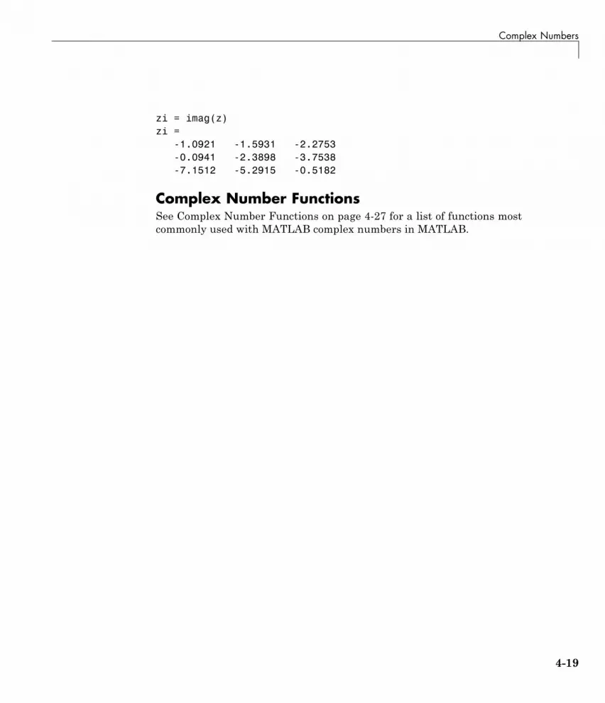
Complex Numbers
zi = imag(z)zi =
-1.0921 -1.5931 -2.2753-0.0941 -2.3898 -3.7538-7.1512 -5.2915 -0.5182
Complex Number FunctionsSee Complex Number Functions on page 4-27 for a list of functions mostcommonly used with MATLAB complex numbers in MATLAB.
4-19

4 Numeric Classes
Infinity and NaN
In this section...
“Infinity” on page 4-20
“NaN” on page 4-20
“Infinity and NaN Functions” on page 4-21
InfinityMATLAB represents infinity by the special value inf. Infinity results fromoperations like division by zero and overflow, which lead to results too largeto represent as conventional floating-point values. MATLAB also providesa function called inf that returns the IEEE arithmetic representation forpositive infinity as a double scalar value.
Several examples of statements that return positive or negative infinity inMATLAB are shown here.
x = 1/0x =Inf
x = 1.e1000x =
Inf
x = exp(1000)x =
Inf
x = log(0)x =
-Inf
Use the isinf function to verify that x is positive or negative infinity:
x = log(0);
isinf(x)ans =
1
NaNMATLAB represents values that are not real or complex numbers with aspecial value called NaN, which stands for Not a Number. Expressions like 0/0and inf/inf result in NaN, as do any arithmetic operations involving a NaN:
4-20

Infinity and NaN
x = 0/0x =
NaN
Use the isnan function to verify that the real part of x is NaN:
isnan(x)ans =
1
MATLAB also provides a function called NaN that returns the IEEE arithmeticrepresentation for NaN as a double scalar value:
x = NaN;
whos xName Size Bytes Class
x 1x1 8 double
Logical Operations on NaNBecause two NaNs are not equal to each other, logical operations involving NaNalways return false, except for a test for inequality, (NaN ~= NaN):
NaN > NaNans =
0
NaN ~= NaNans =
1
Infinity and NaN FunctionsSee Infinity and NaN Functions on page 4-28 for a list of functions mostcommonly used with inf and NaN in MATLAB.
4-21

4 Numeric Classes
Identifying Numeric ClassesYou can check the data type of a variable x using any of these commands.
Command Operation
whos x Display the data type of x.
xType = class(x); Assign the data type of x to a variable.
isnumeric(x) Determine if x is a numeric type.
isa(x, 'integer')isa(x, 'uint64')isa(x, 'float')isa(x, 'double')isa(x, 'single')
Determine if x is the specified numeric type.(Examples for any integer, unsigned 64-bit integer,any floating point, double precision, and singleprecision are shown here).
isreal(x) Determine if x is real or complex.
isnan(x) Determine if x is Not a Number (NaN).
isinf(x) Determine if x is infinite.
isfinite(x) Determine if x is finite.
4-22

Display Format for Numeric Values
Display Format for Numeric Values
In this section...
“Default Display” on page 4-23
“Display Format Examples” on page 4-23
“Setting Numeric Format in a Program” on page 4-24
Default DisplayBy default, MATLAB displays numeric output as 5-digit scaled, fixed-pointvalues. You can change the way numeric values are displayed to any of thefollowing:
• 5-digit scaled fixed point, floating point, or the best of the two
• 15-digit scaled fixed point, floating point, or the best of the two
• A ratio of small integers
• Hexadecimal (base 16)
• Bank notation
All available formats are listed on the format reference page.
To change the numeric display setting, use either the format function orthe Preferences dialog box (accessible from the MATLAB File menu). Theformat function changes the display of numeric values for the duration of asingle MATLAB session, while your Preferences settings remain active fromone session to the next. These settings affect only how numbers are displayed,not how MATLAB computes or saves them.
Display Format ExamplesHere are a few examples of the various formats and the output produced fromthe following two-element vector x, with components of different magnitudes.
Check the current format setting:
get(0, 'format')
4-23

4 Numeric Classes
ans =short
Set the value for x and display in 5-digit scaled fixed point:
x = [4/3 1.2345e-6]x =
1.3333 0.0000
Set the format to 5-digit floating point:
format short exx =
1.3333e+00 1.2345e-06
Set the format to 15-digit scaled fixed point:
format longxx =
1.333333333333333 0.000001234500000
Set the format to 'rational' for small integer ratio output:
format rationalxx =
4/3 1/810045
Set an integer value for x and display it in hexadecimal (base 16) format:
format hexx = uint32(876543210)x =
343efcea
Setting Numeric Format in a ProgramTo temporarily change the numeric format inside a program, get the originalformat using the get function and save it in a variable. When you finish
4-24

Display Format for Numeric Values
working with the new format, you can restore the original format settingusing the set function as shown here:
origFormat = get(0, 'format');format('rational');
-- Work in rational format --
set(0,'format', origFormat);
4-25

4 Numeric Classes
Function SummaryMATLAB provides these functions for working with numeric classes:
• Integer Functions on page 4-26
• Floating-Point Functions on page 4-27
• Complex Number Functions on page 4-27
• Infinity and NaN Functions on page 4-28
• Class Identification Functions on page 4-28
• Output Formatting Functions on page 4-28
Integer Functions
Function Description
int8, int16,int32, int64
Convert to signed 1-, 2-, 4-, or 8-byte integer.
uint8, uint16,uint32, uint64
Convert to unsigned 1-, 2-, 4-, or 8-byte integer.
ceil Round towards plus infinity to nearest integer
class Return the data type of an object.
fix Round towards zero to nearest integer
floor Round towards minus infinity to nearest integer
isa Determine if input value has the specified data type.
isinteger Determine if input value is an integer array.
isnumeric Determine if input value is a numeric array.
round Round towards the nearest integer
4-26

Function Summary
Floating-Point Functions
Function Description
double Convert to double precision.
single Convert to single precision.
class Return the data type of an object.
isa Determine if input value has the specified data type.
isfloat Determine if input value is a floating-point array.
isnumeric Determine if input value is a numeric array.
eps Return the floating-point relative accuracy. This valueis the tolerance MATLAB uses in its calculations.
realmax Return the largest floating-point number your computercan represent.
realmin Return the smallest floating-point number yourcomputer can represent.
Complex Number Functions
Function Description
complex Construct complex data from real and imaginarycomponents.
i or j Return the imaginary unit used in constructing complexdata.
real Return the real part of a complex number.
imag Return the imaginary part of a complex number.
isreal Determine if a number is real or imaginary.
4-27

4 Numeric Classes
Infinity and NaN Functions
Function Description
inf Return the IEEE value for infinity.
isnan Detect NaN elements of an array.
isinf Detect infinite elements of an array.
isfinite Detect finite elements of an array.
nan Return the IEEE value for Not a Number.
Class Identification Functions
Function Description
class Return data type (or class).
isa Determine if input value is of the specified data type.
isfloat Determine if input value is a floating-point array.
isinteger Determine if input value is an integer array.
isnumeric Determine if input value is a numeric array.
isreal Determine if input value is real.
whos Display the data type of input.
Output Formatting Functions
Function Description
format Control display format for output.
4-28

5
The Logical Class
• “Find Array Elements That Meet a Condition” on page 5-2
• “Determine if Arrays Are Logical” on page 5-8
• “Reduce Logical Arrays to Single Value” on page 5-12
• “Truth Table for Logical Operations” on page 5-15

5 The Logical Class
Find Array Elements That Meet a ConditionYou can filter the elements of an array by applying one or more conditionsto the array. For instance, if you want to examine only the even elements ina matrix, find the location of all 0s in a multidimensional array, or replaceNaN values in a discrete set of data. You can perform these tasks using acombination of the relational and logical operators. The relational operators(>, <, >=, <=, ==, ~=) impose conditions on the array, and you can applymultiple conditions by connecting them with the logical operators and, or, andnot, respectively denoted by &, |, and ~.
In this section...
“Apply a Single Condition” on page 5-2
“Apply Multiple Conditions” on page 5-4
“Replace Values that Meet a Condition” on page 5-5
Apply a Single ConditionTo apply a single condition, start by creating a 5-by-5 matrix, A, that containsrandom integers between 1 and 15.
rng(0);A = randi(15,5)
A =
13 2 3 3 1014 5 15 7 12 9 15 14 13
14 15 8 12 1510 15 13 15 11
Use the relational less than operator, <, to determine which elements of Aare less than 9. Store the result in B.
B = A < 9
B =
5-2

Find Array Elements That Meet a Condition
0 1 1 1 00 1 0 1 11 0 0 0 00 0 1 0 00 0 0 0 0
The result is a logical matrix. Each value in B represents a logical 1 (true)or logical 0 (false) state to indicate whether the corresponding element of Afulfills the condition A < 9. For example, A(1,1) is 13, so B(1,1) is logical 0(false). However, A(1,2) is 2, so B(1,2) is logical 1 (true).
Although B contains information about which elements in A are less than9, it doesn’t tell you what their values are. Rather than comparing the twomatrices element by element, use B to index into A.
A(B)
ans =
22538371
The result is a column vector of the elements in A that are less than 9. SinceB is a logical matrix, this operation is called logical indexing. In this case,the logical array being used as an index is the same size as the other array,but this is not a requirement. For more information, see “Using Logicals inArray Indexing”.
Some problems require information about the locations of the array elementsthat meet a condition rather than their actual values. In this example, usethe find function to locate all of the elements in A less than 9.
I = find(A < 9)
I =
5-3

5 The Logical Class
367
1114161722
The result is a column vector of linear indices. Each index describes thelocation of an element in A that is less than 9, so in practice A(I) returnsthe same result as A(B). The difference is that A(B) uses logical indexing,whereas A(I) uses linear indexing.
Apply Multiple ConditionsYou can use the logical and, or, and not operators to apply any number ofconditions to an array; the number of conditions is not limited to one or two.
First, use the logical and operator, denoted &, to specify two conditions: theelements must be less than 9 AND greater than 2. Specify the conditions as alogical index to view the elements that satisfy both conditions.
A(A<9 & A>2)
ans =
53837
The result is a list of the elements in A that satisfy both conditions. Be sureto specify each condition with a separate statement connected by a logicaloperator. For example, you cannot specify the conditions above by A(2<A<9),since it evaluates to A(2<A | A<9).
Next, find the elements in A that are less than 9 AND even numbered.
5-4

Find Array Elements That Meet a Condition
A(A<9 & ~mod(A,2))
ans =
228
The result is a list of all even elements in A that are less than 9. The useof the logical NOT operator, ~, converts the matrix mod(A,2) into a logicalmatrix, with a value of logical 1 (true) located where an element is evenlydivisible by 2.
Finally, find the elements in A that are less than 9 AND even numberedAND not equal to 2.
A(A<9 & ~mod(A,2) & A~=2)
ans =
8
The result, 8, is even, less than 9, and not equal to 2. It is the only element inA that satisfies all three conditions.
Use the find function to get the index of the 8 element that satisfies theconditions.
find(A<9 & ~mod(A,2) & A~=2)
ans =
14
The result indicates that A(14) = 8.
Replace Values that Meet a ConditionSometimes it is useful to simultaneously change the values of several existingarray elements. Use logical indexing with a simple assignment statement toreplace the values in an array that meet a condition.
5-5

5 The Logical Class
Replace all values in A that are greater than 10 with the number 10.
A(A>10) = 10
A =
10 2 3 3 1010 5 10 7 12 9 10 10 10
10 10 8 10 1010 10 10 10 10
A now has a maximum value of 10.
Replace all values in A that are not equal to 10 with a NaN value.
A(A~=10) = NaN
A =
10 NaN NaN NaN 1010 NaN 10 NaN NaN
NaN NaN 10 10 1010 10 NaN 10 1010 10 10 10 10
The resulting matrix has element values of 10 or NaN.
Replace all of the NaN values in A with zeros and apply the logical NOToperator, ~A.
A(isnan(A)) = 0;C = ~A
C =
0 1 1 1 00 1 0 1 11 1 0 0 00 0 1 0 00 0 0 0 0
5-6

Find Array Elements That Meet a Condition
The resulting matrix has values of logical 1 (true) in place of the NaN values,and logical 0 (false) in place of the 10s. The logical NOT operation, ~A,converts the numeric array into a logical array such that A&C returns a matrixof logical 0 (false) values and A|C returns a matrix of logical 1 (true) values.
See Also nan | Logical Operators: Short Circuit | isnan | find | and | or| xor | not
5-7

5 The Logical Class
Determine if Arrays Are LogicalTo determine whether an array is logical, you can test the entire array or eachelement individually. This is useful when you want to confirm the outputdata type of a function.
This page shows several ways to determine if an array is logical.
In this section...
“Identify Logical Matrix” on page 5-8
“Test an Entire Array” on page 5-9
“Test Each Array Element” on page 5-9
“Summary Table” on page 5-10
Identify Logical MatrixCreate a 3-by-6 matrix and locate all elements greater than 0.5.
A = gallery('uniformdata',[3,6],0) > 0.5
A =
1 0 0 0 1 00 1 0 1 1 11 1 1 1 0 1
The result, A, is a 3-by-6 logical matrix.
Use the whos function to confirm the size, byte count, and class (or data type)of the matrix, A.
whos A
Name Size Bytes Class Attributes
A 3x6 18 logical
The result confirms that A is a 3-by-6 logical matrix.
5-8

Determine if Arrays Are Logical
Test an Entire ArrayUse the islogical function to test whether A is logical.
islogical(A)
ans =
1
The result is logical 1 (true).
Use the class function to display a string with the class name of A.
class(A)
ans =
logical
The result confirms that A is logical.
Test Each Array ElementCreate a cell array, C, and use the 'islogical' option of the cellfun functionto identify which cells contain logical values.
C = {1, 0, true, false, pi, A};cellfun('islogical',C)
ans =
0 0 1 1 0 1
The result is a logical array of the same size as C.
To test each element in a numeric matrix, use the arrayfun function.
arrayfun(@islogical,A)
ans =
1 1 1 1 1 1
5-9

5 The Logical Class
1 1 1 1 1 11 1 1 1 1 1
The result is a matrix of logical values of the same size as A.arrayfun(@islogical,A) always returns a matrix of all logical 1 (true)or logical 0 (false) values.
Summary TableUse these MATLAB functions to determine if an array is logical.
Function Syntax Output Size Description
whos(A) N/A Displays the name,size, storage bytes,class, and attributes ofvariable A.
islogical(A) scalar Returns logical 1(true) if A is a logicalarray; otherwise, itreturns logical 0(false). The resultis the same as usingisa(A,'logical').
isa(A,'logical') scalar Returns logical 1 (true)if A is a logical array;otherwise, it returnslogical 0 (false). Theresult is the same asusing islogical(A).
class(A) single string Returns a string withthe name of the class ofvariable A.
5-10

Determine if Arrays Are Logical
Function Syntax Output Size Description
cellfun('islogical',A)Array of the same sizeas A
For cell arrays only.Returns logical 1(true) for each cell thatcontains a logical array;otherwise, it returnslogical 0 (false).
arrayfun(@islogical,A)Array of the same sizeas A
Returns an array oflogical 1 (true) valuesif A is logical; otherwise,it returns an array oflogical 0 (false) values.
See Also islogical | isa | class | cellfun | arrayfun | whos
5-11

5 The Logical Class
Reduce Logical Arrays to Single ValueSometimes the result of a calculation produces an entire numeric or logicalarray when you need only a single logical true or false value. In this case,use the any or all functions to reduce the array to a single scalar logical forfurther computations.
The any and all functions are natural extensions of the logical | (OR) and& (AND) operators, respectively. However, rather than comparing justtwo elements, the any and all functions compare all of the elements in aparticular dimension of an array. It is as if all of those elements are connectedby & or | operators and the any or all functions evaluate the resulting longlogical expression(s). Therefore, unlike the core logical operators, the anyand all functions reduce the size of the array dimension that they operateon so that it has size 1. This enables the reduction of many logical valuesinto a single logical condition.
First, create a matrix, A, that contains random integers between 1 and 25.
rng(0)A = randi(25,5)
A =
21 3 4 4 1723 7 25 11 14 14 24 23 22
23 24 13 20 2416 25 21 24 17
Next, use the mod function along with the logical NOT operator, ~, todetermine which elements in A are even.
A = ~mod(A,2)
A =
0 0 1 1 00 0 0 0 01 1 1 0 1
5-12

Reduce Logical Arrays to Single Value
0 1 0 1 11 0 0 1 0
The resulting matrices have values of logical 1 (true) where an element iseven, and logical 0 (false) where an element is odd.
Since the any and all functions reduce the dimension that they operate on tosize 1, it normally takes two applications of one of the functions to reduce a2–D matrix into a single logical condition, such as any(any(A)). However,if you use the notation A(:) to regard all of the elements of A as a singlecolumn vector, you can use any(A(:)) to get the same logical informationwithout nesting the function calls.
Determine if any elements in A are even.
any(A(:))
ans =
1
The result is logical 1 (true).
You can perform logical and relational comparisons within the function callto any or all. This makes it easy to quickly test an array for a variety ofproperties.
Determine if all elements in A are odd.
all(~A(:))
ans =
0
The result is logical 0 (false).
Determine whether any main or super diagonal elements in A are even.
any(diag(A) | diag(A,1))
Error using |
5-13

5 The Logical Class
Inputs must have the same size.
MATLAB returns an error since the vectors returned by diag(A) anddiag(A,1) are not the same size.
To reduce each diagonal to a single scalar logical condition and allow logicalshort-circuiting, use the any function on each side of the short-circuit ORoperator, ||.
any(diag(A)) || any(diag(A,1))
ans =
1
The result is logical 1 (true). It no longer matters that diag(A) anddiag(A,1) are not the same size.
See Also any | all | and | or | xor | Logical Operators: Short Circuit
5-14

Truth Table for Logical Operations
Truth Table for Logical OperationsThe following reference table shows the results of applying the binary logicaloperators to a series of logical 1 (true) and logical 0 (false) scalar pairs.To calculate NAND, NOR or XNOR logical operations, simply apply thelogical NOT operator to the result of a logical AND, OR, or XOR operation,respectively.
Inputs A and B andA & B orA | B xorxor(A,B) not~A
0 0 0 0 0 1
0 1 0 1 1 1
1 0 0 1 1 0
1 1 1 1 0 0
See Also and | or | xor | not | Logical Operators: Short Circuit
5-15

5 The Logical Class
5-16

6
Characters and Strings
• “Creating Character Arrays” on page 6-2
• “Cell Arrays of Strings” on page 6-7
• “Formatting Strings” on page 6-10
• “String Comparisons” on page 6-25
• “Searching and Replacing” on page 6-28
• “Converting from Numeric to String” on page 6-30
• “Converting from String to Numeric” on page 6-32
• “Function Summary” on page 6-35

6 Characters and Strings
Creating Character Arrays
In this section...
“Creating a Character String” on page 6-2
“Creating a Rectangular Character Array” on page 6-3
“Identifying Characters in a String” on page 6-4
“Working with Space Characters” on page 6-5
“Expanding Character Arrays” on page 6-6
Creating a Character StringCreate a string by enclosing a sequence of letters in single quotation marks,such as
myString = 'Hello, world';
If the text contains a single quotation mark, include two quotation markswithin the string definition.
otherString = 'You''re right';
In the MATLAB computing environment, all variables are arrays, and stringsare of type char (character arrays).
whos myString
Name Size Bytes Class Attributes
myString 1x12 24 char
Functions such as uint16 convert characters to their numeric codes:
str_numeric = uint16(str)
str_numeric =72 101 108 108 111
The char function converts the integer vector back to characters:
6-2

Creating Character Arrays
str_alpha = char([72 101 108 108 111])
str_alpha =Hello
Creating a Rectangular Character ArrayYou can join two or more strings together to create a new character array.This is called concatenation and is explained for numeric arrays in thesection “Concatenating Matrices”. As with numeric arrays, you can combinecharacter arrays vertically or horizontally to create a new character array.
Alternatively, combine strings into a cell array. Cell arrays are flexiblecontainers that allow you to easily combine strings of varying length.
Combining Strings VerticallyTo combine strings into a two-dimensional character array, use either of thesemethods:
• Apply the MATLAB concatenation operator, []. Separate each row with asemicolon (;). Each row must contain the same number of characters. Forexample, combine three strings of equal length:
dev_title = ['Thomas R. Lee'; ...'Sr. Developer'; ...'SFTware Corp.'];
If the strings have different lengths, pad with space characters as needed.For example:
mgr_title = ['Harold A. Jorgensen '; ...'Assistant Project Manager'; ...'SFTware Corp. '];
• Call the char function. If the strings are different length, char pads theshorter strings with trailing blanks so that each row has the same numberof characters. For example, combine three strings of different lengths:
mgr_title = char('Harold A. Jorgensen', ...'Assistant Project Manager', 'SFTware Corp.');
6-3

6 Characters and Strings
The char function creates a 3-by-25 character array mgr_title.
Combining Strings HorizontallyTo combine strings into a single row vector, use either of these methods:
• Apply the MATLAB concatenation operator, []. Separate the input stringswith a comma or a space. This method preserves any trailing spaces in theinput arrays. For example, combine several strings:
name = 'Thomas R. Lee';title = 'Sr. Developer';company = 'SFTware Corp.';
full_name = [name ', ' title ', ' company]
MATLAB returns
full_name =Thomas R. Lee, Sr. Developer, SFTware Corp.
• Call the string concatenation function, strcat. This method removestrailing spaces in the inputs. For example, combine strings to create ahypothetical email address:
name = 'myname ';domain = 'mydomain ';ext = 'com ';
address = strcat(name, '@', domain, '.', ext)
MATLAB returns
address [email protected]
Identifying Characters in a StringUse any of the following functions to identify a character or string, or certaincharacters in a string:
6-4

Creating Character Arrays
Function Description
ischar Determine whether the input is a character array.
isletter Find all alphabetic letters in the input string.
isspace Find all space characters in the input string.
isstrprop Find all characters of a specific category.
str = 'Find the space characters in this string';% | | | | | |% 5 9 15 26 29 34
find(isspace(str))ans =
5 9 15 26 29 34
Working with Space CharactersThe blanks function creates a string of space characters. The followingexample creates a string of 15 space characters:
s = blanks(15)s =
To make the example more useful, append a '|' character to the beginningand end of the blank string so that you can see the output:
['|' s '|'] % Make result visible.ans =
| |
Insert a few nonspace characters in the middle of the blank string:
s(6:10) = 'AAAAA';
['|' s '|'] % Make result visible.ans =
| AAAAA |
You can justify the positioning of these characters to the left or right usingthe strjust function:
6-5

6 Characters and Strings
sLeft = strjust(s, 'left');
['|' sLeft '|'] % Make result visible.ans =
|AAAAA |
sRight = strjust(s, 'right');
['|' sRight '|'] % Make result visible.ans =
| AAAAA|
Remove all trailing space characters with deblank:
sDeblank = deblank(s);
['|' sDeblank '|'] % Make result visible.ans =
| AAAAA|
Remove all leading and trailing spaces with strtrim:
sTrim = strtrim(s);
['|' sTrim '|'] % Make result visible.ans =
|AAAAA|
Expanding Character ArraysGenerally, MathWorks does not recommend expanding the size of an existingcharacter array by assigning additional characters to indices beyond thebounds of the array such that part of the array becomes padded with zeros.
6-6

Cell Arrays of Strings
Cell Arrays of Strings
In this section...
“Converting to a Cell Array of Strings” on page 6-7
“Functions for Cell Arrays of Strings” on page 6-8
Converting to a Cell Array of StringsCreating strings in a regular MATLAB array requires that all strings in thearray be of the same length. This often means that you have to pad blanks atthe end of strings to equalize their length. However, another type of MATLABarray, the cell array, can hold different sizes and types of data in an arraywithout padding. Cell arrays provide a more flexible way to store strings ofvarying length.
The cellstr function converts a character array into a cell array of strings.Consider this character array:
data = ['Allison Jones';'Development ';'Phoenix '];
Each row of the matrix is padded so that all have equal length (in this case,13 characters).
Now use cellstr to create a column vector of cells, each cell containing oneof the strings from the data array:
celldata = cellstr(data)celldata =
'Allison Jones''Development''Phoenix'
Note that the cellstr function strips off the blanks that pad the rows of theinput string matrix:
length(celldata{3})ans =
7
6-7

6 Characters and Strings
The iscellstr function determines if the input argument is a cell array ofstrings. It returns a logical 1 (true) in the case of celldata:
iscellstr(celldata)ans =
1
Use char to convert back to a standard padded character array:
strings = char(celldata)strings =
Allison JonesDevelopmentPhoenix
length(strings(3,:))ans =
13
For more information on cell arrays, see “Access Data in a Cell Array” onpage 10-5.
Functions for Cell Arrays of StringsThis table describes the MATLAB functions for working with cell arrays.
Function Description
cellstr Convert a character array to a cell array of strings.
char Convert a cell array of strings to a character array.
deblank Remove trailing blanks from a string.
iscellstr Return true for a cell array of strings.
sort Sort elements in ascending or descending order.
strcat Concatenate strings.
strcmp Compare strings.
You can also use the following set functions with cell arrays of strings.
6-8

Cell Arrays of Strings
Function Description
intersect Set the intersection of two vectors.
ismember Detect members of a set.
setdiff Return the set difference of two vectors.
setxor Set the exclusive OR of two vectors.
union Set the union of two vectors.
unique Set the unique elements of a vector.
6-9

6 Characters and Strings
Formatting Strings
In this section...
“Functions that Use Format Strings” on page 6-10
“The Format String” on page 6-11
“Input Value Arguments” on page 6-12
“The Formatting Operator” on page 6-13
“Constructing the Formatting Operator” on page 6-14
“Setting Field Width and Precision” on page 6-20
“Restrictions for Using Identifiers” on page 6-23
Functions that Use Format StringsThe following MATLAB functions offer the capability to compose a string thatincludes ordinary text and data formatted to your specification:
• sprintf — Write formatted data to an output string
• fprintf—Write formatted data to an output file or the Command Window
• warning— Display formatted data in a warning message
• error— Display formatted data in an error message and abort
• assert— Generate an error when a condition is violated
• MException — Capture error information
The syntax of each of these functions includes formatting operators similarto those used by the printf function in the C programming language. Forexample, %s tells MATLAB to interpret an input value as a string, and %dmeans to format an integer using decimal notation.
The general formatting syntax for these functions is
functionname(..., format_string, value1, value2, ..., valueN)
6-10

Formatting Strings
where the format_string argument expresses the basic content andformatting of the final output string, and the value arguments that followsupply data values to be inserted into the string.
Here is a sample sprintf statement, also showing the resulting output string:
sprintf('The price of %s on %d/%d/%d was $%.2f.', ...'bread', 7, 1, 2006, 2.49)
ans =The price of bread on 7/1/2006 was $2.49.
Note The examples in this section of the documentation use only the sprintffunction to demonstrate how string formatting works. However, you can runthe examples using the fprintf, warning, and error functions as well.
The Format StringThe first input argument in the sprintf statement shown above is theformat_string:
'The price of %s on %d/%d/%d was $%.2f.'
This argument can include ordinary text, formatting operators and, in somecases, special characters. The formatting operators for this particular stringare: %s, %d, %d, %d, and %.2f.
Following the format_string argument are five additional input arguments,one for each of the formatting operators in the string:
'bread', 7, 1, 2006, 2.49
When MATLAB processes the format string, it replaces each operator withone of these input values.
Special CharactersSpecial characters are a part of the text in the string. But, because theycannot be entered as ordinary text, they require a unique character sequenceto represent them. Use any of the following character sequences to insertspecial characters into the output string.
6-11

6 Characters and Strings
To Insert a . . . Use . . .
Single quotation mark ''
Percent character %%
Backslash \\
Alarm \a
Backspace \b
Form feed \f
New line \n
Carriage return \r
Horizontal tab \t
Vertical tab \v
Hexadecimal number, N \xN
Octal number, N \N
Input Value ArgumentsIn the syntax
functionname(..., format_string, value1, value2, ..., valueN)
The value arguments must immediately follow format_string in theargument list. In most instances, you supply one of these value argumentsfor each formatting operator used in the format_string. Scalars, vectors,and numeric and character arrays are valid value arguments. You cannotuse cell arrays or structures.
If you include fewer formatting operators than there are values to insert,MATLAB reuses the operators on the additional values. This example showstwo formatting operators and six values to insert into the string:
sprintf('%s = %d\n', 'A', 479, 'B', 352, 'C', 651)ans =
A = 479B = 352C = 651
6-12

Formatting Strings
You can also specify multiple value arguments as a vector or matrix. Theformat_string needs one %s operator for the entire matrix or vector:
mvec = [77 65 84 76 65 66];
sprintf('%s ', char(mvec))ans =
MATLAB
Sequential and Numbered Argument Specification
You can place value arguments in the argument list either sequentially (thatis, in the same order in which their formatting operators appear in the string),or by identifier (adding a number to each operator that identifies which valueargument to replace it with). By default, MATLAB uses sequential ordering.
To specify arguments by a numeric identifier, add a positive integer followedby a $ sign immediately after the % sign in the operator. Numbered argumentspecification is explained in more detail under the topic “Value Identifiers”on page 6-20.
Ordered Sequentially Ordered By Identifier
sprintf('%s %s %s', ...'1st', '2nd', '3rd')
ans =1st 2nd 3rd
sprintf('%3$s %2$s %1$s', ...'1st', '2nd', '3rd')
ans =3rd 2nd 1st
The Formatting OperatorFormatting operators tell MATLAB how to format the numeric or charactervalue arguments and where to insert them into the string. These operatorscontrol the notation, alignment, significant digits, field width, and otheraspects of the output string.
A formatting operator begins with a % character, which may be followed by aseries of one or more numbers, characters, or symbols, each playing a role infurther defining the format of the insertion value. The final entry in this seriesis a single conversion character that MATLAB uses to define the notation
6-13

6 Characters and Strings
style for the inserted data. Conversion characters used in MATLAB are basedon those used by the printf function in the C programming language.
Here is a simple example showing five formatting variations for a commonvalue:
A = pi*100*ones(1,5);
sprintf(' %f \n %.2f \n %+.2f \n %12.2f \n %012.2f \n', A)ans =
314.159265 % Display in fixed-point notation (%f)314.16 % Display 2 decimal digits (%.2f)+314.16 % Display + for positive numbers (%+.2f)
314.16 % Set width to 12 characters (%12.2f)000000314.16 % Replace leading spaces with 0 (%012.2f)
Constructing the Formatting OperatorThe fields that make up a formatting operator in MATLAB are as shown here,in the order they appear from right to left in the operator. The rightmost field,the conversion character, is required; the five to the left of that are optional.Each of these fields is explained in a section below:
• Conversion Character — Specifies the notation of the output.
• Subtype — Further specifies any nonstandard types.
• Precision — Sets the number of digits to display to the right of the decimalpoint, or the number of significant digits to display.
• Field Width — Sets the minimum number of digits to display.
• Flags — Controls the alignment, padding, and inclusion of plus or minussigns.
• Value Identifiers — Map formatting operators to value input arguments.Use the identifier field when value arguments are not in a sequential orderin the argument list.
Here is an example of a formatting operator that uses all six fields. (Spacecharacters are not allowed in the operator. They are shown here only toimprove readability of the figure).
6-14
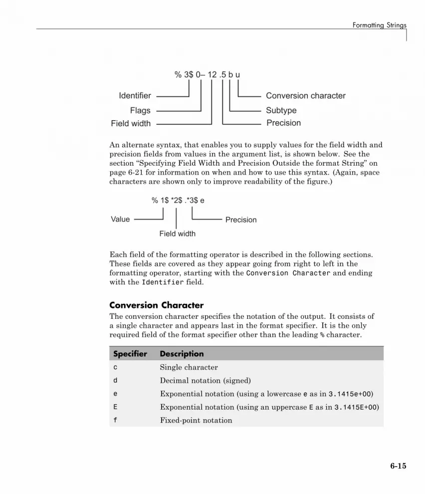
Formatting Strings
��������������
������������������������������
����� ��������������!����
" ��#$�
An alternate syntax, that enables you to supply values for the field width andprecision fields from values in the argument list, is shown below. See thesection “Specifying Field Width and Precision Outside the format String” onpage 6-21 for information on when and how to use this syntax. (Again, spacecharacters are shown only to improve readability of the figure.)
Each field of the formatting operator is described in the following sections.These fields are covered as they appear going from right to left in theformatting operator, starting with the Conversion Character and endingwith the Identifier field.
Conversion CharacterThe conversion character specifies the notation of the output. It consists ofa single character and appears last in the format specifier. It is the onlyrequired field of the format specifier other than the leading % character.
Specifier Description
c Single character
d Decimal notation (signed)
e Exponential notation (using a lowercase e as in 3.1415e+00)
E Exponential notation (using an uppercase E as in 3.1415E+00)
f Fixed-point notation
6-15

6 Characters and Strings
Specifier Description
g The more compact of %e or %f. (Insignificant zeros do notprint.)
G Same as %g, but using an uppercase E
o Octal notation (unsigned)
s String of characters
u Decimal notation (unsigned)
x Hexadecimal notation (using lowercase letters a–f)
X Hexadecimal notation (using uppercase letters A–F)
This example uses conversion characters to display the number 46 in decimal,fixed-point, exponential, and hexadecimal formats:
A = 46*ones(1,4);
sprintf('%d %f %e %X', A)ans =46 46.000000 4.600000e+01 2E
SubtypeThe subtype field is a single alphabetic character that immediately precedesthe conversion character. The following nonstandard subtype specifiers aresupported for the conversion characters %o, %x, %X, and %u.
b The underlying C data type is a double rather than an unsignedinteger. For example, to print a double-precision value inhexadecimal, use a format like '%bx'.
t The underlying C data type is a float rather than an unsigned integer.
To specify the number of bits for the conversion of an integer value(corresponding to conversion characters %d, %i, %u, %o, %x, or %X), use one ofthe following subtypes.
6-16

Formatting Strings
l 64-bit value.
h 16-bit value.
Precisionprecision in a formatting operator is a nonnegative integer that immediatelyfollows a period. For example, the specifier %7.3f, has a precision of 3.For the %g specifier, precision indicates the number of significant digits todisplay. For the %f, %e, and %E specifiers, precision indicates how manydigits to display to the right of the decimal point.
Here are some examples of how the precision field affects different typesof notation:
sprintf('%g %.2g %f %.2f', pi*50*ones(1,4))ans =157.08 1.6e+02 157.079633 157.08
Precision is not usually used in format specifiers for strings (i.e., %s). If youdo use it on a string and if the value p in the precision field is less than thenumber of characters in the string, MATLAB displays only p characters of thestring and truncates the rest.
You can also supply the value for a precision field from outside of the formatspecifier. See the section “Specifying Field Width and Precision Outside theformat String” on page 6-21 for more information on this.
For more information on the use of precision in formatting, see “SettingField Width and Precision” on page 6-20.
Field WidthField width in a formatting operator is a nonnegative integer that tellsMATLAB the minimum number of digits or characters to use when formattingthe corresponding input value. For example, the specifier %7.3f, has a widthof 7.
Here are some examples of how the width field affects different types ofnotation:
6-17

6 Characters and Strings
sprintf('|%e|%15e|%f|%15f|', pi*50*ones(1,4))ans =|1.570796e+02| 1.570796e+02|157.079633| 157.079633|
When used on a string, the field width can determine whether MATLABpads the string with spaces. If width is less than or equal to the number ofcharacters in the string, it has no effect.
sprintf('%30s', 'Pad left with spaces')ans =
Pad left with spaces
You can also supply a value for field width from outside of the formatspecifier. See the section “Specifying Field Width and Precision Outside theformat String” on page 6-21 for more information on this.
For more information on the use of field width in formatting, see “SettingField Width and Precision” on page 6-20.
FlagsYou can control the output using any of these optional flags:
Character Description Example
A minus sign (-) Left-justifies theconverted argumentin its field.
%-5.2d
A plus sign (+) Always prints a signcharacter (+ or –).
%+5.2d
A space ( ) Inserts a space before thevalue.
% 5.2f
6-18

Formatting Strings
Character Description Example
Zero (0) Pads with zeros ratherthan spaces.
%05.2f
A pound sign (#) Modifies selected numericconversions:
• For %o, %x, or %X, print0, 0x, or 0X prefix.
• For %f, %e, or %E, printdecimal point evenwhen precision is 0.
• For %g or %G, do notremove trailing zerosor decimal point.
%#5.0f
Right- and left-justify the output. The default is to right-justify:
sprintf('right-justify: %12.2f\nleft-justify: %-12.2f', ...12.3, 12.3)
ans =right-justify: 12.30left-justify: 12.30
Display a + sign for positive numbers. The default is to omit the + sign:
sprintf('no sign: %12.2f\nsign: %+12.2f', ...12.3, 12.3)
ans =no sign: 12.30sign: +12.30
Pad to the left with spaces or zeros. The default is to use space-padding:
sprintf('space-padded: %12.2f\nzero-padded: %012.2f', ...5.2, 5.2)
ans =space-padded: 5.20
6-19

6 Characters and Strings
zero-padded: 000000005.20
Note You can specify more than one flag in a formatting operator.
Value IdentifiersBy default, MATLAB inserts data values from the argument list into thestring in a sequential order. If you have a need to use the value argumentsin a nonsequential order, you can override the default by using a numericidentifier in each format specifier. Specify nonsequential arguments with aninteger immediately following the % sign, followed by a $ sign.
Ordered Sequentially Ordered By Identifier
sprintf('%s %s %s', ...'1st', '2nd', '3rd')
ans =1st 2nd 3rd
sprintf('%3$s %2$s %1$s', ...'1st', '2nd', '3rd')
ans =3rd 2nd 1st
Setting Field Width and PrecisionThis section provides further information on the use of the field width andprecision fields of the formatting operator:
• “Effect on the Output String” on page 6-20
• “Specifying Field Width and Precision Outside the format String” on page6-21
• “Using Identifiers In the Width and Precision Fields” on page 6-22
Effect on the Output StringThe figure below illustrates the way in which the field width and precisionsettings affect the output of the string formatting functions. In this figure,the zero following the % sign in the formatting operator means to add leadingzeros to the output string rather than space characters:
6-20

Formatting Strings
��%�&'( ��)�� ����%�'
��*�����$���������$ ���� ������������������
�����������$���������$ ������� ��������������
������!����+�!�,�)$��������+���$�,�� �����������$����������
����� �������$�������������������� ����
���-����$������
.�� �������!�������/���0�����������������������!����1����
General rules for formatting
• If precision is not specified, it defaults to 6.
• If precision (p) is less than the number of digits in the fractional part of theinput value (f), then only p digits are shown to the right of the decimalpoint in the output, and that fractional value is rounded.
• If precision (p) is greater than the number of digits in the fractional part ofthe input value (f), then p digits are shown to the right of the decimal pointin the output, and the fractional part is extended to the right with p-f zeros.
• If field width is not specified, it defaults to precision + 1 + the number ofdigits in the whole part of the input value.
• If field width (w) is greater than p+1 plus the number of digits in the wholepart of the input value (n), then the whole part of the output value isextended to the left with w-(n+1+p) space characters or zeros, dependingon whether or not the zero flag is set in the Flags field. The default is toextend the whole part of the output with space characters.
Specifying Field Width and Precision Outside the format StringTo specify field width or precision using values from a sequential argumentlist, use an asterisk (*) in place of the field width or precision field of theformatting operator.
6-21

6 Characters and Strings
This example formats and displays three numbers. The formatting operatorfor the first, %*f, has an asterisk in the field width location of the formattingoperator, specifying that just the field width, 15, is to be taken from theargument list. The second operator, %.*f puts the asterisk after the decimalpoint meaning, that it is the precision that is to take its value from theargument list. And the third operator, %*.*f, specifies both field width andprecision in the argument list:
sprintf('%*f %.*f %*.*f', ...15, 123.45678, ... % Width for 123.45678 is 153, 16.42837, ... % Precision for rand*20 is .36, 4, pi) % Width & Precision for pi is 6.4
ans =123.456780 16.428 3.1416
You can mix the two styles. For example, this statement gets the field widthfrom the argument list and the precision from the format string:
sprintf('%*.2f', 5, 123.45678)ans =
123.46
Using Identifiers In the Width and Precision FieldsYou can also derive field width and precision values from a nonsequential(i.e., numbered) argument list. Inside the formatting operator, specify fieldwidth and/or precision with an asterisk followed by an identifier number,followed by a $ sign.
This example from the previous section shows how to obtain field width andprecision from a sequential argument list:
sprintf('%*f %.*f %*.*f', ...15, 123.45678, ...3, 16.42837, ...6, 4, pi)
ans =123.456780 16.428 3.1416
6-22

Formatting Strings
Here is an example of how to do the same thing using numbered ordering.Field width for the first output value is 15, precision for the second value is3, and field width and precision for the third value is 6 and 4, respectively.If you specify field width or precision with identifiers, then you must specifythe value with an identifier as well:
sprintf('%1$*4$f %2$.*5$f %3$*6$.*7$f', ...123.45678, 16.42837, pi, 15, 3, 6, 4)
ans =123.456780 16.428 3.1416
Restrictions for Using IdentifiersIf any of the formatting operators in a string include an identifier field, thenall of the operators in that string must do the same; you cannot use bothsequential and nonsequential ordering in the same function call.
Valid Syntax Invalid Syntax
sprintf('%d %d %d %d', ...1, 2, 3, 4)
ans =1 2 3 4
sprintf('%d %3$d %d %d', ...1, 2, 3, 4)
ans =1
If your command provides more value arguments than there are formattingoperators in the format string, MATLAB reuses the operators. However,MATLAB allows this only for commands that use sequential ordering.You cannot reuse formatting operators when making a function call withnumbered ordering of the value arguments.
Valid Syntax Invalid Syntax
sprintf('%d', 1, 2, 3, 4)ans =
1234
sprintf('%1$d', 1, 2, 3, 4)ans =
1
Also, do not use identifiers when the value arguments are in the form of avector or array:
6-23

6 Characters and Strings
Valid Syntax Invalid Syntax
v = [1.4 2.7 3.1];
sprintf('%.4f %.4f %.4f', v)ans =
1.4000 2.7000 3.1000
v = [1.4 2.7 3.1];
sprintf('%3$.4f %1$.4f %2$.4f', v)ans =
Empty string: 1-by-0
6-24

String Comparisons
String ComparisonsThere are several ways to compare strings and substrings:
• You can compare two strings, or parts of two strings, for equality.
• You can compare individual characters in two strings for equality.
• You can categorize every element within a string, determining whethereach element is a character or white space.
These functions work for both character arrays and cell arrays of strings.
Comparing Strings for EqualityYou can use any of four functions to determine if two input strings areidentical:
• strcmp determines if two strings are identical.
• strncmp determines if the first n characters of two strings are identical.
• strcmpi and strncmpi are the same as strcmp and strncmp, except thatthey ignore case.
Consider the two strings
str1 = 'hello';str2 = 'help';
Strings str1 and str2 are not identical, so invoking strcmp returns logical 0(false). For example,
C = strcmp(str1,str2)C =
0
Note For C programmers, this is an important difference between theMATLAB strcmp and C strcmp() functions, where the latter returns 0 ifthe two strings are the same.
6-25

6 Characters and Strings
The first three characters of str1 and str2 are identical, so invoking strncmpwith any value up to 3 returns 1:
C = strncmp(str1, str2, 2)C =
1
These functions work cell-by-cell on a cell array of strings. Consider the twocell arrays of strings
A = {'pizza'; 'chips'; 'candy'};B = {'pizza'; 'chocolate'; 'pretzels'};
Now apply the string comparison functions:
strcmp(A,B)ans =
100
strncmp(A,B,1)ans =
110
Comparing for Equality Using OperatorsYou can use MATLAB relational operators on character arrays, as long asthe arrays you are comparing have equal dimensions, or one is a scalar. Forexample, you can use the equality operator (==) to determine where thematching characters are in two strings:
A = 'fate';B = 'cake';
A == Bans =
0 1 0 1
All of the relational operators (>, >=, <, <=, ==, ~=) compare the values ofcorresponding characters.
6-26

String Comparisons
Categorizing Characters Within a StringThere are three functions for categorizing characters inside a string:
1 isletter determines if a character is a letter.
2 isspace determines if a character is white space (blank, tab, or new line).
3 isstrprop checks characters in a string to see if they match a categoryyou specify, such as
• Alphabetic
• Alphanumeric
• Lowercase or uppercase
• Decimal digits
• Hexadecimal digits
• Control characters
• Graphic characters
• Punctuation characters
• Whitespace characters
For example, create a string named mystring:
mystring = 'Room 401';
isletter examines each character in the string, producing an output vectorof the same length as mystring:
A = isletter(mystring)A =
1 1 1 1 0 0 0 0
The first four elements in A are logical 1 (true) because the first fourcharacters of mystring are letters.
6-27

6 Characters and Strings
Searching and ReplacingMATLAB provides several functions for searching and replacing characters ina string. (MATLAB also supports search and replace operations using regularexpressions. See Regular Expressions.)
Consider a string named label:
label = 'Sample 1, 10/28/95';
The strrep function performs the standard search-and-replace operation.Use strrep to change the date from '10/28' to '10/30':
newlabel = strrep(label, '28', '30')newlabel =
Sample 1, 10/30/95
strfind returns the starting position of a substring within a longer string. Tofind all occurrences of the string 'amp' inside label, use
position = strfind(label, 'amp')position =
2
The position within label where the only occurrence of 'amp' begins is thesecond character.
The textscan function parses a string to identify numbers or substrings.Describe each component of the string with conversion specifiers, such as%s for strings, %d for integers, or %f for floating-point numbers. Optionally,include any literal text to ignore.
For example, identify the sample number and date string from label:
parts = textscan(label, 'Sample %d, %s');parts{:}
ans =1
ans ='10/28/95'
6-28

Searching and Replacing
To parse strings in a cell array, use the strtok function. For example:
c = {'all in good time'; ...'my dog has fleas'; ...'leave no stone unturned'};
first_words = strtok(c)
6-29

6 Characters and Strings
Converting from Numeric to String
In this section...
“Function Summary” on page 6-30
“Converting to a Character Equivalent” on page 6-31
“Converting to a String of Numbers” on page 6-31
“Converting to a Specific Radix” on page 6-31
Function SummaryThe functions listed in this table provide a number of ways to convert numericdata to character strings.
Function Description Example
char Convert a positive integer to an equivalentcharacter. (Truncates any fractional parts.)
[72 105] → 'Hi'
int2str Convert a positive or negative integer to acharacter type. (Rounds any fractional parts.)
[72 105]→ '72 105'
num2str Convert a numeric type to a character type of thespecified precision and format.
[72 105] →'72/105/' (formatset to %1d/)
mat2str Convert a numeric type to a character type of thespecified precision, returning a string MATLABcan evaluate.
[72 105] → '[72105]'
dec2hex Convert a positive integer to a character type ofhexadecimal base.
[72 105]→ '48 69'
dec2bin Convert a positive integer to a character type ofbinary base.
[72 105]→ '10010001101001'
dec2base Convert a positive integer to a character type ofany base from 2 through 36.
[72 105] → '110151' (base set to 8)
6-30

Converting from Numeric to String
Converting to a Character EquivalentThe char function converts integers to Unicode character codes and returns astring composed of the equivalent characters:
x = [77 65 84 76 65 66];char(x)ans =
MATLAB
Converting to a String of NumbersThe int2str, num2str, and mat2str functions convert numeric values tostrings where each character represents a separate digit of the input value.The int2str and num2str functions are often useful for labeling plots. Forexample, the following lines use num2str to prepare automated labels for thex-axis of a plot:
function plotlabel(x, y)plot(x, y)str1 = num2str(min(x));str2 = num2str(max(x));out = ['Value of f from ' str1 ' to ' str2];xlabel(out);
Converting to a Specific RadixAnother class of conversion functions changes numeric values into stringsrepresenting a decimal value in another base, such as binary or hexadecimalrepresentation. This includes dec2hex, dec2bin, and dec2base.
6-31

6 Characters and Strings
Converting from String to Numeric
In this section...
“Function Summary” on page 6-32
“Converting from a Character Equivalent” on page 6-33
“Converting from a Numeric String” on page 6-33
“Converting from a Specific Radix” on page 6-34
Function SummaryThe functions listed in this table provide a number of ways to convertcharacter strings to numeric data.
Function Description Example
uintN (e.g., uint8) Convert a character to an integer code thatrepresents that character.
'Hi' → 72 105
str2num Convert a character type to a numeric type. '72 105'→ [72 105]
str2double Similar to str2num, but offers betterperformance and works with cell arrays ofstrings.
{'72' '105'} → [72105]
hex2num Convert a numeric type to a character typeof specified precision, returning a string thatMATLAB can evaluate.
'A' →'-1.4917e-154'
hex2dec Convert a character type of hexadecimal baseto a positive integer.
'A' → 10
bin2dec Convert a positive integer to a character typeof binary base.
'1010' → 10
base2dec Convert a positive integer to a character typeof any base from 2 through 36.
'12' → 10 (if base ==8)
6-32

Converting from String to Numeric
Converting from a Character EquivalentCharacter arrays store each character as a 16-bit numeric value. Use one ofthe integer conversion functions (e.g., uint8) or the double function to convertstrings to their numeric values, and char to revert to character representation:
name = 'Thomas R. Lee';
name = double(name)name =
84 104 111 109 97 115 32 82 46 32 76 101 101
name = char(name)name =
Thomas R. Lee
Converting from a Numeric StringUse str2num to convert a character array to the numeric value represented bythat string:
str = '37.294e-1';
val = str2num(str)val =
3.7294
The str2double function converts a cell array of strings to thedouble-precision values represented by the strings:
c = {'37.294e-1'; '-58.375'; '13.796'};
d = str2double(c)d =
3.7294-58.375013.7960
whosName Size Bytes Class
c 3x1 224 cell
6-33

6 Characters and Strings
d 3x1 24 double
Converting from a Specific RadixTo convert from a character representation of a nondecimal number to thevalue of that number, use one of these functions: hex2num, hex2dec, bin2dec,or base2dec.
The hex2num and hex2dec functions both take hexadecimal (base 16) inputs,but hex2num returns the IEEE double-precision floating-point number itrepresents, while hex2dec converts to a decimal integer.
6-34

Function Summary
Function SummaryMATLAB provides these functions for working with character arrays:
• Functions to Create Character Arrays on page 6-35
• Functions to Modify Character Arrays on page 6-35
• Functions to Read and Operate on Character Arrays on page 6-36
• Functions to Search or Compare Character Arrays on page 6-36
• Functions to Determine Class or Content on page 6-36
• Functions to Convert Between Numeric and String Classes on page 6-37
• Functions to Work with Cell Arrays of Strings as Sets on page 6-37
Functions to Create Character Arrays
Function Description
'str' Create the string specified between quotes.
blanks Create a string of blanks.
sprintf Write formatted data to a string.
strcat Concatenate strings.
char Concatenate strings vertically.
Functions to Modify Character Arrays
Function Description
deblank Remove trailing blanks.
lower Make all letters lowercase.
sort Sort elements in ascending or descending order.
strjust Justify a string.
strrep Replace one string with another.
strtrim Remove leading and trailing white space.
upper Make all letters uppercase.
6-35

6 Characters and Strings
Functions to Read and Operate on Character Arrays
Function Description
eval Execute a string with MATLAB expression.
sscanf Read a string under format control.
Functions to Search or Compare Character Arrays
Function Description
regexp Match regular expression.
strcmp Compare strings.
strcmpi Compare strings, ignoring case.
strfind Find one string within another.
strncmp Compare the first N characters of strings.
strncmpi Compare the first N characters, ignoring case.
strtok Find a token in a string.
textscan Read data from a string.
Functions to Determine Class or Content
Function Description
iscellstr Return true for a cell array of strings.
ischar Return true for a character array.
isletter Return true for letters of the alphabet.
isstrprop Determine if a string is of the specified category.
isspace Return true for white-space characters.
6-36

Function Summary
Functions to Convert Between Numeric and String Classes
Function Description
char Convert to a character or string.
cellstr Convert a character array to a cell array of strings.
double Convert a string to numeric codes.
int2str Convert an integer to a string.
mat2str Convert a matrix to a string you can run eval on.
num2str Convert a number to a string.
str2num Convert a string to a number.
str2double Convert a string to a double-precision value.
Functions to Work with Cell Arrays of Strings as Sets
Function Description
intersect Set the intersection of two vectors.
ismember Detect members of a set.
setdiff Return the set difference of two vectors.
setxor Set the exclusive OR of two vectors.
union Set the union of two vectors.
unique Set the unique elements of a vector.
6-37

6 Characters and Strings
6-38

7
Categorical Arrays
• “Create Categorical Arrays” on page 7-2
• “Convert Table Variables Containing Strings to Categorical” on page 7-7
• “Plot Categorical Data” on page 7-13
• “Compare Categorical Array Elements” on page 7-20
• “Combine Categorical Arrays” on page 7-24
• “Access Data Using Categorical Arrays” on page 7-28
• “Work with Protected Categorical Arrays” on page 7-35
• “Advantages of Using Categorical Arrays” on page 7-41
• “Ordinal Categorical Arrays” on page 7-44
• “Other MATLAB Functions Supporting Categorical Arrays” on page 7-48

7 Categorical Arrays
Create Categorical ArraysThis example shows how to create a categorical array. categorical is a datatype for storing data with values from a finite set of discrete categories. Thesecategories can have a natural order, but it is not required. A categorical arrayprovides efficient storage and convenient manipulation of data, while alsomaintaining meaningful names for the values. Categorical arrays are oftenused in a table to define groups of rows.
By default, categorical arrays contain categories that have no mathematicalordering. For example, the discrete set of pet categories {'dog' 'cat''bird'} has no meaningful mathematical ordering, so MATLAB® uses thealphabetical ordering {'bird' 'cat' 'dog'}. ordinal categorical arrayscontain categories that have a meaningful mathematical ordering. Forexample, the discrete set of size categories {'small', 'medium', 'large'}has the mathematical ordering small < medium < large.
Create Categorical Array from Cell Array of Strings
You can use the categorical function to create a categorical array from anumeric array, logical array, cell array of strings, or an existing categoricalarray.
Create a 1-by-11 cell array of strings containing state names from NewEngland.
state = {'MA','ME','CT','VT','ME','NH','VT','MA','NH','CT','RI'};
Convert the cell array of strings, state, to a categorical array that has nomathematical order.
state = categorical(state)
class(state)
state =
Columns 1 through 9
7-2

Create Categorical Arrays
MA ME CT VT ME NH VT MA NH
Columns 10 through 11
CT RI
ans =
categorical
List the discrete categories in the variable state.
categories(state)
ans =
'CT''MA''ME''NH''RI''VT'
The categories are listed in alphabetical order.
Create Ordinal Categorical Array from Cell Array of Strings
Create a 1-by-8 cell array of strings containing the sizes of eight objects.
AllSizes = {'medium','large','small','small','medium',...'large','medium','small'};
The cell array of strings, AllSizes, has three distinct values: 'large','medium', and 'small'. With the cell array of strings, there is no convenientway to indicate that small < medium < large.
7-3

7 Categorical Arrays
Convert the cell array of strings, AllSizes, to an ordinal categorical array.Use valueset to specify the values small, medium, and large, which definethe categories. For an ordinal categorical array, the first category specified isthe smallest and the last category is the largest.
valueset = {'small','medium','large'};sizeOrd = categorical(AllSizes,valueset,'Ordinal',true)
class(sizeOrd)
sizeOrd =
Columns 1 through 6
medium large small small medium large
Columns 7 through 8
medium small
ans =
categorical
The order of the values in the categorical array, sizeOrd, remains unchanged.
List the discrete categories in the categorical variable, sizeOrd.
categories(sizeOrd)
ans =
'small''medium''large'
7-4

Create Categorical Arrays
The categories are listed in the specified order to match the mathematicalordering small < medium < large.
Create Ordinal Categorical Array by Binning Data
Create a vector of 100 integers between 1 and 44.
x = gallery('integerdata',44,[100,1],1);
Use the histc function to create three bins for the data from x. Put all valuesbetween 1 and 15 into bin one, all the values between 15 and 30 into bin two,and all the values between 30 and 45 into bin three. Each bin includes the leftendpoint, but does not include the right endpoint.
[~,bin] = histc(x,[1,15,30,45]);
bin is a 100-by-1 vector indicating the bin number for each entry from x.
Create and ordinal categorical array, sizeOrd2, where the three bins becomethe categories, small, medium, and large.
valueset = 1:3;catnames = {'small','medium','large'};
sizeOrd2 = categorical(bin,valueset,catnames,'Ordinal',true);
sizeOrd2 is a 100-by-1 ordinal categorical array with three categories, suchthat small < medium < large.
Use the summary function to print a summary of the categorical array.
summary(sizeOrd2)
small 33medium 36large 31
There are 33 elements in the category small, 36 in the category medium, and31 in the category large.
7-5

7 Categorical Arrays
See Also categorical | categories | summary
RelatedExamples
• “Convert Table Variables Containing Strings to Categorical” on page 7-7• “Access Data Using Categorical Arrays” on page 7-28• “Compare Categorical Array Elements” on page 7-20
Concepts • “Advantages of Using Categorical Arrays” on page 7-41• “Ordinal Categorical Arrays” on page 7-44
7-6

Convert Table Variables Containing Strings to Categorical
Convert Table Variables Containing Strings to CategoricalThis example shows how to convert a variable in a table from a cell array ofstrings to a categorical array.
Load Sample Data and Create a Table
Load sample data gathered from 100 patients.
load patients
whos
Name Size Bytes Class Attribu
Age 100x1 800 doubleDiastolic 100x1 800 doubleGender 100x1 12212 cellHeight 100x1 800 doubleLastName 100x1 12416 cellLocation 100x1 15008 cellSelfAssessedHealthStatus 100x1 12340 cellSmoker 100x1 100 logicalSystolic 100x1 800 doubleWeight 100x1 800 double
Store the patient data from Age, Gender, Height, Weight,SelfAssessedHealthStatus, and Location in a table. Use the uniqueidentifiers in the variable LastName as row names.
T = table(Age,Gender,Height,Weight,...SelfAssessedHealthStatus,Location,...'RowNames',LastName);
Convert Table Variables from Cell Arrays of Strings to Categorical Arrays
The cell arrays of strings, Gender and Location, contain small a discreteset of unique values.
7-7

7 Categorical Arrays
Convert Gender and Location to categorical arrays.
T.Gender = categorical(T.Gender);T.Location = categorical(T.Location);
The variable, SelfAssessedHealthStatus, contains four unique values:Excellent, Fair, Good, and Poor.
Convert SelfAssessedHealthStatus to an ordinal categorical array, suchthat the categories have the mathematical ordering Poor < Fair < Good <Excellent.
T.SelfAssessedHealthStatus = categorical(SelfAssessedHealthStatus,...{'Poor','Fair','Good','Excellent'},'Ordinal',true);
Print a Summary
View the data type, description, units, and other descriptive statistics for eachvariable by using summary to summarize the table.
format compact
summary(T)
Variables:Age: 100x1 double
Values:min 25median 39max 50
Gender: 100x1 categoricalValues:
Female 53Male 47
Height: 100x1 doubleValues:
min 60median 67max 72
Weight: 100x1 double
7-8

Convert Table Variables Containing Strings to Categorical
Values:min 111median 142.5max 202
SelfAssessedHealthStatus: 100x1 ordinal categoricalValues:
Poor 11Fair 15Good 40Excellent 34
Location: 100x1 categoricalValues:
County General Hospital 39St. Mary's Medical Center 24VA Hospital 37
The table variables Gender, SelfAssessedHealthStatus, and Locationare categorical arrays. The summary contains the counts of the number ofelements in each category. For example, the summary indicates that 53 of the100 patients are female and 47 are male.
Select Data Based on Categories
Create a subtable, T1, containing the age, height, and weight of all femalepatients who were observed at County General Hospital. You can easilycreate a logical vector based on the values in the categorical arrays Genderand Location.
rows = T.Location=='County General Hospital' & T.Gender=='Female';
rows is a 100-by-1 logical vector with logical true (1) for the table rows wherethe gender is female and the location is County General Hospital.
Define the subset of variables.
vars = {'Age','Height','Weight'};
Use parentheses to create the subtable, T1.
T1 = T(rows,vars)
7-9

7 Categorical Arrays
T1 =Age Height Weight___ ______ ______
Brown 49 64 119Taylor 31 66 132Anderson 45 68 128Lee 44 66 146Walker 28 65 123Young 25 63 114Campbell 37 65 135Evans 39 62 121Morris 43 64 135Rivera 29 63 130Richardson 30 67 141Cox 28 66 111Torres 45 70 137Peterson 32 60 136Ramirez 48 64 137Bennett 35 64 131Patterson 37 65 120Hughes 49 63 123Bryant 48 66 134
A is a 19-by-3 table.
Since ordinal categorical arrays have a mathematical ordering for theircategories, you can perform element-wise comparisons of strings withrelational operations, such as greater than and less than.
Create a subtable, T2, of the gender, age, height, and weight of all patientswho assessed their health status as poor or fair.
First, define the subset of rows to include in table T2.
rows = T.SelfAssessedHealthStatus<='Fair';
Then, define the subset of variables to include in table T2.
vars = {'Gender','Age','Height','Weight'};
7-10

Convert Table Variables Containing Strings to Categorical
Use parentheses to create the subtable T2.
T2 = T(rows,vars)
T2 =Gender Age Height Weight______ ___ ______ ______
Johnson Male 43 69 163Jones Female 40 67 133Thomas Female 42 66 137Jackson Male 25 71 174Garcia Female 27 69 131Rodriguez Female 39 64 117Lewis Female 41 62 137Lee Female 44 66 146Hall Male 25 70 189Hernandez Male 36 68 166Lopez Female 40 66 137Gonzalez Female 35 66 118Mitchell Male 39 71 164Campbell Female 37 65 135Parker Male 30 68 182Stewart Male 49 68 170Morris Female 43 64 135Watson Female 40 64 127Kelly Female 41 65 127Price Male 31 72 178Bennett Female 35 64 131Wood Male 32 68 183Patterson Female 37 65 120Foster Female 30 70 124Griffin Male 49 70 186Hayes Male 48 66 177
T2 is a 26-by-4 table.
RelatedExamples
• “Create a Table” on page 8-2• “Create Categorical Arrays” on page 7-2• “Access Data in a Table” on page 8-29• “Access Data Using Categorical Arrays” on page 7-28
7-11

7 Categorical Arrays
Concepts • “Advantages of Using Categorical Arrays” on page 7-41• “Ordinal Categorical Arrays” on page 7-44
7-12

Plot Categorical Data
Plot Categorical DataThis example shows how to plot data from a categorical array.
Load Sample Data
Load sample data gathered from 100 patients.
load patients
whos
Name Size Bytes Class Attribu
Age 100x1 800 doubleDiastolic 100x1 800 doubleGender 100x1 12212 cellHeight 100x1 800 doubleLastName 100x1 12416 cellLocation 100x1 15008 cellSelfAssessedHealthStatus 100x1 12340 cellSmoker 100x1 100 logicalSystolic 100x1 800 doubleWeight 100x1 800 double
Create Categorical Arrays from Cell Arrays of Strings
The workspace variable, Location, is a cell array of strings that contains thethree unique medical facilities where patients were observed.
To access and compare data more easily, convert Location to a categoricalarray.
Location = categorical(Location);
Summarize the categorical array.
summary(Location)
7-13

7 Categorical Arrays
County General Hospital 39St. Mary's Medical Center 24VA Hospital 37
39 patients were observed at County General Hospital, 24 at St. Mary’sMedical Center, and 37 at the VA Hospital.
The workspace variable, SelfAssessedHealthStatus, contains four uniquevalues, Excellent, Fair, Good, and Poor.
Convert SelfAssessedHealthStatus to an ordinal categorical array, suchthat the categories have the mathematical ordering Poor < Fair < Good <Excellent.
SelfAssessedHealthStatus = categorical(SelfAssessedHealthStatus,...{'Poor' 'Fair' 'Good' 'Excellent'},'Ordinal',true);
Summarize the categorical array, SelfAssessedHealthStatus.
summary(SelfAssessedHealthStatus)
Poor 11Fair 15Good 40Excellent 34
Plot a Histogram
Create a histogram bar plot directly from a categorical array.
figure()hist(SelfAssessedHealthStatus)title('Self Assessed Health Status')
7-14

Plot Categorical Data
The function hist accepts the categorical array, SelfAssessedHealthStatus,and plots the category counts for each of the four categories.
Create a histogram of the hospital location for only the patients who assessedtheir health as Fair or Poor.
figure()hist(Location(SelfAssessedHealthStatus<='Fair'))title('Location of Patients in Fair or Poor Health')
7-15

7 Categorical Arrays
Create a Pie Chart
You can use the numeric output from the countcats function to create othertypes of plots.
Create a pie chart of the self assessed health status of the 100 patients.
figure()h = pie(countcats(SelfAssessedHealthStatus));title('Self Assessed Health Status From 100 Patients')
7-16

Plot Categorical Data
% Add the category names to the pie chart labels. Use strcat to prepend% the category names to the percentage labels.textObjs = findobj(h,'Type','text');oldStr = get(textObjs,{'String'});
set(textObjs,{'String'},...strcat(categories(SelfAssessedHealthStatus),oldStr))
Create a Scatter Plot
7-17

7 Categorical Arrays
Convert the cell array of strings to a categorical array.
Gender = categorical(Gender);
Summarize the categorical array, Gender.
summary(Gender)
Female 53Male 47
Gender is a 100-by-1 categorical array with two categories, Female and Male.
Use the categorical array, Gender, to access Weight and Height data for eachgender separately.
X1 = Weight(Gender=='Female');Y1 = Height(Gender=='Female');
X2 = Weight(Gender=='Male');Y2 = Height(Gender=='Male');
X1 and Y1 are 53-by-1 numeric arrays containing data from the femalepatients.
X2 and Y2 are 47-by-1 numeric arrays containing data from the male patients.
Create a scatter plot of height vs. weight. Indicate data from the femalepatients with a circle and data from the male patients with a cross.
figure()h1 = scatter(X1,Y1,'o');hold onh2 = scatter(X2,Y2,'x');
title('Height vs. Weight')xlabel('Weight (lbs)')ylabel('Height (in)')
7-18

Plot Categorical Data
See Also categorical | summary | countcats | hist | pie | bar | rose | scatter
RelatedExamples
• “Access Data Using Categorical Arrays” on page 7-28
7-19

7 Categorical Arrays
Compare Categorical Array ElementsThis example shows how to use relational operations with a categorical array.
Create Categorical Array from Cell Array of Strings
Create a 2-by-4 cell array of strings.
C = {'blue' 'red' 'green' 'blue';...'blue' 'green' 'green' 'blue'};
colors = categorical(C)
colors =
blue red green blueblue green green blue
colors is a 2-by-4 categorical array.
List the categories of the categorical array.
categories(colors)
ans =
'blue''green''red'
Determine If Elements Are Equal
Use the relational operator, eq (==), to compare the first and second rows ofcolors.
colors(1,:) == colors(2,:)
7-20

Compare Categorical Array Elements
ans =
1 0 1 1
Only the values in the second column differ between the rows.
Compare Entire Array to String
Compare the entire categorical array, colors, to the string 'blue' to find thelocation of all blue values.
colors == 'blue'
ans =
1 0 0 11 0 0 1
There are four blue entries in colors, one in each corner of the array.
Convert to an Ordinal Categorical Array
Add a mathematical ordering to the categories in colors. Specify the categoryorder that represents the ordering of color spectrum, red < green < blue.
colors = categorical(colors,{'red','green' 'blue'},'Ordinal',true)
colors =
blue red green blueblue green green blue
The elements in the categorical array remain the same.
7-21

7 Categorical Arrays
List the discrete categories in colors.
categories(colors)
ans =
'red''green''blue'
Compare Elements Based on Order
Determine if elements in the first column of colors are greater than theelements in the second column.
colors(:,1) > colors(:,2)
ans =
11
Both values in the second column, red and green, are greater than thecorresponding values in the first column, blue.
Find all the elements in colors that are less than 'blue'.
colors < 'blue'
ans =
0 1 1 00 1 1 0
7-22

Compare Categorical Array Elements
The function lt (<) indicates the location of all green and red values with 1.
See Also categorical | categories
RelatedExamples
• “Access Data Using Categorical Arrays” on page 7-28
Concepts • “Relational Operations”• “Advantages of Using Categorical Arrays” on page 7-41• “Ordinal Categorical Arrays” on page 7-44
7-23

7 Categorical Arrays
Combine Categorical ArraysThis example shows how to combine two categorical arrays.
Create Categorical Arrays
Create a categorical array, A, containing the preferred lunchtime beverage of25 students in classroom A.
A = gallery('integerdata',3,[25,1],1);A = categorical(A,1:3,{'milk' 'water' 'juice'});
A is a 25-by-1 categorical array with three distinct categories: milk, water,and juice.
Summarize the categorical array, A.
summary(A)
milk 8water 8juice 9
Eight students in classroom A prefer milk, eight prefer water, and nineprefer juice.
Create another categorical array, B, containing the preferences of 28 studentsin classroom B.
B = gallery('integerdata',3,[28,1],3);B = categorical(B,1:3,{'milk' 'water' 'juice'});
B is a 28-by-1 categorical array containing the same categories as A.
Summarize the categorical array, B.
summary(B)
milk 12water 10
7-24

Combine Categorical Arrays
juice 6
Twelve students in classroom B prefer milk, ten prefer water, and six preferjuice.
Concatenate Categorical Arrays
Concatenate the data from classrooms A and B into a single categorical array,Group1.
Group1 = [A;B];
Summarize the categorical array, Group1
summary(Group1)
milk 20water 18juice 15
Group1 is a 53-by-1 categorical array with three categories: milk, water,and juice.
Create Categorical Array with Different Categories
Create a categorical array, Group2, containing data from 50 students whowere given the additional beverage option of soda.
Group2 = gallery('integerdata',4,[50,1],2);Group2 = categorical(Group2,1:4,{'juice' 'milk' 'soda' 'water'});
Summarize the categorical array, Group2.
summary(Group2)
juice 18milk 10soda 13water 9
7-25

7 Categorical Arrays
Group2 is a 50-by-1 categorical array with four categories: juice, milk,soda, and water.
Concatenate Arrays with Different Categories
Concatenate the data from Group1 and Group2.
students = [Group1;Group2];
Summarize the resulting categorical array, students.
summary(students)
milk 30water 27juice 33soda 13
Concatenation appends the categories exclusive to the second input, soda, tothe end of the list of categories from the first input, milk, water, juice, soda.
Use reordercats to change the order of the categories in the categoricalarray, students.
students = reordercats(students,{'juice','milk','water','soda'});
categories(students)
ans =
'juice''milk''water''soda'
Union of Categorical Arrays
7-26

Combine Categorical Arrays
Use the function union to find the unique responses from Group1 and Group2.
C = union(Group1,Group2)
C =
milkwaterjuicesoda
union returns the combined values from Group1 and Group2 with norepetitions. In this case, C is equivalent to the categories of the concatenation,students.
All of the categorical arrays in this example were nonordinal. To combineordinal categorical arrays, they must have the same sets of categoriesincluding their order.
See Also categorical | categories | summary | union | cat | horzcat | vertcat
RelatedExamples
• “Create Categorical Arrays” on page 7-2• “Convert Table Variables Containing Strings to Categorical” on page 7-7• “Access Data Using Categorical Arrays” on page 7-28
Concepts • “Ordinal Categorical Arrays” on page 7-44
7-27

7 Categorical Arrays
Access Data Using Categorical Arrays
In this section...
“Select Data By Category” on page 7-28
“Common Ways to Access Data Using Categorical Arrays” on page 7-28
Select Data By CategorySelecting data based on its values is often useful. This type of data selectioncan involve creating a logical vector based on values in one variable, and thenusing that logical vector to select a subset of values in other variables. Youcan create a logical vector for selecting data by finding values in a numericarray that fall within a certain range. Additionally, you can create the logicalvector by finding specific discrete values. When using categorical arrays,you can easily:
• Select elements from particular categories. For categorical arrays,use the logical operators == or ~= to select data that is in, or not in, aparticular category. To select data in a particular group of categories, usethe ismember function.
For ordinal categorical arrays, use inequalities >, >=, <, or <= to find data incategories above or below a particular category.
• Delete data that is in a particular category. Use logical operators toinclude or exclude data from particular categories.
• Find elements that are not in a defined category. Categoricalarrays indicate which elements do not belong to a defined category by<undefined>. Use the isundefined function to find observations withouta defined value.
Common Ways to Access Data Using CategoricalArraysThis example shows how to index and search using categorical arrays. You canaccess data using categorical arrays stored within a table in a similar manner.
Load Sample Data
7-28

Access Data Using Categorical Arrays
Load sample data gathered from 100 patients.
load patients
whos
Name Size Bytes Class Attribu
Age 100x1 800 doubleDiastolic 100x1 800 doubleGender 100x1 12212 cellHeight 100x1 800 doubleLastName 100x1 12416 cellLocation 100x1 15008 cellSelfAssessedHealthStatus 100x1 12340 cellSmoker 100x1 100 logicalSystolic 100x1 800 doubleWeight 100x1 800 double
Create Categorical Arrays from Cell Arrays of Strings
To compare strings in character arrays and cell arrays of strings, you mustuse strcmp, which can be cumbersome. To access and compare data moreeasily, convert Gender and Location to categorical arrays.
Gender = categorical(Gender);Location = categorical(Location);
Search for Members of a Single Category
For categorical arrays, you can use the logical operators == and ~= to find thedata that is in, or not in, a particular category.
Determine if there are any patients observed at the location, 'RampartGeneral Hospital'.
any(Location=='Rampart General Hospital')
7-29

7 Categorical Arrays
ans =
0
There are no patients observed at Rampart General Hospital.
Search for Members of a Group of Categories
You can use ismember to find data in a particular group of categories. Createa logical vector for the patients observed at County General Hospital orVA Hospital.
VA_CountyGenIndex = ...ismember(Location,{'County General Hospital','VA Hospital'});
VA_CountyGenIndex is a 100-by-1 logical array containing logical true(1) for each element in the categorical array Location that is a memberof the category County General Hospital or VA Hospital. The output,VA_CountyGenIndex contains 76 nonzero elements.
Use the logical vector, VA_CountyGenIndex to select the LastName of thepatients observed at either County General Hospital or VA Hospital.
VA_CountyGenPatients = LastName(VA_CountyGenIndex);
VA_CountyGenPatients is a 76-by-1 cell array of strings.
Select Elements in a Particular Category to Plot
Use the summary function to print a summary containing the category namesand the number of elements in each category.
summary(Location)
County General Hospital 39St. Mary's Medical Center 24VA Hospital 37
7-30

Access Data Using Categorical Arrays
Location is a 100-by-1 categorical array with three categories. CountyGeneral Hospital occurs in 39 elements, St. Mary s Medical Center in24 elements, and VA Hospital in 37 elements.
Use the summary function to print a summary of Gender.
summary(Gender)
Female 53Male 47
Gender is a 100-by-1 categorical array with two categories. Female occurs in53 elements and Male occurs in 47 elements.
Use logical operator == to access the age of only the female patients. Thenplot a histogram of this data.
figure()hist(Age(Gender=='Female'))title('Age of Female Patients')
7-31

7 Categorical Arrays
hist(Age(Gender=='Female')) plots the age data for the 53 female patients.
Delete Data from a Particular Category
You can use logical operators to include or exclude data from particularcategories. Delete all patients observed at VA Hospital from the workspacevariables, Location and Age.
Location = Location(Location~='VA Hospital');Age = Age(Location~='VA Hospital');
7-32

Access Data Using Categorical Arrays
Now, Location is a 63-by-1 categorical array, and Age is a 63-by-1 numericarray.
List the categories of Location, as well as the number of elements in eachcategory.
summary(Location)
County General Hospital 39St. Mary's Medical Center 24VA Hospital 0
The patients observed at VA Hospital are deleted from Location, but VAHostpital is still a category.
Use the removecats function to remove VA Hospital from the categoriesof Location.
Location = removecats(Location,'VA Hospital');
Verify that the category, VA Hospital, was removed.
categories(Location)
ans =
'County General Hospital''St. Mary's Medical Center'
Location is a 63-by-1 categorical array that has two categories.
Check for Undefined Data
Remove the category County General Hospital from Location.
Location = removecats(Location,'County General Hospital');
Display the first eight elements of the categorical array, Location.
7-33

7 Categorical Arrays
Location(1:8)
ans =
<undefined>St. Mary's Medical Center<undefined>St. Mary's Medical CenterSt. Mary's Medical Center<undefined><undefined>St. Mary's Medical Center
After removing the category, County General Hospital, elements thatpreviously belonged to that category no longer belong to any category definedfor Location. Categorical arrays denote these elements as undefined.
Use the function isundefined to find observations that do not belong to anycategory.
undefinedIndex = isundefined(Location);
undefinedIndex is a 63-by-1 categorical array containing logical true (1) forall undefined elements in Location.
See Also categorical | categories | summary | any | hist | removecats |isundefined
RelatedExamples
• “Create Categorical Arrays” on page 7-2• “Convert Table Variables Containing Strings to Categorical” on page 7-7• “Plot Categorical Data” on page 7-13• “Compare Categorical Array Elements” on page 7-20• “Work with Protected Categorical Arrays” on page 7-35
Concepts • “Advantages of Using Categorical Arrays” on page 7-41• “Ordinal Categorical Arrays” on page 7-44
7-34

Work with Protected Categorical Arrays
Work with Protected Categorical ArraysThis example shows how to work with a categorical array with protectedcategories.
When you create a categorical array with the function categorical, you havethe option of specifying whether or not the categories are protected. Ordinalcategorical arrays always have protected categories, but you also can create anonordinal categorical array that is protected using the 'Protected',truename-value pair argument.
When you assign values that are not in the array’s list of categories, thearray updates automatically so that it’s list of categories includes the newvalues. Similarly, you can combine (nonordinal) categorical arrays that havedifferent categories. The categories in the result include the categories fromboth arrays.
When you assign new values to a protected categorical array, the values mustbelong to one of the existing categories. Similarly, you can only combineprotected arrays that have the same categories.
• If you want to combine two nonordinal categorical arrays that haveprotected categories, they must have the same categories, but the orderdoes not matter. The resulting categorical array uses the category orderfrom the first array.
• If you want to combine two ordinal categorical array (that always haveprotected categories), they must have the same categories, including theirorder.
To add new categories to the array, you must use the function addcats.
Create an Ordinal Categorical Array
Create a categorical array containing the sizes of 10 objects. Use the namessmall, medium, and large for the values 'S', 'M', and 'L'.
A = categorical({'M';'L';'S';'S';'M';'L';'M';'L';'M';'S'},...{'S','M','L'},{'small','medium','large'},'Ordinal',true)
A =
7-35

7 Categorical Arrays
mediumlargesmallsmallmediumlargemediumlargemediumsmall
A is a 10-by-1 categorical array.
Display the categories of A.
categories(A)
ans =
'small''medium''large'
Verify That the Categories Are Protected
When you create an ordinal categorical array, the categories are alwaysprotected.
Use the isprotected function to verify that the categories of A are protected.
tf = isprotected(A)
tf =
1
The categories of A are protected.
Assign a Value in a New Category
7-36

Work with Protected Categorical Arrays
Try to add the value 'xlarge' to the categorical array, A.
A(2) = 'xlarge'
Error using categorical/subsasgn (line 55)Cannot add a new category 'xlarge' to this categorical arraybecause its categories are protected. Use ADDCATEGORIES toadd the new category.
If you try to assign a new value, that does not belong to one of the existingcategories, then MATLAB returns an error.
Use addcats to add a new category for xlarge. Since A is ordinal you mustspecify the order for the new category.
A = addcats(A,'xlarge','After','large');
Now, you assign a value for 'xlarge', since it has an existing category.
A(2) = 'xlarge'
A =
mediumxlargesmallsmallmediumlargemediumlargemediumsmall
A is now a 10-by-1 categorical array with four categories, such that small <medium < large < xlarge.
Combine Two Ordinal Categorical Arrays
Create another ordinal categorical array, B, containing the sizes of five items.
B = categorical([2;1;1;2;2],1:2,{'xsmall','small'},'Ordinal',true)
7-37

7 Categorical Arrays
B =
smallxsmallxsmallsmallsmall
B is a 5-by-1 categorical array with two categories such that xsmall < small.
To combine two ordinal categorical arrays (which always have protectedcategories), they must have the same categories and the categories mustbe in the same order.
Add the category 'xsmall' to A before the category 'small'.
A = addcats(A,'xsmall','Before','small');
categories(A)
ans =
'xsmall''small''medium''large''xlarge'
Add the categories {'medium','large','xlarge'} to B after the category'small'.
B = addcats(B,{'medium','large','xlarge'},'After','small');
categories(B)
ans =
'xsmall''small''medium''large'
7-38

Work with Protected Categorical Arrays
'xlarge'
The categories of A and B are now the same including their order.
Vertically concatenate A and B.
C = [A;B]
C =
mediumlargesmallsmallmediumlargemediumlargemediumsmallxlargesmallxsmallxsmallsmallsmall
The values from B are appended to the values from A.
List the categories of C.
categories(C)
ans =
'xsmall''small''medium''large''xlarge'
7-39

7 Categorical Arrays
C is a 16-by-1 ordinal categorical array with five categories, such that xsmall< small < medium < large < xlarge.
See Also categorical | categories | summary | isprotected | isordinal | addcats
RelatedExamples
• “Create Categorical Arrays” on page 7-2• “Convert Table Variables Containing Strings to Categorical” on page 7-7• “Access Data Using Categorical Arrays” on page 7-28• “Combine Categorical Arrays” on page 7-24
Concepts • “Ordinal Categorical Arrays” on page 7-44
7-40

Advantages of Using Categorical Arrays
Advantages of Using Categorical Arrays
In this section...
“Natural Representation of Categorical Data” on page 7-41
“Mathematical Ordering for Strings” on page 7-41
“Reduce Memory Requirements” on page 7-42
Natural Representation of Categorical Datacategorical is a data type to store data with values from a finite set ofdiscrete categories. One common alternative to using categorical arraysis to use character arrays or cell arrays of strings. To compare strings incharacter arrays and cell arrays of strings, you must use strcmp which can becumbersome. With categorical arrays, you can use the logical operator eq (==)to compare strings in the same way that you compare numeric arrays. Theother common alternative to using categorical arrays is to store categoricaldata using integers in numeric arrays. Using numeric arrays loses all theuseful descriptive information from the category names, and also tends tosuggest that the integer values have their usual numeric meaning, which, forcategorical data, they do not.
Mathematical Ordering for StringsCategorical arrays are convenient and memory efficient containers fornonnumeric data with values from a finite set of discrete categories. Theyare especially useful when the categories have a meaningful mathematicalordering, such as an array with entries from the discrete set of categories{'small','medium','large'} where small < medium < large.
An ordering other than alphabetical order is not possible with characterarrays or cell arrays of strings. Thus, inequality comparisons, such as greaterand less than, are not possible. With categorical arrays, you can use relationaloperations to test for equality and perform element-wise comparisons ofstrings that have a meaningful mathematical ordering.
7-41

7 Categorical Arrays
Reduce Memory RequirementsThis example shows how to compare the memory required to store dataas a cell array of strings versus a categorical array. Categorical arrayshave categories that are defined as strings, which can be costly to store andmanipulate in a cell array of strings or char array. Categorical arrays storeonly one copy of each category name, often reducing the amount of memoryrequired to store the array.
Create a sample cell array of strings.
state = [repmat({'MA'},25,1);repmat({'NY'},25,1);...repmat({'CA'},50,1);...repmat({'MA'},25,1);repmat({'NY'},25,1)];
Display information about the variable state.
whos state
Name Size Bytes Class Attributes
state 150x1 17400 cell
The variable state is a cell array of strings requiring 17,400 bytes of memory.
Convert state to a categorical array.
state = categorical(state);
Display the discrete categories in the variable state.
categories(state)
ans =
'CA''MA''NY'
7-42

Advantages of Using Categorical Arrays
state contains 150 elements, but only three distinct categories.
Display information about the variable state.
whos state
Name Size Bytes Class Attributes
state 150x1 754 categorical
There is a significant reduction in the memory required to store the variable.
See Also categorical | categories
RelatedExamples
• “Create Categorical Arrays” on page 7-2• “Convert Table Variables Containing Strings to Categorical” on page 7-7• “Compare Categorical Array Elements” on page 7-20• “Access Data Using Categorical Arrays” on page 7-28
Concepts • “Ordinal Categorical Arrays” on page 7-44
7-43

7 Categorical Arrays
Ordinal Categorical Arrays
In this section...
“Order of Categories” on page 7-44
“How to Create Ordinal Categorical Arrays” on page 7-44
“Working with Ordinal Categorical Arrays” on page 7-47
Order of Categoriescategorical is a data type to store data with values from a finite set ofdiscrete categories, which can have a natural order. You can specify andrearrange the order of categories in all categorical arrays. However, youonly can treat ordinal categorical arrays as having a mathematical orderingto their categories. Use an ordinal categorical array if you want to use thefunctions min, max, or relational operations, such as greater than and lessthan.
The discrete set of pet categories {'dog' 'cat' 'bird'} has no meaningfulmathematical ordering. You are free to use any category order and themeaning of the associated data does not change. For example, pets =categorical({'bird','cat','dog','dog','cat'}) creates a categoricalarray and the categories are listed in alphabetical order, {'bird' 'cat''dog'}. You can choose to specify or change the order of the categories to{'dog' 'cat' 'bird'} and the meaning of the data does not change.
ordinal categorical arrays contain categories that have a meaningfulmathematical ordering. For example, the discrete set of size categories{'small', 'medium', 'large'} has the mathematical ordering small <medium < large. The first category listed is the smallest and the last categoryis the largest. The order of the categories in an ordinal categorical arrayaffects the result from relational comparisons of ordinal categorical arrays.
How to Create Ordinal Categorical ArraysThis example shows how to create an ordinal categorical array using thecategorical function with the 'Ordinal',true name-value pair argument.
Ordinal Categorical Array from a Cell Array of Strings
7-44

Ordinal Categorical Arrays
Create an ordinal categorical array, sizes, from a cell array of strings, A.Use valueset, specified as a vector of unique values, to define the categoriesfor sizes.
A = {'medium' 'large';'small' 'medium'; 'large' 'small'};valueset = {'small', 'medium', 'large'};
sizes = categorical(A,valueset,'Ordinal',true)
sizes =
medium largesmall mediumlarge small
sizes is 3-by-2 ordinal categorical array with three categories such thatsmall < medium < large. The order of the values in valueset becomesthe order of the categories of sizes.
Ordinal Categorical Array from Integers
Create an equivalent categorical array from an array of integers. Usethe values 1, 2, and 3 to define the categories small, medium, and large,respectively.
A2 = [2 3; 1 2; 3 1];valueset = 1:3;catnames = {'small','medium','large'};
sizes2 = categorical(A2,valueset,catnames,'Ordinal',true)
sizes2 =
medium largesmall mediumlarge small
7-45

7 Categorical Arrays
Compare sizes and sizes2
isequal(sizes,sizes2)
ans =
1
sizes and sizes2 are equivalent categorical arrays with the same orderingof categories.
Convert a Categorical Array from Nonordinal to Ordinal
Create a nonordinal categorical array from the cell array of strings, A.
sizes3 = categorical(A)
sizes3 =
medium largesmall mediumlarge small
Determine if the categorical array is ordinal.
isordinal(sizes3)
ans =
0
sizes3 is a nonordinal categorical array with three categories,{'large','medium','small'}. The categories of sizes3 are the sorted
7-46

Ordinal Categorical Arrays
unique values from A. You must use the input argument, valueset, to specifya different category order.
Convert sizes3 to an ordinal categorical array, such that small < medium< large.
sizes3 = categorical(sizes3,{'small','medium','large'},'Ordinal',true);
sizes3 is now a 3-by-2 ordinal categorical array equivalent to sizes andsizes2.
Working with Ordinal Categorical ArraysIn order to combine or compare two categorical arrays, the sets of categoriesfor both input arrays must be identical, including their order. Furthermore,ordinal categorical arrays are always protected. Therefore, when you assignvalues to an ordinal categorical array, the values must belong to one ofthe existing categories. For more information see “Work with ProtectedCategorical Arrays” on page 7-35.
See Also categorical | categories | isordinal | isequal
RelatedExamples
• “Create Categorical Arrays” on page 7-2• “Convert Table Variables Containing Strings to Categorical” on page 7-7• “Compare Categorical Array Elements” on page 7-20• “Access Data Using Categorical Arrays” on page 7-28
Concepts • “Advantages of Using Categorical Arrays” on page 7-41
7-47

7 Categorical Arrays
Other MATLAB Functions Supporting Categorical ArraysMany functions in MATLAB operate on categorical arrays in much thesame way that they operate on other arrays. A few of these functions mightexhibit special behavior when operating on a categorical array. If multipleinput arguments are ordinal categorical arrays, the function often requiresthat they have the same set of categories, including order. Furthermore, afew functions, such as max and gt, require that the input categorical arraysare ordinal.
The following table lists notable MATLAB functions that operate oncategorical arrays in addition to other arrays.
sizelengthndimsnumel
isrowiscolumn
cathorzcatvertcat
isequalisequaln
eqneltlegegt
minmax
intersectismembersetdiffsetxoruniqueunion
histtimes
sortsortrowsissorted
permutereshapetransposectranspose
doublesingleint8int16int32int64uint8uint16uint32uint64charcellstr
7-48

8
Tables
• “Create a Table” on page 8-2
• “Add and Delete Table Rows” on page 8-9
• “Add and Delete Table Variables” on page 8-13
• “Clean Messy and Missing Data in Tables” on page 8-18
• “Modify Units, Descriptions and Table Variable Names” on page 8-25
• “Access Data in a Table” on page 8-29
• “Calculations on Tables” on page 8-38
• “Advantages of Using Tables” on page 8-43

8 Tables
Create a TableThis example shows how to create a table. table is a data type to collectheterogeneous data and metadata properties, such as variable names, rownames, descriptions, and variable units, in a single container.
Tables are suitable for column-oriented or tabular data that are often storedas columns in a text file or in a spreadsheet. Each column in a file becomes avariable in the table. Each variable (column) in a table can have a differentdata type and a different size, but each variable must have the same numberof rows. For example, you can use a table to store experimental data, withrows representing different observations and columns representing differentmeasured variables.
View Sample Data from a File
The sample comma-delimited text file, patients.dat, contains informationon 100 different patients. You can use type patients.dat to view thecontents of the file. Below are the first six lines.
LastName,Gender,Age,Location,Height,Weight,Smoker,Systolic,Diastolic,SelfAsSmith,Male,38,County General Hospital,71,176,1,124,93,ExcellentJohnson,Male,43,VA Hospital,69,163,0,109,77,FairWilliams,Female,38,St. Mary's Medical Center,64,131,0,125,83,GoodJones,Female,40,VA Hospital,67,133,0,117,75,FairBrown,Female,49,County General Hospital,64,119,0,122,80,Good
The first line contains column headings and each tabular entry is separatedby a comma.
Create a Table Using Default Settings
Convert the sample delimited text file, patients.dat, to a table using thereadtable function with default settings. You also can use the readtablefunction to convert an Excel® spreadsheet file to a table. The readtablefunction accepts delimited text files with extensions .txt, .dat, or .csv andspreadsheet files with extensions .xls or .xlsx.
T = readtable('patients.dat');
Return the size of the table.
8-2

Create a Table
size(T)
ans =
100 10
The table, T, contains 100 rows and ten variables.
Display the first five rows and first five variables of the table.
T(1:5,1:5)
ans =
LastName Gender Age Location Height__________ ________ ___ ___________________________ ______
'Smith' 'Male' 38 'County General Hospital' 71'Johnson' 'Male' 43 'VA Hospital' 69'Williams' 'Female' 38 'St. Mary's Medical Center' 64'Jones' 'Female' 40 'VA Hospital' 67'Brown' 'Female' 49 'County General Hospital' 64
By default, readtable uses the first row of the text file forvariable names. If the first row does not contain variable names,you can specify the optional name-value pair argument T =readtable(filename,'ReadVariableNames',false to change the defaultbehavior.
Additionally, you can create a table by combining or converting variables thatexist in the MATLAB workspace. This table summarizes the functions youcan use to create a table from workspace variables.
Data Source in MATLABWorkspace
Function for Conversion to Table
Heterogeneous collection ofworkspace variables
table
Numeric array array2table
8-3

8 Tables
Data Source in MATLABWorkspace
Function for Conversion to Table
Cell array cell2table
Structure array struct2table
Summarize the Table
View the data type, description, units, and other descriptive statistics for eachvariable by using summary to summarize the table.
format compact
summary(T)
Variables:LastName: 100x1 cell stringGender: 100x1 cell stringAge: 100x1 double
Values:min 25median 39max 50
Location: 100x1 cell stringHeight: 100x1 double
Values:min 60median 67max 72
Weight: 100x1 doubleValues:
min 111median 142.5max 202
Smoker: 100x1 doubleValues:
min 0median 0max 1
Systolic: 100x1 double
8-4

Create a Table
Values:min 109median 122max 138
Diastolic: 100x1 doubleValues:
min 68median 81.5max 99
SelfAssessedHealthStatus: 100x1 cell string
The table is heterogeneous. The variables LastName, Gender, Location, andSelfAssessedHealthStatus are cell arrays of strings, and the other variablesare numeric with a data type of double.
Set the format back to the default.
format
Add Row Names
Tables can be subscripted using parentheses much like ordinary numericarrays. But in addition to numeric and logical indices, you can use variableand row names as indices. Use the unique identifiers in the variable,LastName, as row names. Then, delete the variable LastName from the table.
T.Properties.RowNames = T.LastName;T.LastName = [];
Alternatively, you can import the file using readtable with the'ReadRowNames',true name-value pair argument to indicate that the firstcolumn contains row names.
Return the size of the table.
size(T)
ans =
100 9
8-5

8 Tables
T contains 100 rows and nine variables. The row and variable names,respectively, are not included in the size of a table.
Display the first five rows and last four variables of the table.
T(1:5,6:9)
ans =
Smoker Systolic Diastolic SelfAssessedHealthStatus______ ________ _________ ________________________
Smith 1 124 93 'Excellent'Johnson 0 109 77 'Fair'Williams 0 125 83 'Good'Jones 0 117 75 'Fair'Brown 0 122 80 'Good'
The elements of the first column in the text file, LastName, are now rownames. Row names and variable names are table properties. You can alwaysadd or change the row names of an existing table by modifying the propertyT.Properties.RowNames.
Combine Two Variables into a Single Variable
Create a new variable for blood pressure as a horizontal concatenation of thetwo variables Systolic and Diastolic. Then, delete the variables Systolicand Diastolic.
T.BloodPressure = [T.Systolic T.Diastolic];T(:,{'Systolic' 'Diastolic'}) = [];
Return the size of the table.
size(T)
ans =
100 8
T contains 100 rows and eight variables. The row and variable names,respectively, are not included in the size of a table. Furthermore, size
8-6

Create a Table
counts eight variables, even though the variable BloodPressure containstwo columns.
Display the first five rows and last four variables of the table.
T(1:5,5:8)
ans =
Weight Smoker SelfAssessedHealthStatus BloodPress______ ______ ________________________ ___________
Smith 176 1 'Excellent' 124Johnson 163 0 'Fair' 109Williams 131 0 'Good' 125Jones 133 0 'Fair' 117Brown 119 0 'Good' 122
The new variable, BloodPressure contains two columns of data and is thelast variable in the table.
Create a New Variable from Existing Variables
Create a new variable in the table, BMI, based on data in existing variables,Weight and Height. Then populate the variable units and variabledescriptions properties for this variable.
T.BMI = (T.Weight*0.453592)./(T.Height*0.0254).^2;T.Properties.VariableUnits{'BMI'} = 'kg/m^2';T.Properties.VariableDescriptions{'BMI'} = 'Body Mass Index';
Return the size of the table.
size(T)
ans =
100 9
T contains 100 rows and nine variables.
8-7

8 Tables
Display the first five rows and last four variables of the table.
T(1:5,6:9)
ans =
Smoker SelfAssessedHealthStatus BloodPressure B______ ________________________ _______________ __
Smith 1 'Excellent' 124 93 24Johnson 0 'Fair' 109 77 24Williams 0 'Good' 125 83 22Jones 0 'Fair' 117 75 20Brown 0 'Good' 122 80 20
See Also readtable | table | array2table | cell2table | struct2table | TableProperties | summary
RelatedExamples
• “Add and Delete Table Rows” on page 8-9• “Add and Delete Table Variables” on page 8-13• “Clean Messy and Missing Data in Tables” on page 8-18• “Modify Units, Descriptions and Table Variable Names” on page 8-25• “Access Data in a Table” on page 8-29
Concepts • “Advantages of Using Tables” on page 8-43
8-8

Add and Delete Table Rows
Add and Delete Table RowsThis example shows how to add and delete rows in a table. You can alsoedit tables using the Variables Editor.
Load Sample Data
Load the sample patients data and create a table, T.
load patients
T = table(LastName,Gender,Age,Height,Weight,Smoker,Systolic,Diastolic);size(T)
ans =
100 8
The table, T, has 100 rows and 8 variables (columns).
Add Rows by Concatenation
Create a comma-delimited file, morePatients.txt, with the followingadditional patient data.
LastName,Gender,Age,Height,Weight,Smoker,Systolic,DiastolicAbbot,Female,31,65,156,1,128,85Bailey,Female,38,68,130,0,113,81Cho,Female,35,61,130,0,124,80Daniels,Female,48,67,142,1,123,74
Append the rows in the file to the end of the table, T.
T2 = readtable('morePatients.txt');Tnew = [T;T2];size(Tnew)
ans =
104 8
8-9

8 Tables
The table Tnew has 104 rows. In order to vertically concatenate two tables,both tables must have the same number of variables, with the same variablenames. If the variable names are different, you can directly assign new rowsin a table to rows from another table. For example, T(end+1:end+4,:) = T2.
Add Rows from a Cell Array
If you want to append new rows stored in a cell array, first convert the cellarray to a table, and then concatenate the tables.
cellPatients = {'LastName','Gender','Age','Height','Weight',...'Smoker','Systolic','Diastolic';'Edwards','Male',42,70,158,0,116,83;'Falk','Female',28,62,125,1,120,71};
T2 = cell2table(cellPatients(2:end,:));T2.Properties.VariableNames = cellPatients(1,:);
Tnew = [Tnew;T2];size(Tnew)
ans =
106 8
Add Rows from a Structure
You also can append new rows stored in a structure. Convert the structure toa table, and then concatenate the tables.
structPatients(1,1).LastName = 'George';structPatients(1,1).Gender = 'Male';structPatients(1,1).Age = 45;structPatients(1,1).Height = 76;structPatients(1,1).Weight = 182;structPatients(1,1).Smoker = 1;structPatients(1,1).Systolic = 132;structPatients(1,1).Diastolic = 85;
structPatients(2,1).LastName = 'Hadley';structPatients(2,1).Gender = 'Female';structPatients(2,1).Age = 29;
8-10

Add and Delete Table Rows
structPatients(2,1).Height = 58;structPatients(2,1).Weight = 120;structPatients(2,1).Smoker = 0;structPatients(2,1).Systolic = 112;structPatients(2,1).Diastolic = 70;
Tnew = [Tnew;struct2table(structPatients)];size(Tnew)
ans =
108 8
Omit Duplicate Rows
Use unique to omit any rows in a table that are duplicated.
Tnew = unique(Tnew);size(Tnew)
ans =
106 8
Two duplicated rows are deleted.
Delete Rows by Row Number
Delete rows 18, 20, and 21 from the table.
Tnew([18,20,21],:) = [];size(Tnew)
ans =
103 8
The table contains information on 103 patients now.
Delete Rows by Row Name
8-11

8 Tables
First, specify the variable of identifiers, LastName, as row names. Then,delete the variable, LastName, from Tnew. Finally, use the row name to indexand delete rows.
Tnew.Properties.RowNames = Tnew.LastName;Tnew.LastName = [];Tnew('Smith',:) = [];size(Tnew)
ans =
102 7
The table now has one less row and one less variable.
Search for Rows To Delete
You also can search for observations in the table. For example, delete rowsfor any patients under the age of 30.
toDelete = Tnew.Age<30;Tnew(toDelete,:) = [];size(Tnew)
ans =
85 7
The table now has 17 fewer rows.
See Also table | readtable | array2table | cell2table | struct2table | TableProperties
RelatedExamples
• “Add and Delete Table Variables” on page 8-13• “Clean Messy and Missing Data in Tables” on page 8-18
8-12

Add and Delete Table Variables
Add and Delete Table VariablesThis example shows how to add and delete column-oriented variables in atable. You also can edit tables using the Variables Editor.
Load Sample Data
Load the sample patients data and create two tables. Create one table, T, withinformation collected from a patient questionnaire and create another table,T1, with data measured from the patient.
load patients
T = table(Age,Gender,Smoker);T1 = table(Height,Weight,Systolic,Diastolic);
Display the first five rows of each table.
T(1:5,:)T1(1:5,:)
ans =
Age Gender Smoker___ ________ ______
38 'Male' true43 'Male' false38 'Female' false40 'Female' false49 'Female' false
ans =
Height Weight Systolic Diastolic______ ______ ________ _________
71 176 124 93
8-13

8 Tables
69 163 109 7764 131 125 8367 133 117 7564 119 122 80
The table T has 100 rows and 3 variables.
The table T1 has 100 rows and 4 variables.
Add Variables by Concatenating Tables
Add variables to the table, T, by horizontally concatenating it with T1.
T = [T T1];
Display the first five rows of the table, T.
T(1:5,:)
ans =
Age Gender Smoker Height Weight Systolic Diastolic___ ________ ______ ______ ______ ________ _________
38 'Male' true 71 176 124 9343 'Male' false 69 163 109 7738 'Female' false 64 131 125 8340 'Female' false 67 133 117 7549 'Female' false 64 119 122 80
The table, T, now has 7 variables and 100 rows.
If the tables that you are horizontally concatenating have row names, horzcatconcatenates the tables by matching the row names. Therefore, the tablesmust use the same row names, but the row order does not matter.
Add and Delete Variables by Name
8-14

Add and Delete Table Variables
First create a new variable for blood pressure as a horizontal concatenationof the two variables Systolic and Diastolic. Then, delete the variablesSystolic and Diastolic by name using dot indexing.
T.BloodPressure = [T.Systolic T.Diastolic];
T.Systolic = [];T.Diastolic = [];
Alternatively, you can also use parentheses with named indexing to delete thevariables Systolic and Diastolic at once, T(:,{'Systolic','Diastolic'})= [];.
Display the first five rows of the table, T.
T(1:5,:)
ans =
Age Gender Smoker Height Weight BloodPressure___ ________ ______ ______ ______ _____________
38 'Male' true 71 176 124 9343 'Male' false 69 163 109 7738 'Female' false 64 131 125 8340 'Female' false 67 133 117 7549 'Female' false 64 119 122 80
T now has 6 variables and 100 rows.
Add a new variable, BMI, in the table, T, to contain the body mass index foreach patient. BMI is a function of height and weight.
T.BMI = (T.Weight*0.453592)./(T.Height*0.0254).^2;
The operators ./ and .^ in the calculation of BMI indicate element-wisedivision and exponentiation, respectively.
8-15

8 Tables
Display the first five rows of the table, T.
T(1:5,:)
ans =
Age Gender Smoker Height Weight BloodPressure BMI___ ________ ______ ______ ______ _____________ _____
38 'Male' true 71 176 124 93 24.5443 'Male' false 69 163 109 77 24.0738 'Female' false 64 131 125 83 22.4840 'Female' false 67 133 117 75 20.8349 'Female' false 64 119 122 80 20.42
T has 100 rows and 7 variables.
Delete Variables by Number
Delete the third variable, Smoker, and the sixth variable, BloodPressure,from the table.
T(:,[3,6]) = [];
Display the first five rows of the table, T.
T(1:5,:)
ans =
Age Gender Height Weight BMI___ ________ ______ ______ ______
38 'Male' 71 176 24.54743 'Male' 69 163 24.07138 'Female' 64 131 22.48640 'Female' 67 133 20.83149 'Female' 64 119 20.426
8-16

Add and Delete Table Variables
T has 100 rows and 5 variables.
See Also table | array2table | cell2table | struct2table | readtable
RelatedExamples
• “Add and Delete Table Rows” on page 8-9• “Clean Messy and Missing Data in Tables” on page 8-18• “Modify Units, Descriptions and Table Variable Names” on page 8-25
8-17

8 Tables
Clean Messy and Missing Data in TablesThis example shows how to find, clean, and delete table rows with missingdata.
Create and Load Sample Data
Create a comma-separated text file, messy.csv, that contains the followingdata.
afe1,3,yes,3,3egh3,.,no,7,7wth4,3,yes,3,3atn2,23,no,23,23arg1,5,yes,5,5jre3,34.6,yes,34.6,34.6wen9,234,yes,234,234ple2,2,no,2,2dbo8,5,no,5,5oii4,5,yes,5,5wnk3,245,yes,245,245abk6,563,,563,563pnj5,463,no,463,463wnn3,6,no,6,6oks9,23,yes,23,23wba3,,yes,NaN,14pkn4,2,no,2,2adw3,22,no,22,22poj2,-99,yes,-99,-99bas8,23,no,23,23gry5,NA,yes,NaN,21
There are many different missing data indicators in messy.csv.
• Empty string ('')
• period (.)
• NA
• NaN
8-18

Clean Messy and Missing Data in Tables
• -99
Create a table from the comma-separated text file and indicate that the firstrow of the file does not represent variable names. Use the 'TreatAsEmpty'name-value pair argument with readtable to specify strings to treat asempty values.
T = readtable('messy.csv',...'ReadVariableNames',false,...'TreatAsEmpty',{'.','NA'})
T =
Var1 Var2 Var3 Var4 Var5______ ____ _____ ____ ____
'afe1' 3 'yes' 3 3'egh3' NaN 'no' 7 7'wth4' 3 'yes' 3 3'atn2' 23 'no' 23 23'arg1' 5 'yes' 5 5'jre3' 34.6 'yes' 34.6 34.6'wen9' 234 'yes' 234 234'ple2' 2 'no' 2 2'dbo8' 5 'no' 5 5'oii4' 5 'yes' 5 5'wnk3' 245 'yes' 245 245'abk6' 563 '' 563 563'pnj5' 463 'no' 463 463'wnn3' 6 'no' 6 6'oks9' 23 'yes' 23 23'wba3' NaN 'yes' NaN 14'pkn4' 2 'no' 2 2'adw3' 22 'no' 22 22'poj2' -99 'yes' -99 -99'bas8' 23 'no' 23 23'gry5' NaN 'yes' NaN 21
T is a table with 21 rows and 5 variables. 'TreatAsEmpty' only applies tonumeric columns in the file and cannot handle numeric literals, such as '-99'.
8-19

8 Tables
Summarize the Table
View the data type, description, units, and other descriptive statistics for eachvariable by using summary to summarize the table.
summary(T)
Variables:
Var1: 21x1 cell string
Var2: 21x1 doubleValues:
min -99median 14max 563NaNs 3
Var3: 21x1 cell string
Var4: 21x1 doubleValues:
min -99median 7max 563NaNs 2
Var5: 21x1 doubleValues:
min -99median 14max 563
When you import data from a file, the default is for readtable to read anyvariables with nonnumeric elements as a cell array of strings.
Find Rows with Missing Values
8-20

Clean Messy and Missing Data in Tables
Display the subset of rows from the table, T, that have at least one missingvalue.
TF = ismissing(T,{'' '.' 'NA' NaN -99});T(any(TF,2),:)
ans =
Var1 Var2 Var3 Var4 Var5______ ____ _____ ____ ____
'egh3' NaN 'no' 7 7'abk6' 563 '' 563 563'wba3' NaN 'yes' NaN 14'poj2' -99 'yes' -99 -99'gry5' NaN 'yes' NaN 21
readtable replaced '.' and 'NA' with NaN in the numeric variables, Var2,Var4, and Var5.
Replace Missing Value Indicators
Clean the data so that the missing values indicated by code -99 have thestandard MATLAB numeric missing value indicator, NaN.
T = standardizeMissing(T,-99)
T =
Var1 Var2 Var3 Var4 Var5______ ____ _____ ____ ____
'afe1' 3 'yes' 3 3'egh3' NaN 'no' 7 7'wth4' 3 'yes' 3 3'atn2' 23 'no' 23 23'arg1' 5 'yes' 5 5'jre3' 34.6 'yes' 34.6 34.6'wen9' 234 'yes' 234 234'ple2' 2 'no' 2 2'dbo8' 5 'no' 5 5
8-21

8 Tables
'oii4' 5 'yes' 5 5'wnk3' 245 'yes' 245 245'abk6' 563 '' 563 563'pnj5' 463 'no' 463 463'wnn3' 6 'no' 6 6'oks9' 23 'yes' 23 23'wba3' NaN 'yes' NaN 14'pkn4' 2 'no' 2 2'adw3' 22 'no' 22 22'poj2' NaN 'yes' NaN NaN'bas8' 23 'no' 23 23'gry5' NaN 'yes' NaN 21
standardizeMissing replaces three instances of -99 with NaN.
Create a Table with Complete Rows
Create a new table, T2, that contains only the complete rows—those withoutmissing data.
TF = ismissing(T);T2 = T(~any(TF,2),:)
T2 =
Var1 Var2 Var3 Var4 Var5______ ____ _____ ____ ____
'afe1' 3 'yes' 3 3'wth4' 3 'yes' 3 3'atn2' 23 'no' 23 23'arg1' 5 'yes' 5 5'jre3' 34.6 'yes' 34.6 34.6'wen9' 234 'yes' 234 234'ple2' 2 'no' 2 2'dbo8' 5 'no' 5 5'oii4' 5 'yes' 5 5'wnk3' 245 'yes' 245 245'pnj5' 463 'no' 463 463'wnn3' 6 'no' 6 6'oks9' 23 'yes' 23 23
8-22

Clean Messy and Missing Data in Tables
'pkn4' 2 'no' 2 2'adw3' 22 'no' 22 22'bas8' 23 'no' 23 23
T2 contains 16 rows and 5 variables.
Organize the Data
Sort the rows of T2 in descending order by Var3, and then in ascending orderby Var1.
T2 = sortrows(T2,{'Var3','Var1'},{'descend','ascend'})
T2 =
Var1 Var2 Var3 Var4 Var5______ ____ _____ ____ ____
'afe1' 3 'yes' 3 3'arg1' 5 'yes' 5 5'jre3' 34.6 'yes' 34.6 34.6'oii4' 5 'yes' 5 5'oks9' 23 'yes' 23 23'wen9' 234 'yes' 234 234'wnk3' 245 'yes' 245 245'wth4' 3 'yes' 3 3'adw3' 22 'no' 22 22'atn2' 23 'no' 23 23'bas8' 23 'no' 23 23'dbo8' 5 'no' 5 5'pkn4' 2 'no' 2 2'ple2' 2 'no' 2 2'pnj5' 463 'no' 463 463'wnn3' 6 'no' 6 6
In Var3, the rows are grouped first grouped by 'yes', followed by 'no'. Thenin Var1, the rows are listed alphabetically.
See Also readtable | summary | ismissing | sortrows
8-23

8 Tables
RelatedExamples
• “Add and Delete Table Rows” on page 8-9• “Add and Delete Table Variables” on page 8-13• “Modify Units, Descriptions and Table Variable Names” on page 8-25• “Access Data in a Table” on page 8-29
8-24

Modify Units, Descriptions and Table Variable Names
Modify Units, Descriptions and Table Variable NamesThis example shows how to access and modify table properties for variableunits, descriptions and names. You also can edit these property values usingthe Variables Editor.
Load Sample Data
Load the sample patients data and create a table.
load patientsBloodPressure = [Systolic Diastolic];
T = table(Gender,Age,Height,Weight,Smoker,BloodPressure);
Display the first five rows of the table, T.
T(1:5,:)
ans =
Gender Age Height Weight Smoker BloodPressure________ ___ ______ ______ ______ _____________
'Male' 38 71 176 true 124 93'Male' 43 69 163 false 109 77'Female' 38 64 131 false 125 83'Female' 40 67 133 false 117 75'Female' 49 64 119 false 122 80
T has 100 rows and 6 variables.
Add Variable Units
Specify units for each variable in the table by modifying the table property,VariableUnits. Specify the variable units as a cell array of strings.
T.Properties.VariableUnits = {'' 'Yrs' 'In' 'Lbs' '' ''};
8-25

8 Tables
An individual empty string within the cell array indicates that thecorresponding variable does not have units.
Add a Variable Description for a Single Variable
Add a variable description for the variable, BloodPressure. Assign a singlestring to the element of the cell array of strings containing the description forBloodPressure.
T.Properties.VariableDescriptions{'BloodPressure'} = 'Systolic/Diastolic';
You can use the variable name, 'BloodPressure', or the numeric index ofthe variable, 6, to index into the cell array of strings containing the variabledescriptions.
Summarize the Table
View the data type, description, units, and other descriptive statistics for eachvariable by using summary to summarize the table.
summary(T)
Variables:
Gender: 100x1 cell string
Age: 100x1 doubleUnits: YrsValues:
min 25median 39max 50
Height: 100x1 doubleUnits: InValues:
min 60median 67
8-26

Modify Units, Descriptions and Table Variable Names
max 72
Weight: 100x1 doubleUnits: LbsValues:
min 111median 142.5max 202
Smoker: 100x1 logicalValues:
true 34false 66
BloodPressure: 100x2 doubleDescription: Systolic/DiastolicValues:
BloodPressure_1 BloodPressure_2_______________ _______________
min 109 68median 122 81.5max 138 99
The BloodPressure variable has a description and the Age, Height, Weight,and BloodPressure variables have units.
Change a Variable Name
Change the variable name for the first variable from Gender to Sex.
T.Properties.VariableNames{'Gender'} = 'Sex';
Display the first five rows of the table, T.
T(1:5,:)
8-27

8 Tables
ans =
Sex Age Height Weight Smoker BloodPressure________ ___ ______ ______ ______ _____________
'Male' 38 71 176 true 124 93'Male' 43 69 163 false 109 77'Female' 38 64 131 false 125 83'Female' 40 67 133 false 117 75'Female' 49 64 119 false 122 80
In addition to properties for variable units, descriptions and names, thereare table properties for row and dimension names, a table description, anduser data.
See Also readtable | table | array2table | cell2table | struct2table | summary| Table Properties
RelatedExamples
• “Add and Delete Table Variables” on page 8-13• “Access Data in a Table” on page 8-29
8-28

Access Data in a Table
Access Data in a Table
In this section...
“Ways to Index into a Table” on page 8-29
“Create Table from Subset of Larger Table” on page 8-30
“Create Array from the Contents of Table” on page 8-34
Ways to Index into a TableA table is a container for storing column-oriented variables that have thesame number of rows. Parentheses allow you to select a subset of the datain a table and preserve the table container. Curly braces and dot indexingallow you to extract data from a table.
If you use curly braces, the resulting array is the horizontal concatenationof the specified table variables containing only the specified rows. The datatypes of all the specified variables must be compatible for concatenation. Youcan then perform calculations using MATLAB functions.
Dot indexing extracts data from one table variable. The result is an array ofthe same data type as extracted variable. You can follow the dot indexingwith parentheses to specify a subset of rows to extract from a variable.
Summary of Table Indexing MethodsConsider a table, T.
Type ofIndexing
Result Syntax rows vars/var
Parentheses table T(rows,vars)One or more rows One or morevariables
CurlyBraces
extracteddata
T{rows,vars}One or more rows One or morevariables
8-29

8 Tables
Type ofIndexing
Result Syntax rows vars/var
DotIndexing
extracteddata
T.var
T.(varindex)
All rows One variable
DotIndexing
extracteddata
T.var(rows)One or more rows One variable
How to Specify Rows to AccessWhen indexing into a table with parentheses, curly braces, or dot indexing,you can specify rows as a colon, numeric indices, or logical expressions.Furthermore, you can index by name using a single row name or a cell arrayof row names.
A logical expression can contain curly braces or dot indexing to extract datafrom which you can define the subset of rows. For example, rows = T.Var2>0returns a logical array with logical true (1) for rows where the value in thevariable Var2 is greater than zero.
How to Specify Variables to AccessWhen indexing into a table with parentheses or curly braces, you can specifyvars as a colon, numeric indices, logical expressions, a single variable name,or a cell array of row names.
When using dot indexing, you must specify a single variable to access. For asingle variable name, use T.var. For a single variable index, specified as apositive integer, use T.(varindex).
Create Table from Subset of Larger TableThis example shows how to create a table from a subset of a larger table.
Load Sample Data
Load the sample patients data and create a table. Use the unique identifiersin LastName as row names.
load patients
8-30

Access Data in a Table
patients = table(Age,Gender,Height,Weight,Smoker,...'RowNames',LastName);
The table, patients, contains 100 rows and 5 variables.
View the data type, description, units, and other descriptive statistics for eachvariable by using summary to summarize the table.
summary(patients)
Variables:
Age: 100x1 doubleValues:
min 25median 39max 50
Gender: 100x1 cell string
Height: 100x1 doubleValues:
min 60median 67max 72
Weight: 100x1 doubleValues:
min 111median 142.5max 202
Smoker: 100x1 logicalValues:
8-31

8 Tables
true 34false 66
Index Using Numeric Indices
Create a subtable containing the first five rows and all the variables from thetable, patients. Use numeric indexing within the parentheses to specify thedesired rows and variables. This is similar to indexing with numeric arrays.
T1 = patients(1:5,:)
T1 =
Age Gender Height Weight Smoker___ ________ ______ ______ ______
Smith 38 'Male' 71 176 trueJohnson 43 'Male' 69 163 falseWilliams 38 'Female' 64 131 falseJones 40 'Female' 67 133 falseBrown 49 'Female' 64 119 false
T1 is a 5-by-5 table. In addition to numeric indices, you can use row orvariable names inside the parentheses. In this case, using row indices and acolon is more compact than using row or variable names.
Index Using Names
Select all the data for the patients with the last names 'Adams' and 'Brown'.In this case, it is simpler to use the row names than to use the numeric index.
T2 = patients({'Adams','Brown'},:)
T2 =
Age Gender Height Weight Smoker
8-32

Access Data in a Table
___ ________ ______ ______ ______
Adams 48 'Female' 66 137 falseBrown 49 'Female' 64 119 false
T2 is a 2-by-5 table.
Index Using a Logical Expression
Create a new table, T3, containing the gender, height, and weight of thepatients under the age of 30. Select only the rows where the value in thevariable, Age, is less than 30.
Use dot notation to extract data from a table variable and a logical expressionto define the subset of rows based on that extracted data.
rows = patients.Age<30;vars = {'Gender','Height','Weight'};
rows is a 100-by-1 logical array containing logical true (1) for rows where thevalue in the variable, Age, is less than 30.
Use parentheses to return a table containing the desired subset of the data.
T3 = patients(rows,vars)
T3 =
Gender Height Weight________ ______ ______
Moore 'Male' 68 183Jackson 'Male' 71 174Garcia 'Female' 69 131Walker 'Female' 65 123Hall 'Male' 70 189Young 'Female' 63 114Hill 'Female' 64 138
8-33

8 Tables
Rivera 'Female' 63 130Cooper 'Female' 65 127Cox 'Female' 66 111Howard 'Female' 68 134James 'Male' 66 186Jenkins 'Male' 69 189Perry 'Female' 64 120Alexander 'Male' 69 171
T3 is a 15-by-3 table.
Create Array from the Contents of TableThis example shows how to extract the contents of a table using curly bracesor dot indexing.
Load Sample Data
Load the sample patients data and create a table. Use the unique identifiersin LastName as row names.
load patients
patients = table(Age,Gender,Height,Weight,Smoker,...'RowNames',LastName);
The table, patients, contains 100 rows and 5 variables.
Extract Multiple Rows and Multiple Variables
Extract data from multiple variables in the table, patients by using curlybraces. Since dot indexing extracts data from a single variable at a time,braces are more convenient when you want to extract more than one variable.
Extract the height and weight for the first five patients. Use numeric indicesto select the subset of rows, 1:5, and variable names to select the subset ofvariables, {Height,Weight}.
A = patients{1:5,{'Height','Weight'}}
8-34

Access Data in a Table
A =
71 17669 16364 13167 13364 119
A is a 5-by-2 numeric array.
Extract Data from One Variable
Use dot indexing to easily extract the contents of a single variable. Plot ahistogram of the numeric data in the variable, Weight.
figure()hist(patients.Weight)title(' Patient Weight')
8-35

8 Tables
patients.Weight is a double-precision column vector with 100 rows.Alternatively, you can use curly braces, patients{:,'Weight'}, to extractall the rows for the variable Weight.
To specify a subset of rows for a single variable, you can follow the dotindexing with parentheses or curly braces. Extract the heights of thenonsmoker patients under the age of 30.
Use dot notation to extract data from table variables and a logical expressionto define the subset of rows based on that extracted data.
8-36

Access Data in a Table
rows = patients.Smoker==false & patients.Age<30;
Use dot notation to extract the desired rows from the variable, Height.
patients.Height(rows)
ans =
6871706364636566686664
The output is a 11-by-1 numeric array. Alternatively, you can specify thesingle variable, Height, within curly braces to extract the desired data,patients{rows,'Height'}.
See Also table | Table Properties | summary
RelatedExamples
• “Create a Table” on page 8-2• “Modify Units, Descriptions and Table Variable Names” on page 8-25• “Calculations on Tables” on page 8-38
Concepts • “Advantages of Using Tables” on page 8-43
8-37

8 Tables
Calculations on TablesThis example shows how to perform calculation on tables.
The functions rowfun and varfun apply a specified function to a table, yetmany other functions require numeric or homogeneous arrays as inputarguments. You can extract data from individual variables using dot indexingor from one or more variables using curly braces. The extracted data is thenan array that you can use as input to other functions.
Create and Load Sample Data
Create a comma-separated text file, testScores.csv, that contains thefollowing data.
LastName,Gender,Test1,Test2,Test3HOWARD,male,90,87,93WARD,male,87,85,83TORRES,male,86,85,88PETERSON,female,75,80,72GRAY,female,89,86,87RAMIREZ,female,96,92,98JAMES,male,78,75,77WATSON,female,91,94,92BROOKS,female,86,83,85KELLY,male,79,76,82
Create a table from the comma-separated text file and use the uniqueidentifiers in the first column as row names.
T = readtable('testScores.csv','ReadRowNames',true)
T =
Gender Test1 Test2 Test3-------- ----- ----- -----
HOWARD 'male' 90 87 93WARD 'male' 87 85 83TORRES 'male' 86 85 88PETERSON 'female' 75 80 72GRAY 'female' 89 86 87
8-38

Calculations on Tables
RAMIREZ 'female' 96 92 98JAMES 'male' 78 75 77WATSON 'female' 91 94 92BROOKS 'female' 86 83 85KELLY 'male' 79 76 82
T is a table with 10 rows and 4 variables.
Summarize the Table
View the data type, description, units, and other descriptive statistics for eachvariable by using summary to summarize the table.
summary(T)
Variables:
Gender: 10x1 cell string
Test1: 10x1 doubleValues:
min 75median 86.5max 96
Test2: 10x1 doubleValues:
min 75median 85max 94
Test3: 10x1 doubleValues:
min 72median 86max 98
The summary contains the minimum, average, and maximum score for eachtest.
Find the Average Across Each Row
8-39

8 Tables
Extract the data from the second, third, and fourth variables using curlybraces, {}, find the average of each row, and store it in a new variable,TestAvg.
T.TestAvg = mean(T{:,2:end},2)
T =
Gender Test1 Test2 Test3 TestAvg-------- ----- ----- ----- -------
HOWARD 'male' 90 87 93 90WARD 'male' 87 85 83 85TORRES 'male' 86 85 88 86.333PETERSON 'female' 75 80 72 75.667GRAY 'female' 89 86 87 87.333RAMIREZ 'female' 96 92 98 95.333JAMES 'male' 78 75 77 76.667WATSON 'female' 91 94 92 92.333BROOKS 'female' 86 83 85 84.667KELLY 'male' 79 76 82 79
Alternatively, you can use the variable names,T{:,{'Test1','Test2','Test3'}} or the variable indices, T{:,2:4} toselect the subset of data.
Compute Statistics Using a Grouping Variable
Compute the mean and maximum of TestAvg for each gender.
varfun(@mean,T,'InputVariables','TestAvg',...'GroupingVariables','Gender')
ans =
Gender GroupCount mean_TestAvg-------- ---------- ------------
female 'female' 5 87.067male 'male' 5 83.4
Replace Data Values
8-40

Calculations on Tables
The maximum score for each test is 100. Use curly braces to extract the datafrom the table and convert the test scores to a 25 point scale.
T{:,2:end} = T{:,2:end}*25/100
T =
Gender Test1 Test2 Test3 TestAvg-------- ----- ----- ----- -------
HOWARD 'male' 22.5 21.75 23.25 22.5WARD 'male' 21.75 21.25 20.75 21.25TORRES 'male' 21.5 21.25 22 21.583PETERSON 'female' 18.75 20 18 18.917GRAY 'female' 22.25 21.5 21.75 21.833RAMIREZ 'female' 24 23 24.5 23.833JAMES 'male' 19.5 18.75 19.25 19.167WATSON 'female' 22.75 23.5 23 23.083BROOKS 'female' 21.5 20.75 21.25 21.167KELLY 'male' 19.75 19 20.5 19.75
Change a Variable Name
Change the variable name from TestAvg to Final.
T.Properties.VariableNames{end} = 'Final'
T =
Gender Test1 Test2 Test3 Final-------- ----- ----- ----- ------
HOWARD 'male' 22.5 21.75 23.25 22.5WARD 'male' 21.75 21.25 20.75 21.25TORRES 'male' 21.5 21.25 22 21.583PETERSON 'female' 18.75 20 18 18.917GRAY 'female' 22.25 21.5 21.75 21.833RAMIREZ 'female' 24 23 24.5 23.833JAMES 'male' 19.5 18.75 19.25 19.167WATSON 'female' 22.75 23.5 23 23.083BROOKS 'female' 21.5 20.75 21.25 21.167KELLY 'male' 19.75 19 20.5 19.75
8-41

8 Tables
See Also table | Table Properties | summary | rowfun | varfun
RelatedExamples
• “Access Data in a Table” on page 8-29
8-42

Advantages of Using Tables
Advantages of Using Tables
In this section...
“Conveniently Store Mixed-Type Data in Single Container” on page 8-43
“Access Data Using Numeric or Named Indexing” on page 8-46
“Use Table Properties to Store Metadata” on page 8-48
Conveniently Store Mixed-Type Data in SingleContainerYou can use the table data type to collect mixed-type data and metadataproperties, such as variable name, row names, descriptions, and variableunits, in a single container. Tables are suitable for column-oriented ortabular data that is often stored as columns in a text file or in a spreadsheet.For example, you can use a table to store experimental data, with rowsrepresenting different observations and columns representing differentmeasured variables.
Tables consist of rows and column-oriented variables. Each variable in atable can have a different data type and a different size, but each variablemust have the same number of rows.
For example, load sample patients data.
load patients
Then, combine the workspace variables, Systolic and Diastolic into asingle BloodPressure variable and convert the workspace variable, Gender,from a cell array of strings to a categorical array.
BloodPressure = [Systolic Diastolic];Gender = categorical(Gender);
whos('Gender','Age','Smoker','BloodPressure')
Name Size Bytes Class Attributes
Age 100x1 800 double
8-43

8 Tables
BloodPressure 100x2 1600 doubleGender 100x1 550 categoricalSmoker 100x1 100 logical
The variables Age, BloodPressure, Gender, and Smoker have varying datatypes and are candidates to store in a table since they all have the samenumber of rows, 100.
Now, create a table from the variables and display the first five rows.
T = table(Gender,Age,Smoker,BloodPressure);T(1:5,:)
ans =
Gender Age Smoker BloodPressure______ ___ ______ _______________
Male 38 true 124 93Male 43 false 109 77Female 38 false 125 83Female 40 false 117 75Female 49 false 122 80
The table displays in a tabular format with the variable names at the top.
Each variable in a table is a single data type. For example, if you add a newrow to the table, MATLAB forces consistency of the data type between thenew data and the corresponding table variables. If you try to add informationfor a new patient where the first column contains the patient’s age instead ofgender, you receive an error.
T(end+1,:) = {37,{'Female'},true,[130 84]}
Error using table/subsasgnParens (line 200)Invalid RHS for assignment to a categorical array.
Error in table/subsasgn (line 61)t = subsasgnParens(t,s,b,creating);
8-44

Advantages of Using Tables
The error occurs because MATLAB cannot assign numeric data to thecategorical array, Gender.
For comparison of tables with structures, consider the structure array,StructArray, that is equivalent to the table, T.
StructArray = table2struct(T)
'StructArray =
101x1 struct array with fields:
GenderAgeSmokerBloodPressure
Structure arrays organize records using named fields. Each field’s value canhave a different data type or size. Now, display the named fields for the firstelement of StructArray.
StructArray(1)
ans =
Gender: [1x1 categorical]Age: 38
Smoker: 1BloodPressure: [124 93]
Fields in a structure array are analogous to variables in a table. However,unlike with tables, you cannot enforce homogeneity within a field. Forexample, you can have some values of S.Gender that are categorical arrayelements, 'Male' or 'Female', others that are strings, 'Male' or 'Female',and others that are integers, 0 or 1.
Now consider the same data stored in a scalar structure, with four fields eachcontaining one variable from the table.
ScalarStruct = struct(...'Gender',{Gender},...
8-45
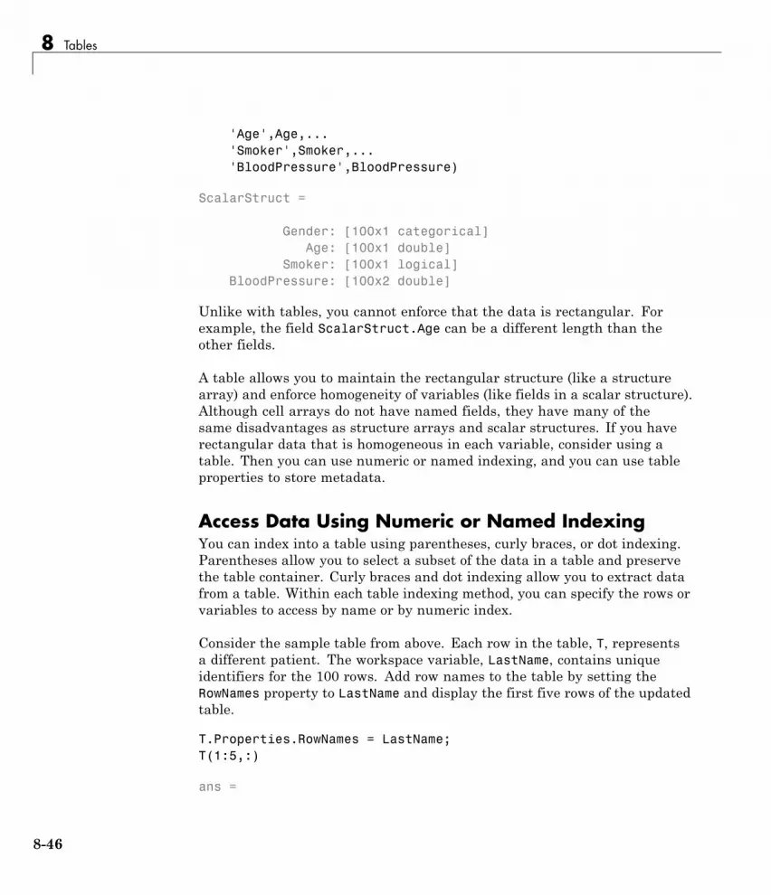
8 Tables
'Age',Age,...'Smoker',Smoker,...'BloodPressure',BloodPressure)
ScalarStruct =
Gender: [100x1 categorical]Age: [100x1 double]
Smoker: [100x1 logical]BloodPressure: [100x2 double]
Unlike with tables, you cannot enforce that the data is rectangular. Forexample, the field ScalarStruct.Age can be a different length than theother fields.
A table allows you to maintain the rectangular structure (like a structurearray) and enforce homogeneity of variables (like fields in a scalar structure).Although cell arrays do not have named fields, they have many of thesame disadvantages as structure arrays and scalar structures. If you haverectangular data that is homogeneous in each variable, consider using atable. Then you can use numeric or named indexing, and you can use tableproperties to store metadata.
Access Data Using Numeric or Named IndexingYou can index into a table using parentheses, curly braces, or dot indexing.Parentheses allow you to select a subset of the data in a table and preservethe table container. Curly braces and dot indexing allow you to extract datafrom a table. Within each table indexing method, you can specify the rows orvariables to access by name or by numeric index.
Consider the sample table from above. Each row in the table, T, representsa different patient. The workspace variable, LastName, contains uniqueidentifiers for the 100 rows. Add row names to the table by setting theRowNames property to LastName and display the first five rows of the updatedtable.
T.Properties.RowNames = LastName;T(1:5,:)
ans =
8-46

Advantages of Using Tables
Gender Age Smoker BloodPressure______ ___ ______ _______________
Smith Male 38 true 124 93Johnson Male 43 false 109 77Williams Female 38 false 125 83Jones Female 40 false 117 75Brown Female 49 false 122 80
In addition to labeling the data, you can use row and variable names to accessdata in the table. For example, use named indexing to display the gender andblood pressure of the patients Williams and Brown.
T({'Williams','Brown'},{'Age','BloodPressure'})
ans =
Age BloodPressure___ _______________
Williams 38 125 83Brown 49 122 80
Now, use numeric indexing to return an equivalent subtable. Return the thirdand fifth row from the second and fourth variables.
T(3:2:5,2:2:4)
ans =
Age BloodPressure___ _______________
Williams 38 125 83Brown 49 122 80
With cell arrays or structures, you do not have the same flexibility to usenamed or numeric indexing.
8-47

8 Tables
• With a cell array, you must use strcmp to find desired named data, andthen you can index into the array.
• With a scalar structure or structure array, it is not possible to refer to afield by number. Furthermore, with a scalar structure, you cannot easilyselect a subset of variables or a subset of observations. With a structurearray, you can select a subset of observations, but you cannot select asubset of variables.
• With a table, you can access data by named index or by numeric index.Furthermore, you can easily select a subset of variables and a subset ofrows.
For more information on table indexing, see “Access Data in a Table” on page8-29.
Use Table Properties to Store MetadataIn addition to storing data, tables have properties to store metadata, such asvariable names, row names, descriptions, and variable units. You can access aproperty using T.Properties.PropName, where T is the name of the table andPropName is one of the table properties.
For example, add a table description, variable descriptions, and variable unitsfor Age.
T.Properties.Description = 'Simulated Patient Data';
T.Properties.VariableDescriptions = ...{'Male or Female' ...'' ...'true or false' ...'Systolic/Diastolic'};
T.Properties.VariableUnits{'Age'} = 'Yrs';
Individual empty strings within the cell array for VariableDescriptionsindicate that the corresponding variable does not have a description. Formore information, see Table Properties.
To print a table summary, use the summary function.
8-48

Advantages of Using Tables
summary(T)
Description: Simulated Patient Data
Variables:
Gender: 100x1 cell stringDescription: Male or Female
Age: 100x1 doubleUnits: YrsValues:
min 25median 39max 50
Smoker: 100x1 logicalDescription: true or falseValues:
true 34false 66
BloodPressure: 100x2 doubleDescription: Systolic/DiastolicValues:
BloodPressure_1 BloodPressure_2_______________ _______________
min 109 68median 122 81.5max 138 99
Structures and cell arrays do not have properties for storing metadata.
See Also table | summary
8-49

8 Tables
RelatedExamples
• “Create a Table” on page 8-2• “Modify Units, Descriptions and Table Variable Names” on page 8-25• “Access Data in a Table” on page 8-29
8-50

9
Structures
• “Create a Structure Array” on page 9-2
• “Access Data in a Structure Array” on page 9-5
• “Concatenate Structures” on page 9-9
• “Generate Field Names from Variables” on page 9-11
• “Access Data in Nested Structures” on page 9-12
• “Access Elements of a Nonscalar Struct Array” on page 9-14
• “Ways to Organize Data in Structure Arrays” on page 9-16
• “Memory Requirements for a Structure Array” on page 9-20

9 Structures
Create a Structure ArrayThis example shows how to create a structure array. A structure is a datatype that groups related data using data containers called fields. Each fieldcan contain data of any type or size.
Store a patient record in a scalar structure with fields name, billing, andtest.
patient.name = 'John Doe';patient.billing = 127.00;patient.test = [79, 75, 73; 180, 178, 177.5; 220, 210, 205];patient
patient =
name: 'John Doe'billing: 127
test: [3x3 double]
Add records for other patients to the array by including subscripts after thearray name.
patient(2).name = 'Ann Lane';patient(2).billing = 28.50;patient(2).test = [68, 70, 68; 118, 118, 119; 172, 170, 169];patient
patient =
1x2 struct array with fields:
9-2

Create a Structure Array
namebillingtest
Each patient record in the array is a structure of class struct. An array ofstructures is often referred to as a struct array. Like other MATLAB arrays, astruct array can have any dimensions.
A struct array has the following properties:
• All structs in the array have the same number of fields.
• All structs have the same field names.
• Fields of the same name in different structs can contain different typesor sizes of data.
Any unspecified fields for new structs in the array contain empty arrays.
patient(3).name = 'New Name';patient(3)
ans =
name: 'New Name'billing: []
test: []
Access data in the structure array to find how much the first patient owes,and to create a bar graph of his test results.
amount_due = patient(1).billingbar(patient(1).test)title(['Test Results for ', patient(1).name])
amount_due =
9-3

9 Structures
127
RelatedExamples
• “Create a Cell Array” on page 10-3• “Create a Table” on page 8-2
Concepts • “Cell vs. Struct Arrays” on page 10-18• “Advantages of Using Tables” on page 8-43
9-4

Access Data in a Structure Array
Access Data in a Structure ArrayThis example shows how to access the contents of a structure array. Torun the code in this example, load several variables into a scalar (1-by-1)structure named S.
S = load('clown.mat')
S =
X: [200x320 double]map: [81x3 double]
caption: [2x1 char]
The variables from the file (X, caption, and map) are now fields in the struct.
Access the data using dot notation of the form structName.fieldName. Forexample, pass the numeric data in field X to the image function:
image(S.X)colormap(S.map)
9-5

9 Structures
To access part of a field, add indices as appropriate for the size and type of datain the field. For example, pass the upper left corner of X to the image function:
upperLeft = S.X(1:50,1:80);image(upperLeft);
9-6

Access Data in a Structure Array
If a particular field contains a cell array, use curly braces to access the data,such as S.cellField{1:50,1:80}.
Data in Nonscalar Structure Arrays
Create a nonscalar array by loading data from the file mandrill.mat intoa second element of array S:
S(2) = load('mandrill.mat')
9-7

9 Structures
Each element of a structure array must have the same fields. Both clown.matand mandrill.mat contain variables X, map, and caption.
S is a 1-by-2 array.
S =1x2 struct array with fields:
Xmapcaption
For nonscalar structures, the syntax for accessing a particular field isstructName(indices).fieldName. Redisplay the clown image, specifying theindex for the clown struct (1):
image(S(1).X)colormap(S(1).map)
Add indices to select and redisplay the upper left corner of the field contents:
upperLeft = S(1).X(1:50,1:80);image(upperLeft)
Note You can index into part of a field only when you refer to a singleelement of a structure array. MATLAB does not support statements suchas S(1:2).X(1:50,1:80), which attempt to index into a field for multipleelements of the structure.
Related Information
• “Access Data in Nested Structures” on page 9-12
• “Access Elements of a Nonscalar Struct Array” on page 9-14
• “Generate Field Names from Variables” on page 9-11
9-8

Concatenate Structures
Concatenate StructuresThis example shows how to concatenate structure arrays using the []operator. To concatenate structures, they must have the same set of fields,but the fields do not need to contain the same sizes or types of data.
Create scalar (1-by-1) structure arrays struct1 and struct2, each with fieldsa and b:
struct1.a = 'first';struct1.b = [1,2,3];
struct2.a = 'second';struct2.b = rand(5);
Just as concatenating two scalar values such as [1, 2] creates a 1-by-2numeric array, concatenating struct1 and struct2,
combined = [struct1, struct2]
creates a 1-by-2 structure array:
combined =1x2 struct array with fields:
ab
When you want to access the contents of a particular field, specify the index ofthe structure in the array. For example, access field a of the first structure:
combined(1).a
This code returns
ans =first
Concatenation also applies to nonscalar structure arrays. For example, createa 2-by-2 structure array named new:
new(1,1).a = 1; new(1,1).b = 10;new(1,2).a = 2; new(1,2).b = 20;
9-9

9 Structures
new(2,1).a = 3; new(2,1).b = 30;new(2,2).a = 4; new(2,2).b = 40;
Because the 1-by-2 structure combined and the 2-by-2 structure new both havetwo columns, you can concatenate them vertically with a semicolon separator:
larger = [combined; new]
This code returns a 3-by-2 structure array,
larger =3x2 struct array with fields:
ab
where, for example,
larger(2,1).a =1
For related information, see:
• “Creating and Concatenating Matrices”
• “Access Data in a Structure Array” on page 9-5
• “Access Elements of a Nonscalar Struct Array” on page 9-14
9-10

Generate Field Names from Variables
Generate Field Names from VariablesThis example shows how to derive a structure field name at run time from avariable or expression. The general syntax is
structName.(dynamicExpression)
where dynamicExpression is a variable or expression that returns a characteror string. Field names that you reference with expressions are called dynamicfield names.
For example, create a field name from the current date:
currentDate = datestr(now,'mmmdd');myStruct.(currentDate) = [1,2,3]
If the current date reported by your system is February 29, then this codeassigns data to a field named Feb29:
myStruct =Feb29: [1 2 3]
Field names, like variable names, must begin with a letter, can containletters, digits, or underscore characters, and are case sensitive. To avoidpotential conflicts, do not use the names of existing variables or functions asfield names. For more information, see “Variable Names” on page 1-8.
9-11

9 Structures
Access Data in Nested StructuresThis example shows how to index into a structure that is nested withinanother structure. The general syntax for accessing data in a particular fieldis
structName(index).nestedStructName(index).fieldName(indices)
When a structure is scalar (1-by-1), you do not need to include the indices torefer to the single element. For example, create a scalar structure s, wherefield n is a nested scalar structure with fields a, b, and c:
s.n.a = ones(3);s.n.b = eye(4);s.n.c = magic(5);
Access the third row of field b:
third_row_b = s.n.b(3,:)
Variable third_row_b contains the third row of eye(4).
third_row_b =0 0 1 0
Expand s so that both s and n are nonscalar (1-by-2):
s(1).n(2).a = 2 * ones(3);s(1).n(2).b = 2 * eye(4);s(1).n(2).c = 2 * magic(5);
s(2).n(1).a = '1a'; s(2).n(2).a = '2a';s(2).n(1).b = '1b'; s(2).n(2).b = '2b';s(2).n(1).c = '1c'; s(2).n(2).c = '2c';
Structure s now contains the data shown in the following figure.
9-12

Access Data in Nested Structures
s(1)
.n(1) .a 1 1 11 1 11 1 1
.b 1 0 0 00 1 0 00 0 1 00 0 0 1
.c 17 24 1 8 1523 5 7 14 16 4 6 13 20 2210 12 19 21 311 18 25 2 9
.n(2) 2 2 22 2 22 2 2
2 0 0 00 2 0 00 0 2 00 0 0 2
34 48 2 16 3046 10 14 28 32 8 12 26 40 4420 24 38 42 622 36 50 4 18
s(2)
.n(1) .a 1a
.b
.c
.n(2)
1b
1c
2a
2b
2c
.a
.b
.c
.a
.b
.c
Access part of the array in field b of the second element in n within the firstelement of s:
part_two_eye = s(1).n(2).b(1:2,1:2)
This returns the 2-by-2 upper left corner of 2 * eye(4):
part_two_eye =2 00 2
9-13

9 Structures
Access Elements of a Nonscalar Struct ArrayThis example shows how to access and process data from multiple elements ofa nonscalar structure array:
Create a 1-by-3 structure s with field f:
s(1).f = 1;s(2).f = 'two';s(3).f = 3 * ones(3);
Although each structure in the array must have the same number of fieldsand the same field names, the contents of the fields can be different types andsizes. When you refer to field f for multiple elements of the structure array,such as
s(1:3).f
or
s.f
MATLAB returns the data from the elements in a comma-separated list,which displays as follows:
ans =1
ans =two
ans =3 3 33 3 33 3 3
You cannot assign the list to a single variable with the syntax v = s.fbecause the fields can contain different types of data. However, you canassign the list items to the same number of variables, such as
[v1, v2, v3] = s.f;
9-14

Access Elements of a Nonscalar Struct Array
or assign to elements of a cell array, such as
c = {s.f};
If all of the fields contain the same type of data and can form a hyperrectangle,you can concatenate the list items. For example, create a structure nums withscalar numeric values in field f, and concatenate the data from the fields:
nums(1).f = 1;nums(2).f = 2;nums(3).f = 3;
allNums = [nums.f]
This code returns
allNums =1 2 3
If you want to process each element of an array with the same operation, usethe arrayfun function. For example, count the number of elements in fieldf of each struct in array s:
numElements = arrayfun(@(x) numel(x.f), s)
The syntax @(x) creates an anonymous function. This code calls the numelfunction for each element of array s, such as numel(s(1).f), and returns
numElements =1 3 9
For related information, see:
• “Comma-Separated Lists” on page 2-61
• “Anonymous Functions” on page 17-23
9-15

9 Structures
Ways to Organize Data in Structure ArraysThere are at least two ways you can organize data in a structure array: planeorganization and element-by-element organization. The method that best fitsyour data depends on how you plan to access the data, and, for very large datasets, whether you have system memory constraints.
Plane organization allows easier access to all values within a field.Element-by-element organization allows easier access to all informationrelated to a single element or record. The following sections include anexample of each type of organization:
• “Plane Organization” on page 9-16
• “Element-by-Element Organization” on page 9-18
When you create a structure array, MATLAB stores information about eachelement and field in the array header. As a result, structures with moreelements and fields require more memory than simpler structures thatcontain the same data. For more information on memory requirements forarrays, see “Memory Allocation” on page 26-2.
Plane OrganizationConsider an RGB image with three arrays corresponding to color intensityvalues.
9-16

Ways to Organize Data in Structure Arrays
If you have arrays RED, GREEN, and BLUE in your workspace, then thesecommands create a scalar structure named img that uses plane organization:
img.red = RED;img.green = GREEN;img.blue = BLUE;
Plane organization allows you to easily extract entire image planes fordisplay, filtering, or other processing. For example, multiply the red intensityvalues by 0.9:
adjustedRed = .9 * img.red;
If you have multiple images, you can add them to the img structure, so thateach element img(1),...,img(n) contains an entire image. For an examplethat adds elements to a structure, see the following section.
9-17

9 Structures
Element-by-Element OrganizationConsider a database with patient information. Each record contains data forthe patient’s name, test results, and billing amount.
These statements create an element in a structure array named patient:
patient(1).name = 'John Doe';patient(1).billing = 127.00;patient(1).test = [79, 75, 73; 180, 178, 177.5; 220, 210, 205];
Additional patients correspond to new elements in the structure. For example,add an element for a second patient:
patient(2).name = 'Ann Lane';patient(2).billing = 28.50;patient(2).test = [68, 70, 68; 118, 118, 119; 172, 170, 169];
Element-by-element organization supports simple indexing to access data fora particular patient. For example, find the average of the first patient’s testresults, calculating by rows (dimension 2) rather than by columns:
aveResultsDoe = mean(patient(1).test,2)
This code returns
aveResultsDoe =
9-18

Ways to Organize Data in Structure Arrays
75.6667178.5000212.0000
For information on processing data from more than one element at a time, see“Access Data in a Structure Array” on page 9-5.
9-19

9 Structures
Memory Requirements for a Structure ArrayStructure arrays do not require completely contiguous memory. However,each field requires contiguous memory, as does the header that MATLABcreates to describe the array. For very large arrays, incrementally increasingthe number of fields or the number of elements in a field results in Out ofMemory errors.
Allocate memory for the contents by assigning initial values with the structfunction, such as
newStruct(1:25,1:50) = struct('a',ones(20),'b',zeros(30),'c',rand(40));
This code creates and populates a 25-by-50 structure array S with fields a,b, and c.
If you prefer not to assign initial values, you can initialize a structure arrayby assigning empty arrays to each field of the last element in the structurearray, such as
newStruct(25,50).a = [];newStruct(25,50).b = [];newStruct(25,50).c = [];
or, equivalently,
newStruct(25,50) = struct('a',[],'b',[],'c',[]);
However, in this case, MATLAB only allocates memory for the header, andnot for the contents of the array.
For more information, see:
• “Preallocating Memory”
• “Memory Allocation” on page 26-2
9-20

10
Cell Arrays
• “What Is a Cell Array?” on page 10-2
• “Create a Cell Array” on page 10-3
• “Access Data in a Cell Array” on page 10-5
• “Add Cells to a Cell Array” on page 10-8
• “Delete Data from a Cell Array” on page 10-9
• “Combine Cell Arrays” on page 10-10
• “Pass Contents of Cell Arrays to Functions” on page 10-11
• “Preallocate Memory for a Cell Array” on page 10-17
• “Cell vs. Struct Arrays” on page 10-18
• “Multilevel Indexing to Access Parts of Cells” on page 10-20

10 Cell Arrays
What Is a Cell Array?A cell array is a data type with indexed data containers called cells. Eachcell can contain any type of data. Cell arrays commonly contain lists of textstrings, combinations of text and numbers from spreadsheets or text files,or numeric arrays of different sizes.
There are two ways to refer to the elements of a cell array. Enclose indicesin smooth parentheses, (), to refer to sets of cells — for example, to define asubset of the array. Enclose indices in curly braces, {}, to refer to the text,numbers, or other data within individual cells.
For more information, see:
• “Create a Cell Array” on page 10-3
• “Access Data in a Cell Array” on page 10-5
10-2

Create a Cell Array
Create a Cell ArrayThis example shows how to create a cell array using the {} operator or thecell function.
When you have data to put into a cell array, create the array using the cellarray construction operator, {}:
myCell = {1, 2, 3;'text', rand(5,10,2), {11; 22; 33}}
Like all MATLAB arrays, cell arrays are rectangular, with the same numberof cells in each row. myCell is a 2-by-3 cell array:
myCell =[ 1] [ 2] [ 3]'text' [5x10x2 double] {3x1 cell}
You also can use the {} operator to create an empty 0-by-0 cell array,
C = {}
If you plan to add values to a cell array over time or in a loop, you can createan empty n-dimensional array using the cell function:
emptyCell = cell(3,4,2)
emptyCell is a 3-by-4-by-2 cell array, where each cell contains an emptyarray, []:
emptyCell(:,:,1) =[] [] [] [][] [] [] [][] [] [] []
emptyCell(:,:,2) =
[] [] [] [][] [] [] [][] [] [] []
10-3

10 Cell Arrays
RelatedExamples
• “Access Data in a Cell Array” on page 10-5• “Multidimensional Cell Arrays”• “Create a Structure Array” on page 9-2• “Create a Table” on page 8-2
Concepts • “Cell vs. Struct Arrays” on page 10-18• “Advantages of Using Tables” on page 8-43
10-4

Access Data in a Cell Array
Access Data in a Cell ArrayThis example shows how to read and write data to and from a cell array. Torun the code in this example, create a 2-by-3 cell array of text and numericdata:
C = {'one', 'two', 'three';1, 2, 3};
There are two ways to refer to the elements of a cell array. Enclose indicesin smooth parentheses, (), to refer to sets of cells—for example, to define asubset of the array. Enclose indices in curly braces, {}, to refer to the text,numbers, or other data within individual cells.
Cell Indexing with Smooth Parentheses, ()
Cell array indices in smooth parentheses refer to sets of cells. For example,the command
upperLeft = C(1:2,1:2)
creates a 2-by-2 cell array:
upperLeft ='one' 'two'[ 1] [ 2]
Update sets of cells by replacing them with the same number of cells. Forexample, the statement
C(1,1:3) = {'first','second','third'}
replaces the cells in the first row of C with an equivalent-sized (1-by-3) cellarray:
C ='first' 'second' 'third'[ 1] [ 2] [ 3]
If cells in your array contain numeric data, you can convert the cells to anumeric array using the cell2mat function:
10-5

10 Cell Arrays
numericCells = C(2,1:3)numericVector = cell2mat(numericCells)
numericCells is a 1-by-3 cell array, but numericVector is a 1-by-3 array oftype double:
numericCells =[1] [2] [3]
numericVector =1 2 3
Content Indexing with Curly Braces, {}
Access the contents of cells—the numbers, text, or other data within thecells—by indexing with curly braces. For example, the command
last = C{2,3}
creates a numeric variable of type double, because the cell contains a doublevalue:
last =3
Similarly, this command
C{2,3} = 300
replaces the contents of the last cell of C with a new, numeric value:
C ='first' 'second' 'third'[ 1] [ 2] [ 300]
When you access the contents of multiple cells, such as
C{1:2,1:2}
MATLAB creates a comma-separated list. Because each cell can containa different type of data, you cannot assign this list to a single variable.However, you can assign the list to the same number of variables as cells.MATLAB assigns to the variables in column order. For example,
10-6

Access Data in a Cell Array
[r1c1, r2c1, r1c2, r2c2] = C{1:2,1:2}
returns
r1c1 =first
r2c1 =1
r1c2 =second
r2c2 =2
If each cell contains the same type of data, you can create a single variableby applying the array concatenation operator, [], to the comma-separatedlist. For example,
nums = [C{2,:}]
returns
nums =1 2 300
For more information, see:
• “Multilevel Indexing to Access Parts of Cells” on page 10-20
• “Comma-Separated Lists” on page 2-61
10-7

10 Cell Arrays
Add Cells to a Cell ArrayThis example shows how to add cells to a cell array.
Create a 1-by-3 cell array:
C = {1, 2, 3};
Assign data to a cell outside the current dimensions:
C{4,4} = 44
MATLAB expands the cell array to a rectangle that includes the specifiedsubscripts. Any intervening cells contain empty arrays:
C =[1] [2] [3] [][] [] [] [][] [] [] [][] [] [] [44]
Add cells without specifying a value by assigning an empty array as thecontents of a cell:
C{5,5} = []
C is now a 5-by-5 cell array:
C =[1] [2] [3] [] [][] [] [] [] [][] [] [] [] [][] [] [] [44] [][] [] [] [] []
For related examples, see:
• “Access Data in a Cell Array” on page 10-5
• “Combine Cell Arrays” on page 10-10
• “Delete Data from a Cell Array” on page 10-9
10-8

Delete Data from a Cell Array
Delete Data from a Cell ArrayThis example shows how to remove data from individual cells, and how todelete entire cells from a cell array. To run the code in this example, create a3-by-3 cell array:
C = {1, 2, 3; 4, 5, 6; 7, 8, 9};
Delete the contents of a particular cell by assigning an empty array to thecell, using curly braces for content indexing, {}:
C{2,2} = []
This code returns
C =[1] [2] [3][4] [] [6][7] [8] [9]
Delete sets of cells using standard array indexing with smooth parentheses,(). For example, this command
C(2,:) = []
removes the second row of C:
C =[1] [2] [3][7] [8] [9]
For related examples, see:
• “Add Cells to a Cell Array” on page 10-8
• “Access Data in a Cell Array” on page 10-5
10-9

10 Cell Arrays
Combine Cell ArraysThis example shows how to combine cell arrays by concatenation or nesting.To run the code in this example, create several cell arrays with the samenumber of columns:
C1 = {1, 2, 3};C2 = {'A', 'B', 'C'};C3 = {10, 20, 30};
Concatenate cell arrays with the array concatenation operator, []. In thisexample, vertically concatenate the cell arrays by separating them withsemicolons:
C4 = [C1; C2; C3]
C4 is a 3-by-3 cell array:
C4 =[ 1] [ 2] [ 3]'A' 'B' 'C'[10] [20] [30]
Create a nested cell array with the cell array construction operator, {}:
C5 = {C1; C2; C3}
C5 is a 3-by-1 cell array, where each cell contains a cell array:
C5 ={1x3 cell}{1x3 cell}{1x3 cell}
For more information, see “Concatenating Matrices”.
10-10

Pass Contents of Cell Arrays to Functions
Pass Contents of Cell Arrays to FunctionsThese examples show several ways to pass data from a cell array to aMATLAB® function that does not recognize cell arrays as inputs.
Pass the contents of a single cell by indexing with curly braces, {}.
This example creates a cell array that contains text and a 20-by-2 array ofrandom numbers.
randCell = {'Random Data', rand(20,2)};plot(randCell{1,2})title(randCell{1,1})
10-11

10 Cell Arrays
Plot only the first column of data by indexing further into the content(multilevel indexing).
figureplot(randCell{1,2}(:,1))title('First Column of Data')
10-12

Pass Contents of Cell Arrays to Functions
Combine numeric data from multiple cells using the cell2mat function.
This example creates a 5-by-2 cell array that stores temperature data forthree cities, and plots the temperatures for each city by date.
temperature(1,:) = {'01-Jan-2010', [45, 49, 0]};temperature(2,:) = {'03-Apr-2010', [54, 68, 21]};temperature(3,:) = {'20-Jun-2010', [72, 85, 53]};temperature(4,:) = {'15-Sep-2010', [63, 81, 56]};temperature(5,:) = {'31-Dec-2010', [38, 54, 18]};
10-13

10 Cell Arrays
allTemps = cell2mat(temperature(:,2));dates = datenum(temperature(:,1), 'dd-mmm-yyyy');
plot(dates, allTemps)datetick('x','mmm')
Pass the contents of multiple cells as a comma-separated list to functions thataccept multiple inputs.
10-14

Pass Contents of Cell Arrays to Functions
This example plots X against Y , and applies line styles from a 2-by-3 cellarray C.
X = -pi:pi/10:pi;Y = tan(sin(X)) - sin(tan(X));
C(:,1) = {'LineWidth'; 2};C(:,2) = {'MarkerEdgeColor'; 'k'};C(:,3) = {'MarkerFaceColor'; 'g'};
plot(X, Y, '--rs', C{:})
10-15

10 Cell Arrays
Concepts • “Access Data in a Cell Array” on page 10-5• “Multilevel Indexing to Access Parts of Cells” on page 10-20• “Comma-Separated Lists” on page 2-61
10-16

Preallocate Memory for a Cell Array
Preallocate Memory for a Cell ArrayThis example shows how to initialize and allocate memory for a cell array.
Cell arrays do not require completely contiguous memory. However, each cellrequires contiguous memory, as does the cell array header that MATLABcreates to describe the array. For very large arrays, incrementally increasingthe number of cells or the number of elements in a cell results in Out ofMemory errors.
Initialize a cell array by calling the cell function, or by assigning to the lastelement. For example, these statements are equivalent:
C = cell(25,50);C{25,50} = [];
MATLAB creates the header for a 25-by-50 cell array. However, MATLABdoes not allocate any memory for the contents of each cell.
For more information, see:
• “Preallocating Memory”
• “Memory Allocation” on page 26-2
10-17

10 Cell Arrays
Cell vs. Struct ArraysThis example compares cell and structure arrays, and shows how to store datain each type of array. Both cell and structure arrays allow you to store dataof different types and sizes.
Structure Arrays
Structure arrays contain data in fields that you access by name.
For example, store patient records in a structure array.
patient(1).name = 'John Doe';patient(1).billing = 127.00;patient(1).test = [79, 75, 73; 180, 178, 177.5; 220, 210, 205];
patient(2).name = 'Ann Lane';patient(2).billing = 28.50;patient(2).test = [68, 70, 68; 118, 118, 119; 172, 170, 169];
Create a bar graph of the test results for each patient.
numPatients = numel(patient);for p = 1:numPatients
figurebar(patient(p).test)title(patient(p).name)
end
Cell Arrays
Cell arrays contain data in cells that you access by numeric indexing.Common applications of cell arrays include storing lists of text strings andstoring heterogeneous data from spreadsheets.
For example, store temperature data for three cities over time in a cell array.
temperature(1,:) = {'01-Jan-2010', [45, 49, 0]};temperature(2,:) = {'03-Apr-2010', [54, 68, 21]};temperature(3,:) = {'20-Jun-2010', [72, 85, 53]};temperature(4,:) = {'15-Sep-2010', [63, 81, 56]};
10-18

Cell vs. Struct Arrays
temperature(5,:) = {'31-Dec-2010', [38, 54, 18]};
Plot the temperatures for each city by date.
allTemps = cell2mat(temperature(:,2));dates = datenum(temperature(:,1), 'dd-mmm-yyyy');
plot(dates,allTemps)datetick('x','mmm')
Other Container Arrays
Struct and cell arrays are the most commonly used containers for storingheterogeneous data. Tables are convenient for storing heterogeneouscolumn-oriented or tabular data. Alternatively, use map containers, or createyour own class.
See Also cell | containers.Map | table | struct
RelatedExamples
• “Access Data in a Cell Array” on page 10-5• “Access Data in a Structure Array” on page 9-5• “Access Data in a Table” on page 8-29
Concepts • “Advantages of Using Tables” on page 8-43
10-19

10 Cell Arrays
Multilevel Indexing to Access Parts of CellsThis example explains techniques for accessing data in arrays stored withincells of cell arrays. To run the code in this example, create a sample cell array:
myNum = [1, 2, 3];myCell = {'one', 'two'};myStruct.Field1 = ones(3);myStruct.Field2 = 5*ones(5);
C = {myNum, 100*myNum;myCell, myStruct};
Access the complete contents of a particular cell using curly braces, {}. Forexample,
C{1,2}
returns the numeric vector from that cell:
ans =100 200 300
Access part of the contents of a cell by appending indices, using syntax thatmatches the data type of the contents. For example:
• Enclose numeric indices in smooth parentheses. For example, C{1,1}returns the 1-by-3 numeric vector, [1, 2, 3]. Access the second elementof that vector with the syntax
C{1,1}(1,2)
which returns
ans =2
• Enclose cell array indices in curly braces. For example, C{2,1} returns thecell array {'one', 'two'}. Access the contents of the second cell withinthat cell array with the syntax
C{2,1}{1,2}
10-20

Multilevel Indexing to Access Parts of Cells
which returns
ans =two
• Refer to fields of a struct array with dot notation, and index into the arrayas described for numeric and cell arrays. For example, C{2,2} returns astructure array, where Field2 contains a 5-by-5 numeric array of fives.Access the element in the fifth row and first column of that field with thesyntax
C{2,2}.Field2(5,1)
which returns
ans =5
You can nest any number of cell and structure arrays. For example, addnested cells and structures to C.
C{2,1}{2,2} = {pi, eps};C{2,2}.Field3 = struct('NestedField1', rand(3), ...
'NestedField2', magic(4), ...'NestedField3', {{'text'; 'more text'}} );
These assignment statements access parts of the new data:
copy_pi = C{2,1}{2,2}{1,1}
part_magic = C{2,2}.Field3.NestedField2(1:2,1:2)
nested_cell = C{2,2}.Field3.NestedField3{2,1}
MATLAB displays:
copy_pi =3.1416
part_magic =16 25 11
10-21

10 Cell Arrays
nested_cell =more text
RelatedExamples
• “Access Data in a Cell Array” on page 10-5
10-22

11
Function Handles
• “What Is a Function Handle?” on page 11-2
• “Creating a Function Handle” on page 11-3
• “Calling a Function Using Its Handle” on page 11-7
• “Preserving Data from the Workspace” on page 11-10
• “Applications of Function Handles” on page 11-13
• “Saving and Loading Function Handles” on page 11-19
• “Advanced Operations on Function Handles” on page 11-20
• “Functions That Operate on Function Handles” on page 11-27

11 Function Handles
What Is a Function Handle?A function handle is a callable association to a MATLAB function. It containsan association to that function that enables you to invoke the functionregardless of where you call it from. This means that, even if you are outsidethe normal scope of a function, you can still call it if you use its handle.
With function handles, you can:
• Pass a function to another function
• Capture data values for later use by a function
• Call functions outside of their normal scope
• Save the handle in a MAT-file to be used in a later MATLAB session
See “Applications of Function Handles” on page 11-13 for an explanationof each of these applications.
11-2

Creating a Function Handle
Creating a Function Handle
In this section...
“Maximum Length of a Function Name” on page 11-4
“The Role of Scope, Precedence, and Overloading When Creating a FunctionHandle” on page 11-4
“Obtaining Permissions from Class Methods” on page 11-5
“Using Function Handles for Anonymous Functions” on page 11-6
“Arrays of Function Handles” on page 11-6
You construct a handle for a specific function by preceding the function namewith an @ sign. The syntax is:
h = @functionname
where h is the variable to which the returned function handle is assigned.
Use only the function name, with no path information, after the @ sign. Ifthere is more than one function with this name, MATLAB associates withthe handle the one function source it would dispatch to if you were actuallycalling the function.
Create a handle h for a function plot that is on your MATLAB path:
h = @plot;
Once you create a handle for a function, you can invoke the function bymeans of the handle instead of using the function name. Because the handlecontains the absolute path to its function, you can invoke the function fromany location that MATLAB is able to reach, as long as the program file forthe function still exists at this location. This means that functions in one filecan call functions that are not on the MATLAB path, local functions in aseparate file, or even functions that are private to another folder, and thusnot normally accessible to that caller.
11-3

11 Function Handles
Maximum Length of a Function NameFunction names used in handles are unique up to N characters, where N isthe number returned by the function namelengthmax. If the function nameexceeds that length, MATLAB truncates the latter part of the name.
For function handles created for Java constructors, the length of anysegment of the package name or class name must not exceed namelengthmaxcharacters. (The term segment refers to any portion of the name that liesbefore, between, or after a dot. For example, java.lang.String has threesegments). The overall length of the string specifying the package and classhas no limit.
The Role of Scope, Precedence, and OverloadingWhen Creating a Function HandleAt the time you create a function handle, MATLAB must decide exactly whichfunction it is to associate the handle to. In doing so, MATLAB uses the samerules used to determine which file to invoke when you make a function call.To make this determination, MATLAB considers the following:
• Scope — The function named must be on the MATLAB path at the timethe handle is constructed.
• Precedence — MATLAB selects which function(s) to associate thehandle with, according to the function precedence rules described underDetermining Which Function Gets Called.
• Overloading — If additional files on the path overload the function forany of the fundamental MATLAB classes, such as double or char, thenMATLAB associates the handle with these files, as well.
Program files that overload a function for classes other than the standardMATLAB classes are not associated with the function handle at the time itis constructed. Function handles do operate on these types of overloadedfunctions, but MATLAB determines which implementation to call at the timeof evaluation in this case.
11-4

Creating a Function Handle
Obtaining Permissions from Class MethodsWhen creating a function handle inside a method of a class, the functionis resolved using the permissions of that method. When MATLAB invokesthe function handle, it does so using the permissions of the class. This givesMATLAB the same access as the location where the function handle wascreated, including access to private and protected methods accessible to thatclass.
ExampleThis example defines two methods. One, updateObj, defines a listenerfor an event called Update, and the other , callbackfcn, responds to thisevent whenever it should occur. The latter function is a private functionand thus would not normally be within the scope of the notify function.However, because @callbackfcn is actually a function handle, it retains thepermissions of the context that created the function handle:
classdef updateObj < handleevents
Updateend
methodsfunction obj = updateObj(varargin)
addlistener(obj, 'Update', @callbackfcn);notify(obj, 'Update');
endend
methods (Access = private)function obj = callbackfcn(obj, varargin)
disp('Object Updated')disp(obj);
endend
end
To run this function, invoke updateObj at the MATLAB command line.
11-5

11 Function Handles
Using Function Handles for Anonymous FunctionsFunction handles also serve as the means of invoking anonymous functions.An anonymous function is a one-line expression-based MATLAB functionthat does not require a program file.
For example, the statement
sqr = @(x) x.^2;
creates an anonymous function that computes the square of its inputargument x. The @ operator makes sqr a function handle, giving you a meansof calling the function:
sqr(20)ans =
400
Like nested functions, a handle to an anonymous function also stores all datathat will be needed to resolve the handle when calling the function. Sharessame issues as nested functions do.
See the documentation on “Anonymous Functions” on page 17-23 for moreinformation.
Arrays of Function HandlesTo create an array of function handles, you must use a cell array:
trigFun = {@sin, @cos, @tan};
For example, to plot the cosine of the range -pi to pi at 0.01 intervals, use
plot(trigFun{2}(-pi:0.01:pi))
11-6

Calling a Function Using Its Handle
Calling a Function Using Its Handle
In this section...
“Calling Syntax” on page 11-7
“Calling a Function with Multiple Outputs” on page 11-8
“Returning a Handle for Use Outside of a Function File” on page 11-8
“Example — Using Function Handles in Optimization” on page 11-9
Function handles can give you access to functions you might not be able toexecute. For instance, with a handle you can call a function even if it is nolonger on your MATLAB path. You can also call a local function from outsideof the file that defines that function.
Calling SyntaxThe syntax for calling a function using a function handle is the same as thatused when calling the function directly. For example, if you call functionmyFun like this:
[out1, out2, ...] = myFun(in1, in2, ...);
then you would call it using a handle in the same way, but using the handlename instead:
fHandle = @myFun;[out1, out2, ...] = fHandle(in1, in2, ...);
There is one small difference. If the function being called takes no inputarguments, then you must call the function with empty parentheses placedafter the handle name. If you use only the handle name, MATLAB justidentifies the name of the function:
% This identifies the handle. % This invokes the function.
fHandle = @computer; fHandle = @computer;fHandle fHandle()ans = ans =
@computer PCWIN
11-7

11 Function Handles
Calling a Function with Multiple OutputsThe example below returns multiple values from a call to an anonymousfunction. Create anonymous function f that locates the nonzero elements ofan array, and returns the row, column, and value of each element in variablesrow, col, and val:
f = @(X)find(X);
Call the function on matrix m using the function handle f. Because thefunction uses the MATLAB find function which returns up to three outputs,you can specify from 0 to 3 outputs in the call:
m = [3 2 0; -5 0 7; 0 0 1]m =
3 2 0-5 0 70 0 1
[row col val] = f(m);
valval =
3-5271
Returning a Handle for Use Outside of a Function FileAs stated previously, you can use function handles to call a function that mayotherwise be hidden or out of scope. This example function getHandle returnsa function handle fHandle to a caller that is outside of the file:
function fHandle = getHandlefHandle = @subFun;
function res = subFun(t1, t2, varargin);...
11-8

Calling a Function Using Its Handle
Call getHandle to obtain a function handle with which to invoke the localfunction. You can now call the local function as you would any functionthat is in scope:
f1 = getHandle;result = f1(startTime, endTime, procedure);
Example — Using Function Handles in OptimizationFunction handles can be particularly useful in optimization work. If you havethe MathWorks Optimization Toolbox™ installed, click on any of the linksbelow to find information and examples on this topic:
• “Passing Extra Parameters” — Calling objective or constraint functionsthat have parameters in addition to the independent variable.
• “Anonymous Function Objectives” — Use function handles in writingsimple objective functions.
• “Nonlinear Curve Fitting with lsqcurvefit” — An example usinglsqcurvefit, which takes two inputs for the objective.
11-9

11 Function Handles
Preserving Data from the Workspace
In this section...
“Preserving Data with Anonymous Functions” on page 11-10
“Preserving Data with Nested Functions” on page 11-11
Both anonymous functions and nested functions make use of variable datathat is stored outside the body of the function itself. For example, theanonymous function shown here uses two variables: X and K. You pass the Xvariable into the anonymous function whenever you invoke the function. Thevalue for K however is taken from the currently active workspace:
K = 200;fAnon = @(X)K * X;
fAnon([2.54 1.43 0.68 1.90 1.02 2.13]);
What would happen if you tried to invoke this function after you cleared Kfrom the workspace? Or if you saved the anonymous function to a .mat fileand then loaded it into an entirely separate computing environment whereK is not defined?
The answer is that MATLAB stores any values needed by an anonymous (ornested) function within the handle itself. It does this at the time you constructthe handle. This does not include values from the argument list as thesevalues get passed in whenever you call the function.
Preserving Data with Anonymous FunctionsIf you create an anonymous function at the MATLAB command window, thatfunction has access to the workspace of your current MATLAB session. If youcreate the function inside of another function, then it has access to the outerfunction’s workspace. Either way, if your anonymous function depends uponvariables from an outside workspace, then MATLAB stores the variables andtheir values within the function handle at the time the handle is created.
This example puts a 3-by-5 matrix into the base workspace, and then creates afunction handle to an anonymous function that requires access to the matrix.
11-10

Preserving Data from the Workspace
Create matrix A and anonymous function testAnon:
A = magic(5); A(4:5,:) = []A =
17 24 1 8 1523 5 7 14 164 6 13 20 22
testAnon = @(x)x * A; % Anonymous function
Call the anonymous function via its handle, passing in a multiplier value.This multiplies all elements by 5.2:
testAnon(5.2)ans =
88.4000 124.8000 5.2000 41.6000 78.0000119.6000 26.0000 36.4000 72.8000 83.200020.8000 31.2000 67.6000 104.0000 114.4000
Clear variable A from the base workspace and verify that this action has noeffect on the output of the anonymous function:
clear A
testAnon(5.2)ans =
88.4000 124.8000 5.2000 41.6000 78.0000119.6000 26.0000 36.4000 72.8000 83.200020.8000 31.2000 67.6000 104.0000 114.4000
This works because the variable A and its value at the time the anonymousfunction is created is preserved within the function handle that also providesaccess to the anonymous function. See “Variables in the Expression” on page17-24 for more information.
Preserving Data with Nested FunctionsNested functions are similar to anonymous functions in their ability topreserve workspace data needed by a function handle. In this case however,the workspace belongs to one of the functions inside of which the handle isbeing created. See “Sharing Variables Between Parent and Nested Functions”
11-11

11 Function Handles
on page 17-33 and “Using Handles to Store Function Parameters” on page17-35 for more information on this subject.
This example shows a function getHandles that returns a handle to nestedfunction getApproxVal_V4. The nested function uses two variables, constand adjust, from the workspace of the outer function. Calling getHandlescreates a function handle to the nested function and also stores these twovariables within that handle so that they will be available whenever thenested function is invoked:
function handle = getHandles(adjust)const = 16.3;handle = @getApproxVal_V4;
function vOut = getApproxVal_V4(vectIn)vOut = ((vectIn+adjust)*const) + ((vectIn-adjust)*const);end
end
Call the getHandles function to obtain a handle to the nested function:
adjustVal = 0.023;getApproxValue = getHandles(adjustVal);
getApproxValue([0.67 -0.09 1.01 0.33 -0.14 -0.23])ans =
21.8420 -2.9340 32.9260 10.7580 -4.5640 -7.4980
The documentation on “Examining a Function Handle” on page 11-20 explainshow to see which variables are stored within a particular function handle.Another helpful resource is “Using Handles to Store Function Parameters” onpage 17-35.
Loading a Saved Handle to a Nested FunctionIf you save a function handle to a nested function and, at some later date,modify the function and then reload the handle, you may observe unexpectedbehavior from the restored handle. when you invoke the function from thereloaded handle.
11-12

Applications of Function Handles
Applications of Function Handles
In this section...
“Example of Passing a Function Handle” on page 11-13
“Pass a Function to Another Function” on page 11-13
“Capture Data Values For Later Use By a Function” on page 11-15
“Call Functions Outside of Their Normal Scope” on page 11-18
“Save the Handle in a MAT-File for Use in a Later MATLAB Session” onpage 11-18
Example of Passing a Function HandleThe following example creates a handle for a function supplied by MATLABcalled humps and assigns it to the variable h. (The humps function returns astrong maxima near x = 0.3 and x = 0.9).
h = @humps;
After constructing the handle, you can pass it in the argument list of a callto some other function, as shown here. This example passes the functionhandle h that was just created as the first argument in a call to fminbnd. Thisfunction then minimizes over the interval [0.3, 1].
x = fminbnd(h, 0.3, 1)x =
0.6370
Using a function handle enables you to pass different functions for fminbnd touse in determining its final result.
Pass a Function to Another FunctionThe ability to pass variables to a function enables you to run the function ondifferent values. In the same way, you can pass function handles as inputarguments to a function, thus allowing the called function to change theoperations it runs on the input data.
11-13

11 Function Handles
Example 1 — Run integral on Varying FunctionsRun the integral function on varying input functions:
a = 0; b = 5;
integral(@log, a, b)ans =
3.0472
integral(@sin, a, b)ans =
0.7163
integral(@humps, a, b)ans =
12.3566
Example 2 — Run integral on Anonymous FunctionsRun integral on a MATLAB built-in function or an anonymous function:
n = integral(@log, 0, 3);
n = integral(@(x)x.^2, 0, 3);
Change the parameters of the function you pass to integral with a simplemodification of the anonymous function that is associated with the functionhandle input:
a = 3.7;z = integral(@(x)x.^a, 0, 3);
Example 3 — Compare integral Results on Different FunctionsCompare the integral of the cosine function over the interval [a, b]:
a = 0; b = 10;int1 = integral(@cos,a,b)
int1 =
11-14

Applications of Function Handles
-0.5440
with the integral over the same interval of the piecewise polynomial pp thatapproximates the cosine function by interpolating the computed values xand y:
x = a:b;y = cos(x);pp = spline(x,y);int2 = integral(@(x)ppval(pp,x), a, b)
int2 =-0.5485
Capture Data Values For Later Use By a FunctionYou can do more with a function handle than just create an association to acertain function. By using anonymous functions, you can also capture certainvariables and their values from the function workspace and store them inthe handle. These data values are stored in the handle at the time of itsconstruction, and are contained within the handle for as long as it exists.Whenever you then invoke the function by means of its handle, MATLABsupplies the function with all variable inputs specified in the argument listof the function call, and also any constant inputs that were stored in thefunction handle at the time of its construction.
Storing some or all input data in a function handle enables you to reliablyuse the same set of data with that function regardless of where or when youinvoke the handle. You can also interrupt your use of a function and resumeit with the same data at a later time simply by saving the function handle toa MAT-file.
Example 1 — Constructing a Function Handle that PreservesIts VariablesCompare the following two ways of implementing a simple plotting functioncalled draw_plot. The first case creates the function as one that you wouldcall by name and that accepts seven inputs specifying coordinate and propertyinformation:
function draw_plot(x, y, lnSpec, lnWidth, mkEdge, mkFace, mkSize)
11-15

11 Function Handles
plot(x, y, lnSpec, ...
'LineWidth', lnWidth, ...
'MarkerEdgeColor', mkEdge, ...
'MarkerFaceColor', mkFace, ...
'MarkerSize', mkSize)
The second case implements draw_plot as an anonymous function to becalled by a function handle, h. The draw_plot function has only two inputsnow; the remaining five are specified only on a call to the handle constructorfunction, get_plot_handle:
function h = get_plot_handle(lnSpec, lnWidth, mkEdge, ...mkFace, mkSize)
h = @draw_plot;function draw_plot(x, y)
plot(x, y, lnSpec, ...'LineWidth', lnWidth, ...'MarkerEdgeColor', mkEdge, ...'MarkerFaceColor', mkFace, ...'MarkerSize', mkSize)
endend
Because these input values are required by the draw_plot function but are notmade available in its argument list, MATLAB supplies them by storing themin the function handle for draw_plot at the time it is constructed. Constructthe function handle h, also supplying the values to be stored in handle:
h = get_plot_handle('--rs', 2, 'k', 'g', 10);
Now call the function, specifying only the x and y inputs:
x = -pi:pi/10:pi;y = tan(sin(x)) - sin(tan(x));h(x, y) % Draw the plot
The later section on “Examining a Function Handle” on page 11-20 continuesthis example by showing how you can examine the contents of the functionand workspace contents of this function handle.
11-16

Applications of Function Handles
Example 2 — Varying Data Values Stored in a Function HandleValues stored within a handle to a nested function do not have to remainconstant. The following function constructs and returns a function handle h tothe anonymous function addOne. In addition to associating the handle withaddOne, MATLAB also stores the initial value of x in the function handle:
function h = counterx = 0;h = @addOne;
function y = addOne;x = x + 1;y = x;end
end
The addOne function that is associated with handle h increments variable xeach time you call it. This modifies the value of the variable stored in thefunction handle:
h = counter;h()ans =
1h()ans =
2
Example 3 — You Cannot Vary Data in a Handle to anAnonymous FunctionUnlike the example above, values stored within a handle to an anonymousfunction do remain constant. Construct a handle to an anonymous functionthat just returns the value of x, and initialize x to 300. The value of x withinthe function handle remains constant regardless of how you modify x externalto the handle:
x = 300;h = @()x;
x = 50;h()
11-17

11 Function Handles
ans =300
clear xh()ans =
300
Call Functions Outside of Their Normal ScopeBy design, only functions within a program file are permitted to access localfunctions defined within that file. However, if, in this same file, you were toconstruct a function handle for one of the internal local functions, and thenpass that handle to a variable that exists outside of the file, access to thatlocal function would be essentially unlimited. By capturing the access to thelocal function in a function handle, and then making that handle available tofunctions external to the file (or to the command line), the example extendsthat scope. An example of this is shown in the preceding section, “CaptureData Values For Later Use By a Function” on page 11-15.
Private functions also have specific access rules that limit their availabilitywith the MATLAB environment. But, as with local functions, MATLABallows you to construct a handle for a private function. Therefore, you cancall it by means of that handle from any location or even from the MATLABcommand line, should it be necessary.
Save the Handle in a MAT-File for Use in a LaterMATLAB SessionIf you have one or more function handles that you would like to reuse in a laterMATLAB session, you can store them in a MAT-file using the save functionand then use load later on to restore them to your MATLAB workspace.
11-18

Saving and Loading Function Handles
Saving and Loading Function HandlesYou can save and load function handles in a MAT-file using the MATLAB saveand load functions. If you load a function handle that you saved in an earlierMATLAB session, the following conditions could cause unexpected behavior:
• Any of the files that define the function have been moved, and thus nolonger exist on the path stored in the handle.
• You load the function handle into an environment different from that inwhich it was saved. For example, the source for the function either doesnot exist or is located in a different folder than on the system on whichthe handle was saved.
In both of these cases, the function handle is now invalid because it is nolonger associated with any existing function code. Although the handle isinvalid, MATLAB still performs the load successfully and without displayinga warning. Attempting to invoke the handle, however, results in an error.
Invalid or Obsolete Function HandlesIf you create a handle to a function that is not on the MATLAB path, or if youload a handle to a function that is no longer on the path, MATLAB catchesthe error only when the handle is invoked. You can assign an invalid handleand use it in such operations as func2str. MATLAB catches and reports anerror only when you attempt to use it in a runtime operation.
11-19

11 Function Handles
Advanced Operations on Function Handles
In this section...
“Examining a Function Handle” on page 11-20
“Converting to and from a String” on page 11-21
“Comparing Function Handles” on page 11-23
Examining a Function HandleUse the functions function to examine the contents of a function handle.
Caution MATLAB provides the functions function for querying anddebugging purposes only. Because its behavior may change in subsequentreleases, you should not rely upon it for programming purposes.
The following example is a continuation of an example in an earlier section ofthe Function Handles documentation. See Example 1 in the section “CaptureData Values For Later Use By a Function” on page 11-15 for the completeexample.
Construct a function handle that contains both a function association, anddata required by that function to execute. The following function constructsthe function handle, h:
function h = get_plot_handle(lnSpec, lnWidth, mkEdge, ...mkFace, mkSize)
h = @draw_plot;function draw_plot(x, y)
plot(x, y, lnSpec, ...'LineWidth', lnWidth, ...'MarkerEdgeColor', mkEdge, ...'MarkerFaceColor', mkFace, ...'MarkerSize', mkSize)
endend
11-20

Advanced Operations on Function Handles
Use functions to examine the contents of the returned handle:
f = functions(h)f =
function: 'get_plot_handle/draw_plot'type: 'nested'file: 'D:\matlab\work\get_plot_handle.m'
workspace: {[1x1 struct]}
The call to functions returns a structure with four fields:
• function — Name of the function or local function to which the handleis associated. (Function names that follow a slash character (/) areimplemented in the program code as local functions.)
• type— Type of function (e.g., simple, nested, anonymous)
• file — Filename and path to the file. (For built-in functions, this is thestring 'MATLAB built-in function')
• workspace— Variables in the function workspace at the time the handlewas constructed, along with their values
Examine the workspace variables that you saved in the function handle:
f.workspace{:}ans =
h: @get_plot_handle/draw_plotlnSpec: '--rs'
lnWidth: 2mrkrEdge: 'k'mrkrFace: 'g'mrkrSize: 10
Converting to and from a StringTwo functions, str2func and func2str enable you to convert between astring containing a function name and a function handle that is associatedwith that function name.
11-21

11 Function Handles
Converting a String to a Function HandleAnother means of creating a function handle is to convert a string that holdsa function name to a handle for the named function. You can do this usingthe str2func function:
handle = str2func('functionname');
The example below takes the name of a function as the first argument. Itcompares part of the name to see if this is a polynomial function, converts thefunction string to a function handle if it is not, and then calls the function bymeans of its handle:
function run_function(funcname, arg1, arg2)if strncmp(funcname, 'poly', 4)
disp 'You cannot run polynomial functions on this data.'return
elseh = str2func(funcname);h(arg1, arg2);
end
Note Nested functions are not accessible to str2func. To construct afunction handle for a nested function, you must use the function handleconstructor, @.
Converting a Function Handle to a StringYou can also convert a function handle back into a string using the func2strfunction:
functionname = func2str(handle);
This example converts the function handle h to a string containing the functionname, and then uses the function name in a message displayed to the user:
function call_h(h, arg1, arg2)sprintf('Calling function %s ...\n', func2str(h))h(arg1, arg2)
11-22

Advanced Operations on Function Handles
Comparing Function HandlesThis section describes how MATLAB determines whether or not separatefunction handles are equal to each other:
• “Comparing Handles Constructed from a Named Function” on page 11-23
• “Comparing Handles to Anonymous Functions” on page 11-23
• “Comparing Handles to Nested Functions” on page 11-24
• “Comparing Handles Saved to a MAT-File” on page 11-25
Comparing Handles Constructed from a Named FunctionMATLAB considers function handles that you construct from the same namedfunction (e.g., handle = @sin) to be equal. The isequal function returns avalue of true when comparing these types of handles:
func1 = @sin;func2 = @sin;isequal(func1, func2)ans =
1
If you save these handles to a MAT-file, and then load them back into theworkspace later on, they are still equal.
Comparing Handles to Anonymous FunctionsUnlike handles to named functions, any two function handles that representthe same anonymous function (i.e., handles to anonymous functions thatcontain the same text) are not equal. This is because MATLAB cannotguarantee that the frozen values of non-argument variables (such as A, below)are the same.
A = 5;h1 = @(x)A * x.^2;h2 = @(x)A * x.^2;
isequal(h1, h2)ans =
0
11-23

11 Function Handles
Note In general, MATLAB may underestimate the equality of functionhandles. That is, a test for equality may return false even when the functionshappen to behave the same. But in cases where MATLAB does indicateequality, the functions are guaranteed to behave in an identical manner.
If you make a copy of an anonymous function handle, the copy and theoriginal are equal:
h1 = @(x)A * x.^2; h2 = h1;isequal(h1, h2)ans =
1
Comparing Handles to Nested FunctionsMATLAB considers function handles to the same nested function to be equalonly if your code constructs these handles on the same call to the functioncontaining the nested functions. Given this function that constructs twohandles to the same nested function:
function [h1, h2] = test_eq(a, b, c)h1 = @findZ;h2 = @findZ;
function z = findZz = a.^3 + b.^2 + c';end
end
function handles constructed from the same nested function and on the samecall to the parent function are considered equal:
[h1 h2] = test_eq(4, 19, -7);
isequal(h1, h2),ans =
1
while those constructed from different calls are not considered equal:
11-24

Advanced Operations on Function Handles
[q1 q2] = test_eq(3, -1, 2);
isequal(h1, q1)ans =
0
Comparing Handles Saved to a MAT-FileIf you save equivalent anonymous or nested function handles to separateMAT-files, and then load them back into the MATLAB workspace, they areno longer equal. This is because saving the function handle loses track ofthe original circumstances under which the function handle was created.Reloading it results in a function handle that compares as being unequal tothe original function handle.
Create two equivalent anonymous function handles:
h1 = @(x) sin(x);h2 = h1;
isequal(h1, h2)ans =
1
Save each to a different MAT-file:
save fname1 h1;save fname2 h2;
Clear the MATLAB workspace, and then load the function handles back intothe workspace:
clear allload fname1load fname2
The function handles are no longer considered equal:
isequal(h1, h2)ans =
11-25

11 Function Handles
0
Note, however, that equal anonymous and nested function handles that yousave to the same MAT-file are equal when loaded back into MATLAB.
11-26

Functions That Operate on Function Handles
Functions That Operate on Function HandlesMATLAB provides the following functions for working with function handles.See the reference pages for these functions for more information.
Function Description
functions Return information describing a function handle.
func2str Construct a function name string from a functionhandle.
str2func Construct a function handle from a function namestring.
save Save a function handle from the current workspace toa MAT-file.
load Load a function handle from a MAT-file into the currentworkspace.
isa Determine if a variable contains a function handle.
isequal Determine if two function handles are handles to thesame function.
11-27

11 Function Handles
11-28

12
Map Containers
• “Overview of the Map Data Structure” on page 12-2
• “Description of the Map Class” on page 12-4
• “Creating a Map Object” on page 12-6
• “Examining the Contents of the Map” on page 12-9
• “Reading and Writing Using a Key Index” on page 12-11
• “Modifying Keys and Values in the Map” on page 12-15
• “Mapping to Different Value Types” on page 12-18

12 Map Containers
Overview of the Map Data StructureA Map is a type of fast key lookup data structure that offers a flexible meansof indexing into its individual elements. Unlike most array data structuresin the MATLAB software that only allow access to the elements by means ofinteger indices, the indices for a Map can be nearly any scalar numeric valueor a character string.
Indices into the elements of a Map are called keys. These keys, along with thedata values associated with them, are stored within the Map. Each entry of aMap contains exactly one unique key and its corresponding value. Indexinginto the Map of rainfall statistics shown below with a string representing themonth of August yields the value internally associated with that month, 37.3.
327.2 368.2 197.6 178.4 100.0 69.9 32.3 37.3 19.0 37.0 73.2 110.91551.0
JanFebMarAprMayJunJulAugSepOctNovDecAnnual
KEYS VALUES
Aug 37.3
Mean monthly rainfall statistics (mm)
Keys are not restricted to integers as they are with other arrays. Specifically,a key may be any of the following types:
• 1-by-N character array
• Scalar real double or single
12-2

Overview of the Map Data Structure
• Signed or unsigned scalar integer
The values stored in a Map can be of any type. This includes arrays ofnumeric values, structures, cells, strings, objects, or other Maps.
Note A Map is most memory efficient when the data stored in it is a scalarnumber or a character array.
12-3

12 Map Containers
Description of the Map Class
In this section...
“Properties of the Map Class” on page 12-4
“Methods of the Map Class” on page 12-5
A Map is actually an object, or instance, of a MATLAB class called Map. It isalso a handle object and, as such, it behaves like any other MATLAB handleobject. This section gives a brief overview of the Map class. For more details,see the containers.Map reference page.
Properties of the Map ClassAll objects of the Map class have three properties. You cannot write directly toany of these properties; you can change them only by means of the methodsof the Map class.
Property Description Default
Count Unsigned 64-bit integer that represents the totalnumber of key/value pairs contained in the Mapobject.
0
KeyType String that indicates the type of all keys containedin the Map object. KeyType can be any of thefollowing: double, single, char, and signed orunsigned 32-bit or 64-bit integer. If you attempt toadd keys of an unsupported type, int8 for example,MATLAB makes them double.
char
ValueType String that indicates the type of values containedin the Map object. If the values in a Map are allscalar numbers of the same type, ValueType is setto that type. If the values are all character arrays,ValueType is 'char'. Otherwise, ValueType is'any'.
any
12-4

Description of the Map Class
To examine one of these properties, follow the name of the Map object witha dot and then the property name. For example, to see what type of keysare used in Map mapObj, use
mapObj.KeyType
A Map is a handle object. As such, if you make a copy of the object, MATLABdoes not create a new Map; it creates a new handle for the existing Map thatyou specify. If you alter the Map’s contents in reference to this new handle,MATLAB applies the changes you make to the original Map as well. You can,however, delete the new handle without affecting the original Map.
Methods of the Map ClassThe Map class implements the following methods. Their use is explained in thelater sections of this documentation and also in the function reference pages.
Method Description
isKey Check if Map contains specified key
keys Names of all keys in Map
length Length of Map
remove Remove key and its value from Map
size Dimensions of Map
values Values contained in Map
12-5

12 Map Containers
Creating a Map Object
In this section...
“Constructing an Empty Map Object” on page 12-6
“Constructing An Initialized Map Object” on page 12-7
“Combining Map Objects” on page 12-8
A Map is an object of the Map class. It is defined within a MATLAB packagecalled containers. As with any class, you use its constructor function tocreate any new instances of it. You must include the package name whencalling the constructor:
newMap = containers.Map(optional_keys_and_values)
Constructing an Empty Map ObjectWhen you call the Map constructor with no input arguments, MATLABconstructs an empty Map object. When you do not end the command with asemicolon, MATLAB displays the following information about the object youhave constructed:
newMap = containers.Map()newMap =
containers.Map handlePackage: containers
Properties:Count: 0
KeyType: 'char'ValueType: 'any'
Methods, Events, Superclasses
The properties of an empty Map object are set to their default values:
• Count = 0
• KeyType = 'char'
• ValueType = 'any'
12-6

Creating a Map Object
Once you construct the empty Map object, you can use the keys and valuesmethods to populate it. For a summary of MATLAB functions you can usewith a Map object, see “Methods of the Map Class” on page 12-5
Constructing An Initialized Map ObjectMost of the time, you will want to initialize the Map with at least some keysand values at the time you construct it. You can enter one or more sets ofkeys and values using the syntax shown here. The brace operators ({}) arenot required if you enter only one key/value pair:
mapObj = containers.Map({key1, key2, ...}, {val1, val2, ...});
For those keys and values that are character strings, be sure that youspecify them enclosed within single quotation marks. For example, whenconstructing a Map that has character string keys, use
mapObj = containers.Map(...{'keystr1', 'keystr2', ...}, {val1, val2, ...});
As an example of constructing an initialized Map object, create a new Map forthe following key/value pairs taken from the monthly rainfall map shownearlier in this section.
327.2 368.2 197.6 178.4 100.0 69.9 32.3 37.3 19.0 37.0 73.2 110.91551.0
JanFebMarAprMayJunJulAugSepOctNovDecAnnual
KEYS VALUES
12-7

12 Map Containers
k = {'Jan', 'Feb', 'Mar', 'Apr', 'May', 'Jun', ...'Jul', 'Aug', 'Sep', 'Oct', 'Nov', 'Dec', 'Annual'};
v = {327.2, 368.2, 197.6, 178.4, 100.0, 69.9, ...32.3, 37.3, 19.0, 37.0, 73.2, 110.9, 1551.0};
rainfallMap = containers.Map(k, v)rainfallMap =
containers.Map handlePackage: containers
Properties:Count: 13
KeyType: 'char'ValueType: 'double'
Methods, Events, Superclasses
The Count property is now set to the number of key/value pairs in the Map,13, the KeyType is char, and the ValueType is double.
Combining Map ObjectsYou can combine Map objects vertically using concatenation. However, theresult is not a vector of Maps, but rather a single Map object containing allkey/value pairs of the contributing Maps. Horizontal vectors of Maps are notallowed. See “Building a Map with Concatenation” on page 12-13, below.
12-8

Examining the Contents of the Map
Examining the Contents of the MapEach entry in a Map consists of two parts: a unique key and its correspondingvalue. To find all the keys in a Map, use the keys method. To find all ofthe values, use the values method.
Create a new Map called tickets that maps airline ticket numbers to theholders of those tickets. Construct the Map with four key/value pairs:
ticketMap = containers.Map(...{'2R175', 'B7398', 'A479GY', 'NZ1452'}, ...{'James Enright', 'Carl Haynes', 'Sarah Latham', ...'Bradley Reid'});
Use the keys method to display all keys in the Map. MATLAB lists keys oftype char in alphabetical order, and keys of any numeric type in numericalorder:
keys(ticketMap)ans =
'2R175' 'A479GY' 'B7398' 'NZ1452'
Next, display the values that are associated with those keys in the Map. Theorder of the values is determined by the order of the keys associated withthem.
This table shows the keys listed in alphabetical order:
keys values
2R175 James Enright
A479GY Sarah Latham
B7398 Carl Haynes
NZ1452 Bradley Reid
The values method uses the same ordering of values:
values(ticketMap)ans =
12-9

12 Map Containers
'James Enright' 'Sarah Latham' 'Carl Haynes' 'Bradley Reid'
12-10

Reading and Writing Using a Key Index
Reading and Writing Using a Key Index
In this section...
“Reading From the Map” on page 12-11
“Adding Key/Value Pairs” on page 12-12
“Building a Map with Concatenation” on page 12-13
When reading from the Map, use the same keys that you have defined andassociated with particular values. Writing new entries to the Map requiresthat you supply the values to store with a key for each one .
Note For a large Map, the keys and value methods use a lot of memory astheir outputs are cell arrays.
Reading From the MapAfter you have constructed and populated your Map, you can begin to use it tostore and retrieve data. You use a Map in the same manner that you would anarray, except that you are not restricted to using integer indices. The generalsyntax for looking up a value (valueN) for a given key (keyN) is shown here. Ifthe key is a character string, enclose it in single quotation marks:
valueN = mapObj(keyN);
You can find any single value by indexing into the map with the appropriatekey:
passenger = ticketMap('2R175')passenger =
James Enright
Find the person who holds ticket A479GY:
sprintf(' Would passenger %s please come to the desk?\n', ...ticketMap('A479GY'))
ans =Would passenger Sarah Latham please come to the desk?
12-11

12 Map Containers
To access the values of multiple keys, use the values method, specifyingthe keys in a cell array:
values(ticketMap, {'2R175', 'B7398'})ans =
'James Enright' 'Carl Haynes'
Map containers support scalar indexing only. You cannot use the colonoperator to access a range of keys as you can with other MATLAB classes. Forexample, the following statements throw an error:
ticketMap('2R175':'B7398')ticketMap(:)
Adding Key/Value PairsUnlike other array types, each entry in a Map consists of two items: the valueand its key. When you write a new value to a Map, you must supply its key aswell. This key must be consistent in type with any other keys in the Map.
Use the following syntax to insert additional elements into a Map:
existingMapObj(newKeyName) = newValue;
Add two more entries to the ticketMap used in the above examples, Verifythat the Map now has five key/value pairs:
ticketMap('947F4') = 'Susan Spera';ticketMap('417R93') = 'Patricia Hughes';
ticketMap.Countans =
6
List all of the keys and values in Map ticketMap:
keys(ticketMap), values(ticketMap)ans =
'2R175' '417R93' '947F4' 'A479GY' 'B7398' 'NZ1452'ans =
Columns 1 through 3
12-12

Reading and Writing Using a Key Index
'James Enright' 'Patricia Hughes' 'Susan Spera'Columns 4 through 6
'Sarah Latham' 'Carl Haynes' 'Bradley Reid'
Building a Map with ConcatenationYou can add key/value pairs to a Map in groups using concatenation. Theconcatenation of Map objects is different from other classes. Instead ofbuilding a vector of s, MATLAB returns a single Map containing the key/valuepairs from each of the contributing Map objects.
Rules for the concatenation of Map objects are:
• Only vertical vectors of Map objects are allowed. You cannot create anm-by-n array or a horizontal vector of s. For this reason, vertcat issupported for Map objects, but not horzcat.
• All keys in each map being concatenated must be of the same class.
• You can combine Maps with different numbers of key/value pairs. Theresult is a single Map object containing key/value pairs from each of thecontributing maps:
tMap1 = containers.Map({'2R175', 'B7398', 'A479GY'}, ...{'James Enright', 'Carl Haynes', 'Sarah Latham'});
tMap2 = containers.Map({'417R93', 'NZ1452', '947F4'}, ...{'Patricia Hughes', 'Bradley Reid', 'Susan Spera'});
% Concatenate the two maps:ticketMap = [tMap1; tMap2];
The result of this concatenation is the same 6-element map that wasconstructed in the previous section:
ticketMap.Countans =
6
keys(ticketMap), values(ticketMap)ans =
'2R175' '417R93' '947F4' 'A479GY' 'B7398' 'NZ1452'
12-13

12 Map Containers
ans =Columns 1 through 3
'James Enright' 'Patricia Hughes' 'Susan Spera'Columns 4 through 6
'Sarah Latham' 'Carl Haynes' 'Bradley Reid'
• Concatenation does not include duplicate keys or their values in theresulting Map object.
In the following example, both objects m1 and m2 use a key of 8. In Map m1,8 is a key to value C; in m2, it is a key to value X:
m1 = containers.Map({1, 5, 8}, {'A', 'B', 'C'});m2 = containers.Map({8, 9, 6}, {'X', 'Y', 'Z'});
Combine m1 and m2 to form a new Map object, m:
m = [m1; m2];
The resulting Map object m has only five key/value pairs. The value C wasdropped from the concatenation because its key was not unique:
keys(m), values(m)ans =
[1] [5] [6] [8] [9]ans =
'A' 'B' 'Z' 'X' 'Y'
12-14

Modifying Keys and Values in the Map
Modifying Keys and Values in the Map
In this section...
“Removing Keys and Values from the Map” on page 12-15
“Modifying Values” on page 12-15
“Modifying Keys” on page 12-16
“Modifying a Copy of the Map” on page 12-16
Note Keep in mind that if you have more than one handle to a Map,modifying the handle also makes changes to the original Map. See “Modifyinga Copy of the Map” on page 12-16, below.
Removing Keys and Values from the MapUse the remove method to delete any entries from a Map. When calling thismethod, specify the Map object name and the key name to remove. MATLABdeletes the key and its associated value from the Map.
The syntax for the remove method is
remove(mapName, 'keyname');
Remove one entry (the specified key and its value) from the Map object:
remove(ticketMap, 'NZ1452');values(ticketMap)ans =
Columns 1 through 3'James Enright' 'Patricia Hughes' 'Susan Spera'
Columns 4 through 5'Sarah Latham' 'Carl Haynes'
Modifying ValuesYou can modify any value in a Map simply by overwriting the current value.The passenger holding ticket A479GY is identified as Sarah Latham:
12-15

12 Map Containers
ticketMap('A479GY')ans =
Sarah Latham
Change the passenger’s first name to Anna Latham by overwriting the originalvalue for the A479GY key:
ticketMap('A479GY') = 'Anna Latham';
Verify the change:
ticketMap('A479GY')ans =
'Anna Latham';
Modifying KeysTo modify an existing key while keeping the value the same, first removeboth the key and its value from the Map. Then create a new entry, this timewith the corrected key name.
Modify the ticket number belonging to passenger James Enright:
remove(ticketMap, '2R175');ticketMap('2S185') = 'James Enright';
k = keys(ticketMap); v = values(ticketMap);str1 = ' ''%s'' has been assigned a new\n';str2 = ' ticket number: %s.\n';
fprintf(str1, v{1})fprintf(str2, k{1})
'James Enright' has been assigned a newticket number: 2S185.
Modifying a Copy of the MapBecause ticketMap is a handle object, you need to be careful when makingcopies of the Map. Keep in mind that by copying a Map object, you are really
12-16

Modifying Keys and Values in the Map
just creating another handle to the same object. Any changes you make tothis handle are also applied to the original Map.
Make a copy of Map ticketMap. Write to this copy, and notice that the changeis applied to the original Map object itself:
copiedMap = ticketMap;
copiedMap('AZ12345') = 'unidentified person';ticketMap('AZ12345')ans =
unidentified person
Clean up:
remove(ticketMap, 'AZ12345');clear copiedMap;
12-17

12 Map Containers
Mapping to Different Value Types
In this section...
“Mapping to a Structure Array” on page 12-18
“Mapping to a Cell Array” on page 12-19
It is fairly common to store other classes, such as structures or cell arrays, ina Map structure. However, Maps are most memory efficient when the datastored in them belongs to one of the basic MATLAB types such as double,char, integers, and logicals.
Mapping to a Structure ArrayThe following example maps airline seat numbers to structures that containinformation on who occupies the seat. To start out, create the followingstructure array:
s1.ticketNum = '2S185'; s1.destination = 'Barbados';s1.reserved = '06-May-2008'; s1.origin = 'La Guardia';s2.ticketNum = '947F4'; s2.destination = 'St. John';s2.reserved = '14-Apr-2008'; s2.origin = 'Oakland';s3.ticketNum = 'A479GY'; s3.destination = 'St. Lucia';s3.reserved = '28-Mar-2008'; s3.origin = 'JFK';s4.ticketNum = 'B7398'; s4.destination = 'Granada';s4.reserved = '30-Apr-2008'; s4.origin = 'JFK';s5.ticketNum = 'NZ1452'; s5.destination = 'Aruba';s5.reserved = '01-May-2008'; s5.origin = 'Denver';
Map five of the seats to one of these structures:
seatingMap = containers.Map( ...{'23F', '15C', '15B', '09C', '12D'}, ...{s5, s1, s3, s4, s2});
Using this Map object, find information about the passenger, who hasreserved seat 09C:
seatingMap('09C')ans =
12-18
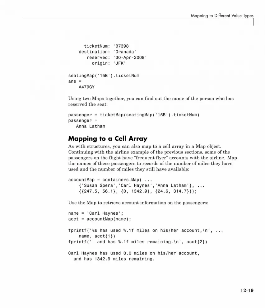
Mapping to Different Value Types
ticketNum: 'B7398'destination: 'Granada'
reserved: '30-Apr-2008'origin: 'JFK'
seatingMap('15B').ticketNumans =
A479GY
Using two Maps together, you can find out the name of the person who hasreserved the seat:
passenger = ticketMap(seatingMap('15B').ticketNum)passenger =
Anna Latham
Mapping to a Cell ArrayAs with structures, you can also map to a cell array in a Map object.Continuing with the airline example of the previous sections, some of thepassengers on the flight have “frequent flyer” accounts with the airline. Mapthe names of these passengers to records of the number of miles they haveused and the number of miles they still have available:
accountMap = containers.Map( ...{'Susan Spera','Carl Haynes','Anna Latham'}, ...{{247.5, 56.1}, {0, 1342.9}, {24.6, 314.7}});
Use the Map to retrieve account information on the passengers:
name = 'Carl Haynes';acct = accountMap(name);
fprintf('%s has used %.1f miles on his/her account,\n', ...name, acct{1})
fprintf(' and has %.1f miles remaining.\n', acct{2})
Carl Haynes has used 0.0 miles on his/her account,and has 1342.9 miles remaining.
12-19

12 Map Containers
12-20

13
Combining Unlike Classes
• “Valid Combinations of Unlike Classes” on page 13-2
• “Combining Unlike Integer Types” on page 13-3
• “Combining Integer and Noninteger Data” on page 13-6
• “Combining Cell Arrays with Non-Cell Arrays” on page 13-7
• “Empty Matrices” on page 13-8
• “Concatenation Examples” on page 13-9

13 Combining Unlike Classes
Valid Combinations of Unlike ClassesMatrices and arrays can be composed of elements of most any MATLAB datatype as long as all elements in the matrix are of the same type. If you doinclude elements of unlike classes when constructing a matrix, MATLABconverts some elements so that all elements of the resulting matrix are ofthe same type.
Data type conversion is done with respect to a preset precedence of classes.The following table shows the five classes you can concatenate with an unliketype without generating an error (that is, with the exception of characterand logical).
TYPE character integer single double logical
character character character character character invalid
integer character integer integer integer integer
single character integer single single single
double character integer single double double
logical invalid integer single double logical
For example, concatenating a double and single matrix always yields amatrix of type single. MATLAB converts the double element to single toaccomplish this.
Concepts • “Combining Unlike Integer Types” on page 13-3• “Combining Integer and Noninteger Data” on page 13-6• “Combining Cell Arrays with Non-Cell Arrays” on page 13-7• “Concatenation Examples” on page 13-9
13-2

Combining Unlike Integer Types
Combining Unlike Integer Types
In this section...
“Overview” on page 13-3
“Example of Combining Unlike Integer Sizes” on page 13-4
“Example of Combining Signed with Unsigned” on page 13-4
OverviewIf you combine different integer types in a matrix (e.g., signed with unsigned,or 8-bit integers with 16-bit integers), MATLAB returns a matrix in which allelements are of one common type. MATLAB sets all elements of the resultingmatrix to the data type of the left-most element in the input matrix. Forexample, the result of the following concatenation is a vector of three 16-bitsigned integers:
A = [int16(450) uint8(250) int32(1000000)]
MATLAB also displays a warning to inform you that the result may not bewhat you had expected:
A = [int16(450) uint8(250) int32(1000000)];Warning: Concatenation with dominant (left-most) integer classmay overflow other operands on conversion to return class.
You can disable this warning by entering the following two commands directlyafter the operation that caused the warning. The first command retrievesthe message identifier associated with the most recent warning issued byMATLAB. The second command uses this identifier to disable any furtherwarnings of that type from being issued:
[msg, intcat_msgid] = lastwarn;warning('off', intcat_msgid);
To re-enable the warning so that it will now be displayed, use
warning('on', intcat_msgid);
13-3

13 Combining Unlike Classes
You can use these commands to disable or enable the display of any MATLABwarning.
Example of Combining Unlike Integer SizesAfter disabling the integer concatenation warnings as shown above,concatenate the following two numbers once, and then switch their order. Thereturn value depends on the order in which the integers are concatenated.The left-most type determines the data type for all elements in the vector:
A = [int16(5000) int8(50)]A =
5000 50
B = [int8(50) int16(5000)]B =
50 127
The first operation returns a vector of 16-bit integers. The second returns avector of 8-bit integers. The element int16(5000) is set to 127, the maximumvalue for an 8-bit signed integer.
The same rules apply to vertical concatenation:
C = [int8(50); int16(5000)]C =
50127
Note You can find the maximum or minimum values for any MATLABinteger type using the intmax and intmin functions. For floating-point types,use realmax and realmin.
Example of Combining Signed with UnsignedNow do the same exercise with signed and unsigned integers. Again, theleft-most element determines the data type for all elements in the resultingmatrix:
13-4

Combining Unlike Integer Types
A = [int8(-100) uint8(100)]A =
-100 100
B = [uint8(100) int8(-100)]B =
100 0
The element int8(-100) is set to zero because it is no longer signed.
MATLAB evaluates each element prior to concatenating them into a combinedarray. In other words, the following statement evaluates to an 8-bit signedinteger (equal to 50) and an 8-bit unsigned integer (unsigned -50 is set tozero) before the two elements are combined. Following the concatenation, thesecond element retains its zero value but takes on the unsigned int8 type:
A = [int8(50), uint8(-50)]A =
50 0
13-5

13 Combining Unlike Classes
Combining Integer and Noninteger DataIf you combine integers with double, single, or logical classes, all elementsof the resulting matrix are given the data type of the left-most integer. Forexample, all elements of the following vector are set to int32:
A = [true pi int32(1000000) single(17.32) uint8(250)]
13-6

Combining Cell Arrays with Non-Cell Arrays
Combining Cell Arrays with Non-Cell ArraysCombining a number of arrays in which one or more is a cell array returns anew cell array. Each of the original arrays occupies a cell in the new array:
A = [100, {uint8(200), 300}, 'MATLAB'];whos A
Name Size Bytes Class Attributes
A 1x4 477 cell
Each element of the combined array maintains its original class:
fprintf('Classes: %s %s %s %s\n',...class(A{1}),class(A{2}),class(A{3}),class(A{4}))
Classes: double uint8 double char
13-7

13 Combining Unlike Classes
Empty MatricesIf you construct a matrix using empty matrix elements, the empty matricesare ignored in the resulting matrix:
A = [5.36; 7.01; []; 9.44]A =
5.36007.01009.4400
13-8

Concatenation Examples
Concatenation Examples
In this section...
“Combining Single and Double Types” on page 13-9
“Combining Integer and Double Types” on page 13-9
“Combining Character and Double Types” on page 13-10
“Combining Logical and Double Types” on page 13-10
Combining Single and Double TypesCombining single values with double values yields a single matrix. Notethat 5.73*10^300 is too big to be stored as a single, thus the conversion fromdouble to single sets it to infinity. (The class function used in this examplereturns the data type for the input value).
x = [single(4.5) single(-2.8) pi 5.73*10^300]x =
4.5000 -2.8000 3.1416 Inf
class(x) % Display the data type of xans =
single
Combining Integer and Double TypesCombining integer values with double values yields an integer matrix. Notethat the fractional part of pi is rounded to the nearest integer. (The int8function used in this example converts its numeric argument to an 8-bitinteger).
x = [int8(21) int8(-22) int8(23) pi 45/6]x =
21 -22 23 3 8class(x)ans =
int8
13-9

13 Combining Unlike Classes
Combining Character and Double TypesCombining character values with double values yields a character matrix.MATLAB converts the double elements in this example to their characterequivalents:
x = ['A' 'B' 'C' 68 69 70]x =
ABCDEF
class(x)ans =
char
Combining Logical and Double TypesCombining logical values with double values yields a double matrix.MATLAB converts the logical true and false elements in this example todouble:
x = [true false false pi sqrt(7)]x =
1.0000 0 0 3.1416 2.6458
class(x)ans =
double
13-10

14
Using Objects
• “MATLAB Objects” on page 14-2
• “General Purpose Vs. Specialized Arrays” on page 14-5
• “Key Object Concepts” on page 14-8
• “Creating Objects” on page 14-11
• “Accessing Object Data” on page 14-14
• “Calling Object Methods” on page 14-16
• “Desktop Tools Are Object Aware” on page 14-19
• “Getting Information About Objects” on page 14-21
• “Copying Objects” on page 14-27
• “Destroying Objects” on page 14-34

14 Using Objects
MATLAB Objects
In this section...
“Getting Oriented” on page 14-2
“What Are Objects and Why Use Them?” on page 14-2
“Working with Objects” on page 14-3
“Objects In the MATLAB Language” on page 14-3
“Other Kinds of Objects Used by MATLAB” on page 14-4
Getting OrientedThis section provides information for people using objects. It does not providea thorough treatment of object-oriented concepts, but instead focuses on whatyou need to know to use the objects provided with MATLAB.
If you are interested in object-oriented programming in the MATLABlanguage, see “Object-Oriented Programming”. For background informationon objects, see object-oriented design.
What Are Objects and Why Use Them?In the simplest sense, objects are special-purpose data structures that have aspecific set of operations that you can perform on the data they contain.
You do not need to know how objects implement operations or store data. Thisfact makes objects modular and easy to pass within application programs. Italso isolates your code from changes to the object’s design and implementation.
MATLAB uses objects because they are a convenient way to package data.Working with objects in MATLAB is like working with any variables and isoften more convenient because objects are optimized for specific purposes.Think of an object as a neatly packaged collection of data that includesfunctions that operate on the data. The documentation for any particularobject describes how to use it.
Objects are organized collections of data and functions that have beendesigned for specific purposes.
14-2

MATLAB® Objects
For example, an object might contain time series data that consists ofvalue/time-sample pairs and associated information like units, sampleuniformity, and so on. This object can have a set of specific operationsdesigned to perform analysis, such as filtering, interpolating, and plotting.
Working with ObjectsYou can perform the common operations on objects like you can on anyvariable. For example, you can do the following things with objects:
• Create it and assign a variable name so you can reference it again
• Assign or reassign data to it (see “Accessing Object Data” on page 14-14)
• Operate on its data (see “Calling Object Methods” on page 14-16)
• Convert it to another class (if this operation is supported by the object’sclass)
• Save it to a MAT-file so you can reload it later (see save)
• Copy it (see “Copying Objects” on page 14-27)
• Clear it from the workspace (clear)
Any object can have restrictions on how you create it, access its data, or whatoperations you can perform on it. Refer to the documentation for the particularMATLAB object for a description of what you can do with that object.
Objects In the MATLAB LanguageThe MATLAB language uses many specialized objects. For example,MException objects capture information when errors occur, timer objectsexecute code at a certain time interval, the serial object enables you tocommunicate with devices connected to your computer’s serial port, and soon. MATLAB toolboxes often define objects to manage data and analysesperformed by the toolbox.
Objects provide specific functionality that is not necessarily available fromgeneral purpose language components.
14-3

14 Using Objects
Other Kinds of Objects Used by MATLABThe MATLAB language enables you to use objects that are defined other inlanguages. The following objects are different from the MATLAB objectsdescribed in this documentation. See the individual sections referenced belowfor information on using these objects.
• Handle Graphics® objects create graphs and GUIs. These objects provide aset/get interface to property values. You cannot subclass graphics objects.See “Graphics Objects” for more information.
• Java classes enable you to access the capabilities of Java classes fromMATLAB programs. See “Call Java Libraries” for more information.
• Microsoft COM objects enable you to integrate these software componentsinto your application. See
“Call COM Objects” for more information.
• Microsoft .NET objects enable you to integrate .NET assemblies into yourapplication. See “Call .NET Libraries” for more information.
• User-defined MATLAB objects created prior to Version 7.6 used differentsyntax for class definition (no classdef block) and exhibit other differences.See “Compatibility with Previous Versions ” for more information.
14-4

General Purpose Vs. Specialized Arrays
General Purpose Vs. Specialized Arrays
In this section...
“How They Differ” on page 14-5
“Using General-Purpose Data Structures” on page 14-5
“Using Specialized Objects” on page 14-6
How They DifferThe MATLAB language uses both general-purpose and specialized arrays.For example, numeric, struct, and cell arrays provide general-purposedata storage. You typically extract data from the array and pass this data tofunctions (for example, to perform mathematical analysis). Then, you storethe result in general-purpose arrays.
When using a specialized object, you typically pass data to a function thatcreates the object. Once created, you use specially defined functions to operateon the data. These functions are unique to the object and are designedspecifically for the type and structure of the data contained by the object.
Using General-Purpose Data StructuresA commonly used general-purpose data structure references data viafieldnames. For example, these statements create a MATLAB struct (aMATLAB structure array):
s.Data = rand(10,1);s.Time = .01:.01:.1;s.Name = 'Data1';s.Units = 'seconds';
The structure s contains two arrays of numbers. However, s is a generic typein the sense that MATLAB does not define special functions to operate on thedata in this particular structure. For example, while s contains two fields thatwould be useful to plot, Data and Time, you cannot pass s to the plot function:
plot(s)Error using plot
14-5

14 Using Objects
Not enough input arguments.
While s has enough information to create a plot of Data versus Time, plotcannot access this data because structures like s can contain any values inits fields and the fields can have any name. Just because one field is namedData does not force you to assign data to that field.
To plot the data in s, you have to extract the data from the fields, pass themas numeric arrays in the desired order to the plot function, add a title,labels, and so on:
plot(s.Time,s.Data)title(['Time Series Plot: ' s.Name])xlabel(['Time (' s.Units ')'])ylabel(s.Name)
You could create a function to perform these steps for you. Other programsusing the structure s would need to create their own functions or access theone you created.
Using Specialized ObjectsCompare the array s above to an object that you have designed specificallyto contain and manipulate time series data. For example, the followingstatement creates a MATLAB® timeseries object. It is initialized to storethe same data as the structure s above:
tsobj = timeseries(rand(10,1),.01:.01:.1,'Name','Data1');
The function that creates the object tsobj, accepts sample data, sampletimes, a property name/property value pair (Name/Data1), and uses a defaultvalue of Units (which is seconds).
The designer of this object created a special version of the plot function thatworks directly with this object. For example:
plot(tsobj)
14-6

General Purpose Vs. Specialized Arrays
Notice how the object’s plot function creates a graph that is plotted andlabeled with the data from the tsobj object. As a user of this object, you donot need write your own code to produce this graph. The class design specifiesthe standard way to present graphs of timeseries data and all clients of thisobject use the same code for plotting.
14-7

14 Using Objects
Key Object Concepts
In this section...
“Basic Concepts” on page 14-8
“Classes Describe How to Create Objects” on page 14-8
“Properties Contain Data” on page 14-9
“Methods Implement Operations” on page 14-9
“Events are Notices Broadcast to Listening Objects” on page 14-10
Basic ConceptsThere are some basic concepts that are fundamental to objects. Objectsrepresent something in the real world, like an error condition or the setof data you collected in a product test. Objects enable you to do somethinguseful, like provide an error report or analyze and present the results of tests.
There are basic components that MATLAB uses to realize the design of anobject. These components include:
• Classes
• Properties
• Methods
• Events
Classes Describe How to Create ObjectsA class defines a set of similar objects. It is a description from which MATLABcreates a particular instance of the class, and it is the instance (that is, theobject) that contains actual data. Therefore, while there is a timeseriesclass, you work with timeseries objects.
Classes are defined in code files — either as separate .m files or built-in to theMATLAB executable. Objects are specific representations of a class that youaccess through workspace variables.
14-8

Key Object Concepts
Properties Contain DataObjects store data in properties. Consider a timeseries object as an example.timeseries object properties contain time series data, corresponding timevalues, and related information, such as units, events, data quality, andinterpolation method. MATLAB objects enable you to access property datadirectly (see “Accessing Object Data” on page 14-14 for information onproperty syntax).
Properties are sometimes called fields in other programming languages andare similar to the fields of MATLAB structures. Properties have descriptivenames, such as Data and DataInfo, in the case of timeseries objects, andcan contain any kind of MATLAB data, including other objects.
An object, then, is a container for a predefined set of data. Unlike a cell arrayor structure, you cannot add new properties or delete defined propertiesfrom an object. Doing so would compromise the object’s intended purposeand violate the class design.
The class design can restrict the values you can assign to a property. Forexample, a Length property might restrict possible values to positive integersor might be read only and determine its own value when queried.
Methods Implement OperationsClass methods are functions designed to work with objects of a particularclass. Methods enable the class designer to implement specific operations thatare optimized for the data contained in the object. You do not have to extractthe data from the object, modify its format, and pass it to a general-purposeMATLAB function because the class defines methods with an awareness ofthe object’s structure.
Methods can define operations that are unique to a particular class of object,such as adding a data sample to an existing set of time series data, or canoverload common operations in a way that makes sense for the particularobject. For example, timeseries objects have an addsample method to adda new data sample to an existing timeseries object. Also, timeseriesoverloads the MATLAB plot function to work with timeseries objects.
14-9

14 Using Objects
MATLAB software determines which overloaded version of a method to callbased on the class of the object passed as an argument. If you execute aMATLAB statement like:
tsobjnew = tsobj1 + tsobj2;
where tsobj1 and tsobj2 are timeseries objects, MATLAB calls thetimeseries version of the + operation (if defined) and returns a newtimeseries object.
Because the timeseries class defines the operation, you can add atimeseries object to a scalar number:
tsobjnew = tsobj1 + 4;
The class definition determines what happens when you add a scalar doubleto a timeseries object (the scalar is added to each Data value).
Methods make working with objects convenient for the user, but also provideadvantages to the class designer. Methods hide implementation details fromusers—you do not need to create your own functions to access and manipulatedata, as you would when using general-purpose data structures like structsand cell arrays. This provides the flexibility to change the internal designof an object without affecting object clients (i.e., application programs thatuse the objects).
Events are Notices Broadcast to Listening ObjectsClasses can defined names for specific actions and trigger the broadcast ofnotices when those actions occur. Listeners respond to the broadcast of anevent notice by executing a predefined function.
For example, objects can listen for the change of the value of a property andexecute a function when that change occurs. If an object defines an event forwhich you can define a listening object, the object’s documentation describesthat event. See “Events” for information on how class designers use events.
14-10

Creating Objects
Creating Objects
In this section...
“Class Constructor” on page 14-11
“When to Use Package Names” on page 14-11
Class ConstructorUsually, you create an object by calling a function designed for the purpose ofcreating that specific class of object. For example, the following code creates atimeseries object and assigns it to the variable tsboj:
load count.dat % Load some datatsobj = timeseries(count(:,1),1:24,'Name','Data1');
The timeseries constructor creates an object and initializes its data with thevalues specified as arguments. Classes that create objects define a specialmethod whose purpose is to create objects of the class. This method has thesame name as the class and is called the class constructor.
However, in some cases, you might create objects by calling other functions oreven using a GUI. For example, a try-catch block can return an MExceptionobject that contains information about a specific error condition. In this case,you do not explicitly create the object, rather it is returned by the catchstatement (see “Accessing Object Data” on page 14-14 for an example).
When to Use Package NamesA package is a container that provides a logical grouping for class and functiondefinitions. The class and function names within a given package must beunique, but can be reused in other packages. Packages are folders that beginwith the + character.
If a package folder contains a class definition, then you must use the packagename when calling the class constructor. For example, this statement createsa Map object, whose class definition file is in a folder in the containerspackage:
mapobj = containers.Map({'rose','bicycle'},{'flower','machine'});
14-11

14 Using Objects
You need to use the package name to refer to:
• Class constructors (e.g., containers.Map), which you call to create an object
• Static methods (methods that do not require an object of the class as anargument)
• Package functions (functions defined in the package)
However, because MATLAB uses the class of an object to determine whichordinary method to call, you do not need to use the package name inconjunction with object references. For example, suppose you have thefollowing folder structure:
pathfolder/+packagename/@ClassName/ClassName.mpathfolder/+packagename/@ClassName/staticMethodName.mpathfolder/+packagename/functionName.m
In the following examples, obj is the object you are creating.
% Create object of ClassNameobj = packagename.ClassName(...);
% Call methodNameobj.methodName(...);
% Set or get the value of property PropertyNameobj.PropertyName = x;x = obj.PropertyName;
% Call static method staticMethodNamepackagename.ClassName.staticMethodName(...);
% Call package function functionNamepackagename.functionName(...)
If a package folder contains a class definition file, then consider the packagename as part of the class name. Wherever you need to use the class name,include the package name. For example, containers.Map is the full classname of the Map class.
14-12

Creating Objects
See the object’s user documentation for the syntax you need to use to createobjects.
See “Organizing Classes in Folders” and “Packages Create Namespaces” formore information on the use of packages.
See “Importing Classes” for information on importing packages into functions.
14-13

14 Using Objects
Accessing Object Data
In this section...
“Listing Public Properties” on page 14-14
“Getting Property Values” on page 14-14
“Setting Property Values” on page 14-15
Listing Public Properties
Note Always use the correct case when referring to properties by name.
Display the names of all public object properties using the propertiesfunction with the object’s class name or with an actual object. For example:
>> properties('MException')
Properties for class MException:identifiermessagecausestack
Getting Property ValuesAfter creating an object, you can access the values of its properties:
trya = rand(4);a(17) = 7;
catch me % catch creates an MException object named medisp(['Current error identifier: ' me.identifier])
endCurrent error identifier: MATLAB:indexed_matrix_cannot_be_resized
Access the data in properties using dot notation:
object.PropertyName
14-14

Accessing Object Data
For example, you can access the message property of the MException object,me, with this syntax:
me.messageans =In an assignment A(I) = B, a matrix A cannot be resized.
See “Capture Information About Exceptions” on page 23-5 for moreinformation on using MException objects.
Setting Property ValuesObjects often restrict what values you can assign to them. For example, thefollowing timeseries object has 10 data values, each corresponding to asample time:
tsobj = timeseries(rand(10,1),1:10,'Name','Random Sample');
Now suppose you attempt to set the Data property to a three-element vector:
tsobj.Data = [1 2 3];Error using timeseries.utreshape (line 864)Size of the data array is incompatible with the time vector....
The timeseries class design ensures that the number of data samplesmatches the number of time samples. This illustrates one of the advantages aspecialized object has over a general purpose-data structure like a MATLABstruct.
14-15

14 Using Objects
Calling Object Methods
In this section...
“What Operations Can You Perform” on page 14-16
“Method Syntax” on page 14-16
“Class of Objects Returned by Methods” on page 14-18
What Operations Can You PerformMethods define an object’s behavior. Consequently, classes implementmethods that an object user is unlikely to call directly. The userdocumentation for the object you are using describes the operations you canperform on any particular object.
You can list the methods defined by a class with the methods or methodsviewfunctions:
methods('timeseries')
Methods for class timeseries:
addevent gettsbetweenevents setaddsample horzcat setabstimecreateTstoolNode idealfilter setinterpmethodctranspose init setprop...
Method SyntaxCall an object’s method using dot notation:
returnedValue = object.methodName(args,...)
You also can call a method using function syntax, passing the object as thefirst (left-most) argument.
returnedValue = methodName(object,args,...)
14-16

Calling Object Methods
For example, MException objects have a getReport method that returnsinformation about the error.
trysurf
catch medisp(me.getReport)
end
Error using ==> surf at (line 50)Not enough input arguments.
Dot and function notation are usually equivalent. That is, both of thefollowing statements return the MException report:
rpt = getReport(me); % Call getReport using function notationrpt = me.getReport; % Call getReport using dot notation
Calling the Correct MethodIt is possible for the function syntax to call an unexpected method if there ismore than one object in the argument list. Suppose there are two classes,ClassA and ClassB, that define a method called addData. Suppose furtherthat ClassA is defined as being inferior to ClassB in precedence (somethingthat the class designer can do in the class definition). In this situation, givenobjA is of ClassA and objB is of ClassB, the following two statement calldifferent methods:
addData(objA,objB) % Calls objB.addDataobjA.addData(objB) % Calls objA.addData
If ClassA and ClassB had equal precedence, then the left-most argumentdetermines which method MATLAB calls (i.e., objA.addData in bothstatements).
It is unlikely that you will encounter this particular scenario, however, if youare calling a method that accepts more than one object as arguments, usingdot notation removes any ambiguity about which object’s method MATLABcalls.
14-17

14 Using Objects
Class of Objects Returned by MethodsWhile methods sometimes return objects of the same class, this is not alwaysthe case. For example, the MException object’s getReport returns a characterstring:
trysurf
catch merpt = me.getReport;
end
whosName Size Bytes Class Attributes
me 1x1 1118 MExceptionrpt 1x126 252 char
Methods can return any type of value and properties can contain any type ofvalue. However, class constructor methods always return an object or array ofobjects of the same type as the class.
14-18

Desktop Tools Are Object Aware
Desktop Tools Are Object Aware
In this section...
“Tab Completion Works with Objects” on page 14-19
“Editing Objects with the Variables Editor” on page 14-19
Tab Completion Works with ObjectsMATLAB tab completion works with objects. For example, if you enter anobject name followed by a dot:
tsobj.
and then press the tab key, MATLAB pops up a selection box with a list ofproperties and methods:
The more letters you complete after the dot, the more specific is the list. See“Tab Completion” for more information.
Editing Objects with the Variables EditorYou can use the MATLAB Variables Editor to edit object properties. To openan object in the Variables Editor, you can double-click the object name in theWorkspace browser or use the openvar command:
14-19

14 Using Objects
tsobj = timeseries(rand(10,1),.01:.01:.1,'Name','Data1');openvar tsobj
See “View, Edit, and Copy Variables” for more information.
14-20

Getting Information About Objects
Getting Information About Objects
In this section...
“The Class of Workspace Variables” on page 14-21
“Information About Class Members” on page 14-23
“Logical Tests for Objects” on page 14-24
“Displaying Objects” on page 14-25
“Getting Help for MATLAB Objects” on page 14-25
The Class of Workspace VariablesAll workspace variables are of a specific class. For example, consider thefollowing variable created in your workspace:
load count.dat % Load some datatsobj = timeseries(count(:,1),1:24,'Name','Data1');whos
Name Size Bytes Class Attributes
count 24x3 576 doubletsobj 1x1 1261 timeseries
The whos command lists information about your workspace variables. Noticethat the variable loaded from the count.dat file (count) is an array ofdoubles. You know, therefore, that you can perform indexing and arithmeticoperations on this array. For example:
newcount = sum(count,2);newcount(8:15) = NaN;bar(newcount)
14-21

14 Using Objects
Indexed assignment and the bar function work with inputs of class double.
However, the timeseries class does not define a bar method for timeseriesobjects. The timeseries class defines a plotmethod for graphing because theclass design specified a line plot as the best way to represent time series data.
14-22

Getting Information About Objects
Extracting Data From Object PropertiesSuppose you have a timeseries object and you want to work directly with thenumeric values of the timeseries data. You can extract data from the objectproperties and assign these values to an array. For example
load count.dattsobj = timeseries(sum(count,2),1:24,'Name','DataSum');d = tsobj.Data;t = tsobj.Time;n = tsobj.Name;d(8:15) = NaN;bar(t,d); title(n)
Testing for the Class of an ObjectSuppose you create a function that operates on more than one class of object.If you have a timeseries object, you call the timeseries plot method, butif the object is of class double, you can call the bar function (which isn’tsupported by timeseries objects). You could use isa as in the following codeto make this determination:
obj = tsobj.Data; % Define an input variablefunction myPlotter(obj)
if isa(obj,'timeseries')plot(obj)
elseif isa(obj,'double')bar(obj)
endend
Information About Class MembersThese functions provide information about the object.
Function Purpose
class Return class of object
events List of event names defined by the class
methods List of methods implemented by the class
14-23

14 Using Objects
Function Purpose
methodsview Information on class methods in separate window
properties List of class property names
Logical Tests for ObjectsIn functions, you might need conditional statements to determine the statusof an object before performing certain actions. For example, you mightperform different actions based on the class of an object (see “Testing for theClass of an Object” on page 14-23). The following functions provide logicaltests for objects:
Function Purpose
isa Determine whether argument belongs to a particularclass. True for object’s class and all of object’ssuperclasses.
isequal Determine if two objects are equal.
isobject Determine whether the input is a MATLAB object.
Testing for Object Equalityisequal finds two objects to be equal if all the following conditions are met:
• Both objects are of the same class
• Both objects are of the same size
• All corresponding property values are equal
isequal tests the value of every array element in every property and everyproperty of every object contained in the objects being tested. As containedobjects are tested for equality, MATLAB calls each object’s own version ofisequal (if such versions exist).
If objects contain large amounts of data stored in other objects, then testingfor equality can be a time-consuming process.
14-24

Getting Information About Objects
Identifying MATLAB ObjectsThe isobject function returns true only for MATLAB objects. For Javaobjects, use isjava. For Handle Graphics objects, use ishandle.
Note ishandle returns false for MATLAB handle objects. See “Testing forHandle or Value Class” on page 14-32 for more information.
Displaying ObjectsWhen you issue commands that return objects and do not terminate thosecommands with a semicolon, or when you pass an object to the disp function,MATLAB displays information about the object. For example:
hobj = containers.Map({'Red Sox','Yankees'},{'Boston','New York'})hobj =
containers.Map handlePackage: containers
Properties:Count: 2
KeyType: 'char'ValueType: 'char'
Methods, Events, Superclasses
This information includes links (shown in blue) to documentation on theobject’s class and superclasses, and lists of methods, events, and superclasses.Properties and their current values are also listed.
Some classes (timeseries, for example) redefine how they display objects toprovide more useful information for this particular class.
Getting Help for MATLAB ObjectsYou can get documentation for MATLAB objects using the doc commandwith the class name. To see the reference pages for the objects used in thischapter, use the following commands:
doc timeseries
14-25

14 Using Objects
doc MExceptiondoc containers.Map % Include the package name
14-26

Copying Objects
Copying Objects
In this section...
“Two Copy Behaviors” on page 14-27
“Value Object Copy Behavior” on page 14-27
“Handle Object Copy Behavior” on page 14-28
“Testing for Handle or Value Class” on page 14-32
Two Copy BehaviorsThere are two fundamental kinds of MATLAB classes—handles and values.
Value classes create objects that behave like ordinary MATLAB variableswith respect to copy operations. Copies are independent values. Operationsthat you perform on one object do not affect copies of that object.
Handle classes create objects that behave as references. This is because ahandle, and all copies of this handle, refer to the same underlying object.When you create a handle object, you can copy the handle, but not the datareferenced by the object’s properties. Any operations you perform on a handleobject are visible from all handles that reference that object.
Value Object Copy BehaviorMATLAB numeric variables are of value objects. For example, when you copya to the variable b, both variables are independent of each other. Changingthe value of a does not change the value of b:
a = 8;b = a;
Now reassign a and b is unchanged:
a = 6;bb =
8
14-27

14 Using Objects
Clearing a does not affect b:
clear abb =
8
Value Object PropertiesThe copy behavior of values stored as properties in value objects is the same.For example, suppose vobj1 is a value object with property a:
vobj1.a = 8; % Property is set to a value
If you copy vobj1 to vobj2, and then change the value of vobj1 property a, youcan see that the value of the copied object’s property vobj2.a is unaffected:
vobj2 =vobj1;vobj1.a = 5;
vobj2.aans =
8
Handle Object Copy BehaviorHere is a handle class called HdClass that defines a property called Data.
classdef HdClass < handleproperties
Dataendmethods
function obj = HdClass(val)if nargin > 0
obj.Data = val;end
endend
end
Create an object of this class with the following statement:
14-28

Copying Objects
hobj1 = HdClass(8)
Because this statement is not terminated with a semicolon, MATLAB displaysinformation about the object:
hobj1 =
HdClass handle
Properties:Data: 8
Methods, Events, Superclasses
The variable hobj1 is a handle that references the object created. Copyinghobj1 to hobj2 results in another handle (the variable hobj2) referring tothe same object:
hobj2 = hobj1hobj2 =
HdClass handle
Properties:Data: 8
Methods, Events, Superclasses
Because handle objects reference the data contained in their properties,copying an object copies the handle to a new variable name, but the propertiesstill refer to the same data. For example, given that hobj1 is a handle objectwith property Data:
hobj1.Data
ans =
8
Change the value of hobj1’s Data property and the value of the copied object’sData property also changes:
14-29

14 Using Objects
hobj1.Data = 5;
hobj2.Data
ans =
5
Because hobj2 and hobj1 are handles to the same object, changing the copy,hobj2, also changes the data you access through handle hobj1:
hobj2.Data = 17;hobj1.Data
ans =
17
Copy Method for Handle ClassesHandle classes can derive copy functionality from the matlab.mixin.Copyableclass. Class designers can investigate the use of this class in their class design.
Reassigning Handle VariablesReassigning a handle variable produces the same result as reassigning anyMATLAB variable. When you create a new object and assign it to hobj1:
hobj1 = HdClass(3.14);
hobj1 references the new object, not the same object referenced previously(and still referenced by hobj2).
Clearing Handle VariablesWhen you clear a handle from the workspace, MATLAB removes thevariable, but does not removed the object referenced by the handle. Therefore,given hobj1 and hobj2, which both reference the same object, you can cleareither handle without affecting the object:
hobj1.Data = 2^8;
14-30

Copying Objects
clear hobj1hobj2hobj2 =
HdClass handle
Properties:Data: 256
Methods, Events, Superclasses
If you clear both hobj1 and hobj2, then there are no references to the objectand MATLAB deletes the object and frees the memory used by that object.
Deleting Handle ObjectsTo remove an object referenced by any number of handles, use delete. Givenhobj1 and hobj2, which both reference the same object, if you delete eitherhandle, MATLAB deletes the object:
hobj1 = HdClass(8);hobj2 = hobj1;delete(hobj1)hobj2
hobj2 =
deleted HdClass handle
Methods, Events, Superclasses
See “Destroying Objects” on page 14-34 for more information about objectlifecycle.
Modifying ObjectsWhen you pass an object to a function, MATLAB follows pass by valuesemantics. This means that MATLAB passes a copy of the object to thefunction. If you modify the object in the function, MATLAB modifies only thecopy of the object. The differences in copy behavior between handle and valueclasses are important in such cases:
14-31

14 Using Objects
• Value class — The function must return the modified copy of the objectto the caller.
• Handle class — The copy refers to the same data as the original object.Therefore, the function does not need to return the modified copy.
See “Passing Objects to Functions” for more information.
More Information About Handle and Value ClassesFor information about handle and value classes for class designers, see“Handle Classes” in the Object-Oriented Programming documentation.
Testing for Handle or Value ClassIf you are writing MATLAB programs that copy objects, you might need todetermine if any given object is a handle or a value. To determine if an objectis a handle object, use the isa function:
isa(obj,'handle')
For example, the containers.Map class creates a handle object:
hobj = containers.Map({'Red Sox','Yankees'}, {'Boston','New York'});
isa(hobj,'handle')
ans =
1
hobj is also a containers.Map object:
isa(hobj,'containers.Map')
ans =
1
If you query the class of hobj, you see that it is a containers.Map object:
class(hobj)
14-32

Copying Objects
ans =
containers.Map
The class function returns the specific class of an object, whereas isareturns true for any of the object’s superclasses as well. This behavior isconsistent with the object-oriented concept that an object is a member of all itssuperclasses. Therefore, it is true that a containers.Map object is a handleobject and a containers.Map object.
There is no equivalent test for value classes because there is no value baseclass. If an object is a value object, isa(object,'handle') returns false(i.e., logical 0).
See “Map Containers” for more information on the containers.Map class.
14-33

14 Using Objects
Destroying Objects
In this section...
“Object Lifecycle” on page 14-34
“Difference Between clear and delete” on page 14-34
Object LifecycleAn object’s lifecycle ends when:
• You reassign a new value to that variable.
• The object is no longer used in a function.
• Function execution ends.
MATLAB handle classes have a special method called delete that MATLABcalls when a handle object lifecycle ends.
Calling delete on an object explicitly makes all copies of a handle objectinvalid because it destroys the data associated with the object and freesmemory used by deleted objects. MATLAB calls delete automatically so it isnot necessary for you to do so. Classes can redefine the handle class deletemethod to perform other cleanup operations, like closing files or saving data.
Deleting a handle object renders all copies invalid:
hobj1 = HdClass(8);hobj2 = hobj1;delete(hobj1)hobj2.DataInvalid or deleted object.
Difference Between clear and deleteThe handle class delete method removes the handle object, but does notclear the variable name. The clear function removes a variable name, butdoes not remove the values to which the variable refers. For example, if youhave two variables that refer to the same handle object, you can clear eitherone without affecting the actual object:
14-34

Destroying Objects
hobj = containers.Map({'Red Sox','Yankees'}, {'Boston','New York'});
hobj_copy = hobj;
clear hobj
city = hobj_copy('Red Sox')
city =
Boston
If you call clear on all handle variables that refer to the same handle object,then you have lost access to the object and MATLAB destroys the object. Thatis, when there are no references to an object, the object ceases to exist.
On value objects, you can call clear to remove the variable. However,MATLAB does not automatically call a value class delete method, if oneexists, when you clear the variable.
14-35

14 Using Objects
14-36

15
Defining Your Own Classes
All MATLAB data types are implemented as object-oriented classes. Youcan add data types of your own to your MATLAB environment by creatingadditional classes. These user-defined classes define the structure of yournew data type, and the functions, or methods, that you write for each classdefine the behavior for that data type.
These methods can also define the way various MATLAB operators, includingarithmetic operations, subscript referencing, and concatenation, apply to thenew data types. For example, a class called polynomial might redefine theaddition operator (+) so that it correctly performs the operation of additionon polynomials.
With MATLAB classes you can
• Create methods that overload existing MATLAB functionality
• Restrict the operations that are allowed on an object of a class
• Enforce common behavior among related classes by inheriting from thesame parent class
• Significantly increase the reuse of your code
For more information, see “Classes in the MATLAB Language”.

15 Defining Your Own Classes
15-2

Scripts and Functions
• Chapter 16, “Scripts”
• Chapter 17, “Function Basics”
• Chapter 18, “Function Arguments”
• Chapter 19, “Debugging MATLAB Code”
• Chapter 20, “Presenting MATLAB Code”
• Chapter 21, “Coding and Productivity Tips”
• Chapter 22, “Programming Utilities”


16
Scripts
• “Create Scripts” on page 16-2
• “Add Comments to Programs” on page 16-4
• “Run Code Sections” on page 16-6
• “Scripts vs. Functions” on page 16-16

16 Scripts
Create ScriptsScripts are the simplest kind of program file because they have no inputor output arguments. They are useful for automating series of MATLABcommands, such as computations that you have to perform repeatedly fromthe command line or series of commands you have to reference.
You can open a new script in the following ways:
• Highlight commands from the Command History, right-click, and selectCreate Script.
• Click the New Script button on the Home tab.
• Use the edit function.
This code opens the file file_name:
edit file_name
If file_name is unspecified, MATLAB opens a new file called Untitled.
For example, suppose you save this code that generates random numbersbetween 0 and 100 as a script called numGenerator.m:
columns = 10000;rows = 1;bins = columns/100;
rng(now);list = 100*rand(rows,columns);hist(list,bins)
You can run the code in numGenerator.m using either of these methods:
• Type the script name numGenerator on the command line and press Enter
• Click the Run button on the Editor tab
16-2

Create Scripts
When execution completes, the variables (columns, rows, bins and list)remain in the MATLAB workspace. To see a listing of variables, enter whos atthe command prompt. Scripts share the base workspace with your interactiveMATLAB session and with other scripts.
Concepts • “Base and Function Workspaces” on page 17-9
16-3

16 Scripts
Add Comments to ProgramsThis topic explains how and why to add comments to your program files.
When you write code, it is a good practice to add comments that describethe code. Comments allow others to understand your code, and can refreshyour memory when you return to it later. Add comments to MATLAB codeusing the percent (%) symbol.
Comment lines can appear anywhere in a program file, and you can appendcomments to the end of a line of code. For example,
% Add up all the vector elements.y = sum(x) % Use the sum function.
Comments are also useful for program development and testing—commentout any code that does not need to run. To comment out multiple lines of code,you can use the block comment operators, %{ and %}:
a = magic(3);%{sum(a)diag(a)sum(diag(a))%}sum(diag(fliplr(a)))
The %{ and %} operators must appear alone on the lines that immediatelyprecede and follow the block of help text. Do not include any other text onthese lines.
To comment out part of a statement that spans multiple lines, use an ellipses(...) instead of a percent sign. For example,
header = ['Last Name, ', ...'First Name, ', ...
... 'Middle Initial, ', ...'Title']
16-4

Add Comments to Programs
The MATLAB Editor includes tools and context menu items to help you add,remove, or change the format of comments for MATLAB, Java, and C/C++code. For example, if you paste lengthy text onto a comment line, such as
% This is a program that has a comment that is a little more than 75 columns wide.
disp('Hello, world')
and then press the button next to Comment on the Editor tab, theEditor wraps the comment:
% This is a program that has a comment that is a little more than 75
% columns wide.
disp('Hello, world')
By default, as you type comments in the Editor, the text wraps when it reachesa column width of 75. To change the column where the comment text wraps,or to disable automatic comment wrapping, adjust the Editor/DebuggerLanguage preference settings labeled Comment formatting.
The Editor does not wrap comments with:
• Code section titles (comments that begin with %%)
• Long contiguous strings, such as URLs
• Bulleted list items (text that begins with * or #) onto the preceding line
RelatedExamples
• “Add Help for Your Program” on page 17-5
Concepts • “Editor/Debugger Preferences”
16-5

16 Scripts
Run Code Sections
In this section...
“Divide Your File into Code Sections” on page 16-6
“Evaluate Code Sections” on page 16-7
“Navigate Among Code Sections in a File” on page 16-8
“Example of Evaluating Code Sections” on page 16-9
“Change the Appearance of Code Sections” on page 16-12
“Use Code Sections with Control Statements and Functions” on page 16-13
Divide Your File into Code SectionsMATLAB files often consist of many commands. You typically focus effortson a single part of your program at a time, working with the code in chunks.Similarly, when explaining your files to others, often you describe yourprogram in chunks. To facilitate these processes, use code sections, alsoknown as code cells or cell mode. A code section contains contiguous lines ofcode that you want to evaluate as a group in a MATLAB script, beginningwith two comment characters (%%).
To define code section boundaries explicitly, insert section breaks using thesemethods:
• On the Editor tab, in the Edit section, in the Comment button group, click
.
• Enter two percent signs (%%) at the start of the line where you want tobegin the new code section.
The text on the same line as %% is called the section title . Including sectiontitles is optional, however, it improves the readability of the file and appearsas a heading if you publish your code.
16-6

Run Code Sections
Evaluate Code SectionsAs you develop a MATLAB file, you can use the Editor section features toevaluate the file section-by-section. This method helps you to experimentwith, debug, and fine-tune your program. You can navigate among sections,and evaluate each section individually. To evaluate a section, it must containall the values it requires, or the values must exist in the MATLAB workspace.
The section evaluation features run the section code currently highlightedin yellow. MATLAB does not automatically save your file when evaluatingindividual code sections. The file does not have to be on your search path.
This table provides instructions on evaluating code sections.
Operation Instructions
Run the code in thecurrent section.
• Place the cursor in the code section.
• On the Editor tab, in the Run section, clickRun Section.
Run the code in thecurrent section, andthen move to the nextsection.
• Place the cursor in the code section.
• On the Editor tab, in the Run section, clickRun and Advance.
Run all the code inthe file.
• Type the saved script name in the CommandWindow.
• On the Editor tab, in the Run section, clickRun.
16-7

16 Scripts
Note You cannot debug when running individual code sections. MATLABignores any breakpoints.
Increment Values in Code SectionsYou can increment numbers within a section, rerunning that section afterevery change. This helps you fine-tune and experiment with your code.
To increment or decrement a number in a section:
1 Highlight or place your cursor next to the number.
2 Right-click to open the context menu.
3 Select Increment Value and Run Section. A small dialog box appears.
4 Input appropriate values in the / text box or / text box.
5 Click the , , , or button to add to, subtract from, multiply, ordivide the selected number in your section.
MATLAB runs the section after every click.
Note MATLAB software does not automatically save changes you make tothe numbers in your script.
Navigate Among Code Sections in a FileYou can navigate among sections in a file without evaluating the code withinthose sections. This facilitates jumping quickly from section to section withina file. You might do this, for example, to find specific code in a large file.
16-8

Run Code Sections
Operation Instructions
Move to the nextsection.
• On the Editor tab, in the Run section, clickAdvance.
Move to the previoussection.
• Press Ctrl + Up arrow.
Move to a specificsection.
• On the Editor tab, in the Navigate section, usethe Go To to move the cursor to a selectedsection.
Example of Evaluating Code SectionsThis example defines two code sections in a file called sine_wave.m and thenincrements a parameter to adjust the created plot. To open this file in yourEditor, run the following command, and then save the file to a local folder:
edit(fullfile(matlabroot,'help','techdoc','matlab_env',...'examples','sine_wave.m'))
After the file is open in your Editor:
1 Insert a section break and the following title on the first line of the file.
%% Calculate and Plot Sine Wave
2 Insert a blank line and a second section break after plot(x,y). Add a sectiontitle, Modify Plot Properties, so that the entire file contains this code:
%% Calculate and Plot Sine Wave% Define the range for x.% Calculate and plot y = sin(x).x = 0:1:6*pi;y = sin(x);plot(x,y)
%% Modify Plot Propertiestitle('Sine Wave','FontWeight','bold')xlabel('x')
16-9

16 Scripts
ylabel('sin(x)')set(gca,'Color','w')set(gcf, 'MenuBar', 'none')
3 Save the file.
4 Place your cursor in the section titled Calculate and Plot Sine Wave. Onthe Editor tab, in the Run section, click Run Section.
A figure displaying a course plot of sin(x) appears.
5 Smooth the sine plot.
a Highlight 1 in the statement: x = 0:1:6*pi; .
b Right-click and select Increment Value and Run Section. A smalldialog box appears.
c Type 2 in the / text box.
16-10

Run Code Sections
d Click the button several times.
The sine plot becomes smoother after each subsequent click.
e Close the Figure and save the file.
6 Run the entire sine_wave.m file. A smooth sine plot with titles appears in anew Figure.
16-11

16 Scripts
Change the Appearance of Code SectionsYou can change how code sections appear within the MATLAB Editor.MATLAB highlights code sections in yellow, by default, and divides them withhorizontal lines. When the cursor is positioned in any line within a section,the Editor highlights the entire section.
To change how code sections appear:
1 On the Home tab, in the Environment section, click Preferences.
The Preference dialog box appears.
2 In the left pane, selectMATLAB > Colors > Programming Tools.
3
Under Section display options, select the appearance of your codesections.
16-12

Run Code Sections
You can choose whether to highlight the sections, the color of thehighlighting, and whether dividing lines appear between code sections.
Use Code Sections with Control Statements andFunctionsUnexpected results can appear when using code sections within controlstatements and functions because MATLAB automatically inserts sectionbreaks that do not appear in the Editor unless you insert section breaksexplicitly. This is especially true when nested code is involved. Nested codeoccurs wherever you place a control statement or function within the scope ofanother control statement or function.
MATLAB automatically defines section boundaries in a code block, accordingto this criteria:
• MATLAB inserts a section break at the top and bottom of a file, creating acode section that encompasses the entire file. However, the Editor does nothighlight the resulting section, which encloses the entire file, unless youadd one or more explicit code sections to the file.
• If you define a section break within a control flow statement (such as an ifor while statement), MATLAB automatically inserts section breaks at thelines containing the start and end of the statement.
• If you define a section break within a function, MATLAB inserts sectionbreaks at the function declaration and at the function end statement. If youdo not end the function with an end statement, MATLAB behaves as if theend of the function occurs immediately before the start of the next function.
If an automatic break occurs on the same line as a break you insert, theycollapse into one section break.
Nested Code Section BreaksThe following code illustrates the concept of nested code sections:
t = 0:.1:pi*4;y = sin(t);
for k = 3:2:9%%
16-13

16 Scripts
y = y + sin(k*t)/k;if ~mod(k,3)
%%display(sprintf('When k = %.1f',k));plot(t,y)
endend
If you copy and paste this code into a MATLAB Editor, you see that the twosection breaks create three nested levels:
• At the outermost level of nesting, one section spans the entire file.
MATLAB only defines section in a code block if you specify section breaksat the same level within the code block. Therefore, MATLAB considers thecursor to be within the section that encompasses the entire file.
• At the second-level of nesting, a section exists within the for loop.
16-14

Run Code Sections
• At the third-level of nesting, one section exists within the if statement.
Concepts • “Scripts vs. Functions” on page 16-16
16-15

16 Scripts
Scripts vs. FunctionsThis topic discusses the differences between scripts and functions, and showshow to convert a script to a function.
Program files can be scripts that simply execute a series of MATLABstatements, or they can be functions that also accept input arguments andproduce output. Both scripts and functions contain MATLAB code, and bothare stored in text files with a .m extension. However, functions are moreflexible and more easily extensible.
For example, create a script in a file named triarea.m that computes thearea of a triangle:
b = 5;h = 3;a = 0.5*(b.* h)
After you save the file, you can call the script from the command line:
triarea
a =7.5000
To calculate the area of another triangle using the same script, you couldupdate the values of b and h in the script and rerun it. Each time you run it,the script stores the result in a variable named a that is in the base workspace.
However, instead of manually updating the script each time, you canmake your program more flexible by converting it to a function. Replacethe statements that assign values to b and h with a function declarationstatement. The declaration includes the function keyword, the names ofinput and output arguments, and the name of the function.
function a = triarea(b,h)a = 0.5*(b.* h);
After you save the file, you can call the function with different base and heightvalues from the command line without modifying the script:
16-16

Scripts vs. Functions
a1 = triarea(1,5)a2 = triarea(2,10)a3 = triarea(3,6)
a1 =2.5000
a2 =10
a3 =9
Functions have their own workspace, separate from the base workspace.Therefore, none of the calls to the function triarea overwrite the value of a inthe base workspace. Instead, the function assigns the results to variables a1,a2, and a3.
RelatedExamples
• “Create Scripts” on page 16-2• “Create Functions in Files” on page 17-2
Concepts • “Base and Function Workspaces” on page 17-9
16-17

16 Scripts
16-18

17
Function Basics
• “Create Functions in Files” on page 17-2
• “Add Help for Your Program” on page 17-5
• “Run Functions in the Editor” on page 17-7
• “Base and Function Workspaces” on page 17-9
• “Share Data Between Workspaces” on page 17-10
• “Check Variable Scope in Editor” on page 17-15
• “Types of Functions” on page 17-19
• “Anonymous Functions” on page 17-23
• “Local Functions” on page 17-30
• “Nested Functions” on page 17-32
• “Variables in Nested and Anonymous Functions” on page 17-39
• “Private Functions” on page 17-41
• “Function Precedence Order” on page 17-43

17 Function Basics
Create Functions in FilesThis example shows how to create a function in a program file.
Write a Function
Open a file in a text editor. Within the file, declare the function and addprogram statements:
function f = fact(n)f = prod(1:n);
Function fact accepts a single input argument n, and returns the factorialof n in output argument f.
The definition statement is the first executable line of any function. Functiondefinitions are not valid at the command line or within a script. Each functiondefinition includes these elements.
function keyword(required)
Use lowercase characters for the keyword.
Output arguments(optional)
If your function returns more than one output,enclose the output names in square brackets, such as
function [one,two,three] = myfunction(x)
If there is no output, either omit it,
function myfunction(x)
or use empty square brackets:
function [] = myfunction(x)
17-2

Create Functions in Files
Function name(required)
Valid function names follow the same rules asvariable names. They must start with a letter, andcan contain letters, digits, or underscores.
Note To avoid confusion, use the same name forboth the file and the first function within the file.MATLAB associates your program with the filename, not the function name.
Input arguments(optional)
If your function accepts any inputs, enclose theirnames in parentheses after the function name.Separate inputs with commas, such as
function y = myfunction(one,two,three)
If there are no inputs, you can omit the parentheses.
Tip When you define a function with multiple input or output arguments, listany required arguments first. This allows you to call your function withoutspecifying optional arguments.
The body of a function can include valid MATLAB expressions, control flowstatements, comments, blank lines, and nested functions. Any variables thatyou create within a function are stored within a workspace specific to thatfunction, which is separate from the base workspace.
Functions end with either an end statement, the end of the file, or thedefinition line for another function, whichever comes first. The end statementis required only when a function in the file contains a nested function (afunction completely contained within its parent).
Program files can contain multiple functions. The first function is the mainfunction, and is the function that MATLAB associates with the file name.Subsequent functions that are not nested are called local functions. They areonly available to other functions within the same file.
17-3

17 Function Basics
Save the File
Save the file (in this example, fact.m), either in the current folder or in afolder on the MATLAB search path. MATLAB looks for programs in thesespecific locations.
Call the Function
From the command line, call the new fact function to calculate 5!, using thesame syntax rules that apply to calling functions installed with MATLAB:
x = 5;y = fact(x);
The variables that you pass to the function do not need to have the samenames as the arguments in the function definition line.
See Also function | edit | clear | what | which
RelatedExamples
• “Files and Folders that MATLAB Accesses”• “Add Help for Your Program” on page 17-5• “Support Variable Number of Inputs” on page 18-4
Concepts • “Base and Function Workspaces” on page 17-9• “Local Functions” on page 17-30• “Nested Functions” on page 17-32• “Debugging Process and Features” on page 19-2
17-4

Add Help for Your Program
Add Help for Your ProgramThis example shows how to provide help for the programs you write. Helptext appears in the Command Window when you use the help function.
Create help text by inserting comments at the beginning of your program. Ifyour program includes a function, position the help text immediately belowthe function definition line (the line with the function keyword).
For example, create a function in a file named addme.m that includes help text:
function c = addme(a,b)% ADDME Add two values together.% C = ADDME(A) adds A to itself.% C = ADDME(A,B) adds A and B together.%% See also SUM, PLUS.
switch nargincase 2
c = a + b;case 1
c = a + a;otherwise
c = 0;end
When you type help addme at the command line, the help text displays inthe Command Window:
addme Add two values together.C = addme(A) adds A to itself.C = addme(A,B) adds A and B together.
See also sum, plus.
The first help text line, often called the H1 line, typically includes the programname and a brief description. The Current Folder browser and the help andlookfor functions use the H1 line to display information about the program.
17-5

17 Function Basics
Create See also links by including function names at the end of your helptext on a line that begins with % See also. If the function exists on thesearch path or in the current folder, the help command displays each of thesefunction names as a hyperlink to its help. Otherwise, help prints the functionnames as they appear in the help text.
You can include hyperlinks (in the form of URLs) to Web sites in your helptext. Create hyperlinks by including an HTML <a></a> anchor element.Within the anchor, use a matlab: statement to execute a web command.For example:
% For more information, see <a href="matlab:% web('http://www.mathworks.com')">the MathWorks Web site</a>.
End your help text with a blank line (without a %). The help system ignoresany comment lines that appear after the help text block.
Note When multiple programs have the same name, the help commanddetermines which help text to display by applying the rules described in“Function Precedence Order” on page 17-43. However, if a program has thesame name as a MathWorks function, the Help on Selection option incontext menus always displays documentation for the MathWorks function.
See Also help | lookfor
RelatedExamples
• “Add Comments to Programs” on page 16-4• “Create Help Summary Files (Contents.m)” on page 27-13• “Check Which Programs Have Help” on page 27-10• “Display Custom Documentation” on page 27-16
17-6

Run Functions in the Editor
Run Functions in the EditorThis example shows how to run a function that requires some initial setup,such as input argument values, while working in the Editor.
1 Create a function in a program file named myfunction.m.
function y = myfunction(x)y = x.^2 + x;
This function requires input x.
2 View the commands available for running the function by clicking Run onthe Editor tab. The command at the top of the list is the command thatthe Editor uses by default when you click the Run icon.
3 Replace the text type code to run with an expression that allows you torun the function.
y = myfunction(1:10)
You can enter multiple commands on the same line, such as
x = 1:10; y = myfunction(x)
For more complicated, multiline commands, create a separate script file,and then run the script.
17-7

17 Function Basics
Note Run commands use the base workspace. Any variables that youdefine in a run command can overwrite variables in the base workspacethat have the same name.
4 Run the function by clicking Run or a specific run command from thedrop-down list. For myfunction.m, and an input of 1:10, this resultappears in the Command Window:
y =2 6 12 20 30 42 56 72 90 110
When you select a run command from the list, it becomes the default forthe Run button.
To edit or delete an existing run command, select the command, right-click,and then select Edit or Delete.
17-8

Base and Function Workspaces
Base and Function WorkspacesThis topic explains the differences between the base workspace and functionworkspaces, including workspaces for local functions, nested functions, andscripts.
The base workspace stores variables that you create at the command line.This includes any variables that scripts create, assuming that you run thescript from the command line or from the Editor. Variables in the baseworkspace exist until you clear them or end your MATLAB session.
Functions do not use the base workspace. Every function has its own functionworkspace. Each function workspace is separate from the base workspace andall other workspaces to protect the integrity of the data. Even local functionsin a common file have their own workspaces. Variables specific to a functionworkspace are called local variables. Typically, local variables do not remainin memory from one function call to the next.
When you call a script from a function, the script uses the function workspace.
Like local functions, nested functions have their own workspaces. However,these workspaces are unique in two significant ways:
• Nested functions can access and modify variables in the workspaces of thefunctions that contain them.
• All of the variables in nested functions or the functions that contain themmust be explicitly defined. That is, you cannot call a function or scriptthat assigns values to variables unless those variables already exist in thefunction workspace.
RelatedExamples
• “Share Data Between Workspaces” on page 17-10
Concepts • “Nested Functions” on page 17-32
17-9

17 Function Basics
Share Data Between Workspaces
In this section...
“Introduction” on page 17-10
“Best Practice: Passing Arguments” on page 17-10
“Nested Functions” on page 17-11
“Persistent Variables” on page 17-12
“Global Variables” on page 17-12
“Evaluating in Another Workspace” on page 17-13
IntroductionThis topic shows how to share variables between workspaces or allow them topersist between function executions.
In most cases, variables created within a function are local variables knownonly within that function. Local variables are not available at the commandline or to any other function. However, there are several ways to share databetween functions or workspaces.
Best Practice: Passing ArgumentsThe most secure way to extend the scope of a function variable is to usefunction input and output arguments, which allow you to pass values ofvariables.
For example, create two functions, update1 and update2, that share andmodify an input value. update2 can be a local function in the file update1.m,or can be a function in its own file, update2.m.
function y1 = update1(x1)y1 = 1 + update2(x1);
function y2 = update2(x2)y2 = 2 * x2;
17-10
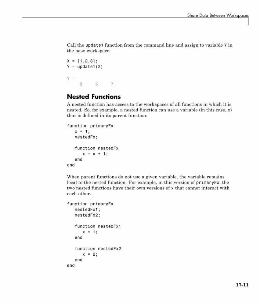
Share Data Between Workspaces
Call the update1 function from the command line and assign to variable Y inthe base workspace:
X = [1,2,3];Y = update1(X)
Y =3 5 7
Nested FunctionsA nested function has access to the workspaces of all functions in which it isnested. So, for example, a nested function can use a variable (in this case, x)that is defined in its parent function:
function primaryFxx = 1;nestedFx;
function nestedFxx = x + 1;
endend
When parent functions do not use a given variable, the variable remainslocal to the nested function. For example, in this version of primaryFx, thetwo nested functions have their own versions of x that cannot interact witheach other.
function primaryFxnestedFx1;nestedFx2;
function nestedFx1x = 1;
end
function nestedFx2x = 2;
endend
17-11

17 Function Basics
For more information, see “Nested Functions” on page 17-32.
Persistent VariablesWhen you declare a variable within a function as persistent, the variableretains its value from one function call to the next. Other local variablesretain their value only during the current execution of a function. Persistentvariables are equivalent to static variables in other programming languages.
Declare variables using the persistent keyword before you use them.MATLAB initializes persistent variables to an empty matrix, [].
For example, define a function in a file named findSum.m that initializes asum to 0, and then adds to the value on each iteration.
function findSum(inputvalue)persistent SUM_X
if isempty(SUM_X)SUM_X = 0;
endSUM_X = SUM_X + inputvalue;
When you call the function, the value of SUM_X persists between subsequentexecutions.
These operations clear the persistent variables for a function:
• clear all
• clear functionname
• Editing the function file
To prevent clearing persistent variables, lock the function file using mlock.
Global VariablesGlobal variables are variables that you can access from functions or fromthe command line. They have their own workspace, which is separate fromthe base and function workspaces.
17-12

Share Data Between Workspaces
However, global variables carry notable risks. For example:
• Any function can access and update a global variable. Other functions thatuse the variable might return unexpected results.
• If you unintentionally give a “new” global variable the same name as anexisting global variable, one function can overwrite the values expected byanother. This error is difficult to diagnose.
Use global variables sparingly, if at all.
If you use global variables, declare them using the global keyword before youaccess them within any particular location (function or command line). Forexample, create a function in a file called falling.m:
function h = falling(t)global GRAVITYh = 1/2*GRAVITY*t.^2;
Then, enter these commands at the prompt:
global GRAVITYGRAVITY = 32;y = falling((0:.1:5)');
The two global statements make the value assigned to GRAVITY at thecommand prompt available inside the function. However, as a more robustalternative, redefine the function to accept the value as an input:
function h = falling(t,gravity)h = 1/2*gravity*t.^2;
Then, enter these commands at the prompt:
GRAVITY = 32;y = falling((0:.1:5)',GRAVITY);
Evaluating in Another WorkspaceThe evalin and assignin functions allow you to evaluate commands orvariable names from strings and specify whether to use the current or baseworkspace.
17-13

17 Function Basics
Like global variables, these functions carry risks of overwriting existing data.Use them sparingly.
evalin and assignin are sometimes useful for callback functions in graphicaluser interfaces to evaluate against the base workspace. For example, create alist box of variable names from the base workspace:
function listBoxfigure;lb = uicontrol('Style','listbox','Position',[10 10 100 100],...
'Callback',@update_listBox);update_listBox(lb)
function update_listBox(src,~)vars = evalin('base','who');set(src,'String',vars)
For other programming applications, consider argument passing and thetechniques described in “Alternatives to the eval Function” on page 2-69.
Concepts • “Base and Function Workspaces” on page 17-9
17-14

Check Variable Scope in Editor
Check Variable Scope in Editor
In this section...
“Use Automatic Function and Variable Highlighting” on page 17-15
“Example of Using Automatic Function and Variable Highlighting” onpage 17-16
Scoping issues can be the source of some coding problems. For instance, if youare unaware that nested functions share a particular variable, the results ofrunning your code might not be as you expect. Similarly, mistakes in usage oflocal, global, and persistent variables can cause unexpected results.
The Code Analyzer does not always indicate scoping issues because sharinga variable across functions is not an error—it may be your intent. UseMATLAB function and variable highlighting features to identify when andwhere your code uses functions and variables. If you have an active Internetconnection, you can watch the Variable and Function Highlighting video foran overview of the major features.
For conceptual information on nested functions and the various types ofMATLAB variables, see “Sharing Variables Between Parent and NestedFunctions” on page 17-33 and “Share Data Between Workspaces” on page17-10.
Use Automatic Function and Variable HighlightingBy default, the Editor indicates functions, local variables, and variables withshared scope in various shades of blue. Variables with shared scope include:global variables, persistent variables, and variables within nested functions.(For more information, see “Nested Functions” on page 17-11.)
To enable and disable highlighting or to change the colors, clickPreferences and selectMATLAB > Colors > Programming tools.
By default, the Editor:
• Highlights all instances of a given function or local variable in sky bluewhen you place the cursor within a function or variable name. For instance:
17-15

17 Function Basics
• Displays a variable with shared scope in teal blue, regardless of the cursorlocation. For instance:
Example of Using Automatic Function and VariableHighlightingConsider the code for a function rowsum:
function rowTotals = rowsum% Add the values in each row and% store them in a new array
x = ones(2,10);[n, m] = size(x);rowTotals = zeros(1,n);for i = 1:n
rowTotals(i) = addToSum;end
function colsum = addToSumcolsum = 0;thisrow = x(i,:);for i = 1:m
colsum = colsum + thisrow(i);end
end
end
When you run this code, instead of returning the sum of the values in eachrow and displaying:
ans =
10 10
MATLAB displays:
17-16

Check Variable Scope in Editor
ans =
0 0 0 0 0 0 0 0 0 10
Examine the code by following these steps:
1 On the Home tab in the Environment section, click Preferencesand select MATLAB > Colors > Programming tools. Ensure thatAutomatically highlight and Variables with shared scope areselected.
2 Copy the rowsum code into the Editor.
Notice the variable appears in teal blue, which indicates i is not a localvariable. Both the rowTotals function and the addToSum functions setand use the variable i.
The variable n, at line 6 appears in black, indicating that it does not spanmultiple functions.
3 Hover the mouse pointer over an instance of variable i.
A tooltip appears: The scope of variable ’i’ spans multiple functions.
4 Click the tooltip link for information about variables whose scope spanmultiple functions.
17-17

17 Function Basics
5 Click an instance of i.
Every reference to i highlights in sky blue and markers appear in theindicator bar on the right side of the Editor.
6 Hover over one of the indicator bar markers.
A tooltip appears and displays the name of the function or variable and theline of code represented by the marker.
7 Click a marker to navigate to the line indicated in tooltip for that marker.
This is particularly useful when your file contains more code than youcan view at one time in the Editor.
Fix the code by changing the instance of i at line 15 to y.
You can see similar highlighting effects when you click on a functionreference. For instance, click on addToSum.
17-18

Types of Functions
Types of Functions
In this section...
“Local and Nested Functions in a File” on page 17-19
“Private Functions in a Subfolder” on page 17-20
“Anonymous Functions Without a File” on page 17-21
Local and Nested Functions in a FileProgram files can contain multiple functions: the main function and anycombination of local or nested functions. Local and nested functions areuseful for dividing programs into smaller tasks, making it easier to read andmaintain your code.
Local functions are subroutines that are available to any other functionswithin the same file. They can appear in the file in any order after the mainfunction in the file. Local functions are the most common way to break upprogrammatic tasks.
For example, create a single program file named myfunction.m that contains amain function, myfunction, and two local functions, squareMe and doubleMe:
function b = myfunction(a)b = squareMe(a) + doubleMe(a);
endfunction y = squareMe(x)
y = x.^2;endfunction y = doubleMe(x)
y = x.*2;end
You can call the main function from the command line or another programfile, although the local functions are only available to myfunction:
myfunction(pi)
ans =16.1528
17-19

17 Function Basics
Nested functions are completely contained within another function. Theprimary difference between nested functions and local functions is that nestedfunctions can use variables defined in parent functions without explicitlypassing those variables as arguments.
Nested functions are useful when subroutines share data, such as GUIapplications that pass data between components. For example, create afunction that allows you to set a value between 0 and 1 using either a slideror an editable text box. If you use nested functions for the callbacks, theslider and text box can share the value and each other’s handles withoutexplicitly passing them:
function myslidervalue = 0;f = figure;s = uicontrol(f,'Style','slider','Callback',@slider);e = uicontrol(f,'Style','edit','Callback',@edittext,...
'Position',[100,20,100,20]);
function slider(obj,~)value = get(obj,'Value');set(e,'String',num2str(value));
endfunction edittext(obj,~)
value = str2double(get(obj,'String'));set(s,'Value',value);
end
end
Private Functions in a SubfolderLike local or nested functions, private functions are accessible only tofunctions in a specific location. However, private functions are not in thesame file as the functions that can call them. Instead, they are in a subfoldernamed private. Private functions are available only to functions in the folderimmediately above the private folder. Use private functions to separate codeinto different files, or to share code between multiple, related functions.
17-20

Types of Functions
Anonymous Functions Without a FileAnonymous functions allow you to define a function without creating aprogram file, as long as the function consists of a single statement. A commonapplication of anonymous functions is to define a mathematical expression,and then evaluate that expression over a range of values using a MATLAB®function function, i.e., a function that accepts a function handle as an input.
For example, this statement creates a function handle named s for ananonymous function:
s = @(x) sin(1./x);
This function has a single input, x . The @ operator creates the functionhandle.
You can use the function handle to evaluate the function for particular values,such as
y = s(pi)
y =
0.3130
Or, you can pass the function handle to a function that evaluates over a rangeof values, such as fplot:
range = [0.01,0.1];fplot(s,range)
17-21

17 Function Basics
Concepts • “Local Functions” on page 17-30• “Nested Functions” on page 17-32• “Private Functions” on page 17-41• “Anonymous Functions” on page 17-23
17-22

Anonymous Functions
Anonymous Functions
In this section...
“What Are Anonymous Functions?” on page 17-23
“Variables in the Expression” on page 17-24
“Multiple Anonymous Functions” on page 17-25
“Functions with No Inputs” on page 17-26
“Functions with Multiple Inputs or Outputs” on page 17-26
“Arrays of Anonymous Functions” on page 17-28
What Are Anonymous Functions?An anonymous function is a function that is not stored in a program file, but isassociated with a variable whose data type is function_handle. Anonymousfunctions can accept inputs and return outputs, just as standard functions do.However, they can contain only a single executable statement.
For example, create a handle to an anonymous function that finds the squareof a number:
sqr = @(x) x.^2;
Variable sqr is a function handle. The @ operator creates the handle, andthe parentheses () immediately after the @ operator include the functioninput arguments. This anonymous function accepts a single input x, andimplicitly returns a single output, an array the same size as x that containsthe squared values.
Find the square of a particular value (5) by passing the value to the functionhandle, just as you would pass an input argument to a standard function.
a = sqr(5)
a =25
17-23

17 Function Basics
Many MATLAB functions accept function handles as inputs so that you canevaluate functions over a range of values. You can create handles either foranonymous functions or for functions in program files. The benefit of usinganonymous functions is that you do not have to edit and maintain a file for afunction that requires only a brief definition.
For example, find the integral of the sqr function from 0 to 1 by passing thefunction handle to the integral function:
q = integral(sqr,0,1);
You do not need to create a variable in the workspace to store an anonymousfunction. Instead, you can create a temporary function handle within anexpression, such as this call to the integral function:
q = integral(@(x) x.^2,0,1);
Variables in the ExpressionFunction handles can store not only an expression, but also variables that theexpression requires for evaluation.
For example, create a function handle to an anonymous function that requirescoefficients a, b, and c.
a = 1.3;b = .2;c = 30;parabola = @(x) a*x.^2 + b*x + c;
Because a, b, and c are available at the time you create parabola, the functionhandle includes those values. The values persist within the function handleeven if you clear the variables:
clear a b cx = 1;y = parabola(x)
y =31.5000
17-24

Anonymous Functions
To supply different values for the coefficients, you must create a new functionhandle:
a = -3.9;b = 52;c = 0;parabola = @(x) a*x.^2 + b*x + c;
x = 1;y = parabola(1)
y =48.1000
You can save function handles and their associated values in a MAT-fileand load them in a subsequent MATLAB session using the save and loadfunctions, such as
save myfile.mat parabola
Multiple Anonymous FunctionsThe expression in an anonymous function can include another anonymousfunction. This is useful for passing different parameters to a function that youare evaluating over a range of values. For example, you can solve the equation
for varying values of c by combining two anonymous functions:
g = @(c) (integral(@(x) (x.^2 + c*x + 1),0,1));
Here is how to derive this statement:
1 Write the integrand as an anonymous function,
@(x) (x.^2 + c*x + 1)
2 Evaluate the function from zero to one by passing the function handle tointegral,
17-25

17 Function Basics
integral(@(x) (x.^2 + c*x + 1),0,1)
3 Supply the value for c by constructing an anonymous function for theentire equation,
g = @(c) (integral(@(x) (x.^2 + c*x + 1),0,1));
The final function allows you to solve the equation for any value of c. Forexample:
g(2)
ans =2.3333
Functions with No InputsIf your function does not require any inputs, use empty parentheses when youdefine and call the anonymous function. For example:
t = @() datestr(now);d = t()
d =26-Jan-2012 15:11:47
Omitting the parentheses in the assignment statement creates anotherfunction handle, and does not execute the function:
d = t
d =@() datestr(now)
Functions with Multiple Inputs or OutputsAnonymous functions require that you explicitly specify the input argumentsas you would for a standard function, separating multiple inputs withcommas. For example, this function accepts two inputs, x and y:
myfunction = @(x,y) (x^2 + y^2 + x*y);
x = 1;
17-26

Anonymous Functions
y = 10;z = myfunction(x,y)
z =
111
However, you do not explicitly define output arguments when you createan anonymous function. If the expression in the function returns multipleoutputs, then you can request them when you call the function. Enclosemultiple output variables in square brackets.
For example, the ndgrid function can return as many outputs as the numberof input vectors. This anonymous function that calls ndgrid can also returnmultiple outputs:
c = 10;mygrid = @(x,y) ndgrid((-x:x/c:x),(-y:y/c:y));[x,y] = mygrid(pi,2*pi);
You can use the output from mygrid to create a mesh or surface plot:
z = sin(x) + cos(y);mesh(x,y,z)
17-27

17 Function Basics
Arrays of Anonymous FunctionsAlthough most MATLAB fundamental data types support multidimensionalarrays, function handles must be scalars (single elements). However, you canstore multiple function handles using a cell array or structure array. Themost common approach is to use a cell array, such as
f = {@(x)x.^2;@(y)y+10;@(x,y)x.^2+y+10};
17-28

Anonymous Functions
When you create the cell array, keep in mind that MATLAB interprets spacesas column separators. Either omit spaces from expressions, as shown in theprevious code, or enclose expressions in parentheses, such as
f = {@(x) (x.^2);@(y) (y + 10);@(x,y) (x.^2 + y + 10)};
Access the contents of a cell using curly braces. For example, f{1} returnsthe first function handle. To execute the function, pass input values inparentheses after the curly braces:
x = 1;y = 10;
f{1}(x)f{2}(y)f{3}(x,y)
ans =1
ans =20
ans =21
Concepts • “Creating a Function Handle” on page 11-3
17-29

17 Function Basics
Local FunctionsThis topic explains the term local function, and shows how to create anduse local functions.
MATLAB program files can contain code for more than one function. The firstfunction in the file (the main function) is visible to functions in other files, oryou can call it from the command line. Additional functions within the fileare called local functions. Local functions are only visible to other functionsin the same file. They are equivalent to subroutines in other programminglanguages, and are sometimes called subfunctions.
Local functions can occur in any order, as long as the main function appearsfirst. Each function begins with its own function definition line.
For example, create a program file named mystats.m that contains a mainfunction, mystats, and two local functions, mymean and mymedian.
function [avg, med] = mystats(x)n = length(x);avg = mymean(x,n);med = mymedian(x,n);end
function a = mymean(v,n)% MYMEAN Example of a local function.
a = sum(v)/n;end
function m = mymedian(v,n)% MYMEDIAN Another example of a local function.
w = sort(v);if rem(n,2) == 1
m = w((n + 1)/2);else
m = (w(n/2) + w(n/2 + 1))/2;endend
17-30

Local Functions
The local functions mymean and mymedian calculate the average and median ofthe input list. The main function mystats determines the length of the list nand passes it to the local functions.
Although you cannot call a local function from the command line or fromfunctions in other files, you can access its help using the help function.Specify names of both the main function and the local function, separatingthem with a > character:
help mystats>mymean
mymean Example of a local function.
Local functions in the current file have precedence over functions in otherfiles. That is, when you call a function within a program file, MATLABchecks whether the function is a local function before looking for other mainfunctions. This allows you to create an alternate version of a particularfunction while retaining the original in another file.
All functions, including local functions, have their own workspaces that areseparate from the base workspace. Local functions cannot access variablesused by other functions unless you pass them as arguments. In contrast,nested functions (functions completely contained within another function) canaccess variables used by the functions that contain them.
See Also localfunctions
Concepts • “Nested Functions” on page 17-32• “Function Precedence Order” on page 17-43
17-31

17 Function Basics
Nested Functions
In this section...
“What Are Nested Functions?” on page 17-32
“Requirements for Nested Functions” on page 17-33
“Sharing Variables Between Parent and Nested Functions” on page 17-33
“Using Handles to Store Function Parameters” on page 17-35
“Visibility of Nested Functions” on page 17-37
What Are Nested Functions?A nested function is a function that is completely contained within a parentfunction. Any function in a program file can include a nested function.
For example, this function named parent contains a nested function namednestedfx:
function parentdisp('This is the parent function')nestedfx
function nestedfxdisp('This is the nested function')
end
end
The primary difference between nested functions and other types of functionsis that they can access and modify variables that are defined in their parentfunctions. As a result:
• Nested functions can use variables that are not explicitly passed as inputarguments.
• In a parent function, you can create a handle to a nested function thatcontains the data necessary to run the nested function.
17-32

Nested Functions
Requirements for Nested Functions
• Typically, functions do not require an end statement. However, to nestany function in a program file, all functions in that file must use an endstatement.
• You cannot define a nested function inside any of the MATLAB programcontrol statements, such as if/elseif/else, switch/case, for, while, ortry/catch.
• You must call a nested function either directly by name (without usingfeval), or using a function handle that you created using the @ operator(and not str2func).
• All of the variables in nested functions or the functions that contain themmust be explicitly defined. That is, you cannot call a function or scriptthat assigns values to variables unless those variables already exist in thefunction workspace. (For more information, see “Variables in Nested andAnonymous Functions” on page 17-39.)
Sharing Variables Between Parent and NestedFunctionsIn general, variables in one function workspace are not available to otherfunctions. However, nested functions can access and modify variables in theworkspaces of the functions that contain them.
This means that both a nested function and a function that contains it canmodify the same variable without passing that variable as an argument. Forexample, in each of these functions, main1 and main2, both the main functionand the nested function can access variable x:
17-33

17 Function Basics
function main1x = 5;nestfun1;
function nestfun1x = x + 1;
end
end
function main2nestfun2;
function nestfun2x = 5;
end
x = x + 1;end
When parent functions do not use a given variable, the variable remainslocal to the nested function. For example, in this function named main, thetwo nested functions have their own versions of x that cannot interact witheach other:
function mainnestedfun1;nestedfun2;
function nestedfun1x = 1;
end
function nestedfun2x = 2;
endend
Functions that return output arguments have variables for the outputs intheir workspace. However, parent functions only have variables for the outputof nested functions if they explicitly request them. For example, this functionparentfun does not have variable y in its workspace:
function parentfunx = 5;nestfun;
function y = nestfuny = x + 1;
17-34

Nested Functions
end
end
If you modify the code as follows, variable z is in the workspace of parentfun:
function parentfunx = 5;z = nestfun;
function y = nestfuny = x + 1;
end
end
Using Handles to Store Function ParametersNested functions can use variables from three sources:
• Input arguments
• Variables defined within the nested function
• Variables defined in a parent function, also called externally scopedvariables
When you create a function handle for a nested function, that handle storesnot only the name of the function, but also the values of externally scopedvariables.
For example, create a function in a file named makeParabola.m. This functionaccepts several polynomial coefficients, and returns a handle to a nestedfunction that calculates the value of that polynomial.
function p = makeParabola(a,b,c)p = @parabola;
function y = parabola(x)y = a*x.^2 + b*x + c;end
17-35

17 Function Basics
end
The makeParabola function returns a handle to the parabola function thatincludes values for coefficients a, b, and c.
At the command line, call the makeParabola function with coefficient valuesof 1.3, .2, and 30. Use the returned function handle p to evaluate thepolynomial at a particular point:
p = makeParabola(1.3,.2,30);
X = 25;Y = p(X)
Y =847.5000
Many MATLAB functions accept function handle inputs to evaluate functionsover a range of values. For example, plot the parabolic equation from -25 to+25:
fplot(p,[-25,25])
17-36

Nested Functions
You can create multiple handles to the parabola function that each usedifferent polynomial coefficients:
firstp = makeParabola(0.8,1.6,32);secondp = makeParabola(3,4,50);range = [-25,25];
figurehold onfplot(firstp,range)fplot(secondp,range,'r:')hold off
Visibility of Nested FunctionsEvery function has a certain scope, that is, a set of other functions to which itis visible. A nested function is available:
• From the level immediately above it. (In the following code, function A cancall B or D, but not C or E.)
17-37

17 Function Basics
• From a function nested at the same level within the same parent function.(Function B can call D, and D can call B.)
• From a function at any lower level. (Function C can call B or D, but not E.)
function A(x, y) % Main functionB(x,y);D(y);
function B(x,y) % Nested in AC(x);D(y);
function C(x) % Nested in BD(x);end
end
function D(x) % Nested in AE(x);
function E(x) % Nested in Ddisp(x)end
endend
The easiest way to extend the scope of a nested function is to create a functionhandle and return it as an output argument, as shown in “Using Handles toStore Function Parameters” on page 17-35. Only functions that can call anested function can create a handle to it.
Concepts • “Variables in Nested and Anonymous Functions” on page 17-39• “Calling a Function Using Its Handle” on page 11-7• “Argument Checking in Nested Functions” on page 18-11
17-38

Variables in Nested and Anonymous Functions
Variables in Nested and Anonymous FunctionsThe scoping rules for nested and anonymous functions require that allvariables used within the function be present in the text of the code.
If you attempt to dynamically add a variable to the workspace of ananonymous function, a nested function, or a function that contains a nestedfunction, then MATLAB issues an error of the form
Attempt to add variable to a static workspace.
This table describes typical operations that attempt dynamic assignment, andthe recommended ways to avoid it.
Type of OperationBest Practice to Avoid DynamicAssignment
load Specify the variable name as an input tothe load function. Or, assign the outputfrom the load function to a structurearray.
eval, evalin, or assignin If possible, avoid using these functionsaltogether. See “Alternatives to the evalFunction” on page 2-69.
Calling a MATLAB script thatcreates a variable
Convert the script to a function andpass the variable using arguments. Thisapproach also clarifies the code.
Assigning to a variable in theMATLAB debugger
Create a global variable for temporaryuse in debugging, such as
K>> global X;K>> X = myvalue;
Another way to avoid dynamic assignment is to explicitly declare the variablewithin the function. For example, suppose a script named makeX.m assignsa value to variable X. A function that calls makeX and explicitly declares Xavoids the dynamic assignment error because X is in the function workspace.A common way to declare a variable is to initialize its value to an empty array:
17-39

17 Function Basics
function noerrorX = [];nestedfx
function nestedfxmakeX
endend
Concepts • “Base and Function Workspaces” on page 17-9
17-40

Private Functions
Private FunctionsThis topic explains the term private function, and shows how to create anduse private functions.
Private functions are useful when you want to limit the scope of a function.You designate a function as private by storing it in a subfolder with thename private. Then, the function is available only to functions in the folderimmediately above the private subfolder, or to scripts called by the functionsthat reside in the parent folder.
For example, within a folder that is on the MATLAB search path, createa subfolder named private. Do not add private to the path. Within theprivate folder, create a function in a file named findme.m:
function findme% FINDME An example of a private function.
disp('You found the private function.')
Change to the folder that contains the private folder and create a file namedvisible.m.
function visiblefindme
Change your current folder to any location and call the visible function.
visible
You found the private function.
Although you cannot call the private function from the command line or fromfunctions outside the parent of the private folder, you can access its help:
help private/findme
findme An example of a private function.
Private functions have precedence over standard functions, so MATLAB findsa private function named test.m before a nonprivate program file named
17-41

17 Function Basics
test.m. This allows you to create an alternate version of a particular functionwhile retaining the original in another folder.
Concepts • “Function Precedence Order” on page 17-43
17-42

Function Precedence Order
Function Precedence OrderThis topic explains how MATLAB determines which function to call whenmultiple functions in the current scope have the same name. The currentscope includes the current file, an optional private subfolder relative to thecurrently running function, the current folder, and the MATLAB path.
MATLAB uses this precedence order:
1 Variables
Before assuming that a name matches a function, MATLAB checks for avariable with that name in the current workspace.
Note If you create a variable with the same name as a function, MATLABcannot run that function until you clear the variable from memory.
2 Imported package functions
A package function is associated with a particular folder. When you importa package function using the import function, it has precedence over allother functions with the same name.
3 Nested functions within the current function
4 Local functions within the current file
5 Private functions
Private functions are functions in a subfolder named private that isimmediately below the folder of the currently running file.
6 Object functions
An object function accepts a particular class of object in its input argumentlist. When there are multiple object functions with the same name,MATLAB checks the classes of the input arguments to determine whichfunction to use.
17-43

17 Function Basics
7 Class constructors in @ folders
MATLAB uses class constructors to create a variety of objects (such astimeseries or audioplayer), and you can define your own classes usingobject-oriented programming. For example, if you create a class folder@polynom and a constructor function @polynom/polynom.m, the constructortakes precedence over other functions named polynom.m anywhere on thepath.
8 Functions in the current folder
9 Functions elsewhere on the path, in order of appearance
When determining the precedence of functions within the same folder,MATLAB considers the file type, in this order:
1 Built-in function
2 MEX-function
3 Simulink® model, with file types in this order:
a SLX file
b MDL file
4 P-file (that is, an encoded program file with a .p extension)
5 Program file with a .m extension
For example, if MATLAB finds a .m file and a P-file with the same namein the same folder, it uses the P-file. Because P-files are not automaticallyregenerated, make sure that you regenerate the P-file whenever you editthe program file.
To determine the function MATLAB calls for a particular input, include thefunction name and the input in a call to the which function. For example,determine the location of the max function that MATLAB calls for doubleand int8 values:
testval = 10;which max(testval)
17-44

Function Precedence Order
% double methodbuilt-in (matlabroot\toolbox\matlab\datafun\@double\max)
testval = int8(10);which max(testval)
% int8 methodbuilt-in (matlabroot\toolbox\matlab\datafun\@int8\max)
For more information, see:
• “Search Path Basics”
• Variables
• “Types of Functions” on page 17-19
• “Class Precedence and MATLAB Path”
17-45

17 Function Basics
17-46

18
Function Arguments
• “Find Number of Function Arguments” on page 18-2
• “Support Variable Number of Inputs” on page 18-4
• “Support Variable Number of Outputs” on page 18-6
• “Validate Number of Function Arguments” on page 18-8
• “Argument Checking in Nested Functions” on page 18-11
• “Ignore Function Inputs” on page 18-13
• “Check Function Inputs with validateattributes” on page 18-14
• “Parse Function Inputs” on page 18-17
• “Input Parser Validation Functions” on page 18-22

18 Function Arguments
Find Number of Function ArgumentsThis example shows how to determine how many input or output argumentsyour function receives using nargin and nargout.
Input Arguments
Create a function in a file named addme.m that accepts up to two inputs.Identify the number of inputs with nargin.
function c = addme(a,b)
switch nargincase 2
c = a + b;case 1
c = a + a;otherwise
c = 0;end
Call addme with one, two, or zero input arguments.
addme(42)
ans =84
addme(2,4000)
ans =4002
addme
ans =0
Output Arguments
18-2

Find Number of Function Arguments
Create a new function in a file named addme2.m that can return one or twooutputs (a result and its absolute value). Identify the number of requestedoutputs with nargout.
function [result,absResult] = addme2(a,b)
switch nargincase 2
result = a + b;case 1
result = a + a;otherwise
result = 0;end
if nargout > 1absResult = abs(result);
end
Call addme2 with one or two output arguments.
value = addme2(11,-22)
value =-11
[value,absValue] = addme2(11,-22)
value =-11
absValue =11
Functions return outputs in the order they are declared in the functiondefinition.
See Also nargin | narginchk | nargout | nargoutchk
18-3

18 Function Arguments
Support Variable Number of InputsThis example shows how to define a function that accepts a variable numberof input arguments using varargin. The varargin argument is a cell arraythat contains the function inputs, where each input is in its own cell.
Create a function in a file named plotWithTitle.m that accepts a variablenumber of paired (x,y) inputs for the plot function and an optional title. Ifthe function receives an odd number of inputs, it assumes that the last inputis a title.
function plotWithTitle(varargin)if rem(nargin,2) ~= 0
myTitle = varargin{nargin};numPlotInputs = nargin - 1;
elsemyTitle = 'Default Title';numPlotInputs = nargin;
end
plot(varargin{1:numPlotInputs})title(myTitle)
Because varargin is a cell array, you access the contents of each cellusing curly braces, {}. The syntax varargin{1:numPlotInputs} creates acomma-separated list of inputs to the plot function.
Call plotWithTitle with two sets of (x,y) inputs and a title.
x = [1:.1:10]; y1 = sin(x); y2 = cos(x);plotWithTitle(x,y1,x,y2,'Sine and Cosine')
You can use varargin alone in an input argument list, or at the end of thelist of inputs, such as
function myfunction(a,b,varargin)
In this case, varargin{1} corresponds to the third input passed to thefunction, and nargin returns length(varargin) + 2.
See Also nargin | varargin
18-4

Support Variable Number of Inputs
RelatedExamples
• “Access Data in a Cell Array” on page 10-5
Concepts • “Argument Checking in Nested Functions” on page 18-11• “Comma-Separated Lists” on page 2-61
18-5

18 Function Arguments
Support Variable Number of OutputsThis example shows how to define a function that returns a variable numberof output arguments using varargout. Output varargout is a cell array thatcontains the function outputs, where each output is in its own cell.
Create a function in a file named magicfill.m that assigns a magic square toeach requested output.
function varargout = magicfillnOutputs = nargout;varargout = cell(1,nOutputs);
for k = 1:nOutputs;varargout{k} = magic(k);
end
Indexing with curly braces {} updates the contents of a cell.
Call magicfill and request three outputs.
[first,second,third] = magicfill
first =1
second =1 34 2
third =8 1 63 5 74 9 2
MATLAB assigns values to the outputs according to their order in thevarargout array. For example, first == varargout{1}.
You can use varargout alone in an output argument list, or at the end ofthe list of outputs, such as
18-6

Support Variable Number of Outputs
function [x,y,varargout] = myfunction(a,b)
In this case, varargout{1} corresponds to the third output that the functionreturns, and nargout returns length(varargout) + 2.
See Also nargout | varargout
RelatedExamples
• “Access Data in a Cell Array” on page 10-5
Concepts • “Argument Checking in Nested Functions” on page 18-11
18-7

18 Function Arguments
Validate Number of Function ArgumentsThis example shows how to check whether your custom function receivesa valid number of input or output arguments. MATLAB performs someargument checks automatically. For other cases, you can use narginchk ornargoutchk.
Automatic Argument Checks
MATLAB checks whether your function receives more arguments thanexpected when it can determine the number from the function definition. Forexample, this function accepts up to two outputs and three inputs:
function [x,y] = myFunction(a,b,c)
If you pass too many inputs to myFunction, MATLAB issues an error. You donot need to call narginchk to check for this case.
[X,Y] = myFunction(1,2,3,4)
Error using myFunctionToo many input arguments.
Use the narginchk and nargoutchk functions to verify that your functionreceives:
• A minimum number of required arguments.
• No more than a maximum number of arguments, when your function usesvarargin or varargout.
Input Checks with narginchk
Define a function in a file named testValues.m that requires at least twoinputs. The first input is a threshold value to compare against the otherinputs.
function testValues(threshold,varargin)minInputs = 2;maxInputs = Inf;narginchk(minInputs,maxInputs)
18-8

Validate Number of Function Arguments
for k = 1:(nargin-1)if (varargin{k} > threshold)
fprintf('Test value %d exceeds %d\n',k,threshold);end
end
Call testValues with too few inputs.
testValues(10)
Error using testValues (line 4)Not enough input arguments.
Call testValues with enough inputs.
testValues(10,1,11,111)
Test value 2 exceeds 10Test value 3 exceeds 10
Output Checks with nargoutchk
Define a function in a file named mysize.m that returns the dimensions ofthe input array in a vector (from the size function), and optionally returnsscalar values corresponding to the sizes of each dimension. Use nargoutchkto verify that the number of requested individual sizes does not exceed thenumber of available dimensions.
function [sizeVector,varargout] = mysize(x)minOutputs = 0;maxOutputs = ndims(x) + 1;nargoutchk(minOutputs,maxOutputs)
sizeVector = size(x);
varargout = cell(1,nargout-1);for k = 1:length(varargout)
varargout{k} = sizeVector(k);end
Call mysize with a valid number of outputs.
18-9

18 Function Arguments
A = rand(3,4,2);[fullsize,nrows,ncols,npages] = mysize(A)
fullsize =3 4 2
nrows =3
ncols =4
npages =2
Call mysize with too many outputs.
A = 1;[fullsize,nrows,ncols,npages] = mysize(A)
Error using mysize (line 4)Too many output arguments.
See Also narginchk | nargoutchk
RelatedExamples
• “Support Variable Number of Inputs” on page 18-4• “Support Variable Number of Outputs” on page 18-6
18-10

Argument Checking in Nested Functions
Argument Checking in Nested FunctionsThis topic explains special considerations for using varargin, varargout,nargin, and nargout with nested functions.
varargin and varargout allow you to create functions that accept variablenumbers of input or output arguments. Although varargin and varargoutlook like function names, they refer to variables, not functions. This issignificant because nested functions share the workspaces of the functionsthat contain them.
If you do not use varargin or varargout in the declaration of a nestedfunction, then varargin or varargout within the nested function refers tothe arguments of an outer function.
For example, create a function in a file named showArgs.m that uses vararginand has two nested functions, one that uses varargin and one that does not.
function showArgs(varargin)nested1(3,4)nested2(5,6,7)
function nested1(a,b)disp('nested1: Contents of varargin{1}')disp(varargin{1})
end
function nested2(varargin)disp('nested2: Contents of varargin{1}')disp(varargin{1})
end
end
Call the function and compare the contents of varargin{1} in the two nestedfunctions.
showArgs(0,1,2)
nested1: Contents of varargin{1}
18-11

18 Function Arguments
0
nested2: Contents of varargin{1}5
On the other hand, nargin and nargout are functions. Within any function,including nested functions, calls to nargin or nargout return the number ofarguments for that function. If a nested function requires the value of narginor nargout from an outer function, pass the value to the nested function.
For example, create a function in a file named showNumArgs.m that passesthe number of input arguments from the primary (parent) function to anested function.
function showNumArgs(varargin)
disp(['Number of inputs to showNumArgs: ',int2str(nargin)]);nestedFx(nargin,2,3,4)
function nestedFx(n,varargin)disp(['Number of inputs to nestedFx: ',int2str(nargin)]);disp(['Number of inputs to its parent: ',int2str(n)]);
end
end
Call showNumArgs and compare the output of nargin in the parent and nestedfunctions.
showNumArgs(0,1)
Number of inputs to showNumArgs: 2Number of inputs to nestedFx: 4Number of inputs to its parent: 2
See Also nargin | nargout | varargin | varargout
18-12

Ignore Function Inputs
Ignore Function InputsThis example shows how to ignore inputs in your function definition usingthe tilde (~) operator.
Use this operator when your function must accept a predefined set of inputs,but your function does not use all of the inputs. Common applicationsinclude defining callback functions, as shown here, or deriving a class froma superclass.
Define a callback for a push button in a file named colorButton.m that doesnot use the eventdata input. Ignore the input with a tilde.
function colorButton
figure;
uicontrol('Style','pushbutton','String','Click me','Callback',@btnCallback)
function btnCallback(h,~)
set(h,'BackgroundColor',rand(3,1))
The function declaration for btnCallback is essentially the same as
function btnCallback(h,eventdata)
However, using the tilde prevents the addition of eventdata to the functionworkspace and makes it clearer that the function does not use eventdata.
You can ignore any number of function inputs, in any position in the argumentlist. Separate consecutive tildes with a comma, such as
myfunction(myinput,~,~)
18-13

18 Function Arguments
Check Function Inputs with validateattributesThis example shows how to verify that the inputs to your function conform toa set of requirements using the validateattributes function.
validateattributes requires that you pass the variable to check and thesupported data types for that variable. Optionally, pass a set of attributesthat describe the valid dimensions or values.
Check Data Type and Other Attributes
Define a function in a file named checkme.m that accepts up to three inputs:a, b, and c. Check whether:
• a is a two-dimensional array of positive double-precision values.
• b contains 100 numeric values in an array with 10 columns.
• c is a nonempty character string or cell array.
function checkme(a,b,c)
validateattributes(a,{'double'},{'positive','2d'})validateattributes(b,{'numeric'},{'numel',100,'ncols',10})validateattributes(c,{'char','cell'},{'nonempty'})
disp('All inputs are ok.')
The curly braces {} indicate that the set of data types and the set of additionalattributes are in cell arrays. Cell arrays allow you to store combinations oftext and numeric data, or text strings of different lengths, in a single variable.
Call checkme with valid inputs.
checkme(pi,rand(5,10,2),'text')
All inputs are ok.
The scalar value pi is two-dimensional because size(pi) = [1,1].
18-14

Check Function Inputs with validateattributes
Call checkme with invalid inputs. The validateattributes function issuesan error for the first input that fails validation, and checkme stops processing.
checkme(-4)
Error using checkme (line 3)Expected input to be positive.
checkme(pi,rand(3,4,2))
Error using checkme (line 4)Expected input to be an array with number of elements equal to 100.
checkme(pi,rand(5,10,2),struct)
Error using checkme (line 5)Expected input to be one of these types:
char, cell
Instead its type was struct.
The default error messages use the generic term input to refer to theargument that failed validation. When you use the default error message,the only way to determine which input failed is to view the specified line ofcode in checkme.
Add Input Name and Position to Errors
Define a function in a file named checkdetails.m that performs the samevalidation as checkme, but adds details about the input name and positionto the error messages.
function checkdetails(a,b,c)
validateattributes(a,{'double'},{'positive','2d'},'','First',1)validateattributes(b,{'numeric'},{'numel',100,'ncols',10},'','Second',2)validateattributes(c,{'char'},{'nonempty'},'','Third',3)
disp('All inputs are ok.')
18-15

18 Function Arguments
The empty string '' for the fourth input to validateattributes is aplaceholder for an optional function name string. You do not need to specifya function name because it already appears in the error message. Specifythe function name when you want to include it in the error identifier foradditional error handling.
Call checkdetails with invalid inputs.
checkdetails(-4)
Error using checkdetails (line 3)Expected input number 1, First, to be positive.
checkdetails(pi,rand(3,4,2))
Error using checkdetails (line 4)Expected input number 2, Second, to be an array withnumber of elements equal to 100.
See Also validateattributes | validatestring
18-16

Parse Function Inputs
Parse Function InputsThis example shows how to define required and optional inputs, assigndefaults to optional inputs, and validate all inputs to a custom function usingthe Input Parser.
The Input Parser provides a consistent way to validate and assign defaultsto inputs, improving the robustness and maintainability of your code. Tovalidate the inputs, you can take advantage of existing MATLAB functions orwrite your own validation routines.
Step 1. Define your function.
Create a function in a file named printPhoto.m. The printPhoto functionhas one required input for the file name, and optional inputs for the finish(glossy or matte), color space (RGB or CMYK), width, and height.
function printPhoto(filename,varargin)
In your function declaration statement, specify required inputs first. Usevarargin to support optional inputs.
Step 2. Create an InputParser object.
Within your function, call inputParser to create a parser object.
p = inputParser;
Step 3. Add inputs to the scheme.
Add inputs to the parsing scheme in your function using addRequired,addOptional, or addParameter. For optional inputs, specify default values.
For each input, you can specify a handle to a validation function that checksthe input and returns a scalar logical (true or false) or errors. The validationfunction can be an existing MATLAB function (such as ischar or isnumeric)or a function that you create (such as an anonymous function or a localfunction).
18-17

18 Function Arguments
In the printPhoto function, filename is a required input. Define finish andcolor as optional input strings, and width and height as optional parametervalue pairs.
defaultFinish = 'glossy';validFinishes = {'glossy','matte'};checkFinish = @(x) any(validatestring(x,validFinishes));
defaultColor = 'RGB';validColors = {'RGB','CMYK'};checkColor = @(x) any(validatestring(x,validColors));
defaultWidth = 6;defaultHeight = 4;
addRequired(p,'filename',@ischar);addOptional(p,'finish',defaultFinish,checkFinish);addOptional(p,'color',defaultColor,checkColor);addParameter(p,'width',defaultWidth,@isnumeric);addParameter(p,'height',defaultHeight,@isnumeric);
Inputs that you add with addRequired or addOptional are positionalarguments. When you call a function with positional inputs, specify thosevalues in the order they are added to the parsing scheme.
Inputs added with addParameter are not positional, so you can pass valuesfor height before or after values for width. However, parameter value inputsrequire that you pass the input name ('height' or 'width') along with thevalue of the input.
If your function accepts optional input strings and parameter name and valuepairs, specify validation functions for the optional input strings. Otherwise,the Input Parser interprets the optional strings as parameter names. Forexample, the checkFinish validation function ensures that printPhotointerprets 'glossy' as a value for finish and not as an invalid parametername.
Step 4. Set properties to adjust parsing (optional).
18-18

Parse Function Inputs
By default, the Input Parser makes assumptions about case sensitivity,function names, structure array inputs, and whether to allow additionalparameter names and values that are not in the scheme. Properties allow youto explicitly define the behavior. Set properties using dot notation, similar toassigning values to a structure array.
Allow printPhoto to accept additional parameter value inputs that do notmatch the input scheme by setting the KeepUnmatched property of the InputParser.
p.KeepUnmatched = true;
If KeepUnmatched is false (default), the Input Parser issues an error wheninputs do not match the scheme.
Step 5. Parse the inputs.
Within your function, call the parse method. Pass the values of all of thefunction inputs.
parse(p,filename,varargin{:});
Step 6. Use the inputs in your function.
Access parsed inputs using these properties of the inputParser object:
• Results — Structure array with names and values of all inputs in thescheme.
• Unmatched— Structure array with parameter names and values that arepassed to the function, but are not in the scheme (when KeepUnmatchedis true).
• UsingDefaults — Cell array with names of optional inputs that areassigned their default values because they are not passed to the function.
Within the printPhoto function, display the values for some of the inputs:
disp(['File name: ',p.Results.filename])disp(['Finish: ', p.Results.finish])
if ~isempty(fieldnames(p.Unmatched))
18-19

18 Function Arguments
disp('Extra inputs:')disp(p.Unmatched)
endif ~isempty(p.UsingDefaults)
disp('Using defaults: ')disp(p.UsingDefaults)
end
Step 7. Call your function.
The Input Parser expects to receive inputs as follows:
• Required inputs first, in the order they are added to the parsing schemewith addRequired.
• Optional positional inputs in the order they are added to the scheme withaddOptional.
• Positional inputs before parameter name and value pair inputs.
• Parameter names and values in the formName1,Value1,...,NameN,ValueN.
Pass several combinations of inputs to printPhoto, some valid and someinvalid:
printPhoto('myfile.jpg')
File name: myfile.jpgFinish: glossyUsing defaults:
'finish' 'color' 'width' 'height'
printPhoto(100)
Error using printPhoto (line 23)Argument 'filename' failed validation ischar.
printPhoto('myfile.jpg','satin')
Error using printPhoto (line 23)Argument 'finish' failed validation with error:Expected input to match one of these strings:
18-20

Parse Function Inputs
glossy, matte
The input, 'satin', did not match any of the valid strings.
printPhoto('myfile.jpg','height',10,'width',8)
File name: myfile.jpgFinish: glossyUsing defaults:
'finish' 'color'
To pass a value for the nth positional input, either specify values for theprevious (n – 1) inputs or pass the input as a parameter name and value pair.For example, these function calls assign the same values to finish (default'glossy') and color:
printPhoto('myfile.gif','glossy','CMYK'); % positional
printPhoto('myfile.gif','color','CMYK'); % name and value
See Also inputParser | varargin
Concepts • “Input Parser Validation Functions” on page 18-22
18-21

18 Function Arguments
Input Parser Validation FunctionsThis topic shows ways to define validation functions that you pass to theInput Parser to check custom function inputs.
The Input Parser methods addRequired, addOptional, and addParametereach accept an optional handle to a validation function. Designate functionhandles with an at (@) symbol.
Validation functions must accept a single input argument, and they musteither return a scalar logical value (true or false) or error. If the validationfunction returns false, the Input Parser issues an error and your functionstops processing.
There are several ways to define validation functions:
• Use an existing MATLAB function such as ischar or isnumeric. Forexample, check that a required input named num is numeric:
p = inputParser;checknum = @isnumeric;addRequired(p,'num',checknum);
parse(p,'text');
Argument 'num' failed validation isnumeric.
• Create an anonymous function. For example, check that input num is anumeric scalar greater than zero:
p = inputParser;checknum = @(x) isnumeric(x) && isscalar(x) && (x > 0);addRequired(p,'num',checknum);
parse(p,rand(3));
Argument 'num' failed validation @(x)isnumeric(x)&&isscalar(x)&&(x>0).
• Define your own function, typically a local function in the same file as yourprimary function. For example, in a file named usenum.m, define a local
18-22

Input Parser Validation Functions
function named checknum that issues custom error messages when theinput num to usenum is not a numeric scalar greater than zero:
function usenum(num)p = inputParser;addRequired(p,'num',@checknum);parse(p,num);
function TF = checknum(x)TF = false;if ~isscalar(x)
error('Input is not scalar');elseif ~isnumeric(x)
error('Input is not numeric');elseif (x <= 0)
error('Input must be > 0');else
TF = true;end
Call the function with an invalid input:
usenum(-1)
Error using usenum (line 4)Argument 'num' failed validation with error:Input must be > 0
See Also inputParser | function_handle | is* | validateattributes
RelatedExamples
• “Parse Function Inputs” on page 18-17
Concepts • “Anonymous Functions” on page 17-23
18-23

18 Function Arguments
18-24

19
Debugging MATLAB Code

19 Debugging MATLAB® Code
Debugging Process and Features
In this section...
“Ways to Debug MATLAB Files” on page 19-2
“Preparing for Debugging” on page 19-2
“Set Breakpoints” on page 19-5
“Run a File with Breakpoints” on page 19-8
“Step Through a File” on page 19-10
“Examine Values” on page 19-11
“Correct Problems and End Debugging” on page 19-17
“Conditional Breakpoints” on page 19-24
“Breakpoints in Anonymous Functions” on page 19-26
“Breakpoints in Methods That Overload Functions” on page 19-27
“Error Breakpoints” on page 19-28
Ways to Debug MATLAB FilesYou can debug MATLAB files using the Editor, which is a graphical userinterface, as well as by using debugging functions from the CommandWindow. You can use both methods interchangeably. These topics and theexample describe both methods.
Preparing for DebuggingDo the following to prepare for debugging:
1 Open the file — To use the Editor for debugging, open it with the file to run.
2 Save changes — If you are editing the file, save the changes before youbegin debugging. If you try to run a file with unsaved changes from withinthe Editor, the file is automatically saved before it runs. If you run a filewith unsaved changes from the Command Window, MATLAB softwareruns the saved version of the file. Therefore, you do not see the resultsof your changes.
19-2

Debugging Process and Features
3 Add the files to a folder on the search path or put them in the currentfolder. Be sure the file you run and any files it calls are in folders that areon the search path. If all required files are in the same folder, you caninstead make that folder the current folder.
Debugging Example — The Collatz ProblemThe debugging process and features are best described using an example. Toprepare to use the example, create two files, collatz.m and collatzplot.m,that produce data for the Collatz problem.
For any given positive integer, n, the Collatz algorithm produces a sequenceof integers. If n equals 1, the sequence is complete. Otherwise, if n is odd,multiply it by 3 and add 1 to get the next integer in the sequence. Otherwise,if n is even, divide it by 2 to get the next integer in the sequence. Repeat theprocess until the sequence terminates with 1. The number of integers in thesequence varies depending on the starting value, n.
The Collatz conjecture is that the sequence always terminates within afinite number of steps. The files for this example are useful for studyingthe behavior of the Collatz algorithm. The file collatz.m generates theCollatz sequence of integers for any given n. The file collatzplot.m plots thelength of the sequence against the starting value for all starting values from 1through a given value m. The plot shows patterns that you can study further.
Following are the results when n is 1, 2, or 3.
n Sequence Number of Integersin the Sequence
1 1 1
2 2 1 2
3 3 10 5 16 8 4 2 1 8
19-3

19 Debugging MATLAB® Code
Files for the Collatz Problem. Following are the two files you use for thedebugging example. To create these files on your system, open two new files.Select and copy the following code from the Help browser and paste it into thefiles. Save and name the files collatz.m and collatzplot.m. Save them toyour current folder or add the folder where you save them to the search path.One of the files has an embedded error to illustrate the debugging features.
Open the files by issuing the following commands, and then saving each fileto a local folder:
open(fullfile(matlabroot,'help','techdoc','matlab_env',...'examples','collatz.m'))
open(fullfile(matlabroot,'help','techdoc','matlab_env',...'examples','collatzplot.m'))
Trial Run for the Example. Open the file collatzplot.m. Make sure thatthe current folder is the folder in which you saved collatzplot.
Try out collatzplot to see if it works correctly. Use a simple input value,for example, 3, and compare the results to those shown in the precedingtable. Typing
collatzplot(3)
produces the plot shown in the following figure.
19-4

Debugging Process and Features
The plot for n = 1 appears to be correct—for 1, the Collatz series is 1, andcontains one integer. But for n = 2 and n = 3, it is wrong. There should be onlyone value plotted for each integer, the number of integers in the sequence,which the preceding table shows to be 2 (for n = 2) and 8 (for n = 3). Instead,multiple values are plotted. Use MATLAB debugging features to isolate theproblem.
Set BreakpointsSet breakpoints to pause execution of the MATLAB file so you can examinevalues where you think the problem can be. You can set breakpoints usingthe Editor, using functions in the Command Window, or both.
19-5

19 Debugging MATLAB® Code
There are three basic types of breakpoints you can set in MATLAB files:
• A standard breakpoint, which stops at a specified line in a file. For details,see “Set Standard Breakpoints” on page 19-7.
• A conditional breakpoint, which stops at a specified line in a file onlyunder specified conditions. For details, see “Conditional Breakpoints” onpage 19-24.
• An error breakpoint that stops in any file when it produces the specifiedtype of warning, error, or NaN or infinite value. For details, see “ErrorBreakpoints” on page 19-28.
You can disable standard and conditional breakpoints so that MATLABtemporarily ignores them, or you can remove them. For details, see “Disableand Clear Breakpoints” on page 19-18. Breakpoints do not persist after youexit the MATLAB session.
You can only set valid standard and conditional breakpoints at executablelines in saved files that are in the current folder or in folders on the searchpath. When you add or remove a breakpoint in a file that is not in a folderon the search path or in the current folder, a dialog box appears. This dialogbox presents options that allow you to add or remove the breakpoint. You caneither change the current folder to the folder containing the file, or you canadd the folder containing the file to the search path.
Do not set a breakpoint at a for statement if you want to examine values atincrements in the loop. For example, in
for n = 1:10m = n+1;
end
MATLAB executes the for statement only once, which is efficient. Therefore,when you set a breakpoint at the for statement and step through the file, youonly stop at the for statement once. Instead place the breakpoint at the nextline, m=n+1 to stop at each pass through the loop.
You cannot set breakpoints while MATLAB is busy, for example, running afile, unless that file is paused at a breakpoint.
19-6

Debugging Process and Features
Set Standard BreakpointsTo set a standard breakpoint using the Editor:
1 If you have changed the file, save it.
2 Either:
• Click in the breakpoint alley at an executable line where you want to setthe breakpoint. The breakpoint alley is the narrow column on the leftside of the Editor, to the right of the line number.
• Position the cursor in an executable line. On the Editor tab, in theBreakpoints section, click Breakpoints, and then select Set/Clear.
Executable lines are preceded by a - (dash). If you attempt to setbreakpoints at lines that are not executable, such as comments or blanklines, MATLAB sets it at the next executable line.
Set Breakpoints for the Example. It is unclear whether the problem inthe example is in collatzplot or collatz. To start, follow these steps:
1 In collatzplot.m, click the dash in the breakpoint alley at line 9 to set abreakpoint.
This breakpoint enables you to step into collatz to see if the problemis there.
2 Set additional breakpoints at lines 10 and 11.
These breakpoints stop the program so you can examine the interim results.
19-7

19 Debugging MATLAB® Code
Valid (Red) and Invalid (Gray) Breakpoints. Red breakpoints indicatevalid standard breakpoints.
Breakpoints are gray for either of these reasons:
• There are unsaved changes in the file. Save the file to make breakpointsvalid. The gray breakpoints become red, indicating they are now valid. Anygray breakpoints that you entered at invalid breakpoint lines automaticallymove to the next valid breakpoint line with a successful file save.
• There is a syntax error in the file. When you set a breakpoint, an errormessage appears indicating where the syntax error is. Fix the syntax errorand save the file to make breakpoints valid.
Function Alternative for Setting BreakpointsTo set a breakpoint using the debugging functions, use dbstop. For theexample, type:
dbstop in collatzplot at 9dbstop in collatzplot at 10dbstop in collatzplot at 11
Run a File with BreakpointsAfter setting breakpoints, run the file from the Command Window or theEditor.
19-8

Debugging Process and Features
Run the ExampleFor the example, run collatzplot for the simple input value, 3, by typing thefollowing in the Command Window:
collatzplot(3)
The example, collatzplot, requires an input argument and therefore runsonly from the Command Window or from the input value(s) specified on theRun drop-down list on the Editor tab.
Results of Running a File Containing BreakpointsRunning the file results in the following:
• The prompt in the Command Window changes to
K>>
indicating that MATLAB is in debug mode.
• The program pauses at the first breakpoint. This means that line will beexecuted when you continue. The pause is indicated in the Editor by thegreen arrow just to the right of the breakpoint. In the example, the pauseis at line 9 of collatzplot, as shown here:
The line at which you are paused displays in the Command Window. Forthe example:
• The function the Function Call Stack field displays on the Editor tabchanges to reflect the current function (sometimes referred to as the calleror calling workspace). The call stack includes local functions as wellas called functions. If you use debugging functions from the CommandWindow, use dbstack to view the current call stack.
• If the file you are running is not in the current folder or a folder on thesearch path, you are prompted to either add the folder to the path orchange the current folder.
19-9

19 Debugging MATLAB® Code
In debug mode, you can set breakpoints, step through programs, examinevariables, and run other functions.
MATLAB software could become nonresponsive if it stops at a breakpointwhile displaying a modal dialog box or figure that your file creates. In thatevent, press Ctrl+C to go to the MATLAB prompt.
Step Through a FileWhile debugging, you can step through a MATLAB file, pausing at pointswhere you want to examine values.
Use any of the following methods:
• Click Step, Step In, Step Out in Editor tab.
• Use the dbstep or dbcont function
Details about these debugging buttons appear in the following table.
Toolbar Button Debug MenuItem
Description FunctionAlternative
Run to Cursor Continue execution of file untilthe line where the cursor ispositioned. Also available on thecontext menu.
None
Step Execute the current line of thefile.
dbstep
Step In Execute the current line of thefile and, if the line is a call toanother function, step into thatfunction.
dbstep in
Continue Resume execution of file untilcompletion or until anotherbreakpoint is encountered.
dbcont
19-10

Debugging Process and Features
Toolbar Button Debug MenuItem
Description FunctionAlternative
Step Out After stepping in, run therest of the called function orlocal function, leave the calledfunction, and pause.
dbstep out
QuitDebugging
Exit debug mode. dbquit out
Continue Running in the ExampleIn the example, collatzplot is paused at line 9. Because the problem resultsare correct for N/n = 1, continue running until N/n = 2. Click Continuethree times to move through the breakpoints at lines 9, 10, and 11. Now theprogram is again paused at the breakpoint at line 9.
Step into the Called Function in the ExampleNow that collatzplot is paused at line 9 during the second iteration, clickStep In or type dbstep in in the Command Window to step into collatz
and walk through that file. Stepping into line 9 of collatzplot goes to line9 of collatz. If collatz is not open in the Editor, it automatically opens ifyou have selected Automatically open files when MATLAB reaches abreakpoint in the Preference dialog box.
The pause indicator at line 9 of collatzplot changes to a hollow arrow ,indicating that MATLAB control is now in a local function called from themain program. The call stack shows that the current function is now collatz.
In the called function, collatz in the example, you can do the same thingsyou can do in the main (calling) function—set breakpoints, run, step through,and examine values.
Examine ValuesWhile the program is paused, you can view the value of any variable currentlyin the workspace. Examine values when you want to see whether a line ofcode has produced the expected result or not. If the result is as expected,
19-11

19 Debugging MATLAB® Code
continue running or step to the next line. If the result is not as you expect,then that line, or a previous line, contains an error. Use the following methodsto examine values:
• “Select the Workspace” on page 19-12
• “View Values as Data Tips in the Editor” on page 19-13
• “View Values in the Command Window” on page 19-13
• “View Values in the Workspace Browser and Variables Editor” on page19-14
• “Evaluate a Selection” on page 19-15
• “Examine Values in the Example” on page 19-15
• “Problems Viewing Variable Values from the Parent Workspace” on page19-16
Many of these methods are used in “Examine Values in the Example” onpage 19-15.
Select the WorkspaceVariables assigned through the Command Window and created using scriptsare considered to be in the base workspace. Variables created in a functionbelong to their own function workspace. To examine a variable, you must firstselect its workspace. When you run a program, the current workspace isshown in the Function Call Stack field. To examine values that are part ofanother workspace for a currently running function or for the base workspace,first select that workspace from the list in the Function Call Stack field.
If you use debugging functions from the Command Window:
• To display the call stack, use dbstack.
• To change to a different workspace, use dbup and dbdown.
• To list the variables in the current workspace, use who or whos.
Workspace in the Example. At line 9 of collatzplot, you stepped in, andthe current line is 9 in collatz. The Function Call Stack field shows thatcollatz is the current workspace.
19-12

Debugging Process and Features
View Values as Data Tips in the EditorTo view the current value of a variable in the Editor, first enable datatips,then use the mouse to display a datatip:
1 On the Home tab, in the Environment section, click Preferences,and select MATLAB > Editor/Debugger > Display.
2 Select Enable datatips in edit mode under General display options.
3 In the Editor, position the mouse pointer to the left of a variable.
The variable’s current value appears in a data tip. The data tip stays inview until you move the pointer. If you have trouble getting the data tipto appear, click in the line containing the variable, and then move thepointer next to the variable.
View Values in the Command WindowYou can examine values while in debug mode at the K>> prompt. To see thevariables currently in the workspace, use who. Type a variable name in theCommand Window and it displays the variable’s current value. For theexample, to see the value of n, type
n
The Command Window displays the expected result
n =
19-13

19 Debugging MATLAB® Code
2
and displays the debug prompt, K>>.
View Values in the Workspace Browser and Variables EditorYou can view the value of variables in the Value column of the Workspacebrowser. The Workspace browser displays all variables in the currentworkspace. To change to another workspace and view its variables, useFunction Call Stack drop-down list on the Editor tab, in theDebug section.
The Value column does not show all details for all variables. To see details,double-click a variable in the Workspace browser. The Variables Editor opens,displaying the content for that variable. You can open the Variables Editordirectly for a variable using openvar.
To see the value of n in the Variables Editor for the example, type
openvar n
and the Variables Editor opens, showing that n = 1 as expected.
19-14

Debugging Process and Features
Evaluate a SelectionSelect a variable or equation in a MATLAB file in the Editor. Right-clickand select Evaluate Selection from the context menu (for a single-buttonmouse, press Ctrl+click). The Command Window displays the value of thevariable or equation. You cannot evaluate a selection while MATLAB is busy,for example, running a file.
Examine Values in the ExampleStep from line 9 through line 13 in collatz. Step again, and the pauseindicator jumps to line 17, just after the if loop, as expected. Step again, toline 18, check the value of sequence in line 17 and see that the array is
2 1
as expected for n = 2. Step again, which moves the pause indicator from line18 to line 11. At line 11, step again. Because next_value is now 1, the whileloop ends. The pause indicator is at line 11 and appears as a green downarrow . This indicates that processing in the called function is complete andprogram control will return to the calling program. Step again from line 11 incollatz and execution is now paused at line 9 in collatzplot.
Note that instead of stepping through collatz, the called function, as wasjust done in this example, you can step out from a called function back to thecalling function, which automatically runs the rest of the called function and
19-15

19 Debugging MATLAB® Code
returns to the next line in the calling function. To step out, use the Step Outbutton or type dbstep out in the Command Window.
In collatzplot, step again to advance to line 10, and then to line 11. Thevariable seq_length in line 10 is a vector with the elements:
1 2
which is correct.
Finally, step again to advance to line 12. Examining the values in line 11, N =2 as expected, but the second variable, plot_seq, has two values, where onlyone value is expected. While the value for plot_seq is as expected:
2 1
it is the incorrect variable for plotting. Instead, seq_length(N) should beplotted.
Problems Viewing Variable Values from the Parent WorkspaceSometimes, if you set a breakpoint in a function, and then attempt to viewthe value of a variable in the parent workspace using the dbup command, thevalue of the variable is currently under construction. Therefore, the value isnot available. This is true whether you view the value by specifying the dbupcommand in the Command Window or by using the Function Call Stackfield on the Editor tab.
In such cases, MATLAB returns the following message, where x is thevariable for which you are trying to examine the value:
K>> xReference to a called function result under construction x.
For example, suppose you have code such as the following:
x = collatz(x);
MATLAB detects that the evaluation of collatz(x) replaces the inputvariable, x. To optimize memory use, MATLAB overwrites the memory thatx currently occupies to hold a new value for x. When you request the value
19-16

Debugging Process and Features
of x, and it is under construction, its value is not available, and MATLABdisplays the error message.
Correct Problems and End DebuggingThe following are some of the ways to correct problems and end the debuggingsession:
• “Change Values and Check Results” on page 19-17
• “End Debugging” on page 19-17
• “Disable and Clear Breakpoints” on page 19-18
• “Save Breakpoints” on page 19-20
• “Correct Problems in a MATLAB File” on page 19-20
• “Complete the Example” on page 19-21
• “Run Parts in MATLAB Files That Have Unsaved Changes” on page 19-23
“Complete the Example” on page 19-21 uses many of these features.
Change Values and Check ResultsWhile debugging, you can change the value of a variable in the currentworkspace to see if the new value produces expected results. While theprogram is paused, assign a new value to the variable in the CommandWindow, Workspace browser, or Variables Editor. Then continue running orstepping through the program. If the new value does not produce the expectedresults, the program has a different problem.
End DebuggingAfter identifying a problem, end the debugging session. You must end adebugging session if you want to change and save a file to correct a problem,or if you want to run other functions in MATLAB.
19-17

19 Debugging MATLAB® Code
Note Quit debug mode before editing a file. If you edit a file while in debugmode, you can get unexpected results when you run the file. If you do edita file while in debug mode, breakpoints turn gray, indicating that resultsmight not be reliable. See “Valid (Red) and Invalid (Gray) Breakpoints” onpage 19-8 for details.
If you attempt to save an edited file while in debug mode, a dialog box opensallowing you to exit debug mode and save the file.
To end debugging, click Quit Debugging, or use the function dbquit.
After quitting debugging, pause indicators in the Editor display no longerappear, and the normal prompt >> appears in the Command Window insteadof the debugging prompt, K>>. You can no longer access the call stack.
Disable and Clear BreakpointsDisable a breakpoint to ignore it temporarily. Clear a breakpoint to remove it.
Disable and Enable Breakpoints. You can disable selected breakpoints sothe program temporarily ignores them and runs uninterrupted, for example,after you think you identified and corrected a problem. This is especiallyuseful for conditional breakpoints—see “Conditional Breakpoints” on page19-24.
To disable a breakpoint, do one of the following:
• Right-click the breakpoint icon, and select Disable Breakpoint from thecontext menu.
• Place your cursor anywhere in a breakpoint line. Click Breakpoints,and selectEnable/Disable from the drop-down list.
To disable a conditional breakpoint, use either of the methods in the precedinglist. An X appears through the breakpoint icon as shown here.
19-18

Debugging Process and Features
When you run dbstatus, the resulting message for a disabled breakpoint is
Breakpoint on line 9 has conditional expression 'false'.
After disabling a breakpoint, you can re-enable it to make it active again oryou can clear it.
To re-enable a breakpoint, do either of the following:
• Right-click the breakpoint icon and select Enable Breakpoint from thecontext menu.
• Place your cursor anywhere in a breakpoint line. Click Breakpoints,and selectEnable/Disable from the drop-down list.
The X no longer appears on the breakpoint icon and program execution willpause at that line.
Clear (Remove) Breakpoints. All breakpoints remain in a file untilyou clear (remove) them or until they are cleared automatically. Clear abreakpoint after determining that a line of code is not causing a problem.
To clear a breakpoint in the Editor:
• Right-click the breakpoint icon and select Clear Breakpoint from thecontext menu.
• Place your cursor anywhere in a breakpoint line. Click Breakpoints,and selectSet/Clear from the drop-down list.
• Use the dbclear in file at lineno command in the Command Window.For the example, clear the breakpoint at line 9 in collatzplot by typing:
dbclear in collatzplot at 9
19-19

19 Debugging MATLAB® Code
To clear all breakpoints in all files:
• Place your cursor anywhere in a breakpoint line. Click Breakpoints,and selectClear All from the drop-down list.
• Use dbclear all in the Command Window.
For the example, clear all of the breakpoints in collatzplot by typing:
dbclear all in collatzplot
Breakpoints clear automatically when you:
• End the MATLAB session.
• Clear the file using clear name or clear all.
Note When clear name or clear all is in a statement in a file that you aredebugging, it clears the breakpoints.
Save BreakpointsYou can use the s=dbstatus syntax and then save s to save the currentbreakpoints to a MAT-file. At a later time, you can load s and restore thebreakpoints using dbstop(s). For more information, including an example,see the dbstatus reference page.
Correct Problems in a MATLAB FileTo correct a problem in a MATLAB file:
1 Quit debugging.
Do not modify a file while MATLAB is in debug mode. If you do, breakpointsturn gray, indicating that results might not be reliable. See “Valid (Red) andInvalid (Gray) Breakpoints” on page 19-8 for details.
2 Modify the file.
3 Save the file.
19-20

Debugging Process and Features
4 Set, disable, or clear breakpoints, as appropriate.
5 Run the file again to be sure that it produces the expected results.
Complete the ExampleTo correct the problem in the example:
1 End the debugging session. One way to do this is to click Quit Debugging
2 In collatzplot.m line 11, change the string plot_seq to seq_length(N)and save the file.
3 Clear the breakpoints in collatzplot.m. One way to do this is by typing
dbclear all in collatzplot
in the Command Window.
4 Run collatzplot for m = 3 by typing
collatzplot(3)
in the Command Window.
5 Verify the result. The figure shows that the length of the Collatz series is 1when n = 1, 2 when n = 2, and 8 when n = 3, as expected.
19-21

19 Debugging MATLAB® Code
6 Test the function for a slightly larger value of m, such as 6, to be sure that theresults are still accurate. To make it easier to verify collatzplot for m = 6as well as the results for collatz, add this line at the end of collatz.m
sequence
which displays the series in the Command Window. The results for whenn = 6 are
sequence =
6 3 10 5 16 8 4 2 1
Then run collatzplot for m = 6 by typing
collatzplot(6)
7 To make debugging easier, you ran collatzplot for a small value of m. Nowthat you know it works correctly, run collatzplot for a larger value toproduce more interesting results. Before doing so, you consider disabling
19-22

Debugging Process and Features
output for the line you just added in step 6, line 19 of collatz.m, by addinga semicolon to the end of the line so it appears as
sequence;
Then run
collatzplot(500)
The following figure shows the lengths of the Collatz series for n = 1 throughn = 500.
Run Parts in MATLAB Files That Have Unsaved ChangesIt is a good practice to modify a MATLAB file after you quit debugging,and then save the modification and run the file. Otherwise, you mightget unexpected results. However, there are situations where you want toexperiment during debugging. Perhaps you want to modify a part of the filethat has not yet run, and then run the remainder of the file without savingthe change. Follow these steps:
1 While stopped at a breakpoint, modify a part of the file that has not yet run.
19-23

19 Debugging MATLAB® Code
Breakpoints turn gray, indicating they are invalid.
2 Select all of the code after the breakpoint, right-click, and then selectEvaluate Selection from the context menu.
You can also use code sections to do this.
Conditional BreakpointsSet conditional breakpoints to cause MATLAB to stop at a specified line in afile only when the specified condition is met. One particularly good use forconditional breakpoints is when you want to examine results after a certainnumber of iterations in a loop. For example, set a breakpoint at line 10 incollatzplot, specifying that MATLAB stop only if N is greater than or equalto 2. This section covers the following topics:
• “Set Conditional Breakpoints” on page 19-24
• “Modify, Disable, or Clear Conditional Breakpoints” on page 19-25
• “Function Alternatives for Manipulating Conditional Breakpoints” onpage 19-25
Set Conditional BreakpointsTo set a conditional breakpoint:
1 Click in the line where you want to set the conditional breakpoint.
2 Click Breakpoints on the Editor tab, and select Set Condition. If astandard breakpoint exists at that line, use this same method to make itconditional.
The MATLAB Editor conditional breakpoint dialog box opens.
3 Type a condition in the dialog box, where a condition is any valid MATLABexpression that returns a logical scalar value. Click OK. As noted in thedialog box, the condition is evaluated before running the line. For theexample, at line 9 in collatzplot, enter the following as the condition:
N>=2
19-24

Debugging Process and Features
A yellow breakpoint icon (indicating the breakpoint is conditional) appearsin the breakpoint alley at that line.
When you run the file, MATLAB software enters debug mode and pausesat the line only when the condition is met. In the collatzplot example,MATLAB runs through the for loop once and pauses on the second iterationat line 9 when N is 2. If you continue executing, MATLAB pauses again at line9 on the third iteration when N is 3.
Modify, Disable, or Clear Conditional BreakpointsThe following table describes how to adjust conditional breakpoints.
To Do This
Modify a condition for abreakpoint in the currentline.
Right-click the conditional breakpoint icon,and then from the context menu, selectSet/Modify Condition.
Disable a conditionalbreakpoint.
Click the associated conditional breakpointicon.
Clear a conditionalbreakpoint.
Double-click the associated conditionalbreakpoint icon.
Function Alternatives for Manipulating Conditional BreakpointsThe following table lists the functions available for adjusting conditionalbreakpoints from the Command Window.
To Use This Function
Set a conditional breakpoint. dbstop
Clear a conditional breakpoint. dbclear
View a list of currently set breakpoints,including the conditional expressionfor each conditional breakpoint.
dbstatus
19-25

19 Debugging MATLAB® Code
Breakpoints in Anonymous FunctionsYou can set multiple breakpoints in a line of MATLAB code that containsanonymous functions. You can do both of the following:
• Set a breakpoint for the line itself (MATLAB software pauses at the startof the line).
• Set a breakpoint for each anonymous function in that line.
When you add a breakpoint to a line containing an anonymous function, theEditor asks where in the line you want to add the breakpoint. If there is morethan one breakpoint in a line, the breakpoint icon is blue, regardless of thestatus of any of the breakpoints on the line.
To display information in a tooltip about all breakpoints on a line, positionthe pointer on the blue icon.
To perform a breakpoint action for a line that can contain multiplebreakpoints, such as Clear Breakpoint, right-click the breakpoint alley atthat line, and then select the action.
When you set a breakpoint in an anonymous function, MATLAB pauses whenthe anonymous function is called.
The following illustration shows the Editor when you set a breakpoint in theanonymous function sqr in line 2, and then run the file. When you run thefile, MATLAB pauses each time that the anonymous function sqr executes.The green arrow shows where the code defines sqr. The white arrow, on line5, indicates where the code calls sqr.
19-26

Debugging Process and Features
Breakpoints in Methods That Overload FunctionsMATLAB functions often call other MATLAB functions and methods toperform their operations. If you set a breakpoint in a class method, and thenrun a MATLAB function that results in calling that method, execution stopsat the breakpoint. This behavior can be confusing if you are unaware that theMATLAB function calls the method containing the breakpoint.
For instance, suppose you do the following:
1 Define a class named MyClass that overloads the MATLAB size function.
2 Create an instance of MyClass.
3 Insert breakpoints within the MyClass size method.
4 Call whos.
When you call the whos function, it calls the size function to obtain sizeinformation about the variables in the workspace. Under the precedingcircumstances, because MyClass overloads the size function, whos calls theMyClass size method instead of the default size function to determinethe size of the MyClass object. Execution stops at the breakpoint you setin the size method. You can enable the MATLAB function to execute tocompletion by either stepping or continuing through the method. To preventthis behavior from recurring, remove the breakpoints.
19-27

19 Debugging MATLAB® Code
Error BreakpointsSet error breakpoints to stop program execution and enter debug modewhen MATLAB encounters a problem. Unlike standard and conditionalbreakpoints, you do not set these breakpoints at a specific line in a specificfile. Rather, once set, MATLAB stops at any line in any file when theerror condition specified by using the error breakpoint occurs. MATLABthen enters debug mode and opens the file containing the error, with thepause indicator at the line containing the error. Files open only when youselect Automatically open file when MATLAB reaches a breakpointunder MATLAB > Editor/Debugger in the Preferences dialog box. Errorbreakpoints remain in effect until you clear them or until you end theMATLAB session. This section covers the following topics:
• “Set and Clear Error Breakpoints” on page 19-28
• “Error Breakpoint Types and Options” on page 19-29
• “Examples of Setting Warning and Error Breakpoints” on page 19-30
• “Function Alternative for Manipulating Error Breakpoints” on page 19-32
Set and Clear Error BreakpointsTo set error breakpoints:
1 On the Editor tab, in the Breakpoints section, click Breakpoints.
2 Select:
• Stop on Errors to stop on all errors.
• Stop on Warnings to stop on all warnings.
• More Error and Warning Handling Options for additional options.This opens the Stop if Errors/Warnings for All Files dialog box
19-28

Debugging Process and Features
To clear error breakpoints, select the Never stop if ... option for allappropriate tabs, and then click OK.
Error Breakpoint Types and OptionsAs the tabs in the Stop if Errors/Warnings for All Files dialog box suggest,there are four basic types of error breakpoints you can set:
• Errors
When an error occurs, execution stops, unless the error is in a try...catchblock. MATLAB enters debug mode and opens the file to the line in the tryportion of the block that produced the error. You cannot resume execution.
• Try/Catch Errors
When an error occurs in a try...catch block, execution pauses. MATLABenters debug mode and opens the file to the line that produced the error.You can resume execution or use debugging features.
19-29

19 Debugging MATLAB® Code
• Warnings
When a warning occurs, MATLAB pauses, enters debug mode, and opensthe file, paused at the line that produced the warning. You can resumeexecution or use debugging features.
• NaN or Inf
When an operator, function call, or scalar assignment produces a NaN(not-a-number) or Inf (infinite) value, MATLAB pauses, enters debugmode, and opens the file. MATLAB pauses immediately after the linethat encountered the value. You can resume execution or use debuggingfeatures.
Select options for these error breakpoints:
• Click Never stop... on a tab to clear that type of breakpoint.
• Click Always stop... on a tab to set that type of breakpoint.
• Select Use message identifiers... on a tab to limit each type of errorbreakpoint (except NaN or Inf). Execution stops only for the error youspecify by the corresponding message identifier.
This option is not available for the NaN or Inf type of error breakpoint.You can add multiple message identifiers, and edit or remove them.
Examples of Setting Warning and Error Breakpoints
Pausing Executing for Warnings. To pause execution when MATLABproduces a warning:
1 Click the Warnings tab.
2 Click Always stop if warning, and then click OK.
Now, when you run a file and MATLAB produces a warning, execution pausesand MATLAB enters debug mode. The file opens in the Editor at the linethat produced the warning.
Set Breakpoints for a Specific Error. To stop execution for a specific erroradd a message identifier:
19-30

Debugging Process and Features
1 Click the Errors, Try/Catch Errors, or Warnings tab.
2 Click Use Message Identifiers.
3 Click Add.
4 In the resulting Add Message Identifier dialog box, type the messageidentifier of the error for which you want to stop. The identifier is of the formcomponent:message (for example, MATLAB:narginchk:notEnoughInputs).Then click OK.
The message identifier you specified appears in the Stop if Errors/Warningsfor All Files dialog box.
5 Click OK.
Obtain Error Message Identifiers. To obtain an error message identifiergenerated by a MATLAB function, run the function to produce the error, andthen call MExeption.last. For example:
surfMException.last
The Command Window displays the MException object, including the errormessage identifier in the identifier field. For this example, it displays:
ans =
MException
Properties:identifier: 'MATLAB:narginchk:notEnoughInputs'
message: 'Not enough input arguments.'cause: {}stack: [1x1 struct]
Methods
Obtain Warning Message Identifiers. To obtain a warning messageidentifier generated by a MATLAB function, run the function to produce thewarning. Then, run:
19-31

19 Debugging MATLAB® Code
[m,id] = lastwarn
MATLAB returns the last warning identifier to id. An example of a warningmessage identifier is MATLAB:concatenation:integerInteraction.
Function Alternative for Manipulating Error BreakpointsThe function equivalent for each option in the Stop if Errors/Warnings forAll Files dialog box, appears to the right of each option. For example, thefunction equivalent for Always stop if error is dbstop if error. Use thesefunctions in the Command Window as listed in the following table.
To Use This Function
Set error breakpoints. dbstop
Clear error breakpoints. dbclear
View a list of currently set breakpoints,including the condition and message identifierfor each error breakpoint.
dbstatus
19-32

20
Presenting MATLAB Code
MATLAB software enables you to present your MATLAB code in variousways. You can share your code and results with others, even if they donot have MATLAB software. You can save MATLAB output in variousformats, including HTML, XML, and LaTeX. If Microsoft Word or MicrosoftPowerPoint® applications are on your Microsoft Windows system, you canpublish to their formats as well.
• “Options for Presenting Your Code” on page 20-2
• “Document and Share Code Using Examples” on page 20-4
• “Publishing MATLAB Code” on page 20-6
• “Publishing Markup” on page 20-8
• “Output Preferences for Publishing” on page 20-29
• “Create a MATLAB Notebook with Microsoft Word” on page 20-45

20 Presenting MATLAB® Code
Options for Presenting Your CodeMATLAB provides options for presenting your code to others.
Method Description Output Formats Details
Command linehelp
Use comments at the startof a MATLAB file to displayhelp comments when youtype help file_name in theCommand Window.
• ASCII text “Add Help for YourProgram” on page 17-5
Publish Use comments with basicmarkup to publish adocument that includestext, bulleted or numberedlists, MATLAB code, andcode results.
• XML
• HTML
• LaTeX
• Microsoft Word(.doc/.docx)
• MicrosoftPowerPoint (ppt)
“Publishing MATLABCode” on page 20-6
Publishing MATLABCode from the Editorvideo
Help BrowserTopics
Create HTML and XMLfiles to provide your ownMATLAB help topics forviewing from the MATLABHelp browser or the Web.
• HTML “Display CustomDocumentation” onpage 27-16
Notebook Use Microsoft Word to createelectronic or printed recordsof MATLAB sessions forclass notes, textbooks ortechnical reports.
• Microsoft Word(.doc/.docx)
“Create a MATLABNotebook with MicrosoftWord” on page 20-45
20-2

Options for Presenting Your Code
Method Description Output Formats Details
You must have MicrosoftWord software installed.
MATLABReportGenerator™
Use MATLAB ReportGenerator to build complexreports.
You must have MATLABReport Generator softwareinstalled.
• RTF
• Word
• HTML
• XML
MATLAB ReportGenerator
20-3

20 Presenting MATLAB® Code
Document and Share Code Using ExamplesAn example is a readable version of a MATLAB code file that shows how toa solve particular problem. MATLAB and all MATLAB toolboxes includeexamples. You also can create your own examples from your source codefiles. Creating an example enables you to clearly document the steps of atask, because examples combine comments, code, and output together in aformatted document.
For instance, the code in the following figure demonstrates the Fourier seriesexpansion for a square wave. When published, the example includes theexplanatory text, code, and output.
MATLAB Code with Markup Published Example
To create an example:
1 Create a MATLAB script or function. Divide the code into steps or sectionsby inserting two percent signs (%%) at the beginning of each section.
20-4

Document and Share Code Using Examples
2 Document the code by adding explanatory comments at the beginning ofthe file and within each section.
Within the comments at the top of each section, you can add markup thatenhances the readability of the output. For example, the code in thepreceding table includes the following markup.
Titles %% Square Waves from Sine Waves
%% Add an Odd Harmonic and Plot It
%% Note About Gibbs Phenomenon
Variable name initalics
% As _k_ increases, ...
LaTeX equation % $$ y = y + \frac{sin(k*t)}{k} $$
3 Publish the code. On the Publish tab, click Publish.
By default, MATLAB creates a subfolder named html, which contains anHTML file and files for each graphic that your code creates. The HTMLfile includes the code, formatted comments, and output. Alternatively, youcan publish to other formats, such as PDF files or Microsoft PowerPointpresentations.
To share published examples with others in the MATLAB community, submitthem to the File Exchange. Include the original .m file and the html subfolder.
See Also publish
Concepts • “MATLAB Code Examples”• “Publishing Markup” on page 20-8• “Output Preferences for Publishing” on page 20-29
ExternalWeb Sites
• File Exchange
20-5

20 Presenting MATLAB® Code
Publishing MATLAB CodePublishing creates a formatted document that includes your code, comments,and output. Common reasons to publish code are to share the documentswith others for teaching or demonstration, or to generate readable, externaldocumentation of your code.
For instance, the code in the following figure demonstrates the Fourier seriesexpansion for a square wave.
MATLAB Code with Markup Published Document
To publish your code:
1 Create a MATLAB script or function. Divide the code into steps or sectionsby inserting two percent signs (%%) at the beginning of each section.
2 Document the code by adding explanatory comments at the beginning ofthe file and within each section.
20-6

Publishing MATLAB® Code
Within the comments at the top of each section, you can add markup thatenhances the readability of the output. For example, the code in thepreceding table includes the following markup.
Titles %% Square Waves from Sine Waves
%% Add an Odd Harmonic and Plot It
%% Note About Gibbs Phenomenon
Variable name initalics
% As _k_ increases, ...
LaTeX equation % $$ y = y + \frac{sin(k*t)}{k} $$
3 Publish the code. On the Publish tab, click Publish.
By default, MATLAB creates a subfolder named html, which contains anHTML file and files for each graphic that your code creates. The HTMLfile includes the code, formatted comments, and output. Alternatively, youcan publish to other formats, such as PDF files or Microsoft PowerPointpresentations.
The sample code that appears in the previous figure is part of the installeddocumentation. You can view the code in the Editor by running this command:
edit(fullfile(matlabroot,'help','techdoc','matlab_env', ...'examples','fourier_demo2.m'))
See Also publish
Concepts • “Publishing Markup” on page 20-8• “Output Preferences for Publishing” on page 20-29
20-7

20 Presenting MATLAB® Code
Publishing Markup
In this section...
“Markup Overview” on page 20-8
“Sections and Section Titles” on page 20-11
“Text Formatting” on page 20-13
“Bulleted and Numbered Lists” on page 20-14
“Text and Code Blocks” on page 20-15
“External Graphics” on page 20-16
“Image Snapshot” on page 20-19
“LaTeX Equations” on page 20-20
“Hyperlinks” on page 20-22
“HTML Markup” on page 20-25
“LaTeX Markup” on page 20-26
Markup OverviewThis section describes how to mark up your MATLAB files so that the codeappears polished when publishing. You can single-source your MATLAB codewith documentation that describes its purpose.
You insert markup three different ways:
• Use the formatting buttons and drop-down menus on the Publish tab toformat the file. This method automatically inserts the text markup for you.
• Select markup from the Insert Text Markup list in the right click menu.
• Type the markup directly in the comments.
The following table provides a summary of the text markup options. Refer tothis table if you are not using the MATLAB Editor, or if you do not want touse the Publish tab to apply the markup.
20-8

Publishing Markup
Note When working with markup:
• Spaces following the comment symbols (%) often determine the format ofthe texts that follows.
• Starting new markup often requires preceding blank comment lines, asshown in examples.
• Markup only works in comments that immediately follow a section break.
Result in Output Example of Corresponding File Markup
“Sections and Section Titles” onpage 20-11 %% SECTION TITLE
% DESCRIPTIVE TEXT
%%% SECTION TITLE WITHOUT SECTION BREAK% DESCRIPTIVE TEXT
“Text Formatting” on page 20-13% _ITALIC TEXT_
% *BOLD TEXT*
% |MONOSPACED TEXT|
% Trademarks:% TEXT(TM)
% TEXT(R)
20-9

20 Presenting MATLAB® Code
Result in Output Example of Corresponding File Markup
“Bulleted and Numbered Lists”on page 20-14 %% Bulleted List
%% * BULLETED ITEM 1% * BULLETED ITEM 2%
%% Numbered List%% # NUMBERED ITEM 1% # NUMBERED ITEM 2%
“Text and Code Blocks” on page20-15 %%
%% PREFORMATTED% TEXT%
%% MATLAB(R) Code%% for i = 1:10% disp x% end%
“External Graphics” on page20-16 %
% <<FILENAME.PNG>>%
“Image Snapshot” on page 20-19 snapnow;
20-10

Publishing Markup
Result in Output Example of Corresponding File Markup
“LaTeX Equations” on page20-20 %% Inline Expression
% $x^2+e^{\pi i}$
%% Block Equation% $$e^{\pi i} + 1 = 0$$
“Hyperlinks” on page 20-22% <http://www.mathworks.com MathWorks>
% <matlab:FUNCTION DISPLAYED_TEXT>
“HTML Markup” on page 20-25%% <html>% <table border=1><tr>% <td>one</td>% <td>two</td></tr></table>% </html>%
“LaTeX Markup” on page 20-26%% LaTeX Markup Example% <latex>% \begin{tabular}{|r|r|}% \hline $n$&$n!$\\% \hline 1&1\\ 2&2\\ 3&6\\% \hline% \end{tabular}% </latex>%
Sections and Section TitlesCode sections allow you to organize, add comments, and execute portions ofyour code. Code sections begin with double percent signs (%%) followed by anoptional section title. The section title displays as a top-level heading (h1in HTML), using a larger, bold font.
20-11

20 Presenting MATLAB® Code
Note You can add comments in the lines immediately following the title.However, if you want an overall document title, you cannot add any MATLABcode before the start of the next section (a line starting with %%).
For instance, the following code produces a polished result when published.
%% Vector Operations% You can perform a number of binary operations on vectors.%%A = 1:3;B = 4:6;%% Dot Product% A dot product of two vectors yields a scalar.% MATLAB has a simple command for dot products.s = dot(A,B);%% Cross Product% A cross product of two vectors yields a third% vector perpendicular to both original vectors.% Again, MATLAB has a simple command for cross products.v = cross(A,B);
By saving the code in an Editor and clicking the Publish button on thePublish tab, MATLAB produces the output as shown in the following figure.Notice that MATLAB automatically inserts a Contents menu from the sectiontitles in the MATLAB file.
20-12

Publishing Markup
Text FormattingYou can mark selected strings in the MATLAB comments so that they displayin italic, bold, or monospaced text when you publish the file. Simply surroundthe text with _, *, or | for italic, bold, or monospaced text, respectively.
For instance, the following lines display each of the text formatting syntaxesif published.
%% Calculate and Plot Sine Wave% _Define_ the *range* for |x|
20-13

20 Presenting MATLAB® Code
Trademark SymbolsIf the comments in your MATLAB file include trademarked terms, you caninclude text to produce a trademark symbol (™) or registered trademarksymbol (®) in the output.
For example, suppose you enter lines in a file as shown below.
%% Basic Matrix Operations in MATLAB(R)% This is a demonstration of some aspects of MATLAB(R)% software and the Neural Network Toolbox(TM) software.
If you publish the file to HTML, it appears in the MATLAB Web browser.
Bulleted and Numbered ListsMATLAB allows bulleted and numbered lists in the comments. You can usethe following syntax to produce bulleted and numbered lists.
%% Two Lists%% * ITEM1% * ITEM2%% # ITEM1% # ITEM2%
Publishing the example code produces the following output.
20-14

Publishing Markup
Text and Code Blocks
Preformatted TextPreformatted text appears in monospace font, maintains white space, anddoes not wrap long lines. Two spaces must appear between the commentsymbol and the text of the first line of the preformatted text.
Publishing the following code produces a preformatted paragraph.
%%% Many people find monospaced texts easier to read:%% A dot product of two vectors yields a scalar.% MATLAB has a simple command for dot products.
20-15

20 Presenting MATLAB® Code
Syntax Highlighted Sample CodeExecutable code appears with syntax highlighting in published documents.You can also highlight sample code. Sample code is code that appears withincomments.
To indicate sample code, you must put three spaces between the commentsymbol and the start of the first line of code. For example, clicking the Codebutton on the Publish tab puts the following code in your Editor.
%%% Teach your computer to count to ten.%% for i = 1:10% disp(x)% end
Publishing this code to HTML produces output in the MATLAB Web browser.
External GraphicsYou can insert text markup to publish an image that the MATLAB code doesnot generate. By default, MATLAB already includes code-generated graphics.
You can insert a generic image called FILENAME.PNG into your publishedoutput:
%%%% <<FILENAME.PNG>>%
20-16

Publishing Markup
MATLAB requires FILENAME.PNG be a relative path from the output locationto your external image or a fully qualified URL. It is a good practice to saveyour image in the same folder that MATLAB publishes its output. Forexample, MATLAB publishes HTML documents to a subfolder html. Saveyour image file in the same subfolder. You can change the output folder bychanging the publish configuration settings.
External Graphics Example Using surf(peaks)This example shows how to insert surfpeaks.jpg into a MATLAB file forpublishing.
To create the surfpeaks.jpg, run the following code in the CommandWindow.
saveas(surf(peaks),'surfpeaks.jpg');
To produce an HTML file containing surfpeaks.jpg from a MATLAB file:
1 Create a subfolder called html in your current folder.
2 Create surfpeaks.jpg by running this code in the Command Window.
saveas(surf(peaks),'html/surfpeaks.jpg');
3 Publish this MATLAB code to HTML.
%% Image Example% This is a graphic:%% <<surfpeaks.jpg>>%
20-17

20 Presenting MATLAB® Code
Valid Image Types for Output File FormatsThe type of images you can include when you publish depends on the outputtype of that document as indicated in this table. For greatest compatibility,MathWorks recommends using the default image format for each output type.
Output FileFormat
Default ImageFormat
Types of Images You Can Include
doc png Any format that your installedversion of Microsoft Office supports.
html png All formats publish successfully.Ensure that the tools you use toview and process the output filescan display the output format youspecify.
20-18

Publishing Markup
Output FileFormat
Default ImageFormat
Types of Images You Can Include
latex png or epsc2 All formats publish successfully.Ensure that the tools you use toview and process the output filescan display the output format youspecify.
pdf bmp bmp and jpg.
ppt png Any format that your installedversion of Microsoft Office supports.
xml png All formats publish successfully.Ensure that the tools you use toview and process the output filescan display the output format youspecify.
Image SnapshotYou can insert code that captures a snapshot of your MATLAB output. Thisis useful, for example, if you have a for loop that modifies a figure that youwant to capture after each iteration.
For example, the following code runs a for loop three times and producesoutput after every iteration. The snapnow command captures all three imagesproduced by the code.
%% Scale magic Data and Display as Image
for i=1:3imagesc(magic(i))snapnow;
end
If you publish the file to HTML, it resembles the following figure. By default,the images in the HTML are larger than shown in the figure. To resizeimages generated by MATLAB code, use the Max image width and Maximage height fields in the Publish settings pane, as described in “OutputPreferences for Publishing” on page 20-29.
20-19

20 Presenting MATLAB® Code
LaTeX Equations
Inline LaTeX ExpressionMATLAB allows you to include an inline LaTeX expression in any code thatyou intend to publish. To insert an inline expression, surround your LaTeXmarkup with dollar sign characters ($).
Note All publishing output types support LaTeX expressions, exceptMicrosoft PowerPoint.
This code contains a LaTeX expression:
%% LaTeX Inline Expression Example%% This is an equation: $x^2+e^{\pi i}$. It is% inline with the text.
If you publish the sample text markup to HTML, the output appears:
20-20

Publishing Markup
LaTeX Display EquationMATLAB allows you to insert LaTeX symbols in blocks offset from the maincomment text. Two dollar sign characters ($$) on each side of your equationdenotes a block LaTeX equation.
This code is a sample text markup.
%% LaTeX Equation Example%% This is an equation:%% $$e^{\pi i} + 1 = 0$$%% It is not in line with the text.
If you publish to HTML, the expression appears as shown here.
20-21

20 Presenting MATLAB® Code
Hyperlinks
Static HyperlinksYou can insert static hyperlinks within a MATLAB comment, and thenpublish the file to HTML, XML or Microsoft Word. When specifying a statichyperlink to a Web location, you must include a complete URL within thecode. This is useful when you want to point the reader to a Web location. Youcan display or hide the URL in the published text. Consider excluding theURL, when you are confident that readers are viewing your output onlineand can click the hyperlink.
Enclose URLs and any replacement text in angled brackets.
%%% For more information, see our Web site:% <http://www.mathworks.com MathWorks>
Publishing the code to HTML produces the following output.
Eliminating the text MathWorks after the URL produces the followingmodified output.
Note If your code produces hyperlinked text in the MATLAB CommandWindow, the output shows the HTML code rather than the hyperlink.
20-22

Publishing Markup
Dynamic HyperlinksYou can insert dynamic hyperlinks, which MATLAB evaluates at the timea reader clicks that link. Dynamic hyperlinks allow you to point the readerto MATLAB code or documentation, or allow the reader to run code. Youimplement these links using matlab: syntax. If the code that follows thematlab: declaration has spaces in it, replace them with %20.
Note Dynamic links only work when viewing HTML in the MATLAB Webbrowser.
Diverse uses of dynamic links include:
• “Dynamic Link to Run Code” on page 20-23
• “Dynamic Link to a File” on page 20-24
• “Dynamic Link to a MATLAB Function Reference Page” on page 20-25
Dynamic Link to Run Code. You can specify a dynamic hyperlink to runcode when a user clicks the hyperlink. For example, the following matlab:syntax creates hyperlinks in the output, which when clicked either enableor disable recycling:
%% Recycling Preference% Click the preference you want:%% <matlab:recycle('off') Disable recycling>%% <matlab:recycle('on') Enable recycling>
When you publish the file to HTML, the results resemble the following.
20-23

20 Presenting MATLAB® Code
When you click one of the hyperlinks, MATLAB sets the recycle commandaccordingly. After clicking a hyperlink, run recycle in the Command Windowto confirm the setting is as you expect.
Dynamic Link to a File. You can specify a link to a file that you know isin your readers’ matlabroot. You do not need to know where each readerinstalled MATLAB. For example, link to the function code for publish.
%%
% See the
% <matlab:edit(fullfile(matlabroot,'toolbox','matlab','codetools','publish.m')) code>
% for the publish function.
Next, publish the file to HTML.
When you click the code link, the MATLAB Editor opens and displays thecode for the publish function. On the reader’s system, MATLAB issues thecommand (although the command does not appear in the reader’s CommandWindow).
20-24

Publishing Markup
Dynamic Link to a MATLAB Function Reference Page. You can specifya link to a MATLAB function reference page using matlab: syntax. Forexample, suppose your readers have MATLAB installed and running. Providea link to the publish reference page:
%%% See the help for the <matlab:doc('publish') publish> function.
Publish the file to HTML.
When you click the publish hyperlink, the MATLAB help browser opens anddisplays the reference page for the publish function. On the reader’s system,MATLAB issues the command, although the command does not appear intheir Command Window.
HTML MarkupYou can insert HTML markup into your MATLAB file. You must type HTMLmarkup; no button on the Publish tab generates it.
Note When you insert text markup for HTML code, the HTML codepublishes only when the specified output file format is HTML.
The following code includes HTML tagging.
%% HTML Markup Example% This is a table:%% <html>% <table border=1><tr><td>one</td><td>two</td></tr>% <tr><td>three</td><td>four</td></tr></table>% </html>%
20-25

20 Presenting MATLAB® Code
If you publish the code to HTML, MATLAB creates a single-row table withtwo columns. The table contains the values one, two, three, and four.
If a section produces command-window output that starts with <html> andends with </html>, MATLAB includes the source HTML in the publishedoutput. For example, MATLAB displays the disp command and makes atable from the HTML code if you publish this code:
disp('<html><table><tr><td>1</td><td>2</td></tr></table></html>')
LaTeX MarkupYou can insert LaTeX markup into your MATLAB file. Any LaTeX markupmust be typed; no button on the Publish tab generates it.
20-26

Publishing Markup
Note When you insert text markup for LaTeX code, that code publishes onlywhen the specified output file format is LaTeX.
The following code is an example of LaTeX markup.
%% LaTeX Markup Example% This is a table:%% <latex>% \begin{tabular}{|c|c|} \hline% $n$ & $n!$ \\ \hline% 1 & 1 \\% 2 & 2 \\% 3 & 6 \\ \hline% \end{tabular}% </latex>
If you publish the file to LaTeX, then the Editor opens a new .tex filecontaining the LaTeX markup.
% This LaTeX was auto-generated from MATLAB code.% To make changes, update the MATLAB code and republish this document.
\documentclass{article}\usepackage{graphicx}\usepackage{color}
\sloppy\definecolor{lightgray}{gray}{0.5}\setlength{\parindent}{0pt}
\begin{document}
\section*{LaTeX Markup Example}
20-27

20 Presenting MATLAB® Code
\begin{par}This is a table:\end{par} \vspace{1em}\begin{par}
\begin{tabular}{|c|c|} \hline$n$ & $n!$ \\ \hline1 & 1 \\2 & 2 \\3 & 6 \\ \hline\end{tabular}
\end{par} \vspace{1em}
\end{document}
MATLAB includes any additional markup necessary to compile this file witha LaTeX program.
Concepts • “Publishing MATLAB Code” on page 20-6• “Output Preferences for Publishing” on page 20-29
20-28

Output Preferences for Publishing
Output Preferences for Publishing
In this section...
“How to Edit Publishing Options” on page 20-29
“Specify Output File” on page 20-30
“Run Code During Publishing” on page 20-31
“Manipulate Graphics in Publishing Output” on page 20-34
“Save a Publish Setting” on page 20-39
“Manage a Publish Configuration” on page 20-41
How to Edit Publishing OptionsUse the default publishing preferences if your code requires no inputarguments and you want to publish to HTML. However, if your code requiresinput arguments, or if you want to specify output settings, code execution, orfigure formats, then specify a custom configuration.
1 Locate the Publish tab and click the Publish button arrow .
2 Select Edit Publishing Options.
The Edit Configurations dialog box opens. Specify output preferences.
20-29

20 Presenting MATLAB® Code
The MATLAB expression pane specifies the code that executes duringpublishing. The Publish settings pane contains output, figure, and codeexecution options. Together, they make what MATLAB refers to as a publishconfiguration. MATLAB associates each publish configuration with an .m file.The name of the publish configuration appears in the top left pane.
Specify Output FileYou specify the output format and location on the Publish settings pane.
MATLAB publishes to these formats.
Format Notes
html Publishes to an HTML document. You can use anExtensible Stylesheet Language (XSL) file.
xml Publishes to XML document. You can use an ExtensibleStylesheet Language (XSL) file.
20-30

Output Preferences for Publishing
Format Notes
latex Publishes to LaTeX document. Does not preserve syntaxhighlighting. You can use an Extensible StylesheetLanguage (XSL) file.
doc Publishes to a Microsoft Word document, if your system isa PC. Does not preserve syntax highlighting.
ppt Publishes to a Microsoft PowerPoint document, if yoursystem is a PC. Does not preserve syntax highlighting.
pdf Publishes to a PDF document.
Note XSL files allow you more control over theappearance of the output document. For more details, seehttp://docbook.sourceforge.net/release/xsl/current/doc/.
Run Code During Publishing
• “Specifying Code” on page 20-31
• “Evaluating Code” on page 20-32
• “Including Code” on page 20-33
• “Catching Errors” on page 20-33
• “Limiting the Amount of Output” on page 20-33
Specifying CodeBy default, MATLAB executes the .m file that you are publishing. However,you can specify any valid MATLAB code in the MATLAB expression pane.For example, if you want to publish a function that requires input, then youshould run the command function(input). Additional code, whose outputyou want to publish, should appear after the functions call. If you clearthe MATLAB expression area, then MATLAB publishes the file withoutevaluating any code.
20-31

20 Presenting MATLAB® Code
Note Publish configurations use the base MATLAB workspace. Therefore,a variable in the MATLAB expression pane overwrites the value for anexisting variable in the base workspace.
Evaluating CodeAnother way to affect what MATLAB executes during publishing is to set theEvaluate code option in the Publish setting pane. This option indicateswhether MATLAB evaluates the code in the .m file that is publishing. If setto true, MATLAB executes the code and includes the results in the outputdocument.
Because MATLAB does not evaluate the code nor include code results whenyou set the Evaluate code option to false, there can be invalid code in thefile. Therefore, consider first running the file with this option set to true.
For example, suppose you include comment text, Label the plot, in a file,but forget to preface it with the comment character. If you publish thedocument to HTML, and set the Evaluate code option to true, the outputincludes an error.
Use the false option to publish the file that contains the publish function.Otherwise, MATLAB attempts to publish the file recursively.
20-32

Output Preferences for Publishing
Including CodeYou can specify whether to display MATLAB code in the final output. If youset the Include code option to true, then MATLAB includes the code in thepublished output document. If set to false, MATLAB excludes the code fromall output file formats, except HTML.
If the output file format is HTML, MATLAB inserts the code as an HTMLcomment that is not visible in the Web browser. If you want to extract thecode from the output HTML file, use the MATLAB grabcode function.
For example, suppose you publishH:/my_matlabfiles/my_mfiles/sine_wave.m to HTML using a publishconfiguration with the Include code option set to false. If you sharethe output with colleagues, they can view it in a Web browser. To see theMATLAB code that generated the output, they can issue the followingcommand from the folder containing sine_wave.html:
grabcode('sine_wave.html')
MATLAB opens the file that created sine_wave.html in the Editor.
Catching ErrorsYou can catch and publish any errors that occur during publishing. Settingthe Catch error option to true includes any error messages in the outputdocument. If you set Catch error to false, MATLAB terminates the publishoperation if an error occurs during code evaluation. However, this option hasno effect if you set the Evaluate code property to false.
Limiting the Amount of OutputYou can limit the number of lines of code output that is included in the outputdocument by specifying the Max # of output lines option in the Publishsettings pane. Setting this option is useful if a smaller, representativesample of the code output suffices.
For example, the following loop generates 100 lines in a published outputunless Max # of output lines is set to a lower value.
for n = 1:100disp(x)
20-33

20 Presenting MATLAB® Code
end;
Manipulate Graphics in Publishing Output
• “Choosing an Image Format” on page 20-34
• “Setting an Image Size” on page 20-35
• “Capturing Figures” on page 20-35
• “Specifying a Custom Figure Window” on page 20-36
• “Creating a Thumbnail” on page 20-39
Choosing an Image FormatWhen publishing, you can choose the image format that MATLAB uses to storeany graphics generated during code execution. The available image formatsin the drop-down list depend on the setting of the Figure capture methodoption. For greatest compatibility, select the default as specified in this table.
Output FileFormat
Default ImageFormat
Types of Images You Can Include
doc png Any format that your installedversion of Microsoft Office supports.
html png All formats publish successfully.Ensure that the tools you use toview and process the output filescan display the output format youspecify.
latex png or epsc2 All formats publish successfully.Ensure that the tools you use toview and process the output filescan display the output format youspecify.
pdf bmp bmp and jpg.
20-34

Output Preferences for Publishing
Output FileFormat
Default ImageFormat
Types of Images You Can Include
ppt png Any format that your installedversion of Microsoft Office supports.
xml png All formats publish successfully.Ensure that the tools you use toview and process the output filescan display the output format youspecify.
Setting an Image SizeYou set the size of MATLAB generated images in the Publish settings paneon the Edit Configurations dialog window. You specify the image size in pixelsto restrict the width and height of images in the output. The pixel values actas a maximum size value because MATLAB maintains an image’s aspectratio. MATLAB ignores the size setting for the following cases:
• When working with external graphics as described in “External Graphics”on page 20-16
• When using vector formats, such as .eps
• When publishing to .pdf
Capturing FiguresYou can capture different aspects of the Figure window by setting the Figurecapture method option. This option determines the window decorations(title bar, toolbar, menu bar, and window border) and plot backgrounds forthe Figure window.
This table summarizes the effects of the various Figure capture methods.
20-35

20 Presenting MATLAB® Code
Use This Figure CaptureMethod
To Get Figure Captures with These Appearance Details
Window Decorations Plot Backgrounds
entireGUIWindow Included for dialog boxes;Excluded for figures
Set to white for figures;matches the screen for dialogboxes
print Excluded for dialog boxes andfigures
Set to white
getframe Excluded for dialog boxes andfigures
Matches the screen plotbackground
entireFigureWindow Included for dialog boxes andfigures
Matches the screen plotbackground
Note Typically, MATLAB figures have the HandleVisibility property set toon. Dialog boxes are figures with the HandleVisibility property set to off orcallback. If your results are different from the results listed in the precedingtable, the HandleVisibility property of your figures or dialog boxes mightbe atypical. For more information, see “HandleVisibility Property”.
Specifying a Custom Figure WindowMATLAB allows you to specify custom appearance for figures it creates. Ifthe Use new figure option in the Publish settings pane is set to true, thenin the published output, MATLAB uses a Figure window at the default sizeand with a white background. If the Use new figure option is set to false,then MATLAB uses the properties from an open Figure window to determinethe appearance of code-generated figures. This preference does not apply tofigures included using the syntax in “External Graphics” on page 20-16.
Use the following code as a template to produce Figure windows that meetyour needs.
% Create figurefigure1 = figure('Name','purple_background',...'Color',[0.4784 0.06275 0.8941]);
20-36

Output Preferences for Publishing
colormap('hsv');
% Create subplotsubplot(1,1,1,'Parent',figure1);box('on');
% Create axis labelsxlabel('x-axis');ylabel({'y-axis'})
% Create titletitle({'Title'});
% Enable printed output to match colors on screenset(figure1,'InvertHardcopy','off')
20-37

20 Presenting MATLAB® Code
By publishing your file with this window open and the Use new figureoption set to false, any code-generated figure takes the properties of theopen Figure window.
Note You must set the Figure capture method option toentireFigureWindow for the final published figure to display all theproperties of the open Figure window.
20-38

Output Preferences for Publishing
Creating a ThumbnailYou can save the first code-generated graphic as a thumbnail image. Youcan use this thumbnail to represent your file on HTML pages. To create athumbnail, follow these steps:
1 On the Publish tab, click the Publish button drop-down arrow and selectEdit Publishing Options. The Edit Configurations dialog box opens.
2 Set the Image Format option to a bitmap format, such as .png or .jpg.MATLAB creates thumbnail images in bitmap formats.
3 Set the Create thumbnail option to true.
MATLAB saves the thumbnail image in the folder specified by the Outputfolder option in the Publish settings pane.
Save a Publish SettingYou can save your publish settings, which allows you to easily reproduceoutput. It can be useful to save your commonly used publish settings.
20-39

20 Presenting MATLAB® Code
When the Publish settings options are set, you can follow these steps tosave the settings:
1 Click Save As when the options are set in the manner you want.
The Save Publish Settings As dialog box opens and displays the names ofall the currently defined publish settings. By default the following publishsettings install with MATLAB:
• Factory Default
You cannot overwrite the Factory Default and can restore them byselecting Factory Default from the Publish settings list.
• User Default
Initially, User Default settings are identical to the Factory Defaultsettings. You can overwrite the User Default settings.
20-40

Output Preferences for Publishing
2 In the Settings Name field, enter a meaningful name for the settings.Then click Save.
You can now use the publish settings with other MATLAB files.
You also can overwrite the publishing properties saved under an existingname. Select the name from the Publish settings list, and then clickOverwrite.
Manage a Publish Configuration
• “Running an Existing Publish Configuration” on page 20-41
• “Creating Multiple Publish Configurations for a File” on page 20-42
• “Reassociating and Renaming Publish Configurations” on page 20-43
• “Using Publish Configurations across Different Systems” on page 20-43
Together, the code in the MATLAB expression pane and the settings inthe Publish settings pane make a publish configuration that is associatedwith one file. These configurations provide a simple way to refer to publishpreferences for individual files.
To create a publish configuration, click the Publish button drop-down arrowon the Publish tab, and select Edit Publishing Options. The EditConfigurations dialog box opens, containing the default publish preferences.In the Publish configuration name field, type a name for the publishconfiguration, or accept the default name. The publish configuration savesautomatically.
Running an Existing Publish ConfigurationAfter saving a publish configuration, you can run it without opening the EditConfigurations dialog box:
1 Click the Publish button drop-down arrow If you position your mousepointer on a publish configuration name, MATLAB displays a tooltipshowing the MATLAB expression associated with the specific configuration.
20-41

20 Presenting MATLAB® Code
2 Select a configuration name to use for the publish configuration. MATLABpublishes the file using the code and publish settings associated with theconfiguration.
Creating Multiple Publish Configurations for a FileYou can create multiple publish configurations for a given file. You mightdo this to publish the file with different values for input arguments,with different publish setting property values, or both. Create a namedconfiguration for each purpose, all associated with the same file. Later youcan run whichever particular publish configuration you want.
Use the following steps as a guide to create new publish configurations.
1 Open a file in your Editor.
2 Click on the Publish button drop-down arrow, and select Edit PublishingOptions. The Edit Configurations dialog box opens.
3 Click the Add button located on the left pane.
A new name appears on the configurations list, filename_n, where thevalue of n depends on the existing configuration names.
20-42

Output Preferences for Publishing
4 If you modify settings in the MATLAB expression or Publish settingpane, MATLAB automatically saves the changes.
Reassociating and Renaming Publish ConfigurationsEach publish configuration is associated with a specific file. If you move orrename a file, redefine its association. If you delete a file, consider deletingthe associated configurations, or associating them with a different file.
When MATLAB cannot associate a configuration with a file, the EditConfigurations dialog box displays the file name in red and a File NotFound message. To reassociate a configuration with another file, perform thefollowing steps.
1 Click the Clear search button on the left pane of the Edit Configurationsdialog box.
2 Select the file for which you want to reassociate publish configurations.
3 In the right pane of the Edit Configurations dialog box, click Choose.... Inthe Open dialog box, navigate to and select the file with which you want toreassociate the configurations.
You can rename the configurations at any time by selecting a configurationfrom the list in the left pane. In the right pane, edit the value for the Publishconfiguration name.
Note To run correctly after a file name change, you might need to change thecode statements in the MATLAB expression pane. For example, change afunction call to reflect the new file name for that function.
Using Publish Configurations across Different SystemsEach time you create or save a publish configurations using the EditConfigurations dialog box, the Editor updates the publish_configurations.mfile in your preferences folder. (This is the folder that MATLAB returns whenyou run the MATLAB prefdir function.)
20-43

20 Presenting MATLAB® Code
Although you can port this file from the preferences folder on one system toanother, only one publish_configurations.m file can exist on a system.Therefore, only move the file to another system if you have not createdany publish configurations on the second system. In addition, because thepublish_configurations.m file might contain references to file paths, besure that the specified files and paths exist on the second system.
MathWorks recommends that you not update publish_configurations.m inthe MATLAB Editor or a text editor. Changes that you make using tools otherthan the Edit Configurations dialog box might be overwritten later.
Concepts • “Publishing MATLAB Code” on page 20-6• “Publishing Markup” on page 20-8
20-44

Create a MATLAB® Notebook with Microsoft® Word
Create a MATLAB Notebook with Microsoft Word
In this section...
“Getting Started with MATLAB Notebooks” on page 20-45
“Creating and Evaluating Cells in a MATLAB Notebook” on page 20-47
“Formatting a MATLAB Notebook” on page 20-53
“Tips for Using MATLAB Notebooks” on page 20-56
“Configuring the MATLAB Notebook Software” on page 20-57
Getting Started with MATLAB NotebooksYou can use the notebook function to open Microsoft Word and recordMATLAB sessions to supplement class notes, textbooks, or technical reports.After executing the notebook function, you run MATLAB commands directlyfrom Word itself. This Word document is known as a MATLAB Notebook. Asan alternative, consider using the MATLAB publish function.
Using the notebook command, you create a Microsoft Word document. Youthen can type text, input cells (MATLAB commands), and output cells (resultsof MATLAB commands) directly into this document. You can format the inputin the same manner as any Microsoft Word document. You can think of thisdocument as a record of an interactive MATLAB session annotated with text,or as a document embedded with live MATLAB commands and output.
Note The notebook command is available only on Windows systems thathave Microsoft Word installed.
Creating or Opening a MATLAB NotebookIf you are running the notebook command for the first time since youinstalled a new version of MATLAB, follow the instructions in “Configuringthe MATLAB Notebook Software” on page 20-57. Otherwise, you can create anew or open an existing notebook:
20-45

20 Presenting MATLAB® Code
• To open a new notebook, execute the notebook function in the MATLABCommand Window.
The notebook command starts Microsoft Word on your system and createsa MATLAB Notebook, called Document1. If a dialog box appears asking youto enable or disable macros, choose to enable macros.
Word adds the Notebook menu to the Word Add-Ins tab, as shown inthe following figure.
Microsoft product screen shot reprinted with permission from MicrosoftCorporation.
• To open an existing notebook, execute notebook file_name in theMATLAB Command Window, where file_name is the name of an existingMATLAB notebook.
Converting a Word Document to a MATLAB Notebook. To convert aMicrosoft Word document to a MATLAB Notebook, insert the document intoa notebook file:
1 Create a MATLAB Notebook.
2 From the Insert tab, in the Text group, click the arrow next to Object.
3 Select Text from File. The Insert File dialog box opens.
4 Navigate and select the Word file that you want to convert in the InsertFile dialog box.
Running Commands in a MATLAB NotebookYou enter MATLAB commands in a notebook the same way you enter textin any other Word document. For example, you can enter the following text
20-46

Create a MATLAB® Notebook with Microsoft® Word
in a Word document. The example uses text in Courier Font, but you canuse any font:
Here is a sample MATLAB Notebook.
a = magic(3)
Execute a single command by pressing Crtl+Enter on the line containingthe MATLAB command. Execute a series of MATLAB commands usingthese steps:
1 Highlight the commands you want to execute.
2 Click the Notebook drop-down list on the Add-Ins tab.
3 Select Evaluate Cell.
MATLAB displays the results in the Word document below the originalcommand or series of commands.
Note A good way to experiment with MATLAB Notebook is to open a samplenotebook, Readme.doc. You can find this file in the matlabroot/notebook/pcfolder.
Creating and Evaluating Cells in a MATLAB Notebook
• “Creating Input Cells” on page 20-47
• “Evaluating Input Cells” on page 20-49
• “Undefining Cells” on page 20-51
• “Defining Calc Zones” on page 20-52
Creating Input CellsInput cells allow you to break up your code into manageable pieces andexecute them independently. To define a MATLAB command in a Worddocument as an input cell:
20-47

20 Presenting MATLAB® Code
1 Type the command into the MATLAB Notebook as text. For example,
This is a sample MATLAB Notebook.
a = magic(3)
2 Position the cursor anywhere in the command, and then select Define InputCell from the Notebook drop-down list. If the command is embedded in a lineof text, use the mouse to select it. The characters appear within cell markers([ ]). Cell markers are bold, gray brackets. They differ from the bracketsused to enclose matrices by their size and weight.
[a = magic(3)]
Creating Autoinit Input Cells. Autoinit cells are identical to input cellswith additional characteristics:
• Autoinit cells evaluate when MATLAB Notebook opens.
• Commands in autoinit cells display in dark blue characters.
To create an autoinit cell, highlight the text, and then select Define AutoInitCell from the Notebook drop-down list.
Creating Cell Groups. You can collect several input cells into a single inputcell, called a cell group. All the output from a cell group appears in a singleoutput cell immediately after the group. Cell groups are useful when you needseveral MATLAB commands to execute in sequence. For instance, defininglabels and tick marks in a plot requires multiple commands:
x = -pi:0.1:pi;plot(x,cos(x))title('Sample Plot')xlabel('x')ylabel('cos(x)')set(gca,'XTick',-pi:pi:pi)set(gca,'XTickLabel',{'-pi','0','pi'})
To create a cell group:
1 Use the mouse to select the input cells that are to make up the group.
20-48

Create a MATLAB® Notebook with Microsoft® Word
2 Select Group Cells from the Notebook drop-down list.
A single pair of cell markers now surrounds the new cell group.
[x = -pi:0.1:pi;plot(x,cos(x))title('Sample Plot')xlabel('x')ylabel('cos(x)')set(gca,'XTick',-pi:pi:pi)set(gca,'XTickLabel',{'-pi','0','pi'})]
When working with cell groups, you should note several behaviors:
• A cell group cannot contain output cells. If the selection includes outputcells, they are deleted.
• A cell group cannot contain text. If the selection includes text, the textappears after the cell group, unless it precedes the first input cell in theselection.
• If you select part or all of an output cell, the cell group includes therespective input cell.
• If the first line of a cell group is an autoinit cell, then the entire group isan autoinit cell.
Evaluating Input CellsAfter you define a MATLAB command as an input cell, you can evaluate it inyour MATLAB Notebook using these steps:
1 Highlight or place your cursor in the input cell you want to evaluate.
2 Select Evaluate Cell in the Notebook drop-down list, or press Ctrl+Enter.
The notebook evaluates and displays the results in an output cell immediatelyfollowing the input cell. If there is already an output cell, its contents updatewherever the output cell appears in the notebook. For example:
This is a sample MATLAB Notebook.
[a = magic(3) ]
20-49

20 Presenting MATLAB® Code
[a =8 1 63 5 74 9 2 ]
To evaluate more than one MATLAB command contained in different, butcontiguous input cells:
1 Select a range of cells that includes the input cells you want to evaluate. Youcan include text that surrounds input cells in your selection.
2 Select Evaluate Cell in the Notebook drop-down list or press Ctrl+Enter.
Note Text or numeric output always displays first, regardless of the order ofthe commands in the group.
When each input cell evaluates, new output cells appear or existing ones arereplaced. Any error messages appear in red, by default.
Evaluating Cell Groups. Evaluate a cell group the same way you evaluatean input cell (because a cell group is an input cell):
1 Position the cursor anywhere in the cell or in its output cell.
2 Select Evaluate Cell in the Notebook drop-down list or press Ctrl+Enter.
When MATLAB evaluates a cell group, the output for all commands in thegroup appears in a single output cell. By default, the output cell appearsimmediately after the cell group the first time the cell group is evaluated. Ifyou evaluate a cell group that has an existing output cell, the results appearin that output cell, wherever it is located in the MATLAB Notebook.
Using a Loop to Evaluate Input Cells Repeatedly. MATLAB allows youto evaluate a sequence of MATLAB commands repeatedly, using these steps:
1 Highlight the input cells, including any text or output cells located betweenthem.
20-50

Create a MATLAB® Notebook with Microsoft® Word
2 Select Evaluate Loop in the Notebook drop-down list. The Evaluate Loopdialog box appears.
Microsoft product screen shot reprinted with permission from MicrosoftCorporation.
3 Enter the number of times you want to evaluate the selected commands in theStop After field, then click Start. The button changes to Stop. Commandevaluation begins, and the number of completed iterations appears in theLoop Count field.
You can increase or decrease the delay at the end of each iteration by clickingSlower or Faster.
Evaluating an Entire MATLAB Notebook. To evaluate an entire MATLABNotebook, select Evaluate MATLAB Notebook in the Notebook drop-downlist. Evaluation begins at the top of the notebook, regardless of the cursorposition and includes each input cell in the file. As it evaluates the file, Wordinserts new output cells or replaces existing output cells.
If you want to stop evaluation if an error occurs, set the Stop evaluating onerror check box on the Notebook Options dialog box.
Undefining CellsYou can always convert cells back to normal text. To convert a cell (input,output, or a cell group) to text:
20-51

20 Presenting MATLAB® Code
1 Highlight the input cell or position the cursor in the input cell.
2 Select Undefine Cells from the Notebook drop-down list.
When the cell converts to text, the cell contents reformat according to theMicrosoft Word Normal style.
Note
• Converting input cells to text also converts their output cells.
• If the output cell is graphical, the cell markers disappear and the graphicdissociates from its input cell, but the contents of the graphic remain.
Defining Calc ZonesYou can partition a MATLAB Notebook into self-contained sections, calledcalc zones. A calc zone is a contiguous block of text, input cells, and outputcells. Section breaks appear before and after the section, defining the calczone. The section break indicators include bold, gray brackets to distinguishthem from standard Word section breaks.
You can use calc zones to prepare problem sets, making each problem acalc zone that you can test separately. A notebook can contain any numberof calc zones.
Note Calc zones do not affect the scope of the variables in a notebook.Variables defined in one calc zone are accessible to all calc zones.
Creating a Calc Zone.
1 Select the input cells and text you want to include in the calc zone.
2 Select Define Calc Zone under the Notebook drop-down list.
A calc zone cannot begin or end in a cell.
20-52

Create a MATLAB® Notebook with Microsoft® Word
Evaluating a Calc Zone.
1 Position the cursor anywhere in the calc zone.
2 Select Evaluate Calc Zone from the Notebook drop-down list or pressAlt+Enter.
By default, the output cell appears immediately after the calc zone the firsttime you evaluate the calc zone. If you evaluate a calc zone with an existingoutput cell, the results appear in the output cell wherever it is located in theMATLAB Notebook.
Formatting a MATLAB Notebook
• “Modifying Styles in the MATLAB Notebook Template” on page 20-53
• “Controlling the Format of Numeric Output” on page 20-54
• “Controlling Graphic Output” on page 20-54
Modifying Styles in the MATLAB Notebook TemplateYou can control the appearance of the text in your MATLAB Notebook bymodifying the predefined styles in the notebook template, m-book.dot. Thesestyles control the appearance of text and cells.
This table describes MATLAB Notebook default styles. For generalinformation about using styles in Microsoft Word documents, see theMicrosoft Word documentation.
Style Font Size Weight Color
Normal Times NewRoman®
10 points N/A Black
AutoInit Courier New 10 points Bold Dark blue
Error Courier New 10 points Bold Red
Input Courier New 10 points Bold Dark green
Output Courier New 10 points N/A Blue
20-53

20 Presenting MATLAB® Code
When you change a style, Word applies the change to all characters in thenotebook that use that style and gives you the option to change the template.Be cautious about changing the template. If you choose to apply the changesto the template, you affect all new notebooks that you create using thetemplate. See the Word documentation for more information.
Controlling the Format of Numeric OutputTo change how numeric output displays, select Notebook Options from theNotebook drop-down list. The Notebook Options dialog box opens, containingthe Numeric format pane.
Microsoft product screen shot reprinted with permission from MicrosoftCorporation.
You can select a format from the Format list. Format choices correspond tothe same options available with the MATLAB format command
The Loose and Compact settings control whether a blank line appearsbetween the input and output cells. To suppress this blank line selectCompact.
Controlling Graphic OutputMATLAB allows you to embed graphics, suppress graphic output and adjustthe graphic size.
By default, MATLAB embeds graphic output in a Notebook. To displaygraphic output in a separate figure window, click Notebook Options fromthe Notebook drop-down list. The Notebook Options dialog box opens,containing the Figure options pane.
20-54

Create a MATLAB® Notebook with Microsoft® Word
Microsoft product screen shot reprinted with permission from MicrosoftCorporation.
From this pane, you can choose whether to embed figures in the MATLABNotebook. You can adjust the height and width of the figure in inches,centimeters, or points.
Note Embedded figures do not include Handle Graphics objects generated bythe uicontrol and uimenu functions.
To prevent an input cell from producing a figure, select Toggle GraphOutput for Cell from the Notebook drop-down list. The string (no graph)appears after the input cell and the input cell does not produce a graph ifevaluated. To undo the figure suppression, select Toggle Graph Output forCell again or delete the text (no graph).
Note Toggle Graph Output for Cell overrides the Embed figures inMATLAB Notebook option, if that option is set.
20-55

20 Presenting MATLAB® Code
Tips for Using MATLAB Notebooks
Protecting the Integrity of Your Workspace in MATLABNotebooksIf you work on more than one MATLAB Notebook in a single word-processingsession, notice that
• Each notebook uses the same MATLAB executable.
• All notebooks share the same workspace. If you use the same variablenames in more than one notebook, data used in one notebook can beaffected by another notebook.
Note You can protect the integrity of your workspace by specifying the clearcommand as the first autoinit cell in the notebook.
Ensuring Data Consistency in MATLAB NotebooksYou can think of a MATLAB Notebook as a sequential record of a MATLABsession. When executed in sequential order, the notebook accurately reflectsthe relationships among the commands.
If, however, you edit input cells or output cells as you refine your notebook,it can contain inconsistent data. Input cells that depend on the contents orthe results of other cells do not automatically recalculate when you make achange.
When working in a notebook, consider selecting Evaluate MATLABNotebook periodically to ensure that your notebook data is consistent.You can also use calc zones to isolate related commands in a section of thenotebook, and then use Evaluate Calc Zone to execute only those input cellscontained in the calc zone.
Debugging and MATLAB NotebooksDo not use debugging functions or the Editor while evaluating cells within aMATLAB Notebook. Instead, use this procedure:
20-56

Create a MATLAB® Notebook with Microsoft® Word
1 Complete debugging files from within MATLAB.
2 Clear all the breakpoints.
3 Access the file using notebook.
If you debug while evaluating a notebook, you can experience problems withMATLAB.
Configuring the MATLAB Notebook SoftwareAfter you install MATLAB Notebook software, but before you begin using it,specify that Word can use macros, and then configure the notebook command.The notebook function installs as part of the MATLAB installation processon Microsoft Windows platforms. For more information, see the MATLABinstallation documentation.
Note Word explicitly asks whether you want to enable macros. If it does not,refer to the Word help. You can search topics relating to macros, such as“enable or disable macros”.
To configure MATLAB Notebook software, type the following in the MATLABCommand Window:
notebook -setup
MATLAB configures the Notebook software and issues these messages inthe Command Window:
Welcome to the utility for setting up the MATLAB Notebookfor interfacing MATLAB to Microsoft Word
Setup complete
When MATLAB configures the software, it:
1 Accesses the Microsoft Windows system registry to locate Microsoft Wordand the Word templates folder. It also identifies the version of Word.
20-57

20 Presenting MATLAB® Code
2 Copies the m-book.dot template to the Word templates folder.
The MATLAB Notebook software supports Word versions 2002, 2003, 2007,and 2010.
After you configure the software, typing notebook in the MATLAB CommandWindow starts Microsoft Word and creates a new MATLAB Notebook.
If you suspect a problem with the current configuration, you can explicitlyreconfigure the software by typing:
notebook -setup
Concepts • “Options for Presenting Your Code” on page 20-2• “Publishing MATLAB Code” on page 20-6
20-58

21
Coding and ProductivityTips
• “Open and Save Files” on page 21-2
• “Check Code for Errors and Warnings” on page 21-7
• “Improve Code Readability” on page 21-23
• “Find and Replace Text in Files” on page 21-30
• “Go To Location in File” on page 21-35
• “Display Two Parts of a File Simultaneously” on page 21-42
• “Add Reminders to Files” on page 21-45
• “Colors in the MATLAB Editor” on page 21-49
• “Code Contains %#ok — What Does That Mean?” on page 21-51
• “MATLAB Code Analyzer Report” on page 21-52
• “Change Default Editor” on page 21-56

21 Coding and Productivity Tips
Open and Save Files
In this section...
“Open Existing Files” on page 21-2
“Save Files” on page 21-4
Open Existing FilesTo open an existing file or files in the Editor, choose the option that achievesyour goals, as described in this table.
Goal Steps Additional Information
Open with associatedtool
Open a file using theappropriate MATLABtool for the file type.
On the Editor (or Home) tab, in theFile section, click
For example, this optionopens a file with a .mextension in the Editor andloads a MAT-file into theWorkspace browser.
Open as text file
Open a file in the Editoras a text file, even if thefile type is associated withanother application ortool.
On the Editor tab, in the File section,click Open , and select Open asText.
This is useful, for example,if you have imported atab-delimited data file(.dat) into the workspaceand you find you want toadd a data point. Open thefile as text in the Editor,make your addition, andthen save the file.
21-2

Open and Save Files
Goal Steps Additional Information
Open function fromwithin file
Open a local function orfunction file from withina file in the Editor.
Position the cursor on the name withinthe open file, and then right-clickand select Open file-name from thecontext menu.
You also can use thismethod to open a variableor Simulink model.
For details, see “Open a Fileor Variable from Within aFile” on page 21-40.
Reopen file
Reopen a recently usedfile.
At the bottom of theOpen drop-downlist, select a file under Recent Files.
To change the numberof files on the list, click
Preferences, andthen select MATLAB andEditor/Debugger. UnderMost recently used filelist, change the value forNumber of entries.
Reopen files at startup
At startup, automaticallyopen the files that wereopen when the previousMATLAB session ended.
On the Home tab, in theEnvironment section, clickPreferences and select MATLABand Editor/Debugger. Then, selectOn restart reopen files fromprevious MATLAB session.
None.
Open file displaying inanother tool
Open a file namedisplaying in anotherMATLAB desktop tool orMicrosoft tool.
Drag the file from the other tool intothe Editor.
For example, drag files fromthe Current Folder browseror from Windows Explorer.
Open file using afunction
Use the edit or open function. For example, typethe following to opencollatz.m:
edit collatz.m
If collatz.m is not on thesearch path or in the current
21-3

21 Coding and Productivity Tips
Goal Steps Additional Information
folder, use the relative orabsolute path for the file.
For special considerations on the Macintosh platform, see “Navigating Withinthe MATLAB Root Folder on Macintosh Platforms”.
Save Files
After you modify a file in the Editor, an asterisk (*) follows the file name. Thisasterisk indicates that there are unsaved changes to the file.
You can perform four different types of save operations, which have variouseffects, as described in this table.
Save Option Steps
Save file to disk and keep file openin the Editor.
On the Editor tab, in the File section,click .
Rename file, save it to disk,and make it the active Editordocument. Original file remainsunchanged on disk.
1 On the Editor tab, in the Filesection, click Save and select SaveAs.
2 Specify a new name, type, or bothfor the file, and then click Save.
Save file to disk under new name.Original file remains open andunsaved.
1 On the Editor tab, in the Filesection, click Save and select SaveCopy As.
MATLAB opens the Select File forBackup dialog box.
2 Specify a name and type for thebackup file, and then click Save.
21-4

Open and Save Files
Save Option Steps
Save changes to all open filesusing current file names.
All files remain open.
1 On the Editor tab, in the Filesection, click Save and select SaveAll.
MATLAB opens the Select File forSave As dialog box for the firstunnamed file.
2 Specify a name and type for anyunnamed file, and then click Save.
3 Repeat step 2 until all unnamed filesare saved.
Recommendations on Saving FilesMathWorks recommends that you save files you create and files fromMathWorks that you edit to a folder that is not in the matlabroot/toolboxfolder tree, where matlabroot is the folder returned when you typematlabroot in the Command Window. If you keep your files inmatlabroot/toolbox folders, they can be overwritten when you install anew version of MATLAB software.
At the beginning of each MATLAB session, MATLAB loads and cachesin memory the locations of files in the matlabroot/toolbox folder tree.Therefore, if you:
• Save files to matlabroot/toolbox folders using an external editor, runrehash toolbox before you use the files in the current session.
• Add or remove files from matlabroot/toolbox folders using file systemoperations, run rehash toolbox before you use the files in the currentsession.
• Modify existing files in matlabroot/toolbox folders using an externaleditor, run clear function-name before you use these files in the currentsession.
21-5

21 Coding and Productivity Tips
For more information, see rehash or “Toolbox Path Caching in MATLAB”.
Autosaving FilesWhen you modify a file in the Editor, the Editor saves a copy of the file usingthe same file name but with an .asv extension every 5 minutes. The autosaveversion is useful if you have system problems and lose changes you made toyour file. In that event, you can open the autosave version, filename.asv,and then save it as filename.m to use the last good version of filename.
To select preferences, click Preferences, and then selectMATLAB > Editor/Debugger > Autosave on the Home tab, in theEnvironment section. You can then:
• Turn the autosave feature on or off.
• Automatically delete autosave files when you close the correspondingsource file.
By default, MATLAB automatically deletes autosave files when you closethe Editor. It is best to keep autosave-to-file relationships clear andcurrent. Therefore, when you rename or remove a file, consider deleting orrenaming the corresponding autosave file.
• Specify the number of minutes between automatic saves.
• Specify the file extension for autosave files.
• Specify a location for autosave files
If you edit a file in a read-only folder and the autosave Location preferenceis Source file directories, then the Editor does not create an autosavecopy of the file.
21-6

Check Code for Errors and Warnings
Check Code for Errors and WarningsMATLAB Code Analyzer can automatically check your code for codingproblems, as described in the following sections:
In this section...
“Automatically Check Code in the Editor — Code Analyzer” on page 21-7
“Create a Code Analyzer Message Report” on page 21-12
“Adjust Code Analyzer Message Indicators and Messages” on page 21-13
“Understand Code Containing Suppressed Messages” on page 21-17
“Understand the Limitations of Code Analysis” on page 21-18
“Enable MATLAB Compiler Deployment Messages” on page 21-22
Automatically Check Code in the Editor — CodeAnalyzerYou can view warning and error messages about your code, and modifyyour file based on the messages. The messages update automatically andcontinuously so you can see if your changes addressed the issues noted inthe messages. Some messages offer additional information, automatic codecorrection, or both.
To use continuous code checking in a MATLAB code file in the Editor:
1 On the Home tab, in the Environment section, click Preferences.
2 Select MATLAB > Code Analyzer, and then select the Enableintegrated warning and error messages check box.
3 Set the Underlining option to Underline warnings and errors, andthen click OK.
4 Open a MATLAB code file in the Editor. This example uses the sample filelengthofline.m that ships with the MATLAB software:
a Open the example file:
21-7
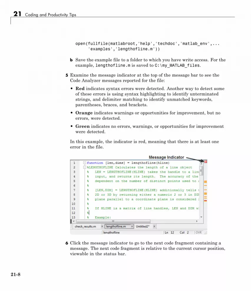
21 Coding and Productivity Tips
open(fullfile(matlabroot,'help','techdoc','matlab_env',...'examples','lengthofline.m'))
b Save the example file to a folder to which you have write access. For theexample, lengthofline.m is saved to C:\my_MATLAB_files.
5 Examine the message indicator at the top of the message bar to see theCode Analyzer messages reported for the file:
• Red indicates syntax errors were detected. Another way to detect someof these errors is using syntax highlighting to identify unterminatedstrings, and delimiter matching to identify unmatched keywords,parentheses, braces, and brackets.
• Orange indicates warnings or opportunities for improvement, but noerrors, were detected.
• Green indicates no errors, warnings, or opportunities for improvementwere detected.
In this example, the indicator is red, meaning that there is at least oneerror in the file.
6 Click the message indicator to go to the next code fragment containing amessage. The next code fragment is relative to the current cursor position,viewable in the status bar.
21-8

Check Code for Errors and Warnings
In the lengthofline example, the first message is at line 22. The cursormoves to the beginning of line 22.
The code fragment for which there is a message is underlined in either redfor errors or orange for warnings and improvement opportunities.
7 View the message by moving the mouse pointer within the underlinedcode fragment.
The message opens in a tooltip and contains a Details button that providesaccess to additional information by extending the message. Not allmessages have additional information.
8 Click the Details button.
The window expands to display an explanation and user action.
9 Modify your code, if needed.
The message indicator and underlining automatically update to reflectchanges you make, even if you do not save the file.
10 On line 28, hover over prod.
The code is underlined because there is a warning message, and it ishighlighted because an automatic fix is available. When you view themessage, it provides a button to apply the automatic fix.
21-9

21 Coding and Productivity Tips
11 Fix the problem by doing one of the following:
• If you know what the fix is (from previous experience), click Fix.
• If you are unfamiliar with the fix, view, and then apply it as follows:
a Right-click the highlighted code (for a single-button mouse, pressCtrl+ click), and then view the first item in the context menu.
b Click the fix.
MATLAB automatically corrects the code.
In this example, MATLAB replaces prod(size(hline)) withnumel(hline).
12 Go to a different message by doing one of the following:
• To go to the next message, click the message indicator or the nextunderlined code fragment.
• To go to a line that a marker represents, click a red or orange line in theindicator bar .
To see the first error in lengthofline, click the first red marker in themessage bar. The cursor moves to the first suspect code fragment in line48. The Details and Fix buttons are dimmed, indicating that there is nomore information about this message and there is no automatic fix.
21-10

Check Code for Errors and Warnings
Multiple messages can represent a single problem or multiple problems.Addressing one might address all of them, or after addressing one, theother messages might change or what you need to do might becomeclearer.
13 Modify the code to address the problem noted in the message—the messageindicators update automatically.
The message suggests a delimiter imbalance on line 48. You can investigatethat as follows:
a On the Home tab, in the Environment section, click Preferences.
b Select MATLAB > Keyboard.
c Under Delimiter Matching, select Match on arrow key, and thenclick OK.
d In the Editor, move the arrow key over each of the delimiters to see ifMATLAB indicates a mismatch.
In the example, it might appear that there are no mismatcheddelimiters. However, code analysis detects the semicolon in parentheses:data{3}(;), and interprets it as the end of a statement. The messagereports that the two statements on line 48 each have a delimiterimbalance.
e In line 48, change data{3}(;) to data{3}(:).
Now, the underline no longer appears in line 48. The single changeaddresses the issues in both of the messages for line 48.
21-11

21 Coding and Productivity Tips
Because the change removed the only error in the file, the messageindicator at the top of the bar changes from red to orange, indicating thatonly warnings and potential improvements remain.
After modifying the code to address all the messages, or disabling designatedmessages, the message indicator becomes green. The example file with allmessages addressed has been saved as lengthofline2.m. Open the correctedexample file with the command:
open(fullfile(matlabroot,'help','techdoc',...'matlab_env', 'examples','lengthofline2.m'))
Create a Code Analyzer Message ReportYou can create a report of messages for an individual file, or for all files in afolder, using one of these methods:
• Run a report for an individual MATLAB code file:
1 On the Editor window, click .
2 Select Show Code Analyzer Report.
A Code Analyzer Report appears in the MATLAB Web Browser.
3 Modify your file based on the messages in the report.
4 Save the file.
5 Rerun the report to see if your changes addressed the issues noted inthe messages.
• Run a report for all files in a folder:
1 On the Current Folder browser, click .
2 Select Reports > Code Analyzer Report.
3 Modify your files based on the messages in the report.
For details, see “MATLAB Code Analyzer Report” on page 21-52.
4 Save the modified file(s).
5 Rerun the report to see if your changes addressed the issues noted inthe messages.
21-12

Check Code for Errors and Warnings
Adjust Code Analyzer Message Indicators andMessagesDepending on the stage at which you are in completing a MATLAB file, youmight want to restrict the code underlining. You can do this by using theCode Analyzer preference referred to in step 1, in “Check Code for Errors andWarnings” on page 21-7. For example, when first coding, you might prefer tounderline only errors because warnings would be distracting.
Code analysis does not provide perfect information about every situation andin some cases, you might not want to change the code based on a message. Ifyou do not want to change the code, and you do not want to see the indicatorand message for that line, suppress them. For the lengthofline example,in line 49, the first message is Terminate statement with semicolon tosuppress output (in functions). Adding a semicolon to the end of astatement suppresses output and is a common practice. Code analysis alertsyou to lines that produce output, but lack the terminating semicolon. If youwant to view output from line 49, do not add the semicolon as the messagesuggests.
There are a few different ways to suppress (turn off) the indicators forwarning and error messages:
• “Suppress an Instance of a Message in the Current File” on page 21-13
• “Suppress All Instances of a Message in the Current File” on page 21-14
• “Suppress All Instances of a Message in All Files” on page 21-15
• “Save and Reuse Code Analyzer Message Settings” on page 21-15
You cannot suppress error messages such as syntax errors. Therefore,instructions on suppressing messages do not apply to those types of messages.
Suppress an Instance of a Message in the Current FileYou can suppress a specific instance of a Code Analyzer message in thecurrent file. For example, using the code presented in “Check Code for Errorsand Warnings” on page 21-7 , follow these steps:
1 In line 49, right-click at the first underline (for a single-button mouse,press Ctrl+click).
21-13

21 Coding and Productivity Tips
2 From the context menu, select Suppress ’Terminate statement withsemicolon...’ > On This Line.
The comment %#ok<NOPRT> appears at the end of the line, which instructsMATLAB not to check for a terminating semicolon at that line. Theunderline and mark in the indicator bar for that message disappear.
3 If there are two messages on a line that you do not want to display,right-click separately at each underline and select the appropriate entryfrom the context menu.
The %#ok syntax expands. For the example, in the code presented in “CheckCode for Errors and Warnings” on page 21-7, ignoring both messages forline 49 adds %#ok<NBRAK,NOPRT>.
Even if Code Analyzer preferences are set to enable this message, thespecific instance of the message suppressed in this way does not appearbecause the %#ok takes precedence over the preference setting. If you laterdecide you want to check for a terminating semicolon at that line, deletethe %#ok<NOPRT> string from the line.
Suppress All Instances of a Message in the Current FileYou can suppress all instances of a specific Code Analyzer message in thecurrent file. For example, using the code presented in “Check Code for Errorsand Warnings” on page 21-7, follow these steps:
1 In line 49, right-click at the first underline (for a single-button mouse,press Ctrl+click).
2 From the context menu, select Suppress ’Terminate statement withsemicolon...’ > In This File.
The comment %#ok<*NOPRT> appears at the end of the line, which instructsMATLAB to not check for a terminating semicolon throughout the file. Allunderlines, as well as marks in the message indicator bar that correspondto this message disappear.
If there are two messages on a line that you do not want to display anywherein the current file, right-click separately at each underline, and then selectthe appropriate entry from the context menu. The %#ok syntax expands. For
21-14

Check Code for Errors and Warnings
the example, in the code presented in “Check Code for Errors and Warnings”on page 21-7, ignoring both messages for line 49 adds %#ok<*NBRAK,*NOPRT>.
Even if Code Analyzer preferences are set to enable this message, the messagedoes not appear because the %#ok takes precedence over the preferencesetting. If you later decide you want to check for a terminating semicolon inthe file, delete the %#ok<*NOPRT> string from the line.
Suppress All Instances of a Message in All FilesYou can disable all instances of a Code Analyzer message in all files. Forexample, using the code presented in “Check Code for Errors and Warnings”on page 21-7, follow these steps:
1 In line 49, right-click at the first underline (for a single-button mouse,press Ctrl+click).
2 From the context menu, select Suppress ’Terminate statement withsemicolon...’ > In All Files.
This modifies the Code Analyzer preference setting.
If you know which message or messages you want to suppress, you can disablethem directly using Code Analyzer preferences, as follows:
1 On the Home tab, in the Environment section, click Preferences.
2 Select MATLAB > Code Analyzer.
3 Search the messages to find the ones you want to suppress.
4 Clear the check box associated with each message you want to suppress inall files.
5 Click OK.
Save and Reuse Code Analyzer Message SettingsYou can specify that you want certain Code Analyzer messages enabledor disabled, and then save those settings to a file. When you want to usea settings file with a particular file, you select it from the Code Analyzer
21-15

21 Coding and Productivity Tips
preferences pane. That setting file remains in effect until you select anothersettings file. Typically, you change the settings file when you have a subset offiles for which you want to use a particular settings file.
Follow these steps:
1 On the Home tab, in the Environment section, click Preferences.
The Preferences dialog box opens.
2 Select MATLAB > Code Analyzer.
3 Enable or disable specific messages, or categories of messages.
4 Click the Actions button , select Save as, and then save the settingsto a txt file.
5 Click OK.
You can reuse these settings for any MATLAB file, or provide the settings fileto another user.
To use the saved settings:
1 On the Home tab, in the Environment section, click Preferences.
The Preferences dialog box opens.
2 Select MATLAB > Code Analyzer.
3 Use the Active Settings drop-down list to select Browse....
The Open dialog box appears.
4 Choose from any of your settings files.
The settings you choose are in effect for all MATLAB files until you selectanother set of Code Analyzer settings.
21-16

Check Code for Errors and Warnings
Understand Code Containing Suppressed MessagesIf you receive code that contains suppressed messages, you might want toreview those messages without the need to unsuppress them first. A messagemight be in a suppressed state for any of the following reasons:
• One or more %#ok<message-ID> directives are on a line of code that elicitsa message specified by <message-ID>.
• One or more %#ok<*message-ID> directives are in a file that elicits amessage specified by <message-ID>.
• It is cleared in the Code Analyzer preferences pane.
• It is disabled by default.
To determine the reasons why some messages are suppressed:
1 Search the file for the %#ok directive and create a list of all the messageIDs associated with that directive.
2 On the Home tab, in the Environment section, click Preferences.
The Preferences dialog box opens.
3 Select MATLAB > Code Analyzer.
4 In the search field, type msgid: followed by one of the message IDs, if any,you found in step 1.
The message list now contains only the message that corresponds tothat ID. If the message is a hyperlink, click it to see an explanation andsuggested action for the message. This can provide insight into why themessage is suppressed or disabled. The following image shows how thePreferences dialog box appears when you enter msgid:CPROP in the searchfield.
21-17

21 Coding and Productivity Tips
5 Click the button to clear the search field, and then repeat step 4 foreach message ID you found in step 1.
6 Display messages that are disabled by default and disabled in thePreferences pane by clicking the down arrow to the right of the search field.Then, click Show Disabled Messages.
7 Review the message associated with each message ID to understand why itis suppressed in the code or disabled in Preferences.
Understand the Limitations of Code AnalysisCode analysis is a valuable tool, but there are some limitations:
• Sometimes, it fails to produce Code Analyzer messages where you expectthem.
By design, code analysis attempts to minimize the number of incorrectmessages it returns, even if this behavior allows some issues to goundetected.
• Sometimes, it produces messages that do not apply to your situation.
When provided with message, click the Detail button for additionalinformation, which can help you to make this determination. Errormessages are almost always problems. However, many warnings are
21-18

Check Code for Errors and Warnings
suggestions to look at something in the code that is unusual and thereforesuspect, but might be correct in your case.
Suppress a warning message if you are certain that the message does notapply to your situation. If your reason for suppressing a message is subtleor obscure, include a comment giving the rationale. That way, those whoread your code are aware of the situation.
For details, see “Adjust Code Analyzer Message Indicators and Messages”on page 21-13.
These sections describe code analysis limitations with respect to the following:
• “Distinguish Function Names from Variable Names” on page 21-19
• “Distinguish Structures from Handle Objects” on page 21-20
• “Distinguish Built-In Functions from Overloaded Functions” on page 21-21
• “Determine the Size or Shape of Variables” on page 21-21
• “Analyze Class Definitions with Superclasses” on page 21-21
• “Analyze Class Methods” on page 21-21
Distinguish Function Names from Variable NamesCode analysis cannot always distinguish function names from variable names.For the following code, if the Code Analyzer message is enabled, code analysisreturns the message, Code Analyzer cannot determine whether xyz is avariable or a function, and assumes it is a function. Code analysiscannot make a determination because xyz has no obvious value assigned toit. However, the program might have placed the value in the workspace in away that code analysis cannot detect.
function y=foo(x)...y = xyz(x);
end
21-19

21 Coding and Productivity Tips
For example, in the following code, xyz can be a function, or can be avariable loaded from the MAT-file. Code analysis has no way of makinga determination.
function y=foo(x)load abc.maty = xyz(x);
end
Variables might also be undetected by code analysis when you use the eval,evalc, evalin, or assignin functions.
If code analysis mistakes a variable for a function, do one of the following:
• Initialize the variable so that code analysis does not treat it as a function.
• For the load function, specify the variable name explicitly in the loadcommand line. For example:
function y=foo(x)load abc.mat xyzy = xyz(x);
end
Distinguish Structures from Handle ObjectsCode analysis cannot always distinguish structures from handle objects. Inthe following code, if x is a structure, you might expect a Code Analyzermessage indicating that the code never uses the updated value of thestructure. If x is a handle object, however, then this code can be correct.
function foo(x)x.a = 3;
end
Code analysis cannot determine whether x is a structure or a handle object. Tominimize the number of incorrect messages, code analysis returns no messagefor the previous code, even though it might contain a subtle and serious bug.
21-20

Check Code for Errors and Warnings
Distinguish Built-In Functions from Overloaded FunctionsCode analysis does not use the MATLAB path information because it can bedifferent, depending on whether you are editing or running the program. Ifsome built-in functions are overloaded in a class or on the path, Code Analyzermessages might apply to the built-in function, but not to the overloadedfunction you are calling. In this case, suppress the message on the line whereit appears or suppress it for the entire file.
For information on suppressing messages, see “Adjust Code Analyzer MessageIndicators and Messages” on page 21-13.
Determine the Size or Shape of VariablesCode analysis has a limited ability to determine the type of variables andthe shape of matrices. Code analysis might produce messages that areappropriate for the most common case, such as for vectors. However, thesemessages might be inappropriate for less common cases, such as for matrices.
Analyze Class Definitions with SuperclassesBecause code analysis looks at one file at a time and does not use the path, ithas no way to analyze superclasses. Therefore, the amount of checking thatcode analysis can provide for a class definition with superclasses is limited.In general, code analysis cannot always tell whether the class is a handleclass. It makes an educated guess, but often cannot get enough information,to make a determination for certain.
Analyze Class MethodsMost class methods must contain at least one argument that is an object ofthe same class as the method. But it does not always have to be the firstargument. When it is, code analysis can determine that an argument is anobject of the class you are defining, and it can do various checks. For example,it can check that the property and method names exist and are spelledcorrectly. However, when code analysis cannot determine that an object is anargument of the class you are defining, then it cannot provide these checks.
21-21

21 Coding and Productivity Tips
Enable MATLAB Compiler Deployment MessagesYou can switch between showing or hiding Compiler deployment messageswhen you work on a file. Change the Code Analyzer preference for thismessage category. Your choice likely depends on whether you are workingon a file to be deployed. When you change the preference, it also changes thesetting in the Editor. The converse is also true—when you change the settingfrom the Editor, it effectively changes this preference. However, if the dialogbox is open at the time you modify the setting in the Editor, you will not seethe changes reflected in the Preferences dialog box . Whether you change thesetting from the Editor or from the Preferences dialog box, it applies to theEditor and to the Code Analyzer Report.
To enable MATLAB Compiler™ deployment messages:
1 On the Home tab, in the Environment section, click Preferences.
The Preferences dialog box opens.
2 Select MATLAB > Code Analyzer.
3 Click the down arrow next to the search field, and then select ShowMessages in Category > MATLAB Compiler (Deployment) Messages.
4 Click the Enable Category button.
5 Clear individual messages that you do not want to display for your code(if any).
6 Decide if you want to save these settings, so you can reuse them next timeyou work on a file to be deployed.
The settings txt file, which you can create as described in “Save and ReuseCode Analyzer Message Settings” on page 21-15, includes the status of thissetting.
21-22

Improve Code Readability
Improve Code Readability
In this section...
“Indenting Code” on page 21-23
“Right-Side Text Limit Indicator” on page 21-25
“Code Folding — Expand and Collapse Code Constructs” on page 21-25
Indenting CodeIndenting code makes reading statements such as while loops easier. To setand apply indenting preferences to code in the Editor:
1 On the Home tab, in the Environment section, click Preferences.
The Preferences dialog box opens.
2 Select MATLAB > Editor/Debugger > Language.
3 Choose a computer language from the Language drop-down list.
4 In the Indenting section, select or clear Apply smart indenting whiletyping, depending on whether you want indenting applied automatically,as you type.
If you clear this option, you can manually apply indenting by selectingthe lines in the Editor to indent, right-clicking, and then selecting SmartIndent from the context menu.
5 Do one of the following:
• If you chose any language other thanMATLAB in step 2, click OK.
• If you choseMATLAB in step 2, select a Function indenting format,and then click OK. Function indent formats are:
– Classic — The Editor aligns the function code with the functiondeclaration.
– Indent nested functions — The Editor indents the function codewithin a nested function.
21-23

21 Coding and Productivity Tips
– Indent all functions — The Editor indents the function code forboth main and nested functions.
The following image illustrates the function indenting formats.
Note Indenting preferences are not available for TLC, VHDL, or Verilog.
Regardless of whether you apply indenting automatically or manually, you canmove selected lines further to the left or right, by doing one of the following:
• On the Editor tab, in the Edit section, click , , or .
• Pressing the Tab key or the Shift+Tab key, respectively.
This works differently if you select the Editor/Debugger Tab preference forEmacs-style Tab key smart indenting—when you position the cursor in
21-24

Improve Code Readability
any line or select a group of lines and press Tab, the lines indent accordingto smart indenting practices.
Right-Side Text Limit IndicatorBy default, a light gray vertical line (rule) appears at column 75 in the Editor,indicating where a line exceeds 75 characters. You can set this text limitindicator to another value, which is useful, for example, if you want to viewthe code in another text editor that has a different line width limit.
To hide, or change the appearance of the vertical line:
1 On the Home tab, in the Environment section, click Preferences.
The Preferences dialog box opens.
2 Select MATLAB > Editor/Debugger > Display.
3 Adjust the settings in the Right-hand text limit section.
Note This limit is a visual cue only and does not prevent text fromexceeding the limit. To wrap comment text at a specified column numberautomatically, adjust the settings in the Comment formatting section underMATLAB > Editor/Debugger > Language in the Preferences dialog box.
Code Folding — Expand and Collapse Code ConstructsCode folding is the ability to expand and collapse certain MATLABprogramming constructs. This improves readability when a file containsnumerous functions or other blocks of code that you want to hide when youare not currently working with that part of the file. MATLAB programmingconstructs include:
• Code sections for running and publishing code
• Class code
• For and parfor blocks
• Function and class help
21-25

21 Coding and Productivity Tips
• Function code
To see the entire list of constructs, select Editor/Debugger > Code Foldingin the Preferences dialog box.
To expand or collapse code, click the plus or minus sign that appears tothe left of the construct in the Editor.
To expand or collapse all of the code in a file, place your cursor anywherewithin the file, right-click, and then select Code Folding > Expand All orCode Folding > Fold All from the context menu.
View Folded Code in a TooltipYou can view code that is currently folded by positioning the pointer over its
ellipsis . The code appears in a tooltip.
The following image shows the tooltip that appears when you place the pointerover the ellipsis on line 23 of lenghtofline.m when a for loop is folded.
Print Files with Collapsed CodeIf you print a file with one or more collapsed constructs, those constructs areexpanded in the printed version of the file.
Code Folding Behavior for Functions that Have No Explicit EndStatementIf you enable code folding for functions and a function in your code does notend with an explicit end statement, you see the following behavior:
21-26

Improve Code Readability
• If a line containing only comments appears at the end of such a function,then the Editor does not include that line when folding the function.MATLAB does not include trailing white space and comments in a functiondefinition that has no explicit end statement.
Code Folding Enabled for Function Code Only on page 21-27 illustrates thisbehavior. Line 13 is excluded from the fold for the foo function.
• If a fold for a code section overlaps the function code, then the Editor doesnot show the fold for the overlapping section.
The three figures that follow illustrate this behavior. The first two figures,Code Folding Enabled for Function Code Only on page 21-27 and CodeFolding Enabled for Cells Only on page 21-28 illustrate how the code foldingappears when you enable it for function code only and then section only,respectively. The last figure, Code Folding Enabled for Both Functions andCells on page 21-29, illustrates the effects when code folding is enabledfor both. Because the fold for section 3 (lines 11–13) overlaps the fold forfunction foo (lines 4–12), the Editor does not display the fold for section 3.
Code Folding Enabled for Function Code Only
21-27

21 Coding and Productivity Tips
Code Folding Enabled for Cells Only
21-28

Improve Code Readability
Code Folding Enabled for Both Functions and Cells
21-29

21 Coding and Productivity Tips
Find and Replace Text in Files
In this section...
“Find Any Text in the Current File” on page 21-30
“Find and Replace Functions or Variables in the Current File” on page 21-30
“Automatically Rename All Functions or Variables in a File” on page 21-32
“Find and Replace Any Text” on page 21-34
“Find Text in Multiple File Names or Files” on page 21-34
“Function Alternative for Finding Text” on page 21-34
“Perform an Incremental Search in the Editor” on page 21-34
Find Any Text in the Current File
1 Within the current file, select the text you want to find.
2 On the Editor tab, in the Navigate section, click Find , and thenselect Find....
A Find & Replace dialog box opens.
3 Click Find Next to continue finding more occurrences of the text.
To find the previous occurrence of selected text (find backwards) in thecurrent file, click Find Previous on the Find & Replace dialog box.
Find and Replace Functions or Variables in theCurrent FileTo search for references to a particular function or variable, use the automatichighlighting feature for variables and functions. This feature is more efficientthan using the text finding tools. Function and variable highlighting indicatesonly references to a particular function or variable, not other occurrences.For instance, it does not find instances of the function or variable name incomments. Furthermore, variable highlighting only includes references to
21-30

Find and Replace Text in Files
the same variable. That is, if two variables use the same name, but are indifferent scopes, highlighting one does not cause the other to highlight.
1 On the Home tab, in the Environment section, click Preferences.
The Preferences dialog box opens.
2 Select MATLAB > Colors > Programming Tools.
3 Under Variable and function colors, select Automatically highlight,deselect Variables with shared scope, and then click Apply.
4 In a file open in the Editor, click an instance of the variable you want tofind throughout the file.
MATLAB indicates all occurrences of that variable within the file by:
• Highlighting them in teal blue (by default) throughout the file
• Adding a marker for each in the indicator bar
If a code analyzer indicator and a variable indicator appear on the sameline in a file, the marker for the variable takes precedence.
5 Hover over a marker in the indicator bar to see the line it represents.
6 Click a marker in the indicator bar to navigate to that occurrence of thevariable.
Replace an instance of a function or variable by editing the occurrence at aline to which you have navigated.
The following image shows an example of how the Editor looks with variablehighlighting enabled. In this image, the variable i appears highlighted in skyblue, and the indicator bar contains three variable markers.
21-31

21 Coding and Productivity Tips
Automatically Rename All Functions or Variables ina FileTo help prevent typographical errors, MATLAB provides a feature that helpsrename multiple references to a function or variable within a file when youmanually change any of the following:
Function or Variable Renamed Example
Function name in a functiondeclaration
Rename foo in: function foo(m)
Input or output variable name in afunction declaration
Rename y or m in: function y =foo(m)
Variable name on the left side ofassignment statement
Rename y in: y = 1
As you rename such a function or variable, a tooltip opens if there is morethan one reference to that variable or function in the file. The tooltip indicates
21-32

Find and Replace Text in Files
that MATLAB will rename all instances of the function or variable in thefile when you press Shift + Enter.
Typically, multiple references to a function appear when you use nestedfunctions or local functions.
Note MATLAB does not prompt you when you change:
• The name of a global variable.
• The function input and output arguments, varargin and varargout.
To undo automatic name changes, click once.
By default, this feature is enabled. To disable it:
1 On the Home tab, in the Environment section, click Preferences.
21-33

21 Coding and Productivity Tips
The Preferences dialog box opens.
2 Select MATLAB > Editor/Debugger > Language.
3 In the Language field, select MATLAB.
4 Clear Enable automatic variable and function renaming.
Find and Replace Any TextYou can search for, and optionally replace specified text within a file. Onthe Editor tab, in the Navigate section, click Find to open and use theFind & Replace dialog box.
Find Text in Multiple File Names or FilesYou can find folders and file names that include specified text, or whosecontents contain specified text. On the Editor tab, in the File section, click
Find Files to open the Find Files dialog box. For details, see “Find Filesand Folders”.
Function Alternative for Finding TextUse lookfor to search for the specified text in the first line of help for all fileswith the .m extension on the search path.
Perform an Incremental Search in the EditorWhen you perform an incremental search, the cursor moves to the next orprevious occurrence of the specified text in the current file. It is similar tothe Emacs search feature. In the Editor, incremental search uses the samecontrols as incremental search in the Command Window. For details, see“Incremental Search Using Keyboard Shortcuts”.
21-34

Go To Location in File
Go To Location in File
In this section...
“Navigate to a Specific Location” on page 21-35
“Set Bookmarks” on page 21-39
“Navigate Backward and Forward in Files” on page 21-39
“Open a File or Variable from Within a File” on page 21-40
Navigate to a Specific LocationThis table summarizes the steps for navigating to a specific location withina file open in the Editor. In some cases, different sets of steps are availablefor navigating to a particular location. Choose the set that works best withyour workflow.
Go To Steps Notes
Line Number1 On the Editor tab, in theNavigate section, click Go To
2 Select Go to Line...
3 Specify the line to which you wantto navigate.
None
1 On the Editor tab, in theNavigate section, click Go To.
2 Under the heading Function,select the local function or nestedfunction to which you want tonavigate.
Includes local functions and nestedfunctions
For both class and function files,the functions list in alphabeticalorder—except that in function files,the name of the main functionalways appears at the top of the list.
Functiondefinition
21-35

21 Coding and Productivity Tips
Go To Steps Notes
1 In the Current Folder browser,click the name of the file open inthe Editor.
2 Click the up arrow at thebottom of Current Folder browserto open the detail panel.
3 In the detail panel, double-clickthe function icon correspondingto the title of the function or localfunction to which you want tonavigate.
Functions list in order of appearancewithin your file.
21-36

Go To Location in File
Go To Steps Notes
Functionreference 1 Click in any instance of the
function name.
2 Press Alt+Up or Alt+Down to goto the next or previous functionreference, respectively.
Variablereference 1 Click in any instance of the
variable name.
2 Press Alt+Up or Alt+Down to goto the next or previous variablereference, respectively.
Code AnalyzerMessage
Press Alt+Up or Alt+Down to go tothe next or previous code analyzermessage, respectively.
Alt+Up and Alt+Down are thedefault keyboard shortcuts forthe actions Go to PreviousUnderline or Highlight and Goto Next Underline or Highlight,respectively.
For more information, see “DefineKeyboard Shortcuts”.
1 On the Editor tab, in theNavigate section, click Go To.
2 Under Sections, select the titleof the code section to which youwant to navigate.
Code Section 1 In the Current Folder browser,click the name of the file that isopen in the Editor.
2 Click the up arrow at thebottom of Current Folder browserto open the detail panel.
3 In the detail panel, double-clickthe section icon corresponding
For more information, see “DivideYour File into Code Sections” onpage 16-6
21-37

21 Coding and Productivity Tips
Go To Steps Notes
to the title of the section to whichyou want to navigate.
Property1 In the Current Folder browser,click the name of the file that isopen in the Editor.
2 Click the up arrow at thebottom of Current Folder browserto open the detail panel.
3 On the detail panel, double-clickthe property icon correspondingto the name of the property towhich you want to navigate.
For more information, see “How toUse Properties”
Method1 In the Current Folder browser,click the name of the file that isopen in the Editor.
2 Click the up arrow at thebottom of Current Folder browserto open the detail panel.
3 In the detail panel, double-clickthe icon corresponding to thename of the method to which youwant to navigate.
For more information, see “How toUse Methods”
Bookmark1 On the Editor tab, in theNavigate section, click Go To.
2 Under Bookmarks, select thebookmark to which you want tonavigate.
For information on setting andclearing bookmarks, see “SetBookmarks” on page 21-39.
21-38

Go To Location in File
Set BookmarksYou can set a bookmark at any line in a file in the Editor so you can quicklynavigate to the bookmarked line. This is particularly useful in long files. Forexample, suppose while working on a line, you want to look at another part ofthe file, and then return. Set a bookmark at the current line, go to the otherpart of the file, and then use the bookmark to return.
To set a bookmark:
1 Position the cursor anywhere on the line.
2 On the Editor tab, in the Navigate section, click Go To .
3 Under Bookmarks, select Set/Clear
A bookmark icon appears to the left of the line.
To clear a bookmark, position the cursor anywhere on the line. Click GoTo and select Set/Clear under Bookmarks.
MATLAB does not maintain bookmarks after you close a file.
Navigate Backward and Forward in FilesTo access lines in a file in the same sequence that you previously navigated oredited them, use and
Interrupting the Sequence of Go Back and Go ForwardThe back and forward sequence is interrupted if you:
1 Click .
2 Click .
3 Edit a line or navigate to another line using the list of features described in“Navigate to a Specific Location” on page 21-35.
You can still go to the lines preceding the interruption point in the sequence,but you cannot go to any lines after that point. Any lines you edit or navigate
21-39

21 Coding and Productivity Tips
to after interrupting the sequence are added to the sequence after theinterruption point.
For example:
1 Open a file.
2 Edit line 2, line 4, and line 6.
3 Click to return to line 4, and then to return to line 2.
4 Click to return to lines 4 and 6.
5 Click to return to line 1.
6 Edit at 3.
This interrupts the sequence. You can no longer use to return to lines 4and 6. You can, however, click to return to line 1.
Open a File or Variable from Within a FileYou can open a function, file, variable, or Simulink model from within a file inthe Editor. Position the cursor on the name, and then right-click and selectOpen selection from the context menu. Based on what the selection is, theEditor performs a different action, as described in this table.
Item Action
Local function Navigates to the local function within the currentfile, if that file is a MATLAB code file. If no functionby that name exists in the current file, the Editorruns the open function on the selection, which opensthe selection in the appropriate tool.
Text file Opens in the Editor.
Figure file (.fig) Opens in a figure window.
21-40

Go To Location in File
Item Action
MATLAB variablethat is in the currentworkspace
Opens in the Variables Editor.
Model Opens in Simulink.
Other If the selection is some other type, Open selectionlooks for a matching file in a private folder in thecurrent folder and performs the appropriate action.
21-41

21 Coding and Productivity Tips
Display Two Parts of a File SimultaneouslyYou can simultaneously display two different parts of a file in the Editor bysplitting the screen display, as shown in the image that follows. This featuremakes it easy to compare different lines in a file or to copy and paste fromone part of a file to another.
See also “Document Layout” for instructions on displaying multiple documentssimultaneously.
The following table describes the various ways you can split the Editor andmanipulate the split-screen views. When you open a document, it opensunsplit, regardless of its split status it had when you closed it.
21-42

Display Two Parts of a File Simultaneously
Operation Instructions
Split the screenhorizontally.
Do either of the following:
• Right-click and, select SplitScreen > Top/Bottom from the Context Menu.
• If there is a vertical scroll bar, as shown in theillustration that follows, drag the splitter bardown.
Split the screenvertically.
Do either of the following:
• From the Context Menu, select SplitScreen > Left/Right.
• If there is a horizontal scroll bar, as shown inthe illustration that follows, drag the splitter barfrom the left of the scroll bar.
Specify the activeview.
Do either of the following:
• From the Context Menu, select SplitScreen > Switch Focus.
• Click in the view you want to make active.
Updates you make to the document in the activeview are also visible in the other view.
Remove the splitter Do one of the following:
• Double-click the splitter.
• From the Context Menu, Split Screen > Off.
21-43

21 Coding and Productivity Tips
21-44

Add Reminders to Files
Add Reminders to FilesAnnotating a file makes it easier to find areas of your code that you intend toimprove, complete, or update later.
To annotate a file, add comments with the text TODO, FIXME, or a string ofyour choosing.
After you annotate several files, run the TODO/FIXME Report, to identify allthe MATLAB code files within a given folder that you have annotated.
This sample TODO/FIXME Report shows files containing the strings TODO,FIXME, and NOTE. The search is case insensitive.
Working with TODO/FIXME Reports
1 Use the Current Folder browser to navigate to the folder containing thefiles for which you want to produce a TODO/FIXME report.
21-45

21 Coding and Productivity Tips
Note You cannot run reports when the path is a UNC (Universal NamingConvention) path; that is, a path that starts with \\. Instead, use an actualhard drive on your system, or a mapped network drive.
2 On the Current Folder browser, click , and then selectReports > TODO/FIXME Report.
The TODO/FIXME Report opens in the MATLAB Web Browser.
3 In the TODO/FIXME Report window, select one or more of the following tospecify the lines that you want the report to include:
• TODO
• FIXME
• The text field check box
You can then enter any text string in this field, including a regularexpression. For example, you can enter NOTE, tbd, or re.*check.
4 Run the report on the files in the current folder, by clicking Rerun ThisReport.
The window refreshes and lists all lines in the MATLAB files within thespecified folder that contain the strings you selected in step 1. Matchesare not case sensitive.
If you want to run the report on a folder other than the one currentlyspecified in the report window, change the current folder. Then, click RunReport on Current Folder.
To open a file in the Editor at a specific line, click the line number in thereport. Then you can change the file, as needed.
Suppose you have a file, area.m, in the current folder. The code for area.mappears in the image that follows.
21-46

Add Reminders to Files
When you run the TODO/FIXME report on the folder containing area.m,with the TODO and FIXME strings selected and the string NOTE specified andselected, the report lists:
9 and rectangle. (todo)14 Fixme: Is the area of hemisphere as below?17 fIXME21 NOTE: Find out from the manager if we need to include
Notice the report includes the following:
• Line 9 as a match for the TODO string. The report includes lines that have aselected string regardless of its placement within a comment.
• Lines 14 and 17 as a match for the FIXME string. The report matchesselected strings in the file regardless of their casing.
21-47

21 Coding and Productivity Tips
• Line 21 as a match for the NOTE string. The report includes lines that havea string specified in the text field, assuming that you select the text field.
21-48

Colors in the MATLAB® Editor
Colors in the MATLAB EditorColors in the Editor help you to read code, identify code elements, andevaluate sections of code. To find out why certain portions of your code appearin color, how to change the color, or learn more about the features highlightedin color, see the table that follows.
Sample (Using Default Colors) What the Color Indicates
Different types of language elements, suchas keywords, comments, and strings appearin different colors. This is called syntaxhighlighting.
See also, “Syntax Highlighting”
Teal blue characters indicate variables withshared scope
Sky blue shading indicates function or variablenames that match the name in which thecursor is currently placed.
See also, “Check Variable Scope in Editor” onpage 17-15.
Orange and red wavy underlines indicatewarning and error conditions, respectively.
Orange shading indicates coding issues thatMATLAB can correct for you.
See also, “Check Code for Errors andWarnings”on page 21-7
21-49

21 Coding and Productivity Tips
Sample (Using Default Colors) What the Color Indicates
Yellow highlighting indicates code sections,which:
• Help you visually identify subsections ofcode
• Enable you to publish and run subsectionsof code.
See also, “Divide Your File into Code Sections”on page 16-6
Red dots represent breakpoints, which you usein debugging.
If you attempt to run your code, MATLAB stopsat the first breakpoint it encounters.
See also, “Debugging Process and Features” onpage 19-2
A gray vertical line indicates the location of aparticular column in the Editor that you canuse to limit line widths.
The Editor does not enforce the limit.
See also, “Right-Side Text Limit Indicator” onpage 21-25
21-50

Code Contains %#ok — What Does That Mean?
Code Contains %#ok — What Does That Mean?If code contains the string %#ok at the end of a line of code, it indicates thatone or more Code Analyzer messages is suppressed. For more information,see “Understand Code Containing Suppressed Messages” on page 21-17.
21-51

21 Coding and Productivity Tips
MATLAB Code Analyzer Report
In this section...
“Running the Code Analyzer Report” on page 21-52
“Changing Code Based on Code Analyzer Messages” on page 21-54
“Other Ways to Access Code Analyzer Messages” on page 21-55
Running the Code Analyzer ReportThe Code Analyzer Report displays potential errors and problems, as well asopportunities for improvement in your code through messages. For example,a common message indicates that a variable foo might be unused.
To run the Code Analyzer Report:
1 In the Current Folder browser, navigate to the folder that contains thefiles you want to check. To use the example shown in this documentation,lengthofline.m, you can change the current folder by running
cd(fullfile(matlabroot,'help','techdoc','matlab_env','examples'))
2 If you plan to modify the example, save the file to a folder for which youhave write access. Then, make that folder the current MATLAB folder. Thisexample saves the file in C:\my_MATLAB_files.
3 In the Current Folder browser, click , and then select Reports > CodeAnalyzer Report.
The report displays in the MATLAB Web Browser, showing those filesidentified as having potential problems or opportunities for improvement.
21-52

MATLAB® Code Analyzer Report
4 For each message in the report, review the suggestion and your code. Clickthe line number to open the file in the Editor at that line, and change the filebased on the message. Use the following general advice:
• If you are unsure what a message means or what to change in the code,click the link in the message if one appears. For details, see “Check Codefor Errors and Warnings” on page 21-7.
• If the message does not contain a link, and you are unsure what a messagemeans or what to do, search for related topics in the Help browser. Forexamples of messages and what to do about them, including specificchanges to make for the example, lengthofline.m, see “Changing CodeBased on Code Analyzer Messages” on page 21-54.
• The messages do not provide perfect information about every situationand in some cases, you might not want to change anything based on themessage. For details, see “Understand the Limitations of Code Analysis”on page 21-18.
• If there are certain messages or types of messages you do not want to see,you can suppress them. For details, see “Adjust Code Analyzer MessageIndicators and Messages” on page 21-13.
21-53
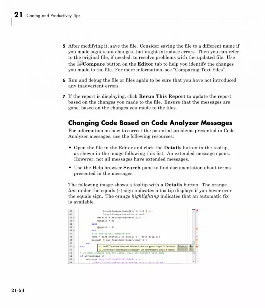
21 Coding and Productivity Tips
5 After modifying it, save the file. Consider saving the file to a different name ifyou made significant changes that might introduce errors. Then you can referto the original file, if needed, to resolve problems with the updated file. Usethe Compare button on the Editor tab to help you identify the changesyou made to the file. For more information, see “Comparing Text Files”.
6 Run and debug the file or files again to be sure that you have not introducedany inadvertent errors.
7 If the report is displaying, click Rerun This Report to update the reportbased on the changes you made to the file. Ensure that the messages aregone, based on the changes you made to the files.
Changing Code Based on Code Analyzer MessagesFor information on how to correct the potential problems presented in CodeAnalyzer messages, use the following resources:
• Open the file in the Editor and click the Details button in the tooltip,as shown in the image following this list. An extended message opens.However, not all messages have extended messages.
• Use the Help browser Search pane to find documentation about termspresented in the messages.
The following image shows a tooltip with a Details button. The orangeline under the equals (=) sign indicates a tooltip displays if you hover overthe equals sign. The orange highlighting indicates that an automatic fixis available.
21-54

MATLAB® Code Analyzer Report
Other Ways to Access Code Analyzer MessagesYou can get Code Analyzer messages using any of the following methods.Each provides the same messages, but in a different format:
• Access the Code Analyzer Report for a file from the Profiler detail report.
• Run the checkcode function, which analyzes the specified file and displaysmessages in the Command Window.
• Run the mlintrpt function, which runs checkcode and displays themessages in the Web Browser.
• Use automatic code checking while you work on a file in the Editor. See“Automatically Check Code in the Editor — Code Analyzer” on page 21-7.
21-55

21 Coding and Productivity Tips
Change Default Editor
In this section...
“Set Default Editor” on page 21-56
“Set Default Editor in '-nodisplay' mode” on page 21-56
Set Default EditorTo specify the default editor for MATLAB:
1 On the Home tab, in the Environment section, click Preferences.The Preferences dialog box opens.
2 Select the MATLAB > Editor/Debugger node on the left pane.
3 In the Editor pane, click Text editor and specify a default text editor.
Set Default Editor in '-nodisplay' modeIf you invoke the edit command while running MATLAB with the-nodisplay option, choose an appropriate text-based editor instead of thedefault editor specified in the Preferences dialog box. This is done differentlydepending on your platform.
Mac PlatformsWhen running MATLAB with the -nodisplay startup option, edit opens theeditor specified in the EDITOR environment variable.
To display the current value of $EDITOR in MATLAB, execute the command:
!printenv EDITOR
UNIX PlatformsWhen runningMATLABwith the -nodisplay option (or without the DISPLAYenvironment variable set) on UNIX platforms, you can find the default editordefined for your system in matlabroot/X11/app-defaults/Matlab.
21-56

Change Default Editor
You can specify the default editor or editor options by adding the followingline to your own.Xdefaults file, located in ~home:
matlab*externalEditorCommand: $EDITOR -option $FILE
where
• $EDITOR is the name of your default editor, for example, emacs. Leavingthe environment variable EDITOR as $EDITOR instruct MATLAB to useyour default system editor.
• -option is a valid option flag you can include for the specified editor.
• $FILE means the file name you type with the edit command opens in thespecified editor.
After adding the line to your.Xdefaults file, run the following before startingMATLAB:
xrdb -merge ~home/.Xdefaults
For example, this code opens foo in the emacs editor:
emacs foo
21-57

21 Coding and Productivity Tips
21-58

22
Programming Utilities
• “Identify Program Dependencies” on page 22-2
• “Protect Your Source Code” on page 22-9
• “Create Hyperlinks that Run Functions” on page 22-12

22 Programming Utilities
Identify Program DependenciesIf you need to know what other functions and scripts your program isdependent upon, use one of the techniques described below.
In this section...
“Simple Display of Program File Dependencies” on page 22-2
“Detailed Display of Program File Dependencies” on page 22-2
“Dependencies Within a Folder” on page 22-3
Simple Display of Program File DependenciesFor a simple display of all program files referenced by a particular function,follow these steps:
1 Type clear functions to clear all functions from memory (see Note below).
Note clear functions does not clear functions locked by mlock. If youhave locked functions (which you can check using inmem) unlock them withmunlock, and then repeat step 1.
2 Execute the function you want to check. Note that the function argumentsyou choose to use in this step are important, because you can get differentresults when calling the same function with different arguments.
3 Type inmem to display all program files that were used when the function ran.If you want to see what MEX-files were used as well, specify an additionaloutput:
[mfiles, mexfiles] = inmem
Detailed Display of Program File DependenciesFor a more detailed display of dependent function information, use thematlab.codetools.requiredFilesAndProducts function. In addition toprogram files, matlab.codetools.requiredFilesAndProducts shows which
22-2

Identify Program Dependencies
MathWorks products a particular function depends on. If you have a function,myFun, that calls to the edge function in the Image Processing Toolbox™:
[fList,pList] = matlab.codetools.requiredFilesAndProducts('myFun.m');fList
fList =
'C:\work\myFun.m'
The only required program file, is the function file itself, myFun.
{pList.Name}'
ans =
'MATLAB''Image Processing Toolbox'
The file, myFun.m, requires both MATLAB and the Image Processing Toolbox.
Dependencies Within a FolderThe Dependency Report shows dependencies among MATLAB code files in afolder. Use this report to determine:
• Which files in the folder are required by other files in the folder
• If any files in the current folder will fail if you delete a file
• If any called files are missing from the current folder
The report does not list:
• Files in the toolbox/matlab folder because every MATLAB user has thosefiles.
Therefore, if you use a function file that shadows a built-in function file,MATLAB excludes both files from the list.
• Files called from anonymous functions.
• The superclass for a class file.
22-3

22 Programming Utilities
• Files called from eval, evalc, run, load, function handles, and callbacks.
MATLAB does not resolve these files until run time, and therefore theDependency Report cannot discover them.
• Some method files.
The Dependency Report finds class constructors that you call in a MATLABfile. However, any methods you execute on the resulting object areunknown to the report. These methods can exist in the classdef file, asseparate method files, or files belonging to superclass or superclasses of amethod file.
To provide meaningful results, the Dependency Report requires the following:
• The search path when you run the report is the same as when you run thefiles in the folder. (That is, the current folder is at the top of the searchpath.)
• The files in the folder for which you are running the report do not changethe search path or otherwise manipulate it.
• The files in the folder do not load variables, or otherwise create nameclashes that result in different program elements with the same name.
Note Do not use the Dependency Report to determine which MATLABcode files someone else needs to run a particular file. Instead use thematlab.codetools.requiredFilesAndProducts function.
Creating Dependency Reports
1 Use the Current Folder pane to navigate to the folder containing the filesfor which you want to produce a Dependency Report.
Note You cannot run reports when the path is a UNC (Universal NamingConvention) path; that is, a path that starts with \\. Instead, use an actualhard drive on your system, or a mapped network drive.
22-4

Identify Program Dependencies
2 On the Current Folder pane, click , and then selectReports > Dependency Report.
The Dependency Report opens in the MATLAB Web Browser.
3 If you want, select one or more options within the report, as follows:
• To see a list of all MATLAB code files (children) called by each file in thefolder (parent), select Show child functions.
The report indicates where each child function resides, for example, ina specified toolbox. If the report specifies that the location of a childfunction is unknown, it can be because:
– The child function is not on the search path.
– The child function is not in the current folder.
– The file was moved or deleted.
• To list the files that call each MATLAB code file, select Show parentfunctions.
The report limits the parent (calling) functions to functions in thecurrent folder.
• To include local functions in the report, select Show subfunctions.The report lists local functions directly after the main function andhighlights them in gray.
4 Click Run Report on Current Folder.
Reading and Working with Dependency ReportsThe following image shows a Dependency Report. It indicates that chirpy.mcalls two files in Signal Processing Toolbox™ and one in Image ProcessingToolbox. It also shows that go.m calls mobius.m, which is in the current folder.
22-5

22 Programming Utilities
22-6

Identify Program Dependencies
The Dependency Report includes the following:
• MATLAB File List
The list of files in the folder on which you ran the Dependency Report.Click a link in this column to open the file in the Editor.
• Children
The function or functions called by the MATLAB file.
Click a link in this column to open the MATLAB file listed in the same row,and go to the first reference to the called function. For instance, supposeyour Dependency Report appears as shown in the previous image. Clicking\images\images\erode.m opens chirpy.m and places the cursor at thefirst line that references erode. In other words, it does not open erode.m.
• Multiple class methods
Because the report is a static analysis, it cannot determine run-timedata types and, therefore, cannot identify the particular class methodsrequired by a file. If multiple class methods match a referenced method,the Dependency Report inserts a question mark link next to the file name.The question mark appears in the following image.
Click the question mark link to list the class methods with the specifiedname that MATLAB might use. MATLAB lists almost all the methodfiles on the search path that match the specified method file (in this case,freqresp.m). Do not be concerned if the list includes methods of classesand MATLAB built-in functions that are unfamiliar to you.
It is not necessary for you to determine which file MATLAB will use.MATLAB determines which method to use depending on the object that theprogram calls at run time.
22-7

22 Programming Utilities
The following image shows the contents of the right side of the WebBrowser after you click the question mark link.
22-8

Protect Your Source Code
Protect Your Source CodeAlthough MATLAB source (.m) code is executable by itself, the contentsof MATLAB source files are easily accessed, revealing design andimplementation details. If you do not want to distribute your proprietaryapplication code in this format, you can use one of these options instead:
• Deploy as P-code — Convert some or all of your source code files to acontent-obscured form called a P-code file (from its .p file extension), anddistribute your application code in this format. When MATLAB P-codesa file, the file is obfuscated not encrypted. While the content in a .p fileis difficult to understand, it should not be considered secure. It is notrecommended that you P-code files to protect your intellectual property.
• Compile into binary format — Compile your source code files using theMATLAB Compiler to produce a standalone application. Distribute thelatter to end users of your application.
Building a Content Obscured Format with P-CodeA P-code file behaves the same as the MATLAB source from which it wasproduced. The P-code file also runs at the same speed as the source file. P-codefiles are purposely obfuscated. They are not encrypted. While the content in a.p file is difficult to understand, it should not be considered secure. It is notrecommended that you P-code files to protect your intellectual property.
Note Because users of P-code files cannot view the MATLAB code, considerproviding diagnostics to enable a user to proceed in the event of an error.
Building the P-Code FileTo generate a P-code file, enter the following command in the MATLABCommand Window:
pcode file1 file2, ...
The command produces the files, file1.p, file2.p, and so on. To convert all.m source files residing in your current folder to P-code files, use the command:
22-9

22 Programming Utilities
pcode *.m
See the pcode function reference page for a description of all syntaxes forgenerating P-code files.
Invoking the P-Code FileYou invoke the resulting P-code file in the same way you invoke the MATLAB.m source file from which it was derived. For example, to invoke file myfun.p,type
[out, out2, ...] = myfun(in1, in2, ...);
To invoke script myscript.p, type
myscript;
When you call a P-code file, MATLAB gives it execution precedence over itscorresponding .m source file. This is true even if you happen to change thesource code at some point after generating the P-code file. Remember toremove the .m source file before distributing your code.
Running Older P-Code Files on Later Versions of MATLABP-code files are designed to be independent of the release under which theywere created and the release in which they are used (backward and forwardcompatibility). New and deprecated MATLAB features can be a problem, butit is the same problem that would exist if you used the original MATLABinput file. To fix errors of this kind in a P-code file, fix the correspondingMATLAB input file and create a new P-code file.
P-code files built using MATLAB Version 7.4 and earlier have a differentformat than those built with more recent versions of MATLAB. You still canuse these older P-code files when you run MATLAB 7.4 and later, but thiscapability could be removed in a future release. MathWorks recommends thatyou rebuild any P-code files that were built with MATLAB 7.4 or earlier usinga more recent version of MATLAB, and then redistribute them as necessary.
22-10

Protect Your Source Code
Building a Standalone ExecutableAnother way to protect your source code is to build it into a standaloneexecutable and distribute the executable, along with any other necessaryfiles, to external customers. You must have the MATLAB Compiler and asupported C or C++ compiler installed to prepare files for deployment. Theend user, however, does not need MATLAB.
To build a standalone application for your MATLAB application, develop anddebug your application following the usual procedure for MATLAB programfiles. Then, generate the executable file or files following the instructions in“Steps by the Developer to Deploy to End Users” in the MATLAB Compilerdocumentation.
22-11

22 Programming Utilities
Create Hyperlinks that Run FunctionsThe special keyword matlab: lets you embed commands in other functions.Most commonly, the functions that contain it display hyperlinks, whichexecute the commands when you click the hyperlink text. Functions thatsupport matlab: syntax include disp, error, fprintf, help, and warning.
Use matlab: syntax to create a hyperlink in the Command Window that runsone or more functions. For example, you can use disp to display the wordHypotenuse as an executable hyperlink as follows:
disp('<a href="matlab:a=3; b=4;c=hypot(a,b)">Hypotenuse</a>')
Clicking the hyperlink executes the three commands following matlab:,resulting in
c =5
Executing the link creates or redefines the variables a, b, and c in the baseworkspace.
The argument to disp is an <a href> HTML hyperlink. Include the fullhypertext string, from '<a href= to </a>' within a single line, that is, do notcontinue a long string on a new line. No spaces are allowed after the opening< and before the closing >. A single space is required between a and href.
You cannot directly execute matlab: syntax. That is, if you type
matlab:a=3; b=4;c=hypot(a,b)
you receive an error, because MATLAB interprets the colon as an arrayoperator in an illegal context:
??? matlab:a=3; b=4;c=hypot(a,b)|
Error: The expression to the left of the equals signis not a valid target for an assignment.
22-12

Create Hyperlinks that Run Functions
You do not need to use matlab: to display a live hyperlink to the Web. Forexample, if you want to link to an external Web page, you can use disp, asfollows:
disp('<a href="http://en.wikipedia.org/wiki/Hypotenuse">Hypotenuse</a>')
The result in the Command Window looks the same as the previous example,but instead opens a page at en.wikipedia.org:
Hypotenuse
Using matlab:, you can:
• “Run a Single Function” on page 22-13
• “Run Multiple Functions” on page 22-13
• “Provide Command Options” on page 22-14
• “Include Special Characters” on page 22-14
Run a Single FunctionUse matlab: to run a specified statement when you click a hyperlink in theCommand Window. For example, run this command:
disp('<a href="matlab:magic(4)">Generate magic square</a>')
It displays this link in the Command Window:
When you click the link, MATLAB runs magic(4).
Run Multiple FunctionsYou can run multiple functions with a single link. For example, run thiscommand:
disp('<a href="matlab: x=0:1:8;y=sin(x);plot(x,y)">Plot x,y</a>')
It displays this link in the Command Window:
22-13

22 Programming Utilities
When you click the link, MATLAB runs this code:
x = 0:1:8;y = sin(x);plot(x,y)
Redefine x in the base workspace:
x = -2*pi:pi/16:2*pi;
Click the hyperlink, Plot x,y again and it changes the current value of xback to 0:1:8. The code that matlab: runs when you click the Plot x,ydefines x in the base workspace.
Provide Command OptionsUse multiple matlab: statements in a file to present options, such as
disp('<a href = "matlab:state = 0">Disable feature</a>')disp('<a href = "matlab:state = 1">Enable feature</a>')
The Command Window displays the links that follow. Depending on whichlink you click, MATLAB sets state to 0 or 1.
Include Special CharactersMATLAB correctly interprets most strings that include special characters,such as a greater than symbol (>). For example, the following statementincludes a greater than symbol (>).
disp('<a href="matlab:str = ''Value > 0''">Positive</a>')
and generates the following hyperlink.
22-14

Create Hyperlinks that Run Functions
Some symbols might not be interpreted correctly and you might need to usethe ASCII value for the symbol. For example, an alternative way to run theprevious statement is to use ASCII 62 instead of the greater than symbol:
disp('<a href="matlab:str=[''Value '' char(62) '' 0'']">Positive</a>')
22-15

22 Programming Utilities
22-16

Software Development
• Chapter 23, “Error Handling”
• Chapter 24, “Program Scheduling”
• Chapter 25, “Performance”
• Chapter 26, “Memory Usage”
• Chapter 27, “Custom Help and Documentation”
• Chapter 28, “Source Control Interface”
• Chapter 29, “Unit Testing”


23
Error Handling
• “Exception Handling in a MATLAB Application” on page 23-2
• “Capture Information About Exceptions” on page 23-5
• “Throw an Exception” on page 23-16
• “Respond to an Exception” on page 23-18
• “Clean Up When Functions Complete” on page 23-23
• “Issue Warnings and Errors” on page 23-30
• “Suppress Warnings” on page 23-34
• “Restore Warnings” on page 23-37
• “Change How Warnings Display” on page 23-40
• “Use try/catch to Handle Errors” on page 23-42

23 Error Handling
Exception Handling in a MATLAB Application
In this section...
“Overview” on page 23-2
“Getting an Exception at the Command Line” on page 23-2
“Getting an Exception in Your Program Code” on page 23-3
“Generating a New Exception” on page 23-4
OverviewNo matter how carefully you plan and test the programs you write, theymay not always run as smoothly as expected when executed under differentconditions. It is always a good idea to include error checking in programs toensure reliable operation under all conditions.
In the MATLAB software, you can decide how your programs respondto different types of errors. You may want to prompt the user for moreinput, display extended error or warning information, or perhaps repeat acalculation using default values. The error-handling capabilities in MATLABhelp your programs check for particular error conditions and execute theappropriate code depending on the situation.
When MATLAB detects a severe fault in the command or program it isrunning, it collects information about what was happening at the time of theerror, displays a message to help the user understand what went wrong, andterminates the command or program. This is called throwing an exception.You can get an exception while entering commands at the MATLAB commandprompt or while executing your program code.
Getting an Exception at the Command LineIf you get an exception at the MATLAB prompt, you have several options onhow to deal with it as described below.
Determine the Fault from the Error MessageEvaluate the error message MATLAB has displayed. Most error messagesattempt to explain at least the immediate cause of the program failure. There
23-2

Exception Handling in a MATLAB® Application
is often sufficient information to determine the cause and what you need todo to remedy the situation.
Review the Failing CodeIf the function in which the error occurred is implemented as a MATLABprogram file, the error message should include a line that looks somethinglike this:
surf
Error using surf (line 50)Not enough input arguments.
The text includes the name of the function that threw the error (surf, in thiscase) and shows the failing line number within that function’s program file.Click the line number; MATLAB opens the file and positions the cursor at thelocation in the file where the error originated. You may be able to determinethe cause of the error by examining this line and the code that precedes it.
Step Through the Code in the DebuggerYou can use the MATLAB Debugger to step through the failing code. Clickthe underlined error text to open the file in the MATLAB Editor at or near thepoint of the error. Next, click the hyphen at the beginning of that line to set abreakpoint at that location. When you rerun your program, MATLAB pausesexecution at the breakpoint and enables you to step through the program code.The command dbstop on error is also helpful in finding the point of error.
See the documentation on “Debugging Process and Features” on page 19-2for more information.
Getting an Exception in Your Program CodeWhen you are writing your own program in a program file, you can catchexceptions and attempt to handle or resolve them instead of allowing yourprogram to terminate. When you catch an exception, you interrupt the normaltermination process and enter a block of code that deals with the faultysituation. This block of code is called a catch block.
Some of the things you might want to do in the catch block are:
23-3

23 Error Handling
• Examine information that has been captured about the error.
• Gather further information to report to the user.
• Try to accomplish the task at hand in some other way.
• Clean up any unwanted side effects of the error.
When you reach the end of the catch block, you can either continue executingthe program, if possible, or terminate it.
The documentation on “Capture Information About Exceptions” on page23-5 describes how to acquire information about what caused the error, and“Respond to an Exception” on page 23-18 presents some ideas on how torespond to it.
Generating a New ExceptionWhen your program code detects a condition that will either make theprogram fail or yield unacceptable results, it should throw an exception. Thisprocedure
• Saves information about what went wrong and what code was executing atthe time of the error.
• Gathers any other pertinent information about the error.
• Instructs MATLAB to throw the exception.
The documentation on “Capture Information About Exceptions” on page 23-5describes how to use an MException object to capture information about theerror, and “Throw an Exception” on page 23-16 explains how to initiate theexception process.
23-4

Capture Information About Exceptions
Capture Information About Exceptions
In this section...
“Overview” on page 23-5
“The MException Class” on page 23-5
“Properties of the MException Class” on page 23-7
“Methods of the MException Class” on page 23-14
OverviewWhen the MATLAB software throws an exception, it captures informationabout what caused the error in a data structure called an MException object.This object is an instance of the MATLAB MException class. You can obtainaccess to the MException object by catching the exception before your programaborts and accessing the object constructed for this particular error via thecatch command. When throwing an exception in response to an error inyour own code, you will have to create a new MException object and storeinformation about the error in that object.
This section describes the MException class and objects constructed fromthat class:
Information on how to use this class is presented in later sections on “Respondto an Exception” on page 23-18 and “Throw an Exception” on page 23-16.
The MException ClassThe figure shown below illustrates one possible configuration of an object ofthe MException class. The object has four properties: identifier, message,stack, and cause. Each of these properties is implemented as a field ofthe structure that represents the MException object. The stack field is anN-by-1 array of additional structures, each one identifying a function, andline number from the call stack. The cause field is an M-by-1 cell array ofMException objects, each representing an exception that is related to thecurrent one.
23-5

23 Error Handling
See “Properties of the MException Class” on page 23-7 for a full description ofthese properties.
230��$��������4�5���
230��$��������4�5���
230��$��������4�5���
230��$��������4�5���
230��$��������4�5���
230��$��������4�5���
230��$��������4�5���
230��$��������4�5���
Object ConstructorAny code that detects an error and throws an exception must also constructan MException object in which to record and transfer information about theerror. The syntax of the MException constructor is
ME = MException(identifier, message)
23-6

Capture Information About Exceptions
where identifier is a MATLAB message identifier of the form
component:mnemonic
that is enclosed in single quotes, and message is a text string, also enclosedin single quotes, that describes the error. The output ME is the resultingMException object.
If you are responding to an exception rather than throwing one, you donot have to construct an MException object. The object has already beenconstructed and populated by the code that originally detected the error.
Properties of the MException ClassThe MException class has four properties. Each of these properties isimplemented as a field of the structure that represents the MException object.Each of these properties is described in the sections below and referencedin the sections on “Respond to an Exception” on page 23-18 and “Throw anException” on page 23-16. All are read-only; their values cannot be changed.
The MException properties are:
• identifier
• message
• stack
• cause
Repeating the surf example shown above, but this time catching theexception, you can see the four properties of the MException object structure.(This example uses try/catch in an atypical fashion. See the section on “Thetry/catch Statement” on page 23-18 for more information on using try/catch).
trysurf
catch MEME
end
23-7

23 Error Handling
Run this at the command line and MATLAB returns the contents of theMException object:
ME =MException object with properties:
identifier: 'MATLAB:narginchk:notEnoughInputs'message: 'Not enough input arguments.'
stack: [1x1 struct]cause: {}
The stack field shows the filename, function, and line number where theexception was thrown:
ME.stackans =
file: 'matlabroot\toolbox\matlab\graph3d\surf.m'name: 'surf'line: 54
The cause field is empty in this case. Each field is described in more detailin the sections that follow.
Message IdentifiersA message identifier is a tag that you attach to an error or warning statementthat makes that error or warning uniquely recognizable by MATLAB. You canuse message identifiers with error reporting to better identify the source ofan error, or with warnings to control any selected subset of the warnings inyour programs.
The message identifier is a read-only character string that specifies acomponent and a mnemonic label for an error or warning. The format ofa simple identifier is
component:mnemonic
A colon separates the two parts of the identifier: component and mnemonic.If the identifier uses more than one component, then additional colons arerequired to separate them. A message identifier must always contain atleast one colon.
23-8

Capture Information About Exceptions
Some examples of message identifiers are
MATLAB:rmpath:DirNotFoundMATLAB:odearguments:InconsistentDataTypeSimulink:actionNotTakenTechCorp:OpenFile:notFoundInPath
Both the component and mnemonic fields must adhere to the following syntaxrules:
• No white space (space or tab characters) is allowed anywhere in theidentifier.
• The first character must be alphabetic, either uppercase or lowercase.
• The remaining characters can be alphanumeric or an underscore.
There is no length limitation to either the component or mnemonic. Theidentifier can also be an empty string.
Component Field. The component field specifies a broad category underwhich various errors and warnings can be generated. Common componentsare a particular product or toolbox name, such as MATLAB or Control, orperhaps the name of your company, such as TechCorp in the precedingexample.
You can also use this field to specify a multilevel component. The followingstatement has a three-level component followed by a mnemonic label:
TechCorp:TestEquipDiv:Waveform:obsoleteSyntax
The component field enables you to guarantee the uniqueness of eachidentifier. Thus, while the internal MATLAB code might use a certainwarning identifier like MATLAB:InconsistentDataType, that does notpreclude you from using the same mnemonic, as long as you precede it witha unique component. For example,
warning('TechCorp:InconsistentDataType', ...'Value %s is inconsistent with existing properties.' ...sprocketDiam)
23-9

23 Error Handling
Mnemonic Field. The mnemonic field is a string normally used as a tagrelating to the particular message. For example, when reporting an errorresulting from the use of ambiguous syntax, a simple component andmnemonic such as the following might be appropriate:
MATLAB:ambiguousSyntax
Message Identifiers in an MException Object. When throwing anexception, create an appropriate identifier and save it to the MExceptionobject at the time you construct the object using the syntax
ME = MException(identifier, string)
For example,
ME = MException('AcctError:NoClient', ...'Client name not recognized.');
ME.identifierans =
AcctError:NoClient
When responding to an exception, you can extract the message identifier fromthe MException object as shown here. Using the surf example again,
trysurf
catch MEid = ME.identifier
end
id =MATLAB:narginchk:notEnoughInputs
Text of the Error MessageAn error message in MATLAB is a read-only character string issued by theprogram code and returned in the MException object. This message can assistthe user in determining the cause, and possibly the remedy, of the failure.
23-10

Capture Information About Exceptions
When throwing an exception, compose an appropriate error message andsave it to the MException object at the time you construct the object usingthe syntax
ME = MException(identifier, string)
If your message string requires formatting specifications, like those availablewith the sprintf function, use this syntax for the MException constructor:
ME = MException(identifier, formatstring, arg1, arg2, ...)
For example,
S = 'Accounts'; f1 = 'ClientName';ME = MException('AcctError:Incomplete', ...
'Field ''%s.%s'' is not defined.', S, f1);
ME.messageans =
Field 'Accounts.ClientName' is not defined.
When responding to an exception, you can extract the error message from theMException object as follows:
trysurf
catch MEmsg = ME.message
end
msg =Not enough input arguments.
The Call StackThe stack field of the MException object identifies the line number,function, and filename where the error was detected. If the error occurs ina called function, as in the following example, the stack field contains theline number, function name, and filename not only for the location of theimmediate error, but also for each of the calling functions. In this case, stack
23-11

23 Error Handling
is an N-by-1 array, where N represents the depth of the call stack. That is, thestack field displays the function name and line number where the exceptionoccurred, the name and line number of the caller, the caller’s caller, etc.,until the top-most function is reached.
When throwing an exception, MATLAB stores call stack information in thestack field. You cannot write to this field; access is read-only.
For example, suppose you have three functions that reside in two separatefiles:
mfileA.m=========================
.
.42 function A1(x, y)43 B1(x, y);
mfileB.m=========================
.
.8 function B1(x, y)9 B2(x, y)
.
.26 function B2(x, y)27 .28 .29 .30 .31 % Throw exception here
Catch the exception in variable ME and then examine the stack field:
for k=1:length(ME.stack)ME.stack(k)
end
23-12

Capture Information About Exceptions
ans =file: 'C:\matlab\test\mfileB.m'name: 'B2'line: 31
ans =file: 'C:\matlab\test\mfileB.m'name: 'B1'line: 9
ans =file: 'C:\matlab\test\mfileA.m'name: 'A1'line: 43
The Cause ArrayIn some situations, it can be important to record information about not onlythe one command that caused execution to stop, but also other exceptions thatyour code caught. You can save these additional MException objects in thecause field of the primary exception.
The cause field of an MException is an optional cell array of relatedMException objects. You must use the following syntax when adding objectsto the cause cell array:
primaryException = addCause(primaryException, secondaryException)
This example attempts to assign an array D to variable X. If the D arraydoes not exist, the code attempts to load it from a MAT-file and then retriesassigning it to X. If the load fails, a new MException object (ME3) is constructedto store the cause of the first two errors (ME1 and ME2):
tryX = D(1:25)
catch ME1try
filename = 'test200';load(filename);X = D(1:25)
catch ME2ME3 = MException('MATLAB:LoadErr', ...
23-13

23 Error Handling
'Unable to load from file %s', filename);ME3 = addCause(ME3, ME1);ME3 = addCause(ME3, ME2);
endend
There are two exceptions in the cause field of ME3:
ME3.causeans =
[1x1 MException][1x1 MException]
Examine the cause field of ME3 to see the related errors:
ME3.cause{:}ans =
MException object with properties:
identifier: 'MATLAB:UndefinedFunction'message: 'Undefined function or method 'D' for input
arguments of type 'double'.'stack: [0x1 struct]cause: {}
ans =
MException object with properties:
identifier: 'MATLAB:load:couldNotReadFile'message: 'Unable to read file test204: No such file or
directory.'stack: [0x1 struct]cause: {}
Methods of the MException ClassThere are ten methods that you can use with the MException class. Thenames of these methods are case-sensitive. See the MATLAB functionreference pages for more information.
23-14

Capture Information About Exceptions
Method Name Description
addCause Append an MException to the causefield of another MException.
disp Display an MException object.
eq Compare MException objects forequality.
getReport Return a formatted message based onthe current exception.
isequal Compare MException objects forequality.
last Return the last uncaught exception.This is a static method.
ne Compare MException objects forinequality.
rethrow Reissue an exception that has previouslybeen caught.
throw Issue an exception.
throwAsCaller Issue an exception, but omit the currentstack frame from the stack field.
23-15

23 Error Handling
Throw an ExceptionWhen your program detects a fault that will keep it from completing asexpected or will generate erroneous results, you should halt further executionand report the error by throwing an exception. The basic steps to take are
1 Detect the error. This is often done with some type of conditional statement,such as an if statement that checks the output of the current operation.
2 Construct an MException object to represent the error. Add a messageidentifier string and error message string to the object when calling theconstructor.
3 If there are other exceptions that may have contributed to the current error,you can store the MException object for each in the cause field of a singleMException that you intend to throw. Use the addCause method for this.
4 Use the throw or throwAsCaller function to have the MATLAB softwareissue the exception. At this point, MATLAB stores call stack information inthe stack field of the MException, exits the currently running function,and returns control to either the keyboard or an enclosing catch block in acalling function.
This example illustrates throwing an exception using the steps just described:
function check_results(resultsArr, dataFile)minValue = 0.09; maxValue = 2.14;
% 1) Detect the error.if any(resultsArr < minValue) || any(resultsArr > maxValue)
% 2) Construct an MException object to represent the error.err = MException('ResultChk:OutOfRange', ...
'Resulting value is outside expected range');fileInfo = dir(dataFile);
% 3) Store any information contributing to the error.if datenum(fileInfo.date) < datenum('Oct09','mmmyy')
errCause = MException('ResultChk:BadInput', ...'Input file %s is out of date.', dataFile);
23-16

Throw an Exception
err = addCause(err, errCause);end
% 4) Throw the exception to stop execution and displayan error message.
throw(err)end
If the program detects the OutOfRange condition, the throw(err) statementthrows an exception at the end. If the BadInput condition is also detected, theprogram also displays this as the cause:
resultsArr = [1.63, 2.05, 0.91, 2.16, 1.5, 2.11 0.72];check_results(resultsArr, 'run33.dat')
Error using check_results (line 20)Resulting value is outside expected range
Caused by:Input file run33.dat is out of date.
23-17

23 Error Handling
Respond to an Exception
In this section...
“Overview” on page 23-18
“The try/catch Statement” on page 23-18
“Suggestions on How to Handle an Exception” on page 23-20
OverviewAs stated earlier, the MATLAB software, by default, terminates the currentlyrunning program when an exception is thrown. If you catch the exception inyour program, however, you can capture information about what went wrong,and deal with the situation in a way that is appropriate for the particularcondition. This requires a try/catch statement.
This section covers the following topics:
The try/catch StatementWhen you have statements in your code that could generate undesirableresults, put those statements into a try/catch block that catches any errorsand handles them appropriately.
A try/catch statement looks something like the following pseudocode. Itconsists of two parts:
• A try block that includes all lines between the try and catch statements.
• A catch block that includes all lines of code between the catch and endstatements.
tryPerform one ...
or more operationsA catch ME
Examine error info in exception object MEAttempt to figure out what went wrongEither attempt to recover, or clean up and abort
23-18

Respond to an Exception
end
B Program continues
The program executes the statements in the try block. If it encounters anerror, it skips any remaining statements in the try block and jumps to thestart of the catch block (shown here as point A). If all operations in the tryblock succeed, then execution skips the catch block entirely and goes to thefirst line following the end statement (point B).
Specifying the try, catch, and end commands and also the code of the tryand catch blocks on separate lines is recommended. If you combine any ofthese components on the same line, separate them with commas:
try, surf, catch ME, ME.stack, endans =
file: 'matlabroot\toolbox\matlab\graph3d\surf.m'name: 'surf'line: 54
Note You cannot define nested functions within a try or catch block.
The Try BlockOn execution, your code enters the try block and executes each statement asif it were part of the regular program. If no errors are encountered, MATLABskips the catch block entirely and continues execution following the endstatement. If any of the try statements fail, MATLAB immediately exitsthe try block, leaving any remaining statements in that block unexecuted,and enters the catch block.
The Catch BlockThe catch command marks the start of a catch block and provides access to adata structure that contains information about what caused the exception.This is shown as the variable ME in the preceding pseudocode. This datastructure is an object of the MATLAB MException class. When an exceptionoccurs, MATLAB constructs an instance of this class and returns it in thecatch statement that handles that error.
23-19

23 Error Handling
You are not required to specify any argument with the catch statement.If you do not need any of the information or methods provided by theMException object, just specify the catch keyword alone.
The MException object is constructed by internal code in the program thatfails. The object has properties that contain information about the errorthat can be useful in determining what happened and how to proceed. TheMException object also provides access to methods that enable you to respondto the exception. See the section on “The MException Class” on page 23-5 tofind out more about the MException class.
Having entered the catch block, MATLAB executes the statements insequence. These statements can attempt to
• Attempt to resolve the error.
• Capture more information about the error.
• Switch on information found in the MException object and respondappropriately.
• Clean up the environment that was left by the failing code.
The catch block often ends with a rethrow command. The rethrow causesMATLAB to exit the current function, keeping the call stack information as itwas when the exception was first thrown. If this function is at the highestlevel, that is, it was not called by another function, the program terminates. Ifthe failing function was called by another function, it returns to that function.Program execution continues to return to higher level functions, unless anyof these calls were made within a higher-level try block, in which case theprogram executes the respective catch block.
More information about the MException class is provided in the section“Capture Information About Exceptions” on page 23-5.
Suggestions on How to Handle an ExceptionThe following example reads the contents of an image file. The try blockattempts to open and read the file. If either the open or read fails, theprogram catches the resulting exception and saves the MException object inthe variable ME1.
23-20

Respond to an Exception
The catch block in the example checks to see if the specified file could not befound. If so, the program allows for the possibility that a common variationof the filename extension (e.g., jpeg instead of jpg) was used by retryingthe operation with a modified extension. This is done using a try/catchstatement nested within the original try/catch.
function d_in = read_image(filename)[path name ext] = fileparts(filename);try
fid = fopen(filename, 'r');d_in = fread(fid);
catch ME1% Get last segment of the error message identifier.idSegLast = regexp(ME1.identifier, '(?<=:)\w+$', 'match');
% Did the read fail because the file could not be found?if strcmp(idSegLast, 'InvalidFid') && ...
~exist(filename, 'file')
% Yes. Try modifying the filename extension.switch extcase '.jpg' % Change jpg to jpeg
filename = strrep(filename, '.jpg', '.jpeg')case '.jpeg' % Change jpeg to jpg
filename = strrep(filename, '.jpeg', '.jpg')case '.tif' % Change tif to tiff
filename = strrep(filename, '.tif', '.tiff')case '.tiff' % Change tiff to tif
filename = strrep(filename, '.tiff', '.tif')otherwise
fprintf('File %s not found\n', filename);rethrow(ME1);
end
% Try again, with modifed filenames.try
fid = fopen(filename, 'r');d_in = fread(fid);
catch ME2fprintf('Unable to access file %s\n', filename);
23-21

23 Error Handling
ME2 = addCause(ME2, ME1);rethrow(ME2)
endend
end
This example illustrates some of the actions that you can take in responseto an exception:
• Compare the identifier field of the MException object against possiblecauses of the error.
• Use a nested try/catch statement to retry the open and read operationsusing a known variation of the filename extension.
• Display an appropriate message in the case that the file truly does notexist and then rethrow the exception.
• Add the first MException object to the cause field of the second.
• Rethrow the exception. This stops program execution and displays theerror message.
Cleaning up any unwanted results of the error is also advisable. For example,your program may have allocated a significant amount of memory that itno longer needs.
23-22

Clean Up When Functions Complete
Clean Up When Functions Complete
In this section...
“Overview” on page 23-23
“Examples of Cleaning Up a Program Upon Exit” on page 23-25
“Retrieving Information About the Cleanup Routine” on page 23-27
“Using onCleanup Versus try/catch” on page 23-28
“onCleanup in Scripts” on page 23-28
OverviewA good programming practice is to make sure that you leave your programenvironment in a clean state that does not interfere with any other programcode. For example, you might want to
• Close any files that you opened for import or export.
• Restore the MATLAB path.
• Lock or unlock memory to prevent or allow erasing MATLAB functionor MEX-files.
• Set your working folder back to its default if you have changed it.
• Make sure global and persistent variables are in the correct state.
MATLAB provides the onCleanup function for this purpose. This function,when used within any program, establishes a cleanup routine for thatfunction. When the function terminates, whether normally or in the event ofan error or Ctrl+C, MATLAB automatically executes the cleanup routine.
The following statement establishes a cleanup routine cleanupFun for thecurrently running program:
cleanupObj = onCleanup(@cleanupFun);
When your program exits, MATLAB finds any instances of the onCleanupclass and executes the associated function handles. The process of generatingand activating function cleanup involves the following steps:
23-23

23 Error Handling
1 Write one or more cleanup routines for the program under development.Assume for now that it takes only one such routine.
2 Create a function handle for the cleanup routine.
3 At some point, generally early in your program code, insert a call to theoncleanup function, passing the function handle.
4 When the program is run, the call to onCleanup constructs a cleanup objectthat contains a handle to the cleanup routine created in step 1.
5 When the program ends, MATLAB implicitly clears all objects that arelocal variables. This invokes the destructor method for each local object inyour program, including the cleanup object constructed in step 4.
6 The destructor method for this object invokes this routine if it exists. Thisperform the tasks needed to restore your programming environment.
You can declare any number of cleanup routines for a program file. Eachcall to onCleanup establishes a separate cleanup routine for each cleanupobject returned.
If, for some reason, the object returned by onCleanup persists beyond the lifeof your program, then the cleanup routine associated with that object is notrun when your function terminates. Instead, it will run whenever the objectis destroyed (e.g., by clearing the object variable).
Your cleanup routine should never rely on variables that are defined outsideof that routine. For example, the nested function shown here on the leftexecutes with no error, whereas the very similar one on the right fails withthe error, Undefined function or variable 'k'. This results from thecleanup routine’s reliance on variable k which is defined outside of the nestedcleanup routine:
function testCleanup function testCleanupk = 3; k = 3;myFun obj = onCleanup(@myFun);
function myFun function myFunfprintf('k is %d\n', k) fprintf('k is %d\n', k)end end
end end
23-24

Clean Up When Functions Complete
Examples of Cleaning Up a Program Upon Exit
Example 1 — Close Open Files on ExitMATLAB closes the file with identifier fid when function openFileSafelyterminates:
function openFileSafely(fileName)fid = fopen(fileName, 'r');c = onCleanup(@()fclose(fid));
s = fread(fid);...
end
Example 2 — Maintain the Selected FolderThis example preserves the current folder whether functionThatMayErrorreturns an error or not:
function changeFolderSafely(fileName)currentFolder = pwd;c = onCleanup(@()cd(currentFolder));
functionThatMayError;end % c executes cd(currentFolder) here.
Example 3 — Close Figure and Restore MATLAB PathThis example extends the MATLAB path to include files in the toolbox\imagesfolders, and then displays a figure from one of these folders. After the figuredisplays, the cleanup routine restore_env closes the figure and restoresthe path to its original state:
function showImageOutsidePath(imageFile)fig1 = figure;imgpath = genpath([matlabroot '\toolbox\images']);
23-25

23 Error Handling
% Define the cleanup routine.cleanupObj = onCleanup(@()restore_env(fig1, imgpath));
% Modify the path to gain access to the image file,% and display the image.addpath(imgpath);rgb = imread(imageFile);fprintf('\n Opening the figure %s\n', imageFile);image(rgb);pause(2);
% This is the cleanup routine.function restore_env(fighandle, newpath)disp ' Closing the figure'close(fighandle);pause(2)
disp ' Restoring the path'rmpath(newpath);end
end
Run the function as shown here. You can verify that the path has beenrestored by comparing the length of the path before and after running thefunction:
origLen = length(path);
showImageOutsidePath('greens.jpg')Opening the figure greens.jpgClosing the figureRestoring the path
currLen = length(path);currLen == origLenans =
1
23-26

Clean Up When Functions Complete
Retrieving Information About the Cleanup RoutineIn Example 3 shown above, the cleanup routine and data needed to call it arecontained in a handle to an anonymous function:
@()restore_env(fig1, imgpath)
The details of that handle are then contained within the object returned bythe onCleanup function:
cleanupObj = onCleanup(@()restore_env(fig1, imgpath));
You can access these details using the task property of the cleanup objectas shown here. (Modify the showImageOutsidePath function by adding thefollowing code just before the comment line that says, “% This is thecleanup routine.”)
disp ' Displaying information from the function handle:'task = cleanupObj.task;fun = functions(task)wsp = fun.workspace{2,1}fprintf('\n');pause(2);
Run the modified function to see the output of the functions command andthe contents of one of the workspace cells:
showImageOutsidePath('greens.jpg')
Opening the figure greens.jpgDisplaying information from the function handle:fun =
function: '@()restore_env(fig1,imgpath)'type: 'anonymous'file: 'c:\work\g6.m'
workspace: {2x1 cell}wsp =
imageFile: 'greens.jpg'fig1: 1
imgpath: [1x3957 char]cleanupObj: [1x1 onCleanup]
rgb: [300x500x3 uint8]
23-27

23 Error Handling
task: @()restore_env(fig1,imgpath)
Closing the figureRestoring the path
Using onCleanup Versus try/catchAnother way to run a cleanup routine when a function terminatesunexpectedly is to use a try, catch statement. There are limitations tousing this technique however. If the user ends the program by typing Ctrl+C,MATLAB immediately exits the try block, and the cleanup routine neverexecutes. The cleanup routine also does not run when you exit the functionnormally.
The following program cleans up if an error occurs, but not in response toCtrl+C:
function cleanupByCatchtry
pause(10);catch
disp(' Collecting information about the error')disp(' Executing cleanup tasks')
end
Unlike the try/catch statement, the onCleanup function responds not onlyto a normal exit from your program and any error that might be thrown, butalso to Ctrl+C. This next example replaces the try/catch with onCleanup:
function cleanupByFuncobj = onCleanup(@()...
disp(' Executing cleanup tasks'));pause(10);
onCleanup in ScriptsonCleanup does not work in scripts as it does in functions. In functions, thecleanup object is stored in the function workspace. When the function exits,this workspace is cleared thus executing the associated cleanup routine.In scripts, the cleanup object is stored in the base workspace (that is, theworkspace used in interactive work done at the command prompt). Becauseexiting a script has no effect on the base workspace, the cleanup object is
23-28

Clean Up When Functions Complete
not cleared and the routine associated with that object does not execute. Touse this type of cleanup mechanism in a script, you would have to explicitlyclear the object from the command line or another script when the first scriptterminates.
23-29

23 Error Handling
Issue Warnings and Errors
In this section...
“Issue Warnings” on page 23-30
“Throw Errors” on page 23-30
“Add Run-Time Parameters to Your Warnings and Errors” on page 23-31
“Add Identifiers to Warnings and Errors” on page 23-32
Issue WarningsYou can issue a warning to flag unexpected conditions detected when runninga program. The warning function prints a warning message to the commandline. Warnings differ from errors in two significant ways:
• Warnings do not halt the execution of the program.
• You can suppress any unhelpful MATLAB warnings.
Use the warning function in your code to generate a warning message duringexecution. Specify the message string as the input argument to the warningfunction:
warning('Input must be a string')
For example, you can insert a warning in your code to verify the softwareversion:
function warningExample1if ~strncmp(version, '7', 1)
warning('You are using a version other than v7')end
Throw ErrorsYou can throw an error to flag fatal problems within the program. Use theerror function to print error messages to the command line. After displayingthe message, MATLAB stops the execution of the current program.
23-30

Issue Warnings and Errors
For example, suppose you construct a function that returns the number ofcombinations of k elements from n elements. Such a function is nonsensicalif k > n; you cannot choose 8 elements if you start with just 4. You mustincorporate this fact into the function to let anyone using combinationsknow of the problem:
function com = combinations(n,k)if k > n
error('Cannot calculate with given values')endcom = factorial(n)/(factorial(k)*factorial(n-k));
end
If the combinations function receives invalid input, MATLAB stops executionimmediately after throwing the error message:
combinations(4,8)
Error using combinations (line 3)Cannot calculate with given values
Add Run-Time Parameters to Your Warnings andErrorsTo make your warning or error messages more specific, insert componentsof the message string at the time of execution. The warning function usesconversion characters that are the same as those used by the sprintffunction. Conversion characters act as placeholders for substrings or values,unknown until the code executes.
For example, this warning uses %s and %d to mark where to insert the valuesof variables arrayname and arraydims:
warning('Array %s has %d dimensions.',arrayname,arraydims)
If you execute this command with arrayname = 'A' and arraydims = 3,MATLAB responds:
Warning: Array A has 3 dimensions.
Adding run-time parameters to your warnings and errors can clarify theproblems within a program. Consider the function combinations from
23-31

23 Error Handling
“Throw Errors” on page 23-30. You can throw a much more informative errorusing run-time parameters:
function com = combinations(n,k)if k > n
error('Cannot choose %i from %i elements',k,n)endcom = factorial(n)/(factorial(k)*factorial(n-k));
end
If this function receives invalid arguments, MATLAB throws an errormessage and stops the program:
combinations(6,9)
Error using combinations (line 3)Cannot choose 9 from 6 elements
Add Identifiers to Warnings and ErrorsA message identifier provides a way to uniquely reference a warning or anerror.
Enable or disable warnings with identifiers. Use an identifying stringargument with the warning function to attach a unique tag to a message:
warning(identifier_string,message_string)
For example, you can add an identifier tag to the previous MATLAB warningabout which version of software is running:
minver = '7';if ~strncmp(version,minver,1)
warning('MYTEST:VERCHK','Running a version other than v%s',minver)end
Adding an identifier to an error message allows for negative testing. However,adding and recovering more information from errors often requires workingwith MException objects.
See Also warning | lastwarn | warndlg | MException
23-32

Issue Warnings and Errors
RelatedExamples
• “Suppress Warnings” on page 23-34• “Restore Warnings” on page 23-37• “Capture Information About Exceptions” on page 23-5• “Exception Handling in a MATLAB Application” on page 23-2
Concepts • “Message Identifiers” on page 23-8
23-33

23 Error Handling
Suppress WarningsYour program might issue warnings that do not always adversely affectexecution. To avoid confusion, you can hide warning messages duringexecution by changing their states from 'on' to 'off'.
To suppress specific warning messages, you must first find the warningidentifier. Each warning message has a unique identifier. To find theidentifier associated with a MATLAB warning, reproduce the warning. Forexample, this code reproduces a warning thrown if MATLAB attempts toremove a nonexistent folder:
rmpath('folderthatisnotonpath');
Warning: "folderthatisnotonpath" not found in path.
Note If this statement does not produce a warning message, use thefollowing code to temporarily enable the display of all warnings, and thenrestore the original warning state:
w = warning ('on','all');rmpath('folderthatisnotonpath');warning(w);
To obtain information about the most recently issued warning, use thewarning or lastwarn functions. This code uses the query state to return adata structure containing the message identifier and the current state ofthe last warning:
w = warning('query','last')
w =
identifier: 'MATLAB:rmpath:DirNotFound'state: 'on'
You can save the identifier field in the variable, id:
id = w.identifier;
23-34

Suppress Warnings
Note warning('query','last') returns the last displayed warning.MATLAB only displays warning messages that have state: 'on'.
Using the lastwarn function, you can retrieve the last-displayed warningmessage:
lastwarn
ans =
"folderthatisnotonpath" not found in path.
Turn Warnings On and OffAfter you obtain the identifier from the query state, use this information todisable or enable the warning associated with that identifier.
Continuing the example from the previous section, turn the warning'MATLAB:rmpath:DirNotFound' off, and repeat the operation.
warning('off',id)rmpath('folderthatisnotonpath');
MATLAB displays no warning.
Turn the warning on, and try to remove a nonexistent path:
warning('on',id)rmpath('folderthatisnotonpath');
Warning: "folderthatisnotonpath" not found in path.
MATLAB now issues a warning.
Tip Turn off the most recently invoked warning withwarning('off','last').
23-35

23 Error Handling
Controlling All WarningsThe term all refers only to those warnings that have been issued or modifiedduring your current MATLAB session. Modified warning states persist onlythrough the current session. Starting a new session restores the defaultsettings.
Use the identifier 'all' to represent the group of all warnings. View the stateof all warnings with either syntax:
warning('query','all')
warning
To enable all warnings and verify the state:
warning('on','all');warning('query','all');
All warnings have the state 'on'.
To disable all warnings and verify the state, use this syntax:
warning('off','all');warning;
All warnings have the state 'off'.
RelatedExamples
• “Restore Warnings” on page 23-37• “Change How Warnings Display” on page 23-40
23-36

Restore Warnings
Restore WarningsMATLAB allows you to save the on-off warning states, modify warningstates, and restore the original warning states. This is useful if you need totemporarily turn off some warnings and later reinstate the original settings.
The following statement saves the current state of all warnings in thestructure array called orig_state:
orig_state = warning;
To restore the original state after any warning modifications, use this syntax:
warning(orig_state);
You also can save the current state and toggle warnings in a single command.For example, the statement, orig_state = warning('off','all'); isequivalent to the commands:
orig_state = warning;warning('off','all');
Disable and Restore a Particular WarningThis example shows you how to restore the state of a particular warning.
1 Query the Control:parameterNotSymmetric warning:
warning('query','Control:parameterNotSymmetric')
The state of warning 'Control:parameterNotSymmetric' is 'on'.
2 Turn off the Control:parameterNotSymmetric warning:
orig_state = warning('off','Control:parameterNotSymmetric')
orig_state =
identifier: 'Control:parameterNotSymmetric'state: 'on'
23-37

23 Error Handling
orig_state contains the warning state before MATLAB turnsControl:parameterNotSymmetric off.
3 Query all warning states:
warning
The default warning state is 'on'. Warnings not set to the default are
State Warning Identifier
off Control:parameterNotSymmetric
MATLAB indicates that Control:parameterNotSymmetric is 'off'.
4 Restore the original state:
warning(orig_state)warning('query','Control:parameterNotSymmetric')
The state of warning 'Control:parameterNotSymmetric' is 'on'.
Disable and Restore Multiple WarningsThis example shows you how to save and restore multiple warning states.
1 Disable three warnings, and query all the warnings:
w(1) = warning('off','MATLAB:rmpath:DirNotFound');w(2) = warning('off','MATLAB:singularMatrix');w(3) = warning('off','Control:parameterNotSymmetric');warning
The default warning state is 'on'. Warnings not set to the default are
State Warning Identifier
off Control:parameterNotSymmetricoff MATLAB:rmpath:DirNotFoundoff MATLAB:singularMatrix
2 Restore the three warnings to their the original state, and query all warnings:
23-38

Restore Warnings
warning(w)warning
All warnings have the state 'on'.
You do not need to store information about the previous warning states in anarray, but doing so allows you to restore warnings with one command.
Note When temporarily disabling multiple warnings, using methods relatedto onCleanup might be advantageous.
Alternatively, you can save and restore all warnings.
1 Enable all warnings, and save the original warning state:
orig_state = warning('on','all');
2 Restore your warnings to the previous state:
warning(orig_state)
See Also warning | onCleanup
RelatedExamples
• “Suppress Warnings” on page 23-34• “Clean Up When Functions Complete” on page 23-23
23-39

23 Error Handling
Change How Warnings DisplayYou can control how warnings appear in MATLAB by modifying two warningmodes, verbose and backtrace.
Mode Description Default
verbose Display a message on how tosuppress the warning.
off (terse)
backtrace Display a stack trace after awarning is invoked.
on (enabled)
Note The verbose and backtrace modes present some limitations:
• prev_state does not contain information about the backtrace or verbosemodes in the statement, prev_state = warning('query','all').
• A mode change affects all enabled warnings.
Enable Verbose WarningsWhen you enable verbose warnings, MATLAB displays an extra line ofinformation with each warning that tells you how to suppress it.
For example, you can turn on all warnings, disable backtrace, and enableverbose warnings:
warning on allwarning off backtracewarning on verbose
Running a command that produces an error displays an extended message:
rmpath('folderthatisnotonpath');
Warning: "folderthatisnotonpath" not found in path.(Type "warning off MATLAB:rmpath:DirNotFound" to suppress this warning.)
23-40

Change How Warnings Display
Display a Stack Trace on a Specific WarningIt can be difficult to locate the source of a warning when it is generated fromcode buried in several levels of function calls. When you enable the backtracemode, MATLAB displays the file name and line number where the warningoccurred. For example, you can enable backtrace and disable verbose:
warning on backtracewarning off verbose
Running a command that produces an error displays a hyperlink with a linenumber:
Warning: "folderthatisnotonpath" not found in path.> In rmpath at 58
Clicking the hyperlink takes you to the location of the warning.
23-41

23 Error Handling
Use try/catch to Handle ErrorsYou can use a try/catch statement to execute code after your programencounters an error. try/catch statements can be useful if you:
• Want to finish the program in another way that avoids errors
• Need to clean up unwanted side effects of the error
• Have many problematic input parameters or commands
Arrange try/catch statements into blocks of code, similar to this pseudocode:
trytry block...
catchcatch block...
end
If an error occurs within the try block, MATLAB skips any remainingcommands in the try block and executes the commands in the catch block.If no error occurs within try block, MATLAB skips the entire catch block.
For example, a try/catch statement can prevent the need to throw errors.Consider the combinations function that returns the number of combinationsof k elements from n elements:
function com = combinations(n,k)com = factorial(n)/(factorial(k)*factorial(n-k));
end
MATLAB throws an error whenever k > n. You cannot construct a set withmore elements, k, than elements you possess, n. Using a try/catch statement,you can avoid the error and execute this function regardless of the order ofinputs:
function com = robust_combine(n,k)try
com = factorial(n)/(factorial(k)*factorial(n-k));catch
com = factorial(k)/(factorial(n)*factorial(k-n));end
23-42

Use try/catch to Handle Errors
end
robust_combine treats any order of integers as valid inputs:
C1 = robust_combine(8,4)C2 = robust_combine(4,8)
C1 =
70
C2 =
70
MATLAB might give you a code analyzer message: Line 4: Best practiceis for CATCH to be followed by an identifier that gets the errorinformation. This message indicates that you can capture more informationabout errors if a variable follows your catch statement:
catch MExc
MExc is an MException class object that contains more information about thethrown error. To learn more about accessing information from MExceptionobjects, see “Exception Handling in a MATLAB Application” on page 23-2.
See Also MException | onCleanup
23-43

23 Error Handling
23-44

24
Program Scheduling
• “Use a MATLAB Timer Object” on page 24-2
• “Timer Callback Functions” on page 24-5
• “Handling Timer Queuing Conflicts” on page 24-10

24 Program Scheduling
Use a MATLAB Timer Object
In this section...
“Overview” on page 24-2
“Example: Displaying a Message” on page 24-3
OverviewThe MATLAB software includes a timer object that you can use to schedulethe execution of MATLAB commands. This section describes how you cancreate timer objects, start a timer running, and specify the processing thatyou want performed when a timer fires. A timer is said to fire when theamount of time specified by the timer object elapses and the timer objectexecutes the commands you specify.
To use a timer, perform these steps:
1 Create a timer object.
You use the timer function to create a timer object.
2 Specify which MATLAB commands you want executed when the timer firesand control other aspects of timer object behavior.
You use timer object properties to specify this information. To learn about allthe properties supported by the timer object, see timer and set. You can alsoset timer object properties when you create them, in step 1.
3 Start the timer object.
After you create the timer object, you must start it, using either the startor startat function.
4 Delete the timer object when you are done with it.
After you are finished using a timer object, you should delete it from memory.See delete for more information.
24-2

Use a MATLAB® Timer Object
Note The specified execution time and the actual execution of a timer canvary because timer objects work in the MATLAB single-threaded executionenvironment. The length of this time lag is dependent on what otherprocessing MATLAB is performing. To force the execution of the callbackfunctions in the event queue, include a call to the drawnow function in yourcode. The drawnow function flushes the event queue.
Example: Displaying a MessageThe following example sets up a timer object that executes a MATLABcommand string after 10 seconds elapse. The example creates a timerobject, specifying the values of two timer object properties, TimerFcn andStartDelay. TimerFcn specifies the timer callback function. This is theMATLAB command string or program file that you want to execute whenthe timer fires. In the example, the timer callback function sets the valueof the MATLAB workspace variable stat and executes the MATLAB dispcommand. The StartDelay property specifies how much time elapses beforethe timer fires.
After creating the timer object, the example uses the start function to startthe timer object. (The additional commands in this example are included toillustrate the timer but are not required for timer operation.)
t = timer('TimerFcn', 'stat=false; disp(''Timer!'')',...'StartDelay',10);
start(t)
stat=true;while(stat==true)
disp('.')pause(1)
end
When you execute this code, it produces this output:
.
.
.
.
24-3

24 Program Scheduling
.
.
.
.
.Timer!
delete(t) % Always delete timer objects after using them.
Concepts • “Timer Callback Functions” on page 24-5
24-4

Timer Callback Functions
Timer Callback Functions
In this section...
“Associating Commands with Timer Object Events” on page 24-5
“Creating Callback Functions” on page 24-6
“Specifying the Value of Callback Function Properties” on page 24-8
Note Callback function execution might be delayed if the callback involvesa CPU-intensive task such as updating a figure.
Associating Commands with Timer Object EventsThe timer object supports properties that let you specify the MATLABcommands that execute when a timer fires, and for other timer objectevents, such as starting, stopping, or when an error occurs. These are calledcallbacks. To associate MATLAB commands with a timer object event, set thevalue of the associated timer object callback property.
The following diagram shows when the events occur during execution of atimer object and give the names of the timer object properties associatedwith each event. For example, to associate MATLAB commands with a startevent, assign a value to the StartFcn callback property. Error callbackscan occur at any time.
24-5

24 Program Scheduling
Timer Object Events and Related Callback Function
Creating Callback FunctionsWhen the time period specified by a timer object elapses, the timer objectexecutes one or more MATLAB functions of your choosing. You can specifythe functions directly as the value of the callback property. You can alsoput the commands in a function file and specify the function as the value ofthe callback property.
Specifying Callback Functions DirectlyThis example creates a timer object that displays a greeting after 5 seconds.The example specifies the value of the TimerFcn callback property directly,putting the commands in a text string.
t = timer('TimerFcn',@(x,y)disp('Hello World!'),'StartDelay',5);
24-6

Timer Callback Functions
Note When you specify the callback commands directly as the value of thecallback function property, the commands are evaluated in the MATLABworkspace.
Putting Commands in a Callback FunctionInstead of specifying MATLAB commands directly as the value of a callbackproperty, you can put the commands in a MATLAB program file and specifythe file as the value of the callback property.
When you create a callback function, the first two arguments must be ahandle to the timer object and an event structure. An event structure containstwo fields: Type and Data. The Type field contains a text string that identifiesthe type of event that caused the callback. The value of this field can be any ofthe following strings: 'StartFcn', 'StopFcn', 'TimerFcn', or 'ErrorFcn'.The Data field contains the time the event occurred.
In addition to these two required input arguments, your callback function canaccept application-specific arguments. To receive these input arguments, youmust use a cell array when specifying the name of the function as the valueof a callback property. For more information, see “Specifying the Value ofCallback Function Properties” on page 24-8.
Example: Writing a Callback FunctionThis example implements a simple callback function that displays the typeof event that triggered the callback and the time the callback occurred. Toillustrate passing application-specific arguments, the example callbackfunction accepts as an additional argument a text string and includes thistext string in the display output. To see this function used with a callbackproperty, see “Specifying the Value of Callback Function Properties” on page24-8.
function my_callback_fcn(obj, event, string_arg)
txt1 = ' event occurred at ';txt2 = string_arg;
event_type = event.Type;
24-7

24 Program Scheduling
event_time = datestr(event.Data.time);
msg = [event_type txt1 event_time];disp(msg)disp(txt2)
Specifying the Value of Callback Function PropertiesYou associate a callback function with a specific event by setting the value ofthe appropriate callback property. You can specify the callback function asa cell array or function handle. If your callback function accepts additionalarguments, you must use a cell array.
The following table shows the syntax for several sample callback functionsand describes how you call them.
Callback Function SyntaxHow to Specify as a PropertyValue for Object t
function myfile(obj, event) t.StartFcn = @myfile
function myfile t.StartFcn = @(~,~)myfile
function myfile(obj, event,arg1, arg2)
t.StartFcn = {@myfile, 5, 6}
This example illustrates several ways you can specify the value of timer objectcallback function properties, some with arguments and some without. To seethe code of the callback function, my_callback_fcn, see “Example: Writinga Callback Function” on page 24-7:
1 Create a timer object.
t = timer('StartDelay', 4, 'Period', 4, 'TasksToExecute', 2, ...'ExecutionMode', 'fixedRate');
2 Specify the value of the StartFcn callback. Note that the example specifiesthe value in a cell array because the callback function needs to accessarguments passed to it:
t.StartFcn = {@my_callback_fcn, 'My start message'};
24-8

Timer Callback Functions
3 Specify the value of the StopFcn callback. Again, the value is specified in acell array because the callback function needs to access the arguments passedto it:
t.StopFcn = { @my_callback_fcn, 'My stop message'};
4 Specify the value of the TimerFcn callback. The example specifies theMATLAB commands in a text string:
t.TimerFcn = @(x,y)disp('Hello World!');
5 Start the timer object:
start(t)
The example outputs the following.
StartFcn event occurred at 10-Mar-2004 17:16:59My start messageHello World!Hello World!StopFcn event occurred at 10-Mar-2004 17:16:59My stop message
6 Delete the timer object after you are finished with it.
delete(t)
See Also timer
24-9

24 Program Scheduling
Handling Timer Queuing ConflictsAt busy times, in multiple-execution scenarios, the timer may need to add thetimer callback function (TimerFcn) to the MATLAB execution queue beforethe previously queued execution of the callback function has completed. Youcan determine how the timer object handles this scenario by setting theBusyMode property to use one of these modes:
In this section...
“Drop Mode (Default)” on page 24-10
“Error Mode” on page 24-12
“Queue Mode” on page 24-13
Drop Mode (Default)If you specify 'drop' as the value of the BusyMode property, the timer objectadds the timer callback function to the execution queue only when the queueis empty. If the execution queue is not empty, the timer object skips theexecution of the callback.
For example, suppose you create a timer with a period of 1 second, but acallback that requires at least 1.6 seconds, as shown here for mytimer.m.
function mytimer()t = timer;
t.Period = 1;t.ExecutionMode = 'fixedRate';t.TimerFcn = @mytimer_cb;t.BusyMode = 'drop';t.TasksToExecute = 5;t.UserData = tic;
start(t)end
function mytimer_cb(h,~)
24-10

Handling Timer Queuing Conflicts
timeStart = toc(h.UserData)pause(1.6);timeEnd = toc(h.UserData)
end
This table describes how the timer manages the execution queue.
ApproximateElapsedTime(Seconds)
Action
0 Start the first execution of the callback.
1 Attempt to start the second execution of the callback. Thefirst execution is not complete, but the execution queue isempty. The timer adds the callback to the queue.
1.6 Finish the first callback execution, and start the second.This action clears the execution queue.
2 Attempt to start the third callback execution. The secondexecution is not complete, but the queue is empty. Thetimer adds the callback to the queue.
3 Attempt to start the fourth callback execution. The thirdcallback is in the execution queue, so the timer drops thisexecution of the function.
3.2 Finish the second callback and start the third, clearing theexecution queue.
4 Attempt to start another callback execution. Because thequeue is empty, the timer adds the callback to the queue.This is the fifth attempt, but only the fourth instance thatwill run.
4.8 Finish the third execution and start the fourth instance,clearing the queue.
5 Attempt to start another callback. An instance is running,but the execution queue is empty, so the timer adds it tothe queue. This is the fifth instance that will run.
24-11

24 Program Scheduling
ApproximateElapsedTime(Seconds)
Action
6 Do nothing: the value of the TasksToExecute property is 5,and the fifth instance to run is in the queue.
6.4 Finish the fourth callback execution and start the fifth.
8 Finish the fifth callback execution.
Error ModeThe 'error' mode for the BusyMode property is similar to the 'drop' mode:In both modes, the timer allows only one instance of the callback in theexecution queue. However, in 'error' mode, when the queue is nonempty,the timer calls the function that you specify using the ErrorFcn property, andthen stops processing. The currently running callback function completes, butthe callback in the queue does not execute.
For example, modify mytimer.m (described in the previous section) so that itincludes an error handling function and sets BusyMode to 'error'.
function mytimer()t = timer;
t.Period = 1;t.ExecutionMode = 'fixedRate';t.TimerFcn = @mytimer_cb;t.ErrorFcn = @myerror;t.BusyMode = 'error';t.TasksToExecute = 5;t.UserData = tic;
start(t)end
function mytimer_cb(h,~)timeStart = toc(h.UserData)
24-12

Handling Timer Queuing Conflicts
pause(1.6);timeEnd = toc(h.UserData)
end
function myerror(h,~)disp('Reached the error function')
end
This table describes how the timer manages the execution queue.
ApproximateElapsedTime(Seconds)
Action
0 Start the first execution of the callback.
1 Attempt to start the second execution of the callback. Thefirst execution is not complete, but the execution queue isempty. The timer adds the callback to the queue.
1.6 Finish the first callback execution, and start the second.This action clears the execution queue.
2 Attempt to start the third callback execution. The secondexecution is not complete, but the queue is empty. Thetimer adds the callback to the queue.
3 Attempt to start the fourth callback execution. The thirdcallback is in the execution queue. The timer does notexecute the third callback, but instead calls the errorhandling function.
3.2 Finish the second callback and start the error handlingfunction.
Queue ModeIf you specify 'queue', the timer object waits until the currently executingcallback function finishes before queuing the next execution of the timercallback function.
24-13

24 Program Scheduling
In 'queue' mode, the timer object tries to make the average time betweenexecutions equal the amount of time specified in the Period property. If thetimer object has to wait longer than the time specified in the Period propertybetween executions of the timer function callback, it shortens the time periodfor subsequent executions to make up the time.
See Also timer
24-14

25
Performance
• “Analyzing Your Program’s Performance” on page 25-2
• “Profiling for Improving Performance” on page 25-4
• “Determining Profiler Coverage” on page 25-27
• “Techniques for Improving Performance” on page 25-29
• “Vectorization” on page 25-33

25 Performance
Analyzing Your Program’s Performance
In this section...
“Overview of Performance Timing Functions” on page 25-2
“Time Functions” on page 25-2
“Time Portions of Code” on page 25-2
“The cputime Function vs. tic/toc and timeit” on page 25-3
Overview of Performance Timing FunctionsThe MATLAB Profiler, the stopwatch timer functions tic and toc andthe timeit function enable you to get information on how your program isperforming and help you identify areas that need improvement. The Profileris useful for measuring relative execution time and identifying specificperformance bottlenecks in code. The timeit function provides a robustmeasurement of the time required for function execution. Since the functionprovides a more vigorous estimate, use it instead of the stopwatch timerfunctions. Use tic and toc to estimate time for smaller portions of code thatare not complete functions.
Time FunctionsTo measure the time required to run a function, use the timeit function. Thetimeit function takes a handle to the function to be measured and returnsthe typical execution time, in seconds. Suppose you have defined a function,computeFunction, that takes two inputs, x and y, that are defined in yourworkspace. You can compute the time to execute the function using timeit.
f = @() computeFunction(x,y); % handle to functiontimeit(f)
Time Portions of CodeIf you need to estimate how long a portion of your program takes to run orcompare the speed of different implementations of portions of your program,you can use the stopwatch timer functions, tic and toc. Invoking tic startsthe timer, and the next toc reads the elapsed time.
25-2

Analyzing Your Program’s Performance
Use tic and toc as shown here:
tic-- The program section to time. --
toc
Keep in mind that tic and toc measure overall elapsed time. Make sure thatno other applications are running in the background on your system thatcould affect the timing of your MATLAB programs.
Time Smaller Sections of CodeShorter programs sometimes run too fast for tic and toc to provide usefuldata. In this case, try measuring the program running repeatedly in a loop,and then average to find the time for a single run.
ticfor k = 1:100
-- The program section to time. --end
toc
The cputime Function vs. tic/toc and timeitAlthough you can measure performance using the cputime function, thetimeit or tic and toc functions are better for this purpose. Generally forCPU-intensive calculations run on Microsoft Windows machines, the elapsedtime using cputime and using tic and toc are close in value, ignoring anyfirst time costs. There are cases, however, that show a significant differencebetween these methods. For example, in the case of a Pentium 4 withhyperthreading running Windows, there can be a significant differencebetween the values returned by cputime versus tic and toc.
Like tic and toc, timeit provides more reliable results than cputime.However, the timeit function additionally takes first-time costs into account.
See Also timeit | tic | toc
RelatedExamples
• “Profiling for Improving Performance” on page 25-4
25-3

25 Performance
Profiling for Improving Performance
In this section...
“What Is Profiling?” on page 25-4
“Profiling Process and Guidelines” on page 25-5
“Using the Profiler” on page 25-6
“Profile Summary Report” on page 25-12
“Profile Detail Report” on page 25-14
“The profile Function” on page 25-20
What Is Profiling?Profiling is a way to measure where a program spends time. To assist you inprofiling, MATLAB software provides a graphical user interface, called theProfiler, which is based on the results returned by the profile function.Once you identify which functions are consuming the most time, you candetermine why you are calling them. Then, look for ways to minimize theiruse and thus improve performance. It is often helpful to decide whether thenumber of times the code calls a particular function is reasonable. Becauseprograms often have several layers, your code might not explicitly call themost time-consuming functions. Rather, functions within your code mightbe calling other time-consuming functions that can be several layers downin the code. In this case it is important to determine which of your functionsare responsible for such calls.
Profiling helps to uncover performance problems that you can solve by:
• Avoiding unnecessary computation, which can arise from oversight
• Changing your algorithm to avoid costly functions
• Avoiding recomputation by storing results for future use
When profiling spends most of its time on calls to a few built-in functions, youhave probably optimized the code as much as you can.
25-4

Profiling for Improving Performance
Note When using the Parallel Computing Toolbox™ software, you can usethe parallel profiler to profile parallel jobs. For details, see “Profiling ParallelCode”.
Profiling Process and GuidelinesHere is a general process you can follow to use the Profiler to improveperformance in your code. This section includes the following topics:
• Using Profiling as a Debugging Tool
• “Using Profiling to Understand an Unfamiliar File” on page 25-6
Tip Premature optimization can increase code complexity unnecessarilywithout providing a real gain in performance. Your first implementationshould be as simple as possible. Then, if speed is an issue, use profiling toidentify bottlenecks.
1 In the summary report produced by the Profiler, look for functions that useda significant amount of time or are called most frequently. See “ProfileSummary Report” on page 25-12 for more information.
2 View the detail report produced by the Profiler for those functions and look forthe lines that use the most time or are called most often. See “Profile DetailReport” on page 25-14 for more information.
Consider keeping a copy of your first detail report as a basis for comparison.After you change the function file, run the Profiler again and compare thereports.
3 Determine whether there are changes you can make to the lines most calledor the most time-consuming lines to improve performance.
For example, if you have a load statement within a loop, load is called everytime the loop is called. You might be able to save time by moving the loadstatement so it is before the loop and therefore is called only once.
25-5

25 Performance
4 Click the links to the files and make the changes you identified for potentialperformance improvement. Save the files and run clear all. Run theProfiler again and compare the results to the original report. Note that thereare inherent time fluctuations that are not dependent on your code. If youprofile the identical code twice, you can get slightly different results each time.
5 Repeat this process to continue improving the performance.
Using Profiling as a Debugging ToolThe Profiler is a useful tool for isolating problems in your code.
For example, if a particular section of a file did not run, you can look at thedetail reports to see what lines did run. The detail report might point youto the problem.
You can also view the lines that did not run to help you develop test casesthat exercise that code.
If you get an error in the file when profiling, the Profiler provides partialresults in the reports. You can see what ran and what did not to help youisolate the problem. Similarly, you can do this if you stop the execution usingCtrl+C. Using Ctrl+C can be useful when a file is taking much more timeto run than expected.
Using Profiling to Understand an Unfamiliar FileFor a lengthy MATLAB code file that you did not create, or with which youare unfamiliar, use the Profiler to see how the file actually works. Use theProfiler detail reports to see the lines called.
If there is an existing GUI tool (or file) like one that you want to create, startprofiling, use the tool, then stop profiling. Look through the Profiler detailreports to see what functions and lines ran. This helps you determine thelines of code in the file that are most like the code you want to create.
Using the ProfilerUse the Profiler to help you determine where you can modify your code tomake performance improvements. The Profiler is a tool that shows you wherea file is spending its time. This section covers:
25-6

Profiling for Improving Performance
• “Running the Profiler” on page 25-7
• “Profiling a Graphical User Interface” on page 25-8
• “Profiling Statements from the Command Window” on page 25-9
• “Changing Fonts for the Profiler” on page 25-9
• “Troubleshooting” on page 25-9
For information about the reports generated by the Profiler, see “ProfileSummary Report” on page 25-12 and “Profile Detail Report” on page 25-14.
Running the ProfilerTo profile a MATLAB code file or a line of code:
1 Launch the Profiler using one of the following methods:
• On the Editor tab, in the Run section, click Run and Time. If you usethis method, the Profiler automatically profiles the code in the currentEditor tab, so skip to step 5.
• On the Home tab, in the Code section, click Run and Time.
• In the Command Window, type profile viewer.
2 Do one of the following in the Profiler:
• For a statement you have not profiled in the current MATLAB session:
In the Run this code field, type the statement you want to run.
For example, you can run the Lotka-Volterra example, which is providedwith MATLAB examples (lotkademo):
[t,y] = ode23('lotka',[0 2],[20;20])
• For a statement you previously profiled in the current MATLAB session:
1 Select the statement from the list box—MATLAB automatically startsprofiling the code.
2 Skip to step 5.
25-7

25 Performance
3 Click Start Profiling.
While the Profiler is running, the Profile time indicator is green and thenumber of seconds it reports increases. The Profile time indicator appearsat the top right of the Profiler window.
When the Profiler finishes, the Profile time indicator becomes dark red andshows the length of time the Profiler ran. The statements you profiled displayas having been executed in the Command Window.
This time is not the actual time that your statements took to run. It is the wallclock (or tic/toc) time elapsed from when you clicked Start Profiling untilprofiling stops. If the time reported is very different from what you expected(for example, hundreds of seconds for a simple statement), you might have hadprofiling on longer than you realize. This time also does not match the timereported in Profiler Summary report statistics, which is based on cpu time bydefault, not wall clock time. To view profile statistics based on wall clock time,use the profile function with the -timer real option as shown in “Using theprofile Function to Change the Time Type Used by the Profiler” on page 25-25.
4 When profiling is complete, the Profile Summary report appears in theProfiler window. For more information about this report, see “ProfileSummary Report” on page 25-12.
Profiling a Graphical User InterfaceYou can run the Profiler for a graphical user interface, such as the FilterDesign and Analysis tool included with Signal Processing Toolbox. You canalso run the Profiler for an interface you created, such as one built usingGUIDE.
To profile a graphical user interface:
1 In the Profiler, click Start Profiling. Make sure that no code appears in theRun this code field.
25-8

Profiling for Improving Performance
2 Start the graphical user interface. (If you do not want to include its startupprocess in the profile, do not click Stop Profiling, step 1, until after youstart the graphical interface.)
3 Use the graphical interface. When you finish, click Stop Profiling in theProfiler.
The Profile Summary report appears in the Profiler.
Profiling Statements from the Command WindowTo profile more than one statement:
1 In the Profiler, clear the Run this code field and click Start Profiling.
2 In the Command Window, enter and run the statements you want to profile.
3 After running all the statements, click Stop Profiling in the Profiler.
The Profile Summary report appears in the Profiler.
Changing Fonts for the ProfilerTo change the fonts used in the Profiler:
1 On the Home tab, in the Environment section, click Preferences .
2 Select Fonts > Custom in the left pane.
3 Under Desktop tools, select Profiler and Comparison Tool.
4 Under Font to use, select the font. For more information, click the Helpbutton in the dialog box.
5 Click Apply or OK. The Profiler font reflects the changes.
TroubleshootingIf your profiling results are not what you expect, and your system has multiplecores and/or processors consider restricting the active number of CPUs to one.See one of the following for details:
25-9

25 Performance
• “Multi-Core Processors — Setting for Most Accurate Profiling on WindowsSystems” on page 25-10
• “Multi-Core Processors — Setting for Most Accurate Profiling on LinuxSystems” on page 25-11
Multi-Core Processors — Setting for Most Accurate Profiling onWindows Systems. If your system uses multiple cores and/or processors,and you plan to profile using CPU time, set the number of active CPUs to onebefore you start profiling. This results in the most accurate and efficientprofiling.
1 Open Windows Task Manager.
2 On the Processes tab, right-click MATLAB.exe and then click Set Affinity.
The Processor Affinity dialog box opens.
3 In the Processor Affinity dialog box, note the current settings, and thenclear all the CPUs except one.
Your Processor Affinity dialog box should appear like the following image.
4 Click OK.
25-10

Profiling for Improving Performance
5 Reset the state of the Profiler so that it recognizes the processor affinitychanges you made. The easiest way to do so is to change the Profilertimer setting to real and then back to cpu, by issuing the following in theCommand Window:
profile -timer realprofile -timer cpu
Remember to set the number of CPUs back to their original settings when youfinish profiling. Rerun the preceding steps, and restore the original selectionsin the Processor Affinity dialog box in step 3.
Multi-Core Processors — Setting for Most Accurate Profiling on Linux®
Systems. If your system uses multiple cores and/or processors, and you planto profile using CPU time, set the number of active CPUs to one before youstart profiling. This results in the most accurate and efficient profiling.
For example, to set the processor affinity to one you can use the Linuxtaskset command, as follows:
1 Get the process ID (PID) of the currently running MATLAB instance:
ps -C MATLABPID TTY TIME CMD8745 pts/1 00:00:50 MATLAB
The PID in this example is 8745.
2 Call the Linux taskset command to get the current number of active CPUsfor the MATLAB process:
taskset -pc 8745pid 8745's current affinity list: 0-3
The -p option specifies that taskset operate on an existing PID, instead ofcreating a new task. The -c option lists the processor numbers.
3 Call the Linux taskset command again — this time to set the processoraffinity for the MATLAB process to one CPU (that is, CPU #0):
taskset -pc 0 8745pid 8745's current affinity list: 0-3
25-11

25 Performance
pid 8745's new affinity list: 0
For more information on the syntax of taskset, execute man taskset froma Linux terminal.
Reset the state of the Profiler so that it recognizes the processor affinitychanges you made. The easiest way to do this is to change the Profilertimer setting to real and then back to cpu, by issuing the following in theCommand Window:
profile -timer realprofile -timer cpu
Remember to set the number of CPUs back to its original setting when youfinish profiling. Rerun the preceding steps, and then restore the originalnumber of CPUs returned.
Profile Summary ReportThe Profile Summary report presents statistics about the overall execution ofthe function and provides summary statistics for each function called. Thereport formats these values in four columns.
• Function Name — A list of all the functions called by the profiledfunction. When first displayed, the functions are listed in order by theamount of time they took to process. To sort the functions alphabetically,click the Function Name link at the top of the column.
• Calls — The number of times the function was called while profiling wason. To sort the report by the number of times functions were called, clickthe Calls link at the top of the column.
• Total Time — The total time spent in a function, including all childfunctions called, in seconds. The time for a function includes time spenton child functions. To sort the functions by the amount of time theyconsumed, click the Total Time link at the top of the column. By default,the summary report displays profiling information sorted by Total Time.Be aware that the Profiler itself uses some time, which is included in theresults. Also note that total time can be zero for files whose running timewas inconsequential.
25-12

Profiling for Improving Performance
• Self Time— The total time spent in a function, not including time for anychild functions called, in seconds. If MATLAB can determine the amount oftime spent for profiling overhead, MATLAB excludes it from the self timealso. (MATLAB excludes profiling overhead from the total time and thetime for individual lines in the Profile Detail Report as well.)
The bottom of the Profiler page contains a message like one of the following,depending on whether MATLAB can determine the profiling overhead:
- Self time is the time spent in a function excluding:
• The time spent in its child functions
• Most of the overhead resulting from the process of profiling
In the present run, self time excludes 0.240 secs of profiling overhead.The amount of remaining overhead reflected in self time cannot bedetermined, and therefore is not excluded.
- Self time is the time spent in a function excluding the time spent in itschild functions. Self time also includes some overhead resulting from theprocess of profiling.
To sort the functions by this time value, click the Self Time link at thetop of the column.
• Total Time Plot — Graphic display showing self time compared to totaltime.
The following is an image of the summary report for the Lotka-Volterra modelused in “Example: Using the profile Function” on page 25-21.
In the summary report, you can:
• Print it, by clicking the Print button .
• Get more detailed information about a particular function by clicking itsname in the Function Name column. See “Profile Detail Report” on page25-14 for more information.
• Sort by a given column by clicking the name of the column. For example,click to sort by the names of the functions included in thesummary report.
25-13

25 Performance
Profile Detail ReportThe Profile Detail report shows profiling results for a selected function thatwas called during profiling. A Profile Detail report has seven sections. Thetopics that follow describe each section. By default, the Profile Detail reportincludes all seven sections, although, depending on the function, not everysection contains data. To return to the Profile Summary report from theProfile Detail report, click in the toolbar of the Profile window.
The following topics provide details about opening and using a Profile DetailReport:
• “Opening the Profile Detail Report” on page 25-15
• “Controlling the Contents of the Detail Report Display” on page 25-15
• “Profile Detail Report Header” on page 25-15
• “Parent Functions” on page 25-16
• “Busy Lines” on page 25-16
25-14

Profiling for Improving Performance
• “Child Functions” on page 25-17
• “Code Analyzer Results” on page 25-18
• “File Coverage” on page 25-19
• “Function Listing” on page 25-19
Opening the Profile Detail ReportTo open the Profile Detail Report:
1 Create a Profile Summary report, as described in “Using the Profiler” onpage 25-6.
2 Click a function name listed in the Profile Summary report.
Controlling the Contents of the Detail Report DisplayTo specify which sections the Profile Detail Report includes:
1 Select report options from the set of check boxes at the top of the report.
2 Click the Refresh button.
Profile Detail Report HeaderThe detail report header includes:
• The name of the function profiled
• The number of times the profiled function was called in the parent function
• The amount of time the profiled function used
• A link that opens the function in your default text editor
• A link that copies the report to a separate window
Creating a copy of the report is helpful when you change the file, run theProfiler for the updated file, and compare the Profile Detail reports for thetwo runs. Do not change files provided with products from MathWorks,that is, files in the matlabroot/toolbox folders.
25-15

25 Performance
Parent FunctionsTo include the Parents section in the Detail Report, select the Show parentfunctions check box. This section of the report provides information aboutthe parent functions, with links to their detail reports. Click the name of aparent function to open a Detail Report for that parent function.
Busy LinesTo include information about the lines of code that used the most amount ofprocessing time in the detail report, select the Show busy lines check box.
25-16

Profiling for Improving Performance
Child FunctionsTo include the Children section of the detail report, select the Show childfunctions check box. This section of the report lists all the functions calledby the profiled function. If the called function is a MATLAB code file, you canview the source code for the function by clicking its name.
25-17

25 Performance
Code Analyzer ResultsTo include the Code Analyzer results section in the detail report display,select the Show Code Analyzer results check box. This section of thereport provides information about problems and potential improvementsfor the function.
25-18

Profiling for Improving Performance
File CoverageTo include the Coverage results section in the detail report display, selectthe Show file coverage check box. This section of the report providesstatistical information about the number of lines in the code that executedduring the profile run.
Function ListingTo include the Function listing section in the detail report display, selectthe Show function listing check box. If the file is a MATLAB code file, theProfile Detail report includes three columns:
• The first column lists the execution time for each line.
• The second column lists the number of times the line was called
• The third column specifies the source code for the function.
In the function listing, the color of the text indicates the following:
• Green — Comment lines
• Black — Lines of code that executed
• Gray — Lines of code that did not execute
25-19

25 Performance
By default, the Profile Detail report highlights lines of code with the longestexecution time. The darker the highlighting, the longer the line of code tookto execute.
To change the lines of code highlighted based on other criteria, use thedrop-down menu in this section of the detail report. The color of thehighlighting changes, depending on the drop-down option you choose. Youcan choose to highlight lines of code called the most, lines of code that were(or were not) executed, or lines called out by the Code Analyzer. Or, you canturn off highlighting by selecting none.
The following image shows that lines highlight in blue when you selectcoverage from the drop-down menu.
The profile FunctionThe Profiler is based on the results returned by the profile function. Theprofile function provides some features that are not available in the GUI.For example, use the profile function to specify that statistics display thetime it takes for statements to run as clock time, instead of CPU time.
This section includes the following topics with respect to the profile function:
• “Example: Using the profile Function” on page 25-21
• “Accessing profile Function Results” on page 25-22
25-20

Profiling for Improving Performance
• “Saving profile Function Reports” on page 25-24
• “Using the profile Function to Change the Time Type Used by the Profiler”on page 25-25
Example: Using the profile FunctionThis example demonstrates how to run profile:
1 To start profile, type the following in the Command Window:
profile on
2 Execute a MATLAB code file. This example runs the Lotka-Volterrapredator-prey population model. For more information about this model, typelotkademo, which runs a demonstration.
[t,y] = ode23('lotka',[0 2],[20;20]);
3 Generate the profile report and display it in the Profiler window. Thissuspends profile.
profile viewer
4 Restart profile, without clearing the existing statistics.
profile resume
The profile function is now ready to continue gathering statistics forany more files you run. It will add these new statistics to those statisticsgenerated in the previous steps.
5 Stop profile when you finish gathering statistics.
profile off
6 To view the profile data, call profile specifying the 'info' argument. Theprofile function returns data in a structure.
p = profile('info')
p =
25-21

25 Performance
FunctionTable: [33x1 struct]FunctionHistory: [2x0 double]ClockPrecision: 1.0000e-03
ClockSpeed: 3.0000e+09Name: 'MATLAB'
Overhead: 0
The FunctionTable indicates that statistics were gathered for 33 functions.
7 To save the profile report, use the profsave function. This function storesthe profile information in separate HTML files, for each function listed inFunctionTable of p.
profsave(p)
By default, profsave puts these HTML files in a subfolder of the currentfolder named profile_results, and displays the summary report in yoursystem browser. You can specify another folder name as an optional secondargument to profsave.
Accessing profile Function ResultsThe profile function returns results in a structure. This example illustrateshow you can access these results:
1 To start profile, specifying the history option, type the following in theCommand Window:
profile on -history
The history option specifies that the report include information about thesequence of functions as they are entered and exited during profiling.
2 Execute a MATLAB code file. This example runs the Lotka-Volterrapredator-prey population model. For more information about this model, typelotkademo, which runs a demonstration.
[t,y] = ode23('lotka',[0 2],[20;20]);
3 Stop profiling.
25-22

Profiling for Improving Performance
profile off
4 Get the structure containing profile results.
stats = profile('info')stats =
FunctionTable: [33x1 struct]FunctionHistory: [2x880 double]ClockPrecision: 1.0000e-03
ClockSpeed: 3.0000e+09Name: 'MATLAB'
Overhead: 0
5 The FunctionTable field is an array of structures, where each structurerepresents a MATLAB function (M-function), MATLAB local function,MEX-function, or, because the builtin option is specified, a MATLAB built-infunction.
stats.FunctionTable
ans =
33x1 struct array with fields:CompleteNameFunctionNameFileNameTypeChildrenParentsExecutedLinesIsRecursiveTotalRecursiveTimePartialDataNumCallsTotalTime
6 View the second structure in FunctionTable.
stats.FunctionTable(2)
25-23

25 Performance
ans =
CompleteName: [1x95 char]FunctionName: 'ode23'
FileName: [1x89 char]Type: 'M-function'
Children: [6x1 struct]Parents: [0x1 struct]
ExecutedLines: [139x3 double]IsRecursive: 0
TotalRecursiveTime: 0PartialData: 0
NumCalls: 1TotalTime: 0.0920
7 To view the history data generated by profile, view the FunctionHistory,for example, stats.FunctionHistory. The history data is a 2-by-n array.The first row contains Boolean values, where 0 (zero) means entrance intoa function and 1 means exit from a function. The second row identifies thefunction being entered or exited by its index in the FunctionTable field. Tosee how to create a formatted display of history data, see the example onthe profile reference page.
Saving profile Function ReportsTo save the profile report, use the profsave function.
This function stores the profile information in separate HTML files, for eachfunction listed in the FunctionTable field of the structure, stats.
profsave(stats)
By default, profsave puts these HTML files in a subfolder of the currentfolder named profile_results. You can specify another folder name as anoptional second argument to profsave.
profsave(stats,'mydir')
25-24

Profiling for Improving Performance
Using the profile Function to Change the Time Type Used bythe ProfilerBy default, MATLAB generates the Profiler Summary report using CPU time,as opposed to real (wall clock) time. This example illustrates how you candirect MATLAB to use real time instead.
Specify that the Profiler use real time instead, by using the profile functionwith the -timer real option, as shown in this example:
1 If the Profiler is currently open, close the Profiler, and if prompted, stopprofiling.
2 Set the timer to real time by typing the following in the Command Window:
profile on -timer real
3 Run the file that you want to profile. This example runs the Lotka-Volterrapredator-prey population model.
[t,y] = ode23('lotka',[0 2],[20;20]);
4 Open the Profiler by typing the following in the Command Window:
profile viewer
The Profiler opens and indicates that it is using real time, as shown in thefollowing image.
5 To change the timer back to using CPU time:
25-25

25 Performance
a Close the Profiler, and if prompted, stop profiling.
b Type the following in the Command Window:
profile on -timer cpu
c Type the following in the Command Window to reopen the Profiler:
profile viewer
25-26

Determining Profiler Coverage
Determining Profiler CoverageWhen you run the Profiler on a file, some code might not run, such as a blockcontaining an if statement.
To determine how much of a file ran when you profiled it, run the CoverageReport:
1 In the Command Window, type profile viewer.
2 Profile a MATLAB code file in the Profiler.
For detailed instructions, see “Profiling for Improving Performance” on page25-4.
3 Ensure the Profiler is not currently profiling.
The Profiler displays a Start Profiling button when the Profiler is notrunning. If the Profiler is running, then do one of the following:
• Wait for it to stop profiling before proceeding to step 4.
• Click Stop Profiling.
The Stop Profiling button is available only when the Profiler is running.
4 Use the Current Folder browser to navigate to the folder containing the filefor which you ran the Profiler.
Note You cannot run reports when the path is a UNC (Universal NamingConvention) path; that is, a path that starts with \\. Instead, use an actualhard drive on your system, or a mapped network drive.
5 On the Current Folder browser, click , and then selectReports > CoverageReport.
The Profiler Coverage Report appears, providing a summary of coveragefor the file you profiled. In the image that follows, the profiled file islengthofline2.m.
25-27

25 Performance
6 Click the Coverage link to see the Profile Detail Report for the file.
25-28

Techniques for Improving Performance
Techniques for Improving Performance
In this section...
“Preallocating Arrays” on page 25-29
“Assigning Variables” on page 25-30
“Using Appropriate Logical Operators” on page 25-31
“Additional Tips on Improving Performance” on page 25-31
Preallocating Arraysfor and while loops that incrementally increase the size of a data structureeach time through the loop can adversely affect performance and memoryuse. Repeatedly resizing arrays often requires MATLAB to spend extra timelooking for larger contiguous blocks of memory, and then moving the arrayinto those blocks. Often, you can improve code execution time by preallocatingthe maximum amount of space required for the array.
The following code displays the amount of time needed to create a scalarvariable, x, and then to gradually increase the size of x in a for loop.
ticx = 0;for k = 2:1000000
x(k) = x(k-1) + 5;endtoc
Elapsed time is 0.301528 seconds.
If you preallocate a 1-by-1,000,000 block of memory for x and initialize it tozero, then the code runs much faster because there is no need to repeatedlyreallocate memory for the growing data structure.
ticx = zeros(1, 1000000);for k = 2:1000000
x(k) = x(k-1) + 5;end
25-29

25 Performance
toc
Elapsed time is 0.011938 seconds.
Use the appropriate preallocation function for the kind of array you wantto initialize:
• zeros for numeric arrays
• cell for character arrays
Preallocating a Nondouble MatrixWhen you preallocate a block of memory to hold a matrix of some type otherthan double, avoid using the method
A = int8(zeros(100));
This statement preallocates a 100-by-100 matrix of int8, first by creating afull matrix of double values, and then by converts each element to int8.Creating the array as int8 values saves time and memory. For example:
A = zeros(100, 'int8');
Assigning VariablesFor best performance, keep the following suggestions in mind when youassign values to variables.
• If you need to store data of a different type, it is advisable to create a newvariable. Changing the class or array shape of an existing variable slowsMATLAB down because it takes extra time to process.
This code changes the type of X from double to char, which has a negativeimpact on performance:
X = 23;.
-- other code --.
X = 'A'; % X changed from type double to char.
-- other code --
25-30

Techniques for Improving Performance
• You should not assign a real value to a variable that already holds acomplex value, and vice versa. Assigning a complex number to a variablethat already holds a real number impacts the performance of your program.
Using Appropriate Logical OperatorsWhen performing a logical AND or OR operation, you have a choice of whetherto use short-circuit operators.
Operator Description
&, | Perform logical AND and OR on arrays element byelement
&&, || Perform logical AND and OR on scalar values withshort-circuiting
In if and while statements, it is more efficient to use the short-circuitoperators, && and ||, because these operators often do not evaluate the entirelogical expression. For example, whenever the first input argument is notnumeric, MATLAB evaluates only the first part of this expression.
if (isnumeric(varargin{1})) && (ischar(varargin{2}))
See Logical Operators: Short Circuit for a discussion about using &&and ||.
Additional Tips on Improving PerformanceIf the performance of your program remains a concern, then consider thefollowing suggestions:
• Split large script files into smaller ones, having the first file call the secondif necessary.
• Construct separate functions (or local functions and nested functions) fromthe larger chunks of code.
• If you have overly complicated functions or expressions, use simpler onesto reduce size. Simpler functions often make good utility functions thatyou can share with others.
• Use functions instead of scripts because they are generally faster.
25-31

25 Performance
• Vectorize your code to take advantage of the full functionality of MATLAB.
• Use a sparse matrix structure to vectorize code without requiring largeamounts of memory.
• Avoid running large processes in the background while executing yourprogram in MATLAB.
• Avoid overloading MATLAB built-in functions on any standard MATLABdata classes because this can negatively affect performance.
Concepts • “Analyzing Your Program’s Performance” on page 25-2• “Profiling for Improving Performance” on page 25-4• “Vectorization” on page 25-33
25-32

Vectorization
Vectorization
In this section...
“Using Vectorization” on page 25-33
“Indexing Methods for Vectorization” on page 25-34
“Array Operations” on page 25-37
“Logical Array Operations” on page 25-37
“Matrix Operations” on page 25-39
“Ordering, Setting, and Counting Operations” on page 25-41
“Functions Commonly Used in Vectorizing” on page 25-43
Using VectorizationMATLAB is optimized for operations involving matrices and vectors. Theprocess of revising loop-based, scalar-oriented code to use MATLAB matrixand vector operations is called vectorization. Vectorizing your code isworthwhile for several reasons:
• Appearance: Vectorized mathematical code appears more like themathematical expressions found in textbooks, making the code easier tounderstand.
• Less Error Prone: Without loops, vectorized code is often shorter. Fewerlines of code mean fewer opportunities to introduce programming errors.
• Performance: Vectorized code often runs much faster than thecorresponding code containing loops.
Vectorizing Code for General ComputingThis code computes the sine of 1,001 values ranging from 0 to 10:
i = 0;for t = 0:.01:10
i = i + 1;y(i) = sin(t);
end
25-33

25 Performance
This is a vectorized version of the same code:
t = 0:.01:10;y = sin(t);
The second code sample usually executes faster than the first and is a moreefficient use of MATLAB. Test execution speed on your system by creatingscripts that contain the code shown, and then use the tic and toc functionsto measure their execution time.
Vectorizing Code for Specific TasksThis code computes the cumulative sum of a vector at every fifth element:
x = 1:10000;ylength = (length(x) - mod(length(x),5))/5;y(1:ylength) = 0;for n= 5:5:length(x)
y(n/5) = sum(x(1:n));end
Using vectorization, you can write a much more concise MATLAB process.This code shows one way to accomplish the task:
x = 1:10000;xsums = cumsum(x);y = xsums(5:5:length(x));
Indexing Methods for VectorizationMany vectorizing techniques rely on flexible MATLAB indexing methods.Three basic types of indexing exist:
• “Subscripted Indexing” on page 25-35
• “Linear Indexing” on page 25-35
• “Logical Indexing” on page 25-36
25-34

Vectorization
Subscripted IndexingIn subscripted indexing, the index values indicate their position withinthe matrix. Thus, if A = 6:10, then A([3 5]) denotes the third and fifthelements of vector A:
A = 6:10;A([3 5])
ans =
8 10
Multidimensional arrays or matrices use multiple index parameters forsubscripted indexing.
A = [11 12 13; 14 15 16; 17 18 19]A(2:3,2:3)
A =
11 12 1314 15 1617 18 19
ans =
15 1618 19
Linear IndexingIn linear indexing, MATLAB assigns every element of a matrix a single indexas if the entire matrix structure stretches out into one column vector.
A = [11 12 13; 14 15 16; 17 18 19];A(6)A([3,1,8])A([3;1;8])
25-35

25 Performance
ans =
18
ans =
17 11 16
ans =
171116
In the previous example, the returned matrix elements preserve the shapespecified by the index parameter. If the index parameter is a row vector,MATLAB returns the specified elements as a row vector.
Note Use the functions sub2ind and ind2sub to convert between subscriptedand linear indices.
Logical IndexingWith logical indexing, the index parameter is a logical matrix that is the samesize as A and contains only 0s and 1s.
MATLAB selects elements of A that contain a 1 in the corresponding positionof the logical matrix:
A = [11 12 13; 14 15 16; 17 18 19];A(logical([0 0 1; 0 1 0; 1 1 1]))
ans =
1715
25-36

Vectorization
181319
Array OperationsArray operators perform the same operation for all elements in the data set.These types of operations are useful for repetitive calculations. For example,suppose you collect the volume (V) of various cones by recording their diameter(D) and height (H). If you collect the information for just one cone, you cancalculate the volume for that single cone:
V = 1/12*pi*(D^2)*H;
Now, collect information on 10,000 cones. The vectors D and H each contain10,000 elements, and you want to calculate 10,000 volumes. In mostprogramming languages, you need to set up a loop similar to this MATLABcode:
for n = 1:10000V(n) = 1/12*pi*(D(n)^2)*H(n));
end
With MATLAB, you can perform the calculation for each element of a vectorwith similar syntax as the scalar case:
%Vectorized CalculationV = 1/12*pi*(D.^2).*H;
Note Placing a period (.) before the operators *, /, and ^, transforms theminto array operators.
Logical Array OperationsA logical extension of the bulk processing of arrays is to vectorize comparisonsand decision making. MATLAB comparison operators accept vector inputsand return vector outputs.
25-37

25 Performance
For example, suppose while collecting data from 10,000 cones, you recordseveral negative values for the diameter. You can determine which values ina vector are valid with the >= operator:
D = [-0.2 1.0 1.5 3.0 -1.0 4.2 3.14];D >= 0
ans =
0 1 1 1 0 1 1
You can directly exploit the logical indexing power of MATLAB to select thevalid cone volumes, Vgood, for which the corresponding elements of D arenonnegative:
Vgood = V(D >= 0);
MATLAB allows you to perform a logical AND or OR on the elements of anentire vector with the functions all and any, respectively. You can throw awarning if all values of D are below zero:
if all(D < 0)warning('All values of diameter are negative.');return;
end
MATLAB can compare two vectors of the same size, allowing you to imposefurther restrictions. This code finds all the values where V is nonnegativeand D is greater than H:
V((V >= 0) & (D > H))
The resulting vector is the same size as the inputs.
To aid comparison, MATLAB contains special values to denote overflow,underflow, and undefined operators, such as inf and nan. Logical operatorsisinf and isnan exist to help perform logical tests for these special values.For example, it is often useful to exclude NaN values from computations:
x = [2 -1 0 3 NaN 2 NaN 11 4 Inf];xvalid = x(~isnan(x))
25-38

Vectorization
xvalid =
2 -1 0 3 2 11 4 Inf
Note Inf == Inf returns true; however, NaN == NaN always returns false.
Matrix OperationsMatrix operations act according to the rules of linear algebra. Theseoperations are most useful in vectorization if you are working withmultidimensional data.
Suppose you want to evaluate a function, F, of two variables, x and y.
F(x,y) = x*exp(-x2 - y2)
To evaluate this function at every combination of points in the x and y, youneed to define a grid of values:
x = -2:0.2:2;y = -1.5:0.2:1.5;[X,Y] = meshgrid(x,y);F = X.*exp(-X.^2-Y.^2);
Without meshgrid, you might need to write two for loops to iterate throughvector combinations. The function ndgrid also creates number grids fromvectors, but can construct grids beyond three dimensions. meshgrid can onlyconstruct 2-D and 3-D grids.
In some cases, using matrix multiplication eliminates intermediate stepsneeded to create number grids:
x = -2:2;y = -1:0.5:1;x'*y
ans =
2.0000 1.0000 0 -1.0000 -2.0000
25-39

25 Performance
1.0000 0.5000 0 -0.5000 -1.00000 0 0 0 0
-1.0000 -0.5000 0 0.5000 1.0000-2.0000 -1.0000 0 1.0000 2.0000
Constructing MatricesWhen vectorizing code, you often need to construct a matrix with a particularsize or structure. Techniques exist for creating uniform matrices. Forinstance, you might need a 5-by-5 matrix of equal elements:
A = ones(5,5)*10;
Or, you might need a matrix of repeating values:
v = 1:5;A = repmat(v,3,1)
A =
1 2 3 4 51 2 3 4 51 2 3 4 5
The function repmat possesses flexibility in building matrices from smallermatrices or vectors. repmat creates matrices by repeating an input matrix:
A = repmat(1:3,5,2)B = repmat([1 2; 3 4],2,2)
A =
1 2 3 1 2 31 2 3 1 2 31 2 3 1 2 31 2 3 1 2 31 2 3 1 2 3
B =
1 2 1 2
25-40

Vectorization
3 4 3 41 2 1 23 4 3 4
The bsxfun function provides a way of combining matrices of differentdimensions. Suppose that matrix A represents test scores, the rows of whichdenote different classes. You want to calculate the difference between theaverage score and individual scores for each class. Your first thought mightbe to compute the simple difference, A - mean(A). However, MATLAB throwsan error if you try this code because the matrices are not the same size.Instead, bsxfun performs the operation without explicitly reconstructing theinput matrices so that they are the same size.
A = [97 89 84; 95 82 92; 64 80 99;76 77 67;...88 59 74; 78 66 87; 55 93 85];
dev = bsxfun(@minus,A,mean(A))
dev =
18 11 016 4 8
-15 2 15-3 -1 -179 -19 -10
-1 -12 3-24 15 1
Ordering, Setting, and Counting OperationsIn many applications, calculations done on an element of a vector depend onother elements in the same vector. For example, a vector, x, might represent aset. How to iterate through a set without a for or while loop is not obvious.The process becomes much clearer and the syntax less cumbersome whenyou use vectorized code.
Eliminating Redundant ElementsA number of different ways exist for finding the redundant elements of avector. One way involves the function diff. After sorting the vector elements,equal adjacent elements produce a zero entry when you use the diff functionon that vector. Because diff(x) produces a vector that has one fewer element
25-41

25 Performance
than x, you must add an element that is not equal to any other element in theset. NaN always satisfies this condition. Finally, you can use logical indexingto choose the unique elements in the set:
x = [2 1 2 2 3 1 3 2 1 3];x = sort(x);difference = diff([x,NaN]);y = x(difference~=0)
y =
1 2 3
Alternatively, you could accomplish the same operation by using the uniquefunction:
y=unique(x);
However, the unique function might provide more functionality than isneeded and slow down the execution of your code. Use the tic and tocfunctions if you want to measure the performance of each code snippet.
Counting Elements in a VectorRather than merely returning the set, or subset, of x, you can count theoccurrences of an element in a vector. After the vector sorts, you can use thefind function to determine the indices of zero values in diff(x) and to showwhere the elements change value. The difference between subsequent indicesfrom the find function indicates the number of occurrences for a particularelement:
x = [2 1 2 2 3 1 3 2 1 3];x = sort(x);difference = diff([x,max(x)+1]);count = diff(find([1,difference]))y = x(find(difference))
count =
3 4 3
25-42

Vectorization
y =
1 2 3
The find function does not return indices for NaN elements. You can count thenumber of NaN and Inf values using the isnan and isinf functions.
count_nans = sum(isnan(x(:)));count_infs = sum(isinf(x(:)));
Functions Commonly Used in Vectorizing
Function Description
all Test to determine if all elements are nonzero
any Test for any nonzeros
cumsum Find cumulative sum
diff Find differences and approximate derivatives
find find indices and values of nonzero elements
ind2sub Convert from linear index to subscripts
ipermute Inverse permute dimensions of a multidimensionalarray
logical Convert numeric values to logical
meshgrid Generate X and Y arrays for 3-D plots
ndgrid Generate arrays for multidimensional functions andinterpolations
permute Rearrange dimensions of a multidimensional array
prod Find product of array elements
repmat Replicate and tile an array
reshape Change the shape of an array
shiftdim Shift array dimensions
sort Sort array elements in ascending or descending order
squeeze Remove singleton dimensions from an array
25-43

25 Performance
Function Description
sub2ind Convert from subscripts to linear index
sum find the sum of array elements
Concepts • “Techniques for Improving Performance” on page 25-29
ExternalWeb Sites
• MathWorks Newsletter: Matrix Indexing in MATLAB
25-44

26
Memory Usage
• “Memory Allocation” on page 26-2
• “Memory Management Functions” on page 26-12
• “Strategies for Efficient Use of Memory” on page 26-15
• “Resolving “Out of Memory” Errors” on page 26-23

26 Memory Usage
Memory Allocation
In this section...
“Memory Allocation for Arrays” on page 26-2
“Data Structures and Memory” on page 26-6
Memory Allocation for ArraysThe topics below provide information on how the MATLAB software allocatesmemory when working with arrays and variables. The purpose is to helpyou use memory more efficiently when writing code. Most of the time,however, you should not need to be concerned with these internal operationsas MATLAB handles data storage for you automatically.
• “Creating and Modifying Arrays” on page 26-2
• “Copying Arrays” on page 26-3
• “Array Headers” on page 26-4
• “Function Arguments” on page 26-6
Note Any information on how the MATLAB software handles data internallyis subject to change in future releases.
Creating and Modifying ArraysWhen you assign a numeric or character array to a variable, MATLABallocates a contiguous virtual block of memory and stores the array data inthat block. MATLAB also stores information about the array data, such as itsclass and dimensions, in a separate, small block of memory called a header.
If you add new elements to an existing array, MATLAB expands the existingarray in memory in a way that keeps its storage contiguous. This usuallyrequires finding a new block of memory large enough to hold the expandedarray. MATLAB then copies the contents of the array from its originallocation to this new block in memory, adds the new elements to the array inthis block, and frees up the original array location in memory.
26-2

Memory Allocation
If you remove elements from an existing array, MATLAB keeps the memorystorage contiguous by removing the deleted elements, and then compacting itsstorage in the original memory location.
Working with Large Data Sets. If you are working with large data sets,you need to be careful when increasing the size of an array to avoid gettingerrors caused by insufficient memory. If you expand the array beyond theavailable contiguous memory of its original location, MATLAB must make acopy of the array and set this copy to the new value. During this operation,there are two copies of the original array in memory. This temporarily doublesthe amount of memory required for the array and increases the risk of yourprogram running out of memory during execution. It is better to preallocatesufficient memory for the largest potential size of the array at the start. See“Preallocating Arrays” on page 25-29.
Copying ArraysInternally, multiple variables can point to the same block of data, thussharing that array’s value. When you copy a variable to another variable (e.g.,B = A), MATLAB makes a copy of the array reference, but not the array itself.As long as you do not modify the contents of the array, there is no need tostore more than one copy of it. If you do modify any elements of the array,MATLAB makes a copy of the array and then modifies that copy.
The following example demonstrates this. Start by creating a simple scriptmemUsed.m to display how much memory is currently being used by yourMATLAB process. Put these two lines of code in the script:
[usr, sys] = memory;usr.MemUsedMATLAB
Get an initial reading of how much memory is currently being used by yourMATLAB process:
format short eng;memUsedans =
295.4977e+006
Create a 2000-by-2000 numeric array A. This uses about 32MB of memory:
26-3

26 Memory Usage
A = magic(2000);memUsedans =
327.6349e+006
Make a copy of array A in B. As there is no need at this point to have twocopies of the array data, MATLAB only makes a copy of the array reference.This requires no significant additional memory:
B = A;memUsedans =
327.6349e+006
Now modify B by making it one half its original size (i.e., set 1000 rows toempty). This requires that MATLAB make a copy of at least the first 1000rows of the A array, and assign that copy to B:
B(1001:2000,:) = [];format short; size(B)ans =
1000 2000
Check the memory used again. Even though B is significantly smaller thanit was originally, the amount of memory used by the MATLAB process hasincreased by about 16 MB (1/2 of the 32 MB originally required for A) becauseB could no longer remain as just a reference to A:
format short eng; memUsedans =
343.6421e+006
Array HeadersWhen you assign an array to a variable, MATLAB also stores informationabout the array (such as class and dimensions) in a separate piece of memorycalled a header. For most arrays, the memory required to store the header isinsignificant. There is a small advantage to storing large data sets in a small
26-4

Memory Allocation
number of large arrays as opposed to a large number of small arrays. This isbecause the former configuration requires fewer array headers.
Structure and Cell Arrays. For structures and cell arrays, MATLAB createsa header not only for each array, but also for each field of the structure andfor each cell of a cell array. Because of this, the amount of memory required tostore a structure or cell array depends not only on how much data it holds,but also on how it is constructed.
For example, take a scalar structure array S1 having fields R, G, and B. Eachfield of size 100-by-50 requires one array header to describe the overallstructure, one header for each unique field name, and one header per fieldfor the 1-by-1 structure array. This makes a total of seven array headersfor the entire data structure:
S1.R(1:100,1:50)S1.G(1:100,1:50)S1.B(1:100,1:50)
On the other hand, take a 100-by-50 structure array S2 in which each elementhas scalar fields R, G, and B. In this case, you need one array header todescribe the overall structure, one for each unique field name, and one perfield for each of the 5,000 elements of the structure, making a total of 15,004array headers for the entire data structure:
S2(1:100,1:50).RS2(1:100,1:50).GS2(1:100,1:50).B
Even though S1 and S2 contain the same amount of data, S1 uses significantlyless space in memory. Not only is less memory required, but there is acorresponding speed benefit to using the S1 format, as well.
See “Cell Arrays” and “Structures” under “Data Structures and Memory”on page 26-6.
Memory Usage Reported By the whos Function. The whos functiondisplays the amount of memory consumed by any variable. For reasons ofsimplicity, whos reports only the memory used to store the actual data. It doesnot report storage for the array header, for example.
26-5

26 Memory Usage
Function ArgumentsMATLAB handles arguments passed in function calls in a similar way. Whenyou pass a variable to a function, you are actually passing a reference to thedata that the variable represents. As long as the input data is not modifiedby the function being called, the variable in the calling function and thevariable in the called function point to the same location in memory. If thecalled function modifies the value of the input data, then MATLAB makesa copy of the original array in a new location in memory, updates that copywith the modified value, and points the input variable in the called functionto this new array.
In the example below, function myfun modifies the value of the array passedinto it. MATLAB makes a copy in memory of the array pointed to by A, setsvariable X as a reference to this new array, and then sets one row of X to zero.The array referenced by A remains unchanged:
A = magic(500);myfun(A);
function myfun(X)X(400,:) = 0;
If the calling function needs the modified value of the array it passed to myfun,you need to return the updated array as an output of the called function,as shown here for variable A:
A = magic(500);A = myfun(A);sprintf('The new value of A is %d', A)
function Y = myfun(X)X(400,:) = 0;Y = X;
Data Structures and MemoryMemory requirements differ for the various types of MATLAB data structures.You may be able to reduce the amount of memory used for these structures byconsidering how MATLAB stores them.
26-6

Memory Allocation
Numeric ArraysMATLAB requires 1, 2, 4, or 8 bytes to store 8-bit, 16-bit, 32-bit, and 64-bitsigned and unsigned integers, respectively. For floating-point numbers,MATLAB uses 4 or 8 bytes for single and double types. To conserve memorywhen working with numeric arrays, MathWorks recommends that you usethe smallest integer or floating-point type that will contain your data withoutoverflowing. For more information, see “Numeric Types”.
Complex ArraysMATLAB stores complex data as separate real and imaginary parts. If youmake a copy of a complex array variable, and then modify only the real orimaginary part of the array, MATLAB creates a new array containing bothreal and imaginary parts.
Sparse MatricesIt is best to store matrices with values that are mostly zero in sparse format.Sparse matrices can use less memory and may also be faster to manipulatethan full matrices. You can convert a full matrix to sparse format using thesparse function.
Compare two 1000-by-1000 matrices: X, a matrix of doubles with 2/3 of itselements equal to zero; and Y, a sparse copy of X. The following example showsthat the sparse matrix requires approximately half as much memory:
whosName Size Bytes Class
X 1000x1000 8000000 double arrayY 1000x1000 4004000 double array (sparse)
Cell ArraysIn addition to data storage, cell arrays require a certain amount of additionalmemory to store information describing each cell. This information isrecorded in a header, and there is one header for each cell of the array. Youcan determine the amount of memory required for a cell array header byfinding the number of bytes consumed by a 1-by-1 cell that contains no data,as shown below for a 32-bit system:
26-7

26 Memory Usage
A = {[]}; % Empty cell array
whos AName Size Bytes Class Attributes
A 1x1 60 cell
In this case, MATLAB shows the number of bytes required for each header inthe cell array on a 32-bit system to be 60. This is the header size that is usedin all of the 32-bit examples in this section. For 64-bit systems, the headersize is assumed to be 112 bytes in this documentation. You can find thecorrect header size on a 64-bit system using the method just shown for 32 bits.
To predict the size of an entire cell array, multiply the number you have justderived for the header by the total number of cells in the array, and thenadd to that the number of bytes required for the data you intend to storein the array:
(header_size x number_of_cells) + data
So a 10-by-20 cell array that contains 400 bytes of data would require 22,800bytes of memory on a 64-bit system:
(112 x 200) + 400 = 22800
Note While numeric arrays must be stored in contiguous memory, structuresand cell arrays do not.
Example 1 – Memory Allocation for a Cell Array. The following 4-by-1cell array records the brand name, screen size, price, and on-sale status forthree laptop computers:
Laptops = {['SuperrrFast 89X', 'ReliablePlus G5', ...'UCanA4dIt 140L6']; ...
[single(17), single(15.4), single(14.1)]; ...[2499.99, 1199.99, 499.99]; ...[true, true, false]};
On a 32-bit system, the cell array header alone requires 60 bytes per cell:
26-8

Memory Allocation
4 cells * 60 bytes per cell = 240 bytes for the cell array
Calculate the memory required to contain the data in each of the four cells:
45 characters * 2 bytes per char = 90 bytes3 doubles * 8 bytes per double = 24 bytes3 singles * 4 bytes per single = 12 bytes3 logicals * 1 byte per logical = 3 bytes
90 + 24 + 12 + 3 = 129 bytes for the data
Add the two, and then compare your result with the size returned byMATLAB:
240 + 129 = 369 bytes total
whos LaptopsName Size Bytes Class Attributes
Laptops 4x1 369 cell
Structures
S.A = [];B = whos('S');B.bytes - 60ans =
64
Compute the memory needed for a structure array as follows:
32-bit systems: fields x ((60 x array elements) + 64) + data64-bit systems: fields x ((112 x array elements) + 64) + data
On a 64-bit computer system, a 4-by-5 structure Clients with fields Addressand Phone uses 4,608 bytes just for the structure:
2 fields x ((112 x 20) + 64) = 2 x (2240 + 64) = 4608 bytes
To that sum, you must add the memory required to hold the data assigned toeach field. If you assign a 25-character string to Address and a 12-character
26-9

26 Memory Usage
string to Phone in each element of the 4-by-5 Clients array, you use 1480bytes for data:
(25+12) characters * 2 bytes per char * 20 elements = 1480 bytes
Add the two and you see that the entire structure consumes 6,088 bytes ofmemory.
Example 1 – Memory Allocation for a Structure Array. Compute theamount of memory that would be required to store the following 6-by-5structure array having the following four fields on a 32-bit system:
A: 5-by-8-by-6 signed 8-bit integer arrayB: 1-by-500 single arrayC: 30-by-30 unsigned 16-bit integer arrayD: 1-by-27 character array
Construct the array:
A = int8(ones(5,8,6));B = single(1:500);C = uint16(magic(30));D = 'Company Name: MathWorks';
s = struct('f1', A, 'f2', B, 'f3', C, 'f4', D);
for m=1:6for n=1:5
s(m,n)=s(1,1);end
end
Calculate the amount of memory required for the structure itself, and then forthe data it contains:
structure = fields x ((60 x array elements) + 64) =4 x ((60 x 30) + 64) = 7,456 bytes
data = (field1 + field2 + field3 + field4) x array elements =(240 + 2000 + 1800 + 54) x 30 = 122,820 bytes
26-10

Memory Allocation
Add the two, and then compare your result with the size returned byMATLAB:
Total bytes calculated for structure s: 7,456 + 122,820 = 130,276
whos sName Size Bytes Class Attributes
s 6x5 130036 struct
26-11

26 Memory Usage
Memory Management FunctionsThe following functions can help you to manage memory use while runningthe MATLAB software:
• memory displays or returns information about how much memory isavailable and how much is used by MATLAB. This includes the following:
- Size of the largest single array MATLAB can create at this time.
- Total size of the virtual address space available for data.
- Total amount of memory used by the MATLAB process for both librariesand data.
- Available and total Virtual Memory for the MATLAB software process.
- Available system memory, including both physical memory and pagingfile.
- Available and the total physical memory (RAM) of the computer.
• whos shows how much memory MATLAB currently has allocated forvariables in the workspace.
• pack saves existing variables to disk, and then reloads them contiguously.This reduces the chances of running into problems due to memoryfragmentation.
• clear removes variables from memory. One way to increase the amountof available memory is to periodically clear variables from memory thatyou no longer need.
If you use pack and there is still not enough free memory to proceed, youprobably need to remove some of the variables you are no longer usingfrom memory. Use clear to do this.
• save selectively stores variables to the disk. This is a useful techniquewhen you are working with large amounts of data. Save data to the diskperiodically, and then use the clear function to remove the saved datafrom memory.
• load reloads a data file saved with the save function.
26-12

Memory Management Functions
• quit exits MATLAB and returns all allocated memory to the system. Thiscan be useful on UNIX systems, which do not free up memory allocated toan application (e.g., MATLAB) until the application exits.
You can use the save and load functions in conjunction with the quitcommand to free memory by:
1 Saving any needed variables with the save function.
2 Quitting MATLAB to free all memory allocated to MATLAB.
3 Starting a new MATLAB session and loading the saved variables backinto the clean MATLAB workspace.
The whos FunctionThe whos command can give you an idea of the memory used by MATLABvariables.
A = ones(10,10);whos
Name Size Bytes Class AttributesA 10x10 800 double
Note that whos does not include information about
• Memory used by MATLAB (for example, Java code and plots).
• Memory used for most objects (e.g., time series, custom) .
• Memory for variables not in the calling workspace .
• Shared data copies. whos shows bytes used for a shared data copy evenwhen it does not use any memory. This example shows that whos reportsan array (A) and a shared data copy of that array (B) separately, eventhough the data exists only once in memory:
Store 400 MB array as A. Memory used = 381MB (715 MB – 334 MB) :
memoryMemory used by MATLAB: 334 MB (3.502e+008 bytes)
A = rand(5e7,1);
26-13

26 Memory Usage
memoryMemory used by MATLAB: 715 MB (7.502e+008 bytes)
whosName Size Bytes Class Attributes
A 50000000x1 400000000 double
Create B and point it to A. Note that although whos shows both A and B,there is only one copy of the data in memory. No additional memory isconsumed by assigning A to B:
B = A;
memoryMemory used by MATLAB: 715 MB (7.502e+008 bytes)
whosName Size Bytes Class Attributes
A 50000000x1 400000000 doubleB 50000000x1 400000000 double
Modifying B(1)copies all of A to B and changes the value of B(1). Memoryused = 382MB (1097 MB – 715 MB). Now there are two copies of the datain memory, yet the output of whos does not change:
B(1) = 3;
memoryMemory used by MATLAB: 1097 MB (1.150e+009 bytes)
whosName Size Bytes Class Attributes
A 50000000x1 400000000 doubleB 50000000x1 400000000 double
26-14

Strategies for Efficient Use of Memory
Strategies for Efficient Use of Memory
In this section...
“Ways to Reduce the Amount of Memory Required” on page 26-15
“Using Appropriate Data Storage” on page 26-17
“How to Avoid Fragmenting Memory” on page 26-20
“Reclaiming Used Memory” on page 26-21
Ways to Reduce the Amount of Memory RequiredThe source of many "out of memory" problems often involves analyzing orprocessing an existing large set of data such as in a file or a database. Thisrequires bringing all or part of the data set into the MATLAB softwareprocess. The following techniques deal with minimizing the required memoryduring this stage.
Load Only As Much Data As You NeedOnly import into MATLAB as much of a large data set as you need for theproblem you are trying to solve. This is not usually a problem when importingfrom sources such as a database, where you can explicitly search for elementsmatching a query. But this is a common problem with loading large flattext or binary files. Rather than loading the entire file, use the appropriateMATLAB function to load parts of files.
MAT-Files. Load part of a variable by indexing into an object that you createwith the matfile function.
Text Files. Use the textscan function to access parts of a large text file byreading only the selected columns and rows. If you specify the number of rowsor a repeat format number with textscan, MATLAB calculates the exactamount of memory required beforehand.
Binary Files. You can use low-level binary file I/O functions, such as fread,to access parts of any file that has a known format. For binary files of anunknown format, try using memory mapping with the memmapfile function.
26-15

26 Memory Usage
Image, HDF, Audio, and Video Files. Many of the MATLAB functions thatsupport loading from these types of files allow you to select portions of thedata to read. For details, see the function reference pages listed in “SupportedFile Formats for Import and Export”.
Process Data By BlocksConsider block processing, that is, processing a large data set one section at atime in a loop. Reducing the size of the largest array in a data set reducesthe size of any copies or temporaries needed. You can use this techniquein either of two ways:
• For a subset of applications that you can break into separate chunks andprocess independently.
• For applications that only rely on the state of a previous block, such asfiltering.
Avoid Creating Temporary ArraysAvoid creating large temporary variables, and also make it a practice toclear those temporary variables you do use when they are no longer needed.For example, when you create a large array of zeros, instead of saving to atemporary variable A, and then converting A to a single:
A = zeros(1e6,1);As = single(A);
use just the one command to do both operations:
A = zeros(1e6,1,'single');
Using the repmat function, array preallocation and for loops are other waysto work on nondouble data without requiring temporary storage in memory.
Use Nested Functions to Pass Fewer ArgumentsWhen working with large data sets, be aware that MATLAB makes atemporary copy of an input variable if the called function modifies its value.This temporarily doubles the memory required to store the array, whichcauses MATLAB to generate an error if sufficient memory is not available.
26-16

Strategies for Efficient Use of Memory
One way to use less memory in this situation is to use nested functions. Anested function shares the workspace of all outer functions, giving the nestedfunction access to data outside of its usual scope. In the example shown here,nested function setrowval has direct access to the workspace of the outerfunction myfun, making it unnecessary to pass a copy of the variable in thefunction call. When setrowval modifies the value of A, it modifies it in theworkspace of the calling function. There is no need to use additional memoryto hold a separate array for the function being called, and there also is noneed to return the modified value of A:
function myfunA = magic(500);
function setrowval(row, value)A(row,:) = value;end
setrowval(400, 0);disp('The new value of A(399:401,1:10) is')A(399:401,1:10)end
Using Appropriate Data StorageMATLAB provides you with different sizes of data classes, such as double anduint8, so you do not need to use large classes to store your smaller segmentsof data. For example, it takes 7 KB less memory to store 1,000 small unsignedinteger values using the uint8 class than it does with double.
Use the Appropriate Numeric ClassThe numeric class you should use in MATLAB depends on your intendedactions. The default class double gives the best precision, but requires 8 bytesper element of memory to store. If you intend to perform complicated mathsuch as linear algebra, you must use a floating-point class such as a double orsingle. The single class requires only 4 bytes. There are some limitationson what you can do with singles, but most MATLAB Math operations aresupported.
If you just need to carry out simple arithmetic and you represent the originaldata as integers, you can use the integer classes in MATLAB. The following is
26-17

26 Memory Usage
a list of numeric classes, memory requirements (in bytes), and the supportedoperations.
Class (Data Type) Bytes Supported Operations
single 4 Most math
double 8 All math
logical 1 Logical/conditional operations
int8, uint8 1 Arithmetic and some simple functions
int16, uint16 2 Arithmetic and some simple functions
int32, uint32 4 Arithmetic and some simple functions
int64, int64 8 Arithmetic and some simple functions
Reduce the Amount of Overhead When Storing DataMATLAB arrays (implemented internally as mxArrays) require room to storemeta information about the data in memory, such as type, dimensions, andattributes. This takes about 80 bytes per array. This overhead only becomesan issue when you have a large number (e.g., hundreds or thousands) ofsmall mxArrays (e.g., scalars). The whos command lists the memory used byvariables, but does not include this overhead.
Because simple numeric arrays (comprising one mxArray) have the leastoverhead, you should use them wherever possible. When data is too complexto store in a simple array (or matrix), you can use other data structures.
Cell arrays are comprised of separate mxArrays for each element. As a result,cell arrays with many small elements have a large overhead.
Structures require a similar amount of overhead per field (see thedocumentation on “Array Headers” on page 26-4 above). Structures withmany fields and small contents have a large overhead and should be avoided.A large array of structures with numeric scalar fields requires much morememory than a structure with fields containing large numeric arrays.
Also note that while MATLAB stores numeric arrays in contiguous memory,this is not the case for structures and cell arrays.
26-18

Strategies for Efficient Use of Memory
Import Data to the Appropriate MATLAB ClassWhen reading data from a binary file with fread, it is a common error tospecify only the class of the data in the file, and not the class of the dataMATLAB uses once it is in the workspace. As a result, the default double isused even if you are reading only 8-bit values. For example,
fid = fopen('large_file_of_uint8s.bin', 'r');a = fread(fid, 1e3, 'uint8'); % Requires 8kwhos a
Name Size Bytes Class Attributes
a 1000x1 8000 double
a = fread(fid, 1e3, 'uint8=>uint8'); % Requires 1kwhos a
Name Size Bytes Class Attributes
a 1000x1 1000 uint8
Make Arrays Sparse When PossibleIf your data contains many zeros, consider using sparse arrays, which storeonly nonzero elements. The example below compares the space required forstorage of an array of mainly zeros:
A = diag(1e3,1e3); % Full matrix with ones on the diagonalAs = sparse(A) % Sparse matrix with only nonzero elementswhos
Name Size Bytes Class
A 1001x1001 8016008 double arrayAs 1001x1001 4020 double array (sparse)
You can see that this array requires only approximately 4 KB to be stored assparse, but approximately 8 MB as a full matrix. In general, for a sparsedouble array with nnz nonzero elements and ncol columns, the memoryrequired is
• 16 * nnz + 8 * ncol + 8 bytes (on a 64 bit machine)
• 12 * nnz + 4 * ncol + 4 bytes (on a 32 bit machine)
26-19

26 Memory Usage
Note that MATLAB does not support all mathematical operations on sparsearrays.
How to Avoid Fragmenting MemoryMATLAB always uses a contiguous segment of memory to store a numericarray. As you manipulate this data, however, the contiguous block can becomefragmented. When memory is fragmented, there may be plenty of free space,but not enough contiguous memory to store a new large variable. Increasingfragmentation can use significantly more memory than is necessary.
Preallocate Contiguous Memory When Creating ArraysIn the course of a MATLAB session, memory can become fragmented dueto dynamic memory allocation and deallocation. for and while loops thatincrementally increase, or grow, the size of a data structure each time throughthe loop can add to this fragmentation as they have to repeatedly find andallocate larger blocks of memory to store the data.
To make more efficient use of your memory, preallocate a block of memorylarge enough to hold the matrix at its final size before entering the loop. Whenyou preallocate memory for an array, MATLAB reserves sufficient contiguousspace for the entire full-size array at the beginning of the computation. Onceyou have this space, you can add elements to the array without having tocontinually allocate new space for it in memory.
For more information on preallocation, see “Preallocating Arrays” on page25-29.
Allocate Your Larger Arrays FirstMATLAB uses a heap method of memory management. It requests memoryfrom the operating system when there is not enough memory available in theheap to store the current variables. It reuses memory as long as the size ofthe memory segment required is available in the heap.
The following statements can require approximately 4.3 MB of RAM. This isbecause MATLAB may not be able to reuse the space previously occupied bytwo 1 MB arrays when allocating space for a 2.3 MB array:
a = rand(1e6,1);
26-20

Strategies for Efficient Use of Memory
b = rand(1e6,1);clearc = rand(2.3e6,1);
The simplest way to prevent overallocation of memory is to allocate the largestvectors first. These statements require only about 2.0 MB of RAM:
c = rand(2.3e6,1);cleara = rand(1e6,1);b = rand(1e6,1);
Long-Term Usage (Windows Systems Only)On 32-bit Microsoft Windows, the workspace of MATLAB can fragment overtime due to the fact that the Windows memory manager does not returnblocks of certain types and sizes to the operating system. Clearing theMATLAB workspace does not fix this problem. You can minimize the problemby allocating the largest variables first. This cannot address, however, theeventual fragmentation of the workspace that occurs from continual use ofMATLAB over many days and weeks, for example. The only solution to this isto save your work and restart MATLAB.
The pack command, which saves all variables to disk and loads them back,does not help with this situation.
Reclaiming Used MemoryOne simple way to increase the amount of memory you have available is toclear large arrays that you no longer use.
Save Your Large Data Periodically to DiskIf your program generates very large amounts of data, consider writing thedata to disk periodically. After saving that portion of the data, use the clearfunction to remove the variable from memory and continue with the datageneration.
26-21

26 Memory Usage
Clear Old Variables from Memory When No Longer NeededWhen you are working with a very large data set repeatedly or interactively,clear the old variable first to make space for the new variable. Otherwise,MATLAB requires temporary storage of equal size before overriding thevariable. For example,
a = rand(100e6,1) % 800 MB arrayb = rand(100e6,1) % New 800 MB arrayError using randOut of memory. Type HELP MEMORY for your options.
clear aa = rand(100e6,1) % New 800 MB array
26-22

Resolving “Out of Memory” Errors
Resolving “Out of Memory” Errors
In this section...
“General Suggestions for Reclaiming Memory” on page 26-23
“Setting the Process Limit” on page 26-23
“Disabling Java VM on Startup” on page 26-25
“Increasing System Swap Space” on page 26-25
“Using the 3GB Switch on Windows Systems” on page 26-26
“Freeing Up System Resources on Windows Systems” on page 26-27
General Suggestions for Reclaiming MemoryThe MATLAB software generates an Out of Memory message whenever itrequests a segment of memory from the operating system that is larger thanwhat is currently available. When you see the Out of Memory message,use any of the techniques discussed under “Strategies for Efficient Use ofMemory” on page 26-15 to help optimize the available memory. If the Out ofMemory message still appears, you can try any of the following:
• Compress data to reduce memory fragmentation.
• If possible, break large matrices into several smaller matrices so that lessmemory is used at any one time.
• If possible, reduce the size of your data.
• Make sure that there are no external constraints on the memory accessibleto MATLAB. (On UNIX systems, use the limit command to check).
• Increase the size of the swap file. We recommend that you configure yoursystem with twice as much swap space as you have RAM. See “IncreasingSystem Swap Space” on page 26-25, below.
• Add more memory to the system.
Setting the Process LimitThe platforms and operating systems that MATLAB supports have differentmemory characteristics and limitations. In particular, the process limit is the
26-23

26 Memory Usage
maximum amount of virtual memory a single process (or application) canaddress. On 32-bit systems, this is the most important factor limiting data setsize. The process limit must be large enough for MATLAB to store all of thedata it is to process, any MATLAB program files, the MATLAB executableitself, and additional state information.
Where possible, choose an operating system that maximizes this number, thatis, a 64-bit operating system. The following is a list of MATLAB supportedoperating systems and their process limits.
Operating System Process Limit
32-bit Microsoft Windows XP, Windows Vista™,Windows 7 and higher
2 GB
32-bit Windows XP with 3 GB boot.ini switch or32-bit Windows Vista or Windows 7 and higher withincreaseuserva set (see later)
3 GB
32-bit Linux (Linux is a registered trademark ofLinus Torvalds)
~3 GB
64-bit Windows or Linux running 32-bit MATLAB ≤ 4 GB
64-bit Windows, Apple Macintosh OS X, or Linuxrunning 64-bit MATLAB
8 TB
To verify the current process limit of MATLAB on Windows systems, usethe memory function.
Maximum possible array: 583 MB (6.111e+008 bytes) *Memory available for all arrays: 1515 MB (1.588e+009 bytes) **Memory used by MATLAB: 386 MB (4.050e+008 bytes)Physical Memory (RAM): 2014 MB (2.112e+009 bytes)
* Limited by contiguous virtual address space available.** Limited by virtual address space available.
When called with one output variable, the memory function returns or displaysthe following values. See the function reference for memory to find out howto use it with more than one output.
26-24

Resolving “Out of Memory” Errors
memory Return Value Description
MaxPossibleArrayBytes Size of the largest single array MATLAB cancurrently create
MemAvailableAllArrays Total size of the virtual address space availablefor data
MemUsedMATLAB Total amount of memory used by the MATLABprocess
View the value against the Total entry in the Virtual Memory section. It isshown as 2 GB in the table, which is the default on Windows XP systems. OnUNIX systems, see the ulimit command to view and set user limits includingvirtual memory.
Disabling Java VM on StartupOn UNIX systems, you can increase the workspace size by approximately400 MB if you start MATLAB without the Java JVM™. To do this, use thecommand line option -nojvm to start MATLAB. This also increases the sizeof the largest contiguous block (and therefore the largest matrix) by aboutthe same.
Using -nojvm comes with a penalty in that you will lose many features thatrely on the Java software, including the entire development environment.
Starting MATLAB with the -nodesktop option does not save any substantialamount of memory.
Shutting down other applications and services (e.g., using msconfig onWindows systems) can help if total system memory is the limiting factor, butusually process limit (on 32-bit machines) is the main limiting factor.
Increasing System Swap SpaceThe total memory available to applications on your computer is comprised ofphysical memory (RAM), plus a page file, or swap file, on disk. The swap filecan be very large (e.g., 16 TB on 32-bit Windows, 512 TB on 64-bit Windows).The operating system allocates the virtual memory of each process to physical
26-25

26 Memory Usage
memory or to the swap file, depending on the needs of the system and otherprocesses.
Most systems allow you to control the size of your swap file. The stepsinvolved depend on the system you are running on.
Note There is no interface for directly controlling the swap space onMacintosh OS X systems.
Windows SystemsUse the Windows Control Panel to change the size of the virtual memorypaging file on your system. For more information, refer to the Windows help.
Linux SystemsYou can change your swap space by using the mkswap and swapon commands.For more information on the above commands, type man followed by thecommand name at the Linux prompt.
Using the 3GB Switch on Windows SystemsMicrosoft Windows XP systems can allocate 3 GB (instead of the default 2GB) to processes, if you set an appropriate switch in the boot.ini file of thesystem. MathWorks recommends that you only do this with Windows XP SP2systems or later. This gives an extra 1 GB of virtual memory to MATLAB, notcontiguous with the rest of the memory. This enables you to store more data,but not larger arrays, as these are limited by contiguous space. This is mostlybeneficial if you have enough RAM (e.g., 3 or 4 GB) to use it.
After setting the switch, confirm the new value of the virtual memory afterrestarting your computer and using the memory function.
[userview systemview] = memory;
systemview.VirtualAddressSpaceans =
Available: 1.6727e+009 % Virtual memory available to MATLAB.Total: 2.1474e+009 % Total virtual memory
26-26

Resolving “Out of Memory” Errors
For more documentation on this option, use the following URL:
http://support.microsoft.com/kb/291988
Similarly, on machines running Microsoft Windows Vista and Windows 7 andhigher, you can achieve the same effect by using the command:
BCDEdit /set increaseuserva 3072
For more information on this option, go to the following website:
http://msdn.microsoft.com
Freeing Up System Resources on Windows SystemsThere are no functions implemented to manipulate the way MATLAB handlesMicrosoft Windows system resources. Windows systems use these resourcesto track fonts, windows, and screen objects. Resources can be depleted byusing multiple figure windows, multiple fonts, or several UI controls. Oneway to free up system resources is to close all inactive windows. Windowssystem icons still use resources.
26-27

26 Memory Usage
26-28

27
Custom Help andDocumentation
• “Create Help for Classes” on page 27-2
• “Check Which Programs Have Help” on page 27-10
• “Create Help Summary Files (Contents.m)” on page 27-13
• “Display Custom Documentation” on page 27-16
• “Display Custom Examples” on page 27-25

27 Custom Help and Documentation
Create Help for Classes
In this section...
“Help Text from the doc Command” on page 27-2
“Custom Help Text” on page 27-3
Help Text from the doc CommandWhen you use the doc command to display help for a class, MATLABautomatically displays information that it derives from the class definition.
For example, create a class definition file named someClass.m with severalproperties and methods, as shown.
classdef someClass%someClass Summary of this class goes here% Detailed explanation goes here
propertiesOne % First public propertyTwo % Second public property
endproperties (Access=private)
Three % Do not show this propertyend
methodsfunction obj = someClass
% Summary of constructorendfunction myMethod(obj)
% Summary of myMethoddisp(obj)
endendmethods (Static)
function myStaticMethod% Summary of myStaticMethod
27-2

Create Help for Classes
endend
end
View the help text and the details from the class definition using the doccommand.
doc someClass
Custom Help TextYou can add information about your classes that both the doc command andthe help command include in their displays. The doc command displays thehelp text at the top of the generated HTML pages, above the informationderived from the class definition. The help command displays the help text inthe Command Window. For details, see:
27-3

27 Custom Help and Documentation
• “Classes” on page 27-4
• “Methods” on page 27-5
• “Properties” on page 27-6
• “Enumerations” on page 27-7
• “Events” on page 27-8
ClassesCreate help text for classes by including comments on lines immediatelyafter the classdef statement in a file. For example, create a file namedmyClass.m, as shown.
classdef myClass% myClass Summary of myClass% This is the first line of the description of myClass.% Descriptions can include multiple lines of text.%% myClass Properties:% a - Description of a% b - Description of b%% myClass Methods:% doThis - Description of doThis% doThat - Description of doThat
propertiesab
end
methodsfunction obj = myClassendfunction doThis(obj)endfunction doThat(obj)end
end
27-4

Create Help for Classes
end
Lists and descriptions of the properties and methods in the initial commentblock are optional. If you include comment lines that contain the name ofyour class followed by Properties or Methods and a colon (:), then MATLABcreates hyperlinks to the help for the properties or methods.
View the help text for the class in the Command Window using the helpcommand.
help myClass
myClass Summary of myClassThis is the first line of the description of myClass.Descriptions can include multiple lines of text.
myClass Properties:a - Description of ab - Description of b
myClass Methods:doThis - Description of doThisdoThat - Description of doThat
MethodsCreate help for a method by inserting comments immediately after thefunction definition statement. For example, modify the class definition filemyClass.m to include help for the doThis method.
function doThis(obj)% doThis Do this thing% Here is some help text for the doThis method.%% See also DOTHAT.
disp(obj)end
27-5

27 Custom Help and Documentation
View the help text for the method in the Command Window using the helpcommand. Specify both the class name and method name, separated by a dot.
help myClass.doThis
doThis Do this thingHere is some help text for the doThis method.
See also doThat.
PropertiesThere are two ways to create help for properties:
• Insert comment lines above the property definition. Use this approach formultiline help text.
• Add a single-line comment next to the property definition.
Comments above the definition have precedence over a comment next to thedefinition.
For example, modify the property definitions in the class definition filemyClass.m.
propertiesa % First property of myClass
% b - Second property of myClass% The description for b has several% lines of text.b % Other comment
end
View the help for properties in the Command Window using the helpcommand. Specify both the class name and property name, separated by a dot.
help myClass.a
a - First property of myClass
help myClass.b
27-6

Create Help for Classes
b - Second property of myClassThe description for b has severallines of text.
EnumerationsLike properties, there are two ways to create help for enumerations:
• Insert comment lines above the enumeration definition. Use this approachfor multiline help text.
• Add a single-line comment next to the enumeration definition.
Comments above the definition have precedence over a comment next to thedefinition.
For example, create an enumeration class in a file named myEnumeration.m.
classdef myEnumerationenumeration
uno, % First enumeration
% DOS - Second enumeration% The description for DOS has several% lines of text.dos % A comment (not help text)
endend
View the help in the Command Window using the help command. Specifyboth the class name and enumeration member, separated by a dot.
help myEnumeration.uno
uno - First enumeration
help myEnumeration.dos
dos - Second enumerationThe description for dos has severallines of text.
27-7

27 Custom Help and Documentation
EventsLike properties and enumerations, there are two ways to create help forevents:
• Insert comment lines above the event definition. Use this approach formultiline help text.
• Add a single-line comment next to the event definition.
Comments above the definition have precedence over a comment next to thedefinition.
For example, create an class in a file named hasEvents.m.
classdef hasEvents < handleevents
Alpha % First event
% Beta - Second event% Additional text about second event.Beta % (not help text)
end
methodsfunction fireEventAlpha(h)
notify(h,'Alpha');end
function fireEventBeta(h)notify(h,'Beta');
endend
end
View the help in the Command Window using the help command. Specifyboth the class name and event, separated by a dot.
help hasEvents.Alpha
Alpha - First event
27-8

Create Help for Classes
help hasEvents.Beta
Beta - Second eventAdditional text about second event.
See Also help | doc
Concepts • “Classes in the MATLAB Language”• “User-Defined Classes”
27-9

27 Custom Help and Documentation
Check Which Programs Have HelpTo determine which of your programs files have help text, you can use theHelp Report.
In the Help Report, you specify a set of help components for which you want tosearch, such as examples or See Also lines. For each file searched, MATLABdisplays the help text for the components it finds. Otherwise, MATLABdisplays a highlighted message to indicate that the component is missing.
To generate a Help Report, in the Current Folder browser, navigate to thefolder you want to check, click , and then select Reports > Help Report.The Help Report displays in the MATLAB Web browser.
27-10

Check Which Programs Have Help
Note You cannot run reports when the path is a UNC (Universal NamingConvention) path; that is, a path that starts with \\. Instead, use an actualhard drive on your system, or a mapped network drive.
This table describes the available options for Help Reports.
Help ReportOption
Description
Show classmethods
Include methods in the report. If you do not select thisoption, then the report includes results for classes, butnot for methods within a class definition file.
Show all help Display all help text found in each file. If you also selectindividual help components, such as Description, thenhelp text appears twice in the report for each file: oncefor the overall help text, and once for the component.
If your program has the same name as other programson the MATLAB search path, then the help commandgenerates a list of those overloaded items andautomatically adds links to the help for those items.
Description Check for an initial, nonempty comment line in the file.This line is sometimes called the H1 line.
Examples Check for examples in the help text. The Help Reportperforms a case-insensitive search for a help line witha single-word variant of example. The report displaysthat line and subsequent nonblank comment lines,along with the initial line number.
27-11

27 Custom Help and Documentation
Help ReportOption
Description
See Also Check for a line in the help that begins with the stringSee also. The report displays the text and the initialline number.
If the programs listed after See also are on the searchpath, then the help command generates hyperlinks tothe help for those programs. The Help Report indicateswhen a program in the See also line is not on the path.
Copyright Check for a comment line in the file that begins withthe string Copyright. When there is a copyright line,the report also checks whether the end year is current.The date check requires that the copyright line includeseither a single year (such as 2012) or a range of yearswith no spaces (such as 2001-2012).
The recommended practice is to include a range of yearsfrom the year you created the file to the current year.
RelatedExamples
• “Add Help for Your Program” on page 17-5• “Create Help Summary Files (Contents.m)” on page 27-13
27-12

Create Help Summary Files (Contents.m)
Create Help Summary Files (Contents.m)
In this section...
“What Is a Contents.m File?” on page 27-13
“Create a Contents.m File” on page 27-14
“Check an Existing Contents.m File” on page 27-14
What Is a Contents.m File?A Contents.m file provides a summary of the programs in a particularfolder. The help, doc, and ver functions refer to Contents.m files to displayinformation about folders.
Contents.m files contain only comment lines. The first two lines are headersthat describe the folder. Subsequent lines list the program files in the folder,along with their descriptions. Optionally, you can group files and includecategory descriptions. For example, view the functions available in thecodetools folder:
help codetools
Commands for creating and debugging codeMATLAB Version 8.0 (R2012b) 02-Oct-2012
Editing and publishingedit - Edit or create a filegrabcode - Copy MATLAB code from published HTMLmlint - Check files for possible problemsnotebook - Open MATLAB Notebook in Microsoft Wordpublish - Publish file containing cells to output filesnapnow - Force snapshot of image for published document
Directory toolsmlintrpt - Run mlint for file or folder, reporting results in browservisdiff - Compare two files (text, MAT, or binary) or folders
...
27-13

27 Custom Help and Documentation
If you do not want others to see a summary of your program files, placean empty Contents.m file in the folder. An empty Contents.m file causeshelp foldername to report No help found for foldername. Without aContents.m file, the help and doc commands display a generated list of allprogram files in the folder.
Create a Contents.m FileWhen you have a set of existing program files in a folder, the easiest way tocreate a Contents.m file is to use the Contents Report. The primary purpose ofthe Contents Report is to check that an existing Contents.m file is up-to-date.However, it also checks whether Contents.m exists, and can generate a newfile based on the contents of the folder. Follow these steps to create a file:
1 In the Current Folder browser, navigate to the folder that contains yourprogram files.
2 Click , and then select Reports > Contents Report.
3 In the report, where prompted to make a Contents.m file, click yes. Thenew file includes the names of all program files in the folder, using thedescription line (the first nonempty comment line) whenever it is available.
4 Open the generated file in the Editor, and modify the file so that the secondcomment line is in this form:
% Version xxx dd-mmm-yyyy
Do not include any spaces in the date. This comment line enables the verfunction to detect the version information.
Check an Existing Contents.m FileVerify whether your Contents.m file reflects the current contents of the folderusing the Contents Report, as follows:
1 In the Current Folder browser, navigate to the folder that contains theContents.m file.
2 Click , and then select Reports > Contents Report.
27-14

Create Help Summary Files (Contents.m)
Note You cannot run reports when the path is a UNC (Universal NamingConvention) path; that is, a path that starts with \\. Instead, use an actualhard drive on your system, or a mapped network drive.
The Contents Report performs the following checks.
Check Whether the Contents.mFile...
Details
Exists If there is no Contents.m file in thefolder, you can create one from thereport.
Includes all programs in the folder Missing programs appear in grayhighlights. You do not need to addprograms that you do not want toexpose to end users.
Incorrectly lists nonexistent files Listed programs that are not in thefolder appear in pink highlights.
Matches the program filedescriptions
The report compares file descriptionsin Contents.m with the firstnonempty comment line in thecorresponding file. Discrepanciesappear in pink highlights. You canupdate either the program file or theContents.m file.
Uses consistent spacing between filenames and descriptions
Fix the alignment by clicking fixspacing at the top of the report.
You can make all the suggested changes by clicking fix all, or open the file inthe Editor by clicking edit Contents.m.
See Also doc | help | ver
27-15

27 Custom Help and Documentation
Display Custom Documentation
In this section...
“Overview” on page 27-16
“Identify Your Documentation (info.xml)” on page 27-17
“Create a Table of Contents (helptoc.xml)” on page 27-20
“Build a Search Database” on page 27-22
“Address Validation Errors for info.xml Files” on page 27-23
OverviewIf you create a toolbox that works with MathWorks products—even if it onlycontains a few functions—you can include with it HTML documentationfiles. Providing HTML files for your toolbox allows you to include figures,diagrams, screen captures, equations, and formatting to make your toolboxhelp more usable.
To display custom documentation:
1 Create HTML help files. Store these files in a common folder, such as anhtml subfolder relative to your primary program files. This folder must beon the MATLAB search path, but outside the matlabroot folder.
Documentation sets often contain:
• A roadmap page (that is, an initial landing page for the documentation)
• Examples and topics that explain how to use the toolbox
• Function or block reference pages
You can create HTML files in any text editor or Web publishing software.MATLAB includes functionality to convert .m files to formatted HTMLfiles. For more information, see “Publishing MATLAB Code” on page 20-6.
2 Create an info.xml file, which enables MATLAB to find and identify yourdocumentation files.
27-16

Display Custom Documentation
3 Create a helptoc.xml file, which creates a Table of Contents for yourdocumentation to display in the Contents pane of the SupplementalSoftware browser. Store this file in the folder that contains your HTMLfiles.
4 Optionally, create a search database for your HTML help files using thebuilddocsearchdb function.
5 View your documentation.
a In the Help browser, navigate to the home page.
b At the bottom of the home page, click Supplemental Software.
The Supplemental Software browser opens in a new window.
Identify Your Documentation (info.xml)The info.xml file specifies the name and icon to display for yourdocumentation set. It also identifies where to find your HTML help filesand the helptoc.xml file. You must create a file named info.xml for eachtoolbox you document.
27-17

27 Custom Help and Documentation
The following listing is a template for info.xml that you can adapt to describeyour toolbox:
<productinfo xmlns:xsi="http://www.w3.org/2001/XMLSchema-instance"
xsi:noNamespaceSchemaLocation="optional">
<?xml-stylesheet type="text/xsl"href="optional"?>
<matlabrelease>2012b</matlabrelease>
<name>MyToolbox</name>
<type>toolbox</type>
<icon></icon>
<help_location>html</help_location>
<help_contents_icon>$toolbox/matlab/icons/bookicon.gif</help_contents_icon>
</productinfo>
The following table describes required elements of the info.xml file.
XML Tag Description Value in Template Notes
<matlabrelease> Release ofMATLAB
R2012b Not displayed in the browser,but indicates when you addedhelp files.
<name> Title oftoolbox
MyToolbox The name of your toolboxthat appears in the browserContents pane.
<type> Label for thetoolbox
toolbox Allowable values: matlab,toolbox, simulink, blockset,links_targets, other.
<icon> Icon for theStart button(obsolete)
No longer used, but the <icon>element is required to parsethe info.xml file.
27-18

Display Custom Documentation
XML Tag Description Value in Template Notes
<help_location> Location ofhelp files
html Name of subfolder containinghelptoc.xml and HTMLhelp files you providefor your toolbox. If not asubfolder, specify the pathto help_location relativeto the info.xml file. If youprovide HTML help filesfor multiple toolboxes, eachhelp_location must be adifferent folder.
<help_contents_icon> Icon todisplay inContentspane
$toolbox/matlab/icons/bookicon.gif
When you define the info.xml file, make sure that:
• You include all required elements.
• The entries are in the same order as in the preceding list.
• File and folder names in the XML exactly match the names of your filesand folders and use upper and lower case letters identically.
• The info.xml file is in a folder on the MATLAB search path.
Note MATLAB parses the info.xml file and displays your documentationwhen you add the folder that contains info.xml to the path. If you createdan info.xml file in a folder already on the path, remove the folder from thepath and then add it again, so that MATLAB parses the file. Make surethat the folder you are adding is not your current folder.
You can include comments in your info.xml file, such as copyright andcontact information. Create comments by enclosing the text on a line withbetween <!-- and --> markup.
27-19

27 Custom Help and Documentation
Create a Table of Contents (helptoc.xml)The helptoc.xml file defines a hierarchy of entries within the Contentspane of the Supplemental Software browser. Each <tocitem> entry in thehelptoc.xml file references one of your HTML help files.
Place the helptoc.xml file in the folder that contains your HTMLdocumentation files. This folder is designated as <help_location> in yourinfo.xml file.
For example, suppose you have created the following HTML files:
• A roadmap or starting page for your toolbox, mytoolbox.html.
• A page that lists your functions, funclist.html.
• Three function reference pages: firstfx.html, secondfx.html, andthirdfx.html.
• An example, myexample.html.
Include file names and descriptions in a helptoc.xml file as follows:
<?xml version='1.0' encoding="utf-8"?>
<toc version="2.0">
<tocitem target="mytoolbox.html">My Toolbox
<tocitem target="funclist.html" image="HelpIcon.FUNCTION">Functions
<tocitem target="firstfx.html">first</tocitem>
<tocitem target="secondfx.html">second</tocitem>
<tocitem target="thirdfx.html">third</tocitem>
</tocitem>
<tocitem target="myexample.html"
image="HelpIcon.EXAMPLES">My Example
</tocitem>
</tocitem>
</toc>
Within the top-level <toc> element, the nested <tocitem> elements definethe structure of your table of contents. Each <tocitem> element has a targetattribute that provides the file name. <tocitem> elements also can include
27-20

Display Custom Documentation
an image attribute to specify icons. Be sure that file and path names exactlymatch those of the files and folders, including upper- and lower-case letters.
The elements in the previous helptoc.xml and info.xml files correspond tothe following display in the browser.
If your HTML pages include anchor elements, you can refer to an anchor inthe target attribute of a <tocitem> element. In HTML files, anchors are ofthe form <a name="anchorid">Any content</a>. In the helptoc.xml file,you can create a link to that anchor using a pound sign (#), such as
<tocitem target="mypage.html#anchorid">Descripive text</tocitem>
Icons for Table of Contents EntriesYou can display icons for your Contents pane entries within your toolbox. Touse standard MathWorks icons, include any of the following icons as imageattributes for <tocitem> elements.
Icon Use For Image Tag String
GettingStartedGuides
HelpIcon.GETTING_STARTED
User Guides HelpIcon.USER_GUIDE
Functions HelpIcon.FUNCTION
Blocks HelpIcon.BLOCK
27-21

27 Custom Help and Documentation
Icon Use For Image Tag String
Examples HelpIcon.EXAMPLES
ReleaseNotes
HelpIcon.RELEASE_NOTES
Include the icons as image attributes in top-level TOC entries. If you providea roadmap page, also include icons for second-level TOC entries under theroadmap.
Template for helptoc.xmlA complete template for helptoc.xml files that includes <tocitem> elementsfor all standard content types, such as Getting Started, User Guide, andRelease Notes, is located in an examples folder included with the MATLABdocumentation. To copy the template file, helptoc_template.xml, to yourcurrent folder and edit the copy, click here or run the following code:
copyfile(fullfile(matlabroot,'help','techdoc','matlab_env', ...
'examples','templates','helptoc_template.xml'),pwd), ...
fileattrib('helptoc_template.xml','+w')
edit('helptoc_template.xml')
Build a Search DatabaseTo support searches of your documentation, create a search database usingthe builddocsearchdb function. When using this function, specify thecomplete path to the folder that contains your HTML files.
For example, suppose your HTML files are in C:\MATLAB\MyToolbox\html.This command creates a searchable database:
builddocsearchdb('C:\MATLAB\MyToolbox\html')
builddocsearchdb creates a subfolder of C:\MATLAB\MyToolbox\html namedhelpsearch, which contains three files:
• A file called deletable.
• A file called segments.
27-22

Display Custom Documentation
• A file having a cfs extension with a name that varies.
You can search for terms in your toolbox from the search bar of theSupplemental Software browser.
Address Validation Errors for info.xml Files
• “About XML File Validation” on page 27-23
• “Entities Missing or Out of Order in info.xml” on page 27-24
• “Unrelated info.xml File” on page 27-24
• “Invalid Constructs in info.xml File” on page 27-24
• “Outdated info.xml File for a MathWorks Product” on page 27-24
About XML File ValidationWhen MATLAB finds an info.xml file on the search path or in the currentfolder, it automatically validates the file against the supported schema. Ifthere is an invalid construct in the info.xml file, MATLAB displays an errorin the Command Window. The error is typically of the form:
Warning: File <yourxmlfile.xml> did not validate....
An info.xml validation error can occur when you start MATLAB or addfolders to the search path.
The following sections describe the primary causes of an XML file validationerror and information to address them.
27-23

27 Custom Help and Documentation
Entities Missing or Out of Order in info.xmlIf you do not list required XML elements in the prescribed order, you receivean XML validation error:
Often, errors result from incorrect ordering of XML tags. Correct the error by updating
the info.xml file contents to follow the guidelines in the MATLAB help documentation.
For a description of the elements you need in an info.xml file and theirrequired ordering, see “Identify Your Documentation (info.xml)” on page27-17.
Unrelated info.xml FileSuppose you have a file named info.xml that has nothing to do with customdocumentation. Because this info.xml file is an unrelated file, if the filecauses an error, the validation error is irrelevant. In this case, the error isnot actually causing any problems, so you can safely ignore it. To preventthe error message from reoccurring, rename the offending info.xml file, orensure that the file is not on the search path or in the current folder.
Invalid Constructs in info.xml FileIf the purpose of the info.xml file is to display custom documentation,correct the reported problem. Use the message in the error to isolate theproblem or use any validator. One validator you can use is from the W3C®
at http://www.w3.org/2001/03/webdata/xsv. For more informationabout the structure of the info.xml file, consult its schema, located atmatlabroot/sys/namespace/info/v1/info.xsd.
Outdated info.xml File for a MathWorks ProductIf you have an info.xml file from a different version of MATLAB, that filecould contain constructs that are not valid with your version. To identify aninfo.xml file from another version, look at the full path names reported inthe error message. The path usually includes a version number, for example,...\MATLAB\R14\.... In this situation, the error is not actually causing anyproblems, so you can safely ignore the error message. To ensure that the errordoes not reoccur, remove the offending info.xml file, or ensure that the fileis not on the search path or in the current folder.
27-24

Display Custom Examples
Display Custom Examples
In this section...
“How to Display Examples” on page 27-25
“Elements of the demos.xml File” on page 27-28
“Thumbnail Images” on page 27-29
How to Display ExamplesIf you have videos, published program scripts, or other files that illustratethe use of your programs, you can display these examples in a MATLABbrowser, as follows.
1 Create your example files. Store the files in a folder that is on the MATLABsearch path, but outside the matlabroot folder.
Tip MATLAB includes a publishing feature that converts scripts orfunctions to formatted HTML files, which you can display as examples. Forinformation about creating these HTML files, see “Publishing MATLABCode” on page 20-6.
2 Create a demos.xml file that describes the name, type, and displayinformation for your examples.
For example, suppose you have a toolbox named My Sample, which containsa script named my_example that you published to HTML. This demos.xmlfile allows you to display my_example and a MATLAB video:
<?xml version="1.0" encoding="utf-8"?>
<demos>
<name>My Sample</name>
<type>toolbox</type>
<icon>HelpIcon.DEMOS</icon>
<description>This text appears on the main page for your examples.</description>
<website><a href="http://www.mathworks.com">Link to your Web site</a></website>
27-25

27 Custom Help and Documentation
<demosection>
<label>First Section</label>
<demoitem>
<label>My Example Title</label>
<type>M-file</type>
<source>my_example</source>
</demoitem>
</demosection>
<demosection>
<label>Second Section</label>
<demoitem>
<label>My Video (5 min, 21 sec)</label>
<type>video</type>
<callback>
playbackdemo('WorkingInTheDevelopmentEnvironment','toolbox/matlab/web/demos');
</callback>
</demoitem>
</demosection>
</demos>
Note <demosection> elements are optional.
3 View your examples.
a In the Help browser, navigate to the home page.
b At the bottom of the home page, click Supplemental Software.
27-26

Display Custom Examples
The Supplemental Software browser opens in a new window. TheContents pane contains an Examples node, which contains the entriescorresponding to your demos.xml file.
27-27

27 Custom Help and Documentation
Tip If your examples do not appear, refresh the browser. In theContents pane, right-click Examples, and then select RefreshExamples.
Alternatively, force a refresh by removing the folder that containsdemos.xml from the path, and then adding it back. When you add thefolder back to the path, make sure it is not the current folder.
Elements of the demos.xml File
• “General Information in <demos>” on page 27-28
• “Categories Using <demosection> (Optional)” on page 27-29
• “Information About Each Example in <demoitem>” on page 27-29
General Information in <demos>Within the demos.xml file, the root tag is <demos>. This tag includes elementsthat determine the contents of the main page for your examples.
XML Tag Notes
<name> Name of your toolbox or collection of examples.
<type> Possible values are matlab, simulink, toolbox, orblockset.
<icon> Icon for your example. You can use a standardicon, HelpIcon.DEMOS, or provide a custom icon byspecifying a path to the icon relative to the locationof the demos.xml file.
<description> The description that appears on the main page foryour examples.
<website> (Optional) Link to a Web site. For example,MathWorks examples include a link to the productpage at http://www.mathworks.com.
27-28

Display Custom Examples
Categories Using <demosection> (Optional)Define categories for your examples by including a <demosection> foreach category. If you include any categories, then all examples must bein categories.
Each <demosection> element contains a <label> that provides the categoryname, and the associated <demoitem> elements.
Information About Each Example in <demoitem>
XML Tag Notes
<label> Defines the title to display in the browser.
<type> Possible values are M-file, model, M-GUI, video,or other.
<source> If <type> is M-file, model, M-GUI, then <source> isthe name of the associated .m file or model file, withno extension. Otherwise, do not include a <source>element, but include a <callback> element.
<file> Use this element only for examples with a <type>value other than M-file when you want to displayan HTML file that describes the example. Specify arelative path from the location of demos.xml.
<callback> Use this element only for examples with a <type>value of video or other to specify an executable fileor a MATLAB command to run the example.
<dependency> (Optional) Specifies other products required to runthe example, such as another toolbox. The text mustmatch a product name specified in an info.xml filethat is on the search path or in the current folder.
Thumbnail ImagesIf your example has an HTML file to describe it, you can include a thumbnail,a small image typifying the example. The demos.xml file does not specifythumbnail images directly.
27-29

27 Custom Help and Documentation
To include a thumbnail, supply a .png image file in the same folder as theHTML file. Keep the image size to within 96-by-64 pixels (width-by-height).Give the .png file the same name as the HTML file. Thus, if the <file>element for your example is ./html/my_example.html, then your thumbnailmust be named my_example.png and reside in the same folder.
When you publish a script to HTML within MATLAB, you get a .pngthumbnail file in the correct place with the correct name by default.
27-30

28
Source Control Interface
The source control interface provides access to your source control systemfrom the MATLAB desktop. Source control systems, also known as versioncontrol, revision control, configuration management, and file managementsystems, are platform dependent—the topics for the Microsoft Windowsplatforms appear first, followed by the topics for the UNIX platforms.
• “Source Control Interface on Microsoft Windows” on page 28-2
• “Set Up Source Control (Microsoft Windows)” on page 28-3
• “Check Files In and Out (Microsoft Windows)” on page 28-11
• “Additional Source Control Actions (Microsoft Windows)” on page 28-14
• “Access Source Control from Editors (Microsoft Windows)” on page 28-23
• “Troubleshoot Source Control Problems (Microsoft Windows)” on page 28-24
• “Source Control Interface on UNIX Platforms” on page 28-26
• “Specify Source Control System (UNIX Platforms)” on page 28-27
• “Check In Files (UNIX Platforms)” on page 28-30
• “Check Out Files (UNIX Platforms)” on page 28-32
• “Undo the Checkout (UNIX Platforms)” on page 28-35

28 Source Control Interface
Source Control Interface on Microsoft WindowsIf you use source control systems to manage your files, you can interfacewith the systems to perform source control actions from within the MATLAB,Simulink, and Stateflow® products. Use menu items in the MATLAB,Simulink, or Stateflow products, or run functions in the MATLAB CommandWindow to interface with your source control systems.
The source control interface on Windows works with any source controlsystem that conforms to the Microsoft Common Source Control standard,Version 1.1. If your source control system does not conform to the standard,use a Microsoft Source Code Control API wrapper product for your sourcecontrol system so that you can interface with it from the MATLAB, Simulink,and Stateflow products.
This documentation uses the Microsoft Visual SourceSafe® software as anexample. Your source control system might use different terminology and notsupport the same options or might use them in a different way. Regardless,you should be able to perform similar actions with your source control systembased on this documentation.
Perform most source control interface actions from the Current Folderbrowser. You can also perform many of these actions for a single file from theMATLAB Editor, a Simulink model window, or a Stateflow chart window—formore information, see “Access Source Control from Editors (MicrosoftWindows)” on page 28-23. Another way to access many of the source controlactions is with the verctrl function.
28-2

Set Up Source Control (Microsoft® Windows®)
Set Up Source Control (Microsoft Windows)
In this section...
“Create Projects in Source Control System” on page 28-3
“Specify Source Control System with MATLAB Software” on page 28-5
“Register Source Control Project with MATLAB Software” on page 28-7
“Add Files to Source Control” on page 28-9
Create Projects in Source Control SystemIn your source control system, create the projects that your folders and fileswill be associated with.
All files in a folder must belong to the same source control project. Be surethe working folder for the project in the source control system specifies thecorrect path to the folder on disk.
Example of Creating Source Control ProjectThis example uses the project my_thesis_files in Microsoft VisualSourceSafe. This illustration of the Current Folder browser shows the path tothe folder on disk, D:\my_thesis_files.
28-3

28 Source Control Interface
The following illustration shows the example project in the source controlsystem.
28-4

Set Up Source Control (Microsoft® Windows®)
To set the working folder in Microsoft Visual SourceSafe for this example,select my_thesis_files, right-click, select Set Working Folder from thecontext menu, and specify D:\my_thesis_files in the resulting dialog box.
Specify Source Control System with MATLAB SoftwareIn MATLAB, specify the source control system you want toaccess. On the Home tab, in the Environment section, clickPreferences > MATLAB > General > Source Control.
The currently selected system is shown in the Preferences dialog box. Thelist includes all installed source control systems that support the MicrosoftCommon Source Control standard.
Select the source control system you want to interface with and click OK.
28-5

28 Source Control Interface
MATLAB remembers preferences between sessions, so you only need toperform this action again when you want to access a different source controlsystem.
Source Control with 64-Bit Versions of MATLABIf you run a 64-bit version of MATLAB and want MATLAB to interfacewith your source control system, your source control system must be 64-bitcompliant. If you have a 32-bit source control system, or if you have a 64-bitsource control system running in 32-bit compatibility mode, MATLAB cannotuse it. In that event, MATLAB displays a warning about the problem in theSource Control preference pane.
Function Alternative for Specifying Source Control SystemA function alternative to select a source control system is not available, butyou can list all available source control systems using verctrl with theall_systems argument. Use cmopts to display the name of the currentlyselected source control system.
28-6
Set Up Source Control (Microsoft® Windows®)
Register Source Control Project with MATLABSoftwareRegister a source control system project with a folder in MATLAB, that is,associate a source control system project with a folder and all files in thatfolder. Do this only one time for any file in the folder, which registers allfiles in that folder:
1 In the MATLAB Current Folder browser, select a file that is in the folderyou want to associate with a project in your source control system. Forexample, select D:\my_thesis_files\wind.m. This will associate all files inthe my_thesis_files folder.
2 Right-click, and from the context menu, select Source Control > RegisterName_of_Source_Control_System Project with MATLAB. TheName_of_Source_Control_System is the source control system youselected using preferences as described in “Specify Source Control Systemwith MATLAB Software” on page 28-5.
28-7

28 Source Control Interface
The following example shows Microsoft Visual SourceSafe.
3 In the resulting Name_of_Source_Control_System Login dialog box,provide the user name and password you use to access your source controlsystem, and click OK.
28-8

Set Up Source Control (Microsoft® Windows®)
4 In the resulting Choose project from Name_of_Source_Control_Systemdialog box, select the source control system project to associate with the folderand click OK. This example shows my_thesis_files.
The selected file, its folder, and all files in the folder, are associated withthe source control system project you selected. For the example, MATLABassociates all files in D:\my_thesis_files with the source control projectmy_thesis_files.
Add Files to Source ControlAdd files to the source control system. Do this only once for each file:
1 In the Current Folder browser, select files you want to add to the sourcecontrol system.
28-9

28 Source Control Interface
2 Right-click, and from the context menu, select Source Control > Add toSource Control.
3 The resulting Add to source control dialog box lists files you selected toadd. You can add text in the Comments field. If you expect to use the filessoon, select the Keep checked out check box (which is selected by default).Click OK.
If you try to add an unsaved file, the file is automatically saved upon adding.
Function AlternativeThe function alternative is verctrl with the add argument.
28-10

Check Files In and Out (Microsoft® Windows®)
Check Files In and Out (Microsoft Windows)
In this section...
“Check Files Into Source Control” on page 28-11
“Check Files Out of Source Control” on page 28-11
“Undoing the Checkout” on page 28-12
Before checking files into and out of your source control system from theMATLAB desktop, be sure to set up your system for use with MATLAB asdescribed in “Set Up Source Control (Microsoft Windows)” on page 28-3.
Check Files Into Source ControlAfter creating or modifying files using MATLAB software or related products,check the files into the source control system by performing these steps:
1 In the Current Folder browser, select the files to check in. A file can be openor closed when you check it in, but it must be saved, that is, it cannot containunsaved changes.
2 Right-click, and from the context menu, select Source Control > Check In.
3 In the resulting Check in file(s) dialog box, you can add text in theComments field. If you want to continue working on the files, select thecheck box Keep checked out. Click OK.
If a file contains unsaved changes when you try to check it in, you will beprompted to save the changes to complete the checkin. If you did not keep thefile checked out and you keep the file open, note that it is a read-only version.
Function AlternativeThe function alternative is verctrl with the checkin argument.
Check Files Out of Source ControlFrom MATLAB, to check out the files you want to modify, perform these steps:
1 In the Current Folder browser, select the files to check out.
28-11

28 Source Control Interface
2 Right-click, and from the context menu, select Source Control > Check Out.
3 The resulting Check out file(s) dialog box lists files you selected to checkout. Enter comment text in the Comments field, which appears if your sourcecontrol system supports comments on checkout. Click OK.
After checking out a file, make changes to it in MATLAB or another product,and save the file. For example, edit a file in the Editor.
If you try to change a file without first having checked it out, the file isread-only, as seen in the title bar, and you will not be able to save anychanges. This protects you from accidentally overwriting the source controlversion of the file.
If you end the MATLAB session, the file remains checked out. You can checkin the file from within MATLAB during a later session, or folder from yoursource control system.
Function AlternativeThe function alternative is verctrl with the checkout argument.
Undoing the CheckoutYou can undo the checkout for files. The files remain checked in, and do nothave any of the changes you made since you last checked them out. To save
28-12

Check Files In and Out (Microsoft® Windows®)
any changes you have made since checking out a particular file click Saveon the Editor tab, select Save As, and supply a different file name beforeyou undo the checkout.
To undo a checkout, follow these steps:
1 In the MATLAB Current Folder browser, select the files for which you wantto undo the checkout.
2 Right-click, and from the context menu, select Source Control > UndoCheckout.
The MATLAB Undo checkout dialog box opens, listing the files you selected.
3 Click OK.
Function AlternativeThe function alternative is verctrl with the undocheckout argument.
28-13

28 Source Control Interface
Additional Source Control Actions (Microsoft Windows)
In this section...
“Getting the Latest Version of Files for Viewing or Compiling” on page 28-14
“Removing Files from the Source Control System” on page 28-15
“Showing File History” on page 28-16
“Comparing the Working Copy of a File to the Latest Version in SourceControl” on page 28-18
“Viewing Source Control Properties of a File” on page 28-20
“Starting the Source Control System” on page 28-21
Getting the Latest Version of Files for Viewing orCompilingYou can get the latest version of a file from the source control system forviewing or running. Getting a file differs from checking it out. When youget a file, it is write protected so you cannot edit it, but when you check outa file, you can edit it.
To get the latest version, follow these steps:
1 In the MATLAB Current Folder browser, select the folders or files that youwant to get. If you select files, you cannot select folders too.
28-14

Additional Source Control Actions (Microsoft® Windows®)
2 Right-click, and from the context menu, select Source Control > Get LatestVersion.
The MATLAB Get latest version dialog box opens, listing the files or foldersyou selected.
3 Click OK.
You can now open the file to view it, run the file, or check out the file forediting.
Function AlternativeThe function alternative is verctrl with the get argument.
Removing Files from the Source Control SystemTo remove files from the source control system, follow these steps:
1 In the MATLAB Current Folder browser, select the files you want to remove.
2 Right-click, and from the context menu, select Source Control > Removefrom Source Control.
The MATLAB Remove from source control dialog box opens, listing thefiles you selected.
28-15

28 Source Control Interface
3 Click OK.
Function AlternativeThe function alternative is verctrl with the remove argument.
Showing File HistoryTo show the history of a file in the source control system, follow these steps:
1 In the MATLAB Current Folder browser, select the file for which you want toview the history.
2 Right-click, and from the context menu, select Source Control > History.
28-16

Additional Source Control Actions (Microsoft® Windows®)
A dialog box, which is specific to your source control system, opens. ForMicrosoft Visual SourceSafe, the History Options dialog box opens, asshown in the following example illustration.
3 Complete the dialog box to specify the range of history you want for theselected file and click OK. For example, enter my_name for User.
28-17

28 Source Control Interface
The history presented depends on your source control system. For MicrosoftVisual SourceSafe, the History dialog box opens for that file, showing thefile’s history in the source control system.
Function AlternativeThe function alternative is verctrl with the history argument.
Comparing the Working Copy of a File to the LatestVersion in Source ControlYou can compare the current working copy of a file with the latest checked-inversion of the file in the source control system. This highlights the differencesbetween the two files, showing the changes you made since you checked outthe file.
To view the differences, follow these steps:
1 In the MATLAB Current Folder browser, select the file for which you want toview differences. This is a file that has been checked out and edited.
28-18

Additional Source Control Actions (Microsoft® Windows®)
2 Right-click, and from the context menu, select SourceControl > Differences.
A dialog box, which is specific to your source control system, opens. ForMicrosoft Visual SourceSafe, the Difference Options dialog box opens.
3 Review the default entries in the dialog box, make any needed changes, andclick OK. The following example is for Microsoft Visual SourceSafe.
The method of presenting differences depends on your source control system.For Microsoft Visual SourceSafe, the Differences for dialog box opens. Thishighlights the differences between the working copy of the file and the latestchecked-in version of the file.
28-19

28 Source Control Interface
Function AlternativeThe function alternative is verctrl with the showdiff or isdiff argument.
Viewing Source Control Properties of a FileTo view the source control properties of a file, follow these steps:
1 In the MATLAB Current Folder browser, select the file for which you want toview properties.
2 Right-click, and from the context menu, select Source Control > Properties.
28-20

Additional Source Control Actions (Microsoft® Windows®)
A dialog box, which is specific to your source control system, opens. Thefollowing example shows the Microsoft Visual SourceSafe properties dialogbox.
Function AlternativeThe function alternative is verctrl with the properties argument.
Starting the Source Control SystemAll the MATLAB source control actions automatically start the source controlsystem to perform the action, if the source control system is not alreadyopen. If you want to start the source control system from MATLAB withoutperforming a specific action source control action,
1 Right-click any folder or file in the MATLAB Current Folder browser
28-21

28 Source Control Interface
2 From the context menu, select Source Control > Start Source ControlSystem.
The interface to your source control system opens, showing the source controlproject associated with the current folder in MATLAB. The following exampleshows the Microsoft Visual SourceSafe Explorer interface.
Function AlternativeThe function alternative is verctrl with the runscc argument.
28-22

Access Source Control from Editors (Microsoft® Windows®)
Access Source Control from Editors (Microsoft Windows)You can create or open a file in the Editor, the Simulink or Stateflow productsand perform most source control actions from their File > Source Controlmenus, rather than from the Current Folder browser. Following are somedifferences in the source control interface process when you use the Editor,Simulink, or Stateflow:
• You can perform actions on only one file at time.
• Some of the dialog boxes have a different icon in the title bar. For example,the Check out file(s) dialog box uses the MATLAB Editor icon insteadof the MATLAB icon.
• You cannot add a new (Untitled) file, but must instead first save the file.
• You cannot register projects from the Simulink or Stateflow products.Instead, register a project using the Current Folder browser, as describedin “Register Source Control Project with MATLAB Software” on page 28-7.
28-23

28 Source Control Interface
Troubleshoot Source Control Problems (MicrosoftWindows)
In this section...
“Source Control Error: Provider Not Present or Not Installed Properly” onpage 28-24
“Restriction Against @ Character” on page 28-25
“Add to Source Control Is the Only Action Available” on page 28-25
“More Solutions for Source Control Problems” on page 28-25
Source Control Error: Provider Not Present or NotInstalled ProperlyIn some cases, MATLAB software recognizes your source control system butyou cannot use source control features for MATLAB. Specifically, when youselectMATLAB > General > Source Control in the Preferences dialog box,or run cmopts, MATLAB lists your source control system, but you cannotperform any source control actions. Only the Start Source Control Systemitem is available, and when you select it, MATLAB displays this error:
Source control provider is not present or not installed properly.
Often, this error occurs because a registry key that MATLAB requires fromthe source control application is not present. Make sure this registry key ispresent:
HKEY_LOCAL_MACHINE\SOFTWARE\SourceCodeControlProvider\InstalledSCCProviders
The registry key refers to another registry key that is similar to
HKEY_LOCAL_MACHINE\SOFTWARE\Microsoft\SourceSafe\SccServerPath
This registry key has a path to a DLL-file in the file system. Make sure theDLL-file exists in that location. If you are not familiar with registry keys, askyour system administrator for help.
28-24

Troubleshoot Source Control Problems (Microsoft® Windows®)
If this does not solve the problem and you use Microsoft Visual SourceSafe, tryrunning a client setup for your source control application. When SourceSafe isinstalled on a server for a group to use, each machine client can run a setupbut is not required to do so. However, some applications that interface withSourceSafe, including MATLAB, require you to run the client setup. Run theclient setup, which should resolve the problem.
If the problem persists, access source control outside of MATLAB.
Restriction Against @ CharacterSome source control systems, such as Perforce® and Synergy™, reserve the @character. Perforce, for example, uses it as a revision specifier. Therefore,you might experience problems if you use these source control systems withMATLAB files and folders that include the @ character in the folder or filename.
You might be able to work around this restriction by quoting nonstandardcharacters in file names, such as with an escape sequence, which some sourcecontrol systems allow. Consult your source control system documentation ortechnical support resources for a workaround.
Add to Source Control Is the Only Action AvailableTo use source control features for a file in the Simulink or Stateflow products,the file’s source control project must first be registered with MATLAB.When a file’s source control project is not registered with MATLAB, allMATLAB > General > Source Control menu items on the Preferencesdialog box are disabled except Add to Source Control. You can select Addto Source, which registers the project with MATLAB, or you can register theproject using the Current Folder browser, as described in “Register SourceControl Project with MATLAB Software” on page 28-7. You can then performsource control actions for all files in that project (folder).
More Solutions for Source Control ProblemsThe latest solutions for problems interfacing MATLAB with a sourcecontrol system appear on the MathWorks Web page for support athttp://www.mathworks.com/support/. Search Solutions and TechnicalNotes for “source control.”
28-25

28 Source Control Interface
Source Control Interface on UNIX PlatformsIf you use a source control system to manage your files, you can checkMATLAB program files and Simulink models, and Stateflow charts into andout of the source control system from within the MATLAB, Simulink, andStateflow products.
The source control interface supports four popular source control systems,as well as a custom option:
• ClearCase® software from IBM® Rational®
• Concurrent Version System (CVS)
• ChangeMan® and PVCS® software from Serena®
• Revision Control System (RCS)
• Custom option — Allows you to build your own interface if you use adifferent source control system. For details, see the reference page forcustomverctrl.
Perform source control interface actions for a single file using menu itemsin the MATLAB Editor, a Simulink model window, or a Stateflow chartwindow. To perform source control actions on multiple files, use the CurrentFolder browser. Alternatively, run source control functions in the CommandWindow, which provide some options not supported with the menu items.
28-26

Specify Source Control System (UNIX® Platforms)
Specify Source Control System (UNIX Platforms)
In this section...
“MATLAB Desktop Alternative” on page 28-27
“Function Alternative” on page 28-28
“Setting a View and Checking Out a Folder with ClearCase Software onUNIX Platforms” on page 28-28
MATLAB Desktop AlternativeTo specify the source control system you want to access, click Preferenceson the Home tab, and selectMATLAB > General > Source Control.
The currently selected system is shown in the Preferences dialog box. Thedefault selection is None.
Select the source control system with which you want to interface and clickOK.
28-27

28 Source Control Interface
MATLAB remembers preferences between sessions, so you only need toperform this action when you want to access a different source control system.
Function AlternativeA function alternative to select a source control system is not available, butyou can list the currently selected source control system by running cmopts.
Setting a View and Checking Out a Folder withClearCase Software on UNIX PlatformsIf you use ClearCase software on a UNIX platform, perform the followingfrom ClearCase:
1 Set a view.
2 Check out the folder that contains files you want to save, check in, or checkout.
28-28

Specify Source Control System (UNIX® Platforms)
You can now use the MATLAB, Simulink, or Stateflow source controlinterfaces to ClearCase software.
28-29

28 Source Control Interface
Check In Files (UNIX Platforms)
In this section...
“Checking In One or More Files Using the Current Folder Browser” onpage 28-30
“Checking In One File Using the Editor, or the Simulink or StateflowProducts” on page 28-30
“Function Alternative” on page 28-31
Checking In One or More Files Using the CurrentFolder Browser
1 From the Current Folder browser, select the file or files to check in. A filecan be open or closed when you check it in, but it must be saved, that is,it cannot contain unsaved changes.
2 Right-click, and from the context menu, select Source Control > Check In.
3 In the resulting Check in file(s) dialog box, you can add text in theComments field. If you want to continue working on the files, select thecheck box Keep checked out. Click OK.
The files are checked into the source control system. If any file containsunsaved changes when you try to check it in, you will be prompted to andmust then save the changes to complete the checkin.
An error appears in the Command Window if a file is already checked in.
If you did not keep a file checked out and you keep that file open, note that itis a read-only version.
Checking In One File Using the Editor, or the Simulinkor Stateflow Products
1 From the Editor, or the Simulink or Stateflow products, with the file open andsaved, select File > Source Control > Check In.
28-30

Check In Files (UNIX® Platforms)
2 In the resulting Check in file(s) dialog box, you can add text in theComments field. If you want to continue working on the files, select thecheck box Keep checked out. Click OK.
Function AlternativeUse checkin to check files into the source control system. The files can beopen or closed when you use checkin. The checkin function takes this form:
checkin({'file1','file2', ...},'comments','comment_text',...'option','value')
For filen, use the complete path and include the file extension. You mustsupply the comments argument and a comments string with checkin.
Use the option argument to
• Check in a file and keep it checked out — set the lock option value to on.
• Check in a file even though it has not changed since the previous check in— set the force option value to on.
The comments argument and the lock and force options apply to all fileschecked in.
Example Using checkin FunctionTo check in the file clock.m with the comment Adjustment for leap year,type
checkin('\myserver\myfiles\clock.m','comments', ...'Adjustment for leap year')
For other examples, see the reference page for checkin.
28-31

28 Source Control Interface
Check Out Files (UNIX Platforms)
In this section...
“Checking Out One or More Files Using the Current Folder Browser” onpage 28-32
“Checking Out a Single File Using the Editor, or the Simulink or StateflowProducts” on page 28-33
“Function Alternative” on page 28-33
Checking Out One or More Files Using the CurrentFolder Browser
1 In the Current Folder browser, select the file or files to check out.
2 Right-click, and from the context menu, select Source Control > CheckOut. The Check out file(s) dialog box opens.
3 Complete the dialog box:
a To check out the versions that were most recently checked in, selectthe Latest version option.
b To check out a specific version of the files, select the Version numberoption and type the version number in the field.
28-32

Check Out Files (UNIX® Platforms)
c To prevent others from checking out the files while you have themchecked out, select Lock latest version. To check out read-onlyversions of the file, clear Lock latest version.
4 Click OK.
An error appears in the Command Window if a file is already checked out.
After checking out files, make changes to them using MATLAB software oranother software product, and save the files. For example, edit a file in theEditor.
If you try to change a file without first having checked it out, the file isread-only, as seen in the title bar, and you will not be able to save anychanges. This protects you from accidentally overwriting the source controlversion of the file.
If you end the MATLAB session, the file or files remain checked out. You cancheck in files from within MATLAB during a later session, or directly fromyour source control system.
Checking Out a Single File Using the Editor, or theSimulink or Stateflow Products
1 Open the MATLAB program file, Simulink model, or Stateflow chart youwant to check out. The title bar indicates the file is read-only.
2 Select File > Source Control > Check Out. The Check out file(s) dialogbox opens.
3 Complete the dialog box as described in step of “Checking Out One or MoreFiles Using the Current Folder Browser” on page 28-32, and click OK.
Function AlternativeUse checkout to check out a file from the source control system. You cancheck out multiple files at once and specify checkout options. The checkoutfunction takes this form:
checkout({'file1','file2', ...},'option','value')
28-33

28 Source Control Interface
For filen, use the complete path and include the file extension.
Use the option argument to
• Check out a read-only version of the file — set the lock option value to off.
• Check out the file even if you already have it checked out — set the forceoption value to on.
• Check out a specific version of the file — use the revision option, andassign the version number to the value argument.
The options apply to all files being checked out. The files can be open or closedwhen you use checkout.
Example Using checkout Function—Check Out a SpecificVersion of a FileTo check out the 1.1 version of the file clock.m, type
checkout('\myserver\myfiles\clock.m','revision','1.1')
For other examples, see the reference page for checkout.
28-34

Undo the Checkout (UNIX® Platforms)
Undo the Checkout (UNIX Platforms)
In this section...
“Impact of Undoing a File Checkout” on page 28-35
“Undoing the Checkout for One or More Files Using the Current FolderBrowser” on page 28-35
“Function Alternative” on page 28-35
Impact of Undoing a File CheckoutWhen you undo the checkout for a file, the file remains checked in, and doesnot have any of the changes you made since you checked it out. To save anychanges you have made since checking out a file, click Save on the Editortab, select Save As, and supply a different file name before you undo thecheckout. Undo the checkout using the Current Folder browser.
Undoing the Checkout for One or More Files Usingthe Current Folder Browser
1 In the MATLAB Current Folder browser, select the file or files for which youwant to undo the checkout.
2 Right-click, and from the context menu, select Source Control > UndoCheckout. MATLAB undoes the checkout.
An error appears in the Command Window if the file is not checked out.
Function AlternativeThe undocheckout function takes this form:
undocheckout({'file1','file2', ...})
Use the complete path for filen and include the file extension. For example,to undo the checkout for the files clock.m and calendar.m, type
undocheckout({'\myserver\myfiles\clock.m',...'\myserver\myfiles\calendar.m'})
28-35

28 Source Control Interface
28-36

29
Unit Testing
• “Write Simple Test Case Using Classes” on page 29-2
• “Write Setup and Teardown Code Using Classes” on page 29-6
• “Types of Qualifications” on page 29-10
• “Write Tests Using Shared Fixtures” on page 29-12
• “Create Basic Custom Fixture” on page 29-17
• “Create Advanced Custom Fixture” on page 29-20
• “Create Basic Parameterized Test” on page 29-28
• “Create Advanced Parameterized Test” on page 29-34
• “Create Simple Test Suites” on page 29-43
• “Run Tests for Various Workflows” on page 29-46
• “Add Plugin to Test Runner” on page 29-50
• “Write Plugins to Extend TestRunner” on page 29-53
• “Create Custom Plugin” on page 29-57
• “Analyze Test Case Results” on page 29-64
• “Analyze Failed Test Results” on page 29-67
• “Dynamically Filtered Tests” on page 29-70
• “Write Function-Based Unit Tests” on page 29-78
• “Write Simple Test Case Using Functions” on page 29-83
• “Write Test Using Setup and Teardown Functions” on page 29-88

29 Unit Testing
Write Simple Test Case Using ClassesThis example shows how to write a unit test for a MATLAB function,quadraticSolver.m.
Create quadraticSolver.m Function
The following MATLAB function solves quadratic equations. Create thisfunction in a folder on your MATLAB path.
function roots = quadraticSolver(a, b, c)% quadraticSolver returns solutions to the% quadratic equation a*x^2 + b*x + c = 0.
if ~isa(a,'numeric') || ~isa(b,'numeric') || ~isa(c,'numeric')error('quadraticSolver:InputMustBeNumeric', ...
'Coefficients must be numeric.');end
roots(1) = (-b + sqrt(b^2 - 4*a*c)) / (2*a);roots(2) = (-b - sqrt(b^2 - 4*a*c)) / (2*a);
end
Create SolverTest Class Definition
To use the matlab.unittest framework, write MATLAB functions (tests) in theform of a test case, a class derived from matlab.unittest.TestCase.
Create a subclass, SolverTest.
classdef SolverTest < matlab.unittest.TestCase
methods (Test)
end
end
The following steps show how to create specific tests. Put these tests insidethe methods block with the (Test) attribute.
29-2

Write Simple Test Case Using Classes
Create Test Method for Real Solutions
Create a test method, testRealSolution, to verify that quadraticSolverreturns the right value for real solutions. For example, the equationx2 - 3x + 2 = 0 has real solutions x = 1 and x = 2. This methodcalls quadraticSolver with the inputs of this equation. The solution,expSolution, is [2,1].
Use the matlab.unittest.TestCase method, verifyEqual to compare theoutput of the function, actSolution, to the desired output, expSolution. Ifthe qualification fails, the test continues execution.
function testRealSolution(testCase)actSolution = quadraticSolver(1,-3,2);expSolution = [2,1];testCase.verifyEqual(actSolution,expSolution);
end
Add this function inside the methods (Test) block.
Create Test Method for Imaginary Solutions
Create a test to verify that quadraticSolver returns the right value forimaginary solutions. For example, the equation x2 - 2x + 10 = 0 hasimaginary solutions x = -1 + 3i and x = -1 - 3i. Add this function,testImaginarySolution, inside the methods (Test) block.
function testImaginarySolution(testCase)actSolution = quadraticSolver(1,2,10);expSolution = [-1+3i, -1-3i];testCase.verifyEqual(actSolution,expSolution);
end
The order of the tests within the block does not matter.
Save Class Definition
The following is the complete SolverTest class definition. Save this file in afolder on your MATLAB path.
classdef SolverTest < matlab.unittest.TestCase
29-3

29 Unit Testing
% SolverTest tests solutions to the quadratic equation% a*x^2 + b*x + c = 0
methods (Test)function testRealSolution(testCase)
actSolution = quadraticSolver(1,-3,2);expSolution = [2,1];testCase.verifyEqual(actSolution,expSolution);
endfunction testImaginarySolution(testCase)
actSolution = quadraticSolver(1,2,10);expSolution = [-1+3i, -1-3i];testCase.verifyEqual(actSolution,expSolution);
endend
end
Run Tests in SolverTest Test Case
Run all the tests in the SolverTest class definition file.
testCase = SolverTest;res = run(testCase)
Running SolverTest..Done SolverTest__________
res =1x2 TestResult array with properties:
NamePassedFailedIncompleteDuration
Totals:2 Passed, 0 Failed, 0 Incomplete.
29-4

Write Simple Test Case Using Classes
0.029079 seconds testing time.
Run Single Test Method
To run the single test, testRealSolution:
testCase = SolverTest;res = run(testCase,'testRealSolution')
Running SolverTest.Done SolverTest__________
res =TestResult with properties:
Name: 'SolverTest/testRealSolution'Passed: 1Failed: 0
Incomplete: 0Duration: 0.0098
Totals:1 Passed, 0 Failed, 0 Incomplete.0.0097953 seconds testing time.
RelatedExamples
• “Analyze Test Case Results” on page 29-64• “Create Simple Test Suites” on page 29-43
29-5

29 Unit Testing
Write Setup and Teardown Code Using Classes
In this section...
“Test Fixtures” on page 29-6
“Test Case with Method-Level Setup Code” on page 29-6
“Test Case with Class-Level Setup Code” on page 29-7
Test FixturesTest fixtures are setup and teardown code that sets up the pretest state ofthe system and returns it to the original state after running the test. Setupand teardown methods are defined in the TestCase class by the followingmethod attributes:
• TestMethodSetup and TestMethodTeardown methods run before and aftereach test method.
• TestClassSetup and TestClassTeardown methods run before and after alltest methods in the test case.
It is good practice for test authors to perform all teardown activitiesfrom within the TestMethodSetup and TestClassSetup blocks using theaddTeardown method instead of implementing corresponding teardownmethods in the TestMethodTeardown and TestClassTeardown blocks. Thisguarantees the teardown is executed in the reverse order of the setup and alsoensures that the test content is exception safe.
Test Case with Method-Level Setup CodeThe following test case, FigurePropertiesTest, contains setup code at themethod level. The TestMethodSetup method creates a figure before runningeach test, and TestMethodTeardown closes the figure afterwards.
classdef FigurePropertiesTest < matlab.unittest.TestCase
propertiesTestFigure
end
29-6

Write Setup and Teardown Code Using Classes
methods(TestMethodSetup)function createFigure(testCase)
%commenttestCase.TestFigure = figure;
endend
methods(TestMethodTeardown)function closeFigure(testCase)
close(testCase.TestFigure);end
end
methods(Test)
function defaultCurrentPoint(testCase)
cp = get(testCase.TestFigure, 'CurrentPoint');testCase.verifyEqual(cp, [0 0], ...
'Default current point is incorrect')end
function defaultCurrentObject(testCase)import matlab.unittest.constraints.IsEmpty;
co = get(testCase.TestFigure, 'CurrentObject');testCase.verifyThat(co, IsEmpty, ...
'Default current object should be empty');end
end
end
Test Case with Class-Level Setup CodeThe following test case, BankAccountTest, contains setup code at the classlevel.
29-7

29 Unit Testing
To setup the BankAccountTest, which tests the BankAccount class exampledescribed in “Developing Classes — Typical Workflow”, add a TestClassSetupmethod, addBankAccountClassToPath. This method adds the path to theBankAccount example file.
classdef BankAccountTest < matlab.unittest.TestCase% Tests the BankAccount class.
methods (TestClassSetup)function addBankAccountClassToPath(testCase)
testCase.addTeardown(@path, addpath(fullfile(matlabroot, ...'help', 'techdoc', 'matlab_oop', 'examples')));
endend
methods (Test)function testConstructor(testCase)
b = BankAccount(1234, 100);testCase.verifyEqual(b.AccountNumber, 1234, ...
'Constructor failed to correctly set account number');testCase.verifyEqual(b.AccountBalance, 100, ...
'Constructor failed to correctly set account balance');end
function testConstructorNotEnoughInputs(testCase)import matlab.unittest.constraints.Throws;testCase.verifyThat(@()BankAccount, ...
Throws('BankAccount:InvalidInitialization'));end
function testDesposit(testCase)b = BankAccount(1234, 100);b.deposit(25);testCase.verifyEqual(b.AccountBalance, 125);
end
function testWithdraw(testCase)b = BankAccount(1234, 100);b.withdraw(25);testCase.verifyEqual(b.AccountBalance, 75);
29-8

Write Setup and Teardown Code Using Classes
end
function testNotifyInsufficientFunds(testCase)callbackExecuted = false;function testCallback(~,~)
callbackExecuted = true;end
b = BankAccount(1234, 100);b.addlistener('InsufficientFunds', @testCallback);
b.withdraw(50);testCase.assertFalse(callbackExecuted, ...
'The callback should not have executed yet');b.withdraw(60);testCase.verifyTrue(callbackExecuted, ...
'The listener callback should have fired');end
endend
See Also matlab.unittest.TestCase | addTeardown
RelatedExamples
• “Write Simple Test Case Using Classes” on page 29-2
29-9

29 Unit Testing
Types of QualificationsQualifications are functions for testing values and responding to failures.There are four types of qualifications:
• Verifications — Produce and record failures without throwing an exception,meaning the remaining tests run to completion.
• Assumptions — Ensure that a test runs only when certain preconditionsare satisfied and the event should not produce a test failure. When anassumption failure occurs, the testing framework marks the test as filtered.
• Assertions — Ensure that the preconditions of the current test are met.
• Fatal assertions — Use this qualification when the failure at the assertionpoint renders the remainder of the current test method invalid or the stateis unrecoverable.
Type of Test Verification Assumption Assertion Fatal AssertionValue is true. verifyTrue assumeTrue assertTrue fatalAssertTrue
Value is false. verifyFalse assumeFalse assertFalse fatalAssertFalse
Value is equal to
specified value.
verifyEqual assumeEqual assertEqual fatalAssertEqual
Value is not equal to
specified value.
verifyNotEqual assumeNotEqual assertNotEqual fatalAssertNotEqual
Two values are
handles to same
instance.
verifySameHandle assumeSameHandle assertSameHandle fatalAssertSameHandle
Value is not handle
to specified instance.
verifyNotSameHandle assumeNotSameHandle assertNotSameHandle fatalAssertNotSameHandle
Function returns
true when evaluated.
verifyReturnsTrue assumeReturnsTrue assertReturnsTrue fatalAssertReturnsTrue
Test produces
unconditional failure.
verifyFail assumeFail assertFail fatalAssertFail
Value meets given
constraint.
verifyThat assumeThat assertThat fatalAssertThat
Value is greater than
specified value.
verifyGreaterThan assumeGreaterThan assertGreaterThan fatalAssertGreaterThan
Value is greater than
or equal to specified
value.
verifyGreaterThanOrEqual assumeGreaterThanOrEqual assertGreaterThanOrEqual fatalAssertGreaterThanOrEqual
29-10

Types of Qualifications
Type of Test Verification Assumption Assertion Fatal AssertionValue is less than
specified value.
verifyLessThan assumeLessThan assertLessThan fatalAssertLessThan
Value is less than
or equal to specified
value.
verifyLessThanOrEqual assumeLessThanOrEqual assertLessThanOrEqual fatalAssertLessThanOrEqual
Value is exact
specified class.
verifyClass assumeClass assertClass fatalAssertClass
Value is object of
specified type.
verifyInstanceOf assumeInstanceOf assertInstanceOf fatalAssertInstanceOf
Value is empty. verifyEmpty assumeEmpty assertEmpty fatalAssertEmpty
Value is not empty. verifyNotEmpty assumeNotEmpty assertNotEmpty fatalAssertNotEmpty
Value has specified
size.
verifySize assumeSize assertSize fatalAssertSize
Value has specified
length.
verifyLength assumeLength assertLength fatalAssertLength
Value has specified
element count.
verifyNumElements assumeNumElements assertNumElements fatalAssertNumElements
String contains
specified string.
verifySubstring assumeSubstring assertSubstring fatalAssertSubstring
String matches
specified regular
expression.
verifyMatches assumeMatches assertMatches fatalAssertMatches
Function throws
specified exception.
verifyError assumeError assertError fatalAssertError
Function issues
specified warning.
verifyWarning assumeWarning assertWarning fatalAssertWarning
Function issues no
warnings.
verifyWarningFree assumeWarningFree assertWarningFree fatalAssertWarningFree
See Also Assumable | Assertable | FatalAssertable | Verifiable |matlab.unittest.qualifications
29-11

29 Unit Testing
Write Tests Using Shared FixturesThis example shows how to use shared fixtures when creating tests. Youcan share test fixtures across test classes using the SharedTestFixturesattribute of the TestCase class. To exemplify this attribute, create multipletest classes in a subdirectory of your current working folder. The test methodsare shown only at a high level.
The two test classes used in this example test the DocPolynom class and theBankAccount class. You can access both classes in MATLAB, but you must addthem to the MATLAB path. A path fixture adds the directory to the currentpath, runs the tests, and removes the directory from the path. Since bothclasses require the same addition to the path, the tests use a shared fixture.
Create a Test for the DocPolynom Class
Create a test file for the DocPolynom class. Create the shared fixture byspecifying the SharedTestFixtures attribute for the TestCase and passing ina PathFixture.
DocPolynomTest Class Definition File
classdef (SharedTestFixtures={matlab.unittest.fixtures.PathFixture( ...fullfile(matlabroot, 'help', 'techdoc', 'matlab_oop', 'examples'))}DocPolynomTest < matlab.unittest.TestCase
% Tests the DocPolynom class.
propertiesmsgEqn = 'Equation under test: ';
end
methods (Test)function testConstructor(testCase)
p = DocPolynom([1, 0, 1]);testCase.verifyClass(p, ?DocPolynom);
end
function testAddition(testCase)p1 = DocPolynom([1, 0, 1]);p2 = DocPolynom([5, 2]);
29-12

Write Tests Using Shared Fixtures
actual = p1 + p2;expected = DocPolynom([1, 5, 3]);
msg = [testCase.msgEqn,...'(x^2 + 1) + (5*x + 2) = x^2 + 5*x + 3'];
testCase.verifyEqual(actual, expected, msg);end
function testMultiplication(testCase)p1 = DocPolynom([1, 0, 3]);p2 = DocPolynom([5, 2]);
actual = p1 * p2;expected = DocPolynom([5, 2, 15, 6]);
msg = [testCase.msgEqn,...'(x^2 + 3) * (5*x + 2) = 5*x^3 + 2*x^2 + 15*x + 6'];
testCase.verifyEqual(actual, expected, msg);end
endend
Create a Test for the BankAccount Class
Create a test file for the BankAccount class. Create the shared fixture byspecifying the SharedTestFixtures attribute for the TestCase and passing ina PathFixture.
BankAccountTest Class Definition File
classdef (SharedTestFixtures={matlab.unittest.fixtures.PathFixture( ...fullfile(matlabroot, 'help', 'techdoc', 'matlab_oop', ...'examples'))}) BankAccountTest < matlab.unittest.TestCase
% Tests the BankAccount class.
methods (Test)function testConstructor(testCase)
b = BankAccount(1234, 100);
29-13

29 Unit Testing
testCase.verifyEqual(b.AccountNumber, 1234, ...'Constructor failed to correctly set account number');
testCase.verifyEqual(b.AccountBalance, 100, ...'Constructor failed to correctly set account balance');
end
function testConstructorNotEnoughInputs(testCase)import matlab.unittest.constraints.Throws;testCase.verifyThat(@()BankAccount, ...
Throws('BankAccount:InvalidInitialization'));end
function testDesposit(testCase)b = BankAccount(1234, 100);b.deposit(25);testCase.verifyEqual(b.AccountBalance, 125);
end
function testWithdraw(testCase)b = BankAccount(1234, 100);b.withdraw(25);testCase.verifyEqual(b.AccountBalance, 75);
end
function testNotifyInsufficientFunds(testCase)callbackExecuted = false;function testCallback(~,~)
callbackExecuted = true;end
b = BankAccount(1234, 100);b.addlistener('InsufficientFunds', @testCallback);
b.withdraw(50);testCase.assertFalse(callbackExecuted, ...
'The callback should not have executed yet');b.withdraw(60);testCase.verifyTrue(callbackExecuted, ...
'The listener callback should have fired');end
29-14

Write Tests Using Shared Fixtures
endend
Build the Test Suite
The classes DocPolynomTest.m and BankAccountTest.m are in your workingdirectory. Create a test suite from your current working directory. If youhave additional tests, they are included in the suite when you use theTestSuite.fromFolder method. Create the test suite at the commandprompt.
import matlab.unittest.TestSuite;suiteFolder = TestSuite.fromFolder(pwd);
Run the Tests
At the command prompt, run the tests in the test suite.
result = run(suiteFolder);
Setting up PathFixture.Description: Adds 'C:\Program Files\MATLAB\R2013b\help\techdoc\matlab_oop\e__________
Running BankAccountTest.....Done BankAccountTest__________
Running DocPolynomTest...Done DocPolynomTest__________
Tearing down PathFixture.Description: Restores the path to its previous state.__________
The test framework sets up the test fixture, runs all the tests in each file,and then tears the fixture down. If the path fixture was set up and torn
29-15

29 Unit Testing
down using TestClassSetup methods, the fixture is set up and torn downtwice—once for each test file.
See Also TestCase | matlab.unittest.fixtures | PathFixture
29-16

Create Basic Custom Fixture
Create Basic Custom FixtureThis example shows how to create a basic custom fixture that changes thedisplay format to hexadecimal representation. The example also shows touse the fixture to test a function that displays a column of numbers as text.After the testing completes, the framework restores the display format toits pretest state.
Create FormatHexFixture Class Definition
In a file in your working folder, create a new class, FormatHexFixture thatinherits from the matlab.unittest.fixtures.Fixture class. Since we wantthe fixture to restore the pretest state of the MATLAB display format, createan OriginalFormat property to keep track of the original display format.
classdef FormatHexFixture < matlab.unittest.fixtures.Fixtureproperties (Access=private)
OriginalFormat;end
Implement Setup and Teardown Methods
Subclasses of the Fixture class must implement the setup method. Use thismethod to record the pretest display format, and set the format to 'hex'. Usethe teardown method to restore the original display format. Define the setupand teardown methods in the methods block of the FormatHexFixture.m file.
methodsfunction setup(fixture)
fixture.OriginalFormat = get(0, 'Format');set(0, 'Format', 'hex');
endfunction teardown(fixture)
set(0, 'Format', fixture.OriginalFormat);end
endend
Apply Custom Fixture
In a file in your working folder, create the following test class, SampleTest.m.
29-17

29 Unit Testing
classdef SampleTest < matlab.unittest.TestCasemethods (Test)
function test1(testCase)testCase.applyFixture(FormatHexFixture);actStr = getColumnForDisplay([1;2;3], 'Small Integers');expStr = ['Small Integers '
'3ff0000000000000''4000000000000000''4008000000000000'];
testCase.verifyEqual(actStr, expStr);end
endend
function str = getColumnForDisplay(values, title)elements = cell(numel(values)+1, 1);elements{1} = title;for idx = 1:numel(values)
elements{idx+1} = displayNumber(values(idx));endstr = char(elements);end
function str = displayNumber(n)str = strtrim(evalc('disp(n);'));end
This test applies the custom fixture and verifies that the displayed column ofhexadecimal representation is as expected.
At the command prompt, run the test.
run(SampleTest);
Running SampleTest.Done SampleTest__________
See Also matlab.unittest.fixtures.Fixture
29-18

Create Basic Custom Fixture
RelatedExamples
• “Create Advanced Custom Fixture” on page 29-20• “Write Tests Using Shared Fixtures” on page 29-12
29-19

29 Unit Testing
Create Advanced Custom FixtureThis example shows how to create a custom fixture that sets an environmentvariable. Prior to testing, this fixture will save the current UserName variable.
Create UserNameEnvironmentVariableFixture Class Definition
In a file in your working folder, create a new class,UserNameEnvironmentVariableFixture that inherits from thematlab.unittest.fixtures.Fixture class. Since you want to pass thefixture a user name, create a UserName property to pass the data betweenmethods.
classdef UserNameEnvironmentVariableFixture < ...
matlab.unittest.fixtures.Fixture
properties (SetAccess=private)
UserName
end
Define Fixture Constructor
In the methods block of the UserNameEnvironmentVariableFixture.mfile, create a constructor method that validates the input and defines theSetupDescription. Have the constructor accept a string and set the fixture’sUserName property.
methods
function fixture = UserNameEnvironmentVariableFixture(name)
validateattributes(name, {'char'}, {'row'}, '','UserName');
fixture.UserName = name;
fixture.SetupDescription = sprintf( ...
'Set the UserName environment variable to "%s".',...
fixture.UserName);
end
Implement setup Method
Subclasses of the Fixture class must implement the setup method. Use thismethod to save the original UserName variable. This method also defines
29-20

Create Advanced Custom Fixture
the TeardownDescription and registers the teardown task of setting theUserName to the original state after testing.
Define the setup method within the methods block of theUserNameEnvironmentVariableFixture.m file.
function setup(fixture)
originalUserName = getenv('UserName');
fixture.assertNotEmpty(originalUserName, ...
'An existing UserName environment variable must be defined.');
fixture.addTeardown(@setenv, 'UserName', originalUserName);
fixture.TeardownDescription = sprintf(...
'Restored the UserName environment variable to "%s".',...
originalUserName);
setenv('UserName', fixture.UserName);
end
end
Implement isCompatible Method
Classes that derive from Fixturemust implement the isCompatibilemethodif the constructor is configurable. Since you can configure the UserNameproperty through the constructor, UserNameEnvironmentVariableFixturemust implement isCompatible.
The isCompatible method is called with two instances of thesame class. In this case, it is called with two instances ofUserNameEnvironmentVariableFixture. The testing framework considersthe two instances compatible if their UserName properties are equal.
In a new methods block within UserNameEnvironmentVariableFixture.m,define an isCompatible method which returns logical 1 (true) or logical 0(false).
methods (Access=protected)
function bool = isCompatible(fixture, other)
bool = strcmp(fixture.UserName, other.UserName);
end
end
Fixture Class Definition Summary
29-21

29 Unit Testing
Below are the complete contents of UserNameEnvironmentVariableFixture.m.
classdef UserNameEnvironmentVariableFixture < ...
matlab.unittest.fixtures.Fixture
properties (SetAccess=private)
UserName
end
methods
function fixture = UserNameEnvironmentVariableFixture(name)
validateattributes(name, {'char'}, {'row'}, '','UserName');
fixture.UserName = name;
fixture.SetupDescription = sprintf( ...
'Set the UserName environment variable to "%s".',...
fixture.UserName);
end
function setup(fixture)
originalUserName = getenv('UserName');
fixture.assertNotEmpty(originalUserName, ...
'An existing UserName environment variable must be defined.');
fixture.addTeardown(@setenv, 'UserName', originalUserName);
fixture.TeardownDescription = sprintf(...
'Restored the UserName environment variable to "%s".',...
originalUserName);
setenv('UserName', fixture.UserName);
end
end
methods (Access=protected)
function bool = isCompatible(fixture, other)
bool = strcmp(fixture.UserName, other.UserName);
end
end
end
Apply Custom Fixture to Single Test Class
In a file in your working folder, create the following test class, ExampleTest.m.
29-22

Create Advanced Custom Fixture
classdef ExampleTest < matlab.unittest.TestCasemethods(TestMethodSetup)
function mySetup(testCase)testCase.applyFixture(...
UserNameEnvironmentVariableFixture('David'));end
end
methods (Test)function t1(~)
fprintf(1, 'Current UserName: "%s"', getenv('UserName'));end
endend
This test uses the UserNameEnvironmentVariableFixture for each test inthe ExampleTest class.
At the command prompt, run the test.
run(ExampleTest);
Running ExampleTestCurrent UserName: "David".Done ExampleTest__________
Apply Custom Fixture as Shared Fixture
In your working folder, create three test classes using a shared fixture. Usinga shared fixture allows the UserNameEnvironmentVariableFixture to beshared across classes.
Create testA.m as follows.
classdef (SharedTestFixtures={...UserNameEnvironmentVariableFixture('David')}) ...testA < matlab.unittest.TestCase
methods (Test)function t1(~)
fprintf(1, 'Current UserName: "%s"', getenv('UserName'));
29-23

29 Unit Testing
endend
end
Create testB.m as follows.
classdef (SharedTestFixtures={...UserNameEnvironmentVariableFixture('Andy')}) ...testB < matlab.unittest.TestCase
methods (Test)function t1(~)
fprintf(1, 'Current UserName: "%s"', getenv('UserName'));end
endend
Create testC.m as follows.
classdef (SharedTestFixtures={...UserNameEnvironmentVariableFixture('Andy')}) ...testC < matlab.unittest.TestCase
methods (Test)function t1(~)
fprintf(1, 'Current UserName: "%s"', getenv('UserName'));end
endend
At the command prompt, run the tests.
runtests({'testA','testB','testC'});
Setting up UserNameEnvironmentVariableFixtureDone setting up UserNameEnvironmentVariableFixture: Set the UserName enviro__________
Running testACurrent UserName: "David".Done testA__________
29-24

Create Advanced Custom Fixture
Tearing down UserNameEnvironmentVariableFixtureDone tearing down UserNameEnvironmentVariableFixture: Restored the UserName__________
Setting up UserNameEnvironmentVariableFixtureDone setting up UserNameEnvironmentVariableFixture: Set the UserName enviro__________
Running testBCurrent UserName: "Andy".Done testB__________
Running testCCurrent UserName: "Andy".Done testC__________
Tearing down UserNameEnvironmentVariableFixtureDone tearing down UserNameEnvironmentVariableFixture: Restored the UserName__________
Recall that the fixtures are compatible if their UserName properties match.The tests in testA and testB use incompatible shared fixtures, since 'David'is not equal to 'Andy'. Therefore, the framework invokes the fixture teardownand setup methods between calls to testA and testB. However, the sharedtest fixture in testC is compatible with the fixture in testB, so the frameworkdoesn’t repeat fixture teardown and setup before testC.
Alternative Approach to Calling addTeardown in setup Method
An alternate approach to using the addTeardown method within the setupmethod is to implement a separate teardown method . Instead of the setupmethod described above, implement the following setup and teardownmethods within UserNameEnvironmentVariableFixture.m.
Alternate UserNameEnvironmentVariableFixture Class Definition
classdef UserNameEnvironmentVariableFixture < ...
matlab.unittest.fixtures.Fixture
29-25

29 Unit Testing
properties (Access=private)
OriginalUser
end
properties (SetAccess=private)
UserName
end
methods
function fixture = UserNameEnvironmentVariableFixture(name)
validateattributes(name, {'char'}, {'row'}, '','UserName');
fixture.UserName = name;
fixture.SetupDescription = sprintf( ...
'Set the UserName environment variable to "%s".',...
fixture.UserName);
end
function setup(fixture)
fixture.OriginalUser = getenv('UserName');
fixture.assertNotEmpty(fixture.OriginalUser, ...
'An existing UserName environment variable must be defined.');
setenv('UserName', fixture.UserName);
end
function teardown(fixture)
fixture.TeardownDescription = sprintf(...
'Restored the UserName environment variable to "%s".',...
fixture.OriginalUser);
setenv('UserName', fixture.OriginalUser);
end
end
methods (Access=protected)
function bool = isCompatible(fixture, other)
bool = strcmp(fixture.UserName, other.UserName);
end
end
end
29-26

Create Advanced Custom Fixture
The setup method does not contain a call to addTeardown or a definitionfor TeardownDescription. These tasks are relegated to the teardownmethod. The alternative class definition contains an additional property,OriginalUser, which allows the information to be passed between methods.
See Also matlab.unittest.fixtures.Fixture
RelatedExamples
• “Create Basic Custom Fixture” on page 29-17• “Write Tests Using Shared Fixtures” on page 29-12
29-27

29 Unit Testing
Create Basic Parameterized TestThis example shows how to create a basic parameterized test.
Create Function to Test
In a file in your working folder, create a function in the file sierpinski.m.This function returns a matrix representing an image of a Sierpinski carpetfractal. It takes as input the fractal level and an optional data type.
function carpet = sierpinski(nLevels,classname)if nargin == 1
classname = 'single';end
mSize = 3^nLevels;carpet = ones(mSize,classname);
cutCarpet(1,1,mSize,nLevels); % begin recursion
function cutCarpet(x,y,s,cL)if cL
ss = s/3; % define subsizefor lx = 0:2
for ly = 0:2if lx == 1 && ly == 1
% remove center squarecarpet(x+ss:x+2*ss-1,y+ss:y+2*ss-1) = 0;
else% recursecutCarpet(x + lx*ss, y + ly*ss, ss, cL-1);
endend
endend
endend
Create TestCarpet Test Class
29-28

Create Basic Parameterized Test
In a file in your working folder, create a new class, TestCarpet, to test thesierpinski function.
classdef TestCarpet < matlab.unittest.TestCase
Define properties Block
Define the properties used for parameterized testing. In the TestCarpet class,define these properties in a property block with the TestParameter attribute.
properties (TestParameter)type = {'single','double','uint16'};level = struct('small', 2,'medium', 4, 'large', 6);side = struct('small', 9, 'medium', 81,'large', 729);
end
The type property contains the different data types you want to test. Thelevel property contains the different fractal level you want to test. The sideproperty contains the number of rows and columns in the Sierpinski carpetmatrix and corresponds to the level property. To provide meaningful namesfor each parameterization value, level and side are defined as structs.
Define Test methods Block
Define the following test methods in the TestCarpet class.
methods (Test)function testRemainPixels(testCase, level)
% expected number pixels equal to 1expPixelCount = 8^level;% actual number pixels equal to 1actPixels = find(sierpinski(level));testCase.verifyNumElements(actPixels,expPixelCount);
end
function testClass(testCase, type, level)testCase.verifyClass(...
sierpinski(level,type), type);end
function testDefaultL1Output(testCase)
29-29

29 Unit Testing
exp = single([1 1 1; 1 0 1; 1 1 1]);testCase.verifyEqual(sierpinski(1), exp);
end
end
The testRemainPixes method tests the output of the sierpinski functionby verifying that the number of nonzero pixels is the same as expectedfor a particular level. This method uses the level property and, therefore,results in three test elements—one for each value in level. The testClassmethod tests the class of the output from the sierpinski function witheach combination of the type and level properties. This approach resultsin nine test elements. The testDefaultL1Output test method does not usea TestParameter property and, therefore, is not parameterized. This testmethod verifies that the level 1 matrix contains the expected values. Sincethe test method is not parameterized, it results in a one test element.
In the test methods above, you did not define the ParameterCombinationattribute of the Test methods block. This attribute is, by default,'exhaustive'. The test framework invokes a given test method once forevery combination of the test parameters.
Define Test methods Block with ParameterCombination Attribute
Define the following test methods in the TestCarpet class to ensure thatthe matrix output by the sierpinski function has the correct number ofelements. Set the ParameterCombination attribute to 'sequential'.
methods (Test, ParameterCombination='sequential')function testNumel(testCase, level, side)
import matlab.unittest.constraints.HasElementCount;testCase.verifyThat(sierpinski(level),...
HasElementCount(side^2));end
endend
Test methods with the ParameterCombination attribute set to 'sequential'are invoked once for each corresponding value of the parameter. Theproperties, level and side, must have the same number of values. Since
29-30

Create Basic Parameterized Test
these properties each have three values, the testNumel method is invokedthree times.
TestCarpet Class Definition Summary
The complete contents of TestCarpet.m follows.
classdef TestCarpet < matlab.unittest.TestCase
properties (TestParameter)type = {'single','double','uint16'};level = struct('small', 2,'medium', 4, 'large', 6);side = struct('small', 9, 'medium', 81,'large', 729);
end
methods (Test)function testRemainPixels(testCase, level)
% expected number pixels equal to 1expPixelCount = 8^level;% actual number pixels equal to 1actPixels = find(sierpinski(level));testCase.verifyNumElements(actPixels,expPixelCount);
end
function testClass(testCase, type, level)testCase.verifyClass(...
sierpinski(level,type), type);end
function testDefaultL1Output(testCase)exp = single([1 1 1; 1 0 1; 1 1 1]);testCase.verifyEqual(sierpinski(1), exp);
endend
methods (Test, ParameterCombination='sequential')function testNumel(testCase, level, side)
import matlab.unittest.constraints.HasElementCount;testCase.verifyThat(sierpinski(level),...
HasElementCount(side^2));
29-31

29 Unit Testing
endend
end
Run All Tests
At the command prompt, create a suite from TestCarpet.m.
suite = matlab.unittest.TestSuite.fromFile('TestCarpet.m');{suite.Name}'
ans =
'TestCarpet/testNumel(level=small,side=small)''TestCarpet/testNumel(level=medium,side=medium)''TestCarpet/testNumel(level=large,side=large)''TestCarpet/testRemainPixels(level=small)''TestCarpet/testRemainPixels(level=medium)''TestCarpet/testRemainPixels(level=large)''TestCarpet/testClass(type=single,level=small)''TestCarpet/testClass(type=single,level=medium)''TestCarpet/testClass(type=single,level=large)''TestCarpet/testClass(type=double,level=small)''TestCarpet/testClass(type=double,level=medium)''TestCarpet/testClass(type=double,level=large)''TestCarpet/testClass(type=uint16,level=small)''TestCarpet/testClass(type=uint16,level=medium)''TestCarpet/testClass(type=uint16,level=large)''TestCarpet/testDefaultL1Output'
The suite had 16 test elements. The element’s Name indicates anyparameterization.
suite.run;
Running TestCarpet................Done TestCarpet__________
29-32

Create Basic Parameterized Test
Run Tests with level Parameter Property Named small
Use the selectIf method of the TestSuite to select test elements that use aparticular parameterization. Select all test elements that use the parametername small in the level parameter property list.
s1 = suite.selectIf('ParameterName','small');{s1.Name}'
ans =
'TestCarpet/testNumel(level=small,side=small)''TestCarpet/testRemainPixels(level=small)''TestCarpet/testClass(type=single,level=small)''TestCarpet/testClass(type=double,level=small)''TestCarpet/testClass(type=uint16,level=small)'
The suite has five elements.
s1.run;
Running TestCarpet.....Done TestCarpet__________
Alternatively, create the same test suite directly from the fromFile method ofTestSuite.
import matlab.unittest.selectors.HasParameter;s1 = matlab.unittest.TestSuite.fromFile('TestCarpet.m',...
HasParameter('Name','small'));
See Also matlab.unittest.TestSuite.selectIf | matlab.unittest.TestCase |matlab.unittest.selectors.HasParameter
RelatedExamples
• “Create Advanced Parameterized Test” on page 29-34
29-33

29 Unit Testing
Create Advanced Parameterized TestThis example shows how to create a test that is parameterized in theTestClassSetup, TestMethodSetup, and Test methods blocks. The exampletest class tests the random number generator.
Test Overview
The TestRand test class is parameterized at three different levels.
ParameterizationLevel
Method Attribute Property Attribute
Test level Test Test
Method setuplevel
TestMethodSetup MethodSetupParameter
Class setup level TestClassSetup ClassSetupParameter
At each test level, you can use the ParameterCombination method attributeto specify the test parameterization.
ParameterCombinationAttribute
Method Invocation
'exhaustive'(default)
Methods are invoked for all combinations ofparameters. The test framework uses thisdefault combination if you do not specify theParameterCombination attribute.
'sequential' Methods are invoked with corresponding values fromeach parameter. Each parameter must contain thesame number of values.
'pairwise' Methods are invoked for every pair of parametervalues at least once. While the test frameworkguarantees that tests are created for every pair ofvalues at least once, you should not rely on that size,ordering, or specific set of test suite elements.
29-34

Create Advanced Parameterized Test
For example, use the combined methods attribute TestMethodSetup,ParameterCombination='sequential' to specify sequential combination ofthe method setup-level parameters defined in the MethodSetupParameterproperties block.
For this example, class setup-level parameterization defines the type ofrandom number generator. The method setup-level parameterizationdefines the seed for the random number generator, and the test-levelparameterization defines the data type and size of the random number output.
Create TestRand Test Class
In a file in your working folder, create a class that inherits frommatlab.unittest.TestCase. This class tests various aspects of randomnumber generation.
classdef TestRand < matlab.unittest.TestCase
Define properties Blocks
Define the properties used for parameterized testing. Each properties blockcorresponds to parameterization at a particular level.
properties (ClassSetupParameter)generator = {'twister','combRecursive','multFibonacci'};
end
properties (MethodSetupParameter)seed = {0, 123, 4294967295};
end
properties (TestParameter)dim1 = struct('small', 1,'medium', 2, 'large', 3);dim2 = struct('small', 2,'medium', 3, 'large', 4);dim3 = struct('small', 3,'medium', 4, 'large', 5);type = {'single','double'};
end
Define Test Class and Test Method Setup Methods
29-35

29 Unit Testing
Define the setup methods at the test class and test method level. Thesemethods register the initial random number generator state. After theframework runs the tests, the methods restore the original state. TheClassSetup method defines the type of random number generator, and theTestMethodSetup seeds the generator.
methods (TestClassSetup)function ClassSetup(testCase, generator)
orig = rng;testCase.addTeardown(@rng, orig);rng(0, generator);
endend
methods (TestMethodSetup)function MethodSetup(testCase, seed)
orig = rng;testCase.addTeardown(@rng, orig);rng(seed);
endend
Define Sequential Parameterized Test Methods
Define a methods block with the Test andParameterCombination='sequential' attributes. The test frameworkinvokes these methods once for each corresponding property value.
methods (Test, ParameterCombination='sequential')function testSize(testCase,dim1,dim2,dim3)
testCase.verifySize(rand(dim1,dim2,dim3),[dim1 dim2 dim3]);end
end
The method tests the size of the output for each corresponding parameterin dim1, dim2, and dim3. For example, to test all the 'medium' valuesuse: testCase.verifySize(rand(2,3,4),[2 3 4]);. For a givenTestClassSetup and TestMethodSetup parameterization, the frameworkcalls the testSize method three times—once each for the 'small', 'medium',and 'large' values.
29-36

Create Advanced Parameterized Test
Define Pairwise Parameterized Test Methods
Define a methods block with the Test andParameterCombination='pairwise' attributes. The test framework invokesthese methods at least once for every pair of property values.
methods (Test, ParameterCombination='pairwise')function testRepeatable(testCase,dim1,dim2,dim3)
state = rng;firstRun = rand(dim1,dim2,dim3);rng(state);secondRun = rand(dim1,dim2,dim3);testCase.verifyEqual(firstRun,secondRun);
endend
The test method verifies that the random number generator resultsare repeatable. For a given TestClassSetup and TestMethodSetupparameterization, the framework calls the testRepeatble method 10 timesto ensure testing of each pair of dim1, dim2, and dim3. However, if theparameter combination attribute is exhaustive, the framework calls themethod 3^3=27 times.
Define Exhaustive Parameterized Test Methods
Define a methods block with the Test attribute or no defined parametercombination. The parameter combination is exhaustive by default. The testframework invokes these methods once for every combination of propertyvalues.
methods (Test)function testClass(testCase,dim1,dim2,type)
testCase.verifyClass(rand(dim1,dim2,type), type);end
end
The test method verifies that the class of the output from rand is the sameas the expected class. For a given TestClassSetup and TestMethodSetupparameterization, the framework calls the testClass method 3*3*2=18 timesto ensure testing of each combination of dim1, dim2, and type.
29-37

29 Unit Testing
TestRand Class Definition Summary
classdef TestRand < matlab.unittest.TestCaseproperties (ClassSetupParameter)
generator = {'twister','combRecursive','multFibonacci'};end
properties (MethodSetupParameter)seed = {0, 123, 4294967295};
end
properties (TestParameter)dim1 = struct('small', 1,'medium', 2, 'large', 3);dim2 = struct('small', 2,'medium', 3, 'large', 4);dim3 = struct('small', 3,'medium', 4, 'large', 5);type = {'single','double'};
end
methods (TestClassSetup)function ClassSetup(testCase, generator)
orig = rng;testCase.addTeardown(@rng, orig);rng(0, generator);
endend
methods (TestMethodSetup)function MethodSetup(testCase, seed)
orig = rng;testCase.addTeardown(@rng, orig);rng(seed);
endend
methods (Test, ParameterCombination='sequential')function testSize(testCase,dim1,dim2,dim3)
testCase.verifySize(rand(dim1,dim2,dim3),[dim1 dim2 dim3]);end
end
29-38

Create Advanced Parameterized Test
methods (Test, ParameterCombination='pairwise')function testRepeatable(testCase,dim1,dim2,dim3)
state = rng;firstRun = rand(dim1,dim2,dim3);rng(state);secondRun = rand(dim1,dim2,dim3);testCase.verifyEqual(firstRun,secondRun);
endend
methods (Test)function testClass(testCase,dim1,dim2,type)
testCase.verifyClass(rand(dim1,dim2,type), type);end
endend
Create Suite from All Tests
At the command prompt, create a suite from TestRand.m class.
suite = matlab.unittest.TestSuite.fromClass(?TestRand)
suite =
1x279 Test array with properties:
NameParameterizationSharedTestFixtures
The test suite contains 279 test elements. For a given TestClassSetup andTestMethodSetup parameterization, the framework creates 3+10+18=31test elements. These 31 elements are called three times—once for eachTestMethodSetup parameterization resulting in 3*31=93 test elements foreach TestClassSetup parameterization. There are three TestClassSetupparameterizations resulting in a total of 3*93=279 test elements.
Examine the names of the first test element.
suite(1).Name
29-39

29 Unit Testing
ans =
TestRand[generator=twister]/[seed=value1]testClass(dim1=small,dim2=small,ty
The name of each element is constructed from the combination of thefollowing:
• Test class: TestRand
• Class setup property and property name: [generator=twister]
• Method setup property and property name: [seed=value1]
• Test method name: testClass
• Test method properties and property names:(dim1=small,dim2=small,type=single)
The name for the seed property isn’t particularly meaningful (value1). Thetesting framework provided this name because the seed property values arenumbers. For a more meaningful name, define the seed property as a structwith more descriptive field names.
Run Suite from Class Using Selector
At the command prompt, create a selector to select test elements that test the'twister' generator for 'single' precision. Omit test elements that useproperties with the 'large' name.
import matlab.unittest.selectors.HasParameters = HasParameter('Property','generator', 'Name','twister') & ...
HasParameter('Property','type', 'Name','single') & ...~HasParameter('Name','large');
suite2 = matlab.unittest.TestSuite.fromClass(?TestRand,s)
suite2 =
1x12 Test array with properties:
NameParameterizationSharedTestFixtures
29-40

Create Advanced Parameterized Test
If you first generate the full suite, construct the same test suite as aboveusing the selectIf method.
suite = matlab.unittest.TestSuite.fromClass(?TestRand);suite2 = selectIf(suite,s);
Run the test suite.
suite2.run;
Running TestRand............Done TestRand__________
Run Suite from Method Using Selector
At the command prompt, create a selector that omits test elements that useproperties with the 'large' or 'medium' name. Limit results to test elementsfrom the testRepeatable method.
import matlab.unittest.selectors.HasParameter
s = ~(HasParameter('Name','large') | HasParameter('Name','medium'));
suite3 = matlab.unittest.TestSuite.fromMethod(?TestRand,'testRepeatable',s);
{suite3.Name}'
ans =
'TestRand[generator=twister]/[seed=value1]testRepeatable(dim1=small,dim2=small,dim3=small)'
'TestRand[generator=twister]/[seed=value2]testRepeatable(dim1=small,dim2=small,dim3=small)'
'TestRand[generator=twister]/[seed=value3]testRepeatable(dim1=small,dim2=small,dim3=small)'
'TestRand[generator=combRecursive]/[seed=value1]testRepeatable(dim1=small,dim2=small,dim3=sm
'TestRand[generator=combRecursive]/[seed=value2]testRepeatable(dim1=small,dim2=small,dim3=sm
'TestRand[generator=combRecursive]/[seed=value3]testRepeatable(dim1=small,dim2=small,dim3=sm
'TestRand[generator=multFibonacci]/[seed=value1]testRepeatable(dim1=small,dim2=small,dim3=sm
'TestRand[generator=multFibonacci]/[seed=value2]testRepeatable(dim1=small,dim2=small,dim3=sm
'TestRand[generator=multFibonacci]/[seed=value3]testRepeatable(dim1=small,dim2=small,dim3=sm
Run the test suite.
29-41

29 Unit Testing
suite3.run;
Running TestRand.........Done TestRand__________
Run All Double Precision Tests
At the command prompt, run all the test elements from TestRand.m thatuse the parameter name 'double'.
runtests('TestRand','ParameterName','double');
Running TestRand.................................................................................Done TestRand__________
See Also matlab.unittest.TestSuite | matlab.unittest.TestCase |matlab.unittest.selectors
RelatedExamples
• “Create Basic Parameterized Test” on page 29-28
29-42

Create Simple Test Suites
Create Simple Test SuitesThis example shows how to combine tests into test suites, usingthe SolverTest test case. Use the static from* methods in thematlab.unittest.TestSuite class to create suites for combinations of your tests,whether they are organized in packages and classes or files and folders, orboth.
Create Quadratic Solver Function
Create the following function that solves roots of the quadratic equation in afile, quadraticSolver.m, in your working folder.
function roots = quadraticSolver(a, b, c)% quadraticSolver returns solutions to the% quadratic equation a*x^2 + b*x + c = 0.
if ~isa(a,'numeric') || ~isa(b,'numeric') || ~isa(c,'numeric')error('quadraticSolver:InputMustBeNumeric', ...
'Coefficients must be numeric.');end
roots(1) = (-b + sqrt(b^2 - 4*a*c)) / (2*a);roots(2) = (-b - sqrt(b^2 - 4*a*c)) / (2*a);
end
Create Test for Quadratic Solver Function
Create the following test class in a file, SolverTest.m, in your working folder.
classdef SolverTest < matlab.unittest.TestCase% SolverTest tests solutions to the quadratic equation% a*x^2 + b*x + c = 0
methods (Test)function testRealSolution(testCase)
actSolution = quadraticSolver(1,-3,2);expSolution = [2,1];testCase.verifyEqual(actSolution,expSolution);
29-43

29 Unit Testing
endfunction testImaginarySolution(testCase)
actSolution = quadraticSolver(1,2,10);expSolution = [-1+3i, -1-3i];testCase.verifyEqual(actSolution,expSolution);
endend
end
Import TestSuite Class
At the command prompt, add the matlab.unittest.TestSuite class to thecurrent import list.
import matlab.unittest.TestSuite;
Make sure the SolverTest class definition file is on your MATLAB path.
Create Suite from SolverTest Class
The fromClass method creates a suite from all Test methods in theSolverTest class.
suiteClass = TestSuite.fromClass(?SolverTest);result = run(suiteClass);
Create Suite from SolverTest Class Definition File
The fromFile method creates a suite using the name of the file to identifythe class.
suiteFile = TestSuite.fromFile('SolverTest.m');result = run(suiteFile);
Create Suite from All Test Case Files in Current Folder
The fromFolder method creates a suite from all test case files in the specifiedfolder. For example, the following files are in the current folder:
• BankAccountTest.m
29-44

Create Simple Test Suites
• DocPolynomTest.m
• FigurePropertiesTest.m
• IsSupportedTest.m
• SolverTest.m
suiteFolder = TestSuite.fromFolder(pwd);result = run(suiteFolder);
Create Suite from Single Test Method
The fromMethod method creates a suite from a single test method.
suiteMethod = TestSuite.fromMethod(?SolverTest,'testRealSolution')'result = run(suiteMethod);
See Also TestSuite
RelatedExamples
• “Write Simple Test Case Using Classes” on page 29-2
29-45

29 Unit Testing
Run Tests for Various Workflows
In this section...
“Set Up Example Tests” on page 29-46
“Run All Tests in Class or Function” on page 29-46
“Run Single Test in Class or Function” on page 29-47
“Run Test Suites by Name” on page 29-48
“Run Test Suites from Test Array” on page 29-48
“Run Tests with Customized Test Runner” on page 29-49
Set Up Example TestsTo explore different ways to run tests, create a class-based test and afunction-based test in your current working folder. For the class-basedtest file use the DocPolynomTest example test presented in thematlab.unittest.qualifications.Verifiable example. For thefunction-based test file use the axesPropertiesTest example test presentedin “Write Test Using Setup and Teardown Functions” on page 29-88.
Run All Tests in Class or FunctionUse the run method of the TestCase class to directly run tests contained ina single test file. When running tests directly, you do not need to explicitlycreate a Test array.
% Directly run a single file of class-based testsresults1 = run(DocPolynomTest);
% Directly run a single file of function-based testsresults2 = run(axesPropertiesTest);
You can also assign the test file output to a variable and run the tests usingthe functional form or dot notation.
% Create Test or TestCase objectst1 = DocPolynomTest; % TestCase object from class-based testt2 = axesPropertiesTest; % Test object from function-based test
29-46

Run Tests for Various Workflows
% Run tests using functional formresults1 = run(t1);results2 = run(t2);
% Run tests using dot notationresults1 = t1.run;results2 = t2.run;
Alternatively, you can run tests contained in a single file by using runtests.
Run Single Test in Class or FunctionRun a single test from within a class-based test file by specifying the testmethod as an input argument to the run method. For example, only run thetest, testMultiplication, from the DocPolynomTest file.
results1 = run(DocPolynomTest,'testMultiplication');
Function-based test files return an array of Test objects instead of a singleTestCase object. You can run a particular test by indexing into the array.However, you must examine the Name field in the test array to ensure you runthe correct test. For example, only run the test, surfaceColorTest, fromthe axesPropertiesTest file.
t2 = axesPropertiesTest; % Test object from function-based testt2(:).Name
ans =
axesPropertiesTest/testDefaultXLim
ans =
axesPropertiesTest/surfaceColorTest
The surfaceColorTest test corresponds to the second element in the array.
Only run the surfaceColorTest test.
29-47

29 Unit Testing
results2 = t2(2).run; % or results2 = run(t2(2));
Run Test Suites by NameYou can run a group, or suite, of tests together. To run the test suite usingruntests, the suite is defined as a cell array of strings representing a testfile, a test class, a package that contains tests or a folder that contains tests.
suite = {'axesPropertiesTest','DocPolynomTest'};runtests(suite);
Run all tests in the current folder using the pwd as input to the runtestsfunction.
runtests(pwd);
Alternatively, you can explicitly create Test arrays and use the run methodto run them.
Run Test Suites from Test ArrayYou can explicitly create Test arrays and use the run method in the TestSuiteclass to run them. Using this approach, you explicitly define TestSuite objectsand, therefore, can examine the contents. The runtests function does notreturn the TestSuite object.
import matlab.unittest.TestSuite;s1 = TestSuite.fromClass(?DocPolynomTest);s2 = TestSuite.fromFile('axesPropertiesTest.m');
% generate test suite and then runfullSuite = [s1 s2];result = run(fullSuite);
Since the suite is explicitly defined, it is easy for you to perform furtheranalysis on the suite, such as rerunning failed tests.
failedTests = fullSuite([result.Failed]);result2 = run(failedTests);
29-48

Run Tests for Various Workflows
Run Tests with Customized Test RunnerYou can specialize the test running by defining a custom test runner andadding plugins. The run method of the TestRunner class operates on aTestSuite object.
import matlab.unittest.TestRunner;import matlab.unittest.TestSuite;import matlab.unittest.plugins.TestSuiteProgressPlugin;
% Generate TestSuite.s1 = TestSuite.fromClass(?DocPolynomTest);s2 = TestSuite.fromFile('axesPropertiesTest.m');suite = [s1 s2];
% Create silent test runner.runner = TestRunner.withNoPlugins;
% Add plugin to display test progress.runner.addPlugin(TestSuiteProgressPlugin);
% Run tests using customized runner.result = run(runner,[s1 s2]);
See Also runtests | matlab.unittest.TestCase.run |matlab.unittest.TestSuite.run | matlab.unittest.TestRunner.run
29-49

29 Unit Testing
Add Plugin to Test RunnerThis example shows how to add a plugin to the test runner. Thematlab.unittest.plugins.TestSuiteProgressPlugin displays progress messagesabout a test case. This plugin is part of the matlab.unittest package.MATLAB uses it for default test runners.
Create a Test for the BankAccount Class
In a file in your working folder, create a test file for the BankAccount class.
classdef BankAccountTest < matlab.unittest.TestCase% Tests the BankAccount class.
methods (TestClassSetup)function addBankAccountClassToPath(testCase)
testCase.addTeardown(@path, addpath(fullfile(matlabroot, ...'help', 'techdoc', 'matlab_oop', 'examples')));
endend
methods (Test)function testConstructor(testCase)
b = BankAccount(1234, 100);testCase.verifyEqual(b.AccountNumber, 1234, ...
'Constructor failed to correctly set account number');testCase.verifyEqual(b.AccountBalance, 100, ...
'Constructor failed to correctly set account balance');end
function testConstructorNotEnoughInputs(testCase)import matlab.unittest.constraints.Throws;testCase.verifyThat(@()BankAccount, ...
Throws('BankAccount:InvalidInitialization'));end
function testDesposit(testCase)b = BankAccount(1234, 100);b.deposit(25);testCase.verifyEqual(b.AccountBalance, 125);
29-50

Add Plugin to Test Runner
end
function testWithdraw(testCase)b = BankAccount(1234, 100);b.withdraw(25);testCase.verifyEqual(b.AccountBalance, 75);
end
function testNotifyInsufficientFunds(testCase)callbackExecuted = false;function testCallback(~,~)
callbackExecuted = true;end
b = BankAccount(1234, 100);b.addlistener('InsufficientFunds', @testCallback);
b.withdraw(50);testCase.assertFalse(callbackExecuted, ...
'The callback should not have executed yet');b.withdraw(60);testCase.verifyTrue(callbackExecuted, ...
'The listener callback should have fired');end
endend
Create Test Suite
At the command prompt, create a test suite, ts, from the BankAccountTesttest case.
ts = matlab.unittest.TestSuite.fromClass(?BankAccountTest);
Show Results with No Plugins
Create a test runner with no plugins.
runner = matlab.unittest.TestRunner.withNoPlugins;res = runner.run(ts);
29-51

29 Unit Testing
No output displayed.
Customize Test Runner
Add the custom plugin, TestSuiteProgressPlugin.
import matlab.unittest.plugins.TestSuiteProgressPlugin;runner.addPlugin(TestSuiteProgressPlugin);res = runner.run(ts);
Running BankAccountTest.....Done BankAccountTest__________
MATLAB displays progress messages about BankAccountTest.
See Also matlab.unittest.plugins
29-52

Write Plugins to Extend TestRunner
Write Plugins to Extend TestRunner
In this section...
“Custom Plugins Overview” on page 29-53
“Extending Test Level Plugin Methods” on page 29-54
“Extending Test Class Level Plugin Methods” on page 29-54
“Extending Test Suite Level Plugin Methods” on page 29-55
Custom Plugins OverviewTestRunnerPlugin methods have three levels: Test Suite, Test Class, andTest. At each level, you implement methods to extend the creation, setup, run,and teardown of tests or test fixtures. The TestRunner runs these methods asshown in the figure.
29-53

29 Unit Testing
The creation methods are the only set of TestRunnerPlugin methods withan output argument. Typically, you extend the creation methods to listenfor various events originating from the test content at the correspondinglevel. Since both TestCase and Fixture instances inherit from the handleclass, you add these listeners using the addlistener method. The methodsthat set up, run and tear down test content extend the way the TestRunnerevaluates the test content.
Extending Test Level Plugin MethodsThe TestRunnerPlugin methods at the test level extend the creation, setup,run, and teardown of a single test suite element. A single test elementconsists of one test method or, if the test is parameterized, one instance ofthe test’s parameterization.
Type ofMethod
Test Level Falls Within Scope of runTest
creation method createTestMethodInstance
setup method setupTestMethod
run method runTestMethod
teardownmethod
teardownTestMethod
At this level, the createTestMethodInstance method is the only pluginmethod with an output argument. It returns the TestCase instancescreated for each Test element. The test framework passes each of theseinstances into corresponding Test methods, and into any methods with theTestMethodSetup or TestMethodTeardown attribute.
The test framework evaluates methods at the test level within the scopeof the runTest method. Provided the test framework completes allTestMethodSetup work, it invokes the plugin methods in this level a singletime per test element.
Extending Test Class Level Plugin MethodsThe TestRunnerPlugin methods at the test class level extend the creation,setup, run, and teardown of test suite elements that belong to the same test
29-54

Write Plugins to Extend TestRunner
class or the same function-based test. These methods apply to a subset of thefull TestSuite that the TestRunner runs.
Type ofMethod
Test Class Level Falls Within Scope of runTestClass
creation method createTestClassInstance
setup method setupTestClass
run method runTest
teardownmethod
teardownTestClass
At this level, the createTestClassInstance method is the only pluginmethod with an output argument. It returns the TestCase instances createdat the class level. For each class, the test framework passes the instance intoany methods with the TestClassSetup or TestClassTeardown attribute.
A test class setup is parameterized if it contains properties with theClassSetupParameter attribute. In this case, the test framework evaluatesthe setupTestClass and teardownTestClass methods as many times as theclass setup parameterization dictates.
The run method at this level, runTest, extends the running of a singleTestSuite element, and incorporates the functionality described for the testlevel plugin methods.
The test framework evaluates methods at the test class level within the scopeof the runTestClass method. If TestClassSetup completes successfully, itinvokes the runTest method one time for each element in the Test array.Each TestClassSetup parameterization invokes the creation, setup, andteardown methods a single time.
Extending Test Suite Level Plugin MethodsThe TestRunnerPlugin methods at the test suite level extend the creation,setup, run, and teardown of shared test fixtures.
29-55
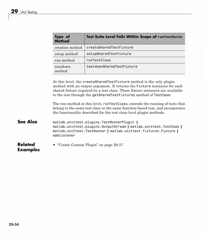
29 Unit Testing
Type ofMethod
Test Suite Level Falls Within Scope of runTestSuite
creation method createSharedTestFixture
setup method setupSharedTestFixture
run method runTestClass
teardownmethod
teardownSharedTestFixture
At this level, the createSharedTestFixture method is the only pluginmethod with an output argument. It returns the Fixture instances for eachshared fixture required by a test class. These fixture instances are availableto the test through the getSharedTestFixtures method of TestCase.
The run method at this level, runTestClass, extends the running of tests thatbelong to the same test class or the same function-based test, and incorporatesthe functionality described for the test class level plugin methods.
See Also matlab.unittest.plugins.TestRunnerPlugin |matlab.unittest.plugins.OutputStream | matlab.unittest.TestCase |matlab.unittest.TestRunner | matlab.unittest.fixtures.Fixture |addlistener
RelatedExamples
• “Create Custom Plugin” on page 29-57
29-56

Create Custom Plugin
Create Custom PluginThis example shows how to create a custom plugin that counts the number ofpassing and failing assertions when running a specified test suite. The pluginprints a brief summary at the end of the testing.
Create AssertionCountingPlugin Class
In a file in your working folder, create a new class, AssertionCountingPlugin,that inherits from the matlab.unittest.plugins.TestRunnerPlugin class.For a complete version of the code for an AssertionCountingPlugin, see"AssertionCountingPlugin Class Definition Summary".
Keep track of the number of passing and failing assertions. Within aproperties block, create NumPassingAssertions and NumFailingAssertionsproperties to pass the data between methods.
propertiesNumPassingAssertions = 0;NumFailingAssertions = 0;
end
Extend Running of TestSuite
Implement the runTestSuite method in a methods block with protectedaccess.
methods (Access = protected)function runTestSuite(plugin, pluginData)
suiteSize = numel(pluginData.TestSuite);fprintf('## Running a total of %d tests\n', suiteSize);
plugin.NumPassingAssertions = 0;plugin.NumFailingAssertions = 0;
[email protected](...plugin, pluginData);
fprintf('## Done running tests\n');plugin.printAssertionSummary();
29-57

29 Unit Testing
endend
The test framework evaluates this method one time. It displays informationabout the total number of tests, initializes the assertion count, and invokes thesuperclass method. After the framework completes evaluating the superclassmethod, the runTestSuite method displays the assertion count summary.
Extend Creation of Shared Test Fixtures and TestCase Instances
Add listeners to AssertionPassed and AssertionFailed events to count theassertions. To add these listeners, extend the methods that the test frameworkuses to create the test content. The test content comprises TestCase instancesfor each Test element, class-level TestCase instances for the TestClassSetupand TestClassTeardown methods, and Fixture instances that are used whena TestCase class has the SharedTestFixtures attribute.
Invoke the corresponding superclass method when you override the creationmethods. The creation methods return the content that the test frameworkcreates for each of their respective contexts. When implementing one of thesemethods, pass this argument out of your own implementation, and add thelisteners required by this plugin.
Add these creation methods to a methods block with protected access.
methods (Access = protected)function fixture = createSharedTestFixture(plugin, pluginData)
fixture = createSharedTestFixture@...matlab.unittest.plugins.TestRunnerPlugin(plugin, pluginData);
fixture.addlistener('AssertionPassed', ...@(~,~)plugin.incrementPassingAssertionsCount);
fixture.addlistener('AssertionFailed', ...@(~,~)plugin.incrementFailingAssertionsCount);
end
function testCase = createTestClassInstance(plugin, pluginData)testCase = createTestClassInstance@...
matlab.unittest.plugins.TestRunnerPlugin(plugin, pluginData);
29-58

Create Custom Plugin
testCase.addlistener('AssertionPassed', ...@(~,~)plugin.incrementPassingAssertionsCount);
testCase.addlistener('AssertionFailed', ...@(~,~)plugin.incrementFailingAssertionsCount);
end
function testCase = createTestMethodInstance(plugin, pluginData)testCase = createTestMethodInstance@...
matlab.unittest.plugins.TestRunnerPlugin(plugin, pluginData);
testCase.addlistener('AssertionPassed', ...@(~,~)plugin.incrementPassingAssertionsCount);
testCase.addlistener('AssertionFailed', ...@(~,~)plugin.incrementFailingAssertionsCount);
endend
Extend Running of Single Test Suite Element
Extend runTest to display the name of each test at run time. Include thisfunction in a methods block with protected access. Like all plugin methods,when you override this method you must invoke the corresponding superclassmethod.
methods (Access = protected)function runTest(plugin, pluginData)
fprintf('### Running test: %s\n', pluginData.Name);
[email protected](...plugin, pluginData);
endend
Define Helper Functions
In a methods block with private access, define three helper functions. Thesefunctions increment the number of passing or failing assertions, and print outthe assertion count summary.
methods (Access = private)function incrementPassingAssertionsCount(plugin)
29-59

29 Unit Testing
plugin.NumPassingAssertions = plugin.NumPassingAssertions + 1;end
function incrementFailingAssertionsCount(plugin)plugin.NumFailingAssertions = plugin.NumFailingAssertions + 1;
end
function printAssertionSummary(plugin)fprintf('%s\n', repmat('_', 1, 30));fprintf('Total Assertions: %d\n', ...
plugin.NumPassingAssertions + plugin.NumFailingAssertions);fprintf('\t%d Passed, %d Failed\n', ...
plugin.NumPassingAssertions, plugin.NumFailingAssertions);end
end
AssertionCountingPlugin Class Definition Summary
classdef AssertionCountingPlugin < ...
matlab.unittest.plugins.TestRunnerPlugin
properties
NumPassingAssertions = 0;
NumFailingAssertions = 0;
end
methods (Access = protected)
function runTestSuite(plugin, pluginData)
suiteSize = numel(pluginData.TestSuite);
fprintf('## Running a total of %d tests\n', suiteSize);
plugin.NumPassingAssertions = 0;
plugin.NumFailingAssertions = 0;
plugin, pluginData);
fprintf('## Done running tests\n');
plugin.printAssertionSummary();
end
29-60

Create Custom Plugin
function fixture = createSharedTestFixture(plugin, pluginData)
fixture = createSharedTestFixture@...
matlab.unittest.plugins.TestRunnerPlugin(plugin, pluginData);
fixture.addlistener('AssertionPassed', ...
@(~,~)plugin.incrementPassingAssertionsCount);
fixture.addlistener('AssertionFailed', ...
@(~,~)plugin.incrementFailingAssertionsCount);
end
function testCase = createTestClassInstance(plugin, pluginData)
testCase = createTestClassInstance@...
matlab.unittest.plugins.TestRunnerPlugin(plugin, pluginData);
testCase.addlistener('AssertionPassed', ...
@(~,~)plugin.incrementPassingAssertionsCount);
testCase.addlistener('AssertionFailed', ...
@(~,~)plugin.incrementFailingAssertionsCount);
end
function testCase = createTestMethodInstance(plugin, pluginData)
testCase = createTestMethodInstance@...
matlab.unittest.plugins.TestRunnerPlugin(plugin, pluginData);
testCase.addlistener('AssertionPassed', ...
@(~,~)plugin.incrementPassingAssertionsCount);
testCase.addlistener('AssertionFailed', ...
@(~,~)plugin.incrementFailingAssertionsCount);
end
function runTest(plugin, pluginData)
fprintf('### Running test: %s\n', pluginData.Name);
plugin, pluginData);
end
end
methods (Access = private)
29-61

29 Unit Testing
function incrementPassingAssertionsCount(plugin)
plugin.NumPassingAssertions = plugin.NumPassingAssertions + 1;
end
function incrementFailingAssertionsCount(plugin)
plugin.NumFailingAssertions = plugin.NumFailingAssertions + 1;
end
function printAssertionSummary(plugin)
fprintf('%s\n', repmat('_', 1, 30));
fprintf('Total Assertions: %d\n', ...
plugin.NumPassingAssertions + plugin.NumFailingAssertions);
fprintf('\t%d Passed, %d Failed\n', ...
plugin.NumPassingAssertions, plugin.NumFailingAssertions);
end
end
end
Create Example Test Class
In your working folder, create the file ExampleTest.m containing the followingtest class.
classdef ExampleTest < matlab.unittest.TestCasemethods(Test)
function testOne(testCase) % Test failstestCase.assertEqual(5, 4);
endfunction testTwo(testCase) % Test passes
testCase.verifyEqual(5, 5);endfunction testThree(testCase) % Test passes
testCase.assertEqual(7*2, 14);end
endend
Add Plugin to TestRunner and Run Tests
At the command prompt, create a test suite from the ExampleTest class.
29-62

Create Custom Plugin
import matlab.unittest.TestSuite;import matlab.unittest.TestRunner;
suite = TestSuite.fromClass(?ExampleTest);
Create a test runner with no plugins. This code creates a silent runner andprovides you with complete control over the installed plugins.
runner = TestRunner.withNoPlugins;
Run the tests.
result = runner.run(suite);
Add AssertionCountingPlugin to the runner and run the tests.
runner.addPlugin(AssertionCountingPlugin)result = runner.run(suite);
## Running a total of 3 tests### Running test: ExampleTest/testOne### Running test: ExampleTest/testTwo### Running test: ExampleTest/testThree## Done running tests______________________________Total Assertions: 21 Passed, 1 Failed
See Also matlab.unittest.plugins.TestRunnerPlugin |matlab.unittest.plugins.OutputStream | matlab.unittest.TestCase |matlab.unittest.TestRunner | matlab.unittest.fixtures.Fixture |addlistener
RelatedExamples
• “Write Plugins to Extend TestRunner” on page 29-53
29-63

29 Unit Testing
Analyze Test Case ResultsThis example shows how to analyze the information returned by a test runnercreated from the SolverTest test case.
Create Quadratic Solver Function
Create the following function that solves roots of the quadratic equation in afile, quadraticSolver.m, in your working folder.
function roots = quadraticSolver(a, b, c)% quadraticSolver returns solutions to the% quadratic equation a*x^2 + b*x + c = 0.
if ~isa(a,'numeric') || ~isa(b,'numeric') || ~isa(c,'numeric')error('quadraticSolver:InputMustBeNumeric', ...
'Coefficients must be numeric.');end
roots(1) = (-b + sqrt(b^2 - 4*a*c)) / (2*a);roots(2) = (-b - sqrt(b^2 - 4*a*c)) / (2*a);
end
Create Test for Quadratic Solver Function
Create the following test class in a file, SolverTest.m, in your working folder.
classdef SolverTest < matlab.unittest.TestCase% SolverTest tests solutions to the quadratic equation% a*x^2 + b*x + c = 0
methods (Test)function testRealSolution(testCase)
actSolution = quadraticSolver(1,-3,2);expSolution = [2,1];testCase.verifyEqual(actSolution,expSolution);
endfunction testImaginarySolution(testCase)
actSolution = quadraticSolver(1,2,10);
29-64

Analyze Test Case Results
expSolution = [-1+3i, -1-3i];testCase.verifyEqual(actSolution,expSolution);
endend
end
Run SolverTest Test Case
Create a test suite, quadTests.
quadTests = matlab.unittest.TestSuite.fromClass(?SolverTest);result = run(quadTests);
Running SolverTest..Done SolverTest__________
All tests passed.
Explore Output Argument, result
The output argument, result, is a matlab.unittest.TestResult object. Itcontains information of the two tests in SolverTest.
whos result
Name Size Bytes Class
result 1x2 248 matlab.unittest.TestResult
Display Information for One Test
To see the information for one value, type:
result(1)
ans =TestResult with properties:
29-65

29 Unit Testing
Name: 'SolverTest/testRealSolution'Passed: 1Failed: 0
Incomplete: 0Duration: 0.0244
Totals:1 Passed, 0 Failed, 0 Incomplete.0.024365 seconds testing time.
RelatedExamples
• “Write Simple Test Case Using Classes” on page 29-2
29-66

Analyze Failed Test Results
Analyze Failed Test ResultsThis example shows how to identify and rerun failed tests.
Create an Incorrect Test Method
Using the SolverTest test case, add a method, testBadRealSolution. Thistest, based on testRealSolution, calls the quadraticSolver function withinputs 1,3,2, but tests the results against an incorrect solution, [2,1].
function testBadRealSolution(testCase)actSolution = quadraticSolver(1,3,2);expSolution = [2,1];testCase.verifyEqual(actSolution,expSolution);
end
Run New Test Suite
Save the updated SolverTest class definition and rerun the tests.
quadTests = matlab.unittest.TestSuite.fromClass(?SolverTest);result1 = run(quadTests);
Running SolverTest.===========================================================================Verification failed in SolverTest/testBadRealSolution.
---------------------Framework Diagnostic:---------------------verifyEqual failed.--> NumericComparator failed.
--> The values are not equal using "isequaln".
Actual Value:-1 -2
Expected Value:2 1
------------------
29-67

29 Unit Testing
Stack Information:------------------In C:\Program Files\MATLAB\R2013a\toolbox\matlab\testframework\+matlab\In c:\work\SolverTest.m (SolverTest.testBadRealSolution) at 15
===========================================================================....Done SolverTest__________
Failure Summary:
Name Failed Incomplete Reason(s)=======================================================================SolverTest/testBadRealSolution X Failed by verifica
>>
Analyze Results
The output tells you SolverTest/testBadRealSolution failed. From theFramework Diagnostic you see the following:
Actual Value:-1 -2
Expected Value:2 1
At this point, you must decide if the error is in quadraticSolver or in yourvalue for expSolution.
Correct Error
Edit the value of expSolution in testBadRealSolution:
expSolution = [-1 -2];
Rerun Tests
Save SolverTest and rerun only the failed tests.
failedTests = quadTests([result1.Failed]);
29-68

Analyze Failed Test Results
result2 = run(failedTests)
Running SolverTest.Done SolverTest__________
result2 =TestResult with properties:
Name: 'SolverTest/testBadRealSolution'Passed: 1Failed: 0
Incomplete: 0Duration: 0.0124
Totals:1 Passed, 0 Failed, 0 Incomplete.0.012382 seconds testing time.
29-69

29 Unit Testing
Dynamically Filtered Tests
In this section...
“Test Methods” on page 29-70
“Method Setup and Teardown Code” on page 29-73
“Class Setup and Teardown Code” on page 29-75
Assumption failures produce filtered tests. In the matlab.unittest.TestResultclass, such a test is marked Incomplete.
Since filtering test content through the use of assumptions does not producetest failures, it has the possibility of creating dead test code. Avoiding thisrequires monitoring of filtered tests.
Test MethodsIf an assumption failure is encountered inside of a TestCase method with theTest attribute, the entire method is marked as filtered, but MATLAB runsthe subsequent Test methods.
The following class contains an assumption failure in one of the methodsin the Test block.
classdef ExampleTest < matlab.unittest.TestCasemethods(Test)
function testA(testCase)testCase.verifyTrue(true);
endfunction testB(testCase)
testCase.assumeEqual(0,1);% remaining test code is not exercised
endfunction testC(testCase)
testCase.verifyFalse(true);end
endend
29-70

Dynamically Filtered Tests
Since the testB method contains an assumption failure, when you run thetest, the testing framework filters that test and marks it as incomplete. Afterthe assumption failure in testB, the testing framework proceeds and executestestC, which contains a verification failure.
ts = matlab.unittest.TestSuite.fromClass(?ExampleTest);res = ts.run;
Running ExampleTest.===========================================================================ExampleTest/testB was filtered.
Details===========================================================================.===========================================================================Verification failed in ExampleTest/testC.
---------------------Framework Diagnostic:---------------------verifyFalse failed.--> The value must evaluate to "false".
Actual Value:1
------------------Stack Information:------------------In C:\work\ExampleTest.m (ExampleTest.testC) at 11
===========================================================================.Done ExampleTest__________
Failure Summary:
Name Failed Incomplete Reason(s)================================================================
29-71

29 Unit Testing
ExampleTest/testB X Filtered by assumption.----------------------------------------------------------------ExampleTest/testC X Failed by verification.
If you examine the TestResult, you notice that there is a passed test, a failedtest, and a test that did not complete due to an assumption failure.
res
res =
1x3 TestResult array with properties:
NamePassedFailedIncompleteDuration
Totals:1 Passed, 1 Failed, 1 Incomplete.0.059433 seconds testing time.
The testing framework keeps track of incomplete tests so that you can monitorfiltered tests for nonexercised test code. You can see information about thesetests within the TestResult object.
res([res.Incomplete])
ans =
TestResult with properties:
Name: 'ExampleTest/testB'Passed: 0Failed: 0
Incomplete: 1Duration: 0.0400
Totals:0 Passed, 0 Failed, 1 Incomplete.
29-72

Dynamically Filtered Tests
0.040017 seconds testing time.
To create a modified test suite from only the filtered tests, select incompletetests from the original test suite.
tsFiltered = ts([res.Incomplete])
tsFiltered =
Test with properties:
Name: 'ExampleTest/testB'Parameterization: []
SharedTestFixtures: []
Method Setup and Teardown CodeIf an assumption failure is encountered inside a TestCase method withthe TestMethodSetup attribute, MATLAB filters the method which wasto be run for that instance. If a test uses assumptions from within theTestMethodSetup block, consider instead using the assumptions in theTestClassSetup block, which likewise filters all Test methods in the classbut is less verbose and more efficient.
One of the methods in the following TestMethodSetup block withinExampleTest.m contains an assumption failure.
methods(TestMethodSetup)function setupMethod1(testCase)
testCase.assumeEqual(1,0);% remaining test code is not exercised
endfunction setupMethod2(testCase)
disp('* Running setupMethod2 *')testCase.assertEqual(1,1);
endend
Updated ExampleTest Class Definition
classdef ExampleTest < matlab.unittest.TestCasemethods(TestMethodSetup)
29-73

29 Unit Testing
function setupMethod1(testCase)testCase.assumeEqual(1,0);% remaining test code is not exercised
endfunction setupMethod2(testCase)
disp('* Running setupMethod2 *')testCase.assertEqual(1,1);
endend
methods(Test)function testA(testCase)
testCase.verifyTrue(true);endfunction testB(testCase)
testCase.assumeEqual(0,1);% remaining test code is not exercised
endfunction testC(testCase)
testCase.verifyFalse(true);end
endend
When you run the test, you see that the framework completes executes all themethods in the TestMethodSetup block that do not contain the assumptionfailure, and it marks as incomplete all methods in the Test block.
ts = matlab.unittest.TestSuite.fromClass(?ExampleTest);res = ts.run;
Running ExampleTest
===========================================================================ExampleTest/testA was filtered.
Details===========================================================================* Running setupMethod2 *.===========================================================================
29-74

Dynamically Filtered Tests
ExampleTest/testB was filtered.Details
===========================================================================* Running setupMethod2 *.===========================================================================ExampleTest/testC was filtered.
Details===========================================================================* Running setupMethod2 *.Done ExampleTest__________
Failure Summary:
Name Failed Incomplete Reason(s)================================================================ExampleTest/testA X Filtered by assumption.
----------------------------------------------------------------ExampleTest/testB X Filtered by assumption.
----------------------------------------------------------------ExampleTest/testC X Filtered by assumption.
The Test methods did not change but all 3 are filtered due to an assumptionfailure in the TestMethodSetup block. The testing framework executesmethods in the TestMethodSetup block without assumption failures, such assetupMethod2. As expected, the testing framework executes setupMethod2 3times, once before each Test method.
Class Setup and Teardown CodeIf an assumption failure is encountered inside of a TestCase method withthe TestClassSetup or TestClassTeardown attribute, MATLAB filters theentire TestCase class.
The methods in the following TestClassSetup block within ExampleTest.mcontains an assumption failure.
methods(TestClassSetup)
29-75

29 Unit Testing
function setupClass(testCase)testCase.assumeEqual(1,0);% remaining test code is not exercised
endend
Updated ExampleTest Class Definition
classdef ExampleTest < matlab.unittest.TestCasemethods(TestClassSetup)
function setupClass(testCase)testCase.assumeEqual(1,0);% remaining test code is not exercised
endend
methods(TestMethodSetup)function setupMethod1(testCase)
testCase.assumeEqual(1,0);% remaining test code is not exercised
endfunction setupMethod2(testCase)
disp('* Running setupMethod2 *')testCase.assertEqual(1,1);
endend
methods(Test)function testA(testCase)
testCase.verifyTrue(true);endfunction testB(testCase)
testCase.assumeEqual(0,1);% remaining test code is not exercised
endfunction testC(testCase)
testCase.verifyFalse(true);end
endend
29-76

Dynamically Filtered Tests
When you run the test, you see that the framework does not execute any ofthe methods in the TestMethodSetup or Test.
ts = matlab.unittest.TestSuite.fromClass(?ExampleTest);res = ts.run;
Running ExampleTest
===========================================================================All tests in ExampleTest were filtered.
Details===========================================================================
Done ExampleTest__________
Failure Summary:
Name Failed Incomplete Reason(s)================================================================ExampleTest/testA X Filtered by assumption.
----------------------------------------------------------------ExampleTest/testB X Filtered by assumption.
----------------------------------------------------------------ExampleTest/testC X Filtered by assumption.
The Test and TestMethodSetup methods did not change but everything isfiltered due to an assumption failure in the TestClassSetup block.
See Also matlab.unittest.qualifications.Assumable | TestCase | TestResult
29-77

29 Unit Testing
Write Function-Based Unit Tests
In this section...
“Create Test Function” on page 29-78
“Run the Tests” on page 29-81
“Analyze the Results” on page 29-82
Create Test FunctionYour test function is a single MATLAB file that contains a main functionand your individual local test functions. Optionally, you can include filefixture and fresh fixture functions. File fixtures consist of setup and teardownfunctions shared across all the tests in a file. These functions are executedonce per test file. Fresh fixtures consist of setup and teardown functions thatare executed before and after each local test function.
Create the Main FunctionThe main function collects all of the local test functions into a test array.Since it is the main function, the function name corresponds to the name ofyour .m file and follows the naming convention of starting or ending in theword ‘test’, which is case-insensitive. In this sample case, the MATLAB file isexampleTest.m. The main function needs to make a call to functionteststo generate a test array, tests. Use localfunctions as the input tofunctiontests to automatically generate a cell array of function handles toall the local functions in your file. This is a typical main function.
function tests = exampleTesttests = functiontests(localfunctions);end
Create Local Test FunctionsIndividual test functions are included as local functions in the same MATLABfile as the main (test-generating) function. These test function names mustbegin or end with the case-insensitive word, ‘test’. Each of the local testfunctions must accept a single input, which is a function test case object,testCase. The Unit Test Framework automatically generates this object. For
29-78

Write Function-Based Unit Tests
more information on creating test functions, see “Write Simple Test CaseUsing Functions” on page 29-83 and “Types of Qualifications” on page 29-10.This is a typical example of skeletal local-test functions.
function testFunctionOne(testCase)% Test specific codeend
function FunctionTwotest(testCase)% Test specific codeend
Create Optional Fixture FunctionsSetup and teardown code, also referred to as test fixture functions, set up thepretest state of the system and return it to the original state after runningthe test. There are two types of these functions: file fixture functions thatrun once per test file, and fresh fixture functions that run before and aftereach local test function. These functions are not required to generate tests.In general, it is preferable to use fresh fixtures over file fixtures to increaseunit test encapsulation.
A function test case object, testCase, must be the only input to file fixture andfresh fixture functions. The Unit Test Framework automatically generatesthis object. The TestCase object is a means to pass information between setupfunctions, test functions, and teardown functions. Its TestData property is,by default, a struct, which allows easy addition of fields and data. Typicaluses for this test data include paths and graphics handles. For an exampleusing the TestData property, see “Write Test Using Setup and TeardownFunctions” on page 29-88.
File Fixture Functions. Use file fixture functions to share setup andteardown functions across all the tests in a file. The names for the filefixture functions must be setupOnce and teardownOnce, respectively. Thesefunctions execute a single time for each file. You can use file fixtures to set apath before testing, and then reset it to the original path after testing. This isa typical example of skeletal file fixture setup and teardown code.
function setupOnce(testCase) % do not change function name% set a new path, for example
29-79

29 Unit Testing
end
function teardownOnce(testCase) % do not change function name% change back to original path, for exampleend
Fresh Fixture Functions. Use fresh fixture functions to set up and tear downstates for each local test function. The names for these fresh fixture functionsmust be setup and teardown, respectively. You can use fresh fixtures toobtain a new figure before testing and to close the figure after testing. This istypical example of skeletal test function level setup and teardown code.
function setup(testCase) % do not change function name% open a figure, for exampleend
function teardown(testCase) % do not change function name% close figure, for exampleend
Program Listing Template
%% Main function to generate testsfunction tests = exampleTesttests = functiontests(localfunctions);end
%% Test Functionsfunction testFunctionOne(testCase)% Test specific codeend
function FunctionTwotest(testCase)% Test specific codeend
%% Optional file fixturesfunction setupOnce(testCase) % do not change function name% set a new path, for example
29-80

Write Function-Based Unit Tests
end
function teardownOnce(testCase) % do not change function name% change back to original path, for exampleend
%% Optional fresh fixturesfunction setup(testCase) % do not change function name% open a figure, for exampleend
function teardown(testCase) % do not change function name% close figure, for exampleend
Run the TestsThe figure below details the tasks executed when you run the tests.
To run tests from the command prompt, use the runtests command withyour MATLAB test file as input. For example:
results = runtests('exampleTest.m')
Alternatively, you can run tests using the run function.
results = run(exampleTest)
29-81

29 Unit Testing
For more information on running tests see the runtests reference page and“Run Tests for Various Workflows” on page 29-46.
Analyze the ResultsTo analyze the test results, examine the output structure from runtests orrun. For each test, the result contains the name of the test function, whetherit passed, failed, or didn’t complete, and the time it took to run the test.For more information, see “Analyze Test Case Results” on page 29-64 and“Analyze Failed Test Results” on page 29-67.
See Also runtests | functiontests | localfunctions
RelatedExamples
• “Write Simple Test Case Using Functions” on page 29-83• “Write Test Using Setup and Teardown Functions” on page 29-88
29-82

Write Simple Test Case Using Functions
Write Simple Test Case Using FunctionsThis example shows how to write a unit test for a MATLAB function,quadraticSolver.m.
Create quadraticSolver.m Function
This MATLAB function solves quadratic equations. Create this function in afolder on your MATLAB path.
function roots = quadraticSolver(a, b, c)% quadraticSolver returns solutions to the% quadratic equation a*x^2 + b*x + c = 0.
if ~isa(a,'numeric') || ~isa(b,'numeric') || ~isa(c,'numeric')error('quadraticSolver:InputMustBeNumeric', ...
'Coefficients must be numeric.');end
roots(1) = (-b + sqrt(b^2 - 4*a*c)) / (2*a);roots(2) = (-b - sqrt(b^2 - 4*a*c)) / (2*a);
end
Create solverTest Function
Create this function in a folder on your MATLAB path.
function tests = solverTesttests = functiontests(localfunctions);end
A call to functiontests using localfunctions as input creates an array oftests from each local function in the solverTest.m file. Each test is a localfunction that follows the naming convention of having ’test’ at the beginningor end of the function name. Local functions that do not follow this conventionare not included in the test array. Test functions must accept a single inputargument into which the test framework passes a function test case object.The function uses this object for verifications assertions, assumptions, andfatal assertions. It contains a TestData structure that allows data to bepassed between setup, test, and teardown functions.
29-83

29 Unit Testing
Create Test Function for Real Solutions
Create a test function, testRealSolution, to verify that quadraticSolverreturns the correct value for real solutions. For example, the equation x2
- 3x + 2 = 0 has real solutions x = 1 and x = 2. This function callsquadraticSolver with the inputs of this equation. The expected solution,expSolution, is [2,1].
Use the qualification function, verifyEqual, to compare the output ofthe function, actSolution, to the desired output, expSolution. If thequalification fails, the framework continues executing the test. Typically,when using verifyEqual on floating point values, you specify a tolerance forthe comparison. For more information, see matlab.unittest.constraints.
Add this function to the solverTest.m file.
function testRealSolution(testCase)actSolution = quadraticSolver(1,-3,2);expSolution = [2,1];verifyEqual(testCase,actSolution,expSolution);end
Create Test Function for Imaginary Solutions
Create a test to verify that quadraticSolver returns the right value forimaginary solutions. For example, the equation x2 - 2x + 10 = 0 hasimaginary solutions x = -1 + 3i and x = -1 - 3i. Typically, whenusing verifyEqual on floating point values, you specify a tolerance for thecomparison. For more information, see matlab.unittest.constraints.
Add this function, testImaginarySolution, to the solverTest.m file.
function testImaginarySolution(testCase)actSolution = quadraticSolver(1,2,10);expSolution = [-1+3i, -1-3i];verifyEqual(testCase,actSolution,expSolution);end
The order of the tests within the solverTest.m file does not matter becausethey are fully independent test cases.
29-84

Write Simple Test Case Using Functions
Save solverTest Function
The following is the complete solverTest.m test file. Save this file in a folderon your MATLAB path.
function tests = solverTesttests = functiontests(localfunctions);end
function testRealSolution(testCase)actSolution = quadraticSolver(1,-3,2);expSolution = [2,1];verifyEqual(testCase,actSolution,expSolution);end
function testImaginarySolution(testCase)actSolution = quadraticSolver(1,2,10);expSolution = [-1+3i, -1-3i];verifyEqual(testCase,actSolution,expSolution);end
Run Tests in solverTest Function
Run the tests.
results = runtests('solverTest.m')
Running solverTest..Done solverTest__________
results =
1x2 TestResult array with properties:
NamePassedFailed
29-85

29 Unit Testing
IncompleteDuration
Totals:2 Passed, 0 Failed, 0 Incomplete.0.19172 seconds testing time.
Both of the tests passed.
Introduce an Error in quadraticSolver.m and Run Tests
Cause one of the tests to fail by forcing roots in quadraticSolver.m to bereal. Before ending the function, add the line: roots = real(roots);. (Donot change solverTest.m.) Save the file and run the tests.
results = runtests('solverTest.m')
Running solverTest.===========================================================================Verification failed in solverTest/testImaginarySolution.
---------------------Framework Diagnostic:---------------------verifyEqual failed.--> NumericComparator failed.
--> Complexity does not match.
Actual Complexity:Real
Expected Complexity:Complex
Actual Value:-1 -1
Expected Value:-1.000000000000000 + 3.000000000000000i -1.000000000000000 - 3.000
------------------Stack Information:
29-86

Write Simple Test Case Using Functions
------------------In C:\work\solverTest.m (testImaginarySolution) at 14In C:\Program Files\MATLAB\R2013b\toolbox\matlab\testframework\+matlab\
===========================================================================.Done solverTest__________
Failure Summary:
Name Failed Incomplete Reason(s)=======================================================================solverTest/testImaginarySolution X Failed by verifi
results =
1x2 TestResult array with properties:
NamePassedFailedIncompleteDuration
Totals:1 Passed, 1 Failed, 0 Incomplete.0.22545 seconds testing time.
The imaginary test verification failed.
Restore quadraticSolver.m to its previous, correct version by removing theroots = real(roots); code.
See Also matlab.unittest.constraints
Concepts • “Write Function-Based Unit Tests” on page 29-78• “Types of Qualifications” on page 29-10
29-87

29 Unit Testing
Write Test Using Setup and Teardown FunctionsThis example shows how to write a unit test for a couple of MATLAB figureaxes properties using fresh fixtures and file fixtures.
Create axesPropertiesTest File
Create a file containing the main function that tests figure axes propertiesand include two test functions. One function verifies that the x-axis limits arecorrect, and the other one verifies that the face color of a surface is correct.
In a folder on your MATLAB path, create axesPropertiesTest.m. In themain function of this file, have functiontests create an array of testsfrom each local function in axesPropertiesTest.m with a call to thelocalfunctions function.
function tests = axesPropertiesTesttests = functiontests(localfunctions);end
Create File Fixture Functions
File fixture functions are setup and teardown code that runs a single time inyour test file. These fixtures are shared across the test file. In this example,the file fixture functions create a temporary folder and set it as the currentworking folder. They also create and save a new figure for testing. Aftertests are complete, the framework reinstates the original working folder anddeletes the temporary folder and saved figure.
In this example, a helper function creates a simple figure — a red cylinder.In a more realistic scenario, this code is part of the product under test andis computationally expensive, thus motivating the intent to create the figureonly once and to load independent copies of the result for each test function.For this example, however, you want to create this helper function as a localfunction to axesPropertiesTest. Note that the test array does not includethe function because its name does not start or end with ‘test’.
Write a helper function that creates a simple red cylinder and add it as alocal function to axesPropertiesTest.
29-88

Write Test Using Setup and Teardown Functions
function f = createFiguref = figure;ax = axes('Parent', f);cylinder(ax,10);h = findobj(ax,'Type','surface');set(h,'FaceColor',[1 0 0]);end
You must name the setup and teardown functions of a file test fixturesetupOnce and teardownOnce, respectively. These functions take a singleinput argument, testCase, into which the test framework automaticallypasses a function test case object. This test case object contains a TestDatastructure that allows data to pass between setup, test, and teardownfunctions. In this example, the TestData structure uses assigned fields tostore the original path, the temporary folder name, and the figure file name.
Create the setup and teardown functions as a local functions toaxesPropertiesTest.
function setupOnce(testCase)% create and change to temporary foldertestCase.TestData.origPath = pwd;testCase.TestData.tmpFolder = ['tmpFolder' datestr(now,30)];mkdir(testCase.TestData.tmpFolder)cd(testCase.TestData.tmpFolder)
% create and save a figuretestCase.TestData.figName = 'tmpFig.fig';aFig = createFigure;saveas(aFig,testCase.TestData.figName,'fig')close(aFig)end
function teardownOnce(testCase)delete(testCase.TestData.figName);cd(testCase.TestData.origPath);rmdir(testCase.TestData.tmpFolder);end
Create Fresh Fixture Functions
29-89

29 Unit Testing
Fresh fixtures are function level setup and teardown code that runs beforeand after each test function in your file. In this example, the functions openthe saved figure and find the handles. After testing, the framework closesthe figure.
You must name fresh fixture functions setup and teardown, respectively.Similar to the file fixture functions, these functions take a single inputargument, testCase. In this example, these functions create a new field inthe TestData structure that includes handles to the figure and to the axes.This allows information to pass between setup, test, and teardown functions.
Create the setup and teardown functions as a local functions toaxesPropertiesTest. Open the saved figure for each test to ensure testindependence.
function setup(testCase)testCase.TestData.Figure = openfig(testCase.TestData.figName);testCase.TestData.Axes = findobj(testCase.TestData.Figure,...
'Type','Axes');end
function teardown(testCase)close(testCase.TestData.Figure);end
In addition to custom setup and teardown code, the Unit Testing Frameworkprovides some classes for creating fixtures. For more information seematlab.unittest.fixtures.
Create Test Functions
Each test is a local function that follows the naming convention of having‘test’ at the beginning or end of the function name. The test array does notinclude local functions that do not follow this convention. Similar to setupand teardown functions, individual test functions must accept a single inputargument, testCase. Use this test case object for verifications, assertions,assumptions, and fatal assertions functions.
The testDefaultXLim function test verifies that the x-axis limits are largeenough to display the cylinder. The lower limit needs to be less than -10,
29-90

Write Test Using Setup and Teardown Functions
and the upper limit needs to be greater than 10. These values come fromthe figure generated in the helper function — a cylinder with a 10 unitradius centered on the origin. This test function opens the figure createdand saved in the setupOnce function, queries the axes limit, and verifiesthe limits are correct. The qualification functions, verifyLessThanOrEqualand verifyGreaterThanOrEqual, takes the test case, the actual value, theexpected value, and optional diagnostic information to display in the case offailure as inputs.
Create the testDefaultXLim function as local function toaxesPropertiesTest.
function testDefaultXLim(testCase)xlim = get(testCase.TestData.Axes, 'XLim');verifyLessThanOrEqual(testCase, xlim(1), -10,...
'Minimum x-limit was not small enough');verifyGreaterThanOrEqual(testCase, xlim(2), 10,...
'Maximum x-limit was not big enough');end
The surfaceColorTest function accesses the figure that you created andsaved in the setupOnce function. surfaceColorTest queries the face color ofthe cylinder and verifies that it is red. The color red has an RGB value of [1 00]. The qualification function, verifyEqual, takes as inputs the test case,the actual value, the expected value, and optional diagnostic informationto display in the case of failure. Typically when using verifyEqual onfloating point-values, you specify a tolerance for the comparison. For moreinformation, see matlab.unittest.constraints.
Create the surfaceColorTest function as local function toaxesPropertiesTest.
function surfaceColorTest(testCase)h = findobj(testCase.TestData.Axes,'Type','surface');co = get(h,'FaceColor');verifyEqual(testCase, co, [1 0 0],'FaceColor is incorrect')end
Now the axesPropertiesTest.m file is complete with a main function, filefixture functions, fresh fixture functions, and two local test functions. You areready to run the tests.
29-91

29 Unit Testing
Run Tests
The next step is to run the tests using the runtests function. In this example,the call to runtests results in the following steps:
1 The main function creates a test array.
2 The file fixture records the working folder, creates a temporary folder,sets the temporary folder as the working folder, then generates andsaves a figure.
3 The fresh fixture setup opens the saved figure and finds the handles.
4 The testDefaultXLim test is run.
5 The fresh fixture teardown closes the figure.
6 The fresh fixture setup opens the saved figure and finds the handles.
7 The surfaceColorTest test is run.
8 The fresh fixture teardown closes the figure.
9 The file fixture teardown deletes the saved figure, changes back to theoriginal path and deletes the temporary folder.
At the command prompt, generate and run the test suite.
results = runtests('axesPropertiesTest.m')
Running axesPropertiesTest..Done axesPropertiesTest__________
results =
1x2 TestResult array with properties:
29-92
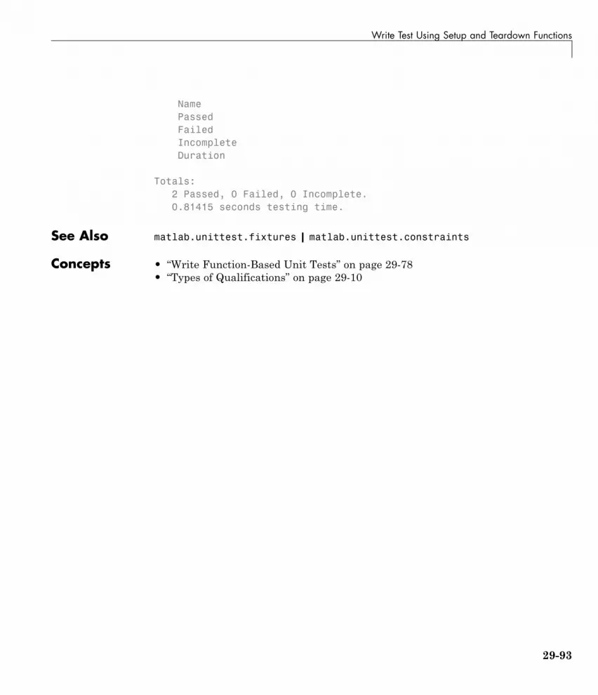
Write Test Using Setup and Teardown Functions
NamePassedFailedIncompleteDuration
Totals:2 Passed, 0 Failed, 0 Incomplete.0.81415 seconds testing time.
See Also matlab.unittest.fixtures | matlab.unittest.constraints
Concepts • “Write Function-Based Unit Tests” on page 29-78• “Types of Qualifications” on page 29-10
29-93