manual - trimble business center v5.0 - transport and main
TRANSCRIPT

Manual Trimble Business Center v5.40 – Processing and Adjusting GNSS Survey Control Networks December 2021

Trimble Business Center v5.40 Manual, Transport and Main Roads, December 2021
Copyright © The State of Queensland (Department of Transport and Main Roads) 2021. Licence
This work is licensed by the State of Queensland (Department of Transport and Main Roads) under a Creative Commons Attribution (CC BY) 4.0 International licence. CC BY licence summary statement In essence, you are free to copy, communicate and adapt this work, as long as you attribute the work to the State of Queensland (Department of Transport and Main Roads). To view a copy of this licence, visit: https://creativecommons.org/licenses/by/4.0/ Translating and interpreting assistance
The Queensland Government is committed to providing accessible services to Queenslanders from all cultural and linguistic backgrounds. If you have difficulty understanding this publication and need a translator, please call the Translating and Interpreting Service (TIS National) on 13 14 50 and ask them to telephone the Queensland Department of Transport and Main Roads on 13 74 68.
Disclaimer While every care has been taken in preparing this publication, the State of Queensland accepts no responsibility for decisions or actions taken as a result of any data, information, statement or advice, expressed or implied, contained within. To the best of our knowledge, the content was correct at the time of publishing. Feedback Please send your feedback regarding this document to: [email protected]
Trimble Business Center v5.40 Manual, Transport and Main Roads, December 2021 i
Contents
1 Introduction and background information ..................................................................................1
1.1 Definitions ....................................................................................................................................... 1
2 Transport and Main Roads GNSS ribbon and access toolbar ..................................................3
2.1 Other useful tools ............................................................................................................................ 3
3 Create and setup a new project ....................................................................................................4
3.1 Create a new project ....................................................................................................................... 4
3.2 Project settings ............................................................................................................................... 5
4 Create Network diagram (independent baselines only).......................................................... 17
5 Import data .................................................................................................................................. 18
5.1 Download data .............................................................................................................................. 18
5.2 Import GNSS data files ................................................................................................................. 18 5.2.1 Fixing static observation data that went out of level during collection ........................ 20 5.2.2 Redundancy ................................................................................................................ 21
5.3 Import Ephemeris data ................................................................................................................. 21 5.3.1 Download ephemeris data ........................................................................................... 22
6 Baseline processing ................................................................................................................... 24
6.1 Seed coordinate ............................................................................................................................ 24 6.1.1 Regulation 13 Certificates ........................................................................................... 25 6.1.2 PM Form 6 ................................................................................................................... 25 6.1.3 Selecting the seed coordinate ..................................................................................... 27 6.1.4 Seeding primary control point – enter coordinates ...................................................... 27
6.2 Disable Dependent baseline ......................................................................................................... 28 6.2.1 Identify and disable dependent baselines procedure .................................................. 29
6.3 Process baselines ......................................................................................................................... 36 6.3.1 Loop Closures ............................................................................................................. 38 6.3.2 Potential problems ....................................................................................................... 41 6.3.3 Errors / Mistakes and problem solving ........................................................................ 46 6.3.4 Analysis ....................................................................................................................... 52 6.3.5 Save Processing Results ............................................................................................ 57
7 Minimally constrained adjustment ............................................................................................ 58
7.1 Enter all known coordinate values ................................................................................................ 58 7.1.1 Add known coordinate values ..................................................................................... 59 7.1.2 Import known coordinates (CORS) ............................................................................. 60 7.1.3 Assign to survey mark and set quality ......................................................................... 62 7.1.4 Import Known Coordinates (PM’s) .............................................................................. 63
7.2 Perform the adjustment ................................................................................................................ 66 7.2.1 Project example 1 ........................................................................................................ 68 7.2.2 Project example 2 ........................................................................................................ 74 7.2.3 Apply a weighting (scalar) strategy ............................................................................. 77 7.2.4 Save network adjustment report .................................................................................. 79
7.3 Export of minimally constrained adjustment results ..................................................................... 80
8 Constrained adjustment ............................................................................................................. 82
8.1 Run the constrained adjustment ................................................................................................... 83 8.1.1 Clear the adjustment results ........................................................................................ 83 8.1.2 Weight datum marks.................................................................................................... 83

Trimble Business Center v5.40 Manual, Transport and Main Roads, December 2021 ii
8.1.3 Option 1 example: Constrain all known horizontal and vertical components .............. 84 8.1.4 Option 3 example: Add a selected group of horizontal constraints, then a selected group of vertical constraints .......................................................................................................... 90 8.1.5 Apply a scalar to the network ...................................................................................... 96
8.2 Constrained adjustment network report ........................................................................................ 96 8.2.1 Save network adjustment report ................................................................................ 100
8.3 Export of constrained adjustment results ................................................................................... 100
9 Additional export and reports ................................................................................................. 102
9.1 ASCII output................................................................................................................................ 102
9.2 Point list report ............................................................................................................................ 103
10 Output of network for Department of Resources (DoR) ....................................................... 105
10.1 Export in RINEX format .............................................................................................................. 105
10.2 Export in TDEF format ................................................................................................................ 109
10.3 Submit to Department of Resources (DoR) ................................................................................ 111
11 Project archival ......................................................................................................................... 111
Appendix A – Configuring TBC ........................................................................................................ 112
Appendix B – Setting up the TBC ribbon ........................................................................................ 115
Appendix C – Create a new Import Format ..................................................................................... 117
Appendix D – Processing and Adjustment Workflow ................................................................... 120
Appendix E – Additional Information .............................................................................................. 122
Addendum - Calculating Survey Uncertainty (SU) and Positional Uncertainty (PU) for GNSS Survey Control Networks.................................................................................................................. 126
A1 Introduction ............................................................................................................................... 126
A2 Uncertainty in Measurement .................................................................................................... 126
A3 Expression of Uncertainty ....................................................................................................... 127
A3.1 Standard deviation ...................................................................................................................... 127
A3.2 Standard error ellipse/ellipsoid ................................................................................................... 130
A3.3 Horizontal circular confidence region ......................................................................................... 132
A3.4 Calculation of Survey Uncertainty (SU) and Positional Uncertainty (PU)................................... 132 A3.4.1 Survey Uncertainty (SU) ............................................................................................ 132 A3.4.2 Positional Uncertainty (PU) ....................................................................................... 134
Processing and Adjusting GNSS Networks
Trimble Business Center v5.40 Manual, Transport and Main Roads, December 2021 1
1 Introduction and background information
This manual has been created to assist Global Navigation Satellite System (GNSS) users to utilise Trimble Business Center (TBC) adjustment software to create a new project, import data, process and adjust a GNSS Fast Static or Static network.
Users of this manual are urged to be familiar with the Intergovernmental Committee on Surveying and Mapping's (ICSM) publications Standard for the Australian Survey Control Network – Special Publication 1 (SP1), Version 2.2, Guideline for the Adjustment and Evaluation of Survey Control – Special Publication 1 (SP1), Version 2.2, and Guideline for Control Surveys by GNSS – Special Publication 1 (SP1), Version 2.2. SP1 is available in both Microsoft word and pdf format from the ICSM website, http://www.icsm.gov.au
SP1 documents Standards and best practice guidelines for Surveys and Reduction. This includes GNSS Survey guidelines, connection to datum, network adjustment and quantifying survey quality in terms of uncertainty.
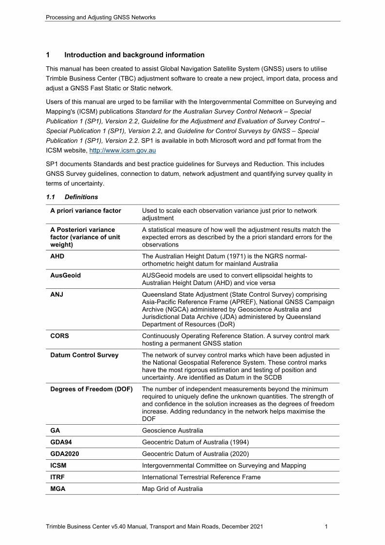
1.1 Definitions
A priori variance factor Used to scale each observation variance just prior to network adjustment
A Posteriori variance factor (variance of unit weight)
A statistical measure of how well the adjustment results match the expected errors as described by the a priori standard errors for the observations
AHD The Australian Height Datum (1971) is the NGRS normal-orthometric height datum for mainland Australia
AusGeoid AUSGeoid models are used to convert ellipsoidal heights to Australian Height Datum (AHD) and vice versa
ANJ Queensland State Adjustment (State Control Survey) comprising Asia-Pacific Reference Frame (APREF), National GNSS Campaign Archive (NGCA) administered by Geoscience Australia and Jurisdictional Data Archive (JDA) administered by Queensland Department of Resources (DoR)
CORS Continuously Operating Reference Station. A survey control mark hosting a permanent GNSS station
Datum Control Survey The network of survey control marks which have been adjusted in the National Geospatial Reference System. These control marks have the most rigorous estimation and testing of position and uncertainty. Are identified as Datum in the SCDB
Degrees of Freedom (DOF) The number of independent measurements beyond the minimum required to uniquely define the unknown quantities. The strength of and confidence in the solution increases as the degrees of freedom increase. Adding redundancy in the network helps maximise the DOF
GA Geoscience Australia
GDA94 Geocentric Datum of Australia (1994)
GDA2020 Geocentric Datum of Australia (2020)
ICSM Intergovernmental Committee on Surveying and Mapping
ITRF International Terrestrial Reference Frame
MGA Map Grid of Australia
Processing and Adjusting GNSS Networks
Trimble Business Center v5.40 Manual, Transport and Main Roads, December 2021 2
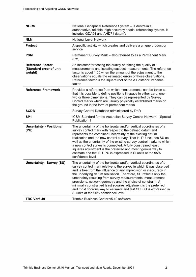
NGRS National Geospatial Reference System – is Australia’s authoritative, reliable, high accuracy spatial referencing system. It includes GDA94 and AHD71 datum’s
NLN National Level Network
Project A specific activity which creates and delivers a unique product or service
PSM Permanent Survey Mark – also referred to as a Permanent Mark (PM)
Reference Factor (Standard error of unit weight)
An indicator for testing the quality of testing the quality of measurements and isolating suspect measurements. The reference factor is about 1.00 when the amount of the adjustment to the observations equals the estimated errors of those observations. Reference factor is the square root of the A Posteriori variance factor
Reference Framework Provides a reference from which measurements can be taken so that it is possible to define positions in space in either zero, one, two or three dimensions. They can be represented by Survey Control marks which are usually physically established marks on the ground in the form of permanent marks
SCDB Survey Control Database administered by DoR
SP1 ICSM Standard for the Australian Survey Control Network – Special Publication 1
Uncertainty - Positional (PU)
The uncertainty of the horizontal and/or vertical coordinates of a survey control mark with respect to the defined datum and represents the combined uncertainty of the existing datum realisation and the new control survey. That is, PU includes SU as well as the uncertainty of the existing survey control marks to which a new control survey is connected. A fully constrained least squares adjustment is the preferred and most rigorous way to estimate and test PU. PU is expressed in SI units at the 95% confidence level
Uncertainty - Survey (SU) The uncertainty of the horizontal and/or vertical coordinates of a survey control mark relative to the survey in which it was observed and is free from the influence of any imprecision or inaccuracy in the underlying datum realisation. Therefore, SU reflects only the uncertainty resulting from survey measurements, measurement precisions, network geometry and the choice of constraint. A minimally constrained least squares adjustment is the preferred and most rigorous way to estimate and test SU. SU is expressed in SI units at the 95% confidence level
TBC Ver5.40 Trimble Business Center v5.40 software
Processing and Adjusting GNSS Networks
Trimble Business Center v5.40 Manual, Transport and Main Roads, December 2021 3
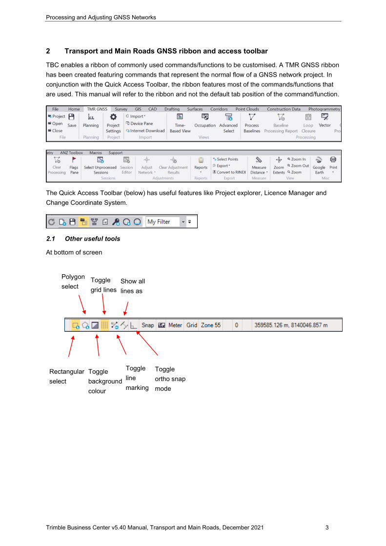
2 Transport and Main Roads GNSS ribbon and access toolbar
TBC enables a ribbon of commonly used commands/functions to be customised. A TMR GNSS ribbon has been created featuring commands that represent the normal flow of a GNSS network project. In conjunction with the Quick Access Toolbar, the ribbon features most of the commands/functions that are used. This manual will refer to the ribbon and not the default tab position of the command/function.
The Quick Access Toolbar (below) has useful features like Project explorer, Licence Manager and Change Coordinate System.
2.1 Other useful tools
At bottom of screen
Rectangular select
Polygon select
Toggle background colour
Toggle grid lines
Toggle line marking
Show all lines as
Toggle ortho snap mode
Processing and Adjusting GNSS Networks
Trimble Business Center v5.40 Manual, Transport and Main Roads, December 2021 4
3 Create and setup a new project
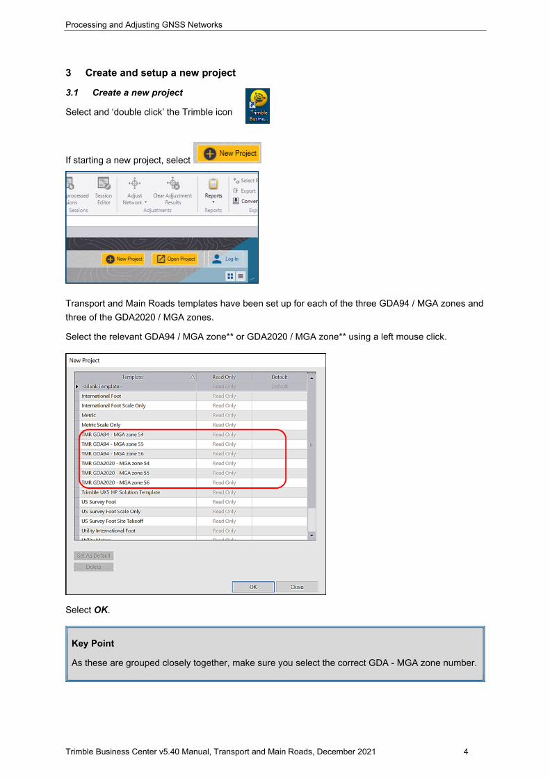
3.1 Create a new project
Select and ‘double click’ the Trimble icon
If starting a new project, select
Transport and Main Roads templates have been set up for each of the three GDA94 / MGA zones and three of the GDA2020 / MGA zones.
Select the relevant GDA94 / MGA zone** or GDA2020 / MGA zone** using a left mouse click.
Select OK.
Key Point
As these are grouped closely together, make sure you select the correct GDA - MGA zone number.
Processing and Adjusting GNSS Networks
Trimble Business Center v5.40 Manual, Transport and Main Roads, December 2021 5
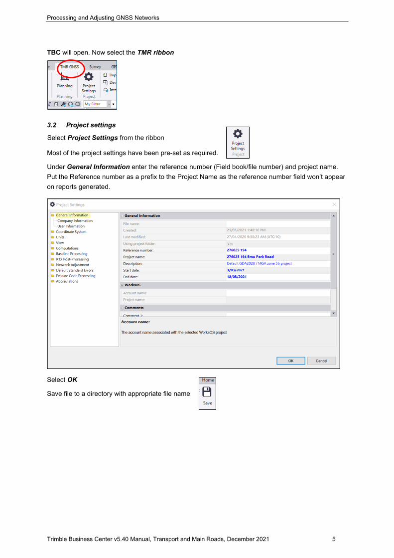
TBC will open. Now select the TMR ribbon
3.2 Project settings
Most of the project settings have been pre-set as required.
Under General Information enter the reference number (Field book/file number) and project name. Put the Reference number as a prefix to the Project Name as the reference number field won’t appear on reports generated.
Select OK
Save file to a directory with appropriate file name
Select Project Settings from the ribbon
Processing and Adjusting GNSS Networks
Trimble Business Center v5.40 Manual, Transport and Main Roads, December 2021 6
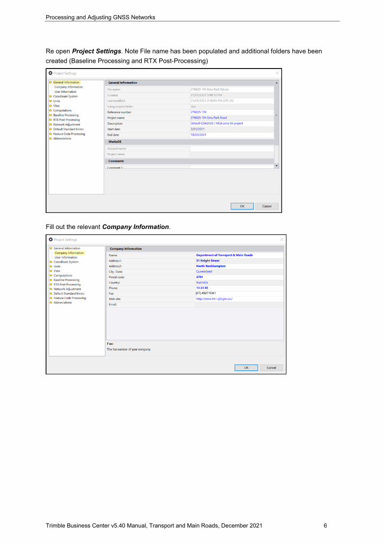
Re open Project Settings. Note File name has been populated and additional folders have been created (Baseline Processing and RTX Post-Processing)
Fill out the relevant Company Information.
Processing and Adjusting GNSS Networks
Trimble Business Center v5.40 Manual, Transport and Main Roads, December 2021 7
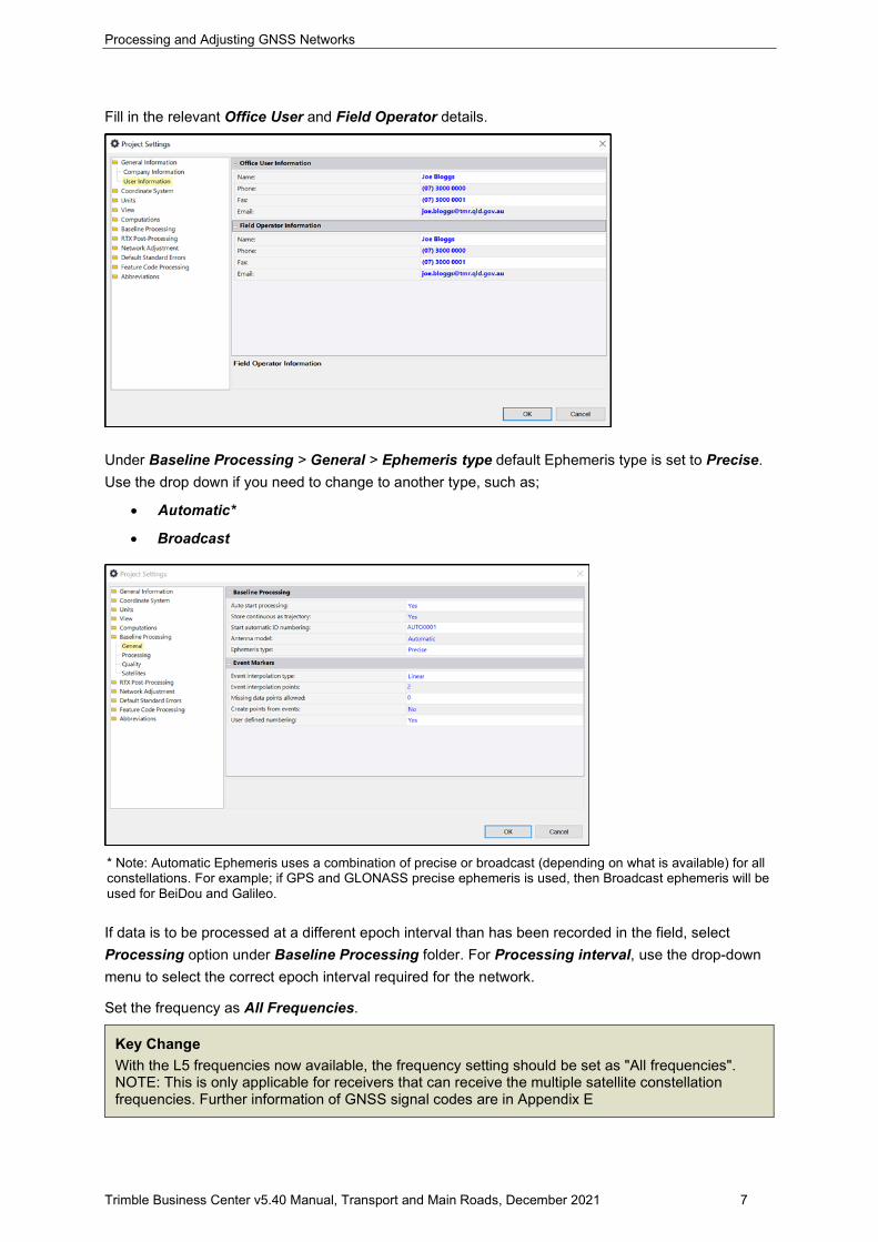
Fill in the relevant Office User and Field Operator details.
Under Baseline Processing > General > Ephemeris type default Ephemeris type is set to Precise. Use the drop down if you need to change to another type, such as;
• Automatic*
• Broadcast
* Note: Automatic Ephemeris uses a combination of precise or broadcast (depending on what is available) for all constellations. For example; if GPS and GLONASS precise ephemeris is used, then Broadcast ephemeris will be used for BeiDou and Galileo.
If data is to be processed at a different epoch interval than has been recorded in the field, select Processing option under Baseline Processing folder. For Processing interval, use the drop-down menu to select the correct epoch interval required for the network.
Set the frequency as All Frequencies.
Key Change With the L5 frequencies now available, the frequency setting should be set as "All frequencies". NOTE: This is only applicable for receivers that can receive the multiple satellite constellation frequencies. Further information of GNSS signal codes are in Appendix E
Processing and Adjusting GNSS Networks
Trimble Business Center v5.40 Manual, Transport and Main Roads, December 2021 8
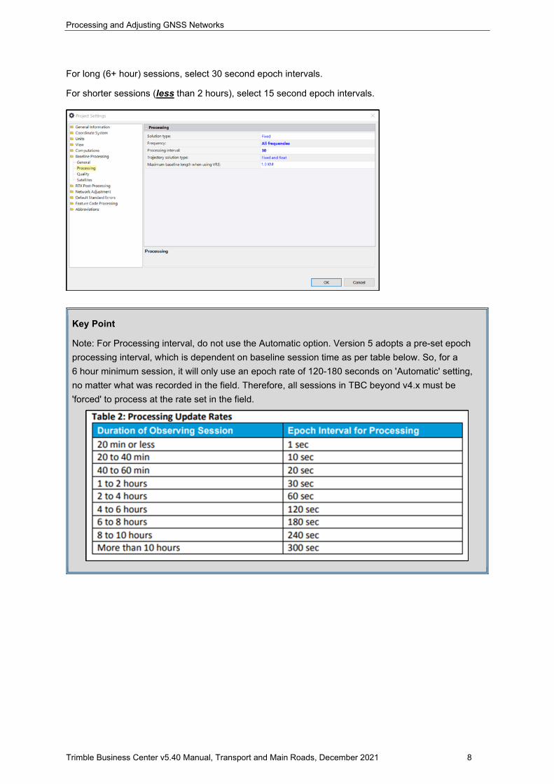
For long (6+ hour) sessions, select 30 second epoch intervals.
For shorter sessions (less than 2 hours), select 15 second epoch intervals.
Key Point
Note: For Processing interval, do not use the Automatic option. Version 5 adopts a pre-set epoch processing interval, which is dependent on baseline session time as per table below. So, for a 6 hour minimum session, it will only use an epoch rate of 120-180 seconds on 'Automatic' setting, no matter what was recorded in the field. Therefore, all sessions in TBC beyond v4.x must be 'forced' to process at the rate set in the field.
Processing and Adjusting GNSS Networks
Trimble Business Center v5.40 Manual, Transport and Main Roads, December 2021 9
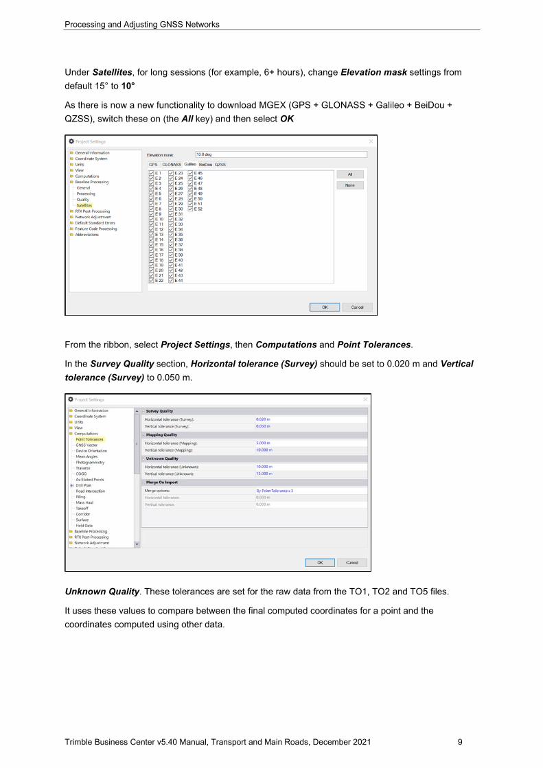
Under Satellites, for long sessions (for example, 6+ hours), change Elevation mask settings from default 15° to 10°
As there is now a new functionality to download MGEX (GPS + GLONASS + Galileo + BeiDou + QZSS), switch these on (the All key) and then select OK
From the ribbon, select Project Settings, then Computations and Point Tolerances.
In the Survey Quality section, Horizontal tolerance (Survey) should be set to 0.020 m and Vertical tolerance (Survey) to 0.050 m.
Unknown Quality. These tolerances are set for the raw data from the TO1, TO2 and TO5 files.
It uses these values to compare between the final computed coordinates for a point and the coordinates computed using other data.
Processing and Adjusting GNSS Networks
Trimble Business Center v5.40 Manual, Transport and Main Roads, December 2021 10
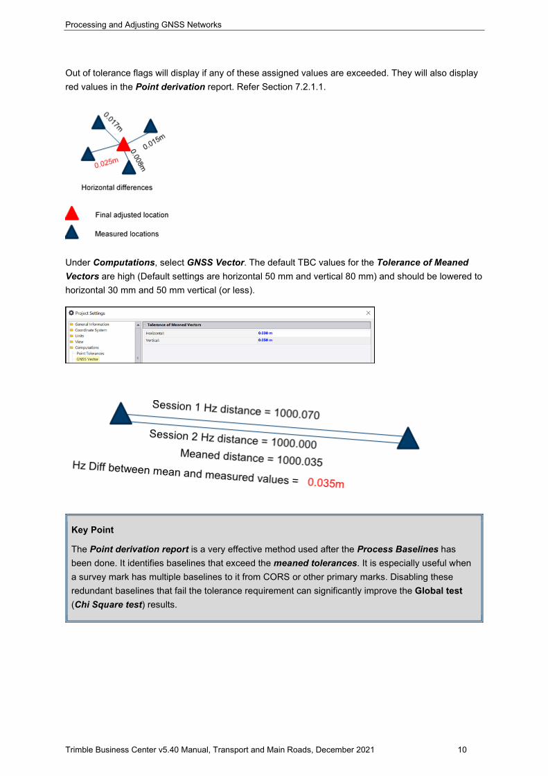
Out of tolerance flags will display if any of these assigned values are exceeded. They will also display red values in the Point derivation report. Refer Section 7.2.1.1.
Under Computations, select GNSS Vector. The default TBC values for the Tolerance of Meaned Vectors are high (Default settings are horizontal 50 mm and vertical 80 mm) and should be lowered to horizontal 30 mm and 50 mm vertical (or less).
Key Point
The Point derivation report is a very effective method used after the Process Baselines has been done. It identifies baselines that exceed the meaned tolerances. It is especially useful when a survey mark has multiple baselines to it from CORS or other primary marks. Disabling these redundant baselines that fail the tolerance requirement can significantly improve the Global test (Chi Square test) results.
Processing and Adjusting GNSS Networks
Trimble Business Center v5.40 Manual, Transport and Main Roads, December 2021 11
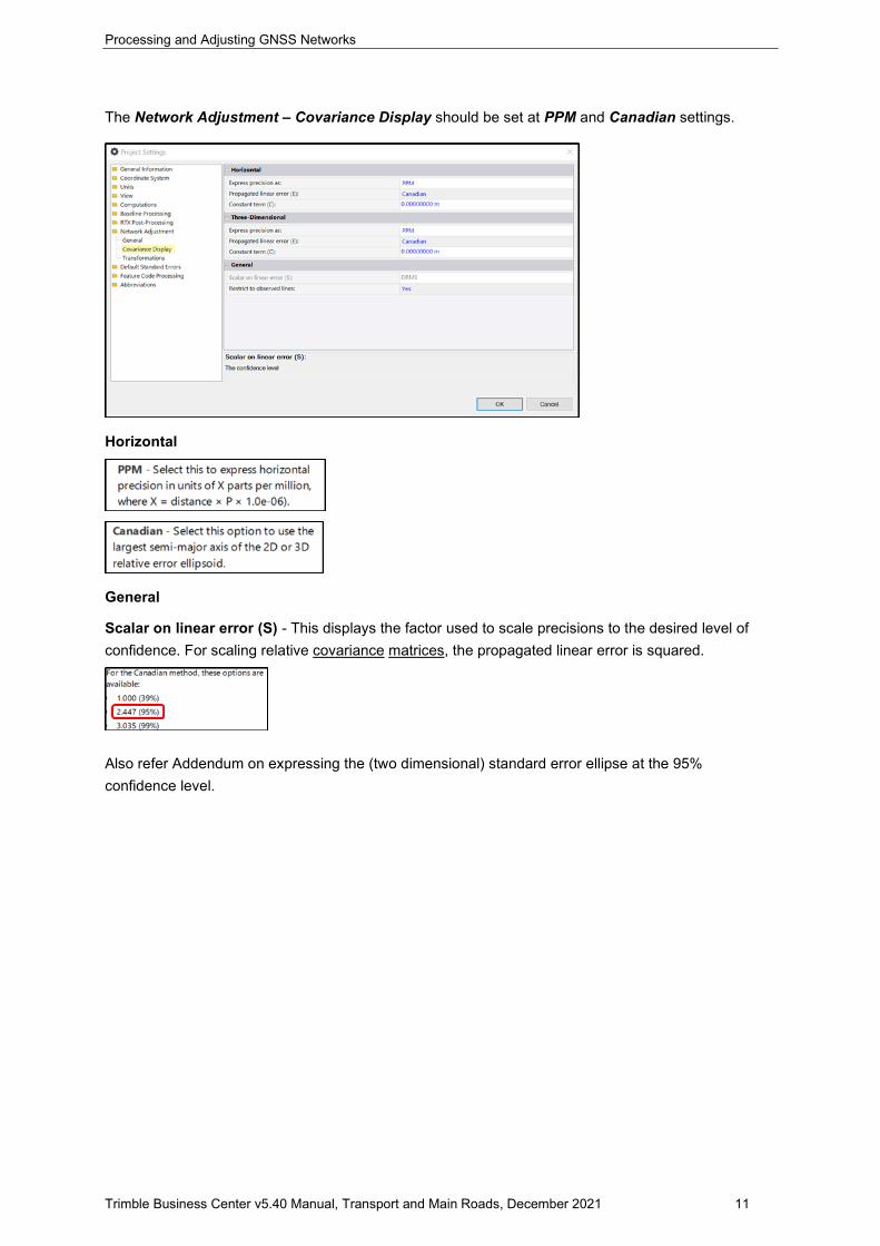
The Network Adjustment – Covariance Display should be set at PPM and Canadian settings.
Horizontal
General
Scalar on linear error (S) - This displays the factor used to scale precisions to the desired level of confidence. For scaling relative covariance matrices, the propagated linear error is squared.
Also refer Addendum on expressing the (two dimensional) standard error ellipse at the 95% confidence level.
Processing and Adjusting GNSS Networks
Trimble Business Center v5.40 Manual, Transport and Main Roads, December 2021 12
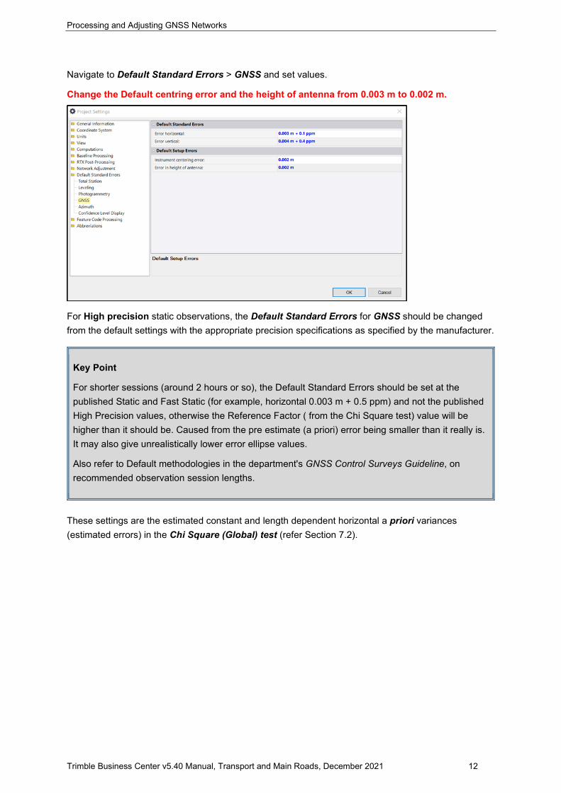
Navigate to Default Standard Errors > GNSS and set values.
Change the Default centring error and the height of antenna from 0.003 m to 0.002 m.
For High precision static observations, the Default Standard Errors for GNSS should be changed from the default settings with the appropriate precision specifications as specified by the manufacturer.
Key Point
For shorter sessions (around 2 hours or so), the Default Standard Errors should be set at the published Static and Fast Static (for example, horizontal 0.003 m + 0.5 ppm) and not the published High Precision values, otherwise the Reference Factor ( from the Chi Square test) value will be higher than it should be. Caused from the pre estimate (a priori) error being smaller than it really is. It may also give unrealistically lower error ellipse values.
Also refer to Default methodologies in the department's GNSS Control Surveys Guideline, on recommended observation session lengths.
These settings are the estimated constant and length dependent horizontal a priori variances (estimated errors) in the Chi Square (Global) test (refer Section 7.2).
Processing and Adjusting GNSS Networks
Trimble Business Center v5.40 Manual, Transport and Main Roads, December 2021 13
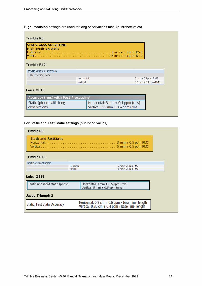
High Precision settings are used for long observation times. (published vales).
Trimble R8
Trimble R10
Leica GS15
For Static and Fast Static settings (published values).
Trimble R8
Trimble R10
Leica GS15
Javad Triumph 2
Processing and Adjusting GNSS Networks
Trimble Business Center v5.40 Manual, Transport and Main Roads, December 2021 14
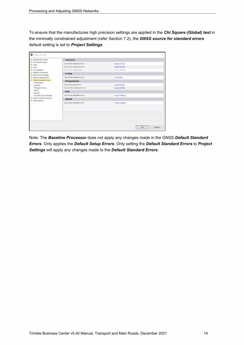
To ensure that the manufactures high precision settings are applied in the Chi Square (Global) test in the minimally constrained adjustment (refer Section 7.2), the GNSS source for standard errors default setting is set to Project Settings.
Note: The Baseline Processor does not apply any changes made in the GNSS Default Standard Errors. Only applies the Default Setup Errors. Only setting the Default Standard Errors to Project Settings will apply any changes made to the Default Standard Errors.
Processing and Adjusting GNSS Networks
Trimble Business Center v5.40 Manual, Transport and Main Roads, December 2021 15
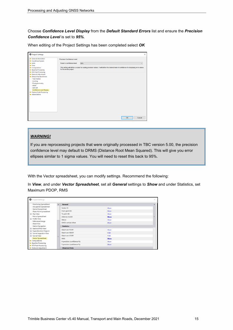
Choose Confidence Level Display from the Default Standard Errors list and ensure the Precision Confidence Level is set to 95%.
When editing of the Project Settings has been completed select OK
WARNING!
If you are reprocessing projects that were originally processed in TBC version 5.00, the precision confidence level may default to DRMS (Distance Root Mean Squared). This will give you error ellipses similar to 1 sigma values. You will need to reset this back to 95%.
With the Vector spreadsheet, you can modify settings. Recommend the following:
In View, and under Vector Spreadsheet, set all General settings to Show and under Statistics, set Maximum PDOP, RMS
Processing and Adjusting GNSS Networks
Trimble Business Center v5.40 Manual, Transport and Main Roads, December 2021 16
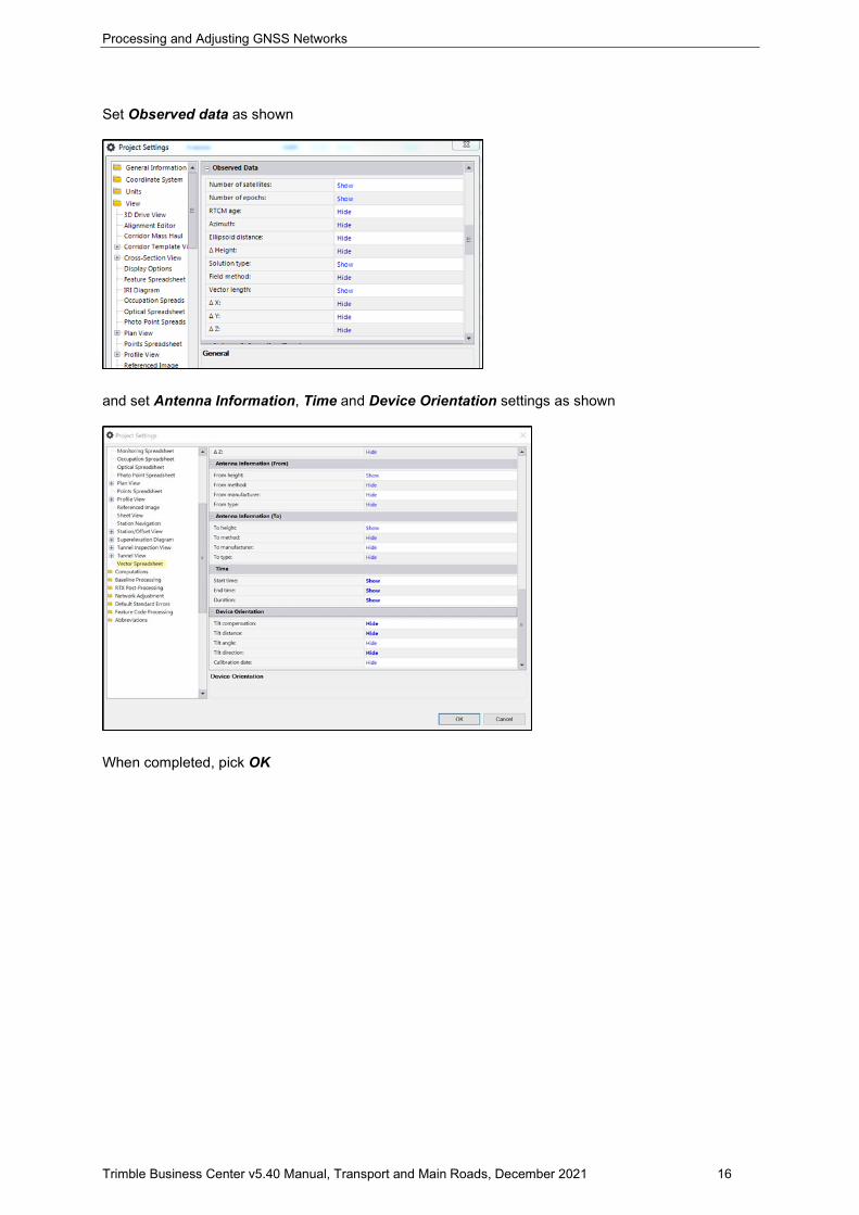
Set Observed data as shown
and set Antenna Information, Time and Device Orientation settings as shown
When completed, pick OK
Processing and Adjusting GNSS Networks
Trimble Business Center v5.40 Manual, Transport and Main Roads, December 2021 17
4 Create Network diagram (independent baselines only)
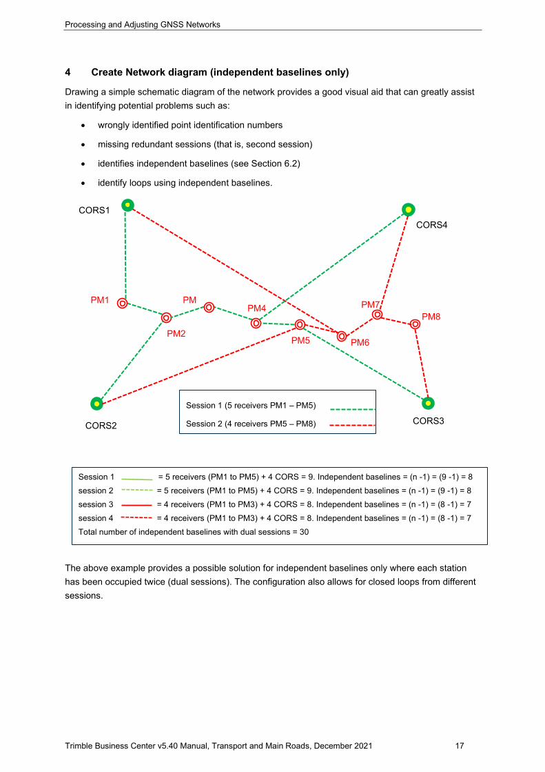
Drawing a simple schematic diagram of the network provides a good visual aid that can greatly assist in identifying potential problems such as:
• wrongly identified point identification numbers
• missing redundant sessions (that is, second session)
• identifies independent baselines (see Section 6.2)
• identify loops using independent baselines.
The above example provides a possible solution for independent baselines only where each station has been occupied twice (dual sessions). The configuration also allows for closed loops from different sessions.
Session 1 (5 receivers PM1 – PM5)
Session 2 (4 receivers PM5 – PM8)
PM5
PM7 PM4
CORS1 CORS4
PM
PM1
PM8
PM6 PM2
CORS3 CORS2
Session 1 = 5 receivers (PM1 to PM5) + 4 CORS = 9. Independent baselines = (n -1) = (9 -1) = 8 session 2 = 5 receivers (PM1 to PM5) + 4 CORS = 9. Independent baselines = (n -1) = (9 -1) = 8 session 3 = 4 receivers (PM1 to PM3) + 4 CORS = 8. Independent baselines = (n -1) = (8 -1) = 7 session 4 = 4 receivers (PM1 to PM3) + 4 CORS = 8. Independent baselines = (n -1) = (8 -1) = 7 Total number of independent baselines with dual sessions = 30
Processing and Adjusting GNSS Networks
Trimble Business Center v5.40 Manual, Transport and Main Roads, December 2021 18
5 Import data
5.1 Download data
Follow the manufacture's procedures to download data from the specific receiver used.
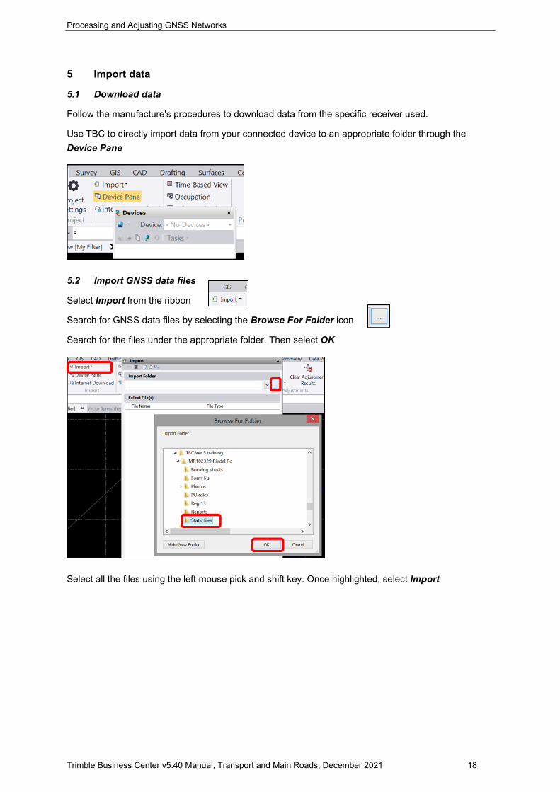
Use TBC to directly import data from your connected device to an appropriate folder through the Device Pane
5.2 Import GNSS data files
Select Import from the ribbon
Search for GNSS data files by selecting the Browse For Folder icon
Search for the files under the appropriate folder. Then select OK
Select all the files using the left mouse pick and shift key. Once highlighted, select Import
Processing and Adjusting GNSS Networks
Trimble Business Center v5.40 Manual, Transport and Main Roads, December 2021 19
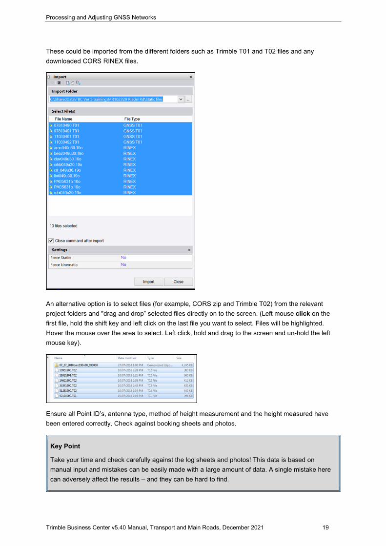
These could be imported from the different folders such as Trimble T01 and T02 files and any downloaded CORS RINEX files.
An alternative option is to select files (for example, CORS zip and Trimble T02) from the relevant project folders and "drag and drop” selected files directly on to the screen. (Left mouse click on the first file, hold the shift key and left click on the last file you want to select. Files will be highlighted. Hover the mouse over the area to select. Left click, hold and drag to the screen and un-hold the left mouse key).
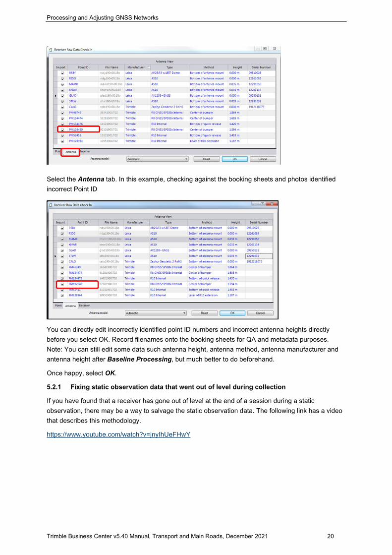
Ensure all Point ID’s, antenna type, method of height measurement and the height measured have been entered correctly. Check against booking sheets and photos.
Key Point
Take your time and check carefully against the log sheets and photos! This data is based on manual input and mistakes can be easily made with a large amount of data. A single mistake here can adversely affect the results – and they can be hard to find.
Processing and Adjusting GNSS Networks
Trimble Business Center v5.40 Manual, Transport and Main Roads, December 2021 20
Select the Antenna tab. In this example, checking against the booking sheets and photos identified incorrect Point ID
You can directly edit incorrectly identified point ID numbers and incorrect antenna heights directly before you select OK. Record filenames onto the booking sheets for QA and metadata purposes. Note: You can still edit some data such antenna height, antenna method, antenna manufacturer and antenna height after Baseline Processing, but much better to do beforehand.
Once happy, select OK.
5.2.1 Fixing static observation data that went out of level during collection
If you have found that a receiver has gone out of level at the end of a session during a static observation, there may be a way to salvage the static observation data. The following link has a video that describes this methodology.
https://www.youtube.com/watch?v=jnyIhUeFHwY
Processing and Adjusting GNSS Networks
Trimble Business Center v5.40 Manual, Transport and Main Roads, December 2021 21
5.2.2 Redundancy
Single occupation methods (single session) have no independency or redundancy. Two sessions provide redundancy on measured baselines. Check all that all independent baselines have at least two sessions. Also refer Section 6.2 on disabling dependent baselines.
A concept that's important in control work with GNSS is redundancy. Redundancy refers to several things, but one way to think of it is that the station is occupied more than once in the conduct of a survey. If it's occupied more than once, several good things happen. The receiver antenna is re-centred over the point more than once. Its height is recorded more than once. And, obviously, baselines or vectors are coming into the point from other stations other than the ones originally located. Redundancy, in other words, being measured more than once, is a useful thing in trying to evaluate the accuracy or the correctness of a network. If one were to use such a scheme on a project and connect into one loop of all the multiple baselines determined by multiple receivers in two sessions, the resulting error of closure would be useful. It could be used to detect mistakes in the work, such as mis-measured heights of instruments. Such a loop would include different sessions. The ranges between the satellites and the receivers defining the baselines in such a circuit would be from different constellations at different times. On the other hand, if it were possible to occupy all stations with multiple receivers simultaneously and do the entire survey in one session, a loop closure would be meaningless (refer Section 6.3.1). GNSS for Geospatial Professionals (https://www.e-education.psu.edu/geog862) Errors caused by lack of redundant measurements Experience has shown that during a static GNSS survey (using dual-frequency geodetic equipment), it is possible to get good loop closure and have very small residuals in the network adjustment, yet still have large errors in the adjusted positions of some stations. This can happen if stations are occupied in one session only. Source: GPS guidebook – Standards and guidelines for land surveying using Global Positioning Systems methods Nov 2004 Ver 1. Survey Advisory Board and the Public Land Survey Office for Washington Department of Natural Resources
5.3 Import Ephemeris data
To obtain the most accurate GNSS Control networks, import final (precise) ephemeris data. It has a latency of 12-18 days. It is especially useful on larger projects covering over 50 km, projects with baselines exceeding 50 km, and where atmospheric events like solar flares have occurred. There are different ephemeris products available. The major ones are:
• Broadcast ephemeris is transmitted by the satellites every 30 seconds but is a projection of expected location and its clock behaviour and therefore not precise.
• Rapid ephemeris is only available for GPS satellites and is usually available with approximately 17 hours latency. The Rapid will make noticeable improvements to the baseline processing results.
• Final (precise) ephemeris is the most precise available but has a latency of 12-18 days. It is especially useful on larger projects covering over 50 km, projects with baselines exceeding 50 km, and where atmospheric events like solar flares have occurred.
Processing and Adjusting GNSS Networks
Trimble Business Center v5.40 Manual, Transport and Main Roads, December 2021 22
It is highly recommended to process using the Final (precise) ephemeris whenever possible. The Rapid ephemeris should be the minimum used. However, GLONASS satellite data will not be used. If the site has poor satellite availability due to obstructions like trees or buildings requiring GLONASS to be used, project planning should allow time for the Final Ephemeris to become available.
Key Point
Broadcast ephemeris should only be used for preliminary processing. However, if proper field practices are followed that include generous session logging lengths for projects covering less than 50 km or baseline lengths less than 50 km, the broadcast ephemeris should generally give reasonable results.
5.3.1 Download ephemeris data
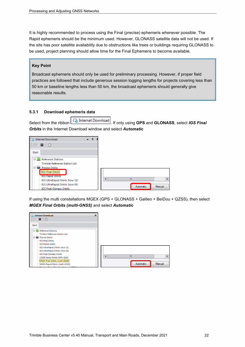
Select from the ribbon . If only using GPS and GLONASS, select IGS Final Orbits in the Internet Download window and select Automatic
If using the multi constellations MGEX (GPS + GLONASS + Galileo + BeiDou + QZSS), then select MGEX Final Orbits (multi-GNSS) and select Automatic
Processing and Adjusting GNSS Networks
Trimble Business Center v5.40 Manual, Transport and Main Roads, December 2021 23
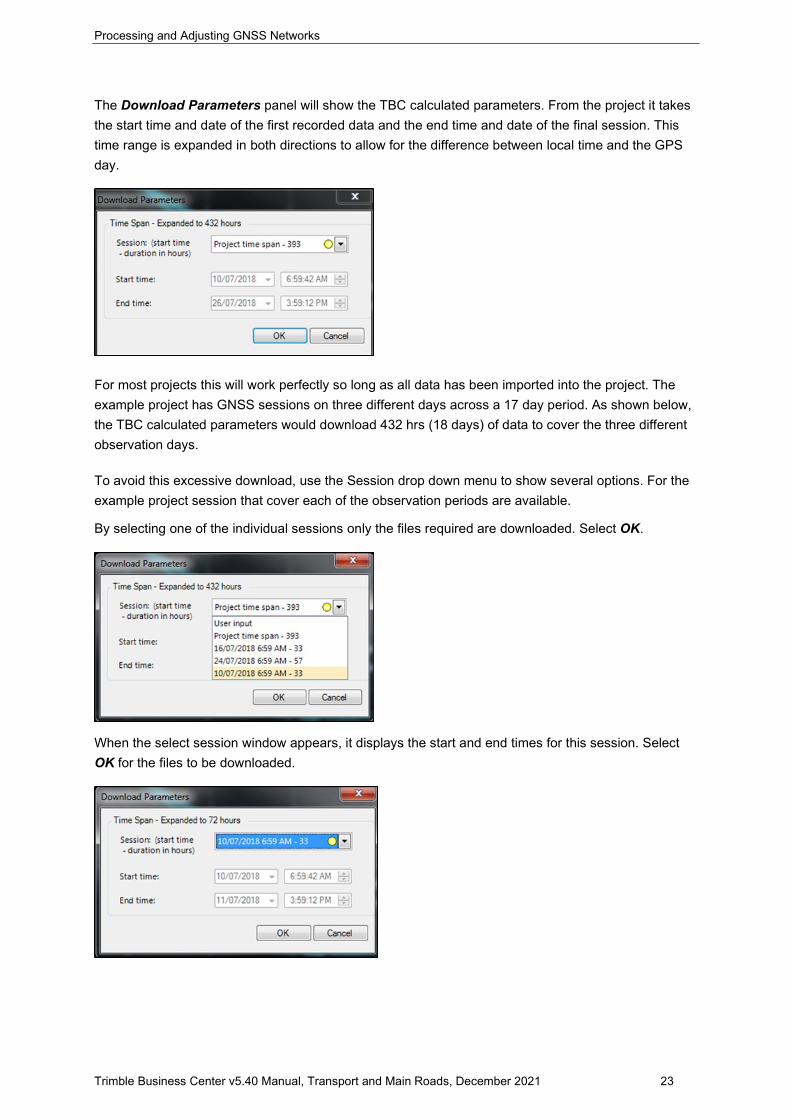
The Download Parameters panel will show the TBC calculated parameters. From the project it takes the start time and date of the first recorded data and the end time and date of the final session. This time range is expanded in both directions to allow for the difference between local time and the GPS day.
For most projects this will work perfectly so long as all data has been imported into the project. The example project has GNSS sessions on three different days across a 17 day period. As shown below, the TBC calculated parameters would download 432 hrs (18 days) of data to cover the three different observation days.
To avoid this excessive download, use the Session drop down menu to show several options. For the example project session that cover each of the observation periods are available.
By selecting one of the individual sessions only the files required are downloaded. Select OK.
When the select session window appears, it displays the start and end times for this session. Select OK for the files to be downloaded.
Processing and Adjusting GNSS Networks
Trimble Business Center v5.40 Manual, Transport and Main Roads, December 2021 24
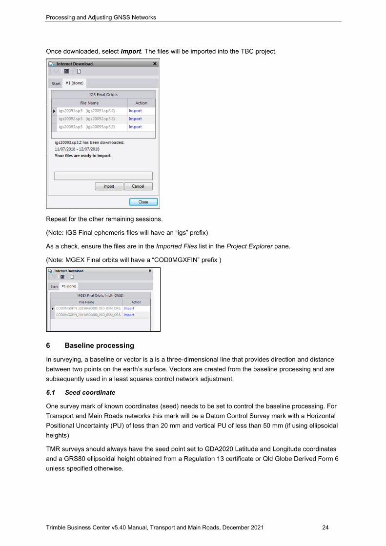
Once downloaded, select Import. The files will be imported into the TBC project.
Repeat for the other remaining sessions.
(Note: IGS Final ephemeris files will have an “igs” prefix)
As a check, ensure the files are in the Imported Files list in the Project Explorer pane.
(Note: MGEX Final orbits will have a “COD0MGXFIN” prefix )
6 Baseline processing
In surveying, a baseline or vector is a is a three-dimensional line that provides direction and distance between two points on the earth’s surface. Vectors are created from the baseline processing and are subsequently used in a least squares control network adjustment.
6.1 Seed coordinate
One survey mark of known coordinates (seed) needs to be set to control the baseline processing. For Transport and Main Roads networks this mark will be a Datum Control Survey mark with a Horizontal Positional Uncertainty (PU) of less than 20 mm and vertical PU of less than 50 mm (if using ellipsoidal heights)
TMR surveys should always have the seed point set to GDA2020 Latitude and Longitude coordinates and a GRS80 ellipsoidal height obtained from a Regulation 13 certificate or Qld Globe Derived Form 6 unless specified otherwise.
Processing and Adjusting GNSS Networks
Trimble Business Center v5.40 Manual, Transport and Main Roads, December 2021 25
Horizontal Registered PSM’s used as Datum Control to derive horizontal coordinates of the survey control network shall have a Horizontal Positional Uncertainty of < 0.020 m. A hierarchical system shall be used when selecting Datum Control PSM’s based on GDA2020 horizontal uncertainty, suitability and stability of the mark. Distance from the project site is also an important consideration. In descending order of desirability:
i. Tier 1 and 2 Continuously Operating Reference Stations (CORS) with Regulation 13 certificate ii. Tier 3 Continuously Operating Reference Stations (CORS) iii. QLD ANJ adjustment PSM’s with PU < 0.020 m iv. PSM’s with PU < 0.020 m.
Vertical A hierarchical system shall be used when selecting PSM’s to derive the height of project survey control. The system is based on GDA2020 ellipsoidal vertical positional uncertainty, AHD quality, and stability of the mark. Distance from the project site is also an important consideration.
i. QLD ANJ adjustment PSM’s with Ellipsoidal PU < 0.050 m & AHD 3rd Order Class C quality ii. AHD 3rd Order Class C quality PSM’s iii. QLD ANJ adjustment PSM’s with Ellipsoidal PU < 0.050 m & AHD 4th Order (minimum
Class D) quality iv. AHD 4th Order (minimum Class D) quality PSM’s.
TMR Surveying Standards
6.1.1 Regulation 13 Certificates
Download reg13 data directly from SmartNet Australia using the following link:
http://smartnetaus.com/reg13/index.html#5/-26.706/134.912
Note: You may need to copy the website’s URL (link) to the browser’s address bar.
The Trimble VRS link is:
https://www.vrsnow.com.au/Map/SensorMap.aspx
Key Point
Note: The values from these links are published in GDA2020. If working with a GDA94 project you will need to calculate values back to GDA94. This can be calculated using 12d Model. A document “Transformations from GDA2020 to GDA94” is located at the following link: https://www.tmr.qld.gov.au/business-industry/Technical-standards-publications/Surveying-support-documents
6.1.2 PM Form 6
If CORS have not been used in the network, select a control PM with the best Uncertainty values. Use Qld Globe to search for most current values. Use the following link:
https://qldglobe.information.qld.gov.au/?topic=surveying
This link displays permanent marks and lot and plan numbers on screen. To select a specific PM
Processing and Adjusting GNSS Networks
Trimble Business Center v5.40 Manual, Transport and Main Roads, December 2021 26
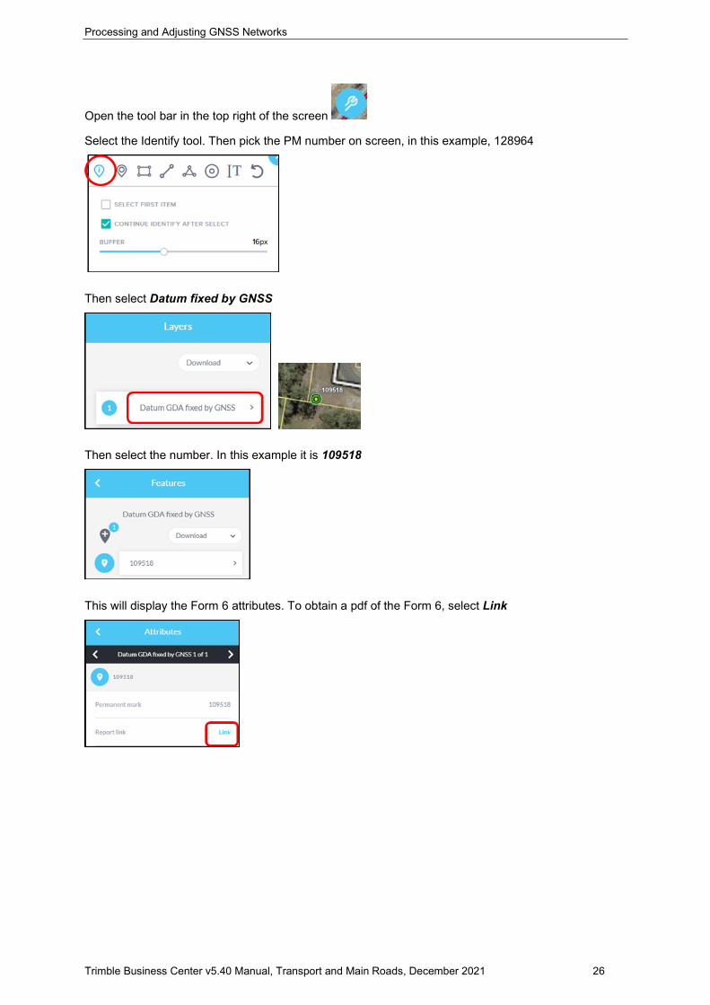
Open the tool bar in the top right of the screen
Select the Identify tool. Then pick the PM number on screen, in this example, 128964
Then select Datum fixed by GNSS
Then select the number. In this example it is 109518
This will display the Form 6 attributes. To obtain a pdf of the Form 6, select Link
Processing and Adjusting GNSS Networks
Trimble Business Center v5.40 Manual, Transport and Main Roads, December 2021 27
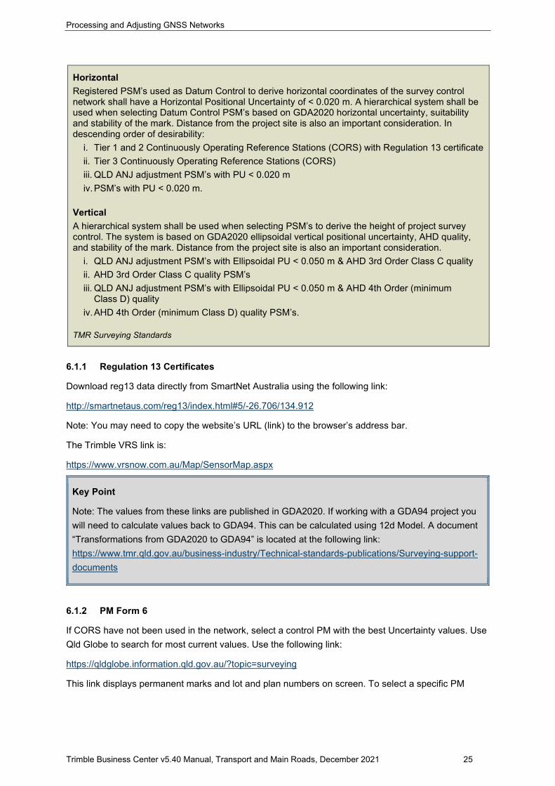
A Qld Globe Form 6 will now be downloaded and display the Horizontal and Vertical Uncertainty of GDA2020 Latitude, Longitude and Ellipsoidal Height of PM’s included in the ANJ adjustment. Choose the PM with the best Uncertainty values as the seed point.
6.1.3 Selecting the seed coordinate
The Datum Control Survey mark with the best Uncertainty values for horizontal and vertical (ellipsoidal) quality should be seeded. A Least Squares Adjustment works best when the adjustments required are minimal. Inaccurate seed coordinates adversely affect the accuracy of the baseline results and therefore the adjustment.
If the network includes CORS they should generally be selected as the Seed point. In addition to having very good Uncertainty values, CORS are likely to be more stable and less likely to be disturbed than a traditional PM. The coordinated position of CORS are regularly checked against Australia’s fundamental network giving extra confidence in the mark. (Be aware some CORS are moving and their Reg 13’s have not been updated)
If the network does not include CORS, the ANJ adjustment PM with the best uncertainties is the next best option. Consideration should also be given to the quality of the mark (stability, condition and obstructions present) and its influence in the network (distance to the project, number of baselines to the mark). For example, seeding a PM with 8 mm uncertainty that is in unstable country, remote to the project, surrounded by trees and with only two baselines to it, may not be the best choice. All of these potential influences need to be considered when assessing the appropriate mark.
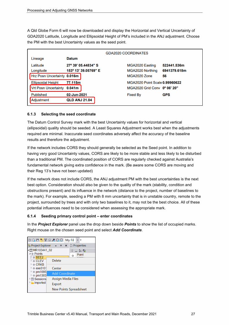
6.1.4 Seeding primary control point – enter coordinates
In the Project Explorer panel use the drop down beside Points to show the list of occupied marks. Right mouse on the chosen seed point and select Add Coordinate.
Processing and Adjusting GNSS Networks
Trimble Business Center v5.40 Manual, Transport and Main Roads, December 2021 28
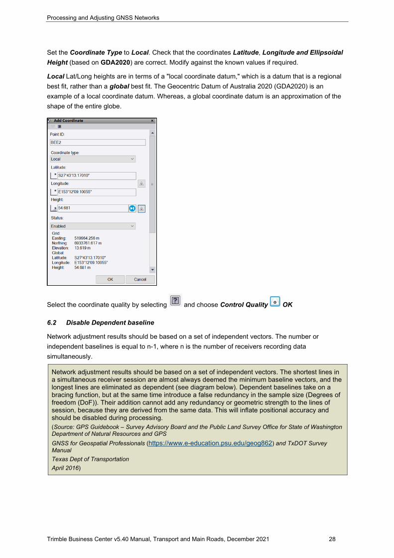
Set the Coordinate Type to Local. Check that the coordinates Latitude, Longitude and Ellipsoidal Height (based on GDA2020) are correct. Modify against the known values if required.
Local Lat/Long heights are in terms of a "local coordinate datum," which is a datum that is a regional best fit, rather than a global best fit. The Geocentric Datum of Australia 2020 (GDA2020) is an example of a local coordinate datum. Whereas, a global coordinate datum is an approximation of the shape of the entire globe.
Select the coordinate quality by selecting and choose Control Quality OK
6.2 Disable Dependent baseline
Network adjustment results should be based on a set of independent vectors. The number or independent baselines is equal to n-1, where n is the number of receivers recording data simultaneously.
Network adjustment results should be based on a set of independent vectors. The shortest lines in a simultaneous receiver session are almost always deemed the minimum baseline vectors, and the longest lines are eliminated as dependent (see diagram below). Dependent baselines take on a bracing function, but at the same time introduce a false redundancy in the sample size (Degrees of freedom (DoF)). Their addition cannot add any redundancy or geometric strength to the lines of session, because they are derived from the same data. This will inflate positional accuracy and should be disabled during processing. (Source: GPS Guidebook – Survey Advisory Board and the Public Land Survey Office for State of Washington Department of Natural Resources and GPS GNSS for Geospatial Professionals (https://www.e-education.psu.edu/geog862) and TxDOT Survey Manual Texas Dept of Transportation April 2016)
Processing and Adjusting GNSS Networks
Trimble Business Center v5.40 Manual, Transport and Main Roads, December 2021 29
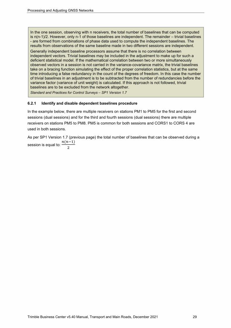
In the one session, observing with n receivers, the total number of baselines that can be computed is n(n-1)/2. However, only n-1 of those baselines are independent. The remainder – trivial baselines - are formed from combinations of phase data used to compute the independent baselines. The results from observations of the same baseline made in two different sessions are independent. Generally independent baseline processors assume that there is no correlation between independent vectors. Trivial baselines may be included in the adjustment to make up for such a deficient statistical model. If the mathematical correlation between two or more simultaneously observed vectors in a session is not carried in the variance-covariance matrix, the trivial baselines take on a bracing function simulating the effect of the proper correlation statistics, but at the same time introducing a false redundancy in the count of the degrees of freedom. In this case the number of trivial baselines in an adjustment is to be subtracted from the number of redundancies before the variance factor (variance of unit weight) is calculated. If this approach is not followed, trivial baselines are to be excluded from the network altogether. Standard and Practices for Control Surveys – SP1 Version 1.7
6.2.1 Identify and disable dependent baselines procedure
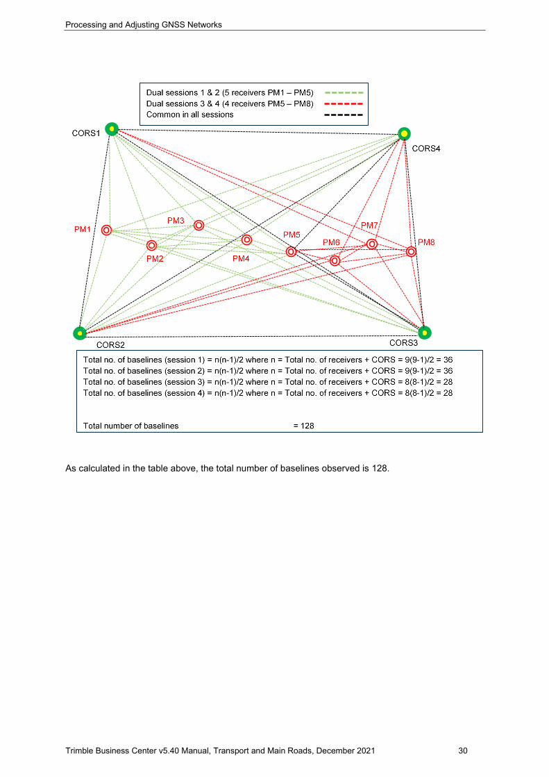
In the example below, there are multiple receivers on stations PM1 to PM5 for the first and second sessions (dual sessions) and for the third and fourth sessions (dual sessions) there are multiple receivers on stations PM5 to PM8. PM5 is common for both sessions and CORS1 to CORS 4 are used in both sessions.
As per SP1 Version 1.7 (previous page) the total number of baselines that can be observed during a
session is equal to: 𝑛𝑛(𝑛𝑛−1)
2
Processing and Adjusting GNSS Networks
Trimble Business Center v5.40 Manual, Transport and Main Roads, December 2021 30
As calculated in the table above, the total number of baselines observed is 128.
Processing and Adjusting GNSS Networks
Trimble Business Center v5.40 Manual, Transport and Main Roads, December 2021 31
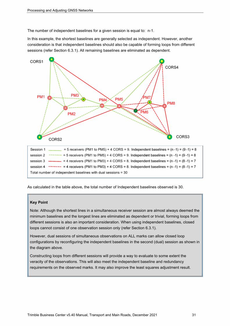
The number of independent baselines for a given session is equal to: n-1.
In this example, the shortest baselines are generally selected as independent. However, another consideration is that independent baselines should also be capable of forming loops from different sessions (refer Section 6.3.1). All remaining baselines are eliminated as dependent.
As calculated in the table above, the total number of Independent baselines observed is 30.
Key Point
Note: Although the shortest lines in a simultaneous receiver session are almost always deemed the minimum baselines and the longest lines are eliminated as dependent or trivial, forming loops from different sessions is also an important consideration. When using independent baselines, closed loops cannot consist of one observation session only (refer Section 6.3.1).
However, dual sessions of simultaneous observations on ALL marks can allow closed loop configurations by reconfiguring the independent baselines in the second (dual) session as shown in the diagram above.
Constructing loops from different sessions will provide a way to evaluate to some extent the veracity of the observations. This will also meet the independent baseline and redundancy requirements on the observed marks. It may also improve the least squares adjustment result.

Processing and Adjusting GNSS Networks
Trimble Business Center v5.40 Manual, Transport and Main Roads, December 2021 32
6.2.1.1 Project example 1
In the project example below (Figure 6.2.1.1(a)), there are 3 receivers occupying 2 permanent marks and a third survey mark that requires to be connected to GDA2020 datum by way of a network adjustment. In addition, there are 3 CORS used the dual sessions. Therefore, the total number of baselines equals 6(6 -1)/2 = 15 for each session. And the number of independent baselines for each session equals 6 -1 = 5.
The shortest lines in a simultaneous receiver session are almost always deemed the minimum baselines and the longest lines are eliminated as dependent or trivial. But you cannot obtain closed loops using the same sessions. However, it is possible to achieve closed loops with different sessions in each loop. It is often a trial and error process during the baseline processing and closed loops to achieve the optimum outcome.
Drawing a diagram as an aid (Figure 6.2.1.1 (b)), it is quite useful to use some form of desktop publishing or drawing software so that you can modify on the fly. This way as a visual tool, you can keep track of your changes, have the right number of baselines per session and can ensure that all the loops consist of different sessions. In addition to visually showing the different sessions, it also allows flexibility to distort the diagram to make cluttered areas much clearer. Another useful addition is to add the Positional Uncertainties (PU) values to the diagram. This can be helpful in selecting which marks should be held fixed in the constrained adjustment (especially for larger networks). In this example, the quality of all of the baselines from one of the CORS (CLEV) during the processing of the baselines (see 6.3) were too poor to be used and were disabled. So the number of independent baselines for each session was reduced to 5-1 = 4. Generally, baselines between CORS are not used.
Figure 6.2.1.1(a) – All baselines
Processing and Adjusting GNSS Networks
Trimble Business Center v5.40 Manual, Transport and Main Roads, December 2021 33
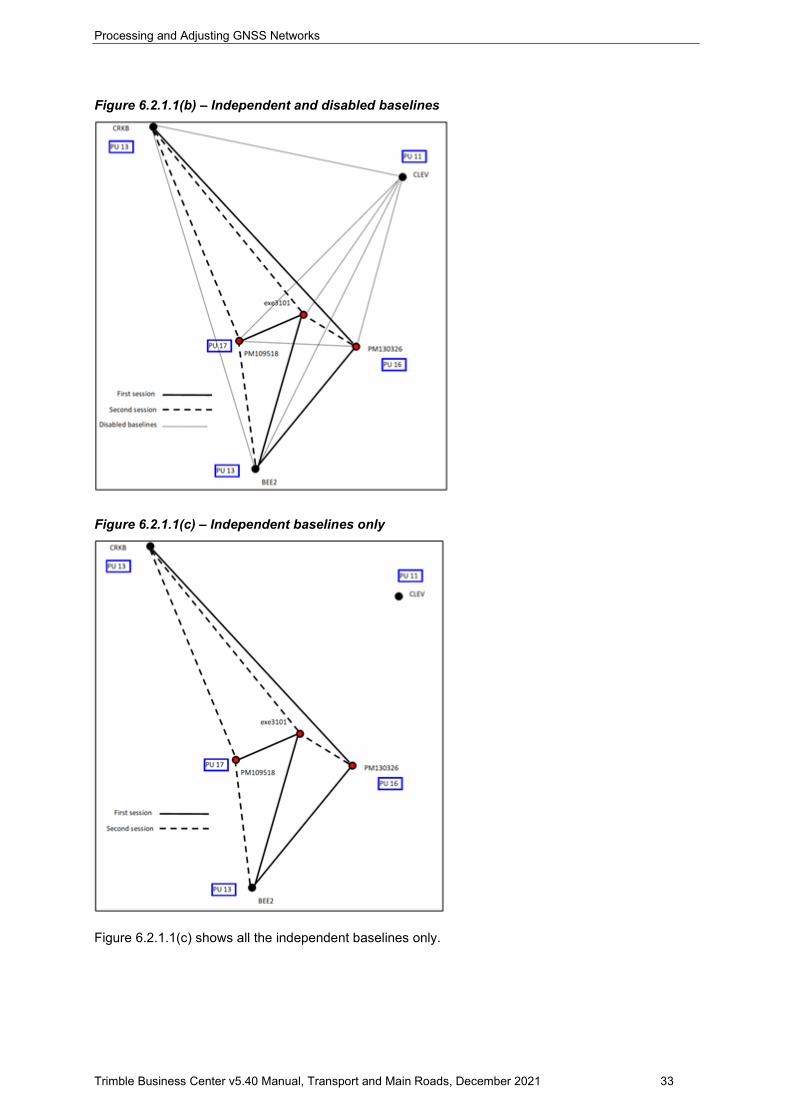
Figure 6.2.1.1(b) – Independent and disabled baselines
Figure 6.2.1.1(c) – Independent baselines only
Figure 6.2.1.1(c) shows all the independent baselines only.
Processing and Adjusting GNSS Networks
Trimble Business Center v5.40 Manual, Transport and Main Roads, December 2021 34
Key Point
NOTE: The most optimum baseline configurations when developing a network diagram is a trial and error process often not achieved until processing the baselines (see Section 6.3), undertaking loop closures (see 6.3.1) and the minimally constrained adjustment has been finalised. (See Section 7.2.1)
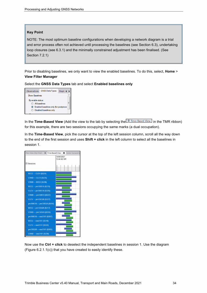
Prior to disabling baselines, we only want to view the enabled baselines. To do this, select, Home > View Filter Manager
Select the GNSS Data Types tab and select Enabled baselines only
In the Time-Based View (Add the view to the tab by selecting the in the TMR ribbon) for this example, there are two sessions occupying the same marks (a dual occupation).
In the Time-Based View, pick the cursor at the top of the left session column, scroll all the way down to the end of the first session and uses Shift + click in the left column to select all the baselines in session 1.
Now use the Ctrl + click to deselect the independent baselines in session 1. Use the diagram (Figure 6.2.1.1(c)) that you have created to easily identify these.
Processing and Adjusting GNSS Networks
Trimble Business Center v5.40 Manual, Transport and Main Roads, December 2021 35
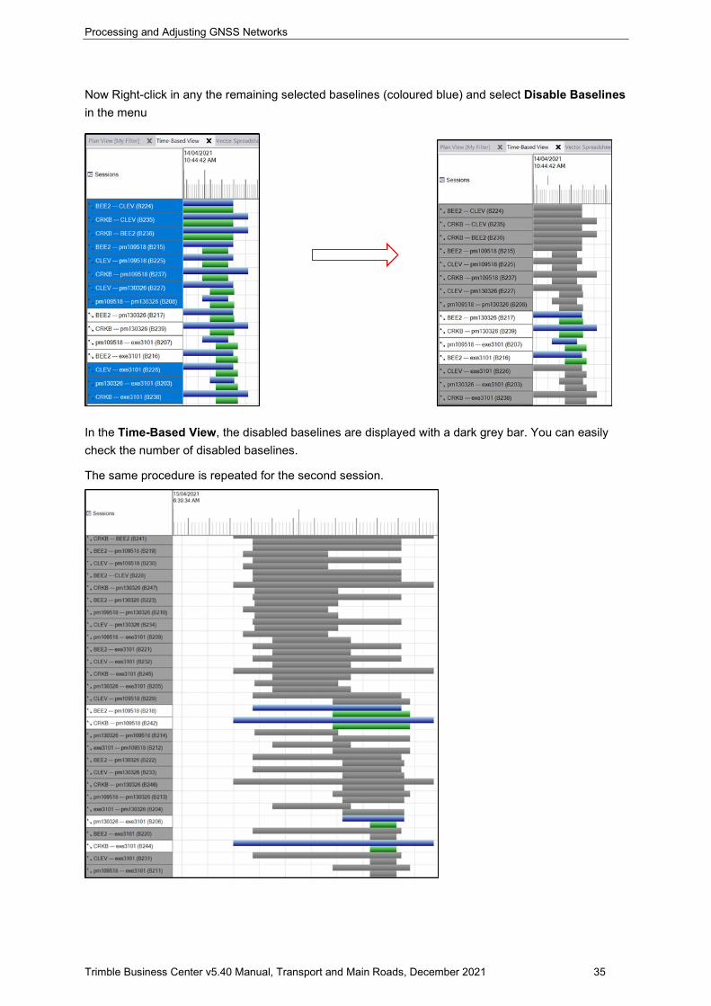
Now Right-click in any the remaining selected baselines (coloured blue) and select Disable Baselines in the menu
In the Time-Based View, the disabled baselines are displayed with a dark grey bar. You can easily check the number of disabled baselines.
The same procedure is repeated for the second session.
Processing and Adjusting GNSS Networks
Trimble Business Center v5.40 Manual, Transport and Main Roads, December 2021 36
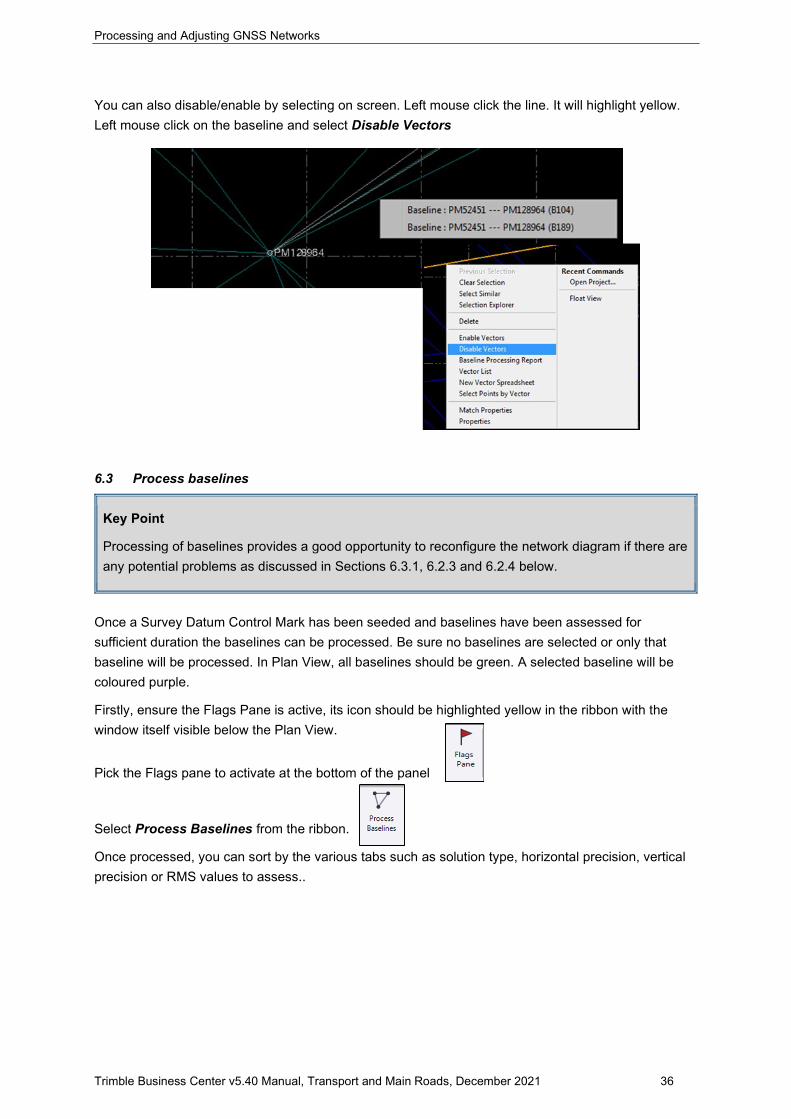
You can also disable/enable by selecting on screen. Left mouse click the line. It will highlight yellow. Left mouse click on the baseline and select Disable Vectors
6.3 Process baselines
Key Point
Processing of baselines provides a good opportunity to reconfigure the network diagram if there are any potential problems as discussed in Sections 6.3.1, 6.2.3 and 6.2.4 below.
Once a Survey Datum Control Mark has been seeded and baselines have been assessed for sufficient duration the baselines can be processed. Be sure no baselines are selected or only that baseline will be processed. In Plan View, all baselines should be green. A selected baseline will be coloured purple.
Firstly, ensure the Flags Pane is active, its icon should be highlighted yellow in the ribbon with the window itself visible below the Plan View.
Pick the Flags pane to activate at the bottom of the panel
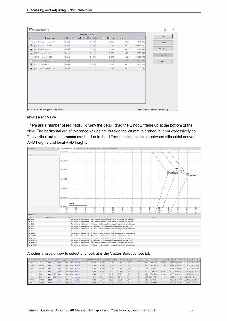
Select Process Baselines from the ribbon.
Once processed, you can sort by the various tabs such as solution type, horizontal precision, vertical precision or RMS values to assess..
Processing and Adjusting GNSS Networks
Trimble Business Center v5.40 Manual, Transport and Main Roads, December 2021 37
Now select Save
There are a number of red flags. To view the detail, drag the window frame up at the bottom of the view. The horizontal out of tolerance values are outside the 20 mm tolerance, but not excessively so. The vertical out of tolerances can be due to the differences/inaccuracies between ellipsoidal derived AHD heights and local AHD heights.
Another analysis view to select and look at is the Vector Spreadsheet tab.
Processing and Adjusting GNSS Networks
Trimble Business Center v5.40 Manual, Transport and Main Roads, December 2021 38
Although there are some high PDOP values (20.00), the other values of H. precision, V Precision and duration lengths are all reasonable.
6.3.1 Loop Closures
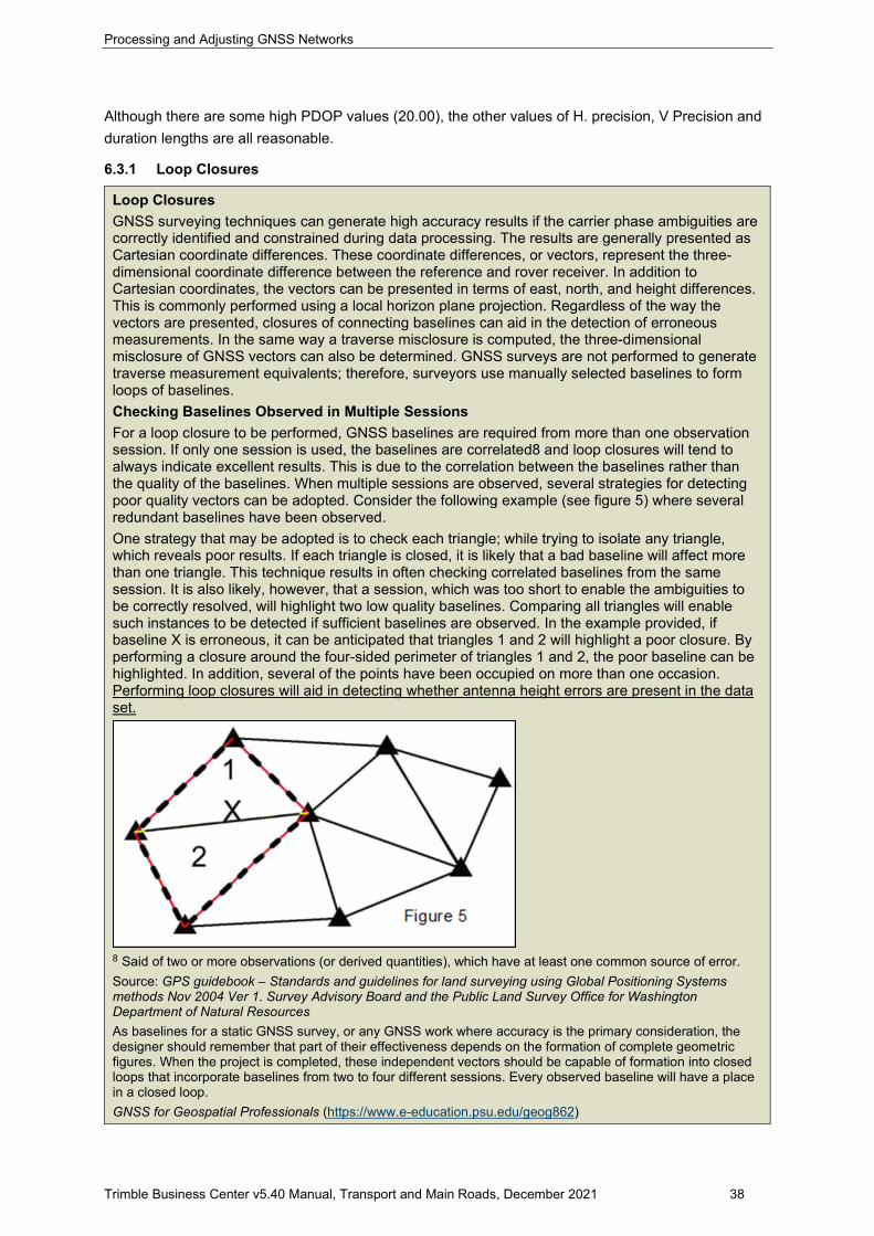
Loop Closures GNSS surveying techniques can generate high accuracy results if the carrier phase ambiguities are correctly identified and constrained during data processing. The results are generally presented as Cartesian coordinate differences. These coordinate differences, or vectors, represent the three-dimensional coordinate difference between the reference and rover receiver. In addition to Cartesian coordinates, the vectors can be presented in terms of east, north, and height differences. This is commonly performed using a local horizon plane projection. Regardless of the way the vectors are presented, closures of connecting baselines can aid in the detection of erroneous measurements. In the same way a traverse misclosure is computed, the three-dimensional misclosure of GNSS vectors can also be determined. GNSS surveys are not performed to generate traverse measurement equivalents; therefore, surveyors use manually selected baselines to form loops of baselines. Checking Baselines Observed in Multiple Sessions For a loop closure to be performed, GNSS baselines are required from more than one observation session. If only one session is used, the baselines are correlated8 and loop closures will tend to always indicate excellent results. This is due to the correlation between the baselines rather than the quality of the baselines. When multiple sessions are observed, several strategies for detecting poor quality vectors can be adopted. Consider the following example (see figure 5) where several redundant baselines have been observed. One strategy that may be adopted is to check each triangle; while trying to isolate any triangle, which reveals poor results. If each triangle is closed, it is likely that a bad baseline will affect more than one triangle. This technique results in often checking correlated baselines from the same session. It is also likely, however, that a session, which was too short to enable the ambiguities to be correctly resolved, will highlight two low quality baselines. Comparing all triangles will enable such instances to be detected if sufficient baselines are observed. In the example provided, if baseline X is erroneous, it can be anticipated that triangles 1 and 2 will highlight a poor closure. By performing a closure around the four-sided perimeter of triangles 1 and 2, the poor baseline can be highlighted. In addition, several of the points have been occupied on more than one occasion. Performing loop closures will aid in detecting whether antenna height errors are present in the data set.
8 Said of two or more observations (or derived quantities), which have at least one common source of error. Source: GPS guidebook – Standards and guidelines for land surveying using Global Positioning Systems methods Nov 2004 Ver 1. Survey Advisory Board and the Public Land Survey Office for Washington Department of Natural Resources As baselines for a static GNSS survey, or any GNSS work where accuracy is the primary consideration, the designer should remember that part of their effectiveness depends on the formation of complete geometric figures. When the project is completed, these independent vectors should be capable of formation into closed loops that incorporate baselines from two to four different sessions. Every observed baseline will have a place in a closed loop. GNSS for Geospatial Professionals (https://www.e-education.psu.edu/geog862)
Processing and Adjusting GNSS Networks
Trimble Business Center v5.40 Manual, Transport and Main Roads, December 2021 39
Loop closures are used to check the quality of and identify any excessive errors in a network of GNSS observations. GNSS Loop Closure should be run after successful processing of the baselines.
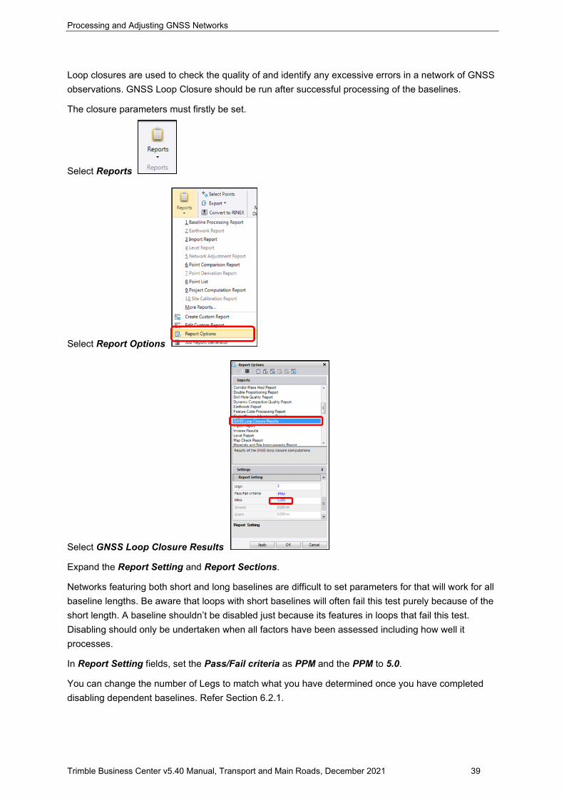
The closure parameters must firstly be set.
Select Reports
Select Report Options
Select GNSS Loop Closure Results
Expand the Report Setting and Report Sections.
Networks featuring both short and long baselines are difficult to set parameters for that will work for all baseline lengths. Be aware that loops with short baselines will often fail this test purely because of the short length. A baseline shouldn’t be disabled just because its features in loops that fail this test. Disabling should only be undertaken when all factors have been assessed including how well it processes.
In Report Setting fields, set the Pass/Fail criteria as PPM and the PPM to 5.0.
You can change the number of Legs to match what you have determined once you have completed disabling dependent baselines. Refer Section 6.2.1.
Processing and Adjusting GNSS Networks
Trimble Business Center v5.40 Manual, Transport and Main Roads, December 2021 40
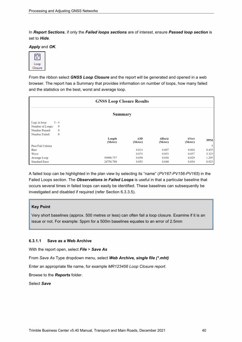
In Report Sections, if only the Failed loops sections are of interest, ensure Passed loop section is set to Hide.
Apply and OK.
From the ribbon select GNSS Loop Closure and the report will be generated and opened in a web browser. The report has a Summary that provides information on number of loops, how many failed and the statistics on the best, worst and average loop.
A failed loop can be highlighted in the plan view by selecting its “name” (PV167-PV156-PV165) in the Failed Loops section. The Observations in Failed Loops is useful in that a particular baseline that occurs several times in failed loops can easily be identified. These baselines can subsequently be investigated and disabled if required (refer Section 6.3.3.5).
Key Point
Very short baselines (approx. 500 metres or less) can often fail a loop closure. Examine if it is an issue or not. For example: 5ppm for a 500m baselines equates to an error of 2.5mm
6.3.1.1 Save as a Web Archive
With the report open, select File > Save As
From Save As Type dropdown menu, select Web Archive, single file (*.mht)
Enter an appropriate file name, for example MR123456 Loop Closure report.
Browse to the Reports folder.
Select Save
Processing and Adjusting GNSS Networks
Trimble Business Center v5.40 Manual, Transport and Main Roads, December 2021 41
Convert to PDF
With the report open;
If required, change the page orientation by selecting the dropdown arrow beside Convert on the PDF toolbar.
Select Preferences and then Page Layout tab. Change the Orientation as appropriate and OK.
Select Convert from the PDF toolbar.
Browse to the projects Reports folder and enter an appropriate file name, for example MR123456 Loop Closure report.
Select Save.
Print to PDF
With the report open, select File > Print
From the Select Printer list, select PDF995.
If required, change the page orientation by selecting Preferences and changing the orientation.
Select the Options tab and choose As laid out on screen.
Select Print, browse to the Reports folder and enter an appropriate file name, for example MR123456 Loop Closure report.
Select Save.
6.3.2 Potential problems
The following are examples of potential problems that can occur and how they can be identified, analysed and fixed.
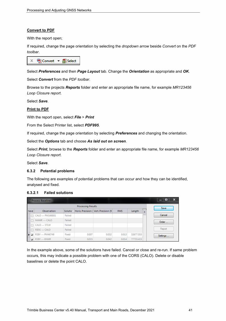
6.3.2.1 Failed solutions
In the example above, some of the solutions have failed. Cancel or close and re-run. If same problem occurs, this may indicate a possible problem with one of the CORS (CALO). Delete or disable baselines or delete the point CALO.
Processing and Adjusting GNSS Networks
Trimble Business Center v5.40 Manual, Transport and Main Roads, December 2021 42
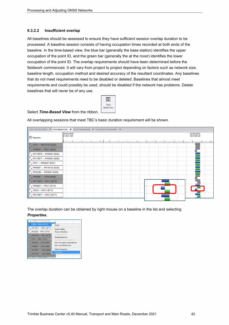
6.3.2.2 Insufficient overlap
All baselines should be assessed to ensure they have sufficient session overlap duration to be processed. A baseline session consists of having occupation times recorded at both ends of the baseline. In the time-based view, the blue bar (generally the base station) identifies the upper occupation of the point ID, and the green bar (generally the at the rover) identifies the lower occupation of the point ID. The overlap requirements should have been determined before the fieldwork commenced. It will vary from project to project depending on factors such as network size, baseline length, occupation method and desired accuracy of the resultant coordinates. Any baselines that do not meet requirements need to be disabled or deleted. Baselines that almost meet requirements and could possibly be used, should be disabled if the network has problems. Delete baselines that will never be of any use.
Select Time-Based View from the ribbon.
All overlapping sessions that meet TBC’s basic duration requirement will be shown.
The overlap duration can be obtained by right mouse on a baseline in the list and selecting Properties.
Processing and Adjusting GNSS Networks
Trimble Business Center v5.40 Manual, Transport and Main Roads, December 2021 43
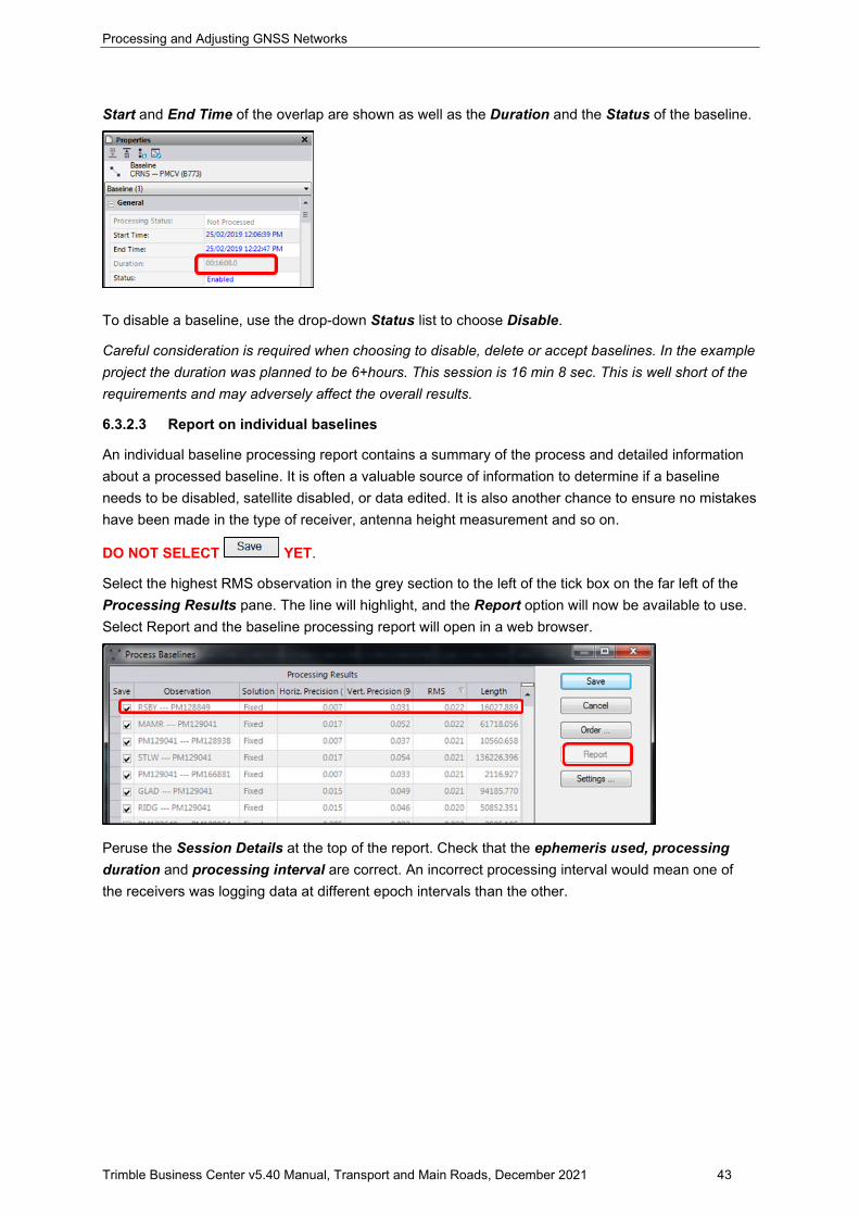
Start and End Time of the overlap are shown as well as the Duration and the Status of the baseline.
To disable a baseline, use the drop-down Status list to choose Disable.
Careful consideration is required when choosing to disable, delete or accept baselines. In the example project the duration was planned to be 6+hours. This session is 16 min 8 sec. This is well short of the requirements and may adversely affect the overall results.
6.3.2.3 Report on individual baselines
An individual baseline processing report contains a summary of the process and detailed information about a processed baseline. It is often a valuable source of information to determine if a baseline needs to be disabled, satellite disabled, or data edited. It is also another chance to ensure no mistakes have been made in the type of receiver, antenna height measurement and so on.
DO NOT SELECT YET.
Select the highest RMS observation in the grey section to the left of the tick box on the far left of the Processing Results pane. The line will highlight, and the Report option will now be available to use. Select Report and the baseline processing report will open in a web browser.
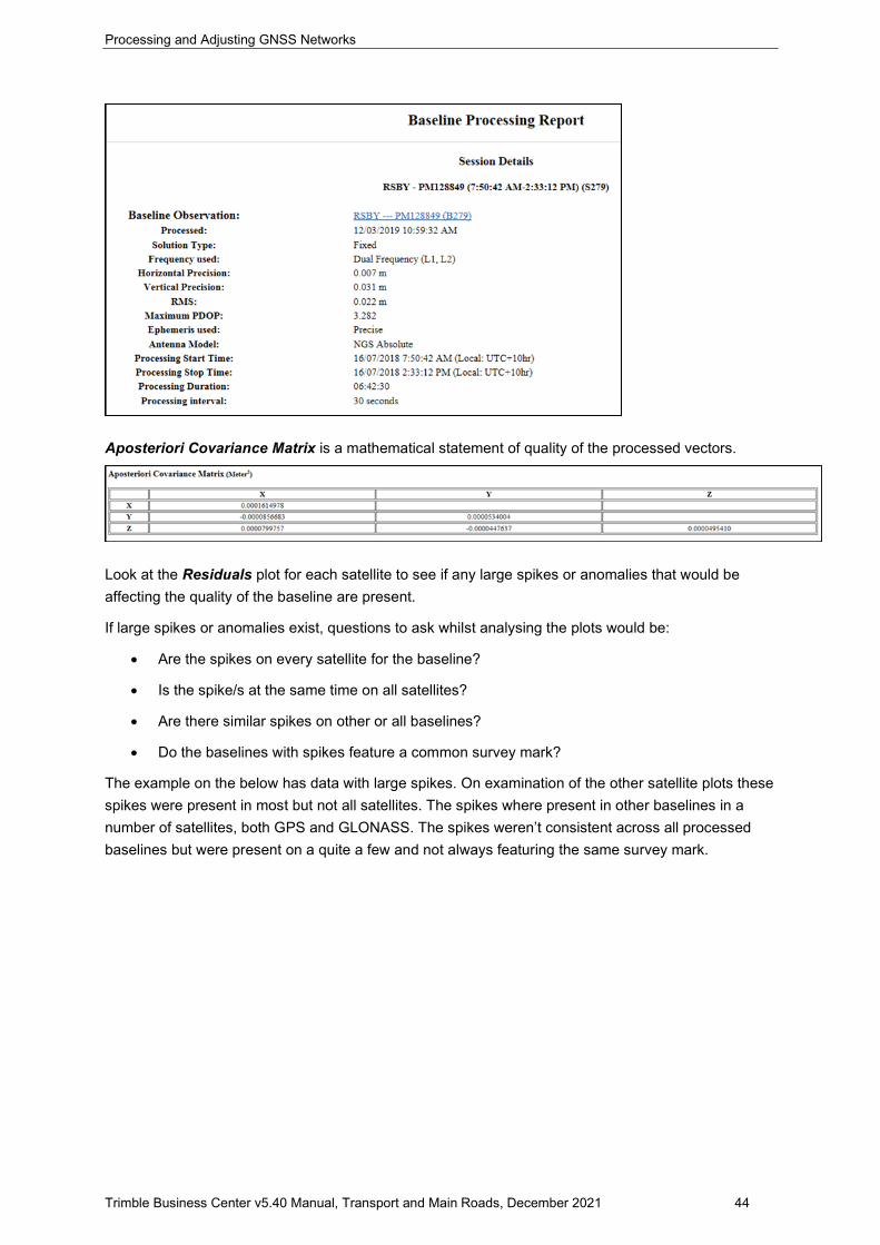
Peruse the Session Details at the top of the report. Check that the ephemeris used, processing duration and processing interval are correct. An incorrect processing interval would mean one of the receivers was logging data at different epoch intervals than the other.
Processing and Adjusting GNSS Networks
Trimble Business Center v5.40 Manual, Transport and Main Roads, December 2021 44
Aposteriori Covariance Matrix is a mathematical statement of quality of the processed vectors.
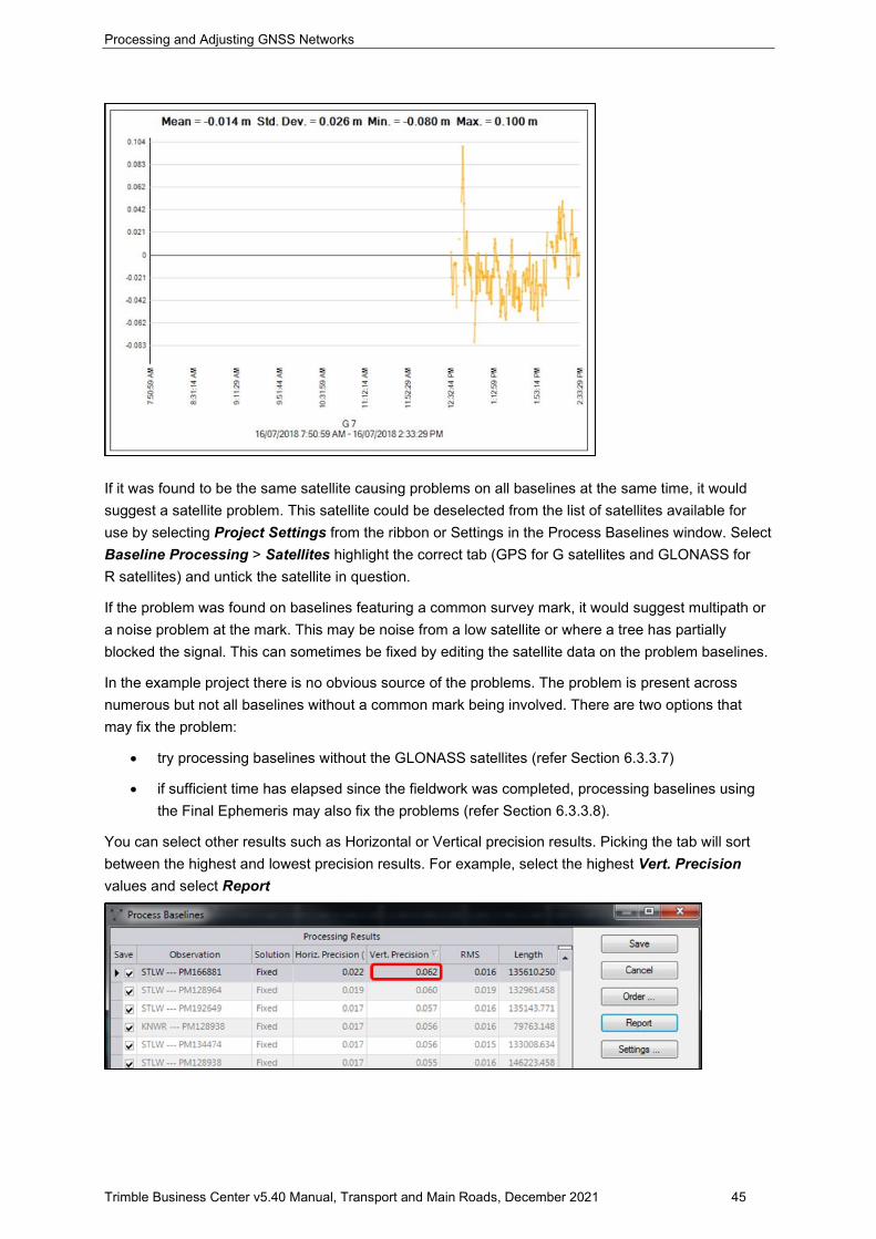
Look at the Residuals plot for each satellite to see if any large spikes or anomalies that would be affecting the quality of the baseline are present.
If large spikes or anomalies exist, questions to ask whilst analysing the plots would be:
• Are the spikes on every satellite for the baseline?
• Is the spike/s at the same time on all satellites?
• Are there similar spikes on other or all baselines?
• Do the baselines with spikes feature a common survey mark?
The example on the below has data with large spikes. On examination of the other satellite plots these spikes were present in most but not all satellites. The spikes where present in other baselines in a number of satellites, both GPS and GLONASS. The spikes weren’t consistent across all processed baselines but were present on a quite a few and not always featuring the same survey mark.
Processing and Adjusting GNSS Networks
Trimble Business Center v5.40 Manual, Transport and Main Roads, December 2021 45
If it was found to be the same satellite causing problems on all baselines at the same time, it would suggest a satellite problem. This satellite could be deselected from the list of satellites available for use by selecting Project Settings from the ribbon or Settings in the Process Baselines window. Select Baseline Processing > Satellites highlight the correct tab (GPS for G satellites and GLONASS for R satellites) and untick the satellite in question.
If the problem was found on baselines featuring a common survey mark, it would suggest multipath or a noise problem at the mark. This may be noise from a low satellite or where a tree has partially blocked the signal. This can sometimes be fixed by editing the satellite data on the problem baselines.
In the example project there is no obvious source of the problems. The problem is present across numerous but not all baselines without a common mark being involved. There are two options that may fix the problem:
• try processing baselines without the GLONASS satellites (refer Section 6.3.3.7)
• if sufficient time has elapsed since the fieldwork was completed, processing baselines using the Final Ephemeris may also fix the problems (refer Section 6.3.3.8).
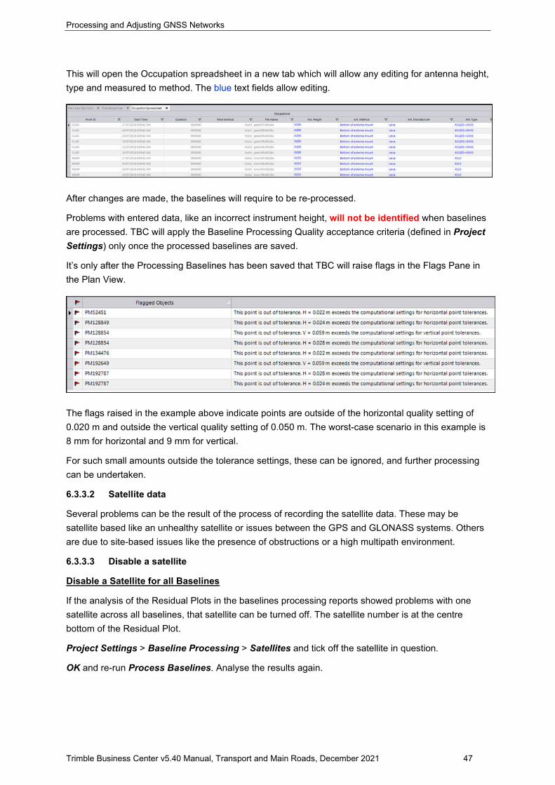
You can select other results such as Horizontal or Vertical precision results. Picking the tab will sort between the highest and lowest precision results. For example, select the highest Vert. Precision values and select Report
Processing and Adjusting GNSS Networks
Trimble Business Center v5.40 Manual, Transport and Main Roads, December 2021 46
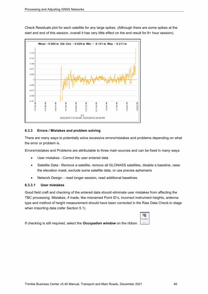
Check Residuals plot for each satellite for any large spikes. (Although there are some spikes at the start and end of this session, overall it has very little effect on the end result for 6+ hour session).
6.3.3 Errors / Mistakes and problem solving
There are many ways to potentially solve excessive errors/mistakes and problems depending on what the error or problem is.
Errors/mistakes and Problems are attributable to three main sources and can be fixed in many ways:
• User mistakes - Correct the user entered data
• Satellite Data - Remove a satellite, remove all GLONASS satellites, disable a baseline, raise the elevation mask, exclude some satellite data, or use precise ephemeris
• Network Design – read longer session, read additional baselines.
6.3.3.1 User mistakes
Good field craft and checking of the entered data should eliminate user mistakes from affecting the TBC processing. Mistakes, if made, like misnamed Point ID’s, incorrect instrument heights, antenna type and method of height measurement should have been corrected in the Raw Data Check-in stage when importing data (refer Section 5.1).
If checking is still required, select the Occupation window on the ribbon.
Processing and Adjusting GNSS Networks
Trimble Business Center v5.40 Manual, Transport and Main Roads, December 2021 47
This will open the Occupation spreadsheet in a new tab which will allow any editing for antenna height, type and measured to method. The blue text fields allow editing.
After changes are made, the baselines will require to be re-processed.
Problems with entered data, like an incorrect instrument height, will not be identified when baselines are processed. TBC will apply the Baseline Processing Quality acceptance criteria (defined in Project Settings) only once the processed baselines are saved.
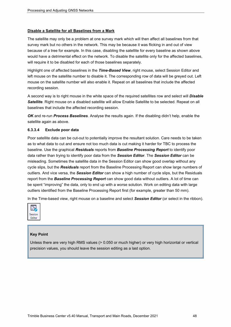
It’s only after the Processing Baselines has been saved that TBC will raise flags in the Flags Pane in the Plan View.
The flags raised in the example above indicate points are outside of the horizontal quality setting of 0.020 m and outside the vertical quality setting of 0.050 m. The worst-case scenario in this example is 8 mm for horizontal and 9 mm for vertical.
For such small amounts outside the tolerance settings, these can be ignored, and further processing can be undertaken.
6.3.3.2 Satellite data
Several problems can be the result of the process of recording the satellite data. These may be satellite based like an unhealthy satellite or issues between the GPS and GLONASS systems. Others are due to site-based issues like the presence of obstructions or a high multipath environment.
6.3.3.3 Disable a satellite
Disable a Satellite for all Baselines
If the analysis of the Residual Plots in the baselines processing reports showed problems with one satellite across all baselines, that satellite can be turned off. The satellite number is at the centre bottom of the Residual Plot.
Project Settings > Baseline Processing > Satellites and tick off the satellite in question.
OK and re-run Process Baselines. Analyse the results again.
Processing and Adjusting GNSS Networks
Trimble Business Center v5.40 Manual, Transport and Main Roads, December 2021 48
Disable a Satellite for all Baselines from a Mark
The satellite may only be a problem at one survey mark which will then affect all baselines from that survey mark but no others in the network. This may be because it was flicking in and out of view because of a tree for example. In this case, disabling the satellite for every baseline as shown above would have a detrimental effect on the network. To disable the satellite only for the affected baselines, will require it to be disabled for each of those baselines separately.
Highlight one of affected baselines in the Time-Based View, right mouse, select Session Editor and left mouse on the satellite number to disable it. The corresponding row of data will be greyed out. Left mouse on the satellite number will also enable it. Repeat on all baselines that include the affected recording session.
A second way is to right mouse in the white space of the required satellites row and select will Disable Satellite. Right mouse on a disabled satellite will allow Enable Satellite to be selected. Repeat on all baselines that include the affected recording session.
OK and re-run Process Baselines. Analyse the results again. If the disabling didn’t help, enable the satellite again as above.
6.3.3.4 Exclude poor data
Poor satellite data can be cut-out to potentially improve the resultant solution. Care needs to be taken as to what data to cut and ensure not too much data is cut making it harder for TBC to process the baseline. Use the graphical Residuals reports from Baseline Processing Report to identify poor data rather than trying to identify poor data from the Session Editor. The Session Editor can be misleading. Sometimes the satellite data in the Session Editor can show good overlap without any cycle slips, but the Residuals report from the Baseline Processing Report can show large numbers of outliers. And vice versa, the Session Editor can show a high number of cycle slips, but the Residuals report from the Baseline Processing Report can show good data without outliers. A lot of time can be spent “improving” the data, only to end up with a worse solution. Work on editing data with large outliers identified from the Baseline Processing Report first (for example, greater than 50 mm).
In the Time-based view, right mouse on a baseline and select Session Editor (or select in the ribbon).
Key Point
Unless there are very high RMS values (> 0.050 or much higher) or very high horizontal or vertical precision values, you should leave the session editing as a last option.
Processing and Adjusting GNSS Networks
Trimble Business Center v5.40 Manual, Transport and Main Roads, December 2021 49
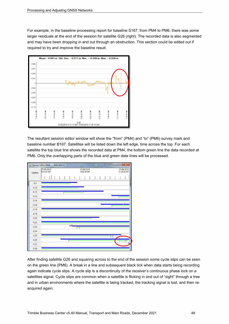
For example, in the baseline processing report for baseline S167, from PM4 to PM6, there was some larger residuals at the end of the session for satellite G26 (right). The recorded data is also segmented and may have been dropping in and out through an obstruction. This section could be edited out if required to try and improve the baseline result.
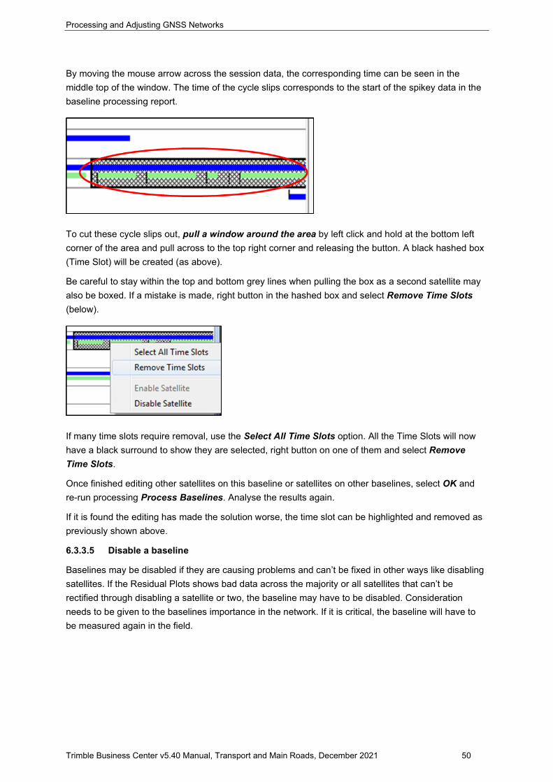
The resultant session editor window will show the “from” (PM4) and “to” (PM6) survey mark and baseline number B167. Satellites will be listed down the left edge, time across the top. For each satellite the top blue line shows the recorded data at PM4, the bottom green line the data recorded at PM6. Only the overlapping parts of the blue and green data lines will be processed.
After finding satellite G26 and squaring across to the end of the session some cycle slips can be seen on the green line (PM6). A break in a line and subsequent black tick when data starts being recording again indicate cycle slips. A cycle slip is a discontinuity of the receiver’s continuous phase lock on a satellites signal. Cycle slips are common when a satellite is flicking in and out of “sight” through a tree and in urban environments where the satellite is being tracked, the tracking signal is lost, and then re-acquired again.
Processing and Adjusting GNSS Networks
Trimble Business Center v5.40 Manual, Transport and Main Roads, December 2021 50
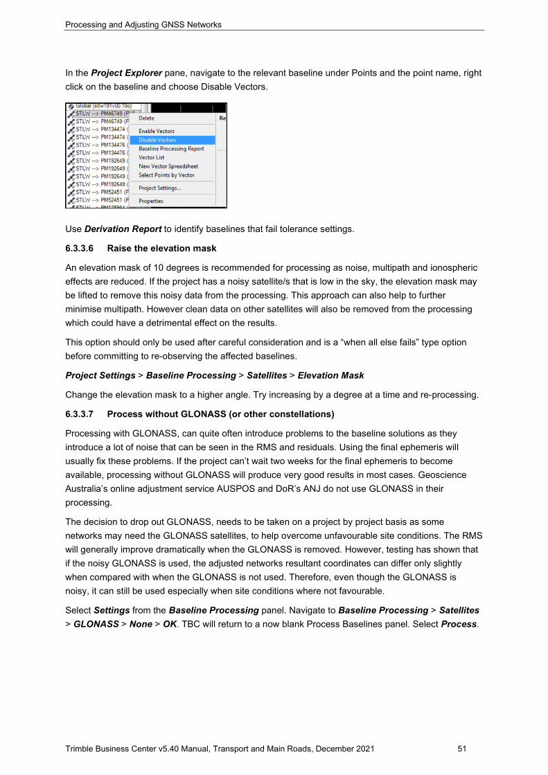
By moving the mouse arrow across the session data, the corresponding time can be seen in the middle top of the window. The time of the cycle slips corresponds to the start of the spikey data in the baseline processing report.
To cut these cycle slips out, pull a window around the area by left click and hold at the bottom left corner of the area and pull across to the top right corner and releasing the button. A black hashed box (Time Slot) will be created (as above).
Be careful to stay within the top and bottom grey lines when pulling the box as a second satellite may also be boxed. If a mistake is made, right button in the hashed box and select Remove Time Slots (below).
If many time slots require removal, use the Select All Time Slots option. All the Time Slots will now have a black surround to show they are selected, right button on one of them and select Remove Time Slots.
Once finished editing other satellites on this baseline or satellites on other baselines, select OK and re-run processing Process Baselines. Analyse the results again.
If it is found the editing has made the solution worse, the time slot can be highlighted and removed as previously shown above.
6.3.3.5 Disable a baseline
Baselines may be disabled if they are causing problems and can’t be fixed in other ways like disabling satellites. If the Residual Plots shows bad data across the majority or all satellites that can’t be rectified through disabling a satellite or two, the baseline may have to be disabled. Consideration needs to be given to the baselines importance in the network. If it is critical, the baseline will have to be measured again in the field.
Processing and Adjusting GNSS Networks
Trimble Business Center v5.40 Manual, Transport and Main Roads, December 2021 51
In the Project Explorer pane, navigate to the relevant baseline under Points and the point name, right click on the baseline and choose Disable Vectors.
Use Derivation Report to identify baselines that fail tolerance settings.
6.3.3.6 Raise the elevation mask
An elevation mask of 10 degrees is recommended for processing as noise, multipath and ionospheric effects are reduced. If the project has a noisy satellite/s that is low in the sky, the elevation mask may be lifted to remove this noisy data from the processing. This approach can also help to further minimise multipath. However clean data on other satellites will also be removed from the processing which could have a detrimental effect on the results.
This option should only be used after careful consideration and is a “when all else fails” type option before committing to re-observing the affected baselines.
Project Settings > Baseline Processing > Satellites > Elevation Mask
Change the elevation mask to a higher angle. Try increasing by a degree at a time and re-processing.
6.3.3.7 Process without GLONASS (or other constellations)
Processing with GLONASS, can quite often introduce problems to the baseline solutions as they introduce a lot of noise that can be seen in the RMS and residuals. Using the final ephemeris will usually fix these problems. If the project can’t wait two weeks for the final ephemeris to become available, processing without GLONASS will produce very good results in most cases. Geoscience Australia’s online adjustment service AUSPOS and DoR’s ANJ do not use GLONASS in their processing.
The decision to drop out GLONASS, needs to be taken on a project by project basis as some networks may need the GLONASS satellites, to help overcome unfavourable site conditions. The RMS will generally improve dramatically when the GLONASS is removed. However, testing has shown that if the noisy GLONASS is used, the adjusted networks resultant coordinates can differ only slightly when compared with when the GLONASS is not used. Therefore, even though the GLONASS is noisy, it can still be used especially when site conditions where not favourable.
Select Settings from the Baseline Processing panel. Navigate to Baseline Processing > Satellites > GLONASS > None > OK. TBC will return to a now blank Process Baselines panel. Select Process.
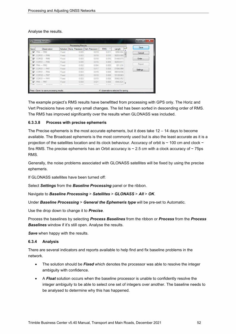
Processing and Adjusting GNSS Networks
Trimble Business Center v5.40 Manual, Transport and Main Roads, December 2021 52
Analyse the results.
The example project’s RMS results have benefitted from processing with GPS only. The Horiz and Vert Precisions have only very small changes. The list has been sorted in descending order of RMS. The RMS has improved significantly over the results when GLONASS was included.
6.3.3.8 Process with precise ephemeris
The Precise ephemeris is the most accurate ephemeris, but it does take 12 – 14 days to become available. The Broadcast ephemeris is the most commonly used but is also the least accurate as it is a projection of the satellites location and its clock behaviour. Accuracy of orbit is ~ 100 cm and clock ~ 5ns RMS. The precise ephemeris has an Orbit accuracy is ~ 2.5 cm with a clock accuracy of ~ 75ps RMS.
Generally, the noise problems associated with GLONASS satellites will be fixed by using the precise ephemeris.
If GLONASS satellites have been turned off:
Select Settings from the Baseline Processing panel or the ribbon.
Navigate to Baseline Processing > Satellites > GLONASS > All > OK.
Under Baseline Processing > General the Ephemeris type will be pre-set to Automatic.
Use the drop down to change it to Precise.
Process the baselines by selecting Process Baselines from the ribbon or Process from the Process Baselines window if it’s still open. Analyse the results.
Save when happy with the results.
6.3.4 Analysis
There are several indicators and reports available to help find and fix baseline problems in the network.
• The solution should be Fixed which denotes the processor was able to resolve the integer ambiguity with confidence.
• A Float solution occurs when the baseline processor is unable to confidently resolve the integer ambiguity to be able to select one set of integers over another. The baseline needs to be analysed to determine why this has happened.
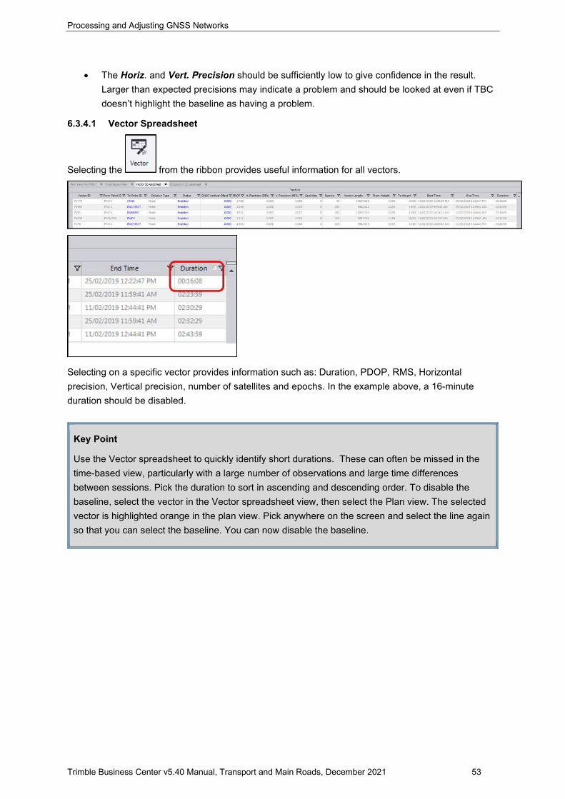
Processing and Adjusting GNSS Networks
Trimble Business Center v5.40 Manual, Transport and Main Roads, December 2021 53
• The Horiz. and Vert. Precision should be sufficiently low to give confidence in the result. Larger than expected precisions may indicate a problem and should be looked at even if TBC doesn’t highlight the baseline as having a problem.
6.3.4.1 Vector Spreadsheet
Selecting the from the ribbon provides useful information for all vectors.
Selecting on a specific vector provides information such as: Duration, PDOP, RMS, Horizontal precision, Vertical precision, number of satellites and epochs. In the example above, a 16-minute duration should be disabled.
Key Point
Use the Vector spreadsheet to quickly identify short durations. These can often be missed in the time-based view, particularly with a large number of observations and large time differences between sessions. Pick the duration to sort in ascending and descending order. To disable the baseline, select the vector in the Vector spreadsheet view, then select the Plan view. The selected vector is highlighted orange in the plan view. Pick anywhere on the screen and select the line again so that you can select the baseline. You can now disable the baseline.
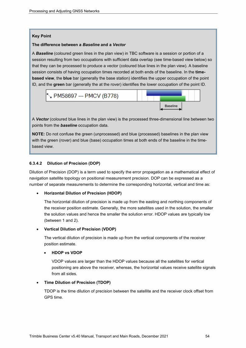
Processing and Adjusting GNSS Networks
Trimble Business Center v5.40 Manual, Transport and Main Roads, December 2021 54
Key Point
The difference between a Baseline and a Vector
A Baseline (coloured green lines in the plan view) in TBC software is a session or portion of a session resulting from two occupations with sufficient data overlap (see time-based view below) so that they can be processed to produce a vector (coloured blue lines in the plan view). A baseline session consists of having occupation times recorded at both ends of the baseline. In the time-based view, the blue bar (generally the base station) identifies the upper occupation of the point ID, and the green bar (generally the at the rover) identifies the lower occupation of the point ID.
A Vector (coloured blue lines in the plan view) is the processed three-dimensional line between two points from the baseline occupation data.
NOTE: Do not confuse the green (unprocessed) and blue (processed) baselines in the plan view with the green (rover) and blue (base) occupation times at both ends of the baseline in the time-based view.
6.3.4.2 Dilution of Precision (DOP)
Dilution of Precision (DOP) is a term used to specify the error propagation as a mathematical effect of navigation satellite topology on positional measurement precision. DOP can be expressed as a number of separate measurements to determine the corresponding horizontal, vertical and time as:
• Horizontal Dilution of Precision (HDOP)
The horizontal dilution of precision is made up from the easting and northing components of the receiver position estimate. Generally, the more satellites used in the solution, the smaller the solution values and hence the smaller the solution error. HDOP values are typically low (between 1 and 2).
• Vertical Dilution of Precision (VDOP)
The vertical dilution of precision is made up from the vertical components of the receiver position estimate.
• HDOP vs VDOP
VDOP values are larger than the HDOP values because all the satellites for vertical positioning are above the receiver, whereas, the horizontal values receive satellite signals from all sides.
• Time Dilution of Precision (TDOP)
TDOP is the time dilution of precision between the satellite and the receiver clock offset from GPS time.
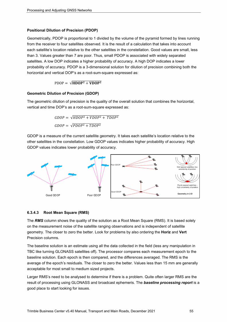
Processing and Adjusting GNSS Networks
Trimble Business Center v5.40 Manual, Transport and Main Roads, December 2021 55
Positional Dilution of Precision (PDOP)
Geometrically, PDOP is proportional to 1 divided by the volume of the pyramid formed by lines running from the receiver to four satellites observed. It is the result of a calculation that takes into account each satellite’s location relative to the other satellites in the constellation. Good values are small, less than 3. Values greater than 7 are poor. Thus, small PDOP is associated with widely separated satellites. A low DOP indicates a higher probability of accuracy. A high DOP indicates a lower probability of accuracy. PDOP is a 3-dimensional solution for dilution of precision combining both the horizontal and vertical DOP’s as a root-sum-square expressed as:
PDOP = √𝐇𝐇𝐇𝐇𝐇𝐇𝐇𝐇𝟐𝟐 + 𝐕𝐕𝐇𝐇𝐇𝐇𝐇𝐇𝟐𝟐
Geometric Dilution of Precision (GDOP)
The geometric dilution of precision is the quality of the overall solution that combines the horizontal, vertical and time DOP’s as a root-sum-square expressed as:
𝐺𝐺𝐺𝐺𝐺𝐺𝐺𝐺 = √𝐻𝐻𝐺𝐺𝐺𝐺𝐺𝐺2 + 𝑉𝑉𝐺𝐺𝐺𝐺𝐺𝐺2 + 𝑇𝑇𝐺𝐺𝐺𝐺𝐺𝐺2
𝐺𝐺𝐺𝐺𝐺𝐺𝐺𝐺 = √𝐺𝐺𝐺𝐺𝐺𝐺𝐺𝐺2 + 𝑇𝑇𝐺𝐺𝐺𝐺𝐺𝐺2
GDOP is a measure of the current satellite geometry. It takes each satellite’s location relative to the other satellites in the constellation. Low GDOP values indicates higher probability of accuracy. High GDOP values indicates lower probability of accuracy.
6.3.4.3 Root Mean Square (RMS)
The RMS column shows the quality of the solution as a Root Mean Square (RMS). It is based solely on the measurement noise of the satellite ranging observations and is independent of satellite geometry. The closer to zero the better. Look for problems by also ordering the Horiz and Vert Precision columns.
The baseline solution is an estimate using all the data collected in the field (less any manipulation in TBC like turning GLONASS satellites off). The processor compares each measurement epoch to the baseline solution. Each epoch is then compared, and the differences averaged. The RMS is the average of the epoch’s residuals. The closer to zero the better. Values less than 15 mm are generally acceptable for most small to medium sized projects.
Larger RMS’s need to be analysed to determine if there is a problem. Quite often larger RMS are the result of processing using GLONASS and broadcast ephemeris. The baseline processing report is a good place to start looking for issues.
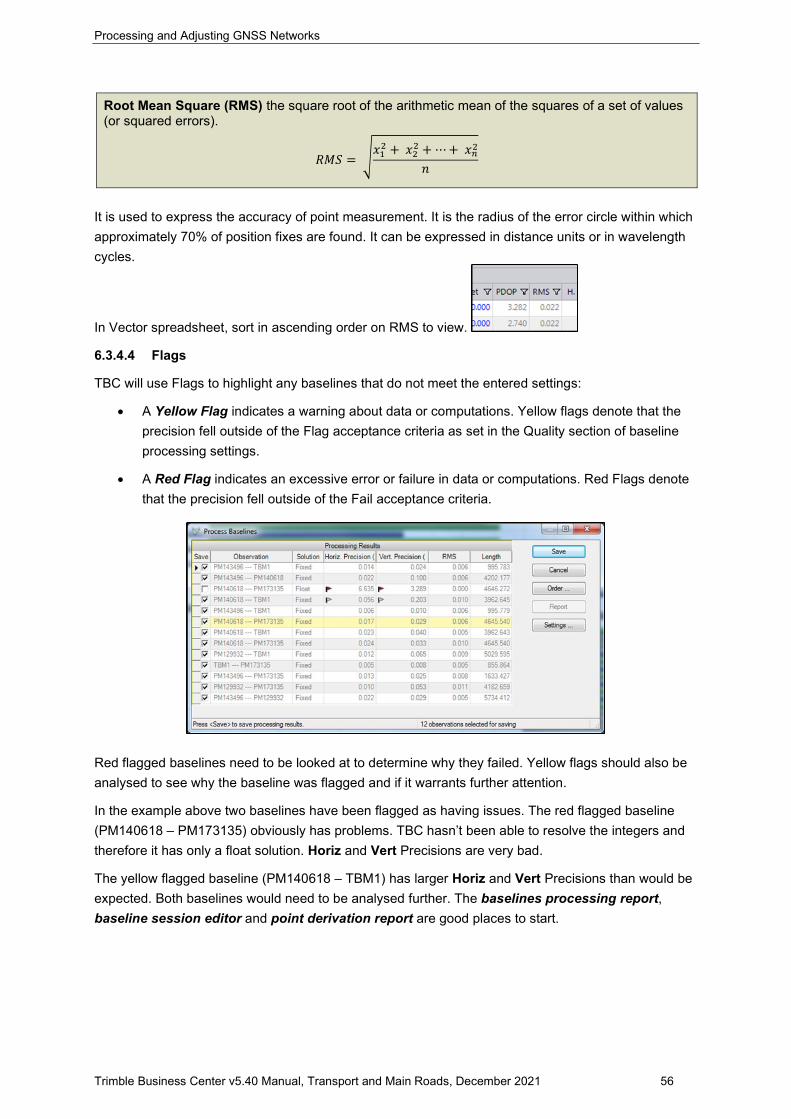
Processing and Adjusting GNSS Networks
Trimble Business Center v5.40 Manual, Transport and Main Roads, December 2021 56
Root Mean Square (RMS) the square root of the arithmetic mean of the squares of a set of values (or squared errors).
𝑅𝑅𝑅𝑅𝑅𝑅 = �𝑥𝑥12 + 𝑥𝑥22 + ⋯+ 𝑥𝑥𝑛𝑛2
𝑛𝑛
It is used to express the accuracy of point measurement. It is the radius of the error circle within which approximately 70% of position fixes are found. It can be expressed in distance units or in wavelength cycles.
In Vector spreadsheet, sort in ascending order on RMS to view.
6.3.4.4 Flags
TBC will use Flags to highlight any baselines that do not meet the entered settings:
• A Yellow Flag indicates a warning about data or computations. Yellow flags denote that the precision fell outside of the Flag acceptance criteria as set in the Quality section of baseline processing settings.
• A Red Flag indicates an excessive error or failure in data or computations. Red Flags denote that the precision fell outside of the Fail acceptance criteria.
Red flagged baselines need to be looked at to determine why they failed. Yellow flags should also be analysed to see why the baseline was flagged and if it warrants further attention.
In the example above two baselines have been flagged as having issues. The red flagged baseline (PM140618 – PM173135) obviously has problems. TBC hasn’t been able to resolve the integers and therefore it has only a float solution. Horiz and Vert Precisions are very bad.
The yellow flagged baseline (PM140618 – TBM1) has larger Horiz and Vert Precisions than would be expected. Both baselines would need to be analysed further. The baselines processing report, baseline session editor and point derivation report are good places to start.
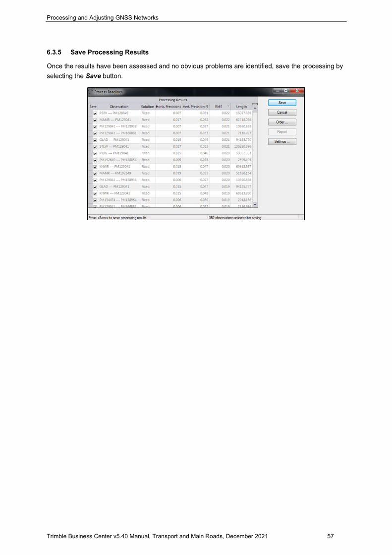
Processing and Adjusting GNSS Networks
Trimble Business Center v5.40 Manual, Transport and Main Roads, December 2021 57
6.3.5 Save Processing Results
Once the results have been assessed and no obvious problems are identified, save the processing by selecting the Save button.
Processing and Adjusting GNSS Networks
Trimble Business Center v5.40 Manual, Transport and Main Roads, December 2021 58
7 Minimally constrained adjustment
Applies a least squares adjustment on the network by minimising the sum of the weighted squared residuals of the observations A minimally constrained network adjustment (or free adjustment) is done initially as a tool to validate the data, check for mistakes and systematic errors and to look at the internal consistency of the observations within the network. It has only enough constraints to define the coordinate system with only one control point held fixed in the survey network. Holding one control point fixed, it shifts observations to the correct location within the chosen datum. Not fixing a control point forces the software to perform a minimally constrained adjustment. A minimally constrained adjustment is accomplished by minimizing the size of the coordinate shift throughout the network. This equates to a mean coordinate shift of 0 (zero) in all dimensions. A minimally constrained or free adjustment acts as one quality control check on the network. This adjustment helps to identify bad observations in the network. If an observation does not fit with the rest of the observations, it is highlighted as an outlier. The minimally constrained or free adjustment also checks on how well the observations hold together as a cohesive unit.
Evaluating Uncertainty Control surveys using least squares The horizontal and/or vertical coordinates and uncertainties of survey control marks in a Datum Control Survey shall be estimated using a rigorous least squares adjustment process. General Purpose Control Surveys should use least squares adjustment to estimate uncertainty. Throughout and following least squares adjustment, survey control projects shall be evaluated to demonstrate the reliability of the survey and the estimated coordinates and uncertainties. The quality of estimated coordinates in an absolute sense shall be evaluated using SU and/or PU as appropriate. Standard for the Australian Survey Control Network – SP1 Version 2.2
A minimally constrained adjustment is used to evaluate the internal observations and the standard errors assigned to them. The quality and internal consistency of the survey network is assessed to verify the GNSS measurement precisions.
7.1 Enter all known coordinate values
All imported marks must have the same name (exact wording), current published values and set to Control Quality if Positional Uncertainty (PU) values are known.
Known control mark coordinates can be imported in several different formats. The survey mark name must be exactly the same (including case) for TBC to assign to the mark correctly. All marks imported using this method will have a Control Quality set on the coordinate. If coordinates of varying quality are imported, the Quality may have to be changed to Unknown before processing baselines as this process will use all Control Quality coordinates. Refer Section 6.3 Process Baselines for more information.
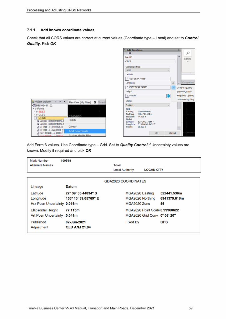
Processing and Adjusting GNSS Networks
Trimble Business Center v5.40 Manual, Transport and Main Roads, December 2021 59
7.1.1 Add known coordinate values
Check that all CORS values are correct at current values (Coordinate type – Local) and set to Control Quality. Pick OK
Add Form 6 values. Use Coordinate type – Grid. Set to Quality Control if Uncertainty values are known. Modify if required and pick OK
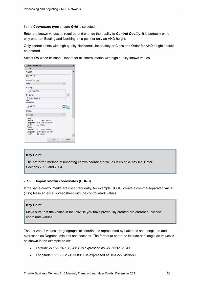
Processing and Adjusting GNSS Networks
Trimble Business Center v5.40 Manual, Transport and Main Roads, December 2021 60
In the Coordinate type ensure Grid is selected.
Enter the known values as required and change the quality to Control Quality. It is perfectly ok to only enter an Easting and Northing on a point or only an AHD height.
Only control points with high quality Horizontal Uncertainty or Class and Order for AHD height should be entered.
Select OK when finished. Repeat for all control marks with high quality known values.
Key Point
The preferred method of importing known coordinate values is using a .csv file. Refer Sections 7.1.2 and 7.1.4
7.1.2 Import known coordinates (CORS)
If the same control marks are used frequently, for example CORS, create a comma-separated value (.csv) file in an excel spreadsheet with the control mark values.
Key Point
Make sure that the values in the .csv file you have previously created are current published coordinate values.
The horizontal values are geographical coordinates represented by Latitudes and Longitude and expressed as Degrees, minutes and seconds. The format to enter the latitude and longitude values is as shown in the example below:
• Latitude 27° 56’ 26.135041” S is expressed as -27.5626135041
• Longitude 153° 22’ 26.499589” E is expressed as 153.2226499589
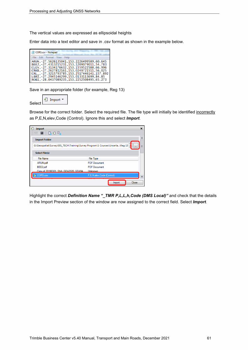
Processing and Adjusting GNSS Networks
Trimble Business Center v5.40 Manual, Transport and Main Roads, December 2021 61
The vertical values are expressed as ellipsoidal heights
Enter data into a text editor and save in .csv format as shown in the example below.
Save in an appropriate folder (for example, Reg 13)
Select
Browse for the correct folder. Select the required file. The file type will initially be identified incorrectly as P,E,N,elev,Code (Control). Ignore this and select Import.
Highlight the correct Definition Name “_TMR P,L,L,h,Code (DMS Local)” and check that the details in the Import Preview section of the window are now assigned to the correct field. Select Import.
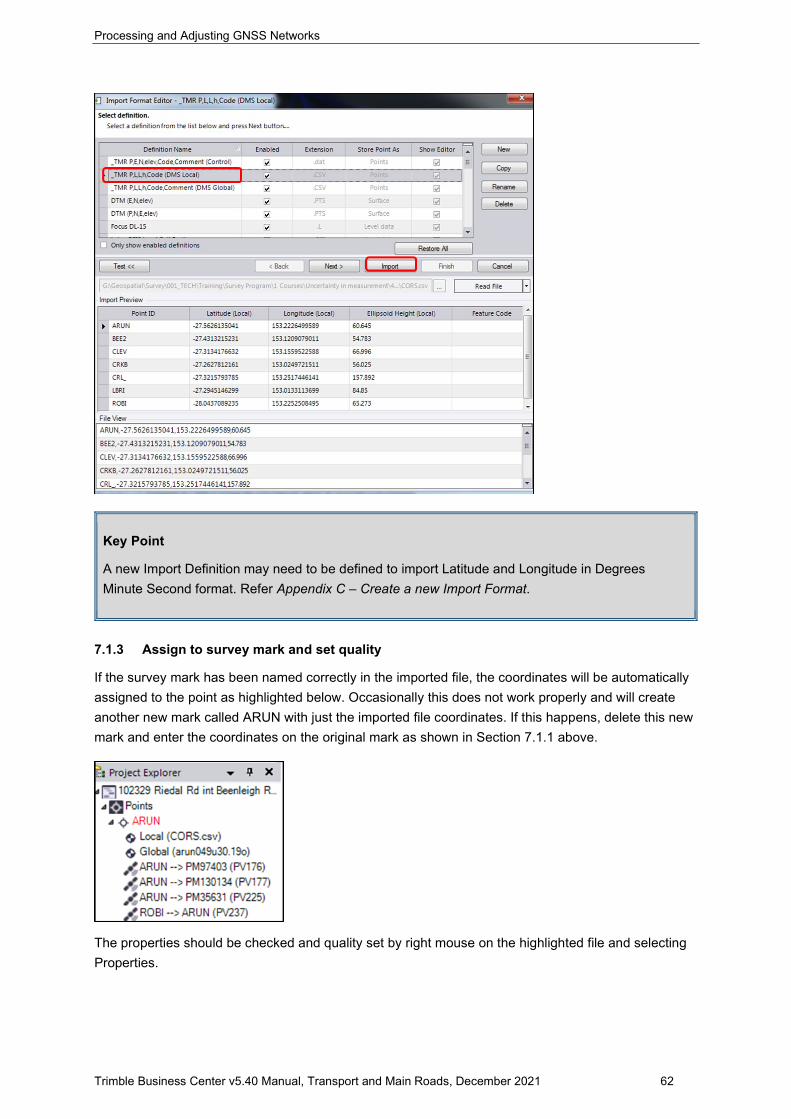
Processing and Adjusting GNSS Networks
Trimble Business Center v5.40 Manual, Transport and Main Roads, December 2021 62
Key Point
A new Import Definition may need to be defined to import Latitude and Longitude in Degrees Minute Second format. Refer Appendix C – Create a new Import Format.
7.1.3 Assign to survey mark and set quality
If the survey mark has been named correctly in the imported file, the coordinates will be automatically assigned to the point as highlighted below. Occasionally this does not work properly and will create another new mark called ARUN with just the imported file coordinates. If this happens, delete this new mark and enter the coordinates on the original mark as shown in Section 7.1.1 above.
The properties should be checked and quality set by right mouse on the highlighted file and selecting Properties.

Processing and Adjusting GNSS Networks
Trimble Business Center v5.40 Manual, Transport and Main Roads, December 2021 63
Check the coordinate information has been correctly imported and assigned. The Quality will have
been set as Control quality
7.1.4 Import Known Coordinates (PM’s)
This is the preferred method of entering coordinates of multiple permanent marks where there can be a mixture of suitable horizontal quality values and AHD height values, horizontal quality values only and AHD height values only.
First, it is necessary to create a comma-separated value (.csv) file in an excel spreadsheet with the control mark values.
The horizontal values are cartographic coordinates expressed as Eastings and Northings. Elevation values are expressed as AHD.
Enter data into an excel spreadsheet and save in a .csv format as shown in the example below.
Save in an appropriate folder (for example, Form 6’s)
Select
Browse for the correct folder. Select the required file. The file type will initially be identified incorrectly as Unknown. Ignore this and select Import.
Highlight the correct Definition Name “P,E,N,elev,Code (Control) and check that the details in the Import Preview section of the window are now assigned to the correct field. Select Import.
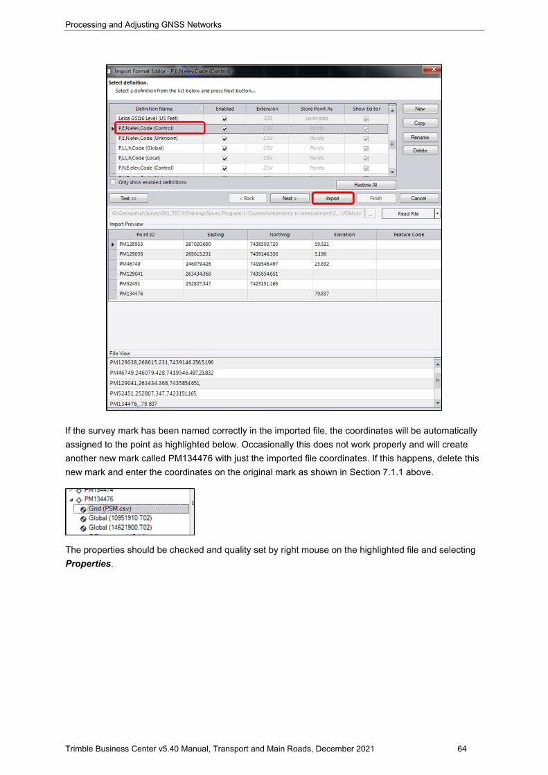
Processing and Adjusting GNSS Networks
Trimble Business Center v5.40 Manual, Transport and Main Roads, December 2021 64
If the survey mark has been named correctly in the imported file, the coordinates will be automatically assigned to the point as highlighted below. Occasionally this does not work properly and will create another new mark called PM134476 with just the imported file coordinates. If this happens, delete this new mark and enter the coordinates on the original mark as shown in Section 7.1.1 above.
The properties should be checked and quality set by right mouse on the highlighted file and selecting Properties.
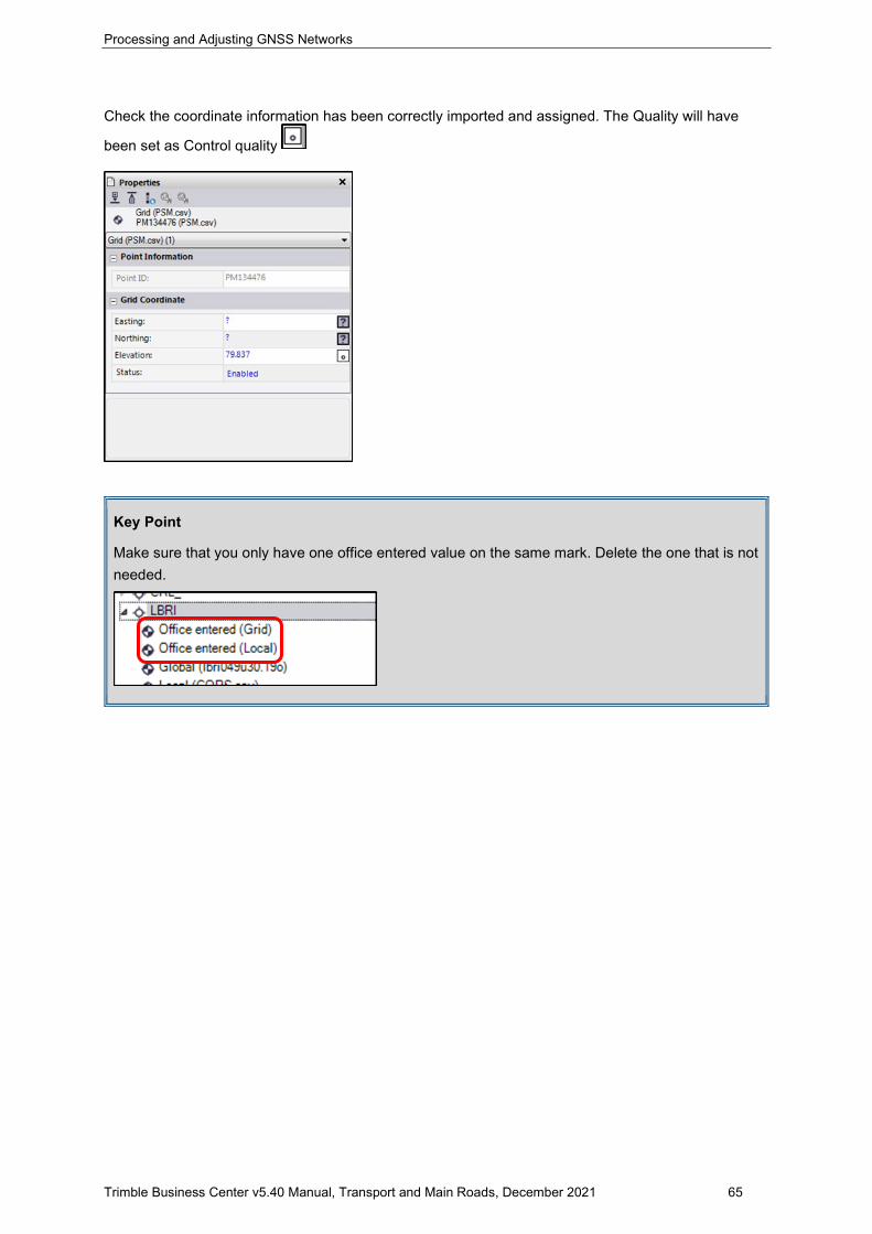
Processing and Adjusting GNSS Networks
Trimble Business Center v5.40 Manual, Transport and Main Roads, December 2021 65
Check the coordinate information has been correctly imported and assigned. The Quality will have
been set as Control quality
Key Point
Make sure that you only have one office entered value on the same mark. Delete the one that is not needed.
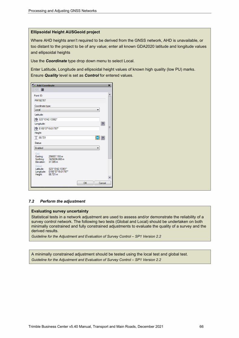
Processing and Adjusting GNSS Networks
Trimble Business Center v5.40 Manual, Transport and Main Roads, December 2021 66
Ellipsoidal Height AUSGeoid project
Where AHD heights aren’t required to be derived from the GNSS network, AHD is unavailable, or too distant to the project to be of any value; enter all known GDA2020 latitude and longitude values and ellipsoidal heights
Use the Coordinate type drop down menu to select Local.
Enter Latitude, Longitude and ellipsoidal height values of known high quality (low PU) marks. Ensure Quality level is set as Control for entered values.
7.2 Perform the adjustment
Evaluating survey uncertainty Statistical tests in a network adjustment are used to assess and/or demonstrate the reliability of a survey control network. The following two tests (Global and Local) should be undertaken on both minimally constrained and fully constrained adjustments to evaluate the quality of a survey and the derived results. Guideline for the Adjustment and Evaluation of Survey Control – SP1 Version 2.2
A minimally constrained adjustment should be tested using the local test and global test. Guideline for the Adjustment and Evaluation of Survey Control – SP1 Version 2.2
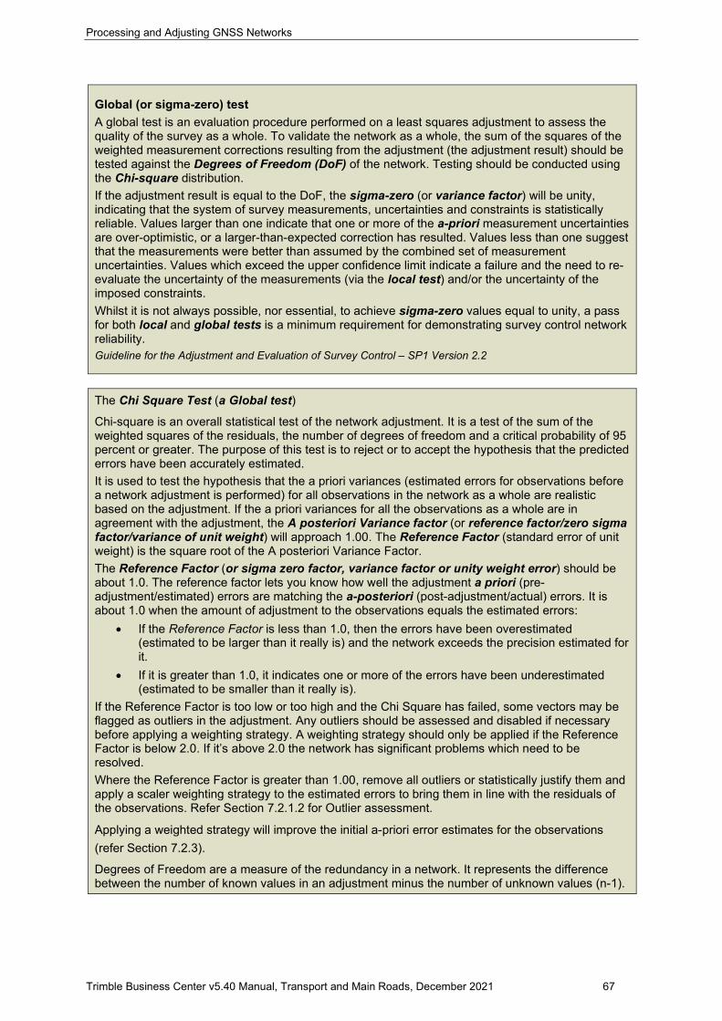
Processing and Adjusting GNSS Networks
Trimble Business Center v5.40 Manual, Transport and Main Roads, December 2021 67
Global (or sigma-zero) test A global test is an evaluation procedure performed on a least squares adjustment to assess the quality of the survey as a whole. To validate the network as a whole, the sum of the squares of the weighted measurement corrections resulting from the adjustment (the adjustment result) should be tested against the Degrees of Freedom (DoF) of the network. Testing should be conducted using the Chi-square distribution. If the adjustment result is equal to the DoF, the sigma-zero (or variance factor) will be unity, indicating that the system of survey measurements, uncertainties and constraints is statistically reliable. Values larger than one indicate that one or more of the a-priori measurement uncertainties are over-optimistic, or a larger-than-expected correction has resulted. Values less than one suggest that the measurements were better than assumed by the combined set of measurement uncertainties. Values which exceed the upper confidence limit indicate a failure and the need to re-evaluate the uncertainty of the measurements (via the local test) and/or the uncertainty of the imposed constraints. Whilst it is not always possible, nor essential, to achieve sigma-zero values equal to unity, a pass for both local and global tests is a minimum requirement for demonstrating survey control network reliability. Guideline for the Adjustment and Evaluation of Survey Control – SP1 Version 2.2
The Chi Square Test (a Global test)
Chi-square is an overall statistical test of the network adjustment. It is a test of the sum of the weighted squares of the residuals, the number of degrees of freedom and a critical probability of 95 percent or greater. The purpose of this test is to reject or to accept the hypothesis that the predicted errors have been accurately estimated. It is used to test the hypothesis that the a priori variances (estimated errors for observations before a network adjustment is performed) for all observations in the network as a whole are realistic based on the adjustment. If the a priori variances for all the observations as a whole are in agreement with the adjustment, the A posteriori Variance factor (or reference factor/zero sigma factor/variance of unit weight) will approach 1.00. The Reference Factor (standard error of unit weight) is the square root of the A posteriori Variance Factor. The Reference Factor (or sigma zero factor, variance factor or unity weight error) should be about 1.0. The reference factor lets you know how well the adjustment a priori (pre-adjustment/estimated) errors are matching the a-posteriori (post-adjustment/actual) errors. It is about 1.0 when the amount of adjustment to the observations equals the estimated errors:
• If the Reference Factor is less than 1.0, then the errors have been overestimated (estimated to be larger than it really is) and the network exceeds the precision estimated for it.
• If it is greater than 1.0, it indicates one or more of the errors have been underestimated (estimated to be smaller than it really is).
If the Reference Factor is too low or too high and the Chi Square has failed, some vectors may be flagged as outliers in the adjustment. Any outliers should be assessed and disabled if necessary before applying a weighting strategy. A weighting strategy should only be applied if the Reference Factor is below 2.0. If it’s above 2.0 the network has significant problems which need to be resolved. Where the Reference Factor is greater than 1.00, remove all outliers or statistically justify them and apply a scaler weighting strategy to the estimated errors to bring them in line with the residuals of the observations. Refer Section 7.2.1.2 for Outlier assessment.
Applying a weighted strategy will improve the initial a-priori error estimates for the observations (refer Section 7.2.3).
Degrees of Freedom are a measure of the redundancy in a network. It represents the difference between the number of known values in an adjustment minus the number of unknown values (n-1).
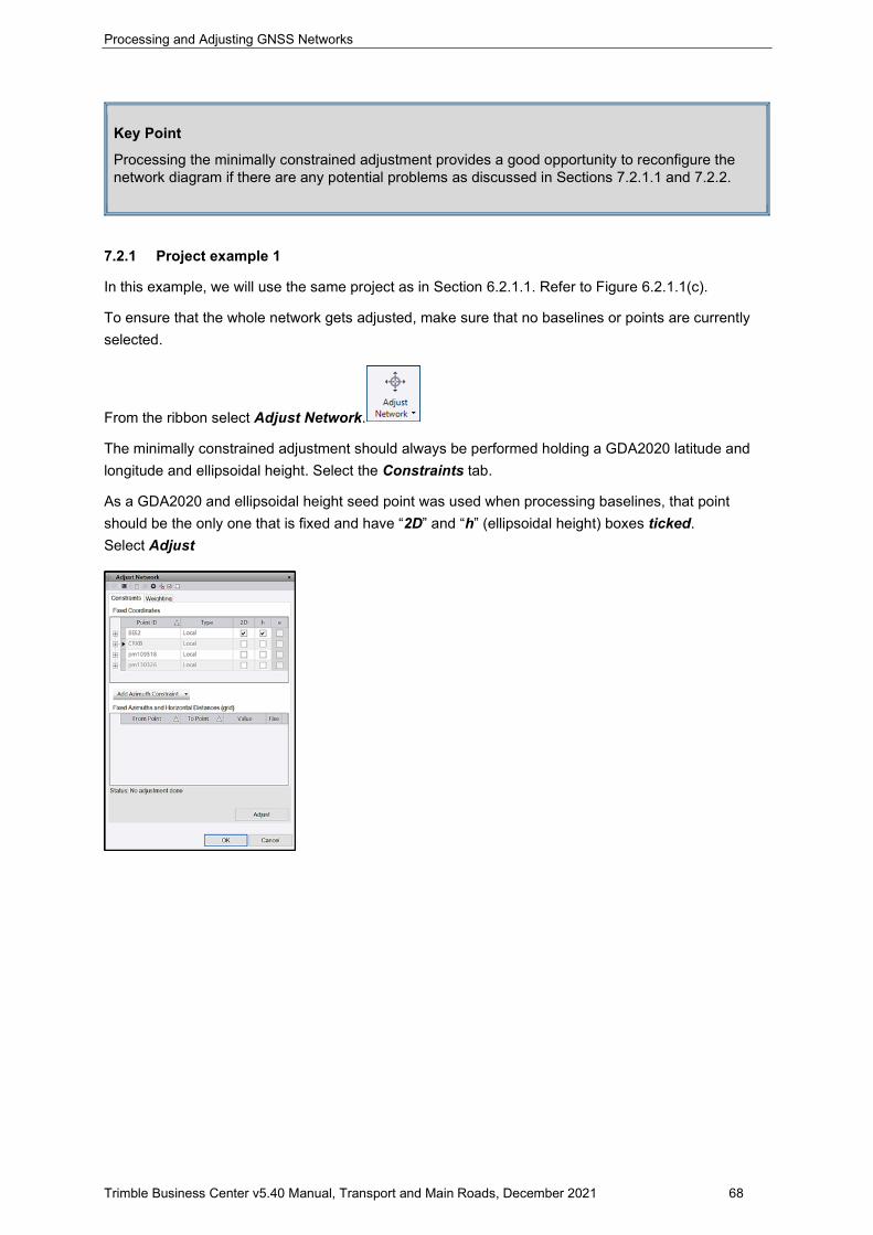
Processing and Adjusting GNSS Networks
Trimble Business Center v5.40 Manual, Transport and Main Roads, December 2021 68
Key Point
Processing the minimally constrained adjustment provides a good opportunity to reconfigure the network diagram if there are any potential problems as discussed in Sections 7.2.1.1 and 7.2.2.
7.2.1 Project example 1
In this example, we will use the same project as in Section 6.2.1.1. Refer to Figure 6.2.1.1(c).
To ensure that the whole network gets adjusted, make sure that no baselines or points are currently selected.
From the ribbon select Adjust Network.
The minimally constrained adjustment should always be performed holding a GDA2020 latitude and longitude and ellipsoidal height. Select the Constraints tab.
As a GDA2020 and ellipsoidal height seed point was used when processing baselines, that point should be the only one that is fixed and have “2D” and “h” (ellipsoidal height) boxes ticked. Select Adjust
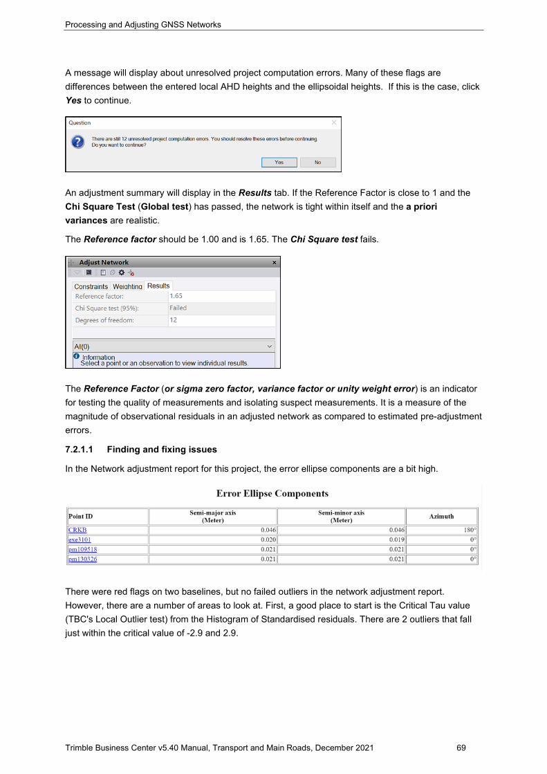
Processing and Adjusting GNSS Networks
Trimble Business Center v5.40 Manual, Transport and Main Roads, December 2021 69
A message will display about unresolved project computation errors. Many of these flags are differences between the entered local AHD heights and the ellipsoidal heights. If this is the case, click Yes to continue.
An adjustment summary will display in the Results tab. If the Reference Factor is close to 1 and the Chi Square Test (Global test) has passed, the network is tight within itself and the a priori variances are realistic.
The Reference factor should be 1.00 and is 1.65. The Chi Square test fails.
The Reference Factor (or sigma zero factor, variance factor or unity weight error) is an indicator for testing the quality of measurements and isolating suspect measurements. It is a measure of the magnitude of observational residuals in an adjusted network as compared to estimated pre-adjustment errors.
7.2.1.1 Finding and fixing issues
In the Network adjustment report for this project, the error ellipse components are a bit high.
There were red flags on two baselines, but no failed outliers in the network adjustment report. However, there are a number of areas to look at. First, a good place to start is the Critical Tau value (TBC's Local Outlier test) from the Histogram of Standardised residuals. There are 2 outliers that fall just within the critical value of -2.9 and 2.9.
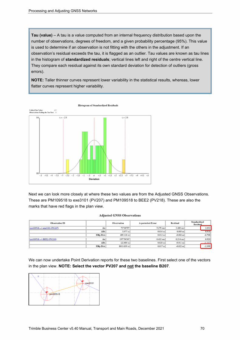
Processing and Adjusting GNSS Networks
Trimble Business Center v5.40 Manual, Transport and Main Roads, December 2021 70
Tau (value) – A tau is a value computed from an internal frequency distribution based upon the number of observations, degrees of freedom, and a given probability percentage (95%). This value is used to determine if an observation is not fitting with the others in the adjustment. If an observation’s residual exceeds the tau, it is flagged as an outlier. Tau values are known as tau lines in the histogram of standardized residuals; vertical lines left and right of the centre vertical line. They compare each residual against its own standard deviation for detection of outliers (gross errors).
NOTE: Taller thinner curves represent lower variability in the statistical results, whereas, lower flatter curves represent higher variability.
Next we can look more closely at where these two values are from the Adjusted GNSS Observations. These are PM109518 to exe3101 (PV207) and PM109518 to BEE2 (PV218). These are also the marks that have red flags in the plan view.
We can now undertake Point Derivation reports for these two baselines. First select one of the vectors in the plan view. NOTE: Select the vector PV207 and not the baseline B207.
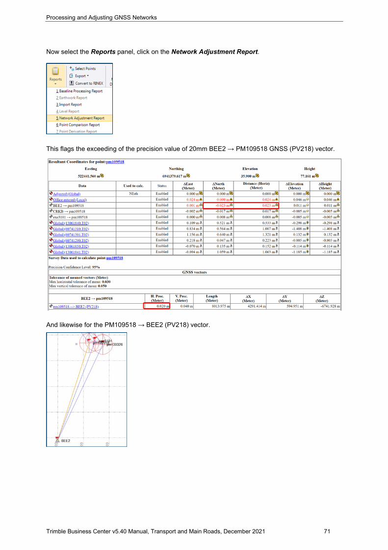
Processing and Adjusting GNSS Networks
Trimble Business Center v5.40 Manual, Transport and Main Roads, December 2021 71
Now select the Reports panel, click on the Network Adjustment Report.
This flags the exceeding of the precision value of 20mm BEE2 → PM109518 GNSS (PV218) vector.
And likewise for the PM109518 → BEE2 (PV218) vector.
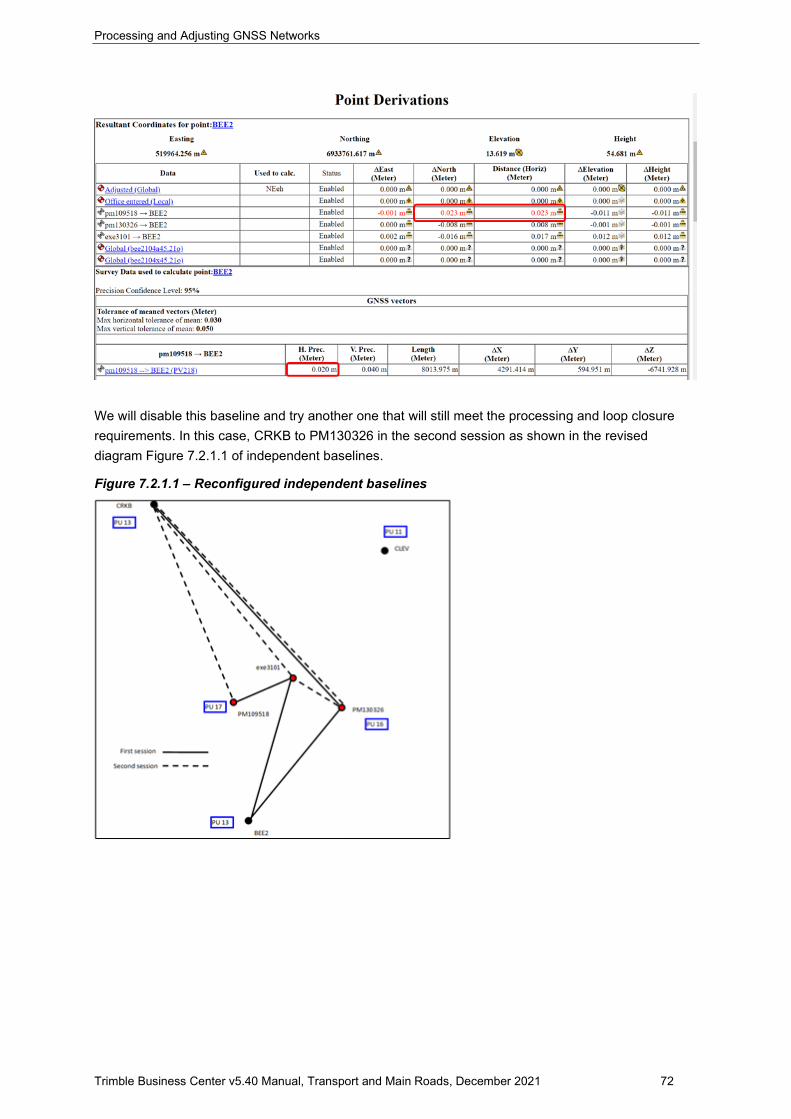
Processing and Adjusting GNSS Networks
Trimble Business Center v5.40 Manual, Transport and Main Roads, December 2021 72
We will disable this baseline and try another one that will still meet the processing and loop closure requirements. In this case, CRKB to PM130326 in the second session as shown in the revised diagram Figure 7.2.1.1 of independent baselines.
Figure 7.2.1.1 – Reconfigured independent baselines
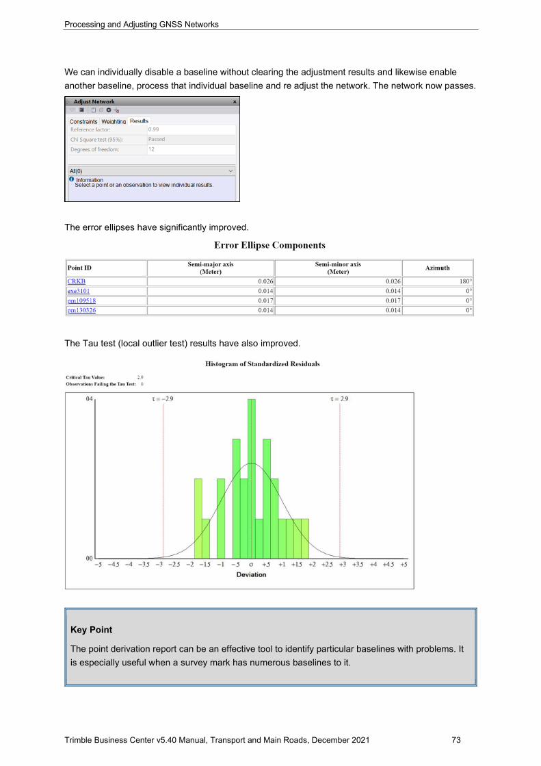
Processing and Adjusting GNSS Networks
Trimble Business Center v5.40 Manual, Transport and Main Roads, December 2021 73
We can individually disable a baseline without clearing the adjustment results and likewise enable another baseline, process that individual baseline and re adjust the network. The network now passes.
The error ellipses have significantly improved.
The Tau test (local outlier test) results have also improved.
Key Point
The point derivation report can be an effective tool to identify particular baselines with problems. It is especially useful when a survey mark has numerous baselines to it.
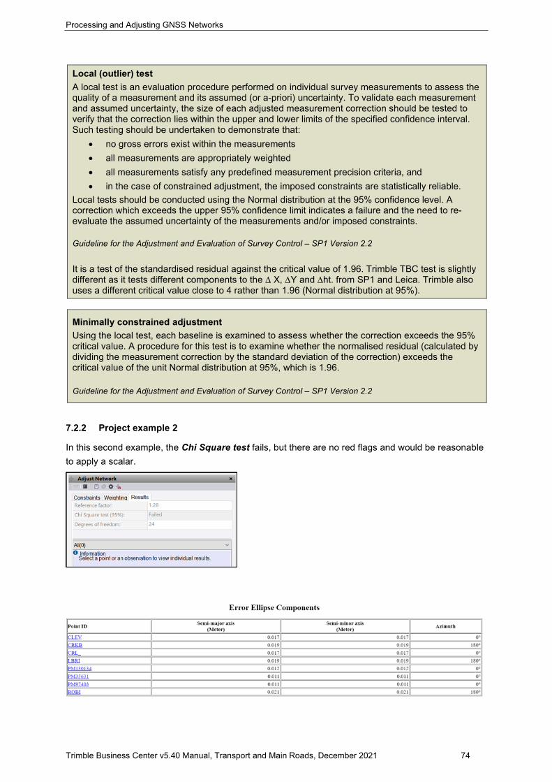
Processing and Adjusting GNSS Networks
Trimble Business Center v5.40 Manual, Transport and Main Roads, December 2021 74
Local (outlier) test A local test is an evaluation procedure performed on individual survey measurements to assess the quality of a measurement and its assumed (or a-priori) uncertainty. To validate each measurement and assumed uncertainty, the size of each adjusted measurement correction should be tested to verify that the correction lies within the upper and lower limits of the specified confidence interval. Such testing should be undertaken to demonstrate that:
• no gross errors exist within the measurements • all measurements are appropriately weighted • all measurements satisfy any predefined measurement precision criteria, and • in the case of constrained adjustment, the imposed constraints are statistically reliable.
Local tests should be conducted using the Normal distribution at the 95% confidence level. A correction which exceeds the upper 95% confidence limit indicates a failure and the need to re-evaluate the assumed uncertainty of the measurements and/or imposed constraints. Guideline for the Adjustment and Evaluation of Survey Control – SP1 Version 2.2 It is a test of the standardised residual against the critical value of 1.96. Trimble TBC test is slightly different as it tests different components to the ∆ X, ∆Y and ∆ht. from SP1 and Leica. Trimble also uses a different critical value close to 4 rather than 1.96 (Normal distribution at 95%).
Minimally constrained adjustment Using the local test, each baseline is examined to assess whether the correction exceeds the 95% critical value. A procedure for this test is to examine whether the normalised residual (calculated by dividing the measurement correction by the standard deviation of the correction) exceeds the critical value of the unit Normal distribution at 95%, which is 1.96. Guideline for the Adjustment and Evaluation of Survey Control – SP1 Version 2.2
7.2.2 Project example 2
In this second example, the Chi Square test fails, but there are no red flags and would be reasonable to apply a scalar.
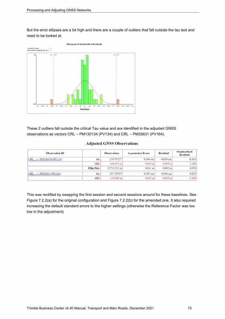
Processing and Adjusting GNSS Networks
Trimble Business Center v5.40 Manual, Transport and Main Roads, December 2021 75
But the error ellipses are a bit high and there are a couple of outliers that fall outside the tau test and need to be looked at.
These 2 outliers fall outside the critical Tau value and are identified in the adjusted GNSS observations as vectors CRL – PM130134 (PV134) and CRL – PM35631 (PV164).
This was rectified by swapping the first session and second sessions around for these baselines. See Figure 7.2.2(a) for the original configuration and Figure 7.2.2(b) for the amended one. It also required increasing the default standard errors to the higher settings (otherwise the Reference Factor was too low in the adjustment)
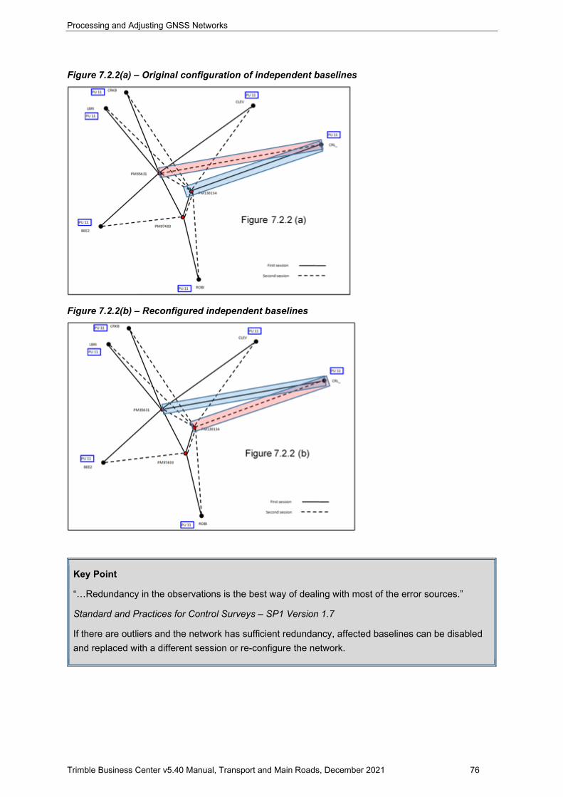
Processing and Adjusting GNSS Networks
Trimble Business Center v5.40 Manual, Transport and Main Roads, December 2021 76
Figure 7.2.2(a) – Original configuration of independent baselines
Figure 7.2.2(b) – Reconfigured independent baselines
Key Point
“…Redundancy in the observations is the best way of dealing with most of the error sources.”
Standard and Practices for Control Surveys – SP1 Version 1.7
If there are outliers and the network has sufficient redundancy, affected baselines can be disabled and replaced with a different session or re-configure the network.
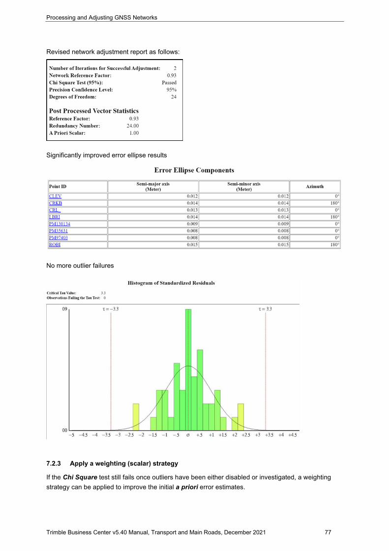
Processing and Adjusting GNSS Networks
Trimble Business Center v5.40 Manual, Transport and Main Roads, December 2021 77
Revised network adjustment report as follows:
Significantly improved error ellipse results
No more outlier failures
7.2.3 Apply a weighting (scalar) strategy
If the Chi Square test still fails once outliers have been either disabled or investigated, a weighting strategy can be applied to improve the initial a priori error estimates.
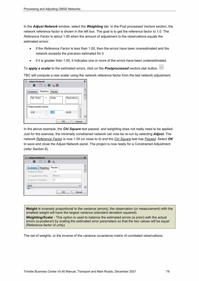
Processing and Adjusting GNSS Networks
Trimble Business Center v5.40 Manual, Transport and Main Roads, December 2021 78
In the Adjust Network window, select the Weighting tab. In the Post processed Vectors section, the network reference factor is shown in the left box. The goal is to get the reference factor to 1.0. The Reference Factor is about 1.00 when the amount of adjustment to the observations equals the estimated errors:
• if the Reference Factor is less than 1.00, then the errors have been overestimated and the network exceeds the precision estimated for it
• if it is greater than 1.00, it indicates one or more of the errors have been underestimated.
To apply a scalar to the estimated errors, click on the Postprocessed vectors star button.
TBC will compute a new scaler using the network reference factor from the last network adjustment.
In the above example, the Chi Square test passed, and weighting does not really need to be applied. Just for the exercise, the minimally constrained network can now be re-run by selecting Adjust. The network Reference Factor is now 1.00 (or close to it) and the Chi Square test has Passed. Select OK to save and close the Adjust Network panel. The project is now ready for a Constrained Adjustment (refer Section 8).
Weight is inversely proportional to the variance (errors), the observation (or measurement) with the smallest weight will have the largest variance (standard deviation squared). Weighting/Scalar - This option is used to balance the estimated errors (a priori) with the actual errors (a-posterori) by scaling the estimated error parameters so that the two values will be equal (Reference factor of unity).
The set of weights, or the inverse of the variance covariance matrix of correlated observations.
Processing and Adjusting GNSS Networks
Trimble Business Center v5.40 Manual, Transport and Main Roads, December 2021 79
Key Point
If you need to re-run a minimally constrained adjustment after conducting a constrained adjustment with weights (refer Section 8.1.2), it is critical to reset the weights to 0.000. Failure to do this will result in erroneous error ellipses for the minimally constrained adjustment.
Key Point
The error ellipses from the minimally constrained adjustment are used to calculate Survey Uncertainty (SU) values (refer Addendum)
GNSS error ellipses are generally close to being circular and should meet the nominated SU values as prescribed in Clause 3.2.1 Static surveys - Guideline for Control Surveys by GNSS SP1, version 2.2, Table 1 (refer 3.4.1.2)
7.2.4 Save network adjustment report
It is highly recommended to save all reports to a Reports folder within the TBC project folder.
Save as Web Archive
With the report open, select File > Save As
From Save As Type dropdown menu to select Web Archive, single file (*.mht)
Browse to the projects Reports folder, and enter an appropriate file name, for example MR123456 Minimal Constrained report
Select Save
Convert to PDF
With the report open;
If required, change the page orientation by selecting the dropdown arrow beside Convert on the PDF
toolbar.
Select Preferences and then Page Layout tab. Change the Orientation as appropriate and OK.
Select Convert from the PDF toolbar.
Browse to the projects Reports folder, enter an appropriate filename, for example MR123456 Minimal Constrained report.
Select Save.
Print to PDF
With the report open, select File > Print
From the Select Printer list, select PDF995.
If required, change the page orientation by selecting Preferences and changing the orientation.
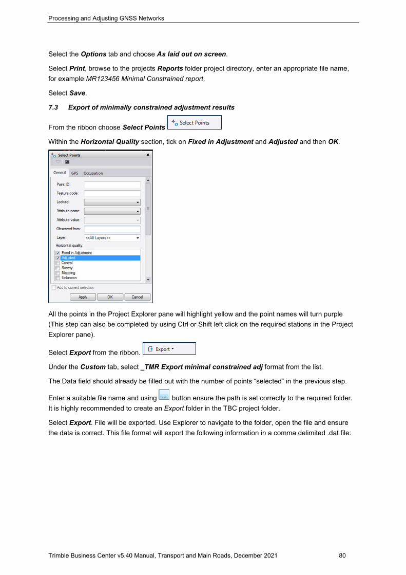
Processing and Adjusting GNSS Networks
Trimble Business Center v5.40 Manual, Transport and Main Roads, December 2021 80
Select the Options tab and choose As laid out on screen.
Select Print, browse to the projects Reports folder project directory, enter an appropriate file name, for example MR123456 Minimal Constrained report.
Select Save.
7.3 Export of minimally constrained adjustment results
From the ribbon choose Select Points
Within the Horizontal Quality section, tick on Fixed in Adjustment and Adjusted and then OK.
All the points in the Project Explorer pane will highlight yellow and the point names will turn purple (This step can also be completed by using Ctrl or Shift left click on the required stations in the Project Explorer pane).
Select Export from the ribbon.
Under the Custom tab, select _TMR Export minimal constrained adj format from the list.
The Data field should already be filled out with the number of points “selected” in the previous step.
Enter a suitable file name and using button ensure the path is set correctly to the required folder. It is highly recommended to create an Export folder in the TBC project folder.
Select Export. File will be exported. Use Explorer to navigate to the folder, open the file and ensure the data is correct. This file format will export the following information in a comma delimited .dat file:
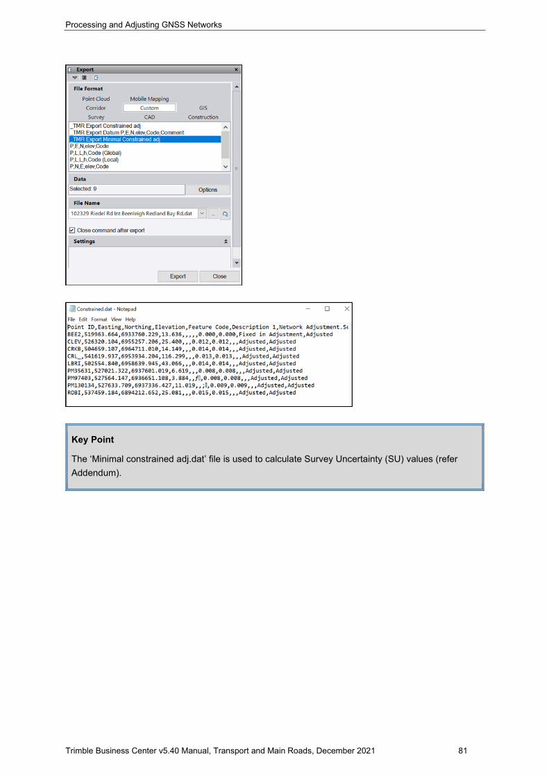
Processing and Adjusting GNSS Networks
Trimble Business Center v5.40 Manual, Transport and Main Roads, December 2021 81
Key Point
The ‘Minimal constrained adj.dat’ file is used to calculate Survey Uncertainty (SU) values (refer Addendum).
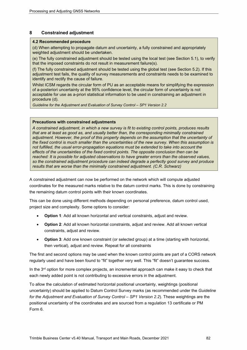
Processing and Adjusting GNSS Networks
Trimble Business Center v5.40 Manual, Transport and Main Roads, December 2021 82
8 Constrained adjustment
4.2 Recommended procedure (d) When attempting to propagate datum and uncertainty, a fully constrained and appropriately weighted adjustment should be undertaken. (e) The fully constrained adjustment should be tested using the local test (see Section 5.1), to verify that the imposed constraints do not result in measurement failure(s). (f) The fully constrained adjustment should be tested using the global test (see Section 5.2). If this adjustment test fails, the quality of survey measurements and constraints needs to be examined to identify and rectify the cause of failure. Whilst ICSM regards the circular form of PU as an acceptable means for simplifying the expression of a-posteriori uncertainty at the 95% confidence level, the circular form of uncertainty is not acceptable for use as a-priori statistical information to be used in constraining an adjustment in procedure (d). Guideline for the Adjustment and Evaluation of Survey Control – SP1 Version 2.2
Precautions with constrained adjustments A constrained adjustment, in which a new survey is fit to existing control points, produces results that are at least as good as, and usually better than, the corresponding minimally constrained adjustment. However, the proof of this property depends on the assumption that the uncertainty of the fixed control is much smaller than the uncertainties of the new survey. When this assumption is not fulfilled, the usual error-propagation equations must be extended to take into account the effects of the uncertainties of the fixed control points. The opposite conclusion then can be reached: It is possible for adjusted observations to have greater errors than the observed values, so the constrained adjustment procedure can indeed degrade a perfectly good survey and produce results that are worse than the minimally constrained adjustment. (C.R. Schwarz)
A constrained adjustment can now be performed on the network which will compute adjusted coordinates for the measured marks relative to the datum control marks. This is done by constraining the remaining datum control points with their known coordinates.
This can be done using different methods depending on personal preference, datum control used, project size and complexity. Some options to consider:
• Option 1: Add all known horizontal and vertical constraints, adjust and review.
• Option 2: Add all known horizontal constraints, adjust and review. Add all known vertical constraints, adjust and review.
• Option 3: Add one known constraint (or selected group) at a time (starting with horizontal, then vertical), adjust and review. Repeat for all constraints
The first and second options may be used when the known control points are part of a CORS network regularly used and have been found to “fit” together very well. This “fit” doesn’t guarantee success.
In the 3rd option for more complex projects, an incremental approach can make it easy to check that each newly added point is not contributing to excessive errors in the adjustment.
To allow the calculation of estimated horizontal positional uncertainty, weightings (positional uncertainty) should be applied to Datum Control Survey marks (as recommended under the Guideline for the Adjustment and Evaluation of Survey Control – SP1 Version 2.2). These weightings are the positional uncertainty of the coordinates and are sourced from a regulation 13 certificate or PM Form 6.
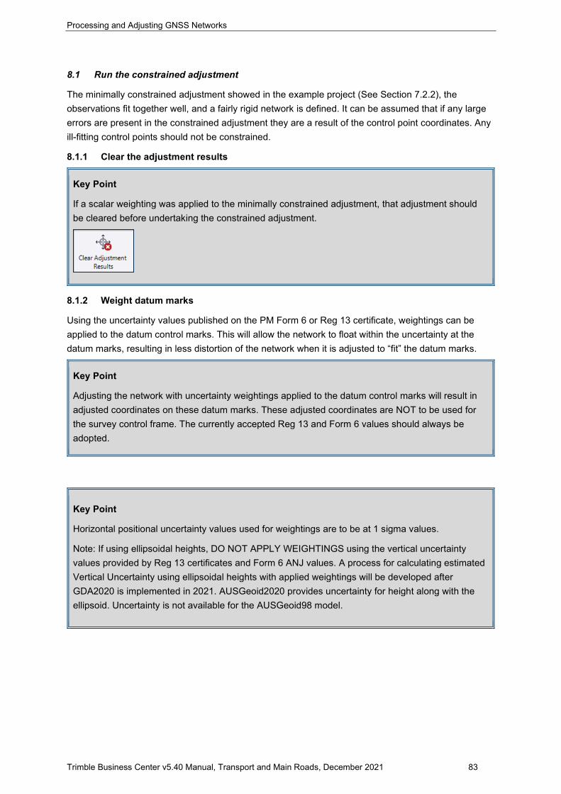
Processing and Adjusting GNSS Networks
Trimble Business Center v5.40 Manual, Transport and Main Roads, December 2021 83
8.1 Run the constrained adjustment
The minimally constrained adjustment showed in the example project (See Section 7.2.2), the observations fit together well, and a fairly rigid network is defined. It can be assumed that if any large errors are present in the constrained adjustment they are a result of the control point coordinates. Any ill-fitting control points should not be constrained.
8.1.1 Clear the adjustment results
Key Point
If a scalar weighting was applied to the minimally constrained adjustment, that adjustment should be cleared before undertaking the constrained adjustment.
8.1.2 Weight datum marks
Using the uncertainty values published on the PM Form 6 or Reg 13 certificate, weightings can be applied to the datum control marks. This will allow the network to float within the uncertainty at the datum marks, resulting in less distortion of the network when it is adjusted to “fit” the datum marks.
Key Point
Adjusting the network with uncertainty weightings applied to the datum control marks will result in adjusted coordinates on these datum marks. These adjusted coordinates are NOT to be used for the survey control frame. The currently accepted Reg 13 and Form 6 values should always be adopted.
Key Point
Horizontal positional uncertainty values used for weightings are to be at 1 sigma values.
Note: If using ellipsoidal heights, DO NOT APPLY WEIGHTINGS using the vertical uncertainty values provided by Reg 13 certificates and Form 6 ANJ values. A process for calculating estimated Vertical Uncertainty using ellipsoidal heights with applied weightings will be developed after GDA2020 is implemented in 2021. AUSGeoid2020 provides uncertainty for height along with the ellipsoid. Uncertainty is not available for the AUSGeoid98 model.
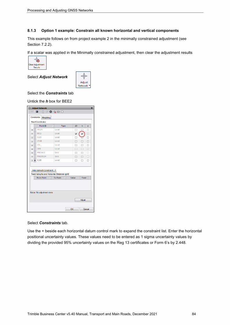
Processing and Adjusting GNSS Networks
Trimble Business Center v5.40 Manual, Transport and Main Roads, December 2021 84
8.1.3 Option 1 example: Constrain all known horizontal and vertical components
This example follows on from project example 2 in the minimally constrained adjustment (see Section 7.2.2).
If a scalar was applied in the Minimally constrained adjustment, then clear the adjustment results
Select Adjust Network
Select the Constraints tab
Untick the h box for BEE2
Select Constraints tab.
Use the + beside each horizontal datum control mark to expand the constraint list. Enter the horizontal positional uncertainty values. These values need to be entered as 1 sigma uncertainty values by dividing the provided 95% uncertainty values on the Reg 13 certificates or Form 6’s by 2.448.
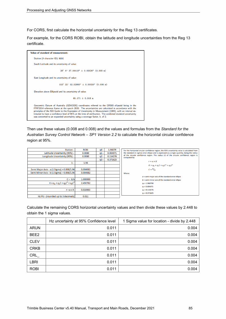
Processing and Adjusting GNSS Networks
Trimble Business Center v5.40 Manual, Transport and Main Roads, December 2021 85
For CORS, first calculate the horizontal uncertainty for the Reg 13 certificates.
For example, for the CORS ROBI, obtain the latitude and longitude uncertainties from the Reg 13 certificate.
Then use these values (0.008 and 0.008) and the values and formulas from the Standard for the Australian Survey Control Network – SP1 Version 2.2 to calculate the horizontal circular confidence region at 95%.
Calculate the remaining CORS horizontal uncertainty values and then divide these values by 2.448 to obtain the 1 sigma values.
Hz uncertainty at 95% Confidence level 1 Sigma value for location - divide by 2.448
ARUN 0.011 0.004
BEE2 0.011 0.004
CLEV 0.011 0.004
CRKB 0.011 0.004
CRL_ 0.011 0.004
LBRI 0.011 0.004
ROBI 0.011 0.004
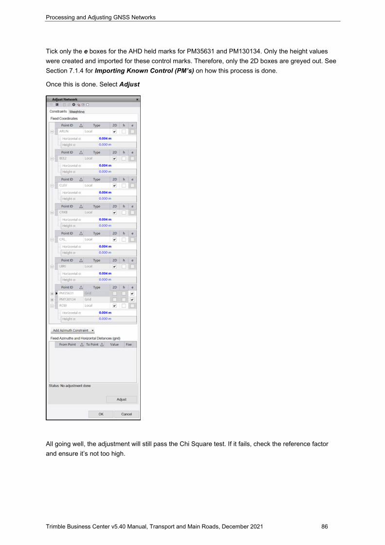
Processing and Adjusting GNSS Networks
Trimble Business Center v5.40 Manual, Transport and Main Roads, December 2021 86
Tick only the e boxes for the AHD held marks for PM35631 and PM130134. Only the height values were created and imported for these control marks. Therefore, only the 2D boxes are greyed out. See Section 7.1.4 for Importing Known Control (PM’s) on how this process is done.
Once this is done. Select Adjust
All going well, the adjustment will still pass the Chi Square test. If it fails, check the reference factor and ensure it’s not too high.
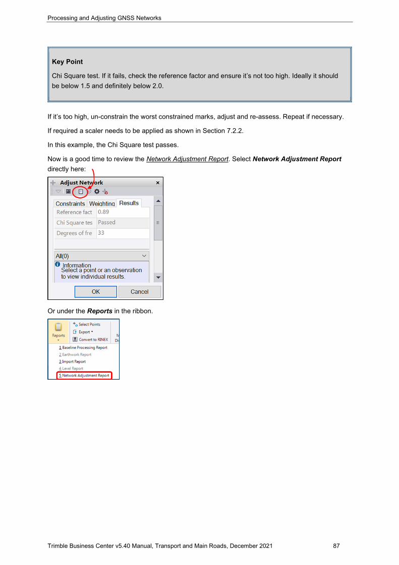
Processing and Adjusting GNSS Networks
Trimble Business Center v5.40 Manual, Transport and Main Roads, December 2021 87
Key Point
Chi Square test. If it fails, check the reference factor and ensure it’s not too high. Ideally it should be below 1.5 and definitely below 2.0.
If it’s too high, un-constrain the worst constrained marks, adjust and re-assess. Repeat if necessary.
If required a scaler needs to be applied as shown in Section 7.2.2.
In this example, the Chi Square test passes.
Now is a good time to review the Network Adjustment Report. Select Network Adjustment Report directly here:
Or under the Reports in the ribbon.

Processing and Adjusting GNSS Networks
Trimble Business Center v5.40 Manual, Transport and Main Roads, December 2021 88
The primary focus is checking the Control Coordinate Comparisons section. This compares the entered control coordinates to their current adjusted coordinates. These comparisons give an early indication as to what marks fit together. This knowledge may change the strategy of the order in which order additional marks will be fixed and the adjustment run. Marks that may potentially not fit the network should be the last to be fixed and run. In the example below, the adjustment differences between the fixed marks are acceptable, and no changes are necessary.
Peruse the Control Coordinate Constraints and check values are correct. Look at the errors in the Adjusted Grid Coordinates. If the network has been observed and processed correctly the errors should be small. The Elevation Error may be large for marks with entered ellipsoidal heights due to inaccuracies in the ellipsoidal to AHD relationship.
A visual representation of the errors can be accessed by left clicking on a point name. The Adjust Network window must still be open as the errors with visualisation will be shown in this window. Several marks can be shown at the same time by dragging a window around the required marks and vectors in the Plan View. Alternately select the points in the Project Explorer pane whilst holding the Ctrl key.
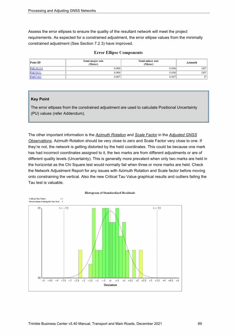
Processing and Adjusting GNSS Networks
Trimble Business Center v5.40 Manual, Transport and Main Roads, December 2021 89
Assess the error ellipses to ensure the quality of the resultant network will meet the project requirements. As expected for a constrained adjustment, the error ellipse values from the minimally constrained adjustment (See Section 7.2.3) have improved.
Key Point
The error ellipses from the constrained adjustment are used to calculate Positional Uncertainty (PU) values (refer Addendum).
The other important information is the Azimuth Rotation and Scale Factor in the Adjusted GNSS Observations. Azimuth Rotation should be very close to zero and Scale Factor very close to one. If they’re not, the network is getting distorted by the held coordinates. This could be because one mark has had incorrect coordinates assigned to it, the two marks are from different adjustments or are of different quality levels (Uncertainty). This is generally more prevalent when only two marks are held in the horizontal as the Chi Square test would normally fail when three or more marks are held. Check the Network Adjustment Report for any issues with Azimuth Rotation and Scale factor before moving onto constraining the vertical. Also the new Critical Tau Value graphical results and outliers failing the Tau test is valuable.
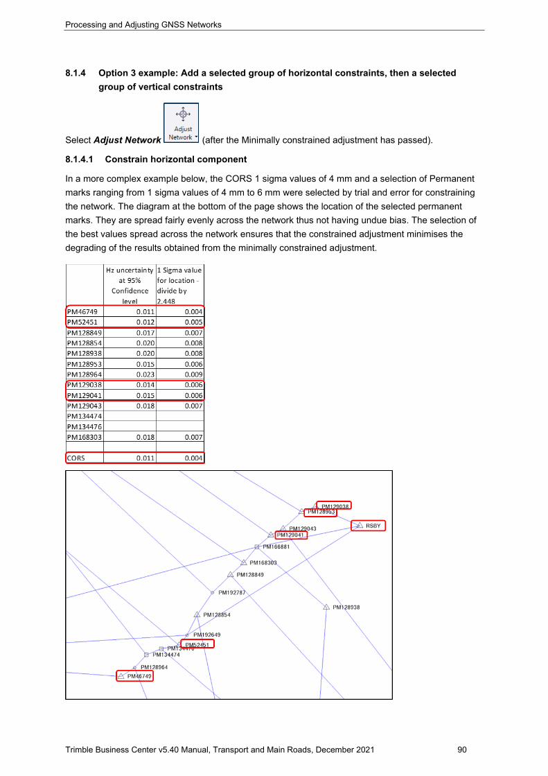
Processing and Adjusting GNSS Networks
Trimble Business Center v5.40 Manual, Transport and Main Roads, December 2021 90
8.1.4 Option 3 example: Add a selected group of horizontal constraints, then a selected group of vertical constraints
Select Adjust Network (after the Minimally constrained adjustment has passed).
8.1.4.1 Constrain horizontal component
In a more complex example below, the CORS 1 sigma values of 4 mm and a selection of Permanent marks ranging from 1 sigma values of 4 mm to 6 mm were selected by trial and error for constraining the network. The diagram at the bottom of the page shows the location of the selected permanent marks. They are spread fairly evenly across the network thus not having undue bias. The selection of the best values spread across the network ensures that the constrained adjustment minimises the degrading of the results obtained from the minimally constrained adjustment.
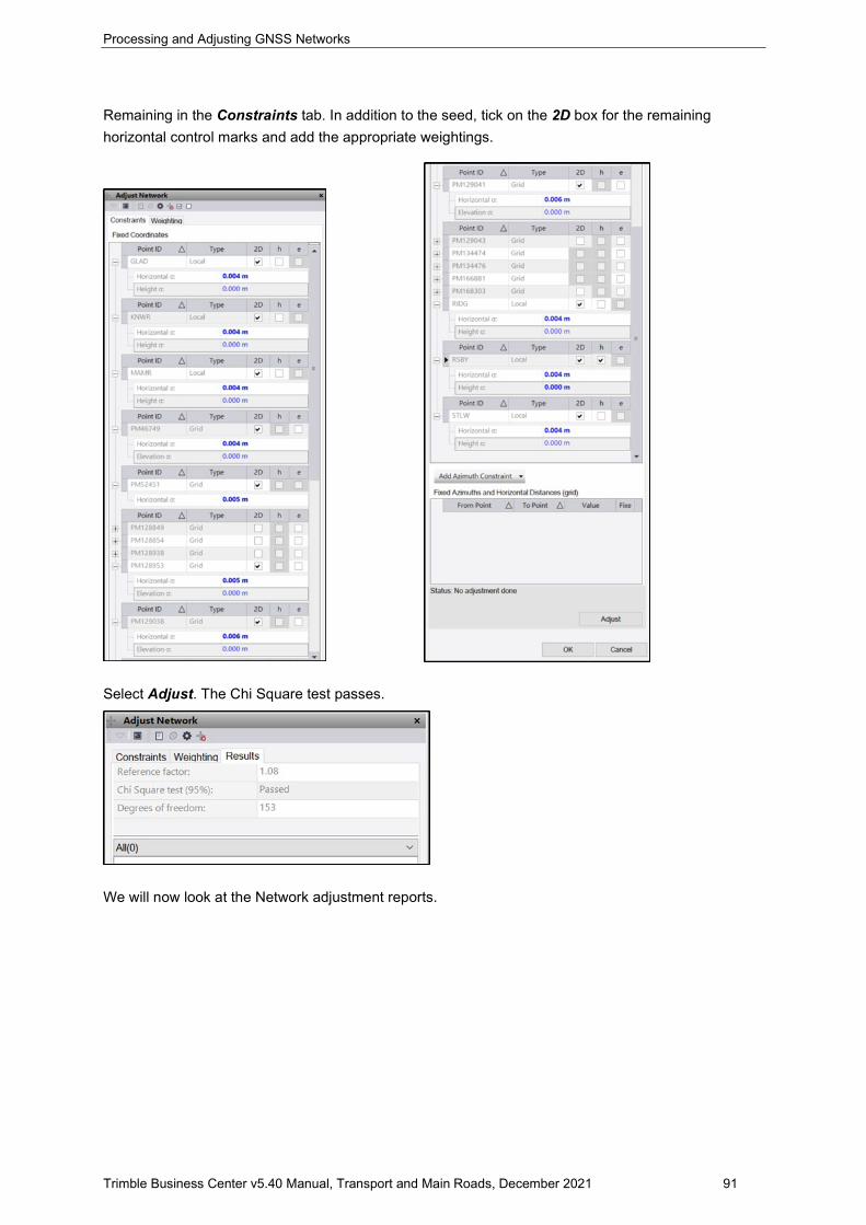
Processing and Adjusting GNSS Networks
Trimble Business Center v5.40 Manual, Transport and Main Roads, December 2021 91
Remaining in the Constraints tab. In addition to the seed, tick on the 2D box for the remaining horizontal control marks and add the appropriate weightings.
Select Adjust. The Chi Square test passes.
We will now look at the Network adjustment reports.
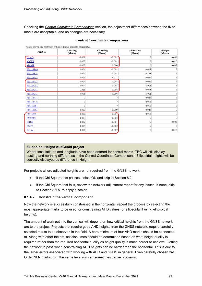
Processing and Adjusting GNSS Networks
Trimble Business Center v5.40 Manual, Transport and Main Roads, December 2021 92
Checking the Control Coordinate Comparisons section, the adjustment differences between the fixed marks are acceptable, and no changes are necessary.
Ellipsoidal Height AusGeoid project Where local latitude and longitude have been entered for control marks, TBC will still display easting and northing differences in the Control Coordinate Comparisons. Ellipsoidal heights will be correctly displayed as difference in Height.
For projects where adjusted heights are not required from the GNSS network:
• if the Chi Square test passes, select OK and skip to Section 8.2
• if the Chi Square test fails, review the network adjustment report for any issues. If none, skip to Section 8.1.5. to apply a scalar.
8.1.4.2 Constrain the vertical component
Now the network is successfully constrained in the horizontal, repeat the process by selecting the most appropriate marks to be used for constraining AHD values (or ellipsoidal if using ellipsoidal heights).
The amount of work put into the vertical will depend on how critical heights from the GNSS network are to the project. Projects that require good AHD heights from the GNSS network, require carefully selected marks to be observed in the field. A bare minimum of four AHD marks should be connected to. Along with other factors, session times should be determined based on what height quality is required rather than the required horizontal quality as height quality is much harder to achieve. Getting the network to pass when constraining AHD heights can be harder than the horizontal. This is due to the larger errors associated with working with AHD and GNSS in general. Even carefully chosen 3rd Order NLN marks from the same level run can sometimes cause problems.
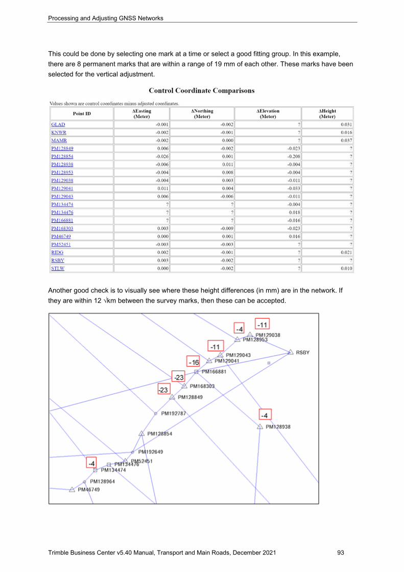
Processing and Adjusting GNSS Networks
Trimble Business Center v5.40 Manual, Transport and Main Roads, December 2021 93
This could be done by selecting one mark at a time or select a good fitting group. In this example, there are 8 permanent marks that are within a range of 19 mm of each other. These marks have been selected for the vertical adjustment.
Another good check is to visually see where these height differences (in mm) are in the network. If they are within 12 √km between the survey marks, then these can be accepted.
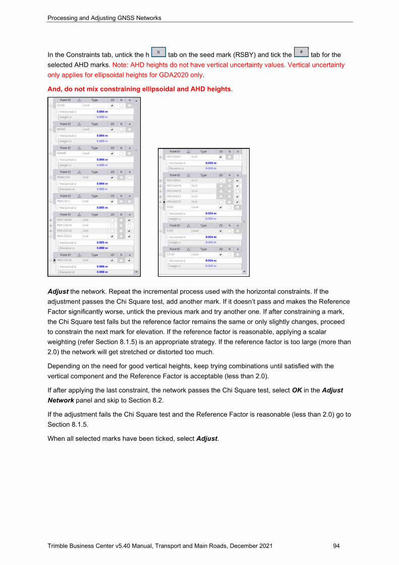
Processing and Adjusting GNSS Networks
Trimble Business Center v5.40 Manual, Transport and Main Roads, December 2021 94
In the Constraints tab, untick the h tab on the seed mark (RSBY) and tick the tab for the selected AHD marks. Note: AHD heights do not have vertical uncertainty values. Vertical uncertainty only applies for ellipsoidal heights for GDA2020 only.
And, do not mix constraining ellipsoidal and AHD heights.
Adjust the network. Repeat the incremental process used with the horizontal constraints. If the adjustment passes the Chi Square test, add another mark. If it doesn’t pass and makes the Reference Factor significantly worse, untick the previous mark and try another one. If after constraining a mark, the Chi Square test fails but the reference factor remains the same or only slightly changes, proceed to constrain the next mark for elevation. If the reference factor is reasonable, applying a scalar weighting (refer Section 8.1.5) is an appropriate strategy. If the reference factor is too large (more than 2.0) the network will get stretched or distorted too much.
Depending on the need for good vertical heights, keep trying combinations until satisfied with the vertical component and the Reference Factor is acceptable (less than 2.0).
If after applying the last constraint, the network passes the Chi Square test, select OK in the Adjust Network panel and skip to Section 8.2.
If the adjustment fails the Chi Square test and the Reference Factor is reasonable (less than 2.0) go to Section 8.1.5.
When all selected marks have been ticked, select Adjust.

Processing and Adjusting GNSS Networks
Trimble Business Center v5.40 Manual, Transport and Main Roads, December 2021 95
In this example, the Chi Square test fails, but is well under Reference factor 1.5.
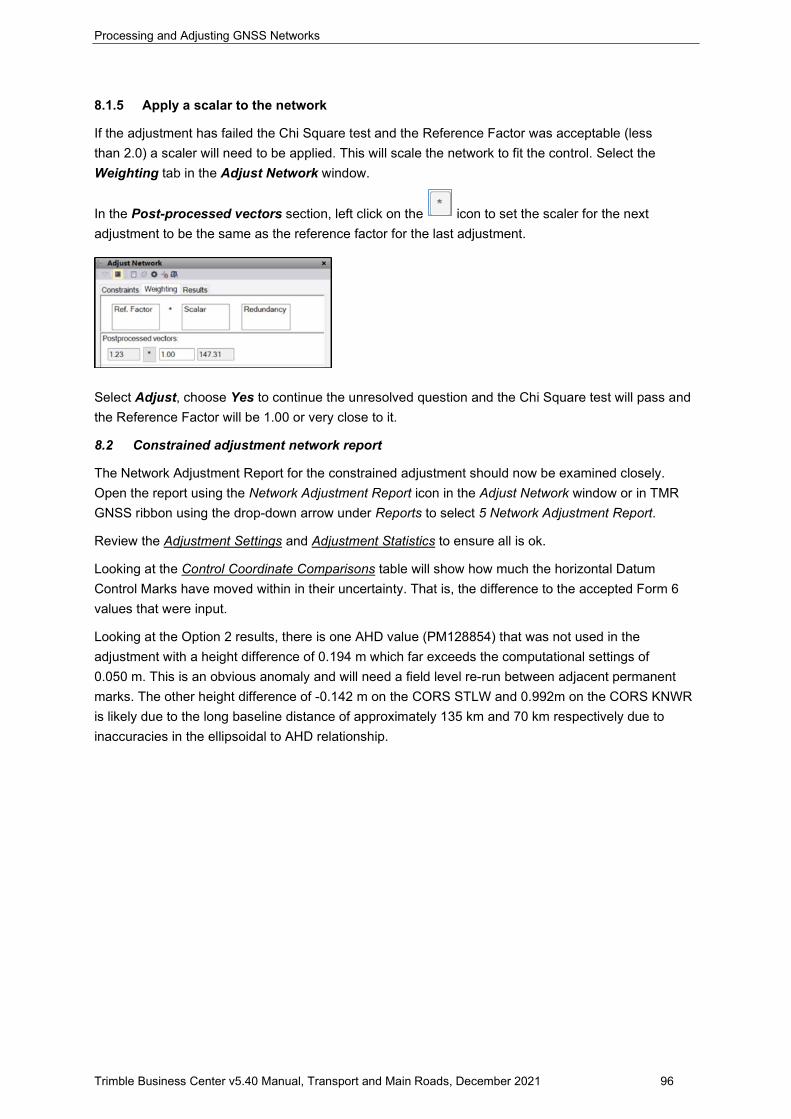
Processing and Adjusting GNSS Networks
Trimble Business Center v5.40 Manual, Transport and Main Roads, December 2021 96
8.1.5 Apply a scalar to the network
If the adjustment has failed the Chi Square test and the Reference Factor was acceptable (less than 2.0) a scaler will need to be applied. This will scale the network to fit the control. Select the Weighting tab in the Adjust Network window.
In the Post-processed vectors section, left click on the icon to set the scaler for the next adjustment to be the same as the reference factor for the last adjustment.
Select Adjust, choose Yes to continue the unresolved question and the Chi Square test will pass and the Reference Factor will be 1.00 or very close to it.
8.2 Constrained adjustment network report
The Network Adjustment Report for the constrained adjustment should now be examined closely. Open the report using the Network Adjustment Report icon in the Adjust Network window or in TMR GNSS ribbon using the drop-down arrow under Reports to select 5 Network Adjustment Report.
Review the Adjustment Settings and Adjustment Statistics to ensure all is ok.
Looking at the Control Coordinate Comparisons table will show how much the horizontal Datum Control Marks have moved within in their uncertainty. That is, the difference to the accepted Form 6 values that were input.
Looking at the Option 2 results, there is one AHD value (PM128854) that was not used in the adjustment with a height difference of 0.194 m which far exceeds the computational settings of 0.050 m. This is an obvious anomaly and will need a field level re-run between adjacent permanent marks. The other height difference of -0.142 m on the CORS STLW and 0.992m on the CORS KNWR is likely due to the long baseline distance of approximately 135 km and 70 km respectively due to inaccuracies in the ellipsoidal to AHD relationship.
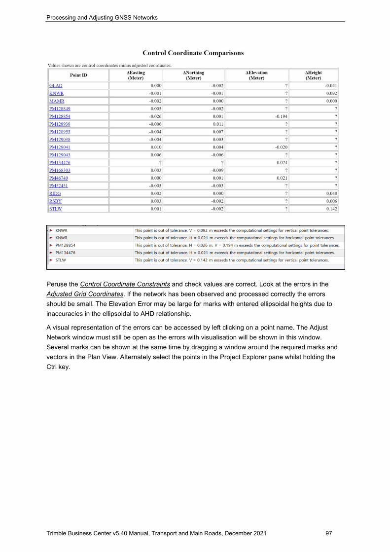
Processing and Adjusting GNSS Networks
Trimble Business Center v5.40 Manual, Transport and Main Roads, December 2021 97
Peruse the Control Coordinate Constraints and check values are correct. Look at the errors in the Adjusted Grid Coordinates. If the network has been observed and processed correctly the errors should be small. The Elevation Error may be large for marks with entered ellipsoidal heights due to inaccuracies in the ellipsoidal to AHD relationship.
A visual representation of the errors can be accessed by left clicking on a point name. The Adjust Network window must still be open as the errors with visualisation will be shown in this window. Several marks can be shown at the same time by dragging a window around the required marks and vectors in the Plan View. Alternately select the points in the Project Explorer pane whilst holding the Ctrl key.
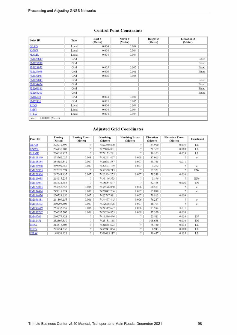
Processing and Adjusting GNSS Networks
Trimble Business Center v5.40 Manual, Transport and Main Roads, December 2021 98
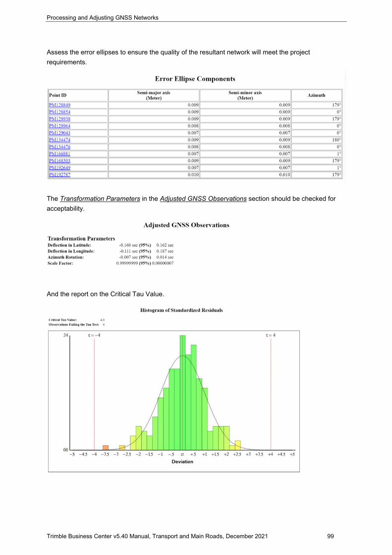
Processing and Adjusting GNSS Networks
Trimble Business Center v5.40 Manual, Transport and Main Roads, December 2021 99
Assess the error ellipses to ensure the quality of the resultant network will meet the project requirements.
The Transformation Parameters in the Adjusted GNSS Observations section should be checked for acceptability.
And the report on the Critical Tau Value.
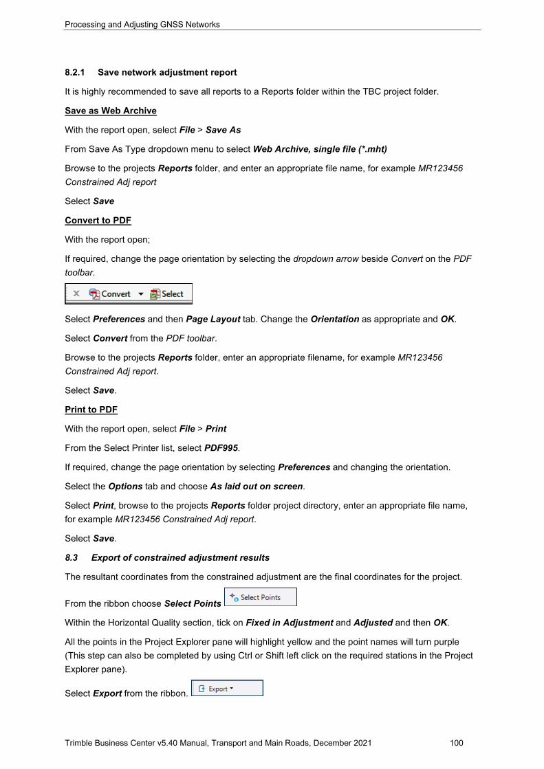
Processing and Adjusting GNSS Networks
Trimble Business Center v5.40 Manual, Transport and Main Roads, December 2021 100
8.2.1 Save network adjustment report
It is highly recommended to save all reports to a Reports folder within the TBC project folder.
Save as Web Archive
With the report open, select File > Save As
From Save As Type dropdown menu to select Web Archive, single file (*.mht)
Browse to the projects Reports folder, and enter an appropriate file name, for example MR123456 Constrained Adj report
Select Save
Convert to PDF
With the report open;
If required, change the page orientation by selecting the dropdown arrow beside Convert on the PDF toolbar.
Select Preferences and then Page Layout tab. Change the Orientation as appropriate and OK.
Select Convert from the PDF toolbar.
Browse to the projects Reports folder, enter an appropriate filename, for example MR123456 Constrained Adj report.
Select Save.
Print to PDF
With the report open, select File > Print
From the Select Printer list, select PDF995.
If required, change the page orientation by selecting Preferences and changing the orientation.
Select the Options tab and choose As laid out on screen.
Select Print, browse to the projects Reports folder project directory, enter an appropriate file name, for example MR123456 Constrained Adj report.
Select Save.
8.3 Export of constrained adjustment results
The resultant coordinates from the constrained adjustment are the final coordinates for the project.
From the ribbon choose Select Points
Within the Horizontal Quality section, tick on Fixed in Adjustment and Adjusted and then OK.
All the points in the Project Explorer pane will highlight yellow and the point names will turn purple (This step can also be completed by using Ctrl or Shift left click on the required stations in the Project Explorer pane).
Select Export from the ribbon.
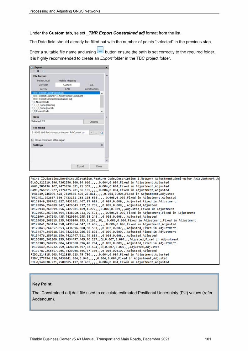
Processing and Adjusting GNSS Networks
Trimble Business Center v5.40 Manual, Transport and Main Roads, December 2021 101
Under the Custom tab, select _TMR Export Constrained adj format from the list.
The Data field should already be filled out with the number of points “selected” in the previous step.
Enter a suitable file name and using button ensure the path is set correctly to the required folder. It is highly recommended to create an Export folder in the TBC project folder.
Key Point
The ‘Constrained adj.dat’ file used to calculate estimated Positional Uncertainty (PU) values (refer Addendum).
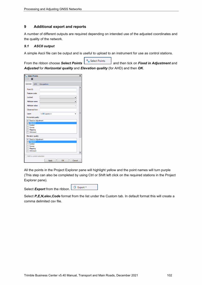
Processing and Adjusting GNSS Networks
Trimble Business Center v5.40 Manual, Transport and Main Roads, December 2021 102
9 Additional export and reports
A number of different outputs are required depending on intended use of the adjusted coordinates and the quality of the network.
9.1 ASCII output
A simple Ascii file can be output and is useful to upload to an instrument for use as control stations.
From the ribbon choose Select Points and then tick on Fixed in Adjustment and Adjusted for Horizontal quality and Elevation quality (for AHD) and then OK.
All the points in the Project Explorer pane will highlight yellow and the point names will turn purple (This step can also be completed by using Ctrl or Shift left click on the required stations in the Project Explorer pane).
Select Export from the ribbon.
Select P,E,N,elev,Code format from the list under the Custom tab. In default format this will create a comma delimited csv file.
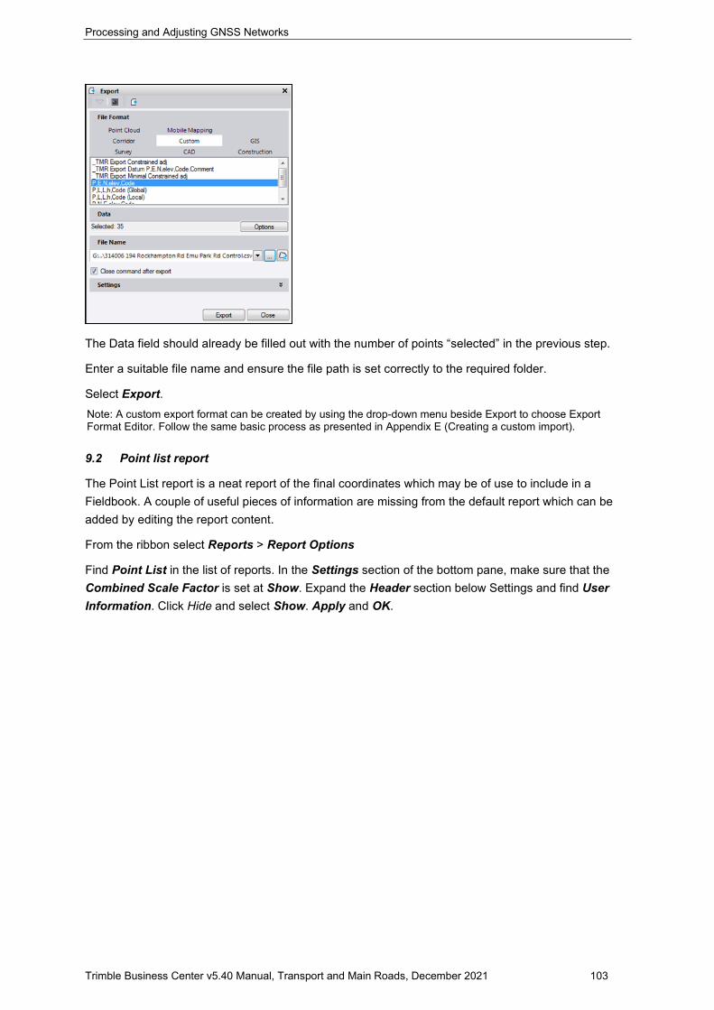
Processing and Adjusting GNSS Networks
Trimble Business Center v5.40 Manual, Transport and Main Roads, December 2021 103
The Data field should already be filled out with the number of points “selected” in the previous step.
Enter a suitable file name and ensure the file path is set correctly to the required folder.
Select Export. Note: A custom export format can be created by using the drop-down menu beside Export to choose Export Format Editor. Follow the same basic process as presented in Appendix E (Creating a custom import).
9.2 Point list report
The Point List report is a neat report of the final coordinates which may be of use to include in a Fieldbook. A couple of useful pieces of information are missing from the default report which can be added by editing the report content.
From the ribbon select Reports > Report Options
Find Point List in the list of reports. In the Settings section of the bottom pane, make sure that the Combined Scale Factor is set at Show. Expand the Header section below Settings and find User Information. Click Hide and select Show. Apply and OK.
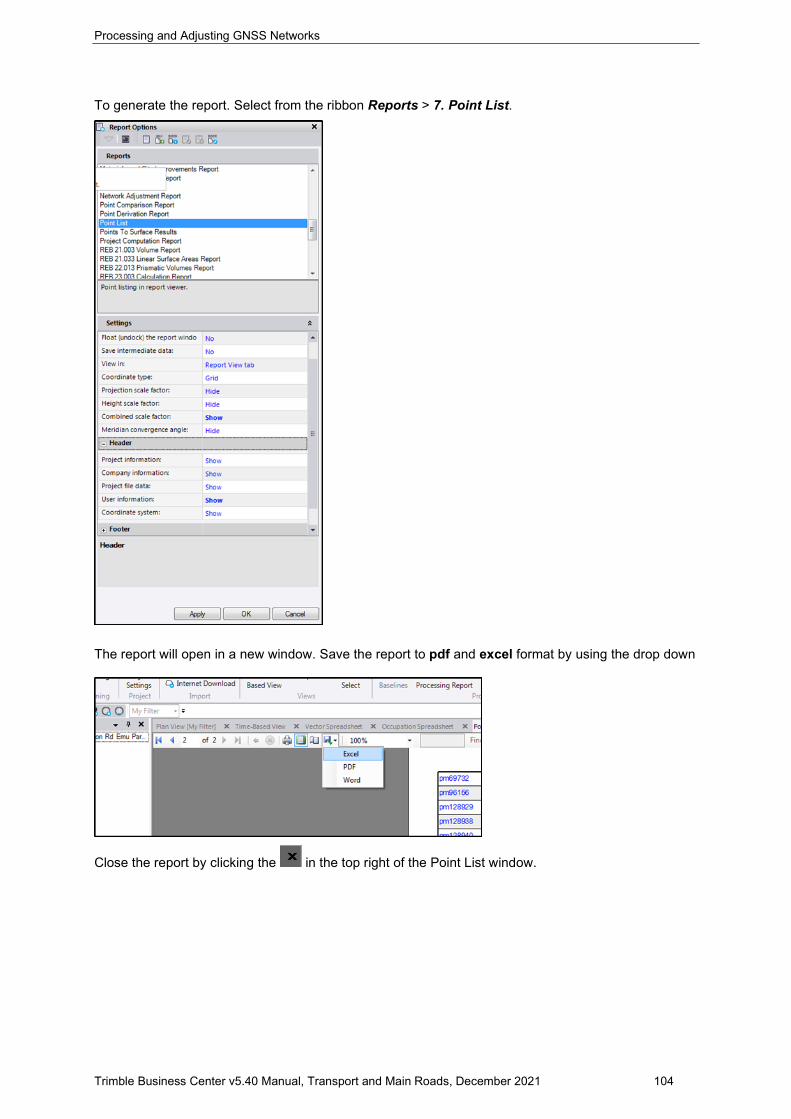
Processing and Adjusting GNSS Networks
Trimble Business Center v5.40 Manual, Transport and Main Roads, December 2021 104
To generate the report. Select from the ribbon Reports > 7. Point List.
The report will open in a new window. Save the report to pdf and excel format by using the drop down
Close the report by clicking the in the top right of the Point List window.
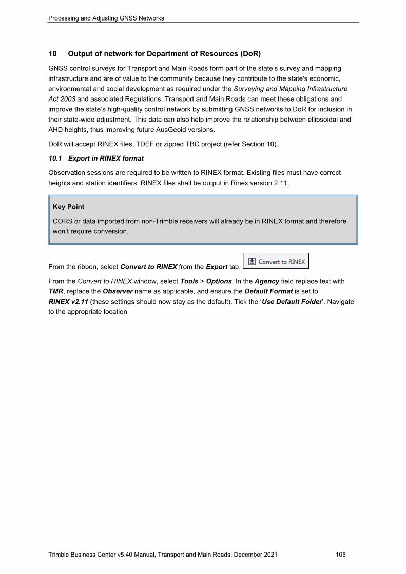
Processing and Adjusting GNSS Networks
Trimble Business Center v5.40 Manual, Transport and Main Roads, December 2021 105
10 Output of network for Department of Resources (DoR)
GNSS control surveys for Transport and Main Roads form part of the state’s survey and mapping infrastructure and are of value to the community because they contribute to the state's economic, environmental and social development as required under the Surveying and Mapping Infrastructure Act 2003 and associated Regulations. Transport and Main Roads can meet these obligations and improve the state’s high-quality control network by submitting GNSS networks to DoR for inclusion in their state-wide adjustment. This data can also help improve the relationship between ellipsoidal and AHD heights, thus improving future AusGeoid versions.
DoR will accept RINEX files, TDEF or zipped TBC project (refer Section 10).
10.1 Export in RINEX format
Observation sessions are required to be written to RINEX format. Existing files must have correct heights and station identifiers. RINEX files shall be output in Rinex version 2.11.
Key Point
CORS or data imported from non-Trimble receivers will already be in RINEX format and therefore won’t require conversion.
From the ribbon, select Convert to RINEX from the Export tab.
From the Convert to RINEX window, select Tools > Options. In the Agency field replace text with TMR, replace the Observer name as applicable, and ensure the Default Format is set to RINEX v2.11 (these settings should now stay as the default). Tick the ‘Use Default Folder’. Navigate to the appropriate location
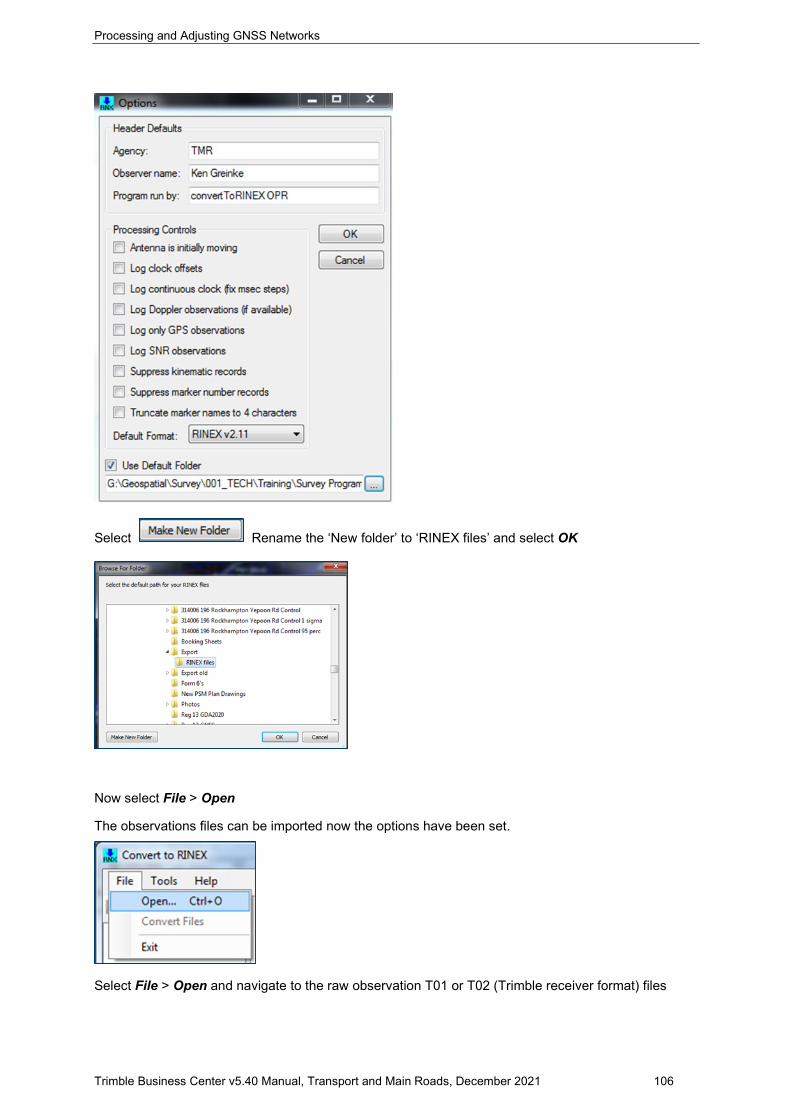
Processing and Adjusting GNSS Networks
Trimble Business Center v5.40 Manual, Transport and Main Roads, December 2021 106
Select Rename the ‘New folder’ to ‘RINEX files’ and select OK
Now select File > Open
The observations files can be imported now the options have been set.
Select File > Open and navigate to the raw observation T01 or T02 (Trimble receiver format) files
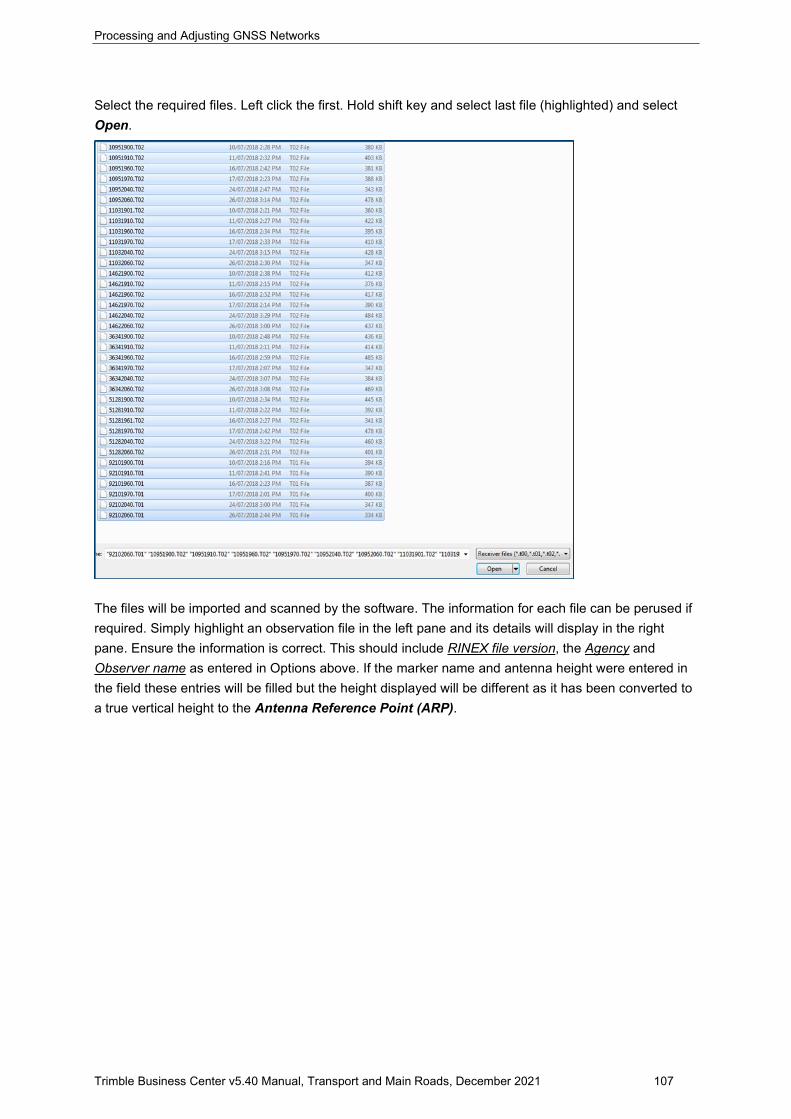
Processing and Adjusting GNSS Networks
Trimble Business Center v5.40 Manual, Transport and Main Roads, December 2021 107
Select the required files. Left click the first. Hold shift key and select last file (highlighted) and select Open.
The files will be imported and scanned by the software. The information for each file can be perused if required. Simply highlight an observation file in the left pane and its details will display in the right pane. Ensure the information is correct. This should include RINEX file version, the Agency and Observer name as entered in Options above. If the marker name and antenna height were entered in the field these entries will be filled but the height displayed will be different as it has been converted to a true vertical height to the Antenna Reference Point (ARP).
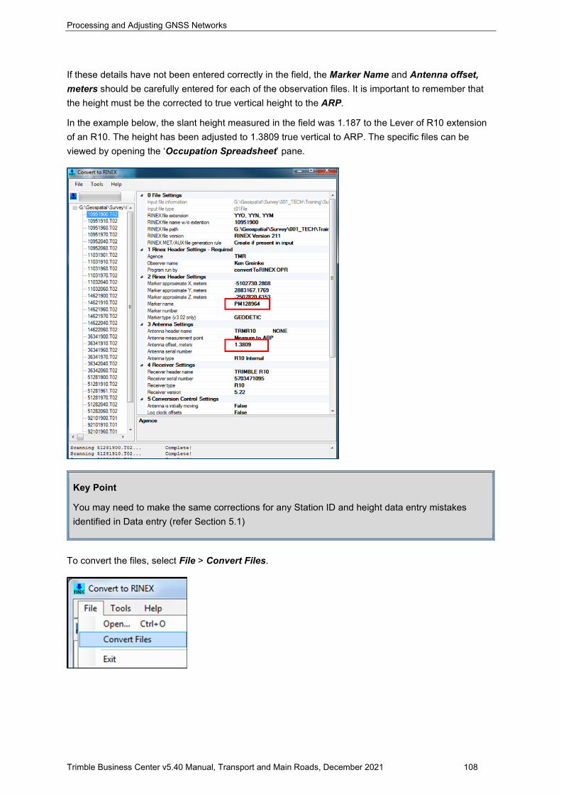
Processing and Adjusting GNSS Networks
Trimble Business Center v5.40 Manual, Transport and Main Roads, December 2021 108
If these details have not been entered correctly in the field, the Marker Name and Antenna offset, meters should be carefully entered for each of the observation files. It is important to remember that the height must be the corrected to true vertical height to the ARP.
In the example below, the slant height measured in the field was 1.187 to the Lever of R10 extension of an R10. The height has been adjusted to 1.3809 true vertical to ARP. The specific files can be viewed by opening the ‘Occupation Spreadsheet’ pane.
Key Point
You may need to make the same corrections for any Station ID and height data entry mistakes identified in Data entry (refer Section 5.1)
To convert the files, select File > Convert Files.
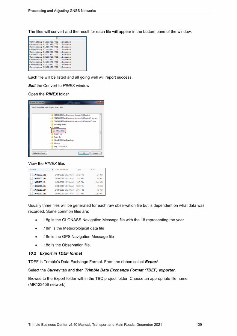
Processing and Adjusting GNSS Networks
Trimble Business Center v5.40 Manual, Transport and Main Roads, December 2021 109
The files will convert and the result for each file will appear in the bottom pane of the window.
Each file will be listed and all going well will report success.
Exit the Convert to RINEX window.
Open the RINEX folder
View the RINEX files
Usually three files will be generated for each raw observation file but is dependent on what data was recorded. Some common files are:
• .18g is the GLONASS Navigation Message file with the 18 representing the year
• .18m is the Meteorological data file
• .18n is the GPS Navigation Message file
• .18o is the Observation file.
10.2 Export in TDEF format
TDEF is Trimble’s Data Exchange Format. From the ribbon select Export.
Select the Survey tab and then Trimble Data Exchange Format (TDEF) exporter.
Browse to the Export folder within the TBC project folder. Choose an appropriate file name (MR123456 network).
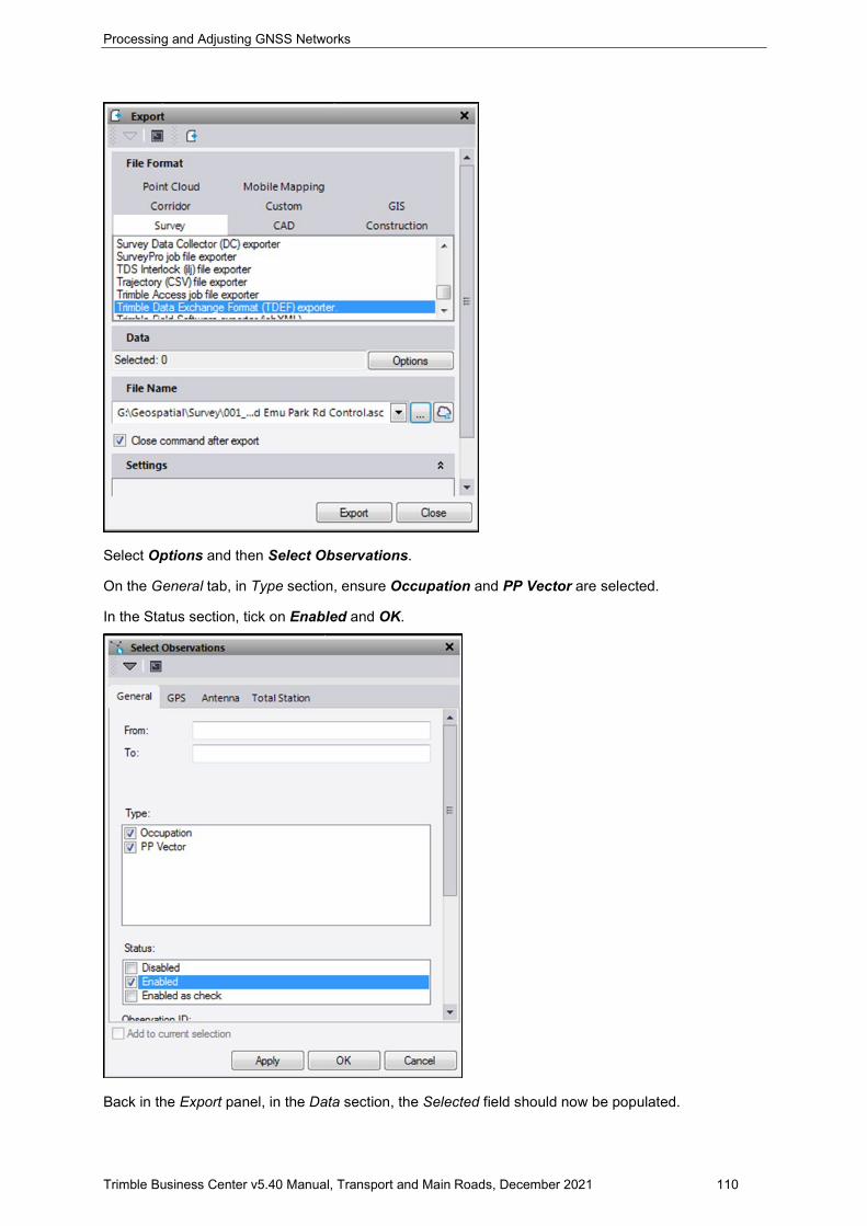
Processing and Adjusting GNSS Networks
Trimble Business Center v5.40 Manual, Transport and Main Roads, December 2021 110
Select Options and then Select Observations.
On the General tab, in Type section, ensure Occupation and PP Vector are selected.
In the Status section, tick on Enabled and OK.
Back in the Export panel, in the Data section, the Selected field should now be populated.
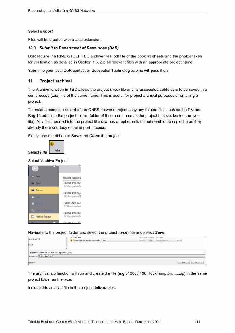
Processing and Adjusting GNSS Networks
Trimble Business Center v5.40 Manual, Transport and Main Roads, December 2021 111
Select Export.
Files will be created with a .asc extension.
10.3 Submit to Department of Resources (DoR)
DoR require the RINEX/TDEF/TBC archive files, pdf file of the booking sheets and the photos taken for verification as detailed in Section 1.3. Zip all relevant files with an appropriate project name.
Submit to your local DoR contact or Geospatial Technologies who will pass it on.
11 Project archival
The Archive function in TBC allows the project (.vce) file and its associated subfolders to be saved in a compressed (.zip) file of the same name. This is useful for project archival purposes or emailing a project.
To make a complete record of the GNSS network project copy any related files such as the PM and Reg 13 pdfs into the project folder (folder of the same name as the project that sits beside the .vce file). Any file imported into the project like raw obs or ephemeris do not need to be copied in as they already there courtesy of the import process.
Firstly, use the ribbon to Save and Close the project.
Select File
Select ‘Archive Project’
Navigate to the project folder and select the project (.vce) file and select Save.
The archival zip function will run and create the file (e.g 310006 196 Rockhampton…...zip) in the same project folder as the .vce.
Include this archival file in the project deliverables.

Processing and Adjusting GNSS Networks
Trimble Business Center v5.40 Manual, Transport and Main Roads, December 2021 112
Appendix A – Configuring TBC
Select File > Options
Select Project Management
Tick on Enable reminder and select a 15 minute reminder
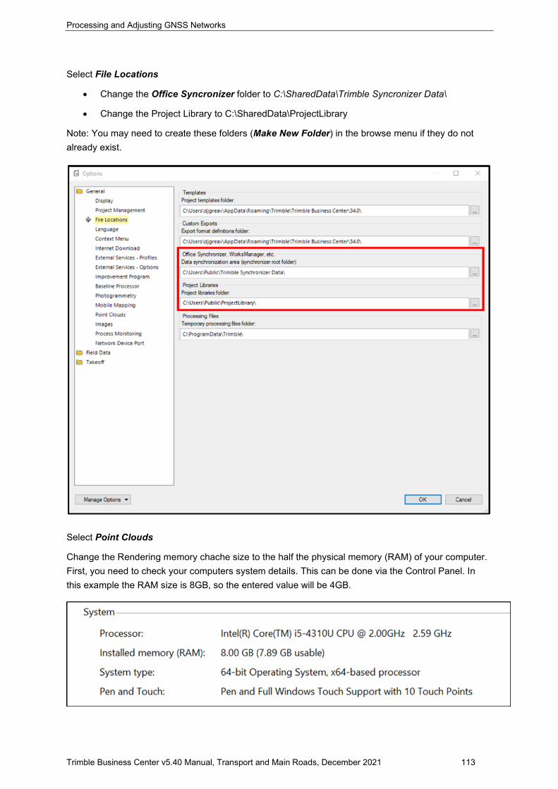
Processing and Adjusting GNSS Networks
Trimble Business Center v5.40 Manual, Transport and Main Roads, December 2021 113
Select File Locations
• Change the Office Syncronizer folder to C:\SharedData\Trimble Syncronizer Data\
• Change the Project Library to C:\SharedData\ProjectLibrary
Note: You may need to create these folders (Make New Folder) in the browse menu if they do not already exist.
Select Point Clouds
Change the Rendering memory chache size to the half the physical memory (RAM) of your computer. First, you need to check your computers system details. This can be done via the Control Panel. In this example the RAM size is 8GB, so the entered value will be 4GB.

Processing and Adjusting GNSS Networks
Trimble Business Center v5.40 Manual, Transport and Main Roads, December 2021 114
Select OK
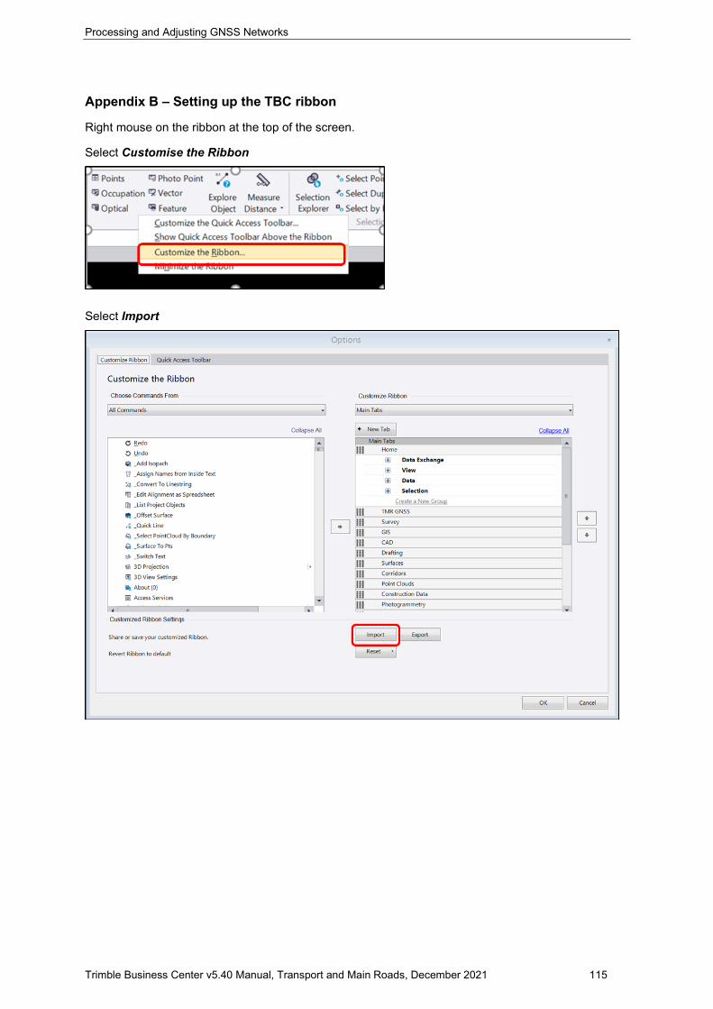
Processing and Adjusting GNSS Networks
Trimble Business Center v5.40 Manual, Transport and Main Roads, December 2021 115
Appendix B – Setting up the TBC ribbon
Right mouse on the ribbon at the top of the screen.
Select Customise the Ribbon
Select Import
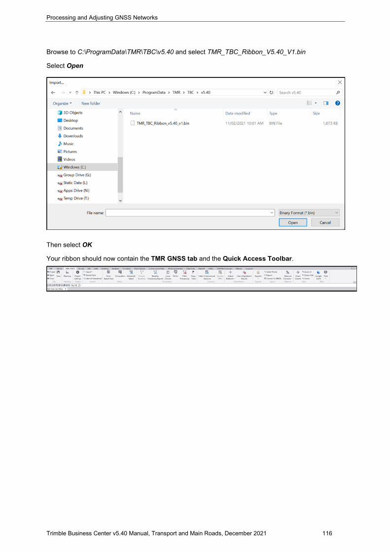
Processing and Adjusting GNSS Networks
Trimble Business Center v5.40 Manual, Transport and Main Roads, December 2021 116
Browse to C:\ProgramData\TMR\TBC\v5.40 and select TMR_TBC_Ribbon_V5.40_V1.bin
Select Open
Then select OK
Your ribbon should now contain the TMR GNSS tab and the Quick Access Toolbar.
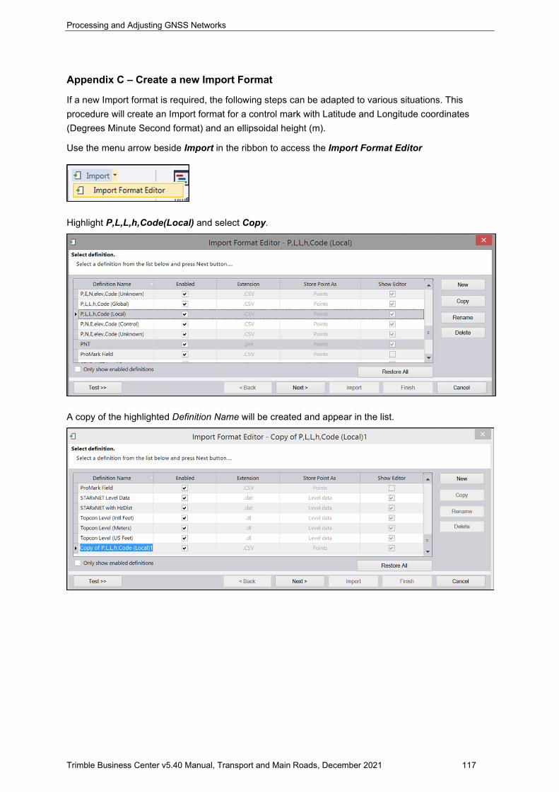
Processing and Adjusting GNSS Networks
Trimble Business Center v5.40 Manual, Transport and Main Roads, December 2021 117
Appendix C – Create a new Import Format
If a new Import format is required, the following steps can be adapted to various situations. This procedure will create an Import format for a control mark with Latitude and Longitude coordinates (Degrees Minute Second format) and an ellipsoidal height (m).
Use the menu arrow beside Import in the ribbon to access the Import Format Editor
Highlight P,L,L,h,Code(Local) and select Copy.
A copy of the highlighted Definition Name will be created and appear in the list.

Processing and Adjusting GNSS Networks
Trimble Business Center v5.40 Manual, Transport and Main Roads, December 2021 118
Left mouse click in the Definition Name field to edit the name. Select Rename and change to {_TMR P,L,L,h,Code (DMS Local)}.Then select Next.
Description and Search Type window allows editing of the Description and the Type. Edit the description as necessary. As a comma delimited file is to be created, leave Delimited selected. Select Next.
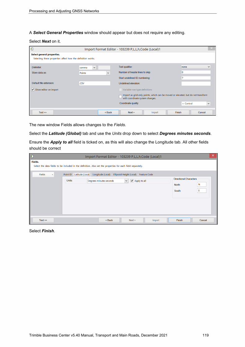
Processing and Adjusting GNSS Networks
Trimble Business Center v5.40 Manual, Transport and Main Roads, December 2021 119
A Select General Properties window should appear but does not require any editing.
Select Next on it.
The new window Fields allows changes to the Fields.
Select the Latitude (Global) tab and use the Units drop down to select Degrees minutes seconds.
Ensure the Apply to all field is ticked on, as this will also change the Longitude tab. All other fields should be correct
Select Finish.
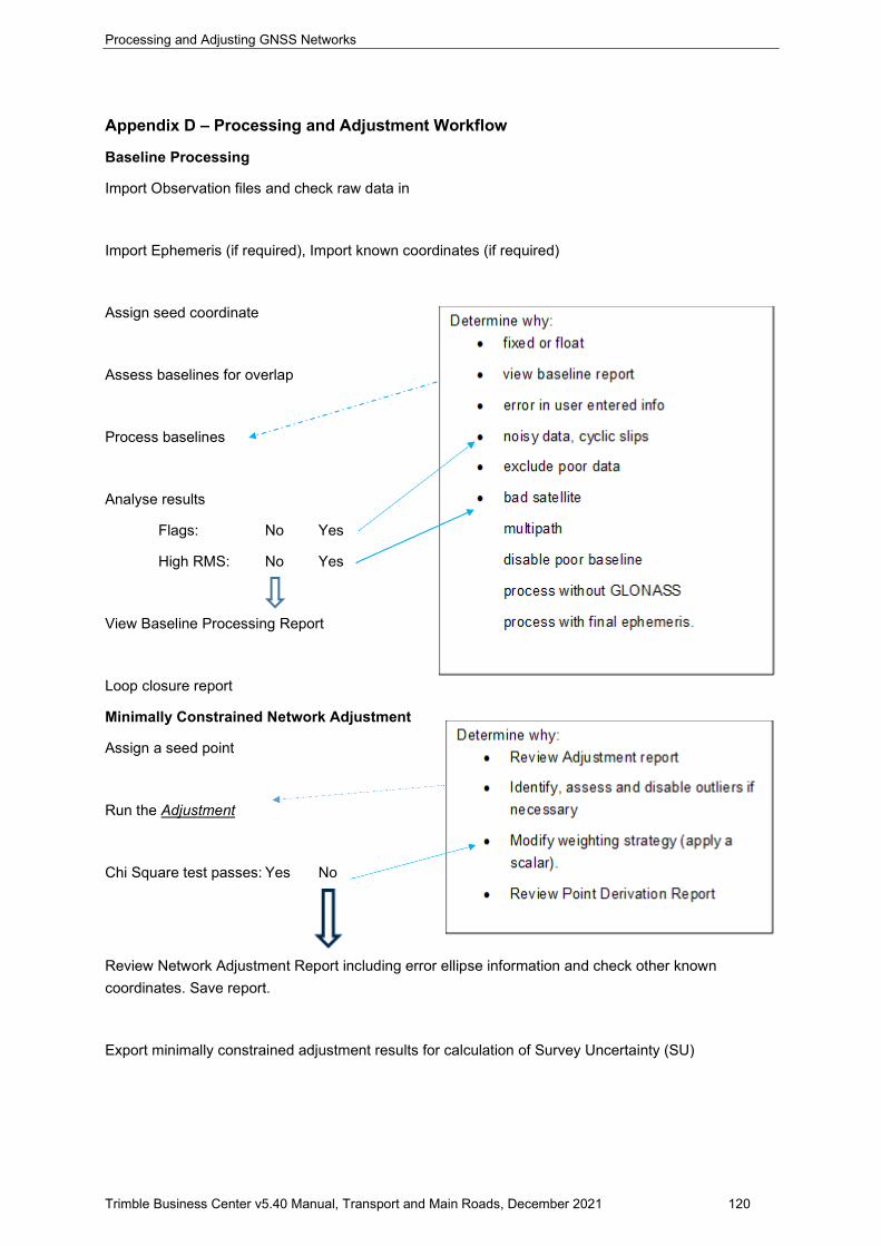
Processing and Adjusting GNSS Networks
Trimble Business Center v5.40 Manual, Transport and Main Roads, December 2021 120
Appendix D – Processing and Adjustment Workflow
Baseline Processing
Import Observation files and check raw data in
Import Ephemeris (if required), Import known coordinates (if required)
Assign seed coordinate
Assess baselines for overlap
Process baselines
Analyse results
Flags: No Yes
High RMS: No Yes
View Baseline Processing Report
Loop closure report
Minimally Constrained Network Adjustment
Assign a seed point
Run the Adjustment
Chi Square test passes: Yes No
Review Network Adjustment Report including error ellipse information and check other known coordinates. Save report.
Export minimally constrained adjustment results for calculation of Survey Uncertainty (SU)

Processing and Adjusting GNSS Networks
Trimble Business Center v5.40 Manual, Transport and Main Roads, December 2021 121
Constrained Network Adjustment
Run the constrained adjustment
Reference factor is close to one and Chi Square test passes
Yes No
Review Network Adjustment Report including error ellipse information. Save report as pdf
Export constrained adjustment results for calculation of estimated Positional Uncertainty (PU)
Output final adjusted coordinates in suitable format if not importing constrained adjustment results into 12d (from 17 above)
Output for DoR
Archive project
Modify weighting strategy (apply a scalar)
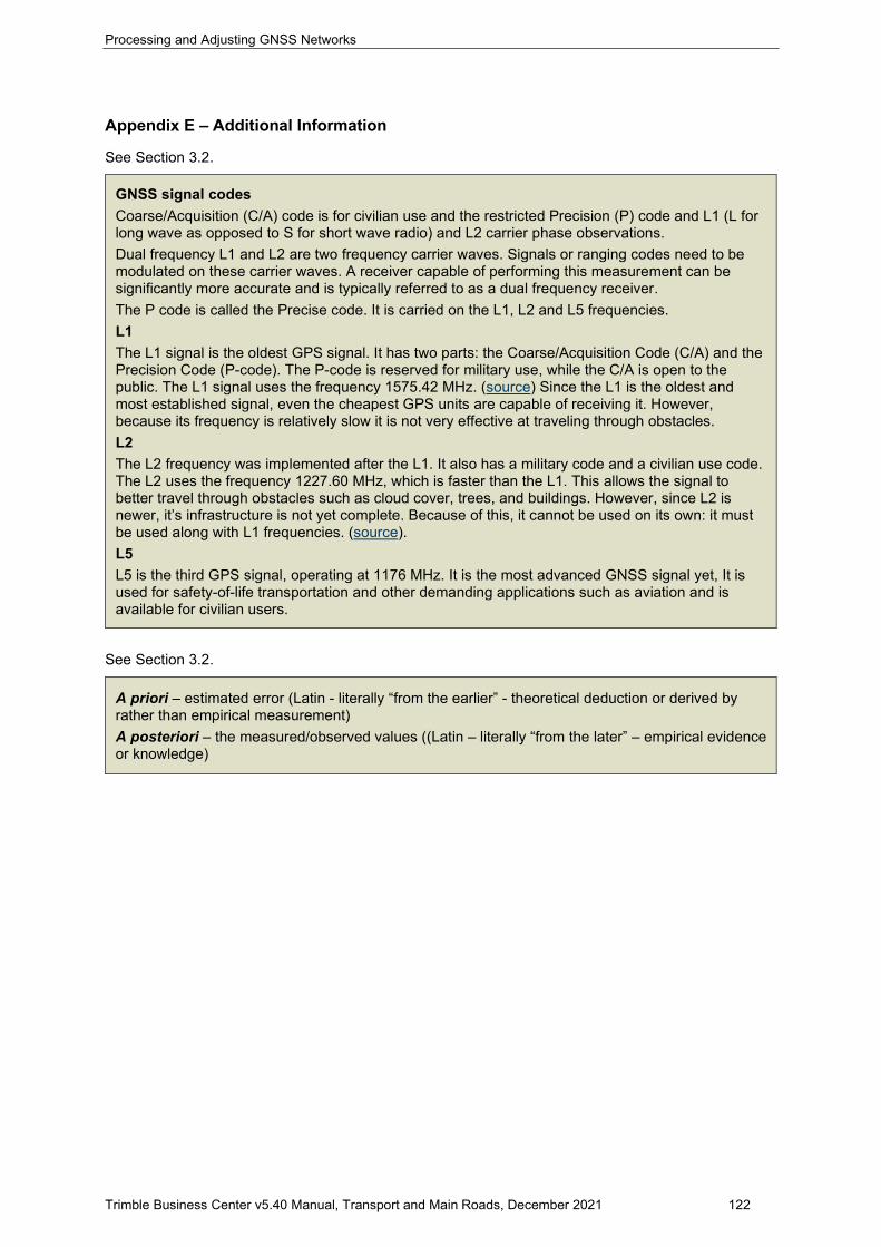
Processing and Adjusting GNSS Networks
Trimble Business Center v5.40 Manual, Transport and Main Roads, December 2021 122
Appendix E – Additional Information
See Section 3.2.
GNSS signal codes Coarse/Acquisition (C/A) code is for civilian use and the restricted Precision (P) code and L1 (L for long wave as opposed to S for short wave radio) and L2 carrier phase observations. Dual frequency L1 and L2 are two frequency carrier waves. Signals or ranging codes need to be modulated on these carrier waves. A receiver capable of performing this measurement can be significantly more accurate and is typically referred to as a dual frequency receiver. The P code is called the Precise code. It is carried on the L1, L2 and L5 frequencies. L1 The L1 signal is the oldest GPS signal. It has two parts: the Coarse/Acquisition Code (C/A) and the Precision Code (P-code). The P-code is reserved for military use, while the C/A is open to the public. The L1 signal uses the frequency 1575.42 MHz. (source) Since the L1 is the oldest and most established signal, even the cheapest GPS units are capable of receiving it. However, because its frequency is relatively slow it is not very effective at traveling through obstacles. L2 The L2 frequency was implemented after the L1. It also has a military code and a civilian use code. The L2 uses the frequency 1227.60 MHz, which is faster than the L1. This allows the signal to better travel through obstacles such as cloud cover, trees, and buildings. However, since L2 is newer, it’s infrastructure is not yet complete. Because of this, it cannot be used on its own: it must be used along with L1 frequencies. (source). L5 L5 is the third GPS signal, operating at 1176 MHz. It is the most advanced GNSS signal yet, It is used for safety-of-life transportation and other demanding applications such as aviation and is available for civilian users.
See Section 3.2.
A priori – estimated error (Latin - literally “from the earlier” - theoretical deduction or derived by rather than empirical measurement) A posteriori – the measured/observed values ((Latin – literally “from the later” – empirical evidence or knowledge)
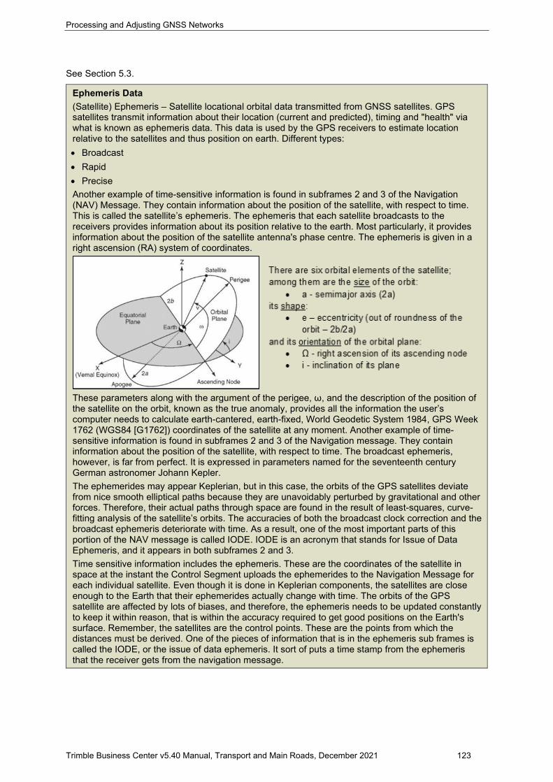
Processing and Adjusting GNSS Networks
Trimble Business Center v5.40 Manual, Transport and Main Roads, December 2021 123
See Section 5.3.
Ephemeris Data (Satellite) Ephemeris – Satellite locational orbital data transmitted from GNSS satellites. GPS satellites transmit information about their location (current and predicted), timing and "health" via what is known as ephemeris data. This data is used by the GPS receivers to estimate location relative to the satellites and thus position on earth. Different types: • Broadcast • Rapid • Precise Another example of time-sensitive information is found in subframes 2 and 3 of the Navigation (NAV) Message. They contain information about the position of the satellite, with respect to time. This is called the satellite’s ephemeris. The ephemeris that each satellite broadcasts to the receivers provides information about its position relative to the earth. Most particularly, it provides information about the position of the satellite antenna's phase centre. The ephemeris is given in a right ascension (RA) system of coordinates.
These parameters along with the argument of the perigee, ω, and the description of the position of the satellite on the orbit, known as the true anomaly, provides all the information the user’s computer needs to calculate earth-cantered, earth-fixed, World Geodetic System 1984, GPS Week 1762 (WGS84 [G1762]) coordinates of the satellite at any moment. Another example of time-sensitive information is found in subframes 2 and 3 of the Navigation message. They contain information about the position of the satellite, with respect to time. The broadcast ephemeris, however, is far from perfect. It is expressed in parameters named for the seventeenth century German astronomer Johann Kepler. The ephemerides may appear Keplerian, but in this case, the orbits of the GPS satellites deviate from nice smooth elliptical paths because they are unavoidably perturbed by gravitational and other forces. Therefore, their actual paths through space are found in the result of least-squares, curve-fitting analysis of the satellite’s orbits. The accuracies of both the broadcast clock correction and the broadcast ephemeris deteriorate with time. As a result, one of the most important parts of this portion of the NAV message is called IODE. IODE is an acronym that stands for Issue of Data Ephemeris, and it appears in both subframes 2 and 3. Time sensitive information includes the ephemeris. These are the coordinates of the satellite in space at the instant the Control Segment uploads the ephemerides to the Navigation Message for each individual satellite. Even though it is done in Keplerian components, the satellites are close enough to the Earth that their ephemerides actually change with time. The orbits of the GPS satellite are affected by lots of biases, and therefore, the ephemeris needs to be updated constantly to keep it within reason, that is within the accuracy required to get good positions on the Earth's surface. Remember, the satellites are the control points. These are the points from which the distances must be derived. One of the pieces of information that is in the ephemeris sub frames is called the IODE, or the issue of data ephemeris. It sort of puts a time stamp from the ephemeris that the receiver gets from the navigation message.
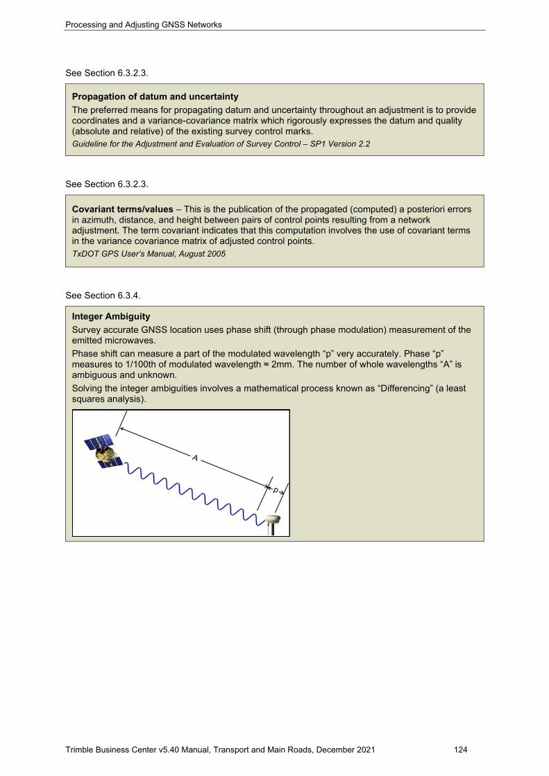
Processing and Adjusting GNSS Networks
Trimble Business Center v5.40 Manual, Transport and Main Roads, December 2021 124
See Section 6.3.2.3.
Propagation of datum and uncertainty The preferred means for propagating datum and uncertainty throughout an adjustment is to provide coordinates and a variance-covariance matrix which rigorously expresses the datum and quality (absolute and relative) of the existing survey control marks. Guideline for the Adjustment and Evaluation of Survey Control – SP1 Version 2.2
See Section 6.3.2.3.
Covariant terms/values – This is the publication of the propagated (computed) a posteriori errors in azimuth, distance, and height between pairs of control points resulting from a network adjustment. The term covariant indicates that this computation involves the use of covariant terms in the variance covariance matrix of adjusted control points. TxDOT GPS User’s Manual, August 2005
See Section 6.3.4.
Integer Ambiguity Survey accurate GNSS location uses phase shift (through phase modulation) measurement of the emitted microwaves. Phase shift can measure a part of the modulated wavelength “p” very accurately. Phase “p” measures to 1/100th of modulated wavelength ≈ 2mm. The number of whole wavelengths “A” is ambiguous and unknown. Solving the integer ambiguities involves a mathematical process known as “Differencing” (a least squares analysis).
Processing and Adjusting GNSS Networks
Trimble Business Center v5.40 Manual, Transport and Main Roads, December 2021 125
See Section 10.1.
Receiver INdependent EXchange. A data interchange format for raw satellite navigation system data. RINEX is in an ASCII file format. The file structure of a RINEX file is as follows: ssssdddf.yyt • ssss: 4 character station identifier • ddd: day of the year of first record or Julian day • f: file sequence number/character or session identifier within day (i.e. 0 to 99, a to z) • yy two digit of the year • t: file type
− o: observation data file (position) − d: compressed observation files − n: navigation file (GPS) − g: navigation file (GLONASS) − l: navigation file (GALILEO) − p: Mixed GNSS navigation file − h: Satellite Based Augmentation System (SBAS) payload navigation file − b: Satellite Based Augmentation System (SBAS) broadcast data file − c: clock file (separate documentation) − s: summary file − m: meteorological file
For example: pmcv042c30.19o • pmcv: Station name • 042: Julian day or day of the year of the first record – 42nd day of year which is 11th February in
this case • c30: File sequence character/number within day (In this example, it is the 30th file of the day) • 19: Two digit of the year (2019) • .o: Type of file (Observation file). n would be a Navigation file, g would be a GLONASS file
Processing and Adjusting GNSS Networks
Trimble Business Center v5.40 Manual, Transport and Main Roads, December 2021 126
Addendum - Calculating Survey Uncertainty (SU) and Positional Uncertainty (PU) for GNSS Survey Control Networks
A1 Introduction
Transport and Main Roads has adopted Uncertainty as defined by ICSM’s Standard for the Australian Survey Control Network – SP1 Version 2.2 as its preferred method of quantifying the quality of control surveys. The Guideline for the Adjustment and Evaluation of Survey Control – Special Publication 1 (SP1), Version 2.2 includes instruction on how to weight Datum Control Survey marks with their positional uncertainty from a PM Form 6 or Regulation 13 certificate. The department’s intention is for project calculated uncertainty values to closely resemble ANJ state-wide adjustment uncertainty values after the Transport and Main Roads network has been included.
Specific output formats have been created to export relevant information to 12d Model where a macro is used to calculate the horizontal Survey Uncertainty (SU) and estimated Positional Uncertainty (PU). An Excel spreadsheet (available on TMR Surveys internal Sharepoint page. For externals, contact [email protected]) has also been created to allow calculation of SU and estimated PU.
A2 Uncertainty in Measurement
Quantifying Survey Control The quality of a control survey shall be quantified in terms of uncertainty. When quantifying survey quality, the following uncertainty categories shall apply: Survey Uncertainty (SU) is the uncertainty of the horizontal and/or vertical coordinates of a survey control mark relative to the survey in which it was observed and is free from the influence of any imprecision or inaccuracy in the underlying datum realisation. Therefore, SU reflects only the uncertainty resulting from survey measurements, measurement precisions, network geometry and the choice of constraint. A minimally constrained least squares adjustment is the preferred and most rigorous way to estimate and test SU. SU is expressed in SI units at the 95% confidence level. Positional Uncertainty (PU) is the uncertainty of the horizontal and/or vertical coordinates of a survey control mark with respect to the defined datum and represents the combined uncertainty of the existing datum realisation and the new control survey. That is, PU includes SU as well as the uncertainty of the existing survey control marks to which a new control survey is connected. A fully constrained least squares adjustment is the preferred and most rigorous way to estimate and test PU. PU is expressed in SI units at the 95% confidence level. Standard for the Australian Survey Control Network – SP1 Version 2.2
Processing and Adjusting GNSS Networks
Trimble Business Center v5.40 Manual, Transport and Main Roads, December 2021 127
Evaluating Uncertainty Control surveys using least squares The horizontal and/or vertical coordinates and uncertainties of survey control marks in a Datum Control Survey shall be estimated using a rigorous least squares adjustment process. General Purpose Control Surveys should use least squares adjustment to estimate uncertainty. Throughout and following least squares adjustment, survey control projects shall be evaluated to demonstrate the reliability of the survey and the estimated coordinates and uncertainties. The quality of estimated coordinates in an absolute sense shall be evaluated using SU and/or PU as appropriate. Standard for the Australian Survey Control Network – SP1 Version 2.2
A3 Expression of Uncertainty
When reporting the absolute Survey Uncertainty (SU) and Positional Uncertainty (PU) of survey control marks in one, two or three dimensions, ICSM recommends that uncertainty be expressed in terms of standard deviations or the standard error ellipse/ellipsoid. ICSM has also adopted the circular confidence region as a means for expressing horizontal uncertainty, since the circular confidence region enables the quality of control surveys to be expressed in a way that is compatible with other geospatial datasets. Therefore, one, two and three-dimensional uncertainty shall be expressed in terms of the 95% confidence level using any one of the following as appropriate:
• standard deviation • standard error ellipse/ellipsoid, or • horizontal circular confidence region.
Standard for the Australian Survey Control Network – SP1 Version 2.2
A3.1 Standard deviation
To express standard deviations for one dimensional components at the 95% confidence level, the uncertainty value is simply computed by scaling the estimated (1 sigma) standard deviation by coverage factor k = 1.960. Guideline for Adjustment and Evaluation of Survey Control – SP1 Version 2.2
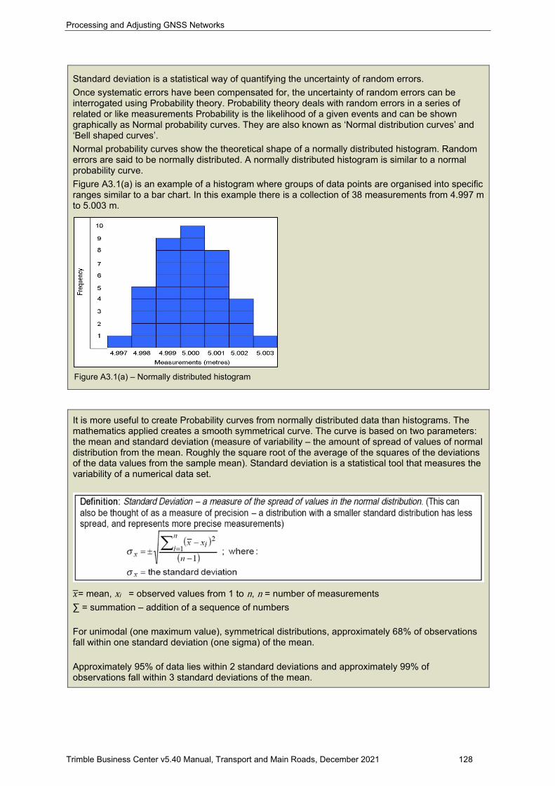
Processing and Adjusting GNSS Networks
Trimble Business Center v5.40 Manual, Transport and Main Roads, December 2021 128
Standard deviation is a statistical way of quantifying the uncertainty of random errors. Once systematic errors have been compensated for, the uncertainty of random errors can be interrogated using Probability theory. Probability theory deals with random errors in a series of related or like measurements Probability is the likelihood of a given events and can be shown graphically as Normal probability curves. They are also known as ‘Normal distribution curves’ and ‘Bell shaped curves’. Normal probability curves show the theoretical shape of a normally distributed histogram. Random errors are said to be normally distributed. A normally distributed histogram is similar to a normal probability curve. Figure A3.1(a) is an example of a histogram where groups of data points are organised into specific ranges similar to a bar chart. In this example there is a collection of 38 measurements from 4.997 m to 5.003 m.
Figure A3.1(a) – Normally distributed histogram
It is more useful to create Probability curves from normally distributed data than histograms. The mathematics applied creates a smooth symmetrical curve. The curve is based on two parameters: the mean and standard deviation (measure of variability – the amount of spread of values of normal distribution from the mean. Roughly the square root of the average of the squares of the deviations of the data values from the sample mean). Standard deviation is a statistical tool that measures the variability of a numerical data set.
𝑥𝑥= mean, xi = observed values from 1 to n, n = number of measurements ∑ = summation – addition of a sequence of numbers For unimodal (one maximum value), symmetrical distributions, approximately 68% of observations fall within one standard deviation (one sigma) of the mean. Approximately 95% of data lies within 2 standard deviations and approximately 99% of observations fall within 3 standard deviations of the mean.
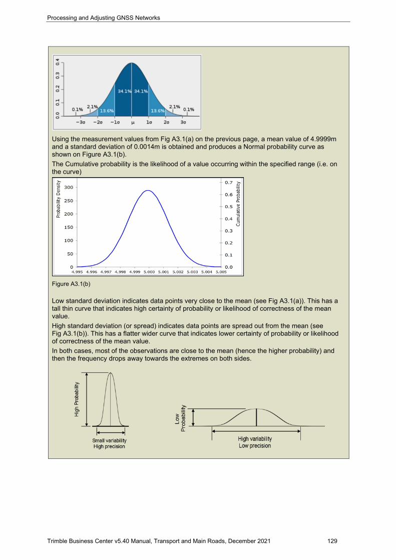
Processing and Adjusting GNSS Networks
Trimble Business Center v5.40 Manual, Transport and Main Roads, December 2021 129
Using the measurement values from Fig A3.1(a) on the previous page, a mean value of 4.9999m and a standard deviation of 0.0014m is obtained and produces a Normal probability curve as shown on Figure A3.1(b). The Cumulative probability is the likelihood of a value occurring within the specified range (i.e. on the curve)
Figure A3.1(b) Low standard deviation indicates data points very close to the mean (see Fig A3.1(a)). This has a tall thin curve that indicates high certainty of probability or likelihood of correctness of the mean value. High standard deviation (or spread) indicates data points are spread out from the mean (see Fig A3.1(b)). This has a flatter wider curve that indicates lower certainty of probability or likelihood of correctness of the mean value. In both cases, most of the observations are close to the mean (hence the higher probability) and then the frequency drops away towards the extremes on both sides.
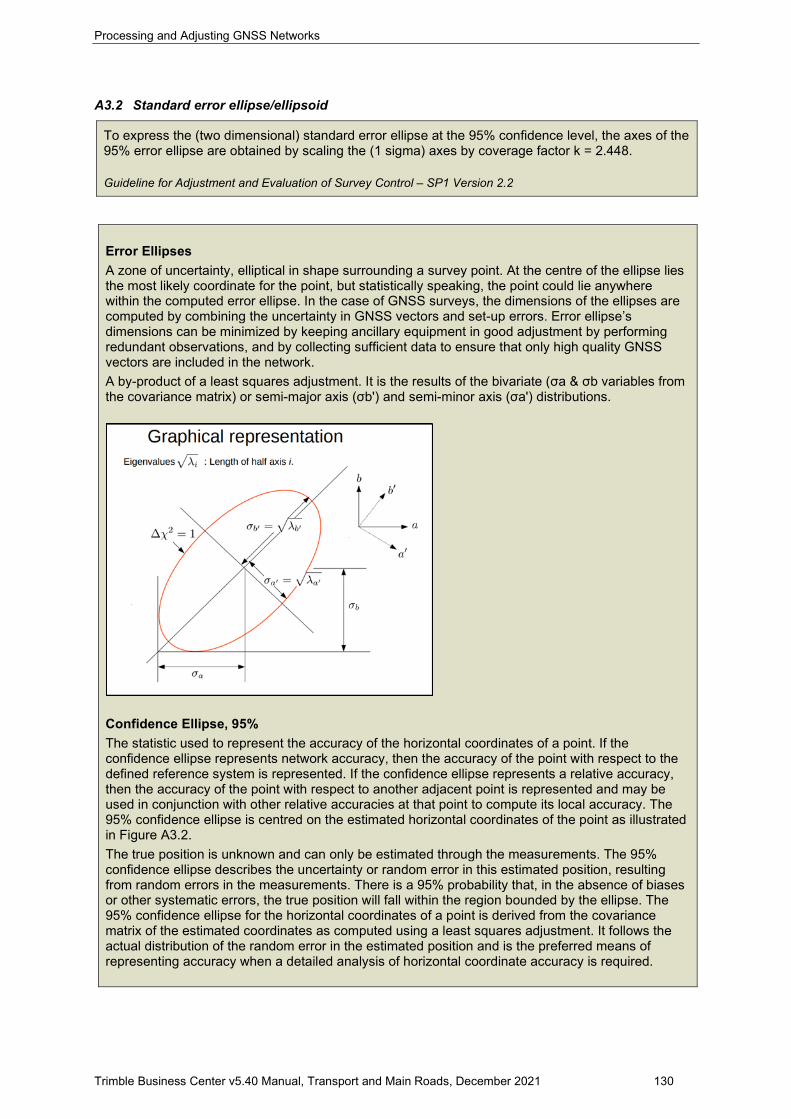
Processing and Adjusting GNSS Networks
Trimble Business Center v5.40 Manual, Transport and Main Roads, December 2021 130
A3.2 Standard error ellipse/ellipsoid
To express the (two dimensional) standard error ellipse at the 95% confidence level, the axes of the 95% error ellipse are obtained by scaling the (1 sigma) axes by coverage factor k = 2.448. Guideline for Adjustment and Evaluation of Survey Control – SP1 Version 2.2
Error Ellipses A zone of uncertainty, elliptical in shape surrounding a survey point. At the centre of the ellipse lies the most likely coordinate for the point, but statistically speaking, the point could lie anywhere within the computed error ellipse. In the case of GNSS surveys, the dimensions of the ellipses are computed by combining the uncertainty in GNSS vectors and set-up errors. Error ellipse’s dimensions can be minimized by keeping ancillary equipment in good adjustment by performing redundant observations, and by collecting sufficient data to ensure that only high quality GNSS vectors are included in the network. A by-product of a least squares adjustment. It is the results of the bivariate (σa & σb variables from the covariance matrix) or semi-major axis (σbʹ) and semi-minor axis (σaʹ) distributions.
Confidence Ellipse, 95% The statistic used to represent the accuracy of the horizontal coordinates of a point. If the confidence ellipse represents network accuracy, then the accuracy of the point with respect to the defined reference system is represented. If the confidence ellipse represents a relative accuracy, then the accuracy of the point with respect to another adjacent point is represented and may be used in conjunction with other relative accuracies at that point to compute its local accuracy. The 95% confidence ellipse is centred on the estimated horizontal coordinates of the point as illustrated in Figure A3.2. The true position is unknown and can only be estimated through the measurements. The 95% confidence ellipse describes the uncertainty or random error in this estimated position, resulting from random errors in the measurements. There is a 95% probability that, in the absence of biases or other systematic errors, the true position will fall within the region bounded by the ellipse. The 95% confidence ellipse for the horizontal coordinates of a point is derived from the covariance matrix of the estimated coordinates as computed using a least squares adjustment. It follows the actual distribution of the random error in the estimated position and is the preferred means of representing accuracy when a detailed analysis of horizontal coordinate accuracy is required.
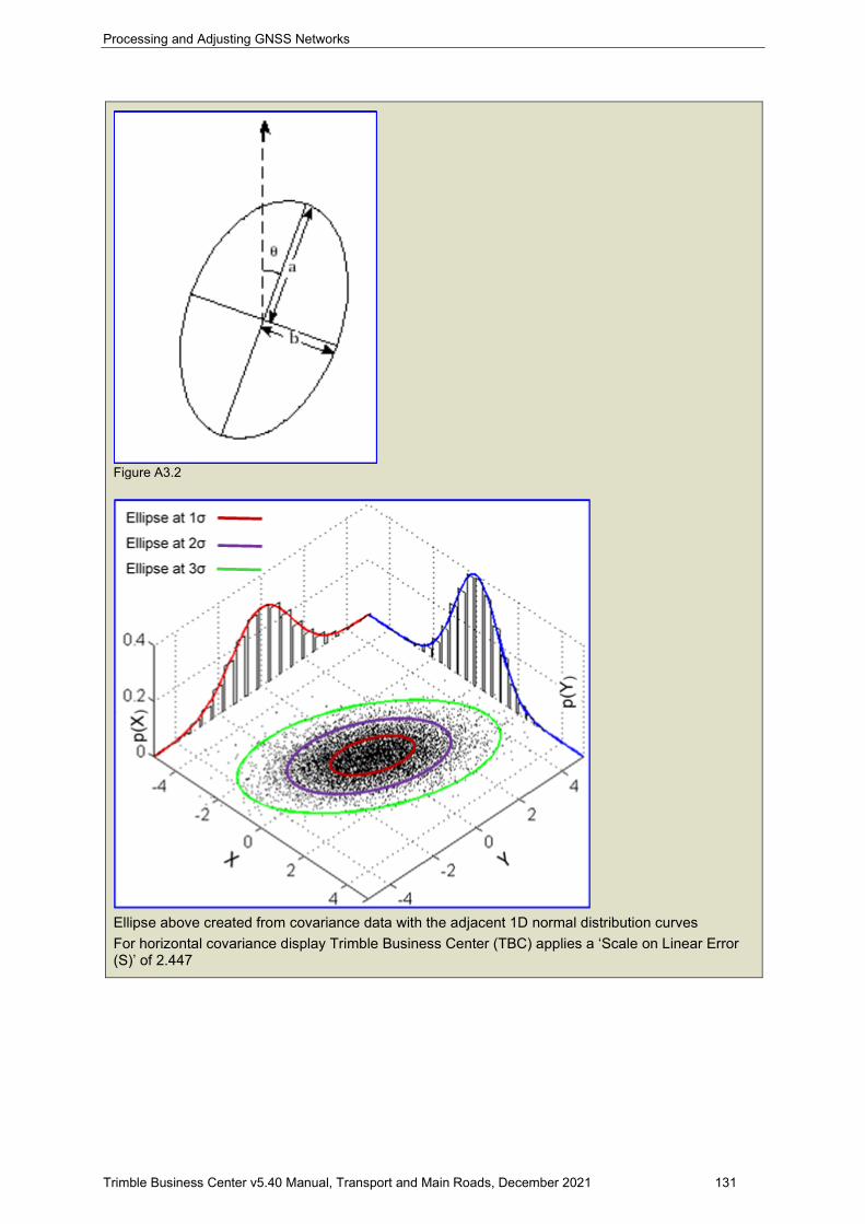
Processing and Adjusting GNSS Networks
Trimble Business Center v5.40 Manual, Transport and Main Roads, December 2021 131
Figure A3.2
Ellipse above created from covariance data with the adjacent 1D normal distribution curves For horizontal covariance display Trimble Business Center (TBC) applies a ‘Scale on Linear Error (S)’ of 2.447
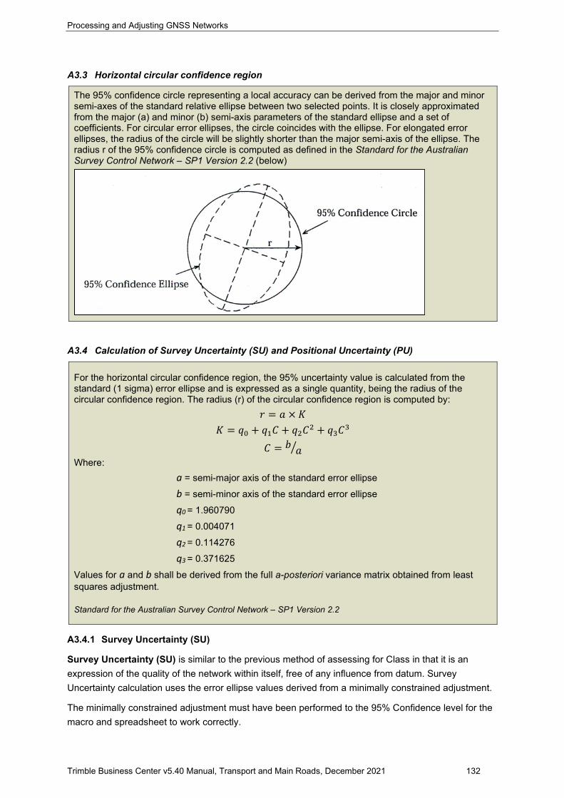
Processing and Adjusting GNSS Networks
Trimble Business Center v5.40 Manual, Transport and Main Roads, December 2021 132
A3.3 Horizontal circular confidence region
The 95% confidence circle representing a local accuracy can be derived from the major and minor semi-axes of the standard relative ellipse between two selected points. It is closely approximated from the major (a) and minor (b) semi-axis parameters of the standard ellipse and a set of coefficients. For circular error ellipses, the circle coincides with the ellipse. For elongated error ellipses, the radius of the circle will be slightly shorter than the major semi-axis of the ellipse. The radius r of the 95% confidence circle is computed as defined in the Standard for the Australian Survey Control Network – SP1 Version 2.2 (below)
A3.4 Calculation of Survey Uncertainty (SU) and Positional Uncertainty (PU)
For the horizontal circular confidence region, the 95% uncertainty value is calculated from the standard (1 sigma) error ellipse and is expressed as a single quantity, being the radius of the circular confidence region. The radius (r) of the circular confidence region is computed by:
𝑟𝑟 = 𝑎𝑎 × 𝐾𝐾 𝐾𝐾 = 𝑞𝑞0 + 𝑞𝑞1𝐶𝐶 + 𝑞𝑞2𝐶𝐶2 + 𝑞𝑞3𝐶𝐶3
𝐶𝐶 = 𝑏𝑏 𝑎𝑎� Where: a = semi-major axis of the standard error ellipse
b = semi-minor axis of the standard error ellipse
q0 = 1.960790
q1 = 0.004071
q2 = 0.114276
q3 = 0.371625
Values for a and b shall be derived from the full a-posteriori variance matrix obtained from least squares adjustment. Standard for the Australian Survey Control Network – SP1 Version 2.2
A3.4.1 Survey Uncertainty (SU)
Survey Uncertainty (SU) is similar to the previous method of assessing for Class in that it is an expression of the quality of the network within itself, free of any influence from datum. Survey Uncertainty calculation uses the error ellipse values derived from a minimally constrained adjustment.
The minimally constrained adjustment must have been performed to the 95% Confidence level for the macro and spreadsheet to work correctly.
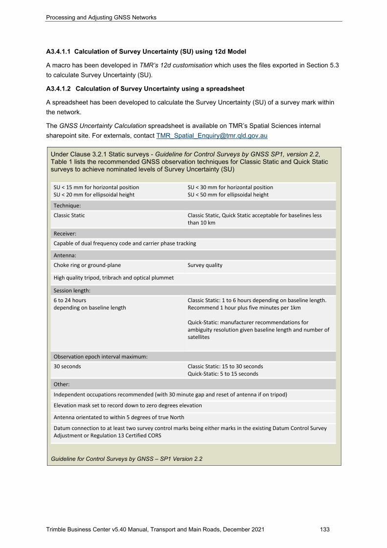
Processing and Adjusting GNSS Networks
Trimble Business Center v5.40 Manual, Transport and Main Roads, December 2021 133
A3.4.1.1 Calculation of Survey Uncertainty (SU) using 12d Model
A macro has been developed in TMR’s 12d customisation which uses the files exported in Section 5.3 to calculate Survey Uncertainty (SU).
A3.4.1.2 Calculation of Survey Uncertainty using a spreadsheet
A spreadsheet has been developed to calculate the Survey Uncertainty (SU) of a survey mark within the network.
The GNSS Uncertainty Calculation spreadsheet is available on TMR’s Spatial Sciences internal sharepoint site. For externals, contact [email protected]
Under Clause 3.2.1 Static surveys - Guideline for Control Surveys by GNSS SP1, version 2.2, Table 1 lists the recommended GNSS observation techniques for Classic Static and Quick Static surveys to achieve nominated levels of Survey Uncertainty (SU)
Guideline for Control Surveys by GNSS – SP1 Version 2.2
SU < 15 mm for horizontal position SU < 20 mm for ellipsoidal height
SU < 30 mm for horizontal position SU < 50 mm for ellipsoidal height Technique:
Classic Static Classic Static, Quick Static acceptable for baselines less than 10 km
Receiver:
Capable of dual frequency code and carrier phase tracking
Antenna:
Choke ring or ground-plane Survey quality
High quality tripod, tribrach and optical plummet
Session length:
6 to 24 hours depending on baseline length
Classic Static: 1 to 6 hours depending on baseline length. Recommend 1 hour plus five minutes per 1km Quick-Static: manufacturer recommendations for ambiguity resolution given baseline length and number of satellites Observation epoch interval maximum:
30 seconds Classic Static: 15 to 30 seconds Quick-Static: 5 to 15 seconds Other:
Independent occupations recommended (with 30 minute gap and reset of antenna if on tripod)
Elevation mask set to record down to zero degrees elevation
Antenna orientated to within 5 degrees of true North
Datum connection to at least two survey control marks being either marks in the existing Datum Control Survey Adjustment or Regulation 13 Certified CORS
Processing and Adjusting GNSS Networks
Trimble Business Center v5.40 Manual, Transport and Main Roads, December 2021 134
A3.4.2 Positional Uncertainty (PU)
Positional Uncertainty (PU) shall be estimated and tested by way of a constrained least squares adjustment.
The two ways to estimate uncertainties No matter what the sources of your uncertainties are, there are two approaches to estimating them: ‘Type A’ and ‘Type B’ evaluations. In most measurement situations, uncertainty evaluations of both types are needed. Type A evaluations - uncertainty estimates using statistics (usually from repeated readings) Type B evaluations - uncertainty estimates from any other information. This could be information from past experience of the measurements, from calibration certificates, manufacturer’s specifications, from calculations, from published information, and from common sense. There is a temptation to think of ‘Type A’ as ‘random’ and ‘Type B’ as ‘systematic’, but this is not necessarily true Combining standard uncertainties Individual standard uncertainties calculated by Type A or Type B evaluations can be combined validly by ‘summation in quadrature’ (also known as ‘root sum of the squares’). The result of this is called the combined standard uncertainty, shown by uc Coverage factor k Having scaled the components of uncertainty consistently, to find the combined standard uncertainty, we may then want to re-scale the result. The combined standard uncertainty may be thought of as equivalent to ‘one standard deviation’, but we may wish to have an overall uncertainty stated at another level of confidence, e.g. 95 percent. This re-scaling can be done using a coverage factor, k. Multiplying the combined standard uncertainty, uc, by a coverage factor gives a result which is called the expanded uncertainty, A particular value of coverage factor gives a particular confidence level for the expanded uncertainty. Most commonly, we scale the overall uncertainty by using the coverage factor k = 2, to give a level of confidence of approximately 95 percent. (k = 2 is correct if the combined standard uncertainty is normally distributed.) Measurement Good Practice Guide No. 11 (Issue 2) – A Beginner’s Guide to Uncertainty of Measurement – Stephanie Bell – Centre for Basic, Thermal and Length Metrology National Physical Laboratory, Teddington, Middlesex, United Kingdom

Processing and Adjusting GNSS Networks
Trimble Business Center v5.40 Manual, Transport and Main Roads, December 2021 135
Measurand Uncertainty Position uncertainties were calculated in accordance with the principles of the ISO Guide to the Expression of Uncertainty in Measurement (1995), with an interval estimated to have a confidence level of 95% at the time of verification. The combined standard uncertainty was converted to an expanded uncertainty using a coverage factor, k, of 2. Type A uncertainty sources were evaluated by adopting an a priori sigma of 0.001 metre for the precision (1 sigma) of the L1-frequency, one-way, phase observation, at zenith. The corresponding uncertainties of all parameters were determined, by standard error propagation theory, in the least-squares estimation process used in the GPS analysis. Since the formal (internal) precision estimates of GPS solutions are well known to be optimistic, a factor of 10 (i.e. variance scale factor of 100) was subsequently applied to the variance-covariance matrix of the computed GDA94 coordinates. Type B uncertainty sources, which in practice contribute to position uncertainty, cannot be estimated from the statistical analysis of short-period (i.e. 7-day) observations; these include environmental effects, such as long-period station loading (deformation) processes. Table 1 shows the major type B uncertainty sources for GPS analysis. Table 1. Type B uncertainty sources (95% C.L.) for position, determined from GPS, and the total uncertainty, assuming the normal distribution of the uncertainty sources, high degrees of freedom and a coverage factor, k, of 2.
Uncertainty Source Positional Uncertainty Horizontal (mm)
Positional Uncertainty Vertical (mm)
Antenna phase centre 3 10
Monument stability 1 1
Other sources including unmodelled crustal loading, satellite orbit variations, atmosphere, tectonics, signal multi-path
6 10
Results of the National GNSS CORS Campaign, June 2013 – G. Hu, J. Dawson – Australian Government Geoscience Australia
In Queensland, to calculate true Positional Uncertainty the project baselines are required to be included in the Department of Resources (DoR) state-wide ANJ adjustment. Transport and Main Roads can calculate the estimated Positional Uncertainty (PU) of the adjusted marks positions, relative to the uncertainty of the datum control marks used. The department’s intention is for project calculated uncertainty values to closely resemble ANJ state-wide adjustment uncertainty values after the departmental network has been included.
PU calculated using the process presented in this manual should be close to the value that will be derived once the network has been submitted to DoR and adjusted within the state-wide ANJ adjustment. Differences may be greater in areas of sparse control where the new network greatly contributes to the ANJ framework.
Estimation of PU uses the marks error ellipse values. The constrained adjustment must have been performed to the 95% Confidence level with CORS and ANJ uncertainty values entered at 95% vales for the macro and spreadsheet to work correctly.
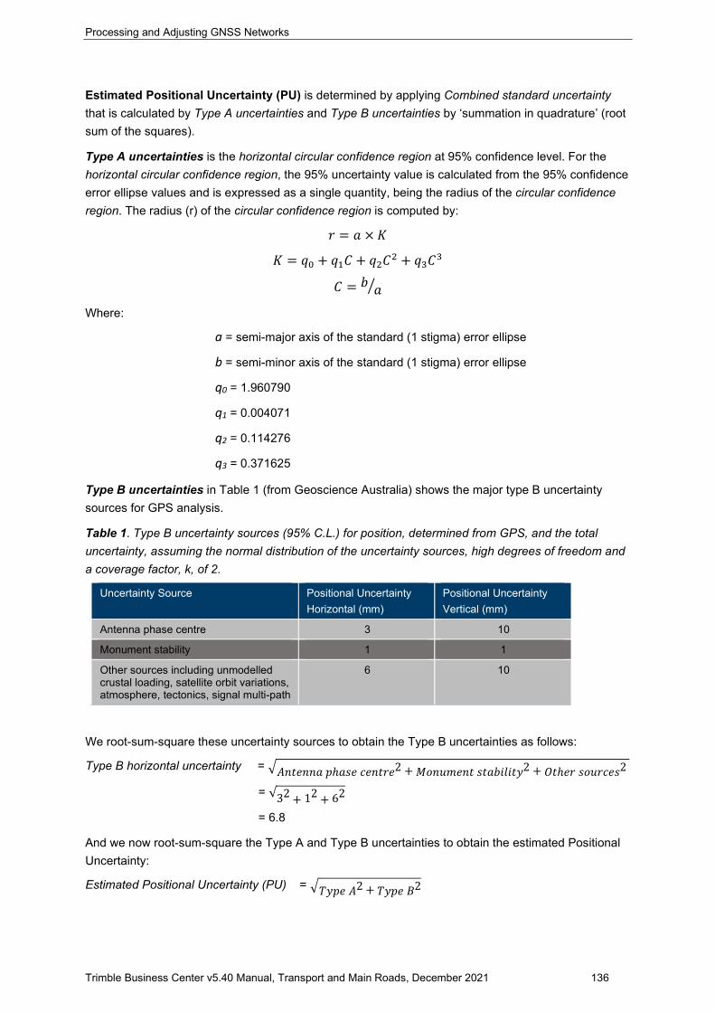
Processing and Adjusting GNSS Networks
Trimble Business Center v5.40 Manual, Transport and Main Roads, December 2021 136
Estimated Positional Uncertainty (PU) is determined by applying Combined standard uncertainty that is calculated by Type A uncertainties and Type B uncertainties by ‘summation in quadrature’ (root sum of the squares).
Type A uncertainties is the horizontal circular confidence region at 95% confidence level. For the horizontal circular confidence region, the 95% uncertainty value is calculated from the 95% confidence error ellipse values and is expressed as a single quantity, being the radius of the circular confidence region. The radius (r) of the circular confidence region is computed by:
𝑟𝑟 = 𝑎𝑎 × 𝐾𝐾
𝐾𝐾 = 𝑞𝑞0 + 𝑞𝑞1𝐶𝐶 + 𝑞𝑞2𝐶𝐶2 + 𝑞𝑞3𝐶𝐶3
𝐶𝐶 = 𝑏𝑏 𝑎𝑎�
Where:
a = semi-major axis of the standard (1 stigma) error ellipse
b = semi-minor axis of the standard (1 stigma) error ellipse
q0 = 1.960790
q1 = 0.004071
q2 = 0.114276
q3 = 0.371625
Type B uncertainties in Table 1 (from Geoscience Australia) shows the major type B uncertainty sources for GPS analysis.
Table 1. Type B uncertainty sources (95% C.L.) for position, determined from GPS, and the total uncertainty, assuming the normal distribution of the uncertainty sources, high degrees of freedom and a coverage factor, k, of 2.
Uncertainty Source Positional Uncertainty Horizontal (mm)
Positional Uncertainty Vertical (mm)
Antenna phase centre 3 10
Monument stability 1 1
Other sources including unmodelled crustal loading, satellite orbit variations, atmosphere, tectonics, signal multi-path
6 10
We root-sum-square these uncertainty sources to obtain the Type B uncertainties as follows:
Type B horizontal uncertainty = �𝐴𝐴𝑛𝑛𝐴𝐴𝐴𝐴𝑛𝑛𝑛𝑛𝑎𝑎 𝑝𝑝ℎ𝑎𝑎𝑎𝑎𝐴𝐴 𝑐𝑐𝐴𝐴𝑛𝑛𝐴𝐴𝑟𝑟𝐴𝐴2 + 𝑅𝑅𝑀𝑀𝑛𝑛𝑀𝑀𝑀𝑀𝐴𝐴𝑛𝑛𝐴𝐴 𝑎𝑎𝐴𝐴𝑎𝑎𝑏𝑏𝑠𝑠𝑠𝑠𝑠𝑠𝐴𝐴𝑠𝑠
2 + 𝐺𝐺𝐴𝐴ℎ𝐴𝐴𝑟𝑟 𝑎𝑎𝑀𝑀𝑀𝑀𝑟𝑟𝑐𝑐𝐴𝐴𝑎𝑎2
= √32 + 12 + 62
= 6.8
And we now root-sum-square the Type A and Type B uncertainties to obtain the estimated Positional Uncertainty:
Estimated Positional Uncertainty (PU) = �𝑇𝑇𝑠𝑠𝑝𝑝𝐴𝐴 𝐴𝐴2 + 𝑇𝑇𝑠𝑠𝑝𝑝𝐴𝐴 𝐵𝐵
2
Processing and Adjusting GNSS Networks
Trimble Business Center v5.40 Manual, Transport and Main Roads, December 2021 137
Example:
Given.
A3.4.1.1 Calculation of Positional Uncertainty (PU) using 12d Model
A macro has been developed in TMR’s 12d customisation which uses the files in Section 6.3 to calculate the estimated Positional Uncertainty (PU).
A3.4.1.2 Calculation of Positional Uncertainty (PU) using a spreadsheet
A spreadsheet has been developed to calculate estimated Positional Uncertainty (PU) of a survey mark within the network.
The GNSS Uncertainty Calculation spreadsheet is available on Transport Main Roads Spatial Sciences internal SharePoint site. For externals, contact [email protected]
Under the TMR Surveying Standards a projects survey control network marks shall meet or exceed a Horizontal Positional Uncertainty (PU) of < 0.030 m at 95% confidence level.