magnetic field in ergodic divertors
TRANSCRIPT
Appendix AMagnetic Field in Ergodic Divertors
In this chapter Iwould like to present a detailed analytical calculations of themagneticfield generated by a set of helical coils. Themethod is demonstrated for themodels oftheDEDof theTEXTORand theEDof theToreSupra. Themain idea of themethod isconcluded in the following.Typically a set of coils are located on the surface of a torus.The density of the current flowing in the coils can be described by the delta functionswith singularities on the coil locations. Using the Poisson summation rule whichgives the relation of the delta functions with the trigonometric functions one canpresent the current density on the surface of torus a sum of infinity number of helicalcurrents, jmn ∝ cos(mθ−nϕ). For the large aspect ratio tokamaks the magnetic fieldgenerated by these helical currents can be found by approximating the system by thecylinder (see, e.g., Morozov and Solov’ev (1966b)) and making corrections due toa toroidicity. This approach allows one to qualitative and quantitatively analyze thepoloidal and toroidal spectra of the magnetic field generated by a set of coils as wellas its radial dependence.
A.1 Magnetic Perturbation in the TEXTOR-DED
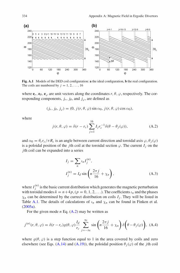
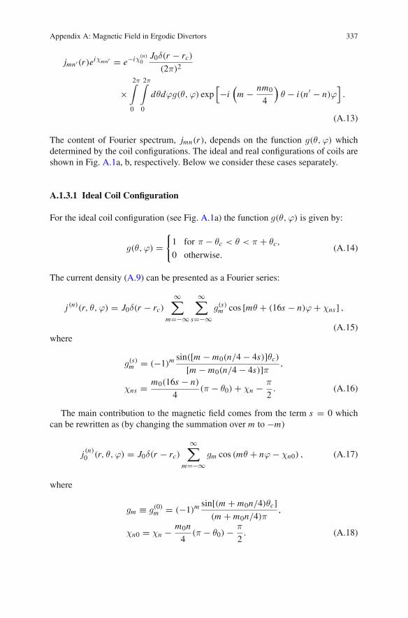
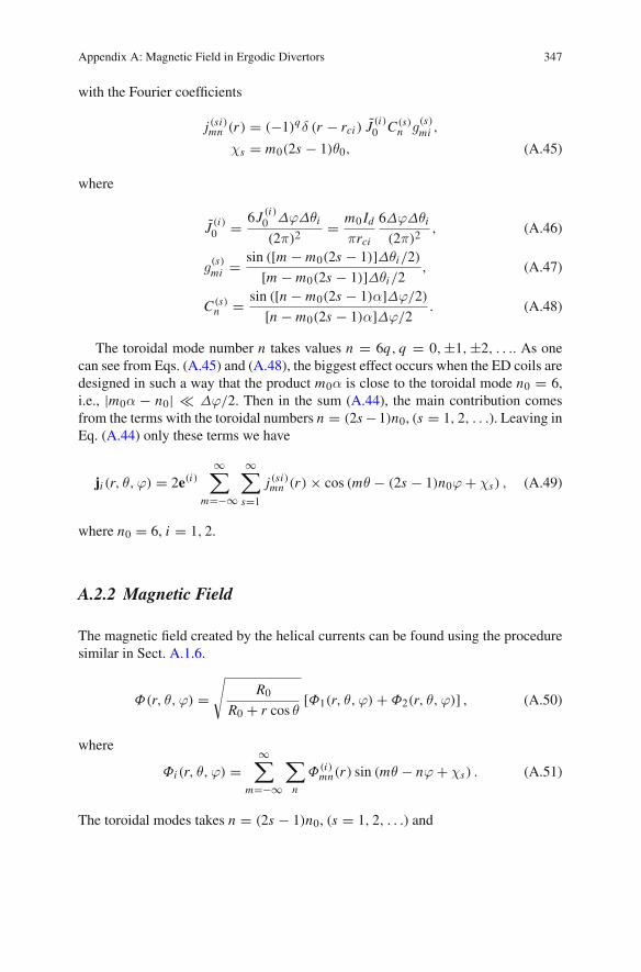
The magnetic field perturbations in the TEXTOR-DED by the set of helical coilsschematically shown in Fig. 9.4a, b. The geometrical locations of the helical coils inthe (ϕ, θ)-plane are plotted in Fig. A.1a for the ideal configuration and in Fig. A.1bfor the real configuration.
A.1.1 Density of Perturbation Currents
It is convenient to introduce the density of DED perturbation currents in order to findthe magnetic perturbations. The current density j(r, θ,ϕ) is introduced as
j = jr er + jθeθ + jϕeϕ, (A.1)
S. Abdullaev, Magnetic Stochasticity in Magnetically Confined Fusion Plasmas, 333Springer Series on Atomic, Optical, and Plasma Physics 78,DOI: 10.1007/978-3-319-01890-4, © Springer International Publishing Switzerland 2014
334 Appendix A: Magnetic Field in Ergodic Divertors
120
140
160
180
200
220
240
0 60 120 180 240 300 360
θ
ϕ
j=1 16 15 14 13 12 11 10 9 8 76 5 4 3 2=
2θc
120
140
160
180
200
220
240
0 60 120 180 240 300 360
θ
ϕ
j=4-1 j=16-13 j=12-9 j=8-5
Δθ
2θc
(a) (b)
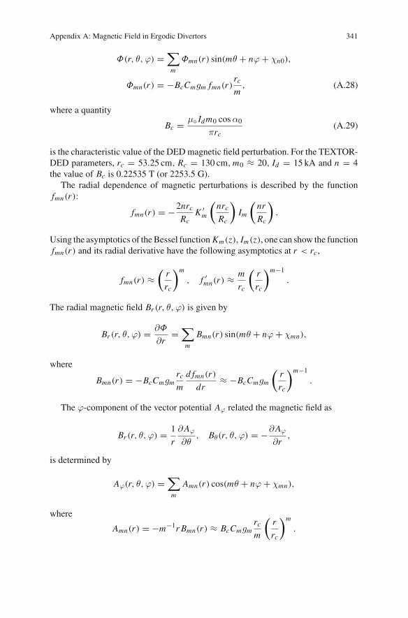
Fig. A.1 Models of the DED coil configuration: a the ideal configuration, b the real configuration.The coils are numbered by j = 1, 2, . . . , 16
where er , eθ, eϕ are unit vectors along the coordinates r, θ,ϕ, respectively. The cor-responding components, jr , jθ, and jϕ, are defined as
( jr , jθ, jϕ) = (0, j (r, θ,ϕ) sinα0, j (r, θ,ϕ) cosα0),
where
j (r, θ,ϕ) = δ(r − rc)
16∑
j=1
I j r−1c δ(θ − θ j (ϕ)), (A.2)
and α0 = θcrc/πRc is an angle between current direction and toroidal axis ϕ, θ j (ϕ)
is a poloidal position of the j th coil at the toroidal section ϕ. The current I j on thej th coil can be expanded into a series
I j =∑
n
ιn I (n)j ,
I (n)j = Id sin
(n2π j
16+ χn
), (A.3)
where I (n)j is the basic current distributionwhich generates themagnetic perturbation
with toroidal modes n = n+4p, (p = 0, 1, 2, . . .). The coefficients ιn and the phasesχn can be determined by the currect distribution on coils I j . They will be listed inTable A.1. The details of calculations of ιn and χn can be found in Finken et al.(2005a).
For the given mode n Eq. (A.2) may be written as
j (n)(r, θ,ϕ) = δ(r − rc)g(θ,ϕ)Id
rc
∞∑
j=−∞sin
(n2π j
16+ χn
)δ
(θ − θ j (ϕ)
), (A.4)
where g(θ,ϕ) is a step function equal to 1 in the area covered by coils and zeroelsewhere (see Eqs. (A.14) and (A.19)), the poloidal position θ j (ϕ) of the j th coil
Appendix A: Magnetic Field in Ergodic Divertors 335
at the section ϕ is given by
θ j = θ(ϕ) − jδθ, θ(ϕ) = θ0 − θc
πϕ. (A.5)
The angle θ01 = θ0 + δθ is a poloidal position of the first coil at the toroidal sectionϕ = 0, δθ is the angular distance between neighboring coils.
A.1.2 Continuous Current Density
Using the coil positions (A.5), we present the current distribution given by Eq. (A.4)as
j (n)(r, θ,ϕ) = δ(r − rc)Id
rcg(θ,ϕ)
∞∑
j=−∞sin
(n2π j
16+ χn
)δ (θ − θ(ϕ) + jδθ) .
(A.6)Using the representation of delta function
δ(x) = 1
2π
∞∫
−∞eixpdp,
one obtains
j (n)(r, θ,ϕ) = Idδ(r − rc)
2πrcg(θ,ϕ)W,
W = Im
⎧⎨
⎩eiχn
∞∫
−∞dpeip(θ−θ(ϕ))
∞∑
j=−∞exp
[i j
(2πn
16+ pδθ
)]⎫⎬
⎭ . (A.7)
Then using the Poisson rule
∞∑
j=−∞ei2π j x = 2π
∞∑
s=−∞δ(s − x),
we have
336 Appendix A: Magnetic Field in Ergodic Divertors
W = Im
⎧⎨
⎩eiχn
∞∫
−∞dpei(θ−θ(ϕ))p
∞∑
s=−∞δ
(s − n
16− pδθ
2π
)⎫⎬
⎭
= 2π
δθ
∞∑
s=−∞sin
(2π(s − n/16)
δθ(θ − θϕ) + χn
). (A.8)
Using the dependence of θ(ϕ) on ϕ given in Eq. (A.5) we reduce (A.7) to
j (n)(r, θ,ϕ) = δ(r − rc)g(θ,ϕ)J0
×∞∑
s=−∞cos
(m0(16s − n)
4θ + n0(16s − n)
4ϕ + χ(n)
s
), (A.9)
where
χ(n)s = −m0(16s − n)
4θ0 + χn − π
2. (A.10)
In (A.9) the following notations are introduced:
J0 = Id
δθrc= 2m0 Id
πrc, m0 = π
2δθ,
n0 = m0θc
π= θc
2δθ, θ0 = θ01 + δθ. (A.11)
Because of periodicity of j (r, θ,ϕ) along ϕwith a period 2π follows that n0 mustbe an integer number equal to n0 = 4l, where l = 1, 2, . . .. Putting n0 = 4, the terms = 0 in Eq. (A.9) which gives the main contribution the perturbed magnetic field inthe plasma can be presented as
j (n)0 (r, θ,ϕ) = δ(r − rc)g(θ,ϕ)J0 cos
(nm0θ/4 + nϕ − χ
(n)0
). (A.12)
A.1.3 Fourier Expansion of the Current Density
For calculations of the magnetic field created by helical coils it is convenient topresent the current density j (n)
0 (r, θ,ϕ) in Fourier series in θ,ϕ:
j (n)(r, θ,ϕ) =∑
m,n′jmn′(r) cos
[mθ + n′ϕ + χmn′
],
where
Appendix A: Magnetic Field in Ergodic Divertors 337
jmn′(r)eiχmn′ = e−iχ(n)0
J0δ(r − rc)
(2π)2
×2π∫
0
2π∫
0
dθdϕg(θ,ϕ) exp[−i
(m − nm0
4
)θ − i(n′ − n)ϕ
].
(A.13)
The content of Fourier spectrum, jmn(r), depends on the function g(θ,ϕ) whichdetermined by the coil configurations. The ideal and real configurations of coils areshown in Fig. A.1a, b, respectively. Below we consider these cases separately.
A.1.3.1 Ideal Coil Configuration
For the ideal coil configuration (see Fig. A.1a) the function g(θ,ϕ) is given by:
g(θ,ϕ) ={1 for π − θc < θ < π + θc,
0 otherwise.(A.14)
The current density (A.9) can be presented as a Fourier series:
j (n)(r, θ,ϕ) = J0δ(r − rc)
∞∑
m=−∞
∞∑
s=−∞g(s)
m cos [mθ + (16s − n)ϕ + χns] ,
(A.15)where
g(s)m = (−1)m sin([m − m0(n/4 − 4s)]θc)
[m − m0(n/4 − 4s)]π ,
χns = m0(16s − n)
4(π − θ0) + χn − π
2. (A.16)
The main contribution to the magnetic field comes from the term s = 0 whichcan be rewritten as (by changing the summation over m to −m)
j (n)0 (r, θ,ϕ) = J0δ(r − rc)
∞∑
m=−∞gm cos (mθ + nϕ − χn0) , (A.17)
where
gm ≡ g(0)m = (−1)m sin[(m + m0n/4)θc]
(m + m0n/4)π,
χn0 = χn − m0n
4(π − θ0) − π
2. (A.18)
338 Appendix A: Magnetic Field in Ergodic Divertors
A.1.3.2 Non-ideal Coil Configuration
For the non-ideal configuration of coils (see Fig. A.1b) the step function g(θ,ϕ) isgiven by
g(θ,ϕ) ={1, for π − θc(ϕ) < θ < π + θc(ϕ),
0, elsewhere,(A.19)
where θc(ϕ) is the piece-wise function
θc(ϕ) = θc0 − 2Δθ
π(ϕ − ϕl) for ϕl < ϕ < ϕl+1,
ϕl = ϕc + (l − 1)π
2, 0 < ϕc <
π
2, l = 0, 1, 2, 3, 4. (A.20)
For the sake of simplicity we consider the term s = 0 in Eq. (A.9), i.e., Eq. (A.12).Furthermore, we need to estimate the integral
fm,n′ = 1
(2π)2
2π∫
0
2π∫
0
dθdϕg(θ,ϕ)e−imθ−in′ϕ.
It is not difficult to show that
fmn′ = −e−iπmδn′,4se−in′ϕc2 sin(mαπ/4)
π2m
2[in′ cos(mθc) + mα sin(mθc)]n′2 − (mα)2
,
where α = 2Δθ/π, θc = θc0−Δθ/2, δn,k is the Kronecker symbol, i.e., δn,k = 0 forn �= k and δn,n = 1. Substituting this expression into (A.13) we obtain the followingexpression for the Fourier components of the current density jmn′(r),
jmn′(r)eiχmn′ = δ(r − rc)eiχ(n)
0 J0 fm−nm0/4,n′−n . (A.21)
From Eq. (A.21) follows that due to non-ideal configuration the current distribution(A.9) creates the toroidal modes n = n + 4s, (s = 0,±1,±2, . . .).
The main contribution to the toroidal spectrum n′ comes from the terms n′ = n.In this case s = 0, and one obtains
fm,0 = e−iπm sin[πmα/4]πmα/4
sin(mθc)
mπ,
and from Eq. (A.21) we obtain
j (n)0 (r, θ,ϕ) = δ(r − rc)
∞∑
m=−∞
∞∑
s=−∞Jm,s cos(mθ + (4s + n)ϕ − χms). (A.22)
Appendix A: Magnetic Field in Ergodic Divertors 339
The Fourier coefficients, Jm,0, corresponding to the term s = 0 which gives the maincontribution to the perturbed field is given by
Jm,0 = J0gmCm, χn0 = χn − m0n
4(π − θ0) − π
2, (A.23)
where gm is given by Eq. (A.18), and
Cm = sin[(m + nm0/4)Δθ/2](m + nm0/4)Δθ/2
(A.24)
is a correction factor due to non-ideal configuration. For the ideal configurationΔθ = 0 and therefore Cm = 1.
One should note that the current distribution (A.3) with n = 4 creates also thetoroidal mode n′ = 0 (see Eq. (A.21)). This mode may disturb the plasma equilib-rium. For this reason in the m : n = 12 : 4 operational mode of the TEXTOR-DEDone applies the compensation coils which annuls the effect of the n′ = 0 mode.
A.1.4 Magnetic Field Perturbations
In this section we present the formulae for the magnetic field created by the surfacecurrent (A.1). Each term in the Fourier expansion (A.22) of this perturbation currentdescribes a helical current on the toroidal surface of radius r = rc. Consider a singlehelical current vector jmn corresponding to the (m, n) mode
jmn(r, θ,ϕ) = δ(r − rc) jmnemn cos(mθ + nϕ + φmn), (A.25)
emn =(0, eθ sinαmn, eϕ cosαmn
),
where eθ and eϕ are unit vectors along the poloidal and toroidal directions, respec-tively, and αmn = nrc/m Rc, (m �= 0), is a helicity, i.e., the angle between a helicalcurrent direction and toroidal axis.
The total current density (A.1) can be presented as a sumof helical currents (A.25),i.e.,
jh(r, θ,ϕ) =∑
mn
jmn(r, θ,ϕ). (A.26)
with the same toroidal components of the vector jmn but different poloidal compo-nents, i.e.,
jmn cosαmn = Jm,(n−k)/4 cosα0,
jmn sinαmn �= Jm,(n−k)/4 sinα0,
340 Appendix A: Magnetic Field in Ergodic Divertors
where k stands for a toroidal mode number n in the basic current distribution (A.3).For the coefficients jmn and the phases, φmn , of the helical current we have
jmn = Jm,(n−k)/4 cosα0
cosαmn, φmn = χm,(n−k)/4. (A.27)
The difference between jh(r, θ,ϕ) (A.26) and j(r, θ,ϕ) (A.1) can be neglected,since the sum of differences of poloidal modes is negligible small, i.e.,
∞∑
m=−∞
(jmn sinαmn − Jm, n−k
4sinα0
)=
∞∑
m=−∞Jm, n−k
4
sin(α0 − αmn)
cosαmn≈ 0.
A.1.5 Cylindrical Approximation
Here we consider the magnetic field created by a single component of the helicalcurrent jmn(r, θ,ϕ) (A.25) in a cylindrical geometry. The magnetic field B of thishelical current can be expressed by the scalar potentialΦ(r, θ,ϕ) (B = ∇Φ(r, θ,ϕ))(see e.g., Morozov and Solov’ev (1966b))
Φ =
⎧⎪⎪⎨
⎪⎪⎩
ai Im
(nrRc
)sin(mθ + nϕ + φmn), for r < rc,
ae Km
(nrRc
)sin(mθ + nϕ + φmn), for r > rc,
where Im(z) and Km(z) are modified Bessel functions. Coefficients ai , ae are foundby the boundary conditions at the r = rc:
Br
∣∣∣r=rc−0
− Br
∣∣∣r=rc+0
= 0,
Bθ
∣∣∣r=rc−0
− Bθ
∣∣∣r=rc+0
= μo jmn cos(mθ + nϕ + φmn) cosαmn .
Using the relations in Eq. (A.27) we have
ai = −μ◦ Jm,(n−k)/4rc cosα0nrc
m R0K ′
m
(nrc
Rc
).
Further we consider only the leading terms s = 0 (A.23) for helical currents.For them we have the following formula for the scalar potential Φ(r, θ,ϕ) of themagnetic field created by a set of helical currents (A.26) inside the toroidal surfacer < rc:
Appendix A: Magnetic Field in Ergodic Divertors 341
Φ(r, θ,ϕ) =∑
m
Φmn(r) sin(mθ + nϕ + χn0),
Φmn(r) = −BcCmgm fmn(r)rc
m, (A.28)
where a quantity
Bc = μ◦ Idm0 cosα0
πrc(A.29)
is the characteristic value of the DEDmagnetic field perturbation. For the TEXTOR-DED parameters, rc = 53.25 cm, Rc = 130 cm, m0 ≈ 20, Id = 15 kA and n = 4the value of Bc is 0.22535 T (or 2253.5 G).
The radial dependence of magnetic perturbations is described by the functionfmn(r):
fmn(r) = −2nrc
RcK ′
m
(nrc
Rc
)Im
(nr
Rc
).
Using the asymptotics of theBessel function Km(z), Im(z), one can show the functionfmn(r) and its radial derivative have the following asymptotics at r < rc,
fmn(r) ≈(
r
rc
)m
, f ′mn(r) ≈ m
rc
(r
rc
)m−1
.
The radial magnetic field Br (r, θ,ϕ) is given by
Br (r, θ,ϕ) = ∂Φ
∂r=∑
m
Bmn(r) sin(mθ + nϕ + χmn),
where
Bmn(r) = −BcCmgmrc
m
d fmn(r)
dr≈ −BcCmgm
(r
rc
)m−1
.
The ϕ-component of the vector potential Aϕ related the magnetic field as
Br (r, θ,ϕ) = 1
r
∂ Aϕ
∂θ, Bθ(r, θ,ϕ) = −∂ Aϕ
∂r,
is determined by
Aϕ(r, θ,ϕ) =∑
m
Amn(r) cos(mθ + nϕ + χmn),
where
Amn(r) = −m−1r Bmn(r) ≈ BcCmgmrc
m
(r
rc
)m
.
342 Appendix A: Magnetic Field in Ergodic Divertors
A.1.6 Toroidal Corrections
According toMorozov and Solov’ev (1966b) the effect of toroidicity on themagneticfield can be taken into account, multiplying the scalar potentialΦ(r, θ,ϕ) by a factor√
R0/R, if the small corrections (n0rc/2R0)m+3 are neglected for each poloidal
component m. In this approximations we have
Φ(r, θ,ϕ) =√
R0
R0 + r cos θ
∑
m
Φmn(r) sin(mθ + nϕ + χn0), (A.30)
where the amplitudes Φmn(r) are given by Eq. (A.28). Then, one can show that thevector potential Aϕ(r, θ,ϕ) is determined by
Aϕ(r, θ,ϕ) = εB0R0a(r, θ,ϕ),
a(r, θ,ϕ) =∑
m
amn(r, θ) cos(mθ + nϕ + χn0), (A.31)
where ε is a dimensionless perturbation parameter defined by
ε = Bc
B0, (A.32)
B0 is the toroidal magnetic field at the center of torus R0, and
amn(r, θ) = − 1
Bc R0
r
m
∂
∂r
(√R0
RΦmn(r)
)
≈ Cmgmrc
m R0
(r
rc
)m√
R0
R0 + r cos θ
(1 − r cos θ
2m(R0 + r cos θ)
).
(A.33)
For the radial component of the magnetic field, Br (r, θ,ϕ), we have
Br (r, θ,ϕ) = 1
r
∂ Aϕ(r, θ,ϕ)
∂θ=∑
m
Bmn(r, θ) sin(mθ + nϕ + χn0),
Bmn(r, θ) ≈ BcCmgm
(r
rc
)m−1√
R0
R0 + r cos θ
(1 − r cos θ
2m(R0 + r cos θ)
).
(A.34)
The radial dependence of the perturbation field is determined by the poloidal modespectra, gm . According (A.24) the latter is localized near the central mode mc =(2s − 1)m0 = nm0/n0, (s = 1, 2, . . .) and has a width Δm = π/Δθi . Therefore,
Appendix A: Magnetic Field in Ergodic Divertors 343
32
34
36
38
40
42
44
46
0 60 120 180 240 300 360
r
θ−1.5
−1.0
−0.5
0.0
0.5
1.0
x10−2
-6
-4
-2
0
2
4
6
100 140 180 220 260
B r [T
]
θ [deg]
x10-3
1
2
(a) (b)
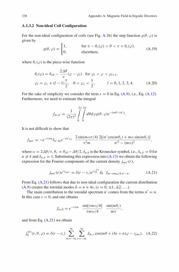
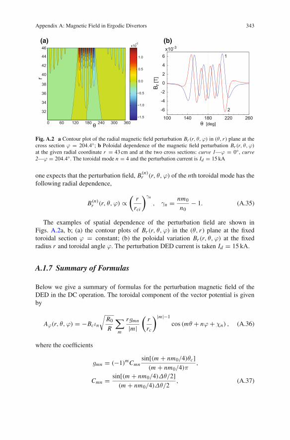
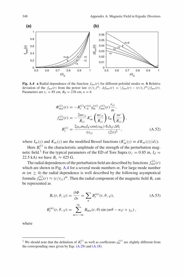
Fig. A.2 a Contour plot of the radial magnetic field perturbation Br (r, θ,ϕ) in (θ, r ) plane at thecross section ϕ = 204.4◦; b Poloidal dependence of the magnetic field perturbation Br (r, θ,ϕ)
at the given radial coordinate r = 43cm and at the two cross sections: curve 1—ϕ = 0◦, curve2—ϕ = 204.4◦. The toroidal mode n = 4 and the perturbation current is Id = 15 kA
one expects that the perturbation field, B(n)r (r, θ,ϕ) of the nth toroidal mode has the
following radial dependence,
B(n)r (r, θ,ϕ) ∝
(r
rci
)γn
, γn = nm0
n0− 1. (A.35)
The examples of spatial dependence of the perturbation field are shown inFigs. A.2a, b; (a) the contour plots of Br (r, θ,ϕ) in the (θ, r ) plane at the fixedtoroidal section ϕ = constant; (b) the poloidal variation Br (r, θ,ϕ) at the fixedradius r and toroidal angle ϕ. The perturbation DED current is taken Id = 15 kA.
A.1.7 Summary of Formulas
Below we give a summary of formulas for the perturbation magnetic field of theDED in the DC operation. The toroidal component of the vector potential is givenby
Aϕ(r, θ,ϕ) = −Bcιn
√R0
R
∑
m
rgmn
|m|(
r
rc
)|m|−1
cos (mθ + nϕ + χn) , (A.36)
where the coefficients
gmn = (−1)mCmnsin[(m + nm0/4)θc]
(m + nm0/4)π,
Cmn = sin[(m + nm0/4)Δθ/2](m + nm0/4)Δθ/2
, (A.37)
344 Appendix A: Magnetic Field in Ergodic Divertors
Table A.1 Coefficients φhand ιn for the different n
n χn ιn
1 3π/16 sin(π/4)/[4 sin(π/16)]2 3π/8 1/[2 sin(π/8)]4 5π/4
√2
describes the poloidal mode spectrum at the given toroidal mode n. In Eq. (A.36)the quantity Bc = μ0m0 Id/πrc is the characteristic magnitude of the DEDmagneticfield, Id is the DED current, the constant m0 determines the central poloidal modenumber nm0/4, rc is the minor radius of the DED coils, χn ≡ χn0. The geometricalpoloidal angle θ is related to the cylindrical coordinates R, Z as θ = arctan(Z/[R −R0]), and the parameter θc is the half of the poloidal section covered by the DEDcoils, Δθ is a geometrical parameter of the coil configuration.
The toroidal mode number n takes the value n = 4 for the 12/4 DED modeconfiguration, n = 2 for the 6/2 mode, and n = 1 for the 3/1 mode, respectively. Thephases χn and the factor ιn in Eq. (A.36) are determined by the coil configuration.For the particular configuration they given by
χn = m0n
4(π − θ0) − χn + π
2, (A.38)
where θ0 is a poloidal angle of the first coil at the section ϕ = 0. The coefficientsχn and ιn for the different values of n are given in Table A.1. The parameters rc, θc,θ0, Δθ, and m0 are determined by the geometry of coil configuration, and take fixedvalues, rc = 0.5325 m, θc = 35.49◦, θ0 = 169.35◦, Δθ = 17.745◦, and m0 ≈ 20.
A.2 Magnetic Field of Tore Supra ED
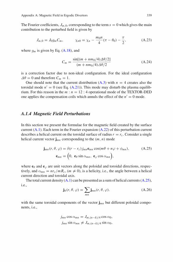
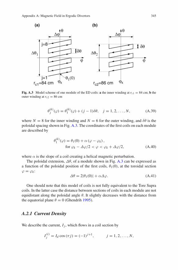
As it was noted in Sect. 9.1.1 and shown in Fig. 9.2 that the ED coil configuration ofthe Tore Supra consists of six identical modules located on outer board the torus. Wemodel the each module by the coil windings shown in Fig. A.3 where arrows indicatethe current direction. The current flows from the feeder located at the beginning ofthe first section j = 1 of the inner side of the winding shown in Fig. A.3a and returnsthrough the outer side of the winding shown in Fig. A.3b. The minor radii of theinner and outer sides are rc1 = 84 cm rc2 = 86 cm, respectively Below we calculatethe magnetic field, created by the current flowing in this coil system by consideringthe inner and outer parts of the winding separately, and by summing those partsafterwards.
Suppose that the modules are centered near the toroidal angles ϕk = (k − 1)Δϕ,Δϕ = 2π/6. The poloidal angle as a function of the toroidal angle of a point locatedin the j th section in the kth module (k = 1, 2, . . . , 6) is given by
Appendix A: Magnetic Field in Ergodic Divertors 345
(a) (b)
ϕ
θ
δθ
Δϕ
Δθ1
j=1
j=8
θ1(0)ϕkrc1=84 cm
ϕ
θ
δθ
Δϕ
Δθ2
ϕkrc2=86 cm
Fig. A.3 Model scheme of one module of the ED coils: a the inner winding at rc1 = 84 cm; b theouter winding at rc2 = 86 cm
θ(k)j (ϕ) = θ
(k)1 (ϕ) + ( j − 1)δθ, j = 1, 2, . . . , N , (A.39)
where N = 8 for the inner winding and N = 6 for the outer winding, and δθ is thepoloidal spacing shown in Fig. A.3. The coordinates of the first coils on each moduleare described by
θ(k)1 (ϕ) = θ1(0) + α (ϕ − ϕk) ,
for ϕk − Δϕ/2 < ϕ < ϕk + Δϕ/2, (A.40)
where α is the slope of a coil creating a helical magnetic perturbation.The poloidal extension, Δθ, of a module shown in Fig. A.3 can be expressed as
a function of the poloidal position of the first coils, θ1(0), at the toroidal sectionϕ = ϕk :
Δθ = 2|θ1(0)| + αΔϕ. (A.41)
One should note that this model of coils is not fully equivalent to the Tore Supracoils. In the latter case the distance between sections of coils in each module are notequidistant along the poloidal angle θ. It slightly decreases with the distance fromthe equatorial plane θ = 0 (Ghendrih 1995).
A.2.1 Current Density
We describe the current, I j , which flows in a coil section by
I (i)j = Id cos (π j) = (−1) j+1, j = 1, 2, . . . , N ,
346 Appendix A: Magnetic Field in Ergodic Divertors
where Id is the current flowing in the coil, i = 1 for the inner part of the windingand i = 2 for its outer part.
Below we shall consider only the long helical section coils since they create themagnetic field perturbations that are resonant with the magnetic field lines of theplasma. The vertical short sections of coils do not contribute to the resonant field,therefore they will not be taken into account.
One can introduce the current density vector j(r, θ,ϕ) of the coil system as
ji (r, θ,ϕ) = e(i) δ(r − rci )
rci
6∑
k=1
g(k)ϕ (ϕ)
N∑
j=1
I (i)j δ
(θ − θ
(k)j (ϕ)
), (A.42)
where e(i) = (er , eθ, eϕ) = (0, sinα0i , cosα0i ) is a unit vector along the helical
section of the coils, α0i = αrci/Rc, Rc = R0 + rci , (i = 1, 2). Here g(k)ϕ (ϕ) is a step
function of the toroidal angle ϕ which takes a non-zero value in the areas coveredby coils, i.e.,
g(k)ϕ (ϕ) =
{1, for ϕk − Δϕ/2 < ϕ < ϕk + Δϕ/2,
0, elsewhere,
Introducing the step function gi (θ) solely depending on the poloidal angle
gi (θ) ={1, for − Δθi/2 < θ < Δθi/2,
0, elsewhere,
the current density (A.42) can after some transformations be reduced to
ji (r, θ,ϕ) = e(i)δ(r − rci )J (i)0 gi (θ)
6∑
k=1
g(k)ϕ (ϕ)
×∞∑
s=−∞cos {m0(2s − 1) [(θ − θ0) − α(ϕ − ϕk)]} . (A.43)
where
m0 = π
δθ, J (i)
0 = m0 Id
πrci, θ0 = θ1(0) − δθ.
One can show that the current density (A.43) can be expanded into a Fourierseries,
ji (r, θ,ϕ) = 2e(i)∞∑
m=−∞
∞∑
n=−∞
∞∑
s=1
j (si)mn (r) cos
(mθ − nϕ + χ(s)
mn
), (A.44)
Appendix A: Magnetic Field in Ergodic Divertors 347
with the Fourier coefficients
j (si)mn (r) = (−1)qδ (r − rci ) J (i)
0 C (s)n g
(s)mi ,
χs = m0(2s − 1)θ0, (A.45)
where
J (i)0 = 6J (i)
0 ΔϕΔθi
(2π)2= m0 Id
πrci
6ΔϕΔθi
(2π)2, (A.46)
g(s)mi = sin ([m − m0(2s − 1)]Δθi/2)
[m − m0(2s − 1)]Δθi/2, (A.47)
C (s)n = sin ([n − m0(2s − 1)α]Δϕ/2)
[n − m0(2s − 1)α]Δϕ/2. (A.48)
The toroidal mode number n takes values n = 6q, q = 0,±1,±2, . . .. As onecan see from Eqs. (A.45) and (A.48), the biggest effect occurs when the ED coils aredesigned in such a way that the product m0α is close to the toroidal mode n0 = 6,i.e., |m0α − n0| � Δϕ/2. Then in the sum (A.44), the main contribution comesfrom the terms with the toroidal numbers n = (2s −1)n0, (s = 1, 2, . . .). Leaving inEq. (A.44) only these terms we have
ji (r, θ,ϕ) = 2e(i)∞∑
m=−∞
∞∑
s=1
j (si)mn (r) × cos (mθ − (2s − 1)n0ϕ + χs) , (A.49)
where n0 = 6, i = 1, 2.
A.2.2 Magnetic Field
The magnetic field created by the helical currents can be found using the proceduresimilar in Sect. A.1.6.
Φ(r, θ,ϕ) =√
R0
R0 + r cos θ[Φ1(r, θ,ϕ) + Φ2(r, θ,ϕ)] , (A.50)
where
Φi (r, θ,ϕ) =∞∑
m=−∞
∑
n
Φ(i)mn(r) sin (mθ − nϕ + χs) . (A.51)
The toroidal modes takes n = (2s − 1)n0, (s = 1, 2, . . .) and
348 Appendix A: Magnetic Field in Ergodic Divertors
(a) (b)
0
0.2
0.4
0.6
0.8
1
0.5 0.6 0.7 0.8 0.9 1
f mn(
r)
r/rc
m=68
1012
14
0
0.01
0.02
0.03
0.04
0.05
0.06
0.5 0.6 0.7 0.8 0.9 1
Δfm
n(r)
r/rc
m=68
1012
14
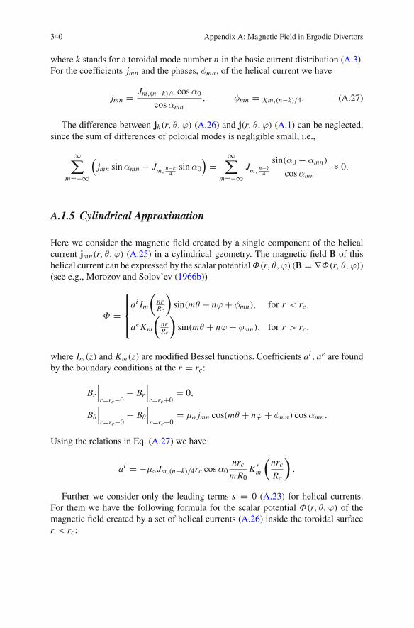
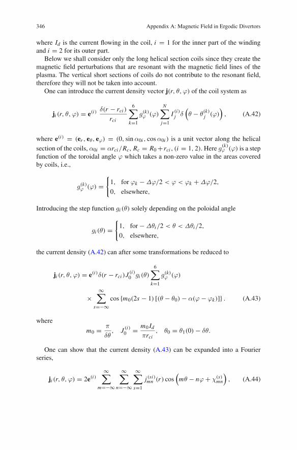
Fig. A.4 a Radial dependence of the function fmn(r) for different poloidal modes m. b Relativedeviation of the fmn(r) from the power law (r/rc)
m : Δ fmn(r) = | fmn(r) − (r/rc)m |/ fmn(r).
Parameters are rc = 85 cm, R0 = 238 cm, n = 6
Φ(i)mn(r) = −B(i)
c C (s)n g(si)
m f (i)mn(r)
rci
m,
f (i)mn(r) = −2nrci
RciK ′
m
(nrci
Rci
)Im
(nr
Rci
),
B(i)c = 2μom0 Id cos(α0i )
πrci
6ΔϕΔθi
(2π)2, (A.52)
where Im(z) and Km(z) are the modified Bessel functions (K ′m(z) ≡ d Km(z)/dz).
Here B(i)c is the characteristic amplitude of the strength of the perturbation mag-
netic field.1 For the typical parameters of the ED of Tore Supra (rc = 0.85 m, Id =22.5 kA) we have Bc ≈ 425 G.
The radial dependences of the perturbation field are described by functions f (i)mn(r)
which are shown in Fig. A.4 for a several mode numbers m. For large mode numberm (m ≥ 4) the radial dependence is well described by the following asymptoticalformula f (i)
mn(r) ≈ (r/rci )m . Then the radial component of the magnetic field Br can
be represented as
Br (r, θ,ϕ) = ∂Φ
∂r=∑
n
B(n)r (r, θ,ϕ), (A.53)
B(n)r (r, θ,ϕ) =
∞∑
m=−∞Bmn(r, θ) sin (mθ − nϕ + χs) ,
where
1 We should note that the definition of B(i)c as well as coefficients g
(si)m are slightly different from
the corresponding ones given by Eqs. (A.29) and (A.18).
Appendix A: Magnetic Field in Ergodic Divertors 349
(a) (b)
−4
−3
−2
−1
0
1
2
3
4x10
−2
−0.5−0.4−0.3−0.2−0.1 0 0.1 0.2 0.3 0.4 0.5
62
64
66
68
70
72
74
76
78
80
θ/2π
r [
cm]
-6
-4
-2
0
2
4
6
-0.5 -0.4 -0.3 -0.2 -0.1 0 0.1 0.2 0.3 0.4 0.5
Br
[T]
θ/2π
1
2
3
ϕ=01 - r=80 cm2 - r=70 cm3 - r=60 cm
x10-2
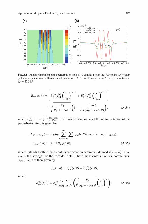
Fig. A.5 Radial component of the perturbation field Br : a contour plot in the (θ, r ) plane (ϕ = 0); bpoloidal dependence at different radial positions r : 1—r = 80 cm, 2—r = 70 cm, 3—r = 60 cm.Id = 22.5 kA
Bmn(r, θ) =[
B(1)c g
(s)m1
(r
rc1
)m−1
+ B(2)c g
(s)m2
(r
rc2
)m−1]
×√
R0
R0 + r cos θ
(1 − r cos θ
2m (R0 + r cos θ)
). (A.54)
where B(i)mns = −B(i)
c C (s)n g
(si)m . The toroidal component of the vector potential of the
perturbation field is given by
Aϕ(r, θ,ϕ) = εB0R0
∞∑
m=−∞
∑
n
amn(r, θ) cos (mθ − nϕ + χmn) ,
amn(r, θ) = m−1r Bmn(r, θ), (A.55)
where ε stands for the dimensionless perturbation parameter, defined as ε = B(1)c /B0,
B0 is the strength of the toroidal field. The dimensionless Fourier coefficients,amn(r, θ), are then given by
amn(r, θ) = a(1)mn(r, θ) + δa(2)
mn(r, θ),
where
a(i)mn(r, θ) = g(i)
mrci
m R0
r
m
d
dr
(√R0
R0 + r cos θ
(r
rci
)m)
. (A.56)
350 Appendix A: Magnetic Field in Ergodic Divertors
Here (i = 1, 2), δ = B(2)c /B(1)
c = rc1Δθ2/ (rc2Δθ1). The phase χmn = χs andtoroidal mode number n = (2s − 1)n0.
The angular dependencies of the perturbation field Br (r, θ,ϕ) at the fixed valuesof radial coordinate r and the toroidal angle ϕ = 0 are plotted in Fig. A.5. The radialdependence of the perturbation field is determined by (A.35). The power law of theradial decay of perturbation field has the lowest exponent, γn=6 = m0 − 1, for thetoroidalmode n = 6 . For the value δθ = 18◦, one hasm0 = π/δθ = 10 the exponentγn=6 = 9. For the next toroidal mode n = 18 we have γn=18 = 3m0 − 1 = 29.
Appendix BMagnetic Field of a Set of Saddle Coils
In this Appendix we give some details of calculations of the magnetic field createdby a set of saddle coils in a tokamak geometry described in Sect. 3.4.1. The method issimilar to the one in the classicalmagnetostatic to the calculation of themagnetic fieldcreated by the circular current loop (see, e.g., Jackson (1998)). But in our case theproblem is reduced to the new integrals which can be considered as the generalizedelliptic integrals.
As was shown in Sect. 3.4.1 the magnetic field created by the set of saddle coilscan be composed a sum of magnetic fields from the horizontal segments lying on thesurfaces Z = const and the ones lying the vertical surfaces (R, Z) (see also Fig. 3.8).We consider the calculations of these magnetic fields separately.
B.1 The magnetic Field of the Current Loop
Let (R, Z ,ϕ) be the cylindrical coordinate system. Consider a current–carryingfilament coil given by curve G in the 3D space. Let dl be an element of this curve,and J(R, Z ,ϕ) be a current flowing in the coil in the form of the circular loop asshown in Fig. 3.8. For the circular loop of radius R j lying in the horizontal planeZ j = constant the current density j(R, Z ,ϕ) has only a component in theϕ direction,
jϕ(R, Z ,ϕ) = Ic(ϕ)δ(R − R j )δ(Z − Z j ),
jx (R, Z ,ϕ) = − jϕ(R, Z ,ϕ) sinϕ,
jy(R, Z ,ϕ) = jϕ(R, Z ,ϕ) cosϕ, (B.1)
where Ic(ϕ) is a current depending on the toroidal angleϕ. Then, the vector potentialA at the point P(R, Z ,ϕ) is determined by the Biot–Savart law,
S. Abdullaev, Magnetic Stochasticity in Magnetically Confined Fusion Plasmas, 351Springer Series on Atomic, Optical, and Plasma Physics 78,DOI: 10.1007/978-3-319-01890-4, © Springer International Publishing Switzerland 2014
352 Appendix B: Magnetic Field of a Set of Saddle Coils
A(R, Z ,ϕ) = μo
4π
∫
G
j(R′, Z ′,ϕ′)dV ′
|r − r j | ,
Ax (R, Z ,ϕ) = μo
4π
∫
G
jx (R′, Z ′,ϕ′)dV ′
|r − r j | = −μo R j
4π
2π∫
0
Iϕ(ϕ j ) sinϕ j dϕ j
|r − r j | ,
Ay(R, Z ,ϕ) = μo
4π
∫
G
jy(R′, Z ′,ϕ j )dV ′
|r − r j | = μo R j
4π
2π∫
0
Iϕ(ϕ j ) cosϕ j dϕ j
|r − r j | , (B.2)
where dV = Rd Rd Zdϕ is a volume element, r j = (R j , Z j ,ϕ j ) are point coordi-nates at the curve G,
|r − r j | =√
R2 + R2j + (Z − Z j )2 − 2R R j cos(ϕ − ϕ j ).
The toroidal component of the vector potential Aϕ is
Aϕ(R, Z ,ϕ) = −Ax (R, Z ,ϕ) sinϕ + Ay(R, Z ,ϕ) cosϕ
= μo R j
4π
∫ 2π
0
Iϕ(ϕ j ) cos(ϕ j − ϕ)dϕ j
|r − r j | . (B.3)
Introducing the notations
D j =√
(R + R j )2 + (Z − Z j )2, k2 = 4R R j/D2j ,
and replacing the integration variable from ϕ j to φ,
φ = (ϕ − ϕ j + π)/2,
0 ≤ ϕ j ≤ 2π, (ϕ + π)/2 ≥ φ ≥ (ϕ − π)/2,
we obtain
Aϕ(R, Z ,ϕ) = −2μo R j
4πD
π/2∫
−π/2
Ic(ϕ − 2φ + π) cos(2φ)dφ√1 − k2 sin2 φ
. (B.4)
Suppose, that the current Ic(ϕ) can be presented as a Fourier series
Ic(ϕ) = I (0)c +
∞∑
n=1
I (n)c cos(nϕ + χn) = I (0)
c + 1
2
∞∑
n=−∞I (n)c einϕ+iχn , (B.5)
Appendix B: Magnetic Field of a Set of Saddle Coils 353
where
I (n)c eiχn = 1
π
2π∫
0
Ic(ϕ)e−inϕdϕ.
Consider a coil system consisting of N pairs of current loops as shown in Figs. 3.7and 3.8. The distribution of current Ic(ϕ) corresponding to this system is
Ic(ϕ) = I0
⎧⎪⎪⎪⎪⎪⎪⎨
⎪⎪⎪⎪⎪⎪⎩
0 for 2kπ/N ≤ ϕ ≤ 2kπ/N + ϕd ,
1 for 2kπ/N + ϕd ≤ ϕ ≤ (2k + 1)π/N − ϕd ,
0 for (2k + 1)π/N − ϕd ≤ ϕ ≤ (2k + 1)π/N + ϕd ,
−1 for (2k + 1)π/N + ϕd ≤ ϕ ≤ 2(k + 1)π/N − ϕd ,
0 for 2(k + 1)π/N − ϕd ≤ ϕ ≤ 2(k + 1)π/N ,
(B.6)
where k = 0, 1, . . . , n − 1, 2kπ/N ≤ ϕ ≤ 2(k + 1)π/N . After some lengthycalculations one can obtain the following formula for the Fourier components I (n)
cfor this current distribution,
π I (n)c eiχn /I0 = 4i
ne−inπ sin
( nπ
2N
)sin
( nπ
2N− nϕd
) sin(nπ)
sin(nπ/N ).
This expression does not vanish only for non-integer numbers n = (2s + 1)N ,(s = 0, 1, 2, . . .):
I (n)c eiχn = Ic
4
(2s + 1)πeiπ/2 cos [(2s + 1)Nϕd ] . (B.7)
Finally, we have
Ic(ϕ) = 4I0π
∞∑
s=0
cos [(2s + 1)Nϕd ]
2s + 1sin [(2s + 1)Nϕ] . (B.8)
Similar formulas can be obtained when the set of coils consists of odd numbers ofsaddle coils as the case shown in Fig. 3.6.
B.1.1 Vector Potential
Using (B.5) the vector potential (B.4) can be reduced to
Aϕ(R, Z ,ϕ) = −μo R j
πD j
{I (0)c a0(R, Z) +
∞∑
n=1
I (n)c a(s)
n (R, Z) sin(nϕ)
}, (B.9)
354 Appendix B: Magnetic Field of a Set of Saddle Coils
where
a0(R, Z) =π/2∫
0
cos(2φ)dφ√1 − k2 sin2 φ
= 1
k2
[(k2 − 2)K (k) + 2E(k)
], (B.10)
a(s)n (R, Z) = (−1)n
π/2∫
0
cos(2nφ) cos(2φ)dφ√1 − k2 sin2 φ
= 1
k2
[(k2 − 2)Kn(k) + 2En(k)
].
(B.11)Here K (k) and E(k) are the complete elliptic integrals with argument k, and theintegral Kn(k) and En(k) are defined by
Kn(k) =π/2∫
0
cos(2nφ)dφ√1 − k2 sin2 φ
,
En(k) =π/2∫
0
cos(2nφ)
√1 − k2 sin2 φdφ. (B.12)
They can be called the generalized elliptic integrals. Note, that K (k) = Kn=0(k) andE(k) = En=0(k).
Therefore the vector potential of the magnetic field created by the circular loopand the corresponding normalized perturbation poloidal flux can be presented as
Aϕ(R, Z ,ϕ) =∞∑
n=0
A(n)ϕ (R, Z) sin(nϕ),
ψ(pert)(R, Z ,ϕ) = − R Aϕ(R, Z)
B0R20
= ε
∞∑
n=0
ψn(R, Z) sin(nϕ), (B.13)
where
A(n)ϕ (R, Z) = μo I0in D j
4πRLn(k),
ψn(R, Z) = − in D j
R0Ln(k), (B.14)
Here the following notations are introduced
Appendix B: Magnetic Field of a Set of Saddle Coils 355
Ln(k) =(1 − k2
2
)Kn(k) − En(k),
in = I (n)c
I0= (−1)n 4
π
cos [(2s + 1)Nϕd ]
2s + 1, n = (2s + 1)N . (B.15)
The non-dimensional perturbation parameter ε is defined as
ε = μo I04πB0R0
. (B.16)
The (R, Z ) components of the magnetic field are given by
(BR, BZ ) =∞∑
n=0
(B(n)
R (R, Z), B(n)Z (R, Z)
)sin(nϕ), (B.17)
where
B(n)Z (R, Z) = 1
R
∂[
R A(n)ϕ (R, Z)
]
∂R= B0εin
{∂D j
∂RLn(k) + D j
∂k2j∂R
d Ln(k)
dk2j
},
(B.18)
B(n)R (R, Z) = −∂ A(n)
ϕ (R, Z)
∂Z= −B0εin
{∂D j
∂ZLn(k) + D j
∂k2j∂Z
d Ln(k)
dk2j
}.
(B.19)
B.1.2 Approximation of the Integrals Ln(k)
One can establish the approximation of the integrals Ln(k), En(k) (B.15) and itsderivative d Ln(k)/dk2 by the series of an expansion in m = k2:
Ln(k) =M∑
k=1
akmk +M∑
k=0
bkmk1 ln
1
m1+ RM , (B.20)
d Ln(k)
dm=
M∑
k=1
ckmk − d
dm1
M∑
k=0
dkmk1 ln
1
m1+ RM , (B.21)
where m1 = 1 − m. The coefficients ak, bk , ck, dk , (k = 1, 2, . . . , M) found by thefitting with the numerically calculated ones are presented in Tables B.1 and B.2 forthe case M = 3.
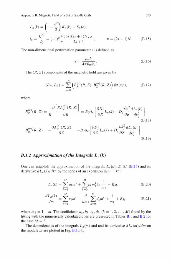
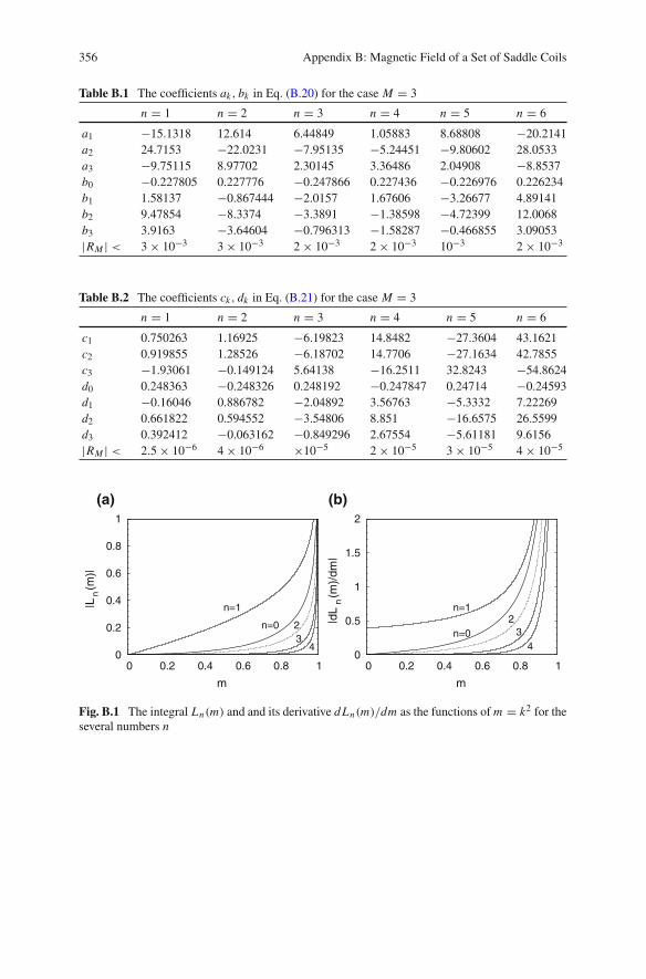
The dependencies of the integrals Ln(m) and and its derivative d Ln(m)/dm onthe module m are plotted in Fig. B.1a, b.
356 Appendix B: Magnetic Field of a Set of Saddle Coils
Table B.1 The coefficients ak , bk in Eq. (B.20) for the case M = 3
n = 1 n = 2 n = 3 n = 4 n = 5 n = 6
a1 −15.1318 12.614 6.44849 1.05883 8.68808 −20.2141a2 24.7153 −22.0231 −7.95135 −5.24451 −9.80602 28.0533a3 −9.75115 8.97702 2.30145 3.36486 2.04908 −8.8537b0 −0.227805 0.227776 −0.247866 0.227436 −0.226976 0.226234b1 1.58137 −0.867444 −2.0157 1.67606 −3.26677 4.89141b2 9.47854 −8.3374 −3.3891 −1.38598 −4.72399 12.0068b3 3.9163 −3.64604 −0.796313 −1.58287 −0.466855 3.09053|RM | < 3 × 10⁻³ 3 × 10⁻³ 2 × 10⁻³ 2 × 10⁻³ 10−3 2 × 10⁻³
Table B.2 The coefficients ck , dk in Eq. (B.21) for the case M = 3
n = 1 n = 2 n = 3 n = 4 n = 5 n = 6
c1 0.750263 1.16925 −6.19823 14.8482 −27.3604 43.1621c2 0.919855 1.28526 −6.18702 14.7706 −27.1634 42.7855c3 −1.93061 −0.149124 5.64138 −16.2511 32.8243 −54.8624d0 0.248363 −0.248326 0.248192 −0.247847 0.24714 −0.24593d1 −0.16046 0.886782 −2.04892 3.56763 −5.3332 7.22269d2 0.661822 0.594552 −3.54806 8.851 −16.6575 26.5599d3 0.392412 −0.063162 −0.849296 2.67554 −5.61181 9.6156|RM | < 2.5 × 10⁻⁶ 4 × 10−6 ×10−5 2 × 10⁻⁵ 3 × 10⁻⁵ 4 × 10⁻⁵
(a) (b)
0
0.2
0.4
0.6
0.8
1
0 0.2 0.4 0.6 0.8 1
|Ln(m
)|
m
n=1
n=0 23
4 0
0.5
1
1.5
2
0 0.2 0.4 0.6 0.8 1
|dL
n(m
)/dm
|
m
n=1
n=02
34
Fig. B.1 The integral Ln(m) and and its derivative d Ln(m)/dm as the functions of m = k2 for theseveral numbers n
Appendix B: Magnetic Field of a Set of Saddle Coils 357
B.2 Magnetic Field of the Vertical Segments of a Setof Saddle Coils
Above we have considered the calculation of the magnetic field created by the hori-zontal segments of the set of saddle coils. Now consider the magnetic field from thesegments of the set on the vertical sections (R, Z ).
B.2.1 Magnetic Field from a Single Vertical Wire
First we consider a single straight wire located along the vertical lines located at thesection (Rc = const, ϕ0 = const) between Z1 < Z < Z2. The current density isgiven by
jz = I0R−10 δ(ϕ − ϕ0)δ(R − R0)
{1, for Z1 < Z < Z2,
0, for Z < Z1, Z > Z2.(B.22)
The magnetic field generated by this wire can be described by the vector potential(0, 0, AZ ) with the non-zero z-component:
AZ (R, Z ,ϕ) = μo
4π
∫
G
jz(R′, Z ′,ϕ′)dV ′
|r − r0| . (B.23)
Using (B.22) it can be calculated directly,
AZ (R, Z ,ϕ) = μo I04π
Z2∫
Z1
d Z0√a2 + (Z − Z0)2
= μo I04π
[ln
Z2 − Z +√a2 + (Z2 − Z)2
Z1 − Z +√a2 + (Z − Z1)2
],
a2 = R2 + R20 − 2R R0 cos(ϕ − ϕ0), (B.24)
where we used the integral
x∫
0
dx√a2 + x2
= ln(x +√
a2 + x2) − ln a. (B.25)
358 Appendix B: Magnetic Field of a Set of Saddle Coils
B.2.2 Set of Straight Wires
Now we consider a set of 2N straight wires located at fixed toroidal angles ϕ(±)k =
(π/N )k ± ϕd , (k = 0, 1, . . . , 2N − 1) between circular loops of radii R1 at Z1and radii R2 at Z2. Suppose the directions of even/odd currents are positive/negativewith the respect to Z axis, and have the same magnitude, i.e., I (±)
k = (−1)k I0. (seeFig. 3.8). Then the current density can be presented as
j = ( jR, jZ ) = (sinα, cosα) j (R, Z ,ϕ), (B.26)
where α is an inclination angle of the wire with respect to the vertical axis Z , i.e.,
tanα = R2 − R1
Z2 − Z1,
and the current density
j (R, Z ,ϕ) = I0δ(R − R0(Z))R−1
×2N−1∑
k=0
(−1)k[δ
(ϕ − kπ
N− ϕd
)+ δ
(ϕ − kπ
N+ ϕd
)]. (B.27)
Using the Poisson summation formula
δ(ϕ) = 1
2π
∞∑
n=−∞cos nϕ = 1
2π
∞∑
n=−∞einϕ, (B.28)
Eq. (B.26) can be transformed to
j (R, Z ,ϕ) = I0δ(R − R0)
πR
∞∑
n=−∞einϕ cos(nϕd)e−iπn(1−1/2N )eiπ/2 sin(πn)
cos(πn/2N ).
(B.29)All terms in (B.29) vanish except ns = (2s + 1)N , (s = 0,±1,±2, . . .). The lattergive
j (R, Z ,ϕ) = I0δ (R − R0(Z)) R−1∞∑
s=0
Js cos (nsϕ) , (B.30)
where
Js = 4N
π(−1)N+1+s cos [nsϕd ] . (B.31)
Appendix B: Magnetic Field of a Set of Saddle Coils 359
B.2.3 Vector Potential
Using the current density (B.26) and (B.30) the magnetic field created by the verticalsegments of the saddle coils can be presented by the R- and Z -components of thevector potential,
A(R, Z ,ϕ) = (AR, AZ ) = μo
4π
∫( jR, jZ )(R′, Z ′,ϕ′) sin dV ′
|r − r0|= μo I0
4π
∞∑
s=0
Js
∫(eR, eZ ) cos(nsϕ
′)d Z ′dϕ′
|r − r0|
= μo I04π
∞∑
s=0
Js
[a(s)(R, Z) cos(nsϕ) + b(s)(R, Z) sin(nsϕ)
], (B.32)
where
a(s)(R, Z) =Z2∫
Z1
2π∫
0
(eR, eZ ) cos(nsφ)d Z ′dφ
D(φ, Z ′),
b(s)(R, Z) = −Z2∫
Z1
2π∫
0
(eR, eZ ) sin(nsφ)d Z ′dφ
D(φ, Z ′), (B.33)
and
eR = sinα(Z ′), eZ = cosα(Z ′),
D(φ, Z ′) =√
R2 + R20(Z ′) − 2R R0(Z ′) cosφ + (Z − Z ′)2. (B.34)
If the segment of a wire connecting Z1 and Z2 is a straight the integral overZ ′ can be calculated analytically. If this segment is not straight it can be presentedas a composed by M number of small straight segments. Each straight segment iconnects the points (Ri , Zi ) and (Ri+1, Zi+1), (i = 1, 2, . . . , M − 1). Then thevectors as(R, Z), bs(R, Z) is given by the sum
a(s)(R, Z) =M∑
i=1
(sinαi , cosαi )a(i)s (R, Z),
b(s)(R, Z) =M∑
i=1
(sinαi , cosαi )b(i)s (R, Z), (B.35)
where sinαi = sinα(Zi ), cosαi = cosα(Zi ),
360 Appendix B: Magnetic Field of a Set of Saddle Coils
a(i)s (R, Z) =
Zi+1∫
Zi
2π∫
0
cos(nsφ)d Z ′dφ
D(φ, Z ′),
b(i)s (R, Z) = −
Zi+1∫
Zi
2π∫
0
sin(nsφ)d Z ′dφ
D(φ, Z ′). (B.36)
The function R0(Z) describes the straight segments between points (Ri , Zi ) and(Ri+1, Zi+1), (i = 1, 2, . . . , M − 1), i.e.,
R0(Z) = Ri + Ri+1 − Ri
Zi+1 − Zi(Z − Zi ) = Ri + βi (Z − Zi ),
βi = Ri+1 − Ri
Zi+1 − Zi= tanαi , Zi ≤ Z ≤ Zi+1. (B.37)
The denominator D(φ, Z ′) in (B.36) can be presented in the form,
D(φ, Z ′) =√
Ai
[a2
i + (Zi − Z ′)2],
where Ai , ai and Zi are given by
Ai = 1 + β2i , Zi = 1
1 + β2i
[Z + Rβi cosφ − (Ri − βi Zi )βi
],
a2i = Ci − Z2
i ,
Ci = 1
1 + β2i
[R2 + (Ri − βi Z1)
2 − 2R(Ri − βi Zi ) cosφ + Z2].
It allows to integrate (B.36) over Z ′ thus reducing them to the one-dimensionalintegral
a(i)s (R, Z) = 1√
Ai
2π∫
0
L(i)g (φ) cos(nsφ)dφ,
b(i)s (R, Z) = − 1√
Ai
2π∫
0
L(i)g (φ) sin(nsφ)dφ, (B.38)
where
L(i)g (φ) = ln
⎡
⎣Zi+1 − Zi +
√a2
i + (Zi+1 − Zi )2
Zi − Zi +√
a2 + (Zi − Zi )2
⎤
⎦ .
Appendix B: Magnetic Field of a Set of Saddle Coils 361
The numerical integration shows that the integral b(i)s (R, Z) is negligibly small.
Furthermore, we neglect this integral.
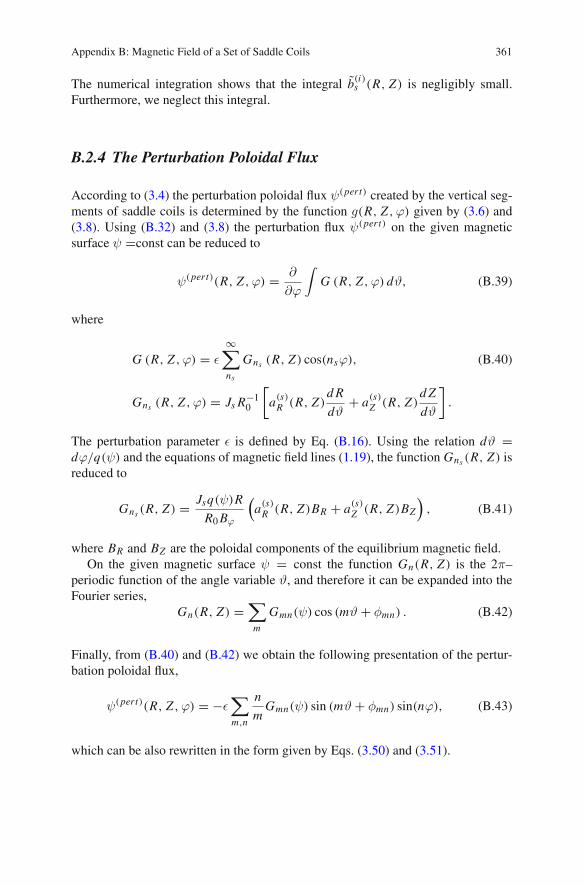
B.2.4 The Perturbation Poloidal Flux
According to (3.4) the perturbation poloidal flux ψ(pert) created by the vertical seg-ments of saddle coils is determined by the function g(R, Z ,ϕ) given by (3.6) and(3.8). Using (B.32) and (3.8) the perturbation flux ψ(pert) on the given magneticsurface ψ =const can be reduced to
ψ(pert)(R, Z ,ϕ) = ∂
∂ϕ
∫G (R, Z ,ϕ) dϑ, (B.39)
where
G (R, Z ,ϕ) = ε
∞∑
ns
Gns (R, Z) cos(nsϕ), (B.40)
Gns (R, Z ,ϕ) = Js R−10
[a(s)
R (R, Z)d R
dϑ+ a(s)
Z (R, Z)d Z
dϑ
].
The perturbation parameter ε is defined by Eq. (B.16). Using the relation dϑ =dϕ/q(ψ) and the equations of magnetic field lines (1.19), the function Gns (R, Z) isreduced to
Gns (R, Z) = Jsq(ψ)R
R0Bϕ
(a(s)
R (R, Z)BR + a(s)Z (R, Z)BZ
), (B.41)
where BR and BZ are the poloidal components of the equilibrium magnetic field.On the given magnetic surface ψ = const the function Gn(R, Z) is the 2π–
periodic function of the angle variable ϑ, and therefore it can be expanded into theFourier series,
Gn(R, Z) =∑
m
Gmn(ψ) cos (mϑ + φmn) . (B.42)
Finally, from (B.40) and (B.42) we obtain the following presentation of the pertur-bation poloidal flux,
ψ(pert)(R, Z ,ϕ) = −ε∑
m,n
n
mGmn(ψ) sin (mϑ + φmn) sin(nϕ), (B.43)
which can be also rewritten in the form given by Eqs. (3.50) and (3.51).
362 Appendix B: Magnetic Field of a Set of Saddle Coils
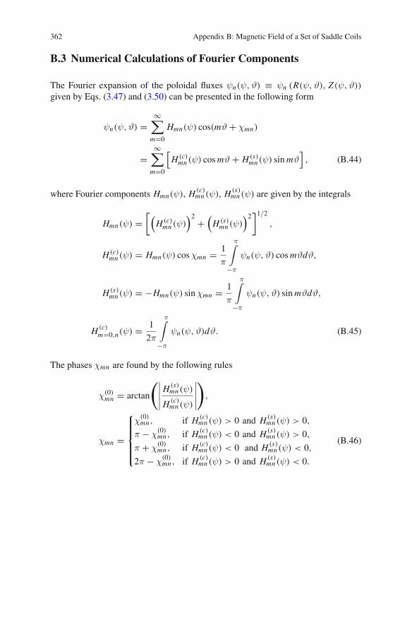
B.3 Numerical Calculations of Fourier Components
The Fourier expansion of the poloidal fluxes ψn(ψ,ϑ) ≡ ψn (R(ψ,ϑ), Z(ψ,ϑ))
given by Eqs. (3.47) and (3.50) can be presented in the following form
ψn(ψ,ϑ) =∞∑
m=0
Hmn(ψ) cos(mϑ + χmn)
=∞∑
m=0
[H (c)
mn (ψ) cosmϑ + H (s)mn (ψ) sinmϑ
], (B.44)
where Fourier components Hmn(ψ), H (c)mn (ψ), H (s)
mn (ψ) are given by the integrals
Hmn(ψ) =[(
H (c)mn (ψ)
)2 +(
H (s)mn (ψ)
)2]1/2,
H (c)mn (ψ) = Hmn(ψ) cosχmn = 1
π
π∫
−π
ψn(ψ,ϑ) cosmϑdϑ,
H (s)mn (ψ) = −Hmn(ψ) sinχmn = 1
π
π∫
−π
ψn(ψ,ϑ) sinmϑdϑ,
H (c)m=0,n(ψ) = 1
2π
π∫
−π
ψn(ψ,ϑ)dϑ. (B.45)
The phases χmn are found by the following rules
χ(0)mn = arctan
(∣∣∣∣∣H (s)
mn (ψ)
H (c)mn (ψ)
∣∣∣∣∣
),
χmn =
⎧⎪⎪⎪⎨
⎪⎪⎪⎩
χ(0)mn, if H (c)
mn (ψ) > 0 and H (s)mn (ψ) > 0,
π − χ(0)mn, if H (c)
mn (ψ) < 0 and H (s)mn (ψ) > 0,
π + χ(0)mn, if H (c)
mn (ψ) < 0 and H (s)mn (ψ) < 0,
2π − χ(0)mn, if H (c)
mn (ψ) > 0 and H (s)mn (ψ) < 0.
(B.46)
Appendix CCalculations of the Poincaré Integrals
Here we present the detailed calculations of the Poincaré integrals (6.59) for theperturbation magnetic fluxes ψ1(ψ,ϑ,ϕ) of type
ψ1 (ψ,ϑ,ϕ) = ψn (ψ,ϑ) sin (nϕ + χn) ,
ψn (ψ,ϑ) =∞∑
m=1
Hmn(ψ)eimϑ =∞∑
m=1
|Hmn(ψ)| eim(ϑ−ϑ0). (C.1)
We assume that the integration in (6.59) is taken over the unperturbed orbit (ψ =const,ϑ(ϕ) = ϕ/q(ψ)) one poloidal turn starting from and ending at the section Σs
(see Fig. 2.4). Recall that ϑ = ±π at the section Σs . Using (C.1) the integral (6.59)is reduced to
P (ϕ,ψ) =πq(ψ)∫
−πq(ψ)
ψn(ψ,ϑ(ϕ′)
)sin
(n[ϕ + ϕ′]) dϕ′
= Kn(ψ) sin(nϕ + χn) + Ln(ψ) cos(nϕ + χn), (C.2)
where
Rn(ψ) = Kn(ψ) + i Ln(ψ) =πq(ψ)∫
−πq(ψ)
ψn (ψ,ϑ(ϕ)) einϕdϕ. (C.3)
Using a Fourier series of ψn (ψ,ϑ) in ϑ we have
S. Abdullaev, Magnetic Stochasticity in Magnetically Confined Fusion Plasmas, 363Springer Series on Atomic, Optical, and Plasma Physics 78,DOI: 10.1007/978-3-319-01890-4, © Springer International Publishing Switzerland 2014
364 Appendix C: Calculations of the Poincaré Integrals
Kn(ψ) = 1
2
∞∑
m=1
Hmn(ψ)
πq∫
−πq
[ei(m/q+n)ϕ + ei(m/q−n)ϕ
]dϕ
= q(ψ)
∞∑
m=1
Hmn(ψ)
[sin (π[m + nq])
m + nq+ sin (π[m − nq])
m − nq
]. (C.4)
Recalling that Hmn(ψ) = |Hmn| exp(−imϑ0) one has at the resonant surface ψm0,n ,(q(ψm0,n) = m0/n),
Kn(ψm0,n) = πq(ψm0,n)|Hm0n(ψm0,n)| cos (nqϑ0) . (C.5)
One can similarly obtain
Ln(ψ) = 1
2i
∞∑
m=1
Hmn(ψ)
πq∫
−πq
[ei(m/q+n)ϕ − ei(m/q−n)ϕ
]dϕ
= −iq(ψ)
∞∑
m=1
Hmn(ψ)
[sin (π[m + nq])
m + nq− sin (π[m − nq])
m − nq
], (C.6)
andLn(ψm0,n) = πq(ψm0,n)|Hm0n(ψm0,n)| sin (nqϑ0) . (C.7)
At the arbitrary ψ the function Rn(ψ) = Kn(ψ) + i Ln(ψ) can be presented as
Rn(ψ) = R(reg)n (ψ) + R(osc)
n (ψ), (C.8)
where R(reg)n (ψ) is the regular part defined as
R(reg)n (ψ) = πq(ψ)H∗
n (ψ; m = nq), (C.9)
and R(osc)n (ψ) is the oscillatory part of the integral Rn(ψ). According to the definition
of the R(reg)n (ψ) the oscillatory part R(osc)
n (ψ) has zeros at the resonant surfacesψmn ,q(ψmn) = m/n, i.e., R(osc)
n (ψmn) = 0. In Eq. (C.9) the function Hn(ψ; m) is definedby Hmn(ψ) by extending the discrete mode number m to the continuous one.
The relation (C.9) can be also obtained from (C.3). Indeed, by replacing thevariable ϕ to ϑ we have
Rn(ψ) = q(ψ)
π∫
−π
ψn (ψ,ϑ(ϕ)) einqϑdϑ. (C.10)
Appendix C: Calculations of the Poincaré Integrals 365
For the integer values of the product nq, nq = m, the latter up to the constant factorπ coincides with the Fourier coefficients Hmn , i.e., Rn(ψ) = πq(ψ)H∗
mn(ψ).
C.1 Determination of Oscillatory Parts of Rn(ψ)
Below we present the method of calculations of R(osc)n (ψ) based on the contour
integration. It can be applied when there exists an analytical formula of the fluxψn(ψ,ϑ). Specifically we use the poloidal fluxes of the perturbation magnetic fieldfor Model I (9.28) and Model II (9.29).
C.1.1 Model I
For Model I with the flux function ψn(ψ,ϑ) (C.1) the integral (C.3) can be taken bya contour integral. Changing the integration variable ϕ to ϑ = ϕ/q the integral (C.3)is reduced to
Rn(ψ) = e−b
π∫
−π
cos(ϑ − ϑ0) − e−b
1 + e−2b − 2e−b cos(ϑ − ϑ0)einqϑdϑ. (C.11)
Introducing a complex integration variable z = eiϑ, dϑ = dz/ i z, we have
sin(ϑ − ϑ0) = eiϑ0
2zi
(z2e−2iϑ0 − 1
),
cos(ϑ − ϑ0) = eiϑ0
2z
(1 + z2e−2iϑ0
),
1 + e−2b − 2e−b cos(ϑ − ϑ0) = z1z[(z − z1)(z2 − z)] ,
z1 = e−b+iϑ0 , z2 = eb+iϑ0 .
The integral (C.11) can be then rewritten as
Rn(ψ) = e2iϑ0
2i
∫
Cϕ
f (z)dz, (C.12)
where Cϕ is the segment −π < θ < π on the unit circle |z| = 1, and
f (z) = znq−1[1 + z2e−2iϑ0 − 2z∗
1z]
(z − z1)(z2 − z).
366 Appendix C: Calculations of the Poincaré Integrals
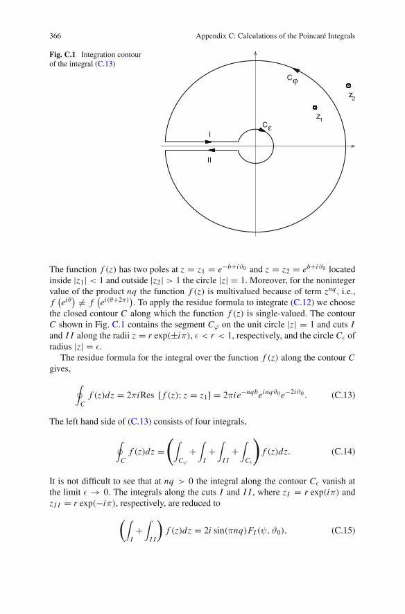
Fig. C.1 Integration contourof the integral (C.13)
I
II
z1
z2
Cε
Cϕ
The function f (z) has two poles at z = z1 = e−b+iϑ0 and z = z2 = eb+iϑ0 locatedinside |z1| < 1 and outside |z2| > 1 the circle |z| = 1. Moreover, for the nonintegervalue of the product nq the function f (z) is multivalued because of term znq , i.e.,f(eiθ) �= f
(ei(θ+2π)
). To apply the residue formula to integrate (C.12) we choose
the closed contour C along which the function f (z) is single-valued. The contourC shown in Fig. C.1 contains the segment Cϕ on the unit circle |z| = 1 and cuts Iand I I along the radii z = r exp(±iπ), ε < r < 1, respectively, and the circle Cε ofradius |z| = ε.
The residue formula for the integral over the function f (z) along the contour Cgives,
∮
Cf (z)dz = 2πiRes [ f (z); z = z1] = 2πie−nqbeinqϑ0e−2iϑ0 . (C.13)
The left hand side of (C.13) consists of four integrals,
∮
Cf (z)dz =
(∫
Cϕ
+∫
I+∫
I I+∫
Cε
)f (z)dz. (C.14)
It is not difficult to see that at nq > 0 the integral along the contour Cε vanish atthe limit ε → 0. The integrals along the cuts I and I I , where zI = r exp(iπ) andzI I = r exp(−iπ), respectively, are reduced to
(∫
I+∫
I I
)f (z)dz = 2i sin(πnq)FI (ψ,ϑ0), (C.15)
Appendix C: Calculations of the Poincaré Integrals 367
where
FI (ψ,ϑ0) =1∫
0
φ(r)rnq−1dr,
φ(I )(r) = 1 + r2e−2iϑ0 + 2re−iϑ0e−b
(r + e−b+iϑ0)(r + eb+iϑ0). (C.16)
From Eqs. (C.12), (C.13) and (C.15) it follows that
Rn(ψ) = R(reg)n (ψ) + R(osc)
n (ψ),
R(reg)n (ψ) = πeinqϑ0e−nqb = πe−nqb [cos(nqϑ0) + i sin(nqϑ0)] ,
R(osc)n (ψ) = −e2iϑ0 sin(πnq)FI (ψ,ϑ0). (C.17)
C.1.2 Asymptotical Expansion
For large nq � 1 the function FI (ψ,ϑ0) (C.16) can be estimated by the asymptoticexpansion in powers of 1/nq. It can be done using an integration by part,
1∫
0
φ(I )(r)rnq−1dr =⎡
⎣φ(I )0
nq− 1
nq
1∫
0
dφ(I )(r)
drrnqdr
⎤
⎦
= 1
nq
{φ(I )0 − 1
nq + 1φ(I )1 + · · ·
}, (C.18)
where
φ(I )0 = φ(I )(1) = cosϑ0 + e−b
cosϑ0 + cosh b,
φ1 = dφ(r)
dr
∣∣∣∣r=1
= −isinh b sin ϑ0
(cosϑ0 + cosh b)2. (C.19)
At ϑ0 = 0 and ϑ0 = π, we have
φ(I )0 (0) = 1 + e−b
1 + cosh b, φ
(I )0 (π) = − 1 − e−b
cosh b − 1.
Near the separatrix b → 0, it has the following asymptotics, φ0(π) ≈ −(2/b)
(1 + O(b)).Finally, the leading terms of asymptotical expansion of R(osc)
n (ψ), in 1/nq can bepresented as
368 Appendix C: Calculations of the Poincaré Integrals
K (osc)n (ψ) = − sin(πnq)
nq
cosϑ0 + e−b
cosϑ0 + cosh b,
L(osc)n (ψ) = sin(πnq)
nq(nq + 1)
sin ϑ0 sinh b
(cosϑ0 + cosh b)2. (C.20)
C.1.3 Model II
For Model II (9.29), integrating by part one arrives to
Rn(ψ) = − nq
π∫
−π
arctan
[sin(ϑ − ϑ0)
cos(ϑ − ϑ0) − eb
]einqϑdϑ
= − 2 sin(πnq)F(ϑ0)
+ ie−b
π∫
−π
cos(ϑ − ϑ0) − e−b
1 + e−2b − 2e−b cos(ϑ − ϑ0)einqϑdϑ, (C.21)
where
F(ϑ) = arctan
[sin ϑ
cosϑ + eb
]. (C.22)
The integral in the last term of (C.21) coincides with the integral (C.11). Then using(C.17), we obtain
Rn(ψ) = R(reg)n (ψ) + R(osc)
n (ψ),
R(reg)n (ψ) = πieinqϑ0e−nqb,
R(osc)n (ψ) = − sin(πnq)
[2F(ϑ0) + ie2iϑ0 FI (ψ,ϑ0)
]. (C.23)
Using (C.20) they can be also presented by
K (reg)n (ψ) = −π sin(nqϑ0)e
−nqb,
L(reg)n (ψ) = π cos(nqϑ0)e
−nqb,
K (osc)n (ψ) = − sin(πnq)
[2F(ϑ0) + 1
nq(nq + 1)
sin ϑ0 sinh b
(cosϑ0 + cosh b)2
],
L(osc)n (ψ) = − sin(πnq)
[2F(ϑ0) + 1
nq
cosϑ0 + e−b
cosϑ0 + cosh b
]. (C.24)
Appendix DAdvanced Version of the Symplectic Mappingfor Hamiltonian Systems
Below we construct the alternative form of the mapping (ϑk, Ik) → (ϑk+1, Ik+1)
for the Hamiltonian system given by Eqs. (6.5) and (6.6). Similar to the methodgiven in Sect. 6.2.2 it is based on the canonical change of variables and the classicalperturbation theory in a finite time interval (see Abdullaev (2002, 2006)). In theinterval tk ≤ t ≤ tk+1 we perform a such a canonical transformation of variables(ϑ, I ) → (Θ, J ) that the new HamiltonianH in the new canonical variables (Θ, J )acquires fast oscillating perturbation terms, i.e.,
H = H0(J ) + εH1(Θ, J, t),
H1(Θ, J, t) = −2H1 (Θ, J, t)N∑
s=1
cos (s Mnt) , (D.1)
where M ≥ 1 is an integer number, N � 1 is the number of harmonics. The canoni-cal change of variables (ϑ, I ) → (Θ, J ) is implemented via the generating functionF(J,ϑ, t) = Jϑ + εS(J,ϑ, t), where the generating function S = S(J,ϑ, t) satis-fies the Hamilton-Jacobi equation
H0
(ϑ, J + ε
∂S
∂ϑ, t
)+ ε
∂S
∂t= H(ϑ, J, t, ε). (D.2)
The generating function S(J,ϑ, t) is sought as a series in powers of ε similar to(6.15). Expanding the Hamilton–Jacobi equation (D.2) in powers of of ε one obtainsH0(J ) = H0(J ), and the equations for Si , (i = 1, 2, . . .):
∂S1∂t
+ ∂H0
∂ J
∂S1∂ϑ
= H1(ϑ, J, t) − H1(ϑ, J, t), (D.3)
∂S j
∂t+ ∂H0
∂ J
∂S j
∂ϑ= −Fj (ϑ, J, t), j ≥ 2, (D.4)
where Fj (ϑ, I, t) are thepolynomial functions of derivatives∂S1/∂ϑ, . . ., ∂S j−1/∂ϑ.
S. Abdullaev, Magnetic Stochasticity in Magnetically Confined Fusion Plasmas, 369Springer Series on Atomic, Optical, and Plasma Physics 78,DOI: 10.1007/978-3-319-01890-4, © Springer International Publishing Switzerland 2014
370 Appendix D: Advanced Version of the Symplectic Mapping for Hamiltonian Systems
In the first order of the perturbation parameter ε the generating function is givenby the integral
S1(ϑ, J, t, t0) =t∫
t0
[H1
(ϑ(t ′), J, t ′
)− H1(ϑ(t ′), J, t ′
) ]dt ′, (D.5)
taken along the unperturbed field line ϑ(t ′) = ϑ + ω(J )(t − t ′), J = const. Thevariable t and the free parameter t0 lie in the intervals: tk ≤ t ≤ tk+1, tk < t0 < tk+1.Using Eq. (D.1) we have
S1(J,ϑ, t, t0) = −t∫
t0
H1(ϑ(t ′), J, t ′)N∑
s=−N
cos(sMnt ′
)dt ′
= − 2π
Mn
t∫
t0
H1(ϑ(t ′), I, t ′)∞∑
k=−∞δ(t ′ − tk
)dt ′, at N → ∞,
(D.6)
where tk = k(2π/Mn), (k = 0,±1,±2, . . .). From Eq. (D.6) it follows that thegenerating function S1 vanishes in the time interval tk < t < tk+1. But it takesnon-zero values at t = tk and t = tk+1 given by Eq. (6.47).
Note that the higher order generating functions S j , ( j ≥ 2), vanish in the wholetime interval tk ≤ t ≤ tk+1 (see Abdullaev (2006)).
Suppose that (Θ(t), J (t)) is a solution of the newHamiltonian (D.1) in the intervaltk < t < tk+1. Then the mapping can be presented by the following successivecanonical transformations
Jk = Jk − ε∂Sk
∂ϑk, Θk = ϑk + ε
∂Sk
∂ Jk,
(Θk+1, Jk+1) = M(Θk, Jk),
Jk+1 = Jk+1 + ε∂Sk+1
∂ϑk+1, ϑk+1 = Θk+1 − ε
∂Sk+1
∂ Jk+1, (D.7)
where (Θk, Jk) = (Θ(tk), J (tk)). The mapping (Θk+1, Jk+1) = M(Θk, Jk) can beconstructed using the regular procedure described in Refs. Abdullaev (2002, 2006).For the Hamiltonian system (D.1) it reads as
Appendix D: Advanced Version of the Symplectic Mapping for Hamiltonian Systems 371
Jk = Jk − ε∂Gk
∂Θk, Θk = Θk + ε
∂Gk
∂ Jk,
Θk+1 = Θk + tk+1 − tkq(Jk)
, Jk+1 = Jk,
Jk+1 = Jk+1 + ε∂Gk+1
∂Θk+1, Θk+1 = Θk+1 − ε
∂Gk+1
∂ Jk+1, (D.8)
determined by the generating function G( J ,Θ, t, t0): Gk = G( Jk,Θk, tk, t0),Gk+1 = G( Jk+1,Θk+1, tk+1, t0). In the first order of ε it is given by
G1(J,Θ, t, t0) = −t∫
t0
H1(Θ(t ′), J, t ′)dt ′
= 2
t∫
t0
H1(Θ(t ′), J, t ′)N∑
s=1
cos(s Mnt ′
)dt ′. (D.9)
As seen from Eq. (D.9) the generating function G1 is determined as an integral fromthe fast oscillating functions.One should expect thatG1 decreaseswith increasing thenumber M . Taking the asymptotical expansion of the integral (D.9) one can obtainthe following estimation for the generating function G1 = G1(J,Θ, tk+1, tk):
G1 ≈ 4π
Mn
N∑
s=1
⎡
⎣P∑
p=1
1
(s Mn)2pf (2p)(tk) + O([smΩ]−2P )
⎤
⎦ , (D.10)
where f (t) ≡ H1(Θ(t), J, t), f (p)(t) ≡ d p f (t)/dt p, (p = 1, 2, . . .). Supposingthat n−2p f (2p)(tk) ∼ 1, one can obtain the following estimation for G1 at largevalues N � 1, P � 1:
|G1| � 2π3
M3n= n2
12(Δt)3 , (D.11)
where Δt = tk+1 − tk = 2π/Mn is a step of the mapping. At the moderately largevalues of M ≥ 8÷ 10 one can neglect the generating function G1, and the mapping(D.7) is reduced to the form (6.44) with the generating functions (6.47). For instance,for M = 8 the divergence of the flux coordinate I of a regular orbit from the onecalculated for M = 128 is 3.6× 10⁻⁷ per one toroidal turn (for ε = 2× 10⁻³). Thisis sufficiently accurate to plot Poincare sections. We have chosen M = 16 for thecalculation of diffusion coefficients.
Amore detailed study of the accuracy of the describedmapping procedure requiresa special investigation.
Appendix EEigenvalues of the Jacobi Matrix
E.1 Jacobi Matrix
In this appendix we present the calculations of the Jacobi matrix (7.44), its eigen-values (7.52) and the Lyapunov exponents of the mapping (6.29)–(6.31) [or (7.32)].We present the latter in the form
M = T−T0T+, (E.1)
of three successive mappings, T−T0T+, each of them are given by Eqs. (6.29), (6.30)and (6.31), respectively. Then the Jacobian matrix (7.44) can be written as a productof three Jacobian matrices, corresponding to three successive mappings,
Jk = Mk+1M0Mk, (E.2)
where
Mk =⎛
⎜⎝
∂ Jk
∂ Ik
∂ Jk
∂ϑk∂Θk
∂ Ik
∂Θk
∂ϑk
⎞
⎟⎠ , (E.3)
M0 =
⎛
⎜⎜⎝
∂ Jk+1
∂ Jk
∂ Jk+1
∂Θk∂Θk
∂ Jk
∂Θk
∂Θk
⎞
⎟⎟⎠ =(
1 0w′(Jk) (tk+1 − tk) 1
), (E.4)
Mk+1 =
⎛
⎜⎜⎝
∂ Ik+1
∂ Jk+1
∂ Ik+1
∂Θk∂ϑk+1
∂ Jk+1
∂ϑk+1
∂Θk
⎞
⎟⎟⎠ . (E.5)
S. Abdullaev, Magnetic Stochasticity in Magnetically Confined Fusion Plasmas, 373Springer Series on Atomic, Optical, and Plasma Physics 78,DOI: 10.1007/978-3-319-01890-4, © Springer International Publishing Switzerland 2014
374 Appendix E: Eigenvalues of the Jacobi Matrix
The derivatives in the matrices (E.3) and (E.5) are easily calculated from themappings given by Eqs. (6.29) and (6.31):
∂ Jk
∂ Ik= 1
1 + εG Jϑ(ϕk),
∂ Jk
∂ϑk= − εGϑϑ(ϕk)
1 + εG Jϑ(ϕk),
∂Θk
∂ Ik= εG J J (ϕk)
1 + εG Jϑ(ϕk),
∂Θk
∂ϑk= 1 + εG Jϑ(ϕk) − ε2G J J (ϕk)Gϑϑ(ϕk)
1 + εG Jϑ(ϕk), (E.6)
and
∂ Ik+1
∂ Jk= 1 + εG Jϑ(ϕk+1) − ε2G J J (ϕk+1)Gϑϑ(ϕk+1)
1 + εG Jϑ(ϕk+1),
∂ Ik+1
∂Θk= εGϑϑ(ϕk+1)
1 + εG Jϑ(ϕk+1),
∂ϑk+1
∂ Jk= − εG J J (ϕk+1)
1 + εG Jϑ(ϕk+1),
∂ϑk+1
∂Θk= 1
1 + εG Jϑ(ϕk+1), (E.7)
where
G J J (ϕ) ≡ ∂2G
∂ J 2 , G Jϑ(ϕ) ≡ ∂2G
∂ J∂ϑ,
Gϑϑ(ϕ) ≡ ∂2G
∂ϑ2 , G(ϕ) = G(ϑ, J,ϕ,ϕ0). (E.8)
E.2 Jacobi Matrix at the Fixed Points
Below we calculate the eigenvalues of the Jacobi matrix J of the mapping (7.32) atthe fixed points considered in Sect. 7.2.2. Putting ϕk = ϕ0 − 2πm0, ϕk+1 = ϕ0 wereduce the corresponding Jacobi matrix to
∂ Ik+1
∂ Ik= 1
1 + εG J,ϑ,
∂ Ik+1
∂ϑk= − εGϑϑ
1 + εG Jϑ,
∂ϑk+1
∂ Ik= w′(Ik+1)2πm0
1 + εG J,ϑ+ εG J J
1 + εG Jϑ(ϕk),
∂ϑk+1
∂ϑk= εGϑϑw′(Ik+1)2πm0
1 + εG J,ϑ+ 1 + εG Jϑ − ε2G J J Gϑϑ
1 + εG Jϑ. (E.9)
Appendix E: Eigenvalues of the Jacobi Matrix 375
Using the generating function G (6.34) in the first order of ε we have
G1 = G1(ϑ0, J,ϕ0 − 2πm0,ϕ0)
= 2πm0
∑
m,n
Hmn(J )[a(xmn) sin (mϑ0 − nϕ0 + χmn)
+ b(xmn) cos (mϑ0 − nϕ0 + χmn)]. (E.10)
According to (7.41) the coefficients a(xmn), b(xmn) near the resonant surfacesIm0n0 , q(Im0n0) = m0/n0, are of order
a(xmn) ∝ ε2,
b(xmn) ={1 + C0ε for m/n = m0/n0,
C0ε for m/n �= m0/n0,
C0ε = −q ′mq2 (I0 − Im0n0). (E.11)
Neglecting small terms of order of ε and ε2, The generating function G1 (E.10) atthe fixed point I0 is reduced to
G1 = 2πm0
∑
m/n=m0/n0
Hmn(I0) cos (mϑ0 − nϕ0 + χmn) . (E.12)
The trace TrJ of the matrix can be reduced to
Tr J = ∂ Ik+1
∂ Ik+ ∂ϑk+1
∂ϑk= 1
1 + εG J,ϑ+ εGϑϑw′(Ik+1)2πm0
1 + εG J,ϑ
+ 1 + εG Jϑ − ε2G J J Gϑϑ
1 + εG Jϑ. (E.13)
Neglecting the terms of ε2 we obtain Eq. (7.53).
E.3 Eigenvalues of Jacobi Matrix
Consider the linearized equations (7.51) near the fixed point. We introduce newcoordinates (x, y) by rotating the coordinates (δJ, δϑ) around the point (0, 0), i.e.,
(xy
)= U
(δJδϑ
), U =
(cosφ − sin φsin φ cosφ
), (E.14)
376 Appendix E: Eigenvalues of the Jacobi Matrix
which would reduce the Eq. (7.51) into form
xk+1 = λ1 xk,
yk+1 = λ2 yk, (E.15)
where λi are constants. The angle φ are found from the eigenvalue problem of thematrix Λ,
ΛU = EU, E =(
λ1 00 λ2
). (E.16)
The eigenvalues λ of the 2 × 2 matrix Λ with det Λ = 1 are determined by thesolution of the quadratic equation
λ2 − 2Aλ + 1 = 0, A = 1
2Tr Λ = 1
2
(∂ Ik+1
∂ Ik+ ∂ϑk+1
∂ϑk
). (E.17)
From Eq. (E.14) we have two solutions:
tan φ1 = − tan φ2 = λ1 − Λ11
Λ12= Λ21
Λ22 − λ2. (E.18)
Appendix FFeatures of the Perturbation Hamiltonianof Guiding-Center Motion
In this appendix we analysis the perturbation Hamiltonian of guiding-center motion(5.38) in the action-angle variables (ϑ,ϑϕ, J, Iϕ) for the magnetic perturbationscreated by the set of saddle coils. Furthermore, we consider only time-independentmagnetic perturbations and neglect the perturbations of the electric field.
The magnetic perturbation fluxes ψ(pert)p (R, Z ,ϕ) of the set of saddle coils
were given in Sect. 3.4 by Eqs. (3.43) and (3.49). Using the latter the perturbationHamiltonian (5.34) can be reduced to
εh1 ≡ εh1(z,ϕ, pz, pϕ, pt ) = ε
3∑
j=1
∑
n
H ( j)n (R, Z) sin(nϕ), (F.1)
where
H ( j)n (R, Z) = Zq
uϕψ( j)n (R, Z)
xc. (F.2)
The dimensionless perturbation parameter ε is defined by Eq. (3.46). The functionsψ
( j)n (R, Z), ( j = 1, 2, 3), are given by (3.44) and (3.50). We recall that R = R0x ,
Z = R0z.Using the relations (5.21) and (5.22) between the coordinates (R = Roxc(pz), Z =
R0z,ϕ) and the action-angle variables (ϑ,ϑϕ, J, Iϕ) the perturbation Hamiltonian(F.1) can be written as
εh1 = ε
3∑
j=1
∑
n
V ( j)n (ϑ; J, Iϕ) sin
(nϑϕ + nG(ϑ; J, Iϕ)
), (F.3)
whereV ( j)
n (ϑ; J, Iϕ) ≡ H ( j)n
(R(ϑ; J, Iϕ), Z(ϑ; J, Iϕ)
).
S. Abdullaev, Magnetic Stochasticity in Magnetically Confined Fusion Plasmas, 377Springer Series on Atomic, Optical, and Plasma Physics 78,DOI: 10.1007/978-3-319-01890-4, © Springer International Publishing Switzerland 2014
378 Appendix F: Features of the Perturbation Hamiltonian of Guiding-Center Motion
For brevitywe notate the first function as V (ϑ), i.e., V ( j)(ϑ) ≡ V ( j)n (ϑ; J, Iϕ). Using
the relation
sin(nϑϕ + nG(ϑ; J, Iϕ)
) = sin(nϑϕ)A(ϑ) + cos(nϑϕ)B(ϑ), (F.4)
where A(ϑ) and B(ϑ) are the 2π–periodic functions of ϑ given by the Fourier series,
A(ϑ) = cos[nG(ϑ; J, Iϕ)
], B(ϑ) = sin
[G(ϑ; J, Iϕ)
], (F.5)
the perturbation Hamiltonian (F.3) can be presented as
εh1 = ε
3∑
j=1
∑
n
V ( j)n (ϑ)
[A(ϑ) sin(nϑϕ) + B(ϑ) cos(nϑϕ)
]. (F.6)
To expand the perturbationHamiltonian h1 in a Fourier series inϑ, one can separatelyfind the Fourier expansions of the functions V ( j)
n (ϑ), A(ϑ), and B(ϑ), and thenmultiply them. Below we study the features of these functions and their Fourierexpansions.
F.1 Fourier Asymptotics of V (ϑ)
Suppose that the function V (ϑ) is given by the following Fourier series
V (ϑ) =∑
m
|Vm | cos(mϑ + χm) = 1
2
∞∑
m=1
(Vmeimϑ + V ∗
me−imϑ)
,
Vm = |Vm |eiχm , (F.7)
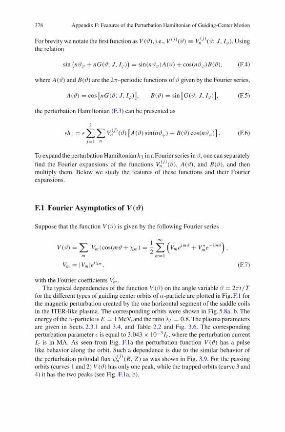
with the Fourier coefficients Vm .The typical dependencies of the function V (ϑ) on the angle variable ϑ = 2πt/T
for the different types of guiding center orbits of α-particle are plotted in Fig.F.1 forthe magnetic perturbation created by the one horizontal segment of the saddle coilsin the ITER-like plasma. The corresponding orbits were shown in Fig. 5.8a, b. Theenergy of theα-particle is E = 1MeV, and the ratioλI = 0.8. The plasmaparametersare given in Sects. 2.3.1 and 3.4, and Table 2.2 and Fig. 3.6. The correspondingperturbation parameter ε is equal to 3.043 × 10⁻³ Ic, where the perturbation currentIc is in MA. As seen from Fig. F.1a the perturbation function V (ϑ) has a pulselike behavior along the orbit. Such a dependence is due to the similar behavior ofthe perturbation poloidal flux ψ
( j)n (R, Z) as was shown in Fig. 3.9. For the passing
orbits (curves 1 and 2) V (ϑ) has only one peak, while the trapped orbits (curve 3 and4) it has the two peaks (see Fig. F.1a, b).
Appendix F: Features of the Perturbation Hamiltonian of Guiding-Center Motion 379
-0.6
-0.4
-0.2
0
0.2
0.4
0.6
0 0.2 0.4 0.6 0.8 1
V(ϑ
)
ϑ/2π
12
3
4
x10-2
Fig. F.1 Dependencies of the perturbation function V (ϑ) (F.1) on the angle variable ϑ along theseveral guiding–center orbits of α-particle. Curve 1 and 2 correspond co-passing and barely co-passing orbits, respectively; curve 3 and 4 correspond to the barely trapped and the trapped orbits,respectively. The magnetic perturbation created by the one single horizontal segment of the setof saddle coils located at (R2, Z2). The energy Ek = 1 MeV, the ratio λI = 0.8. The plasmaparameters and the RMP coils positions are given in Fig. 3.6. The toroidal mode of the perturbationmagnetic field is n = 3. The perturbation current Ic = 1 kA
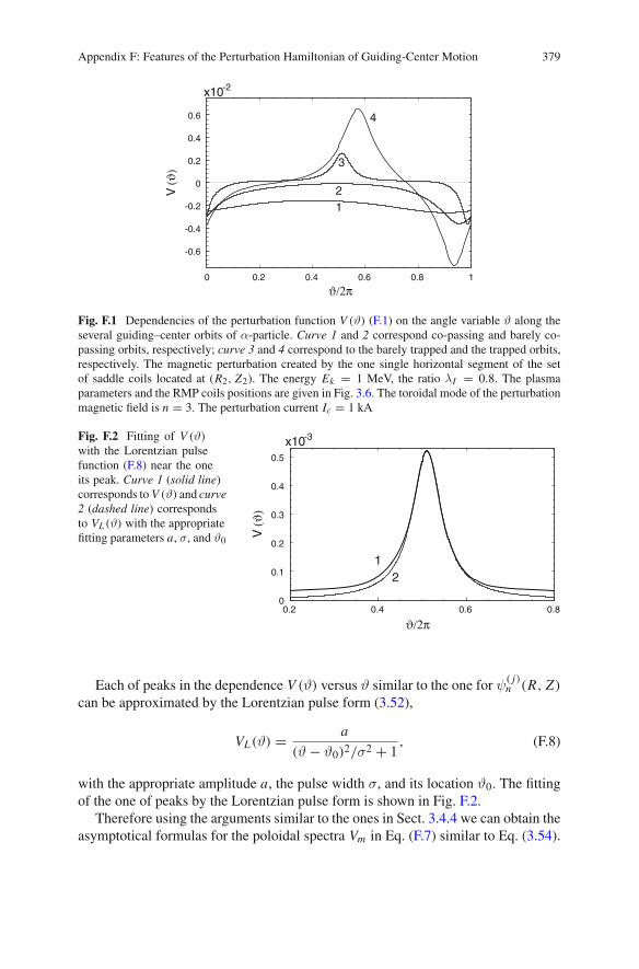
Fig. F.2 Fitting of V (ϑ)
with the Lorentzian pulsefunction (F.8) near the oneits peak. Curve 1 (solid line)corresponds to V (ϑ) and curve2 (dashed line) correspondsto VL (ϑ) with the appropriatefitting parameters a, σ, and ϑ0
0
0.1
0.2
0.3
0.4
0.5
0.2 0.4 0.6 0.8
V(ϑ
)
ϑ/2π
x10-3
12
Each of peaks in the dependence V (ϑ) versus ϑ similar to the one for ψ( j)n (R, Z)
can be approximated by the Lorentzian pulse form (3.52),
VL(ϑ) = a
(ϑ − ϑ0)2/σ2 + 1, (F.8)
with the appropriate amplitude a, the pulse width σ, and its location ϑ0. The fittingof the one of peaks by the Lorentzian pulse form is shown in Fig. F.2.
Therefore using the arguments similar to the ones in Sect. 3.4.4 we can obtain theasymptotical formulas for the poloidal spectra Vm in Eq. (F.7) similar to Eq. (3.54).
380 Appendix F: Features of the Perturbation Hamiltonian of Guiding-Center Motion
However, unlike from the latter the spectrum Vm for the trapped motion will containthe contributions from two Lorentzian peaks.
According to the localization principle2 the asymptotic estimation of the Fourierintegral
Vm = 1
2π
2π∫
0
V (ϑ)e−imϑdϑ, (F.9)
for large m is given by the sum of the contributions from each critical points of thefunction V (ϑ) corresponding its peaks. Near these points V (ϑ) is well approximatedby the Lorentzian function (F.8) whose Fourier transform is given by the exponentialform (3.53). Therefore, the asymptotical formula for Vm at large m will be given by
Vm ≈ 1
2T
⎧⎪⎪⎪⎪⎪⎪⎨
⎪⎪⎪⎪⎪⎪⎩
A(o) exp
(−mC (o)
T− imϑ
(o)0
)− A(i) exp
(−mC (i)
T− imϑ
(i)0
),
for trapped orbits,
A(o) exp
(−mC (o)
T− imϑ
(o)0
), for passing orbits.
(F.10)The parameters A(o,i), C (o,i), and ϑ(o,i)
0 depend on the orbit characteristics. The sub-scripts (o) and (i) stand for the outer and inner branches of the orbit. Particularly,A(o,i) and C (o,i) are similar to the parameters A and C in the asymptotical formula(3.54) and take finite values at the separatrix of the banana orbit as well as at the mag-netic separatrix where the period of motion (transit time) T has singularities as wasshown in Figs. 5.12b and 5.13b. One should notice the period T in the asymptoticalformula (F.9) plays the similar role as the safety factor q(ψ) in Eq. (3.54).
In order to find the parameters A(o,i), C (o,i), and ϑ(o,i)0 it is not necessary to calcu-
late the numerical Fourier transform of V (ϑ) (F.9) as it has been used in Sect. 3.4.4.It is sufficient to find the amplitude a, the width σ, and the peak’s location ϑ0 byfitting the function V (ϑ) near its peaks with the Lorentzian function (F.8). Accordingto Eq. (3.53) the relations between (a,σ) and (A, C) are A = aσT , C = σT .
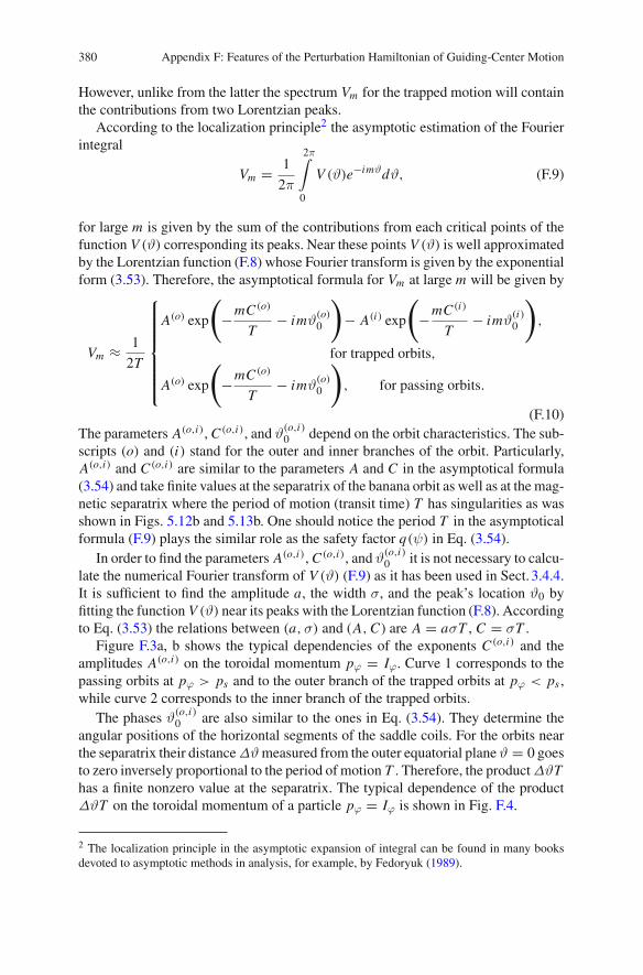
Figure F.3a, b shows the typical dependencies of the exponents C (o,i) and theamplitudes A(o,i) on the toroidal momentum pϕ = Iϕ. Curve 1 corresponds to thepassing orbits at pϕ > ps and to the outer branch of the trapped orbits at pϕ < ps ,while curve 2 corresponds to the inner branch of the trapped orbits.
The phases ϑ(o,i)0 are also similar to the ones in Eq. (3.54). They determine the
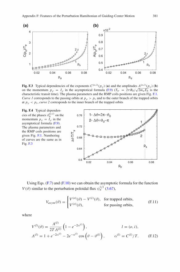
angular positions of the horizontal segments of the saddle coils. For the orbits nearthe separatrix their distanceΔϑmeasured from the outer equatorial plane ϑ = 0 goesto zero inversely proportional to the period of motion T . Therefore, the productΔϑThas a finite nonzero value at the separatrix. The typical dependence of the productΔϑT on the toroidal momentum of a particle pϕ = Iϕ is shown in Fig. F.4.
2 The localization principle in the asymptotic expansion of integral can be found in many booksdevoted to asymptotic methods in analysis, for example, by Fedoryuk (1989).
Appendix F: Features of the Perturbation Hamiltonian of Guiding-Center Motion 381
1
2
3
4
0.02 0.04 0.06 0.08
C(p
ϕ)/T
tr
pϕ
ps1
2
0.4
0.5
0.6
0.7
0.8
0.9
0.02 0.04 0.06 0.08
A(p ϕ
)/Ttr
pϕ
ps1
2
x10-2(a) (b)
Fig. F.3 Typical dependencies of the exponents C (o,i)(pϕ) (a) and the amplitudes A(o,i)(pϕ) (b)on the momentum pϕ = Iϕ in the asymptotical formula (F.9) (Ttr = 2πR0/
√2ma Ek is the
characteristic transit time). The plasma parameters and the RMP coils positions are given Fig. F.1.Curve 1 corresponds to the passing orbits at pϕ > ps and to the outer branch of the trapped orbitsat pϕ < ps , curve 2 corresponds to the inner branch of the trapped orbits
Fig. F.4 Typical dependen-cies of the phases ϑ(o,i)
0 on themomentum pϕ = Iϕ in theasymptotical formula (F.9).The plasma parameters andthe RMP coils positions aregiven Fig. F.1. Numberingof curves are the same as inFig. F.3
0.6
0.64
0.68
0.72
0.76
0.02 0.04 0.06 0.08
ΔϑT
/Ttr
pϕ
1- Δϑ=2π−ϑ02- Δϑ=ϑ0−π
ps
1
2
Using Eqs. (F.7) and (F.10) we can obtain the asymptotic formula for the functionV (ϑ) similar to the perturbation poloidal flux ψ
( j)n (3.67),
Vasym(ϑ) ={
V (o)(ϑ) − V (i)(ϑ), for trapped orbits,
V (o)(ϑ), for passing orbits,(F.11)
where
V (l)(ϑ) = A(l)
2T Λ(l)
(1 − e−2α(l)
), l = (o, i),
Λ(l) = 1 + e−2α(l) − 2e−α(l)cos
(ϑ − ϑ(l)
), α(l) = C (l)/T . (F.12)
382 Appendix F: Features of the Perturbation Hamiltonian of Guiding-Center Motion
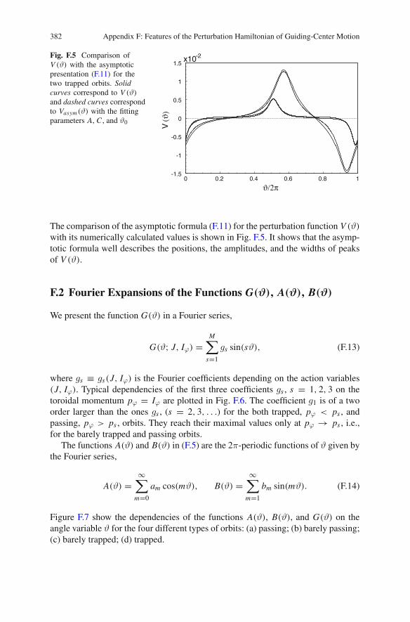
Fig. F.5 Comparison ofV (ϑ) with the asymptoticpresentation (F.11) for thetwo trapped orbits. Solidcurves correspond to V (ϑ)
and dashed curves correspondto Vasym(ϑ) with the fittingparameters A, C , and ϑ0
-1.5
-1
-0.5
0
0.5
1
1.5
0 0.2 0.4 0.6 0.8 1
V(ϑ
)
ϑ/2π
x10-2
The comparison of the asymptotic formula (F.11) for the perturbation function V (ϑ)
with its numerically calculated values is shown in Fig. F.5. It shows that the asymp-totic formula well describes the positions, the amplitudes, and the widths of peaksof V (ϑ).
F.2 Fourier Expansions of the Functions G(ϑ), A(ϑ), B(ϑ)
We present the function G(ϑ) in a Fourier series,
G(ϑ; J, Iϕ) =M∑
s=1
gs sin(sϑ), (F.13)
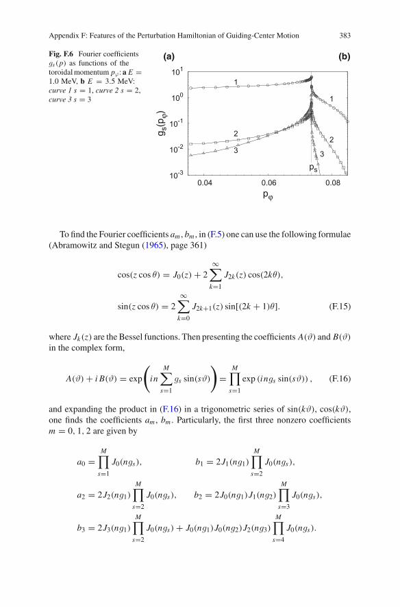
where gs ≡ gs(J, Iϕ) is the Fourier coefficients depending on the action variables(J, Iϕ). Typical dependencies of the first three coefficients gs , s = 1, 2, 3 on thetoroidal momentum pϕ = Iϕ are plotted in Fig. F.6. The coefficient g1 is of a twoorder larger than the ones gs , (s = 2, 3, . . .) for the both trapped, pϕ < ps , andpassing, pϕ > ps , orbits. They reach their maximal values only at pϕ → ps , i.e.,for the barely trapped and passing orbits.
The functions A(ϑ) and B(ϑ) in (F.5) are the 2π-periodic functions of ϑ given bythe Fourier series,
A(ϑ) =∞∑
m=0
am cos(mϑ), B(ϑ) =∞∑
m=1
bm sin(mϑ). (F.14)
Figure F.7 show the dependencies of the functions A(ϑ), B(ϑ), and G(ϑ) on theangle variable ϑ for the four different types of orbits: (a) passing; (b) barely passing;(c) barely trapped; (d) trapped.
Appendix F: Features of the Perturbation Hamiltonian of Guiding-Center Motion 383
Fig. F.6 Fourier coefficientsgs(p) as functions of thetoroidalmomentum pϕ:a E =1.0 MeV, b E = 3.5 MeV:curve 1 s = 1, curve 2 s = 2,curve 3 s = 3
10-3
10-2
10-1
100
101
0.04 0.06 0.08
g s(p
ϕ)
pϕ
ps
1
1
22
3 3
(a) (b)
To find the Fourier coefficients am , bm , in (F.5) one can use the following formulae(Abramowitz and Stegun (1965), page 361)
cos(z cos θ) = J0(z) + 2∞∑
k=1
J2k(z) cos(2kθ),
sin(z cos θ) = 2∞∑
k=0
J2k+1(z) sin[(2k + 1)θ]. (F.15)
where Jk(z) are the Bessel functions. Then presenting the coefficients A(ϑ) and B(ϑ)
in the complex form,
A(ϑ) + i B(ϑ) = exp
(in
M∑
s=1
gs sin(sϑ)
)=
M∏
s=1
exp (ings sin(sϑ)) , (F.16)
and expanding the product in (F.16) in a trigonometric series of sin(kϑ), cos(kϑ),one finds the coefficients am , bm . Particularly, the first three nonzero coefficientsm = 0, 1, 2 are given by
a0 =M∏
s=1
J0(ngs), b1 = 2J1(ng1)
M∏
s=2
J0(ngs),
a2 = 2J2(ng1)
M∏
s=2
J0(ngs), b2 = 2J0(ng1)J1(ng2)
M∏
s=3
J0(ngs),
b3 = 2J3(ng1)
M∏
s=2
J0(ngs) + J0(ng1)J0(ng2)J2(ng3)
M∏
s=4
J0(ngs).

384 Appendix F: Features of the Perturbation Hamiltonian of Guiding-Center Motion
-3
-2
-1
0
1
2
3
0 0.2 0.4 0.6 0.8 1
A(ϑ
), B
(ϑ),
G(ϑ
)
ϑ/2π
1
2
3
(b)
0
0.2
0.4
0.6
0.8
1
0 0.2 0.4 0.6 0.8 1
A(ϑ
), B
(ϑ),
G(ϑ
)
ϑ/2π
1
23
(a)
-4
-2
0
2
4
0 0.2 0.4 0.6 0.8 1
A(ϑ
), B
(ϑ),
G(ϑ
)
ϑ/2π
1
2
3
(c)
-3
-2
-1
0
1
2
3
0 0.2 0.4 0.6 0.8 1
A(ϑ
), B
(ϑ),
G(ϑ
)
ϑ/2π
1
2
3
(d)
Fig. F.7 Dependence of the coefficeints A(ϑ), B(ϑ), G(ϑ) on the angle variable ϑ for α-particleof energy E = 1.0 MeV: a passing orbit; b barely passing; c barely trapped orbit; d trapped orbit.Curve 1 corresponds to A(ϑ), curve 2 corresponds to B(ϑ), curve 3 corresponds to G(ϑ). Thetoroidal mode n = 3
For deeply passing orbits the largest coefficient g1 � 1. Therefore a0 � 1, but thecoefficients am , bm , (m > 1) are much smaller, and can be neglected. Then we haveA(ϑ) ≈ 1, B(ϑ) ≈ 0 (see Fig. F.7a).
For deeply trapped orbits the largest coefficient g1 ∼ 1 and one can neglect othersgs , (s > 1). Then only the coefficient g1 can be retained giving G(ϑ) ≈ g1 sin ϑ (seeFig. F.7d). Therefore we have A(ϑ) ≈ cos(ng1 sin ϑ), B(ϑ) ≈ sin(ng1 sin ϑ).
For the barely trapped orbits the large number of coefficients gs give the contribu-tions to G(ϑ). The latter becomes a steep function of ϑ at the low field side ϑ = 0,πas shown in Fig. F.7c. The functions A(ϑ) and B(ϑ) become also fast-oscillatingthere.
Appendix GDerivation of the Many-Dimensional Full-TurnTransfer Mapping
Below we present the detailed derivation of the full-turn transfer mapping (6.53).First we rewrite the mapping (6.9)–(6.11) in the following form
Ik+1 = Ik + ε
(∂Sk+1
∂ϑk+1− ∂Sk
∂ϑk
), (G.1)
ϑk+1 = ϑk + w(Jk, ε)(τk+1 − τk) − ε
(∂Sk+1
∂ Jk− ∂Sk
∂ Jk
), (G.2)
where Sk ≡ S(ϑk, Jk, τk, τ0, ε), Sk+1 ≡ S(ϑk+1, Jk, τk+1, τ0, ε) are the values ofthe generating function S(ϑ, J, t, τ0, ε) at the time instants τ = τk and τ = τk+1,respectively. The intermediate action variables J are given by
Jk = Ik − ε∂Sk
∂ϑk= Ik+1 − ε
∂Sk+1
∂ϑk+1. (G.3)
In general the mapping (G.1)–(G.3) is exact and valid for arbitrary magnitude of theperturbation parameter ε.
We intend to derive the simplified form of the Poincaré mapping to the sectionΣ of the phase space where the angle variable ϑ ≡ ϑ1 takes constant value ±π,mod 2π. Furthermore we introduce the following notations for the rest of anglevariables Θ = (ϑ2, . . . ,ϑN ,ϑN+1 = t), and the frequencies ω(J ) = ω1(J ), Ω =(ω2, . . . ,ωN ,ωN+1 = 1). We consider the cases of small perturbation parameterε � 1.
In the first order of the perturbation parameter ε the generating function S(ϑ, J, t,τ0, ε) is determined by the integral (6.21). Without loosing the generality one canput H1(J ) = 0. Then according to (6.26) w(J, ε) = ω(J ) and Eq. (6.21) is reducedto
S(ϑ,Θ, J, τ , τ0) = −τ∫
τ0
H1(ϑ0(τ′),Θ0(τ
′)J )dτ ′, (G.4)
S. Abdullaev, Magnetic Stochasticity in Magnetically Confined Fusion Plasmas, 385Springer Series on Atomic, Optical, and Plasma Physics 78,DOI: 10.1007/978-3-319-01890-4, © Springer International Publishing Switzerland 2014
386 Appendix G: Derivation of the Many-Dimensional Full-Turn Transfer Mapping
where integration is taken along the unperturbed trajectory ϑ0(τ′) = ϑ0(τ ) +
ω(J )(τ ′ − τ ), Θ0(τ′) = Θ0(τ ) + Ω(J )(τ ′ − τ ), [ϑ ≡ ϑ0(τ ),Θ ≡ Θ0(τ )].
Since ϑk+1 = ϑk + 2π for the angle variable ϑ from the mapping (G.2) it followsthat
τk+1 − τk = 2π
ω(Jk)+ O(ε), (G.5)
where the terms of order of O(ε) are much smaller than the period of motion alongthe angle ϑ and they can be neglected. The unperturbed orbits ϑ0(τ
′),Θ0(τ′) in (G.4)
can be presented as
ϑ0(τ′) = ϑk+1 + ω(Jk)(τ
′ − τk+1) = ϑk + ω(Jk)(τ′ − τk),
Θ0(τ′) = Θk+1 + Ω(Jk)(τ
′ − τk+1) = Θk + Ω(Jk)(τ′ − τk).
In (G.4) we introduce the new integration variable τ = τ ′ − τ0, where τ0 is the timeinstant when the angle variable ϑ0(τ ) crosses the section ϑ = 0, i.e.,
τ0 = τk+1 + τk
2= τk + π
ω(Jk)= τk+1 − π
ω(Jk). (G.6)
Then ϑ0(τ′) = ϑ0(τ + τ0) = ϑ0(τ ) = ω(J )τ , ϑ0(τk) = −π, and ϑ0(τk+1) = π.
Thus the generating functions Sk in (G.1)–(G.3) are reduced to
Sk ≡ S(−)(Θk, Jk) =0∫
−π/ω(Jk )
H1(ϑ0(τ ),Θ0(τ + τ0), Jk)dτ ,
Sk+1 ≡ S(+)(Θk+1, Jk) = −π/ω(Jk )∫
0
H1(ϑ0(τ ),Θ0(τ + τ0), Jk)dτ , (G.7)
where Θk ≡ Θ(τk). The argument Θ0(τ + τ0) of the perturbation Hamiltonian H1under the integrals (G.7) is a function of Θk or Θk+1, i.e.,
Θ0(τ + τ0) = Θ0(τ ) + Θ0(τ0) − Θ0, (G.8)
where Θ0 is the constant initial phase, and Θ0(τ0) is given by
Θ0(τ0) = Θk + πΩ(Jk)
ω(Jk)= Θk+1 − πΩ(Jk)
ω(Jk). (G.9)
Equation (G.9) gives the relation between Θk and Θk+1 in the zero-order of ε. Usingthis relation the derivative ∂Sk+1/∂Θk+1 can be presented as
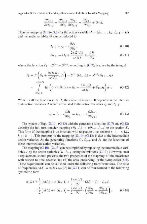
Appendix G: Derivation of the Many-Dimensional Full-Turn Transfer Mapping 387
∂Sk+1
∂Θk+1= ∂Sk+1
∂Θk
∂Θk
∂Θk+1= ∂Sk+1
∂Θk+ O(ε).
Then the mapping (G.1)–(G.3) for the action variables I = (I2, . . . , IN , In+1 = H)
and the angle variables Θ can be reduced to
Ik+1 = Ik − ε∂Pk
∂Θk, (G.10)
Θk+1 = Θk + 2πΩ(Jk)
ω(Jk)+ ε
∂Pk
∂ Jk, (G.11)
where the function Pk = S(−) − S(+), according to (G.7), is given by the integral
Pk ≡ P
(Θk + πΩ(Jk)
ω(Jk), Jk
)= S(−)(Θk, Jk) − S(+)(Θk+1, Jk)
=π/ω(J )∫
−π/ω(J )
H1
(ϑ(τ ),Θ0(τ ) + Θk + πΩ(Jk)
ω(Jk)+ Θ0, Jk
)dτ . (G.12)
We will call the function P(Θ, J ) the Poincaré integral. It depends on the interme-diate action variables J which are related to the action variables Ik and Ik+1:
Jk = Ik − ε∂Sk
∂Θk= Ik+1 − ε
∂Sk+1
∂Θk+1. (G.13)
The system of Eqs. (G.10)–(G.13) with the generating functions (G.7) and (G.12)describe the full–turn transfer mapping (Θk, Ik) → (Θk+1, Ik+1) to the section Σ .This form of the mapping is an invariant with respect to time–reverse τ → −τ , i.e.,k ↔ k + 1. This property of the mapping (G.10)–(G.13) is due to the intermediateaction variables Jk : the generating functions Sk , Sk+1, and Pk are the functions ofthese intermediate action variables.
The mapping (G.10)–(G.13) can be simplified by replacing the intermediate vari-ables J by the action variables (Ik, Ik+1) using the relations (G.13). However, sucha replacement should preserve the two properties of the mapping: (i) the invariancewith respect to time–reverse, and (ii) the area–preserving (or the symplectic) (6.8).These requirements can be satisfied under the following transformations. The ratioof frequencies α(J ) = πΩ(J )/ω(J ) in (G.11) can be transformed to the followingsymmetric form
α(Jk) ≈ 1
2
[α(Ik) + α(Ik+1)
]+ 1
2
∂α(J )
∂ J· (2Jk − Ik − Ik+1)
= 1
2
[α(Ik) + α(Ik+1)
]− ε
2
∂α(J )
∂ J·(
∂Sk
∂Θk+ ∂Sk+1
∂Θk+1
). (G.14)
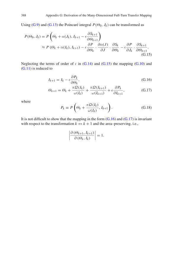
388 Appendix G: Derivation of the Many-Dimensional Full-Turn Transfer Mapping
Using (G.9) and (G.13) the Poincaré integral P(Θ0, Jk) can be transformed as
P(Θ0, Jk) = P
(Θk + α(Jk), Ik+1 − ε
∂Sk+1
∂Θk+1
)
≈ P (Θk + α(Ik), Ik+1) − ε∂P
∂Θk· ∂α(J )
∂ J· ∂Sk
∂Θk− ε
∂P
∂ Jk· ∂Sk+1
∂Θk+1.
(G.15)
Neglecting the terms of order of ε in (G.14) and (G.15) the mapping (G.10) and(G.11) is reduced to
Ik+1 = Ik − ε∂Pk
∂Θk, (G.16)
Θk+1 = Θk + πΩ(Ik)
ω(Ik)+ πΩ(Ik+1)
ω(Ik+1)+ ε
∂Pk
∂ Ik+1, (G.17)
where
Pk ≡ P
(Θk + πΩ(Ik)
ω(Ik), Ik+1
). (G.18)
It is not difficult to show that the mapping in the form (G.16) and (G.17) is invariantwith respect to the transformation k ↔ k + 1 and the area–preserving, i.e.,
∣∣∣∣∂ (Θk+1, Ik+1)
∂ (Θk, Ik)
∣∣∣∣ = 1.
References
Abdullaev, S. S. (1994). Two-dimensional model of kicked oscillator: motion with intermittency.Chaos, 4(3), 569–581.
Abdullaev, S. S. (1999). A new integration method of Hamiltonian systems by symplectic maps.Journal of Physics A: Mathematical, Nuclear and General, 32, 2745–2766.
Abdullaev, S. S. (2000). Structure of motion near saddle points and chaotic transport in Hamiltoniansystems. Physical Review E, 62, 3508–3528.
Abdullaev, S. S. (2002). The Hamilton–Jacobi method and Hamiltonian maps. Journal of PhysicsA: Mathematical, Nuclear and General, 35, 2811–2832.
Abdullaev, S. S. (2004). Canonical maps near separatrix in Hamiltonian systems. Physical ReviewE, 70, 046202.
Abdullaev, S. S. (2004). On mapping models of field lines in a stochastic magnetic field. NuclearFusion, 44, S12–S27.
Abdullaev, S. S. (2005). Asymptotical forms of canonical mappings near separatrix in Hamiltoniansystems. Physical Review E, 72, 046202.
Abdullaev, S. S. (2006).Construction of Mappings for Hamiltonian Systems and Their Applications.Berlin: Springer-Verlag.
Abdullaev, S. S. (2007). Canonical stochastic web map. Physical Review E, 76, 026216.Abdullaev, S. S. (2009).Model of amagnetic field in poloidal divertor tokamaks affected by resonantmagnetic perturbations. Physics of Plasmas, 16, 030701.
Abdullaev, S. S. (2010). Generic magnetic field model in poloidal divertor tokamaks in the presenceof resonant magnetic perturbations. Nuclear Fusion, 50, 034001.
Abdullaev, S. S. (2011). Chaotic transport in Hamiltonian systems perturbed by a weak turbulentwave field. Physical Review E, 84(2), 026204.
Abdullaev, S. S. (2011). Universal asymptotics of poloidal spectra of magnetic perturbations ofsaddle coils in tokamaks. Physics of Plasmas, 18, 020701.
Abdullaev, S. S. (2012). Universal asymptotical behavior of poloidal spectra of resonant magneticperturbations created by a set of saddle coils in tokamaks. Nuclear Fusion, 52, 054002.
Abdullaev, S. S. (2013). On collisional diffusion in a stochastic magnetic field. Physics of Plasmas,20, 082507.
Abdullaev, S. S., Eich, T., & Finken, K. H. (2001). Fractal structure of the magnetic field in thelaminar zone of the dynamic ergodic divertor of the torus experiment for technology-orientedresearch (TEXTOR-94). Physics of Plasmas, 8, 2739–2749.
Abdullaev, S. S., Finken, K., & Forster, M. (2012). New mechanism of runaway electron diffusiondue to mircoturbulence in tokamaks. Physics of Plasmas, 19(7), 072502.
S. Abdullaev, Magnetic Stochasticity in Magnetically Confined Fusion Plasmas, 389Springer Series on Atomic, Optical, and Plasma Physics 78,DOI: 10.1007/978-3-319-01890-4, © Springer International Publishing Switzerland 2014
390 References
Abdullaev, S. S., & Finken, K. H. (1998). Widening the magnetic footprints in a poloidal divertortokamak: a proposal. Nuclear Fusion, 38, 531–544.
Abdullaev, S. S., & Finken, K. H. (2002). Hamiltonian guiding center equations in a toroidal system.Physics of Plasmas, 9, 4193–4204.
Abdullaev, S. S., Finken, K. H., Jakubowski, M., et al. (2003). Overview of magnetic structureinduced by the TEXTOR-DED and the related transport. Nuclear Fusion, 43, 299–313.
Abdullaev, S. S., Wingen, A., & Spatschek, K. H. (2006a). Mapping of drift surfaces in toroidalsystems with chaotic magnetic fields. Physics of Plasmas, 13(4), 042509.
Abdullaev, S. S., Finken, K. H., Jakubowski, M., & Lehnen, M. (2006b). Mapping of stochasticfield lines in poloidal divertor tokamaks. Nuclear Fusion, 46(4), S113–S126.
Abdullaev, S. S., Finken, K. H., Jakubowski, M., et al. (2004). Magnetic field structure in the DEDof TEXTOR and its experimental observation. In J. Connor, O. Sauter, & E. Sindoni (Eds.),Theory of fusion plasmas (pp. 373–379). SIF, Bologna: International Workshop, Societa Italianadi Fisica.
Abdullaev, S. S., Finken, K. H., Kaleck, A., & Spatschek, K. H. (1998). Twist mapping for thedynamics of magnetic field lines in a tokamak ergodic divertor. Physics of Plasmas, 5, 196–210.
Abdullaev, S. S., Finken, K. H., & Spatschek, K. H. (1999). Asymptotical and mapping methods instudy of ergodic divertor magnetic field in a toroidal system. Physics of Plasmas, 6, 153–174.
Abdullaev, S. S., Finken, K., Kudyakov, T., & Lehnen, M. (2010). Asymptotical theory of runawayelectron diffusion due to magnetic turbulence in tokamak plasmas. Contributions to PlasmaPhysics, 50(10), 929–941.
Abdullaev, S. S., Jakubowski, M., Lehnen, M., Schmitz, O., & Unterberg, B. (2008). On descriptionof magnetic stochasticity in poloidal divertor tokamaks. Physics of Plasmas, 15(4), 042508.
Abdullaev, S. S., Van Rompuy, T., Finken, K., et al. (2008). Modelling of magnetic field structure ofthe ergodic divertor of Tore Supra and comparison to the dynamic ergodic divertor of TEXTOR.arXiv:0805.1477v1 (physics.plasm-ph).
Abdullaev, S. S., & Zaslavsky, G. M. (1994). New properties of the ergodic layer. Bulletin of theAmerican Physical Society, 39, 1659.
Abdullaev, S. S., & Zaslavsky, G. M. (1995). Self-similarity of stochastic magnetic field lines nearthe X-point. Physics of Plasmas, 2, 4533–4540.
Abdullaev, S. S., & Zaslavsky, G. M. (1996). Application of the separatrix map to study perturbedfield lines near the separatrix. Physics of Plasmas, 3, 516–528.
Abramowitz, M., & Stegun, I. (Eds.). (1965). Handbook on mathematical functions. New York:Dover Publications.
Aguirre, J., Giné, J., & Peralta-Salas, D. (2008). Integrability of magnetic fields created by currentdistributions. Nonlinearity, 21(1), 51–69.
Aguirre, J., & Peralta-Salas, D. (2007). Realistic examples of chaotic magnetic fields created bywires. Europhysics Letters, 80(6), 60007.
Aguirre, J., Viana, R. L., & Sanjuán, M. A. F. (2009). Fractal structures in nonlinear dynamics.Reviews of Modern Physics, 81, 333–386.
Ahn, T., & Kim, S. (1994). Separatrix map analysis of chaotic transport in planar periodic vorticalflows. Physical Review E, 49, 2900–2911.
Ahn, T., Kim, S., &Kim, G. (1996). Analysis of the separatrix map in hamiltonian systems. PhysicaD, 89, 315–328.
Altmann, E. G., Portela, J. S. E., & Tél, T. (2013). Leaking chaotic systems. Reviews of ModernPhysics, 85, 869–918.
Anosov, D. V. (1967). Geodetic flows on closed Riemanian manifolds of negative curvature. Pro-ceedings of the Steklov Institute of Mathematics, 90, 210.
Arnold, V. I. (1963a). Proof of a theorem of A. N. Kolmogorov’s on the invariance of quasi-periodicmotions under small perturbations of the Hamiltonian. Russian Mathematical Surveys, 5, 9–36.
Arnold, V. I. (1963b). Small denominators and the problems of stability of motion in classical andcelestial mechanics. Russian Mathematical Surveys, 6, 85–191.
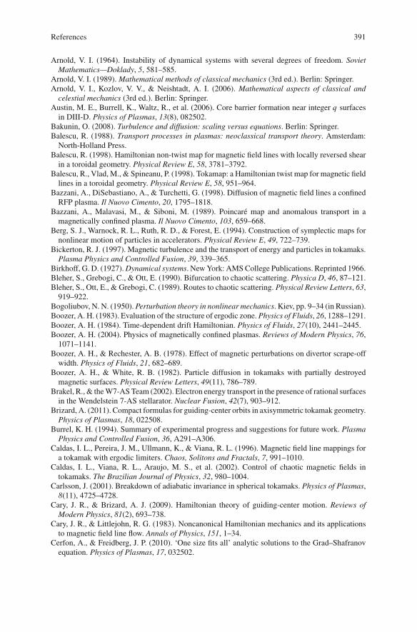
References 391
Arnold, V. I. (1964). Instability of dynamical systems with several degrees of freedom. SovietMathematics—Doklady, 5, 581–585.
Arnold, V. I. (1989). Mathematical methods of classical mechanics (3rd ed.). Berlin: Springer.Arnold, V. I., Kozlov, V. V., & Neishtadt, A. I. (2006). Mathematical aspects of classical and
celestial mechanics (3rd ed.). Berlin: Springer.Austin, M. E., Burrell, K., Waltz, R., et al. (2006). Core barrier formation near integer q surfacesin DIII-D. Physics of Plasmas, 13(8), 082502.
Bakunin, O. (2008). Turbulence and diffusion: scaling versus equations. Berlin: Springer.Balescu, R. (1988). Transport processes in plasmas: neoclassical transport theory. Amsterdam:North-Holland Press.
Balescu, R. (1998). Hamiltonian non-twist map for magnetic field lines with locally reversed shearin a toroidal geometry. Physical Review E, 58, 3781–3792.
Balescu, R., Vlad, M., & Spineanu, P. (1998). Tokamap: a Hamiltonian twist map for magnetic fieldlines in a toroidal geometry. Physical Review E, 58, 951–964.
Bazzani, A., DiSebastiano, A., & Turchetti, G. (1998). Diffusion of magnetic field lines a confinedRFP plasma. Il Nuovo Cimento, 20, 1795–1818.
Bazzani, A., Malavasi, M., & Siboni, M. (1989). Poincaré map and anomalous transport in amagnetically confined plasma. Il Nuovo Cimento, 103, 659–668.
Berg, S. J., Warnock, R. L., Ruth, R. D., & Forest, E. (1994). Construction of symplectic maps fornonlinear motion of particles in accelerators. Physical Review E, 49, 722–739.
Bickerton, R. J. (1997). Magnetic turbulence and the transport of energy and particles in tokamaks.Plasma Physics and Controlled Fusion, 39, 339–365.
Birkhoff, G. D. (1927).Dynamical systems. NewYork: AMSCollege Publications. Reprinted 1966.Bleher, S., Grebogi, C., & Ott, E. (1990). Bifurcation to chaotic scattering. Physica D, 46, 87–121.Bleher, S., Ott, E., & Grebogi, C. (1989). Routes to chaotic scattering. Physical Review Letters, 63,919–922.
Bogoliubov, N. N. (1950). Perturbation theory in nonlinear mechanics. Kiev, pp. 9–34 (in Russian).Boozer, A. H. (1983). Evaluation of the structure of ergodic zone.Physics of Fluids, 26, 1288–1291.Boozer, A. H. (1984). Time-dependent drift Hamiltonian. Physics of Fluids, 27(10), 2441–2445.Boozer, A. H. (2004). Physics of magnetically confined plasmas. Reviews of Modern Physics, 76,1071–1141.
Boozer, A. H., & Rechester, A. B. (1978). Effect of magnetic perturbations on divertor scrape-offwidth. Physics of Fluids, 21, 682–689.
Boozer, A. H., & White, R. B. (1982). Particle diffusion in tokamaks with partially destroyedmagnetic surfaces. Physical Review Letters, 49(11), 786–789.
Brakel, R., & theW7-ASTeam (2002). Electron energy transport in the presence of rational surfacesin the Wendelstein 7-AS stellarator. Nuclear Fusion, 42(7), 903–912.
Brizard, A. (2011). Compact formulas for guiding-center orbits in axisymmetric tokamak geometry.Physics of Plasmas, 18, 022508.
Burrel, K. H. (1994). Summary of experimental progress and suggestions for future work. PlasmaPhysics and Controlled Fusion, 36, A291–A306.
Caldas, I. L., Pereira, J. M., Ullmann, K., & Viana, R. L. (1996). Magnetic field line mappings fora tokamak with ergodic limiters. Chaos, Solitons and Fractals, 7, 991–1010.
Caldas, I. L., Viana, R. L., Araujo, M. S., et al. (2002). Control of chaotic magnetic fields intokamaks. The Brazilian Journal of Physics, 32, 980–1004.
Carlsson, J. (2001). Breakdown of adiabatic invariance in spherical tokamaks. Physics of Plasmas,8(11), 4725–4728.
Cary, J. R., & Brizard, A. J. (2009). Hamiltonian theory of guiding-center motion. Reviews ofModern Physics, 81(2), 693–738.
Cary, J. R., & Littlejohn, R. G. (1983). Noncanonical Hamiltonian mechanics and its applicationsto magnetic field line flow. Annals of Physics, 151, 1–34.
Cerfon, A., & Freidberg, J. P. (2010). ‘One size fits all’ analytic solutions to the Grad–Shafranovequation. Physics of Plasmas, 17, 032502.
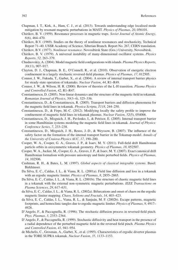
392 References
Chapman, I. T., Kirk, A., Ham, C. J., et al. (2013). Towards understanding edge localised modemitigation by resonant magnetic perturbations in MAST. Physics of Plasmas, 20, 056101.
Chirikov, B. V. (1959). Resonance processes in magnetic traps. Soviet Journal of Atomic Energy,6(6), 464–470.
Chirikov, B.V. (1969). Studies on the theory of nonlinear resonances and stochasticity, TechnicalReport 71–40. USSR Academy of Science, Siberian Branch. Report No. 267, CERN translation.
Chirikov, B.V. (1977). Nonlinear resonance. Novosibirsk State (Gos.) University, Novosibirsk.Chirikov, B. V. (1979). A universal instability of many-dimensional oscillator systems. Physics
Reports, 52, 263–379.Chudnovskiy, A. (2004).Modelmagnetic field configurationswith islands.Plasma Physics Reports,
30(11), 907–917.Clayton, D. J., Chapman, B. E., O’Connell, R., et al. (2010). Observation of energetic electronconfinement in a largely stochastic reversed-field plasmas. Physics of Plasmas, 17, 012505.
Connor, J. W., Fukuda, T., Garbet, X., et al. (2004). A review of internal transport barrier physicsfor steady-state operation of tokamaks. Nuclear Fusion, 44, R1–R49.
Connor, J. W., & Wilson, H. R. (2000). Review of theories of the L-H transition. Plasma Physicsand Controlled Fusion, 42, R1–R47.
Constantinescu, D. (2005). Non-linear dynamics and the structure of the magnetic field in tokamak.Romanian Journal of Physics, 50(3–4), 325–336.
Constantinescu, D., & Constantinescu, R. (2005). Transport barriers and diffusion phenomena forthe magnetic field lines in tokamak. Physica Scripta, T118, 244–250.
Constantinescu, D., & Firpo, M.-C. (2012). Modifying locally the safety profile to improve theconfinement of magnetic field lines in tokamak plasmas. Nuclear Fusion, 52(5), 054006.
Constantinescu, D., Misguich, J. H., Pavlenko, I., & Petrisor, E. (2005). Internal transport barrierin some Hamiltinian systems modeling the magnetic field lines in tokamak. Journal of Physics:Conference Series, 7, 233–238.
Constantinescu, D., Misguich, J. H., Reuss, J.-D., & Weyssow, B. (2007). The influence of thesafety factor on the formation of the internal transport barrier in the Tokamap-model. Annals ofthe University of Craiova Physics AUC, 17, 190–200.
Cooper, W. A., Cooper, G. A., Graves, J. P., & Isaev, M. Y. (2011). Full-field drift Hamiltonianparticle orbits in axisymmetric tokamak geometry. Physics of Plasmas, 18, 052507.
Cooper, W. A., Jucker, M., Cooper, G. A., Graves, J. P., & Isaev, M. Y. (2007). Exact canonical driftHamiltonian formalism with pressure anisotropy and finite perturbed fields. Physics of Plasmas,14, 102506.
Cushman, R. H., & Bates, L. M. (1997). Global aspects of classical integrable systems. Basel:Birkhäuser.
Da Silva, E. C., Caldas, I. L., & Viana, R. L. (2001a). Field line diffusion and loss in a tokamakwith an ergodic magnetic limiter. Physics of Plasmas, 8, 2855–2865.
Da Silva, E. C., Caldas, I. L., & Viana, R. L. (2001b). The structure of chaotic magnetic field linesin a tokamak with the external non-symmetric magnetic perturbations. IEEE Transactions onPlasma Sciences, 29, 617–631.
da Silva, E. C., Caldas, I. L., & Viana, R. L. (2002a). Bifurcations and onset of chaos on the ergodicmagnetic limiter mapping. Chaos, Solitons and Fractals, 14, 403–423.
da Silva, E. C., Caldas, I. L., Viana, R. L., & Sanjuán, M. F. (2002b). Escape patterns, magneticfootprints, and homoclinic tangles due to ergodic magnetic limiter. Physics of Plasmas, 9, 4917–4928.
D’Angelo, F., & Paccagnella, R. (1996). The stochastic diffusion process in reversed-field pinch.Phys. Plasmas, 3, 2353–2364.
D’Angelo, F., & Paccagnella, R. (1999). Stochastic diffusivity and heat transport in the presence ofa radial dependence of the perturbed magnetic field in the reversed field pinch. Plasma Physicsand Controlled Fusion, 41, 941–954.
de Michelis, C., Grosman, A., Garbet, X., et al. (1995). Characteristics of ergodic divertor plasmasin the TORE SUPRA tokamak. Nuclear Fusion, 35, 1133–1153.
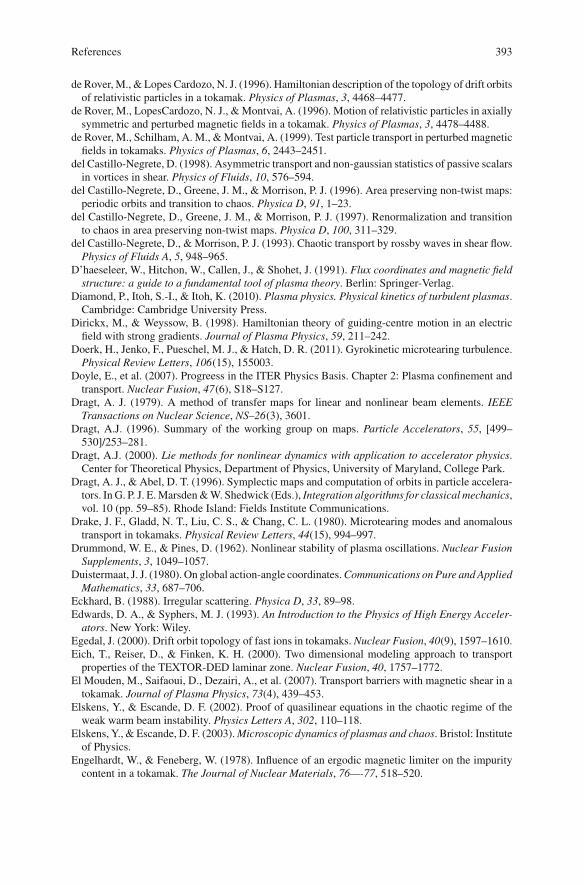
References 393
de Rover, M., & Lopes Cardozo, N. J. (1996). Hamiltonian description of the topology of drift orbitsof relativistic particles in a tokamak. Physics of Plasmas, 3, 4468–4477.
de Rover, M., LopesCardozo, N. J., &Montvai, A. (1996). Motion of relativistic particles in axiallysymmetric and perturbed magnetic fields in a tokamak. Physics of Plasmas, 3, 4478–4488.
de Rover, M., Schilham, A. M., &Montvai, A. (1999). Test particle transport in perturbed magneticfields in tokamaks. Physics of Plasmas, 6, 2443–2451.
del Castillo-Negrete, D. (1998). Asymmetric transport and non-gaussian statistics of passive scalarsin vortices in shear. Physics of Fluids, 10, 576–594.
del Castillo-Negrete, D., Greene, J. M., & Morrison, P. J. (1996). Area preserving non-twist maps:periodic orbits and transition to chaos. Physica D, 91, 1–23.
del Castillo-Negrete, D., Greene, J. M., & Morrison, P. J. (1997). Renormalization and transitionto chaos in area preserving non-twist maps. Physica D, 100, 311–329.
del Castillo-Negrete, D., & Morrison, P. J. (1993). Chaotic transport by rossby waves in shear flow.Physics of Fluids A, 5, 948–965.
D’haeseleer, W., Hitchon, W., Callen, J., & Shohet, J. (1991). Flux coordinates and magnetic fieldstructure: a guide to a fundamental tool of plasma theory. Berlin: Springer-Verlag.
Diamond, P., Itoh, S.-I., & Itoh, K. (2010). Plasma physics. Physical kinetics of turbulent plasmas.Cambridge: Cambridge University Press.
Dirickx, M., & Weyssow, B. (1998). Hamiltonian theory of guiding-centre motion in an electricfield with strong gradients. Journal of Plasma Physics, 59, 211–242.
Doerk, H., Jenko, F., Pueschel, M. J., & Hatch, D. R. (2011). Gyrokinetic microtearing turbulence.Physical Review Letters, 106(15), 155003.
Doyle, E., et al. (2007). Progreess in the ITER Physics Basis. Chapter 2: Plasma confinement andtransport. Nuclear Fusion, 47(6), S18–S127.
Dragt, A. J. (1979). A method of transfer maps for linear and nonlinear beam elements. IEEETransactions on Nuclear Science, NS–26(3), 3601.
Dragt, A.J. (1996). Summary of the working group on maps. Particle Accelerators, 55, [499–530]/253–281.
Dragt, A.J. (2000). Lie methods for nonlinear dynamics with application to accelerator physics.Center for Theoretical Physics, Department of Physics, University of Maryland, College Park.
Dragt, A. J., & Abel, D. T. (1996). Symplectic maps and computation of orbits in particle accelera-tors. In G. P. J. E.Marsden&W. Shedwick (Eds.), Integration algorithms for classical mechanics,vol. 10 (pp. 59–85). Rhode Island: Fields Institute Communications.
Drake, J. F., Gladd, N. T., Liu, C. S., & Chang, C. L. (1980). Microtearing modes and anomaloustransport in tokamaks. Physical Review Letters, 44(15), 994–997.
Drummond, W. E., & Pines, D. (1962). Nonlinear stability of plasma oscillations. Nuclear FusionSupplements, 3, 1049–1057.
Duistermaat, J. J. (1980). On global action-angle coordinates.Communications on Pure and AppliedMathematics, 33, 687–706.
Eckhard, B. (1988). Irregular scattering. Physica D, 33, 89–98.Edwards, D. A., & Syphers, M. J. (1993). An Introduction to the Physics of High Energy Acceler-
ators. New York: Wiley.Egedal, J. (2000). Drift orbit topology of fast ions in tokamaks. Nuclear Fusion, 40(9), 1597–1610.Eich, T., Reiser, D., & Finken, K. H. (2000). Two dimensional modeling approach to transportproperties of the TEXTOR-DED laminar zone. Nuclear Fusion, 40, 1757–1772.
El Mouden, M., Saifaoui, D., Dezairi, A., et al. (2007). Transport barriers with magnetic shear in atokamak. Journal of Plasma Physics, 73(4), 439–453.
Elskens, Y., & Escande, D. F. (2002). Proof of quasilinear equations in the chaotic regime of theweak warm beam instability. Physics Letters A, 302, 110–118.
Elskens, Y., & Escande, D. F. (2003). Microscopic dynamics of plasmas and chaos. Bristol: Instituteof Physics.
Engelhardt, W., & Feneberg, W. (1978). Influence of an ergodic magnetic limiter on the impuritycontent in a tokamak. The Journal of Nuclear Materials, 76—-77, 518–520.
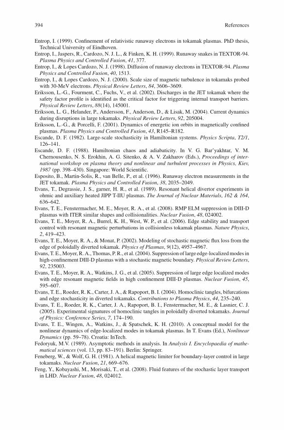
394 References
Entrop, I. (1999). Confinement of relativistic runaway electrons in tokamak plasmas. PhD thesis,Technical University of Eindhoven.
Entrop, I., Jaspers, R., Cardozo, N. J. L., & Finken, K. H. (1999). Runaway snakes in TEXTOR-94.Plasma Physics and Controlled Fusion, 41, 377.
Entrop, I., & Lopes Cardozo, N. J. (1998). Diffusion of runaway electrons in TEXTOR-94. PlasmaPhysics and Controlled Fusion, 40, 1513.
Entrop, I., & Lopes Cardozo, N. J. (2000). Scale size of magnetic turbulence in tokamaks probedwith 30-MeV electrons. Physical Review Letters, 84, 3606–3609.
Eriksson, L.-G., Fourment, C., Fuchs, V., et al. (2002). Discharges in the JET tokamak where thesafety factor profile is identified as the critical factor for triggering internal transport barriers.Physical Review Letters, 88(14), 145001.
Eriksson, L. G., Helander, P., Andersson, F., Anderson, D., & Lisak, M. (2004). Current dynamicsduring disruptions in large tokamaks. Physical Review Letters, 92, 205004.
Eriksson, L.-G., & Porcelli, F. (2001). Dynamics of energetic ion orbits in magnetically confinedplasmas. Plasma Physics and Controlled Fusion, 43, R145–R182.
Escande, D. F. (1982). Large-scale stochasticity in Hamiltonian systems. Physics Scripta, T2/1,126–141.
Escande, D. F. (1988). Hamiltonian chaos and adiabaticity. In V. G. Bar’yakhtar, V. M.Chernousenko, N. S. Erokhin, A. G. Sitenko, & A. V. Zakharov (Eds.), Proceedings of inter-national workshop on plasma theory and nonlinear and turbulent processes in Physics, Kiev,1987 (pp. 398–430). Singapore: World Scientific.
Esposito, B., Martin-Solis, R., van Belle, P., et al. (1996). Runaway electron measurements in theJET tokamak. Plasma Physics and Controlled Fusion, 38, 2035–2049.
Evans, T., Degrassie, J. S., garner, H. R., et al. (1989). Resonant helical divertor experiments inohmic and auxiliary heated JIPP T-IIU plasmas. The Journal of Nuclear Materials, 162 & 164,636–642.
Evans, T. E., Fenstermacher, M. E., Moyer, R. A., et al. (2008). RMP ELM suppression in DIII-Dplasmas with ITER similar shapes and collisionalities. Nuclear Fusion, 48, 024002.
Evans, T. E., Moyer, R. A., Burrel, K. H., West, W. P., et al. (2006). Edge stability and transportcontrol with resonant magnetic perturbations in collisionless tokamak plasmas. Nature Physics,2, 419–423.
Evans, T. E., Moyer, R. A., & Monat, P. (2002). Modeling of stochastic magnetic flux loss from theedge of poloidally diverted tokamak. Physics of Plasmas, 9(12), 4957–4967.
Evans, T. E.,Moyer, R.A., Thomas, P. R., et al. (2004). Suppression of large edge-localizedmodes inhigh-confinement DIII-D plasmas with a stochastic magnetic boundary. Physical Review Letters,92, 235003.
Evans, T. E., Moyer, R. A., Watkins, J. G., et al. (2005). Suppression of large edge localized modeswith edge resonant magnetic fields in high confinement DIII-D plasmas. Nuclear Fusion, 45,595–607.
Evans, T. E., Roeder, R. K., Carter, J. A., & Rapoport, B. I. (2004). Homoclinic tangles, bifurcationsand edge stochasticity in diverted tokamaks. Contributions to Plasma Physics, 44, 235–240.
Evans, T. E., Roeder, R. K., Carter, J. A., Rapoport, B. I., Fenstermacher, M. E., & Lasnier, C. J.(2005). Experimental signatures of homoclinic tangles in poloidally diverted tokamaks. Journalof Physics: Conference Series, 7, 174–190.
Evans, T. E., Wingen, A., Watkins, J., & Spatschek, K. H. (2010). A conceptual model for thenonlinear dynamics of edge-localized modes in tokamak plasmas. In T. Evans (Ed.), NonlinearDynamics (pp. 59–78). Croatia: InTech.
Fedoryuk, M.V. (1989). Asymptotic methods in analysis. In Analysis I. Encyclopaedia of mathe-matical sciences (vol. 13, pp. 83–191). Berlin: Springer.
Feneberg, W., & Wolf, G. H. (1981). A helical magnetic limiter for boundary-layer control in largetokamaks. Nuclear Fusion, 21, 669–676.
Feng, Y., Kobayashi, M., Morisaki, T., et al. (2008). Fluid features of the stochastic layer transportin LHD. Nuclear Fusion, 48, 024012.
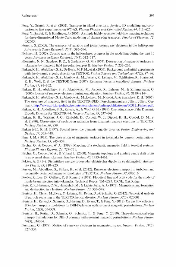
References 395
Feng, Y., Grigull, P., et al. (2002). Transport in island divertors: physics, 3D modelling and com-parison to first experiments on W7-AS. Plasma Physics and Controlled Fusion, 44, 611–625.
Feng, Y., Sardei, F., & Kisslinger, J. (2005). A simple highly accurate field-line mapping techniquefor three-dimensional Monte Carlo modeling of plasma edge transport. Physics of Plasmas, 12,052505.
Ferreira, S. (2005). The transport of galactic and jovian cosmic ray electrons in the heliosphere.Advances in Space Research, 35(4), 586–596.
Fichtner, H. (2005). Cosmic rays in the heliosphere: progress in the modelling during the past 10years. Advances in Space Research, 35(4), 512–517.
Filonenko, N. N., Sagdeev, R. Z., & Zaslavsky, G. M. (1967). Destruction of magnetic surfaces intokamaks by magnetic field irregularities: part II. Nuclear Fusion, 7, 253–266.
Finken, K.H., Abdullaev, S. S., DeBock,M. F.M., et al. (2005). Background and initial experimentswith the dynamic ergodic divertor on TEXTOR. Fusion Science and Technology, 47(2), 87–96.
Finken, K. H., Abdullaev, S. S., Jakubowski,M., Jaspers, R., Lehnen,M., Schlikeiser, R., Spatschek,K. H., Wolf, R. & the TEXTOR Team (2007). Runaway losses in ergodized plasmas. NuclearFusion, 47, 91–102.
Finken, K. H., Abdullaev, S. S., Jakubowski, M., Jaspers, R., Lehnen, M., & Zimmermann, O.(2006). Losses of runaway electrons during ergodization. Nuclear Fusion, 46, S139–S144.
Finken, K.H., Abdullaev, S. S., Jakubowski,M., Lehnen,M., Nicolai, A.&Spatschek, K.H. (2005).The structure of magnetic field in the TEXTOR-DED, Forschungszentrum Jülich, Jülich, Ger-many. http://wwwzb1.fz-juelich.de/contentenrichment/onlinepublikationen/00312_Finken.pdf.
Finken, K. H., Abdullaev, S. S., Kaleck, A., &Wolf, G. H. (1999). Operating space of the DynamicErgodic Divertor for TEXTOR-94. Nuclear Fusion, 39, 637–661.
Finken, K. H., Watkins, J. G., Rüsbuldt, D., Corbett, W. J., Dippel, K. H., Goebel, D. M., etal. (1990). Observation of sychrotron radiation from tokamak runaway electrons in TEXTOR.Nuclear Fusion, 30, 859.
Finken (ed.), K. H. (1997). Special issue: the dynamic ergodic divertor. Fusion Engineering andDesign, 37, 335–448.
Finn, J. M. (1975). The destruction of magnetic surfaces in tokamaks by current perturbations.Nuclear Fusion, 15, 845–854.
Fischer, O., & Cooper, W. A. (1998). Mapping of a stochastic magnetic field in toroidal systems.Plasma Physics Reports, 24, 727–731.
Fischer, O., Cooper, W. A., & Villard, L. (2000). Magnetic topology and guiding centre drift orbitsin a reversed shear tokamak. Nuclear Fusion, 40, 1453–1462.
Fokker, A. (1914). Die mittlere energie rotierender elektrischer dipole im strahlungsfeld. Annalender Physik, 43, 810–820.
Forster, M., Abdullaev, S., Finken, K., et al. (2012). Runaway electron transport in turbulent andresonantly perturbed magnetic topologies of TEXTOR. Nuclear Fusion, 52, 083016.
Fowler, R., Lee, D., Gaffney, P., & Rome, J. (1978). Floc-field line and orbit code for the study ofripple beam injection into tokamaks, Technical Report TM-6293. ORNL, Oak Ridge.
Freis, R. P., Hartman, C.W., Hamzeh, F.M., & Lichtenberg, A. J. (1973).Magnetic island formationand destruction in a levitron. Nuclear Fusion, 13, 533–548.
Frerichs, H., Clever,M., Feng, Y., Lehnen,M., Reiter, D., & Schmitz, O. (2012). Numerical analysisof particle recycling in the TEXTOR helical divertor. Nuclear Fusion, 52(3), 023001.
Frerichs, H., Reiter, D., Schmitz, O., Harting, D., Evans, T., & Feng, Y. (2012). On gas flow effects in3D edge transport simulations for DIII-D plasmas with resonant magnetic perturbations. NuclearFusion, 52(5), 054008.
Frerichs, H., Reiter, D., Schmitz, O., Schmitz, T., & Feng, Y. (2010). Three-dimensional edgetransport simulations for DIII-D plasmas with resonant magnetic perturbations. Nuclear Fusion,50(3), 034004.
Fussmann, G. (1979). Motion of runaway electrons in momentum space. Nuclear Fusion, 19(3),327–334.
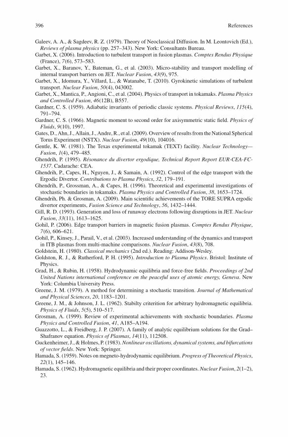
396 References
Galeev, A. A., & Sagdeev, R. Z. (1979). Theory of Neoclassical Diffusion. In M. Leontovich (Ed.),Reviews of plasma physics (pp. 257–343). New York: Consultants Bureau.
Garbet, X. (2006). Introduction to turbulent transport in fusion plasmas. Comptes Rendus Physique(France), 7(6), 573–583.
Garbet, X., Baranov, Y., Bateman, G., et al. (2003). Micro-stability and transport modelling ofinternal transport barriers on JET. Nuclear Fusion, 43(9), 975.
Garbet, X., Idomura, Y., Villard, L., & Watanabe, T. (2010). Gyrokinetic simulations of turbulenttransport. Nuclear Fusion, 50(4), 043002.
Garbet, X., Mantica, P., Angioni, C., et al. (2004). Physics of transport in tokamaks. Plasma Physicsand Controlled Fusion, 46(12B), B557.
Gardner, C. S. (1959). Adiabatic invariants of periodic classic systems. Physical Reviews, 115(4),791–794.
Gardner, C. S. (1966). Magnetic moment to second order for axisymmetric static field. Physics ofFluids, 9(10), 1997.
Gates,D.,Ahn, J., Allain, J., Andre, R., et al. (2009).Overviewof results from theNational SphericalTorus Experiment (NSTX). Nuclear Fusion, 49(10), 104016.
Gentle, K. W. (1981). The Texas experimental tokamak (TEXT) facility. Nuclear Technology—Fusion, 1(4), 479–485.
Ghendrih, P. (1995). Résonance du divertor ergodique, Technical Report Report EUR-CEA-FC-1537. Cadarache: CEA.
Ghendrih, P., Capes, H., Nguyen, J., & Samain, A. (1992). Control of the edge transport with theErgodic Divertor. Contributions to Plasma Physics, 32, 179–191.
Ghendrih, P., Grossman, A., & Capes, H. (1996). Theoretical and experimental investigations ofstochastic boundaries in tokamaks. Plasma Physics and Controlled Fusion, 38, 1653–1724.
Ghendrih, Ph. & Grosman, A. (2009). Main scientific achievements of the TORE SUPRA ergodicdivertor experiments, Fusion Science and Technology, 56, 1432–1444.
Gill, R. D. (1993). Generation and loss of runaway electrons following disruptions in JET. NuclearFusion, 33(11), 1613–1625.
Gohil, P. (2006). Edge transport barriers in magnetic fusion plasmas. Comptes Rendus Physique,7(6), 606–621.
Gohil, P., Kinsey, J., Parail, V., et al. (2003). Increased understanding of the dynamics and transportin ITB plasmas from multi-machine comparisons. Nuclear Fusion, 43(8), 708.
Goldstein, H. (1980). Classical mechanics (2nd ed.). Reading: Addison-Wesley.Goldston, R. J., & Rutherford, P. H. (1995). Introduction to Plasma Physics. Bristol: Institute ofPhysics.
Grad, H., & Rubin, H. (1958). Hydrodynamic equilibria and force-free fields. Proceedings of 2ndUnited Nations international conference on the peaceful uses of atomic energy, Geneva. NewYork: Columbia University Press.
Greene, J. M. (1979). A method for determining a stochastic transition. Journal of Mathematicaland Physical Sciences, 20, 1183–1201.
Greene, J. M., & Johnson, J. L. (1962). Stabilty criterition for arbitrary hydromagnetic equilibria.Physics of Fluids, 5(5), 510–517.
Grosman, A. (1999). Review of experimental achievements with stochastic boundaries. PlasmaPhysics and Controlled Fusion, 41, A185–A194.
Guazzotto, L., & Freidberg, J. P. (2007). A family of analytic equilibrium solutions for the Grad–Shafranov equation. Physics of Plasmas, 14(11), 112508.
Guckenheimer, J., &Holmes, P. (1983).Nonlinear oscillations, dynamical systems, and bifurcationsof vector fields. New York: Springer.
Hamada, S. (1959). Notes on megneto-hydrodynamic equilibrium. Progress of Theoretical Physics,22(1), 145–146.
Hamada, S. (1962). Hydromagnetic equilibria and their proper coordinates.Nuclear Fusion, 2(1–2),23.
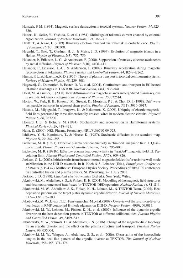
References 397
Hamzeh, F. M. (1974). Magnetic surface destruction in toroidal systems. Nuclear Fusion, 14, 523–536.
Hattori, K., Seike, Y., Yoshida, Z., et al. (1984). Shrinkage of tokamak current channel by externalergodization. Journal of Nuclear Materials, 121, 368–373.
Hauff, T., & Jenko, F. (2009). Runaway electron transport via tokamak microturbulence. Physicsof Plasmas, 16(10), 102308.
Hayashi, T., Sato, T., Gardner, H. J., & Meiss, J. D. (1994). Evolution of magnetic islands in aHeliac. Physics of Plasmas, 2(3), 752–759.
Helander, P., Eriksson, L.-G., & Andersson, F. (2000). Supperssion of runaway electron avalanchesby radial diffusion. Physics of Plasmas, 7(10), 4106–4111.
Helander, P., Eriksson, L.-G., & Andersson, F. (2002). Runaway acceleration during magneticreconnection in tokamaks. Plasma Physics and Controlled Fusion, 44, B247–B262.
Hinton, F. L.,&Hazeltine, R.D. (1976). Theory of plasma transport in toroidal confinement systems.Reviews of Modern Physics, 48, 239–308.
Hogeweij, G., Dumortier, P., Eester, D. V., et al. (2004). Confinement and transport in EC heatedRI-mode discharges in TEXTOR. Nuclear Fusion, 44(4), 533–541.
Hölzl,M.,&Günter, S. (2008). Heat diffusion acrossmagnetic islands and ergodized plasma regionsin realistic tokamak configurations. Physics of Plasmas, 15, 072514.
Horton, W., Park, H. B., Kwon, J. M., Strozzi, D., Morrison, P. J., & Choi, D. I. (1998). Drift wavetest particle transport in reversed shear profile. Physics of Plasmas, 5(11), 3910–3917.
Hosoda, M., Miyaguchi, T., Imagawa, K., & Nakamura, K. (2009). Ubiquity of chaotic magnetic-field lines generated by three-dimensionally crossed wires in modern electric circuits. PhysicalReview E, 80, 067202.
Howard, J. E., & Hohs, S. M. (1984). Stochasticity and reconnection in Hamiltonian systems.Physical Review A, 29, 418–421.
Huba, D. (2000). NRL Plasma, Formulary, NRL/PU/6790-09-523.Ichikawa, Y. H., Kamimura, T., & Hirose, K. (1987). Stochastic diffusion in the standard map.
Physica D, 29, 247–255.Isichenko, M. B. (1991). Effective plasma heat conductivity in “braided” magnetic field. I. Quasi-linear limit. Plasma Physics and Controlled Fusion, 33(7), 795–807.
Isichenko, M. B. (1991b). Effective plasma heat conductivity in “braided” magnetic field. II. Per-colation limit. Plasma Physics and Controlled Fusion, 33(7), 809–826.
Jackson,G.L. (2003). Initial results from the new internalmagnetic field coils for resistivewallmodestabilization in the DIII-D tokamak. In R. Koch & S. Lebedev (Eds.), Europhysics ConferenceAbstracts (p. P-4.47). Mulhouse: European Physics Society. Proceedings of 30th EPS conferenceon controlled fusion and plasma physics, St. Petersburg, 7–11 July 2003.
Jackson, J. D. (1998). Classical electrodynamics (3rd ed.). New York: Wiley.Jakubowski,M., Abdullaev, S. S.,&Finken,K.H. (2004).Modelling of themagnetic field structuresand first measurements of heat fluxes for TEXTOR-DED operation. Nuclear Fusion, 44, S1–S11.
Jakubowski, M. W., Abdullaev, S. S., Finken, K. H., Lehnen, M., & TEXTOR Team, (2005). Heatdeposition patterns on the target plates dynamic ergodic divertor. Journal of Nuclear Materials,337—-339, 176–180.
Jakubowski,M.W., Evans, T. E., Fenstermacher,M., et al. (2009).Overviewof the results on divertorheat loads in RMP controlled H-mode plasmas on DIII-D. Nuclear Fusion, 49(9), 095013.
Jakubowski, M. W., Lehnen, M., Finken, K. H., et al. (2007). Influence of the dynamic ergodicdivertor on the heat deposition pattern in TEXTOR at different collisionalities. Plasma Physicsand Controlled Fusion, 49, S109–S121.
Jakubowski, M. W., Schmitz, O., & Abdullaev, S. S. (2006). Change of the magnetic-field topologyby an ergodic divertor and the effect on the plasma structure and transport. Physical ReviewLetters, 96, 035004.
Jakubowski, M. W., Wingen, A., Abdullaev, S. S., et al. (2006). Observation of the heteroclinictangles in the heat flux pattern of the ergodic divertor at TEXTOR. The Journal of NuclearMaterials, 363–365, 371–376.
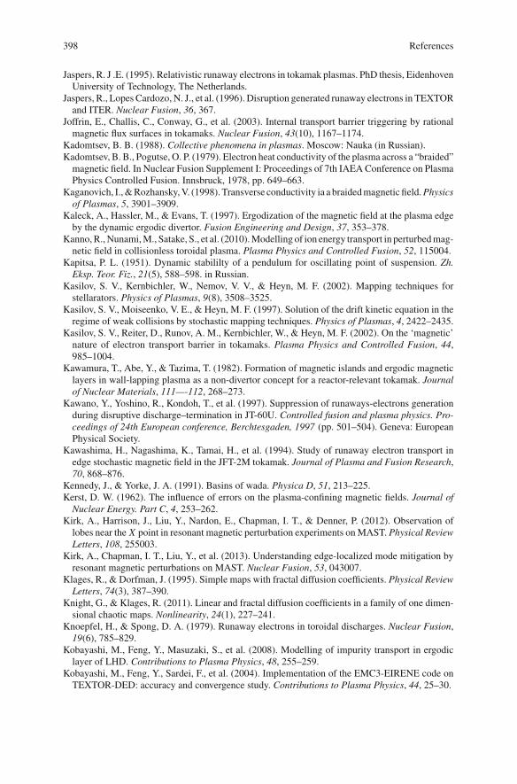
398 References
Jaspers, R. J .E. (1995). Relativistic runaway electrons in tokamak plasmas. PhD thesis, EidenhovenUniversity of Technology, The Netherlands.
Jaspers, R., Lopes Cardozo, N. J., et al. (1996). Disruption generated runaway electrons in TEXTORand ITER. Nuclear Fusion, 36, 367.
Joffrin, E., Challis, C., Conway, G., et al. (2003). Internal transport barrier triggering by rationalmagnetic flux surfaces in tokamaks. Nuclear Fusion, 43(10), 1167–1174.
Kadomtsev, B. B. (1988). Collective phenomena in plasmas. Moscow: Nauka (in Russian).Kadomtsev, B. B., Pogutse, O. P. (1979). Electron heat conductivity of the plasma across a “braided”magnetic field. In Nuclear Fusion Supplement I: Proceedings of 7th IAEAConference on PlasmaPhysics Controlled Fusion. Innsbruck, 1978, pp. 649–663.
Kaganovich, I.,&Rozhansky,V. (1998). Transverse conductivity ia a braidedmagnetic field.Physicsof Plasmas, 5, 3901–3909.
Kaleck, A., Hassler, M., & Evans, T. (1997). Ergodization of the magnetic field at the plasma edgeby the dynamic ergodic divertor. Fusion Engineering and Design, 37, 353–378.
Kanno,R.,Nunami,M., Satake, S., et al. (2010).Modelling of ion energy transport in perturbedmag-netic field in collisionless toroidal plasma. Plasma Physics and Controlled Fusion, 52, 115004.
Kapitsa, P. L. (1951). Dynamic stabililty of a pendulum for oscillating point of suspension. Zh.Eksp. Teor. Fiz., 21(5), 588–598. in Russian.
Kasilov, S. V., Kernbichler, W., Nemov, V. V., & Heyn, M. F. (2002). Mapping techniques forstellarators. Physics of Plasmas, 9(8), 3508–3525.
Kasilov, S. V., Moiseenko, V. E., & Heyn, M. F. (1997). Solution of the drift kinetic equation in theregime of weak collisions by stochastic mapping techniques. Physics of Plasmas, 4, 2422–2435.
Kasilov, S. V., Reiter, D., Runov, A. M., Kernbichler, W., & Heyn, M. F. (2002). On the ‘magnetic’nature of electron transport barrier in tokamaks. Plasma Physics and Controlled Fusion, 44,985–1004.
Kawamura, T., Abe, Y., & Tazima, T. (1982). Formation of magnetic islands and ergodic magneticlayers in wall-lapping plasma as a non-divertor concept for a reactor-relevant tokamak. Journalof Nuclear Materials, 111—-112, 268–273.
Kawano, Y., Yoshino, R., Kondoh, T., et al. (1997). Suppression of runaways-electrons generationduring disruptive discharge–termination in JT-60U. Controlled fusion and plasma physics. Pro-ceedings of 24th European conference, Berchtesgaden, 1997 (pp. 501–504). Geneva: EuropeanPhysical Society.
Kawashima, H., Nagashima, K., Tamai, H., et al. (1994). Study of runaway electron transport inedge stochastic magnetic field in the JFT-2M tokamak. Journal of Plasma and Fusion Research,70, 868–876.
Kennedy, J., & Yorke, J. A. (1991). Basins of wada. Physica D, 51, 213–225.Kerst, D. W. (1962). The influence of errors on the plasma-confining magnetic fields. Journal of
Nuclear Energy. Part C, 4, 253–262.Kirk, A., Harrison, J., Liu, Y., Nardon, E., Chapman, I. T., & Denner, P. (2012). Observation oflobes near the X point in resonant magnetic perturbation experiments onMAST. Physical ReviewLetters, 108, 255003.
Kirk, A., Chapman, I. T., Liu, Y., et al. (2013). Understanding edge-localized mode mitigation byresonant magnetic perturbations on MAST. Nuclear Fusion, 53, 043007.
Klages, R., & Dorfman, J. (1995). Simple maps with fractal diffusion coefficients. Physical ReviewLetters, 74(3), 387–390.
Knight, G., & Klages, R. (2011). Linear and fractal diffusion coefficients in a family of one dimen-sional chaotic maps. Nonlinearity, 24(1), 227–241.
Knoepfel, H., & Spong, D. A. (1979). Runaway electrons in toroidal discharges. Nuclear Fusion,19(6), 785–829.
Kobayashi, M., Feng, Y., Masuzaki, S., et al. (2008). Modelling of impurity transport in ergodiclayer of LHD. Contributions to Plasma Physics, 48, 255–259.
Kobayashi, M., Feng, Y., Sardei, F., et al. (2004). Implementation of the EMC3-EIRENE code onTEXTOR-DED: accuracy and convergence study. Contributions to Plasma Physics, 44, 25–30.
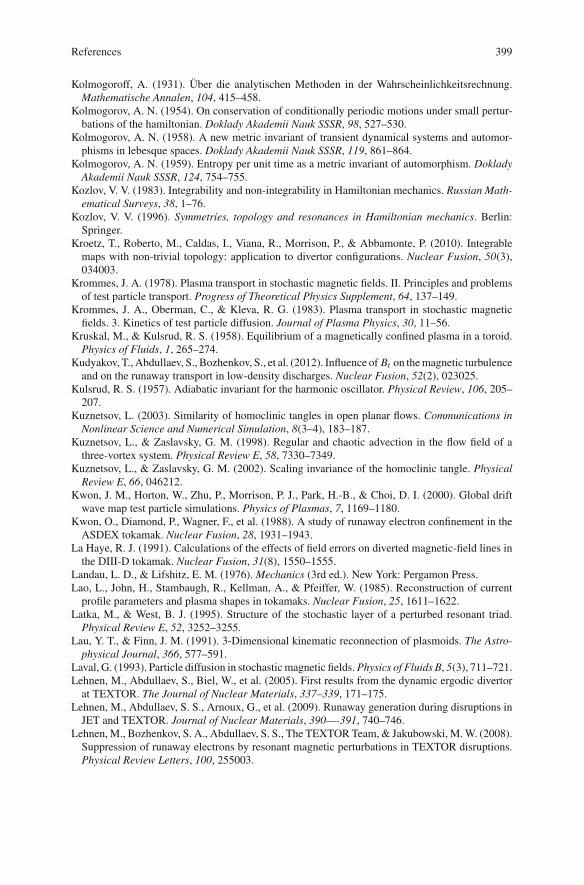
References 399
Kolmogoroff, A. (1931). Über die analytischen Methoden in der Wahrscheinlichkeitsrechnung.Mathematische Annalen, 104, 415–458.
Kolmogorov, A. N. (1954). On conservation of conditionally periodic motions under small pertur-bations of the hamiltonian. Doklady Akademii Nauk SSSR, 98, 527–530.
Kolmogorov, A. N. (1958). A new metric invariant of transient dynamical systems and automor-phisms in lebesque spaces. Doklady Akademii Nauk SSSR, 119, 861–864.
Kolmogorov, A. N. (1959). Entropy per unit time as a metric invariant of automorphism. DokladyAkademii Nauk SSSR, 124, 754–755.
Kozlov, V. V. (1983). Integrability and non-integrability in Hamiltonian mechanics. Russian Math-ematical Surveys, 38, 1–76.
Kozlov, V. V. (1996). Symmetries, topology and resonances in Hamiltonian mechanics. Berlin:Springer.
Kroetz, T., Roberto, M., Caldas, I., Viana, R., Morrison, P., & Abbamonte, P. (2010). Integrablemaps with non-trivial topology: application to divertor configurations. Nuclear Fusion, 50(3),034003.
Krommes, J. A. (1978). Plasma transport in stochastic magnetic fields. II. Principles and problemsof test particle transport. Progress of Theoretical Physics Supplement, 64, 137–149.
Krommes, J. A., Oberman, C., & Kleva, R. G. (1983). Plasma transport in stochastic magneticfields. 3. Kinetics of test particle diffusion. Journal of Plasma Physics, 30, 11–56.
Kruskal, M., & Kulsrud, R. S. (1958). Equilibrium of a magnetically confined plasma in a toroid.Physics of Fluids, 1, 265–274.
Kudyakov, T., Abdullaev, S., Bozhenkov, S., et al. (2012). Influence of Bt on themagnetic turbulenceand on the runaway transport in low-density discharges. Nuclear Fusion, 52(2), 023025.
Kulsrud, R. S. (1957). Adiabatic invariant for the harmonic oscillator. Physical Review, 106, 205–207.
Kuznetsov, L. (2003). Similarity of homoclinic tangles in open planar flows. Communications inNonlinear Science and Numerical Simulation, 8(3–4), 183–187.
Kuznetsov, L., & Zaslavsky, G. M. (1998). Regular and chaotic advection in the flow field of athree-vortex system. Physical Review E, 58, 7330–7349.
Kuznetsov, L., & Zaslavsky, G. M. (2002). Scaling invariance of the homoclinic tangle. PhysicalReview E, 66, 046212.
Kwon, J. M., Horton, W., Zhu, P., Morrison, P. J., Park, H.-B., & Choi, D. I. (2000). Global driftwave map test particle simulations. Physics of Plasmas, 7, 1169–1180.
Kwon, O., Diamond, P., Wagner, F., et al. (1988). A study of runaway electron confinement in theASDEX tokamak. Nuclear Fusion, 28, 1931–1943.
La Haye, R. J. (1991). Calculations of the effects of field errors on diverted magnetic-field lines inthe DIII-D tokamak. Nuclear Fusion, 31(8), 1550–1555.
Landau, L. D., & Lifshitz, E. M. (1976). Mechanics (3rd ed.). New York: Pergamon Press.Lao, L., John, H., Stambaugh, R., Kellman, A., & Pfeiffer, W. (1985). Reconstruction of currentprofile parameters and plasma shapes in tokamaks. Nuclear Fusion, 25, 1611–1622.
Latka, M., & West, B. J. (1995). Structure of the stochastic layer of a perturbed resonant triad.Physical Review E, 52, 3252–3255.
Lau, Y. T., & Finn, J. M. (1991). 3-Dimensional kinematic reconnection of plasmoids. The Astro-physical Journal, 366, 577–591.
Laval, G. (1993). Particle diffusion in stochasticmagnetic fields.Physics of Fluids B, 5(3), 711–721.Lehnen, M., Abdullaev, S., Biel, W., et al. (2005). First results from the dynamic ergodic divertorat TEXTOR. The Journal of Nuclear Materials, 337–339, 171–175.
Lehnen, M., Abdullaev, S. S., Arnoux, G., et al. (2009). Runaway generation during disruptions inJET and TEXTOR. Journal of Nuclear Materials, 390—-391, 740–746.
Lehnen,M., Bozhenkov, S. A., Abdullaev, S. S., The TEXTORTeam, & Jakubowski, M.W. (2008).Suppression of runaway electrons by resonant magnetic perturbations in TEXTOR disruptions.Physical Review Letters, 100, 255003.
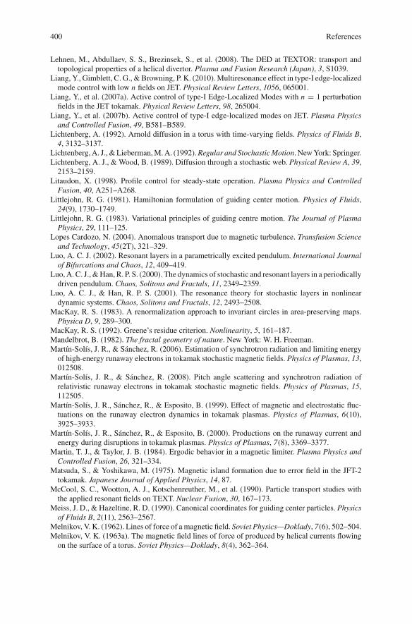
400 References
Lehnen, M., Abdullaev, S. S., Brezinsek, S., et al. (2008). The DED at TEXTOR: transport andtopological properties of a helical divertor. Plasma and Fusion Research (Japan), 3, S1039.
Liang, Y., Gimblett, C. G., &Browning, P. K. (2010).Multiresonance effect in type-I edge-localizedmode control with low n fields on JET. Physical Review Letters, 1056, 065001.
Liang, Y., et al. (2007a). Active control of type-I Edge-Localized Modes with n = 1 perturbationfields in the JET tokamak. Physical Review Letters, 98, 265004.
Liang, Y., et al. (2007b). Active control of type-I edge-localized modes on JET. Plasma Physicsand Controlled Fusion, 49, B581–B589.
Lichtenberg, A. (1992). Arnold diffusion in a torus with time-varying fields. Physics of Fluids B,4, 3132–3137.
Lichtenberg,A. J.,&Lieberman,M.A. (1992).Regular and Stochastic Motion. NewYork: Springer.Lichtenberg, A. J., & Wood, B. (1989). Diffusion through a stochastic web. Physical Review A, 39,2153–2159.
Litaudon, X. (1998). Profile control for steady-state operation. Plasma Physics and ControlledFusion, 40, A251–A268.
Littlejohn, R. G. (1981). Hamiltonian formulation of guiding center motion. Physics of Fluids,24(9), 1730–1749.
Littlejohn, R. G. (1983). Variational principles of guiding centre motion. The Journal of PlasmaPhysics, 29, 111–125.
Lopes Cardozo, N. (2004). Anomalous transport due to magnetic turbulence. Transfusion Scienceand Technology, 45(2T), 321–329.
Luo, A. C. J. (2002). Resonant layers in a parametrically excited pendulum. International Journalof Bifurcations and Chaos, 12, 409–419.
Luo,A. C. J., &Han, R. P. S. (2000). The dynamics of stochastic and resonant layers in a periodicallydriven pendulum. Chaos, Solitons and Fractals, 11, 2349–2359.
Luo, A. C. J., & Han, R. P. S. (2001). The resonance theory for stochastic layers in nonlineardynamic systems. Chaos, Solitons and Fractals, 12, 2493–2508.
MacKay, R. S. (1983). A renormalization approach to invariant circles in area-preserving maps.Physica D, 9, 289–300.
MacKay, R. S. (1992). Greene’s residue criterion. Nonlinearity, 5, 161–187.Mandelbrot, B. (1982). The fractal geometry of nature. New York: W. H. Freeman.Martín-Solís, J. R., & Sánchez, R. (2006). Estimation of synchrotron radiation and limiting energyof high-energy runaway electrons in tokamak stochastic magnetic fields. Physics of Plasmas, 13,012508.
Martín-Solís, J. R., & Sánchez, R. (2008). Pitch angle scattering and synchrotron radiation ofrelativistic runaway electrons in tokamak stochastic magnetic fields. Physics of Plasmas, 15,112505.
Martín-Solís, J. R., Sánchez, R., & Esposito, B. (1999). Effect of magnetic and electrostatic fluc-tuations on the runaway electron dynamics in tokamak plasmas. Physics of Plasmas, 6(10),3925–3933.
Martín-Solís, J. R., Sánchez, R., & Esposito, B. (2000). Productions on the runaway current andenergy during disruptions in tokamak plasmas. Physics of Plasmas, 7(8), 3369–3377.
Martin, T. J., & Taylor, J. B. (1984). Ergodic behavior in a magnetic limiter. Plasma Physics andControlled Fusion, 26, 321–334.
Matsuda, S., & Yoshikawa, M. (1975). Magnetic island formation due to error field in the JFT-2tokamak. Japanese Journal of Applied Physics, 14, 87.
McCool, S. C., Wootton, A. J., Kotschenreuther, M., et al. (1990). Particle transport studies withthe applied resonant fields on TEXT. Nuclear Fusion, 30, 167–173.
Meiss, J. D., & Hazeltine, R. D. (1990). Canonical coordinates for guiding center particles. Physicsof Fluids B, 2(11), 2563–2567.
Melnikov, V. K. (1962). Lines of force of a magnetic field. Soviet Physics—Doklady, 7(6), 502–504.Melnikov, V. K. (1963a). The magnetic field lines of force of produced by helical currents flowingon the surface of a torus. Soviet Physics—Doklady, 8(4), 362–364.
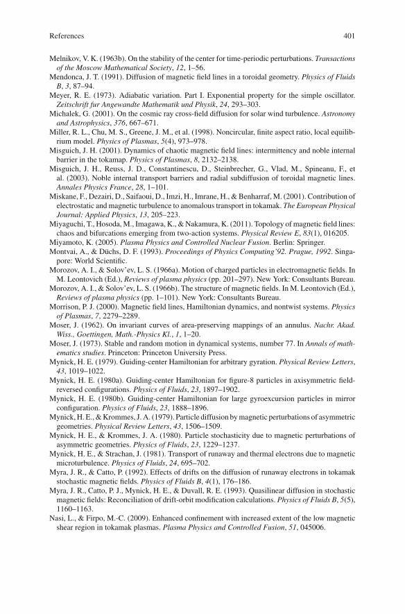
References 401
Melnikov, V. K. (1963b). On the stability of the center for time-periodic perturbations. Transactionsof the Moscow Mathematical Society, 12, 1–56.
Mendonca, J. T. (1991). Diffusion of magnetic field lines in a toroidal geometry. Physics of FluidsB, 3, 87–94.
Meyer, R. E. (1973). Adiabatic variation. Part I. Exponential property for the simple oscillator.Zeitschrift fur Angewandte Mathematik und Physik, 24, 293–303.
Michalek, G. (2001). On the cosmic ray cross-field diffusion for solar wind turbulence. Astronomyand Astrophysics, 376, 667–671.
Miller, R. L., Chu, M. S., Greene, J. M., et al. (1998). Noncircular, finite aspect ratio, local equilib-rium model. Physics of Plasmas, 5(4), 973–978.
Misguich, J. H. (2001). Dynamics of chaotic magnetic field lines: intermittency and noble internalbarrier in the tokamap. Physics of Plasmas, 8, 2132–2138.
Misguich, J. H., Reuss, J. D., Constantinescu, D., Steinbrecher, G., Vlad, M., Spineanu, F., etal. (2003). Noble internal transport barriers and radial subdiffusion of toroidal magnetic lines.Annales Physics France, 28, 1–101.
Miskane, F., Dezairi, D., Saifaoui, D., Imzi, H., Imrane, H., &Benharraf,M. (2001). Contribution ofelectrostatic and magnetic turbulence to anomalous transport in tokamak. The European PhysicalJournal: Applied Physics, 13, 205–223.
Miyaguchi, T., Hosoda,M., Imagawa, K., &Nakamura, K. (2011). Topology ofmagnetic field lines:chaos and bifurcations emerging from two-action systems. Physical Review E, 83(1), 016205.
Miyamoto, K. (2005). Plasma Physics and Controlled Nuclear Fusion. Berlin: Springer.Montvai, A., & Düchs, D. F. (1993). Proceedings of Physics Computing’92. Prague, 1992. Singa-pore: World Scientific.
Morozov, A. I., & Solov’ev, L. S. (1966a). Motion of charged particles in electromagnetic fields. InM. Leontovich (Ed.), Reviews of plasma physics (pp. 201–297). New York: Consultants Bureau.
Morozov, A. I., & Solov’ev, L. S. (1966b). The structure of magnetic fields. In M. Leontovich (Ed.),Reviews of plasma physics (pp. 1–101). New York: Consultants Bureau.
Morrison, P. J. (2000). Magnetic field lines, Hamiltonian dynamics, and nontwist systems. Physicsof Plasmas, 7, 2279–2289.
Moser, J. (1962). On invariant curves of area-preserving mappings of an annulus. Nachr. Akad.Wiss., Goettingen, Math.-Physics Kl., 1, 1–20.
Moser, J. (1973). Stable and random motion in dynamical systems, number 77. In Annals of math-ematics studies. Princeton: Princeton University Press.
Mynick, H. E. (1979). Guiding-center Hamiltonian for arbitrary gyration. Physical Review Letters,43, 1019–1022.
Mynick, H. E. (1980a). Guiding-center Hamiltonian for figure-8 particles in axisymmetric field-reversed configurations. Physics of Fluids, 23, 1897–1902.
Mynick, H. E. (1980b). Guiding-center Hamiltonian for large gyroexcursion particles in mirrorconfiguration. Physics of Fluids, 23, 1888–1896.
Mynick,H. E.,&Krommes, J.A. (1979). Particle diffusion bymagnetic perturbations of asymmetricgeometries. Physical Review Letters, 43, 1506–1509.
Mynick, H. E., & Krommes, J. A. (1980). Particle stochasticity due to magnetic perturbations ofasymmetric geometries. Physics of Fluids, 23, 1229–1237.
Mynick, H. E., & Strachan, J. (1981). Transport of runaway and thermal electrons due to magneticmicroturbulence. Physics of Fluids, 24, 695–702.
Myra, J. R., & Catto, P. (1992). Effects of drifts on the diffusion of runaway electrons in tokamakstochastic magnetic fields. Physics of Fluids B, 4(1), 176–186.
Myra, J. R., Catto, P. J., Mynick, H. E., & Duvall, R. E. (1993). Quasilinear diffusion in stochasticmagnetic fields: Reconciliation of drift-orbit modification calculations. Physics of Fluids B, 5(5),1160–1163.
Nasi, L., & Firpo, M.-C. (2009). Enhanced confinement with increased extent of the low magneticshear region in tokamak plasmas. Plasma Physics and Controlled Fusion, 51, 045006.
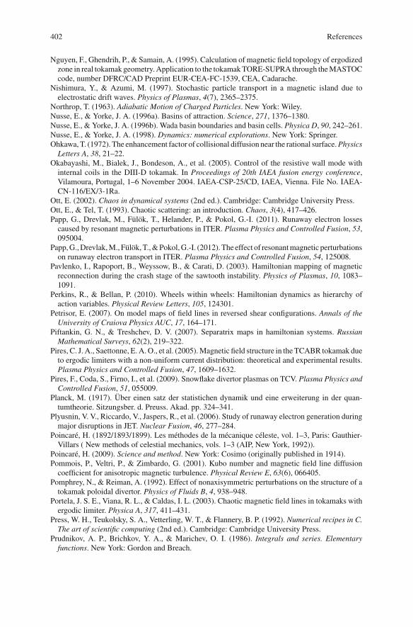
402 References
Nguyen, F., Ghendrih, P., & Samain, A. (1995). Calculation of magnetic field topology of ergodizedzone in real tokamak geometry.Application to the tokamakTORE-SUPRA through theMASTOCcode, number DFRC/CAD Preprint EUR-CEA-FC-1539, CEA, Cadarache.
Nishimura, Y., & Azumi, M. (1997). Stochastic particle transport in a magnetic island due toelectrostatic drift waves. Physics of Plasmas, 4(7), 2365–2375.
Northrop, T. (1963). Adiabatic Motion of Charged Particles. New York: Wiley.Nusse, E., & Yorke, J. A. (1996a). Basins of attraction. Science, 271, 1376–1380.Nusse, E., & Yorke, J. A. (1996b). Wada basin boundaries and basin cells. Physica D, 90, 242–261.Nusse, E., & Yorke, J. A. (1998). Dynamics: numerical explorations. New York: Springer.Ohkawa, T. (1972). The enhancement factor of collisional diffusion near the rational surface.Physics
Letters A, 38, 21–22.Okabayashi, M., Bialek, J., Bondeson, A., et al. (2005). Control of the resistive wall mode withinternal coils in the DIII-D tokamak. In Proceedings of 20th IAEA fusion energy conference,Vilamoura, Portugal, 1–6 November 2004. IAEA-CSP-25/CD, IAEA, Vienna. File No. IAEA-CN-116/EX/3-1Ra.
Ott, E. (2002). Chaos in dynamical systems (2nd ed.). Cambridge: Cambridge University Press.Ott, E., & Tel, T. (1993). Chaotic scattering: an introduction. Chaos, 3(4), 417–426.Papp, G., Drevlak, M., Fülök, T., Helander, P., & Pokol, G.-I. (2011). Runaway electron lossescaused by resonant magnetic perturbations in ITER. Plasma Physics and Controlled Fusion, 53,095004.
Papp,G.,Drevlak,M., Fülök,T.,&Pokol,G.-I. (2012).The effect of resonantmagnetic perturbationson runaway electron transport in ITER. Plasma Physics and Controlled Fusion, 54, 125008.
Pavlenko, I., Rapoport, B., Weyssow, B., & Carati, D. (2003). Hamiltonian mapping of magneticreconnection during the crash stage of the sawtooth instability. Physics of Plasmas, 10, 1083–1091.
Perkins, R., & Bellan, P. (2010). Wheels within wheels: Hamiltonian dynamics as hierarchy ofaction variables. Physical Review Letters, 105, 124301.
Petrisor, E. (2007). On model maps of field lines in reversed shear configurations. Annals of theUniversity of Craiova Physics AUC, 17, 164–171.
Piftankin, G. N., & Treshchev, D. V. (2007). Separatrix maps in hamiltonian systems. RussianMathematical Surveys, 62(2), 219–322.
Pires, C. J. A., Saettonne, E. A.O., et al. (2005).Magnetic field structure in the TCABR tokamak dueto ergodic limiters with a non-uniform current distribution: theoretical and experimental results.Plasma Physics and Controlled Fusion, 47, 1609–1632.
Pires, F., Coda, S., Firno, I., et al. (2009). Snowflake divertor plasmas on TCV. Plasma Physics andControlled Fusion, 51, 055009.
Planck, M. (1917). Über einen satz der statistichen dynamik und eine erweiterung in der quan-tumtheorie. Sitzungsber. d. Preuss. Akad. pp. 324–341.
Plyusnin, V. V., Riccardo, V., Jaspers, R., et al. (2006). Study of runaway electron generation duringmajor disruptions in JET. Nuclear Fusion, 46, 277–284.
Poincaré, H. (1892/1893/1899). Les méthodes de la mécanique céleste, vol. 1–3, Paris: Gauthier-Villars ( New methods of celestial mechanics, vols. 1–3 (AIP, New York, 1992)).
Poincaré, H. (2009). Science and method. New York: Cosimo (originally published in 1914).Pommois, P., Veltri, P., & Zimbardo, G. (2001). Kubo number and magnetic field line diffusioncoefficient for anisotropic magnetic turbulence. Physical Review E, 63(6), 066405.
Pomphrey, N., & Reiman, A. (1992). Effect of nonaxisymmetric perturbations on the structure of atokamak poloidal divertor. Physics of Fluids B, 4, 938–948.
Portela, J. S. E., Viana, R. L., & Caldas, I. L. (2003). Chaotic magnetic field lines in tokamaks withergodic limiter. Physica A, 317, 411–431.
Press, W. H., Teukolsky, S. A., Vetterling, W. T., & Flannery, B. P. (1992). Numerical recipes in C.The art of scientific computing (2nd ed.). Cambridge: Cambridge University Press.
Prudnikov, A. P., Brichkov, Y. A., & Marichev, O. I. (1986). Integrals and series. Elementaryfunctions. New York: Gordon and Breach.
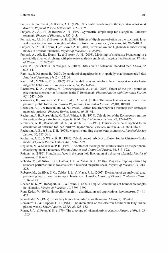
References 403
Punjabi, A., Verma, A., & Boozer, A. H. (1992). Stochastic broadening of the separatrix of tokamakdivertor. Physical Review Letters, 69, 3322–3325.
Punjabi, A., Ali, H., & Boozer, A. H. (1997). Symmetric simple map for a single-null divertortokamak. Physics of Plasmas, 4, 337–345.
Punjabi, A., Ali, H., & Boozer, A. H. (2003). Effects of dipole perturbation on the stochastic layerand magnetic footprint in single-null divertor tokamaks. Physics of Plasmas, 10, 3992–4003.
Punjabi, A., Ali, H., Evans, T., & Boozer, A. H. (2007). Effect of low and high mode number tearingmodes in divertor tokamaks. Physics of Plasmas, 14, 082503.
Punjabi, A., Ali, H., Evans, T., & Boozer, A. H. (2008). Modeling of stochastic broadening in apoloidally diverted discharge with piecewise analytic symplectic mapping flux functions. Physicsof Plasmas, 15, 082507.
Rack, M., Spatschek, K., &Wingen, A. (2012). Diffusion in a collisional standard map. Chaos, 22,023114.
Ram, A., &Dasgupta, B. (2010). Dynamics of charged particles in spatially chaotic magnetic fields.Physics of Plasmas, 17(12), 122104.
Rax, J. M., & White, R. B. (1992). Effective diffusion and nonlocal heat transport in a stochasticmagnetic field. Physical Review Letters, 68, 1523–1526.
Razumova, K. A., Andreev, V., Borshchegovskii, A., et al. (2003). Effect of the q(r) profile onelectron transport barrier formation in the T-10 tokamak. Plasma Physics and Controlled Fusion,45, 1247–1260.
Razumova, K., Andreev, V., Dnestrovskij, A., et al. (2008). The main features of self-consistentpressure profile formation. Plasma Physics and Controlled Fusion, 50(10), 105004.
Rechester, A. B., & Rosenbluth, M. N. (1978). Electron heat transport in a tokamak with destroyedmagnetic surfaces. Physical Review Letters, 40, 38–41.
Rechester, A. B., Rosenbluth,M. N., &White, R. B. (1979). Calculation of the Kolmogorov entropyfor motion along a stochastic magnetic field. Physical Review Letters, 42, 1247–1250.
Rechester, A. B., Rosenbluth, M. N., & White, R. B. (1981). Fourier-space paths applied to thecalculation of diffusion for the Chirikov–Taylor model. Physical Review A, 23, 2664–2672.
Rechester, A. B., & Stix, T. H. (1976). Magnetic braiding due to weak asymmetry. Physical ReviewLetters, 36, 587–591.
Rechester, A. B., &White, R. B. (1980). Calculation of turbulent diffusion for the Chirikov–Taylormodel. Physical Review Letters, 44, 1586–1589.
Regianni, N., & Sakanaka, P. H. (1994). The effect of the magnetic limiter current on the peripheralchaotic region of a tokamak. Plasma Physics and Controlled Fusion, 36, 513–522.
Reiman, A. (1996). Singular surfaces in the open field line region of a divertor tokamak. Physics ofPlasmas, 3, 906–913.
Roberto, M., da Silva, E. C., Caldas, I. L., & Viana, R. L. (2004). Magnetic trapping caused byresonant perturbations in tokamaks with reversed magnetic shear. Physics of Plasmas, 11, 214–225.
Roberto, M., da Silva, E. C., Caldas, I. L., & Viana, R. L. (2005). Derivation of an analytical area-preservingmap to describe transport barriers in tokamaks. Journal of Physics: Conference Series,7, 163–173.
Roeder, R. K. W., Rapoport, B. I., & Evans, T. (2003). Explicit calculations of homoclinic tanglesin tokamaks. Physics of Plasmas, 10, 3796–3799.
Rom-Kedar, V. (1994). Homoclinic tangles—classification and applications. Nonlinearity, 7, 441–473.
Rom-Kedar, V. (1995). Secondary homoclinic bifurcation theorems. Chaos, 5, 385–401.Romanov, Y., & Filippov, G. F. (1961). The interaction of fast electron beams with longitudinalplasma waves. Soviet Physics, JETP, 40, 123–132.
Rome, J. A., & Peng, Y.-K. (1979). The topology of tokamak orbits. Nuclear Fusion, 19(9), 1193–1205.
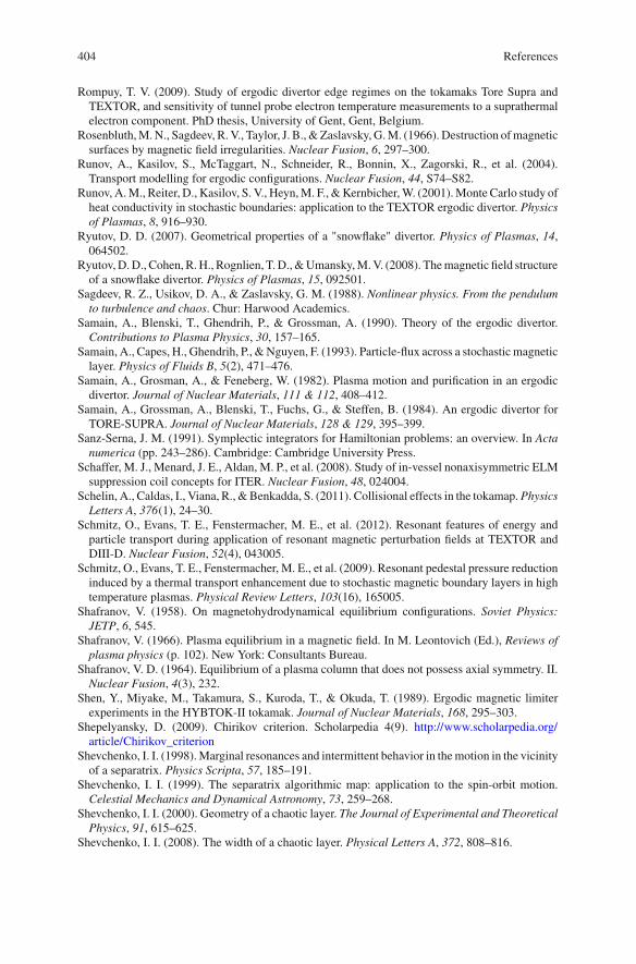
404 References
Rompuy, T. V. (2009). Study of ergodic divertor edge regimes on the tokamaks Tore Supra andTEXTOR, and sensitivity of tunnel probe electron temperature measurements to a suprathermalelectron component. PhD thesis, University of Gent, Gent, Belgium.
Rosenbluth,M.N., Sagdeev, R. V., Taylor, J. B., &Zaslavsky, G.M. (1966). Destruction ofmagneticsurfaces by magnetic field irregularities. Nuclear Fusion, 6, 297–300.
Runov, A., Kasilov, S., McTaggart, N., Schneider, R., Bonnin, X., Zagorski, R., et al. (2004).Transport modelling for ergodic configurations. Nuclear Fusion, 44, S74–S82.
Runov, A.M., Reiter, D., Kasilov, S. V., Heyn,M. F., &Kernbicher,W. (2001).Monte Carlo study ofheat conductivity in stochastic boundaries: application to the TEXTOR ergodic divertor. Physicsof Plasmas, 8, 916–930.
Ryutov, D. D. (2007). Geometrical properties of a "snowflake" divertor. Physics of Plasmas, 14,064502.
Ryutov,D.D., Cohen, R.H., Rognlien, T.D.,&Umansky,M.V. (2008). Themagnetic field structureof a snowflake divertor. Physics of Plasmas, 15, 092501.
Sagdeev, R. Z., Usikov, D. A., & Zaslavsky, G. M. (1988). Nonlinear physics. From the pendulumto turbulence and chaos. Chur: Harwood Academics.
Samain, A., Blenski, T., Ghendrih, P., & Grossman, A. (1990). Theory of the ergodic divertor.Contributions to Plasma Physics, 30, 157–165.
Samain, A., Capes, H., Ghendrih, P., &Nguyen, F. (1993). Particle-flux across a stochastic magneticlayer. Physics of Fluids B, 5(2), 471–476.
Samain, A., Grosman, A., & Feneberg, W. (1982). Plasma motion and purification in an ergodicdivertor. Journal of Nuclear Materials, 111 & 112, 408–412.
Samain, A., Grossman, A., Blenski, T., Fuchs, G., & Steffen, B. (1984). An ergodic divertor forTORE-SUPRA. Journal of Nuclear Materials, 128 & 129, 395–399.
Sanz-Serna, J. M. (1991). Symplectic integrators for Hamiltonian problems: an overview. In Actanumerica (pp. 243–286). Cambridge: Cambridge University Press.
Schaffer, M. J., Menard, J. E., Aldan, M. P., et al. (2008). Study of in-vessel nonaxisymmetric ELMsuppression coil concepts for ITER. Nuclear Fusion, 48, 024004.
Schelin, A., Caldas, I., Viana, R., &Benkadda, S. (2011). Collisional effects in the tokamap.PhysicsLetters A, 376(1), 24–30.
Schmitz, O., Evans, T. E., Fenstermacher, M. E., et al. (2012). Resonant features of energy andparticle transport during application of resonant magnetic perturbation fields at TEXTOR andDIII-D. Nuclear Fusion, 52(4), 043005.
Schmitz, O., Evans, T. E., Fenstermacher, M. E., et al. (2009). Resonant pedestal pressure reductioninduced by a thermal transport enhancement due to stochastic magnetic boundary layers in hightemperature plasmas. Physical Review Letters, 103(16), 165005.
Shafranov, V. (1958). On magnetohydrodynamical equilibrium configurations. Soviet Physics:JETP, 6, 545.
Shafranov, V. (1966). Plasma equilibrium in a magnetic field. In M. Leontovich (Ed.), Reviews ofplasma physics (p. 102). New York: Consultants Bureau.
Shafranov, V. D. (1964). Equilibrium of a plasma column that does not possess axial symmetry. II.Nuclear Fusion, 4(3), 232.
Shen, Y., Miyake, M., Takamura, S., Kuroda, T., & Okuda, T. (1989). Ergodic magnetic limiterexperiments in the HYBTOK-II tokamak. Journal of Nuclear Materials, 168, 295–303.
Shepelyansky, D. (2009). Chirikov criterion. Scholarpedia 4(9). http://www.scholarpedia.org/article/Chirikov_criterion
Shevchenko, I. I. (1998).Marginal resonances and intermittent behavior in themotion in the vicinityof a separatrix. Physics Scripta, 57, 185–191.
Shevchenko, I. I. (1999). The separatrix algorithmic map: application to the spin-orbit motion.Celestial Mechanics and Dynamical Astronomy, 73, 259–268.
Shevchenko, I. I. (2000). Geometry of a chaotic layer. The Journal of Experimental and TheoreticalPhysics, 91, 615–625.
Shevchenko, I. I. (2008). The width of a chaotic layer. Physical Letters A, 372, 808–816.
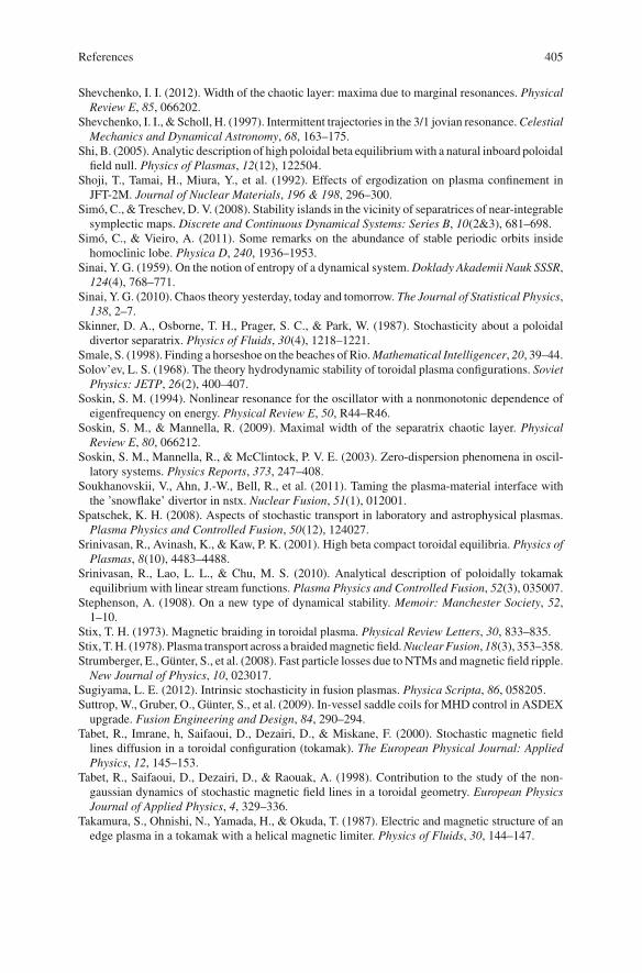
References 405
Shevchenko, I. I. (2012). Width of the chaotic layer: maxima due to marginal resonances. PhysicalReview E, 85, 066202.
Shevchenko, I. I., & Scholl, H. (1997). Intermittent trajectories in the 3/1 jovian resonance.CelestialMechanics and Dynamical Astronomy, 68, 163–175.
Shi, B. (2005). Analytic description of high poloidal beta equilibriumwith a natural inboard poloidalfield null. Physics of Plasmas, 12(12), 122504.
Shoji, T., Tamai, H., Miura, Y., et al. (1992). Effects of ergodization on plasma confinement inJFT-2M. Journal of Nuclear Materials, 196 & 198, 296–300.
Simó, C., & Treschev, D. V. (2008). Stability islands in the vicinity of separatrices of near-integrablesymplectic maps. Discrete and Continuous Dynamical Systems: Series B, 10(2&3), 681–698.
Simó, C., & Vieiro, A. (2011). Some remarks on the abundance of stable periodic orbits insidehomoclinic lobe. Physica D, 240, 1936–1953.
Sinai, Y. G. (1959). On the notion of entropy of a dynamical system. Doklady Akademii Nauk SSSR,124(4), 768–771.
Sinai, Y. G. (2010). Chaos theory yesterday, today and tomorrow. The Journal of Statistical Physics,138, 2–7.
Skinner, D. A., Osborne, T. H., Prager, S. C., & Park, W. (1987). Stochasticity about a poloidaldivertor separatrix. Physics of Fluids, 30(4), 1218–1221.
Smale, S. (1998). Finding a horseshoe on the beaches of Rio.Mathematical Intelligencer, 20, 39–44.Solov’ev, L. S. (1968). The theory hydrodynamic stability of toroidal plasma configurations. Soviet
Physics: JETP, 26(2), 400–407.Soskin, S. M. (1994). Nonlinear resonance for the oscillator with a nonmonotonic dependence ofeigenfrequency on energy. Physical Review E, 50, R44–R46.
Soskin, S. M., & Mannella, R. (2009). Maximal width of the separatrix chaotic layer. PhysicalReview E, 80, 066212.
Soskin, S. M., Mannella, R., & McClintock, P. V. E. (2003). Zero-dispersion phenomena in oscil-latory systems. Physics Reports, 373, 247–408.
Soukhanovskii, V., Ahn, J.-W., Bell, R., et al. (2011). Taming the plasma-material interface withthe ’snowflake’ divertor in nstx. Nuclear Fusion, 51(1), 012001.
Spatschek, K. H. (2008). Aspects of stochastic transport in laboratory and astrophysical plasmas.Plasma Physics and Controlled Fusion, 50(12), 124027.
Srinivasan, R., Avinash, K., & Kaw, P. K. (2001). High beta compact toroidal equilibria. Physics ofPlasmas, 8(10), 4483–4488.
Srinivasan, R., Lao, L. L., & Chu, M. S. (2010). Analytical description of poloidally tokamakequilibrium with linear stream functions. Plasma Physics and Controlled Fusion, 52(3), 035007.
Stephenson, A. (1908). On a new type of dynamical stability. Memoir: Manchester Society, 52,1–10.
Stix, T. H. (1973). Magnetic braiding in toroidal plasma. Physical Review Letters, 30, 833–835.Stix, T.H. (1978). Plasma transport across a braidedmagnetic field.Nuclear Fusion, 18(3), 353–358.Strumberger, E., Günter, S., et al. (2008). Fast particle losses due to NTMs andmagnetic field ripple.
New Journal of Physics, 10, 023017.Sugiyama, L. E. (2012). Intrinsic stochasticity in fusion plasmas. Physica Scripta, 86, 058205.Suttrop, W., Gruber, O., Günter, S., et al. (2009). In-vessel saddle coils for MHD control in ASDEXupgrade. Fusion Engineering and Design, 84, 290–294.
Tabet, R., Imrane, h, Saifaoui, D., Dezairi, D., & Miskane, F. (2000). Stochastic magnetic fieldlines diffusion in a toroidal configuration (tokamak). The European Physical Journal: AppliedPhysics, 12, 145–153.
Tabet, R., Saifaoui, D., Dezairi, D., & Raouak, A. (1998). Contribution to the study of the non-gaussian dynamics of stochastic magnetic field lines in a toroidal geometry. European PhysicsJournal of Applied Physics, 4, 329–336.
Takamura, S., Ohnishi, N., Yamada, H., & Okuda, T. (1987). Electric and magnetic structure of anedge plasma in a tokamak with a helical magnetic limiter. Physics of Fluids, 30, 144–147.
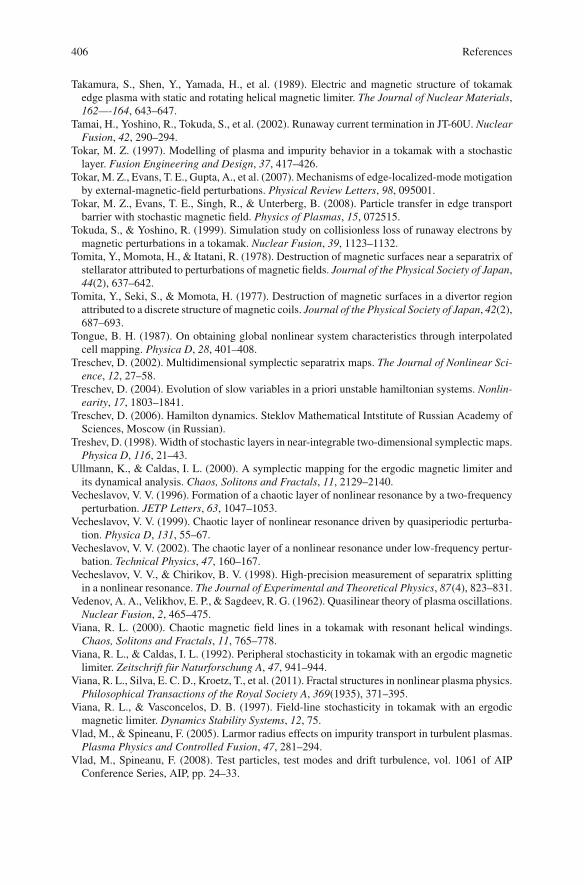
406 References
Takamura, S., Shen, Y., Yamada, H., et al. (1989). Electric and magnetic structure of tokamakedge plasma with static and rotating helical magnetic limiter. The Journal of Nuclear Materials,162—-164, 643–647.
Tamai, H., Yoshino, R., Tokuda, S., et al. (2002). Runaway current termination in JT-60U. NuclearFusion, 42, 290–294.
Tokar, M. Z. (1997). Modelling of plasma and impurity behavior in a tokamak with a stochasticlayer. Fusion Engineering and Design, 37, 417–426.
Tokar, M. Z., Evans, T. E., Gupta, A., et al. (2007). Mechanisms of edge-localized-mode motigationby external-magnetic-field perturbations. Physical Review Letters, 98, 095001.
Tokar, M. Z., Evans, T. E., Singh, R., & Unterberg, B. (2008). Particle transfer in edge transportbarrier with stochastic magnetic field. Physics of Plasmas, 15, 072515.
Tokuda, S., & Yoshino, R. (1999). Simulation study on collisionless loss of runaway electrons bymagnetic perturbations in a tokamak. Nuclear Fusion, 39, 1123–1132.
Tomita, Y., Momota, H., & Itatani, R. (1978). Destruction of magnetic surfaces near a separatrix ofstellarator attributed to perturbations of magnetic fields. Journal of the Physical Society of Japan,44(2), 637–642.
Tomita, Y., Seki, S., & Momota, H. (1977). Destruction of magnetic surfaces in a divertor regionattributed to a discrete structure of magnetic coils. Journal of the Physical Society of Japan, 42(2),687–693.
Tongue, B. H. (1987). On obtaining global nonlinear system characteristics through interpolatedcell mapping. Physica D, 28, 401–408.
Treschev, D. (2002). Multidimensional symplectic separatrix maps. The Journal of Nonlinear Sci-ence, 12, 27–58.
Treschev, D. (2004). Evolution of slow variables in a priori unstable hamiltonian systems. Nonlin-earity, 17, 1803–1841.
Treschev, D. (2006). Hamilton dynamics. Steklov Mathematical Intstitute of Russian Academy ofSciences, Moscow (in Russian).
Treshev, D. (1998). Width of stochastic layers in near-integrable two-dimensional symplectic maps.Physica D, 116, 21–43.
Ullmann, K., & Caldas, I. L. (2000). A symplectic mapping for the ergodic magnetic limiter andits dynamical analysis. Chaos, Solitons and Fractals, 11, 2129–2140.
Vecheslavov, V. V. (1996). Formation of a chaotic layer of nonlinear resonance by a two-frequencyperturbation. JETP Letters, 63, 1047–1053.
Vecheslavov, V. V. (1999). Chaotic layer of nonlinear resonance driven by quasiperiodic perturba-tion. Physica D, 131, 55–67.
Vecheslavov, V. V. (2002). The chaotic layer of a nonlinear resonance under low-frequency pertur-bation. Technical Physics, 47, 160–167.
Vecheslavov, V. V., & Chirikov, B. V. (1998). High-precision measurement of separatrix splittingin a nonlinear resonance. The Journal of Experimental and Theoretical Physics, 87(4), 823–831.
Vedenov, A. A., Velikhov, E. P., & Sagdeev, R. G. (1962). Quasilinear theory of plasma oscillations.Nuclear Fusion, 2, 465–475.
Viana, R. L. (2000). Chaotic magnetic field lines in a tokamak with resonant helical windings.Chaos, Solitons and Fractals, 11, 765–778.
Viana, R. L., & Caldas, I. L. (1992). Peripheral stochasticity in tokamak with an ergodic magneticlimiter. Zeitschrift für Naturforschung A, 47, 941–944.
Viana, R. L., Silva, E. C. D., Kroetz, T., et al. (2011). Fractal structures in nonlinear plasma physics.Philosophical Transactions of the Royal Society A, 369(1935), 371–395.
Viana, R. L., & Vasconcelos, D. B. (1997). Field-line stochasticity in tokamak with an ergodicmagnetic limiter. Dynamics Stability Systems, 12, 75.
Vlad, M., & Spineanu, F. (2005). Larmor radius effects on impurity transport in turbulent plasmas.Plasma Physics and Controlled Fusion, 47, 281–294.
Vlad, M., Spineanu, F. (2008). Test particles, test modes and drift turbulence, vol. 1061 of AIPConference Series, AIP, pp. 24–33.
References 407
Vlad, M., Spineanu, F., Itoh, S.-I., Yagi, M., & Itoh, K. (2005). Turbulent transport of ions withlarge larmor radii. Plasma Physics and Controlled Fusion, 47, 1015–1029.
von Hertweck, F., & Schlüter, A. (1957). Die “adiabatische invarianz” des magnetischen bahnmo-mentes geladener teilchen. Z. Naturforsch. A, 12, 844–849.
Wagner, F., Becker, G., Behringer, K., et al. (1982). Regime of improved confinement and high betain neutral-beam-heated divertor discharges of the asdex tokamak. Physical Review Letters, 49,1408–1412.
Wang, S. (2006). Canonical hamiltonian theory of the guiding-center motion in an axisymmetrictorus, with the different time scales well separated. Physics of Plasmas, 13, 052506.
Warnock, R. L., & Berg, S. J. (1996). Fast symplectic mapping, quasi-invariants, and long-termstability in the LHC. Particle Accelerators, 54, 213–222.
Weeks, E., Urbach, J. S., & Swinney, H. L. (1996). Anomalous diffusion in asymmetric randomwalks with a quasi-geostrophic flow example. Physica D, 97, 291–310.
Weiss, J. B., & Knobloch, E. (1989). Mass transport and mixing by modulated traveling waves.Physical Review A, 40, 2579–2589.
Weitzner, H. (1981). Motion of a charged particle in a nearly axisymmetric magnetic field. Physicsof Fluids, 24(12), 2280–2294.
Weitzner, H. (1995). Single-particle motion in nonaxisymmetric static electric and magnetic fields.Physics of Plasmas, 2(10), 3595–3604.
Weitzner, H., & Pfirsch, D. (1999). Nonperiodicity in space of the magnetic moment series. Physicsof Plasmas, 6(1), 420–423.
Wesson, J. (2004). Tokamaks (3rd ed.). Oxford: Clarendon Press.Weyssow, B., Misguich, J. H., & Balescu, R. (1991). Chaotic diffusion across a magnetic islanddue to a single low-frequency electrostatic wave. Plasma Physics and Controlled Fusion, 33(7),763–793.
White, R. B. (1990). Canonical Hamiltonian guiding center variables. Physics of Fluids B, 2(4),845–872.
White, R. B. (2001). The theory of toroidally confined plasmas (2nd ed.). London: Imperial CollegePress.
White, R. B., Boozer, A. H., & Hay, R. (1982). Drift Hamiltonian in magnetic coordinates. Physicsof Fluids, 25(3), 575–576.
White, R. B., &Chance,M. S. (1984). Hamiltonian guiding center drift orbit calculation for plasmasof arbitrary cross section. Physics of Fluids, 27(10), 2455–2467.
White, R. B., &Wu,Y. (1993). Collisionless transport in a stochasticmagnetic field.Plasma Physicsand Controlled Fusion, 35, 595–599.
White, R. B., & Zakharov, L. E. (2003). Hamiltonian guiding center equations in toroidal magneticconfigurations. Physics of Plasmas, 10(3), 573–577.
Wiggins, S. (2003). Introduction to applied nonlinear dynamical systems and chaos (2nd ed.). NewYork: Springer.
Wingen, A., Abdullaev, S. S., Finken, K. H., & Spatschek, K. H. (2006). Influence of stochasticfields on relativistic electrons. Nuclear Fusion, 46, 941–952.
Wingen, A., Evans, T. E., & Spatschek, K. H. (2009). Footprint structures due to resonant magneticperturbations in DIII-D. Physics of Plasmas, 16, 042504.
Wingen, A., Jakubowski,M., Spatschek, K. H., et al. (2007). Traces of stable and unstablemanifoldsin heat flux patterns. Physics of Plasmas, 14, 042502.
Wingen, A.,&Spatschek, K.H. (2008). Ambipolar stochastic particle diffusion and plasma rotation.Physics of Plasmas, 15, 052305.
Wingen, A., Spatschek, K. H., & Abdullaev, S. S. (2005). Stochastic transport of magnetic fieldlines in the symmetric tokamap. Contributions to Plasma Physics, 45, 500–513.
Wobig, H. (1987). Magnetic surfaces and localized perturbations in the Weldelstein VII-A stellara-tor. Z. Naturforsch. 42a, 1054–1066.
Wobig, H., & Pfirsch, D. (2001). On guiding centre orbits of particles in toroidal systems. PlasmaPhysics and Controlled Fusion, 43, 695–716.
408 References
Wolf, R. (2003). Internal transport barriers in tokamak plasmas. Plasma Physics and ControlledFusion, 45, R1–R91.
Yamagishi, T. (1995). Evaluation of the stochastic layer near separatrix in toroidal divertor. FusionTechnology, 27, 505–508.
Yan, L.W.,&Evans, T. E. (2007). Stochastic boundarymodeling by resonantmagnetic perturbationson DIII-D. Journal of Nuclear Materials, 363—-365, 723–727.
Yavorskij, V. A., Darrow, D., Goloborod’ko, et al. (2002). Fast ion non-adiabaticity in sphericaltokamaks. Nuclear Fusion, 42, 1210–1215.
Yoshida, Z. (1993). A remark on the Hamiltonian form of the magnetic-field-line equations. Physicsof Plasmas, 1(1), 208–209.
Yoshino, R., & Tokuda, S. (2000). Runaway electrons in magnetic turbulence and runaway currenttermination in tokamak discharge. Nuclear Fusion, 40(7), 1293–1309.
Yu, Q. (2006). Numerical modeling of diffusive heat transport across magnetic islands and localstochastic field. Physics of Plasmas, 13(6), 062310.
Yu, Q., & Günter, S. (2009). Effect of resonant magnetic perturbations on particle confinement.Nuclear Fusion, 49(6), 0621001.
Zaslavsky, G.M., &Abdullaev, S. S. (1995). Scaling properties and anomalous transport of particlesinside the stochastic layer. Physical Review E, 51, 3901–3910.
Zaslavsky, G. M., & Chirikov, B. V. (1971). Stochastic instability of non-linear oscillations. SovietPhysics: Uspekhi, 14(5), 549–568.
Zaslavsky, G. M., Sagdeev, R. Z., Usikov, D. A., & Chernikov, A. A. (1991). Weak chaos andquasi-regular patterns. Cambridge: Cambridge University Press.
Zehrfeld, H., Fussmann, G., & Green, B. J. (1981). Electric field effects on relativistic chargedparticle motion in tokamaks. Plasma Physics, 23(5), 473.
Zeng, L., Koslowski, H.R., Liang, et al. (2013). Experimental observation of a magnetic-turbulencethreshold for runaway generation in the TEXTOR tokamak. Physical Review Letters (to bepublished).
Zheng, S. B., Wootton, A. J., & Solano, E. R. (1996). Analytical tokamak equilibrium for shapedplasmas. Physics of Plasmas, 3(3), 1176–1178.
Zhou, R. J., Hu, L. Q., Li, E. Z., et al. (2013a). Investigation of ring-like runaway electron beamsin the EAST tokamak. Plasma Physics and Controlled Fusion, 55(5), 055006.
Zhou, R. J., Hu, L., Li, E., et al. (2013b). Effect of magnetic fluctuations on the confinement anddynamics of runaway electrons in the HT-7 tokamak. Physics of Plasmas, 20(3), 032511.
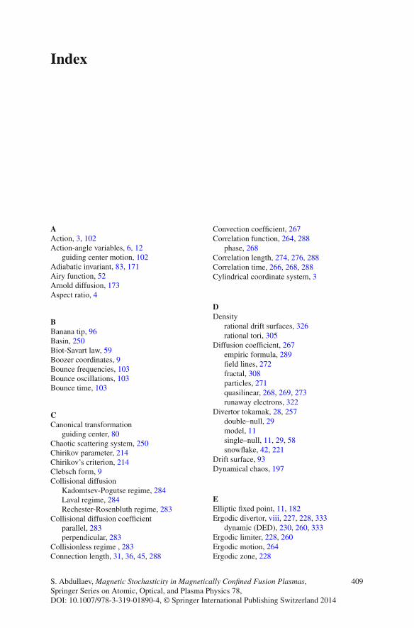
Index
AAction, 3, 102Action-angle variables, 6, 12
guiding center motion, 102Adiabatic invariant, 83, 171Airy function, 52Arnold diffusion, 173Aspect ratio, 4
BBanana tip, 96Basin, 250Biot-Savart law, 59Boozer coordinates, 9Bounce frequencies, 103Bounce oscillations, 103Bounce time, 103
CCanonical transformation
guiding center, 80Chaotic scattering system, 250Chirikov parameter, 214Chirikov’s criterion, 214Clebsch form, 9Collisional diffusion
Kadomtsev-Pogutse regime, 284Laval regime, 284Rechester-Rosenbluth regime, 283
Collisional diffusion coefficientparallel, 283perpendicular, 283
Collisionless regime , 283Connection length, 31, 36, 45, 288
Convection coefficient, 267Correlation function, 264, 288
phase, 268Correlation length, 274, 276, 288Correlation time, 266, 268, 288Cylindrical coordinate system, 3
DDensity
rational drift surfaces, 326rational tori, 305
Diffusion coefficient, 267empiric formula, 289field lines, 272fractal, 308particles, 271quasilinear, 268, 269, 273runaway electrons, 322
Divertor tokamak, 28, 257double–null, 29model, 11single–null, 11, 29, 58snowflake, 42, 221
Drift surface, 93Dynamical chaos, 197
EElliptic fixed point, 11, 182Ergodic divertor, viii, 227, 228, 333
dynamic (DED), 230, 260, 333Ergodic limiter, 228, 260Ergodic motion, 264Ergodic zone, 228
S. Abdullaev, Magnetic Stochasticity in Magnetically Confined Fusion Plasmas, 409Springer Series on Atomic, Optical, and Plasma Physics 78,DOI: 10.1007/978-3-319-01890-4, © Springer International Publishing Switzerland 2014
410 Index
FFast ions, 97, 172Fixed points, 108Fractal, 250Fundamental problem of dynamics, 125
GGauge transformation, 2Golden KAM tori, 170Grad-Shafranov equation, 20
analytical solutions, 20, 27Gyrofrequency, 79
normalized, 86radial oscillations, 79, 86reference, 79
Gyrophase, 80, 87, 171, 317
HHamilton-Jacobi equation, 125, 167Hamiltonian equation, 2, 4
autonomous, 3guiding center, 82, 84, 87, 89in flux coordinates, 6, 49non–autonomous, 3relativistic, 77
Hamiltonian flow, 123Hamiltonian function, 3
guiding center, 80, 82, 86, 89in flux coordinates, 6, 49perturbation, 169, 316relativistic, 77
Hamiltonian monodromy, 116Helical coils, 1, 230, 333Helical currents
density, 1, 3, 7, 14, 333, 335, 339, 346Horseshoe map, 198Hyperbolic fixed point, 11, 33, 182
guiding center, 108Hyperbolicity, 198
IIntegrability, 174integrability, 124Integral invariant, 102Internal (I-) coils, 234Internal transport barriers, 223Invariant tori, 167
KKAM theory, 6, 166
Kinetic equation, 267Kolmogorov entropy, 266Kolmogorov length, 280
finite-length, 280Kolmogorov time, 266, 279Kolmogorov’s technique, 168Kolmogorov’s theorem, 166Kolmogorov-Sinai entropy, 266Kubo number, 297, 315
LLaminar plot, 252Laminar zone, 252, 276Liouville’s equation, 267Lobe, 188, 198Lorentzian pulse, 47, 64, 379Lyapunov exponent, 180
finite-time, 280
MMagnetic chaos, viiiMagnetic coordinates, 9Magnetic field, 1
in flux coordinates, 9poloidal, 5, 23reversed shear, 223toroidal, 5, 21, 23
Magnetic field lines, 1equation, 1open, 250
Magnetic field perturbations, 47DED, 7, 339helical, 50model, 55, 232, 248poloidal spectra, 50, 236poloidal spectra asymptotics, 54, 57, 64,65, 229, 231
poloidal spectra model, 232, 245resonant, 227, 229saddle coils, 60, 63
Magnetic field, plasmaequilibrium, 19standard model, 21three–wire model, 42two–wire model, 38wire model, 36
Magnetic footprints, 154, 195, 243, 255Magnetic island, 204Magnetic moment, 83Magnetic perturbations
poloidal spectra, 50toroidal spectra, 50
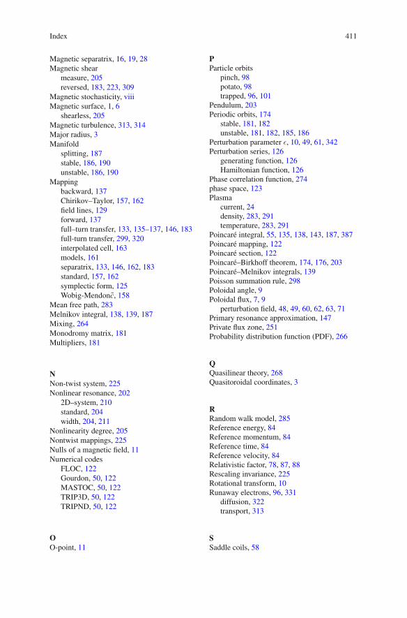
Index 411
Magnetic separatrix, 16, 19, 28Magnetic shear
measure, 205reversed, 183, 223, 309
Magnetic stochasticity, viiiMagnetic surface, 1, 6
shearless, 205Magnetic turbulence, 313, 314Major radius, 3Manifold
splitting, 187stable, 186, 190unstable, 186, 190
Mappingbackward, 137Chirikov–Taylor, 157, 162field lines, 129forward, 137full–turn transfer, 133, 135–137, 146, 183full-turn transfer, 299, 320interpolated cell, 163models, 161separatrix, 133, 146, 162, 183standard, 157, 162symplectic form, 125Wobig-Mendonc, 158
Mean free path, 283Melnikov integral, 138, 139, 187Mixing, 264Monodromy matrix, 181Multipliers, 181
NNon-twist system, 225Nonlinear resonance, 202
2D–system, 210standard, 204width, 204, 211
Nonlinearity degree, 205Nontwist mappings, 225Nulls of a magnetic field, 11Numerical codes
FLOC, 122Gourdon, 50, 122MASTOC, 50, 122TRIP3D, 50, 122TRIPND, 50, 122
OO-point, 11
PParticle orbits
pinch, 98potato, 98trapped, 96, 101
Pendulum, 203Periodic orbits, 174
stable, 181, 182unstable, 181, 182, 185, 186
Perturbation parameter ε, 10, 49, 61, 342Perturbation series, 126
generating function, 126Hamiltonian function, 126
Phase correlation function, 274phase space, 123Plasma
current, 24density, 283, 291temperature, 283, 291
Poincaré integral, 55, 135, 138, 143, 187, 387Poincaré mapping, 122Poincaré section, 122Poincaré–Birkhoff theorem, 174, 176, 203Poincaré–Melnikov integrals, 139Poisson summation rule, 298Poloidal angle, 9Poloidal flux, 7, 9
perturbation field, 48, 49, 60, 62, 63, 71Primary resonance approximation, 147Private flux zone, 251Probability distribution function (PDF), 266
QQuasilinear theory, 268Quasitoroidal coordinates, 3
RRandom walk model, 285Reference energy, 84Reference momentum, 84Reference time, 84Reference velocity, 84Relativistic factor, 78, 87, 88Rescaling invariance, 225Rotational transform, 10Runaway electrons, 96, 331
diffusion, 322transport, 313
SSaddle coils, 58
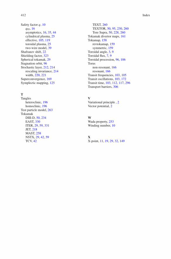
412 Index
Safety factor q, 10q95, 16asymptotics, 16, 35, 44cylindrical plasma, 25effective, 105, 119toroidal plasma, 25two-wire model, 39
Shafranov shift, 22Shielding factor, 323Spherical tokamak, 29Stagnation orbit, 96Stochastic layer, 212, 214
rescaling invariance, 214width, 220, 221
Superconvergence, 169Symplectic mapping, 125
TTangles
heteroclinic, 196homoclinic, 196
Test particle model, 263Tokamak
DIII-D, 50, 234EAST, 330ITER, 29, 59, 331JET, 218MAST, 258NSTX, 29, 42, 59TCV, 42
TEXT, 260TEXTOR, 50, 95, 230, 260Tore Supra, 50, 228, 260
Tokamak divertor maps, 161Tokamap, 158
revtokamap, 159symmetric, 159
Toroidal angle, 3, 9Toroidal flux, 7, 9Toroidal procession, 96, 106Torus
non-resonant, 166resonant, 166
Transit frequencies, 103, 105Transit oscillations, 103, 172Transit time, 103, 112, 117, 296Transport barriers, 306
VVariational principle , 2Vector potential, 2
WWada property, 253Winding number, 10
XX-point, 11, 19, 29, 32, 149