mabud-dissertation-2016.pdf - harvard dash
TRANSCRIPT
Appreciating Housing: The Role of Housing in Politics
CitationMabud, Rakeen. 2016. Appreciating Housing: The Role of Housing in Politics. Doctoral dissertation, Harvard University, Graduate School of Arts & Sciences.
Permanent linkhttp://nrs.harvard.edu/urn-3:HUL.InstRepos:33493473
Terms of UseThis article was downloaded from Harvard University’s DASH repository, and is made available under the terms and conditions applicable to Other Posted Material, as set forth at http://nrs.harvard.edu/urn-3:HUL.InstRepos:dash.current.terms-of-use#LAA
Share Your StoryThe Harvard community has made this article openly available.Please share how this access benefits you. Submit a story .
Accessibility
Appreciating Housing: The Role of Housing inPolitics
A dissertation presented
by
Rakeen Mabud
to
The Department of Government
in partial fulfillment of the requirementsfor the degree of
Doctor of Philosophyin the subject ofPolitical Science
Harvard UniversityCambridge, Massachusetts
April 2016

©2016 —Rakeen Mabud
All rights reserved.
Dissertation Advisor: Professor Jeffry Frieden Rakeen Mabud
Appreciating Housing: The Role of Housing in
Politics
Abstract
While the economic implications of housing have been examined extensively, surpris-
ingly limited attention has been devoted to how the housing market impacts politics. My
dissertation is a three paper compilation that addresses the relationship between housing
and politics. Taken together, this dissertation traces through the ways in which housing
plays a role in American political life, from preference formation to concrete participatory
outcomes such as voting and writing to legislators.
In my first paper, Unemployment Shocks, Housing Wealth and Political Preferences,
I demonstrate that housing has micro-economic implications for the way people smooth
over income shocks. I find that people in counties which experience an unexpected un-
employment shock finance that shock using mortgage loans, and that there is a life-cycle
aspect to such financing. I also find that people perceive social insurance and home equity
as substitutes, but only when access to home equity is relatively high.
My second paper, Lending Support: Agency MBS Issuance and Rewarding Incum-
bents, examines how a shock to housing wealth affects electoral outcomes. I demonstrate
that after experiencing a large increase in mortgage credit post-2000, low-income counties
were more likely to support their incumbents. This effect principally pertains to Demo-
cratic incumbents, who were particularly vocal in advocating for the maintenance of these
iii
loosened credit conditions, and used these conditions to claim credit for providing access
to housing in poorer counties.
Finally, my third paper, Local Economic Information, Foreclosure and Political At-
titudes, delves into the cognitive role that housing plays in making individual political be-
havioral decisions. I find that reading about or seeing a photo of a foreclosed house makes
respondents more likely to send a strongly worded letter to their Member of Congress,
whereas seeing a photo of a foreclosed house is about twice as likely to make respondents
express interest in engaging with their local community. I also find that seeing a photo of a
foreclosure and reading about foreclosures serve as almost perfect substitutes.
iv
| Contents
Abstract iii
Acknowledgments vii
Introduction 1
1 Unemployment Shocks, Housing Wealth and Political Preferences 61.1 Introduction . . . . . . . . . . . . . . . . . . . . . . . . . . . . . . . . . . 61.2 Theory and Hypotheses . . . . . . . . . . . . . . . . . . . . . . . . . . . . 111.3 Data and Research Design . . . . . . . . . . . . . . . . . . . . . . . . . . 181.4 Results . . . . . . . . . . . . . . . . . . . . . . . . . . . . . . . . . . . . . 261.5 Conclusion . . . . . . . . . . . . . . . . . . . . . . . . . . . . . . . . . . 37
2 Lending Support: Agency MBS Issuance and Rewarding Incumbents 402.1 Introduction . . . . . . . . . . . . . . . . . . . . . . . . . . . . . . . . . . 402.2 Housing and Politics . . . . . . . . . . . . . . . . . . . . . . . . . . . . . 432.3 Theory . . . . . . . . . . . . . . . . . . . . . . . . . . . . . . . . . . . . . 492.4 Data and Empirical Strategy . . . . . . . . . . . . . . . . . . . . . . . . . 582.5 Results . . . . . . . . . . . . . . . . . . . . . . . . . . . . . . . . . . . . . 632.6 Conclusion . . . . . . . . . . . . . . . . . . . . . . . . . . . . . . . . . . 71
3 Local Economic Information, Foreclosure, and Political Attitudes 743.1 Introduction . . . . . . . . . . . . . . . . . . . . . . . . . . . . . . . . . . 743.2 Theory . . . . . . . . . . . . . . . . . . . . . . . . . . . . . . . . . . . . . 783.3 Research Design . . . . . . . . . . . . . . . . . . . . . . . . . . . . . . . 813.4 Results . . . . . . . . . . . . . . . . . . . . . . . . . . . . . . . . . . . . . 933.5 Discussion and Potential Mechanisms . . . . . . . . . . . . . . . . . . . . 973.6 Conclusion . . . . . . . . . . . . . . . . . . . . . . . . . . . . . . . . . . 101
A Appendix to Chapter 1: Robustness Checks 104
B Appendix to Chapter 2: Data 105
C Appendix to Chapter 2: House Electoral Data 106v

D Appendix to Chapter 2: Turnout 108
E Appendix to Chapter 3: Summary Statistics and Balance Table 111
F Appendix to Chapter 3: Robustness Checks 112
Bibliography 117
vi
| Acknowledgments
This dissertation would not have been possible without the help and support of many
people.
Jeff Frieden was a fantastic advisor, and I am grateful for his insistence on theoretical
clarity and for constantly pushing me to think more critically about my work. His ability
to get right to the core of the argument is superhuman, and my work is stronger and more
interesting because of his generosity with his time – and because of his willingness to
always chase me down if I hadn’t seen him for a while. I was very fortunate to have the
opportunity to work with Gwyneth McClendon, and her wide-ranging expertise, thoughtful
criticism and incredible work ethic have been inspiring throughout this process. Claudine
Gay has been a wonderful mentor. Not only has she encouraged me to push my work
further, our conversations have been invaluable as I have considered my post-graduation
options.
I am unbelievably grateful to have found the best dissertation group – Jonny Phillips
and Soledad Prillaman. I am truly fortunate to have peers who are not only incredibly
thoughtful scholars, but have also brought so much laughter into the last five years. We have
“baboomed" everything from generals to prospectus defenses, and I can’t wait to “baboom"
your dissertation defenses next year. I’ll bring the chocolate milk and mini-eggs.
Rachel Barringer, Erica Farrell, Karma Longtin, and Chiara Superti have – quite lit-
erally – turned my world upside down on numerous occasions, and I am grateful for the
vii
patience, work ethic and optimism they have helped me cultivate. Many thanks to Julie
Faller and Shelby Grossman for helping me clear my head and encouraging me to always
go further – even if that meant the pace dropped.
I am grateful to the members of the Diversity Working Group for giving me purpose
over the last five years. Special thanks to Emily Clough, from whom I have learned how to
be more articulate, thoughtful and entrepreneurial.
For fruitful discussions, guidance and support, I thank Lisa Abraham, Steve Ansolabehere,
Joyce Chen, Moeena Das, Nadza Durakovic, Jesse Gubb, Alex Hertel-Fernandez, Tor-
ben Iversen, Matt Johnson, Jessica Kim, Heather Law, Steve Levitsky, Christopher Lu-
cas, Xing-Yin Ni, Stephen Pettigrew, Melissa Sands, Rob Schub, Brandon Stewart, Jason
Warner, Akila Weerapana, Shanna Weitz, Tess Wise, and Ariel White. This work has ben-
efited from the financial support of the Institute of Quantitative Social Science and the
Center for American Political Studies. The third paper was approved by the Harvard Uni-
versity Committee on the Use of Human Subjects under Protocol number IRB15-3851. I
also thank Yotam Margalit for sharing his data.
I am so lucky to have a loving and supportive family. My parents, Sayeeda and Abdul,
have sacrificed so much to give me the life I have, and I am eternally grateful to them.
Thank you to my brother Tarub, who is the best listener and one of my best friends.
Finally, to John Marshall, thank you for your countless hours of Stata help, editing,
getting excited about Topkis, and for all your work in making this a fundamentally better
dissertation. More importantly, you have made me a fundamentally better person and I
can’t wait for our next adventure.
viii
| Introduction
While housing has been covered extensively in the economic literature, political scien-
tists have not spent much time writing about the political implications of housing.1 Despite
the lack of attention, there are good reasons to believe that homeowership has important
implications for political activity. Not only is homeownership a widespread phenomenon,
but it is a dimension of American life that touches the social, economic and political
realms. Homeownership cross-cuts many of the other dimensions that social scientists
think about when considering political outcomes, including income, occupation, race and
gender. Where an individual lives determines the neighborhood, schools, and community
he or she is a part of, which can influence all kinds of political behaviors, from whether
individuals are likely to vote (Gerber, Green, and Larimer 2008), to local political engage-
ment (Fischel 2009). Moreover, an individual’s home is often the largest portion of their
wealth asset portfolio (21 percent on average2), and housing is one of the few wealth assets
that individuals simultaneously consume and invest in.
My dissertation is a three paper compilation that addresses the relationship between
housing and politics. In this dissertation, I delve into the reasons that housing is important
to a number of political outcomes. In my first paper, Unemployment Shocks, Housing
Wealth and Political Preferences, I demonstrate that housing is not simply an important
1Notable exceptions include Fischel (2009), Ansell (2014) and Scheve and Slaughter (2001b).
2Data from the 2004 Survey of Consumer Finances, calculated by Munnell, Soto, and Aubry (2007).
1
indicator in the macro-economy, but has important micro-economic implications for the
way people smooth over income shocks. I show that these micro-economic implications
also influences peoples’ policy preferences over social spending. My second paper, Lend-
ing Support: Agency MBS Issuance and Rewarding Incumbents, examines how a shock
to housing wealth affects electoral outcomes. Finally, my third paper, Local Economic In-
formation, Foreclosure and Political Attitudes, delves into the cognitive role that housing
plays in making individual political behavioral decisions.
Paper 1: Unemployment Shocks, Housing Wealth and Political Prefer-
ences
The first paper explores how people use housing wealth to finance unexpected shocks,
particularly unemployment shocks. Using data from the Census, the Home Mortgage Dis-
closure Act, Zillow.com and panel survey data on political preferences, I find that counties
that experience an unemployment shock are more likely to experience an uptick in mort-
gage loan applications. I interpret this as evidence for individuals tapping into housing
wealth when faced with an unexpected shock, which I define as an income shock that is
probabilistic in nature. I also find evidence for the fact that there is a life cycle aspect to
the way individuals draw on housing wealth to weather unexpected shocks. Counties with
large proportions of young and middle-aged people are differentially more likely to see
an uptick in mortgage loan applications when faced with an unemployment shock relative
to counties with large proportions of older people. I demonstrate that housing market liq-
uidity plays a crucial role in determining whether or not the average voter turns to home
equity-based borrowing during an unemployment shock. Finally, I provide evidence con-
sistent with Ansell (2014), namely that people facing an unemployment shock and living
in an area with appreciating house prices prefer less social insurance - but only if they also
2
live in an area where access to home equity is feasible. This suggests that social insurance
private insurance in the form of home equity do serve as substitutes, but only when housing
market liquidity is relatively high.
Paper 2: Lending Support: Agency MBS Issuance and Rewarding In-
cumbents 3
The second paper explores a massive run-up in GSE mortgage-backed security (MBS)
issuance in the early 2000s. This run-up in mortgage issuance started the process that
would eventually end in the largest financial crisis since the Great Depression. At the time,
however, the increased issuance of MBS was seen as a boon in easing credit access and
increasing homeownership among communities had previously lacked access to credit. I
argue that this increase in the availability of housing credit in the pre-crisis period affected
voting for incumbents in the counties that were most affected by GSE policy. I suggest
that legislators both advocated the maintenance of these loosened credit conditions as well
as used these conditions as an opportunity to claim credit for access to housing in poorer
counties. I focus on low-income counties, as they were the areas that were most affected by
the GSE policy. In this paper, I first demonstrate that low-income counties were indeed the
counties that benefited the most from GSE MBS issuance. I also show that these counties
were more likely to support their incumbents after the policy was put in place, especially if
their incumbents were Democrats.
3This study was approved by the Harvard University Committee on the Use of Human Subjects underProtocol number IRB15-3851.
3
Paper 3: Local Economic Information, Foreclosure and Political Atti-
tudes
The final paper takes an experimental approach to examine how the way in which peo-
ple receive information about their local economic environment affects political behavior.
Drawing from the economic voting and political psychology literature, I experimentally
vary the way in which survey respondents receive information about foreclosure rates in
their local area. I find that reading about or seeing a photo of a foreclosed house makes
respondents more likely to send a strongly worded letter to their Member of Congress,
whereas seeing a photo of a foreclosed house is about twice as likely to make respondents
express interest in engaging with their local community when presented with a hypotheti-
cal scenario. I also find that seeing a photo of a foreclosure and reading about foreclosures
serve as substitutes. The evidence suggests that the treatments operate through increased
concerns about the local community, particularly local housing values.
The project touches on several literatures in political science, but engages most with
the literature on economic voting. All three papers start from the core of economic voting
- namely, that voters use the economic environment as a heuristic when making political
choices. Paper 1 demonstrates that not only does housing play an important role in the way
in which people deal with economic shocks, but it also informs political preferences. These
preferences translate into aggregate behaviors such as voting, as demonstrated in Paper 2
and individual behaviors such as writing letters to legislators, as demonstrated in Paper
3. Papers 2 and 3 are also similar in that they examine experiential ways in which voters
receive politically salient information, whether at the individual or local housing market
level.
Taken together, this dissertation traces through the various ways in which housing plays
4

a role in American political life, from preference formation to concrete participatory out-
comes such as voting and writing to legislators, and provides a compelling argument that
we should be paying more attention to housing in the political science literature.
5
1 | Unemployment Shocks, Housing Wealth andPolitical Preferences
1.1 Introduction
In this paper, I explore the relationship between home equity wealth, the way in which
people smooth income shocks, and political preferences for social spending. While there
exists an extensive literature on different types of income shocks and how people weather
such shocks (Krueger and Perri 2009; Baker 2015), there is limited research examining
how people finance income shocks using housing wealth, and how financing shocks in this
way affects political preferences. This paper focuses on unemployment shocks, an income
shock that affects broad swaths of the population. In 2015, the U.S. unemployment rate
was 5.3 percent, which translates to more than 8 million unemployed people.1
I argue that housing wealth, economic decision making, and political preferences are
inexorably linked. The United States is, after all, still feeling the echoes of the housing bub-
ble that started in the mid-2000s. The bubble fueled home values to unprecedented heights,
and this made homeowners feel richer. Less directly, it offered homeowners access to a
new kind of wealth - home equity based borrowing - using homes as collateral (Chinn and
1The denominator of the unemployment rate is the total number of people in the labor force, whichrequires that people are actively searching for employment. It does not capture, therefore, people who haveleft the labor force because of frustration or long-term unemployment.
6
Frieden 2011).2 Although home equity loans became popular as the housing bubble grew,
these financing tools had been used long before the 2005. Housing is and has historically
been a large proportion of household wealth: according to data from the 2004 Survey of
Consumer Finances, housing wealth comprised of about a fifth of a family’s wealth, on
average (Munnell, Soto, and Aubry 2007). Not only is homeownership a widespread phe-
nomenon - in 2010, approximately 65 percent of families in the United States owned their
primary residence (Mazur and Wilson 2011) - but it is a key dimension of American life
that touches the social, economic and political realms.
Having such a large proportion of wealth tied up in one’s home means that it is often the
first store of wealth people turn to when financing an income shock. In this paper, I suggest
that people use home equity to finance unemployment shocks. Because unemployment
shocks are probabilistic and require short-term financing (in comparison to other income
shocks, such as retirement financing) dipping into home equity is a way to quickly access
one’s wealth. Recent work in economics speak to the dynamics I am exploring in this paper.
Campbell and Cocco (2007) find that rising house prices increase consumption through two
channels. First, rising house prices increase a household’s perceived wealth. Second, rising
house prices result in relaxed borrowing constraints. I argue that these channels come into
play when smoothing income shocks, as well as consumption. Rising house prices make
homeowners feel as though their future wealth will be higher, and the availability of home
equity means that homeowners also feel richer now. I take the Campbell and Cocco (2007)
argument one step further and theorize that when an area is hit with an economic shock,
homeowners may see housing wealth as a way to smooth the income shock particularly
2There are two main forms of home equity based borrowing: home equity loans and home equity lines ofcredit (HELOCs). Home equity loans work like a standard mortgage loan - they offer the borrower a fixedamount of money that is paid back in regular installments. If the borrower fails to make payments, the bankcan foreclose on the house. HELOCs work like a credit card: the loans are not for a fixed amount, and theline of credit can be drawn on whenever it is needed. Like traditional home equity loans, HELOCs hold thehome as collateral and if the loan is not paid back on time, the bank can foreclose on the house.
7
when it seems as though home values will continue to rise and home equity is available at
the time of the shock.
I also propose a life-cycle component to the way in which people use housing wealth
to smooth consumption when hit with an unemployment shock. I argue that counties with
large young and middle-aged populations are more likely to experience an uptick in mort-
gage applications because unemployment shocks are most salient this segment of the pop-
ulation. These predictions are consistent with Mian and Sufi (2011), who find that home-
equity based borrowing was concentrated among younger households and households with
lower credit scores.
In the political science literature, Ansell (2014) develops a micro-level theory that
households use home equity as a stock of private insurance, which builds on previous
macro-level work on the potential tradeoff between homeownership and social spending
(Kemeny 1981; Castles 1998; Conley and Gifford 2006; Prasad 2012). In his paper, Ansell
examines the relationship between homeownership and preferences for social insurance,
and finds a direct substitutive relationship between appreciating home values and prefer-
ences for social insurance in the US and UK. The basic mechanism is that when house
prices are appreciating, homeowners not only experience an income effect that makes them
feel wealthier, but also face a greater tax burden associated with home appreciation. Both
the greater tax burden and the income effect move homeowners in an anti-tax direction,
which translates into a decreased preference for social insurance.
This paper addresses the underlying assumption that forms the basis of Ansell’s work,
namely, whether people actually use their homes as a source of income when faced with
a shock. Unlike Ansell (2014), who focuses on social programs that support pensions
and redistribution, my focus on unemployment deliberately distinguishes between “ex-
pected income shocks" (e.g. the need to finance for retirement) and “unexpected income
shocks" (e.g. the need to finance unemployment). I contend that not only do unexpected
8
income shocks such as unemployment and disability disproportionately fall on the young
and middle-aged, but that these sorts of expected shocks require immediate financing. The
immediate need for funds is conducive to home equity based borrowing, which allows
homeowners to access their wealth quickly.
This paper also delves deeper into Ansell’s theory regarding the substitutive nature
of housing wealth as a source of private insurance and preferences for social insurance.
I contend that this relationship only holds when home equity is available and accessible
to the homeowner in the period in which the homeowner is faced with an income shock.
Specifically, I argue that in order for homeowners to rely on their housing wealth as a source
of private financing, they must not only live in an area where house prices are appreciating,
but also where housing liquidity is high.
To test these hypotheses, I examine county-level unemployment shocks and I find that
these shocks are strongly correlated with an increase in mortgage loan applications. These
results suggest that home equity based borrowing is a channel that people pursue when
faced with an income shock. I also show that counties with a large proportion of middle-
aged people are more likely to apply for mortgage loans. I theorize that this is because of
the young, middle-aged and elderly, the middle-aged are the only ones for whom unem-
ployment is salient and who are likely to have home equity to draw on when faced with a
shock. Finally, I demonstrate that counties with a liquid housing market are more likely to
experience an uptick in mortgage loan applications, because it is only when home equity is
accessible to homeowners that they can use it to finance an income shock.
Turning to political preferences, I expand on Ansell’s (2013) claim that when house
prices are appreciating, homeowners use home equity as private insurance, which in turn
substitutes for their demand for social insurance. Using individual panel survey data, I
show that for individuals experiencing an unemployment shock, this relationship holds
only when housing market liquidity is high. This result again points to the importance of
9
home equity availability in income shock financing and in developing political preferences
towards the welfare state.
Other work in political science also delves into the political relationship between hous-
ing wealth and the way in which people finance income shocks. Margalit (2013) uses a
within-subject research design to show how unemployment shocks change peoples’ pref-
erences for social insurance programs. In particular, Margalit demonstrates that unemploy-
ment shocks can have a particularly large positive effect on the desire for more welfare
state spending. I argue that the relationship that Margalit finds is mediated by local hous-
ing market conditions. Similarly, Popa (2013) and Scheve and Slaughter (2001a) find a link
between home values and voter preferences. Popa (2013) argues that the median voter’s
preference over the level of a housing subsidy affects whether a county experiences a hous-
ing bubble or not. Scheve and Slaughter (2001a) find in regions with a preponderance
of “comparative-disadvantage" industries, homeownership will result in decreased prefer-
ence for free trade because increasing free trade will result in lower home values. Fischel
(2009) proposes the “homevoter hypothesis," which argues that because of their large fi-
nancial stake in the local community, homeowners are more likely to participate in local
politics. This paper further explores the mechanism by which home values might translate
into preferences and political action, namely via home equity based borrowing.
The next section lays out the theory and hypotheses. Section 3 describes the data and
specifications used, and Section 4 reports the empirical results. The penultimate section
discusses the results, and the final section concludes.
10
1.2 Theory and Hypotheses
1.2.1 Theory
This project places housing wealth in the center of economically oriented questions
about how people finance economic shocks. I focus primarily on unemployment shocks,
and in the following section lay out why these types of shocks - which I term “unexpected
shocks" - are likely to be financed using housing wealth. I theorize that unemployment
shocks are particularly salient for the younger and middle-aged populations, and that these
age groups are therefore more likely to draw on housing wealth to finance an unemployment
shock, conditional on having housing wealth in the first place. I suggest that while housing
wealth is a financing tool that many may reach for, whether or not they do so depends on the
broader state of the housing market. Moreover, I argue that the ability to draw on housing
wealth when facing an income shock affects preferences for social insurance. A liquid
housing market allows homeowners to use their home equity as a store of private insurance,
which in turn decreases their demand for social spending related to unemployment relief.
Unemployment Shocks
While existing work on the welfare state tends to group together income shocks ranging
from unemployment to retirement financing (Ansell 2014)3, I suggest that these different
shocks have properties that cause people to react to them differently. I argue that there are
two types of income shocks - and associated social insurance programs - that are often con-
flated: “expected" shocks and “unexpected" shocks. Consider, for example, Social Security
and disability insurance, two social insurance programs that I argue address two different
3Some economists argue that retirement financing should not be considered an income shock becauseexpected shocks such as this would suggest consumption smoothing as the best strategy (Hall 1978).
11
kinds of income shocks. Social Security insures individuals against old age and the uncer-
tainty of the length of life. This kind of income shock can be anticipated - everyone has to
finance retirement. On the other hand, disability insurance and unemployment insurance
work to protect the individual from unanticipated shocks that are probabilistic in nature.
In this paper, I refer to anticipated income shocks as “expected shocks," and probabilistic
income shocks as “unexpected shocks." I focus particularly on unemployment shocks be-
cause in addition to there being a particularly strong insurance motive to protect against job
loss - it is not something that is necessarily stratified among different income classes, such
as job related disability - unemployment represents a particularly immediate and hard hit
to income.
While some homeowners can draw on housing wealth to finance such unemployment
shocks, this is dependent on conditions in the housing market in their local area. For those
who cannot draw on housing wealth, the unemployed can turn to publicly funded unem-
ployment insuance, which typically provides a maximum of 26 weeks of support.4 Pub-
lic unemployment insurance provides approximately 50 percent of the recipients’ average
weekly pay.
Life Cycle
There is a life cycle aspect to the way in which people use home equity to finance unex-
pected shocks. The life cycle dimension brings together two important factors: sensitivity
to unemployment shocks and home equity availability. Unemployment shocks are espe-
cially salient for those in the labor force - the young and the middle-aged. Campbell and
Cocco (2007) find that aggregate consumption becomes more responsive to house prices
for older homeowners (and that young renters are essentially unresponsive to changes in
4Congress extended unemployment insurance to 73 weeks in 2010 due to the recession.
12
house prices), which is consistent with the life-cycle theory of income smoothing. Relat-
edly, Sinai and Souleles (2005) demonstrate that homeowners who expect to live in the
home for a long time are hedged against volatility in rents and house prices. This in turn
suggests that changes in house prices for long-term home owners should not affect con-
sumption patterns. This further bolsters the theoretical assertion that younger homeowners
are more likely to experience a wealth effect when house prices are rising, which may lead
them to view their home equity as a way of financing income shocks.
While younger homeowners are more likely to use home equity to finance an unex-
pected shock relative to the older population, middle-aged workers are especially likely to
finance shocks in this way. Not only are unemployment shocks relatively salient to middle-
aged workers - they have not yet retired - but middle-aged people are more likely to have
home equity to draw on to finance a shock relative to younger workers. Middle-aged work-
ers, therefore are the most likely subset of the population to be using home equity to finance
shocks.
Housing Market Conditions
I also suggest that conditions in the housing market affect whether or not people draw
on housing wealth when hit with an unexpected shock such as unemployment. In particular,
how liquid the housing market is when the shock hits will affect the likelihood of financing
using housing wealth. Housing market liquidity refers to how easy it is to extract wealth
out of one’s home. One way to access the equity in a home is by taking out a loan using
the property as collateral. Home equity loans, HELOCs (home equity lines of credit), and
reverse mortgages (for the elderly) are examples of this sort of wealth extraction.5 My
5People can also sell their homes to tap into the built up equity. A large body of work (Venti and Wise1989, 1990, 2004) argues that older homeowners use their housing wealth as a buffer against late life shocks(e.g. spouse death, moving to a nursing home or other events that decrease income and/or raise expenditures),but I do not focus on this sort of financing in this paper.
13
theory is built primarily around the concept of home equity loans, and the data that I use
to test my theory are also most closely associated with home equity loans (rather than
HELOCs or other forms of home-based wealth extraction.)
Campbell and Cocco (2007) demonstrate that increasing housing values, via a wealth
effect channel, increase consumption, and I argue that housing market liquidity affects the
likelihood of financing a shock through a similar channel. When it is easy to access home
equity based wealth, people are more likely to use that wealth to finance a shock. In other
words, if the housing market is liquid, the homeowner may also feel comfortable making
a bet that housing market conditions will continue to improve, which makes the burden of
taking on a second loan less onerous.
Political Preferences
Ansell (2014) argues that home equity serves as a source of private insurance, and as
such, decreases demand for social insurance - if one can self insure, one is less likely to
want to pay into a social insurance system. He argues that when house prices are appre-
ciating, the combination of feeling richer and being faced with a larger tax burden deters
homeowners from increasing support towards social insurance. This paper both theorizes
about the basis of Ansell’s argument - namely, that people use home equity to finance in-
come shocks, and takes the argument one step further. I suggest that unemployment shocks,
housing market liquidity and home equity come together to influence political preferences
for social insurance. Specifically, I argue that in order for Ansell’s substitutive relationship
between home equity and social insurance preferences to hold, homeowners must have
access to their housing wealth. This means that homeowners must both live in a liquid
housing market and have home equity to draw on.
This paper is closely connected to an extensive and well-developed political science
literature on the welfare state. Meltzer and Richard (1981) suggest that welfare state pref-
14
erences are determined by the median voter, and the preferred size of government changes
as the income distribution changes. While Meltzer and Richard focus primarily on income
and productivity, Iversen and Soskice (2001) bring in the idea that skill-based assets also
affect the kind of welfare state that a country will end up with. Like Iversen and Sos-
kice, I focus on assets and their relationship to the welfare state, but turn my attention to
wealth-based assets rather than skill-based ones.
1.2.2 Hypotheses
Loans that use houses as collateral are relatively less costly to acquire in the short term,
but can be more costly than selling the house over the long term. This is because the
immediate transaction costs for selling a home and searching for a new place to live are
relatively high, but in the long run those transaction costs cease to be relevant. While it is
relatively easy to acquire a home equity loan in the short term, paying off the second lien
is generally spread out over a long period of time and can be financially onerous. I predict,
therefore, that homeowners facing different types of shocks will use different methods to
finance an adverse event.
Individual responses reflect both the nature of the shock and the stage of the life cycle in
which people face these different types of shocks. Individuals facing an unexpected shock
such as unemployment are more likely to turn to home equity loans than individuals facing
a expected shock (i.e. retirement). This is because financing an unexpected shock requires
immediate and up-front funds, whereas expected shocks, by definition, can be anticipated
and financed through measures that are less time sensitive, such as selling or downsizing a
home. Selling a home is costly in terms of time, as is finding a place to live. Because the
transaction costs of acquiring a home equity loan are lower than the transaction costs of
selling a house, those facing immediate financial difficulties may be more likely to turn to
15
home equity loans. Alternatively, the homeowner may not need to access the entire value
of the house, and taking out a loan rather than selling allows them to maintain a portion of
their investment. I suggest that because younger and middle-aged people are more sensitive
to unemployment shocks (and unexpected shocks more broadly) than older people because
of their presence in the labor force, they are more likely to use the kind of financing that
allows them to access funds quickly - taking out a loan using their home as collateral.
For a better understanding of what such a home equity loan transaction might look like,
consider a house that is currently valued at $1 million, with an outstanding mortgage (lia-
bility) of $850,000. The maximum amount of value the homeowner can extract out of the
house will depend on the equity on the house - the current value of the house minus mort-
gage liability. In this example the home equity is $150,000 ($1,000,000 - $850,000).6 If the
homeowner would like to take a $20,000 loan using the home as collateral, the bank would
compare the value of the loan the homeowner is asking for to the current equity in the
house. If the value of the home went down, say to $890,000 (keeping the mortgage liability
constant), the bank may be less likely to give the homeowner a $20,000 loan, since the
home equity is only $40,000. If the home value went up to $1.2 million keeping the mort-
gage constant, the homeowner could ask for an increased credit line since the bank knows
that the home equity (now at $350,000) is more than enough to cover a $20,000 loan. This
is a simplistic picture that does not include other criteria that the bank may use, such as the
homeowner’s credit rating, and restrictions on the loan-to-value ratio (currently 80% for
homeowners with a good credit rating). However it illuminates why middle-aged home-
owners might be more likely to use their homes to finance shocks - they are more likely
to own parts of their homes, and therefore have more equity in the house than younger
homeowners who are still likely to be paying off large mortgages.
6Homeowners who are “underwater," where the mortgage liability is greater than the value of the home,are not usually able to acquire home equity loans.
16
Hypothesis 1: Younger homeowners are more likely than older homeowners to finance
unemployment shocks using housing wealth. This is both because unemployment shocks
require immediate financing, which second liens can deliver, and because younger people
are more likely to be affected by unemployment.
Hypothesis 2: Middle-aged adults are more likely to be homeowners than younger adults.
Although both groups are susceptible to unemployment shocks, middle-aged adults are
more likely to be able to finance unexpected shocks using housing wealth because they are
more likely to have enough home equity to do so.
No matter how a homeowner opts to tap their home equity when facing a shock, local
housing market conditions will affect whether or not they do so to begin with. Both ac-
cessibility to housing equity and the willingness of the homeowner to bet on an improving
housing market contribute to how willing and able an individual is to rely on their home to
weather adverse shocks.
Hypothesis 3: When homeowners experience a more liquid or favorable local housing
market, they are more likely to use housing wealth to finance unexpected shocks.
Finally, housing market conditions, life-cycle dynamics and unemployment shocks
come together to influence political preferences towards social insurance. In order for
home equity to serve as a form of private insurance (Ansell 2014), homeowners must be
able to access their wealth quickly to finance the immediate hit to income that an unem-
ployment shock represents. Thus, when homeowners do face a liquid housing market and
have home equity to draw on, they will prefer less social insurance.
17
Hypothesis 4: Homeowners who are hit with an unemployment shock will decrease their
demand for social insurance when facing a liquid local housing market and appreciating
home values. This is because they can finance the unemployment shock using housing
wealth by using home equity as a form of private insurance.
While in some circumstances social insurance might be cheaper than drawing on hous-
ing equity to finance an income shock, unemployment insurance provides at most about
half of an unemployed person’s salary. Presumably, drawing on private insurance allows
the unemployed person to get closer to maintaining their previous standard of living.
1.3 Data and Research Design
1.3.1 Data
To test these hypotheses, I draw on county-level data from the Home Mortgage Disclo-
sure Act (HMDA), demographic data from the U.S. Census, liquidity data from Zillow.com,
and panel survey data to test political preferences.
Home Mortgage Disclosure Act Data
Congress enacted HMDA in 1975, and the law requires financial institutions to record
and report data about mortgages. The dataset contains loan-level information about mort-
gage applications and originations. In this paper, I use data from 1990, 1992, 1994, 1996,
1998, 2000, 2002 and 2004, as well as 2010, 2011, and 2012.7 I focus the majority of my
7I use the same data as Mabud (2016), which details the way in which I acquired and processed the data.While most of my analysis is conducted using data from 1990-2004, the liquidity data are only available for2010-2012. All tables note what years of data are used.
18
analysis in the pre-2004 period to avoid the possible contamination of the effects of the
financial crisis. Lending standards were tightened dramatically between 2007 and 2009,
and lending began to pick up only slightly starting in 2010. I aggregate the data up to the
county level in order to match it with the Census data.
The main dependent variable, loan applications per adult, is constructed from this
dataset. Specifically, I use the total mortgage loan applications by county (from the HMDA
dataset) normalized by the voting age population in 2000, which I get from the American
Community Survey. The sample mean 0.057, with a standard deviation of 0.056. I predict
that people affected by an unemployment shock will finance the shock using home equity
loans. While the ideal measure would therefore use the number of second liens (mortgage
loans that are secured by a first lien), second lien data are only available starting in 2004
and, more importantly, second lien reporting is not compulsory for institutions covered by
the HMDA.
Census Data
To capture unemployment shocks, my main independent variable is the change in the
county-level unemployment rate. To calculate this, I use the Local Area Unemployment
Statistics reported by the U.S. Census. I report non-proportional and proportional changes
over 1 and 2 year periods in the main tables. There is a lot of variation in these data, partic-
ularly in the non-proportional change data - the mean of a 1 year non-proportional change
in the unemployment rate is 0.089, and the standard deviation is 1.416.8 I focus primarily
on such short term changes in unemployment rates, particularly the 1 year change, because
longer term changes in unemployment are more likely to be correlated with broader eco-
nomic downturns, and my aim is to tell a story specifically about job loss at the county level.
8For the 1 year proportional change, the mean is 0.037 and the standard deviation is 0.228.
19
I examine both non-proportional and proportional changes to better understand the types
of counties that draw on home equity to finance shocks. While using non-proportional
changes tells me the effect of an increase in unemployment no matter what the starting
unemployment rate, proportional changes in the unemployment rate capture whether the
county had a high unemployment rate to start with. This is important because we might ex-
pect a 2 percentage point increase in unemployment manifests very differently in a county
with a 2 percent unemployment rate compared to a county with a 10 percent unemployment
rate.
I also draw on county-level age data from Census Intercensal estimates. I construct
three variables: “old population," “middle population,” and “young population," all of
which are normalized by total adult population. “Old population" comprises of ages 65+,
“middle population" comprises of ages 30-64, and “young population" comprises of ages
20-29. I hypothesize that the middle-aged population is most likely to own their home.
Zillow Data
To proxy for local housing market liquidity, I use data from Zillow.com, a well-known
residential real estate website that collects large amounts of geographic specific information
about trends in local housing markets.9 Although these data are all from urban areas and
urban peripheries, this is not particularly problematic given that as of 2014, more than
80 percent of the U.S. population lived in urban areas according to the UN Population
Division. Nevertheless, my results only speak to the urban majority.
I use two separate but closely related measures of housing liquidity drawn from Zil-
low.com. I use a county level measure, the percentage of listings on Zillow with a price
cut during the month, to demonstrate how liquidity conditions the way in which people use
9The data can be accessed here: http://www.zillow.com/research/data/
20
housing wealth to finance unemployment shocks. I also use a zipcode level measure, the
average sales to list price ratio, to examine how housing market liquidity affects individual
level political preferences for social spending.
Both measures use the same logic: in a low liquidity area, individuals list their homes
at a higher price than they eventually sell it at. If a homeowner lists their home on the
market and it stays on the market for a long period, the homeowner will eventually lower
the price. On the flip side, in a high liquidity market, individuals might put their house on
the market, experience higher than expected demand, and end up selling it at a higher price
than the original listing. Liquidity is generally defined as “the number of days a home is on
the market before it sells,"(Krainer 2001) and this measure serves as a good proxy.10
For the county level measure, the percentage of listings on Zillow with a price cut during
the month, I average the data over each year. For ease of interpretation, I reverse code the
variable such that an increase in the “pct. homes not sold at a loss" variable corresponds
to an increase in liquidity. I use the average sales to list price ratio, averaged over each
year, as the zipcode level measure of liquidity. I turn to these data because the data on the
percentage of listings with a price cut during the month are only available at the county
level, and I am able to get more precision by using zipcode level data. In the analysis of
political preferences, I also use Zillow data to construct a measure of annual house price
change by zipcode.
The liquidity measures do not perfectly capture my theory, which suggests that people
will take out home equity loans when hit with an unemployment shock. These measures
are based on selling the home rather than borrowing from it, and therefore captures the
state of the housing market broadly. Since liquidity and the general trends associated with
the housing market are correlated, the measures provide good proxies for the liquidity of
10Zillow does have data on the number of days homes have been on the market, but it is very limited. Dataare here: http://www.zillow.com/research/data/
21
the housing market.
Political Preference Data
To measure political preferences, I use the same dataset as Margalit (2013). The data
are comprised of four waves of a survey that was administered by Yougov/Polimetrix, and
contains a sample of about 3,000 respondents per wave. The first wave of the survey was
carried out in July 2007, and subsequent waves asking about unemployment insurance
were carried out in April 2009, May 2010 and March 2011. In each wave, the same set of
respondents were invited to respond, although there was some attrition and only about 400
respondents were interviewed in all four waves.11
There are two main benefits to using such panel data. First, they allow me to examine
the effect of an individual level unemployment shock, as I can identify people who were
employed in one period and unemployed in the subsequent period. Second, this particular
survey has a question about political preferences which is particularly suited to the question
this paper addresses. The question I use as my main dependent variable is: “Do you support
an increase in the funding of government programs for helping the poor and unemployed
with education, training, employment and social services, even if this might raise your
taxes?" Responses are located on a 5 point scale, where 1 is strongly oppose and 5 is
strongly support.12 Unlike other questions on other surveys about welfare state preferences,
this survey question is specifically about support for the unemployed, rather than about
domestic spending more broadly. Using these data, I also construct a binary variable called
“became unemployed" where 1 is assigned if the respondent became unemployed between
any two survey waves.
11For more details on the data, see Margalit (2013).
12I reverse code the variable from Margalit (2013) for ease of interpretation in the context of this paper.
22
1.3.2 Empirical Strategy
The empirical strategy is designed to test four main questions:
• Do people draw on housing wealth when faced with an unemployment shock?
• Do young, and particularly middle-aged people disproportionately draw on housing
wealth to smooth over income shocks, relative to older people?
• Are people more likely to draw on housing wealth in the event of an unemployment
shock when the housing market is liquid?
• How do home equity and housing market liquidity affect political preferences for
social programs pertaining to unemployment?
Estimating the effects of an unemployment shock on mortgage application rates is dif-
ficult because an unemployment rate shock might be correlated with a broader downturn in
the economy or differences in industry composition across counties (e.g. all counties that
rely on manufacturing are hit with an unemployment shock, and these counties systemat-
ically differ in the way they finance income shocks with counties with a different indus-
try). To address these concerns, I use year and county fixed effects to exploit within-year
and within-county variation. This allows me to exploit changes over time while control-
ling for common shifts in nationwide mortgage application rates and thus control for all
time-invariant county characteristics.13 My specifications are designed to capture the re-
lationship between unemployment shocks and home equity based borrowing as cleanly as
possible.
13There are drawbacks to the data and the models I am using. The theorized behavior would apply onlyto homeowners - renters do not have any home equity to draw on, but I am unable to restrict my analysis tohomeowners.
23
I use four main sets of specifications to test the hypotheses laid out above. All spec-
ifications are estimated using Ordinary Least Squares. First, I examine the relationship
between the change in the county-level unemployment rate and the mortgage application
rate, testing the basic premise that the average voter turns to housing finance when they
experience an unemployment shock:
mortgageapplicationsratect = β1∆unemploymentratect +µc + τt + εct (1.1)
In specification 1, the mortgage application rate and the unemployment rate vary over
time and across counties, where µc and τt are county and year fixed effects, respectively.
The ∆unemploymentrate variable changes across the models; I test this specification us-
ing 1 and 2 year proportional changes in unemployment, as well as 1 and 2 year non-
proportional changes in unemployment.14
The next specification is similar to specification (1). It simply interacts ∆unemploymentrate
with various age groups. By examining how the marginal effect of unemployment rate
increases on the rate of mortgage applications varies with age, I am able to test my pre-
diction that middle-aged people are more relatively more likely to apply for a mortgage
loan conditional on experiencing an unemployment shock than younger people or older
people. In Table 2, the age group variable captures the proportion of people in the county
who are young (20-29) or middle-aged (30-64). This allows me to examine how counties
with large proportions of young and middle-aged people are relatively more likely to draw
on mortgage loans when hit with an unemployment shock, relative to counties with high
proportions of older people.
14Models using longer term changes in unemployment can be found in Appendix 1.
24
mortgageapplicationsratect = β1∆unemploymentratect ∗AgeGroupc (1.2)
+β3∆unemploymentratect +β4AgeGroupc +µc + τt + εct
To test the hypothesis that when housing wealth is accessible, people in those counties
are more likely to use it when an unemployment shock hits, I estimate a specification with
an interaction between the change in unemployment rate and a measure of housing market
liquidity. My liquidity measure varies across both time and county. I use data from 2010,
2011, and 2012 because liquidity data are not available in the earlier years.
mortgageapplicationsratect = β1∆unemploymentrate∗Liquidityct (1.3)
+β3∆unemploymentratect +β4Liquidityct +µc + τt + εct
Finally, I examine the relationship between experiencing an unemployment shock,
housing market liquidity, and housing wealth and political preferences using individual-
level panel data. To do so, I use a triple interaction between “became unemployed," “Avg.
SLP," and “∆ in House Prices" as my independent variable and the answer to the political
preferences question from the survey data as the dependent variable. To consider why a
triple interaction is useful, consider a binary world in an individual either a) became un-
employed or not, b) lives in a high or low liquidity housing market and c) experienced an
increase in home equity in the past year in the zipcode or did not. I predict that when a
homeowner a) becomes unemployed, b) lives in a high liquidity area, and c) lives in a zip-
code that experienced an increase in home equity, their preference for social insurance will
decrease, because they have the ability to self insure using their housing wealth. On the
25
other hand, the unemployed homeowner who lives in a housing market that is illiquid, or
lives in an area that did not experience house price appreciation, is expected to favor social
insurance increases, because housing wealth is not available to finance their income shock.
A triple interaction thus allows me to pinpoint the effect of all three factors changing, al-
though I operationalize it in a continuous rather than binary way.
pre f f orsocialinsuranceiszt = β1becameunemployedi +β2avg.SLPzt +β3∆HPzt (1.4)
+β4becameunemployedi ∗avg.SLPzt +β5becameunemployedi ∗∆HPzt
+β6avg.SLPzt ∗∆HPzt +β7becameunemployedi ∗avg.SLPzt ∗∆HPzt
+µs + τt + εiszt
The dependent variable and “became unemployed" vary at the individual level, but the
liquidity and house price change measures vary over zipcode and time. The baseline spec-
ification (above) uses state and year fixed effects, although I also estimate specifications
including county, zipcode, state year and county-year fixed effects to demonstrate robust-
ness. Such fixed effects allow me to fully control for time-invariant features of the state,
county, or zipcode, as well as regional characteristics that vary across time, including shifts
in regional economic conditions and political attitudes.
1.4 Results
1.4.1 Unemployment Financing
In Table 1.1, I show that there is a positive and significant relationship between an
unemployment rate shock and the rate of mortgage application. A one percentage point
26
Table 1.1: Relationship between Change in Unemployment Rate and Mortgage ApplicationRate
(1) (2) (3) (4)1 yr. ∆ in UR 0.0004***
(0.0001)2 yr. ∆ in UR 0.0002**
(0.0001)1 yr. prop ∆ in UR 0.0062***
(0.0010)2 yr. prop ∆ in UR 0.0073***
(0.0008)Observations 18630 21743 18630 21743Application rate mean 0.06 0.06 0.06 0.06Application rate std. dev. 0.05 0.05 0.05 0.05Unemployment Mean -0.08 -0.07 0.01 0.04Unemployment std. dev. 1.27 1.74 0.21 0.30
Notes: Standard errors clustered by county are in parentheses; all models include yearfixed effects. Years covered in this table are 1992, 1994, 2006, 2008, 2000, 2002 and 2004.*p<0.1, **p<0.05, ***p<0.01
increase in the unemployment rate over one year increases the mortgage application rate
by 0.0004, while doubling the unemployment rate increases the mortgage application rate
by 0.0062 over the same period. As seen in Model 1, this translates to a 0.67 percent
increase in loans per capita, relative to the sample mean. These results suggest that people
in counties hit by an unexpected shock are financing that shock by drawing on housing
wealth.
In Table 1.2, I find that counties with a large proportion of young and middle-aged
people are relatively more likely than counties with predominantly older people to apply
for mortgages following an unemployment rate shock. A one percentage point increase in
the unemployment rate is correlated with a 0.022 increase in mortgage application rates for
the predominantly young and middle-aged counties, as can be seen in Model 1. A similarly
positive and significant correlation can be seen in the rest of the models in Table 1.2. This is
27
likely because unemployment shocks are more salient for younger and middle-aged people,
relative to the older population. In fact, the results suggest that for the older population, an
unemployment shock in their area makes it less likely that they will apply for a loan. This
is likely because unemployment is not a salient shock for the older population.
The coefficient sizes on the interaction terms also suggest that the more temporal the
shock, the more likely people are to react by drawing on mortgage credit. While this might
suggest mortgage loans are not a “last-ditch" attempt to bolster finances, but rather the
first place many people draw on to finance a shock, it is equally plausible that other viable
financing mechanisms do not exist in the short term. It is in the short term, when the effects
of the income shock are likely most acute, that people draw on home equity loan to smooth
consumption. A similar result holds in Tables 1.4 and 1.5.
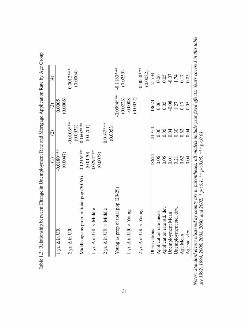
Tables 1.3 and 1.4 test the hypothesis that middle-aged people are more likely to draw
on mortgage loans when facing an unemployment shock than older or younger people.
While an unemployment shock would be salient for younger people, younger people are
less likely than middle-aged people to own their homes outright, making it more difficult
to acquire a home equity loan. Knowing this may deter younger homeowners from seeking
out such a loan to finance an unemployment shock. Older individuals are less likely to find
unemployment as a salient shock, despite being the most likely to own their own home. It
is only the middle-age group that both has home equity and sees unemployment as a salient
shock.
This claim is most clearly supported in Figure 1.1, which plots the marginal effect of a
change in unemployment rate by age category on mortgage applications. As can be seen in
the graph, counties with a large proportion of middle-aged people are most likely to react
to an unemployment rate shock by seeking out home equity loans. As the young population
grows within a county, that also increases the rate of mortgage applications in a county, but
at a slower rate than when the middle-aged population grows within a county. The lowest
28
Tabl
e1.
2:R
elat
ions
hip
betw
een
Cha
nge
inU
nem
ploy
men
tRat
ean
dM
ortg
age
App
licat
ion
Rat
eby
Age
Gro
up-
Mid
dle
and
You
ngA
ges
toge
ther
(1)
(2)
(3)
(4)
You
ng-m
iddl
eas
prop
ortio
nof
tota
lpop
(20-
65)
0.06
15**
*0.
0877
***
0.05
12**
*0.
0735
***
(0.0
175)
(0.0
209)
(0.0
176)
(0.0
209)
1yr
.∆in
UR
-0.0
171*
**(0
.003
9)1
yr.∆
inU
R×
You
ng-m
iddl
e0.
0219
***
(0.0
050)
2yr
.∆in
UR
-0.0
065*
**(0
.002
2)2
yr.∆
inU
R×
You
ng-m
iddl
e0.
0084
***
(0.0
028)
1yr
.pro
p.∆
inU
R-0
.122
7***
(0.0
255)
1yr
.pro
p.∆
inU
R×
You
ng-m
iddl
e0.
1625
***
(0.0
330)
2yr
.pro
p∆
inU
R-0
.048
5***
(0.0
164)
2yr
.pro
p∆
inU
R×
You
ng-m
iddl
e0.
0698
***
(0.0
214)
Obs
erva
tions
1862
421
734
1862
421
734
App
licat
ion
rate
mea
n0.
060.
060.
060.
06A
pplic
atio
nra
test
d.de
v.0.
050.
050.
050.
05U
nem
ploy
men
tMea
n-0
.08
-0.0
70.
010.
04U
nem
ploy
men
tstd
.dev
.1.
271.
740.
210.
30A
geM
ean
0.79
0.79
0.79
0.79
Age
std.
dev.
0.05
0.05
0.05
0.05
Not
es:
Stan
dard
erro
rscl
uste
red
byco
unty
are
inpa
rent
hese
s;al
lmod
els
incl
ude
year
fixed
effe
cts.
Year
sco
vere
din
this
tabl
ear
e19
92,1
994,
2006
,200
8,20
00,2
002
and
2004
.*p<
0.1,
**p<
0.05
,***
p<0.
01
29
Figure 1.1: Marginal Effect of the Change in Unemployment Rate by Age on the MortgageRate Application Rate
point of the marginal effect plot is where the old population is greatest, suggesting that a
change in the unemployment rate does not increase the rate of mortgage applications in
counties with large proportions of elderly people - likely because unemployment shocks
are not salient to this population.
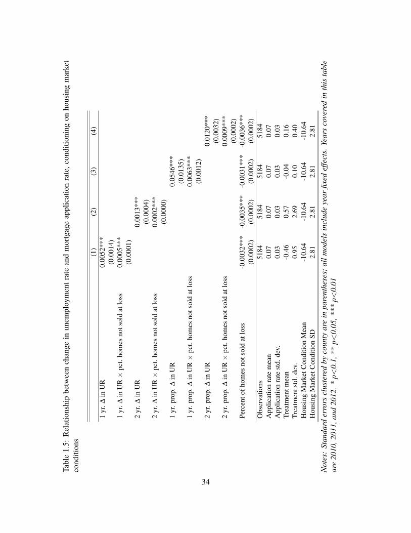
Table 1.5 shows that people are mostly likely to draw on mortgage loans to finance
shocks when they are facing a liquid housing market - when a smaller proportion of homes
on the market are being sold at a loss. As can be seen in Model 1, people living in an area
with 100 percent liquidity are approximately 10 percent more likely to apply for a mortgage
30
Tabl
e1.
3:R
elat
ions
hip
betw
een
Cha
nge
inU
nem
ploy
men
tRat
ean
dM
ortg
age
App
licat
ion
Rat
eby
Age
Gro
up
(1)
(2)
(3)
(4)
1yr
.∆in
UR
-0.0
180*
**0.
0005
(0.0
047)
(0.0
006)
2yr
.∆in
UR
-0.0
103*
**0.
0012
***
(0.0
032)
(0.0
004)
Mid
dle
age
aspr
op.o
ftot
alpo
p(3
0-65
)0.
1216
***
0.16
02**
*(0
.017
0)(0
.020
1)1
yr.∆
inU
R×
Mid
dle
0.02
94**
*(0
.007
8)2
yr.∆
inU
R×
Mid
dle
0.01
67**
*(0
.005
3)Y
oung
aspr
opof
tota
lpop
(20-
29)
-0.0
994*
**-0
.118
3***
(0.0
223)
(0.0
259)
1yr
.∆in
UR×
You
ng-0
.000
8(0
.003
2)2
yr.∆
inU
R×
You
ng-0
.005
8***
(0.0
022)
Obs
erva
tions
1862
421
734
1862
421
734
App
licat
ion
rate
mea
n0.
060.
060.
060.
06A
pplic
atio
nra
test
d.de
v.0.
050.
050.
050.
05U
nem
ploy
men
tMea
n0.
010.
04-0
.08
-0.0
7U
nem
ploy
men
tstd
.dev
.0.
210.
301.
271.
74A
geM
ean
0.62
0.62
0.17
0.17
Age
std.
dev.
0.04
0.04
0.05
0.05
Not
es:
Stan
dard
erro
rscl
uste
red
byco
unty
are
inpa
rent
hese
s;al
lmod
els
incl
ude
year
fixed
effe
cts.
Year
sco
vere
din
this
tabl
ear
e19
92,1
994,
2006
,200
8,20
00,a
nd20
02.*
p<0.
1,**
p<0.
05,*
**p<
0.01
31
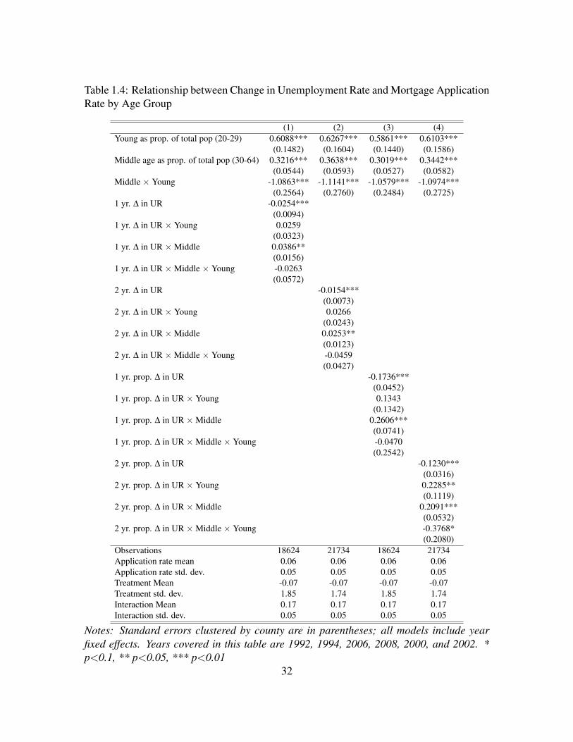
Table 1.4: Relationship between Change in Unemployment Rate and Mortgage ApplicationRate by Age Group
(1) (2) (3) (4)Young as prop. of total pop (20-29) 0.6088*** 0.6267*** 0.5861*** 0.6103***
(0.1482) (0.1604) (0.1440) (0.1586)Middle age as prop. of total pop (30-64) 0.3216*** 0.3638*** 0.3019*** 0.3442***
(0.0544) (0.0593) (0.0527) (0.0582)Middle × Young -1.0863*** -1.1141*** -1.0579*** -1.0974***
(0.2564) (0.2760) (0.2484) (0.2725)1 yr. ∆ in UR -0.0254***
(0.0094)1 yr. ∆ in UR × Young 0.0259
(0.0323)1 yr. ∆ in UR × Middle 0.0386**
(0.0156)1 yr. ∆ in UR × Middle × Young -0.0263
(0.0572)2 yr. ∆ in UR -0.0154***
(0.0073)2 yr. ∆ in UR × Young 0.0266
(0.0243)2 yr. ∆ in UR × Middle 0.0253**
(0.0123)2 yr. ∆ in UR × Middle × Young -0.0459
(0.0427)1 yr. prop. ∆ in UR -0.1736***
(0.0452)1 yr. prop. ∆ in UR × Young 0.1343
(0.1342)1 yr. prop. ∆ in UR × Middle 0.2606***
(0.0741)1 yr. prop. ∆ in UR × Middle × Young -0.0470
(0.2542)2 yr. prop. ∆ in UR -0.1230***
(0.0316)2 yr. prop. ∆ in UR × Young 0.2285**
(0.1119)2 yr. prop. ∆ in UR × Middle 0.2091***
(0.0532)2 yr. prop. ∆ in UR × Middle × Young -0.3768*
(0.2080)Observations 18624 21734 18624 21734Application rate mean 0.06 0.06 0.06 0.06Application rate std. dev. 0.05 0.05 0.05 0.05Treatment Mean -0.07 -0.07 -0.07 -0.07Treatment std. dev. 1.85 1.74 1.85 1.74Interaction Mean 0.17 0.17 0.17 0.17Interaction std. dev. 0.05 0.05 0.05 0.05
Notes: Standard errors clustered by county are in parentheses; all models include yearfixed effects. Years covered in this table are 1992, 1994, 2006, 2008, 2000, and 2002. *p<0.1, ** p<0.05, *** p<0.01
32
loan relative to an area with 0 percent liquidity conditional on experiencing a 1 percentage
point increase in the unemployment rate. Once again, short term shocks are much more
likely to correlate with people turning to mortgage loans to finance the shock, especially
when facing a liquid housing market.
1.4.2 Political Preferences
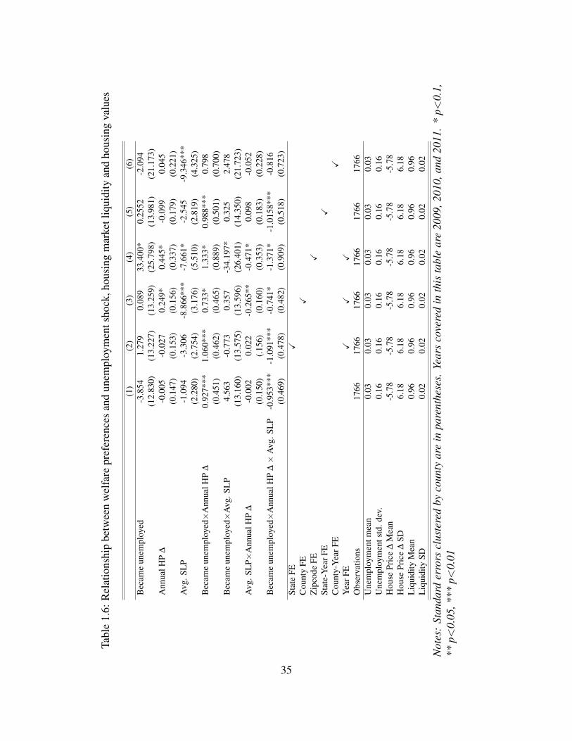
To explore how peoples’ political preferences towards the welfare state shift along with
availability of home equity access, Table 1.6 shows how local housing market conditions,
combined with an unemployment shock, can affect political preferences. I expand the argu-
ment from Ansell (2014) to suggest that local housing market conditions, such as housing
market liquidity, are important predictors of support for social insurance. In Table 1.6, I
demonstrate that after experiencing an unemployment shock, increases in liquidity and lo-
cal home equity are correlated with decreased preference for social spending. This result,
seen in the triple interaction, is consistently negative and significant, holding a variety of
factors constant.
It is interesting to note that becoming unemployed and simply experiencing greater
home equity in the local area (Became unemployed * Annual HP ∆) is not correlated with
decreased preference for social insurance. It is only when market level liquidity conditions
are taken into account that I see a result consistent with the Ansell (2014) prediction. This
suggests that having home equity is not sufficient for a homeowner to rely on that equity
as private insurance; having access to that home equity is crucial for the private and public
insurance tradeoff to hold.
33
Tabl
e1.
5:R
elat
ions
hip
betw
een
chan
gein
unem
ploy
men
trat
ean
dm
ortg
age
appl
icat
ion
rate
,con
ditio
ning
onho
usin
gm
arke
tco
nditi
ons
(1)
(2)
(3)
(4)
1yr
.∆in
UR
0.00
52**
*(0
.001
4)1
yr.∆
inU
R×
pct.
hom
esno
tsol
dat
loss
0.00
05**
*(0
.000
1)2
yr.∆
inU
R0.
0013
***
(0.0
004)
2yr
.∆in
UR×
pct.
hom
esno
tsol
dat
loss
0.00
02**
*(0
.000
0)1
yr.p
rop.
∆in
UR
0.05
46**
*(0
.013
5)1
yr.p
rop.
∆in
UR×
pct.
hom
esno
tsol
dat
loss
0.00
63**
*(0
.001
2)2
yr.p
rop.
∆in
UR
0.01
20**
*(0
.003
2)2
yr.p
rop.
∆in
UR×
pct.
hom
esno
tsol
dat
loss
0.00
09**
*(0
.000
2)Pe
rcen
tofh
omes
nots
old
atlo
ss-0
.003
2***
-0.0
035*
**-0
.003
1***
-0.0
036*
**(0
.000
2)(0
.000
2)(0
.000
2)(0
.000
2)O
bser
vatio
ns51
8451
8451
8451
84A
pplic
atio
nra
tem
ean
0.07
0.07
0.07
0.07
App
licat
ion
rate
std.
dev.
0.03
0.03
0.03
0.03
Trea
tmen
tmea
n-0
.46
0.57
-0.0
40.
16Tr
eatm
ents
td.d
ev.
0.95
2.69
0.10
0.40
Hou
sing
Mar
ketC
ondi
tion
Mea
n-1
0.64
-10.
64-1
0.64
-10.
64H
ousi
ngM
arke
tCon
ditio
nSD
2.81
2.81
2.81
2.81
Not
es:
Stan
dard
erro
rscl
uste
red
byco
unty
are
inpa
rent
hese
s;al
lmod
els
incl
ude
year
fixed
effe
cts.
Year
sco
vere
din
this
tabl
ear
e20
10,2
011,
and
2012
.*p<
0.1,
**p<
0.05
,***
p<0.
01
34
Tabl
e1.
6:R
elat
ions
hip
betw
een
wel
fare
pref
eren
ces
and
unem
ploy
men
tsho
ck,h
ousi
ngm
arke
tliq
uidi
tyan
dho
usin
gva
lues
(1)
(2)
(3)
(4)
(5)
(6)
Bec
ame
unem
ploy
ed-3
.854
1.27
90.
089
33.4
00*
0.25
52-2
.094
(12.
830)
(13.
227)
(13.
259)
(25.
798)
(13.
981)
(21.
173)
Ann
ualH
P∆
-0.0
05-0
.027
0.24
9*0.
445*
-0.0
990.
045
(0.1
47)
(0.1
53)
(0.1
56)
(0.3
37)
(0.1
79)
(0.2
21)
Avg
.SL
P-1
.094
-3.3
06-8
.866
***
-7.6
61*
-2.5
45-9
.346
***
(2.2
80)
(2.7
54)
(3.1
76)
(5.5
10)
(2.8
19)
(4.3
25)
Bec
ame
unem
ploy
ed×
Ann
ualH
P∆
0.92
7***
1.06
0***
0.73
3*1.
333*
0.98
8***
0.79
8(0
.451
)(0
.462
)(0
.465
)(0
.889
)(0
.501
)(0
.700
)B
ecam
eun
empl
oyed×
Avg
.SL
P4.
563
-0.7
730.
357
-34.
197*
0.32
52.
478
(13.
160)
(13.
575)
(13.
596)
(26.
401)
(14.
350)
(21.
723)
Avg
.SL
P×A
nnua
lHP
∆-0
.002
0.02
2-0
.265
**-0
.471
*0.
098
-0.0
52(0
.150
)(.1
56)
(0.1
60)
(0.3
53)
(0.1
83)
(0.2
28)
Bec
ame
unem
ploy
ed×
Ann
ualH
P∆×
Avg
.SL
P-0
.953
***
-1.0
91**
*-0
.741
*-1
.371
*-1
.015
8***
-0.8
16(0
.469
)(0
.478
)(0
.482
)(0
.909
)(0
.518
)(0
.723
)St
ate
FEX
Cou
nty
FEX
Zip
code
FEX
Stat
e-Y
earF
EX
Cou
nty-
Yea
rFE
XY
earF
EX
XX
Obs
erva
tions
1766
1766
1766
1766
1766
1766
Une
mpl
oym
entm
ean
0.03
0.03
0.03
0.03
0.03
0.03
Une
mpl
oym
ents
td.d
ev.
0.16
0.16
0.16
0.16
0.16
0.16
Hou
sePr
ice
∆M
ean
-5.7
8-5
.78
-5.7
8-5
.78
-5.7
8-5
.78
Hou
sePr
ice
∆SD
6.18
6.18
6.18
6.18
6.18
6.18
Liq
uidi
tyM
ean
0.96
0.96
0.96
0.96
0.96
0.96
Liq
uidi
tySD
0.02
0.02
0.02
0.02
0.02
0.02
Not
es:
Stan
dard
erro
rscl
uste
red
byco
unty
are
inpa
rent
hese
s.Ye
ars
cove
red
inth
ista
ble
are
2009
,201
0,an
d20
11.
*p<
0.1,
**p<
0.05
,***
p<0.
01
35
1.4.3 Discussion
The empirical results are consistent with the hypotheses presented above and suggest
that people are drawing on home equity to finance shocks. The consistently positive rela-
tionship between an unemployment rate shock and mortgage applications rules out a key
alternative story. Because unemployment is often correlated with local economic condi-
tions, we might expect that the relationship between an unemployment shock and mortgage
applications would be negative if it was purely driven by broader economic factors. After
all, people are more likely to buy a home or refinance when the local economy is strong.
My results run against these concerns about bias.
One alternative explanation for these results is that because poor economic conditions,
unemployment shocks and declining housing values are all correlated, people are more
likely to apply for mortgage loans in an economic downturn because housing is cheap -
not because they are trying to finance an unemployment shock. However, it is telling that
the more proximate the unemployment shock to the mortgage application, the stronger
the effect. After an economic downturn, a strategic homebuyer would likely wait to see
if home values would drop any further. Moreover, very few people can move quickly
when buying a home - saving for a down payment may take several years. Together, these
arguments suggest that if strategic homebuying was driving my results, longer term lags on
an economic shocks would have a larger effect than immediate shocks to income. While
there likely are a number of strategic homebuyers, we know that many people are not
forward looking with their consumption decisions (Poterba 1988). Finally, this argument
would fly directly in the face of the liquidity results, which suggest that people are more
likely to apply for mortgage loans when economic conditions are good.
Interestingly, the results from 2010-2012 are largely consistent with the results from
earlier years. We might expect housing wealth in the post-crisis period to be different
36
from the pre-crisis period because of increased loss aversion, which tells us that losses
hurt more than gains feel good (Kahneman and Tversky 1979; Machina 1987; Tversky and
Kahneman 1992), on the part of both lenders and borrowers. This seems not to be the
case, and is suggestive of the fact that even at a period when the housing market was just
beginning to recover from the crisis, people were still turning to housing wealth to finance
unexpected income shocks. While this speaks to the entrenched nature of homeownership
in the U.S., it also raises the question of what new financing tools will arise as more and
more people are priced out of buying homes.
While these results are supportive of the hypotheses presented above, refinements to
the data would allow future researchers to explore the relationship between housing, shock
financing and political preferences more clearly. In particular, having access to individual
level credit scores and home equity would allow for a more precise picture of liquidity than
the broad measure I have used in this paper, and would focus on borrowing to finance a
shock rather than selling the home to finance a shock. Similarly, being able to distinguish
between first and second liens would paint a more precise picture of which counties are
drawing on home-equity based borrowing when experiencing an unemployment shock.
1.5 Conclusion
I demonstrate that people use housing to finance unexpected shocks, and that when
available to them, people use housing equity as private insurance - which in turn substitutes
for demand for social insurance. I demonstrate that counties with a large proportion of
middle-aged people are most likely to use home-equity based borrowing, and I theorize
that this is because unemployment shocks are salient and because middle-aged people have
access to housing wealth in a way that younger homeowners do not. Finally, I show that
these factors come together to influence peoples’ support for the welfare state.
37
My work shows that the relationship posited by Ansell (2014) is conditional on access
to housing wealth through the channel of increased liquidity. These results do raise the
question of how we might expect homeowners to react to expected shocks, such as retire-
ment or education financing. Because these shocks are anticipated and need to be financed
over a longer time horizon, homeowners anticipating these shocks may be more concerned
with volatility than liquidity. If the local housing market is extremely volatile, it may be
the case that homeowners do not feel comfortable betting on the fact that house prices will
be high when the time comes to draw on their home equity. In other words, homeowners
living in a volatile market may be more supportive of social insurance than homeowners
living in a more steady one. Moreover, because expected shocks to income might be an-
ticipated, we might expect that people will use consumption smoothing to account for this,
suggesting that homeowners facing expected shocks may not change their preferences on
social spending at all.
While these results provide a start at identifying how unemployment shocks, via hous-
ing wealth and housing market conditions, affect preferences for social insurance, there
are other political outcomes that would merit further exploration. In particular, concrete
behavioral outcomes at the individual level, such as turnout, could tell us whether such
changes in preferences translate into political action. It would also be interesting to in-
vestigate whether social network dynamics play into the relationship between the housing
market and preferences for social insurance.
Moreover, future research could explore how access to housing equity interacts with
other relevant factors in determining preferences for social insurance. For example, Rehm
(2011) finds that moving from the first income quintile to the second is correlated with
an approximately 0.03 decrease in probability for preferring high unemployment benefits.
While income and access to housing wealth are likely correlated, it would be interesting
to explore whether people with high incomes similarly decrease their preference for un-
38
employment benefits when liquidity in their local area is low, conditional on experiencing
an unemployment shock. In other words, is a high income sufficient as a source of private
insurance? On the other hand, poorer homeowners might increase their demand for social
insurance in the face of unemployment to either bundle both types of insurance, or to main-
tain good credit, allowing them to keep their home. Delving into the way in which home
equity interacts with income, and both expected and unexpected shocks provides a clear
avenue for future research.
39
2 | Lending Support: Agency MBS Issuanceand Rewarding Incumbents
2.1 Introduction
In 2007, the housing bubble that had been growing for nearly a decade collapsed, and
house prices came tumbling down from enormous heights. The crash - the worst financial
crisis since the Great Depression - set off a period of economic stagnation across the world.
The seeds of this crash, however, were planted during a period of cautious optimism that
grew into a reckless frenzy of borrowing. With the help of the 2001 Bush tax cuts and
the Federal Reserve holding down low interest rates, American consumers increased their
borrowing by a trillions of dollars in the early 2000s, and many Americans used their new
found access to credit to buy homes. Mortgage lending skyrocketed and the economy
experienced a huge rise in house prices - the Case-Shiller home price index shows house
prices nearly tripling between the 1990s and 2005. Throughout this period, politicians
championed homeownership as a key part of the “American Dream."
Low interest rates and the general availability of mortgage credit in the pre-crisis period
allowed people who had not been able to access mortgage credit before to suddenly buy
homes. In particular, the availability of mortgage credit for those marginalized in the mort-
gage market was helped by a proliferation of mortgage backed securities (MBS) issuance
by Fannie Mae and Freddie Mac (also known as the GSEs - “Government Sponsored Enter-
40
prises"1) in the early 2000s. This paper will explore the question of whether agency-issued
MBS affected voting behavior between 1990 and 2004. Despite the fact that housing is a
key part of an individual’s wealth, surprisingly little attention has been paid to how home-
ownership affects support for political actors, and in particular incumbents, who might be
perceived as being able to facilitate access to mortgage credit.
To address this question, I draw on the economic voting literature, which suggests that
voters use incumbent economic performance to assess candidate quality. I combine insights
from this literature from that of the political business cycles literature, which suggests that
politicians stimulate the economy because they know that voters respond to recent eco-
nomic performance (Nordhaus 1975). In this literature, voters are not sure whether the
incumbent candidate is competent, and might conflate incumbent performance with an ex-
ogenous economic shock (Rogoff 1990). Similarly, I argue in this paper that voters reward
politicians for a positive economic shock even though the shock is not clearly attributable
to the politician him or herself. While politicians themselves cannot control loan origina-
tions in the way they might be able to affect fiscal policy, they do have an incentive to claim
credit.
I predict that low-income counties are most likely to be those that benefit from the
Fannie and Freddie policy which resulted in increased access to mortgage credit, and I will
demonstrate empirically that low-income counties had more loans per capita originated in
the early 2000s than high-income counties.2 It is unlikely that most voters would have been
able to attribute the ease of accessing mortgage credit to GSEs, which are mostly private
entities. I argue that incumbent politicians - particularly Democrats - supported policies
that promoted homeownership for low income areas. Poorer counties, therefore, which are
more likely to experience a proliferation in mortgage origination, are more likely to reward
1Although there are 9 GSEs in total, I refer only to Fannie and Freddie in this document.
2Origination simply refers to the process of creating a mortgage after a mortgage application is accepted.
41
their political incumbents for increased mortgage credit availability. I also find evidence
that Democratic incumbents in low-income counties are more likely to be rewarded than
Republican incumbents in low-income counties.
I test these hypotheses using Senate electoral data in the period from 1990 to 2004.
Fannie and Freddie MBS issuance ramped up in 2000 and peaked in 2003. I identify 2000-
2004 as the “post-reform" period, in which mortgage credit is widely available, and 1990-
1999 as the “pre-reform" period, when mortgage credit was still tight. I examine how the
increase in credit after 2000 differentially affected high and low income countries. To do
this, I use a difference-in-differences design to first examine whether low-income counties
were more likely to receive more loans per capita than high-income counties in the post-
reform period. I then examine the reduced form effect of increased access to mortgage
credit among low-income counties on voting behavior. These results form the basis of the
story I subsequently tell using an instrumental variables framework, where I instrument for
the mortgage loans being originated using the interaction of being in the post-reform period
and county income.
I find that low-income counties do originate more loans than high-income counties in
the post-reform period. Moreover, low-income counties are more likely to vote for the in-
cumbent party in the post-reform period, particularly if the incumbent is a Democrat. These
results suggest that voters do care about homeownership, and importantly, that they are not
able to correctly attribute who should be rewarded for the ease of acquiring a mortgage.
Although Fannie and Freddie have ties to the public sector, they are private corporations.3
The fact that voters reward incumbents for a Fannie/Freddie reform suggests that politicians
have an incentive to claim credit for policies that they have little to no control over.
3This has been true for the vast majority of Fannie and Freddie history - Congress privatized the GSEsin 1968, and in 2008, the GSEs were taken into Conservatorship by the Federal Housing Finance Authorityafter rapid deterioration in the housing markets.
42
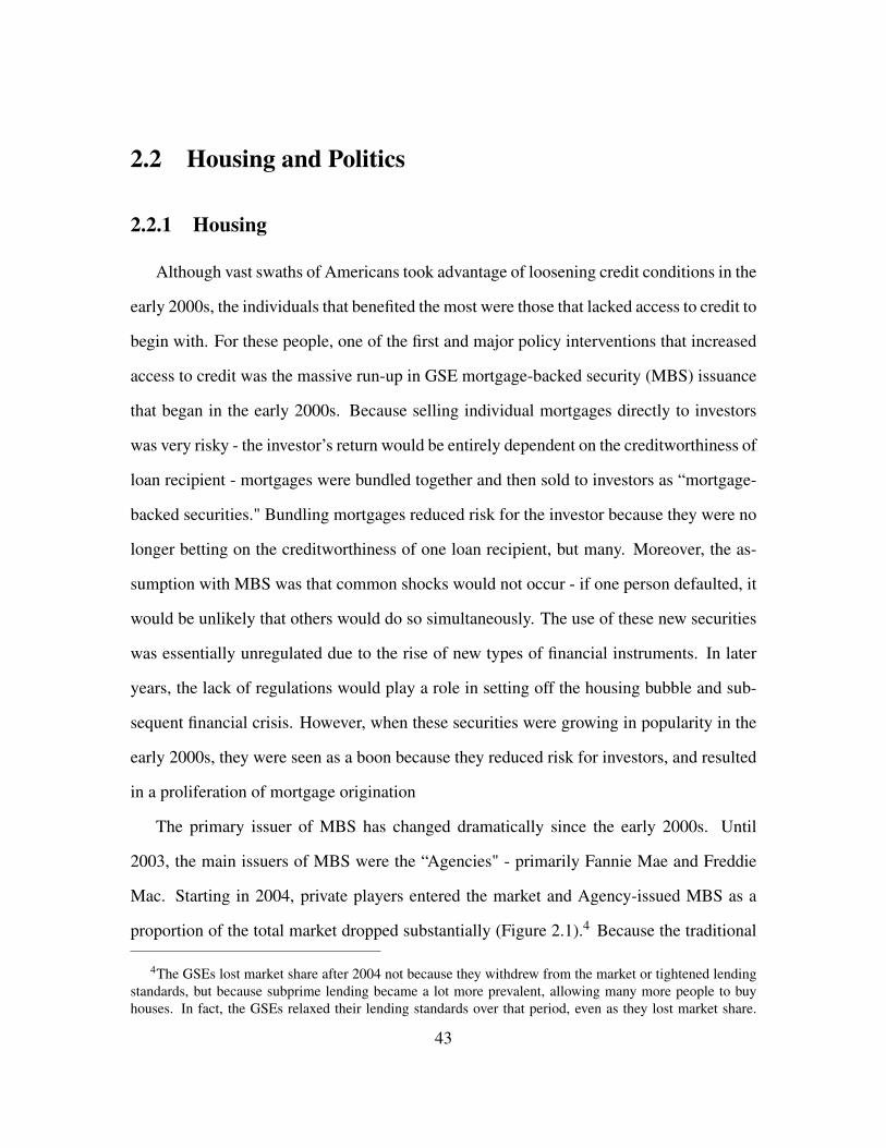
2.2 Housing and Politics
2.2.1 Housing
Although vast swaths of Americans took advantage of loosening credit conditions in the
early 2000s, the individuals that benefited the most were those that lacked access to credit to
begin with. For these people, one of the first and major policy interventions that increased
access to credit was the massive run-up in GSE mortgage-backed security (MBS) issuance
that began in the early 2000s. Because selling individual mortgages directly to investors
was very risky - the investor’s return would be entirely dependent on the creditworthiness of
loan recipient - mortgages were bundled together and then sold to investors as “mortgage-
backed securities." Bundling mortgages reduced risk for the investor because they were no
longer betting on the creditworthiness of one loan recipient, but many. Moreover, the as-
sumption with MBS was that common shocks would not occur - if one person defaulted, it
would be unlikely that others would do so simultaneously. The use of these new securities
was essentially unregulated due to the rise of new types of financial instruments. In later
years, the lack of regulations would play a role in setting off the housing bubble and sub-
sequent financial crisis. However, when these securities were growing in popularity in the
early 2000s, they were seen as a boon because they reduced risk for investors, and resulted
in a proliferation of mortgage origination
The primary issuer of MBS has changed dramatically since the early 2000s. Until
2003, the main issuers of MBS were the “Agencies" - primarily Fannie Mae and Freddie
Mac. Starting in 2004, private players entered the market and Agency-issued MBS as a
proportion of the total market dropped substantially (Figure 2.1).4 Because the traditional
4The GSEs lost market share after 2004 not because they withdrew from the market or tightened lendingstandards, but because subprime lending became a lot more prevalent, allowing many more people to buyhouses. In fact, the GSEs relaxed their lending standards over that period, even as they lost market share.
43
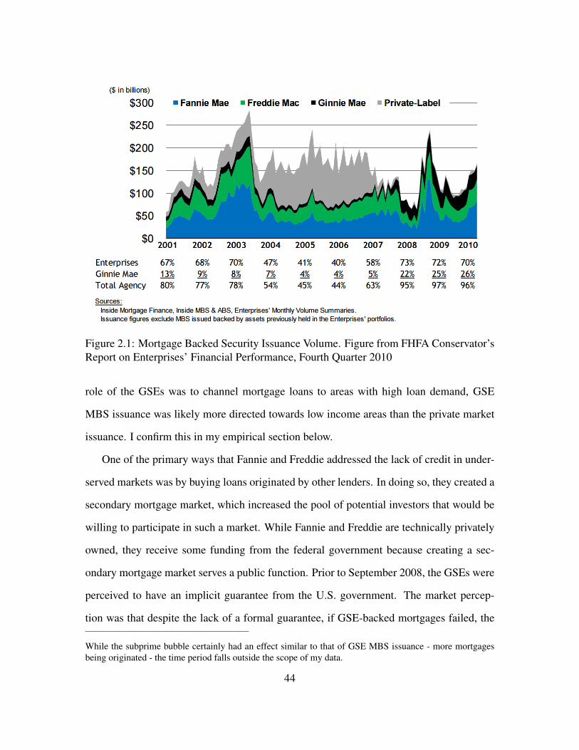
Figure 2.1: Mortgage Backed Security Issuance Volume. Figure from FHFA Conservator’sReport on Enterprises’ Financial Performance, Fourth Quarter 2010
role of the GSEs was to channel mortgage loans to areas with high loan demand, GSE
MBS issuance was likely more directed towards low income areas than the private market
issuance. I confirm this in my empirical section below.
One of the primary ways that Fannie and Freddie addressed the lack of credit in under-
served markets was by buying loans originated by other lenders. In doing so, they created a
secondary mortgage market, which increased the pool of potential investors that would be
willing to participate in such a market. While Fannie and Freddie are technically privately
owned, they receive some funding from the federal government because creating a sec-
ondary mortgage market serves a public function. Prior to September 2008, the GSEs were
perceived to have an implicit guarantee from the U.S. government. The market percep-
tion was that despite the lack of a formal guarantee, if GSE-backed mortgages failed, the
While the subprime bubble certainly had an effect similar to that of GSE MBS issuance - more mortgagesbeing originated - the time period falls outside the scope of my data.
44
$0
$500,000
$1,000,000
$1,500,000
$2,000,000
$2,500,000
$3,000,000
$3,500,000
$4,000,000
1985 1990 1995 2000 2005 2010 2015
Figure 2.2: Single family conventional mortgage originations over time, in millions ofdollars. Data are from the Federal Housing Finance Agency, Current Market Data
government would step in and save the GSEs. This implicit guarantee is the reason that in-
vestors felt secure in participating in the GSE-created secondary market, and the increased
security/reduced risk likely translated to lower costs for borrowers (Passmore 2005).
The implicit guarantee, along with the fact that increased MBS issuance decreased the
risk associated with originating mortgages, played a role in the huge jump in originated
mortgages starting in 2000 (Figure 2.2). The jump in the value of mortgage originations
in the early 2000s cannot be overstated. From 1990 to 1999, the average value of conven-
tional mortgages issued was approximately 770 billion dollars. In the following decade,
the average value of conventional mortgages jumped to 1.8 trillion dollars. From 2000 to
2001, the value of conventional mortgages issued more than doubled.
45
As I demonstrate in the empirical section below, lower income areas were much more
likely to be affected by GSE policy than higher income areas. This is partially because
bundling loans in ways that ostensibly reduced risk meant that loans were cheaper to ac-
quire. Moreover, by bundling together loans that were of different quality, lenders could
easily unload their risk on to securitizers, which made lenders more willing to originate
lower quality loans.
Other factors likely played a role in mortgage credit proliferation during this time pe-
riod as well. It is likely that as mortgage credit became more widely available in the bubble
economy, higher income areas became saturated and the flow of credit was redirected to-
wards areas that did not have access to credit prior to 2000. This explanation would result
in the same sorts of effects without any sort of deliberate policy change by the GSEs. More-
over, interest rates were extremely low in the post-2000 period, which would also facilitate
the increase in mortgage credit in the economy. While these other channels for loan pro-
vision may be in effect along with GSE provision of mortgages, they move in the same
direction as any shift in GSE policy over this time period: all of these channels lead to
more mortgage originations. My empirical work focuses on loan originations and greater
access to mortgage credit rather than GSE policy explicitly, but there is still reason to think
that given the massive increase in GSE loan originations, as well as the close ties between
many members of Congress and the GSEs, GSE policy did play a major role in what was
going on in the housing market at the time. In particular, the close ties between the GSEs
and members of Congress offer us an explanation for why voters might be rewarding their
incumbents after experiencing an uptick in loan originations.
46
2.2.2 Economic Voting
A massive spike in mortgage lending with a focus on lower income areas had widespread
economic reverberations. I contend that the increase in MBS issuance also had political ef-
fects. The relationship between economic conditions and voting has been widely explored
in the economic voting literature. This literature examines “economic voting" - namely the
idea that voters use information about how well or badly the economy is doing to assess
incumbent performance and subsequently make voting decisions on the basis of that infor-
mation (Duch and Stevenson 2008). The starting point for much of this literature is V.O.
Key’s “The Responsible Electorate" (Key 1966). Key pushes back against the idea that
voters are uninformed about political issues (Campbell et al. (1966), Converse (2006)) and
suggests instead that voters use information to update their beliefs and evaluate incumbent
performance. In their recent review piece, Healy and Malhotra (2013a) suggest several
frames for thinking about the literature that has come out of Key (1966): a sanctioning
model of economic voting, a selection model, and a cognitive model.
The sanctioning model suggests that voters punish poor performing incumbents and re-
ward high performing incumbents - essentially the premise of Key (1966), formalized by
Barro (1973) and Ferejohn (1986). The selection model suggests that voters elect politi-
cians who will perform well in the future (Fearon (1999), Alt, Bueno de Mesquita, and
Rose (2011)). It is important to point out that the sanctioning and selection models are
hard to distinguish: it is not clear whether voters are rewarding politicians for past eco-
nomic performance, or if voters are using past economic performance to assess potential
future economic performance. The cognitive model is a somewhat newer portion of the
economic voting literature, and suggests that voters use heuristics to make decisions when
information is costly to acquire (e.g. Achen and Bartels (2004)). The cognitive frame also
touches on how events outside the control of politicians - such as natural disasters (Healy
47
and Malhotra (2009), Bechtel and Hainmueller (2011), Gasper and Reeves (2011)) - can
affect voting patterns.
While this paper touches on all three branches of the economic voting model using
housing as a new avenue into exploring economic voting, this paper also ties in with the po-
litical business cycles literature, which suggests that politicians have an incentive to change
fiscal policy before an election to appeal to voters (Nordhaus 1975), but voters are unable to
assess whether or not the politicians or an exogeneous shock is actually responsible for the
change in economic conditions (Rogoff 1990).5 While voters use economic information to
assess candidate quality, incumbent candidates can also use local economic conditions to
shape how they are perceived by voters. They can do this in at least two ways: first, incum-
bents can use their power in office to change the political environment, and then campaign
on the basis of their work in office. Alternatively, and perhaps more perniciously, incum-
bents can claim credit for positive change in the local economy even if they have no real
claim to any of the policy changes that led to the change in the economic environment. In
this paper, I argue that the in the case of loan originations in the early 2000s, the latter was
at play.
I contend that incumbents, especially Democrats, are able to claim credit for increased
loan origination, regardless of whether they have the ability to actually affect GSE policy.
While I remain somewhat agnostic about whether members of Congress could legitimately
take credit for the boom in mortgage origination, I do provide some evidence that suggests
that incumbent politicians are knowledgeable about GSE issues, and that partisan differ-
ences existed on the positions taken on GSE oversight and regulation.
Given the outsize role housing has played in dictating the course of the U.S. economy
in the last decade, it is important to understand how it interacts with the political realm.
5Alesina (1989) argues that political business cycles do not in fact exist, as rational voters would anticipatethis strategy by politicians.
48
Both Democrats and Republicans have historically courted voters using the promise of
homeownership, and research in England has shown that this sort of relationship may hold
- Field (1997) demonstrates that Thatcher’s “Right to Buy" program increased Conservative
vote shares in 1992. This paper suggests a similar phenomenon benefitting the opposite end
of the political spectrum, namely that Democratic politicians are being rewarded for access
to mortgage credit in their constituencies.
2.3 Theory
2.3.1 Link between GSEs and Legislators
There are several reasons to think that GSE policy would have an effect on voting be-
havior and perception of incumbents/incumbent party. First, although the GSEs were not
technically part of the federal government, they were perceived to have close ties to govern-
ment. As a paper from the Fed’s Board of Governors states, “the housing-related govern-
ment sponsored enterprises...[had] an ambiguous relationship with the federal government"
(Passmore 2005). This refers to the the implicit federal backing by the government, despite
any legal claim to a guarantee. Passmore (2005) states, “The markets’ impression that the
government implicitly backs Fannie Mae and Freddie Mac is based on the GSEs’ history,
on the size of their portfolios, on the fact that the government mandates housing goals for
these firms, and on the many indicia of explicit government support...The result is an am-
biguous relationship between the GSEs and the federal government in which investors infer
government support while government officials deny it."
The GSEs not only enjoyed perceived ties and backing from the federal government,
but also had real, concrete institutional ties. As Passmore (2005) states, “the government
provides the GSEs with a line of credit from the Department of the Treasury, fiscal agency
49
services through the Federal Reserve, U.S. agency status for GSE securities, exemptions
from securities registration requirements, exemptions from bank regulations on security
holdings, and tax exemptions." The close relationship between the GSEs and the govern-
ment also extended from perceived and actual institutional ties with the federal government,
to personal ties with many members of Congress. For example, the New York Times ran
a 2012 article about Newt Gingrich’s close ties with Fannie and Freddie that spanned from
1994 to long after he left Congress in 1999. The GSEs reportedly sponsored a trip for
Gingrich, and on other occasions Gingrich was instrumental in policy outcomes that were
favorable for the GSEs (Lichtblau 2012). While the Times profiled the Gingrich ties be-
cause of his 2012 presidential run, it is highly likely that other members of Congress - not
constrained to Republicans - were also closely associated with the GSEs. As I will show
in the following paragraphs, members of Congress were knowledgeable about GSE in-
volvement in mortgage origination and whether their own constituencies were particularly
affected by GSE policy.
Fairly concrete links between the GSEs and politicians in and of themselves may not
have an effect on voting behavior, but through a variety of channels, voters may make the
connection between their incumbent politicians and housing policy. In particular, there are
three possible channels by which voters connect incumbent politicians with GSE policy:
issue ownership, voter perception of influence, and credit claiming. While in this paper I
am agnostic as to which of these channels are at play, there is some evidence to suggest
that some combination of factors allow voters to draw this connection between incumbents
and housing.
First, existing literature has demonstrated that some voters may perceive access to mort-
gage credit as a policy area “owned" by a particular party. Some issues, such as national
security, are more closely tied to a particular party (Gadarian 2010; Petrocik 1996). While
this may be true for housing, it is not obvious which party would be perceived as “owning"
50
housing as a policy area. The Clinton administration released a document in 1995 titled
“The National Ownership Society: Partners in an American Dream." In a note at the begin-
ning of the document, President Clinton states that the goal of the initiative is to generate up
to 8 million additional homeowners from 1995 through the year 2000, focusing on helping
middle-income and low- income families, racial and ethnic minorities, families with chil-
dren, and young adults (The National Homeownership Strategy: Partners in an American
Dream 1995). President Bush also championed expanding homeownership as a part of his
presidential campaigns and when he was in office. Shortly after taking office, President
Bush hosted a conference on the need for minority homeownership. In his remarks ad-
dressing the conference, he says, “one of the larger obstacles to minority homeownership
is financing...We think it’s important...that federal money to help low-income Americans go
from being somebody who leases to somebody who owns...it is a way to help us meet this
dream of 5.5 million additional families owning their home." (President Hosts Conference
on Minority Homeownership 2002)
Although both parties were championing the importance of homeownership as a part
of the “American Dream" at the time, this was happening on a higher level than the one
most relevant to voters. When it came to members of Congress, both Republicans and
Democrats touted the importance of homeownership, but the Democrats were much more
vocal about the importance of ensuring the spread of mortgage credit when it came to
actual policy. While neither party wanted to be seen as the anti-homeownership party,
Republicans in Congress were much more cautious about pushing the sorts of policies that
would indeed result in increased mortgage origination. As such, if voters are to reward
their incumbents for domestic housing policy, I predict that the Democrats are more likely
to benefit from a time of eased credit conditions. Congressional Democrats’ vociferous
defense of mortgage proliferation also better positioned them to take credit for the policies
underpinning mortgage origination.
51
Moreover, it is possible that voters perceived incumbents, and particularly Democrats,
to have influence over mortgage origination - regardless of whether or not politicians ac-
tually did have any sway over these policies. Incumbent politicians had an advantage over
their competitors because housing finance and GSE reform were being actively discussed
in Congress in the post-2000 period. In particular, many of the Democrats were adamantly
against any sort of reform that would restrict mortgage access.
While Republicans seemed intent on reforming aspects of housing finance that would
have restricted access to mortgages, many Democrats spoke passionately in committee
meetings about the need to keep mortgages flowing to areas that did not generally have
access to them. For example, the Subcommittee of Capital Markets, Securities, and Gov-
ernment Sponsored Enterprises in the House of Representatives held a series of meetings
and roundtables in the 2000. The Chair of the Subcommittee at the time was Richard Baker,
a Republican who introduced H.R. 3703: the “Housing Finance Regulatory Improvement
Act." The purpose of the bill was to come up with a new regulatory structure for the GSEs,
which would place oversight of housing finance under a new board in lieu of the institutions
that were playing oversight roles at the time.6
The major debate in these subcommittee discussions was whether there was any need
to address uncertain future market disruptions that would affect the housing market and
mortgage access. In his support of the bill, Representative Baker speaks strongly about the
need to assess risk in advance. In his opening statement on July 20, 2000, Baker states,
“And so here we are in the year 2000 being told that the GSEs are above re-proach, and that with such smart and capable people running the show weshould not even examine the financial condition of these enterprises. Smartpeople who have operated a highly profitable enterprise, at least in the nearterm, should never be questioned. That certainly was the accepted view just
6These entities were the Department of Housing and Urban Development (HUD) and the Federal HousingFinance Board.
52
before LTCM failed...Today the GSEs are very well managed, profitable, anda significant contributor to facilitating home ownership for many people. Butthat does not obviate the requirement to appropriate regulatory oversight. Likeany business enterprise, they are not immune to business reversals. It is ourresponsibility, as Members of Congress, to examine the regulatory system andthe consequences of failing to govern the current dominance of these activi-ties."(H.R. 3703 - Housing Finance Regulatory Improvement Act, Part 2 Hear-ing Before the Subcommittee on Capital Markets, Securities, and GovernmentSponsored Enterprises 2000)
Discussing the same bill, Democrats not only express hesitation about preemptive re-
form, but many seem to be concerned that this is a ploy to staunch the flow of mortgages
that are going to districts with poorer and minority constituents. Maxine Waters, a Demo-
cratic representative from California, said in a subcommittee meeting,
“...and so we don’t have any risk. We don’t have any unsoundness. We don’thave GSEs that are unstable. We only have them that are performing, per-forming well, and doing a pretty good job. Now I want to tell you I have mydifferences with them from time to time and I am pushing them and I wantthem to expand to be able to provide more mortgages for poor people...weshould all be worried about spreading out this wealth and making sure that allcommunities have access to the opportunities so there can be more mortgages,more capital flowing."(H.R. 3703 - Housing Finance Regulatory ImprovementAct, Part 1 Hearing Before the Subcommittee on Capital Markets, Securities,and Government Sponsored Enterprises 2000)
Similarly, Carolyn Maloney, a Democratic representative from New York, speaks at length
not only about why she is in favor of the GSEs mortgage origination policies, but also about
her close relationship with the GSEs. She states that,
“Fannie Mae and Freddie Mac have been tremendously successful in the dis-trict that I represent and really in New York City in providing loans for all kindsof people. They have really helped to grow home ownership, which I feel is animportant social goal...I approached Fannie back in 1998, because I don’t havehomes in my district...I said, ‘You are doing great things to help Harlem andHistoria [sic] and other areas of the city...but you are not doing anything forthe low-income people in Central Manhattan.’ Within six weeks, they came
53
back and devised a program to provide loans for co-ops and condominiumsand have proceeded to grow home ownership dramatically. And to tell you thetruth, I was very impressed that they had that type of flexibility to come backwith a program that was really tailored to the economic problems or challengesof the district that I represent."(H.R. 3703 - Housing Finance Regulatory Im-provement Act, Part 1 Hearing Before the Subcommittee on Capital Markets,Securities, and Government Sponsored Enterprises 2000)
Representative Maloney goes on to discuss how the H.R. 3707, which would change the
regulatory structure of GSE oversight, would decrease the extent to which the GSEs could
be responsive to the needs of her constituents. Congressional Democrats, therefore, seem
much more protective of increased mortgage origination, and generally seemed more con-
cerned about the prospect of stemming the flow of mortgages going towards poorer areas
than Republicans.
Although the evidence above is from a subcommittee of the House Financial Services
committee, the debate and to some extent the corresponding party lines were also present
in the Senate. In May 2001 testimony in a Subcommittee of the Senate Banking Commit-
tee, what is striking is that both Democrats and Republicans speak about housing finance
with relatively fluency. For example, Senator Wayne Allard, a Republican from Colorado,
asks the Chairman of the body that regulates the GSEs, the Office of Federal Housing
Enterprise Oversight (OFHEO) fairly detailed questions about how the GSEs use deriva-
tives (The Housing Mission of the Office of Federal Housing Enterprise Oversight and
the Financial Safety and Soundness of Fannie Mae and Freddie Mac, Hearing Before the
Subcommittee on Housing and Transportation 2001). At the time, understanding of the
secondary mortgage market was fairly limited - it certainly was not the common knowl-
edge that it is post-2008. These sorts of discussions with OFHEO and the GSEs prepared
these legislators to be able to speak about housing finance in a way that challengers were
likely not equipped to do.
While GSE regulation seems to be less divisive along party lines among Senators than
54
members of the House, there is still some evidence that Democrats were much more fa-
vorable towards delaying regulatory changes. For example, Senator Debbie Stabenow, a
Democrat from Michigan, not only praises the GSEs more effusively than her Republican
colleagues, but she also echoes some of the comments of her Democratic colleagues in the
house:
“On the issue of regulation of the GSEs, I do not believe that now is the timeto do anything that would disrupt or redically change the regulatory regime.The GSEs and their regulator have the opportunity to serve as a model forhow risk-based capital rules can work effectively.”(The Housing Mission of theOffice of Federal Housing Enterprise Oversight and the Financial Safety andSoundness of Fannie Mae and Freddie Mac, Hearing Before the Subcommitteeon Housing and Transportation 2001)
Although Senate Republicans do not push aggressively for GSE reform, none of the
Republican statements contain the strong opposition to increased GSE regulation that the
Democrats seemingly espouse.
Finally, there is also some evidence that Democrats were campaigning on these issues,
though these data are much harder to come by than transcripts of Congressional hearings -
in part because there is no incentive to make information about promoting the GSEs avail-
able post-2008. In the one instance I was able to find kind of material, it was on a website
for a multi-year academic study on lobbying and policymaking in the U.S. (Baumgart-
ner et al. 2011). The project’s website contains both quantitative data and documentation
from a variety of policy areas that the researchers were interested in. One such piece of
documentation is from Senator Paul Sabanes’ (D-MD) website from 2003. At the time,
he was the chair of the Senate Banking Committee, and the document from the website
clearly explains his support for making “home ownership more widely available to first
time homebuyers, including minorities," and the steps he himself has taken to ensure “an
estimated 15,000 new homeowners every year."
55
Broadly, it is important to note that Members of Congress were well versed in topics
of housing finance. Unlike the broader public, who would come to learn about the ins and
outs of the housing market after the bubble burst, Members had knowledge that they could
use to back policies that would directly support their constitutents, such as Representative
Maloney, or to claim credit for the ease of mortgage access, as in the case of Senator
Sarbanes.
2.3.2 Hypotheses
I expect to see that voters who did not have access to mortgage credit before the run-up
in MBS issuance will suddenly be able to access credit, attribute the access to credit to their
incumbent politicians (perhaps because of credit claiming), and reward those politicians in
the next election. I expect that this effect will only exist for those who are particularly
affected by the run-up in MBS issuance - those who did not have access to mortgage credit
before Fannie and Freddie flooded the market. In my empirical section, which is conducted
at the county level, I focus on low income counties.
Low-income mortgage applicants are more likely to have low credit scores. Combined
with inability to put down large down payments, low-income borrowers are less likely to
have access to mortgage credit (Archer, Ling, and McGill 2002). Even when access is
available, the terms of the loan are often unfavorable. A major effect of the GSEs’ MBS
issuance in the early 2000s was that credit standards became more lax. Private lenders
realized they could bundle their “good" and “bad" loans together, reducing the risk they
took on. As a result, lenders began originating more and more “bad" loans - an effect
that became obvious when the housing bubble burst in 2007. We know with the benefit
of hindsight that many of the borrowers who received loans in the early 2000s had bad
credit scores, took on mortgages they could not afford and were low income (Mian and
56
Sufi 2009). Ambrose and Thibodeau (2004) find that the GSEs were especially targeting
low-income areas in their mortgage purchases in the late 1990s, and their policy increased
the supply of mortgage credit in low income areas.
Hypothesis 1: In the period after the ramp-up in Agency MBS issuance, coun-
ties with poorer populations will be more likely to benefit from the GSE re-
form. In particular, counties with a lower median income will have more loans
per capita originated in the period after the reform relative to counties with a
higher median income.
Although voters are not always clear about the channels by which policy is conducted
(Carsey and Wright 1998; Healy and Malhotra 2013a), legislators were discussing issues
of housing finance and mortgage access during the early 2000s, both within Congressional
contexts, as well as to the public at large. There is therefore reason to believe that voters
would make a connection between access to mortgages and the political sphere.
Hypothesis 2: Due to increased mortgage credit availability, incumbent vote
share should increase in areas with lower median income.
Finally, because of some combination of Democrats being perceived to “own" home-
ownership as an issue area, voters perceiving that Democrats are responsible for more mort-
gage origination - perhaps because of their defense of homeownership in committee meet-
ings in Congress - and credit claiming by incumbents, I expect that Democrats are more
likely to be rewarded for increased mortgage origination than Republicans.
Hypothesis 3: If voters reward their incumbents for increased access to mort-
gage credit, Democratic incumbents are more likely to be rewarded than Re-
publicans.
57
2.4 Data and Empirical Strategy
2.4.1 Data
In this paper, I use several datasets, including the Home Mortgage Disclosure Act
(HMDA), Census data and county-level voting returns from Congressional Quarterly. Sum-
mary tables for the variables I use are below.
Home Mortgage Disclosure Act: The HMDA dataset is a rich resource that to my
knowledge has not yet been used extensively in political science.7 It contains loan-level
information by year, and includes variables such as: the value of the mortgage loan ap-
plied for, whether the applicant was accepted or rejected, and a variety of demographic
characteristics of the applicant and co-applicant. Each year of the dataset has millions of
observations. For the purposes of this paper, I use data from 1990, 1992, 1994, 1996, 1998,
2000, 2002 and 2004. I aggregate the data up to county levels in order to match it with the
voting data. The average loan amount is approximately $100,000.8
In this dataset, loans are primarily first or second liens; the data are not clean enough
to distinguish between the two. Loan origination is a binary measure, and I sum this mea-
sure within counties to get the total number of loan originations per county per year. I
then divide this value by the total population, which results in the variable I use: loans
originated per capita (hereby referred to as loans per capita). I use this to test hypothesis
1, namely whether lower median income counties had more loans originated than higher
7Sen (2010) uses these data, but limits the scope to one year of data.
8More recent years of these data can be found on the website of the Consumer Financial ProtectionBureau, but for older datasets, I had to go to the Federal Financial Institutions Examination Council, whereI used the LAR and TS Raw Data Windows Application to access the raw mortgage application data. In thisapplication I could download the total data for each year. I wrote R code that collapsed the data to the censustract level, and then created Stata datasets of 500,000 observations each. In Stata, I then appended the dataand collapsed it to the county level to be used in this project. For 2010, 2011 and 2012, which I use in otherprojects, I downloaded each state-year by hand.
58
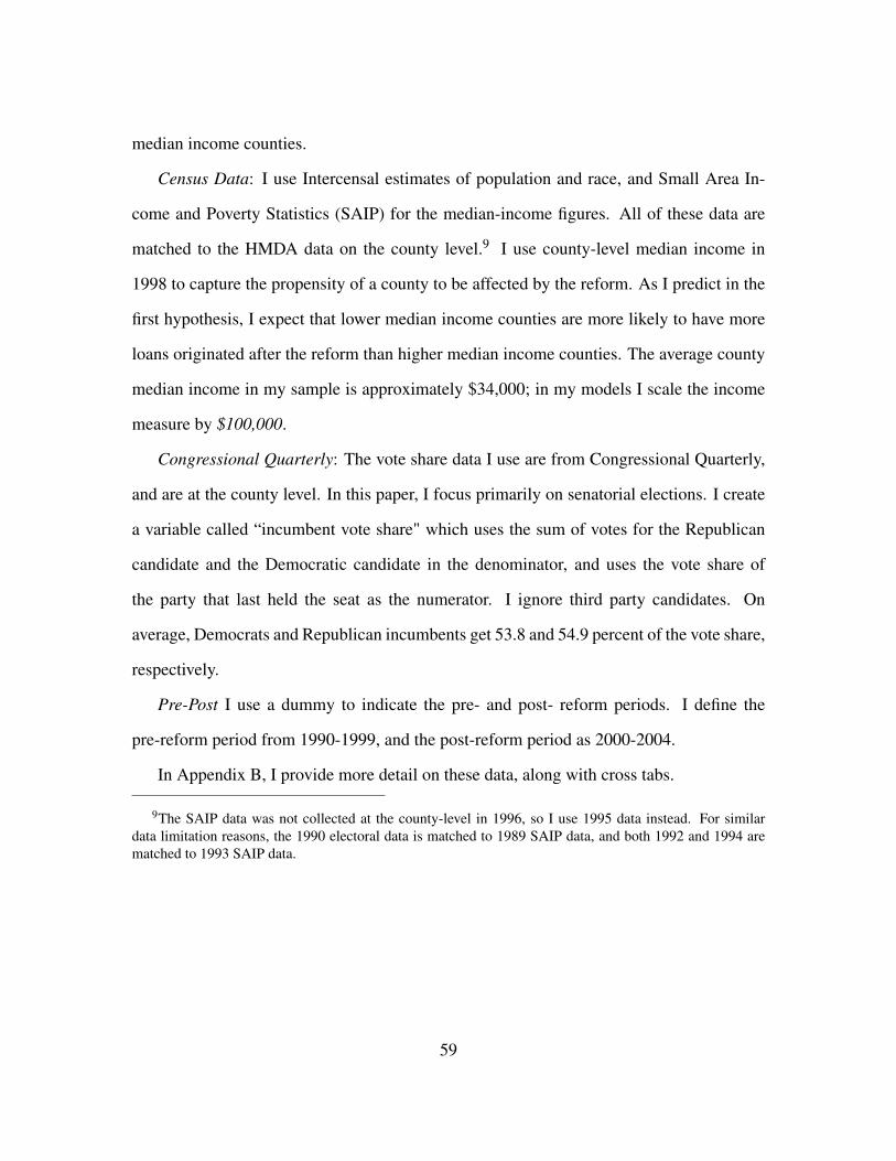
median income counties.
Census Data: I use Intercensal estimates of population and race, and Small Area In-
come and Poverty Statistics (SAIP) for the median-income figures. All of these data are
matched to the HMDA data on the county level.9 I use county-level median income in
1998 to capture the propensity of a county to be affected by the reform. As I predict in the
first hypothesis, I expect that lower median income counties are more likely to have more
loans originated after the reform than higher median income counties. The average county
median income in my sample is approximately $34,000; in my models I scale the income
measure by $100,000.
Congressional Quarterly: The vote share data I use are from Congressional Quarterly,
and are at the county level. In this paper, I focus primarily on senatorial elections. I create
a variable called “incumbent vote share" which uses the sum of votes for the Republican
candidate and the Democratic candidate in the denominator, and uses the vote share of
the party that last held the seat as the numerator. I ignore third party candidates. On
average, Democrats and Republican incumbents get 53.8 and 54.9 percent of the vote share,
respectively.
Pre-Post I use a dummy to indicate the pre- and post- reform periods. I define the
pre-reform period from 1990-1999, and the post-reform period as 2000-2004.
In Appendix B, I provide more detail on these data, along with cross tabs.
9The SAIP data was not collected at the county-level in 1996, so I use 1995 data instead. For similardata limitation reasons, the 1990 electoral data is matched to 1989 SAIP data, and both 1992 and 1994 arematched to 1993 SAIP data.
59
Table 2.1: Summary Table, Senate Data
Variable Observations Mean Std. Dev. Min MaxIncumbent Vote Share 11,018 0.575 0.139 0.150 0.966Loans Per Capita 11,018 0.003 0.004 0 0.096Pre/post 11,018 0.360 0.480 0 1Median Inc. 1998 (100,000s) 11,018 0.341 0.079 0.165 0.846Republican Incumbent 11,018 0.503 0.500 0 1Year 11,018 1997.33 4.680 1990 2004
2.4.2 Empirical Strategy
DD Design
To estimate the effect of loan origination on voting behavior, I use two different designs:
a difference-in-difference (DD) framework and an instrumental variables (IV) framework.
In the DD design, I exploit the differential impacts of the changes in GSE lending in 2000
across income groups. In particular, I examine how the reform differentially affected home
loans per capita and ultimately voting behavior in counties with differing median income
levels. The DD design can pinpoint the effect of being both in the post-reform period and
being in a low median income county.
Ultimately, what I want to explore is how incumbent vote shares were affected by in-
creased loan origination, driven by Fannie and Freddie. To do this, I first demonstrate
that the reform affected access to mortgage credit differentially across low and high in-
come counties. I then demonstrate that counties that have more loans per capita originated
are differentially more likely to vote for their incumbents. Finally, I use a differences-in-
differences-in-differences (DDD) strategy to explore the effect of being in the post-reform
period, in a low-income county with a Republican incumbent.
Model (2.1) looks at the relationship between being in a county that is likely to be
more affected by the increased MBS issuance post-2000 and how that affects the number
60
of loans per capita. I expect that in poorer counties, those that are more likely to respond
to the reform, there should be more loans per capita originated in the post-2000 period.
Poorer counties have more individuals who would only qualify for a mortgage when credit
is widely available and standards are lowered. I use pre-reform 1998 levels for median
income because I expect that that the marginal effect of increased credit in the market will
be highest in those areas. Model (2.1) is a test of hypothesis 1. The DD comes from the
interaction between the pre/post reform dummy and the income variable.
loanspercapitacst = β (xcs)+ γ(xcs ∗ pre/postt)+θ(yeart ∗ xcs)+µst + εcst (2.1)
Variation on loans per capita is on county (c), state (s) and time (t), where µ refers
to state-year fixed effects. “Pre/post" is a dummy that indicates pre- or post-200010, and
x is a measure of propensity to respond to treatment. In my empirical specification, I
operationalize x using county median income in 1998. We might think that poorer counties
are more likely to respond to increased loan origination because a greater number of people
in those counties will have increased access to mortgage lending because of GSE policy.
Models (2.2) and (2.3) use incumbent vote share as the outcome variable. Model (2.2)
is a test of hypothesis 2 - namely that areas with lower median income are more likely
to reward their incumbent. I use a DD design once again, pinpointing the effect of being
both in the post reform period and in a lower income county. Model (2.3) tests hypothesis
3, using a DDD model to identify the effect of lower income counties with Republican
incumbents in the post-reform period.
10Although Figure 2.1 does not show MBS issuance before 2001, it was negligible in the late 90s relativeto the boom in the early 2000s.
61
votesharecst = βxcs + γ(xcs ∗ pre/postt)+θ(yeart ∗ xcs)+µst + εcst (2.2)
votesharecst = βxcs + γ(xcs ∗ pre/postt)+θ(yeart ∗ xcs)+σ(pre/postt ∗RepIncst) (2.3)
+2δ (xcs ∗RepIncst)+λ (yeart ∗RepIncst)+φ(xcs ∗ pre/postt ∗RepIncst)
+κ(yeart ∗RepIncst ∗ xcs)+µst + εcst
IV Design
In the IV framework, I instrument for loan origination using the interaction between
county median income and being in the post-2000 period. The first stage is equation (2.1)
above. The structural equation I am estimating is as follows, where I am instrumenting for
loanspercapitacs using the interaction between xcs and prepostt .
votesharecst = β1loanspercapitacs +β2xcs +θ(yeart ∗ xcs)+µst + εcst (2.4)
In addition to the identifying assumptions that need to hold for the DD framework, the
IV specification requires two things. First, that there is a strong first stage; namely that
the interaction between county median income and being in the post-2000 period is in fact
a strong predictor of loan origination. As I will demonstrate empirically below, there is
an extremely strong first stage for the IV model. Second, the exclusion restriction has to
hold, which means that there weren’t other things changing for low income counties in
the post-2000 people that would also affect vote share. Even if the DD specification is
preferred, I still need to compellingly demonstrate that these result are not being driven by
events external to the increase in loan origination for lower income counties in this period.
I discuss this below.
62
2.5 Results
2.5.1 Poorer counties receive more loans per capita
I focus first on hypothesis 1, which suggests that poorer counties will receive more
loans per capita than richer counties. Model 1 in Table 2.2 is the relevant model. I find
that a one standard deviation increase in median income results in a 0.0001 decrease in
loans per capita in the post reform period. A one unit increase in median income refers to
a $100,000 increase in median income. The coefficient on “pre/post*MedInc98" remains
significant and negative across all the specifications.
2.5.2 Voting Outcomes
In the theory section above, I offer two hypotheses related to voting outcomes. The
first, hypothesis 2, predicts that poorer counties are more likely to reward incumbents for
increased access to mortgage credit. The second, hypothesis 3, predicts that areas with
lower median income are especially likely to reward Democratic incumbents.
Poorer counties are more likely to experience a large quantity of loan originations (as
seen above in the test of hypothesis 1) and sudden access to mortgage credit provides in-
cumbents with an opportunity to talk about their hand in providing loose mortgage access
conditions, and voters may perceive incumbents to have a hand in ensuring access to mort-
gage credit. I test this hypothesis in models 2 and 3 in Table 2.2. I find that this indeed the
case - there is a negative coefficient on pre-post*median income in 1998, suggesting that
counties with a higher median income in 1998 are less likely to vote for the incumbent in
the post-reform period. I find a relatively large effect, with a coefficient of -0.362, which
means that a one standard deviation increase in median income ($100,000) results in an
almost 3 percentage point decrease in the incumbent vote share.
63
Model 3 uses an IV specification and finds similar results. I use the interaction of being
in the post-2000 period and median income in 1998 as an instrument for loans per capita.
The first stage results, which can be seen in Model 1, have a strong F statistic of 14.61.
Similarly to Model 2, I find that counties that experienced more loans per capita were more
likely to support incumbents in the post-2000 period.
The second hypothesis related to voting outcomes is hypothesis 3, in which I predict
that areas with lower median income are especially likely to reward Democratic incum-
bents. To test this, I run a triple interaction between the pre/post reform period, whether the
county has a Republican incumbent, and the median income measure in Table 2.2, Model 4.
I find results broadly consistent with my hypotheses. This can be seen in Figure 2.3, which
shows the marginal effect of median income on Democratic and Republican incumbent
vote share relative to the pre-2000 period. Although the difference between Democrats and
Republicans is not significant, I do find that relative to the pre-2000 period, the marginal
effect of an increase in median income is negative for Democratic vote share.
I run the same models using House electoral data, which are discussed further in Ap-
pendix B. I also examine the effect of mortgage originations on turnout, and the inconclu-
sive results are presented in Appendix C. I do demonstrate that controlling for changes in
turnout pre- and post- the reform does not affect my results.
2.5.3 Exclusion Restriction
The exclusion restriction demands that my instrument, the interaction between being
in the post-2000 period and county median income, cannot affect incumbent vote share
though any channel except the housing market.
By far the biggest event with political consequences happening around this period is
the bombing of the World Trade Center and subsequent entry into war. If these events dis-
64
Figure 2.3: Marginal Effect of Median Income on Incumbent Vote Share relative to thePre-2000 Period
65
Table 2.2: Relationship between Income and Loan Origination and Senate Incumbent VoteShare
Model 1 Model 2 Model 3 Model 4Loans Per Capita Inc. Vote Share Inc. Vote Share Inc. Vote Share
(OLS) (OLS) (IV) (OLS)MedInc98 0.134 -63.110∗∗ -67.386∗∗
(0.172) (17.497) (18.797)Pre/post*MedInc98 -0.003∗∗ -0.362∗∗ -0.379∗∗
(0.000) (0.141) (0.138)Year*MedInc98 -0.000 0.032∗∗ 0.034
(0.000) (0.141) (0.009)RepInc*MedInc98 38.462∗∗
(18.647)Pre/post*RepInc*MedInc98 0.210
(0.142)RepInc*Year*MedInc98 -0.019∗∗
(0.009)Loans per capita 144.376∗∗
(71.095)State-Year Fixed Effects X X X XFirst Stage F Statistic 14.61N 11,454 11,018 11,018 11,018
Notes: Standard errors clustered by county are in parentheses. ∗∗ marks significance at95 percent, ∗ marks significance at 90 percent. All models are weighted by total countypopulation
proportionately affected lower median income counties, 9/11 could explain one of the two
outcomes - incumbent vote share by party. One way in which 9/11 could disproportion-
ately affect lower median income counties is if those counties were the ones most likely to
bear the brunt of the demand for soldiers in Afghanistan. Because the Republicans are so
closely tied to issues of national security (Gadarian 2010), and President Bush was such a
symbolic figure during the initial days of the “War on Terror", it is possible that people in
lower income counties blamed the Republicans for entry into the war, and turned against
them in subsequent elections. Note that this does not explain why low income counties
in the post-2000 period were rewarding their incumbents, it simply provides a plausible
explanation for why the Democrats might have gained electoral ground in this period.
To examine this possible violation of the exclusion restriction, I examine opinion data
66
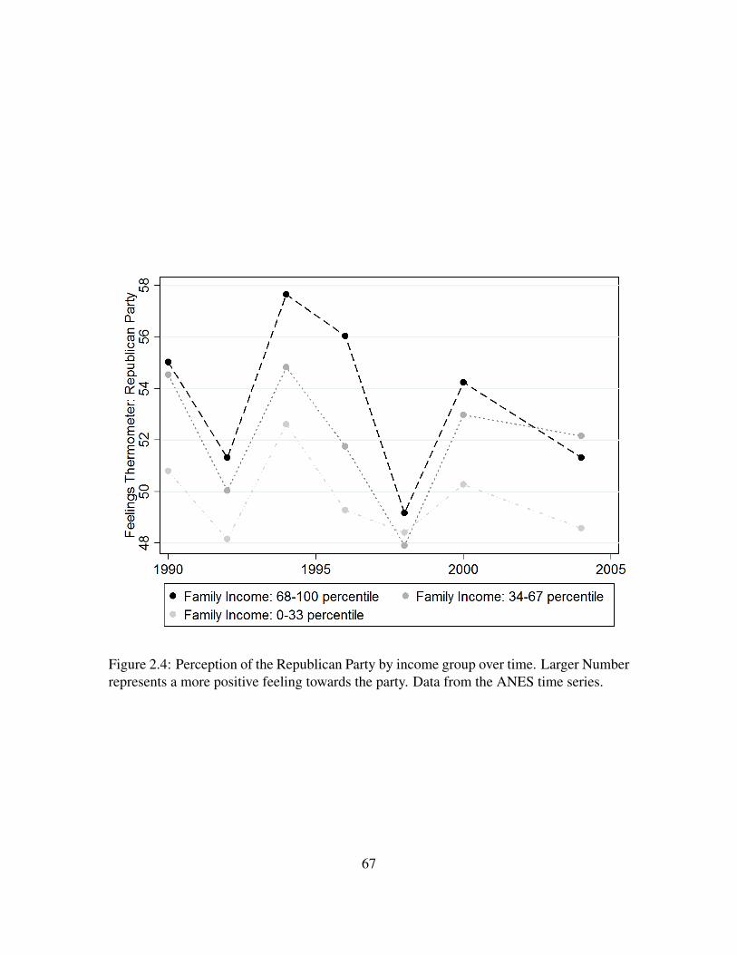
Figure 2.4: Perception of the Republican Party by income group over time. Larger Numberrepresents a more positive feeling towards the party. Data from the ANES time series.
67
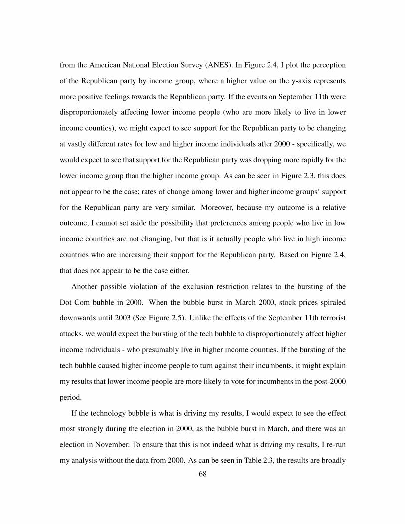
from the American National Election Survey (ANES). In Figure 2.4, I plot the perception
of the Republican party by income group, where a higher value on the y-axis represents
more positive feelings towards the Republican party. If the events on September 11th were
disproportionately affecting lower income people (who are more likely to live in lower
income counties), we might expect to see support for the Republican party to be changing
at vastly different rates for low and higher income individuals after 2000 - specifically, we
would expect to see that support for the Republican party was dropping more rapidly for the
lower income group than the higher income group. As can be seen in Figure 2.3, this does
not appear to be the case; rates of change among lower and higher income groups’ support
for the Republican party are very similar. Moreover, because my outcome is a relative
outcome, I cannot set aside the possibility that preferences among people who live in low
income countries are not changing, but that is it actually people who live in high income
countries who are increasing their support for the Republican party. Based on Figure 2.4,
that does not appear to be the case either.
Another possible violation of the exclusion restriction relates to the bursting of the
Dot Com bubble in 2000. When the bubble burst in March 2000, stock prices spiraled
downwards until 2003 (See Figure 2.5). Unlike the effects of the September 11th terrorist
attacks, we would expect the bursting of the tech bubble to disproportionately affect higher
income individuals - who presumably live in higher income counties. If the bursting of the
tech bubble caused higher income people to turn against their incumbents, it might explain
my results that lower income people are more likely to vote for incumbents in the post-2000
period.
If the technology bubble is what is driving my results, I would expect to see the effect
most strongly during the election in 2000, as the bubble burst in March, and there was an
election in November. To ensure that this is not indeed what is driving my results, I re-run
my analysis without the data from 2000. As can be seen in Table 2.3, the results are broadly
68
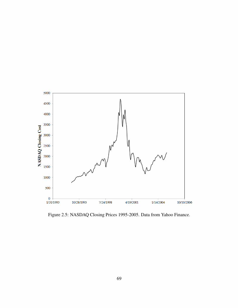
Figure 2.5: NASDAQ Closing Prices 1995-2005. Data from Yahoo Finance.
69
the same as when 2000 is included in the data. Moreover, we can refer back to Figure 2.4
and see that higher income people are not changing their attitudes towards the Republican
party at rates that are different from the lower income individuals.
Table 2.3: Relationship between Income and Loans Per Capita and Senate Incumbent VoteShare, excluding 2000
Model 1 Model 2 Model 3Loans Per Capita Inc. Vote Share Inc. Vote Share
(OLS) (OLS) (IV)MedInc98 -0.106 -54.164∗∗
(0.134) (16.115)Pre/post*MedInc98 -0.004∗∗ -0.307∗∗
(0.001) (0.095)Year*MedInc98 0.000 0.027
(0.000) (0.008)RepInc*MedInc98
Pre/post*RepInc*MedInc98
RepInc*Year*MedInc98
Loans per capita 77.492∗∗
(26.409)State-Year Fixed Effects X X XFirst Stage F Statistic 39.21N 10,185 10,185 10,185
Notes: Standard errors clustered by county are in parentheses. ∗∗ marks significance at95 percent, ∗ marks significance at 90 percent. All models are weighted by total countypopulation
Finally, we might expect that voters were not supporting their incumbents because of
the provision of mortgage credit, but because of the generally booming economy and strong
job market. This violation of the exclusion restriction would suggest that my instrument
was working though unemployment rate channels - the lower income areas were more
likely to experience a drop in the unemployment rate and subsequently reward their incum-70
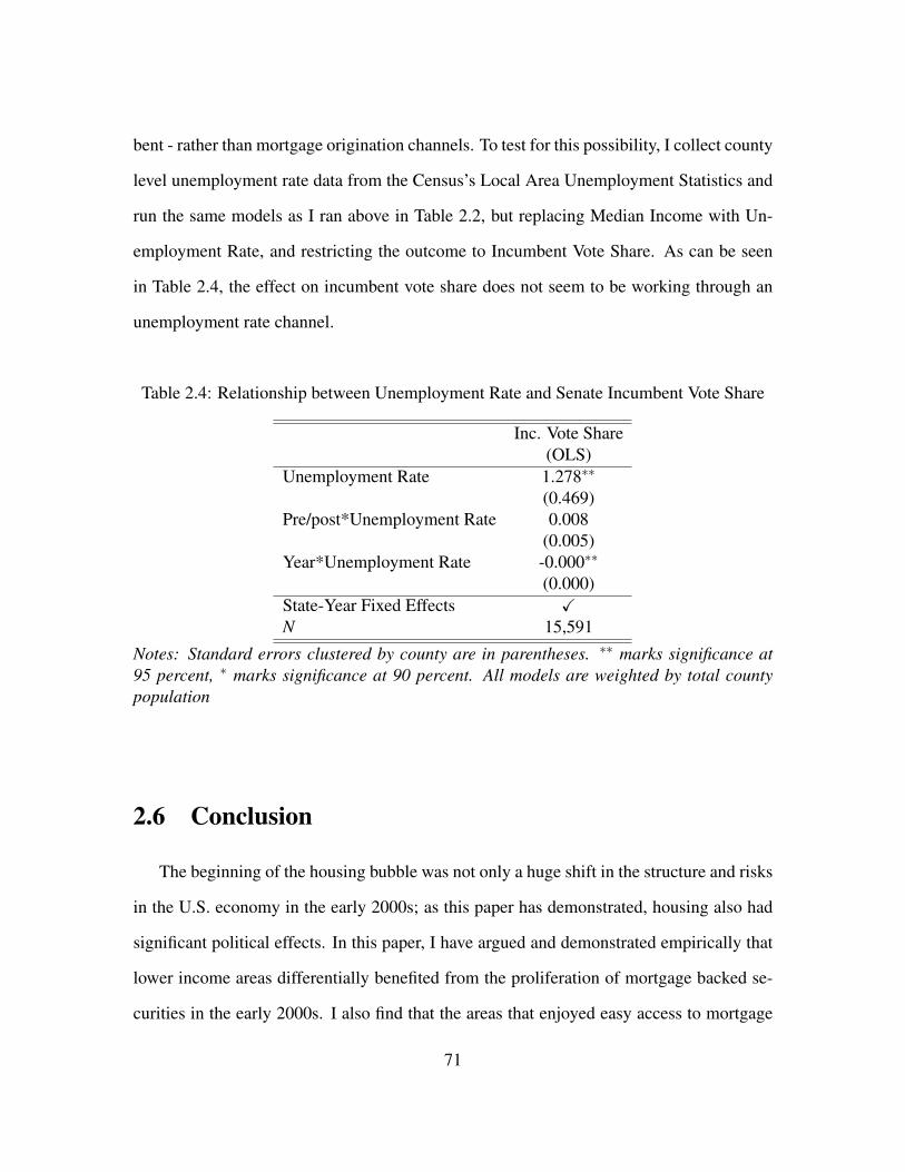
bent - rather than mortgage origination channels. To test for this possibility, I collect county
level unemployment rate data from the Census’s Local Area Unemployment Statistics and
run the same models as I ran above in Table 2.2, but replacing Median Income with Un-
employment Rate, and restricting the outcome to Incumbent Vote Share. As can be seen
in Table 2.4, the effect on incumbent vote share does not seem to be working through an
unemployment rate channel.
Table 2.4: Relationship between Unemployment Rate and Senate Incumbent Vote Share
Inc. Vote Share(OLS)
Unemployment Rate 1.278∗∗
(0.469)Pre/post*Unemployment Rate 0.008
(0.005)Year*Unemployment Rate -0.000∗∗
(0.000)State-Year Fixed Effects XN 15,591
Notes: Standard errors clustered by county are in parentheses. ∗∗ marks significance at95 percent, ∗ marks significance at 90 percent. All models are weighted by total countypopulation
2.6 Conclusion
The beginning of the housing bubble was not only a huge shift in the structure and risks
in the U.S. economy in the early 2000s; as this paper has demonstrated, housing also had
significant political effects. In this paper, I have argued and demonstrated empirically that
lower income areas differentially benefited from the proliferation of mortgage backed se-
curities in the early 2000s. I also find that the areas that enjoyed easy access to mortgage
71
credit subsequently rewarded their incumbent legislators, and I demonstrate this through
both a DD and IV framework. I suggest that incumbents had a leg up on challenger politi-
cians because issues of housing finance were being actively discussed in Congress at the
time, and that in some cases, they were able to campaign on these issues. Finally, I pro-
vide suggestive evidence that Democrats were more likely to benefit from the mortgage
origination boom than Republicans.
I argue that voters do not distinguish between the role of politicians and the role of the
GSEs in ensuring greater access to mortgage credit. While it is impossible to distinguish
what portion of this relationship is because voters do not understand who is responsible for
policy changes and what portion is politicians taking credit for GSE policy, it does raise
the question of whether this relationship would hold outside the U.S. context. Housing
is a uniquely important policy tool in the U.S., historically and at present. Even a quick
glance at the history of redlining and other exclusionary policies, as well as the inception
of the 2008 financial crisis, makes abundantly clear that housing plays an outsize role in
the political and economic realms in the U.S.. However, homeownership is also seen as
a marker of success; it is constantly referred to by political actors as a key part of the
“American Dream." In largely rental societies such as Germany and Switzerland (Andrews
and Sánchez 2011), where homeownership is neither common nor glorified, not only do
extra-political actors have less of an incentivize homeownership, but politicians have less
incentive to take credit for these policies. The role of housing and voting behavior in
primarily rental societies is an important future research agenda.
Another important agenda for future research is the interaction between race and poli-
cies such as the GSE reform in this paper. As stated above, the U.S. has a long history of
exclusionary housing targeted at Black populations. When I run the same models above us-
ing proportion Black as my x value, I do not find significant results. It is somewhat curious
that the expected relationship holds for low income areas but not for areas with a large pro-
72
portion of Black people. A look at the correlation between these two variables shows that
areas with large black populations are indeed poorer (the correlation is negative) but the
magnitude of the correlation is small (-0.059). These results do beg the question, however,
of why areas with large Black populations continue to be left out of surges of mortgage
lending despite policies such as the Fair Housing Act that seek to address racial disparities
in mortgage lending. It is possible that poor Black populations were actively discriminated
against by the GSEs, and were not able to receive loans that poor white counties were able
to receive or that poor Blacks did not want these loans. It is also possible that minori-
ties are concentrated in urban environments, where it’s much harder to purchase, where
as low-income whites may be more likely to live in rural or suburban areas where home
purchasing is a bit easier. Further exploration of the data, especially with regard to who
applies for mortgages in this period, is warranted.
Unlike other papers (Achen and Bartels 2004; Healy, Malhotra, and Mo 2010) that
focus on how changes out of a politician’s hands affect voting, this paper focuses on an
area in which there are likely close ties between political actors and Fannie and Freddie.
So while this paper is in part about how voters perceive economic conditions and subse-
quently assign rewards or blame, it also addresses a deeper, more normative question about
democratic accountability. So many aspects of economic performance, including ease of
access to mortgage credit, are only marginally under the control of politicians. This cre-
ates perverse incentives for elected politicians: to claim credit for economic successes that
are out of their hands, and to develop crony-esque relationships with extra-political actors.
If voters are rewarding incumbents based on policies set by these extra-political actors,
then incumbents are being re-elected on information that may not accurately signal the true
quality of the incumbent.
73
3 | Local Economic Information, Foreclosure,and Political Attitudes
3.1 Introduction
Voters receive information about their local political and economic environment in a
myriad of ways. Hearing sound bites of political candidates on the news, talking about a
recent political debate with neighbors, and observing visible signs of blight in the neigh-
borhood are all different forms of information gathering that a voter may undertake on a
day to day basis. Although the political science literature has explored the ways in which
information affects political behavior, little is known about how different types of informa-
tion differentially affect political behavior. In this paper, I delve into this question using
the housing market as a frame through which to understand how the form of information
people receive affects their likelihood of political and community participation.
The role of information in political behavior has long been studied in political sci-
ence. A large literature shows how information supports electoral accountability (Ashworth
2012; Healy and Malhotra 2013b), and plays an important role in determining political be-
havior (Tolbert and McNeal 2003) and preference formation (Bullock 2011). Moreover,
previous work by Ansolabehere, Meredith, and Snowberg (2014) demonstrates that the lo-
cal environment matters for political behavior. However, this literature has not yet explored
how the form of the information respondents receive shapes their political behavior.
74
In particular, little is known about whether voters’ political behavior responds primar-
ily to visual images or factual written information. It is important to differentiate between
these two channels of information because many people either do not actively consume or
have access to factual written information. Visual images may be more easily accessible to
many, and more easily understood. To examine this question, I will use a survey experiment
to identify whether the way in which people receive information about their local economic
environment affects whether or not they choose to engage in political action. Ascertaining
how different forms of information and their combinations induce political action has inter-
esting implications for canvassers, political campaigns, broadcast media and other groups
that rely on emotional responses to elicit a political outcome.
I suggest that experiential signals about the local economy, such as driving past a fore-
closed house in one’s neighborhood, may be more emotionally salient than reading a news
piece on local foreclosure rates. Given that both signals about the local economy convey
the same information, at least in this particular experiment, comparing signals along the
dimension of emotional salience allows me to examine the extent to which these two types
of information acquisition are substitutes or complements. To test this empirically, I exam-
ine how showing survey respondents photographs of foreclosures and giving them factual
written information pertaining to local foreclosure rates affect survey respondents’ decision
to submit a pre-prepared (strong or weakly worded) letter to their Member of Congress or
express interest in participating politically in their local community.
Using Amazon’s Mechanical Turk, I randomize the form of information respondents
receive about local foreclosures. To induce concern about foreclosure, some respondents
receive photos of foreclosed homes to capture the effect of seeing a foreclosed home in
one’s hypothetical local area. Other respondents receive numerical information about the
high foreclosure rate in their hypothetical local area by reading a paragraph designed to
mimic reading about one’s local economic area in a newspaper. In addition, there are two
75
other treatment conditions: one receives both the photo and numerical information, while
the reference category receives no information about foreclosures. For both the photo and
numerical foreclosure information, respondents understood the information as representing
a foreclosure rate twice as high as the state average. The experimental design thus allows
me to identify whether emotionally salient information or non-emotionally salient infor-
mation has a larger effect on political action, and the extent to which the different types of
information serve as substitutes or complements.
The results suggest that receiving information about foreclosures, in either format, al-
ters respondent behavior. For both the visual and written treatments, the foreclosure infor-
mation increases the probability of respondents sending a strongly worded letter expressing
concern about foreclosures to their Member of Congress by 3 percentage points. However,
the information treatments do not significantly increase the probability of sending a weakly
worded letter. The photo and numerical treatments act as substitutes, such that receiving
a second signal does not meaningfully increase the likelihood that a voter contacts their
Congressman.
While both forms of information equally impact the main behavioral outcome, the
photo of a foreclosed home has a significantly larger impact on interest in local politi-
cal participation. Both the photo treatment and the numerical information treatments have
a strong positive effect on the respondents’ likelihood of indicating interest in participat-
ing politically. However, the treatment effect on those who are administered the emotional
prime (seeing the photo) is twice as large, which suggests a greater interest in talking
to neighbors about foreclosures, attending community meetings about struggling home-
owners, signing a petition for more aid to the community and voting for a candidate that
supports increased foreclosure relief, than those who simply read the paragraph.
Finally, I examine a number of mechanisms through which the treatments could op-
erate. First, I find that being shown a photo of a foreclosed home causes people to ex-
76
press significantly more worry about foreclosures, while receiving numerical information
about foreclosures does not. Second, the effects appear to be driven by local concerns.
Both treatments, but especially the photo treatment, cause voters to express greater concern
about local housing values, while the visual treatment also significantly increases concern
about local crime. Third, there is no evidence to suggest that the treatments affect personal
concerns, emotional responses or systemic concerns. Although both visual and written
information play an important role, these results suggest that visual information can have
stronger behavioral effects than information transmitted through a more traditional source
of politically relevant information.
Examining the way in which voters receive information at the local level has impor-
tant implications for democracy. Because people are often involved in politics at the local
level (Fischel 2009), the way in which individuals understand the local economy and draw
political inferences may affect political participation and behavior. Moreover, there are
various costs associated with consuming different types of information. While it may take
concerted effort to spend a half hour watching and comprehending the news, it may be less
costly to internalize local economic conditions by looking out the window during one’s
commute. If, as I argue in this paper, formal and informal channels convey the same in-
formation to consumers, the findings offer political scientists a deeper understanding of
three important factors in the study of political behavior. First, we would have a broader
understanding of what comprises “political information" - that is, information that trans-
mits details about the environment that resonate politically. Second, we can better identify
which voters have access to politically relevant information. Finally, we will have a better
understanding of the types of informational strategies that could be most effective for those
trying to elicit political behavior, such as political campaigns and canvassers.
The next section presents the theoretical grounding for this project, which draws pri-
marily on the political psychology and economic voting literatures. Section 3 goes through
77
the research design, including the estimation strategy. Section 4 examines the two main
results, and conducts some robustness checks. The penultimate section goes over potential
mechanisms and the final section concludes.
3.2 Theory
A large literature argues that individuals vote according to the economic environment
(Key 1966; Healy and Malhotra 2013a). This economic voting literature provides im-
portant evidence illuminating how information about the local economic environment can
affect political behavior. Key (1966) argues against the idea that voters are uninformed
about political issues (Campbell et al. 1966; Converse 2006) and instead argues that voters
take in information about their environment and use that information to evaluate politician
performance. Rational models have proposed that voters may sanction incumbents to ad-
dress moral hazard (Barro 1973; Ferejohn 1986) or select better politicians (Fearon 1999;
Alt, Bueno de Mesquita, and Rose 2011). Alternatively, the cognitive model suggests that
voters use heuristics to make decisions when information is costly to acquire (Achen and
Bartels 2004).
There is considerable evidence linking economic conditions and vote choice (Fiorina
1978, 1981; Ansolabehere, Rodden, and Snyder 2008), which this experiment builds on
theoretically. In particular, this experiment is closely related to Ansolabehere et al’s (2014)
work on “mecro" level voting, which theorizes that voters’ perceptions of economic condi-
tions are shaped by the economic condition of those most like them (Ansolabehere, Mered-
ith, and Snowberg 2014).
While housing is an important component of the local economy, the political econ-
omy literature has only started to incorporate it into the economic voting literature. Mabud
(2016) demonstrates that a sudden influx of loan originations significantly increases the
78
likelihood that counties that experience this influx reelect their incumbent, but only if the
incumbent is a Democrat. Ansell (2014) also brings together housing and political prefer-
ences, where he suggests that people use home equity as a form of private insurance, which
in turn substitutes for homeowners’ demand for social insurance. Moreover, the persistent
effects of the financial crisis (Chinn and Frieden 2011) have made housing a particularly
salient signal about the health of the local economy.
While the economic voting literature emphasizes the role of information, it does not
distinguish between the behavioral effects of different forms of information. This paper
addresses this gap by exploring the different ways in which people receive information
about their local environment and their differential effects on political behavior. There is
reason to think that the way in which voters receive information affects political behavior
(Durante and Knight 2012; Healy and Lenz 2014; Alt, Lassen, and Marshall 2016). For
example, Alt, Lassen, and Marshall (2016) demonstrate that the credibility of the source
of an economic signal affects whether or not sophisticated voters update their beliefs about
the economic environment, and thereby influences whether or not economic voting takes
place. Unlike Alt, Lassen, and Marshall (2016), this experiment is focuses on differences
in the form of these signals rather than the credibility of their source.
3.2.1 Visual Information and the Cognitive Approach
Although the extensive literature on economic voting suggests that traditional methods
of acquiring information about the local economy matter for political behavior, I argue that
visual information also serves as important source of politically relevant information for
people (Prior 2014). I suggest that being shown a photo of a foreclosed house may more
emotionally salient than considering statistics read in a paragraph.
An extensive literature in political psychology explores the importance of emotionally
79
salient informational signals for political participation. This can be broken down into two
major schools of thought: the Affective Intelligence Theory (AIT) (Marcus, Neuman, and
MacKuen 2000) and cognitive appraisal theory (Folkman et al. 1986; Lazarus 1991; Lerner
and Keltner 2000, 2001). AIT relates to the study of emotions, particularly the way in which
instinctual reactions affect decision making. In the political science literature, AIT has been
applied to explain how emotions might shape political behavior (Achen and Bartels 2004;
Gomez, Hansford, and Krause 2007; Healy, Malhotra, and Mo 2010). Cognitive appraisal
theory, on the other hand, suggests that people incorporate their own personal interpretation
of an event when formulating emotions. Cognitive theories also suggest that people put
more weight on what caused the event than AIT.
As elaborated in Valentino et al. (2011), these theories explain the different emotional
responses to varying stimuli, and where these emotional responses come from (Averill
1983; Smith and Ellsworth 1985; Lerner and Keltner 2000, 2001; Smith and Kirby 2004;
Brader, Groenendyk, and Valentino 2010). The literature suggests that emotional cues,
which are more likely to elicit specific attributions of blame, are also more likely to elicit
more concrete and sustained behavioral responses (Valentino et al. 2011). Moreover, Or-
toleva and Snowberg (2013) suggest that people falsely believe that their own experiences
are highly generalizable, because they underestimate the correlation of local shocks. This
suggests that people may over-respond to specific information that generates an emotional
response.
Visual information may be working through emotional channels, but work in social
psychology and sociology provides additional channels through which visual information
may be politically relevant. Fahmy, Bock, and Wanta (2014) write about the extensive
research that demonstrates that visuals are crucially important in inducing consumer be-
havior (Marks and Olson 1981), and that people react to visual images differently based on
their demographic backgrounds (Scott 1994). Moreover, literature exploring the role that
80
urban blight plays in community perception is especially relevant to this work. Sampson
and Raudenbush (2004) find that as the proportion of minorities in a community increases,
residents of all races perceive greater disorder. Their work suggests that visual informa-
tion - implicitly or explicitly - in perpetuating social biases, may of which likely play in to
political action.
Whether or not visual information and written information act as substitutes or com-
plements is not clear. On one hand, people who consume visual information may not seek
or have access to more traditional forms of information. This might suggest that these two
types of information would act like substitutes, primarily because they would be targeting
different populations. On the other hand, it is possible that while these types of information
convey the same factual information, they do not convey the same content about institutions
(e.g. who the relevant legislator is, how to contact them, etc.). This would suggest that these
different types of information act as complements.
3.3 Research Design
Drawing from this literature, this paper addresses two main questions:
• Does visual information matter for political behavior?
• Do visual information and written salient information act as substitutes or comple-
ments?
The research design, explained below, is designed to address these two key questions.
3.3.1 Sample
The platform used to recruit survey respondents for this paper is Amazon’s Mechanical
Turk, an online platform that has been widely used for experimental work in recent years81
(Berinsky, Huber, and Lenz 2012). The survey was carried out during the first week of
January 2016. Survey respondents were paid $0.60 for completing a survey expected to
take approximately 6 minutes.1
My final sample includes 4,510 respondents, of which approximately half are women.
The sample skews slightly more Democratic, although the modal response to a question
about party affiliation was a 5,on a 0-10 scale ranging from Democratic to Republican.
The vast majority of respondents identify as non-Hispanic Whites, and most respondents
are between 25 and 34 years old. The average annual household income of respondents is
between 40 and 49 thousand dollars. The vast majority of my sample are citizens.2 Further
summary statistics about the sample can be found in Appendix E (Table E.1).
3.3.2 Treatments
This project compares four different treatment conditions, which are outlined in the di-
agram below. These conditions are designed to test how the form of economic information,
whether it is emotionally salient or not, affects political behavior. In this experiment, the
emotionally salient treatment is showing respondents a photo of a foreclosed house. Re-
spondents are asked to imagine the house is in their local area, so the treatment is attempt-
ing to mimic seeing a foreclosed house in one’s own neighborhood. Given the hypothetical
nature of this information, the results are likely to represent lower bounds on the effects
of providing such information. Respondents are also randomly assigned less emotionally
salient information, where they are given information from a website that reports housing
statistics for the same area. All respondents to the survey saw the following paragraph.
1I piloted this survey with approximately 200 respondents. The pilot respondents were paid $0.50 forfor completing the survey, and I raised the rate to $0.60 after the pilot results indicated that it was takingrespondents slightly longer than expected. The $0.10/minute rate is fairly standard according to Berinsky,Huber, and Lenz (2012) and conversations with peers who have conducted similar survey experiments.
2Only 52 respondents are not citizens. Results are virtually identical when dropping these individuals.
82
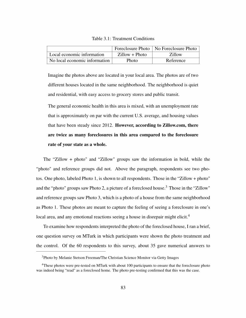
Table 3.1: Treatment Conditions
Foreclosure Photo No Foreclosure PhotoLocal economic information Zillow + Photo ZillowNo local economic information Photo Reference
Imagine the photos above are located in your local area. The photos are of two
different houses located in the same neighborhood. The neighborhood is quiet
and residential, with easy access to grocery stores and public transit.
The general economic health in this area is mixed, with an unemployment rate
that is approximately on par with the current U.S. average, and housing values
that have been steady since 2012. However, according to Zillow.com, there
are twice as many foreclosures in this area compared to the foreclosure
rate of your state as a whole.
The “Zillow + photo" and “Zillow" groups saw the information in bold, while the
“photo" and reference groups did not. Above the paragraph, respondents see two pho-
tos. One photo, labeled Photo 1, is shown to all respondents. Those in the “Zillow + photo"
and the “photo" groups saw Photo 2, a picture of a foreclosed house.3 Those in the “Zillow"
and reference groups saw Photo 3, which is a photo of a house from the same neighborhood
as Photo 1. These photos are meant to capture the feeling of seeing a foreclosure in one’s
local area, and any emotional reactions seeing a house in disrepair might elicit.4
To examine how respondents interpreted the photo of the foreclosed house, I ran a brief,
one question survey on MTurk in which participants were shown the photo treatment and
the control. Of the 60 respondents to this survey, about 35 gave numerical answers to
3Photo by Melanie Stetson Freeman/The Christian Science Monitor via Getty Images
4These photos were pre-tested on MTurk with about 100 participants to ensure that the foreclosure photowas indeed being “read" as a foreclosed home. The photo pre-testing confirmed that this was the case.
83

Figure 3.1.a: Photo 1, photo from Google Maps
84

Figure 3.1.b: Photo 2, photo by Melanie Stetson Freeman/The Christian Science Monitorvia Getty Images
85
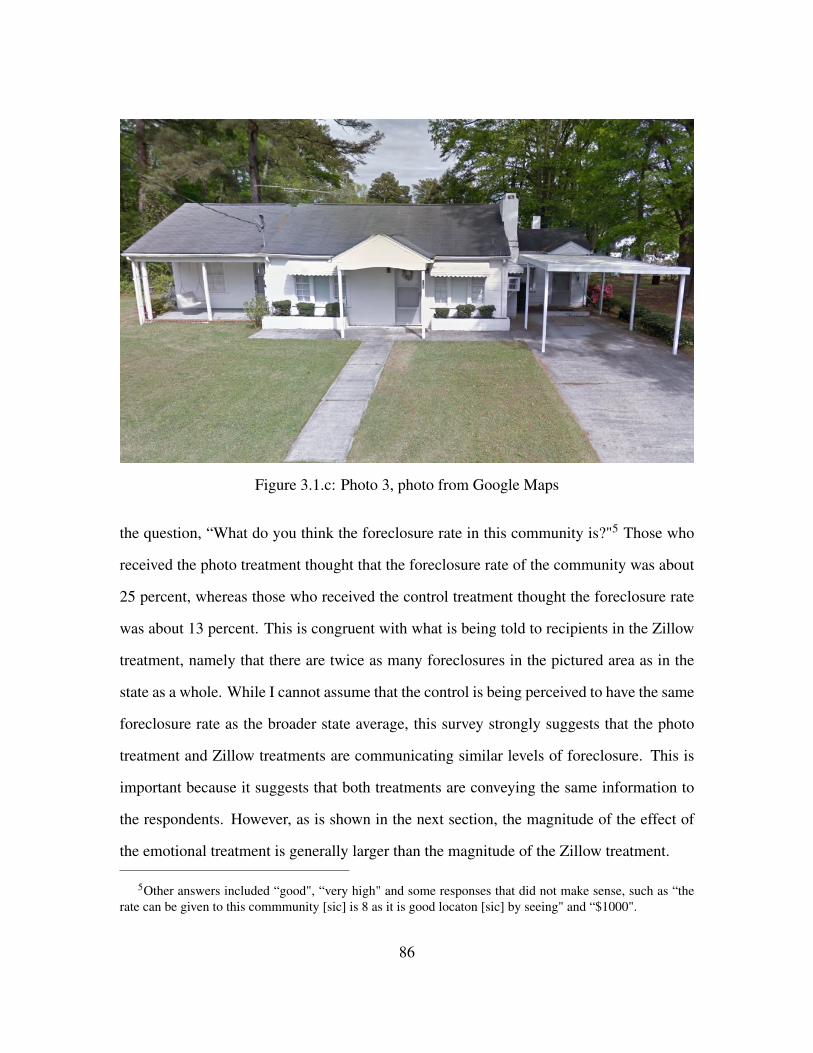
Figure 3.1.c: Photo 3, photo from Google Maps
the question, “What do you think the foreclosure rate in this community is?"5 Those who
received the photo treatment thought that the foreclosure rate of the community was about
25 percent, whereas those who received the control treatment thought the foreclosure rate
was about 13 percent. This is congruent with what is being told to recipients in the Zillow
treatment, namely that there are twice as many foreclosures in the pictured area as in the
state as a whole. While I cannot assume that the control is being perceived to have the same
foreclosure rate as the broader state average, this survey strongly suggests that the photo
treatment and Zillow treatments are communicating similar levels of foreclosure. This is
important because it suggests that both treatments are conveying the same information to
the respondents. However, as is shown in the next section, the magnitude of the effect of
the emotional treatment is generally larger than the magnitude of the Zillow treatment.
5Other answers included “good", “very high" and some responses that did not make sense, such as “therate can be given to this commmunity [sic] is 8 as it is good locaton [sic] by seeing" and “$1000".
86
3.3.3 Outcomes
To examine how these two different treatments affect political behavior, I elicit several
behavioral responses. The first outcome is whether the respondent chooses to send a letter
to their member of Congress and the tone of the letter sent. I also examine hypothetical
behavior by asking a series of questions about what the respondent would do if they lived
in the neighborhood they saw photos of.
For the first behavioral outcome, respondents are asked if they would like to send a
letter to their Member of Congress. The question reads, “Would you like to send a letter
to your Member of Congress supporting more assistance for struggling homeowners?" Re-
spondents can select “yes," “no," and “maybe". Several questions later, respondents who
selected “yes" or “maybe" are asked to select from a choice of two slightly differently
worded letters. Respondents who are prompted to answer this question can also select a
response that suggests that they no longer want to send the letter. I code a variable called
“sent letter," where “1" is assigned to those who selected one of the letters in the second
question, and “0" is assigned to those who either said “no" to the first question, or did not
select one of the letter texts in the second question.
The second outcome measure is based on responses to a question that reads, “You
said earlier that you might be interested in writing to your Member of Congress about
struggling homeowners. Please select one of the texts below to send to your Congressman
or Congresswoman." Respondents can select from three choices, where choice 1 is:
“Dear [Congressperson’s name], I am deeply concerned about the plight ofstruggling homeowners in America. I am outraged that Congress has not donemore to help homeowners who are facing foreclosure, and urge you to takeimmediate action to address this important issue. Sincerely, [Your name]"
Choice two is:
87
“Dear [Congressperson’s name], I am concerned about the challenges facinghomeowners in America. I am upset that Congress has not done more to helphomeowners facing foreclosure, and urge you to take action to address thisissue. Sincerely, [Your name]"
Respondents can also choose an option that says “I changed my mind, I don’t want to write
to my Member of Congress." “Strong letter" is coded such that respondents who chose the
first possible response are coded as “1", while all others (including those who answered
“no” to the first question about wanting to send a letter at all) are coded as “0".
Finally, respondents are posed with a number of hypothetical actions that the respondent
could take if they lived in the neighborhood they saw pictured. Respondents can indicate,
from 1-10 (where 10 is high) how likely they are to take any of the following actions:
• “Talk to your neighbors about foreclosures"
• “Attend a community meeting about struggling homeowners"
• “Sign a petition for more economic aid to the community"
• “Vote for a candidate that supports increased foreclosure relief"
This set of hypothetical questions allows me to get at the distinction that Valentino et al.
(2011) draw between what causes “expressive" political actions and what could cause sus-
tained political action. They argue that anxiety is more likely to lead to expressive behavior
whereas anger leads to sustained behavior. Conditional on seeing the emotional responses
Valentino et al. (2011) expect, the hypothetical set is helpful for distinguishing between
costly and less costly political behavior. If I do not observe the anticipated behavioral
responses, the responses to this battery of hypotheticals is still a useful measure for the
propensity for political action.
88
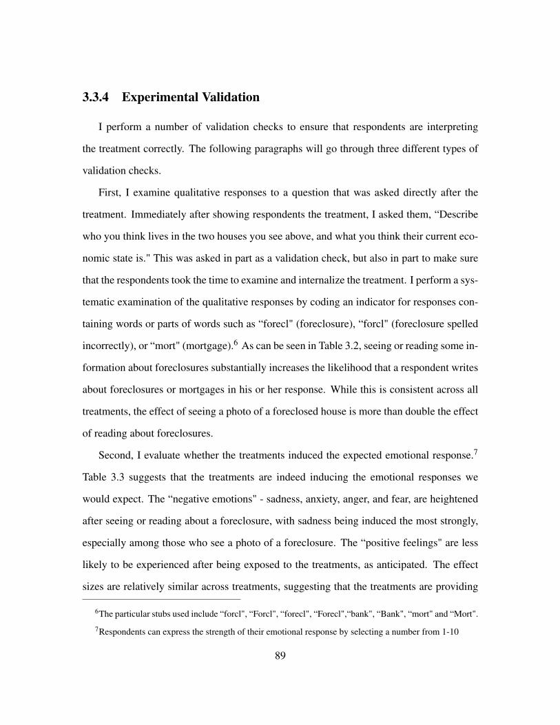
3.3.4 Experimental Validation
I perform a number of validation checks to ensure that respondents are interpreting
the treatment correctly. The following paragraphs will go through three different types of
validation checks.
First, I examine qualitative responses to a question that was asked directly after the
treatment. Immediately after showing respondents the treatment, I asked them, “Describe
who you think lives in the two houses you see above, and what you think their current eco-
nomic state is." This was asked in part as a validation check, but also in part to make sure
that the respondents took the time to examine and internalize the treatment. I perform a sys-
tematic examination of the qualitative responses by coding an indicator for responses con-
taining words or parts of words such as “forecl" (foreclosure), “forcl" (foreclosure spelled
incorrectly), or “mort" (mortgage).6 As can be seen in Table 3.2, seeing or reading some in-
formation about foreclosures substantially increases the likelihood that a respondent writes
about foreclosures or mortgages in his or her response. While this is consistent across all
treatments, the effect of seeing a photo of a foreclosed house is more than double the effect
of reading about foreclosures.
Second, I evaluate whether the treatments induced the expected emotional response.7
Table 3.3 suggests that the treatments are indeed inducing the emotional responses we
would expect. The “negative emotions" - sadness, anxiety, anger, and fear, are heightened
after seeing or reading about a foreclosure, with sadness being induced the most strongly,
especially among those who see a photo of a foreclosure. The “positive feelings" are less
likely to be experienced after being exposed to the treatments, as anticipated. The effect
sizes are relatively similar across treatments, suggesting that the treatments are providing
6The particular stubs used include “forcl", “Forcl", “forecl", “Forecl",“bank", “Bank", “mort" and “Mort".
7Respondents can express the strength of their emotional response by selecting a number from 1-10
89
Table 3.2: Relationship between treatments and typing “foreclosure",“mortgage", or“bank" in qualitative responses
(1) (2) (3) (4)Reference Category 0.034*** 0.073*** 0.122*** 0.034***
(0.005) (0.006) (0.007) (0.005)Any treatment 0.161***
(0.009)Photo treatment 0.160*** 0.178***
(0.010) (0.013)Zillow treatment 0.065*** 0.080***
(0.011) (0.011)Zillow × Photo -0.038*
(0.021)Observations 4510 4510 4510 4510
Notes: Robust errors in parentheses. * p<0.1, ** p<0.05, *** p<0.01
the same kind of information to survey respondents.
While some of the political psychology literature predicts that different types of stimuli
have different emotional responses (Smith and Ellsworth 1985; Smith and Kirby 2004;
Lerner and Keltner 2000, 2001), this does not seem to be the case here. As can be seen in
Table 3.3, the coefficients on the different treatments in Models 2 and 3 are not significantly
different from each other, making it difficult to say what emotional channel the results are
working through.
Finally, I perform a number of balance checks to ensure that my treatments are well
balanced along a number of dimensions, including political preferences and demographics.
I test for balance on concern for animal rights, concern for foreclosures, concern for immi-
gration, ethnicity, age, gender, citizenship, income, and homeowner status. As expected,
there are no significant differences between treatment assignments.8 A balance table can
8Because demographic questions were asked towards the end of the survey, I cannot check for balanceon covariates like political affiliation or other evaluative questions that may be affected by the treatment (e.g.whether the respondent would like to own a home in the future).
90
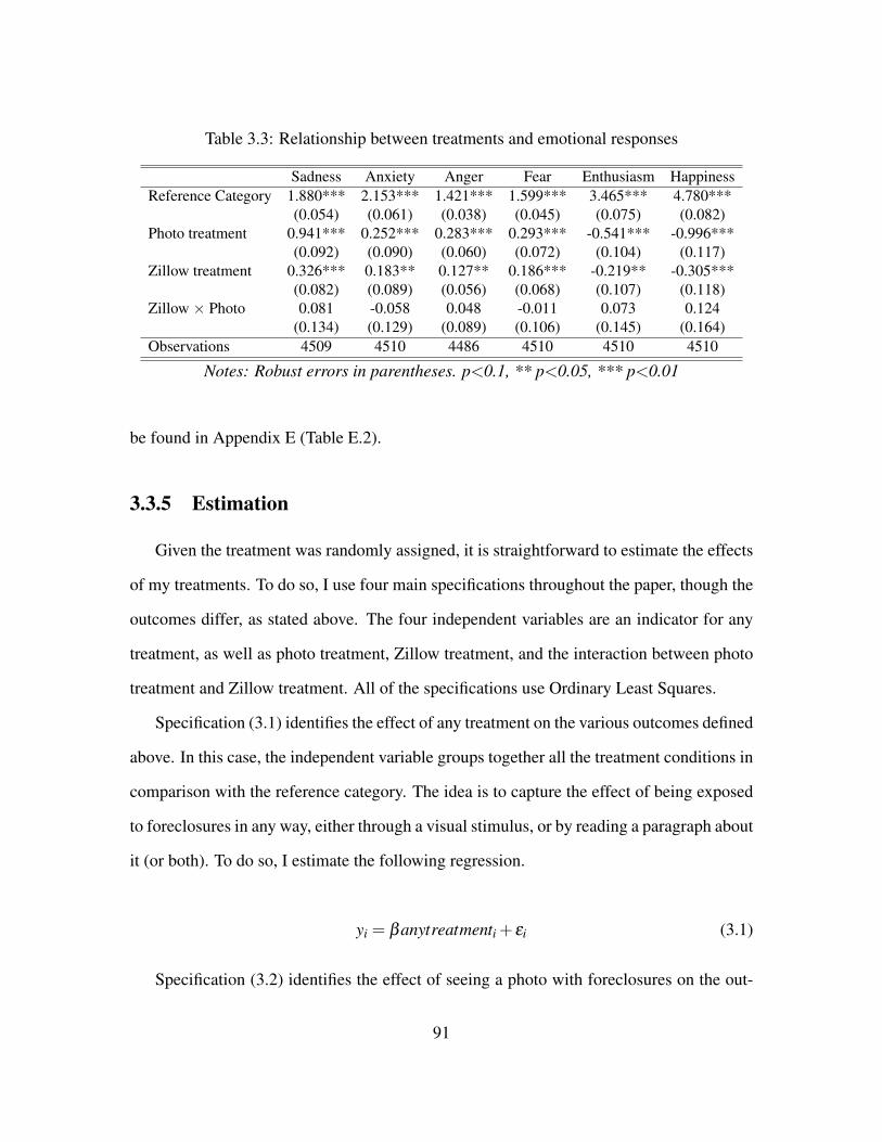
Table 3.3: Relationship between treatments and emotional responses
Sadness Anxiety Anger Fear Enthusiasm HappinessReference Category 1.880*** 2.153*** 1.421*** 1.599*** 3.465*** 4.780***
(0.054) (0.061) (0.038) (0.045) (0.075) (0.082)Photo treatment 0.941*** 0.252*** 0.283*** 0.293*** -0.541*** -0.996***
(0.092) (0.090) (0.060) (0.072) (0.104) (0.117)Zillow treatment 0.326*** 0.183** 0.127** 0.186*** -0.219** -0.305***
(0.082) (0.089) (0.056) (0.068) (0.107) (0.118)Zillow × Photo 0.081 -0.058 0.048 -0.011 0.073 0.124
(0.134) (0.129) (0.089) (0.106) (0.145) (0.164)Observations 4509 4510 4486 4510 4510 4510
Notes: Robust errors in parentheses. p<0.1, ** p<0.05, *** p<0.01
be found in Appendix E (Table E.2).
3.3.5 Estimation
Given the treatment was randomly assigned, it is straightforward to estimate the effects
of my treatments. To do so, I use four main specifications throughout the paper, though the
outcomes differ, as stated above. The four independent variables are an indicator for any
treatment, as well as photo treatment, Zillow treatment, and the interaction between photo
treatment and Zillow treatment. All of the specifications use Ordinary Least Squares.
Specification (3.1) identifies the effect of any treatment on the various outcomes defined
above. In this case, the independent variable groups together all the treatment conditions in
comparison with the reference category. The idea is to capture the effect of being exposed
to foreclosures in any way, either through a visual stimulus, or by reading a paragraph about
it (or both). To do so, I estimate the following regression.
yi = βanytreatmenti + εi (3.1)
Specification (3.2) identifies the effect of seeing a photo with foreclosures on the out-
91
come. The independent variable, photo treatment, brings together the “photo" and “Zil-
low + photo" treatments, and the reference category is the combined “Zillow" and control
groups. Like specification (3.1) the idea is to capture what effect, if any, the photo is having
on the outcome variable. Specification (3.3), which uses “Zillow treatment" as the inde-
pendent variable, is similarly structured. The independent variable is the combination of
the “Zillow" and “Zillow + photo" treatments, while the reference category is the combi-
nation of the control and “photo" treatment. Specification (3.3) allows me to examine the
effect of reading about foreclosures on the outcome. I estimate the following regressions,
respectively.
yi = γ phototreatmenti + εi (3.2)
yi = ωzillowtreatmenti + εi (3.3)
Finally, specification (3.4) identifies the effect of the interaction between the photo
treatment and Zillow treatment on the outcome variable. Examining the interaction term
is useful because it allows me to examine the effects of both the photo treatment and Zil-
low treatment at the same time, as well as determine whether the treatments are acting
as substitutes or complements. In this case, a substitution effect would mean that once a
respondent is exposed to one of the treatments, adding the second treatment group would
not induce her to increase her likelihood of sending a letter (or any of the other outcomes).
A substitution effect would manifest itself as a negative coefficient on the interaction. A
complementary effect, on the other hand, would manifest itself as a positive coefficient on
the interaction, suggesting that being exposed to one treatment, and then subsequently to
another, makes whatever behavioral response is being measured in that model more likely.
The interaction term in the following specification identifies this effect.
92
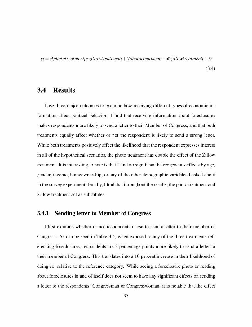
yi = θ phototreatmenti ∗ zillowtreatmenti + γ phototreatmenti +ωzillowtreatmenti + εi
(3.4)
3.4 Results
I use three major outcomes to examine how receiving different types of economic in-
formation affect political behavior. I find that receiving information about foreclosures
makes respondents more likely to send a letter to their Member of Congress, and that both
treatments equally affect whether or not the respondent is likely to send a strong letter.
While both treatments positively affect the likelihood that the respondent expresses interest
in all of the hypothetical scenarios, the photo treatment has double the effect of the Zillow
treatment. It is interesting to note is that I find no significant heterogeneous effects by age,
gender, income, homeownership, or any of the other demographic variables I asked about
in the survey experiment. Finally, I find that throughout the results, the photo treatment and
Zillow treatment act as substitutes.
3.4.1 Sending letter to Member of Congress
I first examine whether or not respondents chose to send a letter to their member of
Congress. As can be seen in Table 3.4, when exposed to any of the three treatments ref-
erencing foreclosures, respondents are 3 percentage points more likely to send a letter to
their member of Congress. This translates into a 10 percent increase in their likelihood of
doing so, relative to the reference category. While seeing a foreclosure photo or reading
about foreclosures in and of itself does not seem to have any significant effects on sending
a letter to the respondents’ Congressman or Congresswoman, it is notable that the effect
93
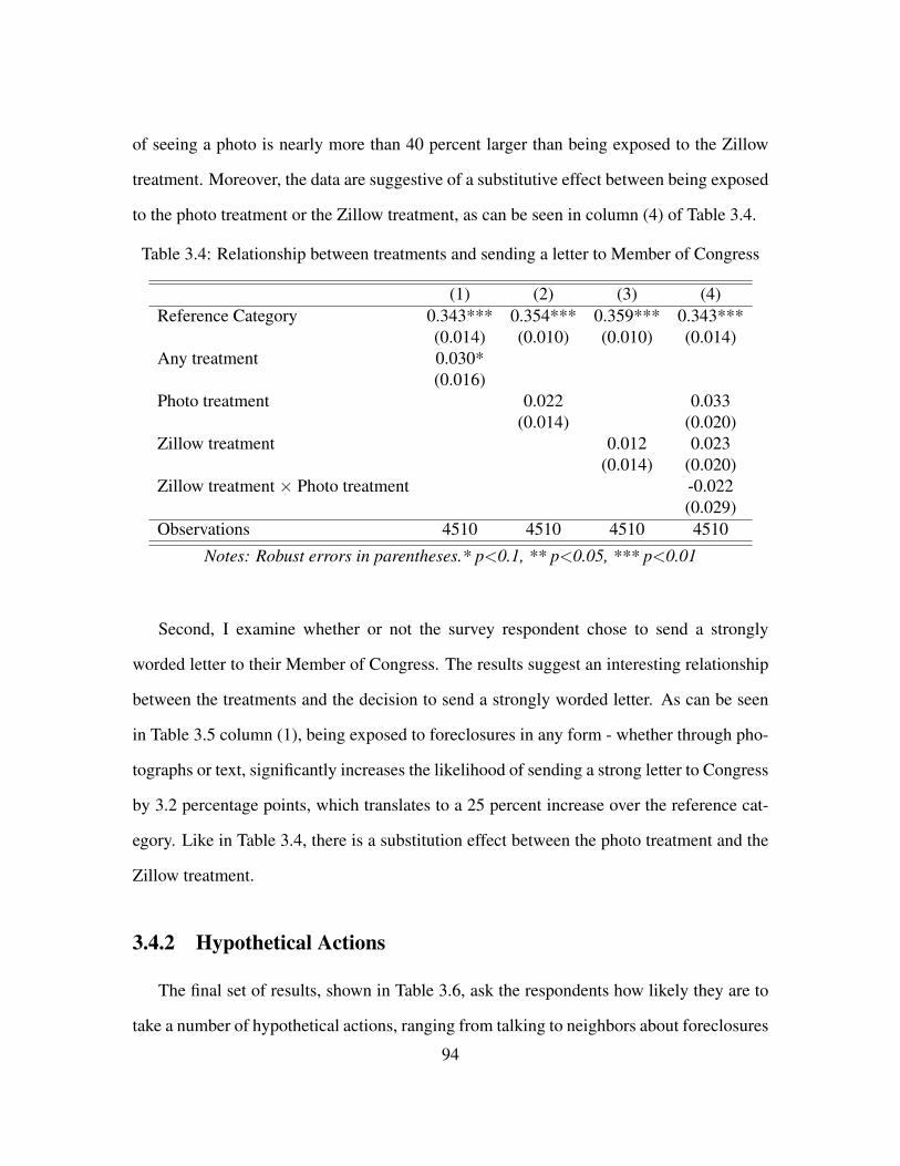
of seeing a photo is nearly more than 40 percent larger than being exposed to the Zillow
treatment. Moreover, the data are suggestive of a substitutive effect between being exposed
to the photo treatment or the Zillow treatment, as can be seen in column (4) of Table 3.4.
Table 3.4: Relationship between treatments and sending a letter to Member of Congress
(1) (2) (3) (4)Reference Category 0.343*** 0.354*** 0.359*** 0.343***
(0.014) (0.010) (0.010) (0.014)Any treatment 0.030*
(0.016)Photo treatment 0.022 0.033
(0.014) (0.020)Zillow treatment 0.012 0.023
(0.014) (0.020)Zillow treatment × Photo treatment -0.022
(0.029)Observations 4510 4510 4510 4510
Notes: Robust errors in parentheses.* p<0.1, ** p<0.05, *** p<0.01
Second, I examine whether or not the survey respondent chose to send a strongly
worded letter to their Member of Congress. The results suggest an interesting relationship
between the treatments and the decision to send a strongly worded letter. As can be seen
in Table 3.5 column (1), being exposed to foreclosures in any form - whether through pho-
tographs or text, significantly increases the likelihood of sending a strong letter to Congress
by 3.2 percentage points, which translates to a 25 percent increase over the reference cat-
egory. Like in Table 3.4, there is a substitution effect between the photo treatment and the
Zillow treatment.
3.4.2 Hypothetical Actions
The final set of results, shown in Table 3.6, ask the respondents how likely they are to
take a number of hypothetical actions, ranging from talking to neighbors about foreclosures
94
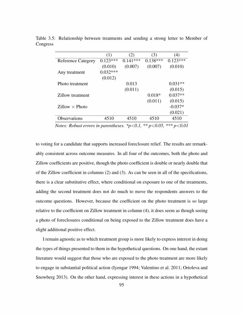
Table 3.5: Relationship between treatments and sending a strong letter to Member ofCongress
(1) (2) (3) (4)Reference Category 0.123*** 0.141*** 0.138*** 0.123***
(0.010) (0.007) (0.007) (0.010)Any treatment 0.032***
(0.012)Photo treatment 0.013 0.031**
(0.011) (0.015)Zillow treatment 0.018* 0.037**
(0.011) (0.015)Zillow × Photo -0.037*
(0.021)Observations 4510 4510 4510 4510
Notes: Robust errors in parentheses. *p<0.1, ** p<0.05, *** p<0.01
to voting for a candidate that supports increased foreclosure relief. The results are remark-
ably consistent across outcome measures. In all four of the outcomes, both the photo and
Zillow coefficients are positive, though the photo coefficient is double or nearly double that
of the Zillow coefficient in columns (2) and (3). As can be seen in all of the specifications,
there is a clear substitutive effect, where conditional on exposure to one of the treatments,
adding the second treatment does not do much to move the respondents answers to the
outcome questions. However, because the coefficient on the photo treatment is so large
relative to the coefficient on Zillow treatment in column (4), it does seem as though seeing
a photo of foreclosures conditional on being exposed to the Zillow treatment does have a
slight additional positive effect.
I remain agnostic as to which treatment group is more likely to express interest in doing
the types of things presented to them in the hypothetical questions. On one hand, the extant
literature would suggest that those who are exposed to the photo treatment are more likely
to engage in substantial political action (Iyengar 1994; Valentino et al. 2011; Ortoleva and
Snowberg 2013). On the other hand, expressing interest in these actions in a hypothetical
95
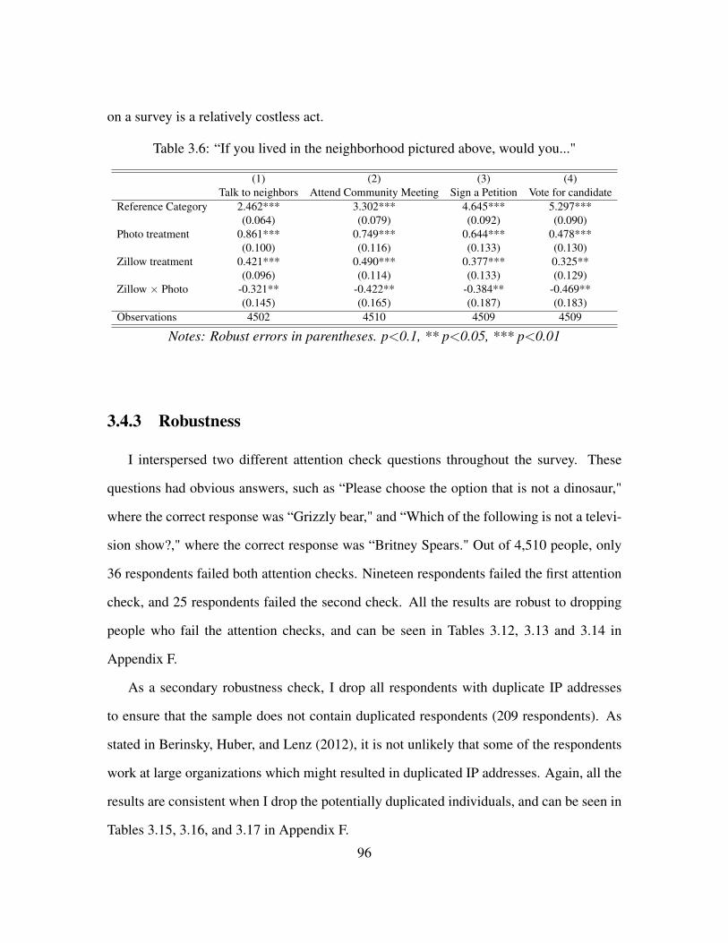
on a survey is a relatively costless act.
Table 3.6: “If you lived in the neighborhood pictured above, would you..."
(1) (2) (3) (4)Talk to neighbors Attend Community Meeting Sign a Petition Vote for candidate
Reference Category 2.462*** 3.302*** 4.645*** 5.297***(0.064) (0.079) (0.092) (0.090)
Photo treatment 0.861*** 0.749*** 0.644*** 0.478***(0.100) (0.116) (0.133) (0.130)
Zillow treatment 0.421*** 0.490*** 0.377*** 0.325**(0.096) (0.114) (0.133) (0.129)
Zillow × Photo -0.321** -0.422** -0.384** -0.469**(0.145) (0.165) (0.187) (0.183)
Observations 4502 4510 4509 4509
Notes: Robust errors in parentheses. p<0.1, ** p<0.05, *** p<0.01
3.4.3 Robustness
I interspersed two different attention check questions throughout the survey. These
questions had obvious answers, such as “Please choose the option that is not a dinosaur,"
where the correct response was “Grizzly bear," and “Which of the following is not a televi-
sion show?," where the correct response was “Britney Spears." Out of 4,510 people, only
36 respondents failed both attention checks. Nineteen respondents failed the first attention
check, and 25 respondents failed the second check. All the results are robust to dropping
people who fail the attention checks, and can be seen in Tables 3.12, 3.13 and 3.14 in
Appendix F.
As a secondary robustness check, I drop all respondents with duplicate IP addresses
to ensure that the sample does not contain duplicated respondents (209 respondents). As
stated in Berinsky, Huber, and Lenz (2012), it is not unlikely that some of the respondents
work at large organizations which might resulted in duplicated IP addresses. Again, all the
results are consistent when I drop the potentially duplicated individuals, and can be seen in
Tables 3.15, 3.16, and 3.17 in Appendix F.
96
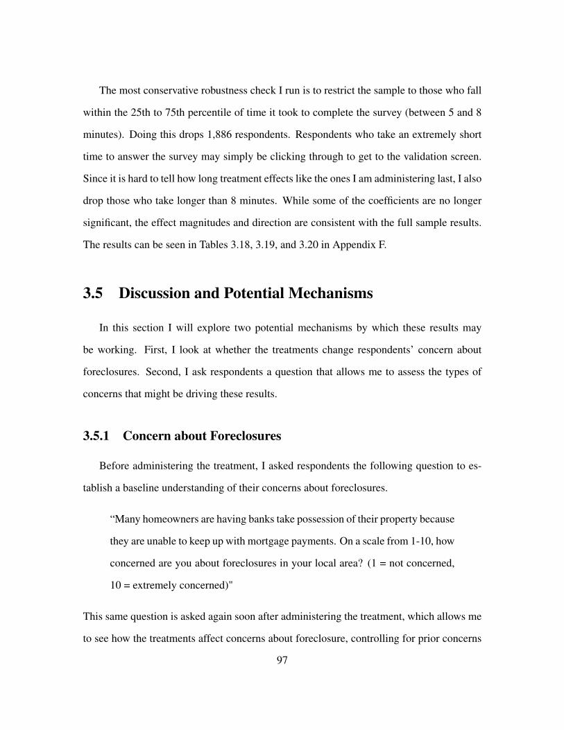
The most conservative robustness check I run is to restrict the sample to those who fall
within the 25th to 75th percentile of time it took to complete the survey (between 5 and 8
minutes). Doing this drops 1,886 respondents. Respondents who take an extremely short
time to answer the survey may simply be clicking through to get to the validation screen.
Since it is hard to tell how long treatment effects like the ones I am administering last, I also
drop those who take longer than 8 minutes. While some of the coefficients are no longer
significant, the effect magnitudes and direction are consistent with the full sample results.
The results can be seen in Tables 3.18, 3.19, and 3.20 in Appendix F.
3.5 Discussion and Potential Mechanisms
In this section I will explore two potential mechanisms by which these results may
be working. First, I look at whether the treatments change respondents’ concern about
foreclosures. Second, I ask respondents a question that allows me to assess the types of
concerns that might be driving these results.
3.5.1 Concern about Foreclosures
Before administering the treatment, I asked respondents the following question to es-
tablish a baseline understanding of their concerns about foreclosures.
“Many homeowners are having banks take possession of their property because
they are unable to keep up with mortgage payments. On a scale from 1-10, how
concerned are you about foreclosures in your local area? (1 = not concerned,
10 = extremely concerned)"
This same question is asked again soon after administering the treatment, which allows me
to see how the treatments affect concerns about foreclosure, controlling for prior concerns
97
(Table 3.7). Although respondents may find it odd that they are being asked the same
question twice in one survey, this would likely bias against finding any results. Respondents
are likely to respond to the question in the same way when asked the question a second
time. Even if respondents think harder about the importance of foreclosures because of
the emphasis placed on this question (by virtue of it being asked twice) and change their
response, this would not explain any differences in treatment effects.
Given that any bias from asking this question twice likely biases against finding results,
it is notable that being exposed to the photo treatment increases concerns for foreclosures
by nearly 0.13 units on the scale, whereas being exposed to the Zillow treatment does not
have a significant effect (Table 3.7). I can therefore conclude that being exposed to the
photo of a foreclosed home is what is causing people to shift how worried they are about
foreclosures, although the changes in expressed concern are relatively small. These results
are consistent with the large coefficients on the photo treatment variable in the hypothetical
scenarios, as well as the relative sizes of the coefficients when looking at whether the
respondent chooses to send a letter to Congress.
3.5.2 Potential Mechanisms
To understand the types of concerns that may be driving the topline results, I conduct
a second mechanism check. Respondents were asked the following question, where all of
the responses could be categorized into 1 of 4 categories: personal responses, emotional re-
sponses, local responses, and systemic responses. Asking this question offers some insight
into the mechanisms that may be at play in a respondent’s decision to send a certain type of
letter or respond to the hypothetical scenarios in a certain way. The order of the statements
was randomized.
“Select all of the statements you agree with:
98
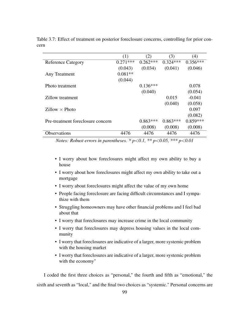
Table 3.7: Effect of treatment on posterior foreclosure concerns, controlling for prior con-cern
(1) (2) (3) (4)Reference Category 0.271*** 0.262*** 0.324*** 0.356***
(0.043) (0.034) (0.041) (0.046)Any Treatment 0.081**
(0.044)Photo treatment 0.136*** 0.078
(0.040) (0.054)Zillow treatment 0.015 -0.041
(0.040) (0.058)Zillow × Photo 0.097
(0.082)Pre-treatment foreclosure concern 0.863*** 0.863*** 0.859***
(0.008) (0.008) (0.008)Observations 4476 4476 4476 4476
Notes: Robust errors in parentheses. * p<0.1, ** p<0.05, *** p<0.01
• I worry about how foreclosures might affect my own ability to buy ahouse
• I worry about how foreclosures might affect my own ability to take out amortgage
• I worry about foreclosures might affect the value of my own home
• People facing foreclosure are facing difficult circumstances and I sympa-thize with them
• Struggling homeowners may have other financial problems and I feel badabout that
• I worry that foreclosures may increase crime in the local community
• I worry that foreclosures may depress housing values in the local com-munity
• I worry that foreclosures are indicative of a larger, more systemic problemwith the housing market
• I worry that foreclosures are indicative of a larger, more systemic problemwith the economy"
I coded the first three choices as “personal," the fourth and fifth as “emotional," the
sixth and seventh as “local," and the final two choices as “systemic." Personal concerns are99
those that are specific to the individual respondent, such as the respondent’s own ability to
buy a home or take out a mortgage. Emotional responses are those that suggest that the
respondent is feeling empathy for those facing foreclosure. I also try to get at the level at
which these concerns are operating - either at the local level, or at a broader, more systemic
level.
In Table 3.8, it is clear that the treatments induced respondent concern about local
issues such as crime and local housing values. No treatment has a significant effect on
any of the other categories of potential mechanisms. To delve deeper into what aspect
of local concerns are potentially driving the topline results, columns (3a) and (3b) break
out the two components of the “local" category: crime and housing values. The results
suggest that respondents are concerned about primarily about local housing values, where
both treatments have significant coefficients, though the coefficients are not significantly
different from each other, so I cannot say if the photo treatment or the Zillow treatment is
doing more of the work. In specification (3a), the photo treatment is significantly different
from the Zillow treatment.
Table 3.8: Potential Mechanisms - Treatment effects on expressed concerns
(1) (2) (3) (3a) (3b) (4)Personal Emotional Local Local (crime) Local (housing values) Systemic
Reference Category 0.561*** 0.828*** 0.580*** 0.408*** 0.420*** 0.724***(0.015) (0.011) (0.015) (0.015) (0.015) (0.013)
Photo treatment 0.006 0.021 0.077*** 0.087*** 0.060*** 0.014(0.021) (0.016) (0.020) (0.021) (0.021) (0.019)
Zillow treatment 0.025 -0.003 0.027 0.011 0.043** 0.006(0.021) (0.016) (0.021) (0.021) (0.021) (0.019)
Zillow × Photo -0.017 -0.017 -0.023 -0.003 -0.038 0.007(0.029) (0.022) (0.029) (0.030) (0.030) (0.026)
Observations 4510 4510 4510 4510 4510 4510
Notes: Robust errors in parentheses. * p<0.1, ** p<0.05, *** p<0.01
100
3.6 Conclusion
This paper sheds light on an important aspect of the relationship between information
and political behavior. Using a survey experiment on MTurk, I find that being exposed to
information about foreclosures in the local economic area make respondents more likely to
send a letter to their Member of Congress. While both the photo and written information
affect the likelihood that respondents express interest in hypothetical behavioral scenarios,
the effect of the emotionally salient information is twice the magnitude of the written fore-
closure rate. Throughout the study, the photo and Zillow treatments serve as substitutes.
Consistent with previous research about emotionally charged information (Valentino et al.
2011; Iyengar 1994) and overconfidence in one’s own perceptions (Ortoleva and Snowberg
2013), those who are given more specific information about foreclosures are more likely to
express a willingness to engage in political action.
These results are surprising when considering that the scope of the treatments is rel-
atively limited. Although both the photos and the paragraphs with housing information
are designed to mimic the way in which people receive information about their local eco-
nomic environment in real life, both treatments rely on respondents buying the hypothetical
premise that the information is about their “local area." Given that we may not expect a
weak treatment such as this to have strong effects, it is especially surprising that I find large
effects on concrete behavioral measures, such as choosing to send a strongly worded letter
to a Congress member. These results suggest that when faced with similar information
about foreclosures in the context of the respondents’ actual neighborhood, the respondent
may have an even stronger behavioral effect than what is evident in this online experiment.
The degree to which the photo treatment and the Zillow treatment act as almost perfect
substitutes, at least with respect to writing a letter to Congress, is also notable. It is surpris-
ing that information that has weight because of the emotional response that it creates is as
101
effective in inducing a political response as concrete facts. While the extant literature does
expect emotionally salient information to induce behavioral change through blame attribu-
tion (Valentino et al. 2011; Malhotra and Kuo 2008) and economic information to affect
voter behavior through heuristics (Fiorina 1981; Key 1966), it is notable that these different
channels seem to convey similar information and induce similar effect magnitudes. In other
words, respondents seem to perceive emotionally salient information to be as legitimate as
factual information that does not have an emotional component. This may be because, as
Lupia and McCubbins (1998) suggest, that the cognitive resources that any one person can
employ in assessing various pieces of information are limited. Even when presented with
multiple pieces of evidence, people can only draw implications from one piece of evidence
at a time. This suggests that in order to induce behavior, campaigns or canvassers may not
need to undergo the most costly route of offering multiple sources of information to induce
behavioral change. However, future work should consider how durable such responses are
over time.
The substitution effect also suggests that people can access politically relevant informa-
tion without using traditional sources of information, such as reading the news or watching
television. Research on political information in a variety of political contexts (Carpini and
Keeter 1997) relies on these traditional methods of accessing political information to mea-
sure how informed voters are. This paper suggests that we may be underestimating the
extent to which people are informed about politically relevant topics. This is particularly
important given that this paper shows that both informal sources of information as well as
more traditional ones, convey similar information to their consumers.
The broader democratic implications of this work are less clear cut. While this paper
demonstrates that people glean politically relevant information through visual channels,
and that these informal channels provide roughly the same information as more traditional
forms of information consumption, people rarely contact their representative outside of the
102
context of this experiment. This may be in part because the experiment provides more than
just the information - it also provides an appropriately written letter and an offer to send
the letter to the respondent’s representative. While visual channels convey the same infor-
mation as more traditional ones, traditional sources of information may also provide other
resources that encourage political behavior, such as institutional information including who
the respondent’s representative is and how to get in touch with them. So while an individ-
ual who sees foreclosures in their neighborhood may be upset about them, an individual
who watches the news might have a better sense of who her representative is and how to
contact her. Although the design of this experiment does not allow for me to capture these
sorts of informational differences that come from consuming emotionally salient news as
compared to less emotionally salient news, future work could attempt to disentangle the
package of information that comes from different types of sources.
Finally, my findings have important implications for canvassers, political campaigns,
and other groups that rely on emotional responses to elicit a political outcome. The results
suggest that the more emotionally salient the information given to an individual is, the
more likely they are to express interest in engaging politically with that action, and that
offering additional information through more traditional channels does not have an effect on
political activity. For a canvasser, sharing information with an individual that is relatively
experiential to that individual and that has a focal point for blame, is the likeliest way
to elicit a political response from the individual. Although this project comes with the
uncertainty and external validity concerns of any experimental set-up, it provides clear
testable implications for future research.
103
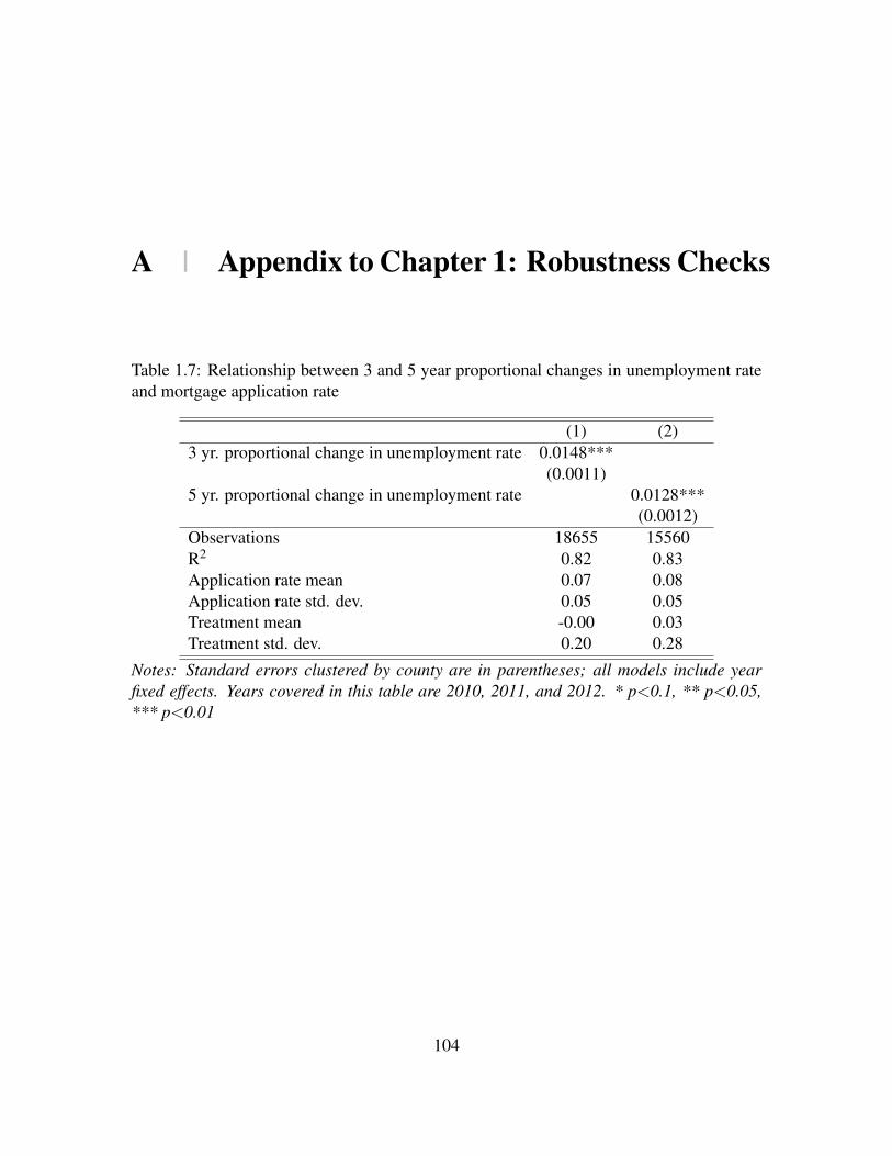
A | Appendix to Chapter 1: Robustness Checks
Table 1.7: Relationship between 3 and 5 year proportional changes in unemployment rateand mortgage application rate
(1) (2)3 yr. proportional change in unemployment rate 0.0148***
(0.0011)5 yr. proportional change in unemployment rate 0.0128***
(0.0012)Observations 18655 15560R2 0.82 0.83Application rate mean 0.07 0.08Application rate std. dev. 0.05 0.05Treatment mean -0.00 0.03Treatment std. dev. 0.20 0.28
Notes: Standard errors clustered by county are in parentheses; all models include yearfixed effects. Years covered in this table are 2010, 2011, and 2012. * p<0.1, ** p<0.05,*** p<0.01
104
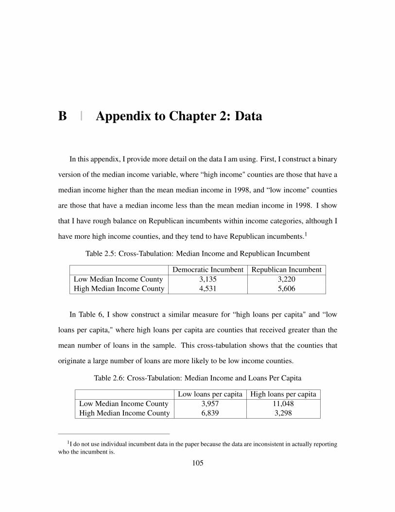
B | Appendix to Chapter 2: Data
In this appendix, I provide more detail on the data I am using. First, I construct a binary
version of the median income variable, where “high income" counties are those that have a
median income higher than the mean median income in 1998, and “low income" counties
are those that have a median income less than the mean median income in 1998. I show
that I have rough balance on Republican incumbents within income categories, although I
have more high income counties, and they tend to have Republican incumbents.1
Table 2.5: Cross-Tabulation: Median Income and Republican Incumbent
Democratic Incumbent Republican IncumbentLow Median Income County 3,135 3,220High Median Income County 4,531 5,606
In Table 6, I show construct a similar measure for “high loans per capita" and “low
loans per capita," where high loans per capita are counties that received greater than the
mean number of loans in the sample. This cross-tabulation shows that the counties that
originate a large number of loans are more likely to be low income counties.
Table 2.6: Cross-Tabulation: Median Income and Loans Per Capita
Low loans per capita High loans per capitaLow Median Income County 3,957 11,048High Median Income County 6,839 3,298
1I do not use individual incumbent data in the paper because the data are inconsistent in actually reportingwho the incumbent is.
105
C | Appendix to Chapter 2: House ElectoralData
In this appendix, I run the same models as in Table 2 using House electoral data. These
data are somewhat less reliable than the Senate electoral data; House electoral results are
not commonly collected at the county level. Because of this, I only have data from 1992,
1998, 2002 and 2004, resulting in only about 60 percent of the data I have for Senate elec-
tions. When I run these models using House data, I find results broadly consistent with the
Senate data, although I do not find a strong first stage as I do when I use Senate electoral
data. I find similar signs on the coefficients, and the magnitudes of the point estimates are
fairly close to the Senate estimates as well.
106
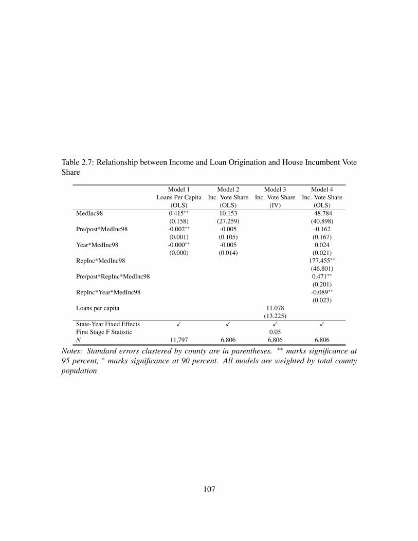
Table 2.7: Relationship between Income and Loan Origination and House Incumbent VoteShare
Model 1 Model 2 Model 3 Model 4Loans Per Capita Inc. Vote Share Inc. Vote Share Inc. Vote Share
(OLS) (OLS) (IV) (OLS)MedInc98 0.415∗∗ 10.153 -48.784
(0.158) (27.259) (40.898)Pre/post*MedInc98 -0.002∗∗ -0.005 -0.162
(0.001) (0.105) (0.167)Year*MedInc98 -0.000∗∗ -0.005 0.024
(0.000) (0.014) (0.021)RepInc*MedInc98 177.455∗∗
(46.801)Pre/post*RepInc*MedInc98 0.471∗∗
(0.201)RepInc*Year*MedInc98 -0.089∗∗
(0.023)Loans per capita 11.078
(13.225)State-Year Fixed Effects X X X XFirst Stage F Statistic 0.05N 11,797 6,806 6,806 6,806
Notes: Standard errors clustered by county are in parentheses. ∗∗ marks significance at95 percent, ∗ marks significance at 90 percent. All models are weighted by total countypopulation
107
D | Appendix to Chapter 2: Turnout
As an extension to the main results, I examine the effect of loan origination on turnout.
There are two possible mechanisms by which increased loan origination in lower-income
counties affects incumbent vote share. First, it is possible that increased loan origination,
possibly in combination with incumbent campaigning on the issues, results in a mobilizing
effect where voters in areas that experience more loan origination are more likely to turnout
in the subsequent election. Second, it is possible that while the pool of voters turning out
is static, voters switch their votes from Republican to Democrat.
To test for whether the mobilization effect is outweighing the vote switching effect, I
run the same models as in Table 2, except using a measure for turnout as the outcome. I
construct my turnout measure by totaling all of the votes cast in a single election, and then
dividing by the citizen voting age population to scale for the size of the county. If the effect
of pre/post ∗medianincome was insignificant, we could infer that the mobilization effect
was not the driver of my incumbent vote share results. If I do find significant results, it is
suggestive of the fact that voters are mobilizing, but does not preclude the possibility that
voters are also changing which party they are voting for.
The results, presented in Table 8, offer mixed evidence about whether or not a mobi-
lization effect is taking place. Model 1 shows that in the post-2000 period, lower income
counties were more likely to turnout relative to higher income counties, which would be
suggestive of a mobilization story. Using the same IV specification as in Model 3 in Table
108
Table 2.8: Relationship between County Level Median Income and Turnout
Model 1 Model 2 Model 3Turnout Turnout Turnout(OLS) (IV) (OLS)
MedInc98 -54.308∗∗ -50.474∗∗
(7.828) (9.446)Pre/post*MedInc98 0.162∗∗ 0.193∗∗
(0.025) (0.043)Year*MedInc98 0.027∗∗ 0.025∗∗
(0.004) (0.005)RepInc*MedInc98 -8.998
(13.235)Pre/post*RepInc*MedInc98 -0.078
(0.063)RepInc*Year*MedInc98 0.005
(0.007)Loans per capita -113.887∗
(15.732)State-Year Fixed Effects X X XFirst Stage F Statistic 66.56N 11,432 11,454 11,432
Notes: Standard errors clustered by county are in parentheses. ∗∗ marks significance at95 percent, ∗ marks significance at 90 percent. All models are weighted by total countypopulation
2, Model 2 in Table 3 shows that the areas that originated more loans per capita experi-
enced lower turnout in the subsequent election relative to areas with fewer loan origina-
tions, which is the opposite of what we would expect after seeing the results in Model 1.
In Model 3, I show that relative to low-income Republican areas, low-income Democratic
areas were more likely to increase their turnout in the post-2000 period (though it is impor-
tant to note that these results are not statistically significant). These results are inconclusive
and do not clearly point to either a mobilization effect or a vote switching one, although
Model 3 does seem to be broadly in line with what we would expect to see if Democrats
were mobilizing more than the Republicans. The inconclusiveness of the results may be
109
due to data limitations, as I do not have an accurate measure of the total number of regis-
tered voters in each county. However, as I demonstrate in Table 9, it is reassuring that the
main results hold even when controlling for changes in turnout after the reform.
Table 2.9: Relationship between County Level Median Income and Incumbent Vote Share,Controlling for Turnout
Model 1 Model 2 Model 3Inc. Vote Share Inc. Vote Share Inc. Vote Share
(OLS) (IV) (OLS)MedInc98 -63.577∗∗ -66.524∗∗
(18.142) (19.484)Pre/post*MedInc98 -0.260∗ -0.278∗∗
(0.136) (0.137)Year*MedInc98 0.032∗∗ 0.033∗∗
(0.009) (0.010)Turnout 0.145∗∗ 0.146∗∗
(0.035) (0.036)Pre/post * Turnout -0.325∗∗ -0.310∗∗
(0.097) (0.094)RepInc*MedInc98 35.843∗
(18.670)Pre/post*RepInc*MedInc98 0.198
(0.142)RepInc*Year*MedInc98 -0.018∗
(0.009)Loans per capita 1.804
(11.934)State-Year Fixed Effects X X XFirst Stage F Statistic 90.37N 10,996 10,996 10,996
Notes: Standard errors clustered by county are in parentheses. ∗∗ marks significance at95 percent, ∗ marks significance at 90 percent. All models are weighted by total countypopulation
110
E | Appendix to Chapter 3: Summary Statis-tics and Balance Table
Table 3.9: Summary Table, Data
Variable Observations Mean Std. Dev. Min MaxState 4,508 25.505 15.075 1 52Geography 4, 510 2.338 0.791 1 4Party Affiliation 4,510 4.108 2.690 0 10Gender 4,510 1.545 0.532 1 4Race 4,510 1.551 1.331 1 7Hispanic 4,507 1.945 0.273 1 3Age 4,510 2.363 1.120 0 5Citizen 4,510 0.988 0.111 0 1Income 4,510 4.476 2.777 0 9Homeowner 4,510 0.402 0.490 0 1
Table 3.10: Validation Check -Balance Table
Variable Control Mean T1 Mean T2 Mean T3 Mean P valueConcern - animal rights 6.616 6.521 6.493 6.509 0.148Concern - foreclosures 4.571 4.458 4.665 4.695 0.164Concern - immigration 4.812 4.773 4.902 4.889 0.728Hispanic 1.907 1.900 1.919 1.914 0.539Age 2.330 2.353 2.367 2.400 0.506Female 0.515 0.506 0.499 0.543 0.289Male 0.476 0.483 0.463 0.451 0.414Citizen 1.011 1.011 1.012 1.014 0.899Income 4.489 4.375 4.556 4.490 0.471Homeowner 0.401 0.377 0.410 0.420 0.171
111
F | Appendix to Chapter 3: Robustness Checks
This appendix contains the tables that correspond to the robustness checks. First, I drop
all of the respondents who failed the attention checks (36 respondents). Next, I drop all
respondents with duplicate IP addresses to ensure that the sample does not have duplicate
respondents (209 respondents). The most conservative robustness check I run is to restrict
the sample to those who fall within the 25th to 75th percentile of time it took to complete
the survey (between 5 and 8 minutes). Doing this drops 1,886 respondents.
Table 3.11: Relationship between treatments and sending letter to Member of Congress,dropping failed attention checks
(1) (2) (3) (4)Reference Category 0.344*** 0.354*** 0.359*** 0.344***
(0.014) (0.010) (0.010) (0.014)Any treatment 0.028*
(0.016)Photo treatment 0.022 0.031
(0.014) (0.020)Zillow treatment 0.011 0.020
(0.014) (0.020)Zillow treatment × Photo treatment -0.019
(0.029)Observations 4474 4474 4474 4474
Notes: Robust errors in parentheses. *p<0.1, ** p<0.05, *** p<0.01
112
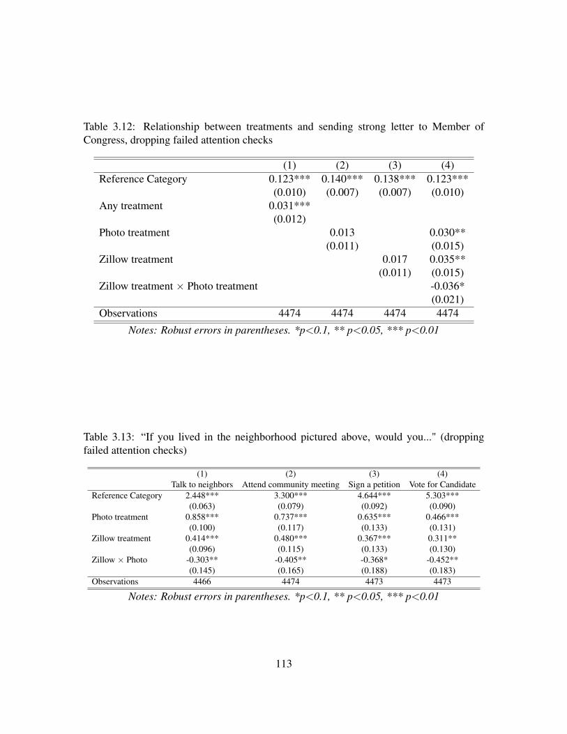
Table 3.12: Relationship between treatments and sending strong letter to Member ofCongress, dropping failed attention checks
(1) (2) (3) (4)Reference Category 0.123*** 0.140*** 0.138*** 0.123***
(0.010) (0.007) (0.007) (0.010)Any treatment 0.031***
(0.012)Photo treatment 0.013 0.030**
(0.011) (0.015)Zillow treatment 0.017 0.035**
(0.011) (0.015)Zillow treatment × Photo treatment -0.036*
(0.021)Observations 4474 4474 4474 4474
Notes: Robust errors in parentheses. *p<0.1, ** p<0.05, *** p<0.01
Table 3.13: “If you lived in the neighborhood pictured above, would you..." (droppingfailed attention checks)
(1) (2) (3) (4)Talk to neighbors Attend community meeting Sign a petition Vote for Candidate
Reference Category 2.448*** 3.300*** 4.644*** 5.303***(0.063) (0.079) (0.092) (0.090)
Photo treatment 0.858*** 0.737*** 0.635*** 0.466***(0.100) (0.117) (0.133) (0.131)
Zillow treatment 0.414*** 0.480*** 0.367*** 0.311**(0.096) (0.115) (0.133) (0.130)
Zillow × Photo -0.303** -0.405** -0.368* -0.452**(0.145) (0.165) (0.188) (0.183)
Observations 4466 4474 4473 4473
Notes: Robust errors in parentheses. *p<0.1, ** p<0.05, *** p<0.01
113
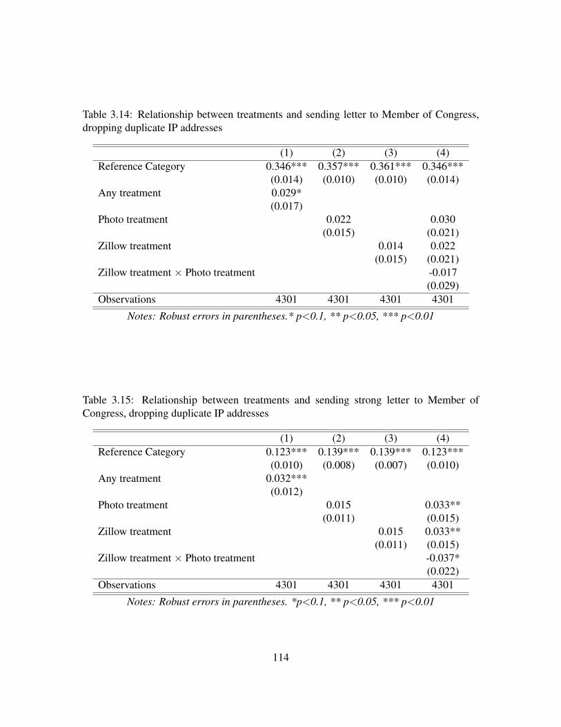
Table 3.14: Relationship between treatments and sending letter to Member of Congress,dropping duplicate IP addresses
(1) (2) (3) (4)Reference Category 0.346*** 0.357*** 0.361*** 0.346***
(0.014) (0.010) (0.010) (0.014)Any treatment 0.029*
(0.017)Photo treatment 0.022 0.030
(0.015) (0.021)Zillow treatment 0.014 0.022
(0.015) (0.021)Zillow treatment × Photo treatment -0.017
(0.029)Observations 4301 4301 4301 4301
Notes: Robust errors in parentheses.* p<0.1, ** p<0.05, *** p<0.01
Table 3.15: Relationship between treatments and sending strong letter to Member ofCongress, dropping duplicate IP addresses
(1) (2) (3) (4)Reference Category 0.123*** 0.139*** 0.139*** 0.123***
(0.010) (0.008) (0.007) (0.010)Any treatment 0.032***
(0.012)Photo treatment 0.015 0.033**
(0.011) (0.015)Zillow treatment 0.015 0.033**
(0.011) (0.015)Zillow treatment × Photo treatment -0.037*
(0.022)Observations 4301 4301 4301 4301
Notes: Robust errors in parentheses. *p<0.1, ** p<0.05, *** p<0.01
114
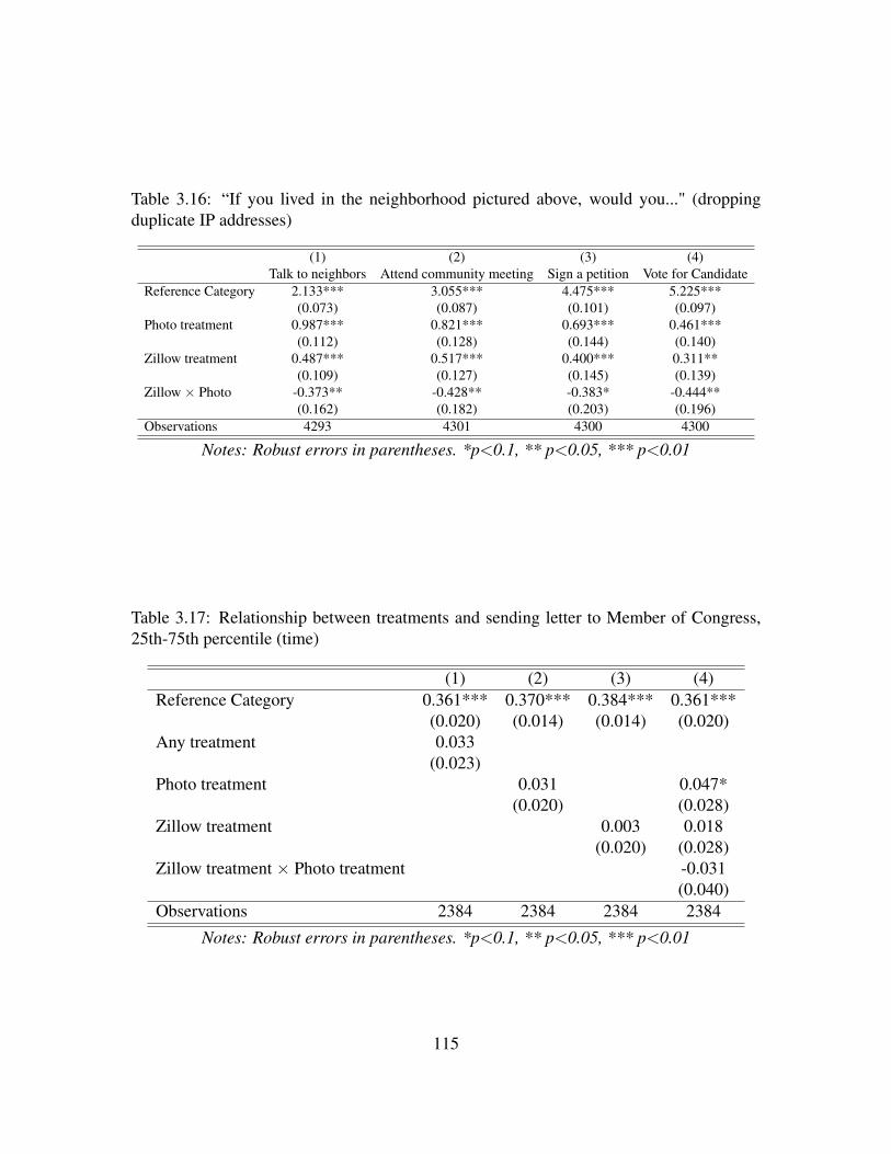
Table 3.16: “If you lived in the neighborhood pictured above, would you..." (droppingduplicate IP addresses)
(1) (2) (3) (4)Talk to neighbors Attend community meeting Sign a petition Vote for Candidate
Reference Category 2.133*** 3.055*** 4.475*** 5.225***(0.073) (0.087) (0.101) (0.097)
Photo treatment 0.987*** 0.821*** 0.693*** 0.461***(0.112) (0.128) (0.144) (0.140)
Zillow treatment 0.487*** 0.517*** 0.400*** 0.311**(0.109) (0.127) (0.145) (0.139)
Zillow × Photo -0.373** -0.428** -0.383* -0.444**(0.162) (0.182) (0.203) (0.196)
Observations 4293 4301 4300 4300
Notes: Robust errors in parentheses. *p<0.1, ** p<0.05, *** p<0.01
Table 3.17: Relationship between treatments and sending letter to Member of Congress,25th-75th percentile (time)
(1) (2) (3) (4)Reference Category 0.361*** 0.370*** 0.384*** 0.361***
(0.020) (0.014) (0.014) (0.020)Any treatment 0.033
(0.023)Photo treatment 0.031 0.047*
(0.020) (0.028)Zillow treatment 0.003 0.018
(0.020) (0.028)Zillow treatment × Photo treatment -0.031
(0.040)Observations 2384 2384 2384 2384
Notes: Robust errors in parentheses. *p<0.1, ** p<0.05, *** p<0.01
115
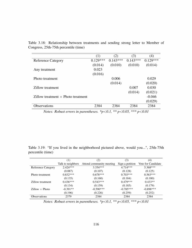
Table 3.18: Relationship between treatments and sending strong letter to Member ofCongress, 25th-75th percentile (time)
(1) (2) (3) (4)Reference Category 0.129*** 0.143*** 0.143*** 0.129***
(0.014) (0.010) (0.010) (0.014)Any treatment 0.023
(0.016)Photo treatment 0.006 0.029
(0.014) (0.020)Zillow treatment 0.007 0.030
(0.014) (0.021)Zillow treatment × Photo treatment -0.046
(0.029)Observations 2384 2384 2384 2384
Notes: Robust errors in parentheses. *p<0.1, ** p<0.05, *** p<0.01
Table 3.19: “If you lived in the neighborhood pictured above, would you...", 25th-75thpercentile (time)
(1) (2) (3) (4)Talk to neighbors Attend community meeting Sign a petition Vote for Candidate
Reference Category 2.424*** 3.354*** 4.714*** 5.368***(0.087) (0.107) (0.128) (0.125)
Photo treatment 0.832*** 0.678*** 0.703*** 0.563***(0.135) (0.160) (0.184) (0.180)
Zillow treatment 0.436*** 0.543*** 0.479*** 0.433**(0.134) (0.159) (0.185) (0.179)
Zillow × Photo -0.391** -0.590*** -0.785*** -0.898***(0.196) (0.226) (0.259) (0.252)
Observations 2379 2384 2384 2384
Notes: Robust errors in parentheses. *p<0.1, ** p<0.05, *** p<0.01
116
| Bibliography
Achen, Christopher H, and Larry M Bartels. 2004. “Blind retrospection: Electoral re-sponses to drought, flu, and shark attacks.”.
Alesina, Alberto. 1989. “Politics and business cycles in industrial democracies.” Economicpolicy 4 (8): 55–98.
Alt, James E, David Dreyer Lassen, and John Marshall. 2016. “Credible Sources and So-phisticated Voters: When Does New Information Induce Economic Voting?” Journal ofPolitics 78 (2): 327-343.
Alt, James, Ethan Bueno de Mesquita, and Shanna Rose. 2011. “Disentangling accountabil-ity and competence in elections: evidence from US term limits.” The Journal of Politics73 (01): 171–186.
Ambrose, Brent W, and Thomas G Thibodeau. 2004. “Have the GSE affordable housinggoals increased the supply of mortgage credit?” Regional Science and Urban Economics34 (3): 263–273.
Andrews, Dan, and Aida Caldera Sánchez. 2011. “The evolution of homeownership rates inselected OECD countries: Demographic and public policy influences.” OECD Journal:Economic Studies 2011 (1): 1–37.
Ansell, Ben. 2014. “The political economy of ownership: Housing markets and the welfarestate.” American Political Science Review 108 (02): 383–402.
Ansolabehere, Stephen, Jonathan Rodden, and James M Snyder. 2008. “The strength ofissues: Using multiple measures to gauge preference stability, ideological constraint,and issue voting.” American Political Science Review 102 (02): 215–232.
Ansolabehere, Stephen, Marc Meredith, and Erik Snowberg. 2014. “Mecro-Economic Vot-ing: Local Information and Micro-Perceptions of the Macro-Economy.” Economics &Politics 26 (3): 380–410.
Archer, Wayne, David Ling, and Gary McGill. 2002. “Prepayment risk and lower-incomemortgage borrowers.” Low Income Homeownership: Examining the Unexamined Goal:279–321.
117
Ashworth, Scott. 2012. “Electoral accountability: recent theoretical and empirical work.”Annual Review of Political Science 15: 183–201.
Averill, James R. 1983. “Studies on anger and aggression: Implications for theories ofemotion.” American psychologist 38 (11): 1145.
Baker, Scott R. 2015. “Debt and the consumption response to household income shocks.”Available at SSRN.
Barro, Robert J. 1973. “The control of politicians: an economic model.” Public choice14 (1): 19–42.
Baumgartner, Frank, Jeffrey Berry, Marie Hojnacki, David Kimball, and Beth Leech. 2011.“Advocacy and Public Policymaking.”
Bechtel, Michael M, and Jens Hainmueller. 2011. “How Lasting Is Voter Gratitude? AnAnalysis of the Short-and Long-Term Electoral Returns to Beneficial Policy.” AmericanJournal of Political Science 55 (4): 852–868.
Berinsky, Adam J, Gregory A Huber, and Gabriel S Lenz. 2012. “Evaluating online labormarkets for experimental research: Amazon. com’s Mechanical Turk.” Political Analysis20 (3): 351–368.
Brader, Ted, Eric W Groenendyk, and Nicholas A Valentino. 2010. “Fight or flight? Whenpolitical threats arouse public anger and fear.” Unpublished manuscript, Ann Arbor,Michigan.
Bullock, John G. 2011. “Elite influence on public opinion in an informed electorate.” Amer-ican Political Science Review 105 (03): 496–515.
Campbell, Angus, Philip E Converse, Warren E Miller, and E Donald. 1966. Stokes. 1960.The American Voter. New York: Wiley.
Campbell, John Y, and Joao F Cocco. 2007. “How do house prices affect consumption?Evidence from micro data.” Journal of Monetary Economics 54 (3): 591–621.
Carpini, Michael X Delli, and Scott Keeter. 1997. What Americans know about politics andwhy it matters. Yale University Press.
Carsey, Thomas M, and Gerald C Wright. 1998. “State and national factors in gubernatorialand senatorial elections.” American Journal of Political Science: 994–1002.
Castles, Francis G. 1998. “The really big trade-off: Home ownership and the welfare statein the new world and the old.” Acta politica 33: 5–19.
Chinn, Menzie D, and Jeffrey Frieden. 2011. Lost Decades: The Making of America’s DebtCrisis and the Long Recovery. W.W. Norton.
118
Conley, Dalton, and Brian Gifford. 2006. “Home ownership, social insurance, and the wel-fare state.” In Sociological Forum. Vol. 21 Springer pp. 55–82.
Converse, Philip E. 2006. “The nature of belief systems in mass publics.” Critical Review18 (1-3): 1–74.
Duch, Raymond M, and Randolph T Stevenson. 2008. The economic vote: How politicaland economic institutions condition election results. Cambridge University Press.
Durante, Ruben, and Brian Knight. 2012. “Partisan control, media bias, and viewer re-sponses: Evidence from Berlusconi’s Italy.” Journal of the European Economic Associ-ation 10 (3): 451–481.
Fahmy, Shahira, Mary Angela Bock, and Wayne Wanta. 2014. “With What Effect III: Re-search on Behavioral Effects of Visual Communication.” In Visual Communication The-ory and Research. Springer.
Fearon, James D. 1999. “Electoral accountability and the control of politicians: select-ing good types versus sanctioning poor performance.” Democracy, accountability, andrepresentation 22.
Ferejohn, John. 1986. “Incumbent performance and electoral control.” Public choice 50 (1):5–25.
Field, William H. 1997. “Policy and the British voter: Council housing, social change, andparty preference in the 1980s.” Electoral Studies 16 (2): 195–202.
Fiorina, Morris P. 1978. “Economic retrospective voting in American national elections: Amicro-analysis.” American Journal of Political Science: 426–443.
Fiorina, Morris P. 1981. “Some problems in studying the effects of resource allocation incongressional elections.” American Journal of Political Science: 543–567.
Fischel, William A. 2009. Homevoter Hypothesis: how home values influence local gov-ernment taxation, school finance, and land-use policies. Harvard University Press.
Folkman, Susan, Richard S Lazarus, Christine Dunkel-Schetter, Anita DeLongis, andRand J Gruen. 1986. “Dynamics of a stressful encounter: cognitive appraisal, coping,and encounter outcomes.” Journal of personality and social psychology 50 (5): 992.
Gadarian, Shana Kushner. 2010. “The politics of threat: How terrorism news shapes foreignpolicy attitudes.” The Journal of Politics 72 (02): 469–483.
Gasper, John T, and Andrew Reeves. 2011. “Make it rain? Retrospection and the atten-tive electorate in the context of natural disasters.” American Journal of Political Science55 (2): 340–355.
119
Gerber, Alan S, Donald P Green, and Christopher W Larimer. 2008. “Social pressure andvoter turnout: Evidence from a large-scale field experiment.” American Political ScienceReview 102 (01): 33–48.
Gomez, Brad T, Thomas G Hansford, and George A Krause. 2007. “The Republicansshould pray for rain: Weather, turnout, and voting in US presidential elections.” Journalof Politics 69 (3): 649–663.
Hall, Robert. 1978. “Stochastic implications of the Life Cycle—Permanent Income Hy-pothesis: Theory and Evidence.” The Journal of Political Economy 86 (6): 971–987.
Healy, Andrew, and Gabriel S Lenz. 2014. “Substituting the End for the Whole: WhyVoters Respond Primarily to the Election-Year Economy.” American Journal of PoliticalScience 58 (1): 31–47.
Healy, Andrew J, Neil Malhotra, and Cecilia Hyunjung Mo. 2010. “Irrelevant events affectvoters’ evaluations of government performance.” Proceedings of the National Academyof Sciences 107 (29): 12804–12809.
Healy, Andrew, and Neil Malhotra. 2009. “Myopic voters and natural disaster policy.”American Political Science Review 103 (03): 387–406.
Healy, Andrew, and Neil Malhotra. 2013a. “Childhood Socialization and Political Atti-tudes: Evidence from a Natural Experiment.” The Journal of Politics 75 (04): 1023–1037.
Healy, Andrew, and Neil Malhotra. 2013b. “Childhood Socialization and Political Atti-tudes: Evidence from a Natural Experiment.” The Journal of Politics 75 (04): 1023–1037.
H.R. 3703 - Housing Finance Regulatory Improvement Act, Part 1 Hearing Before theSubcommittee on Capital Markets, Securities, and Government Sponsored Enterprises.2000
H.R. 3703 - Housing Finance Regulatory Improvement Act, Part 2 Hearing Before theSubcommittee on Capital Markets, Securities, and Government Sponsored Enterprises.2000
Iversen, Torben, and David Soskice. 2001. “An asset theory of social policy preferences.”American Political Science Review 95 (4): 875–894.
Iyengar, Shanto. 1994. Is anyone responsible?: How television frames political issues.University of Chicago Press.
Kahneman, Daniel, and Amos Tversky. 1979. “Prospect theory: An analysis of decisionunder risk.” Econometrica: Journal of the Econometric Society: 263–291.
120
Kemeny, Jim. 1981. The myth of home-ownership: Private versus public choices in housingtenure. Routledge.
Key, Valdimer Orlando. 1966. The responsible electorate. Belknap Press of Harvard Uni-versity Press.
Krainer, John. 2001. “A theory of liquidity in residential real estate markets.” Journal ofUrban Economics 49 (1): 32–53.
Krueger, Dirk, and Fabrizio Perri. 2009. “How do households respond to income shocks?”TechnicalReport, University of Minnesota.
Lazarus, Richard S. 1991. “Progress on a cognitive-motivational-relational theory of emo-tion.” American psychologist 46 (8): 819.
Lerner, Jennifer S, and Dacher Keltner. 2000. “Beyond valence: Toward a model ofemotion-specific influences on judgement and choice.” Cognition & Emotion 14 (4):473–493.
Lerner, Jennifer S, and Dacher Keltner. 2001. “Fear, anger, and risk.” Journal of personalityand social psychology 81 (1): 146.
Lichtblau, Eric. 2012. “Gingrich’s Deep Ties to Fannie Mae and Freddie Mac.” New YorkTimes.
Lupia, Arthur, and Mathew D McCubbins. 1998. The democratic dilemma: Can citizenslearn what they need to know? Cambridge University Press.
Mabud, Rakeen. 2016. Lending Support: Agency MBS Issuance and Rewarding Incum-bents. Technical report.
Machina, Mark J. 1987. “Choice under uncertainty: Problems solved and unsolved.” Jour-nal of Economic Perspectives: 121-154.
Malhotra, Neil, and Alexander G Kuo. 2008. “Attributing blame: The public’s response toHurricane Katrina.” The Journal of Politics 70 (01): 120–135.
Marcus, George E, W Russell Neuman, and Michael MacKuen. 2000. Affective intelligenceand political judgment. University of Chicago Press.
Margalit, Yotam. 2013. “Explaining social policy preferences: Evidence from the GreatRecession.” American Political Science Review 107 (01): 80–103.
Marks, Larry J, and Jerry C Olson. 1981. “Toward a cognitive structure conceptualizationof product familiarity.” Advances in consumer research 8 (1): 145–150.
121
Mazur, Christopher, and Ellen Wilson. 2011. Housing Charac-teristics 2010. Technical report United States Census Bureau.https://www.census.gov/prod/cen2010/briefs/c2010br-07.pdf.
Meltzer, Allan H, and Scott F Richard. 1981. “A rational theory of the size of government.”The Journal of Political Economy: 914–927.
Mian, Atif, and Amir Sufi. 2009. “The Consequences of Mortgage Credit Expansion: Ev-idence from the U.S. Mortgage Default Crisis.” The Quarterly Journal of Economics124 (4): 1449-1496.
Mian, Atif R, and Amir Sufi. 2011. House prices, home equity-based borrowing, and theUS household leverage crisis. Technical report.
Munnell, Alicia Haydock, Mauricio Soto, and Jean-Pierre Aubry. 2007. Do People Planto Tap Their Home Equity in Retirement? Center for Retirement Research at BostonCollege Chestnut Hill, MA.
Nordhaus, William D. 1975. “The political business cycle.” The review of economic studies42 (2): 169–190.
Ortoleva, Pietro, and Erik Snowberg. 2013. Overconfidence in political behavior. Technicalreport National Bureau of Economic Research.
Passmore, Wayne. 2005. “The GSE Implicit Subsidy and the Value of Government Ambi-guity.” Public choiceFinance and Economics Discussion Series.
Petrocik, John R. 1996. “Issue ownership in presidential elections, with a 1980 case study.”American journal of political science: 825–850.
Popa, Mircea. 2013. “The Political Causes of Real Estate Bubbles.”.
Poterba, James M. 1988. “Are consumers forward looking? Evidence from fiscal experi-ments.” The American Economic Review 78 (2): 413–418.
Prasad, Monica. 2012. The land of too much: American abundance and the paradox ofpoverty. Harvard University Press.
President Hosts Conference on Minority Homeownership. 2002.
Prior, Markus. 2014. “Visual political knowledge: A different road to competence?” Jour-nal of Politics 76 (1): 41–57.
Rehm, Philipp. 2011. “Social policy by popular demand.” World Politics 63 (2): 271–299.
Rogoff, Kenneth. 1990. “Equilibrium Political Budget Cycles.” American Economic Re-view 80: 21-36.
122
Sampson, Robert J, and Stephen W Raudenbush. 2004. “Seeing disorder: Neighborhoodstigma and the social construction of âAIJbroken windowsâAI.” Social psychology quar-terly 67 (4): 319–342.
Scheve, Kenneth F, and Matthew J Slaughter. 2001a. “Labor market competition and indi-vidual preferences over immigration policy.” Review of Economics and Statistics 83 (1):133–145.
Scheve, Kenneth F, and Matthew J Slaughter. 2001b. “What determines individual trade-policy preferences?” Journal of International Economics 54 (2): 267–292.
Scott, Linda M. 1994. “Images in advertising: The need for a theory of visual rhetoric.”Journal of consumer research: 252–273.
Sen, Maya. 2010. “Quantifying Discrimination: the role of race and gender in the awardingof subprime mortgage loans.” Available at SSRN 1593183.
Sinai, Todd, and Nicholas S Souleles. 2005. “Owner-occupied housing as a hedge againstrent risk.” The Quarterly Journal of Economics 120 (2): 763–789.
Smith, Craig A, and Leslie D Kirby. 2004. “Appraisal as a pervasive determinant of anger.”.
Smith, Craig A, and Phoebe C Ellsworth. 1985. “Patterns of cognitive appraisal in emo-tion.” Journal of personality and social psychology 48 (4): 813.
The Housing Mission of the Office of Federal Housing Enterprise Oversight and the Finan-cial Safety and Soundness of Fannie Mae and Freddie Mac, Hearing Before the Subcom-mittee on Housing and Transportation. 2001
The National Homeownership Strategy: Partners in an American Dream. 1995. Technicalreport Dept. of Housing and Urban Development.
Tolbert, Caroline J, and Ramona S McNeal. 2003. “Unraveling the effects of the Interneton political participation?” Political research quarterly 56 (2): 175–185.
Tversky, Amos, and Daniel Kahneman. 1992. “Advances in prospect theory: Cumulativerepresentation of uncertainty.” Journal of Risk and uncertainty 5 (4): 297–323.
Valentino, Nicholas A, Ted Brader, Eric W Groenendyk, Krysha Gregorowicz, and Vin-cent L Hutchings. 2011. “Election nightâAZs alright for fighting: The role of emotionsin political participation.” The Journal of Politics 73 (01): 156–170.
Venti, Steven F, and David A Wise. 1989. “Aging, moving, and housing wealth.” In Theeconomics of aging. University of Chicago Press.
Venti, Steven F, and David A Wise. 1990. “But they donâAZt want to reduce housingequity.” In Issues in the Economics of Aging. University of Chicago Press, 1990.
123

Venti, Steven F, and David A Wise. 2004. “Aging and housing equity: Another look.” InPerspectives on the Economics of Aging. University of Chicago Press.
124