logimix: a self-applicable partial evaluator for prolog

Logimix: A Self-Applicable Partial Evaluator for Prolog∗

Torben Æ. MogensenDIKU, Department of Computer Science,

University of CopenhagenCopenhagen, Denmark

e-mail: [email protected]

Anders BondorfDIKU, Department of Computer Science,

University of CopenhagenCopenhagen, Denmarke-mail: [email protected]

Abstract

We present a self-applicable partial evaluator for a large subset of full Prolog. The partial evaluator,called Logimix, is the result of applying our experience from partial evaluation of functional languagesto Prolog. Great care is taken to preserve the operational semantics of the partially evaluatedprograms, including the effects of non-logical predicates and side effects.

At the same time, we also want the partial evaluator to handle large programs in reasonabletime. This has led us to use simple strategies whenever possible, in particular we let most of thechoices made during partial evaluation depend on the results of a prior binding time analysis. Wehave successfully applied Logimix to interpreters, yielding compiled programs where virtually allinterpretation overhead is removed. Self-application of Logimix yields stand-alone compilers and acompiler generator.

To obtain a clear distinction between the different meta-levels when doing self-application, inputprograms to the partial evaluator are represented as ground terms (as in e.g. [4]). Nevertheless, weimplement unification in the partial evaluator by unification in the underlying Prolog system. Thissignificantly improves upon [4] which use explicitly coded meta-unification.

We show the text of the central parts of the partial evaluator.

1 Introduction

Partial evaluation of Prolog has in the eighties been investigated by several people, primarily as a toolfor compiling by partially evaluating interpreters.

Self-applicable partial evaluation of Prolog is investigated in [5] [6] [4]. [5] extends the classical threeline meta-interpreter to perform partial evaluation. This gives a very short partial evaluator, but as notedin [4] the operational semantics are not always preserved when self-application is attempted.

Fuller uses a different approach [6]: the source program is represented as a ground term, which is givenas input to the partial evaluator. The language is restricted to pure logic and care is taken to preservesemantics. Unification is simulated by meta-unification on ground terms that represent run-time termswith variables. Though self-application is performed, the resulting programs are very large and slow.

The first efficiently self-applicable and semantically safe partial evaluator for Prolog appears to theone reported in [4]. The source program is represented as a ground term as in Fuller’s work, but byusing binding time annotations [8], efficient self-application is achieved: compiling by using a stand-alonecompiler generated by self-application is several times faster than by specializing an interpreter.

In this paper we improve upon [4] in several ways. (1) Most importantly, we avoid using meta-unification by simulating unification meta-circularly by unification of the underlying system. This givessignificant efficiency improvements. (2) We make more thorough use of binding time information, in par-ticular to decide unfolding; this results in smaller and faster compilers. (3) The binding time requirementsare less restrictive: more variables become static, that is, more work can be done at partial evaluationtime. (4) More of Prolog’s control features are treated.

∗This work was partly supported by ESPRIT Basic Research Actions project 3124 “Semantique”

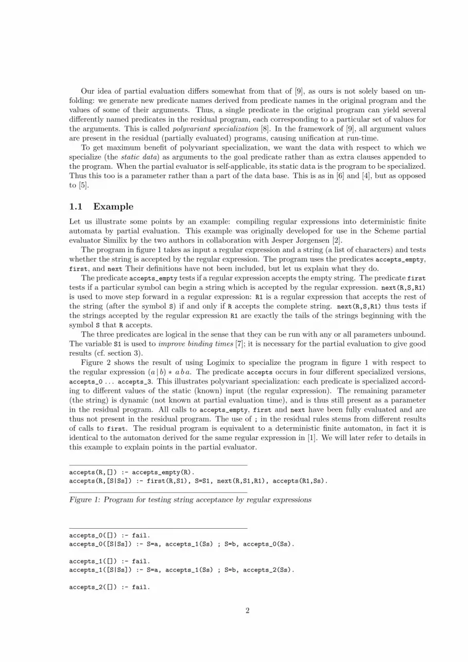
Our idea of partial evaluation differs somewhat from that of [9], as ours is not solely based on un-folding: we generate new predicate names derived from predicate names in the original program and thevalues of some of their arguments. Thus, a single predicate in the original program can yield severaldifferently named predicates in the residual program, each corresponding to a particular set of values forthe arguments. This is called polyvariant specialization [8]. In the framework of [9], all argument valuesare present in the residual (partially evaluated) programs, causing unification at run-time.

To get maximum benefit of polyvariant specialization, we want the data with respect to which wespecialize (the static data) as arguments to the goal predicate rather than as extra clauses appended tothe program. When the partial evaluator is self-applicable, its static data is the program to be specialized.Thus this too is a parameter rather than a part of the data base. This is as in [6] and [4], but as opposedto [5].

1.1 Example

Let us illustrate some points by an example: compiling regular expressions into deterministic finiteautomata by partial evaluation. This example was originally developed for use in the Scheme partialevaluator Similix by the two authors in collaboration with Jesper Jørgensen [2].

The program in figure 1 takes as input a regular expression and a string (a list of characters) and testswhether the string is accepted by the regular expression. The program uses the predicates accepts_empty,first, and next Their definitions have not been included, but let us explain what they do.

The predicate accepts_empty tests if a regular expression accepts the empty string. The predicate firsttests if a particular symbol can begin a string which is accepted by the regular expression. next(R,S,R1)

is used to move step forward in a regular expression: R1 is a regular expression that accepts the rest ofthe string (after the symbol S) if and only if R accepts the complete string. next(R,S,R1) thus tests ifthe strings accepted by the regular expression R1 are exactly the tails of the strings beginning with thesymbol S that R accepts.

The three predicates are logical in the sense that they can be run with any or all parameters unbound.The variable S1 is used to improve binding times [7]; it is necessary for the partial evaluation to give goodresults (cf. section 3).

Figure 2 shows the result of using Logimix to specialize the program in figure 1 with respect tothe regular expression (a | b) ∗ a b a. The predicate accepts occurs in four different specialized versions,accepts_0 . . . accepts_3. This illustrates polyvariant specialization: each predicate is specialized accord-ing to different values of the static (known) input (the regular expression). The remaining parameter(the string) is dynamic (not known at partial evaluation time), and is thus still present as a parameterin the residual program. All calls to accepts_empty, first and next have been fully evaluated and arethus not present in the residual program. The use of ; in the residual rules stems from different resultsof calls to first. The residual program is equivalent to a deterministic finite automaton, in fact it isidentical to the automaton derived for the same regular expression in [1]. We will later refer to details inthis example to explain points in the partial evaluator.

accepts(R,[]) :- accepts_empty(R).

accepts(R,[S|Ss]) :- first(R,S1), S=S1, next(R,S1,R1), accepts(R1,Ss).

Figure 1: Program for testing string acceptance by regular expressions

accepts_0([]) :- fail.

accepts_0([S|Ss]) :- S=a, accepts_1(Ss) ; S=b, accepts_0(Ss).




2


accepts_3([]).


Figure 2: Residual program

1.2 The partial evaluator

The partial evaluator consists of two parts: a meta-circular self-interpreter to perform the static partsof the program, and a specializer that unfolds non-static goals or specializes them with respect to theirstatic arguments. The specializer calls the interpreter to execute the static subgoals. This division of thepartial evaluator reflects the different behaviours of interpretation and specialization: interpretation canfail or return multiple solutions, whereas specialization should always succeed with exactly one specializedgoal.

2 The Interpreter

The meta-circular interpreter has the program as a ground parameter, but simulates unification,backtracking and other control directly by the same contructs in the underlying Prolog system.We have included only those control features that are possible to interpret in this way, that is(_,_), (_;_), (\+_), (_->_;_),. . . , but not ! (cut). Cut could in most cases be handled (though wedo not do so) by pre-transforming uses of ! to uses of (_->_;_). Predicates that are not defined in theprogram are assumed to be basic (predefined) predicates.

Program ::= program(Decls,[Pred])

Pred ::= pred(Name,Arity,[Clause])

Clause ::= clause([Name],[Term],Goal)

Goal ::= basic(Name,[Term]) — predefined predicates

| call(Name,[Term]) — user defined predicates

| true

| fail

| Goal, Goal

| \+ Goal — negation by failure

| Goal; Goal

| ifcut(Goal,Goal,Goal) — (. . . -> . . . ; . . . )

| if(Goal,Goal,Goal)

Term ::= var(Name)

| Name. [Term]

Figure 3: Abstract syntax for Prolog programs

2.1 Representation of programs

The abstract syntax (as ground terms) of Prolog programs is shown in figure 3; [N] means “list of N”.Figure 4 shows the regular expression program in abstract syntax.

3

program([],

[pred(accepts,2,

[clause([0],[var(0),[[]]],

basic(accepts_empty,[var(0)])),

clause([0,1,2,3,4],[var(0),[.,var(1),var(2)]],

(basic(first,[var(0),var(3)]),

basic(=,[var(3),var(1)]),

basic(next,[var(0),var(3),var(4)]),

call(accepts,[var(4),var(2)])))])])

Figure 4: Example of program in abstract syntax

2.2 Interpreter text

The full self-interpreter is shown in Appendix A.The predicate eval/4 solves a goal. It takes as arguments the goal, the entire program, a list of names ofthe variables in the goal and a list of the values that are bound to these variables. During interpretation,the first three of these arguments will be ground. Calls to basic (predefined) predicates are handled byconverting the abstract syntax of the call to normal Prolog syntax, and then passing this term to call/1.The predicate decode_list/4 uses the name and variable lists to convert a list of terms from abstractsyntax to concrete syntax. A call to a user defined predicate is handled by decoding the argument terms,and then calling call_pred/4 with the decoded terms and the functor and arity of the predicate. Controlprimitives are handled completely meta-circularly.

The predicate call_pred/4 finds the definition of the predicate in the program and callscall_clauses/3. This predicate tries each clause in turn, first making new variables for the clause,then decoding the patterns on the left-hand side, unifying these with the arguments and then, if theunification succeeds, solving the right-hand side.

3 The Specializer

The specializer requires annotation of variables as static or dynamic (i.e. non-static) and annotationof whether or not to unfold calls to user defined predicates. Static variables are neither more nor lessbound than they would be during normal (full) evaluation. This ensures that even meta-logical predicates(like var/1) have the same behaviour at specialization time as during a normal evaluation. Goals areconsidered static if they can be fully evaluated at partial evaluation time, while preserving semantics. Thenon-static goals are called dynamic. This means that they contain only static variables and that they dono side-effects, nor depend on a state that can be modified by side-effects. Dynamic goals are specializedwith respect to the values of the static variables. This involves evaluating static subgoals and unfoldingsome user defined predicates (depending on their annotation) and creating specialized predicates for thecalls that aren’t unfolded.

Binding of static variables happen only when evaluating static goals, and these bindings will only bevisible to later static goals (which may be parts of dynamic goals). This means: no backward unification.Such backwards unification could change the behaviour of non-logical predicates like var/1. Additionally,static goals are annotated by the potential number of solutions (“at most one” or “any number”). Thisis not essential, but allows the cases with at most one solution to be handled by a simpler procedure.

We use the following specialization strategy:

1. Variables in the program are always considered either static or dynamic. That is, a variable cannotchange status from static to dynamic (or vice versa) during its life-time. This decision greatlysimplifies the handling of variables, as we otherwise would have to insert explicit substitutions atthe points where a variable changes status. If a particular program should require such a changeto get good results from partial evaluation, this can be simulated by introducing new variables.This was done in the regular expression example where the variable S1 is a static copy of S. S1

4

remains static after unification with S, as it is ground at this time. Note that, when we say that avariable is non-ground, we mean that a variable from the program text has been instantiated witha non-ground value (and is thus no longer a free variable).

2. Static subgoals are evaluated by the meta-circular interpreter. The specializer needs the solution setof the static subgoals in a list and thus uses an equivalent of findall/3 when calling the interpreter.The remaining subgoals are specialized according to each solution, and the resulting residual goalsare combined with (_;_). This is done by special treatment of (_,_) when the first subgoal is static.The regular expression example shows this: the call to first(R,S1) yields two substitutions for S1,namely a and b. The remaining goal is specialized in two versions, separated by (_;_).

Note that this means that forward unification only happens across commas: no bindings go “up”the syntax tree. This can have the effect that (s1,(d1,s2)) will pass bindings from s1 to s2, but((s1,d1),s2) will not since the goal before the second comma is not fully static. Again, this strategyis chosen to simplify the specializer so it need only return residual goals and not bindings of staticvariables. The limitation can to some extend be overcome by simple modifications to the programprior to specialization, but it is rarely a problem. Indeed, parsing s1,d1,s2 will yield the better ofthe two forms. If the specializer returned bindings, then we would risk exponential code explosion,as each set of bindings would cause a new specialization of the remaining subgoals.

3. When user defined predicates are not unfolded, they are suspended. Suspension replaces the call bya call to a renamed (residual) version, which is specialized with respect to the static parameters.In the example, calls to the goal accepts are suspended and specialized with respect to the valueof R, yielding the specialized predicates accepts_0 . . . accepts_3. The definition of the residualpredicate will be added to the residual program at a later time if a previous call to the sameresidual predicate has not already caused this. We use side effects to record which specializedpredicates we have already added to the residual program. Suspension of user defined predicatesdoes not change the bindings of static variables, but static variables in the parameters have to beground. It is assumed that the annotation of variables ensures this.

4. Unfolding non-static user defined predicates does not change the bindings of static variables either.This is related to the fact that static values are propagated only through commas, cf. item 2 above.

5. During unfolding, if the unfolded predicate has several matching clauses, the specialized right handsides of these are combined with (_;_) into a single goal which is inserted in place of the call. Thisavoids the duplication problem that pure Horn-clause unfolding has. Note that, had we allowedbackwards unification, we might be forced to do backwards unification with respect to severalsubstitutions produced by matching against several clauses during unfolding. This would force usto copy the entire right hand side in which the unfolding took place, just like in pure Horn-clauseunfolding. Figure 5 shows the difference between Horn-clause unfolding and unfolding using (_;_).

6. If a predicate call is not fully executed by the interpreter, all non-ground variables occurring in itare treated as dynamic. This is because they after the call could be less ground than they wouldhave been, had the call been evaluated. As variables cannot change binding time status duringpartial evaluation, such variables are dynamic throughout their scope cf. item 1 and 2.

7. If a basic predicate has side effects or depends on global state, it is not evaluated during partialevaluation, even if all its parameters are fully ground. This ensures that side effects occur in thesame order when running the residual program, as when running the original program. Othermeta-logical predicates (var/1, ==/2, etc.) are performed if their arguments are static. Note thatstatic parameters to basic predicates can be non-ground.

5

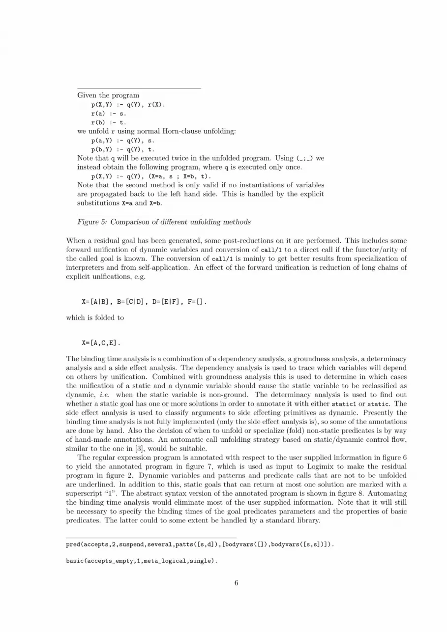
Given the programp(X,Y) :- q(Y), r(X).

r(a) :- s.

r(b) :- t.

we unfold r using normal Horn-clause unfolding:p(a,Y) :- q(Y), s.

p(b,Y) :- q(Y), t.

Note that q will be executed twice in the unfolded program. Using (_;_) weinstead obtain the following program, where q is executed only once.

p(X,Y) :- q(Y), (X=a, s ; X=b, t).

Note that the second method is only valid if no instantiations of variablesare propagated back to the left hand side. This is handled by the explicitsubstitutions X=a and X=b.

Figure 5: Comparison of different unfolding methods

When a residual goal has been generated, some post-reductions on it are performed. This includes someforward unification of dynamic variables and conversion of call/1 to a direct call if the functor/arity ofthe called goal is known. The conversion of call/1 is mainly to get better results from specialization ofinterpreters and from self-application. An effect of the forward unification is reduction of long chains ofexplicit unifications, e.g.

X=[A|B], B=[C|D], D=[E|F], F=[].

which is folded to

X=[A,C,E].

The binding time analysis is a combination of a dependency analysis, a groundness analysis, a determinacyanalysis and a side effect analysis. The dependency analysis is used to trace which variables will dependon others by unification. Combined with groundness analysis this is used to determine in which casesthe unification of a static and a dynamic variable should cause the static variable to be reclassified asdynamic, i.e. when the static variable is non-ground. The determinacy analysis is used to find outwhether a static goal has one or more solutions in order to annotate it with either static1 or static. Theside effect analysis is used to classify arguments to side effecting primitives as dynamic. Presently thebinding time analysis is not fully implemented (only the side effect analysis is), so some of the annotationsare done by hand. Also the decision of when to unfold or specialize (fold) non-static predicates is by wayof hand-made annotations. An automatic call unfolding strategy based on static/dynamic control flow,similar to the one in [3], would be suitable.

The regular expression program is annotated with respect to the user supplied information in figure 6to yield the annotated program in figure 7, which is used as input to Logimix to make the residualprogram in figure 2. Dynamic variables and patterns and predicate calls that are not to be unfoldedare underlined. In addition to this, static goals that can return at most one solution are marked with asuperscript “1”. The abstract syntax version of the annotated program is shown in figure 8. Automatingthe binding time analysis would eliminate most of the user supplied information. Note that it will stillbe necessary to specify the binding times of the goal predicates parameters and the properties of basicpredicates. The latter could to some extent be handled by a standard library.

pred(accepts,2,suspend,several,patts([s,d]),[bodyvars([]),bodyvars([s,s])]).

basic(accepts_empty,1,meta_logical,single).

6

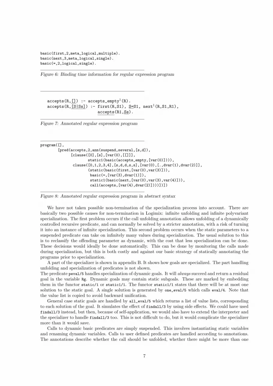
basic(first,2,meta_logical,multiple).

basic(next,3,meta_logical,single).

basic(=,2,logical,single).

Figure 6: Binding time information for regular expression program

accepts(R,[]) :- accepts_empty1(R).accepts(R,[S|Ss]) :- first(R,S1), S=S1, next1(R,S1,R1),

accepts(R1,Ss).

Figure 7: Annotated regular expression program

program([],

[pred(accepts,2,ann(suspend,several,[s,d]),

[clause([0],[s],[var(0),[[]]],

static1(basic(accepts_empty,[var(0)]))),

clause([0,1,2,3,4],[s,d,d,s,s],[var(0),[.,dvar(1),dvar(2)]],

(static(basic(first,[var(0),var(3)])),

basic(=,[var(3),dvar(1)]),

static1(basic(next,[var(0),var(3),var(4)])),

call(accepts,[var(4),dvar(2)])))])])

Figure 8: Annotated regular expression program in abstract syntax

We have not taken possible non-termination of the specialization process into account. There arebasically two possible causes for non-termination in Logimix: infinite unfolding and infinite polyvariantspecialization. The first problem occurs if the call unfolding annotation allows unfolding of a dynamicallycontrolled recursive predicate, and can normally be solved by a stricter annotation, with a risk of turningit into an instance of infinite specialization. This second problem occurs when the static parameters to asuspended predicate can take on infinitely many values during specialization. The usual solution to thisis to reclassify the offending parameter as dynamic, with the cost that less specialization can be done.These decisions would ideally be done automatically. This can be done by monitoring the calls madeduring specialization, but this is both costly and against our basic strategy of statically annotating theprograms prior to specialization.

A part of the specializer is shown in appendix B. It shows how goals are specialized. The part handlingunfolding and specialization of predicates is not shown.The predicate peval/5 handles specialization of dynamic goals. It will always succeed and return a residualgoal in the variable Rg. Dynamic goals may contain static subgoals. These are marked by embeddingthem in the functor static/1 or static1/1. The functor static1/1 states that there will be at most onesolution to the static goal. A single solution is generated by one_eval/5 which calls eval/4. Note thatthe value list is copied to avoid backward unification.

General case static goals are handled by all_eval/5 which returns a list of value lists, correspondingto each solution of the goal. It simulates the effect of findall/3 by using side effects. We could have usedfindall/3 instead, but then, because of self-application, we would also have to extend the interpreter andthe specializer to handle findall/3 too. This is not difficult to do, but it would complicate the specializermore than it would save.

Calls to dynamic basic predicates are simply suspended. This involves instantiating static variablesand renaming dynamic variables. Calls to user defined predicates are handled according to annotations.The annotations describe whether the call should be unfolded, whether there might be more than one

7

clause that matches, and the binding times of the parameters to the clause. If the call is suspended, thearguments are divided into static and dynamic according to the binding time annotation. The originalpredicate name and the static parameters are used to make a new name for the specialized predicate.This is handled by suspend/4, which also ensures that the definition of the specialized predicate will beadded to the residual program. The residual goal for the call is a call to the specialized predicate withthe dynamic arguments of the original call as arguments.

When specializing a _,_, a special case is made when the first subgoal is static and the second is not.All the solutions of the static goal are found, and the second subgoal is specialized according to eachsolution. The solutions are combined with _;_ to form the residual goal. Again, static goals with at mostone solution are given special treatment. If the first subgoal is dynamic, a residual _,_ goal is produced.

Negation (\+/1) just gives rise to a residual \+/1 and _;_ to a residual _;_. The two if-then-elseconstructs reduce to one of their branches when their condition is static. They differ in what happens ifthere is more than one solution to the condition.

4 Experiments

The specializer and the self-interpreter have been implemented. Logimix has been successfully applied tointerpreters (including the self-interpreter), yielding compiled programs where virtually all interpretationoverhead is removed. Self-application of Logimix yields stand-alone compilers and compiler generators.See the table in figure 9; the figures are for execution under SICStus Prolog version 0.6 on a SPARCstation2. The size of the generated compiler generator cogen is approximately 30KB. Generating cogen requiredmore than 12MB heap/stack space. Early versions used twice that, but after elimination of unnecessarybacktrack points in the specializer, we obtained the present result.

job time/s speedupoutput = sint(sint, data) 2.25 13.7output = target(data) 0.16target = mix(sintann, sint) 19.2 1.78target = comp(sint) 10.8comp = mix(mixann, sintann) 19.3 1.35comp = cogen(sintann) 14.4cogen = mix(mixann,mixann) 172. 1.14cogen = cogen(mixann) 152.

Figure 9: Logimix performance

Even though our partial evaluation strategy is quite conservative, we get quite good results, e.g.from specializing interpreters. This can, however, require attention to binding times when writing theinterpreter. We are not likely to get good results from off-the-shelf interpreters without modifying themto improve binding times. With the presented self-interpreter our residual programs are similar to theoriginal programs. Thus we have essentially removed all of the interpretation overhead.

The speedup (about 56%) from using a generated compiler rather than compiling by specializingthe self-interpreter is modest compared to our experiences from the functional world [8]. This is mainlybecause a substantial part of the specialization time is spent on reductions of the residual goals, somethingthat is dependent on the programs that are compiled and thus not available at compiler generation time.Compiler generation by using a compiler generator is about 26% faster than specializing the specializerdirectly. The reduction time is used mainly for folding chains of explicit unifications caused by unfoldingrecursive calls. The self-interpreter and the partial evaluator (which uses the interpreter) generate manysuch chains through calls to decode and make-vars. Other programs like the regular expression examplegenerate virtually no such chains, so the speedup of their corresponding “compilers” are better.

8

5 Conclusion

We have presented a simple and efficient self-applicable partial evaluator for a non-trivial subset of Prolog.We have shown that the simple minded strategy can yield good speed-ups of even fairly large programsand that self-application can be done with fair results. We have had great use of our experience frompartial evaluation of functional programs.

References[1] A.V. Aho, R. Sethi, and J.D. Ullman. Compilers: Principles, Techniques, and Tools. Addison-Wesley, 1986.

[2] A. Bondorf. Self-Applicable Partial Evaluation. PhD thesis, DIKU, University of Copenhagen, Denmark,1990. Revised version: DIKU Report 90/17.

[3] A. Bondorf and O. Danvy. Automatic autoprojection of recursive equations with global variables and abstractdata types. Science of Computer Programming, 16:151–195, 1991.

[4] A. Bondorf, F. Frauendorf, and M. Richter. An Experiment in Automatic Self-Applicable Partial Evaluationof Prolog. Technical Report 335, Lehrstuhl Informatik V, University of Dortmund, Germany, 1990. 20 pages.

[5] H. Fujita and K. Furukawa. A self-applicable partial evaluator and its use in incremental compilation. NewGeneration Computing, 6(2,3):91–118, 1988.

[6] D.A. Fuller. Partial Evaluation and Mix Computation in Logic Programming. PhD thesis, Imperial College,London, England, February 1989. 222 pages.

[7] C.K. Holst and J. Hughes. Towards binding-time improvement for free. In S.L. Peyton Jones, G. Hutton,and C. Kehler Holst, editors, Functional Programming, Glasgow 1990, pages 83–100, Springer-Verlag, 1991.

[8] N.D. Jones, P. Sestoft, and H. Søndergaard. Mix: a self-applicable partial evaluator for experiments incompiler generation. Lisp and Symbolic Computation, 2(1):9–50, 1989.

[9] J.W. Lloyd and J.C. Shepherdson. Partial Evaluation in Logic Programming. Technical Report CS-87-09,Department of Computer Science, University of Bristol, England, 1987. Revised version in [10].

[10] J.W. Lloyd and J.C. Shepherdson. Partial evaluation in logic programming. Journal of Logic Programming,11:217–242, 1991.

Appendix A

% meta_int(++Program,++Name,++Arity,?[Value])

meta_int(program(_,P),N,Arity,Args) :- call_pred(P,N,Arity,Args).

call_pred(P,N,Arity,Args) :-

is_member(pred(N,Arity,Clauses),P), call_clauses(Clauses,P,Args).

call_clauses(Clauses,P,Args) :-

member(clause(Vars,Patts,Rhs),Clauses),

make_vars(Vars,Vs),

decode_list(Patts,Vars,Vs,Patts1),

Args = Patts1,

eval(Rhs,P,Vars,Vs).

% eval(++Goal,++Program,++[Name],?[Value])

eval(basic(N,Args),_,Ns,Vs) :-

decode_list(Args,Ns,Vs,Nargs), G =.. [N|Nargs], call(G).

eval(call(N,Args),P,Ns,Vs) :-

length(Args,Arity),

decode_list(Args,Ns,Vs,Nargs),

call_pred(P,N,Arity,Nargs).

eval(true,_,_,_).

eval(fail,_,_,_) :-

fail.

eval((G1 , G2),P,Ns,Vs) :-

eval(G1,P,Ns,Vs), eval(G2,P,Ns,Vs).

eval((\+ G),P,Ns,Vs) :-

\+ eval(G,P,Ns,Vs).

eval((G1 ; G2),P,Ns,Vs) :-

eval(G1,P,Ns,Vs) ; eval(G2,P,Ns,Vs).

eval(ifcut(G1,G2,G3),P,Ns,Vs) :-

eval(G1,P,Ns,Vs) ->

eval(G2,P,Ns,Vs) ; eval(G3,P,Ns,Vs).

eval(if(G1,G2,G3),P,Ns,Vs) :-

if(eval(G1,P,Ns,Vs),eval(G2,P,Ns,Vs),eval(G3,P,Ns,Vs)).

make_vars([],[]).

make_vars([_|Ns],[_|Vs]) :- make_vars(Ns,Vs).

decode(var(N),Ns,Vs,V) :- lookup(N,Ns,Vs,V).

decode([N|Args],Ns,Vs,V) :-

decode_list(Args,Ns,Vs,Nargs), V =.. [N|Nargs].

decode_list([],_,_,[]).

decode_list([T1|Ts],Ns,Vs,[Tn1|Tns]) :-

decode(T1,Ns,Vs,Tn1), decode_list(Ts,Ns,Vs,Tns).

lookup(N,[M|Ns],[W|Vs],V) :- (N = M) -> V = W ; lookup(N,Ns,Vs,V).

is_member(X,[Y|L]) :- X = Y -> true ; is_member(X,L).

member(X,[X|_]).

member(X,[_|L]) :- member(X,L).

Figure 10: Meta-circular interpeter

Appendix B

% one_eval(++Goal,++Program,++[Name],?[Value],?[Value])

one_eval(G,P,Ns,Vs,Vs1) :- copy_term(Vs,Vs1), eval(G,P,Ns,Vs1).

% all_eval(++Goal,++Program,++[Name],?[Value],?[[Value]])

all_eval(G,P,Ns,Vs,Vss) :-

all_eval_init(Key),

(if(eval(G,P,Ns,Vs), (recordz(Key,Vs,_), fail), true) ->

fail ; key_to_list(Key,Vss)).

% peval(++Goal,++Program,++[Name],?[Value],?Rgoal)

peval(static1(G),P,Ns,Vs,Rg) :-

one_eval(G,P,Ns,Vs,_) -> Rg = true ; Rg = fail.

peval(static(G),P,Ns,Vs,Rg) :-

all_eval(G,P,Ns,Vs,Vss) -> make_true_list(Vss,Rg) ; Rg = fail.

peval(basic(N,Args),_,Ns,Vs,basic(N,Rargs)) :-

residualize_term_list(Args,Ns,Vs,Rargs).

peval(call(N,Args),P,Ns,Vs,Rg) :-

length(Args,Arity),

is_member(pred(N,Arity,ann(Unf,Match,Pbts),Clauses),P),

(Unf = unfold ->

(build_actuals(Pbts,Args,Ns,Vs,Nargs),

unfold_list(Match,Clauses,P,Pbts,Nargs,Rg)) ;

(find_statics_and_dynamics(Pbts,Args,Ns,Vs,Sargs,Dargs),

suspend(N,Arity,Sargs,Newn),

Rg = call(Newn,Dargs))).

peval((G1 , G2),P,Ns,Vs,Rg) :-

G1 = static1(G) ->

(one_eval(G,P,Ns,Vs,Vss) -> peval(G2,P,Ns,Vss,Rg) ; Rg = fail) ;

(G1 = static(G) ->

(all_eval(G,P,Ns,Vs,Vss) ->

peval_or_list(G2,P,Ns,Vss,Rg) ; Rg = fail) ;

(peval(G1,P,Ns,Vs,Rg1), peval(G2,P,Ns,Vs,Rg2), Rg = (Rg1 , Rg2))).

peval((\+ G),P,Ns,Vs,(\+ Rg)) :-

peval(G,P,Ns,Vs,Rg).

peval((G1 ; G2),P,Ns,Vs,(Rg1 ; Rg2)) :-

peval(G1,P,Ns,Vs,Rg1), peval(G2,P,Ns,Vs,Rg2).

peval(ifcut(G1,G2,G3),P,Ns,Vs,Rg) :-

G1 = static1(G) ->

(one_eval(G,P,Ns,Vs,Vs1) ->

peval(G2,P,Ns,Vs1,Rg) ; peval(G3,P,Ns,Vs,Rg)) ;

(G1 = static(G) ->

(all_eval(G,P,Ns,Vs,[Vs1|_]) ->

peval(G2,P,Ns,Vs1,Rg) ; peval(G3,P,Ns,Vs,Rg)) ;

(Rg = ifcut(Rg1,Rg2,Rg3),

peval(G1,P,Ns,Vs,Rg1), peval(G2,P,Ns,Vs,Rg2), peval(G3,P,Ns,Vs,Rg3))).

peval(if(G1,G2,G3),P,Ns,Vs,Rg) :-

G1 = static1(G) ->

(one_eval(G,P,Ns,Vs,Vss) ->

peval(G2,P,Ns,Vss,Rg) ; peval(G3,P,Ns,Vs,Rg)) ;

(G1 = static(G) ->

(all_eval(G,P,Ns,Vs,Vss) ->

peval_or_list(G2,P,Ns,Vss,Rg) ; peval(G3,P,Ns,Vs,Rg)) ;

(Rg = if(Rg1,Rg2,Rg3),

peval(G1,P,Ns,Vs,Rg1), peval(G2,P,Ns,Vs,Rg2), peval(G3,P,Ns,Vs,Rg3))).

peval_or_list(G,P,Ns,[Vs|Vss],Rg) :-

peval(G,P,Ns,Vs,Rg1),

(Vss = [] ->

Rg = Rg1 ; (Rg = (Rg1 ; Rg2), peval_or_list(G,P,Ns,Vss,Rg2))).

Figure 11: Part of the specializer

logimix: a self-applicable partial evaluator for prolog

Documents