Local Search Heuristics for Two-Stage FlowShop Problems with Secondary Criterion

Jatinder N. D. GuptaDepartment of Management

Ball State UniversityMuncie, IN 47306, USA

Karsten Hennig and Frank WernerOtto-von-Guericke-Universitat

Fakultat fur Mathematik39106 Magdeburg, Germany

June 21, 2005

Abstract

This paper develops and compares different local search heuristics for the two-stage flow shop problem with makespan minimization as the primary criterion andthe minimization of total flow time, total weighted flow time and total weightedtardiness as the secondary criterion. We consider simulated annealing, thresholdaccepting, tabu search and multi-level search. The latter type of algorithms ischaracterized by the use of different neighbourhoods within the search. In thecomparison we also include a genetic algorithm from the literature. In this paperwe analyze the influence of the parameters of these heuristics and the startingsolution. The algorithms have been tested on problems with up to 80 jobs.

Keywords: flowshop scheduling, secondary criterion, local search, tabu search, thresholdaccepting, simulated annealing, multi-level search, empirical evaluation

1 Introduction

Traditional research to solve multi-stage scheduling problems has focused on single crite-

rion. However, based on a survey of industrial scheduling practices, Panwalkar et al. [32]

reported that managers develop schedules based on multicriteria. Therefore, the research

for single criterion scheduling problems may not be applicable to multicriteria problems.

Because of this, multicriteria scheduling problems are receiving much attention recently

[30].

Multicriteria scheduling problems can be modeled in three different ways. First,

when the criteria are equally important, we can generate all the efficient solutions for the

problem. Then by using multiattribute decision methods, tradeoffs are made between

these solutions. Second, when the criteria are weighted differently, we can define an

objective function as the sum of weighted functions and transform the problem into a

single criterion scheduling problem. Finally, when there is a hierarchy of priority levels

for the criteria, we can first solve the problem for the first priority criterion, ignoring the

other criteria and then solve the same problem for the second priority criterion under

the constraint that the optimal solution of the first priority criterion does not change.

Termed scheduling with secondary criteria, this procedure is continued until we solve the

problem with last priority criterion as the objective and the optimal solutions of the other

criteria as the constraints.

For a scheduling problem with two criteria of interest, if the first two approaches are

required, we call the problem a bicriteria scheduling problem. If the second approach is

required, we term the problem a secondary criterion problem. Using the standard three

field notation [25], a bicriteria scheduling problem for finding all efficient solutions can

be represented as α|β|F (C1, C2), where α denotes the machine environment, β corre-

sponds to the deviations from standard scheduling assumptions, and F (C1, C2) indicates

that efficient solutions relative to criteria C1 and C2 are being sought. If the bicriteria

scheduling problem involves the sum of weighted values of two objective functions, the

problem is denoted as α|β|Fw(C1, C2), where Fw(C1, C2) represents the weighted sum

of two criteria C1 and C2. Similarly, a secondary criterion problem can be denoted as

1

α|β|Fh(C2/C1), where C1 and C2 denote the primary criterion and secondary crite-

rion, respectively, and the notation Fh(C2/C1) represents the hierarchical optimization

of criterion C2 given that criterion C1 is at its optimal value.

The literature on multiple and bicriteria problems for single machine problems is

summarized by Dileepan and Sen [12], Fry et al [14], Hoogeveen [20] and and Lee

and Vairaktarakis [26]. Nagar et al. [30] provide a detailed survey of the multiple

and bicriteria scheduling research involving multiple machines. Daniels and Chamber

[8] developed constructive procedures including a heuristic algorithm to solve problem

F ||F (Cmax, Tmax). Chen and Vempati [6] developed a backward branch-and-bound algo-

rithm for problem F2||Fh(∑

Ci/Cmax). A forward branch and bound algorithm for prob-

lem F2||Fh(∑

Ci/Cmax) is developed by Rajendran [33]. However, both Rajendran’s, and

Chen and Vempati’s algorithms cannot efficiently solve problems involving 20 or more

jobs. Rajendran [33] developed two heuristics for problem F2||Fh(∑

Ci/Cmax) problem

and tested their effectiveness in solving problems involving 25 or less jobs. Other con-

structive algorithms for this problem have been given in [19], where problems with up

to 80 jobs have been considered. A genetic algorithm for this problem has been given in

[31]. This algorithm has been tested on problems also with up to 80 jobs.

In this paper, we develop and compare different local search heuristics to solve the

problems F2||Fh(∑

Ci/Cmax), F2||Fh(∑

wiCi/Cmax) and F2||Fh(∑

wiTi/Cmax). While

problem F2||Cmax can be solved in O(nlogn) computational time [21], the problem

F2||∑ Ci is NP-hard in the strong sense [15]. From these results, it follows that prob-

lem F2||Fh(∑

Ci/Cmax) and also the other two problems considered are NP-hard in the

strong sense [5].

The rest of the paper is organized as follows. Section 2 describes the neighbourhoods

that we apply in the local search algorithms. In Section 3 we describe the different types

of local search heuristics.

The computational results of our experiments are given in detail in Section 4. Finally,

Section 5 provides conclusions of this research and suggests some directions for future

research.

2

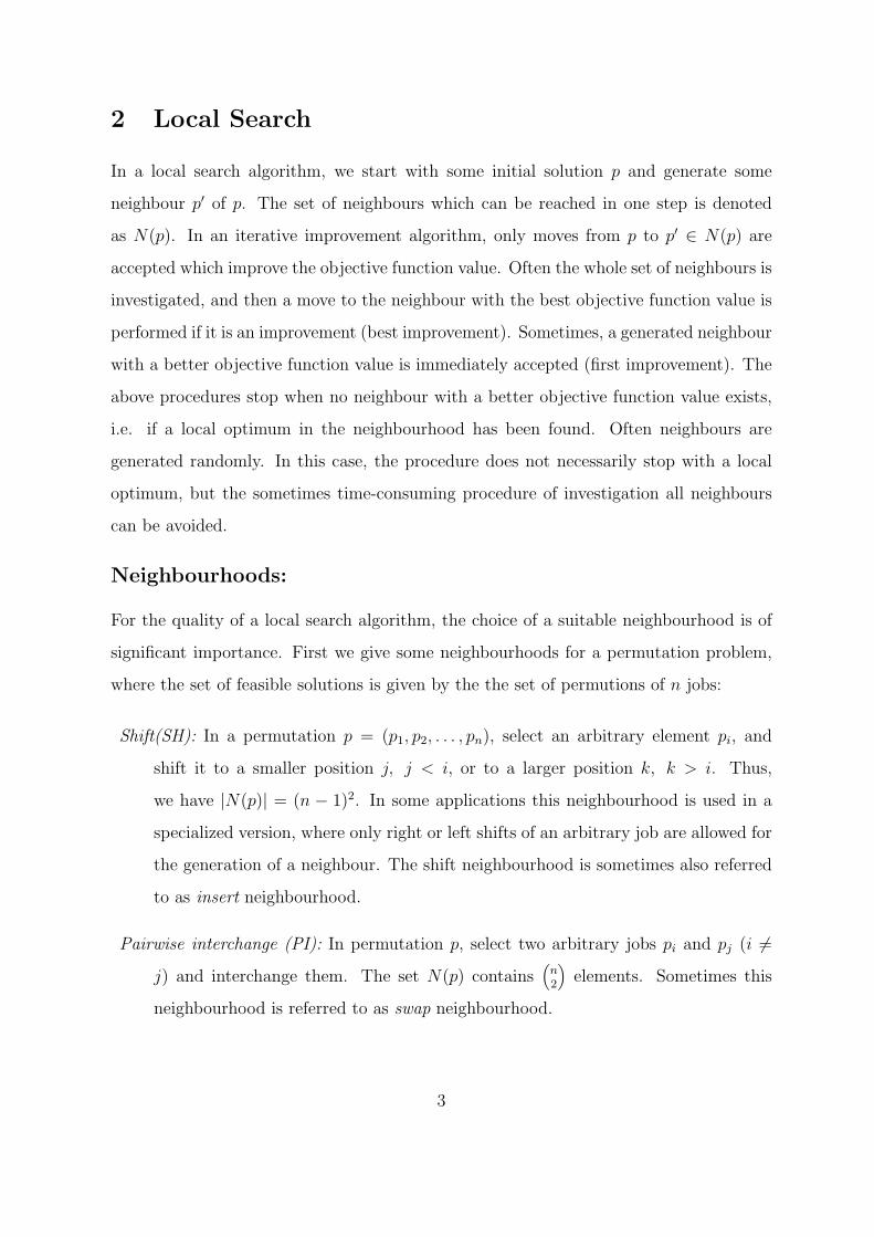
2 Local Search

In a local search algorithm, we start with some initial solution p and generate some

neighbour p′ of p. The set of neighbours which can be reached in one step is denoted

as N(p). In an iterative improvement algorithm, only moves from p to p′ ∈ N(p) are

accepted which improve the objective function value. Often the whole set of neighbours is

investigated, and then a move to the neighbour with the best objective function value is

performed if it is an improvement (best improvement). Sometimes, a generated neighbour

with a better objective function value is immediately accepted (first improvement). The

above procedures stop when no neighbour with a better objective function value exists,

i.e. if a local optimum in the neighbourhood has been found. Often neighbours are

generated randomly. In this case, the procedure does not necessarily stop with a local

optimum, but the sometimes time-consuming procedure of investigation all neighbours

can be avoided.

Neighbourhoods:

For the quality of a local search algorithm, the choice of a suitable neighbourhood is of

significant importance. First we give some neighbourhoods for a permutation problem,

where the set of feasible solutions is given by the the set of permutions of n jobs:

Shift(SH): In a permutation p = (p1, p2, . . . , pn), select an arbitrary element pi, and

shift it to a smaller position j, j < i, or to a larger position k, k > i. Thus,

we have |N(p)| = (n − 1)2. In some applications this neighbourhood is used in a

specialized version, where only right or left shifts of an arbitrary job are allowed for

the generation of a neighbour. The shift neighbourhood is sometimes also referred

to as insert neighbourhood.

Pairwise interchange (PI): In permutation p, select two arbitrary jobs pi and pj (i 6=j) and interchange them. The set N(p) contains

(n2

)elements. Sometimes this

neighbourhood is referred to as swap neighbourhood.

3

Adjacent pairwise interchange (API): This is a special case of both the shift and the

pairwise interchange neighbourhood. In permutation p, two adjacent jobs pi and

pi+1 (1 ≤ i ≤ n − 1) are interchanged to generate a neighbour p′. Thus, we have

|N(p)| = n− 1.

k-Pairwise Interchange (kPI): This is a generalization of the pairwise interchange neigh-

bourhood. A neighbour is generated from p by performing at most k consecutive

pairwise interchanges.

(k1, k2)-Adjacent pairwise interchange neighbourhood (k1, k2−API): In this neighbour-

hood, a neighbour is generated from p by performing k successive adjacent pairwise

interchanges, where k1 ≤ k ≤ k2.

A neighbourhood structure may be represented by a directed, an undirected or a

mixed graph. The set of vertices is the set of feasible solutions M , and there is an arc

from p ∈ M to each neighbour p′ ∈ N(p). In the case of p′ ∈ N(p) and p ∈ N(p′), we

replace both arcs by an undirected edge. We denote the graphs describing the above

neighbourhoods as G(SH), G(PI), G(API), G(kPI) and G(k1−k2−API), respectively.

Obviously, all these graphs are undirected, i.e. these neighbourhoods are symmetric.

Note that the graphs representing the right and left shift neighbourhoods are directed.

For the problem under consideration, only a subset of the permutations of n jobs

is feasible. In this case, the set of neighbours N(p) of a feasible sequence in the shift

neighbourhood is the set of feasible sequences that can be obtained by a shift of a job. The

next theorem gives an important property for the API neighbourhood since it guarantees

that a local search algorithm may reach a global optimum from an arbitrary starting

solution.

Theorem 1 Let M be the set of feasible sequences for a problem F2//Fh(∑

Ci/Cmax).

Then the graph G(API) is connected.

Proof: Let p = (p1, . . . , pn) and p′ = (p′1, . . . , p′n) be two permutations with minimum

makespan. Moreover, let i ≥ 1 be the smallest and j ≤ n be the greatest position on which

4

in p and p′ different jobs are sequenced. For N∗ = {pi, . . . , pj}, let p∗ = (p∗i , . . . , p∗j) be the

Johnson sequence for the jobs of set N∗ and p = (p1, . . . , pi−1, p∗i , . . . , p

∗j , pj+1, . . . , pn}.

Then it is clear that both from p and from p′, there is a path in G(API) to p∗ such that

all permutations (vertices) on the paths have a minimum makespan value (there are done

consecutive pairwise interchanges such that after an interchange, the corrosponding pair

(k, l) of jobs satisfies min{ak, bl} ≤ min{al, bk}). By connecting both paths from p to p

and from p to p′, we obtain the statement of the theorem. 2

As a consequence, also the other neighbourhoods that have been introduced above

are connected. The same is true for the other two secondary criteria considered in this

paper (since this property does not depend on the secondary criterion).

Dominance:

In [19], there have been given the following sufficient optimality criterion.

Theorem 2 A schedule p = (p1, p2, . . . , pn) satisfying the conditions

min{api; bpi+1

} ≤ min{api+1; bpi

}, 1 ≤ i ≤ n− 1 (1)

api≤ api+1

, 1 ≤ i ≤ n− 1 (2)

bpi≤ bpi+1

, 1 ≤ i ≤ n− 1 (3)

optimally solves problem F2//Fh(∑

Ci/Cmax).

We incorporate this optimality criterion into the local search algorithms as follows.

Assume that a shift neighbour p′ of sequence p has been generated by moving a job u

to the right such that the new adjacent job to the right is job v, i.e. we have p′ =

(. . . , u, v, . . .). Then we check conditions (1) - (3) for the jobs p′′i := v and p′′i+1 := u.

If these conditions are satisfied, we may interchange both jobs without increasing the

makespan and the flow time values, i.e. sequence p′ is dominated by sequence p′′ =

(. . . , v, u, . . .) and we have ‘enlarged’ the shift of job u by one position.

In a similar way we apply this approach when an adjacent pairwise interchange of jobs

pi = u and pj = v with i < j has been performed to generate p′. In this case we try to

interchange job u with its current neighbour to the right and then job v consecutively with

5

its left neighhbour as long as interchanges are justified by Theorem 2. This dominance

criterion is denoted as DOM1.

We also consider the following stronger dominance criterion which includes Theorem

2 as a special case for C2 =∑

Ci.

Theorem 3 Let C2 = F ∈ {∑ Ci,∑

wiCi,∑

wiTi}, p′ = (p1, . . . , pi−1, pi, pi+1, . . . , pn),

p′′ = (p1, . . . , pi−1, pi+1, pi, pi+2, . . . , pn), and π′ and π′′ be the partial sequences of the first

i + 1 jobs of p′ and p′′, respectively. If

Cmax(π′′) ≤ Cmax(π

′) and F (π′′) ≤ F (π′)

then Cmax(p′′) ≤ Cmax(p

′) and F (p′′) ≤ F (p′) hold, i.e. sequence p′ is dominated by

sequence p′′.

This dominance criterion is denoted as DOM2 and will be applied only in the API

neighbourhood as described later. Contrary to DOM1, it can be applied to all secondary

criteria considered in this paper. We note that both dominance criteria can be checked

in constant time for a pair of adjacent jobs.

Stopping criterion:

The stopping criterion is the method used to terminate the search process. There are

three common stopping criteria for local search algorithms: a maximum number of iter-

ations or solutions reached, no improvement of the best solution for a specified number

of iterations, or a maximum CPU time allowed to solve a problem. The second criterion

may be more efficient in speed, but since the number of iterations with no improvement

will be affected by the complexity of the solution space and the problem size, a suitable

number of iterations is difficult to determine. Using a limit on the maximum CPU time

is partially captured in setting the maximum number of iterations. Therefore, and for

the comparibility of the different heuristics, the first stopping criterion is chosen.

6

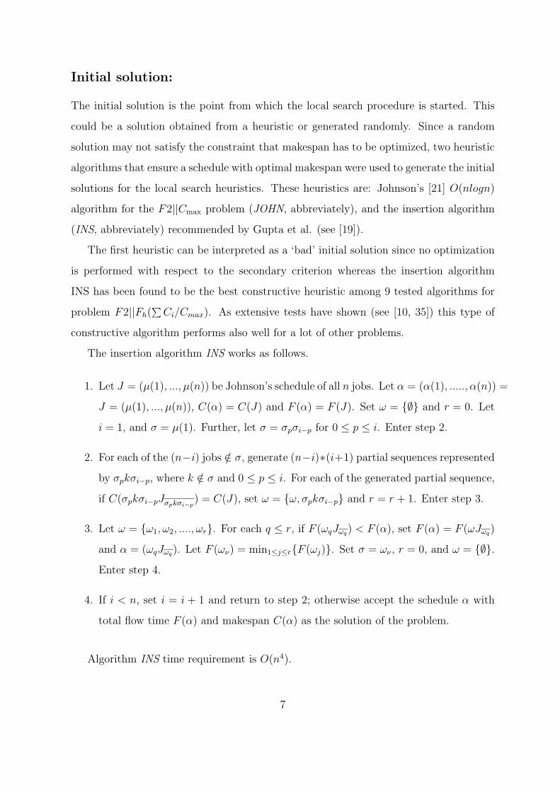
Initial solution:

The initial solution is the point from which the local search procedure is started. This

could be a solution obtained from a heuristic or generated randomly. Since a random

solution may not satisfy the constraint that makespan has to be optimized, two heuristic

algorithms that ensure a schedule with optimal makespan were used to generate the initial

solutions for the local search heuristics. These heuristics are: Johnson’s [21] O(nlogn)

algorithm for the F2||Cmax problem (JOHN, abbreviately), and the insertion algorithm

(INS, abbreviately) recommended by Gupta et al. (see [19]).

The first heuristic can be interpreted as a ‘bad’ initial solution since no optimization

is performed with respect to the secondary criterion whereas the insertion algorithm

INS has been found to be the best constructive heuristic among 9 tested algorithms for

problem F2||Fh(∑

Ci/Cmax). As extensive tests have shown (see [10, 35]) this type of

constructive algorithm performs also well for a lot of other problems.

The insertion algorithm INS works as follows.

1. Let J = (µ(1), ..., µ(n)) be Johnson’s schedule of all n jobs. Let α = (α(1), ....., α(n)) =

J = (µ(1), ..., µ(n)), C(α) = C(J) and F (α) = F (J). Set ω = {∅} and r = 0. Let

i = 1, and σ = µ(1). Further, let σ = σpσi−p for 0 ≤ p ≤ i. Enter step 2.

2. For each of the (n−i) jobs /∈ σ, generate (n−i)∗(i+1) partial sequences represented

by σpkσi−p, where k /∈ σ and 0 ≤ p ≤ i. For each of the generated partial sequence,

if C(σpkσi−pJσpkσi−p) = C(J), set ω = {ω, σpkσi−p} and r = r + 1. Enter step 3.

3. Let ω = {ω1, ω2, ...., ωr}. For each q ≤ r, if F (ωqJωq) < F (α), set F (α) = F (ωJωq)

and α = (ωqJωq). Let F (ων) = min1≤j≤r{F (ωj)}. Set σ = ων , r = 0, and ω = {∅}.Enter step 4.

4. If i < n, set i = i + 1 and return to step 2; otherwise accept the schedule α with

total flow time F (α) and makespan C(α) as the solution of the problem.

Algorithm INS time requirement is O(n4).

7

3 Simulated Annealing

Simulated Annealing (SA) has its origin in statistical physics, where the process of cooling

solids slowly until they reach a low energy state is called annealing. It has originally been

proposed by Metropolis et al. [29] and was first applied to combinatorial optimization

problems by Kirkpatrick et al. [23] and by Cerny [7]. In such an algorithm, the sequence

of the objective function values does not necessarily monotonically decrease.

Starting with an initial sequence p, a neighbour p′ is generated (usually randomly) in

a certain neighbourhood. Then the difference

∆ = F (p′)− F (p)

in the values of the objective function F is calculated. When ∆ ≤ 0, sequence p′ is

accepted as the new starting solution for the next iteration. In the case of ∆ > 0,

sequence p′ is accepted as new starting solution with probability exp(−∆/T ), where T

is a parameter known as the temperature.

Typically, in the initial stages the temperature is rather high so that escaping from

a local optimum in the first iterations is rather easy. After having generated a certain

number TCON of sequences, the temperature usually decreases. Often, this is done by

a geometric cooling scheme. In this case, the new temperature T new is chosen such that

T new = λT old, where 0 < λ < 1 and T old denotes the old temperature. An alternative

cooling scheme has been given for instance by Lundy and Mees [17]. They perform

a single iteration at a constant temperature, and the new temperature is obtained by

T new = T old/(1 + βT old), where β is a constant expressed in terms of the initial and final

temperature and the number of iterations. Under the Lundy-Mees cooling scheme the

temperature decreases faster than in a geometric scheme. So, more iterations are then

performed at a lower temperature.

A possible stopping criterion would then be a cycle of a final temperature, which is

sufficiently close to zero (for instance 0.01 as in [10]). Since we use for all heuristics a

given number of generated solutions as stopping criterion, we determine on the base of

the inital temperature T 0, the final temperature T = 0.01 and the number TCON of

8

generated solutions with a constant temperature, the reduction factor λ in the geometric

cooling scheme.

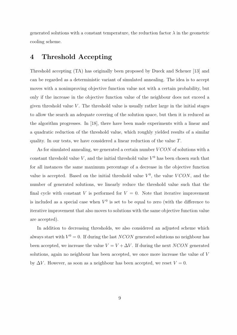
4 Threshold Accepting

Threshold accepting (TA) has originally been proposed by Dueck and Scheuer [13] and

can be regarded as a deterministic variant of simulated annealing. The idea is to accept

moves with a nonimproving objective function value not with a certain probability, but

only if the increase in the objective function value of the neighbour does not exceed a

given threshold value V . The threshold value is usually rather large in the initial stages

to allow the search an adequate covering of the solution space, but then it is reduced as

the algorithm progresses. In [18], there have been made experiments with a linear and

a quadratic reduction of the threshold value, which roughly yielded results of a similar

quality. In our tests, we have considered a linear reduction of the value T .

As for simulated annealing, we generated a certain number V CON of solutions with a

constant threshold value V , and the initial threshold value V 0 has been chosen such that

for all instances the same maximum percentage of a decrease in the objective function

value is accepted. Based on the initial threshold value V 0, the value V CON , and the

number of generated solutions, we linearly reduce the threshold value such that the

final cycle with constant V is performed for V = 0. Note that iterative improvement

is included as a special case when V 0 is set to be equal to zero (with the difference to

iterative improvement that also moves to solutions with the same objective function value

are accepted).

In addition to decreasing thresholds, we also considered an adjusted scheme which

always start with V 0 = 0. If during the last NCON generated solutions no neighbour has

been accepted, we increase the value V = V +∆V . If during the next NCON generated

solutions, again no neighbour has been accepted, we once more increase the value of V

by ∆V . However, as soon as a neighbour has been accepted, we reset V = 0.

9

5 Tabu Search Algorithm

Tabu search’s (TS) origin dates back to the 1960’s and 1970’s and was proposed in its

present form by Glover [16]. The majority of the applications of TS started in late 1980’s

[34]. TS has been applied to transportation problems (such as traveling salesman and

vehicle routing), layout and circuit design problems (quadratic assignment and electronic

circuit design), neural networks (non-convex optimization and learning in an associate

memory), telecommunications problem (bandwidth packing, path assignment), schedul-

ing problems (employee scheduling, resource scheduling), multi-constraint 0-1 knapsack

problem, large scale controlled rounding, general fixed charge problem, bottleneck prob-

lems and graph problems which include maximum clique, graph coloring, graph parti-

tioning, and stable sets in large graph problems. One of the common applications of

TS is in production scheduling. Taillard [36] and Widmer and Hertz [38] solve a n-job,

m-machine flow shop problem for makespan criterion. Widmer [37] developed a TS ap-

proach to job shop scheduling with tooling constraint. Daniels and Mazzola [9] presented

a TS approach for flexible-resource job shop scheduling. Dell’Amico and Trubian [11]

solved the job shop scheduling problem. Their procedure alternates between assigning

operations at the beginning and at the end of a known partial schedule. The single ma-

chine scheduling problem with delay penalties and set-up costs was studied by Laguna

and Glover [24]. They integrated target analysis as an effective mean to diversify within

tabu search. Barnes and Laguna [2] solved the multiple machine weighted flow time

problem. Kim [22] experimented with minimizing mean tardiness as the performance

measures in a flow shop problem.

TS can be viewed as an iterative process which explores the solution space by re-

peatedly making moves from one solution, p, to another solution, p′, located in the

neighbourhood, N(p), of p. These moves are performed with an ultimate goal of reach-

ing a good solution by the evaluation of some objective function F (p) to be optimized.

However, contrary to other traditional iterative approaches, in Tabu Search, the function

F (p′) need not be better than F (p) in every iteration. The search will be terminated

when some stopping condition is satisfied.

10

One of the main ideas of TS, as its name depicts, is its use of a flexible memory

(tabu list) to tabu certain moves for a period of time. In every iteration of TS, a move

will be instantly assigned to the tabu list when the move is chosen to lead the search

from the current solution to its neighbour solution. This move will then not be chosen

for a number of immediately succeeding iterations. This number of iterations is denoted

as tabu list size, and the size is limited to a certain length. When the list has reached

its specified length, the move that was assigned to the list earliest is released from the

list and the most current move is inserted. With an appropriate design of the tabu list,

TS is able to prevent cycling of the search and guide the search to the solution regions

which have not been examined and approach to good solutions in the solution space.

However, design of the tabu list may also prohibit the search to some solution regions

which are appealing. Glover [16] suggested a method, aspiration criterion, to make up

this drawback. The idea of aspiration criterion is that if a specific move which is currently

tabued but has the potential to lead the search to good solution regions, then that move

should be removed from the tabu list (aspired). Several aspiration criteria can be used

to measure the potentiality of a tabued move. The common one is to remove a tabued

move from the tabu list if this move can provide a better solution than the incumbent

solution.

The performance of TS may be affected by several factors, for instance the initial

solution, the neighbourhood, the tabu list size, aspiration criterion, and the stopping

criterion [36].

In our experiments, we considered the SH and PI neighbourhoods with a random

generation of neighbours, and the API neighbourhood with a complete examination of

the neighbourhood. In all neighbourhoods, a move is accepted only if it maintains the

minimum makespan.

The neighbourhood size NSIZE represents the number of candidate solutions to be

evaluated in each iteration of the search process. Tabu search uses two common types of

neighbourhood size. The first kind is to evaluate all possible neighbours and select the

best non-tabued solution in each iteration. This kind of examination may be suitable if

the cardinality of the neighbourhood is not too large. The quality of the solution obtained

11

by this neighbourhood examination may be good but the diversification capability of TS

may be affected. The second type is to evaluate only a fixed number of neighbours in

one iteration. This type of neighbourhood examination may improve the capability of

diversification of TS.

Tabu list is the salient feature of tabu search. It contains a list of moves that has been

made and are therefore forbidden or tabued. Too small a tabu list may cause cycling of

tabu search, while too large a tabu list may prohibit TS to reach certain good solution

regions. Past research [16, 37] indicates that it is reasonable to set the list sizes to be

constant.

To describe the tabu list, we consider order and position attributes. We describe the

application of these attributes to the SH and PI neighbourhoods.

Order attribute:

SH neighbourhood – If a job i is shifted to the right immediately after job j by an

accepted move, we add the pair (j, i) to the list. Analogously, if job i has been

shifted to the left immediately before job k, we add the pair (i, k) to the list.

PI neighbourhood – If two jobs i and j are interchanged by an accepted move, we add

the pair (j, i) to the list.

Position attribute:

SH neighbourhood – If a job i from position k is shifted to another position, we store

the pair (i, k).

PI neighbourhood – If the jobs i and j from positions k and l are interchanged, we store

the pairs (i, k) and (j, l).

If the API neighbourhood is applied, we use for its simplicity the description of the

tabu list given for the SH neighbourhood. Applying the order attribute, a sequence is

tabu, if any of the ordered job pairs in the tabu list are sequenced in reverse order. A

neighbour is tabu under the position attribute list, if any job i is sequenced at a position

k for which the pair (i, k) is contained in the tabu list (SH neighbourhood), or if jobs i

12

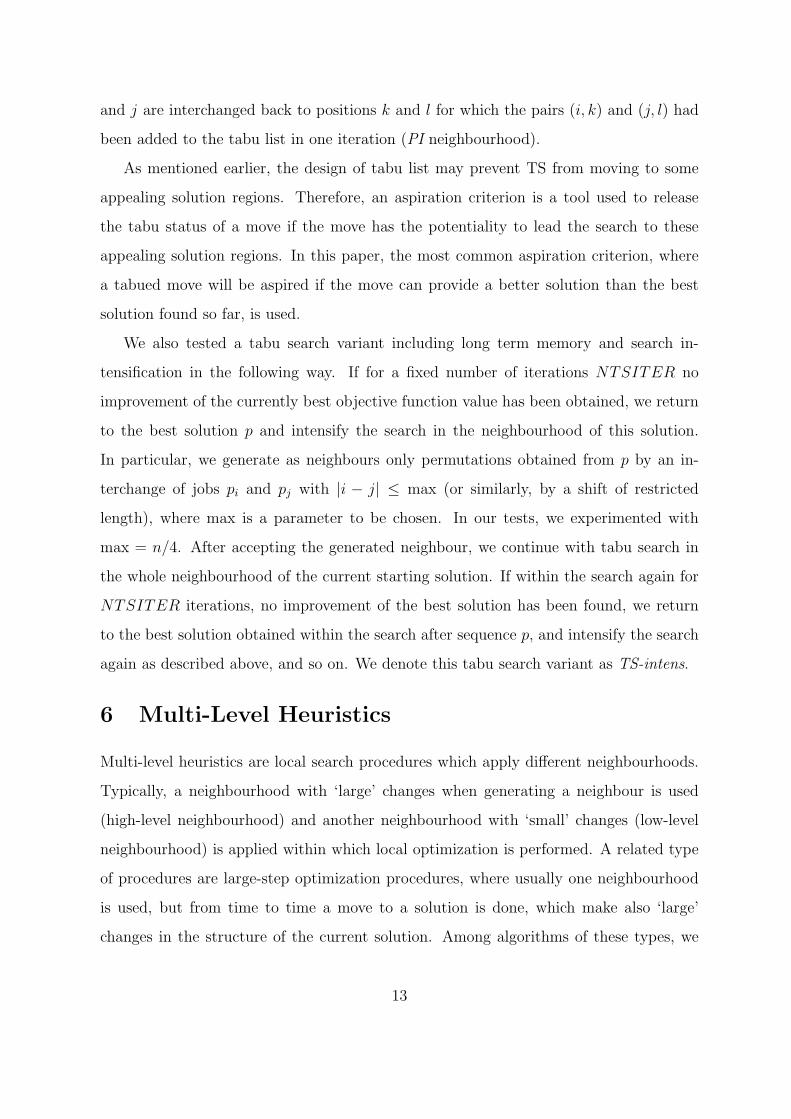
and j are interchanged back to positions k and l for which the pairs (i, k) and (j, l) had

been added to the tabu list in one iteration (PI neighbourhood).

As mentioned earlier, the design of tabu list may prevent TS from moving to some

appealing solution regions. Therefore, an aspiration criterion is a tool used to release

the tabu status of a move if the move has the potentiality to lead the search to these

appealing solution regions. In this paper, the most common aspiration criterion, where

a tabued move will be aspired if the move can provide a better solution than the best

solution found so far, is used.

We also tested a tabu search variant including long term memory and search in-

tensification in the following way. If for a fixed number of iterations NTSITER no

improvement of the currently best objective function value has been obtained, we return

to the best solution p and intensify the search in the neighbourhood of this solution.

In particular, we generate as neighbours only permutations obtained from p by an in-

terchange of jobs pi and pj with |i − j| ≤ max (or similarly, by a shift of restricted

length), where max is a parameter to be chosen. In our tests, we experimented with

max = n/4. After accepting the generated neighbour, we continue with tabu search in

the whole neighbourhood of the current starting solution. If within the search again for

NTSITER iterations, no improvement of the best solution has been found, we return

to the best solution obtained within the search after sequence p, and intensify the search

again as described above, and so on. We denote this tabu search variant as TS-intens.

6 Multi-Level Heuristics

Multi-level heuristics are local search procedures which apply different neighbourhoods.

Typically, a neighbourhood with ‘large’ changes when generating a neighbour is used

(high-level neighbourhood) and another neighbourhood with ‘small’ changes (low-level

neighbourhood) is applied within which local optimization is performed. A related type

of procedures are large-step optimization procedures, where usually one neighbourhood

is used, but from time to time a move to a solution is done, which make also ‘large’

changes in the structure of the current solution. Among algorithms of these types, we

13

mention the algorithms by Martin et al. [28], Brucker et al. [3, 4], Lourenco [27] and

Danneberg et al. [10].

Martin et al. [28] applied such an approach to the traveling salesman problem. They

use the 4-opt neighbourhood as high-level neighbourhood and the 3-opt neighbourhood

as low-level neighbourhood. Recall that in the k-opt neighbourhood, a neighbour of a

tour is generated by replacing k arcs of the current tour by k other arcs such that again

a feasible tour results.

The papers by Brucker et al. [3, 4] consider different scheduling problems for which

the local optimization within the low-level neighbourhood can be done in a constructive

way during the generation of a high-level neighbour. In particular, various scheduling

problems on one machine, on parallel machines and in a flow shop environment have been

considered. By applying structural properties of the problem considered, the high-level

neighbourhood is defined as the set of feasible solutions that are locally optimal with

respect to some low-level neighbourhood, often based on the API neighbourhood.

Lourenco [27] considered the job shop scheduling problem. In this paper, certain ad-

jacent pairwise interchanges of two operations are considered to generate a neigbour, and

a large step is defined by performing some adjacent pairwise interchanges consecutively,

or by reoptimizing the sequence of operations on a machine by applying the shifting

bottleneck procedure [1].

In [10], a multi-level approach has been applied to the permutation flow shop schedul-

ing problem with batch processing, where the processing time of a batch is given by the

maximum processing time of the operations contained in a batch, and additionally the

maximum batch size is limited. The jobs are partitioned into groups, and batches can

only be formed by jobs of the same group. In that paper, the search is guided by three pa-

rameters V, h, and l. In the first step of an iteration, an ‘acceptable’ high-level neighbour

is generated. It means that the first generated high-level neighbour with an objective

function value which is not more than V % worse than that of the current starting solu-

tion. However, if h high-level neighbours have been generated and none of these satisfies

the above condition, the best of them is accepted high-level neighbour.

Then, from the accepted high-level neighbour, iterative improvement is performed in

14

the low-level neighbourhood. To avoid a complete investigation of the low-level neigh-

bourhood the maximum number of low-level neighbour generated in one iteration is

limited by the parameter l. The sequence obtained is taken as generated (iterative)

neighbour. In [10], this neighbour is compared with the starting solution of the current

iteration by applying a simulated annealing procedure. There have been considered dif-

ferent types of high- and low-level neighbours, based on certain types of batch changes

(the sequence of batches changes) and job changes (a job is shifted into another batch or

exchanged with a job from another batch from the same group). To get a fair comparison,

the same number of solutions as for the other heuristics was generated.

In this study, we consider the following high-level neighbourhoods in such a multi-

level algorithm:

a) PI \ API - a neighbour is obtained by performing a shift, which is not an adjacent

pairwise interchange;

b) k − PI with k ∈ {2, 3} and

c) (k1, k2)-API.

In case b), we first decide how many pairwise interchanges will be performed. Then,

we choose successively job pairs to perform the pairwise interchanges such that no job

is twice selected. For simplicity, in case c) we perform consecutively adjacent pairwise

randomly chosen interchanges (thus, it may happen that such an interchange reverses

some interchange previously made).

As the low-level neighbourhood, we always use the API neighbourhood including

dominance criterion DOM2. To perform local optimization starting from the high-level

neighbour p′, we consider two randomly determined consecutive jobs p′i and p′i+1, i =

1, . . . , n− 1. If they satisfy conditions (1) - (3) (which can be checked in constant time),

the interchange of both jobs need not be considered since it may not improve the objective

function value. Otherwise, we consider sequence p′′, obtained from p′ by interchanging

both jobs. If the partial sequences π′ and π′′ satisfy the conditions of Theorem 3, we

replace sequence p′ by sequence p′′.

Applying multi-level search, we usually generate several high-level and low-level neigh-

bours within one iteration. Since our stopping criterion is based on the number of solu-

15

tions generated, we count the number of objective function value calculations that have

been done, and only after each iteration, we check whether the stopping criterion is sat-

isfied. For accepting an iterative neighbour, we consider different acceptance schemes:

1) TA scheme: Each iterative neighbours is accepted whose increase in the objective

function value in comparison with that of the starting solution of the current iteration

does not exceed a given bound V . We use the same bound V as for the acceptance of

a generated high-level neighbour within an iteration, namely V = F (p)/T with current

starting solution p and different values of T ∗.

2) Iterative improvement scheme: Only iterative neighbours with a better objective func-

tion value are accepted.

3) modified nonimproving scheme: If for a certain number of iterations NMLITER no

improvement of the best solution so far has been obtained, we return to the best solution

p and continue the search from there. If later again no improvement within NMLITER

iterations has been obtained, we return to the best solution found after p and continue

from there, and so on. This acceptance scheme corresponds to that used in the tabu

search variant TS-intens.

4) SA scheme: We apply simulated annealing as described in Section 3 with the differ-

ence that after generating an iterative neighbour the temperature is decreased stronger

in accordance with the nunber of solutions that have been generated within one iteration.

This guarantees that the search finishes with the final value T = 0.01 too (see [10]).

7 Genetic algorithm

For comparison purposes we included into our tests a genetic algorithm GA given in [31]

originally for C2 =∑

Ci. This algorithm can be used immediately also for the other C2

criteria considered in this paper.

Genetic algorithms are probabilistic search techniques, based on the mechanism of

evolution. The solution space is usually represented by a population. New structures

are generated by applying simple genetic operators such as crossover, mutation, and

inversion to the parent structures. The members with higher fitness values (i.e. better

16

objective function values) in the current population will have higher probability of being

selected as parents, which is similar to Darwin’s concept of survival of the fittest. The

initial population is randomly generated, which means that the feasibility of the final

solution would not be guarenteed. Therefore, in the initial population always at least

one solution having the minimum makespan is included (for instance, by applying a

constructive method given in [19]), and the best solution is saved in every generation. In

this way, the feasibility of the final solution is guarenteed.

In our tests, we included the vector evaluated approach from [31]. In this case, the

fitness value of a solution is a vector representing the function values with respect to both

criteria. A sub-population for each criterion is generated by selecting the best soltions

for the criterion from the current population. Then, solutions with good fitness values

in each sub-population are selected and recombined in each generation to evolve the

solution which minimize criterion C2 subject to a minimum makespan. We note that the

mutation operation is based on the pairwise interchange of two jobs in the corresponding

sequence. For further details, the reader is referred to [31]. We adjusted the parameters

population size and number of generations such that the same number of solutions as for

the other types of algorithms are generated. Details will be given in Section 8.

8 Computational Results

This effectiveness of each proposed local search heuristic in finding an optimal or near op-

timal solution was empirically evaluated by solving a large number of problem instances.

In this section, we first describe the design of expriments and the manner in which various

parameter values were set. Subsequently, we discuss the experimental results.

Design of experiments

The performance of the local search heuristics was evaluated with 4 groups of problems,

each classified by the number of jobs (20, 40, 60, and 80). Within each group, 20 different

instances were randomly generated for each objective function considered. For initial

experiments used to find the best parameter settings for each heuristic, the processing

17

times of the jobs for each of the problems were integers from the uniform distribution

[1, 100]. All algorithms were coded in C and run on a Power PC 603e (166 MHz). For all

three objective functions considered, all parameter tests used a ‘bad’ starting sequence

obtained by algorithm JOHN and a ‘good’ starting solution obtained by the insertion

algorithm INS.

Our initial experiments considered a constant number of generated sequences (NSOL =

4000), and a number of generations linearly depending on the number of jobs (NSOL =

100n). In most cases, the results turned out to be superior for a linear number of gen-

erated permutations (in particular for the problems with n = 80). Therefore, we use in

the following the latter variant exclusively. We describe the parameter settings that were

tested for the individual algorithms.

For simulated annealing, we first tested the influence of parameters T 0 and TCON .

In particular, we considered the following variants for both the PI and the SH neighbour-

hoods:

a) T 01 = F (p0)/5 and T 0

2 = F (p0)/15;

b) TCON1 = 1 and TCON2 = n/2.

Subsequently, we investigated whether the inclusion of criterion DOM1 improved the

performance of simulated annealing for C2 =∑

Ci.

For threshold accepting, we considered a variant TA-I that does not accept inferior

moves (i.e. we set V = 0). For decreasing threshold schemes (variant TA-dec), we

considered:

a) V 01 = F (p0)/2000, V 0

2 = F (p0)/1000 and V 03 = F (p0)/200;

b) V CON1 = 1 and V CON2 = n/2.

Concerning variable threshold schemes (variant TA-var), we considered:

a) ∆V1 = F (p∗)/2000, ∆V2 = F (p∗)/5000 and ∆V3 = F (p∗)/10000;

b) NCON1 = 20 and NCON2 = 40.

where p∗ denotes the current starting solution within the search.

For tabu search, we first tested for a larger length of the tabu list (LS = 7) and

a larger neighbourhood size (NSIZE = 20), the influence of both attributes, position

and order, for both the PI and the SH neighbourhoods. Then we experimented with

18

alternative values of the parameters LS and NSIZE:

a) LS ∈ {3, 5, 12};b) NSIZE ∈ {10, 40, 60, n/4, n}.

We also checked whether the variant TA-intens improved the results obtained so far

with tabu search. For comparison purposes, we also tested a TS variant with complete

investigation of the nontabu neighbours in the API neighbourhood.

For the multi-level search, we first used the TA acceptance scheme for an iterative

neighbour with the following variants in our initial tests:

(k1, k2)−API: We experimented with h ∈ {8, 15, 20}, l ∈ {10, 20, 40}, T ∗ ∈ {1000, 2000, 5000}and 2 ≤ k1 < k2 ≤ 20.

PI \ API: We experimented with h, l ∈ {3, 5, 10, 15, 20} and T ∗ ∈ {1000, 2000, 5000}.Having settled the above parameters, we then compared the high-level neighbour-

hoods 2−PI and 3−PI with PI \API again for the TA acceptance scheme, and finally

we compared several acceptance schemes.

Comparison of neighbourhoods

First, we compared both the SH and the PI neighbourhood on some parameter variants

for simulated annealing, threshold accepting, and tabu search. For each parameter con-

stellation considered, we observed quite similar trends. For one typical variant of each

metaheuristic, Table 1 shows the percentage improvements over the starting solution. In

almost all cases, the PI neighbourhood performed better (and sometimes even clearly

better). This is in contrast to results for scheduling problems with makespan minimiza-

tion, where often the SH neighbourhood is superior. Due to the above results, we applied

in multi-level search only PI-based neighbourhoods.

T a b l e 1

Parameter setting for the metaheuristics

For local search heuristics, the parameter setting usually does not depend on the quality

of the starting solution or on the objective function. For this reason, we recommend

19

a setting that works well from an overall point of view. However, as seen from Table

1, there are large differences in the achieved percentage improvements depending on

the starting solution and the objective function considered. Most improvments were

obtained for C2 =∑

wiTi which indeed appeared to be the ‘most complicated’ criterion.

This usually leads to higher percentage improvements, and the differences become larger

for the individual variants of an algorithm. For C2 =∑

Ci criterion, the insertion

algorithm produces a rather good solution so that iterative algorithms produced only

small additional percentage improvements. Although algorithm INS is a constructive one,

the required number of functional value computations is rather large. In particular, for

the problem sizes included into our experiments, algorithm INS considers 1521 sequences

for n = 20, 11441 sequences for n = 40, 37761 sequences for n = 60, and 88481 sequences

for n = 80. Consequently, for larger values of n, the constructive algorithm requires

considerably larger number of sequences than the iterative variants tested here (and,

therefore, requires larger computational times).

Concerning simulated annealing, the choice of TCON hardly influenced the results.

Since keeping the temperature constant for a certain number of iterations did not improve

the results, for simplicity, we choose TCON1. Moreover, use of T 01 turned out to be

slightly superior to T 02 . The consideration of a dominance criterion DOM1 within the

simulated annealing algorithm for C2 =∑

Ci did not improve the results (the differences

in the average percentage improvements are lower than 0.02 % and have practically no

influence).

For threshold accepting with decreasing threshold schemes, a high initial threshold

values (V 02 , V 0

3 ) worked poorly. Variant V 01 clearly performed best. This variant mostly

outperformed variant TA-I. For C2 =∑

wiTi and the starting solution determined by

algorithm JOHN, the improvements over the starting solution for this variant were more

than 2% higher than with TA-I.

In connection with variable threshold schemes, we observed that results become better

for a smaller value of ∆V , and we recommend the use of ∆V3. Concerning parameter

NCON , the results are almost identical for C2 ∈ {∑ Ci,∑

wiCi}, but NCON1 performs

better for C2 =∑

wiTi. Thus, we recommend NCON1. In particular, we found that

20

the variable threshold schemes were superior to decreasing schemes, and the percentage

improvements over the starting solution were sometimes more than 1 % higher than with

decreasing schemes. In the comparative study, therefore, we include threshold accepting

with the above recommended variable threshold scheme, and for comparison purposes

the variant TA-I.

Applying tabu search, we observed that for LS = 7 and NSIZE = 20, the position

attribute performed better, both for the PI and the SH neighbourhood. The complete in-

vestigation of the API neighbourhood within a TS algorithm produced poor results. This

can be explained by the observation that, even when applying an iterative improvement

algorithm with complete investigation of the API neighbourhood, there were on average

more than 40,000 sequences required to determine a local optimum for the problems with

n = 80 when starting with Johnson’s sequence, but on the other hand, the results were

still rather poor.

Having fixed the position attribute and the PI neighbourhood, we found that LS = 3

and NSIZE = n obtained the best results and thus were used in the following exper-

iments. In particular, longer tabu lengths (LS = 12) and smaller neighbourhood sizes

(NSIZE = 10) clearly performed worse.

With the above parameter settings, we tested this variant against TA-intens for the

PI neighbourhood. The intensification of TS did not improve the results as the aver-

age percentage impovements for TA-intens are up to 0.26 % lower for NTSITER = 8

which turned out to be the best choice. However, this could have been due to the large

neighbourhood size of n and the rather small number of tabu search iterations (100).

Nevertheless, since the results with TS-intens were still better than those with TS using

smaller neighbourhood sizes and larger sizes, we included this variant into our compara-

tive study since it might be advantageous in the case of a larger number of iterations.

For multi-level procedures, we first tested the PI \ API high-level neighbourhood

together with the TA acceptence scheme. We found that the number l of low-level

neighbours should not be larger than the number h of high-level neighbours (which cor-

responds to the results for permutation flow shop problems with batch processing [10]).

In particular, we found that variants with h ∈ {3, 5} and l = 15 performed poorly. In

21

general, a ratio h/l between 2:1 and 3:1 appears to be recommendable, and variants with

h ∈ {10, 15} and l = 5 produced good results. Concerning parameter T ∗ we observed

that larger values of T ∗ (i.e. smaller threshold values) were superior. For the comparative

study, therefore, we used the variant with h = 15, l = 5 and T ∗ = 5000.

When applying high-level neighbourhood (k1, k2) − API, we found that the results

are not competitive with neighbourhood PI \ API. Higher values of h(h = 15) and

of (k1, k2) (approximately (k1, k2) = (10, 12)) were the best variants for this high-level

neighbourhood. However, rather high values of l worked better in this case (e.g. l = 40

outperforms l ∈ {10, 20}) which indicates that much expense must be invested in the

low-level optimization.

Moreover, with the parameter settings for high-level neighbourhood PI \ API, we

found that the use of 2 − PI yielded results of comparable quality, but the application

of 3 − PI led to considerably worse results. Thus, neither a high-level neighbourhood

with few small changes ((10, 12) − API) nor with too large changes (3 − PI) can be

recommended.

Finally we tested the variant with the PI \API neighbourhood recommended above

against the alternative acceptance schemes. We found that the TA acceptance scheme

produced the best results, followed by the SA acceptance scheme (which is only slightly

worse). The biggest differences in the percentage improvements were observed for C2 =∑

wiTi and the use of algorithm INS for determining the starting solution, where the

average percentage improvements with the TA acceptance scheme were more than 2 %

higher than with the iterative improvement acceptance scheme.

Comparative Evaluation of Heuristics

We now discuss the comparative effectiveness of various heuristics in finding an optimal

or near-optimal schedule. For this purpose, heuristics with the above parameter settings

and the PI neighbourhood were used. For each number of jobs considered, 20 instances

of the following three type of problems were generated:

Class 1: The processing times on M1 and M2 are integers from the uniform distribution

22

[1,100].

Class 2: The processing times on M1 are integers from the uniform distribution [1,50] and

the processing times on M2 are integers from the uniform distribution [1,100].

Class 3: The processing times on M1 are integers from the uniform distribution [1,100] and

the processing times on M2 are integers from the uniform distribution [1,50].

In our comparative study, we used in addition to NSOL = 100n, variants with

NSOL = 200n and NSOL = 300n. In the genetic algorithm we always applied a popu-

lation size of 2n. To generate the same number of solutions as with the other algorithms,

we set the number of generated populations equal to 50, 100 and 150, respectively. Con-

cerning the initial population, 50% of the solutions were randomly generated, and the

other half was obtained by using algorithm JOHN and some random modifications of

this sequence as well as by using algorithm INS and again some modifications of this

sequence.

T a b l e s 2 - 7

For any algorithm and any type of problems, Tables 2 – 7 depict the average per-

centage deviation from the best value obtained for each instance of the corresponding

20 instances of each series (the lowest percentage deviations obtained are shown in bold

face), where ML denotes the multi-level procedure with the PI \ API high-level neigh-

bourhood and ML(2) denotes the multi-level procedure with the 2 − API high-level

neighbourhood.

In the case of C2 =∑

Ci (see Tables 2 and 3), the multi-level procedures have

provided the best results independent on the starting solution. Both high-level neigh-

bourhoods PI \ API and 2 − PI yielded good results. However, it should be noted

that the constructive algorithm INS obviously produced excellent starting solutions (on

average, the deviation from the best obtained value is approximately only 1%, for large

problems usually even smaller). Due to this, the results with the good starting solution

INS were slightly better than those with the bad starting solution JOHN. When starting

23

the population based on solution JOHN, the convergence of the genetic algorithm was

rather slow.

For C2 =∑

wiCi (see Tables 4 and 5), the multi-level procedures starting with solu-

tion JOHN, produced the best results. The high-level neighbourhood 2−PI outperformed

the high-level neighbourhood PI \API. When using INS as starting solution, simulated

annealing, tabu search and multi-level procedures worked best. The tabu search variant

performed particularly well for short runs (NSOL = 100n). For NSOL = 300n, algo-

rithm ML(2) produced the best results (67 times with starting solution INS and 65 times

with JOHN), followed by algorithm SA (41 times with INS and 53 times with JOHN)

and algorithm ML (23 times with INS and 52 times JOHN).

For the C2 =∑

wiTi criterion, Tables 6 and 7 show that simulated annealing has

clearly obtained the best results. We assume that this is due to the very large differences

in the objective function values of the starting solution and the final heuristic solution

(even when using INS as starting solution, the initial objective function value is usually

approximately between 200% and 250% over the best function value obtained). For this

reason, often a procedure that goes ‘straight forward to better solutions’ is preferable. For

the larger-sized problems (n ≥ 60), even the iterative improvement variant TA-I is not

so bad. This indicates that the probability of getting trapped in a local optimum in early

stages of the search procdure is rather small and that the ‘refined’ search variants such

as multi-level procedures only ‘lose’ time (when setting a maximum number of generated

solution in the range considered as a stopping criterion). However, for the small-sized

problems (n = 20), ML(2) works particularly well. For problems with C2 =∑

wiTi,

there is a need for looking for better initial solutions (as the algorithm INS does not use

any rule for breaking ties in the case of equal function values of partial solutions).

The computational time of the iterative algorithms for the 2-machine problem under

consideration is rather small. When taking a maximum number of generated solutions

as stopping criterion, most algorithms used approximately the same time (except the

genetic algorithm which needs larger times due to the more time consuming procedure of

performing the cross-overs in comparison with a single pairwise interchange). In particu-

lar, for all 20 instances of a series with n = 80 and NSOL = 300n = 24000, the required

24

time was about 13 seconds.

Concerning different types of problems, class 1 problems are the most difficult prob-

lems. An indication of this observation are the higher percentage deviations of the iter-

ative improvement variant TA-I from the best function value obtained.

Summary of Experimental Findings

We now summarize the findings of our empirical evaluation of various heuristics as follows:

• In contrast to several scheduling problems with minimizing the makespan, for the

F2||Fh(C2/Cmax) problem where C2 is any of the three objective functions con-

sidered, the use of the pairwise interchange neighbourhood leads to better results

than the shift neighbourhood.

• For threshold accepting, variable threshold scheme outperformed decreasing thresh-

old schemes. For simulated annealing, a cooling scheme should be used which ini-

tially allows an increase in the objective function value by a certain percentage over

the starting value with a fixed probability (instead of a fixed value of the increase).

For tabu search, the position attribute together with a small size of the tabu list

(and thus a less restrictive tabu list) performed best. Random investigation of the

pairwise interchange neighbourhood when the neighbourhood size is equal to the

number of jobs worked best. Complete investigation of all nontabu neigbours in

the adjacent pairwise interchange neighbourhood worked poorly. The inclusion of

the intensification strategy did not improve the results which is probably due to

the big neighbourhood size and the rather small number of iterations in the initial

parameter tests.

• For the multi-level algorithms, choice of the high-level neighbourhood significantly

influences the quality of results. For the problem under consideration, the use of a

(nonadjacent) pairwise interchange or the use of at most two pairwise interchanges

worked best. The application of several consecutive adjacent pairwise interchanges

for generating a high-level neighbour did not yield competitive results. In the

25

low-level neighbourhood, a local optimum need not necessarily be determined. It

was important to include some structural properties in the investigation of the

adjacent pairwise interchange neighbourhood (in our tests we included criterion

DOM2 to exclude nonpromising neighbours immediately). A ratio of approximately

3:1 between generated high-level and low-level neighbours in one iteration is suitable

for the recommended high-level neighbourhood.

• From the comparative study of the different type of algorithms, we found that for

problems with C2 =∑

Ci and C2 =∑

wiCi, the multi-level algorithms generally

produced the best results. In this case, the use of high-level neighbourhoods PI \API and 2 − PI can be recommended, where the 2 − PI neighbourhood is even

preferable when considering how often the best value has been obtained.

• For the problems with C2 =∑

wiTi, we found that simulated annealing obtained

the best results. Due to considerably larger differences between the initial and

final objective function values, even iterative improvements algorithms worked bet-

ter than expected, especially for problems with a large number of jobs. Refined

algorithms such as multi-level probably lose too much time at the early stages

while investigating several high-level neighbours in parallel and performing only

small moves in the low-level neighbourhood. However, this observation confirms

the need for the development of better constructive algorithms to start with better

solutions.

• The genetic algorithm converges rather slowly. Due to this, a larger number of

generated solutions is required to produce competitive results. The variable thresh-

old scheme in algorithm TA was chosen since linear threshold schemes performed

poorly. However, it could also be advantageous to apply variable ‘cooling’ schemes

in algorithm SA. Both tested tabu search variants TS and TS-intens produced re-

sults of comparable quality, where in general TS is slightly superior.

• While the problems with the three different hierarchical criteria were similar as far

as the set of feasible solutions and the neighbourhood relations are concerned, the

26

comparative performance of heuristics is different for various problems. This was

mainly due to the range of the differences in the objective function values of the

starting and final solutions which influenced the choice of the suitable procedure.

For problems with large differences in these values (i.e. C2 =∑

wiTi) and a large

number of jobs, the threshold variants TA-var and sometimes even TA-I could

lead to better intermediate results than algorithm SA (which performed well for

this problem type) since in the initial phase unnecessary increases in the objective

function values are avoided.

9 Conclusions

This paper developed and tested various local search heuristics for solving the two-stage

flow shop problem with a secondary criterion . We designed experiments and analyzed the

effects of various parameters used in local search algorithms in optimally solving the given

problem. Our experimental results indicate that local search algorithms can significantly

improve the quality of a solution obtained by a polynomially bounded algorithm. Use

of pairwise interchange neighbourhood was found to lead to better results than the shift

neighbourhood.

The multi-level search heuristics were found to be most appropriate for the flowtime

related obejctive functions, while simulated annealing worked best for the due date related

objective function. Use of structural properties of an optimal solution of the specific

problem generally improved the performance of the local search heuristics. The genetic

algorithm was found to yield poor results unless it is augmented with some other local

search heuristics.

This research also indicates some directions for future research. Firstly, extension of

the proposed local search heuristics to solve m-stage flowshop problems with a secondary

criterion is both interesting and useful. Secondly, use of local search heuristics should be

explored for finding an improvement potential of various polynomially bounded schedul-

ing heuristics. Thirdly, several other due date related criteria, like the earliness and

tardiness penalties should be considered in future research. Fourthly, consideration of

27

different primary criterion (other than makespan) would be worthwhile. Fifthly, future

research could investigate the combination of several strategies into one algorithm. This

could include changes in the neighbourhood applied during the algorithm or a combina-

tion of different procedures. For instance, one could start with a descent algorithm (or

with a variable acceptance scheme like in TA-var), and when the search comes to a point

where the search for better solution becomes more difficult, one could change to refined

search strategies like multi-level to guide the search to ‘better’ regions in the solution

space. Finally, further study of local search techniques to solve other types of bicriteria

scheduling problems will be interesting and useful.

References

[1] Adams, J., Balas, E., and Zawack, D., ”The shifting bottleneck procedure for job

shop scheduling”, Management Sci., 34, 391 - 401 (1988).

[2] Barnes, J. W., and Laguna, M., ”Solving the multiple-machine weighted flow time

problem using tabu search,” IIE Transactions, Vol. 25, 121-128 (1993).

[3] Brucker, P., Hurink, J., and Werner, F., ”Improving local search heuristics for some

scheduling problems,” Discrete Applied Mathematics 65, 87 - 107 (1996).

[4] Brucker, P., Hurink, J., and Werner, F., ”Improving local search heuristics for some

scheduling problems. Part II,” Discrete Applied Mathematics 72, 47-69 (1997).

[5] Chen, C.L., and Bulfin, R. L., ”Complexity results for multi-machine multi-criteria

scheduling problems,” Proceedings of the Third Industrial Engineering Research Con-

ference, pp. 662-665 (1994).

[6] Chen, C.L., and Vempati, V.S., Multicriteria flow shop scheduling: minimizing total

flow time and maximum completion time, Working paper, Department of Industrial

Engineering, Mississippi State University (1992).

[7] Cerny, V., ”Thermodynamical approach to the traveling salesman problem”, J. Op-

timization Theory and Applications 45, 41 - 51 (1985).

[8] Daniels, R.L., and Chambers, R.J., ”Multiobjective flow shop scheduling,” Naval

Research Logistic Quarterly, 37, 981-995 (1990).

[9] Daniels, R.L., and Mazzolla, J.B., ”A tabu search heuristic for the flexible-resource

flow shop scheduling problem,” Annals of Operations Research.

28

[10] Danneberg, D., Tautenhahn, T., Werner, F., ”A comparison of heuristic algorithms

for flow shop scheduling problems with setup times and limited batch size,” Preprint

52/1997, Otto-von-Guericke-Universitat Magdeburg, 1997.

[11] Dell’Amico, M., and Trubian, M., ”Applying tabu search to the job-shop scheduling

problem,” Annals of Operations Research.

[12] Dileepan, P., and Sen, T., Bicriterion static scheduling research for a single machine,

OMEGA, Vol. 16, No. 1, pp. 53-59 (1988).

[13] Dueck, G., and Scheuer, T., ”Threshold accepting: a general purpose optimization

algorithm appearing superior to simulated annealing,” J. Comp. Physics 90, 161-175

(1990).

[14] Fry, T. D., Armstrong, R. D., and Lewis, H., A Framework for Single Machine Mul-

tiple Objective Sequencing Research, OMEGA, Vol. 17, No. 6, pp. 595-607 (1989).

[15] Garey, M.R., Johnson, D.S., and Sethi, R., ”The complexity of flow shop and job

shop scheduling,” Mathematics of Operations Research, Vol. 1, 117-129 (1976).

[16] Glover, F., ”Tabu search, part I,” ORSA Journal on Computing, Vol. 1, 190-206

(1989).

[17] Lundy, M., and Mees, A., ”Convergence of an annealing algorithm,” Math. Program-

ming 34, 111-124 (1986).

[18] Glass, C.A., and C.N. Potts, ”A comparison of local search methods for flow shop

scheduling,” Annals Oper. Res. 63, 489 - 509 (1996).

[19] Gupta. J.N.D., Neppalli, V.R., Werner, F.: ”Minimizing Total Flow Time in

a 2-Machine Flowshop Problem with Minimum Makespan, ” Otto-von-Guericke-

Universitat, FMA, Preprint 21/97, Magdeburg (1997).

[20] Hoogeveen, H., Single-machine bicriteria scheduling, PhD Dissertation, Center for

Mathematics and Computer Science, Amsterdam, The Netherlands, 1992.

[21] Johnson S. M., ”Optimal two- and three-stage production schedules with set-up

times included,” Naval Research Logistics Quarterly, 1, 61-68 (1954).

[22] Kim, Y., ”Heuristics for flow shop scheduling problems minimizing mean tardiness,”

Journal of the Operational Research Society, Vol. 44, 19-28 (1993).

[23] Kirkpatrick, S., Gelatt, C.D. Jr., Vecchi, M.P., ”Optimization by Simulated Anneal-

ing,” Science 220, 671 - 680 (1983).

29

[24] Laguna, M., and Glover F., ”Integrating target analysis and tabu search for improved

scheduling systems,” Expert Systems with Applications: An International Journal.

[25] Lawler, E. L., Lenstra, J. K., Rinnooy Kan, A. H. G., and Shmoys, D. B., Sequencing

and scheduling: algorithms and complexity. In Logistics of Production and Inventory.

(S. C. Graves, A. H. G. Rinnooy Kan and P. H. Zipkin, Eds) pp. 445-522, North

Holland, Amsterdam, Netherlands (1995).

[26] Lee, C.-Y., and Vairaktarakis, G. L., Complexity of Single Machine Hierarchical

Scheduling: A Survey, Research Report No. 93-10, Department of Industrial and

Systems Engineering, University of Florida, Gainesville, Fl, USA (1993).

[27] Lourenco, H.R., ”Job-shop scheduling: Computational study of large-step optimiza-

tion methods,” European Journal of Oper. Res. 83, 347 - 364 (1995).

[28] Martin, O., Otto, S.W., and Felten, E.W., ”Large-step Markov chain for the TSP

incorporating local search heuristics,” Operations Research Letters 11, 219 - 224

(1992)

[29] Metropolis, M., Rosenbluth, A., Rosenbluth, M., Teller, A. and Teller, M., ”Equation

of state calculations by fast computing machines,” J. Chemical Physics 21, 1953,

1087-1092.

[30] Nagar, A., Haddock, J., and Heragu, S., ”Multiple and bicriteria scheduling: A

literature survey,” European Journal of Operational Research, Vol. 81, pp. 88-104

(1995).

[31] Nepalli, V.R., Chen, C.-L., Gupta, J.N.D., ”Genetic algorithms for the two-stage

bicriteria flow shop problem”, European Journal of Operational Research, Vol. 95,

pp. 356 – 373 (1996).

[32] Panwalkar, S. S., Dudek, R. K., and Smith, M. L., ”Sequencing research and the

industrial scheduling problem,” in Symposium on the Theory of Scheduling and its

application, Elmaghraby, S. E. edition, Springer, New York (1973).

[33] Rajendran C., ”Two-stage flow shop scheduling problem with bicriteria,” Journal of

the Operational Research Society, 43, No. 9, 871-884 (1992).

[34] Reeves, C. R., Modern heuristic techniques for combinatorial problems, Blackwell

Scientific, Oxford (1993).

[35] Sotskov, Y.N., Tautenhahn, T., Werner, F., Heuristics for Permutation Flow Shop

Scheduling with Batch Setup Times, OR Spektrum, Vol. 18, 67 – 80 (1996).

[36] Taillard, E., ”Some efficient heuristic methods for the flow shop sequencing prob-

lem,” European Journal of Operational Research, Vol. 47, 65-67 (1990).

30

[37] Widmer, M., ”Job shop scheduling with tooling constraints: a tabu search ap-

proach,” Journal of the Operational Research Society, Vol. 42, 75-82 (1991).

[38] Widmer, M., and Hertz, A., ”A new heuristic method for the flow shop sequencing

problem,” European Journal of Operational Research, Vol. 41, 186-193 (1989).

31