life cycle assessment as a tool for assessing biomethane production sustainability
TRANSCRIPT
Part V
Susta inabi l i ty in anaerobic d igest ion

Chapter 16
Life cycle assessment as a tool for assessing biomethane production sustainabi l ity
Nicholas E. Korres26 Grigoroviou str, Pat is ia , GR–11141, Athens, GreeceEmai l : [email protected]
Introduction
Energy supply is considered worldwide as one of the most important challenges of the future accompanied by many interrelated ecological and economic issues. The energy and transport sectors have been proved to be the main drivers of the greenhouse effect causing global climate changes (WHo, 2006). With the current level of energy consumption, world market energy consumption is projected to increase by 44 per cent from 2006 (497 EJ) to 2030 (715 EJ) (IEo, 2009).
Increased energy consumption, as reported by the Fourth Assessment Report of the Intergovernmental Panel on Climate Change (IPCC) is, in conjunction with the world’s growing population, leading to the rapid projected increase in greenhouse gas (gHg) emissions (IPCC, 2007). Co2 emissions are projected to rise from 29 billion tons in 2006 to 33.1 billion tons in 2015 and 40.4 billion tons in 2030, corresponding to an increase of 39 per cent (IEo, 2009).
Alternative options which could simultaneously mitigate climate change and reduce the dependence on fossil sources are already in development, with the use of biomass for energy production deemed to be one of the most promising (Cherubini and Stromman, 2011). It is usually mentioned that renewable energy sources have a large potential to contribute to sustainable development by providing a wide variety of socioeconomic benefits, including diversification of energy supply, enhanced regional and rural development opportunities, creation of a domestic industry and employment opportunities (del Rio and Burguillo, 2009).
nevertheless, with increasing use of biomass for energy, questions arise about the validity of bioenergy as a means to reduce greenhouse gas emissions and dependence on fossil fuels (Haas et al., 2001; gerin et al., 2007; Cherubini et al., 2009). As concluded in the 47th Discussion Forum on life Cycle Assessment (lCA), in Berne, Switzerland (Emmenegger et al., 2012) there is often a trade-off with other environmental impacts, mainly linked to agricultural production, such as eutrophication or ecotoxicity.
The advantages of biogas production by agricultural biomass and organic wastes are highlighted in the Renewable Directive (EC, 2009) in which it is stated “The use of agricultural material such as manure, slurry and other animal and organic waste for biogas production has, in view of the high greenhouse gas emission saving potential, significant environmental advantages in terms of heat and power production and its use [of biogas] as biofuel. Biogas installations can, as a result of their decentralised nature and the regional investment structure, contribute significantly to sustainable development in rural areas and offer farmers new income opportunities”.
318 Nicholas E. Korres
In the same Directive (Article 17) it is also stated that if a biofuel is to be considered sustainable “the gHg emission saving from the use of biofuels and bioliquids taken into account…shall be at least 35% whereas from 2017 gHg emission savings shall be at least 50% and from 2018 60%”.
Under this scenario it has been shown that biogas production has an important potential for the production of biomethane as a transport fuel (murphy and Power, 2008) in terms of energy inputs (Smyth et al., 2009) and gHg emissions (Korres et al., 2010).
Structure and components of Li fe Cycle assessment
life Cycle Assessment (lCA) is a structured, comprehensive and internationally standardised method formalised by the International Standards organisation (ISo) (ISo, 1997) to identify and quantify all relevant emissions and resources consumed together with the related environmental and health impacts including resource depletion issues that are associated with the production of any goods or services, thereby enabling the evaluation and comparison of environmental improvement options (EC, JRC, IES, 2010; garofalo, 2011). This is particularly important in the case of bioenergy production since consideration of all energy inputs and outputs through the whole production cycle of the product is needed for the determination of energy efficiency of a renewable energy source (Salter and Banks, 2009). In the case of biofuels a full lCA needs to include both direct and indirect (as defined below) emissions (Hitchcock and lane, 2008). It has to be noted that an energy balance is not directly related to a greenhouse gas balance. nitrous oxide (n2o), lime and biogas production per se have been found the main pollutants throughout the biomethane production chain (Korres et al., 2010, 2011; Arnold 2011). For conventional fuels, the direct gHg emissions form the majority of total emissions although indirect emissions can also be significant. In the case of light-duty vehicles, for example, indirect emissions account for around 15 per cent of life cycle emissions (SmmT, 2006).
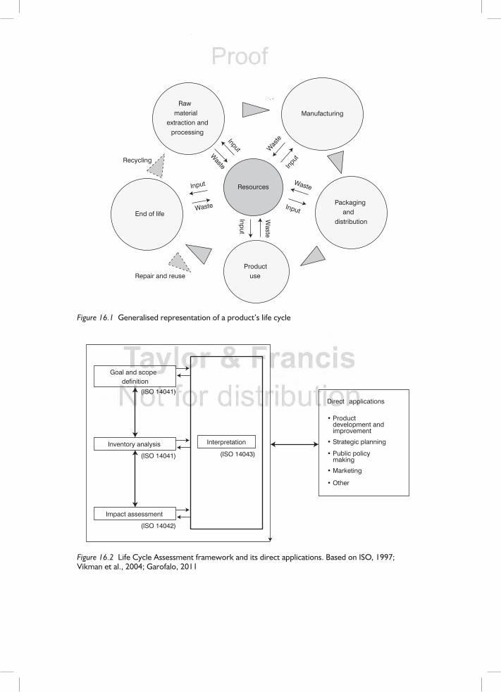
lCA is considered by the scientific community as one of the best methodologies for the evaluation of the environmental burdens associated with bioenergy production (Consoli et al., 1993) and resources utilised during the life of the product because it offers a holistic and systemic view of a product through its whole life cycle (Payraudeau et al., 2007). In contrast to other environmental management tools, which tend to focus on specific life stages of a product or process, lCA analyses the entire life cycle, i.e. upstream and downstream the supply-chain (garofalo, 2011). Usually, the assessment includes the entire life cycle of the product, process or activity from the extraction of resources and process of raw materials, through production, use and recycling, up to the disposal of remaining waste (Figure 16.1).
Additionally, lCA provides a well-established and comprehensive framework to compare the production of renewable energy with fossil-based and nuclear energy technologies (Sathaye et al., 2011).
lCA is a systematic, phased approach and encompasses four components (Figure 16.2) as determined by the ISo series, i.e. ISo 14040 (principles and framework), ISo 14041 (goal, scope and inventory analysis), ISo 14042 (impact assessment), ISo 14043 (life cycle interpretation) and ISo 14047–14049 (rules of documentation and examples on impact assessment and inventory) (ISo, 1997, 1998a, 1998b, 1999). more particularly:
i goal and scope definition, where the boundaries for the assessment are determined along with the level of detail and the functional basis for comparison;
Raw material
extraction and processing
Resources
Manufacturing
Packaging and
distribution
Product use
End of life Input
Waste
Recycling
Repair and reuse
Input
Waste
Inpu
t
Was
teInput
Waste
Input
Waste
Figure 16.1 Generalised representation of a product’s life cycle
Goal and scope definition
Inventory analysis
Impact assessment
Interpretation
• Product development and improvement
• Strategic planning
• Public policy making
• Marketing
• Other
Direct applications(ISO 14041)
(ISO 14041)
(ISO 14042)
(ISO 14043)
Figure 16.2 Life Cycle Assessment framework and its direct applications. Based on ISO, 1997; Vikman et al., 2004; Garofalo, 2011
320 Nicholas E. Korres
ii Inventory analysis, in which the energy, raw materials and related emissions, for each process presented in a flow chart are quantified;
iii Impact assessment, which quantifies and groups the effects of the resource use and emissions into a number of environmental impact categories which may be weighted for importance;
iv Interpretation, which reports the results and evaluates the opportunities to reduce the environmental impact of the product or service.
The performance of an lCA can assist in i) the identification of opportunities to improve the product’s environmental aspects throughout its whole life; ii) decision-making in industry, governmental and non-governmental organisations (e.g. strategy planning, priority setting, etc.); iii) the selection of relevant environmental performance indicators and adequate measurement techniques; and iv) marketing opportunities for “greener” products (e.g. eco-labelling, environmental product declaration, etc.) (ISo, 1997).
The ISo standards have been applied in a large number of assessments of bioenergy systems, but there is still substantial variation among these as to the way in which the standard is implemented. This variability is an inherent characteristic of the ISo standards since they are not constructed as precisely defined tools, but rather as sets of guidelines for good practice. Some parts of the ISo standards, e.g. allocation rules, are continuously under development (Ekvall and Finnveden 2001; Jungmeier et al. 2002; vikman et al., 2004). Additionally, methodological challenges still exist such as the assessment of how direct and indirect land use change emissions and their credits to the bioenergy production, or how the influence of heavy metal flows or the characterisation of pesticidal effects on the bioenergy assessment are made (Korres, 2010). Furthermore, the implementation of a life cycle approach in certification or legislation schemes, as shown in the example of the Renewable Energy Directive of the European Union (Emmenegger et al., 2012) outline another challenge in the application of lCA. These statements are interesting because the quality of lCA methodology used for energy system assessments requires continuous interpretation and updating of data and results are needed. These general aspects, as reported by vikman et al. (2004), are 1) accuracy, which is expressed by the comprehensiveness of the functional unit and system boundaries in time and space and consistency (e.g. consistent treatment of actual and reference system) of the study; 2) transparency in assumptions and calculations, use of flow charts and sensitivity analyses; and 3) efficiency, where an appropriate level of detail must be balanced by ease-of-use and comparable output parameters. Hence, the aim of this chapter is to provide an overview of the objectives, characteristics and components of lCA methodology and to highlight some of the challenging issues for lCA practitioners. This is done in the context of the four phases of lCA as described above for biogas/biomethane production.
Methodological framework
various approaches have been adopted by lCA practitioners on the type of lCA used. generally, the categories mostly analysed by the application of lCA are fossil energy consumption and related gHg emissions, i.e. carbon releases into the atmosphere along with other process related emissions (yu and Chen, 2008). Based on the choice of boundaries various assessments can be applied such as i) a partial lCA from cradle to farm gate (includes production and harvesting of AD feedstock/biomass) or gate to gate (a partial lCA looking
Life cycle assessment 321
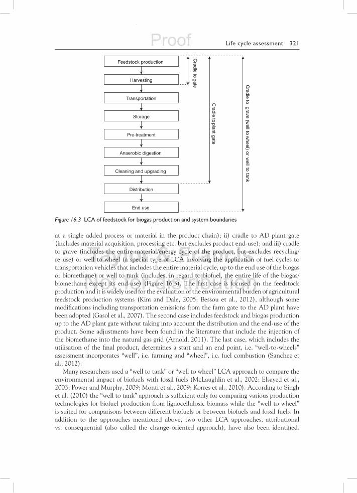
at a single added process or material in the product chain); ii) cradle to AD plant gate (includes material acquisition, processing etc. but excludes product end-use); and iii) cradle to grave (includes the entire material/energy cycle of the product, but excludes recycling/re-use) or well to wheel (a special type of lCA involving the application of fuel cycles to transportation vehicles that includes the entire material cycle, up to the end use of the biogas or biomethane) or well to tank (includes, in regard to biofuel, the entire life of the biogas/biomethane except its end-use) (Figure 16.3). The first case is focused on the feedstock production and it is widely used for the evaluation of the environmental burden of agricultural feedstock production systems (Kim and Dale, 2005; Bessou et al., 2012), although some modifications including transportation emissions from the farm gate to the AD plant have been adopted (gasol et al., 2007). The second case includes feedstock and biogas production up to the AD plant gate without taking into account the distribution and the end-use of the product. Some adjustments have been found in the literature that include the injection of the biomethane into the natural gas grid (Arnold, 2011). The last case, which includes the utilisation of the final product, determines a start and an end point, i.e. “well-to-wheels” assessment incorporates “well”, i.e. farming and “wheel”, i.e. fuel combustion (Sanchez et al., 2012).
many researchers used a “well to tank” or “well to wheel” lCA approach to compare the environmental impact of biofuels with fossil fuels (mclaughlin et al., 2002; Elsayed et al., 2003; Power and murphy, 2009; monti et al., 2009; Korres et al., 2010). According to Singh et al. (2010) the “well to tank” approach is sufficient only for comparing various production technologies for biofuel production from lignocellulosic biomass while the “well to wheel” is suited for comparisons between different biofuels or between biofuels and fossil fuels. In addition to the approaches mentioned above, two other lCA approaches, attributional vs. consequential (also called the change-oriented approach), have also been identified.
Feedstock production
Harvesting
Transportation
Pre-treatment
Storage
Anaerobic digestion
Cleaning and upgrading
Distribution
End use
Cradle to gate
Cradle to plant gate
Cradle to grave (w
ell to wheel ) or w
ell to tank
Figure 16.3 LCA of feedstock for biogas production and system boundaries
322 Nicholas E. Korres
multifunctional processes which inevitably occur throughout the biofuels production chain necessitate choices on how to treat co-products in the lCA model. These choices have a strong effect on the performance of the lCA and the distinction between attributable and consequential lCA was developed in the process of resolving the methodological debates over allocation issues and data choices (Thomassen et al., 2008). This distinction is particularly relevant when defining system boundaries in the life cycle inventory (lCI) (Finnveden et al., 2009). Resource flow and related pollution, in the former, is attributed to the unit of analysis of the product under examination by linking together attributable processes along its life cycle (ISo, 2006a). In other words, resource flows and related pollution within the system under study are attributed to the delivery of a specified amount of the functional unit (Rebitzer et al., 2004). Therefore, attributional lCA methodology accounts for immediate physical flows (i.e., resources, material, energy and emissions) involved across the life cycle of a product and typically utilises average data for each unit process within the life cycle (Weidema, 2003; Earles and Halog, 2011). Consequential lCA on the other hand includes processes which are expected to change as a consequence of a change in demand for the unit analysis (Sonnemann and vigon, 2011). In other words, the consequential approach estimates how pollution and resource flows within a system change in response to a change in output of the functional unit (Ekvall and Weidema, 2004; Rebitzer et al., 2004).
The consequential approach makes use of data that is not constrained and can respond to changes in demand that occurs as a result of changes in production volumes, production technologies, public policies and consumer behaviours (Arnold, 2011). This approach can provide valuable insight in certain applications such as evaluating reduction projects or making public policy decisions (Bhatia et al., 2011). Wenzel and Petersen (2009) reported that the consequential approach requires a comparative lCA, i.e. that alternatives are compared since they are equivalent and provide the same services (primary and secondary). The primary service is the “main function” of the system (e.g. biomethane production as a transport fuel) whereas secondary services are defined as products/services arising from processes in the system under investigation (e.g. the nutrient value of the digestate that can replace mineral fertilisers or the electrical energy of the biogas produced from slurry that can replace equal amount of electricity from the grid).
The core differences between consequential and attributional lCA are that the former includes the processes which are actually affected by a change in demand, instead of the averages used in attributional lCA (Weidema, 2003; Earles and Halog, 2011). Based on this difference, Schmidt (2010) reported that the main argument for the application of the consequential approach is that only the actual affected processes are included whereas those that are not likely to respond to a change in demand should be excluded from the assessment since this will not reflect the actual change in environmental impact. It is obvious that application of the consequential approach can reduce the cost of lCA. Additionally, attributional lCA uses average data reflecting the actual physical flows instead of marginal data used in the consequential approach (Finnveden et al., 2009).
An obstacle for the application of the consequential approach is the difficulty of collecting appropriate and accurate data. Ekvall and Andrae (2006), lesage et al. (2007) and Thomassen et al. (2008) noted that the adoption of consequential lCA can reveal unique environmental insights beyond attributional lCA. However, vieira and Horvath (2008) found little difference between the two approaches.
Life cycle assessment 323
Goal and scope def in it ion
The goal and scope definition phase of an lCA includes several decisions that are of relevance for all subsequent steps (Frischknecht and Jungbluth, 2007). They include the exact formulation of what is to be investigated and how this investigation is to be carried out, along with data requirements (Udo de Haes and van Rooijen, 2005). The scope usually addresses i) the product system to be studied; ii) the function of the product system; iii) the functional unit of the product system; iv) product system boundaries; v) allocation methods; vi) types of impact and methodology of impact assessment; and vii) data requirements, assumptions and limitations (Rebitzer et al., 2004; Udo de Haes and van Rooijen, 2005; labutong et al., 2012). nevertheless, the lCA process is iterative and the scope may be revised over the course of the inventory analysis, impact assessment, and interpretation. The goal of an lCA study should unambiguously state the intended application to the intended audience of the study whereas the scope should be adequately defined so as to ensure compatibility with the goal (Singh et al., 2010). Data quality is defined by time, place, technology, and registration method, e.g. measured data or calculated data (Hartmann, 2006). The scope and goal definition of the lCA varies according to socio-economic, environmental and legislative issues but also according to the technicalities on which the framework for the development of the lCA is administered. The technical factors might include the aim of the study, the product and function of the product system, allocation methods (in case of the attributional lCA approach as discussed previously), assumptions and other factors.
It is also worth mentioning the effects imposed by legislation upon the scope and goal definition. For example, in the case of biofuels sustainability, as stated by Renewable Directive 2009/28/EC (EC, 2009), is defined by emissions savings when compared with the fossil fuel it replaces on a whole life cycle analysis. In addition, according to Directive 2009/28/EC, Annex v, C–13, “emissions from the fuel in use shall be taken to be zero for biofuels and bioliquids”. Hence emissions from combustion of biomethane in vehicles should not be taken into consideration, although there is a debate going on in the scientific community concerning this approach. Such legislative impacts obviously determine not only the functional unit of the system assessed but also the inputs and related environmental burdens that should be considered in the life cycle inventory (lCI) and impact assessment development.
Furthermore, an energy balance is not directly related to a greenhouse gas balance because a biofuel system that generates significant quantities of fuel per hectare (gJ/ha) may not necessarily be sustainable. Emissions associated with agricultural production of biomass, source of fertiliser, sources of parasitic or consumed energy demand, and efficiency of vehicle may deem a product unsustainable.
In many lCA studies the scope can be driven by policy issues (Deasy and Power, 2011) or the goal may be multifaceted as when driven by different feedstocks (Thyo and Wenzel, 2007; Stucki et al., 2011) or different technologies (Arnold, 2011). The integration of simple rules into the formulation of goal and scope definition using, for example, root definition or the CATWoE model, which both originate from soft system methodology (SSm), could clarify and enhance the understanding of the whole process. The first step in SSm is to formulate the root definition of the system under study, assessment or design. A properly structured root definition comprises three elements (i.e. what, how, why) and is of the form “a system to do X, by (means of) y, in order to achieve z”. In other words, the “what” component is the immediate aim of the system, the “how” component is the means of achieving that aim and the “why” component is the longer term aim of the purposeful activity (Korres,
324 Nicholas E. Korres
2004). In terms of lCA scope and goal components a possible root definition could be “a system to evaluate the sustainability of biogas production by the employment of the lCA technique, as described by ISo 14040 standards, in order to improve part of or the entire biogas production chain in terms of human health and/or natural environment and/or natural resources and/or …”. Improvements of root definition can be achieved by the employment of CATWoE methodology which supports the identification and categorisation of all elements (e.g. stakeholders, processes, environment etc.) of the system under analysis (Korres, 2004). more particularly, “C” stands for the Customers of the system, those who would be the victims or beneficiaries of the purposeful activity, those who are on the receiving end of whatever it is that the system does (e.g. rural community, stakeholders, policy makers, investors in renewable energy, scholars etc.); “A” stands for the Actors of the system, those who would do the activities, those who transform inputs to outputs (e.g. AD operators, engineers, agronomists etc.); “T” stands for the Transformation Process, the activity which changes a defined input into a defined output (e.g. anaerobic digestion and the break down of lignocellulosic material); “W” stands for Weltanshauung, the view of the world that makes this definition meaningful (e.g. cheap clean energy, mitigation of climate change, etc.); “O” stands for the Owner(s) of the system, those who could stop the activity; “E” stands for the Environmental constraints, the constraints in the environment that the system takes as given (e.g. it includes any social, technical or economic factors, rather than describing the natural environment alone) (Elghali, 2002).
Funct iona l un i t
The functional unit is the quantified measure of performance of a product system. It describes the function of the product and it is the basis for the calculations in lCA assessments (ISo, 1997; Bligny et al., 2012). In all bioenergy assessment systems the choice of an appropriate functional unit, as the basis for comparisons, is of major importance (e.g. Ekvall and Finnveden, 2001). This is particularly so in studies of systems with more than one output, e.g. energy systems where a combination of heat and electricity is co-generated (CHP-plants) (vikman et al., 2004). All material and energy flows and the effects resulting from these flows are related to the functional unit. This makes the functional unit a base for a variety of comparisons (Hartmann, 2006). The preferred functional unit must be defined and measurable. In practice the functional unit consists of a qualitatively defined function or property (e.g. environmental impact) and a quantified unit (e.g. 1 m3 or 1 mJ of fuel). There is significant diversity in relation to the functional unit used in lCA, particularly in the case of biofuels. Korres et al. (2010) defined the functional unit as m3 biomethane yr–1 whereas, based on the 2009 EU Renewable Directive (EC, 2009) for the evaluation of grass-biomethane sustainability as a transport fuel, the environmental impacts were expressed as g Co2 equivalent (Co2e) mJ–1 energy replaced. Börjesson et al. (2011) in their lCA of biofuels in Sweden including biogas from waste (food industry and household), biogas from manure and biogas from crops (i.e. sugar beets, ley crops and maize) used “environmental impact per mJ fuel” as the functional unit. They argued that other options such as “environmental impact per kilometre of transport service” could increase uncertainty in the results when improvements in the fuel efficiency of different vehicles, for example, are implemented rapidly and new technologies such as electric hybrid technology are introduced. They also stated that the functional unit expressed as per “mJ of fuel” can be easily converted into per kilometre of transport service for the specific vehicles in question. nevertheless, according
Life cycle assessment 325
to Bergsma et al. (2006) the functional unit when biofuels are compared with conventional fuels should be “1 km driving of a standard car on gasoline or diesel”. This way, efficiency differences between biofuels and conventional fuels which are claimed can be included. According to Cherubini et al. (2009) and Kim and Dale (2009) the functional unit “per hectare and year” should be used for fuels based on crops in parallel with “per mJ fuel” (and if possible per km transport service). This would allow the area efficiency to be assessed given the increased competition of cropland for food, feed and energy. gasol et al. (2007) used the “per ha per year cultivation ” of Brassica carinata as the system function whereas the energy stored in the crop from one year (83.69 gJ) was used as an energy reference value in order to compare the natural gas and biomass systems. Arnold (2011) used “nm3 of biogas/ton fresh matter (Fm)” as the functional unit for the production of biogas from various substrates, i.e. maize, rye, sorghum, whole crop triticale and barley silage and the grass Landsberger Gemenge, a mixture of hairy vetch (Vicia villosa), crimson clover (Trifolium incarnátum) and Italian ryegrass (Lolium multiflorum). The basis for comparing bio-electricity and fossil electricity is “1 kWhe delivered to the customer” (Bergsma et al., 2006) whereas in other studies the functional unit of electric energy produced by the biogas plant is “1 TJ electricity fed into the public electricity network” (Hartmann, 2006). nevertheless, in attributional life Cycle Inventory (lCI), as Rebitzer et al. (2004) reported, results describe the environmental exchanges of the average electricity production in a geographic area and/or an electricity supplier. According to some authors the results could be presented as the emissions per mWh produced. The magnitude of the functional unit (megawatt hour, smaller, or larger) does not affect the conclusions since the average emissions of the electricity system scale linearly with the functional unit. In some lCA studies it can be helpful to use several functional units. If this is the case their use must be explained in detail while the goal definition is developed, especially if the comparison between the production of various kinds of biofuels or the cultivation of land is the object of the study (Bergsma et al., 2006). According to lindfors et al. (1999) the definition of the functional unit of a product system must take the following aspects into consideration: i) the efficiency of the product; ii) the durability of the life span of the product; and iii) the performance quality standard (if any).
Boundar ies o f the system
The choices and assumptions made during system modelling, especially those concerning the system boundaries and the processes that should be included within these boundaries, are often decisive for the result of an lCA study (lundin et al., 2000; Rebitzer et al., 2004). As mentioned by Tillman et al. (1994), the system must be delimited by boundaries, which encapsulate all processes and activities that will be included in the study. It is therefore understood that the selection of appropriate boundary conditions is a fundamental point in a sustainability analysis as the use of different boundaries in fact means using different inputs or outputs of the system under study, resulting in the generation of incomparable results.
Assessment of the gHg benefits requires particular knowledge of bioenergy production and conversion technology per se (Horne and matthews, 2004). Energy, Co2 and parameters affecting gHg emissions such as emission factors are the main lCA parameters of interest in gHg accounting and can be further defined as primary energy inputs, net Co2 savings and gHg emissions, compared with current fossil fuel equivalents. nevertheless, the literature on biofuel lCAs contains conflicting studies that often employ differing units and system boundaries, making comparisons across studies difficult (Kammen et al., 2008)]. Different
326 Nicholas E. Korres
lCA practitioners treat system boundaries in a different way which can reduce accuracy and increase uncertainty between comparisons of various studies. For example, fuels comparisons in a lCA study was made on the basis of the energy content of the fuel, excluding end-use conversion (Elsayed et al. 2003) whereas in other studies the system boundaries have been expanded to include the transportation work in the functional unit (Beer et al. 2002; Jungmeier and Hausberger, 2002). The system boundary should as far as possible include all relevant life cycle stages and processes (EC, JRC, IES, 2010) although this would result in a complicated analysis (Tillman et al., 1994) because of the difficulty of handling large life-cycle inventories (Hartmann, 2006).
Dimensions within system boundaries, as Tillman et al. (1994) and guinee et al. (2002) reported, are:
i Boundaries between the technological system and environment. The lCA usually begins at the extraction point of raw materials and covers the entire life cycle of the final product up to final stages which normally include waste generation in any stage, i.e. gaseous, liquid or solid (Figure 16.1). nevertheless, partial lCAs as mentioned earlier are included in this category (e.g. cradle to gate).
ii Boundaries between current life cycle and related life cycles of other products or between the technological system under study and other technological systems. In this case most activities are interrelated and for that reason must be isolated from each other for further study. It is obvious that the system boundary between the technological system under study and other technological systems is affected in various other ways by the lCA approach as for example when a consequential lCA is applied.
iii Boundaries between significant and insignificant processes. The identification of system boundaries between “significant” and “insignificant” processes is difficult because often it is not known, at the beginning of a study, which processes based on data collected/measured/estimated are significant or not (Finnveden et al., 2009).
iv Spatial (geographical) boundaries. geography holds an important role in most lCA studies since many processes such as electricity production, waste management, feedstock production, transport systems along with ecosystem sensitivity etc. differ from one area to another.
v Temporal boundaries. lCAs are conducted to evaluate present impacts but also to predict future scenarios although limitations due to technologies involved, pollutants lifespan etc. entail high uncertainty. Incorporation of stochastic modelling and/or simulation techniques, including the time dimension, could benefit lCA performance.
vi Boundaries which are based on the production of capital goods in which the evaluation of the economic feasibility of new and more eco-friendly processes in comparison with current technologies can be achieved.
Finnveden et al. (2009) stated that spatial and temporal limits as lCA boundaries could be received as special technological and environmental boundaries cases. It is recommended, whenever reasonable, to use expanded system boundaries, since this will give the most accurate representation of the real system functions under study. This may be the best approach when the functions provided are strongly integrated, and thus extremely difficult to separate. In co-product situations, where some form of causality might be used for allocation, then allocation may be the most feasible approach in order to avoid systems which are too large (lindfors et al., 1999).
Life cycle assessment 327
Reference system
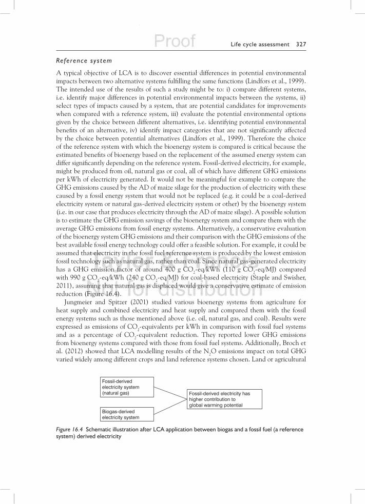
A typical objective of lCA is to discover essential differences in potential environmental impacts between two alternative systems fulfilling the same functions (lindfors et al., 1999). The intended use of the results of such a study might be to: i) compare different systems, i.e. identify major differences in potential environmental impacts between the systems, ii) select types of impacts caused by a system, that are potential candidates for improvements when compared with a reference system, iii) evaluate the potential environmental options given by the choice between different alternatives, i.e. identifying potential environmental benefits of an alternative, iv) identify impact categories that are not significantly affected by the choice between potential alternatives (lindfors et al., 1999). Therefore the choice of the reference system with which the bioenergy system is compared is critical because the estimated benefits of bioenergy based on the replacement of the assumed energy system can differ significantly depending on the reference system. Fossil-derived electricity, for example, might be produced from oil, natural gas or coal, all of which have different gHg emissions per kWh of electricity generated. It would not be meaningful for example to compare the gHg emissions caused by the AD of maize silage for the production of electricity with these caused by a fossil energy system that would not be replaced (e.g. it could be a coal-derived electricity system or natural gas-derived electricity system or other) by the bioenergy system (i.e. in our case that produces electricity through the AD of maize silage). A possible solution is to estimate the gHg emission savings of the bioenergy system and compare them with the average gHg emissions from fossil energy systems. Alternatively, a conservative evaluation of the bioenergy system gHg emissions and their comparison with the gHg emissions of the best available fossil energy technology could offer a feasible solution. For example, it could be assumed that electricity in the fossil fuel reference system is produced by the lowest emission fossil technology such as natural gas, rather than coal. Since natural gas-generated electricity has a gHg emission factor of around 400 g Co2-eq/kWh (110 g Co2-eq/mJ) compared with 990 g Co2-eq/kWh (240 g Co2-eq/mJ) for coal-based electricity (Staple and Swisher, 2011), assuming that natural gas is displaced would give a conservative estimate of emission reduction (Figure 16.4).
Jungmeier and Spitzer (2001) studied various bioenergy systems from agriculture for heat supply and combined electricity and heat supply and compared them with the fossil energy systems such as those mentioned above (i.e. oil, natural gas, and coal). Results were expressed as emissions of Co2-equivalents per kWh in comparison with fossil fuel systems and as a percentage of Co2-equivalent reduction. They reported lower gHg emissions from bioenergy systems compared with those from fossil fuel systems. Additionally, Broch et al. (2012) showed that lCA modelling results of the n2o emissions impact on total gHg varied widely among different crops and land reference systems chosen. land or agricultural
Fossil-derived electricity system (natural gas)
Biogas-derived electricity system
Fossil-derived electricity has higher contribution toglobal warming potential
Figure 16.4 Schematic illustration after LCA application between biogas and a fossil fuel (a reference system) derived electricity
328 Nicholas E. Korres
reference system defines what the cultivated land area would be used for if the investigated product were not to be produced (Jungk et al., 2002). When a comparison is being made between a bioenergy and a fossil energy carrier, it is always necessary to define an alternative way in which the required land might be used if not for the production of energy (Jungk et al., 2002). Therefore, the choice of proven reference system can be of great significance for the policy makers, utilities providers and industry by allowing the identification of effective agricultural biomass options in order to reach emission reduction targets. omission of alternative land use for the production system under concern would not adequately assess impact and would put any claim of sustainability in question.
Life Cycle Inventory
The life Cycle Inventory Analysis (lCIA) specifies the processes that occur during the life cycle of a product. In lCI, an inventory is made of all the inputs and outputs of processes that occur during the life cycle of a product (Udo de Haes and van Rooijen, 2005).
Procedures
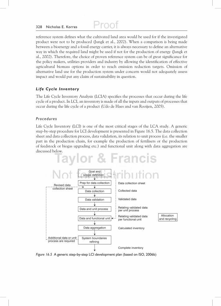
life Cycle Inventory (lCI) is one of the most critical stages of the lCA study. A generic step-by-step procedure for lCI development is presented in Figure 16.5. The data collection sheet and data collection process, data validation, its relation to unit process (i.e. the smaller part in the production chain, for example the production of fertilisers or the production of feedstock or biogas upgrading etc.) and functional unit along with data aggregation are discussed below.
Goal andscope definition
Prep for data collection
Data collection
Data validation
Data and unit process
Data and functional unit
Data aggregation
System boundaries refining
Allocation and recycling
Data collection sheet
Collected data
Validated data
Relating validated data per unit process
Relating validated data per functional unit
Complete inventory
Calculated inventory
Additional data or unit process are required
Revised data collection sheet
Figure 16.5 A generic step-by-step LCI development plan (based on ISO, 2006b)
Life cycle assessment 329
DATA COLLECTION AND DATA COLLECTION SHEET
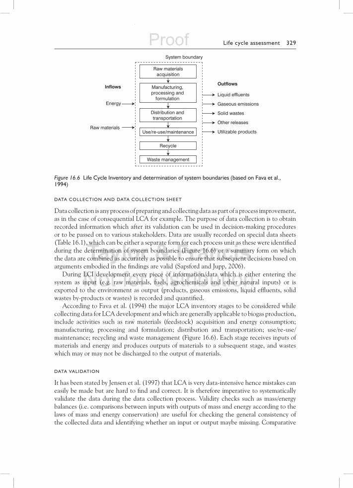
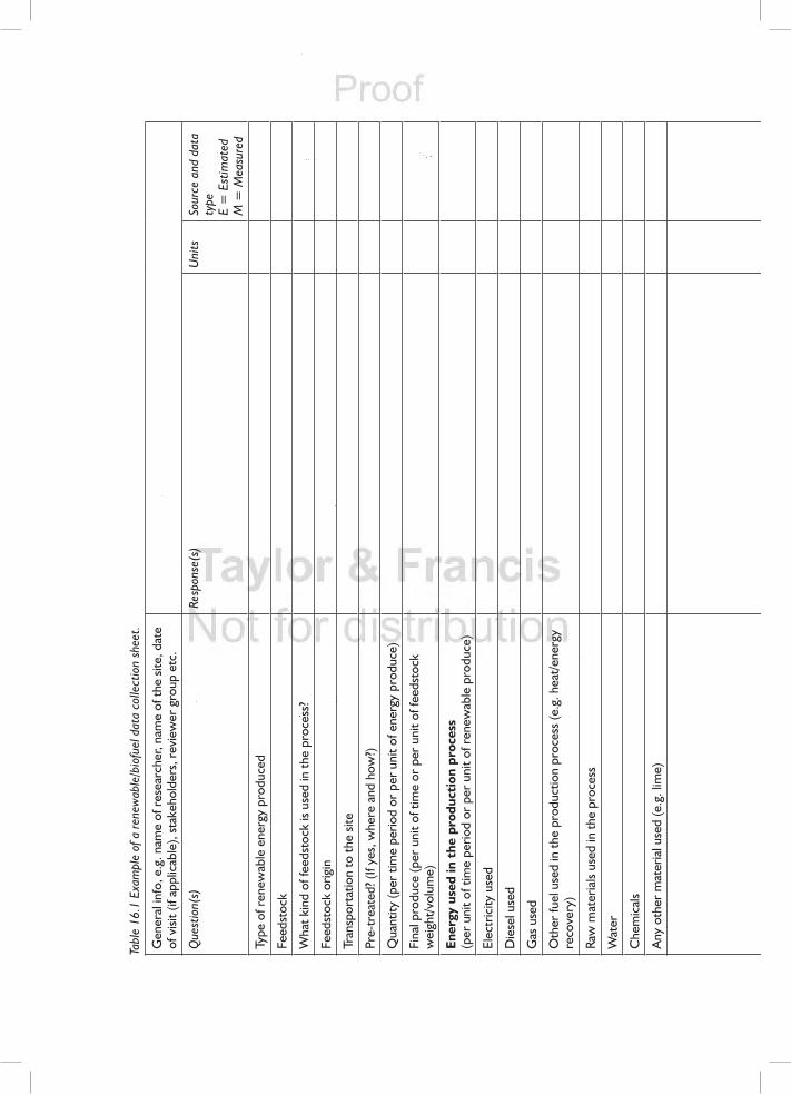
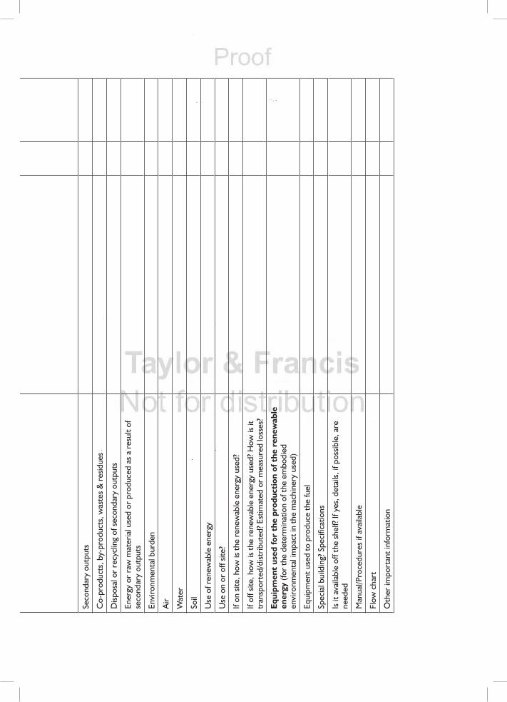
Data collection is any process of preparing and collecting data as part of a process improvement, as in the case of consequential lCA for example. The purpose of data collection is to obtain recorded information which after its validation can be used in decision-making procedures or to be passed on to various stakeholders. Data are usually recorded on special data sheets (Table 16.1), which can be either a separate form for each process unit as these were identified during the determination of system boundaries (Figure 16.6) or a summary form on which the data are combined as accurately as possible to ensure that subsequent decisions based on arguments embodied in the findings are valid (Sapsford and Jupp, 2006).
During lCI development every piece of information/data which is either entering the system as input (e.g. raw materials, fuels, agrochemicals and other natural inputs) or is exported to the environment as output (products, gaseous emissions, liquid effluents, solid wastes by-products or wastes) is recorded and quantified.
According to Fava et al. (1994) the major lCA inventory stages to be considered while collecting data for lCA development and which are generally applicable to biogas production, include activities such as raw materials (feedstock) acquisition and energy consumption; manufacturing, processing and formulation; distribution and transportation; use/re-use/maintenance; recycling and waste management (Figure 16.6). Each stage receives inputs of materials and energy and produces outputs of materials to a subsequent stage, and wastes which may or may not be discharged to the output of materials.
DATA VALIDATION
It has been stated by Jensen et al. (1997) that lCA is very data-intensive hence mistakes can easily be made but are hard to find and correct. It is therefore imperative to systematically validate the data during the data collection process. validity checks such as mass/energy balances (i.e. comparisons between inputs with outputs of mass and energy according to the laws of mass and energy conservation) are useful for checking the general consistency of the collected data and identifying whether an input or output maybe missing. Comparative
aRaw materials
cquisition
f
Manufacturing, processing and
ormulation
Distribution and transportation
Use/re-use/maintenance
Recycle
Waste management
Liquid effluents
Gaseous emissions
Solid wastes
Other releases
Utilizable products
Outflows
Energy
Raw materials
Inflows
System boundary
Figure 16.6 Life Cycle Inventory and determination of system boundaries (based on Fava et al., 1994)
Tabl
e 16
.1 E
xam
ple
of a
rene
wab
le/b
iofu
el d
ata
colle
ctio
n sh
eet.
Gen
eral
info
, e.g
. nam
e of
res
earc
her,
nam
e of
the
site,
dat
e of
visi
t (if
appl
icab
le),
stak
ehol
ders
, rev
iew
er g
roup
etc
.
Que
stio
n(s)
Resp
onse
(s)
Uni
tsSo
urce
and
dat
a ty
peE
= E
stim
ated
M =
Mea
sure
d
Type
of r
enew
able
ene
rgy
prod
uced
Feed
stoc
k
Wha
t kin
d of
feed
stoc
k is
used
in th
e pr
oces
s?
Feed
stoc
k or
igin
Tran
spor
tatio
n to
the
site
Pre-
trea
ted?
(If y
es, w
here
and
how
?)
Qua
ntity
(per
tim
e pe
riod
or p
er u
nit o
f ene
rgy
prod
uce)
Fina
l pro
duce
(per
uni
t of t
ime
or p
er u
nit o
f fee
dsto
ck
wei
ght/
volu
me)
Ener
gy u
sed
in t
he p
rodu
ctio
n pr
oces
s (p
er u
nit o
f tim
e pe
riod
or p
er u
nit o
f ren
ewab
le p
rodu
ce)
Elec
tric
ity u
sed
Die
sel u
sed
Gas
use
d
Oth
er fu
el u
sed
in th
e pr
oduc
tion
proc
ess
(e.g
. hea
t/en
ergy
re
cove
ry)
Raw
mat
eria
ls us
ed in
the
proc
ess
Wat
er
Che
mic
als
Any
oth
er m
ater
ial u
sed
(e.g
. lim
e)
Seco
ndar
y ou
tput
s
Co-
prod
ucts
, by-
prod
ucts
, was
tes
& r
esid
ues
Disp
osal
or
recy
clin
g of
sec
onda
ry o
utpu
ts
Ener
gy o
r ra
w m
ater
ial u
sed
or p
rodu
ced
as a
res
ult o
f se
cond
ary
outp
uts
Envi
ronm
enta
l bur
den
Air
Wat
er
Soil
Use
of r
enew
able
ene
rgy
Use
on
or o
ff sit
e?
If on
site
, how
is th
e re
new
able
ene
rgy
used
?
If of
f site
, how
is th
e re
new
able
ene
rgy
used
? How
is it
tr
ansp
orte
d/di
strib
uted
? Est
imat
ed o
r m
easu
red
loss
es?
Equi
pmen
t us
ed fo
r th
e pr
oduc
tion
of t
he r
enew
able
en
ergy
(for
the
dete
rmin
atio
n of
the
embo
died
en
viro
nmen
tal i
mpa
ct in
the
mac
hine
ry u
sed)
Equi
pmen
t use
d to
pro
duce
the
fuel
Spec
ial b
uild
ing?
Spe
cific
atio
ns
Is it
ava
ilabl
e of
f the
she
lf? If
yes
, det
ails,
if p
ossib
le, a
re
need
ed
Man
ual/P
roce
dure
s if
avai
labl
e
Flow
cha
rt
Oth
er im
port
ant i
nfor
mat
ion
332 Nicholas E. Korres
analysis of emission factors from similar processes for assessing data plausibility can be conducted (Palsson and Riise, 2011). Any anomalies in the data can be replaced by (alternative) data values complying with the data quality requirements (Jensen et al., 1997). During the collection of data for various processes in the product system, it may be necessary to allocate the inputs and outputs between different products. This may be necessary for processes that produce more than one product. In this case, the use of raw materials and energy, and the releases to air, water and land will need to be divided between the products. The remaining stages of the lCI development, i.e. relating data to unit process and the functional unit, data aggregation and when necessary, refining system boundaries, form the compilation of the inventory result with the collected data (ISo, 1998; Palsson and Riise, 2011).
DATA AGGREGATION AND RELATING PROCESSES
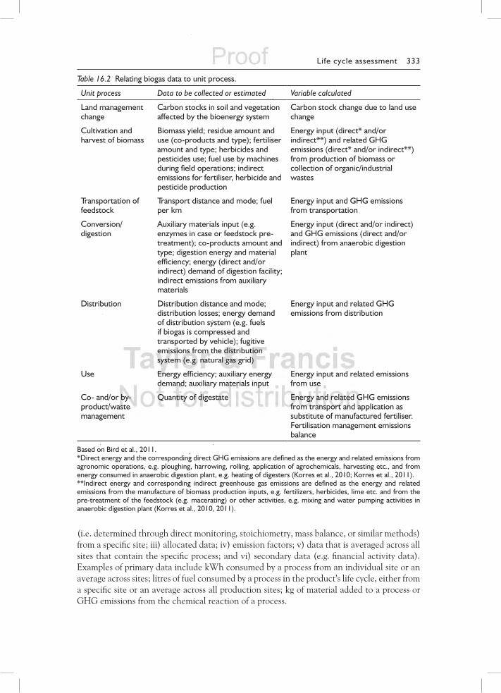
Structuring and preparing the collected data for the unit processes included in the product system by relating them to the unit process and then normalising them to the functional unit (Bird et al., 2011) is the first step before data aggregation. Table 16.2 shows data requirements for the gHg and energy balances of a biogas production system.
The reference flow of each unit process, which was determined during the construction of the flow chart (Figures 16.7, 16.8 and 16.9) relates the collected data for inputs (raw materials and energy) and outputs to this particular flow and consequently to the corresponding unit process. The normalisation of data to the functional unit involves the scaling of the inputs and outputs in each unit process to the functional unit. In other words, normalisation of the data to the functional unit assigns the corresponding inputs and outputs (i.e. energy and environmental burdens) from each unit process to the functional unit.
The actions with which normalisation of the data can be achieved include: i) calculation of the scaling factors of each unit process by using the flow chart and the corresponding inputs and outputs data for each unit process; attention should be given in situations where, for example, electricity or other products are used in several included unit processes; ii) scaling factors for transport are usually derived by multiplying the amount of material transported with the distance the material is transported; iii) scaling each unit process to the functional unit. The scaling factors are used to scale all inputs and outputs for each included unit process. This is achieved by multiplying the inputs and outputs for each unit process with the corresponding scaling factor. The scaled unit process delivers the amount of material needed to produce the functional unit. The next step in the inventory development is the aggregation of the inputs and outputs for all unit processes included in the system. For example, Co2 emissions to air from all unit processes are added together into the total Co2 emission to air for the biogas production chain. This is the inventory result for the entire production system.
Data categor ies
Primary data are clearly preferred to secondary data during the lCI development. As Bhatia et al. (2011) stated, primary data are collected from specific processes of a product’s life cycle and include: i) activity data (the quantitative measures of a level of activity or a unit process that results in gHg emissions or removals) including process activity data and financial activity data (these are always secondary types of data); ii) direct emissions data
Life cycle assessment 333
(i.e. determined through direct monitoring, stoichiometry, mass balance, or similar methods) from a specific site; iii) allocated data; iv) emission factors; v) data that is averaged across all sites that contain the specific process; and vi) secondary data (e.g. financial activity data). Examples of primary data include kWh consumed by a process from an individual site or an average across sites; litres of fuel consumed by a process in the product’s life cycle, either from a specific site or an average across all production sites; kg of material added to a process or gHg emissions from the chemical reaction of a process.
Table 16.2 Relating biogas data to unit process.
Unit process Data to be collected or estimated Variable calculated
Land management change
Carbon stocks in soil and vegetation affected by the bioenergy system
Carbon stock change due to land use change
Cultivation and harvest of biomass
Biomass yield; residue amount and use (co-products and type); fertiliser amount and type; herbicides and pesticides use; fuel use by machines during field operations; indirect emissions for fertiliser, herbicide and pesticide production
Energy input (direct* and/or indirect**) and related GHG emissions (direct* and/or indirect**) from production of biomass or collection of organic/industrial wastes
Transportation of feedstock
Transport distance and mode; fuel per km
Energy input and GHG emissions from transportation
Conversion/digestion
Auxiliary materials input (e.g. enzymes in case or feedstock pre-treatment); co-products amount and type; digestion energy and material efficiency; energy (direct and/or indirect) demand of digestion facility; indirect emissions from auxiliary materials
Energy input (direct and/or indirect) and GHG emissions (direct and/or indirect) from anaerobic digestion plant
Distribution Distribution distance and mode; distribution losses; energy demand of distribution system (e.g. fuels if biogas is compressed and transported by vehicle); fugitive emissions from the distribution system (e.g. natural gas grid)
Energy input and related GHG emissions from distribution
Use Energy efficiency; auxiliary energy demand; auxiliary materials input
Energy input and related emissions from use
Co- and/or by-product/waste management
Quantity of digestate Energy and related GHG emissions from transport and application as substitute of manufactured fertiliser. Fertilisation management emissions balance
Based on Bird et al., 2011.*Direct energy and the corresponding direct GHG emissions are defined as the energy and related emissions from agronomic operations, e.g. ploughing, harrowing, rolling, application of agrochemicals, harvesting etc., and from energy consumed in anaerobic digestion plant, e.g. heating of digesters (Korres et al., 2010; Korres et al., 2011).**Indirect energy and corresponding indirect greenhouse gas emissions are defined as the energy and related emissions from the manufacture of biomass production inputs, e.g. fertilizers, herbicides, lime etc. and from the pre-treatment of the feedstock (e.g. macerating) or other activities, e.g. mixing and water pumping activities in anaerobic digestion plant (Korres et al., 2010, 2011).
334 Nicholas E. Korres
ACTIVITY DATA
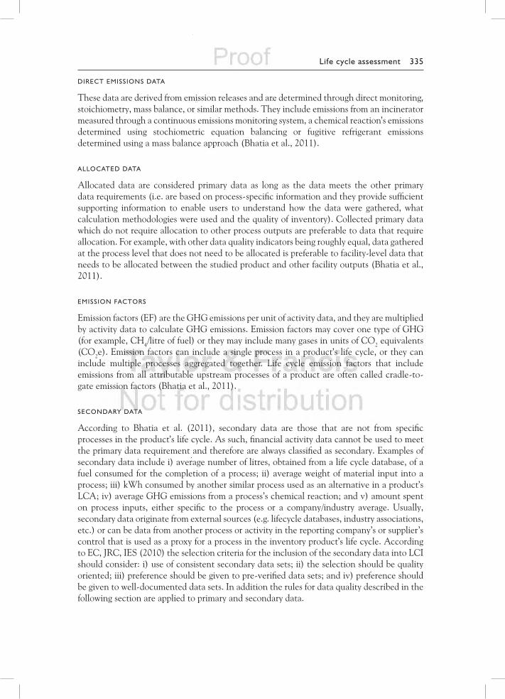
more specifically, process activity data measure the physical inputs/outputs or other metrics of a process and when combined with a process emission factor result in the calculation of gHg emissions. They include energy data (e.g. KJ of energy consumed), mass data (e.g. kg of a material), volume (e.g. volume of chemicals or fuels used), area (e.g. cultivated area), distance (e.g. distance feedstock travelled to AD plant), and time (e.g. retention time). In contrast, financial activity data consist of monetary measures of a process that results in gHg emissions. They measure the financial transaction associated with a process. These data, when combined with a financial emission factor (e.g., environmentally extended input–output emission factor, EEIoEF) result in the calculation of gHg emissions. An example taken from Saunders et al. (2006) demonstrates how financial activity data can be used for the calculation of gHg emissions in barley production (UK) used as feedstock. A similar analysis requires information on the production system in the UK regarding yield of barley, inputs used by type and associated energy and emission coefficients. Such data are provided by the John Nix Farm Management Pocket Book (nix, 2004 cited in Saunders et al., 2006). The data listed in Table 16.3 are general and not necessarily accurate but will be used to demonstrate the following example on financial data activity.
The calculation of the energy and the emission component from the information provided in Table 16.3 requires the conversion of the inputs into their physical quantities and in some cases breaking them down further. An assumption made, for reasons of simplicity, was that machinery repairs, seed costs and fixed costs were excluded for calculations of energy and associated emissions in barley production. The cost of fuel and repairs for barley equals £100/ha. A more detailed breakdown shows that the cost of fuel, electricity and oil equals £35/ha and the cost of machinery repairs equals £40/ha in a medium sized cereal production system (100–200 ha). Therefore 46.67 per cent of fuel and repairs is billed to fuel. Consequently, given the £100 price reported in Table 16.3 for fuel and repairs, the input of fuel, electricity and oil is £46.67/ha. The transformation of the fuel value into the physical amount of litres consumed in the process (i.e. diesel equivalent), knowing the cost of the fuel consumed in a process and the cost of the fuel per litre, can be easily found. The price of “red diesel” or gas oil, which is only available to farmers and has very small rates of excise duty attached, is assumed to be 24p per litre, hence the diesel used in barley production equals 194.5 litres/ha. The energy coefficient of diesel, as reported by Saunders et al. (2006), equals 41.2 mJ/l hence 8013 mJ/ha or 1233 mJ/t of barley. The Co2 emissions associated with barley production can be calculated by multiplying the energy component per tonne of barley found above with the emission factor of 65.1 g Co2/mJ (e.g. 65.1/1000 × 1233 = 80.2 kg Co2/t of barley).
Table 16.3 Financial activity data in winter barley production.
Inputs and outputs Item input/output per ha
Barley yield (average) 6.5 tonnes
Fuel and repairs £100.00
Fertiliser £87.50
Sprays £85.00
Seed £37.50
Source: Nix, 2004 cited in Saunders et al., 2006
Life cycle assessment 335
DIRECT EMISSIONS DATA
These data are derived from emission releases and are determined through direct monitoring, stoichiometry, mass balance, or similar methods. They include emissions from an incinerator measured through a continuous emissions monitoring system, a chemical reaction’s emissions determined using stochiometric equation balancing or fugitive refrigerant emissions determined using a mass balance approach (Bhatia et al., 2011).
ALLOCATED DATA
Allocated data are considered primary data as long as the data meets the other primary data requirements (i.e. are based on process-specific information and they provide sufficient supporting information to enable users to understand how the data were gathered, what calculation methodologies were used and the quality of inventory). Collected primary data which do not require allocation to other process outputs are preferable to data that require allocation. For example, with other data quality indicators being roughly equal, data gathered at the process level that does not need to be allocated is preferable to facility-level data that needs to be allocated between the studied product and other facility outputs (Bhatia et al., 2011).
EMISSION FACTORS
Emission factors (EF) are the gHg emissions per unit of activity data, and they are multiplied by activity data to calculate gHg emissions. Emission factors may cover one type of gHg (for example, CH4/litre of fuel) or they may include many gases in units of Co2 equivalents (Co2e). Emission factors can include a single process in a product’s life cycle, or they can include multiple processes aggregated together. life cycle emission factors that include emissions from all attributable upstream processes of a product are often called cradle-to-gate emission factors (Bhatia et al., 2011).
SECONDARY DATA
According to Bhatia et al. (2011), secondary data are those that are not from specific processes in the product’s life cycle. As such, financial activity data cannot be used to meet the primary data requirement and therefore are always classified as secondary. Examples of secondary data include i) average number of litres, obtained from a life cycle database, of a fuel consumed for the completion of a process; ii) average weight of material input into a process; iii) kWh consumed by another similar process used as an alternative in a product’s lCA; iv) average gHg emissions from a process’s chemical reaction; and v) amount spent on process inputs, either specific to the process or a company/industry average. Usually, secondary data originate from external sources (e.g. lifecycle databases, industry associations, etc.) or can be data from another process or activity in the reporting company’s or supplier’s control that is used as a proxy for a process in the inventory product’s life cycle. According to EC, JRC, IES (2010) the selection criteria for the inclusion of the secondary data into lCI should consider: i) use of consistent secondary data sets; ii) the selection should be quality oriented; iii) preference should be given to pre-verified data sets; and iv) preference should be given to well-documented data sets. In addition the rules for data quality described in the following section are applied to primary and secondary data.
336 Nicholas E. Korres
Data qual i ty
As already mentioned, a comprenhensive lCI involves the collection and integration of hundreds upon thousands of pieces of data regarding the product, process or activity under study (Fava and Pomper, 1997). As such, it is essential that the manegement of data quality is an integral part of the overall process. Data quality was defined by SETAC (cited in Fava and Pomper, 1997) as: “…the degree of confidence one has in the individual data input from a source and in the data set as a whole and ultimately in the decisions based on the life cycle study using such data as input.” many authors (Fava et al., 1994; Fava and Pomper, 1997; Jensen et al., 1997; Bhatia et al., 2011; labutong et al., 2012) have agreed about the type and number of quality indicators that can be used in assessing data quality. These include an assessment of the necessary level of the following. i) Precision, i.e. a measure of the spread of the data set values about their mean. Precision measures such as mean and standard deviation of reported values can be calculated and reported for each process unit along the entire life cycle). ii) Completeness, i.e. the degree to which the data are statistically representative of the process sites or the percentage of locations reporting primary data from the potential number in existence for each data category in a unit process. iii) Consistency, i.e. one of the most important qualitative measures for the assessment of the methodology is uniformity of application to the various components of the analysis. iv) Representativeness, i.e. a qualitative assessment of the degree to which the data set used in the analysis is a true and accuarate measurement of the average processes under examination. In many cases more specified indicators such as technological (i.e. representation of the actual technology used in the assessment), geographical (i.e. representation of the actual geograpical location of the processes within the inventory boundaries) and temporal (i.e. representation of actual time or process age) can be used to assess the reprsentativeness of the data. v) Reproducibility, i.e. a qualitative measurement that assesses the possibility of performing the calculations and reproducing the results reported in the study. vi) Comparability, i.e. a measure by which the boundary of the system under examination, data categories, assumptions, sampling methodology and quality assurance are clearly documented and so permit comparisons to be made on the results and conclusions obtained for different components of an analysis. vii) Accesibility or availability, i.e. whether information concerning the study is available to either internal or external reviewers for examination of the methodology and data values. viii) Reliability, i.e. the degree to which the sources, data collection methods and validation/verification procedures used to obtain the data are dependable. Finally the identification of outliers (i.e. extreme values in the data set which deviate markedly from the main body of data and strongly influence the outcome of descriptive measures such as the mean) through statistical tests (e.g. Dixon test, grubb’s test for outliers), or other data anomalies or missing values, is of major importance for the quality of lCI. The application of data warehousing and data mining techniques as described in Chapter 13 has proved an invaluable tool towards smoothing data sets, particularly when these originate from a continuous process control.
Cut-of f c r i ter ion (a)
The cut-off criterion (a), according to ISo 14044, is the specification of the amount of material or energy flow or the level of environmental significance associated with unit processes or product systems to be excluded from lCI. According to yu (2009), the cut-off criterion is a key point in the system boundary determination. In principle, an lCA should track all the processes in the life cycle of the product system, but in practice, due to the lack
Life cycle assessment 337
of readily accessible data, this may not be feasible. The cut-off criteria used in the lCA should be described clearly (Singh et al., 2010) and define an appropriate balance between result representativeness and data collection effort by users (Chomkhamsri and Pelletier, 2011). It is important to clarify and describe rules for omitting inventory data which are negligible from the point of view of being relevant in the study (IEC, 2008). Using cut-off rules should not give the perception of “hiding” information but rather to facilitate the data collection for practitioners. Cut-off criteria are quantified in relation to the percentage of environmental impacts estimated to be excluded because of the cut-off (e.g. it is usually suggested that the percentage of the overall environmental impact or that of a selected impact category related to cutting off should equal no more than 5 per cent of the total environmental impact) (EC, JRC, IES, 2010). nevertheless, as stated by IEC (2008) a default value for a cut-off rule of 1 per cent regarding energy, mass and environmental relevance should apply to upstream and core processes. This means that for the overall lCI result of the product 99 per cent of the elementary flows by energy content, mass and environmental relevance are included.
Flow d iagrams and ca lcu lat ions
Before data collection, all sub-systems included in the production system under study need to be defined at the level of detail intended to be used in the study. Flow diagrams (input–output models) at the maximum possible resolution (level of details) are quite often used to fulfil this task and it is recommended that the inventory data be given in relation to those flow diagrams (lindfors et al., 1999).
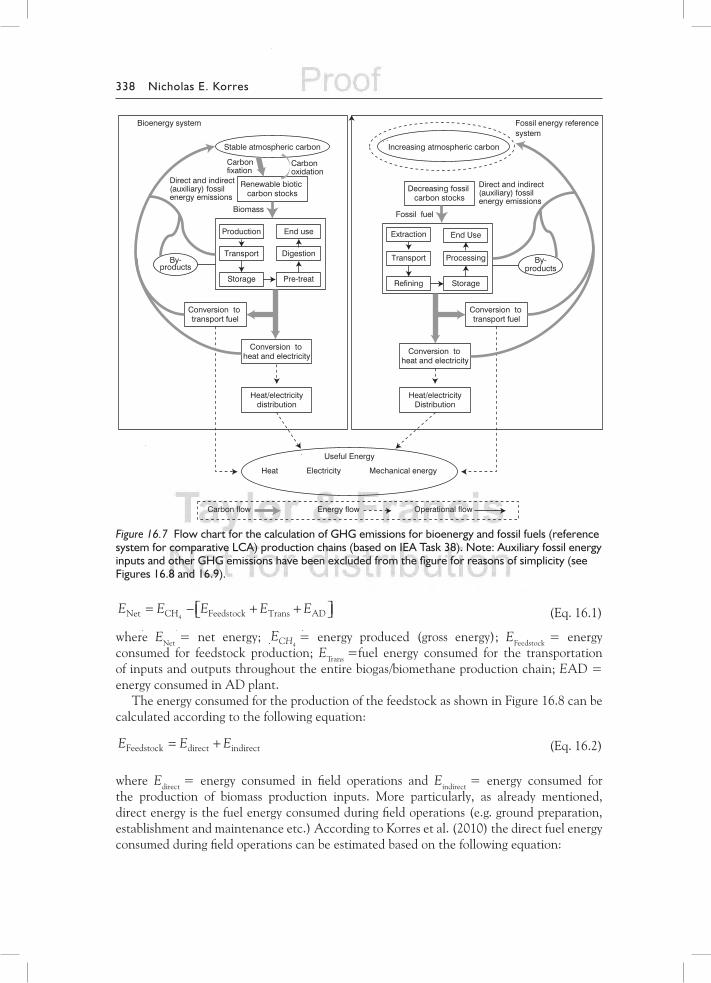
The flow chart in Figure 16.7 summarises the fundamental data which characterise most bioenergy production technologies for the calculation of the gHg emissions throughout the entire production chain. As such, it represents major inter-linked processes which comprise a biomass technology where each major process is identified and related data are specified for the inputs and outputs associated with it. Consequently, in terms of biomass technologies, the main materials are the initial input resources (seeds, fertiliser, land etc.) and the main products are forms of delivered energy (solid, liquid and gaseous fuels, heat, electricity etc. which are purchased by the consumers for operating equipment, appliances, and other devices). Intermediate products exchanged between processes are included up to the level of detail at which clarity is not jeopardised. However, it is essential for the flow chart to indicate any co-products, by-products or wastes which occur at any stage of the production chain.
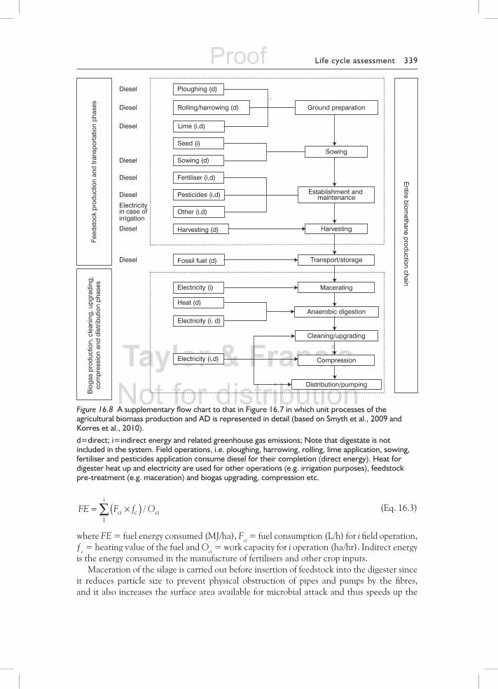
In addition to the flow chart in Figure 16.7, a supplementary, more detailed, biomethane production flow chart can be used, as shown in Figure 16.8. The production of feedstock is represented in detail along with direct and indirect energy flows and related emissions.
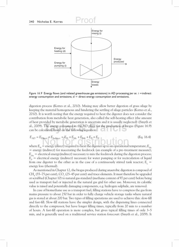
Figure 16.9 adds more detail into the overall biogas/biomethane production chain since it depicts an overall view of the energies (and related gHg emissions) that are involved in AD per se (named as “Anaerobic Digestion” in Figure 16.8).
CALCULATION METHOD FOR DIRECT AND INDIRECT ENERGY FOR BIOGAS/BIOMETHANE PRODUCTION FROM AGRICULTURAL BIOMASS
When performing a sustainability analysis of a technology, great care should be taken in the evaluation of both direct and indirect energy, under the defined system boundaries, by converting all the material flows into energy units. In brief, the analysis of energy balance for biogas/biomethane production (as depicted in Figures 16.8 and 16.9) may be calculated based on the following equation:
338 Nicholas E. Korres
E E E E ENet CH Feedstock Trans AD= − + + 4 (Eq. 16.1)
where Enet = net energy; ECH4= energy produced (gross energy); EFeedstock = energy
consumed for feedstock production; ETrans =fuel energy consumed for the transportation of inputs and outputs throughout the entire biogas/biomethane production chain; EAD = energy consumed in AD plant.
The energy consumed for the production of the feedstock as shown in Figure 16.8 can be calculated according to the following equation:
E E EFeedstock direct indirect= + (Eq. 16.2)
where Edirect = energy consumed in field operations and Eindirect = energy consumed for the production of biomass production inputs. more particularly, as already mentioned, direct energy is the fuel energy consumed during field operations (e.g. ground preparation, establishment and maintenance etc.) According to Korres et al. (2010) the direct fuel energy consumed during field operations can be estimated based on the following equation:
Renewable biotic carbon stocks
Stable atmospheric carbon
Carbon fixation
Carbon oxidation
Transport
Storage Pre-treat
Digestion
Biomass
Conversion to transport fuel
Conversion to heat and electricity
By-products
Increasing atmospheric carbon
Fossil fuel
Conversion to transport fuel
Decreasing fossil carbon stocks
Extraction
Transport
Storage
Processing
Conversion to heat and electricity
By-products
Heat/electricitydistribution
Heat/electricityDistribution
Useful Energy
Heat Electricity Mechanical energy
Carbon flow Energy flow Operational flow
Bioenergy system Fossil energy reference system
Production End use
Refining
End Use
Direct and indirect (auxiliary) fossil energy emissions
Direct and indirect (auxiliary) fossil energy emissions
Figure 16.7 Flow chart for the calculation of GHG emissions for bioenergy and fossil fuels (reference system for comparative LCA) production chains (based on IEA Task 38). Note: Auxiliary fossil energy inputs and other GHG emissions have been excluded from the figure for reasons of simplicity (see Figures 16.8 and 16.9).
Life cycle assessment 339
FE F f Oi
ci c ci= ×( )∑1
/ (Eq. 16.3)
where FE = fuel energy consumed (mJ/ha), Fci = fuel consumption (l/h) for i field operation, ƒc = heating value of the fuel and Oci = work capacity for i operation (ha/hr). Indirect energy is the energy consumed in the manufacture of fertilisers and other crop inputs.
maceration of the silage is carried out before insertion of feedstock into the digester since it reduces particle size to prevent physical obstruction of pipes and pumps by the fibres, and it also increases the surface area available for microbial attack and thus speeds up the
Feed
stoc
k pr
oduc
tion
and
tran
spor
tatio
n ph
ases
Bio
gas
prod
uctio
n, c
lean
ing,
upg
radi
ng,
com
pres
sion
and
dis
trib
utio
n ph
ases
E
ntire biomethane production chain
HarvestingHarvesting (d)
MaceratingElectricity (i)
Anaerobic digestion
Transport/storageFossil fuel (d)
Electricity (i,d) Compression
Distribution/pumping
Cleaning/upgrading
Seed (i)
Sowing (d)Sowing
Fertiliser (i,d)
Pesticides (i,d) Establishment and maintenance
Ploughing (d)
Rolling/harrowing (d) Ground preparation
Lime (i,d)
Other (i,d)
Diesel
Diesel
Diesel
Diesel
Diesel
Diesel
Diesel
Diesel
Electricity in case of irrigation
Electricity (i, d)
Heat (d)
Figure 16.8 A supplementary flow chart to that in Figure 16.7 in which unit processes of the agricultural biomass production and AD is represented in detail (based on Smyth et al., 2009 and Korres et al., 2010).d=direct; i=indirect energy and related greenhouse gas emissions; Note that digestate is not included in the system. Field operations, i.e. ploughing, harrowing, rolling, lime application, sowing, fertiliser and pesticides application consume diesel for their completion (direct energy). Heat for digester heat up and electricity are used for other operations (e.g. irrigation purposes), feedstock pre-treatment (e.g. maceration) and biogas upgrading, compression etc.
340 Nicholas E. Korres
digestion process (Korres et al., 2010). mixing may allow better digestion of grass silage by keeping the material homogenous and hindering the settling of silage particles (Korres et al., 2010). It is worth noting that the energy required to heat the digester does not consider the contribution from metabolic heat generation, also called the self-heating effect (the amount of heat provided by metabolic generation is uncertain and it is usually neglected) (Smyth et al., 2009). The energy consumed in the AD plant for the production of biogas (Figure 16.9) can be calculated based on the following equation:
E E E E E E E EAD Direct Indirect H Mc Mx P L= + = + + + + (Eq. 16.4)
where EH = energy (direct) required to heat the digester up to an operational temperature; Emc = energy (indirect) for macerating the feedstock (an example of a pre-treatment measure); Emx = electrical energy(indirect) necessary to mix the feedstock during the digestion process; EP = electrical energy (indirect) necessary for water pumping or for recirculation of liquid from one digester to the other as in the case of a continuously stirred tank reactor; El = energy loss (thermal).
As mentioned in Chapter 12, the biogas produced during anaerobic digestion is composed of CH4 (55–75 per cent), Co2 (25–45 per cent) and trace elements. It must therefore be upgraded or scrubbed (Chapter 10) to natural gas standard (methane content of 97 per cent) before being used as transport fuel or injected in the natural gas grid for other use. moreover, its calorific value is raised and potentially damaging components, e.g. hydrogen sulphide, are removed.
In case of biomethane use as a transport fuel, filling stations have to compress the gas from mains pressure to about 250 bar in order to fully charge vehicle storage tanks where natural gas is stored at about 200 bar. Two types of filling operations are used to achieve this: slow-fill and fast-fill. Slow-fill stations have the simpler design, with the dispensing lines connected directly to the compressor, but have longer filling times, typically from 20 min to a number of hours. A fast-fill operation is more complex, but gives typical filling times of only 3–5 min, and is generally used on a traditional service station forecourt (Smyth et al., 2009). It
Energy for heating (d)
Energy for mixing (i)
Energy for pumping (i)
Energy produced
Energy losses
Figure 16.9 Energy flows (and related greenhouse gas emissions) in AD processing per se. i =indirect energy consumption and emissions; d = direct energy consumption and emissions.
Life cycle assessment 341
is understood that energy is consumed during all these operations where biogas is upgraded, compressed and distributed or transported to gas grid or filling stations.
Detailed analysis and calculations of the net energy (and related emissions) in bioreactors which involve the thermal and the electrical energy necessary to run the bioreactor, are reported in Anonymous (2007); Smyth et al. (2009); Ruggeri et al. (2010) and Korres et al. (2010).
The following equation should be considered as well for the evaluation of the total indirect energy:
E E E E E E EAInd Chem Mat Constr Main Decom mort= + + + + + (Eq. 16.5)
where EChem = energy required for chemicals production; Emat = energy required for construction of materials; EConstr = energy required for plant building; Emain = energy required for maintenance; Elab = energy required for labour; EDecom = energy required for decommissioning; EAmort = energy required for amortisation.
In many lCA studies, particularly for biofuels, the indirect energy consumed in the manufacture of machinery and equipment, also known as embodied energy (i.e. a cradle-to-gate analysis of the life cycle energy of a product, inclusive of the latent energy in the materials, the energy used during material acquisition and the energy used in manufacturing intermediate and final products) is not considered. This is in line with the “Proposal for a Directive on the promotion of energy from renewable sources” from the Commission of the European Communities (EC, 2009), which states that the manufacture of machinery and equipment is not taken into account when calculating the greenhouse gas impact of biofuels.
The energy consumption in labour during the entire biogas/biomethane production chain deserves particular attention. This can be separated into three components, namely i) the energy of food for the biological support expressed as caloric value; ii) the direct and indirect energy consumption for the entire food lCA (i.e. production, transportation, conservation and preparation); and iii) all the other direct and indirect energy forms linked to daily activities such as energy consumed in clothing, appliances, fuel for transportation etc. It is understood that the evaluation of the energy consumed on labour is inherently difficult (Brown and Herendeen, 1996; Cleveland and Costanza, 2010) and it is often disregarded, although it could be of major significance when comparing different labour vs. capital intensive technologies (e.g. gasification vs. energy crop cultivation). A simplified energy balance of biogas production and usage in a Cambodian family farm is shown in the Appendix.
CALCULATION METHOD FOR GHG EMISSIONS FROM BIOGAS/BIOMETHANE SYSTEM
The EU Renewable Energy Directive, Annex v Part C, provides a methodology (Equation 6) to calculate the greenhouse gas emissions from a biofuel system (EC, 2009), although, as the author of this chapter believes, its application is suitable for any bioenergy use and type. The functional unit is specified in gCo2equiv/mJfuel.
E E E E E E E E E EB ec L P TD U SCA CCS CCR EE= + + + + − − − − (Eq. 16.6)
where EB = total emissions from biofuel; EEC = emissions from cultivation/acquisition of raw materials; El = emissions from land use change; EP = emissions from processing; ETD
342 Nicholas E. Korres
= emissions from transport and distribution; EU = emissions from the biofuel in use; ESCA = emission savings via improved agricultural management; ECCS = emission savings from carbon capture and geological storage; ECCR = emission savings from carbon capture and replacement; and EEE = emission savings from excess electricity from cogeneration burning of agricultural crop residues.
Exceptions exist as in the case of the emissions from biofuels in use. A debate has been going on for some time as to whether these emissions should be taken into account in the overall biofuel environmental performance or not. Furthermore, as stated by Ahlgren et al. (2009) the Directive contains very little information on the methodology for calculating the emissions of greenhouse gases from cultivation of crops for biofuel production. more specifically, in Article 19, Annex v, Chapter C, Item 6, it is stated that “Emissions from the extraction or cultivation of raw materials, EEC, shall include emissions from the extraction or cultivation process itself; from the collection of raw materials; from waste and leakages; and from the production of chemicals or products used in extraction or cultivation. Capture of Co2 in the cultivation of raw materials shall be excluded. Certified reductions of greenhouse gas emissions from flaring at oil production sites anywhere in the world shall be deducted. Estimates of emissions from cultivation may be derived from the use of averages calculated for smaller geographical areas than those used in the calculation of the default values, as an alternative to using actual values.”
However, the Directive is clear on the choice of allocation method; co-products shall be allocated a share of the greenhouse gas emissions proportional to the lower heating value of the products. Agricultural crop residues are not assumed to have any value and are not burdened with any of the emissions from the cultivation (Article 19, Annex v, Chapter C, Items 17 and 18): “Where a fuel production process produces, in combination, the fuel for which emissions are being calculated and one or more other products (‘co-products’), greenhouse gas emissions shall be divided between the fuel or its intermediate product and the co-products in proportion to their energy content (determined by lower heating value in the case of co-products other than electricity).”
In support of the above, Thamsiriroj and murphy (2010) stated that the highlight of the methodology is that it allows for both the allocation by energy content and the substitution approach to be included. Parameters including EEC, EP, and ETD are allocated to the main product, co-products, and by-products based on their lower heating values. The substitution approach is allowed through the parameter ECCR when applied to the use of co-products, by-products, and residues from the biofuel system.
The equation above allows for the global warming potential (gWP) of Co2, CH4, and n2o. Co2 with gWP of one for 1 kg Co2 is used as a reference gas for the measurement of the emissions. The gWP of 1 kg of n2o and CH4 is 296 and 23 respectively. The volume of gHg emissions in terms of Co2e can be calculated using equation (7).
GHG kg of CO e CO kg CH kg N O kg2 2 4 223 296( ) = ( ) + × ( ) + × ( ) (Eq. 16.7)
Assessment of biogas/biomethane sustainability can be achieved by the calculation of the converted gHg savings compared with fossil fuels based on equation (8).
GHG Savings F B F= −( )E E E/ (Eq. 16.8)
where EB = total emissions from the biofuel and EF = total emissions from the fossil fuel comparator.
Life cycle assessment 343
Calculations of nitrous oxide (including these from fertilisation due to its importance in gHg emissions) (Broch and Hoekman, 2012) and methane due to their high gWP as suggested by IPCC (1996) are shown below:
N O Direct fertiliser-N + manure-N + fixed-N + crop residu2 = ee-N
EF histosol area EF1 2
( )× + ×
(Eq. 16.9)
where fixed-n = fraction of nitrogen in n-fixing crops; crop residue-n = fraction of nitrogen in crop residue. The default emission factor EF1 is 0.0125 kg n2o-n/kg n input and the default emission factor EF2 is 5 kg n2o-n/ha yr for histosol soils in temperate regions, and 10 kg n2o-n/ha yr for histosol soils in tropical regions.
According to Bouwman (1996) direct n2o emissions from agricultural soils are calculated as follows:
ER NN O applied21 0 0125= + ×. (Eq. 16.10)
where ERN O2 is the emission rate (kg n2o-n ha–1 y–1), the value of 1 kg n ha–1 is the
background emission rate and Napplied is the fertiliser application rate (kg n ha–1 y–1). According to the same author and Hamelin et al. (2010), Equation (10) may not be adequate to estimate emissions for specified local conditions or specific crops. However, the IPCC methodology (IPCC, 2006) for estimating of direct n2o emission from synthetic fertiliser applied to agricultural soils is based on Bouwman’s (1996) work. It assumes the emission to be a fixed percentage, 1.25 ± 1%, of the n applied (Smith et al., 1997).
Elevated concentrations of dissolved n2o in groundwater, drainage ditches, rivers and estuaries contaminated by agricultural and sewage nitrogen have been observed, suggesting that indirect n2o emissions associated with agriculture may be just as important as direct emissions (minami and ohsawa, 1990; Seitzinger and Kroeze, 1998). Consequently both short- and long-term n2o inventories considering the fate of indirect agricultural nitrogen have been developed (nevison, 1999). Indirect n2o emissions can be calculated based on equation (11).
N O Indirect N O G N O L N O S2 2 2 2= ( ) + ( ) + ( ) (Eq. 16.11)
where n2o(g) = volatilisation and subsequent atmospheric deposition of nH3 and nox; n2o(l) = nitrogen leaching and runoff; n2o(S) = human consumption of crops followed by municipal sewage treatment. n2o(l) accounts for over 75 per cent of estimated indirect emissions. n2o(g) and n2o(l) are closely linked to and dependent on assumptions about the fate of fertiliser and manure, while n2o(S) is calculated from independent activity data (nevison, 1999).
In case of a livestock production system (dairy or beef) inclusion into the biogas production system (expansion of system boundaries) nutrient losses/emissions (direct and indirect n2o and nH3 emissions) from animal waste management systems (i.e. during waste storage and waste handling before and after spread to the soil) but also emissions from urine and dung deposited on the pasture by livestock (Edwards-Jones et al., 2009) should also be considered in lCI (Figure 16.10).
The example depicted in Figure 16.11 represents a situation where slurry is deposited outside (outside storage with natural crust cover) by outdoor fed dry cattle and daily
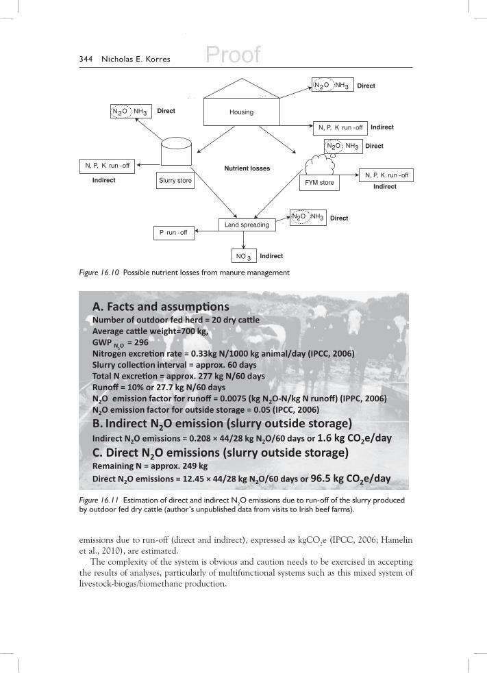
344 Nicholas E. Korres
N2O NH3
N, P, K run -off
Slurry store
N2O NH3
N, P, K run -off
FYM store
N2O NH3
N, P, K run -off
Land spreading
NO 3
N2O NH3
P run -off
Housing
Nutrient losses
Direct
Direct
Direct
Direct
Indirect
Indirect
Indirect
Indirect
Figure 16.10 Possible nutrient losses from manure management
A. Facts and assump�onsNumber of outdoor fed herd = 20 dry ca�le Average ca�le weight=700 kg,GWP N2O
= 296Nitrogen excre�on rate = 0.33kg N/1000 kg animal/day (IPCC, 2006)Slurry collec�on interval = approx. 60 daysTotal N excre�on = approx. 277 kg N/60 daysRunoff = 10% or 27.7 kg N/60 daysN2O emission factor for runoff = 0.0075 (kg N2O-N/kg N runoff) (IPPC, 2006)N2O emission factor for outside storage = 0.05 (IPCC, 2006)B. Indirect N2O emission (slurry outside storage)Indirect N2O emissions = 0.208 × 44/28 kg N2O/60 days or 1.6 kg CO2e/dayC. Direct N2O emissions (slurry outside storage)Remaining N = approx. 249 kgDirect N2O emissions = 12.45 × 44/28 kg N2O/60 days or 96.5 kg CO2e/day
Figure 16.11 Estimation of direct and indirect N2O emissions due to run-off of the slurry produced by outdoor fed dry cattle (author’s unpublished data from visits to Irish beef farms).
emissions due to run-off (direct and indirect), expressed as kgCo2e (IPCC, 2006; Hamelin et al., 2010), are estimated.
The complexity of the system is obvious and caution needs to be exercised in accepting the results of analyses, particularly of multifunctional systems such as this mixed system of livestock-biogas/biomethane production.
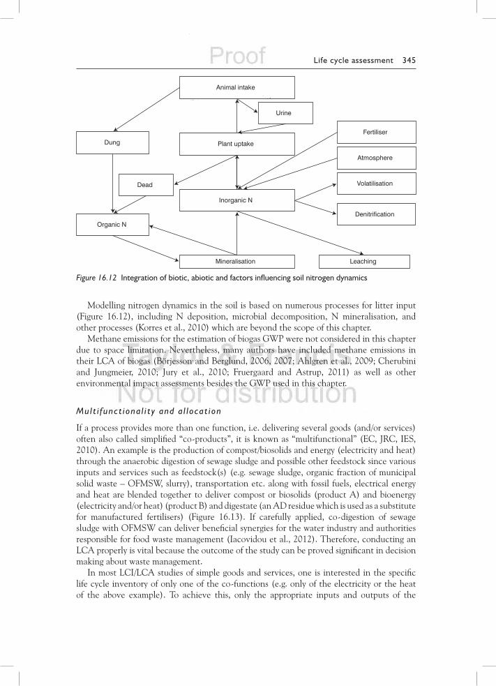
Life cycle assessment 345
modelling nitrogen dynamics in the soil is based on numerous processes for litter input (Figure 16.12), including n deposition, microbial decomposition, n mineralisation, and other processes (Korres et al., 2010) which are beyond the scope of this chapter.
methane emissions for the estimation of biogas gWP were not considered in this chapter due to space limitation. nevertheless, many authors have included methane emissions in their lCA of biogas (Börjesson, and Berglund, 2006, 2007; Ahlgren et al., 2009; Cherubini and Jungmeier, 2010; Jury et al., 2010; Fruergaard and Astrup, 2011) as well as other environmental impact assessments besides the gWP used in this chapter.
Mult i funct iona l i ty and a l locat ion
If a process provides more than one function, i.e. delivering several goods (and/or services) often also called simplified “co-products”, it is known as “multifunctional” (EC, JRC, IES, 2010). An example is the production of compost/biosolids and energy (electricity and heat) through the anaerobic digestion of sewage sludge and possible other feedstock since various inputs and services such as feedstock(s) (e.g. sewage sludge, organic fraction of municipal solid waste – oFmSW, slurry), transportation etc. along with fossil fuels, electrical energy and heat are blended together to deliver compost or biosolids (product A) and bioenergy (electricity and/or heat) (product B) and digestate (an AD residue which is used as a substitute for manufactured fertilisers) (Figure 16.13). If carefully applied, co-digestion of sewage sludge with oFmSW can deliver beneficial synergies for the water industry and authorities responsible for food waste management (Iacovidou et al., 2012). Therefore, conducting an lCA properly is vital because the outcome of the study can be proved significant in decision making about waste management.
In most lCI/lCA studies of simple goods and services, one is interested in the specific life cycle inventory of only one of the co-functions (e.g. only of the electricity or the heat of the above example). To achieve this, only the appropriate inputs and outputs of the
Animal intake
Fertiliser
Atmosphere
Volatilisation
Denitrification
Plant uptake
Inorganic N
LeachingMineralisation
Organic N
Dung
Dead
Urine
Figure 16.12 Integration of biotic, abiotic and factors influencing soil nitrogen dynamics
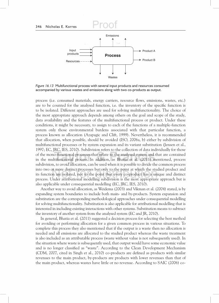
346 Nicholas E. Korres
process (i.e. consumed materials, energy carriers, resource flows, emissions, wastes, etc.) are to be counted for the analysed function, i.e. the inventory of the specific function is to be isolated. Different approaches are used for solving multifunctionality. The choice of the most appropriate approach depends among others on the goal and scope of the study, data availability and the features of the multifunctional process or product. Under these conditions, it might be necessary, to assign to each of the functions of a multiple-function system only those environmental burdens associated with that particular function, a process known as allocation (Azapagic and Clift, 1999). nevertheless, it is recommended that allocation, when possible, should be avoided (ISo, 2006a, b) either by subdivision of multifunctional processes or by system expansion and its variant substitution (Jensen et al., 1997; EC, JRC, IES, 2010). Subdivision refers to the collection of data individually for those of the mono-functional processes that relate to the analysed system and that are contained in the multifunctional process. In addition, as Bhatia et al. (2011) mentioned, process subdivision, to avoid allocation, can be used when it is possible to divide the common process into two or more distinct processes but only to the point at which the studied product and its function are isolated, not to the point that every co-product has a unique and distinct process. Under attributional modelling subdivision is the most appropriate approach but is also applicable under consequential modelling (EC, JRC, IES, 2010).
Another way to avoid allocation, as Weidema (2003) and vikman et al. (2004) stated, is by expanding system boundaries to include both main- and by-products. System expansion and substitution are the corresponding methodological approaches under consequential modelling for solving multifunctionality. Substitution is also applicable for attributional modelling that is interested in including existing interactions with other systems. Substitution means to subtract the inventory of another system from the analysed system (EC and JR, 2010).
In general, Bhatia et al. (2011) suggested a decision process for selecting the best method for avoiding or performing allocation for a given common process in various situations. To complete this process they also mentioned that if the output is a waste then no allocation is needed and all emissions are allocated to the studied product whereas the waste treatment is also included as an attributable process (waste without value is not subsequently used). In the situation where waste is subsequently used, that output would have some economic value and is no longer classified as “waste”. According to the Clean Development mechanism (CDm, 2007, cited in Singh et al., 2010) co-products are defined as products with similar revenues to the main product, by-products are products with lower revenues than that of the main product, whereas wastes have little or no revenue. According to SAIC (2006) co-
Input products
Wastes
Resources
Process
Emissions
Product A
Product B
Figure 16.13 Multifunctional process with several input products and resources consumed accompanied by various wastes and emissions along with two co-products as output.
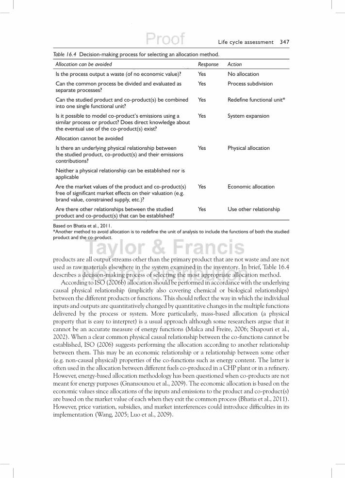
Life cycle assessment 347
products are all output streams other than the primary product that are not waste and are not used as raw materials elsewhere in the system examined in the inventory. In brief, Table 16.4 describes a decision-making process of selecting the most appropriate allocation method.
According to ISo (2006b) allocation should be performed in accordance with the underlying causal physical relationship (implicitly also covering chemical or biological relationships) between the different products or functions. This should reflect the way in which the individual inputs and outputs are quantitatively changed by quantitative changes in the multiple functions delivered by the process or system. more particularly, mass-based allocation (a physical property that is easy to interpret) is a usual approach although some researchers argue that it cannot be an accurate measure of energy functions (malca and Freire, 2006; Shapouri et al., 2002). When a clear common physical causal relationship between the co-functions cannot be established, ISo (2006) suggests performing the allocation according to another relationship between them. This may be an economic relationship or a relationship between some other (e.g. non-causal physical) properties of the co-functions such as energy content. The latter is often used in the allocation between different fuels co-produced in a CHP plant or in a refinery. However, energy-based allocation methodology has been questioned when co-products are not meant for energy purposes (gnansounou et al., 2009). The economic allocation is based on the economic values since allocations of the inputs and emissions to the product and co-product(s) are based on the market value of each when they exit the common process (Bhatia et al., 2011). However, price variation, subsidies, and market interferences could introduce difficulties in its implementation (Wang, 2005; luo et al., 2009).
Table 16.4 Decision-making process for selecting an allocation method.
Allocation can be avoided Response Action
Is the process output a waste (of no economic value)? Yes No allocation
Can the common process be divided and evaluated as separate processes?
Yes Process subdivision
Can the studied product and co-product(s) be combined into one single functional unit?
Yes Redefine functional unit*
Is it possible to model co-product’s emissions using a similar process or product? Does direct knowledge about the eventual use of the co-product(s) exist?
Yes System expansion
Allocation cannot be avoided
Is there an underlying physical relationship between the studied product, co-product(s) and their emissions contributions?
Yes Physical allocation
Neither a physical relationship can be established nor is applicable
Are the market values of the product and co-product(s) free of significant market effects on their valuation (e.g. brand value, constrained supply, etc.)?
Yes Economic allocation
Are there other relationships between the studied product and co-product(s) that can be established?
Yes Use other relationship
Based on Bhatia et al., 2011.*Another method to avoid allocation is to redefine the unit of analysis to include the functions of both the studied product and the co-product.
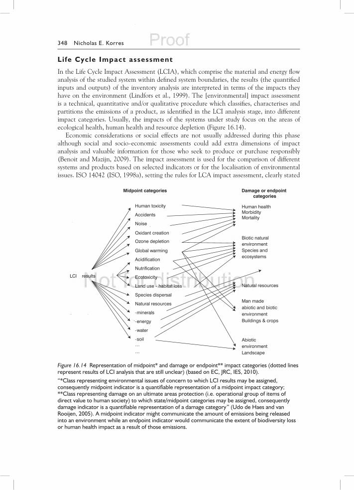
348 Nicholas E. Korres
Life Cycle Impact assessment
In the life Cycle Impact Assessment (lCIA), which comprise the material and energy flow analysis of the studied system within defined system boundaries, the results (the quantified inputs and outputs) of the inventory analysis are interpreted in terms of the impacts they have on the environment (lindfors et al., 1999). The [environmental] impact assessment is a technical, quantitative and/or qualitative procedure which classifies, characterises and partitions the emissions of a product, as identified in the lCI analysis stage, into different impact categories. Usually, the impacts of the systems under study focus on the areas of ecological health, human health and resource depletion (Figure 16.14).
Economic considerations or social effects are not usually addressed during this phase although social and socio-economic assessments could add extra dimensions of impact analysis and valuable information for those who seek to produce or purchase responsibly (Benoit and mazijn, 2009). The impact assessment is used for the comparison of different systems and products based on selected indicators or for the localisation of environmental issues. ISo 14042 (ISo, 1998a), setting the rules for lCA impact assessment, clearly stated
LCI results
Natural resources
Man made abiotic and biotic environmentBuildings & crops
Human toxicity
Accidents
Noise
Oxidant creation
Ozone depletion
Global warming
Acidification
Nutrification
Ecotoxicity
Land use - habitat loss
Species dispersal
Natural resources
-minerals
-energy
-water
-soil
Human healthMorbidityMortality
Biotic natural environmentSpecies and ecosystems
Abiotic environmentLandscape
Midpoint categories Damage or endpoint categories
…
…
Figure 16.14 Representation of midpoint* and damage or endpoint** impact categories (dotted lines represent results of LCI analysis that are still unclear) (based on EC, JRC, IES, 2010).“*Class representing environmental issues of concern to which LCI results may be assigned, consequently midpoint indicator is a quantifiable representation of a midpoint impact category; **Class representing damage on an ultimate areas protection (i.e. operational group of items of direct value to human society) to which state/midpoint categories may be assigned, consequently damage indicator is a quantifiable representation of a damage category” (Udo de Haes and van Rooijen, 2005). A midpoint indicator might communicate the amount of emissions being released into an environment while an endpoint indicator would communicate the extent of biodiversity loss or human health impact as a result of those emissions.
Life cycle assessment 349
that three steps are mandatory for the determination of impact categories: first, selection and definition of impact categories (i.e. identifying relevant environmental impact categories such as those of global warming, acidification, terrestrial toxicity); second, classification (i.e. assigning lCI results to the impact categories, e.g., classifying carbon dioxide emissions to global warming); third, characterisation (i.e. modelling lCI impacts within impact categories using science-based conversion factors, e.g. modelling the potential impact of carbon dioxide and methane on global warming). The remaining steps of the impact assessment procedure concern the normalisation of impacts (i.e. in this step potential impacts expressed in such a manner that can be compared, e.g. global warming impact of carbon dioxide and methane for the two options), the grouping of impact indicators (i.e. arrangement or ranking the indicators by location, e.g. local, regional and global as in Table 16.5), weighting (i.e. emphasising the most important potential impacts) and finally evaluating and reporting lCI analysis results.
Interpretation of LCa
life Cycle Assessment interpretation is a systematic process to evaluate the results of the inventory analysis and impact assessment, to select the preferred product, process or service with a clear understanding of the uncertainty and the assumptions used to generate the results (SAIC, 2006). life Cycle Assessment interpretation is performed in interaction with the three other phases of the lCA. If the results of the inventory analysis or the impact assessment are found not to fulfil the requirements defined in the goal and scoping phase, the inventory analysis must be improved, e.g. by revising the system boundaries, further data collection etc. followed by an improved impact assessment (Jensen et al., 1997). The main issues (ISo, 1997) relating to the interpretation are i) the identification of significant environmental issues; ii) evaluation of the methodology and results based on quality criteria described earlier in this chapter (e.g. completeness, consistency etc.); and iii) checking that the conclusions are consistent with the requirements of the goal and scope of the study. If these conditions are satisfied the conclusions of the study can be reported and recommendation for action based on these can be suggested.
Conclusions
lCA has be proved an invaluable tool for the examination of the sustainability of biogas production but caution is necessary for the proper application of working protocols and rules. more particularly, the functional unit(s) of the studied system(s) should properly describe the services provided and be clearly defined and reported. Where consistent with the goal of the study, the reference alternatives, particularly in comparative studies, should be chosen so as to be representative of the purpose and to maximise the data quality of the compared alternatives. legislative issues and recent policies in the bioenergy production arena require a clear and concise conclusion to be drawn upon the completion of lCA based on clear evidence. The development of the life Cycle Inventory, one of the core phases of the technique, should follow a strict protocol so comparability, representativeness and completeness are fulfilled. To assist decision-makers, recommendations should be based on solid evidence which in turn should be based on proper analysis. life Cycle Assessment can be highly misleading if used in an undisciplined way. However, it can be an invaluable tool if practised properly. Furthermore, social and socio-economic assessments could add extra dimensions to impact analysis and valuable information for those who seek to produce
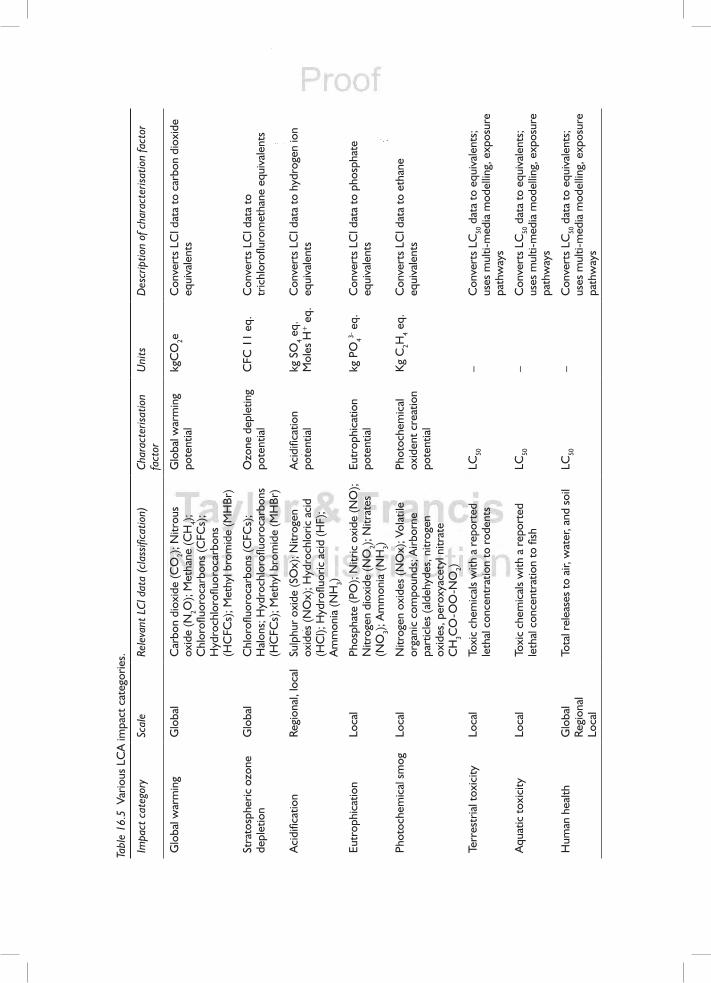
Tabl
e 16
.5 V
ario
us L
CA
impa
ct c
ateg
orie
s.
Impa
ct c
ateg
ory
Scal
eRe
leva
nt L
CI d
ata
(cla
ssifi
catio
n)Ch
arac
teris
atio
n fa
ctor
Uni
tsD
escr
iptio
n of
cha
ract
erisa
tion
fact
or
Glo
bal w
arm
ing
Glo
bal
Car
bon
diox
ide
(CO
2); N
itrou
s ox
ide
(N2O
); M
etha
ne (C
H4)
; C
hlor
ofluo
roca
rbon
s (C
FCs)
; H
ydro
chlo
roflu
oroc
arbo
ns
(HC
FCs)
; Met
hyl b
rom
ide
(MH
Br)
Glo
bal w
arm
ing
pote
ntia
lkg
CO
2eC
onve
rts
LCI d
ata
to c
arbo
n di
oxid
e eq
uiva
lent
s
Stra
tosp
heric
ozo
ne
depl
etio
nG
loba
lC
hlor
ofluo
roca
rbon
s (C
FCs)
; H
alon
s; H
ydro
chlo
roflu
oroc
arbo
ns
(HC
FCs)
; Met
hyl b
rom
ide
(MH
Br)
Ozo
ne d
eple
ting
pote
ntia
lC
FC 1
1 eq
.C
onve
rts
LCI d
ata
to
tric
hlor
oflur
omet
hane
equ
ival
ents
Aci
dific
atio
nRe
gion
al, l
ocal
Sulp
hur
oxid
e (S
Ox)
; Nitr
ogen
ox
ides
(NO
x); H
ydro
chlo
ric a
cid
(HC
l); H
ydro
fluor
ic a
cid
(HF)
; A
mm
onia
(NH
3)
Aci
dific
atio
n po
tent
ial
kg S
O4 e
q.
Mol
es H
+ e
q.C
onve
rts
LCI d
ata
to h
ydro
gen
ion
equi
vale
nts
Eutr
ophi
catio
nLo
cal
Phos
phat
e (P
O);
Nitr
ic o
xide
(NO
); N
itrog
en d
ioxi
de (N
O2)
; Nitr
ates
(N
O3)
; Am
mon
ia (N
H3)
Eutr
ophi
catio
n po
tent
ial
kg P
O43-
eq.
Con
vert
s LC
I dat
a to
pho
spha
te
equi
vale
nts
Phot
oche
mic
al s
mog
Loca
lN
itrog
en o
xide
s (N
Ox)
; Vol
atile
or
gani
c co
mpo
unds
; Airb
orne
pa
rtic
les
(ald
ehyd
es, n
itrog
en
oxid
es, p
erox
yace
tyl n
itrat
e C
H3C
O-O
O-N
O2)
Phot
oche
mic
al
oxid
ent c
reat
ion
pote
ntia
l
Kg
C2H
4 eq.
Con
vert
s LC
I dat
a to
eth
ane
equi
vale
nts
Terr
estr
ial t
oxic
ityLo
cal
Toxi
c ch
emic
als
with
a r
epor
ted
leth
al c
once
ntra
tion
to r
oden
tsLC
50–
Con
vert
s LC
50 d
ata
to e
quiv
alen
ts;
uses
mul
ti-m
edia
mod
ellin
g, e
xpos
ure
path
way
s
Aqu
atic
toxi
city
Loca
lTo
xic
chem
ical
s w
ith a
rep
orte
d le
thal
con
cent
ratio
n to
fish
LC50
–C
onve
rts
LC50
dat
a to
equ
ival
ents
; us
es m
ulti-
med
ia m
odel
ling,
exp
osur
e pa
thw
ays
Hum
an h
ealth
Glo
bal
Regi
onal
Loca
l
Tota
l rel
ease
s to
air,
wat
er, a
nd s
oil
LC50
–C
onve
rts
LC50
dat
a to
equ
ival
ents
; us
es m
ulti-
med
ia m
odel
ling,
exp
osur
e pa
thw
ays
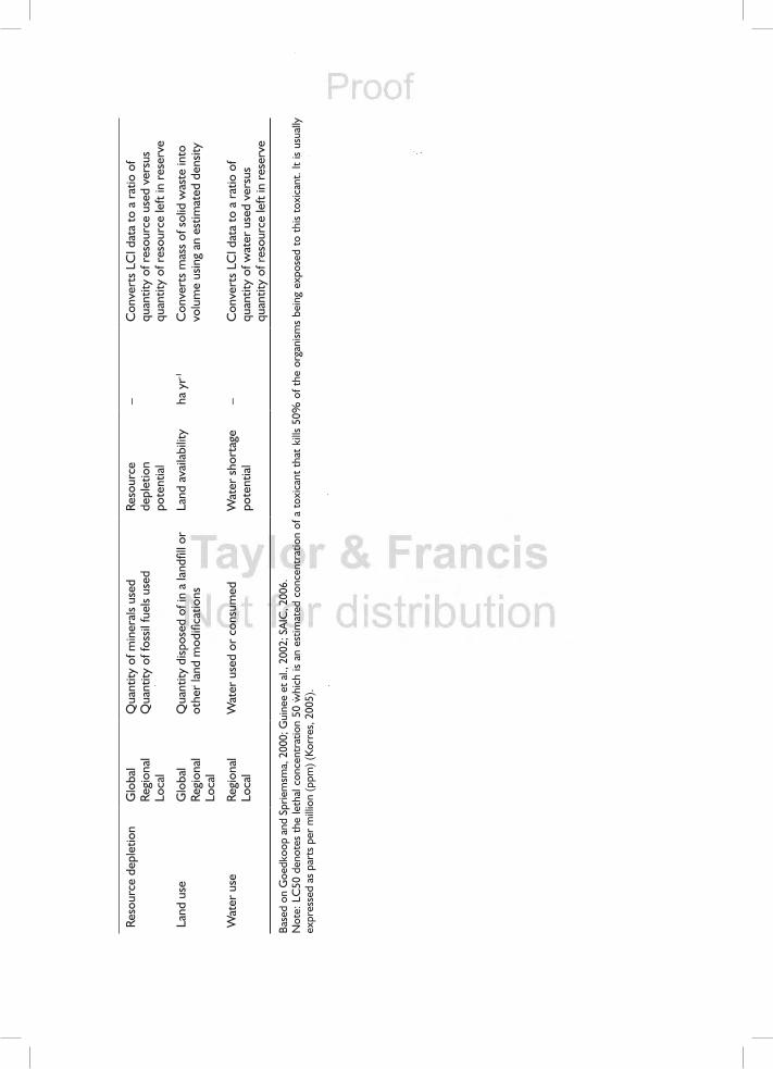
Reso
urce
dep
letio
nG
loba
lRe
gion
alLo
cal
Qua
ntity
of m
iner
als
used
Qua
ntity
of f
ossil
fuel
s us
edRe
sour
ce
depl
etio
n po
tent
ial
–C
onve
rts
LCI d
ata
to a
rat
io o
f qu
antit
y of
res
ourc
e us
ed v
ersu
s qu
antit
y of
res
ourc
e le
ft in
res
erve
Land
use
Glo
bal
Regi
onal
Loca
l
Qua
ntity
disp
osed
of i
n a
land
fill o
r ot
her
land
mod
ifica
tions
Land
ava
ilabi
lity
ha y
r-1C
onve
rts
mas
s of
sol
id w
aste
into
vo
lum
e us
ing
an e
stim
ated
den
sity
Wat
er u
seRe
gion
alLo
cal
Wat
er u
sed
or c
onsu
med
Wat
er s
hort
age
pote
ntia
l–
Con
vert
s LC
I dat
a to
a r
atio
of
quan
tity
of w
ater
use
d ve
rsus
qu
antit
y of
res
ourc
e le
ft in
res
erve
Base
d on
Goe
dkoo
p an
d Sp
riem
sma,
200
0; G
uine
e et
al.,
200
2; S
AIC
, 200
6.N
ote:
LC
50 d
enot
es t
he le
thal
con
cent
ratio
n 50
whi
ch is
an
estim
ated
con
cent
ratio
n of
a t
oxic
ant
that
kill
s 50
% o
f the
org
anism
s be
ing
expo
sed
to t
his
toxi
cant
. It
is us
ually
ex
pres
sed
as p
arts
per
mill
ion
(ppm
) (Ko
rres
, 200
5).
352 Nicholas E. Korres
or purchase responsibly. The establishment of interactions with other scientific approaches such as data warehouse and data mining techniques, statistics and/or even simulation or soft system methodology approaches are likely to improve the lCA process. Although nothing was mentioned here about sensitivity analysis or uncertainty, major issues in lCA, the detailed step-by-step instructions on lCI and lCIA along with the numerous and explicit graphical information which accompany the examples should provoke and intrigue the curiosity of the conscientious scholar to find her/his way forward.
references
Ahlgren, S., Hansson, P.A., Kimming, m., Aronsson, P., and lundkvist, H. (2009) ‘greenhouse gas emissions from cultivation of agricultural crops for biofuels and production of biogas from manure’, Implementation of the Directive of the European Parliament and of the Council on the promotion of the use of energy from renewable sources. Revised according to instructions for interpretation of the Directive from the European Commission 30 July 2009, Dnr SlU ua 12-4067/08.
Anonymous (2007) ‘Energy balance optimisation for an integrated arable/livestock farm unit’, Cropgen, Renewable energy from crops and agrowastes, SES6-CT-2004-502824, University of vienna (BoKU-IFA).
Arnold, K. (2011) ‘greenhouse gas balance of biomethane – which substrates are suitable?’, Energy Science and Technology, vol. 1, no 2, pp67–75.
Azapagic, A. and Clift, R. (1999) ‘Allocation of environmental burdens in co-product systems: product-related burdens’, International Journal Life Cycle Assessment, vol. 4, no 6, pp357–369.
Beer, T., grant, T., morgan, g., lapszewicz, J., Anyon, P., Edwards, J., nelson, P., Watson, H. and Williams, D. (2002) ‘Comparison of transport fuels – life cycle emissions analysis of alternative fuels for heavy vehicles’, Commonwealth Scientific and Industrial Research organisation, Aspendale, Australia.
Benoit, C. and mazijn, B. (2009) ‘guidelines for Social life Cycle Assessment of Products’, United nations Environment Programme.
Bergsma, g., vroonhof, J. and Dornburg, v. (2006) ‘The greenhouse gas calculation methodology for biomass-based electricity, heat and fuels’, Project group “Sustainable Production of Biomass” Report from Working group Co2 methodology.
Bessou, C., Basset-mens, C., Tran, T. and Benoist, A. (2012) ‘lCA applied to perennial cropping systems: a review focused on the farm stage’, International Journal Life Cycle Assessment, doi 10.1007/s11367-012-0502-z.
Bhatia, P., Cummis, C., Brown, A., Draucker, l., Rich, D. and lahd, H. (2011) ‘Product life Cycle Accounting and Reporting Standard’, greenhouse gas Protocol, World Resources Institute and World Business Council for Sustainable Development.
Bird, n., Cowie, A., Cherubini, F., and Jungmeier, g. (2011) ‘Using a life cycle assessment approach to estimate the net greenhouse gas emissions of bioenergy’, International Energy Agency, Bioenergy:ExCo:2011:03.
Bligny, J.C., Pennington, D., De Camillis, C., Palyi, B., Bauer, C., Schenker, U., King, H., martin, n. et al. (2012) ‘EnvIFooD Protocol Environmental Assessment of Food and Drink Protocol’, Draft version 0.1, Pilot Testing, november 2012, European Food Sustainable Consumption & Production Round Table.
Börjesson, P. and Berglund, m. (2006) ‘Environmental systems analysis of biogas systems – Part I: Fuel-cycle emissions’, Biomass and Bioenergy, vol. 30, no. 5, pp469–485.
Börjesson, P. and Berglund, m. (2007) ‘Environmental systems analysis of biogas systems – Part II: The environmental impact of replacing various reference systems’, Biomass and Bioenergy, vol. 31, no. 5, pp326–344.
Life cycle assessment 353
Börjesson, P., Tufvesson, l. and lantz, m. (2011) ‘life Cycle Assessment of biofuels in Sweden’, lund University, Dept. of Technology and Society, Environmental and Energy Systems Studies, Report no. 70, may 2010.
Bouwman, A.F. (1996) ‘Direct emissions of nitrous oxide from agricultural soils’, Nutrient Cycling in Agroecosystems, vol. 46, pp53–70.
Broch, A. and Hoekman, S.K. (2012) ‘Transportation fuel life cycle analysis. A review of indirect land use change and agricultural n2o emissions’, CRC Project no. E-88-2, Final Report, Desert Research Institute, life Cycle Associates, January 2012.
Broch, A., Hoekman, S.K. and Unnasch, S. (2012) ‘A review of indirect land use change and agricultural n2o emissions. Transportation fuel life cycle analysis’, CRC Project no. E-88-2, Final Report.
Brown, m.T. and Herendeen, R.A. (1996) ‘Embodied energy analysis and EmERgy analysis: a comparative view’, Ecological Economics, vol.19, no 3, pp219–235.
Cherubini, F. and Jungmeier, g. (2010) ‘lCA of a biorefinery concept producing bioethanol, bioenergy, and chemicals from switchgrass’, International Journal Life Cycle Assessment, vol. 15, pp53–66.
Cherubini, F. and Stromman, A.H. (2011) ‘life cycle assessment of bioenergy systems: State of the art and future challenges’, Bioresource Technology, vol. 102, pp437–451.
Cherubini, F., Bird, n.D., Cowie, A., Jungmeier, g., Schlamadinger, B. and Woess-gallasch, S. (2009) ‘Energy-and greenhouse gas-based lCA of biofuel and bioenergy systems: Key issues, ranges and recommendations’, Resources, Conservation and Recycling, vol. 53, pp434–447.
Chomkhamsri, K. and Pelletier, n. (2011) ‘Analysis of Existing Environmental Footprint methodologies for Products and organizations: Recommendations, Rationale, and Alignment’, Deliverable 1 to the Administrative Arrangement between Dg Environment and Joint Research Centre no. n 070307/2009/552517, including Amendment no 1 from December 2010, European Commission (EC), Joint Research Centre (JRC), Institute for Environment and Sustainability (IES).
Cleveland, C.J. and Costanza, R. (2010) ‘net Energy Analysis. In: Encyclopedia of Earth, national Council for Science and Environment, http://www.eoearth.org/article/net_energy_analysis [Accessed July 2012].
Consoli, F., Allen, D., Boustead, I., Fava, J., Franklin, W., Jensen, A.A., de oude, n., Parrish, R., Perriman, R., Postlethwaite, D., Quay, B., Séguin, J. and vigon, B. (eds). (1993) ‘guidelines for life-cycle assessment: a code of practice’, Society of Environmental Toxicology and Chemistry (SETAC); SETAC Workshop, Sesimbra, Portugal, 31 march – 3 April 1993.
Deasy, E. and Power n. (2011) ‘A life-cycle technical assessment of biofuels options for Ireland’, In Proceedings of the ITRN2011, Biofuel options for Ireland, 31 August – 1 September, University College Cork, Cork, Ireland.
del Rio, P. and Burguillo, m. (2009) ‘An empirical analysis of the impact of renewable energy deployment on local sustainability’, Renewable and Sustainable Energy Reviews, vol. 13, pp1314–1325.
Earles, J.m. and Halog, A. (2011) ‘Consequential life cycle assessment: a review’, International Journal Life Cycle Assessment, vol. 16, pp445–453.
EC (2009) ‘Directive 2009/28/EC of The European Parliament and of The Council of 23 April 2009 on the promotion of the use of energy from renewable sources and amending and subsequently repealing Directives 2001/77/EC and 2003/30/EC’, Official Journal of the European Union 2009, pp16–62.
EC, JRC, IES (2010) International Reference Life Cycle Data System (ILCD) Handbook – General guide for Life Cycle Assessment – Detailed guidance, EUR 24708 En, 1st edn march 2010, European Commission – Joint Research Centre – Institute for Environment and Sustainability, luxembourg, Publications office of the European Union.
Edwards-Jones, g., Plassmn, K. and Harris, I.m. (2009) ‘Carbon footprint of lamb and beef production systems: insights from an empirical analysis of farms in Wales, UK’, Journal of Agricultural Science, vol. 147, pp707–719.
Ekvall, T. and Andrae, A. (2006) ‘Attributional and consequential environmental assessment of the shift to lead-free solders’, International Journal Life Cycle Assessment, vol. 11, no5, pp344–353.
354 Nicholas E. Korres
Ekvall, T. and Finnveden, g. (2001) ‘Allocation in ISo 14041 – a critical review’, Journal of Cleaner Production, vol.9, pp197–208.
Ekvall, T. and Weidema, B. (2004) ‘System boundaries and input data in consequential life cycle inventory analysis’, International Journal Life Cycle Assessment, vol. 9, no.3, pp161–171.
Elghali, l. (2002) ‘Decision support tools for environmental policy decisions and their relevance to life Cycle Assessment’, CES Working Paper 2/02, August 2002, TRl limited, ISSn 1464-8083.
Elsayed, m.A., matthews, R. and mortimer, n.D. (2003) ‘Carbon and energy balances for a range of biofuels options’, Final report, Prepared for the Department of Trade and Industry, Renewable Energy Programme Unit of Sheffield Hallam University and Forest Research.
Emmenegger, m.F., Stucki, m. and Hermle, S. (2012) ‘lCA of energetic biomass utilization: actual projects and new developments – April 23, 2012, Berne, Switzerland’, International Journal Life Cycle Assessment, vol. 17, pp1142–1147.
Fava, J. and Pomper, S. (1997) ‘life cycle critical review! Does it work? Implementing a critical review process as a key element of the aluminium beverage container lCA’, International Journal Life Cycle Assessment, vol. 2, no.3 pp145–153.
Fava, J.A., Denison, R., Jones, B., Curran, m.A., vigon, B., Selke, S and Barnum J. (eds) (1994) ‘A technical framework for life cycle assessment’, Society of Environmental Toxicology and Chemistry (SETAC) and SETAC Foundation for Environmental Education, Fl.
Finnveden, g., Hauschild, m.z., Ekvall, T., guinee, J., Reinout Heijungs, R., Hellweg, S. Koehler, A., Pennington, D. and Suh, S. (2009) ‘Recent developments in life Cycle Assessment’, Journal of Environmental Management, vol. 91, no 1, pp1–21.
Frischknecht, R. and Jungbluth, n. (eds) (20070 ‘overview and methodology. Data v2.0 (2007)’, Ecoinvent report no. 1, Dubendorf, December 2007.
Fruergaard, T. and Astrup, T. (2011) ‘optimal utilization of waste-to-energy in an lCA perspective’, Waste Management, vol. 31, pp572–582.
garofalo, R. (2011) ‘lifecycle assessment and environmental assessment’, Aquafuel FP7-241301-2, Algae and aquatic biomass for a sustainable production of 2nd generation biofuels, Coordination Action FP7-EnERgy-2009-1.
gasol, C.m., gabarrell, X., Anton, A., Rigola, m., Carrasco, J., Ciria, P., Solano, m.l. and Rieradevall, J. (2007) ‘life cycle assessment of a Brassica carinata bioenergy cropping system in southern Europe’, Biomass and Bioenergy, vol. 31, pp543–555.
gerin, P.A., vliegen, F. and Jossart, J.m. (2007) ‘Energy and Co2 balance of maize and grass as energy crops for anaerobic digestion’, Bioresource Technology, vol. 99, pp2620–2627.
gnansounou, E., Dauriat, A., villegas, J. and Panichelli, l. (2009) ‘life cycle assessment of biofuels: energy and greenhouse gas balances’, Bioresource Technology, vol. 100, no 21, pp4919–4930.
goedkoop, m.J. and Spriemsma, R. (2000) The Eco-Indicator 99. A Damage Oriented Method for Life Cycle Impact Assessment. Methodology Report and Methodology Annex, 17 April 2000 2nd edn, available at www.pre.nl
guinee, J.B., gorree, m., Heijungs, R., Huppes, g., Kleijn, R., de Koning, A., van oers, l., Wegener Sleeswijk, A., Suh, S., Udo de Haes, H.A., de Bruijn, J.A., van Duin, R. and Huijbregts, m.A.J. (2002) Handbook on Life Cycle Assessment: Operational Guide to the ISO Standards, Series: Eco-efficiency in Industry and Science, Kluwer Academic Publishers, london, Dordrecht.
Haas, g., Wetterich, F. and Kopke, U. (2001) ‘Comparing intensive, extensified and organic grassland farming in southern germany by process life cycle assessment’, Agriculture, Ecosystems and Environment, vol. 83, pp43–53.
Hamelin, l., Wesnaes, m., Wenzel, H. and Petersen, B.m. (2010) ‘life cycle assessment of biogas from separated slurry’, Environmental Project no. 1329 2010 miljoprojekt, Environmental Protection Agency, Danish ministry of the Environment.
Hartmann, J.K. (2006) ‘life-cycle-assessment of industrial scale biogas plants’, Dissertation zur Erlangung des Doktorgrades, der Fakultät für Agrarwissenschaften, der georg-August-Universität göttingen, göttingen, Juli 2006.
Life cycle assessment 355
Hitchcock, g. and lane, B. (2008) ‘lCA Road Transport Biofuels’, Final Report v7, Sustainable Transport Solutions.
Horne, R.E. and matthews, R. (2004) ‘BIomITRE Technical manual’, Biomass-based climate change mitigation through renewable energy (BIomITRE) Project number: nnE5-00069-2002, november 2004.
Iacovidou, E., ohandja, D.g. and voulvounis, n. (2012) ‘Food waste co-digestion with sewage sludge – realising its potential in the UK’, Journal of Environmental Management, vol. 112, pp267–274.
IEC (2008) ‘Supporting Annexes for Environmental product declarations. Annex A: Application of lCA methodology’, International EPD Cooperation (IEC), EPD, version 1.0, dated 2008-02-29.
IEo (2009) ‘International Energy outlook’, Energy Information Administration, office of Integrated Analysis and Forecasting, US Department of Energy, Washington DC.
IPCC (1996) ‘Revised 1996 IPCC guidelines for national greenhouse gas Inventories: Reference manual’.
IPCC (2006) ‘guidelines for national greenhouse gas Inventories’, Prepared by the national greenhouse gas Inventories Programme, Eggleston, H.S., Buendia, l., miwa, K., ngara, T. and Tanabe, K. (eds). Published: IgES, Japan, http://www.ipccnggip.iges.or.jp/public/2006gl/index.html [Accessed June 2012].
IPCC (2007) ‘Climate change 2007: mitigation’, In: metz, B. et al. (Eds.) Contribution of Working Group 3 to the Fourth Assessment Report of the Intergovernmental Panel on Climate Change, Cambridge, UK and new york.
ISo (1997) ‘Environmental management – life Cycle Assessment – Principles and Framework’ (ISo/FDIS 14040). ISo TC 207. International organization of Standardization.
ISo (1998a) ‘Environmental management – life Cycle Assessment – Impact Assessment –ISo 14042:2000’, ISo TC 207/SC5/Wg4, International Standards organization (ISo), geneva, Switzerland, http://www.iso.org/iso/catalogue_detail?csnumber=37456.
ISo (1998b) ‘Environmental management – life Cycle Assessment – life Cycle Interpretation – ISo 14043:2000’, ISo TC 207, International Standards organization (ISo), geneva, Switzerland, http://www.iso.org/iso/catalogue_detail?csnumber=37456.
ISo (1999), ‘Environmental management – life Cycle Assessment – goal, scope and inventory analysis – ISo 14041:1999’, International organization for Standardization (ISo), geneva, Switzerland, http://www.iso.org/iso/catalogue_detail?csnumber=37456.
ISo (2006a) ‘ISo norm 14044:2006 International Standard’. In: ‘Environmental management – life Cycle Assessment – Requirements and guidelines’, International organisation for Standardisation, geneva, Switzerland.
ISo (2006b) ‘ISo norm 14040:2006. life cycle assessment: principles and framework. Environmental management’, International organisation for Standardisation, geneva.
Jensen, A.A., Hoffman, l., møller, B.T., Schmidt, A., Christiansen, K., Elkington, J. and van Dijk, F. (1997) ‘life Cycle Assessment. A guide to approaches, experiences and information sources’, Environmental Issues Series, no.6, European Environmental Agency.
Jungk, n.C., Reinhardt, g.A. and gartner, S.o. (2002) ‘Agricultural reference systems in life Cycle Assessments’, in van Ierland, E.C. and oude lansink, A. (eds), Economics of sustainable energy in agriculture, Kluwer Academic Publishers, pp105–119.
Jungmeier, g., and Hausberger, S. (2002) ‘greenhouse gas emissions of cars with biofuels in Austria – A comparison to cars with conventional fuel’, in Biomass for Energy, Industry and Climate Protection, 12th European Biomass Conference, ETA-Florence, Amsterdam, The netherlands, pp1128–1131.
Jungmeier, g. and Spitzer, J. (2001) ‘greenhouse gas emissions of bioenergy from agriculture compared to fossil energy for heat and electricity supply’, Nutrient Cycling in Agroecosystems, vol. 60, no 1–3, pp 267–273.
Jungmeier, g., Werner, F., Jarnehammar, A., Hohenthal, C. and Richter, K. (2002) ‘Allocation in lCA of wood-based products – Experiences of Cost Action E9 Part I. methodology’. International Journal of Life Cycle Assessment, 7, pp290–294
356 Nicholas E. Korres
Jury, C., Benetto, E., Koster, D., Schmitt, B. and Welfring, J. (2010) ‘life Cycle Assessment of biogas production by monofermentation of energy crops and injection into the natural gas grid’, Biomass and Bioenergy, vol. 34, no 1, pp54–66.
Kammen, D.m., Farrell, A.E., Plevin, R.J., Jones, A.D., nemet, g.F. and Delucchi, m.A. (2008) ‘Energy and greenhouse Impacts of Biofuels: A Framework for Analysis’, oECD Research Roundtable-Energy & greenhouse gas Impacts of Biofuels, Research Report, UCB-ITS-TSRC-RR–2008-1, eScholarship, University of California, http://escholarship.org/uc/item/7zg2 x 23t [accessed, August 2012].
Kim, S. and Dale, B.E. (2005) ‘life cycle assessment of various cropping systems utilized for producing biofuels: Bioethanol and biodiesel’, Biomass and Bioenergy, vol. 29, pp426–439.
Kim, S. and Dale, B.E (2009) ‘Regional variations in greenhouse gas emissions of biobased products in the United States – corn-based ethanol and soybean oil’, International Journal of Life Cycle Assessment, vol. 14, pp540–546.
Korres, n.E. (2004) ‘Introduction to Soft System methodology’, Personal notes from the postgraduate course in operational Research and Applied Statistics at Salford University, UK.
Korres, n.E. (2005) Encyclopaedic dictionary of weed science. Theory and digest, Intercept (Andover, UK) and lavoisier SAS (Paris, France).
Korres, n.E. (2010) Food Climate Research network (FCRn). Interview Series 2010 Cycle, november 2010, http://fcrn.org.uk/interviewSeries/interviews/index.htm [Accessed August 2012].
Korres, n.E., Singh, A., nizami, A.S. and murphy, J.D. (2010) ‘Is grass biomethane a sustainable transport biofuel?’, Biofuels, Bioproducts and Biorefining, vol. 4, no 3, pp310–325.
Korres, n.E., Thamsiriroj, T., Smyth, B., nizami A.S., Singh, A. and murphy J.D. (2011). ‘grass biomethane for agriculture and energy’, In lichtfouse, E. (Ed.), ‘genetics, Biofuels and local Farming Systems’, Sustainable Agriculture Reviews, vol. 7, pp5–50. Springer Science & Business media.
labutong, n., mosley, J., Smith, R. and Willard, J. (2012) ‘life-cycle modeling and environmental impact assessment of commercial scale biogas production’, mSc Thesis, University of michigan, School of natural Resources and Environment.
lesage, P., Ekvall, T., Deschenes, l. and Samson, R.J. (2007) ‘Environmental assessment of brown-field rehabilitation using two different life cycle inventory models: part 2’, International Journal of Life Cycle Assessment, vol. 12, no. 7, pp497–513.
lindfors, l.g., Christiansen, K., Hoffman, l., Kruger, I., virtanen, y., Juntilla, v., Hanssen, o.J. and Ronning, A. (1999) ‘nordic guidelines on life-cycle Assessment: nord’, 1995:20, 3rd edn, nordic Council of ministers, Copenhagen.
lundin, m., Bengtsson, m. and molander, S. (2000) ‘life cycle assessment of wastewater systems – Influence of system boundaries and scale on calculated environmental loads’, Environmental Science and Technology, vol.34, pp180–186.
luo, l., van der voet, E., Huppes, g. and Udo de Haes, H.A. (2009) ‘Allocation issues in lCA methodology: a case study of corn stover-based fuel ethanol’, International Journal of Life Cycle Assessment, vol. 14, pp529–539.
malca, J. and Freire, F. (2006) ‘Renewability and life-cycle energy efficiency of bioethanol and bio-ethyl tertiary butyl ether (bioETBE): assessing the implications of allocation’, Energy, vol. 31, pp3362–3380.
mclaughlin, S.B., Delatorreugarte, D.g., garten Jr., C.T., lynd, l.R., Sanderson, m.A., Tolbert, v.R., and Wolf, D.D. (2002) ‘High-value renewable energy from prairie grasses’, Environmental Science and Technology, vol. 36, pp2122–2129.
minami, K. and ohsawa, A. (1990) ‘Emission of nitrous oxide dissolved in drainage water from agricultural land’, in Bouwman, A.F. (ed.). Soils and the greenhouse effect. John Wiley & Sons, new york. pp503–509.
monti, A., Fazio, S., and venturi, g. (2009) ‘Cradle-to-farm gate life cycle assessment in perennial energy crops’, European Journal of Agronomy, vol.31, pp77–84.
Life cycle assessment 357
murphy, J.D. and Power, n.m. (2008) ‘An argument for using biomethane generated from grass as a biofuel in Ireland’, Biomass and Bioenergy, vol. 33, no 3, pp504–512.
nevison, C. (1999) ‘Indirect n2o Emissions from Agriculture’, Good Practice Guidance and Uncertainty Management in National Greenhouse Gas Inventories, pp381–397, http://www.ipcc-nggip.iges.or.jp/public [Accessed november 2012].
Palsson, A.C. and Riise, E. (2011) ‘Performing the inventory in a lCA study’, TOSCA Sustainability Framework, http://www.tosca-life.info/ [Accessed September 2012].
Payraudeau, S., van der Werf, H.m.g. and vertes, F. (2007) ‘Analysis of the uncertainty associated with the estimation of nitrogen losses from farming systems’, Agricultural Systems, vol. 94, pp416–430.
Power, n. and murphy, J.D. (2009) ‘Which is the preferable transport fuel on a greenhouse gas basis: biomethane or ethanol?’, Biomass and Bioenergy, vol. 33, pp1403–1412.
Rebitzer, g., Ekvall, T., Frischknecht, R., Hunkeler, D., norris, g., Rydberg, T., Schmidt, W.P., Suh, S., Weidema, B.P., and Pennington, D.W. (2004) ‘life cycle assessment. Part 1: framework, goal and scope definition, inventory analysis, and applications’, Environmental International, vol.30, no 5, pp701–720.
Ruggeri B., Tommasi T. and Sassi g. (2010). ‘Energy balance of dark anaerobic fermentation as a tool for sustainability analysis’, International Journal of Hydrogen Energy, vol. 35, pp10202–10211.
SAIC (2006) ‘life cycle assessment: principles and practice’, Scientific Applications International Corporation (SAIC), Report no. EPA/600/R-06/060. national Risk management Research laboratory, office of Research and Development, US Environmental Protection Agency, Cincinnati, oH.
Salter, A. and Banks, C.J. (2009) ‘Establishing an energy balance for crop-based digestion’, Water Science & Technology, vol. 59, no 6, pp1053–1060.
Sanchez, S.T., Woods, J., Akhurst, m., Brander, m., o’Hare, m., Dawson, T.P., Edwards, R., liska, A.J and malpas, R. (2012) ‘Accounting for indirect land-use change in the life cycle assessment of biofuel supply chains’, Journal of the Royal Society Interface, doi:10.1098/rsif.2011.0769.
Sapsford, R. and Jupp, v. (2006) Data Collection and Analysis, The open University, SAgE, london, California, new Delhi.
Sathaye, J., lucon, o., Rahman, A., Christensen, J., Denton, F., Fujino, J., Heath, g., Kadner, S., mirza, m., Rudnick, H., Schlaepfer, and Shmakin, A. (2011) ‘Renewable Energy in the Context of Sustainable Development’, in Edenhofer, o., Pichs-madruga, R., Sokona, y., Seyboth, K., matschoss, P., Kadner, S., zwickel, T., Eickemeier, P., Hansen, g., Schlomer, S. and von Stechow, C. (eds), IPCC Special Report on Renewable Energy Sources and Climate Change Mitigation, Cambridge University Press, Cambridge, UK and new york.
Saunders, C., Barber, A. and Taylor. g. (2006) ‘Food miles-comparative energy/emissions performance of new zealand’s agriculture industry’, Research Report 285, lincoln University new zealand, http://www.lincoln. ac.nz/documents/2328_rr285_s13389.pdf [Accessed march 2012].
Schmidt, J.H. (2010) ‘Comparative life cycle assessment of rapeseed oil and palm oil’, International Journal Life Cycle Assessment, vol. 15, pp183–197.
Seitzinger, S.P. and Kroeze, C. (1998) ‘global distribution of nitrous oxide production and n inputs in freshwater and coastal marine ecosystems’, Global Biogeochemical Cycles, vol. 12, pp93–113.
Shapouri, H., Duffield, J. and Wang, m. (2002) ‘The energy balance of corn ethanol: an update’, Agricultural Economic Report no. 813. US Department of Agriculture.
Singh, A., Pant, D., Korres n.E., nizami, A.S., Prasad, S. and murphy, J.D. (2010) ‘Key issues in life cycle assessment of ethanol production from lignocellulosic biomass: A review’, Bioresource Technology, vol.101, pp5003–5012.
Smith, K., Bouwman, l., and Braatz, B. (1997) ‘n2o: Direct Emissions from Agricultural Soils’, Good Practice Guidance and Uncertainty Management in National Greenhouse Gas Inventories, pp361–380, http://www.ipcc-nggip.iges.or.jp/public [Accessed november 2012].
SmmT (2006) ‘Annual Co2 Report: 2006’, Society of motor manufactures and Traders.
358 Nicholas E. Korres
Smyth, B.m., murphy, J.D. and o’Brien, C.m. (2009) ‘What is the energy balance of grass biomethane in Ireland and other temperate northern European climates?’ Renewable and Sustainable Energy Reviews, vol. 13, no 9, pp2349–2360.
Sonnemann, g. and vigon, B. (2011) ‘global guidance principles for life Cycle Assessment databases. A basis for greener processes and products’, Shonan guidance Principles, UnEP/SETAC life Cycle Initiative.
Staple, g.C. and Swisher, J.n (2011) ‘The climate impact of natural gas and coal-fired electricity: A review of fuel chain emissions based on updated EPA national inventory data’, American Clear Skies Foundation, April 2011, www.cleanskies.org [Accessed July 2012].
Stucki, m., Jungbluth, n. and leuenberger, m. (2011) ‘life Cycle Assessment of Biogas Production from Different Substrates’, version 103298_SB_154346_lCA Biogas_ESU-services_v1.0, ESU-services, December 2011, www.esu-services.ch [accessed September 2012].
Thamsiriroj, T. and murphy, J.D. (2010) ‘Can rape seed biodiesel meet the European Union sustainability criteria for biofuels?’, Energy Fuels, vol. 24, no3, pp1720–1730.
Thomassen, m.A., Dalgaard, R., Heijungs, R. and de Boer, I. (2008) ‘Attributional and consequential lCA of milk production’, International Journal of Life Cycle Assessment, vol. 13, pp339–349.
Thyo, K.A. and Wenzel, H. (2007) ‘life Cycle Assessment of biogas from maize silage and from manure – for transport and for heat and power production under displacement of natural gas based heat works and marginal electricity in northern germany’, 2nd draft, June 21, 2007, Report for Xergi A/S, Institute for Product Development.
Tillman, A.m., Ekvall, T., Baumann, H. and Rydberg, T. (1994) ‘Choice of system boundaries in life Cycle Assessment’, Journal of Cleaner Production, vol. 2, no1, pp21–29.
Udo de Haes, H.A. and van Rooijen, m. (2005) ‘life Cycle Approaches. The road from analysis to practice’, UnEP/SETAC-life Cycle Initiative, United nations Environment Programme.
vieira, P.S. and Horvath, A. (2008) ‘Assessing the end-of-life impacts of buildings’, Environmental Science and Technology, vol.42, no.13, pp4663–4669.
vikman, P., gustavsson, l. and Klang, A. (2004) ‘Evaluating greenhouse gas balances and mitigation costs of bioenergy systems – A review of methodologies’, Biomass-based Climate Change mitigation through Renewable Energy (BIomITRE)-Work-package 1, June 2004.
Wang, g.R. (2005) ‘Sugarcane’, in Taiwan Agriculture Encyclopedia, 3rd edn (Taiwan nong-jia yao-lan- zeng-siou-ding san-ban). Council of Agriculture, Executive yuan, Taiwan. pp171–180.
Weidema, B.P. (2003) ‘market information in life cycle assessment’, Environmental Project no. 863, Danish Environmental Protection Agency, Copenhagen.
Wenzel, m.H.W. and Petersen, B.m. (2009) ‘life Cycle Assessment of Slurry management Technologies’, Environmental Project no. 1298 2009. Environmental Protection Agency. Danish ministry of the Environment.
WHo (World Health organisation) (Ed.) (2006) Energy, sustainable development and health (19.04.2006), online: http://www.euro.who.int/globalchange/topics/20030310_7 [Accessed August 2012].
yu, B. (2009) ‘life cycle environmental and economic impact of using switchgrass derived bioethanol as transport fuel’. master Thesis. leiden University, the netherlands.