laplace-beltrami eigenvalues and topological features of eigenfunctions for statistical shape...

Computer-Aided Design 41 (2009) 739–755

Contents lists available at ScienceDirect

Computer-Aided Design

journal homepage: www.elsevier.com/locate/cad

Laplace–Beltrami eigenvalues and topological features of eigenfunctions forstatistical shape analysisMartin Reuter a,b,∗, Franz-Erich Wolter c, Martha Shenton d, Marc Niethammer e,fa Department of Mechanical Engineering, Massachusetts Institute of Technology, Cambridge, United Statesb A.A. Martinos Center for Biomedical Imaging, Massachusetts General Hospital, Harvard Medical School, Boston, United Statesc Inst. für Mensch-Maschine-Kommunikation, Leibniz Universität Hannover, Germanyd Brigham and Women’s Hospital, Harvard Medical School, Boston, United Statese Department of Computer Science, UNC-Chapel Hill, United Statesf Biomedical Research Imaging Center, School of Medicine, UNC - Chapel Hill, United States

a r t i c l e i n f o

Article history:Received 29 October 2008Accepted 19 February 2009

Keywords:Laplace–Beltrami spectraEigenvaluesEigenfunctionsNodal domainsMorse–Smale complexReeb graphBrain structureCaudate nucleusSchizotypal personality disorder

a b s t r a c t

This paper proposes the use of the surface-based Laplace–Beltrami and the volumetric Laplace eigenvaluesand eigenfunctions as shapedescriptors for the comparison and analysis of shapes. These spectralmeasuresare isometry invariant and therefore allow for shape comparisons with minimal shape pre-processing.In particular, no registration, mapping, or remeshing is necessary. The discriminatory power of the 2Dsurface and 3D solid methods is demonstrated on a population of female caudate nuclei (a subcorticalgray matter structure of the brain, involved in memory function, emotion processing, and learning) ofnormal control subjects and of subjectswith schizotypal personality disorder. The behavior andpropertiesof the Laplace–Beltrami eigenvalues and eigenfunctions are discussed extensively for both the Dirichletand Neumann boundary condition showing advantages of the Neumann vs. the Dirichlet spectra in 3D.Furthermore, topological analyses employing the Morse–Smale complex (on the surfaces) and the Reebgraph (in the solids) are performedon selected eigenfunctions, yielding shape descriptors, that are capableof localizing geometric properties and detecting shape differences by indirectly registering topologicalfeatures such as critical points, level sets and integral lines of the gradient field across subjects. The useof these topological features of the Laplace–Beltrami eigenfunctions in 2D and 3D for statistical shapeanalysis is novel.

© 2009 Elsevier Ltd. All rights reserved.

1. Introduction

Morphometric studies of brain structures have classically beenbased on volume measurements. More recently, shape studies ofgray matter brain structures have become popular. Methodologiesfor shape comparison may be divided into global and localshape analysis approaches. While local shape comparisons [1–3]yield powerful, spatially localized results that are relativelystraightforward to interpret, they usually rely on a number ofpre-processing steps. In particular, one-to-one correspondencesbetween surfaces need to be established, shapes need to beregistered and resampled, possibly influencing shape comparisons.While global shape comparison cannot spatially localize shapechanges, global approaches may be formulated with a significantly

∗ Corresponding author at: Martinos Center for Biomedical Imaging, Mass.General Hospital, Harvard Medical, Boston, MA, United States.E-mail address: [email protected] (M. Reuter).URL: http://reuter.mit.edu (M. Reuter).

0010-4485/$ – see front matter© 2009 Elsevier Ltd. All rights reserved.doi:10.1016/j.cad.2009.02.007

reduced number of assumptions and pre-processing steps, stayingas true as possible to the original data.This paper describes a methodology for global shape compari-

son based on the Laplace–Beltrami eigenvalues and for local com-parison based on selected eigenfunctions (without the need toregister the shapes). The Laplace–Beltrami operator for non-rigidshape analysis of surfaces and solids was first introduced in [4–6]together with a description of the background and up to cubic fi-nite element computations on different representations (trianglemeshes, tetrahedra, NURBS patches). In [7,8] the eigenvalues of the(mass density) Laplace operatorwere used to analyze pixel images.This article focuses on statistical analyses of the Laplace–Beltramioperator on triangulated surfaces and of the volumetric Laplace op-erator on 3D solids and extends earlier works [9,10] by addition-ally analyzing eigenfunctions and their topological features to lo-calize shape differences. [9] introduces the analysis of eigenval-ues of the 2D surface to medical applications. Especially [10] canbe seen as a preliminary study to this work, already involvingeigenvalues and eigenfunctions for shape analysis. Related workin anatomical shape processing that uses eigenfunctions of the

http://www.elsevier.com/locate/cad

http://www.elsevier.com/locate/cad

mailto:[email protected]

http://reuter.mit.edu




http://dx.doi.org/10.1016/j.cad.2009.02.007

740 M. Reuter et al. / Computer-Aided Design 41 (2009) 739–755

Laplace–Beltrami operator computed via standard linear FEM ontriangle meshes includes [11,12] who employ the eigenfunctionsas an orthogonal basis for smoothing and the nodal domains ofthe first eigenfunction for partitioning of brain structures. In [13]a Reeb graph is constructed for the first eigenfunction of a mod-ified Laplace–Beltrami operator on 2D surface representations tobe used as a skeletal shape representation. The modified operatorgives more weight to points located on the geodesic medial axis(also called cut locus [14]) which originated in computational ge-ometry (see [15,16] for its computation) and has become useful inbiomedical imaging. In [17] the Laplace–Beltrami operator is em-ployed for surface parametrization but without computing eigen-functions or eigenvalues.Previous approaches for global shape analysis in medical imag-

ing describe the use of invariant moments [18], the shape index[19], and global shape descriptors based on spherical harmonics[20]. The proposed methodology based on the Laplace–Beltramispectrum differs in the following ways from such approaches.1. It may be used to analyze surfaces or solids independently

of their isometric embedding whereas methods based on sphericalharmonics or invariant moments are not isometry invariant (find-ing large shape differences in bendable near-isometric shapes thatmight only be located differently but otherwise the same, e.g. aperson in different body postures). Furthermore, some sphericalharmonics-based methods require spherical representations andinvariant moments do not easily generalize to arbitrary Rieman-nian manifolds.2. Onlyminimal pre-processing of the data is required, in partic-

ular no registration is needed. 3D volume data may be representedby its 2D boundary surface, separating the object interior from itsexterior or by the 3D volume itself (a volumetric, region-based ap-proach). In the former case, the extraction of a surface approx-imation from a binary image volume is the only pre-processingstep required. In the volumetric case even this pre-processing stepcan be avoided and computations may be performed directly onthe voxels of a given binary segmentation.1 This is in sharp con-trast to other shape comparison methods, requiring additional ob-ject registration, remeshing, etc. The presented Laplace–Beltramieigenvalues and eigenfunctions are invariant to rigid transforma-tions, isometries, and to grid/mesh discretization (as long as thediscretization is sufficiently accurate) [6] and fairly robust with re-spect to noise.This article summarizes and significantly extends previous

Laplace–Beltrami shape analysis work on subcortical brain struc-tures [9,10]. Results are presented both for the 2D surface case(triangle mesh), as well as for 3D solids consisting of non-uniformvoxel data. Neumann spectra are used as shape descriptors in 3D,with powerful discrimination properties for coarse geometry dis-cretizations. In addition to the eigenvalues (allowing only globalshape comparisons), new eigenfunction analyses are introducedemploying theMorse–Smale complex and Reeb graph to shed lighton the behavior of the spectra as well as on local shape differences.This can be done by automatically defining local geometric featuresdescribed by topological features of the eigenfunctions (e.g. criticalpoints, nodal domains, level sets and integral curves of the gradientfield). The first eigenfunctions indirectly register these features ro-bustly across shapes, therefore an explicit mesh registration is notnecessary. In this paper we are mainly interested in the statisticalanalysis of populations of shapes. We use a study of differences in

1 Note that of course other pre-processing steps might be necessary to initiallyobtain the geometric data, such as scanning, manual or automatic segmentation ofthe image. For the purpose of shape analysis, the shape has to be given in a standardrepresentation, which is usually 3D voxel data or 2D triangular meshes.

a subcortical structure (the caudate nucleus) as a real world exam-ple to demonstrate the applicability of the presentedmethods. Thepresented topological study of eigenfunctions is a novel approachfor statistical shape analyses.Section 2 describes the theoretical background of the Laplace–

Beltrami operator and the numerical computation of its eigenval-ues and eigenfunctions. Normalizations of the spectra, propertiesof the Neumann spectrum as well as the influence of noise and ofthe discretization are investigated. Section 3 gives an overview ofthe used topological structures, namely theMorse–Smale complexand the Reeb graph while Section 4 explains the statistical meth-ods used for the analysis of populations of Laplace–Beltrami spec-tra. Results for two populations of female caudate shapes are givenin Section 5. This section is subdivided into the 2D and 3D analy-ses. Within each of these subsections, we start with a global anal-ysis on the eigenvalues and continue with local shape measuresderived from a selection of eigenfunctions. The paper concludeswith a summary and outlook in Section 6.

2. Shape-DNA: The Laplace–Beltrami spectrum

In this section we introduce the necessary background forthe computation of the Laplace–Beltrami spectrum beginning se-quence (also called ‘‘Shape-DNA’’). The ‘‘Shape-DNA’’ is a finger-print or signature computed only from the intrinsic geometry ofan object. It can be used to identify and compare objects like sur-faces and solids independently of their representation, positionand (if desired) independently of their size. This methodology wasfirst introduced in [4] though a sketchy description of basic ideasand goals of this methodology is already contained in [21]. TheLaplace–Beltrami spectrum can be regarded as the set of squaredfrequencies (the so-called natural or resonant frequencies) that areassociated to the eigenmodes of a generalized oscillating mem-brane defined on the manifold. We will review the basic theory inthe general case (for more details refer to [6] and especially [5]).

2.1. Definitions

Let f be a real-valued function, with f ∈ C2, defined on aRiemannianmanifoldM (differentiablemanifold with Riemannianmetric). The Laplace–Beltrami Operator 1 is:

1f := div(grad f ) (1)

with grad f the gradient of f and div the divergence on themanifold(Chavel [22]). The Laplace–Beltrami operator is a linear differentialoperator. It can be calculated in local coordinates. Given a localparametrization

ψ : Rn → Rn+k (2)

of a submanifoldM of Rn+k with

gij := 〈∂iψ, ∂jψ〉, G := (gij),

W :=√detG, (g ij) := G−1,

(3)

(where i, j = 1, . . . , n and det denotes the determinant) theLaplace–Beltrami operator becomes:

1f =1W

∑i,j

∂i(g ijW∂jf ). (4)

If M is a domain in the Euclidean plane M ⊂ R2, theLaplace–Beltrami operator reduces to the well-known Laplacian:

1f =∂2f(∂x)2

+∂2f(∂y)2

. (5)

M. Reuter et al. / Computer-Aided Design 41 (2009) 739–755 741

Fig. 1. Eigenfunction 30 and 50 of the disk.

The wave equation

1u = utt , (6)

may be decomposed into its time dependent and its spatiallydependent parts

u(x, t) = f (x)a(t). (7)

Separating variables in the wave equation yields [23]

1ff=atta= −λ, λ = const.

Thus, the vibrational modes may be obtained through theHelmholtz equation (also known as the Laplacian eigenvalueproblem) on manifoldM with or without boundary

1f = −λf . (8)

The solutions of this equation represent the spatial part of thesolutions of the wave equation (with an infinite number ofeigenvalue λi and eigenfunction fi pairs). In the case of M beinga planar region, f (u, v) in Eq. (8) can be understood as the naturalvibration form (also eigenfunction) of a homogeneous membranewith the eigenvalue λ. The square roots of the eigenvalues arethe resonant or natural frequencies (ωi =

√λi). If a periodic

external driving force is applied at one of these frequencies, anunbounded response will be generated in the medium (important,for example, for the construction of bridges). In this work thematerial properties are assumed to be uniform. The standardboundary condition of a fixed membrane is the Dirichlet boundarycondition where f ≡ 0 on the boundary of the domain (seeFig. 1 for two eigenfunctions of the disk). In some cases we alsoapply the Neumann boundary condition where the derivative inthe normal direction of the boundary ∂ f

∂n ≡ 0 is zero along theboundary. Here the normal direction n of the boundary should notbe confused with a normal of the embedded Riemannian manifold(e.g., surface normal). n is normal to the boundary and tangential tothemanifold. Wewill speak of the Dirichlet or Neumann spectrumdepending on the boundary condition used.The spectrum is defined to be the family of eigenvalues of the

Helmholtz equation (Eq. (8)), consisting of a diverging sequence0 ≤ λ1 ≤ λ2 ≤ · · · ↑ +∞, with each eigenvalue repeatedaccording to its multiplicity and with each associated finite-dimensional eigenspace (represented by the corresponding base ofeigenfunctions). In the case of the Neumann boundary conditionand for closed surfaces without boundary the first eigenvalue λ1 isalways equal to zero, because in this case the constant functionsare solutions of the Helmholtz equation. We then omit the firsteigenvalue so that λ1 will be the first non-zero eigenvalue.Because of the rather simple Euclidean nature of the voxel rep-

resentations used later, themore general (Riemannian) definitionsgiven above are not necessarily needed to understand the com-putation in the 3D voxel case. Nevertheless, the metric terms arehelpful when dealing with cuboid voxels (as we do) and of coursefor analyzing the 2D boundary surfaces of the shapes. Furthermore,

Fig. 2. Objects with same shape index but different spectra.

this approach clarifies that the eigenvalues are indeed isometry in-variants with respect to the Riemannian manifold. Note that twosolid bodies embedded in R3 are isometric if and only if they arecongruent (translated, rotated and mirrored). In the surface casethis is not true, since non-congruent but isometric surfaces exist.

2.2. Properties

The following paragraphs describe the well-known results onthe Laplace–Beltrami operator and its spectrum.(i) The spectrum is isometry invariant as it only depends onthe gradient and divergence which in turn are defined to bedependent only on the Riemannian structure of the manifold(Eq. (4)), i.e., the intrinsic geometry.

(ii) Furthermore, scaling an n-dimensional manifold by the factora results in eigenvalues scaled by the factor 1

a2. Therefore,

by normalizing the eigenvalues, shape can be comparedregardless of the object’s scale (and position as mentionedearlier).

(iii) Changes of themembrane’s shape result in continuous changesof its spectrum [23].

(iv) The spectrum does not characterize the shape completely,since some non-isometric manifolds with the same spectrumexist (for example see [24]). Nevertheless these artificiallyconstructed cases appear to be very rare cf. [6] (e.g., in theplane they have to be concavewith corners and until now onlyisospectral pairs could be found).

(v) A substantial amount of geometrical and topological informa-tion is known to be contained in the spectrum [25] (Dirichletas well as Neumann). Even thoughwe cannot crop a spectrumwithout losing information, we showed in [5] that it is pos-sible to extract important information just from the first fewDirichlet eigenvalues (approx. 500).

(vi) The nodal lines (or nodal surfaces in 3D) are the zero level setsof the eigenfunctions. When the eigenfunctions are orderedby the size of their eigenvalues, then the nodes of the ntheigenfunction divide the domain intomaximal n sub-domains,called the nodal domains [23]. Usually the number of nodaldomains stays far below n.

(vii) The spectra have more discrimination power than simplemeasures like surface area, volume or the shape index (thenormalized ratio between surface area and volume, SI =A3/(36πV 2) − 1) [19]. See Fig. 2 for simple shapes withidentical shape index, that can be distinguished by theirLaplace–Beltrami spectrum.2 Furthermore, as opposed to thespectrum, a moment-based method did not detect significantshape differences in the medical application presented inSection 5. The discrimination power of the spectra canbe increased when employing both the spectra of the 2Dboundary surface and the 3D solid body (cf. isospectral GWWprisms in [6]).

For more properties see [6,5].

2 In fact, Riemannian volume and volume of the boundary are spectrallydetermined (see also [6] where these values were numerically extracted from thebeginning sequence of the spectrum in several 2D and 3D cases).


2.3. Variational formulation

For the numerical computation, the first step is to translatethe Helmholtz equation into a variational formulation. This isaccomplished using Green’s formula∫ ∫

ϕ1f dσ = −∮ϕ∂ f∂nds−

∫ ∫∇(f , ϕ)dσ . (9)

(Blaschke [26] p.227) with the Nabla operator defined as

∇(f , ϕ) := Df G−1 (Dϕ)T =∑

(∂if g ij ∂jϕ) (10)

with the vector Df = (∂1f , ∂2f , . . .). Employing the Dirichlet(f , ϕ ≡ 0) or the Neumann ( ∂ f

∂n ≡ 0) boundary condition (Eq. (9))simplifies to∫ ∫

ϕ1f dσ = −∫ ∫

∇(f , ϕ)dσ . (11)

The Helmholtz equation (8) is multiplied with test functionsϕ ∈ C2, complying with the boundary condition. By integratingover the area and using (11) one obtains:

ϕ1f = −λϕf

⇔

∫ ∫ϕ1f dσ = −λ

∫ ∫ϕf dσ

⇔

∫ ∫∇(ϕ, f ) dσ = λ

∫ ∫ϕf dσ

⇔

∫ ∫Df G−1 (Dϕ)T dσ = λ

∫ ∫ϕf dσ

(12)

(with dσ = Wdudv being the surface element in the 2D caseor the volume element dσ = Wdudvdw in the 3D case). Everyfunction f ∈ C2 on the open domain and continuous on theboundary solving the variational equation for all test functions ϕis a solution to the Laplace eigenvalue problem (Braess [27], p.35).This variational formulation is used to obtain a system of equationsconstructing an approximation of the solution.

2.4. Implementation

To solve the Helmholtz equation on any Riemannian manifoldthe Finite Element Method (FEM) [28] can be employed. Wechoose a tessellation of the manifold into the so-called elements(e.g., triangles or cuboid voxel). Then linearly independent testfunctions with up to cubic degree (the form functions Fi) canbe defined on the triangles or cuboid voxel elements (explainedin the next section). The high degree functions lead to a betterapproximation and consequently to better results, but becauseof their higher degree of freedom more node points have to beinserted into the elements. See [5] or [6] for a detailed descriptionof the discretization used in FEM that finally leads to the followinggeneral eigenvalue problem

AU = λBU (13)

with the matrices

A = (alm) :=(∫ ∫

DFl G−1 (DFm)Tdσ),

B = (blm) :=(∫ ∫

FlFmdσ),

(14)

where Fl is a piecewise polynomial form functionwith value one atnode l and zero at all other nodes. HereU is the vector (U1, . . . ,Un)containing the unknown values of the solution at each node andA, B are sparse positive (semi-)definite symmetric matrices. Thesolution vectors U (eigenvectors) with corresponding eigenvalues

λ can then be calculated. The eigenfunctions are approximatedby∑UiFi. In the case of the Dirichlet boundary condition, the

boundary nodes do not get a number assigned to them and donot show up in this system. In the case of a Neumann boundarycondition, every node is treated exactly the same, no matter if it isa boundary node or an inner node. Since only a small number ofeigenvalues is needed, a Lanczos algorithm [29] can be employedto solve this large symmetric eigenvalue problem much fasterthan with a direct method. In this work we use the ARPACKpackage [30] togetherwith SuperLU [31] and a shift-invertmethod,to compute the eigenfunctions and eigenvalues starting from thesmallest eigenvalue in increasing eigenvalue order. The sparsesolver implemented in Matlab uses a very similar indirect method.It should be noted that the integrals mentioned above are

independent of the mesh (as long as the mesh fulfills somerefinement and condition standards). Since the solution of thesparse generalized eigenvalue problemcanbedone efficientlywithexternal libraries, we will now focus on the construction of thematrices A and B.

2.5. Form functions

In order to compute the entries of the two matrices A and B(Eq. (14)) we need the form functions Fi and their partialderivatives (∂kFi) in addition to the metric values from Eq. (3). Theform functions are a basis of functions representing the solutionspace.Any piecewise polynomial function F of degree d can easily

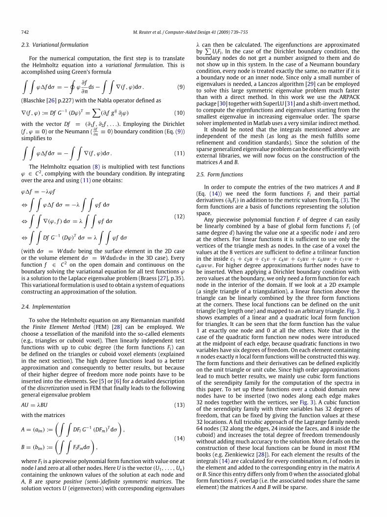
be linearly combined by a base of global form functions Fi (ofsame degree d) having the value one at a specific node i and zeroat the others. For linear functions it is sufficient to use only thevertices of the triangle mesh as nodes. In the case of a voxel thevalues at the 8 vertices are sufficient to define a trilinear functionin the inside c1 + c2u + c3v + c4w + c5uv + c6uw + c7vw +c8uvw. For higher degree approximations further nodes have tobe inserted. When applying a Dirichlet boundary condition withzero values at the boundary, we only need a form function for eachnode in the interior of the domain. If we look at a 2D example(a single triangle of a triangulation), a linear function above thetriangle can be linearly combined by the three form functionsat the corners. These local functions can be defined on the unittriangle (leg length one) andmapped to an arbitrary triangle. Fig. 3shows examples of a linear and a quadratic local form functionfor triangles. It can be seen that the form function has the value1 at exactly one node and 0 at all the others. Note that in thecase of the quadratic form function new nodes were introducedat the midpoint of each edge, because quadratic functions in twovariables have six degrees of freedom. On each element containingn nodes exactly n local form functionswill be constructed this way.The form functions and their derivatives can be defined explicitlyon the unit triangle or unit cube. Since high order approximationslead to much better results, we mainly use cubic form functionsof the serendipity family for the computation of the spectra inthis paper. To set up these functions over a cuboid domain newnodes have to be inserted (two nodes along each edge makes32 nodes together with the vertices, see Fig. 3). A cubic functionof the serendipity family with three variables has 32 degrees offreedom, that can be fixed by giving the function values at these32 locations. A full tricubic approach of the Lagrange family needs64 nodes (32 along the edges, 24 inside the faces, and 8 inside thecuboid) and increases the total degree of freedom tremendouslywithout adding much accuracy to the solution. More details on theconstruction of these local functions can be found in most FEMbooks (e.g. Zienkiewicz [28]). For each element the results of theintegrals (14) are calculated for every combinationm, l of nodes inthe element and added to the corresponding entry in the matrix Aor B. Since this entry differs only from 0when the associated globalform functions Fi overlap (i.e. the associated nodes share the sameelement) the matrices A and Bwill be sparse.


Fig. 3. A linear and a quadratic form function and location of 32 nodes for cubicserendipity FEM voxel.

2.6. Cuboid voxel elements

For piecewise flat objects the computation described abovecan be simplified, thus speeding up the construction of the twomatrices A and B significantly. If the local geometry is flat we donot need to integrate numerically on themanifold since themetricG (see Eq. (3)) is constant throughout each element. The integralscan be computed once for the unit element explicitly and thenmapped linearly to the corresponding element. This makes thetime consuming numerical integration process needed for curvedsurfaces or solids completely unnecessary.As opposed to the case of a surface triangulation with a

piecewise flat triangle mesh (with possibly different types oftriangles), the uniform decomposition of a 3D solid into cuboidvoxels leads to even simpler finite elements. A parametrizationover the unit cube of a cuboidwith side length s1, s2, s3 (and volumeV ) yields a diagonal first fundamental matrix G:

G = diag((s1)2, (s2)2, (s3)2

)(15)

W =√det(G) = (s1)2(s2)2(s3)2 = V (16)

G−1 = diag(1(s1)2

,1(s2)2

,1(s3)2

). (17)

These values are not only constant for an entire voxel, they areidentical for each voxel (since the voxels are identical). Thereforewe can pre-compute the contribution of every voxel to thematrices A and B once for the whole problem after setting up theform functions Fl as described above:

al(i),m(j)+ = V∫ ∫ 1

0

∫ (3∑k=1

∂kFi ∂kFj(sk)2

)dudvdw

bl(i),m(j)+ = V∫ ∫ 1

0

∫FiFjdudvdw.

(18)

The local indices i, j label the (e.g. 32) nodes of the cuboid voxelelement and thus the corresponding local form functions and theirpartial derivatives. These integrals can be pre-computed for everycombination i, j. In order to add (+ =) these local results into thelarge matrices A and B only a lookup of the global vertex indicesl(i),m(j) for each voxel is necessary. Therefore the constructionof the matrices A and B can be accomplished in O(n) time for nelements.

2.7. Normalizing the spectrum

As mentioned above, the Laplace–Beltrami spectrum is adiverging sequence. Analytic solutions for the spectrum and theeigenfunctions are only known for a limited number of shapes(e.g., the sphere, the cuboid, the cylinder, the solid ball). Theeigenvalues for the unit 2-sphere for example are λi = i(i + 1),i ∈ N0 with multiplicity 2i + 1. In general the eigenvaluesasymptotically tend to a linewith a slope dependent on the surfacearea of the 2D manifoldM

λn ∼4πnarea(M)

, as n ↑ ∞. (19)

Therefore a difference in surface area manifests itself in differentslopes of the eigenvalue asymptotes. Fig. 4 shows the behaviorof the spectra of a population of spheres and a population ofellipsoids respectively. The sphere population is based on a unitsphere where Gaussian noise is added in the direction normalto the surface of the noise-free sphere. Gaussian noise is addedin the same way to the ellipsoid population. Since the twobasic shapes (sphere and ellipsoid) differ in surface area, theirunnormalized spectra diverge (Fig. 4a), so larger eigenvalues leadto a better discrimination of groups. Surface area normalizationgreatly improves the spectral alignment (Fig. 4b). Fig. 4c and dshow zoom-ins of the spectra for small eigenvalues. Even for thesurface area normalized case, the spectra of the two populationsclearly differ. Therefore the spectra can be used to pick up thedifference in shape in addition to the size differences.A similar analysis can be done for 3D solids. The eigenvalues for

the cuboid (3D solid) with side length s1, s2 and s3 for example are

λM,N,O = π2(M2

(s1)2+N2

(s2)2+O2

(s3)2

)with M,N,O ∈ N+ for the Dirichlet case and M,N,O ∈ N for theNeumann case. In general the Dirichlet and Neumann eigenvaluesof a 3D solid asymptotically tend to a curve dependent on thevolume of the 3D manifoldM:

λn ∼

(6π2nvol(M)

) 23

, as n ↑ ∞. (20)

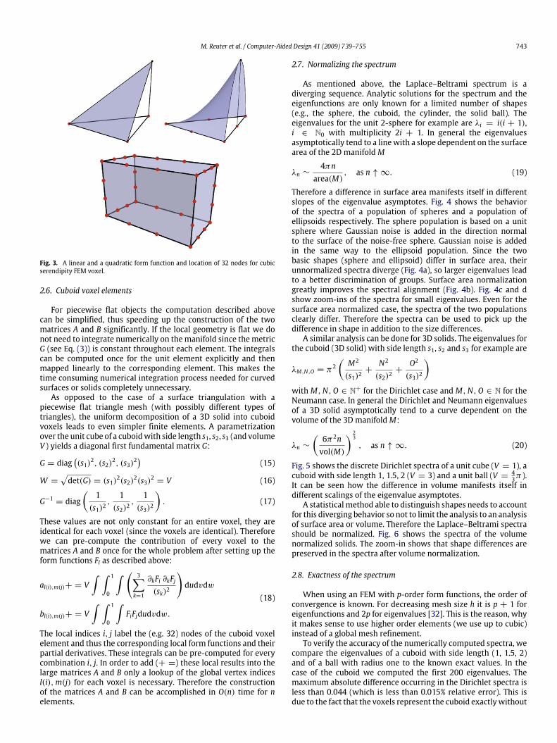
Fig. 5 shows the discrete Dirichlet spectra of a unit cube (V = 1), acuboid with side length 1, 1.5, 2 (V = 3) and a unit ball (V = 4

3π ).It can be seen how the difference in volume manifests itself indifferent scalings of the eigenvalue asymptotes.A statistical method able to distinguish shapes needs to account

for this diverging behavior so not to limit the analysis to an analysisof surface area or volume. Therefore the Laplace–Beltrami spectrashould be normalized. Fig. 6 shows the spectra of the volumenormalized solids. The zoom-in shows that shape differences arepreserved in the spectra after volume normalization.

2.8. Exactness of the spectrum

When using an FEM with p-order form functions, the order ofconvergence is known. For decreasing mesh size h it is p + 1 foreigenfunctions and 2p for eigenvalues [32]. This is the reason, whyit makes sense to use higher order elements (we use up to cubic)instead of a global mesh refinement.To verify the accuracy of the numerically computed spectra, we

compare the eigenvalues of a cuboid with side length (1, 1.5, 2)and of a ball with radius one to the known exact values. In thecase of the cuboid we computed the first 200 eigenvalues. Themaximum absolute difference occurring in the Dirichlet spectra isless than 0.044 (which is less than 0.015% relative error). This isdue to the fact that the voxels represent the cuboid exactlywithout


Fig. 4. Spectral behavior from top to bottom: (a) unnormalized, (b) Areanormalized, (c) unnormalized (zoom), (d) Area normalized (zoom).

any approximation error at the boundary. The Neumann spectrahave only a maximum absolute difference of less than 0.01 (whichis less than 0.005% relative error), due to the higher resolution atthe boundary.In the case of the ball an exact voxel representation is not

possible, therefore the numerical results differ more strongly fromthe analytical ones especially for high eigenvalues (up to 6%relative error for the first 100 Dirichlet eigenvalues). Since theexact values of the object represented by the voxelization areunknown, a fair analysis of the accuracy of the computation isdifficult. Nevertheless, it is interesting to see that the numericalvalues closely approximate the exact ones of the ball the morevoxels are used (see Fig. 7, the value r describes the number ofvoxels used in the direction of the radius).

Fig. 5. Unnormalized exact spectra of cube, cuboid, ball.

Fig. 6. Volume normalized spectra and zoom-in.

Fig. 7. Approximation of the ball.


Fig. 8. The first 150 eigenvalues of the cube with tail subtracted from theeigenvalues of the cube for the Dirichlet and Neumann case.

2.9. Neumann spectrum

To demonstrate that Neumann spectra can be used to pick upsignificant geometric features much faster than Dirichlet spectrathe eigenvalues of the cube with a tail (see Fig. 8, left) werecomputed for the Neumann and the Dirichlet boundary conditionand compared to the values of the cube. Fig. 8 (right) showsthe differences of the first 150 eigenvalues for the two differentboundary conditions. Since the cube with tail has a larger volume,its eigenvalues are expected to be smaller than the values of thecube (see Section 2.2(ii)). This fact is reflected in the graph (Fig. 8,right) where the differences are always positive. It can be clearlyseen that the Neumann spectrum picks up the differences muchearlier than the Dirichlet spectrum. This is due to the fact that theNeumann boundary condition allows the solutions to oscillate atthe boundary whereas the Dirichlet condition forces them to bezero on the boundary, strongly reducing their freedom especiallyin the region of the tail.A 2D example of a square with a tail (ST ) illustrates the different

behaviors of Neumann and Dirichlet boundary conditions. Figs. 9and 10 depict a comparison of a few eigenfunctions of the squarewith tail (ST ) and of the unit square (S1) for both the Dirichletand the Neumann case. For the Dirichlet case (Fig. 9), the lowereigenfunctions do not detect the attached tail (Fig. 9a,e and b,f).For higher frequencies the nodal domains shrink (Fig. 9c,g) untilthey are finally able to slip into the smaller features. Because of therestrictive Dirichlet boundary condition, this only occurs aroundthe 18th eigenfunction. From a signal processing point of view itis sensible that functions with higher frequencies can be used toanalyze smaller features.The Neumann spectrum behaves differently (Fig. 10). Because

of the higher degree of freedom (with respect to the freevibration of the eigenfunctions at the boundary), small featureslike the tail influence the eigenfunctions already very early. It isunnecessary to compare the smallest eigenvalue which is alwayszero with constant eigenfunctions. But already the first non-constant eigenfunction (Fig. 10d) is very different from the firstnon-constant eigenfunctions of the square (Fig. 10a) since theextremum is shifted into the tail. This is reflected in a changeof more than 50% of the corresponding eigenvalue. The nexteigenfunction (Fig. 10e) of ST on the other hand is zero in thetail region and therefore almost identical with (Fig. 10a). Thecorresponding eigenvalues are almost the same. Also the next feweigenfunctions (Fig. 10 b ↔ f and c ↔ g) correspond with eachother on the square region.

2.10. Influence of noise

As demonstrated in Section 2.7, volumenormalizations can leadto good spectral alignments. Nevertheless, having identical noise

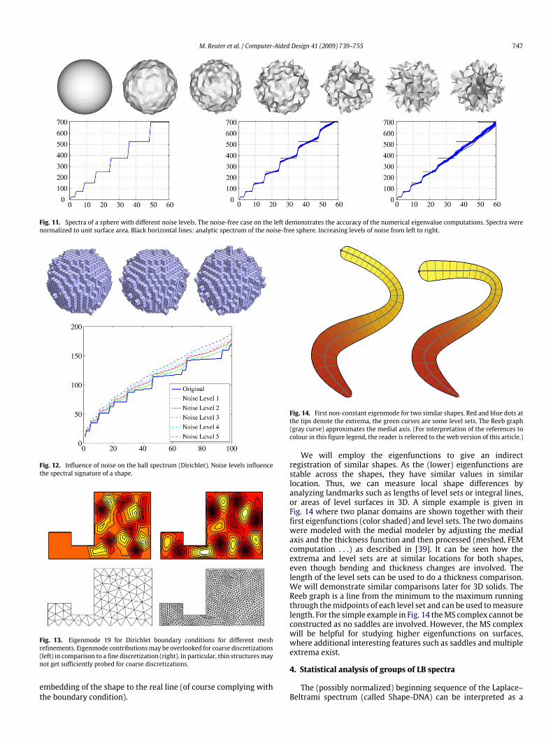
levels for the shape populations under investigation is essential,since different noise levelswill affect surface areas differently (highnoise levels yield highly irregular bounding surfaces especially ifthe voxel resolution is low). Because surface area is contained inthe spectrum this has an influence on the eigenvalues. Violating theassumption of similar noise levels therefore leads to the detectionof noise level differences as opposed to shape differences, asdemonstrated in Fig. 11 for noisy spheres (surfaces) and Fig. 12where the spectra of the ball (solid) are depicted with differentlevels of added noise. A fixed probability for adding a voxel to orremoving a voxel from the object boundary was chosen for eachexperiment. Only voxels maintaining 6-connectivity were addedor removed, guaranteeing a single 6-connected solid component.Increasing the noise level moves the corresponding spectra furtherapart. It can be seen in Fig. 12 that the ball cannot be accuratelyrepresented with only a low voxel resolution, especially with highnoise levels, the spectramove far apart. Such a noisy ball could alsobe seen as a noisy cube. For the analysis of identically acquired andprocessed shapes – e.g., obtained through manual segmentationsof MRI (magnetic resonance image) data – a similar noise level is areasonable assumption;we also assume the accuracy of the spectracalculations to stay the same for the whole population.

2.11. Influence of the discretization

Domain discretizations can significantly affect computationalresults. Fig. 13 shows a 2D example for a domain consistingof a small and a large square connected by a thin rectangle.Insufficient degrees of freedom, due to a coarse discretization,can lead to insufficiently resolved vibrational modes. In particular,thin structures may simply be overlooked if not enough nodesare contained in them. The Neumann spectra are not influencedas strongly by the discretization, as they allow free nodes on theboundary.

3. Topological analysis of eigenfunctions

Eigenfunctions are real-valued functions defined on the wholemanifold. They aremore difficult to deal with than eigenvalues butcan be studied with topological methods, for example analyzinglevel sets and critical points. For the topological analysis ofeigenfunctions we will construct the Morse–Smale (MS) complexon 2D surface representations and the Reeb graph inside the 3Dvoxel volume.The MS complex [33,34] splits the domain of a function h into

regions of uniform gradient flow. Its edges are specific integrallines (maximal paths on the surface and whose tangent vectorsagree with the gradient of h) that run from the saddles to theextrema. For the construction of the MS complex for piecewiselinear functions on triangulated surfaces see [35], where theconcept of persistence is also described. It can be used, for example,to remove topological noise from the complex by pairing andcanceling saddle/extrema combinations.The MS complex is closely related to the Reeb graph [36], that

captures the evolution of the level set components of the functionand is often used in shape analysis applications. A level set is thepre-image h−1(x) for a specific level x ∈ R. The Reeb graph of afunction h is obtained by contracting the connected componentsof the level sets to points. Thus the branching points and leaves(end points) in a Reeb graph correspond to level set componentsthat contain a critical point of h. The leaves are the extrema whilethe branching points are saddles, where one edge is split intotwo (or more) or where edges are merged. The other points canbe considered to lie on the edges between leaves and branchingpoints. Note that the Reeb graph is a 1D topological structure(a graph) with no preferred way of drawing it in the plane or space


Fig. 9. Eigenfunctions for Dirichlet boundary conditions for a square (top) and a square with tail (bottom). Low frequency (low eigenvalue) eigenfunctions do not probe thetail region due to the restrictive Dirichlet boundary conditions. Differences are picked up for high frequencies only where the higher spatial frequencies of the eigenfunctionsallow for a probing of the tail region.

Fig. 10. Eigenfunctions for Neumann boundary conditions for a square (top) and a square with a tail (bottom). Differences between the shapes are picked up already forsmall eigenvalues, since the Neumann boundary conditions allow the tail to swing freely for low frequencies.

or attaching it to M (as opposed to the MS complex). Its edges areoftenmanually attached to the shape by selecting the center of therepresented level set.Both theMS complex and the Reeb graph have been extensively

used for shape processing and topological simplification. e.g. theMS complex has been constructed for a user selected eigenfunctionof the mesh Laplacian for the purpose of meshing in [37].So why is it of interest to study the eigenfunctions at

all? In fact in addition to their relation to the corresponding

eigenvalue (as demonstrated in the examples) they have someinteresting properties. They are also isometry invariant and changecontinuouslywhen the shape is deformed (althoughwhen orderedaccording to the magnitude of their eigenvalues, the orderingmight switch). The functions with the smallest eigenvalues aremore robust against shape change or noise, as they presentthe lower frequency modes. Another feature is their optimalembedding property used in manifold learning (see [38]). Forexample the first non-constant eigenfunction gives the smoothest


Fig. 11. Spectra of a sphere with different noise levels. The noise-free case on the left demonstrates the accuracy of the numerical eigenvalue computations. Spectra werenormalized to unit surface area. Black horizontal lines: analytic spectrum of the noise-free sphere. Increasing levels of noise from left to right.

Fig. 12. Influence of noise on the ball spectrum (Dirichlet). Noise levels influencethe spectral signature of a shape.

Fig. 13. Eigenmode 19 for Dirichlet boundary conditions for different meshrefinements. Eigenmode contributionsmay be overlooked for coarse discretizations(left) in comparison to a fine discretization (right). In particular, thin structuresmaynot get sufficiently probed for coarse discretizations.

embedding of the shape to the real line (of course complying withthe boundary condition).

Fig. 14. First non-constant eigenmode for two similar shapes. Red and blue dots atthe tips denote the extrema, the green curves are some level sets. The Reeb graph(gray curve) approximates the medial axis. (For interpretation of the references tocolour in this figure legend, the reader is referred to the web version of this article.)

We will employ the eigenfunctions to give an indirectregistration of similar shapes. As the (lower) eigenfunctions arestable across the shapes, they have similar values in similarlocation. Thus, we can measure local shape differences byanalyzing landmarks such as lengths of level sets or integral lines,or areas of level surfaces in 3D. A simple example is given inFig. 14 where two planar domains are shown together with theirfirst eigenfunctions (color shaded) and level sets. The two domainswere modeled with the medial modeler by adjusting the medialaxis and the thickness function and then processed (meshed, FEMcomputation . . .) as described in [39]. It can be seen how theextrema and level sets are at similar locations for both shapes,even though bending and thickness changes are involved. Thelength of the level sets can be used to do a thickness comparison.We will demonstrate similar comparisons later for 3D solids. TheReeb graph is a line from the minimum to the maximum runningthrough themidpoints of each level set and can be used tomeasurelength. For the simple example in Fig. 14 theMS complex cannot beconstructed as no saddles are involved. However, the MS complexwill be helpful for studying higher eigenfunctions on surfaces,where additional interesting features such as saddles andmultipleextrema exist.

4. Statistical analysis of groups of LB spectra

The (possibly normalized) beginning sequence of the Laplace–Beltrami spectrum (called Shape-DNA) can be interpreted as a


point v ∈ Rn≥0 in the n-dimensional positive Euclidean space.

Given the Shape-DNA vi of many individual objects divided intotwo populations A and B we use permutation tests to comparegroup features to each other (200,000 permutations were usedfor all tests). We call a set of objects the object population.Permutation testing is a nonparametric, computationally simpleway of establishing group differences by randomly permutinggroup labels. Let SA = {vi} and SB = {vj} denote two sets ofShape-DNA associated to individuals for group A and for groupB respectively. Assume for example that we want to investigateif elements in SA have on average a larger Euclidean norm thanthe elements in SB (due to some external influences). A possibletest statistic stat would be the sum of the lengths of the elementsin SA (stat :=

∑vi∈SA‖vi‖). For the permutation test we then

randomly distribute the subjects into groups A and B, keeping thenumber of elements per group fixed. We define the p-value to bethe fraction of these permutations having a greater or equal sumstat than the original set SA (in other words the relative frequencyof occasions where the random label outperforms the originallabeling). The values of SA will be considered significantly largerthan the ones of SB at a prespecified significance level α if p ≤ α(taken as α = 5% here). Note, that rejecting the null hypothesisof two populations being equal given a significance level α onlyimplies that the probability of making a type I error (i.e., theprobability of detecting false positives; ‘‘detecting a differencewhen there is none in reality’’) is α, but does not exclude thepossibility of making such an error.Confidence intervals for the estimated p-values p̂ may be

computed following Nettleton et al. [40] for 100(1 − γ )%confidence as(p̂− Ψ−1

(1−

γ

2

)√p̂(1− p̂)/N,

p̂+ Ψ−1(1−

γ

2

)√p̂(1− p̂)/N

)where

Ψ−1(x) =√2 erf −1(2x− 1)

is the inverse of the cumulative distribution function of thestandard normal distribution, erf −1(·) is the inverse error function,N denotes the number of samples (200,000 in our case). Theapproximation is based on the binomial distribution and holds forNp ≥ 5. Fig. 15 shows the confidence intervals for a confidencerange of [90%, 99%] for p-values p ∈ {0.0001, 0.05}. Note,that the plots are the same, except for scaling, which dependsonly on the different p-values. While these are just probabilisticcharacterizations of the confidence in the estimated p-value theydemonstrate that using 200,000 permutations will give goodestimations up to the first or even the second non-zero decimalplace.We use three different kinds of statistical analyses (all shapes

are initially corrected for brain volume differences, also see [41]for details on permutation testing):(1) A nonparametric, permutation test to analyze the scalarquantities: volume and surface area.

(2) A nonparametric, multivariate permutation test based on themaximum t-statistic to analyze the high-dimensional spectralfeature vectors (Shape-DNA in 2D and 3D cases).

(3) Independent permutation tests of the spectral feature vec-tor components across groups (as in (2)), followed by a falsediscovery rate (FDR) approach to correct for multiple compar-isons, to analyze the significance of individual vector compo-nents.

To test scalar values the absolute mean difference is used as thetest statistic s = |µa−µb|, where theµi indicates the groupmeans.Themaximum t-statistic is chosen due to the usually small numberof available samples in medical image analysis, compared to the

dimensionality of the Shape-DNA feature vectors (preventing theuse of the Hotelling T 2 statistic [42]). It is defined as

stat = tmax := max1≤j≤N

|v̄A,j − v̄B,j|SEj

. (21)

Here, N is the vector dimension, v̄A,j indicates the mean of the jthvector component of group A, and SEj is the pooled standard errorestimate of the jth vector component, defined as

SEj =

√(nA − 1)σ 2A,j + (nB − 1)σ

2B,j√

1nA+

1nB

, (22)

where ni is the number of subjects in group i (with i ∈ A, B)and σi,j is the standard deviation of vector component j of group i.The maximum t-statistic is particularly sensitive to differences inat least one of the components of the feature vector [43]. It is asummary statistic, which allows for the detection of differencesbetween feature vectors across populations. However, it doesnot determine which components show statistically significantdifferences.Nevertheless, testing the individual statistical significance of

vector components is possible. Such testing needs to be performedover a whole set of components, since it is usually not knownbeforehand which component of a Shape-DNA vector will be agood candidate for statistical testing. (i.e., we can in general notsimply pick one individual vector component (eigenvalue) forstatistical testing.) To account for multiple comparisons whentesting over a whole set of vector components, the significancelevel needs to be adjusted (since ‘‘the chance of finding differencesthat are purely random in nature increases with the number oftests performed’’). See [44,41] for background on schemes formultiple comparison corrections.

5. Results

Volume measurements are the simplest means of morphome-tric analysis. While volume analysis results are easy to interpret,they only characterize onemorphometric aspect of a structure. Thefollowing Sections describe the Laplace–Beltrami and the volumet-ric Laplace spectrum as amethod for amore complete global struc-tural description using the analysis of a caudate as an exemplarybrain structure. Note, that it makes sense to look at the 2D sur-face and at the 3D solid as the spectra of the surfaces contain otherinformation than the solid spectra. In [6] examples of isospectral3D solids (orthogonal ‘‘GWW’’ prism) were presented, where thespectral analysis of their 2D boundary shells was capable of distin-guishing the shapes.For brevity all results are presented for the right caudate only.

5.1. Populations and pre-processing

Magnetic Resonance Images (MRI) of the brains of thirty-twoneuroleptic-naïve female subjects diagnosedwith Schizotypal Per-sonality Disorder (SPD) and of 29 female normal control subjectswere acquired on a 1.5-T General Electric MR scanner. Spoiled-gradient recalled acquisition (SPGR) images (voxel dimensions0.9375× 0.9375× 1.5 mm) were obtained coronally. The imageswere used to delineate the caudate nucleus (see Fig. 16) and to esti-mate the intracranial content (ICC) used for volume normalizationto adjust for different head sizes. For details see [45].The caudate nucleuswas delineatedmanually by an expert [45].

For the 2D surface analysis the isosurfaces separating the binarylabelmaps of the caudate shapes from the background were ex-tracted using marching cubes (while assuring spherical topology).Analysis was then performed on the resulting triangulated surface


Fig. 15. Confidence intervals for p ∈ {0.0001, 0.05}with N = 200,000 permutations.

Fig. 16. Example of a caudate shape consisting of cuboid voxels (left). Exemplarycaudate surface shape unsmoothed and with spherical harmonics smoothing(right).

directly (referred to as unsmoothed surfaces in what follows) aswell as on the same set of surfaces smoothed and resampled usingspherical harmonics3 (referred to as smoothed surfaces inwhat fol-lows). The unsmoothed surfaces are used as a benchmark datasetsubject to only minimal pre-processing, whereas the smoothedsurfaces are used to demonstrate the influence of additional pre-processing. See Fig. 16(right) for an example of a smoothed and anunsmoothed caudate.

5.2. Volume and area analysis

For comparison, results for a volume and a surface area analysisare shown in Fig. 17. As has been previously reported for thisdataset [45], subjects with schizotypal personality disorder exhibita statistically significant volume reduction compared to the normalcontrol subjects. While smoothing plays a negligible role for thevolume results (smoothed: p = 0.008, volume loss 7.0%, i.e., thereis a chance of p = 0.008 that the volume loss is a random effect;unsmoothed: p = 0.013, volume loss 6.7%), the absolute valuesof the surface area are affected more, since smoothing impactssurface areamore than volume. The results for the female caudatesshow the same trend for the surface areas in the smoothed and theunsmoothed cases.

5.3. Laplace–Beltrami spectrum results (2D surface)

The LB spectrumwas computed for the female caudate popula-tion (on the surfaces) using the two different normalizations:1. The shapes were volume normalized to unit intracranial content(UIC) (using the ICC measurements) to account for differenthead sizes.

3 We used the spherical harmonics surfaces as generated by the UNC shapeanalysis package [1].

Fig. 17. Group comparisons for volume differences (top) and surface areadifferences (bottom). Smoothed results prefix ‘s’, unsmoothed results prefix ‘us’.Volume and surface area reductions are observed for the SPD population incomparison to the normal control population.

2. The shapes were normalized to unit caudate surface area (UCA)to analyze shape differences independently of size.

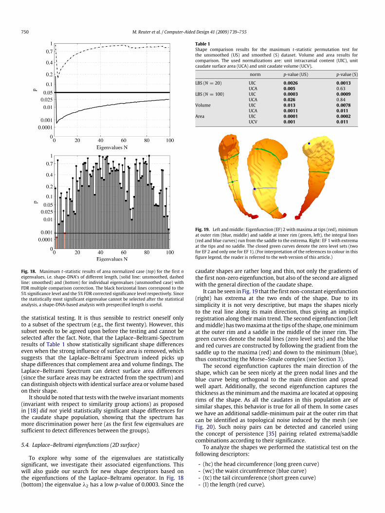
A maximum t-statistic permutation test on a 100D spectral shapedescriptor shows significant shape differences (see Table 1) forcaudate surface area normalization for the unsmoothed surfaces,but not for the smoothed ones. Surface area normalization is thestrictest normalization in terms of spectral alignment. Testing forsurface area independently yields statistically significant results,listed in Table 1.Fig. 18 indicates that using too many eigenvalues has a

slightly detrimental effect on the observed statistical significance.This is sensible, since higher order modes correspond to higherfrequencies and are thus more likely noise, which can overwhelm


Fig. 18. Maximum t-statistic results of area normalized case (top) for the first neigenvalues, i.e. shape-DNA’s of different length, (solid line: unsmoothed, dashedline: smoothed) and (bottom) for individual eigenvalues (unsmoothed case) withFDR multiple comparison correction. The black horizontal lines correspond to the5% significance level and the 5% FDR corrected significance level respectively. Sincethe statistically most significant eigenvalue cannot be selected after the statisticalanalysis, a shape-DNA-based analysis with prespecified length is useful.

the statistical testing. It is thus sensible to restrict oneself onlyto a subset of the spectrum (e.g., the first twenty). However, thissubset needs to be agreed upon before the testing and cannot beselected after the fact. Note, that the Laplace–Beltrami-Spectrumresults of Table 1 show statistically significant shape differenceseven when the strong influence of surface area is removed, whichsuggests that the Laplace–Beltrami Spectrum indeed picks upshape differences that complement area and volume findings. TheLaplace–Beltrami Spectrum can detect surface area differences(since the surface areas may be extracted from the spectrum) andcan distinguish objects with identical surface area or volume basedon their shape.It should be noted that testswith the twelve invariantmoments

(invariant with respect to similarity group actions) as proposedin [18] did not yield statistically significant shape differences forthe caudate shape population, showing that the spectrum hasmore discrimination power here (as the first few eigenvalues aresufficient to detect differences between the groups).

5.4. Laplace–Beltrami eigenfunctions (2D surface)

To explore why some of the eigenvalues are statisticallysignificant, we investigate their associated eigenfunctions. Thiswill also guide our search for new shape descriptors based onthe eigenfunctions of the Laplace–Beltrami operator. In Fig. 18(bottom) the eigenvalue λ2 has a low p-value of 0.0003. Since the

Table 1Shape comparison results for the maximum t-statistic permutation test forthe unsmoothed (US) and smoothed (S) dataset. Volume and area results forcomparison. The used normalizations are: unit intracranial content (UIC), unitcaudate surface area (UCA) and unit caudate volume (UCV).

norm p-value (US) p-value (S)

LBS (N = 20) UIC 0.0026 0.0013UCA 0.005 0.63

LBS (N = 100) UIC 0.0003 0.0009UCA 0.026 0.84

Volume UIC 0.013 0.0078UCA 0.0011 0.011

Area UIC 0.0001 0.0002UCV 0.001 0.011

Fig. 19. Left andmiddle: Eigenfunction (EF) 2 with maxima at tips (red), minimumat outer rim (blue, middle) and saddle at inner rim (green, left), the integral lines(red and blue curves) run from the saddle to the extrema. Right: EF 1 with extremaat the tips and no saddle. The closed green curves denote the zero level sets (twofor EF 2 and only one for EF 1). (For interpretation of the references to colour in thisfigure legend, the reader is referred to the web version of this article.)

caudate shapes are rather long and thin, not only the gradients ofthe first non-zero eigenfunction, but also of the second are alignedwith the general direction of the caudate shape.It can be seen in Fig. 19 that the first non-constant eigenfunction

(right) has extrema at the two ends of the shape. Due to itssimplicity it is not very descriptive, but maps the shapes nicelyto the real line along its main direction, thus giving an implicitregistration along their main trend. The second eigenfunction (leftandmiddle) has twomaxima at the tips of the shape, oneminimumat the outer rim and a saddle in the middle of the inner rim. Thegreen curves denote the nodal lines (zero level sets) and the blueand red curves are constructed by following the gradient from thesaddle up to the maxima (red) and down to the minimum (blue),thus constructing the Morse–Smale complex (see Section 3).The second eigenfunction captures the main direction of the

shape, which can be seen nicely at the green nodal lines and theblue curve being orthogonal to the main direction and spreadwell apart. Additionally, the second eigenfunction captures thethickness as theminimum and themaxima are located at opposingrims of the shape. As all the caudates in this population are ofsimilar shapes, this behavior is true for all of them. In some caseswe have an additional saddle-minimum pair at the outer rim thatcan be identified as topological noise induced by the mesh (seeFig. 20). Such noisy pairs can be detected and canceled usingthe concept of persistence [35] pairing related extrema/saddlecombinations according to their significance.To analyze the shapes we performed the statistical test on the

following descriptors:

- (hc) the head circumference (long green curve)- (wc) the waist circumference (blue curve)- (tc) the tail circumference (short green curve)- (l) the length (red curve).


Fig. 20. Noisy Morse–Smale complex of the second non-constant eigenfunctionon the outer rim (left) and close-up (middle). After canceling the saddle with theclosest minimum, only one minimum remains and the red integral lines from thesaddle to the two maxima at the head and tail disappear. (For interpretation of thereferences to colour in this figure legend, the reader is referred to the web versionof this article.)

We obtained the following p-values for the unit intracranialcontent (UIC) and the unit caudate surface area (UCA) normalizedcases:

UIC UCA

hc p = 0.0015 p = 0.45wc p = 0.0016 p = 0.053tc p = 0.007 p = 0.039l p = 0.21 p = 0.0003

The statistically significant cases are printed in bold. For theintracranial content normalized case significant differences aredetected in all the three circumferences, but not in the lengthsof the shape. The caudate surface area normalization principallyreverses the results. This could be expected as the main surfacearea lies in the shells of these cylindrical shapes and not atthe cylinder caps. Therefore a surface area normalization seemsto adjust the circumferences and changes the lengths instead.Nevertheless, we still pick up statistically significant differences inthe tail region of the shapes (which can also be expected as thehead has more surface area than the tail).The intracranial content normalized results suggest that

shape differences are mainly in shape thickness as opposed toshape length. Fig. 21 shows a group comparison of the waistcircumferences (top) of the ICC normalized shapes, as well as thedifferences in length after caudate area normalization (bottom).Note also that in the unit caudate area case, the length indicates anincrease in mean distance between the nodal lines. This explainswhy the corresponding eigenvalue is also significantly smallerfor the SPD population (as it is related to the frequency of theoscillation, which is related to the size of the oscillating domains).Similar to Fig. 14 it is possible to wrap more level sets around

the caudate shapes (see Fig. 22), with the difference that now weget closed curves. Again the level sets yield an indirect registrationof the shapes and present a method to detect local circumferencedifferences. Note that we could actually construct a commonparametrization (e.g. on the sphere) by taking the level and theposition on the closed level set as the two parameters, but thisexplicit parametrization is not needed. Fig. 23 shows a plot of thelevel set lengths of a few caudate shapes. The p-value for thewholepopulation can be found in Fig. 24 and indicate that not only thethinner regions in the tail (level 0.2) are significantly different, butalso the region at the beginning of the head (level 0.7) shows highlysignificant differences.

5.5. Laplace spectrum results (3D solid)

As we deal with 3D solid objects it makes sense to also lookat the solid instead of analyzing the surface only. The Laplacespectrum of the 3D voxel data was computed for two differentnormalizations:

(i) The shapeswere volumenormalized tounit intracranial content(using the ICC measurements) to account for different headsizes.

(ii) The shapes were normalized to unit caudate volume to analyzeshape differences independently.In order to get more inner nodes especially into the very thin

tail region of the caudate shapeswe additionally employed the dualof the voxel graph. The dual voxel graph is the voxel image whereeach voxel of the original image (regular voxel image) is consideredto be a vertex of the dual graph. Voxels inside the domain becomeinner vertices while voxel just outside the domain’s boundary nowbecome boundary vertices. Fig. 25 depicts a 2D case (using pixels)with the original regular domain on the left and the dual on theright. The dual graph enlarges the domain by half a layer thuscreating new inner nodes needed especially inside the thinnerfeatures (tail). The use of the dual graph is helpful since a globalrefinement of the voxels leads to large FEMmodels that may causememory problems on some standard PC’s. Note that in 3D thenumber of voxels increases by the factor 8 for each refinement step,this will quickly get large, especially if a higher order FEM is used,needing many nodes per voxel. The main difficulty lies in solvingthe large eigenvalue problem as the LU decomposition (SuperLUlibary) might require a lot of additional memory if a large amountof fill-ins is generated.4Since the two populations show significant differences in

volume, surface area, local shape thickness and in their 2D surfacespectra (see above), we expect to find significant differences alsoin their 3D volume spectra. The following paragraphs present firstthe Dirichlet, then at the Neumann spectrum results for both theregular and dual voxel graph.

5.5.1. Dirichlet spectraFig. 26 shows the statistical results for the regular voxel

graph and its dual for the caudate populations. The graph showsthe corresponding p-value (see Section 4) when using the firstN eigenvalues of the spectra for the statistical analysis (unitintracranial content). Recall that not just a single eigenvalue is usedbut the whole beginning sequence of the first N values (thereforewe call these plots accumulated statistic plots). A p-value belowthe 5% horizontal line is considered to be statistically significant. Insuch a case the beginning sequence of the spectrum is consideredto be able to distinguish between the two caudate populations(NC and SPD).Fig. 26 shows that the beginning sequence of the Dirichlet

spectrum does not yield any statistically significant results.Employing the dual graph yields lower p-values when highereigenvalues get involved. This observation is sensible, consideringthe fact that especially in the thin tail part of the caudates onlyvery few inner nodes exist (see Section 2.11 for the effects oflow resolution). The dual graph has more degrees of freedom,introducing inner nodes in the thin tail area, and thereforeimproves the result. In unit caudate volume case we did notfind any significant differences either. For a detailed analysisemploying the Dirichlet spectrum higher voxel resolutions wouldbe necessary. Due to the low voxel resolution the computedeigenfunctions do not seem to accurately represent the realeigenfunctions of the caudate shapes.

5.5.2. Neumann spectraAs demonstrated in Section 2.9, the Neumann spectrum

can help to identify shape differences much earlier than theDirichlet spectrum. Fig. 27 shows the accumulated statisticsplots for different normalizations of the Neumann spectra forthe regular and the dual case. In both cases (regular and dual)

4 The examples in this paper were run on computers with up to 3GB memorywithout any problems.


Fig. 21. Group comparisons for waist circumference differences (left) and length differences (right) after caudate area normalization. A waist length reduction can beobserved for the SPD population in comparison to the normal controls (unit ICC). After caudate area normalization, an increase in length can be seen.

Fig. 22. 100 level sets wrapped around two exemplary caudate shapes using thefirst eigenfunction. The absence of any saddles guarantees that each level set hasonly one component.

Fig. 23. Lengths of level sets (mapped onto the unit interval) of 8 exemplary shapes(sampling at 200 levels). Solid red curves: SPD subjects, dashed curves: normalcontrols.

Fig. 24. p-value for thewhole population on each level set (sampling at 200 levels).The horizontal line marks the significance level corrected for multiple comparisons(FDR).

Fig. 25. Regular pixel domain (left) and its dual (right).

the intracranial content normalized spectra show very similarbehavior (Fig. 27a,b): already very early, significant differencesare detected. Because these differences might simply reflectthe different caudate volumes (known to be significant) anormalization to unit caudate volume (Fig. 27c,d) is applied toreveal volume independent shape differences. The eigenvalues inthe regular case (Fig. 27c) do not show statistically significantshape differences until about 150 eigenvalues are involved,however, the dual case (Fig. 27d) shows a significant p-valuealready for 50 or more eigenvalues used. The reason seemsto be that the higher frequency eigenfunctions have smallernodal domains and can thus better detect the smaller features,presumably in the tail region. This assumption aligns with theDirichlet case (Fig. 26 dual) where better p-values are obtainedwhen employing higher frequencies.The accumulated results in Fig. 27 can be partially explained by

analyzing the p-values of the individual eigenvalues (see Fig. 28).It can be seen that the p-value of the eigenvalue λ5 is very low inboth the regular and the dual voxel graphs (marked in red). Thisleads to significant results very early in the accumulated plots.Furthermore, the low p-values around the 50th eigenvalue (the52nd in particular, also marked in red) in the dual case seem toproduce the significant results in the accumulated plots above.

5.6. Laplace eigenfunctions (3D solid)

Similar to the analysis of interesting eigenfunctions in the 2Dsurface case it makes sense to analyze the eigenfunctions in 3D. Bylooking at the nodal surfaces (zero level sets) of the eigenfunctionsλ5 and λ52 (Fig. 29) it can be noticed that these eigenfunctions,whose gradient field is always orthogonal to the nodal surfaces,again follow the main trend of the shape (for the 52nd functiononly in the tail region). We focus on the 5th eigenfunction (dueto its simplicity) and analyze its nodal surfaces with respect totwo hypotheses. As can be seen in the example in Fig. 29, thenodal surfaces of the 5th eigenfunction are usually 4 separatedcomponents (true in all except for 3 cases). First we want to relatethe eigenfunction to the significant eigenvalue. As the eigenvaluesare the square roots of the frequencies of the oscillation, the sizeof the nodal domains and therefore the distances of the nodalsurfaces (green lines in Fig. 29 bottom) should yield significantresults after the caudate volume normalization. Furthermore, we


Fig. 26. Accumulative maximum t-statistic results (unit intracranial content, Dirichlet) for the regular (left) and the dual (right) voxel graphs. Employing the dual graphyields lower p-values. This may be attributed to the better suitability of the dual graph for probing the thin tail regions of the caudate shapes. However, there is no statisticaldifference at a significance level of α = 5%.

(a) Regular, unit intracranial content. (b) Dual, unit intracranial content.

(c) Regular, unit caudate volume. (d) Dual, unit caudate volume.

Fig. 27. Accumulated statistic, Neumann boundary conditions. Statistically significant shape differences are detected as expected for the unit intracranial content cases (aand b) (due to the caudate volume differences between the SPD and the NC populations). After caudate volume normalization (c and d), differences are first detected for thedual graph analysis (d), presumably because the additional degrees of freedom enable a proper probing of the caudate tail regions.

know from the 2D analysis that significant changes in thickness(before caudate area normalization) are present mainly in the tailregion of the shapes. Therefore, we will test the hypotheses that1. the mean distance of the nodal surfaces (l1) on the unit volumecaudates are larger for the SPD population (leading to a smallereigenvalue EV5).

2. the mean boundary length (l2) and the mean surface area(l3) of the small nodal surface components in the tail region(removing the large component in the head) are smaller for theSPD population.For the first experiment, we compute the barycenter of

the vertices of each nodal surface component and use it as arepresentation of that component. We then connect neighboringcomponents with each other (green line in Fig. 29 bottom) andcompute the mean distance between neighboring components.

Note that the green line is a skeletal representation of the shape.In fact, it is the Reeb graph [36], as each level set componentis represented by a node (red dot) which is connected to itsneighbors by the green edges. Thus, this skeletal model representsthe topological structure of the analyzed eigenfunction EV5 whichyields an interesting shape descriptor, that could be used for otherapplication, such as non-rigid registration. For both experimentsweobtained the followingp-values for theunit intracranial content(UIC) and unit caudate volume (UCV) cases:

UIC UCV

l1 p = 0.21 p = 0.0099l2 p = 0.0001 p = 0.0003l3 p = 0.0019 p = 0.015


Fig. 28. p-values for the individual eigenvalueswith Neumann boundary conditionfor the regular (top) and dual (bottom) voxel graph.

Fig. 29. Nodal surfaces of eigenfunction 52 (top) and 5 (bottom), where thecentroids are connected.

For the first experiment we have significant values for themean distances of the nodal surfaces after caudate volumenormalization. We detect an increase in length for the SPD

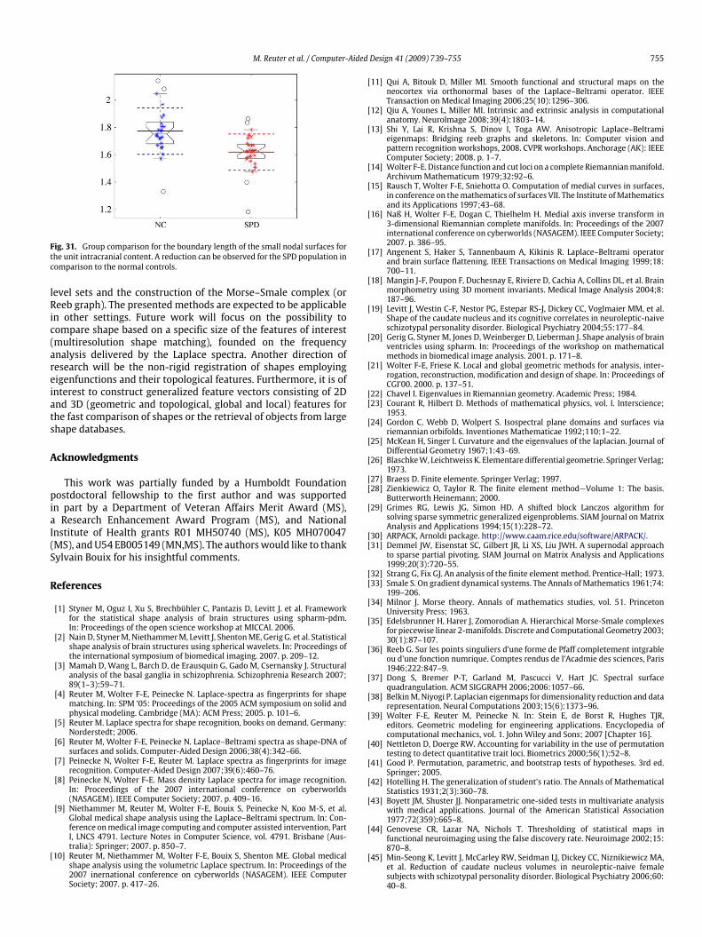
population, which goes in line with the significant decrease ofthe 5th eigenvalue, related to the size of the nodal domains (seeFig. 30). All the values for l2 and l3 are statistically significant,where especially the mean boundary lengths (similar to the waistand tail circumferences in 2D) are highly significant (see also Fig. 31for the direct comparison of the boundary lengths in the UIC case).

6. Conclusion

This paper describesmethods for global and local shape analysisusing the Laplace–Beltrami eigenvalues and eigenfunctions withDirichlet andNeumannboundary conditions for 2D surfaces (trian-glemeshes) and 3D volumetric solids (voxel data). The eigenvaluesand eigenfunctions including their geometric and topological fea-tures are defined invariantly wrt. mesh, location, parametrizationand depend on the isometry type only. Our experiments corrobo-rate their robustness wrt. noise. We demonstrated their discrimi-nation power successfully at a real application in medical imagingto distinguish populations of similar shapes.The Laplace–Beltrami eigenvalues are well suited as a global

shape descriptor, without the need to register the shapes. Theycould successfully be employed to detect true shape differencesof the two populations (using the maximum t-statistic) evenafter normalization hinting at caudate shape differences inSchizotypal Personality Disorder. It could be demonstrated thatthe volumetric Neumann spectra can detect statistically significantshape differences when applied directly to the voxel data. Thesecomputations are feasible on a standard desktop computer. TheNeumann spectra are of interest, since they recognize shapedifferences much earlier than the Dirichlet spectra and also workmuch better if the voxel resolution is very low. Especially thehigher eigenvalues yield statistically significant results, indicatingtrue shape differences mainly in areas with smaller features.Additionally, we proposed a novelmethod to employ the eigen-

functions on surfaces for the detection and registration of featuresacross shapes. We introduced a topological analysis (Morse–Smalecomplex and nodal curves) of selected eigenfunctions to define ge-ometric features and to localize shape differences (here the localthickness of the caudate shapes). Also the topological analysis ofeigenfunctions in 3D data is new and yields interesting geometricentities (distance, boundary length and surface areas of nodal sur-faces) which underline the shape differences in the presented ap-plication (thickness differences and length differences for the unitvolume caudates). These geometric properties also contribute to-wards an interpretation of the corresponding eigenvalues.The presented results are promising and show that the spectra

(eigenfunctions and eigenvalues) of the Laplace–Beltrami operatorare capable shape descriptors, especially when combined with atopological analysis, such as locations of extrema, behavior of the

Fig. 30. Group comparison for the eigenvalue 5 (left) and mean distance of the nodal surfaces (right) for the unit intracranial content. A reduction of the eigenvalue and acorresponding increase of the distances can be observed for the SPD population in comparison to the normal controls.


Fig. 31. Group comparison for the boundary length of the small nodal surfaces forthe unit intracranial content. A reduction can be observed for the SPD population incomparison to the normal controls.

level sets and the construction of the Morse–Smale complex (orReeb graph). The presented methods are expected to be applicablein other settings. Future work will focus on the possibility tocompare shape based on a specific size of the features of interest(multiresolution shape matching), founded on the frequencyanalysis delivered by the Laplace spectra. Another direction ofresearch will be the non-rigid registration of shapes employingeigenfunctions and their topological features. Furthermore, it is ofinterest to construct generalized feature vectors consisting of 2Dand 3D (geometric and topological, global and local) features forthe fast comparison of shapes or the retrieval of objects from largeshape databases.

Acknowledgments

This work was partially funded by a Humboldt Foundationpostdoctoral fellowship to the first author and was supportedin part by a Department of Veteran Affairs Merit Award (MS),a Research Enhancement Award Program (MS), and NationalInstitute of Health grants R01 MH50740 (MS), K05 MH070047(MS), andU54 EB005149 (MN,MS). The authorswould like to thankSylvain Bouix for his insightful comments.

References

[1] Styner M, Oguz I, Xu S, Brechbühler C, Pantazis D, Levitt J. et al. Frameworkfor the statistical shape analysis of brain structures using spharm-pdm.In: Proceedings of the open science workshop at MICCAI. 2006.

[2] Nain D, StynerM, NiethammerM, Levitt J, ShentonME, Gerig G. et al. Statisticalshape analysis of brain structures using spherical wavelets. In: Proceedings ofthe international symposium of biomedical imaging. 2007. p. 209–12.

[3] Mamah D, Wang L, Barch D, de Erausquin G, Gado M, Csernansky J. Structuralanalysis of the basal ganglia in schizophrenia. Schizophrenia Research 2007;89(1–3):59–71.

[4] Reuter M, Wolter F-E, Peinecke N. Laplace-spectra as fingerprints for shapematching. In: SPM ’05: Proceedings of the 2005 ACM symposium on solid andphysical modeling. Cambridge (MA): ACM Press; 2005. p. 101–6.

[5] Reuter M. Laplace spectra for shape recognition, books on demand. Germany:Norderstedt; 2006.

[6] Reuter M, Wolter F-E, Peinecke N. Laplace–Beltrami spectra as shape-DNA ofsurfaces and solids. Computer-Aided Design 2006;38(4):342–66.

[7] Peinecke N, Wolter F-E, Reuter M. Laplace spectra as fingerprints for imagerecognition. Computer-Aided Design 2007;39(6):460–76.

[8] Peinecke N, Wolter F-E. Mass density Laplace spectra for image recognition.In: Proceedings of the 2007 international conference on cyberworlds(NASAGEM). IEEE Computer Society; 2007. p. 409–16.

[9] Niethammer M, Reuter M, Wolter F-E, Bouix S, Peinecke N, Koo M-S, et al.Global medical shape analysis using the Laplace–Beltrami spectrum. In: Con-ference onmedical image computing and computer assisted intervention, PartI, LNCS 4791. Lecture Notes in Computer Science, vol. 4791. Brisbane (Aus-tralia): Springer; 2007. p. 850–7.

[10] Reuter M, Niethammer M, Wolter F-E, Bouix S, Shenton ME. Global medicalshape analysis using the volumetric Laplace spectrum. In: Proceedings of the2007 inernational conference on cyberworlds (NASAGEM). IEEE ComputerSociety; 2007. p. 417–26.

[11] Qui A, Bitouk D, Miller MI. Smooth functional and structural maps on theneocortex via orthonormal bases of the Laplace–Beltrami operator. IEEETransaction on Medical Imaging 2006;25(10):1296–306.

[12] Qiu A, Younes L, Miller MI. Intrinsic and extrinsic analysis in computationalanatomy. NeuroImage 2008;39(4):1803–14.

[13] Shi Y, Lai R, Krishna S, Dinov I, Toga AW. Anisotropic Laplace–Beltramieigenmaps: Bridging reeb graphs and skeletons. In: Computer vision andpattern recognition workshops, 2008. CVPR workshops. Anchorage (AK): IEEEComputer Society; 2008. p. 1–7.

[14] Wolter F-E. Distance function and cut loci on a complete Riemannianmanifold.ArchivumMathematicum 1979;32:92–6.

[15] Rausch T, Wolter F-E, Sniehotta O. Computation of medial curves in surfaces,in conference on themathematics of surfaces VII. The Institute ofMathematicsand its Applications 1997;43–68.

[16] Naß H, Wolter F-E, Dogan C, Thielhelm H. Medial axis inverse transform in3-dimensional Riemannian complete manifolds. In: Proceedings of the 2007international conference on cyberworlds (NASAGEM). IEEE Computer Society;2007. p. 386–95.

[17] Angenent S, Haker S, Tannenbaum A, Kikinis R. Laplace–Beltrami operatorand brain surface flattening. IEEE Transactions on Medical Imaging 1999;18:700–11.

[18] Mangin J-F, Poupon F, Duchesnay E, Riviere D, Cachia A, Collins DL, et al. Brainmorphometry using 3D moment invariants. Medical Image Analysis 2004;8:187–96.

[19] Levitt J, Westin C-F, Nestor PG, Estepar RS-J, Dickey CC, Voglmaier MM, et al.Shape of the caudate nucleus and its cognitive correlates in neuroleptic-naiveschizotypal personality disorder. Biological Psychiatry 2004;55:177–84.

[20] Gerig G, Styner M, Jones D,Weinberger D, Lieberman J. Shape analysis of brainventricles using spharm. In: Proceedings of the workshop on mathematicalmethods in biomedical image analysis. 2001. p. 171–8.

[21] Wolter F-E, Friese K. Local and global geometric methods for analysis, inter-rogation, reconstruction, modification and design of shape. In: Proceedings ofCGI’00. 2000. p. 137–51.

[22] Chavel I. Eigenvalues in Riemannian geometry. Academic Press; 1984.[23] Courant R, Hilbert D. Methods of mathematical physics, vol. I. Interscience;

1953.[24] Gordon C, Webb D, Wolpert S. Isospectral plane domains and surfaces via

riemannian orbifolds. Inventiones Mathematicae 1992;110:1–22.[25] McKean H, Singer I. Curvature and the eigenvalues of the laplacian. Journal of

Differential Geometry 1967;1:43–69.[26] BlaschkeW, Leichtweiss K. Elementare differential geometrie. SpringerVerlag;

1973.[27] Braess D. Finite elemente. Springer Verlag; 1997.[28] Zienkiewicz O, Taylor R. The finite element method—Volume 1: The basis.

Butterworth Heinemann; 2000.[29] Grimes RG, Lewis JG, Simon HD. A shifted block Lanczos algorithm for

solving sparse symmetric generalized eigenproblems. SIAM Journal on MatrixAnalysis and Applications 1994;15(1):228–72.

[30] ARPACK, Arnoldi package. http://www.caam.rice.edu/software/ARPACK/.[31] Demmel JW, Eisenstat SC, Gilbert JR, Li XS, Liu JWH. A supernodal approach

to sparse partial pivoting. SIAM Journal on Matrix Analysis and Applications1999;20(3):720–55.

[32] Strang G, Fix GJ. An analysis of the finite element method. Prentice-Hall; 1973.[33] Smale S. On gradient dynamical systems. The Annals of Mathematics 1961;74:

199–206.[34] Milnor J. Morse theory. Annals of mathematics studies, vol. 51. Princeton

University Press; 1963.[35] Edelsbrunner H, Harer J, Zomorodian A. Hierarchical Morse-Smale complexes

for piecewise linear 2-manifolds. Discrete and Computational Geometry 2003;30(1):87–107.

[36] Reeb G. Sur les points singuliers d’une forme de Pfaff completement intgrableou d’une fonction numrique. Comptes rendus de l’Acadmie des sciences, Paris1946;222:847–9.

[37] Dong S, Bremer P-T, Garland M, Pascucci V, Hart JC. Spectral surfacequadrangulation. ACM SIGGRAPH 2006;2006:1057–66.

[38] BelkinM, Niyogi P. Laplacian eigenmaps for dimensionality reduction and datarepresentation. Neural Computations 2003;15(6):1373–96.

[39] Wolter F-E, Reuter M, Peinecke N. In: Stein E, de Borst R, Hughes TJR,editors. Geometric modeling for engineering applications. Encyclopedia ofcomputational mechanics, vol. 1. John Wiley and Sons; 2007 [Chapter 16].

[40] Nettleton D, Doerge RW. Accounting for variability in the use of permutationtesting to detect quantitative trait loci. Biometrics 2000;56(1):52–8.

[41] Good P. Permutation, parametric, and bootstrap tests of hypotheses. 3rd ed.Springer; 2005.

[42] Hotelling H. The generalization of student’s ratio. The Annals of MathematicalStatistics 1931;2(3):360–78.

[43] Boyett JM, Shuster JJ. Nonparametric one-sided tests in multivariate analysiswith medical applications. Journal of the American Statistical Association1977;72(359):665–8.

[44] Genovese CR, Lazar NA, Nichols T. Thresholding of statistical maps infunctional neuroimaging using the false discovery rate. Neuroimage 2002;15:870–8.

[45] Min-Seong K, Levitt J, McCarley RW, Seidman LJ, Dickey CC, Niznikiewicz MA,et al. Reduction of caudate nucleus volumes in neuroleptic-naive femalesubjects with schizotypal personality disorder. Biological Psychiatry 2006;60:40–8.

http://www.caam.rice.edu/software/ARPACK/

laplace-beltrami eigenvalues and topological features of eigenfunctions for statistical shape...

Documents