labour shortages and wage growth - european central bank
TRANSCRIPT
Working Paper Series Labour shortages and wage growth
Erik Frohm
Disclaimer: This paper should not be reported as representing the views of the European Central Bank (ECB). The views expressed are those of the authors and do not necessarily reflect those of the ECB.
No 2576 / July 2021
Abstract
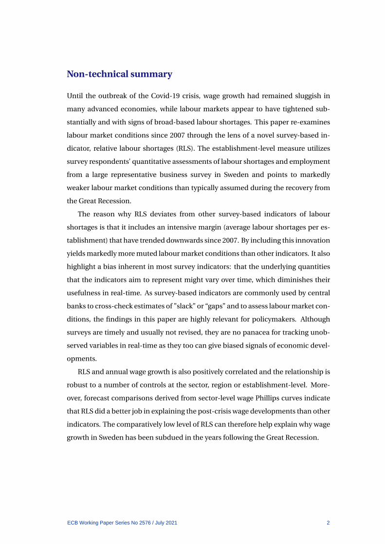
Tight labour markets are usually accompanied by mounting wage pres-sures. Yet, in the past decade, wage growth has remained subdued despite theappearance of widespread labour shortages. This paper re-examines labourmarket conditions since 2007 through the lens of a novel indicator, relativelabour shortages (RLS), based on data from a large representative business sur-vey in Sweden. Four main results emerge from the analysis: (1), the time-seriesaverage of RLS suggested much weaker labour market conditions during the2013–2019 recovery from the Great Recession and during the Covid-19 pan-demic in 2020 than qualitative surveys or the vacancy-unemployment ratio.(2), the reason is that RLS contains a time-varying intensive margin of labourshortages not recorded in most surveys, which has been trending downwardssince the Great Recession. (3), fixed-effects regressions with several aggregate-,sector, region and establishment-level controls confirm that RLS is stronglyand positively correlated with annual wage growth at the establishment-level. (4), sector-level wage Phillips curves show that the subdued level of RLScan help explain the sluggish wage growth in Sweden since the Great Recession.
Keywords: Wage inflation, labour markets, survey data.
JEL codes: C80, E31, E60, J23, J31.
ECB Working Paper Series No 2576 / July 2021 1
Non-technical summary
Until the outbreak of the Covid-19 crisis, wage growth had remained sluggish in
many advanced economies, while labour markets appear to have tightened sub-
stantially and with signs of broad-based labour shortages. This paper re-examines
labour market conditions since 2007 through the lens of a novel survey-based in-
dicator, relative labour shortages (RLS). The establishment-level measure utilizes
survey respondents’ quantitative assessments of labour shortages and employment
from a large representative business survey in Sweden and points to markedly
weaker labour market conditions than typically assumed during the recovery from
the Great Recession.
The reason why RLS deviates from other survey-based indicators of labour
shortages is that it includes an intensive margin (average labour shortages per es-
tablishment) that have trended downwards since 2007. By including this innovation
yields markedly more muted labour market conditions than other indicators. It also
highlight a bias inherent in most survey indicators: that the underlying quantities
that the indicators aim to represent might vary over time, which diminishes their
usefulness in real-time. As survey-based indicators are commonly used by central
banks to cross-check estimates of ”slack” or “gaps” and to assess labour market con-
ditions, the findings in this paper are highly relevant for policymakers. Although
surveys are timely and usually not revised, they are no panacea for tracking unob-
served variables in real-time as they too can give biased signals of economic devel-
opments.
RLS and annual wage growth is also positively correlated and the relationship is
robust to a number of controls at the sector, region or establishment-level. More-
over, forecast comparisons derived from sector-level wage Phillips curves indicate
that RLS did a better job in explaining the post-crisis wage developments than other
indicators. The comparatively low level of RLS can therefore help explain why wage
growth in Sweden has been subdued in the years following the Great Recession.
ECB Working Paper Series No 2576 / July 2021 2
1. Introduction
Until the outbreak of the Covid-19 crisis, wage growth had remained sluggish in
many advanced economies, despite the appearance of tight labour markets and
broad-based labour shortages. Jerome Powell, chairman of the Federal Reserve
Board in the United States referred to the absence of higher wage growth as a
”puzzle”1 and similar sentiments have been expressed by Andrew Haldane, Chief
Economist of the Bank of England2 and former European Central Bank (ECB) Ex-
ecutive Board member Benoıt Cœure.3 Powell’s puzzle of high resource utilization
and subdued nominal wage growth has also been prominent in Sweden, a small,
open and inflation-targeting economy (Sveriges Riksbank, 2017).
Several explanations have been suggested for the apparent disconnect between
labour market conditions and wages: the ”flattening” of the wage Phillips curve.4
These include the globalization of production (Borio et al., 2018), automation
(Leduc and Liu, 2020), lower matching efficiency in the labour market (Jonsson
and Theobald, 2019) or weaker bargaining power of labour (Krueger, 2018). Other
strands of the literature argue that traditional measures of labour market conditions
underestimate true labour market slack (see for example Hong et al. 2018, Barni-
chon and Mesters 2018 and Abraham et al. 2020) or that the relationship between
wage growth and slack is non-linear (Daly and Hobijn 2014 and Linde and Trabandt
2019).
This paper makes several contributions to the literature. First, it presents a novel
1”But there is still a bit of a puzzle in that we’re hearing about labour shortages now all over thecountry in many, many different occupations in different geographies. And one would have expected, Iwould have expected, that wages would move up a little bit more.”, see Powell (2018).
2”We have seen an unusual pattern emerge here over recent years. Jobs growth has been strong, withover 2 million new jobs created since the end of 2012. But pay growth has remained weak by historicstandards, averaging around 2% annually.”, see Haldane (2018).
3”Despite a rapid fall in the unemployment rate, wages have remained stubbornly low. Annualgrowth in compensation per employee hovered around 1.2% since mid-2014 and only increased to 1.5%at the end of last year – substantially below its historical average of 2.1%”, see Coeure (2017).
4For example, Galı and Gambetti (2019) document changes to the wage Phillips curve in the UnitedStates, with reduced form as well as conditional estimates. They find a declining slope with condi-tional estimates, albeit somewhat less than reduced form estimates would suggest.
ECB Working Paper Series No 2576 / July 2021 3
survey-based measure of labour shortages to track labour market slack, derived
from respondents’ quantitative assessment in a large, representative, business sur-
vey in Sweden, the Public Employment Service’s interview survey (the AFU).5 The
new indicator, relative labour shortages (RLS), is the ratio of respondents’ assess-
ment of labour shortages over the past six months and total employment at the es-
tablishments. It has the advantage over other indicators that it is direct measure
as perceived by respondents themselves and is not dependent on statistical filter-
ing techniques or judgement that cause real-time estimates of ”gaps” to be fraught
with uncertainty (Orphanides and van Norden 2002 or Berge 2020).6
Second, according to RLS, there was markedly more slack in the Swedish labour
market during the 2013–2019 recovery from the Great Recession and during the
Covid-19 pandemic in 2020 than what was indicated by conventional qualitative
survey based measures (QS) or the standard vacancy-unemployment (V/U) ratio,
see Figure 1. The reason why RLS deviates from the conventional survey indica-
tor of labour shortages (QS) is that it provides a picture of the intensive margin of
labour shortages (i.e. the average RLS per establishment) and not only the exten-
sive margin (i.e. the proportion of respondents experiencing labour shortages) that
is commonly captured in business surveys.7 As seen in the Figure, this innovation
turns out to be important. By including the intensive margin of labour shortages
yields markedly more muted labour market conditions since the Great Recession
and shields RLS from the ”New Modesty” that can bias survey indicators based
purely on qualitative responses (Gayer and Marc 2018 and National Institute of Eco-
nomic Research 2018a).8
5Frohm (2019) provides an earlier account of how the new-survey based measure could be used.6One promising way of circumventing the problem with large revisions to output gap measures is
outlined in Beckworth (2020). Instead of making assumptions about the potential level of demand,past projections by professional forecasters are used to infer a ”neutral” level of aggregate demandthat can be used to calculate a nominal GDP gap.
7That the quantitative signal from qualitative indicators can vary over time also applies to otherindicators of economic slack, some of which are used in Frohm (2020).
8”New Modesty” refers to a psychological or cognitive effect: that respondents’ answers to qual-itative survey questions are relative to a ‘normal’ benchmark. After a severe recession for example,respondents may have lowered their underlying reference standard to a lower level of economic ac-
ECB Working Paper Series No 2576 / July 2021 4
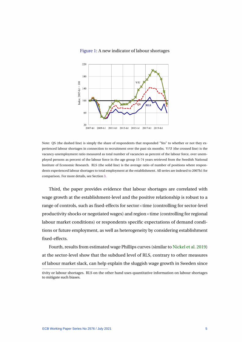
Figure 1: A new indicator of labour shortages
Note: QS (the dashed line) is simply the share of respondents that responded ”Yes” to whether or not they ex-
perienced labour shortages in connection to recruitment over the past six months. V/U (the crossed line) is the
vacancy-unemployment ratio measured as total number of vacancies as percent of the labour force, over unem-
ployed persons as percent of the labour force in the age group 15-74 years retrieved from the Swedish National
Institute of Economic Research. RLS (the solid line) is the average ratio of number of positions where respon-
dents experienced labour shortages to total employment at the establishment. All series are indexed to 2007h1 for
comparison. For more details, see Section 3.
Third, the paper provides evidence that labour shortages are correlated with
wage growth at the establishment-level and the positive relationship is robust to a
range of controls, such as fixed-effects for sector×time (controlling for sector-level
productivity shocks or negotiated wages) and region×time (controlling for regional
labour market conditions) or respondents specific expectations of demand condi-
tions or future employment, as well as heterogeneity by considering establishment
fixed-effects.
Fourth, results from estimated wage Phillips curves (similar to Nickel et al. 2019)
at the sector-level show that the subdued level of RLS, contrary to other measures
of labour market slack, can help explain the sluggish wage growth in Sweden since
tivity or labour shortages. RLS on the other hand uses quantitative information on labour shortagesto mitigate such biases.
ECB Working Paper Series No 2576 / July 2021 5
the Great Recession.
The findings in this paper are highly relevant for policymakers at central banks
as qualitative survey-based indicators are often used to assess labour market con-
ditions in real-time and to cross-check other estimates of ”slack” or “gaps” (see for
example Nyman 2010 for Sweden, ECB 2015 for the euro area and Tito 2018 for the
United States). Survey indicators are also used to inform policy decisions. For ex-
ample, several members of the Executive Board of the Swedish central bank high-
lighted record-level labour shortages as a motivation for the decision to begin tight-
ening monetary policy at the December 2018 Monetary Policy Meeting (Sveriges
Riksbank, 2018a).
The analysis in this paper suggest that labour markets were not as tight as other
measures indicated during the recovery and they would likely have to tighten more
substantially to provide impetus to wage growth and inflation, in line with the the-
oretical analysis of Daly and Hobijn (2014) and Linde and Trabandt (2019) and ag-
gregate empirical analyses by Byrne and Zekaite (2018) and Nickel et al. (2019) for
the euro area.
The rest of this paper is organized as follows: Section 2 describes the Swedish
Public Employment Service’s interview survey and the data used. Section 3 presents
the measure of relative labour shortages, Section 4 estimates the relationship be-
tween RLS and wage growth at the establishment-level and Section 5 estimates
sector-level wage Phillips curves and illustrate how RLS compares to other mea-
sures of economic slack in explaining wage growth in the recovery from the Great
Recession. Section 6 concludes.
2. The Public Employment Service’s Interview Survey
The backbone of this paper is detailed micro data from the Swedish Public Employ-
ment Service’s interview survey (the AFU), which has existed in different constella-
tions since the 1960s and been an important tool for the Swedish Public Employ-
ECB Working Paper Series No 2576 / July 2021 6
ment Service’s regional and national labour market forecasts.9 Before 2007, how-
ever, the micro data were not kept in a systematic manner and cannot be retrieved.
The dataset used in this paper covers more than 250,000 responses and around
10,000 establishments are included in each biannual survey wave. The sample in
the survey is drawn from Statistics Sweden’s Business Register and is stratified by es-
tablishment sizes (employment at establishments), sectors (SNI 2007/NACE Rev.2.)
and Swedish regions (”lan”). The sample frame includes establishments with more
than five employees and all establishments with more than 100 employees are in-
cluded, see Table A.1. The survey is representative for Sweden as a whole and at the
regional level.
To increase the weight of small sample units that also represent many small units
in the population that were not included in the sample, sample weights are included
from 2013h1 and onward.10 When greater weight is given to small sample units
(column 3 in Table A.1), the respective sector employment shares in the survey are
closer to the population. For example, industry accounts for a slightly smaller share
in the sample with 18.8% (31.2% unweighted), compared to 20.4% in the popula-
tion. The weighting also improves the representatives among size-classes: for small
establishments (0-19 employees), the weight increases from 6.2% to 34.1%, closer
to 33.7% in the population. With weights, large establishments account for 30.2%
instead of 71.2% unweighted and compared to 44.9% in the population.
As sample weights are not available prior to 2013h1, I use simple averages to cal-
culate the aggregate time-series. This means that the time-series are not necessarily
representative for the population as a whole, although the total number of employ-
ees covered by the sample alone accounts for more than a fourth of total Swedish
9See for example the Swedish Public Employment Service report, Arbetsmarknadsutsikter hosten2019-2020. (”Prospects of the Swedish labour market 2019-2020, fall”).
10The sample weights are simply w = (N − O)/n, where N is the number of establishments inthe population, O is oversampling and n the sampled units. When the Swedish Public EmploymentService report their figures, they utilize sample weights from 2013h1 onward and equally weighteddata from before then.
ECB Working Paper Series No 2576 / July 2021 7
business employment.11
2.1 Design and survey questions
Respondents in the survey are typically the CEO, CFO or senior managers at the es-
tablishments and the interviewers are local employment officers at the Public Em-
ployment Service. The survey is conducted face-to-face or by phone, which allows
the interviewers to ask more detailed questions than in mail-out questionnaires or
web surveys. This is precisely what makes this survey unique: besides gathering
qualitative Likert-scale type responses for assessments and expectations (that is,
”Increase”, ”Unchanged”, ”Decreased”), it also gathers quantitative assessments (of
for example labour shortages, employment and wage growth) and expectations (of
employment).
Participation in the survey is voluntary. Nonetheless, the response rate is
markedly high, on average above 80 percent. According to the Swedish Public Em-
ployment Service, the high response rate is a result of long-standing relationships
between interviewers and interviewees.
The questions from the survey used in this paper reads as follows:12
• The number of employees at the establishment (excluding contract staff). Pro-
vide the number of persons and your expectations for the future:
A year ago: Currently: In a year: In two years:
• Have you experienced labour shortages in connection with recruitment over the
past six months?
Yes, No or Have not needed to recruit
If yes:
11In more detail, for 2014h1, the total number of employees covered by the survey sample was732,329 as compared to 3,251,000 in the population for 2014. This is roughly equal across surveywaves.
12The full questionnaire is available at https://arbetsformedlingen.se/om-oss/statistik-och-analyser.
ECB Working Paper Series No 2576 / July 2021 8
– Provide the number of positions where you experienced labour shortages:
• Quantify by how much the average salary (per employee) has increased at the
establishment over the last year:
Less than 1%, 1%-2%, 2%-3%, 3%-4%, 4%-5%, 5%-6%, 6%-7% and above 7%
2.2 Change in survey mode and provider in 2020
At the beginning of 2020, the responsibility for the AFU-survey was outsourced by
the Public Employment Service to Statistics Sweden (SCB). Following the change,
the survey mode was altered from face-to-face and telephone interviews to a web-
based survey. In the two waves conducted in 2020, the response rate fell from the
previous highs of around 80 percent to around 30-40 percent. The fall in the re-
sponse rate can partially be attributed to the Covid-19 crisis, but it cannot be ex-
cluded that the change in survey mode and survey supplier have (strongly) affected
the response rates.
As such, the time-series after 2019 should be taken with more caution than the
period 2007h1–2019h2.13 In the econometric analysis in Section 4, only data from
2007h1-2018h1 will be used as identifiers for regions, sectors and establishments
(from 2013h1), are available. Time-series computations and the analysis in Section
5 as well as simple correlations will utilize data for the full period (2007h1-2020h2).
2.3 Comparison with other sources
One important aspect when dealing with non-standard sources is to ensure that the
data corresponds to other statistics, when applicable. In the following, I compare
variables available from the AFU with other official sources. For example, the pro-
portion of respondents in the AFU who report labour shortages is compared with
the same figure from the National Institute of Economic Research (NIER) Economic
13Instead of having a responses for around 10,000 establishments, the 2020h1 and 2020h2 waveshad only around 4,000 responses respectively.
ECB Working Paper Series No 2576 / July 2021 9
Tendency Survey, and wage growth is compared with short-term statistics from the
National Mediation Office (NMO), which is the main source used to track nominal
wage developments in Sweden.
To compare labour shortages from the AFU with the NIER-survey, I calculate
the proportion of respondents that respond ”Yes” to whether they have experienced
labour shortages. There are a couple of differences between the two surveys. First,
the AFU survey is conducted bi-annually whereas the NIER survey is conducted
quarterly. Second, the NIER survey simply asks their respondents to answer the
statement: ”Labour shortages at present?” with the response alternative ”Yes” or ”No”
whereas the AFU asks respondents to answer the question: ”Have you experienced
labour shortages in connection with recruitment over the past six months?” with the
response alternatives ”Yes”, ”No” or ”Have not needed to recruit”. To enable compar-
isons, I calculate the average of the NIER labour shortages for the first and second
quarter when comparing to the AFU:s first half of the year observation, and the third
and fourth quarter for the second half of the year.
Nominal annual wage growth computed from the AFU is compared with data
from the NMO. I use the mid-point of answers to the wage question in the AFU
survey. That is, 0.5% represents responses that are in the bin ”less than 1%”, 1.5%
if the bin is ”1%-2%” and 2.5% if the bin is ”2%-3%” and so on. Nominal annual
wage growth from the National Mediation Office is the wage sum divided by the
number of hours worked. Overall, qualitative labour shortages and aggregate wage
growth are very similar to those obtained from other sources in Sweden, see Figure
2. The comparability is also matched for broad sectors of the economy: industry,
construction, retail trade and services, see Figure A.1 and A.2 in the Appendix.
3. A measure of relative labour shortages (RLS)
In search models of the labour market (see for example Shimer 2005), tightness is
defined as the vacancy-unemployment ratio. A higher ratio of vacancies to unem-
ECB Working Paper Series No 2576 / July 2021 10
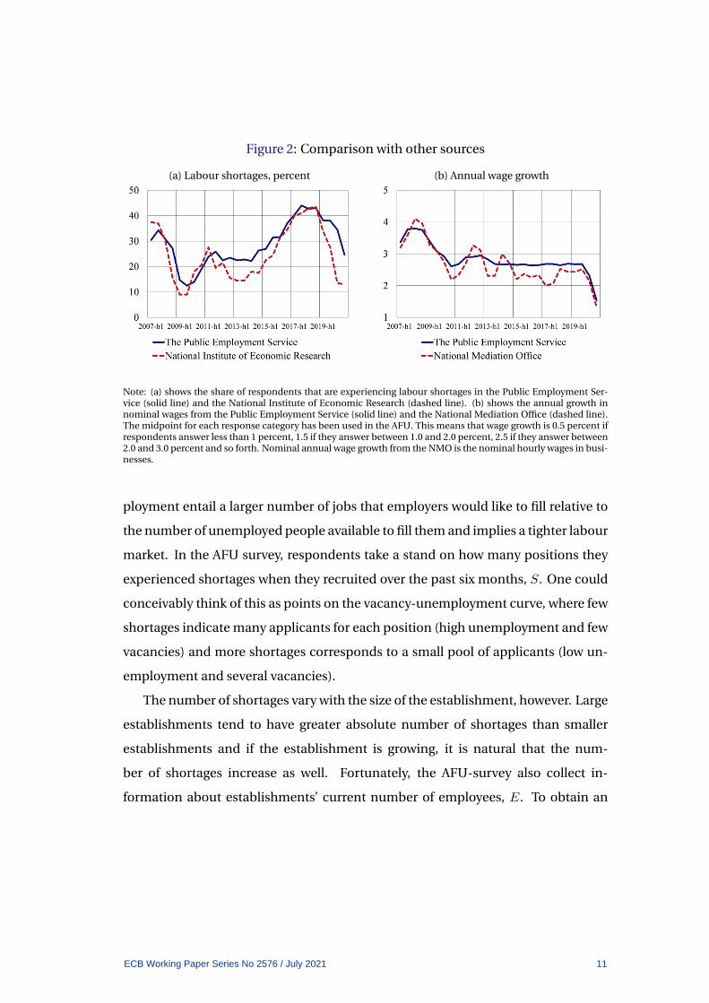
Figure 2: Comparison with other sources
(a) Labour shortages, percent (b) Annual wage growth
Note: (a) shows the share of respondents that are experiencing labour shortages in the Public Employment Ser-vice (solid line) and the National Institute of Economic Research (dashed line). (b) shows the annual growth innominal wages from the Public Employment Service (solid line) and the National Mediation Office (dashed line).The midpoint for each response category has been used in the AFU. This means that wage growth is 0.5 percent ifrespondents answer less than 1 percent, 1.5 if they answer between 1.0 and 2.0 percent, 2.5 if they answer between2.0 and 3.0 percent and so forth. Nominal annual wage growth from the NMO is the nominal hourly wages in busi-nesses.
ployment entail a larger number of jobs that employers would like to fill relative to
the number of unemployed people available to fill them and implies a tighter labour
market. In the AFU survey, respondents take a stand on how many positions they
experienced shortages when they recruited over the past six months, S. One could
conceivably think of this as points on the vacancy-unemployment curve, where few
shortages indicate many applicants for each position (high unemployment and few
vacancies) and more shortages corresponds to a small pool of applicants (low un-
employment and several vacancies).
The number of shortages vary with the size of the establishment, however. Large
establishments tend to have greater absolute number of shortages than smaller
establishments and if the establishment is growing, it is natural that the num-
ber of shortages increase as well. Fortunately, the AFU-survey also collect in-
formation about establishments’ current number of employees, E. To obtain an
ECB Working Paper Series No 2576 / July 2021 11
establishment-level measure of relative labour shortages, the number of labour
shortages Sit are divided by the total number of employees at the establishment
Eit as in (1):
RLSit =SitEit
(1)
Here, i is a establishment and t a survey round. This establishment-level mea-
sure of relative labour shortages (RLS) is continuous and relative: a higher value
means that the number of positions where establishments experience labour short-
ages are increasing relative to the size of the establishment and is what one would
expect when the labour market tightens. Similarly, a lower value means that es-
tablishments are experiencing less shortages and indicate a looser labour market.14
Establishments with no labour shortages or have not needed to recruit have a RLS
value of zero.
3.1 The evolution of RLS over time
The aggregate measure of RLS is simply the average of the establishment-level indi-
cator over time:
RLSt =1
Yt
Yt∑i=1
SitEit
(2)
where Y is the total number of responses to the question: ”Have you expe-
rienced labour shortages in connection to recruitment over the past six months?”.
Figure 3 plots the time-series average of RLS with the conventional survey-based
indicator for labour shortages (QS) as well as the vacancy-unemployment ratio
(V/U), indexed to 100 in 2007h1 for comparison.15 From 2011h1 and onward, RLS
14To deal with very extreme values reported in the survey, I winsorize the number of shortages andemployment at the 99.5th percentile. The measures is however robust in choosing both higher andlower percentile values for winsorizing. See Figure A.6 in the Appendix.
15The series are also calculated the broad sectors of the economy (industry, construction, retailtrade and services) in Figure A.3 and is also replicated for Swedish regions (NUTS1) in Figure A.7 in
ECB Working Paper Series No 2576 / July 2021 12
was markedly lower than QS and the vacancy-unemployment ratio (V/U). More-
over, and contrary to these other indicators, RLS was only above its 2007h1 level
in 2017h2 and fell back below it in 2018h1. Differently, the QS indicator and the
V/U was above the 2007h1 level already in 2015 and thus signalled stronger labour
market conditions than RLS.
Figure 3: Relative labour shortages (RLS) and other indicators
Note: QS (the dashed line) is simply the share of respondents that responded ”Yes” to whether or not they experi-enced labour shortages in connection to recruitment over the past six months. V/U (crossed line) is the vacancy-unemployment ratio measured as total number of vacancies as percent of the labour force, over unemployed per-sons as percent of the labour force in the age group 15-74 years retrieved from the Swedish National Institute ofEconomic Research. RLS (the solid line) is the average ratio of number of positions where respondents experiencedlabour shortages to total employment at the establishment. All series are indexed to 2007h1 for comparison.
The reason why RLS indicate more labour market slack than the other survey-
based measure is that the indicator provides information on the supply and de-
mand of labour from a recruiting firm’s perspective, rather than providing merely
the direction of labour market tightness in case of QS (i.e. the proportion of re-
spondents experiencing labour shortages). The fact that RLS and QS diverge tells us
that an increasing number of respondents (the extensive margin) perceived labour
shortages during the recovery, but that their quantitative assessment of labour
the Appendix and with sample weights from 2013h1-onward in Figure A.5.
ECB Working Paper Series No 2576 / July 2021 13
shortages (the intensive margin) was decreasing.
That the intensive margin is important to take into consideration can be shown
with (3), which decomposes (2) into two parts: the extensive margin, which is sim-
ply the the proportion of respondents that experience labour shortages, y/Y , where
y is the number of respondents responding ”Yes” to if they experience labour short-
ages andY is all responses.16 The second part of the expression is the average labour
shortages per establishment, i.e the intensive margin.
RLSt =ytYt︸︷︷︸
extensive margin
× 1
yt
yt∑i=1
SitEit︸ ︷︷ ︸
intensive margin
(3)
Most business surveys record only the first part of (3) and implicitly assume that
the second part is fixed, or not varying much, over time. This assumption has clear
downsides. If, for example, a large fraction of establishments experience short-
ages of specialized competencies, they may report a shortage of labour or perceive
labour as an important factor limiting production in a survey (increasing y), even
though the number of positions and wages for those staff are only a small part of
the total employment and wage bill at the establishment. If this behaviour is perva-
sive across many respondents, rising qualitative labour shortages, or the extensive
margin, may not indicate that the labour market has tightened in overall terms, but
simply that many establishments are experiencing shortages of a narrow set of skills
and competencies.17 Figure 4 shows that the intensive margin of labour shortages
has indeed been trending downward and been far below the 2007h1 level all through
the recovery from the Great Recession in Sweden.18
16That is, the sum of responses of ”Yes”, ”No” and ”Have not needed to recruit”.17In the Riksbank Business Survey, a small-scale interview survey conducted by the Swedish Cen-
tral Bank, respondents have highlighted that labour shortages have mainly been acute for specializedcompetencies rather than for broad groups of staff, see Sveriges Riksbank (2018b).
18Figure A.4 in the Appendix shows the evolution of the extensive and intensive margin over timefor also the four broad sectors of the economy, industry, construction, retail and services. Across allsectors, the intensive margin measure is markedly lower in the 2013-2020 period than before the GreatRecession.
ECB Working Paper Series No 2576 / July 2021 14
Figure 4: Intensive and extensive margin of RLS
Note: The extensive margin (the dashed line) is the share of respondents that responded ”Yes” to whether or notthey experienced labour shortages in connection to recruitment over the past six months. The intensive margin(the solid line) is the average ratio of number of positions where respondents experienced labour shortages relativeto total employment at the establishment. Both series are indexed to 2007h1 for comparison.
That the intensive margin is trending downwards suggests that the quantitative
signal from purely qualitative surveys of labour shortages becomes less reliable as a
gauge of labour market conditions or ”slack”. This problem with qualitative survey
data has also been highlighted for other indicators by Gayer and Marc (2018) and
National Institute of Economic Research (2018a). It should be noted, as shown by
Muller (2009), Lui et al. (2011) and Frohm and Hokkanen (2019) that qualitative
survey data do tend to reflect movements in matched quantitative statistics at the
firm-level. The purpose of this paper is not questioning this basic finding, but rather
to point out that the quantitative signal might vary over time which is indeed the
case in the AFU.
Although the split of labour shortages into an intensive and extensive margin
in this paper cannot readily be replicated for other countries or jurisdictions, due
to the specifics of the AFU survey, it is unlikely that Swedish respondents behave
very differently from those in other advanced economies when answering qualita-
ECB Working Paper Series No 2576 / July 2021 15
tive surveys. If the results are specific to Sweden alone, it would imply that survey
results in general (such as those from the DG-ECFIN Economic Tendency Survey or
the Purchasing Manager Indices) are not comparable cross jurisdictions and coun-
tries.19
Asking respondents directly about quantitative assessments is one way of deal-
ing with the problems inherent in qualitative survey data. Recent examples, other
than the AFU, are business surveys developed by the Federal Reserve Bank of At-
lanta (Survey of Business Uncertainty) see, Altig et al. (2020a) or Altig et al. (2020b)
and the Bank of England (Decision Maker Panel), see Bloom et al. (2018). These
surveys ask respondents’ about their quantitative assessment of the current situa-
tion and future developments for a number of economic variables, with promising
results for assessing, for example, the evolution of business uncertainty.
3.2 Sectors driving the evolution of RLS
With the detailed data in the AFU, RLS is decomposed into the contributions from
the main (NACE Rev.2.) economic sectors to gain more insights into whether the
drivers of aggregate labour shortages have changed over time. Ideally, the survey
would collect information on which specific occupations or roles are in shortages
and the current composition of the occupations or roles within the establishment.
This would enable a more detailed analysis of how shortages of certain occupa-
tions within sectors evolve over time. Nonetheless, the current structure of the sur-
vey suffices to break down labour shortages into narrow economic sectors (5-digit
NACE Rev. 2).
Figure 5 shows the decomposition which reveals that the relatively high labour
shortages in 2007–2008 were driven roughly equally by traditional blue-collar sec-
tors such as industry, construction and retail trade, and the heterogeneous services
19Figure A.8 shows that the percentage of responses that labour shortages are a main factor limitingproduction in the European DG-ECFIN Economic Tendency Survey in Sweden and the euro area arestrongly correlated.
ECB Working Paper Series No 2576 / July 2021 16
sector. In contrast, labour shortages during the recovery from the crisis, and espe-
cially after 2013, were largely driven by shortages in the services sectors, whereas
those in industry, construction and retail trade only increased slowly. By 2017–
2018, these same sectors only contributed to about one third of the aggregate labour
shortages.
Figure 5: Relative labour shortages (RLS) and contribution of sectors
Note: RLS (the solid black line) is the average ratio of number of positions where respondents experienced labourshortages to total employment at the establishment. It is decomposed into the contributions from industry (bluebars), construction (red bars), retail trade (yellow bars), services (green bars) and other sectors (gray bars).
A further decomposition within the services sector reveal that labour shortages
in primarily the ”welfare” sectors (health and elderly care, and to a lesser extent ed-
ucation services), drove the increase after the crisis in Sweden, see Figure 6.20 These
services sub-sectors are very different from other types of services or sectors. The
reason is that health and elderly care, as well as education, is almost entirely funded
by the Swedish government, either nationally, regionally or from the municipalities.
20In Sweden, welfare services are usually defined as those in health care, elderly care and education.Welfare services are defined as NACE Rev.2. 5-digit codes above 85000 and below 90000
ECB Working Paper Series No 2576 / July 2021 17
Figure 6: Relative labour shortages (RLS) in services, the contribution of sub-sectors
Note: RLS (the solid black line) is the average ratio of number of positions where respondents experienced labourshortages to total employment at the establishment in the services sector. It is decomposed into the contributionsfrom services sub-sectors.
Even though many providers of welfare services are subject to competition and the
services are open to the entry of new providers, revenues (per patient or student)
are determined by political decisions (Svanborg-Sjovall, 2014).
The scope to adjust wages to economic conditions, such as labour shortages, is
hence smaller for firms in these sectors than firms in other sectors where revenues
and profits are determined by market processes. In Section 4 I explore empirically
whether wage growth at establishments in the welfare sectors do indeed respond
differently to RLS than other establishments.
4. Relationship between RLS and wage growth
Since the AFU both collects respondent’s assessment of their average annual nom-
inal wage growth and RLS, it is possible to examine how wage growth varies across
ECB Working Paper Series No 2576 / July 2021 18
levels of RLS. This is done in Figure 7 by computing deciles of RLS and average wage
growth at each decile. Here, decile = 0 is all firms with no labour shortages and
the rest of the deciles are computed for firms with positive values of RLS.21 Average
wage growth is slightly higher for establishments with no labour shortages than es-
tablishments with labour shortages below the 3rd decile. From the 4th decile of RLS
and onward, average wage growth is higher than when RLS = 0. For establishments
at decile 10 for example, wage growth is 0.4 percentage points higher than if RLS
= 0.
Figure 7: Wage growth across deciles of labour shortages
(a) Wage growth (b) Wage growth distribution
Note: The figure in (a) shows the average annual nominal wage growth for each decile of RLS. The group ”0” is all
establishments without any labour shortages. RLS at decile 1 for all establishments is 0.006, at 2 0.016, at 3 0.030,
at 4 0.045, at 5 0.066, at 6 0.914, at 7 0.120, at 8 0.159, at 9 0.230 and at 10 0.657.
Panel (b) in Figure 7 shows that also the distribution of wage growth varies across
deciles of RLS. For establishments in the first decile of RLS, more than 80 percent re-
spond that wages increase in the 2-4 percent range, which can be contrasted with
around two thirds of establishments in the 10th decile. Changes in the distribution
of RLS is also largely accompanied by a higher share of responses that wages in-
21Again, the same Figures are available for establishments in industry, construction, retail trade andservices in Figure A.9 and A.10 in the Appendix.
ECB Working Paper Series No 2576 / July 2021 19
creases by more than 4 percent annually.
Figure 7 are however only cross-sectional correlations that do not controls for
potential confounders or omitted variables. The next section proceeds to investi-
gate whether the relationship between RLS and wage growth is robust to further
controls.
4.1 Fixed-effects regressions
To further control for observable and unobservable factors that affect wage growth
at the establishment, a dynamic lag panel fixed-effects regression is employed. The
dynamic structure allows for both current and past levels of RLS to affect wage
growth, as wages might respond with a lag to labour shortages. The estimated re-
gression is:
wi,t = γ + λt +
3∑k=0
βkRLSi,t−k + βXXi,t + εi,t (4)
where, w is nominal annual wage growth and RLS is relative labour shortages. k
denotes the number of lags used which are set to three, informed by the fact that the
correlation coefficient between different measures of economic slack and aggregate
wage growth is usually the highest between 3-6 quarters, see National Institute of
Economic Research (2018b). X is a vector of additional controls for expectations of
demand conditions, γ is either a sector×region or establishment fixed-effect, λ is
a time (or sector×time or region×time) fixed-effect and ε is the error term. i is an
establishment and t a survey wave.
The wage variable used in this paper is ordinal, with responses being grouped
in several bins of wage growth (less than 1%, 1-2% and so forth). When the left side
of the equation is on an ordinal scale, it is usually advised to use a ordered logit
estimator. However, there is no consensus in the literature on how to implement an
fixed-effects estimator for the ordered logit model (see Dickerson et al. 2014) and
ignoring observational heterogeneity could severely bias the estimates. As shown by
ECB Working Paper Series No 2576 / July 2021 20
Riedl and Geishecker (2014) in Monte Carlo simulations linear fixed-effects models
delivers essentially the same results as several proposed ordinal logit fixed-effects
models. I will thus proceed to use linear fixed-effects models in the main text. The
results are however robust to use ordered logit fixed-effects and estimates with the
”Blow-Up and Cluster” (BUC) estimator presented in Baetschmann et al. (2015) are
included in Table A.4 in Appendix A.
First the baseline results examine the coefficient and significance of RLS
is examined with sets of fixed-effects for region, sector and time. Second,
establishment-level controls are added for expected demand conditions and
forward-looking behaviour. Third, the relationship between wage growth and RLS
is investigated when also controlling for heterogeneity with establishment fixed-
effects.22
4.2 Baseline results
Column (1) in Table 1 shows the baseline estimates with year fixed-effects (con-
trolling for, for example, the aggregate business cycle or national economic pol-
icy). The baseline estimates in column (1) confirms the positive relationship out-
lined in Figure 7. Higher RLS is associated with an increase in wage growth. Col-
umn (2) further controls for negotiated wages and sector-level productivity with
sector×time fixed-effects, column (3) adds fixed-effects for sector×region to con-
trol for time-invariant differences across sectors in certain regions and column (4)
adds region×time fixed-effects, to control for regional economic conditions. In this
specification, RLS has an 0.47 percentage point impact on wage growth after 1.5
years. Note that this effect is the effect on wage-drift, as negotiated wages are con-
trolled for with the sector×time fixed-effects.23
22Recall that the AFU is an unbalanced panel with a large number of respondents only participatingone, two or three times and not necessarily in a row. This means that the estimates will contain about30% of the sample observations.
23About 9/10 employees in Sweden are affected by sector-level col-lective bargaining agreements. See https://www.mi.se/other-languages/about-the-mediation-office-the-swedish-model-and-wage-statistics-in-english/
ECB Working Paper Series No 2576 / July 2021 21
Table 1: Wage growth and RLS
(1) (2) (3) (4) (5) (6) (7)
Constant 2.777*** 2.786*** 2.780*** 2.780*** 2.773*** 2.754*** 2.648***
(0.007) (0.006) (0.004) (0.004) (0.004) (0.006) (0.004)
RLSt 0.212*** 0.205** 0.209** 0.210** 0.191** 0.204** 0.849***
(0.082) (0.085) (0.091) (0.092) (0.088) (0.091) (0.155)
RLSt−1 0.089 0.084 0.089 0.086 0.067 0.083 0.086
(0.070) (0.063) (0.061) (0.060) (0.055) (0.059) (0.161)
RLSt−2 0.248*** 0.162** 0.162** 0.163** 0.165** 0.166** 0.009
(0.068) (0.067) (0.067) (0.067) (0.070) (0.068) (0.140)
RLSt−3 0.171*** 0.074 0.062 0.065 0.060 0.061 0.105
(0.065) (0.051) (0.050) (0.050) (0.050) (0.051) (0.070)
Total effect 0.721*** 0.525*** 0.522*** 0.524*** 0.483*** 0.514*** 1.049***
(0.131) (0.126) (0.136) (0.137) (0.133) (0.136) (0.313)
Obs 65,997 63,352 61,780 61,780 57,929 60,898 61,780
R2 0.128 0.263 0.345 0.351 0.359 0.354 0.496
Clusters 6,001 5,716 4,293 4,293 4,208 4,277 4,293
FE S-R S-R S-R S-R S-R
Time-FE T T-S T-S T-S, T-R T-S, T-R T-S, T-R T-S, T-R
Note: *, **, and *** denote p< 0.10, p< 0.05, and p< 0.01, respectively. S = sector, R = region and T = time. Standard
errors are clustered at the sector×region level. The total effect refers to the linear combination of parameter esti-
mates (k = 0, k = 1, k = 2 and k = 3). Column (5) includes respondent’s expectations of employment growth at
the establishment next 24 months as a measure of expectations and Column (6) a qualitative measure if the level of
demand is expected to increase in the next 12 months. (7) includes weights for employment at the establishment.
ECB Working Paper Series No 2576 / July 2021 22
4.3 Additional controls
column (5)-(7) in table 1 adds additional establishment-level controls. Column (5)
adds respondents’ expectations of employment growth at the establishment the
next two years (a proxy for future demand conditions). It is calculated by using the
(log) difference of answers to the question on the number of employees currently
and expectations of number of employees in the next 24 months.
Column (6) swaps this variable with another proxy for forward-looking wage-
setting, namely answers to the question ”Do you judge demand for your goods and or
services to increase, decrease or remain unchanged over the next 6-12 months?”. Col-
umn (7) weighs the results by the number of employees at the establishments. The
results are also replicated for the broad sectors of the economy with sector×region,
as well as sector×time and region×time fixed-effects in Table A.2 in Appendix A.
Note that the sector×time fixed-effects are calculated for NACE Rev. 2 5-digit sec-
tors, so they can still be used in the broad sector-level regressions. Results remain
significant and of the same magnitude as in the baseline regressions.
4.4 Establishment fixed-effects
In this section, only the within-establishment variation is used to estimate the effect
of RLS on wage growth. The results are in Table 2. Overall, the effect of RLS is sig-
nificant and positive, meaning that RLS can also help explain wage growth within
establishments. The total effect of RLS on wage growth is between 0.38-0.48 per-
centage points depending on whether additional controls for future demand con-
ditions are included. Note that this is the effect when heterogeneity, sector shocks
(sector productivity and negotiated wages) and regional shocks are controlled for.
As seen in section 3.2, labour shortages in services and in particular welfare ser-
vices increased sharply during the recovery from the Great Recession and was one
important factor behind the rise in the aggregate RLS. With welfare services being
largely funded by national, regional or municipal governments, the impact of labour
ECB Working Paper Series No 2576 / July 2021 23
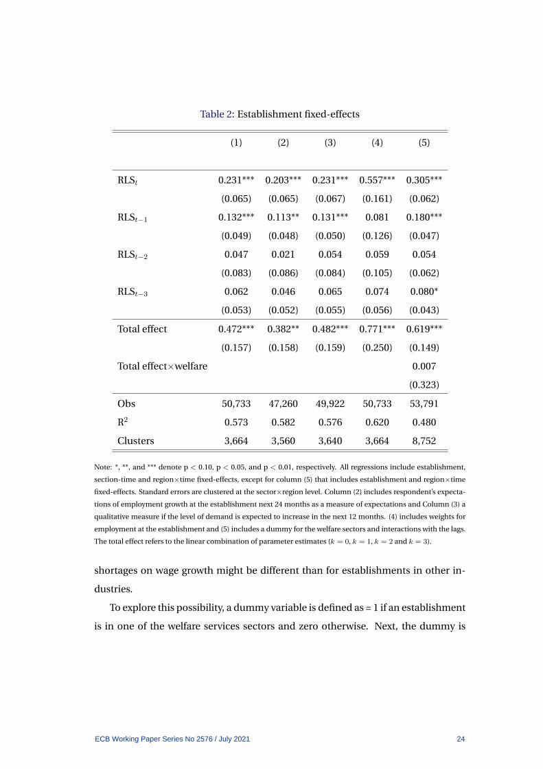
Table 2: Establishment fixed-effects
(1) (2) (3) (4) (5)
RLSt 0.231*** 0.203*** 0.231*** 0.557*** 0.305***
(0.065) (0.065) (0.067) (0.161) (0.062)
RLSt−1 0.132*** 0.113** 0.131*** 0.081 0.180***
(0.049) (0.048) (0.050) (0.126) (0.047)
RLSt−2 0.047 0.021 0.054 0.059 0.054
(0.083) (0.086) (0.084) (0.105) (0.062)
RLSt−3 0.062 0.046 0.065 0.074 0.080*
(0.053) (0.052) (0.055) (0.056) (0.043)
Total effect 0.472*** 0.382** 0.482*** 0.771*** 0.619***
(0.157) (0.158) (0.159) (0.250) (0.149)
Total effect×welfare 0.007
(0.323)
Obs 50,733 47,260 49,922 50,733 53,791
R2 0.573 0.582 0.576 0.620 0.480
Clusters 3,664 3,560 3,640 3,664 8,752
Note: *, **, and *** denote p < 0.10, p < 0.05, and p < 0.01, respectively. All regressions include establishment,
section-time and region×time fixed-effects, except for column (5) that includes establishment and region×time
fixed-effects. Standard errors are clustered at the sector×region level. Column (2) includes respondent’s expecta-
tions of employment growth at the establishment next 24 months as a measure of expectations and Column (3) a
qualitative measure if the level of demand is expected to increase in the next 12 months. (4) includes weights for
employment at the establishment and (5) includes a dummy for the welfare sectors and interactions with the lags.
The total effect refers to the linear combination of parameter estimates (k = 0, k = 1, k = 2 and k = 3).
shortages on wage growth might be different than for establishments in other in-
dustries.
To explore this possibility, a dummy variable is defined as = 1 if an establishment
is in one of the welfare services sectors and zero otherwise. Next, the dummy is
ECB Working Paper Series No 2576 / July 2021 24
interacted with the measures of RLS. As sector×region or sector×time fixed-effects
would absorb the effect of the dummy, these are dropped. Only region×time fixed-
effects are thus included to control for regional labour market conditions and the
specification reported in column (5) is therefore less comprehensive than the other
establishment-level regressions.24
The results suggest again that for all establishments, the total effect of RLS on
wage growth is 0.62 percentage points and statistically significant at the 0.01 percent
level. However, for establishments in the welfare services sector wage growth does
not appear significantly related to labour shortages. Comparing the point estimates
across the lags of RLS shows that labour shortages have no statistically significant
effect on wage growth for these sectors.
That wages seem to respond differently for establishments in welfare services
than for other sectors can be a (compositional) reason to why an increase in the
aggregate RLS has not led to wage pressures in the 2013-2019 period.
5. Wage forecasts in the recovery
Until now, the aggregate RLS indicator has been presented and been compared with
other measures of labour market conditions. The positive relationship between RLS
and wage growth at the establishment-level has also been highlighted. What is im-
portant for macroeconomic policy however is the aggregate implications. That is,
can RLS help explain the low wage growth in the economic recovery from the Great
Recession and does it do a better job than conventional indicators?
To answer this question, disaggregated wage Phillips curves are employed, in the
spirit of McLeay and Tenreyro (2020) and Hazell et al. (2020). Whereas these earlier
studies focus on regional price Phillips curves, I utilize the sectoral dimension in
the AFU by aggregating the establishment-level data to NACE Rev. 2. 2-digit sectors,
yielding 71 observations for each period. This level of aggregation ensures enough
24The full regression table with interactions is in Appendix A in Table A.3.
ECB Working Paper Series No 2576 / July 2021 25
observations to be able to construct a stable comparison index QS (the qualitative
survey measure of labour shortages) as well as RLS.
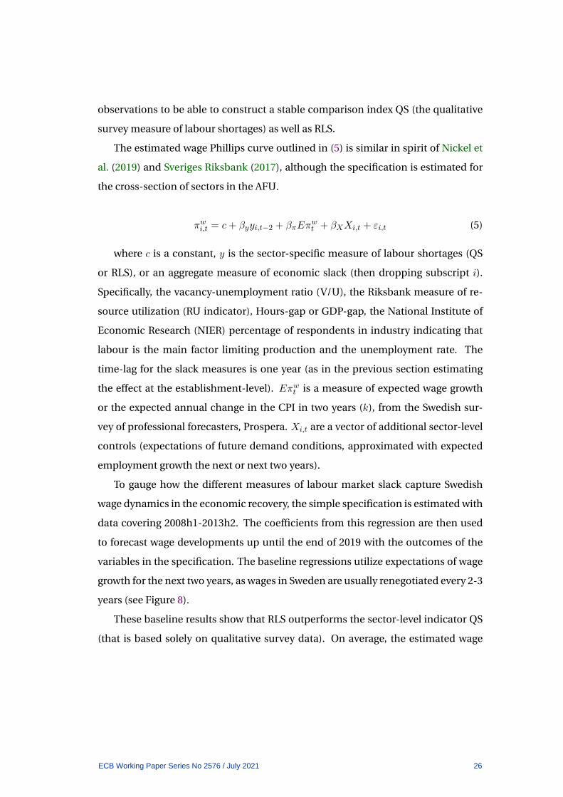
The estimated wage Phillips curve outlined in (5) is similar in spirit of Nickel et
al. (2019) and Sveriges Riksbank (2017), although the specification is estimated for
the cross-section of sectors in the AFU.
πwi,t = c+ βyyi,t−2 + βπEπwt + βXXi,t + εi,t (5)
where c is a constant, y is the sector-specific measure of labour shortages (QS
or RLS), or an aggregate measure of economic slack (then dropping subscript i).
Specifically, the vacancy-unemployment ratio (V/U), the Riksbank measure of re-
source utilization (RU indicator), Hours-gap or GDP-gap, the National Institute of
Economic Research (NIER) percentage of respondents in industry indicating that
labour is the main factor limiting production and the unemployment rate. The
time-lag for the slack measures is one year (as in the previous section estimating
the effect at the establishment-level). Eπwt is a measure of expected wage growth
or the expected annual change in the CPI in two years (k), from the Swedish sur-
vey of professional forecasters, Prospera. Xi,t are a vector of additional sector-level
controls (expectations of future demand conditions, approximated with expected
employment growth the next or next two years).
To gauge how the different measures of labour market slack capture Swedish
wage dynamics in the economic recovery, the simple specification is estimated with
data covering 2008h1-2013h2. The coefficients from this regression are then used
to forecast wage developments up until the end of 2019 with the outcomes of the
variables in the specification. The baseline regressions utilize expectations of wage
growth for the next two years, as wages in Sweden are usually renegotiated every 2-3
years (see Figure 8).
These baseline results show that RLS outperforms the sector-level indicator QS
(that is based solely on qualitative survey data). On average, the estimated wage
ECB Working Paper Series No 2576 / July 2021 26
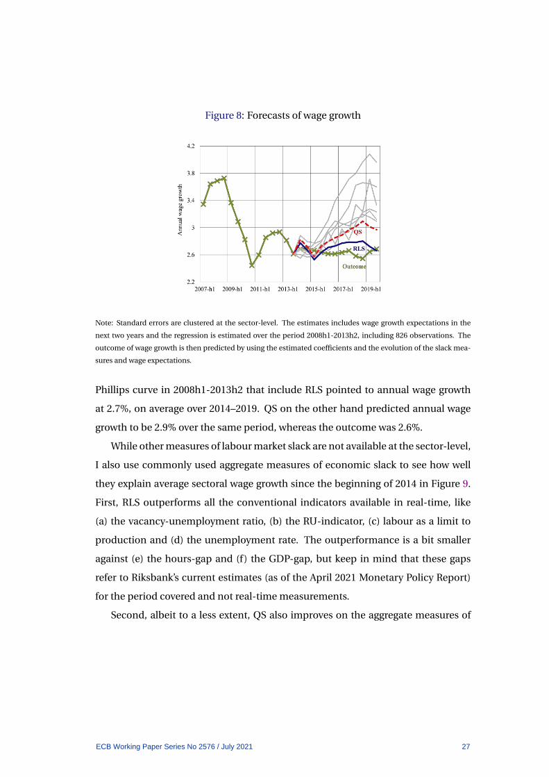
Figure 8: Forecasts of wage growth
Note: Standard errors are clustered at the sector-level. The estimates includes wage growth expectations in the
next two years and the regression is estimated over the period 2008h1-2013h2, including 826 observations. The
outcome of wage growth is then predicted by using the estimated coefficients and the evolution of the slack mea-
sures and wage expectations.
Phillips curve in 2008h1-2013h2 that include RLS pointed to annual wage growth
at 2.7%, on average over 2014–2019. QS on the other hand predicted annual wage
growth to be 2.9% over the same period, whereas the outcome was 2.6%.
While other measures of labour market slack are not available at the sector-level,
I also use commonly used aggregate measures of economic slack to see how well
they explain average sectoral wage growth since the beginning of 2014 in Figure 9.
First, RLS outperforms all the conventional indicators available in real-time, like
(a) the vacancy-unemployment ratio, (b) the RU-indicator, (c) labour as a limit to
production and (d) the unemployment rate. The outperformance is a bit smaller
against (e) the hours-gap and (f) the GDP-gap, but keep in mind that these gaps
refer to Riksbank’s current estimates (as of the April 2021 Monetary Policy Report)
for the period covered and not real-time measurements.
Second, albeit to a less extent, QS also improves on the aggregate measures of
ECB Working Paper Series No 2576 / July 2021 27
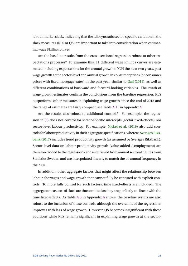
labour market slack, indicating that the idiosyncratic sector-specific variation in the
slack measures (RLS or QS) are important to take into consideration when estimat-
ing wage Phillips curves.
Are the baseline results from the cross-sectional regression robust to other ex-
pectations processes? To examine this, 11 different wage Phillips curves are esti-
mated including expectations for the annual growth of CPI the next two years, past
wage growth at the sector-level and annual growth in consumer prices (or consumer
prices with fixed mortgage-rates) in the past year, similar to Galı (2011), as well as
different combinations of backward and forward-looking variables. The swath of
wage growth estimates confirm the conclusions from the baseline regression: RLS
outperforms other measures in explaining wage growth since the end of 2013 and
the range of estimates are fairly compact, see Table A.11 in Appendix A.
Are the results also robust to additional controls? For example, the regres-
sion in (5) does not control for sector-specific intercepts (sector fixed-effects) nor
sector-level labour productivity. For example, Nickel et al. (2019) also add con-
trols for labour productivity in their aggregate specifications, whereas Sveriges Riks-
bank (2017) includes trend productivity growth (as assumed by Sveriges Riksbank).
Sector-level data on labour productivity growth (value added / employment) are
therefore added to the regressions and is retrieved from annual sectoral figures from
Statistics Sweden and are interpolated linearly to match the bi-annual frequency in
the AFU.
In addition, other aggregate factors that might affect the relationship between
labour shortages and wage growth that cannot fully be captured with explicit con-
trols. To more fully control for such factors, time fixed-effects are included. The
aggregate measures of slack are thus omitted as they are perfectly co-linear with the
time fixed-effects. As Table A.5 in Appendix A shows, the baseline results are also
robust to the inclusion of these controls, although the overall fit of the regressions
improves with lags of wage growth. However, QS becomes insignificant with these
additions while RLS remains significant in explaining wage growth at the sector-
ECB Working Paper Series No 2576 / July 2021 28
Figure 9: Forecasts of wage growth
(a) Vacancy-unemployment ratio (b) RU-indicator
(c) NIER, labour as limit to production (d) Unemployment rate
(e) GDP-gap (f) Hours-gap
Note: Standard errors are clustered at the sector-level. RLS is the solid blue line, the comparison measures (de-
noted in the title) are highlighted in dashed red lines.
level.
Overall, the establishment and sector-level empirical evidence supports the no-
ECB Working Paper Series No 2576 / July 2021 29
tion that labour markets would have to tighten more significantly for wages to in-
crease at a faster rate, in line with the theoretical analysis of Daly and Hobijn (2014)
and Linde and Trabandt (2019) and aggregate empirical analyses by Byrne and
Zekaite (2018) and Nickel et al. (2019) for the euro area.
6. Concluding remarks
This paper has presented a novel measure of labour market conditions in Sweden
based on data from a large-scale business survey, relative labour shortages (RLS).
The indicator pointed to markedly more slack in the Swedish labour market dur-
ing the economic recovery from the Great Recession (2013–2019) as well as dur-
ing the Covid-19 pandemic (in 2020) than other qualitative survey indicators or the
vacancy-unemployment ratio.
By decomposing RLS into an extensive margin (number of establishments with
labour shortages) and an intensive margin (average labour shortage per establish-
ment) provides insights into why conventional qualitative survey based measures
of labour market conditions, that are based on the percentage of respondents an-
swering ”Yes” or ”No” to whether they experience labour shortages or if labour is
perceived as a limit to production, have overstated labour market conditions after
the Great Recession. The analysis in this paper cautions about how to interpret the
level of these type of qualitative indicators (as described in Nyman 2010, ECB 2015
and Tito 2018) and what they imply for wage growth.
One solution to this issue with purely qualitative survey data is to ask respon-
dents directly about quantitative assessments, as in the Swedish AFU. Other recent
examples are business surveys developed by the Federal Reserve Bank of Atlanta
(Survey of Business Uncertainty) see, Altig et al. (2020a) and Altig et al. (2020b) and
the Bank of England (Decision Maker Panel), see Bloom et al. (2018).
Importantly, the analysis in this paper shows that RLS is positively correlated
with establishments’ wage growth, also when adding establishment-level controls
ECB Working Paper Series No 2576 / July 2021 30
and fixed-effects. In addition, forecast comparisons derived from sector-level wage
Phillips curves indicate that RLS did a better job in explaining the post-crisis de-
velopments in wage growth than other indicators. Nonetheless, the paper does not
provide causal evidence that RLS lead to higher wage growth. Future research could
examine the existence of a causal relationship with either the use of instruments or
regional or sector-level shocks.
Overall, the weak developments of RLS during the economic recovery from the
Great Recession is evidence that the Swedish labour market was not as tight as con-
ventional measures suggested and can help explain why wage growth was muted
over this period and will remain low during the Covid-19 pandemic. Looking ahead,
the results suggest that labour markets would have to tighten substantially to give
impetus to wage growth.
ECB Working Paper Series No 2576 / July 2021 31
References
Abraham, Katharine G, John C Haltiwanger, and Lea E Rendell, “How Tight is the US
Labor Market?,” BPEA Conference Draft, Spring, 2020.
Altig, Dave, Scott Baker, Jose Maria Barrero, Nicholas Bloom, Philip Bunn, Scarlet
Chen, Steven J Davis, Julia Leather, Brent Meyer, Emil Mihaylov et al., “Economic
uncertainty before and during the COVID-19 pandemic,” Journal of Public Eco-
nomics, 2020, 191, 104274.
Altig, David, Jose Maria Barrero, Nicholas Bloom, Steven J Davis, Brent Meyer, and
Nicholas Parker, “Surveying business uncertainty,” Journal of Econometrics, 2020.
Baetschmann, Gregori, Kevin E Staub, and Rainer Winkelmann, “Consistent Esti-
mation of the Fixed Effects Ordered Logit Model,” Journal of the Royal Statistical
Society: Series A (Statistics in Society), 2015, 178 (3), 685–703.
Barnichon, Regis and Geert Mesters, “On the demographic adjustment of unem-
ployment,” Review of Economics and Statistics, 2018, 100 (2), 219–231.
Beckworth, David, “The Stance of Monetary Policy: The NGDP Gap,” Mercatus Pol-
icy Brief Series: NGDP Gap, 2020.
Berge, Travis J, “Time-varying uncertainty of the Federal Reserve’s output gap esti-
mate,” Finance and Economics Discussion Series, Divisions of Research Statistics
and Monetary Affairs, Federal Reserve Board, 2020, (2020-012).
Bloom, Nicholas, Philip Bunn, Scarlet Chen, Paul Mizen, Pawel Smietanka, Greg
Thwaites, and Garry Young, “Brexit and uncertainty: insights from the Decision
Maker Panel,” Fiscal Studies, 2018, 39 (4), 555–580.
Borio, Claudio EV, Piti Disyatat, Mikael Juselius, and Phurichai Rungcharoenkitkul,
“Monetary policy in the grip of a pincer movement,” Bank of International Settle-
ments Working Paper Series, 2018, 706.
ECB Working Paper Series No 2576 / July 2021 32
Byrne, David and Zivile Zekaite, “Missing wage growth in the euro area: is the wage
Philips curve non-linear?,” Central Bank of Ireland Economic Letters, 2018, (9).
Coeure, Benoıt, “Scars or scratches? Hysteresis in the euro area,” 2017. Speech at
the International Center for Monetary and Banking Studies, Geneva, 19 May.
Daly, Mary C and Bart Hobijn, “Downward nominal wage rigidities bend the Phillips
curve,” Journal of Money, Credit and Banking, 2014, 46 (S2), 51–93.
Dickerson, Andy, Arne Risa Hole, and Luke A Munford, “The relationship between
well-being and commuting revisited: Does the choice of methodology matter?,”
Regional Science and Urban Economics, 2014, 49, 321–329.
ECB, “A survey-based measure of slack for the euro area,” ECB Economic Bulletin,
Box, 2015, 6.
Frohm, Erik, “Lower labour shortage could partly explain low wage growth,” Sveriges
Riksbank Economic Commentaries, 2019, 11.
, “Price-setting and economic slack: Evidence from firm-level survey data,” Jour-
nal of Macroeconomics, 2020, p. 103235.
and Jyry Hokkanen, “Learning by listening - interview with companies reflect
economic developments,” Sveriges Riksbank Economic Commentaries, 2019, 14.
Galı, Jordi, “The return of the wage Phillips curve,” Journal of the European Eco-
nomic Association, 2011, 9 (3), 436–461.
and Luca Gambetti, “Has the US wage phillips curve flattened? A semi-
structural exploration,” National Bureau of Economic Research Working Paper,
2019, (25476).
Gayer, Christian and Bertrand Marc, “A ‘New Modesty’? Level Shifts in Survey Data
and the Decreasing Trend of ‘Normal’Growth,” European Commission Discussion
Paper, 2018, (083).
ECB Working Paper Series No 2576 / July 2021 33
Haldane, Andrew G, “Pay Power,” 2018. Speech at the Acas “Future of Work” Con-
ference Congress Centre, London, 10 October.
Hazell, Jonathon, Juan Herreno, Emi Nakamura, and Jon Steinsson, “The slope of
the Phillips Curve: evidence from US states,” Technical Report, National Bureau
of Economic Research 2020.
Hong, Mr Gee Hee, Zsoka Koczan, Weicheng Lian, and Mr Malhar S Nabar, “More
slack than meets the eye? Recent wage dynamics in advanced economies,” Inter-
national Monetary Fund Working Paper Series, 2018, (18/50).
Jonsson, Magnus and Emelie Theobald, “A changed labour market–effects on prices
and wages, the Phillips curve and the Beveridge curve,” Sveriges Riksbank Eco-
nomic Review, 2019, (1), 28–49.
Krueger, Alan B, “Reflections on dwindling worker bargaining power and monetary
policy,” in “Luncheon Address at the Jackson Hole Economic Symposium,” Vol. 24
2018.
Leduc, Sylvain and Zheng Liu, “Robots or Workers? A Macro Analysis of Automation
and Labor Markets,” Federal Reserve Bank of San Francisco Working paper series,
2020, (17).
Linde, Jesper and Mathias Trabandt, “Resolving the missing deflation puzzle,” CEPR
Discussion Paper, 2019, (DP13690).
Lui, Silvia, James Mitchell, and Martin Weale, “Qualitative Business Surveys: Signal
or Noise?,” Journal of the Royal Statistical Society: Series A (Statistics in Society),
2011, 174 (2), 327–348.
McLeay, Michael and Silvana Tenreyro, “Optimal inflation and the identification of
the Phillips curve,” NBER Macroeconomics Annual, 2020, 34 (1), 199–255.
ECB Working Paper Series No 2576 / July 2021 34
Muller, Christian, “The information content of qualitative survey data,” OECD Jour-
nal: Journal of Business Cycle Measurement and Analysis, 2009, 2009 (1), 1–12.
National Institute of Economic Research, “Har sambandet mellan Barome-
terindikatorn och BNP-tillvaxt andrats over tid? (”Has the correlation be the Eco-
nomic Tendency Survey and GDP growth changed over time?” in English),” Article
in Economic Tendency Survey, June, 2018, pp. 14–17.
, “Lonebildningsrapporten, 2018 (”Wage Formation in Sweden, 2018” in En-
glish),” Wage formation report, 2018.
Nickel, Christiane, Elena Bobeica, Gerrit Koester, Eliza Lis, and Mario Porqueddu,
“Understanding low wage growth in the euro area and European countries,” Eu-
ropean Central Bank Occasional Paper Series, 2019, (232).
Nyman, Christina, “An indicator of resource utilisation,” Sveriges Riksbank Eco-
nomic Commentaries, 2010, 4.
Orphanides, Athanasios and Simon van Norden, “The unreliability of output-gap
estimates in real time,” Review of Economics and Statistics, 2002, 84 (4), 569–583.
Powell, Jerome, “Interview by Kai Ryssdal, Marketplace,” 2018. July 12, 2018.
Transcript available at https://www.marketplace.org/2018/07/12/economy/
powell-transcript/.
Riedl, Maximilian and Ingo Geishecker, “Keep it simple: Estimation Strategies for
Ordered Response Models with Fixed Effects,” Journal of Applied Statistics, 2014,
41 (11), 2358–2374.
Shimer, Robert, “The cyclical behavior of equilibrium unemployment and vacan-
cies,” American Economic Review, 2005, 95 (1), 25–49.
Svanborg-Sjovall, Karin, “Privatising the Swedish welfare state,” Economic Affairs,
2014, 34 (2), 181–192.
ECB Working Paper Series No 2576 / July 2021 35
Sveriges Riksbank, “Monetary Policy Report, July,” 2017.
, “Monetary Policy Minutes, December,” 2018.
, “Riksbank Business Survey, December,” 2018.
Tito, D. Maria, “Help Wanted: Evaluating Labor Shortages in Manufacturing,” FEDS
Notes, 2018, March 9.
ECB Working Paper Series No 2576 / July 2021 36
A. Appendix: Figures and tables
Figure A.1: Comparison of qualitative labour shortages with the NIER-survey
(a) Industry (b) Construction
(c) Retail trade (d) Services
Note: The solid lines in the Figure are calculated as the share of respondents responding ”Yes” to whether theyexperience labour shortages or not in the AFU. The dashed lines are data from the NIER. For construction, thecomparison is made with answers to the question: What are the greatest impediments for more construction andthe response alternative ”labour shortages”.
ECB Working Paper Series No 2576 / July 2021 37
Figure A.2: Comparison of annual wage growth with the NIER/NMO
(a) Industry (b) Construction
(c) Services
Note: The Figure shows the annual nominal wage growth from the AFU (solid lines) and estimates for threesectors by the National Institute of Economic Research and the National Mediation Office (NMO) (dashed lines).The midpoint for each response category has been used for wage growth from the AFU. This means that wagegrowth is 0.5 percent if respondents answers less than 1 percent, 1.5 if they answer between 1.0 and 2.0 percent,2.5 if the answer between 2.0 and 3.0 percent and so forth. Nominal wage growth from the National Institute ofEconomic Research and the NMO is wage growth per hour worked. Services sector includes retail trade. Data isannual.
ECB Working Paper Series No 2576 / July 2021 38
Figure A.3: Relative labour shortages, RLS
(a) Industry (b) Construction
(c) Retail trade (d) Services
Note: NACE Rev. 2. codes corresponding to industry is 10-33, construction is 41-43, retail trade 45-47 and servicesall NACE Rev. 2. codes above 47.
ECB Working Paper Series No 2576 / July 2021 39
Figure A.4: Relative labour shortages, RLS: extensive and intensive margin
(a) Industry (b) Construction
(c) Retail trade (d) Services
Note: NACE Rev. 2. codes corresponding to industry is 10-33, construction is 41-43, retail trade 45-47 and servicesall NACE Rev. 2. codes above 47.
ECB Working Paper Series No 2576 / July 2021 40
Figure A.5: Labour shortages, sample weights from 2013h1-onward
(a) Total
RLS
QS
0
40
80
120
160
2007-h12009-h1 2011-h1 2013-h1 2015-h1 2017-h1
Inde
x: 2
007-
h1 =
100
(b) Industry
0
40
80
120
160
2007-h12009-h1 2011-h1 2013-h1 2015-h1 2017-h1In
dex:
200
7-h1
= 1
00(c) Construction
0
40
80
120
160
2007-h12009-h1 2011-h1 2013-h1 2015-h1 2017-h1
Inde
x: 2
007-
h1 =
100
(d) Retail trade
0
40
80
120
160
2007-h12009-h1 2011-h1 2013-h1 2015-h1 2017-h1
Inde
x: 2
007-
h1 =
100
(e) Services
0
40
80
120
160
2007-h12009-h1 2011-h1 2013-h1 2015-h1 2017-h1
Inde
x: 2
007-
h1 =
100
Note: NACE Rev. 2. codes corresponding to industry is 10-33, construction is 41-43, retail trade 45-47 andservices all NACE Rev. 2. codes above 47. The series uses sample weights from 2013h1 onward and utilizes thenon-weighted averages to back-link the series.
ECB Working Paper Series No 2576 / July 2021 41
Figure A.6: RLS across various winzorizing percentiles
20
40
60
80
100
120
2007-h1 2009-h1 2011-h1 2013-h1 2015-h1 2017-h1
Inde
x: 2
007-
h1 =
100
Note: The figure shows the RLS measure computed for various choices of winzorizing percentile, indexed to 2007-
h1 = 100. The bands cover the 99.9th to 85th percentile.
ECB Working Paper Series No 2576 / July 2021 42

Figure A.7: Labour shortages for regions (NUTS1)
(a) SE1 - East Sweden (b) SE2 - South Sweden
(c) SE3 - North Sweden
Note: NUTS1 SE1 correspond to East Sweden, which includes the ”lan” Stockholm, Uppsala, Sodermanland,Ostergotland, Orebro and Vastmanland. SE2 - South Sweden includes Jonkoping, Kronoberg, Kalmar, Got-land, Blekinge, Sk, Halland and Vastergotland. SE3 - North Sweden includes Varmland, Dalarna, Gavleborg,Vasternorrland, Jamtland, Vasterbotten and Norrbotten.
ECB Working Paper Series No 2576 / July 2021 43
Figure A.8: Sweden and euro area
(a) Industry (b) Services
Note: The dashed (solid) lines are the % of responses, indexed to 100 in 2007h1, for the euro area (Sweden) thatanswer ”labour shortages” to the question: ”What main factors are currently limiting your production?” in theDG-ECFIN Economic Tendency Survey.
ECB Working Paper Series No 2576 / July 2021 44
Figure A.9: Wage growth across deciles of labour shortages
(a) Industry (b) Construction
(c) Retail trade (d) Services
Note: The figure shows the average annual nominal wage growth for each decile of RLS across sector groupings,which corresponds to NACE Rev. 2. Industry (10-33), construction (41-43), retail trade (45-47) and services (allsectors above 47). The group ”0” is all establishments without any labour shortages. RLS at decile 1 for industryare 0.003, 0.007, 0.011, 0.018, 0.025, 0.038, 0.059, 0.093, 0.143 and 0.368. For construction, its 0.013, 0.032, 0.050,0.070, 0.093, 0.117, 0.150, 0.200, 0.283, 0.684. For retail trade, 0.007, 0.017, 0.0299, 0.045, 0.066, 0.092, 0.127, 0.166,0.221, 0.489. For services, 0.009, 0.023, 0.037, 0.054, 0.074, 0.010, 0.131, 0.179, 0.251 0.699.
ECB Working Paper Series No 2576 / July 2021 45
Figure A.10: Wage growth distribution across deciles of labour shortages
(a) Industry (b) Construction
(c) Retail trade (d) Services
Note: The figure shows the distribution of wage growth across deciles of RLS. The group ”0” is all establishmentswithout any labour shortages. See Figure A.9 for the RLS values for the various deciles.
ECB Working Paper Series No 2576 / July 2021 46
Figure A.11: Swathe of wage growth forecasts
(a) RLS (b) QS
(c) Vacancy-unemployment ratio (d) RU-indicator
(e) NIER, labour as limit to production (f) Unemployment rate
(g) GDP-gap (h) Hours-gap
Note: Standard errors are clustered at the sector level. The swaths shows the range of estimates from wage Phillips
curves with different specifications.
ECB Working Paper Series No 2576 / July 2021 47
Table A.1: Employment in the AFU sample and total population, in 2014
Emp, smpl Emp, pop Emp, smpl∗
Industry 31.2% 20.4% 18.8%
Construction 6.8% 11.0% 9.8%
Retail trade 11.3% 18.7% 17.7%
Services 50.6% 49.9% 53.7%
0-19 employees 6.2% 33.7% 34.1%
20-49 employees 9.3% 12.7% 21.7%
50-99 employees 13.3% 8.7% 14.0%
100+ employees 71.2% 44.9% 30.2%
Stockholm 23.0% 26.1% 27.6%
Vastergotland 16.8% 16.9% 17.1%
Skane 10.3% 12.4% 14.3%
Ostergotland 3.5% 4.3% 3.9%
Jonkoping 3.8% 3.7% 3.8%
Uppsala 2.8% 3.4% 2.6%
Halland 3.0% 3.0% 2.7%
Orebro 3.5% 2.8% 2.6%
Dalarna 3.1% 2.6% 2.7%
Vasterbotten 2.8% 2.6% 2.2%
Gavleborg 3.0% 2.6% 2.5%
Norrbotten 2.9% 2.5% 2.2%
Vastmanland 3.6% 2.5% 2.5%
Varmland 2.9% 2.4% 2.2%
Sodermanland 2.7% 2.4% 2.1%
Vasternorrland 2.9% 2.4% 2.2%
Kalmar 2.7% 2.2% 2.2%
Kronoberg 3.0% 2.0% 2.0%
Blekinge 1.9% 1.5% 1.3%
Jamtland 1.1% 1.2% 0.9%
Gotland 0.6% 0.6% 0.4%
Note: The percentages are calculated for the establishments in the AFU (sample) and the population (pop) andare aggregated across broad industry classifications according to NACE Rev. 2. The figures for the population areobtained from Statistics Sweden. * denotes employment figures with sample weights.
ECB Working Paper Series No 2576 / July 2021 48
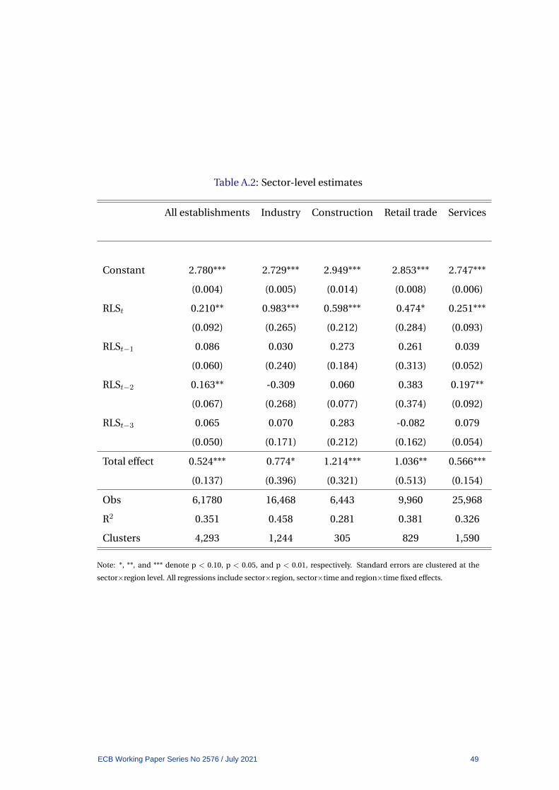
Table A.2: Sector-level estimates
All establishments Industry Construction Retail trade Services
Constant 2.780*** 2.729*** 2.949*** 2.853*** 2.747***
(0.004) (0.005) (0.014) (0.008) (0.006)
RLSt 0.210** 0.983*** 0.598*** 0.474* 0.251***
(0.092) (0.265) (0.212) (0.284) (0.093)
RLSt−1 0.086 0.030 0.273 0.261 0.039
(0.060) (0.240) (0.184) (0.313) (0.052)
RLSt−2 0.163** -0.309 0.060 0.383 0.197**
(0.067) (0.268) (0.077) (0.374) (0.092)
RLSt−3 0.065 0.070 0.283 -0.082 0.079
(0.050) (0.171) (0.212) (0.162) (0.054)
Total effect 0.524*** 0.774* 1.214*** 1.036** 0.566***
(0.137) (0.396) (0.321) (0.513) (0.154)
Obs 6,1780 16,468 6,443 9,960 25,968
R2 0.351 0.458 0.281 0.381 0.326
Clusters 4,293 1,244 305 829 1,590
Note: *, **, and *** denote p < 0.10, p < 0.05, and p < 0.01, respectively. Standard errors are clustered at the
sector×region level. All regressions include sector×region, sector×time and region×time fixed effects.
ECB Working Paper Series No 2576 / July 2021 49
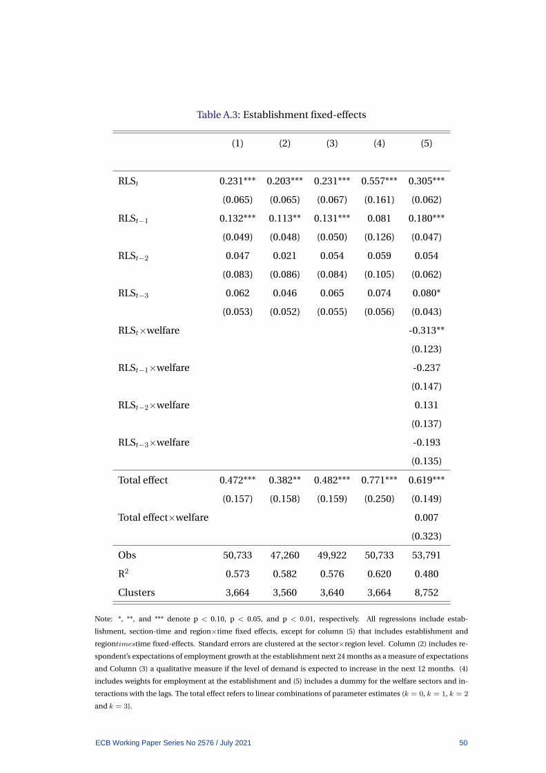
Table A.3: Establishment fixed-effects
(1) (2) (3) (4) (5)
RLSt 0.231*** 0.203*** 0.231*** 0.557*** 0.305***
(0.065) (0.065) (0.067) (0.161) (0.062)
RLSt−1 0.132*** 0.113** 0.131*** 0.081 0.180***
(0.049) (0.048) (0.050) (0.126) (0.047)
RLSt−2 0.047 0.021 0.054 0.059 0.054
(0.083) (0.086) (0.084) (0.105) (0.062)
RLSt−3 0.062 0.046 0.065 0.074 0.080*
(0.053) (0.052) (0.055) (0.056) (0.043)
RLSt×welfare -0.313**
(0.123)
RLSt−1×welfare -0.237
(0.147)
RLSt−2×welfare 0.131
(0.137)
RLSt−3×welfare -0.193
(0.135)
Total effect 0.472*** 0.382** 0.482*** 0.771*** 0.619***
(0.157) (0.158) (0.159) (0.250) (0.149)
Total effect×welfare 0.007
(0.323)
Obs 50,733 47,260 49,922 50,733 53,791
R2 0.573 0.582 0.576 0.620 0.480
Clusters 3,664 3,560 3,640 3,664 8,752
Note: *, **, and *** denote p < 0.10, p < 0.05, and p < 0.01, respectively. All regressions include estab-
lishment, section-time and region×time fixed effects, except for column (5) that includes establishment and
regiontimestime fixed-effects. Standard errors are clustered at the sector×region level. Column (2) includes re-
spondent’s expectations of employment growth at the establishment next 24 months as a measure of expectations
and Column (3) a qualitative measure if the level of demand is expected to increase in the next 12 months. (4)
includes weights for employment at the establishment and (5) includes a dummy for the welfare sectors and in-
teractions with the lags. The total effect refers to linear combinations of parameter estimates (k = 0, k = 1, k = 2
and k = 3).
ECB Working Paper Series No 2576 / July 2021 50
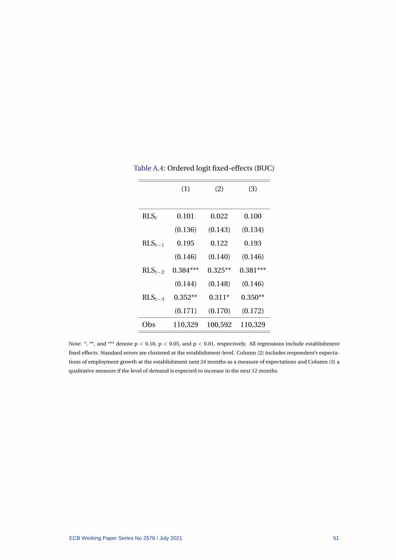
Table A.4: Ordered logit fixed-effects (BUC)
(1) (2) (3)
RLSt 0.101 0.022 0.100
(0.136) (0.143) (0.134)
RLSt−1 0.195 0.122 0.193
(0.146) (0.140) (0.146)
RLSt−2 0.384*** 0.325** 0.381***
(0.144) (0.148) (0.146)
RLSt−3 0.352** 0.311* 0.350**
(0.171) (0.170) (0.172)
Obs 110,329 100,592 110,329
Note: *, **, and *** denote p < 0.10, p < 0.05, and p < 0.01, respectively. All regressions include establishment
fixed effects. Standard errors are clustered at the establishment-level. Column (2) includes respondent’s expecta-
tions of employment growth at the establishment next 24 months as a measure of expectations and Column (3) a
qualitative measure if the level of demand is expected to increase in the next 12 months.
ECB Working Paper Series No 2576 / July 2021 51
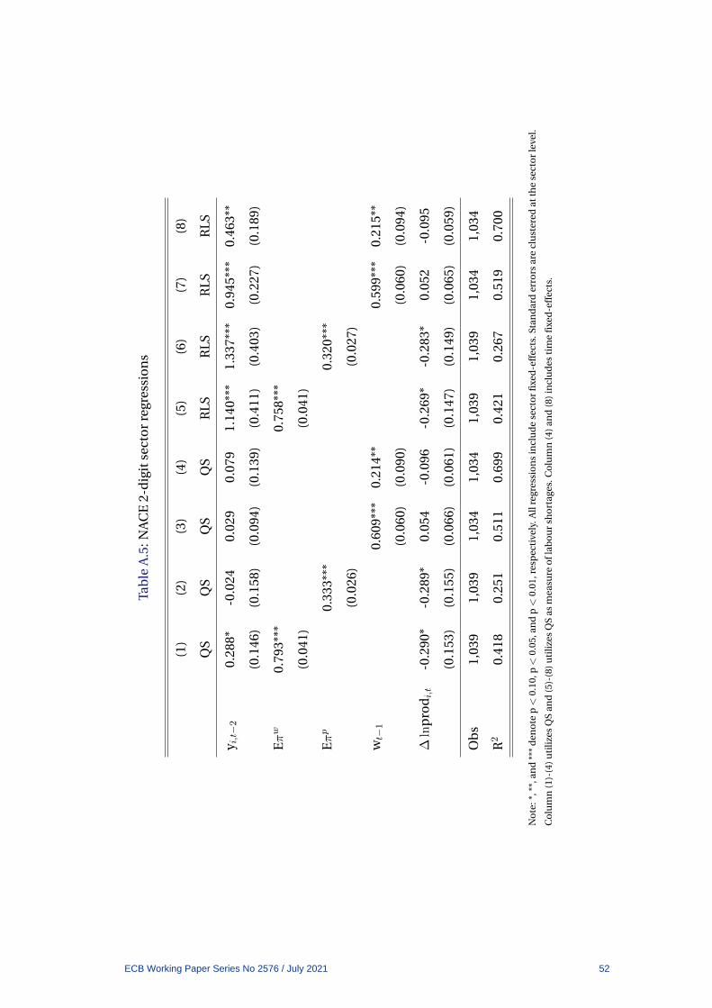
Tab
leA
.5:N
AC
E2-
dig
itse
cto
rre
gres
sio
ns
(1)
(2)
(3)
(4)
(5)
(6)
(7)
(8)
QS
QS
QS
QS
RLS
RLS
RLS
RLS
y i,t−2
0.28
8*-0
.024
0.02
90.
079
1.14
0***
1.33
7***
0.94
5***
0.46
3**
(0.1
46)
(0.1
58)
(0.0
94)
(0.1
39)
(0.4
11)
(0.4
03)
(0.2
27)
(0.1
89)
Eπw
0.79
3***
0.75
8***
(0.0
41)
(0.0
41)
Eπp
0.33
3***
0.32
0***
(0.0
26)
(0.0
27)
wt−
10.
609*
**0.
214*
*0.
599*
**0.
215*
*
(0.0
60)
(0.0
90)
(0.0
60)
(0.0
94)
∆ln
pro
di,t
-0.2
90*
-0.2
89*
0.05
4-0
.096
-0.2
69*
-0.2
83*
0.05
2-0
.095
(0.1
53)
(0.1
55)
(0.0
66)
(0.0
61)
(0.1
47)
(0.1
49)
(0.0
65)
(0.0
59)
Ob
s1,
039
1,03
91,
034
1,03
41,
039
1,03
91,
034
1,03
4
R2
0.41
80.
251
0.51
10.
699
0.42
10.
267
0.51
90.
700
No
te:*
,**,
and
***
den
ote
p<
0.10
,p<
0.05
,an
dp<
0.01
,res
pec
tive
ly.A
llre
gres
sio
ns
incl
ud
ese
cto
rfi
xed
-eff
ects
.Sta
nd
ard
erro
rsar
ecl
ust
ered
atth
ese
cto
rle
vel.
Co
lum
n(1
)-(4
)u
tiliz
esQ
San
d(5
)-(8
)u
tiliz
esQ
Sas
mea
sure
ofl
abo
ur
sho
rtag
es.C
olu
mn
(4)
and
(8)
incl
ud
esti
me
fixe
d-e
ffec
ts.
ECB Working Paper Series No 2576 / July 2021 52

Acknowledgements I am grateful to an anonymous referee, Niklas Amberg, Annelie Almérus, Katalin Bodnár, Håkan Gustavsson, Iida Häkkinen Skans, Valerie Jarvis, Mathias Klein, Åsa Olli Segendorf, Emelie Theobald and Andreas Westermark for useful suggestions. I also thank seminar participants at the European Central Bank (ECB), Sveriges Riksbank, the Swedish Ministry of Labour, the Swedish National Institute for Economic Research (NIER) and the Swedish Public Employment Office for their comments. The opinions expressed in this paper are the sole responsibility of the author and should not be interpreted as reflecting the views of Sveriges Riksbank or the European Central Bank. An earlier version of this paper was circulated as Sveriges Riksbank Working Paper Series, No 394. Erik Frohm European Central Bank, Frankfurt am Main, Germany; email: [email protected]
© European Central Bank, 2021
Postal address 60640 Frankfurt am Main, Germany Telephone +49 69 1344 0 Website www.ecb.europa.eu
All rights reserved. Any reproduction, publication and reprint in the form of a different publication, whether printed or produced electronically, in whole or in part, is permitted only with the explicit written authorisation of the ECB or the authors.
This paper can be downloaded without charge from www.ecb.europa.eu, from the Social Science Research Network electronic library or from RePEc: Research Papers in Economics. Information on all of the papers published in the ECB Working Paper Series can be found on the ECB’s website.
PDF ISBN 978-92-899-4762-6 ISSN 1725-2806 doi:10.2866/609231 QB-AR-21-067-EN-N