laboratory evidence on how managers intuitively value real growth options

LABORATORY EVIDENCEONHOWMANAGERSINTUITIVELY VALUE REAL GROWTHOPTIONS

Sydney D. Howell and Axel J. JÌgle*

INTRODUCTION

The theory of real options is important for the management of many types ofreal assets, and seems likely to change some basic conclusions inmicroeconomics and utility theory according to e.g. Brennan and Schwartz(1985), McDonald and Siegel (1986), and Dixit and Pindyck (1994). It istherefore an important question whether the judgements of human decisionmakers are in line with the prescriptions of the theory. If they are, the theoryis empirically uninstructive, being a mere formalisation of what managersalready know intuitively; but if intuitive judgements are not in line with thetheory, important needs arise for training, and interesting questions arise onthe functioning of markets for real assets. For example it is sometimes allegedthat managers, at least in the West, have a tendency to `underinvest' (e.g.Hayes and Garwin, 1982; and Hodder and Riggs, 1982), and this might beexplainable on the hypothesis that managers tend to undervalue the optioncontent of investments.

Previous research relevant to this question is divided. Some real optiontheorists have stated that intuitive decisions by managers are in closeragreement with real options theory than with more traditional capitalbudgeting techniques which are now known to be incomplete, such as simpleNPV, and decision tree analysis (DTA) with a constant cost of capital. Theybase this conclusion both on observations of actual decisions by commodity-using companies e.g. Dixit and Pindyck (1994), and also on informal reportsby managers as to whether they agree or disagree with the results of specificanalyses e.g. ibid. (1994), Barwise et al. (1987), and Kemna (1993). However,beyond Busby and Pitts (forthcoming), we are not aware of any publishedresearch which tests in a systematic fashion how far and under what conditionsmanagers' intuition agrees with the theory. There is a considerable literature(sometimes called Human Information Processing, or HIP) on the modellingof human intuition and on the testing of intuitive judgements against

Journal of Business Finance&Accounting, 24(7) & (8), September 1997, 0306-686X

ß Blackwell Publishers Ltd. 1997, 108 Cowley Road, Oxford OX4 1JF, UKand 350Main Street, Malden, MA 02148, USA. 915

* The authors are from Manchester Business School. This research was supported by a TomLupton scholarship fromManchester Business School. The authors wish to thank Dean A. Paxsonand an anonymous referee for helpful comments. Comments by Milan Lehocky and Jose Pereiraon an earlier draft of this paper are also gratefully acknowledged. The usual caveats apply.

Address for correspondence: Sydney D. Howell, Manchester Business School, Booth StreetWest, Manchester M15 6PB, UK.

normative (usually statistical) models of the situation (a good summary iscontained in Libby and Lewis, 1982). There is a descriptive strand of suchmodelling which is often ascribed to the so-called `lens' school of Brunswick(1952). The `lens' model assumes no normative rules for the problem, andstresses that we can only observe realistic decision behaviour in situations thatthe human judge has become accustomed to (i.e. in actual work or lifedecisions, or in laboratory experiments which have extremely completesettings and realistic parameter values). The `lens' approach is in line withour emerging knowledge of neural nets, which are thought to be a formalmodel of human and other intuitive pattern learning (e.g. Wood andDasgupta, 1995). It seems that a neural net is capable of learningapproximately correct classification and decision behaviour, but only withinthe range of parameter values on which it has been trained.

The so called `Bayesian' research school of HIP, in contrast, examinesproblems for which a normative model (e.g. Bayes' theorem) is known, andmeasures how far the human judge confirms to the normative theory. Bayesianresearch tends to show that human judges are not statistically rational, but it issometimes possible to assume that the human judge is in fact rationally usingsome model unsuspected by the researcher (e.g. if the subject has unexpectedpatterns of prior belief and utilities, or, in the option context, if the subjectreads a more complex option structure into the problem than the researcherintended). This saves the hypothesis of human rationality, but makes itunobservable.

The present research is partly laboratory experiment and partlyquestionnaire survey. We asked 82 practising managers in nine leadingcompanies to take hypothetical decisions on a series of investment casestudies. Each case study requires the manager in effect to value a so-called`growth option' (Myers 1977 and 1984; and Kester 1984). For reasons ofscarcity of time on the part of our subjects we have not explored the variousother types of real options discussed by Trigeorgis (1996), such as the optionto delay, the option to expand or contract etc., and other options, includingmanagerial flexibility or compound options. This laboratory research designpartly reflects the Bayesian strand of research into HIP, in that a normativemodel exists, though the subject may not read the same model into thesituation as the researcher intends. The research also contains a `lens' schoolaspect, in that our case narratives are intended to be realistic and plausible,and qualitatively relevant to the various volatility and other parametersettings they contain.

As a further `lens' or descriptive dimension to our research, we asked thesubjects some survey questions about their own personal situations, and aboutthe kind of investment decisions they themselves face at work. The purpose ofthis survey was to establish our subjects' attitude to the assumptions thatunderlie the real option model, to find out what parameter settings of thismodel would be most realistic for their own situations, and to find out any

916 HOWELL AND JØGLE

ß Blackwell Publishers Ltd 1997

other major factors which might make the chosen real option model realisticor unrealistic in their eyes (e.g. a lack of growth options in their own industry,or the presence of non-financial or `political' factors in investment decisions).

The paper is organised as follows. The next section identifies the model andthe theoretical assumptions we used. After that, we highlight some mainfeatures of the research implementation and describe our sample. We thenreport the patterns identified in the data. After that, we attempt to formmoregeneral explanations of the patterns observed in the data, and relate these tothe issues identified in the literature. We conclude the paper by consideringthe wider potential implications of the findings for capital budgeting practice.

THE THEORETICALMODEL ANDASSUMPTIONSOF THE EXPERIMENT

The European, non dividend paying form of financial option has often beenconsidered a realistic way to model a growth option on real assets, and theBlack-Scholes (B-S) option pricing model has often been used as a short-cut,practical procedure to value this (e.g. Brealey andMyers, 1991; Nichols 1994;and Trigeorgis, 1996).1 The B-S option valuation formula is (Black andScholes, 1973, equation 13):

c � SN�d1� ÿ Xeÿr�Tÿt�N�d2� �1�where:

d1 � ln SX

ÿ �� r� �2

2

� ��T ÿ t�

��T ÿ tp

d2 �ln S

X

ÿ �� rÿ �2

2

� ��T ÿ t�

��T ÿ tp � d1 ÿ �

��T ÿ tp

with:

c = Call option price, or, in real options terms, the value of the realoption;

S = Stock price, or the present value (PV) of the follow-up project'scash flows;

X = Exercise price, or the follow-up project's initial investment cost;� = Volatility;

T ÿ t = Maturity, or the development time of the pioneer project;r = Risk-free interest rate;

N(d) = Cumulative normal distribution function.

Our investment case studies have various text narratives, but all assume acommon underlying real option structure. Across the case studies we vary

HOWMANAGERS VALUEGROWTHOPTIONS 917


three of themost important parameters of the B-Smodel (i.e. the current priceof the underlying asset S, its volatility �, and the option maturity T ÿ t). Tominimise the burden on subjects we do not vary the risk free interest rate r, asthis is exogenously given and relatively stable, nor do we vary the exerciseprice X, as this mainly affects the `moneyness' of the option. In fact we needonly change the price of the underlying asset S in order to vary the moneyness'of the option (from òut-of-the-money', S<X, through àt-the-money', S=X,to ìn-the-money', S>X).2

All our 14 case studies assume the following underlying structure. A pioneerproject is to be undertaken. The net present value (invariably negative) ofundertaking the pioneer project equates to the cost of acquiring, as opposedto the value of, a real growth option. We include this cost in the case studynarratives for intuitive realism. It does not occur in the B-S model. In termsof the B-S model, this investment cost can be seen as a (generally incorrect)price of the option, which offers opportunities for arbitrage. If the theoreticaloption value c of the real option falls below this price, the option should not bebought, (but rather, if possible, sold).3

After a fixed period of years (equivalent to the maturity, or life,T ÿ t of theB-S financial option) it becomes possible to invest (or not as desired) in afollow up project (in B-S terms, to exercise the option). The initial cost of thefollow up project is presented to our subjects in the form of its value at theexpiration dateT, as discounted (at the risk-free rate) to their time of decisiont. This follow-up cost equates (in its compounded actual future money value)to the future exercise price X of the B-S financial option.

The follow up project has an expected future present value (PV) of cashflows at the time of decision t (equivalent to the price of the underlying asset Sin the B-S model). This expected PV is expected to evolve following a log-normal distribution over the maturity of the real option (corresponding tothe volatility of the underlying asset price �, which is assumed to be constantover time in the B-S financial model). We present our subjects withinformation on this volatility by telling them the PV, at their decision time t,of the upper and lower one standard deviation limits of the expected PVdistribution at the expiration date T. We do not tell subjects the risk freereturn (parameter r in the B-S model) thus forcing them to take an intuitivedecision. We did however ourselves use a value of 6% as a proxy for the actualcurrent sterling risk free rate of return,4 when we solved the B-S model to getthe theoretical option values. This rate is assumed to be an intertemporalconstant by the B-S model.

In order to try to elicit intuitively natural decisions, we explained theunderlying unity of the conceptual structure of the cases, but presented thisconceptual structure in varying text narratives (in which the pioneer projectwas variously described as test marketing, R&D development, pilot product,etc.). We might have chosen a more complex financial option as ourfundamental model, for example a compound option (Geske, 1979) and/or



multiple operating options (Trigeorgis, 1996). A more complex model wouldbe able to include explicit allowances for additional real options, such as theoption to delay the follow-up project, the option to rescale the follow upproject, or the currency risk aspect of the projects etc. These seem fruitfulareas for future work. The dividend paying option (Merton,1973) hassometimes been suggested as a useful model for valuing the option to delayan investment. However, the value of the real option to delay depends oncompetitive conditions, and these may not be well modelled as a dividendpaying financial option (see e.g. Smit and Ankum, 1993). Our casenarratives do not explicitly encourage the subjects to assume more complexoptions, but clearly there is some risk that various qualitatively different casenarratives may bias the subjects to perceive possible additional real optionsin different ways. We return to this point in our interpretation in the lastsection.

Our case studies vary the quantitative B-S parameters in the followingways. Cases A1 to A7 vary only the expected PV of the cash flows of the followup project (this varies the current stock price S and hence the `moneyness' ofthe option, in B-S terms). Cases B1 to B5 vary the volatility (�).In the naive NPV approach, as the uncertainty (volatility) associated with

the cash flows from an investment increases, the cash flows will be discountedmore heavily. If the uncertainty `proceeds too far', i.e. if it falls beyond therange with which managers feel intuitively comfortable, no investment maybe made. In the real options framework, uncertainty has the opposite effect:it increases the value of the option. This is because higher volatility raises thechance that the asset price may exceed the exercise price before the optionexpires (Hamilton andMitchell, 1990).

Cases C1 and C2 (jointly as departures from A3) vary several factors. Themain variation is in the maturity (T ÿ t) of the option. In the naive NPVapproach, lengthening the maturity of a single payoff reduces present value,as a result of the time value of money. Again, within the real optionsframework, lengthened maturity has an opposite effect. Extending the timeduring which the option may be exercised increases the probability that theasset price may exceed the exercise price during that time period (HamiltonandMitchell, 1990).

As we did not change the (discounted) values of the other model parametersin cases C1 and C2, the changes in maturity also imply slight changes in theundiscounted values of the exercise price and the volatility. Given the well-known limitations of human information processing capability, it seemspossible that respondents who answered case studies C1 and C2 (plus one casestudy from the A- or B-sequences) might be overtaxed by the multiple sourcesof variation over such a set of case studies, resulting in confusion of thevaluations. Empirical valuations on C1 and C2 will therefore be interpretedparticularly carefully.



QUESTIONNAIRE SURVEY AND SAMPLE

For reasons of time we could only ask each subject (respondent) to value threeof the 14 cases. We also asked all respondents to fill in a questionnaire survey,covering (1) the frequency of real growth options in the respondent'scompany, (2) the perceived realism of the assumptions underlying real optionstheory in general, and underlying this specific model in particular (e.g. thatthe exercise price X is reasonably stable), (3) the perceived realism of theoption parameter settings used in the case studies, and on (4) the process ofinvestment decision making in the respondent's company.5 We call this set ofindustry survey information the `questionnaire variables.' The questionnairealso collects nine pieces of information about each respondent's individualprofessional background. We call this subset of professional informationvariables the `grouping' variables, since we used this personal information toselect and compare subgroups of the respondents.

The sample consists of 82 respondents from nine major British companies infive industries (oil, aerospace, telecommunications, pharmaceuticals andbrewing). The sample was obtained by personal and postal enquiry. Of the55 largest British Plcs in various industries whom we approached, fiveparticipated in the research (9%). In addition, we asked 12 alumni ofManchester Business School working in (other) major British Plcs to act as`gatekeepers' for their companies, and four agreed to co-operate (33%). Thissample is presumably biased towards managers who have some interest in realoptions. In addition to 21 research instruments completed during personalvisits, we received replies to 61 out of 120 research instruments that were eitherpostally distributed or left in a participating company on the day of a personalvisit (50%).

The data collected from each respondent include the respondent'svaluations of a subset of the 14 case studies, the respondent's answers to the21 industry survey questions (this information was coded into 30`questionnaire variables') and information on nine personal and rolecharacteristics of each respondent (this information was coded into nine`grouping variables').

When analysing the sample, where possible, we tried to use each groupingvariable so as to split the subjects into equally sized subgroups, having `low'and `high' values of the variable concerned. Six of the grouping variables arenaturally dichotomous. For two of the grouping variables, data arecontinuous and we used a value close to the median to divide the sample intotwo. In the following definition of the grouping variables, we will, for eachgrouping variable, define the meaning of the `high' level of the groupingvariable first, and the meaning of the `low' level of the grouping variablesecond.

The first few grouping variables classify the business environment in whicha respondent is working, but at a rather general level (namely `Industry'



defines a respondent as being employed either in the oil, aerospace,telecommunications, pharmaceuticals, or brewing industry, and `Sector'defines a respondent as being currently employed either in one of the last twoindustries, which are consumer goods-related, or in one of the first threeindustries, which are capital goods-related). The second set of groupingvariables classify the professional experience of the individual respondent inmore detail (namely `Experience', i.e. above or below the approximatesample median number of years in business; `Position', i.e. employed atdirector or at manager levels, `Function', i.e. employed in the financialfunction of a company or not; `Level', i.e. employed at corporate headquartersor inside a business unit; and `Involvement', i.e. a high or a low level of formaland informal involvement in investment decision making). The third set ofgrouping variables captures details of the respondent's educationalbackground, which are potentially independent of the respondent's age orlength of business experience, namely `Business Education', i.e. whether arespondent had a degree in a business-related subject or not, and`Qualification', i.e. postgraduate degree/professional qualification or not.

All nine grouping variables seem plausible as having potential influence ona respondent's `gut feel' concerning investment decision making. The ninewere not completely independent of each other. We observed nine significantcorrelations between grouping variables (out of a potential 36). Several ofthese correlations merely reflect redundancies in our set of variables, oruncontroversial relationships between variables, for example the correlationsbetween Sector and Industry (which by definition overlap), betweenExperience and Position, between Function and Involvement, Level, andQualification, between Level and Qualification, and between BusinessEducation and Involvement and Function. We did not find any othersubstantively important correlations, for example there was not a significantnegative correlation between Position and Business Education, or Experienceand Business Education, which might have been predicted from the relativelyrecent expansion of business education.

DATA ANALYSIS

The simplest statistical model of the accuracy of a set of judgements has twoparameters, namely bias (mean) and dispersion (variance). We examined themeans and the variances of the case study valuations, both for the wholesample and for various subgroups of respondents.

The first four rows of Table 1 contain the various values of the option modelparameters as used in each case study, namely the settings for the expected PVof the follow-up project's cash flows (the asset price S, in the row `PV of CFs'),the volatility of this PV (the asset's volatility),6 the time until the follow-upinvestment can be made (the maturity T ÿ t), and the follow-up project's



initial investment cost (the exercise price X, in row `Init(ial) invest(ment)cost'). The fifth row (`theoretical OV') contains the theoretical value c of thereal option according to the B-S option pricing model, row six contains theNPV of the follow-up project (i.e. S-PV of X), and row seven contains theintrinsic value of the real option, which is max(0, S ÿ X). This is the notionalvalue of the option if exercised immediately. Row eight contains the timevalue of the option, i.e. the difference between the option value c and theintrinsic value as defined above. The next row indicates the `moneyness' ofthe real option.

The remaining five rows of Table 1 contain the empirical data generated byrespondents, namely: the average empirical valuation of each case study (bythe entire sample, in row `Empirical valua(tion)'); the discrepancy betweenthis empirical valuation and the theoretical option value; this discrepancyexpressed as a % of the theoretical option value (in row `D/theor. OV'); thesignificance of the discrepancy between the empirical valuation and thetheoretical option value, as identified by a t-test at 5% significance; and thesample size for each case study.

Table 1 shows that for 12 out of the 14 case studies, the mean empiricalvaluation was (considerably) higher than the NPV. This hints that, in thepresent sample and experiment, the naive NPV-rule is a poor description ofhow managers empirically value growth options. In what follows we willtherefore discuss how far real option theory (and particularly its B-S variant)can act as an alternative explanation of the empirical results.

The table shows further that in the A-sequence of case studies (i.e. casestudies A1 to A7, in which we varied only the expected PV of the follow-upproject's cash flows, and hence the moneyness of the option), case studies A4and A5 have the highest time values, and A6 and A7 have the highest intrinsicvalues (but lower time values). Our respondents valued case A1 correctly (inB-S terms). They significantly overvalued the sequence of case studies A2 toA5, and by progressively increasing amounts, except for case A4, which theyinsignificantly undervalued. Case studies A6 and A7 however, theysignificantly undervalued.

In the B-sequence of case studies we progressively increased the volatility ofthe expected PV of the follow-up project's cash flows. Cases B1 to B4 were allsignificantly overvalued (positive discrepancy) but this overvaluation brokedown in case B5, which happens to have an extremely high volatility (this casestudy was significantly undervalued). We found no clear trend in the size ofthe overvaluation over the sequence of case studies B1 to B4.

The differences between case studies C1 and C2 include an increase in thedevelopment time required for the pioneer project (optionmaturity), and alsoa slightly higher initial investment cost of the follow-up project (higherexercise price) and a slight increase in the volatility per unit time of theexpected PV of the follow-up project's cash flows. Case studies C1 and C2 areboth significantly overvalued by respondents, C2 more so than C1. In



Table 1

Parameter Settings and Valuations of the Investment Case Studies

A1 A2 A3 A4 A5 A6 A7 B1 B2 B3 B4 B5 C1 C2

PV of CFs 2.50 5.00 10.00 15.00 20.00 25.00 30.00 10.00 10.00 10.00 10.00 10.00 10.00 10.00Volatility 0.45 0.45 0.45 0.45 0.45 0.45 0.45 0.17 0.32 0.58 0.70 0.81 0.26 0.59Maturity 3.00 3.00 3.00 3.00 3.00 3.00 3.00 3.00 3.00 3.00 3.00 3.00 1.00 5.00Init. invest. cost 12.00 12.00 12.00 12.00 12.00 12.00 12.00 12.00 12.00 12.00 12.00 12.00 10.60 13.50Theoretical OV 0.06 0.50 3.00 6.80 11.10 15.70 20.40 1.20 2.20 3.80 4.60 5.20 1.00 4.90NPV ÿ7.50 ÿ5.00 0.00 5.00 10.00 15.00 20.00 0.00 0.00 0.00 0.00 0.00 0.00 0.00Intrinsic value 0.00 0.00 0.00 3.00 8.00 13.00 18.00 0.00 0.00 0.00 0.00 0.00 0.00 0.00Time value 0.06 0.50 3.00 3.80 3.10 2.70 2.40 1.20 2.20 3.80 4.60 5.20 1.00 4.90

Moneyness Out-of-the-money In-the-money Out-of-the-money

Empirical valuation 0.00 1.70 4.00 6.30 15.40 11.40 13.80 3.20 6.50 4.80 8.00 4.10 5.70 9.10Discrepancy ÿ0.10 1.20 1.00 ÿ0.50 4.30 ÿ3.30 ÿ6.60 2.00 4.30 1.00 3.40 ÿ1.10 4.70 4.20D/theor. OV [%] ÿ133.00 240.00 33.00 ÿ7.00 39.00 ÿ21.00 ÿ32.00 167.00 195.00 26.00 74.00 ÿ21.00 470.00 86.00Significance ns S S ns S S S S S S S S S SSample size 17.00 18.00 20.00 19.00 18.00 15.00 17.00 17.00 12.00 16.00 17.00 17.00 15.00 16.00

Notes:r = 0.06, ns = not significant at 5% level of significance, S = significant at 5% level of significance.

HOW

MANAGERSVALUEGROWTH

OPTIO

NS

923

ßBlackw

ellPublishersL

td1997

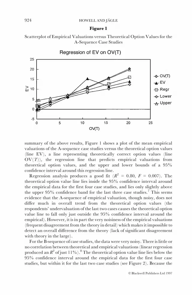
summary of the above results, Figure 1 shows a plot of the mean empiricalvaluations of the A-sequence case studies versus the theoretical option values(line EV), a line representing theoretically correct option values (lineOV(T)), the regression line that predicts empirical valuations fromtheoretical option values, and the upper and lower bounds of a 95%confidence interval around this regression line.

Regression analysis produces a good fit (R2 = 0.80, F = 0.007). Thetheoretical option value line lies inside the 95% confidence interval aroundthe empirical data for the first four case studies, and lies only slightly abovethe upper 95% confidence band for the last three case studies.7 This seemsevidence that the A-sequence of empirical valuation, though noisy, does notdiffer much in overall trend from the theoretical option values (therespondents' undervaluation of the last two cases causes the theoretical optionvalue line to fall only just outside the 95% confidence interval around theempirical). However, it is in part the very noisiness of the empirical valuations(frequent disagreement from the theory in detail) whichmakes it impossible todetect an overall difference from the theory (lack of significant disagreementwith theory in the large).

For the B-sequence of case studies, the data were very noisy. There is little orno correlation between theoretical and empirical valuations (linear regressionproduced an R2 of just 11%).8 The theoretical option value line lies below the95% confidence interval around the empirical data for the first four casestudies, but within it for the last two case studies (see Figure 2). Because the

Figure 1

Scatterplot of Empirical Valuations versus Theoretical Option Values for theA-Sequence Case Studies



slope of the regression of empirical values on theoretical values was notsignificantly different from zero (F = 0.52), theoretical values do not predictempirical values. However, it is notable that the confidence interval aroundthis regression slope is wide enough to include the slope (1) as well as the slope(zero), i.e. the tendency of the (biased and noisy) empirical valuations to risewith increased volatility does not agree with theory, but it does notsignificantly disagree with theory either. It did not seem useful to produce ascatterplot for the two case studies in the C-sequence, which were groupedwith various A or B series cases for different respondents.

We next tried to identify whether the grouping variables (professional androle characteristics of the respondents) helped to explain the case studyvaluations, and if so which grouping variables were most important. Table 2contains in its first row a ranking of the grouping variables, in terms of the sizeof their influence on (more accurately correlation with) the case studyvaluations. We compiled this ranking from a range of tests for correlationbetween the empirical case study valuations and the grouping variableconcerned (sign test, correlation analysis, multiple linear regression analysis,and One-Way ANOVA). It can be seen that Sector is the most importantgrouping variable, followed by Industry and Experience, followed byQualification and Position. The grouping variable Sector is merely a

Figure 2

Scatterplot of Empirical Valuations versus Theoretical Option Values for theB-Sequence Case Studies



simplified recoding of the grouping variable Industry, so it is not surprisingthat these variables have similar levels of importance.

The row `Direction' indicates the direction of a grouping variable'sinfluence on the valuation responses. A plus sign indicates a significantlyhigher valuation by those respondents coded as showing a `high' level in theparticular grouping variable. The row `Rationality' additionally indicateswhether this grouping variable led to significantly more rational (in B-S termsassuming risk neutral valuation) valuation responses or not.

Within the grouping variable Industry, it seems that the oil industryovervalued the case studies least, followed by the pharmaceuticals industry,whereas the brewing industry overvalued the case studies most. It is perhapsunsurprising that the more highly experienced, more highly qualified, andmore senior respondents all tend to differ from the average valuationbehaviour in the same direction (since these three grouping variables areempirically correlated, and may all measure related aspects of advancementin a respondent's career). However, it seems more surprising that these factorsall tend to make for less rational (i.e. higher) valuations.

Table 3 gives our findings on the variance or dispersion of the empiricalvaluations, and the apparent effect of each grouping variable on variance.9

The sign and the significance of the influence of each grouping variable uponthe variance of the case study valuations were identified by an F-test (havingtested the data for normality). Note that because we measured the variancesaround the (possibly incorrect) mean valuation of each case study, thesevariances are an indication of the `unanimity' of a subgroup of respondents,rather than of their `accuracy'.

It appears from the table that high levels of the grouping variables Sector,Position, Function, and Involvement led to more unanimity in valuation(lower variance). This means that more unanimity is shown in consumergoods-related industries, and among (broadly speaking) the more senior and

Table 2

Importance and Direction of the Grouping Variables' Influence on theMeanCase Study Valuations

Sector Industry Experience Position Function Level Involvement Business QualificationEducation

Importance 1 2 2 4 6 5 6 5 3Direction + n.a. + + ÿ + ÿ + +Rationality x n.a. x o * o * x *

Notes:H =High level of grouping variable; L = Low level.+: mean (H)>mean (L),ÿ: opposite, *: Hmore rational, x: L less rational, o: (H) and (L) equallyrational.



influential respondents (who also, as we saw above, make higher over-valuations, and hence tend to be apparently on average less rational).We alsochecked for how consistent the individual managers were, i.e. whether anindividual manager tended to overvalue or undervalue consistently across allthe three cases answered. We found that the respondents individually do notfollow an overall pattern of mean over- or undervaluation very closely.10

However, we found that respondents working in a company's headquartersare significantly more consistent than respondents working in an operationalbusiness unit.

This completes our description of patterns in the empirical case studyvaluations. We next report the patterns within the responses to ourquestionnaire survey. We used correlation analysis to look for relationshipsbetween the `grouping' variables and the `questionnaire' variables (broadlyspeaking, the former were personal data, plus the main industry and sectoridentity, and the latter were more detailed industry and work-role data).

Table 3

The Direction and Strength of Each Grouping Variable's Influence on the`Unanimity' of the Subgroup

Sector Experience Position Function Level Involvement Business QualificationEducation

Importance 1 2 1 1 ns 1 2 nsDirection + + + + + + ÿ ÿNotes:+ : Std. dev. (H)> Std. dev. (L), -: Std. dev. (H)< Std. dev. (L).

Table 4

Results of Correlation Analysis: Ability of Questionnaire Responses to PredictGrouping Variables

Sector Industry Experience Position Function Level Involvement Business QualificationEducation

N 9 10 3 1 9 3 3 4 4n 12 11 4 6 12 5 3 5 5Significance S S ns s S ns ns ns S

Notes:N = count of grouping variables correlated at 5%; n = count of grouping variables correlated at10%.Overall significance (on binomial test) of the count of significant correlations versus frequency ex-pected order null hypothesis of 5% or 10%.S = significant at 5% level of significance, s = significant at 10% level of significance.



We found that the `grouping' variables that were most correlated with the`questionnaire' variables were Industry (significantly correlated at 5% withten questionnaire variables, see Table 4) and Sector (nine significantcorrelations in Table 4), and Function (nine significant correlations in Table4). Of these, it is not surprising that Industry and Sector have similar andstrong relationships with the questionnaire variables, since these two groupingvariables have overlapping definitions, and many of the questionnairevariables simply operationalise the differences between industries in B-Sparameter terms, e.g. the maturity and volatility of real options.Among the means of the responses to our `questionnaire' variables

(concerning the real investment situation within the respondent's company)the following seem important: Respondents believed on average that only40% of the projects in their industry generate potential follow-up investmentopportunities (i.e. real growth options).When asked to identify the contexts inwhich these follow-up projects arise (i.e. R&D, marketing, processimprovements, as built into commercial contracts, or other), the context mostoften mentioned was R&D but its frequency was reported as only `sometimes'(number three on a five-point scale from `never' to `always'). Interindustrydifferences were not strong in these responses, but in general the respondentsin telecommunications perceived fewest follow-up opportunities in anycontext, and the respondents in brewing perceived most, closely followed bythose from the oil industry.

Respondents agreed on average that it is desirable to apply quantitativeanalysis, rather than the currently applied qualitative analysis of follow-upinvestment opportunities, and that profit prospects for a product were `veryseldom' certain over its whole life. The respondents estimate on average thatthey can forecast production costs accurately for longer ahead thancompetition or market conditions. The average perceived volatility figure forthe cash flows of an actual project was 23%, (which compares interestinglyand plausibly to the average annualUK stockmarket volatility which is about17%, see note 6). Finally, while the majority of respondents agreed with thestatement that they would generally look at a pioneer project and a follow-upproject as one single project, they also stated that their companies' decisionmaking did not fundamentally differ from the approach hinted at in the casestudies. It therefore seems likely that these respondents did not intend toexpress an irrational (i.e. naive NPV) approach to the option decision, inwhich an option (project) is bought only when it is in the money.

DISCUSSIONOF FINDINGS

The respondents overvalue the cases by an unweighted average of 78% of thetheoretical option value (average of row `D/OV(T)' in Table 1). It appearsthat they give a larger relative overvaluation to options which have small



theoretical values (A1,A2,B1andB2).The `relativemisvaluation'measures ofthese case studies, due to their small denominators, are extremely sensitive tosmall absolutemisvaluations. If we therefore review the results excluding thesecase studies, and also excluding casesC1 andC2 (results forwhichmight be lessmeaningful, as argued above), we arrive at a core which we could argue is the`most informative' set of case studies. For this core set themeanovervaluation isonly 11%, which can be regarded as approximately correct valuation.

The results of the regression relationship between empirical valuations andtheoretical option values for all cases in the A- and B- sequences indicate (inaggregate) three instances of significant undervaluation (A4^A6), and threeof significant overvaluation (B1^B3). This suggests that overall, the casestudies are approximately valued correctly (in B-S terms), although withconsiderable noise.

This might appear to suggest that respondents' intuition is compatible withreal option theory, under the particular conditions of this experiment.However, the lack of significant disagreement between empirical valuationsand theory is partly due to the extremely high level of noise in the empiricalvaluations. We will argue shortly that since subgroups of respondents differsignificantly from each other, no single model (theoretical or other) unites allthe responses.

One possible `lens' type explanation exists for the actual pattern of over- andundervaluation seen in the A-sequence of case studies (i.e. greaterovervaluation ö as an absolute money amount ö for options near themoney).11This is that the respondents are not accustomed to encountering realoptions that are either very deeply in-the-money or very far out-of-the-money.An alternative explanation is that the respondents place too much weight onthe time value of the option (which is driven ultimately by volatility) and/orput too littleweight on the intrinsic value of the option (i.e. the value the optionwould have if exercised immediately). Our respondents, on this view, areovervaluing the option components in many of the experimental case studies(in which such options are pointed out explicitly). This might seem to implythat they should never underinvest in the real world. However, therespondents are also on average undervaluing the `NPV-component' (i.e.,roughly the intrinsic value) of some of the case investments. If in the real worldrespondents undervalue NPVs, and if in addition they do not identify all thegrowth options available to them (in the real world these are not pointed outexplicitly, and, to judge from their questionnaire responses, our respondentsfind it hard to identify many follow-up investment opportunities inside theirown companies) our respondents might yet underinvest. If so, this might beimproved by training in identifying real options.

Over cases B1 to B4 in the B-sequence of case studies, in which we varied thevolatility, the empirical valuations (though on average too high) rise (in avery erratic fashion) roughly as prescribed by real options theory. Althoughthis does not mean that the respondents are fully option-rational, it certainly



suggests that the respondents do not hold the naive NPV view that volatility(variance) is bad for any investment.

While the earlier case studies of the B-sequence (namely B1 to B4) wereovervalued, this broke down at the very high volatility of case study B5, whichwas undervalued. A possible explanation is that respondents may not beaccustomed to a volatility as high as this, where � = 81%, and therefore loseconfidence in their usually over-generous valuation of volatility (a `lens' typeinterpretation). Respondents might feel that this very high volatility isunacceptably `risky', which would be a departure from option rationality, atleast for a fully diversified portfolio of projects.

Responses to changes in volatility across our B-cases are quite erratic andonly approximately in line with theory. On the other hand, when, as in theC-sequence, higher volatility is associated with a more concrete variable, inthe form of longer maturity, the empirical valuation of the option does veryclearly increase in the direction required by theory. This might be explainableif respondents believe that a longer lasting project has a better chance tobenefit from favourable changes in economic conditions than a short project.It might be a goal of future training in real options to point out to managersthat, provided they can exercise managerial flexibility, the same benefit existsfor shorter but extremely risky projects.

A general consideration, in the face of the widespread trend toovervaluation of many of the individual case studies, concerns our choice of anon dividend-paying, European option pricing model (B-S) for thecalculation of our theoretical option values. The apparent overvaluationsmight arise because authors are applying the `wrong' real option model.Dividend paying models would of course produce lower theoretical optionvalues, but this would only increase the apparent overvaluation by ourrespondents. Other option structure assumptions might however, lead tohigher theoretical option values than ours, for example, compound options(i.e. options on options, cf. Geske, 1979), multiple operating options(Trigeorgis, 1996), or models which relax some of the original B-Sassumptions (e.g. stochastic volatility option pricing models (Hull andWhite,1988), for other assumptions cf. Paxson, 1996).It is, for example, conceivable that our respondents intuitively assume the

existence of an additional option to delay the follow up project, after thematurity of the European option as described in our cases (this is an additionalAmerican option, leading to a compound option situation). Equally they mayassume multiple operating flexibility options (the option to vary the scale ofthe follow up project, the option to close down the follow up project, etc.),and are for these reasons `overvaluing' the case studies.

We therefore tried to identify those case studies whose text narrativesappear most likely to permit an additional option to delay at maturity (noneof the cases gave explicit clues on other types of options, such as operatingflexibility). The relevant case studies were B5, A7, B2, and C2. However, the



respondents overvalued two of these cases but undervalued the other two.Hence it does not seem that the respondents systematically incorporated animplied option to delay in their valuations.

Another hypothesis to explain the individual overvaluations is that ourrespondents might have intuitively assumed a higher volatility than the onegiven in the case narratives, for those case studies which contain transactionsdenominated in currencies other than sterling.12 This `overcompensation' forcurrency volatility might lead to overvaluation of the `foreign investment'case studies, which are A2, A3, A4, B1, C1, and C2. We checked this bycomparing the average percentage discrepancy from theory and found thatfor these six case studies it is 164% as compared to 16% for all other casestudies. However, the very high average percentage discrepancies of the`foreign investment' case studies may be related to the fact that all of these casestudies have very small theoretical option values (and their percentagediscrepancies are therefore heavily influenced by a given absolutemisvaluation).

Finally, other behavioural biases might have influenced the results in someor all groups, such as overreaction to some textual `novelty factor', over-optimism, use of biased valuation heuristics, e.g. due to risk fondness, orsystematic misunderstandings.

The grouping variable that seems most influential over (or correlated with)the case study valuations is Sector, so that respondents from different Sectorsare most likely to decide differently on a case study. Sector is a two levelvariable, which is itself a summary of Industry, a five level variable. The latterwas the second most important grouping variable. Among the individualindustries, the oil industry and the pharmaceuticals industries value the casestudies most correctly (under B-S assumptions). Some sectors of theseindustries are already using real options in capital budgeting. The brewingindustry shows the highest and least rational valuations.

The next most important grouping variable for mean valuation is(Business) Experience. More Experience increases decision makers'valuations (and accordingly makes them less rational) and makes them moreunanimous, an apparent reversal of the common association between meanand variance. Significant valuation differences arise for another importantgrouping variable, Position, except that the reduction in rationality is notsignificant. These grouping variables could be proxies for personal seniority,and high levels of senioritymay imply higher self-confidence andmore sharingof collective experience (on Pareto's principle of the circulation of elites).

In general, the questionnaire survey response revealed that the assumptionsof our chosen real option model (European, non dividend-paying) and thespecific parameter settings used in the case studies are perceived by ourrespondents as being quite realistic, with the exception of case B5 (atypicallyhigh volatility) and possibly cases A1, A6 and A7 (options very far from themoney).



Oil managers report a higher level of agreement than others with theassumptions required by the real options framework, and they also show lessover-valuation (in this laboratory experiment). Commercialmanagers show ahigher level of agreement with the assumptions required by the real optionsframework than do financial managers, but the commercial managers showstronger overvaluation (which also means less òption-rationality', in thepresent study). This valuation behaviour conforms to the traditionalstereotypes of these two functions, but the association between acceptance ofoption assumptions and high mean option valuation behaviour seems theopposite of that found for oil managers versus others. It seems that cognitiveattitudes to real option theory are not the dominant driver of valuation biases.

CONCLUSIONS

Various capital budgeting theorists have asserted or assumed that theintuition ofmanagers is consistent with real growth option theory. The presentstudy has set out to collect systematic laboratory evidence to compare with theanecdotal real world evidence of these authors (Dixit and Pindyck, 1994; andKemna, 1993).

For a particular form of real option theory, namely growth optionsmodelled as European, non dividend-paying options, and for a particular setof hypothetical parameters and textual case narratives, we find that ourskilled managerial decision makers agree only approximately with real optiontheory. They tend on average to value growth options in an erratic way (bothover- and under-valuations occurred), and they become more conservativewhen the option is far in- or far-out-of-the-money, or when volatility isextremely high. Overvaluation seems to be a function of Ìndustry', beinglowest in the oil industry, and it is also a function of (Business) Èxperience'and `Position' being highest for more senior people.

In all, the present study suggests that there is only a weak and approximatecorrespondence between management's intuition and real growth optiontheory. The directions of the effects on valuations of varying the moneyness,the volatility, and the maturity of an option are only approximately asprescribed by theory, with wide systematic and unsystematic variations. Thiscan be seen as reinforcing the relevance of training in growth option theory tocorporate capital budgeting.

In their responses to our questionnaire, the respondents report that some ofthe assumed parameter values used in our case studies are more realistic thanothers. It is notable that the respondents' valuations are most conservative forsituations which they are least likely to consider in their work, namely, for veryfar out-of-the-money and very deeply in-the-money options, and for very highvolatilities. Respondents seem receptive, or òpen', to the assumptions implicitin the real options framework, as seen, for example, in their willingness to treat



the exercise price of the real option as predictable. Presumably our sample waspartly self selected for its receptivity to real options concepts.

These results parallel the results of much previous research into human(intuitive) information processing in general. As in many so-called `Bayesian'studies, we have found that the normative model assumed by the authors doesnot strictly speaking describe the behaviour of respondents. The respondentscan only be alleged to be rational if we invoke their (differential) use ofunobserved additional models or parameters, such as the valuation ofadditional real options not mentioned in our case studies, or other factors.However, the respondents do tend to judge approximately in line with thetheoretical model (typically with an upward bias andwith considerable noise)over that range of parameter variation which is relatively more familiar tothem. A model of the average respondent might therefore conceivablyoutperform a randomly chosen respondent (the concept of `bootstrapping',cf. e.g. Marais et. al., 1984). These findings resemble many previousdescriptive findings in the `lens' tradition of HIP research.

The implications of this research for real world capital budgeting seem to bethat training is needed, and it is also likely to be acceptable to managers. Theuse of teams of decision makers might offer the chance to reduce the noise orvariance (but not the bias) of intuitive option valuations. It does not seempossible to account for the often reported tendency of Western managers tounderinvest by any tendency on their part to undervalue the real optioncontents of investments.

Avenues for future research based on the present findings include extendingthe realism of the laboratory research, relating the findings to actual decisionmaking in companies, adding other kinds of options and other parametersettings, studying the effect of team decision making and of bootstrapping,and applying the research to other companies, industries, and countries.

NOTES

1 For our case studies, we apply the Black-Scholes model as derived using the `capital assetpricing model'. This derivation evolves from the requirement that the option earn anexpected rate of return commensurate with the risk involved in holding the option as an asset(Black and Scholes, 1973, equations (15)^(21)). An equilibrium-derived B-S model doestherefore not rely on the ability to trade, replicate or otherwise justify risk neutral valuationin pricing contingent claims. Also note that the (continuous) B-S model produces the samevalues as, but is simpler and more direct than, a properly specified (discrete) decision treeanalysis (DTA) (cf. Smith and Nau, 1995).

2 Note that for a financial option, the intrinsic value max (0, S ÿ X) that underlies the conceptof `moneyness' is sometimes defined as the profit or loss available from exercising the optionimmediately. In our real growth option model, however, and in general for a Europeanoption, there is of course no means of exercising the option in advance of its maturity.

3 In the present study, respondents were actually asked to indicate this net `arbitrage' profit/loss. Consequently, to arrive at the option valuation c implicit in this profit/loss, theinvestment cost had to be added to the reported arbitrage profit or loss. In this way, we were



able to compare the (adjusted) empirical valuations of the case studies given by therespondents with the theoretical values suggested by real option theory.

4 The proxy we used was the average UK three month Treasury bill rate during the time ofdata collection (Feb. 1995 to June 1995), which was close to 6%. This rate is of course reallya discount rate for near-term (three month) cash flows, which is less than the maturity of ouroptions of (inmost cases) three years. However, the next longer suitable proxy for the risk-freeinterest rate, Treasury notes, have a maturity between six and a half and ten years, which istoo long for our purpose. Moreover, the risk premium of T notes over bills would have to besubtracted from the T note yield, potentially offsetting the normally positive differencebetween T notes and bills (cf. Brealey and Myers, 1991). At this point it is noteworthy thatsensitivity analyses showed that, for our case studies, the option value is largely unaffected byplausible variation of the risk-free interest rate.

5 Our set of case studies, and our questionnaire survey can be received from the authors. It iscontained in JÌgle (1997).

6 Note that the various volatility values (namely 45% in the A sequence of case studies,between 17%and 81% in the B sequence of case studies, and 26% and 59% in the C sequenceof case studies) were chosen by the researcher before the experiment. They compare to theaverage annual UK stock market volatility which is about 17% (International MonetaryFund, 1995). It seems realistic to expect individual projects to show higher volatilities thancomplete companies, or even completemarkets. In our questionnaire the respondents seemedto find the volatilities we used fairly realistic, though they find many on the high side. It is afield for future research to select different values.

7 The regression equation obtained is: y = 1.8 + 0.7x, where y is empirical valuation and x istheoretical value. The upper/lower confidence bands for the mean of y given x are (95%confidence level): y = 1.8 + 0.7x�=ÿ t(0.95, nÿ 2) 2.53 (1/n + (xÿ 8.2)^2 / 368)^0.5

8 The regression equation obtained is: y= 3.8 + 0.4x. The upper/lower confidence bands for themean of y given x are (95% confidence level): y= 3.8 + 0.4x�=ÿ t(0.95, nÿ 2) 1.55 (1/n+ (xÿ3.3)^2 / 11.3)^0.5.

9 A very small component of variance is imported by the fact that our questionnaire forcesthe respondents to value the option using a standard set of integer values, whereas thetheoretical values (as adjusted to add the cost of the pioneer project) are not in generalintegers. This source of variance contributes between 1% and 5% of total observedvariance for most of the cases, and 10% of total observed variance for the lowest valuedcases.

10 We found however, that somemanagers were significantlymore or less consistent than others,e.g. on a Chi-square test (assuming a constant, normal distribution of valuations) some 11 outof 82 managers showed significantly high consistency at a 95% confidence level.

11 Intriguingly, this would seem to be the opposite of the well known `smile' effect in financialmarkets, where implied volatilities seem `overgenerous' for options that are far from themoney. The smile effect ultimately suggests that the market overvalues options that are faraway from the money, or that the B-S model, which assumes constant volatility, is notcapturing important market assumptions.

12 Strictly speaking these `foreign investment' case studies should be valued at different risk-freeinterest rates.

REFERENCES

Barwise, P., P. Marsh and R. Wensley (1987), `Strategic Investment Decisions', Research inMarketing, Vol. 9, pp. 1^57.

Black F. and M. Scholes (1973), `The Pricing of Options and Corporate Liabilities', Journal ofPolitical Economy, Vol. 81 (May^June), pp. 637^54.

Brealey, R.A. and S.C. Myers (1991), Principles of Corporate Finance (McGraw-Hill).Brennan, M.J. and E.S. Schwartz (1985), `Evaluating Natural Resource Investments', Journal of

Business, Vol. 58 (April), pp. 135^57.Brunswick, E. (1952),The Conceptual Framework of Psychology (University of Chicago Press).Busby, J.S. and C.G.C.Pitts (forthcoming), `Real Options in Practice: an Exploratory Survey of



How Finance Officers Deal With Flexibility in Capital Appraisal', Management AccountingResearch.

Dixit, A.K. and R.S. Pindyck (1994), Investment Under Uncertainty (Princeton University Press).Geske, R. (1979), `The Valuation of Compound Options', Journal of Financial Economics, Vol. 7

(March), pp. 63^81.Hamilton, W.F. and G.R. Mitchell (1990), `What Is Your R&DWorth?',TheMcKinsey Quarterly

(Autumn), pp. 150^60.Hayes, R.H. and D.A. Garvin (1982), `Managing as if Tomorrow Mattered', Harvard Business

Review, Vol. 60 (May^June), pp. 71^9.Hodder, J.E. and H.E. Riggs (1982), `Pitfalls in Evaluating Risky Projects', Harvard Business

Review, Vol. 60 (May^June), pp. 128^35.Hull, J. (1993),Options, Futures, and Other Derivative Securities (Prentice Hall).________________________ and A. White (1988), Àn Analysis of the Bias in Option Pricing Caused by a Stocastic

Volatility', Advances in Futures and Options Research, Vol. 3, pp. 29^61.International Monetary Fund (1995), International Financial Statistics, Vol. 11 (November).JÌgle, A.J. (1997), À Laboratory Comparison of Managers' Investment Decision Making

Behaviour with the Decisions Recommended by Real Options Theory', UnpublishedDoctoral Dissertation (Manchester Business School).

Kemna, A.G.Z. (1993), `Case Studies on Real Options', FinancialManagement, Vol. 22 (Autumn),pp. 259^70.

Kester, W.C. (1984), `Today's Options for Tomorrow's Growth',Harvard Business Review, Vol. 62(MarchÂpril), pp. 153^60.

Libby, R. and B.L. Lewis (1982), `Human Information Processing Research in Accounting: TheState of the Art in 1982', Accounting, Organisations and Society, Vol. 7 (Autumn), pp. 231^85.

Marais, M.L., J.M. Patell and M.A. Wolfson (1984), `The Experimental Design of ClassificationModels: An Application of Recursive Partitioning and Bootstrapping of Commercial BankLoan Classifications', Journal of Accounting Research, Vol. 22 (Supplement), pp. 87^114.

McDonald, R. and D. Siegel (1986), `The Value of Waiting to Invest', Quarterly Journal ofEconomics, Vol. 10 (November), pp. 705^27.

Merton, R. (1973), `Theory of Rational Option Pricing', Bell Journal of Economics andManagementScience, Vol. 4 (Spring), pp. 141^83.

Myers, S.C. (1977), `Determinants of Corporate Borrowing', Journal of Financial Economics, Vol. 5(November), pp. 147^75.

________________________ (1984), `Finance Theory and Financial Strategy', Interfaces, Vol. 14 (January^February),pp. 126^37.

Nichols, N.A. (1994), `Scientific Management at Merck: An Interview with CFO Judy Lewent',Harvard Business Review, Vol. 72 (Jan^Feb), pp. 89^99.

Paxson, D.A. (1996), `Real Options', in Blackwell's Encyclopedia of Financial Economics (Blackwell).Rubinstein,M. (1976), `The Valuation of Uncertain Income Streams and the Pricing of Options',

The Bell Journal of Economics, Vol. 7 (Autumn), pp. 407^25.Smit, H.T.J. and L.A. Ankum (1993), À Real Options and Game-theoretic Approach to

Corporate Investment Strategy Under Competition', Financial Management, Vol. 22(Autumn), pp. 241^50.

Smith J.E. and R.F. Nau (1995), `Valuing Risky Projects: Option Pricing Theory and DecisionAnalysis',Management Science, Vol. 41 (May), pp. 795^813.

Trigeorgis, L. (1996), Real OptionsöManagerial Flexibility and Strategy in Resource Allocation(MIT Press).

Wood, D. and B. Dasgupta (1995), Àn Innovative Tool for Financial DecisionMaking: The Caseof Artificial Neural Networks', Creativity and Innovation Management, Vol. 4 (September), pp.172^83.



laboratory evidence on how managers intuitively value real growth options

Documents