la-ur- 09-00380 - mcnp
TRANSCRIPT
Form 836 (7/06)
LA-UR-Approved for public release;distribution is unlimited.
Los Alamos National Laboratory, an affirmative action/equal opportunity employer, is operated by the Los Alamos National Security, LLCfor the National Nuclear Security Administration of the U.S. Department of Energy under contract DE-AC52-06NA25396. By acceptanceof this article, the publisher recognizes that the U.S. Government retains a nonexclusive, royalty-free license to publish or reproduce thepublished form of this contribution, or to allow others to do so, for U.S. Government purposes. Los Alamos National Laboratory requeststhat the publisher identify this article as work performed under the auspices of the U.S. Department of Energy. Los Alamos NationalLaboratory strongly supports academic freedom and a researcher’s right to publish; as an institution, however, the Laboratory does notendorse the viewpoint of a publication or guarantee its technical correctness.
Title:
Author(s):
Intended for:
09-00380
Criticality Calculations with MCNP5: A Primer
Roger BrewerX-1 TALos Alamos National Laboratory
World Wide Web releaseJanuary 2009
MCNP Criticality Primer III
LA-UR 09-00380 1/201
Criticality Calculations with MCNP5TM: A Primer
First Edition Authors: Charles D. Harmon, II* Robert D. Busch* Judith F. Briesmeister R. Arthur Forster Second Edition Editor: Tim Goorley Third Edition Author/Editor: Roger Brewer
ABSTRACT The purpose of this primer is to assist the nuclear criticality safety analyst to perform computer calculations using the Monte Carlo code MCNP. Because of the closure of many experimental facilities, reliance on computer simulation is increasing. Often the analyst has little experience with specific codes available at his/her facility. This Primer helps the analyst understand and use the MCNP Monte Carlo code for nuclear criticality analyses. It assumes no knowledge of or particular experience with Monte Carlo codes in general or with MCNP in particular. The document begins with a QuickStart chapter that introduces the basic concepts of using MCNP. The following chapters expand on those ideas, presenting a range of problems from simple cylinders to 3-dimensional lattices for calculating keff confidence intervals. Input files and results for all problems are included. The primer can be used alone, but its best use is in conjunction with the MCNP5 manual. After completing the primer, a criticality analyst should be capable of performing and understanding a majority of the calculations that will arise in the field of nuclear criticality safety.
MCNP, MCNP5, and “MCNP Version 5” are trademarks of the Regents of the University of California, Los Alamos National Laboratory.
MCNP Criticality Primer III
LA-UR 09-00380 2/201
TABLE OF CONTENTS ABSTRACT ___________________________________________________________ 1
TABLE OF CONTENTS_________________________________________________ 2
TABLE OF CONTENTS_________________________________________________ 2
TABLE OF GREY TEXT BOXES _________________________________________ 7
INTRODUCTION ______________________________________________________ 8
Chapter 1: MCNP Quickstart ____________________________________________ 10
1.1 WHAT YOU WILL BE ABLE TO DO:______________________________ 10
1.2 MCNP INPUT FILE FORMAT ____________________________________ 10 1.2.A Title Card ___________________________________________________ 10 1.2.B General Card Format___________________________________________ 11 1.2.C Cell Cards ___________________________________________________ 11 1.2.D Surface Cards ________________________________________________ 13 1.2.E Data Cards ___________________________________________________ 13
1.3 EXAMPLE 1.3: BARE PU SPHERE ________________________________ 16 1.3.A Problem Description ___________________________________________ 16 1.3.B Title Card____________________________________________________ 16 1.3.C Cell Cards ___________________________________________________ 16 1.3.D Surface Cards ________________________________________________ 17 1.3.E Data Cards ___________________________________________________ 18
1.4 RUNNING MCNP5 ______________________________________________ 20 1.4.A Output ______________________________________________________ 21
1.5 SUMMARY _____________________________________________________ 22
Chapter 2: Reflected Systems ____________________________________________ 23
2.1 WHAT YOU WILL BE ABLE TO DO:______________________________ 23
2.2 PROBLEM DESCRIPTION _______________________________________ 23
2.3 EXAMPLE 2.3: BARE PU CYLINDER _____________________________ 23 2.3.A Geometry____________________________________________________ 24 2.3.B Alternate Geometry Description – Macrobody_______________________ 29 2.3.C Materials ____________________________________________________ 29 2.3.D MCNP Criticality Controls ______________________________________ 30 2.3.E Example 2.3 MCNP Input File ___________________________________ 30 2.3.F Output ______________________________________________________ 31
2.4 EXAMPLE 2.4: PU CYLINDER, RADIAL U REFLECTOR____________ 31 2.4.A Geometry____________________________________________________ 32 2.4.B Alternate Geometry Description – Macrobody_______________________ 34 2.4.C Materials ____________________________________________________ 34 2.4.D MCNP Criticality Controls ______________________________________ 35 2.4.E Example 2.4 MCNP Input File ____________________________________ 35
MCNP Criticality Primer III
LA-UR 09-00380 3/201
2.4.F Output ______________________________________________________ 36
2.5 EXAMPLE 2.5: PU CYLINDER, U REFLECTOR ____________________ 36 2.5.A Geometry____________________________________________________ 37 2.5.B Materials ____________________________________________________ 39 2.5.C MCNP Criticality Controls ______________________________________ 39 2.5.D Example 2.5 MCNP Input File ___________________________________ 39 2.5.E Output ______________________________________________________ 40
2.6 SUMMARY _____________________________________________________ 40
Chapter 3: S(α,β) Thermal Neutron Scattering Laws for Moderators ____________ 41
3.1 WHAT YOU WILL BE ABLE TO DO:______________________________ 41
3.2 S(α,β) THERMAL NEUTRON SCATTERING LAWS_________________ 41
3.3 PROBLEM DESCRIPTION _______________________________________ 41
3.4 EXAMPLE 3.4: BARE UO2F2 SOLUTION CYLINDER________________ 42 3.4.A Geometry____________________________________________________ 42 3.4.B Alternate Geometry Description - Macrobodies ______________________ 45 3.4.C Materials ____________________________________________________ 46 3.4.D MCNP Criticality Controls ______________________________________ 46 3.4.E Example 3.4 MCNP Input File ___________________________________ 48 3.4.F Output ______________________________________________________ 48
3.5 MCNP keff OUTPUT______________________________________________ 49
3.6 SUMMARY _____________________________________________________ 53
Chapter 4: Simple Repeated Structures ____________________________________ 54
4.1 WHAT YOU WILL BE ABLE TO DO ______________________________ 54
4.2 PROBLEM DESCRIPTION _______________________________________ 54
4.3 EXAMPLE 4.3: REPEATED STRUCTURES, 2 CYLINDERS __________ 54 4.3.A Geometry____________________________________________________ 54 4.3.B Materials ____________________________________________________ 60 4.3.C MCNP Criticality Controls ______________________________________ 61 4.3.D Example 4.3 MCNP Input File ___________________________________ 61 4.3.E Output ______________________________________________________ 62
4.4 PLOTTING THE PROBLEM GEOMETRY _________________________ 62
4.5 SUMMARY _____________________________________________________ 68
Chapter 5: Hexahedral (Square) Lattices __________________________________ 69
5.1 WHAT YOU WILL BE ABLE TO DO ______________________________ 69
5.2 PROBLEM DESCRIPTION _______________________________________ 69
5.3 EXAMPLE 5.3: SQUARE LATTICE OF 3x2 PU CYLINDERS _________ 70 5.3.A Geometry____________________________________________________ 70 5.3.B Materials ____________________________________________________ 75
MCNP Criticality Primer III
LA-UR 09-00380 4/201
5.3.C MCNP Criticality Controls ______________________________________ 75 5.3.D Example 5.3 MCNP Input File ___________________________________ 75 5.3.E Output ______________________________________________________ 77
5.4 EXAMPLE 5.4: CHANGING MATERIALS IN SELECTED ELEMENTS 80
5.5 EXAMPLE 5.5: A LATTICE WITH ONE EMPTY ELEMENT _________ 83
5.6 EXAMPLE 5.6: CHANGING SIZE OF CELLS FILLING A LATTICE __ 84
5.7 SUMMARY _____________________________________________________ 85
Chapter 6: Hexagonal (Triangular) Lattices ________________________________ 86
6.1 WHAT YOU WILL BE ABLE TO DO ______________________________ 86
6.2 PROBLEM DESCRIPTION _______________________________________ 86
6.3 EXAMPLE 6.3: HEXAGONAL LATTICE OF PU CYLINDERS ________ 87 6.3.A Geometry____________________________________________________ 87 6.3.B Materials ____________________________________________________ 97 6.3.C MCNP Criticality Controls ______________________________________ 98 6.3.D Example 6.3 MCNP Input File ___________________________________ 98
6.4 PLOT OF GEOMETRY _________________________________________ 100
6.5 EXAMPLE 6.5: EXPANDED FILL CARD IN TRIANGULAR LATTICE 101
6.6 EXAMPLE 6.6: NONEQUILATERAL TRIANGULAR LATTICE _____ 102
6.7 SUMMARY ____________________________________________________ 103
Chapter 7: 3-Dimensional Square Lattices_________________________________ 104
7.1 WHAT YOU WILL BE ABLE TO DO _____________________________ 104
7.2 PROBLEM DESCRIPTION ______________________________________ 104
7.3 EXAMPLE 7.3: 3D (3x2x2) LATTICE______________________________ 105 7.3.A Solution Cylinder ____________________________________________ 105 7.3.B Square Lattice Cell ___________________________________________ 106 7.3.C Lattice Window______________________________________________ 107 7.3.D “Rest of the World”___________________________________________ 108
7.4 MATERIALS __________________________________________________ 108
7.5 MCNP CRITICALITY CONTROLS_______________________________ 108
7.6 EXAMPLE 7.3 MCNP INPUT FILE _______________________________ 109
7.7 OUTPUT ______________________________________________________ 110
7.8 PLOT OF GEOMETRY _________________________________________ 110
7.9 EXAMPLE 7.9: 3-D LATTICE WITH ONE WATER ELEMENT ______ 111
7.10 USING SDEF INSTEAD OF KSRC _______________________________ 112
7.11 SUMMARY ___________________________________________________ 113
Chapter 8: Advanced Topics ____________________________________________ 114
MCNP Criticality Primer III
LA-UR 09-00380 5/201
8.1 What you will be able to do _______________________________________ 114
8.2 Convergence of Fission Source Distribution and keff___________________ 114
8.3 Total vs. prompt υ & Delayed Neutron Data ________________________ 117
8.4 Unresolved Resonance Treatment__________________________________ 118
8.5 Shannon Entropy _______________________________________________ 118
8.6 Validation and Verification _______________________________________ 118
Primer summary______________________________________________________ 122
APPENDIX A: Monte Carlo Techniques __________________________________ 123
I. INTRODUCTION________________________________________________ 123
II. MONTE CARLO APPROACH ____________________________________ 123
III. CRITICALITY CALCULATIONS ________________________________ 124
IV. Monte Carlo Common Terms. ____________________________________ 126
IV. Monte Carlo Common Terms. ____________________________________ 127
APPENDIX B: Specifications & Atom Densities Of Selected Materials _________ 131
APPENDIX C: Listing of Available Cross-Sections _________________________ 141
APPENDIX D: Geometry PLOT and Tally MCPLOT Commands ______________ 142
APPENDIX E: MCNP Surface Cards ____________________________________ 150
APPENDIX F: MCNP Forum FAQ______________________________________ 153
Question: Best Nuclear Data for Criticality Calculations__________________ 154
Question: Transformation and Source Coordinates Problem ______________ 155
Question: Bad Trouble, New Source Has Overrun the Old Source__________ 156
Question: Photo-neutron Production in Deuterium ______________________ 156
Question: Zero Lattice Element Hit – Source Difficulty___________________ 157
Question: Zero Lattice Element Hit – Fill Problem ______________________ 158
Question: Zero Lattice Element Hit – Large Lattices _____________________ 159
APPENDIX G: Example Problem Input Decks _____________________________ 161
Example Problem 1-2. ______________________________________________ 161
Example Problem 2-3. ______________________________________________ 177
Example Problem 2-3m. _____________________________________________ 178
Example Problem 2-4. ______________________________________________ 178
Example Problem 2-4m. _____________________________________________ 179
Example Problem 2-5. ______________________________________________ 179

MCNP Criticality Primer III
LA-UR 09-00380 6/201
Example Problem 2-5m. _____________________________________________ 180
Example Problem 3-4. ______________________________________________ 180
Example Problem 3-4m. _____________________________________________ 181
Example Problem 3-4nomt. __________________________________________ 181
Example Problem 4-3. ______________________________________________ 182
Example Problem 5-3. ______________________________________________ 183
Example Problem 5-4. ______________________________________________ 184
Example Problem 5-5. ______________________________________________ 185
Example Problem 5-6. ______________________________________________ 186
Example Problem 6-3. ______________________________________________ 187
Example Problem 6-5. ______________________________________________ 188
Example Problem 7-3. ______________________________________________ 190
Example Problem 7-9. ______________________________________________ 191
Example Problem 7-10. _____________________________________________ 193
Example Problem 8-1. ______________________________________________ 193
Appendix H: Overview of the MCNP Visual Editor Computer _________________ 198
Background _______________________________________________________ 198
Display Capabilities ________________________________________________ 198
Creation Capabilities _______________________________________________ 199
Installation Notes __________________________________________________ 199
References ________________________________________________________ 200
MCNP Criticality Primer III
LA-UR 09-00380 7/201
TABLE OF GREY TEXT BOXES Grey Box 1. – Preferred ZAID format: Library Extension._____________________ 15
Grey Box 2. – Surface Sense. ____________________________________________ 26
Grey Box 3. – Intersections and Unions. ___________________________________ 27
Grey Box 4. – Normalization of Atom Fractions._____________________________ 35
Grey Box 5. – Complement Operator (#). ___________________________________ 38
Grey Box 6. – Order of Operations. _______________________________________ 44
Grey Box 7. – Alternative Cell 3 Descriptions. _______________________________ 45
Grey Box 8. – The Criticality Problem Controls. _____________________________ 47
Grey Box 9. – Final keff Estimator Confidence Interval. _______________________ 50
Grey Box 10. – Continuing a Calculation from RUNTPE and Customizing the OUTP File._________________________________________________________________ 52
Grey Box 11. – The Universe Concept. _____________________________________ 57
Grey Box 12. – Simple like m but trcl Example. _______________________ 59
Grey Box 13. – Surfaces Generated by Repeated Structures. ___________________ 67
Grey Box 14. – Finding Coordinates For ksrc Card. ________________________ 77
Grey Box 15. – Filling Lattice Elements Individually._________________________ 81
Grey Box 16. – Planes in an Equilateral Hexagonal Lattice. ___________________ 94
Grey Box 17. – Ordering of Hexagonal Prism Lattice Elements. ________________ 96
Grey Box 18. – Example Monte Carlo Process. _____________________________ 126
MCNP Criticality Primer III
LA-UR 09-00380 8/201
INTRODUCTION With the closure of many experimental facilities, the nuclear criticality safety
analyst increasingly is required to rely on computer calculations to identify safe limits for the handling and storage of fissile materials. However, in many cases, the analyst has little experience with the specific codes available at his/her facility. This Primer will help you, the analyst, understand and use the MCNP Monte Carlo code for nuclear criticality safety analyses. It assumes that you have a college education in a technical field. There is no assumption of familiarity with Monte Carlo codes in general or with MCNP in particular. Appendix A gives an introduction to Monte Carlo techniques. The primer is designed to teach by example, with each example illustrating two or three features of MCNP that are useful in criticality analyses.
Beginning with a QuickStart chapter, the primer gives an overview of the basic requirements for MCNP input and allows you to run a simple criticality problem with MCNP. This chapter is not designed to explain either the input or the MCNP options in detail; but rather it introduces basic concepts that are further explained in following chapters. Each chapter begins with a list of basic objectives that identify the goal of the chapter, and a list of the individual MCNP features that are covered in detail in the unique chapter example problems. The example problems are named after the chapter and section they are first presented in. It is expected that on completion of the primer you will be comfortable using MCNP in criticality calculations and will be capable of handling most of the situations that normally arise in a facility. The primer provides a set of basic input files that you can selectively modify to fit the particular problem at hand.
Although much of the information to do an analysis is provided for you in the primer, there is no substitute for understanding your problem and the theory of neutron interactions. The MCNP code is capable only of analyzing the problem as it is specified; it will not necessarily identify inaccurate modeling of the geometry, nor will it know when the wrong material has been specified. Remember that a single calculation of keff and its associated confidence interval with MCNP or any other code is meaningless without an understanding of the context of the problem, the quality of the solution, and a reasonable idea of what the result should be.
The primer provides a starting point for the criticality analyst using MCNP. Complete descriptions are provided in the MCNP manual. Although the primer is self-contained, it is intended as a companion volume to the MCNP manual. The primer provides specific examples of using MCNP for criticality analyses while the manual provides information on the use of MCNP in all aspects of particle transport calculations. The primer also contains a number of appendices that give the user additional general information on Monte Carlo techniques, the default cross sections available with MCNP, surface descriptions, and other reference data. This information is provided in appendices so as not to obscure the basic information illustrated in each example.
To make the primer easy to use, there is a standard set of notation that you need to know. The text is set in Times New Roman type. Information that you type into an input file is set in Courier. Characters in the Courier font represent commands, keywords, or data that would be used as computer input. The character “Ъ” will be used to represent a blank line in the first chapter. Because the primer often references the MCNP manual, these references will be set in braces, e.g. {see MCNP Manual Chapter xx}. Material

MCNP Criticality Primer III
LA-UR 09-00380 9/201
presented in a gray box is provided for more in-depth discussions of general MCNP concepts.
It is hoped that you find the primer useful and easy to read. As with most manuals, you will get the most out of it if you start with Chapter One and proceed through the rest of the chapters in order. Each chapter assumes that you know and are comfortable with the concepts discussed in the previous chapters. Although it may be tempting to pickup the primer and immediately go to the example problem that is similar to your analysis requirement, this approach will not provide you with the background or the confidence in your analysis that is necessary for safe implementation of procedures and limits. There is no substitute for a thorough understanding of the techniques used in an MCNP analysis. A little extra time spent going through the primer and doing the examples will save many hours of confusion and embarrassment later. After studying the primer, you will find it a valuable tool to help make good, solid criticality analyses with MCNP.
MCNP Criticality Primer III
LA-UR 09-00380 10/201
Chapter 1: MCNP Quickstart
1.1 WHAT YOU WILL BE ABLE TO DO: 1) Interpret an MCNP input file. 2) Setup and run a simple criticality problem on MCNP. 3) Interpret keff information from MCNP output.
1.2 MCNP INPUT FILE FORMAT The MCNP input file describes the problem geometry, specifies the materials and
source, and defines the results you desire from the calculation. The geometry is constructed by defining cells that are bounded by one or more surfaces. Cells can be filled with a material or be void.
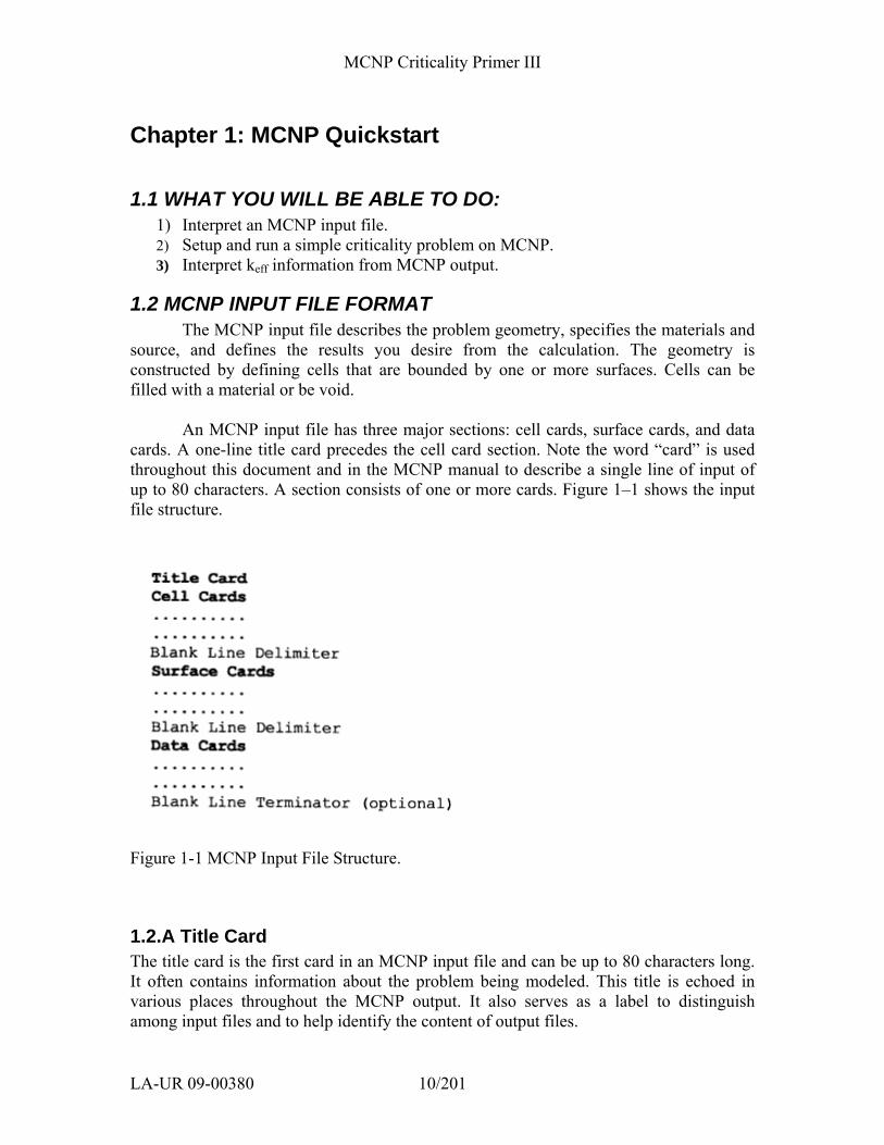
An MCNP input file has three major sections: cell cards, surface cards, and data cards. A one-line title card precedes the cell card section. Note the word “card” is used throughout this document and in the MCNP manual to describe a single line of input of up to 80 characters. A section consists of one or more cards. Figure 1–1 shows the input file structure.
Figure 1-1 MCNP Input File Structure.
1.2.A Title Card The title card is the first card in an MCNP input file and can be up to 80 characters long. It often contains information about the problem being modeled. This title is echoed in various places throughout the MCNP output. It also serves as a label to distinguish among input files and to help identify the content of output files.
MCNP Criticality Primer III
LA-UR 09-00380 11/201
1.2.B General Card Format The cards in each section can be in any order and alphabetic characters can be
upper, lower, or mixed case. MCNP uses a blank line delimiter to denote separation between the three different sections. In this chapter only, we will use a “Ъ” to identify these blank lines.
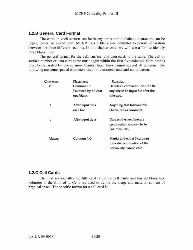
The general format for the cell, surface, and data cards is the same. The cell or surface number or data card name must begin within the first five columns. Card entries must be separated by one or more blanks. Input lines cannot exceed 80 columns. The following are some special characters used for comments and card continuation.
1.2.C Cell Cards The first section after the title card is for the cell cards and has no blank line
delimiter at the front of it. Cells are used to define the shape and material content of physical space. The specific format for a cell card is:
MCNP Criticality Primer III
LA-UR 09-00380 12/201
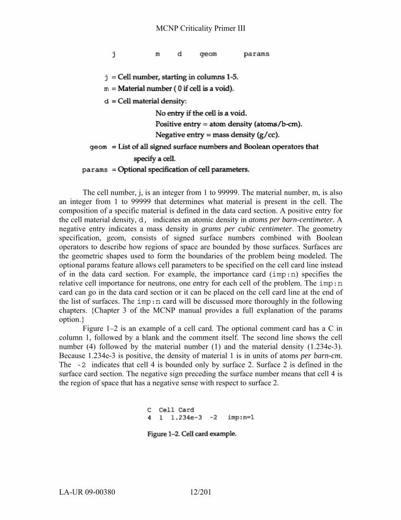
The cell number, j, is an integer from 1 to 99999. The material number, m, is also an integer from 1 to 99999 that determines what material is present in the cell. The composition of a specific material is defined in the data card section. A positive entry for the cell material density, d, indicates an atomic density in atoms per barn-centimeter. A negative entry indicates a mass density in grams per cubic centimeter. The geometry specification, geom, consists of signed surface numbers combined with Boolean operators to describe how regions of space are bounded by those surfaces. Surfaces are the geometric shapes used to form the boundaries of the problem being modeled. The optional params feature allows cell parameters to be specified on the cell card line instead of in the data card section. For example, the importance card (imp:n) specifies the relative cell importance for neutrons, one entry for each cell of the problem. The imp:n card can go in the data card section or it can be placed on the cell card line at the end of the list of surfaces. The imp:n card will be discussed more thoroughly in the following chapters. {Chapter 3 of the MCNP manual provides a full explanation of the params option.}
Figure 1–2 is an example of a cell card. The optional comment card has a C in column 1, followed by a blank and the comment itself. The second line shows the cell number (4) followed by the material number (1) and the material density (1.234e-3). Because 1.234e-3 is positive, the density of material 1 is in units of atoms per barn-cm. The -2 indicates that cell 4 is bounded only by surface 2. Surface 2 is defined in the surface card section. The negative sign preceding the surface number means that cell 4 is the region of space that has a negative sense with respect to surface 2.
MCNP Criticality Primer III
LA-UR 09-00380 13/201
1.2.D Surface Cards The specific format for a surface card is:
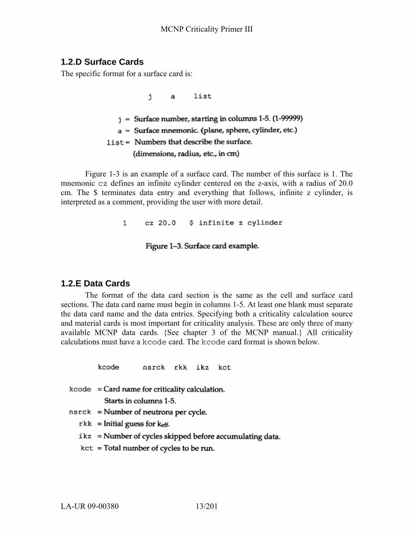
Figure 1-3 is an example of a surface card. The number of this surface is 1. The
mnemonic cz defines an infinite cylinder centered on the z-axis, with a radius of 20.0 cm. The $ terminates data entry and everything that follows, infinite z cylinder, is interpreted as a comment, providing the user with more detail.
1.2.E Data Cards The format of the data card section is the same as the cell and surface card
sections. The data card name must begin in columns 1-5. At least one blank must separate the data card name and the data entries. Specifying both a criticality calculation source and material cards is most important for criticality analysis. These are only three of many available MCNP data cards. {See chapter 3 of the MCNP manual.} All criticality calculations must have a kcode card. The kcode card format is shown below.
MCNP Criticality Primer III
LA-UR 09-00380 14/201
Figure 1-4 is an example of a kcode card. The problem will be run with 5000 neutrons per cycle and an initial guess for keff of 1.0. Fifty cycles will be skipped before keff data accumulation begins, and a total of 250 cycles will be run.
kcode 5000 1.0 50 250
Figure 1-4. Example of kcode card.
Criticality problems often use a ksrc card to specify the initial spatial fission distribution. Other methods to specify starting fission source locations will be discussed in a later chapter. The ksrc format is shown in Figure 1–5. A fission source point will be placed at each point with coordinates (Xk, Yk, Zk). As many source points as needed can be placed within the problem geometry. All locations must be in locations with importance greater than 0, and at least one of the source points must be within a region of fissile material for the problem to run. The ksrc card format is:
Figure 1–5 shows an example of a ksrc card. Two initial fission source points are used. The first is located at the coordinates (1,0,0) and the second at (12, 3, 9).
Next we discuss the material card. The format of the material, or m card, is
mn zaid1 fraction1 zaid2 fraction2 ….
mn = Material card name (m) followed immediately by the
material number (n) on the card. The mn cards starts in columns 1-5.
zaid = Atomic number followed by the atomic mass of the isotope. Preferably (optionally) followed by the data library extension, in the form of .##L (period, two digits, one letter).
fraction = Nuclide fraction
MCNP Criticality Primer III
LA-UR 09-00380 15/201
(+) Atom weight (-) Weight fraction
An example of a material card where two isotopes of plutonium are used is shown
in Figure 1-6. The material number n is an integer from 1 to 99999. Each material can be composed of many isotopes. Default cross-sections are used when no extension is given. {Chapter 3 and Appendix G of the MCNP manual describe how to choose cross sections from different libraries.}
m1 94239.66c 2.442e-2 94240.66c 1.673e-3 Figure 1-6. Data card of default ZAIDs with material format in atom fractions.
The first ZAID is 94239.66c followed by the atom fraction. The atomic number is 94, plutonium. The atomic mass is 239 corresponding to the 239 isotope of plutonium. The .66c is the extension used to specify the ENDF66 (continuous energy) library. A second isotope in the material begins immediately after the first using the same format and so on until all material components have been described. Notice that the material data is continued on a second line. If a continuation line is desired or required, make sure the data begins after the fifth column of the next line, or end the previous line with an ampersand (&). Because the fractions are entered as positive numbers, the units are atoms/b-cm. If the atom or weight fractions do not add to unity, MCNP will automatically renormalize them.
Grey Box 1. – Preferred ZAID format: Library Extension.
Preferred ZAID format: Library Extension. The preferred method of specifying the ZAID is to use an extension to denote
the specific library you want to use. Different data libraries contain different data sets, and may differ in evaluation temperature, incident particle energy range, photon production, presence or absence of delayed neutron data, unresolved resonance treatment data and secondary charged particle data. It is important to look in Appendix G of the MCNP manual and verify that for each ZAID, the data library you intend to use matches the conditions of your MCNP simulation. The common (continuous-energy) extensions for recent data libraries (based on ENDF/B-VI) are .62c, .66c, and .60c.
When no extension (or a partial extension) is given, the first matching ZAID
listed in the xsdir file is used. This file is usually located in the directory where the MCNP data libraries are stored. To verify the data libraries used in the mcnp run, look in the output file.
MCNP Criticality Primer III
LA-UR 09-00380 16/201
1.3 EXAMPLE 1.3: BARE PU SPHERE This introduction should provide enough information to run a simple example
problem. It is our intent that you gain confidence in using MCNP right away, so we walk through this sample problem step by step, explaining each line of input. For the present it is important that you enter this problem exactly as we describe it. As you gain more experience with MCNP, you may find other ways to setup input files that are more logical to you. For example, you may find it easier to work out the surface cards before doing the cell cards.
1.3.A Problem Description This problem is a bare sphere of plutonium metal with a coating of nickel (also
known as Jezebel). Experimental parameters are (Reference 1):
Delta-phase Pu metal sphere: radius = 6.3849 cm N239 = Atom density of 239Pu3.7047e-2 atom/barn-cm N240 = Atom density of 240Pu 1.7512e-3 atom/barn-cm N241 = Atom density of 241Pu 1.1674e-4 atom/barn-cm NGa = Atom density of Ga 1.3752e-3 atom/barn-cm
Spherical nickel coating: Thisckness = 0.0127 cm NNi = Atom density of Ni 9.3122e-2 atom/barn-cm
Now you are ready to begin entering the example problem. First open a new file
named example. All text shown in the courier font is what you need to type in. Each new card, as it is discussed, is indicated by an arrow in the left margin. The first line in the file must be the title card, which is followed by the three major sections of an MCNP input file (cells, surfaces, and data).
1.3.B Title Card A one line title card is required and can be up to 80 characters in length. There is
no blank line between the title card and the cell cards.
Example 1-2. Jezebel. Bare Pu sphere w/ Ni shell
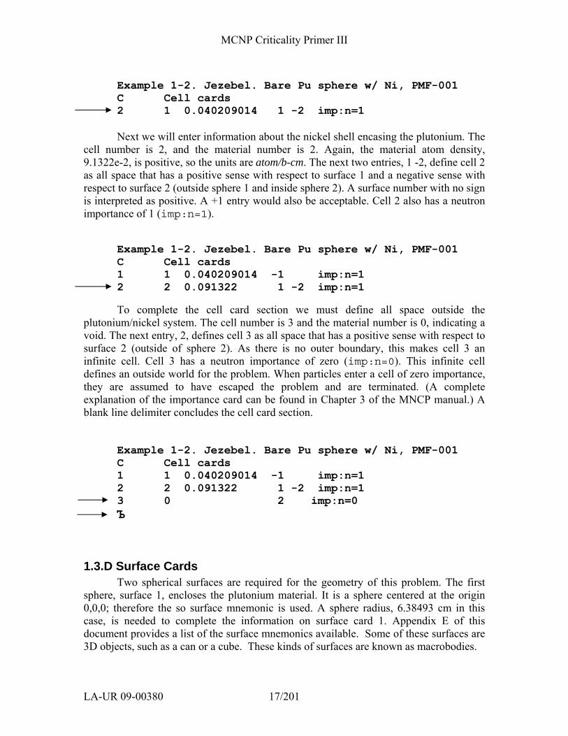
1.3.C Cell Cards The problem requires description of the plutonium sphere and a nickel shell, as
shown in Figure 1-7. We will enter the plutonium cell information first. The comment card shows how it helps make the input file easier to follow. The cell number is 1 and the material number is 1. The material density, 4.0290e-2, is the sum of the material densities of the plutonium isotopes present in the sphere. Because 4.0290e-2 is positive, the units are atoms/b-cm. The next entry, -1, indicates that cell 1 (inside the sphere) is all space having a negative sense with respect to surface 1. The imp:n=l says this cell has an importance (imp) for neutrons (:n) of 1.
MCNP Criticality Primer III
LA-UR 09-00380 17/201
Example 1-2. Jezebel. Bare Pu sphere w/ Ni, PMF-001 C Cell cards 2 1 0.040209014 1 -2 imp:n=1
Next we will enter information about the nickel shell encasing the plutonium. The
cell number is 2, and the material number is 2. Again, the material atom density, 9.1322e-2, is positive, so the units are atom/b-cm. The next two entries, 1 -2, define cell 2 as all space that has a positive sense with respect to surface 1 and a negative sense with respect to surface 2 (outside sphere 1 and inside sphere 2). A surface number with no sign is interpreted as positive. A +1 entry would also be acceptable. Cell 2 also has a neutron importance of 1 (imp:n=1).
Example 1-2. Jezebel. Bare Pu sphere w/ Ni, PMF-001 C Cell cards 1 1 0.040209014 -1 imp:n=1 2 2 0.091322 1 -2 imp:n=1
To complete the cell card section we must define all space outside the
plutonium/nickel system. The cell number is 3 and the material number is 0, indicating a void. The next entry, 2, defines cell 3 as all space that has a positive sense with respect to surface 2 (outside of sphere 2). As there is no outer boundary, this makes cell 3 an infinite cell. Cell 3 has a neutron importance of zero (imp:n=0). This infinite cell defines an outside world for the problem. When particles enter a cell of zero importance, they are assumed to have escaped the problem and are terminated. (A complete explanation of the importance card can be found in Chapter 3 of the MNCP manual.) A blank line delimiter concludes the cell card section.
Example 1-2. Jezebel. Bare Pu sphere w/ Ni, PMF-001 C Cell cards 1 1 0.040209014 -1 imp:n=1 2 2 0.091322 1 -2 imp:n=1 3 0 2 imp:n=0 Ъ
1.3.D Surface Cards Two spherical surfaces are required for the geometry of this problem. The first
sphere, surface 1, encloses the plutonium material. It is a sphere centered at the origin 0,0,0; therefore the so surface mnemonic is used. A sphere radius, 6.38493 cm in this case, is needed to complete the information on surface card 1. Appendix E of this document provides a list of the surface mnemonics available. Some of these surfaces are 3D objects, such as a can or a cube. These kinds of surfaces are known as macrobodies.
MCNP Criticality Primer III
LA-UR 09-00380 18/201
Example 1-2. Jezebel. Bare Pu sphere w/ Ni, PMF-001 C Cell cards 1 1 0.040209014 -1 imp:n=1 2 2 0.091322 1 -2 imp:n=1 3 0 2 imp:n=0 Ъ C Surface cards 1 so 6.3849
The second sphere, surface 2, also is centered at the origin, but it has radius of
6.39763 cm. The inner surface of the nickel shell corresponds exactly to the outer surface of the plutonium sphere, which is already defined as surface 1. A blank line concludes the surface card section. Example 1-2. Jezebel. Bare Pu sphere w/ Ni, PMF-001
C Cell cards 1 1 0.040209014 -1 imp:n=1 2 2 0.091322 1 -2 imp:n=1 3 0 2 imp:n=0 Ъ C Surface cards 1 so 6.3849 2 so 6.3976 Ъ
1.3.E Data Cards This example illustrates a criticality calculation, so the kcode card is required.
The number of neutrons per keff cycle is 5000. The number of source neutrons depends on the system and the number of cycles being run. An initial estimate of keff is 1.0 because this example’s final result is expected to be very close to critical. We will skip 50 keff cycles to allow the spatial fission source to settle to an equilibrium before keff values are used for averaging for the final keff estimate. A total of 250 keff cycles will be run.
Example 1-2. Jezebel. Bare Pu sphere w/ Ni, PMF-001 C Cell cards 1 1 0.040209014 -1 imp:n=1 2 2 0.091322 1 -2 imp:n=1 3 0 2 imp:n=0 Ъ C Surface cards 1 so 6.3849 2 so 6.3976 Ъ C Data cards C Criticality Control Cards
MCNP Criticality Primer III
LA-UR 09-00380 19/201
kcode 5000 1.0 50 250
The entries on the ksrc card place one fission source point at (0,0,0), the center of the plutonium sphere. For the first keff cycle, 5000 neutrons with a fission energy distribution will start at the origin. More source points can be used but are not necessary for this example. After the first cycle, neutrons will start at locations where fissions occurred in the previous cycle. The fission energy distribution of each such source neutron will be based upon the nuclide in which that fission occurred. Example 1-2. Jezebel. Bare Pu sphere w/ Ni, PMF-001
C Cell cards 1 1 0.040209014 -1 imp:n=1 2 2 0.091322 1 -2 imp:n=1 3 0 2 imp:n=0 Ъ C Surface cards 1 so 6.3849 2 so 6.3976 Ъ C Data cards C Criticality Control Cards kcode 5000 1.0 50 250 ksrc 0 0 0 The last information needed for this problem is a description of our materials.
Material 1, in cell 1, is plutonium, and material 2, in cell 2, is nickel. The material number on the m card is the same as the material number used on the cell card. Material 1, ml, has three isotopes of plutonium and one of gallium. The ZAID of Pu-239 is 94239.66c, followed by the nuclide atom fraction (3.7047e-2). The .66c extension indicates that the ENDF66c data library is used, which is based on the ENDF/B-VI release 6. {Look in Appendix G of the MCNP manual to view its evaluation temperature (293.6 K), νbar (prompt or total), etc.} The combined use of the ACTI (extension .62c) and ENDF66 (.66c) data libraries in this primer correspond to the final release of ENDF/B-VI. The other nuclides are treated in the same manner. Because of the length of the ml data card line, a continuation card is required. Blanks in columns 1-5 indicate this line is a continuation of the last card.
Example 1-2. Jezebel. Bare Pu sphere w/ Ni, PMF-001 C Cell cards 1 1 0.040209014 -1 imp:n=1 2 2 0.091322 1 -2 imp:n=1 3 0 2 imp:n=0 Ъ C Surface cards 1 so 6.3849
MCNP Criticality Primer III
LA-UR 09-00380 20/201
2 so 6.3976 Ъ C Data cards C Criticality Control Cards kcode 5000 1.0 50 250 ksrc 0 0 0 C Materials Cards m1 94239.66c 3.7047e-2 94240.66c 1.751e-3 94241.66c 1.17e-4 31000.66c 1.375e-3
Material 2, m2, is the nickel that coats the plutonium. The ZAIDs of the naturally occurring isotopes of nickel are 28058, 28060, 28061, 28062, 28064, all of which use the .66c extension for this problem. Each of these isotopes is followed by its normalized atomic (number) abundance: 0.6808, 0.2622, 0.0114, 0.0363, 0.0093, respectively. There is an older data set of naturally occurring nickel (ZAID 28000), and its nuclide atom fraction (1.0). The three zeros following the atomic number (28) indicate that this cross-section evaluation is for elemental nickel, where the five stable nickel isotopes are combined into one cross-section set. The newer cross section evaluation is preferred, however. The optional blank line terminator indicates the end of the data card section and the end of the input file.
Example 1-2. Jezebel. Bare Pu sphere w/ Ni, PMF-001 C Cell cards 1 1 0.040209014 -1 imp:n=1 2 2 0.091322 1 -2 imp:n=1 3 0 2 imp:n=0 Ъ C Surface cards 1 so 6.38493 2 so 6.39763 Ъ C Data cards C Criticality Control Cards kcode 5000 1.0 50 250 ksrc 0 0 0 C Materials Cards m1 94239.66c 3.7047e-2 94240.66c 1.751e-3 94241.66c 1.17e-4 31000.66c 1.375e-3 m2 28058.66c 0.6808 28060.66c 0.2622 28061.66c 0.0114 28062.66c 0.0363 28064.66c 0.0093
1.4 RUNNING MCNP5 We will assume that MCNP has been installed on the machine you are using. The
default names of the input and output files are INP and OUTP, respectively. To run MCNP5 with different file names, type mcnp inp= and then the file name of the example
MCNP Criticality Primer III
LA-UR 09-00380 21/201
problem followed by outp= and the name of the output file. The file names must be limited to 8 characters or less. Mcnp5 inp=ex12 outp=exlout
MCNP5 writes information to the screen about how the calculation is progressing. Once the calculation is complete, check the output file to see your results. The run time for this problem should be on the order of three minutes.
1.4.A Output First, let’s assume the run was successful. There is a significant amount of
information contained in the output file, but right now we are interested in the keff results. Therefore, we will skip past most of the information. Output skipped over... 1. Echo of input file. 2. Description of cell densities and masses. 3. Material and cross-section information. 4. keff estimator cycles. 5. Neutron creation and loss summary table. 6. Neutron activity per cell. After the “Neutron Activity Per Cell” you will see... keff results for: .. Jezebel. Bare Pu sphere w/ Ni shell
This is the beginning of the criticality calculation evaluation summary table. Check to see that the cycle values of the three estimators for keff – k(collision), k(absorption), and k(track length) – appear normally distributed at the 95 or 99 percent confidence level. See that all the cells with fissionable material have been sampled. The final estimated combined keff, in the dashed box, should be very close to 1 (0.99902 ± 0.00057 (1σ)), computed on a Windows 2000 Pentium IV computer at LANL with the ENDF66c data library.) You can confirm that you used the same nuclear data by searching for print table 100 in the output file.
The combined keff and standard deviation can be used to form a confidence interval for the problem. If your results are similar to these then you have successfully created the input file and run MCNP.
If your input did not run successfully, you can look at the FATAL ERROR messages in the example1 outut file. They are also displayed at the terminal. These error messages should not be ignored because they often indicate an incorrectly specified calculation. FATAL ERRORS must be corrected before the problem will run. One can use the “nofatal” option to run MCNP. The use of “nofatal” is highly discouraged and it’s use will not be discussed here. The use of “nofatal” can result in incorrect keff calculations because of the potential for incorrect problem specifications.
MCNP5 also provides WARNING messages to inform you of possible problems. For example, this calculation has the WARNING message “neutron energy cutoff is

MCNP Criticality Primer III
LA-UR 09-00380 22/201
below some cross-section tables.” The lower energy limit for most neutron cross-section data is 10e-11 MeV. The default problem energy cutoff is 0 MeV, clearly below the lowest energy data point. In all room temperature energy (2.5*10-8 MeV) problems, this message can be ignored. All WARNING messages from an MCNP calculation should be examined and understood to be certain that a problem of concern has not been detected. However, a problem will run with WARNING messages.
1.5 SUMMARY This chapter has helped you to:
1) Interpret an MCNP input file. 2) Setup and run a criticality problem with MCNP5. 3) Interpret neutron multiplication information from MCNP5 output.
{See the MCNP manual, Chapter 5, Section IV, for an annotated partial listing emphasizing the criticality aspects of the output from a criticality calculation.}
Now that you have successfully run MCNP, you are ready to learn about the more complex options available with MCNP. The following chapters present these options in a format similar to the Quickstart chapter.
MCNP Criticality Primer III
LA-UR 09-00380 23/201
Chapter 2: Reflected Systems
In the QuickStart chapter you ran a simple problem with MCNP and gained some confidence in using the code. This chapter provides a more detailed explanation of the commands used in the QuickStart chapter. Example problems are taken from LA-10860 and represent computational models of criticality benchmark experiments. Each example problem is selected to focus on two or three specific MCNP commands.
2.1 WHAT YOU WILL BE ABLE TO DO: 1) Interpret the sense of a surface. 2) Use the Boolean intersection, union, and complement geometry operators. 3) Define a multi-cell problem.
2.2 PROBLEM DESCRIPTION This set of examples uses a plutonium metal cylinder and examines three different
configurations (LA-10860 p. 101). The three configurations are a bare (unreflected) system, and two natural uranium reflected systems: one with a radial reflector and one with both a radial and an axial reflector. In each configuration the central cylinder of plutonium has a diameter of 9.87 cm while the height of the plutonium cylinder varies with the reflection conditions. The plutonium material is the same for each configuration; therefore, the plutonium atom density (N239) is the same for all three analyses. Note that for many materials both a mass density (g/cc) and an atom density (atoms/b-cm) are provided. Either is sufficient to describe materials in MCNP. Be warned, however, that the internal conversion from mass density to number density may not be consistent with the latest isotopic data (e.g., Chart of Nuclides).
2.3 EXAMPLE 2.3: BARE PU CYLINDER
The bare plutonium cylinder is modeled first. This example discusses the sense of a surface and the Boolean intersection and union geometry operators. The data for this example follows.
MCNP Criticality Primer III
LA-UR 09-00380 24/201
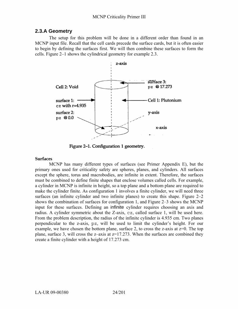
2.3.A Geometry The setup for this problem will be done in a different order than found in an
MCNP input file. Recall that the cell cards precede the surface cards, but it is often easier to begin by defining the surfaces first. We will then combine these surfaces to form the cells. Figure 2–1 shows the cylindrical geometry for example 2.3.
Surfaces
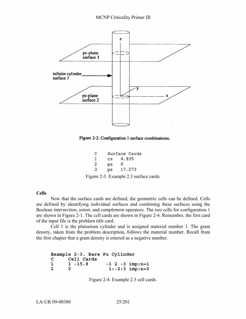
MCNP has many different types of surfaces (see Primer Appendix E), but the primary ones used for criticality safety are spheres, planes, and cylinders. All surfaces except the sphere, torus and macrobodies, are infinite in extent. Therefore, the surfaces must be combined to define finite shapes that enclose volumes called cells. For example, a cylinder in MCNP is infinite in height, so a top plane and a bottom plane are required to make the cylinder finite. As configuration 1 involves a finite cylinder, we will need three surfaces (an infinite cylinder and two infinite planes) to create this shape. Figure 2–2 shows the combination of surfaces for configuration 1, and Figure 2–3 shows the MCNP input for these surfaces. Defining an infinite cylinder requires choosing an axis and radius. A cylinder symmetric about the Z-axis, cz, called surface 1, will be used here. From the problem description, the radius of the infinite cylinder is 4.935 cm. Two planes perpendicular to the z-axis, pz, will be used to limit the cylinder’s height. For our example, we have chosen the bottom plane, surface 2, to cross the z-axis at z=0. The top plane, surface 3, will cross the z–axis at z=17.273. When the surfaces are combined they create a finite cylinder with a height of 17.273 cm.
MCNP Criticality Primer III
LA-UR 09-00380 25/201
Figure 2-3. Example 2.3 surface cards.
Cells
Now that the surface cards are defined, the geometric cells can be defined. Cells are defined by identifying individual surfaces and combining these surfaces using the Boolean intersection, union, and complement operators. The two cells for configuration 1 are shown in Figure 2-1. The cell cards are shown in Figure 2-4. Remember, the first card of the input file is the problem title card.
Cell 1 is the plutonium cylinder and is assigned material number 1. The gram density, taken from the problem description, follows the material number. Recall from the first chapter that a gram density is entered as a negative number.
Example 2-3. Bare Pu Cylinder C Cell Cards 1 1 -15.8 -1 2 -3 imp:n=1 2 0 1:-2:3 imp:n=0
Figure 2-4. Example 2.3 cell cards.
MCNP Criticality Primer III
LA-UR 09-00380 26/201
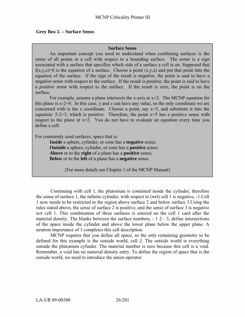
Grey Box 2. – Surface Sense.
Continuing with cell 1, the plutonium is contained inside the cylinder, therefore the sense of surface 1, the infinite cylinder, with respect to (wrt) cell 1 is negative, -1.Cell 1 now needs to be restricted to the region above surface 2 and below surface 3.Using the rules stated above, the sense of surface 2 is positive, and the sense of surface 3 is negative wrt cell 1. This combination of three surfaces is entered on the cell 1 card after the material density. The blanks between the surface numbers, - 1 2 - 3, define intersections of the space inside the cylinder and above the lower plane below the upper plane. A neutron importance of 1 completes this cell description.
MCNP requires that you define all space, so the only remaining geometry to be defined for this example is the outside world, cell 2. The outside world is everything outside the plutonium cylinder. The material number is zero because this cell is a void. Remember, a void has no material density entry. To define the region of space that is the outside world, we need to introduce the union operator.
Surface Sense An important concept you need to understand when combining surfaces is the sense of all points in a cell with respect to a bounding surface. The sense is a sign associated with a surface that specifies which side of a surface a cell is on. Supposed that f(x,y,z)=0 is the equation of a surface. Choose a point (x,y,z) and put that point into the equation of the surface. If the sign of the result is negative, the point is said to have a negative sense with respect to the surface. If the result is positive, the point is said to have a positive sense with respect to the surface. If the result is zero, the point is on the surface. For example, assume a plane intersects the x-axis at x=2. The MCNP equation for this plane is x-2=0. In this case, y and z can have any value, so the only coordinate we are concerned with is the x coordinate. Choose a point, say x=5, and substitute it into the equation: 5-2=3, which is positive. Therefore, the point x=5 has a positive sense with respect to the plane at x=2. You do not have to evaluate an equation every time you define a cell. For commonly used surfaces, space that is: Inside a sphere, cylinder, or cone has a negative sense; Outside a sphere, cylinder, or cone has a positive sense; Above or to the right of a plane has a positive sense; Below or to the left of a plane has a negative sense. {For more details see Chapter 1 of the MCNP Manual}
MCNP Criticality Primer III
LA-UR 09-00380 27/201
Grey Box 3. – Intersections and Unions.
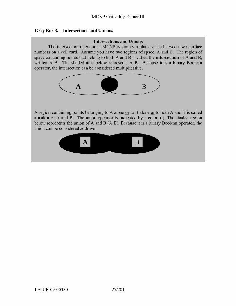
Intersections and Unions The intersection operator in MCNP is simply a blank space between two surface numbers on a cell card. Assume you have two regions of space, A and B. The region of space containing points that belong to both A and B is called the intersection of A and B, written A B. The shaded area below represents A B. Because it is a binary Boolean operator, the intersection can be considered multiplicative.
A region containing points belonging to A alone or to B alone or to both A and B is called a union of A and B. The union operator is indicated by a colon (:). The shaded region below represents the union of A and B (A:B). Because it is a binary Boolean operator, the union can be considered additive.
A B
BA
MCNP Criticality Primer III
LA-UR 09-00380 28/201
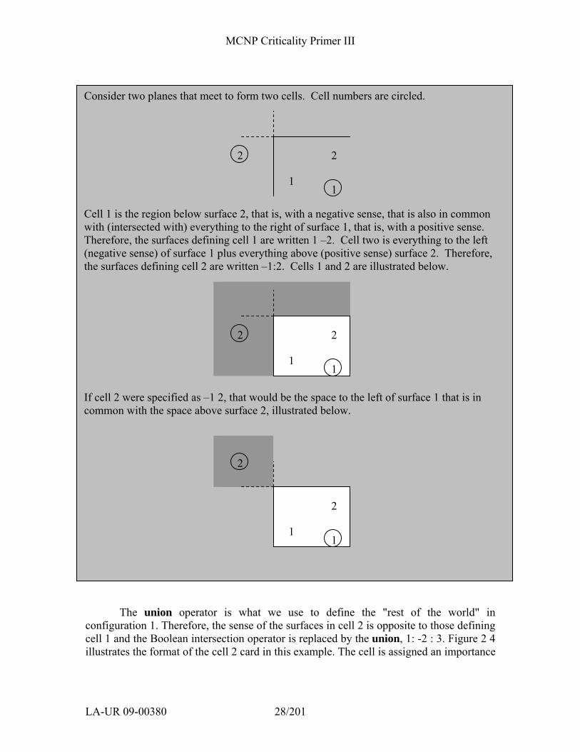
The union operator is what we use to define the "rest of the world" in configuration 1. Therefore, the sense of the surfaces in cell 2 is opposite to those defining cell 1 and the Boolean intersection operator is replaced by the union, 1: -2 : 3. Figure 2 4 illustrates the format of the cell 2 card in this example. The cell is assigned an importance
Consider two planes that meet to form two cells. Cell numbers are circled. Cell 1 is the region below surface 2, that is, with a negative sense, that is also in common with (intersected with) everything to the right of surface 1, that is, with a positive sense. Therefore, the surfaces defining cell 1 are written 1 –2. Cell two is everything to the left (negative sense) of surface 1 plus everything above (positive sense) surface 2. Therefore, the surfaces defining cell 2 are written –1:2. Cells 1 and 2 are illustrated below. If cell 2 were specified as –1 2, that would be the space to the left of surface 1 that is in common with the space above surface 2, illustrated below.
2 2
1 1
2 2
1 1
2
2
1 1
MCNP Criticality Primer III
LA-UR 09-00380 29/201
of zero. Any particles entering cell 2 need to be terminated immediately because once particles leave the cylinder they have no chance of returning.
2.3.B Alternate Geometry Description – Macrobody Another way to describe the same geometry is to use a pre-existing 3D object
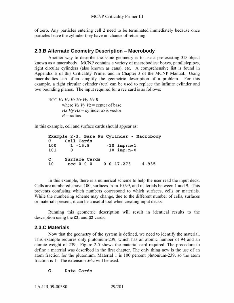
known as a macrobody. MCNP contains a variety of macrobodies: boxes, parallelepipes, right circular cylinders (also known as cans), etc. A comprehensive list is found in Appendix E of this Criticality Primer and in Chapter 3 of the MCNP Manual. Using macrobodies can often simplify the geometric description of a problem. For this example, a right circular cylinder (rcc) can be used to replace the infinite cylinder and two bounding planes. The input required for a rcc card is as follows:
RCC Vx Vy Vz Hx Hy Hz R
where Vx Vy Vz = center of base Hx Hy Hz = cylinder axis vector R = radius
In this example, cell and surface cards should appear as:
Example 2-3. Bare Pu Cylinder - Macrobody C Cell Cards 100 1 -15.8 -10 imp:n=1 101 0 10 imp:n=0
C Surface Cards 10 rcc 0 0 0 0 0 17.273 4.935
In this example, there is a numerical scheme to help the user read the input deck.
Cells are numbered above 100, surfaces from 10-99, and materials between 1 and 9. This prevents confusing which numbers correspond to which surfaces, cells or materials. While the numbering scheme may change, due to the different number of cells, surfaces or materials present, it can be a useful tool when creating input decks.
Running this geometric description will result in identical results to the description using the cz, and pz cards.
2.3.C Materials Now that the geometry of the system is defined, we need to identify the material.
This example requires only plutonium-239, which has an atomic number of 94 and an atomic weight of 239. Figure 2-5 shows the material card required. The procedure to define a material was described in the first chapter. The only thing new is the use of an atom fraction for the plutonium. Material 1 is 100 percent plutonium-239, so the atom fraction is 1. The extension .66c will be used.
C Data Cards
MCNP Criticality Primer III
LA-UR 09-00380 30/201
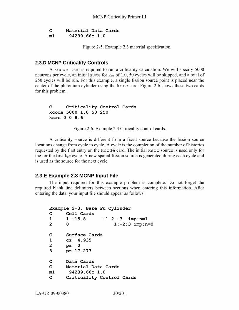
C Material Data Cards m1 94239.66c 1.0
Figure 2-5. Example 2.3 material specification
2.3.D MCNP Criticality Controls A kcode card is required to run a criticality calculation. We will specify 5000
neutrons per cycle, an initial guess for keff of 1.0, 50 cycles will be skipped, and a total of 250 cycles will be run. For this example, a single fission source point is placed near the center of the plutonium cylinder using the ksrc card. Figure 2-6 shows these two cards for this problem.
C Criticality Control Cards kcode 5000 1.0 50 250 ksrc 0 0 8.6
Figure 2-6. Example 2.3 Criticality control cards.
A criticality source is different from a fixed source because the fission source locations change from cycle to cycle. A cycle is the completion of the number of histories requested by the first entry on the kcode card. The initial ksrc source is used only for the for the first keff cycle. A new spatial fission source is generated during each cycle and is used as the source for the next cycle.
2.3.E Example 2.3 MCNP Input File The input required for this example problem is complete. Do not forget the
required blank line delimiters between sections when entering this information. After entering the data, your input file should appear as follows: Example 2-3. Bare Pu Cylinder
C Cell Cards 1 1 -15.8 -1 2 -3 imp:n=1 2 0 1:-2:3 imp:n=0 C Surface Cards 1 cz 4.935 2 pz 0 3 pz 17.273 C Data Cards C Material Data Cards m1 94239.66c 1.0 C Criticality Control Cards
MCNP Criticality Primer III
LA-UR 09-00380 31/201
kcode 5000 1.0 50 250 ksrc 0 0 8.6
The problem can be run by typing...
mcnp5 inp=filel outp=file2 runtpe=file3 where inp, outp, and runtpe are the default names for the input file, the output file, and the binary results file, respectively. The runtpe file is useful for plotting problem results and for continuing a calculation as discussed in later chapters of the Primer. The name option is useful for automatically naming files. It uses the inp name as the base and appends the appropriate letter (o for outp and r for runtpe).
mcnp5 name=ex23 produces an outp file named ex23o, a runtpe file ex23r, and a source file ex23s.
2.3.F Output At this time we are only interested in looking at the keff result in the output. Recall
from the first chapter that there is a good deal of information to be skipped to find final estimated combined collision/absorption/track-length keff. Your result should be close to 1.01. The result on a Windows 2000 Pentium 4 computer with the ENDF66c data library at LANL was 1.01403 with an estimated standard deviation of 0.00066 (1σ). If your result is not close to ours, check your input to make sure your surface dimensions are correct and that material densities are correctly entered on the cell cards.
2.4 EXAMPLE 2.4: PU CYLINDER, RADIAL U REFLECTOR The second problem in this chapter takes example 2.3 and adds a radial natural
uranium reflector. This example introduces how to define cells within cells.
MCNP Criticality Primer III
LA-UR 09-00380 32/201
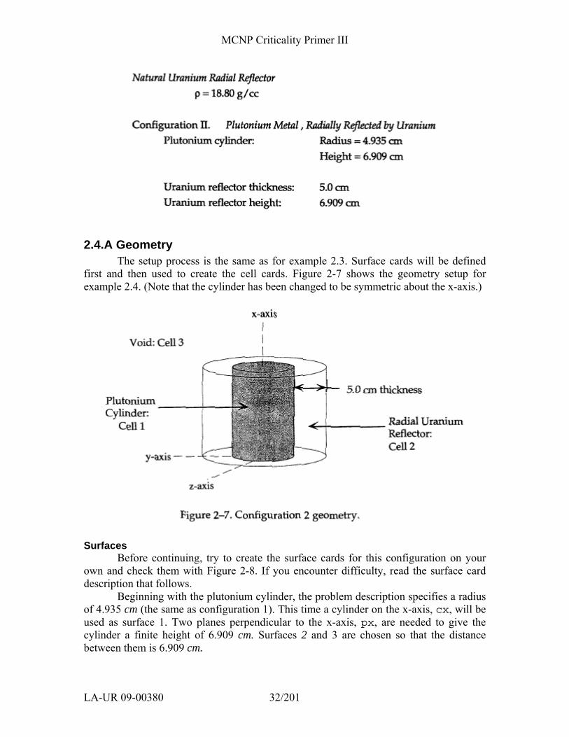
2.4.A Geometry The setup process is the same as for example 2.3. Surface cards will be defined
first and then used to create the cell cards. Figure 2-7 shows the geometry setup for example 2.4. (Note that the cylinder has been changed to be symmetric about the x-axis.)
Surfaces
Before continuing, try to create the surface cards for this configuration on your own and check them with Figure 2-8. If you encounter difficulty, read the surface card description that follows.
Beginning with the plutonium cylinder, the problem description specifies a radius of 4.935 cm (the same as configuration 1). This time a cylinder on the x-axis, cx, will be used as surface 1. Two planes perpendicular to the x-axis, px, are needed to give the cylinder a finite height of 6.909 cm. Surfaces 2 and 3 are chosen so that the distance between them is 6.909 cm.
MCNP Criticality Primer III
LA-UR 09-00380 33/201
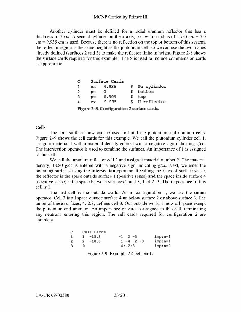
Another cylinder must be defined for a radial uranium reflector that has a thickness of 5 cm. A second cylinder on the x-axis, cx, with a radius of 4.935 cm + 5.0 cm = 9.935 cm is used. Because there is no reflection on the top or bottom of this system, the reflector region is the same height as the plutonium cell, so we can use the two planes already defined (surfaces 2 and 3) to make the reflector finite in height, Figure 2-8 shows the surface cards required for this example. The $ is used to include comments on cards as appropriate.
Cells
The four surfaces now can be used to build the plutonium and uranium cells. Figure 2–9 shows the cell cards for this example. We call the plutonium cylinder cell 1, assign it material 1 with a material density entered with a negative sign indicating g/cc-The intersection operator is used to combine the surfaces. An importance of 1 is assigned to this cell.
We call the uranium reflector cell 2 and assign it material number 2. The material density, 18.80 g/cc is entered with a negative sign indicating g/cc. Next, we enter the bounding surfaces using the intersection operator. Recalling the rules of surface sense, the reflector is the space outside surface 1 (positive sense) and the space inside surface 4 (negative sense) ~ the space between surfaces 2 and 3, 1 -4 2 -3. The importance of this cell is 1.
The last cell is the outside world. As in configuration 1, we use the union operator. Cell 3 is all space outside surface 4 or below surface 2 or above surface 3. The union of these surfaces, 4:-2:3, defines cell 3. Our outside world is now all space except the plutonium and uranium. An importance of zero is assigned to this cell, terminating any neutrons entering this region. The cell cards required for configuration 2 are complete.
Figure 2-9. Example 2.4 cell cards.
MCNP Criticality Primer III
LA-UR 09-00380 34/201
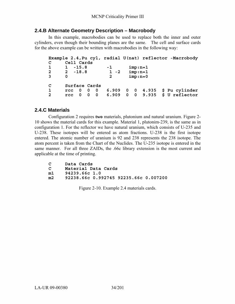
2.4.B Alternate Geometry Description – Macrobody In this example, macrobodies can be used to replace both the inner and outer cylinders, even though their bounding planes are the same. The cell and surface cards for the above example can be written with macrobodies in the following way:
Example 2.4,Pu cyl, radial U(nat) reflector -Macrobody C Cell Cards 1 1 -15.8 -1 imp:n=1 2 2 -18.8 1 -2 imp:n=1 3 0 2 imp:n=0
C Surface Cards 1 rcc 0 0 0 6.909 0 0 4.935 $ Pu cylinder 2 rcc 0 0 0 6.909 0 0 9.935 $ U reflector
2.4.C Materials Configuration 2 requires two materials, plutonium and natural uranium. Figure 2-
10 shows the material cards for this example. Material 1, plutonim-239, is the same as in configuration 1. For the reflector we have natural uranium, which consists of U-235 and U-238. These isotopes will be entered as atom fractions. U-238 is the first isotope entered. The atomic number of uranium is 92 and 238 represents the 238 isotope. The atom percent is taken from the Chart of the Nuclides. The U-235 isotope is entered in the same manner. For all three ZAIDs, the .66c library extension is the most current and applicable at the time of printing.
C Data Cards C Material Data Cards m1 94239.66c 1.0 m2 92238.66c 0.992745 92235.66c 0.007200
Figure 2-10. Example 2.4 materials cards.
MCNP Criticality Primer III
LA-UR 09-00380 35/201
Grey Box 4. – Normalization of Atom Fractions.
2.4.D MCNP Criticality Controls The entries on the required kcode card do not change from example 2-3.
Because we made the cylinder shorter, we will move the initial source point closer to the center of the cylinder at 3.5 cm on the x-axis. Figure 2-11 shows the criticality controls for this example.
C Criticality Control Cards kcode 5000 1.0 50 250 ksrc 3.5 0 0
Figure 2-11. Example 2.4 criticality control cards.
2.4.E Example 2.4 MCNP Input File The input for this problem is complete. Double check your input for entry errors
and do not forget the blank-line delimiters between sections. After you have entered this information, the input file should appear as follows
Normalization of Atom Fractions The atom fractions of the two uranium isotopes do not add exactly to 1.00. When this occurs, MCNP renormalizes the values. For example, if you have trace elements in a material that you do not include in the material card, the atom fractions will not add up to exactly 1.0. MCNP will then add up the specific fractions and renormalize then to sum to 1.0. A WARNING message informs you that the fractions did not add either to one or to the density on the cell card.
MCNP Criticality Primer III
LA-UR 09-00380 36/201
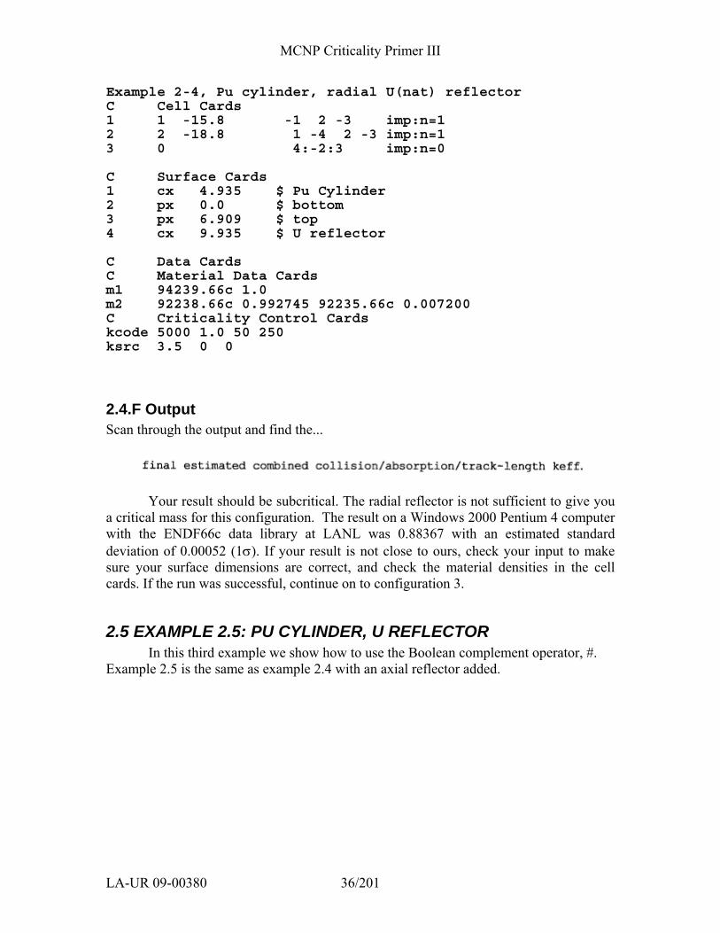
Example 2-4, Pu cylinder, radial U(nat) reflector C Cell Cards 1 1 -15.8 -1 2 -3 imp:n=1 2 2 -18.8 1 -4 2 -3 imp:n=1 3 0 4:-2:3 imp:n=0 C Surface Cards 1 cx 4.935 $ Pu Cylinder 2 px 0.0 $ bottom 3 px 6.909 $ top 4 cx 9.935 $ U reflector C Data Cards C Material Data Cards m1 94239.66c 1.0 m2 92238.66c 0.992745 92235.66c 0.007200 C Criticality Control Cards kcode 5000 1.0 50 250 ksrc 3.5 0 0
2.4.F Output Scan through the output and find the...
Your result should be subcritical. The radial reflector is not sufficient to give you a critical mass for this configuration. The result on a Windows 2000 Pentium 4 computer with the ENDF66c data library at LANL was 0.88367 with an estimated standard deviation of 0.00052 (1σ). If your result is not close to ours, check your input to make sure your surface dimensions are correct, and check the material densities in the cell cards. If the run was successful, continue on to configuration 3.
2.5 EXAMPLE 2.5: PU CYLINDER, U REFLECTOR In this third example we show how to use the Boolean complement operator, #.
Example 2.5 is the same as example 2.4 with an axial reflector added.
MCNP Criticality Primer III
LA-UR 09-00380 37/201
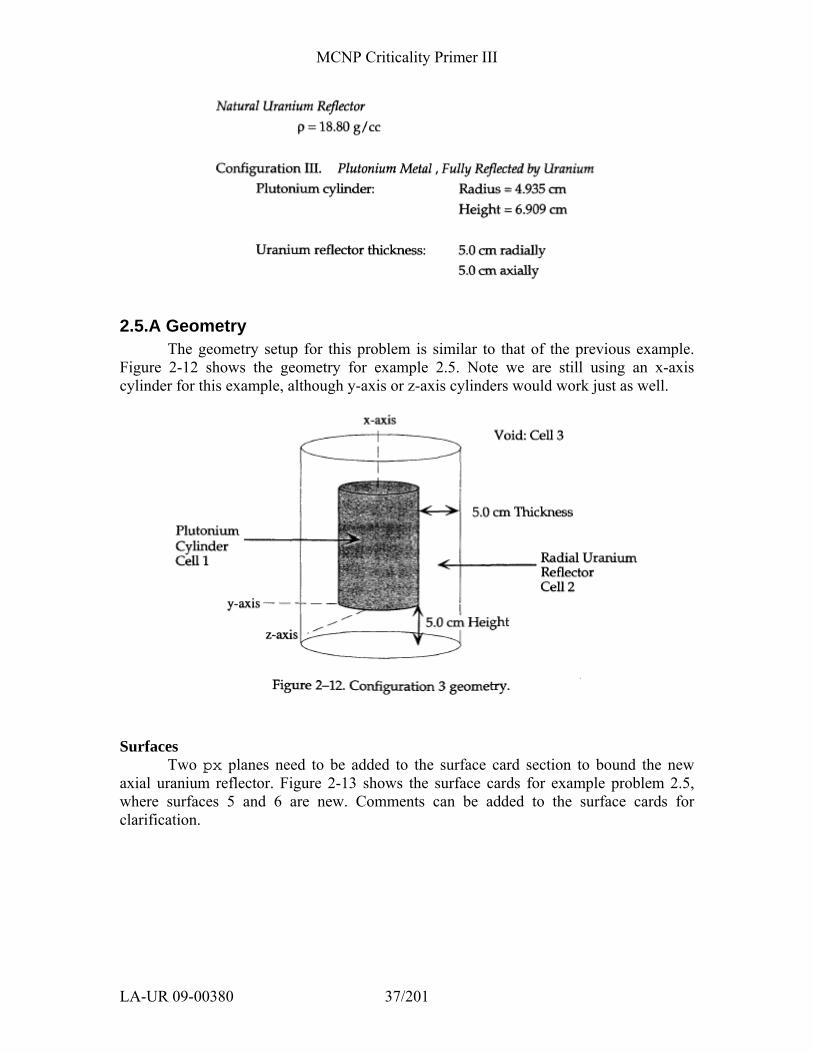
2.5.A Geometry The geometry setup for this problem is similar to that of the previous example.
Figure 2-12 shows the geometry for example 2.5. Note we are still using an x-axis cylinder for this example, although y-axis or z-axis cylinders would work just as well.
Surfaces
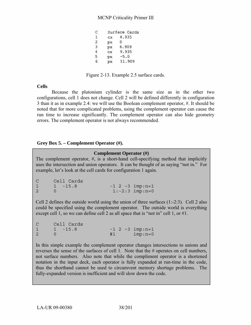
Two px planes need to be added to the surface card section to bound the new axial uranium reflector. Figure 2-13 shows the surface cards for example problem 2.5, where surfaces 5 and 6 are new. Comments can be added to the surface cards for clarification.
MCNP Criticality Primer III
LA-UR 09-00380 38/201
Figure 2-13. Example 2.5 surface cards. Cells
Because the plutonium cylinder is the same size as in the other two configurations, cell 1 does not change. Cell 2 will be defined differently in configuration 3 than it as in example 2.4: we will use the Boolean complement operator, #. It should be noted that for more complicated problems, using the complement operator can cause the run time to increase significantly. The complement operator can also hide geometry errors. The complement operator is not always recommended. Grey Box 5. – Complement Operator (#).
Complement Operator (#) The complement operator, #, is a short-hand cell-specifying method that implicitly uses the intersection and union operators. It can be thought of as saying “not in.” For example, let’s look at the cell cards for configuration 1 again. C Cell Cards 1 1 -15.8 -1 2 –3 imp:n=1 2 0 1:-2:3 imp:n=0 Cell 2 defines the outside world using the union of three surfaces (1:-2:3). Cell 2 also could be specified using the complement operator. The outside world is everything except cell 1, so we can define cell 2 as all space that is “not in” cell 1, or #1. C Cell Cards 1 1 -15.8 -1 2 –3 imp:n=1 2 0 #1 imp:n=0 In this simple example the complement operator changes intersections to unions and reverses the sense of the surfaces of cell 1. Note that the # operates on cell numbers, not surface numbers. Also note that while the compliment operator is a shortened notation in the input deck, each operator is fully expanded at run-time in the code, thus the shorthand cannot be used to circumvent memory shortage problems. The fully-expanded version is inefficient and will slow down the code.
MCNP Criticality Primer III
LA-UR 09-00380 39/201
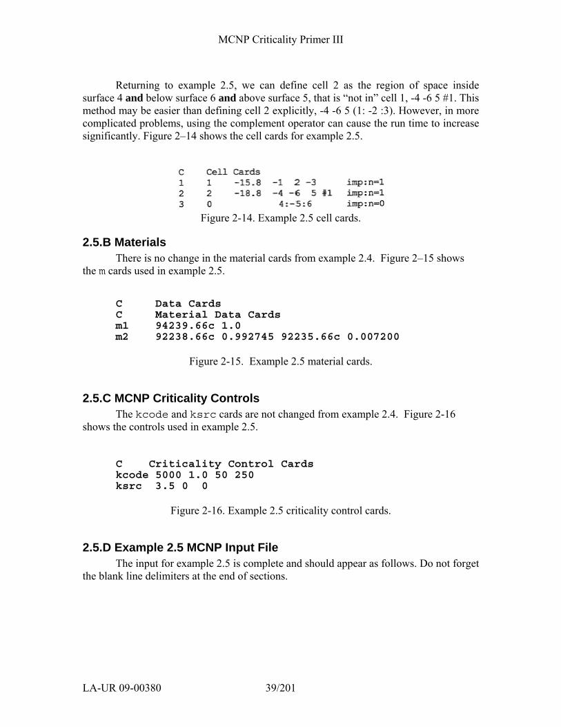
Returning to example 2.5, we can define cell 2 as the region of space inside
surface 4 and below surface 6 and above surface 5, that is “not in” cell 1, -4 -6 5 #1. This method may be easier than defining cell 2 explicitly, -4 -6 5 (1: -2 :3). However, in more complicated problems, using the complement operator can cause the run time to increase significantly. Figure 2–14 shows the cell cards for example 2.5.
Figure 2-14. Example 2.5 cell cards.
2.5.B Materials There is no change in the material cards from example 2.4. Figure 2–15 shows
the m cards used in example 2.5.
C Data Cards C Material Data Cards m1 94239.66c 1.0 m2 92238.66c 0.992745 92235.66c 0.007200
Figure 2-15. Example 2.5 material cards.
2.5.C MCNP Criticality Controls The kcode and ksrc cards are not changed from example 2.4. Figure 2-16
shows the controls used in example 2.5.
C Criticality Control Cards kcode 5000 1.0 50 250 ksrc 3.5 0 0
Figure 2-16. Example 2.5 criticality control cards.
2.5.D Example 2.5 MCNP Input File The input for example 2.5 is complete and should appear as follows. Do not forget
the blank line delimiters at the end of sections.
MCNP Criticality Primer III
LA-UR 09-00380 40/201
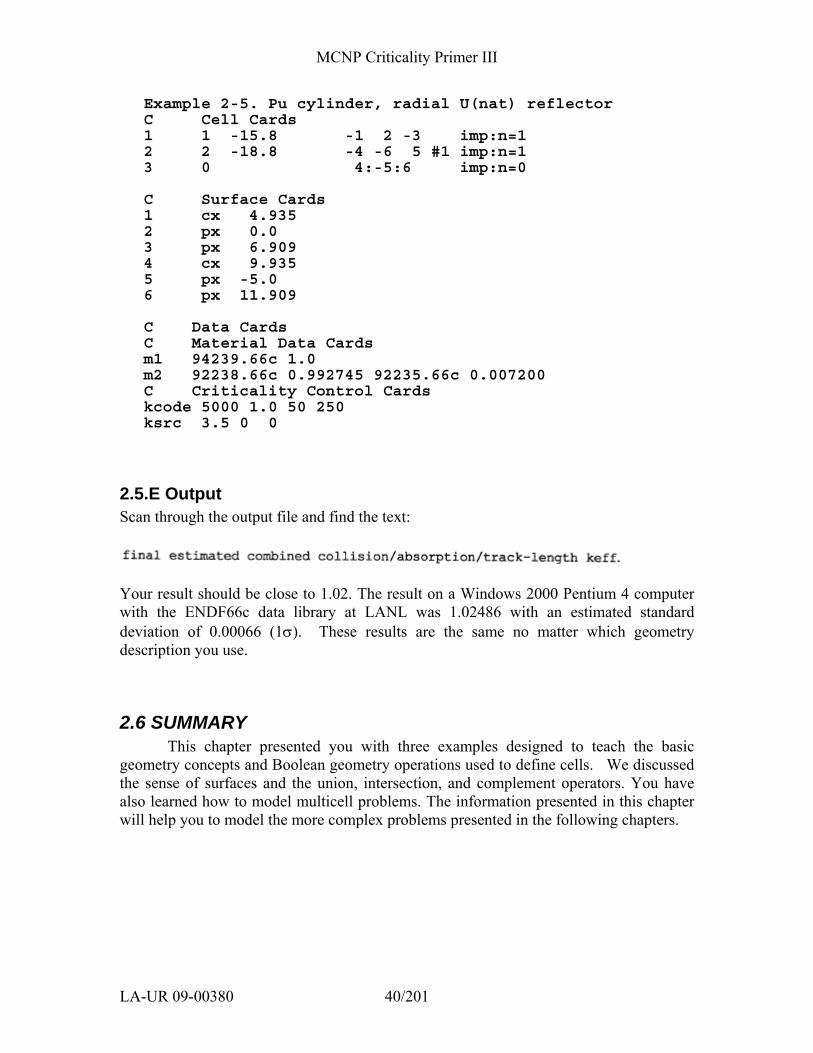
Example 2-5. Pu cylinder, radial U(nat) reflector C Cell Cards 1 1 -15.8 -1 2 -3 imp:n=1 2 2 -18.8 -4 -6 5 #1 imp:n=1 3 0 4:-5:6 imp:n=0 C Surface Cards 1 cx 4.935 2 px 0.0 3 px 6.909 4 cx 9.935 5 px -5.0 6 px 11.909 C Data Cards C Material Data Cards m1 94239.66c 1.0 m2 92238.66c 0.992745 92235.66c 0.007200 C Criticality Control Cards kcode 5000 1.0 50 250 ksrc 3.5 0 0
2.5.E Output Scan through the output file and find the text:
Your result should be close to 1.02. The result on a Windows 2000 Pentium 4 computer with the ENDF66c data library at LANL was 1.02486 with an estimated standard deviation of 0.00066 (1σ). These results are the same no matter which geometry description you use.
2.6 SUMMARY This chapter presented you with three examples designed to teach the basic
geometry concepts and Boolean geometry operations used to define cells. We discussed the sense of surfaces and the union, intersection, and complement operators. You have also learned how to model multicell problems. The information presented in this chapter will help you to model the more complex problems presented in the following chapters.
MCNP Criticality Primer III
LA-UR 09-00380 41/201
Chapter 3: S(α,β) Thermal Neutron Scattering Laws for Moderators
This chapter presents the use of S(α,β) thermal neutron scattering laws for use with problems containing hydrogenous and other moderating material. It also demonstrates how to handle a void region that is not defined as the “rest of the world.” An explanation of the basic features of the MCNP & output is provided.
3.1 WHAT YOU WILL BE ABLE TO DO: 1) Use and understand S(α,β) thermal neutron scattering laws. 2) Understand the order of geometry operations on cell cards. 3) See effects of S(α,β) treatment. 4) Interpret keff output.
3.2 S(α,β) THERMAL NEUTRON SCATTERING LAWS Let’s begin with a description of why we use S(α,β) scattering laws. When the
neutron energy drops below a few eV, the thermal motion of scattering nuclei strongly affects collisions. The simplest model to account for this effect is the free gas model that assumes the nuclei are present in the form of a monatomic gas. This is the MCNP default for thermal neutron interactions. In reality, most nuclei will be present as components of molecules in liquids or solids. For bound nuclei, energy can be stored in vibrations and rotations. The binding of individual nuclei will affect the interaction between thermal neutrons and that material. The S(α,β) scattering laws are used to account for the bound effects of the nuclei. It is important to recognize that the binding effects for hydrogen in water are different than for hydrogen in polyethylene. MCNP has different S(α,β) data for hydrogen, as well as other elements. See the MCNP Manual to see what materials have available neutron scattering law data.
3.3 PROBLEM DESCRIPTION This example is a bare (unreflected) UO2F2 solution cylinder (LA-10860 p.32).
The weight percent of 235U in the uranium is 4.89 %. The solution has a radius of 20.12 cm and a height of 100.0 cm. An aluminum tank with a thickness of 0.1587 cm on the sides and bottom, and a height of 110.0 cm contains the solution. There is no lid on the tank. The region from the top of the solution to the top of the aluminum tank is void. The data for this problem follows:
MCNP Criticality Primer III
LA-UR 09-00380 42/201
3.4 EXAMPLE 3.4: BARE UO2F2 SOLUTION CYLINDER
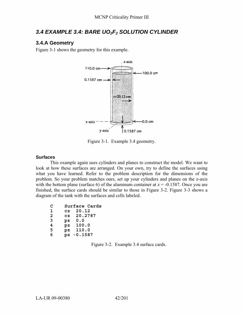
3.4.A Geometry Figure 3-1 shows the geometry for this example.
Figure 3-1. Example 3.4 geometry.
Surfaces
This example again uses cylinders and planes to construct the model. We want to look at how these surfaces are arranged. On your own, try to define the surfaces using what you have learned. Refer to the problem description for the dimensions of the problem. So your problem matches ours, set up your cylinders and planes on the z-axis with the bottom plane (surface 6) of the aluminum container at z = -0.1587. Once you are finished, the surface cards should be similar to those in Figure 3-2. Figure 3-3 shows a diagram of the tank with the surfaces and cells labeled.
C Surface Cards 1 cz 20.12 2 cz 20.2787 3 pz 0.0 4 pz 100.0 5 pz 110.0 6 pz -0.1587
Figure 3-2. Example 3.4 surface cards.
MCNP Criticality Primer III
LA-UR 09-00380 43/201
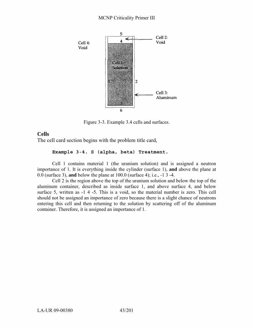
Figure 3-3. Example 3.4 cells and surfaces.
Cells The cell card section begins with the problem title card,
Example 3-4. S (alpha, beta) Treatment.
Cell 1 contains material 1 (the uranium solution) and is assigned a neutron importance of 1. It is everything inside the cylinder (surface 1), and above the plane at 0.0 (surface 3), and below the plane at 100.0 (surface 4); i.e., -1 3 -4.
Cell 2 is the region above the top of the uranium solution and below the top of the aluminum container, described as inside surface 1, and above surface 4, and below surface 5, written as -1 4 -5. This is a void, so the material number is zero. This cell should not be assigned an importance of zero because there is a slight chance of neutrons entering this cell and then returning to the solution by scattering off of the aluminum container. Therefore, it is assigned an importance of 1.
MCNP Criticality Primer III
LA-UR 09-00380 44/201
Grey Box 6. – Order of Operations.
Continuing with our example, cell 3 is the aluminum container. You can describe the aluminum container in at least three ways. We show one way here by treating the container as a combination of an aluminum shell plus a bottom disk. The axial region (1 -2 -5 3) is unioned with (or added to) the bottom region of aluminum (-2 - 3 6), written (1
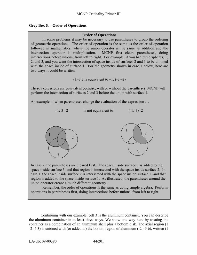
Order of Operations In some problems it may be necessary to use parentheses to group the ordering
of geometric operations. The order of operation is the same as the order of operation followed in mathematics, where the union operator is the same as addition and the intersection operator is multiplication. MCNP first clears parentheses, doing intersections before unions, from left to right. For example, if you had three spheres, 1, 2, and 3, and you want the intersection of space inside of surfaces 2 and 3 to be unioned with the space inside of surface 1. For the geometry shown in case 1 below, here are two ways it could be written.
-1:-3:2 is equivalent to –1: (-3 –2) These expressions are equivalent because, with or without the parentheses, MCNP will perform the intersection of surfaces 2 and 3 before the union with surface 1. An example of when parentheses change the evaluation of the expression …
-1:-3 –2 is not equivalent to (-1:-3) -2
1
3
2 2
3
1
In case 2, the parentheses are cleared first. The space inside surface 1 is added to the space inside surface 3, and that region is intersected with the space inside surface 2. In case 1, the space inside surface 2 is intersected with the space inside surface 2, and that region is added to the space inside surface 1. As illustrated, the parentheses around the union operator crease a much different geometry. Remember, the order of operations is the same as doing simple algebra. Perform operations in parentheses first, doing intersections before unions, from left to right.
MCNP Criticality Primer III
LA-UR 09-00380 45/201
-2 -5 3) : (-2 -3 6). Cell 4 is the “rest of the world” void cell. The union operator is used again to describe everything outside of the solution and aluminum container. The cell cards for this geometry are shown in Figure 3-4.
Example 3-4. S(alpha, beta) Treatment C Cell Cards 1 1 9.6586E-2 -1 3 -4 imp:n=1 2 0 -1 4 -5 imp:n=1 3 2 -2.7 (1 -2 -5 3):(-2 -3 6) imp:n=1 4 0 2:5:-6 imp:n=0
Figure 3-4. Example 3.4 Cell Cards.
Grey Box 7. – Alternative Cell 3 Descriptions.
3.4.B Alternate Geometry Description - Macrobodies As the problem geometry increases in complexity, there become many different
ways to specify that geometry in MCNP. One possible combination of macrobodies is given below. Example 3-4, UO2F2 Cylinder, S(alpha,beta) Treatment C Cell Cards 1 100 9.6586E-2 -10 imp:n=1 2 0 -20 imp:n=1 3 101 -2.7 10 20 -30 imp:n=1 4 0 30 imp:n=0 C Surface Cards 10 rcc 0 0 0 0 0 100.0 20.12 $ Can of UO2F2 20 rcc 0 0 100 0 0 10.0 20.12 $ Void gap above UO2F2 30 rcc 0 0 -0.1587 0 0 110.1587 20.2787 $Exterior of Al can
Alternative Cell 3 Descriptions Convince yourself that the two alternative descriptions of cell 3 that follow are correct. 3 2 -2.7 1 –2 -5 3 5 2 -2.7 -2 –3 6
or 3 2 -2.7 (1:-3) –5 –2 6
MCNP Criticality Primer III
LA-UR 09-00380 46/201
3.4.C Materials Material 1 is the uranium solution. The uranium is in the form of UO2F2 in water
(H2O), so we have two oxygen concentrations. The two have been combined in this case but can be left separate. The library extensions for these two ZAIDs, .62c, use data from the ENDF/B-VI.8 evaluation, which is the final release of ENDF/B-VI. However, U and Pu isotopes (except for a few minor ones) are unchanged from ENDF/B-VI.6. The MCNP ZAID extension corresponding to these unchanged isotopes is .66c. Following the m1 card is the S(α,β) card (mt1) that specifies that the S(α,β) thermal scattering law for hydrogen are to be applied to material 1. The light water identifier, lwtr, tells the code to apply the S(α,β) treatment to the hydrogen present in material 1 and treat it as if bound in light water instead of as a free gas. {Appendix G of the MCNP manual gives a complete listing of available S(α,β) materials.} The .60t extension indicates that the scattering laws are based on ENDF/B-VI.3.
Aluminum, which has an atomic number of 13 and an atomic weight of 27, is material 2. The partial ZAID is 13027. The atomic weight is always input as three integers so a zero must precede any atomic weight between 10 and 99 while two zeros must precede atomic weights less than 10. Aluminum is the only isotope being used in material 2 so we can enter an atom fraction of 1; 100 percent of the material is aluminum. Figure 3-5 shows the material cards for this problem.
C Data Cards C Materials Library Cards m1 1001.62c 5.7058e-2 8016.62c 3.2929e-2 9019.62c 4.3996e-3 92238.66c 2.0909e-3 92235.66c 1.0889e-4 mt1 lwtr.60t m2 13027.62c 1
Figure 3-5. Example 3.4 material cards.
3.4.D MCNP Criticality Controls The kcode card is identical to the previous examples. On the ksrc card, we will
put the source at approximately the center of the solution, or at the coordinates (0, 0, 50.0). Figure 3-4 shows the controls for this example.
C Criticality Control Cards kcode 5000 1.0 50 250 ksrc 0 0 50.0
Figure 3-6. Example 3.4 control cards.
MCNP Criticality Primer III
LA-UR 09-00380 47/201
Grey Box 8. – The Criticality Problem Controls.
The Criticality Problem Controls The following discussion presents guidelines for performing criticality calculations. Each problem should be examined to assess if these guidelines are appropriate. The Monte Carlo method can exhibit a small bias in the calculated keff. If at least 5000 (preferably 10,000) neutrons per keff are used, this bias should not be a factor in MCNP results. The larger the number of neutrons per keff cycle requested in the first entry on the kcode card, the smaller the bias. Therefore, it is wise to run as many neutron histories as you can afford, combined with using at least 200 active keff cycles. Two hundred is a large enough number of active cycles to determine that the problem appears to behave normally and the fission source is converged. At least 30 active cycles are required by MCNP to produce the final table of keff results. Fewer active cycles do not provide enough information to assess the quality of the calculation. In addition, the creation of confidence intervals not provided by MCNP is more difficult with a smaller number of cycles. There is no maximum number of cycles that can be calculated. The number of active cycles should not become so large that the estimated standard deviation in the final keff result becomes much smaller than the very small bias in keff. Typically, 200 to 500 active keff cycles should be acceptable for criticality safety applications. The initial guess of keff (the second entry on the kcode card) only affects the creation of fission source points for the second keff cycle. A severe underestimation of the initial guess will result in the creation of too many source points and vice versa. Source points in future cycles are unaffected by the initial guess of keff.
Enough keff cycles must be declared to be inactive (the third entry on the kcode card) so that the calculated spatial fission source has converged to the fundamental mode. The closer the initial source approximates the shape of the fundamental mode, the fewer cycles you need to skip. Point sources can be specified easily using the ksrc card. It is wise to put at least one point into each fissionable region, especially for largely-spaced array elements. Reactor core criticality calculations that have thousands of fuel rods do not require as many initial points because the rods are in close proximity to one another. It is usually best to skip at least 50 keff cycles for a ksrc initial source. The real test to see if enough cycles were skipped is printed in the output file and will be discussed in chapter 8. A uniform source can be created using the source definition sdef card and may allow a fewer keff cycles to be skipped. The best initial source distribution is from an SRCTP file from a previous calculation of a similar system. This file is automatically created by MCNP for every criticality calculation. Even fewer keff cycles usually can be skipped in this case. {See Chapter 2, Section VIII, in the MCNP5 manual for more discussion of these topics.}

MCNP Criticality Primer III
LA-UR 09-00380 48/201
3.4.E Example 3.4 MCNP Input File This completes the input requirements for example 3.4. Your completed input file
should resemble the following. Do not forget the blank line delimiters.
Example 3-4. UO2F2 Cylinder, S(alpha,beta) Treatment C Cell Cards 1 1 9.6586E-2 -1 3 -4 imp:n=1 2 0 -1 4 -5 imp:n=1 3 2 -2.7 (1 -2 -5 3):(-2 -3 6) imp:n=1 4 0 2:5:-6 imp:n=0 C Surface Cards 1 cz 20.12 2 cz 20.2787 3 pz 0.0 4 pz 100.0 5 pz 110.0 6 pz -0.1587 C Data Cards C Materials Library Cards m1 1001.62c 5.7058e-2 8016.62c 3.2929e-2 9019.62c 4.3996e-3 92238.66c 2.0909e-3 92235.66c 1.0889e-4 mt1 lwtr.60t m2 13027.62c 1 C Criticality Control Cards kcode 5000 1.0 50 250 ksrc 0 0 50.0
3.4.F Output After successfully running the problem, you should get a keff of approximately l.0
The result on a Windows 2000 Pentium 4 computer with the .62c & .66c data libraries at LANL was 0.99842 with an estimated standard deviation of 0.00077 (1σ). If you run the same problem without the S(α,β) treatment you will see a noticeable difference in keff. The result without the S(α,β) treatment on a Windows 2000 Pentium 4 computer with the ENDF66c data library at LANL was 0.97912 with an estimated standard deviation of 0.00083 (1σ). Much larger differences are possible, depending on the problem. For the majority of criticality calculations, it is strongly recommended that the appropriate S(α,β) cross sections be used. We want to stress the fact that you must analyze the system you are modeling and decide which method is appropriate for what you are analyzing.
A situation may arise where you would want to use the S(α,β) thermal neutron scattering law but the data for that material does not exist. Lucite (C4H6O2) is an example. The thermal treatment should be used for this material, but S(α,β) thermal neutron scattering law for Lucite does not exist. You can run the problem with the free gas treatment or make an S(α,β) substitution on the mt card. Polyethylene or water
MCNP Criticality Primer III
LA-UR 09-00380 49/201
S(α,β) data for hydrogen could be used. S(α,β) thermal neutron scattering laws are available for both of these. Polyethylene would probably be the best substitution because both polyethylene and Lucite are linked hydrocarbons and solids. You should run all reasonable options available and choose the most conservative result.
We refer to the use of the S(α,β) thermal neutron scatting law for problems at room temperature. While most criticality applications will make use of the room temperature evaluations, there may be a need for cross sections at different temperatures. The MCNP data libraries contain many thermal neutron cross sections at room temperature and higher temperatures, and scattering laws for materials in the temperature range from 20 to 2000 K. {See Appendix G of the MCNP Manual for more information}.
3.5 MCNP keff OUTPUT Examine the dashed box on the “keff results for:” page. This box will
be produced for at least 30 active cycles as long as at least one estimator set of values appears normally distributed at the 68% 95% or 99% confidence level. The final result in the box is the estimated value of keff using a combination of the three individual estimators along with its estimated standard deviation. Estimated 68%, 95% and 99% confidence intervals are given in the box.
The result of a Monte Carlo criticality calculation (or any other type of Monte Carlo calculation) is a confidence interval. For criticality, this means that the result is not just keff, but keff plus and minus some number of estimated standard deviations to form a confidence interval (based on the Central Limit Theorem) in which the true answer is expected to lie a certain fraction of the time. The number of standard deviations used (for example, from a Student's t Table) determines the fraction of the time that the confidence interval will include the true answer, for a selected confidence level. For example, a valid 99% confidence interval should include the true result 99% of the time. There is always some probability (in this example, 1%) that the true result will lie outside of the confidence interval. To reduce this probability to an acceptable level, either the confidence interval must be increased according to the desired Student's t percentile, or more histories need to be run to get a smaller estimated standard deviation. Running more histories is generally preferable.
The 68%, 95%, and 99% confidence intervals correspond ±1, ±2 and ±2.6 σ respectively.
MCNP Criticality Primer III
LA-UR 09-00380 50/201
Grey Box 9. – Final keff Estimator Confidence Interval.
Returning to our problem, examine the first three lines after the title card on the "keff results for :" page. The first line describes the initial source used. The
Final keff Estimator Confidence Interval Calculating keff consists of estimating the average number of fission neutrons produced in one fission generation per fission neutron born. A fission generation is the life of fission neutrons from birth to death by escape, parasitic capture, or absorption leading to fission. The computational equivalent of a fission generation in MCNP is the keff cycle. The number of neutrons calculated in each keff cycle is specified by the first entry on the kcode card. As these fission neutrons are born, transported, and terminated in a keff cycle, the fission source points are created for the next keff cycle. It is essential that enough keff values are accumulated so that the fission source distribution has converged to the fundamental mode. A poorer initial spatial distribution requires that more keff cycles be skipped before convergence is achieved. MCNP uses three different methods for calculating keff from each neutron random walk in a cycle: absorption, collision, and track length. {See Chapter 2, Section VIII, of the MCNP manual for more details.} Because no one keff estimator is optimal for all problems, MCNP uses a statistical combination of all three to provide a combined keff estimate. In general, the combined keff estimate is the best one to use and is the result enclosed in the dashed box in the output. Always examine all the keff results on the keff results page. The combined keff estimate is usually between the extreme keff values. Occasionally when the three keff estimators are highly positively correlated, the combined keff estimate will lie outside the extreme values. This behavior is expected because if one keff estimator is above the precise keff result, the others are likely also to be above that result because of the positive correlation. The reverse is also true. It is extremely important to emphasize that the keff result from a Monte Carlo criticality calculation is a confidence interval for keff that is formed by adding and subtracting a multiple of the final estimated standard deviation from the final estimated keff. A properly formed confidence interval from a valid calculation should include the precise keff result the fraction of the time used to create the confidence interval. There will always be some probability that the precise result lies outside of the confidence interval. MCNP provides the estimated final keff confidence intervals at the 68%, 95% and 99% levels when at least 30 active keff cycles have been calculated. {Further discussion on many aspects of keff confidence intervals are described in the MCNP manual, Chapter 2 Section VIII.}
MCNP Criticality Primer III
LA-UR 09-00380 51/201
second line provides information about the criticality problem defined on the kcode card. The third line shows what was actually run for this problem. the initial fission neutron source distribution used the 1 source points that were input on the ksrc card. the criticality problem was scheduled to skip 50 cycles and run a total of 250 cycles with nominally 5000 neutrons per cycle. this problem has run 50 inactive cycles with 250291 neutron histories and 200 active cycles with 999870 neutron histories.
Continuing on, the fourth line tells you if the problem finished. The fifth line is extremely important because it states whether or not all cells containing fissionable material were sampled. If all the cells containing fissionable material were not sampled, a warning message will be printed with a list of the cells that were not sampled. Such a calculation should probably be rerun with more settling cycles, and/or a different initial spatial source distribution to ensure sampling of all cells with fissionable material. this calculation has completed the requested number of keff cycles using a total of 1250161 fission neutron source histories. all cells with fissionable material were sampled and had fission neutron source points.
The next part of the output describes the results of the normality checks for each of the three keff estimators. The number of neutrons per cycle is usually large enough so that the individual keff estimators will appear to be distributed as though they were sampled from a normal distribution. MCNP checks to see if the keff values appear to be normally distributed, fit at the 68%, then 95% confidence level, and, if not, then at the 99% confidence interval. A WARNING is printed if an estimator appears not to be normally distributed at the 99% level. This situation is equivalent to a 99% confidence interval not including the precise answer, which will occur 1% of the time.
It is unlikely that all three of the keff estimators will not appear normally distributed at the same time. MCNP will not print the dashed box results in this case, although the results are available elsewhere in the output. Additional information is supplied in the output to assist the user in determining the cause of this behavior. One situation that can cause this behavior to occur is when the fission neutron source has not converged. Even when all three sets of keff data appear not to be normally distributed, it is still possible that each of the three average keff results would be normally distributed if many independent calculations were made. The user is cautioned to examine the problem output carefully to assess the possible cause(s) for the abnormal behavior. Additional independent calculations can be made, if necessary, using the dbcn card. {See Chapter 3 and Chapter 5 of the MCNP manual for more information.}
MCNP Criticality Primer III
LA-UR 09-00380 52/201
Grey Box 10. – Continuing a Calculation from RUNTPE and Customizing the OUTP File.
Continuing a Calculation from RUNTPE and Customizing the OUTP File An MCNP calculation can be continued for more keff cycles by using the RUNTPE file that is generated automatically for all problems. RUNTPE contains all of the problem information and the calculated results, including the fission source point information for the next cycle. The input file for a continued run requires only the following two cards: continue kcode 5000 1.0 50 400 The first three entries on the kcode card are ignored. The fourth entry sets a new upper limit to the total number of active cycles to be run in the calculation. Runs can be continued to any number of active cycles for the calculation. Runs can be continued any number of times. The MCNP execution line for a continue run is: mcnp c inp=filename1 runtpe=filename2 Where fileneame1 is the input file shown above and filename2 is the name of the RUNTPE file. If you lose the output file from a calculation, it can be regenerated from the RUNTPE with the following continuation input file: continue nps –1 The length of the OUTP file can be controlled by the print card. A print card followed by no entries provides all of the MCNP output possible. Numerical entries can include or exclude selected print table numbers from the output. {See Chapter 3 of the MCNP manual.}
MCNP Criticality Primer III
LA-UR 09-00380 53/201
3.6 SUMMARY
After completing the first three chapters of this Primer you should be able to model successfully any simple system that does not involve repeated structures or arrays. After running a problem you should be able to determine from the output whether or not the run was successful.
The main objective of this chapter was to demonstrate and show the effects of S(α,β) thermal neutron scattering laws. In the field of criticality safety, in thermal neutron cases the appropriate S(α,β) scattering laws should be used, but it is up to the user to determine which set of scattering laws will give the best analysis of the problem. When possible, multiple runs should be made to understand the system and to know what is driving the system. Remember, the S(α,β) thermal neutron scattering laws used in this chapter are at room temperature. If needed, other temperatures neutron cross sections are provided in the MCNP cross section library.
This chapter gave a description of some of the statistical output features of MCNP for criticality purposes that helps the user to determine if a run is statistically a success or if it should be rerun.
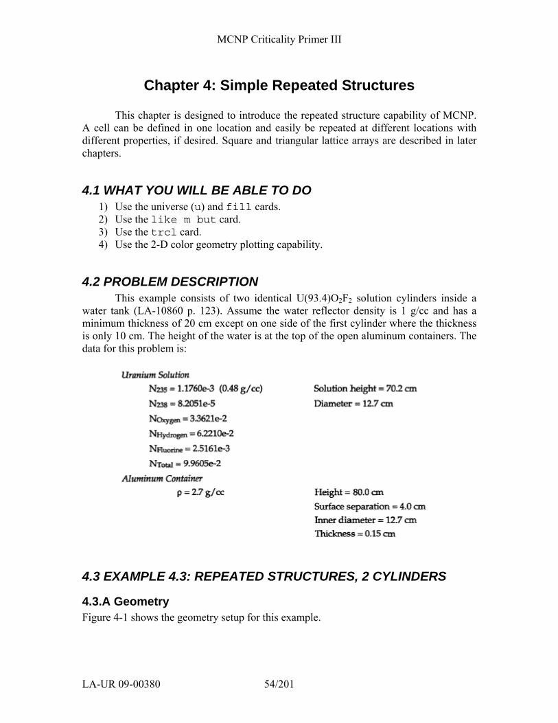
MCNP Criticality Primer III
LA-UR 09-00380 54/201
Chapter 4: Simple Repeated Structures This chapter is designed to introduce the repeated structure capability of MCNP.
A cell can be defined in one location and easily be repeated at different locations with different properties, if desired. Square and triangular lattice arrays are described in later chapters.
4.1 WHAT YOU WILL BE ABLE TO DO 1) Use the universe (u) and fill cards. 2) Use the like m but card. 3) Use the trcl card. 4) Use the 2-D color geometry plotting capability.
4.2 PROBLEM DESCRIPTION This example consists of two identical U(93.4)O2F2 solution cylinders inside a
water tank (LA-10860 p. 123). Assume the water reflector density is 1 g/cc and has a minimum thickness of 20 cm except on one side of the first cylinder where the thickness is only 10 cm. The height of the water is at the top of the open aluminum containers. The data for this problem is:
4.3 EXAMPLE 4.3: REPEATED STRUCTURES, 2 CYLINDERS
4.3.A Geometry Figure 4-1 shows the geometry setup for this example.
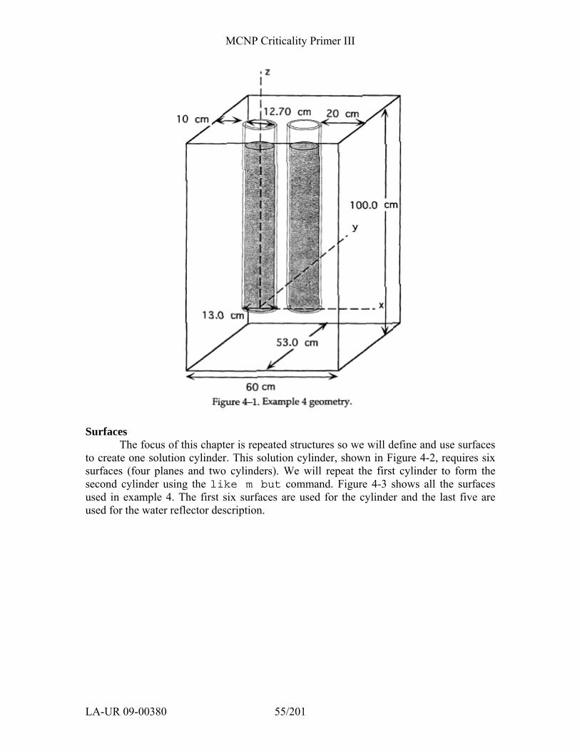
MCNP Criticality Primer III
LA-UR 09-00380 55/201
Surfaces The focus of this chapter is repeated structures so we will define and use surfaces
to create one solution cylinder. This solution cylinder, shown in Figure 4-2, requires six surfaces (four planes and two cylinders). We will repeat the first cylinder to form the second cylinder using the like m but command. Figure 4-3 shows all the surfaces used in example 4. The first six surfaces are used for the cylinder and the last five are used for the water reflector description.
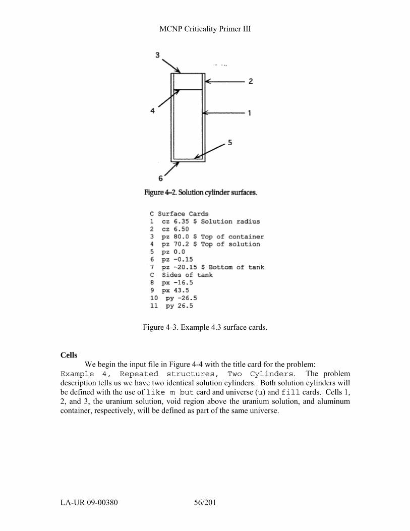
MCNP Criticality Primer III
LA-UR 09-00380 56/201
Figure 4-3. Example 4.3 surface cards.
Cells We begin the input file in Figure 4-4 with the title card for the problem:
Example 4, Repeated structures, Two Cylinders. The problem description tells us we have two identical solution cylinders. Both solution cylinders will be defined with the use of like m but card and universe (u) and fill cards. Cells 1, 2, and 3, the uranium solution, void region above the uranium solution, and aluminum container, respectively, will be defined as part of the same universe.
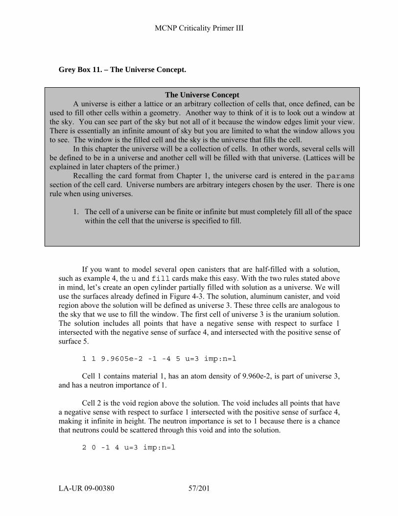
MCNP Criticality Primer III
LA-UR 09-00380 57/201
Grey Box 11. – The Universe Concept.
If you want to model several open canisters that are half-filled with a solution,
such as example 4, the u and fill cards make this easy. With the two rules stated above in mind, let’s create an open cylinder partially filled with solution as a universe. We will use the surfaces already defined in Figure 4-3. The solution, aluminum canister, and void region above the solution will be defined as universe 3. These three cells are analogous to the sky that we use to fill the window. The first cell of universe 3 is the uranium solution. The solution includes all points that have a negative sense with respect to surface 1 intersected with the negative sense of surface 4, and intersected with the positive sense of surface 5.
1 1 9.9605e-2 -1 -4 5 u=3 imp:n=l Cell 1 contains material 1, has an atom density of 9.960e-2, is part of universe 3,
and has a neutron importance of 1.
Cell 2 is the void region above the solution. The void includes all points that have a negative sense with respect to surface 1 intersected with the positive sense of surface 4, making it infinite in height. The neutron importance is set to 1 because there is a chance that neutrons could be scattered through this void and into the solution.
2 0 -1 4 u=3 imp:n=l
The Universe Concept A universe is either a lattice or an arbitrary collection of cells that, once defined, can be
used to fill other cells within a geometry. Another way to think of it is to look out a window at the sky. You can see part of the sky but not all of it because the window edges limit your view. There is essentially an infinite amount of sky but you are limited to what the window allows you to see. The window is the filled cell and the sky is the universe that fills the cell. In this chapter the universe will be a collection of cells. In other words, several cells will be defined to be in a universe and another cell will be filled with that universe. (Lattices will be explained in later chapters of the primer.) Recalling the card format from Chapter 1, the universe card is entered in the params section of the cell card. Universe numbers are arbitrary integers chosen by the user. There is one rule when using universes.
1. The cell of a universe can be finite or infinite but must completely fill all of the space within the cell that the universe is specified to fill.
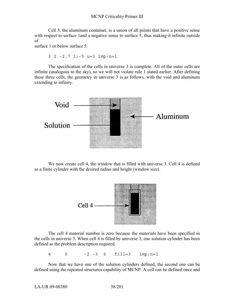
MCNP Criticality Primer III
LA-UR 09-00380 58/201
Cell 3, the aluminum container, is a union of all points that have a positive sense with respect to surface 1and a negative sense to surface 5, thus making it infinite outside of surface 1 or below surface 5.
3 2 -2.7 1:-5 u=3 imp:n=l The specification of the cells in universe 3 is complete. All of the outer cells are
infinite (analogous to the sky), so we will not violate rule 1 stated earlier. After defining these three cells, the geometry in universe 3 is as follows, with the void and aluminum extending to infinity.
We now create cell 4, the window that is filled with universe 3. Cell 4 is defined as a finite cylinder with the desired radius and height (window size).
The cell 4 material number is zero because the materials have been specified in the cells in universe 3. When cell 4 is filled by universe 3, one solution cylinder has been defined as the problem description required.
4 0 -2 –3 6 fill=3 imp:n=1 Now that we have one of the solution cylinders defined, the second one can be
defined using the repeated structures capability of MCNP. A cell can be defined once and
MCNP Criticality Primer III
LA-UR 09-00380 59/201
repeated many times using the like m but construct. This feature reduces the amount of input required from the user. In this example we will use the like m but feature to make the second cylinder. The format of the like m but card follows.
J like m but list
j = cell number. like = keyword for cell to be repeated. m = a previously defined cell number that is to be
repeated. but = keyword for differences between cells m and j . list = specifications that define the differences
between cells m and j . The list term is usually the x, y, and z coordinates of the repeated cell, but can be another cell or universe.
Most of the data cards can be included in the list specification {see Chapter 3
of the MCNP manual for a complete listing of cards available}. For this example we will use the trcl specification that describes the relation of the origin of one cell to the origin of another.
trcl = 01 02 03
The first three entries are the x, y, z values of the origin of translated cell. {See Chapter 3 of the MCNP manual.}
Grey Box 12. – Simple like m but trcl Example.
Now let’s continue with example 4.3. After defining the first solution cylinder,
cell 4, using the u and fill cards, we want to create a second, identical solution cylinder with the like m but card, cell 5, and translate it along the x-axis with the trcl mnemonic so that the surface separation between the aluminum tanks is 4.0 cm. A cell is translated relative to the coordinates of its origin. The origin of the cell being repeated is (0, 0, 0). The center-to-center spacing of the two solution cylinders is 17 cm. By simply translating the origin of cell 4, filled with universe 3, a second, identical solution cylinder is defined. The cell 5 description follows.
5 like 4 but trcl (17 0 0)
Simple like m but trcl Example Assume we have defined cell 1 as a sphere with its origin at (0, 0, 0). Cell 2 is identical to cell 1 but it is located 10 cm to the left and 20 cm above cell 1 making the cell 2 origin (-10 0 20). Cell 2, using the like m but card, is defined as follows. The parentheses are required. 2 like 1 but trcl (-10 0 20)
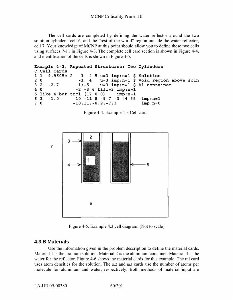
MCNP Criticality Primer III
LA-UR 09-00380 60/201
The cell cards are completed by defining the water reflector around the two
solution cylinders, cell 6, and the ”rest of the world” region outside the water reflector, cell 7. Your knowledge of MCNP at this point should allow you to define these two cells using surfaces 7-11 in Figure 4-3. The complete cell card section is shown in Figure 4-4, and identification of the cells is shown in Figure 4-5.
Example 4-3, Repeated Structures: Two Cylinders C Cell Cards 1 1 9.9605e-2 -1 -4 5 u=3 imp:n=1 $ Solution 2 0 -1 4 u=3 imp:n=1 $ Void region above soln 3 2 -2.7 1:-5 u=3 imp:n=1 $ Al container 4 0 -2 -3 6 fill=3 imp:n=1 5 like 4 but trcl (17 0 0) imp:n=1 6 3 -1.0 10 -11 8 -9 7 -3 #4 #5 imp:n=1 7 0 -10:11:-8:9:-7:3 imp:n=0
Figure 4-4. Example 4-3 Cell cards.
Figure 4-5. Example 4.3 cell diagram. (Not to scale)
4.3.B Materials Use the information given in the problem description to define the material cards.
Material 1 is the uranium solution. Material 2 is the aluminum container. Material 3 is the water for the reflector. Figure 4-6 shows the material cards for this example. The ml card uses atom densities for the solution. The m2 and m3 cards use the number of atoms per molecule for aluminum and water, respectively. Both methods of material input are

MCNP Criticality Primer III
LA-UR 09-00380 61/201
appropriate and selection of either method is generally based on the data available for the problem. A WARNING message will be printed in the output because the atom fractions on the m3 card do not add up to either the density on the cell 6 card or to 1.0. MCNP will renormalize the values given and continue executing the problem. Light water S(α,β) cross sections are used for both the uranium solution and water reflector because both contain hydrogen bound in the water molecule.
C Data Cards C Materials Cards m1 1001.62c 6.2210e-2 8016.62c 3.3621e-2 9019.62c 2.5161e-3 92235.66c 1.1760e-3 92238.66c 8.2051e-5 mt1 lwtr.60t m2 13027.62c 1.0 m3 1001.62c 2 8016.62c 1 mt3 lwtr.60t
Figure 4-6. Example 4.3 material cards.
4.3.C MCNP Criticality Controls The kcode specification remains the same as previous examples, but there is one
change in the ksrc card. We have added a second initial source point for the additional solution cylinder. One of the reasons for this change is to ensure efficient sampling of the fissile material in the second solution cylinder. Without the added source point, the number of settling cycles chosen for the kcode card would need to be larger to ensure a converged spatial distribution of fission source points in the second cylinder. Figure 4-7 shows the control cards for this example.
C Control Cards kcode 5000 1.0 50 250 ksrc 0 0 35 17 0 35
Figure 4-7. Example 4.3 control cards.
4.3.D Example 4.3 MCNP Input File This completes the input requirements for this example. The completed input file
should resemble the following. Do not forget the blank line delimiters.
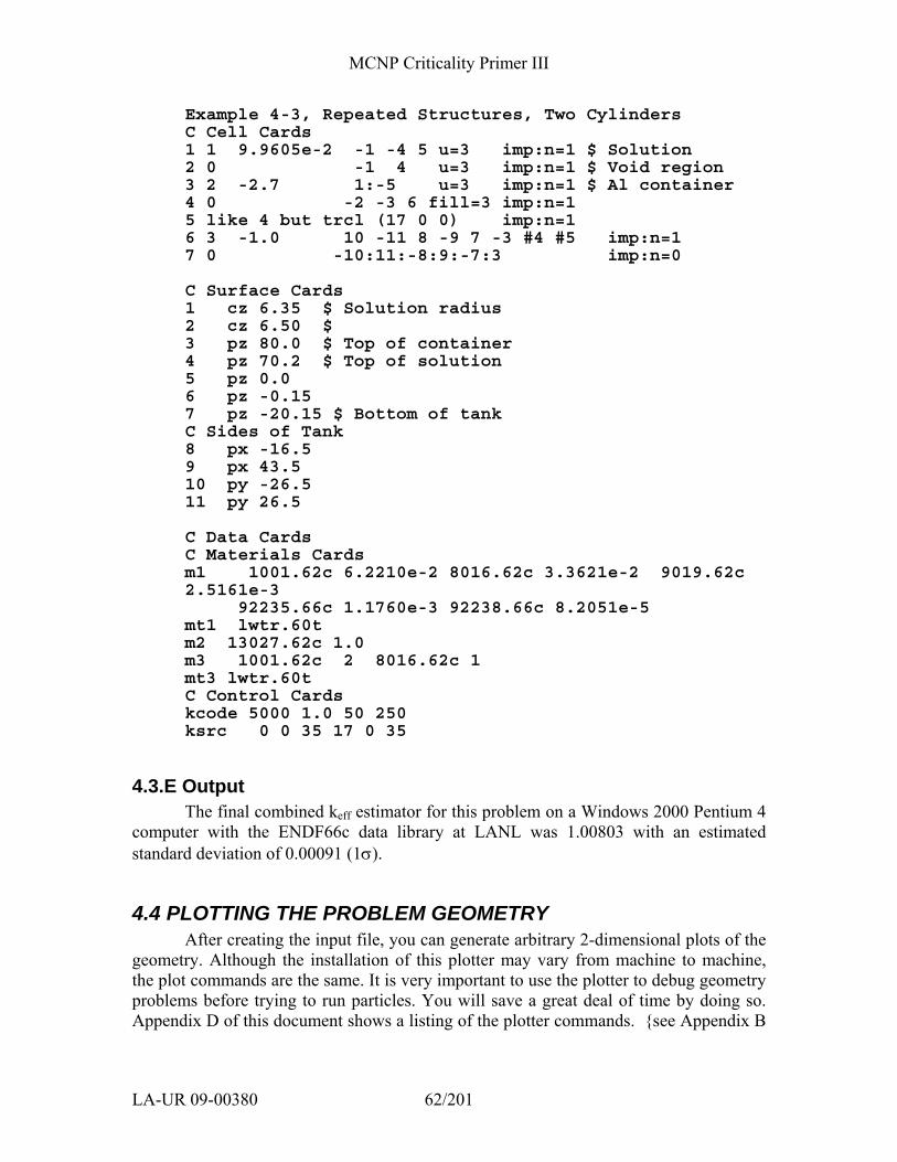
MCNP Criticality Primer III
LA-UR 09-00380 62/201
Example 4-3, Repeated Structures, Two Cylinders C Cell Cards 1 1 9.9605e-2 -1 -4 5 u=3 imp:n=1 $ Solution 2 0 -1 4 u=3 imp:n=1 $ Void region 3 2 -2.7 1:-5 u=3 imp:n=1 $ Al container 4 0 -2 -3 6 fill=3 imp:n=1 5 like 4 but trcl (17 0 0) imp:n=1 6 3 -1.0 10 -11 8 -9 7 -3 #4 #5 imp:n=1 7 0 -10:11:-8:9:-7:3 imp:n=0 C Surface Cards 1 cz 6.35 $ Solution radius 2 cz 6.50 $ 3 pz 80.0 $ Top of container 4 pz 70.2 $ Top of solution 5 pz 0.0 6 pz -0.15 7 pz -20.15 $ Bottom of tank C Sides of Tank 8 px -16.5 9 px 43.5 10 py -26.5 11 py 26.5 C Data Cards C Materials Cards m1 1001.62c 6.2210e-2 8016.62c 3.3621e-2 9019.62c 2.5161e-3 92235.66c 1.1760e-3 92238.66c 8.2051e-5 mt1 lwtr.60t m2 13027.62c 1.0 m3 1001.62c 2 8016.62c 1 mt3 lwtr.60t C Control Cards kcode 5000 1.0 50 250 ksrc 0 0 35 17 0 35
4.3.E Output The final combined keff estimator for this problem on a Windows 2000 Pentium 4
computer with the ENDF66c data library at LANL was 1.00803 with an estimated standard deviation of 0.00091 (1σ).
4.4 PLOTTING THE PROBLEM GEOMETRY After creating the input file, you can generate arbitrary 2-dimensional plots of the
geometry. Although the installation of this plotter may vary from machine to machine, the plot commands are the same. It is very important to use the plotter to debug geometry problems before trying to run particles. You will save a great deal of time by doing so. Appendix D of this document shows a listing of the plotter commands. {see Appendix B
MCNP Criticality Primer III
LA-UR 09-00380 63/201
of the MCNP manual for a detailed description of the plotter and plot commands.} The format for plotting follows. mcnp inp=filename ip where ip = initiate and plot
After receiving the plot prompt, pressing the carriage return or enter key will display a default plot. The default plot is a PX slice centered at (0, 0, 0) with an extent of -100 cm to 100 cm on the Y-axis and -100 cm to 100 cm on the Z-axis. Geometry errors are shown as red dotted lines. Keywords and entries can be entered after the prompt to get any 2- dimensional view desired. Only enough of the keyword has to be typed to make it unique. For example, “or” will specify the origin keyword.
We will discuss seven plot keywords. Although shown here in upper case to set them off from the rest of the text, either upper or lower case is acceptable.
ORIGIN vx vy vz – The coordinate about which the plot is centered.
Default = 0 0 0. EXTENT eh ev - Sets the scale of the plot in cm so that eh is the
horizontal distance from the origin to either side of the plot and ev is the vertical distance from the origin to the top and bottom of the plot. If one value is entered, it is duplicated for the second entry. Default 100 100
PX vx – Draws y-z plot plane at X=VX. Default px 0 PY vy – Draws x-z plot plane at y=vy. PZ vz – Draws x-y plot plane at Z=VZ. LABEL s c – Put labels of size s on the surfaces and labels of size c
on the cells. Default: 1 0 (no cell labels) SHADE n color –Make material n the color chosen.
{See Appendix B of the MCNP Manual for more plot commands}.
After clicking in the upper left hand corner of the plot window, you will see a default plot showing a slice through the origin on the y-axis and z-axis with the surfaces labeled.
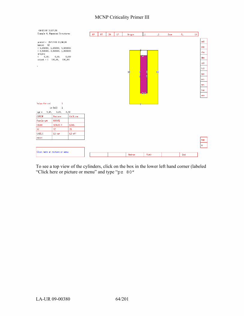
MCNP Criticality Primer III
LA-UR 09-00380 64/201
To see a top view of the cylinders, click on the box in the lower left hand corner (labeled “Click here or picture or menu” and type “pz 80”
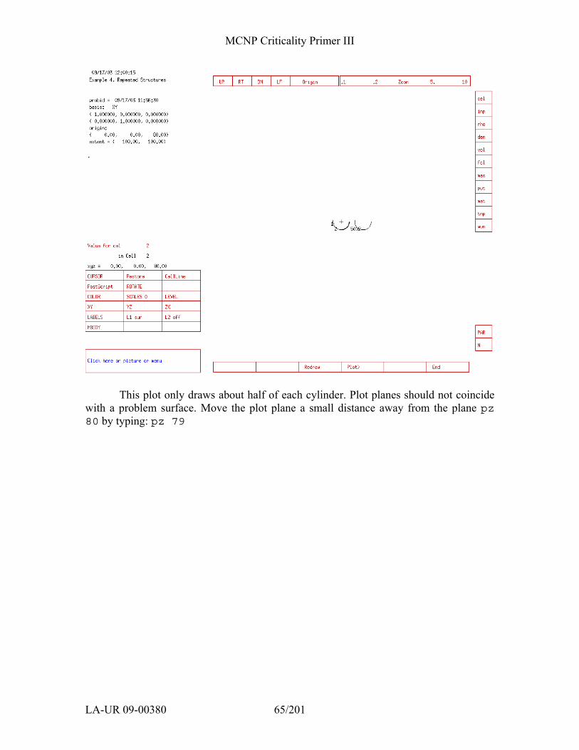
MCNP Criticality Primer III
LA-UR 09-00380 65/201
This plot only draws about half of each cylinder. Plot planes should not coincide with a problem surface. Move the plot plane a small distance away from the plane pz 80 by typing: pz 79
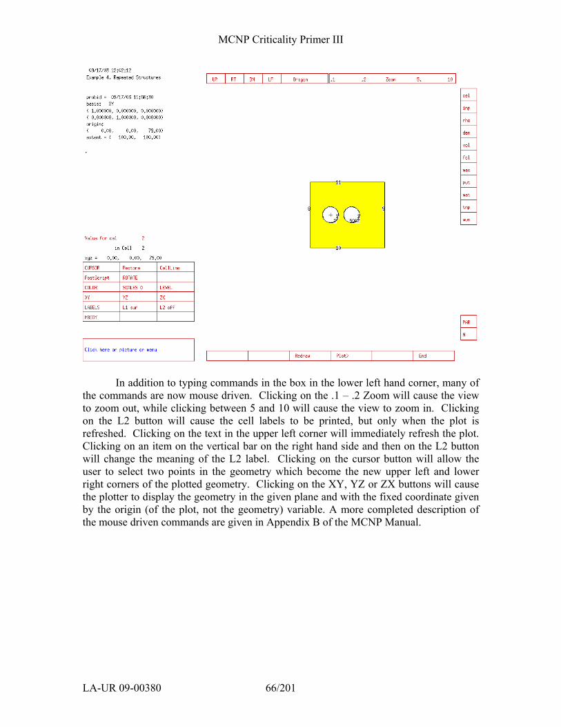
MCNP Criticality Primer III
LA-UR 09-00380 66/201
In addition to typing commands in the box in the lower left hand corner, many of
the commands are now mouse driven. Clicking on the .1 – .2 Zoom will cause the view to zoom out, while clicking between 5 and 10 will cause the view to zoom in. Clicking on the L2 button will cause the cell labels to be printed, but only when the plot is refreshed. Clicking on the text in the upper left corner will immediately refresh the plot. Clicking on an item on the vertical bar on the right hand side and then on the L2 button will change the meaning of the L2 label. Clicking on the cursor button will allow the user to select two points in the geometry which become the new upper left and lower right corners of the plotted geometry. Clicking on the XY, YZ or ZX buttons will cause the plotter to display the geometry in the given plane and with the fixed coordinate given by the origin (of the plot, not the geometry) variable. A more completed description of the mouse driven commands are given in Appendix B of the MCNP Manual.

MCNP Criticality Primer III
LA-UR 09-00380 67/201
Grey Box 13. – Surfaces Generated by Repeated Structures.
To plot cell numbers instead of surface numbers, type:
label 0 1 To make the size of the cell numbers larger, type
la 1 2 This puts both cell and surface numbers in the plot and increases the size of the cell numbers. Materials in cells are plotted in color. To see the material numbers of cells type:
la 0 1 mat
Some other cell quantities that can be plotted are:
den: mass density rho: atom density mas: mass imp: n: importances vol: volume cel: cell number (default)
To change the color of material 1 from its default color, purple, type
shade 1 yellow To see what colors are available, type
options
Surfaces Generated by Repeated Structures This view shows both solution cylinders and the water reflector. Notice that the
surfaces of the left cylinder (cell 4) are numbered as defined in the input file. The cylinder on the right is the repeated structure. The outer cylinder surface number is different for cell 5. The inner cylinder is still surface 1, but the outer cylinder is 5002. When using repeated structures, MCNP will renumber the translated surfaces if needed as follows: 1000*cell number + surface number. The planes for cell 5 were renumbered also, but because planes are infinite, surfaces 5003 and 5006 are identical to surfaces 3 and 6, and the code prints the WARNING message: 2 surfaces were deleted for being the same as others.
The surface numbers of the cells in a universe do not get incremented. Surfaces 1, 4 and 5 are in both cells 4 and 5.

MCNP Criticality Primer III
LA-UR 09-00380 68/201
We suggest that you experiment with the commands to get a feel for how the
plotter works.
4.5 SUMMARY This chapter introduced repeated structures, which is a very powerful capability
available in MCNP. With this command you can create geometries that involve many identical structures and still vary their characteristics. By defining one structure, you are easily able to reproduce that structure in as many places as needed.
Geometry plotting is a powerful tool. By plotting your geometry before transporting particles, geometry errors can be corrected. You can also make sure that the geometry setup is what you actually want it to be by displaying cell quantities.
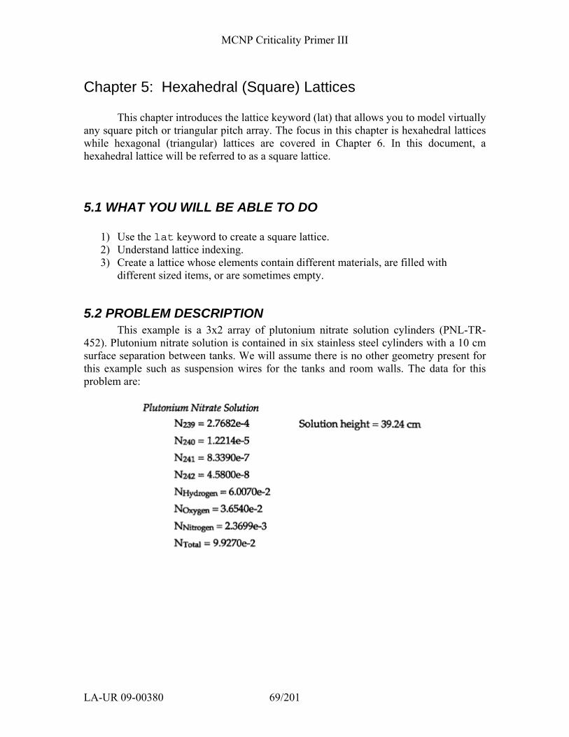
MCNP Criticality Primer III
LA-UR 09-00380 69/201
Chapter 5: Hexahedral (Square) Lattices
This chapter introduces the lattice keyword (lat) that allows you to model virtually any square pitch or triangular pitch array. The focus in this chapter is hexahedral lattices while hexagonal (triangular) lattices are covered in Chapter 6. In this document, a hexahedral lattice will be referred to as a square lattice.
5.1 WHAT YOU WILL BE ABLE TO DO
1) Use the lat keyword to create a square lattice. 2) Understand lattice indexing. 3) Create a lattice whose elements contain different materials, are filled with
different sized items, or are sometimes empty.
5.2 PROBLEM DESCRIPTION This example is a 3x2 array of plutonium nitrate solution cylinders (PNL-TR-
452). Plutonium nitrate solution is contained in six stainless steel cylinders with a 10 cm surface separation between tanks. We will assume there is no other geometry present for this example such as suspension wires for the tanks and room walls. The data for this problem are:
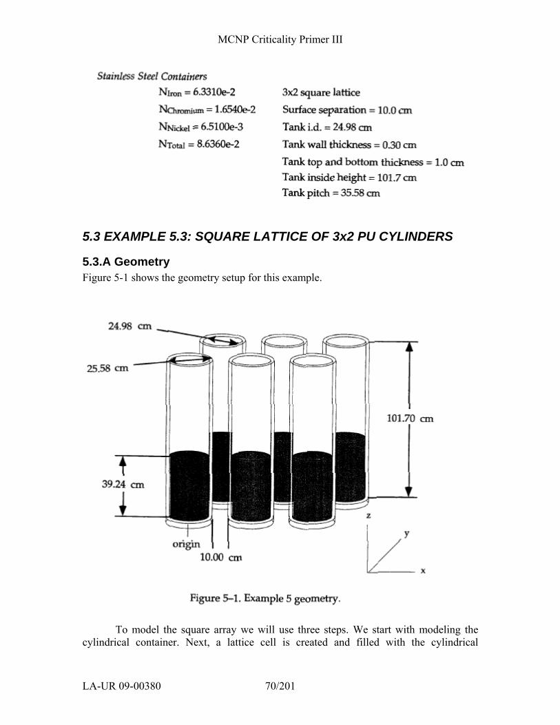
MCNP Criticality Primer III
LA-UR 09-00380 70/201
5.3 EXAMPLE 5.3: SQUARE LATTICE OF 3x2 PU CYLINDERS
5.3.A Geometry Figure 5-1 shows the geometry setup for this example.
To model the square array we will use three steps. We start with modeling the cylindrical container. Next, a lattice cell is created and filled with the cylindrical
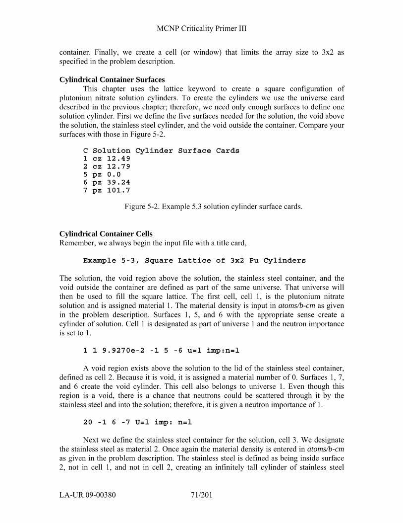
MCNP Criticality Primer III
LA-UR 09-00380 71/201
container. Finally, we create a cell (or window) that limits the array size to 3x2 as specified in the problem description.
Cylindrical Container Surfaces
This chapter uses the lattice keyword to create a square configuration of plutonium nitrate solution cylinders. To create the cylinders we use the universe card described in the previous chapter; therefore, we need only enough surfaces to define one solution cylinder. First we define the five surfaces needed for the solution, the void above the solution, the stainless steel cylinder, and the void outside the container. Compare your surfaces with those in Figure 5-2.
C Solution Cylinder Surface Cards 1 cz 12.49 2 cz 12.79 5 pz 0.0 6 pz 39.24 7 pz 101.7
Figure 5-2. Example 5.3 solution cylinder surface cards.
Cylindrical Container Cells Remember, we always begin the input file with a title card,
Example 5-3, Square Lattice of 3x2 Pu Cylinders The solution, the void region above the solution, the stainless steel container, and the void outside the container are defined as part of the same universe. That universe will then be used to fill the square lattice. The first cell, cell 1, is the plutonium nitrate solution and is assigned material 1. The material density is input in atoms/b-cm as given in the problem description. Surfaces 1, 5, and 6 with the appropriate sense create a cylinder of solution. Cell 1 is designated as part of universe 1 and the neutron importance is set to 1.
1 1 9.9270e-2 -1 5 -6 u=l imp:n=l
A void region exists above the solution to the lid of the stainless steel container, defined as cell 2. Because it is void, it is assigned a material number of 0. Surfaces 1, 7, and 6 create the void cylinder. This cell also belongs to universe 1. Even though this region is a void, there is a chance that neutrons could be scattered through it by the stainless steel and into the solution; therefore, it is given a neutron importance of 1.
20 -1 6 -7 U=l imp: n=l
Next we define the stainless steel container for the solution, cell 3. We designate
the stainless steel as material 2. Once again the material density is entered in atoms/b-cm as given in the problem description. The stainless steel is defined as being inside surface 2, not in cell 1, and not in cell 2, creating an infinitely tall cylinder of stainless steel
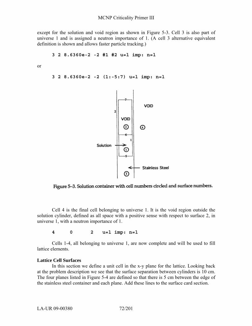
MCNP Criticality Primer III
LA-UR 09-00380 72/201
except for the solution and void region as shown in Figure 5-3. Cell 3 is also part of universe 1 and is assigned a neutron importance of 1. (A cell 3 alternative equivalent definition is shown and allows faster particle tracking.)
3 2 8.6360e-2 -2 #1 #2 u=l imp: n=l or
3 2 8.6360e-2 -2 (1:-5:7) u=l imp: n=l
Cell 4 is the final cell belonging to universe 1. It is the void region outside the solution cylinder, defined as all space with a positive sense with respect to surface 2, in universe 1, with a neutron importance of 1.
4 0 2 u=l imp: n=l
Cells 1-4, all belonging to universe 1, are now complete and will be used to fill
lattice elements. Lattice Cell Surfaces
In this section we define a unit cell in the x-y plane for the lattice. Looking back at the problem description we see that the surface separation between cylinders is 10 cm. The four planes listed in Figure 5-4 are defined so that there is 5 cm between the edge of the stainless steel container and each plane. Add these lines to the surface card section.

MCNP Criticality Primer III
LA-UR 09-00380 73/201
C Beginning of Lattice Surfaces 8 px 17.79 9 px –17.79 10 py 17.79 11 py -17.79
Figure 5-4. Example 5 lattice cell surface cards.
Lattice Cell Card
When defining a square lattice, MCNP requires that at least 4 sides must be specified. Opposite sides must be identical and parallel. Two sides can be omitted, resulting in an infinite lattice in that dimension. A cell is defined to be a lattice with the lat keyword that is entered in the params section of the cell card.
lat = 1 square lattice
Cell 5 is the lattice cell and will be filled with the cells belonging to universe 1.
Cell 5 is given a material number of 0 because the materials have been defined in cells 1-4. Cell 5 is all space with a negative sense with respect to (wrt) surface 8, a positive sense wrt surface 9, a negative sense wrt surface 10, and a positive sense wrt surface 11. We have defined a unit slab, infinite in z, that is duplicated in the x and y directions by the lat card. The order of these surfaces on the cell card is important. It determines in which spatial directions the lattice indices increase and decrease. Each lattice element has a unique location identifier. The first index increases beyond the first surface listed and decreases beyond the second surface listed, etc., as shown in Figure 5-5. Therefore, surfaces parallel to each other must be listed as pairs. Surface 8 is parallel to surface 9. Surface 10 is parallel to surface 11. The element [0, 0, 0] is the one defined on the cell card.

MCNP Criticality Primer III
LA-UR 09-00380 74/201
Surface 8 is opposite surface 9, and surface 10 is opposite surface 11. We define
the cell as a square lattice, lat=l, and fill the cell with universe 1, fill=l. This specification creates an infinite lattice in only the x and y direction. The lattice cell itself is infinite in the ± z direction. This infinite lattice is designated as universe 2. A neutron importance of 1 completes the cell.
5 0 -8 9 -10 11 lat=l fill=l u=2 imp:n=l
The last step for this problem is to take universe 2, cell 5, and put it in a window to limit it to a 3x2 finite array. We need to define six more surfaces for the problem. Recall an important fact about filled cells and filling universes discussed in Chapter 4.
Because cell 5 defines an infinite array we can choose a window cell that will enclose any six of the lattice cells. Figure 5-6 shows the surfaces chosen for the window cell. A px plane at 88.95 an is at the right edge of the third lattice cell from the origin (17.79 cm + 2*35.58 cm). The other bounding plane is defined in the same manner.
C Window Surfaces 3 pz -1.0 4 pz 102.7 12 px 88.95 14 py 53.37
Figure 5-6. Example 5 window surface cards.
Surfaces 3 and 4, the top and bottom of the problem, limit the z-extent so the array height is 103.7 cm.
We can now define cell 6. The material number is zero because the materials have already been defined in cells 1-4. The cell is then bound in the positive sense of surface 9, the negative sense of surface 12, the positive sense of surface 11, the negative sense of surface 14, the positive sense of surface 3, and the negative sense of surface 4. The cell, or window, is filled with universe 2. Remember, universe 2 is the infinite array defined by cell 5. Cell 6 data is completed by entering a neutron importance of 1.
6 0 9 -12 11 -14 3 -4 fill=2 imp:n=l
Cell 7 defines the “rest of the world”, a union of space outside cell 6. It has a material number of 0 and a neutron importance of 0, so that escaping particles are terminated.
7 0 -9:12:-11:14:-3:4 imp:n=0 or
MCNP Criticality Primer III
LA-UR 09-00380 75/201
7 0 #6 imp:n=0
5.3.B Materials Material cards should be entered as described in previous chapters using the
information provided in the problem description. Because the plutonium is in a solution, light water S(α,β) cross-sections should be used for material 1. Your material cards should be similar to those in Figure 5-7. C Material cards m1 1001.62c 6.0070-2 8016.62c 3.6540-2 7014.62c 2.3699-3 94239.66c 2.7682-4 9424.66c 1.2214-5 94241.66c 8.3390-7 94242.66c 4.5800-8 mt1 lwtr.60t m2 24050.62c 7.195-4 24052.62c 1.38589-2 24053.62c 1.5713-3 24054.62c 3.903-4 26056.62c 3.704-3 26056.62c 5.80869-2 26057.62c 1.342-3 26058.62c 1.773-4 28058.62c 4.432-3 28060.62c 1.7069-3 28061.62c 7.42-5 28062.62c 2.363-4 28064.62c 6.05-5
Figure 5-7. Example 5 material cards.
The “e” notation (e-2) used in previous examples is optional and has been omitted here.
5.3.C MCNP Criticality Controls The kcode specification remains the same from the previous example, but there
are changes in the ksrc card. For this example we have placed an initial source point in each solution cylinder to ensure sampling during the settling cycles. Figure 5-8 shows the control cards for this example. C Control Cards kcode 5000 1.0 50 250 c one source point in each volume of Pu Solution ksrc 0 0 19.62 35.58 0 19.62 71.16 0 19.62 0 35.58 19.62 35.58 35.58 19.62 71.16 35.58 19.62
Figure 5-8. Example 5.3 control cards.
5.3.D Example 5.3 MCNP Input File The input for this example is complete. The input file should resemble the
following. Do not forget the blank line delimiters. Comments following a $ have been used on the cell cards.
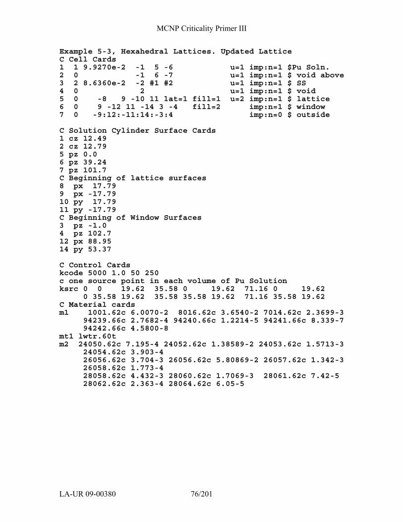
MCNP Criticality Primer III
LA-UR 09-00380 76/201
Example 5-3, Hexahedral Lattices. Updated Lattice C Cell Cards 1 1 9.9270e-2 -1 5 -6 u=1 imp:n=1 $Pu Soln. 2 0 -1 6 -7 u=1 imp:n=1 $ void above 3 2 8.6360e-2 -2 #1 #2 u=1 imp:n=1 $ SS 4 0 2 u=1 imp:n=1 $ void 5 0 -8 9 -10 11 lat=1 fill=1 u=2 imp:n=1 $ lattice 6 0 9 -12 11 -14 3 -4 fill=2 imp:n=1 $ window 7 0 -9:12:-11:14:-3:4 imp:n=0 $ outside C Solution Cylinder Surface Cards 1 cz 12.49 2 cz 12.79 5 pz 0.0 6 pz 39.24 7 pz 101.7 C Beginning of lattice surfaces 8 px 17.79 9 px -17.79 10 py 17.79 11 py -17.79 C Beginning of Window Surfaces 3 pz -1.0 4 pz 102.7 12 px 88.95 14 py 53.37 C Control Cards kcode 5000 1.0 50 250 c one source point in each volume of Pu Solution ksrc 0 0 19.62 35.58 0 19.62 71.16 0 19.62 0 35.58 19.62 35.58 35.58 19.62 71.16 35.58 19.62 C Material cards m1 1001.62c 6.0070-2 8016.62c 3.6540-2 7014.62c 2.3699-3 94239.66c 2.7682-4 94240.66c 1.2214-5 94241.66c 8.339-7 94242.66c 4.5800-8 mt1 lwtr.60t m2 24050.62c 7.195-4 24052.62c 1.38589-2 24053.62c 1.5713-3 24054.62c 3.903-4 26056.62c 3.704-3 26056.62c 5.80869-2 26057.62c 1.342-3 26058.62c 1.773-4 28058.62c 4.432-3 28060.62c 1.7069-3 28061.62c 7.42-5 28062.62c 2.363-4 28064.62c 6.05-5
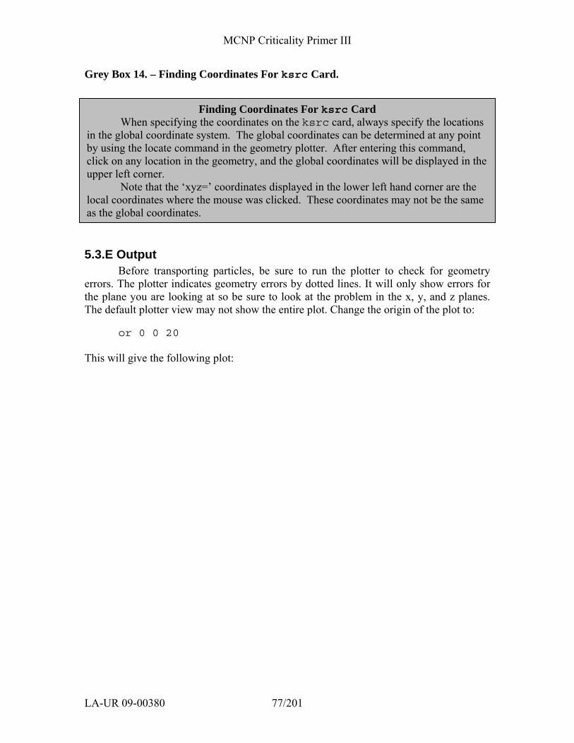
MCNP Criticality Primer III
LA-UR 09-00380 77/201
Grey Box 14. – Finding Coordinates For ksrc Card.
5.3.E Output Before transporting particles, be sure to run the plotter to check for geometry
errors. The plotter indicates geometry errors by dotted lines. It will only show errors for the plane you are looking at so be sure to look at the problem in the x, y, and z planes. The default plotter view may not show the entire plot. Change the origin of the plot to:
or 0 0 20 This will give the following plot:
Finding Coordinates For ksrc Card When specifying the coordinates on the ksrc card, always specify the locations in the global coordinate system. The global coordinates can be determined at any point by using the locate command in the geometry plotter. After entering this command, click on any location in the geometry, and the global coordinates will be displayed in the upper left corner. Note that the ‘xyz=’ coordinates displayed in the lower left hand corner are the local coordinates where the mouse was clicked. These coordinates may not be the same as the global coordinates.
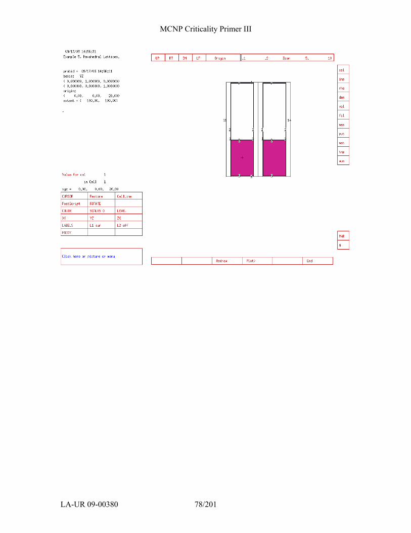
MCNP Criticality Primer III
LA-UR 09-00380 78/201
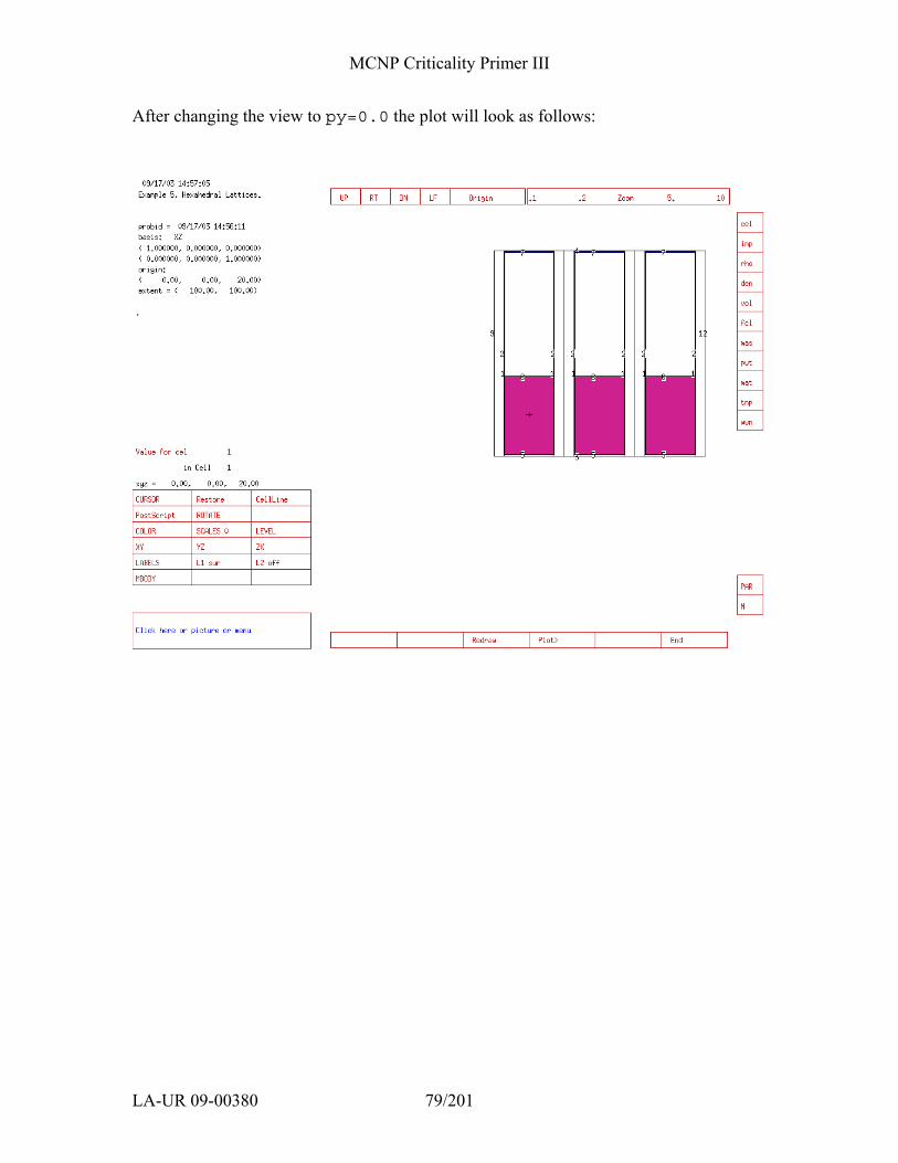
MCNP Criticality Primer III
LA-UR 09-00380 79/201
After changing the view to py=0.0 the plot will look as follows:
MCNP Criticality Primer III
LA-UR 09-00380 80/201
A view of the pz plane at 10 cm will look as follows:
The final combined keff estimator for this problem on a Windows 2000 Pentium 4 computer with the ENDF66c data library at LANL was 0.98536 with an estimated standard deviation of 0.00102 (1σ).
5.4 EXAMPLE 5.4: CHANGING MATERIALS IN SELECTED ELEMENTS
Example 5.3 was filled with six identical items. The fill specification was a single number that specified the universe that filled every element of the lattice. This example illustrates the expanded form of the fill card. Example 5.3 is modified by filling two of the containers with graphite.
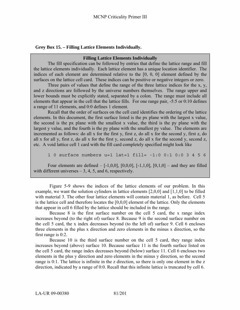
MCNP Criticality Primer III
LA-UR 09-00380 81/201
Grey Box 15. – Filling Lattice Elements Individually.
Figure 5-9 shows the indices of the lattice elements of our problem. In this
example, we want the solution cylinders in lattice elements [2,0,0] and [1,1,0] to be filled with material 3. The other four lattice elements will contain material 1, as before. Cell 5 is the lattice cell and therefore locates the [0,0,0] element of the lattice. Only the elements that appear in cell 6 filled by the lattice should be included in the range.
Because 8 is the first surface number on the cell 5 card, the x range index increases beyond (to the right of) surface 8. Because 9 is the second surface number on the cell 5 card, the x index decreases beyond (to the left of) surface 9. Cell 6 encloses three elements in the plus x direction and zero elements in the minus x direction, so the first range is 0:2.
Because 10 is the third surface number on the cell 5 card, they range index increases beyond (above) surface 10. Because surface 11 is the fourth surface listed on the cell 5 card, the range index decreases beyond (below) surface 11. Cell 6 encloses two elements in the plus y direction and zero elements in the minus y direction, so the second range is 0:1. The lattice is infinite in the z direction, so there is only one element in the z direction, indicated by a range of 0:0. Recall that this infinite lattice is truncated by cell 6.
Filling Lattice Elements Individually The fill specification can be followed by entries that define the lattice range and fill the lattice elements individually. Each lattice element has a unique location identifier. The indices of each element are determined relative to the [0, 0, 0] element defined by the surfaces on the lattice cell card. These indices can be positive or negative integers or zero. Three pairs of values that define the range of the three lattice indices for the x, y, and z directions are followed by the universe numbers themselves. The range upper and lower bounds must be explicitly stated, separated by a colon. The range must include all elements that appear in the cell that the lattice fills. For one range pair, -5:5 or 0:10 defines a range of 11 elements, and 0:0 defines 1 element. Recall that the order of surfaces on the cell card identifies the ordering of the lattice elements. In this document, the first surface listed is the px plane with the largest x value, the second is the px plane with the smallest x value, the third is the py plane with the largest y value, and the fourth is the py plane with the smallest py value. The elements are incremented as follows: do all x for the first y, first z, do all x for the second y, first z, do all x for all y, first z, do all x for the first y, second z, do all x for the second y, second z, etc. A void lattice cell 1 card with the fill card completely specified might look like 1 0 surface numbers u=1 lat=1 fill= -1:0 0:1 0:0 3 4 5 6 Four elements are defined – [-1,0,0], [0,0,0], [-1,1,0], [0,1,0] – and they are filled with different universes – 3, 4, 5, and 6, respectively.
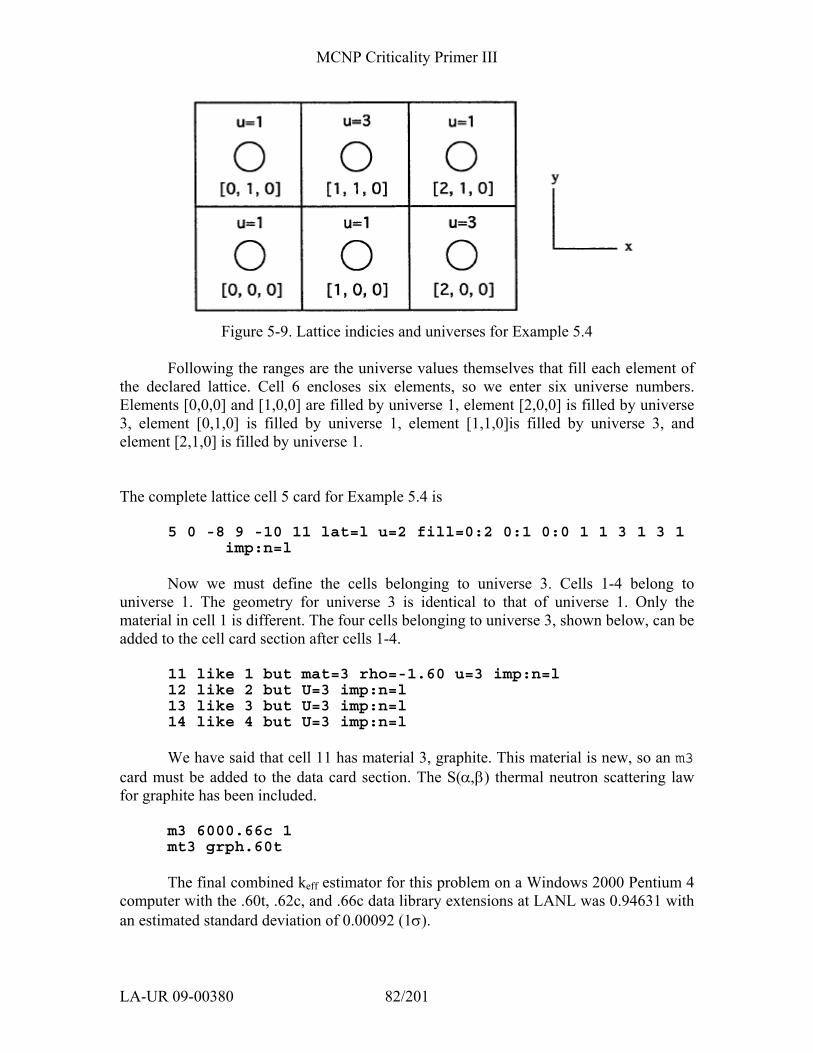
MCNP Criticality Primer III
LA-UR 09-00380 82/201
Figure 5-9. Lattice indicies and universes for Example 5.4
Following the ranges are the universe values themselves that fill each element of
the declared lattice. Cell 6 encloses six elements, so we enter six universe numbers. Elements [0,0,0] and [1,0,0] are filled by universe 1, element [2,0,0] is filled by universe 3, element [0,1,0] is filled by universe 1, element [1,1,0]is filled by universe 3, and element [2,1,0] is filled by universe 1. The complete lattice cell 5 card for Example 5.4 is
5 0 -8 9 -10 11 lat=l u=2 fill=0:2 0:1 0:0 1 1 3 1 3 1 imp:n=l
Now we must define the cells belonging to universe 3. Cells 1-4 belong to universe 1. The geometry for universe 3 is identical to that of universe 1. Only the material in cell 1 is different. The four cells belonging to universe 3, shown below, can be added to the cell card section after cells 1-4.
11 like 1 but mat=3 rho=-1.60 u=3 imp:n=l 12 like 2 but U=3 imp:n=l 13 like 3 but U=3 imp:n=l 14 like 4 but U=3 imp:n=l
We have said that cell 11 has material 3, graphite. This material is new, so an m3
card must be added to the data card section. The S(α,β) thermal neutron scattering law for graphite has been included.
m3 6000.66c 1 mt3 grph.60t
The final combined keff estimator for this problem on a Windows 2000 Pentium 4
computer with the .60t, .62c, and .66c data library extensions at LANL was 0.94631 with an estimated standard deviation of 0.00092 (1σ).
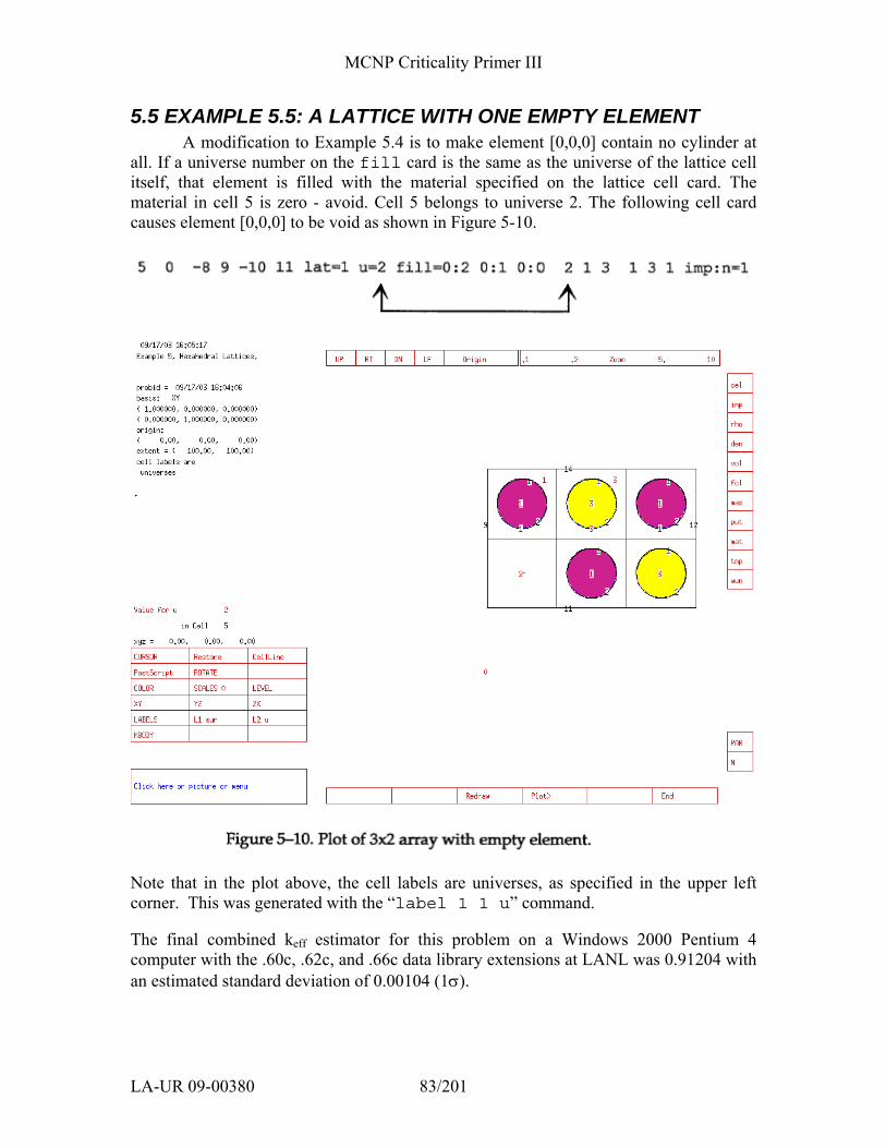
MCNP Criticality Primer III
LA-UR 09-00380 83/201
5.5 EXAMPLE 5.5: A LATTICE WITH ONE EMPTY ELEMENT A modification to Example 5.4 is to make element [0,0,0] contain no cylinder at
all. If a universe number on the fill card is the same as the universe of the lattice cell itself, that element is filled with the material specified on the lattice cell card. The material in cell 5 is zero - avoid. Cell 5 belongs to universe 2. The following cell card causes element [0,0,0] to be void as shown in Figure 5-10.
Note that in the plot above, the cell labels are universes, as specified in the upper left corner. This was generated with the “label 1 1 u” command. The final combined keff estimator for this problem on a Windows 2000 Pentium 4 computer with the .60c, .62c, and .66c data library extensions at LANL was 0.91204 with an estimated standard deviation of 0.00104 (1σ).
MCNP Criticality Primer III
LA-UR 09-00380 84/201
5.6 EXAMPLE 5.6: CHANGING SIZE OF CELLS FILLING A LATTICE
In Example 5.6 we want to change the radius of the solution cylinder in elements [1,0,0] and [2,1,0]. In Example 5.3, the inner radius of the cylinder is 12.49 cm (surface 1), and the outer radius is 12.79 cm (surface 2). In Example 5.6, the inner cylinder radius is 5 cm, and the outer radius is 5.5 cm. The cell 5 card is similar to Example 5.4.
5 0 -8 9 -10 11 lat=l u=2 fill=0:2 0:1 0:0 1 3 1 1 1 3 imp:n=l
The four cells belonging to universe 3 are defined differently. Two new surfaces will be used and need to be added to the surface card section.
21 cz 5 22 cz 5.5
Because the geometrical dimensions have changed, we cannot take advantage of
the like m but construct. The description of cells 21-24 is very similar to cells 1-4, however. Add these cell cards to the example 5.3 input file after cells 1-4.
21 3 -1.60 -21 5 -6 u=3 imp:n=l 22 0 -21 6 -7 u=3 imp:n=l 23 2 8.6360e-2 -22 #21 #22 u=3 imp:n=l 24 0 22 U=3 imp:n=l
The material in cell 21 is graphite as in example 5.4, with a density of 1.60 g/cc.
An m3 and an mt3 card need to be added to the data card section.
m3 6000.66c 1 mt3 grph.60t
If you plot this input file with the following command
pz 0 or 35 20 1 ex 55 you see that the radial size of two cylinders is smaller.
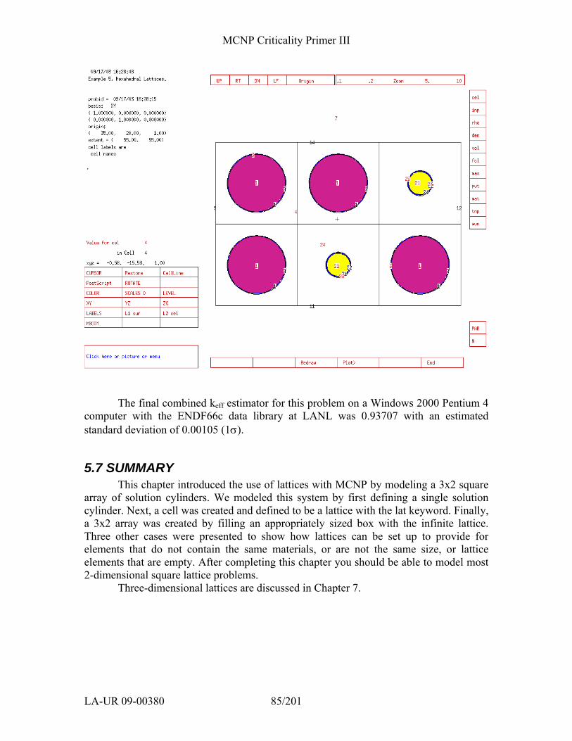
MCNP Criticality Primer III
LA-UR 09-00380 85/201
The final combined keff estimator for this problem on a Windows 2000 Pentium 4
computer with the ENDF66c data library at LANL was 0.93707 with an estimated standard deviation of 0.00105 (1σ).
5.7 SUMMARY This chapter introduced the use of lattices with MCNP by modeling a 3x2 square
array of solution cylinders. We modeled this system by first defining a single solution cylinder. Next, a cell was created and defined to be a lattice with the lat keyword. Finally, a 3x2 array was created by filling an appropriately sized box with the infinite lattice. Three other cases were presented to show how lattices can be set up to provide for elements that do not contain the same materials, or are not the same size, or lattice elements that are empty. After completing this chapter you should be able to model most 2-dimensional square lattice problems.
Three-dimensional lattices are discussed in Chapter 7.

MCNP Criticality Primer III
LA-UR 09-00380 86/201
Chapter 6: Hexagonal (Triangular) Lattices
This chapter continues discussion of the lattice keyword (lat) by modeling a triangular pitch array.
6.1 WHAT YOU WILL BE ABLE TO DO
1) Create general planes to define a hexagonal lattice element. 2) Use the lat keyword to create a hexagonal (triangular pitch) lattice. 3) Understand hexagonal lattice indexing.
6.2 PROBLEM DESCRIPTION Example 6.3 is a hexagonal array of seven open U(93.2% enrichment)O2F2
solution cylinders (LA-10860 page 125). The uranium-fluoride solution is contained in seven aluminum cylinders with a 7.60 cm surface separation between cylinders. There is 20 cm of water reflection below and radially about the cylinders. There is no water above the aluminum containers. The data for this problem are:
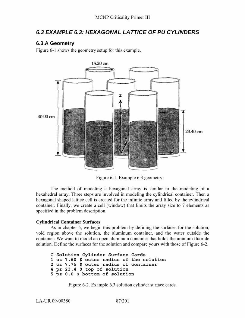
MCNP Criticality Primer III
LA-UR 09-00380 87/201
6.3 EXAMPLE 6.3: HEXAGONAL LATTICE OF PU CYLINDERS
6.3.A Geometry Figure 6-1 shows the geometry setup for this example.
Figure 6-1. Example 6.3 geometry.
The method of modeling a hexagonal array is similar to the modeling of a
hexahedral array. Three steps are involved in modeling the cylindrical container. Then a hexagonal shaped lattice cell is created for the infinite array and filled by the cylindrical container. Finally, we create a cell (window) that limits the array size to 7 elements as specified in the problem description. Cylindrical Container Surfaces
As in chapter 5, we begin this problem by defining the surfaces for the solution, void region above the solution, the aluminum container, and the water outside the container. We want to model an open aluminum container that holds the uranium fluoride solution. Define the surfaces for the solution and compare yours with those of Figure 6-2.
C Solution Cylinder Surface Cards 1 cz 7.60 $ outer radius of the solution 2 cz 7.75 $ outer radius of container 4 pz 23.4 $ top of solution 5 pz 0.0 $ bottom of solution
Figure 6-2. Example 6.3 solution cylinder surface cards.
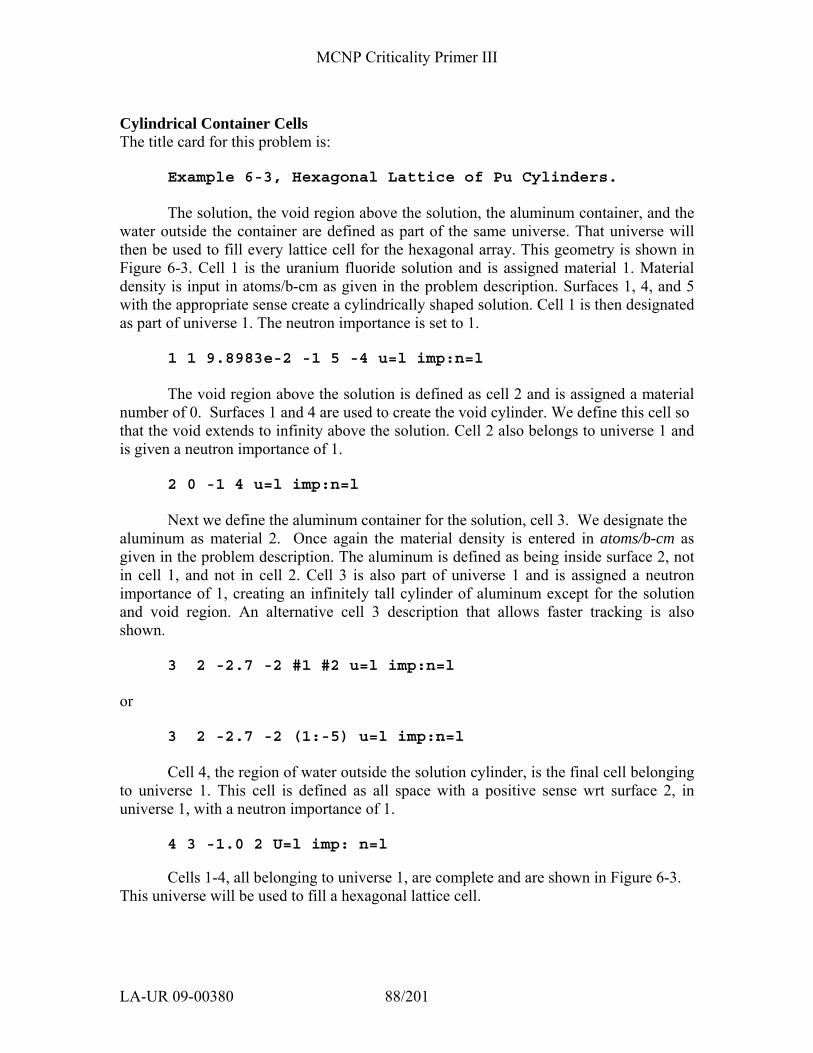
MCNP Criticality Primer III
LA-UR 09-00380 88/201
Cylindrical Container Cells The title card for this problem is:
Example 6-3, Hexagonal Lattice of Pu Cylinders.
The solution, the void region above the solution, the aluminum container, and the water outside the container are defined as part of the same universe. That universe will then be used to fill every lattice cell for the hexagonal array. This geometry is shown in Figure 6-3. Cell 1 is the uranium fluoride solution and is assigned material 1. Material density is input in atoms/b-cm as given in the problem description. Surfaces 1, 4, and 5 with the appropriate sense create a cylindrically shaped solution. Cell 1 is then designated as part of universe 1. The neutron importance is set to 1.
1 1 9.8983e-2 -1 5 -4 u=l imp:n=l
The void region above the solution is defined as cell 2 and is assigned a material
number of 0. Surfaces 1 and 4 are used to create the void cylinder. We define this cell so that the void extends to infinity above the solution. Cell 2 also belongs to universe 1 and is given a neutron importance of 1.
2 0 -1 4 u=l imp:n=l
Next we define the aluminum container for the solution, cell 3. We designate the aluminum as material 2. Once again the material density is entered in atoms/b-cm as given in the problem description. The aluminum is defined as being inside surface 2, not in cell 1, and not in cell 2. Cell 3 is also part of universe 1 and is assigned a neutron importance of 1, creating an infinitely tall cylinder of aluminum except for the solution and void region. An alternative cell 3 description that allows faster tracking is also shown.
3 2 -2.7 -2 #1 #2 u=l imp:n=l or
3 2 -2.7 -2 (1:-5) u=l imp:n=l Cell 4, the region of water outside the solution cylinder, is the final cell belonging
to universe 1. This cell is defined as all space with a positive sense wrt surface 2, in universe 1, with a neutron importance of 1.
4 3 -1.0 2 U=l imp: n=l
Cells 1-4, all belonging to universe 1, are complete and are shown in Figure 6-3.
This universe will be used to fill a hexagonal lattice cell.
MCNP Criticality Primer III
LA-UR 09-00380 89/201
Lattice Cell Surfaces
In this section we define the unit cell in the x-y plane for the hexagonal lattice. Opposite sides of the six-sided lattice cell must be equal in length and parallel. The dimension of concern that determines the six surfaces of the lattice cell is the pitch of the solution containers. The following “prescription” can be used to calculate the general planes for any hexagonal lattice formed from equilateral triangles. The pitch for this example is calculated by adding the outer diameter of the aluminum container and the surface separation.
The pitch for this example is calculated by adding the outer diameter of the aluminum container and the surface separation.
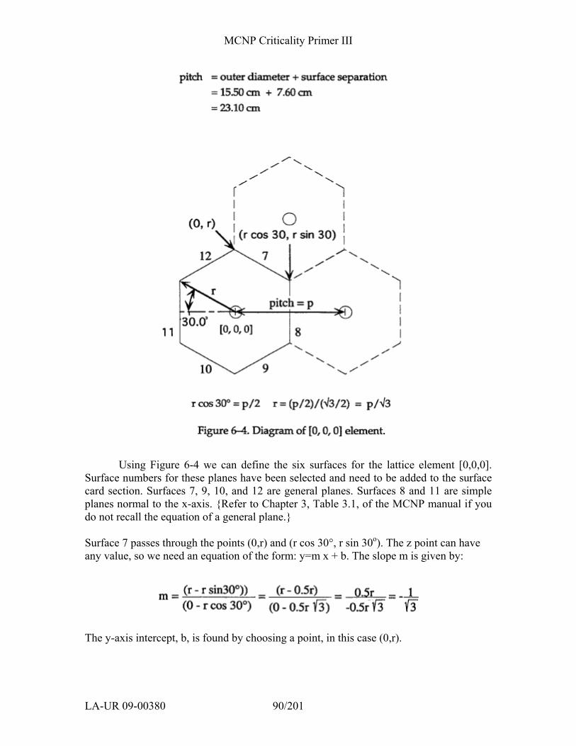
MCNP Criticality Primer III
LA-UR 09-00380 90/201
Using Figure 6-4 we can define the six surfaces for the lattice element [0,0,0]. Surface numbers for these planes have been selected and need to be added to the surface card section. Surfaces 7, 9, 10, and 12 are general planes. Surfaces 8 and 11 are simple planes normal to the x-axis. {Refer to Chapter 3, Table 3.1, of the MCNP manual if you do not recall the equation of a general plane.} Surface 7 passes through the points (0,r) and (r cos 30°, r sin 30o). The z point can have any value, so we need an equation of the form: y=m x + b. The slope m is given by:
The y-axis intercept, b, is found by choosing a point, in this case (0,r).
MCNP Criticality Primer III
LA-UR 09-00380 91/201
Therefore the equation for surface 7 is:
MCNP wants this equation entered as Ax + By + Cz = D, where A = -m and D = r,
Therefore the coefficients of the equation for surface 7 are:
The pitch, p, has already been defined as 23.10, so the surface 7 general plane is entered as:
7 p l 1.73205 0 23.1 Surface 8 passes through the x-axis at p/2. Therefore surface 8 is defined as:
8 px 11.55 Surface 9 is defined similarly to surface 7. This plane passes through the points (0,-r) and (r cos 30°, -r sin 30o). As with surface 7, the z-point can have any value, so we need an equation of the form y = mx + b.
MCNP Criticality Primer III
LA-UR 09-00380 92/201
The surface 9 general plane is entered as:
9 p -1 1.73205 0 -23.1 Follow the same logic for surface 10 to get the following equation of the plane.
The MCNP input would then appear as:
10 p 1 1.73205 0 -23.1 Surface 11 is a plane that passes through the x-axis at -p/2.
11 PX -11.55

MCNP Criticality Primer III
LA-UR 09-00380 93/201
The final surface for lattice cell is a plane that passes through the point (0, r) and (-r cos 30o, r sin 30o). Follow the same procedure as with surfaces 7, 9, and 10 to get the needed equation.
12 P -1 1.73205 0 23.1
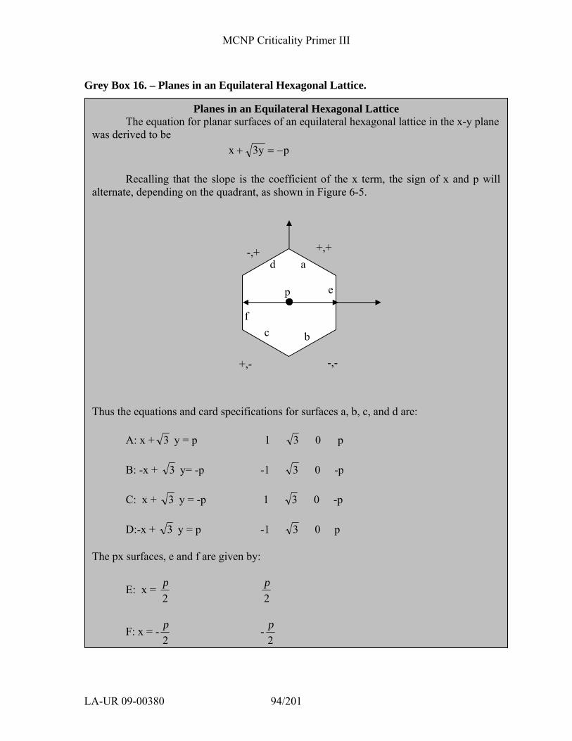
MCNP Criticality Primer III
LA-UR 09-00380 94/201
Grey Box 16. – Planes in an Equilateral Hexagonal Lattice.
Planes in an Equilateral Hexagonal Lattice The equation for planar surfaces of an equilateral hexagonal lattice in the x-y plane was derived to be
p3yx −=+
Recalling that the slope is the coefficient of the x term, the sign of x and p will alternate, depending on the quadrant, as shown in Figure 6-5. Thus the equations and card specifications for surfaces a, b, c, and d are: A: x + 3 y = p 1 3 0 p B: -x + 3 y= -p -1 3 0 -p C: x + 3 y = -p 1 3 0 -p D:-x + 3 y = p -1 3 0 p The px surfaces, e and f are given by:
E: x = 2p
2p
F: x = -2p -
2p
-,+ +,+
-,- +,-
p
a
b c
d
e
f
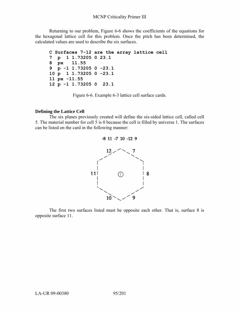
MCNP Criticality Primer III
LA-UR 09-00380 95/201
Returning to our problem, Figure 6-6 shows the coefficients of the equations for the hexagonal lattice cell for this problem. Once the pitch has been determined, the calculated values are used to describe the six surfaces.
C Surfaces 7-12 are the array lattice cell 7 p 1 1.73205 0 23.1 8 px 11.55 9 p -1 1.73205 0 -23.1 10 p 1 1.73205 0 -23.1 11 px -11.55 12 p -1 1.73205 0 23.1
Figure 6-6. Example 6-3 lattice cell surface cards.
Defining the Lattice Cell The six planes previously created will define the six-sided lattice cell, called cell
5. The material number for cell 5 is 0 because the cell is filled by universe 1. The surfaces can be listed on the card in the following manner:
The first two surfaces listed must be opposite each other. That is, surface 8 is opposite surface 11.
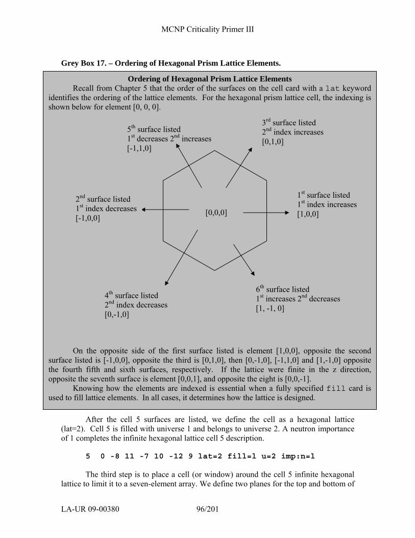
MCNP Criticality Primer III
LA-UR 09-00380 96/201
Grey Box 17. – Ordering of Hexagonal Prism Lattice Elements.
After the cell 5 surfaces are listed, we define the cell as a hexagonal lattice (lat=2). Cell 5 is filled with universe 1 and belongs to universe 2. A neutron importance of 1 completes the infinite hexagonal lattice cell 5 description. 5 0 -8 11 -7 10 -12 9 lat=2 fill=l u=2 imp:n=l
The third step is to place a cell (or window) around the cell 5 infinite hexagonal lattice to limit it to a seven-element array. We define two planes for the top and bottom of
Ordering of Hexagonal Prism Lattice Elements Recall from Chapter 5 that the order of the surfaces on the cell card with a lat keyword identifies the ordering of the lattice elements. For the hexagonal prism lattice cell, the indexing is shown below for element [0, 0, 0].
On the opposite side of the first surface listed is element [1,0,0], opposite the second
surface listed is [-1,0,0], opposite the third is [0,1,0], then [0,-1,0], [-1,1,0] and [1,-1,0] opposite the fourth fifth and sixth surfaces, respectively. If the lattice were finite in the z direction, opposite the seventh surface is element [0,0,1], and opposite the eight is [0,0,-1]. Knowing how the elements are indexed is essential when a fully specified fill card is used to fill lattice elements. In all cases, it determines how the lattice is designed.
6th surface listed 1st increases 2nd decreases [1, -1, 0]
1st surface listed 1st index increases [1,0,0]
3rd surface listed 2nd index increases [0,1,0]
5th surface listed 1st decreases 2nd increases [-1,1,0]
4th surface listed 2nd index decreases [0,-1,0]
[0,0,0] 2nd surface listed 1st index decreases [-1,0,0]
MCNP Criticality Primer III
LA-UR 09-00380 97/201
the solution cylinders and define a cylinder that has a radius such that only 7 lattice elements can be contained within. Figure 6-7 shows the surfaces chosen for this example.
C Window Surfaces 3 pz 40.0 $ Top of aluminum cylinder 6 pz -1.0 $ bottom of aluminum container 13 cz 32.0 $ cylinder for array window
Figure 6-7. Example 6.3 window surface cards.
We will call the window cell 6. The material number is zero because the cell is filled by the lattice, universe 2. The cell is bound in the negative sense of surface 13, the positive sense of surface 6, and the negative sense of surface 3. Cell 6 is filled with universe 2 and has a neutron importance of 1. The infinite lattice is now limited to a system of seven solution cylinders in a hexagonal configuration. 6 0 -13 6 -3 fill=2 imp:n=l
In the problem description there is infinite water reflection except above the solution cylinders. A thickness of 20 cm of water adequately models infinite reflectors for neutrons. Two surfaces need to be added to the surface card section as shown in Figure 6-8. The cylinder is 20 cm beyond surface 13, and the plane is 20 cm below surface 6.
C Reflector Surfaces 14 cz 52.0 $ outer radius of reflector 15 pz -21.0 $ botmmon edge of reflector
Figure 6-8. Example 6.3 water reflector surfaces.
The water reflector is defined as cell 7. It is assigned material number 3, water with a density of 1 g/cc. Cell 7 is all space that is a union of the positive sense wrt surface 13 and the negative sense wrt surface 6, intersected with all space that is negative wrt surface 3, positive wrt surface 15, and negative wrt surface 14. A neutron importance of 1 completes the cell. 7 3 -1.0 (13:-6) -3 15 -14 imp:n=l
The final cell is the “rest of the world”. Cell 8 is given a material number of 0. The neutron importance for this cell is 0. 8 0 14:3:-15 imp:n=0
6.3.B Materials Material cards are constructed and entered as described previously, using the
information provided in the problem description. Your material cards should resemble
MCNP Criticality Primer III
LA-UR 09-00380 98/201
those in Figure 6-9. Materials 1 and 3 should use the S(α,β) thermal neutron scattering law for hydrogen in light water.
C Data Cards C Material Cards m1 1001.62c 6.1063-2 8016.62c 3.3487-2 9019.62c 2.9554-3 92235.66c 1.3784-3 92238.66c 9.9300-5 mt1 lwtr.60t m2 13027.62c 1.0 m3 1001.62c 2 8016.62c 1 mt3 lwtr.60t
Figure 6-9. Example 6.3 material cards.
6.3.C MCNP Criticality Controls The kcode specification is the same as in example 5. On the ksrc card, again
we will put a criticality source point in each solution cylinder. Figure 6-10 shows the control cards for this example.
C Criticality Control Cards kcode 5000 1.0 50 250 ksrc 0 0 11.7 -23.1 0 11.7 23.1 0 11.7 -11.55 20.0 11.7 -11.5 -20.0 11.7 11.55 20.0 11.7 11.5 -20.0 11.7
Figure 6-10. Example 6.3 criticality control cards.
For large problems with fissile material at many locations, MCNP has other
methods of defining the initial starting source points. Whether the problem is tightly or loosely coupled may also affect your choice of method of initial source description. It is much more important to put at least one ksrc fission source point in each fissile region for a loosely coupled problem. {Further discussion can be found in the MCNP manual.}
6.3.D Example 6.3 MCNP Input File The input for example 6.3 is complete. The input file should resemble the
following. Do not forget the blank line delimiters.
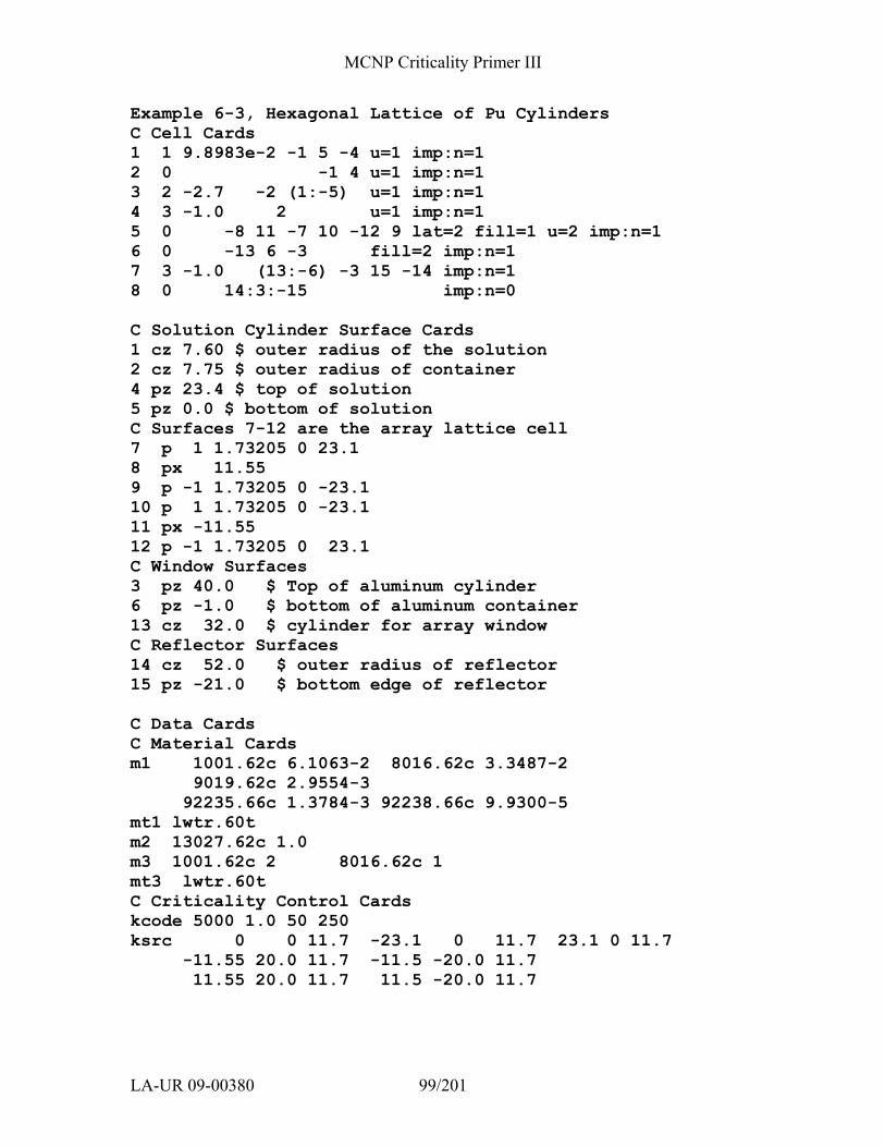
MCNP Criticality Primer III
LA-UR 09-00380 99/201
Example 6-3, Hexagonal Lattice of Pu Cylinders C Cell Cards 1 1 9.8983e-2 -1 5 -4 u=1 imp:n=1 2 0 -1 4 u=1 imp:n=1 3 2 -2.7 -2 (1:-5) u=1 imp:n=1 4 3 -1.0 2 u=1 imp:n=1 5 0 -8 11 -7 10 -12 9 lat=2 fill=1 u=2 imp:n=1 6 0 -13 6 -3 fill=2 imp:n=1 7 3 -1.0 (13:-6) -3 15 -14 imp:n=1 8 0 14:3:-15 imp:n=0 C Solution Cylinder Surface Cards 1 cz 7.60 $ outer radius of the solution 2 cz 7.75 $ outer radius of container 4 pz 23.4 $ top of solution 5 pz 0.0 $ bottom of solution C Surfaces 7-12 are the array lattice cell 7 p 1 1.73205 0 23.1 8 px 11.55 9 p -1 1.73205 0 -23.1 10 p 1 1.73205 0 -23.1 11 px -11.55 12 p -1 1.73205 0 23.1 C Window Surfaces 3 pz 40.0 $ Top of aluminum cylinder 6 pz -1.0 $ bottom of aluminum container 13 cz 32.0 $ cylinder for array window C Reflector Surfaces 14 cz 52.0 $ outer radius of reflector 15 pz -21.0 $ bottom edge of reflector C Data Cards C Material Cards m1 1001.62c 6.1063-2 8016.62c 3.3487-2 9019.62c 2.9554-3 92235.66c 1.3784-3 92238.66c 9.9300-5 mt1 lwtr.60t m2 13027.62c 1.0 m3 1001.62c 2 8016.62c 1 mt3 lwtr.60t C Criticality Control Cards kcode 5000 1.0 50 250 ksrc 0 0 11.7 -23.1 0 11.7 23.1 0 11.7 -11.55 20.0 11.7 -11.5 -20.0 11.7 11.55 20.0 11.7 11.5 -20.0 11.7
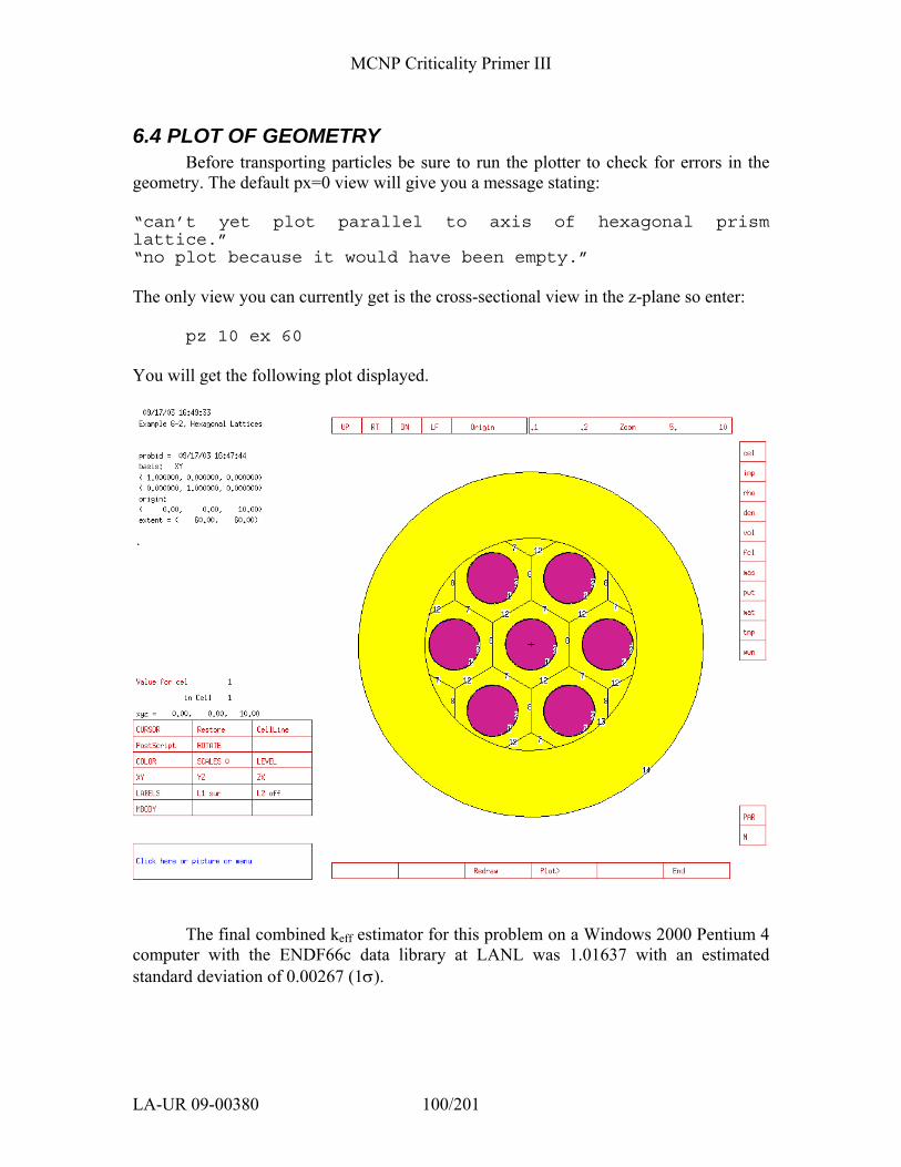
MCNP Criticality Primer III
LA-UR 09-00380 100/201
6.4 PLOT OF GEOMETRY Before transporting particles be sure to run the plotter to check for errors in the
geometry. The default px=0 view will give you a message stating: “can’t yet plot parallel to axis of hexagonal prism lattice.” “no plot because it would have been empty.” The only view you can currently get is the cross-sectional view in the z-plane so enter:
pz 10 ex 60 You will get the following plot displayed.
The final combined keff estimator for this problem on a Windows 2000 Pentium 4
computer with the ENDF66c data library at LANL was 1.01637 with an estimated standard deviation of 0.00267 (1σ).
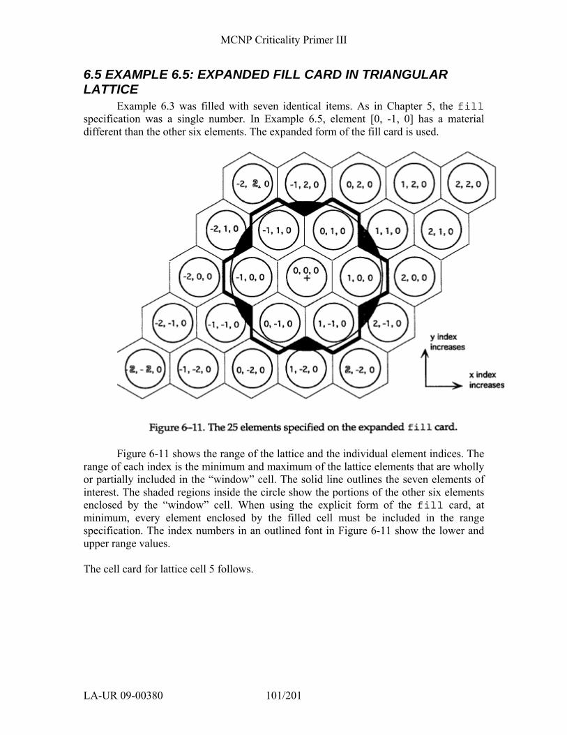
MCNP Criticality Primer III
LA-UR 09-00380 101/201
6.5 EXAMPLE 6.5: EXPANDED FILL CARD IN TRIANGULAR LATTICE
Example 6.3 was filled with seven identical items. As in Chapter 5, the fill specification was a single number. In Example 6.5, element [0, -1, 0] has a material different than the other six elements. The expanded form of the fill card is used.
Figure 6-11 shows the range of the lattice and the individual element indices. The
range of each index is the minimum and maximum of the lattice elements that are wholly or partially included in the “window” cell. The solid line outlines the seven elements of interest. The shaded regions inside the circle show the portions of the other six elements enclosed by the “window” cell. When using the explicit form of the fill card, at minimum, every element enclosed by the filled cell must be included in the range specification. The index numbers in an outlined font in Figure 6-11 show the lower and upper range values. The cell card for lattice cell 5 follows.
MCNP Criticality Primer III
LA-UR 09-00380 102/201
In this problem the x range is -2 to 2 (5 elements in x), the y range is -2 to 2 (5
elements in y), and the z range is 0 to 0 (1 element in z). Twenty-five universe numbers, one for each element, must be entered. Recall the order of index incrementing: first z, first y, all x; first z, second y, all x, etc. Some of the elements are clearly not involved in the area of interest, [-2, -2, 0] for example. Those elements can be filled with the universe number of the lattice cell itself, in this case universe 2, making those elements void. A small part of element [1, -2, 0] is included in the “window”, so it should be filled by universe 1.
The material in element [0, -1, 0] is changed from the uranium-fluoride solution to graphite. The universe number for the [0, -1, 0] element is 3. The following cells need to be added to the cell card section after surface 4 for universe 3.
9 like 1 but mat=4 rho=-1.60 u=3 imp:n=l 10 like 2 but u=3 imp:n=l 11 like 3 but u=3 imp:n=l 12 like 4 but u=3 imp:n=l
Also, add graphite to the materials using the following:
m4 6000.66c 1 mt4 grph.60t
Using Figure 6-11 and the 25 entries on the fill card, identify which element is
filled by what universe on your own. Notice that the fill array has 5 rows and 5 columns. Each line corresponds to a horizontal row in Figure 6-11. In a large problem, this practice helps keep track of the entries in the large array.
The importance of all lattice elements is set to 1. Recall that no particles ever will
be tracked in some of the elements. When a particle in element [1, 0, 0] crosses the cylindrical surface, it will enter cell 6 and be tracked at that level.
6.6 EXAMPLE 6.6: NONEQUILATERAL TRIANGULAR LATTICE It is possible to describe a lattice that is not equilateral. Using the example 6.3
input, change the following surface cards:
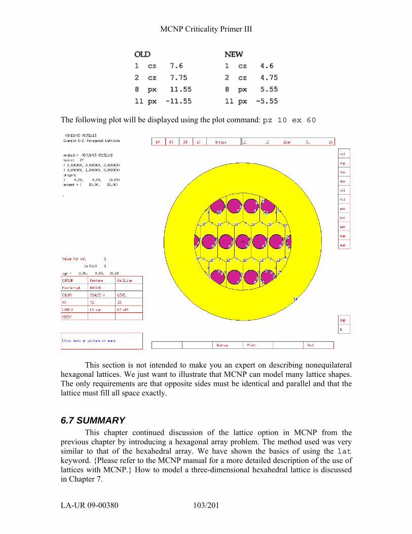
MCNP Criticality Primer III
LA-UR 09-00380 103/201
The following plot will be displayed using the plot command: pz 10 ex 60
This section is not intended to make you an expert on describing nonequilateral hexagonal lattices. We just want to illustrate that MCNP can model many lattice shapes. The only requirements are that opposite sides must be identical and parallel and that the lattice must fill all space exactly.
6.7 SUMMARY This chapter continued discussion of the lattice option in MCNP from the
previous chapter by introducing a hexagonal array problem. The method used was very similar to that of the hexahedral array. We have shown the basics of using the lat keyword. {Please refer to the MCNP manual for a more detailed description of the use of lattices with MCNP.} How to model a three-dimensional hexahedral lattice is discussed in Chapter 7.
MCNP Criticality Primer III
LA-UR 09-00380 104/201
Chapter 7: 3-Dimensional Square Lattices This chapter builds on the example from Chapter 5 to create a three-dimensional
square lattice of solution cylinders. Much of the example remains unchanged. If you do not understand the input in this example, refer to Chapter 5 for a more detailed description of this problem. The 3-dimensional hexagonal lattice is constructed in a similar manner, so no examples are presented in this document.
7.1 WHAT YOU WILL BE ABLE TO DO
1) Create a 3-D hexahedral (square) lattice. 2) Fill the lattice elements with various materials. 3) Create a universe 0 lattice.
7.2 PROBLEM DESCRIPTION This example is the hexahedral array of six plutonium nitrate solution cylinders
(LA-1086O, page 125) from Chapter 5. It is modified to create a second layer of six elements for a total of 12 solution cylinders. Recall that the data for this problem is:
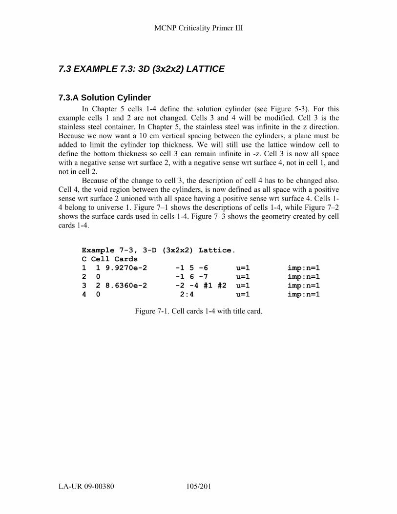
MCNP Criticality Primer III
LA-UR 09-00380 105/201
7.3 EXAMPLE 7.3: 3D (3x2x2) LATTICE
7.3.A Solution Cylinder In Chapter 5 cells 1-4 define the solution cylinder (see Figure 5-3). For this
example cells 1 and 2 are not changed. Cells 3 and 4 will be modified. Cell 3 is the stainless steel container. In Chapter 5, the stainless steel was infinite in the z direction. Because we now want a 10 cm vertical spacing between the cylinders, a plane must be added to limit the cylinder top thickness. We will still use the lattice window cell to define the bottom thickness so cell 3 can remain infinite in -z. Cell 3 is now all space with a negative sense wrt surface 2, with a negative sense wrt surface 4, not in cell 1, and not in cell 2.
Because of the change to cell 3, the description of cell 4 has to be changed also. Cell 4, the void region between the cylinders, is now defined as all space with a positive sense wrt surface 2 unioned with all space having a positive sense wrt surface 4. Cells 1- 4 belong to universe 1. Figure 7–1 shows the descriptions of cells 1-4, while Figure 7–2 shows the surface cards used in cells 1-4. Figure 7–3 shows the geometry created by cell cards 1-4.
Example 7-3, 3-D (3x2x2) Lattice. C Cell Cards 1 1 9.9270e-2 -1 5 -6 u=1 imp:n=1 2 0 -1 6 -7 u=1 imp:n=1 3 2 8.6360e-2 -2 -4 #1 #2 u=1 imp:n=1 4 0 2:4 u=1 imp:n=1
Figure 7-1. Cell cards 1-4 with title card.
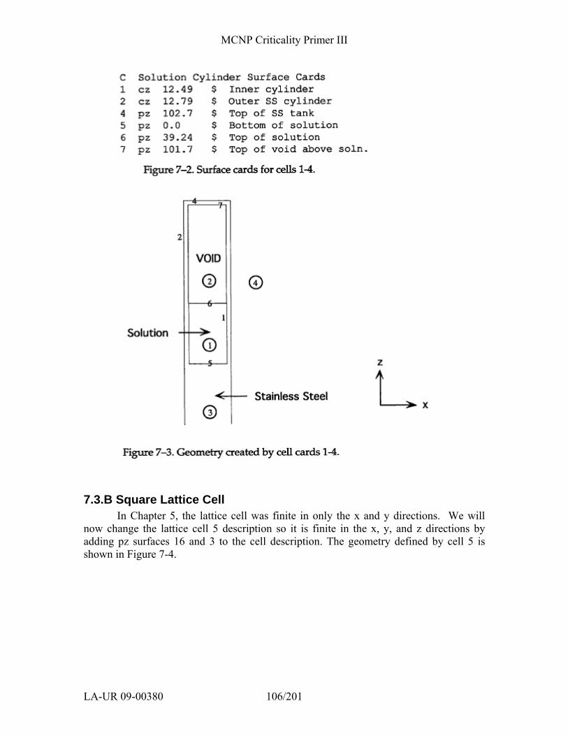
MCNP Criticality Primer III
LA-UR 09-00380 106/201
7.3.B Square Lattice Cell In Chapter 5, the lattice cell was finite in only the x and y directions. We will
now change the lattice cell 5 description so it is finite in the x, y, and z directions by adding pz surfaces 16 and 3 to the cell description. The geometry defined by cell 5 is shown in Figure 7-4.
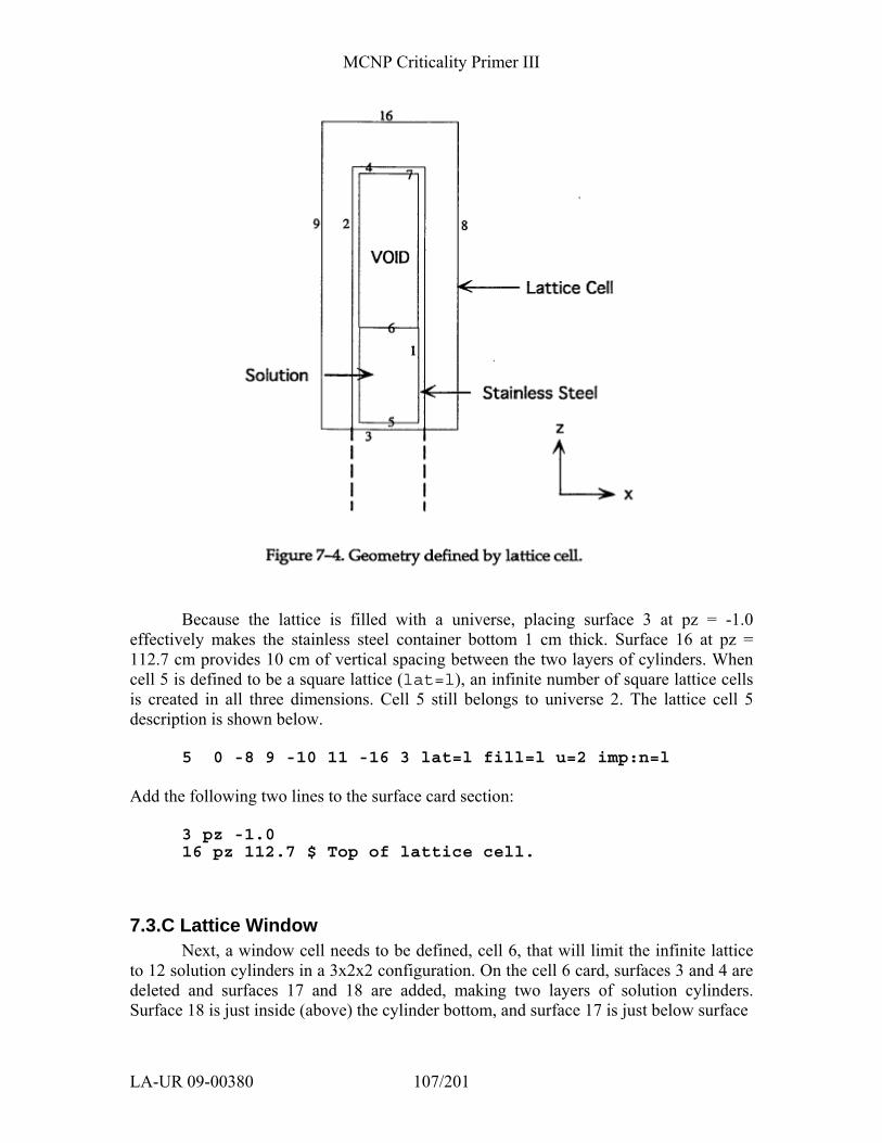
MCNP Criticality Primer III
LA-UR 09-00380 107/201
Because the lattice is filled with a universe, placing surface 3 at pz = -1.0 effectively makes the stainless steel container bottom 1 cm thick. Surface 16 at pz = 112.7 cm provides 10 cm of vertical spacing between the two layers of cylinders. When cell 5 is defined to be a square lattice (lat=l), an infinite number of square lattice cells is created in all three dimensions. Cell 5 still belongs to universe 2. The lattice cell 5 description is shown below.
5 0 -8 9 -10 11 -16 3 lat=l fill=l u=2 imp:n=l
Add the following two lines to the surface card section:
3 pz -1.0 16 pz 112.7 $ Top of lattice cell.
7.3.C Lattice Window Next, a window cell needs to be defined, cell 6, that will limit the infinite lattice
to 12 solution cylinders in a 3x2x2 configuration. On the cell 6 card, surfaces 3 and 4 are deleted and surfaces 17 and 18 are added, making two layers of solution cylinders. Surface 18 is just inside (above) the cylinder bottom, and surface 17 is just below surface
MCNP Criticality Primer III
LA-UR 09-00380 108/201
16. These surfaces limit the infinite lattice in the z direction. Cell 6 still is filled by universe 2. The description of cell 6 follows.
6 0 13 -12 15 -14 18 -16 fill=2 imp:n=l Add the following line to the surface card section:
18 pz -114.7 $ Bottom of lattice cell.
7.3.D “Rest of the World” The final cell for this problem, cell 7, defines the “rest of the world”. Cell 7 is
given a material number of 0 and a neutron importance of 0.
7 0 -13:12:-15:14:-18:16 imp:n=0
7.4 MATERIALS The material cards for this problem do not require any change from example 5
and can be copied directly as shown in Figure 7–5. C Data Cards C Material Cards m1 1001.62c 6.0070-2 8016.62c 3.6540-2 7014.62c 2.3699-3 94239.66c 2.7682-4 94240.66c 1.2214-5 94241.66c 8.3390-7 94242.666c 4.5800-8 mt1 lwtr.60t m2 24050.62c 7.195-4 24052.62c 1.38589-2 24053.62c 1.5713-3 24054.62c 3.903-4 26056.62c 3.704-3 26056.62c 5.80869-2 26057.62c 1.342-3 26058.62c 1.773-4 28058.62c 4.432-3 28060.62c 1.7069-3 28061.62c 7.42-5 28062.62c 2.363-4 28064.62c 6.05-5
Figure 7-5. Example 7.3 material cards.
7.5 MCNP CRITICALITY CONTROLS The kcode specification remains the same from the previous example. Six
source points are added on the ksrc card to those defined in example 5, so each solution cylinder has a source point. Figure 7-6 shows the control cards for this example.
C Criticality Control Cards kcode 5000 1.0 50 250 ksrc 0 0 19.62 35.58 0 19.62 71.16 0 19.62
MCNP Criticality Primer III
LA-UR 09-00380 109/201
0 35.58 19.92 35.58 35.58 19.62 71.16 35.58 19.62 C These source points are place in the added cylinders 0 0 -94.08 35.58 0 -94.08 71.16 0 -94.08
0 35.58 -94.08 35.58 35.58 -94.08 71.16 35.58 -94.08
Figure 7-6. Example 7.3 control cards.
7.6 EXAMPLE 7.3 MCNP INPUT FILE The input requirements for this example are complete. The input file should
resemble the following.
Example 7-3, 3-D (3x2x2) Lattice C Cell Cards 1 1 9.9270e-2 -1 5 -6 u=1 imp:n=1 2 0 -1 6 -7 u=1 imp:n=1 3 2 8.6360e-2 -2 -4 #1 #2 u=1 imp:n=1 4 0 2:4 u=1 imp:n=1 5 0 -8 9 -10 11 -16 3 lat=1 u=2 fill=1 imp:n=1 6 0 9 -12 11 -14 18 -16 fill=2 imp:n=1 7 0 -9:12:-11:14:-18:16 imp:n=0 C Solution Cylinder Surface Cards 1 cz 12.49 $ Inner cylinder 2 cz 12.79 $ Outer SS cylinder 4 pz 102.7 $ Top of SS tank 5 pz 0.0 $ Bottmon of Solution 6 pz 39.24 $ Top of Solution 7 pz 101.7 $ Top of void above soln. C Beginning of Lattice Surfaces 8 px 17.79 9 px -17.79 10 py 17.79 11 py -17.79 C Window Surfaces 3 pz -1.0 12 px 88.95 14 py 53.37 C Surfaces 16 and 18 bound the lattice in the z direction 16 pz 112.7 $ Top of lattice cell 18 pz -114.7 $ Bottom of lattice cell C Data Cards C Material Cards m1 1001.62c 6.0070-2 8016.62c 3.6540-2 7014.62c 2.3699-3 94239.66c 2.7682-4 94240.66c 1.2214-5 94241.66c 8.3390-7 94242.666c 4.5800-8 mt1 lwtr.60t m2 24050.62c 7.195-4 24052.62c 1.38589-2 24053.62c 1.5713-3 24054.62c 3.903-4
MCNP Criticality Primer III
LA-UR 09-00380 110/201
26056.62c 3.704-3 26056.62c 5.80869-2 26057.62c 1.342-3 26058.62c 1.773-4 28058.62c 4.432-3 28060.62c 1.7069-3 28061.62c 7.42-5 28062.62c 2.363-4 28064.62c 6.05-5 C Criticality Control Cards kcode 5000 1.0 50 250 ksrc 0 0 19.62 35.58 0 19.62 71.16 0 19.62 0 35.58 19.92 35.58 35.58 19.62 71.16 35.58 19.62 C These source points are place in the added cylinders 0 0 -94.08 35.58 0 -94.08 71.16 0 -94.08 0 35.58 -94.08 35.58 35.58 -94.08 71.16 35.58 -94.08
7.7 OUTPUT The final combined keff estimator for this problem on a Windows 2000 Pentium 4
computer with the ENDF66c data library at LANL was 0.99588 with an estimated standard deviation of 0.00102 (1σ).
7.8 PLOT OF GEOMETRY Before transporting particles, run the plotter to check for geometry errors in the
cell descriptions. The default plot extent will show only part of the geometry. Change the extent to bring the entire geometry into view:
ex 150 The plot should appear as follows

MCNP Criticality Primer III
LA-UR 09-00380 111/201
7.9 EXAMPLE 7.9: 3-D LATTICE WITH ONE WATER ELEMENT Now we want to change the material in one of the cylinders in this system.
Recalling what we learned in Chapter 5, each lattice element has a unique lattice location identifier. The [0, 0, 0] element is the one described on the lattice cell card. The indices increase and decrease according to the order of the surfaces entered on the lattice cell card. The first index increases in the +x direction, and the second index increases in the +y direction as in Chapter 5. The fifth surface listed is the pz plane with the largest z value, and the sixth is the pz plane with the smallest z value, so the third index increases in +z direction. The range of the indices for cell 6 are 0:2,0:1, and -1:0. The elements are incremented as follows: do all x for the first y, first z; do all x for the second y, first z; do all x for all y, first z; do all x for the first y, second z; do all x for second y, second z, etc. With this in mind, we replace the fissile solution in element (1, 1, -1) with water.
A water-filled cylinder will be defined and belong to universe 3. The geometry for universe 3 is identical to universe 1. Only the material in cell 1 is different. The four cells belonging to universe 3, shown below, can be added to the cell cards section of example 7 after cells 1-4.
MCNP Criticality Primer III
LA-UR 09-00380 112/201
The complete lattice cell 5 card is now:
Cell 11 is defined with material 3, so an m3 card, water, must be added to the data card section. Because we are using water, S(α,β) cross-section data for hydrogen in water are used. The new material cards are:
m3 1001.62c 2 8016.62c 1 mt3 lwtr.60t
All elements except one are filled with universe 1, while the [1,1, -1] element is
filled with universe 3. An alternative way of writing cell 5 is:
where 5r repeats the previous universe value 5 more times.
The final combined keff estimator for this problem on a Windows 2000 Pentium 4 computer with the .66c, .62c and .60t data libraries at LANL was 0.99243 with an estimated standard deviation of 0.00095 (1σ).
7.10 USING SDEF INSTEAD OF KSRC Although the ksrc can be used to specify explicit source points, the sdef card can alternatively be used to specify complex source distributions in a criticality simulation. Using either method only affects the source distribution in the first cycle of a criticality simulation, and subsequent cycles use the locations of fission events.
The sdef card can be used in a criticality calculation to specify a source points in a volume or distribution of points in the same manner as it can be used in a fixed-source simulation. Sampled source points which are not in fissile material are accepted.
When repeated structures are used, the “path” to the lowest level cell can be specified, using the same syntax as for a tally. If this path is given, coordinates given on the pos, x, y or z keywords apply to the “local” coordinate system. The syntax is a parenthesize-contained sequence of cells in consecutive universe levels, separated by “<”

MCNP Criticality Primer III
LA-UR 09-00380 113/201
and ending with the appropriate universe 0 cell. These cells occupy the same volume but in different universes. A path used for specifying source locations cannot contain more than one cell on the same universe level. Additionally, the path cannot be an entry on the sdef card, but must be entered on a si distribution used by the cel keyword on the sdef card. If a cell in the path is a lattice, the lattice indices should also be specified.
For example, the following cards illustrate the used of the sdef, si and sp cards to be used in place of the ksrc card in example 7-9.
sdef cel=d1 pos=0 0 20.62 si1 L (1<5[0 0 -1]<6) (1<5[1 0 -1]<6) (1<5[2 0 -1]<6) (1<5[0 1 -1]<6) (1<5[0 1 –1]<6) (1<5[2 1 -1]<6) (1<5[0 0 0]<6) (1<5[1 0 0]<6) (1<5[2 0 0]<6) (1<5[0 1 0]<6) (1<5[1 1 0]<6) (1<5[2 1 0]<6) sp1 1 1 1 1 1 1 1 1 1 1 1
The sdef keyword cel=dl says that the source cells are given by a distribution, where d1 points to the si1 card. The keyword pos defines the xyz location of the source point. The si1 card describes the path to the level 0 universe cell, starting with the cell which contains the source point (cell 1) which fills the lattice cell (5) and each individual lattice element [0 0 –1]. Finally, the universe 0 cell is listed. The L on the si1 card indicates that discrete values will follow. Because element 5 [1 1 -1] contains only water, it is not included in the list on the si1 card. The spl card provides the probabilities of choosing a particular cell. In this case, the probabilities are equal. Lattice element entries cannot be specified on the sdef card, a si, sp distribution must be used, even if only one lattice element is specified. {To understand the cards above, see the MCNP manual, Chapter 3, Section D.} If a universe level path is not given, coordinates given apply to the global coordinate system. For example, the alternative form of the sdef card can be used, with the same coordinates as would be given on the ksrc card. sdef pos=d1 si1 L 0 0 19.62 35.58 0 19.62 71.16 0 19.62 0 35.58 19.92 35.58 35.58 19.62 71.16 35.58 19.62 0 0 -94.08 35.58 0 -94.08 71.16 0 -94.08 0 35.58 -94.08 35.58 35.58 -94.08 71.16 35.58 -94.08 sp1 1 1 1 1 1 1 1 1 1 1 1 1
7.11 SUMMARY This chapter modified the example from Chapter 5 and made the lattice 3-
dimensional by defining a lattice cell that was finite in the x, y, and z directions. We showed how to specify each element of a 3-dimensional hexahedral lattice and discussed a universe 0 lattice. {Please refer to the MCNP manual for a more detailed description of the use of lattices with MCNP.}

MCNP Criticality Primer III
LA-UR 09-00380 114/201
Chapter 8: Advanced Topics
8.1 What you will be able to do
In this chapter, you will learn:
1) How to verify that the fission source distribution and keff have converged. 2) The importance of the total vs. prompt υ . 3) The importance of delayed neutron data and how to use it. 4) The importance of the unresolved resonance treatment and how to use it.
8.2 Convergence of Fission Source Distribution and keff When a ksrc card is used to specify the initial spatial distribution of fission events in fissile material, this distribution is a rough approximation to the actual distribution. While subsequent cycles track neutrons and record new fission distributions, it may take many cycles, ten or hundreds depending on the problem, before this distribution reaches the fundamental mode. Until the fundamental mode is reached, cycles should not be used in the final calculation of keff. This is why the 3rd entry on the kcode card, i.e. the number of “skipped” cycles, should be greater than 50, as a general rule, not always necessary. Check to see if σmin occurs in a skipped cycle, as described in the following paragraph. For complex geometries or weakly coupled systems, skipping 50 cycles may not be enough. To verify that the fission source distribution has reached fundamental mode within these skipped cycles, open the output file and search for the line: 1individual and collision/absorption/track-length keffs for different numbers of inactive cycles skipped for fission source settling
The subsequent table will list the active neutrons and estimated keff assuming the problem had been run with the number of skipped cycles given. Read down the column for the combined keff estimate (normality average k(c/a/t)), the estimated standard deviation will very likely, but not always, be at a minimum when the fundamental mode is reached. The cycle when this minimum occurs should be an inactive cycle. The cycle marked with the asterisk indicated the number of actual skipped cycles, i.e. the number of skipped cycles specified on the kcode card. If the asterisk appears in a cycle before this minimum is reached, the number of skipped cycles needs to be increased and the problem should be re-run.
The statistical behavior of keff should be analyzed. By looking at the table of the estimated keff and one standard deviation interval vs cycle number (plot of the estimated col/abs/track-length keff one standard deviation
MCNP Criticality Primer III
LA-UR 09-00380 115/201
interval versus cycle number). As the cycle numbers approach the final cycle, the value of keff should oscillate around the final value of keff. The final standard deviation should also be less than 0.001. For values higher than this, the estimation of the standard deviation is suspect and may not be correct.
The two most important aspects of a criticality calculation are: 1) sampling all of the fissionable material adequately and 2) ensuring that the fundamental eigenvalue is achieved before and during the active keff cycles. MCNP has checks to assist the user in ensuring that both of these conditions are met. MCNP verifies that at least one fission source point is generated in each cell containing fissionable material. A single warning message or multiple warning messages will be printed in the output file. The following is a set of warning messages that could result. the following cells with fissionable material had no neutron tracks entering x y warning. z fissionable cells had no neutron tracks enetering the following cells with fissionable material had no neutron tracks entering x y warning. z fissionable cells had no neutron collisions the following cells with fissionable material had no fission source points x y warning. z fissionable cells had no fission source points
As shown above, the printed message includes a list of cells that did not have any particles entering, and/or no collisions, and/or no fission source points. For repeated structures, a source point in any cell repeated satisfies the test and no warning message(s) would be printed. These warning messages were printed when running Example 1.2a, which is the detailed model of Jezebel. These warning messages were printed as a result of many small parts composed of fissionable material. The warning messages were corrected using two methods: 1) running more histories, and 2) use of the FCL card. The FCL card forces a collision to occur in the specified cell.
One basic assumption that is made for a satisfactory criticality calculation is that the fundamental eigenvalue for the fission source has been achieved after the specified number of cycles is skipped. MCNP attempts to assess this condition in several ways. The estimated combined keff and its estimated standard deviation for the first and second active cycle halves of the problem are compared. A warning message is printed in the output file if either the difference of the two values of combined col/abs/track-length keff does not appear to be zero or the ratio of the larger to the smaller estimated standard deviations of the two col/abs/track-length keff is larger than the 3-σ (99% confidence interval). Failure of either or both checks implies that the fundamental eigenvalue has not been achieved. The output file should be inspected carefully. The following warning message is printed. warning. the k( collision) cycle values do not appear normally distributed at the 99 percent confidence level warning. the k(absorption) cycle values do not appear normally distributed at the 99 percent confidence level
MCNP Criticality Primer III
LA-UR 09-00380 116/201
the k(trk length) cycle values appear normally distributed at the 95 percent confidence level
To correct this condition, the user has some options. First it is suggested that the user run more histories. Also one could re-run the problem using a different random number seed. If the warning message(s) persist, the user should carefully check the input file for geometry errors (not necessarily fatal geometry errors). Also the user should check the nuclear data.
In the past, the random number seed was changed using the DBCN card. The DBCN card can still be used to change the random number seed, but a warning message will be generated. DBCN RNSEED RNSEED – the random number seed, the seed has to be an odd integer. The user can select it at random or use the last random number seed printed in the output file.
In the current version of MCNP, the user has the option of selecting different random number seeds and different random number generators using RAND card. The RAND card is the recommended way of changing the random number seed. RAND GEN SEED STRIDE HIST GEN – random number generator. There are four choice: 1) 1 – Lehmer 48 bit congruential generator with a period of 7.0x10¹³ numbers, 2) 2 – L’Ecuyer 63 bit generator with 9.2x10¹⁸ numbers, 3) 3 – similar to 2, and 4) 4 – similar to 2 and 3. SEED – random number seed, must be an odd integer. STRIDE – number of random numbers between source particle. If the user runs many histories, a warning message may be printed saying the the random number stride has been exceeded. HIST – 8 byte integer value, very rare use for criticality calculations.
Use of the RAND card and the DBCN card to change the random number and/or the random number generator is rare for criticality calculations. The only use in criticality is when the problem is large. Many histories and a very small standard deviation is desired. Again, Example 1.2a resulted in the warning messages described above. The warning messages were corrected by 1) running more histories, and 2) using random number generator 2, the L’Ecuyer 63 bit generator. Criticality safety analysts would not typically run a problem like Example 1.2a. This is an example of part of the evaluation process for the International Handbook of Evaluated Critical Experiments that can be used for validation. Validation and verification will be described briefly in a subsequent section.
MCNP checks to determine which number of cycles skipped produces the minimum estimated standard deviation for the combined keff estimator. If this number is
MCNP Criticality Primer III
LA-UR 09-00380 117/201
larger than the number of cycles skipped, then MCNP will print a message that not enough inactive cycles were skipped. It is highly recommended that all warning messages be investigated and understood before proceeding with any criticality calculation.
8.3 Total vs. prompt υ & Delayed Neutron Data A small but important fraction (~1%) of the neutrons emitted in fission events are
delayed neutrons emitted as a result of fission-product decay at times later than prompt fission neutrons. MCNP users have always been able to specify whether or not to include delayed fission neutrons by using either totυ (prompt plus delayed) or υ (prompt only).
However, in versions of MCNP up through and including 4B, all fission neutrons (whether prompt or delayed) were produced instantaneously and with an energy sampled from the spectra specified for prompt fission neutrons.
For many applications this approach is adequate. However, it is another example of a data approximation that is unnecessary. Therefore, Versions 4C and later of MCNP allow delayed fission neutrons to be sampled from time and energy spectra as specified in nuclear data evaluations. The libraries with detailed delayed fission neutron data are listed in Table G-2 with a “yes” in the “DN” column.
If (1) MCNP is using totυ , (2) the data for the collision isotope includes delayed-
neutron spectra, and (3) the use of detailed delayed-neutron data has not been preempted (see the PHYS:N card in the MCNP5 Manual), then each fission neutron is first determined by MCNP to be either a prompt fission neutron or a delayed fission neutron. Assuming analog sampling, the type of emitted neutron is determined from the ratio of delayed υ (Ein) to total υ (Ein).
The explicit sampling of a delayed-neutron spectrum implemented in MCNP 4C and more recent versions has two effects. One is that the delayed neutron spectra have the correct energy distribution; they tend to be softer than the prompt spectra. The second is that experiments measuring neutron decay after a pulsed source can now be modeled with MCNP because the delay in neutron emission following fission is properly accounted for. In this treatment, a natural sampling of prompt and delayed neutrons is implemented as the default and an additional delayed neutron biasing control is available to the user via the PHYS:N card. The biasing allows the number of delayed neutrons produced to be increased artificially because of the low probability of a delayed neutron occurrence. The delayed neutron treatment is intended to be used with the TOTNU option in MCNP, giving the user the flexibility to use the time-dependent treatment of delayed neutrons whenever the delayed data are available. For more information on the TOTNU option and the PHYS:N card see Chapter 2, Section IV (Physics), Subsection C (Neutron Interactions) in the MCNP Manual.
MCNP Criticality Primer III
LA-UR 09-00380 118/201
The impact of sampling delayed-neutron energy spectra on reactivity calculations has been studied. As expected, most of the reactivity impacts are very small, although changes of 0.1-0.2% in keff were observed for certain cases. Overall, inclusion of delayed-neutron spectra can be expected to produce small positive reactivity changes for systems with significant fast neutron leakage and small negative changes for some systems in which a significant fraction of the fissions occurs in isotopes with an effective fission threshold (e.g., 238U and 240Pu).
8.4 Unresolved Resonance Treatment Within the unresolved resonance range (e.g., in ENDF/B-VI, 2.25 - 25 keV for
235U, 10 - 149.03 keV for 238U, and 2.5 - 30 keV for 239Pu), continuous-energy neutron cross sections appear to be smooth functions of energy. This behavior occurs not because of the absence of resonances, but rather because the resonances are so close together that they are unresolved. Furthermore, the smoothly-varying cross sections do not account for resonance self-shielding effects, which may be significant for systems whose spectra peak in or near the unresolved resonance range.
Fortunately, the resonance self-shielding effects can be represented accurately in terms of probabilities based on a stratified sampling technique. This technique produces tables of probabilities for the cross sections in the unresolved resonance range. Sampling the cross section in a random walk from these probability tables is a valid physics approximation so long as the average energy loss in a single collision is much greater than the average width of a resonance; that is, if the narrow resonance approximation is valid. Then the detail in the resonance structure following a collision is statistically independent of the magnitude of the cross sections prior to the collision.
The utilization of probability tables is not a new idea in Monte Carlo applications. Versions of MCNP up through and including 4B did not take full advantage of the unresolved resonance data provided by evaluators. Instead, smoothly varying average cross sections were used in the unresolved range. As a result, any neutron self-shielding effects in this energy range were unaccounted for. Better utilizations of unresolved data have been known and demonstrated for some time, and the probability table treatment has been incorporated into MCNP Version 4C and its successors. The column “UR” in Table G.2 of Appendix G lists whether unresolved resonance probability table data is available for each nuclide library.
Sampling cross sections from probability tables is straightforward. At each of a number of incident energies there is a table of cumulative probabilities (typically 20) and the value of the near-total, elastic, fission, and radiative capture cross sections and heat deposition numbers corresponding to those probabilities. These data supplement the usual continuous data; if probability tables are turned off (see PHYS:N card in the MCNP5 Manual), then the usual smooth cross section is used. But if the probability tables are turned on (default), if they exist for the nuclide of a collision, and if the energy of the collision is in the unresolved resonance energy range of the probability tables, then the cross sections are sampled from the tables.
The impact of the probability-table approach has been studied and found to have negligible impact for most fast and thermal systems. Small but significant changes in
MCNP Criticality Primer III
LA-UR 09-00380 119/201
reactivity may be observed for plutonium and 233U systems, depending upon the detailed shape of the spectrum. However, the probability-table method can produce substantial increases in reactivity for systems that include large amounts of 238U (or other actinides with effective thresholds for fission) and have high fluxes within the unresolved resonance region. Calculations for such systems will produce significantly nonconservative results unless the probability-table method is employed.
For more information on unresolved resonance probability tables, see Chapter 2, Section IV (Physics), Subsection C (Neutron Interactions) of the MCNP Manual.
8.5 Shannon Entropy
To assist users in assessing the convergence of the fission source spatial distribution, MCNP computes a quantity called the Shannon entropy of the fission source distribution. The Shannon entropy provides a single number for each cycle to help characterize convergence of the fission source distribution.Line plots of Shannon entropy vs. cycle are easier to interpret and assess than are 2-D or 3-D plots of the source distribution vs. cycle. If the HSRC card is not entered, MCNP determines a grid that encloses the fission sites for the cycle. The number of grid boxes will be determined by dividing the number of histories per cycle by 20. The nearest integer for each direction will produce an equal number of grid boxes. The grid will always be 4x4x4 or larger. Upon completion of the problem, MCNP will compute the average value for the last half of the active cycles, as well as the standard deviation. MCNP reports the first cycle found (active or inactive) where the entropy falls within one standard deviation of the average for the last half of the cycles. MCNP will provide a recommendation for the number of cycles that should be inactive or skipped. The plots of the entropy vs. cycle should be examined to verify that the number of inactive cycles is adequate for fission source convergence.
The user has the option of allowing MCNP to compute the grid or the user can input the grid. If the user allows MCNP to determine the grid, the grid will be expanded as necessary. The grid size will never be reduced. It can only expand. If the fission source sites for a cycle fall outside of the grid or if the grid is provided by the user using the HSRC card, then warning messages can result when 1) 90% of the grid-boxes have zero scores for a cycle or 2) 25% of the fission source is located outside the grid. Either of these messages is an indication that the user should reconsider and change the HSRC card. For most problems it is recommended that MCNP compute the grid. However, there are times where the user should input the grid.
When running criticality calculations with MCNP, it is essential that users examine the convergence of both keff and the fission source distribution (using Shannon entropy). If either keff or the fission source distribution is not converged prior to starting the active cycles, then the results from the calculation is suspect.
The HSRC card is an optional card for computing Shannon entropy of the fission source distribution in criticality calculations. If the HSRC card is absent, or less than nine entries are supplied, or nx* ny* nz* are 0, then MCNP will automatically determine a mesh that encloses all of the fission source sites in a cycle. This automatic mesh will be expanded if necessary on later cycles. The minimum number of mesh cells for the automatic mesh is 4x4x4. If the HSRC card is supplied, one or more intervals may be

MCNP Criticality Primer III
LA-UR 09-00380 120/201
specified for each of the x-, y-, and z-directions. The HSRC mesh card for computing the Shannon Entropy of Fission Source Distribution takes the following form. HSRC nx xmin xmax ny ymin ymax nz zmin zmax nx = number of mesh intervals in x-direction, nx>0 xmin = minimum x-value for mesh xmax = maximum x-value for mesh
8.6 Validation and Verification There is still some controversy involving what is validation and verification
(V&V). Basically verification is ensuring MCNP is solving the correct equations and validation is ensuring that MCNP is solving the equations correctly. The MCNP user need not concern him or herself with any of the controversy involving the exact definition of V&V.
MCNP incorporates many features to ensure that the user does not misuse the code. However, there is no substitute for satisfactory V&V. The MCNP team performs many checks to ensure that the code is validated and verified for most applications. However, there are many applications in Nuclear Criticality Safety which the MCNP team cannot do. The responsibility falls upon the analyst to ensure that the code falls within the range of applicability for the problem. In fact, the ANSI standards, ISO standards, DOE orders, and Nuclear Regulatory Guidelines mandate that the criticality safety analyst validate and verify the code for each and every application.
The onus of verification falls upon the code developer. Validation is required of the user by the regulatory authorities. MCNP, as do most other criticality codes provide the user with input and/or output files that can be used for validation of typical systems. If the process or operation being evaluated is atypical, the user must validate MCNP. There are many tools at the user’s disposal. One such tool is used for the first example problem: Jezebel, a bare sphere of plutonium metal. This example problem can be found in the “International Handbook of Evaluated Critical Experiments”, commonly called the Handbook. The Handbook contains many experiments, critical and subcritical, that the user can use for validation. The user must understand that validation does not only involve MCNP, but also the application of data libraries.
In addition, many criticality safety departments maintain a library of experiments and/or input files that cover the range of applicability for the processes and operations for which they provide guidance. ANSI and ISO standards also provide guidance for typical operations and processes. However, should the user be confronted with an operation for which there is little or no corporate knowledge, the user must perform research to obtain experiment(s) to validate MCNP. Thousands of critical experiments were performed in the US between 1945 and today. More were performed in nuclear facilities in other countries. Often, but not always, the experimental results are published in refereed journals. The purpose of the Handbook is to consolidate, evaluate, and publish these

MCNP Criticality Primer III
LA-UR 09-00380 121/201
experiments in a single comprehensive document. Considering the number of experiments performed over the years, only the best experiments are evaluated in the Handbook. A user may have to perform a literature search to obtain experiment(s) for their own application.
MCNP Criticality Primer III
LA-UR 09-00380 122/201
Primer summary This document was designed to help a nuclear criticality safety analyst understand
and use the MCNP Monte Carlo code. It began with a simple criticality problem, the Quickstart chapter, which introduced the basic concepts of using MCNP. The chapters that followed expanded on the ideas presented in the Quickstart chapter by presenting a varying range of problems from simple cylinders to 3-dimensional lattices. Although this primer was written to be a stand alone document, it is recommended that it be used in conjunction with the current MCNP manual. Many of the concepts discussed in the primer are described in greater detail in the MCNP manual.
After completing this primer, a criticality analyst should be capable of handling many of the situations that will arise in the field of nuclear criticality safety. The input files, provided in this document, can be modified by the analyst to fit a wide variety of problems.
The primer provides the necessary information to create and run criticality problems; it does not attempt to teach the theory of neutron interaction. MCNP is only capable of analyzing the problem specified and will not know whether or not the problem was described correctly or if the proper materials were input. We remind you that a single calculation of keff and its associated confidence interval with MCNP or any other code is meaningless without an understanding of the context of the problem, the quality of the solution, and a reasonable idea of what the result should be.
MCNP Criticality Primer III
LA-UR 09-00380 123/201
APPENDIX A: Monte Carlo Techniques
I. INTRODUCTION Monte Carlo methods are used in nuclear applications such as shielding, radiation
transport, and neutron physics analysis. Monte Carlo refers to a statistical method wherein the expected characteristics of particles (e.g. particle flux) are estimated by sampling a large number of individual particle histories whose trajectories are simulated by a digital computer. In some cases, there are equations that adequately describe the behavior of such systems and that can be solved either analytically or numerically. Why then, if this is the case, would anyone want to use Monte Carlo techniques? The basic advantage of Monte Carlo techniques over the deterministic techniques (e.g., numerical solution of the Boltzmann transport equation) is that Monte Carlo more accurately represents the geometry and nuclear data than do deterministic techniques. Deterministic methods require reasonably simple geometries for the numerical techniques to work and use multigroup group approximations in lieu of continuous energy cross section data. Monte Carlo techniques can handle complex geometries and continuous energy cross section data, in addition to the simple geometries with multigroup data.
In many cases, the geometry of a system is more complex than a cylinder or a stack of cubes; it often includes both cylindrical and planar surfaces. For these situations, Monte Carlo performs better as it statistically evaluates the system with few approximations rather than trying for a numerical approximation to the analytic description. The disadvantages of Monte Carlo are that it is statistical in nature and does not provide an exact solution to the problem. All results represent estimates with associated uncertainties. Also, Monte Carlo techniques can be quite time consuming on a computer if very small uncertainties are required. The relationship between Monte Carlo and deterministic techniques can best be summarized as: deterministic techniques provide an exact solution to an approximation of the problem while Monte Carlo techniques provide an approximate solution to an exact representation of the problem.
II. MONTE CARLO APPROACH When a neutron traverses a material, it interacts with the constituent atoms of that
material. It gets scattered or absorbed depending on the cross sections of the material. These processes occur statistically in nature with the probability of occurrence determined by the cross section. No one can predict exactly how far one particle will travel in a material before interacting; however, one can predict the distribution of flight distances that a large number of those particles will have prior to the first interaction. Using “random” numbers, the computer can generate a statistical history for the life of each particle (a random walk analysis). That is, an individual particle may experience many scattering interactions before finally being absorbed or leaking from the system. Random numbers (a set of numbers which have no pattern and are sampled uniformly between zero and one) are used at each interaction to determine which process (absorption, fission, elastic scattering, etc.) occurs, how much energy is lost, what is the new direction of the particle (for scattering), or how many neutrons are created in a
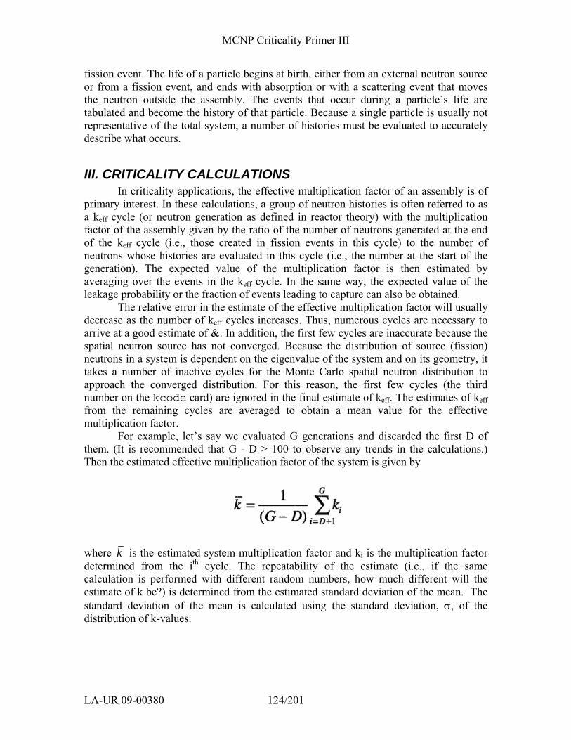
MCNP Criticality Primer III
LA-UR 09-00380 124/201
fission event. The life of a particle begins at birth, either from an external neutron source or from a fission event, and ends with absorption or with a scattering event that moves the neutron outside the assembly. The events that occur during a particle’s life are tabulated and become the history of that particle. Because a single particle is usually not representative of the total system, a number of histories must be evaluated to accurately describe what occurs.
III. CRITICALITY CALCULATIONS In criticality applications, the effective multiplication factor of an assembly is of
primary interest. In these calculations, a group of neutron histories is often referred to as a keff cycle (or neutron generation as defined in reactor theory) with the multiplication factor of the assembly given by the ratio of the number of neutrons generated at the end of the keff cycle (i.e., those created in fission events in this cycle) to the number of neutrons whose histories are evaluated in this cycle (i.e., the number at the start of the generation). The expected value of the multiplication factor is then estimated by averaging over the events in the keff cycle. In the same way, the expected value of the leakage probability or the fraction of events leading to capture can also be obtained.
The relative error in the estimate of the effective multiplication factor will usually decrease as the number of keff cycles increases. Thus, numerous cycles are necessary to arrive at a good estimate of &. In addition, the first few cycles are inaccurate because the spatial neutron source has not converged. Because the distribution of source (fission) neutrons in a system is dependent on the eigenvalue of the system and on its geometry, it takes a number of inactive cycles for the Monte Carlo spatial neutron distribution to approach the converged distribution. For this reason, the first few cycles (the third number on the kcode card) are ignored in the final estimate of keff. The estimates of keff from the remaining cycles are averaged to obtain a mean value for the effective multiplication factor.
For example, let’s say we evaluated G generations and discarded the first D of them. (It is recommended that G - D > 100 to observe any trends in the calculations.) Then the estimated effective multiplication factor of the system is given by
where k is the estimated system multiplication factor and ki is the multiplication factor determined from the ith cycle. The repeatability of the estimate (i.e., if the same calculation is performed with different random numbers, how much different will the estimate of k be?) is determined from the estimated standard deviation of the mean. The standard deviation of the mean is calculated using the standard deviation, σ, of the distribution of k-values.
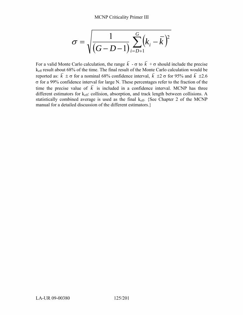
MCNP Criticality Primer III
LA-UR 09-00380 125/201
( ) ( )∑+=
−−−
=G
Dii kk
DG 1
2
11σ
For a valid Monte Carlo calculation, the range k - σ to k + σ should include the precise keff result about 68% of the time. The final result of the Monte Carlo calculation would be reported as: k ± σ for a nominal 68% confidence interval, k ±2 σ for 95% and k ±2.6 σ for a 99% confidence interval for large N. These percentages refer to the fraction of the time the precise value of k is included in a confidence interval. MCNP has three different estimators for keff: collision, absorption, and track length between collisions. A statistically combined average is used as the final keff. {See Chapter 2 of the MCNP manual for a detailed discussion of the different estimators.}
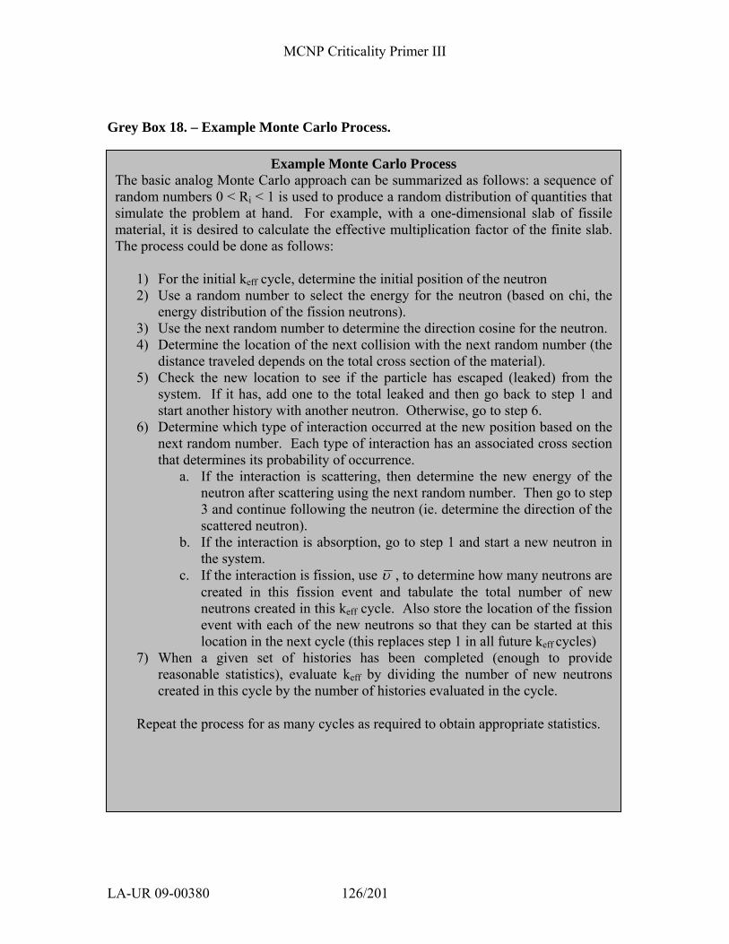
MCNP Criticality Primer III
LA-UR 09-00380 126/201
Grey Box 18. – Example Monte Carlo Process.
Example Monte Carlo Process The basic analog Monte Carlo approach can be summarized as follows: a sequence of random numbers 0 < Ri < 1 is used to produce a random distribution of quantities that simulate the problem at hand. For example, with a one-dimensional slab of fissile material, it is desired to calculate the effective multiplication factor of the finite slab. The process could be done as follows:
1) For the initial keff cycle, determine the initial position of the neutron 2) Use a random number to select the energy for the neutron (based on chi, the
energy distribution of the fission neutrons). 3) Use the next random number to determine the direction cosine for the neutron. 4) Determine the location of the next collision with the next random number (the
distance traveled depends on the total cross section of the material). 5) Check the new location to see if the particle has escaped (leaked) from the
system. If it has, add one to the total leaked and then go back to step 1 and start another history with another neutron. Otherwise, go to step 6.
6) Determine which type of interaction occurred at the new position based on the next random number. Each type of interaction has an associated cross section that determines its probability of occurrence.
a. If the interaction is scattering, then determine the new energy of the neutron after scattering using the next random number. Then go to step 3 and continue following the neutron (ie. determine the direction of the scattered neutron).
b. If the interaction is absorption, go to step 1 and start a new neutron in the system.
c. If the interaction is fission, use υ , to determine how many neutrons are created in this fission event and tabulate the total number of new neutrons created in this keff cycle. Also store the location of the fission event with each of the new neutrons so that they can be started at this location in the next cycle (this replaces step 1 in all future keff cycles)
7) When a given set of histories has been completed (enough to provide reasonable statistics), evaluate keff by dividing the number of new neutrons created in this cycle by the number of histories evaluated in the cycle.
Repeat the process for as many cycles as required to obtain appropriate statistics.
MCNP Criticality Primer III
LA-UR 09-00380 127/201
IV. Terminology
IV.1 Monte Carlo Terminology The following is a listing of common terms used in Monte Carlo techniques: 1. Monte Carlo – A numerical analysis technique that uses random sampling to estimate the solution of a physical or mathematical problem. 2. Random Numbers – An infinite set of numbers that are uniformly distributed from 0 to 1 and are independent. We actually use pseudorandom numbers, a deterministic reproducible sequence of random numbers generated by a computer that satisfies statistical tests for randomness. 3. Monte Carlo Weight - The number of physical particles W that a Monte Carlo particle represents. The weight can be a fraction. 4. Random Walk – The random selection of events for a particle history. 5. History – The complete random walk of a Monte Carlo particle from its birth in the source to its death, including all progeny. 6. Monte Carlo Track-A branch, or subset, of a history that can be obtained by physical events (for example, fissions) or by variance reduction techniques (for example, geometry splitting) 7. Score-Contribution from a track to a tally. 8. History Score – Sum of all scores from one source particle’s tracks. 9. Tally – Used interchangeably with score. Also, the quantity we want to estimate (average score), obtained by summing all scores from all histories. Sometimes called an 10. Relative Error – The standard deviation of the mean of a tally or keff, divided by the mean. The error refers to the precision of the tally, not to its accuracy. 11. Importance – the expected score per unit weight of a track at phase-space point. 12. Flux – The product of particle density and particle speed. The flux is mathematically and physically equivalent to the sum of the lengths of all Monte Carlo tracks per unit volume per unit time. Flux is in units of particles/cm2/shake. 13. Fluence – Integral of flux over time. If the MCNP source is in units of particles, the flux tallies are really fluence tallies. If the MCNP source is in units of particles per unit time, the flux tallies are truly fluxes. Fluence has units of particles/cm2.
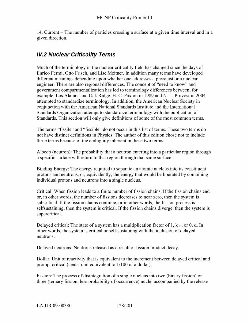
MCNP Criticality Primer III
LA-UR 09-00380 128/201
14. Current – The number of particles crossing a surface at a given time interval and in a given direction.
IV.2 Nuclear Criticality Terms Much of the terminology in the nuclear criticality field has changed since the days of Enrico Fermi, Otto Frisch, and Lise Meitner. In addition many terms have developed different meanings depending upon whether one addresses a physicist or a nuclear engineer. There are also regional differences. The concept of “need to know” and government compartmentalization has led to terminology differences between, for example, Los Alamos and Oak Ridge. H. C. Paxton in 1989 and N. L. Pruvost in 2004 attempted to standardize terminology. In addition, the American Nuclear Society in conjunction with the American National Standards Institute and the International Standards Organization attempt to standardize terminology with the publication of Standards. This section will only give definitions of some of the most common terms. The terms “fissile” and “fissible” do not occur in this list of terms. These two terms do not have distinct definitions in Physics. The author of this edition chose not to include these terms because of the ambiguity inherent in these two terms. Albedo (neutron): The probability that a neutron entering into a particular region through a specific surface will return to that region through that same surface. Binding Energy: The energy required to separate an atomic nucleus into its constituent protons and neutrons, or, equivalently, the energy that would be liberated by combining individual protons and neutrons into a single nucleus. Critical: When fission leads to a finite number of fission chains. If the fission chains end or, in other words, the number of fissions decreases to near zero, then the system is subcritical. If the fission chains continue, or in other words, the fission process is selfsustaining, then the system is critical. If the fission chains diverge, then the system is supercritical. Delayed critical: The state of a system has a multiplication factor of 1, keff, or 0, α. In other words, the system is critical or self-sustaining with the inclusion of delayed neutrons. Delayed neutrons: Neutrons released as a result of fission product decay. Dollar: Unit of reactivity that is equivalent to the increment between delayed critical and prompt critical (cents: unit equivalent to 1/100 of a dollar). Fission: The process of disintegration of a single nucleus into two (binary fission) or three (ternary fission, less probability of occurrence) nuclei accompanied by the release

MCNP Criticality Primer III
LA-UR 09-00380 129/201
of neutrons and other atomic and subatomic particles. Fission can occur spontaneously, or it can be induced by an incident neutron, photon, or other particle. Fissionable: A nuclide with a finite probability of undergoing fission. Fission barrier: The barrier or the amount of energy needed to be overcome to result in a fission event. Isotope: A species of an element which has a different atomic mass based upon the fact that there are different numbers of neutrons. Liquid Drop Model of Fission: Primary theoretical mechanism used to explain nuclear fission. In this hypothesis, the nucleus or liquid drop is a spheroid or approximated as a spheroid existing in space. The nucleus becomes perturbed or excited. The perturbation or excitation may be caused either by interaction with an external energetic particle or the nucleus itself can be unstable. The perturbed or excited nucleus then undergoes fission. Multiplication factor (α or keff): The ratio of the number of neutrons from one generation to the next generation. Nuclear Reactivity: The change in the effective multiplication factor of a multiplying system. The units of reactivity can be dollars, cents, or ∆keff. Nuclide: An individual atom defined by the atomic mass, atomic number, or sometimes by an elevated energy (often termed metastable). Prompt critical: The system is critical on prompt neutrons. The multiplication factor is 1 + β (delayed neutron fraction). Prompt neutrons: Neutrons released within 10-13 seconds of a fission event.

MCNP Criticality Primer III
LA-UR 09-00380 130/201

MCNP Criticality Primer III
LA-UR 09-00380 131/201
APPENDIX B: Specifications & Atom Densities Of Selected Materials
The following material compositions, specifications, and atom densities have been compiled from various sources. They are provided for the convenience of users of computer codes for nuclear analysis. No warranty is made nor is any legal liability or responsibility assumed for the accuracy, completeness, or usefulness of the following information. Reference to any specific commercial product by trade name or registered trademark does not necessarily constitute or imply its endorsement.
Atomic weights used in the following were taken from “Nuclides and Isotopes,
Fourteenth Edition, General Electric Company, San Jose, California. Atom densities are given in units of atoms/barn-cm.
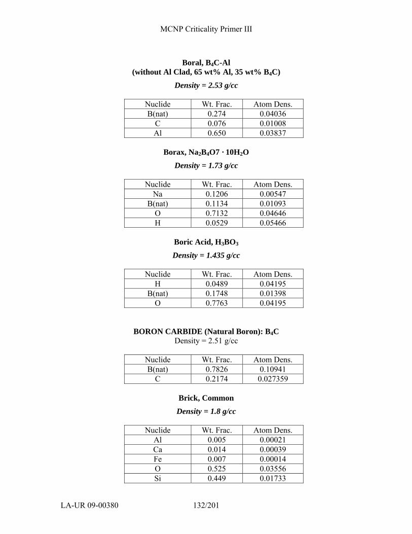
MCNP Criticality Primer III
LA-UR 09-00380 132/201
Boral, B4C-Al
(without Al Clad, 65 wt% Al, 35 wt% B4C)
Density = 2.53 g/cc
Nuclide Wt. Frac. Atom Dens. B(nat) 0.274 0.04036
C 0.076 0.01008 Al 0.650 0.03837
Borax, Na2B4O7 · 10H2O
Density = 1.73 g/cc
Nuclide Wt. Frac. Atom Dens. Na 0.1206 0.00547
B(nat) 0.1134 0.01093 O 0.7132 0.04646 H 0.0529 0.05466
Boric Acid, H3BO3
Density = 1.435 g/cc
Nuclide Wt. Frac. Atom Dens. H 0.0489 0.04195
B(nat) 0.1748 0.01398 O 0.7763 0.04195
BORON CARBIDE (Natural Boron): B4C Density = 2.51 g/cc
Nuclide Wt. Frac. Atom Dens. B(nat) 0.7826 0.10941
C 0.2174 0.027359
Brick, Common
Density = 1.8 g/cc
Nuclide Wt. Frac. Atom Dens. Al 0.005 0.00021 Ca 0.014 0.00039 Fe 0.007 0.00014 O 0.525 0.03556 Si 0.449 0.01733
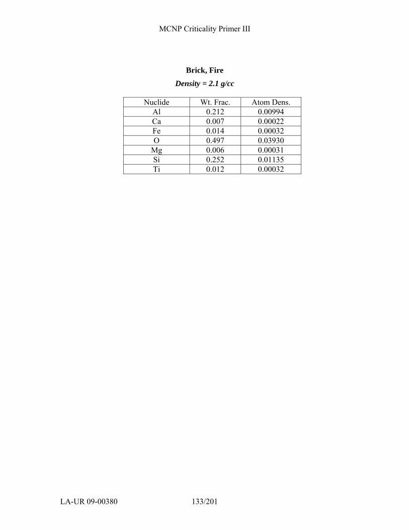
MCNP Criticality Primer III
LA-UR 09-00380 133/201
Brick, Fire
Density = 2.1 g/cc
Nuclide Wt. Frac. Atom Dens. Al 0.212 0.00994 Ca 0.007 0.00022 Fe 0.014 0.00032 O 0.497 0.03930
Mg 0.006 0.00031 Si 0.252 0.01135 Ti 0.012 0.00032
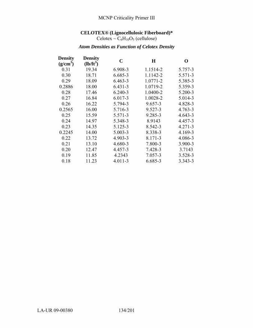
MCNP Criticality Primer III
LA-UR 09-00380 134/201
CELOTEX® (Lignocellulosic Fiberboard)* Celotex ~ C6H10O5 (cellulose)
Atom Densities as Function of Celotex Density
Density (g/cm3)
Density (lb/ft3) C H O
0.31 19.34 6.908-3 1.1514-2 5.757-3 0.30 18.71 6.685-3 1.1142-2 5.571-3 0.29 18.09 6.463-3 1.0771-2 5.385-3
0.2886 18.00 6.431-3 1.0719-2 5.359-3 0.28 17.46 6.240-3 1.0400-2 5.200-3 0.27 16.84 6.017-3 1.0028-2 5.014-3 0.26 16.22 5.794-3 9.657-3 4.828-3
0.2565 16.00 5.716-3 9.527-3 4.763-3 0.25 15.59 5.571-3 9.285-3 4.643-3 0.24 14.97 5.348-3 8.9143 4.457-3 0.23 14.35 5.125-3 8.542-3 4.271-3
0.2245 14.00 5.003-3 8.338-3 4.169-3 0.22 13.72 4.903-3 8.171-3 4.086-3 0.21 13.10 4.680-3 7.800-3 3.900-3 0.20 12.47 4.457-3 7.428-3 3.7143 0.19 11.85 4.2343 7.057-3 3.528-3 0.18 11.23 4.011-3 6.685-3 3.343-3
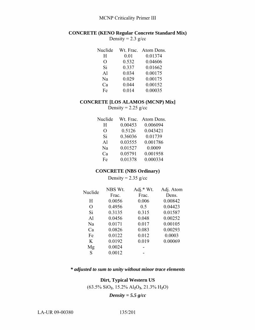
MCNP Criticality Primer III
LA-UR 09-00380 135/201
CONCRETE (KENO Regular Concrete Standard Mix) Density = 2.3 g/cc
Nuclide Wt. Frac. Atom Dens.
H 0.01 0.01374 O 0.532 0.04606 Si 0.337 0.01662 Al 0.034 0.00175 Na 0.029 0.00175 Ca 0.044 0.00152 Fe 0.014 0.00035
CONCRETE [LOS ALAMOS (MCNP) Mix]
Density = 2.25 g/cc
Nuclide Wt. Frac. Atom Dens.H 0.00453 0.006094 O 0.5126 0.043421 Si 0.36036 0.01739 Al 0.03555 0.001786 Na 0.01527 0.0009 Ca 0.05791 0.001958 Fe 0.01378 0.000334
CONCRETE (NBS Ordinary)
Density = 2.35 g/cc
Nuclide NBS Wt. Frac.
Adj.* Wt. Frac.
Adj. Atom Dens.
H 0.0056 0.006 0.00842 O 0.4956 0.5 0.04423 Si 0.3135 0.315 0.01587 Al 0.0456 0.048 0.00252 Na 0.0171 0.017 0.00105 Ca 0.0826 0.083 0.00293 Fe 0.0122 0.012 0.0003 K 0.0192 0.019 0.00069
Mg 0.0024 - S 0.0012 -
* adjusted to sum to unity without minor trace elements
Dirt, Typical Western US (63.5% SiO2, 15.2% Al2O3, 21.3% H2O)
Density = 5.5 g/cc
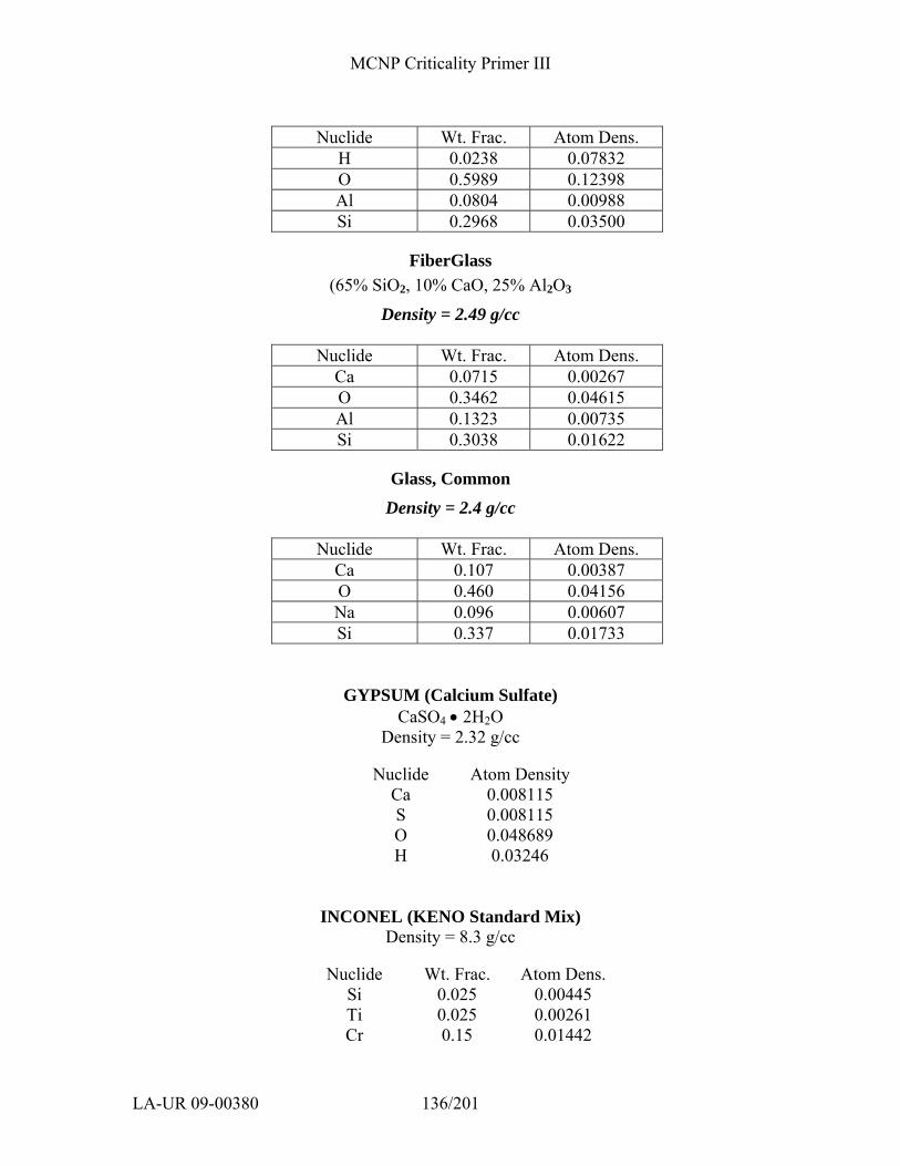
MCNP Criticality Primer III
LA-UR 09-00380 136/201
Nuclide Wt. Frac. Atom Dens.
H 0.0238 0.07832 O 0.5989 0.12398 Al 0.0804 0.00988 Si 0.2968 0.03500
FiberGlass (65% SiO2, 10% CaO, 25% Al2O3
Density = 2.49 g/cc
Nuclide Wt. Frac. Atom Dens. Ca 0.0715 0.00267 O 0.3462 0.04615 Al 0.1323 0.00735 Si 0.3038 0.01622
Glass, Common
Density = 2.4 g/cc
Nuclide Wt. Frac. Atom Dens. Ca 0.107 0.00387 O 0.460 0.04156 Na 0.096 0.00607 Si 0.337 0.01733
GYPSUM (Calcium Sulfate) CaSO4 • 2H2O
Density = 2.32 g/cc
Nuclide Atom DensityCa 0.008115 S 0.008115 O 0.048689 H 0.03246
INCONEL (KENO Standard Mix) Density = 8.3 g/cc
Nuclide Wt. Frac. Atom Dens.
Si 0.025 0.00445 Ti 0.025 0.00261 Cr 0.15 0.01442
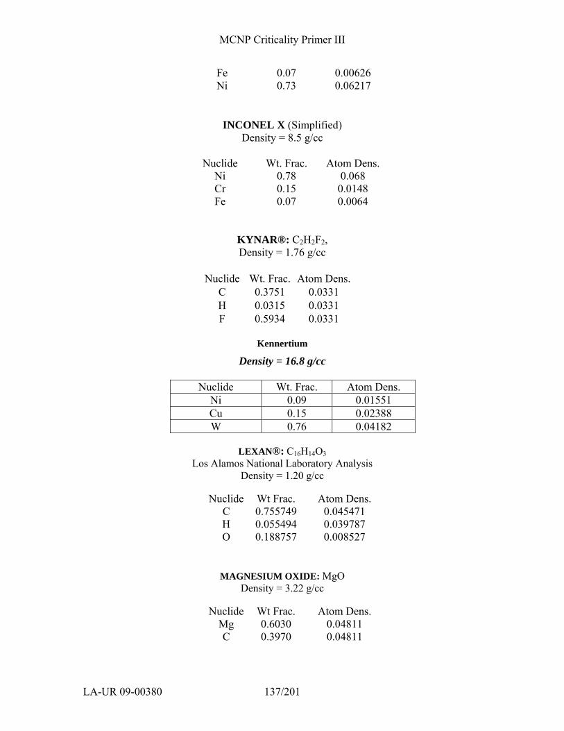
MCNP Criticality Primer III
LA-UR 09-00380 137/201
Fe 0.07 0.00626 Ni 0.73 0.06217
INCONEL X (Simplified)
Density = 8.5 g/cc
Nuclide Wt. Frac. Atom Dens. Ni 0.78 0.068 Cr 0.15 0.0148 Fe 0.07 0.0064
KYNAR®: C2H2F2, Density = 1.76 g/cc
Nuclide Wt. Frac. Atom Dens.
C 0.3751 0.0331 H 0.0315 0.0331 F 0.5934 0.0331
Kennertium
Density = 16.8 g/cc
Nuclide Wt. Frac. Atom Dens. Ni 0.09 0.01551 Cu 0.15 0.02388 W 0.76 0.04182
LEXAN®: C16H14O3
Los Alamos National Laboratory Analysis Density = 1.20 g/cc
Nuclide Wt Frac. Atom Dens.
C 0.755749 0.045471 H 0.055494 0.039787 O 0.188757 0.008527
MAGNESIUM OXIDE: MgO
Density = 3.22 g/cc
Nuclide Wt Frac. Atom Dens. Mg 0.6030 0.04811 C 0.3970 0.04811
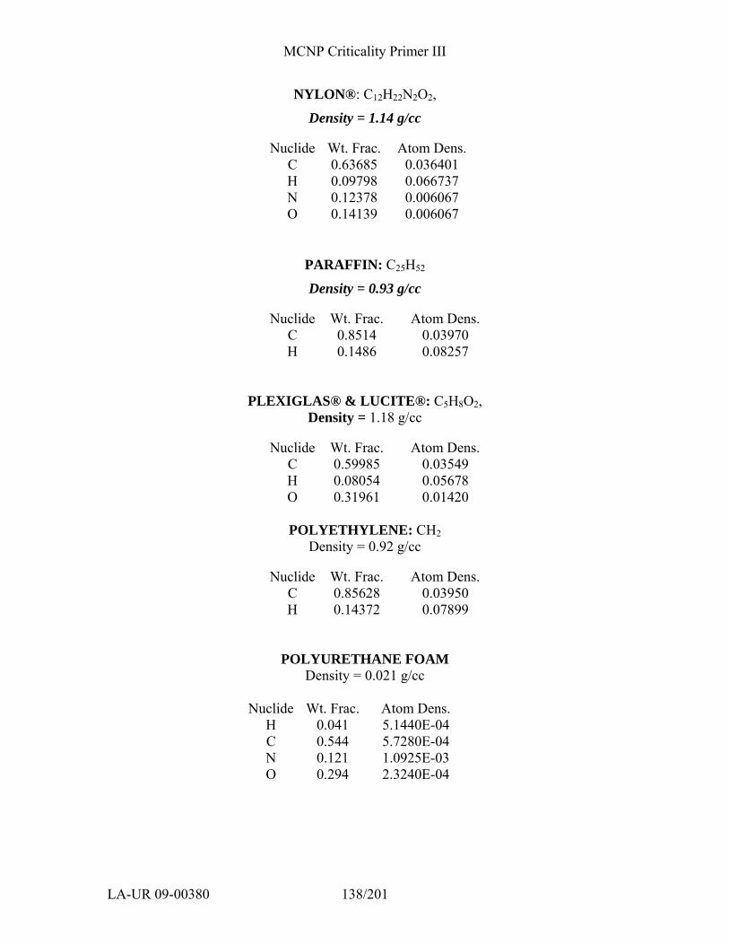
MCNP Criticality Primer III
LA-UR 09-00380 138/201
NYLON®: C12H22N2O2,
Density = 1.14 g/cc
Nuclide Wt. Frac. Atom Dens. C 0.63685 0.036401 H 0.09798 0.066737 N 0.12378 0.006067 O 0.14139 0.006067
PARAFFIN: C25H52
Density = 0.93 g/cc
Nuclide Wt. Frac. Atom Dens. C 0.8514 0.03970 H 0.1486 0.08257
PLEXIGLAS® & LUCITE®: C5H8O2, Density = 1.18 g/cc
Nuclide Wt. Frac. Atom Dens.
C 0.59985 0.03549 H 0.08054 0.05678 O 0.31961 0.01420
POLYETHYLENE: CH2
Density = 0.92 g/cc
Nuclide Wt. Frac. Atom Dens. C 0.85628 0.03950 H 0.14372 0.07899
POLYURETHANE FOAM Density = 0.021 g/cc
Nuclide Wt. Frac. Atom Dens.
H 0.041 5.1440E-04 C 0.544 5.7280E-04 N 0.121 1.0925E-03 O 0.294 2.3240E-04
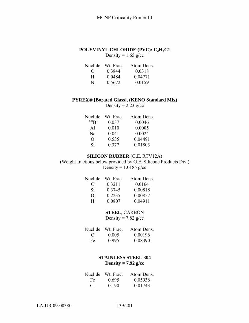
MCNP Criticality Primer III
LA-UR 09-00380 139/201
POLYVINYL CHLORIDE (PVC): C2H3C1
Density = 1.65 g/cc
Nuclide Wt. Frac. Atom Dens. C 0.3844 0.0318 H 0.0484 0.04771 N 0.5672 0.0159
PYREX® [Borated Glass], (KENO Standard Mix)
Density = 2.23 g/cc
Nuclide Wt. Frac. Atom Dens. natB 0.037 0.0046 Al 0.010 0.0005 Na 0.041 0.0024 O 0.535 0.04491 Si 0.377 0.01803
SILICON RUBBER (G.E. RTV12A)
(Weight fractions below provided by G.E. Silicone Products Div.) Density = 1.0185 g/cc
Nuclide Wt. Frac. Atom Dens.
C 0.3211 0.0164 Si 0.3745 0.00818 O 0.2235 0.00857 H 0.0807 0.04911
STEEL, CARBON Density = 7.82 g/cc
Nuclide Wt. Frac. Atom Dens.
C 0.005 0.00196 Fe 0.995 0.08390
STAINLESS STEEL 304 Density = 7.92 g/cc
Nuclide Wt. Frac. Atom Dens.
Fe 0.695 0.05936 Cr 0.190 0.01743
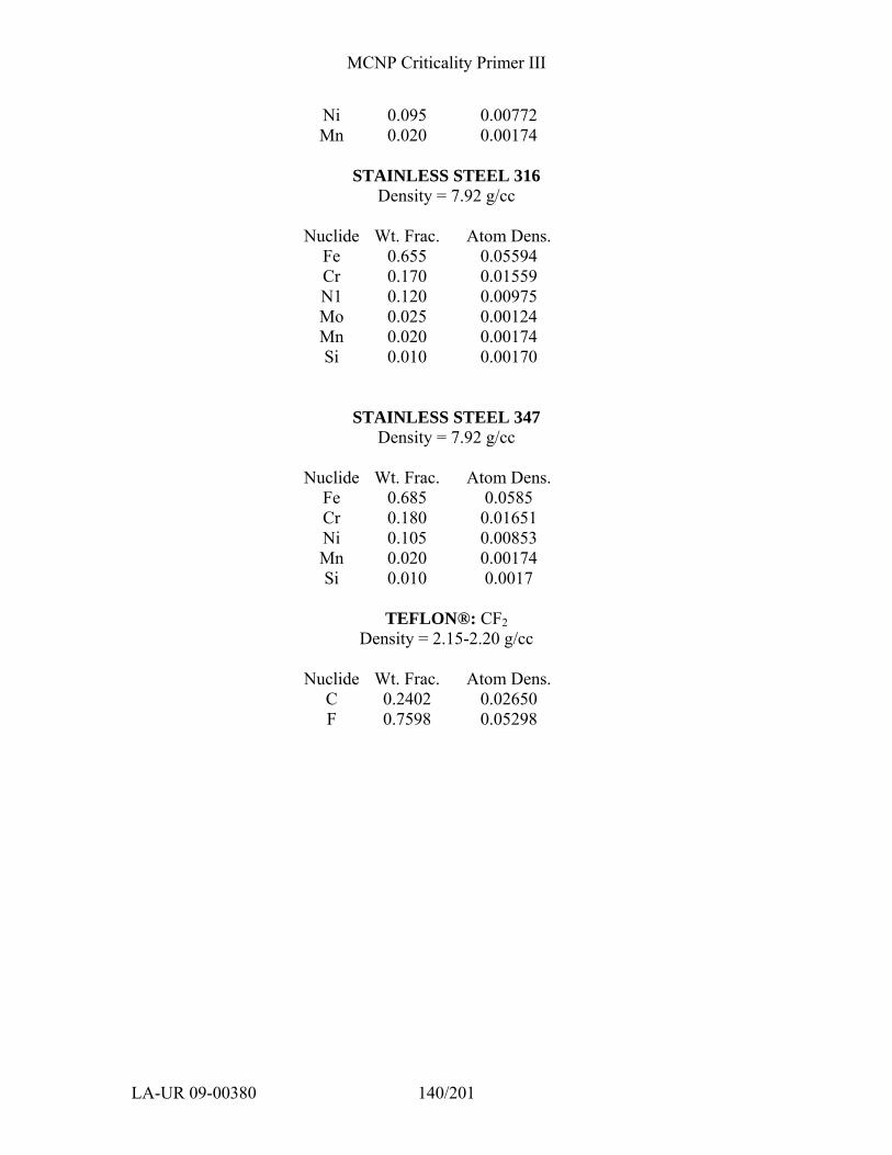
MCNP Criticality Primer III
LA-UR 09-00380 140/201
Ni 0.095 0.00772 Mn 0.020 0.00174
STAINLESS STEEL 316
Density = 7.92 g/cc
Nuclide Wt. Frac. Atom Dens. Fe 0.655 0.05594 Cr 0.170 0.01559 N1 0.120 0.00975 Mo 0.025 0.00124 Mn 0.020 0.00174 Si 0.010 0.00170
STAINLESS STEEL 347 Density = 7.92 g/cc
Nuclide Wt. Frac. Atom Dens.
Fe 0.685 0.0585 Cr 0.180 0.01651 Ni 0.105 0.00853 Mn 0.020 0.00174 Si 0.010 0.0017
TEFLON®: CF2
Density = 2.15-2.20 g/cc
Nuclide Wt. Frac. Atom Dens. C 0.2402 0.02650 F 0.7598 0.05298

MCNP Criticality Primer III
LA-UR 09-00380 141/201
APPENDIX C: Listing of Available Cross-Sections Please refer to the MCNP Manual for listing of available ZAIDs and S(α,β). This list changes and the user may need to use data other than what is recommended. It is recommended that users be aware of the data they are using and the application of particular data sets.

MCNP Criticality Primer III
LA-UR 09-00380 142/201
APPENDIX D: Geometry PLOT and Tally MCPLOT Commands
This appendix contains only a summary of the available commands for the geometry and tally plotting capabilities included in MCNP. All commands can be shortened to the fewest letters that unambiguously identify the command. {Please refer to Appendix B of the MCNP5 manual for a complete listing of commands.}
PLOT
Used to plot two-dimensional slices of a problem geometry specified in the input file. This feature is invaluable when debugging geometries. Commands are shown in upper case but can be input in lower case. PLOT examples have been shown in several of the Primer chapters.
A. Geometry PLOT Input and Execute Line Options To plot geometries with MCNP, enter the following command: mcnp ip inp=filename options where ‘ip‘ stands for initiate and plot. ‘options’ is explained in the following paragraphs. The most common method of plotting is with an interactive graphics terminal. MCNP will read the input file, perform the normal checks for consistency, and then display the interactive geometry- plotting window on the terminal screen.
When X Windows is in use, the plot window supports a variety of interactive
features that assist the user in selecting the plot. The interactive options are discussed after the discussion of the command-line plot options.
The following four additional plot options can be entered on the execution line in addition to the standard MCNP execution options: NOTEK
Suppress plotting at the terminal and send all plots to the graphics metafile, PLOTM. This is used for production and batch situations and when the user’s terminal has no graphics capability.
COM=aaaa
Use file aaaa as the source of plot requests. When an EOF is read, control is transferred to the terminal. In a production or batch situation, end the file with an END command to prevent transfer of control. Never end the COM file with a blank line. If COM is absent, the terminal is used as the source of plot requests.
PLOTM=aaaa
Name the graphics metafile aaaa. The default name is PLOTM.ps. This file is a standard postscript file.
MCNP Criticality Primer III
LA-UR 09-00380 143/201
COMOUT=aaaa
Name the plot-commands output file aaaa. The default name is COMOUT. MCNP writes the COMOUT file in order to give the user the opportunity to do the same plotting at some later time, using all or part of the old COMOUT file as the COM file in the second run.
When names are defaulted, unique names for the output files, PLOTM.ps and COMOUT, will be chosen by MCNP to avoid overwriting existing files. Unique names are created by changing the last letter of the default name until the next available name is found. For example, if the file PLOTM.ps already exists, MCNP tries the name PLOTN.ps, etc., until it finds an available name.
MCNP can be run in a batch environment without much difficulty, but the user interaction with the plotter is significantly reduced. When not using an interactive graphics terminal, use the NOTEK option on the MCNP execution line or set TERM=0 along with other PLOT commands when first prompted by PLOT. (Note: For geometry plotting with X Windows, a plot window will appear before the first plot request as the interactive plot window is created. To prevent this, use the NOTEK option.) Every view plotted will be put in a postscript file called PLOTn where n begins at M and goes to the next letter in the alphabet if PLOTM exists. In the interactive mode, plots can be sent to this graphics metafile with the FILE keyword (see the keyword description in Section B for a complete explanation). The PLOTn.ps file is a postscript file that can be sent to a postscript printer.
A plot request consists of a sequence of commands terminated by pressing the ENTER key. A command consists of a keyword, usually followed by some parameters. Lines can be continued by typing an & (ampersand) before pressing the ENTER key, but each keyword and its parameters must be complete on one line. The & character can be used in the COM file as well as at the plot prompt. Keywords and parameters are blank-delimited. A plot request line cannot have more than 80 characters on a single line. Use the & to enter more complex commands. Commas and equal signs are interpreted as blanks. Keywords can be shortened to any degree as long as they are not ambiguous and are spelled correctly. Parameters following the keywords cannot be abbreviated.
Numbers can be entered in free-form format and do not require a decimal point for floating point data. Keywords and parameters remain in effect until you change them. Note: If a shortened, ambiguous keyword is used, the entire command line will be rejected and a message to that effect will be printed to the terminal. The commands OPTIONS, HELP and ‘?’ display a list of the keywords to help the user recall the correct keyword.
Before describing the individual plotting commands, it may help to explain the
mechanics of 2-dimensional (2D) plotting. To obtain a 2D slice of a geometry, the user must decide where the slice should be taken and how much of the slice should be viewed on the terminal screen. The slice is actually a 2D plane that may be arbitrarily oriented in space; therefore, the first problem is to decide the plane position and orientation. In an
MCNP Criticality Primer III
LA-UR 09-00380 144/201
orthogonal 3-dimensional coordinate system, the three axes are perpendicular to each other. An orthogonal axis system is defined with a set of BASIS vectors on the 2D plane used to slice the geometry to determine the plot orientation. The first BASIS vector is the horizontal direction on the screen. The second BASIS vector is the vertical direction on the screen. The surface normal for the plane being viewed is perpendicular to the two BASIS vectors.
How much of the slice to view is determined next. The center of the view plane is set with the ORIGIN command which serves two purposes: first, for planes not corresponding to simple coordinate planes, it determines the position of the plane being viewed; second, the origin becomes the center of the cross-sectional slice being viewed. For example, for a Y-Z plot, the x-coordinate given with the PX command determines the location of the PX plane. The ORIGIN is given as an x, y, and z-coordinate and is the center of the plot displayed.
Because planes are infinite and only a finite area can be displayed at any given
time, you must limit the extent of the cross-sectional plane being displayed with the EXTENT command. For instance, a plane defined with PX=X1 at an ORIGIN of X1,Y1, and Z1 would produce a Y-Z plane at X = X1, centered at Y1 and Z1 using the default BASIS vectors for a PX plane of 0 1 0 and 0 0 1..
The BASIS vectors are arbitrary vectors in space. This may seem confusing to the
new user, but the majority of plots are PX, PY, or PZ planes where the BASIS vectors are defaulted. For the majority of geometry plots, these simple planes are sufficient and you do not have to enter BASIS vectors. The flexibility of the BASIS option can also be used to examine the geometry from more obscure views.
All the plot parameters for the MCNP plotter have defaults. To obtain a plot, click on the plot area of the interactive screen or, if in command line mode, press ENTER. The default geometry plot is a PX plane centered at 0,0,0 with an extent of 100 to 100 on Y and 100 to 100 on Z. The y-axis will be the horizontal axis of the plot, and the z-axis will be the vertical axis. Surface labels are printed. This default is the equivalent of entering the command line:
origin 0 0 0 extent 100 100 basis 0 1 0 0 0 1 label 1 0 By resetting selected plot parameters, any desired plot can be obtained. Most parameters remain set until changed, either by the same command with new values or by a conflicting command. Warning: Placing the plot plane exactly on a surface of the geometry is not a good idea. For example, if the input geometry has a PX plane at X=0, that plane coincides with the default plot plane. Several things can result when such alignment occurs. Some portion of the geometry may be displayed in dotted lines, which usually indicates a geometry error. Some portion of the geometry may simply not show up at all. Very infrequently the code may crash with an error. To prevent all of these unpleasantries, move the plot plane a short space away from surfaces.
MCNP Criticality Primer III
LA-UR 09-00380 145/201
1. Device–Control Commands Normally PLOT draws plots on the user’s terminal and nowhere else. By using
the following commands, the user can specify that plots not be drawn on the terminal and/or that they be sent to a graphics metafile or postscript file for processing later by a graphics utility program that will send the plots to other graphics devices. TERM n This command sets the output device type according to n:
0 terminal with no graphics capability. No plots will be drawn on the terminal, and all plots will be sent to the graphics file. TERM 0 is equivalent to putting NOTEK on MCNP’s execute line. 1 Restore visible plotting window on next plot request.
FILE aa
Send (or do not send) plots to the postscript file PLOTM.PS according to the value of the parameter aa. The graphics file is not created until the first FILE command is entered. FILE has no effect in the NOTEK or TERM=0 cases. The allowed values of aa are:
blank - only the current plot is sent to the graphics metafile.
ALL - the current plot and all subsequent plots are sent to the metafile until another FILE command is entered.
NONE the current plot is not sent to the metafile nor are any subsequent plots sent until another FILE command is entered. VIEWPORT aa Make the viewport rectangular or square according to the value of aa.
The default is RECT. This option does not affect the appearance of the plot. It only determines whether space is provided beside the plot for a legend and around the plot for scales. The allowed values of aa are:
RECT allows space beside the plot for a legend and around the plot for scales.
SQUARE
The legend area, the legend, and scales are omitted, making it possible to print a sequence of plots on some sort of strip medium so as to produce one long picture free from interruptions by legends. Note: use of the SQUARE option disables the interactive window plotter capability. 2. General Commands &
Continue reading commands for the current plot from the next input line. The & must be the last item on the line.
INTERACT
MCNP Criticality Primer III
LA-UR 09-00380 146/201
Return to the interactive, mouse-driven geometry plot interface. This Command is used to return from the terminal-command interface when the PLOT option is invoked from the interactive plotter. RETURN
If PLOT was called by MCPLOT, control returns to MCPLOT. Otherwise RETURN has no effect. MCPLOT
Call or return to MCPLOT, the tally/cross-section plotter. PAUSE n
Use with the COM=aaaa option. Hold each picture for n seconds. If no n Value is provided, each picture remains until the ENTER key is pressed. END
Terminate execution of PLOT. 3. Inquiry Commands
When one of these commands is encountered, the requested display is made and then PLOT waits for the user to enter another line, which can be just pressing the ENTER key, before resuming. The same thing will happen if PLOT sends any kind of warning or comment to the user as it prepares the data for a plot. OPTIONS or ? or HELP
Display a list of the PLOT command keywords and available colors. STATUS
Display the current values of the plotting parameters. 4. Plot Commands
Plot commands define the values of the parameters used in drawing the next plot. Parameters entered for one plot remain in effect for subsequent plots until they are overridden, either by the same command with new values or by a conflicting command.
BASIS X1 Y1 Z1 X2 Y2 Z2
Orient the plot so that the direction (X1 Y1 Z1) points to the right and the direction (X2 Y2 Z2) points up. The default values are 0 1 0 0 0 1, causing the y-axis to point to the right and the z-axis to point up. The two vectors do not have to be normalized, but they should be orthogonal. If the two vectors are not orthogonal, MCPLOT will choose an arbitrary second vector that is orthogonal to the first vector. MCPLOT will ignore the command if parallel or zero-length vectors are entered. ORIGIN VX VY VZ

MCNP Criticality Primer III
LA-UR 09-00380 147/201
Position the plot so that the origin, which is in the middle of the plot, is at the point (VX,VY,VZ). The default values are 0 0 0. The BASIS vectors are relative to this point. EXTENT EH EV
Set the scale of the plot so that the horizontal distance from the plot origin to either side of the plot is EH and the vertical distance from the origin to the top or bottom is EV. If EV is omitted, it will be set equal to EH. If EV is not equal to EH, the plot will be distorted. The default values are 100 and 100 giving a 200x200 viewport. PX VX
Plot a cross section of the geometry in a plane perpendicular to the x-axis at a distance VX from the geometry origin. This command is a shortcut equivalent of BASIS 0 1 0 0 0 1 ORIGIN VX vy vz, where vy and vz are the current values of VY and VZ. PY VY
Plot a cross section of the geometry in a plane perpendicular to the y-axis at a distance VY from the geometry origin. PZ VZ
Plot a cross section of the geometry in a plane perpendicular to the z-axis at a distance VZ from the geometry origin. LABEL S C DES
Put labels of size S on the surfaces and labels of size C in the cells. Use the quantity indicated by DES for the cell labels. C and DES are optional parameters. The sizes are relative to 0.01 times the height of the view surface. If S or C is zero, that kind of label will be omitted. If S or C is not zero, it must be in the range from 0.2 to 100. The defaults are S=1, C=0 and DES=CEL. The allowed values of DES follow, where “:p” can be :N for neutrons, :P for photons, and :E for electrons. Following each DES value is a short description of the meaning of the values.
CEL cell names IMP:p importances RHO atom density DEN mass density VOL volume FCL:p forced collision MAS mass PWT photon-production weight MAT material number
MCNP Criticality Primer III
LA-UR 09-00380 148/201
TMPn temperature (n=index of time) WWNn:p weight window lower bound (n=energy or time interval) EXT:p exponential transform PDn detector contribution (n=tally number) DXC:p DXTRAN contribution
U universe LAT lattice type FILL filling universe NONU fission turnoff
LEVEL n Plot only the nth level of a repeated structure geometry. A negative entry (default)
plots the geometry at all levels. MBODY
Use macrobody surface numbers or macrobody surface facet numbers as surface labels.
on display only the macrobody surface number. This is the default. off display the macrobody surface facet numbers.
MESH n
Plot the superimposed weight-window mesh. Only a weight-window mesh read in from a WWINP file can be plotted. n can have the following values:
0 no lines 1 cell lines only 2 weight window mesh lines only 3 both cell and weight window mesh lines To plot the values of the mesh windows, set the cell labels to WWNn:p, where n" is the weight-window energy interval and ":p" is :N for neutrons, P for photons, or E for electrons (See the LABEL command).
SCALES n
Put scales and a grid on the plot. Scales and grids are incompatible with VIEWPORT SQUARE. n can have the following values:
0 neither scales nor a grid. This is the default. 1 scales on the edges.

MCNP Criticality Primer III
LA-UR 09-00380 149/201
2 scales on the edges and a grid on the plot. COLOR n
Turn color on or off, set the resolution, or select physical property for color shading. The parameter n can have the following values:
on turn color on. off turn color off. 50.n.3000set the color resolution to n. A larger value increases resolution and
drawing time. by aa Select physical property to use for geometry shading
Currently allowed options for ‘COLOR BY’ are: mat material (default) den gram density rho atomic density tmp temperature
When (den/rho/temp) is used, the geometry will be shaded by the value of the selected property using a set of 64 shades. Linear interpolation between the minimum non-zero value and the maximum value is used to select the color. A color bar legend of the shades will be drawn in the right margin. The legend is labeled with the property name and the minimum and maximum values. See Figure B-1 for an example of coloring by density (den). Coloring by material (mat) does not invoke a color bar legend. SHADE M1 = parameter... M K = parameter
Parameter can be a color name or a number from 1-64 representing the color index. Make the cells containing problem material number Mi a particular color. This is only valid when ‘MAT’ is used to COLOR BY (the default). Use the LABEL command to display material numbers. Parameter designates the desired color (e.g., green, blue, etc.). Note: color names are case-sensitive. The OPTIONS command will list available colors if your display is a color monitor. (The index of a color name is in top-bottom, left-right order.)
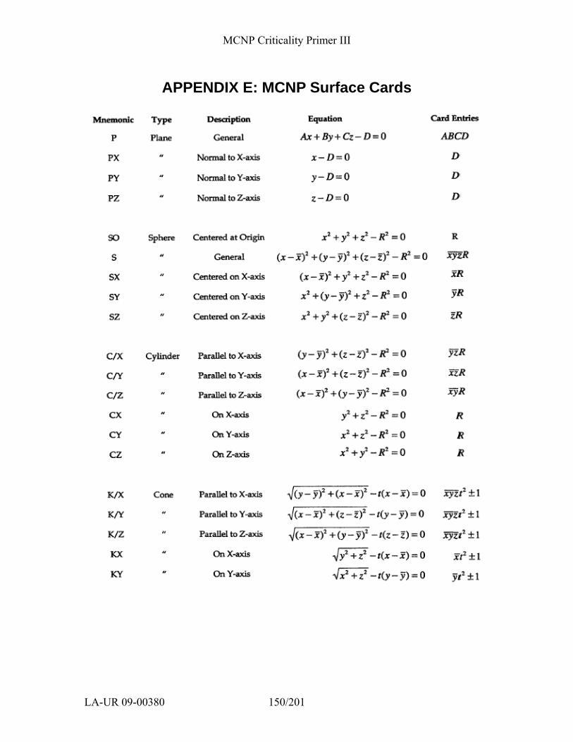
MCNP Criticality Primer III
LA-UR 09-00380 150/201
APPENDIX E: MCNP Surface Cards
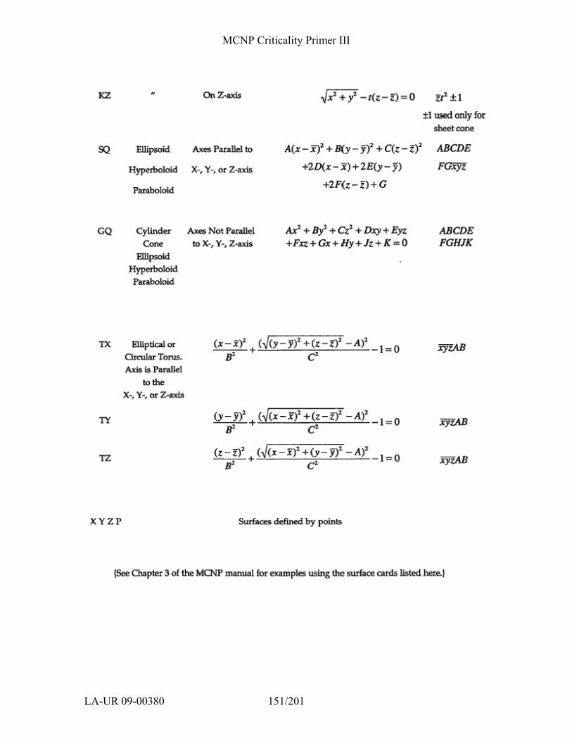
MCNP Criticality Primer III
LA-UR 09-00380 151/201
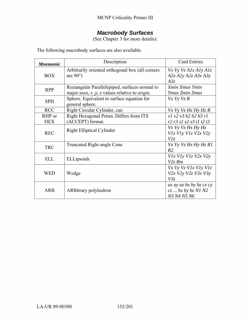
MCNP Criticality Primer III
LA-UR 09-00380 152/201
Macrobody Surfaces (See Chapter 3 for more details):
The following macrobody surfaces are also available.
Mnemonic Description Card Entries
BOX Arbitrarily oriented orthogonal box (all corners are 90°)
Vx Vy Vz A1x A1y A1z A2x A2y A2z A3x A3y A3z
RPP Rectangular Parallelepiped, surfaces normal to major axes, x ,y, z values relative to origin.
Xmin Xmax Ymin Ymax Zmin Zmax
SPH Sphere. Equivalent to surface equation for general sphere.
Vx Vy Vz R
RCC Right Circular Cylinder, can Vx Vy Vz Hx Hy Hz R RHP or HEX
Right Hexagonal Prism. Differs from ITS (ACCEPT) format.
v1 v2 v3 h2 h2 h3 r1 r2 r3 s1 s2 s3 t1 t2 t3
REC Right Elliptical Cylinder
Vx Vy Vz Hx Hy Hz V1z V1y V1z V2x V2y V2z
TRC Truncated Right-angle Cone
Vx Vy Vz Hx Hy Hz R1 R2
ELL ELLipsoids V1x V1y V1z V2x V2y V2z Rm
WED Wedge Vx Vy Vz V1x V1y V1z V2x V2y V2z V3x V3y V3z
ARB ARBitrary polyhedron ax ay az bx by bz cx cy cz ... hx by hz N1 N2 N3 N4 N5 N6
MCNP Criticality Primer III
LA-UR 09-00380 153/201
APPENDIX F: MCNP Forum FAQ
This appendix contains some common user questions and answers on criticality topics presented to the email group 0. The common answers are also given. The complete list of MCNP questions and answers can be found on the RSICC MCNP Notebook webpage, http://www-rsicc.ornl.gov/enote.html Emails relating to specific versions of MCNP are found at: http://www-rsicc.ornl.gov/ENOTE/enotmcnp.html [for MCNP] http://www-rsicc.ornl.gov/ENOTE/past.html [for Versions prior to MCNP4C] http://epicws.epm.ornl.gov/ENOTE/enotmcnp4c.html [for MCNP4C] http://www-rsicc.ornl.gov/ENOTE/enotmcnp5.html [for MCNP5]

MCNP Criticality Primer III
LA-UR 09-00380 154/201
Question: Best Nuclear Data for Criticality Calculations Hello All MCNP5-ENDFBVI Release 2: Is there any general guidance available for the user with respect to choosing the 'best' nuclear data for any given criticality calculation? E.g. I have seen 92235 and 92235.50c used in various places. I appreciate that there probably isn’t a simple answer to this one - broad guidance only is sought, and pointers to any useful more detailed guidance documentation on this subject would be appreciated. Thanks in advance Regards Andrew Barnes [email protected] Answer ********************************************************************************* The nuclear data in the MCNP libraries are intended to be faithful reproductions of the data source -- e.g., ENDF60 (.60c) is based on ENDF/B-VI release 2, ENDF66 (.66c) is based on ENDF/B-VI release 6, and the .50c data are based on ENDF/B-V. The sources for the individual data files are identified in Table G.2 in Appendix G of the MCNP manual. There is no single set that always gives the best agreement with experimental data. For criticality calculations, for example, one set may tend to give better agreement for cases with fast spectra and another for cases with thermal spectra. In general terms, newer data are preferable to older data, but that is not necessarily the case for every isotope in all possible configurations. For criticality applications, probably the best way to proceed is to select a single set of data (e.g., .60c or .66c), perform validation calculations to establish a reactivity bias, and then use that set of data in combination with the bias to determine reactivity for similar cases. Sorry, but there just isn't an easy answer to your question. One thing I definitely would not recommend is using identifiers without a suffix (92235 as opposed to 92235.50c). In such cases, MCNP uses the first file for that isotope listed in the XSDIR file. The XSDIR file that is released from Los Alamos with the data libraries lists the most recent data set first, the next most recent next, etc. However, if you or someone else has altered that sequence, the only way to know in advance which cross sections you actually will be using is to check the XSDIR file. Russ Mosteller

MCNP Criticality Primer III
LA-UR 09-00380 155/201
[email protected] ********************************************************************************* Question: Transformation and Source Coordinates Problem Hi All- I have a transformation applied to cells to rotate and translate. When i place my point sources, do i place them in the "new" coordinate system or the "old" one? The cells containing sources were tranformed but other cells stayed fixed. Please inform me. Thany you in advance! Cynthia Tozian [email protected] Answer ***************************************************************************** Hi, I think you can place the point sources in the new coordinate system. You can verify it by checking the geometry in a viewer (to observe if the rotation/translation is OK) and add a print card (print 110) to check the first 50 starting histories in mcnp coordinate system. Moreover, you can specify for example SDEF X=x0 Y=y0 Z=z0 Cell=6, where cell 6 has been transformed. Then if particles do not start in cell 6, MCNP indicates an error. Benjamin Gonzalez [email protected] ***************************************************************************** The point source coordinates are AFTER the transformation is applied. For example, consider a sphere centered on the origin with a transformation that is only a translation (10, 0, 0). After the transformation, the sphere is centered at (10, 0, 0). To specify a point source at the center of the sphere, the location of the source is (10, 0, 0), NOT (0, 0, 0). You can use the MCNP geometry plotter or the 2D plots in Sabrina to find the coordinates for the point source. The plots show the geometry after the transformation is applied. Kenneth A. Van Riper [email protected] *****************************************************************************

MCNP Criticality Primer III
LA-UR 09-00380 156/201
Question: Bad Trouble, New Source Has Overrun the Old Source Dear MCNP users, running MCNP4B engaged with Monteburn I met the following error I never saw before: bad trouble in subroutine colidk of mcrun source particle no. 2078 starting random number = 158979194342901 the new source has overrun the old source. run terminated because of bad trouble. has anyone seen the same? bye all Piero Neuhold [email protected] Answer ************************************************************************ Fission sites for each cycle are those points generated by the previous cycle. For the initial cycle, fission sites can come from an SRCTP file from a similar geometry, from a KSRC card, or from a volume distribution specified by an SDEF card. If in the first cycle the source being generated overruns the current source, the initial guess (2nd entry on kcode card) is probably too low. The code then proceeds to print a comment, continues without writing a new source, calculates keff, reads the initial source back in, and begins the problem using instead of keff. If the generated source again overruns the current source after the first cycle, the job terminates and either a better initial guess of keff or more source space (5th entry on kcode card) should be specified on the next try. MCNP5 Manual. **************************************************************************
Question: Photo-neutron Production in Deuterium Does anyone know of a patch for photoneutron production in Deuterium? Thanks and Best Regards Dean [email protected] Answer ********************************************************************* Hello Dean, A patch for photoneutron production in Deuterium(and Be) was given in old(1985) reprint: ORNL/TM-13073,F.X.Gallmeier, General Purpose Photoneutron Production in MCNP4A
MCNP Criticality Primer III
LA-UR 09-00380 157/201
Best regards, A_Rogov [email protected] **********************************************************************
Question: Zero Lattice Element Hit – Source Difficulty Hello I have made a box (10 x 10 x 20) chopped up in smaller boxes ( 1 x 1 x 1) but when I try to run it, I get the following message; "zero lattice element hit" My guess is that something is wrong (?) with the indices for the smaller boxes in the tally row below. My code looks like this: 1 1 -1.00 -1 fill=1 imp:n=1 2 1 -1.00 -2 lat=1 u=1 imp:n=1 3 0 1 imp:n=0 1 box -5 -5 -10 10 0 0 0 10 0 0 0 20 2 box -5 -5 -10 1 0 0 0 1 0 0 0 1 F4:n 1 (2<2[0:9 0:9 0:19]) Does somebody know what to do? Kind regards Christofer Willman [email protected] Answer ************************************************************************* It would be most helpful if the entire input file is provided when asking for help. This file has no source so I added the following: sdef pos 0 0 0 The code gave the following error message: bad trouble in subroutine findel of mcrun source particle no. 1 starting random number = 6647299061401 zero lattice element hit. It would also be helpful if the entire error is provided when asking for help. Assuming that this is the real input file and that it gave the error above the problem is pretty simple. The point 0 0 0 is on a surface of the problem. I moved the source off the surface: sdef pos .1 .1 .1 and seem to have successfully transported particles. You could also specify sur= The entire input file is: 1 0 -1 fill=1 imp:n=1 2 0 -2 lat=1 u=1 imp:n=1 3 0 1 imp:n=0 1 box -5 -5 -10 10 0 0 0 10 0 0 0 20 2 box -5 -5 -10 1 0 0 0 1 0 0 0 1 f4:n 1 (2<2[0:9 0:9 0:19]) sdef pos .1 .1 .1 print
MCNP Criticality Primer III
LA-UR 09-00380 158/201
Judith Briesmeister [email protected] **************************************************************************
Question: Zero Lattice Element Hit – Fill Problem Dear Colleague, I've been trying to specify a source in the case of repeated structures in a geometry having a number of levels, i.e. a hexagone lattice filled with another hexagone lattice where each hexagone has a small cylinder where I'd like to place my source. Perhaps someone has already had a similar problem. I get 2 different error messages: a) bad trouble in subroutine sourcb of mcrun source particle no. 3 starting random number = 274972369747969 the sampling efficiency in source cell 8 is too low. b) bad trouble in subroutine newcel of mcrun source particle no. 24 starting random number = 127574596640797 zero lattice element hit. depending on the level where I try to place my source. I attach my sample to this message. Thanks for your help or coments in advance. Yours Sincerely, Danas Ridikas [email protected] Answer ******************************************************************************** I took your file, placed another sphere around your geometry and tried starting source particles in that sphere, at pos 0 0 505 and changed the importances to allow this. MCNP reports; mcnp ver=4c2 ld=01/20/01 12/20/01 10:48:32 warning. universe map (print table 128) disabled. warning. surface 22 appears more than once in a chain. warning. surface 23 appears more than once in a chain. total fission nubar data are being used. warning. 1 materials had unnormalized fractions. print table 40. warning. surface 11 is not used for anything. warning. surface 12 is not used for anything. imcn is done dump 1 on file runtpe nps = 0 coll = 0 ctm = 0.00 nrn = 0 xact is done dynamic storage = 648512 words, 2594048 bytes. cp0 = 0.01 geometry error in newcel bad trouble in subroutine newcel of mcrun source particle no. 2 starting random number = 130407176137285 zero lattice element hit.

MCNP Criticality Primer III
LA-UR 09-00380 159/201
This usually indicates that you have your fills incorrectly defined. I have not considered what geometry description you have wrong. Have you set up this file in sections, verifying that each piece is correct before you add the next complicated fill? If not, I suggest that you do so. Then after your geometry is correctly defined, worry about the sdef card. Judith Briesmeister [email protected] ************************************************************************************* Dear Danas, it seems to me, that at the source definition you nedd a more, lower level cell, because cell 10 is a lattice. I modifed the sdef to .......... cel 1:2:8:10:11 .............. eff 0.0001 and the code calculated some value of keff, while it it stopped becuse of zero element hit. I met with this error earlier, and the reason was, that I did not fill a cell with with a lattice completely, i.e. the lattice had elements without expilict definitions on lat card, which were used in filling the cell. Best regards and Marry Christmas Gabor Hordosy KFKI Atomic Energy Research Institute [email protected] ********************************************************************************
Question: Zero Lattice Element Hit – Large Lattices Dear MCNPers, in the past I asked the forum for advice on the simulations of CT voxel based simulations. My runs seemed to stop in the lack of enough memory to run the problems. In one of the input files I have then provided in the list I had a CT input data package of 36 slices and an image resolution of 512x512 pixels. Now that I have modified the input file again with a lower in plane resolution of 128 x 128 pixels I tried to rerun the modified input deck on a Windows PC with a Pentium 1GHz processor and 512MB RAM memory, but as soon as I execute the command line it comes to the following error message: forrtl: severe (157): Programm Exception - access violation As I am not able to run my input deck on a supercomputer or on a UNIX workstation, could someone try to run the input deck I am attching to my email (zipped) and tell me if this error message comes due to a wrong input (maybe geometry) or because of inadequate memory? Is there one that could tell me how to recompile MCNP4c2 and how could I increase the mdas value to overcome this limitation, if of course this is the reason. Maybe people who have already experience with such big amount of input data and worked on CT based geometries could give me specific advice. Please be patient and find the time to have a look and make comments and suggestions. I would be grateful to you. Thank you very much Giorgos A. [email protected] ********************************************************************************** Dear MCNP-users, first of all I would like to thank all of you who responded and made me understand the errors that were evident in my input file geometry. First of all I made a mistake in the material card input and then it was found that the lattice element number was more than 128x128x36 and this because some space characters were interpreted as zeros, a material number that is not defined and not allowed as well. So this was the main mistake. I corrected both mistakes and I am now attaching the new input file. When I tried to execute the new input file I now got another error message:

MCNP Criticality Primer III
LA-UR 09-00380 160/201
bad trouble in mcrun in routine newcel source particle no. 1 starting random number 54879631254789 zero lattice element hit. Tim Goorley wrote that this problem happened in the past too, but as I haven't found any related emails and answers, could someone tell what is wrong in order to correct it? Thanks all of you once more in advance. I am attaching the corrected input fie as a .txt file (zipped) Kind regards, Giorgos A. ********************************************************************************** Answer Dear Giorgos, after giving the lattice cell, when you specify the index boundaries as -64:63 -64:63 -18:17, you fill the volume -11.69994 < x < 11.517, -11.69994 < y < 11.517 and -0.8172 < z < 0.7718 (with universes 1, 2 or 3). Beside this volume the filling of the lattice element is undefined, but you try to fill the volume -11.7 < x < 11.7, -11.7 < y < 11.7 and -5.4 < z < 5.4. You can check this if you make two plots, for example 0.1 0.1 0.1 ex 0.5 pz 0 and or 0.1 0.1 0.1 ex 0.5 pz 1. When I modified the boundaries of cell 501 as written above, (more exactly, a little bit narrower), the MCNP run terminated properly. I think that the" zero lattice element hit" message is caused by this type of problem in some other cases too. Best regards, Gabor [email protected] **********************************************************************************
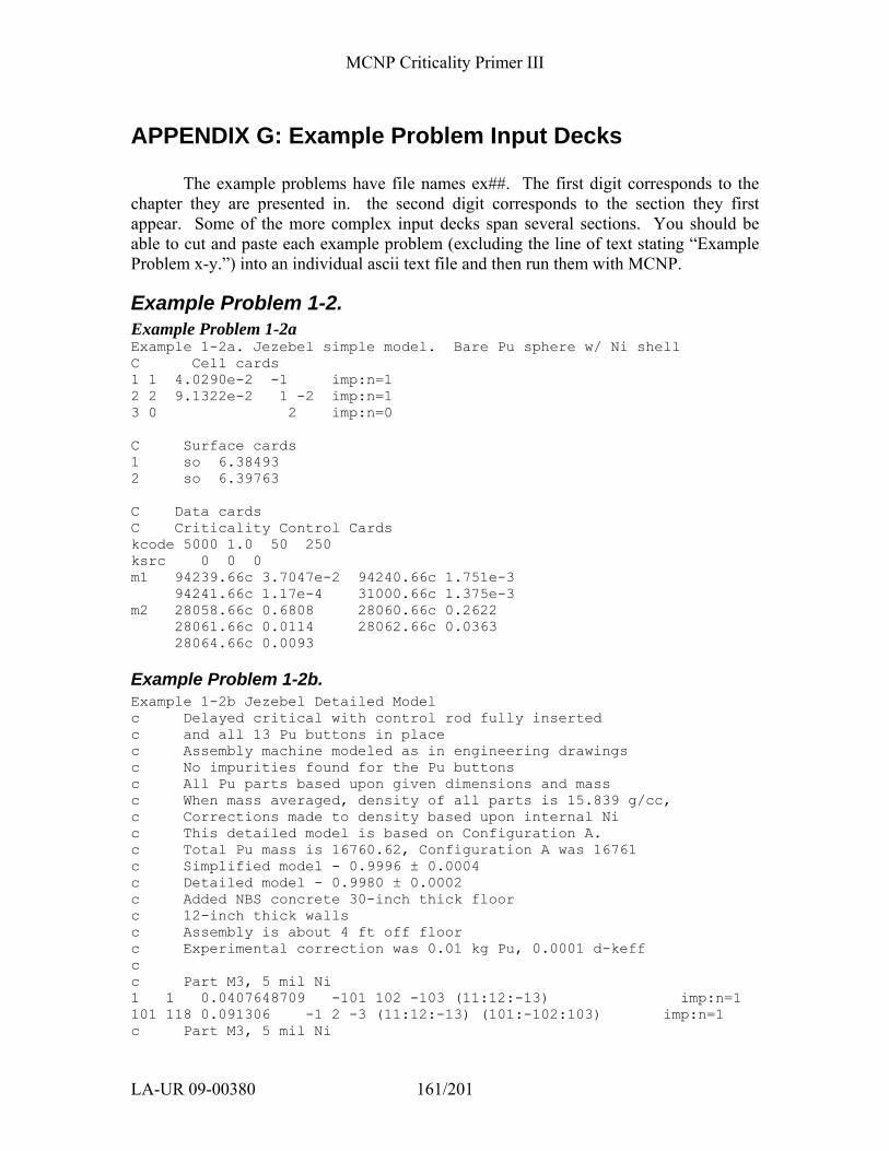
MCNP Criticality Primer III
LA-UR 09-00380 161/201
APPENDIX G: Example Problem Input Decks
The example problems have file names ex##. The first digit corresponds to the chapter they are presented in. the second digit corresponds to the section they first appear. Some of the more complex input decks span several sections. You should be able to cut and paste each example problem (excluding the line of text stating “Example Problem x-y.”) into an individual ascii text file and then run them with MCNP.
Example Problem 1-2. Example Problem 1-2a Example 1-2a. Jezebel simple model. Bare Pu sphere w/ Ni shell C Cell cards 1 1 4.0290e-2 -1 imp:n=1 2 2 9.1322e-2 1 -2 imp:n=1 3 0 2 imp:n=0 C Surface cards 1 so 6.38493 2 so 6.39763 C Data cards C Criticality Control Cards kcode 5000 1.0 50 250 ksrc 0 0 0 m1 94239.66c 3.7047e-2 94240.66c 1.751e-3 94241.66c 1.17e-4 31000.66c 1.375e-3 m2 28058.66c 0.6808 28060.66c 0.2622 28061.66c 0.0114 28062.66c 0.0363 28064.66c 0.0093
Example Problem 1-2b. Example 1-2b Jezebel Detailed Model c Delayed critical with control rod fully inserted c and all 13 Pu buttons in place c Assembly machine modeled as in engineering drawings c No impurities found for the Pu buttons c All Pu parts based upon given dimensions and mass c When mass averaged, density of all parts is 15.839 g/cc, c Corrections made to density based upon internal Ni c This detailed model is based on Configuration A. c Total Pu mass is 16760.62, Configuration A was 16761 c Simplified model - 0.9996 ± 0.0004 c Detailed model - 0.9980 ± 0.0002 c Added NBS concrete 30-inch thick floor c 12-inch thick walls c Assembly is about 4 ft off floor c Experimental correction was 0.01 kg Pu, 0.0001 d-keff c c Part M3, 5 mil Ni 1 1 0.0407648709 -101 102 -103 (11:12:-13) imp:n=1 101 118 0.091306 -1 2 -3 (11:12:-13) (101:-102:103) imp:n=1 c Part M3, 5 mil Ni
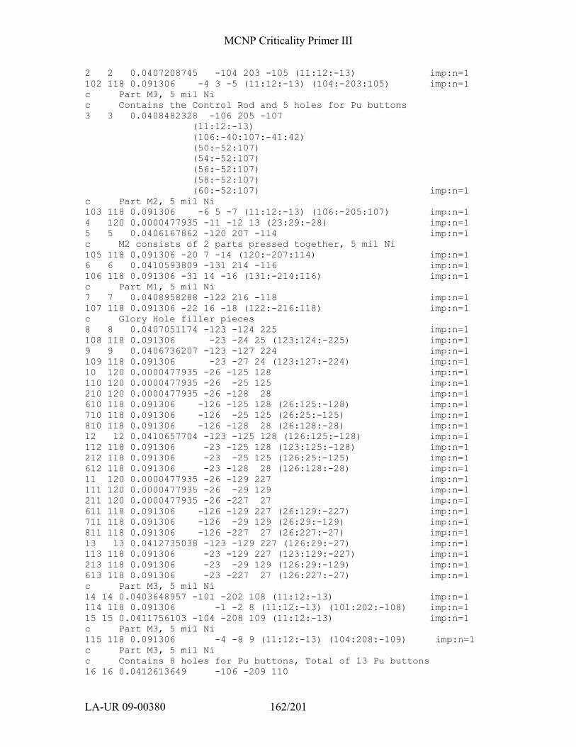
MCNP Criticality Primer III
LA-UR 09-00380 162/201
2 2 0.0407208745 -104 203 -105 (11:12:-13) imp:n=1 102 118 0.091306 -4 3 -5 (11:12:-13) (104:-203:105) imp:n=1 c Part M3, 5 mil Ni c Contains the Control Rod and 5 holes for Pu buttons 3 3 0.0408482328 -106 205 -107 (11:12:-13) (106:-40:107:-41:42) (50:-52:107) (54:-52:107) (56:-52:107) (58:-52:107) (60:-52:107) imp:n=1 c Part M2, 5 mil Ni 103 118 0.091306 -6 5 -7 (11:12:-13) (106:-205:107) imp:n=1 4 120 0.0000477935 -11 -12 13 (23:29:-28) imp:n=1 5 5 0.0406167862 -120 207 -114 imp:n=1 c M2 consists of 2 parts pressed together, 5 mil Ni 105 118 0.091306 -20 7 -14 (120:-207:114) imp:n=1 6 6 0.0410593809 -131 214 -116 imp:n=1 106 118 0.091306 -31 14 -16 (131:-214:116) imp:n=1 c Part M1, 5 mil Ni 7 7 0.0408958288 -122 216 -118 imp:n=1 107 118 0.091306 -22 16 -18 (122:-216:118) imp:n=1 c Glory Hole filler pieces 8 8 0.0407051174 -123 -124 225 imp:n=1 108 118 0.091306 -23 -24 25 (123:124:-225) imp:n=1 9 9 0.0406736207 -123 -127 224 imp:n=1 109 118 0.091306 -23 -27 24 (123:127:-224) imp:n=1 10 120 0.0000477935 -26 -125 128 imp:n=1 110 120 0.0000477935 -26 -25 125 imp:n=1 210 120 0.0000477935 -26 -128 28 imp:n=1 610 118 0.091306 -126 -125 128 (26:125:-128) imp:n=1 710 118 0.091306 -126 -25 125 (26:25:-125) imp:n=1 810 118 0.091306 -126 -128 28 (26:128:-28) imp:n=1 12 12 0.0410657704 -123 -125 128 (126:125:-128) imp:n=1 112 118 0.091306 -23 -125 128 (123:125:-128) imp:n=1 212 118 0.091306 -23 -25 125 (126:25:-125) imp:n=1 612 118 0.091306 -23 -128 28 (126:128:-28) imp:n=1 11 120 0.0000477935 -26 -129 227 imp:n=1 111 120 0.0000477935 -26 -29 129 imp:n=1 211 120 0.0000477935 -26 -227 27 imp:n=1 611 118 0.091306 -126 -129 227 (26:129:-227) imp:n=1 711 118 0.091306 -126 -29 129 (26:29:-129) imp:n=1 811 118 0.091306 -126 -227 27 (26:227:-27) imp:n=1 13 13 0.0412735038 -123 -129 227 (126:29:-27) imp:n=1 113 118 0.091306 -23 -129 227 (123:129:-227) imp:n=1 213 118 0.091306 -23 -29 129 (126:29:-129) imp:n=1 613 118 0.091306 -23 -227 27 (126:227:-27) imp:n=1 c Part M3, 5 mil Ni 14 14 0.0403648957 -101 -202 108 (11:12:-13) imp:n=1 114 118 0.091306 -1 -2 8 (11:12:-13) (101:202:-108) imp:n=1 15 15 0.0411756103 -104 -208 109 (11:12:-13) imp:n=1 c Part M3, 5 mil Ni 115 118 0.091306 -4 -8 9 (11:12:-13) (104:208:-109) imp:n=1 c Part M3, 5 mil Ni c Contains 8 holes for Pu buttons, Total of 13 Pu buttons 16 16 0.0412613649 -106 -209 110
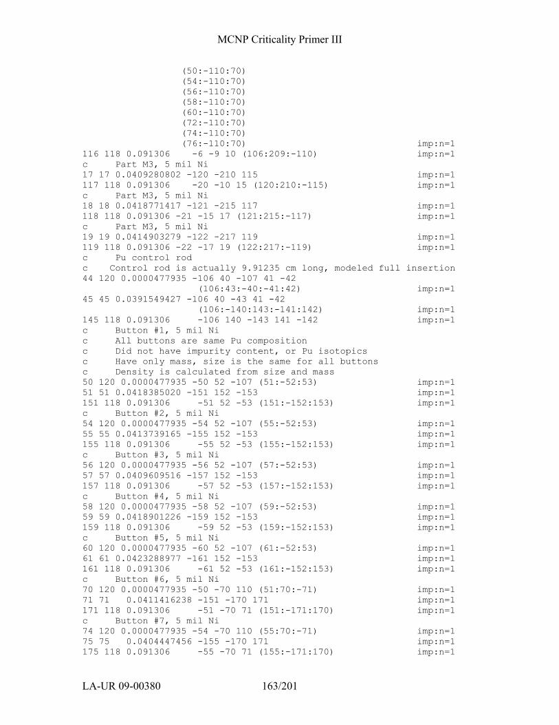
MCNP Criticality Primer III
LA-UR 09-00380 163/201
(50:-110:70) (54:-110:70) (56:-110:70) (58:-110:70) (60:-110:70) (72:-110:70) (74:-110:70) (76:-110:70) imp:n=1 116 118 0.091306 -6 -9 10 (106:209:-110) imp:n=1 c Part M3, 5 mil Ni 17 17 0.0409280802 -120 -210 115 imp:n=1 117 118 0.091306 -20 -10 15 (120:210:-115) imp:n=1 c Part M3, 5 mil Ni 18 18 0.0418771417 -121 -215 117 imp:n=1 118 118 0.091306 -21 -15 17 (121:215:-117) imp:n=1 c Part M3, 5 mil Ni 19 19 0.0414903279 -122 -217 119 imp:n=1 119 118 0.091306 -22 -17 19 (122:217:-119) imp:n=1 c Pu control rod c Control rod is actually 9.91235 cm long, modeled full insertion 44 120 0.0000477935 -106 40 -107 41 -42 (106:43:-40:-41:42) imp:n=1 45 45 0.0391549427 -106 40 -43 41 -42 (106:-140:143:-141:142) imp:n=1 145 118 0.091306 -106 140 -143 141 -142 imp:n=1 c Button #1, 5 mil Ni c All buttons are same Pu composition c Did not have impurity content, or Pu isotopics c Have only mass, size is the same for all buttons c Density is calculated from size and mass 50 120 0.0000477935 -50 52 -107 (51:-52:53) imp:n=1 51 51 0.0418385020 -151 152 -153 imp:n=1 151 118 0.091306 -51 52 -53 (151:-152:153) imp:n=1 c Button #2, 5 mil Ni 54 120 0.0000477935 -54 52 -107 (55:-52:53) imp:n=1 55 55 0.0413739165 -155 152 -153 imp:n=1 155 118 0.091306 -55 52 -53 (155:-152:153) imp:n=1 c Button #3, 5 mil Ni 56 120 0.0000477935 -56 52 -107 (57:-52:53) imp:n=1 57 57 0.0409609516 -157 152 -153 imp:n=1 157 118 0.091306 -57 52 -53 (157:-152:153) imp:n=1 c Button #4, 5 mil Ni 58 120 0.0000477935 -58 52 -107 (59:-52:53) imp:n=1 59 59 0.0418901226 -159 152 -153 imp:n=1 159 118 0.091306 -59 52 -53 (159:-152:153) imp:n=1 c Button #5, 5 mil Ni 60 120 0.0000477935 -60 52 -107 (61:-52:53) imp:n=1 61 61 0.0423288977 -161 152 -153 imp:n=1 161 118 0.091306 -61 52 -53 (161:-152:153) imp:n=1 c Button #6, 5 mil Ni 70 120 0.0000477935 -50 -70 110 (51:70:-71) imp:n=1 71 71 0.0411416238 -151 -170 171 imp:n=1 171 118 0.091306 -51 -70 71 (151:-171:170) imp:n=1 c Button #7, 5 mil Ni 74 120 0.0000477935 -54 -70 110 (55:70:-71) imp:n=1 75 75 0.0404447456 -155 -170 171 imp:n=1 175 118 0.091306 -55 -70 71 (155:-171:170) imp:n=1
MCNP Criticality Primer III
LA-UR 09-00380 164/201
c Button #8, 5 mil Ni 76 120 0.0000477935 -56 -70 110 (57:70:-71) imp:n=1 77 77 0.0412448650 -157 -170 171 imp:n=1 177 118 0.091306 -57 -70 71 (157:-171:170) imp:n=1 c Button #9, 5 mil Ni 78 120 0.0000477935 -58 -70 110 (59:70:-71) imp:n=1 79 79 0.0398511086 -159 -170 171 imp:n=1 179 118 0.091306 -59 -70 71 (159:-171:170) imp:n=1 c Button #10, 5 mil Ni 80 120 0.0000477935 -60 -70 110 (61:70:-71) imp:n=1 81 81 0.0396704365 -161 -170 171 imp:n=1 181 118 0.091306 -61 -70 71 (161:-171:170) imp:n=1 c Button #11, 5 mil Ni 82 120 0.0000477935 -72 -70 110 (73:70:-71) imp:n=1 83 83 0.0408060898 -173 -170 171 imp:n=1 183 118 0.091306 -73 -70 71 (173:-171:170) imp:n=1 c Button #12, 5 mil Ni 84 120 0.0000477935 -74 -70 110 (75:70:-71) imp:n=1 85 85 0.0405737971 -175 -170 171 imp:n=1 185 118 0.091306 -75 -70 71 (175:-171:170) imp:n=1 c Button #13, 5 mil Ni 86 120 0.0000477935 -76 -70 110 (77:70:-71) imp:n=1 87 87 0.0406512280 -177 -170 171 imp:n=1 187 118 0.091306 -77 -70 71 (177:-171:170) imp:n=1 c Cap top 300 130 0.06110248 -300 16 -301 (22:18:-16) imp:n=1 c Cap Bottom 301 130 0.06110248 -300 -17 302 (22:17:-19) imp:n=1 c 316 sstl Bolt inside of beveled part of top cap 302 131 0.08533207 -306 -303 301 imp:n=1 c Exterior top cap, beveled part 303 130 0.06110248 -305 -303 301 (306:303:-301) imp:n=1 c Bottom cap, beveled part 304 130 0.06110248 -307 -302 304 imp:n=1 c Top Assembly support 305 120 0.0000477935 -308 303 -312 imp:n=1 306 130 0.06110248 -309 303 -312 (308:-303:312) imp:n=1 307 120 0.0000477935 -308 312 -313 imp:n=1 308 130 0.06110248 -309 312 -313 (308:-312:313) imp:n=1 309 120 0.0000477935 -308 313 -314 imp:n=1 310 130 0.06110248 -309 313 -314 (308:-313:314) imp:n=1 311 120 0.0000477935 -308 314 -310 imp:n=1 312 130 0.06110248 -309 314 -310 (308:-314:310) imp:n=1 c Bottom assy support 313 120 0.0000477935 -308 -304 315 imp:n=1 314 130 0.06110248 -309 -304 315 (308:304:-315) imp:n=1 315 120 0.0000477935 -308 -315 316 imp:n=1 316 130 0.06110248 -309 -315 316 (308:315:-316) imp:n=1 317 120 0.0000477935 -308 -316 317 imp:n=1 318 130 0.06110248 -309 -316 317 (308:316:-317) imp:n=1 319 120 0.0000477935 -308 -317 311 imp:n=1 320 130 0.06110248 -309 -317 311 (308:317:-311) imp:n=1 c Top Spider assy support 321 130 0.06110248 -318 -313 312 (309:-312:313) imp:n=1 322 130 0.06110248 -319 -314 313 (309:-313:314) imp:n=1 c Bottom Spider assy support 323 130 0.06110248 -320 -315 316 (309:315:-316) imp:n=1
MCNP Criticality Primer III
LA-UR 09-00380 165/201
324 130 0.06110248 -321 -316 317 (309:316:-317) imp:n=1 c 316 sstl belly band 325 131 0.08533207 -322 -3 8 (1:3:-2) (1:2:-8) imp:n=1 c 316 sstl, wire guides 338 120 0.0000477935 -331 -3 8 (323:3:-8) imp:n=1 339 131 0.08533207 -327 -3 8 (331:3:-8) imp:n=1 340 120 0.0000477935 -332 -3 8 (324:3:-8) imp:n=1 341 131 0.08533207 -328 -3 8 (332:3:-8) imp:n=1 342 120 0.0000477935 -333 -3 8 (325:3:-8) imp:n=1 343 131 0.08533207 -329 -3 8 (333:3:-8) imp:n=1 344 120 0.0000477935 -334 -3 8 (326:3:-8) imp:n=1 345 131 0.08533207 -330 -3 8 (334:3:-8) imp:n=1 c 316 sstl, upper off axis wire guides 346 120 0.0000477935 -331 -351 352 (323:351:-352) imp:n=1 347 131 0.08533207 -327 -351 352 (331:351:-352) imp:n=1 348 120 0.0000477935 -332 -351 352 (324:351:-352) imp:n=1 349 131 0.08533207 -328 -351 352 (332:351:-352) imp:n=1 350 120 0.0000477935 -333 -351 352 (325:351:-352) imp:n=1 351 131 0.08533207 -329 -351 352 (333:351:-352) imp:n=1 352 120 0.0000477935 -334 -351 352 (326:351:-352) imp:n=1 353 131 0.08533207 -330 -351 352 (334:351:-352) imp:n=1 c 316 sstl, lower off axis wire guides 354 120 0.0000477935 -331 -354 353 (323:354:-353) imp:n=1 355 131 0.08533207 -327 -354 353 (331:354:-353) imp:n=1 356 120 0.0000477935 -332 -354 353 (324:354:-353) imp:n=1 357 131 0.08533207 -328 -354 353 (332:354:-353) imp:n=1 358 120 0.0000477935 -333 -354 353 (325:354:-353) imp:n=1 359 131 0.08533207 -329 -354 353 (333:354:-353) imp:n=1 360 120 0.0000477935 -334 -354 353 (326:354:-353) imp:n=1 361 131 0.08533207 -330 -354 353 (334:354:-353) imp:n=1 c 316 sstl wire 400 131 0.08533207 -323 -310 351 imp:n=1 401 131 0.08533207 -323 -351 352 imp:n=1 402 131 0.08533207 -323 -352 3 imp:n=1 403 131 0.08533207 -323 -3 8 imp:n=1 404 131 0.08533207 -323 -8 354 imp:n=1 405 131 0.08533207 -323 -354 353 imp:n=1 406 131 0.08533207 -323 -353 311 imp:n=1 410 131 0.08533207 -324 -310 351 imp:n=1 411 131 0.08533207 -324 -351 352 imp:n=1 412 131 0.08533207 -324 -352 3 imp:n=1 413 131 0.08533207 -324 -3 8 imp:n=1 414 131 0.08533207 -324 -8 354 imp:n=1 415 131 0.08533207 -324 -354 353 imp:n=1 416 131 0.08533207 -324 -353 311 imp:n=1 420 131 0.08533207 -325 -310 351 imp:n=1 421 131 0.08533207 -325 -351 352 imp:n=1 422 131 0.08533207 -325 -352 3 imp:n=1 423 131 0.08533207 -325 -3 8 imp:n=1 424 131 0.08533207 -325 -8 354 imp:n=1 425 131 0.08533207 -325 -354 353 imp:n=1 426 131 0.08533207 -325 -353 311 imp:n=1 430 131 0.08533207 -326 -310 351 imp:n=1 431 131 0.08533207 -326 -351 352 imp:n=1 432 131 0.08533207 -326 -352 3 imp:n=1
MCNP Criticality Primer III
LA-UR 09-00380 166/201
433 131 0.08533207 -326 -3 8 imp:n=1 434 131 0.08533207 -326 -8 354 imp:n=1 435 131 0.08533207 -326 -354 353 imp:n=1 436 131 0.08533207 -326 -353 311 imp:n=1 c Spider assy arms c ZX Upper right arm 500 120 0.0000477935 -525 -502 503 imp:n=1 501 130 0.06110248 -501 -502 503 (525:502:-503) imp:n=1 c ZX lower right arm 502 120 0.0000477935 -526 -505 506 imp:n=1 503 130 0.06110248 -504 -505 506 (526:505:-506) imp:n=1 c ZX upper left arm 504 120 0.0000477935 -527 -508 509 imp:n=1 505 130 0.06110248 -507 -508 509 (527:508:-509) imp:n=1 c ZX lower left arm 506 120 0.0000477935 -528 511 -512 imp:n=1 507 130 0.06110248 -510 511 -512 (528:512:-511) imp:n=1 c YZ upper right arm 508 120 0.0000477935 -529 -514 515 imp:n=1 509 130 0.06110248 -513 -514 515 (529:514:-515) imp:n=1 c YZ upper left arm 510 120 0.0000477935 -530 -517 518 imp:n=1 511 130 0.06110248 -516 -517 518 (530:517:-518) imp:n=1 c YZ lower right arm 512 120 0.0000477935 -531 -520 521 imp:n=1 513 130 0.06110248 -519 -520 521 (531:520:-521) imp:n=1 c YZ lower left arm 514 120 0.0000477935 -532 -523 524 imp:n=1 515 130 0.06110248 -522 -523 524 (532:523:-524) imp:n=1 c air around Assembly, added surface 600 21 120 0.0000477935 -700 701 -702 703 -704 705 (322:3:-8) (4:-3:5) (11:12:-13) (6:-5:7) (20:14:-7) (31:16:-14) (300:301:-16) (305:303:-301) (309:-303:312) (318:-312:313) (319:-313:314) (309:-314:310) (4:8:-9) (6:-10:9) (20:10:-15) (21:15:-17) (300:17:-302) (307:302:-304) (309:304:-315) (320:315:-316) (321:316:-317) (309:317:-311) (323:310:-351) (324:310:-351) (325:310:-351) (326:310:-351)
MCNP Criticality Primer III
LA-UR 09-00380 167/201
(327:351:-352) (328:351:-352) (329:351:-352) (330:351:-352) (323:352:-3) (324:352:-3) (325:352:-3) (326:352:-3) (327:3:-8) (328:3:-8) (329:3:-8) (330:3:-8) (323:8:-354) (324:8:-354) (325:8:-354) (326:8:-354) (327:354:-353) (328:354:-353) (329:354:-353) (330:354:-353) (323:353:-311) (324:353:-311) (325:353:-311) (326:353:-311) (501:502:-503) (504:505:-506) (507:508:-509) (510:-511:512) (513:514:-515) (516:517:-518) (519:520:-521) (522:523:-524) imp:n=1 700 132 0.0764 -706 707 -708 709 -710 711 (700:-701:702:-703:704:-705) imp:n=1 701 120 0.0000477935 -600 (706:-707:708:-709:710:-711) imp:n=1 c Added surface 600 and cell 600, Air around assembly 600 0 600 imp:n=0 1 so 6.60273 101 so 6.59003 2 pz 0.00000 102 pz 0.0127 202 pz -0.0127 3 pz 0.396875 103 pz 0.384175 203 pz 0.409575 4 cz 6.44525 104 cz 6.43255 5 pz 1.3096875 105 pz 1.2969875 205 pz 1.3223875 6 so 6.44525 106 so 6.43255 7 pz 2.21234 107 pz 2.19964 207 pz 2.22504
MCNP Criticality Primer III
LA-UR 09-00380 168/201
8 pz -0.396875 108 pz -0.384175 208 pz -0.409575 9 pz -1.3096875 109 pz -1.2969875 209 pz -1.3223875 10 pz -2.21234 110 pz -2.19964 210 pz -2.22504 11 cx 0.6477 12 px 6.57 13 px -6.57 14 pz 6.37994 114 pz 6.36724 214 pz 6.39264 15 pz -6.37994 115 pz -6.36724 215 pz -6.39264 16 pz 6.50494 116 pz 6.49224 216 pz 6.51764 17 pz -6.50494 117 pz -6.49224 217 pz -6.51764 18 pz 6.81744 118 pz 6.80474 19 pz -6.81744 119 pz -6.80474 20 so 6.51002 120 so 6.49732 21 kz -3.892216 0.2447 121 kz -4.019216 0.2447 22 cz 1.2827 122 cz 1.27 23 cx 0.6223 123 cx 0.6096 24 px 2.90449 124 px 2.89179 224 px 2.91719 25 px -2.89179 125 px -2.90449 225 px -2.87909 26 cx 0.11938 c Added surface 126 to add Ni coat to onside of hole in GH filler 126 cx 0.13208 27 px 4.17449 127 px 4.16179 227 px 4.18719 28 px -4.17449 128 px -4.16179 29 px 4.93047 129 px 4.91777 31 kz 3.892216 0.2447 131 kz 4.019216 0.2447 40 pz 1.6891 140 pz 1.7018 41 py 3.3782
MCNP Criticality Primer III
LA-UR 09-00380 169/201
141 py 3.3909 42 py 4.3434 142 py 4.3307 43 pz 2.17878 143 pz 2.16408 50 c/z -2.8726 -2.8726 1.2954 51 c/z -2.8726 -2.8726 1.2446 151 c/z -2.8726 -2.8726 1.2319 52 pz 1.56464 152 pz 1.57734 53 pz 2.18694 153 pz 2.17424 54 c/z 2.8726 -2.8726 1.2954 55 c/z 2.8726 -2.8726 1.2446 155 c/z 2.8726 -2.8726 1.2319 56 c/z -4.0625 0 1.2954 57 c/z -4.0625 0 1.2446 157 c/z -4.0625 0 1.2319 58 c/z 4.0625 0 1.2954 59 c/z 4.0625 0 1.2446 159 c/z 4.0625 0 1.2319 60 c/z 0 -4.0625 1.2954 61 c/z 0 -4.0625 1.2446 161 c/z 0 -4.0625 1.2319 70 pz -1.56464 71 pz -2.18694 170 pz -1.57734 171 pz -2.17424 72 c/z -2.8726 2.8726 1.2954 73 c/z -2.8726 2.8726 1.2446 173 c/z -2.8726 2.8726 1.2319 74 c/z 0 4.0625 1.2954 75 c/z 0 4.0625 1.2446 175 c/z 0 4.0625 1.2319 76 c/z 2.8726 2.8726 1.2954 77 c/z 2.8726 2.8726 1.2446 177 c/z 2.8726 2.8726 1.2319 c Cap top and bottom, estimated to be 1/8-inch thick radially 300 cz 1.6002 c Cap top, estimated to be 1/8-inch thick axially 301 pz 7.13494 302 pz -7.13494 303 pz 8.40494 304 pz -8.40494 305 kz 9.33494 0.25 c 3/8-inch bolt 306 cz 0.375 307 kz -9.33494 0.25 c Upper and lower assembly support, hollow al 2014, 10-mil thick 308 cz 0.45085 309 cz 0.47625 310 pz 30.0 311 pz -30.0 312 pz 9.5475 313 pz 10.5 314 pz 11.4525 315 pz -9.5475
MCNP Criticality Primer III
LA-UR 09-00380 170/201
316 pz -10.5 317 pz -11.4525 318 kz 8.3 0.25 319 kz 12.7 0.25 320 kz -8.3 0.25 321 kz -12.7 0.25 c Belly band 322 so 6.92023 c Assembly wires 323 c/z 0 7.23773 0.15875 324 c/z 0 -7.23773 0.15875 325 c/z 7.23773 0 0.15875 326 c/z -7.23773 0 0.15875 c Assembly wire guides 327 c/z 0 7.23773 0.315 328 c/z 0 -7.23773 0.315 329 c/z 7.23773 0 0.315 330 c/z -7.23773 0 0.315 331 c/z 0 7.23773 0.16 332 c/z 0 -7.23773 0.16 333 c/z 7.23773 0 0.16 334 c/z -7.23773 0 0.16 c Off-axis assembly wire guides 351 pz 4.575575 352 pz 3.38495 353 pz -4.575575 354 pz -3.38495 501 1 cz 0.28125 502 9 pz 3.9 503 10 pz -3.2 504 2 cz 0.28125 505 11 pz 3.9 506 12 pz -3.2 507 3 cz 0.28125 508 13 pz 3.9 509 14 pz -3.0 510 4 cz 0.28125 511 15 pz -3.9 512 16 pz 3.1 513 5 cz 0.28125 514 17 pz 3.1 515 18 pz -3.9 516 6 cz 0.28125 517 19 pz 3.75 518 20 pz -3.1 519 7 cz 0.28125 520 21 pz 3.05 521 22 pz -3.8 522 8 cz 0.28125 523 23 pz 3.8 524 24 pz -3.05 525 1 cz 0.25585 526 2 cz 0.25585 527 3 cz 0.25585 528 4 cz 0.25585 529 5 cz 0.25585 530 6 cz 0.25585

MCNP Criticality Primer III
LA-UR 09-00380 171/201
531 7 cz 0.25585 532 8 cz 0.25585 c Added surface 600 and cell 600 600 so 1000.00 700 pz 254.00 701 pz -121.92 702 px 254.00 703 px -254.00 704 py 254.00 705 py -254.00 706 pz 285.00 707 pz -199.00 708 px 285.00 709 px -285.00 710 py 285.00 711 py -285.00 *tr1 3.8 0 7 45 90 45 90 0 90 135 90 45 1 *tr2 -3.8 0 7 135 90 45 90 0 90 45 90 45 1 *tr3 3.8 0 -7 135 90 45 90 0 90 45 90 45 1 *tr4 -3.8 0 -7 45 90 45 90 0 90 135 90 45 1 *tr5 0 3.8 7 0 90 90 90 45 45 90 135 45 1 *tr6 0 -3.8 7 0 90 90 90 135 45 90 45 45 1 *tr7 0 3.8 -7 0 90 90 90 135 45 90 45 45 1 *tr8 0 -3.8 -7 0 90 90 90 45 45 90 135 45 1 *tr9 3.8 0 7 65 90 25 90 0 90 3j 1 *tr10 3.8 0 7 88 90 2 90 0 90 3j 1 *tr11 -3.8 0 7 3j 90 0 90 25 90 65 1 *tr12 -3.8 0 7 3j 90 0 90 2 90 88 1 *tr13 3.8 0 -7 115 90 25 90 0 90 3j 1 *tr14 3.8 0 -7 89 90 1 90 0 90 3j 1 *tr15 -3.8 0 -7 65 90 25 90 0 90 3j 1 *tr16 -3.8 0 -7 89 90 1 90 0 90 3j 1 *tr17 0 3.8 7 90 90 0 6j 1 *tr18 0 3.8 7 90 65 25 6j 1 c Fixed tr card, should have been the same angles as tr22 c The original tr19 card resulted in lost particles c *tr19 0 -3.8 7 70 65 115 6j 1 *tr19 0 -3.8 7 70 65 115 6j 1 *tr20 0 -3.8 7 90 90 0 6j 1 *tr21 0 3.8 -7 90 90 0 6j 1 *tr22 0 3.8 -7 70 65 115 6j 1 *tr23 0 -3.8 -7 90 65 25 6j 1 *tr24 0 -3.8 -7 90 90 0 6j 1 m1 94239. 0.0372245612 94240. 0.0017522223 94241. 0.0001163288 31000. 0.0013823646 6012. 0.0001323813 8016. 0.0001344529 26054. 0.0000011665 26056. 0.0000176428 26057. 0.0000004005 26058. 0.0000000520 95241. 0.0000032980 m2 94239. 0.0371700781 94240. 0.0017496577

MCNP Criticality Primer III
LA-UR 09-00380 172/201
94241. 0.0001161585 31000. 0.0013667184 6012. 0.0001555202 8016. 0.0001459357 26054. 0.0000007597 26056. 0.0000114897 26057. 0.0000002608 26058. 0.0000000339 95241. 0.0000042618 m3 94239. 0.0372863309 94240. 0.0017551300 94241. 0.0001165218 31000. 0.0013709929 6012. 0.0001560066 8016. 0.0001463921 26054. 0.0000007621 26056. 0.0000115257 26057. 0.0000002616 26058. 0.0000000340 95241. 0.0000042752 m5 94239. 0.0370893372 94240. 0.0017458571 94241. 0.0001159062 31000. 0.0013773429 6012. 0.0001319004 8016. 0.0001339645 26054. 0.0000011623 26056. 0.0000175787 26057. 0.0000003990 26058. 0.0000000518 95241. 0.0000032860 m6 94239. 0.0377703068 94240. 0.0014134214 94241. 0.0001563934 94242. 0.0000779170 31000. 0.0013523941 6012. 0.0001413242 8016. 0.0001385120 26054. 0.0000002557 26056. 0.0000038671 26057. 0.0000000878 26058. 0.0000000114 95241. 0.0000048901 m7 94239. 0.0376198560 94240. 0.0014077913 94241. 0.0001557704 94242. 0.0000776067 31000. 0.0013470071 6012. 0.0001407613 8016. 0.0001379603 26054. 0.0000002547 26056. 0.0000038517 26057. 0.0000000874 26058. 0.0000000113 95241. 0.0000048706 m8 94239. 0.0371699971 94240. 0.0017496539
MCNP Criticality Primer III
LA-UR 09-00380 173/201
94241. 0.0001161583 31000. 0.0013803383 6012. 0.0001321872 8016. 0.0001342558 26054. 0.0000011648 26056. 0.0000176169 26057. 0.0000003999 26058. 0.0000000519 95241. 0.0000032931 m9 94239. 0.0371557698 94240. 0.0017489842 94241. 0.0001161137 31000. 0.0013798100 6012. 0.0001321367 8016. 0.0001342044 26054. 0.0000002005 26056. 0.0000030318 26057. 0.0000000688 26058. 0.0000000089 95241. 0.0000032919 m12 94239. 0.0375139949 94240. 0.0017658466 94241. 0.0001172333 31000. 0.0013931129 6012. 0.0001334105 8016. 0.0001354983 26054. 0.0000002029 26056. 0.0000030687 26057. 0.0000000697 26058. 0.0000000090 95241. 0.0000033236 m13 94239. 0.0377037830 94240. 0.0017747801 94241. 0.0001178264 31000. 0.0014001609 6012. 0.0001340855 8016. 0.0001361838 26054. 0.0000002025 26056. 0.0000030626 26057. 0.0000000695 26058. 0.0000000090 95241. 0.0000033404 m14 94239. 0.0368545412 94240. 0.0017348049 94241. 0.0001151724 31000. 0.0013551163 6012. 0.0001542000 8016. 0.0001446968 26054. 0.0000001295 26056. 0.0000019586 26057. 0.0000000445 26058. 0.0000000058 95241. 0.0000042257 m15 94239. 0.0375947638 94240. 0.0017696484 94241. 0.0001174856 31000. 0.0013823338
MCNP Criticality Primer III
LA-UR 09-00380 174/201
6012. 0.0001572971 8016. 0.0001476031 26054. 0.0000001313 26056. 0.0000019858 26057. 0.0000000451 26058. 0.0000000059 95241. 0.0000043105 m16 94239. 0.0376730565 94240. 0.0017733338 94241. 0.0001177303 31000. 0.0013852126 6012. 0.0001576247 8016. 0.0001479105 26054. 0.0000001318 26056. 0.0000019940 26057. 0.0000000453 26058. 0.0000000059 95241. 0.0000043195 m17 94239. 0.0373882602 94240. 0.0017599279 94241. 0.0001168404 31000. 0.0013884437 6012. 0.0001329635 8016. 0.0001350442 26054. 0.0000001991 26056. 0.0000030116 26057. 0.0000000684 26058. 0.0000000089 95241. 0.0000033125 m18 94239. 0.0385225606 94240. 0.0014415719 94241. 0.0001595082 94242. 0.0000794689 31000. 0.0013793291 6012. 0.0001441389 8016. 0.0001412707 26054. 0.0000002608 26056. 0.0000039441 26057. 0.0000000895 26058. 0.0000000116 95241. 0.0000049874 m19 94239. 0.0381667326 94240. 0.0014282563 94241. 0.0001580348 94242. 0.0000787348 31000. 0.0013665884 6012. 0.0001428075 8016. 0.0001399658 26054. 0.0000002584 26056. 0.0000039077 26057. 0.0000000887 26058. 0.0000000115 95241. 0.0000049414 m45 94239. 0.0358689437 94240. 0.0016884115 94241. 0.0001120924 31000. 0.0013712385
MCNP Criticality Primer III
LA-UR 09-00380 175/201
6012. 0.0000300052 8016. 0.0000422351 26054. 0.0000003909 26056. 0.0000059115 26057. 0.0000001342 26058. 0.0000000174 28058. 0.0000037057 28060. 0.0000013796 28061. 0.0000000590 28062. 0.0000001848 28064. 0.0000000459 25055. 0.0000180400 95241. 0.0000121473 m51 94239. 0.0384789148 94240. 0.0018112258 94241. 0.0001202730 31000. 0.0014280884 m55 94239. 0.0380516350 94240. 0.0017911135 94241. 0.0001189374 31000. 0.0014122305 m57 94239. 0.0376718308 94240. 0.0017732359 94241. 0.0001177503 31000. 0.0013981346 m59 94239. 0.0385263903 94240. 0.0018134605 94241. 0.0001204214 31000. 0.0014298504 m61 94239. 0.0389299323 94240. 0.0018324555 94241. 0.0001216827 31000. 0.0014448272 m71 94239. 0.0378379952 94240. 0.0017810574 94241. 0.0001182697 31000. 0.0014043016 m75 94239. 0.0371970755 94240. 0.0017508889 94241. 0.0001162663 31000. 0.0013805148 m77 94239. 0.0379329462 94240. 0.0017855268 94241. 0.0001185664 31000. 0.0014078256 m79 94239. 0.0366511070 94240. 0.0017251898 94241. 0.0001145598 31000. 0.0013602520 m81 94239. 0.0364849426 94240. 0.0017173684 94241. 0.0001140404 31000. 0.0013540850 m83 94239. 0.0375294042 94240. 0.0017665318 94241. 0.0001173051 31000. 0.0013928487
MCNP Criticality Primer III
LA-UR 09-00380 176/201
m85 94239. 0.0373157644 94240. 0.0017564756 94241. 0.0001166373 31000. 0.0013849198 m87 94239. 0.0373869777 94240. 0.0017598277 94241. 0.0001168599 31000. 0.0013875627 c Nickel coat, no known impurities m118 28058. 0.062161125 28060. 0.023940433 28061. 0.001040888 28062. 0.003314408 28064. 0.000849146 c Typical air, 0.00115 g/cc m120 7014. 0.0000381259 8016. 0.0000095012 18000. 0.0000001664 c Al 2014, assy machine m130 13027. 0.05878575 29063. 0.00081336 29065. 0.00036252 14000. 0.00054420 25055. 0.00024729 12000. 0.00034936 c 316 SSTL, bolt on top m131 24050. 0.00067319 24052. 0.01296704 24053. 0.00147019 24054. 0.00036523 26054. 0.00352047 26056. 0.05521418 26057. 0.00127579 26058. 0.00016850 28058. 0.00658843 28060. 0.00253744 28061. 0.00011032 28062. 0.00035129 28064. 0.00009000 m132 1001. 0.00842 8016. 0.04423 13027. 0.00252 14028. 0.014690958 14029. 0.000718176 14030. 0.000460866 11023. 0.00105 20000. 0.00293 26054. 0.000041788 26056. 0.000632003 26057. 0.000014347 26058. 0.000001862 19000. 0.00069 kcode 10000 1.0 100 1010 ksrc 4.5528 0 0 fcl:n 0 0 0 1 0 0 0 0 0 1 1 0 0 0 0 0 0 0 0 1 1 1 1 1 1 1 1 1 1 1 1 1 1 1 1 1 1 1 1 1 1 1 1 1 1
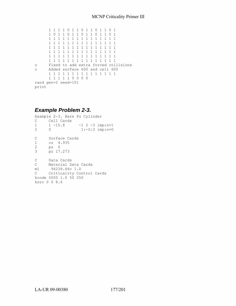
MCNP Criticality Primer III
LA-UR 09-00380 177/201
1 1 1 1 0 1 1 0 1 1 0 1 1 0 1 1 0 1 1 0 1 1 0 1 1 0 1 1 0 1 1 1 1 1 1 1 1 1 1 1 1 1 1 1 1 1 1 1 1 1 1 1 1 1 1 1 1 1 1 1 1 1 1 1 1 1 1 1 1 1 1 1 1 1 1 1 1 1 1 1 1 1 1 1 1 1 1 1 1 1 1 1 1 1 1 1 1 1 1 1 1 1 1 1 1 1 1 1 1 1 1 1 1 1 1 1 1 1 1 1 c Fixed to add extra forced collisions c Added surface 600 and cell 600 1 1 1 1 1 1 1 1 1 1 1 1 1 1 1 1 1 1 1 1 0 0 0 0 rand gen=2 seed=101 print
Example Problem 2-3. Example 2-3. Bare Pu Cylinder C Cell Cards 1 1 -15.8 -1 2 -3 imp:n=1 2 0 1:-2:3 imp:n=0 C Surface Cards 1 cz 4.935 2 pz 0 3 pz 17.273 C Data Cards C Material Data Cards m1 94239.66c 1.0 C Criticality Control Cards kcode 5000 1.0 50 250 ksrc 0 0 8.6
MCNP Criticality Primer III
LA-UR 09-00380 178/201
Example Problem 2-3m. Example 2-3. Bare Pu Cylinder - Macrobody C Cell Cards 1 1 -15.8 -1 imp:n=1 2 0 1 imp:n=0 C Surface Cards 1 rcc 0 0 0 0 0 17.273 4.935 C Data Cards m1 94239.66c 1.0 kcode 5000 1.0 50 250 ksrc 0 0 8.6
Example Problem 2-4. Example 2-4. Pu cylinder, radial U(nat) reflector C Cell Cards 1 1 -15.8 -1 2 -3 imp:n=1 2 2 -18.8 1 -4 2 -3 imp:n=1 3 0 4:-2:3 imp:n=0 C Surface Cards 1 cx 4.935 $ Pu Cylinder 2 px 0.0 $ bottom 3 px 6.909 $ top 4 cx 9.935 $ U reflector C Data Cards C Material Data Cards m1 94239.66c 1.0 m2 92238.66c 0.992745 92235.66c 0.007200 C Criticality Control Cards kcode 5000 1.0 50 250 ksrc 3.5 0 0

MCNP Criticality Primer III
LA-UR 09-00380 179/201
Example Problem 2-4m. Example 2-4. Pu cylinder, radial U(nat) refl. - Macrobody C Cell Cards 1 1 -15.8 -1 imp:n=1 2 2 -18.8 1 -2 imp:n=1 3 0 2 imp:n=0 C Surface Cards 1 rcc 0 0 0 6.909 0 0 4.935 $ Pu cylinder 2 rcc 0 0 0 6.909 0 0 9.935 $ U reflector C Data Cards m1 94239.66c 1.0 m2 92238.66c 0.992745 92235.66c 0.007200 kcode 5000 1.0 50 250 ksrc 3.5 0 0
Example Problem 2-5. Example 2-5. Pu cylinder, radial U(nat) reflector C Cell Cards 1 1 -15.8 -1 2 -3 imp:n=1 2 2 -18.8 -4 -6 5 #1 imp:n=1 3 0 4:-5:6 imp:n=0 C Surface Cards 1 cx 4.935 2 px 0.0 3 px 6.909 4 cx 9.935 5 px -5.0 6 px 11.909 C Data Cards C Material Data Cards m1 94239.66c 1.0 m2 92238.66c 0.992745 92235.66c 0.007200 C Criticality Control Cards kcode 5000 1.0 50 250 ksrc 3.5 0 0
MCNP Criticality Primer III
LA-UR 09-00380 180/201
Example Problem 2-5m. Example 2-5, Pu cylinder, radial U(nat) reflector - Macrobody C Cell Cards 1 1 -15.8 -1 imp:n=1 2 2 -18.8 1 -2 imp:n=1 3 0 2 imp:n=0 C Surface Cards 1 rcc 0 0 0 6.909 0 0 4.935 $ Pu cylinder 2 rcc -5 0 0 16.909 0 0 9.935 $ U reflector C Data Cards m1 94239.66c 1.0 m2 92238.66c 0.992745 92235.66c 0.007200 kcode 5000 1.0 50 250 ksrc 3.5 0 0
Example Problem 3-4. Example 3-4. S(alpha, beta) Treatment C Cell Cards 1 1 9.6586E-2 -1 3 -4 imp:n=1 2 0 -1 4 -5 imp:n=1 3 2 -2.7 (1 -2 -5 3):(-2 -3 6) imp:n=1 4 0 2:5:-6 imp:n=0 C Surface Cards 1 cz 20.12 2 cz 20.2787 3 pz 0.0 4 pz 100.0 5 pz 110.0 6 pz -0.1587 C Data Cards C Material Data Cards m1 1001.62c 5.7058e-2 8016.62c 3.2929e-2 9019.62c 4.3996e-3 92238.66c 2.0909e-3 92235.66c 1.0889e-4 mt1 lwtr.60t m2 13027.62c 1 C Criticality Control Cards kcode 5000 1.0 50 250 ksrc 0 0 50.0
MCNP Criticality Primer III
LA-UR 09-00380 181/201
Example Problem 3-4m. Example 3-4. S(alpha, beta) Treatment with Macrobodies C Cell Cards 1 100 9.6586E-2 -10 imp:n=1 2 0 -20 imp:n=1 3 101 -2.7 10 20 -30 imp:n=1 4 0 30 imp:n=0 C Surface Cards 10 rcc 0 0 0 0 0 100.0 20.12 $ Can of UO2F2 20 rcc 0 0 100 0 0 10.0 20.12 $ Void gap above UO2F2 30 rcc 0 0 -0.1587 0 0 110.1587 20.2787 $ Exterior shell of Al C Data Cards m100 1001.62c 5.7058e-2 8016.62c 3.2929e-2 9019.62c 4.3996e-3 92238.66c 2.0909e-3 92235.66c 1.0889e-4 mt100 lwtr.60t m101 13027.62c 1 kcode 5000 1.0 50 250 ksrc 0 0 50.0
Example Problem 3-4nomt. Example 3-4. NO S(alpha, beta) Treatment! C Cell Cards 1 1 9.6586E-2 -1 3 -4 imp:n=1 2 0 -1 4 -5 imp:n=1 3 2 -2.7 (1 -2 -5 3):(-2 -3 6) imp:n=1 4 0 2:5:-6 imp:n=0 C Surface Cards 1 cz 20.12 2 cz 20.2787 3 pz 0.0 4 pz 100.0 5 pz 110.0 6 pz -0.1587 C Data Cards m1 1001.62c 5.7058e-2 8016.62c 3.2929e-2 9019.62c 4.3996e-3 92238.66c 2.0909e-3 92235.66c 1.0889e-4 c mt1 lwtr.60t m2 13027.62c 1 kcode 5000 1.0 50 250 ksrc 0 0 50.0
MCNP Criticality Primer III
LA-UR 09-00380 182/201
Example Problem 4-3. Example 4-3, Repeated Structures: Two Cylinders C Cell Cards 1 1 9.9605e-2 -1 -4 5 u=3 imp:n=1 $ Solution 2 0 -1 4 u=3 imp:n=1 $ Void region above solution 3 2 -2.7 1:-5 u=3 imp:n=1 $ Al container 4 0 -2 -3 6 fill=3 imp:n=1 5 like 4 but trcl (17 0 0) imp:n=1 6 3 -1.0 10 -11 8 -9 7 -3 #4 #5 imp:n=1 7 0 -10:11:-8:9:-7:3 imp:n=0 C Surface Cards 1 cz 6.35 $ Solution radius 2 cz 6.50 $ 3 pz 80.0 $ Top of container 4 pz 70.2 $ Top of solution 5 pz 0.0 6 pz -0.15 7 pz -20.15 $ Bottom of tank C Sides of Tank 8 px -16.5 9 px 43.5 10 py -26.5 11 py 26.5 C Data Cards C Materials Cards m1 1001.62c 6.2210e-2 8016.62c 3.3621e-2 9019.62c 2.5161e-3 92235.66c 1.1760e-3 92238.66c 8.2051e-5 mt1 lwtr.60t m2 13027.62c 1.0 m3 1001.62c 2 8016.62c 1 mt3 lwtr.60t C Control Cards kcode 5000 1.0 50 250 ksrc 0 0 35 17 0 35
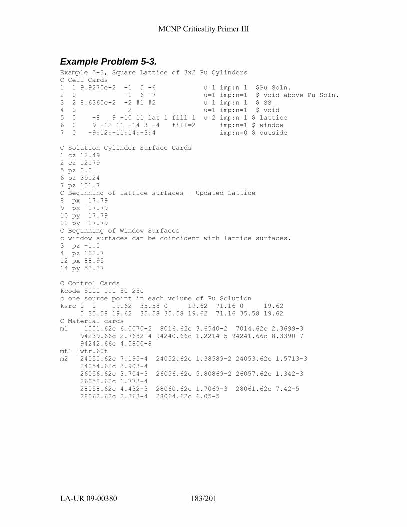
MCNP Criticality Primer III
LA-UR 09-00380 183/201
Example Problem 5-3. Example 5-3, Square Lattice of 3x2 Pu Cylinders C Cell Cards 1 1 9.9270e-2 -1 5 -6 u=1 imp:n=1 $Pu Soln. 2 0 -1 6 -7 u=1 imp:n=1 $ void above Pu Soln. 3 2 8.6360e-2 -2 #1 #2 u=1 imp:n=1 $ SS 4 0 2 u=1 imp:n=1 $ void 5 0 -8 9 -10 11 lat=1 fill=1 u=2 imp:n=1 $ lattice 6 0 9 -12 11 -14 3 -4 fill=2 imp:n=1 $ window 7 0 -9:12:-11:14:-3:4 imp:n=0 $ outside C Solution Cylinder Surface Cards 1 cz 12.49 2 cz 12.79 5 pz 0.0 6 pz 39.24 7 pz 101.7 C Beginning of lattice surfaces - Updated Lattice 8 px 17.79 9 px -17.79 10 py 17.79 11 py -17.79 C Beginning of Window Surfaces c window surfaces can be coincident with lattice surfaces. 3 pz -1.0 4 pz 102.7 12 px 88.95 14 py 53.37 C Control Cards kcode 5000 1.0 50 250 c one source point in each volume of Pu Solution ksrc 0 0 19.62 35.58 0 19.62 71.16 0 19.62 0 35.58 19.62 35.58 35.58 19.62 71.16 35.58 19.62 C Material cards m1 1001.62c 6.0070-2 8016.62c 3.6540-2 7014.62c 2.3699-3 94239.66c 2.7682-4 94240.66c 1.2214-5 94241.66c 8.3390-7 94242.66c 4.5800-8 mt1 lwtr.60t m2 24050.62c 7.195-4 24052.62c 1.38589-2 24053.62c 1.5713-3 24054.62c 3.903-4 26056.62c 3.704-3 26056.62c 5.80869-2 26057.62c 1.342-3 26058.62c 1.773-4 28058.62c 4.432-3 28060.62c 1.7069-3 28061.62c 7.42-5 28062.62c 2.363-4 28064.62c 6.05-5
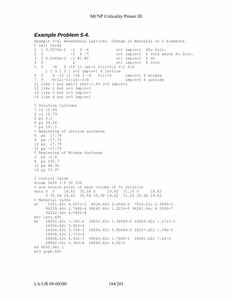
MCNP Criticality Primer III
LA-UR 09-00380 184/201
Example Problem 5-4. Example 5-4, Hexahedral Lattices. Change in Material in 2 elements. C Cell Cards 1 1 9.9270e-2 -1 5 -6 u=1 imp:n=1 $Pu Soln. 2 0 -1 6 -7 u=1 imp:n=1 $ void above Pu Soln. 3 2 8.6360e-2 -2 #1 #2 u=1 imp:n=1 $ SS 4 0 2 u=1 imp:n=1 $ void 5 0 -8 9 -10 11 lat=1 fill=0:2 0:1 0:0 1 1 3 1 3 1 u=2 imp:n=1 $ lattice 6 0 9 -12 11 -14 3 -4 fill=2 imp:n=1 $ window 7 0 -9:12:-11:14:-3:4 imp:n=0 $ outside 11 like 1 but mat=3 rho=-1.60 u=3 imp:n=1 12 like 2 but u=3 imp:n=1 13 like 3 but u=3 imp:n=1 14 like 4 but u=3 imp:n=1 C Solution Cylinder 1 cz 12.49 2 cz 12.79 5 pz 0.0 6 pz 39.24 7 pz 101.7 C Beginning of lattice surfaces 8 px 17.79 9 px -17.79 10 py 17.79 11 py -17.79 C Beginning of Window Surfaces 3 pz -1.0 4 pz 102.7 12 px 88.95 14 py 53.37 C Control Cards kcode 5000 1.0 50 250 c one source point in each volume of Pu Solution ksrc 0 0 19.62 35.58 0 19.62 71.16 0 19.62 0 35.58 19.62 35.58 35.58 19.62 71.16 35.58 19.62 C Material cards m1 1001.62c 6.0070-2 8016.62c 3.6540-2 7014.62c 2.3699-3 94239.66c 2.7682-4 94240.66c 1.2214-5 94241.66c 8.3390-7 94242.66c 4.5800-8 mt1 lwtr.60t m2 24050.62c 7.195-4 24052.62c 1.38589-2 24053.62c 1.5713-3 24054.62c 3.903-4 26056.62c 3.704-3 26056.62c 5.80869-2 26057.62c 1.342-3 26058.62c 1.773-4 28058.62c 4.432-3 28060.62c 1.7069-3 28061.62c 7.42-5 28062.62c 2.363-4 28064.62c 6.05-5 m3 6000.66c 1 mt3 grph.60t
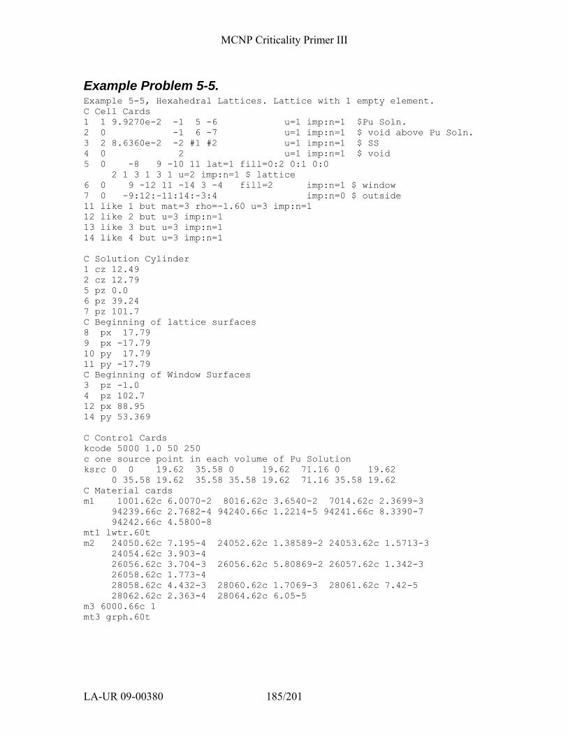
MCNP Criticality Primer III
LA-UR 09-00380 185/201
Example Problem 5-5. Example 5-5, Hexahedral Lattices. Lattice with 1 empty element. C Cell Cards 1 1 9.9270e-2 -1 5 -6 u=1 imp:n=1 $Pu Soln. 2 0 -1 6 -7 u=1 imp:n=1 $ void above Pu Soln. 3 2 8.6360e-2 -2 #1 #2 u=1 imp:n=1 $ SS 4 0 2 u=1 imp:n=1 $ void 5 0 -8 9 -10 11 lat=1 fill=0:2 0:1 0:0 2 1 3 1 3 1 u=2 imp:n=1 $ lattice 6 0 9 -12 11 -14 3 -4 fill=2 imp:n=1 $ window 7 0 -9:12:-11:14:-3:4 imp:n=0 $ outside 11 like 1 but mat=3 rho=-1.60 u=3 imp:n=1 12 like 2 but u=3 imp:n=1 13 like 3 but u=3 imp:n=1 14 like 4 but u=3 imp:n=1 C Solution Cylinder 1 cz 12.49 2 cz 12.79 5 pz 0.0 6 pz 39.24 7 pz 101.7 C Beginning of lattice surfaces 8 px 17.79 9 px -17.79 10 py 17.79 11 py -17.79 C Beginning of Window Surfaces 3 pz -1.0 4 pz 102.7 12 px 88.95 14 py 53.369 C Control Cards kcode 5000 1.0 50 250 c one source point in each volume of Pu Solution ksrc 0 0 19.62 35.58 0 19.62 71.16 0 19.62 0 35.58 19.62 35.58 35.58 19.62 71.16 35.58 19.62 C Material cards m1 1001.62c 6.0070-2 8016.62c 3.6540-2 7014.62c 2.3699-3 94239.66c 2.7682-4 94240.66c 1.2214-5 94241.66c 8.3390-7 94242.66c 4.5800-8 mt1 lwtr.60t m2 24050.62c 7.195-4 24052.62c 1.38589-2 24053.62c 1.5713-3 24054.62c 3.903-4 26056.62c 3.704-3 26056.62c 5.80869-2 26057.62c 1.342-3 26058.62c 1.773-4 28058.62c 4.432-3 28060.62c 1.7069-3 28061.62c 7.42-5 28062.62c 2.363-4 28064.62c 6.05-5 m3 6000.66c 1 mt3 grph.60t
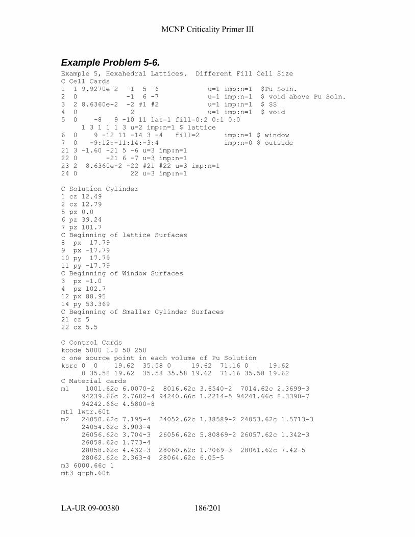
MCNP Criticality Primer III
LA-UR 09-00380 186/201
Example Problem 5-6. Example 5, Hexahedral Lattices. Different Fill Cell Size C Cell Cards 1 1 9.9270e-2 -1 5 -6 u=1 imp:n=1 $Pu Soln. 2 0 -1 6 -7 u=1 imp:n=1 $ void above Pu Soln. 3 2 8.6360e-2 -2 #1 #2 u=1 imp:n=1 $ SS 4 0 2 u=1 imp:n=1 $ void 5 0 -8 9 -10 11 lat=1 fill=0:2 0:1 0:0 1 3 1 1 1 3 u=2 imp:n=1 $ lattice 6 0 9 -12 11 -14 3 -4 fill=2 imp:n=1 $ window 7 0 -9:12:-11:14:-3:4 imp:n=0 $ outside 21 3 -1.60 -21 5 -6 u=3 imp:n=1 22 0 -21 6 -7 u=3 imp:n=1 23 2 8.6360e-2 -22 #21 #22 u=3 imp:n=1 24 0 22 u=3 imp:n=1 C Solution Cylinder 1 cz 12.49 2 cz 12.79 5 pz 0.0 6 pz 39.24 7 pz 101.7 C Beginning of lattice Surfaces 8 px 17.79 9 px -17.79 10 py 17.79 11 py -17.79 C Beginning of Window Surfaces 3 pz -1.0 4 pz 102.7 12 px 88.95 14 py 53.369 C Beginning of Smaller Cylinder Surfaces 21 cz 5 22 cz 5.5 C Control Cards kcode 5000 1.0 50 250 c one source point in each volume of Pu Solution ksrc 0 0 19.62 35.58 0 19.62 71.16 0 19.62 0 35.58 19.62 35.58 35.58 19.62 71.16 35.58 19.62 C Material cards m1 1001.62c 6.0070-2 8016.62c 3.6540-2 7014.62c 2.3699-3 94239.66c 2.7682-4 94240.66c 1.2214-5 94241.66c 8.3390-7 94242.66c 4.5800-8 mt1 lwtr.60t m2 24050.62c 7.195-4 24052.62c 1.38589-2 24053.62c 1.5713-3 24054.62c 3.903-4 26056.62c 3.704-3 26056.62c 5.80869-2 26057.62c 1.342-3 26058.62c 1.773-4 28058.62c 4.432-3 28060.62c 1.7069-3 28061.62c 7.42-5 28062.62c 2.363-4 28064.62c 6.05-5 m3 6000.66c 1 mt3 grph.60t
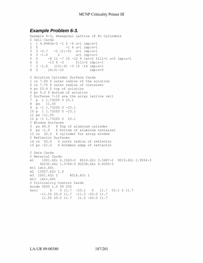
MCNP Criticality Primer III
LA-UR 09-00380 187/201
Example Problem 6-3. Example 6-3, Hexagonal Lattice of Pu Cylinders C Cell Cards 1 1 9.8983e-2 -1 5 -4 u=1 imp:n=1 2 0 -1 4 u=1 imp:n=1 3 2 -2.7 -2 (1:-5) u=1 imp:n=1 4 3 -1.0 2 u=1 imp:n=1 5 0 -8 11 -7 10 -12 9 lat=2 fill=1 u=2 imp:n=1 6 0 -13 6 -3 fill=2 imp:n=1 7 3 -1.0 (13:-6) -3 15 -14 imp:n=1 8 0 14:3:-15 imp:n=0 C Solution Cylinder Surface Cards 1 cz 7.60 $ outer radius of the solution 2 cz 7.75 $ outer radius of container 4 pz 23.4 $ top of solution 5 pz 0.0 $ bottom of solution C Surfaces 7-12 are the array lattice cell 7 p 1 1.73205 0 23.1 8 px 11.55 9 p -1 1.73205 0 -23.1 10 p 1 1.73205 0 -23.1 11 px -11.55 12 p -1 1.73205 0 23.1 C Window Surfaces 3 pz 40.0 $ Top of aluminum cylinder 6 pz -1.0 $ bottom of aluminum container 13 cz 32.0 $ cylinder for array window C Reflector Surfaces 14 cz 52.0 $ outer radius of reflector 15 pz -21.0 $ botmmon edge of reflector C Data Cards C Material Cards m1 1001.62c 6.1063-2 8016.62c 3.3487-2 9019.62c 2.9554-3 92235.66c 1.3784-3 92238.66c 9.9300-5 mt1 lwtr.60t m2 13027.62c 1.0 m3 1001.62c 2 8016.62c 1 mt3 lwtr.60t C Criticality Control Cards kcode 5000 1.0 50 250 ksrc 0 0 11.7 -23.1 0 11.7 23.1 0 11.7 -11.55 20.0 11.7 -11.5 -20.0 11.7 11.55 20.0 11.7 11.5 -20.0 11.7
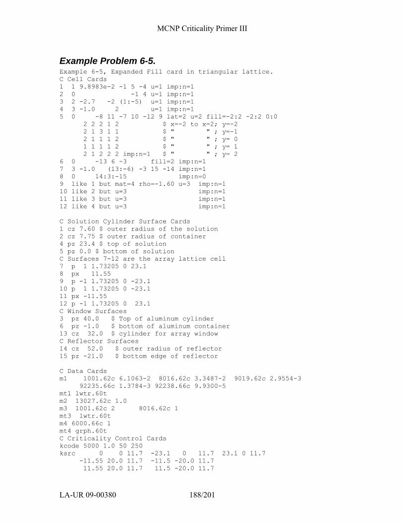
MCNP Criticality Primer III
LA-UR 09-00380 188/201
Example Problem 6-5. Example 6-5, Expanded Fill card in triangular lattice. C Cell Cards 1 1 9.8983e-2 -1 5 -4 u=1 imp:n=1 2 0 -1 4 u=1 imp:n=1 3 2 -2.7 -2 (1:-5) u=1 imp:n=1 4 3 -1.0 2 u=1 imp:n=1 5 0 -8 11 -7 10 -12 9 lat=2 u=2 fill=-2:2 -2:2 0:0 2 2 2 1 2 $ x=-2 to x=2; y=-2 2 1 3 1 1 $ " " ; y=-1 2 1 1 1 2 $ " " ; y= 0 1 1 1 1 2 $ " " ; y= 1 2 1 2 2 2 imp:n=1 $ " " ; y= 2 6 0 -13 6 -3 fill=2 imp:n=1 7 3 -1.0 (13:-6) -3 15 -14 imp:n=1 8 0 14:3:-15 imp:n=0 9 like 1 but mat=4 rho=-1.60 u=3 imp:n=1 10 like 2 but u=3 imp:n=1 11 like 3 but u=3 imp:n=1 12 like 4 but u=3 imp:n=1 C Solution Cylinder Surface Cards 1 cz 7.60 $ outer radius of the solution 2 cz 7.75 $ outer radius of container 4 pz 23.4 $ top of solution 5 pz 0.0 $ bottom of solution C Surfaces 7-12 are the array lattice cell 7 p 1 1.73205 0 23.1 8 px 11.55 9 p -1 1.73205 0 -23.1 10 p 1 1.73205 0 -23.1 11 px -11.55 12 p -1 1.73205 0 23.1 C Window Surfaces 3 pz 40.0 $ Top of aluminum cylinder 6 pz -1.0 $ bottom of aluminum container 13 cz 32.0 $ cylinder for array window C Reflector Surfaces 14 cz 52.0 $ outer radius of reflector 15 pz -21.0 $ bottom edge of reflector C Data Cards m1 1001.62c 6.1063-2 8016.62c 3.3487-2 9019.62c 2.9554-3 92235.66c 1.3784-3 92238.66c 9.9300-5 mt1 lwtr.60t m2 13027.62c 1.0 m3 1001.62c 2 8016.62c 1 mt3 lwtr.60t m4 6000.66c 1 mt4 grph.60t C Criticality Control Cards kcode 5000 1.0 50 250 ksrc 0 0 11.7 -23.1 0 11.7 23.1 0 11.7 -11.55 20.0 11.7 -11.5 -20.0 11.7 11.55 20.0 11.7 11.5 -20.0 11.7
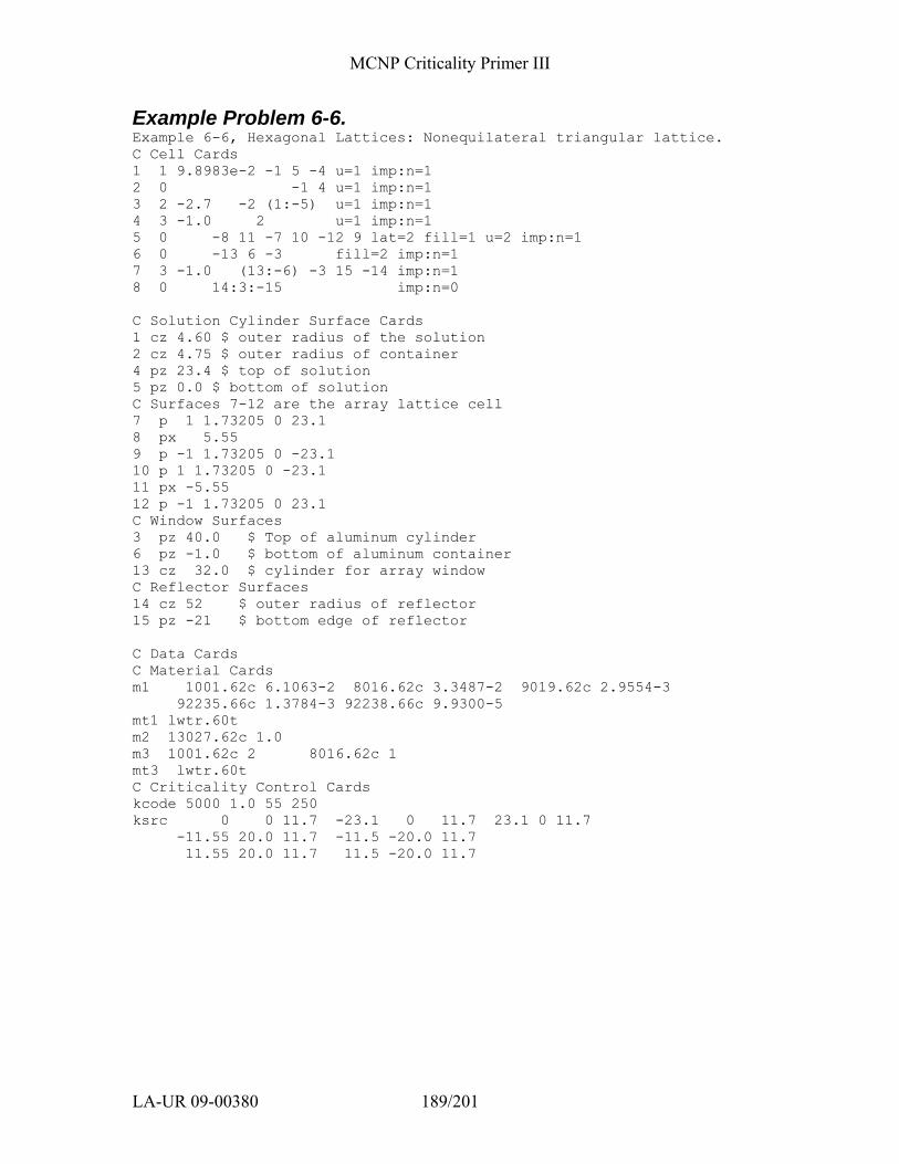
MCNP Criticality Primer III
LA-UR 09-00380 189/201
Example Problem 6-6. Example 6-6, Hexagonal Lattices: Nonequilateral triangular lattice. C Cell Cards 1 1 9.8983e-2 -1 5 -4 u=1 imp:n=1 2 0 -1 4 u=1 imp:n=1 3 2 -2.7 -2 (1:-5) u=1 imp:n=1 4 3 -1.0 2 u=1 imp:n=1 5 0 -8 11 -7 10 -12 9 lat=2 fill=1 u=2 imp:n=1 6 0 -13 6 -3 fill=2 imp:n=1 7 3 -1.0 (13:-6) -3 15 -14 imp:n=1 8 0 14:3:-15 imp:n=0 C Solution Cylinder Surface Cards 1 cz 4.60 $ outer radius of the solution 2 cz 4.75 $ outer radius of container 4 pz 23.4 $ top of solution 5 pz 0.0 $ bottom of solution C Surfaces 7-12 are the array lattice cell 7 p 1 1.73205 0 23.1 8 px 5.55 9 p -1 1.73205 0 -23.1 10 p 1 1.73205 0 -23.1 11 px -5.55 12 p -1 1.73205 0 23.1 C Window Surfaces 3 pz 40.0 $ Top of aluminum cylinder 6 pz -1.0 $ bottom of aluminum container 13 cz 32.0 $ cylinder for array window C Reflector Surfaces 14 cz 52 $ outer radius of reflector 15 pz -21 $ bottom edge of reflector C Data Cards C Material Cards m1 1001.62c 6.1063-2 8016.62c 3.3487-2 9019.62c 2.9554-3 92235.66c 1.3784-3 92238.66c 9.9300-5 mt1 lwtr.60t m2 13027.62c 1.0 m3 1001.62c 2 8016.62c 1 mt3 lwtr.60t C Criticality Control Cards kcode 5000 1.0 55 250 ksrc 0 0 11.7 -23.1 0 11.7 23.1 0 11.7 -11.55 20.0 11.7 -11.5 -20.0 11.7 11.55 20.0 11.7 11.5 -20.0 11.7
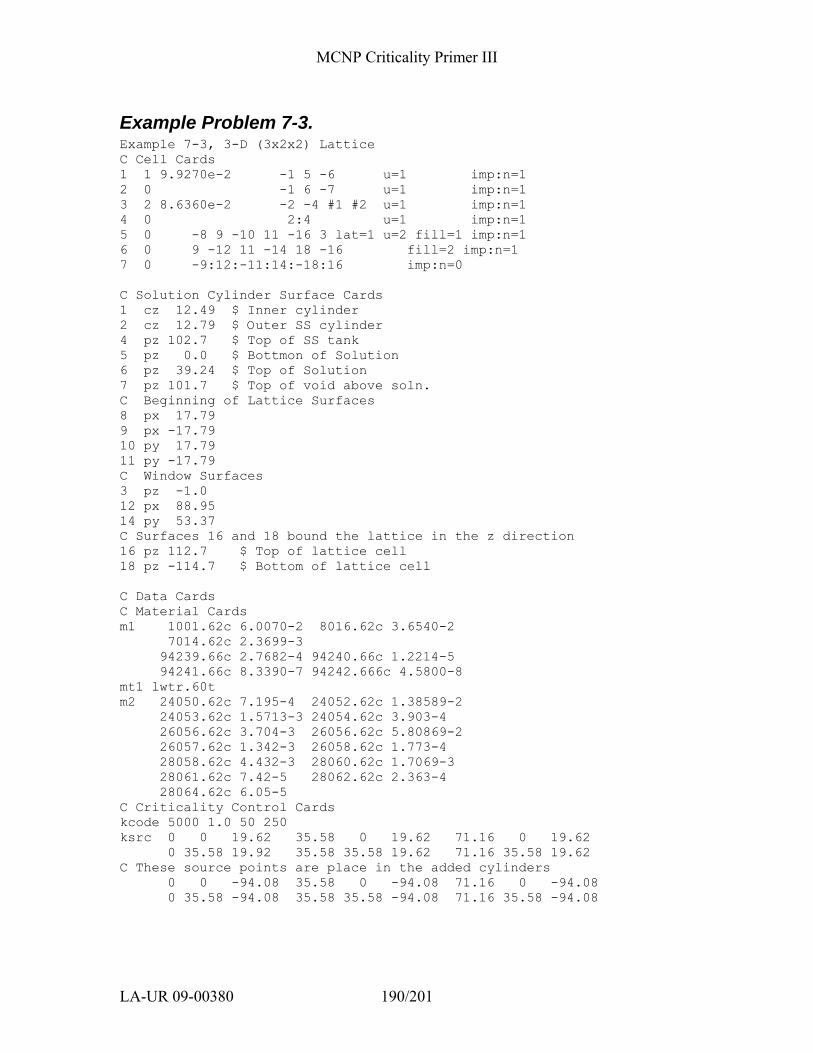
MCNP Criticality Primer III
LA-UR 09-00380 190/201
Example Problem 7-3. Example 7-3, 3-D (3x2x2) Lattice C Cell Cards 1 1 9.9270e-2 -1 5 -6 u=1 imp:n=1 2 0 -1 6 -7 u=1 imp:n=1 3 2 8.6360e-2 -2 -4 #1 #2 u=1 imp:n=1 4 0 2:4 u=1 imp:n=1 5 0 -8 9 -10 11 -16 3 lat=1 u=2 fill=1 imp:n=1 6 0 9 -12 11 -14 18 -16 fill=2 imp:n=1 7 0 -9:12:-11:14:-18:16 imp:n=0 C Solution Cylinder Surface Cards 1 cz 12.49 $ Inner cylinder 2 cz 12.79 $ Outer SS cylinder 4 pz 102.7 $ Top of SS tank 5 pz 0.0 $ Bottmon of Solution 6 pz 39.24 $ Top of Solution 7 pz 101.7 $ Top of void above soln. C Beginning of Lattice Surfaces 8 px 17.79 9 px -17.79 10 py 17.79 11 py -17.79 C Window Surfaces 3 pz -1.0 12 px 88.95 14 py 53.37 C Surfaces 16 and 18 bound the lattice in the z direction 16 pz 112.7 $ Top of lattice cell 18 pz -114.7 $ Bottom of lattice cell C Data Cards C Material Cards m1 1001.62c 6.0070-2 8016.62c 3.6540-2 7014.62c 2.3699-3 94239.66c 2.7682-4 94240.66c 1.2214-5 94241.66c 8.3390-7 94242.666c 4.5800-8 mt1 lwtr.60t m2 24050.62c 7.195-4 24052.62c 1.38589-2 24053.62c 1.5713-3 24054.62c 3.903-4 26056.62c 3.704-3 26056.62c 5.80869-2 26057.62c 1.342-3 26058.62c 1.773-4 28058.62c 4.432-3 28060.62c 1.7069-3 28061.62c 7.42-5 28062.62c 2.363-4 28064.62c 6.05-5 C Criticality Control Cards kcode 5000 1.0 50 250 ksrc 0 0 19.62 35.58 0 19.62 71.16 0 19.62 0 35.58 19.92 35.58 35.58 19.62 71.16 35.58 19.62 C These source points are place in the added cylinders 0 0 -94.08 35.58 0 -94.08 71.16 0 -94.08 0 35.58 -94.08 35.58 35.58 -94.08 71.16 35.58 -94.08
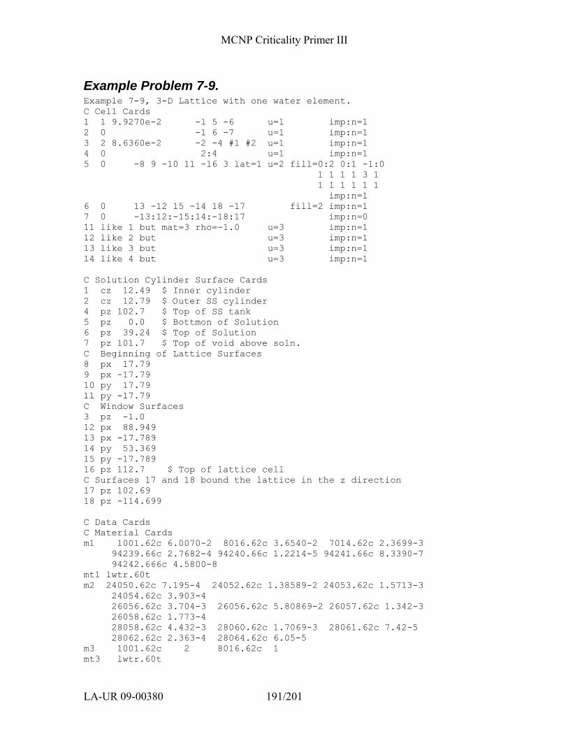
MCNP Criticality Primer III
LA-UR 09-00380 191/201
Example Problem 7-9. Example 7-9, 3-D Lattice with one water element. C Cell Cards 1 1 9.9270e-2 -1 5 -6 u=1 imp:n=1 2 0 -1 6 -7 u=1 imp:n=1 3 2 8.6360e-2 -2 -4 #1 #2 u=1 imp:n=1 4 0 2:4 u=1 imp:n=1 5 0 -8 9 -10 11 -16 3 lat=1 u=2 fill=0:2 0:1 -1:0 1 1 1 1 3 1 1 1 1 1 1 1 imp:n=1 6 0 13 -12 15 -14 18 -17 fill=2 imp:n=1 7 0 -13:12:-15:14:-18:17 imp:n=0 11 like 1 but mat=3 rho=-1.0 u=3 imp:n=1 12 like 2 but u=3 imp:n=1 13 like 3 but u=3 imp:n=1 14 like 4 but u=3 imp:n=1 C Solution Cylinder Surface Cards 1 cz 12.49 $ Inner cylinder 2 cz 12.79 $ Outer SS cylinder 4 pz 102.7 $ Top of SS tank 5 pz 0.0 $ Bottmon of Solution 6 pz 39.24 $ Top of Solution 7 pz 101.7 $ Top of void above soln. C Beginning of Lattice Surfaces 8 px 17.79 9 px -17.79 10 py 17.79 11 py -17.79 C Window Surfaces 3 pz -1.0 12 px 88.949 13 px -17.789 14 py 53.369 15 py -17.789 16 pz 112.7 $ Top of lattice cell C Surfaces 17 and 18 bound the lattice in the z direction 17 pz 102.69 18 pz -114.699 C Data Cards C Material Cards m1 1001.62c 6.0070-2 8016.62c 3.6540-2 7014.62c 2.3699-3 94239.66c 2.7682-4 94240.66c 1.2214-5 94241.66c 8.3390-7 94242.666c 4.5800-8 mt1 lwtr.60t m2 24050.62c 7.195-4 24052.62c 1.38589-2 24053.62c 1.5713-3 24054.62c 3.903-4 26056.62c 3.704-3 26056.62c 5.80869-2 26057.62c 1.342-3 26058.62c 1.773-4 28058.62c 4.432-3 28060.62c 1.7069-3 28061.62c 7.42-5 28062.62c 2.363-4 28064.62c 6.05-5 m3 1001.62c 2 8016.62c 1 mt3 lwtr.60t
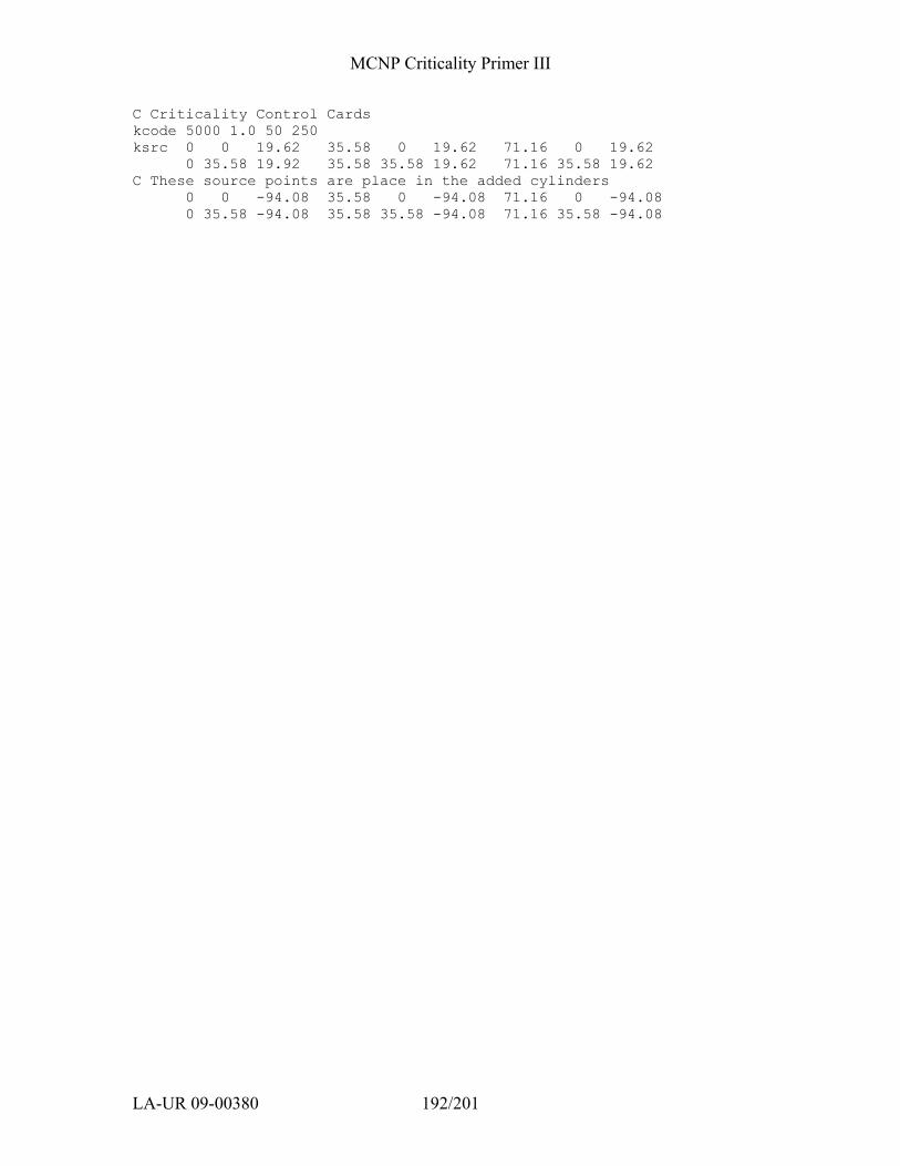
MCNP Criticality Primer III
LA-UR 09-00380 192/201
C Criticality Control Cards kcode 5000 1.0 50 250 ksrc 0 0 19.62 35.58 0 19.62 71.16 0 19.62 0 35.58 19.92 35.58 35.58 19.62 71.16 35.58 19.62 C These source points are place in the added cylinders 0 0 -94.08 35.58 0 -94.08 71.16 0 -94.08 0 35.58 -94.08 35.58 35.58 -94.08 71.16 35.58 -94.08
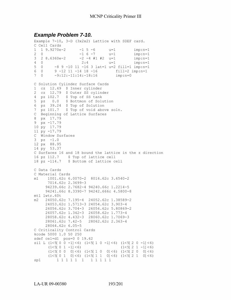
MCNP Criticality Primer III
LA-UR 09-00380 193/201
Example Problem 7-10. Example 7-10, 3-D (3x2x2) Lattice with SDEF card. C Cell Cards 1 1 9.9270e-2 -1 5 -6 u=1 imp:n=1 2 0 -1 6 -7 u=1 imp:n=1 3 2 8.6360e-2 -2 -4 #1 #2 u=1 imp:n=1 4 0 2:4 u=1 imp:n=1 5 0 -8 9 -10 11 -16 3 lat=1 u=2 fill=1 imp:n=1 6 0 9 -12 11 -14 18 -16 fill=2 imp:n=1 7 0 -9:12:-11:14:-18:16 imp:n=0 C Solution Cylinder Surface Cards 1 cz 12.49 $ Inner cylinder 2 cz 12.79 $ Outer SS cylinder 4 pz 102.7 $ Top of SS tank 5 pz 0.0 $ Bottmon of Solution 6 pz 39.24 $ Top of Solution 7 pz 101.7 $ Top of void above soln. C Beginning of Lattice Surfaces 8 px 17.79 9 px -17.79 10 py 17.79 11 py -17.79 C Window Surfaces 3 pz -1.0 12 px 88.95 14 py 53.37 C Surfaces 16 and 18 bound the lattice in the z direction 16 pz 112.7 $ Top of lattice cell 18 pz -114.7 $ Bottom of lattice cell C Data Cards C Material Cards m1 1001.62c 6.0070-2 8016.62c 3.6540-2 7014.62c 2.3699-3 94239.66c 2.7682-4 94240.66c 1.2214-5 94241.66c 8.3390-7 94242.666c 4.5800-8 mt1 lwtr.60t m2 24050.62c 7.195-4 24052.62c 1.38589-2 24053.62c 1.5713-3 24054.62c 3.903-4 26056.62c 3.704-3 26056.62c 5.80869-2 26057.62c 1.342-3 26058.62c 1.773-4 28058.62c 4.432-3 28060.62c 1.7069-3 28061.62c 7.42-5 28062.62c 2.363-4 28064.62c 6.05-5 C Criticality Control Cards kcode 5000 1.0 50 250 sdef cel=d1 pos=0 0 19.62 si1 L (1<5[0 0 -1]<6) (1<5[1 0 -1]<6) (1<5[2 0 -1]<6) (1<5[0 1 -1]<6) (1<5[2 1 -1]<6) (1<5[0 0 0]<6) (1<5[1 0 0]<6) (1<5[2 0 0]<6) (1<5[0 1 0]<6) (1<5[1 1 0]<6) (1<5[2 1 0]<6) sp1 1 1 1 1 1 1 1 1 1 1 1
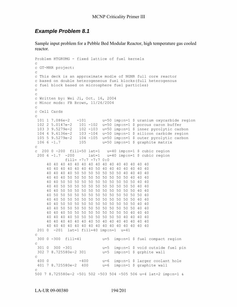
MCNP Criticality Primer III
LA-UR 09-00380 194/201
Example Problem 8.1 Sample input problem for a Pebble Bed Modular Reactor, high temperature gas cooled reactor. Problem HTGRUMG - fixed lattice of fuel kernels c c GT-MHR project: c c This deck is an approximate modle of NGNR full core reactor c based on double heterogeneous fuel blocks(full heterogenous c fuel block based on microsphere fuel particles) c c c Written by: Wei Ji, Oct. 16, 2004 c Minor mods: FB Brown, 11/26/2004 c c Cell Cards c 101 1 7.086e-2 -101 u=50 imp:n=1 $ uranium oxycarbide region 102 2 5.0147e-2 101 -102 u=50 imp:n=1 $ porous caron buffer 103 3 9.5279e-2 102 -103 u=50 imp:n=1 $ inner pyrolytic carbon 104 4 9.6136e-2 103 -104 u=50 imp:n=1 $ silicon carbide region 105 5 9.5279e-2 104 -105 u=50 imp:n=1 $ outer pyrolytic carbon 106 6 -1.7 105 u=50 imp:n=1 $ graphite matrix c c 200 0 -200 fill=50 lat=1 u=40 imp:n=1 $ cubic region 200 6 -1.7 -200 lat=1 u=40 imp:n=1 $ cubic region fill= -7:7 -7:7 0:0 40 40 40 40 40 40 40 40 40 40 40 40 40 40 40 40 40 40 40 40 40 40 50 40 40 40 40 40 40 40 40 40 40 40 50 50 50 50 50 50 50 40 40 40 40 40 40 40 50 50 50 50 50 50 50 50 50 40 40 40 40 40 50 50 50 50 50 50 50 50 50 50 50 40 40 40 40 50 50 50 50 50 50 50 50 50 50 50 40 40 40 40 50 50 50 50 50 50 50 50 50 50 50 40 40 40 50 50 50 50 50 50 50 50 50 50 50 50 50 40 40 40 50 50 50 50 50 50 50 50 50 50 50 40 40 40 40 50 50 50 50 50 50 50 50 50 50 50 40 40 40 40 50 50 50 50 50 50 50 50 50 50 50 40 40 40 40 40 50 50 50 50 50 50 50 50 50 40 40 40 40 40 40 40 50 50 50 50 50 50 50 40 40 40 40 40 40 40 40 40 40 40 50 40 40 40 40 40 40 40 40 40 40 40 40 40 40 40 40 40 40 40 40 40 40 201 0 -201 lat=1 fill=40 imp:n=1 u=41 c 300 0 -300 fill=41 u=5 imp:n=1 $ fuel compact region c 301 0 300 -301 u=5 imp:n=1 $ void outside fuel pin 302 7 8.725580e-2 301 u=5 imp:n=1 $ grphite wall c 400 0 -400 u=6 imp:n=1 $ larger coolant hole 401 7 8.725580e-2 400 u=6 imp:n=1 $ graphite wall c 500 7 8.725580e-2 -501 502 -503 504 -505 506 u=4 lat=2 imp:n=1 &
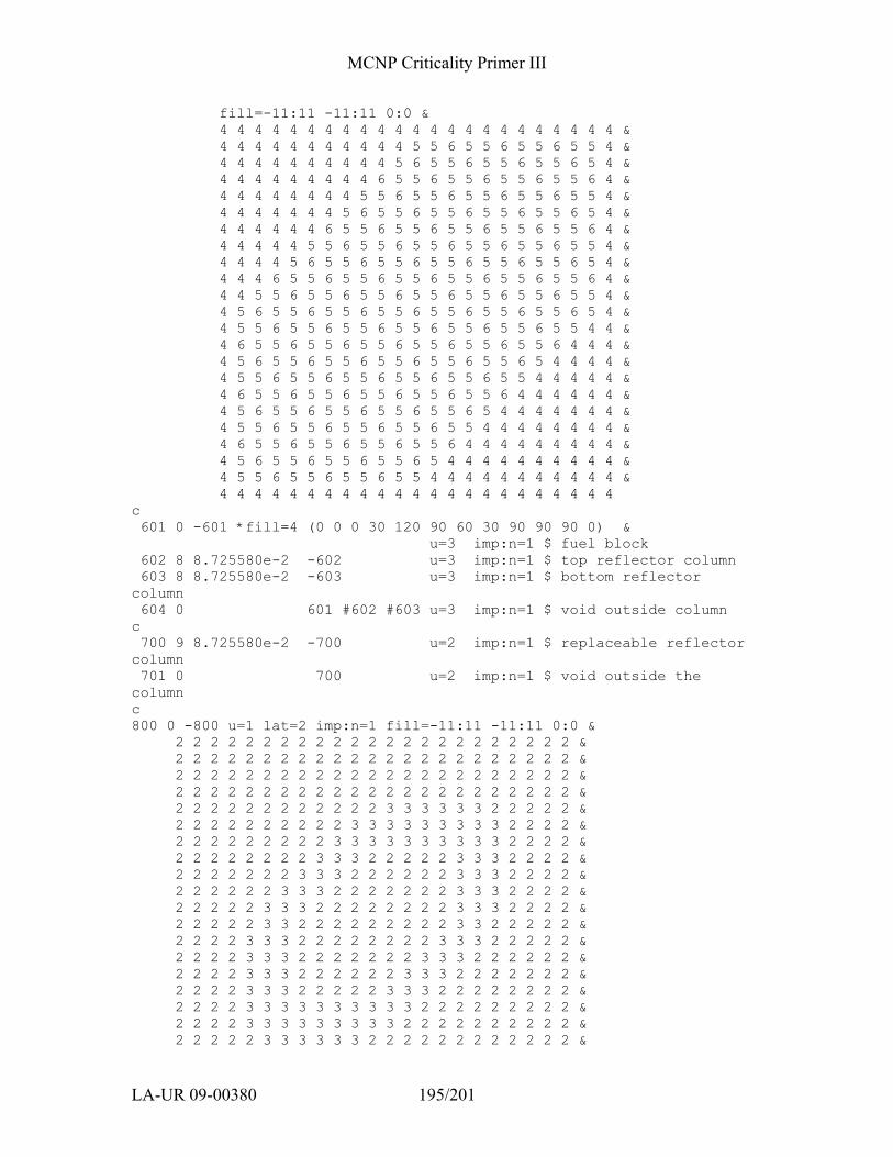
MCNP Criticality Primer III
LA-UR 09-00380 195/201
fill=-11:11 -11:11 0:0 & 4 4 4 4 4 4 4 4 4 4 4 4 4 4 4 4 4 4 4 4 4 4 4 & 4 4 4 4 4 4 4 4 4 4 4 5 5 6 5 5 6 5 5 6 5 5 4 & 4 4 4 4 4 4 4 4 4 4 5 6 5 5 6 5 5 6 5 5 6 5 4 & 4 4 4 4 4 4 4 4 4 6 5 5 6 5 5 6 5 5 6 5 5 6 4 & 4 4 4 4 4 4 4 4 5 5 6 5 5 6 5 5 6 5 5 6 5 5 4 & 4 4 4 4 4 4 4 5 6 5 5 6 5 5 6 5 5 6 5 5 6 5 4 & 4 4 4 4 4 4 6 5 5 6 5 5 6 5 5 6 5 5 6 5 5 6 4 & 4 4 4 4 4 5 5 6 5 5 6 5 5 6 5 5 6 5 5 6 5 5 4 & 4 4 4 4 5 6 5 5 6 5 5 6 5 5 6 5 5 6 5 5 6 5 4 & 4 4 4 6 5 5 6 5 5 6 5 5 6 5 5 6 5 5 6 5 5 6 4 & 4 4 5 5 6 5 5 6 5 5 6 5 5 6 5 5 6 5 5 6 5 5 4 & 4 5 6 5 5 6 5 5 6 5 5 6 5 5 6 5 5 6 5 5 6 5 4 & 4 5 5 6 5 5 6 5 5 6 5 5 6 5 5 6 5 5 6 5 5 4 4 & 4 6 5 5 6 5 5 6 5 5 6 5 5 6 5 5 6 5 5 6 4 4 4 & 4 5 6 5 5 6 5 5 6 5 5 6 5 5 6 5 5 6 5 4 4 4 4 & 4 5 5 6 5 5 6 5 5 6 5 5 6 5 5 6 5 5 4 4 4 4 4 & 4 6 5 5 6 5 5 6 5 5 6 5 5 6 5 5 6 4 4 4 4 4 4 & 4 5 6 5 5 6 5 5 6 5 5 6 5 5 6 5 4 4 4 4 4 4 4 & 4 5 5 6 5 5 6 5 5 6 5 5 6 5 5 4 4 4 4 4 4 4 4 & 4 6 5 5 6 5 5 6 5 5 6 5 5 6 4 4 4 4 4 4 4 4 4 & 4 5 6 5 5 6 5 5 6 5 5 6 5 4 4 4 4 4 4 4 4 4 4 & 4 5 5 6 5 5 6 5 5 6 5 5 4 4 4 4 4 4 4 4 4 4 4 & 4 4 4 4 4 4 4 4 4 4 4 4 4 4 4 4 4 4 4 4 4 4 4 c 601 0 -601 *fill=4 (0 0 0 30 120 90 60 30 90 90 90 0) & u=3 imp:n=1 $ fuel block 602 8 8.725580e-2 -602 u=3 imp:n=1 $ top reflector column 603 8 8.725580e-2 -603 u=3 imp:n=1 $ bottom reflector column 604 0 601 #602 #603 u=3 imp:n=1 $ void outside column c 700 9 8.725580e-2 -700 u=2 imp:n=1 $ replaceable reflector column 701 0 700 u=2 imp:n=1 $ void outside the column c 800 0 -800 u=1 lat=2 imp:n=1 fill=-11:11 -11:11 0:0 & 2 2 2 2 2 2 2 2 2 2 2 2 2 2 2 2 2 2 2 2 2 2 2 & 2 2 2 2 2 2 2 2 2 2 2 2 2 2 2 2 2 2 2 2 2 2 2 & 2 2 2 2 2 2 2 2 2 2 2 2 2 2 2 2 2 2 2 2 2 2 2 & 2 2 2 2 2 2 2 2 2 2 2 2 2 2 2 2 2 2 2 2 2 2 2 & 2 2 2 2 2 2 2 2 2 2 2 2 3 3 3 3 3 3 2 2 2 2 2 & 2 2 2 2 2 2 2 2 2 2 3 3 3 3 3 3 3 3 3 2 2 2 2 & 2 2 2 2 2 2 2 2 2 3 3 3 3 3 3 3 3 3 3 2 2 2 2 & 2 2 2 2 2 2 2 2 3 3 3 2 2 2 2 2 3 3 3 2 2 2 2 & 2 2 2 2 2 2 2 3 3 3 2 2 2 2 2 2 3 3 3 2 2 2 2 & 2 2 2 2 2 2 3 3 3 2 2 2 2 2 2 2 3 3 3 2 2 2 2 & 2 2 2 2 2 3 3 3 2 2 2 2 2 2 2 2 3 3 3 2 2 2 2 & 2 2 2 2 2 3 3 2 2 2 2 2 2 2 2 2 3 3 2 2 2 2 2 & 2 2 2 2 3 3 3 2 2 2 2 2 2 2 2 3 3 3 2 2 2 2 2 & 2 2 2 2 3 3 3 2 2 2 2 2 2 2 3 3 3 2 2 2 2 2 2 & 2 2 2 2 3 3 3 2 2 2 2 2 2 3 3 3 2 2 2 2 2 2 2 & 2 2 2 2 3 3 3 2 2 2 2 2 3 3 3 2 2 2 2 2 2 2 2 & 2 2 2 2 3 3 3 3 3 3 3 3 3 3 2 2 2 2 2 2 2 2 2 & 2 2 2 2 3 3 3 3 3 3 3 3 3 2 2 2 2 2 2 2 2 2 2 & 2 2 2 2 2 3 3 3 3 3 3 2 2 2 2 2 2 2 2 2 2 2 2 &
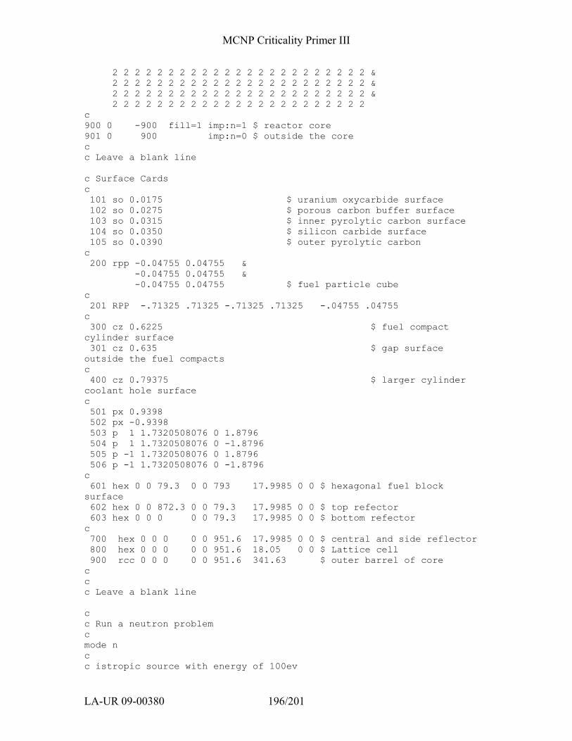
MCNP Criticality Primer III
LA-UR 09-00380 196/201
2 2 2 2 2 2 2 2 2 2 2 2 2 2 2 2 2 2 2 2 2 2 2 & 2 2 2 2 2 2 2 2 2 2 2 2 2 2 2 2 2 2 2 2 2 2 2 & 2 2 2 2 2 2 2 2 2 2 2 2 2 2 2 2 2 2 2 2 2 2 2 & 2 2 2 2 2 2 2 2 2 2 2 2 2 2 2 2 2 2 2 2 2 2 2 c 900 0 -900 fill=1 imp:n=1 $ reactor core 901 0 900 imp:n=0 $ outside the core c c Leave a blank line c Surface Cards c 101 so 0.0175 $ uranium oxycarbide surface 102 so 0.0275 $ porous carbon buffer surface 103 so 0.0315 $ inner pyrolytic carbon surface 104 so 0.0350 $ silicon carbide surface 105 so 0.0390 $ outer pyrolytic carbon c 200 rpp -0.04755 0.04755 & -0.04755 0.04755 & -0.04755 0.04755 $ fuel particle cube c 201 RPP -.71325 .71325 -.71325 .71325 -.04755 .04755 c 300 cz 0.6225 $ fuel compact cylinder surface 301 cz 0.635 $ gap surface outside the fuel compacts c 400 cz 0.79375 $ larger cylinder coolant hole surface c 501 px 0.9398 502 px -0.9398 503 p 1 1.7320508076 0 1.8796 504 p 1 1.7320508076 0 -1.8796 505 p -1 1.7320508076 0 1.8796 506 p -1 1.7320508076 0 -1.8796 c 601 hex 0 0 79.3 0 0 793 17.9985 0 0 $ hexagonal fuel block surface 602 hex 0 0 872.3 0 0 79.3 17.9985 0 0 $ top refector 603 hex 0 0 0 0 0 79.3 17.9985 0 0 $ bottom refector c 700 hex 0 0 0 0 0 951.6 17.9985 0 0 $ central and side reflector 800 hex 0 0 0 0 0 951.6 18.05 0 0 $ Lattice cell 900 rcc 0 0 0 0 0 951.6 341.63 $ outer barrel of core c c c Leave a blank line c c Run a neutron problem c mode n c c istropic source with energy of 100ev
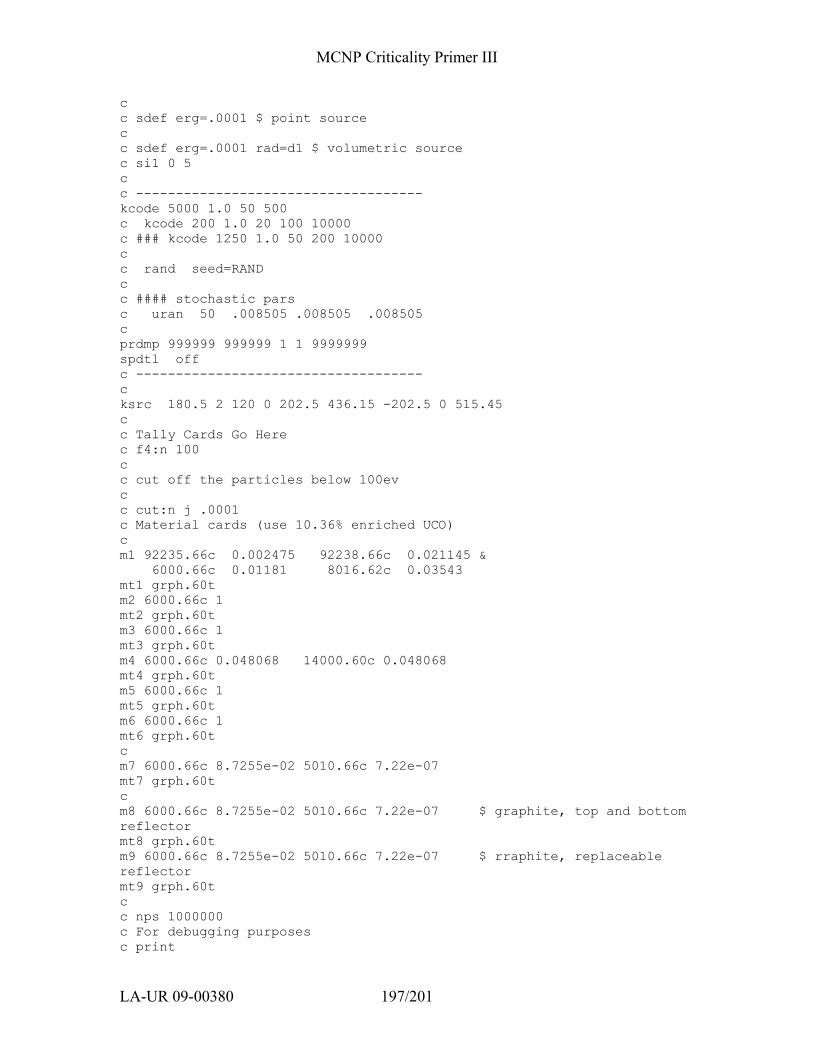
MCNP Criticality Primer III
LA-UR 09-00380 197/201
c c sdef erg=.0001 $ point source c c sdef erg=.0001 rad=d1 $ volumetric source c si1 0 5 c c ------------------------------------ kcode 5000 1.0 50 500 c kcode 200 1.0 20 100 10000 c ### kcode 1250 1.0 50 200 10000 c c rand seed=RAND c c #### stochastic pars c uran 50 .008505 .008505 .008505 c prdmp 999999 999999 1 1 9999999 spdtl off c ------------------------------------ c ksrc 180.5 2 120 0 202.5 436.15 -202.5 0 515.45 c c Tally Cards Go Here c f4:n 100 c c cut off the particles below 100ev c c cut:n j .0001 c Material cards (use 10.36% enriched UCO) c m1 92235.66c 0.002475 92238.66c 0.021145 & 6000.66c 0.01181 8016.62c 0.03543 mt1 grph.60t m2 6000.66c 1 mt2 grph.60t m3 6000.66c 1 mt3 grph.60t m4 6000.66c 0.048068 14000.60c 0.048068 mt4 grph.60t m5 6000.66c 1 mt5 grph.60t m6 6000.66c 1 mt6 grph.60t c m7 6000.66c 8.7255e-02 5010.66c 7.22e-07 mt7 grph.60t c m8 6000.66c 8.7255e-02 5010.66c 7.22e-07 $ graphite, top and bottom reflector mt8 grph.60t m9 6000.66c 8.7255e-02 5010.66c 7.22e-07 $ rraphite, replaceable reflector mt9 grph.60t c c nps 1000000 c For debugging purposes c print
MCNP Criticality Primer III
LA-UR 09-00380 198/201
Appendix H: Overview of the MCNP Visual Editor Computer L.L. Carter and R.A. Schwarz
Background The Monte Carlo N-Particle (MCNP) Visual Editor (References 1-9) was developed to help users of the MCNP code view and create MCNP input files. Work on the Visual Editor started around 1992. Starting with Version 5 of MCNP, the Visual Editor is included with the release of the MCNP package. The Visual Editor is a graphical interface written in C++ that is linked directly to the MCNP Fortran code. Thus the Visual Editor contains all of MCNP inside the executable. When running the Visual Editor, it is not using the MCNP you have installed on your system but is using the MCNP internally compiled into the code. Additional information on the Visual Editor can be found in the references, especially the manual supplied with MCNP Version 5 (Reference 8).
Display Capabilities The Visual Editor provides a graphical interface for viewing the geometry, using the basic plotting capabilities within MCNP. This allows the user to change the view by selecting the origin, extent and basis and to show cell labels. The graphical user interface also incorporates the tally plotting features of MCNP contained in the MCPLOT package. This will allow the user to plot tally and cross section data. The Visual Editor includes some advanced visualization options including a 3D ray tracing option, a 3D radiography option, and the ability to project source points and collision points onto the plot plane and also source generation points for a KCODE calculation. For these advanced options the Visual Editor is running the internal version of MCNP, this means the input file must be a valid input file that does not produce any fatal errors. The Visual Editor also has an input window that will show the complete contents of the input file. If the user changes the input by hand and then chooses the “Save - Update” option in the input window menu the plot views will be updated to show the changes.

MCNP Criticality Primer III
LA-UR 09-00380 199/201
Creation Capabilities Along with the display capabilities outlined above, the Visual Editor provides a number of different aids for creating an MCNP geometry. The Visual Editor allows the user to create surfaces, which show up as infinite surfaces in the plot window. The user can then create cells from these infinite surfaces, by dragging across the surfaces that bound the cell and then selecting the inside region of the cell to get the proper sense for the surfaces. Additional aids exist for creating and editing rectangular and hex lattices. The Visual Editor also supports the use of fills and universes. The Visual Editor supports all data cards and allows the enhanced creation and modification of materials, transformations and importances. For the creation of materials, the Visual Editor reads the xsdir file for the MCNP set up on the computer to determine the set of isotopes available for creating materials. The Visual Editor then allows the user to select the isotopes that make up the material and specify the mass or atom fractions to create a new material. Materials can be store in a material library so that any input file that is read into the Visual Editor can access them. For importances, the user can set the importance for each cell by clicking on the cell in the plot window with the mouse. Additionally the user can drag the mouse across a number of cells and set the importance in all the cells that have been dragged across. The importance can be set to a specific value or it can be set to increase by a user specified factor for each cell in the drag to set the importance to increase in a uniform fashion.
Installation Notes
With release 5 the Visual Editor is only available on Windows platforms. For most applications, the Visual Editor executable can be used as distributed. If you want to have access to the material libraries, you need to create a “vised.defaults” file indicating the location of the material library files. The size of the fonts used by the windows are fixed and can not be changed. The font used is called “small fonts”. If the Visual Editor windows appear too large for your screen, it is recommended that you increase your screen resolution. The ideal screen resolution is 1280x1024. The development of the Windows Visual Editor is done on a Windows 2000 platform. For best performance, it is recommended that users run the Visual Editor in Windows 2000 or Windows XP. Table 1 below lists the different operating systems and what is
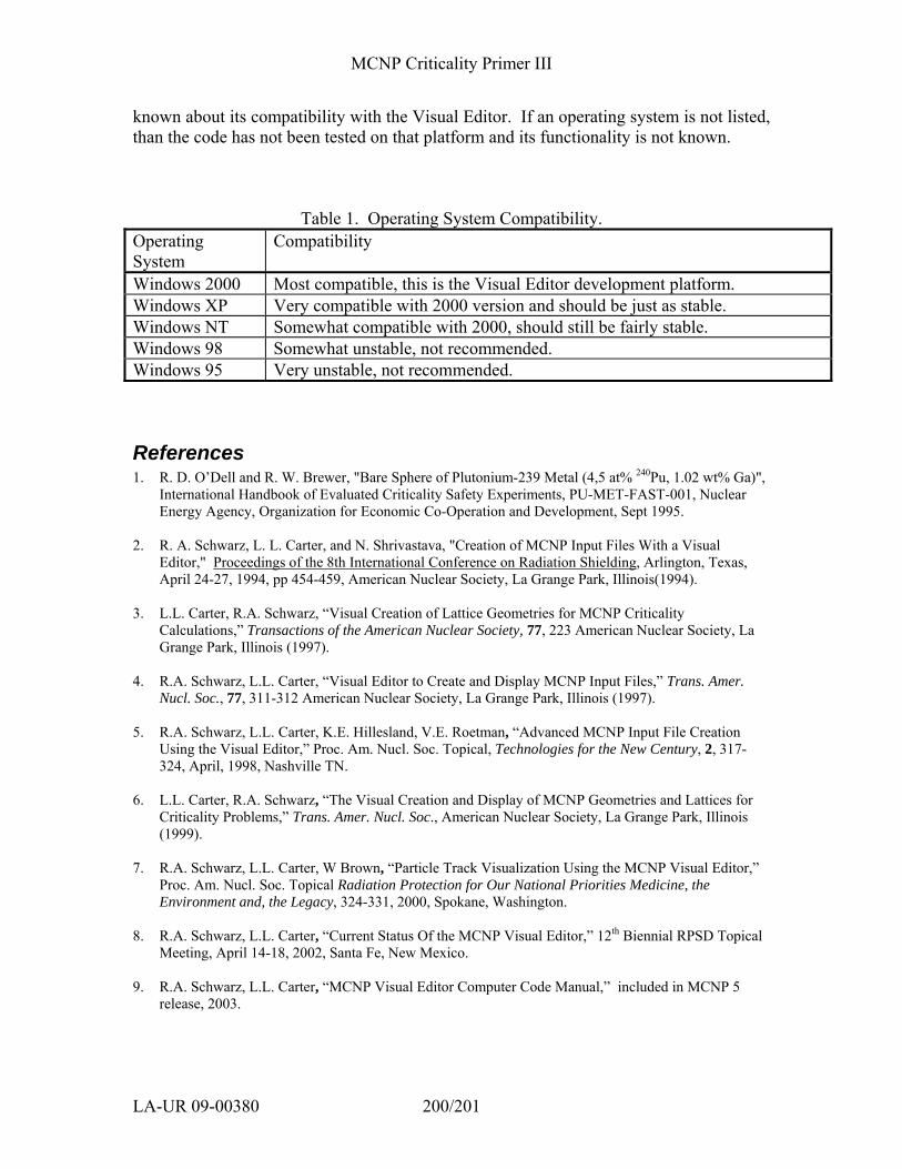
MCNP Criticality Primer III
LA-UR 09-00380 200/201
known about its compatibility with the Visual Editor. If an operating system is not listed, than the code has not been tested on that platform and its functionality is not known.
Table 1. Operating System Compatibility. Operating System
Compatibility
Windows 2000 Most compatible, this is the Visual Editor development platform. Windows XP Very compatible with 2000 version and should be just as stable. Windows NT Somewhat compatible with 2000, should still be fairly stable. Windows 98 Somewhat unstable, not recommended. Windows 95 Very unstable, not recommended.
References 1. R. D. O’Dell and R. W. Brewer, "Bare Sphere of Plutonium-239 Metal (4,5 at% 240Pu, 1.02 wt% Ga)",
International Handbook of Evaluated Criticality Safety Experiments, PU-MET-FAST-001, Nuclear Energy Agency, Organization for Economic Co-Operation and Development, Sept 1995.
2. R. A. Schwarz, L. L. Carter, and N. Shrivastava, "Creation of MCNP Input Files With a Visual
Editor," Proceedings of the 8th International Conference on Radiation Shielding, Arlington, Texas, April 24-27, 1994, pp 454-459, American Nuclear Society, La Grange Park, Illinois(1994).
3. L.L. Carter, R.A. Schwarz, “Visual Creation of Lattice Geometries for MCNP Criticality
Calculations,” Transactions of the American Nuclear Society, 77, 223 American Nuclear Society, La Grange Park, Illinois (1997).
4. R.A. Schwarz, L.L. Carter, “Visual Editor to Create and Display MCNP Input Files,” Trans. Amer.
Nucl. Soc., 77, 311-312 American Nuclear Society, La Grange Park, Illinois (1997). 5. R.A. Schwarz, L.L. Carter, K.E. Hillesland, V.E. Roetman, “Advanced MCNP Input File Creation
Using the Visual Editor,” Proc. Am. Nucl. Soc. Topical, Technologies for the New Century, 2, 317-324, April, 1998, Nashville TN.
6. L.L. Carter, R.A. Schwarz, “The Visual Creation and Display of MCNP Geometries and Lattices for
Criticality Problems,” Trans. Amer. Nucl. Soc., American Nuclear Society, La Grange Park, Illinois (1999).
7. R.A. Schwarz, L.L. Carter, W Brown, “Particle Track Visualization Using the MCNP Visual Editor,”
Proc. Am. Nucl. Soc. Topical Radiation Protection for Our National Priorities Medicine, the Environment and, the Legacy, 324-331, 2000, Spokane, Washington.
8. R.A. Schwarz, L.L. Carter, “Current Status Of the MCNP Visual Editor,” 12th Biennial RPSD Topical
Meeting, April 14-18, 2002, Santa Fe, New Mexico. 9. R.A. Schwarz, L.L. Carter, “MCNP Visual Editor Computer Code Manual,” included in MCNP 5
release, 2003.

MCNP Criticality Primer III
LA-UR 09-00380 201/201
10. A.L. Schwarz, R.A. Schwarz, L.L. Carter, “3D Plotting Capabilities in the Visual Editor for Release 5 of MCNP,” Nuclear Mathematical and Computational Sciences: A Century in Review, A Century Anew, April 6-11, 2003 on CD-ROM, American Nuclear Society, La Grange Park, Illinois (2003)