The Spitzer Space Telescope First-Look Survey:

KPNO MOSAIC-1 R-band Images and Source Catalogs

Dario Fadda1, Buell T. Jannuzi2, Alyson Ford2, Lisa J. Storrie-Lombardi1

[January, 2004 – Submitted to AJ]

ABSTRACT

We present R-band images covering more than 11 square degrees of sky that were obtained inpreparation for the Spitzer Space Telescope First Look Survey (FLS). The FLS was designed tocharacterize the mid-infrared sky at depths 2 orders of magnitude deeper than previous surveys.The extragalactic component is the first cosmological survey done with Spitzer. Source catalogsextracted from the R-band images are also presented. The R-band images were obtained usingthe MOSAIC-1 camera on the Mayall 4m telescope of the Kitt Peak National Observatory. Tworelatively large regions of the sky were observed to modest depth: the main FLS extra galac-tic field (17h18m00s +59o30′00′′.0 J2000; l= 88.3, b= +34.9) and ELAIS-N1 field (16h10m01s

+54o30′36′′.0 J2000; l= 84.2, b= +44.9). While both of these fields were in early plans for theFLS, only a single deep pointing test observation were made at the ELAIS-N1 location. Thelarger Legacy program SWIRE (Lonsdale et al., 2003) will include this region among its sur-veyed areas. The data products of our KPNO imaging (images and object catalogs) are madeavailable to the community through the World Wide Web (via the Spitzer Science Center andNOAO Science Archives). The overall quality of the images is high. The measured positions ofsources detected in the images have RMS uncertainties in their absolute positions of order 0.35arc-seconds with possible systematic offsets of order 0.1 arc-seconds, depending on the referenceframe of comparison. The relative astrometric accuracy is much better than 0.1 of an arc-second.Typical delivered image quality in the images is 1.1 arc-seconds full width at half maximum. Im-ages are relatively deep since they reach a median 5σ depth limiting magnitude of R=25.5 (Vega),as measured within a 1.35 × FWHM aperture for which the S/N ratio is maximal. Catalogs havebeen extracted using SExtractor using thresholds in area and flux for which the number of falsedetections is below 1% at R=25. Only sources with S/N greater than 3 have been retained inthe final catalogs. Comparing the galaxy number counts from our images with those of deeperR-band surveys, we estimate that our observations are 50% complete at R=24.5. These limits indepth are sufficient to identify a substantial fraction of the infrared sources which will be detectedby Spitzer.

Subject headings: astronomical data bases:catalogs — galaxies: photometry

1Spitzer Science Center, California Institute of Technol-ogy, MS 220-6, Pasadena, CA 91125

2National Optical Astronomy Observatory, Tucson, AZ85719

1. Introduction

One of the main advantages of the Spitzer SpaceTelescope (formerly known as the Space InfraredInfrared Telescope Facility; SIRTF, Gallagher etal. 2003) is the possibility to make extragalacticsurveys of large regions of the sky in a relativelyshort time covering wavelengths from the near-IR

1

to the far-IR with the instruments IRAC (Fazioet al. 1998) and MIPS (Rieke et al. 1996). Com-pared to Spitzer’s predecessors (e.g. IRAS, Soiferet al. 1983, and ISO, Kessler et al. 1996), there areimprovements in the detectors (number of pixelsand better responsivity), the collecting area of theprimary mirror (85cm diameter), and Sun-Earth-Moon avoidance constraints due Spitzer’s helio-centric orbit. Spitzer can also make observationssimultaneously in multiple bands (with IRAC–3.6and 4.5 or 5.8 and 8 µm; with MIPS–24, 70 and160 µm).

Many extragalactic surveys are already sched-uled with Spitzer as Legacy programs (SWIRE,Lonsdale et al. 2003; GOODS, Dickinson &Giavalisco 2001) or as observations by the In-strument Teams (Wide, Deep and Ultra-DeepSpitzer surveys which will cover regions like theBootes field of the NOAO Deep Wide-Field Sur-vey, the Groth strip, Lockman Hole, XMM-Deepand so on, see e.g. Dole et al. 2001). The FirstLook Survey utilizes 112 hours of Director’s Dis-cretionary time on Spitzer and includes extra-galactic, galactic, and ecliptic components (seehttp://ssc.spitzer.caltech.edu/fls/). These datawill be available to all observers when the SpitzerScience Archive opens in May, 2004. The purposeof the FLS is to characterize the mid-infraredsky at previously unexplored depths and makethese data rapidly available to the astronomicalcommunity. The extragalactic component is com-prised of a 4 square degree survey with IRACand MIPS near the north ecliptic pole centered atJ1718+5930. These observations were executedon Spitzer December 1-11, 2003.

To fully exploit the Spitzer FLS data we haveobtained ancillary surveys at optical (this paper)and radio wavelengths (Condon et al. 2003).Given the modest spatial resolution of the Spitzer

imagers (the point spread function is large, espe-cially in the mid and far-IR, e.g. 5.7 arcsecondsfull width at half maximum, FWHM, for the 24µm channel), the first problem to solve for theinfrared sources detected by Spitzer will be to as-sociate these sources with an optical counterpart,when possible. This will then allow the higherspatial resolution of the available optical imagesto assist with the source classification (e.g. asstars, galaxies or QSO) and enable targeting ofsubsets of the sources for spectroscopy with opti-

cal or near-IR spectrographs. Since many of theinfrared sources that will be detected by Spitzer

will be dust-obscured galaxies with faint opticalcounterparts, the complementary optical imagingmust be relatively deep.

Although a deep multi-wavelength optical sur-vey would be more useful, allowing one to com-pute photometric redshifts (e.g. the NOAO DeepWide-Field Survey, Jannuzi and Dey 1999, Brownet al. 2003), the task of deeply covering a largeregion of sky in a homogeneous manner is quitetime-consuming. Therefore, for the initial opti-cal ancillary survey we chose to observe the entirefield in the R-band. NOAO provided 4 nights ofDirector’s Discretionary time on the KPNO 4min May, 2000, for this survey. We have limitedmulti-wavelength optical observations to the cen-tral portion of the FLS field. The Sloan DigitalSky Survey included the FLS field in their earlyrelease observations (Stoughton et al. 2002) andmosaics and catalogs for the region are also nowavailable (Hogg et al. 2004).

In this paper, we present the R-band optical ob-servations made with the MOSAIC-1 camera onthe Mayall 4m Telescope of Kitt Peak NationalObservatory. Centered on the main FLS field, aregion 9.4 square degrees in area was imaged. Inaddition, 2.3 square degrees covering the ELAIS-N1 field was also observed. Although originallythe ELAIS-N1 field was planned to be part of theFLS program, the FLS observations of the ELAIS-N1 field have now been revised to a very deep10’×10’ pointing to evaluate the confusion lim-its of the MIPS instrument. The remainder ofthe ELAIS-N1 field will now be imaged as partof a larger survey in this region, a portion of theSWIRE Spitzer Legacy Survey (Lonsdale et al.,2003).

In section 2 we review the overall observingstrategy and describe the MOSAIC-1 observa-tions. In section 3 we discuss the techniques usedin the data reduction including the astrometricand photometric calibration of the images. Wedescribe in section 4 the data products made pub-licly available. We detail in section 5 the criteriaused to detect, classify, and photometrically mea-sure objects in the images. Section 5 also includesa description of the information available in ourcatalogs. In section 6 we examine the quality ofthe imaging data by comparing them with other

2

available data sets. Finally, a brief summary isgiven in section 7.

2. Observations

The optical observations of the FLS region(centered at 17h18m00s +59o30′00′′, J2000) andof the ELAIS-N1 region (centered at 16h10m01s

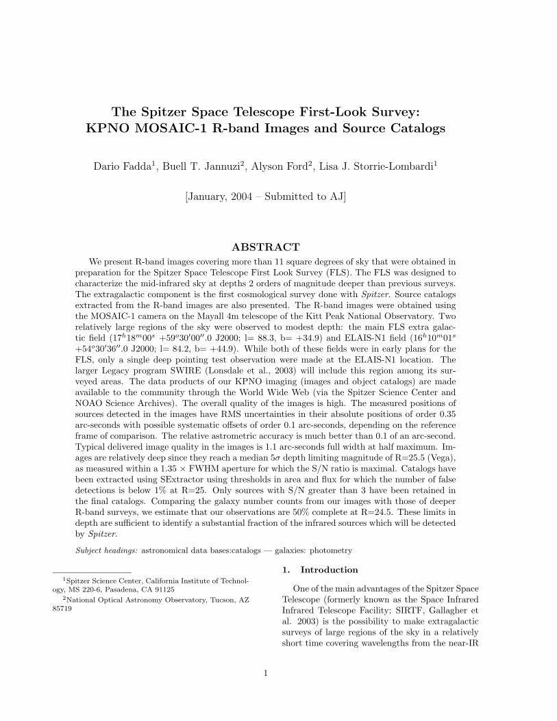
+54o30′36′′, J2000, see Oliver et al. 2000) werecarried out using the MOSAIC-1 camera on theMayall 4m Telescope at the Kitt Peak NationalObservatory. The MOSAIC-1 camera is comprisedof eight thinned, back-illuminated SITe 2048 ×4098 CCDs with a projected pixel size of 0.258arcsec (Muller et al. 1998). The 8 CCDs are phys-ically separated by gaps with widths of approxi-mately 14 and 15.5 arcsec along the right ascen-sion and declination directions, respectively. Thefull field of view of the camera is therefore 36 × 36square arcmin, with a filling factor of 97%. Ob-servations were performed using the Harris SetKron-Cousins R-band filter whose main featuresare summarized in Table 1. The transmissioncurve of the filter is shown in Figure 1 togetherwith the resulting modifications that would be in-troduced by the corrector and camera optics, theCCD quantum efficiency, and atmospheric extinc-tion.

For organizational purposes we chose to dividethe proposed FLS survey region into 30 subfieldseach roughly the size of an individual MOSAIC-1pointing. The coordinates of these subfields arelisted in Table 2. During our observing run wewere able to complete observations for 26 of thesesubfields. We similarly divided the ELAIS-N1 fieldinto 12 subfields, but only completed observationsfor 5 of these fields. Each subfield was observed fora minimum of three 10 min exposures. In practice,some images were not suitable (poor seeing, flatfielding problem, or some other defect) and werenot included in the final coadded or “stacked” im-ages we are providing to the community. Table 2lists in Col. 4 the number of exposures which wereobtained and included in the coadded or “stacked”images. In order to provide some coverage in theregions of the sky that would fall in the inter-chipgaps, the positions of successive exposures of agiven field were offset on order of an arcminuterelative to each other. In general the first expo-sure was at the nominal (tabulated) position, the

Fig. 1.— Transmission curve of the R-band fil-ter (solid line) used for the observations. Thedashed line indicates the combined response whenconsidering also the CCD quantum efficiency, thethroughput of the prime focus corrector, and theatmospheric absorption with a typical airmass of1.2.

second shifted by 41.5′ in α and −62.3′ in δ, andthe third with a shift of −41.5′ and 62.3′ in αand δ. In a few cases an additional position with∆α = 20.8′ and ∆β = 31.1′ has been observed.For a few fields, observations have been repeateddue to the bad seeing or pointing errors.

The KPNO imaging observations were made onMay 4-7,9 2000 UT. A log of the observations issummarized in Table 3, which lists for each groupof observations: the date of the observations (Col.1); the subfield name (Col.2); the integration timeand the number of exposures (Col. 3); and the see-ing (delivered image quality expressed as FWHMin arcseconds of bright unsaturated stars) range ofeach exposure (Col. 4).

During a portion of the observing run, thepointing of the telescope was incorrectly initial-ized, resulting in approximately a 24′ error inthe pointing for some fields. These are noted inthe observing log. Since the 24′ offset did notmap exactly on to our subfield grid, we chose to

3

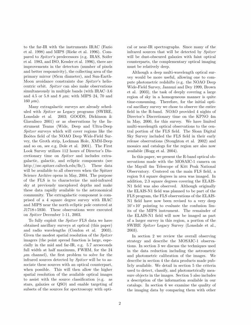
Fig. 2.— The KPNO fields in the FLS region covermost of the MIPS (grey) and IRAC (dark grey)Spitzer observations.

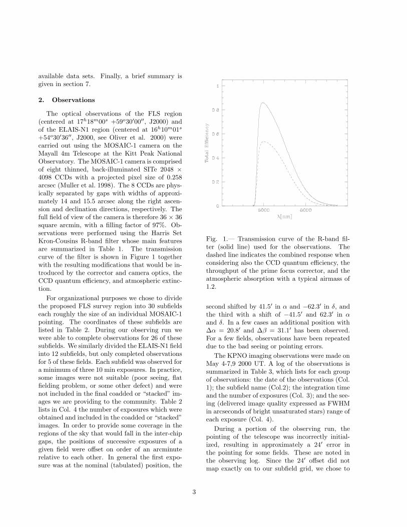
make stacked or combined images for several ofthe subfields. This was done for subfields # 11and # 17 in the FLS region and subfields (# 6,# 9 and # 10) of ELAIS-N1. In Figures 2 and 3we show the positions of each subfield on the skywith respect to the fields which have been coveredwith the IRAC and MIPS instruments on-boardSpitzer. In Figure 3 we display the position ofthe subfields in the ELAIS-N1 region and the re-gion observed with ISOCAM as part of the Euro-pean Large Area ISO Survey (ELAIS, Oliver et al.2000). The shaded square indicates the area whichhas been observed to test the confusion MIPS 24micron confusion limits, as part of the FLS obser-vations.

3. Data Reduction

3.1. Basic Reductions

The processing of the rawMOSAIC-1 exposuresfollowed the steps outlined in version 7.01 of “TheNOAO Deep Wide-Field Survey MOSAIC DataReductions Guide”3 and discussed by Jannuzi et

3www.noao.edu/noao/noaodeep/ReductionOpt/frames.html

al. (in preparation). The bulk of the softwareused to process the images and generate combinedimages for each subfield from the individual 10minute exposures is described by Valdes (2002)and contained as part of the MSCRED softwarepackage (v4.7), which is part of IRAF.4

The image quality of the final stacks is variable,as was the seeing during the run. Users of the im-ages should be aware that the detailed shape ofthe point spread function in a given image stackcould be variable across the field, not only becauseof residual distortions in the camera, but becausea given position in the field might be the aver-age of different input images, each with their ownpoint spread function. No attempt was made tomatch the PSFs of the individual images before

4IRAF is distributed by the National Optical AstronomyObservatory, which is operated by the Association of Uni-versities for Research in Astronomy, Inc., under a cooper-ative agreement with the National Science Foundation

Fig. 3.— The KPNO fields in the ELAIS-N1 re-gion. The dashed line corresponds to the regionobserved by ISOCAM at 14.3 µm (Oliver et al.2000). The grey shaded square is the field ob-served with Spitzer to test the MIPS 24 micronconfusion limit. The SWIRE planned field (Lons-dale et al. 2003) is marked with a dash-dottedline.

4

combining the images.

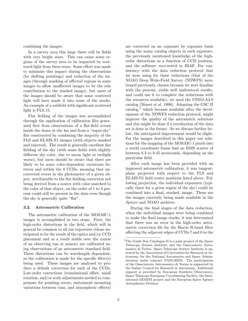
In a survey area this large there will be fieldswith very bright stars. This can cause some re-gions of the survey area to be impacted by scat-tered light from these stars. Some effort was madeto minimize this impact during the observations(by shifting pointings) and reduction of the im-ages (through masking of affected regions in someimages to allow unaffected images to be the solecontribution to the stacked image), but users ofthe images should be aware that some scatteredlight will have made it into some of the stacks.An example of a subfield with significant scatteredlight is FLS 15.

Flat fielding of the images was accomplishedthrough the application of calibration files gener-ated first from observations of a flat-field screeninside the dome at the 4m and from a “super-sky”flat constructed by combining the majority of theFLS and ELAIS-N1 images (with objects maskedand rejected). The result is generally excellent flatfielding of the sky (with some fields with slightlydifferent sky color, due to moon light or twilightworse), but users should be aware that there arelikely to be some color-dependent variations be-tween and within the 8 CCDs, meaning that un-corrected errors in the photometry of a given ob-ject, attributable to the flat fielding correction notbeing derived from a source with color matched tothe color of that object, on the order of 1 to 3 per-cent could still be present in the data even thoughthe sky is generally quite “flat”.

3.2. Astrometric Calibration

The astrometric calibration of the MOSAIC-1images is accomplished in two steps. First, thehigh-order distortions in the field, which will ingeneral be common to all our exposures (those an-ticipated to be the result of the optics and/or CCDplacement and as a result stable over the courseof an observing run or season) are calibrated us-ing observations of an astrometric standard field.These distortions can be wavelength dependent,so the calibration is made for the specific filter(s)being used. These images are analyzed to pro-duce a default correction for each of the CCDs.Low-order corrections (translational offset, smallrotation, and/or scale adjustments needed to com-pensate for pointing errors, instrument mountingvariations between runs, and atmospheric effects)

are corrected on an exposure by exposure basisusing the many catalog objects in each exposure,the previously mentioned knowledge of the high-order distortions as a function of CCD position,and the software msccmatch in IRAF. For con-sistency with the data reduction protocol thatwe were using for these reductions (that of theNOAO Deep Wide-Field Survey (NDWFS) men-tioned previously, chosen because we were familiarwith the process, yields well understood results,and could use it to complete the reductions withthe resources available), we used the USNO-A2.0catalog (Monet et al. 1998). Adopting the GSC IIcatalog,5 which became available after the devel-opment of the NDWFS reduction protocol, mightimprove the quality of the astrometric solutionsand this might be done if a rereduction of the dataset is done in the future. As we discuss further be-low, the anticipated improvement would be slight.For the images described in this paper our solu-tions for the mapping of the MOSAIC-1 pixels intoa world coordinate frame had an RMS scatter ofbetween 0.3 to 0.45 arcseconds, depending on theparticular field.

After each image has been provided with animproved astrometric calibration, it was tangent-plane projected with respect to the FLS andELAIS-N1 field center positions listed above. Fol-lowing projection, the individual exposures (typi-cally three for a given region of the sky) could becombined into a final, stacked, image. These arethe images currently being made available in theSpitzer and NOAO archives.

During the final stages of the data reduction,when the individual images were being combinedto make the final image stacks, it was determinedthat there was an error in the high-order astro-metric correction file for the Harris R-band filteraffecting the adjacent edges of CCDs 7 and 8 in the

5The Guide Star Catalogue-II is a joint project of the SpaceTelescope Science Institute and the Osservatorio Astro-nomico di Torino. Space Telescope Science Institute is op-erated by the Association of Universities for Research in As-tronomy, for the National Aeronautics and Space Admin-istration under contract NAS5-26555. The participationof the Osservatorio Astronomico di Torino is supported bythe Italian Council for Research in Astronomy. Additionalsupport is provided by European Southern Observatory,Space Telescope European Coordinating Facility, the Inter-national GEMINI project and the European Space AgencyAstrophysics Division.

5

MOSAIC-1 camera. The original solutions for thehigh order distortion terms were determined on achip by chip basis with no requirement that thesolution be continuous across the entire field. Ingeneral, while this requirement was not imposed,it was met by the solutions provided by NOAO.However, for the R-band the solution available atthe time we were reducing the data was discon-tinuous at the CCD7 and CCD8 boundary. Sinceour image stacks are made from the combinationof three or more images that are offset by 30 arc-seconds to an arcminute from each other, this dif-ference between the solutions for the two CCDscan result in a mis-mapping, into RA and DECspace, of a region of the sky imaged first on CCD7and then on CCD8. The error is small, and intro-duces at most an additional 0.1′′ uncertainty to thepositions of sources in the affected region (whichis located in the SE Corner of each field, about25% of the field up from the southern edge), butwill result in a degradation of the PSF for objectsaffected in this region. The size of the affectedregion in each subfield is approximately 8.5′ East-West and 2.5′ North-South, or a bit less than 2%of the surveyed area.

3.3. Photometric calibration

Since not all the subfields were observed duringnights with photometric conditions, we derived acoherent photometric system in two steps. First,we computed the relative photometric zero-pointsbetween the different stacked images of the sub-fields. Since each subfield overlaps its neighborby approximately two arcminutes, we can esti-mate the extinction difference between them usinga set of common sources. This can be expressedin terms of zero-point that, by definition, includesthe effects of airmass and extinction. Because eachframe has multiple overlaps, the number of frame-to-frame magnitude differences is over-determinedwith respect to the number of frames. There-fore, one can derive the relative zero-point for eachframe simultaneously using a least squares estima-tor. We extracted the sources from each subfieldusing as a first guess for the zero-point that wecomputed for a central subfield (#18 and #5 forthe FLS and ELAIS-N1 fields, respectively). Foreach overlap between contiguous fields, we selectedthe pairs of stars with magnitude 18 < R < 21 andcomputed the median of the difference in mag-

nitudes by using a 3σ clipping procedure. Themagnitudes considered were the auto magnitudes(MAG AUTO) from SExtractor, which are fairlyrobust with respect to seeing variations. To esti-mate the relative zero-points in the sense of theleast squares, we minimized the sum:

∑

i>j

N2ij(zi − zj −∆ij)

2, (1)

where zi is the variation with respect to the ini-tial guess of the zero-point of the subfield i, and∆ij is the median of the differences of magnitudefor the set of the Nij source pairs in the overlap-ping region between the subfields i and j. Solvingthe linear system obtained by imposing that thederivatives of (1) with respect each zi are equal tozero, we corrected the initial guesses for the zero-points. The procedure was then iterated until thenumber of pairs Nij became stable.

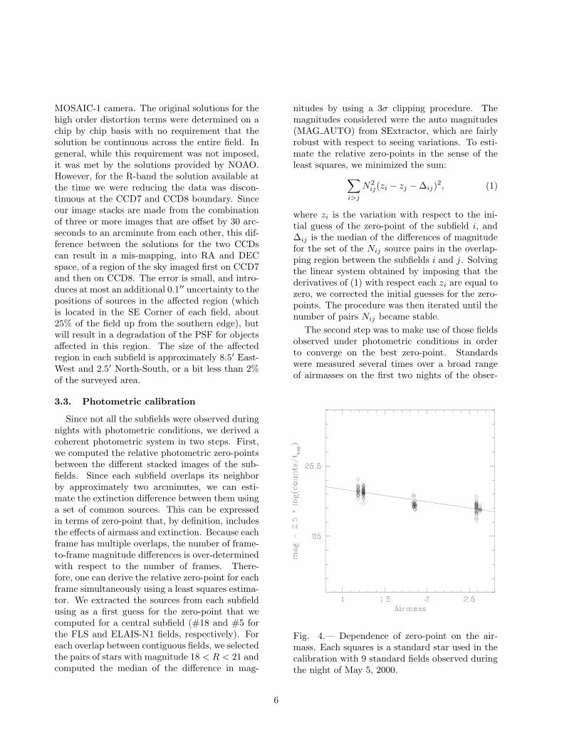
The second step was to make use of those fieldsobserved under photometric conditions in orderto converge on the best zero-point. Standardswere measured several times over a broad rangeof airmasses on the first two nights of the obser-

Fig. 4.— Dependence of zero-point on the air-mass. Each squares is a standard star used in thecalibration with 9 standard fields observed duringthe night of May 5, 2000.

6

vations, which had the best photometric condi-tions. Only the second night (May 5) was reallyphotometric since all the measurements are coher-ent (see Figure 4). Magnitudes were calibrated tothe Kron-Cousins system using Landolt standardstaken from Landolt (1992). They have been ob-tained using an aperture of 6 arcsec in diameter,large enough to obtain accurate measurements ac-cording to the growth curves of all the measuredstars. We have fitted the linear relationship:

m = m0 − 2.5 log(C/texp) +mX ∗A, (2)

with m magnitude of Landolt standard, A airmassduring the observation, C counts during the ex-posure time texp, m0 and mX the zero and ex-tinction terms, respectively. We used an iterative3σ clipping in order to discard deviant measure-ments, finding the best fit for m0 = 25.42 andmX = −0.09. The standard deviation of the resid-uals for the best fit is 0.03.

4. Data Products

The analysis of the survey data produced a setof intermediate and final products, images and cat-alogs, which are publicly available at the SpitzerScience Center and NOAO Science Archives6. Inparticular, we provide the astronomical commu-nity with:

Coadded (Stacked) Images of the Sub-fields: sky-subtracted, fully processed coaddedframes for each subfield. The subfields are mappedusing a tangential projection. The size of eachfits compressed image is 220 MB. For each image,a bad pixel mask and an exposure map is given(in the pixel-list IRAF format). The photomet-ric zero-point of each subfield after the absolutephotometric calibration of the frame appears inthe header of the image. A full description of theheader keywords is available at the http sites.

Low-resolution field image: sky-subtracted,fully processed coadded images of the whole field.The images have been created to give a generaloverview of the FLS and ELAIS-N1 fields and havebeen produced using a 1.3 arcsec pixel size (cor-responding to five times the original size of thepixel). Users are discouraged from using them to

6ssc.spitzer.caltech.edu/fls/extragal/noaor.html andwww.noao.edu

extract sources and compute photometry. Theseimages have a size of approximatively 380 Mb and80 Mb.

Single subfield catalogs: object catalogs as-sociated with each single subfield. A full descrip-tion of the parameters available is described in thefollowing Section. The catalogs are in ASCII for-mat.

5. Catalogs

The main goal of this survey is to catalog galax-ies and faint stars and make a first distinction be-tween stars and galaxies on the basis of their inten-sity profiles. Several bright objects (mainly stars)are saturated and excluded from the catalog, butcan be found in catalogs from shallower surveys(like the Sloan Digital Sky Survey in the case ofthe FLS region, see e.g. Stoughton et al. 2002and Hogg et al. 2004). The source extraction wasperformed with the SExtractor package (Bertin &Arnouts 1996; ver. 2.3) which is well suited forsurveys with low to moderate source density as isthe case of our surveys.

5.1. Detection

Several parameters have to be fixed to achievean efficient source extraction with SExtractor.The first problem is the evaluation of the back-ground. SExtractor proceeds computing a mini-

background on a scale large enough to contain sev-eral faint objects and filtering it with a box-car toavoid the contamination by isolated, extended ob-jects. Finally, a full-resolution background mapis obtained by interpolation and it is subtractedfrom the science image. In our case, many brightstars populate the FLS field since it has a moder-ate galactic latitude (34.9 degrees) while the prob-lem is less important in the case of the ELAIS-N1field (gal. latitude: 44.9 degrees). To evaluatea background which is not locally dominated bybright stars we adopted meshes of 128×128 pix-els for the mini-background corresponding to 33.0arcsec and used a 9×9 box-car for the median-filtering.

In order to improve the detection of faintsources, the image is filtered to enhance the spa-tial frequency typical of the sources with respectto those of the background noise. A Gaussianfilter with an FWHM similar to the seeing of the

7

image (in our case 4 pixels, since the overall seeingis 1.1) has been used. Although the choice of aconvolution kernel with a constant FWHM maynot always be optimal since the seeing is varyingin the different images, the impact on detectabilityis fairly small (Irwin 1985). Moreover, it has theadvantage of requiring no changes of the relativedetection threshold.

Finally, the detection is made on the background-subtracted and filtered image looking for groupsof connected pixel above the detection threshold.Thresholding is in fact the most efficient way todetect low surface brightness objects. In our case,we fixed the minimum number of connected pix-els to 15 and the detection threshold to 0.8 (inunits of the standard deviation of the backgroundnoise), which corresponds to a typical limiting sur-face brightness µR ∼ 26 mag arcsec−2. For thedetection we made use also of the exposure map asa weight considered to set the noise level for eachpixel. Some pixels have a null weight since theycorrespond to saturated objects, trails of brightobjects and other artifacts. These pixels are alsomarked in the bad pixel mask and the false detec-tions around these image artifacts are flagged andeasily excluded from our final catalogs.

Only objects detected with a signal-to-noisegreater than 3 (based on the total magnitude er-rors) are accepted in our final catalog.

Although not well suited to detect objects incrowded fields, SExtractor allows one also to de-blend close objects using a multiple isophotal anal-ysis technique. Two parameters affect the de-blending: the number of thresholds used to splita set of connected pixels according to their lumi-nosity peaks and the minimal contrast (light ina peak divided by the total light in the object)used to decide if deblending a sub-object from therest of the object. In our analysis we used a highnumber of thresholds (64) and a very low minimalcontrast (1.5 e−5). Nevertheless, a few blendedobjects still remain in the catalogs. Visual inspec-tion or other extraction algorithms more efficientin crowded fields (e.g, DAOPHOT) are needed totreat these particular cases.

5.2. Photometry

The photometry has been performed on thestacked images. Several measurements were made:

aperture and isophotal magnitudes and an esti-mate of the total magnitudes. We measured theaperture magnitude within a diameter of 3 arcsec,roughly corresponding to three times the overallseeing. Total magnitudes (MAG AUTO) are es-timated using an elliptical aperture with an ap-proach similar to that proposed by Kron (1980).Since these fields have been selected in sky regionswith low Galactic extinction to observe extragalac-tic infrared sources, the corrections for Galacticextinction (Schlegel et al. 1998) are small: 0.06and 0.01 on average for the FLS and ELAIS-N1fields, respectively.

The total magnitude of sources close to brightobjects are usually inaccurate since the local back-ground is affected by the halo of the bright objectsand the Kron radius is not correctly computed. Toimprove the photometry for these sources we havesubtracted bright saturated stars from the imagesand excluded from the catalogs the sources de-tected in square boxes around these stars wherethe subtraction is not correct. Moreover, we haveconsidered bright extended galaxies and excludedfrom the catalogs all the sources inside the Kron el-lipses of the galaxies. In fact, most of these sourcesare bright regions of the galaxies or their photom-etry is highly affected by the diffuse luminosity ofthe galaxies.

To subtract bright saturated stars from the im-ages we have computed radial density profiles onconcentric annuli around the stars. Then, aftersubtracting these profiles, we have removed thediffraction spikes by fitting their profiles along theradius at different angles with Chebyshev polyno-mials. As visible in Figures 5 and 6, the back-ground is much more uniform and the spikes be-come shorter. This improves the photometry forthe objects surrounding the stars and avoid thedetection of faint false sources on the diffractionspikes.

The correction works well for most of the stars,although we exclude from the catalogs the immedi-ate neighborhood. In the case of very bright stars( Fig 6), multiple reflections between the CCD andthe optics make difficult the subraction of a me-dian radial profile and a faint halo is still visibleafter the correction.

8

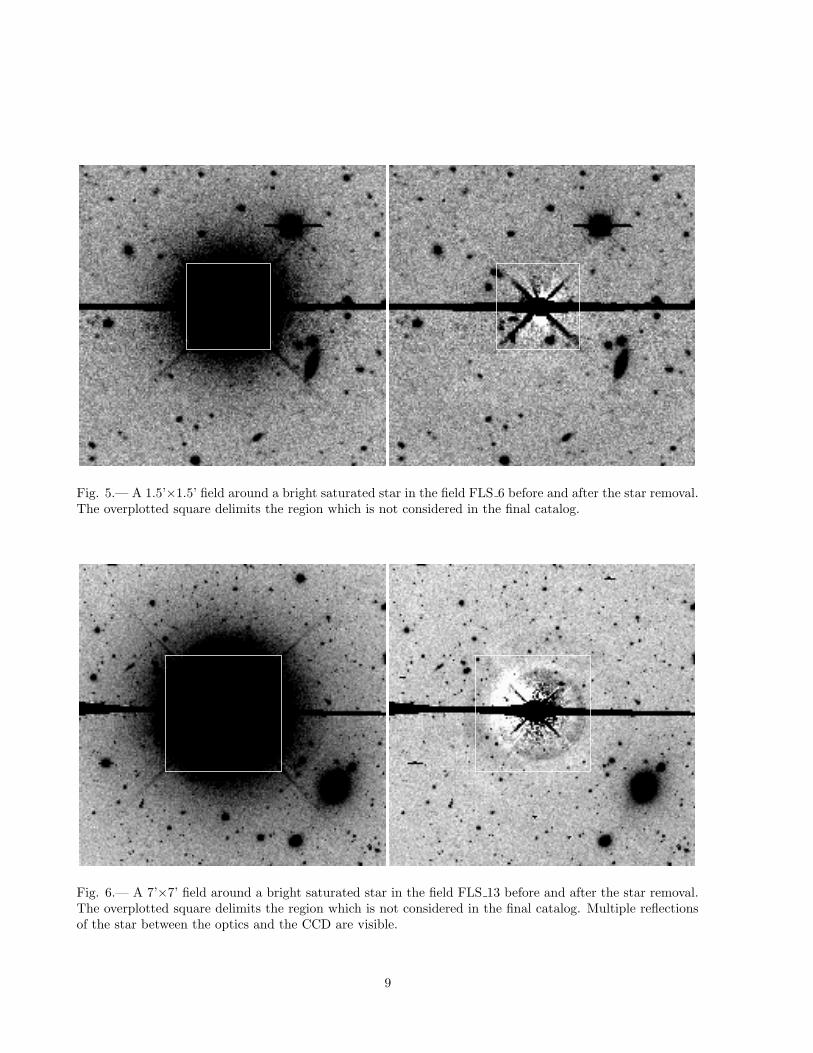
Fig. 5.— A 1.5’×1.5’ field around a bright saturated star in the field FLS 6 before and after the star removal.The overplotted square delimits the region which is not considered in the final catalog.

Fig. 6.— A 7’×7’ field around a bright saturated star in the field FLS 13 before and after the star removal.The overplotted square delimits the region which is not considered in the final catalog. Multiple reflectionsof the star between the optics and the CCD are visible.

9

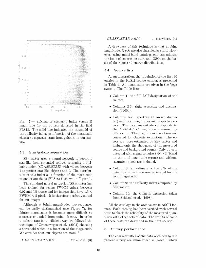
Fig. 7.— SExtractor stellarity index versus Rmagnitude for the objects detected in the fieldFLS18. The solid line indicates the threshold ofthe stellarity index as a function of the magnitudechosen to separate stars from galaxies in our sur-vey.

5.3. Star/galaxy separation

SExtractor uses a neural network to separatestar-like from extended sources returning a stel-larity index (CLASS STAR) with values between1 (a perfect star-like object) and 0. The distribu-tion of this index as a function of the magnitudein one of our fields (FLS18) is shown in Figure 7.

The standard neural network of SExtractor hasbeen trained for seeing FWHM values between0.02 and 5.5 arcsec and for images that have 1.5 <FWHM < 5 pixels. It is therefore perfectly suitedfor our images.

Although at bright magnitudes two sequencescan be easily distinguished (see Figure 7), forfainter magnitudes it becomes more difficult toseparate extended from point objects. In orderto select stars in an efficient way, we followed thetechnique of Groenewegen et al. (2002) choosinga threshold which is a function of the magnitude.We consider that our objects are stars if:

CLASS STAR > 0.85 ... for R < 23 (3)

CLASS STAR > 0.90 ... elsewhere. (4)

A drawback of this technique is that at faintmagnitudes QSOs are also classified as stars. How-ever, using multi-band catalogs one can addressthe issue of separating stars and QSOs on the ba-sis of their spectral energy distributions.

5.4. Source lists

As an illustration, the tabulation of the first 30entries in the FLS 2 source catalog is presentedin Table 4. All magnitudes are given in the Vegasystem. The Table lists:

• Column 1: the full IAU designation of thesource;

• Columns 2-3: right ascension and declina-tion (J2000);

• Columns 4-7: aperture (3 arcsec diame-ter) and total magnitudes and respective er-rors. The total magnitude corresponds tothe MAG AUTO magnitude measured bySExtractor. The magnitudes have been notcorrected for Galactic extinction. The er-rors are those estimated by SExtractor andinclude only the shot-noise of the measuredsource and background counts. Only objectsdetected with signal to noise S/N ≥ 3 (basedon the total magnitude errors) and withoutsaturated pixels are included.

• Column 8: an estimate of the S/N of thedetection, from the errors estimated for thetotal magnitude;

• Column 9: the stellarity index computed bySExtractor;

• Column 10: the Galactic extinction takenfrom Schlegel et al. (1998).

All the catalogs in the archive are in ASCII for-mat. Each catalog has been verified with severaltests to check the reliability of the measured quan-tities with other sets of data. The results of someof these tests are described in the next section.

6. Survey performance

The characteristics of the data obtained by thepresent survey are summarized in Table 5 which

10

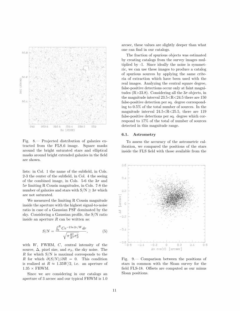
Fig. 8.— Projected distribution of galaxies ex-tracted from the FLS 6 image. Square masksaround the bright saturated stars and ellipticalmasks around bright extended galaxies in the fieldare shown.

lists: in Col. 1 the name of the subfield, in Cols.2-3 the center of the subfield, in Col. 4 the seeingof the combined image, in Cols. 5-6 the 3σ and5σ limiting R Cousin magnitudes, in Cols. 7-8 thenumber of galaxies and stars with S/N ≥ 3σ whichare not saturated.

We measured the limiting R Cousin magnitudeinside the aperture with the highest signal-to-noiseratio in case of a Gaussian PSF dominated by thesky. Considering a Gaussian profile, the S/N ratioinside an aperture R can be written as:

S/N =

∫ R

0Ce−2 ln 2r/W dr√

π R2

∆2σ2S

, (5)

with W , FWHM, C, central intensity of thesource, ∆, pixel size, and σS , the sky noise. TheR for which S/N is maximal corresponds to theR for which ∂(S/N)/∂R = 0. This conditionis realized at R ≈ 1.35W/2, i.e. an aperture of1.35 × FHWM.

Since we are considering in our catalogs anaperture of 3 arcsec and our typical FHWM is 1.0

arcsec, these values are slightly deeper than whatone can find in our catalogs.

The fraction of spurious objects was estimatedby creating catalogs from the survey images mul-tiplied by -1. Since ideally the noise is symmet-ric, we can use these images to produce a catalogof spurious sources by applying the same crite-ria of extraction which have been used with thereal images. Analyzing the central square degree,false-positive detections occur only at faint magni-tudes (R>23.8). Considering all the 3σ objects, inthe magnitude interval 23.5<R<24.5 there are 150false-positive detection per sq. degree correspond-ing to 0.5% of the total number of sources. In themagnitude interval 24.5<R<25.5, there are 119false-positive detections per sq. degree which cor-respond to 17% of the total of number of sourcesdetected in this magnitude range.

6.1. Astrometry

To assess the accuracy of the astrometric cal-ibration, we compared the positions of the starsinside the FLS field with those available from the

Fig. 9.— Comparison between the positions ofstars in common with the Sloan survey for thefield FLS-18. Offsets are computed as our minusSloan positions.

11

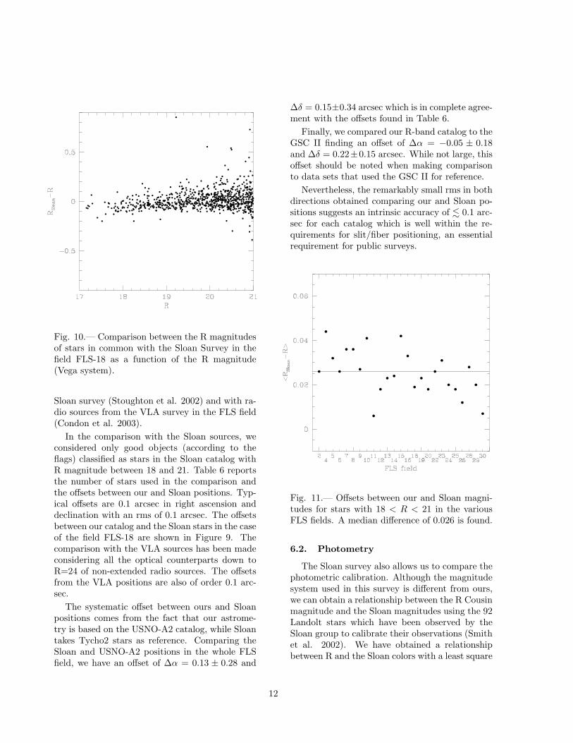
Fig. 10.— Comparison between the R magnitudesof stars in common with the Sloan Survey in thefield FLS-18 as a function of the R magnitude(Vega system).

Sloan survey (Stoughton et al. 2002) and with ra-dio sources from the VLA survey in the FLS field(Condon et al. 2003).

In the comparison with the Sloan sources, weconsidered only good objects (according to theflags) classified as stars in the Sloan catalog withR magnitude between 18 and 21. Table 6 reportsthe number of stars used in the comparison andthe offsets between our and Sloan positions. Typ-ical offsets are 0.1 arcsec in right ascension anddeclination with an rms of 0.1 arcsec. The offsetsbetween our catalog and the Sloan stars in the caseof the field FLS-18 are shown in Figure 9. Thecomparison with the VLA sources has been madeconsidering all the optical counterparts down toR=24 of non-extended radio sources. The offsetsfrom the VLA positions are also of order 0.1 arc-sec.

The systematic offset between ours and Sloanpositions comes from the fact that our astrome-try is based on the USNO-A2 catalog, while Sloantakes Tycho2 stars as reference. Comparing theSloan and USNO-A2 positions in the whole FLSfield, we have an offset of ∆α = 0.13 ± 0.28 and

∆δ = 0.15±0.34 arcsec which is in complete agree-ment with the offsets found in Table 6.

Finally, we compared our R-band catalog to theGSC II finding an offset of ∆α = −0.05 ± 0.18and ∆δ = 0.22±0.15 arcsec. While not large, thisoffset should be noted when making comparisonto data sets that used the GSC II for reference.

Nevertheless, the remarkably small rms in bothdirections obtained comparing our and Sloan po-sitions suggests an intrinsic accuracy of . 0.1 arc-sec for each catalog which is well within the re-quirements for slit/fiber positioning, an essentialrequirement for public surveys.

Fig. 11.— Offsets between our and Sloan magni-tudes for stars with 18 < R < 21 in the variousFLS fields. A median difference of 0.026 is found.

6.2. Photometry

The Sloan survey also allows us to compare thephotometric calibration. Although the magnitudesystem used in this survey is different from ours,we can obtain a relationship between the R Cousinmagnitude and the Sloan magnitudes using the 92Landolt stars which have been observed by theSloan group to calibrate their observations (Smithet al. 2002). We have obtained a relationshipbetween R and the Sloan colors with a least square

12

fit:R = −0.17 + r′ − 0.22(r′ − i′). (6)

Using a biweight estimator, the difference betweenthe real R and the value estimated with the rela-tionship (6) is on average of 0.0001 (with an rms of0.007). In spite of the large scatter, the relation-ship is useful from a statistical point of view sincewe are interested only in confirming our magnitudezero-point.

We have therefore compared the magnitudes ofthe stars in the FLS fields with the values de-duced from the Sloan survey with the equation(6). Table 6 summarizes the median differencesin magnitude between our measurements (auto-

magnitudes) and the model complete magnitudeas computed by Sloan for stars with magnitude18 < R < 21 in the different FLS fields. In Fig-ure 10 we show the distribution of the magnitudeoffsets in the case of the central field FLS-18, whilein Figure 11 we illustrate the offsets for the vari-ous fields. The median difference of 0.026 betweenour and Sloan measurements is consistent with ourerror in the evaluation of the zero points and ispartly due to the different algorithms used in com-puting the total magnitudes.

6.3. Number counts

Counting galaxies and stars as a function of themagnitude allows one to evaluate the overall char-acteristics of a catalog as depth and homogeneity.

In Figures 12 and 14 we show star and galaxycounts in the FLS region and compare them withanalogous counts using the Sloan Digital Sky Sur-vey (Stoughton et al. 2002).

To compare the two distributions, we havetransformed the SDSS magnitudes into the R Vegamagnitudes using the relationship 6.

In the case of star counts (Fig. 12), the countsfrom our survey and the SDSS agree very well be-tween R=18 and R=22. For magnitudes brighterthan R=18, most of the stars detected in our sur-vey are saturated and do not appear in our cata-logs. Star counts drop very rapidly for magnitudesfainter than R=24 since the profile criterion usedfor the star/galaxy separation fails for faint ob-jects. For comparison, we show in Figure 12 thestar counts in the ELAIS field and those in theChandra field (Groenewegen et al., 2002). Thesefields, which lie at higher galactic latitudes are, as

Fig. 12.— Star counts in the central square de-gree of the FLS region from our R images (solidline) and Sloan Digital Sky Survey catalogs (dot-ted line). For comparison, the dashed line refersto the counts in the Chandra South region (Groe-newegen et al., 2002).

expected, less populated by stars.

To evaluate the variation in the number countsdue to the varying observing conditions, we havecomputed the counts for each of the subfield in theFLS field. In Figure 13 we show these counts aswell as the median counts with error bars corre-sponding to the standard deviation as measuredfrom the observed scatter in the counts of the dif-ferent subfields. One can easily see that a few sub-fields (#4, #7, #8, #15 and #26) are less deepthan the other ones, as expected from the quanti-ties measured in Table 5. Fortunately, these fieldsare external and have been only partially coveredby Spitzer observations. The other 20 fields in theFLS are quite homogeneous.

Median counts are then reported in Figure 14 tocompare them with the results from other surveys.The dotted line corresponds the counts from SDSSin the FLS field (Stoughton et al. 2002) com-puted transforming the SDSS magnitudes into theR Vega magnitudes using the relationship in equa-tion (6). The points from the general SDSS counts

13

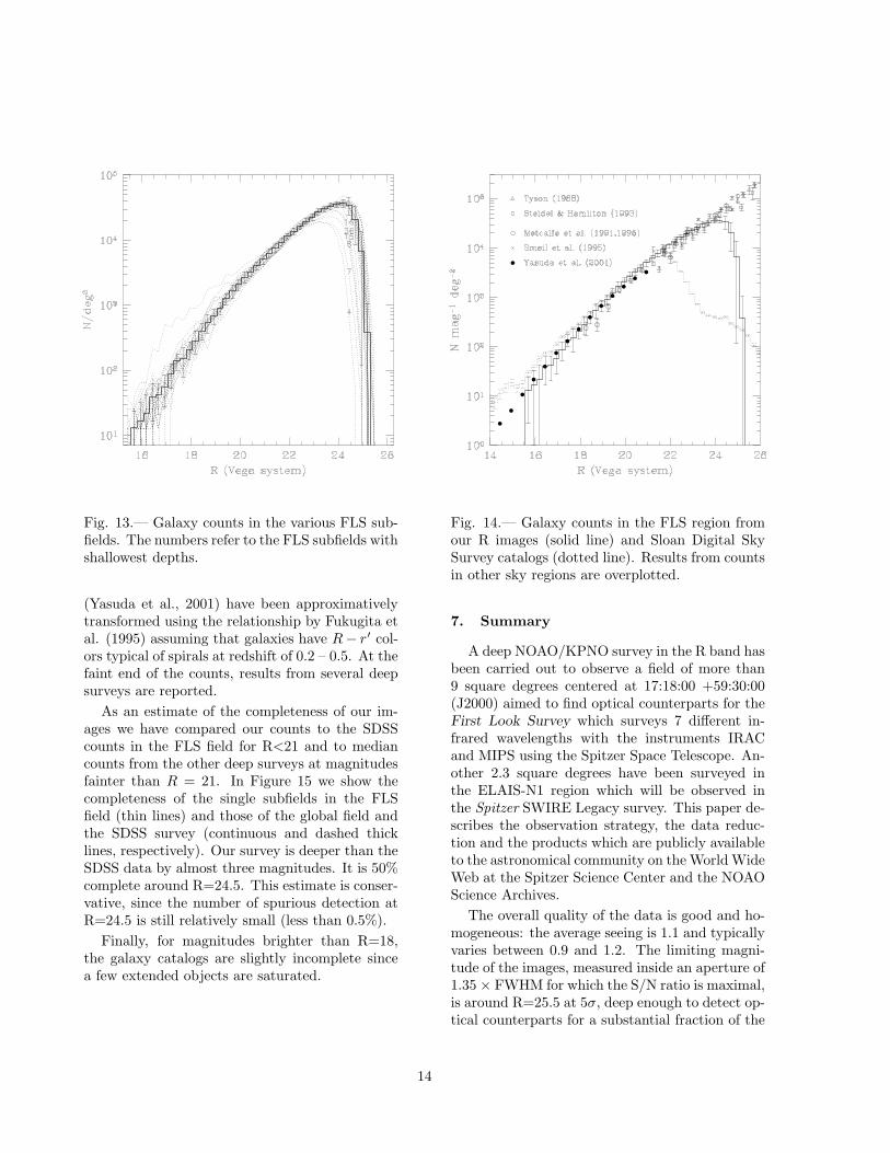
Fig. 13.— Galaxy counts in the various FLS sub-fields. The numbers refer to the FLS subfields withshallowest depths.

(Yasuda et al., 2001) have been approximativelytransformed using the relationship by Fukugita etal. (1995) assuming that galaxies have R− r′ col-ors typical of spirals at redshift of 0.2 – 0.5. At thefaint end of the counts, results from several deepsurveys are reported.

As an estimate of the completeness of our im-ages we have compared our counts to the SDSScounts in the FLS field for R<21 and to mediancounts from the other deep surveys at magnitudesfainter than R = 21. In Figure 15 we show thecompleteness of the single subfields in the FLSfield (thin lines) and those of the global field andthe SDSS survey (continuous and dashed thicklines, respectively). Our survey is deeper than theSDSS data by almost three magnitudes. It is 50%complete around R=24.5. This estimate is conser-vative, since the number of spurious detection atR=24.5 is still relatively small (less than 0.5%).

Finally, for magnitudes brighter than R=18,the galaxy catalogs are slightly incomplete sincea few extended objects are saturated.

Fig. 14.— Galaxy counts in the FLS region fromour R images (solid line) and Sloan Digital SkySurvey catalogs (dotted line). Results from countsin other sky regions are overplotted.

7. Summary

A deep NOAO/KPNO survey in the R band hasbeen carried out to observe a field of more than9 square degrees centered at 17:18:00 +59:30:00(J2000) aimed to find optical counterparts for theFirst Look Survey which surveys 7 different in-frared wavelengths with the instruments IRACand MIPS using the Spitzer Space Telescope. An-other 2.3 square degrees have been surveyed inthe ELAIS-N1 region which will be observed inthe Spitzer SWIRE Legacy survey. This paper de-scribes the observation strategy, the data reduc-tion and the products which are publicly availableto the astronomical community on theWorldWideWeb at the Spitzer Science Center and the NOAOScience Archives.

The overall quality of the data is good and ho-mogeneous: the average seeing is 1.1 and typicallyvaries between 0.9 and 1.2. The limiting magni-tude of the images, measured inside an aperture of1.35 × FWHM for which the S/N ratio is maximal,is around R=25.5 at 5σ, deep enough to detect op-tical counterparts for a substantial fraction of the

14

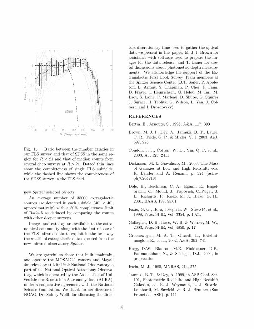
Fig. 15.— Ratio between the number galaxies inour FLS survey and that of SDSS in the same re-gion for R < 21 and that of median counts fromseveral deep surveys at R > 21. Dotted thin linesshow the completeness of single FLS subfields,while the dashed line shows the completeness ofthe SDSS survey in the FLS field.

new Spitzer selected objects.

An average number of 35000 extragalacticsources are detected in each subfield (40’ × 40’,approximatively) with a 50% completeness limitof R=24.5 as deduced by comparing the countswith other deeper surveys.

Images and catalogs are available to the astro-nomical community along with the first release ofthe FLS infrared data to exploit in the best waythe wealth of extragalactic data expected from thenew infrared observatory Spitzer.

We are grateful to those that built, maintain,and operate the MOSAIC-1 camera and Mayall4m telescope at Kitt Peak National Observatory, apart of the National Optical Astronomy Observa-tory, which is operated by the Association of Uni-versities for Research in Astronomy, Inc. (AURA),under a cooperative agreement with the NationalScience Foundation. We thank former director ofNOAO, Dr. Sidney Wolff, for allocating the direc-

tors discretionary time used to gather the opticaldata we present in this paper, M. J. I. Brown forassistance with software used to prepare the im-ages for the data release, and T. Lauer for use-ful discussions about photometric depth measure-ments. We acknowledge the support of the Ex-tragalactic First Look Survey Team members atthe Spitzer Science Center (B.T. Soifer, P. Apple-ton, L. Armus, S. Chapman, P. Choi, F. Fang,D. Frayer, I. Heinrichsen, G. Helou, M. Im., M.Lacy, S. Laine, F. Marleau, D. Shupe, G. SquiresJ. Surace, H. Teplitz, G. Wilson, L. Yan, J. Col-bert, and I. Drozdovsky)

REFERENCES

Bertin, E., Arnouts, S., 1996, A&A, 117, 393

Brown, M. J. I., Dey, A., Jannuzi, B. T., Lauer,T. R., Tiede, G. P., & Mikles, V. J. 2003, ApJ,597, 225

Condon, J. J., Cotton, W. D., Yin, Q. F. et al.,2003, AJ, 125, 2411

Dickinson, M. & Giavalisco, M., 2003, The Massof Galaxies at Low and High Redshift, eds.R. Bender and A. Renzini, p. 324 (astro-ph/0204213)

Dole, H., Beichman, C. A., Egami, E., Engel-bracht, C., Mould, J., Papovich, C.,Puget, J.L., Richards, P., Rieke, M. J., Rieke, G. H.,2001, BAAS, 199, 55.01

Fazio, G. G., Hora, Joseph L. W., Steve P., et al.,1998, Proc. SPIE, Vol. 3354, p. 1024.

Gallagher, D. B., Irace, W. R. & Werner, M. W.,2003, Proc. SPIE, Vol. 4850, p. 17

Groenewegen, M. A. T., Girardi, L., Hatzimi-naoglou, E., et al., 2002, A&A, 392, 741

Hogg, D.W., Blanton, M.R., Finkbeiner, D.P.,Padmanabhan, N., & Schlegel, D.J., 2004, inpreparation

Irwin, M. J., 1985, MNRAS, 214, 575

Jannuzi, B. T., & Dey, A. 1999, in ASP Conf. Ser.191, Photometric Redshifts and High RedshiftGalaxies, ed. R. J. Weymann, L. J. Storrie-Lombardi, M. Sawicki, & R. J. Brunner (SanFrancisco: ASP), p. 111

15

Kessler, M. F., Steinz, J. A., Anderegg, M. E., etal., 1996, A&A, 315, 27

Kron, R. G., 1980, ApJS, 43, 305

Landolt, A. U., 1992, AJ, 104, 340

Lonsdale, C. J., Smith, H. E., Rowan-Robinson,M. et al, 2003, PASP, 115, 897

Metcalfe, N., Shanks, T., Fong, R., & Jones, L. R.1991, MNRAS, 249, 498

Metcalfe, N., Shanks, T., Fong, R., & Roche, N.1995, MNRAS, 273, 257

Monet, D. B. A., et al. 1998, “The USNO-A2.0Catalogue”, VizieR Online Data Catalogue

Muller, G. P., Reed, R., Armandroff, T., Boroson,T. A., & Jacoby, G. H., 1998, Proc. SPIE, 3355,577

Oliver, S., Rowan-Robinson, M., Alexander, D. M.et al., 2000, MNRAS, 316, 749

Rieke, G. H., Young, E. T., Rivlis, G. & Gautier,T. N., 1996, BAAS, 28, 1274

Schlegel, D., Finkbeiner, D., & Davis, M., 1998,ApJ, 500, 525

Smail, I., Hogg, D. W., Yan, L., & Cohen, J. G.,1995, ApJ, 449, L105

Smith J.A., Tucker D.L., Kent S. et al., 2002, AJ,123, 2121

Soifer, B.T., Neugebauer, G., Beichman, C.A.,Houck, J.R., Rowan-Robinson, M. 1983, in In-frared technology IX; Proceedings of the NinthAnnual Meeting, San Diego, CA, August 23-25, 1983. Bellingham, WA, SPIE - The Inter-national Society for Optical Engineering, 297

Steidel, C. C., & Hamilton, D., 1993, AJ, 105,2017

Stoughton, C., Lupton, R.H., Bernardi, M., et al.2002, AJ, 123, 485

Tyson, J. A., 1988, AJ, 96, 1

Valdes, F. G., 2003, in “Automated Data Anal-ysis in Astronomy”, editors Ranjan Gupta,Harinder P. Singh, & Coryn A. L. Bailer-Jones,Narosa Publishing House, New Delhi, p. 309

Yasuda, N., Fukugita, M., Narayanan, V. K. etal., 2001, AJ, 122, 1104

This 2-column preprint was prepared with the AAS LATEXmacros v5.0.

16

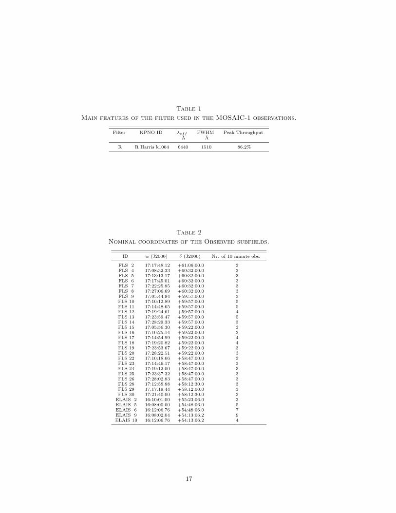
Table 1

Main features of the filter used in the MOSAIC-1 observations.

Filter KPNO ID λeff FWHM Peak ThroughputA A

R R Harris k1004 6440 1510 86.2%

Table 2

Nominal coordinates of the Observed subfields.

ID α (J2000) δ (J2000) Nr. of 10 minute obs.

FLS 2 17:17:48.12 +61:06:00.0 3FLS 4 17:08:32.33 +60:32:00.0 3FLS 5 17:13:13.17 +60:32:00.0 3FLS 6 17:17:45.01 +60:32:00.0 3FLS 7 17:22:25.85 +60:32:00.0 3FLS 8 17:27:06.69 +60:32:00.0 3FLS 9 17:05:44.94 +59:57:00.0 3FLS 10 17:10:12.89 +59:57:00.0 5FLS 11 17:14:48.65 +59:57:00.0 5FLS 12 17:19:24.61 +59:57:00.0 4FLS 13 17:23:59.47 +59:57:00.0 5FLS 14 17:28:29.33 +59:57:00.0 3FLS 15 17:05:56.30 +59:22:00.0 3FLS 16 17:10:25.14 +59:22:00.0 3FLS 17 17:14:54.99 +59:22:00.0 4FLS 18 17:19:20.82 +59:22:00.0 4FLS 19 17:23:53.67 +59:22:00.0 3FLS 20 17:28:22.51 +59:22:00.0 3FLS 22 17:10:18.66 +58:47:00.0 3FLS 23 17:14:46.17 +58:47:00.0 3FLS 24 17:19:12.00 +58:47:00.0 3FLS 25 17:23:37.32 +58:47:00.0 3FLS 26 17:28:02.83 +58:47:00.0 3FLS 28 17:12:58.88 +58:12:30.0 3FLS 29 17:17:19.44 +58:12:00.0 3FLS 30 17:21:40.00 +58:12:30.0 3ELAIS 2 16:10:01.00 +55:23:06.0 3ELAIS 5 16:08:00.00 +54:48:06.0 5ELAIS 6 16:12:06.76 +54:48:06.0 7ELAIS 9 16:08:02.04 +54:13:06.2 9ELAIS 10 16:12:06.76 +54:13:06.2 4

17

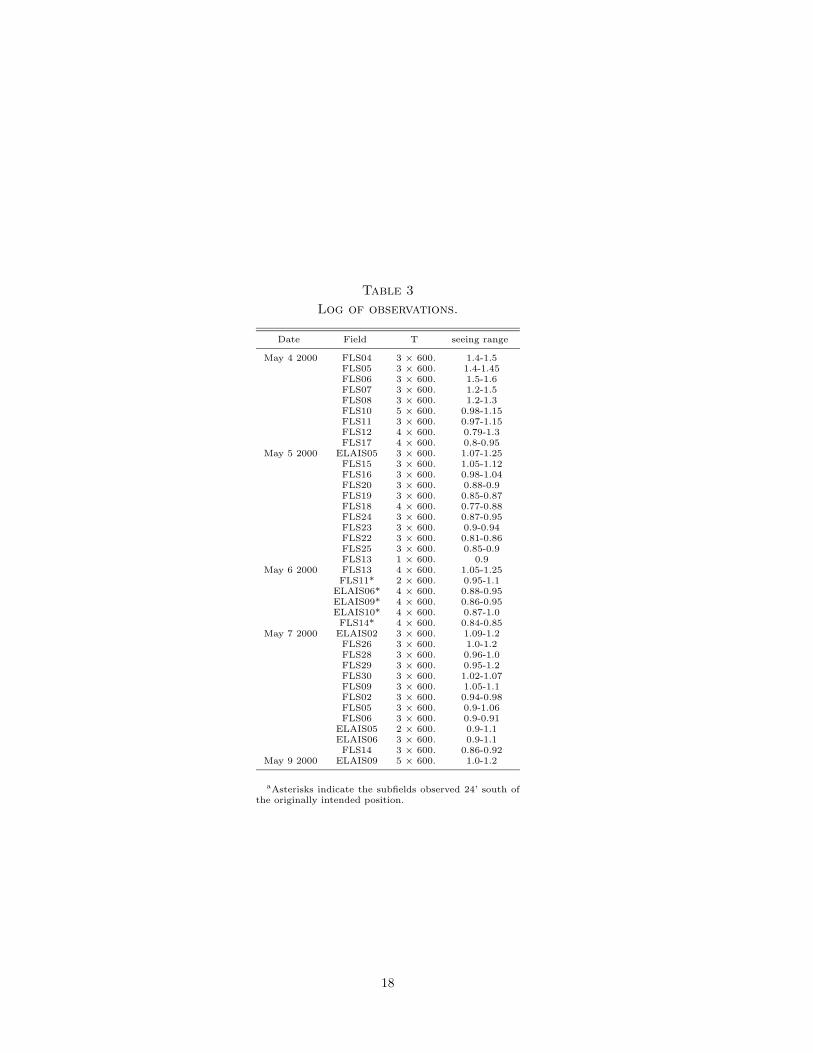
Table 3

Log of observations.

Date Field T seeing range

May 4 2000 FLS04 3 × 600. 1.4-1.5FLS05 3 × 600. 1.4-1.45FLS06 3 × 600. 1.5-1.6FLS07 3 × 600. 1.2-1.5FLS08 3 × 600. 1.2-1.3FLS10 5 × 600. 0.98-1.15FLS11 3 × 600. 0.97-1.15FLS12 4 × 600. 0.79-1.3FLS17 4 × 600. 0.8-0.95

May 5 2000 ELAIS05 3 × 600. 1.07-1.25FLS15 3 × 600. 1.05-1.12FLS16 3 × 600. 0.98-1.04FLS20 3 × 600. 0.88-0.9FLS19 3 × 600. 0.85-0.87FLS18 4 × 600. 0.77-0.88FLS24 3 × 600. 0.87-0.95FLS23 3 × 600. 0.9-0.94FLS22 3 × 600. 0.81-0.86FLS25 3 × 600. 0.85-0.9FLS13 1 × 600. 0.9

May 6 2000 FLS13 4 × 600. 1.05-1.25FLS11* 2 × 600. 0.95-1.1ELAIS06* 4 × 600. 0.88-0.95ELAIS09* 4 × 600. 0.86-0.95ELAIS10* 4 × 600. 0.87-1.0FLS14* 4 × 600. 0.84-0.85

May 7 2000 ELAIS02 3 × 600. 1.09-1.2FLS26 3 × 600. 1.0-1.2FLS28 3 × 600. 0.96-1.0FLS29 3 × 600. 0.95-1.2FLS30 3 × 600. 1.02-1.07FLS09 3 × 600. 1.05-1.1FLS02 3 × 600. 0.94-0.98FLS05 3 × 600. 0.9-1.06FLS06 3 × 600. 0.9-0.91ELAIS05 2 × 600. 0.9-1.1ELAIS06 3 × 600. 0.9-1.1FLS14 3 × 600. 0.86-0.92

May 9 2000 ELAIS09 5 × 600. 1.0-1.2

aAsterisks indicate the subfields observed 24’ south ofthe originally intended position.

18

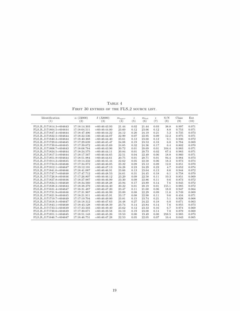
Table 4

First 30 entries of the FLS 2 source list.

Identification α (J2000) δ (J2000) maper ε mtot ε S/N Class Ext(1) (2) (3) (4) (5) (6) (7) (8) (9) (10)

FLS R J171814.3+604643 17:18:14.303 +60:46:43.93 21.44 0.02 21.44 0.03 38.8 0.997 0.071FLS R J171804.5+604644 17:18:04.511 +60:46:44.00 23.60 0.12 23.66 0.12 8.8 0.753 0.071FLS R J171847.4+604644 17:18:47.496 +60:46:44.22 24.12 0.20 24.19 0.21 5.2 0.735 0.073FLS R J171822.5+604644 17:18:22.536 +60:46:44.07 22.99 0.07 22.95 0.09 12.2 0.975 0.071FLS R J171840.3+604644 17:18:40.368 +60:46:44.40 23.61 0.12 23.60 0.12 9.1 0.936 0.072FLS R J171729.6+604645 17:17:29.639 +60:46:45.47 24.08 0.19 23.53 0.18 6.0 0.784 0.069FLS R J171739.6+604645 17:17:39.672 +60:46:45.69 24.65 0.32 24.36 0.17 6.4 0.802 0.070FLS R J171808.7+604643 17:18:08.784 +60:46:43.96 20.72 0.01 20.69 0.01 104.4 0.983 0.071FLS R J171824.5+604644 17:18:24.575 +60:46:44.11 20.84 0.01 20.73 0.02 67.4 0.983 0.071FLS R J171817.5+604644 17:18:17.567 +60:46:44.65 22.51 0.04 22.49 0.06 18.8 0.960 0.071FLS R J171851.9+604644 17:18:51.984 +60:46:44.61 20.75 0.01 20.71 0.01 94.4 0.984 0.073FLS R J171914.2+604645 17:19:14.232 +60:46:45.44 22.62 0.05 22.58 0.06 18.3 0.973 0.074FLS R J171734.8+604646 17:17:34.872 +60:46:46.05 23.22 0.09 23.12 0.09 12.0 0.851 0.070FLS R J171912.1+604647 17:19:12.191 +60:46:47.13 24.28 0.23 24.29 0.23 4.7 0.652 0.074FLS R J171841.0+604646 17:18:41.087 +60:46:46.91 23.66 0.13 23.64 0.13 8.6 0.944 0.072FLS R J171747.7+604648 17:17:47.712 +60:46:48.53 24.61 0.31 24.45 0.18 6.1 0.758 0.070FLS R J171726.8+604646 17:17:26.807 +60:46:46.12 23.29 0.09 22.58 0.11 10.3 0.851 0.069FLS R J171827.8+604646 17:18:27.887 +60:46:46.99 23.30 0.09 22.86 0.11 9.6 0.873 0.072FLS R J171834.5+604648 17:18:34.560 +60:46:48.28 23.94 0.17 23.89 0.14 7.6 0.945 0.072FLS R J171838.2+604644 17:18:38.279 +60:46:44.40 20.22 0.01 20.19 0.01 155.1 0.985 0.072FLS R J171631.4+604647 17:16:31.487 +60:46:47.20 23.47 0.11 21.60 0.06 18.8 0.947 0.064FLS R J171731.9+604646 17:17:31.967 +60:46:46.99 23.09 0.08 22.29 0.09 11.6 0.749 0.069FLS R J171821.9+604645 17:18:21.911 +60:46:45.91 23.17 0.08 22.98 0.11 9.6 0.434 0.071FLS R J171719.7+604649 17:17:19.704 +60:46:49.00 23.81 0.15 23.74 0.21 5.1 0.928 0.068FLS R J171618.3+604647 17:16:18.312 +60:46:47.63 24.48 0.27 24.22 0.18 6.0 0.671 0.063FLS R J171843.1+604648 17:18:43.128 +60:46:48.39 23.74 0.14 23.84 0.14 7.6 0.955 0.073FLS R J171733.5+604649 17:17:33.503 +60:46:49.40 23.62 0.12 23.33 0.16 6.7 0.974 0.069FLS R J171730.6+604649 17:17:30.671 +60:46:49.58 24.10 0.19 23.08 0.14 7.8 0.879 0.069FLS R J171851.1+604645 17:18:51.143 +60:46:45.26 19.53 0.00 19.49 0.00 258.5 0.985 0.073FLS R J171646.7+604647 17:16:46.751 +60:46:47.28 22.53 0.05 22.05 0.07 16.4 0.043 0.065

19

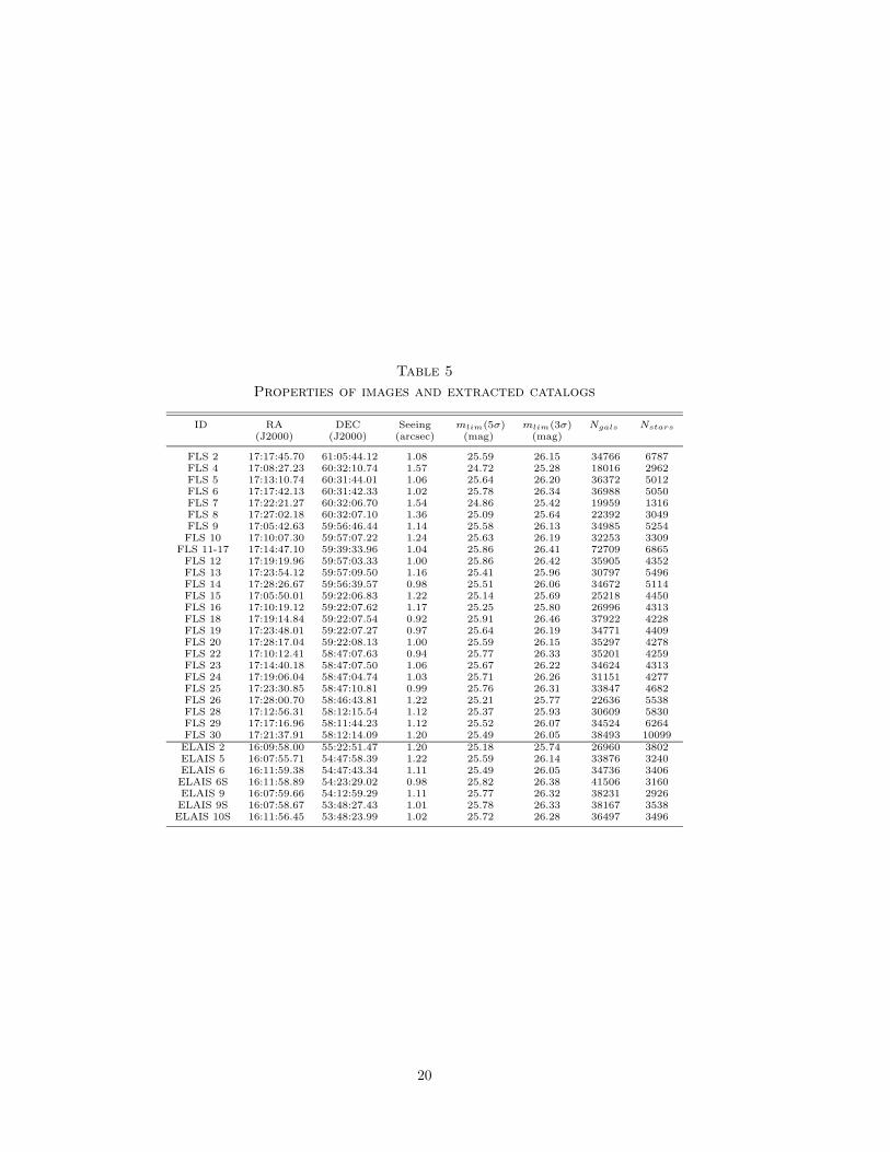
Table 5

Properties of images and extracted catalogs

ID RA DEC Seeing mlim(5σ) mlim(3σ) Ngals Nstars

(J2000) (J2000) (arcsec) (mag) (mag)

FLS 2 17:17:45.70 61:05:44.12 1.08 25.59 26.15 34766 6787FLS 4 17:08:27.23 60:32:10.74 1.57 24.72 25.28 18016 2962FLS 5 17:13:10.74 60:31:44.01 1.06 25.64 26.20 36372 5012FLS 6 17:17:42.13 60:31:42.33 1.02 25.78 26.34 36988 5050FLS 7 17:22:21.27 60:32:06.70 1.54 24.86 25.42 19959 1316FLS 8 17:27:02.18 60:32:07.10 1.36 25.09 25.64 22392 3049FLS 9 17:05:42.63 59:56:46.44 1.14 25.58 26.13 34985 5254FLS 10 17:10:07.30 59:57:07.22 1.24 25.63 26.19 32253 3309FLS 11-17 17:14:47.10 59:39:33.96 1.04 25.86 26.41 72709 6865FLS 12 17:19:19.96 59:57:03.33 1.00 25.86 26.42 35905 4352FLS 13 17:23:54.12 59:57:09.50 1.16 25.41 25.96 30797 5496FLS 14 17:28:26.67 59:56:39.57 0.98 25.51 26.06 34672 5114FLS 15 17:05:50.01 59:22:06.83 1.22 25.14 25.69 25218 4450FLS 16 17:10:19.12 59:22:07.62 1.17 25.25 25.80 26996 4313FLS 18 17:19:14.84 59:22:07.54 0.92 25.91 26.46 37922 4228FLS 19 17:23:48.01 59:22:07.27 0.97 25.64 26.19 34771 4409FLS 20 17:28:17.04 59:22:08.13 1.00 25.59 26.15 35297 4278FLS 22 17:10:12.41 58:47:07.63 0.94 25.77 26.33 35201 4259FLS 23 17:14:40.18 58:47:07.50 1.06 25.67 26.22 34624 4313FLS 24 17:19:06.04 58:47:04.74 1.03 25.71 26.26 31151 4277FLS 25 17:23:30.85 58:47:10.81 0.99 25.76 26.31 33847 4682FLS 26 17:28:00.70 58:46:43.81 1.22 25.21 25.77 22636 5538FLS 28 17:12:56.31 58:12:15.54 1.12 25.37 25.93 30609 5830FLS 29 17:17:16.96 58:11:44.23 1.12 25.52 26.07 34524 6264FLS 30 17:21:37.91 58:12:14.09 1.20 25.49 26.05 38493 10099ELAIS 2 16:09:58.00 55:22:51.47 1.20 25.18 25.74 26960 3802ELAIS 5 16:07:55.71 54:47:58.39 1.22 25.59 26.14 33876 3240ELAIS 6 16:11:59.38 54:47:43.34 1.11 25.49 26.05 34736 3406ELAIS 6S 16:11:58.89 54:23:29.02 0.98 25.82 26.38 41506 3160ELAIS 9 16:07:59.66 54:12:59.29 1.11 25.77 26.32 38231 2926ELAIS 9S 16:07:58.67 53:48:27.43 1.01 25.78 26.33 38167 3538ELAIS 10S 16:11:56.45 53:48:23.99 1.02 25.72 26.28 36497 3496

20

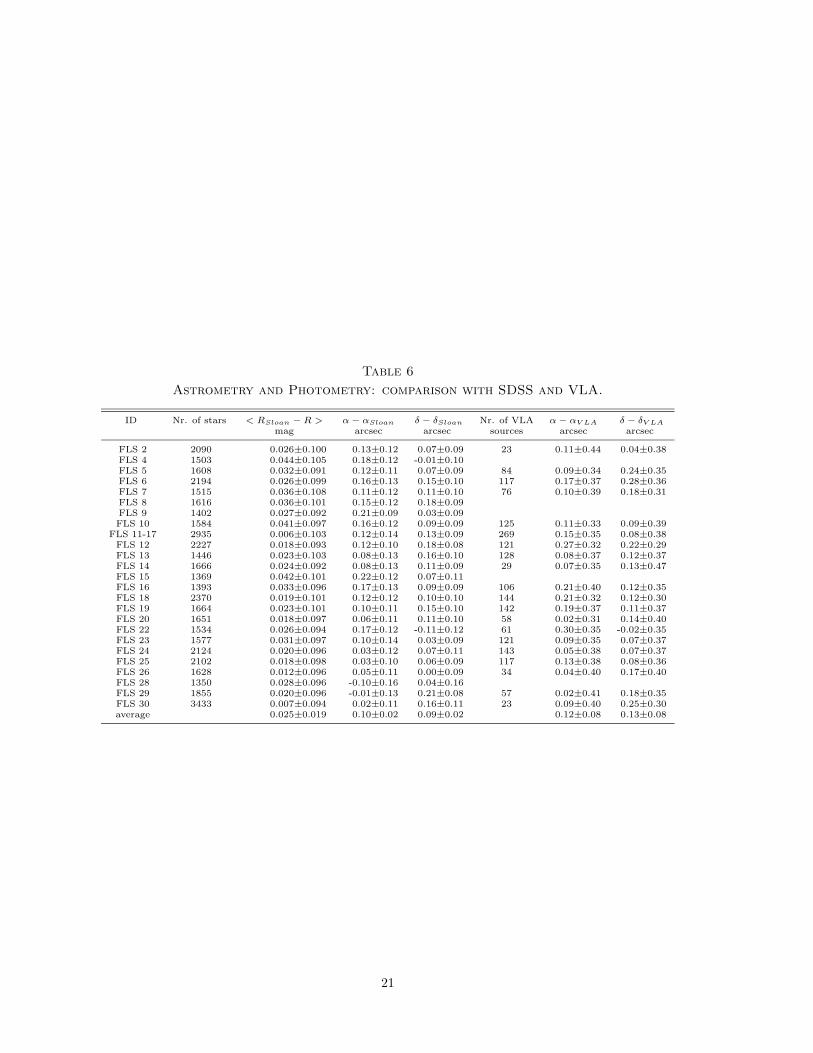
Table 6

Astrometry and Photometry: comparison with SDSS and VLA.

ID Nr. of stars < RSloan − R > α− αSloan δ − δSloan Nr. of VLA α− αV LA δ − δV LA

mag arcsec arcsec sources arcsec arcsec

FLS 2 2090 0.026±0.100 0.13±0.12 0.07±0.09 23 0.11±0.44 0.04±0.38FLS 4 1503 0.044±0.105 0.18±0.12 -0.01±0.10FLS 5 1608 0.032±0.091 0.12±0.11 0.07±0.09 84 0.09±0.34 0.24±0.35FLS 6 2194 0.026±0.099 0.16±0.13 0.15±0.10 117 0.17±0.37 0.28±0.36FLS 7 1515 0.036±0.108 0.11±0.12 0.11±0.10 76 0.10±0.39 0.18±0.31FLS 8 1616 0.036±0.101 0.15±0.12 0.18±0.09FLS 9 1402 0.027±0.092 0.21±0.09 0.03±0.09FLS 10 1584 0.041±0.097 0.16±0.12 0.09±0.09 125 0.11±0.33 0.09±0.39FLS 11-17 2935 0.006±0.103 0.12±0.14 0.13±0.09 269 0.15±0.35 0.08±0.38FLS 12 2227 0.018±0.093 0.12±0.10 0.18±0.08 121 0.27±0.32 0.22±0.29FLS 13 1446 0.023±0.103 0.08±0.13 0.16±0.10 128 0.08±0.37 0.12±0.37FLS 14 1666 0.024±0.092 0.08±0.13 0.11±0.09 29 0.07±0.35 0.13±0.47FLS 15 1369 0.042±0.101 0.22±0.12 0.07±0.11FLS 16 1393 0.033±0.096 0.17±0.13 0.09±0.09 106 0.21±0.40 0.12±0.35FLS 18 2370 0.019±0.101 0.12±0.12 0.10±0.10 144 0.21±0.32 0.12±0.30FLS 19 1664 0.023±0.101 0.10±0.11 0.15±0.10 142 0.19±0.37 0.11±0.37FLS 20 1651 0.018±0.097 0.06±0.11 0.11±0.10 58 0.02±0.31 0.14±0.40FLS 22 1534 0.026±0.094 0.17±0.12 -0.11±0.12 61 0.30±0.35 -0.02±0.35FLS 23 1577 0.031±0.097 0.10±0.14 0.03±0.09 121 0.09±0.35 0.07±0.37FLS 24 2124 0.020±0.096 0.03±0.12 0.07±0.11 143 0.05±0.38 0.07±0.37FLS 25 2102 0.018±0.098 0.03±0.10 0.06±0.09 117 0.13±0.38 0.08±0.36FLS 26 1628 0.012±0.096 0.05±0.11 0.00±0.09 34 0.04±0.40 0.17±0.40FLS 28 1350 0.028±0.096 -0.10±0.16 0.04±0.16FLS 29 1855 0.020±0.096 -0.01±0.13 0.21±0.08 57 0.02±0.41 0.18±0.35FLS 30 3433 0.007±0.094 0.02±0.11 0.16±0.11 23 0.09±0.40 0.25±0.30average 0.025±0.019 0.10±0.02 0.09±0.02 0.12±0.08 0.13±0.08

21