james_okstate_0664d_13483.pdf - shareok
TRANSCRIPT
THE ELUCIDATION AND QUANTIFICATION OF THE
DECOMPOSITION PRODUCTS OF SODIUM
DITHIONITE AND THE DETECTION OF
PEROXIDE VAPORS WITH
THIN FILMS
By
TRAVIS HOUSTON JAMES
Bachelor of Science in Chemistry
Hillsdale College
Hillsdale, MI
2009
Submitted to the Faculty of the
Graduate College of the
Oklahoma State University
in partial fulfillment of
the requirements for
the Degree of
DOCTOR OF PHILOSOPHY
July, 2014
ii
THE ELUCIDATION AND QUANTIFICATION OF THE
DECOMPOSOTION PRODUCTS OF SODIUM
DITHIONITE AND THE DETECTION OF
PEROXIDE VAPORS WITH
THIN FILMS
Dissertation Approved:
Dr. Nicholas F. Materer
Dissertation Advisor
Dr. Allen Apblett
Dr. Frank Blum
Dr. Richard Bunce
Dr. Ziad El-Rassi
Dr. Tyler Ley

iii Acknowledgements reflect the views of the author and are not endorsed by committee
members or Oklahoma State University.
ACKNOWLEDGEMENTS
I would like to thank anyone who, whether I am aware of his or her actions or not, has
contributed meaningfully to my life and my efforts.
iv
Name: TRAVIS HOUSTON JAMES
Date of Degree: JULY, 2014
Title of Study: THE ELUCIDATION AND QUANTIFICATION OF THE
DECOMPOSOTION PRODUCTS OF SODIUM DITHIONITE AND
THE DETECTION OF PEROXIDE VAPORS WITH THIN FILMS
Major Field: CHEMISTRY
Abstract:
Sodium dithionite (Na2S2O4) is an oxidizable sulfur oxyanion often employed as a
reducing agent in environmental and synthetic chemistry. When exposed to the
atmosphere, dithionite degrades through a series of decomposition reactions to form a
number of compounds, with the primary two being bisulfite (HSO32-
) and thiosulfate
(S2O32-
). Ten samples of sodium dithionite ranging from brand new to nearly fifty years
old were analyzed using ion chromatography; from this, a new quantification method for
dithionite and thiosulfate was achieved and statistically validated against the current three
iodometric titration method used industrially. Additional sample analysis with Raman
spectroscopy of solid and dissolved samples identified unique compounds in the oldest
samples, including dithionate (S2O62-
) and tetrathionate (S4O62-
).
Additionally, titania nanoparticles in a hydroxypropyl cellulose matrix were used to
prepare films on polycarbonate slides and coatings on cellulose papers. The exposure of
these materials to hydrogen peroxide gas led to the development of an intense yellow
color. Using an inexpensive web camera and a tungsten lamp to measure the reflected
light, first-order behavior in the color change was observed when exposed to peroxide
vapor of less than 50 ppm. For 50 mass percent titania nanoparticles in hydroxypropyl
cellulose films on polycarbonate, the detection limit was estimated to be 90 ppm after a
1-minute measurement and 1.5 ppm after a 1-hour integration. The coatings on the filter
paper had a threefold higher sensitivity compared to the films, with a detection limit of
5.4 ppm peroxide for a 1-minute measurement and 0.09 ppm peroxide for a 1-hour
integration period. Further experimentation with the effects of acid loading on the filter
paper coatings identified these as possible sensors for organic peroxides. With the
addition of sulfuric acid, the support was changed from cellulose to glass microfiber or
silica. This coatings showing increased sensitivity when compared to coatings with
hydrochloric acid. Finally, coatings containing an ionic liquid solvent and
trifluoromethanesulfonic acid were produced and found to have increased longevity.
These coatings have potential as peroxide vapor sensors for both industrial and security
applications.
v
TABLE OF CONTENTS
Chapter Page
I. INTRODUCTION ......................................................................................................1
A. Sodium Dithionite ..............................................................................................2
B. History of Synthesis and Quantification of Sodium Dithionite .........................8
C. A Brief Review of Thin Film Production ........................................................13
D. Applications of Titania ....................................................................................16
E. Detection of Gaseous Peroxides ......................................................................17
II. A METHOD FOR RAPID QUANTIFICATION OF SODIUM DITHIONITE
AND ITS DECOMPOSOTION PRODUCTS BY ION
CHROMATOGRAPHY ........................................................................................22
A. Introduction ......................................................................................................22
B. Experimental Details ........................................................................................23
B.1. Sodium Dithionite Samples ......................................................................23
B.2. Solution Preparation .................................................................................24
B.3. Ion Chromatography Setup ......................................................................24
B.4. Titration Methodology .............................................................................25
C. Results and Discussion ....................................................................................28
C.1. Ion Chromatography Results ....................................................................29
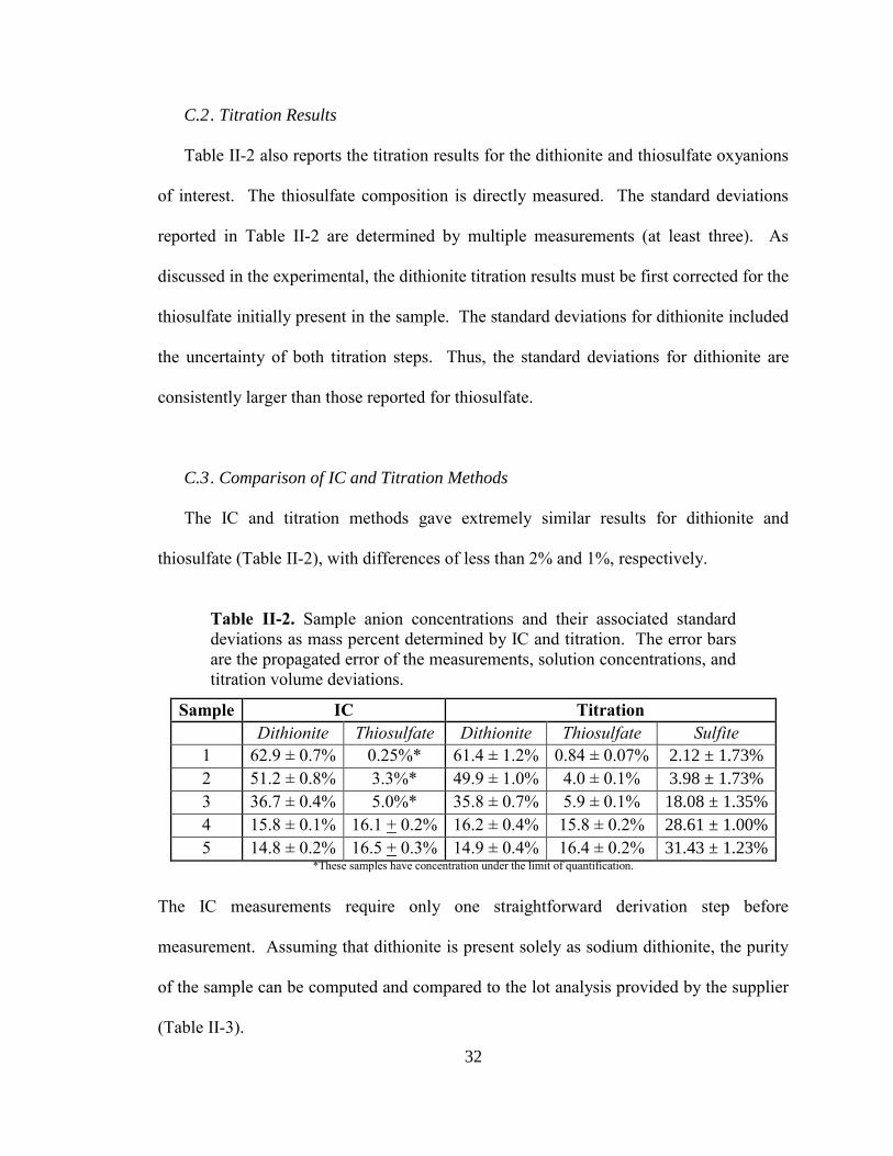
C.2. Titration Results .......................................................................................32
C.3. Comparison of IC and Titration Methods ................................................32
D. Conclusion .......................................................................................................34
III. SODIUM DITHIONITE PURITY AND DECOMPOSITION PRODUCTS IN
SOLID SAMPLES SPANNING 50 YEARS ........................................................36
A. Introduction ......................................................................................................36
B. Experimental Details ........................................................................................37
B.1. Sodium Dithionite Samples ......................................................................37
B.2. Materials and Synthesis of Polythionates.................................................38
B.3. Raman Spectroscopy ................................................................................40
B.4. Titration and Ion Chromatograph Methodology ......................................41
vi
Chapter Page
C. Results and Discussions ...................................................................................42
C.1. Raman Analysis of Sodium Dithionite Samples ......................................42
C.2. Titration and Chromatography Results ....................................................46
D. Conclusion ........................................................................................................52
IV. TITANIA-HYDROXYPROPYL CELLULOSE THIN FILMS FOR THE
DETECTION OF PEROXIDE VAPORS .............................................................53
A. Introduction ......................................................................................................53
B. Experimental Details ........................................................................................54
B.1. Preparation of Titanium(IV) Isoproproxide-Hydroxypropyl
Cellulose Solution ....................................................................................54
B.2. Preparation of Sol-Gel Films and Coatings..............................................54
B.3. Titanium(IV) Oxysulfate Solution for Peroxide Quantification ..............57
B.4. Peroxide Solutions for Gas Exposure.......................................................57
B.5. Film Testing Apparatus ............................................................................58
B.6. Particle Size Measurement .......................................................................61
B.7. Electron and Atomic Force Microscopies ................................................61
C. Results and Discussion .....................................................................................61
C.1. Stability and Characterization of the Films and Coatings ........................61
C.2. Reaction Kinetics .....................................................................................67
C.3. Peroxide Sensitivity and Reaction Mechanism ........................................74
D. Conclusion .......................................................................................................75
V. PRELIMINARY WORK FOR THE DETECTION OF ORGANIC PEROXIDES
AND EFFECTS OF ACID CONCENTRATION SENSING FILMS ...................77
A. Introduction ......................................................................................................77
B. Experimental Details ........................................................................................79
B.1. Preparation of Titanium(IV) Isoproproxide-Hydroxypropyl
Cellulose Solution ....................................................................................79
B.2. Preparation of Titanyl Sulfate in Buffered Ionic Liquid Solutions ..........79
B.3. Preparation of Sol-Gel Coatings on Glass Filter Paper and Ionic
Liquid Coatings on Silica Slides ..............................................................80
B.4. Surface Area Analysis of Filter Paper and Silica Substrates ...................81
B.5. Setup and Testing Methodology for the High Acid Content
Coatings ....................................................................................................81
C. Results and Discussions ...................................................................................82
C.1. Reactivity to Organic Peroxides ...............................................................82
C.2. Surface Area Analyses of Substrates .......................................................84
C.3. Solution Sensitivities to Hydrogen Peroxide Vapor ................................84
vii
Chapter Page
C.4. Long Term Stability and Sensitivities of Sol-Gel and Ionic Liquid
Solutions ..........................................................................................................86
C.5. Reaction Kinetics .....................................................................................88
D. Conclusions ......................................................................................................94
CONCLUDING REMARKS .................................................................................95
REFERENCES ......................................................................................................97
APPENDICES .....................................................................................................108
viii
LIST OF TABLES
Table Page
II-1. Sodium dithionite samples, suppliers, production date and lot analyses ........23
II-2. Sample anion concentrations and their associated standard deviations
as mass percent determined by IC and titration .............................................32
II-3. Compositions in mass percent for neutral sodium dithionite
determined by IC and titration methods .........................................................33
III-1. Sodium dithionite sample information, including the production data
and lot analyses ..............................................................................................37
III-2. Characteristic vibrational frequencies for both the solid material and
solutions compiled from published sources ...................................................43
III-3. Sample composition as percent of anion mass in sample mass
measured by a three-step iodometric titration ................................................47
III-4. Sample composition of dithionite and thiosulfate as percent anion
sample mass, measured by ion chromatography ............................................49
III-5. Sodium sample content as measured by ion chromatography ........................50
III-6. Sodium dithionite compositions as mass percent of the ionic
compound in the samples, taken from lot analyses, ion
chromatography and iodometric titrations .....................................................51
IV-1. Film quality after drying on polycarbonate slides as a function of
titania mass percent or loading .......................................................................62
IV-2. Effects of layering and thickness on stability of 60 mass percent
titania films on polycarbonate ........................................................................63
ix
LIST OF FIGURES
Figure Page
I-1. Structure of the dithionite ion..........................................................................6
I-2. Frost diagrams for sulfur oxyanions in oxic and anoxic solutions ..................7
I-3. Molecular structures of triacetone triperoxide and hexamethylene
triperoxide diamine .......................................................................................18
I-4. The mononuclear and dinuclear titanium(IV) peroxo complexes .................20
II-1. Ion chromatogram for dithionite analysis .....................................................29
III-1. Raman spectra for three solid samples as a function of age ..........................44
IV-1. Layout and deposition method for production of films on glass and
polycarbonate slides ......................................................................................55
IV-2. Diagram for the production of coated filter papers .......................................56
IV-3. Schematic diagram of the peroxide exposure apparatus ...............................58
IV-4. False-color images of the height and surface roughness of a 50 mass
percent titania-cellulose film, measured by AFM .........................................64
IV-5. DLS analyses of a cellulose solution before addition of titanium
isoproproxide and immediately after addition of titanium
isoproproxide ................................................................................................65
IV-6. DLS analyses of a titania-cellulose solution after stirring for one day
and for one week ...........................................................................................65
IV-7. Scanning electron micrograph of two week-old titania-cellulose films
at magnifications of 3000X and 20000X ......................................................66
IV-8. Original recording of film on a polycarbonate slide before and after
peroxide exposure .........................................................................................68
IV-9. Isolated red channel of film on a polycarbonate slide before and after
peroxide exposure .........................................................................................68
IV-10. Intensity versus exposure time for a 50 mass percent titania film and
the first-order behavior of the first 10 minutes of exposure .........................69
x
Figure Page
IV-11. Phenomenological first-order rate constants for 50 mass percent
titania films and coatings ..............................................................................70
IV-12. Phenomenological first-order rate constants for 0, 25 and 50 mass
percent titania coatings as a function of gas phase hydrogen peroxide
concentration .................................................................................................73
V-1. Layout of silica strips used for film exposures ..............................................80
V-2. Picture of titania coatings on glass filter paper with sulfuric acid and
hydrochloric acid following exposure to TATP and HMTD for six
hours ..............................................................................................................83
V-3. Hydrochloric and sulfuric acid coatings following a surface contact
test with HMTD ............................................................................................83
V-4. Phenomenological first-order rate constants of the sulfuric acid,
titania sol-gel films and the titanyl-ionic liquid coatings with sulfuric
and trifluoromethanesulfonic acids ...............................................................85
V-5. Normalized color change rates for coatings of the sulfuric acid,
titania sol-gel films and the titanyl-ionic liquid coatings with sulfuric
and trifluoromethanesulfonic acids ...............................................................86
V-6. Coatings exposed to peroxide after aging one day and two weeks ...............87
V-7. Intensity versus exposure time for hydrochloric and sulfuric acid
coatings .........................................................................................................88
V-8. TATP exposure to acid coatings ....................................................................89
V-9. Intensity versus exposure time of the closest quarter of hydrochloric
and sulfuric acid coatings to the solid organic peroxides .............................90
V-10. First-order behavior of the first two hours of acid coating exposure
to organic peroxides ......................................................................................91
V-11. Intensity versus exposure time of the closest quarter of hydrochloric
and sulfuric acid coatings to pre-diffused TATP vapors ..............................93
1
CHAPTER I
INTRODUCTION
This introduction, as with the following dissertation, is broken into two parts.
The first part of the dissertation (Chapters II – III) details my research with sodium
dithionite. Topics of discussion include an instrumental approach for dithionite and
thiosulfate quantification (Chapter II) and a study of the long-term decomposition
products of sodium dithionite in the solid phase (Chapter III). The second part of the
dissertation (Chapters IV and V) describes research accomplished with titania-cellulose
thin films produced through a sol-gel method. These films show sensitivity to both
hydrogen peroxide (Chapter IV) and organic peroxides (Chapter V); as such, the
sensitivities and limits of quantification of the films will be discussed. As such, there is
great potential for these films to be used as sensors for industrial and security purposes.
Given the two unique projects presented in this dissertation, this introductory chapter will
present a brief history about the important compounds, the unique characteristics that
make them of interest, and methods in which they are used.
2
A. Sodium Dithionite
Sodium dithionite, i.e. sodium hydrosulfite, (Na2S2O4) is a complex sulfur oxyanion
of great importance in the industrial, textile, and environmental fields.1 In these sectors,
the primary role of sodium dithionite is generally as a reducing agent due to its extremely
strong oxidizing potential. Dithionite’s role as a reducing agent is well exemplified by its
use for the bleaching of cellulose in wood pulping and fixation of indigo and indanthrene
dyes in fabrics in the textile industries,2-9
which together have consumed nearly 80% of
the annually-produced U.S. supply over the last twenty-five years.10-13
It is also used as a
reducing agent in chemical syntheses14-16
and, with iron(III), for treatment and
remediation of water supplies containing heavy metal, complex organic, and chlorinated
pollutants.17-20
As a strong reducing agent, sodium dithionite is particularly unstable, both in
solutions and in the solid crystalline form. In solutions, the reaction pathway for the
oxidation of sodium dithionite is highly dependent upon the pH of the environment, the
oxygen content, and the temperature at which compound breakdown occurs.
Additionally, the inevitable presence of additional sulfur oxyanions gives rise to
numerous competing side reactions and unknown complex equilibria.21-26
With this in
mind, there have been a great number of decomposition studies at varied pH levels and
solution compositions, resulting in numerous proposed and sometimes contradictory
intermediates and overall decomposition mechanisms.27
While the complete picture
describing dithionite decomposition in extremely complicated solutions has yet to be
resolved, there have been notable advances in the understanding of the overall trends in
these systems.
3
The initial decomposition products of dithionite as a function of pH have been
elucidated. When in an acidic solution (pH < 5.5), sodium dithionite rapidly decomposes
to form sodium thiosulfate (Na2S2O3) and sodium metabisulfite (Na2S2O5) [Equation I-
1].1,28
2 Na2S2O4 + H+
(excess) → Na2S2O3 + Na2S2O5 [Equation I-1]
In neutral solutions, sodium dithionite reacts with water to produce a 2:1 ratio of sodium
bisulfite (NaHSO3) and sodium thiosulfate (Na2S2O3) [Equation I-2].21,27-29
2 Na2S2O4 + H2O → 2 NaHSO3 + Na2S2O3
[Equation I-2]
It has been reported that any dithionite remaining in solution can react with the
thiosulfate produced to generate hydrogen sulfide gas (H2S) and sodium bisulfite, which
can further react to form elemental sulfur (S0
) [Equations I-3 and I-4].30
2 Na2S2O4 +Na2S2O3 + 2 H2O + H+ → H2S + 3 NaHSO3
[Equation I-3]
2 H2S + NaHSO3 → 3 S0 + 3 H2O
[Equation I-4]
Weakly alkaline (pH ~ 8) solutions with no dissolved oxygen have a stabilizing effect on
dithionite solutions, which can be stored in a cold environment for an extended but
unspecified period of time.1 If the alkalinity of the solution is further increased to near
pH = 13 or nearly any amount of oxygen is present in the solution, dithionite has been
reported to decompose through various pathways, producing a number of sulfur anions
including thiosulfate, sulfite (SO32-
), and sulfide (S2-
) [Equations I-5 - I-7].1,5,31
2 Na2S2O4 + 2 NaOH → Na2S2O3 + 2 Na2SO3 + H2O
[Equation I-5]
Na2S2O4 + 4 NaOH → 2 Na2SO3 + 2 H2O [Equation I-6]
3 Na2S2O4 + 6 NaOH → Na2S + 5 Na2SO3 + 3 H2O [Equation I-7]
4
As can be imagined, given the sheer number of possible reactions that can occur in any
solution of dithionite, complete characterization and quantification of every species
present is extremely difficult.
There are several proposed mechanisms for the decomposition pathway of dithionite
in solution. In 1941, Kolthoff and Miller suggested that dithionite decomposition
occurred through the creation of two SO2 anions, with the -1 charged radical in slightly
acidic solutions and the -2 anion produced if pH < 5.5.32
These possibilities were in
agreement with later research by Rinker and coworkers, who studied the decomposition
of dithionite in solutions of varied temperature, pH and oxygen content.24,33
In the first
study, it was found that the rate of dithionite decomposition in alkaline solutions with
high oxygen content was first order with respect to oxygen and half order with respect to
dithionite, a result of the SO2- ion as an intermediate in the reactions [Equations I-8 and I-
9].
S2O42-
⇌ 2 SO2-
[Equation I-8]
SO2- + O2 → Products [Equation I-9]
Further work performed in slightly acidic solutions (pH between 4.8 – 7.0) and elevated
temperatures (60 – 80 °C) revealed that decomposition under certain conditions occurred
via a two-step process: an initial induction period followed by a rapid autocatalytic
process. During the induction period, the rate of decomposition of dithionite was
inversely proportional to the amount present in the solution. It was also determined that
induction time decreased with increasing H+ concentration, with the induction time going
to zero when solution pH < 4.5. Immediately following the induction period, there was a
rapid decrease in the dithionite concentration. It was found that the reaction rate was
5
three-halves order in dithionite and one-half order in H+. The rate controlling reaction
was suggested to be
HS2O4- + HSO2
• → HSO3
• + HS2O3
- [Equation I-10]
with the HSO2 radical being a product of the proton-mediated dissociation of dithionite.
These findings were echoed by Wayman and Lem, who focused on the effects that
possible decomposition products had on the decomposition rate.34
It was also observed
by Wayman and Lem as well as Rinker et al. that immediately prior to the onset of the
rapid autocatalytic decomposition of dithionite, the solutions became turbid and cloudy,
possibly due to the formation of colloidal sulfur in solution. It is possible that the
turbidity could be due to the production of elemental sulfur, which could act as a catalyst
for dithionite decomposition; however, no direct analysis of the turbid solution was
performed to confirm the identity of the colloidal species. Additional testing of the
dithionite decomposition in the presence of possible side products showed that other
sulfur oxyanions had no effect on the rate of decomposition; however, in the presence of
small amounts of sulfide, the induction period was removed and decomposition
progressed at an extremely accelerated rate.
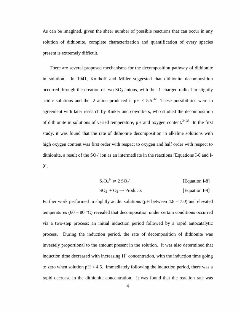
The molecular explanation for the ready decomposition of dithionite and its strength
as a reducing agent comes from two characteristics: dithionite’s abnormally long S-S
bond and the low oxidation state of the sulfur atoms. The structure of dithionite as a solid
is that of an eclipsed dimer of two SO2 units, connected by an S-S bond of 2.39
angstroms in length (see Figure I-1).35
6
Figure I-1. Structure of the dithionite anion, with the -2 charge spread
over the four oxygen atoms. The unmarked OSO and SSO bonding angles
are 108.2° and 98.7°, respectively.
For comparison, the lengths of the S-S bonds in the most prevalent form of elemental
sulfur, α-octasulfur, and in dithionate (S2O62-
), another sulfur oxyanion, have been
measured to be 2.04 and 2.15 angstroms, respectively.36,37
As a result of this much
longer disulfide bond, dithionite is more reactive than many other compounds containing
shorter disulfide bonds, a direct result of the weakened bond. For this reason, dithionite
may easily dissociated into two SO2- subunits or undergo protonated decomposition to
HSO2•. One electron spin resonance study was able to confirm the formation of the SO2
•
radical at elevated temperatures.38
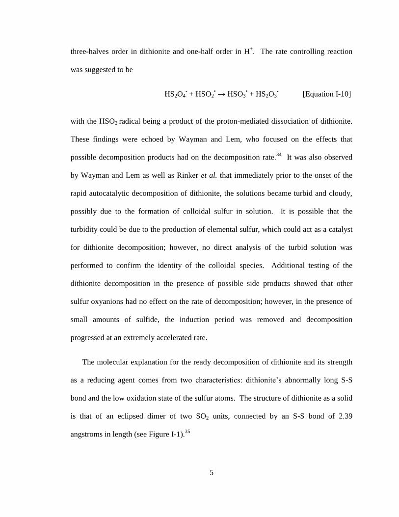
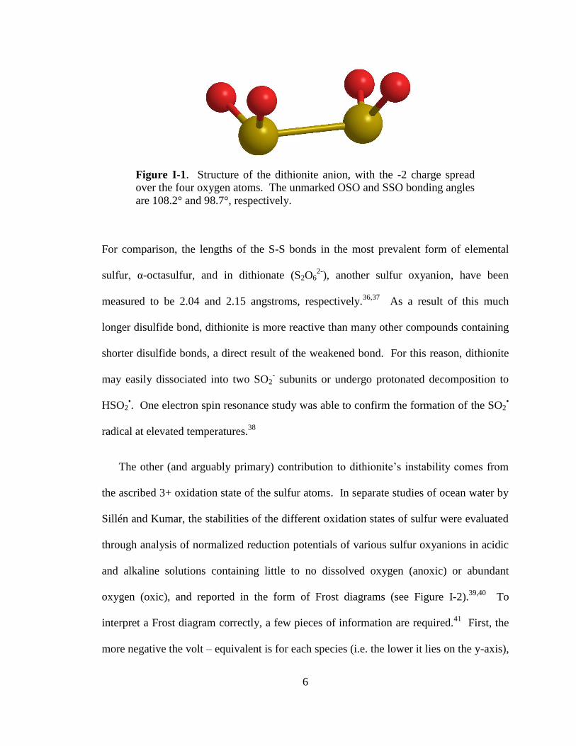
The other (and arguably primary) contribution to dithionite’s instability comes from
the ascribed 3+ oxidation state of the sulfur atoms. In separate studies of ocean water by
Sillén and Kumar, the stabilities of the different oxidation states of sulfur were evaluated
through analysis of normalized reduction potentials of various sulfur oxyanions in acidic
and alkaline solutions containing little to no dissolved oxygen (anoxic) or abundant
oxygen (oxic), and reported in the form of Frost diagrams (see Figure I-2).39,40
To
interpret a Frost diagram correctly, a few pieces of information are required.41
First, the
more negative the volt – equivalent is for each species (i.e. the lower it lies on the y-axis),
7
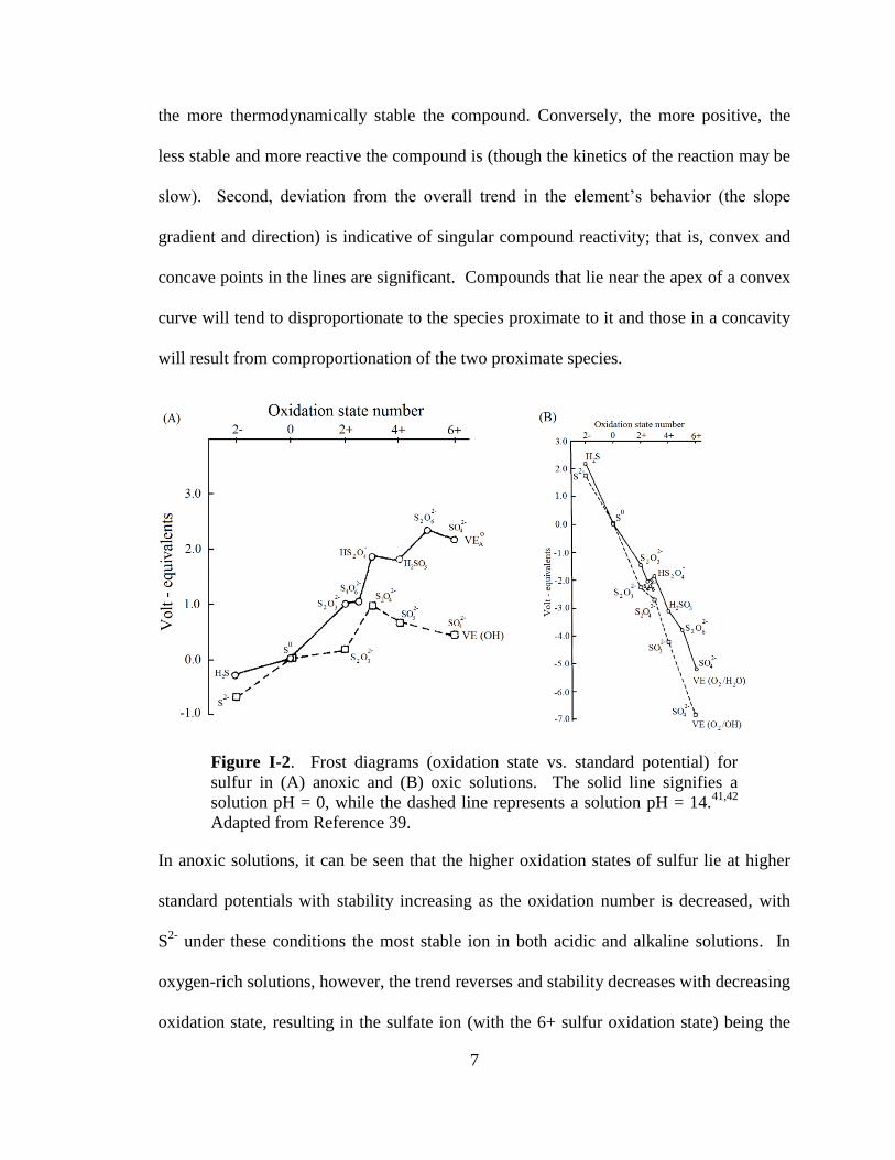
the more thermodynamically stable the compound. Conversely, the more positive, the
less stable and more reactive the compound is (though the kinetics of the reaction may be
slow). Second, deviation from the overall trend in the element’s behavior (the slope
gradient and direction) is indicative of singular compound reactivity; that is, convex and
concave points in the lines are significant. Compounds that lie near the apex of a convex
curve will tend to disproportionate to the species proximate to it and those in a concavity
will result from comproportionation of the two proximate species.
Figure I-2. Frost diagrams (oxidation state vs. standard potential) for
sulfur in (A) anoxic and (B) oxic solutions. The solid line signifies a
solution pH = 0, while the dashed line represents a solution pH = 14.41,42
Adapted from Reference 39.
In anoxic solutions, it can be seen that the higher oxidation states of sulfur lie at higher
standard potentials with stability increasing as the oxidation number is decreased, with
S2-
under these conditions the most stable ion in both acidic and alkaline solutions. In
oxygen-rich solutions, however, the trend reverses and stability decreases with decreasing
oxidation state, resulting in the sulfate ion (with the 6+ sulfur oxidation state) being the
8
most stable. Given the more negative reduction potentials present in both oxic and
anoxic solutions, the alkaline solution provided a better stabilizing environment for sulfur
compounds compared to the acidic solution. Interestingly, it is apparent that in each of
the four solutions described, dithionite lies at the apex of a small convex part of the
curve, indicating the tendency of dithionite to decompose into sulfite and thiosulfate, the
neighboring sulfur oxyanions. While in anoxic environments, the eventual end product
of dithionite decomposition would likely be of a lower oxidation state (sulfur or sulfide).
However, given the ubiquity of molecular oxygen in both the atmosphere and in
untreated water, it is much more likely that any dithionite sample will dissociate and
eventually decompose to sulfate (Figure I-2B).
B. History of Synthesis and Quantification
Dithionite was reportedly first produced by Georg Stahl in 1718 upon reduction of
aqueous sulfur dioxide with iron, although the original work detailing this could not be
located and verification of this comes from secondary sources.1,43
While work describing
the use of dithionite as a reducing agent and the elemental composition was completed in
the 19th
century,44-46
it was not until 1907 that a method for producing crystalline
anhydrous sodium dithionite from sulfur dioxide using zinc dust with sodium hydroxide
was accomplished by Bazlen.47
Once this production method was reported and
anhydrous, high purity dithionite was made widely available, there was a surge of
dithionite research, including some initial studies on the mechanisms and kinetics of the
decomposition of dithionite. Even at this early date, one of the primary focuses was in
9
determining a method for direct quantification of dithionite in a solution containing other
reducible sulfur oxyanion species.
The primary and most quantitative method for dithionite determination in the early
20th
century was a colorimetric titration using a known solution of indigo dye i.e. 2,2'-
Bis(2,3-dihydro-3-oxoindolyliden) which, when reacted with a solution of dithionite in an
air-free environment, produced a direct measure of dithionite content.48 Unfortunately,
this method required an advanced workup and a complex setup to maintain an inert
atmosphere for the titration. Additionally, considering the kilogram or more scale of the
product, it was required to be both economically and temporally justified. This titration
method was useful in situations where numerous or constant measurements of dithionite
were required, though not ideal for situations when a simple, individual measurement was
required.49
In 1923, Merriman described a simple, two-step titration procedure to quantify
dithionite which required no inert atmosphere or complex setup. The first part of this
method involves the reaction of a solid sample of dithionite with formaldehyde,
producing two sodium formaldehyde adducts.
Na2S2O4 + 2 CH2O + H2O → HOCH2SO2Na + HOCH2SO3Na [Equation I-11]
The first listed product, sodium hydroxymethanesulfinate (industrially known as
Rongalite), is produced. This adduct is titratable with iodine.
HOCH2SO2- + 2 I3
- + 2 H2O → SO4
2- + 6 I
- + 5 H
+ + CH2O [Equation I-12]
10
The other product, sodium hydroxymethanesulfonate (HMS), does not react with iodine
and thus there is no direct interference with the titration of Rongalite. This procedure
was found to be highly accurate for relatively pure samples of dithionite and was
recommended for industrial use. However, in older samples, the impurities present from
dithionite decomposition could also be reduced by iodine, resulting in measurement
errors by the single titration.
This issue was resolved by Robert Wollak in 1930.50
In his seminal paper, Wollak
detailed a series of three iodometric titrations which eliminated the interferences from
additional reducible species and measured the amounts of dithionite, thiosulfate, and
sulfite (i.e. bisulfite) present in the samples. This approach became the standard method
for dithionite quantification and analysis in the textile and paper-making industries for the
next fifty years.51
Following its publication, the Wollak method was reviewed by
numerous authors, many of whom found the methodology unsatisfactory due to potential
errors in measurement resulting from the presence of additional unreduced species
(mainly thiosulfate and bisulfite) in high concentration and pH effects. Zocher and
Saechtling reported that the thiosulfate measurement was prone to error, while Danehy
and Zubritsky considered the Wollak procedure “unexceptional” and cited concern over
potential errors resulting from high bisulfite concentrations.52,53
In response to these
concerns, William P. Kilroy highlighted the possible errors associated with the Wollak
procedure, and published a revised Wollak method for dithionite analysis in a series of
papers.54-56
This revised method is currently used for dithionite quantification in industry
and analytical laboratories.
11
Kilroy’s revised method follows the same three iodometric titration structure.56
In the
first titration, a sample is reacted with an excess of iodine to convert all reducible ions to
non-reactive species [Equations I-13 – I-15].
S2O42-
+ 3 I2 + 4 H2O → 2 HSO4- + 6 HI [Equation I-13]
2 S2O32-
+ I2 → S4O62-
+ 2 I- [Equation I-14]
HSO3- + I2 + H2O → HSO4
- + 2 HI [Equation I-15]
Following this, sodium hydroxide is added to adjust the final pH to 8 - 10, which causes
the reaction of sulfite with dithionate [Equation I-16].
S4O62-
+ SO32-
→ S2O32-
+ S3O62-
[Equation I-16]
The thiosulfate can then be directly titrated with iodine, as seen in Equation I-14. The
number of moles of iodine used to titrate the thiosulfate, be it equal to A, are proportional
to the amount of thiosulfate originally present in the sample, equal to 4A. In the second
titration, a basic solution of formaldehyde is added to a sample of dithionite, forming the
Rongalite adduct, which is titratable (see Equation I-11 and I-12). The moles of iodine
used in this titration (B) react with both Rongalite and thiosulfate, meaning the difference
of (B – 2A)/2 yields the amount of dithionite initially present. The last titration is a direct
titration of the sample and quantifies all reducible species present (Equations I-13 – I-15).
If the moles of iodine in this titration used are equal to C, then the amount of sulfite
present in the solution is equal to (2C + 2A – 3B)/2 moles. Of note, Kilroy went one step
further and has described a four-step titration in which sulfide is also quantified, but it
requires a substantial amount of specialized glassware and an inert atmosphere,
complicating an already challenging titration scheme.57
12
Considering the expense and difficulties in repeatedly preparing the iodine and
thiosulfate standards used in the titrations as well as the extensive glassware setup and the
need for high accuracy and precision when performing these titrations, alternate methods
for dithionite composition analysis using existing instrumentation has been the major
research focus for dithionite recently. The use of analytical instrumentation has a major
advantage over the titration approach – namely, each species can be directly quantified
and is not dependent on the accurate quantification of another species (i.e. subtracting
thiosulfate to determine the dithionite composition in the first and second titration).
Direct quantification has the added benefit of decreasing the propagated error of the
measurement. Reported methods for dithionite quantification include capillary
electrophoresis,23
chromatography,58
cyclic voltammetry,21
differential pulse
polarography,59
ion-pair chromatography,60
and isotachophoresis.22
Of the
chromatographic studies, the capillary electrophoresis work of de Carvalho and Schwedt
was the most quantitative, determining dithionite, thiosulfate, sulfite and sulfate.23
However, in each of these studies, no direct statistical comparison of the equivalency of
the instrumental method to the accepted titration methodology was presented,
underscoring the need for mathematical validation of the proposed instrumental
equivalent to the accepted iodometric titration. An instrumental quantification approach
yields an additional benefit – if additional sulfur oxyanion impurities are present, these
compounds may be directly detectable and identifiable. In the accepted titration
procedure, the identities of the additional decomposition products cannot be elucidated
beyond the fact that they may be reducible through the iodometric titration, which would
result in measurement errors. Direct detection by an instrument is preferable in that these
13
additional decomposition products could be identified. With the use of ion
chromatography (IC), such an approach is described in Chapter II.
C. A Brief Review of Thin Film Production
From the first published description61
by Paul Drude in 1889 to the current deposition
methods used industrially for integrated circuit technologies, thin films and coatings have
grown into a broad research area of both industrial and academic significance.
Historically, the term ‘thin film’ describes a layer or coating nanometers to micrometers
in thickness, deposited onto some other, generally flat material (substrate).62
With the
wide range of materials to use as either the film or substrate along with numerous
deposition methods possible, there are almost a limitless number of permutations for the
integration of thin films into a desired application.
Historically, the unique traits imparted by thin films have been known since before
their description by Drude. Well known examples of the early use of thin films include
glass mirrors backed by a thin layer of metal (first described by the Roman scholar Pliny
the Elder in the year 77 CE63
) and the application of thin gold films (i.e. gold leaf) to
cover statues and other items of significance, both for beauty as well as protection of the
underlying surface (seen in numerous cultures, from ancient Egypt to modern day).64
For
most purposes, the early use of thin films and coatings was primarily for imparting or
enhancing a particular quality of the substrate (e.g. reflectance, durability, impression of
opulence) and not for a self-contained characteristic the film possessed. As both research
and technology in this field has matured, the focus of thin films has shifted from this
14
substrate-centric view to one in which the film plays an equal if not superior role
compared to the substrate. This shift in thin film philosophy has undoubtedly come from
the increased amount of control in film creation resulting from the numerous deposition
methods which have been described. While the application of gold leaf (generally 0.3 – 2
μm thick) was accomplished by hand, current thin film production methods do not
require direct contact and instead can be accomplished through the production method
itself.
Broadly, thin film production methods can be separated into two categories: physical
and chemical depositions.65
Physical deposition methods generally use a solid starting
material and, through a physical method such as vaporization, evaporation, or sputtering
of a sample, transfer atoms of the compound through a vacuum environment to a
substrate on which it is deposited. In this process, the starting material and the thin film
material at the end can be the same chemically, although the structure may be altered (i.e.
amorphous to polycrystalline or a well-defined crystalline lattice structure), or there may
be a reaction which produces the film. Choice examples of this method include sputter
and RF-coil depositions, thermal evaporation, and molecular beam epitaxy. Conversely,
chemical deposition methods widely employ a chemical reaction occurring in the solution
or vapor phase, or at the gas-solid interface to produce the film. The deposited material is
usually some stoichiometric mixture of the reacting compounds or film built of
alternating layers of the reactants, in some situations having produced a layer which is
only one atom thick. Given the number of possible starting materials and subsequent
reactions, chemical deposition is more versatile and offers a wider range of possible
reactants and products. Well known deposition methods include chemical vapor
15
deposition, atomic layer deposition, electroplating, and the sol-gel method. While many
of the vapor phase deposition methods offer more control in terms of layer thickness and
crystalline homogeneity, the sol-gel approach is attractive due to the low temperatures at
which it occurs, lower operating cost as it does not require a vacuum environment, and
good particle size control to ensure a homogenous film.66
Due to these characteristics,
the sol-gel method plays a key role in the preparation and development of new materials
or as a proof-of-concept step in film productions.
In the traditional sol-gel process, a metal alkoxide is mixed with an alcohol or water-
based solution.41,65-68
When mixed, the alkoxide group is hydrolyzed and forms a
colloidal solution of metal oxides or hydroxides and an alcohol. Over time, the colloidal
particles will aggregate through polycondensation, producing an alcohol or water, while
this product and the remaining solvent is removed. This can occur either through
evaporation or by directed heating of the solution (a process called sintering). If the sol is
applied to a substrate during the polycondensation and sintering steps, the final product is
a gel film composed of colloidal particles of the ceramic metal oxide. The classic sol-gel
reaction is the production of silicon dioxide (silica) from tetramethyl orthosilicate
[Equations I-17 and I-18].66,68
Si(OMe)4 + 4 H2O → Si(OH)4 + 4 MeOH
[Equation I-17]
Si(OH)4 → SiO2 + 2 H2O
[Equation I-18]
This sol-gel route is similar to the first reported sol-gel method by Jacques-Joseph
Ebelman in 1845, who hydrolyzed a silicic acid ester to obtain a transparent ceramic
material.67,69
However, it was not until 1939 that Geffcken and Berger detailed and
patented the use of the sol-gel method for the building of layered films.70
Since then,
16
numerous other metal and mixed metal oxides have been produced using the sol-gel
method.
D. Applications of Titania
One metal oxide which has garnered much attention recently is titania (i.e. titanium
dioxide, TiO2). Titania is the most prominent and important titanium compounds, and
represents the bulk of the geologically extractable form of titanium.71
Titania has found
widespread use in the 20th
century, as an ingredient in cosmetics, sunscreen, paints, and
toothpaste.66,72
However, it was not until its use for the photolysis of water by Fujishima
and Honda in 197273
and its incorporation into the first dye-sensitized solar cell by
O'Regan and Grätzel in 198874
that a renewed focus on titania research was initiated.
The following decades contained a dramatic rise in the amount of published research
using TiO2.72
Over the next two decades, many new applications for titania were
described. As it possesses interesting optical properties (i.e. band gap) and strong UV
absorbance, titania has been reported as a strong candidate for thin film coatings on glass
for the creation of self-cleaning windows, which are able to repel dirt and decompose
organic materials when they come in contact with the windows surface.66,75-77
It has also
been found to be a good photocatalyst, useful in the oxidation and treatment of organic
and pharmaceutical environmental pollutants.78,79
One of the most dynamic applications has been the use of titania as a sensing material
for gases. Generally, a titania surface is positioned as to allow some gas of interest to be
directed over the surface. During this time, the electrical properties (usually surface
17
resistance) of the material are monitored, where a change in the monitored property is
indicative of the gas of interest being present in the sample.80-84
However, sensors based
on these titania films and powders generally suffer from detection ranges that are highly
dependent on the particle size and surface structure of the TiO2 (i.e. rutile, anatase,
amorphous) or require an elevated operating temperature and complicated operating
parameters for accurate measurements.81
New preparation methods for less complex
sensors using these materials are desired to alleviate these shortcomings. Of note, titania
powders and films have been used for detection of ethanol,81
hydrogen sulfide,85
carbon
monoxide83,84
and many other gaseous compounds.80
E. Detection of Gaseous Peroxides
Peroxides (O22-
) are extremely strong oxidizing agents of great importance in many
industrial and biological fields. Arguably the most prominent of these oxidants,
hydrogen peroxide (H2O2), finds use as a bleaching agent in the paper and textile
industries, which together consume over half of the annually produced supply,5,86
and as
a reagent for treatment of organic and other pollutants in water supplies.87,88
Gaseous
hydrogen peroxide is often used in the food and medicinal fields as a cleaning technique
in situations where a sterile environment with no bacterial or microbial growth is
essential.89-95
Due to its strong oxidizing potential, the Occupational Safety and Health
Administration (OSHA) has set a permissible average exposure limit of 1 ppm over an
eight hour day.96
This limit requires users to be constantly monitored. The primary
OSHA-approved method for quantification of gaseous peroxide include drawing the
18
atmosphere in question through an acidified solution of titanium oxide sulfate,97
where an
optical measurement of the solution at approximately 410 nm can determine the peroxide
concentration. This method is still the preferred laboratory standard technique for
gaseous peroxide quantification. Another less quantitative method is the use of Dräger
tubes specific to hydrogen peroxide, where a color change over a measured length of a
stationary phase indicates peroxide concentration.98
Additional methods for peroxide
detection and quantification include fluorometric,99-102
amperometric,103-106
spectroscopic
analysis,107-110
and electrochemical sensing.111
Many of these methods cannot be easily
automated as they require pre-concentration of the atmosphere in solution and some
amount of wet chemistry, or require constant attention by a technician to ensure
instrumental stability.
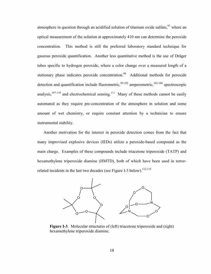
Another motivation for the interest in peroxide detection comes from the fact that
many improvised explosive devices (IEDs) utilize a peroxide-based compound as the
main charge. Examples of these compounds include triacetone triperoxide (TATP) and
hexamethylene triperoxide diamine (HMTD), both of which have been used in terror-
related incidents in the last two decades (see Figure I-3 below).112-115
Figure I-3. Molecular structures of (left) triacetone triperoxide and (right)
hexamethylene triperoxide diamine.
19
Because these compounds do not contain a nitro group or metal atoms and are instead
comprised of carbon, hydrogen, oxygen and nitrogen, the detection of these compounds
through spectroscopic means is difficult in air given the inevitable presence of species
possessing similar spectroscopic shifts.116,117
These compounds also possess low vapor
pressures, making sampling from the atmosphere difficult.118
Reported methods for the
detection of these compounds include ion mobility spectroscopy (IMS),119-122
laser-
induced breakdown spectroscopy (LIBS),123-125
gas exposure over mixed metal and metal
oxide materials,126-128
surface enhanced Raman spectroscopy (SERS),125,129
and mass
spectrometry.130-133
While useful, these approaches are hampered by an inability to
miniaturize instrumentation for field use, a required pre-concentration of the sample for
analysis, necessary wet chemistry, and a lack of real-time measurement capability.
A simple approach to detection would be one where a simple yes-no system can
indicate the presence of peroxides through an event such as a change in color. This can
possibly be addressed through the creation of titanium peroxo complexes. It has been
well known that titanium peroxo complexes form in acidic solutions, resulting in an
intense yellow or orange-red color. This behavior was originally reported by Sehönn in
1870, who remarked on the intense color formed.134
Many studies attempted to elucidate
the molecular formula for the colored product, with a number of crystalline compounds
being isolated but found to be amorphous and structurally unresolvable.135-137
It was not
until 1970 that Schwarzenbach, Müehlebach, and Müeller successfully characterized
some of these compounds crystallized with organic acids and EDTA using X-Ray
diffraction.138
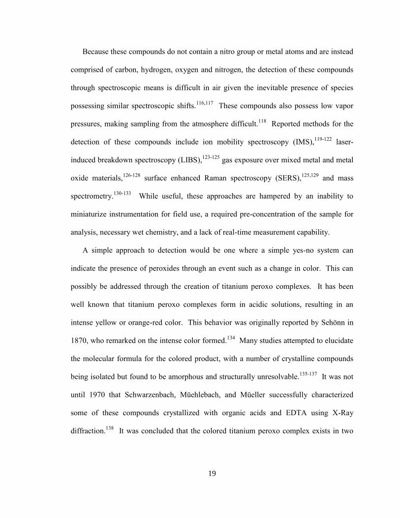
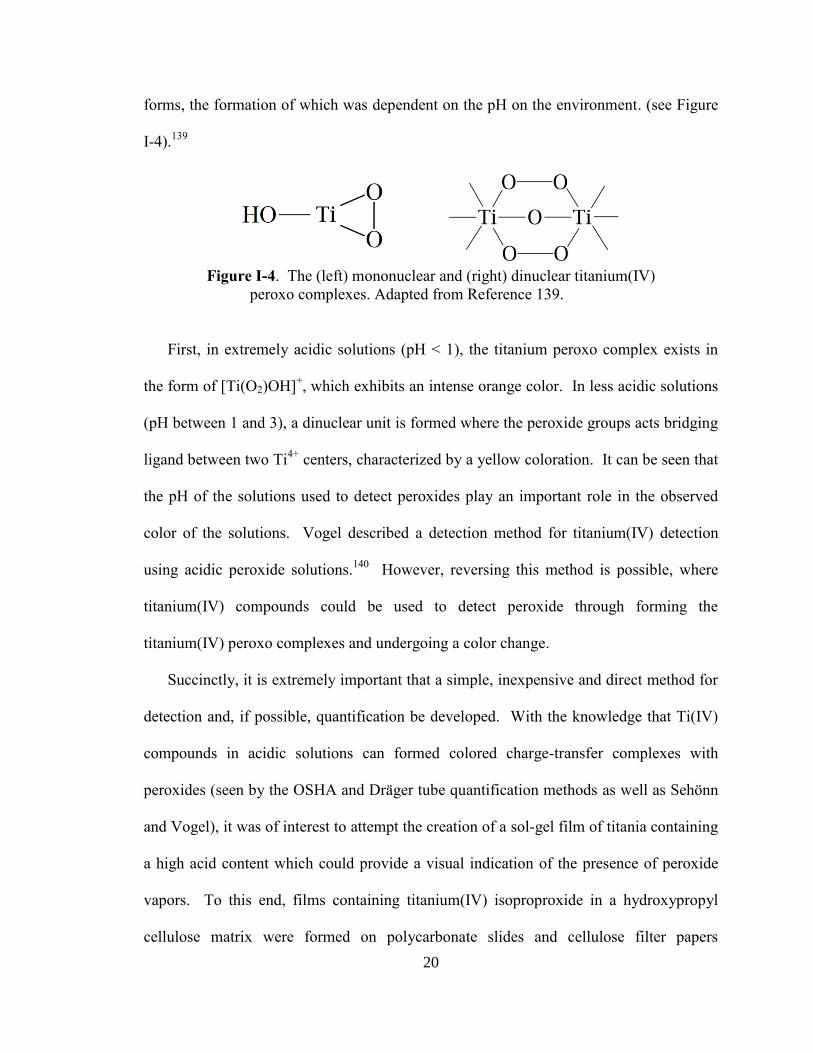
It was concluded that the colored titanium peroxo complex exists in two
20
forms, the formation of which was dependent on the pH on the environment. (see Figure
I-4).139
Figure I-4. The (left) mononuclear and (right) dinuclear titanium(IV)
peroxo complexes. Adapted from Reference 139.
First, in extremely acidic solutions (pH < 1), the titanium peroxo complex exists in
the form of [Ti(O2)OH]+, which exhibits an intense orange color. In less acidic solutions
(pH between 1 and 3), a dinuclear unit is formed where the peroxide groups acts bridging
ligand between two Ti4+
centers, characterized by a yellow coloration. It can be seen that
the pH of the solutions used to detect peroxides play an important role in the observed
color of the solutions. Vogel described a detection method for titanium(IV) detection
using acidic peroxide solutions.140
However, reversing this method is possible, where
titanium(IV) compounds could be used to detect peroxide through forming the
titanium(IV) peroxo complexes and undergoing a color change.
Succinctly, it is extremely important that a simple, inexpensive and direct method for
detection and, if possible, quantification be developed. With the knowledge that Ti(IV)
compounds in acidic solutions can formed colored charge-transfer complexes with
peroxides (seen by the OSHA and Dräger tube quantification methods as well as Sehönn
and Vogel), it was of interest to attempt the creation of a sol-gel film of titania containing
a high acid content which could provide a visual indication of the presence of peroxide
vapors. To this end, films containing titanium(IV) isoproproxide in a hydroxypropyl
cellulose matrix were formed on polycarbonate slides and cellulose filter papers
21
according to a method previously described by Kozuka and coworkers,141
without
calcination after the initial drying period. When exposed to peroxide vapors, the films
change from colorless to yellow, with the final coloration dependent on the amount of
titania present. It is anticipated that these films can be integrated into a low-cost sensor
to monitor peroxide concentrations in industrial workplaces.
22
CHAPTER II
A METHOD FOR RAPID QUANTIFICATION OF SODIUM DITHIONITE AND ITS
DECOMPOSITION PRODUCTS BY ION CHROMATOGRAPHY
A. Introduction
As was extensively discussed in the introductory Chapter, sodium dithionite (Na2S2O4) is an
oxidizable sulfur oxyanion often employed as a reducing agent in the textile and paper industries,
environmental remediation treatments and synthetic chemistry. 2-20 This industrially important
reagent slowly decomposes in both the solid and solution phases into a variety of sulfur
oxyanions. For this reason, a method for the rapid assessment of purity of a given sample is
crucial for its continued use. Despite the importance of this material to the wood pulping and
textile industries, a rapid, reliable method to quantify dithionite and its decomposition products
remains a challenge. Currently, a three-step iodometric titration formulated by Wollak and
revised by Kilroy is used for routine sample analysis.50,56
However, this method requires
extensive bench-top chemistry and a high level of precision for accurate measurements of
dithionite and its decomposition products. Ion chromatography can provide a simple one-step
method that can easily be automated to rapidly and accurately determine the concentration of
dithionite and its decomposition product, thiosulfate. The results are statistically non-different
with those obtained using a multi-step iodometric titration, validating the proposed instrumental
approach.
23
B. Experimental Details
B.1 . Sodium Dithionite Samples
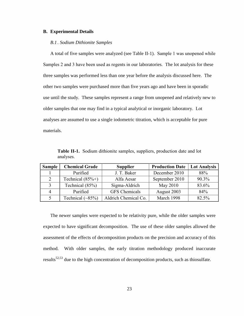
A total of five samples were analyzed (see Table II-1). Sample 1 was unopened while
Samples 2 and 3 have been used as regents in our laboratories. The lot analysis for these
three samples was performed less than one year before the analysis discussed here. The
other two samples were purchased more than five years ago and have been in sporadic
use until the study. These samples represent a range from unopened and relatively new to
older samples that one may find in a typical analytical or inorganic laboratory. Lot
analyses are assumed to use a single iodometric titration, which is acceptable for pure
materials.
Table II-1. Sodium dithionite samples, suppliers, production date and lot
analyses.
Sample Chemical Grade Supplier Production Date Lot Analysis
1 Purified J. T. Baker December 2010 88%
2 Technical (85%+) Alfa Aesar September 2010 90.3%
3 Technical (85%) Sigma-Aldrich May 2010 83.6%
4 Purified GFS Chemicals August 2003 84%
5 Technical (~85%) Aldrich Chemical Co. March 1998 82.5%
The newer samples were expected to be relativity pure, while the older samples were
expected to have significant decomposition. The use of these older samples allowed the
assessment of the effects of decomposition products on the precision and accuracy of this
method. With older samples, the early titration methodology produced inaccurate
results52,53
due to the high concentration of decomposition products, such as thiosulfate.
24
B.2 . Solution Preparation
Potassium iodate (Mallinckrodt), dried at 95 °C for 24 hours prior to use, was used as
a primary standard. Iodate was used to reduce potassium iodide to triiodide and
standardize a 0.10 M sodium thiosulfate pentahydrate (Fisher, Certified ACS) solution.
A 0.050 M solution of triiodide was made by mixing iodine (Spectrum) and a 2:1 excess
of potassium iodide (Fisher, Certified ACS) in 2 L water. Using the standardized
thiosulfate solution, this solution was standardized by titration with thiosulfate to four
significant digits.142
The 0.10 and 5.0 x 10⁻³
M triiodide solutions were prepared and
standardized in a similar manner. The 37% (w/w) formaldehyde solution was obtained
from Fisher (Certified ACS) and used as supplied. Sodium hydroxymethanesulfinate
hydrate (Aldrich) was used for calibration of the ion chromatograph. Iodometric titration
was used to determine hydration of the Rongalite sample. All solutions were prepared
using ultrapure water (18 MΩ-cm).
B.3 . Ion Chromatography Setup
A Metrohm Advanced IC-2 System was utilized for sample analysis. For thiosulfate
and Rongalite quantification, the apparatus was equipped with a Metrosep A Supp 7-250
column and a Metrosep RP Guard column, both heated to 35 °C. A 3.60 mM sodium
carbonate (EMD, Anhydrous ACS Grade) mobile phase was used with a flow rate of 0.7
mL/min. An 853 suppressor module was fed with a 0.10 M H2SO4 (Pharmco-Aaper,
ACS Reagent) solution and deionized water. A CO2 and an H2O absorber cartridge
preceded the air inlet.
25
IC samples were prepared by adding an accurately weighed 1.0000 g sample of
dithionite to 75 mL of a basic formaldehyde solution. As discussed in Chapter I, the
reaction of formaldehyde with dithionite quantitatively forms Rongalite (i.e. sodium
hydroxymethanesulfinate, HOCH2SO2Na) and HMS (i.e. sodium
hydroxymethanesulfonate, HOCH2SO3Na).
Na2S2O4 + 2 CH2O + H2O → HOCH2SO2Na + HOCH2SO3Na [Equation II-1]
The formaldehyde solution contained 37.5 mL of the stock 37% formaldehyde solution
which was diluted with 37.5 mL water and made basic with 7 or 8 drops of 10 M sodium
hydroxide. After allowing reaction of the dithionite for approximately 20 minutes, the
solution was diluted to 250 mL. From this solution, 50 mL aliquots were removed and
further diluted to 2 L for IC analysis. At least three injections were analyzed per sample.
B.4 . Titration Methodology
While a brief survey of the iodometric titration method for dithionite analysis was
discussed in Chapter I, a more thorough exploration of the topic is presented here. The
titration results are labeled X, Y and Z as in the original publication.56
When a dithionite
sample is added to a solution of iodine under acidic conditions, Equations II-2 - II-4 can
occur depending on the species present.
S2O42-
+ 3 I2 + 4 H2O → 2 HSO4- + 6 HI [Equation II-2]
2 S2O32-
+ I2 → S4O62-
+ 2 I-
[Equation II-3]
HSO3- + I2 + H2O → HSO4
- + 2 HI [Equation II-4]
For these reactions, triiodide (I3-) and not iodine was used due to the presence of excess
iodide and the insolubility of elemental iodine due to the large equilibrium constant for
26
the complex ion formation.143
In addition, under acidic conditions sulfite (SO32-
) is
typically protonated and is present as bisulfite (HSO3-).
The thiosulfate (S2O32-
) concentration in the sample was determined by first reacting
a dithionite solution with excess triiodide. Typically, approximately 1.0000 g of the
dithionite sample was accurately weighed and dissolved in 75 mL 0.2500 M of triiodide
solution containing 10 g of sodium acetate trihydrate. This was a scale-up from the
original method which used 0.4000 g of dithionite for analysis. The rationale for this
action was to obtain five significant digits in the analyses for statistical purposes. For
older samples suspected to contain little sodium dithionite by weight (< 40%), 12.5 mL
of a 3.5 M equivalent molar acetic acid-acetate buffer was used, as recommended by
Kilroy.56
Once all reducible sulfur species were reacted, excess sulfite was added in the
form of a 10% sulfite solution until all the triiodide was removed and the solution became
clear. Next, an additional 8 mL of the sulfite solution was added to regenerate the
thiosulfate ion from the tetrathionate (S4O62-
) ion (II-Equation 5).
S4O62-
+ SO32-
→ S2O32-
+ S3O62-
[Equation II-5]
After these steps, the solution became acidic and was neutralized with 10 M sodium
hydroxide using phenolphthalein as an indicator. Following neutralization, 10 mL of
37% formaldehyde followed by 25 mL of 20% acetic acid was added. This process
removed the unreacted sulfite by reacting it with formaldehyde under acidic conditions to
produce HMS.
SO32-
+ CH2O → HOCH2SO3- [Equation II-6]
27
A 50 mL aliquot was taken from the sample and acidified with 20% acetic acid to a pH of
3.5 to 4 as indicated by pH paper. Finally, the thiosulfate concentration was determined
through titration of the pH-adjusted aliquot with the 5.00 x 10⁻³
M triiodide solution
(Equation II-2). At least three aliquots were titrated per sample. If the amount of
triiodide required to titrate the thiosulfate was A, the total amount of thiosulfate present
in the sample was deemed to be 4A, as seen in Equations II-2 and II-4 (two S2O32-
ions
are required to form one S4O62-
ion, which is then converted back to one S2O32-
ion) and
the titration (Equation II-2) stoichiometry.
Once the thiosulfate is determined, the dithionite concentration can be quantified by
reaction with formaldehyde to form Rongalite and HMS. Similar to the IC samples,
1.0000 g of the dithionite sample was weighed precisely and then added to 75 mL of
basic formaldehyde solution described in the IC experimental. After 20 minutes, a 10 mL
aliquot was removed. The aliquot was diluted with 150 mL of water and made acidic
using 7.5 mL of an acetic acid-acetate buffer (3.5 M acetic acid and 3.5 M sodium
acetate). The resulting solution was titrated with the 0.050 M triiodide solution. Again,
at least three aliquots were titrated. In an idealized pure dithionite sample, an iodometric
titration will provide the concentration of Rongalite and, in turn, the original
concentration of dithionite.
HOCH2SO2- + 2I3
- + 2H2O → SO4
2- + 6I
- + 5H
+ + CH2O [Equation II-7]
However, any thiosulfate present in the original sample will also react with the triiodide
(Equation II-3). Thus, if the amount of triiodide required to titrate the Rongalite solution
is B, the dithionite concentration was equal to (B - 2A)/2.
28
The final titration quantifies the amount of all reducible species present, namely
thiosulfate, dithionite, and sulfite. Again, the reaction was scaled up for more accurate
measurements. In this titration, 50 mL of 0.15 M triiodide and either 13 mL of the 3.5 M
acetic acid-acetate buffer solution or 10 g sodium acetate trihydrate were mixed in a 250
mL volumetric flask, to which 1.0000 g of sample was added slowly. Once diluted, a 25
mL aliquot was removed and titrated with a 0.1000 M thiosulfate solution using starch as
the indicator. This titration measures the amount of reducible species present as a whole,
and the back titration with thiosulfate quantifies how much iodine was initially
consumed. The amount of thiosulfate required to titrate is subtracted from the initial
amount of iodine present; the difference, which would be the moles of iodine consumed
when the sample is added to the iodine solution is labeled C. When combined with
Equations II-2 - II-4, the amount of sulfite present in the original sample is equal to (2C +
2A – 3B)/2.
C. Results and Discussion
For dithionite analysis, the five samples were reacted with formaldehyde and
analyzed by ion chromatography and the three-step titration method.
29
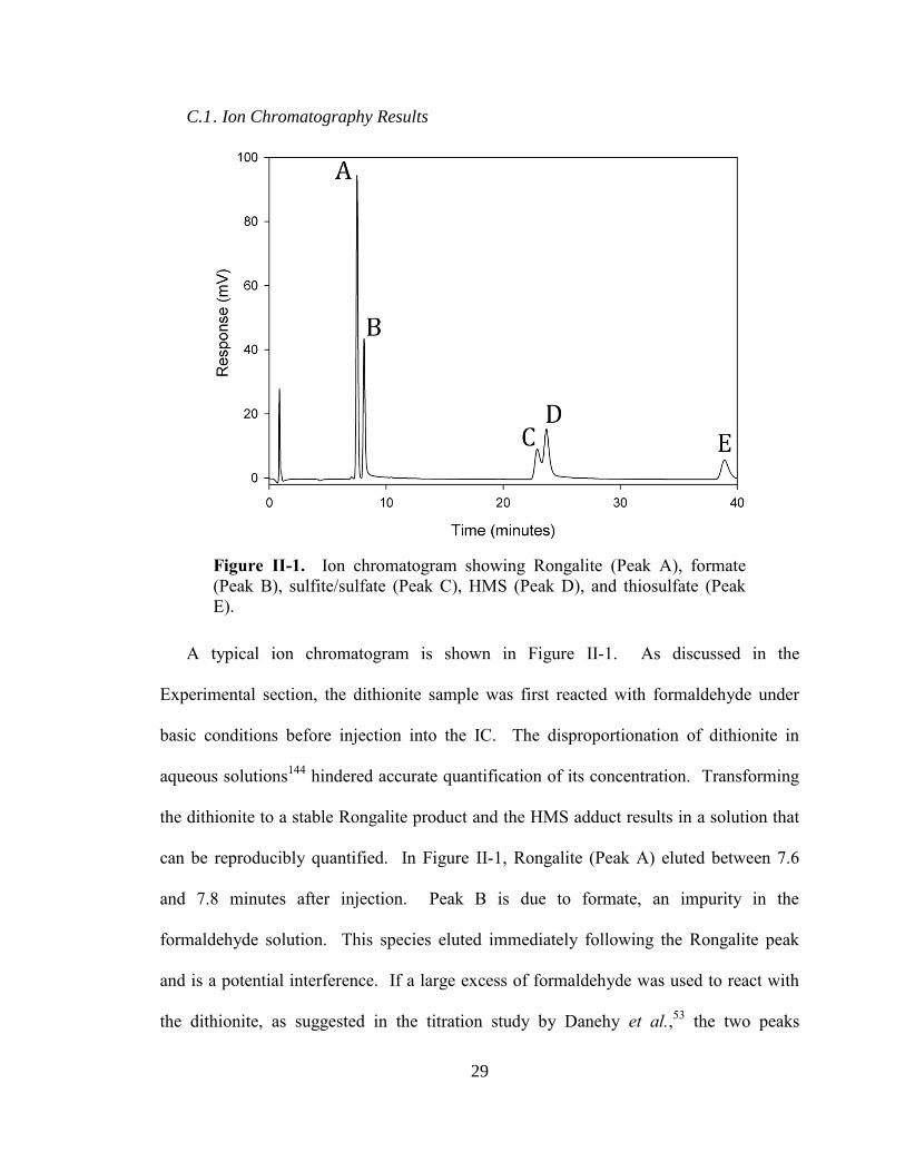
C.1 . Ion Chromatography Results
Figure II-1. Ion chromatogram showing Rongalite (Peak A), formate
(Peak B), sulfite/sulfate (Peak C), HMS (Peak D), and thiosulfate (Peak
E).
A typical ion chromatogram is shown in Figure II-1. As discussed in the
Experimental section, the dithionite sample was first reacted with formaldehyde under
basic conditions before injection into the IC. The disproportionation of dithionite in
aqueous solutions144
hindered accurate quantification of its concentration. Transforming
the dithionite to a stable Rongalite product and the HMS adduct results in a solution that
can be reproducibly quantified. In Figure II-1, Rongalite (Peak A) eluted between 7.6
and 7.8 minutes after injection. Peak B is due to formate, an impurity in the
formaldehyde solution. This species eluted immediately following the Rongalite peak
and is a potential interference. If a large excess of formaldehyde was used to react with
the dithionite, as suggested in the titration study by Danehy et al.,53
the two peaks
30
coeluted and made quantification impossible. Thus, the method of Kilroy,56
which
employed a much lower concentration of formaldehyde, was used. Given that Rongalite
is quantitatively produced from the initial dithionite present (Equation II-1), measurement
of this peak allows dithionite and thus the purity of the sample to be quantified.
In addition to Rongalite, HMS is also formed (Peak D). Equation II-1 implies that
HMS is also quantitatively produced from the initial dithionite. Since HMS can also be
formed from a reaction with sulfite and formaldehyde under acidic conditions (Equation
II-6), it was initially hoped that both dithionite and sulfite could be quantified by
measurement of both the Rongalite and HMS peaks. However, analysis showed that the
resulting HMS peak area, calibrated using HMS standards, was inconsistent with this
assumption. This signifies that HMS is either not quantitatively produced or decomposes
in the alkaline mobile phase during the one-hour time scale of the experiment.
Furthermore, the HMS species is partially coeluted with the Peak C. Standard solutions
of both sulfite and sulfate produced peaks at approximately the same retention time as
Peak Cs. These species are probably due to impurities in the initial material, due to the
decomposition of dithionite, or generated from the reaction of formaldehyde with
dithionite. This coelution prevents the quantification of this HMS, sulfite and sulfate. It
is possible that an IC injection of an unfunctionalized (i.e. no formaldehyde) sample of
dithionite solution could potentially prevent the coelution and allow for sulfite and sulfate
quantification. However, since these coelutions do not affect the measurement of
Rongalite and the determination of the dithionite, no further steps were taken. Finally, the
thiosulfate (Peak E) was well separated from all other species with a retention time of
38.4 minutes and was easily quantified.
31
The Rongalite concentrations were determined by the peak areas of Peak A. For the
calibration plot (R2 = 1.00), four different Rongalite solutions were prepared. The
concentrations of the dithionite anion were determined from the Rongalite concentration
using Equation II-1 and are tabulated in Table II-2. The thiosulfate anion is an expected
decomposition product of dithionite144
and was quantified by measuring the peak area
(for Peak E). A calibration curve (R2
= 1.00) was also generated using four different
sodium thiosulfate pentahydrate solutions. The standard deviations for the IC results are
also reported in Table II-2 and were determined using multiple injections (at least three),
and from the slope in the calibration plot and the dilution steps required to prepare the
samples. Both the Rongalite and thiosulfate calibration curves can be found in Appendix
A.
Both the dithionite and thiosulfate calibrations plots were analyzed to determine the
limits of quantification using the methodology developed by Hubaux and Vos.145
For the
used calibration curve, the limit of quantification for sodium dithionite is 0.3% by mass.
All samples are significantly above this limit. For the thiosulfate anion, the peak area in
the newer samples (1 through 3) is relatively small. Although two samples with different
dilution factors could have been utilized, the conditions used to optimize the
determination of dithionite results in a limit of quantification at the 95% confidence level
of 5% thiosulfate by mass. Thus, the thiosulfate concentration determined by IC in Table
II-2 is at or under this limit and the error bars are not reported.
32
C.2 . Titration Results
Table II-2 also reports the titration results for the dithionite and thiosulfate oxyanions
of interest. The thiosulfate composition is directly measured. The standard deviations
reported in Table II-2 are determined by multiple measurements (at least three). As
discussed in the experimental, the dithionite titration results must be first corrected for the
thiosulfate initially present in the sample. The standard deviations for dithionite included
the uncertainty of both titration steps. Thus, the standard deviations for dithionite are
consistently larger than those reported for thiosulfate.
C.3 . Comparison of IC and Titration Methods
The IC and titration methods gave extremely similar results for dithionite and
thiosulfate (Table II-2), with differences of less than 2% and 1%, respectively.
Table II-2. Sample anion concentrations and their associated standard
deviations as mass percent determined by IC and titration. The error bars
are the propagated error of the measurements, solution concentrations, and
titration volume deviations.
Sample IC Titration
Dithionite Thiosulfate Dithionite Thiosulfate Sulfite
1 62.9 ± 0.7% 0.25%* 61.4 ± 1.2% 0.84 ± 0.07% 2.12 ± 1.73%
2 51.2 ± 0.8% 3.3%* 49.9 ± 1.0% 4.0 ± 0.1% 3.98 ± 1.73%
3 36.7 ± 0.4% 5.0%* 35.8 ± 0.7% 5.9 ± 0.1% 18.08 ± 1.35%
4 15.8 ± 0.1% 16.1 + 0.2% 16.2 ± 0.4% 15.8 ± 0.2% 28.61 ± 1.00%
5 14.8 ± 0.2% 16.5 + 0.3% 14.9 ± 0.4% 16.4 ± 0.2% 31.43 ± 1.23% *These samples have concentration under the limit of quantification.
The IC measurements require only one straightforward derivation step before
measurement. Assuming that dithionite is present solely as sodium dithionite, the purity
of the sample can be computed and compared to the lot analysis provided by the supplier
(Table II-3).
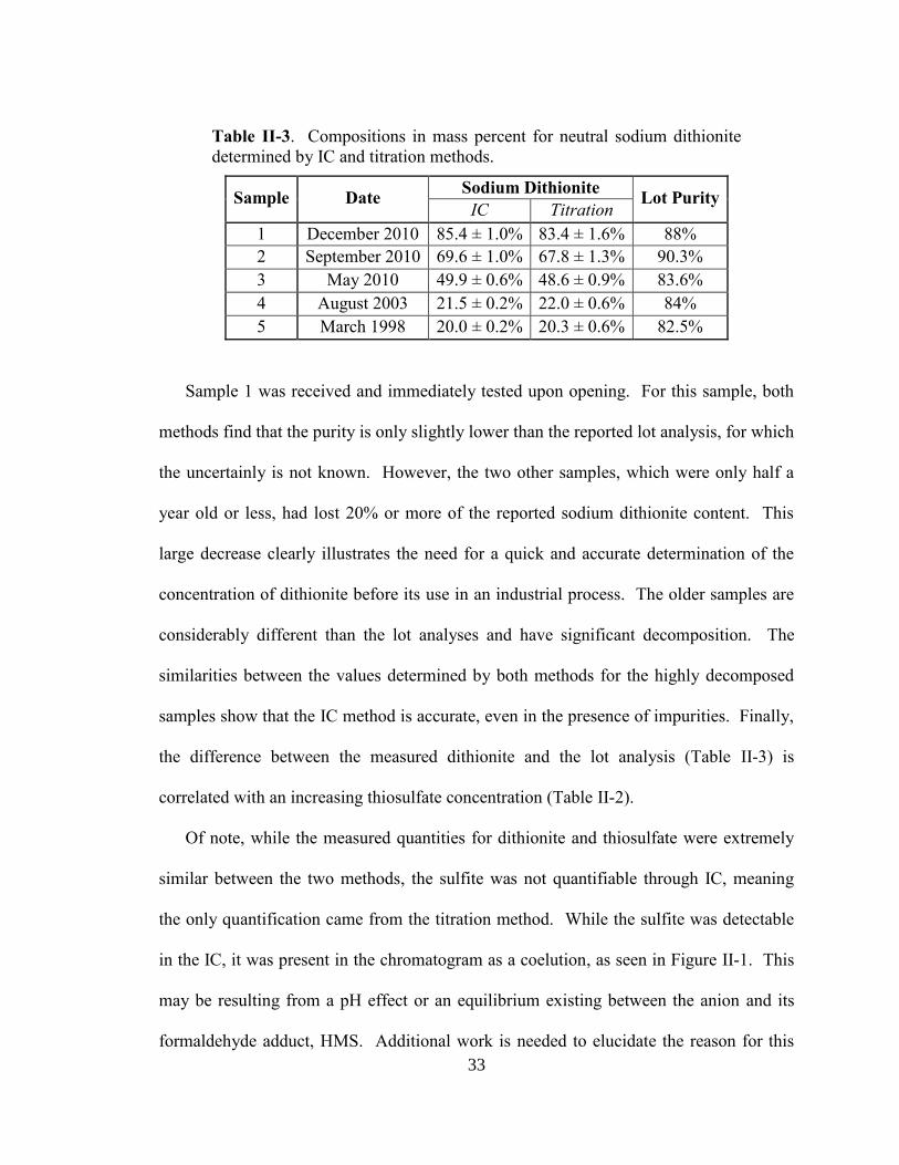
33
Table II-3. Compositions in mass percent for neutral sodium dithionite
determined by IC and titration methods.
Sample Date Sodium Dithionite
Lot Purity IC Titration
1 December 2010 85.4 ± 1.0% 83.4 ± 1.6% 88%
2 September 2010 69.6 ± 1.0% 67.8 ± 1.3% 90.3%
3 May 2010 49.9 ± 0.6% 48.6 ± 0.9% 83.6%
4 August 2003 21.5 ± 0.2% 22.0 ± 0.6% 84%
5 March 1998 20.0 ± 0.2% 20.3 ± 0.6% 82.5%
Sample 1 was received and immediately tested upon opening. For this sample, both
methods find that the purity is only slightly lower than the reported lot analysis, for which
the uncertainly is not known. However, the two other samples, which were only half a
year old or less, had lost 20% or more of the reported sodium dithionite content. This
large decrease clearly illustrates the need for a quick and accurate determination of the
concentration of dithionite before its use in an industrial process. The older samples are
considerably different than the lot analyses and have significant decomposition. The
similarities between the values determined by both methods for the highly decomposed
samples show that the IC method is accurate, even in the presence of impurities. Finally,
the difference between the measured dithionite and the lot analysis (Table II-3) is
correlated with an increasing thiosulfate concentration (Table II-2).
Of note, while the measured quantities for dithionite and thiosulfate were extremely
similar between the two methods, the sulfite was not quantifiable through IC, meaning
the only quantification came from the titration method. While the sulfite was detectable
in the IC, it was present in the chromatogram as a coelution, as seen in Figure II-1. This
may be resulting from a pH effect or an equilibrium existing between the anion and its
formaldehyde adduct, HMS. Additional work is needed to elucidate the reason for this
34
issue. In situations where quantification of the sulfite is required, the titration method
should be used.
To confirm the similarities between the two analytical methods, a mean t-test analysis
was performed. The calculated dithionite t-values are all less than 2.0 with an average of
1.6 and a minimum of 0.7. All values are below the critical t-value of 2.78 for a 95%
confidence level and four degrees of freedom (i.e. N – 2, where N is the six observations
made). Thus, the differences between the measured means for both these methods are not
statistically significant. For thiosulfate, the t-values for sample 4 and 5 were 1.56 and
0.35, respectively, again implying that these methods produce results that are not
statistically different. Since the first three samples are under the quantification limit for
the given IC procedure, the calculated t-values were not calculated.
D. Conclusions
Five sodium dithionite samples were analyzed for dithionite composition using the
established multi-step iodometric titration method and an ion chromatography (IC)
approach. The IC method provided a simple one-step protocol to rapidly and accurately
determine the concentration of dithionite. For the method presented, the limit of
detection for sodium dithionite was 0.3% percent by mass, more than sufficient to
determine the purity of the sample. The IC results were in excellent agreement with
those obtained by titration, even for samples with significant decomposition. Once the IC
calibration curves were generated, only one injection was required for determination the
purity of a dithionite sample. The process, including the generation of the calibration
curve, could be automated. In contrast, the titration method required multiple standard
35
solutions of triiodide, complex bench-top chemistry and, because the thiosulfate was
required to determine dithionite concentration, significant skill is required. Compared to
the titration method, the IC approach required less solution preparation and sample
analysis and the results could be rapidly obtained. However, analysis for sulfite was only
possible using the titration method, as the IC approach could not quantify sulfite.
36
CHAPTER III
SODIUM DITHIONITE PURITY AND DECOMPOSITION PRODUCTS IN SOLID
SAMPLES SPANNING 50 YEARS
A. Introduction
Having previously validated the use of ion chromatography for analysis of sodium
dithionite (Chapter II), ten samples of solid sodium dithionite (Na2S2O4) at various stages
of decomposition were analyzed using iodometric titration, ion chromatography, and
Raman spectroscopy. Raman analysis of the soluted samples was also performed.
Sample ages at the time of analysis ranged from within a month of being produced to
1963, nearly half a century old. As the sample age increased, there was a significant
decrease in the measured dithionite and sodium compositions with a corresponding
increase in the decomposition products of sulfite, thiosulfate, and sulfate. Significant
decrease in purity occurs over first month for samples used as laboratory chemical
regents. This decomposition is likely a result of the adsorption and reaction of water
when the sample was exposed to atmosphere as well as redox reactions between oxygen
and sulfur oxide species present in the samples.
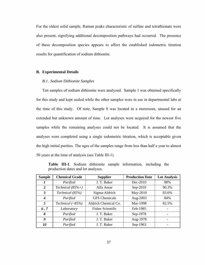
37
For the oldest solid sample, Raman peaks characteristic of sulfate and tetrathionate were
also present, signifying additional decomposition pathways had occurred. The presence
of these decomposition species appears to affect the established iodometric titration
results for quantification of sodium dithionite.
B. Experimental Details
B.1 . Sodium Dithionite Samples
Ten samples of sodium dithionite were analyzed. Sample 1 was obtained specifically
for this study and kept sealed while the other samples were in use in departmental labs at
the time of this study. Of note, Sample 8 was located in a storeroom, unused for an
extended but unknown amount of time. Lot analyses were acquired for the newest five
samples while the remaining analyses could not be located. It is assumed that the
analyses were completed using a single iodometric titration, which is acceptable given
the high initial purities. The ages of the samples range from less than half a year to almost
50 years at the time of analysis (see Table III-1).
Table III-1. Sodium dithionite sample information, including the
production dates and lot analyses.
Sample Chemical Grade Supplier Production Date Lot Analysis
1 Purified J. T. Baker Dec-2010 88%
2 Technical (85%+) Alfa Aesar Sep-2010 90.3%
3 Technical (85%) Sigma-Aldrich May-2010 83.6%
4 Purified GFS Chemicals Aug-2003 84%
5 Technical (~85%) Aldrich Chemical Co. Mar-1998 82.5%
6 , 7 Laboratory Fisher Scientific Feb-1985 -
8 Purified J. T. Baker Sep-1978 -
9 Purified J. T. Baker Aug-1978 -
10 Purified J. T. Baker Sep-1963 -
38
This span provides a wide range of samples with various degrees of decomposition in
which to examine the decomposition products and assess the success of the different
analytical techniques utilized. To ensure accurate sampling, all samples were
homogenized through grinding and shaking of the powder before analysis.
B.2 . Materials and Synthesis of Polythionates
Solid samples and solutions of sodium sulfite anhydrous (Fisher, Certified ACS),
sodium sulfate (EMD, ACS), sodium thiosulfate pentahydrate (Fisher, Certified ACS),
sodium metabisulfite (Mallinckrodt, Analytical Reagent), and sodium persulfate (Aldrich,
ACS) were used as standards for Raman spectrum peak identification.
Sodium dithionate (Na2S2O6) was synthesized and purified as previously reported.146
In this approach, sodium sulfite and silver nitrate are reacted to prepare silver sulfite,
which is then reduced to give sodium dithionate [Equations III-1 and III-2].
Na2SO3 + 2 AgNO3 → Ag2SO3 + 2 NaNO3 [Equation III-1]
Ag2SO3 + Na2SO3 → Na2S2O6 + 2 Ag [Equation III-2]
To save on the cost of production (namely, the amount of silver nitrate used), the
described synthetic route was scaled down by a factor of 20. To begin, 5 g (0.04 moles)
of sodium sulfite was added to 50 mL of H2O while stirring. Once dissolved, a solution
of 6.5 g (0.038 moles) of silver nitrate (GFS Chemicals, > 99.9%) in 10 mL of H2O was
slowly added. The stirring solution was heated to boiling point, until the silver sulfite
precipitate dissolved and was replaced by a precipitation of pure silver. The solution was
vacuum filtered, and the removed silver precipitate was washed with two quantities of 5
mL of boiling H2O. The filtrate was heated until the solution volume was approximately
39
15 mL, at which time the solution was cooled to room temperature and placed into an ice
bath to effect crystallization. The crystals were filtered out and kept unwashed while the
filtrate was further heated, mixed with 15 mL of boiling ethanol (Pharmco-Aaper,
ACS/USP Grade), cooled and allowed to crystallize. The crystalline product was added
to the first quantity of precipitate left on the filter and then pressed, washed with 5 mL of
ethanol and 3 mL of acetone, and air dried for one hour. Recrystallization of the sodium
dithionate product was performed with 5 mL of a 1:1 ethanol:water mixture heated to 80
ºC. The crystals were placed into a 50 mL round-bottom flask and stored at 4 ºC.
Anhydrous sodium trithionate (Na2S3O6) was produced as a nonhydrated crystal as
previously reported,147
although it was scaled down by a factor of 10. In brief, 15 g
(0.060 moles) of sodium thiosulfate pentahydrate was dissolved in 9 mL of H2O and
stirred into an ice bath. Over a period of forty minutes, 14 mL of 30% hydrogen peroxide
(BDH) was added dropwise. Following this, more ice was added to the bath and the
temperature was kept below 5 ºC for two hours. Following the precipitation, filtration
and washing of sodium sulfate crystals with 25 mL of chilled (0 ºC) ethanol, the filtrate
was removed. After mixing with 25 mL of chilled ethanol and filtering, an additional
120 mL of chilled ethanol was added, the solution stirred, and cooled in an ice bath for
two hours. The produced trithionate crystals were filtered, washed with 5 mL portions of
ethanol and acetone, and dried overnight in a vacuum desiccator. As with dithionate, the
trithionate crystals were placed into a 50 mL round-bottom flask and stored at 4 ºC.
Sodium tetrathionate dihydrate (Na2S4O6•2H2O) was the last compound synthesized
for this study, using the method reported by Blitz and Blitz.148
Again, the scale of the
synthesis was reduced by an order of magnitude. Succinctly, 5 g (0.02 moles) of sodium
40
thiosulfate pentahydrate was mixed with 2.6 g (0.010 moles) of iodine and 2 mL of H2O
in a mortar and ground to a fine paste. The paste was transferred with 25 mL of ethanol
to an Erlenmeyer flask and left to sit for three hours. Over this time, the sodium
tetrathionate product was precipitated; this product was washed with an additional 25 mL
ethanol to remove any residual iodine. Purification of the sodium tetrathionate was
accomplished with its dissolution in 2.5 mL of H2O, addition of 5 x 1 mL ethanol
portions to the solution at five minute intervals, and letting sit undisturbed in a vacuum
desiccator for ten hours. The formed crystals were then vacuum filtered, washed with 5
mL of chilled ethanol, and transferred into a beaker stored in a desiccator. After drying
overnight, the sodium tetrathionate crystals were placed into a 50 mL round-bottomed
flask and stored at 4 ºC.
B.3 . Raman Spectroscopy
A Nicolet NXR 9610 FT-Raman spectrometer was used for the Raman analysis. The
commercially-obtained and synthesized reference samples were utilized for characteristic
peak identification. Samples were analyzed in both their solid and solution phases (0.10
g in 8 mL of H2O) from 200 to 2000 cm-1
with a 4 cm-1
resolution and a minimum of 800
scans per compound to minimize noise. The laser power was reduced to 0.20 Watts to
prevent compound degradation or destruction of either the solid samples or the Mylar
sheet covering the cell window in which the solutions were contained. An InGaAs
detector was used. The recorded Raman spectra can be found in Appendix B.
41
B.4 . Titration and Ion Chromatograph Methodology
Samples were iodometrically titrated using the Wollak method as adapted by Kilroy
and described in Chapter II.50,56
As discussed by Kilroy, dithionite, thiosulfate and sulfite
are determined from the results of three titrations of the samples under different
conditions. 56
For ion chromatography, a Metrohm Advanced IC-2 System was utilized
for sample analysis. Briefly, 1.0000 g of a dithionite sample was reacted with 70 mL of a
1:1 formaldehyde/water solution made slightly basic (pH = 10) with 10 M NaOH. After
mixing for 20 minutes, the solution was diluted to a volume of 250 mL of H2O. From
this, a 50 mL aliquot was removed with a 50 mL Class A transfer pipette and diluted with
RO-grade H2O to 2 L, which was used for IC analysis. A minimum of three aliquots
were analyzed per sample.
Solutions of sodium hydroxymethanesulfinate x•hydrate i.e. Rongalite (Aldrich) and
sodium thiosulfate pentahydrate were used to construct calibration curves for the ion
chromatograph. An iodometric titration was used to determine the extent of hydration of
the Rongalite sample, which was found to be 77.15% Ronaglite ion mass per sample
mass. These curves were constructed with four points each measured three times (R2 =
1). These calibrations allowed the concentrations of thiosulfate and dithionite,
determined from the Rongalite concentration, to be quantified. A detailed description of
the ion chromatograph methodology and the three-part titration can be found in Chapter
II and the measured calibration curves can be found in Appendix A.
In cation detection mode, the system was run with no chemical suppression. The
column was switched to a Metrohm C2 150 cation exchange column set to 35 °C. The
mobile phase was comprised of a 1.70 mM HNO3 and 0.70 mM dipicolinic acid solution
42
and was run at 0.7 mL/min. For sodium sample analysis, approximately 0.10 g sample
was dissolved in 1 L of RO-grade H2O and injected into the IC, with four injections made
per sample. For sodium quantification, a calibration curve was constructed with five
sodium chloride solutions (ranging from 0.50 to 1.80 mM) and showed excellent linearity
(R2
= 1). The obtained sodium calibration curve can be found in Appendix A.
C. Results and Discussion
C.1 . Raman Analysis of Sodium Dithionite Samples
Raman analyses of the samples as solids and aqueous solutions were performed.
Raman spectroscopy provides qualitative information on the species present in each
sample. As the dithionite decomposed, there were noticeable changes in the associated
Raman spectra. To qualitatively determine composition of the samples, Table III-2 lists
the characteristic vibrations for possible species both as solids and in solution, compiled
from published sources.149,150
When possible, standards were prepared and measured to
confirm the assignments. In addition, the intensities and primary peaks were not the
same for solid and solution samples, and relative intensity differences were not
interpreted as concentration differences.
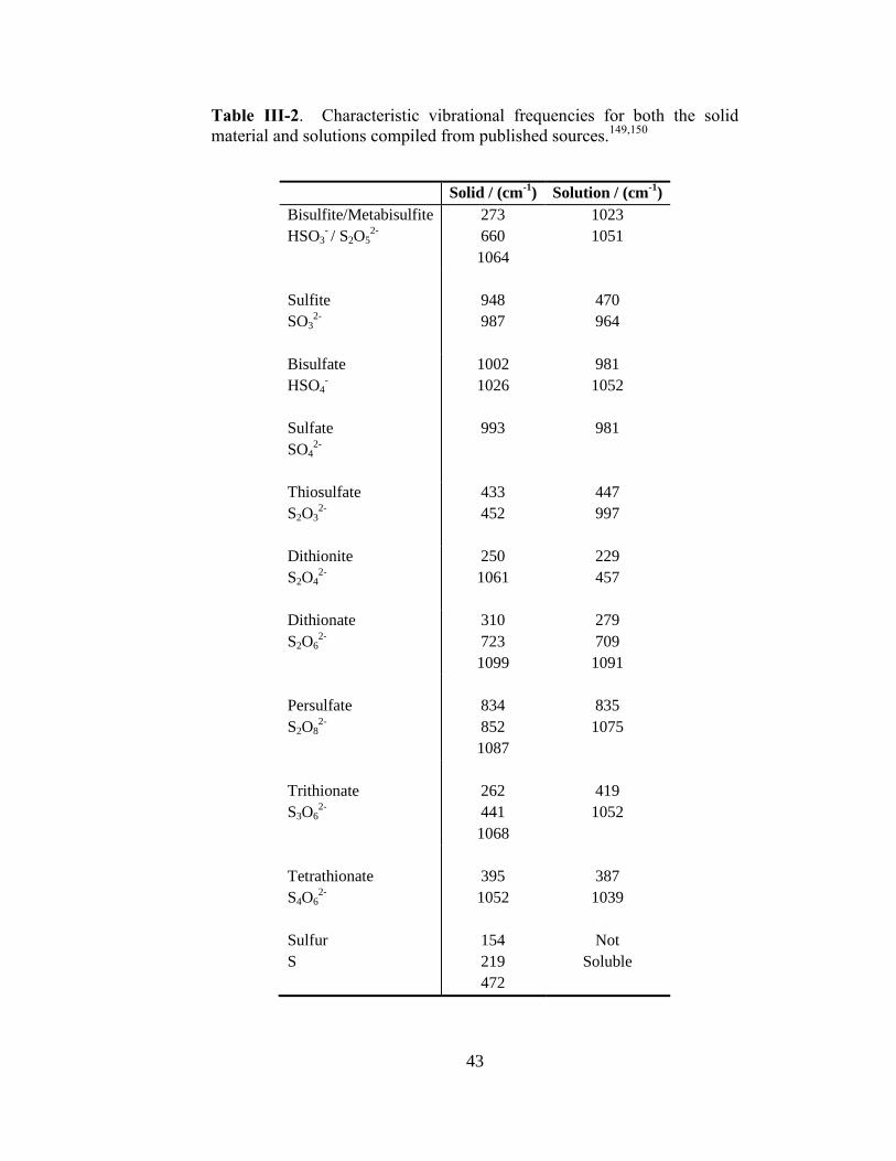
43
Table III-2. Characteristic vibrational frequencies for both the solid
material and solutions compiled from published sources.149,150
Solid / (cm-1
) Solution / (cm-1
)
Bisulfite/Metabisulfite
HSO3- / S2O5
2-
273
660
1064
1023
1051
Sulfite
SO32-
948
987
470
964
Bisulfate
HSO4-
Sulfate
SO42-
1002
1026
993
981
1052
981
Thiosulfate
S2O32-
433
452
447
997
Dithionite
S2O42-
250
1061
229
457
Dithionate
S2O62-
310
723
1099
279
709
1091
Persulfate
S2O82-
834
852
1087
835
1075
Trithionate
S3O62-
262
441
1068
419
1052
Tetrathionate
S4O62-
395
1052
387
1039
Sulfur
S
154
219
472
Not
Soluble
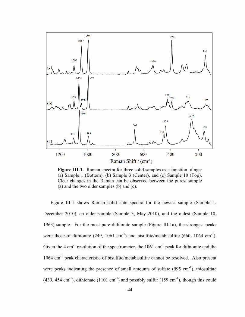
44
Figure III-1. Raman spectra for three solid samples as a function of age:
(a) Sample 1 (Bottom), (b) Sample 3 (Center), and (c) Sample 10 (Top).
Clear changes in the Raman can be observed between the purest sample
(a) and the two older samples (b) and (c).
Figure III-1 shows Raman solid-state spectra for the newest sample (Sample 1,
December 2010), an older sample (Sample 3, May 2010), and the oldest (Sample 10,
1963) sample. For the most pure dithionite sample (Figure III-1a), the strongest peaks
were those of dithionite (249, 1061 cm-1
) and bisulfite/metabisulfite (660, 1064 cm-1
).
Given the 4 cm-1
resolution of the spectrometer, the 1061 cm-1
peak for dithionite and the
1064 cm-1
peak characteristic of bisulfite/metabisulfite cannot be resolved. Also present
were peaks indicating the presence of small amounts of sulfate (995 cm-1
), thiosulfate
(439, 454 cm-1
), dithionate (1101 cm-1
) and possibly sulfur (159 cm-1
), though this could
45
be due to vibrations in the S-S bond of dithionite. Commercially available sodium
dithionite typically has purity below 90% and many of these compounds are expected to
be present in the material. As the age of the samples increased (see Figure III-1b), a
decrease was seen in the strongest dithionite peak (249 cm-1
) without a decrease of the
1061 cm-1
peak, possibly signifying the creation of bisulfite/metabisulfite as a
decomposition product of dithionite. Consistent with dithionite decomposition, there was
a noticeable increase in the thiosulfate and sulfate peak intensities with sample age as
well as the appearance of tetrathionate (393, 1047 cm-1
). Interestingly, the spectrum of
Sample 8 contained strong dithionite peaks with weaker peaks for decomposition
products, signifying less decomposition of the dithionite. Despite being over 30 years
old, Sample 8 was well sealed with tape and subsequently had significantly less
atmospheric exposure with respect to other samples of similar age or even younger.
Present in every solid sample was a peak between 1098 and 1101 cm-1
, characteristic of
dithionate (1099 cm-1
). While a minor feature in the newest samples, dithionite was one
of the primary features in the oldest sample (Sample 10, 1963). Besides this, the oldest
sample also contained additional features not present in the other samples. Raman
spectroscopy identified tetrathionate (394, 1046 cm-1
) and sulfate (996 cm-1
) with smaller
peaks possibly indicating bisulfite or metabisulfate. The identity of the species
responsible for the peak at 526 cm-1
is undetermined.
Additional analyses of aqueous samples produced form these solids were performed
to determine if any substantial changes occur during the solution preparation. Samples
were prepared by dissolving 0.10 g of solid in 8 mL of water. Although the intensities
and wavenumbers of the various species will change once solvated (Table III-2), the
46
composition of the solution should remain unchanged within the measurement time.
Consistent with the solid sample, the strongest peak present in solution for samples less
than one year old was that of dithionite (226, 579 cm-1
). However, illustrating the
importance of not interpreting relative peak intensities as differences in concentration, the
thiosulfate (457 cm-1
) was also one of the strongest peaks in the liquid sample as opposed
to bisulfite/metabisulfite in the solid sample. Titration and ion chromatograph results
(Tables III-3 and III-4) discussed below show that thiosulfate comprises less than 2% of
Sample 1 by mass. Additional peaks characteristic of thiosulfate (447 cm-1
),
sulfate/bisulfate (981 cm-1
), and bisulfite/metabisulfite (1052 cm-1
) were also present.
Most samples show an additional peak at 1091 cm-1
, characteristic of dithionate, which
increases with the age of the sample. This pattern is consistent with the results obtained
from the solids. Also consistent with the solid-state spectroscopy, the spectrum for a
solution of the oldest sample was distinguishing. The only peaks present in the spectrum
were identified as sulfate/bisulfate (981 cm-1
), tetrathionate (389, 1039 cm-1
) and
dithionate (1091 cm-1
) with no other signal peaks present.
C.2 . Titration and Chromatography Results
A three-step iodometric titration was used to determine the composition of the
dithionite samples. The titration methodology was performed as previously described in
Kilroy and the previous Chapter.56
The use of three titrations was required to accurately
determine the dithionite composition in the presence of the additional reducible species,
thiosulfate and sulfite. Of the ten samples analyzed, the most recently produced samples
were expected to contain more dithionite and less decomposition products than older
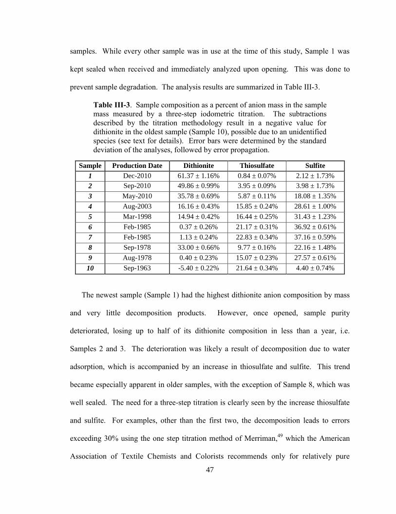
47
samples. While every other sample was in use at the time of this study, Sample 1 was
kept sealed when received and immediately analyzed upon opening. This was done to
prevent sample degradation. The analysis results are summarized in Table III-3.
Table III-3. Sample composition as a percent of anion mass in the sample
mass measured by a three-step iodometric titration. The subtractions
described by the titration methodology result in a negative value for
dithionite in the oldest sample (Sample 10), possible due to an unidentified
species (see text for details). Error bars were determined by the standard
deviation of the analyses, followed by error propagation.
Sample Production Date Dithionite Thiosulfate Sulfite
1 Dec-2010 61.37 ± 1.16% 0.84 ± 0.07% 2.12 ± 1.73%
2 Sep-2010 49.86 ± 0.99% 3.95 ± 0.09% 3.98 ± 1.73%
3 May-2010 35.78 ± 0.69% 5.87 ± 0.11% 18.08 ± 1.35%
4 Aug-2003 16.16 ± 0.43% 15.85 ± 0.24% 28.61 ± 1.00%
5 Mar-1998 14.94 ± 0.42% 16.44 ± 0.25% 31.43 ± 1.23%
6 Feb-1985 0.37 ± 0.26% 21.17 ± 0.31% 36.92 ± 0.61%
7 Feb-1985 1.13 ± 0.24% 22.83 ± 0.34% 37.16 ± 0.59%
8 Sep-1978 33.00 ± 0.66% 9.77 ± 0.16% 22.16 ± 1.48%
9 Aug-1978 0.40 ± 0.23% 15.07 ± 0.23% 27.57 ± 0.61%
10 Sep-1963 -5.40 ± 0.22% 21.64 ± 0.34% 4.40 ± 0.74%
The newest sample (Sample 1) had the highest dithionite anion composition by mass
and very little decomposition products. However, once opened, sample purity
deteriorated, losing up to half of its dithionite composition in less than a year, i.e.
Samples 2 and 3. The deterioration was likely a result of decomposition due to water
adsorption, which is accompanied by an increase in thiosulfate and sulfite. This trend
became especially apparent in older samples, with the exception of Sample 8, which was
well sealed. The need for a three-step titration is clearly seen by the increase thiosulfate
and sulfite. For examples, other than the first two, the decomposition leads to errors
exceeding 30% using the one step titration method of Merriman,49
which the American
Association of Textile Chemists and Colorists recommends only for relatively pure
48
samples.51
These quantitative results are consistent with the Raman spectra above; the
composition of the dithionite samples can be clearly seen to shift to thiosulfate and sulfite
as the samples age. Being the oldest dithionite sample tested, it was expected that
Sample 10 would have the lowest measured dithionite composition and the highest
composition of thiosulfate and sulfite. However, when determined through titration, not
only was the dithionite composition for this sample found to be negative, but the sulfite
composition was also extremely low (4.40%) compared to the samples preceding it
(≥20%). These unexpected results can be understood when reviewing the titration
method. In this method, the dithionite concentration is calculated as the difference
between two titrations, one for thiosulfate and one for dithionite and thiosulfate.56
However, the thiosulfate titration assumes that no additional products that can reduce
iodine are present. In fact, Raman spectroscopy for this sample indicated the presence of
dithionate and tetrathionate in the sample. It has been established that in the presence of
sulfite under basic conditions, tetrathionate reacts to form thiosulfate and trithionate
(Equation I-16). It is likely that this species decomposed during the solution preparation
for titration and produced a reducible compound, most likely thiosulfate or possibly
another anion through a different mechanism, which reacted with iodine and affected the
results. The sulfite could have been consumed by tetrathionate to produce thiosulfate, or
it is also possible that the sulfite composition is extremely low for this sample, having
been converted to a more stable decomposition product (e.g. sulfate).
Ion chromatography can directly analyze anions and cations in solution by chemical
separation. This allows the dithionite and thiosulfate in the dithionite samples to be
determined independently (see Table III-4). Solutions were produced by dissolving
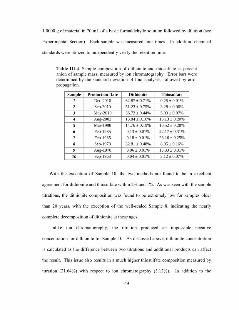
49
1.0000 g of material in 70 mL of a basic formaldehyde solution followed by dilution (see
Experimental Section). Each sample was measured four times. In addition, chemical
standards were utilized to independently verify the retention time.
Table III-4. Sample composition of dithionite and thiosulfate as percent
anion of sample mass, measured by ion chromatography. Error bars were
determined by the standard deviation of four analyses, followed by error
propagation.
Sample Production Date Dithionite Thiosulfate
1 Dec-2010 62.87 ± 0.71% 0.25 ± 0.01%
2 Sep-2010 51.23 ± 0.75% 3.28 ± 0.06%
3 May-2010 36.72 ± 0.44% 5.03 ± 0.07%
4 Aug-2003 15.84 ± 0.16% 16.13 ± 0.20%
5 Mar-1998 14.76 ± 0.19% 16.52 ± 0.28%
6 Feb-1985 0.13 ± 0.01% 22.17 ± 0.31%
7 Feb-1985 0.18 ± 0.01% 23.16 ± 0.25%
8 Sep-1978 32.81 ± 0.48% 8.95 ± 0.16%
9 Aug-1978 0.06 ± 0.01% 15.33 ± 0.31%
10 Sep-1963 0.04 ± 0.01% 3.12 ± 0.07%
With the exception of Sample 10, the two methods are found to be in excellent
agreement for dithionite and thiosulfate within 2% and 1%. As was seen with the sample
titrations, the dithionite composition was found to be extremely low for samples older
than 20 years, with the exception of the well-sealed Sample 8, indicating the nearly
complete decomposition of dithionite at these ages.
Unlike ion chromatography, the titration produced an impossible negative
concentration for dithionite for Sample 10. As discussed above, dithionite concentration
is calculated as the difference between two titrations and additional products can affect
the result. This issue also results in a much higher thiosulfate composition measured by
titration (21.64%) with respect to ion chromatography (3.12%). In addition to the
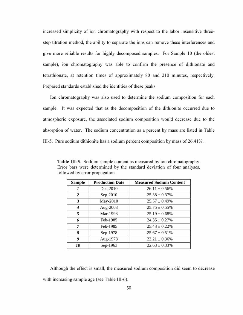
50
increased simplicity of ion chromatography with respect to the labor insensitive three-
step titration method, the ability to separate the ions can remove these interferences and
give more reliable results for highly decomposed samples. For Sample 10 (the oldest
sample), ion chromatography was able to confirm the presence of dithionate and
tetrathionate, at retention times of approximately 80 and 210 minutes, respectively.
Prepared standards established the identities of these peaks.
Ion chromatography was also used to determine the sodium composition for each
sample. It was expected that as the decomposition of the dithionite occurred due to
atmospheric exposure, the associated sodium composition would decrease due to the
absorption of water. The sodium concentration as a percent by mass are listed in Table
III-5. Pure sodium dithionite has a sodium percent composition by mass of 26.41%.
Table III-5. Sodium sample content as measured by ion chromatography.
Error bars were determined by the standard deviation of four analyses,
followed by error propagation.
Sample Production Date Measured Sodium Content
1 Dec-2010 26.11 ± 0.56%
2 Sep-2010 25.38 ± 0.37%
3 May-2010 25.57 ± 0.49%
4 Aug-2003 25.75 ± 0.55%
5 Mar-1998 25.19 ± 0.68%
6 Feb-1985 24.35 ± 0.27%
7 Feb-1985 25.43 ± 0.22%
8 Sep-1978 25.67 ± 0.51%
9 Aug-1978 23.21 ± 0.36%
10 Sep-1963 22.63 ± 0.33%
Although the effect is small, the measured sodium composition did seem to decrease
with increasing sample age (see Table III-6).
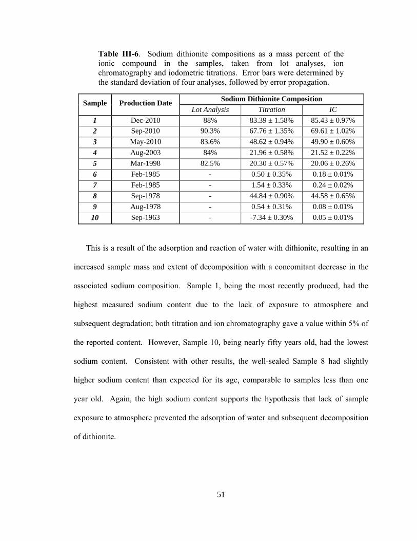
51
Table III-6. Sodium dithionite compositions as a mass percent of the
ionic compound in the samples, taken from lot analyses, ion
chromatography and iodometric titrations. Error bars were determined by
the standard deviation of four analyses, followed by error propagation.
Sample Production Date Sodium Dithionite Composition
Lot Analysis Titration IC
1 Dec-2010 88% 83.39 ± 1.58% 85.43 ± 0.97%
2 Sep-2010 90.3% 67.76 ± 1.35% 69.61 ± 1.02%
3 May-2010 83.6% 48.62 ± 0.94% 49.90 ± 0.60%
4 Aug-2003 84% 21.96 ± 0.58% 21.52 ± 0.22%
5 Mar-1998 82.5% 20.30 ± 0.57% 20.06 ± 0.26%
6 Feb-1985 - 0.50 ± 0.35% 0.18 ± 0.01%
7 Feb-1985 - 1.54 ± 0.33% 0.24 ± 0.02%
8 Sep-1978 - 44.84 ± 0.90% 44.58 ± 0.65%
9 Aug-1978 - 0.54 ± 0.31% 0.08 ± 0.01%
10 Sep-1963 - -7.34 ± 0.30% 0.05 ± 0.01%
This is a result of the adsorption and reaction of water with dithionite, resulting in an
increased sample mass and extent of decomposition with a concomitant decrease in the
associated sodium composition. Sample 1, being the most recently produced, had the
highest measured sodium content due to the lack of exposure to atmosphere and
subsequent degradation; both titration and ion chromatography gave a value within 5% of
the reported content. However, Sample 10, being nearly fifty years old, had the lowest
sodium content. Consistent with other results, the well-sealed Sample 8 had slightly
higher sodium content than expected for its age, comparable to samples less than one
year old. Again, the high sodium content supports the hypothesis that lack of sample
exposure to atmosphere prevented the adsorption of water and subsequent decomposition
of dithionite.
52
D. Conclusion
Ten samples of sodium dithionite at various ages and stages of degradation were
analyzed to determine the sample compositions. It was determined that as a sample aged,
various degradation products were formed due to water adsorption. For new samples, the
primary species found were dithionite, thiosulfate and sulfite (possibly as bisulfite), with
dithionite composition decreasing as the age of the sample increased. For the oldest
samples, there was the appearance of sulfate and dithionate. Unique to the oldest sample
was the presence of tetrathionate, indicative of the more advanced stage of sample
decomposition. When these oxidized byproducts are present, analysis through iodometric
titration can be problematic.
53
CHAPTER IV
TITANIA-HYDROXYPROPYL CELLULOSE THIN FILMS FOR THE DETECTION
OF PEROXIDE VAPORS
A. Introduction
Titania nanoparticles in a hydroxypropyl cellulose matrix produced using a sol-gel
method was utilized to prepare films on polycarbonate slides and coatings on cellulose
filter papers. The exposure of these colorless films to hydrogen peroxide vapor leads to
the development of an intense yellow color. Using a tungsten lamp and an inexpensive
web camera to measure the reflected light, first-order behavior in the color change was
observed when exposed to peroxide vapor of less than 50 ppm. For 50 mass percent
titania nanoparticles in hydroxypropyl cellulose films on polycarbonate, the detection
limit was estimated to be 90 ppm after a one minute measurement and 1.5 ppm after a
one hour integration. The coatings on the filter paper had a threefold higher sensitivity
compared to the films, with a detection limit of 5.4 ppm peroxide for a one minute
measurement and 0.09 ppm peroxide after a one hour integration. The high sensitivity
and rapid response of these films makes them a promising material for use as a sensitive
peroxide detector.
54
B. Experimental Details
B.1 . Preparation of Titanium(IV) Isopropoxide-Hydroxypropyl Cellulose Solution
A solution of titanium(IV) isopropoxide with hydroxypropyl cellulose in 2-propanol
was produced following the procedure outlined by Kozuka and coworkers.141
Briefly, 1 g
of hydroxypropyl cellulose (Alfa Aesar, M.W. = 100,000) was dissolved in 70 mL of 2-
propanol (Pharmco-Aaper, ACS Reagent). A measured amount of titanium(IV)
isopropoxide (Alfa Aesar, 97 %) was then added dropwise while stirring. After stirring
for one hour under nitrogen, 1.5 g of concentrated hydrochloric acid (Pharmco-Aaper,
ACS Reagent) diluted with 20 mL of 2-propanol was added to the titanium-cellulose
solution while swirling the solution. The final solution was stirred under nitrogen for 24
hours before use. Solutions with varying quantities of titania were prepared up to the
point where sufficient titania was present to yield a 60 mass percent
titania/(titania+cellulose) film, assuming that the titanium(IV) isopropoxide was
completely converted to titania. After production, the solutions were pale yellow and
stored under nitrogen. Film preparation was typically performed within 12 hours after
the initial 24-hour mixing period.
B.2 . Preparation of Sol-Gel Films on Polycarbonate and Filter Papers
Polycarbonate slides (2.54 x 7.62 x 0.152 cm) were sonicated in ethanol for 30
minutes and dried in air. Once dried, an excess volume of the titanium(IV) isopropoxide-
cellulose solution was applied to a slide held in an aluminum slide holder (0.040” deep).
A Gardco 8-path wet film applicator was used to remove the excess solution and produce
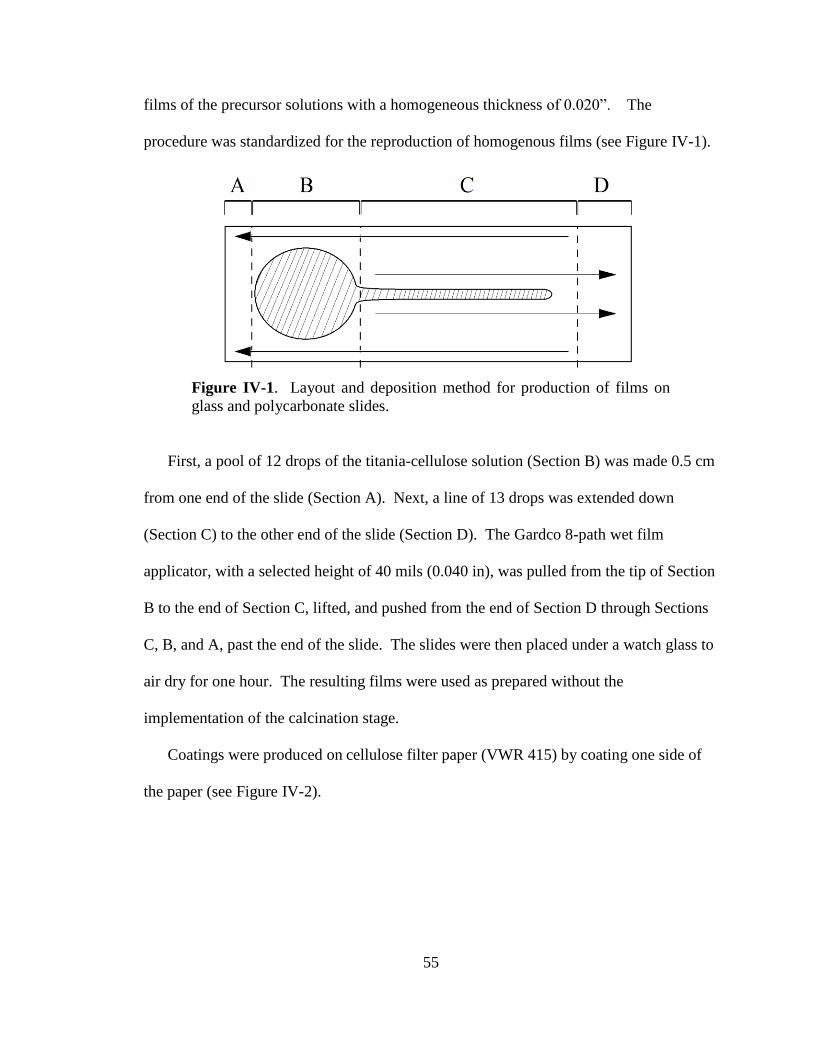
55
films of the precursor solutions with a homogeneous thickness of 0.020”. The
procedure was standardized for the reproduction of homogenous films (see Figure IV-1).
Figure IV-1. Layout and deposition method for production of films on
glass and polycarbonate slides.
First, a pool of 12 drops of the titania-cellulose solution (Section B) was made 0.5 cm
from one end of the slide (Section A). Next, a line of 13 drops was extended down
(Section C) to the other end of the slide (Section D). The Gardco 8-path wet film
applicator, with a selected height of 40 mils (0.040 in), was pulled from the tip of Section
B to the end of Section C, lifted, and pushed from the end of Section D through Sections
C, B, and A, past the end of the slide. The slides were then placed under a watch glass to
air dry for one hour. The resulting films were used as prepared without the
implementation of the calcination stage.
Coatings were produced on cellulose filter paper (VWR 415) by coating one side of
the paper (see Figure IV-2).
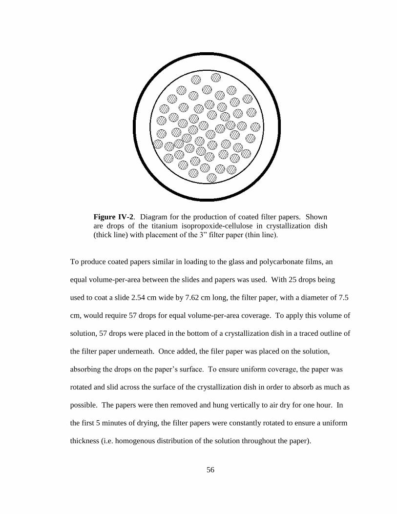
56
Figure IV-2. Diagram for the production of coated filter papers. Shown
are drops of the titanium isopropoxide-cellulose in crystallization dish
(thick line) with placement of the 3” filter paper (thin line).
To produce coated papers similar in loading to the glass and polycarbonate films, an
equal volume-per-area between the slides and papers was used. With 25 drops being
used to coat a slide 2.54 cm wide by 7.62 cm long, the filter paper, with a diameter of 7.5
cm, would require 57 drops for equal volume-per-area coverage. To apply this volume of
solution, 57 drops were placed in the bottom of a crystallization dish in a traced outline of
the filter paper underneath. Once added, the filer paper was placed on the solution,
absorbing the drops on the paper’s surface. To ensure uniform coverage, the paper was
rotated and slid across the surface of the crystallization dish in order to absorb as much as
possible. The papers were then removed and hung vertically to air dry for one hour. In
the first 5 minutes of drying, the filter papers were constantly rotated to ensure a uniform
thickness (i.e. homogenous distribution of the solution throughout the paper).
57
B.3 . Titanium(IV) Oxysulfate Solution for Peroxide Quantification
The colorimetric procedure developed by OSHA was utilized to measure the peroxide
vapor concentration.97
This method requires a solution of titanium(IV) oxysulfate in
sulfuric acid. This was produced by dissolving a mixture of 5.5 g of dehydrated
TiOSO4∙xH2O (Strem Chemicals) and 20 g of ammonium sulfate (Spectrum, A.C.S.
Reagent) in a heated solution of 100 mL of sulfuric acid (Pharmco-Aaper, A.C.S.
Reagent). After cooling, the resulting pale yellow solution was added to 350 mL of
ultrapure water, again cooled to room temperature, filtered through a 0.40 µm filter to
remove any suspended materials, and diluted to a final volume of 500 mL.
B.4 . Peroxide Solutions for Gas Exposure
Peroxide solutions of various concentrations were made through dilution of a 30%
hydrogen peroxide stock solution (BDH). Given that the uptake of hydrogen peroxide
gas from the solution phase in the bubbler is a turbulent process, direct control of the
created vapor concentration is not possible; both solution concentration and temperature
as well as carrier gas flow rate can greatly affect the concentration of the produced
peroxide vapor. For these reasons, solutions with numerous concentrations (1, 2, 5, 10,
15, and 20% hydrogen peroxide by volume) were made and stored in a refrigerator at 4
ºC when not being used. When used, each solution was warmed to room temperature
over the course of one hour and then poured into the bubbler. While these actions did not
ensure reproducible behavior of peroxide uptake, standardization of the method was
important for similar exposure conditions.
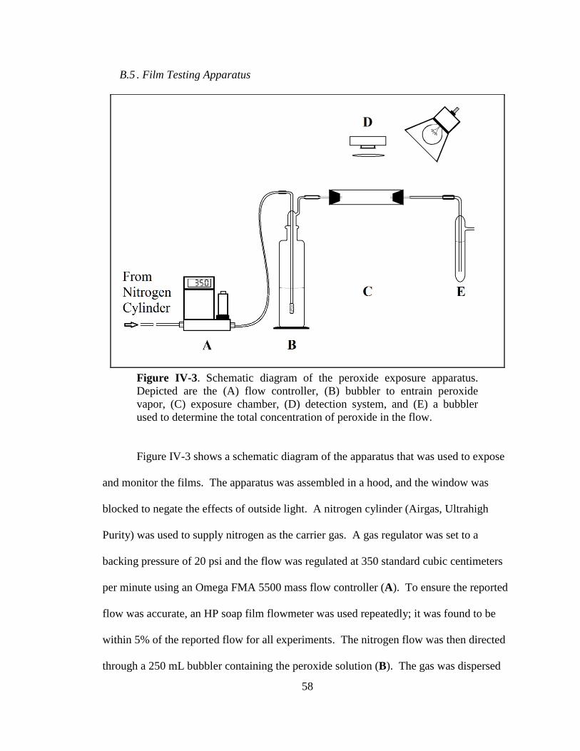
58
B.5 . Film Testing Apparatus
Figure IV-3. Schematic diagram of the peroxide exposure apparatus.
Depicted are the (A) flow controller, (B) bubbler to entrain peroxide
vapor, (C) exposure chamber, (D) detection system, and (E) a bubbler
used to determine the total concentration of peroxide in the flow.
Figure IV-3 shows a schematic diagram of the apparatus that was used to expose
and monitor the films. The apparatus was assembled in a hood, and the window was
blocked to negate the effects of outside light. A nitrogen cylinder (Airgas, Ultrahigh
Purity) was used to supply nitrogen as the carrier gas. A gas regulator was set to a
backing pressure of 20 psi and the flow was regulated at 350 standard cubic centimeters
per minute using an Omega FMA 5500 mass flow controller (A). To ensure the reported
flow was accurate, an HP soap film flowmeter was used repeatedly; it was found to be
within 5% of the reported flow for all experiments. The nitrogen flow was then directed
through a 250 mL bubbler containing the peroxide solution (B). The gas was dispersed
59
into the solution using a sintered glass head, which distributed the gas through the
solution to ensure a steady uptake of the peroxide vapor. Next, the peroxide-enriched gas
was directed into a glass cell containing the sample, either a coated polycarbonate slide or
a cellulose filter paper. The glass cell (C) had a piece of white paper attached on its
outside bottom to create a white background. A 20 W incandescent light was positioned
above the cell to provide homogenous lighting for the slide and a Logitech Pro 9000 USB
camera recorded images of the sample during exposure to peroxide vapor (D). Between
the camera and the cell was a Leiz Wetzlar BG 12 blue bandpass filter, which isolated the
wavelengths between 300 and 500 nanometers. After leaving the cell, the gas progressed
through a bubbler containing 25 mL of the titanium(IV) oxysulfate solution (E), which
reacted with the peroxide in the gas and produced a color change that was proportional to
the total quantity of peroxide in the gas. A second bubbler was attached following the
first one to confirm complete reaction of entrained peroxide vapor with the titanium(IV)
oxysulfate solution. There was no measured absorbance change in the second bubbler’s
solution when run with 30% peroxide solution for 30 minutes, which indicated that the
peroxide vapor was completely reacted in the first bubbler. The total peroxide
concentration was determined using a colorimetric method that utilized the absorption of
the titanium(IV) oxysulfate solution at 410 nm.97
A Cary 50 Bio UV-VIS spectrometer
was used for the absorption measurement and was calibrated as per this colorimetric
method. The peroxide concentration in the gas was computed using the total
concentration in titanium(IV) oxysulfate solution, the flow rate which was fixed at 350
sccm for all experiments, and the exposure time of the films to the flowing gas. This
process was performed for every exposure to determine the vapor concentration. The
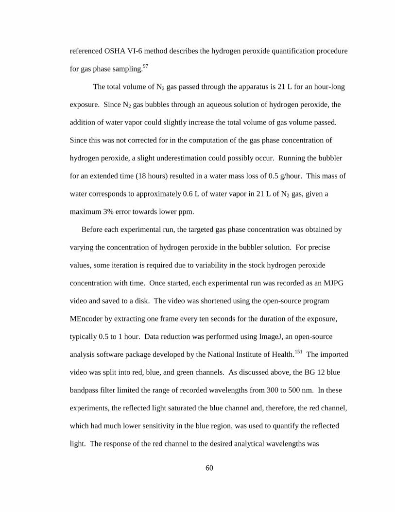
60
referenced OSHA VI-6 method describes the hydrogen peroxide quantification procedure
for gas phase sampling.97
The total volume of N2 gas passed through the apparatus is 21 L for an hour-long
exposure. Since N2 gas bubbles through an aqueous solution of hydrogen peroxide, the
addition of water vapor could slightly increase the total volume of gas volume passed.
Since this was not corrected for in the computation of the gas phase concentration of
hydrogen peroxide, a slight underestimation could possibly occur. Running the bubbler
for an extended time (18 hours) resulted in a water mass loss of 0.5 g/hour. This mass of
water corresponds to approximately 0.6 L of water vapor in 21 L of N2 gas, given a
maximum 3% error towards lower ppm.
Before each experimental run, the targeted gas phase concentration was obtained by
varying the concentration of hydrogen peroxide in the bubbler solution. For precise
values, some iteration is required due to variability in the stock hydrogen peroxide
concentration with time. Once started, each experimental run was recorded as an MJPG
video and saved to a disk. The video was shortened using the open-source program
MEncoder by extracting one frame every ten seconds for the duration of the exposure,
typically 0.5 to 1 hour. Data reduction was performed using ImageJ, an open-source
analysis software package developed by the National Institute of Health.151
The imported
video was split into red, blue, and green channels. As discussed above, the BG 12 blue
bandpass filter limited the range of recorded wavelengths from 300 to 500 nm. In these
experiments, the reflected light saturated the blue channel and, therefore, the red channel,
which had much lower sensitivity in the blue region, was used to quantify the reflected
light. The response of the red channel to the desired analytical wavelengths was
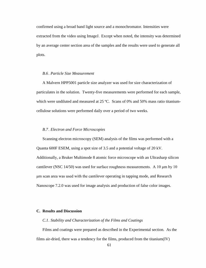
61
confirmed using a broad band light source and a monochromator. Intensities were
extracted from the video using ImageJ. Except when noted, the intensity was determined
by an average center section area of the samples and the results were used to generate all
plots.
B.6 . Particle Size Measurement
A Malvern HPP5001 particle size analyzer was used for size characterization of
particulates in the solution. Twenty-five measurements were performed for each sample,
which were undiluted and measured at 25 ºC. Scans of 0% and 50% mass ratio titanium-
cellulose solutions were performed daily over a period of two weeks.
B.7 . Electron and Force Microscopies
Scanning electron microscopy (SEM) analysis of the films was performed with a
Quanta 600F ESEM, using a spot size of 3.5 and a potential voltage of 20 kV.
Additionally, a Bruker Multimode 8 atomic force microscope with an Ultrasharp silicon
cantilever (NSC 14/50) was used for surface roughness measurements. A 10 μm by 10
μm scan area was used with the cantilever operating in tapping mode, and Research
Nanoscope 7.2.0 was used for image analysis and production of false color images.
C. Results and Discussion
C.1 . Stability and Characterization of the Films and Coatings
Films and coatings were prepared as described in the Experimental section. As the
films air-dried, there was a tendency for the films, produced from the titanium(IV)
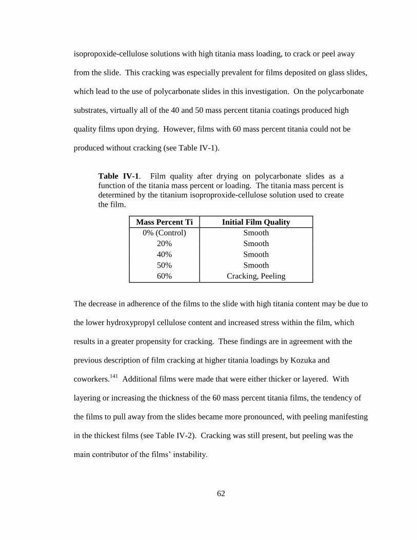
62
isopropoxide-cellulose solutions with high titania mass loading, to crack or peel away
from the slide. This cracking was especially prevalent for films deposited on glass slides,
which lead to the use of polycarbonate slides in this investigation. On the polycarbonate
substrates, virtually all of the 40 and 50 mass percent titania coatings produced high
quality films upon drying. However, films with 60 mass percent titania could not be
produced without cracking (see Table IV-1).
Table IV-1. Film quality after drying on polycarbonate slides as a
function of the titania mass percent or loading. The titania mass percent is
determined by the titanium isoproproxide-cellulose solution used to create
the film.
Mass Percent Ti Initial Film Quality
0% (Control) Smooth
20% Smooth
40%
50%
Smooth
Smooth
60% Cracking, Peeling
The decrease in adherence of the films to the slide with high titania content may be due to
the lower hydroxypropyl cellulose content and increased stress within the film, which
results in a greater propensity for cracking. These findings are in agreement with the
previous description of film cracking at higher titania loadings by Kozuka and
coworkers.141
Additional films were made that were either thicker or layered. With
layering or increasing the thickness of the 60 mass percent titania films, the tendency of
the films to pull away from the slides became more pronounced, with peeling manifesting
in the thickest films (see Table IV-2). Cracking was still present, but peeling was the
main contributor of the films’ instability.
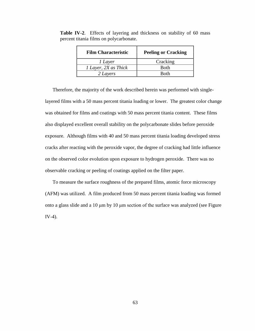
63
Table IV-2. Effects of layering and thickness on stability of 60 mass
percent titania films on polycarbonate.
Film Characteristic Peeling or Cracking
1 Layer Cracking
1 Layer, 2X as Thick Both
2 Layers Both
Therefore, the majority of the work described herein was performed with single-
layered films with a 50 mass percent titania loading or lower. The greatest color change
was obtained for films and coatings with 50 mass percent titania content. These films
also displayed excellent overall stability on the polycarbonate slides before peroxide
exposure. Although films with 40 and 50 mass percent titania loading developed stress
cracks after reacting with the peroxide vapor, the degree of cracking had little influence
on the observed color evolution upon exposure to hydrogen peroxide. There was no
observable cracking or peeling of coatings applied on the filter paper.
To measure the surface roughness of the prepared films, atomic force microscopy
(AFM) was utilized. A film produced from 50 mass percent titania loading was formed
onto a glass slide and a 10 μm by 10 μm section of the surface was analyzed (see Figure
IV-4).
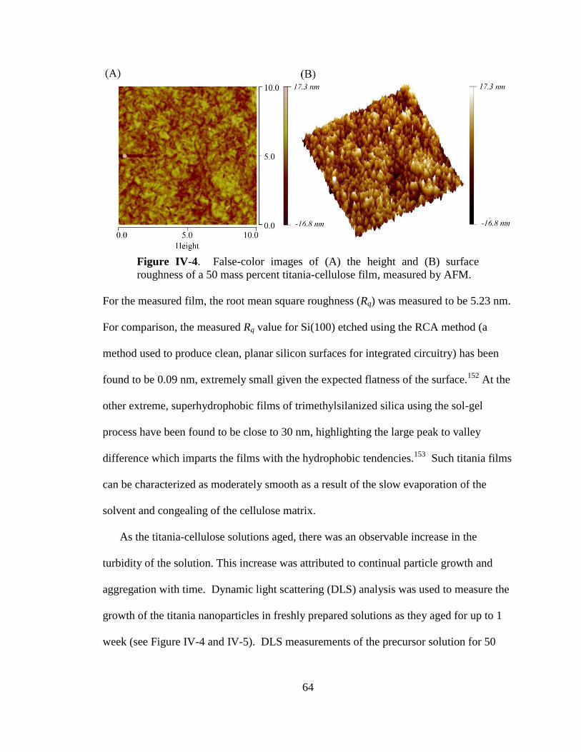
64
Figure IV-4. False-color images of (A) the height and (B) surface
roughness of a 50 mass percent titania-cellulose film, measured by AFM.
For the measured film, the root mean square roughness (Rq) was measured to be 5.23 nm.
For comparison, the measured Rq value for Si(100) etched using the RCA method (a
method used to produce clean, planar silicon surfaces for integrated circuitry) has been
found to be 0.09 nm, extremely small given the expected flatness of the surface.152
At the
other extreme, superhydrophobic films of trimethylsilanized silica using the sol-gel
process have been found to be close to 30 nm, highlighting the large peak to valley
difference which imparts the films with the hydrophobic tendencies.153
Such titania films
can be characterized as moderately smooth as a result of the slow evaporation of the
solvent and congealing of the cellulose matrix.
As the titania-cellulose solutions aged, there was an observable increase in the
turbidity of the solution. This increase was attributed to continual particle growth and
aggregation with time. Dynamic light scattering (DLS) analysis was used to measure the
growth of the titania nanoparticles in freshly prepared solutions as they aged for up to 1
week (see Figure IV-4 and IV-5). DLS measurements of the precursor solution for 50
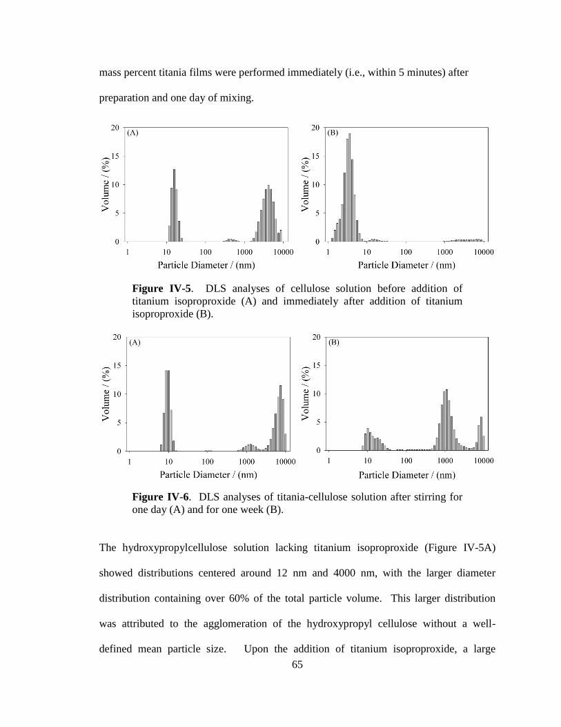
65
mass percent titania films were performed immediately (i.e., within 5 minutes) after
preparation and one day of mixing.
Figure IV-5. DLS analyses of cellulose solution before addition of
titanium isoproproxide (A) and immediately after addition of titanium
isoproproxide (B).
Figure IV-6. DLS analyses of titania-cellulose solution after stirring for
one day (A) and for one week (B).
The hydroxypropylcellulose solution lacking titanium isoproproxide (Figure IV-5A)
showed distributions centered around 12 nm and 4000 nm, with the larger diameter
distribution containing over 60% of the total particle volume. This larger distribution
was attributed to the agglomeration of the hydroxypropyl cellulose without a well-
defined mean particle size. Upon the addition of titanium isoproproxide, a large
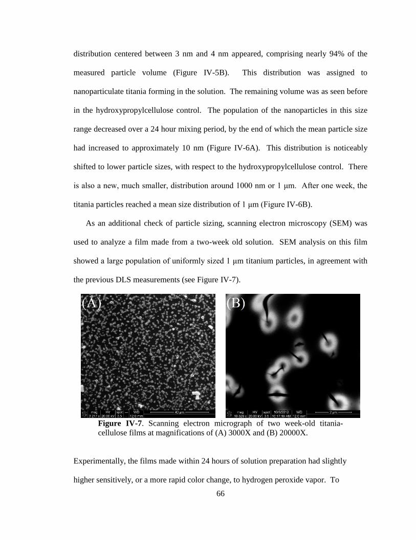
66
distribution centered between 3 nm and 4 nm appeared, comprising nearly 94% of the
measured particle volume (Figure IV-5B). This distribution was assigned to
nanoparticulate titania forming in the solution. The remaining volume was as seen before
in the hydroxypropylcellulose control. The population of the nanoparticles in this size
range decreased over a 24 hour mixing period, by the end of which the mean particle size
had increased to approximately 10 nm (Figure IV-6A). This distribution is noticeably
shifted to lower particle sizes, with respect to the hydroxypropylcellulose control. There
is also a new, much smaller, distribution around 1000 nm or 1 μm. After one week, the
titania particles reached a mean size distribution of 1 μm (Figure IV-6B).
As an additional check of particle sizing, scanning electron microscopy (SEM) was
used to analyze a film made from a two-week old solution. SEM analysis on this film
showed a large population of uniformly sized 1 μm titanium particles, in agreement with
the previous DLS measurements (see Figure IV-7).
Figure IV-7. Scanning electron micrograph of two week-old titania-
cellulose films at magnifications of (A) 3000X and (B) 20000X.
Experimentally, the films made within 24 hours of solution preparation had slightly
higher sensitively, or a more rapid color change, to hydrogen peroxide vapor. To
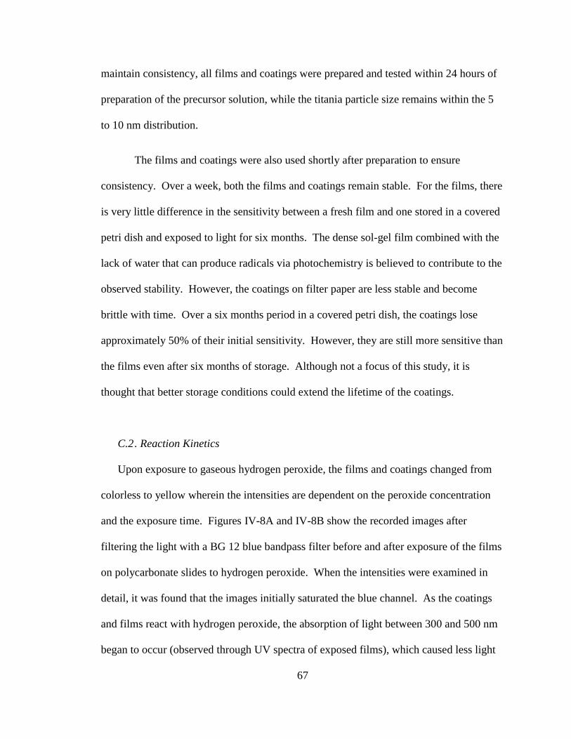
67
maintain consistency, all films and coatings were prepared and tested within 24 hours of
preparation of the precursor solution, while the titania particle size remains within the 5
to 10 nm distribution.
The films and coatings were also used shortly after preparation to ensure
consistency. Over a week, both the films and coatings remain stable. For the films, there
is very little difference in the sensitivity between a fresh film and one stored in a covered
petri dish and exposed to light for six months. The dense sol-gel film combined with the
lack of water that can produce radicals via photochemistry is believed to contribute to the
observed stability. However, the coatings on filter paper are less stable and become
brittle with time. Over a six months period in a covered petri dish, the coatings lose
approximately 50% of their initial sensitivity. However, they are still more sensitive than
the films even after six months of storage. Although not a focus of this study, it is
thought that better storage conditions could extend the lifetime of the coatings.
C.2 . Reaction Kinetics
Upon exposure to gaseous hydrogen peroxide, the films and coatings changed from
colorless to yellow wherein the intensities are dependent on the peroxide concentration
and the exposure time. Figures IV-8A and IV-8B show the recorded images after
filtering the light with a BG 12 blue bandpass filter before and after exposure of the films
on polycarbonate slides to hydrogen peroxide. When the intensities were examined in
detail, it was found that the images initially saturated the blue channel. As the coatings
and films react with hydrogen peroxide, the absorption of light between 300 and 500 nm
began to occur (observed through UV spectra of exposed films), which caused less light
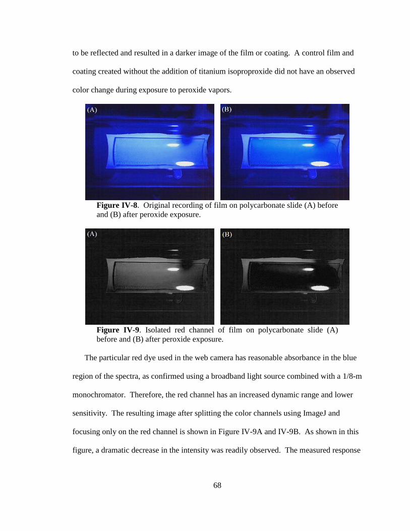
68
to be reflected and resulted in a darker image of the film or coating. A control film and
coating created without the addition of titanium isoproproxide did not have an observed
color change during exposure to peroxide vapors.
Figure IV-8. Original recording of film on polycarbonate slide (A) before
and (B) after peroxide exposure.
Figure IV-9. Isolated red channel of film on polycarbonate slide (A)
before and (B) after peroxide exposure.
The particular red dye used in the web camera has reasonable absorbance in the blue
region of the spectra, as confirmed using a broadband light source combined with a 1/8-m
monochromator. Therefore, the red channel has an increased dynamic range and lower
sensitivity. The resulting image after splitting the color channels using ImageJ and
focusing only on the red channel is shown in Figure IV-9A and IV-9B. As shown in this
figure, a dramatic decrease in the intensity was readily observed. The measured response
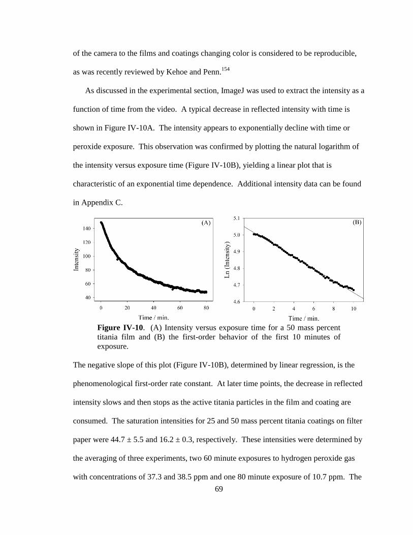
69
of the camera to the films and coatings changing color is considered to be reproducible,
as was recently reviewed by Kehoe and Penn.154
As discussed in the experimental section, ImageJ was used to extract the intensity as a
function of time from the video. A typical decrease in reflected intensity with time is
shown in Figure IV-10A. The intensity appears to exponentially decline with time or
peroxide exposure. This observation was confirmed by plotting the natural logarithm of
the intensity versus exposure time (Figure IV-10B), yielding a linear plot that is
characteristic of an exponential time dependence. Additional intensity data can be found
in Appendix C.
Figure IV-10. (A) Intensity versus exposure time for a 50 mass percent
titania film and (B) the first-order behavior of the first 10 minutes of
exposure.
The negative slope of this plot (Figure IV-10B), determined by linear regression, is the
phenomenological first-order rate constant. At later time points, the decrease in reflected
intensity slows and then stops as the active titania particles in the film and coating are
consumed. The saturation intensities for 25 and 50 mass percent titania coatings on filter
paper were 44.7 ± 5.5 and 16.2 ± 0.3, respectively. These intensities were determined by
the averaging of three experiments, two 60 minute exposures to hydrogen peroxide gas
with concentrations of 37.3 and 38.5 ppm and one 80 minute exposure of 10.7 ppm. The
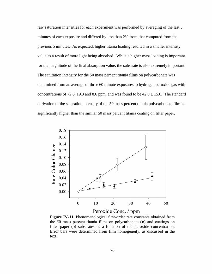
70
raw saturation intensities for each experiment was performed by averaging of the last 5
minutes of each exposure and differed by less than 2% from that computed from the
previous 5 minutes. As expected, higher titania loading resulted in a smaller intensity
value as a result of more light being absorbed. While a higher mass loading is important
for the magnitude of the final absorption value, the substrate is also extremely important.
The saturation intensity for the 50 mass percent titania films on polycarbonate was
determined from an average of three 60 minute exposures to hydrogen peroxide gas with
concentrations of 72.6, 19.3 and 8.6 ppm, and was found to be 42.0 ± 15.0. The standard
derivation of the saturation intensity of the 50 mass percent titania polycarbonate film is
significantly higher than the similar 50 mass percent titania coating on filter paper.
Figure IV-11. Phenomenological first-order rate constants obtained from
the 50 mass percent titania films on polycarbonate (●) and coatings on
filter paper (Ο) substrates as a function of the peroxide concentration.
Error bars were determined from film homogeneity, as discussed in the
text.
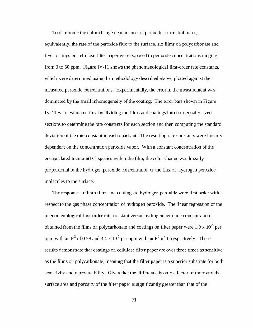
71
To determine the color change dependence on peroxide concentration or,
equivalently, the rate of the peroxide flux to the surface, six films on polycarbonate and
five coatings on cellulose filter paper were exposed to peroxide concentrations ranging
from 0 to 50 ppm. Figure IV-11 shows the phenomenological first-order rate constants,
which were determined using the methodology described above, plotted against the
measured peroxide concentrations. Experimentally, the error in the measurement was
dominated by the small inhomogeneity of the coating. The error bars shown in Figure
IV-11 were estimated first by dividing the films and coatings into four equally sized
sections to determine the rate constants for each section and then computing the standard
deviation of the rate constant in each quadrant. The resulting rate constants were linearly
dependent on the concentration peroxide vapor. With a constant concentration of the
encapsulated titanium(IV) species within the film, the color change was linearly
proportional to the hydrogen peroxide concentration or the flux of hydrogen peroxide
molecules to the surface.
The responses of both films and coatings to hydrogen peroxide were first order with
respect to the gas phase concentration of hydrogen peroxide. The linear regression of the
phenomenological first-order rate constant versus hydrogen peroxide concentration
obtained from the films on polycarbonate and coatings on filter paper were 1.0 x 10⁻³
per
ppm with an R2 of 0.98 and 3.4 x 10
-3 per ppm with an R
2 of 1, respectively. These
results demonstrate that coatings on cellulose filter paper are over three times as sensitive
as the films on polycarbonate, meaning that the filter paper is a superior substrate for both
sensitivity and reproducibility. Given that the difference is only a factor of three and the
surface area and porosity of the filter paper is significantly greater than that of the
72
polycarbonate substrate, the porous nature of the filter paper is not likely the cause of the
different rates. The coating was prepared using a similar amount of the sol-gel precursor
solution per unit area as that of the films, eliminating one advantage of a porous
substrate. In addition to sensitivity, the background noise for the films and coatings
were measured to be 5.2 and 1.1 intensity units, respectively. One major difference
between the films and coatings is that the films are transparent and require a white
background material to be placed under the slide, resulting in loss in the reflected
intensity. The coatings are white and require no additional background material to reflect
the light. Thus, some of the difference between the films and coatings could result from
small differences in the experimental setup. Importantly, our measurements show that
the chemistry that occurs on these materials is similar. Finally, for higher hydrogen
peroxide concentrations, the measured errors for the phenomenological first-order rate
constants in Figure 6 were larger than those found for lower concentrations. This was a
result of the films and coatings close to the peroxide inlet exhibiting a greater initial rate
of coloration.
The effect of titania mass loading on the phenomenological first-order rate constant of
the coatings was studied using 0, 25 and 50 mass percent titania mass, where the 0 mass
loading was used as a control. Figure IV-12 shows the response of these coatings to
exposures of various peroxide concentrations.
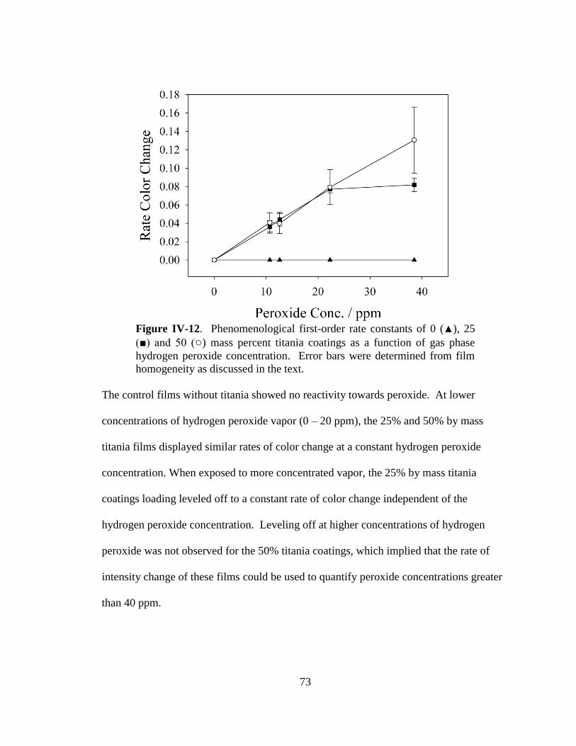
73
Figure IV-12. Phenomenological first-order rate constants of 0 (▲), 25
(■) and 50 (○) mass percent titania coatings as a function of gas phase
hydrogen peroxide concentration. Error bars were determined from film
homogeneity as discussed in the text.
The control films without titania showed no reactivity towards peroxide. At lower
concentrations of hydrogen peroxide vapor (0 – 20 ppm), the 25% and 50% by mass
titania films displayed similar rates of color change at a constant hydrogen peroxide
concentration. When exposed to more concentrated vapor, the 25% by mass titania
coatings loading leveled off to a constant rate of color change independent of the
hydrogen peroxide concentration. Leveling off at higher concentrations of hydrogen
peroxide was not observed for the 50% titania coatings, which implied that the rate of
intensity change of these films could be used to quantify peroxide concentrations greater
than 40 ppm.
74
C.3 . Peroxide Sensitivity and Reaction Mechanism
The experimental results (Figures IV-11 and IV-12) can be qualitatively understood
by a reaction mechanism that depends on the flux of hydrogen peroxide to the surface.
The phenomenological first-order rate constant at each peroxide concentration appears to
depend only on this flux (flux of hydrogen peroxide to the surface). Therefore, the
surface reaction rate for the formation of the color species is fast relative to the arrival
rate. The final coloration depends only on the concentration of available sites,
presumably the encapsulated titanium(IV) species within the film that are completely
consumed at later time points. This hypothesis is further supported by the linear
dependence of the rate constant on hydrogen peroxide concentration because the flux of
hydrogen peroxide molecules to the surface has a linear dependence on the gas phase
concentration or partial pressure. Additionally consistent with this model is the
independence of the phenomenological rate constant with titania loading (Figure IV-12).
The fast surface reaction rate implies that, at these peroxide concentrations, the measured
rate should be independent of the number of reactive sites within the films and coatings.
However, the ultimate capacity of these films is limited by the number of active sites
provided by the encapsulated titanium(IV) species; thus, higher loading is associated with
greater ultimate color change in the presence of peroxide vapor.
The slope of the phenomenological rate constant versus peroxide concentration
(Figures IV-11 and IV-12) is an indicator of film and coating sensitivity to peroxide
vapor. Color change per ppm of hydrogen peroxide directly correlated with film and
coating sensitivity to peroxide vapor wherein a larger color change resulted in greater the
sensitivity. Using the concentrations tested herein, the cellulose coatings clearly
75
provided greater sensitivity. A more quantitative estimate was obtained using the slopes
and the background noise of the detection system. The background noise for the films
and coatings was measured to be 5.2 and 1.1 intensity units, respectively. The major
limiting factor is the sensitivity of the web camera. Using 3σ as an estimate of the limit of
detection for the intensity measurements combined with predetermined measurement
times, the minimum detectible slope or intensity change was estimated. The minimum
detectible slope, in turn, was used to identify the detection limit in ppm. For the 50 mass
percent titania films on polycarbonate, the detection limit was estimated to be 90 ppm
hydrogen peroxide for a 1-minute measurement and 1.5 ppm for a 1-hour integration.
The coatings on filter paper had a much lower detection limit of 5.4 ppm hydrogen
peroxide for a 1-minute measurement minute and 0.09 ppm hydrogen peroxide for a 1-
hour integration.
D. Conclusion
Sol-gel methods were used to produce titania in a hydroxypropyl cellulose matrix
as films on polycarbonate or coatings on cellulose. These films and coatings had
reactivity toward hydrogen peroxide and changed color from colorless to an intense
yellow when exposed to hydrogen peroxide. The films on polycarbonate with a
titania/(titania+cellulose) mass percent greater than 50% had a tendency to crack. Using
an inexpensive web camera and a tungsten lamp to measure the reflected light, it was
determined that the films exhibited a first-order behavior with regard to color change
when exposed to peroxide vapor of less than 50 ppm. As the titania content present in the
films increased, less light was reflected at saturation. However, the mass ratio in the
76
solution did not affect the response rate for hydrogen peroxide concentrations below 25
ppm. For the 50 mass percent titania films on polycarbonate, the detection limit was
estimated to be 90 and 1.5 ppm for a 1-minute measurement and a 1-hour integration,
respectively. The coatings on cellulose provided a threefold increase in sensitivity
compared to the films on polycarbonate, with a detection limit of 5.4 ppm hydrogen
peroxide for a 1-minute measurement and 0.09 ppm hydrogen peroxide for an hour-long
integration. The major limiting factor was the sensitivity of the web camera. Using a
more sensitive detection technique, it may be possible to use the reflected intensity from
these films as an extremely sensitive hydrogen peroxide detector. Ongoing studies are
being conducted to determine the response of these films to organic peroxides.
Nevertheless, a sensor utilizing the titania-cellulose coating may be constructed to
monitor peroxide vapor exposure in workplaces to determine whether exposure levels are
within the OSHA permissible average exposure limit of 1 ppm of peroxide vapor over an
8-hour day.96
77
CHAPTER V
THE OPTIMIZATION OF SENSING COATINGS FOR THE DETECTION OF
ORGANIC PEROXIDE VAPORS
A. Introduction
After optimizing and determining the sensitivities of titania-cellulose films and
coatings to peroxide vapors in the previous Chapter, it was decided to see if these sensing
materials could be utilized to detect organic peroxide (e.g. triacetone triperoxide – TATP;
hexamethylene triperoxide diamine - HMTD) vapors in a similar fashion. Notably more
difficult to detect due to the lower reactivity and vapor pressure, organic peroxides are of
great concern due to their historical use as the materials for the main charge in terrorist
improvised explosive devices (IEDs).112-115
Current methods for detection of these
compounds include many approaches utilizing air sampling and ion-mobility
spectroscopy,119-122
laser-induced breakdown spectroscopy,123-125
and mass
spectrometry.130-133
However, these methods are difficult and require complicated
operating parameters. By comparison, detection of organic peroxide vapors through a
color-change mechanism (such as the sol-gel coatings to hydrogen peroxide discusses last
Chapter) would be ideal, as this would provide a clear yes-no indicator for their presence.
78
However, when the sol-gel coatings studied the last chapter were exposed to organic
peroxides, it was found that they were not extremely sensitive to organic peroxide vapors,
and only displayed a color change after an extended amount of exposure time (e.g. more
than 3 hours). It was discussed in a recent article that reaction of TATP with acid
produced hydrogen peroxide, to which the films and coatings are already sensitive.155
With this in mind, a variety of solutions with titanium(IV) and high acid content were
produced to evaluate propensity for organic peroxide vapor detection. Solutions
produced include the titania sol-gel in cellulose solution described last Chapter, but with
higher acid concentrations. It was observed that the sensitivity of these coatings
increased dramatically to TATP vapor (Pvapor ~ 10-2
torr at 25 °C) while vapors from
HMTD remain difficult to detect, possibly due to HMTD’s much lower vapor pressure
(Pvapor ~ 10-4
torr at 25 ºC).118
Additional coatings of an acidified solution of titanyl
sulfate on a silica substrate were produced containing an ionic liquid in place of
isopropanol as the solvent and either sulfuric or trifluoromethanesulfonic acid. Through
this substitution of an ionic liquid, the coatings were protected against drying out; thus, as
the acidic environment was maintained, the usable lifetime of the produced coatings was
extended. The most sensitvite coating with the ionic liquid was found to be that made
with trifluoromethanesulfonic acid, which showed an equal sensitivity to organic
peroxides as the sol-gel coatings, with the added benefit of long-term stability.
79
B. Experimental Details
B.1 . Preparation of Titanium(IV) Isoproproxide-Hydroxylpropyl Cellulose Solutions
Solutions of titanium(IV) isopropoxide with hydroxypropyl cellulose in 2-propanol
and of titanyl sulfate (i.e. titanium(IV) oxysulfate) in buffered ionic liquid solutions with
sulfuric or trifluoromethanesulfonic acid were produced following the procedure outlined
in the Experimental section of Chapter IV. The only alteration was in the amount of acid
added following the addition of titanium(IV) isoproproxide for the sol-gel coatings. In
place of 1.5 g of concentrated hydrochloric acid (Pharmco-Aaper, ACS Reagent), the
acid content was quadrupled to be 6.0 g of hydrochloric acid in one solution. For the
second solution, concentrated sulfuric acid (Pharmco-Aaper, ACS Reagent) was
substituted for hydrochloric acid and the amount added was 6.2 g (for pH equivalence).
B.2 . Preparation of Titanyl Sulfate in Buffered Ionic Liquid Solutions
Solutions of titanyl sulfate (i.e. titanium(IV) oxysulfate) in a buffered ionic liquid
solution were produced. First, 1.69 g of H2O (RO, 18 MΩ-cm) was mixed with either
0.38 g of concentrated sulfuric acid (Pharmco-Aaper, ACS Reagent) or 0.58 g of
trifluoromethanesulfonic acid (Alfa Aesar, 98+%) in a test tube. To these solutions, 0.50
g of solid titanium(IV) oxysulfate was added and the tube was immersed in a boiling
water bath for five minutes to dissolve the solid. The tube was removed and cooled to
room temperature, after which the solution was filtered through a 0.22 µm syringe filter
to remove any undissolved particulates. Following this, 0.81 g of 1-ethyl-3-
methylimidzolium hydrogen sulfate (Aldrich, 95%), acting as an ionic liquid in the
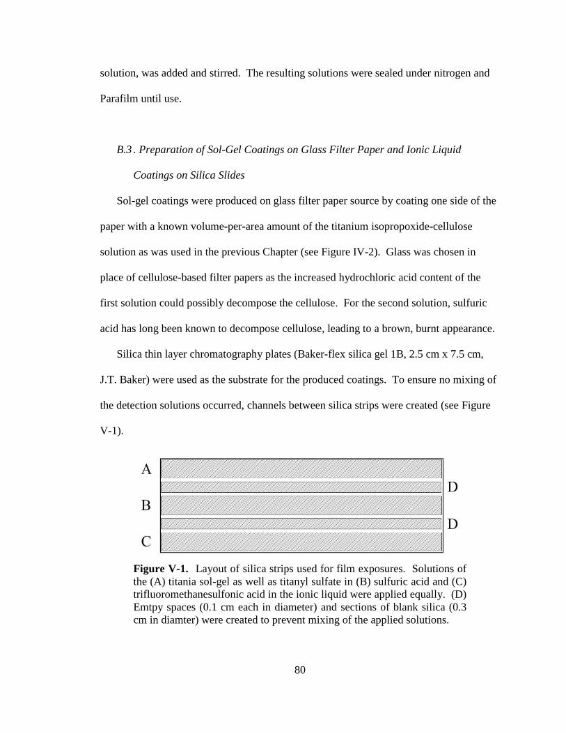
80
solution, was added and stirred. The resulting solutions were sealed under nitrogen and
Parafilm until use.
B.3 . Preparation of Sol-Gel Coatings on Glass Filter Paper and Ionic Liquid
Coatings on Silica Slides
Sol-gel coatings were produced on glass filter paper source by coating one side of the
paper with a known volume-per-area amount of the titanium isopropoxide-cellulose
solution as was used in the previous Chapter (see Figure IV-2). Glass was chosen in
place of cellulose-based filter papers as the increased hydrochloric acid content of the
first solution could possibly decompose the cellulose. For the second solution, sulfuric
acid has long been known to decompose cellulose, leading to a brown, burnt appearance.
Silica thin layer chromatography plates (Baker-flex silica gel 1B, 2.5 cm x 7.5 cm,
J.T. Baker) were used as the substrate for the produced coatings. To ensure no mixing of
the detection solutions occurred, channels between silica strips were created (see Figure
V-1).
Figure V-1. Layout of silica strips used for film exposures. Solutions of
the (A) titania sol-gel as well as titanyl sulfate in (B) sulfuric acid and (C)
trifluoromethanesulfonic acid in the ionic liquid were applied equally. (D)
Emtpy spaces (0.1 cm each in diameter) and sections of blank silica (0.3
cm in diamter) were created to prevent mixing of the applied solutions.
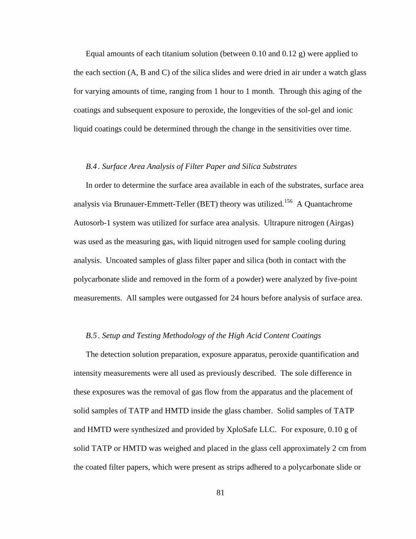
81
Equal amounts of each titanium solution (between 0.10 and 0.12 g) were applied to
the each section (A, B and C) of the silica slides and were dried in air under a watch glass
for varying amounts of time, ranging from 1 hour to 1 month. Through this aging of the
coatings and subsequent exposure to peroxide, the longevities of the sol-gel and ionic
liquid coatings could be determined through the change in the sensitivities over time.
B.4 . Surface Area Analysis of Filter Paper and Silica Substrates
In order to determine the surface area available in each of the substrates, surface area
analysis via Brunauer-Emmett-Teller (BET) theory was utilized.156
A Quantachrome
Autosorb-1 system was utilized for surface area analysis. Ultrapure nitrogen (Airgas)
was used as the measuring gas, with liquid nitrogen used for sample cooling during
analysis. Uncoated samples of glass filter paper and silica (both in contact with the
polycarbonate slide and removed in the form of a powder) were analyzed by five-point
measurements. All samples were outgassed for 24 hours before analysis of surface area.
B.5 . Setup and Testing Methodology of the High Acid Content Coatings
The detection solution preparation, exposure apparatus, peroxide quantification and
intensity measurements were all used as previously described. The sole difference in
these exposures was the removal of gas flow from the apparatus and the placement of
solid samples of TATP and HMTD inside the glass chamber. Solid samples of TATP
and HMTD were synthesized and provided by XploSafe LLC. For exposure, 0.10 g of
solid TATP or HMTD was weighed and placed in the glass cell approximately 2 cm from
the coated filter papers, which were present as strips adhered to a polycarbonate slide or
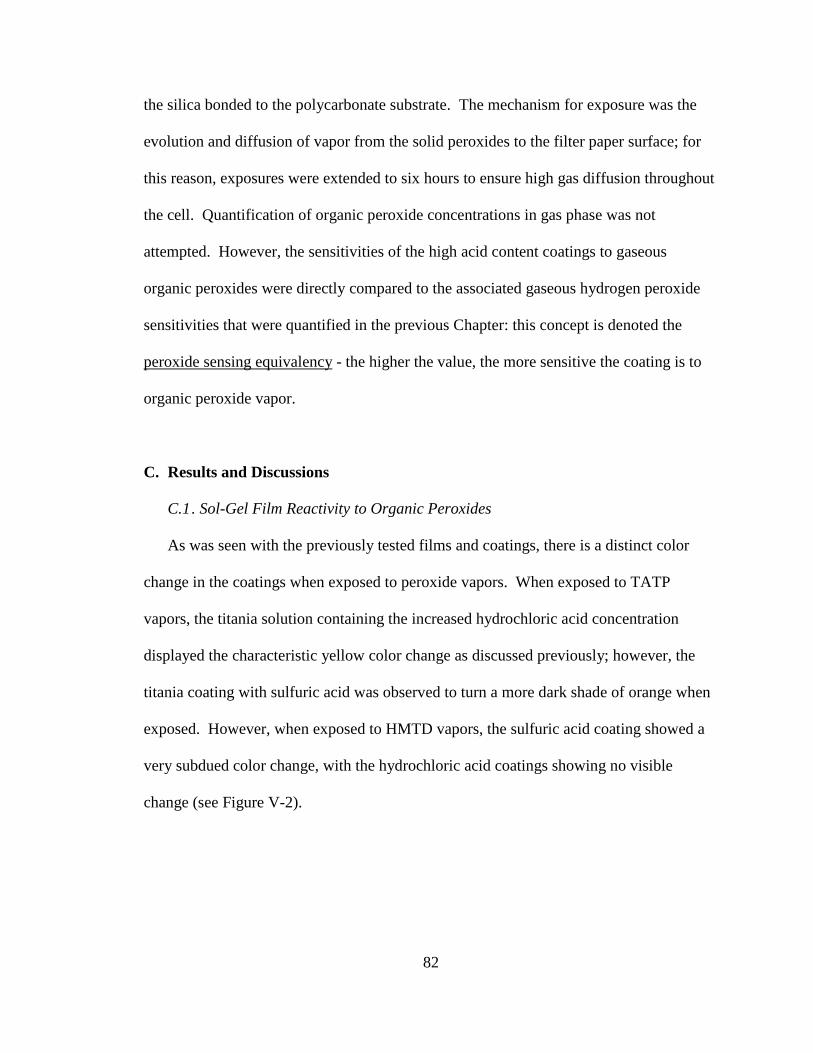
82
the silica bonded to the polycarbonate substrate. The mechanism for exposure was the
evolution and diffusion of vapor from the solid peroxides to the filter paper surface; for
this reason, exposures were extended to six hours to ensure high gas diffusion throughout
the cell. Quantification of organic peroxide concentrations in gas phase was not
attempted. However, the sensitivities of the high acid content coatings to gaseous
organic peroxides were directly compared to the associated gaseous hydrogen peroxide
sensitivities that were quantified in the previous Chapter: this concept is denoted the
peroxide sensing equivalency - the higher the value, the more sensitive the coating is to
organic peroxide vapor.
C. Results and Discussions
C.1 . Sol-Gel Film Reactivity to Organic Peroxides
As was seen with the previously tested films and coatings, there is a distinct color
change in the coatings when exposed to peroxide vapors. When exposed to TATP
vapors, the titania solution containing the increased hydrochloric acid concentration
displayed the characteristic yellow color change as discussed previously; however, the
titania coating with sulfuric acid was observed to turn a more dark shade of orange when
exposed. However, when exposed to HMTD vapors, the sulfuric acid coating showed a
very subdued color change, with the hydrochloric acid coatings showing no visible
change (see Figure V-2).
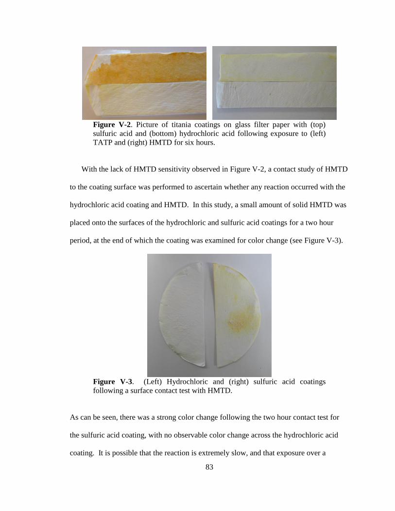
83
Figure V-2. Picture of titania coatings on glass filter paper with (top)
sulfuric acid and (bottom) hydrochloric acid following exposure to (left)
TATP and (right) HMTD for six hours.
With the lack of HMTD sensitivity observed in Figure V-2, a contact study of HMTD
to the coating surface was performed to ascertain whether any reaction occurred with the
hydrochloric acid coating and HMTD. In this study, a small amount of solid HMTD was
placed onto the surfaces of the hydrochloric and sulfuric acid coatings for a two hour
period, at the end of which the coating was examined for color change (see Figure V-3).
Figure V-3. (Left) Hydrochloric and (right) sulfuric acid coatings
following a surface contact test with HMTD.
As can be seen, there was a strong color change following the two hour contact test for
the sulfuric acid coating, with no observable color change across the hydrochloric acid
coating. It is possible that the reaction is extremely slow, and that exposure over a
84
greater time (e.g. >1 day) may result in a color change; however, this supposition has not
been explored further.
C.2 . Surface Area Analyses of Substrates
BET analysis was used to measure the surface areas of the uncoated substrates.
While numerous attempts were made, the surface area for the glass filter papers was
unmeasurable. It is unknown as to the reason for this outcome, but it is possible that the
surface area was below the measurement limit of the instrument. For the silica substrate,
the measured surface area was found to be 2.53 x 10² m
2/g when still applied to the
polycarbonate slide. In terms of slide area, this equates to 2.80 m2/cm
2 silica slide.
When removed from the slide and in a purely powder form, the surface area was found to
increase to 3.24 x 10² m
2/g, likely due to the less dense nature of the powder versus the
plated form. Given this high surface area, the substrate of choice was switched from
glass filter paper to silica slides.
C.3 . Solution Sensitivities to Hydrogen Peroxide Vapor
To ascertain how the higher acid content of the sulfuric sol-gel and buffered ionic
liquid coatings would affect peroxide reactivity, the produced films and coatings were
exposed to hydrogen peroxide at four concentrations. This was completed to give a point
of reference of comparison between the lower acid content films and coatings (Chapter
IV) and the higher acid content coatings made for organic peroxides. These
measurements also can be used to determine the minimum possible concentration of
TATP vapor, as it has been detailed that three molecules of hydrogen peroxide (or
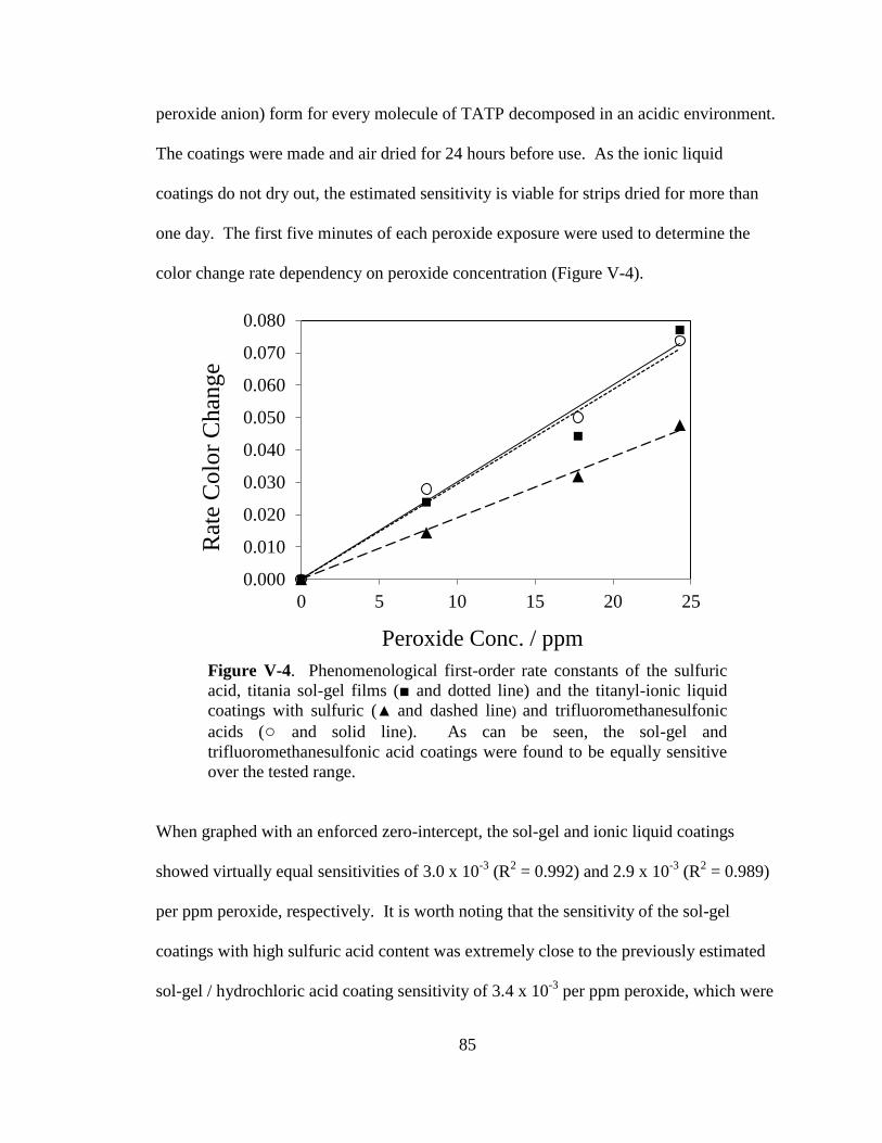
85
peroxide anion) form for every molecule of TATP decomposed in an acidic environment.
The coatings were made and air dried for 24 hours before use. As the ionic liquid
coatings do not dry out, the estimated sensitivity is viable for strips dried for more than
one day. The first five minutes of each peroxide exposure were used to determine the
color change rate dependency on peroxide concentration (Figure V-4).
Figure V-4. Phenomenological first-order rate constants of the sulfuric
acid, titania sol-gel films (■ and dotted line) and the titanyl-ionic liquid
coatings with sulfuric (▲ and dashed line) and trifluoromethanesulfonic
acids (○ and solid line). As can be seen, the sol-gel and
trifluoromethanesulfonic acid coatings were found to be equally sensitive
over the tested range.
When graphed with an enforced zero-intercept, the sol-gel and ionic liquid coatings
showed virtually equal sensitivities of 3.0 x 10⁻³
(R2 = 0.992) and 2.9 x 10
-3 (R
2 = 0.989)
per ppm peroxide, respectively. It is worth noting that the sensitivity of the sol-gel
coatings with high sulfuric acid content was extremely close to the previously estimated
sol-gel / hydrochloric acid coating sensitivity of 3.4 x 10⁻³
per ppm peroxide, which were
0.000
0.010
0.020
0.030
0.040
0.050
0.060
0.070
0.080
0 5 10 15 20 25
Rat
e C
olo
r C
han
ge
Peroxide Conc. / ppm
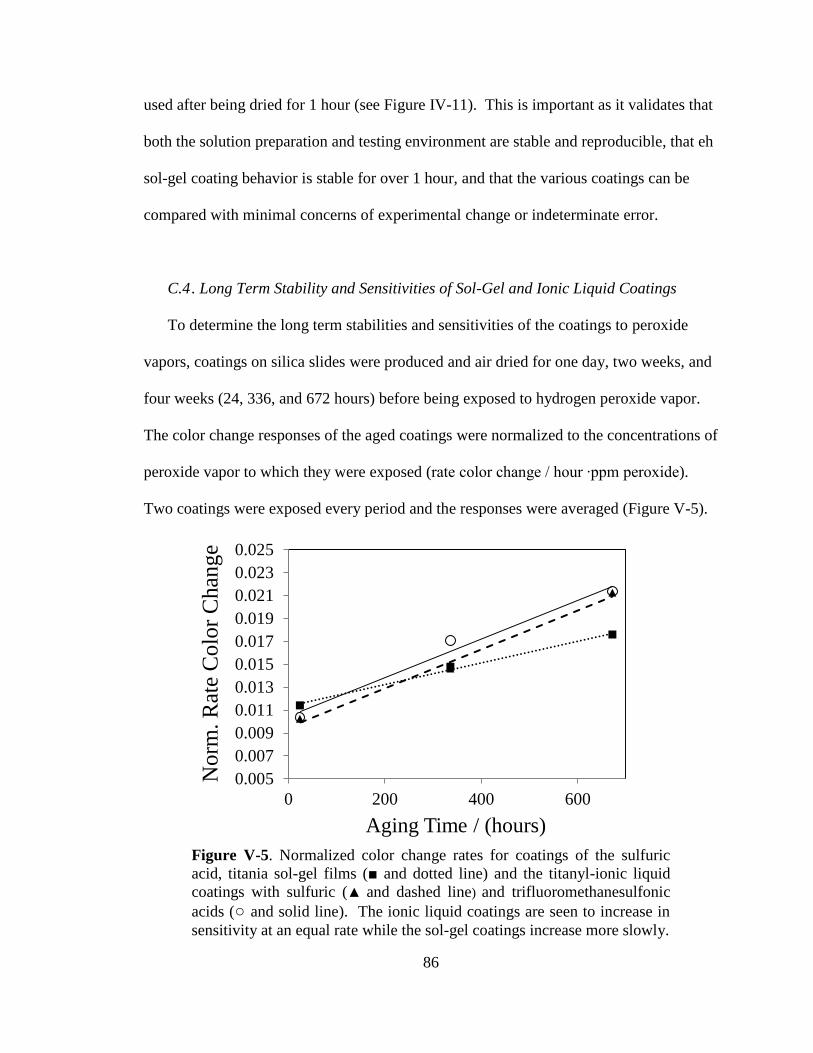
86
used after being dried for 1 hour (see Figure IV-11). This is important as it validates that
both the solution preparation and testing environment are stable and reproducible, that eh
sol-gel coating behavior is stable for over 1 hour, and that the various coatings can be
compared with minimal concerns of experimental change or indeterminate error.
C.4 . Long Term Stability and Sensitivities of Sol-Gel and Ionic Liquid Coatings
To determine the long term stabilities and sensitivities of the coatings to peroxide
vapors, coatings on silica slides were produced and air dried for one day, two weeks, and
four weeks (24, 336, and 672 hours) before being exposed to hydrogen peroxide vapor.
The color change responses of the aged coatings were normalized to the concentrations of
peroxide vapor to which they were exposed (rate color change / hour ∙ppm peroxide).
Two coatings were exposed every period and the responses were averaged (Figure V-5).
Figure V-5. Normalized color change rates for coatings of the sulfuric
acid, titania sol-gel films (■ and dotted line) and the titanyl-ionic liquid
coatings with sulfuric (▲ and dashed line) and trifluoromethanesulfonic
acids (○ and solid line). The ionic liquid coatings are seen to increase in
sensitivity at an equal rate while the sol-gel coatings increase more slowly.
0.005
0.007
0.009
0.011
0.013
0.015
0.017
0.019
0.021
0.023
0.025
0 200 400 600
No
rm. R
ate
Colo
r C
han
ge
Aging Time / (hours)
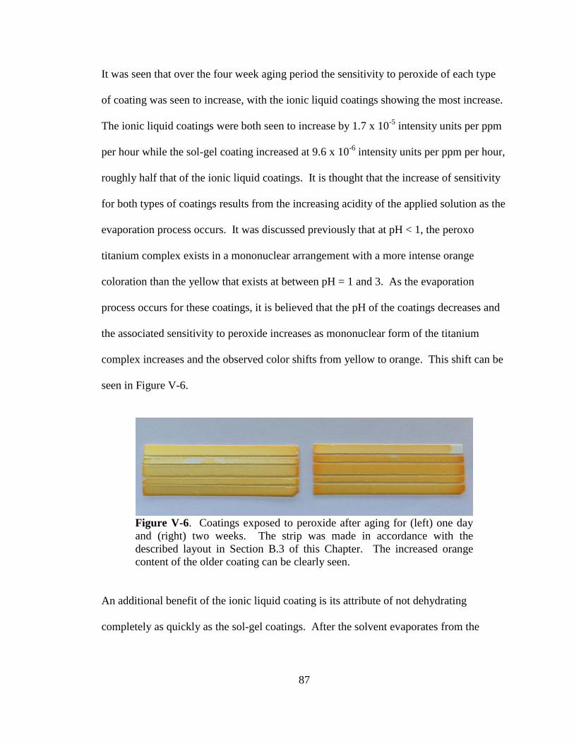
87
It was seen that over the four week aging period the sensitivity to peroxide of each type
of coating was seen to increase, with the ionic liquid coatings showing the most increase.
The ionic liquid coatings were both seen to increase by 1.7 x 10⁻⁵
intensity units per ppm
per hour while the sol-gel coating increased at 9.6 x 10⁻⁶
intensity units per ppm per hour,
roughly half that of the ionic liquid coatings. It is thought that the increase of sensitivity
for both types of coatings results from the increasing acidity of the applied solution as the
evaporation process occurs. It was discussed previously that at pH < 1, the peroxo
titanium complex exists in a mononuclear arrangement with a more intense orange
coloration than the yellow that exists at between pH = 1 and 3. As the evaporation
process occurs for these coatings, it is believed that the pH of the coatings decreases and
the associated sensitivity to peroxide increases as mononuclear form of the titanium
complex increases and the observed color shifts from yellow to orange. This shift can be
seen in Figure V-6.
Figure V-6. Coatings exposed to peroxide after aging for (left) one day
and (right) two weeks. The strip was made in accordance with the
described layout in Section B.3 of this Chapter. The increased orange
content of the older coating can be clearly seen.
An additional benefit of the ionic liquid coating is its attribute of not dehydrating
completely as quickly as the sol-gel coatings. After the solvent evaporates from the
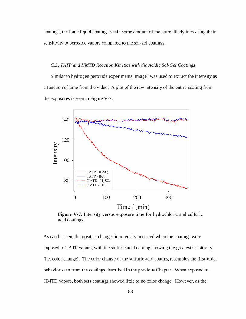
88
coatings, the ionic liquid coatings retain some amount of moisture, likely increasing their
sensitivity to peroxide vapors compared to the sol-gel coatings.
C.5 . TATP and HMTD Reaction Kinetics with the Acidic Sol-Gel Coatings
Similar to hydrogen peroxide experiments, ImageJ was used to extract the intensity as
a function of time from the video. A plot of the raw intensity of the entire coating from
the exposures is seen in Figure V-7.
Figure V-7. Intensity versus exposure time for hydrochloric and sulfuric
acid coatings.
As can be seen, the greatest changes in intensity occurred when the coatings were
exposed to TATP vapors, with the sulfuric acid coating showing the greatest sensitivity
(i.e. color change). The color change of the sulfuric acid coating resembles the first-order
behavior seen from the coatings described in the previous Chapter. When exposed to
HMTD vapors, both sets coatings showed little to no color change. However, as the
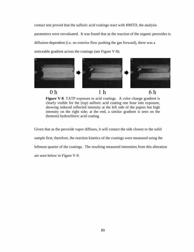
89
contact test proved that the sulfuric acid coatings react with HMTD, the analysis
parameters were reevaluated. It was found that as the reaction of the organic peroxides is
diffusion-dependent (i.e. no exterior flow pushing the gas forward), there was a
noticeable gradient across the coatings (see Figure V-8).
Figure V-8. TATP exposure to acid coatings. A color change gradient is
clearly visible for the (top) sulfuric acid coating one hour into exposure,
showing reduced reflected intensity at the left side of the papers but high
intensity on the right side; at the end, a similar gradient is seen on the
(bottom) hydrochloric acid coating.
Given that as the peroxide vapor diffuses, it will contact the side closest to the solid
sample first; therefore, the reaction kinetics of the coatings were measured using the
leftmost quarter of the coatings. The resulting measured intensities from this alteration
are seen below in Figure V-9.
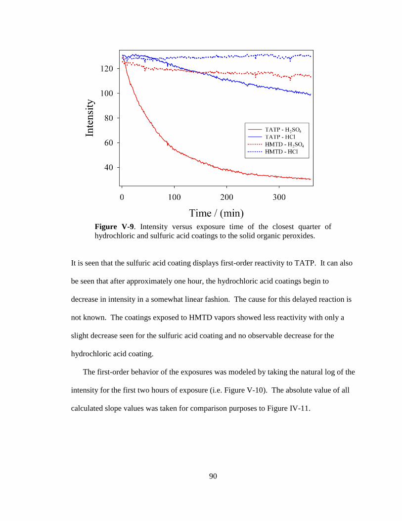
90
Figure V-9. Intensity versus exposure time of the closest quarter of
hydrochloric and sulfuric acid coatings to the solid organic peroxides.
It is seen that the sulfuric acid coating displays first-order reactivity to TATP. It can also
be seen that after approximately one hour, the hydrochloric acid coatings begin to
decrease in intensity in a somewhat linear fashion. The cause for this delayed reaction is
not known. The coatings exposed to HMTD vapors showed less reactivity with only a
slight decrease seen for the sulfuric acid coating and no observable decrease for the
hydrochloric acid coating.
The first-order behavior of the exposures was modeled by taking the natural log of the
intensity for the first two hours of exposure (i.e. Figure V-10). The absolute value of all
calculated slope values was taken for comparison purposes to Figure IV-11.
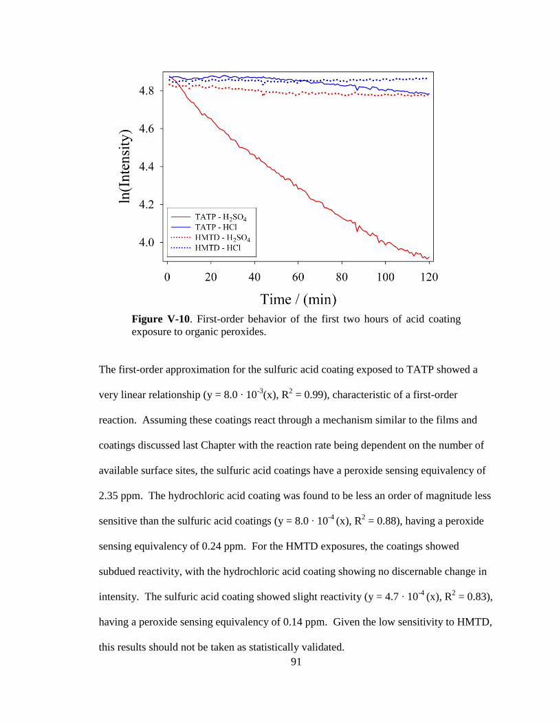
91
Figure V-10. First-order behavior of the first two hours of acid coating
exposure to organic peroxides.
The first-order approximation for the sulfuric acid coating exposed to TATP showed a
very linear relationship (y = 8.0 ∙ 10-3
(x), R2 = 0.99), characteristic of a first-order
reaction. Assuming these coatings react through a mechanism similar to the films and
coatings discussed last Chapter with the reaction rate being dependent on the number of
available surface sites, the sulfuric acid coatings have a peroxide sensing equivalency of
2.35 ppm. The hydrochloric acid coating was found to be less an order of magnitude less
sensitive than the sulfuric acid coatings (y = 8.0 ∙ 10-4
(x), R2 = 0.88), having a peroxide
sensing equivalency of 0.24 ppm. For the HMTD exposures, the coatings showed
subdued reactivity, with the hydrochloric acid coating showing no discernable change in
intensity. The sulfuric acid coating showed slight reactivity (y = 4.7 ∙ 10-4
(x), R2 = 0.83),
having a peroxide sensing equivalency of 0.14 ppm. Given the low sensitivity to HMTD,
this results should not be taken as statistically validated.
92
The diffusion of the organic peroxides in the glass cell is a complicating factor: for
this reason, a new testing method was tried to minimize the diffusion gradient across the
cell. To accomplish this, a 0.10 g sample of TATP was left to diffuse in the airtight glass
exposure cell for 12 hours or more, with one end of the tube sealed with Parafilm. To
insert the coatings for testing, a thin slice was made in the Parafilm with a razor blade.
Through this cut the slide was pushed into position under the camera using a spatula, and
the end was resealed with another piece of Parafilm. From sample introduction and
positioning to recording the exposure, the process took less than 15 seconds, minimizing
the loss of vaporized TATP. However, possibility due to the reactivity of the TATP with
the cell, the diffusion gradient could not be eliminated.
Using this procedure, the sol-gel coatings were exposed for two hours for comparison
purposes, and the intensities of the closest quarter of the film were analyzed to be
comparable to Figure V-10 (see Figure V-11).
93
Figure V-11. Intensity versus exposure time of the closest quarter of
hydrochloric and sulfuric acid coatings pre-diffused TATP vapors.
For comparison purposes, when modeled as a first-order reaction, the measured rate
of color change can give a quantity for comparing the coating sensitivities. For the
hydrochloric coating, the calculated peroxide sensing equivalency was found to be 0.29
ppm, statistically non-different from the non-diffusion controlled exposure. For the
sulfuric coating, the calculated peroxide sensing equivalency was found to be 2.56 ppm,
slightly more sensitive than in the non-diffusion controlled exposure. However, given
that diffusion of TATP was still an issue, this numbers should qualitative and not
quantitative. When comparing the hydrochloric and sulfuric acid coatings, it is worth
noting that the sulfuric acid coatings also detected HMTD vapors, whereas the
hydrochloric acid coatings did not. This would seem to indicate that the sulfuric acid
coating is superior for organic peroxide detection.
94
D. Conclusion
The preliminary effect of acid loading on the sensitivity of titania-cellulose coatings
to organic peroxide vapors was discussed. Titania-cellulose coatings containing
hydrochloric and sulfuric acid were exposed to organic peroxide vapors diffusing from
solid samples of TATP and HMTD, with the change in reflected intensity being used to
determine the coating sensitivities to the gaseous peroxides. It was observed that both
hydrochloric and sulfuric acid coatings displayed first-order kinetics in the presence of
diffusing TATP vapor, with peroxide sensing equivalencies of 0.24 and 2.35 ppm,
respectively. When exposed to HMTD, the hydrochloric acid coating displayed no
reactivity (i.e. color change), a finding supported by a surface contact test with HMTD,
which also showed no color change. The sulfuric acid was weakly sensitive to HMTD
vapors, with a peroxide sensing equivalency of 0.14 ppm and first-order kinetics similar
to TATP exposure; however, this projection suffers from a high amount of uncertainty.
When exposed to saturated TATP vapors previously diffused in the exposure cell, the
hydrochloric acid coating displayed an unchanged sensitivity and a statistically non-
different peroxide sensing equivalency of 0.29 ppm. However, the sulfuric acid coating
displayed second-order behavior, indicating a more complicated reaction mechanism for
the coating. When modeled as a first-order reaction for comparison purposes, the sulfuric
acid coating possessed a peroxide sensing equivalency of 2.56 ppm, slightly increased
from the non-diffusion controlled exposure. Additional exposures are required to
statistically validate these projected sensitivities.
95
CONCLUDING REMARKS
A. Sodium Dithionite
Following the Introduction, the first three Chapters of this dissertation review the
research accomplished with sodium dithionite. Chapter II details the development and
validation of a new method for dithionite and thiosulfate quantification using ion
chromatography; it is hoped that this method for analysis could be utilized in industry in
place of the standard three iodometric titration approach, which requires both additional
time and resources when compared to the new method. During the course of this study, a
peculiarity was seen to occur when the oldest sample was titrated – a calculated negative
dithionite composition. This finding led the research discussed in Chapter III, where a
study of the long-term composition of samples of sodium dithionite was performed.
Using Raman spectroscopy in addition to the previously utilized methods, extended S-S
bonding compounds were found to form over time, including tetrathionate and possibly
trithionate. In such advanced stages of dithionite degradation, it is suggested that the ion
chromatographic method be used for composition analysis as the titration method can be
affected by the additional reducible species present.
96
B. Titania-Cellulose Thin Films for Peroxide Detection
Having recognized acidic titanium(IV) solutions as a superior detection method for
peroxide vapors, it was decided to ascertain whether or not thin films composed similarly
could behave as the solutions did. To this end, thin films on polycarbonate and coatings
on filter paper were made and exposed to peroxide concentrations, which was described
in Chapter V. These materials were found to be reactive to hydrogen peroxide vapor,
with the most sensitive coatings showing a one minute limit of detection of 5.4 ppm
peroxide. However, these coatings showed only slight reactivity to organic peroxides
(i.e. TATP, HMTD). A literature review found that higher acid content resulting in the
production of hydrogen peroxide following decomposition of organic peroxide vapors.
With this in mind, higher acid content coatings and their sensitivities to TATP and
HMTD were evaluated, as reviewed in Chapter VI. Coatings with higher acid
concentrations were found to be moderately sensitive to TATP, with sulfuric acid
coatings showing a peroxide sensing equivalency of 2.35 ppm. For HMTD however,
while reactive when in contact with the solid organic peroxide, very low sensitivity was
seen in exposures. This is likely as result of the much lower vapor pressure of HMTD
relative to TATP, but additional work negating the effects of diffusion and solely
quantifying the sensitivities of these coatings is continuing. It is intended for these
materials to be manufactured for industrial safety and national security purposes.
97
REFERENCES
1. Barbera, J. J.; Metzger, A.; Wolf, M. In Ullmann's Encyclopedia of Industrial
Chemistry 2000; Vol. 34, p 695.
2. Suess, H. U. Restaurator 2009, 30, 245.
3. Gorenšek, M.; Gorjanc, M.; Recelj, P.; Meden, A. Text. Res. J. 2008, 78, 524.
4. Kunttou, K.; Hongyo, S.; Maeda, S.; Mishima, K. Text. Res. J. 2005, 75, 149.
5. Carter, H. A. J. Chem. Educ. 1996, 73, 1068.
6. Torimoto, N. J. Chem. Educ. 1987, 64, 332.
7. Fox, M. R. Vat Dyestuffs and Vat Dyeing; 1st ed.; John Wiley & Sons: New York,
1947.
8. Matthews, J. M. Bleaching and Related Processes; 1st ed.; J. J. Little & Ives Co.:
New York, 1921.
9. Yoe, J. H.; Edgar, G. J. Phys. Chem. 1923, 27, 65.
10. Anonymous Chemical Market Reporter 1997, 251, 45.
11. Anonymous Chemical Market Reporter 2000, 257, 33.
12. Kirschner, M. Chemical Market Reporter 2003, 263, 27.
13. Kirschner, M. Chemical Market Reporter 2006, 269, 26.
14. De Vries, J. G.; Kellogg, R. M. J. Org. Chem. 1980, 45, 4126.
15. Kazmi, S. A.; Shorter, A. L.; McArdle, J. V. Inorg. Chem. 1984, 23, 4332.
98
16. Jeong, Y. U.; Manthiram, A. Inorg. Chem. 2001, 40, 73.
17. Boparai, H. K.; Shea, P. J.; Comfort, S. D.; Snow, D. D. Environ. Sci. Technol.
2006, 40, 3043.
18. Langell, M. A.; Kadossov, E.; Boparai, H.; Shea, P. Surf. Interface Anal. 2009,
41, 941.
19. Su, C.; Ludwig, R. D. Environ. Sci. Technol. 2005, 39, 6208.
20. Xie, Y.; Cwiertny, D. M. Environ. Sci. Technol. 2010, 44, 8649.
21. de Carvalho, L. M.; Schwedt, G. Electroanal. 2001, 13, 596.
22. Novakov, M.; Krivankov, L.; Bartos, M.; Urbanova, V.; Vytras, K. Talanta 2007,
74, 183.
23. de Carvalho, L. M.; Schwedt, G. J. Chromatogr. A 2005, 1099, 185.
24. Rinker, R. G.; Lynn, S.; Mason, D. M.; Corcoran, W. H. Ind. Eng. Chem. Res.
1965, 4, 282.
25. De Groot, D. C. Fresenius J. Anal. Chem 1967, 229, 335.
26. Brown, L.; Szekeres, L. Talanta 1979, 26, 414.
27. DePoy, P. E.; Mason, D. M. Faraday Symp. Chem. S. 1974, 9, 47.
28. Steudel, R.; Munchow, V. J. Chromatogr. A 1992, 623, 174.
29. Kovacs, K. M.; Rabai, G. Chem. Commun. 2002, 790.
30. Čermák, V.; Smutek, M. Collect. Czech. Chem. Commun. 1975, 40, 24.
31. Lister, M. W.; Garvie, R. C. Can. J. Chem. 1959, 37, 1567.
32. Kolthoff, I. M.; Miller, C. S. J. Am. Chem. Soc. 1941, 63, 2818.
33. Rinker, R. G.; Gordon, T. P.; Mason, D. M.; Sakaida, R. R.; Corcoran, W. H. J.
Phys. Chem. 1960, 64, 573.
99
34. Wayman, M.; Lem, W. J. Can. J. Chem. 1970, 48, 782.
35. Takahashi, H.; Kaneko, N.; Miwa, K. Spectrochim. Acta. A. - M. 1982, 38, 1147.
36. Nehb, W.; Vydra, K. In Ullmann's Encyclopedia of Industrial Chemistry; Wiley-
VCH: Weinheim, 2012; Vol. 35, p 5.
37. Greenwood, N. N.; Earnshaw, A. Chemistry of the Elements (2nd Edition);
Elsevier, 1997.
38. Janzen, E. G. J. Phys. Chem. 1972, 76, 157.
39. Kumar, M. Mar. Chem. 1981, 10, 475.
40. Sillén, L. G. Oceanography 1961, 32.
41. Shriver, D.; Atkins, P.; Overton, T.; Rourke, J.; Armstrong, F.; Weller, M.
Inorganic Chemistry; W. H. Freeman and Company: New York, 2006.
42. Wong, G. T. F. Mar. Chem. 1980, 9, 1.
43. Frank, M. Textile Colorist 1915, 37, 4.
44. Bernthsen, A. Ber. Dtscu. Chem. Ges. 1881, 14, 438.
45. Schönbein, C. F. J. Prakt. Chem. 1854, 61, 193.
46. Schützenberger, M. P. Compt. Rend. 1869, 69, 6.
47. Bazlen, M.; Google Patents: 1907.
48. Bernthsen, A. In The Chemical News and Journal of Physical Science; Crookes,
W., Ed.; Edwin John Davey: London, 1881; Vol. 43, p 79.
49. Merriman, R. W. J. Soc. Chem. Ind. 1923, 42, 290.
50. Wollak, R. Fresenius J. Anal. Chem 1930, 80, 1.
100
51. Wood, P. J.; Wiest, E. G.; Apsey, C. W.; Brubaker, C. H.; Fernald, B. B.; Kelton,
S. C.; Petschow, J.; Pond, W. F.; Simpson, C. T. Assay of Sodium Hydrosulfite, American
Association of Textile Chemists and Colorists, 1957.
52. Zocher, H.; Saechtling, H. Fresenius J. Anal. Chem. 1939, 117, 392.
53. Danehy, J. P.; Zubritsky, C. W. Anal. Chem. 1974, 46, 391.
54. Kilroy, W. P. Talanta 1978, 25, 359.
55. Kilroy, W. P. Talanta 1979, 26, 111.
56. Kilroy, W. P. Talanta 1980, 27, 343.
57. Kilroy, W. P. Talanta 1983, 30, 419.
58. Stutts, K. J. Anal. Chem. 1987, 59, 543.
59. de Carvalho, L. M.; Schwedt, G. Anal. Chim. Acta 2001, 436, 293.
60. Weiß, J.; Göbl, M. Fresenius J. Anal. Chem 1985, 320, 439.
61. Drude, P. Ann. Phys. 1889, 272, 532.
62. Leaver, K. D.; Chapman, B. N. Thin Films; Wykeham Publiations: London, 1971.
63. Secundus, G. P.; T., H. H.; Bostock, J. Natural History; H. G. Bohn: London,
1855; Vol. 6.
64. Ohring, M. Materials Science of Thin Films; Academic Press, 2002.
65. Eishanbini-Riad, A.; Barlow, F. D. Thin Film Technology Handbook; McGraw-
Hill Professional: New York, 1997.
66. Smart, L. E.; Moore, E. A. Solid State Chemistry: An Introduction; CRC Press,
2005.
67. Dimitriev, Y.; Ivanova, Y.; Iordanova, R. Journal of the University of Chemical
Technology and Metallurgy 2008, 43, 12.
101
68. Dislich, H.; Hinz, P. J. Non-Cryst. Solids 1982, 48, 11.
69. Bowman, J. E. Memoirs and Proceedings of the Chemical Society 1845, 3, 248.
70. Geffcken, W.; Berger, E.; Reichspatent, D., Ed.; Jeaner Glaswerk Schott & Gen.:
Germany, 1939.
71. Sibum, H.; Güther, V.; Roidl, O.; Habashi, F.; Wolf, H. U. In Ullmann's
Encyclopedia of Industrial Chemistry; Wiley-VCH Verlag GmbH & Co. KGaA: 2000.
72. Kamat, P. V. J. Phys. Chem. Lett. 2011, 2, 839.
73. Fujishima, A.; Honda, K. Nature 1972, 238, 37.
74. O'Regan, B.; Gratzel, M. Nature 1991, 353, 737.
75. Reisch, M. Chem. Eng. News 2001, 79, 8.
76. Remillard, J. T.; McBride, J. R.; Nietering, K. E.; Drews, A. R.; Zhang, X. J.
Phys. Chem. B 2000, 104, 4440.
77. Xi, B.; Verma, L. K.; Li, J.; Bhatia, C. S.; Danner, A. J.; Yang, H.; Zeng, H. C.
ACS Appl. Mater. Interfaces 2012, 4, 1093.
78. Rajeshwar, K.; Ibanez, J. G. J. Chem. Ed. 1995, 72, 1044.
79. Daghrir, R.; Drogui, P.; Robert, D. Ind. Eng. Chem. Res. 2013, 52, 3581.
80. Gaikwad, V. B.; Jain, G. H. In Sensing Technology (ICST), 2011 Fifth
International Conference on 2011, p 239.
81. Hu, P.; Du, G.; Zhou, W.; Cui, J.; Lin, J.; Liu, H.; Liu, D.; Wang, J.; Chen, S.
ACS Appl. Mater. Interfaces 2010, 2, 3263.
82. Kim, I.-D.; Rothschild, A.; Hyodo, T.; Tuller, H. L. Nano Lett. 2006, 6, 193.
83. Su, J.; Zou, X.-X.; Zou, Y.-C.; Li, G.-D.; Wang, P.-P.; Chen, J.-S. Inorg. Chem.
2013, 52, 5924.
102
84. Tolmachoff, E.; Memarzadeh, S.; Wang, H. J. Phys. Chem. C 2011, 115, 21620.
85. Munz, M.; Langridge, M. T.; Devarepally, K. K.; Cox, D. C.; Patel, P.; Martin, N.
A.; Vargha, G.; Stolojan, V.; White, S.; Curry, R. J. ACS Appl. Mater. Interfaces 2013, 5,
1197.
86. Hage, R.; Lienke, A. Angew. Chem. Int. Ed. 2006, 45, 206.
87. Chen, H.-W.; Chen, C.-Y.; Wang, G.-S. Chemosphere 2011, 85, 591.
88. Meneses, M.; Pasqualino, J. C.; Castells, F. Chemosphere 2010, 81, 266.
89. Shintani, H. Biocontrol Sci. 2009, 14, 39.
90. Demirkol, O.; Cagri-Mehmetoglu, A.; Qiang, Z.; Ercal, N.; Adams, C. J. Agric.
Food Chem. 2008, 56, 10414.
91. Qiang, Z.; Demirkol, O.; Ercal, N.; Adams, C. J. Agric. Food Chem. 2005, 53,
9830.
92. Castle, L.; Mercer, A. J.; Gilbert, J. J. Food. Protect. 1995, 58, 5.
93. Reidmiller, J. S.; Baldeck, J. D.; Rutherford, G. C.; Marquis, R. E. J. Food.
Protect. 2003, 66, 8.
94. Fichet, G.; Antloga, K.; Comoy, E.; Deslys, J. P.; McDonnell, G. J. Hosp. Infect.
2007, 67, 278.
95. Pottage, T.; Richardson, C.; Parks, S.; Walker, J. T.; Bennett, A. M. J. Hosp.
Infect. 2010, 74, 55.
96. OSHA; Labor, U. S. D. o., Ed. 1910.
97. OSHA; U. S. Department of Labor: 1978; Vol. 2012.
98. OSHA; U. S. Department of Labor: 2004.
103
99. Abo, M.; Urano, Y.; Hanaoka, K.; Terai, T.; Komatsu, T.; Nagano, T. J. Am.
Chem. Soc. 2011, 133, 10629.
100. Ohta, T.; Yamauchi, Y.; Takitani, S. Fresenius J. Anal. Chem. 1992, 343, 550.
101. Qi, B.; Zhu, Y. Z.; Hu, M.; Zhang, Y.; Tang, X. Anal. Lett. 2001, 34, 1247.
102. Luo, W.; Li, Y.-S.; Yuan, J.; Zhu, L.; Liu, Z.; Tang, H.; Liu, S. Talanta 2010, 81,
901.
103. Toniolo, R.; Geatti, P.; Bontempelli, G.; Schiavon, G. J. Electroanal. Chem.
2001, 514, 123.
104. Kuwata, S.; Sadaoka, Y. Sensor. Actua. B: Chemical 2000, 65, 325.
105. Wiedemair, J.; van Dorp, H. D. S.; Olthuis, W.; van den Berg, A. Electrophoresis
2012, 33, 3181.
106. Kulys, J. Sensors and Actuators B: Chemical 1992, 9, 143.
107. Lewis, D. J. Phys. Chem. 1958, 62, 1145.
108. Possanzini, M.; Di Palo, V. Anal. Chim. Acta 1995, 315, 225.
109. Satterfield, C. N.; Bonnell, A. H. Anal. Chem. 1955, 27, 1174.
110. Matsubara, C.; Kudo, K.; Kawashita, T.; Takamura, K. Anal. Chem. 1985, 57,
1107.
111. Huang, H.; Dasgupta, P. K. Talanta 1997, 44, 605.
112. Amani, M.; Chu, Y.; Waterman, K. L.; Hurley, C. M.; Platek, M. J.; Gregory, O.
J. Sensor. Actua. B: Chemical 2012, 162, 7.
113. Belluck, P.; Chang, K. In The New York Times; The New York Times: New York,
2001, p 1.
114. Oxley, J. C.; Smith, J. L.; Moran, J.; Nelson, K.; Utley, W. E. 2004, 349.
104
115. Perks, B.; Sanderson, K. Terror plot sparks frenzied speculation about liquid
explosives. Chemistry World [Online Early Access]. Published Online: 2006.
http://www.rsc.org/chemistryworld/News/2006/August/11080602.asp (accessed
6/3/2013).
116. Dubnikova, F.; Kosloff, R.; Almog, J.; Zeiri, Y.; Boese, R.; Itzhaky, H.; Alt, A.;
Keinan, E. J. Am. Chem. Soc. 2005, 127, 1146.
117. Dubnikova, F.; Kosloff, R.; Zeiri, Y.; Karpas, Z. J. Phys. Chem. A 2002, 106,
4951.
118. Moore, D. Sens. Imaging 2007, 8, 9.
119. Buttigieg, G. A.; Knight, A. K.; Denson, S.; Pommier, C.; Bonner Denton, M.
Forensice Sci. Int. 2003, 135, 53.
120. Oxley, J. C.; Smith, J. L.; Kirschenbaum, L. J.; Marimganti, S.; Vadlamannati, S.
J. Forensic Sci. 2008, 53, 690.
121. MacCrehan, W.; Moore, S.; Hancock, D. Anal. Chem. 2011, 83, 9054.
122. Fan, W.; Young, M.; Canino, J.; Smith, J.; Oxley, J.; Almirall, J. Anal. Bioanal.
Chem. 2012, 403, 401.
123. Lazic, V.; Palucci, A.; Jovicevic, S.; Carapanese, M.; Poggi, C.; Buono, E. In
Proceedings of SPIE; Fountain, A. W., Gardner, P. J., Eds. 2010; Vol. 7665, p 76650V.
124. Lazic, V.; Palucci, A.; Jovicevic, S.; Carpanese, M. Spectrochim. Acta. B. 2011,
66, 644.
125. Botti, S.; Carpanese, M.; Cantarini, L.; Giubileo, G.; Lazic, V.; Jovicevic, S.;
Palucci, A.; Puiu, A. In Proceedings of SPIE; Fountain, A. W., Gardner, P. J., Eds. 2010;
Vol. 7665, p 76650O.
105
126. Subarna, B.; Susanta, K. M.; Mano, M.; Indu , B. M. Nanotechnology 2009, 20,
075502.
127. Chowdhuri, A.; Sharma, A.; Gupta, V. In Proceedings of SPIE; Fountain, A. W.,
Gardner, P. J., Eds. 2011; Vol. 8018, p 80181V.
128. Capua, E.; Cao, R.; Sukenik, C. N.; Naaman, R. Sensor. Actua. B: Chemical
2009, 140, 122.
129. Wackerbarth, H.; Salb, C.; Gundrum, L.; Niederkrüger, M.; Christou, K.;
Beushausen, V.; Viöl, W. Appl. Opt. 2010, 49, 4362.
130. Wilson, P. F.; Prince, B. J.; McEwan, M. J. Anal. Chem. 2005, 78, 575.
131. Mullen, C.; Irwin, A.; Pond, B. V.; Huestis, D. L.; Coggiola, M. J.; Oser, H. Anal.
Chem. 2006, 78, 3807.
132. Romolo, F. S.; Cassioli, L.; Grossi, S.; Cinelli, G.; Russo, M. V. Forensic Sci. Int.
2013, 224, 96.
133. Shen, C.; Li, J.; Han, H.; Wang, H.; Jiang, H.; Chu, Y. Int. J. Mass. Spectrom.
2009, 285, 100.
134. Sehönn, G. Z. Anal. Chem. Freseniu. 1870, 9, 41.
135. Patel, C. C.; Mohan, M. S. Nature 1960, 186, 803.
136. Schwarz, R. Z. Anorg. Allg. Chem. 1933, 210, 303.
137. Jere, G. V.; Patel, C. C. Nature 1962, 194, 470.
138. Schwarzenbach, G.; Müehlebach, J.; Müeller, K. Inorg. Chem. 1970, 9, 2381.
139. Ohya, Y. In Handbook of Sol-Gel Science and Technology : Processing
Characterization and Applications; 1st ed.; Sakka, S., Ed.; Kluwer Academic Publishers:
Norwell, Massachusetts, 2005; Vol. 1, p 109.
106
140. Vogel, A. I. Textbook of Quantitative Chemical Analysis; 5th ed.; Longman
Scientific & Technical: New York, 1989.
141. Kusabe, M.; Kozuka, H.; Abe, S.; Suzuki, H. J. Sol-Gel Sci. Technol. 2007, 44,
111.
142. Harris, D. C. Quantitative Chemical Analysis; 7th ed.; W. H. Freeman and
Company: New York, 2007.
143. Haga, K.; Iwaya, K.; Kaneko, R. Bull. Chem. Soc. Jpn 1985, 59, 5.
144. Williams, W. J. Handbook of Anion Determination; Butterworths & Co.: London,
1979.
145. Hubaux, A.; Vos, G. Anal. Chem. 1970, 42, 849.
146. Schlessinger, G. G. Inorganic Laboratory Preparations; Chemical Publishing
Company: New York, 1962.
147. Wood, A.; Kelly, D. Arch. Microbiol. 1986, 144, 71.
148. Biltz, H.; Biltz, W. Laboratory Methods of Inorganic Chemistry; John Wiley &
Sons: New York, 1928.
149. Degen, I. A.; Newman, G. A. Spectrochim. Acta. A. - M. 1993, 49, 859.
150. Meyer, B.; Ospina, M.; Peter, L. B. Anal. Chim. Acta 1980, 117, 301.
151. Schneider, C. A.; Rasband, W. S.; Eliceiri, K. W. Nat. Meth. 2012, 9, 671.
152. Gilicinski, A. G.; Rynders, R. M.; Beck, S. E.; Strausser, Y. E.; Stets, J. R.;
Felker, B. S.; Bohling, D. A. MRS Online Proceedings Library 1993, 324, null.
153. Goswami, D.; Medda, S. K.; De, G. ACS Appl. Mater. Interfaces 2011, 3, 3440.
154. Kehoe, E.; Penn, R. L. J. Chem. Ed. 2013, 90, 1191.
155. Sella, E.; Shabat, D. Chem. Commun. 2008, 0, 5701.

107
156. Brunauer, S.; Emmett, P. H.; Teller, E. J. Am. Chem. Soc. 1938, 60, 309.
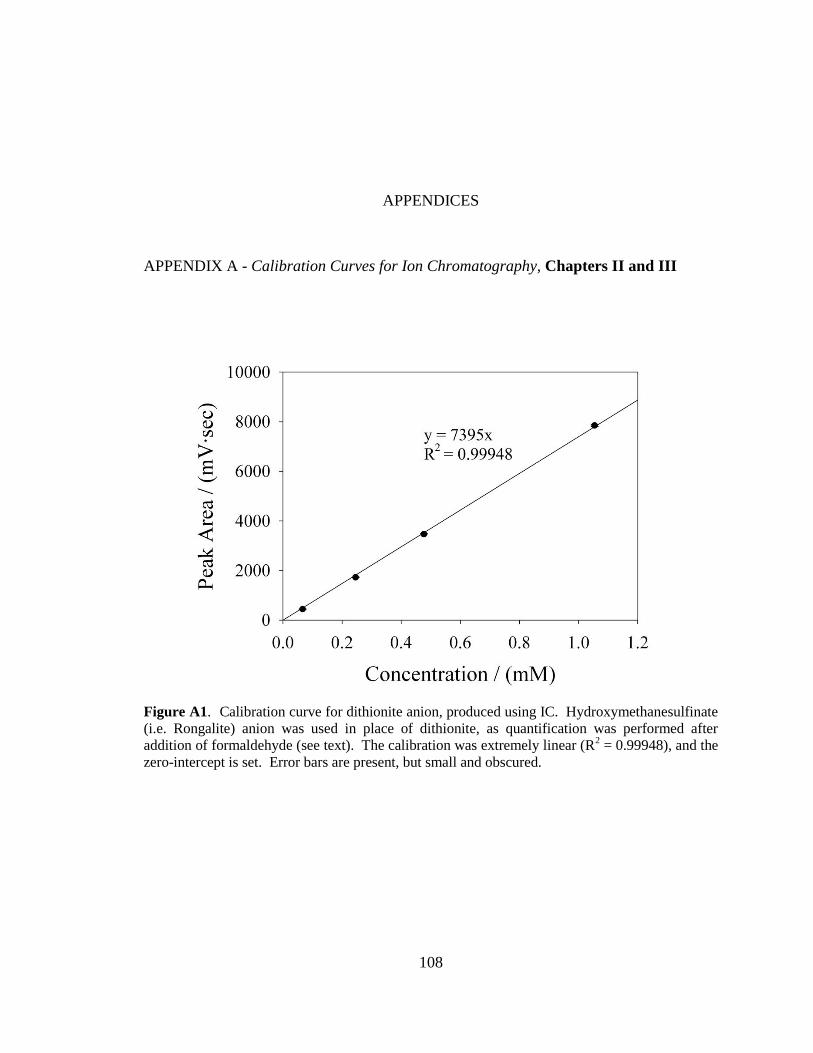
108
APPENDICES
APPENDIX A - Calibration Curves for Ion Chromatography, Chapters II and III
Figure A1. Calibration curve for dithionite anion, produced using IC. Hydroxymethanesulfinate
(i.e. Rongalite) anion was used in place of dithionite, as quantification was performed after
addition of formaldehyde (see text). The calibration was extremely linear (R2 = 0.99948), and the
zero-intercept is set. Error bars are present, but small and obscured.
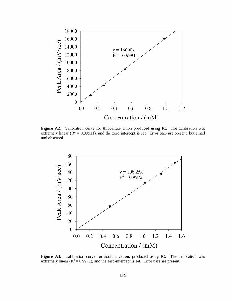
109
Figure A2. Calibration curve for thiosulfate anion produced using IC. The calibration was
extremely linear (R2 = 0.99911), and the zero intercept is set. Error bars are present, but small
and obscured.
Figure A3. Calibration curve for sodium cation, produced using IC. The calibration was
extremely linear (R2 = 0.9972), and the zero-intercept is set. Error bars are present.
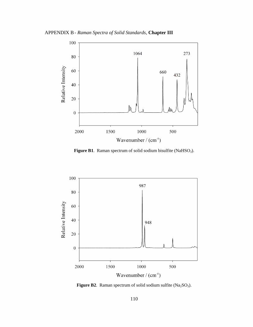
110
APPENDIX B - Raman Spectra of Solid Standards, Chapter III
Figure B1. Raman spectrum of solid sodium bisulfite (NaHSO3).
Figure B2. Raman spectrum of solid sodium sulfite (Na2SO3).
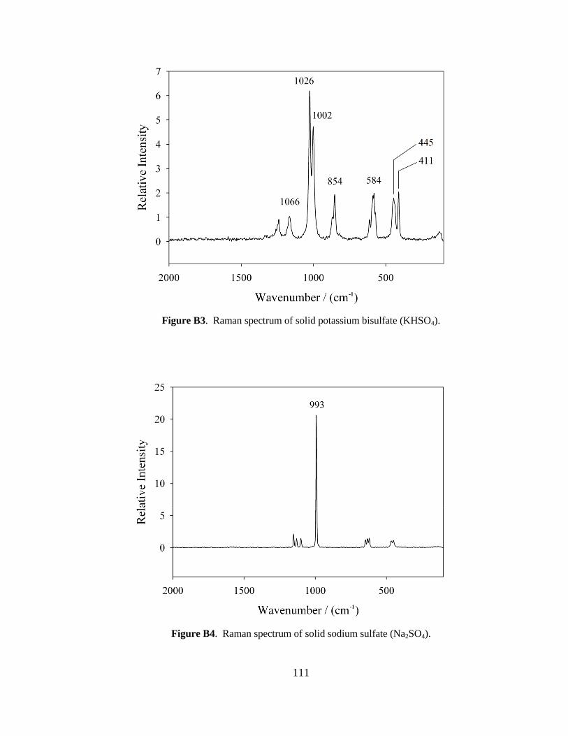
111
Figure B3. Raman spectrum of solid potassium bisulfate (KHSO4).
Figure B4. Raman spectrum of solid sodium sulfate (Na2SO4).
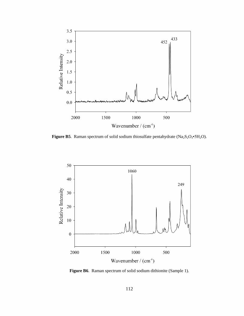
112
Figure B5. Raman spectrum of solid sodium thiosulfate pentahydrate (Na2S2O3•5H2O).
Figure B6. Raman spectrum of solid sodium dithionite (Sample 1).
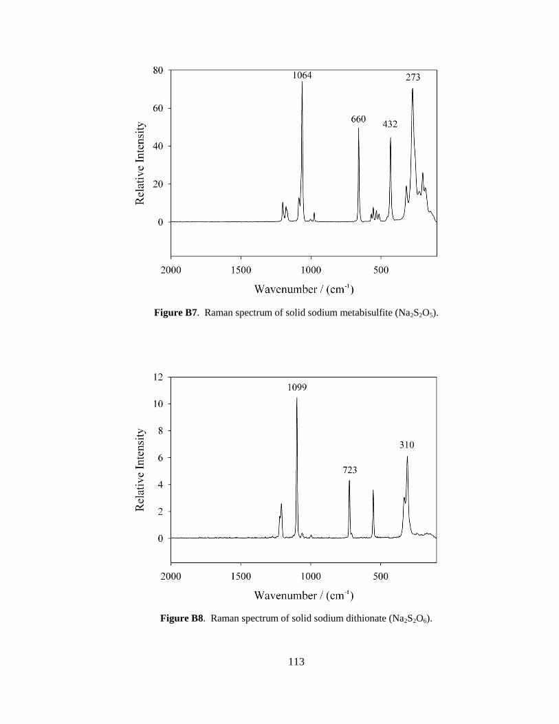
113
Figure B7. Raman spectrum of solid sodium metabisulfite (Na2S2O5).
Figure B8. Raman spectrum of solid sodium dithionate (Na2S2O6).
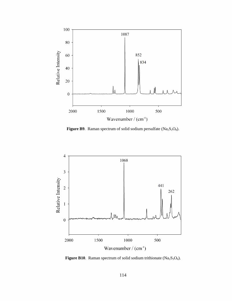
114
Figure B9. Raman spectrum of solid sodium persulfate (Na2S2O8).
Figure B10. Raman spectrum of solid sodium trithionate (Na2S3O6).
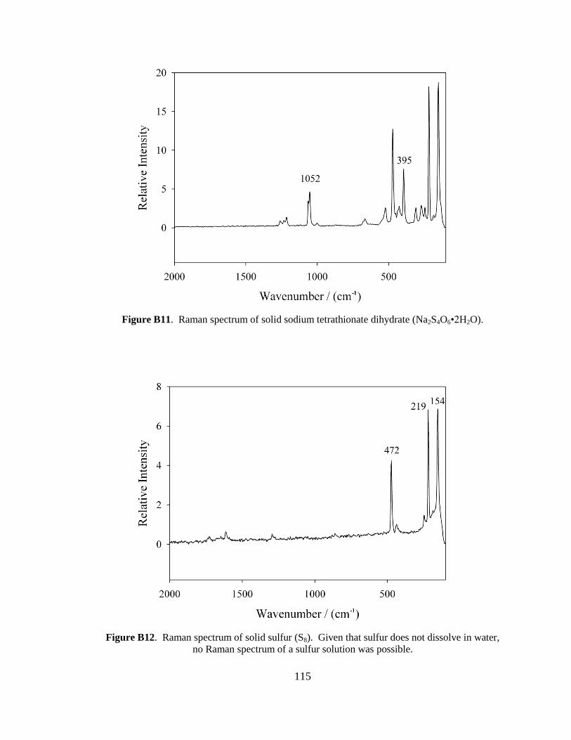
115
Figure B11. Raman spectrum of solid sodium tetrathionate dihydrate (Na2S4O6•2H2O).
Figure B12. Raman spectrum of solid sulfur (S8). Given that sulfur does not dissolve in water,
no Raman spectrum of a sulfur solution was possible.
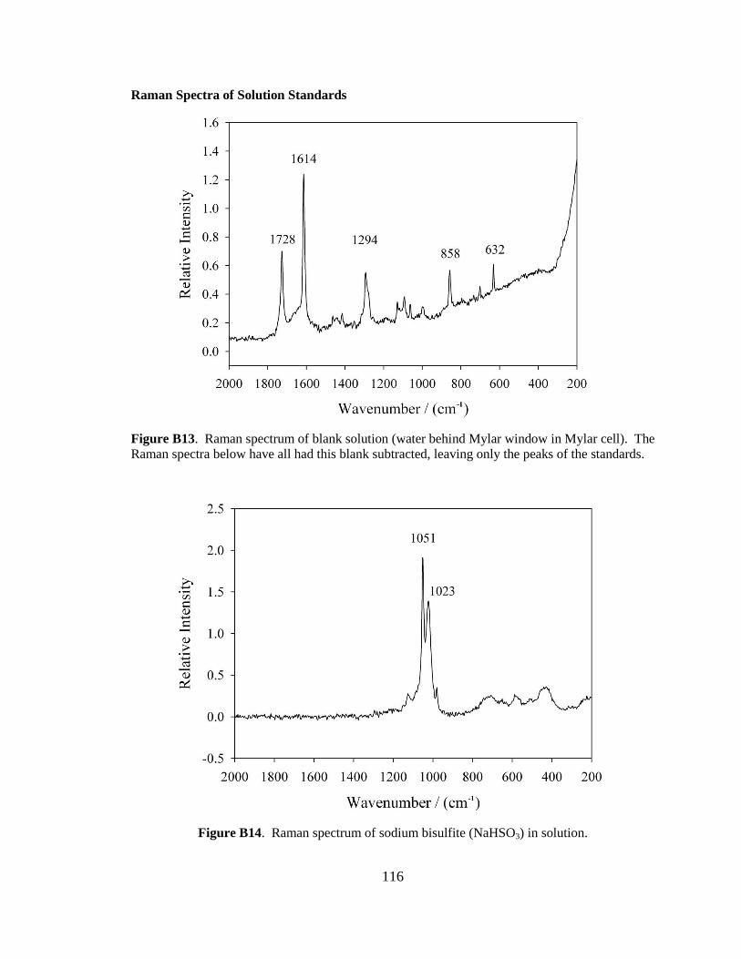
116
Raman Spectra of Solution Standards
Figure B13. Raman spectrum of blank solution (water behind Mylar window in Mylar cell). The
Raman spectra below have all had this blank subtracted, leaving only the peaks of the standards.
Figure B14. Raman spectrum of sodium bisulfite (NaHSO3) in solution.
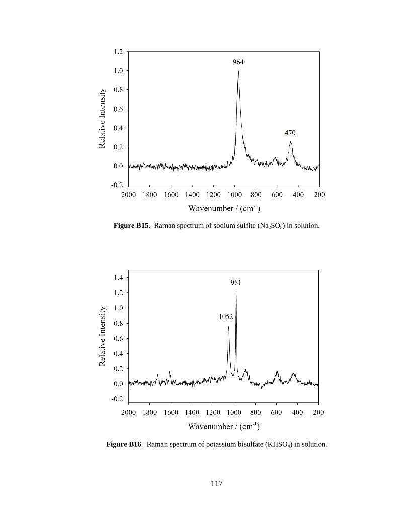
117
Figure B15. Raman spectrum of sodium sulfite (Na2SO3) in solution.
Figure B16. Raman spectrum of potassium bisulfate (KHSO4) in solution.
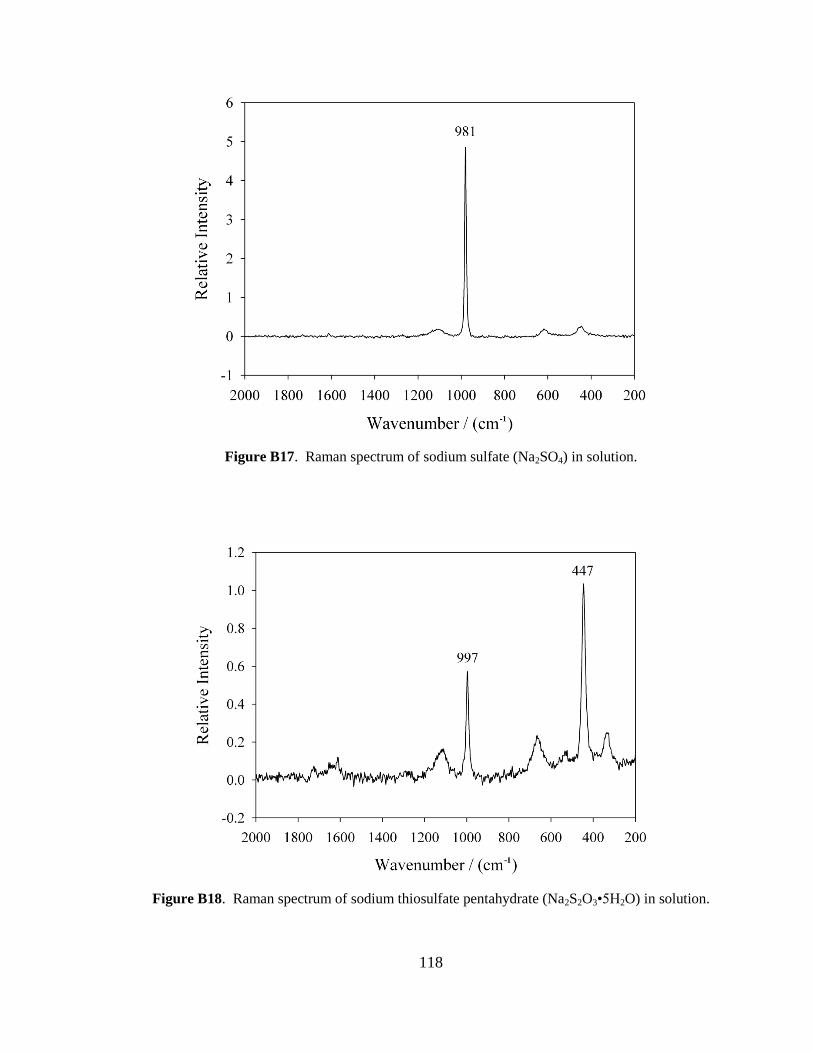
118
Figure B17. Raman spectrum of sodium sulfate (Na2SO4) in solution.
Figure B18. Raman spectrum of sodium thiosulfate pentahydrate (Na2S2O3•5H2O) in solution.
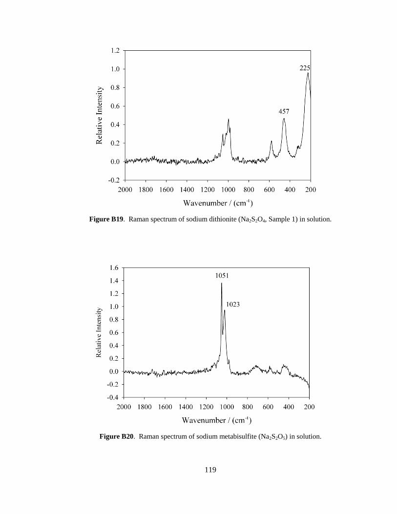
119
Figure B19. Raman spectrum of sodium dithionite (Na2S2O4, Sample 1) in solution.
Figure B20. Raman spectrum of sodium metabisulfite (Na2S2O5) in solution.
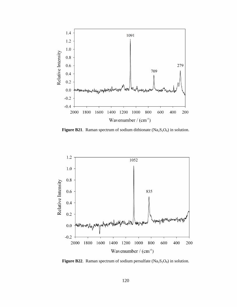
120
Figure B21. Raman spectrum of sodium dithionate (Na2S2O6) in solution.
Figure B22. Raman spectrum of sodium persulfate (Na2S2O8) in solution.
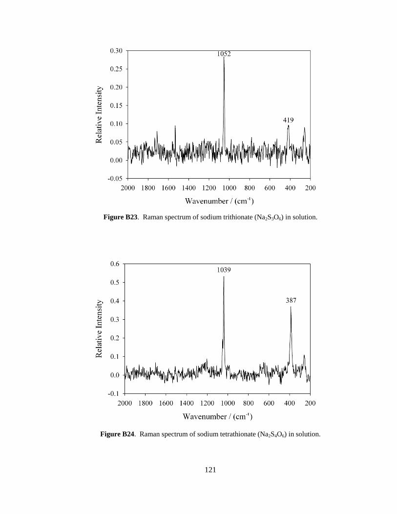
121
Figure B23. Raman spectrum of sodium trithionate (Na2S3O6) in solution.
Figure B24. Raman spectrum of sodium tetrathionate (Na2S4O6) in solution.
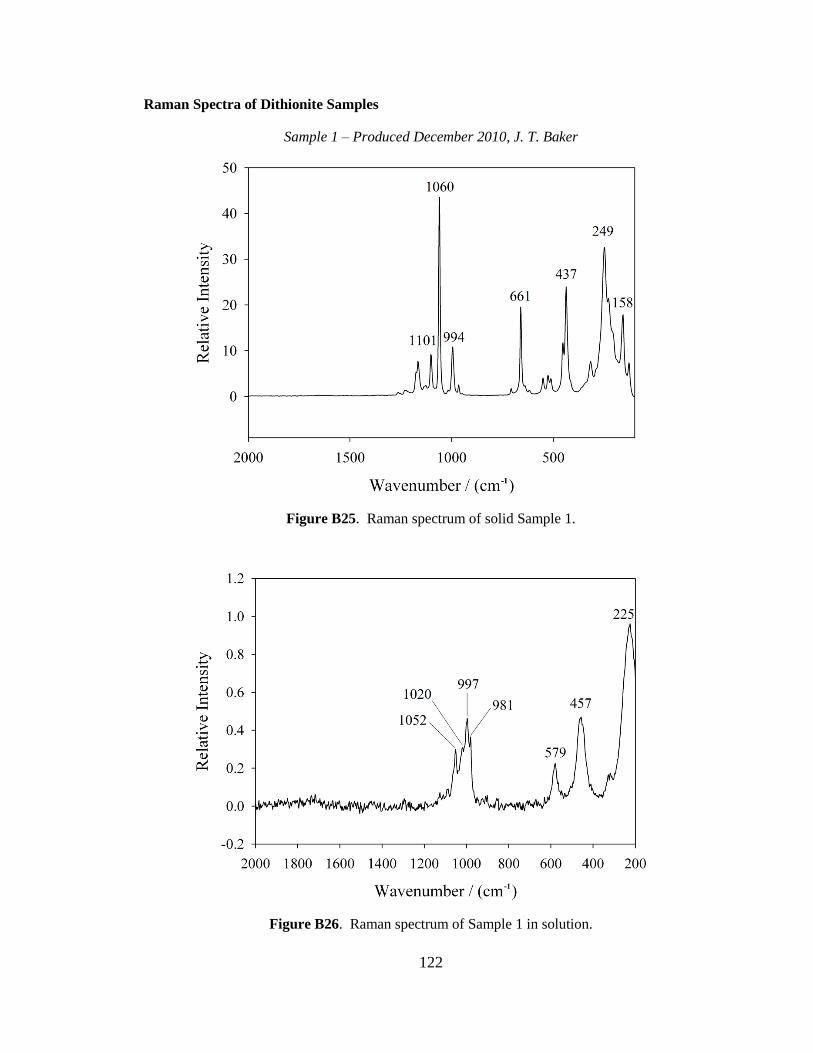
122
Raman Spectra of Dithionite Samples
Sample 1 – Produced December 2010, J. T. Baker
Figure B25. Raman spectrum of solid Sample 1.
Figure B26. Raman spectrum of Sample 1 in solution.
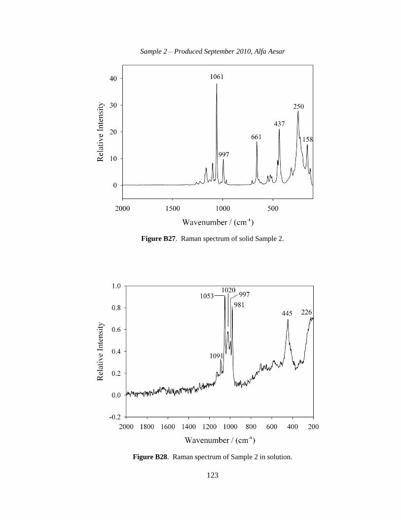
123
Sample 2 – Produced September 2010, Alfa Aesar
Figure B27. Raman spectrum of solid Sample 2.
Figure B28. Raman spectrum of Sample 2 in solution.
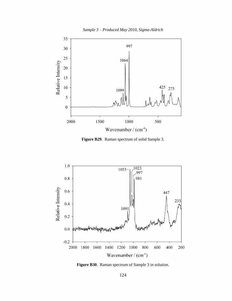
124
Sample 3 – Produced May 2010, Sigma-Aldrich
Figure B29. Raman spectrum of solid Sample 3.
Figure B30. Raman spectrum of Sample 3 in solution.
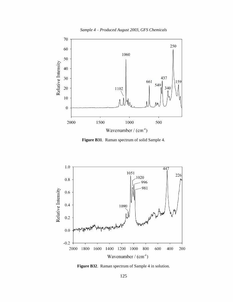
125
Sample 4 – Produced August 2003, GFS Chemicals
Figure B31. Raman spectrum of solid Sample 4.
Figure B32. Raman spectrum of Sample 4 in solution.
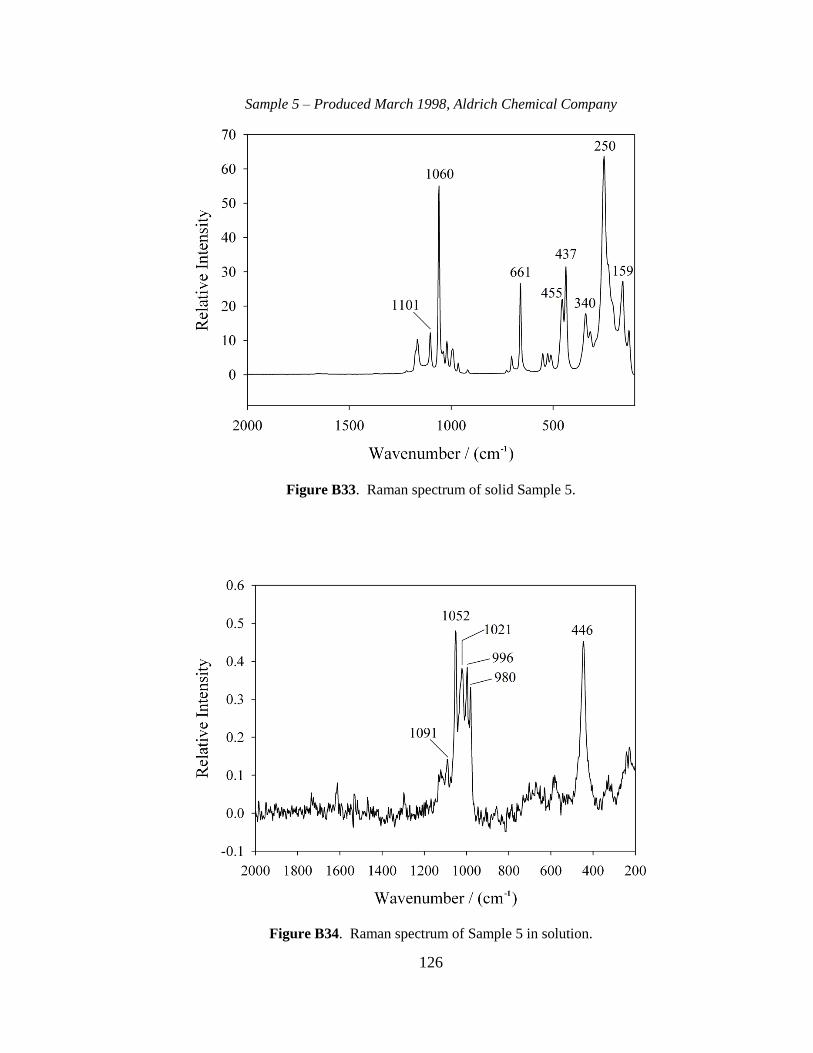
126
Sample 5 – Produced March 1998, Aldrich Chemical Company
Figure B33. Raman spectrum of solid Sample 5.
Figure B34. Raman spectrum of Sample 5 in solution.
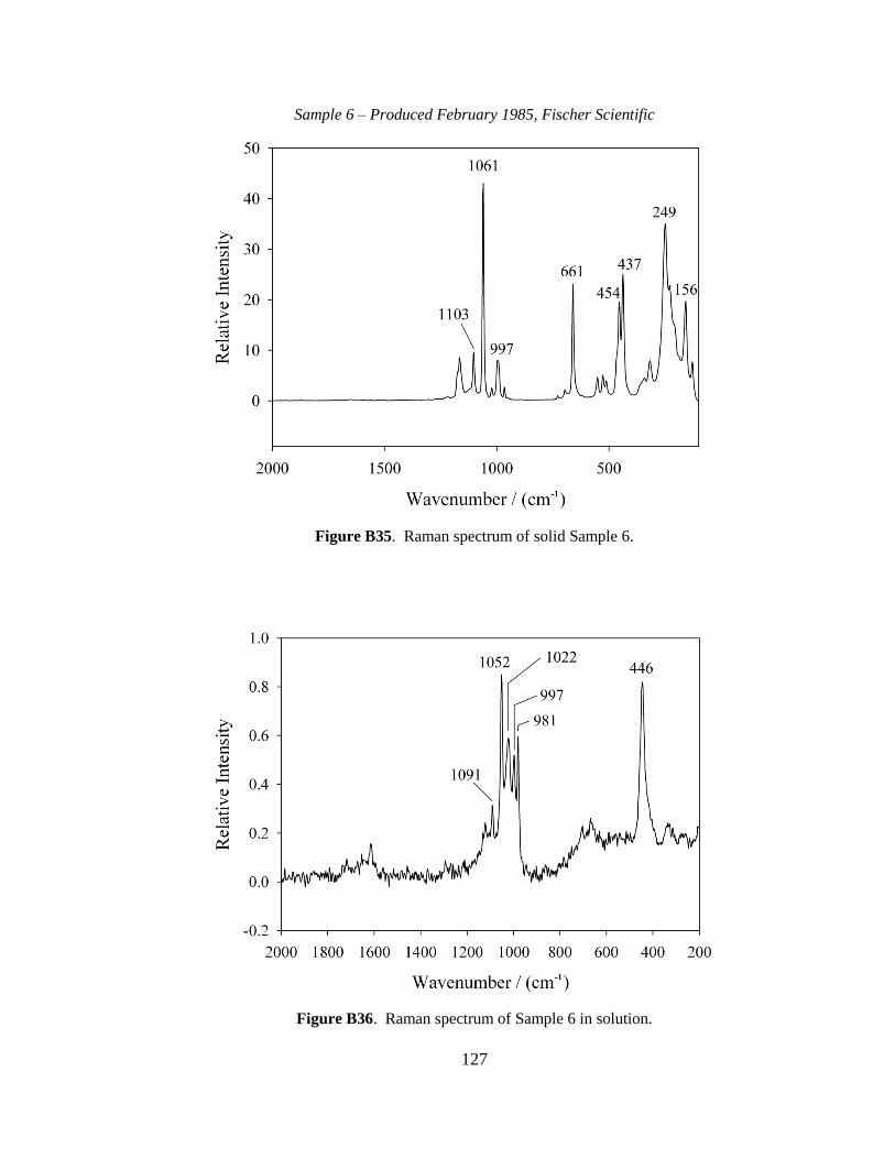
127
Sample 6 – Produced February 1985, Fischer Scientific
Figure B35. Raman spectrum of solid Sample 6.
Figure B36. Raman spectrum of Sample 6 in solution.
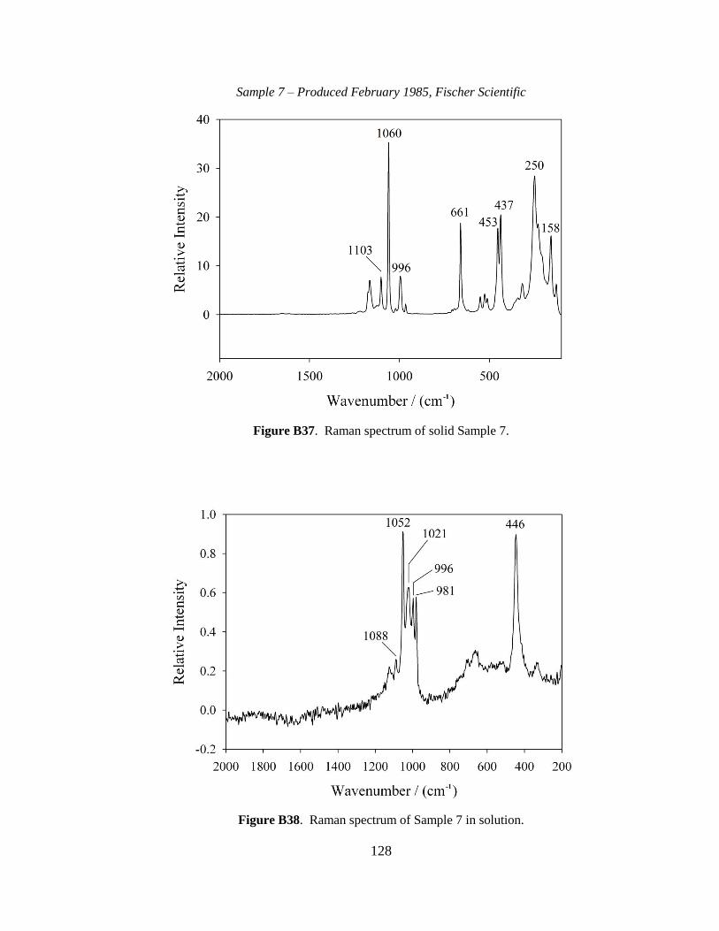
128
Sample 7 – Produced February 1985, Fischer Scientific
Figure B37. Raman spectrum of solid Sample 7.
Figure B38. Raman spectrum of Sample 7 in solution.
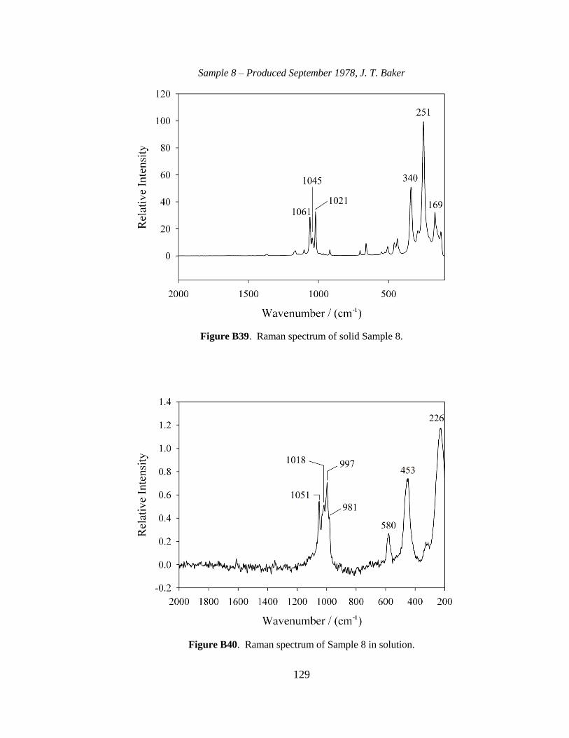
129
Sample 8 – Produced September 1978, J. T. Baker
Figure B39. Raman spectrum of solid Sample 8.
Figure B40. Raman spectrum of Sample 8 in solution.
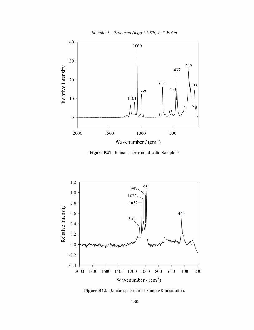
130
Sample 9 – Produced August 1978, J. T. Baker
Figure B41. Raman spectrum of solid Sample 9.
Figure B42. Raman spectrum of Sample 9 in solution.
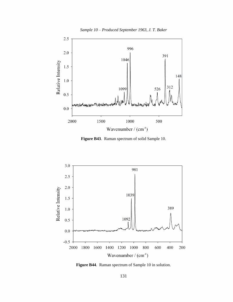
131
Sample 10 – Produced September 1963, J. T. Baker
Figure B43. Raman spectrum of solid Sample 10.
Figure B44. Raman spectrum of Sample 10 in solution.
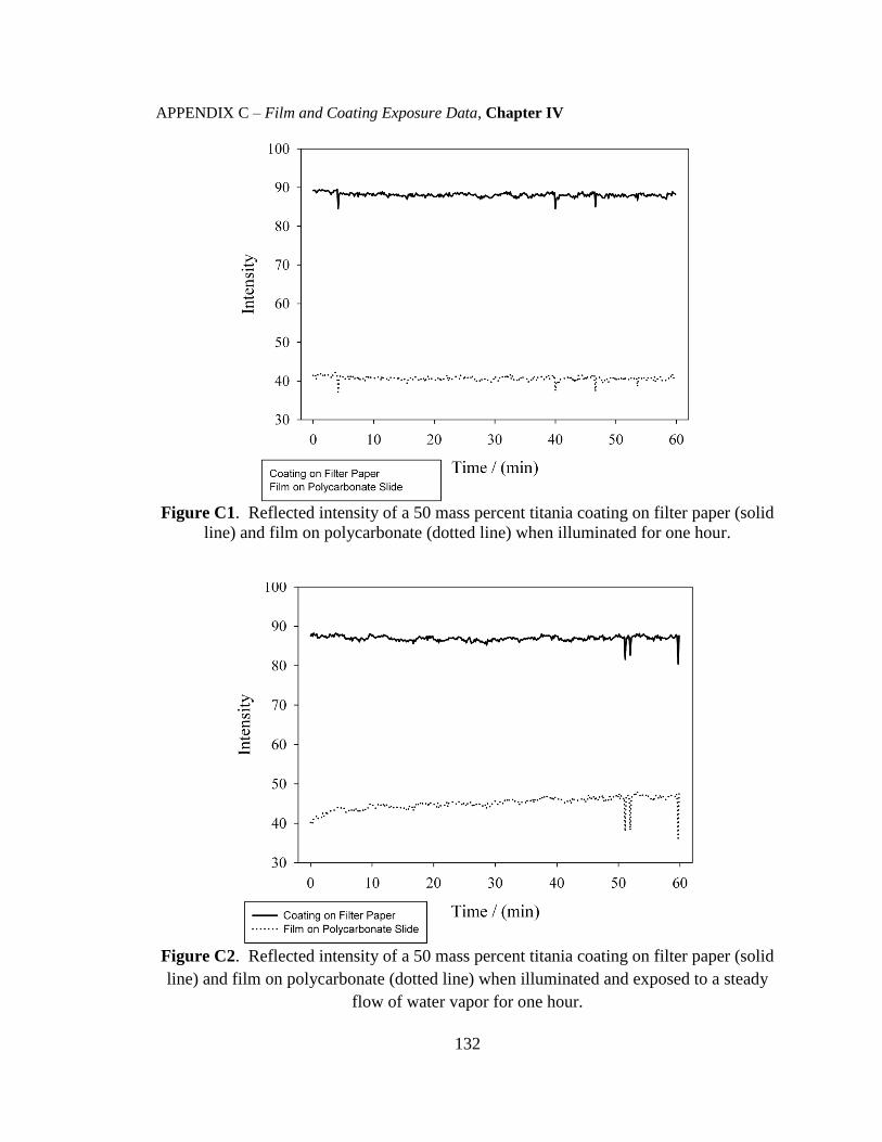
132
APPENDIX C – Film and Coating Exposure Data, Chapter IV
Figure C1. Reflected intensity of a 50 mass percent titania coating on filter paper (solid
line) and film on polycarbonate (dotted line) when illuminated for one hour.
Figure C2. Reflected intensity of a 50 mass percent titania coating on filter paper (solid
line) and film on polycarbonate (dotted line) when illuminated and exposed to a steady
flow of water vapor for one hour.
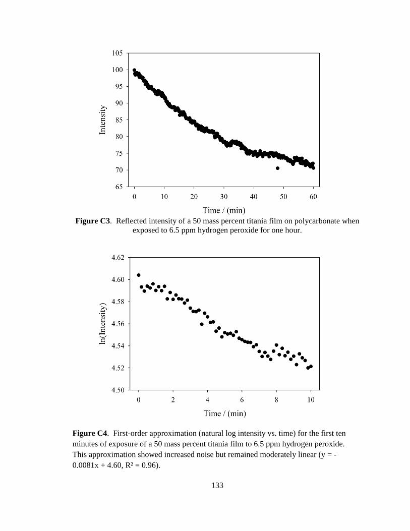
133
Figure C3. Reflected intensity of a 50 mass percent titania film on polycarbonate when
exposed to 6.5 ppm hydrogen peroxide for one hour.
Figure C4. First-order approximation (natural log intensity vs. time) for the first ten
minutes of exposure of a 50 mass percent titania film to 6.5 ppm hydrogen peroxide.
This approximation showed increased noise but remained moderately linear (y = -
0.0081x + 4.60, R² = 0.96).
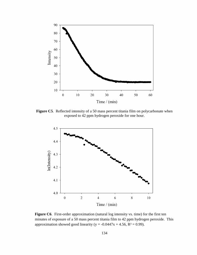
134
Figure C5. Reflected intensity of a 50 mass percent titania film on polycarbonate when
exposed to 42 ppm hydrogen peroxide for one hour.
Figure C6. First-order approximation (natural log intensity vs. time) for the first ten
minutes of exposure of a 50 mass percent titania film to 42 ppm hydrogen peroxide. This
approximation showed good linearity (y = -0.0447x + 4.56, R² = 0.99).
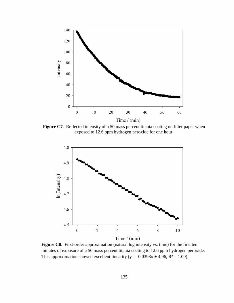
135
Figure C7. Reflected intensity of a 50 mass percent titania coating on filter paper when
exposed to 12.6 ppm hydrogen peroxide for one hour.
Figure C8. First-order approximation (natural log intensity vs. time) for the first ten
minutes of exposure of a 50 mass percent titania coating to 12.6 ppm hydrogen peroxide.
This approximation showed excellent linearity (y = -0.0398x + 4.96, R² = 1.00).
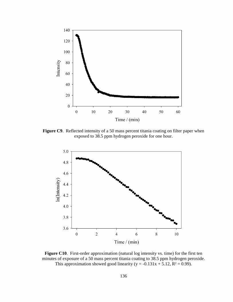
136
Figure C9. Reflected intensity of a 50 mass percent titania coating on filter paper when
exposed to 38.5 ppm hydrogen peroxide for one hour.
Figure C10. First-order approximation (natural log intensity vs. time) for the first ten
minutes of exposure of a 50 mass percent titania coating to 38.5 ppm hydrogen peroxide.
This approximation showed good linearity (y = -0.131x + 5.12, R² = 0.99).
VITA
Travis Houston James
Candidate for the Degree of
Doctor of Philosophy
Title: THE ELUCIDATION AND QUANTIFICATION OF THE
DECOMPOSITION PRODUCTS OF SODIUM DITHIONITE AND THE
DETECTION OF PEROXIDE VAPORS WITH THIN FILMS
Major Field: Chemistry
Biographical:
Personal Data:
Born in Aix En Provence, France, on April 3, 1986, the son of Randal and
Cheryl James.
Education:
Completed the requirements for the Doctor of Philosophy in Chemistry in
Chemistry at Oklahoma State University, Stillwater, Oklahoma in July, 2014.
Completed the requirements for Bachelors of Science in Chemistry at Hillsdale
College, Hillsdale, MI, in May 2009.
Experience:
Employed by Hillsdale College as an undergraduate teaching assistant, 2008-
2009; employed by Oklahoma State University as a graduate teaching and
research assistant, 2009 to present.
Professional Memberships:
American Chemical Society, Phi Lambda Upsilon Chemical Honorary Society