Is it is or is it Ain’t my Obligation? Regional Debt in Monetary

Unions∗

Russell Cooper, †Hubert Kempf ‡and Dan Peled§

October 23, 2003

Abstract

This paper studies the implications of the circulation of interest bearing regional debt in a monetary

union, such as the Patacones issued by the Buenos Aires government in Argentina. Does the circulation

of this debt have the same monetary implications as the printing of money by a regional government?

Or are the obligations of this debt simply backed by future taxation with no inflationary consequences?

We argue here that both outcomes can arise in equilibrium. In the model economy we consider

there are multiple equilibria which reflect the perceptions of agents regarding the manner in which the

debt obligations will be met. In one equilibrium, termed Ricardian, the future obligations are met with

taxation by a regional government while in the other, termed Monetization, the central bank is induced

to print money to finance the region’s obligations. The multiplicity of equilibria reflects a commitment

problem of the central bank. A key indicator of the selected equilibrium is the distribution of the holdings

of the regional debt. We use the model to assess the impact of policy measures, such as fiscal restrictions,

within a monetary union.

∗We are grateful to the CNRS and the NSF for financial support and to the late Louis Jordan from whom we freely borrowed

the title. Cooper thanks the Research Department at the Federal Reserve Bank of Minneapolis for its support. Helpful comments

and questions from Maria Alzua, Marco Bassetto, Patrick Kehoe, Todd Keister, Robert E. Lucas and John Shea as well as

seminar participants at the Federal Reserve Bank of Dallas, the Bank of Israel, the University of Maryland, the Anglo-French

seminar in macroeconomics, the European University Institute, the University of Pavia and the University of Bologna are very

much appreciated.†Department of Economics, University of Texas, Austin, TX. 78712, cooper@eco.utexas.edu‡EUREQua, Universite Paris-1 Pantheon-Sorbonne, 106 Boulevard de l’Hopital, F-75013 Paris, France, kempf@univ-paris1.fr§Department of Economics, University of Haifa, Haifa 31905, Israel, dpeled@econ.haifa.ac.il

1

1 Motivation

This paper studies the inflationary implications of regional debt in a federation. Consider a federation of

regions (states) in which monetary policy is centralized but fiscal policy is determined at the regional level.

Individual countries, such as Argentina and the U.S., fit this description as does a coalition of countries

which delegate monetary policy to a single central bank, such as the European Monetary Union.

The recent experience in Argentina motivates an analysis of the link between regional debt and inflation.

The Argentine province of Buenos Aires circulated about 18 million pesos of interest bearing provincial

bonds starting in July 2001, during the currency board regime in Argentina. In fact, the notes comprising

this debt, called Patacones, were almost of the same size and had a design quite similar to the Argentine

peso. The initial issue of Patacones were paid-off with interest in July 2002. At that time, about 2.65

billion pesos of new regional debt was issued with a maturity of November 13, 2006. Interestingly, the

province announced that taxes could be paid with this debt, evidently at face value. In addition, the federal

government issued 3.3 billion pesos of small denomination bonds called Lecops. Other provinces have also

issued small denomination debt.1 Ongoing negotiations with the IMF have focused on reductions in regional

deficits and the termination of new issues of the small denomination regional debt. 2

This experience in Argentina reflects the interplay between different government levels within a country.

But these interactions are a more general phenomenon: they appear within any country with regional

governmental levels, such as the states within the U.S., and in a monetary union, such as the EMU. Thus,

we are interested in addressing the following questions:

• Is the circulation of debt by a regional government equivalent to the creation of money by the central

bank and thus inflationary?

• Or, does the issuance of such debt lead to the postponement of taxation without any money creation

and thus without any inflation?

• What types of government interventions, such as limitations on regional debt, are required?

¿From a positive perspective, addressing the first two questions provides insight into the inflationary

implications of regional debt. Thus we answer the question posed in the title. This analysis will also allow

us to evaluate various forms of intervention which, as we shall see, may indeed be welfare improving. Our

theory is therefore helpful in assessing the current fiscal situation in Argentina and the ongoing debate over

the excessive deficits in countries belonging to the EMU.

We address these questions in an abstract monetary model of a federation sharing a common currency

and show the existence of two types of equilibria. This multiplicity reflects a commitment problem of the1To create some perspective, nominal GDP in Argentina in the fourth quarter of 2002 was 342 billion pesos and the money

supply (M1) was 42 billion pesos in January 2003. We are extremely grateful to Maria Alzua for supplying us with these data

about the regional debt and to George McCandless and Carlos Zarazaga for discussions on this experience. The money supply

and nominal GDP figures are from http://www.mecon.gov.ar/progeco/dsbb.htm.2An IMF assessment of the situation in Argentina and proposed measures for reform are summarized at

http://www.imf.org/external/np/sec/pr/2003/pr0309.htm.

2

central government. We thus argue that the inflationary effects of regional debt must be determined by the

interactions of the market participants and cannot be ascertained a priori. From this perspective, policy

interventions may be useful to coordinate on a socially preferred outcome.

In one equilibrium, which we term Ricardian, the regional debt is simply a bond. These bonds finance

a transfer to young agents in a region and these agents save in anticipation of future taxes. If the regional

debt is held largely by its citizens, the central government will not bail-out the region but instead allow it

to default. Anticipating this, the regional government will prefer to tax its own citizens to repay the debt.

So the circulation of these regional bonds does not lead to any money creation.

In a second equilibrium, which we term Monetization, all agents anticipate a bail-out by the central

government. Thus they all hold money and debt and, given this distribution of debt holdings, the central

bank will choose to monetize the debt. Anticipating this, the regional government will not raise taxes to pay

the debt but will choose to turn the obligation over to the central bank. 3 Here the circulation of regional

bonds is analogous to money creation by the central bank. This monetization of the debt will lead a region

to run excessive deficits since the burden of the debt is shared by all regions.

The multiplicity of equilibria reflects a commitment problem by the central government vis-a-vis the

regional government. If it were feasible, the central government would commit to never bailing out the

regional government. Absent this ability to commit, the desire to ex-post equalize per capita consumption

across regions may lead the central government to bail-out a regional government.

The key distinguishing feature across the two equilibria is whether the debt is widely held in the economy

or concentrated with agents in the bond-issuing region. In the former case, there is a bail-out as the

central government will pay-off the regional debt. Knowing this, the regional government does not meet its

obligation. In the latter case, the effects of the default are isolated as the agents in the bond-issuing region

are, in effect, defaulting on themselves. Consequently, the central government will allow default rather than

pay the obligation of the region. Anticipating this, the regional government will prefer to tax its citizens

and a Ricardian equilibrium arises. In all cases individuals are indifferent with regards to the composition

of their portfolios: it is the aggregate distribution of holdings which is key to the equilibrium outcome.

To make the analysis transparent, the first section of the paper studies a real version of this problem.

The second section of paper studies these same themes in a monetary economy. This basic commitment

problem of the government emerges again though here we study the behavior of a central bank and its use of

the inflation tax. We again find multiple equilibria which are differentiated by the holdings of regional debt.

The more widely held the regional debt, the more likely is a bail-out by the central bank. Though it is not

directly part of our analysis, it might be that small denomination debt, such as that issued by the province of

Buenos Aires, is more likely to circulate throughout the economy thus enhancing the possibility of a bail-out.

In the fourth section, we offer a discussion of policy remedies for the socially excessive debt-financed regional

spending in the Monetization equilibrium. Some interventions, such as limits on debt or even dollarization3This theme of a region inducing monetization is present in related papers, including Aizenman (1992), Zarazaga (1995),

Chari and Kehoe (1998), Chari and Kehoe (2002), Cooper and Kempf (2001) and Cooper and Kempf (2000). Here that

argument is made in a setting with bonds and money. Further, those papers do not characterize the multiplicity of equilibria

that may occur.

3

may be socially desirable. The last section concludes. 4

2 A Real Game

Consider a two-period economy composed of two regions, indexed i=1,2. There are Ni agents in region i and

total population is given by N =∑

Ni. As the equilibria will depend on the fraction of agents in region 1,

we define ∆ ≡ N1N . Agents have endowments in youth and old age and have access to a storage technology.

For any individual in region i, the pair of consumption levels is denoted (ciy, cio). The lifetime utility

function has the following form: u(ciy)+ v(cio) and we assume that both u(·) and v(·) are strictly increasing

and strictly concave.

Two levels of government are active: the government of region 1, denoted RG, and a central government,

denoted CG. These governments have different objectives: the region 1 government is only concerned with

the welfare of its citizens while the central government considers the welfare of all agents living in the

federation. The RG makes a real transfer to region 1 agents in period 1 and can levy a lump-sum tax on

region 1 agents in period 2. The CG makes no transfers and can levy a lump-sum tax on all agents in period

2.

The game played by the CG and the RG is given in Figure 1. The timing of moves is the following:

• Period 1:

– Young agents in region 1 receive a real transfer, denoted g1, from their government.

– Transfers to region 1 agents are financed by issuing regional debt, B1 = N1g1.

– All young agents make savings decisions in anticipation of period 2 government policies.

• Period 2:

– the region 1 government chooses to tax region 1 agents to finance its debt obligation or to pass

the obligation to the central government.

– if the region 1 government does not levy the tax, then the central government can choose to levy

an economy-wide tax to finance the debt obligation of region 1.

– if the central government decides not to levy this tax, then region 1 automatically defaults on its

debt and region 1 agents bear a default cost, denoted κ.5

Figure 1 here

4The discussion of dollarization draws upon Cooper and Kempf (2001) and the arguments for constraints is related to the

points made in Chari and Kehoe (2002) and Cooper and Kempf (2000).5Though there is a default cost, we have no theory about the implications of default. Thus the default cost plays a very

modest role: we assume that κ is negligible and use it solely to “break ties”.

4

We search for sub-game perfect Nash equilibria of this game. Accordingly, the central government is

restricted to choices which are credible. Put differently, the central government may threaten not to bail-

out a regional government but these threats have an influence on the equilibrium outcome only if they are

credible.

Before proceeding, it is useful to characterize the planner’s solution as a benchmark. Assume that the

planner chooses an allocation of consumption goods over time and over regions at the start of time given

the endowments of agents in each period, and given a technology that creates x units of period 2 goods per

unit stored in period 1. Let the objective function of the planner be the population weighted average of the

lifetime utilities of individual agents, ∆(u(cy1) + v(co1)) + (1 − ∆)(u(cy2) + v(co2)), where cyi and coi are

the consumption levels of a young agent in region i in youth and old-age, respectively. Then the solution is

to equalize consumption of agents across regions and the optimal consumption profile (cy∗, co∗) satisfies the

Euler equation u′(cy∗) = xv′(co∗).

We term this the commitment solution as it corresponds to the outcome if the central government could

commit, at the start of period 1 before young agents make their saving decision, not to levy an economy-wide

tax to bail-out the regional government. Of course, in the extensive form game outlined above, the central

government does not have this commitment ability. We now turn to an analysis of the equilibria for the

game without commitment.6

2.1 Period 1 Optimization

Region i young agents solve

maxsiu(ωy + gi − si) + v(ωo + six− τ − τ i) (1)

where si is real savings, gi is a real transfer in youth per capita in region i, ωy is the endowment in youth,

ωo is the endowment in old age, τ is a common tax and τ i is the regional tax. Savings takes two forms:

storage (ki) and the holding of region 1 debt (bi). The return on storage is given by x and, in equilibrium,

this is the return on regional debt as well. Assume that the only action is in region 1 so that g2 ≡ τ2 ≡ 0.

The first-order condition for this problem is

u′(cyi) = xv′(coi) (2)

for i = 1, 2. The savings decision will depend, in part, on the taxes that young agents anticipate in period

2. Nonetheless, it is straightforward to see that as u(c) is strictly concave, s1 > s2.7

The composition of saving though is indeterminate as government debt must offer the same return as

storage for an equilibrium in which debt is held to exist. Still it is important for characterizing the set of

equilibria to keep track of the distribution of debt holdings.6Thus the problem falls within the general class of team incentive problems where the central government is the principal

and the regional governments are the agents. The structure of the problem is thus similar to the family incentive problem and

the infamous ”Rotten Kid Theorem” as formalized in Bergstrom (1989) and extended in Lindbeck and Weibull (1988).7This reflects two features of the problem: g1 > g2 = 0 and τ1 ≥ τ2 = 0. The result that s1 > s2 then follows from (2) as

u(c) is strictly concave.

5

Denote the per-capita saving of region i and its composition by si = ki + bi. Let θ = N1b1

B1 = ∆b1

Bwhere

B ≡ B1

N is the level of region 1 debt divided by total population. By symmetry, (1− θ) = (1−∆)b2

B.

2.2 Bail-out Equilibrium

In a bail-out equilibrium, τ1 = 0 and τ = ∆g1x = Bx. Savings by the two regions are given by the first-order

conditions anticipating this common tax. We show there is a continuum of bail-out equilibria, indexed by

the share of the debt held by agents in region 1.8

Proposition 1 There exists a bail-out equilibrium for θ ∈ [0, ∆].

Proof: To characterize the set of bail-out equilibria, we first check the incentives of the central government

assuming the regional government has decided not to tax its citizens. We then check the incentives of the

regional government and the private agents in turn.

For the CG, let W b and W d denote social welfare under a bail-out and a default respectively. In a bail-out

equilibrium, the consumption of an old region i agent is coi = ωo + six− τ where the tax satisfies τ = Bx.

Thus, W b is:

W b = ∆v(ωo + s1x− Bx) + (1−∆)v(ωo + s2x− Bx) (3)

Under a default, consumption is given by coi = ω0 + kix. Using si = bi + ki and the definition of θ, social

welfare under a default is:

W d = ∆v

(ωo + (s1 − θB

∆)x

)+ (1−∆)v

(ωo + (s2 − (1− θ)B

(1−∆))x

)(4)

If θ = ∆, W b = W d. With a negligible value of κ, the CG will choose bail-out over default.

Next, we establish that k1 > k2 for any θ ≤ ∆. At θ = ∆, b1 = b2 so that s1 > s2 implies k1 > k2.

As θ decreases, b1 falls relative to b2 and so k1 increases relative to k2 since s1 and s2, given by (2), are

independent of θ. Hence, k1 > k2 for any θ ≤ ∆. Consequently, the derivative of W d with respect to θ,

given by −[v′(ωo + k1x)− v′(ωo + k2x)]Bx, is positive when θ ≤ ∆.

So, W b = W d when θ = ∆ implies W b > W d for θ < ∆. This implies that the CG will bail-out the

regional government for θ ≤ ∆.

Anticipating this, the region 1 government will always choose not to tax for θ ≤ ∆. If it did levy a tax

τ1, the consumption of region 1 old agents would be co1 = ωo + (s1 − B∆ )x since τ1 = B

∆x = g1x.9 With

∆ < 1, co1 > co1 so that the regional government prefers not to tax its citizens.

In anticipation of these choices by the governments, private agents’ savings decisions satisfy (2) under

the expectation of τ1 = 0 and τ = Bx. Thus there exists a bail-out equilibrium for θ ≤ ∆. ¥The proof rests upon the basic intuition associated with the ex post incentive of the central government

to redistribute resources towards a more equal allocation. For θ ≤ ∆, consumption levels are more equal8We are grateful to Marco Bassetto for discussions which led to the enhanced development of this section relative to an

earlier draft.9Since this defection of the regional government arises in period 2, the level of region 1 saving is the same as it is along the

equilibrium path. It follows that c01 < c02 since 0 < s1 − s2 < g1.

6

across regions under a bail-out than under a default. Consequently, the CG is unable to commit not to

redistribute resources. The regional government recognizes this and chooses not to tax it citizens.

There is a subtle point here. Total consumption in the second period is fixed, given endowments and

storage decisions. So, the redistribution by the CG increases the consumption of region 2 agents and reduces

the consumption of region 1 agents relative to the default allocation. Thus the redistribution per se is not

favorable to region 1 agents. Still, their consumption is higher under a bail-out than if they paid the entire

tax bill. Put differently, the analysis above shows co1 ≥ co1 > co1.10 The first inequality indicates the

lost consumption of redistribution and the second inequality indicates that consumption is higher under a

bail-out than regional taxation. In effect, the region 1 agents are able to take advantage of the desires of the

CG to redistribute consumption away from them.

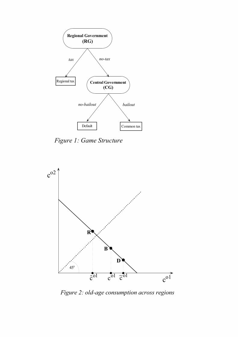
Figure 2 here

This is illustrated in Figure 2 which indicates the consumption levels of the old agents in both regions

under different allocations. This graph takes as given the savings decisions of the agents and thus total

resources available for consumption are fixed, as indicated by the negatively sloped resource constraint. The

allocation under a bail-out is labelled B, the allocation under default is labelled D and the one under regional

taxation is labelled R. As seen in this figure, the bail-out of the CG redistributes from region 1 to region 2

agents relative to the default allocation. Still this allocation is preferred by region 1 to the one achievable

with regional taxation.

2.3 A Ricardian Equilibrium

In this section we construct a Ricardian equilibrium in which the regional government uses its tax to pay-

off the debt issued to finance the transfer, g1. Thus τ1 = xg1 and τ = 0 along the equilibrium path. In

equilibrium, the region 1 agents will save the transfer to pay for their future taxes: s1 = s2+g1. This condition

relating s1 to s2 is an immediate consequence of (2) under the expectation of a Ricardian equilibrium.

Proposition 2 There exists a Ricardian equilibrium for θ = 1.

Proof: To construct this equilibrium, we assume that only region 1 agents choose to hold region 1 debt.

That is, in the proposed equilibrium, s2 = k2 so that s1 = s2 + b1. Hence θ = 1. At the individual level,

this is without loss of generality as debt and storage have the same return of x. Given this conjectured

equilibrium, we check the incentives of the central and regional governments as well as the private agents.

Since the CG moves last, we check its incentives first. If the regional government deviates from the

candidate equilibrium and chooses not to raise taxes to pay the debt obligation, will the CG allow default?

Let W b again denote social welfare if the central government bails-out the region:

W b = ∆v(ωo + s1x− τ) + (1−∆)v(ωo + s2x− τ). (5)10If θ < ∆ , then co1 > co1. This implies that points B and D are distinct in the figure below.

7

¿From the curvature in v(·), using s1 = s2 + g1, and setting τ = ∆g1x from the CG’s budget constraint,

W b < v(ωo + (∆s1 + (1−∆)s2)x− τ) = v(ωo + s2x). (6)

If the central government allows default then social welfare, denoted W d, is given by

W d = ∆v(ωo + (s1 − g1)x) + (1−∆)v(ωo + s2x) = v(ωo + s2x), (7)

where the last equality again uses s1 = s2 + g1.11 In (7), the consumption of region 1 agents reflects the

default on the debt they hold and the absence of taxation. Hence, from (6) and (7), W d > W b.

Anticipating that the central government will not bail-out, the regional government can choose to tax its

own citizens or allow a default. If region 1 levies a tax, the consumption of its citizens is co1 = ωo+(s1−g1)x,

exactly the same consumption that occurs under a default. With a negligible κ the regional government will

prefer to tax its citizens.

Finally, from (2), it is easy to check that region 1 agents will simply save the entire transfer in order to

pay their tax obligations to the regional government: i.e. s1 = s2 + g1. Given the construction that only

region 1 agents hold region 1 debt, all agents have the same real storage: i.e. s1 = s2 + g1 and s2 = k2 imply

k1 = k2.

So private agents are optimizing and neither the regional nor the central government has an incentive to

deviate. Hence there is an equilibrium in which regional debt is paid-off by regional taxation. ¥It is important to understand more intuitively this equilibrium. From (6) and (7), the central government

is interested in the ex post distribution of consumption across agents in the different regions. Since v(·) is

strictly concave, the CG prefers a more equitable allocation. The result that W d > W b reflects the fact that

default delivers more equitable consumption across the regions than would a bail-out.

Note too that this is an isolated equilibrium. That is, for θ < 1, there will not exist a Ricardian

equilibrium. When θ < 1, the regional government will no longer be indifferent between taxing its citizen

and allowing the CG to default. Instead it will strictly prefer default since, with θ < 1 some of its tax

revenues will flow to region 2 agents.12

3 A Monetary Economy with Regional Debt

This analysis of the real game serves two purposes. First it highlights the commitment problem of the central

authority within a federation. Second, it indicates that a central government will ex post use its tax and

transfer power to redistribute resources across regions. This incentive will be relevant even in a monetary

economy.

Yet the discussion of regional debt occurs in a monetary setting where the connection between regional

debt and inflation arises from the use of the inflation tax by a central government. Thus understanding

the interactions between the regional and central government in a monetary setting is important. Here we

construct an overlapping generations model. Instead of assuming there exists a central government which can11As noted earlier, we are setting the default cost at 0 and using it only to break ties. Thus κ is not in W d.12However, with κ > 0 it is possible to support other Ricardian equilibria.

8

tax all agents, there is a central bank (CB) which can print money and transfer it to the regional government

to pay its obligations. In the overlapping generations model, agents live for two periods. Lifetime utility

is given by u(cy) + v(co) and we assume that u(·) and v(·) are strictly increasing and strictly concave. All

agents are endowed with ωy units of the consumption good in youth and ωo in old age. Agents have access

to a storage technology that yields x > 1 units of the consumption good in period t + 1 for each unit stored

in period t. In addition, agents may save by holding debt issued by the region 1 government. Finally, there

is a legal restriction that requires money to be held in proportion to the level of real storage, as in Smith

(1994). One interpretation is that access to the storage technology requires an intermediary which must hold

money as a reserve requirement.13

Agents live in one of two regions. As in the previous section, the key is the game between the region 1

government and the central bank (CB). There is a second group of agents living in region 2, whose government

does not issue debt.14 Nonetheless region 2 agents are important as their welfare is reflected in the decisions

of the CB. Each young agent of generation t born in region 1 receives a real transfer of g∗ from the regional

government and that government sells debt of B∗.15 Governments are associated with a generation not a

time period; the regional government elected in period t sells its debt and then in period t + 1 decides either

to tax the consumption of the old within its region or to turn the obligation over to the CB.16

Formally, we consider a extensive form game, played each period, which is similar to that in the previous

section. Here though the move of the central government has been replaced by a choice of the central bank.

• regional government either raises taxes to pay its obligation (pay) or not (no pay) and passes it to

the CB

• if the regional government chooses (no pay), the CB either pays the obligation, financed by printing

money, or denies it

• if the CB denies the obligation, then the region defaults and its citizens suffer a penalty/loss of κ.

This game is played in period t+1 by the regional government representing region 1, generation t agents.

Importantly, the taxation decisions associated with generation t agents are made in period t+1 after savings

decisions have been made by that generation.

We construct two types of steady states for this economy. In the first, which is an extension of the bail-out

equilibrium, the CB monetizes the debt of the regional government. In the second, akin to the Ricardian

outcome, the CB refuses to monetize and, in anticipation, the regional government taxes its citizens.13We are grateful to Todd Keister for discussions on this point. Alternatively, we could assume there is a reserve requirement

on all savings, including the holding of government debt. If we assume that the regional bond has a small nominal value, as is

the cases with patacones, there is no need for it to be intermediated and thus no basis for a reserve requirement.14In the context of Argentina, region 1 is intended to represent the province of Buenos Aires and region 2 representing the

citizens outside of this region. This simplification clearly misses the fact that other regions have also issued small denomination

debt. But the province of Buenos Aires accounts for about 60 % of the regional debt outstanding.15Hereafter, variables with an ∗ are steady state equilibrium values.16In fact, this is apparently without loss of generality since a regional government in period t has no influence over any state

variables that matter for future generations.

9

The co-existence of these equilibria again reflects the commitment problem faced by the CB, as in the

real game. In the extensive form game, the CB has the weighted utilities of all old agents as its objective.

Accordingly, it is ultimately interested in equalizing the real consumptions of these agents. Whether or

not it allows default on the debt depends on the holdings of this debt across agents. In the monetization

equilibrium, the debt is widely held and allowing default is undesirable due to the penalty. But, if the debt

is held by region 1 agents, then default by the CB leads to more equitable consumption. This supports a

decision to tax by the regional government and thus a Ricardian equilibrium.

Thus which equilibrium will prevail depends on who holds the regional debt. Since, in equilibrium, agents

get the same return from holding the regional debt as from storage (i.e. default never actually occurs in

equilibrium), agents are indifferent with respect to their portfolios.17 Despite this indifference at the level of

the individual, the outcomes in the two equilibria may be quite different.

3.1 Equilibrium with Monetization

Here we construct a stationary equilibrium in which the CB monetizes the obligation rather than allowing

default. The agents anticipate this and adjust their saving accordingly. Further, the region chooses no pay

and sends the obligation to the CB. In equilibrium, the CB prefers monetization over default. There is an

interpretation of the patacones in this equilibrium. Their creation is ultimately inflationary as the CB is

unable to stop itself from monetizing the regional debt.

Along the equilibrium path, each region 1 government transfers g∗ to each young agent of region 1.

These transfers are financed by issuing one-period debt each period of B∗ per capita.18 By the regional

government’s budget constraint, B∗ = ∆g∗ where ∆ is the population size of region 1.

We begin with the optimization problem of a representative young agent in region i, period t. That agent

solves

maxki,bi,miu(ωy + gi − ki − bi −mi) + v(ωo + kix + biR + miπ) (8)

where gi is the real transfer to each region 1 young agent. There are three types of savings: ki is real

storage with return x, bi is the holding of real debt with a real return of R and mi is the holding of real

money. We impose a legal restriction, mi ≥ λki, to generate a demand for money. The real return on the

holding of money, π, is the inverse of (one plus) the inflation rate. Along the equilibrium path, the inflation

is anticipated by young agents.

Since the return on holding of money will, in equilibrium, be less than the return on storage, the reserve

requirement will bind: mi = λki. Thus the return on storage, given the reserve requirement, is x+λπ1+λ per

unit placed in storage.19 In equilibrium, this must be the same as the return on regional debt, R.

With this in mind, the optimization problem simplifies to

maxsu(ωy + gi − si) + v(ωo + siR) (9)17Interestingly, the Patacones have traded at less than face value perhaps indicating that private agents place positive

probability on default.18So here these variables are divided by total population, normalized at 1, and not region 1 population.19Put differently, it costs 1 + λ units of consumption today to get x + λπ units of consumption tomorrow. Hence the return

per unit stored is the ratio.

10

where si ≡ ki(1+λ)+bi represents total saving and R = x+λπ1+λ . The optimal savings decision, which depends

on R, is denoted by si∗(R), and satisfies

u′(ωy + gi − si∗) = Rv′(ωo + si∗R) (10)

for i = 1, 2.

Since only region 1 has transfers, set g1 > 0 and g2 = 0. This implies that s1∗ > s2∗. If, to the contrary,

s1∗ ≤ s2∗, then the left-side of (10) would be lower for region 1 agents and the right-side would be higher.

This would violate (10). We assume throughout that si is strictly positive, i.e. wy is sufficiently large

relative to wo. Further, in the equilibria we construct, the constraint that ki ≥ 0 does not bind, i.e. B∗ is

not too large. The rate of inflation is determined from market clearing and the activity of the central bank.

Monetization of the debt B∗ by the central bank implies

M ′ −M

p′= RB∗. (11)

Here unprimed variables are current ones and primed ones are future variables. So, for any generation, M

is the current money supply and M ′ is the future stock of money. Likewise, p is the current prices of goods

in terms of money and p′ is the future price. 20

A monetary equilibrium requires that the supply of real money balances (by both old agents and the CB)

equals the demand by the young who have to meet their reserve requirement. So market clearing implies

M

p= λk∗(R). (12)

Here k∗(R) ≡ ∆k∗1(R) + (1−∆)k∗2(R) and represents total storage. Using (12) in (11) yields

M ′

p′− M

p

p

p′= λk∗(R)(1− π) = RB∗ (13)

where π = pp′ .

These conditions for market clearing, along with the choices of young agents will characterize a steady

state equilibrium with monetization. This equilibrium is comprised of a vector of choices by agents in each

region and a rate of return on money: (k1∗, s1∗, k2∗, s2∗, π∗). Along the equilibrium path, given the constant

level of government debt B∗, there will be constant growth of the money supply, constant inflation and thus

a constant real return on money, π∗. This gets factored into the return on savings so that R∗ = x+λπ∗1+λ is

the return on savings along the equilibrium path and determines si∗. As storage and regional debt have the

same return, we can freely construct agents’ portfolios as part of the equilibrium. We focus on steady state

equilibria where all young agents of region 1 holds a fraction θ of the outstanding debt: b1∗ = θB∗∆ .

In characterizing the individual decisions and market clearing, we have assumed an equilibrium with CB

monetization. There are no regional taxes assumed in (10) and all financing was through money creation, as

in (11). We need to check that this is an equilibrium by evaluating the incentives of the regional government

and the central bank. The following intuition underlies the proof of Proposition 3.

First, consider the incentives of the CB. Its choice about monetizing the regional debt influences the

current nominal money supply and thus may redistribute purchasing power across old agents. But this20As we focus on steady states, we have ignored all the t subscripts.

11

choice has no effect on future generations since the inherited stock of fiat money is completely neutral.21 So

the CB looks only at the welfare of the current old. If it bails-out, then social welfare, W b, is given by

W b = ∆v(ωo + R∗s1∗) + (1−∆)v(ωo + R∗s2∗) (14)

in the steady state. If the CB allows default, then the welfare of the current old is given by

W d = ∆v(ωo + k1∗(x + λ)) + (1−∆)v(ωo + k2∗(x + λ)) (15)

since, under default, there is no return on the holding of government debt and no inflation for this generation

of old agents.22

To compare W d against W b we have to compare the ex post consumption levels. As argued in the

proof of Proposition 3, the consumption allocation under bail-out is closer to the social optimum of equal

consumption and hence W b > W d. Finally, we need to be sure that the region will pass the obligation to

the CB given that it recognizes the CB will choose to monetize, i.e. W b > W d. Again this is intuitive: why

pay a tax which can in part be passed to other agents? This is formalized in the proof of Proposition 3.

Proposition 3 For θ ≤ ∆, there exists a steady state for a given of level of region 1 debt, B∗, in which the

central bank monetizes the regional debt obligation.

Proof. First, we argue that there exists a (k1∗, s1∗, k2∗, s2∗, π∗) which solves the conditions for a stationary

monetary equilibrium. Second, we check the incentives of the regional and central governments.

The existence proof relies on two equilibrium conditions: (13) and R(π) = x+λπ1+λ . Substitution of R(π)

into (13) yields:

λk(π)(1− π) = B∗[x + λπ

1 + λ]. (16)

Here k(π) reflects the dependence of aggregate savings and thus aggregate storage (given B∗) on R(π).

Denote the left-side of (16) by H(π) and the right-side by G(π). Clearly G(π) is linear with a positive

intercept. With B∗ ≥ 0, π ∈ [0, 1] from (13). H(1) = 0 and thus H(1) < G(1). Since both functions are

continuous, if H(0) > G(0), there will exist a π which solves (16). We assume endowments such that there

is positive saving at π = 0. Hence for B∗ sufficiently low, H(0) > G(0) and so there will exist a π, denoted

π∗, solving (16). Given π∗, R∗ is determined and thus so are total saving and storage. This proof holds for

θ ≤ ∆.

To see the incentive of the CB to monetize use (13) and b1∗ = B∗ θ∆ to write the consumption of old

agents under monetization as

co1∗ = ωo + b1∗R∗ + k1∗(x + λπ∗) = ωo + k1∗(x + λ) + R∗B∗(

θ

∆− k1∗

k∗

)(17)

co2∗ = ωo + b2∗R∗ +2∗ (x + λπ∗) = ωo + k2∗(x + λ) + R∗B∗(

(1− θ)(1−∆)

− k2∗

k∗

)(18)

21So while the stock of fiat money is changing over time, it has no influence on the set of feasible consumption allocations.22Importantly, we are considering a one-time deviation from a candidate equilibrium. As before, the default cost is assumed

to be negligible and is not included in W d.

12

Write the consumption of old agents in region i under default as

coi = ωo + ki∗(x + λ). (19)

¿From these expressions, total consumption available to all agents in a given period is independent of

whether the CB choses to bail-out the region or allow a default. That is, ∆co1 +(1−∆) co2 = ωo +ki∗(x+λ)

under both default and bail-out. Thus, if consumption allocations under the bail-out were more equal than

they are under default, (assuming that in both cases region 1 old agents had higher consumption), then the

CB would choose bail-out.

Recall that si = ki (1 + λ) + bi. Since s∗1 > s∗2 holds by (10) for any θ, and b1 ≤ b2 for θ ≤ ∆, it

follows that k1∗ > k∗ > k2∗ for θ ≤ ∆. Further, the consumption of region 1 agents exceeds that of region 2

agents in the monetization equilibrium since s∗1 > s∗2. So, inflation redistributes consumption from region

1 to region 2 agents, (but does not eliminate the advantage in region 1 consumption). Thus, relative to the

allocation under default, consumption is more equal under monetization. From the strict concavity of v(·),W b > W d and the CB will prefer to monetize rather than allow default.

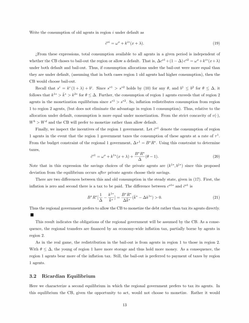
Finally, we inspect the incentives of the region 1 government. Let co1 denote the consumption of region

1 agents in the event that the region 1 government taxes the consumption of these agents at a rate of τ1.

From the budget constraint of the regional 1 government, ∆τ1 = B∗R∗. Using this constraint to determine

taxes,

co1 = ωo + k1∗(x + λ) +B∗R∗

∆(θ − 1). (20)

Note that in this expression the savings choices of the private agents are (k1∗, b1∗) since this proposed

deviation from the equilibrium occurs after private agents choose their savings.

There are two differences between this and old consumption in the steady state, given in (17). First, the

inflation is zero and second there is a tax to be paid. The difference between co1∗ and co1 is

B∗R∗[1∆− k1∗

k∗] =

B∗R∗

∆k∗(k∗ −∆k1∗) > 0. (21)

Thus the regional government prefers to allow the CB to monetize the debt rather than tax its agents directly.

This result indicates the obligations of the regional government will be assumed by the CB. As a conse-

quence, the regional transfers are financed by an economy-wide inflation tax, partially borne by agents in

region 2.

As in the real game, the redistribution in the bail-out is from agents in region 1 to those in region 2.

With θ ≤ ∆, the young of region 1 have more storage and thus hold more money. As a consequence, the

region 1 agents bear more of the inflation tax. Still, the bail-out is preferred to payment of taxes by region

1 agents.

3.2 Ricardian Equilibrium

Here we characterize a second equilibrium in which the regional government prefers to tax its agents. In

this equilibrium the CB, given the opportunity to act, would not choose to monetize. Rather it would

13

allow default. In anticipation of this, the region will tax. Given this, the agents in region 1 save more and

thus pay taxes from this extra savings. In the equilibrium this extra savings is in the form of holding of

debt. Therefore only region 1 agents hold the debt. This concentrated holding of debt is essential for the

construction of the Ricardian equilibrium. It makes clear how the distribution of debt holdings matters for

the equilibrium outcome.

In this Ricardian equilibrium, assets like the Patacones issued by the regional government in Argentina

are not money in the traditional sense as their creation is not associated with increases in prices. Instead,

they simply represent debt, backed by future taxes.23

To characterize this outcome we return to the basic optimization problems and equilibrium conditions.

The representative young agent in region i, period t solves

maxsu(ωy + gi − si) + v(ωo + siR− τ i). (22)

This optimization yields

u′(ωy + gi − s∗i) = Rv′(ωo + s∗iR− τ i) (23)

where τ2 = g2 ≡ 0. Along this equilibrium path there will be no inflation so R = x+λ1+λ .

In the construction of this equilibrium, we assume that only region 1 agents hold regional debt: b1∗ =

B∗/∆, b2∗ = 0. Further, we conjecture (and prove in Proposition 4) that s1∗ = s2∗ + b1∗ so that k1∗ = k2∗.

There is a money market clearing condition that is analogous to (12). This condition will determine the

price level given the fixed money supply and the storage decisions of the agents.

To argue that there is an equilibrium with regional taxation and no monetization by the CB, we need to

check the incentives for the levels of the government and private agents. This is done formally in Proposition

4; we bring out the intuition here.

We start in the sub-game where the regional government has decided not to tax and the CB must choose

to monetize the debt or allow default. This is a deviation from the equilibrium we are trying to construct.

Social welfare under a CB bail-out is

W b = ∆v(ωo + k1∗(x + λπ) + b1∗R) + (1−∆)v(ωo + k2∗(x + λπ)) (24)

where (ki∗, bi∗) are obtained from optimal savings along an equilibrium path from (23).24 Here π is again

the inverse of the inflation rate and inflation is caused by the monetization of the debt by the CB. If the

central bank does not bail-out and there is a default, then social welfare is given by

W d = ∆v(ωo + k∗1(x + λ)) + (1−∆)v(ωo + k∗2(x + λ)) (25)

so agents avoid the inflation tax but only get a return on their storage and money holdings.

The proof of Proposition 4 shows that W d > W b. This reflects two factors which were present in the

proof of Proposition 3 as well. First, the actual resources available to distribute to the old agents is the same23In the model there is no rollover option. But, if this were possible, then with a limit on debt issues the game we outline

between the regional government and the central bank will ultimately occur.24Recall we assume b2∗ = 0 along the equilibrium path.

14

regardless of the action of the central bank. Second, the central bank wishes to obtain the most equitable

distribution of consumption across the old agents since v(·) is strictly concave. This is achieved under default

given that k1∗ = k2∗.

Anticipating this, region 1 will prefer to raise taxes rather than allowing default. Interestingly, in both

cases, the consumption of region 1 old agents is the same. Intuitively, the taxes they pay to the regional

government are just used to pay-off the debt which they hold. But, by taxing, the regional government can

avoid the infinitesimal default penalty.

Proposition 4 There exists a steady state equilibrium given B∗ in which the regional debt is held only by

region 1 agents and the regional government chooses to raise taxes to pay its obligations.

Proof. First, we argue that there exists a (k1∗, s1∗, k2∗, s2∗, π∗) which satisfies the conditions for a

stationary monetary equilibrium. Second, we check the incentives of the regional and central governments.

In the steady state, the level of region 1 transfers to each young agent is g∗, the total per capita debt

outstanding is B∗. By the budget constraint of region 1, B∗ = ∆g∗ and taxes in old age are given by

∆τ1 = R∗B∗ so that τ1 = R∗g∗. The debt held by each agent in region 1 is b1∗ where ∆b1∗ = B∗ and region

2 agents do not hold any debt.

In equilibrium, the saving decisions of the agents are given by

u′(ωy + gi − ki∗(1 + λ)− bi∗) = R∗v′(ωo + ki∗(x + λ) + R∗bi∗ − τ i) (26)

where R∗ = x+λ1+λ . With τ1 = R∗g∗, k1∗ = k2∗ and b1∗ = B∗/∆ clearly satisfy the first order conditions.

Thus the equilibrium level of per capita storage (k∗) satisfies

u′(ωy − k∗(1 + λ)) = R∗v′(ωo + k∗(x + λ)). (27)

Given the strict concavity of u(·) and v(·), and ωy sufficiently larger than ωo, there exists a unique k∗ ≥ 0

which solves this condition.

We now turn to the incentives of the central bank. We argue that if the region does not set taxes to

pay its debt obligation, then the central bank will not monetize. To see why, from (25) and k1∗ = k2∗, the

consumption levels of agents are equal if the CB allows a default. However, the allocation under monetization

provides greater consumption for region 1 agents since they bear only a fraction of the inflation tax and receive

full repayment of their debt.

Yet, the total consumption of the old is the same, regardless of default or monetization. Under default,

total consumption of the old agents is

ωo + k∗(x + λ). (28)

Under monetization, total consumption is

ωo + k∗(x + λ) + λ(π − 1)k∗ + B∗R∗. (29)

where the rate of inflation is determined from the money creation needed to finance the bail-out as in (13).

Thus if the monetary authority deviates and bails-out the region, the resulting inflation cancels out the last

15

two terms in (29). Hence total consumption is the same regardless of default or bail-out.25 Since a bail-out

leads to a less equitable consumption distribution, the CB will prefer default to monetization.

Given that the CB will not monetize the debt, the regional government will tax rather than default. This

allows them to avoid the infinitesimal default penalty, κ. Under both regional taxation and default, the

consumption of the region 1 old is given by ωo + k∗(x + λ).

3.3 Choice of B∗

The equilibria described in the previous section take the steady state level of region 1 debt, B∗, as given.

We now explore the determination of this level of debt.

Let V (B) be the welfare of a region 1 agent if the stock of debt is B. In the Ricardian equilibrium,

the choice of B is, by construction, irrelevant for the welfare of region 1 agents. But in the monetization

equilibrium, this is not the case. If one takes, for example, the perspective that the equilibrium will be

determined by a sunspot process, then V (B) places some weight on the monetization equilibrium and the

remaining probability on the Ricardian equilibrium.26 Since welfare of region 1 agents is independent of B in

the Ricardian equilibrium, the only effect of B occurs when the monetization equilibrium is selected. Thus

we focus our discussion of the choice of B assuming the selection of the monetization equilibrium.

So consider

V (B) = u(ωy +B

∆− s) + v(ωo + sR(B)). (30)

This is the level of lifetime expected utility for a representative region 1 agent in an equilibrium with

monetization. Here B is the level of debt per capita so that B∆ is the level of debt, and thus the transfer in

youth, per young region 1 agent. The function R(B) is the return on savings if the stock of debt is B from

the equilibrium with monetization, see (13). Our main result is that the regional government will prefer a

positive level of transfers given the positive probability that the central bank will bail-out this obligation.

Proposition 5 The solution to (30) entails B > 0.

Proof. Using the envelope condition and region 1 agents’ optimal choice of s given B and R(B), the

optimal choice of B by the region 1 government satisfies

V ′(B) = v′(co)[R(B)

∆− sR′(B)] = 0. (31)

To show V ′(0) > 0, we view both R and π as functions of B, using R = x+λπ1+λ and (13) rewritten as

λk(R)(1− π) = RB. (32)

25This result could have been anticipated in a stationary monetary equilibrium, where the real money balances of young

agents, which finance the returns on old agents money holdings, are invariant to default or bail-out on debt held by the previous

generation.26The timing might be as follows. The regional government chooses B and then a sunspot occurs which selects from the set

of equilibria insofar as young agents condition their portfolio choice on the sunspot. This timing may occur each period or just

at the start of time.

16

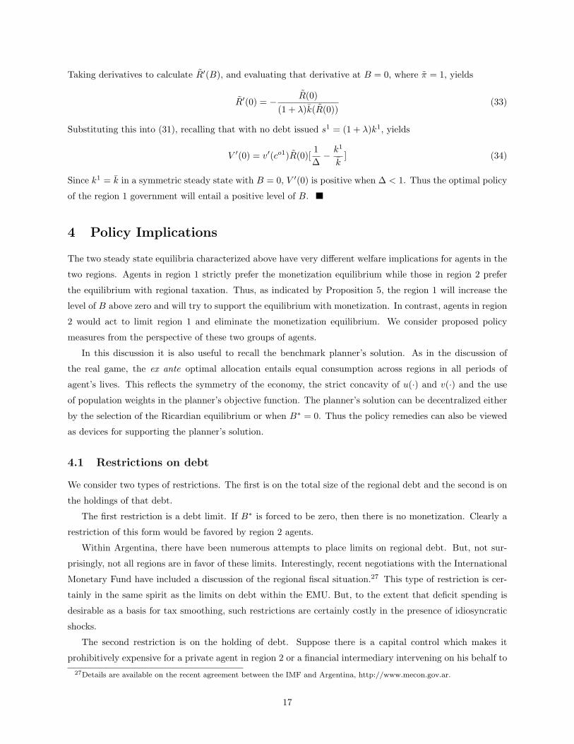
Taking derivatives to calculate R′(B), and evaluating that derivative at B = 0, where π = 1, yields

R′(0) = − R(0)(1 + λ)k(R(0))

(33)

Substituting this into (31), recalling that with no debt issued s1 = (1 + λ)k1, yields

V ′(0) = v′(co1)R(0)[1∆− k1

k] (34)

Since k1 = k in a symmetric steady state with B = 0, V ′(0) is positive when ∆ < 1. Thus the optimal policy

of the region 1 government will entail a positive level of B.

4 Policy Implications

The two steady state equilibria characterized above have very different welfare implications for agents in the

two regions. Agents in region 1 strictly prefer the monetization equilibrium while those in region 2 prefer

the equilibrium with regional taxation. Thus, as indicated by Proposition 5, the region 1 will increase the

level of B above zero and will try to support the equilibrium with monetization. In contrast, agents in region

2 would act to limit region 1 and eliminate the monetization equilibrium. We consider proposed policy

measures from the perspective of these two groups of agents.

In this discussion it is also useful to recall the benchmark planner’s solution. As in the discussion of

the real game, the ex ante optimal allocation entails equal consumption across regions in all periods of

agent’s lives. This reflects the symmetry of the economy, the strict concavity of u(·) and v(·) and the use

of population weights in the planner’s objective function. The planner’s solution can be decentralized either

by the selection of the Ricardian equilibrium or when B∗ = 0. Thus the policy remedies can also be viewed

as devices for supporting the planner’s solution.

4.1 Restrictions on debt

We consider two types of restrictions. The first is on the total size of the regional debt and the second is on

the holdings of that debt.

The first restriction is a debt limit. If B∗ is forced to be zero, then there is no monetization. Clearly a

restriction of this form would be favored by region 2 agents.

Within Argentina, there have been numerous attempts to place limits on regional debt. But, not sur-

prisingly, not all regions are in favor of these limits. Interestingly, recent negotiations with the International

Monetary Fund have included a discussion of the regional fiscal situation.27 This type of restriction is cer-

tainly in the same spirit as the limits on debt within the EMU. But, to the extent that deficit spending is

desirable as a basis for tax smoothing, such restrictions are certainly costly in the presence of idiosyncratic

shocks.

The second restriction is on the holding of debt. Suppose there is a capital control which makes it

prohibitively expensive for a private agent in region 2 or a financial intermediary intervening on his behalf to27Details are available on the recent agreement between the IMF and Argentina, http://www.mecon.gov.ar.

17

hold region 1 debt. Then this intervention implies that monetization is no longer a steady state and makes

the Ricardian equilibrium the only steady state equilibrium. This restriction is in the interest of region 2

agents. Such restrictions on the holding of debt emulate a commitment device ruling out monetization.

In Argentina, the small-denomination debt of the Buenos Aires region, the so-called Patacones, issued

in July 2002 allowed for the repayment of public obligations using these notes. But no other regions appear

willing to accept these notes for payment of taxes. While this is not a policy that prohibits Patacones to be

held outside of the Buenos Aires region, this policy clearly reduces their attractiveness for residents of other

regions.

4.2 Dollarization

A commitment by the central bank not to bail-out any regional government would of course eliminate the

monetization equilibrium. This is precisely the provision included in the Maastricht Treaty in the case of

the EMU. But of course, this begs the question: what is the basis of this commitment power?

There is a more drastic measure, which has been recently widely discussed both by policymakers and

economists: dollarization. This entails the complete surrender of monetary sovereignty, say by Argentina to

the US, and not just restrictions on the supply of money.28 Clearly dollarization eliminates the possibility

of monetization by the Argentine central bank. But there are two important caveats.

First, there is still the possibility that the Argentine central government will bail-out by means of central

taxes. This corresponds to the real game analysis in section 2. As we have shown in that section, there are

still multiple equilibria, indexed by the distribution of debt holding across regions. Hence dollarization per

se does not eliminate the multiplicity of equilibria, nor does it eliminate the ability of a regional government

to exert (ex post) pressure on the central government.

Second, under dollarization, a version of the multi-region monetary economy studied above reappears

at the world level. Suppose that it is Argentina that dollarizes and adopts the currency issued by the U.S.

central bank. Assume that prior to dollarization, the U.S. had succeeded in eliminating pressures by the

states on the federal government.29 Now with dollarization, the U.S. is like region 1 in the model of section

3 and Argentina now behaves as the region 2 passive government and does not issue debt. There is one

important difference though: the U.S. central bank does not include the welfare of Argentina in its objective.

Clearly there is now a gain to monetization of the debt by the U.S. central bank since part of this tax

will be paid by citizens of Argentina. Does this imply that the U.S. central bank will be willing to monetize

in order to help U.S. citizens through an by inflation tax partly paid by Argentina? More generally, what

are the consequences of dollarization for the existence of multiple equilibria in the world economy?

To study these issues we consider a world economy formed of the U.S. and Argentina. Under dollarization

the only currency used in the world economy is the dollar, issued by the U.S. central bank, here called the

FED. The U.S. Treasury is the sole active government (equivalent to Region 1 in the previous example),

28Cooper and Kempf (2001) explores the benefits of dollarization as a substitute for the commitment power of a central bank

in a multi-region economy (call it ”Argentina”) without regional debt.29Exactly how this is done within the U.S. is an open question, but for now we assume that the central U.S. government has

adequate commitment relative to its states.

18

making transfers to young U.S. agents by issuing debt and possibly taxing its old agents. Moreover we

assume that the FED and the Treasury only care about the welfare of U.S. citizens. Variables with the

superscript 1 now refer to the American economy, variables with the superscript 2 refer to the Argentine

economy. We denote by ∆ the fraction of the world population in the U.S. A fraction θ of the amount of

debt issued by the U.S. government B∗ is equally held by U.S. agents.

We find that dollarization indeed may support the monetization equilibrium. This is true if a sufficiently

large fraction of the debt is held in the US. Then the FED may be induced to bail-out the US government,

and so doing will harm Argentina. In other words, dollarization does not solve per se the possibility of

monetization. Again, the issue of debt distribution is crucial for the definition of the equilibrium in this

economy. We also find that there is no longer a Ricardian equilibrium. The FED will always prefer to

monetize and thus the U.S. government never levies a tax on U.S. citizens.

We find that dollarization indeed may support the monetization equilibrium. This is true if a sufficiently

large fraction of the debt is held in the U.S. Then the FED may be induced to bail-out the U.S. government,

and so doing will harm Argentine citizens who pay the inflation tax. In this case, dollarization does not

solve the possibility of monetization.

We also find that there is no longer a Ricardian equilibrium. The FED will always prefer to monetize and

thus the U.S. government never levies a tax on U.S. citizens. In effect, dollarization solves the multiplicity

of monetary equilibria but by eliminating the virtuous one! These results are now derived formally.

4.2.1 The monetization equilibrium

We now construct a monetization equilibrium in which the FED bails-out the US Treasury. Interestingly,

the conditions for this type of equilibrium are quite different from those given in Proposition 3. Instead of a

monetization equilibrium requiring that region 1 agents hold a small fraction of the debt, under dollarization

the bail-out equilibrium requires that region 1 agents hold a large fraction of the debt.

Proposition 6 Under dollarization, for a given value of B∗, there exists a monetization equilibrium for θ

sufficiently close to 1.

Proof. To characterize the monetarization equilibria, we check the incentives of the U.S. Treasury and the

FED. Beginning with the FED, note that it takes into consideration the utility of old region 1 (American)

agents only. Hence the FED’s choice of default or bail-out depends only on the consumption of region 1

agents in these two outcomes. As in (17), the consumption levels of U.S. citizens under a monetized bail-out

is

co1∗ = ωo + b1∗R∗ + k1∗(x + λπ∗) = ωo + k1∗(x + λ) + R∗B∗(

θ

∆− k1∗

k∗

), (35)

and by (19) for i = 1 under default:

co1 = ωo + k1∗(x + λ). (36)

The FED will choose to monetize rather than default iff co1∗ > co1. From the above expressions:

co1∗ > co1 ⇔(

θ

∆− k1∗

k∗

)> 0. (37)

19

Since k∗ ≡ ∆k1∗ + (1−∆)k2∗, this inequality holds for θ = 1. By continuity, it holds for θ near 1.

Therefore when θ, the fraction of debt held by U.S. residents, is sufficiently large, the FED will monetize

the US debt. This is preferred by the Treasury since the difference in consumption level under bail-out exceeds

that under taxation of U.S. citizens, as in (21). Thus for θ near 1, there is a monetization equilibrium.

The relative gain of a bail-out over default from the FED’s perspective depends on the relative inflation

tax burden on U.S. residents. As more Argentine residents hold dollars, the more they bear of the inflation

tax. The demand for money is proportional to the amount of capital held by Argentine residents. Therefore

the higher is θ, the smaller is the share of capital held by US citizens and the larger is the inflation tax borne

by Argentina.

Clearly this is a cost of dollarization for Argentine citizens, since they bear not only any Argentine taxes

to finance their own public goods, but also the inflation tax for the benefit of U.S. citizens. Cooper and

Kempf (2001) discuss the implications of a treaty between the U.S. and Argentina as an incentive device on

the U.S. central bank to limit the inflation tax.

Note that we obtained the opposite result than that of the previous section. There, the monetary

authority, caring about equalizing consumption among regions, chooses the best way to redistribute from

region 1 to region 2. In the case of dollarization, as the FED cares only about the U.S. welfare, it chooses

the best way to redistribute from region 2 to region 1.

4.2.2 The Ricardian equilibrium

We now turn to the possibility of a Ricardian equilibrium. In contrast to Section 3, there is no Ricardian

equilibrium in this economy.

Proposition 7 Under dollarization, for a given value of B∗, there is no Ricardian equilibrium.

Proof. In a Ricardian equilibrium, agents in region 1 anticipate future taxes and thus s1 = s2 + B∗∆ . As

both the U.S. Treasury and the FED have the same objective of maximizing the consumption of old U.S.

agents, the outcome of the game played each period will provide to U.S. agents the maximal consumption

level.

In a Ricardian equilibrium, the U.S. Treasury levies a tax on U.S. citizens so that the consumption of a

region 1 old agent is:

co1 = ωo + k1∗(x + λ) +R∗B∗

∆(θ − 1). (38)

Suppose instead that the U.S. Treasury does not levy the tax. The consumption levels under a bail-out

(viewed as a defection for a candidate Ricardian equilibrium) and a default are given in (35) and (36),

respectively, where the values of ki∗ in these expressions is part of the candidate Ricardian equilibrium.

Comparing (38) and (35), bail-out dominates regional taxation for region 1, co1 ≥ co1, since k1

k≤ 1

∆ .

And the inequality is strict if k2∗ > 0. If k2∗ = 0, then the consumption under default is higher than that

under bail-out: co1 ≥ co1 and thus default dominates the consumption under taxation. Thus there is no

equilibrium in which the U.S. Treasury taxes U.S. citizens since it will always prefer the outcome under

either a bail-out or a default.

20

This result stands in contrast to that in Proposition 4 in which there was an isolated Ricardian equilibrium

in which region 1 agents held all of that debt. In that equilibrium, the central bank preferred default to

a bail-out since the allocation under a default was equal across old agents in the two regions. But, under

dollarization, the objective of the FED coincides with the U.S. Treasury and so the payment of taxes by U.S.

citizens is dominated by either a bail-out or a default.

5 Conclusion

The goal of this paper was to determine the impact of issuing small denomination debt by a regional

government, such as the patacones circulating in Argentina. Two leading views are relevant: (i) the debt is

just a claim on future tax revenues and (ii) the debt was “like” money and hence printing it was tantamount

to the printing of fiat money and thus was inflationary.

Our analysis indicates that both interpretations are consistent with an equilibrium of our monetary

model. The multiplicity reflects a commitment problem on the part of the central government. Without

commitment, the central government will ex post always redistribute consumption to achieve greater equality

in consumption across different regions. Depending on the distribution of the holding of the regional gov-

ernment debt, this desire for redistribution may lead the central government to bail-out a region or it may

lead the central government to allow default. In equilibrium, the distribution of the holdings of government

debt has powerful effects on the incentives for the central government. The more equal is this distribution,

the more likely it is that the central government will prefer a bail-out to a costly default.

The commitment problem of the central government has some important incentive effects on the regions.

A bail-out creates a free-rider problem in that regional governments will have an incentive to run inefficiently

large deficits in anticipation of a government bail-out.30 Not surprisingly, other agents in the economy will

have an incentive to erect impediments to this free-rider problem including: debt restrictions, limits on the

holding of debt by other regions and even dollarization.

As a final note, the analysis did not require that the regional debt be small denomination. Nonetheless

the paper does provide an explanation for the choice of denomination. As argued above, monetization of

the regional debt is more likely if that debt is widely held. From that perspective, small denomination debt

may be more likely to circulate outside a narrow set of individuals and banks within a region. Thus the

government of region 1 may perceive a gain to issuing small denomination debt.

References

Aizenman, J. (1992): “Competitive Externality and Optimal Seigniorage,” Journal of Money, Credit and

Banking, 24, 61–71.30This point is brought out in the context of monetary unions in Chari and Kehoe (1998), Chari and Kehoe (2002) and

Cooper and Kempf (2000). Interestingly, the free-rider problem exists in our setting even when the central government can

optimally choose a partial bail-out, where in the face of no payment by the region it selects a fraction of the regional debt that

it pays off, letting default on the remaining debt. This, despite the “envelope argument”, (see Chari and Kehoe (2002)).

21

Bergstrom, T. (1989): “A Fresh Look at the Rotten Kid Theorem- and Other Household Mysteries,”

Journal of Political Economy, 97(5), 1138–59.

Chari, V. V., and P. Kehoe (1998): “On the Need for Fiscal Constraints in a Monetary Union,” Federal

Reserve Bank of Minneapolis, Working Paper #589.

(2002): “Time Inconsistency and Free-Riding in a Monetary Union,” Federal Reserve Bank of

Minneapolis, Staff Report # 308.

Cooper, R., and H. Kempf (2000): “Designing Stabilization Policy in a Monetary Union,” NBER Working

Paper #7607, forthcoming Review of Economic Studies.

(2001): “Dollarization and the conquest of hyperinflation in divided societies,” Federal Reserve

Bank of Minneapolis Quarterly Review, 25(3).

Lindbeck, A., and J. Weibull (1988): “Altruism and time consistency - the economics of fait accompli,”

Journal of Political Economy, 96(6), 1165–82.

Smith, B. (1994): “Efficiency and Determinacy of Equilibrium under Inflation Targeting,” Economic Theory,

4(3), 327–44.

Zarazaga, C. (1995): “Hyperinflations and Moral Hazard in the Appropriation of Seignorage,” Federal

Reserve Bank of Dallas, Working Paper 95-17.

22

Regional Government(RG)

Central Government(CG)

tax no-tax

Regional tax

no-bailout bailout

Default Common tax

Figure 1: Game Structure

co2

450

R

B

D

co1

Figure 2: old-age consumption across regions

1oc 1oc 1oc~