ipsp2021 industrial problem solving with physics
TRANSCRIPT

PROCEEDINGS OF THE EVENTIPSP2021INDUSTRIAL PROBLEM SOLVING WITH PHYSICSTrento (Italy)July 19-24, 2021


Proceedings of the event IPSP2021Industrial Problem Solving with Physics
Trento, July 19 – 24, 2021
EditorsMattia MancinelliMichele OrlandiLuca Tubiana
TrentoUniversita degli Studi di Trento

All rights reserved. No part of this book may be reproduced in any form, byphotostat, microform, retrieval system, or any other means, without prior writtenpermission of the editors.
Proceedings of the event IPSP2018: Industrial Problem Solving with Physics:Trento, July 19 – 24, 2021 / editors Mattia Mancinelli, Michele Orlandi, LucaTubiana. - Trento: Universita degli Studi di Trento, 2021. - 63 p.: ill. - ISBN:978-88-8443-965-9.
©2021 by Scientific Committee of IPSP2021Latex class available at https://github.com/mrgrass/IPSP_latex_Class

PREFACE
Confindustria Trento is a partner of IPSP since the very first edition. When thefounders of the competition – three PhD students of the Physics Department ofthe University of Trento – presented us their idea, we decided to join the projectmainly for three reasons. First of all, it is a bottom-up initiative managed byproactive students. Second, it contributes to promote the role of graduates andPhDs in Physics within the industrial sector. Third, it can really help to narrowthe gap between research and industry.So far, our experience with IPSP has been extremely positive. Companies whoparticipated in IPSP have obtained innovative solutions to their technical problems,with important effects on their products and productive processes. That is whywe will support IPSP in the future as well. Let’s innovate together!
Alessandro Santini, Confindustria Trento
Since its founding in 1986, Trentino Sviluppo has been promoting the connectionbetween research, business and education. On these pillars we built PoloMeccatronica, a technology hub where companies, students and researcherswork side by side to face the challenges posed by Industry 4.0. Technologytransfer, innovation and cross-fertilization are also the basis of ProM Facility, ourcutting-edge laboratory where SMEs, industrial groups, startups and researchersdevelop and patent new business ideas related to the additive manufacturing andprototyping fields.Recognizing the importance of the circular transfer of knowledge, we are thereforeproud to renew our commitment to the IPSP initiative. To us, this competitionrepresents a gainful opportunity for both young talents – who can test theiracademic skills on the ground – and enterprises – which can experiment innovativesolutions to achieve their goals as well as make contact with the most brilliantphysicists of the future. Finally, we wish luck and success to the new 2022 edition!
Paolo Gregori, Polo Meccatronica
iii

iv PREFACE
Industrial Problem Solving with Physics has reached its 6th edition in 2021 andfrom a Technology Transfer perspective, it has consolidated a new model ofindustry-academia collaboration which allows industrial problems to be solvedquickly and effectively in one week. A growing trend within the initiative consistsof a series of meetings among the University and the enterprises involved in IPSPafter the event, fostering long-term collaborations encouraged by the contributionof Trentino Sviluppo – Polo Meccatronica and Confindustria Trento. Indeed, oneof the main targets of IPSP is the development of a strong link between Universitylaboratories and enterprises. Both applied research and the placement of youngscientists can profit from the dialogue promoted by this event.
Vanessa Ravagni, Directorate of Research Services and Valorization,University of Trento

INTRODUCTION
Industrial Problem Solving with Physics (IPSP) is an annual event organizedby the Department of Physics, the Doctoral School of Physics and the ResearchSupport and Valorization Division of the University of Trento, in collaborationwith Confindustria Trento and Polo Meccatronica-Trentino Sviluppo. The mainobjective of the initiative is to promote the collaboration between the Departmentof Physics and the industrial world.IPSP reached its sixth edition in 2021, thanks to its huge success since its launchin 2014. The idea of such an event was presented to the Department of Physicsand the University of Trento by three physics PhD students and was well received.The three PhD students formed the “Scientific Committee” of IPSP which hasbeen an important element in this initiative until today. To encourage a vastparticipation and to provide more credit for the initiative, this edition was directedby three physics researchers who had the role of tutor for each team.IPSP is composed of problems, which are proposed by companies, and participants(“brains”). For one full-time week, the brains (master or PhD students, post-docs,and researchers) try different ideas and various approaches to solve the problemsand on the final day of the event present their solutions. The proposed solutionshave been helpful and practical in all editions. The strengths of IPSP include theefficient format, the presence of young brains on the one hand and experiencesof the companies on the other one and lots of team spirit. In addition, it hassuccessfully promoted the young physicists (scientists) in industries and pavedthe path for more collaboration with them through industrial projects, doctoratescholarships and traineeship possibilities for undergraduate and graduate students.It has also been an exemplar for some similar initiatives organized by otherdepartments of the University of Trento or by innovation-oriented organizations.This book contains the proceedings of IPSP2021 and describes in detail theactivities carried out by the three teams. It is organized in three chapters, eachof which begins with a brief overview of the company and a description of theproposed problem, followed by the undertaken strategies, the technical procedures,and the final solutions. At the end of each chapter suggestions and conclusionsare presented.
Mattia Mancinelli, Michele Orlandi, Luca Tubiana
v

CHAPTER
ONE
PHYSICAL BASED SIMULATION OF A REAL-TIMELIDAR SENSOR WITHIN A RENDERING
ENVIRONMENT BASED ON UNREAL ENGINE 4
D. Bazzanella, S. Bontorin, F. Callegari, B. Degli Esposti, S. Rabaglia, L.
Wolswijk, and Alessandro Zunino
Tutor: Mattia Mancinelli
1.1 Introduction
1.1.1 The company
AnteMotion [1] is a joint venture of EnginSoft Spa (Italy), LHP EngineeringSolutions Inc (USA) and V2R Srl (Italy), three realities of the Automotive IndustryR&D, whose skills converge in AnteMotion in order to satisfy the growing simulativeneeds of the field. Their core business is focused on creating virtual environmentsthrough a Real-Time Render Engine for training, validating and assessing thefunctional safety of both Virtual Drivers and ADAS Systems (Advanced DriverAssistance Systems). The simulation framework is real-time oriented and exploitsa Real Time Engine (Unreal) developed for gaming that provides state of the artrendering quality of dynamic environments in virtual reality and dome projection.
1.1.2 The problem
The success of autonomous driving depends on how accurate sensors and softwareused by the car are. The software is usually based on Artificial Neural Network(ANN) whose aim is to interpret the data coming from a multitude of differentkinds of sensors and produces a decision. The sensors can be camera, radar,proximity sensor and LiDAR (Light Detection and Ranging). The accuracy ofANN in general depends on the data set dimension and quality. A good data setshould contain ‘all’ the possible scenarios that the network will manage during
1
2 CHAPTER 1. ANTEMOTION TEAM
the operation. Once trained the network is tested on different data from the oneused for the training. AnteMotion (AM) is capable to provide a platform to test(and eventually train) the accuracy of these ANN by generating virtual data sets.The problem submitted to IPSP 2021 is framed on these concepts. In particular,AM asked to accurately model a LiDAR sensor within the Real-Time Engineframework used to render the virtual reality. A physical model of a LiDAR isrequired to produce real data from the virtual reality used to test the accuracy ofANN used in the autonomous driving software. A wrong model would producefake data from the driving session that in turn would give an incorrect judgementof ANN accuracy.In addition, AM requested the model to be lightweight, as theirintention is to run it in real time. For this reason, simulation performance andphysical accuracy should be balanced in order to satisfy both requests.
1.1.3 Problem solving approach
This section is intended as a guideline for the reading of the whole document:its goal is to show how the problem has been addressed and how the differentactivities have been carried out by the team. Section 1.2 reports the state of theart of the automotive LiDAR sensors: the different types, the working principlesand operating specifications of actual devices on the market have been reported.Then, the document contains a description of the physical phenomena and modelsimplemented in the solution proposed to the company: Section 1.3 explains theequations involved in the different scenarios and the assumptions introducedto perform a realistic simulation. The software and the virtual tools used toimplement the proposed solution are shown in Section 1.4: further, it contains alsoa detailed description of the structure of the algorithms and in the communicationbetween the different layers of the software. Section 1.5 shows the results obtainedby the implementation of the physical models in our solution.
1.2 Existing LiDAR devices
1.2.1 Types of LiDAR
LiDAR devices exploit light to identify target positions and map their distances.Typically, a pulsed illumination is used to determine such distances, by measuringthe time of flight (ToF) between the emission and the detection of the light pulse.However, also interferometric approaches, relying on the phase detection of amodulated light signal, are widely adopted.In the automotive sector, LiDARs are fundamental elements for autonomousdriving, as they are responsible for scanning the environment around the vehicle.To do so, autonomous driving car manufacturers have adopted four main scanningtechnologies so far: rotational or spinning, MEMS-based, FLASH and OpticalPhase Array (OPA) LiDAR sensors.
Spinning LiDAR Sensors In this kind of device, a set of laser emitters anddetectors are assembled in a rotational stage. This configuration relies on
1.2. EXISTING LIDAR DEVICES 3
the fast spinning (few tens of Hz) of the sensor to have a 360° scanningof the surrounding area. Thus, a full horizontal field of view (HFOV) canbe achieved with this device. The number of emitters/receivers and theirorientation determines then the Vertical Field of View (VFOV) and theangular resolution of the illumination.
MEMS LiDAR Sensors By applying the proper voltage signal, MEMS (MicroElectronic Mechanical Systems) can transduce tiny displacements. So, thesteering of miniaturised mirrors fabricated on MEMS allows scanning ofa certain area, when they are combined with laser beams and detectors.Typically, these sensors do not provide huge FoV but the simultaneous useof many of them provides a good scanning coverage.
FLASH LiDAR Sensors Similarly to a flash camera, FLASH LiDARs use awide-area laser pulse to illuminate the environment in front of it and anarray of photodetectors captures the back-scattered light. Although the FoVis limited also in this class of devices, the data capture rate is much faster.
Optical Phase Arrays (OPA) LiDAR Sensors The OPA principle is basedon the control of the optical wave-front shape to control the direction ofthe illumination beam, so no moving mechanical parts are required. Byproperly applying different phase shifts to each light emitter, the overalllight distribution is effectively steered to point in different directions.
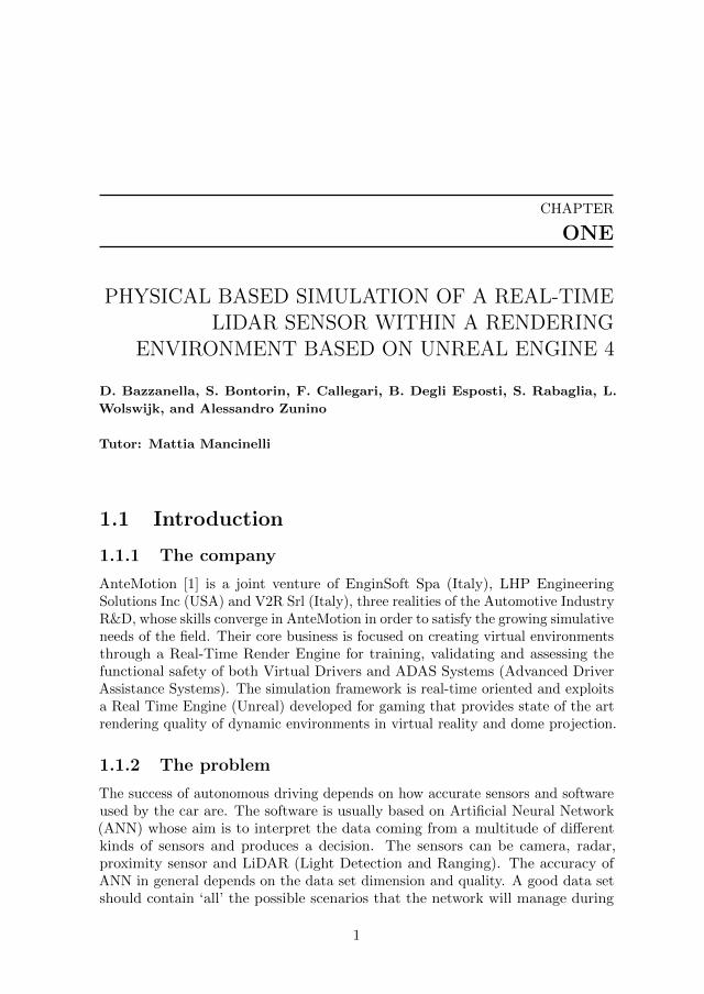
1.2.2 Spinning LiDAR : working principle
Our solution carries out a simulation of a spinning LiDAR sensor. This deviceallows to determine the distance of an obstacle (also called target) by measuringthe delay, usually called Time Of Flight (TOF), between the time at which thelight source of the LiDAR emits a light pulse and the time at which the light getsback at the detector, after being reflected or backscattered by the target.The distance between the LiDAR and the obstacle is usually called range R andis proportional to the time of flight tTOF [2]:
R = ctTOF
2, (1.1)
where c is the speed of light, which is constant under the assumption that thepropagation occurs within the same medium (air). The factor of 2 takes intoaccount the fact that the light travels forth and back.
The maximum measurable range would be theoretically limited only by themaximum time interval that can be measured by the time counter. In practice,being this time interval large enough, the maximum range becomes limited byother factors, which are mainly related to the energy losses during the propagationand reflection of the light pulse. The intensity of the light that reaches thedetector depends on the power of the LiDAR laser source, on the losses due to thepropagation through the air and on the fraction of light that is reflected back by
4 CHAPTER 1. ANTEMOTION TEAM
Figure 1.1: TOF measurement principle, image from [2]
a given object reaching the detector’s sensitive area. The maximum detectablerange results then to be ultimately limited by the signal-to-noise ratio (SNR) ofthe detector, in terms of the minimum light intensity of the return signal that canbe distinguished from the electronic noise of the high-bandwidth detection circuit.To identify the maximum range, another aspect to be considered is the ambiguitydistance (the maximum range which can be measured unambiguously) [2], whichin the pulsed approach is limited by the presence of more than one simultaneouspulse in flight, and thus related to the repetition rate of the laser. From equation1.1 the ambiguity distance results of the order of 150 m for a laser with a repetitionrate close to the MHz range.Since the pulsed principle is based on the direct measurement of the round triptime between light pulse emission and the return of the pulse-echo resulting fromthe backscattering from a target object, the light pulses need to be as short aspossible (usually a few ns) and with large optical power in order to obtain a higherSNR.The peak laser power that can be used is determined by laser safety regulations,which quantify the maximum optical power for a given exposure time [3]. The useof pulsed lasers with short pulse duration allows to remain in the class 1 laser-safetyclass (where no safety glasses are required) while exploiting high peak powers, upto the order of 500W for pulse duration of a fraction of ns. Such large irradiancepower, together with the use of wavelength-selective optical filters, allows to neglectthe solar background, making pulsed LiDARs particularly suitable for outdoorapplications as in the automotive field.An optical power of this order of magnitude might seem large, but one mustconsider that only a fraction of the optical energy of the emitted laser pulses isreceived back at the detector, especially if the target surface is, as in most cases,diffusive, which scatters the incoming light in multiple directions. This meansthat very sensitive detectors are needed in order to detect the faint pulses receivedfrom distant diffusive objects. In our simulation we considered a peak power of100W, but this input parameter can be easily changed to account for differentlight sources.Another important aspect is the range resolution, i.e. the minimum range difference
1.2. EXISTING LIDAR DEVICES 5
that can be resolved, which is related to the bandwidth of the detector. The rangeresolution can change significantly from low cost to more expensive LiDARs , withtypical values going from 20 cm [4] to 2-3 cm [5]. This corresponds to minimumtime resolutions of the detector ∆t = 2∆R/c, respectively of 1.3 ns and 0.2 ns.The bandwidth of the detector must therefore be at least of the order of the GHz.
Knowing the required bandwidth, we can estimate the SNR that limits themaximum measurable range. Considering, for instance, the noise equivalent powerof a high quality detector [6], NEP ∼ 6.6 pW/
√Hz we can estimate the noise
threshold as: Pnoise = NEP√BW ∼ 0.2µW . In Subsection 1.3.3 we explain more
in detail how this estimation of the noise threshold is implemented in our physicalmodel.
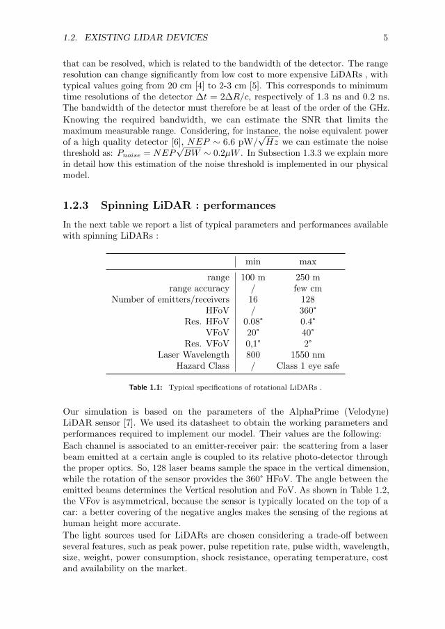
1.2.3 Spinning LiDAR : performances
In the next table we report a list of typical parameters and performances availablewith spinning LiDARs :
min max
range 100 m 250 mrange accuracy / few cm
Number of emitters/receivers 16 128HFoV / 360°
Res. HFoV 0.08° 0.4°VFoV 20° 40°
Res. VFoV 0,1° 2°Laser Wavelength 800 1550 nm
Hazard Class / Class 1 eye safe
Table 1.1: Typical specifications of rotational LiDARs .
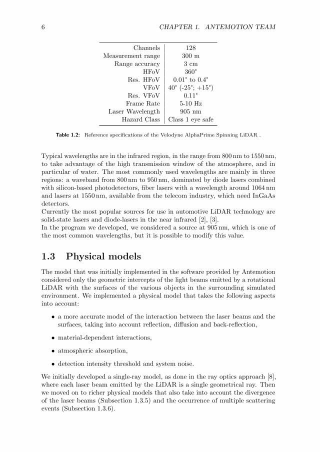
Our simulation is based on the parameters of the AlphaPrime (Velodyne)LiDAR sensor [7]. We used its datasheet to obtain the working parameters andperformances required to implement our model. Their values are the following:
Each channel is associated to an emitter-receiver pair: the scattering from a laserbeam emitted at a certain angle is coupled to its relative photo-detector throughthe proper optics. So, 128 laser beams sample the space in the vertical dimension,while the rotation of the sensor provides the 360° HFoV. The angle between theemitted beams determines the Vertical resolution and FoV. As shown in Table 1.2,the VFov is asymmetrical, because the sensor is typically located on the top of acar: a better covering of the negative angles makes the sensing of the regions athuman height more accurate.
The light sources used for LiDARs are chosen considering a trade-off betweenseveral features, such as peak power, pulse repetition rate, pulse width, wavelength,size, weight, power consumption, shock resistance, operating temperature, costand availability on the market.
6 CHAPTER 1. ANTEMOTION TEAM
Channels 128Measurement range 300 m
Range accuracy 3 cmHFoV 360°
Res. HFoV 0.01° to 0.4°VFoV 40° (-25°; +15°)
Res. VFoV 0.11°Frame Rate 5-10 Hz
Laser Wavelength 905 nmHazard Class Class 1 eye safe
Table 1.2: Reference specifications of the Velodyne AlphaPrime Spinning LiDAR .
Typical wavelengths are in the infrared region, in the range from 800 nm to 1550 nm,to take advantage of the high transmission window of the atmosphere, and inparticular of water. The most commonly used wavelengths are mainly in threeregions: a waveband from 800 nm to 950 nm, dominated by diode lasers combinedwith silicon-based photodetectors, fiber lasers with a wavelength around 1064 nmand lasers at 1550 nm, available from the telecom industry, which need InGaAsdetectors.Currently the most popular sources for use in automotive LiDAR technology aresolid-state lasers and diode-lasers in the near infrared [2], [3].In the program we developed, we considered a source at 905 nm, which is one ofthe most common wavelengths, but it is possible to modify this value.
1.3 Physical models
The model that was initially implemented in the software provided by Antemotionconsidered only the geometric intercepts of the light beams emitted by a rotationalLiDAR with the surfaces of the various objects in the surrounding simulatedenvironment. We implemented a physical model that takes the following aspectsinto account:
• a more accurate model of the interaction between the laser beams and thesurfaces, taking into account reflection, diffusion and back-reflection,
• material-dependent interactions,
• atmospheric absorption,
• detection intensity threshold and system noise.
We initially developed a single-ray model, as done in the ray optics approach [8],where each laser beam emitted by the LiDAR is a single geometrical ray. Thenwe moved on to richer physical models that also take into account the divergenceof the laser beams (Subsection 1.3.5) and the occurrence of multiple scatteringevents (Subsection 1.3.6).
1.3. PHYSICAL MODELS 7
1.3.1 Model of the laser-surface interactions
Urban environments usually contain a variety of surfaces, each of which interactsdifferently with a laser beam. Our work summarises this large variability to threetypes of interactions, which cover effectively the vast majority of all possiblelight-surface interactions.
• The first type is the diffusive material, which is found everywhere in opaque,non-metallic surfaces, e.g. walls, pavement, and wood surfaces.
• The second type is the reflective material, which is associated to eithermetallic surfaces, e.g. mirrors and metallic paint, or transparent materials,e.g. glass surfaces, in which part of the light is refracted and part is reflected.
• The last type is the back-reflecting material, mostly found on traffic signsand pedestrian crossings, which are often covered with a retro-reflectingsurface, to increase their visibility.
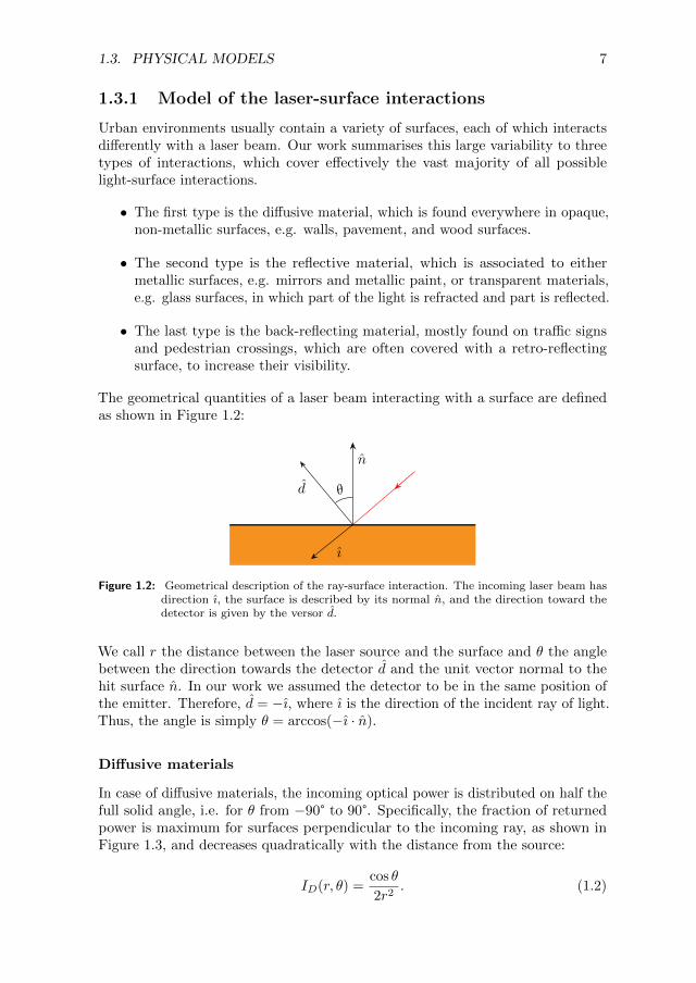
The geometrical quantities of a laser beam interacting with a surface are definedas shown in Figure 1.2:
ı
n
d θ
Figure 1.2: Geometrical description of the ray-surface interaction. The incoming laser beam hasdirection ı, the surface is described by its normal n, and the direction toward thedetector is given by the versor d.
We call r the distance between the laser source and the surface and θ the anglebetween the direction towards the detector d and the unit vector normal to thehit surface n. In our work we assumed the detector to be in the same position ofthe emitter. Therefore, d = −ı, where ı is the direction of the incident ray of light.Thus, the angle is simply θ = arccos(−ı · n).
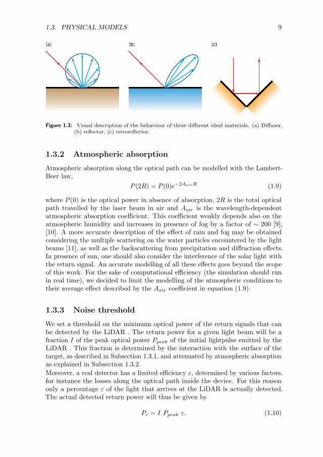
Diffusive materials
In case of diffusive materials, the incoming optical power is distributed on half thefull solid angle, i.e. for θ from −90° to 90°. Specifically, the fraction of returnedpower is maximum for surfaces perpendicular to the incoming ray, as shown inFigure 1.3, and decreases quadratically with the distance from the source:
ID(r, θ) =cos θ
2r2. (1.2)
8 CHAPTER 1. ANTEMOTION TEAM
In order to satisfy the energy conservation law, the following equation holds:∫ 90°
−90°ID(r, θ)dθ =
1
r2. (1.3)
where the 1/r2 term describes the divergence of the back-scattered light.
Reflective materials
In case of reflective materials, the incoming ray is reflected with the same incidenceangle, but opposite to the normal to the surface, as shown in Figure 1.3. However,real materials might scatter light also at different angles, mainly because of surfaceroughness. In order to take this into consideration, we modelled the distributionof reflected rays with a Gaussian curve centred at the reflection angle −θ. Informula:
IR(θ;σ) =1
σ√2π
exp
(−2(θ
σ
)2), (1.4)
where σ is the angular width, specific to each material.Similarly to the case of diffusive materials, to satisfy the energy conservation law,the distribution is normalized. Indeed∫ 90°
−90°IR(r, θ)dθ ≈
∫ ∞
−∞IR(r, θ)dθ = 1, (1.5)
where the approximation holds because typically σ ≪ 90°.
Retro-reflecting materials
In case of retro-reflecting materials (see Figure 1.3) the ray is reflected backwardswith the same intensity of the incoming beam:
IC = 1. (1.6)
Realistic materials
The full model of a material is ultimately described by a weighted sum of thesethree ideal models. The fraction of the initial power that returns back is in totalgiven by:
I(r, θ) = α · ID(r, θ) + β · IR(θ) + γ · IC , (1.7)
where α, β, and γ and positive coefficients for the individual models. In order torespect the conservation of energy, the following constraint holds
α+ β + γ ≤ 1, (1.8)
where the equality is observed when no loss is present.
1.3. PHYSICAL MODELS 9
Figure 1.3: Visual description of the behaviour of three different ideal materials. (a) Diffuser,(b) reflector, (c) retroreflector.
1.3.2 Atmospheric absorption
Atmospheric absorption along the optical path can be modelled with the Lambert-Beer law,
P (2R) = P (0)e−2AairR (1.9)
where P (0) is the optical power in absence of absorption, 2R is the total opticalpath travelled by the laser beam in air and Aair is the wavelength-dependentatmospheric absorption coefficient. This coefficient weakly depends also on theatmospheric humidity and increases in presence of fog by a factor of ∼ 200 [9],[10]. A more accurate description of the effect of rain and fog may be obtainedconsidering the multiple scattering on the water particles encountered by the lightbeams [11], as well as the backscattering from precipitation and diffraction effects.In presence of sun, one should also consider the interference of the solar light withthe return signal. An accurate modelling of all these effects goes beyond the scopeof this work. For the sake of computational efficiency (the simulation should runin real time), we decided to limit the modelling of the atmospheric conditions totheir average effect described by the Aair coefficient in equation (1.9).
1.3.3 Noise threshold
We set a threshold on the minimum optical power of the return signals that canbe detected by the LiDAR . The return power for a given light beam will be afraction I of the peak optical power Ppeak of the initial lightpulse emitted by theLiDAR . This fraction is determined by the interaction with the surface of thetarget, as described in Subsection 1.3.1, and attenuated by atmospheric absorptionas explained in Subsection 1.3.2.
Moreover, a real detector has a limited efficiency ε, determined by various factors,for instance the losses along the optical path inside the device. For this reasononly a percentage ε of the light that arrives at the LiDAR is actually detected.The actual detected return power will thus be given by
Pr = I Ppeak ε. (1.10)
10 CHAPTER 1. ANTEMOTION TEAM
In Subsection 1.2.2 we estimated the optical power corresponding to the detectornoise as
Pnoise = NEP√BW , (1.11)
where NEP is the noise-equivalent-power and BW the detector bandwidth.To treat the stochastic noise on our detected signals, we add, on top of our returnsignals Pr, a Gaussian noise distribution PG, having standard deviation Pnoise.The actual detected power becomes
Pout = Pr + PG. (1.12)
Setting a detection threshold Pmin of three standard deviations, we obtain that areturn signal is detectable if:
Pout > 3Pnoise = Pmin. (1.13)
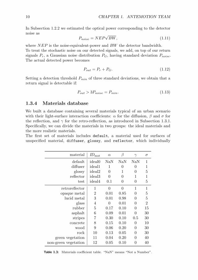
1.3.4 Materials database
We built a database containing several materials typical of an urban scenariowith their light-surface interaction coefficients: α for the diffusion, β and σ forthe reflection, and γ for the retro-reflection, as introduced in Subsection 1.3.1.Specifically, we can divide the materials in two groups: the ideal materials andthe more realistic materials.The first set of materials includes default, a material used for surfaces ofunspecified material, diffuser, glossy, and reflector, which individually
material IDmat α β γ σ
default ideal0 NaN NaN NaN 1diffuser ideal1 1 0 0 1glossy ideal2 0 1 0 5
reflector ideal3 0 0 1 1test ideal4 0.1 0 0 5
retroreflector 1 0 0 1 1opaque metal 2 0.01 0.85 0 5lucid metal 3 0.01 0.98 0 5
glass 4 0 0.01 0 2rubber 5 0.17 0.10 0 15asphalt 6 0.09 0.01 0 30stripes 7 0.30 0.10 0.5 30
concrete 8 0.15 0.10 0 10wood 9 0.06 0.20 0 30rock 10 0.13 0.05 0 30
green vegetation 11 0.04 0.20 0 40non-green vegetation 12 0.05 0.10 0 40
Table 1.3: Materials coefficient table. “NaN” means “Not a Number”.

1.3. PHYSICAL MODELS 11
implement the diffusive, reflective, and retro-reflection effects, and a test material,used for modelling a flat surface diffusing 10% of the incoming optical power.
The second set of materials contains the main materials that can be found in anurban scenery, among which asphalt and stripes, which we used to model aroad surface, glass, rubber and metal, which we used to model cars, and othermaterials such as wood, rocks and vegetation.
Since we did not have the possibility to perform reflectivity measurements directly,we looked online for typical reflectivity coefficients of the different materials, inorder to obtain a realistic scenery. In [12] the authors describe an experimentalprocedure to obtain the reflectivity and diffusion coefficients for different materials,using a laser source and measuring the back-scattered light at different angles.They also provide the experimental values for some materials. Other coefficientswere obtained using as reference the NASA Ecostress Library [13].
The optical properties of a material depend on the wavelength. We considered aLiDAR operating at a wavelength of 905 nm, for which the coefficients are reportedin Table 1.3. Each of these materials is contained in an ordered dictionary and isaccessed via a positive integer index IDmat.
1.3.5 Spot divergence model (Roses)
The first change to our single ray model is the inclusion of the spot divergence.Each laser beam is modelled as a 3D cone, so that the width of the beam is alinear function of the distance from the corresponding LiDAR emitter (see Figure1.4). The divergence Θ of the beam is defined as the angle between the axis ofthe cone and its surface. Typical divergence of laser diodes is of the order of1mrad (≈ 0.057°) [7]. Hence, the diameter of the laser spot at a distance L canbe evaluated as d(L) = 2L sin(Θ). At 50m and 100m the spot diameter will bed|50m ≃ 5 cm and d|100m = 10 cm, respectively. This means that, in some cases,the LiDAR will detect a signal reflected from the edge of the beam and not fromthe centre.
To take this effect into account, we discretised each beam into Nroses = 1+n rays:one in the centre and the remaining n distributed on the beam’s conical surface.The number of rays in each rose has been fixed to Nroses = 5, but in principle can
Figure 1.4: Sketch of the modelling of beam divergence. The Gaussian beam is sampled bymultiple rays of light with an angular separation defined by wave optics theory.
12 CHAPTER 1. ANTEMOTION TEAM
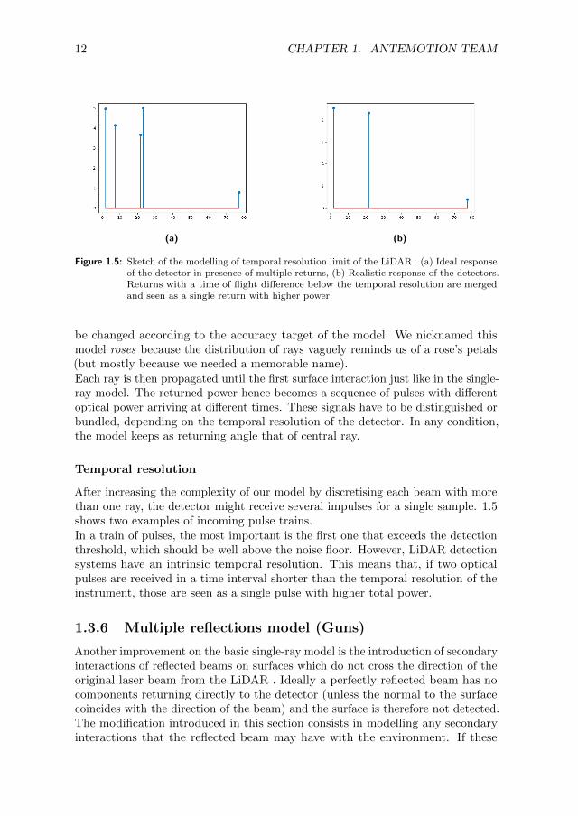
(a) (b)
Figure 1.5: Sketch of the modelling of temporal resolution limit of the LiDAR . (a) Ideal responseof the detector in presence of multiple returns, (b) Realistic response of the detectors.Returns with a time of flight difference below the temporal resolution are mergedand seen as a single return with higher power.
be changed according to the accuracy target of the model. We nicknamed thismodel roses because the distribution of rays vaguely reminds us of a rose’s petals(but mostly because we needed a memorable name).Each ray is then propagated until the first surface interaction just like in the single-ray model. The returned power hence becomes a sequence of pulses with differentoptical power arriving at different times. These signals have to be distinguished orbundled, depending on the temporal resolution of the detector. In any condition,the model keeps as returning angle that of central ray.
Temporal resolution
After increasing the complexity of our model by discretising each beam with morethan one ray, the detector might receive several impulses for a single sample. 1.5shows two examples of incoming pulse trains.In a train of pulses, the most important is the first one that exceeds the detectionthreshold, which should be well above the noise floor. However, LiDAR detectionsystems have an intrinsic temporal resolution. This means that, if two opticalpulses are received in a time interval shorter than the temporal resolution of theinstrument, those are seen as a single pulse with higher total power.
1.3.6 Multiple reflections model (Guns)
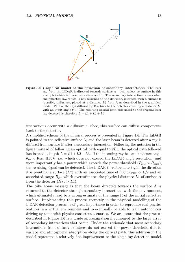
Another improvement on the basic single-ray model is the introduction of secondaryinteractions of reflected beams on surfaces which do not cross the direction of theoriginal laser beam from the LiDAR . Ideally a perfectly reflected beam has nocomponents returning directly to the detector (unless the normal to the surfacecoincides with the direction of the beam) and the surface is therefore not detected.The modification introduced in this section consists in modelling any secondaryinteractions that the reflected beam may have with the environment. If these
1.3. PHYSICAL MODELS 13
L3
L1
L2
A
A*B
θin
Figure 1.6: Graphical model of the detection of secondary interactions: The laserray from the LiDAR is directed towards surface A (ideal reflective surface in thisexample) which is placed at a distance L1. The secondary interaction occurs whenthe reflected ray, which is not returned to the detector, interacts with a surface B(possibly diffusive), placed at a distance L2 from A as described in the graphicalmodel. Part of the rays diffused by B return to the detector covering a distance L3with an input angle θin. The resulting optical path associated to the original laserray detected is therefore L = L1 + L2 + L3
interactions occur with a diffusive surface, this surface can diffuse componentsback to the detector.A simplified scheme of the physical process is presented in Figure 1.6. The LiDARis pointed to the reflective surface A, and the laser beam is detected after a ray isdiffused from surface B after a secondary interaction. Following the notation in thefigure, instead of following an optical path equal to 2L1, the optical path followedhas instead a length L = L1+L2+L3. If the incoming ray has an incidence angleθin < Res. HFoV, i.e. which does not exceed the LiDAR angle resolution, andmore importantly has a power which exceeds the power threshold (Pout > Pmin),the resulting signal can be detected. The LiDAR therefore detects, in the directionit is pointing, a surface (A*) with an associated time of flight tTOF ∝ L/c and anassociated range RA∗ which overestimates the physical distance L1 of surface Afrom the detector (RA∗ > L1).The take home message is that the beam directed towards the surface A isreturned to the detector through secondary interactions with the environment,which ultimately lead to a wrong estimate of the range R of the initial reflectivesurface. Implementing this process correctly in the physical modelling of theLiDAR detection process is of great importance in order to reproduce real physicsfeatures in a virtual environment and to eventually be able to train autonomousdriving systems with physics-consistent scenarios. We are aware that the processdescribed in Figure 1.6 is a crude approximation if compared to the large arrayof secondary interactions that occur. Under the rationale that most secondaryinteractions from diffusive surfaces do not exceed the power threshold due tosurface and atmospheric absorption along the optical path, this addition in themodel represents a relatively fine improvement to the single ray detection model.

14 CHAPTER 1. ANTEMOTION TEAM
Algorithm 1 A pseudocode description of pointcloud physics reflections()
set initial parametersload input data structurefor beam in beams do
i← 0while i < Nref do
get physics informationif material is a diffuser then
propagate to detectorcompute surface interaction and absorptionadd noiseif Pout > Pmin and θin < resolution then
store the beamelse:
store dummy values and continue to the next beamend ifi← i+ 1
else material is a reflector:compute surface interaction and absorptioncompute relative distance to next Nref secondary reflection pointscompute the forward power propagated to next point in pathi← i+ 1
end ifend while
end forreturn output data structure
We nicknamed our multiple reflections model guns because the laser reflectionphenomenon reminds us of bullet ricochet.
Description of secondary reflections algorithm
In this subsection a brief description of the implementation of the guns algorithmis presented. The function pointcloud physics reflections() takes as input atensor of size Nppf ×Nref × 8, with Nppf being the number of optical paths to beprocessed, Nref being the maximum allowed number of reflections and 8 being thesize of the vector
(px,py,pz,nx,ny,nz, IDmat, θ)
that contains physical information about the surface interactions (for more details,see Subsection 1.4.5). A pseudocode description of the function is given inAlgorithm 1. The output data structure is a 3D point cloud with a scalar Pout
(the optical power) associated to each point. We stress that this model returnsa single point for each optical path. The difference between this point and theLiDAR ’s position has the same direction as the first segment of the optical path,but a possibly greater distance (because the distance depends on the total time of
1.3. PHYSICAL MODELS 15
flight and the interaction with diffusive and retro-reflective materials). The powerPout depends on all the surface interactions that occurred in the optical path.In the current implementation, the algorithm does not evaluate the possibility of asecondary reflection from a pure reflector exactly back to the detector (except forthe case of retro-reflectors which is handled separately). All the data is generatedfrom secondary reflections that meet diffusive materials. We remark that the gunsmodel is based on solid physical principles, but still requires additional validationand testing.
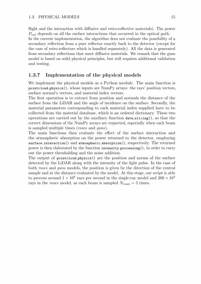
1.3.7 Implementation of the physical models
We implement the physical models as a Python module. The main function ispointcloud physics(), whose inputs are NumPy arrays: the rays’ position vectors,surface normal’s vectors, and material index vectors.The first operation is to extract from position and normals the distance of thesurface from the LiDAR and the angle of incidence on the surface. Secondly, thematerial parameters corresponding to each material index supplied have to becollected from the material database, which is an ordered dictionary. These twooperations are carried out by the auxiliary function data slicing(), so that thecorrect dimensions of the NumPy arrays are respected, especially when each beamis sampled multiple times (roses and guns).The main functions then evaluate the effect of the surface interaction andthe atmospheric absorption on the power returned to the detector, employingsurface interaction() and atmospheric absorption(), respectively. The returnedpower is then elaborated by the function intensity processing(), in order to carryout the power thresholding and the noise addition.The output of pointcloud physics() are the position and norms of the surfacedetected by the LiDAR along with the intensity of the light pulse. In the case ofboth roses and guns models, the position is given by the direction of the centralsample and at the distance evaluated by the model. At this stage, our script is ableto process around 1× 10⁶ rays per second in the single-ray model and 200× 103
rays in the roses model, as each beam is sampled Nroses = 5 times.
16 CHAPTER 1. ANTEMOTION TEAM
1.4 Implementation of a virtual LiDAR
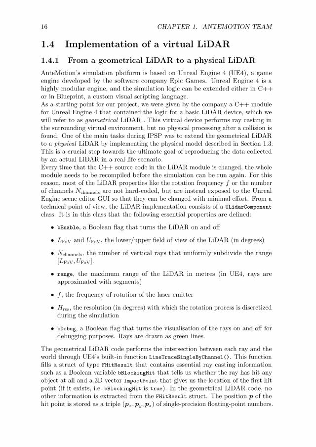
1.4.1 From a geometrical LiDAR to a physical LiDAR
AnteMotion’s simulation platform is based on Unreal Engine 4 (UE4), a gameengine developed by the software company Epic Games. Unreal Engine 4 is ahighly modular engine, and the simulation logic can be extended either in C++or in Blueprint, a custom visual scripting language.As a starting point for our project, we were given by the company a C++ modulefor Unreal Engine 4 that contained the logic for a basic LiDAR device, which wewill refer to as geometrical LiDAR . This virtual device performs ray casting inthe surrounding virtual environment, but no physical processing after a collision isfound. One of the main tasks during IPSP was to extend the geometrical LiDARto a physical LiDAR by implementing the physical model described in Section 1.3.This is a crucial step towards the ultimate goal of reproducing the data collectedby an actual LiDAR in a real-life scenario.Every time that the C++ source code in the LiDAR module is changed, the wholemodule needs to be recompiled before the simulation can be run again. For thisreason, most of the LiDAR properties like the rotation frequency f or the numberof channels Nchannels are not hard-coded, but are instead exposed to the UnrealEngine scene editor GUI so that they can be changed with minimal effort. From atechnical point of view, the LiDAR implementation consists of a ULidarComponent
class. It is in this class that the following essential properties are defined:
• bEnable, a Boolean flag that turns the LiDAR on and off
• LFoV and UFoV, the lower/upper field of view of the LiDAR (in degrees)
• Nchannels, the number of vertical rays that uniformly subdivide the range[LFoV, UFoV].
• range, the maximum range of the LiDAR in metres (in UE4, rays areapproximated with segments)
• f , the frequency of rotation of the laser emitter
• Hres, the resolution (in degrees) with which the rotation process is discretizedduring the simulation
• bDebug, a Boolean flag that turns the visualisation of the rays on and off fordebugging purposes. Rays are drawn as green lines.
The geometrical LiDAR code performs the intersection between each ray and theworld through UE4’s built-in function LineTraceSingleByChannel(). This functionfills a struct of type FHitResult that contains essential ray casting informationsuch as a Boolean variable bBlockingHit that tells us whether the ray has hit anyobject at all and a 3D vector ImpactPoint that gives us the location of the first hitpoint (if it exists, i.e. bBlockingHit is true). In the geometrical LiDAR code, noother information is extracted from the FHitResult struct. The position p of thehit point is stored as a triple (px,py,pz) of single-precision floating-point numbers.

1.4. IMPLEMENTATION OF A VIRTUAL LIDAR 17
For more information on Unreal Engine 4’s C++ API, we refer to the officialdocumentation at https://docs.unrealengine.com [14].
Surface normal information
The physical model introduced in Section 1.3 requires the surface normal nat every hit point. Just like the location of the hit point, this informationcan be extracted from the FHitResult struct that Unreal Engine 4 returns fromLineTraceSingleByChannel(): it is in the ImpactNormal field. Every normal n isstored as a triple (nx,ny,nz) of single-precision floating-point numbers and is, ofcourse, a unit vector.
Physical material information
The physical model that we implement for the LiDAR simulation is based on thestudy of the interaction between light and materials. Therefore, it is necessarythat the program provides also the information on the materials of the hit surface,in addition to the coordinates and surface normal of the impact point. We havesolved this problem in the following way.
First, in Unreal Engine 4’s editor we have defined 12 custom surface types (seeFig. 1.7) that correspond to the materials considered inside the physical model(see Table 1.3). The number that identifies the surface type is an arbitrary integeridentifier IDmat. Second, we have created a custom physical material (using UE4’sterminology) for each surface type. For example, the Dark asphalt surface type(IDmat = 6) was assigned to a newly created asphalt physical material. Then,the right physical material was assigned to every part of every 3D model in thescene (some models, like cars, have more than one material). Third, we haveenabled the detection of the physical material during ray casting by setting bothbReturnPhysicalMaterial and bTraceComplex to true in the FCollisionQueryParamsstruct that is passed to every call of LineTraceSingleByChannel(). Finally, we haveextracted the surface type ID of the material at every hit point by reading thePhysMaterial.SurfaceType subfield of the FHitResult struct.
In Unreal Engine 4, a static mesh is associated to each object and, based onthe collision complexity, it can be either simple or complex. Simple collision isagainst primitives like cubes, spheres, capsules, and convex hulls, while complexcollision is against the complete triangle mesh of a given object. If we use simplecollisions, we can associate only one physical material to each object, becausethe program sees the object as a single homogeneous geometrical shape. Withcomplex collisions, however, every object can be composed by multiple parts, andwe can associate a different physical material to each of them. The only drawbackof complex collisions is that they have a higher computational cost. Therefore,we have enabled complex collisions only for a small number of objects that weconsider essential for our simulation.

18 CHAPTER 1. ANTEMOTION TEAM
Figure 1.7: UE4’s editor settings related to surface IDs and physical materials.
1.4.2 Data flow in and out of the physical model
In computer graphics, the frame rate (expressed in frames per second or FPS) isthe frequency at which virtual environments are updated and consecutive images(frames) are displayed after rendering. Unreal Engine 4, unless instructed otherwise,tries to compute as many frames as possible every second in order to have smootheranimations, more accurate simulations and to react more quickly to external eventsor user inputs. Some frames may be more expensive to compute than others, sothe time required to compute each frame is a variable quantity ∆t. The quantity∆t is on average equal to the reciprocal of the FPS, and is used as the time stepof the animations and of the game physics.Let ω = 360°f be the angular velocity of the laser emitters of a spinning LiDARdevice. After a time ∆t, the emitters rotate by the angle
∆φ = ω∆t.
In our simulation, we want to cast Nchannels rays every time that the emittersrotate by Hres degrees, so the total number Nrpf of rays per frame is
Nrpf = Nchannels∆φ
Hres.
Of course, there is no guarantee that ∆φ is an integer multiple of Hres; in practicewe solve this problem by rounding down the ratio of two angles. By taking Hres
to be independent of ∆φ, we effectively decouple the number of acquisitions persecond of the simulated LiDAR device from the frame rate of the simulation.
Input data structures
We have seen that, for every frame, Nrpf rays are cast from the LiDAR emitters. Inreal life, multiple channels work in parallel, but in a software simulation it makes

1.4. IMPLEMENTATION OF A VIRTUAL LIDAR 19
sense to serialise every vertical scan by simulating the movement of a single emitter(called LidarSpanner in the source code). During a vertical scan, the emitter willmove in Nchannels uniform steps from the angle LFoV to the angle UFoV. Thevertical resolution of the device is therefore
Vres =UFoV − LFoV
Nchannels − 1
After each vertical scan, the LiDAR emitter rotates horizontally by Hres degrees.This process fixes an order in which rays are cast.As explained in the previous subsection, the physical model of Section 1.3 takes asinput three different kinds of data: the location of the hit point, the normal vectorto the surface at the hit point and the material ID of the surface. This data isencoded as a vector of 7 single-precision floating-point numbers
(px,py,pz,nx,ny,nz, IDmat).
The material ID is actually an integer, but we have chosen to encode it as a floatin order to keep the data types homogeneous. We remark that integer arithmeticin the [−224, 224] range is exact for single-precision floating-point numbers, so wedon’t face any rounding problems. If the ray has no collisions with any object inthe scene (within range), the corresponding data is the conventional vector
(1, 1, 1, 1, 0, 0, 0).
The position and normal information is arbitrary; what really matters is that thematerial is set to 0. This is how our physical model knows to ignore the collisioninformation and skip the ray.For efficiency reasons, our physical model doesn’t handle one hit point at a time.Instead, all the vectors for each ray in a frame are stacked in a matrix Din, and itis this Nrpf × 7 matrix that is passed to the physical model.
Output data structures
As we have seen in Section 1.3, our physical model takes in a point cloud andoutputs two different kinds of data: the reconstructed position (qx, qy, qz) of eachpoint (which will always have the same direction as the input position p, but apossibly different length) and the optical power Pout of the return signal thatreaches the LiDAR sensor.For reasons that will be explained later, we want to keep the number of columnsin the output data equal to the one of input data, so the output is obtained bystacking rows of the form
(qx, qy, qz, 0, 0, 0, Pout)
to form a matrix Dout. The number of rows of Dout is at most Nrpf. It canbe strictly smaller if the physical model discards any input data (either becauseIDmat = 0, or because Pout is below the detection threshold).
20 CHAPTER 1. ANTEMOTION TEAM
1.4.3 Additional LiDAR properties
Frame of reference
A triple of real numbers has no physical meaning by itself: the correspondencebetween numbers and quantities such as positions, normals, etc, is established bythe choice of a frame of reference (FoR).In the context of LiDAR simulations, there are two natural choices for a frame ofreference: one relative to the ground, and one relative to the roof of the car onwhich the LiDAR is installed. We refer to these two frames of reference as groundspace and car space, respectively. Moreover, a third frame of reference we haveto work with is the one defined by UE4’s default Cartesian axes. The position,orientation and scaling of all 3D models in any given virtual scene is expressedwith respect to this frame of reference. This is why in UE4’s documentation thiscoordinate system is known as world space.Different frames of reference serve different purposes. On the one hand, thetraining process of the machine learning algorithms behind autonomous drivingrequires inputs in car space, since this is by definition the frame of reference of areal LiDAR mounted on the roof of a car. On the other hand, the visualisation ofthe point cloud data generated by the LiDAR is better done in ground space, as itallows us to coherently overlap data captured at different positions of the LiDAR;as the car travels around a neighbourhood, the point cloud can grow and show ushow the sensor maps the surrounding environment over time.During IPSP, we have added a property to the LiDAR component called refFrame
that allows users to switch the output data between ground space and car space.We remark that this choice has no effect on our physical model, because thesimulation is defined in terms of intrinsic quantities like angles, distances, etc,and these are invariant up to rigid motions (like those of a car with respect to theground).Ground space and world space are at rest with respect to each other, so it istechnically possible to choose world space as our ground space. However, thereare a few technical reasons to avoid this identification:
• Unreal Engine units correspond to centimetres, while our physical modelexpects metres (SI base units in general).
• The origin of world space may be very far from the virtual environment ofinterest. For example, in the 3D scene that we were provided by Antemotion(see Section 1.5), the main street was placed at (−1902,−10695, 150). Thisoffset would make it harder to visualise the results of the simulation.
• World space is a left-handed coordinate system, but right-handed coordinatesystems are preferred in physics. The Python visualisation library Open3D(see Subsection 1.4.4) also expects a right-handed coordinate system.
Therefore, we have chosen to define ground space as the frame of reference whoseorigin is the location of the car at the beginning of the simulation and whoseCartesian axes x, y, z have the same orientation as the axes y, x, z in world space.
1.4. IMPLEMENTATION OF A VIRTUAL LIDAR 21
We have swapped the x and y axes on purpose, to get a right-handed coordinatesystem.The function LineTraceSingleByChannel() returns data in world space, so we hadto write code to convert this data to either car space or ground space (depending onthe setting of the LiDAR component). The code that implements this conversioncan be found in the function ULidarComponent::parseHit().
Linear LiDAR movement
In the geometrical LiDAR code, the device is stationary at run time, and it canonly be moved manually when the routine is stopped. LiDARs are used as sensorsfor self-driving cars, so during IPSP we have added a velocity property to theLiDAR component. Every frame, the new function moveLidar() performs themovement of the LiDAR by calling the function AddLocalOffset() that incrementsthe position on the y axis by ∆t · vy. We have implemented the movement onlyalong the y axis, but it is possible to introduce a velocity also along the x axis(we recall that the ground is parallel to the xy-plane).
1.4.4 LiDAR data visualiser
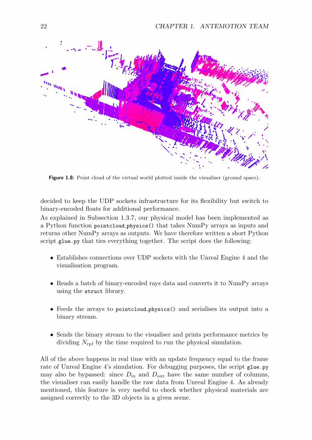
The company provides a program that visualises the simulated signals collected bythe LiDAR , based on the Python library Open3D. The program opens a whitewindow with drawn two black points, that are used to set the reference scale. Thephysical model gives as output a point cloud, composed by the coordinates of theimpacts points (q), for which the returned light intensity is above a fixed threshold,and the corresponding signal intensities (Pout).The program plots these points using an RGB colour map to associate a colour toeach intensity, reported with logarithmic scale (Fig. 1.8). The colour map spansfrom blue, for less intense signals, to red, for more intense ones. The program plotsthe point cloud in real time and periodically clears the windows to avoid excessiveoverdrawing. The point cloud can be visualised using the ground space or the carspace reference frames (Subsection 1.4.3), selecting the option through the UE4interface. Moreover, the user can decide to plot the raw point cloud generated byUnreal Engine 4, with a colour map based on the material IDs (IDmat), insteadof the intensities. We introduce this feature to check that associations betweenobject and material were right. In this case the colour map spans from yellow tored. Last, the program gives the possibility to overlap the visualised point cloudwith the picture of the virtual world (see Fig. 1.9). In this way, we can more easilyvalidate the implemented physical model.
Data flow
We have seen what kind of data is exchanged between Unreal Engine 4, ourphysical simulation and the visualiser, but we have not yet described how data isexchanged. In the geometrical LiDAR code, communication happened in real timeby exchanging floating-point numbers encoded as text over UDP sockets. Afterevaluating possible alternatives with AnteMotion’s developer Mattia Affabris, we
22 CHAPTER 1. ANTEMOTION TEAM
Figure 1.8: Point cloud of the virtual world plotted inside the visualiser (ground space).
decided to keep the UDP sockets infrastructure for its flexibility but switch tobinary-encoded floats for additional performance.
As explained in Subsection 1.3.7, our physical model has been implemented asa Python function pointcloud physics() that takes NumPy arrays as inputs andreturns other NumPy arrays as outputs. We have therefore written a short Pythonscript glue.py that ties everything together. The script does the following:
• Establishes connections over UDP sockets with the Unreal Engine 4 and thevisualisation program.
• Reads a batch of binary-encoded rays data and converts it to NumPy arraysusing the struct library.
• Feeds the arrays to pointcloud physics() and serialises its output into abinary stream.
• Sends the binary stream to the visualiser and prints performance metrics bydividing Nrpf by the time required to run the physical simulation.
All of the above happens in real time with an update frequency equal to the framerate of Unreal Engine 4’s simulation. For debugging purposes, the script glue.py
may also be bypassed: since Din and Dout have the same number of columns,the visualiser can easily handle the raw data from Unreal Engine 4. As alreadymentioned, this feature is very useful to check whether physical materials areassigned correctly to the 3D objects in a given scene.

1.4. IMPLEMENTATION OF A VIRTUAL LIDAR 23
Figure 1.9: Overlay between the UE4 virtual world and the generated point cloud. On top, thepoint cloud is produced using the geometrical model and the colour map is based onthe material IDs. On the bottom, the point cloud is generated using the implementedphysical model, and the colour map, that represents low (high) intensities with yellow(blue), is based on the returned intensity of each point.
1.4.5 Data flow for advanced physical models
In this subsection, we explain how the data structures described in Subsection 1.4.2have to be extended in order to support the richer physical models of Subsections1.3.5 and 1.3.6.
Data structures for the spot divergence model (roses)
If the basic physical model is extended by taking into account the effects of spotdivergence, the simulation of a single laser beam requires multiple rays, followingthe discretization process outlined in Subsection 1.3.5. As previously stated, wehave settled for a 5-rays model, with one ray at the centre of the beam and theother 4 rays arranged in a cross shape around it. The angle between the centralray and any of the surrounding rays is equal to the beam divergence Θ and can beconfigured by setting the beamDivergence parameter of the LiDAR component inUE4’s editor. The 5 rays in every beam can be visualised for debugging purposesby turning on the Boolean property bDebug.
24 CHAPTER 1. ANTEMOTION TEAM
Once again, the data associated to each ray is encoded as a vector
(px,py,pz,nx,ny,nz, IDmat),
but this time we need to fix an order for the rays that belong to the same beam.We have chosen the following order: the first ray is the central one; the other raysare counted in counter-clockwise order starting from the one on the right of thecentral one.Let Nbpf be the number of beams per frame. In the basic physical model, datafor each ray is stacked into a matrix of size Nbpf × 7. This time around we havean extra dimension (the ray index in every beam), so the input data Din is atensor of size Nbpf × 5× 7. In our code, we have chosen to store Din in row-majororder (generalised to tensors, i.e. contiguous elements are accessed by changingthe rightmost index). This is because row-major order is the default for both C++and NumPy.As explained in Subsection 1.3.5, each beam produces one point of output afterprocessing, so the data structure Dout is a matrix with 7 columns and at mostNbpf rows. The rows of Dout contain the same data as in the base physical model.
Data structures for the multiple reflections model (guns)
If the basic physical model is extended by taking into account the effects ofmultiple reflections, the description of the optical path of a single laser beamrequires multiple segments. Let pi−1 and pi be the endpoints of each segment,with pi being the position of the i-th hit point after the ray has bounced i − 1times. By definition, p0 is the position of the LiDAR detector, and the directionof the segment p1 − p0 is the same as the LiDAR ’s emitter. At every hit pointpi, the direction of the outcoming ray is computed by reflecting the incoming raypi − pi−1 along the surface normal ni. The index i goes from 1 to the maximumnumber of reflections allowed Nref. The variable Nref can be configured by settingthe maxBounces parameter of the LiDAR component in UE4’s editor. The segmentsof every beam’s optical path can be visualised for debugging purposes by turningon the Boolean property bDebug.Let θi be the angle (in degrees) between the segment pi − p0 and the segmentp1 − p0. Then, the data associated to each segment is encoded as a vector
(pix,p
iy,p
iz,n
ix,n
iy,n
iz, ID
imat, θ
i) for all i = 1, . . . , Nref.
If the ray that travels in the pi − pi−1 direction has no collisions with any objectin the scene, the corresponding data is the conventional vector
(1, 1, 1, 1, 0, 0, 0, 90).
Let Nppf be the number of optical paths per frame. In the basic physical model,data for each ray is stacked into a matrix of size Nppf × 7. This time around wehave an extra dimension (the segment index i in every optical path), so the inputdata Din is a tensor of size Nppf ×Nref × 8. Once again, we have chosen to storeDin in row-major order.
1.5. DESCRIPTION OF THE DATA GENERATED BY THE MODELS 25
If IDimat = 0, then our physical model knows that the i-th reflected ray has no
intersection with any surface. Therefore, the vectors
(pjx,p
jy,p
jz,n
jx,n
jy,n
jz, ID
jmat, θ
j)
for all j = i+ 1, . . . , Nref are technically redundant. However, we store them inDin anyway just to keep the size of every path’s data constant.As explained in Subsection 1.3.6, each optical path produces one point of outputafter processing, so the data structure Dout is a matrix with 7 columns and atmost Nppf rows. The rows of Dout contain the same data as in the base physicalmodel.
1.5 Description of the data generated by themodels
1.5.1 Description of the test scene
The virtual world made available by AnteMotion is an industrial urban scenariostructured in blocks with industrial buildings and sheds. Along the roads you canfind signs, cars, pedestrian crossings and some obstacles made up of municipalwaste. We focused our attention on an area where a car was present to have aprecise benchmark for the model.
1.5.2 Remarkable cases description
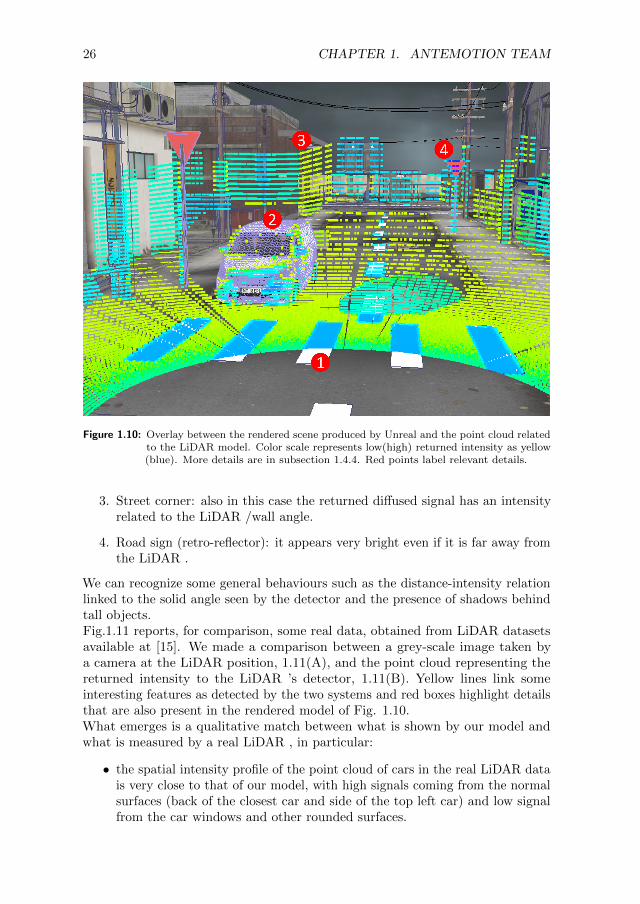
This section is intended to validate the data produced by the model. We show asimulated point cloud in which physical behaviours are clearly reproduced andmake a qualitative comparison with a real LiDAR point cloud taken from theKITTI repository [15]. The outcome of the model mostly depends on the accuracyof the material database, in fact it can be fine-tuned to a specific scene or targetby a careful selection of the materials coefficients. The best accuracy would beachieved by including coefficients directly derived from dedicated experiments suchas: direct laser reflectivity versus angle measure or real LiDAR data analysis ofthe collected intensity in a controlled environment.Figure 1.10 reports an overlay between the rendered scene produced by Unrealand the point cloud produced by the LiDAR model. Major frames highlighted byred circles are described below:
1. pedestrian crossings (partial retro-reflector): they are close to the LiDARdevice and have high reflectivity. A very high signal is measured comparedto the asphalt.
2. car: it is composed of several materials such as metals, glasses and tires. Theangle dependence of the diffusion/reflection from metal is clearly described.The front of the car has a very high signal compared to the other metallicparts. The front glass is also recognised as black because all the light isreflected upwards.
26 CHAPTER 1. ANTEMOTION TEAM
Figure 1.10: Overlay between the rendered scene produced by Unreal and the point cloud relatedto the LiDAR model. Color scale represents low(high) returned intensity as yellow(blue). More details are in subsection 1.4.4. Red points label relevant details.
3. Street corner: also in this case the returned diffused signal has an intensityrelated to the LiDAR /wall angle.
4. Road sign (retro-reflector): it appears very bright even if it is far away fromthe LiDAR .
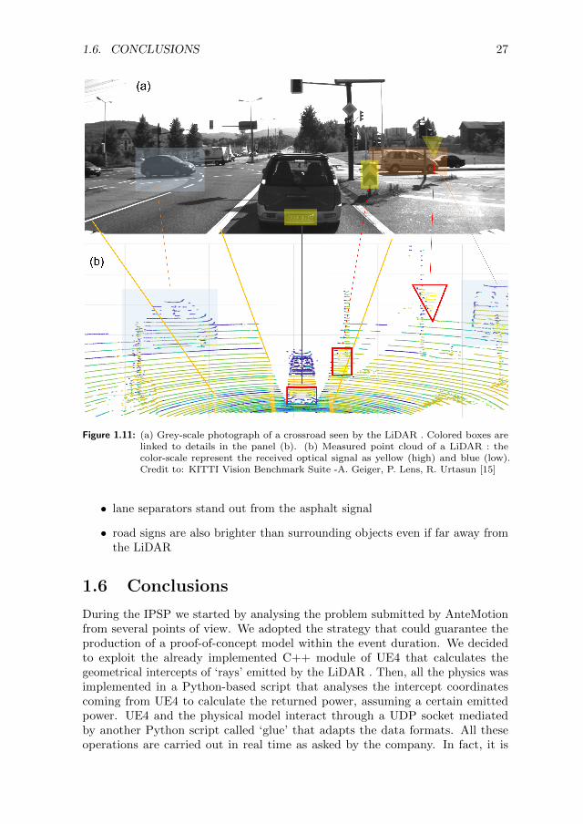
We can recognize some general behaviours such as the distance-intensity relationlinked to the solid angle seen by the detector and the presence of shadows behindtall objects.Fig.1.11 reports, for comparison, some real data, obtained from LiDAR datasetsavailable at [15]. We made a comparison between a grey-scale image taken bya camera at the LiDAR position, 1.11(A), and the point cloud representing thereturned intensity to the LiDAR ’s detector, 1.11(B). Yellow lines link someinteresting features as detected by the two systems and red boxes highlight detailsthat are also present in the rendered model of Fig. 1.10.What emerges is a qualitative match between what is shown by our model andwhat is measured by a real LiDAR , in particular:
• the spatial intensity profile of the point cloud of cars in the real LiDAR datais very close to that of our model, with high signals coming from the normalsurfaces (back of the closest car and side of the top left car) and low signalfrom the car windows and other rounded surfaces.
1.6. CONCLUSIONS 27
Figure 1.11: (a) Grey-scale photograph of a crossroad seen by the LiDAR . Colored boxes arelinked to details in the panel (b). (b) Measured point cloud of a LiDAR : thecolor-scale represent the received optical signal as yellow (high) and blue (low).Credit to: KITTI Vision Benchmark Suite -A. Geiger, P. Lens, R. Urtasun [15]
• lane separators stand out from the asphalt signal
• road signs are also brighter than surrounding objects even if far away fromthe LiDAR
1.6 Conclusions
During the IPSP we started by analysing the problem submitted by AnteMotionfrom several points of view. We adopted the strategy that could guarantee theproduction of a proof-of-concept model within the event duration. We decidedto exploit the already implemented C++ module of UE4 that calculates thegeometrical intercepts of ‘rays’ emitted by the LiDAR . Then, all the physics wasimplemented in a Python-based script that analyses the intercept coordinatescoming from UE4 to calculate the returned power, assuming a certain emittedpower. UE4 and the physical model interact through a UDP socket mediatedby another Python script called ‘glue’ that adapts the data formats. All theseoperations are carried out in real time as asked by the company. In fact, it is
28 CHAPTER 1. ANTEMOTION TEAM
possible to run the physics model while maintaining the typical frame rate atwhich UE4 runs (120 FPS in our tests).The physical model accounts for all the principal phenomena that influence theperformance of a real LiDAR such as diffusion, reflection, atmospheric absorption,diffraction (roses), multiple reflections (guns), detection noise, and device efficiency.Most of these parameters are material dependent. For this reason, we createda database where materials properties are fixed by three coefficients that canbe optimised by the final user. The most accurate way would be to createan experimental database where the coefficients are directly measured throughdedicated experiments.Furthermore, the physics can be improved by adding the refraction effect indielectric materials. This phenomenon can be crucial in environments where alot of glass is present as, for instance, in a modern city or along streets withshop windows. Another important effect is the so-called fata morgana, a mirageseen along streets during summer. Especially in warm climate cities, the asphaltbecomes very hot, determining an abrupt change of the refractive index of the airclose to the surface, which causes an upwards deflection of the LiDAR ’s rays withlarge angles of incidence. This reduces the amount of returned rays and so theinformation related to the horizontal street signs. Even the sun irradiance, thatis varying during the day, should be considered because it affects the LiDAR ’sdetection system that becomes ‘blind’ under certain circumstances.In conclusion, within the short time span of the IPSP event, we successfullyproduced an implementation of a physical model that includes the major physicalphenomena involved in the LiDAR working mechanisms. The resulting numericalmodel is capable of running in real-time together with UE4 simulating theenvironment and a third software visualising the output.
Bibliography
[1] Antemotion. URL https://www.antemotion.com/.
[2] Santiago Royo and Maria Ballesta-Garcia. An overview of lidar imagingsystems for autonomous vehicles. Applied Sciences, 9(19), 2019. ISSN 2076-3417. doi: 10.3390/app9194093. URL https://www.mdpi.com/2076-3417/
9/19/4093.
[3] Paul F. McManamon. LiDAR Technologies and Systems. 2019. doi:https://doi.org/10.1117/3.2518254.
[4] A. Ortiz Arteaga, D. Scott, and J. Boehm. Initial investigation of a low-costautomotive lidar system. The International Archives of the Photogrammetry,Remote Sensing and Spatial Information Sciences, XLII-2/W17:233–240,2019. doi: 10.5194/isprs-archives-XLII-2-W17-233-2019. URL https:
//www.int-arch-photogramm-remote-sens-spatial-inf-sci.net/
XLII-2-W17/233/2019/.
[5] Bashar Alsadik. Performance assessment of mobile laser scanning systemsusing velodyne hdl-32e. Surveying and Geospatial Engineering Journal, 1(1):
BIBLIOGRAPHY 29
28 – 33, 01 2021. doi: 10.38094/sgej116. URL https://sgej.org/index.
php/sgej/article/view/6.
[6] Thorlabs. URLhttps://www.thorlabs.com/newgrouppage9.cfm?objectgroup_id=4.
[7] Velodyne. URL https://velodynelidar.com/products/alpha-prime/.
[8] John E Greivenkamp. Field guide to geometrical optics, volume 1. SPIE pressBellingham, WA, 2004.
[9] J. Wojtanowski, M. Zygmunt, M. Kaszczuk, Z. Mierczyk, and M. Muzal.Comparison of 905 nm and 1550 nm semiconductor laser rangefinders’performance deterioration due to adverse environmental conditions. Opto-Electronics Review, 22(3):183–190, 09 2014. ISSN 1896-3757. doi: 10.2478/s11772-014-0190-2. URL https://doi.org/10.2478/s11772-014-0190-2.
[10] Mario Bijelic, Tobias Gruber, and Werner Ritter. A benchmark for lidarsensors in fog: Is detection breaking down? pages 760–767, 06 2018. doi:10.1109/IVS.2018.8500543.
[11] Jake Jacobsen. Application in illumination design - analaysing lidar returnsignal strengths for target optical surfaces and atmospheric conditions.Synopsys, white paper, 05 2020. URL shorturl.at/fEOSX.
[12] Stefan Muckenhuber, Hannes Holzer, and Zrinka Bockaj. Automotive lidarmodelling approach based on material properties and lidar capabilities.Sensors, 20(11), 2020. ISSN 1424-8220. doi: 10.3390/s20113309. URLhttps://www.mdpi.com/1424-8220/20/11/3309.
[13] Jet Propulsion Laboratory California Institute of Technology NASA. Ecostressspectral library. URL https://speclib.jpl.nasa.gov/library.
[14] URL https://docs.unrealengine.com.
[15] A Geiger, P. Lens, and R. Urtasun. URL http://www.cvlibs.net/
datasets/kitti/raw_data.php.

CHAPTER
TWO
COOLING OF A FLUID BY MEANS OF PHASETRANSITION HEAT SINKS
P. Battocchio, R. Di Falco, R. Iacomino, L. Pace, L. Pagani, S. Quercetti, G.
Sacco, and S. Santi
Tutor: Michele Orlandi
2.1 Introduction
2.1.1 The company
Areaderma is a cosmetic company in Trentino that has been producing cosmeticsfor third parties and class I and IIA medical devices for more than 30 years[1].The research and development team is constantly looking for new technologies,cutting-edge methodologies, modern raw materials and new formulative solutionsto provide to customers. Areaderma aims at the environmental sustainability ofits business. In this regard, to reduce more and more the energy consumption,the company would like to change the technology used to cool products duringprocessing. For the current process, the company uses machines where the heatingis obtained by heating elements immersed in the reactor tank, while cooling isachieved by circulating cold water in an insulated cavity surrounding the tankswhere the product is processed. In addition to being energy-intensive, the coolingphase takes a long time. The goal, therefore, is to be able to optimize times andreduce energy consumption during this phase of processing, switching to a modularsetup, capable of processing an emulsion in standardized quantity over a fixedtime range. This will allow the possibility to process several different types ofproducts in the same working shift. The idea is to use a removable tank for eachdifferent product so that cleaning and maintenance operations can be done offlinewhile the setup is processing the next batch in the sequence.
31
32 CHAPTER 2. AREADERMA TEAM
2.1.2 The problem
The problem proposed by Areaderma during the IPSP 2021 event concerns thestudy of a cooling system based on Heat Pipes. Since the tank is rotating, removableand made of plastic material, the water-bath configuration cannot be exploiteddue to the excessive complexity and/or the very low efficiency. A natural questionarises: whether a more efficient way of cooling cosmetic creams exists and if suchmethodology could be in principle implemented in an industrial environment. Tofind an answer, Areaderma proposed to our group to study if heat pipes can begood candidates to lower the temperature of cream in the shortest time possibleand if this device is to be considered among the solutions that can be used in theirprocesses.The specific goal is to cool a mass of cosmetic cream composed of a mix of 75% ofwater and 25% of oil, lowering the temperature from 85°C to 35°C in 300 seconds.The surface of the tank available to insert cooling devices is a circular sector sincethe remaining area is needed for the mechanical parts and to add ingredients.
2.2 Heat Pipe
The heat pipe is a highly effective passive device used to transmit heat. Heat pipesallow high transfer rates over considerable distances, with minimal temperaturedrops, exceptional flexibility, simple construction, and easy control, all without aneed for external pumping power. The heat pipe is essentially a closed, evacuatedchamber whose inside walls are covered with a capillary structure that is saturatedwith a volatile fluid, usually water.The operation of a heat pipe is based on cyclic phase transitions of the fluidinside it and combines two principles of physics: vapor heat transfer and capillaryaction. Vapor heat transfer is responsible for transporting the heat energy fromthe evaporator section at one end of the pipe to the condenser section at theother end. Thus heat is subtracted to the system by exploiting the latent heat ofevaporation of water.Capillary action is responsible for returning the condensed working fluid backto the evaporator section to complete the cycle[2]. The function of the workingfluid within the heat pipe is to absorb the heat energy received at the evaporatorsection and remove it from the system by undergoing a phase transition (that is,evaporation), then transport it through the pipe and release this energy at thecondenser end by reverting back to the liquid phase. When a liquid vaporizes, twophenomena happen. First, a large quantity of heat is absorbed from the contactarea, because energy is needed to separate molecules that are in contact in theliquid state. The quantity of energy required to evaporate a unit mass of liquidat a given temperature is called the latent heat of vaporization.Second, as theworking fluid vaporizes, the pressure at the evaporator end of the pipe increases,due to the thermal excitation of the molecules comprising the newly created vapor.The vapor pressure leads to a pressure gradient between the ends of the pipethat causes the vapor to move toward the condenser section. When the vaporarrives at the condenser section it encounters a temperature lower than that of the
2.3. ENERGY BALANCE 33
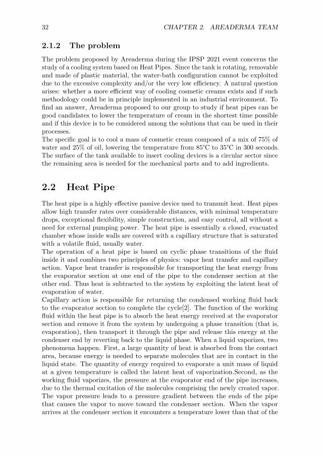
evaporator, therefore it reverts to the liquid state by releasing the thermal energystored in its heat of vaporization. Since the heat exchange at the two ends of theheat pipe occurs thanks to phase transitions, the temperature along the entirelength of the heat pipe tends to remain constant. The movement of the condensedworking fluid back to the evaporator side is then provided by capillary action.Different types of working fluids, such as water, acetone, methanol, ammonia, orsodium can be used in heat pipes based on the required operating temperature.The length of a heat pipe is divided into three parts: the evaporator section,adiabatic (transport) section, and condenser section as depicted in Fig. 2.1 [3].The most common heat pipes have a diameter between 0.2 cm and 1 cm and alength between 5 cm and 35 cm and can dissipate from 9 W to 220 W.
Figure 2.1: Heat Pipe [3]
2.3 Energy Balance
In this section, we describe the energy balance initially considered assuming wateras working fluid. We have that: Qa = m(H2O)Cp∆T +mH2Oλ Where Qa is theabsorbed heat, mH2O is the water mass, Cp is the specific heat capacity, ∆T is thetemperature increment and λ is the latent heat of evaporation. The first term ofthe right side of the equation corresponds to the sensible heat, which is negligiblebecause it is about three orders of magnitude smaller than the latent heat ofvaporization.Through this equation, we determined that, in order to subtract to the systemthe desired amount of heat, the total amount of water that should vaporize is
mH2O = 1.35kg and so, corresponding todm
dt= 4.48
g
sin a time interval of 300 s.
Considering that the emulsion must reach a temperature of 35°C, we have assumedthat the boiling point for the water inside the heat pipe is 30°C, so we determinedan inner pressure of 0.03 bar.We then designed, implemented and tested two different approaches: the first one(Heat Pipe Array Cooler) exploits a series of heat pipes; while the second one(Phase Transition Pressure Cooler) partially exploits the working principles ofheat pipes and is developed to overcome their main limitations.
34 CHAPTER 2. AREADERMA TEAM
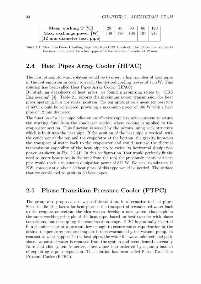
Mean working T [°C] 20 40 60 80 120Max. exchange power [W] 148 178 186 197 218
(12 mm diameter heat pipe)
Table 2.1: Maximum Power Handling Capability from CRS datasheet. The bottom row representsthe maximum power for a heat pipe with the external diameter of 12 mm.
2.4 Heat Pipes Array Cooler (HPAC)
The most straightforward solution would be to insert a high number of heat pipesin the hot emulsion in order to reach the desired cooling power of 11 kW. Thissolution has been called Heat Pipes Array Cooler (HPAC).By studying datasheets of heat pipes, we found a promising series by “CRSEngineering” [4]. Table 2.1 reports the maximum power transmission for heatpipes operating in a horizontal position. For our application a mean temperatureof 60°C should be considered, providing a maximum power of 186 W with a heatpipe of 12 mm diameter.
The function of a heat pipe relies on an effective capillary action system to returnthe working fluid from the condenser section where cooling is applied to theevaporator section. This function is served by the porous lining wick structurewhich is built into the heat pipe. If the position of the heat pipe is vertical, withthe condenser at the top and the evaporator at the bottom, the gravity improvesthe transport of water back to the evaporator and could increase the thermaltransmission capability of the heat pipe up to twice its horizontal dissipationpower, as shown in Fig. 2.2 [4]. In this configuration (that would perfectly fit theneed to insert heat pipes in the tank from the top) the previously mentioned heatpipe would reach a maximum dissipation power of 372 W. We need to subtract 11KW, consequently, about 30 heat pipes of this type would be needed. The surfacethat we considered to position 30 heat pipes.
2.5 Phase Transition Pressure Cooler (PTPC)
The group also proposed a new possible solution, in alternative to heat pipes.Since the limiting factor for heat pipes is the transport of recondensed water backto the evaporator section, the idea was to develop a new system that exploitsthe same working principle of the heat pipe, based on heat transfer with phasetransitions, but decoupling the condensation stage. H 2O is gradually insertedin a chamber kept at a pressure low enough to ensure water vaporization at thedesired temperature; produced vapour is then evacuated by the vacuum pump. Incontrast to what happens in the heat pipes, the water follows a unidirectional path,since evaporated water is removed from the system and recondensed externally.Note that this system is active, since vapor is transferred by a pump insteadof exploiting vapour expansion. This solution has been called Phase TransitionPressure Cooler (PTPC).
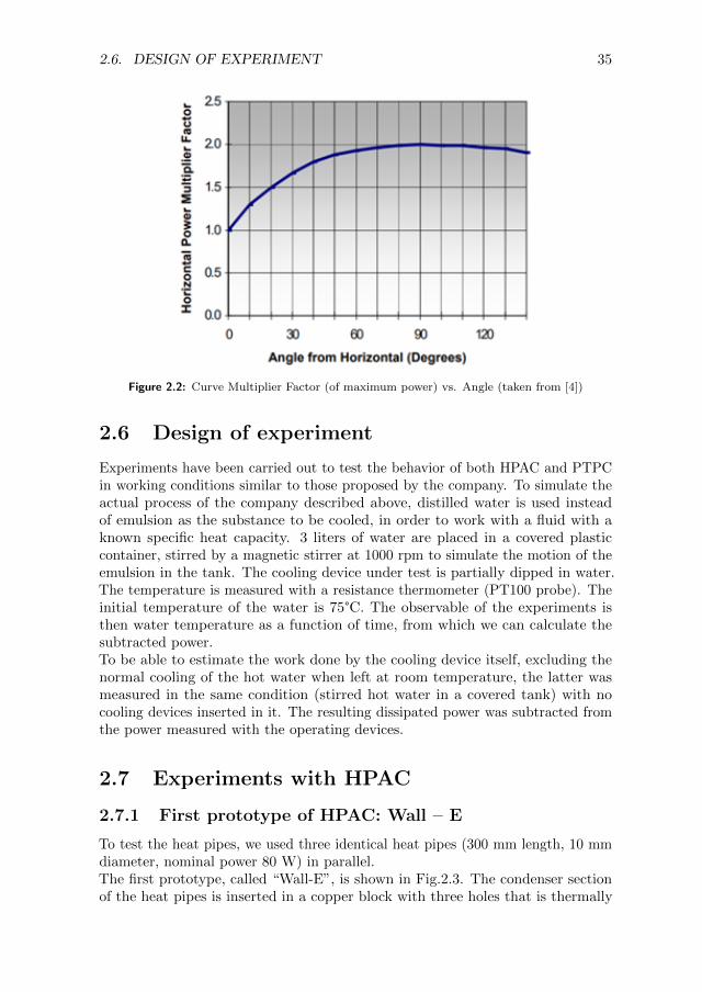
2.6. DESIGN OF EXPERIMENT 35
Figure 2.2: Curve Multiplier Factor (of maximum power) vs. Angle (taken from [4])
2.6 Design of experiment
Experiments have been carried out to test the behavior of both HPAC and PTPCin working conditions similar to those proposed by the company. To simulate theactual process of the company described above, distilled water is used insteadof emulsion as the substance to be cooled, in order to work with a fluid with aknown specific heat capacity. 3 liters of water are placed in a covered plasticcontainer, stirred by a magnetic stirrer at 1000 rpm to simulate the motion of theemulsion in the tank. The cooling device under test is partially dipped in water.The temperature is measured with a resistance thermometer (PT100 probe). Theinitial temperature of the water is 75°C. The observable of the experiments isthen water temperature as a function of time, from which we can calculate thesubtracted power.To be able to estimate the work done by the cooling device itself, excluding thenormal cooling of the hot water when left at room temperature, the latter wasmeasured in the same condition (stirred hot water in a covered tank) with nocooling devices inserted in it. The resulting dissipated power was subtracted fromthe power measured with the operating devices.
2.7 Experiments with HPAC
2.7.1 First prototype of HPAC: Wall – E
To test the heat pipes, we used three identical heat pipes (300 mm length, 10 mmdiameter, nominal power 80 W) in parallel.The first prototype, called “Wall-E”, is shown in Fig.2.3. The condenser sectionof the heat pipes is inserted in a copper block with three holes that is thermally
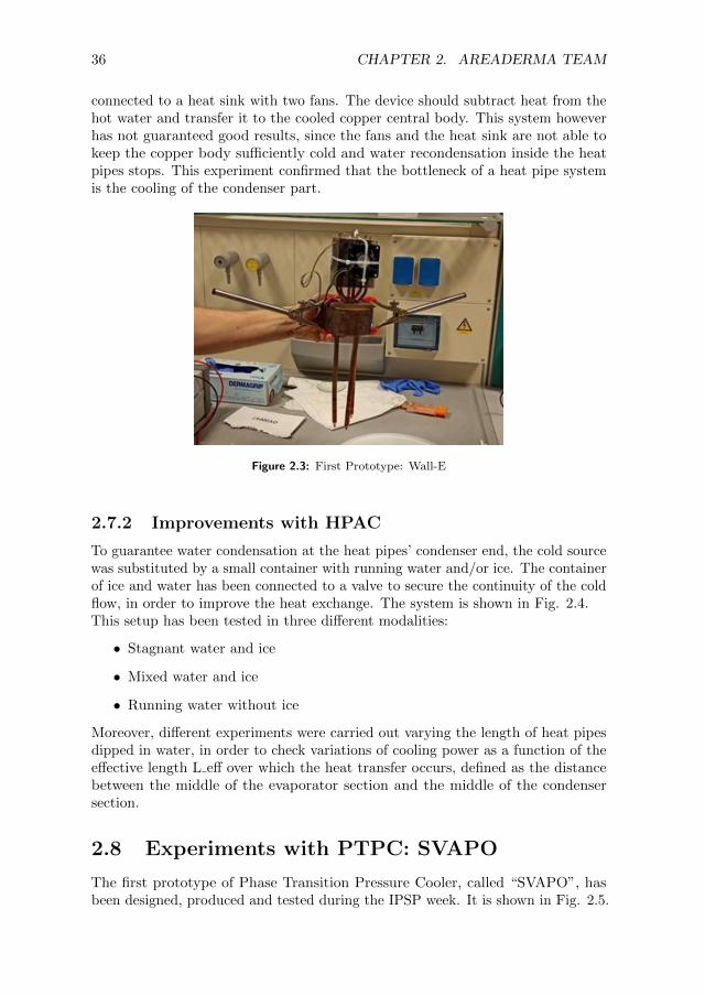
36 CHAPTER 2. AREADERMA TEAM
connected to a heat sink with two fans. The device should subtract heat from thehot water and transfer it to the cooled copper central body. This system howeverhas not guaranteed good results, since the fans and the heat sink are not able tokeep the copper body sufficiently cold and water recondensation inside the heatpipes stops. This experiment confirmed that the bottleneck of a heat pipe systemis the cooling of the condenser part.
Figure 2.3: First Prototype: Wall-E
2.7.2 Improvements with HPAC
To guarantee water condensation at the heat pipes’ condenser end, the cold sourcewas substituted by a small container with running water and/or ice. The containerof ice and water has been connected to a valve to secure the continuity of the coldflow, in order to improve the heat exchange. The system is shown in Fig. 2.4.This setup has been tested in three different modalities:
• Stagnant water and ice
• Mixed water and ice
• Running water without ice
Moreover, different experiments were carried out varying the length of heat pipesdipped in water, in order to check variations of cooling power as a function of theeffective length L eff over which the heat transfer occurs, defined as the distancebetween the middle of the evaporator section and the middle of the condensersection.
2.8 Experiments with PTPC: SVAPO
The first prototype of Phase Transition Pressure Cooler, called “SVAPO”, hasbeen designed, produced and tested during the IPSP week. It is shown in Fig. 2.5.
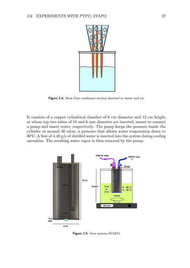
2.8. EXPERIMENTS WITH PTPC: SVAPO 37
Figure 2.4: Heat Pipe condenser section inserted in water and ice
It consists of a copper cylindrical chamber of 6 cm diameter and 12 cm height,at whose top two tubes of 10 and 6 mm diameter are inserted, meant to connecta pump and insert water, respectively. The pump keeps the pressure inside thecylinder at around 30 mbar, a pressure that allows water evaporation down to30°C. A flow of 4.48 g/s of distilled water is inserted into the system during coolingoperation. The resulting water vapor is then removed by the pump.
Figure 2.5: New system SVAPO

38 CHAPTER 2. AREADERMA TEAM
2.9 Results and discussion
The graph in Fig. 2.6 shows the temperature as a function of time of the twodevices designed. The blue curve is obtained with the HPAC system consistingof three heat pipes in mixed water and ice, while the red one shows resultsobtained with the SVAPO. For comparison, the dashed line represents the trend oftemperature as a function of time without the use of any cooling device (“Blank”in the picture).
Figure 2.6: Water temperature as a function of time
The HPAC succeeds in lowering the temperature of the water from 73°C toapproximately 45°C in 450 seconds, while Svapo, in the same amount of time,succeeds in reaching a temperature of about 63°C. The resulting subtracted poweris 680 W for the HPAC and 300 W for SVAPO.At the same time, simulations of the operation of HPAC were carried out bymodifying a COMSOL model [5] and obtaining results in the same order ofmagnitude of the measured value.An additional experiment, with a similar procedure to the others, was also carriedout with SVAPO to check its correct working and confirm that heat is subtractedfrom the system by the evaporation of the water inside the copper chamber. Duringthis experiment a fixed quantity of water is injected into the chamber where itevaporates cooling down the hot water in the container; if no more water is injected,once it is completely evaporated the temperature decrease in time slows downsince heat is no more absorbed by the system. This can be seen in Fig. 2.7, whichshows a step behavior of the temperature with time: each time water is injectedinto the system, cooling velocity increases, and then it progressively decreasesas all the water inside the chamber evaporates, confirming the expected workingprinciple of this apparatus.
The best results in terms of powers subtracted to the hot water mass are obtainedusing the HPAC system. However, it must be noted that the SVAPO was notworking in its optimal conditions and can likely be improved substantially:
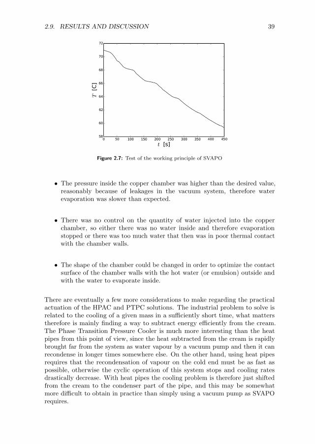
2.9. RESULTS AND DISCUSSION 39
Figure 2.7: Test of the working principle of SVAPO
• The pressure inside the copper chamber was higher than the desired value,reasonably because of leakages in the vacuum system, therefore waterevaporation was slower than expected.
• There was no control on the quantity of water injected into the copperchamber, so either there was no water inside and therefore evaporationstopped or there was too much water that then was in poor thermal contactwith the chamber walls.
• The shape of the chamber could be changed in order to optimize the contactsurface of the chamber walls with the hot water (or emulsion) outside andwith the water to evaporate inside.
There are eventually a few more considerations to make regarding the practicalactuation of the HPAC and PTPC solutions. The industrial problem to solve isrelated to the cooling of a given mass in a sufficiently short time, what matterstherefore is mainly finding a way to subtract energy efficiently from the cream.The Phase Transition Pressure Cooler is much more interesting than the heatpipes from this point of view, since the heat subtracted from the cream is rapidlybrought far from the system as water vapour by a vacuum pump and then it canrecondense in longer times somewhere else. On the other hand, using heat pipesrequires that the recondensation of vapour on the cold end must be as fast aspossible, otherwise the cyclic operation of this system stops and cooling ratesdrastically decrease. With heat pipes the cooling problem is therefore just shiftedfrom the cream to the condenser part of the pipe, and this may be somewhatmore difficult to obtain in practice than simply using a vacuum pump as SVAPOrequires.

40 CHAPTER 2. AREADERMA TEAM
2.10 Conclusions
The problem proposed by Areaderma consisted in finding a way to rapidly cooldown a given mass of cream in the shortest time possible. The method initiallyproposed by the company was to exploit heat pipes, passive elements with thecapacity of fast transferring heat from one side to the other by exploiting vapourexpansion inside the pipe.The work done during the week can be summarized as follows. Initially a firstsystem based on heat pipes called Wall-E was developed, this allowed a betterunderstanding of the working principle of heat pipes and their main limitations.We found that the main problem of the heat pipes is related to the efficientcooling of their condenser end, which otherwise stops the cyclic behavior of theseelements. The study of the operation principles of heat pipes was also carried onby performing some simulations in COMSOL.The work then proceeded with the development of two cooling systems: one basedon heat pipes, which is an evolution of Wall-E, and another one that exploitsonly the evaporation part of the heat pipe cycle, called SVAPO. The evolutionof Wall-E consisted in an improvement of the cooling of the heat pipes by usingice, while SVAPO exploited the low temperature evaporation of water obtainedreducing pressure in a copper chamber, with the generated vapour removed bymeans of a vacuum pump.Some experiments were carried out by cooling a fixed mass of water using thesesystems in order to measure their efficiency. The system based on heat pipesturned out to be more efficient than SVAPO, however SVAPO was only in aninitial stage of development and was not working in its optimal conditions. Wethen concluded that SVAPO can be a possible interesting solution for Areaderma,both in terms of dissipated power and from the practical actuation point of view.
Bibliography
[1] Areaderma. URL https://www.areaderma.it/.
[2] G. Yale Eastman. The heat pipe. Scientific American, 218(5):38–47, may1968. doi: 10.1038/scientificamerican0568-38. URL https://doi.org/10.
1038%2Fscientificamerican0568-38.
[3] Amir Faghri. Review and advances in heat pipe science and technology.Journal of Heat Transfer, 134(12), oct 2012. doi: 10.1115/1.4007407. URLhttps://doi.org/10.1115%2F1.4007407.
[4] URL https:
//www.heat-pipes.com/media/a4-heat-pipes-v26-hadston-2010.pdf.
[5] URL https://www.comsol.it/model/
heat-pipe-with-accurate-liquid-and-gas-properties-90311.

CHAPTER
THREE
POSITIONING OF A WEATHER STATION FOR THEDETECTION OF ENVIRONMENTAL DATA OF A
TURBINE FOR TECHNICAL SNOWMAKING
F. Bellamoli, S. Bini, F. Brugnara, M. Castelluzzo, E. Cozzolino, G. Dalmasso,
R. Franchi, and C. Montesano
Tutor: Luca Tubiana
At the request of the company, the technical part of this chapter has been
replaced by a generic summary of the work carried out by the team during
IPSP2021.
3.1 Introduction
3.1.1 The company
Since 1990 TechnoAlpin has been designing and manufacturing turnkeysnowmaking systems for ski resorts all over the world. The company’s turnoverhas reached 230 million euros. The love for snow and the passion for innovationhave transformed TechnoAlpin into a leader in the sector, which mainly aims tooffer each customer a customized solution.Each plant is thus subjected to careful evaluation to adapt it to the specific needsof individual customers. The product range is constantly being expanded inorder to produce snow of the highest quality with maximum energy efficiency. Inaddition to outdoor solutions, TechnoAlpin also offers turnkey solutions for indoorsnowmaking, in order to make the exclusive snow experience accessible at anylatitude. Over 2,400 customers in more than 55 countries rely on TechnoAlpin’sknow-how, followed by over 700 employees in 35 offices.
41

42 CHAPTER 3. TECHNOALPIN TEAM
3.1.2 The problem
A snowmaking system consists of several components: pipes, pumping stations,wells, basins for water collection and snow guns often called ”cannons”. Thelatter can be of different types, mainly we can divide them into turbines orlances. TechnoAlpin produces various models of snow blowers. Each turbineis equipped with its own weather station. In order to produce snow, certainenvironmental conditions must be met. In particular, the combination of airtemperature and humidity, defined as wet bulb temperature for insiders, must bebelow a certain threshold. It is therefore essential to have precise weather valuesfor each snowmaking point. The turbines are usually located on the edges of theski slopes at a distance of about 50-100 m from one another. It may thereforehappen that one turbine is a few kilometers away from another one and at analtitude of even 1000-1500 m higher. This means that if with the turbine furtherupstream snow can be produced due to the correct environmental conditions,it does not necessarily mean that there are the same conditions for the turbinefurther downstream from the plant.All turbines can operate automatically controlled by the centralized managementsoftware. It is therefore essential to correctly measure the weather data, especiallyin extreme conditions, that is, when a variation of even half a degree meansthat water and not snow comes out of the turbine. In the same way, an incorrectdetection can lead to a shutdown of the turbine when it could instead be productive.The weather station in the old TechnoAlpin turbine models was positioned outsidethe turbine. In the new models, however, it has been integrated into the turbinecover as can be seen in Fig.3.1.
Figure 3.1: TechnoAlpin TR10 snow generator
Therefore, the challenge proposed by TechnoAlpin is to evaluate an alternativepositioning of the turbine weather station such as to be able to detect environmentalvalues with extreme precision without these being minimally influenced by anyfactors that may lead to an alteration of the values themselves (for examplepresence of snow, ice near the sensors, etc.)
3.2. THE SOLUTION 43
3.2 The solution
In the study carried out during the IPSP2021, the team of PhD and Master studentsworked in parallel with experimental measurements on snow generators at theTechnoAlpin headquarters in Bolzano and with theoretical models to characterizethe temperature behavior inside the turbine.The results clearly show that the observed deviation between the temperaturemeasured inside or outside the turbine depends on the operation of the turbineitself. These results derive from different temperature measurements carried out indifferent conditions: generator inside or outside the laboratory, different climaticconditions outside, etc.In particular, the measurements confirmed what the company previously observedthat the temperature inside the hull is higher than the outside temperature. Theteam then concentrated on establishing the coefficient of the difference noted.Through the thermodynamic study of the system, the two main contributions thatcause the temperature coefficient have been analyzed: a) the energy transferredfrom the fan to the air in the form of pressure and kinetic energy and b) thedissipated energy that heats the turbine and the air inside.It has been seen that the experimental and theoretical approaches have providedconsistent results, thus proving that the main physical phenomena involved havebeen correctly identified. The values obtained from the study give the companythe opportunity to evaluate interesting ideas for a new design of the studied device.The company was advised to carry out a series of experimental tests in typicalworking conditions, that is, in winter and with low temperatures, to further confirmthe proposed model, even if the thermodynamic considerations studied are stillrobust.


CREDITS
45

46 CREDITS
The entire group on the opening day
From left to right, front row on knees: Bruno Degli Esposti, Ersilia Cozzolino,Sofia Santi.
From left to right, back row: Mattia Affabris (AnteMotion), MicheleCastelluzzo, Luca Pagani, Luca Gasbarro (AnteMotion), Sara Rabaglia, VivianaMaria Filı, Riccardo Franchi, Alessandro Zunino, Fabio Callegari, Giuseppe Sacco,Federico Bellamoli, Rossella Di Falco, Pietro Battocchio, Ludovica Pace, GiorgioDalmasso (on knees), Luisa Cunico (TechnoAlpin), Romano Iacomino, DavidTschager (TechnoAlpin), Massimo Stroppari (Areaderma), Cesare Montesano,Luigi Miori (Areaderma), Davide Bazzanella, Sebastiano Bontorin, FrancescaScandolari (Areaderma), Fabio Brugnara, Louise Wolswijk, Flavio Deflorian(Rector of the University of Trento), Sophie Bini, Mattia Mancinelli (Departmentof Physics, UniTrento), Giuseppe Caputo (Head of Research Valorization andImpact Office, UniTrento), Michele Orlandi (Department of Physics, UniTrento),Luca Tubiana (Department of Physics, UniTrento).
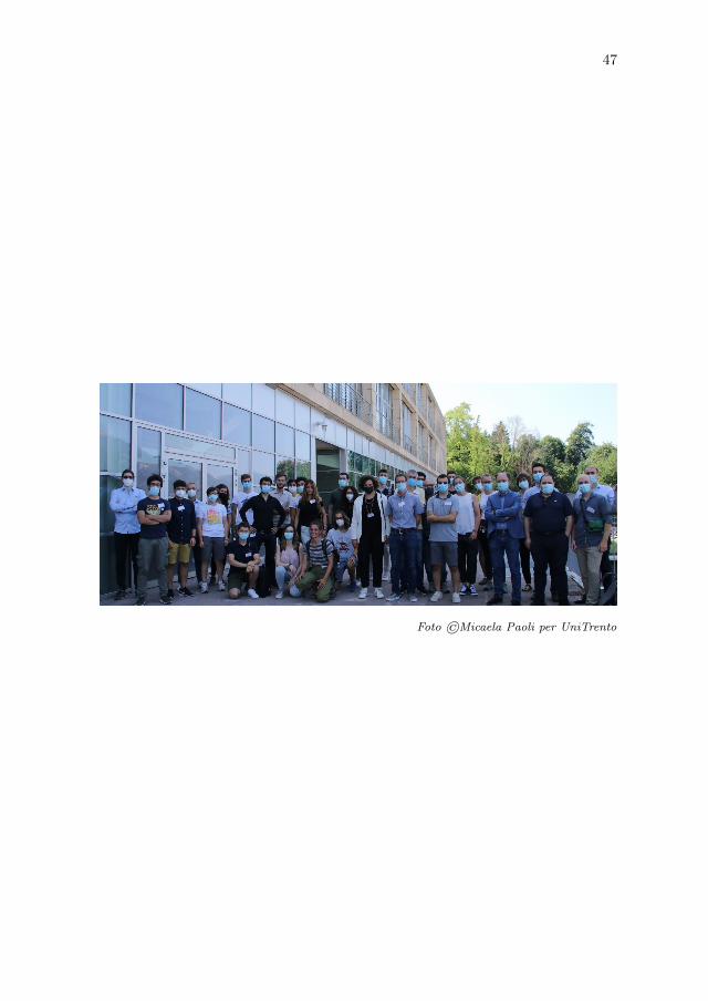
47
Foto ©Micaela Paoli per UniTrento

48 CREDITS
AnteMotion team
From left to right: Mattia Affabris, Alessandro Zunino, Fabio Callegari,Mattia Mancinelli, Sara Rabaglia, Louise Wolswijk, Davide Bazzanella, SebastianoBontorin, Bruno Degli Esposti.

49
Foto ©Mattia Mancinelli per UniTrento

50 CREDITS
Areaderma team
From left to right: Giuseppe Sacco, Sofia Santi, Ludovica Pace, Rossella Di Falco,Massimo Stroppari, Francesca Scandolari, Michele Orlandi, Pietro Battocchio,Sara Quercetti, Luca Pagani, Romano Iacomino.
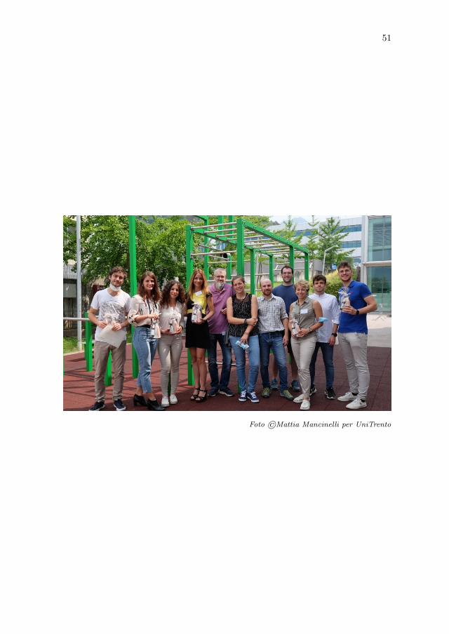
51
Foto ©Mattia Mancinelli per UniTrento

52 CREDITS
TechnoAlpin team
From left to right Fabio Brugnara, Riccardo Franchi, Luca Tubiana, GiorgioDalmasso, Cesare Montesano, Luisa Cunico, David Tschager, Sophie Bini, FedericoBellamoli, Michele Castelluzzo, Ersilia Cozzolino.
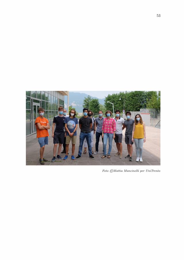
53
Foto ©Mattia Mancinelli per UniTrento

ACKNOWLEDGMENTS
Foremost, we would like to express our special thanks to the organizing bodiesof Industrial Problem Solving with Physics: Department of Physics, DoctoralSchool in Physics, Research Support and Valorization Division of the Universityof Trento, Confindustria Trento and Polo Meccatronica-Trentino Sviluppo. Weare particularly grateful to the head of the Department of Physics, Prof. FrancoDalfovo, for his constant interest and support. We thank Vanessa Ravagni andGiuseppe Caputo for their advice and assistance regarding intellectual propertiesand Alessandro Santini, Daniele Berti and Paolo Gregori for helping us get intouch with some potential participating companies.We extend our special thanks to all the companies which believed in this projectand decided to nominate themselves. Our sincere thanks go to the participatingcompanies representatives: Luca Gasbarro and Mattia Affabris from AnteMotion,Massimo Stroppari and Francesca Scandolari from Areaderma, and Luisa Cunicoand David Tschager from TechnoAlpin whose interesting and challenging inputsmake this event possible. Besides the participating companies, we are gratefulto our technical sponsor, COMSOL, who provided us with the free licence andconsultancy for their software.IPSP would not have certainly been possible without the enthusiasm of the studentsand researchers who joined us in this adventure. We thank them all for theirfundamental contribution.We would also like to thank the staff of the Laboratori Didattici of the Departmentof Physics, in particular Mauro Hueller, for their availability, instrumentation,and personal knowledge throughout the week, and the staff of the MechanicalWorkshop for their assistance in the realization of prototypes. A huge thank yougoes to the Nanolab group who provided us with the workstation used by theAnteMotion team. We also thank the staff of the Secretary of the Departmentof Physics for their continued support for the organization of IPSP2021 and theCommunication Office - Polo Collina of the University of Trento for handling theonline contents and paper materials.Finally, we thank all the people who supported us in the realization of IndustrialProblem Solving with Physics, edition 2021.
Mattia Mancinelli, Michele Orlandi, Luca TubianaSientific Committee of IPSP2021
55


Industrial Problem Solving with Physics (IPSP) is a one-week event organized by the Department of Physics and the Research and Technology Transfer Support Division of the University of Trento, in collaboration with Confindustria Trento and Polo Meccatronica - Trentino Sviluppo. 3 companies and 30 brains (post-graduate students (Master’s degree and PhD) and research fellows) are selected and work together to find solutions to practical industrial problems proposed by the participating companies. Young and motivated researchers have the chance to show off their skills in tackling new practical challenges. The participating companies, on the other hand, obtain solutions to their problems and experience an alternative problem solving strategy.
SCIENTIFIC COMMITTEEMattia Mancinelli, Department of PhysicsMichele Orlandi, Department of PhysicsLuca Tubiana, Department of Physics
ADVISORY BOARDFranco Dalfovo, Department of PhysicsGiovanni Andrea Prodi, Doctoral Programme in PhysicsVanessa Ravagni, Directorate of Research Services and ValorizationAlessandro Santini, Confindustria TrentoPaolo Gregori, Polo Meccatronica
event.unitn.it/ipsp2021
ISBN 978-88-8443-965-9
Participating companies
Technical sponsor