ionospheric effects on gps range finding using 3d ray-tracing and nelder-mead optimisation algorithm

Ionospheric Effects on GPS Range Finding Using 3D Ray-Tracing and Nelder-Mead Optimisation Algorithm

1SITI SARAH NIK ZULKIFLI, 1*MARDINA ABDULLAH, 2AZAMI ZAHARIM, 1*MAHAMOD ISMAIL

1Department of Electrical, Electronics and Systems Engineering,

Faculty of Engineering, Universiti Kebangsaan Malaysia, 43600 Bangi, Selangor Darul Ehsan,

MALAYSIA

2Unit of Fundamental Engineering Studies, Universiti Kebangsaan Malaysia,

43600 Bangi, Selangor Darul Ehsan, MALAYSIA

*Affiliate fellow, Institute of Space Science,

Universiti Kebangsaan Malaysia, 43600 Bangi, Selangor Darul Ehsan,

MALAYSIA

[email protected], [email protected], [email protected], [email protected]

Abstract: - The Earth’s ionosphere plays a crucial role in Global Positioning System (GPS) accuracy because this layer represents the largest source of positioning error for the users of the GPS after the turn-off of Selective Availability (SA). This paper studies the ionospheric effect on transionospheric signal propagation for the Earth-satellite path using 3D Jones Ray-Tracing utilizing Nelder-Mead optimisation algorithm. The ionospheric delay or advance is obtained from the difference between the distance of the ray path from the satellite to the receiver determined from the ray-tracing and the distance for propagation over the line of sight (LOS) at the velocity of light in vacuum. The difference between the standard dual-frequency models corrected range and LOS, known as Residual Range Error (RRE) is calculated. Results show that the RRE of group delay value is different from RRE of phase advance. On the other hand, the group and phase path is longer when considering the geomagnetic field effect on both GPS frequencies L1 and L2. The higher order term in total electron content (TEC) calculation that relates to the refractive index is normally neglected due to its small value, but it is clearly shown that it does have some effects in ray-tracing. This analysis needs to be considered for more accurate GPS range finding. Key-Words: GPS, Ionosphere, ray-tracing, Nelder-Mead optimization, RRE 1 Introduction Global Positioning System (GPS) is space-based radio navigation system operated by the US Air Force for the United States Government [1]. Two GPS service are provided in the effort to make the service available to the greatest number of users without adversely effecting national security interests. The Precise Positioning Service (PPS) is available primarily to the military of the United States and its allies for use, but the Standard Positioning Service (SPS) is designed to provide less accurate positioning capability for civil users throughout

the world. GPS is a satellite-based navigation system made up of a network of 24 satellites, which are distributed in six orbital planes around the globe at an altitude of about 20,162.61 km. The total signal for each satellite in GPS comprises of two transmission signals: the L1 signal having carrier frequency of 1,575.42 MHz and the L2 signal of 1,227.60 MHz [2]. After the turn off of the SPS known as Selective Availability (SA), the ionosphere represents the largest source of positioning error for GPS users [3]. The ionosphere is defined as the region at the upper atmosphere that covers

WSEAS TRANSACTIONS on MATHEMATICSSiti Sarah Nik Zulkifli, Mardina Abdullah, Azami Zaharim, Mahamod Ismail

ISSN: 1109-2769 1 Issue 1, Volume 8, January 2009

approximately 90 to 1000 kilometres above the Earth’s surface [4]. It is a dynamic medium through which signals are delayed and refracted either when reflected back towards the Earth or while propagating through the peak electron density into outer space. Due to the inhomogeneity of the propagation medium in the ionosphere, the GPS signal does not travel along a perfectly straight line [5, 6]. Wrong approximation is often made due to the notion that the ray paths from the satellite transmitter to the receiver on the ground, or vice-versa are straight lines. In addition, the effects of the ionosphere can cause range-rate errors for GPS satellite users who require high accuracy measurements [7]. The ray path characteristics are determined by numerically integrating the differential equations where the methods permit arbitrary variations of the medium properties in all three dimensions [8]. There are several well-known methods for integrating a coupled set of ordinary diferential equations, but one of the most common is the Runge-Kutta method. This method involves a series of range steps [9]. A versatile three-dimensional program has been built based on this method [10]. The modified Jones 3D ray-tracing program is a signal propagation prediction method, applied to ionospheric models to estimate and mitigate ionospheric effects on the signals [11]. The procedure can handle a wide variety of ionospheric descriptions, including the effect of the Earth’s magnetic field. Included in the program is also a number of subroutines corresponding to different electron density models, where the subroutines calculate the electron density value and its derivatives with respect to the three polar coordinates at each integration point. Advanced ionospheric modelling technology may hold the potential to further reduce errors in activities and obtain more accurate results in ray-tracing predictions [12].

This paper implies the result of the absolute range error (group delay) and relative range error (phase advance) values when a signal propagates in the ionosphere. In addition, a study on the group and phase path when considering the geomagnetic field effects on both GPS frequencies L1 and L2 was also performed. 2 Method for Calculating Ray Paths in

Ray-Tracing Program The Jones 3D ray-tracing program is a numerical complex that can be used to determine and find all important ray paths that connect a given transmitter and receiver either or both of which may be on a satellite on a particular frequency [10]. The ray-tracing method in the ionosphere is based on Hamiltonian optics. Haselgrove gives Hamilton’s equations in three dimensions which uses a set of six first-order differential

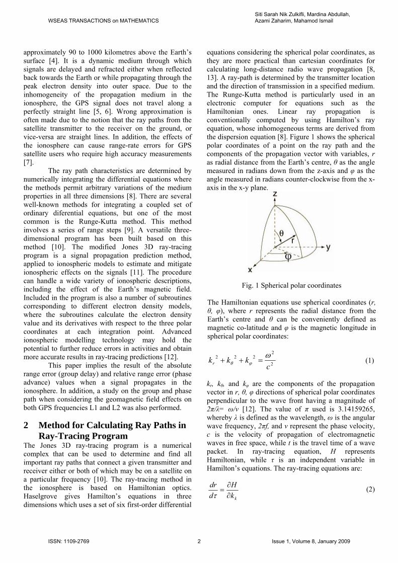
equations considering the spherical polar coordinates, as they are more practical than cartesian coordinates for calculating long-distance radio wave propagation [8, 13]. A ray-path is determined by the transmitter location and the direction of transmission in a specified medium. The Runge-Kutta method is particularly used in an electronic computer for equations such as the Hamiltonian ones. Linear ray propagation is conventionally computed by using Hamilton’s ray equation, whose inhomogeneous terms are derived from the dispersion equation [8]. Figure 1 shows the spherical polar coordinates of a point on the ray path and the components of the propagation vector with variables, r as radial distance from the Earth’s centre, θ as the angle measured in radians down from the z-axis and φ as the angle measured in radians counter-clockwise from the x-axis in the x-y plane.

Fig. 1 Spherical polar coordinates

The Hamiltonian equations use spherical coordinates (r, θ, φ), where r represents the radial distance from the Earth’s centre and θ can be conveniently defined as magnetic co-latitude and φ is the magnetic longitude in spherical polar coordinates:

2

2222

ckkkr

ωϕθ =++ (1)

kr, kθ, and kφ are the components of the propagation vector in r, θ, φ directions of spherical polar coordinates perpendicular to the wave front having a magnitude of 2π/λ= ω/ν [12]. The value of π used is 3.14159265, whereby λ is defined as the wavelength, ω is the angular wave frequency, 2πf, and ν represent the phase velocity, c is the velocity of propagation of electromagnetic waves in free space, while t is the travel time of a wave packet. In ray-tracing equation, H represents Hamiltonian, while τ is an independent variable in Hamilton’s equations. The ray-tracing equations are:

kkH

ddr

∂∂

=τ

(2)



θτθ

kH

rdd

∂∂

=1 (3)

ϕθτϕ

kH

rdd

∂∂

=sin1 (4)

ωτ ∂∂

−=H

ddt

(5)

τϕθ

τθ

τ ϕθ ddk

ddk

rH

ddkr sin++

∂∂

−= (6)

⎟⎠⎞

⎜⎝⎛ +−

∂∂

−=τϕθ

τθτ ϕθθ

ddrk

ddrkH

rddk

cos1 (7)

⎟⎟⎠

⎞⎜⎜⎝

⎛−−

∂∂

−=τθθ

τθ

ϕθτ ϕϕϕ

ddrk

ddrkH

rddk

cossinsin1

ττω

∂∂

=H

dd

(9)

From the equations, (7) and (8) are a set of six differential equations. They are integrated simultaneously to obtain the parameters of the ray path. The method of integrating equations is the Runge-Kutta process. P’ is defined as group path length in P’ = ct relative to s = vt. P’ = ct is the independent variable because the derivatives with respect to P’ are independent of the choice of Hamiltonian that allows the program to switch to Hamiltonian in the middle of a path. Below are the equations obtained by dividing equations (2) through (9) by c times of equation (5):

ω∂∂∂∂

−=H

kHcdP

dr r1' (10)

ωθ θ

∂∂∂∂

−=H

kHrcdP

d 1'

(11)

ωθϕ ϕ

∂∂

∂∂−

HkH

rcdPd

sin1

' (12)

'sin1

' ' dPdk

dPdk

HrH

cdPdkr ϕθθ

ω ϕθ ++∂∂∂∂

−= (13)

⎟⎟⎠

⎞⎜⎜⎝

⎛+−

∂∂∂∂

= ''' cos11dPdrk

dPdrk

HH

crdPdk ϕθ

ωθ

ϕθθ (14)

⎟⎟⎠

⎞⎜⎜⎝

⎛+−

∂∂∂∂

= ''' cos1sin1

dPdrk

dPdrk

HH

crdPdk θθ

ωϕ

θ ϕθϕ (15)

( )''' 2

121

dPd

dPd

dPfd ω

πω

π=

Δ=

Δ (16)

ωπ ∂∂∂∂

=H

tH21

The six simultaneous differential equations are used in equations (14) and (15), which are the Runge-Kutta method. Runge-Kutta is computed based only on information from the immediately preceding value to obtain the succesive value so it comes out with more points in a single step length. 3 Nelder-Mead Optimization Algorithm After travelling through the ionosphere, GPS rays should have arrived precisely at the receiver, and vice versa, so that a more precise time and position result could be measured [14]. Since the ray tracing program cannot directly calculate those ray paths that arrive at a specified receiver, all it can do is to calculate the path of a ray when given the transmitter location, frequency and specified angles of elevation and azimuth for direction of transmission; otherwise, the ray misses a specific target. Before tracing the ray, the directions to transmit the ray should be known, so that it will arrive at the receiver. Before the Nelder-Mead optimisation program is approached, there are no general solutions to this problem; the user of a ray-tracing program has to rely on some sort of trial and error technique to find those ray-paths that connect the transmitter and receiver [15]. In general, the direction of transmission varied until a ray that reaches the receiver is found.

(8)

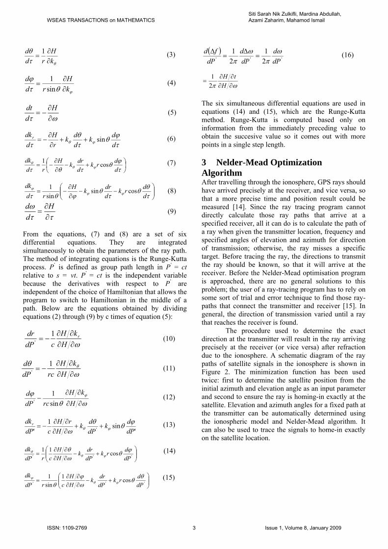
The procedure used to determine the exact direction at the transmitter will result in the ray arriving precisely at the receiver (or vice versa) after refraction due to the ionosphere. A schematic diagram of the ray paths of satellite signals in the ionosphere is shown in Figure 2. The minimization function has been used twice: first to determine the satellite position from the initial azimuth and elevation angle as an input parameter and second to ensure the ray is homing-in exactly at the satellite. Elevation and azimuth angles for a fixed path at the transmitter can be automatically determined using the ionospheric model and Nelder-Mead algorithm. It can also be used to trace the signals to home-in exactly on the satellite location.



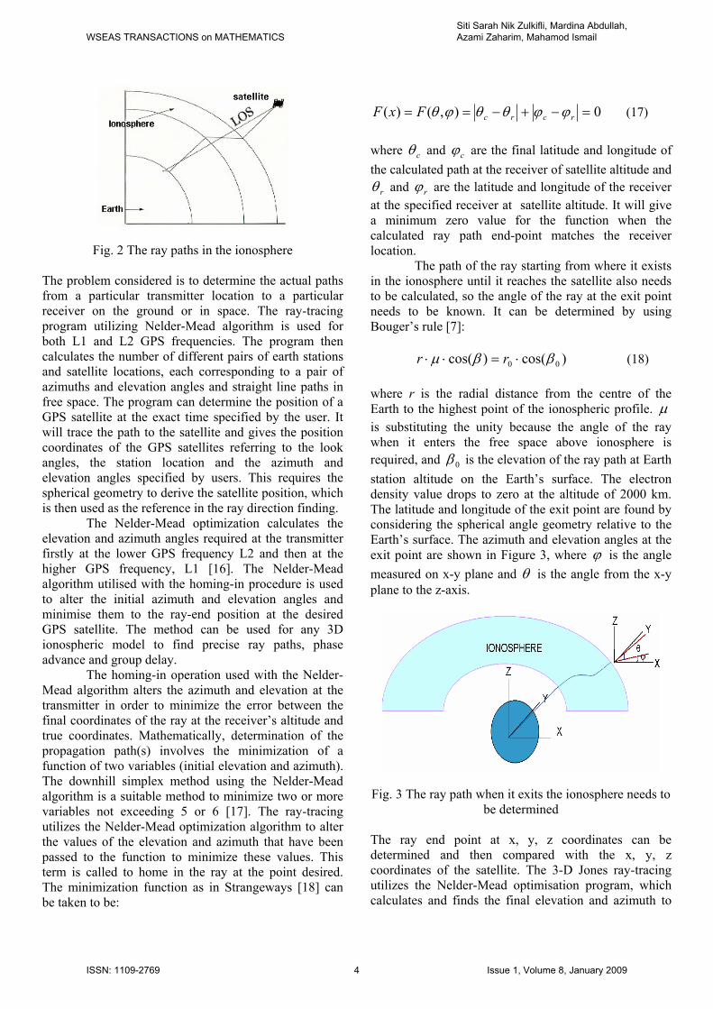
Fig. 2 The ray paths in the ionosphere The problem considered is to determine the actual paths from a particular transmitter location to a particular receiver on the ground or in space. The ray-tracing program utilizing Nelder-Mead algorithm is used for both L1 and L2 GPS frequencies. The program then calculates the number of different pairs of earth stations and satellite locations, each corresponding to a pair of azimuths and elevation angles and straight line paths in free space. The program can determine the position of a GPS satellite at the exact time specified by the user. It will trace the path to the satellite and gives the position coordinates of the GPS satellites referring to the look angles, the station location and the azimuth and elevation angles specified by users. This requires the spherical geometry to derive the satellite position, which is then used as the reference in the ray direction finding.

The Nelder-Mead optimization calculates the elevation and azimuth angles required at the transmitter firstly at the lower GPS frequency L2 and then at the higher GPS frequency, L1 [16]. The Nelder-Mead algorithm utilised with the homing-in procedure is used to alter the initial azimuth and elevation angles and minimise them to the ray-end position at the desired GPS satellite. The method can be used for any 3D ionospheric model to find precise ray paths, phase advance and group delay.

The homing-in operation used with the Nelder-Mead algorithm alters the azimuth and elevation at the transmitter in order to minimize the error between the final coordinates of the ray at the receiver’s altitude and true coordinates. Mathematically, determination of the propagation path(s) involves the minimization of a function of two variables (initial elevation and azimuth). The downhill simplex method using the Nelder-Mead algorithm is a suitable method to minimize two or more variables not exceeding 5 or 6 [17]. The ray-tracing utilizes the Nelder-Mead optimization algorithm to alter the values of the elevation and azimuth that have been passed to the function to minimize these values. This term is called to home in the ray at the point desired. The minimization function as in Strangeways [18] can be taken to be:

0),()( =−+−== rcrcFxF ϕϕθθϕθ (17)

where cθ and cϕ are the final latitude and longitude of the calculated path at the receiver of satellite altitude and

rθ and rϕ are the latitude and longitude of the receiver at the specified receiver at satellite altitude. It will give a minimum zero value for the function when the calculated ray path end-point matches the receiver location.

The path of the ray starting from where it exists in the ionosphere until it reaches the satellite also needs to be calculated, so the angle of the ray at the exit point needs to be known. It can be determined by using Bouger’s rule [7]:

)cos()cos( 00 ββμ ⋅=⋅⋅ rr (18) where r is the radial distance from the centre of the Earth to the highest point of the ionospheric profile. μ is substituting the unity because the angle of the ray when it enters the free space above ionosphere is required, and 0β is the elevation of the ray path at Earth station altitude on the Earth’s surface. The electron density value drops to zero at the altitude of 2000 km. The latitude and longitude of the exit point are found by considering the spherical angle geometry relative to the Earth’s surface. The azimuth and elevation angles at the exit point are shown in Figure 3, where ϕ is the angle measured on x-y plane and θ is the angle from the x-y plane to the z-axis.

Fig. 3 The ray path when it exits the ionosphere needs to be determined

The ray end point at x, y, z coordinates can be determined and then compared with the x, y, z coordinates of the satellite. The 3-D Jones ray-tracing utilizes the Nelder-Mead optimisation program, which calculates and finds the final elevation and azimuth to



reach the final target at the satellite location in space. The program works to get ( ) ( ) 0, ≈= ϕθFxF where the ray-end point matches with the satellite location. The termination tolerance of this function set to a value of 10-4 is generally employed. 4 Group Delay and Phase Advance GPS employs two carrier frequencies allowing receivers equipped with dual frequency operation to be used. A by-product of GPS receiver is the ability to estimate ionospheric total electron content (TEC) from the group delay measurements on these two carrier frequencies and thus remove it directly. The GPS estimation of TEC can be further improved by combining the above group delay estimates with carrier phase based estimates [19]. Group delay or propagation delay results from the fact that the signals travel slower in the ionosphere than they do in free space in contrast to the phase advance, which travels faster in the ionosphere than in free space for the same path [20]. The information conveyed on a modulated L band carrier, arrives late (group delay) by exactly the same amount of time that the carrier arrives early if only the first order terms is considered.

When travelling through the ionosphere, the propagation of the signals suffers a delay. In particular, phase changes due to refraction leading to propagation errors of up to 50 m for single-frequency GPS users depending on the TEC along the ray path [21]. In general, both signals, L1 and L2 are assumed to travel along the same path through the ionosphere in a straight line connecting transmitter with receiver, implying that both frequency rays pass through the same TEC [22]. If the difference in ionospheric delays between the L1 and L2 frequencies transmitted by the GPS satellites is measured, first-order range error contributions of the ionosphere can be determined and removed by differencing measurements [21]. Thus, the group delay equation is:

12 PP − =40.3TEC ( 2

12

2

11ff

− ) (19)

where P1 is the group path length that corresponds to the high GPS frequency (f1=1575.42 MHz) and P2 is the group path length that corresponds to the low GPS frequency (f2=1227.6 MHz). The extra ionospheric delay due to the non unity refractive index is assumed to be proportional to 1/f2, ignoring higher order terms. Ionospheric constant factor as in k=40.3x1016ms-2 TECU-1, I1=k/f1

2 and I2=((f12 /f2

2) I1), where I1 and I2 are the group delay or phase advance corresponding to the high GPS frequency f1, and the low GPS frequency f2 respectively. Thus the group path can simply be defined as: P1=PLOS +I1 and P2 =PLOS +I2, where PLOS is the true path length of the line of sight. By eliminating the

ionospheric delay from the above equations, PLOS can be obtained as in the equation (2) below, which is known as dual frequency method currently used to correct the ionospheric delay [23].

21

22

221

22

1

1ff

Pff

PPLOS

−

−

= (20)

From the ionospheric delay which is determined from ray tracing, the RRE can be calculated. Equation (3) shows how the RRE value is obtained. RRE is the difference between the line of sight (LOS) and the range from dual frequency model correction (determined from ray-tracing) [23].

21

22

221

22

21

1ff

Pf

PfP

LOSRRE−

−

−=

(21)

The ionospheric delay or advance at the reference station on Earth, tdref is obtained from the distance of the ray path to the receiver from the satellite, Pr

s (which is determined from ray-tracing) and the distance for propagation over the LOS at the velocity of light in vacuum. The equation is given as:

LOSPtd srref −= (22)

where Pr

s is the ray path from the satellite to the receiver. Comparisons are made between the signal path from reference station to satellite carried by frequency carriers (L1 and L2) and the signal path from mobile station to the satellite carried by the same frequency carriers. 5 Ionospheric Model It is not yet and may never be possible to sufficiently measure the ionosphere at any given instant to perform the effective ray-tracing; this has led to the use of ionospheric electron density model. The ionosphere is generated by NeQuick model to represent the ionosphere profiles in the region of interest [24]. For this work, the program began with the evaluation of the ionospheric profile from empirical model of the electron density distribution, NeQuick at GPS station at Universiti Kebangsaan Malaysia (2° 55’ N, 101° 46’ E). The 3D Jones ray-tracing program is a numerical complex used to investigate the ionospheric effect for both carrier phase and group delay in transionospheric propagation. The algorithms used are in the function of elevation



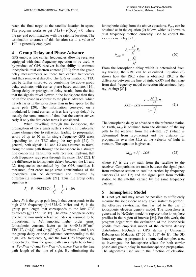
angles and TEC along the path from satellite to the Earth station. The program will trace the phase path and group path with or without geomagnetic field. In this work, the electron density profile was fitted with exponential layers and used as input to improve the ray-tracing program. Figure 4 shows the process of matching the NeQuick ionospheric profile by 24 exponential layers. NeQuick electron density profile has the electron concentration that can be calculated along an arbitrarily chosen ray-path and the resultant profile is smooth (continuous first-order spatial

derivatives), which is important in ray-tracing. This is based on the fact that the ray-tracing technique requires a continuous function [25]. The result from ray-tracing can be used to determine the RRE and ionospheric delay of earth-satellite path propagation. This program is used with homing-in method to trace GPS signals from a particular receiver to a particular satellite (or vice versa) taking into account the Earth’s geomagnetic field to determine the path length of the group and phase for both GPS frequencies (L1 and L2) [26].

-2 0 2 4 6 8 10 12 14 16x 1011

0

500

1000

1500

2000

2500

3000

Electron Density [el. m-3]

Hei

ght [

km]

Fig. 4 Matching NeQuick ionospheric p ofile by a number of exponential layers

6 Results and Discussion the residual range

RREФ decreases. When the geomagnetic field is

r

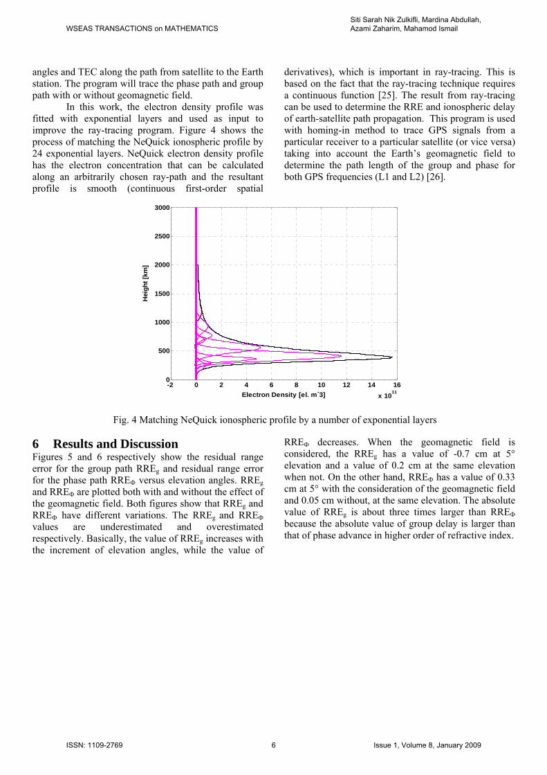
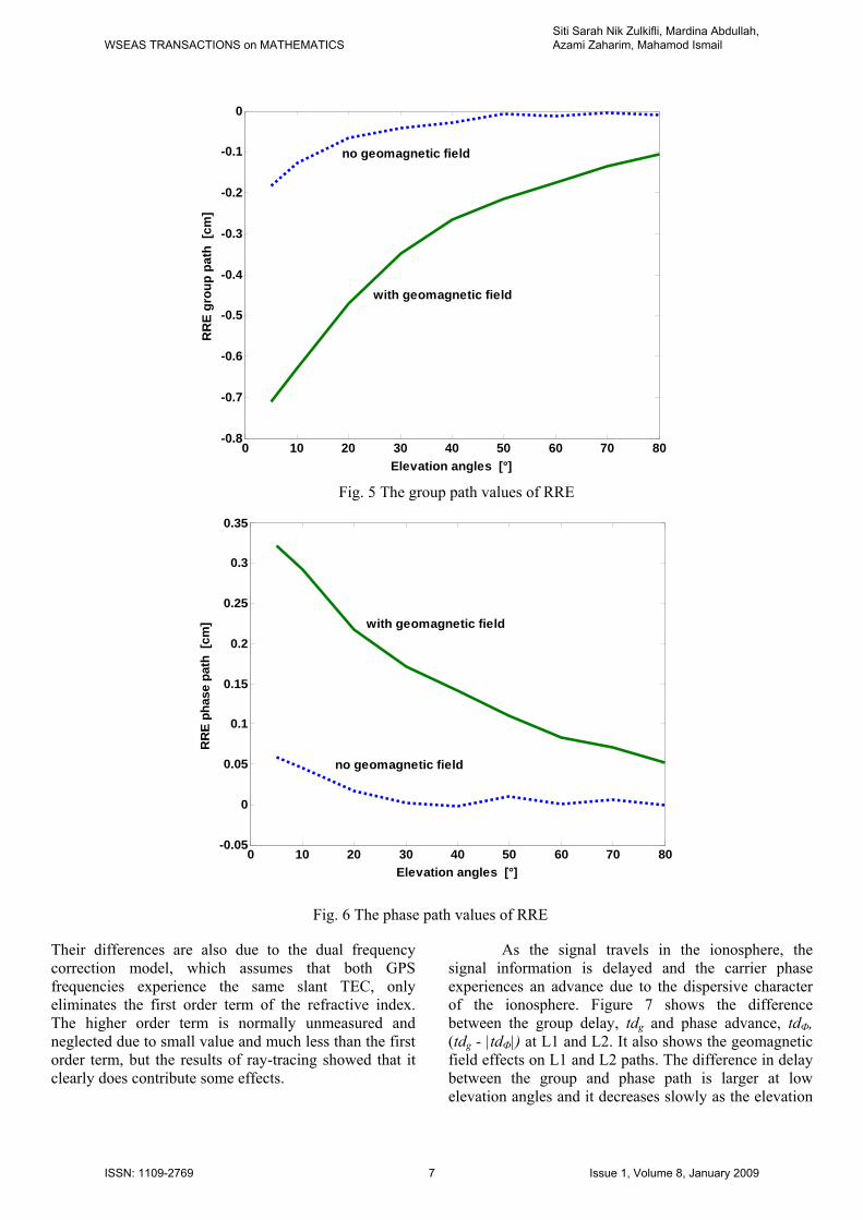
Figures 5 and 6 respectively show error for the group path RREg and residual range error for the phase path RREФ versus elevation angles. RREg and RREФ are plotted both with and without the effect of the geomagnetic field. Both figures show that RREg and RREФ have different variations. The RREg and RREФ values are underestimated and overestimated respectively. Basically, the value of RREg increases with the increment of elevation angles, while the value of

considered, the RREg has a value of -0.7 cm at 5° elevation and a value of 0.2 cm at the same elevation when not. On the other hand, RREФ has a value of 0.33 cm at 5° with the consideration of the geomagnetic field and 0.05 cm without, at the same elevation. The absolute value of RREg is about three times larger than RREФ because the absolute value of group delay is larger than that of phase advance in higher order of refractive index.



0 10 20 30 40 50 60 70 80-0.8

-0.7

-0.6

-0.5

-0.4

-0.3

-0.2

-0.1

0

Elevation angles [°]

RR

E gr

oup

path

[cm

]

no geomagnetic field

with geomagnetic field

Fig. 5 The group path values of RRE

0 10 20 30 40 50 60 70 80-0.05

0

0.05

0.1

0.15

0.2

0.25

0.3

0.35


RR

E ph

ase

path

[cm

] with geomagnetic field

no geomagnetic field

Fig. 6 The phase path values of RRE

Their differences are also due to the dual frequency correction model, which assumes that both GPS frequencies experience the same slant TEC, only eliminates the first order term of the refractive index. The higher order term is normally unmeasured and neglected due to small value and much less than the first order term, but the results of ray-tracing showed that it clearly does contribute some effects.

As the signal travels in the ionosphere, the signal information is delayed and the carrier phase experiences an advance due to the dispersive character of the ionosphere. Figure 7 shows the difference between the group delay, tdg and phase advance, tdФ, (tdg - |tdФ|) at L1 and L2. It also shows the geomagnetic field effects on L1 and L2 paths. The difference in delay between the group and phase path is larger at low elevation angles and it decreases slowly as the elevation



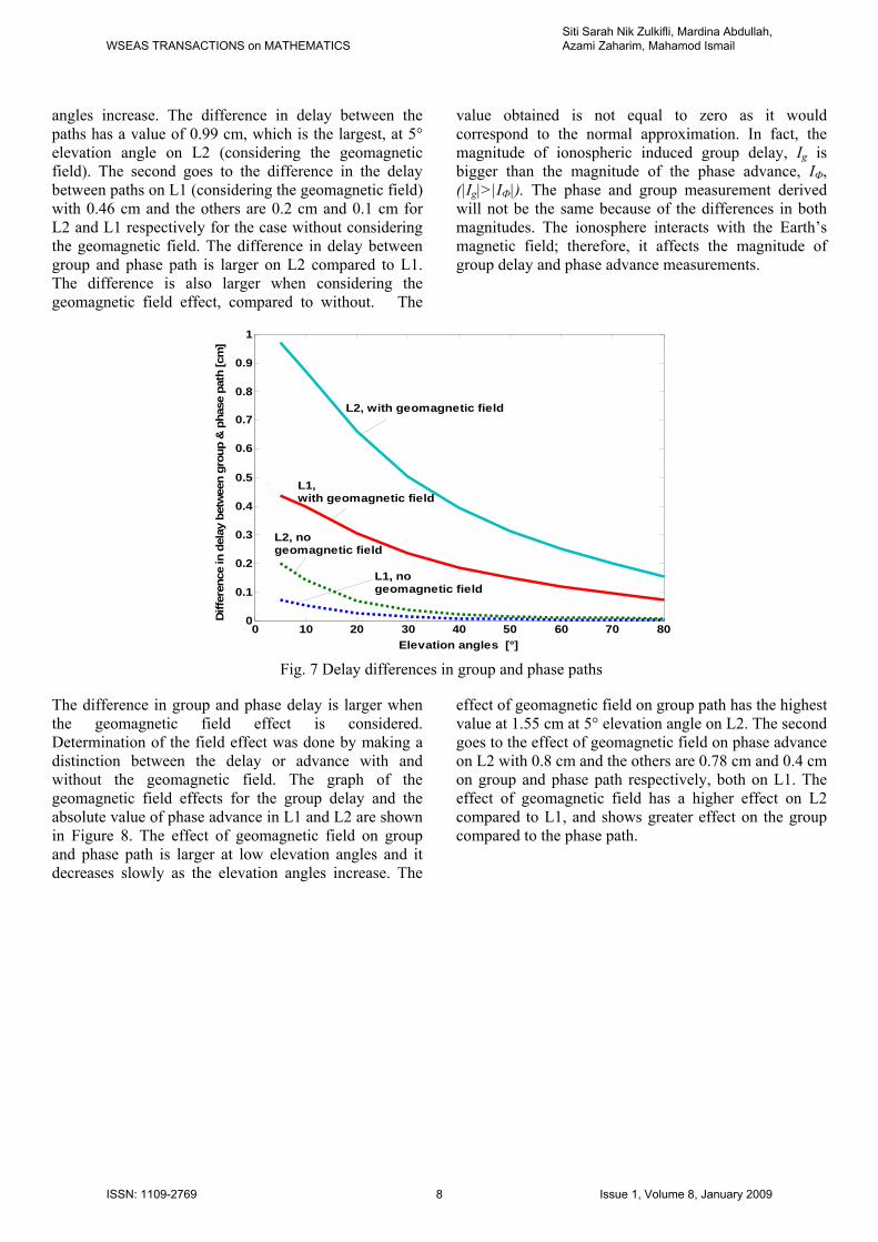
angles increase. The difference in delay between the paths has a value of 0.99 cm, which is the largest, at 5° elevation angle on L2 (considering the geomagnetic field). The second goes to the difference in the delay between paths on L1 (considering the geomagnetic field) with 0.46 cm and the others are 0.2 cm and 0.1 cm for L2 and L1 respectively for the case without considering the geomagnetic field. The difference in delay between group and phase path is larger on L2 compared to L1. The difference is also larger when considering the geomagnetic field effect, compared to without. The

value obtained is not equal to zero as it would correspond to the normal approximation. In fact, the magnitude of ionospheric induced group delay, Ig is bigger than the magnitude of the phase advance, IФ, (|Ig|>|IФ|). The phase and group measurement derived will not be the same because of the differences in both magnitudes. The ionosphere interacts with the Earth’s magnetic field; therefore, it affects the magnitude of group delay and phase advance measurements.

0 10 20 30 40 50 60 70 800

0.1

0.2

0.3

0.4

0.5

0.6

0.7

0.8

0.9

1


Diff

eren

ce in

del

ay b

etw

een

grou

p &

pha

se p

ath

[cm

]

L2, with geomagnetic field

L1, with geomagnetic field

L2, no geomagnetic field

L1, no geomagnetic field

Fig. 7 Delay differences in group and phase paths

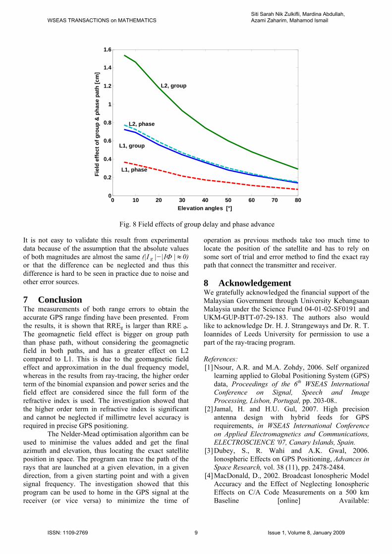
The difference in group and phase delay is larger when the geomagnetic field effect is considered. Determination of the field effect was done by making a distinction between the delay or advance with and without the geomagnetic field. The graph of the geomagnetic field effects for the group delay and the absolute value of phase advance in L1 and L2 are shown in Figure 8. The effect of geomagnetic field on group and phase path is larger at low elevation angles and it decreases slowly as the elevation angles increase. The

effect of geomagnetic field on group path has the highest value at 1.55 cm at 5° elevation angle on L2. The second goes to the effect of geomagnetic field on phase advance on L2 with 0.8 cm and the others are 0.78 cm and 0.4 cm on group and phase path respectively, both on L1. The effect of geomagnetic field has a higher effect on L2 compared to L1, and shows greater effect on the group compared to the phase path.



0 10 20 30 40 50 60 70 800

0.2

0.4

0.6

0.8

1

1.2

1.4

1.6


Fiel

d ef

fect

of g

roup

& p

hase

pat

h [c

m]

L2, group

L2, phase

L1, group

L1, phase

Fig. 8 Field effects of group delay and phase advance

It is not easy to validate this result from experimental data because of the assumption that the absolute values of both magnitudes are almost the same (|I g |−|IФ |≈ 0) or that the difference can be neglected and thus this difference is hard to be seen in practice due to noise and other error sources. 7 Conclusion The measurements of both range errors to obtain the accurate GPS range finding have been presented. From the results, it is shown that RREg is larger than RRE Ф. The geomagnetic field effect is bigger on group path than phase path, without considering the geomagnetic field in both paths, and has a greater effect on L2 compared to L1. This is due to the geomagnetic field effect and approximation in the dual frequency model, whereas in the results from ray-tracing, the higher order term of the binomial expansion and power series and the field effect are considered since the full form of the refractive index is used. The investigation showed that the higher order term in refractive index is significant and cannot be neglected if millimetre level accuracy is required in precise GPS positioning.

The Nelder-Mead optimisation algorithm can be used to minimise the values added and get the final azimuth and elevation, thus locating the exact satellite position in space. The program can trace the path of the rays that are launched at a given elevation, in a given direction, from a given starting point and with a given signal frequency. The investigation showed that this program can be used to home in the GPS signal at the receiver (or vice versa) to minimize the time of

operation as previous methods take too much time to locate the position of the satellite and has to rely on some sort of trial and error method to find the exact ray path that connect the transmitter and receiver.

8 Acknowledgement We gratefully acknowledged the financial support of the Malaysian Government through University Kebangsaan Malaysia under the Science Fund 04-01-02-SF0191 and UKM-GUP-BTT-07-29-183. The authors also would like to acknowledge Dr. H. J. Strangeways and Dr. R. T. Ioannides of Leeds University for permission to use a part of the ray-tracing program. References: [1] Nsour, A.R. and M.A. Zohdy, 2006. Self organized

learning applied to Global Positioning System (GPS) data, Proceedings of the 6th WSEAS International Conference on Signal, Speech and Image Processing, Lisbon, Portugal, pp. 203-08..

[2] Jamal, H. and H.U. Gul, 2007. High precision antenna design with hybrid feeds for GPS requirements, in WSEAS International Conference on Applied Electromagnetics and Communications, ELECTROSCIENCE '07, Canary Islands, Spain.

[3] Dubey, S., R. Wahi and A.K. Gwal, 2006. Ionospheric Effects on GPS Positioning, Advances in Space Research, vol. 38 (11), pp. 2478-2484.

[4] MacDonald, D., 2002. Broadcast Ionospheric Model Accuracy and the Effect of Neglecting Ionospheric Effects on C/A Code Measurements on a 500 km Baseline [online] Available:



http://www.novatel.com/Documents/Waypoint/Reports/iono.pdf [accessed 06 August 2008].

[5] Bassiri, S. & Hajj, G. A. 1993. Higher-order Ionospheric Effects on the Global Positioning System Observables and Means of Modeling Them, Manuscripta Geodaetica, vol. 18 (6), pp. 280–89.

[6] Ioannides, R. T. & Strangeways, H. J. 2000. Ionosphere-induced errors in GPS range-finding using MQP modelling, ray-tracing and nelder-mead Optimisation, in Millennium Conference on Antennas and Propagation, AP2000, vol. II, Davos, Switzerland, pp. 404–08.

[7] Bradford, W.P. and J.J. J. Spilker, eds., 1996. Global Positioning System: Theory and applications, vol. I and II. Washington DC, USA: American Institute of Aeronautics and Astronautics.

[8] Ioannides, R.T., 2002. Ionospheric Modelling and Path Determination for GPS Range-Finding Correction, PhD thesis, School of Electronic and Electrical Engineering, University of Leeds, U.K.

[9] Brian, D.D. and J.A. Colosi, 1998. Ray-Tracing for Ocean Acoustic Tomography, University of Washington, Seattle, Washington, Technical Memorandum APL-UW TM 3-98.

[10]Jones, R. M. and J.J. Stephenson, 1975. A Versatile Three-Dimensional Ray Tracing Computer Program For Radio Waves in the Ionosphere, tech. rep., U.S. Department of Commerce.

[11]Abdullah, M., H.J. Strangeways and D.M.A. Walsh, 2007. Effects on Ionospheric Horizontal Gradients on Differential GPS, Acta Geophysica, vol. 55 (4), pp. 509–523.

[12]Shayne, C.A., 2006. Comparison of Ray-Tracing Through Ionospheric Models, Master’s thesis, Department of Defense, Air Force Institute of Technology, U.S.

[13]Haselgrove, C.B. and J. Haselgrove, 1959. Twisted Ray Paths in the Ionosphere, Proceeding Physical Society, London, vol. 75, pp. 357-363.

[14]Sadeghi, M. and M. Gholami, 2008. Time Synchronizing Signal by GPS Satellites, WSEAS Transactions on Communications, vol. 7 (5), pp. 521-530.

[15]Davies, K. 1996. Ionospheric Radio, IEE Electromagnetic Waves Series 31, London: Peter Peregrinus Ltd. on behalf of the Institution of Electrical Engineers.

[16]Abdullah, M., H. J. Strangeways & D. M. A. Walsh, 2003. Accurate ionospheric error correction for differential GPS, in 12th International Conference on Antennas and Propagation, ICAP 2003, Exeter, UK.

[17]Ioannides, R.T. and H. J. Strangeways, 2002. Improved ionospheric correction for dual frequency

GPS, 27th General Assembly of URSI, Maastricht, the Netherlands.

[18]Strangeways, H.J., 2000. Effect of Horizontal Gradients on Ionospherically Reflected or Transionospheric Paths Using a Precise Homing-In Method, Journal of Atmospheric and Solar-Terrestrial Physics, vol. 62 (15), pp. 1361-1376.

[19]Knight, M.F. and D.A. Gray, 1996. Maximum likelihood estimation of ionospheric total electron content using GPS, International Symposium on Signal Processing and its Applications, ISSPA, pp.250-253.

[20]Davies, K. and E. K. Smith, 2002. Ionospheric effects on satellite land mobile systems, IEEE Antenna’s and Propagation Magazine, vol. 44 (No. 6), pp. 24-31.

[21]Jakowski, N., E. Sardon, E. Engler, A. Jungstand and D. Klahn, 1996. Relationships between GPS-signal propagation errors and EISCAT observations, Annales Geophysicae, vol. 14 (12), pp. 1429-1436.

[22]Ioannides, R. T. and H. J. Strangeways, 2000. Ionosphere-induced errors in GPS range finding using MQP modelling, ray-tracing and Nelder-Mead optimisation, in Millennium Conference on Antennas and Propagation, AP2000, vol. II, pp. 404–08.

[23]Abdullah, M., 2004. Modelling and Determination of Ionospheric Effects on Relative GPS measurements, Ph.D. dissertation, School of Electronic and Electrical Engineering, University of Leeds.

[24]International Telecommunication Union (ITU) official website [online] Available: http://www.itu.int/publ/R-SOFT-SG3/en [accessed 24 October 2008].

[25]Stankov, S. M., P. Marinov and I. Kutiev, 2007. Comparison of Nequick, PIM, and TSM Model Results for The Topside Ionosphere Plasma Scale and Transition Heights, Advances in Space Research, vol.39, pp. 767-773.

[26]Strangeways, H.J., M. Abdullah and D.M.A. Walsh, 2003. A method for improving the accuracy of differential GPS positioning, in European Co-operation in the field of Scientific and Technical Research - Effects of the Upper Atmosphere on Terrestrial and Earth-satellite Communications, COST271 Conference.

