ionospheric error analysis in gps measurements

585

ANNALS OF GEOPHYSICS, VOL. 51, N. 4 August 2008

Key words Differential GPS error sources – ionos-pheric errors – carrier-phase positioning – Geome-try-Free Linear Combination – RTK GPS

1. Introduction

Atmospheric refraction remains the greatestlimitation of GPS in applications requiring cen-timetric accuracy in real-time. Indeed, the pre-cise positioning via satellite requires special at-tention to the propagation of GPS signalsthrough the atmosphere yet (Hernández-Pajareset al., 1999), at the same time, the system itselfhas proven to be a very efficient instrument in

observations of the ionosphere (Coster et al.,1992; Lin, 2001).

As is known, by utilzing the GPS RTK dif-ferential technique, carrier-phase based posi-tioning results in a rapid and high precision po-sitioning when the ambiguities are fixed to theircorrect integer values.

As regards real-time differential techniques,the resolution of phase ambiguity is nonethelessstrongly influenced by the entity of certaintypes of GPS measurement errors, especiallythose involving ionospheric errors. The studyhighlights a substantial variation in perform-ance identified by the loss of spatial correlationhypothesis validity. In increasing the distances,the OTF resolution procedure for integer phaseambiguity became complicated in terms of timeand reliability with repercussions on positionaccuracy (Wanninger, 1995).

With the aim of obtaining an increment inthe resolution capacity of integer phase ambi-guity, the primary objective was to reduce the

Ionospheric error analysis in GPS measurements

Nicola Crocetto (1), Folco Pingue (2), Salvatore Ponte (3), Giovanni Pugliano (4) and Vincenzo Sepe (2)(1) Dipartimento di Ingegneria Civile, Seconda Università di Napoli, Aversa (CE), Italy(2) Istituto Nazionale di Geofisica e Vulcanologia, Osservatorio Vesuviano, Napoli, Italy

(3) Dipartimento di Ingegneria Aerospaziale e Meccanica, Seconda Università di Napoli, Aversa (CE), Italy(4) Dipartimento per le Tecnologie, Facoltà di Ingegneria, Università degli Studi «Parthenope», Napoli, Italy

AbstractThe results of an experiment aimed at evaluating the effects of the ionosphere on GPS positioning applicationsare presented in this paper. Specifically, the study, based upon a differential approach, was conducted utilizingGPS measurements acquired by various receivers located at increasing inter-distances. The experimental re-search was developed on the basis of two groups of baselines: the first group comprises «short» baselines (lessthan 10 km); the second group is characterized by greater distances (up to 90 km). The obtained results werecompared either upon the basis of the geometric characteristics, for six different baseline lengths, using 24 hoursof data, or upon temporal variations, by examining two periods of varying intensity in ionospheric activity re-spectively coinciding with the maximum of the 23 solar cycle and in conditions of low ionospheric activity. Theanalysis revealed variations in terms of inter-distance as well as different performances primarily owing to tem-poral modifications in the state of the ionosphere.

Mailing address: Dott. Giovanni Pugliano, Diparti-mento per le Tecnologie, Facoltà di Ingegneria, Universitàdegli Studi «Parthenope», Centro Direzionale, Isola C4,80143 Napoli, Italy; tel: +39 0815476734; Fax: +390815476777; e-mail: [email protected]

Miscellanea 9-03-2009 14:42 Pagina 585

586

N. Crocetto, F. Pingue, S. Ponte, G. Pugliano and V. Sepe

differential ionospheric error present in thedouble difference observable. This error wascaused by the fact that certain types of GPSmeasurement errors, including ionospheric er-rors, are not adequately reduced by double dif-ference processing, and are thus expressed asdifferential terms in the double phase equation.With this objective in mind, it was necessary toexamine this type of error, understand the be-haviour of the cause which might produce itand evaluate the effects on the measurements.

The following are the results of a study ofionospheric error, conducted via the utilzationof GPS measurements collected by continuous-ly operating stations in Campania. It can be ob-served that the test was conducted on data ac-quired in two periods of differing ionophericactivity intensity, respectively during the maxi-mum of the solar cycle and in conditions ofweak ionospheric activity.

2. Phenomena of the upper atmosphere

Modern knowledge of the ionosphere hasprovided an adequate comprehension of itsmorphology as well as the basic mechanismscaused by solar radiation. Nonetheless, sensi-tivity to phenomena of a different nature makesthe ionosphere extremely variable. Its very be-haviour reveals daily and seasonal variationsand depends on the influence of solar activity.The state of the ionosphere also depends on ge-ographic latitude and the geomagnetic field. Inaddition to the preceding variations, defined asregular variations, there are other irregularitieswhich may occasionally intensify and consti-tute so-called ionospheric perturbances.

As the very name of the ionosphere indi-cates, there is a significant concentration of ionsand free electrons in the upper strata of the at-mosphere. It extends for approximately 50 kmto 1000 km above the surface of the earth andhas a dispersive effect on GPS signal frequen-cies.

Owing to the effects of refraction, apartfrom a negligible, curvilinear deviation of thesignal trajectory, the ionosphere determines avariation in the speed of propagation. This in-fluence depends on the frequency and is func-

tion of the number of electrons along the signaltrajectory.

Omitting terms superior to the second orderterms, ionospheric error for phase measure-ments is given in cycles by the following ex-pression (Klobuchar, 1996)

(2.1)

where:I = 40.3 TEC (cycles · m/s2);c is the speed of light in a vacuum;f is the frequency.

TEC (Total Electron Content) represents theparameter adopted to describe the state of theionosphere and is the electron content of a 1-m2

column along the signal path between satelliteS and receiver R and is given by the integrationof Ne electron density extended to the entireionospheric path:

(2.2)

where:TEC is expressed in TEC units (TECU) con 1

TECU = 1016 electrons/m2;Ne is the density of electrons (electrons/m3).

Considering that the state of the ionosphereessentially depends upon the sun’s electromag-netic radiations, which are responsible for ion-ization, and corpuscular swarms of solar wind,which produce perturbances, it can consequent-ly be observed that TEC undergoes numerousvariations which are caused by solar phenome-na (Gao and Liu, 2002; Leitinger et al., 1975;Liao and Gao, 2001).

The pattern of TEC values is characterisedby daily, seasonal and eleven-year periodicitieswhich are related to solar activity.

Daily TEC variations are essentially causedby changes in the structure of the ionospherewhich occur between night and day. In particu-lar, the trend of electronic density is influencedby solar radiation and by the recombinationtime. Therefore, as regards daily TEC values, amaximum value is frequently produced onehour after solar noon, generally between 1:00p.m. and 3:00 p.m. local time; occasionally, an-

TEC N dse

R

S

= #

dcfI

ion =-


587


other peak can be recorded during the hours af-ter sunset (Hernández-Pajares et al., 2006).

TEC values also have seasonal variationsbased upon the months of the year. In theNorthern hemisphere, minimum values arerecorded during summer and maximum valuesduring both the equinoxes and winter. The enti-ty of TEC may be two to three times greater inwinter as opposed to summer.

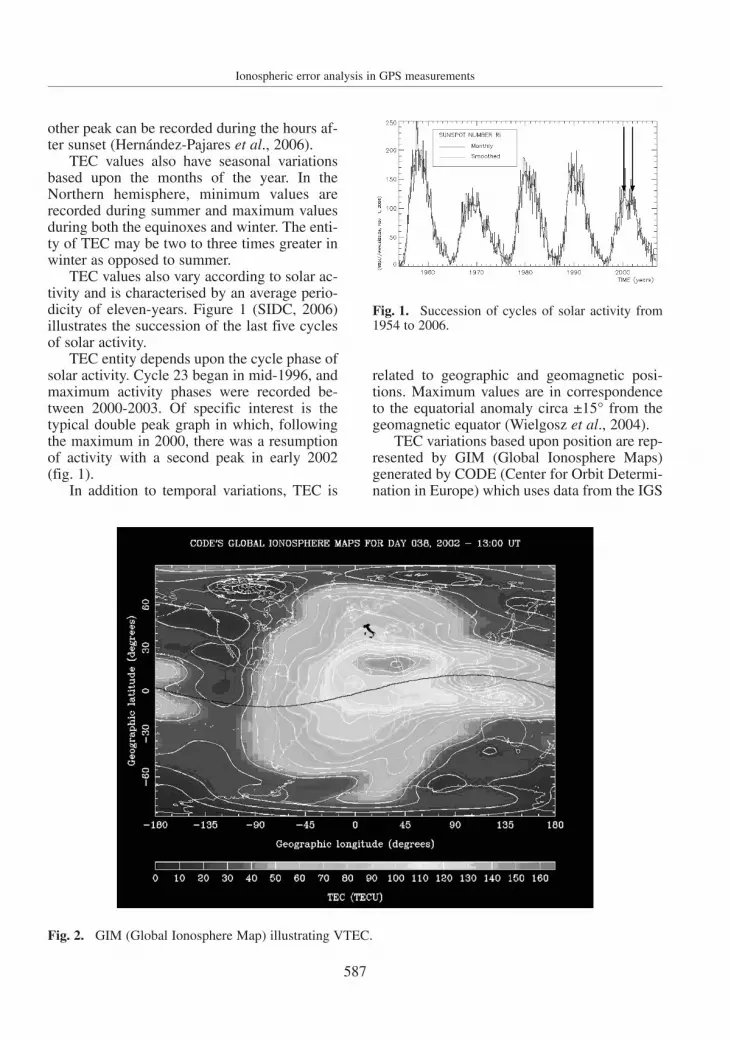
TEC values also vary according to solar ac-tivity and is characterised by an average perio-dicity of eleven-years. Figure 1 (SIDC, 2006)illustrates the succession of the last five cyclesof solar activity.

TEC entity depends upon the cycle phase ofsolar activity. Cycle 23 began in mid-1996, andmaximum activity phases were recorded be-tween 2000-2003. Of specific interest is thetypical double peak graph in which, followingthe maximum in 2000, there was a resumptionof activity with a second peak in early 2002(fig. 1).

In addition to temporal variations, TEC is

related to geographic and geomagnetic posi-tions. Maximum values are in correspondenceto the equatorial anomaly circa ±15° from thegeomagnetic equator (Wielgosz et al., 2004).

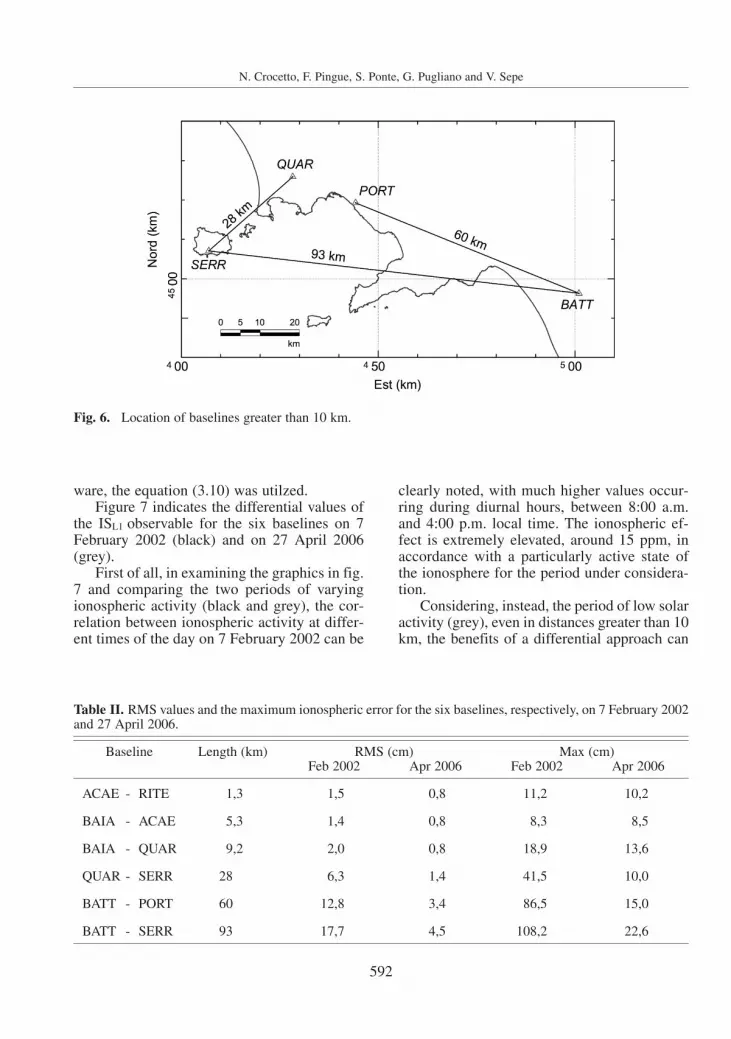
TEC variations based upon position are rep-resented by GIM (Global Ionosphere Maps)generated by CODE (Center for Orbit Determi-nation in Europe) which uses data from the IGS

Fig. 1. Succession of cycles of solar activity from1954 to 2006.

Fig. 2. GIM (Global Ionosphere Map) illustrating VTEC.


588


international network of GPS stations (CODE,2002; Schaer, 1999). Figure 2 illustrates verti-cal, diurnal TEC values during conditions of in-tense ionospheric activity. The typical dual«tail» structure travels in an east-west directionalong the geomagnetic equator reflecting ap-parent solar motion around the earth.

There is another factor which interacts withGPS measurements in the ionosphere: the pres-ence of local perturbances within the ionos-pheric structure causes amplitude fading andphase fluctuation of the received signal. Thisphenomenon, known as scintillation (Aarons,1982), has proven to be highly non-correlatedin both spatial and temporal terms.

The effects of ionospheric scintillation, es-pecially frequent during periods of maximumsolar activity, are predominant in equatorial(±10°-20° geomagnetic latitude), auroral (65°-75°) and polar (>75°) regions. When effects arealso produced at mid-latitudes, it is an exten-sion from the equatorial and auroral regions(Skone, 1998; Skone and De Jong, 1999).

Scintillations are generally recorded duringnight-time hours, between sunset to mid-nightand occasionally even later, in all regions. Fur-thermore, that there are seasonal variations re-lated to the longitude which produce the great-est effects from September to March in the areaextending from the Americas to India, and fromApril to August in the Pacific region (Wan-ninger, 1993).

3. Geometry-Free linear combination forionospheric delay analysis

In order to examine ionospheric error, weintend to introduce a mathematical formula ca-pable of expressing the differential delay basedupon phase measurements from GPS referencestations.

Among the various combinations of phasemeasurements derived from the two carrier fre-quencies L1 and L2 which are prevalently usedin GPS models, the geometry-free (Pugliano,2004) combination has proven to be especiallyuseful in examining ionospheric refraction er-rors.

By utilzing a double frequency receiver, the

ΦGF observable generated by a linear combina-tion of L1 and L2 carrier frequency phasemeasurements, expressed in meters, can be ob-tained from the following expression:

(3.1)

where:ΦGF is the geometry-free observable ex-

pressed in meters;λ1, λ2 are the wave lengths of the carrier fre-

quencies (19.03 cm for L1 and 24.42cm for L2);

φ1, φ2 are the phase measurements, respec-tively, of L1 carrier frequency and theL2 carrier frequency, in cycles;

Φ1, Φ2 are the phase measurements in meters.It is observed that geometry-free combina-

tion can only be expressed in meters. This pe-culiarity is in agreement with the fact that thecorresponding λGF wavelength, based uponequation (3.2), is �.

(3.2)

where:µ1, µ2 are the µ1 = λ1 e µ2= –λ2 coefficients.

Equations of phase measurements φ1 andφ2, expressed in cycles, are considered:

(3.3)

where:ρ geometric distance between the satellite

and the receiver;d ρ satellite orbit error;c speed of light;dt satellite clock error;dT receiver clock error;dtrop tropospheric error;dion ionospheric error, in cycles;N phase ambiguity (integer number of

wavelengths expressed in cycles);ε(φ) phase measurement noise (multipath and

receiver noise);

1

1

d cdt cdT d

d N

d cdt cdT d

d N

11

1 1

22

2 2

trop

ion

trop

ion

1

2

λ ρ ρ

ε ϕ

λ ρ ρ

ε ϕ

φ

φ

= + + - + -

- + +

= + + - + -

- + +

^

^

^

^

h

h

h

h

,1 21 2 2 1

1 2λ µ µ µ λ µ λλ λ= +^ h

1 1 2 2 1 2GF λ λφ φΦ Φ Φ= - = -


589


and considering that dion in meters is given,based upon the equation (2.1), by

(3.4)

the geometry-free observable is thus defined,based upon (3.1), by the following expression:

(3.5)

It should be noted that this expression is in-dependent of clocks and geometry (receiver andsatellites coordinates), and thus gives origin tothe name geometry-free.

The objective is to use this observable for anestimate of ionospheric refraction on phasemeasurements.

In applying double difference processing,the following is obtained from the equation (3.5)

(3.6)

Considering that for distances greater than10 km between receivers, multipath and receiv-er noise are negligible in comparison withionospheric error, therefore, the equation (3.6)becomes

(3.7)

Furthermore, from the formula (2.1) the fol-lowing can be deduced in differential terms

(3.8)

Therefore, by substituting equation (3.8) into

dcf

I1

ion1dd∆ ∆=-

If f

f fN N

22

12

12

22

1 1 2 2GFd d d dλ λ∆ ∆ Φ ∆ ∆- = - - +] g

If f

f fN

N

12

22

22

12

1 1

2 2 1 2

GFd d d

d d d

λ

λ ε ε

∆ Φ ∆ ∆

∆ ∆ Φ ∆ Φ

=- - + -

- + -

d

] ]

n

g g

If f

f fN

N

d cdt cdT

dfI N

d cdt cdT d

fI N

GF

trop

trop

12

22

22

12

1 1

2 2 1 2

12 1 1 1

22 2 2 2

ρ ρ

λ ε

ρ ρ

λ ε

λ

λ ε ε

ΦΦ

Φ

Φ Φ

=

+ + - +

+ - + ++

-

+ + - + -

+ +=

=--

+ -

- + -

J

L

KKK

J

L

KKK

]

]

d

] ]

N

P

OOO

N

P

OOO

g

g

n

g g

dcfI

cfI

fc

fI

ion 2$ $λ=- =- =-

(3.7), the following is obtained in cycles

(3.9)

Lastly, the ionospheric differential error forL1 carrier frequency can be obtained, in me-ters, by multiplying equation (3.9) by the λ1

wavelength in order to obtain

(3.10)

The definite observable (3.10) is also desig-nated with the term ionospheric signal sinceresidual error, for the most part, can be attrib-uted to the ionosphere.

Given a priori known receiver coordinatesand ambiguities between stations, equation(3.10) therefore allows us to express differentialionospheric error through double difference ofthe geometry-free observable given by

(3.11)

4. Analysis of results

In adopting the above described method, theentity of differential ionospheric error on meas-urements from seven observation points wasevaluated.

An area in the Campania territory was se-lected as a test zone (fig. 3).

Specifically, six permanent stations as wellas a temporary receiver were utilized. Five ofthe six existing stations belong to the ItalianNational Institute of Geophysics and Vulcanol-ogy - the Vesuvius Observatory and are part ofa permanent GPS network in the integrated ge-odetic monitoring system of the Neapolitan vol-canic area (Pingue et al., 2002), the sixth is thepermanent station of the «G.C. Gloriosi» Tech-nical Institute in Battipaglia.

The measurements utilzed were taken con-currently from seven different stations at a rateof 30 s, over a 24 hour period.

The experimental research was developed

1 2GFd d d∆ Φ ∆ Φ ∆ Φ= -

ISf f

fN N1

22

12

22

1 1 2 2L GFd d d dλ λ∆ ∆ Φ ∆ ∆= - - +] g

1d

cf f f

f f

N N

1 22

12

12

22

1 1 2 2

ion

GF

1d

d d dλ λ

∆

∆ Φ ∆ ∆

= -- +

d

]

n

g


590


either upon the basis of the geometric charac-teristics, on six different baseline lengths, using24 hours of data, or based upon temporal varia-tions, by examining two days of measurementsrespectively coinciding with the maximum ofthe 23 solar cycle on 7 February 2002 and inconditions of low ionospheric activity on 27April 2006 (fig. 4) (SIDC, 2006).

The baselines selected for comparison withthe six different lengths are reported in table I.

Two groups can be observed: the first groupis comprised of baselines of less than 10 kmwhich correspond to the class of «short» base-lines (fig. 5).

The second group is characterized bygreater distances, the placement of which is il-lustrated in fig. 6.

Given the ambiguity between stations asobtained from processing with Bernese soft-

Fig. 3. Test Area.

Table I. Lengths of the selected baselines.

Baseline Length(km)

ACAE - RITE 1.3

BAIA - ACAE 5.3

BAIA - QUAR 9.2

QUAR - SERR 28

BATT - PORT 60

BATT - SERR 93


591


Fig. 4. Solar Activity - Cycle 23.

Fig. 5. Location of short baselines.


592


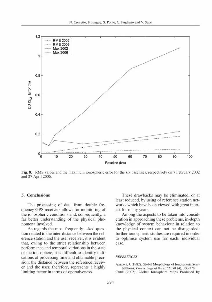
ware, the equation (3.10) was utilzed.Figure 7 indicates the differential values of

the ISL1 observable for the six baselines on 7February 2002 (black) and on 27 April 2006(grey).

First of all, in examining the graphics in fig.7 and comparing the two periods of varyingionospheric activity (black and grey), the cor-relation between ionospheric activity at differ-ent times of the day on 7 February 2002 can be

clearly noted, with much higher values occur-ring during diurnal hours, between 8:00 a.m.and 4:00 p.m. local time. The ionospheric ef-fect is extremely elevated, around 15 ppm, inaccordance with a particularly active state ofthe ionosphere for the period under considera-tion.

Considering, instead, the period of low solaractivity (grey), even in distances greater than 10km, the benefits of a differential approach can

Table II. RMS values and the maximum ionospheric error for the six baselines, respectively, on 7 February 2002and 27 April 2006.

Baseline Length (km) RMS (cm) Max (cm)Feb 2002 Apr 2006 Feb 2002 Apr 2006

ACAE - RITE 1,3 1,5 0,8 11,2 10,2

BAIA - ACAE 5,3 1,4 0,8 8,3 8,5

BAIA - QUAR 9,2 2,0 0,8 18,9 13,6

QUAR - SERR 28 6,3 1,4 41,5 10,0

BATT - PORT 60 12,8 3,4 86,5 15,0

BATT - SERR 93 17,7 4,5 108,2 22,6

Fig. 6. Location of baselines greater than 10 km.


593


be noted: for the 93 km baseline, the ionospher-ic error is reduced in terms of RMS, to 4.5 cmwith a maximum value of 22.6 cm.

The results of comparisons conducted forthe measurement days of 7 February 2002 and27 April 2006 are reported in table II.

Furthermore, these results are representedin fig. 8 in terms of baseline length.

It can be observed that the differing per-formances are not only associated with varia-tions in distance but primarily reveal apprecia-ble variations owing to temporal modificationsin the state of the ionosphere.

The slightly sloping pattern of the graphics

corresponding to the period of low solar activi-ty (grey) reveal that, under these conditions,ionospheric behaviour does not vary apprecia-bly from place to place.

During maximum solar activity (black), asdistances increase, the trend of the RMS valuesindicate a reduction in spatial correlation whichis maintained only for distances between re-ceivers which are less than 5 km. For the meas-urements of 2002, the entity of differentialionospheric error grew even less than the 10 kmthreshold. However, this behaviour is accentu-ated when maximum values are taken into con-sideration.

Fig. 7. Ionospheric error, respectively, for 7 February 2002 (black) and 27 April 2006 (grey).


594


5. Conclusions

The processing of data from double fre-quency GPS receivers allows for monitoring ofthe ionospheric conditions and, consequently, afar better understanding of the physical phe-nomena involved.

As regards the most frequently asked ques-tion related to the inter-distance between the ref-erence station and the user receiver, it is evidentthat, owing to the strict relationship betweenperformance and temporal variations in the stateof the ionosphere, it is difficult to identify indi-cations of processing time and obtainable preci-sion: the distance between the reference receiv-er and the user, therefore, represents a highlylimiting factor in terms of operativeness.

These drawbacks may be eliminated, or atleast reduced, by using of reference station net-works which have been viewed with great inter-est for many years.

Among the aspects to be taken into consid-eration in approaching these problems, in-depthknowledge of system behaviour in relation tothe physical context can not be disregarded:further ionospheric studies are required in orderto optimise system use for each, individualcase.

REFERENCES

AARONS, J. (1982): Global Morphology of Ionospheric Scin-tillations, Proceedings of the IEEE, 70 (4), 360-378.

CODE (2002): Global Ionosphere Maps Produced by

Fig. 8. RMS values and the maximum ionospheric error for the six baselines, respectively on 7 February 2002and 27 April 2006.


595


CODE, http://www.aiub.unibe.ch/ionosphere.html,(Global Center for Orbit Determination in Europe, As-tronomical Institute, University of Bern).

COSTER, A.J., E.M. GAPOSCHKIN and L.E. THORNTON

(1992): Real-time ionospheric monitoring system us-ing GPS, Navigation: Journal of Institute of Naviga-tion, 39 (2), 191-204.

GAO, Y. and Z.Z. LIU (2002): Precise Ionosphere ModelingUsing Regional GPS Network Data, Journal of GlobalPositioning Systems, 1 (1), 18-24.

HERNÁNDEZ-PAJARES, M., J.M. JUAN, J. SANZ and O.L.COLOMBO (1999): Precise Ionospheric Determinationand its Application to Real-Time GPS Ambiguity Res-olution, in Proceedings of Institute of Navigation ION-GPS 1999, (Nashville).

HERNÁNDEZ-PAJARES, M., J.M. JUAN and J. SANZ (2006):Medium scale Traveling Ionospheric Disturbances af-fecting GPS measurements: Spatial and Temporalanalysis, Journal of Geophysical Research, 111.

KLOBUCHAR, J. A. (1996): Global Positioning System: The-ory and Applications, Vol. I, Cap. 12: Ionospheric Ef-fects on GPS, (American Institute of Aeronautics andAstronautics Inc.), pp. 485-515.

LEITINGER, R., G. SCHMIDT and A. TAURIAINEN (1975): Anevaluation method combining the differential Dopplermeasurements from two stations that enables the calcu-lation of the electron content of the ionosphere, Jour-nal of Geophysics, 41, 201-213.

LIAO, X. and Y. GAO (2001): High-Precision Ionospheric TECRecovery Using a Regional-Area GPS Network. Naviga-tion, Journal of Institute of Navigation, 48 (2), 101-111.

LIN, L. (2001): Remote sensing of ionosphere using GPSmeasurements, in 22nd Asian Conference on RemoteSensing, (Singapore).

PINGUE, F., G. BERRINO, P. CAPUANO, C. DEL GAUDIO, F.OBRIZZO, G. P. RICCIARDI, C. RICCO, V. SEPE, S. E. P.BORGSTROM, G. CECERE, P. DE MARTINO, V. D’ERRICO,A. LA ROCCA, S. MALASPINA, S. PINTO, A. RUSSO, C.

SERIO, V. SINISCALCHI, U. TAMMARO and I. AQUINO

(2002): Sistema integrato di monitoraggio geodeticodell’area vulcanica attiva napoletana: reti permanenti erilevamenti periodici, Atti della 6a ConferenzaNazionale delle Associazioni Scientifiche per le Infor-mazioni Territoriali e Ambientali (ASITA), (Perugia)vol. II, pp. 1751-1764.

PUGLIANO, G. (2004): Monitoraggio locale della ionosferaattraverso misure GPS, in «Annali della Facoltà diScienze e Tecnologie», (Università degli Studi diNapoli Parthenope),vol. LXVIII, pp. 87-102.

SCHAER, S. (1999): Mapping and Predicting the Earth’sIonosphere Using the Global Positioning System, Ph.Ddissertation, (University of Berne).

SIDC (2006): Sunspot Index Graphics, http://sidc.oma.be/in-dex.php3, Sunspot Index Data Center, Royal Observa-tory of Belgium.

SKONE, S. (1998): Wide Area Ionosphere Grid Modeling inthe Auroral Region, Ph.D dissertation, (The Universityof Calgary).

SKONE, S. and M. DE JONG (1999): The Impact of Geomag-netic Substorms on GPS Receiver Performance, Pro-ceedings of the International Symposium on GPS,(Tsukuba, Japan).

WANNINGER, L. (1993): Effects of the Equatorial Ionos-phere on GPS, GPSWorld, Advanstar Communica-tions, pp. 48-54.

WANNINGER, L. (1995): Improved Ambiguity Resolution byRegional Differential Modeling of the Ionosphere, inProceedings of Institute of Navigation ION-GPS,(Palm Springs), pp. 55-62.

WIELGOSZ, P., L.W. BARAN, I.I. SHAGIMURATOV and M.V.ALESHNIKOVA (2004): Latitudinal variations of TECover Europe obtained from GPS observation, AnnalesGeophysicae, 22, 405-415.

(received February 6, 2008;accepted May 8, 2008)


ionospheric error analysis in gps measurements

Documents