158 Int. J. Computer Applications in Technology, Vol. x, Nos. x, 200x

Copyright © 2008 Inderscience Enterprises Ltd.

Supply chain optimisation using Evolutionary Algorithms

Marco Aurélio Falcone Tritec Motors, R. Ema Tanner de Andrade, 1892, Vila Ferrari – 83606-360, Campo Largo (PR), Brazil E-mail: mgf8@daimlerchrysler.com

Heitor Silvério Lopes Federal Technological University of Paraná/CPGEI, Av. 7 de setembro, 3165, 80230-901 Curitiba (PR), Brazil E-mail: hslopes@pesquisador.cnpq.br

Leandro dos Santos Coelho*

Pontifical Catholic University of Paraná/PPGEPS/LAS, R. Imaculada Conceição, 1155, 80215-901 Curitiba (PR), Brazil E-mail: leandro.coelho@pucpr.br *Corresponding author

Abstract: This paper describes the application of Evolutionary Algorithms (EAs) to the optimisation of a simplified supply chain in an integrated production-inventory-distribution system. The performance of four EAs (Genetic Algorithm (GA), Evolutionary Programming (EP), Evolution Strategies (ES) and Differential Evolution (DE)) was evaluated with numerical sumulations. Results were also compared with other similar approach in the literature. DE was the algorithm that led to better results, outperforming previously published solutions. The robustness of EAs in general, and the efficiency of DE, in particular, suggest their great utility for the supply chain optimisation problem, as well as for other logistics-related problems.

Keywords: evolutionary computation; Genetic Algorithms; GA; Differential Evolution; DE; logistics; supply chain.

Reference to this paper should be made as follows: Falcone, M.A., Lopes, H.S. and dos Santos Coelho, L. (2008) ‘Supply chain optimisation using Evolutionary Algorithms’, Int. J. Computer Applications in Technology, Vol. x, Nos. x, pp.xxx–xxx.

Biographical notes: Marco Aurélio Falcone received his BSc in Industrial Engineering and MSc in Production Engineering from São Paulo State University (UNESP) at Ilha Solteira, and Pontifical Catholic University of Paraná, Brazil, in 1993 and 2004, respectively. Since 2000, he has worked for Tritec Motors as Foreign Trade and Transportation Manager. His research interests are applications of evolutionary computation for logistics systems.

Heitor Silvério Lopes received his BSc in Electrical Engineering and the MSc in Biomedical Engineering from the Federal Technological University of Paraná (UTFPR), Curitiba, Brazil, in 1984 and 1990, respectively, and his PhD in Electrical Engineering and Information Systems from the Federal University of Santa Catarina, Brazil, in 1996. He is Adjunct Professor of the Department of Electronics, UTFPR, and founded the Bioinformatics laboratory in 1997. He has worked as a reviewer for several international journals and conferences, and published around 150 papers in journals, conferences and book chapters. His current research interests include evolutionary computation, data mining, bioinformatics and reconfigurable computing.

Leandro dos Santos Coelho received his BSc in Computer Science and BSc in Electrical Engineering from the Federal University of Santa Maria (UFSM), Brazil, in 1994 and 2000, respectively. He got his MSc and PhD in Computer Science and Electrical Engineering from the Federal University of Santa Catarina (UFSC), Brazil, in 1997 and 2000, respectively. He is an Associate Professor at the Department of Automation and Systems, Pontifical Catholic

Supply chain optimisation using Evolutionary Algorithms 159

University of Paraná (PUCPR/CCET/PPGEPS), in Curitiba, Brazil. He serves as a reviewer for several international journals. His research interests are power systems, computational intelligence, optimisation methods, and advanced control systems

1 Introduction

The project of logistic systems could be defined as “the art of combining the right amount of the right products, delivered to the right place at the right time”. Usually this project is referred to as supply chain problems. Nowadays, the success of a company depends on its efficiency in managing its supply chains.

A supply chain is a network of facilities and distribution options that performs the functions of procurement of materials, transformation of these materials into intermediate and finished products, and the distribution of these finished products to customers. Supply chains exist in both service and manufacturing organisations. Realistic supply chains have multiple end products with shared components, facilities and capacities (Ermis et al., 2004).

Usually, business unities along a supply chain operate independently, having their own objectives that are often conflicting with each other. Therefore, an essential condition to the success of a company is the conception of a strategy for coordinating the several business unities in a supply chain, leading to an effective management at strategic, tactical and operational levels. The efficiency of a supply chain is influenced by several factors, such as: stock management, production planning, production costs, scheduling and distribution strategies, and customer-specific demand, among others.

Planning and modelling the production, stocking and distribution systems of a supply chain is an important support for decision making in a competitive market. According to Dong (2001), the several approaches for modelling and optimisation of a supply chain can be classified into five classes:

• project of the supply chain

• integer-mixed programming optimisation

• stochastic programming

• heuristic methods

• simulation-based methods.

Modelling a supply chain has the following two purposes: to analyse the dynamics of the supply chain so as to identify strategies that minimise its dynamics; and to validate an accurate model that represents a supply chain.

Conventional numerical optimisation methods in supply chain design can get trapped in local maximum due to hill climbing. Several problems of supply chain optimisation arise from difficulties in applying calculus-based analytical methods to parameter optimisation under constraint conditions. Further, the objective functions needed in these numerical methods must be ‘well-behaved’. In this context, EAs have been used in many problems, dealing with

multidimensional and multimodal search. Among the basic characteristics that differentiate EAs from the traditional optimisation methods are:

• search based on a population of points, rather than an isolated point

• use only the information of an objective function (fitness)

• usually employ probabilistic transition rules instead of deterministic ones.

The objective of this work is to compare EAs for the optimisation of a supply chain, based on a case study proposed by Mak and Wong (1995). EAs are general-purpose search methods inspired by the principles of natural evolution of the living beings and genetics. EAs use a population of structures (individuals) which, in turn, represent points in the search space of possible solutions to a given problem. The performance of the following EAs is compared: GA, EP, ES and DE.

2 Supply chain optimisation and related work

Supply chains are systems with four highly interconnected elements: suppliers, manufacturing, distribution network and customers. Each of these elements gives rise to a complex structure whose behaviour affects the performance of the entire system (López et al., 2003). Supply chain management is a critically significant strategy that enterprises depend on in meeting the challenges of today’s highly competitive and dynamic business environments (Rabelo et al., 2004).

In today’s ever-changing markets, maintaining an efficient and flexible supply chain is critical for every enterprise. The ability to manage the complete supply chain, often across several companies and to optimise decisions has been increasingly recognised as a crucial competitive factor.

In order to retain and strengthen their competitiveness in the market, organisations need to coordinate and integrate all their business operations right from raw materials purchase stage to product distribution stage, with sustainability considerations. Sustainability involves the multiple objectives of social, economic, resources and environmental sustainability; some of them are conflicting (Zhou et al., 2000).

Supply chain optimisation area is attracting a great deal of attention from industry and academia, and, in special, chemical and electromechanical industries (Grossmann, 2004; Fu, 2002; Terzi and Cavalieri, 2004). Design and optimisation of supply chain configuration is a problem at the highest level, and at the strategic level. Supply

160 M.A. Falcone et al.

chain configuration design includes deciding about: facility location, stocking location, production policy (make-to-stock or make-to-order), production capacity (quantity and flexibility), assignment of distribution resources and transportation modes while imposing standards on the operational units for performance excellence. Therefore, the aim of supply chain configuration optimisation is to find the best or the near best alternative configuration with which the supply chain can achieve a high level of performance (Truong and Azadivar, 2003).

Formally, the optimisation of a supply chain is an integer programming problem or a constrained mixed-integer problem. Depending on how it was formulated, it can be a very hard problem for classical optimisation methods. Consequently, several methodologies for optimising a supply chain have been proposed in the literature. These methodologies can be organised into main categories (Fu, 2002):

• stochastic approximation (gradient-based methods) (Kleywegt and Shapiro, 2001)

• meta-models, such as response surface (Fu, 2001), artificial neural networks (Choy et al., 2003) and fuzzy systems (Giannoccaro et al., 2003)

• random search-based methods (Vergara et al., 2002).

Among the many methods proposed in the recent literature, it can be cited: branch-and-bound (Dakin, 1965), cut-plane (Miller, 1999), approximation methods (Li, 1992), tabu search (Glover and Laguna, 1997), scatter search (Lourenço, 2001) and simulated annealing (Baydar, 2002). Regarding EAs, GAs have been the most popular for supply chain optimisation problems. See, for instance, Disney et al. (2000), Zhou et al. (2002), Lee et al. (2002), Vergara et al. (2002), Jeong et al. (2002), Ding et al. (2003), Smirnov et al. (2004) and Torabi et al. (2005).

3 Methodology

3.1 Scope of the problem

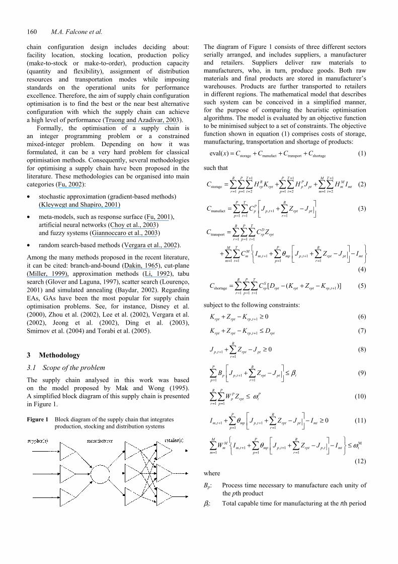
The supply chain analysed in this work was based on the model proposed by Mak and Wong (1995). A simplified block diagram of this supply chain is presented in Figure 1.

Figure 1 Block diagram of the supply chain that integrates production, stocking and distribution systems

The diagram of Figure 1 consists of three different sectors serially arranged, and includes suppliers, a manufacturer and retailers. Suppliers deliver raw materials to manufacturers, who, in turn, produce goods. Both raw materials and final products are stored in manufacturer’s warehouses. Products are further transported to retailers in different regions. The mathematical model that describes such system can be conceived in a simplified manner, for the purpose of comparing the heuristic optimisation algorithms. The model is evaluated by an objective function to be minimised subject to a set of constraints. The objective function shown in equation (1) comprises costs of storage, manufacturing, transportation and shortage of products:

storage manufact transport shortageeval( )x C C C C= + + + (1)

such that 1 1 1

storage1 1 2 1 2 1 2

R P T P T M TR P Mrp rpt p pt m mt

r p t p t m tC H K H J H I

+ + +

= = = = = = =

= + +∑∑∑ ∑∑ ∑∑ (2)

manufact , 11 1 1

P T RPp p t rpt pt

p t rC C J Z J+

= = =

= + −

∑∑ ∑ (3)

transport1 1 1

, 1 , 11 1 1 1

R P TDrp rpt

r p t

M T P RMm m t mp p t rpt pt mt

m t p r

C C Z

C I J Z J Iθ

= = =

+ += = = =

=

+ + + − −

∑∑∑

∑∑ ∑ ∑ (4)

shortage , 11 1 1

[ ( )]R P T

Srp rpt rpt rpt rp t

r p tC C D K Z K +

= = =

= − + −∑∑∑ (5)

subject to the following constraints:

, 1 0rpt rpt rp tK Z K ++ − ≥ (6)

, 1rpt rpt rp t rptK Z K D++ − ≤ (7)

, 11

0R

p t rpt ptr

J Z J+=

+ − ≥∑ (8)

, 11 1

P R

p p t rpt pt tp r

B J Z J β+= =

+ − ≤

∑ ∑ (9)

1 1

R PP P

p rpt tr p

W Z ω= =

≤∑∑ (10)

, 1 , 11 1

0P R

m t mp p t rpt pt mtp r

I J Z J Iθ+ += =

+ + − − ≥

∑ ∑ (11)

M, 1 , 1 , t

1 1 1

M P RM

m m t mp p t rpt p t mtm p r

W I J Z J Iθ ω+ += = =

+ + − − ≤

∑ ∑ ∑ (12)

where

Bp: Process time necessary to manufacture each unity of the pth product

βt: Total capable time for manufacturing at the tth period

Supply chain optimisation using Evolutionary Algorithms 161

DrpC : Cost of delivering one unity of the pth product from

the manufacturer to the rth retailer MmC : Cost of delivering one unity of the mth raw material

from the supplier to the manufacturer PpC : Cost of manufacturing each unity of the pth product SrpC : Cost of shortage of each unity of the pth product

from the manufacturer to the rth retailer Drpt: Demand of the pth product from the manufacturer to

the rth retailer in the tth period MmH : Storage cost for each unity of the mth raw material

kept in the inlet stock of the manufacturer PpH : Storage cost of each unity of the pth product kept

in the outlet stock of the manufacturer RrpH : Storage cost of each unity of the pth product kept

in the rth retailer Imt: Amount of the mth raw material stored kept in the

inlet stock of the manufacturer, at the beginning of the tth period

Jpt: Amount of the pth product stored in the manufacturing sector, at the beginning of the tth period

Krpt: Amount of the pth product stored in the rth retailer, at the beginning of the tth period

MmW : Weight of each unity of the mth raw material P

pW : Weight of each unity of the pth product Mtω : Load limit for transporting materials from supplier to

manufacturer at the tth period Ptω : Load limit for transporting products from

manufacturer to retailers at the tth period MrptZ : Amount of the pth product sent from the

manufacturer to the rth retailer, at the tth period θmp: Amount of the mth raw material necessary to produce

each unity of the pth product.

The objective function (equation (1)) minimises the sum of the costs relative to storage, manufacture, transport, and product shortage. Equations (2)–(5) define the composition of the costs relative to storage (Cstorage), manufacture (Cmanufact), transport (Ctransport) and product shortage (Cshortage), respectively. Equations (6) and (8) impose that both sales and production must be positive. In the same way, in equation (11) imposes that the amount of raw material sent from suppliers to manufacturer must be also positive. Equation (7) limits sales up to the demand of the product, for each period and retailer. Equation (9) limits the production capacity to a given value. Equations (10) and (12) limit, respectively, the total weight of the transported products and raw materials.

The approach adopted for this case study was formulated like an integer programming problem, in which the decision variables that compose vector x, to be optimised by the EAs, are:

( 1,2,..., ; 2,3,..., )( 1,2,..., ; 2,3,..., )( 1, 2,..., ; 1, 2,3,..., ; 2,3,..., )( 1, 2,..., ; 1, 2,3,..., ; 2,3,..., )

mt

pt

rpt

rpt

I m M t TJ p P t TK r R p P t TZ r R p P t T

= = = = = = = = = =

where Imt, Jpt, Krpt, Zrpt ≥ 0.

3.2 Constraint handling

When applying EAs to the optimisation of a supply chain, a key issue is how constraints related to the problem are handled by algorithm. During the last decades, several methods have been proposed for constraint handling in EAs, and they can be grouped into four categories: methods that preserve solutions feasibility, penalty-based methods, methods that clearly distinguish between feasible and unfeasible solutions and hybrid methods.

When EAs are used for constrained optimisation problems, it is usual to handle constraints using the concept of penalty functions (that penalise unfeasible solutions). That is, it is tried to solve an unconstrained problem in the search space S using a modified fitness function such as:

( ), ifeval( )

( ) penalty( ), otherwisef x x F

xf x x

∈= +

(13)

where penalty(x) is zero if no constraint is violated, and it is positive otherwise. Usually, the penalty function is based on a distance measure to the nearest solution in the feasible region F or on the effort to repair the solution. Therefore, equation (14) shows how the fitness function is primarily defined as a maximisation problem.

1fitness1 eval( )x

=+

(14)

where x is the set of decision variables to the supply chain problem, that is, Imt, Jpt, Krpt, Zrpt.

The methodology proposed for constraint handling is divided in two steps. The first step aims at finding solutions for the decision variables that lie within user-defined upper (limupper) and lower (limlower) bounds, that is, x ∈ [limlower, limupper]. Whenever a lower bound or an upper bound restriction is not satisfied, a repair rule is applied, according to equations (15) and (16), respectively:

upper lower[0, 1] {lim ( ) lim ( )}i i i ix x w rand x x= + ⋅ ⋅ − (15)

upper lower[0, 1] {lim ( ) lim ( )}i i i ix x w rand x x= − ⋅ ⋅ − (16)

where w ∈ [0, 1] is a user-defined parameter and rand[0, 1] is an uniformly distributed random value between 0 and 1.

In the second step decision variables are considered inequalities (gi(x) ≤ 0). In this work we maximise the fitness function defined in equation (14), and thus equation (13) is rewritten as:

162 M.A. Falcone et al.

1

( ), when ( ) 0eval( )

( ) ( ), when ( ) 0

ir

i ii

f x g xx

f x r q g x g x=

≤= + ⋅ ⋅ >

∑ (17)

where q is a positive constant (arbitrarily set to 500,000) and r is the number of constraints gi(x) that were not satisfied.

4 Evolutionary Algorithms (EAs) EAs are general-purpose methods for optimisation, belonging to a class of meta-heuristics inspired by the evolution of living beings and genetics. EAs usually do not require deep mathematical knowledge of the problem but do not guarantee the optimal solution in a finite time. However, they are useful for large scale optimisation problems, dealing efficiently with huge and irregular search spaces. EAs use a population of structures (individuals), where each one is a candidate solution for the optimisation problem. Since they are population-based methods, they do a parallel search of the space of possible solutions, and are less susceptive to local minima. Therefore, EAs are suited for solving a broad range of complex problems, characterised by discontinuity, non-linearity and multivariability. The usefulness of a given solution is obtained from the environment by means of a fitness function. The population of solutions evolves throughout generations, based on probabilistic transitions and using cooperation and auto-adaptation of individuals.

There are many variants of EAs, but the main differences rely on: how individuals are represented, the genetic operators that modify individuals (especially mutation and crossover), and the selection procedure. Most current approaches of EAs descend from principles of four main methodologies: GA, EP, ES and DE.

4.1 Genetic Algorithm (GA) GAs were invented by Holland (1975) and they are the most widely used EA. A GA is a stochastic method for optimisation that employs a population of individuals (candidate solutions) that evolve throughout generations. Individuals undergo a selection procedure that embodies the principle of the survival of the fittest. Selected individuals (ancestors) generate descendents by means of the application of genetic operators, usually crossover and mutation. The basic GA includes the following steps (Goldberg, 1989):

i Create the initial population with Nind individuals. Each individual is encoded as a vector xi ∈ {0, 1} (canonical representation) or xi ∈ (real representation). Vectors are randomly initiated, according to a uniform distribution.

ii Evaluate each solution xi, i = 1, …, Nind, according to its utility to the problem in hand, using a fitness function.

iii Select the most fitted individuals using a selection strategy.

iv Apply crossover and/or mutation to the selected pool of individuals so as to generate a new population.

v Repeat Steps (ii)–(iv) until a stopping criterion is met.

Crossover is responsible for exchanging genetic material between individuals, creating new ones. It accomplishes a local search in the surroundings of the ancestors’ positions in the search space. Mutation randomly changes particular positions of an individual, and it is aimed at recovering lost genetic material and globally exploring the search space.

The main control parameters of a GA are: population size, structure and length of an individual, crossover and mutation probabilities and selection procedure. In general, there is no recipe to set those parameters for a given problem, and then they are set empirically.

4.2 Evolution Strategies (ES) ESs were first developed to solve engineering optimisation problems. Rechenberg (1973) and Schwefel (1975) proposed the original ES. It uses a mutation operator that produces a single descendent from a given ancestor, therefore, denominated ES – (1 + 1). This ES was progressively generalised to ES – (µ + λ), that is, several ancestors (µ > 1) and descendents (λ > 1) every generation. According to the selection mechanism, ESs can be either ‘plus strategy’ – ES – (µ + λ), or ‘comma strategy’ – ES – (µ, λ). In the first strategy, µ ancestors generate λ descendents and then both ancestors and descendents compete together for survival. In the second strategy, λ descendents compete to survive and ancestors are fully substituted every generation.

Individuals are directly represented by real-valued vectors (xi, σx), xi, σxi ∈ n. As usual, the initial population is randomly created, but both parameters and corresponding standard deviations are kept within user-defined ranges. Mutation operates over each element xi, by adding random numbers with normal distribution, zero mean and variance

2 ,xiσ denoted 2(0, ).xiN σ A new solution vector ( , )i xix σ′ ′ is then created by using an updating rule with lognormal distribution, such that (Bäck, 1996):

ind( ) ( ) (0, 1), 1, ,i i xix t x t N i Nσ′ = + = … (18)

ind( ) ( ) exp[ (0, 1)+ (0, 1)], 1, ,xi xi it t N N i Nσ σ τ τ′ ′= ⋅ ⋅ ⋅ = … (19)

where Nind is the number of individuals of the population; Ni(0, 1) is the Gaussian distribution for each component i. Mutation of σxi is based on a global search factor τ′⋅N(0, 1) and a local search factor τ⋅Ni(0, 1). In the case of global search, only one value N(0, 1) is generated and used by all

2xiσ of the current generation. In the case of local search, Ni

(0, 1), a new value is generated for every individual,

Supply chain optimisation using Evolutionary Algorithms 163

with normal distribution, zero mean and variance 2xiσ .

These factors are defined by the following equations:

1

2 npτ = (20)

12 np

τ ′ =×

(21)

where np is the number of dimensions of the function to be optimised. Crossover operator, when used, is similar to those used in GAs with floating point representation.

4.3 Evolutionary Programming (EP) Fogel and colleagues develop EP in the 1960s (Fogel et al., 1966), focusing the evolution of finite state machines. Similar to the other EAs presented previously, EP also uses the same evolutionary concepts. EP is closer to ES than to GA, since it simulates evolution, emphasising more the phenotypical (comportmental) relationship between populations than the genotypical (ancestors and descendents) relationship. Selection in EP is typically probabilistic. Mutation in EP uses the Gaussian distribution, while in ES it has lognormal distribution. Individuals in EP are represented in the same way as in ES: real-valued vectors (xi, σxi), where xi, σxi ∈ n and i = 1, …, Nind. Optimisation using EP is accomplished by the following steps (Fogel, 1994):

i Create the initial population with Nind individuals using uniformly distributed random numbers within previously defined ranges.

ii Compute the fitness for each individual.

iii Generate a single descendent ( , ),i xix σ′ ′ from each ancestor (xi, σxi), according to the following equations:

ind( ) ( ) (0, 1), 1, ,i i xix t x t N i Nσ′ = + = … (22)

ind( ) ( ) (0, 1), 1, .xi xi xit t N i Nσ σ ασ′ = + = … (23)

where α is a scale factor, xi(t), ( ),ix t′ σxi(t), and ( )xi tσ ′ denote the ith component of vectors xi, ,ix′ σxi and ,xiσ ′ respectively. Term N(0, 1) is a Gaussian distribution with zero mean and standard deviation 1.

iv Evaluate each descendent ix′ using a fitness function.

v Compare all solutions xi and .ix′ For each solution to be selected, k opponents are selected at random, and the best of the tournament wins. The individuals of the solution vectors xi and ix′ that have won many times in the tournaments are finally selected to be ancestors in the next generation.

vi Apply mutation to ancestors so as to generate a new population of descendents.

vii Repeat Steps (ii)–(vi) until a stopping criterion is met.

4.4 Differential Evolution (DE)

Storn and Price (1995) first introduced the DE algorithm few years ago. The DE was successfully applied by Storn (1997) to the optimisation of some well-known non-linear, non-differentiable and non-convex functions. DE is an approach for the treatment of real-valued optimisation problems. DE combines simple arithmetic operators with the classical operators of crossover, mutation and selection to evolve a randomly generated starting population to a final solution.

DE is similar to a (µ, λ) ES, but in DE the mutation is not done via some separately defined probability density function. Also, DE uses of a population-derived noise to adapt the mutation rate of the evolution process. DE is simple to implement and offers a reasonable speed of operation.

The different variants of DE are classified using the following notation: DE/α/β/δ, where α indicates the method for selecting the parent chromosome that will form the base of the mutated vector, β indicates the number of difference vectors used to perturb the base chromosome, and δ indicates the crossover mechanism used to create the child population. A bin acronym indicates that crossover is controlled by a series of independent binomial experiments. In this work, the variant of DE called DE/rand/1/bin is adopted.

DE, at each time step, mutates vectors by adding weighted, random vector differentials to them. If the cost of the trial vector is better than that of the target, the target vector is replaced by trial vector in the next generation. The variant implemented in this paper was the DE/rand/1/bin and it is given by the following steps (Storn, 1997):

i Initialise a population of Nind individuals (solution vectors) with random values generated according to a uniform probability distribution in the n dimensional problem space.

ii For each individual, evaluate its fitness value.

iii Mutate individuals in according to equation:

1 2 3, , ,( 1) ( ) [ ( ) ( )]i i r m i r i rz t x t f x t x t+ = + − (24)

where 1 2

( ) [ ( ), ( ), ..., ( )]n

Ti i i iz t z t z t z t= stands for

the position of the ith individual of a mutant vector; r1, r2 and r3 are mutually different integers and also different from the running index, i, randomly

164 M.A. Falcone et al.

selected with uniform distribution from the set ind{1, 2, , 1, 1, , };i i N− +… … fm > 0 is a real parameter,

called mutation factor, which controls the amplification of the difference between two individuals so as to avoid search stagnation and it is usually taken from the range [0.1, 1].

iv Following the mutation operation, crossover is applied in the population. For each mutant vector, zi(t + 1), an index rnbr(i) ∈ {1, 2, …, Nind} is randomly chosen, and a trial vector,

1 2( 1) [ ( 1), ( 1),i i iu t u t u t+ = + +

, ( 1)] ,n

Tiu t +… is generated with

( 1), if (rand ( ) ) or ( rand ( )),( 1)

( ), if (rand ( ) ) or ( rand ( )).j

j

j

i

ii

z t b j CR j b iu t

x t b j CR j b i

+ ≤ =+ = > ≠ (25)

To decide whether or not the trial vector ui(t + 1) should be a member of the next generation’s population, it is compared to its corresponding target vector xi(t). Thus, if Fc denotes the objective function under minimisation, then

( 1), if ( 1) ( ( )),( 1)

( ), otherwise.i c c i

ii

u t F t F x tx t

x t+ + <

+ =

(26)

v Loop to Step (ii) until a stopping criterion is met, usually a maximum number of iterations (generations).

In the above equations, i = 1, 2, …, Nind is the individual’s index of population; j = 1, 2, …, n is the position in n dimensional individual; t is the time (generation);

1 2( ) [ ( ), ( ), , ( )]

n

Ti i i ix t x t x t x t= … stands for the position

of the ith individual of population of N real-valued n-dimensional vectors; randb( j) is the jth evaluation of a uniform random number generation with [0, 1]; CR is a crossover rate in the range [0, 1]; and Fc is the evaluation of cost function. Usually, the performance of a DE algorithm depends on three variables: the population size N, the mutation factor fm, and the crossover rate CR.

5 Results

The optimisation was based on the following assumptions: all stocks (raw materials and products) are initially empty and there are M = 3 raw materials, P = 2 products, R = 3 retailers and T = 3 periods. The same parameters of this simplified supply chain problem referred by Mak and Wong (1995) were optimised in this work, as follows:

• products demands Drpt at each period are forecasted as:

111 112 113

121 122 123

211 212 213

221 222 223

311 312 313

321 322 323

80; 60; 70;50; 50; 55;60; 75; 65;45; 65; 85;80; 70; 90;50; 70; 40

D D DD D DD D DD D DD D DD D D

= = == = == = == = == = == = =

• machine processing time, Bp:

(B1, B2) = (1, 1)

• allotted time for manufacturing, βt:

(β1, β2, β3) = (800, 800,800)

• transportation cost from manufacturer to retailers, :DrpC

11 12 21 22 31 32( , , , , , ) (1, 1, 4, 4, 2, 2)D D D D D DC C C C C C =

• transportation cost from supplier to manufacturer, :MmC

1 2 3( , , ) (0,3; 0,3; 0, 2)M M MC C C =

• manufacture cost, :PpC

1 2( , ) (20, 15)P PC C =

• shortage cost, :SrpC

11 12 21 22 31 32( , , , , , ) (1000, 500, 1800,1000, 1000, 1000)

S S S S S SC C C C C C =

• storage cost in the inlet stock, :MmH

1 2 3( , , ) (5, 8, 6)M M MH H H =

• storage cost in the outlet stock, :PpH

1 2( , ) (4, 3)P PH H =

• storage cost of products in the retailers, :RrpH

11 12 21 22 31 32( , , , , , ) (8, 4, 12, 8, 8, 8)R R R R R RH H H H H H =

• raw material weight, :MmW

1 2 3( , , ) (3, 2, 2)M M MW W W =

• product weight, :PpW

1 2( , ) (7, 13)P PW W =

• load limit from supplier to manufacturer, :Mtω

1 2 3( , , ) (5000, 5000, 5000)M M Mω ω ω =

• load limit from manufacturer to retailers, :Ptω

1 2 3( , , ) (3000, 3000, 3000)P P Pω ω ω =

• amount of raw material used in products, :mpθ

11 12 21 22 31 32( , , , , , ) (1, 3, 2, 1, 1, 2).θ θ θ θ θ θ =

For each of the previously described EA, a total of 50 experiments were done, using the parameters before mentioned and different initial random seeds. For all EAs, individuals are composed by the decision variables Imt, Jpt, Krpt, Zrpt, which are rounded to the nearest integer, when computing the function eval(x). Variables were allowed to span within the following ranges: 0 ≤ Imt ≤ 20, 0 ≤ Jpt ≤ 20, 0 ≤ Krpt ≤ 30 and 0 ≤ Zrpt ≤ 120.

It is assumed that the four EAs were run under the same set up. A total of 150,000 fitness evaluations (30 individuals; 5,000 generations) was done by each EA,

Supply chain optimisation using Evolutionary Algorithms 165

every run. Other particular parameters used in the standard EAs were fixed empirically as follows:

• GA: representation of individuals by binary strings, roullete wheel selection with elitism, and crossover and mutation probabilities: 0.80 and 0.10, respectively

• ES: representation of individuals by real vectors, ES-(µ+λ) with five ancestors that generate 25 descendents

• EP: representation of individuals by real vectors, selection by tournament, α = 0.01

• DE: DE/rand/1/bin with CR = 0.8 and fm = 0.4

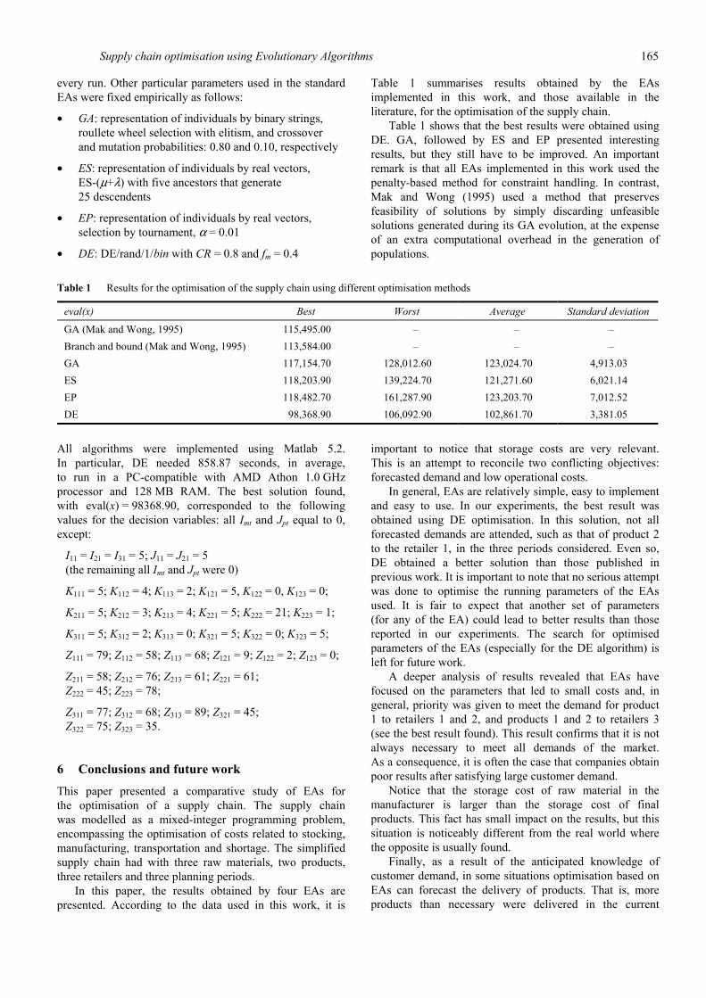
Table 1 summarises results obtained by the EAs implemented in this work, and those available in the literature, for the optimisation of the supply chain.

Table 1 shows that the best results were obtained using DE. GA, followed by ES and EP presented interesting results, but they still have to be improved. An important remark is that all EAs implemented in this work used the penalty-based method for constraint handling. In contrast, Mak and Wong (1995) used a method that preserves feasibility of solutions by simply discarding unfeasible solutions generated during its GA evolution, at the expense of an extra computational overhead in the generation of populations.

Table 1 Results for the optimisation of the supply chain using different optimisation methods

eval(x) Best Worst Average Standard deviation

GA (Mak and Wong, 1995) 115,495.00 – – – Branch and bound (Mak and Wong, 1995) 113,584.00 – – – GA 117,154.70 128,012.60 123,024.70 4,913.03 ES 118,203.90 139,224.70 121,271.60 6,021.14 EP 118,482.70 161,287.90 123,203.70 7,012.52 DE 98,368.90 106,092.90 102,861.70 3,381.05

All algorithms were implemented using Matlab 5.2. In particular, DE needed 858.87 seconds, in average, to run in a PC-compatible with AMD Athon 1.0 GHz processor and 128 MB RAM. The best solution found, with eval(x) = 98368.90, corresponded to the following values for the decision variables: all Imt and Jpt equal to 0, except:

I11 = I21 = I31 = 5; J11 = J21 = 5 (the remaining all Imt and Jpt were 0)

K111 = 5; K112 = 4; K113 = 2; K121 = 5, K122 = 0, K123 = 0;

K211 = 5; K212 = 3; K213 = 4; K221 = 5; K222 = 21; K223 = 1;

K311 = 5; K312 = 2; K313 = 0; K321 = 5; K322 = 0; K323 = 5;

Z111 = 79; Z112 = 58; Z113 = 68; Z121 = 9; Z122 = 2; Z123 = 0;

Z211 = 58; Z212 = 76; Z213 = 61; Z221 = 61; Z222 = 45; Z223 = 78;

Z311 = 77; Z312 = 68; Z313 = 89; Z321 = 45; Z322 = 75; Z323 = 35.

6 Conclusions and future work

This paper presented a comparative study of EAs for the optimisation of a supply chain. The supply chain was modelled as a mixed-integer programming problem, encompassing the optimisation of costs related to stocking, manufacturing, transportation and shortage. The simplified supply chain had with three raw materials, two products, three retailers and three planning periods.

In this paper, the results obtained by four EAs are presented. According to the data used in this work, it is

important to notice that storage costs are very relevant. This is an attempt to reconcile two conflicting objectives: forecasted demand and low operational costs.

In general, EAs are relatively simple, easy to implement and easy to use. In our experiments, the best result was obtained using DE optimisation. In this solution, not all forecasted demands are attended, such as that of product 2 to the retailer 1, in the three periods considered. Even so, DE obtained a better solution than those published in previous work. It is important to note that no serious attempt was done to optimise the running parameters of the EAs used. It is fair to expect that another set of parameters (for any of the EA) could lead to better results than those reported in our experiments. The search for optimised parameters of the EAs (especially for the DE algorithm) is left for future work.

A deeper analysis of results revealed that EAs have focused on the parameters that led to small costs and, in general, priority was given to meet the demand for product 1 to retailers 1 and 2, and products 1 and 2 to retailers 3 (see the best result found). This result confirms that it is not always necessary to meet all demands of the market. As a consequence, it is often the case that companies obtain poor results after satisfying large customer demand.

Notice that the storage cost of raw material in the manufacturer is larger than the storage cost of final products. This fact has small impact on the results, but this situation is noticeably different from the real world where the opposite is usually found.

Finally, as a result of the anticipated knowledge of customer demand, in some situations optimisation based on EAs can forecast the delivery of products. That is, more products than necessary were delivered in the current

166 M.A. Falcone et al.

period, and the surplus were set aside for the next one. Again, storage costs are minimal when compared to the shortage costs.

The EAs are capable of optimising integer, discrete and continuous variables and capable of handling nonlinear objective functions in the investigation of other optimisation problems in decision support systems, transportation and logistics environment, such as integrated production and distribution planning in supply chain, warehousing, and transportation.

Future work will include the hybridisation of the EAs, by using a local search technique, such as branch-and-bound or 2-opt. Hybrid approaches, combining of the efficient global search of EAs and the effectiveness of deterministic local search, has proved to be useful for hard combinatorial problems (see, for instance, Lopes and Coelho, 2005). Possibly, it will give good results for real-world problems of supply chain optimisation.

References Bäck, T. (1996) Evolutionary Algorithms in Theory and Practice,

Oxford University Press, Oxford. Baydar, C. (2002) ‘A hybrid parallel simulated annealing

algorithm to optimize store performance’, Genetic and Evolutionary Computation Conference, GECCO-2002, Workshop on Evolutionary Computing for Optimisation in Industry, New York, NY, USA.

Choy, K.L., Lee, W.B. and Lo, V. (2003) ‘Design of an intelligent supplier relationship management system: a hybrid case based neural network approach’, Expert Systems with Applications, Vol. 24, pp.225–237.

Dakin, R. (1965) ‘A tree-search algorithm for mixed integer programming problems’, Computer Journal, Vol. 8, pp.250–255.

Ding, H., Benyoucef, L. and Xie, X. (2003) ‘A simulation-optimization approach using genetic search for supplier selection’, in Chick, S., Sánchez, P.J., Ferrin, D. and Morrice, D.J. (Eds.): Proceedings of the Winter Simulation Conference, New Orleans, Louisiana, USA, pp.1260–1267.

Disney, S.M., Naim, M.M. and Towill, D.R. (2000) ‘Genetic algorithm optimisation of a class inventory control systems’, International Journal of Production Economics, Vol. 68, pp.259–278.

Dong, M. (2001) Process Modeling, Performance Analysis and Configuration Simulation in Integrated Supply Chain Network Design, Doctoral Dissertation, Department of Industrial and Systems Engineering, Virginia Polytechnic Institute and State University, Blacksburg, Virginia, USA.

Ermis, M., Sahingoz, O.K. and Ulengin, F. (2004) ‘Mobile agent based supply chain modelling with neural network controlled services’, Proceedings of 4th International ICSC Symposium on Engineering of Intelligent Systems, Island of Madeira, Portugal, pp.1–8.

Fogel, D.B. (1994) ‘An introduction to simulated evolutionary optimization’, IEEE Transactions on Neural Networks, Vol. 5, No. 1, pp.3–14.

Fogel, L.J., Owens, A.J. and Walsh, M.J. (1966) Artificial Intelligence through Simulated Evolution, John Wiley, New York, NY, USA.

Fu, M.C. (2001) ‘Simulation optimization’, in Peters, B.A., Smith, J.S., Medeiros, D.J. and Rohrer, M.W. (Eds.): Proceedings of the Winter Simulation Conference, Arlington, VA, USA, pp.53–61.

Fu, M.C. (2002) ‘Optimization for simulation: theory and practice’, INFORMS Journal on Computing, Vol. 14, No. 3, pp.192–215.

Giannoccaro, I., Pontrandolfo, P. and Scozzi, B. (2003) ‘A fuzzy echelon approach for inventory management in supply chains’, European Journal of Operational Research, Vol. 149, pp.185–196.

Glover, F. and Laguna, M. (1997) Tabu Search, Kluwer Academic Publishers, London, UK.

Goldberg, D. (1989) Genetic Algorithms in Search Optimization and Machine Learning, Addison-Wesley, Reading, MA.

Grossmann, I.E. (2004) ‘Challenges in the new millennium: product discovery and design, enterprise and supply chain optimization, global life cycle assessment’, Computers and Chemical Engineering, Vol. 29, pp.29–39.

Holland, J.H. (1975) Adaptation in Natural and Artificial Systems, The University of Michigan Press, Ann Arbor, USA.

Jeong, B., Jung, H-S. and Park, N-K. (2002) ‘A computerized causal forecasting system using genetic algorithms in supply chain management’, The Journal of Systems and Software, Vol. 60, pp.223–237.

Kleywegt, A.J. and Shapiro, A. (2001) ‘Stochastic optimization’, in Salvendy, G. (Ed.): Handbook of Industrial Engineering, 3rd ed., John Wiley, pp.2625–2650.

Lee, Y.H., Jeong, C.S. and Moon, C. (2002) ‘Advanced planning and scheduling with outsourcing in manufacturing supply chain’, Computers and Industrial Engineering, Vol. 43, pp.351–374.

Li, H.L. (1992) ‘An approximate method for local optima for nonlinear mixed integer programming problems’, Computers and Operational Research, Vol. 19, No. 5, pp.435–444.

Lopes, H.S. and Coelho, L.S. (2005) ‘Particle swarm optimization with fast local search for the blind traveling salesman problem’, Proceedings of 5th International Conference on Hybrid Intelligent Systems, Rio de Janeiro, Brazil, pp.245–250.

López, E-P., Ydstie, B.E. and Grossmann, I.E. (2003) ‘A model predictive control strategy for supply chain optimization’, Computers and Chemical Engineering, Vol. 27, pp.1201–1218.

Lourenço, H.R. (2001) Supply Chain Management: An Opportunity for Metaheuristics, Department of Economic and Business, Universitat Pompeu Fabra, Barcelona, Spain, Series Economics Working with number 538, pp.1–25.

Mak, K.L. and Wong, Y.S. (1995) ‘Design of integrated production-inventory-distribution systems using genetic algorithm’, Proceedings of Genetic Algorithms in Engineering Systems: Innovations and Applications, Glasgow, UK, pp.454–460.

Miller, A.J. (1999) Polyhedral Approaches to Capacitated Lot-sizing Problems, PhD Thesis, School of Industrial and Systems Engineering, Georgia Institute of Technology, December, USA.

Rabelo, L., Helal, M. and Lertpattarapong, C. (2004) ‘Analysis of supply chains using system dynamics, neural nets, and eigenvalues’, in Ingalis, R.G., Rossetti, M.D., Smith, J.S. and Peters, B.A. (Eds.): Proceedings of the 2004 Winter Simulation Conference, Washington DC, USA, pp.1136–1144.

Supply chain optimisation using Evolutionary Algorithms 167

Rechenberg, I. (1973) Evolutionsstrategie: Optimierung technischer Systeme nach Prinzipien der biologischen Evolution, Frommann-Holzboog Verlag, Stuttgart, Germany.

Schwefel, H-P. (1975) Kybernetischer Evolution als Strategie der experimentellen Forschung in der Strömungstechnik, Diploma Thesis, Technical University of Berlin, Germany.

Smirnov, A.V., Sheremetov, L.B., Chilov, N. and Cortes, J.R. (2004) ‘Soft-computing technologies for configuration of cooperative supply chain’, Applied Soft Computing, Vol. 4, pp.87–107.

Storn, R. (1997) ‘Differential evolution – a simple and efficient heuristic for global optimization over continuous spaces’, Journal of Global Optimization, Vol. 11, No. 4, pp.341–359.

Storn, R. and Price, K. (1995) Differential Evolution: A Simple and Efficient Adaptive Scheme for Global Optimization wover Continuous Spaces, Technical Report TR-95-012, International Computer Science Institute, Berkeley, USA.

Terzi, S. and Cavalieri, S. (2004) ‘Simulation in the supply chain context: a survey’, Computers in Industry, Vol. 53, pp.3–16.

Torabi, S.A., Ghomi, S.M.T.F. and Karimi, B. (2005) ‘A hybrid genetic algorithm for the finite horizon economic and delivery scheduling in supply chains’, European Journal of Operational Research, Vol. 173, No. 1, 2006, pp.173–189.

Truong, T.H. and Azadivar, F. (2003) ‘Simulation based optimization for supply chain configuration design’, in Chick, S., Sánchez, P.J., Ferrin, D. and Morrice, D.J. (Eds.): Proceedings of the 2003 Winter Simulation Conference, New Orleans, Louisiana, USA, pp.1268–1275.

Vergara, F.E., Khouja, M. and Michalewicz, Z. (2002) ‘An evolutionary algorithm for optimizing material flow in supply chains’, Computers and Industrial Engineering, Vol. 43, pp.407–421.

Zhou, Z., Cheng, S. and Hua, B. (2000) ‘Supply chain optimization of continuous process industries with sustainability considerations’, Computers and Chemical Engineering, Vol. 24, pp.1151–1158.

Zhou, G., Min, H. and Gen, M. (2002) ‘The balanced allocation of customers to multiple distribution centers in the supply chain network: a genetic algorithm approach’, Computers and Industrial Engineering, Vol. 43, pp.251–261.