Electronic copy available at: http://ssrn.com/abstract=1399247

Managers’ Investment Timing Decisions

under Endogenous Compensation Contracts∗

Keiichi Hori†

Faculty of Economics, Ritsumeikan University

Hiroshi Osano‡

Institute of Economic Research, Kyoto University

June 8, 2011

∗The authors would like to thank Kong-Pin Chen, Eric Chou, Shinsuke Ikeda, Xu Peng, HirofumiUchida, Noriyuki Yanagawa, and seminar participants at the Research Institute of Economy, Trade &

Industry (RIETI), the 2008 Contract Theory Workshop (Academia Sinica), the Monetary Economics

Workshop, and Keio University for their helpful comments. This research is financially supported by the

Japan Society for the Promotion of Science under Grant No.(C) 17530142 and Nomura Foundation for

Social Science.†Faculty of Economics, Ritsumeikan University, 1-1-1 Noji-higashi, Kusatsu, Shiga 525-8577, Japan.‡Corresponding author. Institute of Economic Research, Kyoto University, Sakyo-ku, Kyoto 606-8501,

Japan. phone: +81-75-753-7131, fax: +81-75-753-7138, e-mail: h.osano@fx5.ecs.kyoto-u.ac.jp

1

Electronic copy available at: http://ssrn.com/abstract=1399247

Managers’ Investment Timing Decisions

under Endogenous Compensation Contracts

Abstract

This paper considers how managers choose the timing of investment in risky but value-

increasing projects with a liquidation possibility for their firm when their personal objec-

tives are not aligned with those of shareholders but their compensation is endogenously

determined. Using a real options approach for a broad class of managerial preferences,

we show that without hidden information, the startup of the project is more likely to

be delayed with a higher liquidation possibility, whereas the grant size of stock-based

managerial compensation is independent of the liquidation possibility but is decreasing

in the volatility of the firm’s cash flow stream and the degree of managerial impatience if

the manager is risk neutral. We also indicate that restricted stock is optimal in a general

class of compensation schedules, regardless of the manager’s risk preferences. Further, if

there exists hidden information on the volatility of project returns and if the risk-neutral

manager is as impatient as the shareholders, the equilibrium must be pooling. Then, the

startup of the high- (low-)volatility project is advanced (delayed) in comparison with the

case without hidden information.

JEL Classification: D86, G30, G34, M52.

Keywords: agency conflicts, investment timing, real options, restricted stock, stock op-

tions.

2

Electronic copy available at: http://ssrn.com/abstract=1399247

1. Introduction

This paper considers the problem of the optimal timing of investment to be decided

by a manager under uncertainty and a liquidation possibility when his objectives are

not aligned with those of shareholders but his compensation is endogenously determined.

In the literature analyzing investment decisions under uncertainty, the effect of the irre-

versibility of investment has been highlighted by McDonald and Siegel (1986) and Dixit

and Pindyck (1994). This irreversibility creates an option value in waiting to launch a

risky but value-increasing investment project, and strongly affects the decision maker’s in-

centives in undertaking the project. However, in many modern corporations, the manager

is delegated the authority to choose when to launch investment projects. If the manager’s

objectives are not aligned with those of shareholders, the option value of the manager

waiting to invest is different from that of shareholders waiting to invest. Thus, man-

agers are likely to determine the investment (or disinvestment) timing opportunistically

(see Morellec (2004) and Lambrecht and Myers (2007, 2008)). In addition, managerial

compensation also has impacts on option values for managers waiting to invest. Hence,

shareholders should design managerial compensation schemes that succeed in inducing

managers to choose the timing of investments more appropriately from the shareholders’

point of view.

To capture these perspectives, we develop an agency conflict model with real options

and a liquidation possibility and analyze an optimal incentive contract for managers in a

dynamic setting. In this setting, managers are assumed to be more or equally impatient as

a firm’s initial shareholders and to incur effort costs for investment.1 The primary purpose

of this paper is to examine how the optimal timing of investment decisions is determined

by the manager when his objectives are not aligned with those of the shareholders and his

compensation is endogenously determined, and explore what kind of contract is optimal

from a dynamic incentive viewpoint in a general class of compensation schedules.

Our basic model builds on an agency setting in which the risk-neutral shareholders of

a firm delegate decisions regarding the start of an investment project to a risk-neutral

manager with limited liability, and provide him with incentives to start the project. The

1Another approach to representing a manager’s concerns about the subjective value of the firm’s cash

flow is to assume that the manager is risk averse. In Section 7.3, we show that our main results are

unaffected by assuming that the manager is risk averse.

3

manager may be as impatient as the shareholders or more impatient. As the firm’s setup

costs and the manager’s effort costs for starting the project are sunk, the decision to launch

the investment project is irreversible. Such irreversibility, together with the uncertain

future value of the firm, means that there is an opportunity cost associated with investing

today. This makes it essential for both the shareholders and the manager to select, as

discussed in the real options literature, the appropriate time for starting the project.

However, where managers’ objectives are not aligned with those of the shareholders,

the startup timing appropriate for the manager is different from that appropriate for

shareholders. Besides, managers’ decisions about whether to expend their effort costs are

usually unobservable if there is a possibility of project failure, that is, liquidation after the

start of the project. Then, it is impossible to write a complete contract specifying actions

required for an efficient timing decision. However, even in this case, it is possible to write

a contract contingent on the value of the firm’s cash flow stream by using a stock-based

compensation contract. Therefore, we consider how investment timing and optimal stock-

based compensation schemes are endogenously determined. An explicit example of our

investment problem is that of a corporate manager who chooses the timing of investment

in risky real projects. The basic model is also extended to the hidden information and

risk-averse manager models in Sections 6 and 7.3.

Even for a broad class of managerial preferences, our main findings show that as long

as agency conflicts exist:

(i) The optimal trigger for the commencement of the project is increasing in the possibility

of liquidation. If the manager is risk neutral, the grant size of stock-based managerial

compensation is independent of the possibility of liquidation but is decreasing in the

volatility of the firm’s cash flow stream and the degree of managerial impatience. If the

manager is risk averse, the effects of these parameters on the grant size of stock-based

compensation depend on the degree of the manager’s relative risk aversion.

(ii) Restricted stock is optimal in a general class of compensation schedules, regardless of

the manager’s risk preferences.2

(iii) If there exists hidden information on the volatility of the project return and if the

2This conclusion does not necessarily suggest that observed compensation practice such as stock

options suffers from any significant defect. Instead, it would be better to state that restricted stock is

optimal if the manager’s investment timing decisions are a major issue, as highlighted by McDonald and

Siegel (1986) and Dixit and Pindyck (1994).

4

risk-neutral manager is as impatient as the shareholders, the equilibrium must be pooling

so that the startup of the high- (low-)volatility project is advanced (delayed) compared

with the case without hidden information.

The intuition behind these results is as follows. First, the uncertainty regarding project

returns and the irreversibility of investments creates an incentive to postpone decisions.

Then, an increase in the liquidation possibility raises the risk of losing the sunk cost upon

liquidation, thus delaying the project start further. This effect can dominate the change

in the risk preference-adjusted factor, even though the manager is risk averse. Second,

suppose that the manager is risk neutral. As an increase in the liquidation possibility

merely raises the risk of losing the sunk cost upon liquidation, the grant size of restricted

stock need not be adjusted so as to internalize this effect. Hence, the grant size of restricted

stock is independent of the possibility of liquidation. On the other hand, the grant size of

restricted stock is decreasing in the volatility of the firm’s cash flow stream and the degree

of managerial impatience because these changes reduce the efficacy of restricted stock in

motivating the manager to choose an earlier launching of the project. Next, suppose that

the manager is risk averse. As changes in the parameters stated above affect the risk

preference-adjusted factor, their comparative static results depend on the degree of the

manager’s relative risk aversion. Third, the nonlinear part of managers’ compensation

merely induces them to demand greater excess returns before they are willing to launch

projects. Because this causes further delay in project startups, the compensation contract

should be linear. In particular, if shareholders award stock options to the manager, the

positive exercise price becomes an additional sunk cost to the manager, regardless of

the manager’s risk preferences. Thus, although the compensation part of stock options

gives the manager a strong incentive to launch the project, the exercise price needs to

be minimized so that restricted stock (which is equivalent to stock options with a zero

exercise price) dominates stock options with positive exercise prices. Finally, if hidden

information on the volatility of project returns exists and if the risk-neutral manager is as

impatient as the shareholders, the necessity of alleviating the adverse selection problem

requires the amount of the grant of restricted stock not to depend on the type of project.

This is because in our setting, the manager with the high-volatility project incurs no

additional costs when imitating the low-volatility project. As the resulting compensation

contract must be pooling, the optimal trigger for project startup is determined so that

5

the high- (low-)volatility project is advanced (delayed) compared with the case without

hidden information.

This paper continues a line of research using the real options model to study firms’

investment decisions. McDonald and Siegel (1986) is the pioneering work in this area.

Hugonnier and Morellec (2007b) examined the impact of managerial risk aversion on

investment decisions when managers face incomplete markets.

The effect of the project liquidation possibility on the investment timing is investigated

in Lyandres and Zhdanov (2010). They indicate that the possibility of default reduces

the value of the option to wait and provides equity holders with an incentive to speed

up investment. By contrast, we show that the start of the project is more likely to be

delayed if the project liquidation possibility is greater. The difference between these

results is because the loss of the investment opportunity arises in the event of default in

Lyandres and Zhdanov (2010), whereas the loss of the sunk investment cost occurs in the

event of project liquidation in our model. We also investigate the effect of the project

liquidation possibility on the managerial compensation schedule.

Recently, several studies explored an agency conflict problem in the real options model

of the firm when there is the separation of ownership by outside stockholders and cor-

porate control by inside managers. Morellec (2004) and Lambrecht and Myers (2008)

discussed the optimal capital structure and investment (or disinvestment) timing prob-

lems under manager—shareholder conflicts. Lambrecht and Myers (2007) also analyzed the

effects of golden parachutes (severance agreements) and other takeover mechanisms on the

manager’s disinvestment decision in declining firms. Dangl, Wu, and Zechner (2008) in-

vestigated how the internal manager replacement and product market discipline interacts

in a mutual fund company. Unlike our approach, these studies assume that the man-

ager’s compensation is linear in firm value, and do not determine the linear stock-based

compensation scheme endogenously although the scheme significantly affects timing deci-

sions.3 By contrast, our paper examines how a managerial compensation contract may be

determined as an incentive instrument for the manager choosing the timing of investment

within a real options framework. Because we show that restricted stock is optimal in a

general class of compensation schedules, our results may justify their restrictions on the

3Although Lambrecht and Myers (2007) derived the optimal golden parachute, the other managerial

compensation parameters are fixed in their model.

6

managerial compensation scheme.

Unlike the real options literature mentioned above, Grenadier and Wang (2005) pro-

vide a model of investment timing under agency conflicts in corporate firms in which the

managerial compensation contract is endogenously determined. Their focus, however, was

on how shareholders discipline the patient or impatient manager by offering an incentive

contract contingent on a trigger point. Hence, in their model, shareholders directly de-

termine the timing of investment by choosing the trigger point, although the manager

manipulates a hidden level of effort that affects the quality of the project. In this setting,

if the manager cannot divert part of the project returns because of the absence of hid-

den information, investment in each quality project is exercised at the full information

level. On the other hand, the focus in our paper is on the situation in which none of the

contracts contingent on a trigger point can be upheld, because the liquidation probabil-

ity of the project renders unobservable whether or not the manager really expends effort

costs for starting the project on the trigger point. In this situation, our focus is how the

patient or impatient manager who manipulates the timing of investments is disciplined

by exploiting a managerial compensation contract. However, to discipline the manager

in this case, shareholders need to design a contract contingent on the value of the firm’s

cash flow stream, that is, by a stock-based contract. Unlike Grenadier and Wang (2005),

this setting provides an opportunistic motivation for the manager choosing the timing of

investing in the risky project. In contrast to Grenadier and Wang (2005), under agency

conflicts over investment timing, we show that, even in the absence of hidden information,

investment in the project is delayed when compared with the full information case. In

addition, we suggest that restricted stock is optimal, although the optimal compensation

contract derived in Grenadier and Wang is different from that commonly used in practice.

In the presence of hidden information, Grenadier and Wang (2005) indicate that un-

der manager—shareholder conflicts, the investment timing of the lower-quality (or higher-

quality) project is delayed (or efficient). On the other hand, Morellec and Schürhoff (2011)

suggest that under initial shareholder—outside investor conflicts, asymmetric information

induces firms with good prospects to speed up investment. Both of these papers prove

that good firms can separate from bad firms in equilibrium under hidden information on

the expected value of the project returns. By contrast, in the hidden information case

on the volatility of project returns in our model, the equilibrium must be pooling: the

7

investment timing of the higher- (lower-)volatility project is further advanced (delayed) in

comparison with the case without hidden information. The reason is that in our setting,

the manager with the high-volatility project incurs no additional costs when imitating the

low-volatility project.

The analysis in this paper is also related to the literature on optimal contracting models

of CEO compensation (see Dittmann and Maug (2007) and Kadan and Swinkels (2008)).

However, these studies employ a static optimal contracting model. By contrast, our

paper is the first to solve the optimal contract offered by a firm in a continuous time, real

option setting where a manager chooses the timing of investment. In our model, agency

conflicts in investment timing arise from the time-consuming features of the manager’s

investment decision, resulting from the irreversibility of the investment decision together

with the uncertain future value of the firm. The model can derive an optimal structure

of the compensation contract that provides incentives for the manager to choose the

appropriate timing of investment in the risky project given these agency conflicts. In the

static optimal contracting model, it is difficult to handle the agency conflict of timing.

Hence, the models imply that stock options are optimal if the manager is risk neutral or

has moderate levels of risk aversion (Dittmann and Maug (2007)), or if the risk-averse

manager does not face higher bankruptcy risk (Kadan and Swinkels (2008)). In contrast,

our model suggests that restricted stock is optimal in a general class of compensation

schedules, including stock options, even for a broad class of managerial preferences. The

reason for this difference is that in our real options model, the nonlinear part of the

compensation schedule induces the manager to delay the timing of investments.

In addition, the standard view of option-based compensation is that stock option con-

tracts create incentives for risk taking. Ross (2004) has recently indicated that it is

possible for the opposite to occur. Considering the possibility of loss aversion, de Meza

and Webb (2007) also suggest a new reason why option-based compensation may lessen

risk-taking behavior. In this paper, we further show that the irreversibility of investment

with uncertain project returns under agency conflicts in investment timing provides a new

reason why stock options may make the manager less inclined to take risky investment

actions than restricted stock compensation.

The rest of the paper is organized as follows. Section 2 presents the basic model and

derives the full information solution as a benchmark. Section 3.1 examines the manager’s

8

optimal trigger strategy given a compensation contract. Section 3.2 characterizes the

optimal compensation contract. Section 4 discusses the comparative static results and

the empirical implications of the model. Section 5 considers a more general compensation

contract and verifies that our main results still hold. Section 6 extends the basic model

to the joint hidden action/hidden information model. Section 7 assesses the robustness

of our main results. The final section concludes the paper. The proofs of all propositions

and lemmas are provided in the Appendix.

2. The Basic Model

2.1. Investment technology.–

We develop a continuous time agency model in which a risk-neutral manager acts as

an agent for a firm. We also use the term ‘firm’ to denote the initial shareholders. The

manager has no personal financial resources, a reservation utility of zero, and limited

liability. The initial shareholders own the firm, and their objective is to maximize the

value of their payoff at time 0. The firm is all-equity financed and operates in capital

markets with no transaction costs. The investors including the initial shareholders may

lend and borrow freely at the risk-free rate r. However, we assume that the manager

could be more impatient than the initial shareholders, and that payoffs are valued by

the manager with the discount rate r + ξ, where ξ ≥ 0.4 Although the manager is riskneutral in the basic model, we extend the basic model to the risk-averse manager model

in Section 7.3 and prove that risk-sharing considerations do not modify our main results.

We consider an investment project that can only be managed by the manager. Because

the manager has specific skills in administering the investment project, he has decision

rights over investment policies. Hence, the manager chooses the timing of project startups.

When the project is launched, the shareholders incur a fixed setup cost CS. If CS is a

monetary cost, the funds for CS are raised by the issue of new equity to the initial

shareholders. As new equity is issued to the initial shareholders, we need not discuss

how much of the project should be financed with new equity or with cash (= revenues

of the assets in place owned by the initial shareholders). We normalize the total number

of outstanding shares to 1 after the issue of new equity. In addition, the manager must

4For justification, see Grenadier and Wang (2005, Section 5).

9

expend effort so that the launched project generates a cash flow stream following the

process of equation (1) defined below. The manager’s effort inflicts physical disutility

CM on the manager, which is measured in the same units as the firm’s cash flow. The

effort disutility cost CM creates incentives for the manager to choose an inefficient startup

timing for the project from the viewpoint of the firm. The two costs CS and CM are sunk

costs and make the decision regarding the project commencement irreversible.

Now, the firm’s instantaneous cash flow x is realized with probability 1 − ε when CS

and CM are expended, and evolves as a geometric Brownian motion:

dx = μxdt+ σxdz, (1)

where μ ∈ [(1/2)σ2, r) is the instantaneous conditional expected percentage change in xper unit of time,5 σ > 0 is the instantaneous conditional standard deviation per unit of

time, and dz is the increment of a standard Wiener process (dz ∼ N (0, dt)). However, nocash flow stream is generated with probability ε even when CS and CM are expended. We

further assume that if CS is not expended (or if CS is expended but CM is not expended),

no cash flow stream is generated with probability 1 (or 1− κ). The probability ε implies

a probability that the project is liquidated after CS and CM are expended.6

For the information structure, we assume that the manager’s decision about whether to

expend CM is unobservable, whereas the shareholders’ decision about whether to expend

CS is observable and verifiable. All other variables, including the firm’s cash flow stream,

are publicly observed, and the diffusion process of x is common knowledge.

2.2. Contracts.–

As the manager chooses the threshold at which he starts the project, the firm needs to

motivate the manager to choose a timing of project startups that is appropriate for the

initial shareholders, by offering a compensation contract at time 0. Then, the firm might

5The restriction of r > μ is standard in the real options literature. The restriction μ ≥ 12σ2 ensures

that the firm is a growing firm. Although this assumption plays an important role if the manager is risk

averse, our results still hold in the case of a declining firm if the manager is risk neutral.6Practically, ε may be viewed as a financial crisis risk where the firm cannot start the project because

the situation of distress ruins the profit opportunities of the project after CS and CM are expended.

Alternatively, ε may be interpreted as an authorization or litigation risk where the authority does not

allow the firm to start the project for unexpected flaws in the project that are unrelated to the manager’s

effort decision but arise after CS and CM are expended.

10

make compensation conditional upon x and the exercise of the project. Because of this,

we might consider compensation contracts that yield the manager a bonus payment of

ω (> 0) if the project is exercised at x = x0, and 0 if the project is not exercised or if

the project is exercised at x 6= x0. If this kind of contract is feasible, the firm can always

induce the manager to select the most convenient timing of investment from the viewpoint

of the initial shareholders by adjusting ω and x0.

In fact, this kind of contract is infeasible because there is a probability ε of project

failure so that a court has trouble judging whether the manager really disrupted the

process of expending the cost. Hence, even though the manager does not expend CM , he

can claim that the firm should pay ω. Hence, this argument shows that the firm has no

incentive to offer the above type of general contingent contract.7

Because of these reasons, and until Section 5, we examine the case where compensation

contracts at time 0 can be described by three parameters: a base salary at time 0, φ;

a number of options on the firm’s stock granted to the manager, α ∈ (0, 1] (expressedas a fraction of all shares outstanding, including an issue of new equity to the initial

shareholders); and an exercise price, P (≥ 0). Thus, a compensation contract can be

represented by (φ,α, P ). Note that: (i) the case of P > 0 corresponds to stock options;

and (ii) the case of P = 0 corresponds to restricted stock.8 Indeed, α = 0 can be excluded

without loss of generality because the manager does not expend CM when α = 0; thus,

no cash flow stream is generated in this case. The restrictions of α and P are naturally

attributed to the inherent features of restricted stock or stock options. In Section 5, we

show that our main results are unaffected, even though a more general compensation

schedule is offered to the manager.

In the present stage of the analysis, we mention the case of P < 0. If P < 0, stock

options are exercised immediately at time 0 using the options argument. The manager

has no incentive to delay the exercise of stock options beyond time 0 because there is a

negative sunk cost and the exercise of stock options is instantaneous. Hence, this case is

7A contract involving a bonus payment ω at the launch of the project also causes the same problem

because the cash flow stream can be generated with probability κ even if CM is not expended. An

alternative contract involves specifying a bonus payment ω contingent on the manager’s report about

his decision to expend CM . However, in our setting, the manager’s report on expending CM imposes no

obligations on him. Hence, the firm has no incentive to offer this class of contract.8Using the options argument, stock options with P = 0 are immediately exercised at time 0. Hence,

they are viewed as restricted stock.

11

viewed as the combination of restricted stock and a base salary at time 0. Thus, without

loss of generality, we can rule out this case.

Additionally, we impose the following restrictions on the contract (φ,α, P ). First, the

manager’s base salary at time 0 cannot be reduced below a certain threshold value. One

plausible economic reason for the sticky base salary restriction is limited liability. Because

we impose limited liability on the part of the manager, we add the sticky base salary

constraint φ ≥ 0 for simplicity.9 However, in Section 7.1, we relax the sticky base salaryconstraint and show that our main results are preserved, particularly if the manager is

more impatient than the initial shareholders.

Second, even if the manager must pay a positive exercise price (P > 0) and does not

receive a sufficiently large base salary, the limited liability constraint can still hold at the

time the stock options are exercised. This is because the manager may be allowed to sell

part of the stock obtained by exercising stock options to pay the exercise price.10

Third, stock options are inalienable, that is, they cannot be sold, transferred, or assigned

to a third party. Furthermore, we assume that stock obtained by the manager through

exercising stock options cannot be sold, except for the purpose of paying the exercise

price.11 We also assume that restricted stock granted to the manager is not tradable. This

assumption is justified by the common practice that restricted stock cannot be freely sold

by executives, and that executives are routinely required (through ownership guidelines

imposed by the board) or pressured (by informed board requirements or through the

desire to signal to markets) to hold more company stock than indicated by an optimal

portfolio standpoint (see Hall and Murphy (2002)). Indeed, the efficacy of stock-based

compensation as an incentive tool depends on its ability to expose the manager to the

risks of the outcomes that his actions will provoke. If the manager was able to diversify,

or could somehow negate this risk, stock-based compensation would not act as such an

effective incentive instrument.

Finally, to obtain an analytical solution, we assume that there is no expiration date on

9This kind of assumption is imposed in Dittmann and Maug (2007) and Kadan and Swinkels (2008).10Otherwise, the manager may use “cashless exercise programs”, under which he pays nothing and

simply receives the value of the spread between the market price and the exercise price in shares of the

company stock (see Hall and Murphy (2002)).11In fact, because the assumption that the stock obtained by the manager through exercising stock

options cannot be traded makes stock options more advantageous to the shareholders, the relaxation of

this assumption does not modify our main results.

12

stock options.12 In addition, we assume that the firm pays dividends after the project

starts.13 We also assume that all granted options are allowed to vest whenever they are

granted. In Section 5, we relax the latter and investigate the effect of vesting conditions.

2.3. The definition of equilibrium.–

The equilibrium of the game is represented as follows. (i) At time 0, the firm offers

the manager a compensation contract (φ,α, P ) to maximize the value of the shareholders’

payoff. (ii) The manager determines the threshold for launching the project and the

timing for exercising stock options to maximize the value of his payoff, given (φ,α, P ).

2.4. The full information solution.–

Before analyzing the equilibrium, we briefly review the full information solution used

as a benchmark. The full information solution is derived by maximizing the value of the

option to invest at x0, provided that the manager’s decision to expend the effort cost CM

is publicly observable, that the project commencement is directly determined by the firm,

and that the manager is compensated for CM so that he is induced to participate in the

project. To simplify the analysis, we focus on the case in which the manager is always

required to expend CM because κ is sufficiently small.

The following proposition characterizes the full information solution.

Proposition 1: Let xFI denote the full information trigger for the commencement of the

project, and let VFI (x) denote the full information value of the option to invest. Then,

xFI

r − μ=

1

1− ε

β

β − 1 (CS + CM) , (2)

VFI (x) =

⎧⎨⎩³

xxFI

´β h(1−ε)xFIr−μ − CS − CM

ifor x < xFI ,

(1−ε)xr−μ − CS − CM for xFI ≤ x,

(3)

where β = 12− μ

σ2+

q¡μ

σ2− 1

2

¢2+ 2r

σ2> 1.

Note that β is the positive root of the characteristic equation 12σ2q(q − 1) + μq =

12As executive stock options typically have a 10-year expiration date, they are American call options

with finite expiration dates. However, we can hardly find analytical solutions in this case. See Karatzas

and Shreve (1998) for details on the differences between American call options with finite expiration dates

and those with infinite expiration dates.13The dividend payment rule is exogenous, as assumed in the standard real options literature.

13

r.14 In the full information case, the discount rate r is used because the firm directly

determines the commencement timing of the project.

Several remarks about this proposition are in order. First, because β > 1 and r > μ,

we have(1−ε)xFIr−μ > CS + CM . In other words, because

(1−ε)xr−μ must be large enough to

compensate for CS + CM , the firm does not start the project until the first time x reaches

the trigger xFI (>r−μ1−ε (CS + CM)). The intuitive reason is that there is an opportunity

cost associated with investing today that is created by irreversible investment and the

uncertain future values of x; that is, the option value of waiting to launch the project

implies an action threshold where the expected value from investing exceeds the cost.

This feature cannot be captured in the static model. Second, the present value operator³xxFI

´βcan be interpreted as a stochastic discount factor that constitutes the present

value of a dollar paid at the time of investment when the discount rate equals r. Finally,

xFI does not depend on the initial value of x0 because of the time-consistent structure of

our model. Hence, xFI is determined independently of time.

3. The Optimal Trigger Strategy and Compensation Contract

In this section, we discuss the impact of agency conflicts, provided that the manager’s

decision to expend CM is unobservable and that the project’s startup is determined by

the manager. In the subsequent analysis, we work backwards to derive the optimal trig-

ger strategy and the optimal compensation contract. We first explore the manager’s

maximization problem with respect to the trigger points for launching the project and

exercising stock options, and then examine the firm’s maximization problem with respect

to the compensation contract. Because we assume that κ is sufficiently small and that

no cash flow stream is generated with probability 1 − κ unless CM is expended, we can

focus on the case where the manager always chooses to expend CM at the launch of the

project under (φ,α, P ) as long as his individual rationality constraint is satisfied. Thus,

we need not consider the incentive compatibility constraint for the manager that induces

him to expend CM at the launch of the project. This implies that we focus on resolving

the manager’s choice of project startup timing strategy.

3.1. The optimal trigger strategy for a given compensation contract.–

14If β is the negative root, VFI (x) is decreasing in x, which contradicts the intuitive explanation.

14

We need to divide the analysis into the following two cases: (i) the manager first starts

the project by bearing CM , and then exercises stock options by paying P per share; and

(ii) the manager first exercises stock options by paying P per share, and then begins the

project by bearing CM . Regardless of which case we deal with, we need to work backwards

to find the solution because the manager’s problem is regarded as a two-stage sequential

maximization problem.

We begin by discussing the first case. As the manager exercises the stock options after

starting the project, we first solve the manager’s problem of when to exercise the stock

options, taking the compensation contract as given. The stock options examined here can

be regarded as American call options with dividends and infinite expiration dates because

we have assumed that there is no expiration date for the stock options and that the firm

pays dividends after the project starts. After finding the value of the stock options held

by the manager, along with the trigger value of x at which the manager exercises stock

options, we next proceed to solve the manager’s problem of when to launch the project,

and derive the value of the manager’s option to launch the project and the trigger value

of x for the commencement. In this stage, the value of the manager’s option to launch

the project is determined given the value of stock options held by the manager and the

corresponding trigger value of x for the exercise of stock options. Hence, our two-stage

sequential maximization problem is to find the value of the compound options.

Indeed, using the result of Dixit and Pindyck (1994, Chapter 10.1), we can show that

if P > 0, the commencement of the project and the exercise of the stock options occur

simultaneously. In other words, it will never be the case that the manager will start the

project and then wait, rather than also exercising the stock options.15 Intuitively, the

manager need not delay the exercise of the stock options, not only because the project

startup and the exercise of stock options are instantaneous but also because there are no

other impediments to exercising these actions in any stages at once. Given this finding,

we can transform the two-stage sequential maximization problem into a one-stage maxi-

mization problem in which the manager simultaneously launches the project and exercises

the stock options by bearing CM and paying P per share.

Similarly, using the result of Dixit and Pindyck (1994), we can prove that if P > 0,

15More specifically, the optimal solution indicates that the trigger level for launching the project in

the first stage is larger than that for exercising the stock options in the second stage. As a result, the

beginning of the project and the exercise of the stock options occur simultaneously.

15

the startup of the project and the exercise of the stock options occur simultaneously,

even though we deal with the second case. Thus, if P > 0, irrespective of the case we

examine, we need only consider the one-stage maximization problem in which the manager

simultaneously launches the project and exercises the stock options by bearing CM and

paying P per share.

If P = 0, the stock options are exercised immediately at time 0 and are reduced to

restricted stock, as argued in Section 2.2. However, the manager’s maximization problem

for P = 0 is the same as that for P > 0, except that the manager need not pay P per

share at the start of the project. In other words, if P = 0, the two-stage sequential

maximization problem is reduced to a one-stage maximization problem with respect to

the exercise timing of the project’s startup.

Let x∗ denote the optimal trigger value of x at which the manager launches the project,

and let G(x) denote the value of the option for the manager to start the project. Now,

solving the transformed one-stage maximization problem of the manager, we obtain the

following proposition.

Proposition 2: If a contract (φ,α, P ) is given, then x∗ and G(x) are

x∗

r + ξ − μ=

1

1− ε

γ

γ − 1∙CM

α+ (1− ε)P

¸> P, (4)

G(x) =

⎧⎨⎩¡xx∗¢γ h

α(1− ε)³

x∗r+ξ−μ − P

´− CM

ifor x < x∗,

α(1− ε)³

xr+ξ−μ − P

´− CM for x∗ ≤ x,

(5)

where γ = 12− μ

σ2+

q¡μ

σ2− 1

2

¢2+

2(r+ξ)

σ2> β > 1.

Note that γ is the positive root of the characteristic equation 12σ2q(q − 1) + μq = r

+ ξ. In this case, the discount rate r + ξ is used because the manager determines the

startup of the project.

Several remarks are in order. First, and as explained in Proposition 1, the option value

of the manager waiting to launch the project implies an action threshold, x∗, where the

expected value of the manager from investing,α(1−ε)x∗r+ξ−μ , exceeds the cost, CM + α(1 −

ε)P , because γ > 1 and r + ξ > μ. In addition, this implies that if stock options are

not vested before the project starts, the manager exercises the stock options immediately

16

upon the vesting. We return to this point in Section 5. Second, because(1−ε)( x∗

r+ξ−μ−P)P

=

11−ε

γ

γ−1CMαP

+ 1γ−1 + ε, the manager is more likely to exercise the stock options deeper in

the money, as γ is smaller, CM is larger, α is smaller, P is smaller, and ε is larger. Third,

x∗ increases with CM and ε. Furthermore, x∗ increases with P but decreases for a larger

α. This implies that decreasing P while increasing α induces the manager to launch the

project earlier because the value of the option for the manager is then larger. Finally, the

present value operator¡xx∗¢γcan again be interpreted as a stochastic discount factor that

constitutes the present value of a dollar paid at the time of investment when the discount

rate equals r + ξ. Furthermore, it follows that¡xx∗¢γ ≤ ¡ x

x∗¢βbecause x < x∗ and γ ≥ β.

This shows that a dollar received at the stopping time described by the trigger strategy

x∗ is worth less to the manager than to the initial shareholders.

3.2. The optimal contract.–

To formalize the firm’s maximization problem, we need to specify the values of the

shareholders’ and manager’s payoffs at time 0, given a contract (φ,α, P ) and the manager’s

optimal trigger point x∗ derived in Proposition 2.

Let WS(x0) and WM(x0) denote the values of the shareholders’ and manager’s payoffs

at time 0, respectively. To simplify the analysis and focus on the more interesting case,

we assume that x0 is not sufficiently large, so that x0 < x∗.16 Then, using Proposition 2

and the fact that the shareholders’ and manager’s present value operators are represented

by¡x0x∗¢βand

¡x0x∗¢γ, respectively, it follows that

WS(x0) = −φ+³x0x∗

´β ∙(1− α)

(1− ε)x∗

r − μ+ α(1− ε)P − CS

¸,

WM(x0) = φ+³x0x∗

´γ ∙α(1− ε)

µx∗

r + ξ − μ− P

¶− CM

¸.

Note that if the contract relation is organized, the firm pays the fixed base salary φ to

the manager at time 0.

16The sufficient condition for this is that (1 − ε)x0 <β

β−1h(r − μ)CS +

γγ−1(r + ξ − μ)CM

i, which

implies that the initial expected value of the firm’s cash flow is smaller than (the multiplier ββ−1 )× [(r−

μ)× (the firm’s setup cost CS) + (the multiplier γγ−1)× (r + ξ − μ)× (the manager’s effort cost CM )].

17

Given Proposition 2, the firm’s problem is presented as follows:

maxφ,α,P

½−φ+

³x0x∗

´β ∙(1− α)

(1− ε)x∗

r − μ+ α(1− ε)P − CS

¸¾, (6)

subject tox∗

r + ξ − μ=

1

1− ε

γ

γ − 1∙CM

α+ (1− ε)P

¸, (IC)

φ+³x0x∗

´γ ∙α(1− ε)

µx∗

r + ξ − μ− P

¶− CM

¸≥ 0, (IR)

φ ≥ 0, (BS)

1 ≥ α > 0, (SR)

P ≥ 0. (EP)

Here, the objective function is provided by WS(x0). (IC) characterizes the incentive

compatibility constraint for the manager with respect to x∗, which means that x∗ is de-

rived from (4) in Proposition 2. (IR) expresses the individual rationality constraint for the

manager, which guarantees thatWM(x0) is larger than or equal to the manager’s reserva-

tion utility of zero. (BS) is the sticky base salary constraint, (SR) is the restriction of the

shareholding ratios of the shareholders and the manager, and (EP) is the nonnegativity

restriction of the exercise price of stock options. Note that as long as (IR) holds, we need

not consider the incentive compatibility constraint for the manager that induces him to

expend CM , as argued at the beginning of this section.

Now, we show the following lemma:

Lemma 1: (IR) is not binding.

The intuition for the result of Lemma 1 is that the expected value of the manager from

investing,α(1−ε)x∗r+ξ−μ , exceeds the cost, CM + α(1− ε)P , because of (IC) and γ > 1. As this

together with (BS) implies φ +¡x0x∗¢γ h

α(1− ε)³

x∗r+ξ−μ − P

´− CM

i> 0, (IR) is never

binding. This intuition is also related to the investment rule of the standard real option

model: The option is exercised at a trigger where the option value is positive.

Let (φ∗,α∗, P ∗) denote the solution to problem (6). Using Lemma 1, we obtain the

following proposition.

18

Proposition 3: The optimal commencement trigger is

x∗ =1

1− ε

β

β − 1∙(r − μ)CS +

γ

γ − 1(r + ξ − μ)CM

¸> xFI . (7)

Furthermore, restricted stock dominates stock options and the base salary, so the optimal

compensation contract is characterized by

φ∗ = P ∗ = 0 and α∗ =β − 1β

γ(r + ξ − μ)CM

(γ − 1)(r − μ)CS + γ(r + ξ − μ)CM. (8)

The values of the shareholders’ and manager’s payoffs at time 0 are

WS(x0) =³x0x∗

´β ∙ β(γ − 1)(r − μ)CS + γ(r + ξ − μ)CM

β(γ − 1)(r − μ)CS + βγ(r + ξ − μ)CM

(1− ε)x∗

r − μ− CS

¸> 0, (9)

WM(x0) =³x0x∗

´γ ∙β − 1β

γ(r + ξ − μ)CM

(γ − 1)(r − μ)CS + γ(r + ξ − μ)CM

(1− ε)x∗

r + ξ − μ− CM

¸> 0.

(10)

The intuition behind this proposition is as follows. As suggested, the project startup

and the exercise of stock options occur simultaneously, not only because they are instan-

taneous but also because there are no other impediments to exercising the actions in all

stages at once. Then, there are two effects when the exercise price increases. First, the

firm’s revenues generated by the manager increase. This effect increases the value of the

shareholders’ option to launch the project. Second, the trigger point for starting the

project increases because the manager must pay the higher exercise price as a sunk cost.

Thus, increasing the exercise price induces the manager to delay launching the project.

The delay reduces the value of the shareholders’ option to launch the project. Indeed,

the second effect always dominates the first. Thus, the exercise price is set to zero. It

also follows from (IC) and γ > 1 that the individual rationality constraint is not binding

because the expected value of the manager from investing exceeds the cost at the optimal

commencement trigger. Hence, as a result of the sticky base salary constraint, the base

salary is set to zero. The reason is that the effect of an increase in the base salary only

decreases the value of the shareholders’ payoff at time 0 because it does not affect any

incentives for the manager to start the project.

19

The optimal trigger x∗ is larger than the full information trigger, xFI . The reason is

that the grant size of restricted stock under the optimal contract α∗ is smaller than that

required to attain xFI .17 This is because there is a trade-off between increasing incentives

to start the project earlier and increasing dilution costs related to the larger grant size of

restricted stock.

Several remarks about this proposition are in order. First, the project startup is ex-

ercised at a higher trigger level than at xFI , irrespective of whether γ > β or γ = β.

The delay (beyond xFI) arises from the fact that the manager cannot fully internalize the

benefits of more efficient investment timing. As an increase in the start trigger beyond

xFI raises the value of the manager’s option to launch the project, he has an incentive for

that at x∗ > xFI . Indeed, as long as the manager’s opportunistic motive exists, or as long

as the manager’s effort cost exists (CM > 0), the trigger is determined at a higher level

than at xFI . This perspective was not discussed in Grenadier and Wang’s (2005) real

options model, because they considered a setting in which the shareholders could directly

determine the commencement trigger when CM = 0. Hence, in their model of hidden

action only, all the trigger levels are determined at the full information level, regardless

of whether γ > β or γ = β. As a result, the trigger levels are unaffected by consideration

of hidden action.

Second, the ratio x∗xFI

measures the relative inefficiency of the trigger policy x∗: x∗xFI

=

1CS+CM

³CS +

γ

γ−1r+ξ−μr−μ CM

´(> 1). The manager’s trigger policy is less efficient as the

setup cost of the shareholders CS decreases or the effort cost of the manager CM increases.

It also follows from Proposition 4 in the next section that the manager’s trigger policy is

less efficient as the volatility of the firm’s cash flow stream σ increases, or as managerial

impatience ξ decreases if σ2

r+ξis sufficiently large. However, the relative inefficiency of the

trigger policy is independent of the liquidation possibility ε.

Third, stock options are never optimal. Instead, restricted stock is optimal, even with

the manager’s risk-neutral preferences. Further, this result holds regardless of whether

the manager is as patient as–or more patient than–the initial shareholders (γ > β or γ

= β). Option-based compensation is often criticized for inducing “too much” risk taking

by manager. However, Ross (2004) indicates that the implicit assumption behind this

argument is that the manager’s von Neumann-Morgenstern utility function has the same

17From (IC) in (6), note that xFI would be attained if α were equal toβ−1β

γγ−1

r+ξ−μr−μ

CMCS+CM

.

20

risk aversion over the entire relevant domain of outcomes. If not, he suggests that it is am-

biguous whether option-based compensation encourages risk taking. de Meza and Webb

(2007) also argue that the presence of loss aversion provides a further reason why risk

taking may be lower with an option contract than with a share or other incentive scheme

that does not protect against the downside. In this paper, we show that the irreversibility

of investment with uncertain project returns under agency conflicts in investment timing

gives another reason why stock options may make the manager less inclined to take risky

investment actions than restricted stock.

4. Comparative Statics and Empirical Implications

4.1. Comparative statics.–

We examine the effects of the key parameters of the model on x∗ and α∗ given by

Proposition 3. The key parameters are the liquidation possibility ε, the volatility of

the firm’s cash flow stream σ and the degree of managerial impatience ξ. As has been

discussed, the parameter ε may be viewed as the financial crisis risk or the authorization

and litigation risk. σ may be interpreted as the uncertainty of the business environment

that the firm faces. ξ may be represented by the manager’s concerns about the firm’s

short-term performance or the threat to the manager from a stochastic termination, as

suggested by Grenadier and Wang (2005). If ξ is reduced when the manager has more job

opportunities outside of the firm, ξ is smaller as the managerial labor market becomes

deeper.

Given the results of Proposition 3, we obtain the following proposition.

Proposition 4: (i) x∗ is increasing in ε and σ. If σ2

r+ξis sufficiently large, x∗ is decreasing

in ξ.

(ii) α∗ is independent of σ. In addition, if ξ = 0 so that γ = β, then α∗ is decreasing in

σ. If σ2

r+ξis sufficiently large, α∗ is decreasing in ξ.

Result (i) indicates that the commencement trigger x∗ becomes higher as ε and σ

increase. A larger ε implies a greater liquidation possibility, which raises the risk of losing

the sunk cost upon liquidation and thus increases the excess returns before launching the

project. This increases x∗, all else being constant. In addition, for a given α, a larger σ

raises the stochastic discount factor¡x0x∗¢βand

¡x0x∗¢γif x∗ is determined as in (4). This

21

increases the value of the manager’s option to wait, thereby motivating the manager to

exercise the option to start the project later. By contrast, result (i) shows that when ξ

increases, x∗ decreases if σ2

r+ξis sufficiently large. This is because the greater managerial

impatience then decreases the value of the manager’s option to wait. Hence, an increase

in ξ induces earlier startup of the project.

Result (ii) shows that the grant size of restricted stock α∗ is independent of ε. Because

an increase in the liquidation possibility merely raises the risk of losing the sunk cost upon

liquidation, the expected value of the manager from investing,(1−ε)x∗r+ξ−μ , is independent of

ε for a given α if x∗ is determined by (4). As ε does not affect any incentives for the

manager to invest, the firm has no incentive to adjust the size of α so as to internalize

the effect of ξ. However, result (ii) suggests that α∗ decreases with σ if γ = β. A

larger σ increases the value of the manager’s option to wait, as stated above. If the

manager’s impatience is not too different from the shareholders’ (γ ' β), an increase in

σ reduces the size of α used in the contract because this effect of σ reduces the efficacy of

restricted stock in motivating the manager to choose an earlier launching of the project.

However, if managerial impatience is sufficiently great, the firm may have to grant more α

to compensate the manager for a decline in the manager’s option value (to invest) caused

by a rise in σ. Result (ii) also implies that α∗ decreases with ξ if σ2

r+ξis sufficiently large.

Because greater managerial impatience then gives the manager more incentive to launch

the project earlier for a given amount of α, the firm can reduce the grant size of α used

in the contract.

4.2. The empirical implications.–

Proposition 4 provides several predictions about investment timing.

Prediction 1: Investment is more delayed, as (i) the financial crisis risk or the autho-

rization and litigation risk is higher, (ii) the volatility of the firm’s cash flow stream is

greater, and (iii) managerial impatience caused either by concerns about the firm’s short-

term preferences or the threat to the manager from a stochastic termination is weaker if

the volatility of the firm’s cash flow stream is sufficiently large relative to the manager’s

discount rate.

Bloom, Bond, and van Reenen (2007) provided evidence that, with irreversibility,

greater uncertainty reduces the variation of the investment level relative to the capital

22

stock in response to demand shocks, that is, the responsiveness of the timing of investment

to demand shocks. This supports the above prediction for the volatility of the firm’s cash

flow stream. The other statements of Prediction 1 provide new empirical implications. In

particular, they suggest that the responsiveness of investment to demand shocks can be

smaller as the financial crisis risk or the authorization and litigation risk is higher or as

managerial short-termism is smaller.

Proposition 4 also gives predictions about the size of restricted stock.

Prediction 2: The likelihood of the use of restricted stock is independent of the extent

of the financial crisis risk or the authorization and litigation risk. If the manager’s and

shareholders’ impatience are not too different, restricted stock is also more likely to be

used as the volatility of the firm’s cash flow stream is smaller. Furthermore, restricted

stock is more likely to be used as managerial impatience caused by concerns about the

firm’s short-term preferences or the threat to the manager from a stochastic termination

is weaker, if the volatility of the firm’s cash flow stream is sufficiently large relative to the

manager’s discount rate.

The previous empirical studies provide predictions only of the size of stock-based com-

pensation. If the size of stock-based compensation positively varies with the size of re-

stricted stock, we can relate this prediction to the following literature. First, several

empirical studies suggest that pay-for-performance measures decrease as firm income be-

comes more volatile. Garen (1994), Aggarwal and Samwick (1999), Kraft and Niederprüm

(1999), and Dee, Lulseged, and Nowlin (2005) showed that executive pay in riskier firms

responds less to the firm’s stock market performance than executive pay in less risky

firms. If the manager’s impatience is not too different from the shareholders’, these find-

ings support the prediction of the volatility of the firm’s cash flow stream. Furthermore,

Jin (2002) and Garvey and Milbourn (2003) extended the above work by decomposing risk

into its systematic and idiosyncratic components, and found that idiosyncratic risk has a

significant negative effect on pay sensitivities. Jin (2002) also indicated that incentives for

CEOs likely to face binding short-selling constraints decrease with systematic as well as

nonsystematic risk. If the idiosyncratic component increases managerial short-termism,

these findings are consistent with not only the prediction for the volatility of the firm’s

cash flow stream but also the prediction for managerial impatience.

23

Second, Cyert, Kang, and Kumar (2002) reported that default risk is strongly nega-

tively related to the size of CEO equity compensation. This finding is consistent with the

above prediction for managerial impatience. On the other hand, managerial impatience

decreases as the managerial labor market becomes deeper. If the US has a deeper man-

agerial labor market, our prediction is also consistent with the stylized feature that stock-

based compensation for US managers is considerably larger than that found elsewhere.

Furthermore, Bebchuk and Grinstein (2005) indicated that stock-based compensation in

the US increased considerably during the period 1993—2003. This tendency coincides with

the increased occupational mobility of executives, as suggested by Murphy and Zábojník

(2004). These findings also support our predictions of managerial impatience.

Finally, the statement of the financial crisis risk or the authorization and litigation risk

provides new empirical implications.

5. More General Compensation Contracts

We consider a more general compensation schedule. Because publicly observable vari-

ables that relate to the manager’s action are the trigger value of x for the commencement

and the firm’s cash flow stream of x(·) ≡ x(τ) | 0 ≤ τ ≤ ∞, the compensation scheduleis represented by ωχ(x0) + S(x(·)), without loss of generality, where χ(x0) = 1 if x0 =

(the trigger value of x for the commencement) and χ(x0) = 0 if x0 6= (the trigger value

of x for the commencement). However, for the reasons discussed in Section 2.2, we can

neglect the bonus payment ωχ(x0) at the start of the project. Hence, in this section, we

focus on the nonlinear compensation contract S(x(·)).18 Holmstrom and Milgrom (1987)also formalize this kind of contract in their investigation of a continuous time, Brownian

motion version of the principal—agent model.

Because it is a highly complicated task to tackle this problem directly, we use the

following two approximations to S(x(·)). One is that S(x(·)) is approximated by differentN + 1 stock options given by (αi, Pi) | i = 0, . . . , N , ΣNi=0αi = α ≤ 1, αi > 0, Pi ≥ 0for a sufficiently large integer N ≥ 0. Because the firm determines (αi, Pi) endogenously,this type of contract allows the firm to control not only the level of compensation but

18For the same reason, we can ignore the bonus payment ωχ(x0), where χ(x0) = 1 if x0 = x00, and χ(x0)= 0 if x0 6= x00; and x00 is a threshold value of the firm’s cash flow stream, which is larger than the triggervalue of x for the commencement.

24

also the timing for rewarding the manager by making the compensation contingent on

x(·). Furthermore, if the larger (smaller) αi can be associated with the larger (smaller)Pi, this type of contract can approximate both concave and convex types of compensation

schedule. Hence, if N is sufficiently large, this type of contract can well approximate the

class of general compensation schedules contingent on x(·).Now, we obtain the following proposition.

Proposition 5: Suppose that the firm grants N + 1 stock options given by (αi, Pi)| i = 0, . . . , N , ΣNi=0αi = α ∈ (0, 1], αi > 0, Pi ≥ 0. Then, for any integer N ≥0 and any α ∈ (0, 1], the project’s startup and the exercise of all stock options occursimultaneously. Furthermore, the optimal contract involves Pi = 0 for every i. Thus, the

results of Propositions 2—4 still hold.

The intuitive explanation is as follows. Supposing that the launching of the project

and the exercise of all the k stock options occur simultaneously, as a result, P0 = · · · =Pk−1 = 0. Then, if the firm additionally offers the manager the (k + 1)th stock options,

the manager need not delay the exercise of the (k + 1)th stock options or the project’s

adoption, not only because its startup and the exercise of the (k + 1)th stock options

are instantaneous but also because there are no other impediments to exercising these

actions in any stages at once. Hence, these actions occur simultaneously. Furthermore,

the optimal contract involves Pk = 0 because increasing Pk induces the manager to delay

launching the project, thereby decreasing the value of the shareholders’ interest in the

project.

Another approximation is represented by N + 1 “performance-vested” stock options

for a sufficiently large integer N ≥ 0. When the stock options plan allows the N + 1 stock

options to become exercisable only when the options are vested under some conditions,

the manager cannot exercise the N + 1 options granted to him until the conditions are

realized, even if the stock prices reach the optimal trigger points. As argued below, if N is

sufficiently large, this type of contract can approximate the class of nondecreasing, general

compensation schedule of x(·) appropriately. If vesting conditions affect the manager’smotivation to start the project and relax the incentive constraint, the linear compensation

schedule may not be optimal.

More specifically, we suppose that for i = 0, . . . , N , the firm grants the manager

25

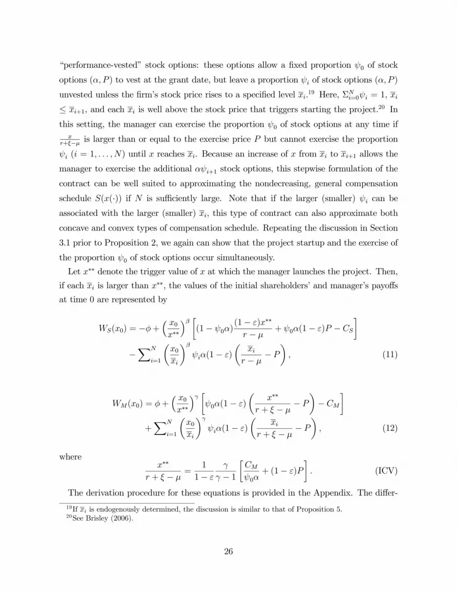
“performance-vested” stock options: these options allow a fixed proportion ψ0 of stock

options (α, P ) to vest at the grant date, but leave a proportion ψi of stock options (α, P )

unvested unless the firm’s stock price rises to a specified level xi.19 Here, ΣNi=0ψi = 1, xi

≤ xi+1, and each xi is well above the stock price that triggers starting the project.20 Inthis setting, the manager can exercise the proportion ψ0 of stock options at any time if

xr+ξ−μ is larger than or equal to the exercise price P but cannot exercise the proportion

ψi (i = 1, . . . , N) until x reaches xi. Because an increase of x from xi to xi+1 allows the

manager to exercise the additional αψi+1 stock options, this stepwise formulation of the

contract can be well suited to approximating the nondecreasing, general compensation

schedule S(x(·)) if N is sufficiently large. Note that if the larger (smaller) ψi can be

associated with the larger (smaller) xi, this type of contract can also approximate both

concave and convex types of compensation schedule. Repeating the discussion in Section

3.1 prior to Proposition 2, we again can show that the project startup and the exercise of

the proportion ψ0 of stock options occur simultaneously.

Let x∗∗ denote the trigger value of x at which the manager launches the project. Then,

if each xi is larger than x∗∗, the values of the initial shareholders’ and manager’s payoffs

at time 0 are represented by

WS(x0) = −φ+³ x0x∗∗

´β ∙(1− ψ0α)

(1− ε)x∗∗

r − μ+ ψ0α(1− ε)P − CS

¸−XN

i=1

µx0

xi

¶β

ψiα(1− ε)

µxi

r − μ− P

¶, (11)

WM(x0) = φ+³ x0x∗∗

´γ ∙ψ0α(1− ε)

µx∗∗

r + ξ − μ− P

¶− CM

¸+XN

i=1

µx0

xi

¶γ

ψiα(1− ε)

µxi

r + ξ − μ− P

¶, (12)

wherex∗∗

r + ξ − μ=

1

1− ε

γ

γ − 1∙CM

ψ0α+ (1− ε)P

¸. (ICV)

The derivation procedure for these equations is provided in the Appendix. The differ-

19If xi is endogenously determined, the discussion is similar to that of Proposition 5.20See Brisley (2006).

26

ence from the model in the previous sections is that the proportion ψ0 of stock options

is exercised at the start of the project, whereas the proportion ψi of stock options is

exercised at the prespecified level xi for i = 1, . . . , N .

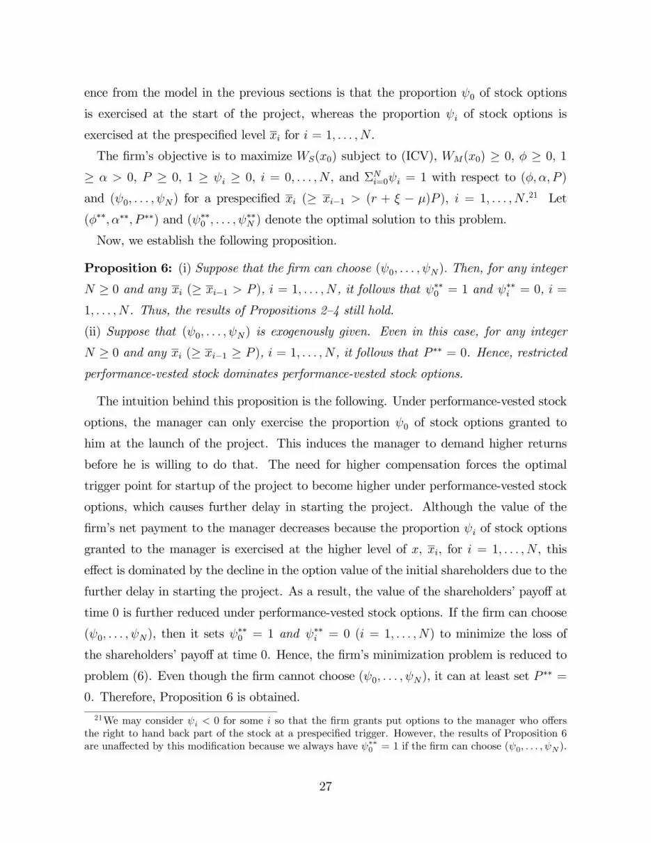
The firm’s objective is to maximize WS(x0) subject to (ICV), WM(x0) ≥ 0, φ ≥ 0, 1≥ α > 0, P ≥ 0, 1 ≥ ψi ≥ 0, i = 0, . . . , N , and ΣNi=0ψi = 1 with respect to (φ,α, P )

and (ψ0, . . . ,ψN) for a prespecified xi (≥ xi−1 > (r + ξ − μ)P ), i = 1, . . . , N .21 Let

(φ∗∗,α∗∗, P ∗∗) and (ψ∗∗0 , . . . ,ψ∗∗N ) denote the optimal solution to this problem.

Now, we establish the following proposition.

Proposition 6: (i) Suppose that the firm can choose (ψ0, . . . ,ψN). Then, for any integer

N ≥ 0 and any xi (≥ xi−1 > P ), i = 1, . . . , N , it follows that ψ∗∗0 = 1 and ψ∗∗i = 0, i =

1, . . . , N . Thus, the results of Propositions 2—4 still hold.

(ii) Suppose that (ψ0, . . . ,ψN) is exogenously given. Even in this case, for any integer

N ≥ 0 and any xi (≥ xi−1 ≥ P ), i = 1, . . . , N , it follows that P ∗∗ = 0. Hence, restrictedperformance-vested stock dominates performance-vested stock options.

The intuition behind this proposition is the following. Under performance-vested stock

options, the manager can only exercise the proportion ψ0 of stock options granted to

him at the launch of the project. This induces the manager to demand higher returns

before he is willing to do that. The need for higher compensation forces the optimal

trigger point for startup of the project to become higher under performance-vested stock

options, which causes further delay in starting the project. Although the value of the

firm’s net payment to the manager decreases because the proportion ψi of stock options

granted to the manager is exercised at the higher level of x, xi, for i = 1, . . . , N , this

effect is dominated by the decline in the option value of the initial shareholders due to the

further delay in starting the project. As a result, the value of the shareholders’ payoff at

time 0 is further reduced under performance-vested stock options. If the firm can choose

(ψ0, . . . ,ψN), then it sets ψ∗∗0 = 1 and ψ∗∗i = 0 (i = 1, . . . , N) to minimize the loss of

the shareholders’ payoff at time 0. Hence, the firm’s minimization problem is reduced to

problem (6). Even though the firm cannot choose (ψ0, . . . ,ψN), it can at least set P∗∗ =

0. Therefore, Proposition 6 is obtained.

21We may consider ψi < 0 for some i so that the firm grants put options to the manager who offers

the right to hand back part of the stock at a prespecified trigger. However, the results of Proposition 6

are unaffected by this modification because we always have ψ∗∗0 = 1 if the firm can choose (ψ0, . . . ,ψN ).

27

Several remarks about Propositions 5 and 6 are in order. First, Proposition 5 suggests

that even though the firm can use the more general compensation schedule approximated

by granting different N + 1 stock options for sufficiently large N , the optimal contract

is reduced to restricted stock so that the optimal start trigger is the same as that in

the linear compensation contract. Proposition 6 also suggests that even though the firm

is allowed to use the more general compensation schedule approximated by the step-

wise performance-based contract for sufficiently large N , the optimal contract is again

restricted stock. In particular, if the size of vested options is endogenous, restricted stock

dominates performance-vested stock options (or performance-vested stock) so that the op-

timal startup trigger is the same as that in the linear compensation contract. Even if the

size of vested options is fixed, restricted performance-vested stock dominates performance-

vested stock options. These findings show that our main results do not depend on the

modeling choice given that the set of allowable compensation tools is exogenously given.

Furthermore, Proposition 6(i) implies that our main results are unaffected, even though

the project startup and the exercise of a proportion of stock options are allowed to occur

at different times. Note that these results hold regardless of whether γ > β or γ = β.

Second, Holmstrom and Milgrom (1987) investigate a continuous time, Brownian mo-

tion version of the principal—agent model in which the agent controls the drift rate, and

derive the conditions under which the optimal compensation scheme is linear. In the

present model, we show that the optimal compensation contract must be linear if the

agent chooses the timing of investment instead of the drift rate of the stochastic process.

In addition, our results may justify the assumption that several real option models that

deal with manager—shareholder conflicts (Morellec (2004), Lambrecht and Myers (2007,

2008), and Dangl, Wu, and Zechner (2008)) take the managerial compensation contract

as the linear stock-based one.

6. Asymmetric Information on the Volatility of Investment Projects

Up to now, we have assumed that there is no hidden information problem. In this

section, and in addition to the hidden action problem, we investigate a hidden information

problem about the informational asymmetry of the riskiness of the project. This extension

enables us to clarify how the manager’s superior information about the riskiness of the

28

project affects the optimal investment strategy and compensation schedule. To this end,

suppose that the investment project managed by the manager may be one of two types,

high volatility (H), σH , or low volatility (L), σL (< σH), with prior probabilities of θ ∈(0, 1) and 1− θ, respectively, at time 0. However, the type of the project is only privately

known by the manager although the prior probability is public information.

To simplify the exposition, we focus on the basic model in Section 2, as well as assuming

that the manager is as impatient as the initial shareholders, that is, ξ = 0. This means that

the discount rates of the two agents are the same: β = γ.22 According to the differences in

volatility, β can take two possible values: one is βH =12− μ

(σH)2+

r³μ

(σH)2− 1

2

´2+ 2r

(σH)2

and the other is βL =12− μ

(σL)2+

r³μ

(σL)2− 1

2

´2+ 2r

(σL)2. It follows from ∂β

∂σ2< 0 that

βH < βL.

Let (φH ,αH , PH) ((φL,αL, PL)) denote the contract offered to the manager with the

investment project of the high (low) volatility, and x∗H (x∗L) denote the optimal com-

mencement trigger for (φH ,αH , PH) ((φL,αL, PL)). Then, we have the following lemma.

Lemma 2: If the manager’s compensation contract depends on the manager’s report on

the type of project, and if the firm believes the report, the manager with the high-volatility

investment project has an incentive to imitate the low-volatility project. By contrast, the

manager with the low-volatility investment project has no incentive to imitate the high-

volatility project.

Lemma 2 implies that when designing the optimal separating contract in this situation,

the firm needs only to consider the self-selection constraint for the manager with σH ,

which prevents the manager with σH from imitating the action of the manager with σL.

Given that Lemma 2 only requires the self-selection constraint for the manager with

σH , the optimal separating contract is now characterized as follows:

maxφH ,φL,αH ,αL,PH ,PL

θ

(−φH +

µx0

x∗H

¶βH∙(1− αH)

(1− ε)x∗Hr − μ

+ αH(1− ε)PH − CS¸)

22Even though β < γ, we can derive the main results of Proposition 7, except that it may be possible

to obtain αS∗H ≥ αS∗L and x∗H ≥ xS∗H > xS∗L ≥ x∗L. This is because if β < γ, we may not exclude the case

where the manager with σL has an incentive to misreport.

29

+(1− θ)

(−φL +

µx0

x∗L

¶βL∙(1− αL)

(1− ε)x∗Lr − μ

+ αL(1− ε)PL − CS¸), (13)

subject tox∗Hr − μ

=1

1− ε

βHβH − 1

∙CM

αH+ (1− ε)PH

¸, (ICH)

x∗Lr − μ

=1

1− ε

βLβL − 1

∙CM

αL+ (1− ε)PL

¸, (ICL)

φH +

µx0

x∗H

¶βH∙αH(1− ε)

µx∗Hr − μ

− PH¶− CM

¸≥ 0, (IRH)

φL +

µx0

x∗L

¶βL∙αL(1− ε)

µx∗Lr − μ

− PL¶− CM

¸≥ 0, (IRL)

φH +

µx0

x∗H

¶βH∙αH(1− ε)

µx∗Hr − μ

− PH¶− CM

¸≥ φL +

µx0bx∗H¶βH

∙αL(1− ε)

µ bx∗Hr − μ

− PL¶− CM

¸, (SS)

bx∗Hr − μ

=1

1− ε

βHβH − 1

∙CM

αL+ (1− ε)PL

¸, (ICDH)

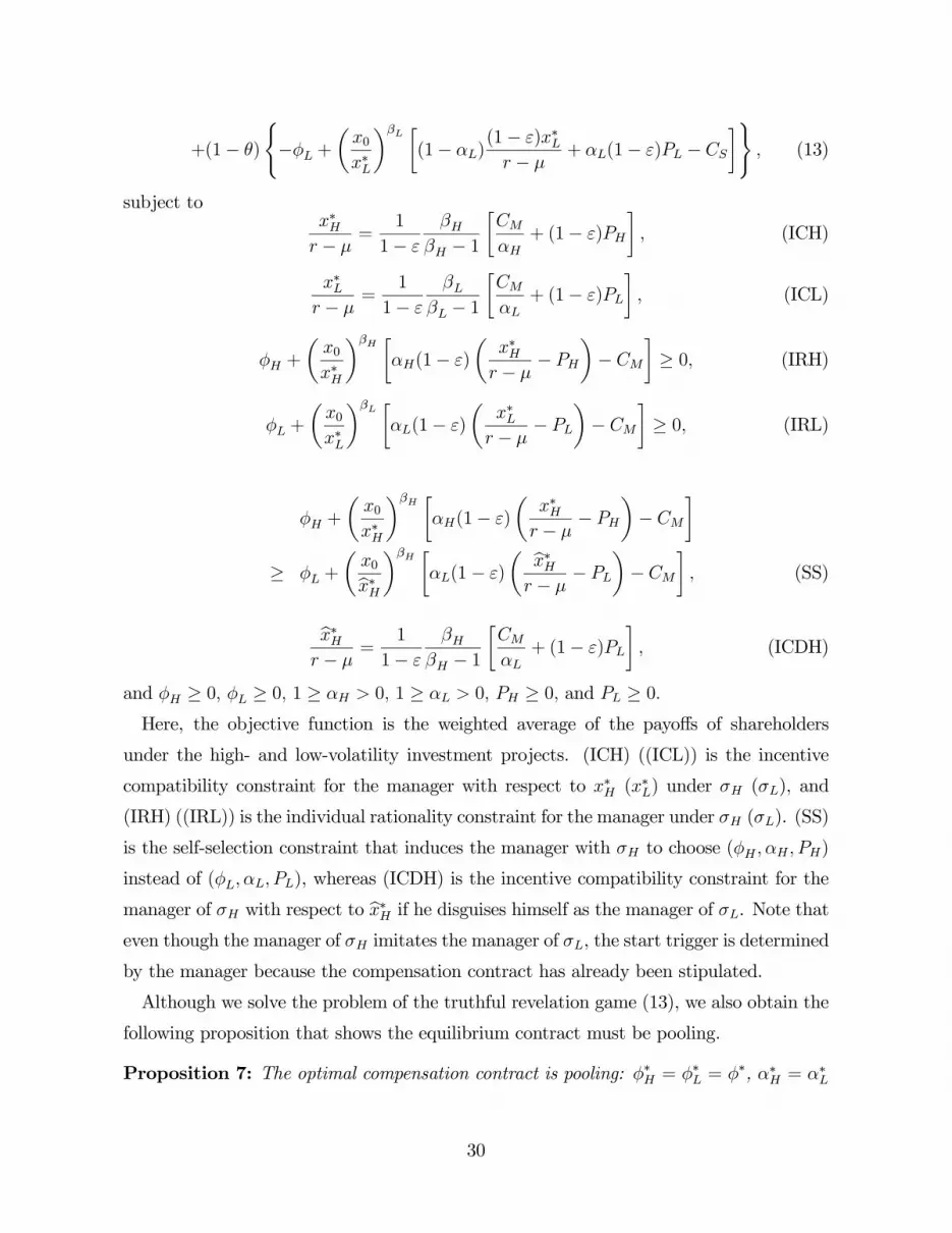
and φH ≥ 0, φL ≥ 0, 1 ≥ αH > 0, 1 ≥ αL > 0, PH ≥ 0, and PL ≥ 0.Here, the objective function is the weighted average of the payoffs of shareholders

under the high- and low-volatility investment projects. (ICH) ((ICL)) is the incentive

compatibility constraint for the manager with respect to x∗H (x∗L) under σH (σL), and

(IRH) ((IRL)) is the individual rationality constraint for the manager under σH (σL). (SS)

is the self-selection constraint that induces the manager with σH to choose (φH ,αH , PH)

instead of (φL,αL, PL), whereas (ICDH) is the incentive compatibility constraint for the

manager of σH with respect to bx∗H if he disguises himself as the manager of σL. Note thateven though the manager of σH imitates the manager of σL, the start trigger is determined

by the manager because the compensation contract has already been stipulated.

Although we solve the problem of the truthful revelation game (13), we also obtain the

following proposition that shows the equilibrium contract must be pooling.

Proposition 7: The optimal compensation contract is pooling: φ∗H = φ∗L = φ∗, α∗H = α∗L

30

= α∗, and P ∗H = P∗L = P

∗. More specifically, φ∗ = 0 and P ∗ = 0; and α∗ satisfies

αS∗H ≡(βH − 1)CM

(βH − 1)CS + βHCM< α∗ <

(βL − 1)CM(βL − 1)CS + βLCM

≡ αS∗L , (14)

where αS∗H (αS∗L ) would be the amount of the stock granted to the manager with σH (σL)

if the volatility of the investment project were observable. Furthermore, the optimal com-

mencement trigger for each type of manager, (x∗H , x∗L), satisfies

x∗Hr − μ

=1

1− ε

βHβH − 1

CM

α∗;x∗Lr − μ

=1

1− ε

βLβL − 1

CM

α∗; and xS∗H > x∗H > x

∗L > x

S∗L , (15)

wherexS∗Hr−μ ≡ 1

1−εβH

βH−1

³CS +

βHβH−1CM

´ ³xS∗Lr−μ ≡ 1

1−εβL

βL−1

³CS +

βLβL−1CM

´´denotes the

corresponding optimal start trigger for αS∗H (αS∗L ).

The intuition behind this proposition is that the positive base salary (even for the

manager with σH) merely decreases the initial shareholders’ payoff at time 0, whereas the

positive exercise price only distorts the investment timing so that it also decreases the

initial shareholders’ payoff at time 0. Hence, only the grant size of restricted stock in the

compensation contract can be used to satisfy the self-selection condition (SS). However,

as long as α∗H < α∗L, the manager with σH attempts to disguise himself as the manager

with σL. Indeed, the manager with σH can receive the higher fraction of the project

returns by mimicking the manager with σL, whereas the former incurs no additional costs

by mimicking the latter. The reason for no additional costs incurred by the manager with

σH depends on the fact that the manager with σH can choose the best start time relative

to the compensation contract, regardless of whether or not the manager with σH mimics

the manager with σL, that is, x∗H = bx∗H . Thus, the commencement trigger of the manager

with σH is not distorted even though the manager with σH mimics the manager with

σL. As a result, we must have α∗H = α∗L = α∗ if the payment to the manager must be

minimized when (SS) is binding. The optimal value of α∗ is obtained by the weighted

value of αS∗H and αS∗L because both of the effects of α∗ on the payoffs of the shareholders

with σH and σL should be considered. The optimal commencement trigger of each type

of manager, (x∗H , x∗L), for α

∗ is then determined by (ICH) and (ICL). It follows from βHβH−1

>βL

βL−1 , αS∗H < α∗ < αS∗L and P ∗H = P

∗L = 0 that x

S∗H > x∗H > x

∗L > x

S∗L .

Several comments are in order. First, the optimal trigger for each type of the manager

31

is increasing in ε, as in the absence of hidden information. Further, the optimal trigger

point for the manager of σH is larger than that for the manager of σL. This is consistent

with the result of Proposition 4(i), in which x∗ is increasing in σ. Second, even under the

adverse selection environment of volatile project returns, the optimal contract is made

up of restricted stock but does not involve stock options. Third, the optimal contract

is pooling: the optimal trigger x∗H (x∗L) for the manager of σH (σL) is lower (higher)

than the optimal trigger derived in the case of no adverse selection where the type of

project is observable. This contrasts with the results of Grenadier and Wang (2005) and

Morellec and Schürhoff (2011), where the optimal contract is separating under asymmetric

information on the expected value of the project returns. Grenadier and Wang (2005)

show that if the manager has the same discount rate as the owner, the optimal investment

trigger for the manager of the lower- (higher-)quality project is higher than (equal to) the

full information level, which is derived in the case of no adverse selection. Conversely,

Morellec and Schürhoff (2011) suggest that the optimal investment trigger for the manager

of the lower- (higher-) quality project is equal to (lower than) the full information level.

Intuitively, in the model in Grenadier and Wang (2005), if the manager has the same

discount rate as the owner, the manager of the higher-quality project desires to hide his

positive private information about project values to extract more rents from the owner.

Hence, it is less costly for the owner to distort the trigger for the manager of the lower-

quality project away from the full information level than to distort the trigger for the

manager of the higher-quality project away from the full information level in order to

induce truthful revelation. As a result, the optimal contract is separating, and only the

distortion of the trigger for the manager of the lower-quality project arises. On the other

hand, in the model in Morellec and Schürhoff (2011), the manager of the higher-quality

project desires to reveal its positive private information whereas the manager of the lower-

quality project desires to mimic the high quality type. Hence, their result is converse to

that of Grenadier and Wang (2005). By way of contrast, in our model the exercise price

must be reduced to zero to attain efficient investment timing. Under this requirement,

there exists no start trigger such that the manager of σL can separate from the manager

of σH by granting restricted stock and starting the project at or below that trigger. The

reason is that the manager of σH can always choose the same start time relative to the

compensation contract, irrespective of whether or not he imitates the manager of σL.

32

This forces the firm to set α∗H = α∗L = α∗. The main difference between our model and

the models of Grenadier and Wang (2005) and Morellec and Schürhoff (2011) is that each

type of the manager can choose the commencement timing of the project in our model

by taking into account only the compensation contract. Hence, even when the manager

with σH mimics the manager with σL, there exist no costs incurred by the manager with

σL. Therefore, the equilibrium must be pooling.

7. Robustness Checks

We now consider whether our main results remain valid even when some of the assump-

tions made in the previous sections are modified.

7.1. Negative base salaries.–

For simplicity, we focus on the basic model in Section 2 although we can deal with

the more general model in Section 5 in a similar way. Proposition 3 depends on the

existence of the sticky base salary constraint, which does not allow for negative base

salaries. Negative base salaries occur when managers invest some of their initial wealth

in their company’s securities. If base salaries can be negative, we interpret this to mean

that the contract requires managers to invest some of their private savings, in addition

to their stock grants, in their company’s securities. In fact, it seems very rare to specify

a contract whereby managers must invest some of their private savings in the company’s

securities. In particular, we can almost entirely exclude this possibility for large publicly

traded firms. However, if we allow base salaries to be negative, we present the following

proposition.

Proposition 8: Suppose that φ is allowed to be negative.

(i) If γ > β, the optimal compensation contract, (φ∗,α∗, P ∗), is characterized by φ∗ =

− ¡x0x∗¢γ CM

γ−1 , 0 < α∗ < 1, and P ∗ = 0. In addition, if ξ is not sufficiently large, the optimal

start trigger, x∗, must satisfy x∗ > xFI .

(ii) If γ = β, then x∗ and (φ∗,α∗, P ∗) are given by x∗ = xFI , φ∗ =− ¡x0

x∗¢β CM (CS+CM )

(β−1)[CS+CM−(1−ε)P∗] ,

α∗ = CMCS+CM−(1−ε)P∗ , and 0 ≤ P ∗ ≤

CS1−ε .

Even though base salaries are allowed to be negative, Proposition 8 suggests the follow-

ing if the manager is more impatient than the initial shareholders (γ > β): The optimal

33

contract is made up of restricted stock but does not involve stock options, and the optimal

trigger x∗ is larger than the full information level xFI if the manager’s and shareholders’

impatience are not too different. Only if γ = β, is xFI attained, and the optimal contract

cannot exclude stock options. Note that α∗ = 1 if P ∗ = CS1−ε . Then, the optimal contract

implies that the manager buys all the stocks of the firm. Hence, as suggested in the static

contract model, the full information allocation is achieved.

In the case of γ = β, the achievement of xFI implies that the opportunistic behavioral

problem of the manager is fully resolved in this case. The indifference between restricted

stock and stock options also depends on the fact that the choice of restricted stock or

stock options does not affect any incentives for the manager to launch the project if base

salaries can be negative. Indeed, if γ = β and base salaries can be negative, these results

are trivial because we end up analyzing the model without any limited liability constraints

for the risk-neutral manager.

By contrast, the optimal contract does not involve stock options in the case of γ >

β. Greater managerial impatience induces the firm not to set negative base salaries to

be sufficiently small because the firm needs to award the manager compensation as early

as possible. This also implies that the firm needs to decrease total compensation for the

manager in this case by minimizing the exercise price, that is, by fixing P ∗ at 0. Because

the firm cannot set base salaries to be sufficiently negative, the grant size of restricted

stock under the optimal contract must be smaller than that required to attain the full

information allocation. If γ is not so different from β, the direct effect of the greater

managerial impatience that decreases the start trigger is dominated by its indirect effect

that raises the trigger through a decrease in the grant size of restricted stock. Hence, x∗

is larger than xFI .

These findings show that when the manager chooses the project’s startup timing, our

main result–that x∗ is larger than xFI and restricted stock is optimal–depends on the

opportunistic behavioral incentive for the risk-neutral manager being more impatient than

the initial shareholders or being constrained by the limited liability. Hence, if the manager

is as impatient as the initial shareholders (γ = β) and if there is no lower bound on how

much the manager can be paid (φ < 0), the firm fixes the optimal commencement trigger

at xFI and becomes indifferent between restricted stock and stock options although an

34

opportunistic behavioral incentive for the risk-neutral manager exists when CM > 0.23

7.2. The stock-based contract plus the bonus payment.–

To simplify the exposition, we focus on the case of the stock-based contract at the initial

time plus a bonus payment ω at the start of the project because the other cases can be

explained in a similar way. In fact, if ω is not sufficiently small, it induces opportunistic

behavior by the manager, as suggested in Section 2.2. Thus, the firm has no incentive to

offer such a contract. Hence, ω must have an upper bound.

Suppose that ω is below the upper bound. If αP − ω > 0, the arguments in the previous

sections can show that restricted stock dominates the mix of stock options and the bonus

payment ω. If αP − ω ≤ 0, the mix of stock options and the bonus payment ω is viewedas that of restricted stock and the bonus payment ω − αP . In any case, we can verify

that restricted stock is optimal, even though the firm can offer the stock-based contract

at time 0 plus the bonus payment ω at the start of the project.

However, the introduction of ω reduces the optimal trigger for the commencement of

the project, thereby enhancing the efficiency of investment timing. In particular, if the

upper bound of ω can be sufficiently large and if hidden information does not exist, this

kind of contract may attain the full information level.

7.3. Risk-averse preferences.–

In previous sections, managers’ concerns about the subjective value of firms’ cash flow

streams are captured by managerial impatience. However, if we consider nondiversifiable

idiosyncratic risks that a risk-averse manager needs to bear, our main results might be

affected by the risk preferences of the manager. In fact, the answer is that the risk prefer-

ences of the manager merely strengthen our main results, just as managerial impatience

does in the previous sections.

To derive this result simply, we need to modify the basic model. First, the manager

has a project that is infinitely lived. Instead of expending the effort cost CM in launching

the investment project, the manager does not end up receiving a fixed benefit b at any

time point until the project is launched. In addition, the fact of whether or not the

manager really receives b is unobservable. This formulation can capture the unobservable

23By contrast, in the static contracting model, tightening the limited liability constraint makes stock

options more advantageous. See Dittmann and Maug (2007).

35

opportunity cost of the manager commencing the investment project. Second, both the

manager and the initial shareholders can also invest in a free technology yielding an

instantaneous return r > 0. Third, we assume that the manager is as impatient as the

initial shareholders, that is, β = γ, because we focus on the effect of risk aversion. Fourth,

the preferences of the manager are represented by the standard CRRA utility function:

E0U(c(·)) ≡ E0∙R∞0e−rt

c(t)1−R

1−R dt¸; R > 0,

where E0 is the expectation operator at time 0, c(·) ≡ c(τ) | 0 ≤ τ ≤ ∞ is the valueof the manager’s consumption stream, and R is the manager’s relative risk aversion.

If R = 1, the case corresponds to the logarithmic utility function. Finally, instead of

the base salary at time 0, the firm initially gives the manager rewards φ that yield the

nonpecuniary benefit B(φ) to the manager at time 0, where B0(φ) > 0.24 Hence, the

utility of the manager at time 0 is then represented by B(φ) + E0U(c(·)). To ensurethat the manager has an incentive to launch the project, we need to put the following

assumption on the manager’s relative risk aversion:

Assumption: ∆ ≡ r + (R− 1)(μ− 12σ2R) > 0.

If this assumption does not hold, the manager never starts the project. Note that when

the manager is risk neutral (R = 0), this assumption reduces to r > μ, which has been

imposed below (1).

In order to characterize the firm’s problem, we exploit the result of Theorem 1 or

Proposition 2 in Hugonnier and Morellec (2007a) to derive the incentive compatibility and

individual rationality constraints for the manager.25 Given that the project is liquidated

with probability 1− ε after CS and CM are expended, the firm’s problem is

maxφ,α,P

(−φ+

µx0

x∗R

¶β ∙(1− α)

(1− ε)x∗Rr − μ

+ α(1− ε)P − CS¸), (16)

24The case of a fixed base salary is discussed at the end of this subsection.25Using arguments similar to those of Chapter 10 in Dixit and Pindyck (1994), we again show that

starting the project occurs simultaneously with the exercise of stock options.

36

subject to

x∗R =

(β∆

(β − 1 +R) r(1− ε)

"(1− ε)

µb

α+ rP

¶1−R+ ε

µb

α

¶1−R#) 11−R

, (ICR)

B(φ) +b1−R

r (1−R) +µx0

x∗R

¶β"(1− ε) (αx∗R)

1−R

∆ (1−R) − (1− ε) (b+ rαP )1−R

+ εb1−R

r (1−R)

#≥ 0,

(IRR)

φ ≥ 0, 1 ≥ α > 0, P ≥ 0. (LLR)

Note that by investing in the project, the manager gives up both a fixed benefit b at each

point of time with probability 1 and a risk-free cash flow stream rαP with probability 1

− ε, and also earns a nondiversifiable risk cash flow stream αx with probability 1 − ε,

whereas the initial shareholders give up a risk-free cash flow stream rCS with probability

1 and receive in return a risky cash flow stream (1−α)x and a risk-free cash flow stream

rαP with probability 1 − ε.

Solving problem (16), we obtain the following proposition:

Proposition 9: Suppose that ε is sufficiently small. The optimal commencement trigger

is

x∗R =β

β − 1∙r − μ

1− εCS + Ωb

¸> xFI ≡ 1

1− ε

(r − μ)β

β − 1µCS +

b

r

¶,

where xFI is the full information solution.26 Furthermore, restricted stock dominates

stock options and the base salary. Then, the optimal compensation contract, (φ∗,α∗, P ∗),

is characterized by

φ∗ = P ∗ = 0 and α∗ =β − 1β

(1− ε)Ωb

(r − μ)CS + (1− ε)Ωb,

where Ω ≡h

β∆

(β−1+R)r(1−ε)

i 11−R.

Corollary to Proposition 9: (i) x∗R is increasing in ε if CS ≥ (1−ε)Ωb(r−μ)(R−1) . x

∗R is also

26xFI is derived by maximizing the firm’s value at time 0, provided that the fact of whether or not the

manager really receives b is publicly observable, that the project commencement is directly determined

by the firm, and that the manager is compensated enough for the loss of b incurred after the investment

that he is induced to participate in the project.

37

increasing in σ. (ii) α∗ is independent of ε if R = 0, and is increasing (decreasing) in ε

if 0 < R < 1 (or if R > 1). α∗ is decreasing in σ if R is close to zero.

Intuitively, the manager again views the exercise price as an additional irreversible sunk

cost although the manager is risk averse. This has a disincentive effect on the manager’s

attitude towards exercising the risky project through giving up b. Hence, even though

the manager is risk averse, restricted stock becomes better at providing the manager with

a greater incentive to launch the risky project because restricted stock does not force

the manager to pay any positive exercise price. Although restricted stock mitigates the

distortion in the investment timing, the manager still has an incentive to delay the start

of the risky project.

With regard to the intuition behind the result for Corollary to Proposition 9, a larger ε

raises the risk of losing the sunk cost upon liquidation and increases the excess returns be-

fore starting the project. However, an increase in ε also affects the risk preference-adjusted

factor Ω. If the shareholder’s sunk cost is large enough, the former effect dominates the

latter effect although the latter effect reduces Ω when 1 < R. For 0 < R < 1, these two

effects move x∗R in the same direction because the latter effect raises Ω. Thus, x∗R is in-

creasing in ε. The two effects of an increase in ε can also affect the grant size of restricted

stock unless the manager is risk neutral. If 0 < R < 1, the latter effect raises Ω and

dominates the former effect. If 1 < R, the latter effect reduces Ω and these two effects

move α∗ in the same direction. Hence, α∗ is increasing (decreasing) in ε if 0 < R < 1 (or if

R > 1). On the other hand, for a given α, a larger σ increases both of the factors β

β−1 and

Ω. These effects increase the value of the manager’s option to wait, thereby increasing

x∗R. However, an increase inβ

β−1 reduces the size of α used in the contract, whereas an

increase in Ω raises the size of α used in the contract. If R is close to zero, the former

effect dominates the latter effect. Hence, α∗ is decreasing in σ.

Although the risk-averse model is somewhat different from the basic model in Section

2, the results of Corollary to Proposition 9 is consistent with the result of Proposition 4 if

we set R = 0. Compared with the risk-neutral case, the main difference is that the grant

size of restricted stock is affected by the liquidation possibility and that the effect of the

liquidation possibility on the commencement trigger may be converse if the shareholder’s

sunk cost is sufficiently large.

In the standard static principal—agent model, the convexity of the fee schedule (as with

38

stock options) clearly makes risky bets more desirable. However, if the manager’s risk

aversion is larger, increasing the exercise price is less likely to induce the manager to be

more responsive to stock price changes above the exercise price because the compensation

schedule is even more convex. Thus, increasing the exercise price a little above zero cannot

induce a higher effort level by the more risk-averse manager at a lower cost. Hence, the

firm prefers stock options only if the manager has moderate levels of risk aversion.27 By

contrast, in our real options model, the effect of delaying investment induces the firm to

prefer restricted stock, even though the manager’s risk aversion is not large.

If the firm initially gives the manager a fixed base salary φ at time 0 that yields a risk-

free cash flow stream rφ to the manager at any point of time, the effect of φ may depend

on how it translates the domain of the utility function U(c(·)) into more or less risk-averseportions. However, because it is more probable that the cash flow stream received by the

manager is larger after launching the project than before, the concavity of the manager’s

utility function implies that the existence of the risk-free cash flow stream rφ at each

point of time decreases the value of the manager’s option to launch the project. Hence,

the fixed base salary must be reduced to 0. Therefore, the results of Proposition 9 are

unaffected, even though the firm is permitted to award the manager a fixed base salary

at time 0.28

8. Conclusion

This paper considers how managers whose objectives are not aligned with those of their

firm’s shareholders choose timing startups of a risky but value-increasing project with a

liquidation possibility when the managerial compensation schedule is designed endoge-

nously. We examine the situation in which the starting trigger point cannot be specified

in the contract, given incomplete and imperfect information. Using the real options

approach for a broad class of managerial preferences, we show that: (i) without hidden

information, project startups are more likely to be delayed with a higher liquidation possi-

bility, whereas the stock-based managerial compensation is independent of the liquidation

possibility but is decreasing in the volatility of the firm’s cash flow stream and the degree

27The numerical calculations in the standard static principal—agent model suggest that the superiority

of restricted stock increases with the manager’s risk aversion. See Dittmann and Maug (2007).28Note that a bonus payment ω at the project’s startup that yields a cash flow stream rω at each point

of time after launching the project is impossible because of the reasons discussed in Section 2.2.

39

of managerial impatience if the manager is risk neutral; (ii) restricted stock is optimal in

a general class of compensation schedules, regardless of the manager’s risk preferences;

and (iii) with hidden information on the volatility of the project return, the equilibrium

must be pooling so that a high- (low-)volatility project is advanced (delayed) compared

with the case without hidden information if the risk-neutral manager is as impatient as

the shareholders.

Our modeling approach suggests the importance of dynamic considerations, not only in

managers’ investment timing, but also in the optimal design of managerial compensation

schedules. One natural extension would involve analyzing how the timing of various orga-

nizational decisions is endogenously determined together with managerial compensation

schemes (for example, see Habib and Mella-Barral (2007) for the formation and dura-

tion of joint ventures, and Lambrecht and Myers (2007) for the mechanism of takeovers,

although these models assume fixed contract payment schedules).

40

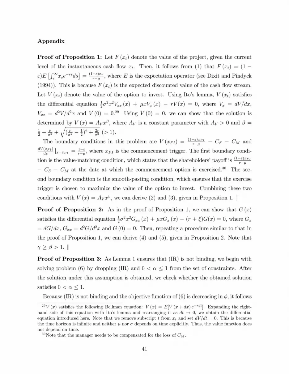
Appendix

Proof of Proposition 1: Let F (xt) denote the value of the project, given the current

level of the instantaneous cash flow xt. Then, it follows from (1) that F (xt) = (1 −ε)E

£R∞τxse

−rsds¤=

(1−ε)xτr−μ , where E is the expectation operator (see Dixit and Pindyck

(1994)). This is because F (xt) is the expected discounted value of the cash flow stream.

Let V (xt) denote the value of the option to invest. Using Ito’s lemma, V (xt) satisfies

the differential equation 12σ2x2Vxx (x) + μxVx (x) − rV (x) = 0, where Vx = dV/dx,

Vxx = d2V/d2x and V (0) = 0.29 Using V (0) = 0, we can show that the solution is

determined by V (x) = AV xβ, where AV is a constant parameter with AV > 0 and β =

12− μ

σ2+q( μ

σ2− 1

2)2 + 2r

σ2(> 1).

The boundary conditions in this problem are V (xFI) =(1−ε)xFIr−μ − CS − CM and

dV (xFI)

dx|x=xFI = 1−ε

r−μ , where xFI is the commencement trigger. The first boundary condi-

tion is the value-matching condition, which states that the shareholders’ payoff is(1−ε)xFIr−μ

− CS − CM at the date at which the commencement option is exercised.30 The sec-

ond boundary condition is the smooth-pasting condition, which ensures that the exercise

trigger is chosen to maximize the value of the option to invest. Combining these two

conditions with V (x) = AV xβ, we can derive (2) and (3), given in Proposition 1. k

Proof of Proposition 2: As in the proof of Proposition 1, we can show that G (x)

satisfies the differential equation 12σ2x2Gxx (x) + μxGx (x) − (r + ξ)G(x) = 0, where Gx

= dG/dx, Gxx = d2G/d2x and G (0) = 0. Then, repeating a procedure similar to that in

the proof of Proposition 1, we can derive (4) and (5), given in Proposition 2. Note that

γ ≥ β > 1. kProof of Proposition 3: As Lemma 1 ensures that (IR) is not binding, we begin with

solving problem (6) by dropping (IR) and 0 < α ≤ 1 from the set of constraints. After

the solution under this assumption is obtained, we check whether the obtained solution

satisfies 0 < α ≤ 1.Because (IR) is not binding and the objective function of (6) is decreasing in φ, it follows

29V (x) satisfies the following Bellman equation: V (x) = E[V (x+ dx) e−rdt]. Expanding the right-hand side of this equation with Ito’s lemma and rearranging it as dt → 0, we obtain the differential

equation introduced here. Note that we remove subscript t from xt and set dV/dt = 0. This is because

the time horizon is infinite and neither μ nor σ depends on time explicitly. Thus, the value function does

not depend on time.30Note that the manager needs to be compensated for the loss of CM .

41

from (BS) that φ = 0. Substituting φ = 0 and x∗ from (IC) into the objective function

of (6), deriving the first-order conditions with respect to α and P , and multiplying these

conditions by³x∗x0

´β, we obtain

(1− ε)

µP − x∗

r − μ

¶−∙(1− α)(1− ε)(1− β)

r − μ+ β

CS − α(1− ε)P

x∗

¸γ(r + ξ − μ)

(γ − 1)(1− ε)

CM

α2= 0,

(A1)

(1− ε)α+

∙(1− α)(1− ε)(1− β)

r − μ+ β

CS − α(1− ε)P

x∗

¸γ(r + ξ − μ)

γ − 1 + ζ = 0,

(A2)

where¡x0x∗¢β

ζ is the nonnegative multiplier associated with the constraint of (EP).

Combining (A1) and (A2), we obtain

ζ = −(1− ε)α2

CM

∙CM

α+ (1− ε)

µP − x∗

r − μ

¶¸. (A3)

Substituting x∗ from (IC) into (A3) leads to

ζ =(1− ε)α2

CM

∙CM

α+ (1− ε)P

¸r + γξ − μ

(γ − 1) (r − μ)> 0.

Because the multiplier associated with (FP) is positive, we must have P = 0.

Now, substituting P = 0 into (A1) and rearranging it with (IC), we show

− (1− ε)x∗

r − μ−∙(1− α)(1− ε)(1− β)

r − μ+ β

CS

x∗

¸x∗

α= 0. (A4)

Further rearranging (A4) with (IC) and P = 0 yields

α =β − 1β

γ(r + ξ − μ)CM

(γ − 1)(r − μ)CS + γ(r + ξ − μ)CM. (A5)

Note that α given by (A5) satisfies 0 < α < 1 because γ > β > 1.

Therefore, (φ∗,α∗, P ∗) = (0, β−1β

γ(r+ξ−μ)CM(γ−1)(r−μ)CS+γ(r+ξ−μ)CM , 0), which is given by (8) of this

proposition. Substituting (φ∗,α∗, P ∗) into (IC), WS(x0), and WM(x0), we obtain (7), (9),

and (10) of this proposition. Note that x∗ > xFI because γ > 1 and ξ > 0. k

42

Proof of Proposition 4: The results of ε and σ are evident. On the other hand, it is

found from ∂β

∂ξ= 0 and ∂γ

∂ξ> 0 that ∂x∗

∂ξ< 0 and ∂α∗

∂ξ< 0 if γ

r+ξ−μ >∂γ∂ξ

γ−1 . Indeed, the

condition of γ

r+ξ−μ >∂γ∂ξ

γ−1 is satisfied if γ is sufficiently close to 1. It follows from the

definition of γ that γ is sufficiently close to 1 if σ2

r+ξis sufficiently large. Hence, we verify

that ∂x∗∂ξ< 0 and ∂α∗

∂ξ< 0 if σ2

r+ξis sufficiently large. k

Proof of Proposition 5: For N = 0, it follows from the arguments of Section 3.1 prior

to Proposition 2 and those of the proof of Propositions 2 and 3 that the statement of this

proposition holds. Suppose that for N = k − 1, the statement of this proposition holds.Then, the commencement of the project and the exercise of all the k stock options occur

simultaneously; and, as a result, P0 = · · · = Pk−1 = 0. Now, suppose that, in addition tothe k stock options, the firm offers a new stock option (αk, Pk), where 0 < Σki=0αi = α0 <

1, αk > 0, and Pk ≥ 0. Then, repeating the arguments of Section 3.1 prior to Proposition2 and those of the proof of Propositions 2 and 3, we can prove that the statement of this

proposition still holds for N = k. k

The derivation of equations (11) and (12): Now, we solve the manager’s problem

by working backwards.

We first find the value of the proportion ψN of stock options for the manager, HN(x).

As discussed in Propositions 1 and 2, we can show that HN (x) = ANxγ, where AN is a

constant parameter with AN > 0. Because the value-matching condition is provided by

HN (xN) = AN (xN)γ= ψNα

³xN

r+ξ−μ − P´, we have

HN (x) =

⎧⎨⎩³xxN

´γψNα

³xN

r+ξ−μ − P´

ψNα³

xr+ξ−μ − P

´ for

for

x < xN ,

xN ≤ x.

Given HN (x), we next find the value of the proportion ψN−1 of stock options for the

manager,HN−1 (x). Again,HN−1 (x) = AN−1xγ, whereAN−1 is a constant parameter with

AN−1 > 0. Because HN−1 (x) = (the value of the option for the manager to exercise the

proportion ψN−1 of stock options) + HN (x), the value-matching condition is expressed by

HN−1 (xN−1) = AN−1 (xN−1)γ= ψN−1α

³xN−1r+ξ−μ − P

´+ HN (xN−1). Hence, we can derive

AN−1 from the value-matching condition. Because xN is larger than xN−1, HN−1 (x) is

43

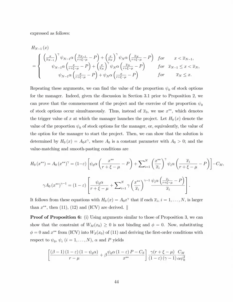
expressed as follows:

HN−1 (x)

=

⎧⎪⎪⎪⎨⎪⎪⎪⎩³

xxN−1

´γψN−1α

³xN−1r+ξ−μ − P

´+³xxN

´γψNα

³xN

r+ξ−μ − P´

ψN−1α³

xr+ξ−μ − P

´+³xxN

´γψNα

³xN

r+ξ−μ − P´

ψN−1α³

xr+ξ−μ − P

´+ ψNα

³x

r+ξ−μ − P´

for

for

for

x < xN−1,

xN−1 ≤ x < xN ,xN ≤ x.

Repeating these arguments, we can find the value of the proportion ψ0 of stock options

for the manager. Indeed, given the discussion in Section 3.1 prior to Proposition 2, we

can prove that the commencement of the project and the exercise of the proportion ψ0

of stock options occur simultaneously. Thus, instead of x0, we use x∗∗, which denotes

the trigger value of x at which the manager launches the project. Let H0 (x) denote the

value of the proportion ψ0 of stock options for the manager, or, equivalently, the value of

the option for the manager to start the project. Then, we can show that the solution is

determined by H0 (x) = A0xγ, where A0 is a constant parameter with A0 > 0; and the

value-matching and smooth-pasting conditions are

H0 (x∗∗) = A0 (x

∗∗)γ = (1−ε)∙ψ0α

µx∗∗

r + ξ − μ− P

¶+XN

i=1

µx∗∗

xi

¶γ

ψiα

µxi

r + ξ − μ− P

¶¸−CM ,

γA0 (x∗∗)γ−1 = (1− ε)

⎡⎣ ψ0α

r + ξ − μ+XN

i=1γ

µx∗∗

xi

¶γ−1 ψiα³

xir+ξ−μ − P

´xi

⎤⎦ .It follows from these equations with H0 (x) = A0x

γ that if each xi, i = 1, . . . , N , is larger

than x∗∗, then (11), (12) and (ICV) are derived. k

Proof of Proposition 6: (i) Using arguments similar to those of Proposition 3, we can

show that the constraint of WM(x0) ≥ 0 is not binding and φ = 0. Now, substituting

φ = 0 and x∗∗ from (ICV) intoWS(x0) of (11) and deriving the first-order conditions with

respect to ψ0, ψi (i = 1, . . . , N), α and P yields∙(β − 1) (1− ε) (1− ψ0α)

r − μ+ β

ψ0α (1− ε)P − CSx∗∗

¸γ(r + ξ − μ)

(1− ε) (γ − 1)CM

αψ20

44

+α (1− ε)

µP − x∗∗

r − μ

¶+ ηψ + η00 = η10, (A6)

−µx∗∗

xi

¶β

α (1− ε)

µxi

r − μ− P

¶+ ηψ − η1i + η0i = 0, i = 1, . . . , N, (A7)

∙(β − 1) (1− ε) (1− ψ0α)

r − μ+ β

ψ0α (1− ε)P − CSx∗∗

¸γ(r + ξ − μ)

(1− ε) (γ − 1)CM

α2ψ0

+ψ0 (1− ε)

µP − x∗∗

r − μ

¶−XN

i=1

µx∗∗

xi

¶β

ψi (1− ε)

µxi

r − μ− P

¶= 0, (A8)

−∙(β − 1) (1− ε) (1− ψ0α)

r − μ+ β

ψ0α (1− ε)P − CSx∗∗

¸γ(r + ξ − μ)

γ − 1 + ψ0α (1− ε)

+XN

i=1

µx∗∗

xi

¶β

ψiα (1− ε) = −ηP , (A9)

where¡x0x∗∗¢β

η10,¡x0x∗∗¢β

η00,¡x0x∗∗¢β

η1i (i = 1, . . . , N),¡x0x∗∗¢β

η0i (i = 1, . . . , N) and¡x0x∗∗¢β

ηP

are the nonnegative multipliers associated with the constraints of 1 ≥ ψ0, ψ0 ≥ 0, 1 ≥ψi (i = 1, . . . , N), ψi ≥ 0 (i = 1, . . . , N) and P ≥ 0, respectively; and ¡ x0

x∗∗¢β

ηψ is the

multiplier associated with the constraint of ΣNi=0ψi = 1. Subtracting both sides of (A8)

multiplied by α from both sides of (A6) multiplied by ψ0 leads to

αXN

i=1

µx∗∗

xi

¶β

ψi(1− ε)

µxi

r − μ− P

¶+ ψ0ηψ + ψ0η

00 = ψ0η

10 = η10. (A10)

Multiplying both sides of (A7) by ψi yields

−ψiµx∗∗

xi

¶β

α (1− ε)

µxi

r − μ− P

¶+ψiηψ−ψiη1i = −ψiη0i = 0, i = 1, . . . , N. (A11)

If ψi = 0 for every i = 1, . . . , N , it follows from ΣNi=1ψi = 1 − ψ0 that ψ0 = 1. Hence,

the result of this proposition is established. If ψi > 0 for some i ∈ (1, . . . , N), it followsfrom (A11), η1i ≥ 0 (i = 1, . . . , N) and xi > P (i = 1, . . . , N) that ηψ > 0. Thus, it alsofollows from (A10), ψ0 ≥ 0, η00 ≥ 0 and xi > P (i = 1, . . . , N) that η10 > 0. However, thisimplies ψ0 = 1, which contradicts ψi > 0 for some i ∈ (1, . . . , N). Thus, we must have ψi= 0 for every i = 1, . . . , N and ψ0 = 1. Again, the result of this proposition is obtained.

(ii) Even though (ψ0, . . . ,ψN) is exogenously given, we still have (A8) and (A9). Hence,

45

rearranging (A9) with (A8) and (ICV) yields

ηP =α2ψ0 (1− ε)

CM

(XN

i=1

µx∗∗

xi

¶β

ψi

∙(1− ε)

µxi

r − μ− P

¶− CM

ψ0α

¸

+ψ0

∙(1− ε)

µx∗∗

r − μ− P

¶− CM

ψ0α

¸¾> 0. (A12)

Given γ > 1, note that xir−μ >

x∗∗r+ξ−μ >

CM(1−ε)ψ0α + P . Hence, we obtain P

∗∗ = 0. k

Proof of Lemma 2: Suppose that the manager’s compensation contract depends on

the manager’s report on the type of project and that the firm believes the report. Let

(φS∗H ,αS∗H , P

S∗H ) ((φ

S∗L ,α

S∗L , P

S∗L )) denote the contract offered to the manager with σH (σL),

and xS∗H (xS∗L ) denote the corresponding optimal commencement trigger for (φS∗H ,α

S∗H , P

S∗H )

((φS∗L ,αS∗L , P

S∗L )). Then, it follows from the arguments of Propositions 2 and 3 with ξ = 0

that (φS∗i ,αS∗i , P

S∗i , x

S∗i ) for i = H,L are determined by

φS∗i = PS∗i = 0 and αS∗i =(βi − 1)CM

(βi − 1)CS + βiCM, i = H,L, (A13)

xS∗ir − μ

=1

1− ε

βiβi − 1

CM

αS∗i, i = H,L. (A14)

Because βH < βL, (A13) implies that αS∗L > αS∗H . Thus, if the manager with σH imitates

the manager with σL, it follows from (A14) that the trigger of the imitating manager,bxS∗H , satisfiesbxS∗Hr − μ

=1

1− ε

βHβH − 1

CM

αS∗L<

xS∗Hr − μ

=1

1− ε

βHβH − 1

CM

αS∗H.

Then, the value of the payoff of the manager with σH at time 0 is higher by imitating the

manager with σL, that is,µx0

xS∗H

¶βH∙αS∗H (1− ε)xS∗H

r − μ− CM

¸=

µx0

xS∗H

¶βHµβHCM

βH − 1− CM

¶

<

µx0bxS∗H¶βH

µβHCM

βH − 1− CM

¶=

µx0bxS∗H¶βH

∙αS∗L (1− ε) bxS∗H

r − μ− CM

¸.

46

Hence, the manager with σH has an incentive to imitate the manager with σL. Conversely,

using similar arguments, we can prove that the manager with σL has no incentive to

imitate the manager with σH . k

Proof of Proposition 7: It is straightforward to see that φL = 0 and that (IRH) and

(IRL) are nonbinding because of (ICH) and (ICL). Hence, we only need to solve problem

(13) by dropping the variable φL and the constraints (IRH) and (IRL).31 Deriving the

first-order conditions with respect to αL and PL and rearranging them with (ICL) and

(ICDH), we can show that

λ4

1− ε

CM

(αL)2=1− θ

βL − 1∙CM

αL+ (1− ε)PL

¸+

λ1

βH − 1∙CM

αL+ (1− ε)PL

¸(x∗L)

βL

(bx∗H)βH (x0)βH−βL > 0,where λ1 and

³x0x∗L

´βLλ4 are the nonnegative multipliers associated with (SS) and PL ≥

0. Hence, PL = 0. On the other hand, deriving the first-order conditions with respect to

φH , αH , and PH and rearranging them with (ICH), we can show that

−θ + λ1 + λ2 = 0, (A15)

λ3CM

(αH)21

1− ε= (λ1 − θ)

∙CM

αH+ (1− ε)PH − (1− ε)x∗H

r − μ

¸=

λ1 − θ

1− βH

∙CM

αH+ (1− ε)PH

¸,

(A16)

where λ2 and³x0x∗H

´βHλ3 are the nonnegative multipliers associated with φH ≥ 0 and PH

≥ 0. As λ3 ≥ 0 and βH > 1, we divide our analysis into the following two cases: (i) λ1 =

θ or (ii) λ1 < θ.

We begin with the case of λ1 = θ. It then follows from (A15) and (A16) that λ2 = λ3

= 0. Substituting λ1 = θ into the first-order condition with respect to αH , we obtain

x∗Hr − μ

=1

1− ε

βHβH − 1

(CS + CM) . (A17)

Substituting λ1 = θ and PL = 0 into the first-order condition with respect to αL and

31Again, we can drop 1 ≥ αH > 0 and 1 ≥ αL > 0 because we can show that the obtained solution

satisfies these constraints.

47

rearranging it with (ICL), (ICDH), and PL = 0, we can also derive

α∗L =CM

CS +

∙βL

βL−1 +θ1−θ

βHβL

1βH−1

³x∗L

x0

´βL ³x0x∗H

´βH¸CM

<CM

CS + CM. (A18)

Thus, it follows from (ICDH), (A17), (A18), and PL = 0 that

x∗Hr − μ

<1

1− ε

βHβH − 1

CM

α∗L=

bx∗Hr − μ

. (A19)

In fact, it is found from λ1 = θ > 0 that (SS) is binding. Substituting (ICH) and (ICDH)

into the binding (SS) and rearranging it with φL = PL = 0, we obtain

φH +

"µx0

x∗H

¶βH

−µx0bx∗H¶βH

#CM

βH − 1= −

µx0

x∗H

¶βH αH (1− ε)PH

βH − 1,

which contradicts (A19). Hence, λ1 = θ is infeasible.

We next proceed to the case of λ1 < θ. Then, it follows from (A15) and (A16) that λ2

> 0 and λ3 > 0. Thus, φH = PH = 0. If (SS) is not binding, (αH ,αL) is determined by

(A13). Then, as the argument of Lemma 2 holds, the manager with σH has an incentive

to imitate the manager with σL. Hence, (SS) must be binding. Substituting (ICH) and

(ICDH) into the binding (SS) and rearranging it with φH = φL = PH = PL = 0, we must

have³x0x∗H

´βH=³x0x∗H

´βH, which reduces to x∗H = bx∗H . It follows from (ICH) and (ICDH)

that α∗H = α∗L = α∗. Substituting α∗H = α∗L = α∗ and φH = φL = PH = PL = 0 into the

objective function of (13) and maximizing it with respect to α∗ yields

θ

½−(1− ε)x∗H

r − μ−∙(1− α∗)(1− βH) (1− ε)

r − μ+ βH

CS

x∗H

¸x∗Hα∗

¾

+(1−θ)½−(1− ε)x∗L

r − μ−∙(1− α∗)(1− βL) (1− ε)

r − μ+ βL

CS

x∗L

¸x∗Lα∗

¾(x∗H)

βH

(x∗L)βL(x0)

βL−βH = 0.

(A20)

Because the definitions of αS∗H and αS∗L imply that αS∗H and αS∗L set the first and second

terms on the left-hand side of (A20) equal to zero, respectively, α∗ must satisfy (14).

Furthermore, substituting αS∗H and αS∗L into (A14), we obtain the representation of xS∗H

48

and xS∗L below (15). Then, it follows fromβH

βH−1 >βL

βL−1 and αS∗H < α∗ < αS∗L that xS∗H >

x∗H > x∗L > x

S∗L .

Summarizing these arguments, we can establish the statement of this proposition. k

Proof of Proposition 8: If φ is allowed to be negative, it must be minimized under the

set of constraints in problem (6) because the objective function of (6) is decreasing in φ.

As (BS) is not binding, (IR) must be binding to minimize the value of φ. Hence,

φ = −³x0x∗

´γ ∙α (1− ε)

µx∗

r + ξ − μ− P

¶− CM

¸. (A21)

Substituting (A21) and (IC) into (6), deriving the first-order conditions with respect to

α and P , and rearranging, we obtain

μ ≥∙³x0x∗

´β−³x0x∗

´γ¸ (1− ε)2x∗

γ(r + ξ − μ)

α2

CM≥ 0, (A22)

where μ is the nonnegative multiplier associated with the constraint of (EP); and the

inequalities in (A22) follow from γ ≥ β (or ξ ≥ 0). Note that the inequalities of (A22)are binding with equality only if γ = β (or ξ = 0).

(i) Suppose that γ > β (or ξ > 0). Then, μ > 0. This implies that P ∗ = 0. Substituting

P ∗ = 0 and x∗ from (IC) into (A21), we see that φ∗ = − ¡x0x∗¢γ CM

γ−1 < 0. Given P∗ = 0, it

also follows from the first-order condition with respect to α that

α∗ =γ(β − 1)(r + ξ − μ)

¡x0x∗¢βCM

(γ − 1)β(r − μ)¡x0x∗¢βCS + γ

n(r − μ)

hβ¡x0x∗¢β − ¡x0

x∗¢γi

+ βξ¡x0x∗¢βo

CM

∈ (0, 1).

Here, α∗ ∈ (0, 1) is derived from γ > β > 1. Substituting this α∗ into (IC) and using

γ > β, we obtain x∗ > 11−ε

β

β−1(r−μ)CS + 11−ε

γ

γ−1(r+ξ−μ)CM > xFI if ξ is not sufficientlylarge.

(ii) If γ = β (or ξ = 0), it is found from the argument of (A22) that μ = 0. Using γ = β

and ξ = 0, it follows from the first-order condition with respect to α that

x∗ =β

β − 1r − μ

1− ε(CS + CM) = xFI . (A23)

49

Combining (IC) and (A23) with γ = β, we see that

α∗ =CM

CS + CM − (1− ε)P ∗. (A24)

Hence, it follows from (A24) with 1 ≥ α and P ≥ 0 that

0 ≤ P ∗ ≤ CS

1− ε. (A25)

Substituting (A24) into (A21) and rearranging it with (A23) yields

φ∗ = −³x0x∗

´β CM(CS + CM)

(β − 1) [CS + CM − (1− ε)P ∗]< 0. (A26)

Thus, the optimal contract is given by (A24)—(A26). The optimal trigger point is given

by (A23). k

Proof of Proposition 9: Without loss of generality, we can assume that x∗R ≥ x0, andthat it must be profitable for the manager to launch the investment project. Then, (IRR)

is not binding. Now, repeating the arguments in the proof of Proposition 3, we can show

that if ε is sufficiently small, then φ = 0 and

ζR = (1− ε)

µr

r − μΩ− 1

¶µb

α+ rP

¶α2

b> 0, (A27)

where³x0x∗R

´βζR is the nonnegative multiplier associated with the constraint of P ≥ 0.

The last inequality of (A27) follows from Ω > r−μrirrespective of R > 1 or R < 1.32 Hence,

we must have P = 0. Furthermore, repeating the arguments in the proof of Proposition

3, we can obtain the optimal values of α∗ and x∗R. Note that α∗ satisfies 0 < α∗ < 1

and x∗R > xFI because Ω > r−μr. Finally, xFI is derived by repeating the arguments in

Proposition 1 or by exploiting the results of Chapter 6 in Dixit and Pindyck (1994). k

Proof of Corollary to Proposition 9: These results can be directly derived by partially

differentiating x∗R and α∗ with respect to ε and σ2. k32Given that β satisfies 1

2σ2β(β − 1) + μβ = r and that ∆ > 0 and μ > 1

2σ2, tedious algebraic

calculation shows that Ω1−R <³

rr−μ

´R−1if R > 1 and ε is sufficiently small, and Ω1−R >

¡r−μr

¢1−Rif

0 < R < 1.

50

References

Aggarwal, Rajesh K., and Andrew A. Samwick, 1999, The other side of the tradeoff: The

impact of risk on executive compensation, Journal of Political Economy 107, 65—105.

Bebchuk, Lucian, and Yaniv Grinstein, 2005, The growth of executive pay, Oxford Review

of Economic Policy 21, 283—303.

Bloom, Nick, Stephen Bond, and John van Reenen, 2007, Uncertainty and investment

dynamics, Review of Economic Studies 74, 391—415.

Brisley, Neil, 2006, Executive stock options: Early exercise provisions and risk-taking in-

centives, Journal of Finance 61, 2487—2509.

Cyert, Richard M., Sok-Hyon Kang, and Praveen Kumar, 2002, Corporate governance,

takeovers, and top-management compensation: Theory and evidence, Management Sci-

ence 48, 453—469.

Dangl, Thomas, Youchang Wu, and Josef Zechner, 2008, Market discipline and internal

governance in the mutual fund industry, Review of Financial Studies 21, 2307—2343.

Dee, Carol C., Ayalew Lulseged, and Tanya S. Nowlin, 2005, Executive compensation and

risk: The case of internet firms, Journal of Corporate Finance 12, 80—96.

de Meza, David, and David C. Webb, 2007, Incentive design under loss aversion, Journal

of the European Economic Association 5, 66—92.

Dittmann, Ingolf, and Ernst Maug, 2007, Lower salaries and no options? On the optimal

structure of executive pay, Journal of Finance 62, 303—343.

Dixit, Avinash K., and Robert S. Pindyck, 1994, Investment under Uncertainty, (Prince-

ton University Press, Princeton).

Garen, John E., 1994, Executive compensation and principal—agent theory, Journal of

Political Economy 102, 1175—1199.

Garvey, Gerald, and Todd Milbourn, 2003, Incentive compensation when executives can

hedge the market: Evidence of relative performance evaluation in the cross-section, Jour-

nal of Finance 58, 1557—1581.

Grenadier, Steven R., and Neng Wang, 2005, Investment timing, agency, and information,

Journal of Financial Economics 75, 493—533.

Habib, Michel, and Pierre Mella-Barral, 2007, The role of knowhow acquisition in the

formation and duration of joint ventures, Review of Financial Studies 20, 189—233.

Hall, Brian J., and Kevin J. Murphy, 2002, Stock options for undiversified executives,

Journal of Accounting Economics 33, 3—42.

Holmstrom, Bengt, and Paul Milgrom, 1987, Aggregation and linearity in the provision

of intertemporal incentives, Econometrica 55, 303—328.

Hugonnier, Julien, and Erwan Morellec, 2007a, Real options and risk aversion, mimeo,

HEC University of Lausanne.

51

Hugonnier, Julien, and Erwan Morellec, 2007b, Corporate control and real investment in

incomplete markets, Journal of Economic Dynamics and Control 31, 1781—1800.

Jin, Li, 2002, CEO compensation, diversification, and incentives, Journal of Financial

Economics 66, 29—63.

Kadan, Ohad, and Jeroen M. Swinkels, 2008, Stocks or options? Moral hazard, firm via-

bility, and the design of compensation contracts, Review of Financial Studies 21, 451—482.

Karatzas, Ioannis and Steven E. Shreve, 1998,Methods of Mathematical Finance, (Springer,

Berlin).

Kraft, Kornelius, and Antonia Niederprüm, 1999, Determinants of management compen-

sation with risk-averse agents and dispersed ownership of the firm, Journal of Economic

Behavior and Organization 40, 17—27.

Lambrecht, Bart M., and Stewart C. Myers, 2007, A theory of takeovers and disinvest-

ment, Journal of Finance 62, 809—845.

Lambrecht, Bart M., and Stewart C. Myers, 2008, Debt and managerial rents in a real-

options model of the firm, Journal of Financial Economics 89, 209—231.

Lyandres, Evgeny, and Alexei Zhdanov, 2010, Accelerated investment effect of risky debt,

Journal of Banking and Finance 34, 2587—2599.

McDonald, Robert, and Daniel Siegel, 1986, The value of waiting to invest, Quarterly

Journal of Economics 101, 707—728.

Morellec, Erwan, 2004. Can managerial discretion explain observed leverage ratios? Re-

view of Financial Studies 17, 257—294.

Morellec, Erwan, and Norman Schürhoff, 2011, Corporate investment and financing under

asymmetric information, Journal of Financial Economics 99, 262—288.

Murphy, Kevin J., and Ján Zábojník, 2004, CEO pay and appointments: A market-based

explanation for recent trends, American Economic Review 94, 192—196.

Ross, Stephen A., 2004, Compensation, incentives, and the duality of risk aversion and

riskiness, Journal of Finance 59, 207—225.

52