INVESTIGATION OF WATER HAMMER PROBLEMS AND POTENTIAL

SOLUTIONS IN PUMP DISCHARGE LINES

A THESIS SUBMITTED TO

THE GRADUATE SCHOOL OF NATURAL AND APPLIED SCIENCES

OF

MIDDLE EAST TECHNICAL UNIVERSITY

BY

RECEP ÇAĞRI ERDEM

IN PARTIAL FULFILLMENT OF THE REQUIREMENTS

FOR

THE DEGREE OF MASTER OF SCIENCE

IN

CIVIL ENGINEERING

DECEMBER 2019

Approval of the thesis:

INVESTIGATION OF WATER HAMMER PROBLEMS AND POTENTIAL

SOLUTIONS IN PUMP DISCHARGE LINES

submitted by RECEP ÇAĞRI ERDEM in partial fulfillment of the requirements for

the degree of Master of Science in Civil Engineering Department, Middle East

Technical University by,

Prof. Dr. Halil Kalıpçılar

Dean, Graduate School of Natural and Applied Sciences

Prof. Dr. Ahmet Türer

Head of Department, Civil Engineering

Prof. Dr. Zafer Bozkuş

Supervisor, Civil Engineering, METU

Examining Committee Members:

Prof. Dr. Mete Köken

Civil Engineering, Middle East Technical University

Prof. Dr. Zafer Bozkuş

Civil Engineering, Middle East Technical University

Assoc. Prof. Dr. Kerem Taştan

Civil Engineering, Gazi University

Assist. Prof. Dr. Elif Oğuz

Civil Engineering, Middle East Technical University

Assist. Prof. Dr. Ali Ersin Dinçer

Civil Engineering, Abdullah Gül University

Date: 12.12.2019

I hereby declare that all information in this document has been obtained and

presented in accordance with academic rules and ethical conduct. I also declare

that, as required by these rules and conduct, I have fully cited and referenced all

material and results that are not original to this work.

Name, Surname:

Signature:

Recep Çağrı Erdem

v

ABSTRACT

INVESTIGATION OF WATER HAMMER PROBLEMS AND POTENTIAL

SOLUTIONS IN PUMP DISCHARGE LINES

Erdem, Recep Çağrı

Master of Science, Civil Engineering

Supervisor: Prof. Dr. Zafer Bozkuş

December 2019,109 Pages

Disturbance in boundary conditions of a hydraulic system could cause rapid change

in flow velocity in confined pipe systems. Pressure wave leading to an event called

water hammer may occur as a consequence of that disturbance. Water hammer could

lead to catastrophic failures on the hydraulic systems. Thus, proper protection

measures should be defined and installed in the system before it is put into operation.

The aim of this study is to analyze a pumped discharge line and ensure its safe

operation against water hammer. For this purpose, the pump discharge line is

examined with a transient software called HAMMER, in which unsteady partial

differential equations of the pipe flow are solved with a widely used Method of

Characteristics (MOC). Pump trip (shut-down) scenarios are tested in the analyses.

High pressures that could cause bursting of the pipe and low pressures which lead to

cavitation are observed in unprotected version of the hydraulic system. Afterwards,

air chambers, flywheels, one-way surge tank and air valve are operated in separate and

combined form. Lastly, comparison of the results is done with and without protection

devices.

Keywords: Water Hammer, Hydraulic Transient, Air Chamber, Air Valve, Surge Tank

vi

ÖZ

POMPALI BORU HATLARINDA SU DARBESİ PROBLEMİNİN VE

POTANSİYEL ÇÖZÜMLERİN ARAŞTIRILMASI

Erdem, Recep Çağrı

Yüksek Lisans, İnşaat Mühendisliği

Tez Danışmanı: Prof. Dr. Zafer Bozkuş

Aralık 2019, 109 Sayfa

Hidrolik sistemlerin sınır koşullarında yaşanabilecek değişimler kapalı boru

sistemlerdeki akışkan hızlarında ani değişimlere sebep olabilir. Bu değişimlerin

sonucu olarak su darbesi olarak adlandırılan basınç dalgalanmaları oluşabilir. Su

darbesi hidrolik sistemlere kalıcı hasar verebilmektedir. Bu sebeple, sistem işletmeye

alınmadan önce uygun koruma yöntemleri belirlenmeli ve sisteme monte edilmelidir.

Bu çalışmanın amacı, pompalı bir boru hattının su darbesine karşı analizlerini yapmak

ve güvenli işletimini sağlamaktır. Bu amaçla söz konusu hat Hammer adı verilen ve

dünyada yaygın olarak kullanılan karakteristikler metodu yardımı ile borulardaki

doğrusal olmayan, zamana bağlı, kısmi diferansiyel akım denklemlerini çözen bir

bilgisayar programı ile incelenmiştir. Analizlerde pompanın ani durması senaryoları

test edilmiştir. Sistemin korumasız halinde, boru patlamasına sebep olabilecek yüksek

basınçlar ve kavitasyona sebep olabilecek düşük basınçlar gözlemlenmiştir. Daha

sonra, sisteme hava kazanı, volan ilavesi, hava vanası ve denge bacası eklenerek ayrı

ayrı ve bir arada olacak şekilde tekrar analizler yapılmıştır. Son aşamada ise korumalı

ve korumasız durumlarda elde edilen sonuçların kıyaslamaları yapılmıştır.

Anahtar Kelimeler: Su Darbesi, Zamana Bağlı Akım, Hava Kazanı, Hava Vanası,

Denge Bacası

vii

To My Wife and To My Dear Family

viii

ACKNOWLEDGEMENTS

I would like to express my gratitude to Prof. Dr. Zafer Bozkuş for his support. It is a

real honor working with him. This thesis could not have been completed without his

help.

I also would like to thank the jury members of my thesis, Prof.Dr. Mete Köken,

Assoc.Prof.Dr. Kerem Taştan, Assist.Prof.Dr. Elif Oğuz and Assist.Prof.Dr. Ali Ersin

Dinçer for their contributions in improving the quality of the thesis.

I really appreciate my family. My father Prof. Dr. İlhan Erdem is always a role model

for me. I always feel my lovely mother Müzeyyen Erdem’s love and support even we

have a long distance. My brilliant and beautiful sister Bahar Erdem deserves special

thanks. They have a main role on every success of my life. My beautiful wife Sema

Bahar has very important effect on this thesis. I always admire her. Without her

support, nothing could be accomplished. I also thank her family, Nursel Bahar and

Ahmet Bahar for their support.

I want to thank Berat Alp Sarıkavak for sharing information and support.

I want to thank my chief engineer Sevi Bodur for her supports.

Onur Seltuğ and Şemsettin Cura deserves special thanks. I am grateful to have such

friends from my childhood.

ix

TABLE OF CONTENTS

ABSTRACT ................................................................................................................. v

ÖZ ............................................................................................................................ vi

ACKNOWLEDGEMENTS ..................................................................................... viii

TABLE OF CONTENTS ........................................................................................... ix

LIST OF TABLES .................................................................................................... xii

LIST OF FIGURES ................................................................................................. xiv

1. INTRODUCTION ................................................................................................ 1

1.1. Introduction ....................................................................................................... 1

1.2. Literature Survey ............................................................................................... 3

1.3. Scope of Study ................................................................................................... 7

2. TRANSIENT FLOW ............................................................................................ 9

2.1. Definition of Transient Flow ............................................................................. 9

2.2. Water Hammer ................................................................................................ 10

2.2.1. General ...................................................................................................... 10

2.2.2. Derivation of Transient Flow Equations ................................................... 11

2.2.3. Derivation of Continuity and Momentum Equations and their Solution .. 16

2.3. Transients caused by Pumps ............................................................................ 22

2.3.1. Sequence of Events during Pump Power Failure...................................... 22

2.3.2. Dimensionless Pump Characteristics ........................................................ 25

2.3.2.1. Definition of Dimensionless Pump Variables .................................... 26

2.3.3. Head Balance Equation and Calculation of Speed Change ...................... 29

x

2.3.3.1. Derivation of Head-Balance Equation ............................................... 29

2.3.3.2. Calculation of Speed Change ............................................................. 31

3. PROTECTION DEVICES .................................................................................. 35

3.1. Air Chambers (Air Vessels) ............................................................................ 35

3.2. Air Valves ........................................................................................................ 44

3.3. Flywheels ......................................................................................................... 45

3.4. One-Way Surge Tanks .................................................................................... 46

4. COMPUTER SOFTWARE ................................................................................ 49

4.1. Brief Information about Software Programs Essentials .................................. 49

4.2. HAMMER Software Program ......................................................................... 50

4.2.1. Working Environment in Hammer ........................................................... 51

5. CASE STUDY .................................................................................................... 59

5.1. Information about Pipeline .............................................................................. 59

5.2. Preliminary Analyses ...................................................................................... 63

5.3. Unprotected Case ............................................................................................ 65

5.4. Flywheel .......................................................................................................... 68

5.5. Protection with an Air Chamber ...................................................................... 69

5.5.1. Air Chamber with a Volume of 6.5 m3 ..................................................... 70

5.5.2. Air Chamber with a Volume of 10 m3 ...................................................... 75

5.5.2.1. Air Chamber Having a Volume of 10 m3 in Different Location ....... 78

5.5.3. Air Chamber with a Volume of 12 m3 ...................................................... 81

5.5.3.1. Air Chamber Having a Volume of 12 m3 w/Changing Outlet Diameter

......................................................................................................................... 84

xi

5.5.3.2. Air Chamber Having a Volume of 12 m3 W/ Different Head Loss

Coefficients ..................................................................................................... 88

5.5.4. Air Chamber with a Volume of 15 m3 ...................................................... 89

5.5.5. Air Chamber with a Volume of 20 m3 ...................................................... 93

5.6. Combination of an Air Valve and Air Chamber ............................................. 96

5.6.1. Air Chamber Having a Volume 15 m3 with an Air Valve ........................ 96

5.6.2. Air Chamber Having a Volume 20 m3 with an Air Valve ........................ 98

5.7. Combination of the Air Chamber and the One-Way Surge Tank ................. 100

5.8. Combination of the Air Chamber with Flywheel .......................................... 102

6. CONCLUSIONS .............................................................................................. 105

REFERENCES ......................................................................................................... 107

xii

LIST OF TABLES

TABLES

Table 2-1: Pump Operation Zones ............................................................................ 28

Table 3-1: Orifice Head Loss Ratio For Inflow and Outflow ( Thorley, 2004) ........ 36

Table 3-2: Hmax/H0 and Hmin/H0 Ratios Given In Stephenson (2002) Chart .............. 41

Table 3-3: Inlet and Outlet Ratios Suggested (Stephenson, 2002) ........................... 42

Table 5-1: Physical Characteristic of the Çokal Dam ............................................... 60

Table 5-2: Dimensions of Steel Pipe Between Pump Station and Treatment Plant .. 60

Table 5-3: Pipe Lengths ............................................................................................ 61

Table 5-4: Pump Parameters ..................................................................................... 62

Table 5-5: Wave Speed ............................................................................................. 63

Table 5-6: Elevations According To Maximum Vapor/Air Volume ........................ 67

Table 5-7: Elevations According To Maximum Hydraulic Grade Line ................... 67

Table 5-8: Air Chamber (6.5 m3) Specifications....................................................... 73

Table 5-9: Comparison of the Air Chamber (6.5 m3) with No Protection Case ....... 74

Table 5-10: Head and Air Volume Decrease in the Pipeline with the Air Chamber (6.5

m3) .............................................................................................................................. 75

Table 5-11: Air Chamber ( 10 m3) Specifications .................................................... 76

Table 5-12: Comparison of Air Chamber ( 10 m3) with No Protection Case ........... 78

Table 5-13: Head and Air Volume Decrease in the Pipeline with Air Chamber (10 m3

and 6.5 m3) ................................................................................................................. 78

Table 5-14: Hydraulic Characteristic of the Pipeline ................................................ 79

Table 5-15: Air Chamber Specifications ( 12 m3) .................................................... 82

Table 5-16: Max Head and Max Air Volume in Pipeline W/Air Chambers............ 84

Table 5-17: Head and Air Volume Change with Air Chambers ............................... 84

Table 5-18: Air Chamber Specifications ( 12 m3) W/ 400 mm Outlet .................... 85

Table 5-19: Air Chamber Specifications (12 m3) w/ Different Head Losses ........... 88

xiii

Table 5-20: Minor Loss Coefficients As Selected 2.5 .............................................. 89

Table 5-21: Minor Loss Coefficient as selected 0.5 for Outflow and 15 for Ratio .. 89

Table 5-22: Air Chamber Specification ( 15 m3) ...................................................... 90

Table 5-23: Air Chamber Specifications (20 m3) ..................................................... 94

Table 5-24: Max Head and Max Air Volume for All Air Chambers ........................ 96

Table 5-25: Air Valve Specification ......................................................................... 96

Table 5-26: Air Chamber Specification ( 15 m3) ...................................................... 97

Table 5-27: Air Valve Specifications ........................................................................ 98

Table 5-28: Air Chamber Specifications (20 m3) ..................................................... 99

Table 5-29: One-Way Surge Tank Specifications................................................... 101

Table 5-30: Air Chamber Specification .................................................................. 101

Table 5-31: Air Chamber Specifications (7.5 m3) .................................................. 103

Table 5-32: Performance Analysis of Protection Devices ...................................... 104

xiv

LIST OF FIGURES

FIGURES

Figure 1-1: Streeter (1963) Pump Station Configuration............................................ 4

Figure 1-2: Miyashiro (1967) One Way Surge Tanks Model Tested In Computer .... 5

Figure 2-1(a): Head Increase in a Pipeline during Sudden Valve Closure ............... 12

Figure 2-2: Continuity Relations in Pipeline ............................................................ 14

Figure 2-3: Continuity Relations in Pipeline ............................................................ 17

Figure 2-4: Characteristic Lines ................................................................................ 21

Figure 2-5: HGL in Pump Discharge Line ............................................................... 24

Figure 2-6: Pump Curves for Closing Valve Situations ........................................... 24

Figure 2-7: Head vs Flow Coefficients ..................................................................... 26

Figure 2-8: Head, Efficiency and Torque vs Flow Coefficients ............................... 26

Figure 2-9: Pump operation zones showing the directions of pump impeller and flow

velocity parameters .................................................................................................... 29

Figure 2-10: Pump Boundary Condition ................................................................... 29

Figure 2-11: Lima and Junior (2017) Complete Curves For a Radial Flow Pump with

a Pump Shutdown Simulation .................................................................................... 33

Figure 3-1: Different Air Chamber Connection Types, (a) Vertical cylindrical air

chamber with bypass line, (b) Vertical cylindrical air chamber with throttle valve in

bypass line, (c) Horizontal cylindrical air chamber with separate inlet-outlet pipe. .. 36

Figure 3-2: Maximum Head Ratio and Minimum Head Ratio w/ K value; ℎ𝑓=0

(Thorley, 2004) .......................................................................................................... 37

Figure 3-3: Maximum Head Ratio and Minimum Head Ratio w/ K value; ℎ𝑓=0.05

(Thorley, 2004) .......................................................................................................... 38

Figure 3-4: S’ Graph w/ Hmin/ H0 and Hmax/ H0 ......................................................... 41

Figure 3-5: Hmin/ H0 vs 𝑔𝑆𝐻0𝐴𝐿𝑣0 Graph ............................................................... 42

Figure 3-6: Air Chamber (Stephenson, 2002) ........................................................... 43

xv

Figure 3-7: Hydraulic System Schematic Diagram (Wang et al, 2019) ................... 44

Figure 3-8: Model of One-way Surge Tank In a Pump Discharge Line (Hu et al. 2008)

.................................................................................................................................... 47

Figure 4-1: Shortcuts in HAMMER.......................................................................... 52

Figure 4-2:FlexTables ............................................................................................... 53

Figure 4-3: Pipe and Junction Properties .................................................................. 54

Figure 4-4: Hammer Interface................................................................................... 55

Figure 4-5: Steady State and Transient Calculation Solvers ..................................... 56

Figure 4-6: Transient Results in Numeric Values ..................................................... 57

Figure 5-1: Pipeline Profile between Pump Station and Water Treatment Plant...... 59

Figure 5-2: Forces On Pipe During Transient ........................................................... 63

Figure 5-3: Transient Time Step Options ................................................................. 64

Figure 5-4: Pump Speed Variation With Respect To Time ...................................... 64

Figure 5-5: All Cases ................................................................................................ 65

Figure 5-6: Vapor Volume In a Pipeline ................................................................... 66

Figure 5-7: Maximum and Minimum HGL In Pump Discharge Line ...................... 66

Figure 5-8: Minimum Hydraulic Grade Line With Different Inertia Values ........... 69

Figure 5-9: Air Volume with Different Moment of Inertia ...................................... 69

Figure 5-10: Maximum and Minimum Heads in the Air Chamber (6.5 m3) ........... 73

Figure 5-11: Air Volume in the Pipeline (6.5 m3) .................................................... 74

Figure 5-12: Gas and Liquid Variations in the Air Chamber (6.5 m3) ..................... 74

Figure 5-13:Maximum and Minimum Heads in the Air Chamber ( 10 m3) ............. 76

Figure 5-14: Air Volume in the Pipeline (10 m3) ..................................................... 77

Figure 5-15: Gas and Liquid Volume Variations in the Air Chamber (10 m3) ........ 77

Figure 5-16: Maximum and Minimum Heads in the Air Chamber ( 10 m3) ............ 80

Figure 5-17: Air Volume in the Pipeline (10 m3) according to Eq. 26 ..................... 80

Figure 5-18: Maximum and Minimum Heads in the Air Chamber ( 12 m3) ............ 82

Figure 5-19: Air Volume in the Pipeline (12 m3) ..................................................... 83

Figure 5-20: Gas and Liquid Volume Variations in the Air Chamber (12 m3) ....... 83

xvi

Figure 5-21: Maximum and Minimum Heads in the Air Chamber ( 12 m3) W/400 mm

orifice ......................................................................................................................... 85

Figure 5-22: Air Volume in the Pipeline (12 m3) W/400 mm Diameter................... 86

Figure 5-23: Gas and Liquid Volume Variations in the Air Chamber (12 m3) w/ 400

mm Diameter .............................................................................................................. 86

Figure 5-24: Maximum and Minimum Head Comparison w/ Different Diameters . 87

Figure 5-25: Comparison of gas and liquid volumes with various outlet diameters

from the chamber ....................................................................................................... 87

Figure 5-26: Maximum and Minimum Head Comparison of Air Chamber with

Different Specifications ............................................................................................. 89

Figure 5-27: Maximum and Minimum Heads in the Air Chamber (15 m3) ............. 91

Figure 5-28: Comparison of Air Chambers with a volume of 15 m3 and 12 m3 ...... 91

Figure 5-29: Air Volume in the Pipeline (15 m3) ..................................................... 92

Figure 5-30: Gas and Liquid Variations in the Air Chamber (15 m3) ...................... 92

Figure 5-31: Maximum and Minimum Heads in the Air Chamber (20 m3) ............. 94

Figure 5-32: Air Volume in the Pipeline (20 m3) ..................................................... 95

Figure 5-33: Gas and Liquid Variations in the Air Chamber (20 m3) ...................... 95

Figure 5-34: Maximum and Minimum Head Air Valve with Air Chamber Having

Volume 15 m3 ............................................................................................................ 97

Figure 5-35: Maximum and Minimum Head Comparison ....................................... 98

Figure 5-36: Maximum and Minimum Head with an Air Valve And Air Chamber(20

m3) .............................................................................................................................. 99

Figure 5-37: Maximum and Minimum Head Air Chamber and One-Way Surge Tank

.................................................................................................................................. 102

Figure 5-38: Maximum and Minimum Heads in the Pipeline w/Air Chamber ( 7.5 m3)

and Flywheel ............................................................................................................ 103

Figure 5-39: Liquid and Gas Variations in the Air Chamber ( 7.5 m3) .................. 104

1

CHAPTER 1

1. INTRODUCTION

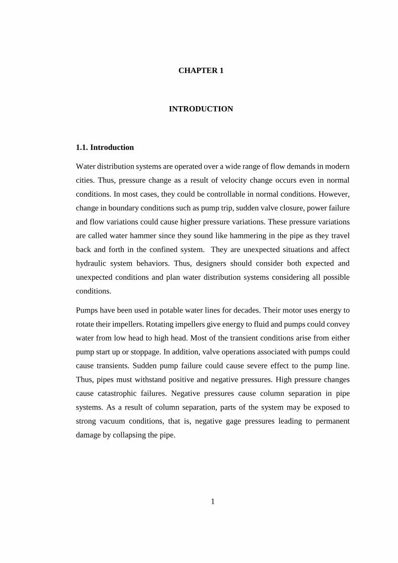
1.1. Introduction

Water distribution systems are operated over a wide range of flow demands in modern

cities. Thus, pressure change as a result of velocity change occurs even in normal

conditions. In most cases, they could be controllable in normal conditions. However,

change in boundary conditions such as pump trip, sudden valve closure, power failure

and flow variations could cause higher pressure variations. These pressure variations

are called water hammer since they sound like hammering in the pipe as they travel

back and forth in the confined system. They are unexpected situations and affect

hydraulic system behaviors. Thus, designers should consider both expected and

unexpected conditions and plan water distribution systems considering all possible

conditions.

Pumps have been used in potable water lines for decades. Their motor uses energy to

rotate their impellers. Rotating impellers give energy to fluid and pumps could convey

water from low head to high head. Most of the transient conditions arise from either

pump start up or stoppage. In addition, valve operations associated with pumps could

cause transients. Sudden pump failure could cause severe effect to the pump line.

Thus, pipes must withstand positive and negative pressures. High pressure changes

cause catastrophic failures. Negative pressures cause column separation in pipe

systems. As a result of column separation, parts of the system may be exposed to

strong vacuum conditions, that is, negative gage pressures leading to permanent

damage by collapsing the pipe.

2

Transient conditions determine system reliability. Therefore, careful selection of

protective devices has an important role at design stage. Negative pressures could be

prevented by one-way surge tanks and air valves. One-way surge tank has a check

valve at the bottom. It is used to separate the surge tank and the pipeline in normal

conditions. The aim of the separation is to reduce height of the surge tank wall. When

pressure falls below the pipeline profile, water is supplied from the surge tank into the

pipeline to prevent negative pressure (Miyashiro, 1967). Air valve is another

alternative for negative pressures. Air is ejected when hydraulic grade line elevation

falls below pipeline profile. Moreover, flywheels could be inserted into pumps to

prevent liquid column separation. Flywheels are used to increase moment of inertia of

the pump motor (Yang, 2001). Air chamber is the valid and reliable solution against

both positive and negative pressures, especially in pumped discharge lines. Water is

transported from the chamber of the air vessel into cavity and positive pressure could

be provided and maintained in the system (Stephenson, 2002). Location of the air

vessel to be placed in the pipeline system has different effects against water hammer.

In most applications, air chambers are placed after the check valve(s) located just

downstream of the pump(s) at the upstream section of the pipeline to prevent flow

reversal through the pumps. However, unsuitable locations could cause unnecessary

size to prevent positive pressure, (Wang et al, 2019).

Models that are created in laboratories are very effective. However, it is difficult to

study in large scale systems because they are not economical and practical. With the

help of computer-aided engineering, lots of simulations could be tested more easily.

Results are compared and, if needed, best protection devices could be selected (Rezaei

et al., 2017)

In this study, computer program called HAMMER is used for testing the system

reliability.

3

1.2. Literature Survey

Hydraulic transient studies have been done for many years. Equation of motion and

equation of continuity which are unsteady nonlinear partial differential equations are

used to describe the time dependent fluid behavior. Method of characteristics which

use compatibility relations is widely used to solve these nonlinear equations,

Chaudhry (1979), and Shani et al., (2017).

Nonlinear equations are complex equations. Therefore, high speed computers are

widely used in transient studies. Streeter (1963) was one of the first researchers that

used high speed computers. Parallel pumps with suction lines between two reservoirs

were examined in his studies. Different specific speeds, diameters, pipe lengths and

moment of inertias were examined in power failure scenario and results were

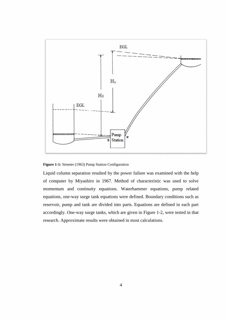
evaluated in IBM 7090 computer. In Figure 1-1, pump station configuration used in

the study is shown. H0 is described as rated head and Hs is described as total dynamic

head produced by pump at steady state condition and EGL is the energy grade line.

4

Figure 1-1: Streeter (1963) Pump Station Configuration

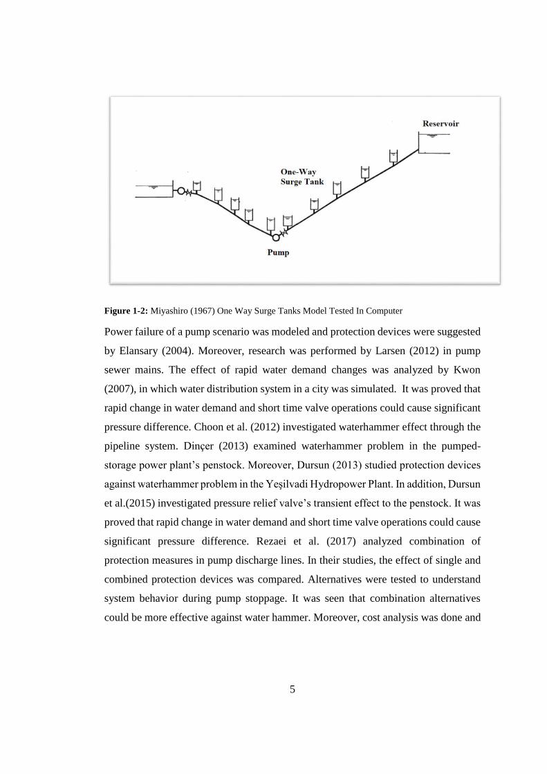
Liquid column separation resulted by the power failure was examined with the help

of computer by Miyashiro in 1967. Method of characteristic was used to solve

momentum and continuity equations. Waterhammer equations, pump related

equations, one-way surge tank equations were defined. Boundary conditions such as

reservoir, pump and tank are divided into parts. Equations are defined in each part

accordingly. One-way surge tanks, which are given in Figure 1-2, were tested in that

research. Approximate results were obtained in most calculations.

5

Figure 1-2: Miyashiro (1967) One Way Surge Tanks Model Tested In Computer

Power failure of a pump scenario was modeled and protection devices were suggested

by Elansary (2004). Moreover, research was performed by Larsen (2012) in pump

sewer mains. The effect of rapid water demand changes was analyzed by Kwon

(2007), in which water distribution system in a city was simulated. It was proved that

rapid change in water demand and short time valve operations could cause significant

pressure difference. Choon et al. (2012) investigated waterhammer effect through the

pipeline system. Dinçer (2013) examined waterhammer problem in the pumped-

storage power plant’s penstock. Moreover, Dursun (2013) studied protection devices

against waterhammer problem in the Yeşilvadi Hydropower Plant. In addition, Dursun

et al.(2015) investigated pressure relief valve’s transient effect to the penstock. It was

proved that rapid change in water demand and short time valve operations could cause

significant pressure difference. Rezaei et al. (2017) analyzed combination of

protection measures in pump discharge lines. In their studies, the effect of single and

combined protection devices was compared. Alternatives were tested to understand

system behavior during pump stoppage. It was seen that combination alternatives

could be more effective against water hammer. Moreover, cost analysis was done and

6

combined applications were found more economical. Flywheel, air chamber and in-

line check valves were tested in that research.

Flywheels are used for increasing pump motor moment of inertia. The purpose of this

is to reduce maximum angular velocity of impellers. They are chosen against liquid

column separation (LCS). Column separation could occur when pressure drops below

pipeline profile. Separation occurs between two water columns especially at high

points. These liquid columns may collide during transient events causing high positive

pressures. LCS studies have been done from the 19th century up to now (Bergant et al.,

2005). Yang (2001) examined two cases in his research against LCS. It was seen that

increasing moment of inertia gives positive outcome. Furthermore, Elansary (2004)

found that flywheels are very successful against negative pressure arising from

emergency pump shutdown. Moreover, Kavurmacıoğlu (2009) evaluated the effect

of increasing pump inertia. In his study, flywheels were found effective. However, it

was noted that increasing inertia is not always practical because inserting big

flywheels could be necessary in some situations.

One-way surge tank is another option against negative pressures. Hu et al. (2008)

studied possible locations of surge tanks. Optimization of surge tanks was done

according to their location and height of the wall. Adding one-way surge tank at high

points was suggested in that study. Kavurmacıoğlu and Karadoğan (2003) claimed

that using one-way surge tank is very effective and economic in pump lines against

transient events. They analyzed single usage of protection device such as air chamber

and combination of it with one-way surge tank. It was concluded that combined usage

reduces air chamber’s volume. Chamani et al. (2012) concluded that size and location

does not affect volume of water supplied from surge tanks. Amount of water that is

used in the pipeline system is constant to avoid LCS according to their studies.

Carmona et al (2019) studied pump discharge lines in Mexico. Effect of air chambers,

air valves and one-way surge tanks were examined in that study.

7

Air valves are mainly used to prevent air existence in the flow. Bianchi et al. (2007)

studied to develop equation for optimum air valve dimensions. Their validation was

tested in the laboratory. It was stated that mathematical model which was developed

in that research could be applicable. Ramezani et al. (2015) researched efficiency of

air valves during normal operations. Proper location and size were also investigated

in that study. It was seen that usage of air valve has several advantages. To illustrate,

combining an air valve with an air chamber could reduce the air chamber volume.

They could be effective against negative pressures. However, periodic maintenance is

required for air valves in most of standards. Most of air valves are inaccessible due to

their locations. Moreover, rapid air flow could create additional high pressures.

Air chamber is the most valid and reliable solution against water hammer, especially

in pump discharge lines. Water is transported from the chamber of the air vessel into

cavity and positive pressure could be provided and maintained in the system.

(Stephenson, 2002). Deciding initial air volume and initial water volume is the most

important step. Thorley (2004) developed mathematical expression and charts for

determining air chamber volume. Furthermore, Stephenson (2002) also studied for

theoretical expression of air chamber volume.

El-Dabaa and Khoris (2018) studied effect of height (h) and diameter (d) ratio of air

chambers. It is concluded that increasing air chamber’s h/d ratio has a positive impact

against water hammer. Wang et al. (2019) studied optimum location of air vessel.

Their study was done for long distance pipelines.

1.3. Scope of Study

Pump discharge lines are used in water distribution lines frequently. Disturbances in

boundaries of the system, may change the fluid velocity, this, in turn, would cause

pressure change in closed pipeline systems. Transient condition such as power failure

leads to abrupt velocity and pressure change in hydraulic systems.

To prevent transient conditions, best protection device should be considered. There

are alternative solutions which are used in operations. However, deciding best one

8

would require extreme attention in some examples. Lots of unnecessary volume or

device could be selected. Moreover, location of them has also importance. In Chapter

2, transient flow concept in pump discharge line is examined. In Chapter 3, brief

information about protection devices is given. Software program that is used in

transient calculation is explained in Chapter 4. In final chapters, case studies are

evaluated.

9

CHAPTER 2

2. TRANSIENT FLOW

The main principles of transient flow are examined in this chapter. In the first part,

transient flow is defined. In the second part, foundations of the water hammer which

are related to basis of the physics or fluid mechanics are described. Continuity

equations and momentum equations are developed. Then, nonlinear hyperbolic partial

differential equations are converted to differential equations by using the method of

characteristics. Equations are determined to obtain algebraic equations that could be

solved in an x-t field with the boundary conditions. The theory of the pump transient

is explained in the final part for the sake of completeness.

2.1. Definition of Transient Flow

Steady state flow means that flow conditions, which are pressure, velocity or

discharge, do not change with time in the pipeline system. If these conditions change

over time at a point in the pipeline, the flow is named as unsteady flow. Steady state

flow could be defined as a unique case of an unsteady flow. Thus, unsteady flow

equations can also be applied to steady state conditions. The transient flow concept is

developed to describe unsteady flow condition in the pipeline or pump discharge line.

When parameters at a point in the pipeline change with time, transient flow occurs in

the hydraulic systems or surroundings.

The transient flow could be classified into two categories. The first one is named as

quasi-steady flow. Discharges or pressure change gradually with time in quasi-steady

flow. Thus, in the short time interval, the flow parameters show very close values

which could be assumed as constant. The second one is named as the true transient

flow. Inertia of liquid and/or flexibility of the fluid and pipe are the main parameters

that affect the true transient flow development. When inertia of the pipeline has

10

significant effect and pipe and flow elasticity has insignificant effect, the true transient

flow is named as rigid-column flow. However, in addition to the inertia effect, the

actual transient flow is named as water hammer, given the elasticity effects of the pipe

and liquid. (Larock et al, 2000).

2.2. Water Hammer

2.2.1. General

Water hammer which means unsteady flow in the pressurized confined line could be

defined as hydraulic shock basically. Sudden speed changes or direction changes lead

to abrupt changes in pressure. These abrupt changes cause shock waves traveling back

and forth through the whole pipeline. When the shock waves meet a solid obstacle, a

hammer sound is heard. This is the reason of the term for water hammer.

Flow in the pipeline could not maintain its steady state form mostly because many

factors in a confined line could affect flow conditions. Pump start up or stoppage,

water demand changes, changes in a tank level or reservoir level, power failures and

many unforeseen events could lead to transient condition in the pipeline system. The

causes of water hammer are classified into four events. (Bentley HAMMER, 2016):

• Cavities, that arise from pump start-up, collapse suddenly and cause high pressure

in the pipeline.

• Pump stoppage could lead to sudden flow velocity change in the pipeline. The

hydraulic grade line drops below pipeline central axis on the discharge side and sub-

atmospheric pressures occur in the pipeline. Sub-atmospheric pressures sometimes

leading to the vapor pressure of the liquid could cause liquid column separation.

• Valve opening or valve closure could cause shock waves in the pipeline system. The

time duration of valve opening or valve closure could cause severe effect to the

hydraulic systems. When the closure time is smaller than the time passed during the

pressure wave travel between the valve and the reservoir and the return movement

11

back to the valve, it is named as sudden valve closure. Sudden valve closure could

lead to sudden velocity change in the pipeline which means abrupt pressure change.

• Usage of improper devices in the pipeline that are selected for protection purposes

may cause in more harm than benefit.

A transient event is generated by sudden changes in the flow conditions in the pipeline

system. These events cause instability in the steady state flow condition. This

imbalance in energy causes the liquid to be trapped, the pipe to elongate and expand.

However, water is not easily compressed, and most of the kinetic energy produced by

the imbalance caused by transients causes significant compressive forces in the

system. The pressure forces rapidly spread over the entire pipeline system and change

the flow and pressure characteristics in the system. The propagation of this pressure

wave may cause cracks or weaken the pipeline and its supports at the most vulnerable

locations.

2.2.2. Derivation of Transient Flow Equations

Transient flow in the confined pipeline is modeled with momentum equations and

continuity equations. Appling the momentum equation to the control volume which is

a portion of the confined system is done firstly. Then, conservation of mass equation

for the liquid in the pipe is developed.

A hydraulic system, consist of a reservoir, a pipeline system and a valve at the end of

the pipeline is shown in Figure 2-1 (a).

When sudden valve closure occurs at the downstream section, the nearest layer of the

liquid to the valve will be in the rest position. The procedure continues for the

successive layers until fluid in the entire pipeline is in the rest position. A shock wave

moves towards the upstream section. The application of the momentum equation is

performed on the control volume shown in Figure 2-1 (b). The absolute pressure wave

velocity moving to the left due to a small change in the valve setting is a-V0. The

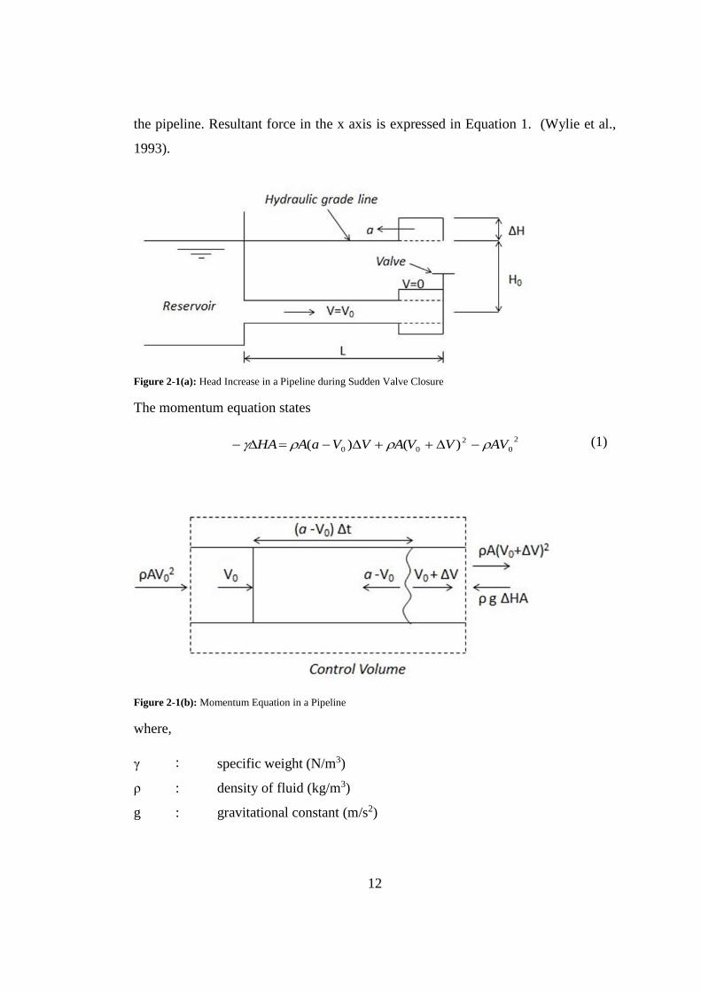
magnitude of the head increase at the valve is proportional to flow velocity change in

12

the pipeline. Resultant force in the x axis is expressed in Equation 1. (Wylie et al.,

1993).

Figure 2-1(a): Head Increase in a Pipeline during Sudden Valve Closure

The momentum equation states

2

0

2

00 )()( AVVVAVVaAHA (1)

Figure 2-1(b): Momentum Equation in a Pipeline

where,

γ : specific weight (N/m3)

ρ : density of fluid (kg/m3)

g : gravitational constant (m/s2)

13

A : pipe cross section area (m2)

V0 : initial velocity (m/s)

∆V : change in flow velocity (m/s)

a : acoustic speed (m/s)

∆H : incremental change in the head (m)

The velocity change is defined as (Vf - V0). Vf could be defined as the final velocity of

the liquid in the pipeline after valve operation. V0 could be defined as the initial

velocity before the valve operation. Equation for the head increase is determined as;

g

Va

a

V

g

VaH

01

(2)

The magnitude of the acoustic speed is enormously high when it is compared with the

initial flow velocity, V0. Thus, the magnitude of V0/a is quite small when it is

compared to 1 for liquids of many pipe types. Velocity is zero when the valve is closed

completely.

0VVV f (3)

Then, ∆V=0-V0 =-V0 , and when it is inserted into Eq.(2) ∆H is described as aV0 /g .

When valve closure has incremental pattern Eq.(2) could be determined as;

V

g

aH

(4)

and it is valid for any movement of the valve until the pressure wave reaches the

upstream end of the pipeline and returns as a reflected wave to the valve. In other

words, this equation applies as long as valve operation duration satisfies t <2L/a,

where L is the length of the pipe.

14

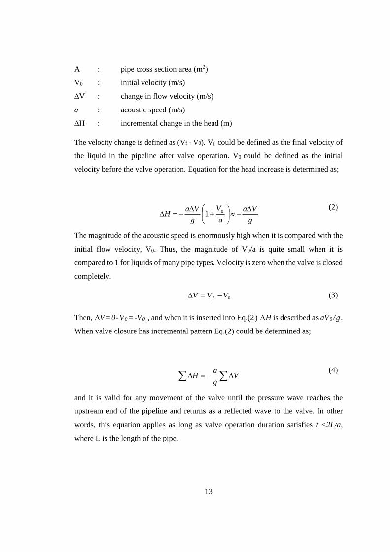
Wave speed expression can be obtained by applying the continuity equation for the

same pipeline under the same conditions. As the rapid valve closure causes pressure

head increase in the pipeline, referring to Fig. 2-2, pipe is stretched with the length

∆S. The magnitude of the stretch depends on a pipe support. It is assumed that the

stretch of the pipe takes place in L/a seconds or the velocity is ∆Sa / L-V0. Thus, ∆V

is equal to (∆S a/L) - V0. During the time elapsed, L/a, the mass of liquid entering the

pipe is ρAV0L/a. This mass is stored in the pipe as the cross-sectional area A increases

in the expanding pipe. Furthermore, the compression of the liquid causes a higher

density of the liquid mass. Eq.5 is obtained from the continuity principle;

Figure 2-2: Continuity Relations in Pipeline

LASAAL

a

LAV0

(5)

Eq.5 is simplified with ∆V= ∆Sa/L-V0 and the following equation is obtained;

A

A

a

V

(6)

To remove ∆V , Eq. 4 may be inserted and if the wave speed is left alone on the left,

a

LV0

15

A

A

Hga 2

(7)

If the extension of the pipe is prevented by the pipe supports, ∆S = 0. At this point we

may bring the bulk modulus of elasticity, defined by;

𝐾 =

𝛥𝑝

𝛥𝜌𝜌

= −𝛥𝑝

𝛥∀∀

(8)

where ∆∀/∀ could be defined as relative change in the original volume. Then,

𝑎2 =

𝐾𝜌

1 +𝐾𝐴

𝛥𝐴𝛥𝑝

(9)

The thick pipe wall could prevent any change in the cross-sectional area of the pipe.

Thus, the pressure increase mostly causes to compression of the fluid in the pipeline

and this compression could cause the density increase. ∆A/∆p becomes quite small

and acoustic speed becomes a ≈ √𝐾 𝜌⁄

On the other hand, for highly flexible pipes, increase in pressure caused by the

transients is often in agreement with the increased cross-sectional area of the pipe.

Thus, 1 is small and insignificant compared to other terms in the denominator.

Then, acoustic wave velocity for highly flexible pipes

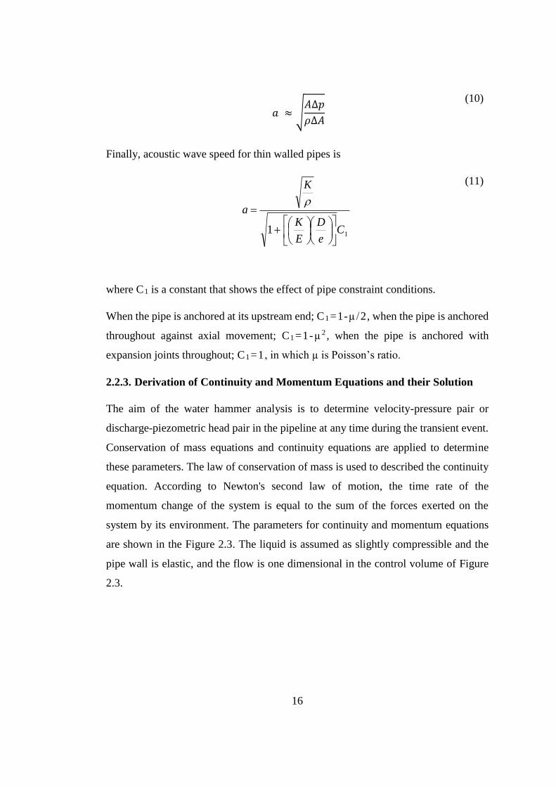
16

𝑎 ≈ √𝐴∆𝑝

𝜌∆𝐴

(10)

Finally, acoustic wave speed for thin walled pipes is

11 Ce

D

E

K

K

a

(11)

where C1 is a constant that shows the effect of pipe constraint conditions.

When the pipe is anchored at its upstream end; C1 =1-µ/2, when the pipe is anchored

throughout against axial movement; C1 =1-µ 2 , when the pipe is anchored with

expansion joints throughout; C1 =1 , in which µ is Poisson’s ratio.

2.2.3. Derivation of Continuity and Momentum Equations and their Solution

The aim of the water hammer analysis is to determine velocity-pressure pair or

discharge-piezometric head pair in the pipeline at any time during the transient event.

Conservation of mass equations and continuity equations are applied to determine

these parameters. The law of conservation of mass is used to described the continuity

equation. According to Newton's second law of motion, the time rate of the

momentum change of the system is equal to the sum of the forces exerted on the

system by its environment. The parameters for continuity and momentum equations

are shown in the Figure 2.3. The liquid is assumed as slightly compressible and the

pipe wall is elastic, and the flow is one dimensional in the control volume of Figure

2.3.

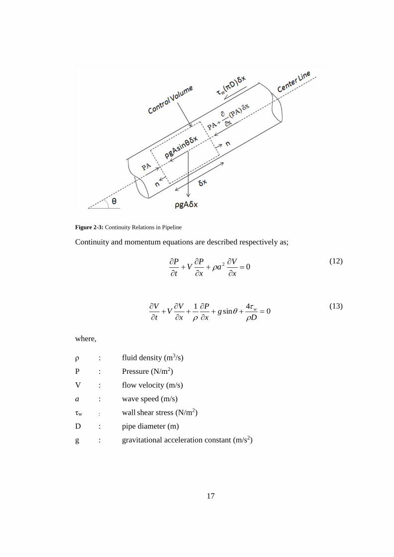
17

Figure 2-3: Continuity Relations in Pipeline

Continuity and momentum equations are described respectively as;

02

x

Va

x

PV

t

P

(12)

0

4sin

1

Dg

x

P

x

VV

t

V w

(13)

where,

ρ : fluid density (m3/s)

P : Pressure (N/m2)

V : flow velocity (m/s)

a : wave speed (m/s)

τw : wall shear stress (N/m2)

D : pipe diameter (m)

g : gravitational acceleration constant (m/s2)

18

These non-linear partial differential equations could not be solved in closed form.

Thus, a numerical solution method of choice should be applied to for their solution.

Among the potential methods, the methods of characteristics (MOC) is selected. For

one-dimensional fluid transient problems, the characteristics method is much better

than other methods in many respects, such as accurate simulation of orthogonal wave

fronts, display of wave propagation, ease of programming and efficiency of

calculations. (Chaudhry, 1979). The software Bentley HAMMER used in this thesis

to analyze the transient event in the pump discharge line is also based on the Method

of Characteristics.

The continuity and momentum equations defined in Eq.(12) and Eq.(13) will be solved

by using the MOC. The dependent variables are pressure and velocity and independent

variables are time and space in these equations. (Wylie et al., 1993).

Momentum equation is labeled by L2 and continuity equation by L1 to simplify the

procedure. In addition, 4𝜏𝜔

𝜌𝐷 +gsinθ is described as F. Multiplier is defined as λ ,

021 LL (14)

0

12

F

x

P

x

VV

t

V

x

Va

x

PV

t

P

(15)

Eq.(15) could be re-arranged as;

0

2

F

x

VaV

t

V

x

PV

t

P

(16)

From calculus we know that:

dt

dx

xtdt

d

(17)

19

First term in Eq.(16) is ⅆ𝑃

ⅆ𝑡 if 𝑉 +

𝜆

𝜌=

ⅆ𝑥

ⅆ𝑡 , and similarly the second term is equal to

ⅆ𝑉

ⅆ𝑡

if 𝑉 +𝜌𝑎2

𝜆=

ⅆ𝑥

ⅆ𝑡 . Consequently, Eq.(14) becomes

0 F

dt

dV

dt

dP

(18)

With the condition that

2aVV

dt

dx

(19)

λ is found from Eq.(19);

a (20)

λ is inserted into Eq.(19);

aV

dt

dx

(21)

The velocity of the pressure wave is quite high when it is compared with the flow

velocity. Thus, V term that is described in Eq.(21) could be omitted. λ value is

obtained in Eq.(20) and it is inserted into Eq.(18), C + and C - equations are obtained

for both plus and minus signs;

0

1 aF

dt

dVa

dt

dP

(22)

C+

a

dt

dx

(23)

20

0

1 aF

dt

dVa

dt

dP

(24)

C-

a

dt

dx

(25)

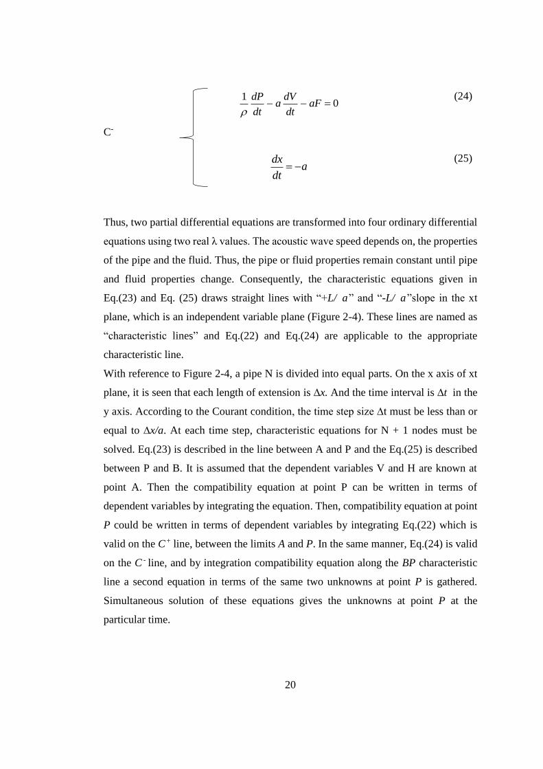
Thus, two partial differential equations are transformed into four ordinary differential

equations using two real λ values. The acoustic wave speed depends on, the properties

of the pipe and the fluid. Thus, the pipe or fluid properties remain constant until pipe

and fluid properties change. Consequently, the characteristic equations given in

Eq.(23) and Eq. (25) draws straight lines with “+L/ a” and “-L/ a”slope in the xt

plane, which is an independent variable plane (Figure 2-4). These lines are named as

“characteristic lines” and Eq.(22) and Eq.(24) are applicable to the appropriate

characteristic line.

With reference to Figure 2-4, a pipe N is divided into equal parts. On the x axis of xt

plane, it is seen that each length of extension is ∆x. And the time interval is ∆t in the

y axis. According to the Courant condition, the time step size ∆t must be less than or

equal to ∆x/a. At each time step, characteristic equations for N + 1 nodes must be

solved. Eq.(23) is described in the line between A and P and the Eq.(25) is described

between P and B. It is assumed that the dependent variables V and H are known at

point A. Then the compatibility equation at point P can be written in terms of

dependent variables by integrating the equation. Then, compatibility equation at point

P could be written in terms of dependent variables by integrating Eq.(22) which is

valid on the C+ line, between the limits A and P. In the same manner, Eq.(24) is valid

on the C - line, and by integration compatibility equation along the BP characteristic

line a second equation in terms of the same two unknowns at point P is gathered.

Simultaneous solution of these equations gives the unknowns at point P at the

particular time.

21

Figure 2-4: Characteristic Lines

In order to facilitate the integration of the compatibility equations, the shear stress

defined by Darcy-Weisbach can be applied in the transient flow.

8

VfVw

(26)

Therefore,

D

VVfgF

2sin

(27)

Then, by multiplying C+ compatibility equation by 𝑎ⅆ𝑡

g =

ⅆ𝑥

g , and by introducing the

pipeline area to write the equation in terms of discharge , the equation may be placed

in a form suitable for integration along the C+ characteristic line.

P

A

P

A

P

A

H

H

Q

Q

X

X

dxQQgDA

fdQ

gA

adH 0

2 2

(28)

A similar procedure can be applied to obtain the following equations;

AAAPAP QRQQQBHHC : (29)

22

BBBPBP QRQQQBHHC : (30)

where gA

aB and

22gDA

xfR

Generally,

PiPPi BQCHC : (31)

in which;

1111: iiiiP QRQBQHC (32)

PiMPi BQCHC : (33)

in which;

1111: iiiiM QRQBQHC (34)

2.3. Transients caused by Pumps

Pump operations could cause devastating consequences to the pump discharge line,

especially during a pump start-up or a sudden pump stoppage. The total inertia of the

pump rotating parts are generally smaller than the liquid inertia in the pump discharge

line. This leads to decrease in pump speed after a power failure. The flow provided by

the pump is reduced. Positive and negative pressures occur in the pipeline. Liquid

column separation could be seen when hydraulic grade line drops below the pipeline

profile. High pressures are seen when the columns are rejoined. Thus, careful

examination should be done for the pump discharge line in the design stage. The worst

case scenario should be taken into account and necessary protection device should be

selected if needed.

2.3.1. Sequence of Events during Pump Power Failure

When the power supply to the pump motor suddenly stops, the only energy left to

move the pump in the forward direction is the kinetic energy of the motor and the

rotating elements of the pump and the entrained water in the pump. Since this energy

23

is generally small compared to what is required to flow towards the discharge head,

the reduction in pump speed is quite rapid.

The lower the pump speed, the lower the water flow in the discharge line adjacent to

the pump.

As a result of these rapid flow changes, sub-normal water pressures are generated in

the discharge line of the pump. These sub-normal pressure waves move rapidly from

the discharge line to the discharge outlet where a wave reflection occurs. After a short

time, the speed of the pump is reduced to a point where no water will flow into the

existing head. If the pump does not have a control valve, the flow in the pump is

reversed, although the pump can still rotate in the forward direction. After a short time,

the pump acting as a turbine achieves the runaway speed.

Three effects must be considered to determine the transient hydraulic conditions and

the discharge line in the pump after a power failure in the pump motor; that is, pump

and motor inertia, pump characteristics and water wave phenomena in the discharge

line.

The effect of pump and motor inertia is derived from the inertia equation. This

equation describes the relationship between pump speed and torque at a given time in

terms of kinetic energy of the rotating system.

The pump characteristics are derived from a complete pump characteristic diagram.

This diagram describes how pump torque and speed change to the head and how it is

discharged throughout the operating range as a pump, energy distributor and turbine.

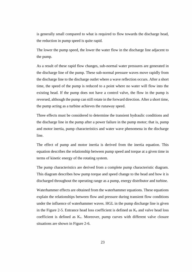
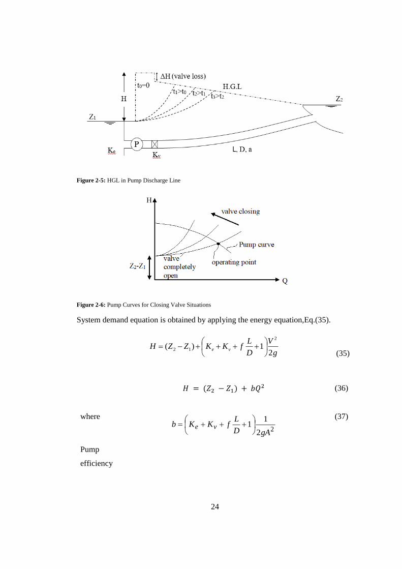
Waterhammer effects are obtained from the waterhammer equations. These equations

explain the relationships between flow and pressure during transient flow conditions

under the influence of waterhammer waves. HGL in the pump discharge line is given

in the Figure 2-5. Entrance head loss coefficient is defined as Ke and valve head loss

coefficient is defined as Kv. Moreover, pump curves with different valve closure

situations are shown in Figure 2-6.

24

Figure 2-5: HGL in Pump Discharge Line

Figure 2-6: Pump Curves for Closing Valve Situations

System demand equation is obtained by applying the energy equation,Eq.(35).

g

V

D

LfKKZZH ve

21)(

2

12

(35)

𝐻 = (𝑍2 − 𝑍1) + 𝑏𝑄2

(36)

where

22

11

gAD

LfKKb ve

(37)

Pump

efficiency

25

𝜂 =

𝛾𝑄𝐻

𝑇𝑤=

𝛾𝑄𝐻

𝑃

(38)

Eq.(38) is defined for pump.

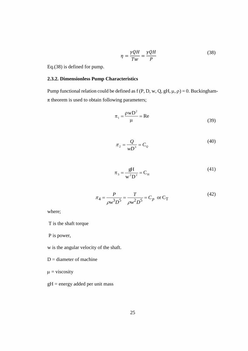
2.3.2. Dimensionless Pump Characteristics

Pump functional relation could be defined as f (P, D, w, Q, gH, , ) = 0. Buckingham-

π theorem is used to obtain following parameters;

Re

wD2

1

(39)

QC

wD

Q

32 (40)

H223 C

Dw

gH

(41)

T52534 Cor pC

Dw

T

Dw

P

(42)

where;

T is the shaft torque

P is power,

w is the angular velocity of the shaft.

D = diameter of machine

= viscosity

gH = energy added per unit mass

26

π1= Reynolds Number

π2= Flow Coefficient

π3= Head Coefficient

π4= Torque Coefficient

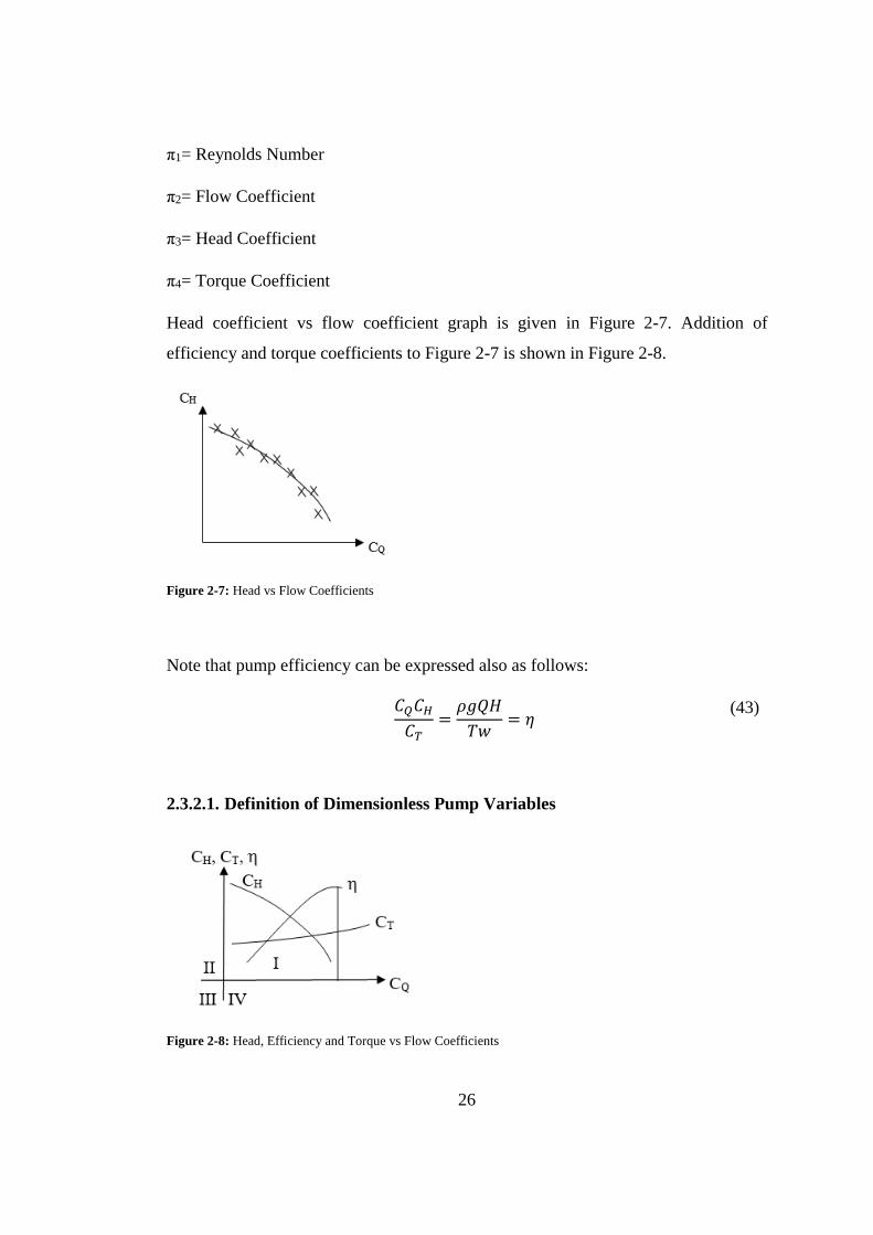
Head coefficient vs flow coefficient graph is given in Figure 2-7. Addition of

efficiency and torque coefficients to Figure 2-7 is shown in Figure 2-8.

Figure 2-7: Head vs Flow Coefficients

Note that pump efficiency can be expressed also as follows:

𝐶𝑄𝐶𝐻

𝐶𝑇=

𝜌𝑔𝑄𝐻

𝑇𝑤= 𝜂

(43)

2.3.2.1. Definition of Dimensionless Pump Variables

Figure 2-8: Head, Efficiency and Torque vs Flow Coefficients

27

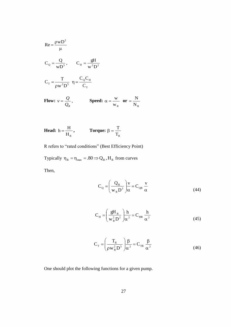
2wDRe

22H3QDw

gHC ,

wD

QC

52TDw

TC

T

HQ

C

CC

Flow: ,RQ

Qv Speed:

Rw

w or

RN

N

Head: RH

Hh , Torque:

RT

T

R refers to “rated conditions” (Best Efficiency Point)

Typically RRmaxR H,Q80. from curves

Then,

vC

v

Dw

QC QR3

R

R

Q

(44)

2HR222

R

R

H

hC

h

Dw

gHC

(45)

2TR252

R

R

T CDw

TC

(46)

One should plot the following functions for a given pump.

28

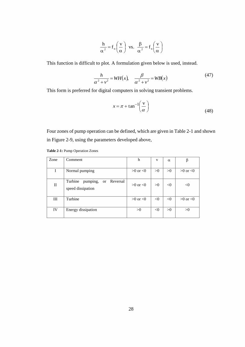
vf s.v

vf

hn2n2

This function is difficult to plot. A formulation given below is used, instead.

xWB

vxWH

v

h

2222 ,

(47)

This form is preferred for digital computers in solving transient problems.

vtan 1x

(48)

Four zones of pump operation can be defined, which are given in Table 2-1 and shown

in Figure 2-9, using the parameters developed above,

Table 2-1: Pump Operation Zones

Zone Comment h v

I Normal pumping >0 or <0 >0 >0 >0 or <0

II Turbine pumping, or Reversal

speed dissipation >0 or <0 >0 <0 <0

III Turbine >0 or <0 <0 <0 >0 or <0

IV Energy dissipation >0 <0 >0 >0

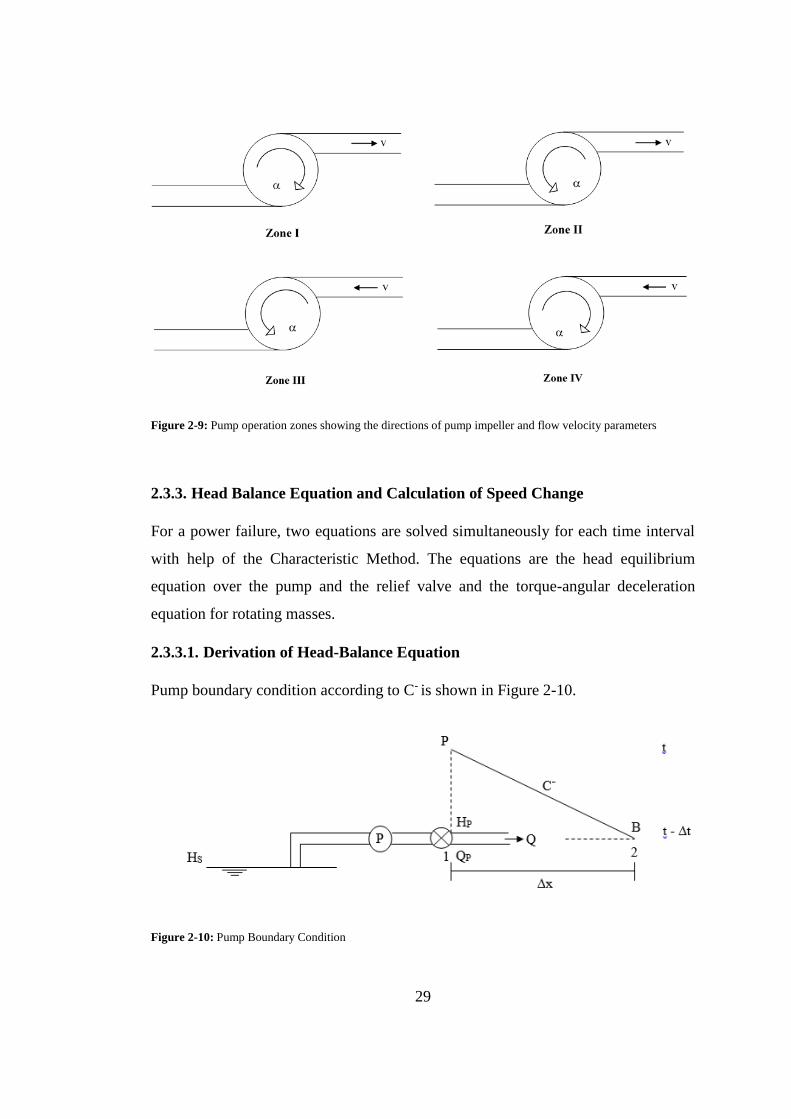
29

Figure 2-9: Pump operation zones showing the directions of pump impeller and flow velocity parameters

2.3.3. Head Balance Equation and Calculation of Speed Change

For a power failure, two equations are solved simultaneously for each time interval

with help of the Characteristic Method. The equations are the head equilibrium

equation over the pump and the relief valve and the torque-angular deceleration

equation for rotating masses.

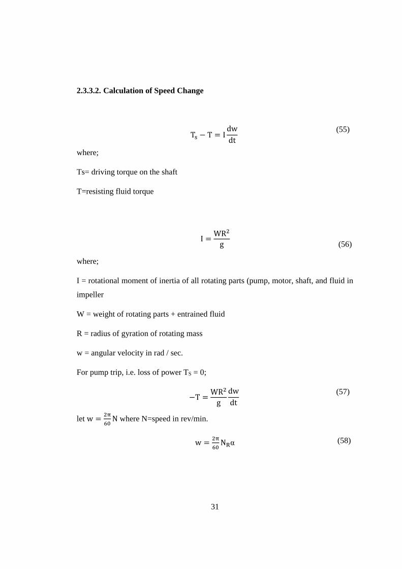
2.3.3.1. Derivation of Head-Balance Equation

Pump boundary condition according to C- is shown in Figure 2-10.

Figure 2-10: Pump Boundary Condition

30

where;

Hp= head at station 1 in pipe

Hs=suction head

H= dynamic pump head

H= head drop across valve

Qp= Instantaneous discharge in pump at time t

HS + H − H = HP (49)

At time t;

HP = CM + BQP (50)

H =

H0

τ2(

QP

Q0)

2

(51)

in which Ho = head loss at the valve initially, Qo = initial discharge ( QR)

The following has been previously defined H = HRh , QP = QR v

H =

ΔH0

Q02

QR2

τ2v2 =

𝐾𝑅

τ2v|v|

(52)

To account for both directions.

Hs + H − ΔH = Hp (53)

HS + HRh −

KR

τ2v|v| = CM + (B QR )v

(54)

τ=fn(t) and h, v are unknown parameters.

31

2.3.3.2. Calculation of Speed Change

Ts − T = I

ⅆw

ⅆt

(55)

where;

Ts= driving torque on the shaft

T=resisting fluid torque

I =

WR2

g

(56)

where;

I = rotational moment of inertia of all rotating parts (pump, motor, shaft, and fluid in

impeller

W = weight of rotating parts + entrained fluid

R = radius of gyration of rotating mass

w = angular velocity in rad / sec.

For pump trip, i.e. loss of power TS = 0;

−T =

WR2

g

ⅆw

ⅆt

(57)

let w =2π

60N where N=speed in rev/min.

w =2π

60NRα (58)

32

β =T

TR (59)

substituting them gives;

−β= [WR2

g

NR

TR

π

30]

ⅆα

ⅆt (60)

Assume ⅆα

ⅆt≅

α−α0

t and β ≅

1

2(β + β0), β0 and α0 refer to conditions at time t- t

β+β0

2 ≅ [

WR2

g

NR

TR

π

30]

(α0−α)

t

(61)

Eq. (61) can be expressed as:

𝛽 + 𝛽0 = 𝐶31(𝑎0 − 𝑎) (62)

in which;

𝐶31 =

𝑊𝑅2

𝑔

𝑁𝑅

𝑇𝑅

𝜋

15𝛥𝑡

(63)

𝐻𝑆 + 𝐻𝑅ℎ −

𝐾𝑅

𝜏2v|v| = 𝐶𝑀 + (𝐵 𝑄𝑅)v

In which,

(64)

ℎ = (𝛼2 + v2)𝑊𝐻(𝑥)

(65)

Eq.(65) becomes

𝐻𝑅(𝛼2 + 𝑣2)𝑊𝐻(𝑥) −𝐾𝑅

𝜏2 𝑣|𝑣| − (𝐵𝑄𝑅)𝑣+(𝐻𝑆 − 𝐶𝑀) = 0 (66)

or FH(α,v)=0 which is the Head-balance equation in terms of v and α. Eq.(62) becomes

with

33

𝛽 = (𝛼2 + 𝑣2)𝑊𝐵(𝑥) (67)

(𝛼2 + 𝑣2)𝑊𝐵(𝑥) + β0 = 𝐶31(𝛼0 − 𝛼) (68)

or FT(α,v)=0

which is the speed-change equation in v and α

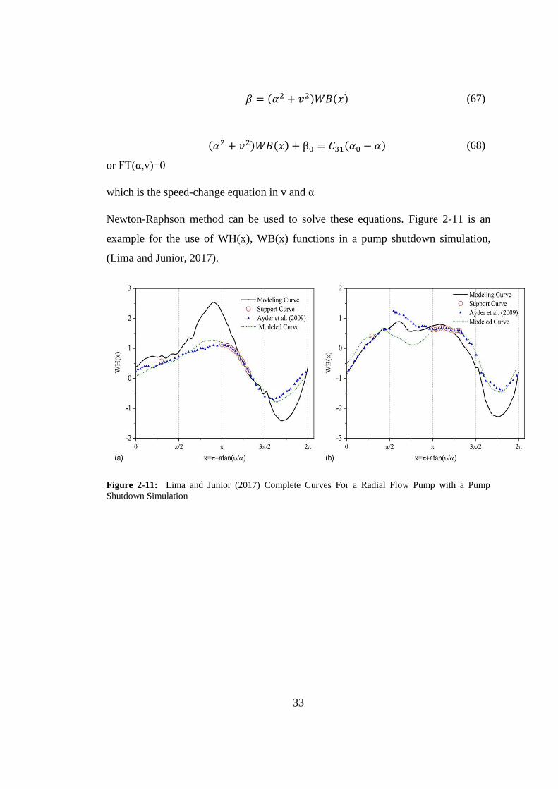
Newton-Raphson method can be used to solve these equations. Figure 2-11 is an

example for the use of WH(x), WB(x) functions in a pump shutdown simulation,

(Lima and Junior, 2017).

Figure 2-11: Lima and Junior (2017) Complete Curves For a Radial Flow Pump with a Pump

Shutdown Simulation

35

CHAPTER 3

3. PROTECTION DEVICES

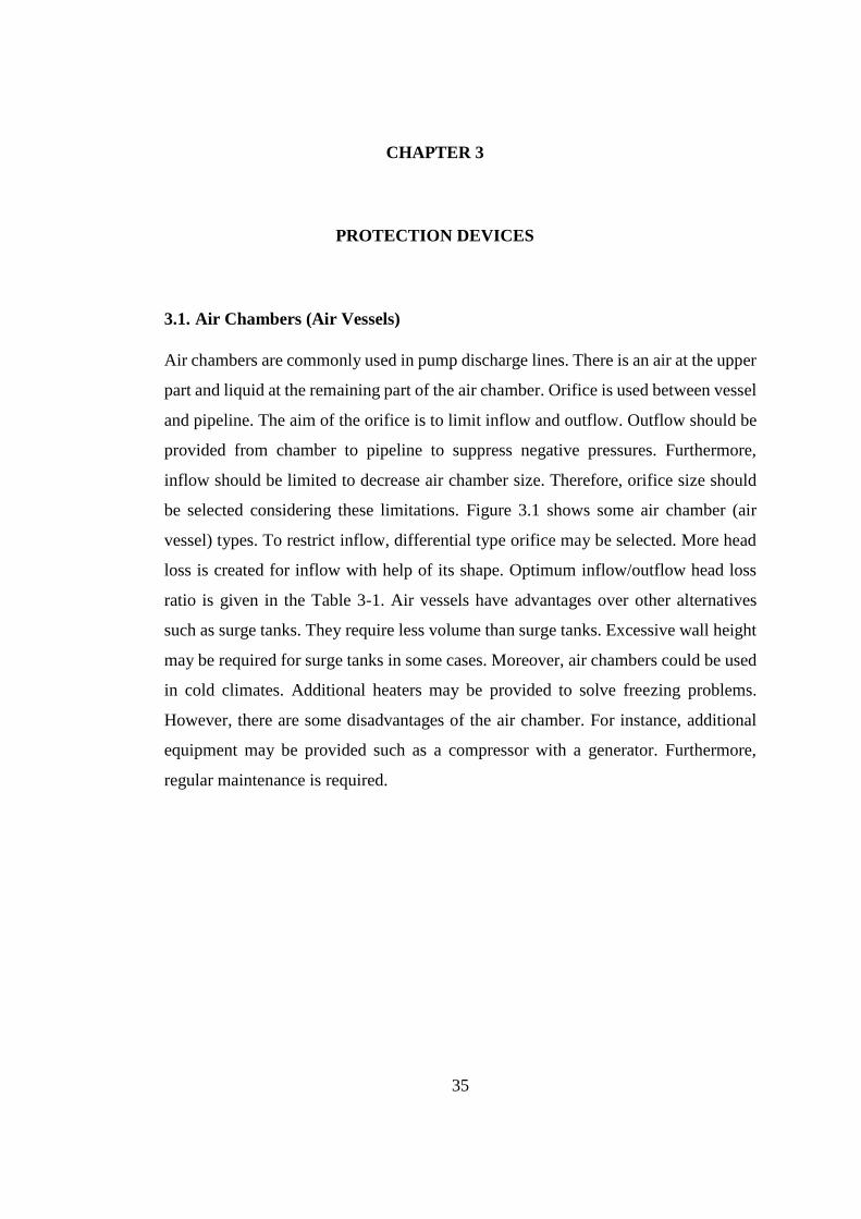
3.1. Air Chambers (Air Vessels)

Air chambers are commonly used in pump discharge lines. There is an air at the upper

part and liquid at the remaining part of the air chamber. Orifice is used between vessel

and pipeline. The aim of the orifice is to limit inflow and outflow. Outflow should be

provided from chamber to pipeline to suppress negative pressures. Furthermore,

inflow should be limited to decrease air chamber size. Therefore, orifice size should

be selected considering these limitations. Figure 3.1 shows some air chamber (air

vessel) types. To restrict inflow, differential type orifice may be selected. More head

loss is created for inflow with help of its shape. Optimum inflow/outflow head loss

ratio is given in the Table 3-1. Air vessels have advantages over other alternatives

such as surge tanks. They require less volume than surge tanks. Excessive wall height

may be required for surge tanks in some cases. Moreover, air chambers could be used

in cold climates. Additional heaters may be provided to solve freezing problems.

However, there are some disadvantages of the air chamber. For instance, additional

equipment may be provided such as a compressor with a generator. Furthermore,

regular maintenance is required.

36

Figure 3-1: Different Air Chamber Connection Types, (a) Vertical cylindrical air chamber with

bypass line, (b) Vertical cylindrical air chamber with throttle valve in bypass line, (c) Horizontal

cylindrical air chamber with separate inlet-outlet pipe.

Table 3-1: Orifice Head Loss Ratio For Inflow and Outflow ( Thorley, 2004)

Type Inflow/Outflow

Head Loss Ratio in Chamber 2.5

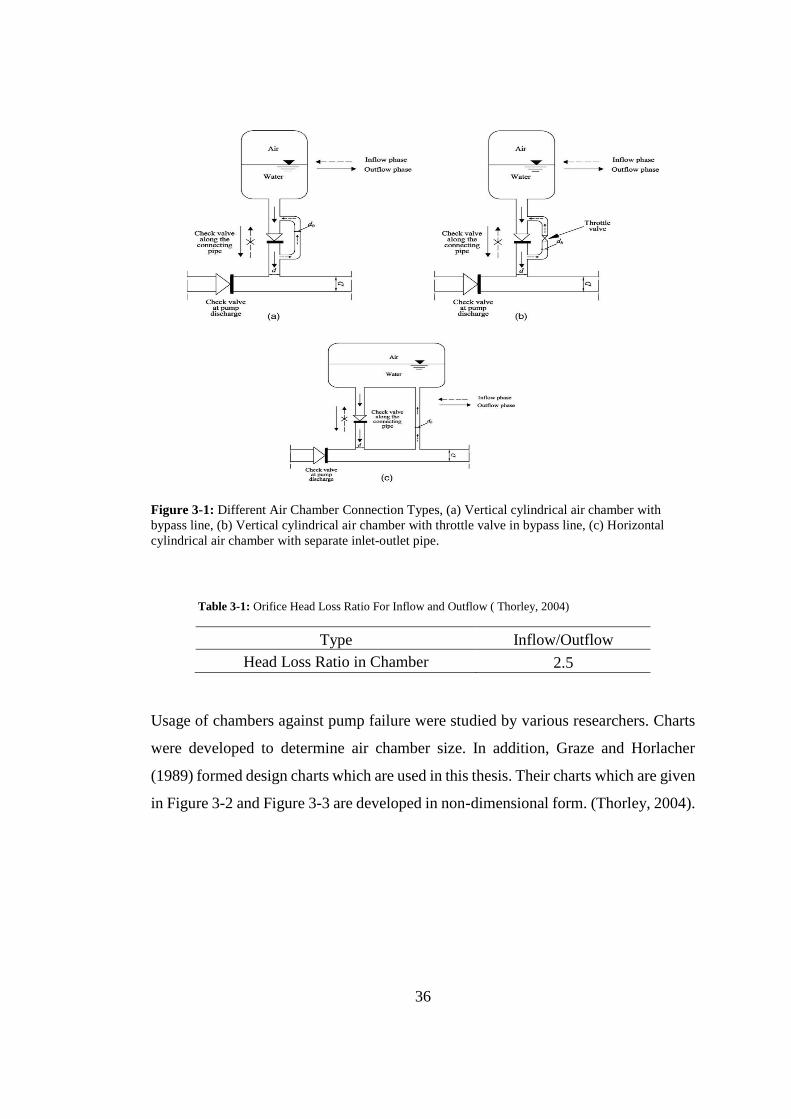
Usage of chambers against pump failure were studied by various researchers. Charts

were developed to determine air chamber size. In addition, Graze and Horlacher

(1989) formed design charts which are used in this thesis. Their charts which are given

in Figure 3-2 and Figure 3-3 are developed in non-dimensional form. (Thorley, 2004).

37

Figure 3-2: Maximum Head Ratio and Minimum Head Ratio w/ K value; ℎ̅𝑓=0 (Thorley, 2004)

38

Figure 3-3: Maximum Head Ratio and Minimum Head Ratio w/ K value; ℎ̅𝑓=0.05 (Thorley, 2004)

Friction parameter is defined:

ℎ̅𝑓 =

ℎ𝐿

ℎ𝑗

(69)

Joukowsky equation could be described as;

39

ℎ𝑗 =𝑐𝑣0

𝑔

(70)

ℎ̅0 =

ℎ0∗

ℎ𝑗=

ℎ0 + ℎ𝑎𝑡𝑚

ℎ𝑗

(71)

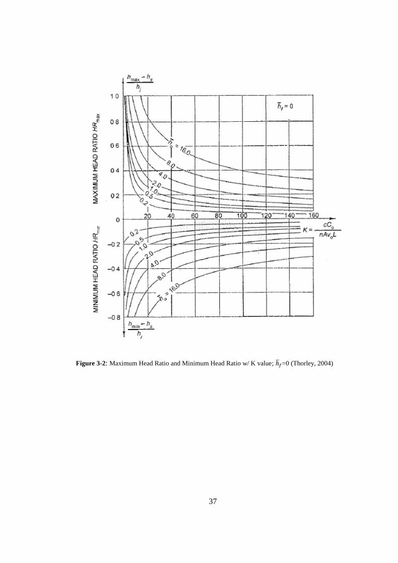
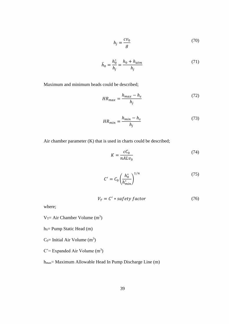
Maximum and minimum heads could be described;

𝐻𝑅𝑚𝑎𝑥 =

ℎ𝑚𝑎𝑥 − ℎ𝑠

ℎ𝑗

(72)

𝐻𝑅𝑚𝑖𝑛 =

ℎ𝑚𝑖𝑛 − ℎ𝑠

ℎ𝑗

(73)

Air chamber parameter (K) that is used in charts could be described;

𝐾 =

𝑐𝐶0

𝑛𝐴𝐿𝑣0

(74)

𝐶′ = 𝐶0 (

ℎ0∗

ℎ𝑚𝑖𝑛∗ )

1∕𝑛

(75)

𝑉𝑇 = 𝐶′ ∗ 𝑠𝑎𝑓𝑒𝑡𝑦 𝑓𝑎𝑐𝑡𝑜𝑟 (76)

where;

VT= Air Chamber Volume (m3)

hS= Pump Static Head (m)

C0= Initial Air Volume (m3)

C’= Expanded Air Volume (m3)

hmax= Maximum Allowable Head In Pump Discharge Line (m)

40

hmin= Minimum Allowable Head In Pump Discharge Line (m)

h0= Sum of the static and friction head (m)

n= Constant from 1 to 1.4

Safety Factor=1.2 or 1.25

c=Wave speed (m/s) (Thorley, 2004)

Results are obtained and K value is written from a suitable chart. Following K value,

air chamber volume is found from Eq.(76).

Stephenson (2002) also developed mathematical equations for certain Hmax/H0 and

Hmin/H0 ratios to determine air chamber volume;

𝑆′ =

𝑔𝑆0𝐻0

𝐴𝐿𝑣0

(77)

which;

S0= Initial air volume in air chamber

S= Air Chamber Volume

H0= Pump Static Head

A=Pipe Area

When Hmin/ H0 and Hmax/H0 ratios are found, S’ is determined according to Figure 3-4

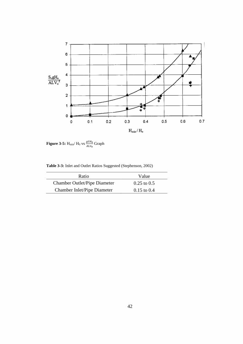
and Table 3-2. Then, air volume is found with Eq.(77). Hmin/ H0 vs 𝑔𝑆𝐻0

𝐴𝐿𝑣0 chart is formed

which is given in Figure 3-5. Instead of S0, S is used in formulation and air chamber

volume is determined. Then, the inlet and outlet pipe ratios are determined according

to parameters given in the Table 3-3. Figure 3-6 can also be examined to understand

the inlet and outlet pipelines in the air chamber.

41

Table 3-2: Hmax/H0 and Hmin/H0 Ratios Given In Stephenson (2002) Chart

Ratio Value S’

Hmax/H0 2.2 0.5

Hmax/H0 1.4 1

Hmax/H0 1.2 8

Hmin/ H0 0.7 8

Hmin/ H0 0.4 1

Hmin/ H0 0.2 0.5

Figure 3-4: S’ Graph w/ Hmin/ H0 and Hmax/ H0

42

Figure 3-5: Hmin/ H0 vs 𝑔𝑆𝐻0

𝐴𝐿𝑣0 Graph

Table 3-3: Inlet and Outlet Ratios Suggested (Stephenson, 2002)

Ratio Value

Chamber Outlet/Pipe Diameter 0.25 to 0.5

Chamber Inlet/Pipe Diameter 0.15 to 0.4

43

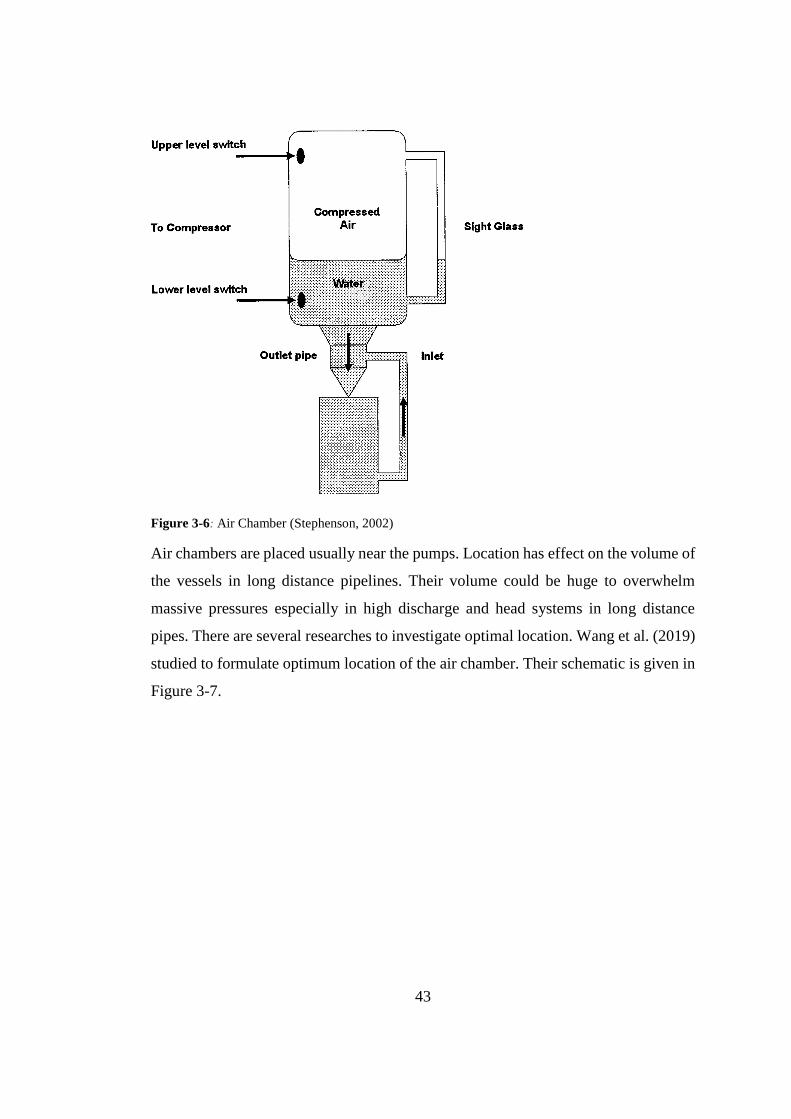
Figure 3-6: Air Chamber (Stephenson, 2002)

Air chambers are placed usually near the pumps. Location has effect on the volume of

the vessels in long distance pipelines. Their volume could be huge to overwhelm

massive pressures especially in high discharge and head systems in long distance

pipes. There are several researches to investigate optimal location. Wang et al. (2019)

studied to formulate optimum location of the air chamber. Their schematic is given in

Figure 3-7.

44

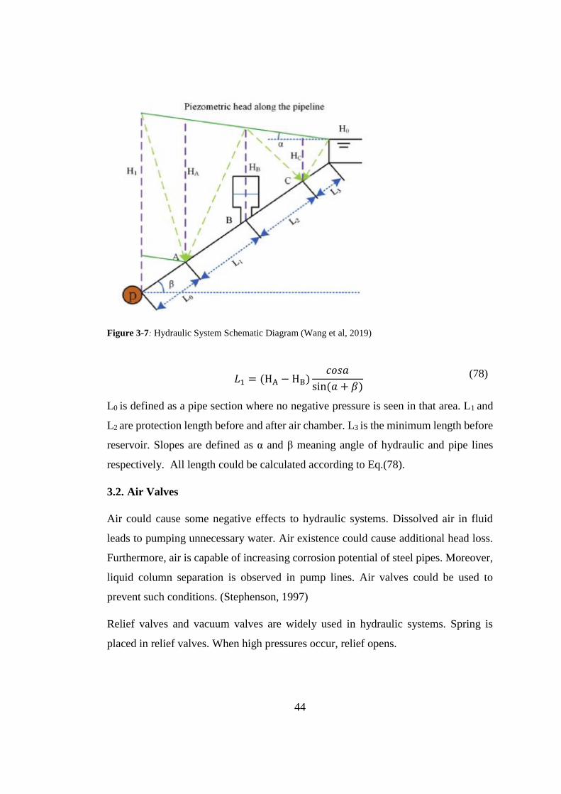
Figure 3-7: Hydraulic System Schematic Diagram (Wang et al, 2019)

𝐿1 = (HA − HB)𝑐𝑜𝑠𝑎

sin (𝑎 + 𝛽)

(78)

L0 is defined as a pipe section where no negative pressure is seen in that area. L1 and

L2 are protection length before and after air chamber. L3 is the minimum length before

reservoir. Slopes are defined as α and β meaning angle of hydraulic and pipe lines

respectively. All length could be calculated according to Eq.(78).

3.2. Air Valves

Air could cause some negative effects to hydraulic systems. Dissolved air in fluid

leads to pumping unnecessary water. Air existence could cause additional head loss.

Furthermore, air is capable of increasing corrosion potential of steel pipes. Moreover,

liquid column separation is observed in pump lines. Air valves could be used to

prevent such conditions. (Stephenson, 1997)

Relief valves and vacuum valves are widely used in hydraulic systems. Spring is

placed in relief valves. When high pressures occur, relief opens.

45

Vacuum valves are used to prevent negative pressures. When pressure drops below

vapor pressure, air influx is provided by them.

Orifice size should be determined carefully. Small diameter may cause providing

insufficient air to pipeline. However, enormous diameters could lead to poor resistance

to air outflow. When air is exhausted, velocity suddenly becomes zero. Sudden

velocity change causes high heads in hydraulic systems. (Bianchi et al, 2007)

Diameters from 50 mm to 200 mm are suggested for vacuum valves.

3.3. Flywheels

Following power failure, reverse flow occurs in a very short time interval. Vacuum

condition could be observed during transient condition. Flywheels are mainly used

against this vacuum condition. Inertia could be defined as resistance to velocity

change. Therefore, resistance magnitude of pump rotating part is an important

parameter in hydraulic systems.

Inertia should be calculated including all rotating parts. Rotating parts could be

Motor

Pump Impeller

Shaft

Flywheel

Shaft inertia could be ignored because it has small value when comparing other

parameters.

Motor inertia could be calculated as;

𝐼𝑚 = 118 (

𝑃

𝑁)

1.48

(79)

where;

P= Power (kW)

46

N= Speed (rpm)

Impeller inertia could be calculated as;

𝐼𝑝 = 1.5 ∗ 107 (

𝑃

𝑁3)

0.9556

(80)

𝑃 =

𝜌 ∗ 𝑄 ∗ ℎ ∗ 𝑔

3.6 ∗ 106 ∗ 𝜂

(81)

Flywheels inertia could be calculated as;

𝐼 = 𝑘 ∗ 𝑚 ∗ 𝑟2

(82)

where

m= flywheel mass (kg)

r= inside diameter of cylinder (m)

k=constant depends on flywheel type

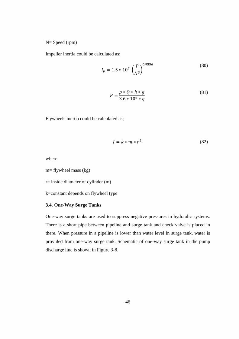
3.4. One-Way Surge Tanks

One-way surge tanks are used to suppress negative pressures in hydraulic systems.

There is a short pipe between pipeline and surge tank and check valve is placed in

there. When pressure in a pipeline is lower than water level in surge tank, water is

provided from one-way surge tank. Schematic of one-way surge tank in the pump

discharge line is shown in Figure 3-8.

47

Figure 3-8: Model of One-way Surge Tank In a Pump Discharge Line (Hu et al. 2008)

From Figure 3-4, continuity equation is written as;

𝑄𝑝=𝑄𝑠𝑡 + 𝑄𝑝2 (83)

𝐻𝑝=𝑍𝑠𝑡 + 𝑅𝑘𝑄𝑠𝑡|𝑄𝑠𝑡| (84)

𝑑𝑍𝑠𝑡

𝑑𝑡=

𝑄𝑠𝑡

𝐴𝑠𝑡

(85)

49

CHAPTER 4

4. COMPUTER SOFTWARE

4.1. Brief Information about Software Programs Essentials

Various software programs exist to simulate transient conditions. Method of

characteristic is widely used for solving hydraulic equations. Gray (1953) is the

pioneer of using the method of characteristic in hydraulic equations and Streeter and

Lai (1962) and Streeter and Wylie (1967) made important contributions. (Thorley,

2004) With the help of this method, internal conditions and boundary conditions could

be estimated in different time and space. In addition, other methods are also formed.

Some of them are acceptable but they are still insufficient in some boundary

conditions.

In computer solution, some assumptions are made:

Mach number is taken as very small values. It means velocity in a pipe is very

low when it is compared with acoustic wave speed.

Compressibility is accepted as negligible. In other words, density could be

taken as constant.

Pipe-wall interaction has small values when it is compared with total head loss.

For elastic modulus and bulk modulus, one constant is taken.

Using proper data has an importance on software program. Devices should be well

defined before running hydraulic transients. Additional information could also be

described when needed. In general,

Pipeline characteristics are diameters, lengths, elevation, pipeline profile, head

losses, bends, reductions, valves, reservoirs, pumps, tanks, air chambers.

50

Fluid parameters are acoustic speed, temperature, pressure, ingredients,

density and bulk modulus.

Transient conditions like sudden valve closure or pump failure are also included

to the system. (Thorley, 2004)

4.2. HAMMER Software Program

Hammer program is developed to evaluate pipelines and pump lines in transient

conditions. All pipe networks could define in that program. HAMMER is a capable

of,

Defining existing models, creating planned pipelines and running transient

simulations

Defining pipe, junction, pump, reservoir, valve conditions,

Transferring of field data from other program forms to HAMMER

Describing transient conditions, time intervals, different scenarios and

different cases

Describing protection measures, surge tanks, air chambers, valves

Analyzing hydraulic system reactions with numerical results and graphical

animations. (Bentley HAMMER, 2016).

Due to these advantages, HAMMER program is chosen for this thesis.

HAMMER software program has also some disadvantages. Firstly, some parameters

are not included in the transient simulations. To illustrate, initial liquid volume in the

air chamber is not a parameter for transient solver. Liquid volume always starts from

zero. Secondly, it takes time to get used to the software program.

However, with its advantages; HAMMER is one of the best software programs that

could be used in hydraulic transient calculations. Thus, HAMMER program is chosen

for this thesis.

51

4.2.1. Working Environment in Hammer

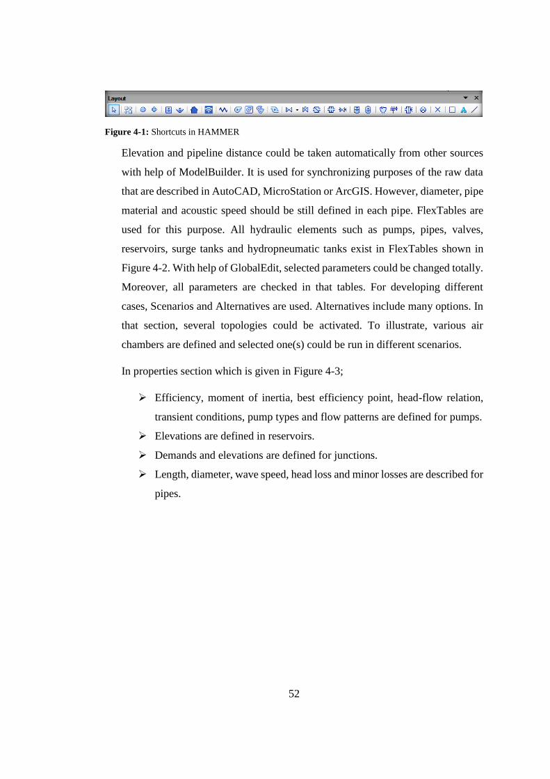
Program has several shortcuts on its interface. Some of them are given in the Figure

4-1. Layouts could be modified according to user-request. Shortcuts on Figure 4-1 are

respectively; Select, Pipe, Junction, Hydrant, Tank, Reservoir, Customer Meter,

SCADA Element, Periodic Head Flow, Pump, Variable Speed Pump, Pump Station,

Turbine, Valves, Valve With Linear Area Change, Check Valve, Orifice Between

Pipes, Discharge To Atmosphere, Surge Tank, Air Chamber, Air Valve, Surge Valve,

Rupture Disk, Isolation Valve, Spot Elevation, Border, Text and Line.

Pipes are main framework of water distribution systems. Diameter, pipe

material, roughness coefficient, length, minor losses, check valves and

acoustic speed are defined in pipe properties.

Junctions are used for mainly connection of pipes, defining elevations and

demands.

Reservoirs are defined for symbolizing water resources such as dams. Water

surface elevations could be defined in different time intervals.

Pumps are defined according to their design conditions. Pump definition is an

important part of the transient simulation. Pump stoppage could be defined in

HAMMER with “shut down after time delay” option. Transient time interval

is described in calculation options. Variable speed pumps could also be defined

with user-defined curve or fixed curve.

Surge Tanks, Air Chambers and Air Valves are selected for protection

purposes. Initial gas volume, initial liquid volume, elevation, inlet diameter,

loss ratio and coefficient and chamber type could be defined in air chambers.

In addition to this, animation graph of air volume and liquid volume with

respect to time could be seen in transient graphs. Operating elevation, type of

tank, inlet diameter and head loss coefficient could be defined in surge tanks.

Different kind of valves could be selected in air valves.

52

Figure 4-1: Shortcuts in HAMMER

Elevation and pipeline distance could be taken automatically from other sources

with help of ModelBuilder. It is used for synchronizing purposes of the raw data

that are described in AutoCAD, MicroStation or ArcGIS. However, diameter, pipe

material and acoustic speed should be still defined in each pipe. FlexTables are

used for this purpose. All hydraulic elements such as pumps, pipes, valves,

reservoirs, surge tanks and hydropneumatic tanks exist in FlexTables shown in

Figure 4-2. With help of GlobalEdit, selected parameters could be changed totally.

Moreover, all parameters are checked in that tables. For developing different

cases, Scenarios and Alternatives are used. Alternatives include many options. In

that section, several topologies could be activated. To illustrate, various air

chambers are defined and selected one(s) could be run in different scenarios.

In properties section which is given in Figure 4-3;

Efficiency, moment of inertia, best efficiency point, head-flow relation,

transient conditions, pump types and flow patterns are defined for pumps.

Elevations are defined in reservoirs.

Demands and elevations are defined for junctions.

Length, diameter, wave speed, head loss and minor losses are described for

pipes.

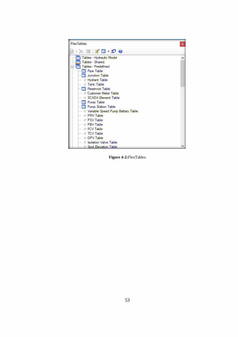
53

Figure 4-2:FlexTables

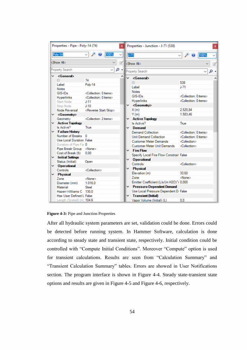
54

Figure 4-3: Pipe and Junction Properties

After all hydraulic system parameters are set, validation could be done. Errors could

be detected before running system. In Hammer Software, calculation is done

according to steady state and transient state, respectively. Initial condition could be

controlled with “Compute Initial Conditions”. Moreover “Compute” option is used

for transient calculations. Results are seen from “Calculation Summary” and

“Transient Calculation Summary” tables. Errors are showed in User Notifications

section. The program interface is shown in Figure 4-4. Steady state-transient state

options and results are given in Figure 4-5 and Figure 4-6, respectively.

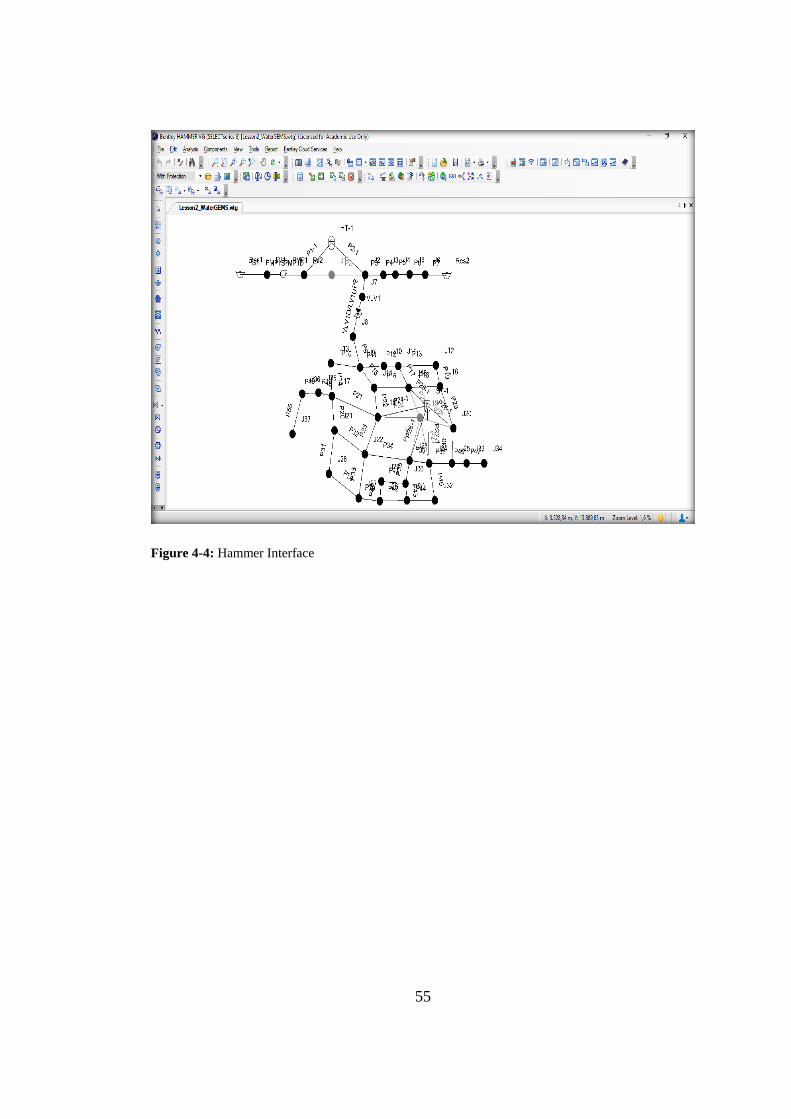
55

Figure 4-4: Hammer Interface

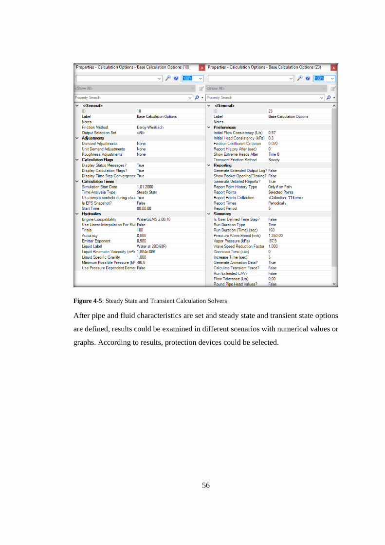
56

Figure 4-5: Steady State and Transient Calculation Solvers

After pipe and fluid characteristics are set and steady state and transient state options

are defined, results could be examined in different scenarios with numerical values or

graphs. According to results, protection devices could be selected.

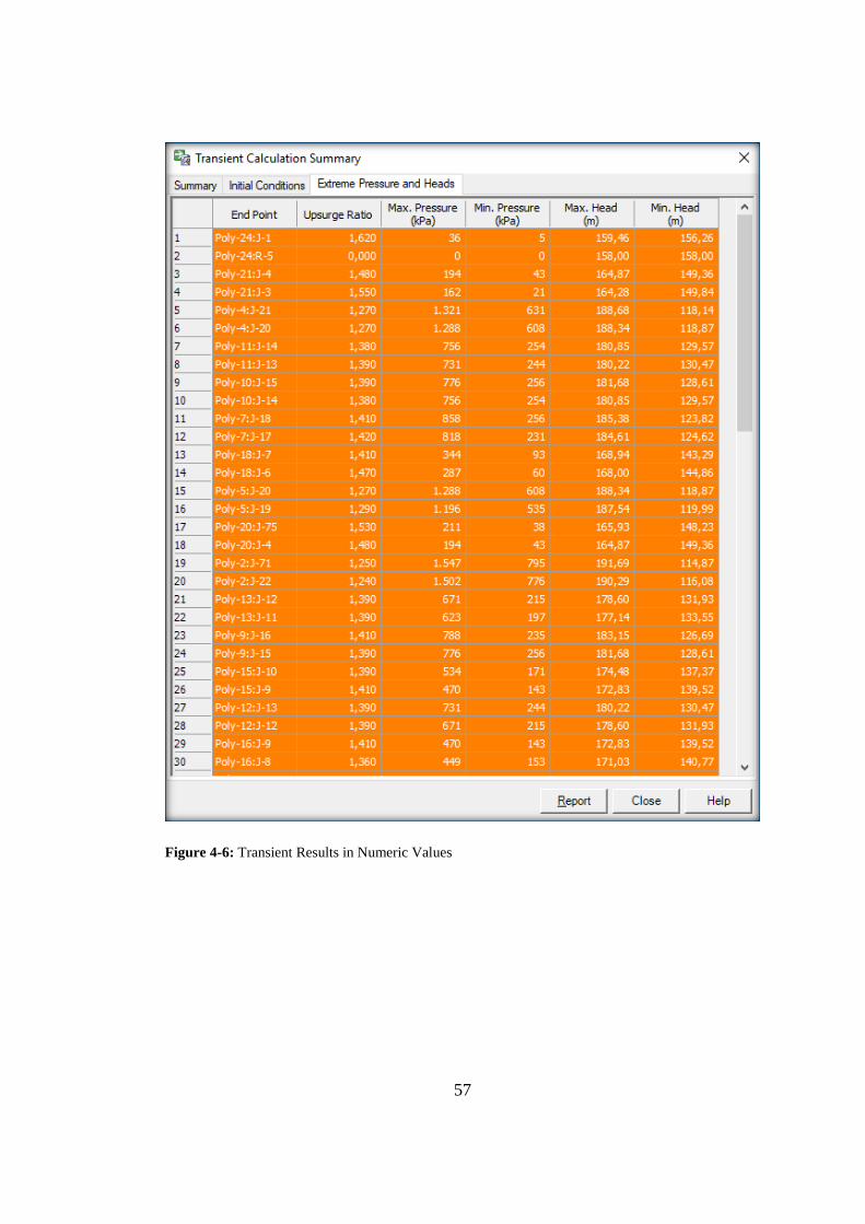
57

Figure 4-6: Transient Results in Numeric Values

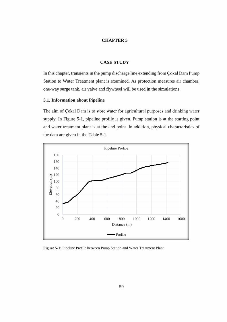
59

CHAPTER 5

5. CASE STUDY

In this chapter, transients in the pump discharge line extending from Çokal Dam Pump

Station to Water Treatment plant is examined. As protection measures air chamber,

one-way surge tank, air valve and flywheel will be used in the simulations.

5.1. Information about Pipeline

The aim of Çokal Dam is to store water for agricultural purposes and drinking water

supply. In Figure 5-1, pipeline profile is given. Pump station is at the starting point

and water treatment plant is at the end point. In addition, physical characteristics of

the dam are given in the Table 5-1.

Figure 5-1: Pipeline Profile between Pump Station and Water Treatment Plant

0

20

40

60

80

100

120

140

160

180

0 200 400 600 800 1000 1200 1400 1600

Ele

vat

ion (

m)

Distance (m)

Pipeline Profile

Profile

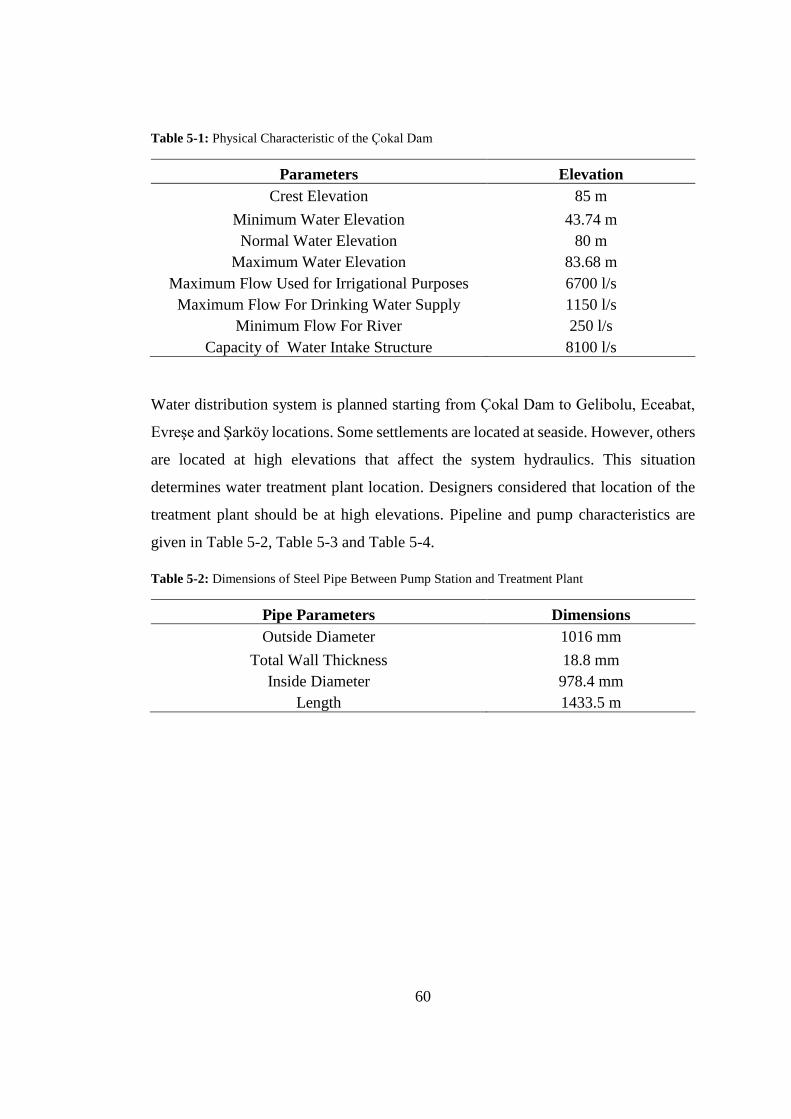
60

Table 5-1: Physical Characteristic of the Çokal Dam

Parameters Elevation

Crest Elevation 85 m

Minimum Water Elevation

Normal Water Elevation

Maximum Water Elevation

Maximum Flow Used for Irrigational Purposes

Maximum Flow For Drinking Water Supply

Minimum Flow For River

Capacity of Water Intake Structure

43.74 m

80 m

83.68 m

6700 l/s

1150 l/s

250 l/s

8100 l/s

Water distribution system is planned starting from Çokal Dam to Gelibolu, Eceabat,

Evreşe and Şarköy locations. Some settlements are located at seaside. However, others

are located at high elevations that affect the system hydraulics. This situation

determines water treatment plant location. Designers considered that location of the

treatment plant should be at high elevations. Pipeline and pump characteristics are

given in Table 5-2, Table 5-3 and Table 5-4.

Table 5-2: Dimensions of Steel Pipe Between Pump Station and Treatment Plant

Pipe Parameters Dimensions

Outside Diameter 1016 mm

Total Wall Thickness

Inside Diameter

Length

18.8 mm

978.4 mm

1433.5 m

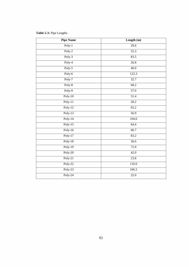
61

Table 5-3: Pipe Lengths

Pipe Name Length (m)

Poly-1 29.6

Poly-2 55.3

Poly-3 83.5

Poly-4 26.8

Poly-5 40.0

Poly-6 123.3

Poly-7 32.7

Poly-8 68.2

Poly-9 57.0

Poly-10 31.4

Poly-11 28.2

Poly-12 65.2

Poly-13 56.9

Poly-14 104.6

Poly-15 64.4

Poly-16 66.7

Poly-17 83.2

Poly-18 36.6

Poly-19 75.9

Poly-20 42.0

Poly-21 23.8

Poly-22 110.0

Poly-23 106.2

Poly-24 22.0

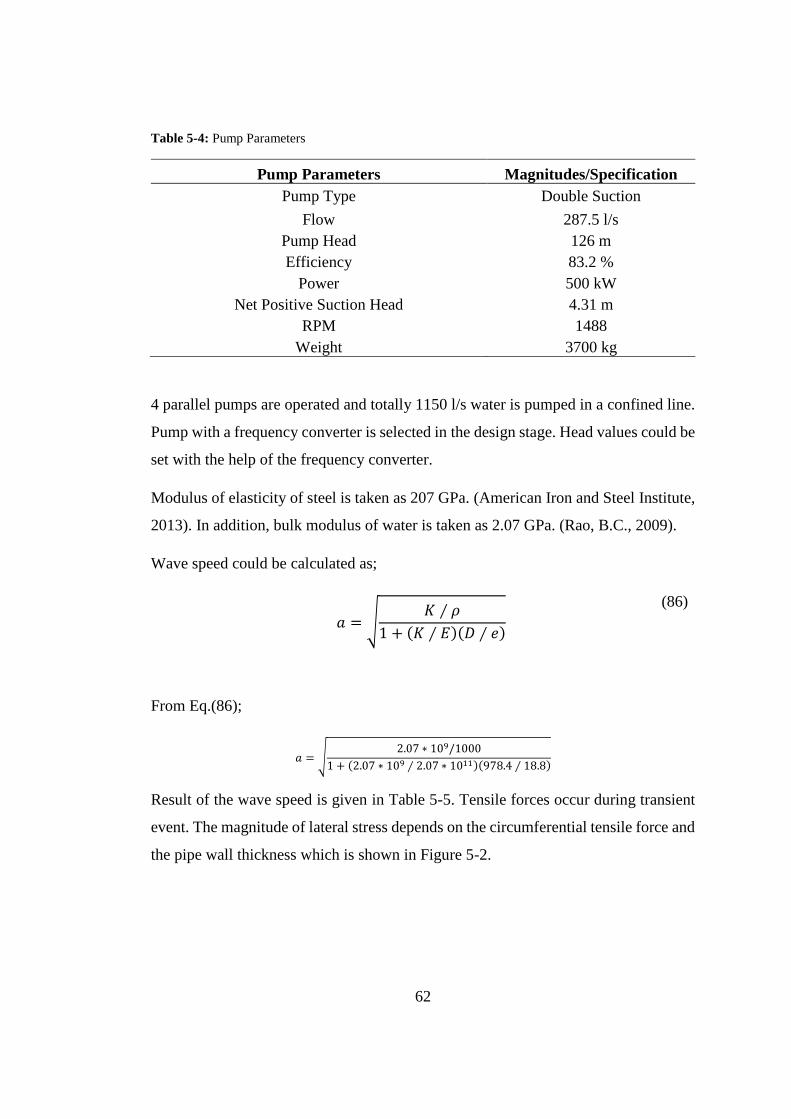
62

Table 5-4: Pump Parameters

Pump Parameters Magnitudes/Specification

Pump Type Double Suction

Flow

Pump Head

Efficiency

Power

Net Positive Suction Head

RPM

Weight

287.5 l/s

126 m

83.2 %

500 kW

4.31 m

1488

3700 kg

4 parallel pumps are operated and totally 1150 l/s water is pumped in a confined line.

Pump with a frequency converter is selected in the design stage. Head values could be

set with the help of the frequency converter.

Modulus of elasticity of steel is taken as 207 GPa. (American Iron and Steel Institute,

2013). In addition, bulk modulus of water is taken as 2.07 GPa. (Rao, B.C., 2009).

Wave speed could be calculated as;

𝑎 = √𝐾 ∕ 𝜌

1 + (𝐾 ∕ 𝐸)(𝐷 ∕ 𝑒)

(86)

From Eq.(86);

𝑎 = √2.07 ∗ 109/1000

1 + (2.07 ∗ 109 ∕ 2.07 ∗ 1011)(978.4 ∕ 18.8)

Result of the wave speed is given in Table 5-5. Tensile forces occur during transient

event. The magnitude of lateral stress depends on the circumferential tensile force and

the pipe wall thickness which is shown in Figure 5-2.

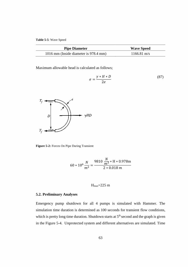
63

Table 5-5: Wave Speed

Pipe Diameter Wave Speed

1016 mm (Inside diameter is 978.4 mm) 1166.81 m/s

Maximum allowable head is calculated as follows;

𝜎 =

𝛾 ∗ 𝐻 ∗ 𝐷

2𝑒

(87)

Figure 5-2: Forces On Pipe During Transient

60 ∗ 106𝑁

𝑚2=

9810 𝑁

𝑚3 ∗ H ∗ 0.978m

2 ∗ 0.018 𝑚

Hmax=225 m

5.2. Preliminary Analyses

Emergency pump shutdown for all 4 pumps is simulated with Hammer. The

simulation time duration is determined as 100 seconds for transient flow conditions,

which is pretty long time duration. Shutdown starts at 5th second and the graph is given

in the Figure 5-4. Unprotected system and different alternatives are simulated. Time

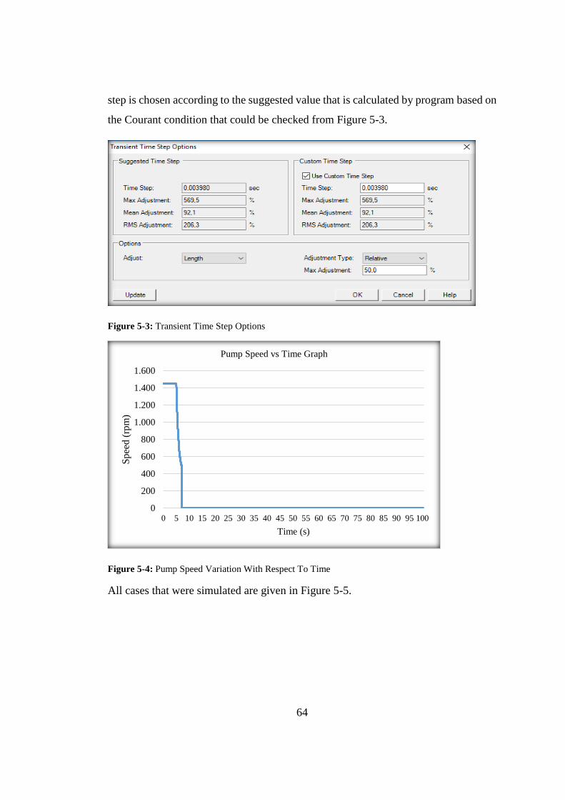
64

step is chosen according to the suggested value that is calculated by program based on

the Courant condition that could be checked from Figure 5-3.

Figure 5-3: Transient Time Step Options

Figure 5-4: Pump Speed Variation With Respect To Time

All cases that were simulated are given in Figure 5-5.

0

200

400

600

800

1.000

1.200

1.400

1.600

0 5 10 15 20 25 30 35 40 45 50 55 60 65 70 75 80 85 90 95 100

Spee

d (

rpm

)

Time (s)

Pump Speed vs Time Graph

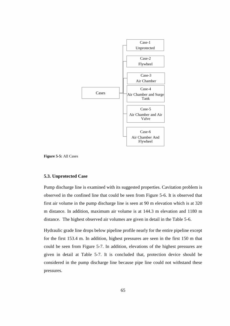
65

Figure 5-5: All Cases

5.3. Unprotected Case

Pump discharge line is examined with its suggested properties. Cavitation problem is

observed in the confined line that could be seen from Figure 5-6. It is observed that

first air volume in the pump discharge line is seen at 90 m elevation which is at 320

m distance. In addition, maximum air volume is at 144.3 m elevation and 1180 m

distance. The highest observed air volumes are given in detail in the Table 5-6.

Hydraulic grade line drops below pipeline profile nearly for the entire pipeline except

for the first 153.4 m. In addition, highest pressures are seen in the first 150 m that

could be seen from Figure 5-7. In addition, elevations of the highest pressures are

given in detail at Table 5-7. It is concluded that, protection device should be

considered in the pump discharge line because pipe line could not withstand these

pressures.

Cases

Case-1

Unprotected

Case-2

Flywheel

Case-3

Air Chamber

Case-4

Air Chamber and Surge Tank

Case-5

Air Chamber and Air Valve

Case-6

Air Chamber And Flywheel

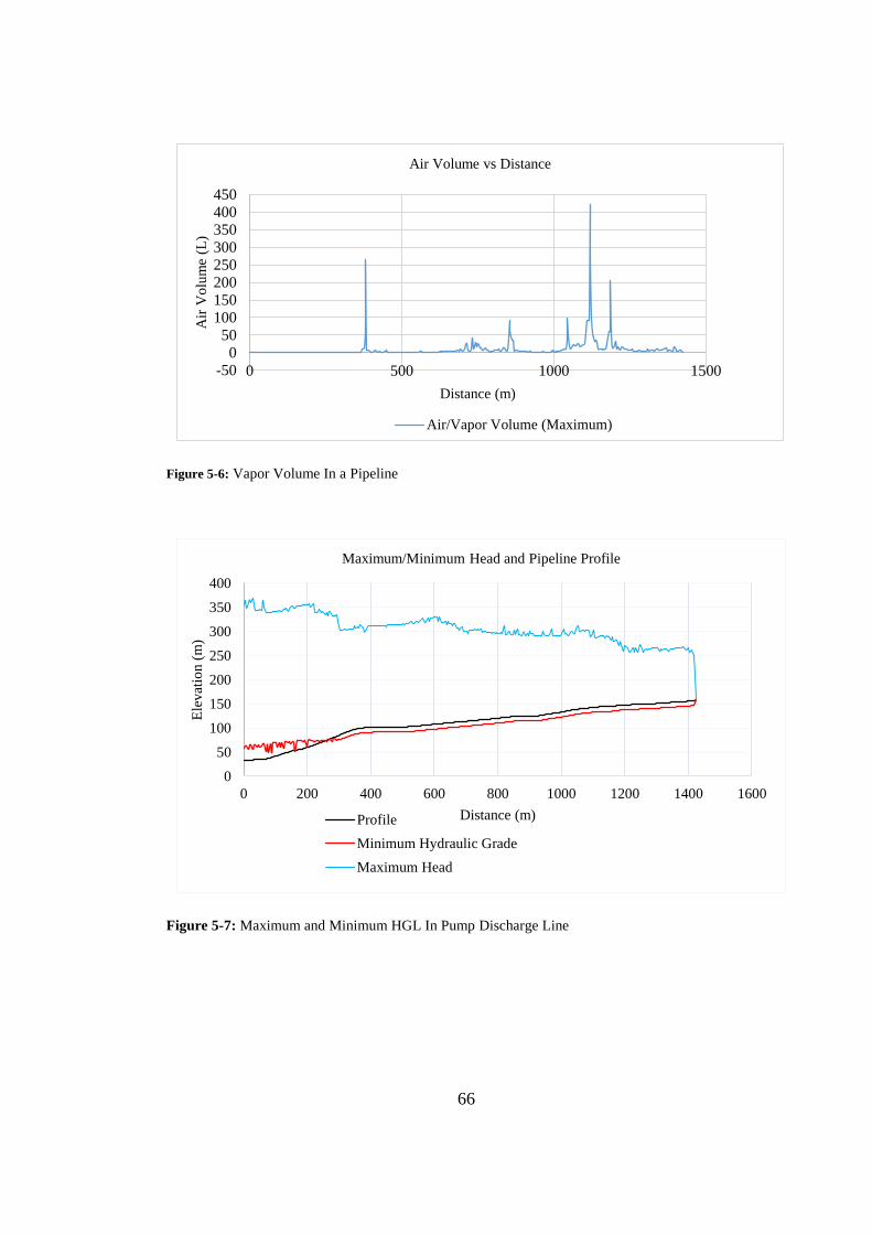
66

Figure 5-6: Vapor Volume In a Pipeline

Figure 5-7: Maximum and Minimum HGL In Pump Discharge Line

-500

50100150200250300

350400450

0 500 1000 1500

Air

Vo

lum

e (L

)

Distance (m)

Air Volume vs Distance

Air/Vapor Volume (Maximum)

0

50

100

150

200

250

300

350

400

0 200 400 600 800 1000 1200 1400 1600

Ele

vat

ion (

m)

Distance (m)

Maximum/Minimum Head and Pipeline Profile

Profile

Minimum Hydraulic Grade

Maximum Head

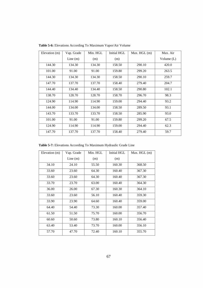
67

Table 5-6: Elevations According To Maximum Vapor/Air Volume

Elevation (m) Vap. Grade

Line (m)

Min. HGL

(m)

Initial HGL

(m)

Max. HGL (m) Max. Air

Volume (L)

144.30 134.30 134.30 158.50 290.10 420.0

101.00 91.00 91.00 159.80 299.20 263.5

144.30 134.30 134.30 158.50 290.10 259.7

147.70 137.70 137.70 158.40 279.40 204.7

144.40 134.40 134.40 158.50 290.80 102.1

138.70 128.70 128.70 158.70 296.70 98.3

124.90 114.90 114.90 159.00 294.40 93.2

144.00 134.00 134.00 158.50 289.50 93.1

143.70 133.70 133.70 158.50 285.90 93.0

101.00 91.00 91.00 159.80 299.20 67.5

124.90 114.90 114.90 159.00 294.40 62.3

147.70 137.70 137.70 158.40 279.40 59.7

Table 5-7: Elevations According To Maximum Hydraulic Grade Line

Elevation (m) Vap. Grade

Line (m)

Min. HGL

(m)

Initial HGL

(m)

Max. HGL (m)

34.10 24.10 55.50 160.30 368.50

33.60 23.60 64.30 160.40 367.30

33.60 23.60 64.30 160.40 367.30

33.70 23.70 63.00 160.40 364.30

36.00 26.00 67.30 160.30 364.10

33.60 23.60 56.10 160.40 359.30

33.90 23.90 64.60 160.40 359.00

64.40 54.40 73.30 160.00 357.40

61.50 51.50 75.70 160.00 356.70

60.60 50.60 73.80 160.10 356.40

63.40 53.40 73.70 160.00 356.10

57.70 47.70 72.40 160.10 355.70

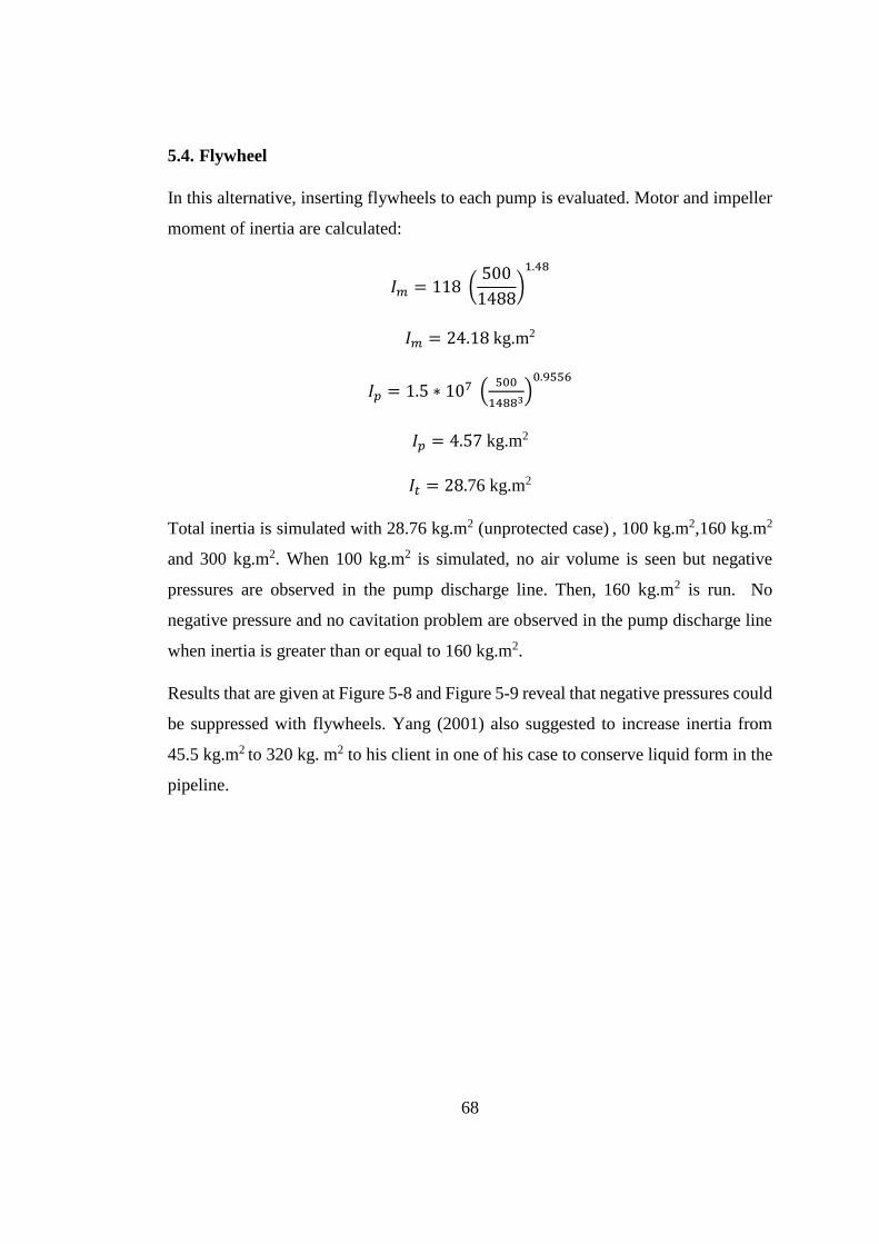
68

5.4. Flywheel

In this alternative, inserting flywheels to each pump is evaluated. Motor and impeller

moment of inertia are calculated:

𝐼𝑚 = 118 (500

1488)

1.48

𝐼𝑚 = 24.18 kg.m2

𝐼𝑝 = 1.5 ∗ 107 (500

14883)

0.9556

𝐼𝑝 = 4.57 kg.m2

𝐼𝑡 = 28.76 kg.m2

Total inertia is simulated with 28.76 kg.m2 (unprotected case) , 100 kg.m2,160 kg.m2

and 300 kg.m2. When 100 kg.m2 is simulated, no air volume is seen but negative

pressures are observed in the pump discharge line. Then, 160 kg.m2 is run. No

negative pressure and no cavitation problem are observed in the pump discharge line

when inertia is greater than or equal to 160 kg.m2.

Results that are given at Figure 5-8 and Figure 5-9 reveal that negative pressures could

be suppressed with flywheels. Yang (2001) also suggested to increase inertia from

45.5 kg.m2 to 320 kg. m2 to his client in one of his case to conserve liquid form in the

pipeline.

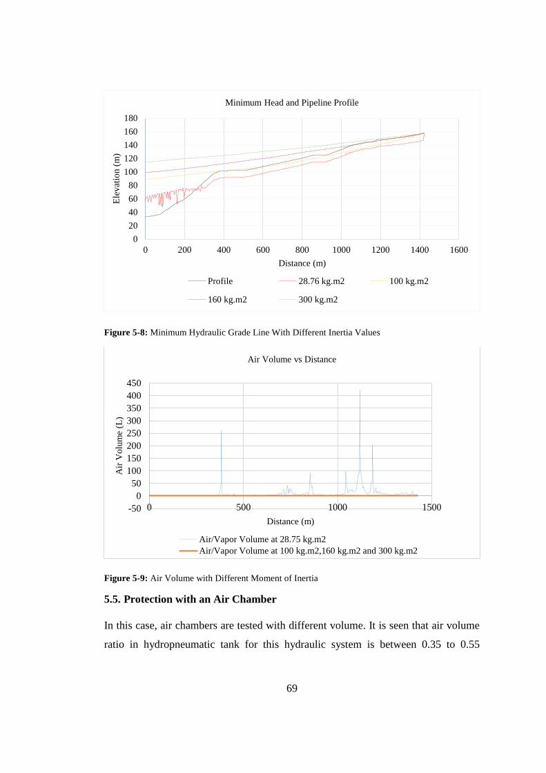
69

Figure 5-8: Minimum Hydraulic Grade Line With Different Inertia Values

Figure 5-9: Air Volume with Different Moment of Inertia

5.5. Protection with an Air Chamber

In this case, air chambers are tested with different volume. It is seen that air volume

ratio in hydropneumatic tank for this hydraulic system is between 0.35 to 0.55

0

20

40

60

80

100

120

140

160

180

0 200 400 600 800 1000 1200 1400 1600

Ele

vat

ion (

m)

Distance (m)

Minimum Head and Pipeline Profile

Profile 28.76 kg.m2 100 kg.m2

160 kg.m2 300 kg.m2

-50

0

50

100

150

200

250

300

350

400

450

0 500 1000 1500

Air

Vo

lum

e (L

)

Distance (m)

Air Volume vs Distance

Air/Vapor Volume at 28.75 kg.m2

Air/Vapor Volume at 100 kg.m2,160 kg.m2 and 300 kg.m2

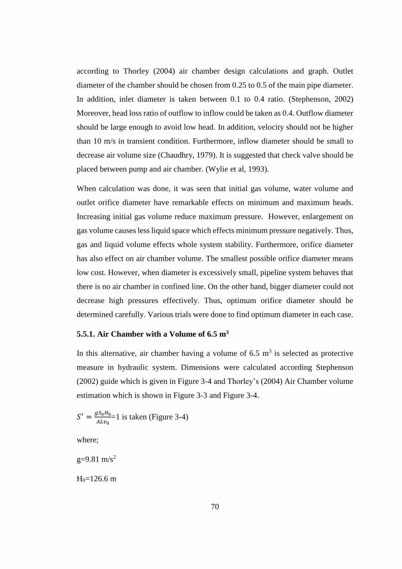
70

according to Thorley (2004) air chamber design calculations and graph. Outlet

diameter of the chamber should be chosen from 0.25 to 0.5 of the main pipe diameter.

In addition, inlet diameter is taken between 0.1 to 0.4 ratio. (Stephenson, 2002)

Moreover, head loss ratio of outflow to inflow could be taken as 0.4. Outflow diameter

should be large enough to avoid low head. In addition, velocity should not be higher

than 10 m/s in transient condition. Furthermore, inflow diameter should be small to

decrease air volume size (Chaudhry, 1979). It is suggested that check valve should be

placed between pump and air chamber. (Wylie et al, 1993).

When calculation was done, it was seen that initial gas volume, water volume and

outlet orifice diameter have remarkable effects on minimum and maximum heads.

Increasing initial gas volume reduce maximum pressure. However, enlargement on

gas volume causes less liquid space which effects minimum pressure negatively. Thus,

gas and liquid volume effects whole system stability. Furthermore, orifice diameter

has also effect on air chamber volume. The smallest possible orifice diameter means

low cost. However, when diameter is excessively small, pipeline system behaves that

there is no air chamber in confined line. On the other hand, bigger diameter could not

decrease high pressures effectively. Thus, optimum orifice diameter should be

determined carefully. Various trials were done to find optimum diameter in each case.

5.5.1. Air Chamber with a Volume of 6.5 m3

In this alternative, air chamber having a volume of 6.5 m3 is selected as protective

measure in hydraulic system. Dimensions were calculated according Stephenson

(2002) guide which is given in Figure 3-4 and Thorley’s (2004) Air Chamber volume

estimation which is shown in Figure 3-3 and Figure 3-4.

𝑆′ =𝑔𝑆0𝐻0

𝐴𝐿𝑣0=1 is taken (Figure 3-4)

where;

g=9.81 m/s2

H0=126.6 m

71

A=0.75 m2

L=1433 m

V0= 1.46 m/s

S0=1.84 m3 initial air volume

S=3 (Figure 3-5)

V’=1.84*3=5.52 m3

V=1.2(safety constant)*V’= 6.6 m3

According to Thorley; (Figure 3-3)

hatm= 10 m

hs= 126.6 m

hL= 3.47 m

h0=130.07 m

a= 1166.81 m/s

V0=1.46 m/s

g= 9.81 m/s2

ℎ𝑗 =1166.81

m

s∗1.46 m/s

9.81𝑚

𝑠2

= 173.7

ℎ̅𝑓 =3.47 m

173.7 𝑚=0.01998

ℎ̅0 =ℎ0

∗

ℎ𝑗=

130.07 𝑚+10 𝑚

173.7 𝑚=0.807

hmax=225 m

hmin=80 m

72

𝐾 =𝑐𝐶0

𝑛𝐴𝐿𝑣0=3 is determined from the ℎ̅𝑓=0.05 chart; (Figure 3-3)

n=1

C0=4.27 m3 Initial Air Volume

𝐶′ = 4.27 m3 ∗ (130.07 𝑚+10 𝑚

80 𝑚+10 𝑚)

1 1⁄

=6.23 m3

V= 6.5 m3 Air Chamber Volume

Trials were done (1.84 m3 -4.27 m3) to determine initial air volume and it was seen 2.3

m3 air volume gives optimum results. Air chamber specifications are given in Table

5-8. The location of the pump station was determined as the nearest possible point

considering that the highest pressures are at the closest points to the pump station. The

outlet orifice diameter was tested according to ratio given in Table 3-3. The outlet

orifice having 190 mm diameter gave the best results in the simulation.

Significant changes are observed in the pipeline. Maximum head and maximum air

volume decreases in remarkable percentage which could be checked from Table 5-9

and Table 5-10. However, negative pressures are seen from 307 m to 1433 m and

cavitation problem is observed that could be seen from Figure 5-10 and Figure 5-11.

When pump stoppage occurs at the 5th second, flow is supplied from the air chamber

and liquid volume decreases. Then, air volume increases in seconds due to reduced

liquid volume given in Figure 5-12.

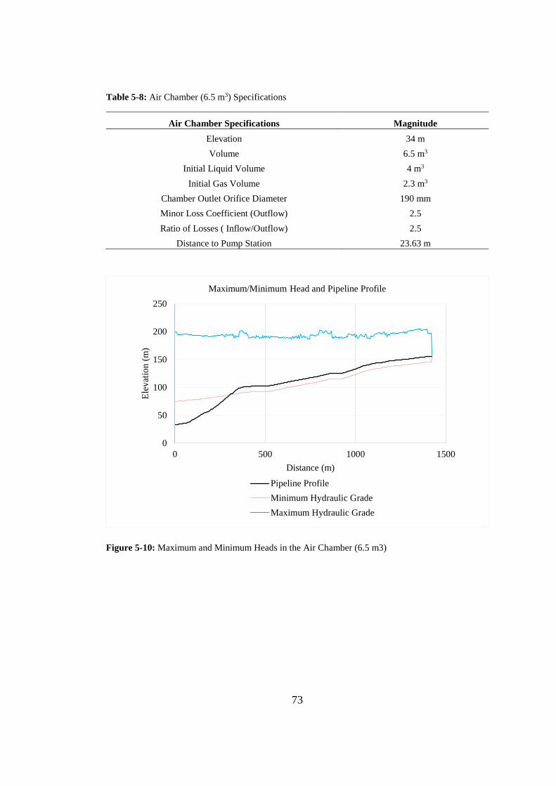
73

Table 5-8: Air Chamber (6.5 m3) Specifications

Air Chamber Specifications Magnitude

Elevation

Volume

Initial Liquid Volume

Initial Gas Volume

Chamber Outlet Orifice Diameter

Minor Loss Coefficient (Outflow)

Ratio of Losses ( Inflow/Outflow)

Distance to Pump Station

34 m

6.5 m3

4 m3

2.3 m3

190 mm

2.5

2.5

23.63 m

Figure 5-10: Maximum and Minimum Heads in the Air Chamber (6.5 m3)

0

50

100

150

200

250

0 500 1000 1500

Ele

vat

ion (

m)

Distance (m)

Maximum/Minimum Head and Pipeline Profile

Pipeline Profile

Minimum Hydraulic Grade

Maximum Hydraulic Grade

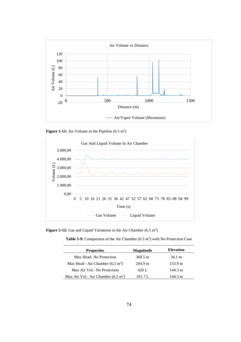
74

Figure 5-11: Air Volume in the Pipeline (6.5 m3)

Figure 5-12: Gas and Liquid Variations in the Air Chamber (6.5 m3)

Table 5-9: Comparison of the Air Chamber (6.5 m3) with No Protection Case

Properties Magnitude Elevation

Max Head- No Protection

Max Head - Air Chamber (6,5 m3)

Max Air Vol.- No Protection

Max Air Vol.- Air Chamber (6,5 m3)

368.5 m

204.9 m

420 L

101.7 L

34.1 m

153.9 m

144.3 m

144.3 m

-20

0

20

40

60

80

100

120

0 500 1000 1500

Air

Vo

lum

e (L

)

Distance (m)

Air Volume vs Distance

Air/Vapor Volume (Maximum)

0,00

1.000,00

2.000,00

3.000,00

4.000,00

5.000,00

0 5 10 16 21 26 31 36 42 47 52 57 62 68 73 78 83 88 94 99

Vo

lum

e (L

)

Time (s)

Gas And Liquid Volume In Air Chamber

Gas Volume Liquid Volume

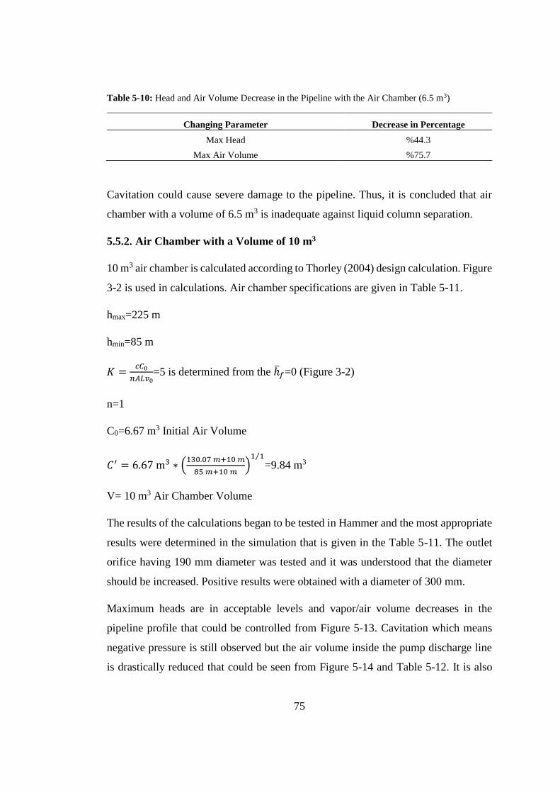
75

Table 5-10: Head and Air Volume Decrease in the Pipeline with the Air Chamber (6.5 m3)

Changing Parameter Decrease in Percentage

Max Head

Max Air Volume

%44.3

%75.7

Cavitation could cause severe damage to the pipeline. Thus, it is concluded that air

chamber with a volume of 6.5 m3 is inadequate against liquid column separation.

5.5.2. Air Chamber with a Volume of 10 m3

10 m3 air chamber is calculated according to Thorley (2004) design calculation. Figure

3-2 is used in calculations. Air chamber specifications are given in Table 5-11.

hmax=225 m

hmin=85 m

𝐾 =𝑐𝐶0

𝑛𝐴𝐿𝑣0=5 is determined from the ℎ̅𝑓=0 (Figure 3-2)

n=1

C0=6.67 m3 Initial Air Volume

𝐶′ = 6.67 m3 ∗ (130.07 𝑚+10 𝑚

85 𝑚+10 𝑚)

1 1⁄

=9.84 m3

V= 10 m3 Air Chamber Volume

The results of the calculations began to be tested in Hammer and the most appropriate

results were determined in the simulation that is given in the Table 5-11. The outlet

orifice having 190 mm diameter was tested and it was understood that the diameter

should be increased. Positive results were obtained with a diameter of 300 mm.

Maximum heads are in acceptable levels and vapor/air volume decreases in the

pipeline profile that could be controlled from Figure 5-13. Cavitation which means

negative pressure is still observed but the air volume inside the pump discharge line

is drastically reduced that could be seen from Figure 5-14 and Table 5-12. It is also

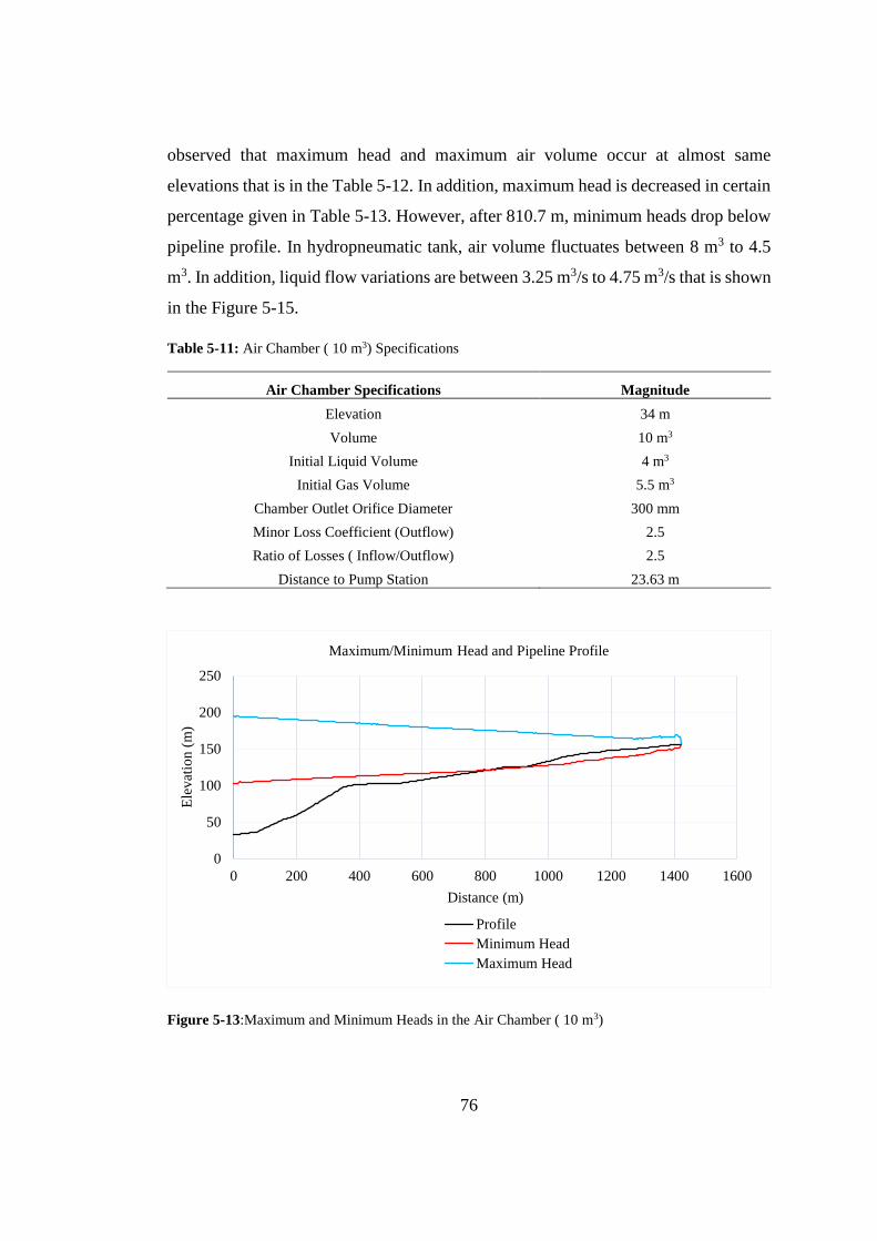
76

observed that maximum head and maximum air volume occur at almost same

elevations that is in the Table 5-12. In addition, maximum head is decreased in certain

percentage given in Table 5-13. However, after 810.7 m, minimum heads drop below

pipeline profile. In hydropneumatic tank, air volume fluctuates between 8 m3 to 4.5

m3. In addition, liquid flow variations are between 3.25 m3/s to 4.75 m3/s that is shown

in the Figure 5-15.

Table 5-11: Air Chamber ( 10 m3) Specifications

Air Chamber Specifications Magnitude

Elevation

Volume

Initial Liquid Volume

Initial Gas Volume

Chamber Outlet Orifice Diameter

Minor Loss Coefficient (Outflow)

Ratio of Losses ( Inflow/Outflow)

Distance to Pump Station

34 m

10 m3

4 m3

5.5 m3

300 mm

2.5

2.5

23.63 m

Figure 5-13:Maximum and Minimum Heads in the Air Chamber ( 10 m3)

0

50

100

150

200

250

0 200 400 600 800 1000 1200 1400 1600

Ele

vat

ion (

m)

Distance (m)

Maximum/Minimum Head and Pipeline Profile

Profile

Minimum Head

Maximum Head

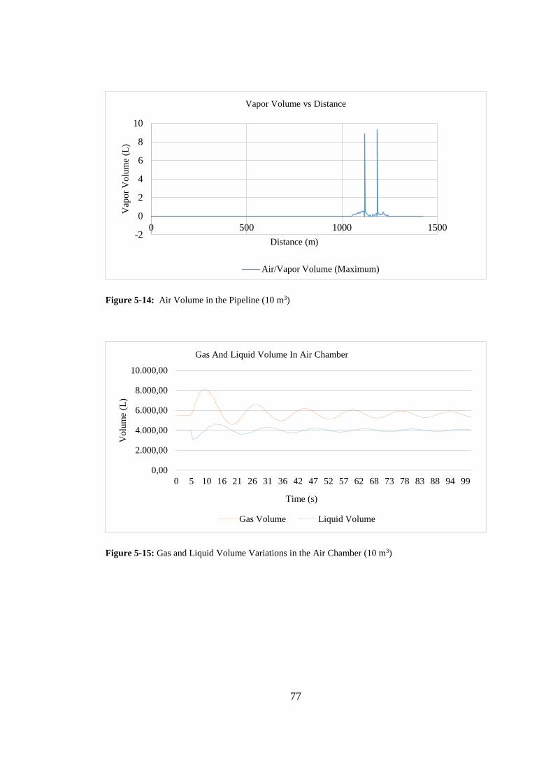
77

Figure 5-14: Air Volume in the Pipeline (10 m3)

Figure 5-15: Gas and Liquid Volume Variations in the Air Chamber (10 m3)

-2

0

2

4

6

8

10

0 500 1000 1500

Vap

or

Vo

lum

e (L

)

Distance (m)

Vapor Volume vs Distance

Air/Vapor Volume (Maximum)

0,00

2.000,00

4.000,00

6.000,00

8.000,00

10.000,00

0 5 10 16 21 26 31 36 42 47 52 57 62 68 73 78 83 88 94 99

Vo

lum

e (L

)

Time (s)

Gas And Liquid Volume In Air Chamber

Gas Volume Liquid Volume

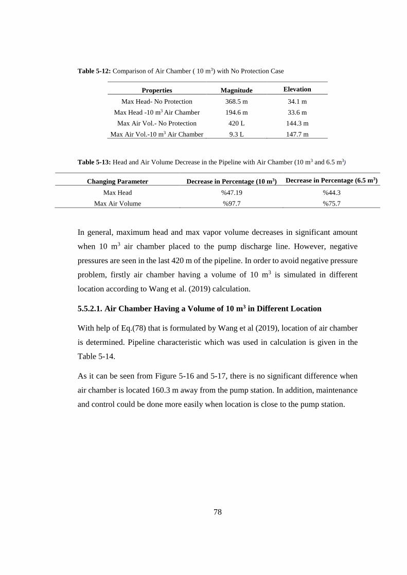
78

Table 5-12: Comparison of Air Chamber ( 10 m3) with No Protection Case

Properties Magnitude Elevation

Max Head- No Protection

Max Head -10 m3 Air Chamber

Max Air Vol.- No Protection

Max Air Vol.-10 m3 Air Chamber

368.5 m

194.6 m

420 L

9.3 L

34.1 m

33.6 m

144.3 m

147.7 m

Table 5-13: Head and Air Volume Decrease in the Pipeline with Air Chamber (10 m3 and 6.5 m3)

Changing Parameter Decrease in Percentage (10 m3) Decrease in Percentage (6.5 m3)

Max Head

Max Air Volume

%47.19

%97.7

%44.3

%75.7

In general, maximum head and max vapor volume decreases in significant amount

when 10 m3 air chamber placed to the pump discharge line. However, negative

pressures are seen in the last 420 m of the pipeline. In order to avoid negative pressure

problem, firstly air chamber having a volume of 10 m3 is simulated in different

location according to Wang et al. (2019) calculation.

5.5.2.1. Air Chamber Having a Volume of 10 m3 in Different Location

With help of Eq.(78) that is formulated by Wang et al (2019), location of air chamber

is determined. Pipeline characteristic which was used in calculation is given in the

Table 5-14.

As it can be seen from Figure 5-16 and 5-17, there is no significant difference when

air chamber is located 160.3 m away from the pump station. In addition, maintenance

and control could be done more easily when location is close to the pump station.

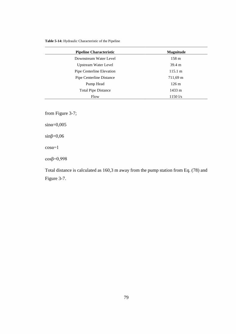
79

Table 5-14: Hydraulic Characteristic of the Pipeline

Pipeline Characteristic Magnitude

Downstream Water Level

Upstream Water Level

Pipe Centerline Elevation

Pipe Centerline Distance

Pump Head

Total Pipe Distance

Flow

158 m

39.4 m

115.1 m

711,69 m

126 m

1433 m

1150 l/s

from Figure 3-7;

sinα=0,005

sinβ=0,06

cosα=1

cosβ=0,998

Total distance is calculated as 160,3 m away from the pump station from Eq. (78) and

Figure 3-7.

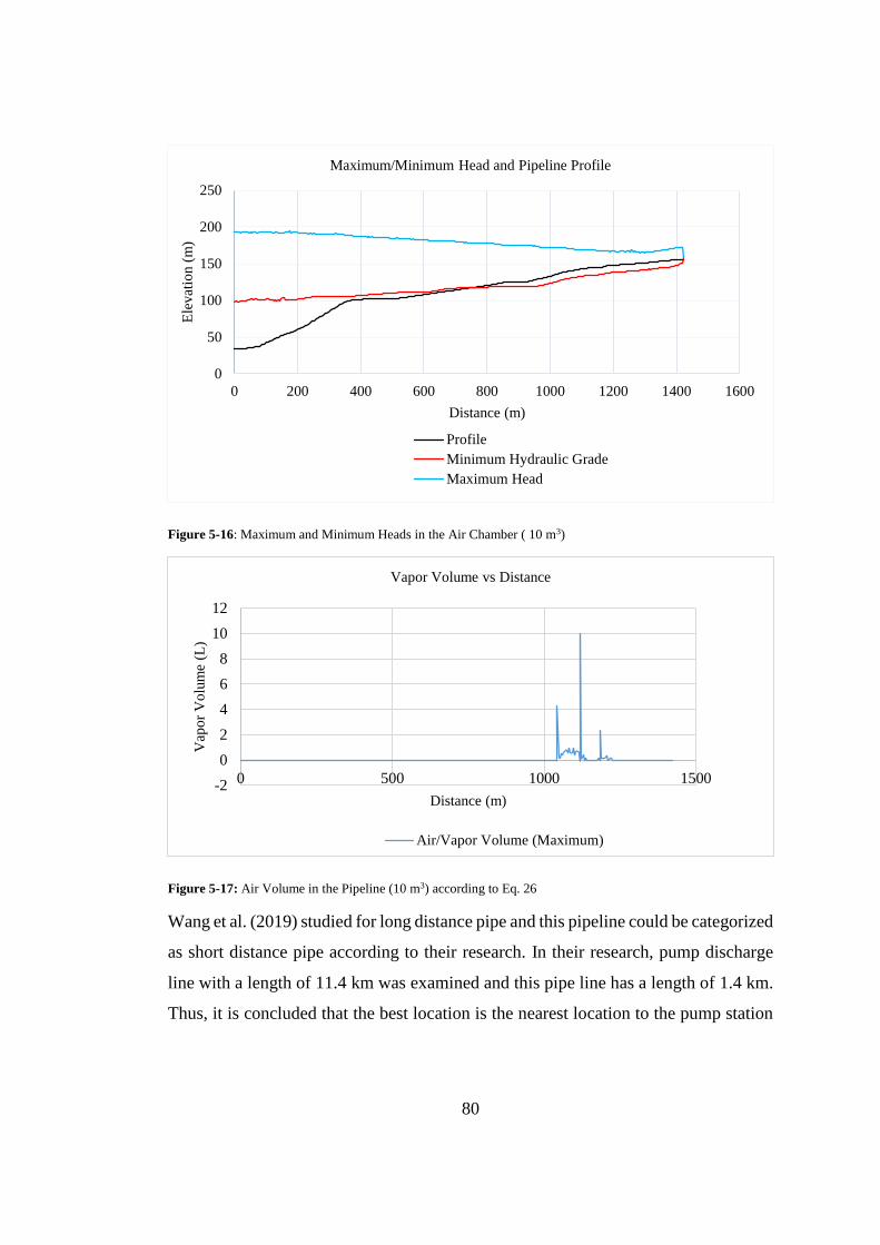
80

Figure 5-16: Maximum and Minimum Heads in the Air Chamber ( 10 m3)

Figure 5-17: Air Volume in the Pipeline (10 m3) according to Eq. 26

Wang et al. (2019) studied for long distance pipe and this pipeline could be categorized

as short distance pipe according to their research. In their research, pump discharge

line with a length of 11.4 km was examined and this pipe line has a length of 1.4 km.

Thus, it is concluded that the best location is the nearest location to the pump station

0

50

100

150

200

250

0 200 400 600 800 1000 1200 1400 1600

Ele

vat

ion (

m)

Distance (m)

Maximum/Minimum Head and Pipeline Profile

Profile

Minimum Hydraulic Grade

Maximum Head

-2

0

2

4

6

8

10

12

0 500 1000 1500

Vap

or

Vo

lum

e (L

)

Distance (m)

Vapor Volume vs Distance

Air/Vapor Volume (Maximum)

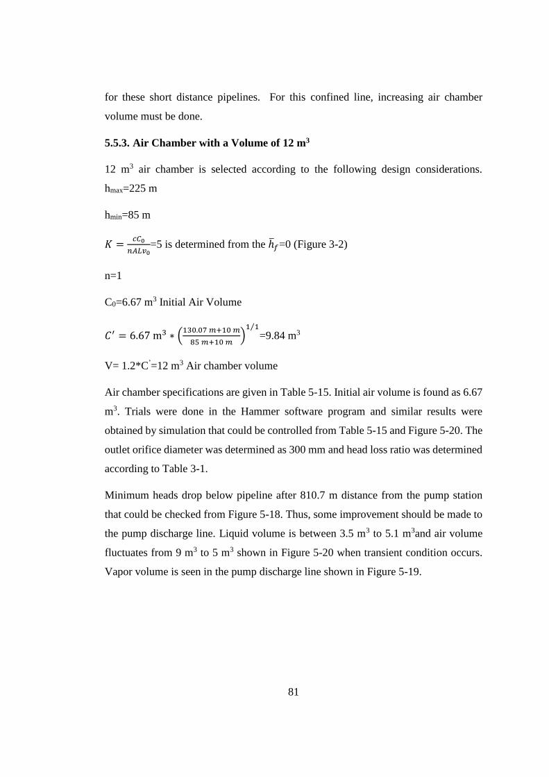
81

for these short distance pipelines. For this confined line, increasing air chamber

volume must be done.

5.5.3. Air Chamber with a Volume of 12 m3

12 m3 air chamber is selected according to the following design considerations.

hmax=225 m

hmin=85 m

𝐾 =𝑐𝐶0

𝑛𝐴𝐿𝑣0=5 is determined from the ℎ̅𝑓=0 (Figure 3-2)

n=1

C0=6.67 m3 Initial Air Volume

𝐶′ = 6.67 m3 ∗ (130.07 𝑚+10 𝑚

85 𝑚+10 𝑚)

1 1⁄

=9.84 m3

V= 1.2*C’=12 m3 Air chamber volume

Air chamber specifications are given in Table 5-15. Initial air volume is found as 6.67

m3. Trials were done in the Hammer software program and similar results were

obtained by simulation that could be controlled from Table 5-15 and Figure 5-20. The

outlet orifice diameter was determined as 300 mm and head loss ratio was determined

according to Table 3-1.

Minimum heads drop below pipeline after 810.7 m distance from the pump station

that could be checked from Figure 5-18. Thus, some improvement should be made to

the pump discharge line. Liquid volume is between 3.5 m3 to 5.1 m3and air volume

fluctuates from 9 m3 to 5 m3 shown in Figure 5-20 when transient condition occurs.

Vapor volume is seen in the pump discharge line shown in Figure 5-19.

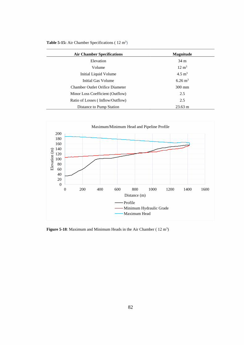
82

Table 5-15: Air Chamber Specifications ( 12 m3)

Air Chamber Specifications Magnitude

Elevation

Volume

Initial Liquid Volume

Initial Gas Volume

Chamber Outlet Orifice Diameter

Minor Loss Coefficient (Outflow)

Ratio of Losses ( Inflow/Outflow)

Distance to Pump Station

34 m

12 m3

4.5 m3

6.26 m3

300 mm

2.5

2.5

23.63 m

Figure 5-18: Maximum and Minimum Heads in the Air Chamber ( 12 m3)

0

20

40

60

80

100

120

140

160

180

200

0 200 400 600 800 1000 1200 1400 1600

Ele

vat

ion (

m)

Distance (m)

Maximum/Minimum Head and Pipeline Profile

Profile

Minimum Hydraulic Grade

Maximum Head

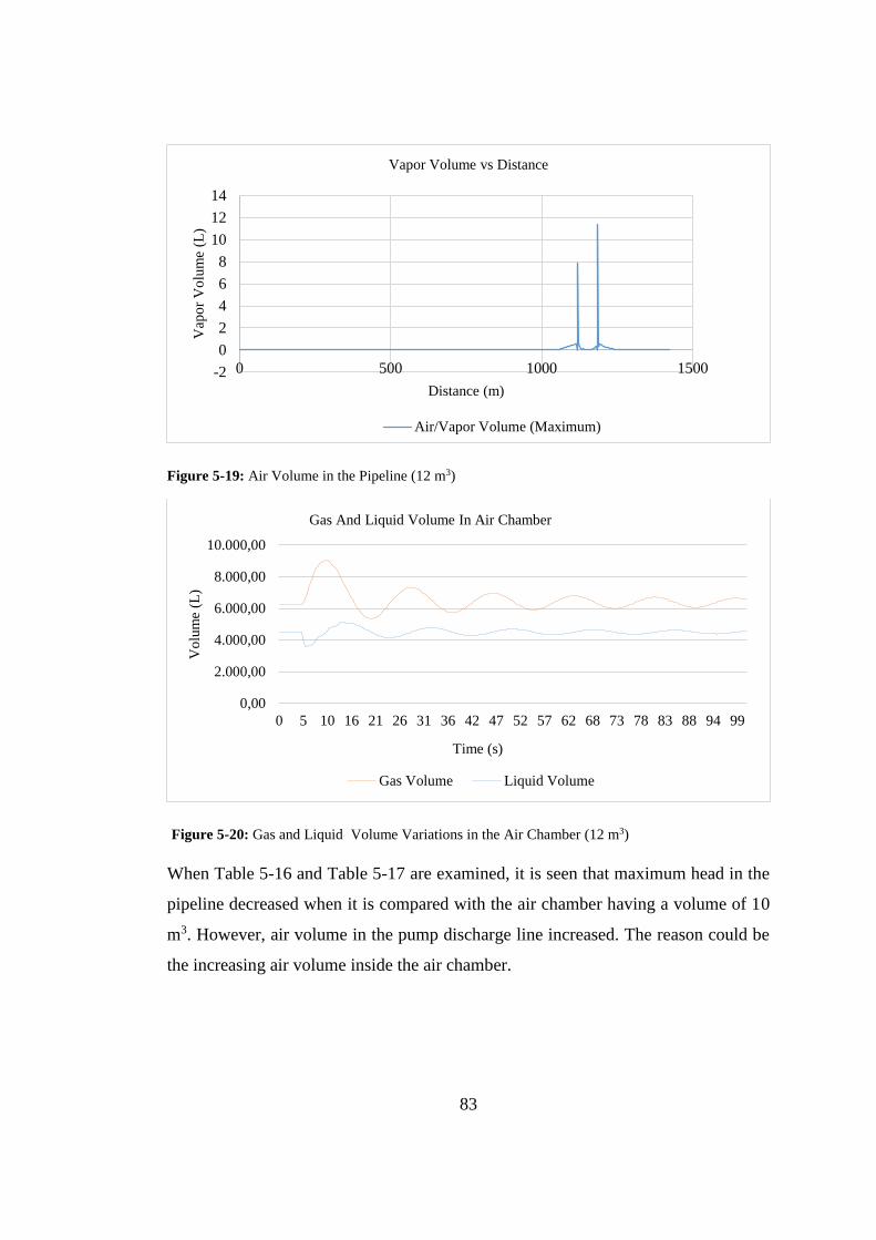
83

Figure 5-19: Air Volume in the Pipeline (12 m3)

Figure 5-20: Gas and Liquid Volume Variations in the Air Chamber (12 m3)

When Table 5-16 and Table 5-17 are examined, it is seen that maximum head in the

pipeline decreased when it is compared with the air chamber having a volume of 10

m3. However, air volume in the pump discharge line increased. The reason could be

the increasing air volume inside the air chamber.

-2

0

2

4

6

8

10

12

14

0 500 1000 1500

Vap

or

Vo

lum

e (L

)

Distance (m)

Vapor Volume vs Distance

Air/Vapor Volume (Maximum)

0,00

2.000,00

4.000,00

6.000,00

8.000,00

10.000,00

0 5 10 16 21 26 31 36 42 47 52 57 62 68 73 78 83 88 94 99

Vo

lum

e (L

)

Time (s)

Gas And Liquid Volume In Air Chamber

Gas Volume Liquid Volume

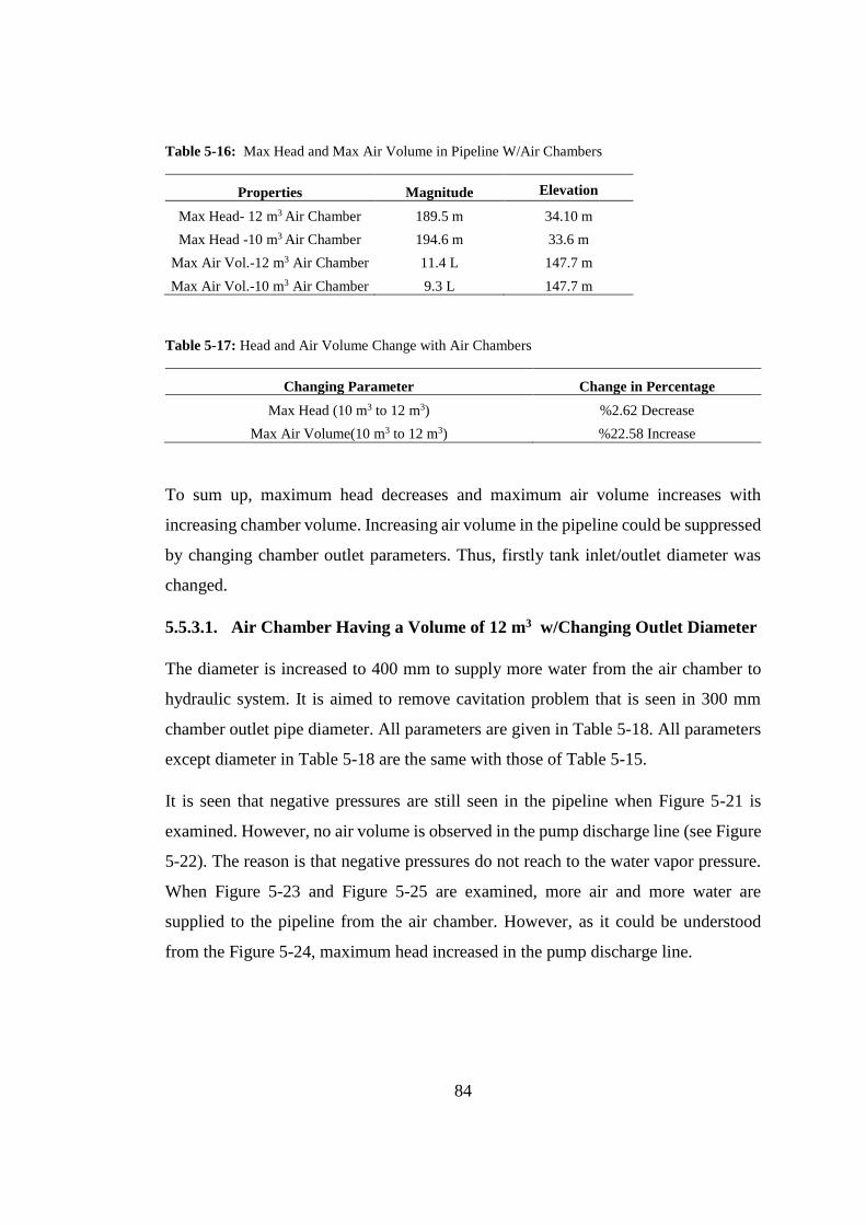
84

Table 5-16: Max Head and Max Air Volume in Pipeline W/Air Chambers

Properties Magnitude Elevation

Max Head- 12 m3 Air Chamber

Max Head -10 m3 Air Chamber

Max Air Vol.-12 m3 Air Chamber

Max Air Vol.-10 m3 Air Chamber

189.5 m

194.6 m

11.4 L

9.3 L

34.10 m

33.6 m

147.7 m

147.7 m

Table 5-17: Head and Air Volume Change with Air Chambers

Changing Parameter Change in Percentage

Max Head (10 m3 to 12 m3)

Max Air Volume(10 m3 to 12 m3)

%2.62 Decrease

%22.58 Increase

To sum up, maximum head decreases and maximum air volume increases with

increasing chamber volume. Increasing air volume in the pipeline could be suppressed

by changing chamber outlet parameters. Thus, firstly tank inlet/outlet diameter was

changed.

5.5.3.1. Air Chamber Having a Volume of 12 m3 w/Changing Outlet Diameter

The diameter is increased to 400 mm to supply more water from the air chamber to

hydraulic system. It is aimed to remove cavitation problem that is seen in 300 mm

chamber outlet pipe diameter. All parameters are given in Table 5-18. All parameters

except diameter in Table 5-18 are the same with those of Table 5-15.

It is seen that negative pressures are still seen in the pipeline when Figure 5-21 is

examined. However, no air volume is observed in the pump discharge line (see Figure

5-22). The reason is that negative pressures do not reach to the water vapor pressure.

When Figure 5-23 and Figure 5-25 are examined, more air and more water are

supplied to the pipeline from the air chamber. However, as it could be understood

from the Figure 5-24, maximum head increased in the pump discharge line.

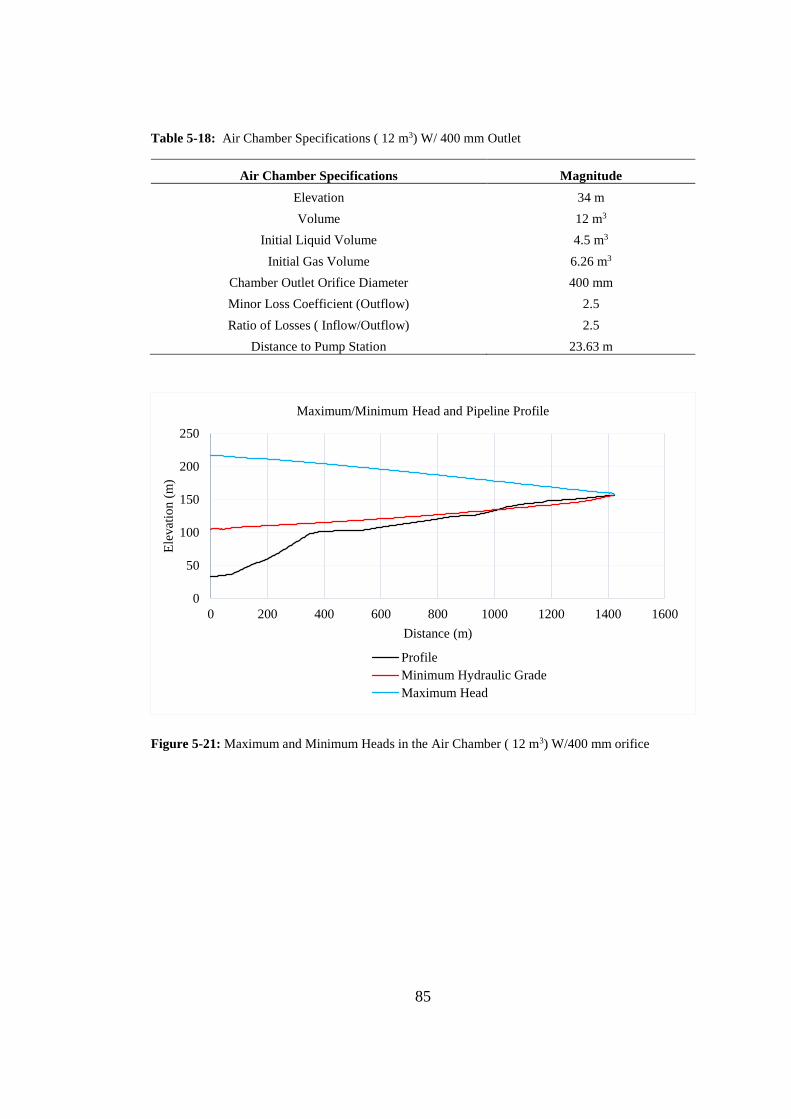
85

Table 5-18: Air Chamber Specifications ( 12 m3) W/ 400 mm Outlet

Air Chamber Specifications Magnitude

Elevation

Volume

Initial Liquid Volume

Initial Gas Volume

Chamber Outlet Orifice Diameter

Minor Loss Coefficient (Outflow)

Ratio of Losses ( Inflow/Outflow)

Distance to Pump Station

34 m

12 m3

4.5 m3

6.26 m3

400 mm

2.5

2.5

23.63 m

Figure 5-21: Maximum and Minimum Heads in the Air Chamber ( 12 m3) W/400 mm orifice

0

50

100

150

200

250

0 200 400 600 800 1000 1200 1400 1600

Ele

vat

ion (

m)

Distance (m)

Maximum/Minimum Head and Pipeline Profile

Profile

Minimum Hydraulic Grade

Maximum Head

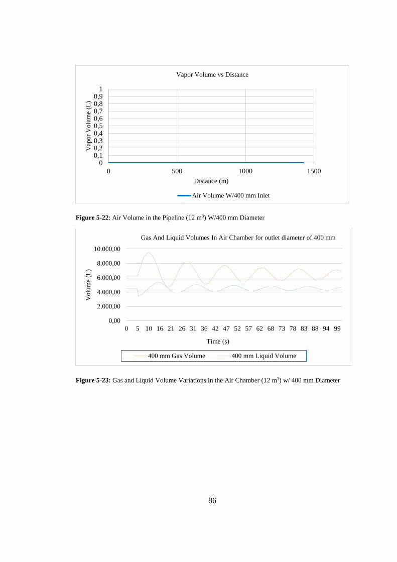
86

Figure 5-22: Air Volume in the Pipeline (12 m3) W/400 mm Diameter

Figure 5-23: Gas and Liquid Volume Variations in the Air Chamber (12 m3) w/ 400 mm Diameter

00,10,20,30,40,50,60,70,80,9

1

0 500 1000 1500

Vap

or

Vo

lum

e (L

)

Distance (m)

Vapor Volume vs Distance

Air Volume W/400 mm Inlet

0,00

2.000,00

4.000,00

6.000,00

8.000,00

10.000,00

0 5 10 16 21 26 31 36 42 47 52 57 62 68 73 78 83 88 94 99

Vo

lum

e (L

)

Time (s)

Gas And Liquid Volumes In Air Chamber for outlet diameter of 400 mm

400 mm Gas Volume 400 mm Liquid Volume

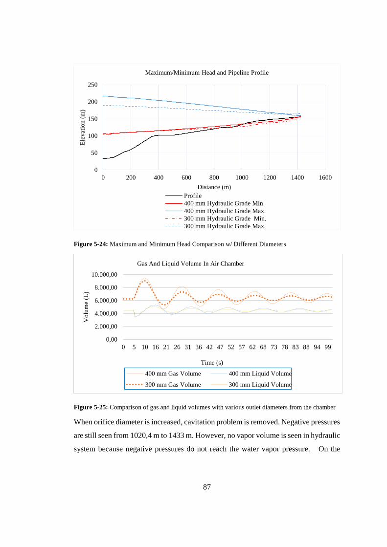
87

Figure 5-24: Maximum and Minimum Head Comparison w/ Different Diameters

Figure 5-25: Comparison of gas and liquid volumes with various outlet diameters from the chamber

When orifice diameter is increased, cavitation problem is removed. Negative pressures

are still seen from 1020,4 m to 1433 m. However, no vapor volume is seen in hydraulic

system because negative pressures do not reach the water vapor pressure. On the

0

50

100

150

200

250

0 200 400 600 800 1000 1200 1400 1600

Ele

vat

ion (

m)

Distance (m)

Maximum/Minimum Head and Pipeline Profile

Profile

400 mm Hydraulic Grade Min.

400 mm Hydraulic Grade Max.

300 mm Hydraulic Grade Min.

300 mm Hydraulic Grade Max.

0,00

2.000,00

4.000,00

6.000,00

8.000,00

10.000,00

0 5 10 16 21 26 31 36 42 47 52 57 62 68 73 78 83 88 94 99

Vo

lum

e (L

)

Time (s)

Gas And Liquid Volume In Air Chamber

400 mm Gas Volume 400 mm Liquid Volume

300 mm Gas Volume 300 mm Liquid Volume

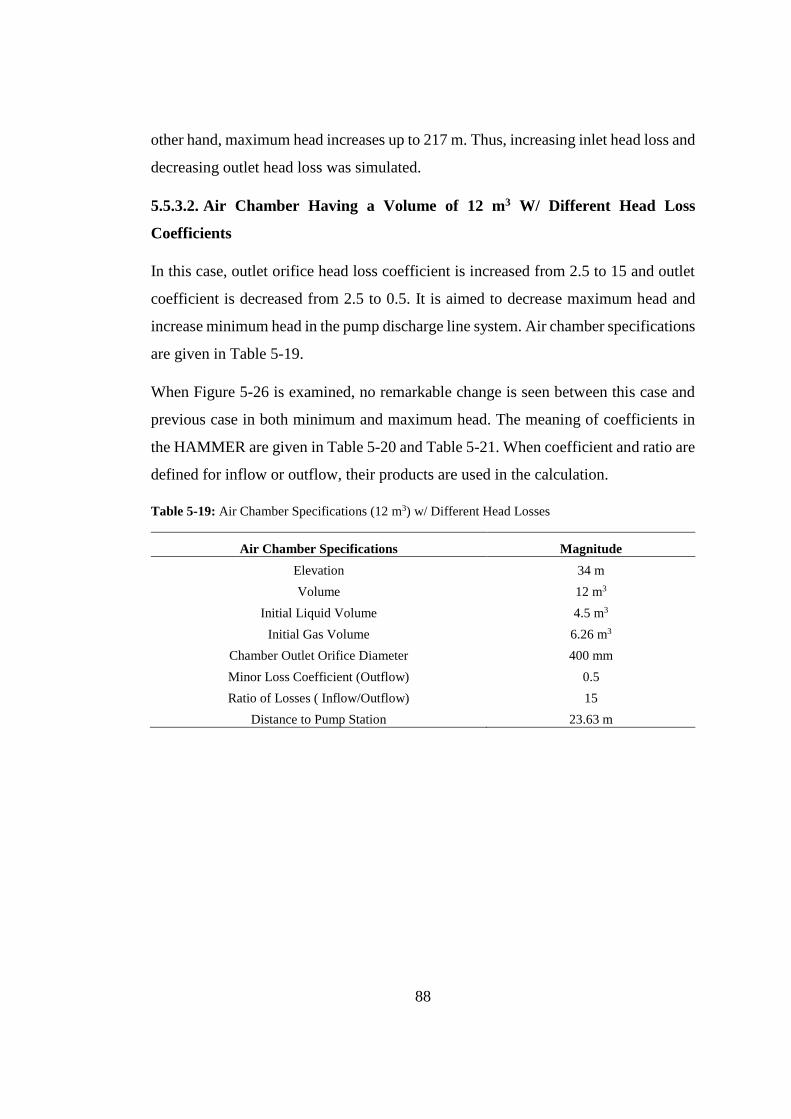
88

other hand, maximum head increases up to 217 m. Thus, increasing inlet head loss and

decreasing outlet head loss was simulated.

5.5.3.2. Air Chamber Having a Volume of 12 m3 W/ Different Head Loss

Coefficients

In this case, outlet orifice head loss coefficient is increased from 2.5 to 15 and outlet

coefficient is decreased from 2.5 to 0.5. It is aimed to decrease maximum head and

increase minimum head in the pump discharge line system. Air chamber specifications

are given in Table 5-19.

When Figure 5-26 is examined, no remarkable change is seen between this case and

previous case in both minimum and maximum head. The meaning of coefficients in

the HAMMER are given in Table 5-20 and Table 5-21. When coefficient and ratio are

defined for inflow or outflow, their products are used in the calculation.

Table 5-19: Air Chamber Specifications (12 m3) w/ Different Head Losses

Air Chamber Specifications Magnitude

Elevation

Volume

Initial Liquid Volume

Initial Gas Volume

Chamber Outlet Orifice Diameter

Minor Loss Coefficient (Outflow)

Ratio of Losses ( Inflow/Outflow)

Distance to Pump Station

34 m

12 m3

4.5 m3

6.26 m3

400 mm

0.5

15

23.63 m

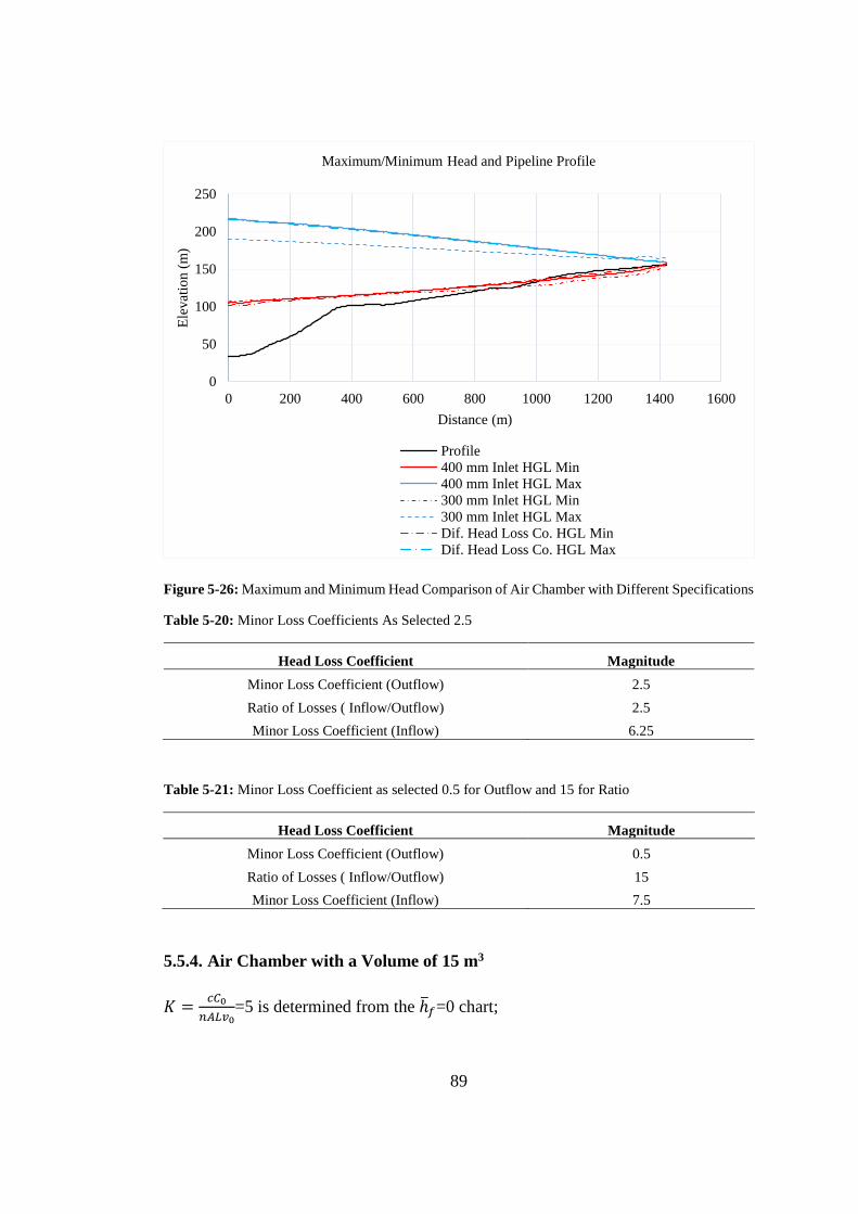
89

Figure 5-26: Maximum and Minimum Head Comparison of Air Chamber with Different Specifications

Table 5-20: Minor Loss Coefficients As Selected 2.5

Head Loss Coefficient Magnitude

Minor Loss Coefficient (Outflow)

Ratio of Losses ( Inflow/Outflow)

Minor Loss Coefficient (Inflow)

2.5

2.5

6.25

Table 5-21: Minor Loss Coefficient as selected 0.5 for Outflow and 15 for Ratio

Head Loss Coefficient Magnitude

Minor Loss Coefficient (Outflow)

Ratio of Losses ( Inflow/Outflow)

Minor Loss Coefficient (Inflow)

0.5

15

7.5

5.5.4. Air Chamber with a Volume of 15 m3

𝐾 =𝑐𝐶0

𝑛𝐴𝐿𝑣0=5 is determined from the ℎ̅𝑓=0 chart;

0

50

100

150

200

250

0 200 400 600 800 1000 1200 1400 1600

Ele

vat

ion (

m)

Distance (m)

Maximum/Minimum Head and Pipeline Profile

Profile

400 mm Inlet HGL Min

400 mm Inlet HGL Max

300 mm Inlet HGL Min

300 mm Inlet HGL Max

Dif. Head Loss Co. HGL Min

Dif. Head Loss Co. HGL Max

90

n=1.4

C0=9.34 m3 Initial Air Volume

𝐶′ = 9.34 m3 ∗ (130.07 𝑚+10 𝑚

85 𝑚+10 𝑚)

1 1⁄

=12.33 m3

V= 1.2*C’=14.8 m3 Air chamber volume

It was seen that 8 m3 initial air volume gave optimum results. Thus, initial air volume

was decreased from 9 m3 to 8 m3. Other parameters that were used in the simulation

are given in the Table 5-22.

When Figure 5-27 and Figure 5-28 are examined, it is seen that maximum head

decreased in a certain amount. However, negative pressure and cavitation problem

were still seen in the pump discharge line as it could be checked from Figure 5-29. In

addition, liquid volume and gas volume variations are given in Figure 5-30.

Table 5-22: Air Chamber Specification ( 15 m3)

Air Chamber Specifications Magnitude

Elevation

Volume

Initial Liquid Volume

Initial Gas Volume

Chamber Outlet Orifice Diameter

Minor Loss Coefficient (Outflow)

Ratio of Losses ( Inflow/Outflow)

Distance to Pump Station

34 m

15 m3

6 m3

8 m3

300 mm

2.5

2.5

23.63

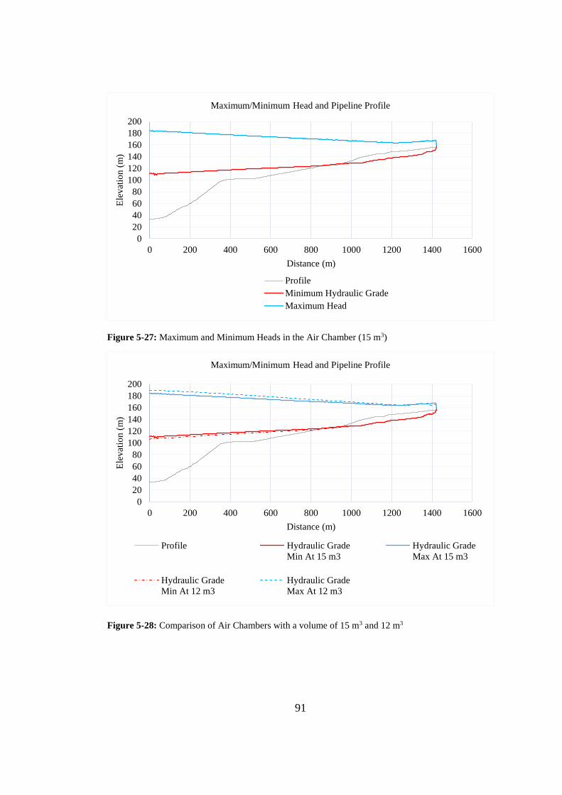
91

Figure 5-27: Maximum and Minimum Heads in the Air Chamber (15 m3)

Figure 5-28: Comparison of Air Chambers with a volume of 15 m3 and 12 m3

0

20

40

60

80

100

120

140

160

180

200

0 200 400 600 800 1000 1200 1400 1600

Ele

vat

ion (

m)

Distance (m)

Maximum/Minimum Head and Pipeline Profile

Profile

Minimum Hydraulic Grade

Maximum Head

0

20

40

60

80

100

120

140

160

180

200

0 200 400 600 800 1000 1200 1400 1600

Ele

vat

ion (

m)

Distance (m)

Maximum/Minimum Head and Pipeline Profile

Profile Hydraulic Grade

Min At 15 m3

Hydraulic Grade

Max At 15 m3

Hydraulic Grade

Min At 12 m3

Hydraulic Grade

Max At 12 m3

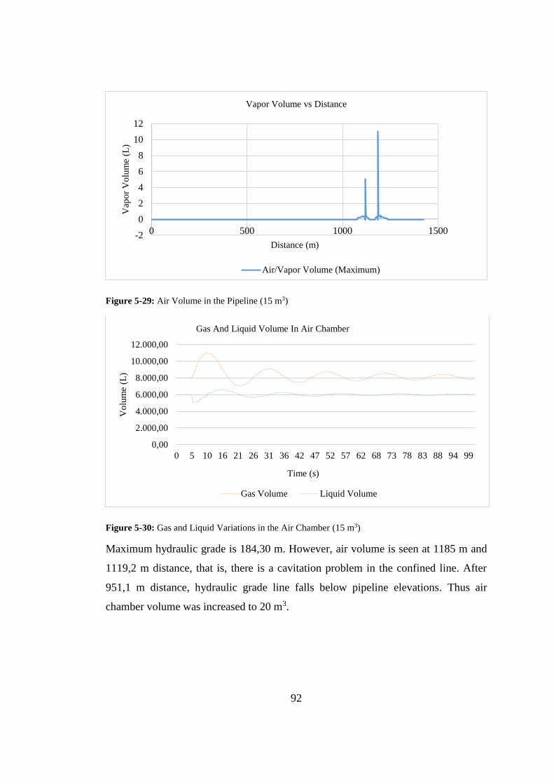
92

Figure 5-29: Air Volume in the Pipeline (15 m3)

Figure 5-30: Gas and Liquid Variations in the Air Chamber (15 m3)

Maximum hydraulic grade is 184,30 m. However, air volume is seen at 1185 m and

1119,2 m distance, that is, there is a cavitation problem in the confined line. After

951,1 m distance, hydraulic grade line falls below pipeline elevations. Thus air

chamber volume was increased to 20 m3.

-2

0

2

4

6

8

10

12

0 500 1000 1500

Vap

or

Vo

lum

e (L

)

Distance (m)

Vapor Volume vs Distance

Air/Vapor Volume (Maximum)

0,00

2.000,00

4.000,00

6.000,00

8.000,00

10.000,00

12.000,00

0 5 10 16 21 26 31 36 42 47 52 57 62 68 73 78 83 88 94 99

Vo

lum

e (L

)

Time (s)

Gas And Liquid Volume In Air Chamber

Gas Volume Liquid Volume

93

5.5.5. Air Chamber with a Volume of 20 m3

𝐾 =𝑐𝐶0

𝑛𝐴𝐿𝑣0=7 is determined from the ℎ̅𝑓=0 chart;

n=1.4

C0=12.15 m3 Initial Air Volume

𝐶′ = 12.15 m3 ∗ (130.07 𝑚+10 𝑚

85 𝑚+10 𝑚)

1 1⁄

=16.25 m3

V= 1.2*C’=20 m3 Air chamber volume

Initial diameter is increased from 300 mm to 370 mm. This increased diameter and all

other possible diameters that are in the range given in Table 3-3 was simulated for all

cases presented here. However, only this case gave positive results. Air volume inside

air chamber was determined as 10 m3 after trials. Air chamber specifications were

given in Table 5-23.

As it could be observed from Figure 5-32, no air volume is observed in the pump

discharge line because negative pressures do not reach to the vapor volume. Change

in minimum head could be observed when Figure 5-31 is compared with Figure 5-24

or Figure 5-28. Moreover, volume variations inside the air chamber is given in Figure

5-33.

In 20 m3 case, minimum hydraulic grade falls below pipeline profile after 1047,7 m.

However, no vapor volume is observed in transient results because head difference

falls approximately 6 m below the pipeline at maximum difference and this means

negative pressures do not reach vapor pressure. Moreover, maximum head that is

observed in the pipeline is 193 m. Results are summarized in the Table 5-24.

94

Table 5-23: Air Chamber Specifications (20 m3)

Air Chamber Specifications Magnitude

Elevation

Volume

Initial Liquid Volume

Initial Gas Volume

Chamber Outlet Orifice Diameter

Minor Loss Coefficient (Outflow)

Ratio of Losses ( Inflow/Outflow)

Distance to Pump Station

34 m

20 m3

9 m3

10 m3

370 mm

2.5

2.5

23.63 m

Figure 5-31: Maximum and Minimum Heads in the Air Chamber (20 m3)

0

50

100

150

200

250

0 200 400 600 800 1000 1200 1400 1600

Ele

vat

ion (

m)

Distance (m)

Maximum/Minimum Head and Pipeline Profile

Profile

Minimum Hydraulic Grade

Maximum Head

95

Figure 5-32: Air Volume in the Pipeline (20 m3)

Figure 5-33: Gas and Liquid Variations in the Air Chamber (20 m3)

00,10,20,30,40,50,60,7

0,80,9

1

0 500 1000 1500

Vap

or

Vo

lum

e (L

)

Distance (m)

Vapor Volume vs Distance

Air/Vapor Volume (Maximum)

0,00

2.000,00

4.000,00

6.000,00

8.000,00

10.000,00

12.000,00

14.000,00

16.000,00

0 5 10 16 21 26 31 36 42 47 52 57 62 68 73 78 83 88 94 99

Vo

lum

e (L

)

Time (s)

Gas And Liquid Volume In Air Chamber

Gas Volume Liquid Volume

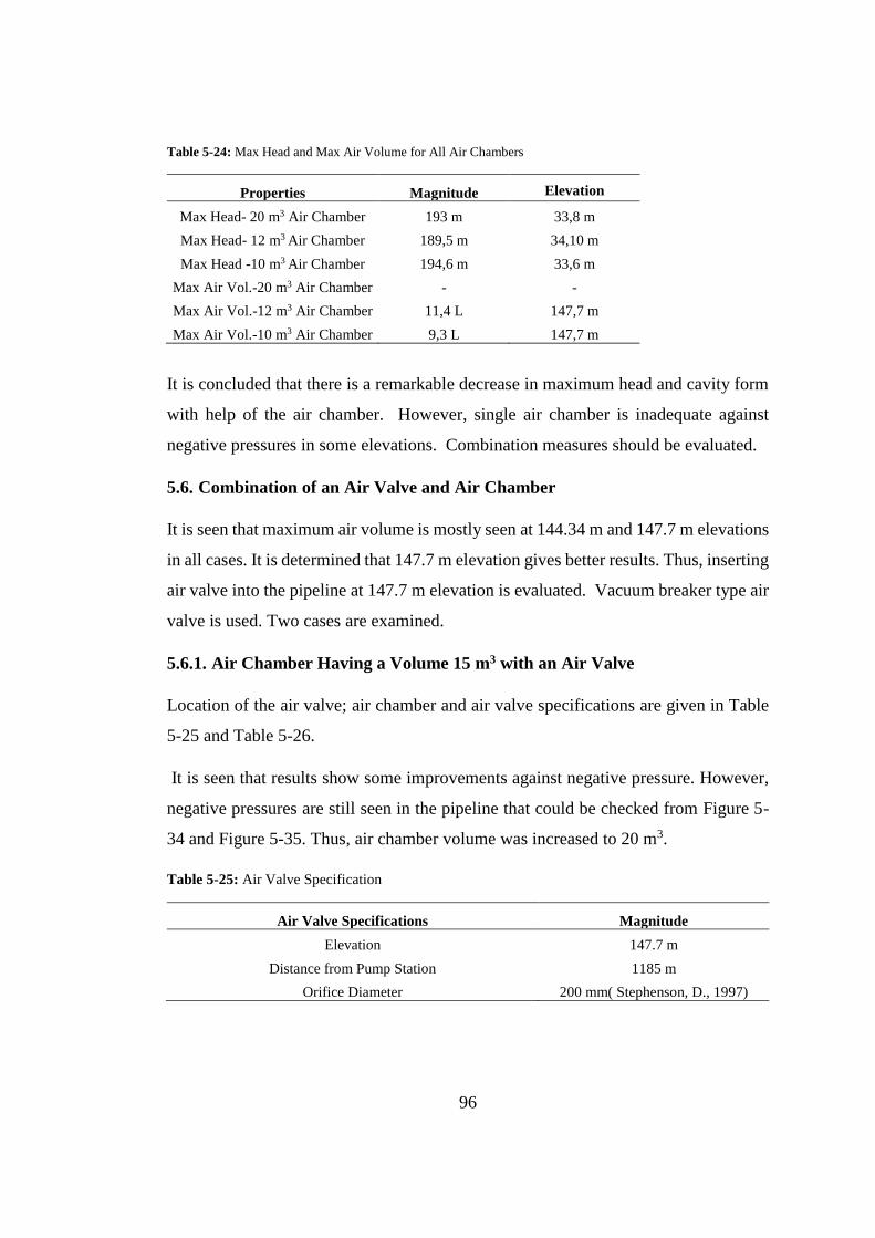
96

Table 5-24: Max Head and Max Air Volume for All Air Chambers

Properties Magnitude Elevation

Max Head- 20 m3 Air Chamber

Max Head- 12 m3 Air Chamber

Max Head -10 m3 Air Chamber

Max Air Vol.-20 m3 Air Chamber

Max Air Vol.-12 m3 Air Chamber

Max Air Vol.-10 m3 Air Chamber

193 m

189,5 m

194,6 m

-

11,4 L

9,3 L

33,8 m

34,10 m

33,6 m

-

147,7 m

147,7 m

It is concluded that there is a remarkable decrease in maximum head and cavity form

with help of the air chamber. However, single air chamber is inadequate against

negative pressures in some elevations. Combination measures should be evaluated.

5.6. Combination of an Air Valve and Air Chamber

It is seen that maximum air volume is mostly seen at 144.34 m and 147.7 m elevations

in all cases. It is determined that 147.7 m elevation gives better results. Thus, inserting

air valve into the pipeline at 147.7 m elevation is evaluated. Vacuum breaker type air

valve is used. Two cases are examined.

5.6.1. Air Chamber Having a Volume 15 m3 with an Air Valve

Location of the air valve; air chamber and air valve specifications are given in Table

5-25 and Table 5-26.

It is seen that results show some improvements against negative pressure. However,

negative pressures are still seen in the pipeline that could be checked from Figure 5-

34 and Figure 5-35. Thus, air chamber volume was increased to 20 m3.

Table 5-25: Air Valve Specification

Air Valve Specifications Magnitude

Elevation

Distance from Pump Station

Orifice Diameter

147.7 m

1185 m

200 mm( Stephenson, D., 1997)

97

Table 5-26: Air Chamber Specification ( 15 m3)

Air Chamber Specifications Magnitude

Elevation

Volume

Initial Liquid Volume

Initial Gas Volume

Chamber Outlet Orifice Diameter

Minor Loss Coefficient (Outflow)

Ratio of Losses ( Inflow/Outflow)

Distance to Pump Station

34 m

15 m3

6 m3

8 m3

300 mm

2.5

2.5

23,63 m

Figure 5-34: Maximum and Minimum Head Air Valve with Air Chamber Having Volume 15 m3

020406080

100120140160180200

0 200 400 600 800 1000 1200 1400 1600

Ele

vat

ion (

m)

Distance (m)

Maximum/Minimum Head and Pipeline Profile

Profile Hydraulic Grade

Min At 15 m3 w AV

Hydraulic Grade

Max At 15 m3 w AV

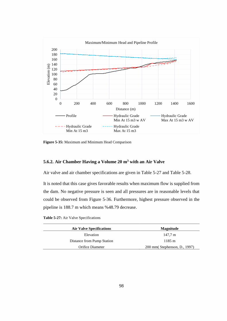
98

Figure 5-35: Maximum and Minimum Head Comparison

5.6.2. Air Chamber Having a Volume 20 m3 with an Air Valve

Air valve and air chamber specifications are given in Table 5-27 and Table 5-28.

It is noted that this case gives favorable results when maximum flow is supplied from

the dam. No negative pressure is seen and all pressures are in reasonable levels that

could be observed from Figure 5-36. Furthermore, highest pressure observed in the

pipeline is 188.7 m which means %48.79 decrease.

Table 5-27: Air Valve Specifications

Air Valve Specifications Magnitude

Elevation

Distance from Pump Station

Orifice Diameter

147,7 m

1185 m

200 mm( Stephenson, D., 1997)

0

20

40

60

80

100

120

140

160

180

200

0 200 400 600 800 1000 1200 1400 1600

Ele

vat

ion (

m)

Distance (m)

Maximum/Minimum Head and Pipeline Profile

Profile Hydraulic Grade

Min At 15 m3 w AV

Hydraulic Grade

Max At 15 m3 w AV

Hydraulic Grade

Min At 15 m3

Hydraulic Grade

Max At 15 m3

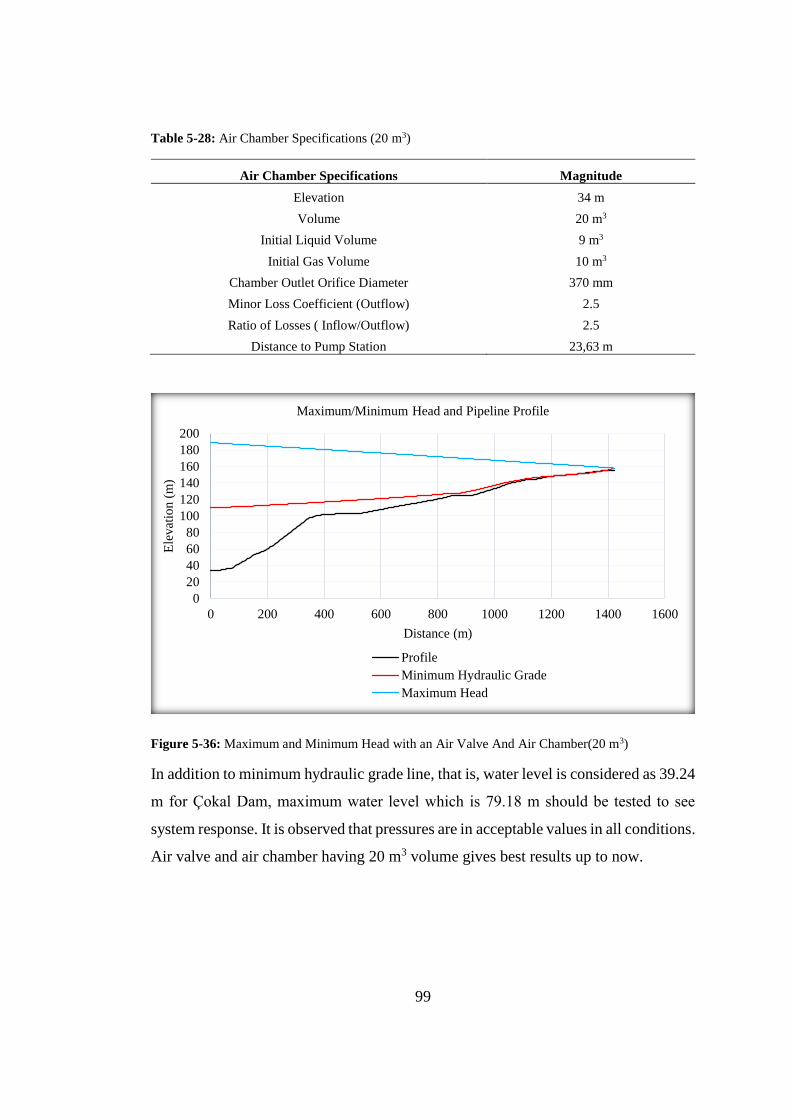
99

Table 5-28: Air Chamber Specifications (20 m3)

Air Chamber Specifications Magnitude

Elevation

Volume

Initial Liquid Volume

Initial Gas Volume

Chamber Outlet Orifice Diameter

Minor Loss Coefficient (Outflow)

Ratio of Losses ( Inflow/Outflow)

Distance to Pump Station

34 m

20 m3

9 m3

10 m3

370 mm

2.5

2.5

23,63 m

Figure 5-36: Maximum and Minimum Head with an Air Valve And Air Chamber(20 m3)

In addition to minimum hydraulic grade line, that is, water level is considered as 39.24

m for Çokal Dam, maximum water level which is 79.18 m should be tested to see

system response. It is observed that pressures are in acceptable values in all conditions.

Air valve and air chamber having 20 m3 volume gives best results up to now.

0

20

40

60

80

100

120

140

160

180

200

0 200 400 600 800 1000 1200 1400 1600

Ele

vat

ion (

m)

Distance (m)

Maximum/Minimum Head and Pipeline Profile

Profile

Minimum Hydraulic Grade

Maximum Head

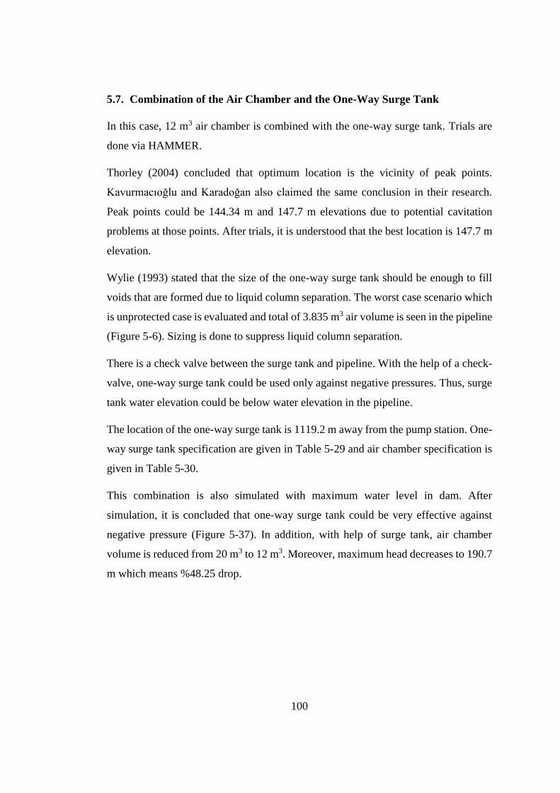
100

5.7. Combination of the Air Chamber and the One-Way Surge Tank

In this case, 12 m3 air chamber is combined with the one-way surge tank. Trials are

done via HAMMER.

Thorley (2004) concluded that optimum location is the vicinity of peak points.

Kavurmacıoğlu and Karadoğan also claimed the same conclusion in their research.

Peak points could be 144.34 m and 147.7 m elevations due to potential cavitation

problems at those points. After trials, it is understood that the best location is 147.7 m

elevation.

Wylie (1993) stated that the size of the one-way surge tank should be enough to fill

voids that are formed due to liquid column separation. The worst case scenario which

is unprotected case is evaluated and total of 3.835 m3 air volume is seen in the pipeline

(Figure 5-6). Sizing is done to suppress liquid column separation.

There is a check valve between the surge tank and pipeline. With the help of a check-

valve, one-way surge tank could be used only against negative pressures. Thus, surge

tank water elevation could be below water elevation in the pipeline.

The location of the one-way surge tank is 1119.2 m away from the pump station. One-

way surge tank specification are given in Table 5-29 and air chamber specification is

given in Table 5-30.

This combination is also simulated with maximum water level in dam. After

simulation, it is concluded that one-way surge tank could be very effective against

negative pressure (Figure 5-37). In addition, with help of surge tank, air chamber

volume is reduced from 20 m3 to 12 m3. Moreover, maximum head decreases to 190.7

m which means %48.25 drop.

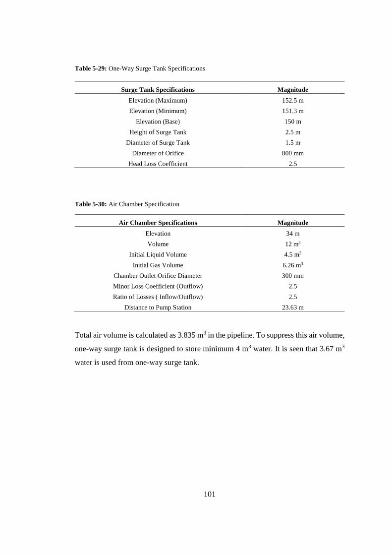
101

Table 5-29: One-Way Surge Tank Specifications

Surge Tank Specifications Magnitude

Elevation (Maximum)

Elevation (Minimum)

Elevation (Base)

Height of Surge Tank

Diameter of Surge Tank

Diameter of Orifice

Head Loss Coefficient

152.5 m

151.3 m

150 m

2.5 m

1.5 m

800 mm

2.5

Table 5-30: Air Chamber Specification

Air Chamber Specifications Magnitude

Elevation

Volume

Initial Liquid Volume

Initial Gas Volume

Chamber Outlet Orifice Diameter

Minor Loss Coefficient (Outflow)

Ratio of Losses ( Inflow/Outflow)

Distance to Pump Station

34 m

12 m3

4.5 m3

6.26 m3

300 mm

2.5

2.5

23.63 m

Total air volume is calculated as 3.835 m3 in the pipeline. To suppress this air volume,

one-way surge tank is designed to store minimum 4 m3 water. It is seen that 3.67 m3

water is used from one-way surge tank.

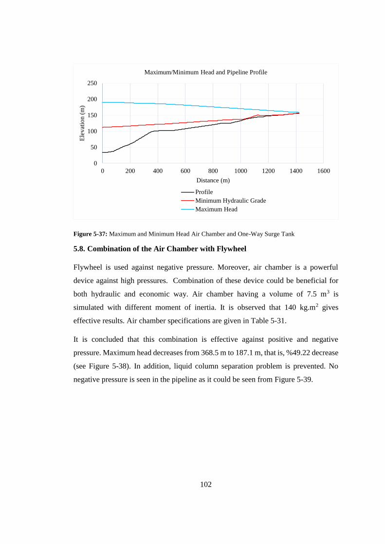
102

Figure 5-37: Maximum and Minimum Head Air Chamber and One-Way Surge Tank

5.8. Combination of the Air Chamber with Flywheel

Flywheel is used against negative pressure. Moreover, air chamber is a powerful

device against high pressures. Combination of these device could be beneficial for

both hydraulic and economic way. Air chamber having a volume of 7.5 m3 is

simulated with different moment of inertia. It is observed that 140 kg.m2 gives

effective results. Air chamber specifications are given in Table 5-31.

It is concluded that this combination is effective against positive and negative

pressure. Maximum head decreases from 368.5 m to 187.1 m, that is, %49.22 decrease

(see Figure 5-38). In addition, liquid column separation problem is prevented. No

negative pressure is seen in the pipeline as it could be seen from Figure 5-39.

0

50

100

150

200

250

0 200 400 600 800 1000 1200 1400 1600

Ele

vat

ion (

m)

Distance (m)

Maximum/Minimum Head and Pipeline Profile

Profile

Minimum Hydraulic Grade

Maximum Head

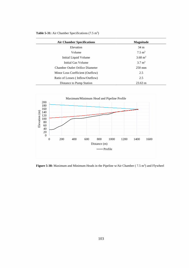
103

Table 5-31: Air Chamber Specifications (7.5 m3)

Air Chamber Specifications Magnitude

Elevation

Volume

Initial Liquid Volume

Initial Gas Volume

Chamber Outlet Orifice Diameter

Minor Loss Coefficient (Outflow)

Ratio of Losses ( Inflow/Outflow)

Distance to Pump Station

34 m

7.5 m3

3.68 m3

3.7 m3

250 mm

2.5

2.5

23.63 m

Figure 5-38: Maximum and Minimum Heads in the Pipeline w/Air Chamber ( 7.5 m3) and Flywheel

020406080

100120140160180200

0 200 400 600 800 1000 1200 1400 1600

Ele

vat

ion (

m)

Distance (m)

Maximum/Minimum Head and Pipeline Profile

Profile

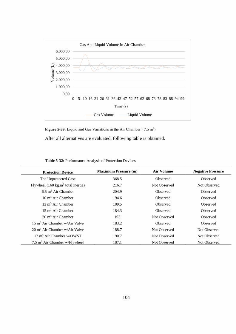
104

Figure 5-39: Liquid and Gas Variations in the Air Chamber ( 7.5 m3)

After all alternatives are evaluated, following table is obtained.

Table 5-32: Performance Analysis of Protection Devices

Protection Device Maximum Pressure (m) Air Volume Negative Pressure

The Unprotected Case

Flywheel (160 kg.m2 total inertia)

6.5 m3 Air Chamber

10 m3 Air Chamber

12 m3 Air Chamber

15 m3 Air Chamber

20 m3 Air Chamber

15 m3 Air Chamber w/Air Valve

20 m3 Air Chamber w/Air Valve

12 m3 Air Chamber w/OWST

7.5 m3 Air Chamber w/Flywheel

368.5

216.7

204.9

194.6

189.5

184.3

193

183.2

188.7

190.7

187.1

Observed

Not Observed

Observed

Observed

Observed

Observed

Not Observed

Observed

Not Observed

Not Observed

Not Observed

Observed

Not Observed

Observed

Observed

Observed

Observed

Observed

Observed

Not Observed

Not Observed

Not Observed

0,00

1.000,00

2.000,00

3.000,00

4.000,00

5.000,00

6.000,00

0 5 10 16 21 26 31 36 42 47 52 57 62 68 73 78 83 88 94 99

Vo

lum

e (L

)

Time (s)

Gas And Liquid Volume In Air Chamber

Gas Volume Liquid Volume

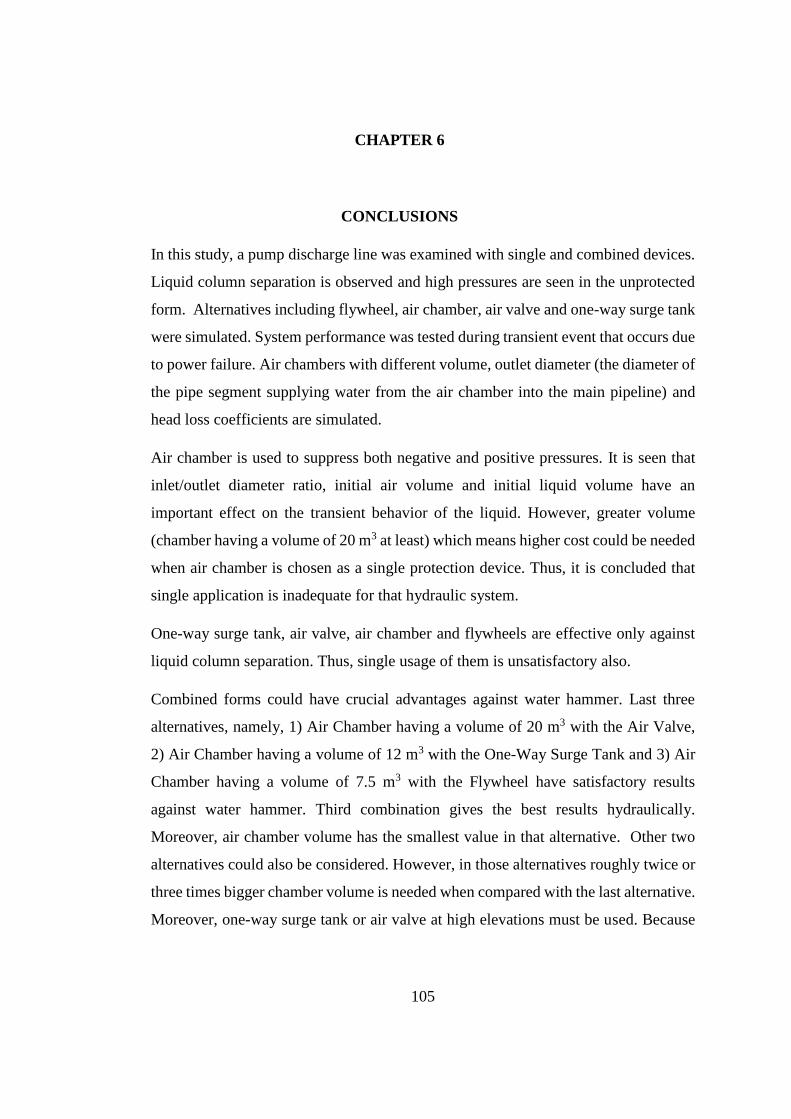
105

CHAPTER 6

6. CONCLUSIONS

In this study, a pump discharge line was examined with single and combined devices.

Liquid column separation is observed and high pressures are seen in the unprotected

form. Alternatives including flywheel, air chamber, air valve and one-way surge tank

were simulated. System performance was tested during transient event that occurs due

to power failure. Air chambers with different volume, outlet diameter (the diameter of

the pipe segment supplying water from the air chamber into the main pipeline) and

head loss coefficients are simulated.

Air chamber is used to suppress both negative and positive pressures. It is seen that

inlet/outlet diameter ratio, initial air volume and initial liquid volume have an

important effect on the transient behavior of the liquid. However, greater volume

(chamber having a volume of 20 m3 at least) which means higher cost could be needed

when air chamber is chosen as a single protection device. Thus, it is concluded that

single application is inadequate for that hydraulic system.

One-way surge tank, air valve, air chamber and flywheels are effective only against

liquid column separation. Thus, single usage of them is unsatisfactory also.

Combined forms could have crucial advantages against water hammer. Last three

alternatives, namely, 1) Air Chamber having a volume of 20 m3 with the Air Valve,

2) Air Chamber having a volume of 12 m3 with the One-Way Surge Tank and 3) Air

Chamber having a volume of 7.5 m3 with the Flywheel have satisfactory results

against water hammer. Third combination gives the best results hydraulically.

Moreover, air chamber volume has the smallest value in that alternative. Other two

alternatives could also be considered. However, in those alternatives roughly twice or

three times bigger chamber volume is needed when compared with the last alternative.

Moreover, one-way surge tank or air valve at high elevations must be used. Because

106

of that they need regular maintenance and their locations would be difficult to access.

In addition, cold climates could be problematic due to freezing conditions in those

elevations.

Overall, protecting pump discharge lines against water hammer should be well

examined at the design stage. Different alternatives should be evaluated properly to

ensure the system stability.

107

REFERENCES

Bentley HAMMER V8i Edition Userʹs Guide. (2016).

Bergant, A., Simpson, A. R., & Tijsseling, A. S. (2005). Water hammer with column

separation : A historical review. Journal of Fluids and Structures 22(2006), 135–171.

Bianchi, A., Mambretti, S., & Pianta, P. (2007). Practical Formulas for the Dimensioning of

Air Valves. Journal of Hydraulic Engineering, 1177–1180 doi:10.1061/(ASCE)0733-

9429(2007) 133:10(1177)

Carmona-Paredes, R.B.,Pozos-Estrada, O. Carmona-Paredes, L.B. Sanchez-Huerta, A. Rodol-

Canales, E.A. Carmona-Paredes, G.J. (2019). Protecting a Pumping Pipeline System

from Low Pressure Transients by Using Air Pockets: A Case Study. Water,

doi:10.3390/w11091786

Chamani, M.R., Pourshahabi, S. & Sheikholeslam, F. (2012). Fuzzy Genetic Algorithm

approach for Optimization of Surge Tanks. Scientia Iranica, 20 (2) 278-285

Chaudhry, M. H. (1979). Applied Hydraulic Transients. New York: Van Nostrand Reinhold

Company

Choon, T. W., Aik, L. K., Aik, L. E., & Hin, T. T. (2012). Investigation of Water Hammer

Effect Through Pipeline System. International Journal on Advanced Science,

Engineering and Information Technology, 2(3), 246.doi: 10.18517/ijaset.2.3.196

Dinçer, A. E. (2013). Investigation of Waterhammer Problems in the Penstocks of Pumped-

Storage Power Plants. Master’s thesis, Middle East Technical University, Ankara,

Turkey.

Dursun S. (2013) Numerical Investigation of Protection Measures against Water Hammer in

the Yeşilvadi Hydropower Plant. Master’s thesis, Middle East Technical University,

Ankara, Turkey.

Dursun, S., Bozkus, Z. and Dinçer A. Ersin. (2015), “Effect of Pressure Relief Valves on the

Fluid Transients in the Penstocks of a Small Run-of-River Plant”, Proceedings of 12th

International Conference on Pressure Surges 2015, Dublin, Ireland 18th-20th November

2015.

Elansary, A.S. (2004) ASCE 2004 Building Parterships. Water Resources 2000. (202), 1-10.

El-dabaa, A. & Khorais, O. (2018). Rationing the Pressurized Air-Vessel Volume for Water

Hammer Protection in Water Pipe Systems. Asian Journal of Engineering and

Technology 06(02), 6-15.

108

Estimation of Pump Moment of Inertia. (2019). Retrieved from Neutrium website:

https://neutrium.net/equipment/estimation-of-pump-moment-of-inertia/,

Hu, J. & Lu, W. (2008). Study on Setting of One-Way Surge Tank in Long Water Supply

Engineering. Paper presented at the Fluid Engineering Conference, Florida USA. ASME

Kavurmacıoğlu, L. (2009,May 6-9) Boru Hatlarında Su Darbesi Olayı ve Önleme

Çareleri.Paper presented at the IX. Ulusal Tesisat Mühendisliği Kongresi, Izmir Turkey

(pp. 927-938.)

Kavurmacıoğlu, L., & Karadoğan, H. (2003, October 8-11) Su Darbesi Projelendirme

Hataları. Paper presented at the VI. Ulusal Tesisat Mühendisliği Kongresi, Izmir Turkey

(pp. 1–7)

Kwon, J. H. (2007) Computer Simulations of Transient Flow in a Real City Water

Distribution System. KSCE Journal of Civil Engineering 11(1), 43-49.

Larock, B., Jeppson, R., & Watters, G. (2000). Hydraulics of Pipeline Systems. Boca Raton,

London, New York, Washington, D.C: CRC Press

Larsen, T. (2012). Water Hammer in Pumped Sewer Mains.Aalboorg: Department of Civil

Engineering, Aalborg University. DCE Lecture notes, No.29

Lima, G.M. & Junior, E.L. (2017). Method to Estimate Complete Curves of Hydraulic Pumps

through the Polymorphism of Existing Curves. Journal of Hydraulic Engineering, 143(8)

London, New York, Washington, D.C.: CRC Press.

Miyashiro, H. (1967). Waterhammer Analysis of Pump Discharge Line with Several One-

Way Surge Tanks. The American Society of Mechanical Engineers. 9, 1-7.

Ramezani, L., Karney, B., & Malekpour, A. (2015). The Challenge of Air Valves: A Selective

Critical Literature Review. Journal of Water Resources Planning and Management,

141(10), 04015017.

Rao, B.C.S (2010) Fluid Mechanics and Machinery, Tata McGraw Hill Education Private

Limited, 7 West Patel Nagar, New Delhi

Rezaei, V., Calamak, M., & Bozkus, Z. (2017). Performance of a Pumped Discharge Line

with Combined Application of Protection Devices Against Water Hammer.KSCE

Journal of Civil Engineering 21, 1493–1500.

Shani, T., & Gupta, T. (2017). Hydraulic Transient Flow Analysis using Method of

Characteristics. International Journal of Innovative Research in Science,Engineering and

Technology 6(7) doi: 10.15680/IJIRSET.2017.0607323

Stephenson, D. (1997). Effects of Air Valves And Pipework On Water Hammer Pressures.

Journal of Transportation Engneering 123(2), 101–106.

109

Stephenson, D. (2002). Simple Guide for Design of Air Vessels for Water Hammer Protection

of Pumping Lines. Journal of Hydraulic Engineering, 128(8), 792–797.

Streeter, V.L. (1963). Waterhammer Analysis of Pipelines. The University of Michigan

Industry Program of the College of Engineering.

Thorley, D. (2004). Fluid Transients in Pipeline Systems. Professional Engineering

Publishing Limited, London and Bury St Edmunds, UK

Wang, X., Zhang, J., Yu, X., Shi, L., Zhao, W., & Xu, H. (2019). Formula for selecting

optimal location of air vessel in long-distance pumping systems. International Journal of

Pressure Vessels and Piping, Vol. 172, pp. 127–133.

Wylie, E. B., Streeter, V. L., Suo, L. (1993). Fluid Transients in Systems. New Jersey:

Prentice-Hall

Yang, K. (2001), Practical Method to Prevent Liquid-Column Separation. Journal of

Hydraulic Engineering 127(7) doi:10.1061/(ASCE)0733-9429