CHAPTER 8_________________________________________________________________________

ELASTIC THEORY OF HYDRAULIC TRANSIENTS(WATER HAMMER)*

In situations where the velocity can change suddenly and the pipeline is relatively long,the elastic properties of the pipe and liquid become significant factors. In Chapter 7 wesaw how a pipeline responded to the sudden closure of a valve. This valve motion causedan increase in pressure head ∆H to occur, which propagated at a speed a. In this chaptergoverning relations for ∆H and a will be developed, thereby broadening the range ofapplications from that of the simple example in Chapter 7.

8.1 THE EQUATION FOR PRESSURE HEAD CHANGE ∆∆∆∆H

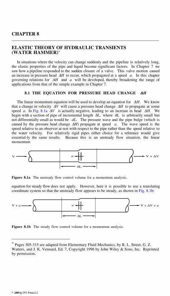
The linear momentum equation will be used to develop an equation for ∆H. We knowthat a change in velocity ∆V will cause a pressure head change ∆H to propagate at somespeed a. In Fig. 8.1a ∆V is actually negative, leading to an increase in head ∆H. Webegin with a section of pipe of incremental length δL, where δL is arbitrarily small butnot differentially small as would be dL. The pressure wave and the pipe bulge (which iscaused by the pressure head change ∆H) propagate at speed a. The wave speed is thespeed relative to an observer at rest with respect to the pipe rather than the speed relative tothe water velocity. For relatively rigid pipes either choice for a reference would giveessential-ly the same results. Because this is an unsteady flow situation, the linearmomentum

V a

δL

V + ∆V

Figure 8.1a The unsteady flow control volume for a momentum analysis.

equation for steady flow does not apply. However, here it is possible to use a translatingcoordinate system so that the unsteady flow appears to be steady, as shown in Fig. 8.1b:

V + a a

δL

V + ∆V + a

Figure 8.1b The steady flow control volume for a momentum analysis.

* Pages 305-315 are adapted from Elementary Fluid Mechanics, by R. L. Street, G. Z.Watters, and J. K. Vennard, Ed. 7, Copyright 1996 by John Wiley & Sons, Inc. Reprintedby permission.

If we move our reference system to the left at a speed a, we have for all appearances asteady flow. From basic fluid mechanics we may then apply the steady one-dimensionallinear momentum equation

Fext∑ = QρV∑( )out − QρV∑( )in (8.1)

where Q is the discharge, ρ is the fluid density, and ΣFext is the sum of the externalforces acting. The momentum correction factor for nonuniform velocity profiles isassumed to be 1.00 in this case.

Considering only the component of this vector equation parallel to the pipe and notingthat the momentum flux enters and leaves the pipe section of length δL at only one crosssection each, we can write

Fext∑( )x = Qρ Vout − Vin( ) (8.2)

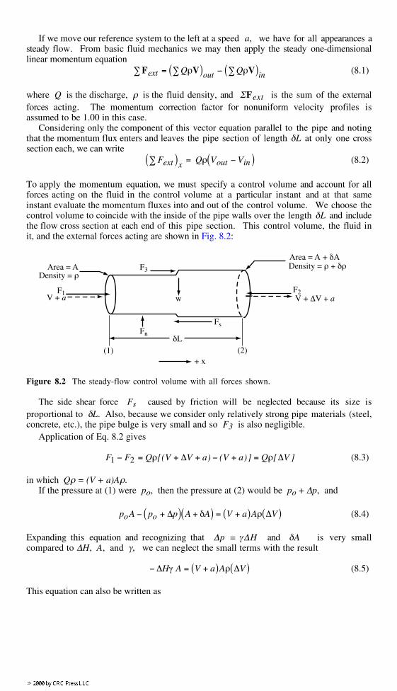
To apply the momentum equation, we must specify a control volume and account for allforces acting on the fluid in the control volume at a particular instant and at that sameinstant evaluate the momentum fluxes into and out of the control volume. We choose thecontrol volume to coincide with the inside of the pipe walls over the length δL and includethe flow cross section at each end of this pipe section. This control volume, the fluid init, and the external forces acting are shown in Fig. 8.2:

Area = ADensity = ρ

F1V + a

(1) (2)

Fn

Fs

F2

F3

V + ∆V + a

Area = A + δADensity = ρ + δρ

w

+ x

δL

Figure 8.2 The steady-flow control volume with all forces shown.

The side shear force Fs caused by friction will be neglected because its size isproportional to δL. Also, because we consider only relatively strong pipe materials (steel,concrete, etc.), the pipe bulge is very small and so F3 is also negligible.

Application of Eq. 8.2 gives

F1 − F2 = Qρ[(V + ∆V + a) − (V + a)] = Qρ[∆V ] (8.3)

in which Qρ = (V + a)Aρ.If the pressure at (1) were po, then the pressure at (2) would be po + ∆p, and

poA − po + ∆p( ) A + δA( ) = V + a( )Aρ ∆V( ) (8.4)

Expanding this equation and recognizing that ∆p = γ∆H and δA is very smallcompared to ∆H, A, and γ, we can neglect the small terms with the result

− ∆Hγ A = V + a( )Aρ ∆V( ) (8.5)

This equation can also be written as

∆H = −ργ

∆V V + a( ) (8.6)

or

∆H = −a∆V

g1 +

V

a

(8.7)

In most rigid pipe situations (even PVC with a wave speed of only 1200 ft/s), the valueof V/a is less than 0.01. Accordingly, Eq. 8.7 is generally (and always in this work)applied as

∆H = −a

g∆V (8.8)

From Eq. 8.8 we see that a decrease in velocity ∆V causes an increase in head ∆H.Further, ∆H depends on the wave speed a and cannot be determined until a value of a isestablished.

8.2 WAVE SPEED FOR THIN-WALLED PIPES

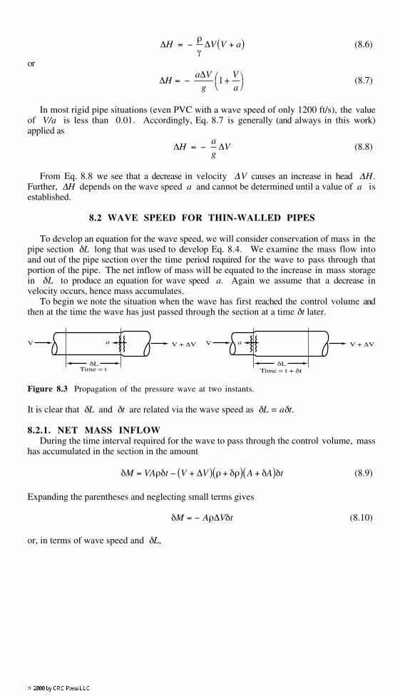
To develop an equation for the wave speed, we will consider conservation of mass in thepipe section δL long that was used to develop Eq. 8.4. We examine the mass flow intoand out of the pipe section over the time period required for the wave to pass through thatportion of the pipe. The net inflow of mass will be equated to the increase in mass storagein δL to produce an equation for wave speed a. Again we assume that a decrease invelocity occurs, hence mass accumulates.

To begin we note the situation when the wave has first reached the control volume andthen at the time the wave has just passed through the section at a time δt later.

V a

δL

V + ∆V

Time = t

V a

δL

V + ∆V

Time = t + δt

Figure 8.3 Propagation of the pressure wave at two instants.

It is clear that δL and δt are related via the wave speed as δL = aδt.

8.2.1. NET MASS INFLOWDuring the time interval required for the wave to pass through the control volume, mass

has accumulated in the section in the amount

δM = VAρδt − V + ∆V( ) ρ + δρ( ) A + δA( )δt (8.9)

Expanding the parentheses and neglecting small terms gives

δM = − Aρ∆Vδt (8.10)

or, in terms of wave speed and δL,

δM = − Aρ∆VδL

a(8.11)

This extra liquid is stored in the control volume partly by being compressed slightly to alarger density and partly by occupying additional space provided by stretching the pipecross section a small amount.

We now proceed to quantify the volume changes for the liquid and the pipe.

8.2.2. CHANGE IN LIQUID VOLUME DUE TO COMPRESSIBILITYBecause the pressure has increased during the passage of a positive pressure wave caused

by a decrease in velocity, the volume of liquid in the section is compressed to a slightlyhigher density. The equation relating the increase in pressure and decrease in volume is theequation defining the bulk modulus of elasticity for a liquid, as can be found in anyelementary fluid mechanics text:

K = −dp

dV / V(8.12)

Here K is the bulk modulus of elasticity of the liquid and p and V are the pressure andvolume of the liquid, respectively. Since K is relatively constant over a wide pressurerange (assuming no entrained gases in the liquid), we can let dp = ∆p and write Eq. 8.6 as

δV = − ∆pV

K(8.13)

where δV is the change in liquid volume in the control volume resulting from thepressure change ∆p.

8.2.3. CHANGE IN PIPE VOLUME DUE TO ELASTICITYWhen the increased pressure stretches the pipe, more space is available to store the

accumulated net inflow of liquid. The pipe may stretch both circumferentially and long-itudinally, so we must consider both contributions to the change in pipe volume.

Developments that are basic to the mechanics of solid materials show the relationbetween the pipe wall strains in the two perpendicular directions. If a material is strainedin one direction by an amount ε1, then a strain ε2 will occur in the perpendicular direction(provided the material is free to strain without developing a stress in that direction)according to ε2 = µε1, where µ is Poisson's ratio. If there is a restriction to free strainin either direction caused either by restraint or applied stress, the relation is morecomplicated. A text on the mechanics of materials will provide the following equations fortwo-dimensional stress which can be applied to thin-walled pipes:

σ1 =ε1 + µε2

1 − µ2 E or ε1 =σ1 − µσ2

E(8.14a)

σ2 =ε2 + µε1

1 − µ 2 E or ε2 =σ2 − µσ1

E(8.14b)

Here σ1 and ε1 are the stress and strain, respectively, in the direction along the pipeaxis, σ2 and ε2 are the values in the circumferential direction, and E is the modulusof elasticity of the pipe wall material. Of course, if the wall material is not homogeneousand isotropic, then a more complex analysis is required.

For water hammer pressure waves there is usually a stress and strain already resident inthe pipe caused by the steady state flow. Hence we write the preceding equations inincremental form

∆σ1 =∆ε1 + µ∆ε2

1 − µ2 E or ∆ε1 =∆σ1 − µ∆σ2

E(8.15a)

∆σ2 =∆ε2 + µ∆ε1

1 − µ2 E or ∆ε2 =∆σ2 − µ∆σ1

E(8.15b)

The change in volume caused by circumferential stretching is

δVc = πDδD

2δL (8.16)

where πδD = πD∆ε2. Combining the two equations gives

δVc =12

πD2δL∆ε2 (8.17)

The change in volume caused by longitudinal stretching is

δVl =π4

D2δL∆ε1 (8.18)

Combining Eqs. 8.17 and 8.18 gives the total volume change due to pipe stretching as

δV =π4

D2δL ∆ε1 + 2∆ε2( ) (8.19)

We now begin the process of replacing the expressions for strain with those for thestress and pressure which cause the strain. The change in circumferential stress in the pipewall under static conditions is

∆σ2 =∆pD

2e(8.20)

where e is the pipe wall thickness. However, the transient conditions of water hammerwould in general cause the pipe to respond dynamically in a manner which can only beanalyzed accurately by carefully considering the mass of the pipe and fitting materials aswell as pipe restraints. That is, any valves, fittings, and other attachments in addition tothe weight of the pipe must be displaced by pressure changes. These displacements are inturn affected by the type and elastic behavior of the pipe restraints. This type of analysiswould be entirely too complex to accomplish in general, so we assume that the staticconditions adequately approximate the dynamic behavior. Experimental results over theyears have generally validated this approach. Substituting the above equation into the firstof Eqs. 8.15b gives

∆pD

2e=

∆ε2 + µ∆ε1

1 − µ2 E (8.21)

While the relation between circumferential stress and pressure is valid for all types ofrestraint, the relation between longitudinal stress and strain varies with restraint type. For

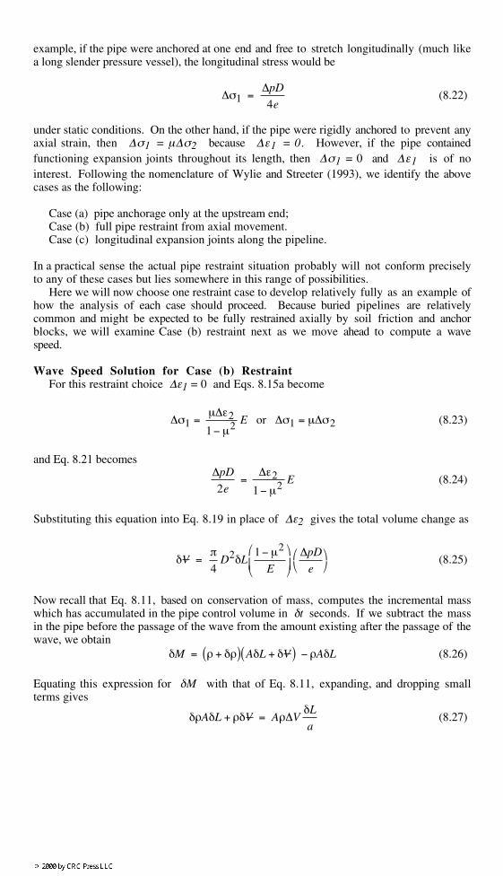
example, if the pipe were anchored at one end and free to stretch longitudinally (much likea long slender pressure vessel), the longitudinal stress would be

∆σ1 =∆pD

4e(8.22)

under static conditions. On the other hand, if the pipe were rigidly anchored to prevent anyaxial strain, then ∆σ1 = µ∆σ2 because ∆ε1 = 0. However, if the pipe containedfunctioning expansion joints throughout its length, then ∆σ1 = 0 and ∆ε1 is of nointerest. Following the nomenclature of Wylie and Streeter (1993), we identify the abovecases as the following:

Case (a) pipe anchorage only at the upstream end;Case (b) full pipe restraint from axial movement.Case (c) longitudinal expansion joints along the pipeline.

In a practical sense the actual pipe restraint situation probably will not conform preciselyto any of these cases but lies somewhere in this range of possibilities.

Here we will now choose one restraint case to develop relatively fully as an example ofhow the analysis of each case should proceed. Because buried pipelines are relativelycommon and might be expected to be fully restrained axially by soil friction and anchorblocks, we will examine Case (b) restraint next as we move ahead to compute a wavespeed.

Wave Speed Solution for Case (b) RestraintFor this restraint choice ∆ε1 = 0 and Eqs. 8.15a become

∆σ1 =µ∆ε2

1 − µ2 E or ∆σ1 = µ∆σ2 (8.23)

and Eq. 8.21 becomes∆pD

2e=

∆ε2

1 − µ2 E (8.24)

Substituting this equation into Eq. 8.19 in place of ∆ε2 gives the total volume change as

δV =π4

D2δL1 − µ2

E

∆pD

e

(8.25)

Now recall that Eq. 8.11, based on conservation of mass, computes the incremental masswhich has accumulated in the pipe control volume in δt seconds. If we subtract the massin the pipe before the passage of the wave from the amount existing after the passage of thewave, we obtain

δM = ρ + δρ( ) AδL + δV( ) − ρAδL (8.26)

Equating this expression for δM with that of Eq. 8.11, expanding, and dropping smallterms gives

δρAδL + ρδV = Aρ∆VδL

a(8.27)

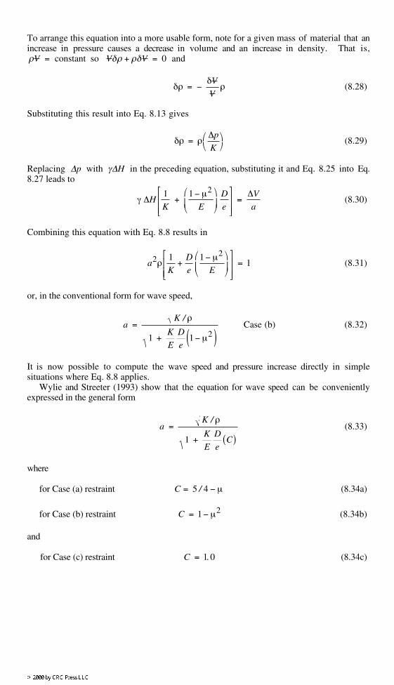
To arrange this equation into a more usable form, note for a given mass of material that anincrease in pressure causes a decrease in volume and an increase in density. That is,ρV = constant so Vδρ + ρδV = 0 and

δρ = −δV

Vρ (8.28)

Substituting this result into Eq. 8.13 gives

δρ = ρ∆p

K

(8.29)

Replacing ∆p with γ∆H in the preceding equation, substituting it and Eq. 8.25 into Eq.8.27 leads to

γ ∆H1K

+1 − µ2

E

D

e

=∆V

a(8.30)

Combining this equation with Eq. 8.8 results in

a2ρ1K

+D

e

1 − µ2

E

= 1 (8.31)

or, in the conventional form for wave speed,

a =K / ρ

1 +K

E

D

e1 − µ2( )

Case (b) (8.32)

It is now possible to compute the wave speed and pressure increase directly in simplesituations where Eq. 8.8 applies.

Wylie and Streeter (1993) show that the equation for wave speed can be convenientlyexpressed in the general form

a =K / ρ

1 +K

E

D

eC( )

(8.33)

where

for Case (a) restraint C = 5 / 4 − µ (8.34a)

for Case (b) restraint C = 1 − µ2 (8.34b)

and

for Case (c) restraint C = 1.0 (8.34c)

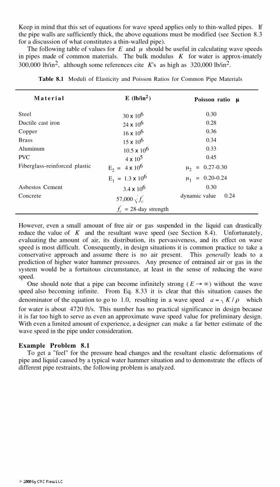
Keep in mind that this set of equations for wave speed applies only to thin-walled pipes. Ifthe pipe walls are sufficiently thick, the above equations must be modified (see Section 8.3for a discussion of what constitutes a thin-walled pipe).

The following table of values for E and µ should be useful in calculating wave speedsin pipes made of common materials. The bulk modulus K for water is approx-imately300,000 lb/in2, although some references cite K's as high as 320,000 lb/in2.

Table 8.1 Moduli of Elasticity and Poisson Ratios for Common Pipe Materials

M a t e r i a l E (lb/in2 ) Poisson ratio µµµµ

Steel 30 x 106 0.30

Ductile cast iron 24 x 106 0.28

Copper 16 x 106 0.36

Brass 15 x 106 0.34

Aluminum 10.5 x 106 0.33

PVC 4 x 105 0.45

Fiberglass-reinforced plastic E2 = 4 x 106 µ2 = 0.27-0.30

E1 = 1.3 x 106 µ1 = 0.20-0.24

Asbestos Cement 3.4 x 106 0.30

Concrete 57,000 fc' dynamic value 0.24

fc' = 28-day strength

However, even a small amount of free air or gas suspended in the liquid can drasticallyreduce the value of K and the resultant wave speed (see Section 8.4). Unfortunately,evaluating the amount of air, its distribution, its pervasiveness, and its effect on wavespeed is most difficult. Consequently, in design situations it is common practice to take aconservative approach and assume there is no air present. This generally leads to aprediction of higher water hammer pressures. Any presence of entrained air or gas in thesystem would be a fortuitous circumstance, at least in the sense of reducing the wavespeed.

One should note that a pipe can become infinitely strong ( E → ∞) without the wavespeed also becoming infinite. From Eq. 8.33 it is clear that this situation causes thedenominator of the equation to go to 1.0, resulting in a wave speed a = K / ρ which

for water is about 4720 ft/s. This number has no practical significance in design becauseit is far too high to serve as even an approximate wave speed value for preliminary design.With even a limited amount of experience, a designer can make a far better estimate of thewave speed in the pipe under consideration.

Example Problem 8.1To get a "feel" for the pressure head changes and the resultant elastic deformations of

pipe and liquid caused by a typical water hammer situation and to demonstrate the effects ofdifferent pipe restraints, the following problem is analyzed.

200'

EL - HGL

Water flows in this 24-inch steel pipeline at a velocity of 6 ft/s. The pipeline has awall thickness of 0.25 inches. First we will calculate the wave speed for the three types ofrestraint by using Eqs. 8.33 and 8.34:

Case (a) a =K / ρ

1 +K

E

D

eC( )

=4720

1 +3 ×105

3 ×10724

0.255 / 4 − 0.30( )

= 3410 ft/s

Case (b) a =4720

1 +3 ×105

3 ×10724

0.251 − 0.302( )

= 3450 ft/s

Case (c) a =4720

1 +3 ×105

3 ×10724

0.251.00( )

= 3370 ft/s

As one can see clearly here, the differences are for all practical purposes insignificant forthis pipe.

Now we will compute with Eq. 8.8 the pressure head changes resulting from suddenvalve closure for all three cases of restraint:

Case (a) ∆H = −a

g∆V = −

341032.2

− 6( ) = 635 ft

Case (b) ∆H = −345032.2

− 6( ) = 643 ft

Case (c) ∆H = −337032.2

− 6( ) = 628 ft

Because the head increase depends directly on the wave speed, the negligible difference inwave speed translates into a head difference of no more than 2%, which is usually anegligible difference.

We now calculate the change in pipe wall stress caused by these head increases for allthree types of restraint:

Case (a) ∆σ2 =∆pD

2e=

635 ×62.4144

× 24

2 × 0.25= 13,210 lb / in2

∆σ1 =∆pD

4e=

12

∆σ2 = 6600 lb / in2

Case (b) ∆σ2 =∆pD

2e=

643 ×62.4144

× 24

2 × 0.25= 13,370 lb / in2

∆σ1 = µ∆σ2 = 0.30 ×13,370 = 4010 lb / in2

Case (c) ∆σ2 =∆pD

2e=

628 ×62.4144

× 24

2 × 0.25= 13,060 lb / in2

∆σ1 = 0

Next we calculate the percentage increase in the pipe diameter caused by the pressure headincrease for all three cases of restraint. Using Eq. 8.15b,

Percent change in D = 100δD

D= 100 × ∆ε2 =

100E

∆σ2 − µ∆σ1( )

Case (a) Percent change =100

30 ×106 13,210 − 0.30 × 6600( ) = 0.037%

Case (b) Percent change =100

30 ×106 13,370 − 0.30 × 4010( ) = 0.041%

Case (c) Percent change =100

30 ×106 13,060 − 0.30 × 0( ) = 0.044%

These results, showing the relatively small elastic deformation of the pipe, substantiatemany of the previous assumptions that were used in neglecting small terms in equations.

Finally, we will look at the water entering the pipe section during the passage of thepressure wave and determine what percentage is accommodated by pipe stretching and whatportion is relegated to water compression. The fraction of liquid directed to liquidcompression is given by the first term in Eq. 8.31.

Percent change in water volume = 100ρa2 1K

= 100ρa2

KThe remainder is due to pipe stretching.

Case (a)Percent change in water volume = 100

1.94 × 34102

300,000 ×144= 52%

Percent accommodated by pipe stretching = 48%

Case (b)Percent change in water volume = 100

1.94 × 34502

300,000 ×144= 53%

Percent accommodated by pipe stretching = 47%

Case (c)Percent change in water volume = 100

1.94 × 33702

300,000 ×144= 51%

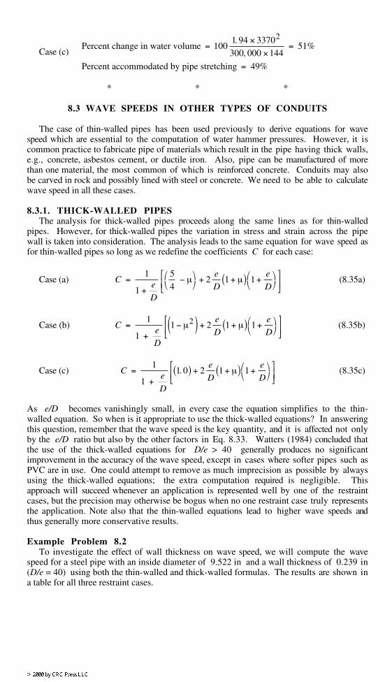
Percent accommodated by pipe stretching = 49%

* * *

8.3 WAVE SPEEDS IN OTHER TYPES OF CONDUITS

The case of thin-walled pipes has been used previously to derive equations for wavespeed which are essential to the computation of water hammer pressures. However, it iscommon practice to fabricate pipe of materials which result in the pipe having thick walls,e.g., concrete, asbestos cement, or ductile iron. Also, pipe can be manufactured of morethan one material, the most common of which is reinforced concrete. Conduits may alsobe carved in rock and possibly lined with steel or concrete. We need to be able to calculatewave speed in all these cases.

8.3.1. THICK-WALLED PIPESThe analysis for thick-walled pipes proceeds along the same lines as for thin-walled

pipes. However, for thick-walled pipes the variation in stress and strain across the pipewall is taken into consideration. The analysis leads to the same equation for wave speed asfor thin-walled pipes so long as we redefine the coefficients C for each case:

Case (a) C =1

1 +e

D

54

− µ

+ 2e

D1 + µ( ) 1 +

e

D

(8.35a)

Case (b) C =1

1 +e

D

1 − µ2( ) + 2e

D1 + µ( ) 1 +

e

D

(8.35b)

Case (c) C =1

1 +e

D

1.0( ) + 2e

D1 + µ( ) 1 +

e

D

(8.35c)

As e/D becomes vanishingly small, in every case the equation simplifies to the thin-walled equation. So when is it appropriate to use the thick-walled equations? In answeringthis question, remember that the wave speed is the key quantity, and it is affected not onlyby the e/D ratio but also by the other factors in Eq. 8.33. Watters (1984) concluded thatthe use of the thick-walled equations for D/e > 40 generally produces no significantimprovement in the accuracy of the wave speed, except in cases where softer pipes such asPVC are in use. One could attempt to remove as much imprecision as possible by alwaysusing the thick-walled equations; the extra computation required is negligible. Thisapproach will succeed whenever an application is represented well by one of the restraintcases, but the precision may otherwise be bogus when no one restraint case truly representsthe application. Note also that the thin-walled equations lead to higher wave speeds andthus generally more conservative results.

Example Problem 8.2To investigate the effect of wall thickness on wave speed, we will compute the wave

speed for a steel pipe with an inside diameter of 9.522 in and a wall thickness of 0.239 in(D/e = 40) using both the thin-walled and thick-walled formulas. The results are shown ina table for all three restraint cases.

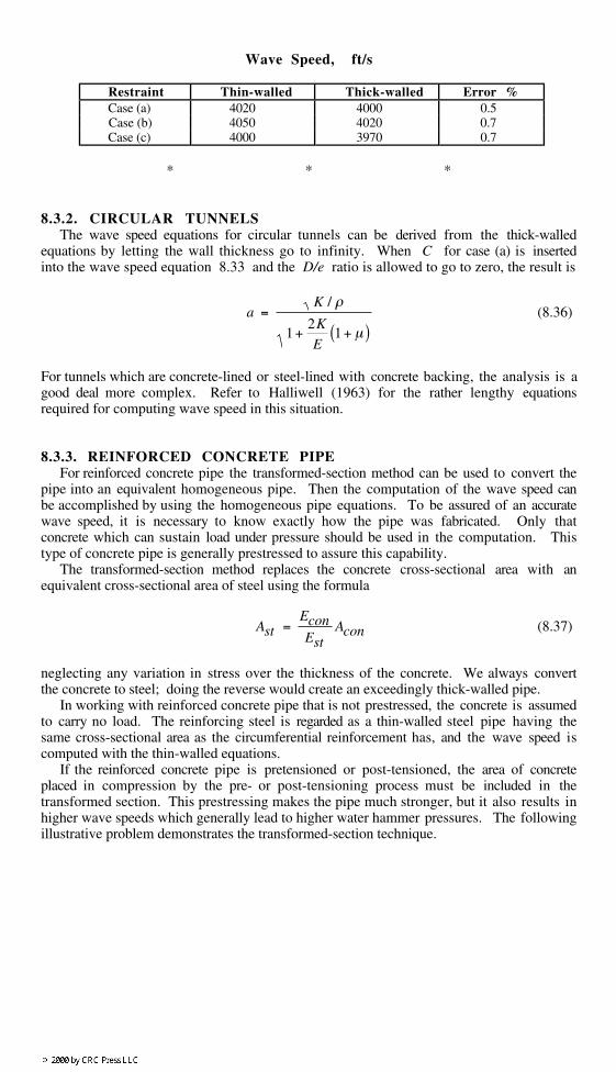
Wave Speed, ft/s

Restraint Thin-walled Thick-walled Error % Case (a) 4020 4000 0.5 Case (b) 4050 4020 0.7 Case (c) 4000 3970 0.7

* * *

8.3.2. CIRCULAR TUNNELSThe wave speed equations for circular tunnels can be derived from the thick-walled

equations by letting the wall thickness go to infinity. When C for case (a) is insertedinto the wave speed equation 8.33 and the D/e ratio is allowed to go to zero, the result is

a =K / ρ

1 +2K

E1 + µ( )

(8.36)

For tunnels which are concrete-lined or steel-lined with concrete backing, the analysis is agood deal more complex. Refer to Halliwell (1963) for the rather lengthy equationsrequired for computing wave speed in this situation.

8.3.3. REINFORCED CONCRETE PIPEFor reinforced concrete pipe the transformed-section method can be used to convert the

pipe into an equivalent homogeneous pipe. Then the computation of the wave speed canbe accomplished by using the homogeneous pipe equations. To be assured of an accuratewave speed, it is necessary to know exactly how the pipe was fabricated. Only thatconcrete which can sustain load under pressure should be used in the computation. Thistype of concrete pipe is generally prestressed to assure this capability.

The transformed-section method replaces the concrete cross-sectional area with anequivalent cross-sectional area of steel using the formula

Ast =EconEst

Acon (8.37)

neglecting any variation in stress over the thickness of the concrete. We always convertthe concrete to steel; doing the reverse would create an exceedingly thick-walled pipe.

In working with reinforced concrete pipe that is not prestressed, the concrete is assumedto carry no load. The reinforcing steel is regarded as a thin-walled steel pipe having thesame cross-sectional area as the circumferential reinforcement has, and the wave speed iscomputed with the thin-walled equations.

If the reinforced concrete pipe is pretensioned or post-tensioned, the area of concreteplaced in compression by the pre- or post-tensioning process must be included in thetransformed section. This prestressing makes the pipe much stronger, but it also results inhigher wave speeds which generally lead to higher water hammer pressures. The followingillustrative problem demonstrates the transformed-section technique.

Example Problem 8.3A 30-in. inside diameter reinforced concrete pipe is pretensioned using 3/8-in diameter

wrapping wire placed 1.25 in on center. The pipe was manufactured by first fabricating athin steel cylinder 0.105 in thick and then centrifugally placing a dense cement mortarlining 0.75 in thick inside the steel cylinder. After curing the liner, the pretensioning isaccomplished by stressing the wire as it is wrapped around the steel cylinder. This processplaces the cement liner in compression. The ends of the wrapping wire are welded to thesteel cylinder to maintain the pretensioning. A one-inch-thick concrete cover is placed overthe wrapping wire as a protective coating. This cover carries no load. A longitudinal pipesection is shown below. Assume the 28-day strength of the concrete is 6000 lb/in2.

CL30"

3/8" wire wrap 1.25" o.c.

0.75"1.375"

0.105"

Using the formula in Table 8.1 for concrete, E is

Econ = 57,000 f c' = 57,000 6000 = 4.4 ×106 lb / in2

The area of steel wire per inch of pipe is π4

× 0.3752/ 1.25 = 0.0884 in2/ in .

The equivalent area of steel that is required to replace the cement lining which wasprestressed during the wrapping process is

Ast =EconEst

Acon =4.4 ×106

30 ×106 × 0.75 = 0.110 in2/ in

Now the thickness of the equivalent steel pipe is

eeq = 0.0884 + 0.110 + 0.105 = 0.303 in

We compute the diameter of the equivalent pipe by locating the centroid of the section asfollows:

r =0.0884 15+0.75+0.105+0.375/2( )+0.110 15+0.75/2( )+0.105 15+0.75+0.105/2( )

0.303

r = 15.74 in. D = 31.5 in.

Now the wave speed is computed using Case (b) restraint because that seems the mostconservative:

a =4720

1 +3 ×105

3 ×10731.5

0.3031 − 0.302( )

= 3380 ft/s

If the effect of the cement mortar lining is neglected, the wave speed drops to 2990 ft/s. Itis the responsibility of the designer to make the judgment as to the proper wave speed touse or, as an alternative, analyze the system under both conditions to determine the moreextreme behavior.

* * *

8.4 EFFECT OF AIR ENTRAINMENT ON WAVE SPEED*

When free air (or any other gas) is present in a pipeline, either as small bubbles or inlarger volumes, the wave speed in the pipeline is decreased dramatically. As a consequence,the wave propagation patterns and the resulting pressures are substantially changed. Wewill demonstrate the effect by using the simplest model of air entrainment.

If the air-water mixture is assumed to be uniformly distributed throughout a portion ofthe pipeline, the wave speed in that portion of the pipeline can be computed by using Eq.8.33. However, care must be taken to insure that the air-water mixture is used indetermining the values of K and ρ. The bulk modulus K for the mixture is developedfrom Eq. 8.12 by replacing the relative change in overall volume by the sum of the relativechanges in volume of the air and water. The result is

Kmix =Kliq

1 + αKliq

Kair− 1

(8.38)

where Kliq and Kair are the bulk moduli of elasticity for liquid and air, respectively, and

α is the void fraction (volume of air ÷ total volume of mixture). For misture density isfound by the same approach to be

ρmix = (1 − α)ρliq (8.39)

Substituting Eqs. 8.38 and 8.39 into Eq. 8.33 and recognizing that Kliq /Kair >> 1, wefind the wave speed to be

a =Kliq / ρmix

1 +Kliq

E

D

eC + α

Kliq

Kair

(8.40)

* This Section is adapted from Elementary Fluid Mechanics, by R. L. Street, G. Z.Watters, and J. K. Vennard, Ed. 7, Copyright 1996 by John Wiley & Sons, Inc. Reprintedby permission.

This same equation and a detailed description of the difficulties encountered in the solutionof water hammer problems which have entrained air is given by Tullis et al. (1976).

It is clear from Eq. 8.40 that the wave speed in the pipeline depends on the pressure inthe pipeline because the values of α and Kair depend on pressure. As a consequence, thewave speed varies with the passage of a pressure wave. This factor greatly complicates ananalysis and makes the accurate prediction of water hammer pressures most difficult.

An example is presented below to demonstrate the dramatic effect that small fractions ofentrained air can have on the wave speed. The first step which must be taken is toestablish a method of determining Kair . As elementary fluid mechanics texts show, Kairdepends on the thermodynamic process followed by the air as it compresses or expands.Wylie and Streeter (1993) suggest using an isothermal process with Kair = p. The otherextreme is to use an isentropic process where Kair = kp = 1.4p. If some provision forheat transfer is made, then a polytropic process with Kair = np = 1.2p (as used later withsurge tanks) may be appropriate. The effects of these various alternatives are shownbelow.

Example Problem 8.4Consider the pipeline of Example Problem 8.1 and consider air entrainment percentages

of 0.10, 0.50, 1.0, and 2.0%. We assume the atmospheric pressure to be 14.7 lb/in2

and use Case (b) restraint. For a polytropic process and an entrained air percentage of0.10%, the wave speed from Eq. 8.40 is

a =

300,000 ×1441.94 1 − 0.001( )

1 +3 ×105

3 ×10724

0.251 − 0.302( ) + 0.001 ×

3 ×105

1.2 ×200 × 62.4

144+ 14.7

= 2270 ft / s

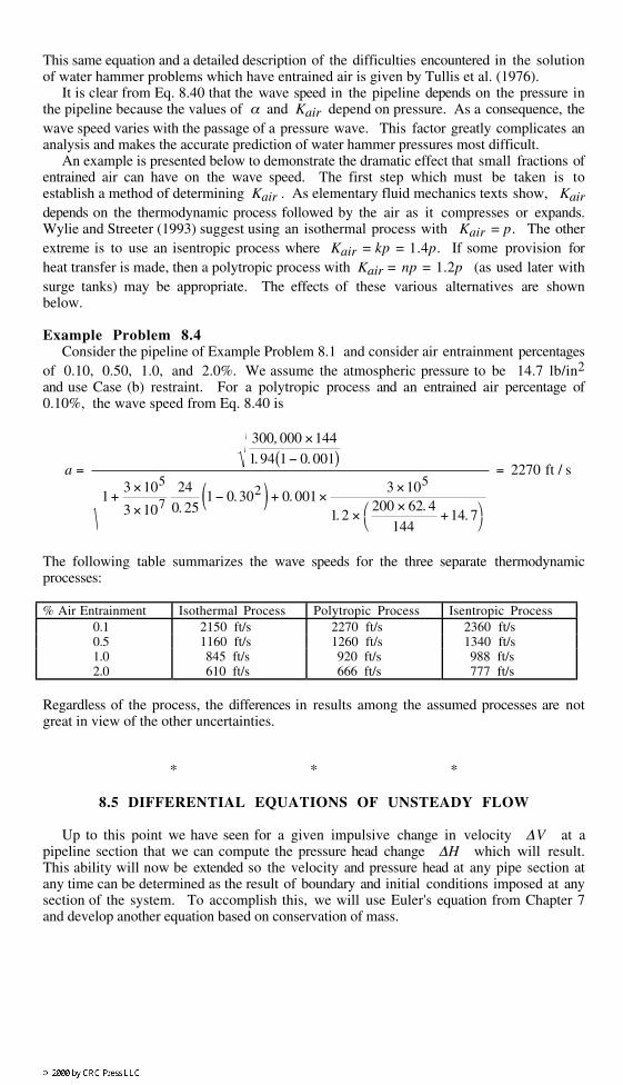
The following table summarizes the wave speeds for the three separate thermodynamicprocesses:

% Air Entrainment Isothermal Process Polytropic Process Isentropic Process 0.1 2150 ft/s 2270 ft/s 2360 ft/s 0.5 1160 ft/s 1260 ft/s 1340 ft/s 1.0 845 ft/s 920 ft/s 988 ft/s 2.0 610 ft/s 666 ft/s 777 ft/s

Regardless of the process, the differences in results among the assumed processes are notgreat in view of the other uncertainties.

* * *

8.5 DIFFERENTIAL EQUATIONS OF UNSTEADY FLOW

Up to this point we have seen for a given impulsive change in velocity ∆V at apipeline section that we can compute the pressure head change ∆H which will result.This ability will now be extended so the velocity and pressure head at any pipe section atany time can be determined as the result of boundary and initial conditions imposed at anysection of the system. To accomplish this, we will use Euler's equation from Chapter 7and develop another equation based on conservation of mass.

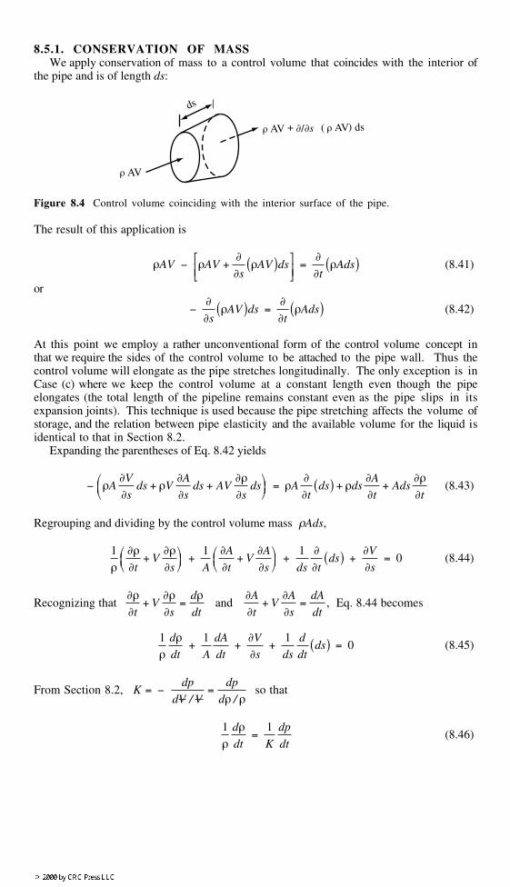
8.5.1. CONSERVATION OF MASSWe apply conservation of mass to a control volume that coincides with the interior of

the pipe and is of length ds:

ds

ρ AV

ρ AV ρ AV ds) (s+ ∂/∂

Figure 8.4 Control volume coinciding with the interior surface of the pipe.

The result of this application is

ρAV − ρAV +∂∂s

ρAV( )ds

=

∂∂t

ρAds( ) (8.41)

or

−∂∂s

ρAV( )ds =∂∂t

ρAds( ) (8.42)

At this point we employ a rather unconventional form of the control volume concept inthat we require the sides of the control volume to be attached to the pipe wall. Thus thecontrol volume will elongate as the pipe stretches longitudinally. The only exception is inCase (c) where we keep the control volume at a constant length even though the pipeelongates (the total length of the pipeline remains constant even as the pipe slips in itsexpansion joints). This technique is used because the pipe stretching affects the volume ofstorage, and the relation between pipe elasticity and the available volume for the liquid isidentical to that in Section 8.2.

Expanding the parentheses of Eq. 8.42 yields

− ρA∂V

∂sds + ρV

∂A

∂sds + AV

∂ρ∂s

ds

= ρA

∂∂t

ds( ) + ρds∂A

∂t+ Ads

∂ρ∂t

(8.43)

Regrouping and dividing by the control volume mass ρAds,

1ρ

∂ρ∂t

+ V∂ρ∂s

+

1A

∂A

∂t+ V

∂A

∂s

+

1ds

∂∂t

ds( ) +∂V

∂s= 0 (8.44)

Recognizing that ∂ρ∂t

+ V∂ρ∂s

=dρdt

and ∂A

∂t+ V

∂A

∂s=

dA

dt, Eq. 8.44 becomes

1ρ

dρdt

+1A

dA

dt+

∂V

∂s+

1ds

d

dtds( ) = 0 (8.45)

From Section 8.2, K = −dp

dV / V=

dp

dρ / ρ so that

1ρ

dρdt

=1K

dp

dt(8.46)

To develop a useful expression for dA/dt in terms of p, the elastic pipe deformationsmust be considered. For the change in cross-sectional area, Eq. 8.17 shows that

dA =dVcdL

=12

πD2dε2 =12

πD2

Edσ2 − µdσ1( ) (8.47)

1A

dA =2E

dσ2 − µdσ1( ) (8.48)

In evaluating these stresses we will again examine Case (b) restraint; hence

dσ2 =D

2edp and dσ1 = µdσ2 (8.49)

so

dσ2 − µdσ1 = 1 − µ2( )dσ2 = 1 − µ2( ) D

2e

dp

dt(8.50)

Finally,1A

dA

dt= 1 − µ2( ) D

eE

dp

dt(8.51)

Considering longitudinal expansion,d ds( ) = dε1ds (8.52)

which is zero for Case (b). Thus1ds

d

dtds( ) = 0 (8.53)

Combining all these results in Eq. 8.45 gives

1K

dp

dt+ 1 − µ2( ) D

eE

dp

dt+

∂V

∂s= 0 (8.54)

dp

dt

1K

+ 1 − µ2( ) D

eE

+∂V

∂s= 0 (8.55)

From Eq. 8.31 it is clear that the term in the brackets is 1

a2ρ. This statement is also

correct for Case (a) and Case (c) pipe restraint. Making this substitution for the terms inbrackets leads to

1ρ

dp

dt+ a2 ∂V

∂s= 0 (8.56)

When we combine this result with the Euler equation of motion, Eq. 7.19, we have twoindependent partial differential equations for p(s,t) and V(s,t):

dV

dt+

1ρ

∂p

∂s+ g

dz

ds+

f

2DV V = 0 (8.57)

a2 ∂V

∂s+

1ρ

dp

dt= 0 (8.58)

8.5.2. INTERPRETATION OF THE DIFFERENTIAL EQUATIONSBefore moving to the solution of these equations in Chapter 9, we can learn about the

nature of these solutions by looking at a linearized subset of the full equations. If we firstexpress the pressure p in terms of the piezometric head H via the relation p = ρg(H - z),then Eqs. 8.57 and 8.58 become

dV

dt+ g

∂H

∂s+

f

2DV V = 0 (8.59)

and

a2 ∂V

∂s+ g

dH

dt= 0 (8.60)

in which the variation of the density ρ is presently assumed to be negligible. The deriva-tive d/dt actually represents both the temporal and convective partial derivative terms. For example,

dV

dt=

∂V

∂t+ V

∂V

∂s(8.61)

and similarly for dH/dt. Thus Eqs. 8.59 and 8.60 actually contain two nonlinearconvective terms in addition to the nonlinear friction term.

Let us assume for the moment that the linear terms in Eqs. 8.59 and 8.60 are largerthan the nonlinear terms and discard the nonlinear terms; we can evaluate later theconsequences of this simplification. Then these equations become

∂V

∂t+ g

∂H

∂s= 0 (8.62)

and

a2 ∂V

∂s+ g

∂H

∂t= 0 (8.63)

Since the equations are now linear, cross-differentiation and some algebra will allow us toeliminate either one of the two dependent variables V and H in favor of the other one.Thus, if we take the partial derivative of Eq. 8.62 with respect to s and the partialderivative of Eq. 8.63 with respect to t, the algebra leads to

∂2H

∂t2 = a2 ∂2H

∂s2 (8.64)

By interchanging the differentiation roles of s and t, we can demonstrate that V is alsogoverned by this equation.

Equation 8.64 is a basic equation of mathematical physics called the wave equation.The parameter a in Eq. 8.64 is known as the wave propagation speed. Hence we expectthe solutions of Eq. 8.64 for either H or V to display the behavior of waves. By meansof a change in the independent variables, we can deduce the general solution of Eq. 8.64 forH; the procedure is identical for V. We begin with H = H(s, t) and V = V(s, t), and wechoose as new independent variables u = t + s/a and v = t - s/a. Application of the chainrule of differentiation to compute the new partial derivatives of H then leads to

4∂2H

∂u∂v= 0 (8.65)

as the new form of the governing equation. The general solution immediately follows as

H − H0 = F1 t +s

a

+ F2 t −s

a

(8.66)

in which F1 and F2 are each an entirely general function of their one argument, and H0is an additive constant of integration which fixes the reference level for the head H.

We turn now to the interpretation of the result expressed in Eq. 8.66. Functions F1and F2 are each wave forms; either or both may exist in a particular problem, dependingon the particular initial and boundary conditions. We focus first on F1: at any instant t1the wave form H described by the function F1 can be any function of the distancevariable s,

F1(s, t1 + δt)F1(s, t1)

s

Pipe

Figure 8.5 Motion of the wave form F1.

as we see on the right side of Fig. 8.5. So long as the argument t + s/a is unchanged,thewave form is unchanged. But as the time t advances, the argument t + s/a can only re-main constant if s/a decreases by δt as t increases by δt; thus the constant wave formmoves in the negative s-direction (to the left), as Fig. 8.5 also shows. We conclude thatF1 describes a left-moving wave. By similar reasoning we find that F2 describes a right-moving wave form. The general solution to Eq. 8.66 is then a superposition of anynumber, one or many, of left- and/or right-moving waves.

Is the neglect of the nonlinear convective acceleration terms justified? These are theterms

V∂V

∂sand V

∂H

∂s(8.67)

If we apply the scaling s ~ at to the terms in Eq. 8.67, we quickly find

V∂V

∂s~

V

a

∂V

∂t

V∂H

∂s~

V

a

∂H

∂t

(8.68)

Since it is almost always true that V/a << 1, the convective terms, initially dropped, arenearly always much smaller than the linear terms that were retained. In later solutions theneglect of these terms will often be an acceptable approximation, although in some waysthe quality of the resulting solution is less precise. Only in rare problems where V/a isnot much smaller than unity is it essential to retain these terms.

8.6 PROBLEMS*

8.1 A high-pressure water system is being designed for use in a lumber mill to removebark from logs. The main portion of the pipe system is 6-inch steel pipe with walls0.219 inches thick. The inside diameter of the pipe is 6.187 inches, and the workingwater pressure in the pipe is 1094 lb/in2. The allowable stress in the steel pipe walls is15,000 lb/in2. Under steady flow conditions the water pressure in the pipe is about 750lb/in2 with a flow velocity of 10 ft/s. Because of the nature of the process, there is aneed for a very rapid valve closure.

(a) Compute the wave speed for all three types of restraint using the thin-walled pipeformulas.

(b) Make a recommendation as to whether the water hammer pressures developed undersudden valve closure could overstress the pipe.

8.2 A 12-inch PVC line is laid above ground using bell-and-spigot joints. It is restrainedlaterally to prevent buckling but is free to strain longitudinally. However, concreteanchors at each bend prevent the pipe from blowing apart. The inside diameter of the pipeis 12.09 inches and the wall thickness is 0.311 inches.

(a) Choose the proper restraint case, and compute the wave speed using the thin-walledpipe formula.

(b) Also calculate the percent increase in pipe volume that is caused when a watervelocity of 10 ft/s is brought suddenly to rest.

(c) What change in diameter does this represent?

8.3 A long water line is to be constructed of T-30 Transite pipe (asbestos cement). Thepipe is rated for a maximum pressure of 300 lb/in2. The inside diameter of the pipe is 18inches, and the outside diameter is 19.70 inches. Lengths of pipe are joined withcouplings and ring gaskets.

(a) Compute the wave speed for all three types of restraint, assuming the thin-walledpipe formulas apply.

(b) Which wave speed would you recommend using? Why?

8.4 When water hammer occurs in the pipe of Problem 8.3, the water is compressed andthe pipe is stretched. What percentage of the volume change can be attributed to watercompression and what percentage to pipe expansion? Assume Case (b) restraint applies.

8.5 Calculate the wave speed in the following situations for Case (b) restraint using thethin-walled pipe formulas:

(a) Steel pipe, 36-inch inside diameter, 0.375-inch wall thickness(b) Ductile cast iron pipe, 18-inch inside diameter, 0.50-inch wall thickness(c) Aluminum pipe, 4-inch inside diameter, 0.10-inch wall thickness(d) Asbestos cement, 11.56-inch inside diameter, 1.26-inch wall thickness(e) Class 125 PVC, 6.22-inch inside diameter, 0.20-inch wall thickness

Note the variation in a for this wide range of pipe sizes and materials.

8.6 For the PVC pipe of Problem 8.5, compute the percent change in cross-sectional areacaused by a sudden velocity change of 10 ft/s.

* Problems 8.1, 8.5, and 8.7-8.11 are adapted from Elementary Fluid Mechanics, by R. L.Street, G. Z. Watters, and J. K. Vennard, Ed. 7, Copyright 1996 by John Wiley & Sons,Inc. Reprinted by permission.

8.7 The wall of a steel pipe 8000 ft long, with a 6 ft inside diameter and a wallthickness of 0.50 inches, is stressed at 7000 lb/in2. Water is flowing at 5 ft/s.

(a) For Case (a) restraint and sudden valve closure, what amount of water enters the pipeafter valve closure?

(b) How is this volume distributed among radial stretching, longitudinal stretching, andwater compression?

8.8 Calculate the wave speed in a water-filled copper tube that is installed withoutlongitudinal restraint. The tube has a 0.375 inch inside diameter, is 75 ft long and has awall thickness of 0.03 inches. The steady state pressure in the tube is 73 lb/in2.

8.9 A Class 51 ductile iron pipe conveys water between two reservoirs. The outsidediameter is 15.30 inches and, for this class of pipe, the wall thickness is 0.36 inches.Assuming the pipe can be considered to be thin-walled, compute the wave speed for allthree types of restraint.

8.10 For the pipe of Problem 8.9, compute the percent change in pipe volume thatoccurs as the result of a sudden stoppage of a 10 ft/s flow of water. Use Case (b)restraint.

What is the percent change in the density of the water?

8.11 A plastic supply pipe in a building water system is anchored at both ends and hasexpansion joints along its entire length. The line is 800 ft long, 6.00 inches insidediameter with a 0.200 inch wall thickness. The modulus of elasticity for this material is500,000 lb/in2. Water in the pipe normally flows at 10 ft/s, and the system valves aredesigned to close very quickly.

(a) If µ = 0.5 for this material, what is the wave speed?(b) If the steady state pressure in the pipe is about 100 lb/in2, estimate the maximum

pressure that could occur in the system under the worst water hammer conditions? (c) What would be the stresses in the pipe walls under these conditions?

8.12 An aluminum irrigation pipeline laid on level ground consists of a series of 20-ftpieces connected rigidly together. The two ends of the pipeline are anchored solidly to theground. If the pipe is 8 inches in inside diameter with 0.10-inch walls, calculate thewave speed in the pipe.

8.13 Class 100 PVC pipe has a nominal diameter of 8 in but has an actual insidediameter of 8.205 in and a wall thickness of 0.210 in.

(a) Calculate the wave speed in this pipe for all three types of restraint using the thin-walled pipe formulas.

(b) Also calculate the percent change in cross-sectional area of this pipe for Case (b)restraint when a flow of velocity of 8 ft/s is suddenly brought to rest.

8.14 For the pipe of Problem 8.13, calculate the wave speed for Case (b) restraint usingthe thick-walled pipe formulas.8.15 In Problem 8.1 the wave speeds for the three restraint conditions were computed,assuming thin-walled pipe, as 4190 ft/s, 4210 ft/s, and 4170 ft/s for Cases (a), (b), and (c),respectively.

(a) Use the thick-walled pipe formulas to recompute the wave speeds, and compute thepercent error caused by using the thin-walled pipe formulas.

(b) For sudden stoppage of a 10 ft/s flow, what is the error in pressure head increasewhen the thin-walled pipe formulas are used?

(c) Is the more accurate figure conservative?

8.16 In Problem 8.3 the wave speeds were computed with the thin-walled pipe formulasfor T-30 Transite pipe as 2830 ft/s, 2870 ft/s, and 2790 ft/s for Cases (a), (b), and (c),respectively. Recompute the three wave speeds using the thick-walled pipe formulas andfind the percent change. Will the use of more accurate wave speeds result in moreconservative pressure head changes?

8.17 A Class 200 PVC pipe has an inside diameter of 3.146 inches and an outsidediameter of 3.500 inches. The pipe sections are to be connected by the bell-and-spigotmethod using ring gaskets. When placed in a trench, the pipeline will be anchored at theends and at all bends by concrete anchor blocks. Compute the wave speed for the pipeline.

8.18 An unlined power tunnel is to be excavated through limestone between a diversiondam and hydroelectric power plant penstocks. If the tunnel is approximately circular incross section and 14.5 ft in diameter, what wave speed is appropriate for use in waterhammer calculations?

8.19 A 12-inch-diameter hydraulic conduit is drilled through a massive part of a concretegravity dam. Estimate the wave speed in this situation for concrete with a 28-day strengthof 4000 lb/in2.

8.20 A circular tunnel which is 18 ft in diameter is being cut through Sierra granite aspart of a hydroelectric power development. For purposes of a water hammer study,compute the wave speed that would apply in this circumstance.

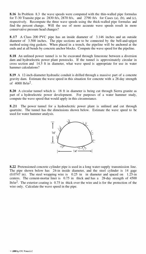
8.21 The power tunnel for a hydroelectric power plant is unlined and cut throughquartzite. The tunnel has the dimensions shown below. Estimate the wave speed to beused for water hammer analysis.

14'

16'

8.22 Pretensioned concrete cylinder pipe is used in a long water-supply transmission line.The pipe shown below has 24-in inside diameter, and the steel cylinder is 14 gage (0.0747 in). The steel wrapping wire is 0.25 in in diameter and spaced on 1.25-incenters. The cement-mortar liner is 0.75 in thick and has a 28-day strength of 4500lb/in2. The exterior coating is 0.75 in thick over the wire and is for the protection of thewire only. Calculate the wave speed in the pipe.

����yyyy

����yyyy

Steel cylinder

Cement mortar liner

Wire wrap 0.25"

0.75"

24"

Exterior coating 1.25" dia.

8.23 A 36-in inside diameter reinforced concrete pipe has steel reinforcing rod wrappedaround the pipe midway within a 4-in wall. The steel rod has an average area of 0.80 in2

per lineal foot of pipe, and each wrap is spaced 3 in on center. Assuming the gasketjoints act as expansion joints, estimate the wave speed in the pipe, both including andexcluding the concrete. The 28-day strength of the concrete is 6000 lb/in2.

8.24 A water project under design will be using embedded-cylinder, prestressed concretepipe. The cylinder is to be fabricated from 10 gage (0.1345 in) steel, and the 7/16-inwire will be wrapped on 1.00-in centers. A sketch of a longitudinal section of the pipe isshown below. All of the concrete in the pipe will have a 28-day strength of 5000 lb/in2.Recommend a wave speed to be used in a water hammer analysis.

��������yyyy����yyyy����yyyy��yyReinforcing wire Shot-coated concrete

protective cover for wire

Steelcylinder

0.75"

2.500"

8.25 A pretensioned 48-inch inside diameter reinforced concrete pipe similar in con-figuration to that of Problem 8.22 is manufactured using a 10 gage (0.1345 inch) steelcylinder wrapped with 0.244-inch diameter steel wire on 1.00-inch centers. The total wallthickness of the pipe is 5.0 inches with a 3.00-inch cement-mortar lining. The cementliner has a 28-day strength of 6000 lb/in2. Assuming the gasket joints act as expansionjoints, calculate the wave speed for the pipe.