�����������������

Citation: Doroszuk, B.; Król, R.

Industry Scale Optimization:

Hammer Crusher and DEM

Simulations. Minerals 2022, 12, 244.

https://doi.org/10.3390/

min12020244

Academic Editor: Rodrigo Magalhães

de Carvalho

Received: 31 December 2021

Accepted: 7 February 2022

Published: 14 February 2022

Publisher’s Note: MDPI stays neutral

with regard to jurisdictional claims in

published maps and institutional affil-

iations.

Copyright: © 2022 by the authors.

Licensee MDPI, Basel, Switzerland.

This article is an open access article

distributed under the terms and

conditions of the Creative Commons

Attribution (CC BY) license (https://

creativecommons.org/licenses/by/

4.0/).

minerals

Article

Industry Scale Optimization: Hammer Crusher andDEM SimulationsBłazej Doroszuk * and Robert Król

Faculty of Geoengineering, Mining and Geology, Wroclaw University of Science and Technology, Na Grobli 15,50-421 Wrocław, Poland; robert.krol@pwr.edu.pl* Correspondence: blazej.doroszuk@pwr.edu.pl

Abstract: The paper shows the preparation of the numerical models necessary for the simulationmapping of industrial-scale crushers of problematic material, such as copper ore with complexlithology. The crushers investigated in this work are located in the KGHM Polska Miedz S.A. copperore processing plant. The complex ore consisting of sandstone, dolomite and shale is modeled usingthe Discrete Element Method (DEM) with Particle Replacement Model (PRM) that was chosen tosimulate the crushing process. The article discusses the tests and calibration of material parametersand proceeds to test a breakage model in a laboratory-scale jaw crusher. The results are finallyvalidated with the data from actual industrial-scale crushers and compared with the simulations. Asan optimization option, the new shape of hammers is proposed and tested in a numerical environment.The performance of the newly designed hammers was examined using numerical methods. Thenumerical tests showed that the new design performed worse than the current solution. As a result,time and money were saved by avoiding industrial tests. In conclusion, the work shows how complexprocesses can be characterized in the numerical environment and used for further analysis.

Keywords: hammer crusher; Discrete Element Method; copper ore; breakage model

1. Introduction

The optimization of various crusher types is very demanding because many factorsinfluence the final product of the crushing process. The feed parameters (grain size, mass,moisture, rock mechanical properties), the method of filling the crusher, the shape of theworking parts, the speed of movement, grate gaps and other parameters all influence theoutput material. In the case of simple crushers, with jaw or cone, where the gap size andthe working frequency can be changed, several mathematical models allow estimations ofthe efficiency and grain size of the crushed product [1–3].

The most important criterion to be considered when designing a crusher is its failure-free operation. Research on copper ore crushers shows that their components are exposedto damage [4], which can be detected by vibration analysis [5,6]. A breaker failure maycause the processing line to stop working or reduce its efficiency [7].

In the case of crushers which employ the collisions rather than the compressionof particles, mathematical modeling of the process has not been a common practice. In-dividual attempts were made [8] mainly to determine how objects disintegrate duringcollisions [9,10]. These models were applied mostly to single particles or in laboratory-scalecrushing [9]. The performance of impact crushers has usually been empirically determined.The literature indicates that a mathematical model was developed in order to describethe efficiency of shaft impact crushers [11]. However, in the case of hammer crushers, theanalysis so far has focused mainly on experiments, most often on a laboratory scale [12] and,in some cases, at an industrial scale, where hammers were analyzed for abrasion [13,14].

Hammer crushers are used in many industries and on different scales [15,16]. In thispublication, the focus will be placed on large-scale hammer crushers used in the mineral

Minerals 2022, 12, 244. https://doi.org/10.3390/min12020244 https://www.mdpi.com/journal/minerals

Minerals 2022, 12, 244 2 of 20

processing industry. Such crushers are usually employed during the first stage of thecomminution of the mined ore performed in the processing plant. Material several dozencentimeters in size can be broken down to tens of millimeters, e.g., in order to prepare it forfurther processing in the mills.

The working part of the hammer crusher—the rotor—is most often made of rounddiscs. The discs are mounted on the axis with spaces preserved between them. Hammersare located around the circumference of the discs. They are installed moveably on mandrelsso as to rotate freely. When the rotor is set in motion, centrifugal force puts hammers inthe working position. On the side opposite to the feeding point, there is a grate whose sizematches the desired size of the crushed product. Crushers also often have liners whichlimit the space between the walls and the rotor so that the crushed material interacts withthe hammers more often.

Copper ore mined in Polish mines operated by KGHM Polska Miedz S.A. is char-acterized by high lithological variability [17]. Depending on the place of extraction, thepercentages of rocks in the ore change. The ore is composed of dolomite, shale and sand-stone. These rocks have different mechanical and strength properties. Therefore, crushersmust be designed to remain operative and operate as efficiently as possible, even when thedominant rock changes in the feed.

The discrete element method (DEM) has been used in the optimization of miningprocesses for several decades [18,19]. Initially, the optimizations were very simplified,but modern computers have enough computing power to allow attempts at simulatinglarge-scale processes [20]. The method of discrete elements enables simulations of boththe behavior of bulk materials and interactions of each particle with other particles andwith the elements of the analyzed system separately. The greater number and the smallersize of the particles, the more computing power is needed to perform the simulation.Crushing models that can be used in a DEM environment have also been developed forsome time [21]. The models are based on various mechanisms, and in this publication weuse the Particle Replacement Model (PRM). The model works in such a way that when thestresses acting on a particle exceed the critical values, the particle is replaced by smallerparticles whose number and size depend on the model input data [22].

While other publications focus on individual stages [8–14,20–22] of preparing or usinga numerical model, this article describes the entire process from its first stage (samplecollection) to its last stage (application of the model). An additional difficulty addressed inthis work and not present in other publications lies in the complexity of the lithology ofthe modeled ore [17], which required the parameterization and the calibration schemes ofnumerical models to be adapted to this specific case. The article also includes a case studyof a specific crusher operating in a processing plant of a copper mine and compares thesimulation results with the data obtained from the mine.

2. Materials and Methods2.1. Rock Samples

Rock samples were collected at the processing plants of KGHM Lubin, Rudna andPolkowice. The material was sampled by a geologist from the technological line. Fromeach region, approximately 90 dm3 of rock material was collected in the form of fragmentsapproximately 0.5–7 dm3 in size. Macroscopic material samples, identified as sandstone,dolomitic shale and dolomite, were collected on an ongoing basis. In most cases, thequalification of the rock material did not raise doubts, except in the cases when some rockfragments showed substantial surface contamination in the form of dust and sticky dampsilty-clay mixture.

As part of the preliminary laboratory work, after washing the surfaces of individualrock fragments, their detailed lithological description was made, followed by the finalpetrographic identification (Figure 1). The individual samples (rock fragments) were thenincluded in the classes listed in Table 1.

Minerals 2022, 12, 244 3 of 20

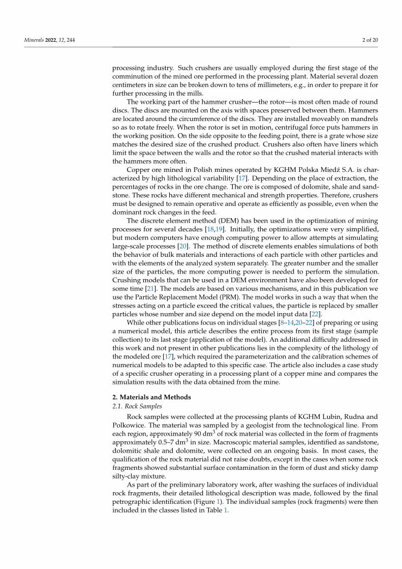
Of all the samples, the material from the Rudna region was characterized by thegreatest diversity. During the macroscopic diagnosis, four different types of sandstonewere distinguished: weathered, coarse-grained, fine-grained as well as a certain type ofsandstone being probably a transitional form with shale. In the samples from the Polkowiceregion, two varieties of sandstone were observed, differing in firmness. In contrast, therewas only one variety in the samples of sandstone collected in the Lubin region.

Figure 1. Collected samples.

Table 1. Rock classes.

Rock\Region Rudna Polkowice Lubin

Dolomite - Calcitic dolomite - Calcitic dolomite - Calcitic dolomite- Limestone dolomite - Limestone dolomite - Limestone dolomite

Shale - Clay-dolomitic shale - Dolomitic shale - Dolomitic shale- Dolomitic shale

Sandstone

- Sandstone 1 - Sandstone 1- Sandstone- Sandstone 2

- Sandstone 3 - Sandstone 2- Sandstone 4

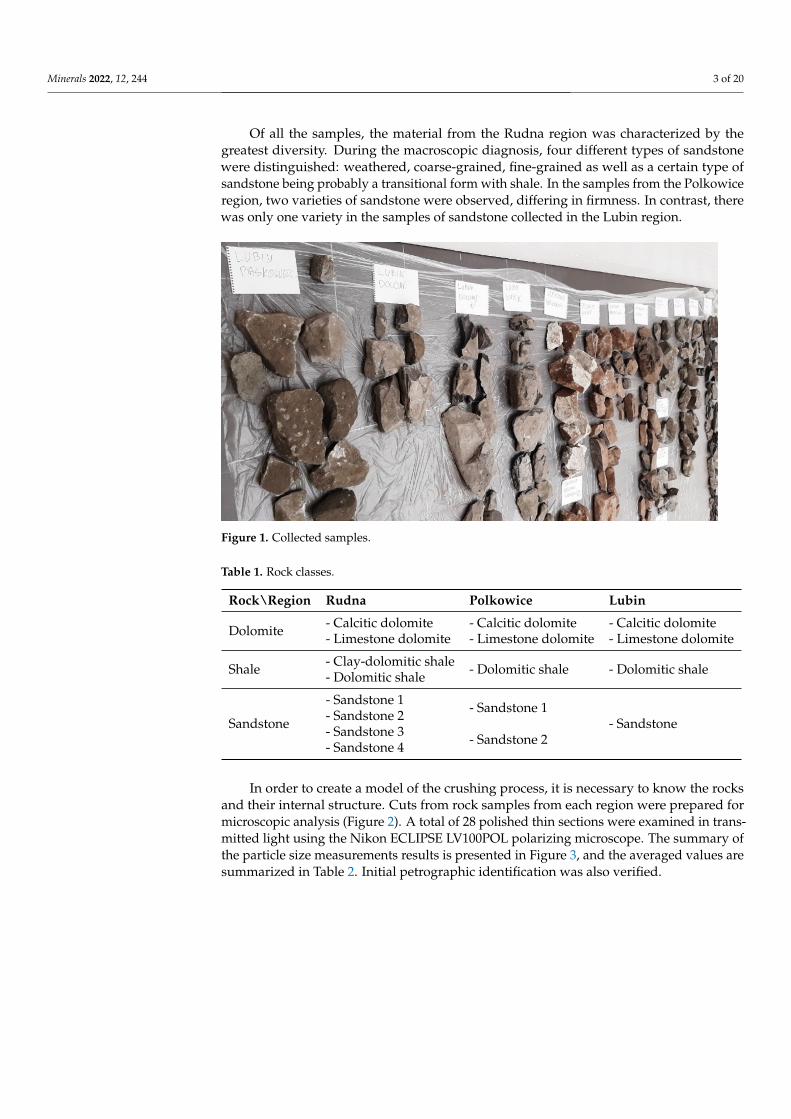
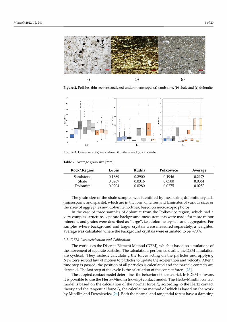
In order to create a model of the crushing process, it is necessary to know the rocksand their internal structure. Cuts from rock samples from each region were prepared formicroscopic analysis (Figure 2). A total of 28 polished thin sections were examined in trans-mitted light using the Nikon ECLIPSE LV100POL polarizing microscope. The summary ofthe particle size measurements results is presented in Figure 3, and the averaged values aresummarized in Table 2. Initial petrographic identification was also verified.

Minerals 2022, 12, 244 4 of 20

Figure 2. Polishes thin sections analyzed under microscope: (a) sandstone, (b) shale and (c) dolomite.

Figure 3. Grain size: (a) sandstone, (b) shale and (c) dolomite.

Table 2. Average grain size [mm].

Rock\Region Lubin Rudna Polkowice Average

Sandstone 0.1689 0.2900 0.1946 0.2178Shale 0.0267 0.0316 0.0500 0.0361

Dolomite 0.0204 0.0280 0.0275 0.0253

The grain size of the shale samples was identified by measuring dolomite crystals(microsparite and sparite), which are in the form of lenses and laminates of various sizes orthe sizes of aggregates and dolomite nodules, based on microscopic photos.

In the case of three samples of dolomite from the Polkowice region, which had avery complex structure, separate background measurements were made for more minorminerals, and grains were described as “large”, i.e., dolomite crystals and aggregates. Forsamples where background and larger crystals were measured separately, a weightedaverage was calculated where the background crystals were estimated to be ~70%.

2.2. DEM Parametrization and Calibration

The work uses the Discrete Element Method (DEM), which is based on simulations ofthe movement of separate particles. The calculations performed during the DEM simulationare cyclical. They include calculating the forces acting on the particles and applyingNewton’s second law of motion to particles to update the acceleration and velocity. After atime step is passed, the position of all particles is calculated and the particle contacts aredetected. The last step of the cycle is the calculation of the contact forces [23].

The adopted contact model determines the behavior of the material. In EDEM software,it is possible to use the Hertz–Mindlin (no-slip) contact model. The Hertz–Mindlin contactmodel is based on the calculation of the normal force Fn according to the Hertz contacttheory and the tangential force Ft, the calculation method of which is based on the workby Mindlin and Deresiewicz [24]. Both the normal and tangential forces have a damping

Minerals 2022, 12, 244 5 of 20

component [25], which is related to the restitution coefficient [26]. The tangential frictionforce is based on Coulomb’s laws of friction [25].

The selection of an appropriately small time step is crucial because if a step greater thanthe critical time step is assumed, it may lead to errors [27]. The value of the critical time stepis influenced by the particle size, density and deformation parameters. Many researchersartificially lower the value of the Kirchhoff modulus to shorten the time required to performthe simulation.

When preparing a simulation with discrete elements, two components can be distin-guished: particles and geometries. Particles are represented by shape, complexity, momentsof inertia as well as mass and volume. The most important parameters characterizingthe particles and geometries include Poisson’s ratio, density and Kirchhoff’s modulusinterchangeably with Young’s modulus. The most difficult values to choose are the coeffi-cients that characterize the interactions of the particles with the materials of the geometryelements and the interactions of the particles with each other. The creation of a contactmodel requires three coefficients: restitution, characterizing the loss of velocity after acollision, as well as static and rolling friction. The ore is a mixture of different rocks withdifferent material parameters. Therefore, it is impossible to determine the parameters moreprecisely than with respect to their ranges or average values.

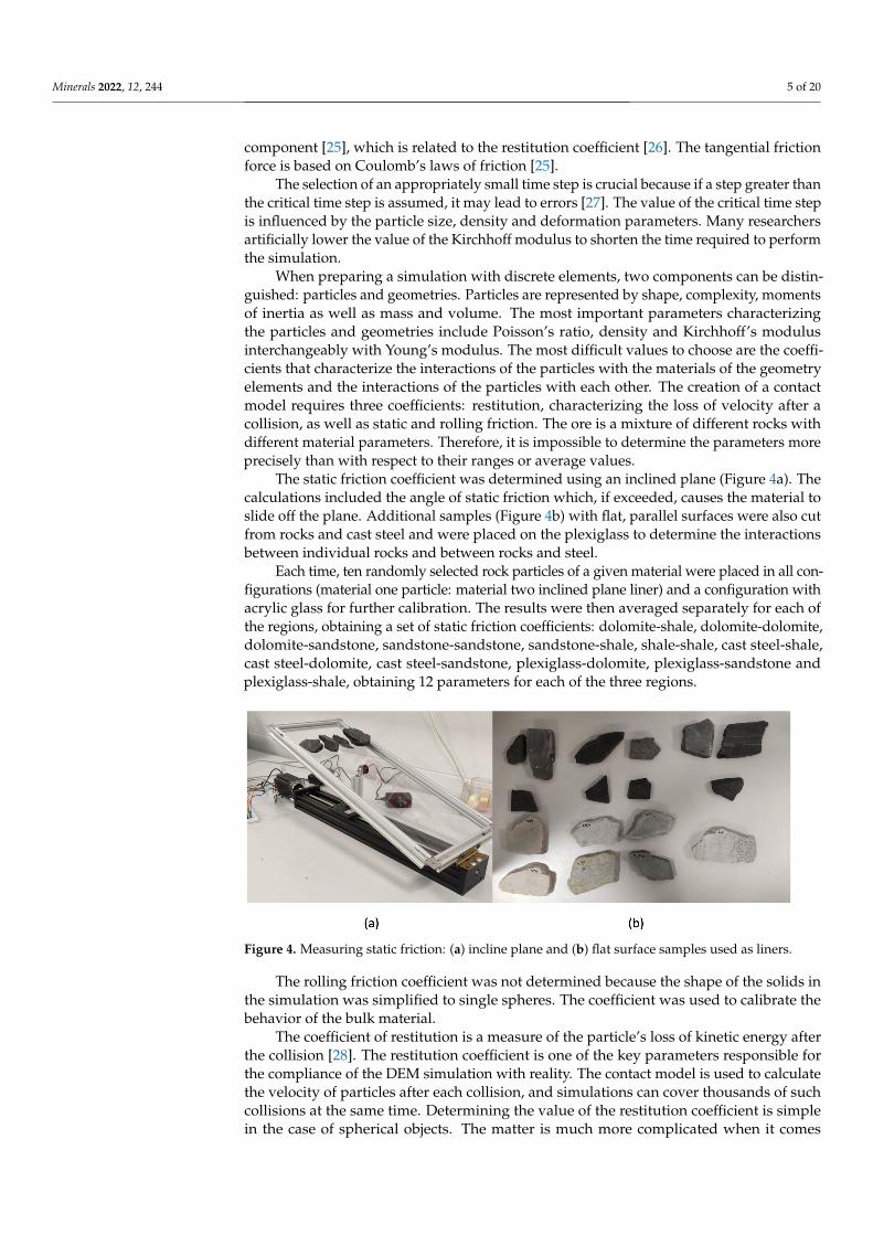
The static friction coefficient was determined using an inclined plane (Figure 4a). Thecalculations included the angle of static friction which, if exceeded, causes the material toslide off the plane. Additional samples (Figure 4b) with flat, parallel surfaces were also cutfrom rocks and cast steel and were placed on the plexiglass to determine the interactionsbetween individual rocks and between rocks and steel.

Each time, ten randomly selected rock particles of a given material were placed in all con-figurations (material one particle: material two inclined plane liner) and a configuration withacrylic glass for further calibration. The results were then averaged separately for each ofthe regions, obtaining a set of static friction coefficients: dolomite-shale, dolomite-dolomite,dolomite-sandstone, sandstone-sandstone, sandstone-shale, shale-shale, cast steel-shale,cast steel-dolomite, cast steel-sandstone, plexiglass-dolomite, plexiglass-sandstone andplexiglass-shale, obtaining 12 parameters for each of the three regions.

Figure 4. Measuring static friction: (a) incline plane and (b) flat surface samples used as liners.

The rolling friction coefficient was not determined because the shape of the solids inthe simulation was simplified to single spheres. The coefficient was used to calibrate thebehavior of the bulk material.

The coefficient of restitution is a measure of the particle’s loss of kinetic energy afterthe collision [28]. The restitution coefficient is one of the key parameters responsible forthe compliance of the DEM simulation with reality. The contact model is used to calculatethe velocity of particles after each collision, and simulations can cover thousands of suchcollisions at the same time. Determining the value of the restitution coefficient is simplein the case of spherical objects. The matter is much more complicated when it comes

Minerals 2022, 12, 244 6 of 20

to irregularly shaped particles, as in the case of the material excavated from the mine.Irregularly shaped particles behave unpredictably after a collision and have a moment ofinertia that is difficult to determine.

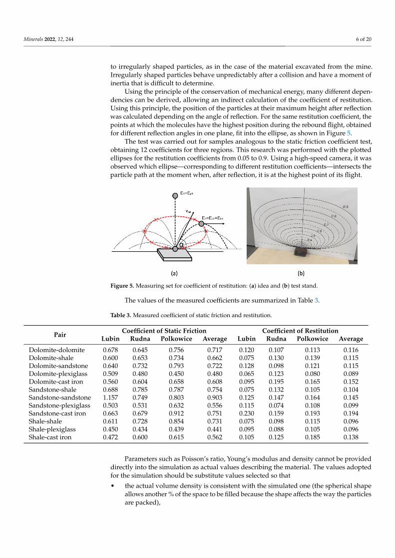
Using the principle of the conservation of mechanical energy, many different depen-dencies can be derived, allowing an indirect calculation of the coefficient of restitution.Using this principle, the position of the particles at their maximum height after reflectionwas calculated depending on the angle of reflection. For the same restitution coefficient, thepoints at which the molecules have the highest position during the rebound flight, obtainedfor different reflection angles in one plane, fit into the ellipse, as shown in Figure 5.

The test was carried out for samples analogous to the static friction coefficient test,obtaining 12 coefficients for three regions. This research was performed with the plottedellipses for the restitution coefficients from 0.05 to 0.9. Using a high-speed camera, it wasobserved which ellipse—corresponding to different restitution coefficients—intersects theparticle path at the moment when, after reflection, it is at the highest point of its flight.

Figure 5. Measuring set for coefficient of restitution: (a) idea and (b) test stand.

The values of the measured coefficients are summarized in Table 3.

Table 3. Measured coefficient of static friction and restitution.

Pair Coefficient of Static Friction Coefficient of RestitutionLubin Rudna Polkowice Average Lubin Rudna Polkowice Average

Dolomite-dolomite 0.678 0.645 0.756 0.717 0.120 0.107 0.113 0.116Dolomite-shale 0.600 0.653 0.734 0.662 0.075 0.130 0.139 0.115Dolomite-sandstone 0.640 0.732 0.793 0.722 0.128 0.098 0.121 0.115Dolomite-plexiglass 0.509 0.480 0.450 0.480 0.065 0.123 0.080 0.089Dolomite-cast iron 0.560 0.604 0.658 0.608 0.095 0.195 0.165 0.152Sandstone-shale 0.688 0.785 0.787 0.754 0.075 0.132 0.105 0.104Sandstone-sandstone 1.157 0.749 0.803 0.903 0.125 0.147 0.164 0.145Sandstone-plexiglass 0.503 0.531 0.632 0.556 0.115 0.074 0.108 0.099Sandstone-cast iron 0.663 0.679 0.912 0.751 0.230 0.159 0.193 0.194Shale-shale 0.611 0.728 0.854 0.731 0.075 0.098 0.115 0.096Shale-plexiglass 0.450 0.434 0.439 0.441 0.095 0.088 0.105 0.096Shale-cast iron 0.472 0.600 0.615 0.562 0.105 0.125 0.185 0.138

Parameters such as Poisson’s ratio, Young’s modulus and density cannot be provideddirectly into the simulation as actual values describing the material. The values adoptedfor the simulation should be substitute values selected so that

• the actual volume density is consistent with the simulated one (the spherical shapeallows another % of the space to be filled because the shape affects the way the particlesare packed),

Minerals 2022, 12, 244 7 of 20

• the forces obtained during the simulation correspond to the real forces transmittedby the particles (for this purpose, the test of uniaxial compression of particles in thecylinder is used) and

• the time step is not too small because Young’s modulus influences the necessary timestep in the simulation to the greatest extent (therefore, the smallest possible Young’smodulus is selected, which ensures a stable simulation and allows a reliable simulationof forces transmitted by particles).

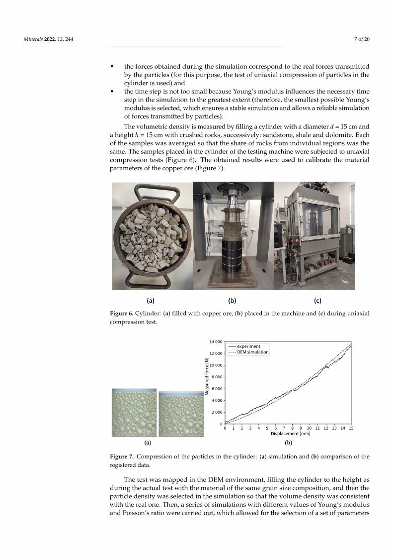
The volumetric density is measured by filling a cylinder with a diameter d = 15 cm anda height h = 15 cm with crushed rocks, successively: sandstone, shale and dolomite. Eachof the samples was averaged so that the share of rocks from individual regions was thesame. The samples placed in the cylinder of the testing machine were subjected to uniaxialcompression tests (Figure 6). The obtained results were used to calibrate the materialparameters of the copper ore (Figure 7).

Figure 6. Cylinder: (a) filled with copper ore, (b) placed in the machine and (c) during uniaxialcompression test.

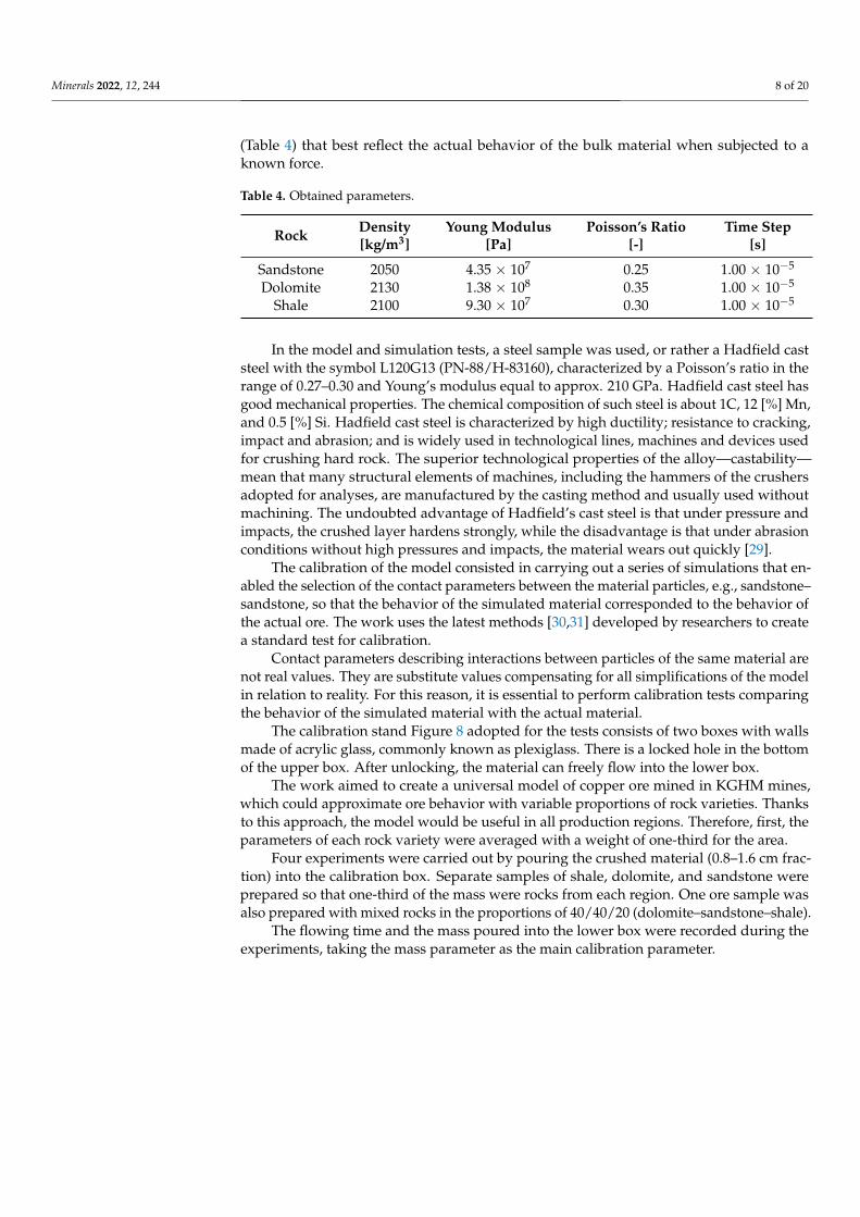
Figure 7. Compression of the particles in the cylinder: (a) simulation and (b) comparison of theregistered data.

The test was mapped in the DEM environment, filling the cylinder to the height asduring the actual test with the material of the same grain size composition, and then theparticle density was selected in the simulation so that the volume density was consistentwith the real one. Then, a series of simulations with different values of Young’s modulusand Poisson’s ratio were carried out, which allowed for the selection of a set of parameters

Minerals 2022, 12, 244 8 of 20

(Table 4) that best reflect the actual behavior of the bulk material when subjected to aknown force.

Table 4. Obtained parameters.

Rock Density Young Modulus Poisson’s Ratio Time Step[kg/m3] [Pa] [-] [s]

Sandstone 2050 4.35 × 107 0.25 1.00 × 10−5

Dolomite 2130 1.38 × 108 0.35 1.00 × 10−5

Shale 2100 9.30 × 107 0.30 1.00 × 10−5

In the model and simulation tests, a steel sample was used, or rather a Hadfield caststeel with the symbol L120G13 (PN-88/H-83160), characterized by a Poisson’s ratio in therange of 0.27–0.30 and Young’s modulus equal to approx. 210 GPa. Hadfield cast steel hasgood mechanical properties. The chemical composition of such steel is about 1C, 12 [%] Mn,and 0.5 [%] Si. Hadfield cast steel is characterized by high ductility; resistance to cracking,impact and abrasion; and is widely used in technological lines, machines and devices usedfor crushing hard rock. The superior technological properties of the alloy—castability—mean that many structural elements of machines, including the hammers of the crushersadopted for analyses, are manufactured by the casting method and usually used withoutmachining. The undoubted advantage of Hadfield’s cast steel is that under pressure andimpacts, the crushed layer hardens strongly, while the disadvantage is that under abrasionconditions without high pressures and impacts, the material wears out quickly [29].

The calibration of the model consisted in carrying out a series of simulations that en-abled the selection of the contact parameters between the material particles, e.g., sandstone–sandstone, so that the behavior of the simulated material corresponded to the behavior ofthe actual ore. The work uses the latest methods [30,31] developed by researchers to createa standard test for calibration.

Contact parameters describing interactions between particles of the same material arenot real values. They are substitute values compensating for all simplifications of the modelin relation to reality. For this reason, it is essential to perform calibration tests comparingthe behavior of the simulated material with the actual material.

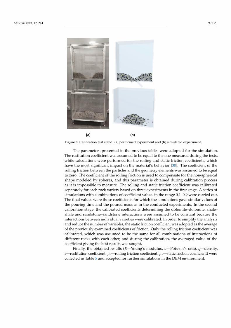
The calibration stand Figure 8 adopted for the tests consists of two boxes with wallsmade of acrylic glass, commonly known as plexiglass. There is a locked hole in the bottomof the upper box. After unlocking, the material can freely flow into the lower box.

The work aimed to create a universal model of copper ore mined in KGHM mines,which could approximate ore behavior with variable proportions of rock varieties. Thanksto this approach, the model would be useful in all production regions. Therefore, first, theparameters of each rock variety were averaged with a weight of one-third for the area.

Four experiments were carried out by pouring the crushed material (0.8–1.6 cm frac-tion) into the calibration box. Separate samples of shale, dolomite, and sandstone wereprepared so that one-third of the mass were rocks from each region. One ore sample wasalso prepared with mixed rocks in the proportions of 40/40/20 (dolomite–sandstone–shale).

The flowing time and the mass poured into the lower box were recorded during theexperiments, taking the mass parameter as the main calibration parameter.

Minerals 2022, 12, 244 9 of 20

Figure 8. Calibration test stand: (a) performed experiment and (b) simulated experiment.

The parameters presented in the previous tables were adopted for the simulation.The restitution coefficient was assumed to be equal to the one measured during the tests,while calculations were performed for the rolling and static friction coefficients, whichhave the most significant impact on the material’s behavior [30]. The coefficient of therolling friction between the particles and the geometry elements was assumed to be equalto zero. The coefficient of the rolling friction is used to compensate for the non-sphericalshape modeled by spheres, and this parameter is obtained during calibration processas it is impossible to measure. The rolling and static friction coefficient was calibratedseparately for each rock variety based on three experiments in the first stage. A series ofsimulations with combinations of coefficient values in the range 0.1–0.9 were carried out.The final values were those coefficients for which the simulations gave similar values ofthe pouring time and the poured mass as in the conducted experiments. In the secondcalibration stage, the calibrated coefficients determining the dolomite–dolomite, shale–shale and sandstone–sandstone interactions were assumed to be constant because theinteractions between individual varieties were calibrated. In order to simplify the analysisand reduce the number of variables, the static friction coefficient was adopted as the averageof the previously examined coefficients of friction. Only the rolling friction coefficient wascalibrated, which was assumed to be the same for all combinations of interactions ofdifferent rocks with each other, and during the calibration, the averaged value of thecoefficient giving the best results was sought.

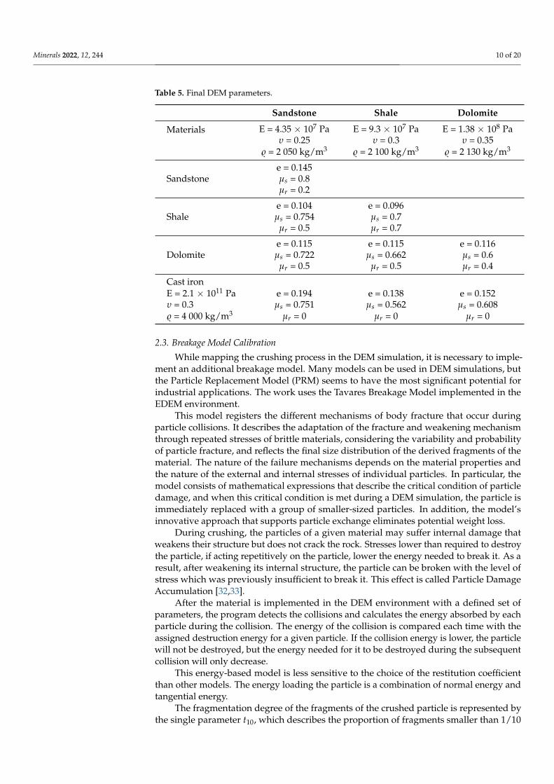
Finally, the obtained results (E—Young’s modulus, υ—Poisson’s ratio, $—density,e—restitution coefficient, µr—rolling friction coefficient, µs—static friction coefficient) werecollected in Table 5 and accepted for further simulations in the DEM environment.

Minerals 2022, 12, 244 10 of 20

Table 5. Final DEM parameters.

Materials

Sandstone Shale Dolomite

E = 4.35 × 107 Pa E = 9.3 × 107 Pa E = 1.38 × 108 Paυ = 0.25 υ = 0.3 υ = 0.35

$ = 2 050 kg/m3 $ = 2 100 kg/m3 $ = 2 130 kg/m3

Sandstonee = 0.145µs = 0.8µr = 0.2

Shalee = 0.104 e = 0.096µs = 0.754 µs = 0.7

µr = 0.5 µr = 0.7

Dolomitee = 0.115 e = 0.115 e = 0.116µs = 0.722 µs = 0.662 µs = 0.6

µr = 0.5 µr = 0.5 µr = 0.4

Cast ironE = 2.1 × 1011 Pa e = 0.194 e = 0.138 e = 0.152υ = 0.3 µs = 0.751 µs = 0.562 µs = 0.608$ = 4 000 kg/m3 µr = 0 µr = 0 µr = 0

2.3. Breakage Model Calibration

While mapping the crushing process in the DEM simulation, it is necessary to imple-ment an additional breakage model. Many models can be used in DEM simulations, butthe Particle Replacement Model (PRM) seems to have the most significant potential forindustrial applications. The work uses the Tavares Breakage Model implemented in theEDEM environment.

This model registers the different mechanisms of body fracture that occur duringparticle collisions. It describes the adaptation of the fracture and weakening mechanismthrough repeated stresses of brittle materials, considering the variability and probabilityof particle fracture, and reflects the final size distribution of the derived fragments of thematerial. The nature of the failure mechanisms depends on the material properties andthe nature of the external and internal stresses of individual particles. In particular, themodel consists of mathematical expressions that describe the critical condition of particledamage, and when this critical condition is met during a DEM simulation, the particle isimmediately replaced with a group of smaller-sized particles. In addition, the model’sinnovative approach that supports particle exchange eliminates potential weight loss.

During crushing, the particles of a given material may suffer internal damage thatweakens their structure but does not crack the rock. Stresses lower than required to destroythe particle, if acting repetitively on the particle, lower the energy needed to break it. As aresult, after weakening its internal structure, the particle can be broken with the level ofstress which was previously insufficient to break it. This effect is called Particle DamageAccumulation [32,33].

After the material is implemented in the DEM environment with a defined set ofparameters, the program detects the collisions and calculates the energy absorbed by eachparticle during the collision. The energy of the collision is compared each time with theassigned destruction energy for a given particle. If the collision energy is lower, the particlewill not be destroyed, but the energy needed for it to be destroyed during the subsequentcollision will only decrease.

This energy-based model is less sensitive to the choice of the restitution coefficientthan other models. The energy loading the particle is a combination of normal energy andtangential energy.

The fragmentation degree of the fragments of the crushed particle is represented bythe single parameter t10, which describes the proportion of fragments smaller than 1/10

Minerals 2022, 12, 244 11 of 20

of the original particle. Derived particles are virtually packed in the mother particle tooverlap to some extent, and when the particle is affected by the destructive energy E f , thederived fragments replace the original particle.

The forces acting on the particles in DEM algorithms depend on the degree of overlap-ping of the spheres, and to avoid the formation of unnaturally large forces when replacingthe particles, when these may overlap, global damping strength, global damping time andlocal damping strength are used. These parameters are responsible for reducing the totalforce acting on the derived particles for a specified period, and local attenuation determineswhat part of the energy after the collision is transferred to the derived particles. Correctselection of these parameters is essential for the particles subjected to unrealistic forcesresulting from the extensive overlapping of spheres to not reach very high speeds.

Each particle has specific destructive energy assigned on the basis of its size, averagedestructive energy, and standard deviation. This energy will change depending on thedistribution described by the equation [32,34]:

P(E) = 1/2[1 + er f (ln E∗ − ln E50/√

2σ)] (1)

E∗ = EmaxE/Emax − E (2)

where E—distribution of fracture energy [J/kg], Emax—the value of the upper limit of thefracture energy distribution [J/kg], E50—distribution median [J/kg] and σ—distributionstandard deviation [-].

The median fracture energy is given by the equation

E50 = E∞/(1 + kp/kst ) [1 + (d0/dp )ϕ ] (3)

where E∞,ϕ—parameters adjusted to the measurement data [J/kg][-], kn, kst—particle andsteel hardness [GPa], dp—representative particle size [mm] and d0—the characteristic grainsize in the rock [mm].

When the particle is not destroyed, a new destructive energy is calculated fromthe relationship

E′f = E f (1− D) (4)

D = [(2γ/(2γ− 5D + 5))(eEk/E f )]2γ/5 (5)

where E f —fracture energy for a specific particle [J], eEk—effective collision energy [J] andγ—damage accumulation factor [-].

The Tavares crushing model is mainly based on the most crucial parameter, t10,described by the equation

t10 = A[1− exp(−b(eEk)/E f )] (6)

where A, b—parameters adjusted to the measurement data [-], E f —fracture energy for aspecific particle [J] and eEk—damage accumulation factor [J].

The larger the t10 value is, the finer the derived particles will be. The grain sizedistribution of the derived grains in the model is based on the standard distributionsdeveloped by Tavares in numerous papers [35,36] and is matched to the t10 value calculatedby the algorithm when replacing the mother particle with derivative particles.

In order to eliminate particle mass losses due to the lack of simulated tiniest fractionsafter fragmentation, which are often dust, the model includes the so-called “dummyparticles”—particles representing the total mass of the tiniest fractions that could not beformed during the breakdown of the parent particle because they were too small. Theseparticles are no longer subject to further degradation and will be treated in the furtheranalysis as part of the tiniest fraction considered.

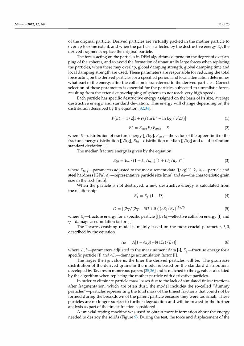
A uniaxial testing machine was used to obtain more information about the energyneeded to destroy the solids (Figure 9). During the test, the force and displacement of the

Minerals 2022, 12, 244 12 of 20

piston were recorded, enabling the determining of the work performed by the machinedestroying the sample, which was equal to the energy of destruction. The total energysupplied to the sample during the test was also determined.

Figure 9. Destroying particles in uniaxial testing: (a) sample during test and (b) registered data.

Rock samples weighing from 250 g to 5 kg were used for the study. Initially, rocksamples randomly selected from among the entire sample set were subjected to uniaxialcompression, and then all fragments formed after destruction and having a mass greaterthan 250 g were compressed once again. The destruction processes of the sample and itsfragments were repeated until all of the particles were reduced to less than 250 g. Afterthe destruction process, the samples were screened and the particle size composition wasdetermined. The fragments that weighed more than 10% of the parent particle were fewand easy to identify. Their mass was measured each time. Composition of the derivedfragments is needed because during the crushing process in the crusher, the rocks arebroken not once, but many times, until the desired size is reached.

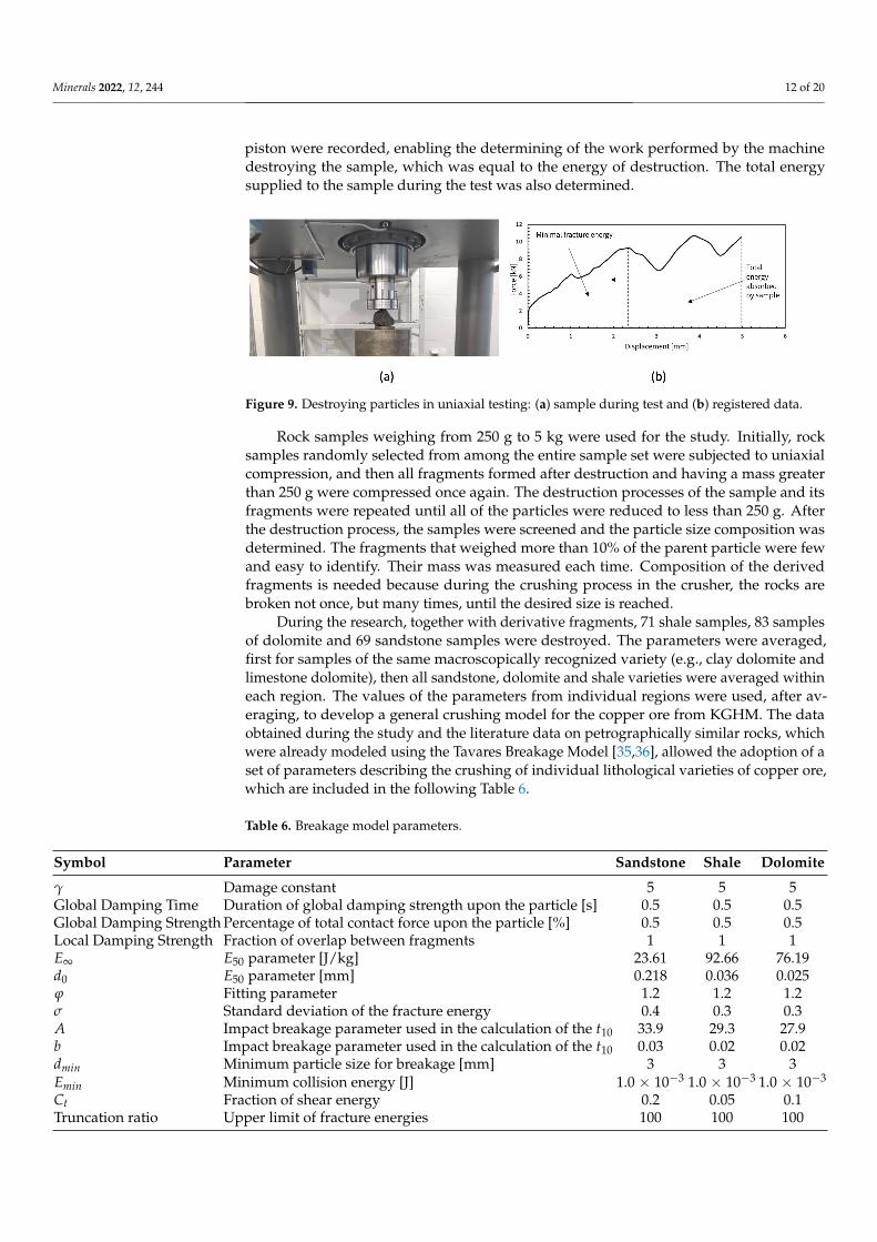
During the research, together with derivative fragments, 71 shale samples, 83 samplesof dolomite and 69 sandstone samples were destroyed. The parameters were averaged,first for samples of the same macroscopically recognized variety (e.g., clay dolomite andlimestone dolomite), then all sandstone, dolomite and shale varieties were averaged withineach region. The values of the parameters from individual regions were used, after av-eraging, to develop a general crushing model for the copper ore from KGHM. The dataobtained during the study and the literature data on petrographically similar rocks, whichwere already modeled using the Tavares Breakage Model [35,36], allowed the adoption of aset of parameters describing the crushing of individual lithological varieties of copper ore,which are included in the following Table 6.

Table 6. Breakage model parameters.

Symbol Parameter Sandstone Shale Dolomite

γ Damage constant 5 5 5Global Damping Time Duration of global damping strength upon the particle [s] 0.5 0.5 0.5Global Damping Strength Percentage of total contact force upon the particle [%] 0.5 0.5 0.5Local Damping Strength Fraction of overlap between fragments 1 1 1E∞ E50 parameter [J/kg] 23.61 92.66 76.19d0 E50 parameter [mm] 0.218 0.036 0.025ϕ Fitting parameter 1.2 1.2 1.2σ Standard deviation of the fracture energy 0.4 0.3 0.3A Impact breakage parameter used in the calculation of the t10 33.9 29.3 27.9b Impact breakage parameter used in the calculation of the t10 0.03 0.02 0.02dmin Minimum particle size for breakage [mm] 3 3 3Emin Minimum collision energy [J] 1.0 × 10−3 1.0 × 10−3 1.0 × 10−3

Ct Fraction of shear energy 0.2 0.05 0.1Truncation ratio Upper limit of fracture energies 100 100 100

Minerals 2022, 12, 244 13 of 20

3. Results of Numerical Analyses3.1. Laboratory Scale

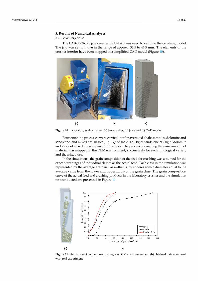
The LAB-03-260/S jaw crusher EKO-LAB was used to validate the crushing model.The jaw was set to move in the range of approx. 32.5 to 46.5 mm. The elements of thecrusher interior have been mapped in a simplified CAD model (Figure 10).

Figure 10. Laboratory scale crusher: (a) jaw crusher, (b) jaws and (c) CAD model.

Four crushing processes were carried out for averaged shale samples, dolomite andsandstone, and mixed ore. In total, 15.1 kg of shale, 12.2 kg of sandstone, 9.2 kg of dolomiteand 25 kg of mixed ore were used for the tests. The process of crushing the same amount ofmaterial was mapped in the DEM environment, successively for each lithological varietyand the mixed ore.

In the simulations, the grain composition of the feed for crushing was assumed for theexact percentages of individual classes as the actual feed. Each class in the simulation wasrepresented by the average grain in class—that is, by spheres with a diameter equal to theaverage value from the lower and upper limits of the grain class. The grain compositioncurve of the actual feed and crushing products in the laboratory crusher and the simulationtest conducted are presented in Figure 11.

Figure 11. Simulation of copper ore crushing: (a) DEM environment and (b) obtained data comparedwith real experiment.

Minerals 2022, 12, 244 14 of 20

The similarity of the grain curves for both the simulated and the actual crushed prod-ucts, obtained for identical technical and technological parameters (adopted for crushing inlaboratory conditions), confirmed that multiparametric DEMs and PRMs of copper ore canbe potentially used to map the process with sufficient accuracy.

3.2. Industrial Crushers

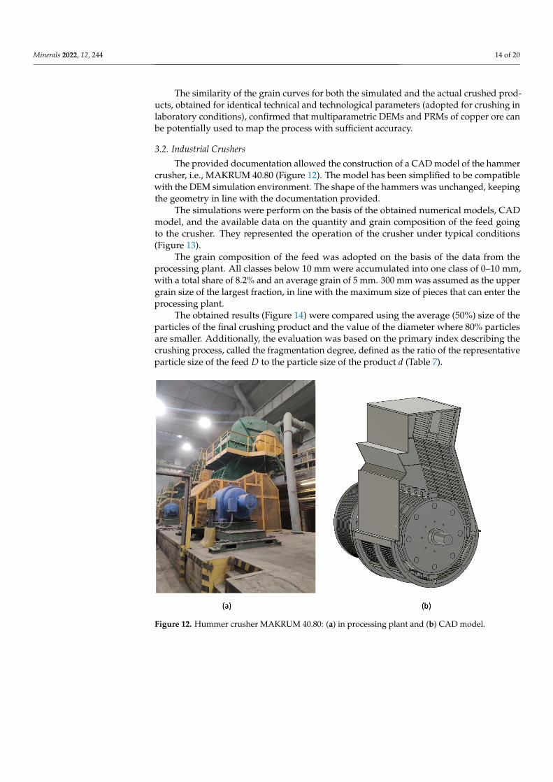
The provided documentation allowed the construction of a CAD model of the hammercrusher, i.e., MAKRUM 40.80 (Figure 12). The model has been simplified to be compatiblewith the DEM simulation environment. The shape of the hammers was unchanged, keepingthe geometry in line with the documentation provided.

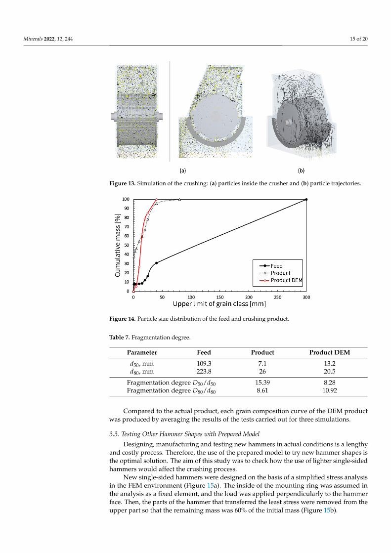
The simulations were perform on the basis of the obtained numerical models, CADmodel, and the available data on the quantity and grain composition of the feed goingto the crusher. They represented the operation of the crusher under typical conditions(Figure 13).

The grain composition of the feed was adopted on the basis of the data from theprocessing plant. All classes below 10 mm were accumulated into one class of 0–10 mm,with a total share of 8.2% and an average grain of 5 mm. 300 mm was assumed as the uppergrain size of the largest fraction, in line with the maximum size of pieces that can enter theprocessing plant.

The obtained results (Figure 14) were compared using the average (50%) size of theparticles of the final crushing product and the value of the diameter where 80% particlesare smaller. Additionally, the evaluation was based on the primary index describing thecrushing process, called the fragmentation degree, defined as the ratio of the representativeparticle size of the feed D to the particle size of the product d (Table 7).

Figure 12. Hummer crusher MAKRUM 40.80: (a) in processing plant and (b) CAD model.

Minerals 2022, 12, 244 15 of 20

Figure 13. Simulation of the crushing: (a) particles inside the crusher and (b) particle trajectories.

Figure 14. Particle size distribution of the feed and crushing product.

Table 7. Fragmentation degree.

Parameter Feed Product Product DEM

d50, mm 109.3 7.1 13.2d80, mm 223.8 26 20.5

Fragmentation degree D50/d50 15.39 8.28Fragmentation degree D80/d80 8.61 10.92

Compared to the actual product, each grain composition curve of the DEM productwas produced by averaging the results of the tests carried out for three simulations.

3.3. Testing Other Hammer Shapes with Prepared Model

Designing, manufacturing and testing new hammers in actual conditions is a lengthyand costly process. Therefore, the use of the prepared model to try new hammer shapes isthe optimal solution. The aim of this study was to check how the use of lighter single-sidedhammers would affect the crushing process.

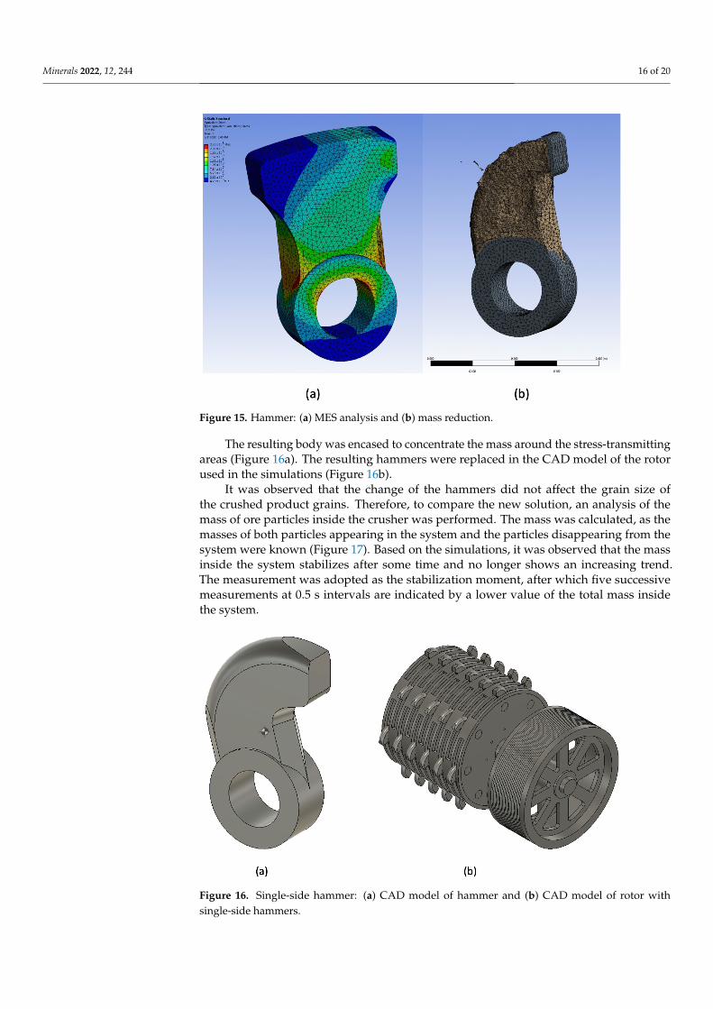
New single-sided hammers were designed on the basis of a simplified stress analysisin the FEM environment (Figure 15a). The inside of the mounting ring was assumed inthe analysis as a fixed element, and the load was applied perpendicularly to the hammerface. Then, the parts of the hammer that transferred the least stress were removed from theupper part so that the remaining mass was 60% of the initial mass (Figure 15b).

Minerals 2022, 12, 244 16 of 20

Figure 15. Hammer: (a) MES analysis and (b) mass reduction.

The resulting body was encased to concentrate the mass around the stress-transmittingareas (Figure 16a). The resulting hammers were replaced in the CAD model of the rotorused in the simulations (Figure 16b).

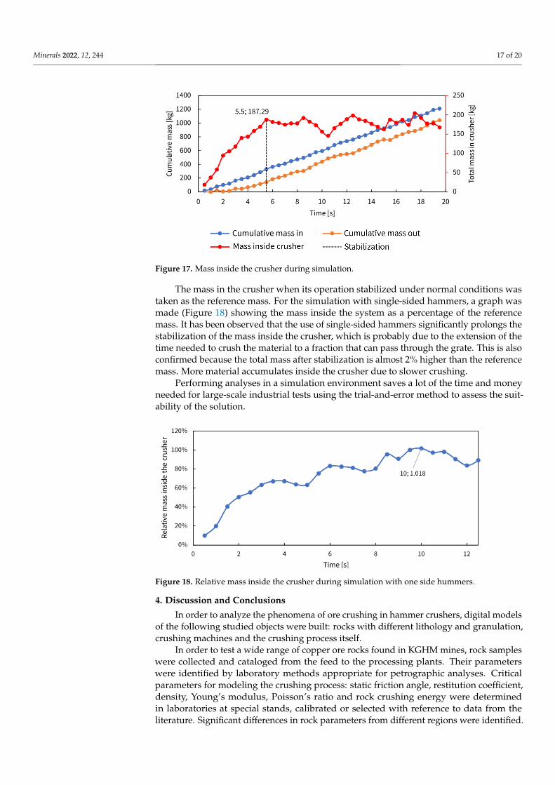
It was observed that the change of the hammers did not affect the grain size ofthe crushed product grains. Therefore, to compare the new solution, an analysis of themass of ore particles inside the crusher was performed. The mass was calculated, as themasses of both particles appearing in the system and the particles disappearing from thesystem were known (Figure 17). Based on the simulations, it was observed that the massinside the system stabilizes after some time and no longer shows an increasing trend.The measurement was adopted as the stabilization moment, after which five successivemeasurements at 0.5 s intervals are indicated by a lower value of the total mass insidethe system.

Figure 16. Single-side hammer: (a) CAD model of hammer and (b) CAD model of rotor withsingle-side hammers.

Minerals 2022, 12, 244 17 of 20

Figure 17. Mass inside the crusher during simulation.

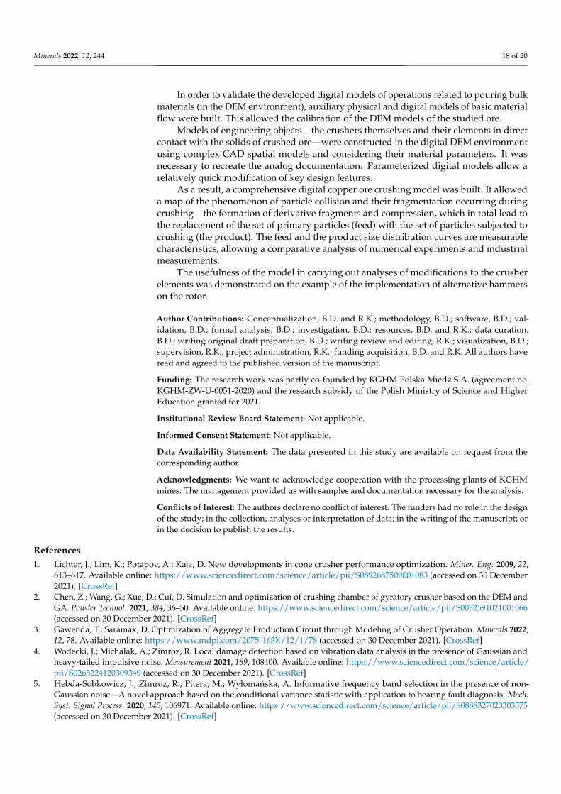
The mass in the crusher when its operation stabilized under normal conditions wastaken as the reference mass. For the simulation with single-sided hammers, a graph wasmade (Figure 18) showing the mass inside the system as a percentage of the referencemass. It has been observed that the use of single-sided hammers significantly prolongs thestabilization of the mass inside the crusher, which is probably due to the extension of thetime needed to crush the material to a fraction that can pass through the grate. This is alsoconfirmed because the total mass after stabilization is almost 2% higher than the referencemass. More material accumulates inside the crusher due to slower crushing.

Performing analyses in a simulation environment saves a lot of the time and moneyneeded for large-scale industrial tests using the trial-and-error method to assess the suit-ability of the solution.

Figure 18. Relative mass inside the crusher during simulation with one side hummers.

4. Discussion and Conclusions

In order to analyze the phenomena of ore crushing in hammer crushers, digital modelsof the following studied objects were built: rocks with different lithology and granulation,crushing machines and the crushing process itself.

In order to test a wide range of copper ore rocks found in KGHM mines, rock sampleswere collected and cataloged from the feed to the processing plants. Their parameterswere identified by laboratory methods appropriate for petrographic analyses. Criticalparameters for modeling the crushing process: static friction angle, restitution coefficient,density, Young’s modulus, Poisson’s ratio and rock crushing energy were determinedin laboratories at special stands, calibrated or selected with reference to data from theliterature. Significant differences in rock parameters from different regions were identified.

Minerals 2022, 12, 244 18 of 20

In order to validate the developed digital models of operations related to pouring bulkmaterials (in the DEM environment), auxiliary physical and digital models of basic materialflow were built. This allowed the calibration of the DEM models of the studied ore.

Models of engineering objects—the crushers themselves and their elements in directcontact with the solids of crushed ore—were constructed in the digital DEM environmentusing complex CAD spatial models and considering their material parameters. It wasnecessary to recreate the analog documentation. Parameterized digital models allow arelatively quick modification of key design features.

As a result, a comprehensive digital copper ore crushing model was built. It alloweda map of the phenomenon of particle collision and their fragmentation occurring duringcrushing—the formation of derivative fragments and compression, which in total lead tothe replacement of the set of primary particles (feed) with the set of particles subjected tocrushing (the product). The feed and the product size distribution curves are measurablecharacteristics, allowing a comparative analysis of numerical experiments and industrialmeasurements.

The usefulness of the model in carrying out analyses of modifications to the crusherelements was demonstrated on the example of the implementation of alternative hammerson the rotor.

Author Contributions: Conceptualization, B.D. and R.K.; methodology, B.D.; software, B.D.; val-idation, B.D.; formal analysis, B.D.; investigation, B.D.; resources, B.D. and R.K.; data curation,B.D.; writing original draft preparation, B.D.; writing review and editing, R.K.; visualization, B.D.;supervision, R.K.; project administration, R.K.; funding acquisition, B.D. and R.K. All authors haveread and agreed to the published version of the manuscript.

Funding: The research work was partly co-founded by KGHM Polska Miedz S.A. (agreement no.KGHM-ZW-U-0051-2020) and the research subsidy of the Polish Ministry of Science and HigherEducation granted for 2021.

Institutional Review Board Statement: Not applicable.

Informed Consent Statement: Not applicable.

Data Availability Statement: The data presented in this study are available on request from thecorresponding author.

Acknowledgments: We want to acknowledge cooperation with the processing plants of KGHMmines. The management provided us with samples and documentation necessary for the analysis.

Conflicts of Interest: The authors declare no conflict of interest. The funders had no role in the designof the study; in the collection, analyses or interpretation of data; in the writing of the manuscript; orin the decision to publish the results.

References1. Lichter, J.; Lim, K.; Potapov, A.; Kaja, D. New developments in cone crusher performance optimization. Miner. Eng. 2009, 22,

613–617. Available online: https://www.sciencedirect.com/science/article/pii/S0892687509001083 (accessed on 30 December2021). [CrossRef]

2. Chen, Z.; Wang, G.; Xue, D.; Cui, D. Simulation and optimization of crushing chamber of gyratory crusher based on the DEM andGA. Powder Technol. 2021, 384, 36–50. Available online: https://www.sciencedirect.com/science/article/pii/S0032591021001066(accessed on 30 December 2021). [CrossRef]

3. Gawenda, T.; Saramak, D. Optimization of Aggregate Production Circuit through Modeling of Crusher Operation. Minerals 2022,12, 78. Available online: https://www.mdpi.com/2075-163X/12/1/78 (accessed on 30 December 2021). [CrossRef]

4. Wodecki, J.; Michalak, A.; Zimroz, R. Local damage detection based on vibration data analysis in the presence of Gaussian andheavy-tailed impulsive noise. Measurement 2021, 169, 108400. Available online: https://www.sciencedirect.com/science/article/pii/S0263224120309349 (accessed on 30 December 2021). [CrossRef]

5. Hebda-Sobkowicz, J.; Zimroz, R.; Pitera, M.; Wyłomanska, A. Informative frequency band selection in the presence of non-Gaussian noise—A novel approach based on the conditional variance statistic with application to bearing fault diagnosis. Mech.Syst. Signal Process. 2020, 145, 106971. Available online: https://www.sciencedirect.com/science/article/pii/S0888327020303575(accessed on 30 December 2021). [CrossRef]

Minerals 2022, 12, 244 19 of 20

6. Hebda-Sobkowicz, J.; Zimroz, R.; Wyłomanska, A. Selection of the Informative Frequency Band in a Bearing Fault Diagnosis inthe Presence of Non-Gaussian Noise—Comparison of Recently Developed Methods. Appl. Sci. 2020, 10, 2657. Available online:https://www.mdpi.com/2076-3417/10/8/2657 (accessed on 30 December 2021). [CrossRef]

7. Sinha, R.; Mukhopadhyay, A. Failure rate analysis of Jaw Crusher: A case study. Sadhana 2019, 44, 17. [CrossRef]8. Nikolov, S. A performance model for impact crushers. Miner. Eng. 2002, 15, 715–721. Available online: https://www.sciencedirect.

com/science/article/pii/S0892687502001747 (accessed on 30 December 2021). [CrossRef]9. Deniz, V. A new size distribution model by t-family curves for comminution of limestones in an impact crusher. Adv. Powder

Technol. 2011, 22, 761–765. Available online: https://www.sciencedirect.com/science/article/pii/S0921883110002141 (accessedon 30 December 2021). [CrossRef]

10. Umucu, Y.; Deniz, V.; Cayirli, S. A New Model for Comminution Behavior of Different Coals in an Impact Crusher. Energy SourcesPart A Recover. Util. Environ. Eff. 2014, 36, 1406–1413. [CrossRef]

11. Segura-Salazar, J.; Barrios, G.; Rodriguez, V.; Tavares, L. Mathematical modeling of a vertical shaft impact crusher using the Whitenmodel. Miner. Eng. 2017, 111, 222–228. Available online: https://www.sciencedirect.com/science/article/pii/S0892687517301681(accessed on 30 December 2021). [CrossRef]

12. Rhee, S. Estimation on separation efficiency of aluminum from base-cap of spent fluorescent lamp in hammer crusher unit. WasteManag. 2017, 67, 259–264. Available online: https://www.sciencedirect.com/science/article/pii/S0956053X17304415 (accessedon 9 December 2021). [CrossRef] [PubMed]

13. Kallel, M.; Zouch, F.; Antar, Z.; Bahri, A.; Elleuch, K. Hammer premature wear in mineral crushing process. Tribol. Int. 2017, 115,493–505. Available online: https://www.sciencedirect.com/science/article/pii/S0301679X17303134 (accessed on 30 December2021). [CrossRef]

14. Kishore, K.; Adhikary, M.; Mukhopadhyay, G.; Bhattacharyya, S. Development of wear resistant hammer heads for coal crushingapplication through experimental studies and field trials. Int. J. Refract. Met. Hard Mater. 2019, 79, 185–196. Available online:https://www.sciencedirect.com/science/article/pii/S0263436818307285 (accessed on 30 December 2021). [CrossRef]

15. Veillet, S.; Tomao, V.; Bornard, I.; Ruiz, K.; Chemat, F. Chemical changes in virgin olive oils as a function of crushing systems:Stone mill and hammer crusher. Comptes Rendus Chim. 2009, 12, 895–904. [CrossRef]

16. Rahimdel, M.J.; Karamoozian, M. Fuzzy TOPSIS method to primary crusher selection for Golegohar Iron Mine (Iran). J. Cent.South Univ. 2014, 21, 4352–4359. [CrossRef]

17. Jurdziak, L.; Kaszuba, D.; Kawalec, W.; Król, R. Idea of Identification of Copper Ore with the Use of Process Analyser TechnologySensors. IOP Conf. Ser. Earth Environ. Sci. 2016, 44, 042037. [CrossRef]

18. Rajamani, R.K.; Mishra, B.K.; Venugopal, R.; Datta, A. Discrete element analysis of tumbling mills. Powder Technol. 2000,109, 105–112. [CrossRef]

19. Cleary, P.W. DEM prediction of industrial and geophysical particle flows. Particuology 2010, 8, 106–118. [CrossRef]20. Esteves, P.M.; Mazzinghy, D.B.; Galéry, R.; Machado, L.C. Industrial Vertical Stirred Mills Screw Liner Wear Profile Compared to

Discrete Element Method Simulations. Minerals 2021, 11, 397. [CrossRef]21. Jiménez-Herrera, N.; Barrios, G.K.; Tavares, L.M. Comparison of breakage models in DEM in simulating impact on particle beds.

Adv. Powder Technol. 2018, 29, 692–706. [CrossRef]22. Rodriguez, V.A.; Barrios, G.K.; Bueno, G.; Tavares, L.M. Investigation of Lateral Confinement, Roller Aspect Ratio and Wear

Condition on HPGR Performance Using DEM-MBD-PRM Simulations. Minerals 2021, 11, 801. [CrossRef]23. Coetzee, C. The modelling of bulk materials handling using the discrete element method. In Proceedings of the 1st African

Conference on Computational Mechanics—An International Conference, AfriComp, Sun City, South Africa, 7–11 January 2009.24. Mindlin, R.D.; Deresiewicz, H. Elastic Spheres in Contact Under Varying Oblique Forces. J. Appl. Mech. 1953, 20, 327–344.

[CrossRef]25. DEM Solutions. EDEM 2.6 Theory Reference Guide; DEM Solutions: Edinburgh, UK, 2014.26. Tsuji, Y.; Tanaka, T.; Ishida, T. Lagrangian numerical simulation of plug flow of cohesionless particles in a horizontal pipe. Powder

Technol. 1992, 71, 239–250. [CrossRef]27. Johnstone, M.W. Calibration of DEM Models for Granular Materials Using Bulk Physical Tests. Ph.D. Thesis, University of

Edinburgh, Edinburgh, UK, 2010.28. Mueller, P.; Antonyuk, S.; Stasiak, M.; Tomas, J.; Heinrich, S.; Mueller, P.; Tomas, J.; Antonyuk, S.; Heinrich, S.; Stasiak, M. The

normal and oblique impact of three types of wet granules. Granul. Matter 2011, 13, 455–463. [CrossRef]29. Bolanowski, K. Wear of working elements made of Hadfield cast steel under industrial conditions. Probl. Eksploat. 2008,

nr 2, 25–32.30. Roessler, T.; Richter, C.; Katterfeld, A.; Will, F. Development of a standard calibration procedure for the DEM parameters

of cohesionless bulk materials—Part I: Solving the problem of ambiguous parameter combinations. Powder Technol. 2019,343, 803–812. [CrossRef]

31. Richter, C.; Rößler, T.; Kunze, G.; Katterfeld, A.; Will, F. Development of a standard calibration procedure for the DEM parametersof cohesionless bulk materials—Part II: Efficient optimization-based calibration. Powder Technol. 2020, 360, 967–976. [CrossRef]

32. Prim, J.; Tavares, L. DEM Simulation of Bed Particle Compression Using The Particle Replacement Model. In Proceedings of the2nd International Conference on Energy, Sustainability and Climate Change, Crete, Greece, 21–27 June 2015.

Minerals 2022, 12, 244 20 of 20

33. Fred C Bond, M. Volume 169—Papers—Comminution—Crushing Tests by Pressure and Impact (T. P. 1895, Min. Tech., Jan.1946, with discussion). 1946. Available online: https://www.911metallurgist.com/wp-content/uploads/2017/12/Bond-F-1946-Crushing-tests-by-pressure-impact.pdf (accessed on 9 December 2021).

34. Tavares, L.M. Analysis of particle fracture by repeated stressing as damage accumulation. Powder Technol. 2009, 190, 327–339.[CrossRef]

35. Tavares, L.M. Chapter 1 Breakage of Single Particles: Quasi-Static. Handb. Powder Technol. 2007, 12, 3–68. [CrossRef]36. Carvalho, R.M.D.; Tavares, L.M. Predicting the effect of operating and design variables on breakage rates using the mechanistic

ball mill model. Miner. Eng. 2013, 43–44, 91–101. [CrossRef]