investigating the effects of internally trapped residuals on the
TRANSCRIPT
Scholars' Mine Scholars' Mine
Masters Theses Student Theses and Dissertations
Fall 2012
Investigating the effects of internally trapped residuals on the Investigating the effects of internally trapped residuals on the
performance of a homogeneous charge compression ignition performance of a homogeneous charge compression ignition
(HCCI) engine (HCCI) engine
Aaron David Attebery
Follow this and additional works at: https://scholarsmine.mst.edu/masters_theses
Part of the Mechanical Engineering Commons
Department: Department:
Recommended Citation Recommended Citation Attebery, Aaron David, "Investigating the effects of internally trapped residuals on the performance of a homogeneous charge compression ignition (HCCI) engine" (2012). Masters Theses. 6926. https://scholarsmine.mst.edu/masters_theses/6926
This thesis is brought to you by Scholars' Mine, a service of the Missouri S&T Library and Learning Resources. This work is protected by U. S. Copyright Law. Unauthorized use including reproduction for redistribution requires the permission of the copyright holder. For more information, please contact [email protected].

INVESTIGATING THE EFFECTS OF INTERNALLY TRAPPED RESIDUALS
ON THE PERFORMANCE OF A HOMOGENEOUS CHARGE
COMPRESSION IGNITION (HCCI) ENGINE
by
AARON DAVID ATTEBERY
A THESIS
Presented to the Faculty of the Graduate School of the
MISSOURI UNIVERSITY OF SCIENCE AND TECHNOLOGY
In Partial Fulfillment of the Requirements for the Degree
MASTER OF SCIENCE IN MECHANICAL ENGINEERING
2012
Approved by
James A. Drallmeier, Advisor Kelly O. Homan
Kakkattukuhy M. Isaac

iii
ABSTRACT
Homogeneous charge compression ignition (HCCI) combustion introduces great
opportunity for decreased emissions along with greater engine efficiencies.
Implementing an innovative combustion mode such as HCCI presents a great challenge
for the engine research community. One such challenge is controlling the innate cyclic
variability from this chemical kinetics controlled auto-ignition event when transitioning
to or from a SI operating mode. This work includes the study of cycle-to-cycle dynamics
that occur within the partial burn regime of an HCCI engine as it approaches the misfire
limit. Within this regime there are many successive incomplete combustion events that
will impact the next cycle through the fuel/air residual, the chemical kinetics, and the
pressure-temperature history of the cylinder during the combustion process. A better
understanding of this process will provide information relevant to developing control
methods for multi-mode operating strategies. Experiments were conducted using a
single cylinder HCCI engine operating in an unstable combustion regime in order to
observe cyclic variability using rapid exhaust pressure and temperature measurements
to appropriately capture any deterministic behavior of the combustion dynamics. On-
board syn-gas strategies were also explored by injecting a reactive species gas, carbon-
monoxide, directly into the cylinder in order to perturb the intake charge and study the
effects this mass injection had on the onset of combustion in HCCI. This could be utilized
as one method of control by an engine control unit in order to push the limits of
unstable combustion as well as keep the engine within stable operating regions.

iv
ACKNOWLEDGMENTS
First, I would like to thank my advisor, Dr. James Drallmeier, for his guidance, his
encouragement, and his patience throughout the past two years. The opportunities
that he presented to me have proven to be invaluable in my development as a young
engineer. I am also indebted to my thesis committee, Dr. James Drallmeier, Dr. Kelly
Homan, and Dr. Kakkattukuzhy Isaac, for their advice and time commitment in reviewing
and criticizing my thesis. I would also like to thanks the National Science Foundation for
their financial support, which allowed this research to become a reality.
Secondly, I want to express my appreciation to Dr. Jeff Massey, who I have had
the honor to work closely with as a friend and a mentee. His selflessness and
willingness to help will never be forgotten. I also want to acknowledge current and
previous graduate students of the engines lab, Shawn Wildhaber, Cory Huck, Avinash
Singh, and Allen Ernst, who all provided a fun and interactive learning environment
during my time here at Missouri S&T. This research could not have been accomplished if
it were not for the staff of MAE Department and Machine Shop; Randall Lewis, Joe Boze,
and Bob Hribar.
Finally, and most importantly, I want to thank my family, particularly my parents,
David and Sherrie Attebery who have been an inspiration to me. Their love and support
they have provided my entire life will never be forgotten and have made my
accomplishments possible. Thank you for everything, Mom and Dad.
v
TABLE OF CONTENTS
Page
ABSTRACT ........................................................................................................................... iii
ACKNOWLEDGMENTS ......................................................................................................... iv
LIST OF ILLUSTRATIONS..................................................................................................... viii
LIST OF TABLES ................................................................................................................... xii
ABBREVIATIONS ................................................................................................................ xiii
SECTION
1. INTRODUCTION .......................................................................................................... 1
2. REVIEW OF THE LITERATURE ...................................................................................... 6
2.1. CYCLIC VARIABILITY ............................................................................................. 6
2.2. SPARK-ASSISTED HCCI ....................................................................................... 12
2.3. SYNTHESIS GAS ADDITION ................................................................................ 16
2.4. SCOPE OF THE INVESTIGATION ......................................................................... 19
3. EXPERIMENTAL SETUP .............................................................................................. 23
3.1. MISSOURI S&T EXPERIMENTAL FACILITY .......................................................... 23
3.1.1. Engine Setup and Control ....................................................................... 23
3.1.2. Engine Performance Instrumentation .................................................... 27
3.1.3. Cyclic Exhaust Measurements ................................................................ 28
3.1.4. Residual Gas Injector .............................................................................. 33
3.2. EXPERIMENTAL PROCEDURE ............................................................................ 36
4. DATA COLLECTION AND ANALYSIS ........................................................................... 40
4.1. CYLINDER PRESSURE DATA ............................................................................... 40
4.1.1. Cylinder Volume and Volume Derivative ............................................... 40
4.1.2. Cylinder Pressure Smoothing ................................................................. 43
4.1.3. Cylinder Pressure Derivative .................................................................. 44
4.1.4. Cylinder Temperature ............................................................................ 45
4.1.5. Heat-Release Calculation........................................................................ 46
vi
4.2. ENGINE PERFORMANCE MEASURES ................................................................. 49
4.2.1. Indicated Mean Effective Pressure ........................................................ 50
4.2.2. Fuel Conversion Efficiency. ..................................................................... 51
4.2.3. Coefficient of Variation .......................................................................... 51
4.2.4. Return Maps ........................................................................................... 52
4.3. RESIDUAL GAS FRACTION ................................................................................. 53
5. CYCLIC DYNAMICS INVESTIGATION .......................................................................... 56
5.1. BASELINE EXPERIMENTS ................................................................................... 57
5.1.1. Pressure Traces and Pressure Rise Rates ............................................... 58
5.1.2. Heat Release and Heat Release Rates .................................................... 63
5.1.3. Capturing Cyclic Exhaust Temperatures ................................................. 65
5.1.4. Exhaust Manifold Pressures ................................................................... 67
5.1.5. Baseline Return Maps ............................................................................ 69
5.2. INCREASED RESIDUAL AMOUNT ....................................................................... 73
5.2.1. Increased Exhaust Manifold Pressure .................................................... 74
5.2.2. General Engine Performance Results ..................................................... 76
5.2.3. Return Maps ........................................................................................... 78
6. MODEL DEVELOPMENT AND ADAPTATIONS ........................................................... 84
6.1. ENGINE CONTROL MODEL ................................................................................ 85
6.2. GENERAL MODEL COMPARISIONS .................................................................... 87
6.3. MODELING THE UNBURNED RESIDUAL ............................................................ 94
6.4. UNBURNED RESIDUAL RESULTS ........................................................................ 97
7. REACTIVE SPECIES GAS INJECTION ......................................................................... 102
7.1. FLOW BENCH TESTING .................................................................................... 102
7.1.1. Methodology ........................................................................................ 104
7.1.2. Mass Flow Calibration Curves .............................................................. 106
7.1.3. Injection Temperature Profiles ............................................................ 108
7.1.4. Thermochemistry Mass Balance .......................................................... 110
7.2. REAL-TIME ENGINE RESULTS .......................................................................... 116
vii
7.2.1. Carbon Monoxide Mass Injection Results ............................................ 116
7.2.2. Equivalent Energy Addition Calculations ............................................. 126
7.2.3. Equivalent Energy Addition Results ..................................................... 128
8. CONCLUSIONS AND FUTURE WORK ....................................................................... 135
8.1. CONCLUSIONS ................................................................................................. 135
8.2. FUTURE WORK ................................................................................................ 138
APPENDICIES
A. RESIDUAL GAS INJECTOR DRAWINGS .................................................................. 141
B. EXPERIMENTAL TESTING MATRICIES ................................................................... 145
C. THERMOCHEMISTRY INTAKE/EXHAUST MASS CALCULATION TABLES ................ 148
BIBLIOGRAPHY ................................................................................................................ 151
VITA ................................................................................................................................ 155
viii
LIST OF ILLUSTRATIONS
Page
Figure 3.1. Engine/dynamometer coupling system with instrumentation .................... 24
Figure 3.2. Hatz 1D50Z engine setup with the HCCI intake system ............................... 25
Figure 3.3. Schematic of custom fabricated atomizing device ...................................... 26
Figure 3.4. Exhaust piping – exhaust manifold back pressure valve ............................. 27
Figure 3.5. Seebeck coefficent compensator chart for FastTEMP thermocouple ......... 30
Figure 3.6. Probe position for cycle resolved temperature and pressure measurements ............................................................................................. 32
Figure 3.7. Thermocouple junction location, engine head with exhaust valve removed ....................................................................................................... 33
Figure 3.8. In-cylinder Residual Gas Injector a. solid model and b. prototype .............. 34
Figure 3.9. Drivven PFI support card with individual injectors ...................................... 35
Figure 3.10. c-RIO FPGA residual gas injector driver system ........................................... 36
Figure 4.1. Geometry of cylinder, piston, connecting rod and crankshaft .................... 41
Figure 4.2. High frequency resonances at TDC and smoothed pressure data............... 43
Figure 4.3. Smoothed pressure evolution within the cylinder ...................................... 44
Figure 4.4. Heat-release analysis showing the effects losses in chemical energy released ........................................................................................................ 47
Figure 4.5. Experimentally determined return maps of IMEPg for an engine set point ....................................................................................................... 53
Figure 5.1. Steady state pressure traces for all engine loads ........................................ 59
Figure 5.2. Pressure trace for steady state operating conditions .................................. 60
Figure 5.3. Experimentally determined pressure rise rates ........................................... 60
Figure 5.4. Partial burn pressure traces for all engine loads ......................................... 62
Figure 5.5. Pressure trace for partial burn regime ......................................................... 62
Figure 5.6. Cumulative heat release curve for steady state operating conditions ........ 63
Figure 5.7. Cumulative heat release curve for partial burn regime ............................... 64
Figure 5.8. Rate of heat release for steady state operating conditions ........................ 64
Figure 5.9. Rate of heat release for partial burn regime ............................................... 65
ix
Figure 5.10. Experimentally measured cyclic exhaust temperatures .............................. 66
Figure 5.11. Exhaust manifold pressures for the steady state case ................................ 68
Figure 5.12. Exhaust manifold pressures for the partial burn regime ............................. 68
Figure 5.13. Indicated Mean Effective Pressure (gross) return maps for all engine loads ............................................................................................................. 69
Figure 5.14. Start of combustion (CA10) return maps for all engine loads ..................... 70
Figure 5.15. Effect of combustion phasing on cyclic exhaust temperature .................... 71
Figure 5.16. Exhaust temperatures correlation on next cycle’s CA10 ............................. 72
Figure 5.17. Motored exhaust manifold pressures - baseline and modified cases ......... 75
Figure 5.18. Increased exhaust manifold pressures for the steady state case ............... 75
Figure 5.19. Increased exhaust manifold pressures for the partial burn regime ............ 76
Figure 5.20. Increased residual gas fraction IMEPg return maps .................................... 79
Figure 5.21. Increased residual gas fraction start of combustion (CA10) return maps ... 80
Figure 5.22. Increased residual gas fraction exhaust temperatures correlation on CA10 ............................................................................................................. 81
Figure 5.23. 50% heat release location (CA50) return maps for φ=0.34 ......................... 82
Figure 5.24. 50% heat release location (CA50) return maps for φ=0.40 ......................... 82
Figure 5.25. 50% heat release location (CA50) return maps for φ=0.50 ......................... 83
Figure 6.1. HCCI pressure evolution modeled as 5 discrete thermodynamic states ..... 86
Figure 6.2. Experimentally determined IMEPg return map, 1800 rpm ......................... 89
Figure 6.3. Model derived IMEPg return map, 1800 rpm .............................................. 89
Figure 6.4. Experimentally determined IMEPg return map, 2600 rpm ......................... 91
Figure 6.5. Model derived IMEPg return map, 2600 rpm .............................................. 91
Figure 6.6. Standard deviation of experimentally determined IMEPg .......................... 92
Figure 6.7. Measured uHC’s of experimental set points ................................................ 93
Figure 6.8. Residual components including burned/unburned residuals from the model ............................................................................................................ 95
Figure 6.9. Standard deviation of models IMEPg compared to experiment ................. 97
Figure 6.10. Modeled uHC’s compared to experiment ................................................... 98
x
Figure 6.11. Variation in models output with all residuals forced to be burned residuals ....................................................................................................... 99
Figure 6.12. Model return map at a partial burn case with unburned residual ............ 100
Figure 6.13. Model return map at a partial burn case without unburned residual ...... 100
Figure 7.1. Residual gas injector flow bench setup...................................................... 103
Figure 7.2. Residual gas injector pressure calibration curves, 50-500 psi ................... 107
Figure 7.3. Residual gas injector pressure calibration curves, 600-2000 psi ............... 107
Figure 7.4. Injection temperature for a single injection at 800 psi.............................. 108
Figure 7.5. Injection temperature for 100 injections at 800 psi .................................. 109
Figure 7.6. Residual gas injector mass percentage calibration curves, 50-500 psi...... 115
Figure 7.7. Residual gas injector mass percentage calibration curves, 600-2000 psi ............................................................................................................... 115
Figure 7.8. Pressure trace comparison of CO mass addition at 800 psi injection pressure ..................................................................................................... 118
Figure 7.9. Pressure trace comparison of CO mass addition at 100 psi injection pressure ..................................................................................................... 118
Figure 7.10. Cumulative heat release of CO mass addition at 800 psi injection pressure ..................................................................................................... 119
Figure 7.11. Cumulative heat release of CO mass addition at 100 psi injection pressure ..................................................................................................... 120
Figure 7.12. Temporal CA10 and CA50 for 0.40% mass injection of 50 cycles, 800 psi ........................................................................................................ 120
Figure 7.13. Temporal IMEPg and burn duration for 0.40% mass inj. of 50 cycles, 800 psi ........................................................................................................ 121
Figure 7.14. Temporal CA10 and CA50 for 0.15% mass injection of 50 cycles, 800 psi ........................................................................................................ 122
Figure 7.15. Temporal IMEPg and burn duration for 0.15% mass inj. of 50 cycles, 800 psi ........................................................................................................ 123
Figure 7.16. Temporal CA10 and CA50 for 0.40% mass injection of 50 cycles, 100 psi ........................................................................................................ 124
Figure 7.17. Temporal IMEPg and burn duration for 0.40% mass inj. of 50 cycles, 100 psi ........................................................................................................ 124
Figure 7.18. Temporal CA10 and CA50 for 0.15% mass injection of 50 cycles, 100 psi ........................................................................................................ 125
xi
Figure 7.19. Temporal IMEPg and burn duration for 0.15% mass inj. of 50 cycles, 100 psi ........................................................................................................ 126
Figure 7.20. Pressure trace comparison of equivalent energy test cases ..................... 130
Figure 7.21. Cumulative heat release for 9.1 gpm and 0.40% CO mass injection, 800 psi ........................................................................................................ 131
Figure 7.22. Cumulative heat release for 9.1 gpm and 0.40% CO mass injection, 100 psi ........................................................................................................ 131
Figure 7.23. Pressure rise rates for equivalent energy test cases ................................. 133
xii
LIST OF TABLES
Page
Table 3.1. Hatz HCCI engine specifications ...................................................................... 23
Table 3.2. Observed engine set points............................................................................. 37
Table 5.1. Baseline Experimental Data Summary ............................................................ 57
Table 5.2. Baseline exhaust pressure set points and residual amounts .......................... 73
Table 5.3. Increased manifold pressure exhaust set points and residual amounts ........ 74
Table 5.4. Increased Residuals Experimental Data Summary .......................................... 77
Table 6.1. Experimental set points for model development ........................................... 88
Table 7.1. Gas properties of Nitrogen and Carbon Monoxide ...................................... 104
Table 7.2. Emissions data collected from Hatz .............................................................. 113
Table 7.3. Intake/exhaust mass balance ........................................................................ 113
Table 7.4. Mass injection percentages........................................................................... 114
Table 7.5. Average engine parameters for CO mass additions...................................... 117
Table 7.6. Lower heating values of CO and fuel ............................................................ 127
Table 7.7. Average engine parameters for equivalent energy addition test cases ....... 128
Table 7.8. Average exhaust temperatures for equivalent energy addition test cases .. 132
xiii
ABBREVIATIONS
Symbol Description
HCCI Homogeneous Charge Compression Ignition
CAI Controlled Autoignition
LTC Low Temperature Combustion
NOx Nitric Oxides Emissions
uHC unburned Hydrocarbons
SOC Start of Combustion
SOI Start of Injection
SI Spark Ignition
CI Compression Ignition
IVC Intake Valve Close
IVO Intake Valve Open
EVC Exhaust Valve Close
EVO Exhaust Valve Open
TDC Top Dead Center
BDC Bottom Dead Center
ATDC After Top Dead Center
BTDC Before Top Dead Center
CAD Crank Angle Degree
EGR Exhaust Gas Recirculation
PRF Primary Reference Fuel
RON Research Octane Number
UTG96 Unleaded Test Gasoline with RON of 96
AFR Air-to-Fuel Ratio
COV Coefficient of Variation
IMEP Indicated Mean Effective Pressure
PRR Pressure Rise Rate
xiv
RHR Rate of Heat Release
HR Heat Release
CA10 10% Heat Release Location in CAD
CA50 50% Heat Release Location in CAD
VVA Variable Valve Actuation
VCR Variable Compression Ratio
OEM Original Equipment Manufacturer
RGI Residual Gas Injector
PFI Port Fuel Injection
DI Direct Injection
NVH Noise, Vibration, and Harshness
LHV Lower Heating Value
LFE Laminar Flow Element
OF Overlap Factor
NN Neural Network
TC Thermocouple
1. INTRODUCTION
Homogeneous charge compression ignition (HCCI) is an advanced combustion
mode that has been gaining a lot of interest this past decade due to the ever increasing
rise in crude oil costs and the stringent government regulations for the automotive
industry concerning fuel efficiency for newer automobiles. In HCCI or controlled
autoignition (CAI) combustion is achieved when a premixed charge of fuel and air is
introduced into the cylinder and compressed until the mixture self-ignites. This type of
combustion has been shown to reduce levels of nitrogen oxide emissions (NOx) while
significantly increasing engine efficiency [1]. The most challenging problem with this
advanced combustion mode is controlling the ignition timing. Since HCCI relies solely on
chemical kinetics in order to occur, the thermodynamic state and the dilution levels of
the charge mixture will directly affect the start of the combustion (SOC) process [2].
Cyclic variations in output parameters are influenced by both the thermodynamic state
and the dilution levels of the charge mixture. The operating range of an HCCI engine is
limited by high pressure rise rates at the most advanced combustion timing and by an
instability limit or misfire/partial burn regime at the most retarded timing. At stable
combustion, variations in performance parameters are small and the cyclic dynamics are
not of concern. However, in the partial burn regime close to the misfire limit, cyclic
variations are extremely high and cause unstable combustion. Since the residual gas
fraction directly affects the temperature and the concentrations of the newly inducted
charge, the characteristics of this residual gas are important parameters when trying to
control the SOC. One of the main difficulties in practical utilization of HCCI is controlling
2
combustion timing and therefore heat release rate in order to avoid the high rate of
heat release that is characterized by high pressure rise rates (PRR) and the partial burn
regime. The influence of various combustion parameters need to be further analyzed so
that control methods can be developed to control the optimum timing of the
autoignition process [2]. When HCCI was first introduced it was concluded that the
progression of combustion is a chemical kinetic process governed by the temperature,
pressure, and composition of the charge in-cylinder [1]. Many studies of this in-cylinder
process have been conducted since the discovery of CAI. The result of this research
includes progress toward understanding and overcoming the hurdles this advanced
combustion mode faces, such as increasing operability at high loads through reduced
pressure rise rates, improving low-load efficiency, and understanding the effects of fuel
on cyclic variations and emissions over the entire operating range [3]. Unfortunately, as
of today practical control strategies do not exist to confidently introduce this
combustion mode to industry. Therefore, it is crucial to further our understanding of
cycle-to-cycle dynamics and how these variations impact performance parameters in
order to develop robust strategies to control the onset of combustion in HCCI engines.
Commercialization of HCCI has been inhibited by the fact that this combustion
mode is not sensible at all engine speeds and loads. This reality indicates the need to be
able to shift from HCCI and conventional spark-ignition (SI) combustion in order to
achieve a wide range of speed and loads that an engine would encounter under normal
operating conditions. Potentially HCCI could be integrated into an engine operating
strategy, where at low or part-load the engine could operate on HCCI and transition into

3
SI where there would be flame propagation at high-loads [1]. However, achieving the
necessary level of control during this transient engine condition is complex and difficult
when there are no means of an external trigger to initiate combustion, unlike in
traditional SI combustion. The timing of autoignition relies heavily on the pressure-
temperature-composition history of the newly inducted air-fuel mixture during the
compression process. This goes to say that if the thermal conditions and composition of
the charge at intake valve closed (IVC) are insufficient then there is no readily available
means to avoid a misfire. Consequently, these mixture qualities at IVC need to be
precisely controlled in order to obtain the optimum combustion timing. This transition
period has been studied by several investigators [11-15] and the term dual-mode SI
combustion or spark-assisted HCCI has been coined. This combustion mode utilizes a
spark to initiate a flame that elevates the temperature and pressure in the cylinder,
driving the rest of the charge into autoignition.
One such strategy that could be used for controlling this auto ignition event is
the cyclic addition of synthesis gas (syn-gas). By replacing part of the base fuel with syn-
gas, or reformed gas, one can alter HCCI combustion characteristics in varying ways
depending on the replacement fraction and the base fuel’s resistance to auto-ignition,
or octane number. This addition of syn-gas, or reformed gas, has been studied [27-31],
but only on a cycle averaged sense. A barrier to using this production of reformed gas
on-board an engine platform for combustion control is the variation of the H2/CO ratio
within the syn-gas composition and proves to be challenging for applied use with small
scale reformers.
4
In summary, it looks as if a practical combustion strategy of an automotive
engine running on HCCI would have to be designed to operate in a dual or multiple-
mode before further research can be conducted on extending the full range of
operation to HCCI. The engine system has to be able to easily switch from one mode to
the other, especially during sudden load transients. Even though dual-mode operation
proves to circumvent problems like high pressure rise rates and excessive engine noise
that HCCI encounters at high-load instances, additional research and improvement
efforts are necessary to understand this advanced combustion mode in the partial burn
regime, where the transition into SI combustion would take place, in order to take full
advantage of its technology.
This thesis outlines the impact that internally trapped exhaust gas residuals have
on the combustion parameters in the partial burn regime. This is beneficial as
understanding the feed forward mechanism that is the cause of these high instabilities
in this region will lead to the development of control schemes that are capable of
pushing the engine toward more stable operating regimes. This work also introduces a
simple burned/unburned residual model into a much larger 5-state physics based
thermodynamic control model in order to capture and correctively predict the cycle-to-
cycle dynamics regarding the operational regime of an HCCI engine in an attempt to
capture this feed forward mechanism so that an adaptive neural network control can
utilize the model and be capable of real-time onboard control. Lastly, this work explores
preliminary results that show the effect of cyclically injecting syn-gas as a possible
control scheme in HCCI combustion. This syn-gas has a profound effect based on
5
injection pressure, amount of mass (and thus energy) injected, and species injected. By
using this syn-gas as a control knob and the information acquired from the residual
study, one can develop a better understanding of HCCI in the partial burn regime, and
work toward operating strategies to be able to transition between modes, such as HCCI-
SI and SI-HCCI so that the full advantage of these low temperature modes can be
discovered.
6
2. REVIEW OF THE LITERATURE
2.1. CYCLIC VARIABILITY
Few experimental studies have been presented on the cause of cyclic dynamics
in an HCCI engine, mainly due to the fact that cyclic dynamics are small outside of the
partial burn regime. Some have attributed the cyclic variation to the charge
temperature at IVC while others have investigated the residuals left over in the cylinder
and/or the back flow of the exhaust gases, in other words the residual gas fraction. In
some cases using hot residual gas is advantageous in order to increase the temperature
of the freshly inducted charge either through an exhaust gas recirculation (EGR) valve or
utilizing a second opening of the exhaust valve during the intake stroke to induct hot
exhaust gases.
A fundamental study on understanding the mechanism underlying the cycle-to-
cycle variations was conducted by Koopmans et al. [4]. In this experiment, HCCI was
achieved by the early closing of the exhaust valve and trapping a portion of the hot
exhaust gas. This gas is compressed during the exhaust stroke and due to the
pressure/temperature relationship its temperature is elevated and then mixed with the
newly inducted charge. This higher overall temperature at IVC causes early ignition
timing and a higher peak pressure. The exhaust gas temperature was lower due to the
amount of time for heat transfer to occur in the exhaust stroke. This lower residual
temperature is carried through into the next charge at IVC. The lower temperature
causes a late timing and lower peak pressures. This cycle’s exhaust gas temperature was
at a much higher temperature than the previous cycle. This cyclic patterned continued
7
causing unstable combustion in the partial burn regime and would eventually lead to a
misfire. A misfire does not produce any residuals at an elevated temperature, the
mixture of the next cycle does not reach the ignition temperature, and thus combustion
does not occur. These oscillations must therefore be avoided. This study found that
combustion phasing is not affected by the residual gas temperature at the end of the
expansion stroke, but rather it is influenced by the gas temperature at the beginning of
the compression stroke. This work focused on the temperature effect of the residual gas
fraction and no chemical effects were considered.
In a following investigation [5] there was a strong emphasis on cycle-to-cycle and
cylinder-to-cylinder deviations and how they limit the operating range of HCCI, mainly
how these effects can change in different zones of the operating region and how they
can be controlled. HCCI was achieved by the use of negative valve overlap and utilizing
trapped residuals to elevate charge temperatures. It was noted that on the borderline
between where ordinary HCCI occurs and the partial burn region, (or where spark-
assisted HCCI would take place) the temperature after the compression stroke is at the
energy limit for reaching auto ignition. High load HCCI was limited by the extremely high
heat release rate and pressure rise rates due to the lowered amount of residuals if the
engine was run without boost pressure. On the other hand, low load HCCI was found to
be restricted by cycle-to-cycle behavior causing combustion timing to oscillate to the
point of misfire. The most important thing to note from this study was that an increased
negative correlation for some engine speeds indicated that it is more than just
temperature that governs this cyclic phenomenon.
8
In an effort to further understand the cause of these cycle-to-cycle variations
and combustion stability, an experimental study was performed using HCCI and varying
fuels from neat n-heptane to primary reference fuels (PRF) 20, 40, 50, and 60 [6]. The
basis for this work is understanding that the chemical kinetics of fuel/air mixtures
dominate HCCI ignition and combustion. Thus, by varying the research octane number
(RON) test fuel, one would expect to gain a better understanding of the combustion
behavior. From this study it was evident that the chemical properties of the test fuels
play an important role in the combustion stabilities and cycle-to-cycle variations of HCCI
combustion. The results revealed that cyclic variability increases significantly with an
increase in the fuels RON however the residual gas fraction composition and exhaust
temperature were not investigated for these fuels.
To further explore the cyclic variability of HCCI combustion, [7] focuses on the
cyclic variation of SOC and its correlation with other parameters. The optimal
combustion process depends on the gradient of charge properties from the initial
localized ignition sites outwards. The development of this combustion can be uniform
and look like a propagating flame front, or it can be random with several secondary
autoignition sites. This study concluded that there are, in general, five key players in
causing cyclic variations in HCCI engines; temperature inhomogeneity and thermal
stratification, mixture compositional inhomogeneity, fluctuations in air/fuel ratio (AFR),
fluctuations in diluents, and turbulence intensity. It was found that variations in SOC are
the most sensitive to temperature at IVC while AFR, pressure at IVC, and rate of EGR are
9
in a decreasing order of importance. While the overall rate of EGR was studied, there
was no discussion on the speciation of the residual or the chemical composition therein.
Another investigation [8] by the same authors in [7] is an extension on the cyclic
variability of SOC. The motivation for this work is to expand on the discussion of the
main sources of cyclic variation in an HCCI engine. The sensitivity of combustion timing
to certain input variables and conditions is important to both understand the cyclic
variation and to control combustion timing effectively. If the physics behind these
variations could be better understood then effective control strategies could be
developed. In this experiment the ignition timing was studied for a range of charge
properties by varying the intake temperature, intake pressure, AFR, EGR rate, speed,
and coolant temperature. This was done for two different fuels on two different single
cylinder engines totaling up to over 430 operating points. From this massive data set
three distinct patterns in cyclic variability were observed; normal cyclic variations,
periodic cyclic variations, and weak/misfired cyclic variations. These distinct patterns go
to show that HCCI cyclic dynamics are not always a random phenomenon. The normal
cyclic patterns observed in the output parameters are a product of the four main
sources of cyclic variation; temperature inhomogeneity and thermal stratification,
mixture compositional inhomogeneity, fluctuations in air/fuel ratio (AFR), and
fluctuations in diluents. This was concluded since the variations in these sources do not
follow any specific pattern or structure. These variations tend to increase with an
increase in EGR rate, but decrease with an increase in equivalence ratio, intake
temperature and coolant temperature. The periodic cyclic variations that were observed
10
were determined to be a direct cause of a fluctuating air mass flow rate. This was due to
experimental setup and not a natural oscillation of HCCI combustion. However, the
weak/misfire cyclic variations indicate that the engine was approaching the misfire limit
and was operating in the partial burn regime. This pattern resulted in heavy amounts of
partially burned fuels (i.e. unburned hydrocarbons) that become part of the residual gas
and are added to the next cycle’s fresh charge. This accounts for the severe oscillations
observed in this operation zone. As discussed before, in order to control this kind of
combustion behavior, the periodic and weak/misfire patterns must be avoided and the
engine should be run in the normal cyclic variation zone. It goes without saying that the
variations in SOC in the normal zone need to be minimized as much as possible. The
cyclic dynamics of the output parameters depends on many different variables, some
correlated to each other and some independent. Further investigation of these variables
is needed to comprehend the physics of the combustion phenomenon that occur.
In a more recent study, [9], researchers were motivated to gain an improved
understanding of the HCCI combustion process by further investigating these cycle-to-
cycle variations. As seen in the previous paragraphs many have examined this
phenomenon and many of the sources that might cause this kind of behavior. In this
experiment the objective was to exclusively observe the cyclic effects of intake air
temperature and AFR in an ethanol fueled, two cylinder engine, at a constant engine
speed. HCCI was achieved by preheating the intake air and was only operated with one
piston. The other piston was run on conventional diesel. It was found that at higher
intake temperatures it is possible to ignite very lean mixtures. The coefficient of
11
variation (COV) of maximum in-cylinder pressure increased with a decreasing AFR
(richer mixtures) and also increased with intake air temperature. However, for all test
points, the variation of maximum in-cylinder pressure is less than 3 percent. This
indicates that the engine was not operated in the partial burn regime where a high COV
of maximum pressure would be observed due to misfired cycles and partially burned
cycles. Another parameter observed was indicated mean effective pressure (IMEP).
IMEP is a valuable measure of an engine's capacity to do work that is independent of
engine displacement. The COV of IMEP increases with an increase in AFR and decreases
with increasing intake air temperature. This is expected as the energy available for
combustion to occur is decreasing with higher AFR and increasing with hotter charge
temperatures. This study was primarily focused on the effects of AFR and intake
temperature, while those sources alter the chemical kinetics, the study did not
investigate the effects of internally trapped residuals or chemical effects of EGR on the
HCCI combustion process.
A more refined investigation of [9] was conducted in [10] where cyclic variability
was categorized ranging from stochastic behavior to a more deterministic behavior. This
was done by analyzing the temporal dynamics of these cyclic variations using statistical
methods and chaos theory. The analysis was performed on the cyclic variation of
combustion timing as the combustion timing directly affects the engine’s performance.
A symbol-statistics method was utilized to find the occurrence of probabilities of data
points at the same operating condition. It was found that as AFR increases, the
determinism in the ignition timing increases. This determinism was also confirmed by
12
the engines return map of the cycle based time series of ignition timing values for an
increase in intake air temperature. By using a ‘symbol sequence statistic method’ it was
determined that the signature of the engine, that is the history of previous cycles, last
for a minimum of 3 cycles. This goes to say that the current combustion process could
be affected by the previous 3 cycles. Therefore, it would be advantageous for an HCCI
combustion controller to retain more information than just the immediate previous
cycle. These findings highlight the importance of symbol sequence statistics and how
useful these tools are in understanding nonlinear cyclic dynamics.
Primarily, investigations of the cyclic dynamics in a homogeneous charge
compression ignition engine are limited to operating regimes that steer clear of the
partial burn regime and the misfire limit. Most push their engines to the misfire point in
order to map out the working limits of the engine but they do not investigate these
cycle-to-cycle variations in detail. It would be in this regime where a multi-mode engine
may transition into another mode of operation, when the HCCI combustion process
cannot maintain stable combustion timing and power output. In the next section, this
multi-mode operating strategy is discussed in greater detail.
2.2. SPARK-ASSISTED HCCI
It has been shown that it may not be possible to maintain HCCI combustion
under all speeds and loads that an engine would experience under transportation
applications. An important technical development to help overcome this problem and
achieve a wide spread use of HCCI is the ability to switch between HCCI and SI
combustion rapidly as speed and load change. It is evident that there are many engine
13
conditions where HCCI is physically possible but has been noted to be very unstable.
Appropriate stabilizing strategies must be implemented in order to maximize its range
to fully use the potential that HCCI combustion represents. This development of multi-
mode switching and HCCI stabilization techniques require that the fundamentals of this
transition between HCCI and SI be well understood, specifically from the perspective of
realistic engine operating conditions.
In a study conducted at Oak Ridge National Labs in Oak Ridge Tennessee [11-12]
experimental observations of cyclic variability in combustion during the transition region
between traditional propagating flame combustion or SI and HCCI is recorded. The
measurements within this region disclose a complex sequence of high COV in
combustion parameters. It was shown that an increase in the zone of stable HCCI like
combustion was possible when using spark assist. This “spark assist” is when a spark is
required to add just enough energy into the system in order to obtain auto ignition. It
was discovered that the cyclic dynamics in the transition zone are dominated by
nonlinear, nonrandom processes. This research suggests that nonlinear EGR feedback is
most likely the major source of these variations. It should be noted that the type of EGR
used in the study was internally trapped residuals achieved by an early closing of the
exhaust valve using variable valve actuation (VVA). The observed patterns of
combustion variability give the impression that they are produced by the strong
nonlinear feedback of the re-circulated gas on succeeding combustion reactions. The
transition starts with the destabilization of SI combustion and ends with steady HCCI
combustion as EGR is increased. Several attempts at making a fast switch from either SI
14
to HCCI or HCCI to SI seem to indicate that the forward and reverse processes may
require different paths of control. These variations within the transition period are
predictable in nature and suggest the possibility of developing on-line diagnostics and
control for expanding stable HCCI operation and helping to improve transition between
the two operating modes. This work goes to show that further analysis of the unstable
region in HCCI would be beneficial in order to exploit future control strategies for this
advanced combustion mode.
In a following investigation [13], methods are described for using cyclic
determinism to extract global kinetic rate parameters that can be used to pinpoint
multiple distinct combustion states and develop a more quantitative understanding of
the SI-HCCI transition region. This application was implemented on indolene-containing
fuels and a never before seen HCCI switching mode was observed. It was concluded that
variations in exhaust temperature tend to be slower and have less of an immediate
impact on SOC on a cycle-to-cycle basis than when compared to the variations in
residual fuel-air charge. However, exhaust temperature variations appear to be filtered
due to the thermal stratification of the combustion chamber and require several cycles
before a noticeable change takes place. This “signature” or combustion history of the
engine due to the previous cycles caused a switching between two distinct types of HCCI
combustion that occurred after top dead center (TDC). One exhibited a strong
correlation as the burn rate constant decreased with increasing temperature and the
other exhibited a weak correlation. These results indicate that the global kinetics that
15
are tied to an engine can be empirically observed during the transition process and
these observations can be used when trying to implement realistic control strategies.
After initial investigations of spark assisted HCCI focused on the sequence of low-
dimensional bifurcations driven by nonlinear feedback between combustion events for
on board control, [14] performed an investigation on wavelet analysis of the time series
combined with conventional statistics and multifractal analysis which revealed
previously undocumented features in the combustion variability during the transition
region. From these results it appears that real-time wavelet decomposition of engine
cylinder pressure may be useful for on-board control and tracking of SI-HCCI combustion
regime shifts. These tools can be beneficial for on board diagnostics but a statistical
breakdown of the patterns in the data do not add any new information to the actual
physical phenomena behind the cyclic dynamics that drive the cyclic variability in the
partial burn region of HCCI combustion. A further understanding of the driving
mechanism for cyclic variability will be of great value to control this onset of auto
ignition.
In [15] a variable compression ratio (VCR) engine was used to investigate the
mixed combustion region and operating conditions from lean SI limit to spark-assisted
HCCI to pure HCCI without spark assistance. The VCR is achieved by tilting the
monohead, which is comprised of the cylinder head and liners, around a pivot so that
the clearance volume changes. It was found that the main drawback of spark-assisted
HCCI is typical SI combustion initiation fluctuations that become present. These
combustion fluctuations are present due to the cycle-to-cycle differences in combustion
16
phasing that were introduced with the initial SI flame kernel development. The
investigators found that spark assistance can be used for controlling the combustion
phasing during mode transitions however there are large fluctuations in the transition
region where cycles experience both auto ignition and flame propagation, and other
cycles only experience partial burn. It was concluded that these intermediate cycles
need to be minimized during mode transfers and that closed loop control of several
different parameters are needed in order to make a smooth and fast transfer. There was
no closed loop control of the VCR in this study; instead several different set points were
tested with different compression ratios. The emissions reported were for the spark
assisted HCCI and only briefly mentioned during the transition region. If a better
understanding of the HCCI limits could be achieved then the use of spark assistance
could be fine-tuned to find optimal combustion phasing when in mode transfer.
2.3. SYNTHESIS GAS ADDITION
The generation of chemically active gas species can be performed through “on-
board” partial reforming of primary hydrocarbon fuels. Such reforming techniques have
been used on a large scale for years in the commercial production of hydrogen gas.
Various fuel reforming techniques exist through which synthesis gas (syn-gas) can be
produced with varying CO/H2/N2 compositions, along with additional trace species.
When properly understood and utilized, the addition of these reformate gases to engine
combustion can be used to impact engine performance. One such strategy that could be
used for controlling the HCCI auto ignition event is the cyclic addition of this syn-gas. By
replacing part of the base fuel with syn-gas, or reformed gas, one can alter HCCI
17
combustion characteristics in varying ways depending on the replacement fraction and
the base fuels resistance to auto-ignition, or octane number.
The impact and potential benefits of reformate addition to HCCI combustion is
an area that is attracting attention and has been investigated under several lights. One
group of investigators observed that the impact of the reformed gas on combustion
phasing depends on the primary fuel’s octane number [29,30]. The results from these
investigations show that the addition of a reformed gas composed of H2 and CO tends to
retard SOC, based on 10% total heat release, of low octane fuels, but that the impact on
high octane is dependent on inlet charge temperature. HCCI combustion with diesel
fuels and pure H2 enrichment has been shown both through modeling and experimental
investigations to retard the combustion phasing and reduce combustion duration [28].
Some work has been done investigating the effect of CO addition to the HCCI
combustion event in quantities similar to what is present in EGR [27]. These studies
investigate the impact that EGR has on the combustion of several fuels (n-heptane, 75%
n-heptane/25% isooctane, 80% n-heptane/20% toluene). However, since they are
investigating from an EGR standpoint, the quantities introduced are only a fraction of
what might be expected from a reformed gas. The maximum amount introduced in
these studies is 2000 ppm [27]. It is not surprising that these low concentrations of CO
showed little to no effect on the combustion characteristics examined.
However, the composition extremes of syn-gas and their effect on n-Heptane
HCCI combustion have been investigated by Hosseini et al. [31]. In this work, it was
demonstrated both experimentally and through numerical simulation that the two
18
extreme cases of reformed gas compositions, with H2/CO ratios of 3/1 and 1/1 by
volume, effectively retard SOC over a wide range of conditions, implying that any
currently known method of producing on-board syn-gas would result in a H2/CO ratio
that would have a similar impact on combustion. These results also showed that the
syn-gas composition with a higher H2 content had a greater impact on combustion. The
same authors investigated the syn-gas addition’s effect on other high and low octane
fuels [29].
Replacing a portion of the total intake fuel energy with an equal amount of
reformed gas energy has been shown to impact diesel type fuels. Enrichment with pure
hydrogen has been shown to have a stronger retarding effect on combustion than
carbon monoxide enrichment, and it is likewise accepted that hydrogen is typically the
dominant species affecting combustion during mixed syn-gas addition. However, as
calculated by Subramanian et al. [28], CO has potential to retard combustion at low
initial temperatures (600K) and advance combustion during higher initial temperatures
(1000K) [28]. Hydrogen, on the other hand, is only believed to possess the capability of
retarding combustion to varying degrees.
The inhibiting effect of syn-gas addition on low octane fuels, at low
temperatures, is believed to be the result of initial consumption of active OH radicals in
the presence of syn-gas being replaced by less active HO2 radicals [28]. At high
temperatures, it is believed that the addition of CO increases the net production of OH
radicals, accelerating the reactivity of the mixture [28].
19
Work to date seems to be on a cycle averaged basis and with reformate that is
introduced upstream from the intake valve. While this leads to a broader understanding
of the syn-gas impact on combustion in a general sense, it does not provide the cycle
resolved detail of the stochastic-deterministic effects that is necessary to understand
the time correlation of multiple engine cycles and successfully implement cycle-to-cycle
control methodologies. Researchers have acknowledged the potential use of syn-gas
addition as a cyclic control mechanism, but have not investigated the effect that the gas
addition has on the higher order trends driving the dynamics as their experiments are
based on cycle-averaged experimental results [29].
2.4. SCOPE OF THE INVESTIGATION
Mainly, investigations of cyclic variability in HCCI engines have been focused
within stable combustion limits. However, the limits of stable HCCI combustion have
been tested and are noted to be different from engine to engine and test stand to test
stand. Interestingly, little investigation has been done with regard to the cycle dynamics
in the partial burn regime at these limits of operation. It is well established that in order
to fully utilize the operating benefits of HCCI, a multi-mode operating strategy must be
implemented. Therefore, the most recent idea is to use spark-assisted HCCI to aid in the
transition between these two combustion modes. It has been shown that transitioning
causes severe cyclic variations in performance parameters of the engine and the risk of
a misfire is prevalent, losing combustion completely.
For the current study, the effects of internally trapped residuals at the partial
burn limit are considered to determine under what conditions these cyclic variations are
20
present and how indicative they are to the transition region in spark-assisted HCCI
combustion. This investigation will provide a fundamental study of the internal EGR and
the “residual signature” on an HCCI combustion engine operating at the partial burn
limit. The goal is to study the relationship between cyclic variations and how these
cycle-to-cycle instabilities affect combustion through the internally trapped residual that
is carried over to the next cycle. Extremely fast thermal sensing equipment will provide
experimental information that will shed insight on cyclic exhaust temperatures and
poimnt to thermal management strategies for HCCI. Using a single cylinder small
displacement engine will eliminate the cylinder-to-cylinder cross talk that occurs in
multi-cylinder engines exhaust manifolds. Currently, most studies focus on engine
performance on a cycle averaged basis to determine if combustion was in a stable
operating zone and only one [4] measured cycle-to-cycle temperatures in order to
capture the physics of the variations. None have operated in the partial burn regime
while investigating the effects of internally trapped residuals on the engines
performance. Cycle-to-cycle comparisons will be conducted to establish any relation
between the exhaust temperature and the newly inducted charge temperature at IVC.
In order to have the ability to control the auto ignition and overall combustion rate of
HCCI, it is important to have a strong understanding of the interaction between the
fuel/air/residual, the chemical kinetics, and the pressure-temperature history of the
cylinder during the combustion process.
Experiments were conducted by using a residual gas injector that was developed
to cyclically inject a reactive species gas, in this case carbon monoxide, to perturb the
21
fresh intake charge through its chemical composition. This perturbation allowed the
chemical effects to be separated from the thermal effects in order to study the kinetics
behind HCCI combustion development. These experiments allowed further insight to
the effects that modulating syn-gas had on SOC and RHR. This was done by running the
engine at a steady operating point and observing how the combustion parameters such
as SOC and RHR were affected. A range of experiments were developed once the
engines response to cyclic addition of syn-gas was understood in order to fully assess
the chemical kinetics behind this non-linear deterministic processes in HCCI at the
partial burn regime/misfire limit.
Found in the following chapters of this thesis is an outline of the experimental
setup and data collection and analysis system at Missouri University of Science and
Technology’s Engine and Spray Dynamics Laboratory. It was on this system that all the
data presented in this thesis were collected and analyzed. Chapter 4 outlines the
equations and methodology behind the data collection and analysis. Here, important
metrics to quantifying engine output and performance measures are discussed and in
detail the signal processing involved in the computation of these metrics. Following this
section is investigation and results on cyclic dynamics in the partial burn regime and the
set points that Missouri S&T’s engine was operated at. This section will compare the
steady state operating regime to the partial burn regime and discuss the stochastic
effects that are influenced by both boundary and inlet conditions, as well as the
deterministic effects from the cycle-to-cycle coupling that inherently exists. Then
Chapter 6 will explore the capability of a 5-state non-linear thermodynamics based
22
engine model [17] to predict the cyclic dynamics regarding the operational partial burn
regime of an HCCI engine. Here a sub model was added that changed the composition
of the residual due to limits set for the partial burn regime. This residual model was
comprised of a burned and unburned residual through the inclusion of unburned
hydrocarbons. The last chapter of results, Chapter 7, outlines preliminary results of the
underlying cycle-by-cycle dynamic impacts of carefully controlled in-cylinder injections
of synthesis gas. By injecting this perturbation gas, in this work carbon monoxide was
used, one can isolate the chemical composition effects of the residuals from the thermal
effects in order to explore the extent of the non-linear effects seen in regions of
instability. This thesis is wrapped up with conclusions and an overview of the data
collected as a result of the aforementioned experiments.
23
3. EXPERIMENTAL SETUP
3.1. MISSOURI S&T EXPERIMENTAL FACILITY
The experimental data is collected at Missouri University of Science and
Technology in the Internal Combustion Engine Laboratory. Here engine performance,
emissions data, and combustion analysis can be collected and analyzed to further
understand cyclic variability of an engine, whether it is an SI, CI, or HCCI engine. This
chapter describes the experimental test bed utilized for this investigation.
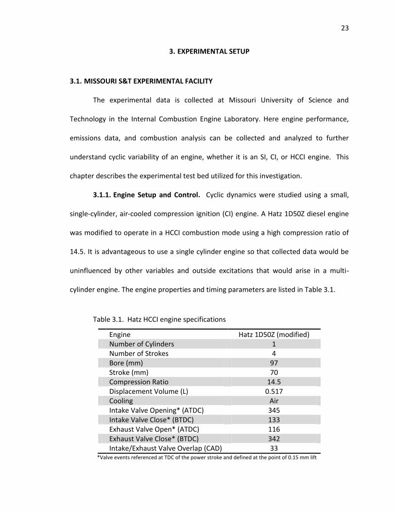
3.1.1. Engine Setup and Control. Cyclic dynamics were studied using a small,
single-cylinder, air-cooled compression ignition (CI) engine. A Hatz 1D50Z diesel engine
was modified to operate in a HCCI combustion mode using a high compression ratio of
14.5. It is advantageous to use a single cylinder engine so that collected data would be
uninfluenced by other variables and outside excitations that would arise in a multi-
cylinder engine. The engine properties and timing parameters are listed in Table 3.1.
Table 3.1. Hatz HCCI engine specifications
Engine Hatz 1D50Z (modified) Number of Cylinders 1 Number of Strokes 4 Bore (mm) 97 Stroke (mm) 70 Compression Ratio 14.5 Displacement Volume (L) 0.517 Cooling Air Intake Valve Opening* (ATDC) 345 Intake Valve Close* (BTDC) 133 Exhaust Valve Open* (ATDC) 116 Exhaust Valve Close* (BTDC) 342 Intake/Exhaust Valve Overlap (CAD) 33
*Valve events referenced at TDC of the power stroke and defined at the point of 0.15 mm lift
24
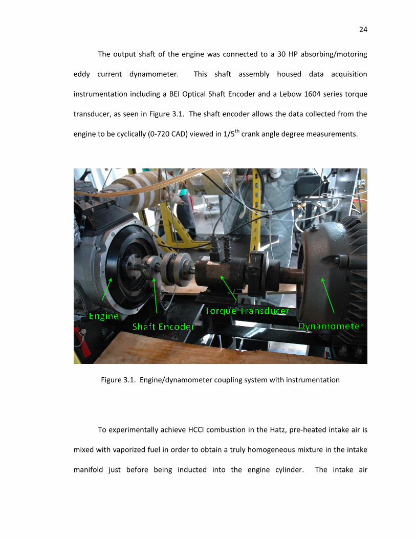
The output shaft of the engine was connected to a 30 HP absorbing/motoring
eddy current dynamometer. This shaft assembly housed data acquisition
instrumentation including a BEI Optical Shaft Encoder and a Lebow 1604 series torque
transducer, as seen in Figure 3.1. The shaft encoder allows the data collected from the
engine to be cyclically (0-720 CAD) viewed in 1/5th crank angle degree measurements.
Figure 3.1. Engine/dynamometer coupling system with instrumentation
To experimentally achieve HCCI combustion in the Hatz, pre-heated intake air is
mixed with vaporized fuel in order to obtain a truly homogeneous mixture in the intake
manifold just before being inducted into the engine cylinder. The intake air
25
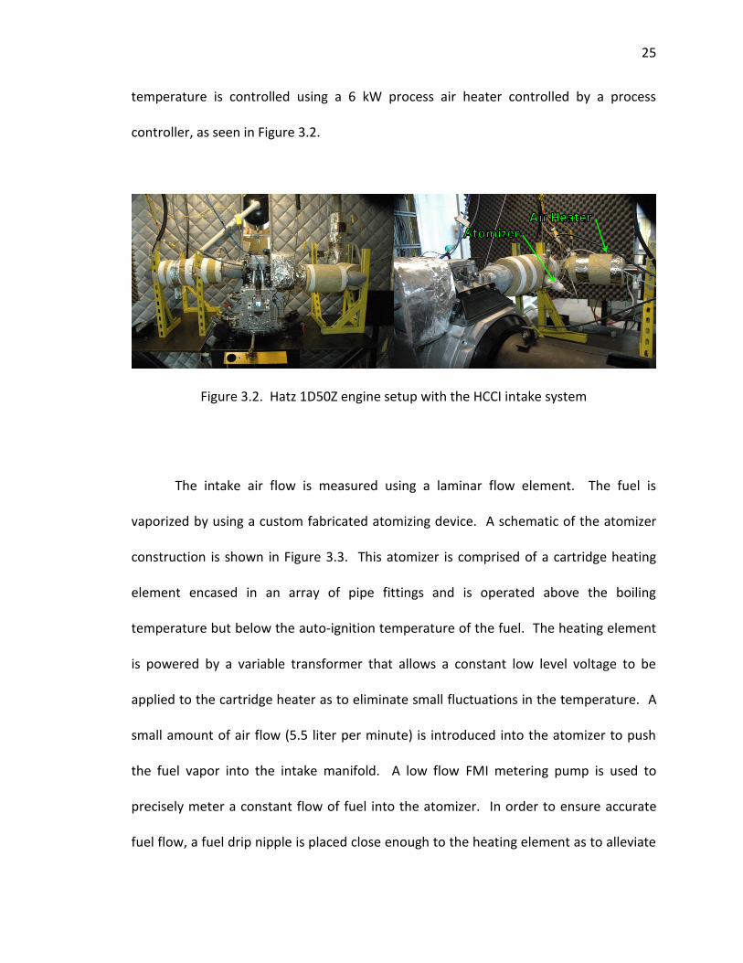
temperature is controlled using a 6 kW process air heater controlled by a process
controller, as seen in Figure 3.2.
Figure 3.2. Hatz 1D50Z engine setup with the HCCI intake system
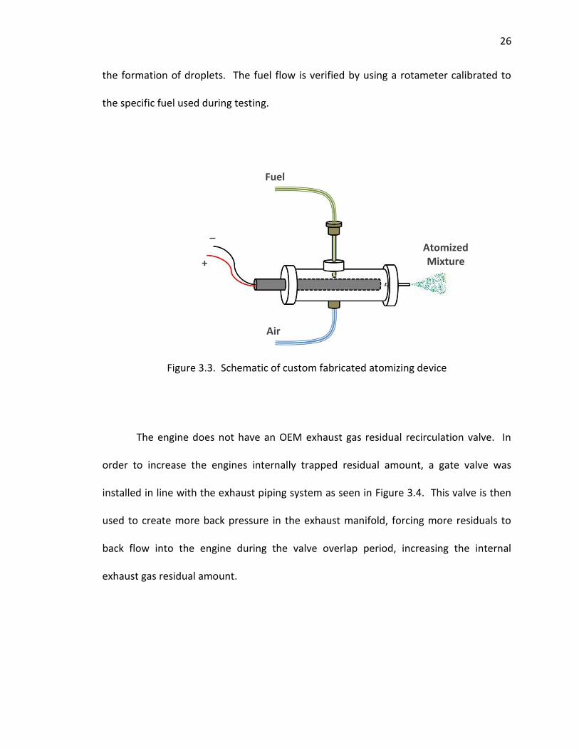
The intake air flow is measured using a laminar flow element. The fuel is
vaporized by using a custom fabricated atomizing device. A schematic of the atomizer
construction is shown in Figure 3.3. This atomizer is comprised of a cartridge heating
element encased in an array of pipe fittings and is operated above the boiling
temperature but below the auto-ignition temperature of the fuel. The heating element
is powered by a variable transformer that allows a constant low level voltage to be
applied to the cartridge heater as to eliminate small fluctuations in the temperature. A
small amount of air flow (5.5 liter per minute) is introduced into the atomizer to push
the fuel vapor into the intake manifold. A low flow FMI metering pump is used to
precisely meter a constant flow of fuel into the atomizer. In order to ensure accurate
fuel flow, a fuel drip nipple is placed close enough to the heating element as to alleviate
26
the formation of droplets. The fuel flow is verified by using a rotameter calibrated to
the specific fuel used during testing.
Figure 3.3. Schematic of custom fabricated atomizing device
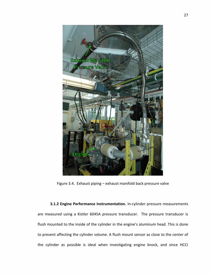
The engine does not have an OEM exhaust gas residual recirculation valve. In
order to increase the engines internally trapped residual amount, a gate valve was
installed in line with the exhaust piping system as seen in Figure 3.4. This valve is then
used to create more back pressure in the exhaust manifold, forcing more residuals to
back flow into the engine during the valve overlap period, increasing the internal
exhaust gas residual amount.
Fuel
Air
_
+
Atomized Mixture
27
Figure 3.4. Exhaust piping – exhaust manifold back pressure valve
3.1.2 Engine Performance Instrumentation. In-cylinder pressure measurements
are measured using a Kistler 6045A pressure transducer. The pressure transducer is
flush mounted to the inside of the cylinder in the engine’s aluminum head. This is done
to prevent affecting the cylinder volume. A flush mount sensor as close to the center of
the cylinder as possible is ideal when investigating engine knock, and since HCCI
28
combustion is an autoignition event, the pressure transducer was chosen to be flush
mounted. The Kistler 6045A pressure transducer is a charge type transducer and
requires a charge amplifier for use. A Kistler Dual Mode Amp Type 5010 charge
amplifier set to 10 MU(bar)/Volt is used to convert the transducer charge into a
readable voltage in the data acquisition system via BNC connections.
In order to complete a full combustion analysis, a number of different exhaust
gas species must be monitored and measured. Three separate California Analytical
Instruments (CAI) emissions analyzers are utilized to determine the concentrations of
each of these species that are contained in the exhaust. Two wet gas analyzers are used
to measure total unburned hydrocarbons (uHC) and nitric oxides (NOx). A wet gas
analyzer requires that the exhaust sample be maintained at an elevated temperature so
that the water vapor does not condense out and harm the machine. This is achieved by
using heated sample lines. A model 300M-HFID flame ionization detector determines
uHC in parts per million while a model 4000-HCLD determines the NOx concentration.
Carbon monoxide (CO), carbon dioxide (CO2), and oxygen (O2) percentages are
measured by a model 300 NDIR dry gas analyzer that condenses the H2O out of the
exhaust stream prior to analysis. In addition to the combustion pressure and emissions
measurements, there are other various temperatures and pressures that are monitored
around the engine test cell.
3.1.3. Cyclic Exhaust Measurements. For a study on exhaust gas residuals and
its effect on the combustion performance parameters, the exhaust temperature and
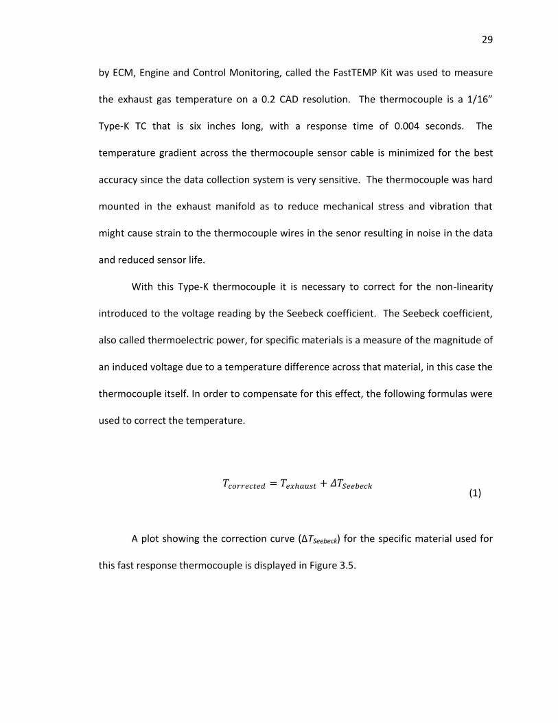
pressure must be collected on a cyclic basis. A fast response thermocouple developed
29
by ECM, Engine and Control Monitoring, called the FastTEMP Kit was used to measure
the exhaust gas temperature on a 0.2 CAD resolution. The thermocouple is a 1/16”
Type-K TC that is six inches long, with a response time of 0.004 seconds. The
temperature gradient across the thermocouple sensor cable is minimized for the best
accuracy since the data collection system is very sensitive. The thermocouple was hard
mounted in the exhaust manifold as to reduce mechanical stress and vibration that
might cause strain to the thermocouple wires in the senor resulting in noise in the data
and reduced sensor life.
With this Type-K thermocouple it is necessary to correct for the non-linearity
introduced to the voltage reading by the Seebeck coefficient. The Seebeck coefficient,
also called thermoelectric power, for specific materials is a measure of the magnitude of
an induced voltage due to a temperature difference across that material, in this case the
thermocouple itself. In order to compensate for this effect, the following formulas were
used to correct the temperature.
A plot showing the correction curve (ΔTSeebeck) for the specific material used for
this fast response thermocouple is displayed in Figure 3.5.
(1)
30
Figure 3.5. Seebeck coefficent compensator chart for FastTEMP thermocouple
-20
-10
0
10
20
30
-100 100 300 500 700 900 1100 1300
De
lta
Co
pm
en
sati
on
(⁰C
)
Measured Temperature (⁰C)
( )
(
(2)
( )
(
(3)
31
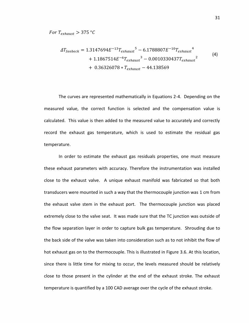
The curves are represented mathematically in Equations 2-4. Depending on the
measured value, the correct function is selected and the compensation value is
calculated. This value is then added to the measured value to accurately and correctly
record the exhaust gas temperature, which is used to estimate the residual gas
temperature.
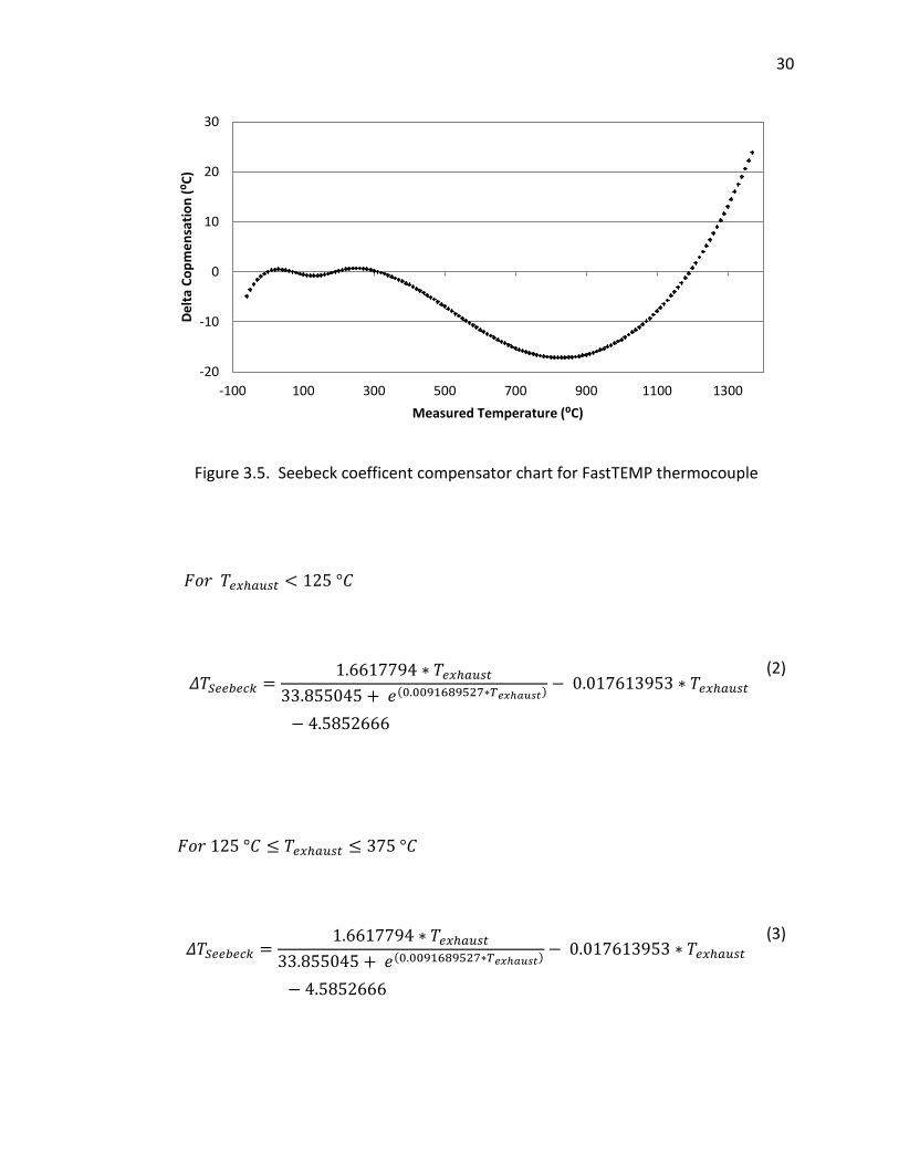
In order to estimate the exhaust gas residuals properties, one must measure
these exhaust parameters with accuracy. Therefore the instrumentation was installed
close to the exhaust valve. A unique exhaust manifold was fabricated so that both
transducers were mounted in such a way that the thermocouple junction was 1 cm from
the exhaust valve stem in the exhaust port. The thermocouple junction was placed
extremely close to the valve seat. It was made sure that the TC junction was outside of
the flow separation layer in order to capture bulk gas temperature. Shrouding due to
the back side of the valve was taken into consideration such as to not inhibit the flow of
hot exhaust gas on to the thermocouple. This is illustrated in Figure 3.6. At this location,
since there is little time for mixing to occur, the levels measured should be relatively
close to those present in the cylinder at the end of the exhaust stroke. The exhaust
temperature is quantified by a 100 CAD average over the cycle of the exhaust stroke.
(
(4)
32
Figure 3.6. Probe position for cycle resolved temperature and pressure measurements
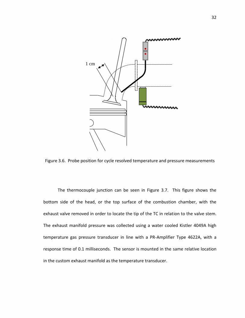
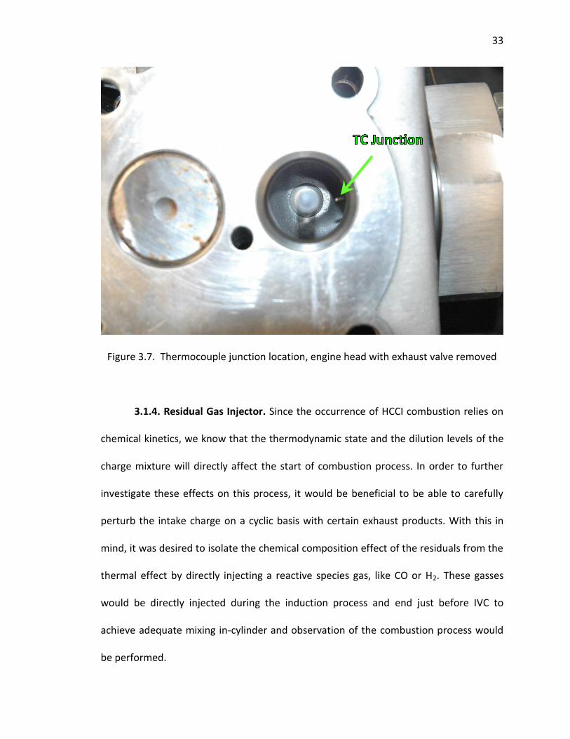
The thermocouple junction can be seen in Figure 3.7. This figure shows the
bottom side of the head, or the top surface of the combustion chamber, with the
exhaust valve removed in order to locate the tip of the TC in relation to the valve stem.
The exhaust manifold pressure was collected using a water cooled Kistler 4049A high
temperature gas pressure transducer in line with a PR-Amplifier Type 4622A, with a
response time of 0.1 milliseconds. The sensor is mounted in the same relative location
in the custom exhaust manifold as the temperature transducer.
1 cm
33
Figure 3.7. Thermocouple junction location, engine head with exhaust valve removed
3.1.4. Residual Gas Injector. Since the occurrence of HCCI combustion relies on
chemical kinetics, we know that the thermodynamic state and the dilution levels of the
charge mixture will directly affect the start of combustion process. In order to further
investigate these effects on this process, it would be beneficial to be able to carefully
perturb the intake charge on a cyclic basis with certain exhaust products. With this in
mind, it was desired to isolate the chemical composition effect of the residuals from the
thermal effect by directly injecting a reactive species gas, like CO or H2. These gasses
would be directly injected during the induction process and end just before IVC to
achieve adequate mixing in-cylinder and observation of the combustion process would
be performed.
34
An injector, called the Residual Gas Injector (RGI), was developed to do just this.
In order to directly inject into the cylinder cycle-by-cycle, the preexisting port for the
original diesel fuel injector was used. The diesel fuel injector is a design of the OEM
engine and is not used for HCCI combustion; however it is installed to keep the
geometry of the cylinder intact during operation. To minimize modifications to the
original head, a residual mass injector was designed and constructed from the original
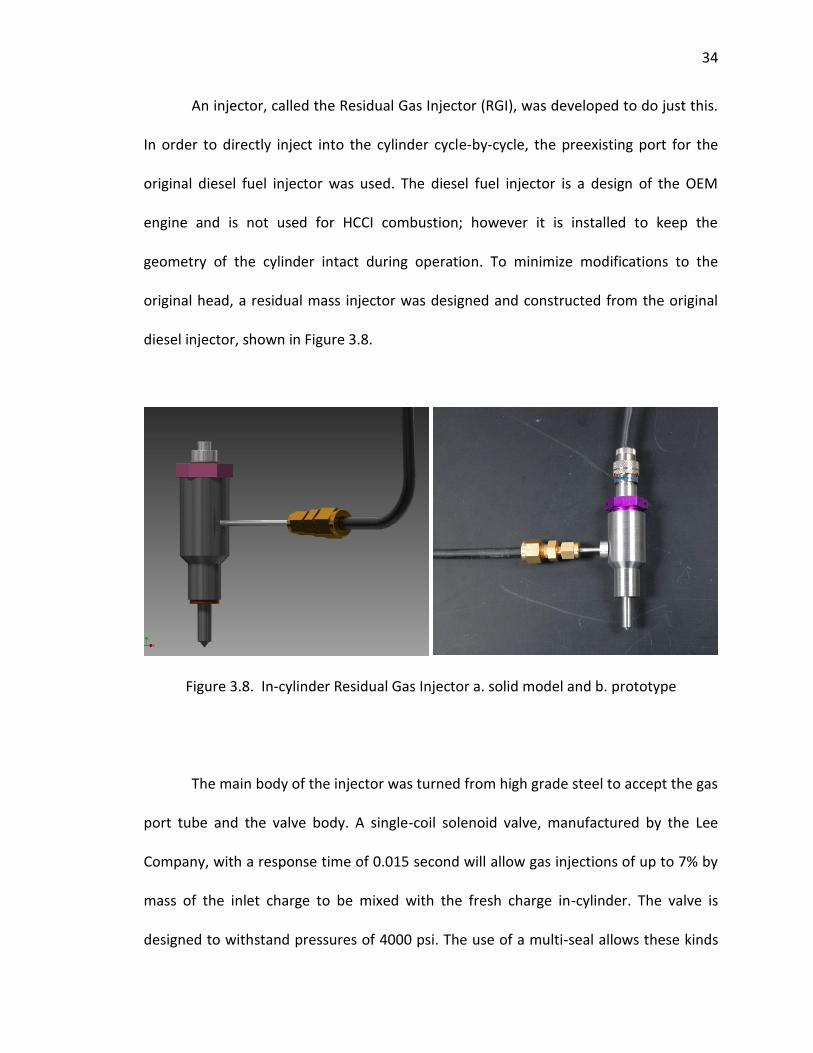
diesel injector, shown in Figure 3.8.
Figure 3.8. In-cylinder Residual Gas Injector a. solid model and b. prototype
The main body of the injector was turned from high grade steel to accept the gas
port tube and the valve body. A single-coil solenoid valve, manufactured by the Lee
Company, with a response time of 0.015 second will allow gas injections of up to 7% by
mass of the inlet charge to be mixed with the fresh charge in-cylinder. The valve is
designed to withstand pressures of 4000 psi. The use of a multi-seal allows these kinds
35
of pressures, developed by the Lee Company. Further figures of the RGI and its
construction can be seen in Appendix A.
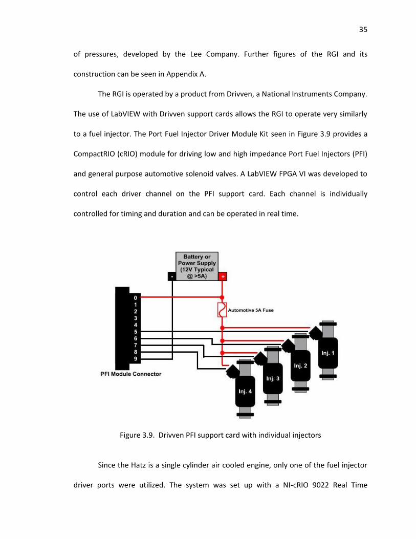
The RGI is operated by a product from Drivven, a National Instruments Company.
The use of LabVIEW with Drivven support cards allows the RGI to operate very similarly
to a fuel injector. The Port Fuel Injector Driver Module Kit seen in Figure 3.9 provides a
CompactRIO (cRIO) module for driving low and high impedance Port Fuel Injectors (PFI)
and general purpose automotive solenoid valves. A LabVIEW FPGA VI was developed to
control each driver channel on the PFI support card. Each channel is individually
controlled for timing and duration and can be operated in real time.
Figure 3.9. Drivven PFI support card with individual injectors
Since the Hatz is a single cylinder air cooled engine, only one of the fuel injector
driver ports were utilized. The system was set up with a NI-cRIO 9022 Real Time
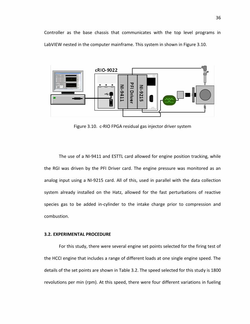
36
Controller as the base chassis that communicates with the top level programs in
LabVIEW nested in the computer mainframe. This system in shown in Figure 3.10.
Figure 3.10. c-RIO FPGA residual gas injector driver system
The use of a NI-9411 and ESTTL card allowed for engine position tracking, while
the RGI was driven by the PFI Driver card. The engine pressure was monitored as an
analog input using a NI-9215 card. All of this, used in parallel with the data collection
system already installed on the Hatz, allowed for the fast perturbations of reactive
species gas to be added in-cylinder to the intake charge prior to compression and
combustion.
3.2. EXPERIMENTAL PROCEDURE
For this study, there were several engine set points selected for the firing test of
the HCCI engine that includes a range of different loads at one single engine speed. The
details of the set points are shown in Table 3.2. The speed selected for this study is 1800
revolutions per min (rpm). At this speed, there were four different variations in fueling
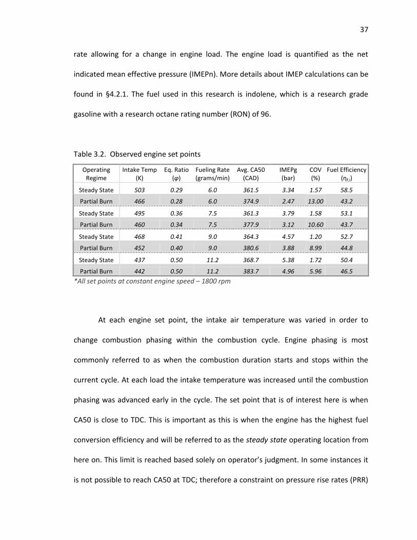
37
rate allowing for a change in engine load. The engine load is quantified as the net
indicated mean effective pressure (IMEPn). More details about IMEP calculations can be
found in §4.2.1. The fuel used in this research is indolene, which is a research grade
gasoline with a research octane rating number (RON) of 96.
Table 3.2. Observed engine set points
Operating Regime
Intake Temp (K)
Eq. Ratio (φ)
Fueling Rate (grams/min)
Avg. CA50 (CAD)
IMEPg (bar)
COV (%)
Fuel Efficiency (ηf,i)
Steady State 503 0.29 6.0 361.5 3.34 1.57 58.5
Partial Burn 466 0.28 6.0 374.9 2.47 13.00 43.2
Steady State 495 0.36 7.5 361.3 3.79 1.58 53.1
Partial Burn 460 0.34 7.5 377.9 3.12 10.60 43.7
Steady State 468 0.41 9.0 364.3 4.57 1.20 52.7
Partial Burn 452 0.40 9.0 380.6 3.88 8.99 44.8
Steady State 437 0.50 11.2 368.7 5.38 1.72 50.4
Partial Burn 442 0.50 11.2 383.7 4.96 5.96 46.5
*All set points at constant engine speed – 1800 rpm
At each engine set point, the intake air temperature was varied in order to
change combustion phasing within the combustion cycle. Engine phasing is most
commonly referred to as when the combustion duration starts and stops within the
current cycle. At each load the intake temperature was increased until the combustion
phasing was advanced early in the cycle. The set point that is of interest here is when
CA50 is close to TDC. This is important as this is when the engine has the highest fuel
conversion efficiency and will be referred to as the steady state operating location from
here on. This limit is reached based solely on operator’s judgment. In some instances it
is not possible to reach CA50 at TDC; therefore a constraint on pressure rise rates (PRR)
38
of 10 bar/CAD is set. In fact it is rarely the case where you will have both CA50 at TDC
and a pressure rise rate of 10 bar/CAD. This constraint limit is set because it is where the
engine is audibly loud and noise, vibration and harshness (NHV) are of concern. This
NHV will eventually lead to the degradation of engine components. Once the set point
of CA50 at TDC, or the pressure rise rate limit is reached, the data is collected. The
intake temperature is reduced in order to phase combustion late in the cycle. Here,
engine variations become very high and the engine approaches a misfire limit. The
coefficient of variation (COV) becomes very high and partial consumption of the fuel/air
charge leads to calling this set point as the partial burn regime. This COV is defined as
the cyclic variability in indicated work per cycle. When the COV is high, greater than
10%, then the engine is considered to be in a region of instability, or partial burn regime.
It is in the partial burn regime where the main focus of this study is localized where the
cyclic dynamics are not fully understood.
The equivalence ratio, φ, is the ratio of actual fuel/air ratio to the stoichiometric
fuel/air ratio. This defines the mixture composition at each set point and is found from
Equation 5.
The fuel properties of indolene are given by the manufacturer and the (F/A)s was
found, through thermochemistry, to be 0.0674. This is a constant for this fuel as the
( ) ( )
(5)
39
carbon-hydrogen ratio is fuel specific. When the equivalence ratio is equal to 1 then the
fuel/air mixture is considered to be at stoichiometric conditions, φ=1. If φ<1 then the
fuel/air mixture is considered to be lean, and if φ>1 then it is considered rich. HCCI
combustion is a very fuel efficient process and part of this is contributed to HCCI
operating in the lean condition, φ<1. This is done due to the rapid release of chemical
energy when autoignition occurs within the cylinder, attributing to the high PRR’s. The
higher the equivalence ratio, the higher the engine load, and the more violent the
combustion becomes, relating to NVH. The highest equivalence ratio used in this study
was φ=0.5.
At the steady state operating points, 400 consecutive cycles of engine data were
collected. These measurements were taken after the engine had stabilized at each
intake temperature for that load. A stable operating point is when there are no longer
any transients in exhaust temperature, pressure rise rates, and amount of heat
released. In the partial burn regime, 1000 consecutive cycles where collected. It is
important to collect this many cycles when studying cyclic dynamics as this information
helps to reveal the cycle-to-cycle dependence. Further details about all engine set points
and averaged observed parameters can be found in Appendix B.
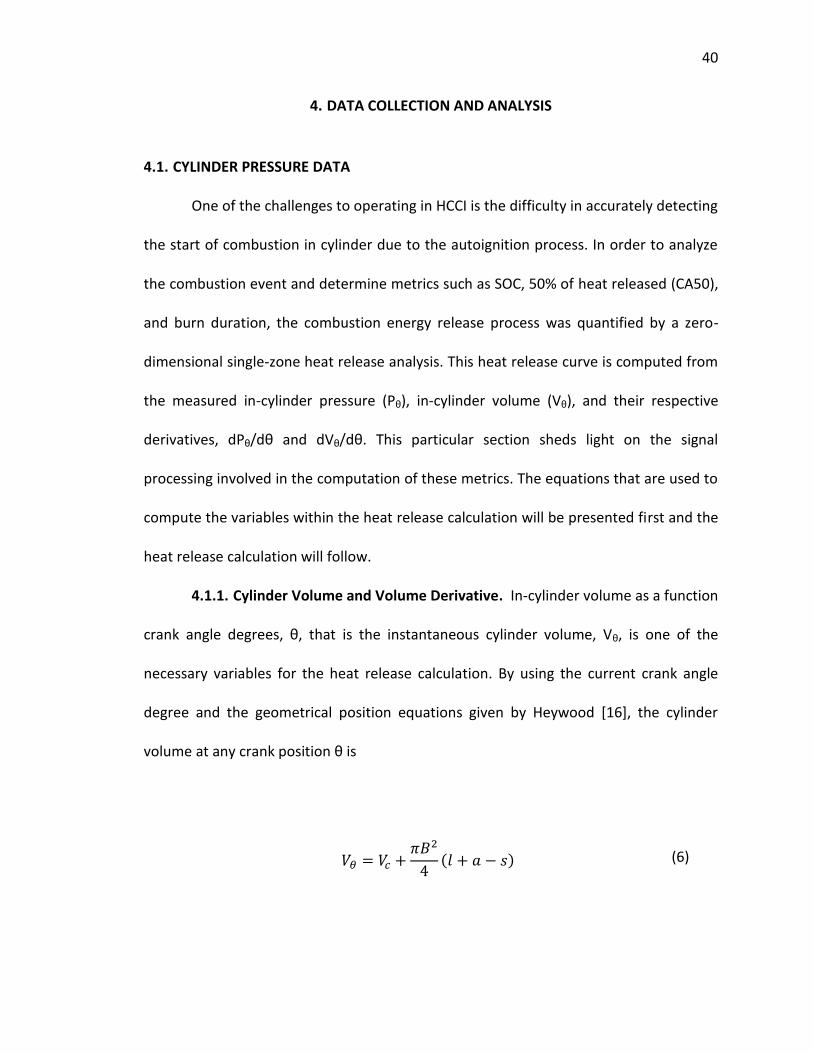
40
4. DATA COLLECTION AND ANALYSIS
4.1. CYLINDER PRESSURE DATA
One of the challenges to operating in HCCI is the difficulty in accurately detecting
the start of combustion in cylinder due to the autoignition process. In order to analyze
the combustion event and determine metrics such as SOC, 50% of heat released (CA50),
and burn duration, the combustion energy release process was quantified by a zero-
dimensional single-zone heat release analysis. This heat release curve is computed from
the measured in-cylinder pressure (Pθ), in-cylinder volume (Vθ), and their respective
derivatives, dPθ/dθ and dVθ/dθ. This particular section sheds light on the signal
processing involved in the computation of these metrics. The equations that are used to
compute the variables within the heat release calculation will be presented first and the
heat release calculation will follow.
4.1.1. Cylinder Volume and Volume Derivative. In-cylinder volume as a function
crank angle degrees, θ, that is the instantaneous cylinder volume, Vθ, is one of the
necessary variables for the heat release calculation. By using the current crank angle
degree and the geometrical position equations given by Heywood [16], the cylinder
volume at any crank position θ is
( )
(6)
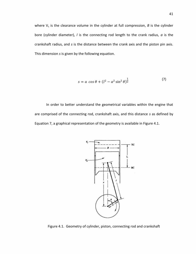
41
where Vc is the clearance volume in the cylinder at full compression, B is the cylinder
bore (cylinder diameter), l is the connecting rod length to the crank radius, a is the
crankshaft radius, and s is the distance between the crank axis and the piston pin axis.
This dimension s is given by the following equation.
In order to better understand the geometrical variables within the engine that
are comprised of the connecting rod, crankshaft axis, and this distance s as defined by
Equation 7, a graphical representation of the geometry is available in Figure 4.1.
Figure 4.1. Geometry of cylinder, piston, connecting rod and crankshaft
( )
(7)

42
To calculate the volume derivative with respect to crank angle degrees, dVθ/dθ,
one would take the derivative of Equation 6 with respect to θ.
Given that the clearance volume, the bore, the connecting rod length, and the
crankshaft axis are all fixed constants, Equation 8 condenses to
Next calculate the derivative of s with respect to crank angle degrees (ds/dθ)
Finally, by substituting Equation 10 into Equation 9, the equation for in-cylinder
volume as a function crank angle degrees, that is the instantaneous cylinder volume, is
[
( )]
(8)
(9)
[
( )
]
(10)
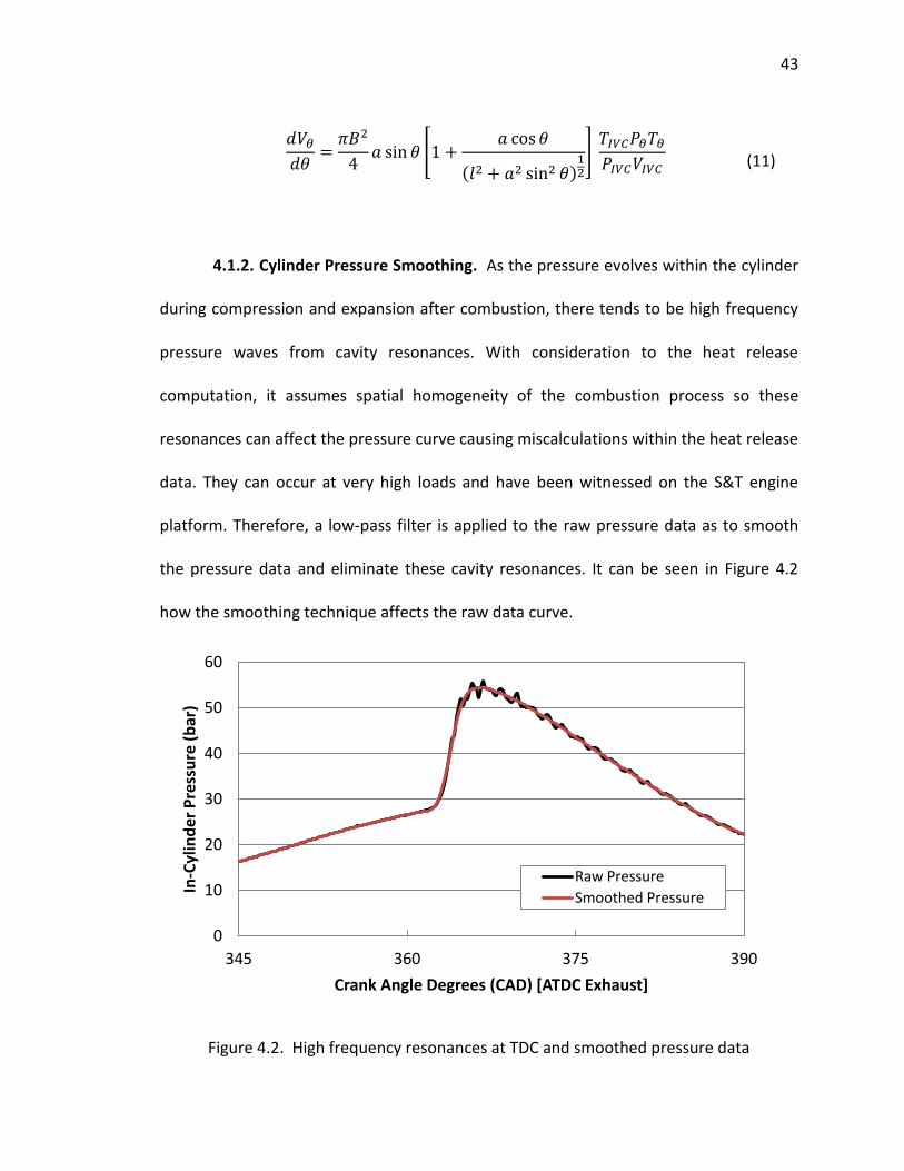
43
4.1.2. Cylinder Pressure Smoothing. As the pressure evolves within the cylinder
during compression and expansion after combustion, there tends to be high frequency
pressure waves from cavity resonances. With consideration to the heat release
computation, it assumes spatial homogeneity of the combustion process so these
resonances can affect the pressure curve causing miscalculations within the heat release
data. They can occur at very high loads and have been witnessed on the S&T engine
platform. Therefore, a low-pass filter is applied to the raw pressure data as to smooth
the pressure data and eliminate these cavity resonances. It can be seen in Figure 4.2
how the smoothing technique affects the raw data curve.
Figure 4.2. High frequency resonances at TDC and smoothed pressure data
0
10
20
30
40
50
60
345 360 375 390
In-C
ylin
der
Pre
ssu
re (
bar
)
Crank Angle Degrees (CAD) [ATDC Exhaust]
Raw Pressure
Smoothed Pressure
[
( )
]
(11)
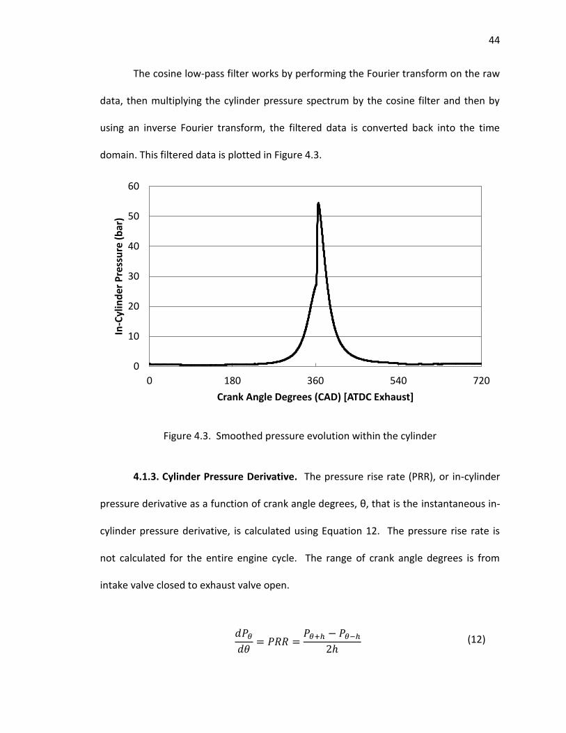
44
The cosine low-pass filter works by performing the Fourier transform on the raw
data, then multiplying the cylinder pressure spectrum by the cosine filter and then by
using an inverse Fourier transform, the filtered data is converted back into the time
domain. This filtered data is plotted in Figure 4.3.
Figure 4.3. Smoothed pressure evolution within the cylinder
4.1.3. Cylinder Pressure Derivative. The pressure rise rate (PRR), or in-cylinder
pressure derivative as a function of crank angle degrees, θ, that is the instantaneous in-
cylinder pressure derivative, is calculated using Equation 12. The pressure rise rate is
not calculated for the entire engine cycle. The range of crank angle degrees is from
intake valve closed to exhaust valve open.
0
10
20
30
40
50
60
0 180 360 540 720
In-C
ylin
der
Pre
ssu
re (
bar
)
Crank Angle Degrees (CAD) [ATDC Exhaust]
(12)
45
In Equation 12, the variable h is defined as the resolution of the shaft encoder.
For this study the BEI Optical Shaft Encoder had a resolution of 1/5th CAD (0.2 crank
angle degrees).
4.1.4. Cylinder Temperature. In-cylinder temperature as a function crank angle
degrees, θ, that is the instantaneous in-cylinder temperature, Tθ, is another one of the
necessary variables for the heat release calculation. For this calculation, the fuel/air
charge is assumed to behave like an ideal gas. In order to treat the system as a closed
thermodynamic system with no mass crossing the boundaries, one can only apply this
technique to the time when the engine is actually a closed system. That is from intake
valve closed (IVC) to exhaust valve open (EVO). During this time the engine is a closed
thermodynamic “chamber”. With these assumptions in mind, the instantaneous in-
cylinder temperature, Tθ, can be calculated by relating the ideal gas equation to the
conservation of mass, yielding Equation 13.
Here the variables TIVC, PIVC, and VIVC are the in-cylinder temperature, in-cylinder
pressure, and in-cylinder volume at IVC, respectively. Due to the measured intake
fuel/air charge temperature, it is assumed that TIVC is fairly well approximated.
(13)
46
4.1.5. Heat-Release Calculation. The heat-release analysis is taken from
Heywood [16]. When calculating heat-release (HR) from the cylinder pressure data
analysis, one can quantify the effects of heat transfer, crevices, and leakage based on
the first law of thermodynamics. An advantage to this approach is that the pressure
fluctuations in cylinder can be directly related to the amount of fuel chemical energy
that is released throughout the combustion process. The first law for this system is
shown in Equation 14.
Where dUs is the change in sensible energy, the term δQch represents the
chemical energy released by combustion, the piston work (δW), δQht is the heat transfer
to the chamber walls, and the mass flux term represents the flow across the boundary.
For these parameters, we monitor and calculate onboard the heat release and heat
release rate. Therefore a gross heat release analysis is used instead of a net HR in order
to be quick enough to be calculated in real time. The difference between this net and
gross HR is the heat transfer to the cylinder walls, head, and piston top and the small
crevice effects. By eliminating these from the first law, replacing piston work with p dV,
and assuming that the change in sensible energy is given by mcv(T) where T is the mean
charge temperature and m is the mass within the system boundary then the equation is
reduced to:
∑
(14)
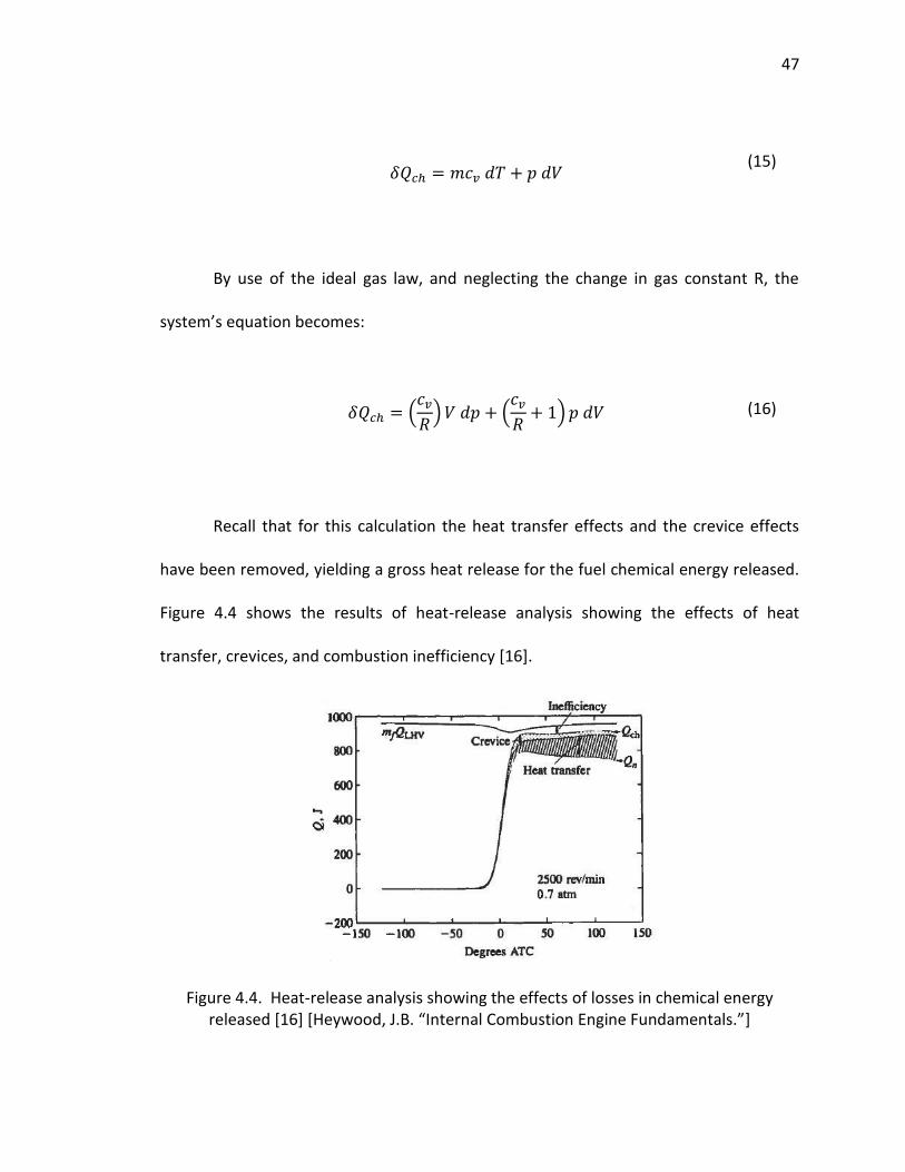
47
By use of the ideal gas law, and neglecting the change in gas constant R, the
system’s equation becomes:
Recall that for this calculation the heat transfer effects and the crevice effects
have been removed, yielding a gross heat release for the fuel chemical energy released.
Figure 4.4 shows the results of heat-release analysis showing the effects of heat
transfer, crevices, and combustion inefficiency [16].
Figure 4.4. Heat-release analysis showing the effects of losses in chemical energy released [16] [Heywood, J.B. “Internal Combustion Engine Fundamentals.”]
(15)
(
) (
)
(16)
48
In order to accurately calculate the term cv/R, the ratio of specific heats (γ) for
burned and unburned gases is used, shown in Equation 17. For an approximate
approach γ is held constant during combustion and has been shown to give adequate
results [16].
Finally, the heat release rate (RHR) is calculated using Equation 18. This HRR is
used to compute the cumulative heat release (HR) by numerically integrating the RHR
equation using the composite trapezoidal rule. This method has been used significantly
in engine combustion analysis and has proven to be a robust method [16].
The HR, RHR, and PRR are all useful in this study of HCCI cyclic dynamics. The
pressure rise rate allows us to maintain a limit of 10 bar/CAD as the pressure evolves
within the cylinder, informing us that we do not want to advance the engine any more
as noise, vibration, and harshness (NVH) becomes a problem and could degrade the
internals of our engine. The HR and RHR inform us of SOC (which for this study we are
(17)
(18)
49
calling CA10), CA50 and burn duration. All these metrics are used to determine cycle-to-
cycle dependence and can be seen in further detail in Chapter 5. CA10 is defined as the
location or crank angle degree, where 10 percent of the total heat released occurs. That
is determined from a maximum heat released value, as seen in Figure 4.4, and then 10
percent of that value is used to determine the relative location of CA10 in crank angle
degrees for that cycle. CA50 is computed in the same fashion; except that its location is
where 50 percent of the total heat released occurs.
4.2. ENGINE PERFORMANCE MEASURES
With regard to homogenous charge compression ignition combustion, the
maximum heat-release rate and the duration of the heat release (burn duration) can
vary between cycles significantly when operating in the partial burn regime close to the
misfire limit. Then the peak cylinder pressure varies accordingly. The faster burning
cycles have substantially higher values of maximum pressure (steady state operating
case) than do the slower burning cycles (partial burn regime), where the steady state
case has maximum RHR near TDC. Operation in the partial burn regime is obviously
undesirable as there is risk of a misfire and from the point of fuel efficiency,
hydrocarbon emissions, torque variations, and roughness. Various measures of cycle-by-
cycle combustion variability are used. It can be defined in terms of variations in the
cylinder pressure between different cycles, or in terms of variations in the details of the
burn process which cause these differences in pressure.
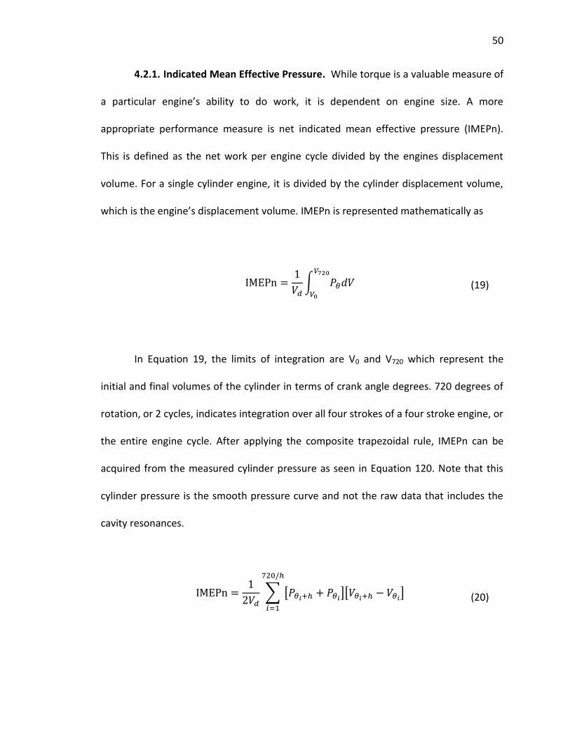
50
4.2.1. Indicated Mean Effective Pressure. While torque is a valuable measure of
a particular engine’s ability to do work, it is dependent on engine size. A more
appropriate performance measure is net indicated mean effective pressure (IMEPn).
This is defined as the net work per engine cycle divided by the engines displacement
volume. For a single cylinder engine, it is divided by the cylinder displacement volume,
which is the engine’s displacement volume. IMEPn is represented mathematically as
In Equation 19, the limits of integration are V0 and V720 which represent the
initial and final volumes of the cylinder in terms of crank angle degrees. 720 degrees of
rotation, or 2 cycles, indicates integration over all four strokes of a four stroke engine, or
the entire engine cycle. After applying the composite trapezoidal rule, IMEPn can be
acquired from the measured cylinder pressure as seen in Equation 120. Note that this
cylinder pressure is the smooth pressure curve and not the raw data that includes the
cavity resonances.
∫
(19)
∑ [ ][ ]
(20)
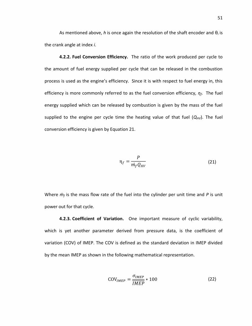
51
As mentioned above, h is once again the resolution of the shaft encoder and θi is
the crank angle at index i.
4.2.2. Fuel Conversion Efficiency. The ratio of the work produced per cycle to
the amount of fuel energy supplied per cycle that can be released in the combustion
process is used as the engine’s efficiency. Since it is with respect to fuel energy in, this
efficiency is more commonly referred to as the fuel conversion efficiency, ηf. The fuel
energy supplied which can be released by combustion is given by the mass of the fuel
supplied to the engine per cycle time the heating value of that fuel (QHV). The fuel
conversion efficiency is given by Equation 21.
Where ṁf is the mass flow rate of the fuel into the cylinder per unit time and P is unit
power out for that cycle.
4.2.3. Coefficient of Variation. One important measure of cyclic variability,
which is yet another parameter derived from pressure data, is the coefficient of
variation (COV) of IMEP. The COV is defined as the standard deviation in IMEP divided
by the mean IMEP as shown in the following mathematical representation.
(21)
(22)
52
COV is usually expressed as a percent, hence the multiplication by 100. It defines
the cyclic variability in indicated work per cycle, and has been found that when
operating in steady state it is near 1-2% and when the engine is found to be in the
partial burn regime, when CA50 is retarded very late in the combustion process, the
COVIMEP exceeds 10%.
4.2.4. Return Maps. A method for examining inherent interactions between
cyclic events is to plot return maps. Return maps show the correlation between each
individual pair of consecutive events in the data set without averaging. By plotting each
successive value of the measured parameter against the succeeding cycle’s measured
parameter we can see when they are related. This return map reflects whether or not
one can represent this oscillation process in terms of some type of simple function such
as:
Where Ψ(i) is the current cycles observed parameter, or measured metric.
Return maps can be advantageous in this study on cyclic dynamics, because return maps
may reveal strong but rarely occurring correlations which sometimes are overwhelmed
in spectral densities by the signals from weaker but more frequently occurring
correlations, and even other “patterns” referred to as noise. Some example return maps
of IMEP of an engine set point are shown in Figure 4.5.
( ) [ ( ) ]
(23)
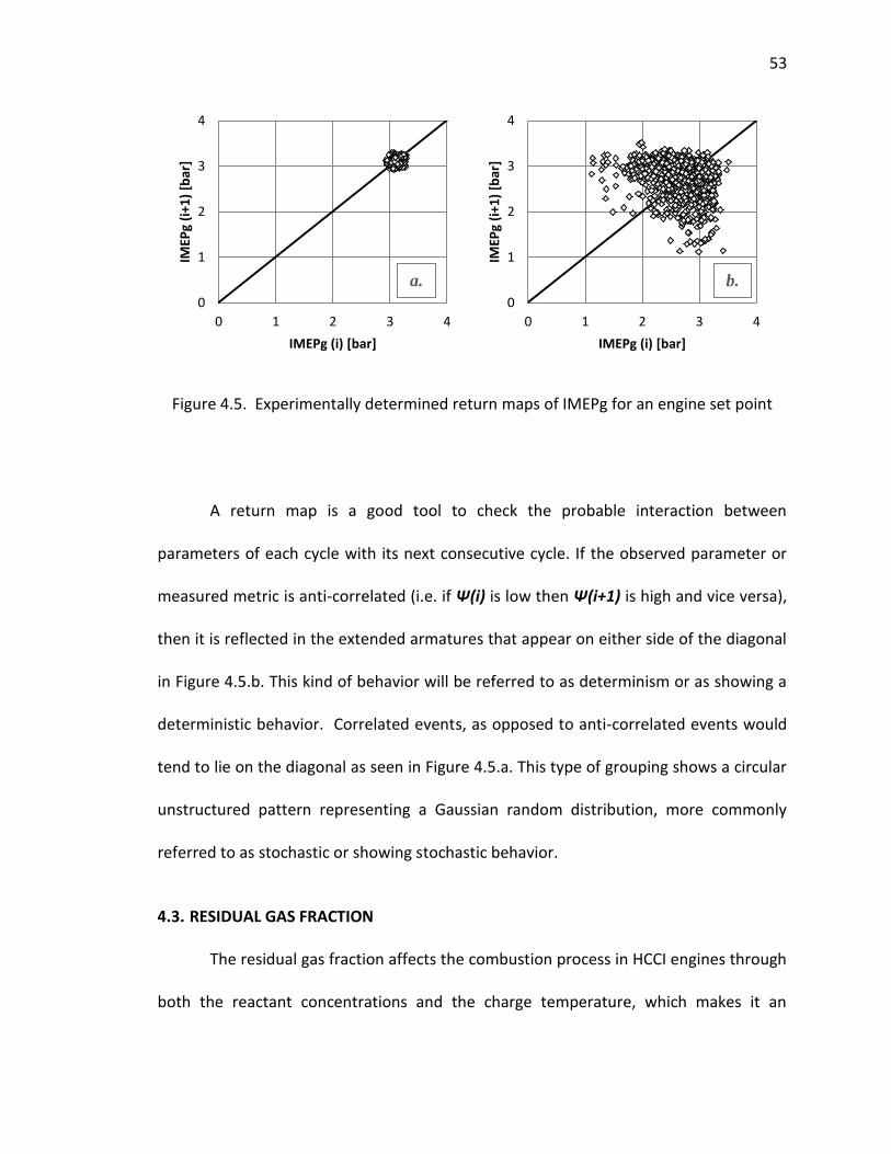
53
Figure 4.5. Experimentally determined return maps of IMEPg for an engine set point
A return map is a good tool to check the probable interaction between
parameters of each cycle with its next consecutive cycle. If the observed parameter or
measured metric is anti-correlated (i.e. if Ψ(i) is low then Ψ(i+1) is high and vice versa),
then it is reflected in the extended armatures that appear on either side of the diagonal
in Figure 4.5.b. This kind of behavior will be referred to as determinism or as showing a
deterministic behavior. Correlated events, as opposed to anti-correlated events would
tend to lie on the diagonal as seen in Figure 4.5.a. This type of grouping shows a circular
unstructured pattern representing a Gaussian random distribution, more commonly
referred to as stochastic or showing stochastic behavior.
4.3. RESIDUAL GAS FRACTION
The residual gas fraction affects the combustion process in HCCI engines through
both the reactant concentrations and the charge temperature, which makes it an
0
1
2
3
4
0 1 2 3 4
IMEP
g (i
+1)
[bar
]
IMEPg (i) [bar]
0
1
2
3
4
0 1 2 3 4
IMEP
g (i
+1)
[bar
]
IMEPg (i) [bar]
a. b.
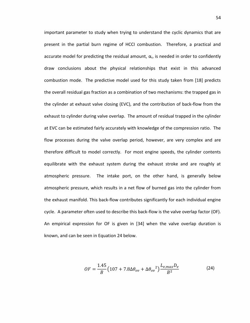
54
important parameter to study when trying to understand the cyclic dynamics that are
present in the partial burn regime of HCCI combustion. Therefore, a practical and
accurate model for predicting the residual amount, αr, is needed in order to confidently
draw conclusions about the physical relationships that exist in this advanced
combustion mode. The predictive model used for this study taken from [18] predicts
the overall residual gas fraction as a combination of two mechanisms: the trapped gas in
the cylinder at exhaust valve closing (EVC), and the contribution of back-flow from the
exhaust to cylinder during valve overlap. The amount of residual trapped in the cylinder
at EVC can be estimated fairly accurately with knowledge of the compression ratio. The
flow processes during the valve overlap period, however, are very complex and are
therefore difficult to model correctly. For most engine speeds, the cylinder contents
equilibrate with the exhaust system during the exhaust stroke and are roughly at
atmospheric pressure. The intake port, on the other hand, is generally below
atmospheric pressure, which results in a net flow of burned gas into the cylinder from
the exhaust manifold. This back-flow contributes significantly for each individual engine
cycle. A parameter often used to describe this back-flow is the valve overlap factor (OF).
An empirical expression for OF is given in [34] when the valve overlap duration is
known, and can be seen in Equation 24 below.
(
)
(24)
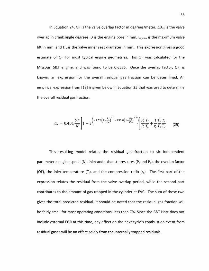
55
In Equation 24, OF is the valve overlap factor in degrees/meter, Δθov is the valve
overlap in crank angle degrees, B is the engine bore in mm, Lv,max is the maximum valve
lift in mm, and Dv is the valve inner seat diameter in mm. This expression gives a good
estimate of OF for most typical engine geometries. This OF was calculated for the
Missouri S&T engine, and was found to be 0.6585. Once the overlap factor, OF, is
known, an expression for the overall residual gas fraction can be determined. An
empirical expression from [18] is given below in Equation 25 that was used to determine
the overall residual gas fraction.
This resulting model relates the residual gas fraction to six independent
parameters: engine speed (N), inlet and exhaust pressures (Pi and Pe), the overlap factor
(OF), the inlet temperature (Ti), and the compression ratio (rc). The first part of the
expression relates the residual from the valve overlap period, while the second part
contributes to the amount of gas trapped in the cylinder at EVC. The sum of these two
gives the total predicted residual. It should be noted that the residual gas fraction will
be fairly small for most operating conditions, less than 7%. Since the S&T Hatz does not
include external EGR at this time, any effect on the next cycle’s combustion event from
residual gases will be an effect solely from the internally trapped residuals.
[
( ( )
( )
)]
(25)
56
5. CYCLIC DYNAMICS INVESTIGATION
The experiments performed in this work are focused on the partial burn regime
of HCCI combustion, where the cyclic variations are high. This cyclic dispersion tends to
present itself in these low temperature combustion (LTC) modes as a result of combined
stochastic and deterministic effects. Stochastic effects are influenced by both boundary
and inlet conditions to the cylinder, while the deterministic effects are generated from
the cycle-to-cycle coupling that inherently exists. As charge dilution is increased, these
factors result in regions of instability and large cyclic variations in SOC and RHR. Upon
entering these partial burn regimes, the deterministic mechanism of combustion tend to
amplify the stochastic variations in a non-linear manner. In order to compare the partial
burn regime to a baseline, the engine was also operated in a region of stable
combustion and high efficiency, known as the steady state operating zone. This steady
state operation is defined as a region where the engine is pushed to a pressure rise rate
(PRR) limit of 10 bar/CAD. The engine phasing, or CA50, is near TDC and this is achieved
by increasing the intake temperature on the engine test bed at S&T. Others achieve
HCCI differently. The partial burn regime is when the engine is phased much later in the
cycle, sometimes as late as 20 degrees after TDC given certain loads. Here partially
consumed charges and misfires lead to increased emissions in NOx and uHCs. It is at
these two operating regimes where most of the data is collected and analyzed.
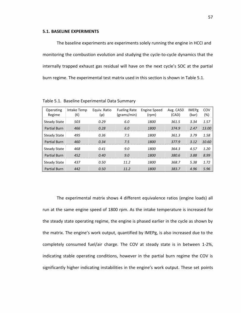
57
5.1. BASELINE EXPERIMENTS
The baseline experiments are experiments solely running the engine in HCCI and
monitoring the combustion evolution and studying the cycle-to-cycle dynamics that the
internally trapped exhaust gas residual will have on the next cycle’s SOC at the partial
burn regime. The experimental test matrix used in this section is shown in Table 5.1.
Table 5.1. Baseline Experimental Data Summary
Operating Regime
Intake Temp (K)
Equiv. Ratio (φ)
Fueling Rate (grams/min)
Engine Speed (rpm)
Avg. CA50 (CAD)
IMEPg (bar)
COV (%)
Steady State 503 0.29 6.0 1800 361.5 3.34 1.57
Partial Burn 466 0.28 6.0 1800 374.9 2.47 13.00
Steady State 495 0.36 7.5 1800 361.3 3.79 1.58
Partial Burn 460 0.34 7.5 1800 377.9 3.12 10.60
Steady State 468 0.41 9.0 1800 364.3 4.57 1.20
Partial Burn 452 0.40 9.0 1800 380.6 3.88 8.99
Steady State 437 0.50 11.2 1800 368.7 5.38 1.72
Partial Burn 442 0.50 11.2 1800 383.7 4.96 5.96
The experimental matrix shows 4 different equivalence ratios (engine loads) all
run at the same engine speed of 1800 rpm. As the intake temperature is increased for
the steady state operating regime, the engine is phased earlier in the cycle as shown by
the matrix. The engine’s work output, quantified by IMEPg, is also increased due to the
completely consumed fuel/air charge. The COV at steady state is in between 1-2%,
indicating stable operating conditions, however in the partial burn regime the COV is
significantly higher indicating instabilities in the engine’s work output. These set points
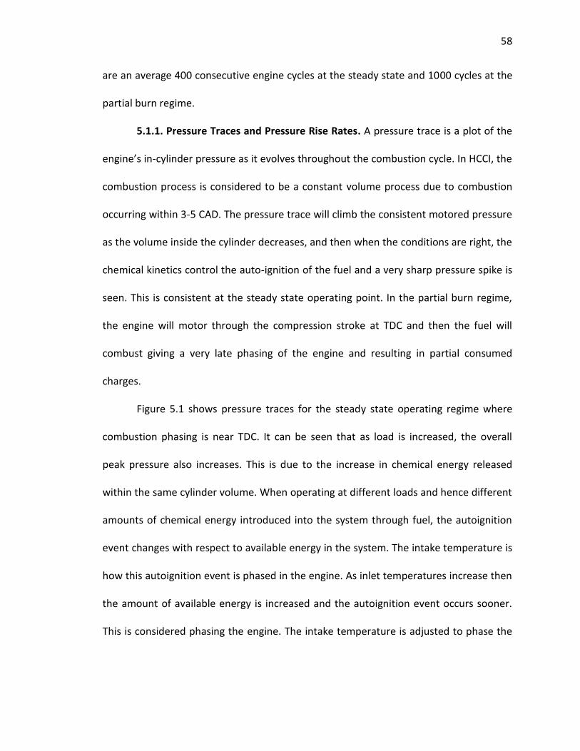
58
are an average 400 consecutive engine cycles at the steady state and 1000 cycles at the
partial burn regime.
5.1.1. Pressure Traces and Pressure Rise Rates. A pressure trace is a plot of the
engine’s in-cylinder pressure as it evolves throughout the combustion cycle. In HCCI, the
combustion process is considered to be a constant volume process due to combustion
occurring within 3-5 CAD. The pressure trace will climb the consistent motored pressure
as the volume inside the cylinder decreases, and then when the conditions are right, the
chemical kinetics control the auto-ignition of the fuel and a very sharp pressure spike is
seen. This is consistent at the steady state operating point. In the partial burn regime,
the engine will motor through the compression stroke at TDC and then the fuel will
combust giving a very late phasing of the engine and resulting in partial consumed
charges.
Figure 5.1 shows pressure traces for the steady state operating regime where
combustion phasing is near TDC. It can be seen that as load is increased, the overall
peak pressure also increases. This is due to the increase in chemical energy released
within the same cylinder volume. When operating at different loads and hence different
amounts of chemical energy introduced into the system through fuel, the autoignition
event changes with respect to available energy in the system. The intake temperature is
how this autoignition event is phased in the engine. As inlet temperatures increase then
the amount of available energy is increased and the autoignition event occurs sooner.
This is considered phasing the engine. The intake temperature is adjusted to phase the
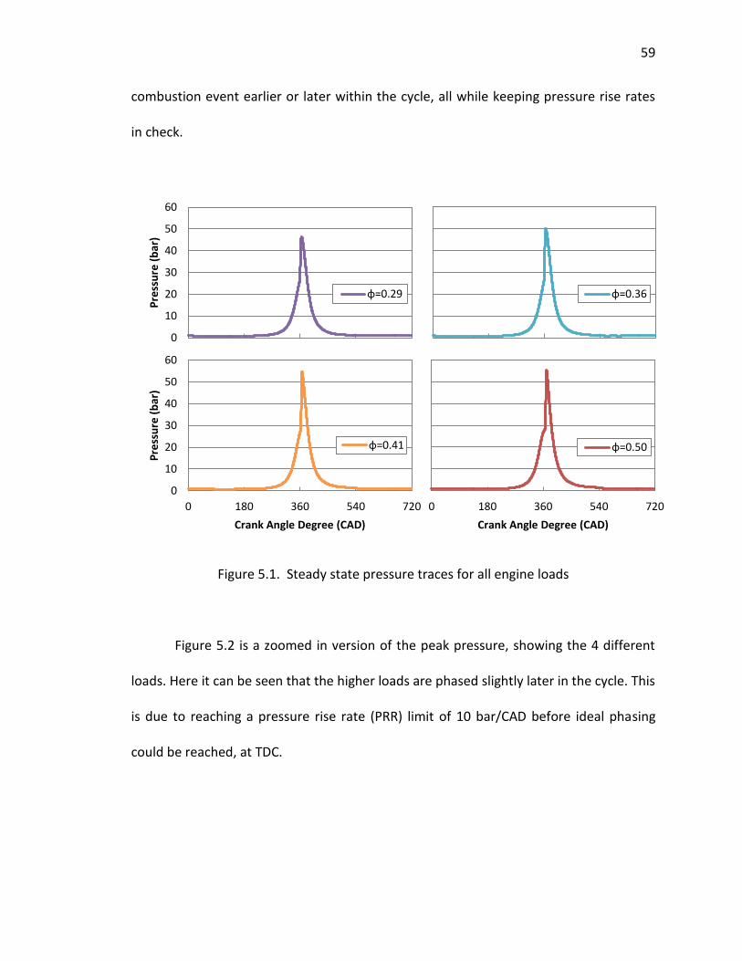
59
combustion event earlier or later within the cycle, all while keeping pressure rise rates
in check.
Figure 5.1. Steady state pressure traces for all engine loads
Figure 5.2 is a zoomed in version of the peak pressure, showing the 4 different
loads. Here it can be seen that the higher loads are phased slightly later in the cycle. This
is due to reaching a pressure rise rate (PRR) limit of 10 bar/CAD before ideal phasing
could be reached, at TDC.
0
10
20
30
40
50
60
Pre
ssu
re (
bar
)
φ=0.29 φ=0.36
0
10
20
30
40
50
60
0 180 360 540 720
Pre
ssu
re (
bar
)
Crank Angle Degree (CAD)
φ=0.41
0 180 360 540 720
Crank Angle Degree (CAD)
φ=0.50
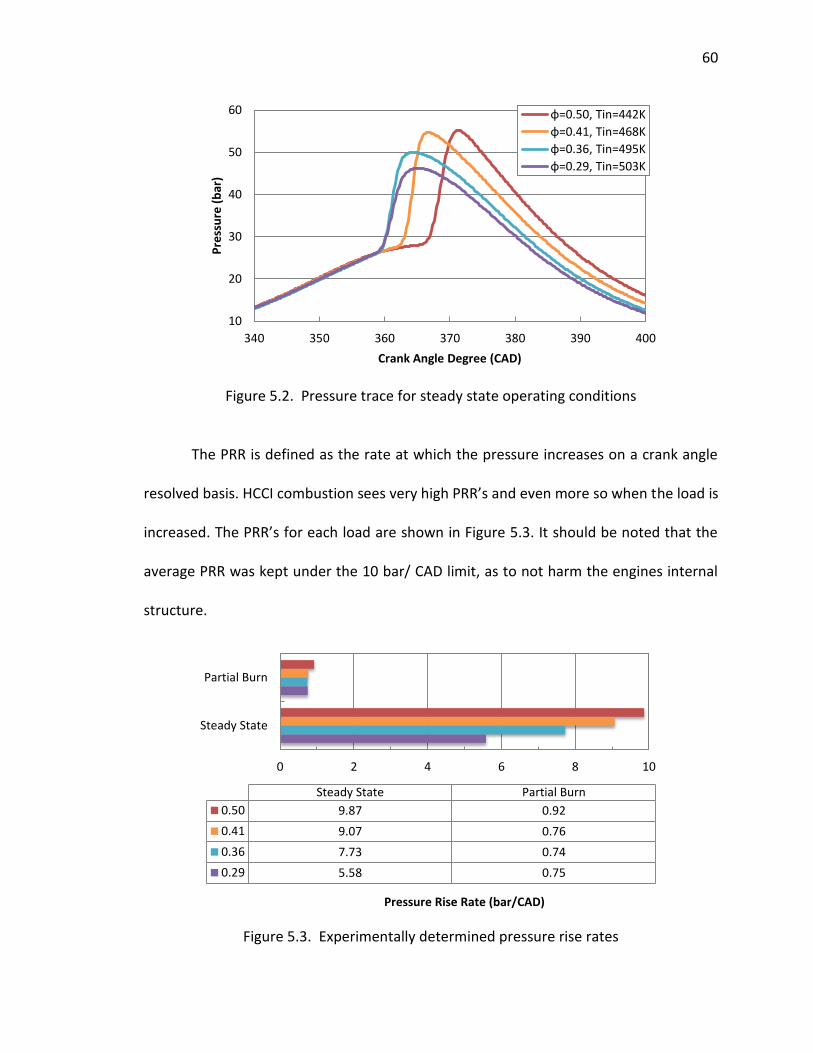
60
Figure 5.2. Pressure trace for steady state operating conditions
The PRR is defined as the rate at which the pressure increases on a crank angle
resolved basis. HCCI combustion sees very high PRR’s and even more so when the load is
increased. The PRR’s for each load are shown in Figure 5.3. It should be noted that the
average PRR was kept under the 10 bar/ CAD limit, as to not harm the engines internal
structure.
Figure 5.3. Experimentally determined pressure rise rates
10
20
30
40
50
60
340 350 360 370 380 390 400
Pre
ssu
re (
bar
)
Crank Angle Degree (CAD)
φ=0.50, Tin=442K
φ=0.41, Tin=468K
φ=0.36, Tin=495K
φ=0.29, Tin=503K
0 2 4 6 8 10
Steady State
Partial Burn
Pressure Rise Rate (bar/CAD)
Steady State Partial Burn
0.50 9.87 0.92
0.41 9.07 0.76
0.36 7.73 0.74
0.29 5.58 0.75
61
The partial burn regime pressure evolution appears as different due to the
combustion phasing and location of this regime. Since combustion occurs very late in
the cycle, the pressure trace will normally show the motored pressure crest when the
engine reaches TDC at 360 CAD, then a small peak will appear after the pressure starts
to decrease indicating combustion. The average CA50 in the partial burn regime is
relative to the load and can be seen in Table 5.1 above. Again, with increased load the
pressure curve is slightly higher due to the amount of energy released from that fuel/air
charge.
The partial burn regime was reached by decreasing the intake temperature
slowly until the engine started to show instabilities. These instabilities are noticeable
audibly, and also through the real-time pressure trace, IMEP values, and in the
monitored exhaust pressure at EVO. The engine was allowed to sit at a set point for
approximately 10 minutes before reducing intake temperature again. Eventually the
partial burn regime is reached and the collected data confirms the trends mentioned
above. If the engine is pushed too far toward the misfire limit, there will be several
consecutive cycles where combustion does not occur and the engine will then start to
motor due to the lack of energy in the intake temperature to start the autoignition
process. Figure 5.4 shows the partial burn pressure traces as they progress with
equivalence ratio. Figure 5.5 is zoomed in on the pressure trace for all 4 loads.
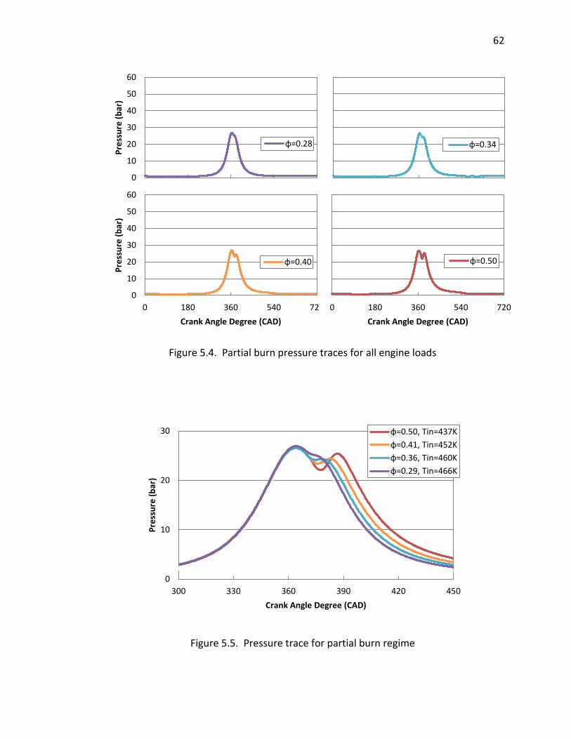
62
Figure 5.4. Partial burn pressure traces for all engine loads
Figure 5.5. Pressure trace for partial burn regime
0
10
20
30
300 330 360 390 420 450
Pre
ssu
re (
bar
)
Crank Angle Degree (CAD)
φ=0.50, Tin=437K
φ=0.41, Tin=452K
φ=0.36, Tin=460K
φ=0.29, Tin=466K
0
10
20
30
40
50
60
Pre
ssu
re (
bar
)
φ=0.28 φ=0.34
0
10
20
30
40
50
60
0 180 360 540 720
Pre
ssu
re (
bar
)
Crank Angle Degree (CAD)
φ=0.40
0 180 360 540 720
Crank Angle Degree (CAD)
φ=0.50
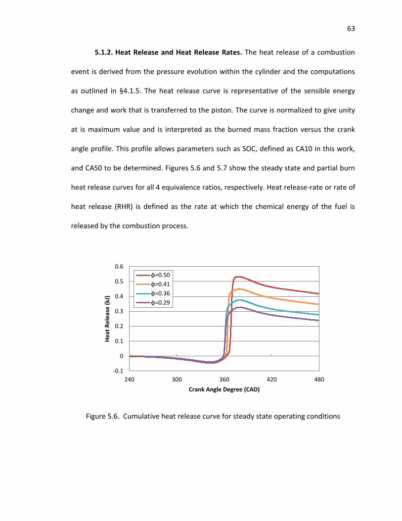
63
5.1.2. Heat Release and Heat Release Rates. The heat release of a combustion
event is derived from the pressure evolution within the cylinder and the computations
as outlined in §4.1.5. The heat release curve is representative of the sensible energy
change and work that is transferred to the piston. The curve is normalized to give unity
at is maximum value and is interpreted as the burned mass fraction versus the crank
angle profile. This profile allows parameters such as SOC, defined as CA10 in this work,
and CA50 to be determined. Figures 5.6 and 5.7 show the steady state and partial burn
heat release curves for all 4 equivalence ratios, respectively. Heat release-rate or rate of
heat release (RHR) is defined as the rate at which the chemical energy of the fuel is
released by the combustion process.
Figure 5.6. Cumulative heat release curve for steady state operating conditions
-0.1
0
0.1
0.2
0.3
0.4
0.5
0.6
240 300 360 420 480
He
at R
ele
ase
(kJ
)
Crank Angle Degree (CAD)
φ=0.50
φ=0.41
φ=0.36
φ=0.29
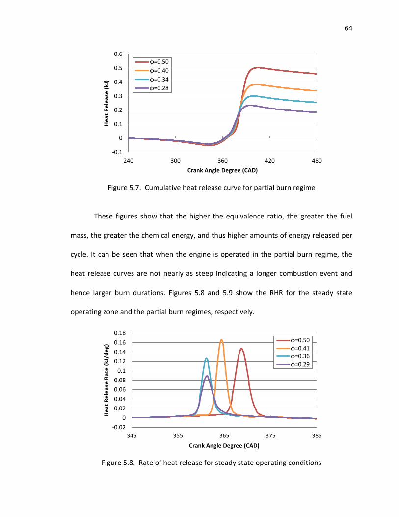
64
Figure 5.7. Cumulative heat release curve for partial burn regime
These figures show that the higher the equivalence ratio, the greater the fuel
mass, the greater the chemical energy, and thus higher amounts of energy released per
cycle. It can be seen that when the engine is operated in the partial burn regime, the
heat release curves are not nearly as steep indicating a longer combustion event and
hence larger burn durations. Figures 5.8 and 5.9 show the RHR for the steady state
operating zone and the partial burn regimes, respectively.
Figure 5.8. Rate of heat release for steady state operating conditions
-0.1
0
0.1
0.2
0.3
0.4
0.5
0.6
240 300 360 420 480
He
at R
ele
ase
(kJ
)
Crank Angle Degree (CAD)
φ=0.50
φ=0.40
φ=0.34
φ=0.28
-0.02
0
0.02
0.04
0.06
0.08
0.1
0.12
0.14
0.16
0.18
345 355 365 375 385
He
at R
ele
ase
Rat
e (
kJ/d
eg)
Crank Angle Degree (CAD)
φ=0.50 φ=0.41 φ=0.36 φ=0.29
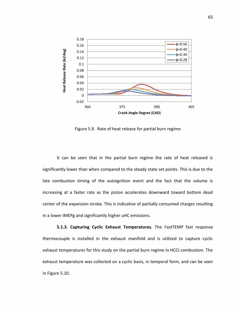
65
Figure 5.9. Rate of heat release for partial burn regime
It can be seen that in the partial burn regime the rate of heat released is
significantly lower than when compared to the steady state set points. This is due to the
late combustion timing of the autoignition event and the fact that the volume is
increasing at a faster rate as the piston accelerates downward toward bottom dead
center of the expansion stroke. This is indicative of partially consumed charges resulting
in a lower IMEPg and significantly higher uHC emissions.
5.1.3. Capturing Cyclic Exhaust Temperatures. The FastTEMP fast response
thermocouple is installed in the exhaust manifold and is utilized to capture cyclic
exhaust temperatures for this study on the partial burn regime in HCCI combustion. The
exhaust temperature was collected on a cyclic basis, in temporal form, and can be seen
in Figure 5.10.
-0.02
0
0.02
0.04
0.06
0.08
0.1
0.12
0.14
0.16
0.18
360 375 390 405
He
at R
ele
ase
Rat
e (
kJ/d
eg)
Crank Angle Degree (CAD)
φ=0.50
φ=0.40
φ=0.34
φ=0.28
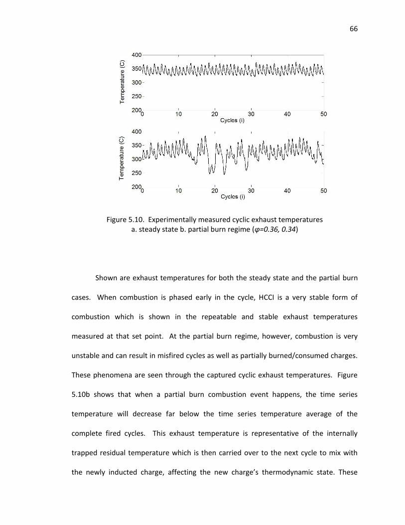
66
Figure 5.10. Experimentally measured cyclic exhaust temperatures a. steady state b. partial burn regime (φ=0.36, 0.34)
Shown are exhaust temperatures for both the steady state and the partial burn
cases. When combustion is phased early in the cycle, HCCI is a very stable form of
combustion which is shown in the repeatable and stable exhaust temperatures
measured at that set point. At the partial burn regime, however, combustion is very
unstable and can result in misfired cycles as well as partially burned/consumed charges.
These phenomena are seen through the captured cyclic exhaust temperatures. Figure
5.10b shows that when a partial burn combustion event happens, the time series
temperature will decrease far below the time series temperature average of the
complete fired cycles. This exhaust temperature is representative of the internally
trapped residual temperature which is then carried over to the next cycle to mix with
the newly inducted charge, affecting the new charge’s thermodynamic state. These
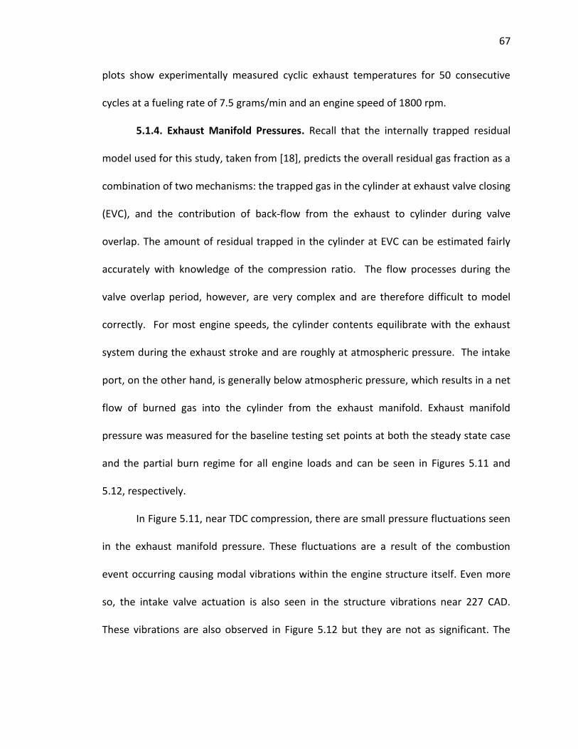
67
plots show experimentally measured cyclic exhaust temperatures for 50 consecutive
cycles at a fueling rate of 7.5 grams/min and an engine speed of 1800 rpm.
5.1.4. Exhaust Manifold Pressures. Recall that the internally trapped residual
model used for this study, taken from [18], predicts the overall residual gas fraction as a
combination of two mechanisms: the trapped gas in the cylinder at exhaust valve closing
(EVC), and the contribution of back-flow from the exhaust to cylinder during valve
overlap. The amount of residual trapped in the cylinder at EVC can be estimated fairly
accurately with knowledge of the compression ratio. The flow processes during the
valve overlap period, however, are very complex and are therefore difficult to model
correctly. For most engine speeds, the cylinder contents equilibrate with the exhaust
system during the exhaust stroke and are roughly at atmospheric pressure. The intake
port, on the other hand, is generally below atmospheric pressure, which results in a net
flow of burned gas into the cylinder from the exhaust manifold. Exhaust manifold
pressure was measured for the baseline testing set points at both the steady state case
and the partial burn regime for all engine loads and can be seen in Figures 5.11 and
5.12, respectively.
In Figure 5.11, near TDC compression, there are small pressure fluctuations seen
in the exhaust manifold pressure. These fluctuations are a result of the combustion
event occurring causing modal vibrations within the engine structure itself. Even more
so, the intake valve actuation is also seen in the structure vibrations near 227 CAD.
These vibrations are also observed in Figure 5.12 but they are not as significant. The
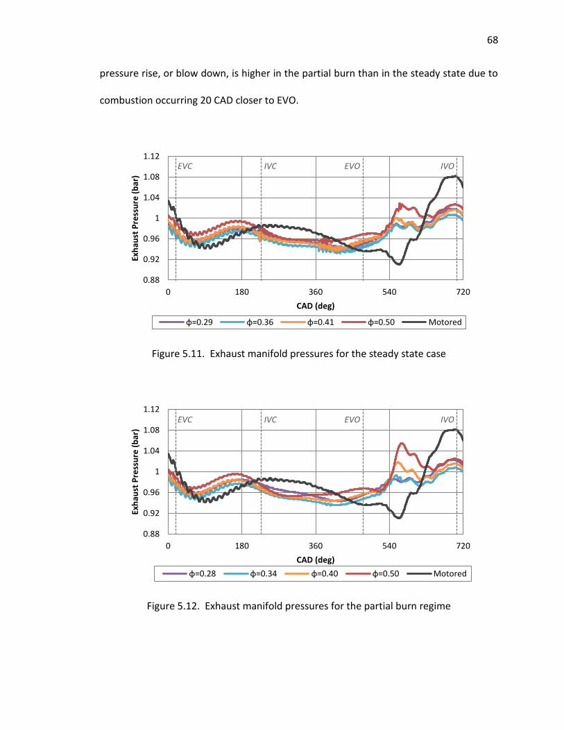
68
pressure rise, or blow down, is higher in the partial burn than in the steady state due to
combustion occurring 20 CAD closer to EVO.
Figure 5.11. Exhaust manifold pressures for the steady state case
Figure 5.12. Exhaust manifold pressures for the partial burn regime
0.88
0.92
0.96
1
1.04
1.08
1.12
0 180 360 540 720
Exh
aust
Pre
ssu
re (
bar
)
CAD (deg)
φ=0.29 φ=0.36 φ=0.41 φ=0.50 Motored
0.88
0.92
0.96
1
1.04
1.08
1.12
0 180 360 540 720
Exh
aust
Pre
ssu
re (
bar
)
CAD (deg)
φ=0.28 φ=0.34 φ=0.40 φ=0.50 Motored
EVC IVO EVO IVC
EVC IVO EVO IVC
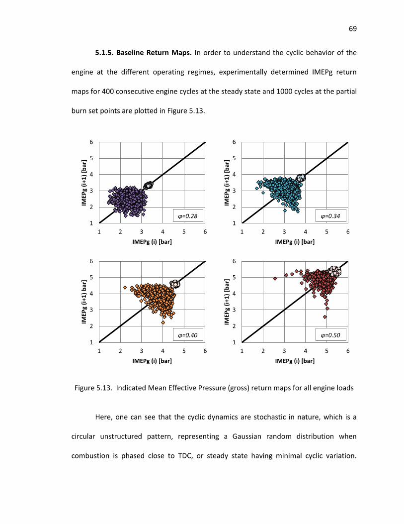
69
5.1.5. Baseline Return Maps. In order to understand the cyclic behavior of the
engine at the different operating regimes, experimentally determined IMEPg return
maps for 400 consecutive engine cycles at the steady state and 1000 cycles at the partial
burn set points are plotted in Figure 5.13.
Figure 5.13. Indicated Mean Effective Pressure (gross) return maps for all engine loads
Here, one can see that the cyclic dynamics are stochastic in nature, which is a
circular unstructured pattern, representing a Gaussian random distribution when
combustion is phased close to TDC, or steady state having minimal cyclic variation.
1
2
3
4
5
6
1 2 3 4 5 6
IMEP
g (i
+1)
[bar
]
IMEPg (i) [bar]
1
2
3
4
5
6
1 2 3 4 5 6IM
EPg
(i+1
) [b
ar]
IMEPg (i) [bar]
1
2
3
4
5
6
1 2 3 4 5 6
IMEP
g (i
+1)
bar
]
IMEPg (i) [bar]
1
2
3
4
5
6
1 2 3 4 5 6
IMEP
g (i
+1)
[bar
]
IMEPg (i) [bar]
φ=0.28 φ=0.34
φ=0.40 φ=0.50
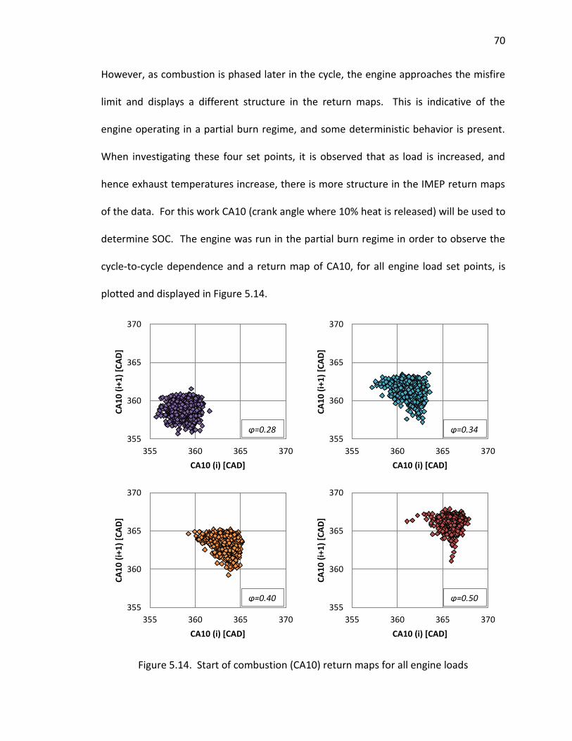
70
However, as combustion is phased later in the cycle, the engine approaches the misfire
limit and displays a different structure in the return maps. This is indicative of the
engine operating in a partial burn regime, and some deterministic behavior is present.
When investigating these four set points, it is observed that as load is increased, and
hence exhaust temperatures increase, there is more structure in the IMEP return maps
of the data. For this work CA10 (crank angle where 10% heat is released) will be used to
determine SOC. The engine was run in the partial burn regime in order to observe the
cycle-to-cycle dependence and a return map of CA10, for all engine load set points, is
plotted and displayed in Figure 5.14.
Figure 5.14. Start of combustion (CA10) return maps for all engine loads
355
360
365
370
355 360 365 370
CA
10
(i+
1)
[CA
D]
CA10 (i) [CAD]
355
360
365
370
355 360 365 370
CA
10
(i+
1)
[CA
D]
CA10 (i) [CAD]
355
360
365
370
355 360 365 370
CA
10
(i+
1)
[CA
D]
CA10 (i) [CAD]
355
360
365
370
355 360 365 370
CA
10
(i+
1)
[CA
D]
CA10 (i) [CAD]
φ=0.28 φ=0.34
φ=0.40 φ=0.50
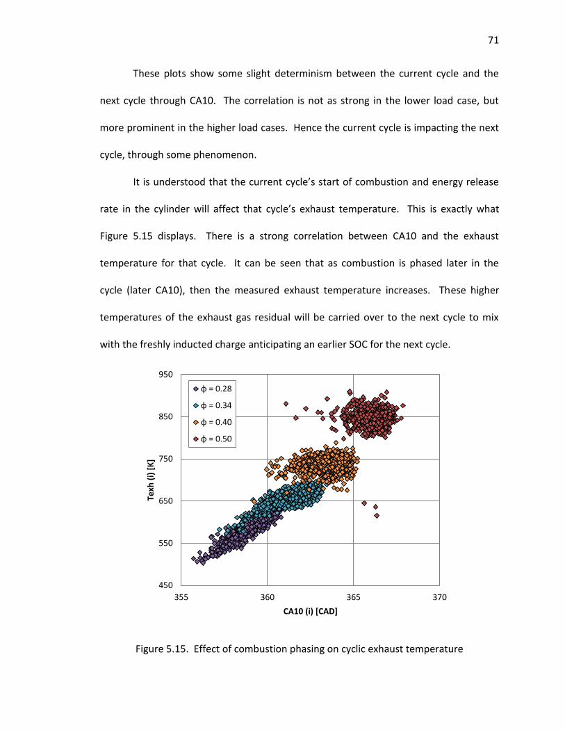
71
These plots show some slight determinism between the current cycle and the
next cycle through CA10. The correlation is not as strong in the lower load case, but
more prominent in the higher load cases. Hence the current cycle is impacting the next
cycle, through some phenomenon.
It is understood that the current cycle’s start of combustion and energy release
rate in the cylinder will affect that cycle’s exhaust temperature. This is exactly what
Figure 5.15 displays. There is a strong correlation between CA10 and the exhaust
temperature for that cycle. It can be seen that as combustion is phased later in the
cycle (later CA10), then the measured exhaust temperature increases. These higher
temperatures of the exhaust gas residual will be carried over to the next cycle to mix
with the freshly inducted charge anticipating an earlier SOC for the next cycle.
Figure 5.15. Effect of combustion phasing on cyclic exhaust temperature
450
550
650
750
850
950
355 360 365 370
Texh
(i)
[K
]
CA10 (i) [CAD]
φ = 0.28
φ = 0.34
φ = 0.40
φ = 0.50
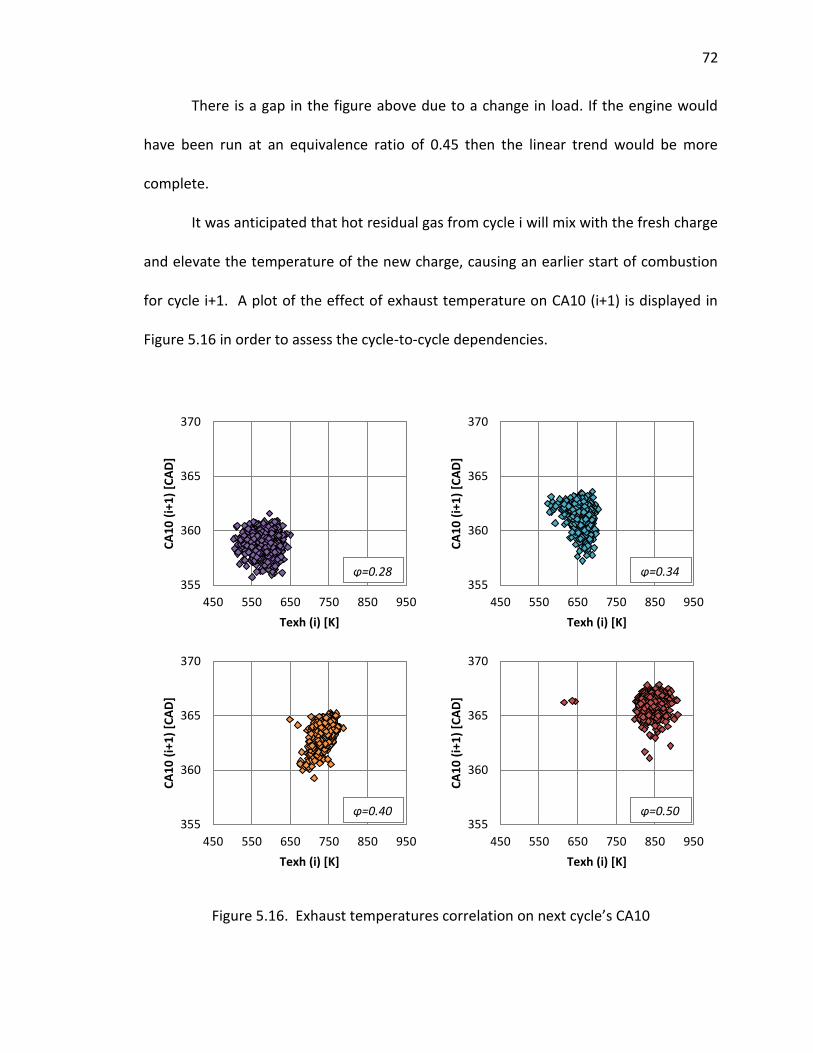
72
There is a gap in the figure above due to a change in load. If the engine would
have been run at an equivalence ratio of 0.45 then the linear trend would be more
complete.
It was anticipated that hot residual gas from cycle i will mix with the fresh charge
and elevate the temperature of the new charge, causing an earlier start of combustion
for cycle i+1. A plot of the effect of exhaust temperature on CA10 (i+1) is displayed in
Figure 5.16 in order to assess the cycle-to-cycle dependencies.
Figure 5.16. Exhaust temperatures correlation on next cycle’s CA10
355
360
365
370
450 550 650 750 850 950
CA
10
(i+
1)
[CA
D]
Texh (i) [K]
355
360
365
370
450 550 650 750 850 950
CA
10
(i+
1)
[CA
D]
Texh (i) [K]
355
360
365
370
450 550 650 750 850 950
CA
10
(i+
1)
[CA
D]
Texh (i) [K]
355
360
365
370
450 550 650 750 850 950
CA
10
(i+
1)
[CA
D]
Texh (i) [K]
φ=0.28 φ=0.34
φ=0.40 φ=0.50
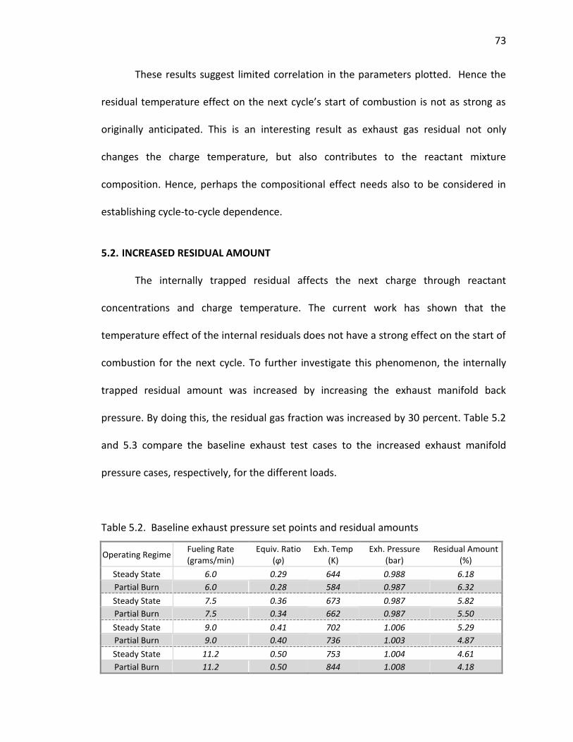
73
These results suggest limited correlation in the parameters plotted. Hence the
residual temperature effect on the next cycle’s start of combustion is not as strong as
originally anticipated. This is an interesting result as exhaust gas residual not only
changes the charge temperature, but also contributes to the reactant mixture
composition. Hence, perhaps the compositional effect needs also to be considered in
establishing cycle-to-cycle dependence.
5.2. INCREASED RESIDUAL AMOUNT
The internally trapped residual affects the next charge through reactant
concentrations and charge temperature. The current work has shown that the
temperature effect of the internal residuals does not have a strong effect on the start of
combustion for the next cycle. To further investigate this phenomenon, the internally
trapped residual amount was increased by increasing the exhaust manifold back
pressure. By doing this, the residual gas fraction was increased by 30 percent. Table 5.2
and 5.3 compare the baseline exhaust test cases to the increased exhaust manifold
pressure cases, respectively, for the different loads.
Table 5.2. Baseline exhaust pressure set points and residual amounts
Operating Regime Fueling Rate (grams/min)
Equiv. Ratio (φ)
Exh. Temp (K)
Exh. Pressure (bar)
Residual Amount (%)
Steady State 6.0 0.29 644 0.988 6.18
Partial Burn 6.0 0.28 584 0.987 6.32
Steady State 7.5 0.36 673 0.987 5.82
Partial Burn 7.5 0.34 662 0.987 5.50
Steady State 9.0 0.41 702 1.006 5.29
Partial Burn 9.0 0.40 736 1.003 4.87
Steady State 11.2 0.50 753 1.004 4.61
Partial Burn 11.2 0.50 844 1.008 4.18
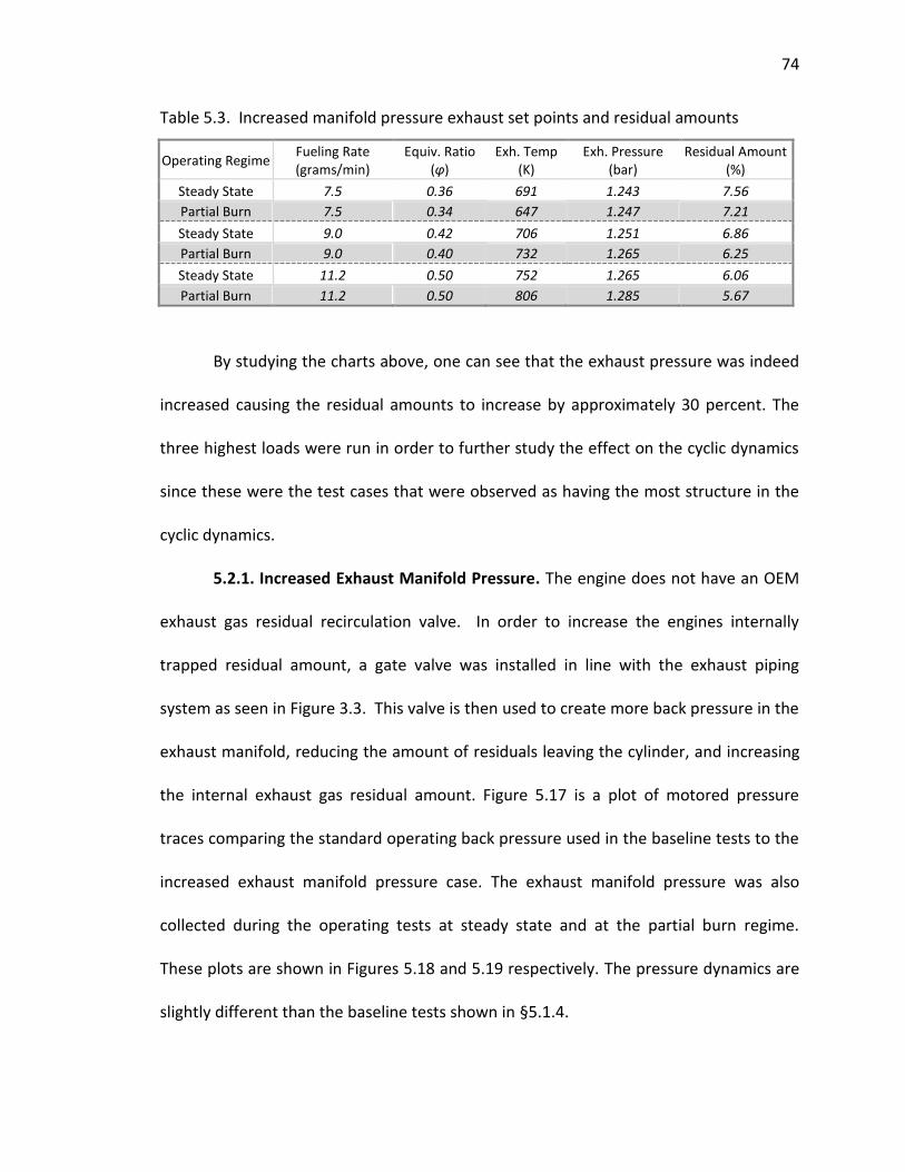
74
Table 5.3. Increased manifold pressure exhaust set points and residual amounts
Operating Regime Fueling Rate (grams/min)
Equiv. Ratio (φ)
Exh. Temp (K)
Exh. Pressure (bar)
Residual Amount (%)
Steady State 7.5 0.36 691 1.243 7.56
Partial Burn 7.5 0.34 647 1.247 7.21
Steady State 9.0 0.42 706 1.251 6.86
Partial Burn 9.0 0.40 732 1.265 6.25
Steady State 11.2 0.50 752 1.265 6.06
Partial Burn 11.2 0.50 806 1.285 5.67
By studying the charts above, one can see that the exhaust pressure was indeed
increased causing the residual amounts to increase by approximately 30 percent. The
three highest loads were run in order to further study the effect on the cyclic dynamics
since these were the test cases that were observed as having the most structure in the
cyclic dynamics.
5.2.1. Increased Exhaust Manifold Pressure. The engine does not have an OEM
exhaust gas residual recirculation valve. In order to increase the engines internally
trapped residual amount, a gate valve was installed in line with the exhaust piping
system as seen in Figure 3.3. This valve is then used to create more back pressure in the
exhaust manifold, reducing the amount of residuals leaving the cylinder, and increasing
the internal exhaust gas residual amount. Figure 5.17 is a plot of motored pressure
traces comparing the standard operating back pressure used in the baseline tests to the
increased exhaust manifold pressure case. The exhaust manifold pressure was also
collected during the operating tests at steady state and at the partial burn regime.
These plots are shown in Figures 5.18 and 5.19 respectively. The pressure dynamics are
slightly different than the baseline tests shown in §5.1.4.
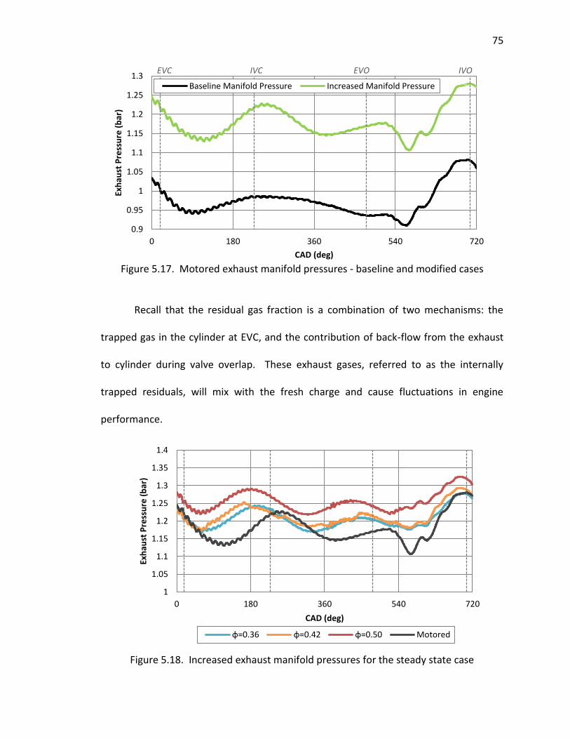
75
Figure 5.17. Motored exhaust manifold pressures - baseline and modified cases
Recall that the residual gas fraction is a combination of two mechanisms: the
trapped gas in the cylinder at EVC, and the contribution of back-flow from the exhaust
to cylinder during valve overlap. These exhaust gases, referred to as the internally
trapped residuals, will mix with the fresh charge and cause fluctuations in engine
performance.
Figure 5.18. Increased exhaust manifold pressures for the steady state case
0.9
0.95
1
1.05
1.1
1.15
1.2
1.25
1.3
0 180 360 540 720
Exh
aust
Pre
ssu
re (
bar
)
CAD (deg)
Baseline Manifold Pressure Increased Manifold Pressure
1
1.05
1.1
1.15
1.2
1.25
1.3
1.35
1.4
0 180 360 540 720
Exh
aust
Pre
ssu
re (
bar
)
CAD (deg)
φ=0.36 φ=0.42 φ=0.50 Motored
EVC IVO EVO IVC
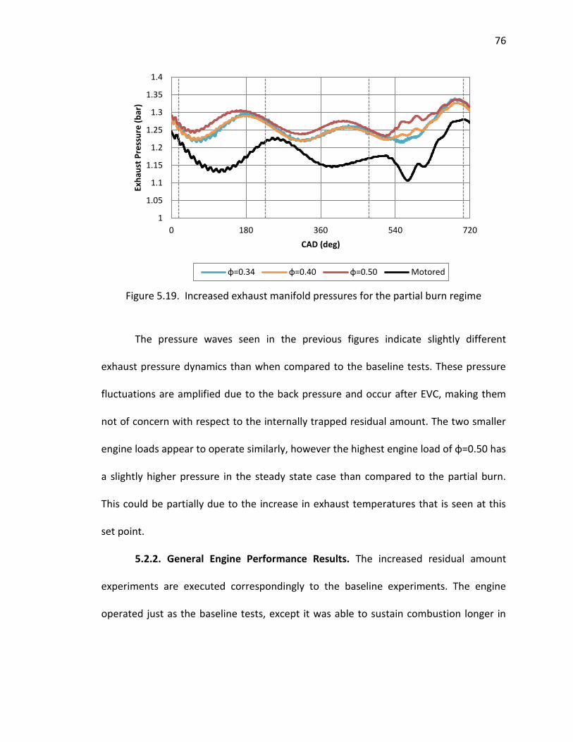
76
Figure 5.19. Increased exhaust manifold pressures for the partial burn regime
The pressure waves seen in the previous figures indicate slightly different
exhaust pressure dynamics than when compared to the baseline tests. These pressure
fluctuations are amplified due to the back pressure and occur after EVC, making them
not of concern with respect to the internally trapped residual amount. The two smaller
engine loads appear to operate similarly, however the highest engine load of φ=0.50 has
a slightly higher pressure in the steady state case than compared to the partial burn.
This could be partially due to the increase in exhaust temperatures that is seen at this
set point.
5.2.2. General Engine Performance Results. The increased residual amount
experiments are executed correspondingly to the baseline experiments. The engine
operated just as the baseline tests, except it was able to sustain combustion longer in
1
1.05
1.1
1.15
1.2
1.25
1.3
1.35
1.4
0 180 360 540 720
Exh
aust
Pre
ssu
re (
bar
)
CAD (deg)
φ=0.34 φ=0.40 φ=0.50 Motored
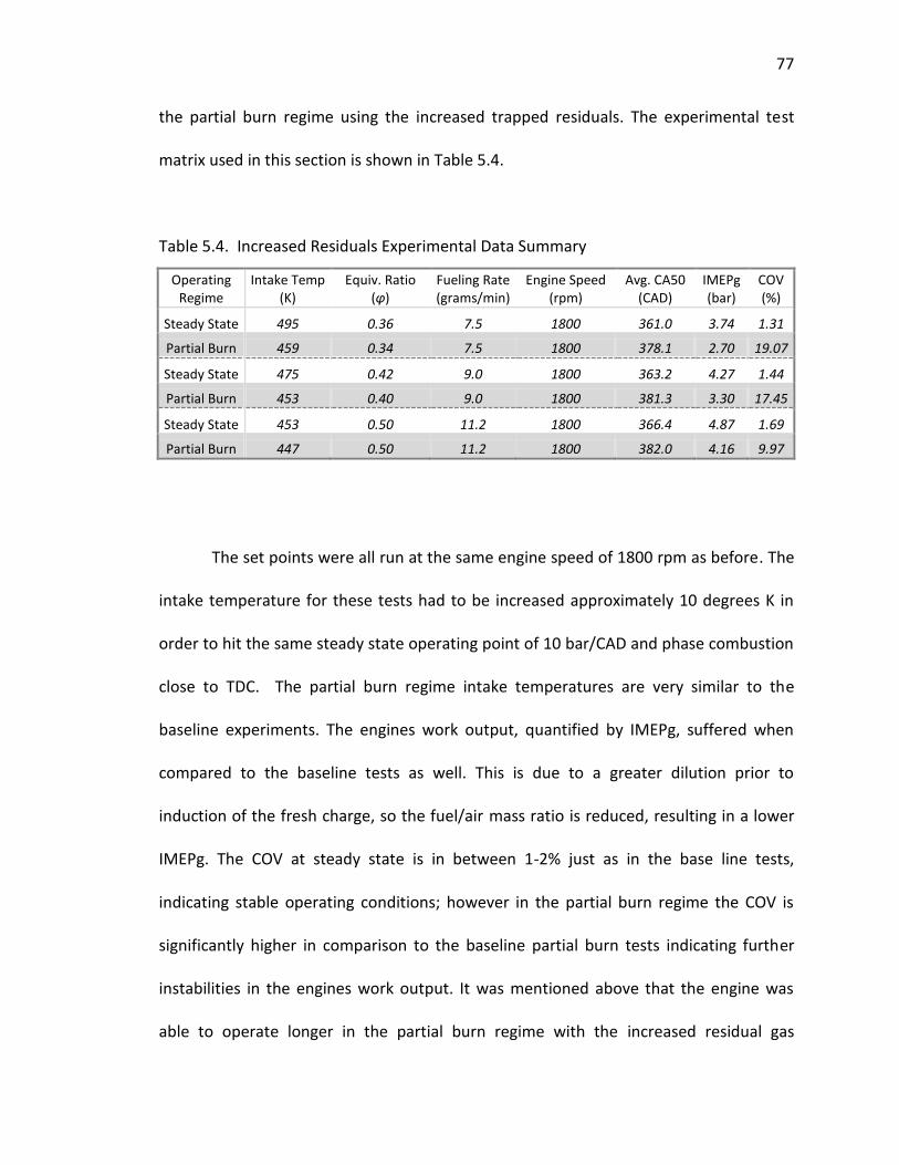
77
the partial burn regime using the increased trapped residuals. The experimental test
matrix used in this section is shown in Table 5.4.
Table 5.4. Increased Residuals Experimental Data Summary
Operating Regime
Intake Temp (K)
Equiv. Ratio (φ)
Fueling Rate (grams/min)
Engine Speed (rpm)
Avg. CA50 (CAD)
IMEPg (bar)
COV (%)
Steady State 495 0.36 7.5 1800 361.0 3.74 1.31
Partial Burn 459 0.34 7.5 1800 378.1 2.70 19.07
Steady State 475 0.42 9.0 1800 363.2 4.27 1.44
Partial Burn 453 0.40 9.0 1800 381.3 3.30 17.45
Steady State 453 0.50 11.2 1800 366.4 4.87 1.69
Partial Burn 447 0.50 11.2 1800 382.0 4.16 9.97
The set points were all run at the same engine speed of 1800 rpm as before. The
intake temperature for these tests had to be increased approximately 10 degrees K in
order to hit the same steady state operating point of 10 bar/CAD and phase combustion
close to TDC. The partial burn regime intake temperatures are very similar to the
baseline experiments. The engines work output, quantified by IMEPg, suffered when
compared to the baseline tests as well. This is due to a greater dilution prior to
induction of the fresh charge, so the fuel/air mass ratio is reduced, resulting in a lower
IMEPg. The COV at steady state is in between 1-2% just as in the base line tests,
indicating stable operating conditions; however in the partial burn regime the COV is
significantly higher in comparison to the baseline partial burn tests indicating further
instabilities in the engines work output. It was mentioned above that the engine was
able to operate longer in the partial burn regime with the increased residual gas
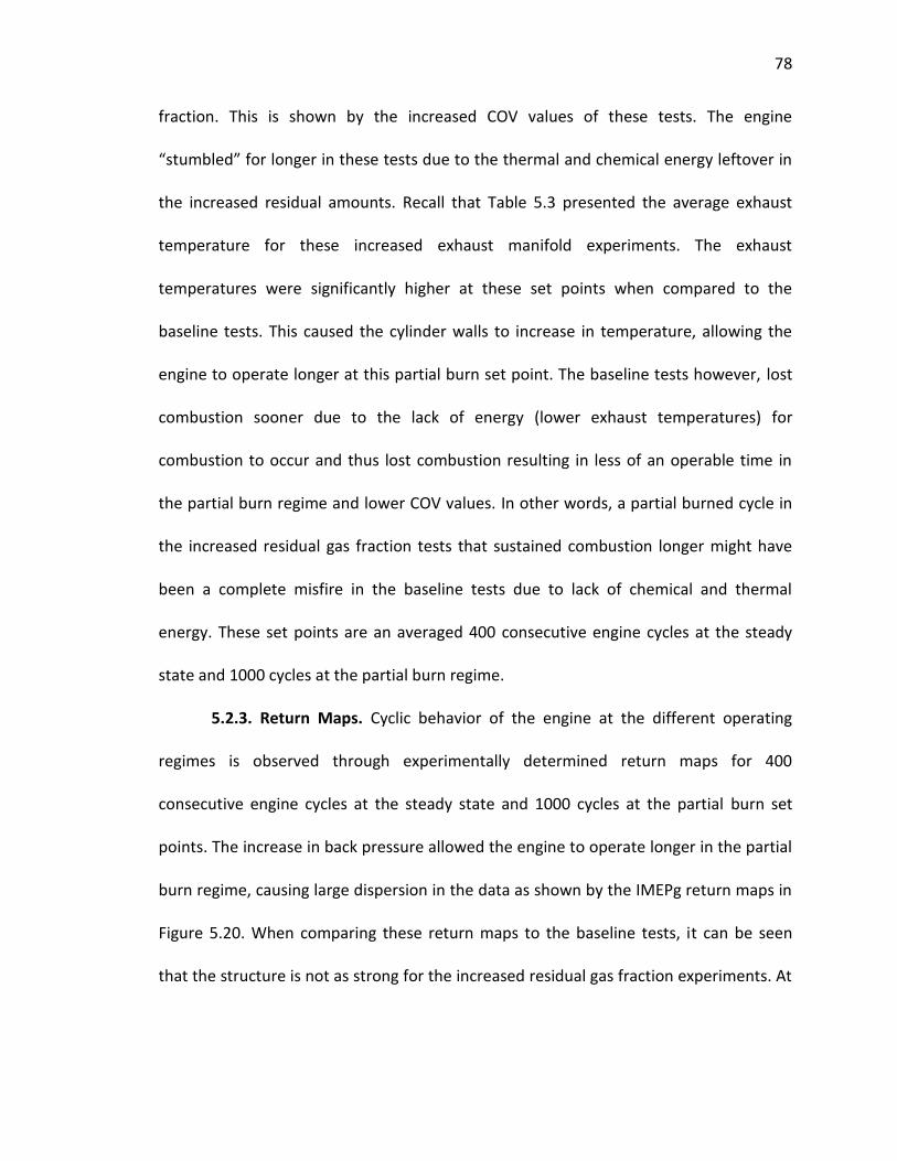
78
fraction. This is shown by the increased COV values of these tests. The engine
“stumbled” for longer in these tests due to the thermal and chemical energy leftover in
the increased residual amounts. Recall that Table 5.3 presented the average exhaust
temperature for these increased exhaust manifold experiments. The exhaust
temperatures were significantly higher at these set points when compared to the
baseline tests. This caused the cylinder walls to increase in temperature, allowing the
engine to operate longer at this partial burn set point. The baseline tests however, lost
combustion sooner due to the lack of energy (lower exhaust temperatures) for
combustion to occur and thus lost combustion resulting in less of an operable time in
the partial burn regime and lower COV values. In other words, a partial burned cycle in
the increased residual gas fraction tests that sustained combustion longer might have
been a complete misfire in the baseline tests due to lack of chemical and thermal
energy. These set points are an averaged 400 consecutive engine cycles at the steady
state and 1000 cycles at the partial burn regime.
5.2.3. Return Maps. Cyclic behavior of the engine at the different operating
regimes is observed through experimentally determined return maps for 400
consecutive engine cycles at the steady state and 1000 cycles at the partial burn set
points. The increase in back pressure allowed the engine to operate longer in the partial
burn regime, causing large dispersion in the data as shown by the IMEPg return maps in
Figure 5.20. When comparing these return maps to the baseline tests, it can be seen
that the structure is not as strong for the increased residual gas fraction experiments. At
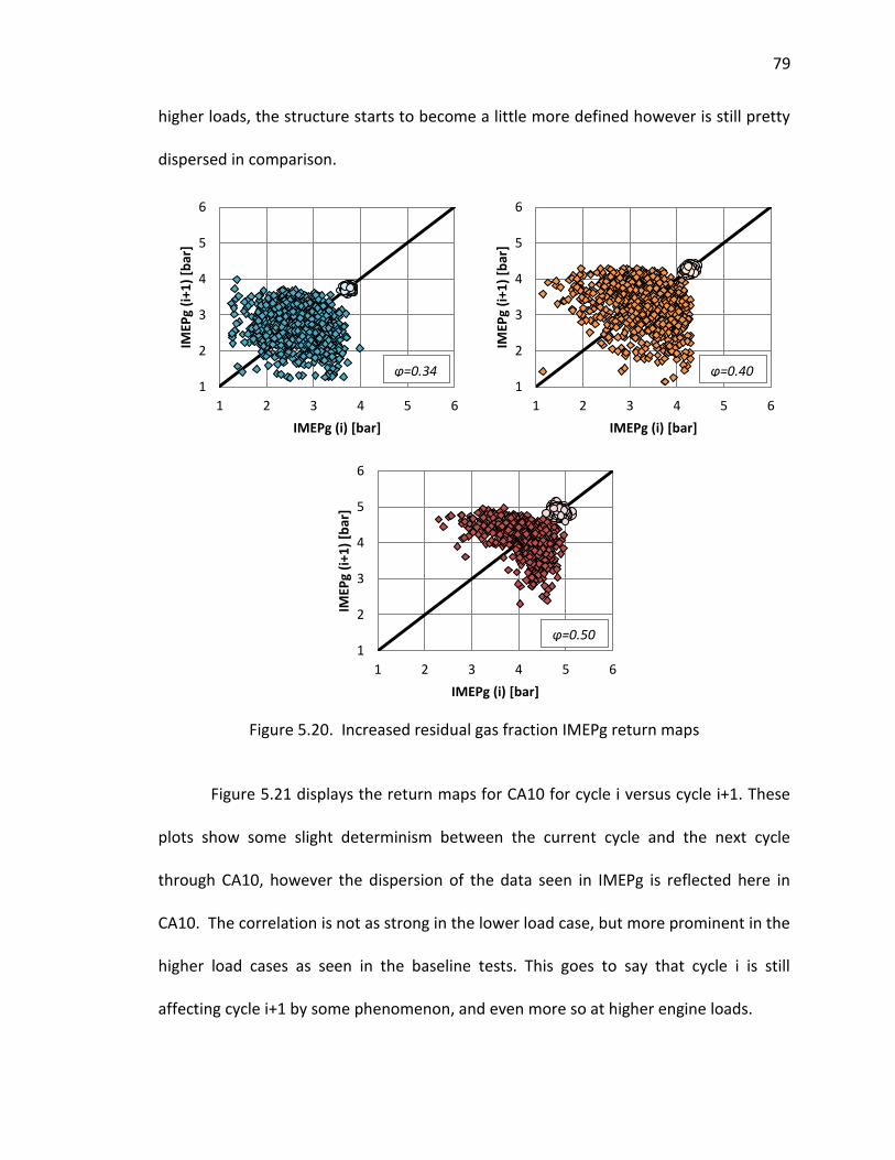
79
higher loads, the structure starts to become a little more defined however is still pretty
dispersed in comparison.
Figure 5.20. Increased residual gas fraction IMEPg return maps
Figure 5.21 displays the return maps for CA10 for cycle i versus cycle i+1. These
plots show some slight determinism between the current cycle and the next cycle
through CA10, however the dispersion of the data seen in IMEPg is reflected here in
CA10. The correlation is not as strong in the lower load case, but more prominent in the
higher load cases as seen in the baseline tests. This goes to say that cycle i is still
affecting cycle i+1 by some phenomenon, and even more so at higher engine loads.
1
2
3
4
5
6
1 2 3 4 5 6
IMEP
g (i
+1)
[bar
]
IMEPg (i) [bar]
1
2
3
4
5
6
1 2 3 4 5 6
IMEP
g (i
+1)
[bar
]
IMEPg (i) [bar]
1
2
3
4
5
6
1 2 3 4 5 6
IMEP
g (i
+1)
[bar
]
IMEPg (i) [bar]
φ=0.34 φ=0.40
φ=0.50
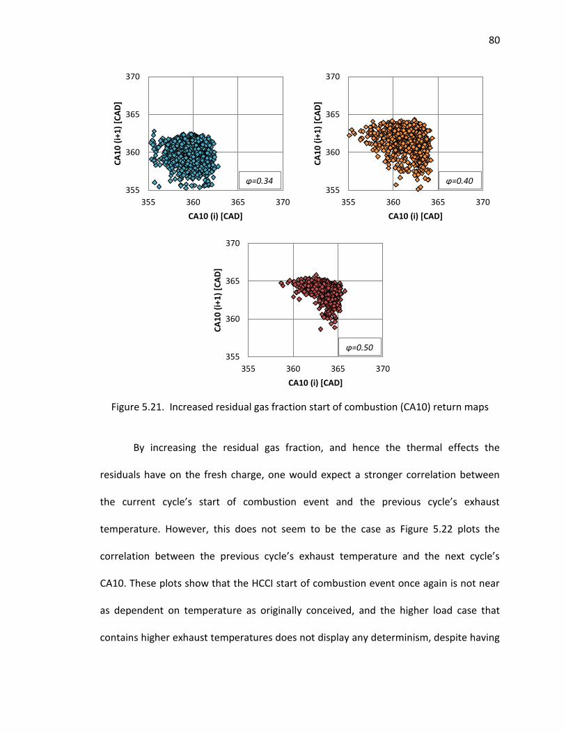
80
Figure 5.21. Increased residual gas fraction start of combustion (CA10) return maps
By increasing the residual gas fraction, and hence the thermal effects the
residuals have on the fresh charge, one would expect a stronger correlation between
the current cycle’s start of combustion event and the previous cycle’s exhaust
temperature. However, this does not seem to be the case as Figure 5.22 plots the
correlation between the previous cycle’s exhaust temperature and the next cycle’s
CA10. These plots show that the HCCI start of combustion event once again is not near
as dependent on temperature as originally conceived, and the higher load case that
contains higher exhaust temperatures does not display any determinism, despite having
355
360
365
370
355 360 365 370
CA
10
(i+
1)
[CA
D]
CA10 (i) [CAD]
355
360
365
370
355 360 365 370
CA
10
(i+
1)
[CA
D]
CA10 (i) [CAD]
355
360
365
370
355 360 365 370
CA
10
(i+
1)
[CA
D]
CA10 (i) [CAD]
φ=0.34 φ=0.40
φ=0.50
81
hot residual temperatures. This goes to say that the next cycle’s combustion event is
more dependent on the chemistry and composition of the residuals than the thermal
effect of the residual gas fraction. This could be the reason that the middle load case,
φ=0.40, has more structure than when compared to the baseline tests due to the
residual gas fraction being increased by approximately 30% and operating in the partial
burn regime could relate some unburned fuel through chemistry back to the fresh
charge. Nonetheless, the case of φ=0.5 has the highest residual gas temperature and
the weakest correlation.
Figure 5.22. Increased residual gas fraction exhaust temperatures correlation on CA10
An interesting result of the increased exhaust manifold pressure, and hence the
internally trapped residual gas fraction, is revealed in Figures 5.23 through 5.25. These
355
360
365
370
450 550 650 750 850 950
CA
10
(i+
1)
[CA
D]
Texh (i) [K]
355
360
365
370
450 550 650 750 850 950
CA
10
(i+
1)
[CA
D]
Texh (i) [K]
355
360
365
370
450 550 650 750 850 950
CA
10
(i+
1)
[CA
D]
Texh (i) [K]
φ=0.34 φ=0.40
φ=0.50
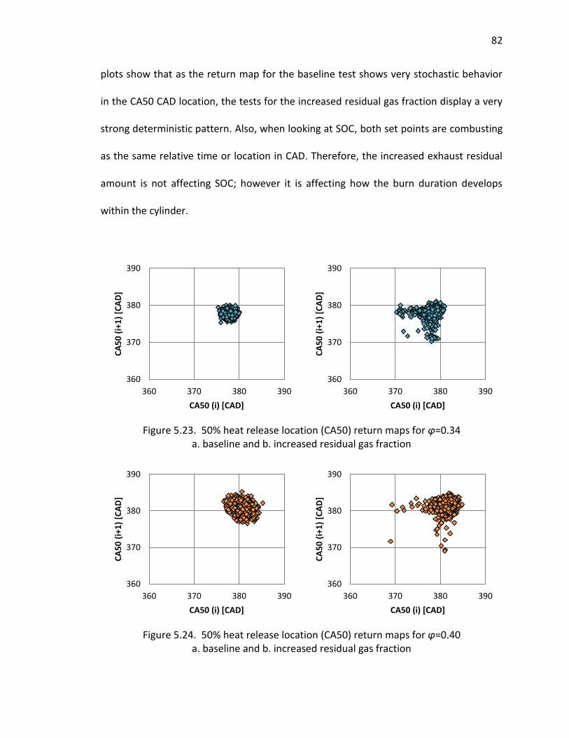
82
plots show that as the return map for the baseline test shows very stochastic behavior
in the CA50 CAD location, the tests for the increased residual gas fraction display a very
strong deterministic pattern. Also, when looking at SOC, both set points are combusting
as the same relative time or location in CAD. Therefore, the increased exhaust residual
amount is not affecting SOC; however it is affecting how the burn duration develops
within the cylinder.
Figure 5.23. 50% heat release location (CA50) return maps for φ=0.34
a. baseline and b. increased residual gas fraction
Figure 5.24. 50% heat release location (CA50) return maps for φ=0.40
a. baseline and b. increased residual gas fraction
360
370
380
390
360 370 380 390
CA
50
(i+
1)
[CA
D]
CA50 (i) [CAD]
360
370
380
390
360 370 380 390
CA
50
(i+
1)
[CA
D]
CA50 (i) [CAD]
360
370
380
390
360 370 380 390
CA
50
(i+
1)
[CA
D]
CA50 (i) [CAD]
360
370
380
390
360 370 380 390
CA
50
(i+
1)
[CA
D]
CA50 (i) [CAD]
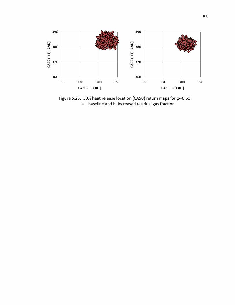
83
Figure 5.25. 50% heat release location (CA50) return maps for φ=0.50
a. baseline and b. increased residual gas fraction
360
370
380
390
360 370 380 390
CA
50
(i+
1)
[CA
D]
CA50 (i) [CAD]
360
370
380
390
360 370 380 390
CA
50
(i+
1)
[CA
D]
CA50 (i) [CAD]
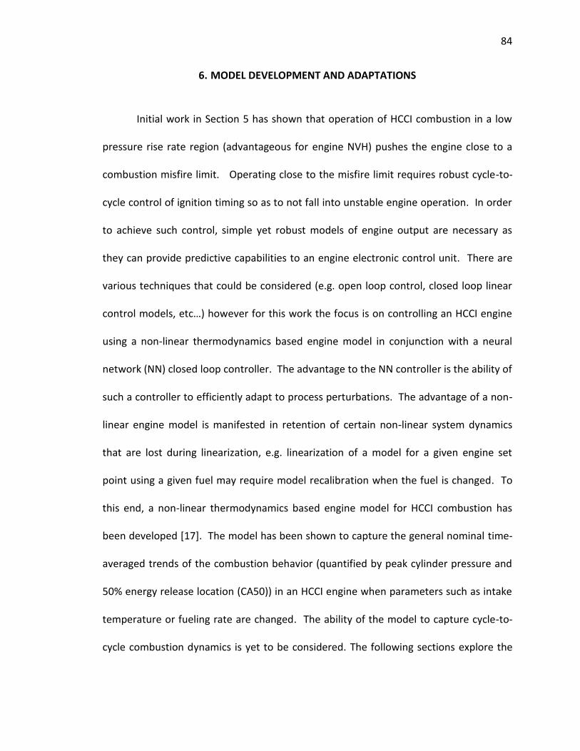
84
6. MODEL DEVELOPMENT AND ADAPTATIONS
Initial work in Section 5 has shown that operation of HCCI combustion in a low
pressure rise rate region (advantageous for engine NVH) pushes the engine close to a
combustion misfire limit. Operating close to the misfire limit requires robust cycle-to-
cycle control of ignition timing so as to not fall into unstable engine operation. In order
to achieve such control, simple yet robust models of engine output are necessary as
they can provide predictive capabilities to an engine electronic control unit. There are
various techniques that could be considered (e.g. open loop control, closed loop linear
control models, etc…) however for this work the focus is on controlling an HCCI engine
using a non-linear thermodynamics based engine model in conjunction with a neural
network (NN) closed loop controller. The advantage to the NN controller is the ability of
such a controller to efficiently adapt to process perturbations. The advantage of a non-
linear engine model is manifested in retention of certain non-linear system dynamics
that are lost during linearization, e.g. linearization of a model for a given engine set
point using a given fuel may require model recalibration when the fuel is changed. To
this end, a non-linear thermodynamics based engine model for HCCI combustion has
been developed [17]. The model has been shown to capture the general nominal time-
averaged trends of the combustion behavior (quantified by peak cylinder pressure and
50% energy release location (CA50)) in an HCCI engine when parameters such as intake
temperature or fueling rate are changed. The ability of the model to capture cycle-to-
cycle combustion dynamics is yet to be considered. The following sections explore the
85
capability of such a model to predict these cycle-to-cycle dynamics regarding the
operational partial burn regime of an HCCI engine.
For an HCCI engine, cyclic dynamics in measures such as temperature and
species will result in next-cycle variations in energy release as well as combustion
timing. Therefore, when considering the ability of a control model to capture the cycle-
to-cycle dynamics of an HCCI engine it must be capable of qualitatively predicting both
variations in ignition timing and engine work output to provide robust combustion
control. Additionally, as will be discussed, the model should be capable of capturing
some details of the residual temperature and composition effects.
6.1. ENGINE CONTROL MODEL
The model considered in this study is the non-linear thermodynamics based
control model described in [17]. This model is a five state thermodynamic model which
has been developed to be utilized in a NN type control scheme for cycle-by-cycle control
of an HCCI engine. A pressure trace of this model is shown in Figure 6.1. The onset of
combustion is modeled using an Arrhenius reaction rate expression which relates the
combustion timing to both charge dilution and temperature. To account for the finite
amount of time required for combustion to occur, a Δθ term is added within the model
which shifts the point of instantaneous combustion from SOC to a point of very high
energy release based on experimental heat release data. Additionally, the effect of
internally trapped exhaust gas residuals on the next cycle’s temperature and
composition are also included. The model has been validated against experimental data
from a single cylinder CI engine operating under HCCI conditions at two different fueling
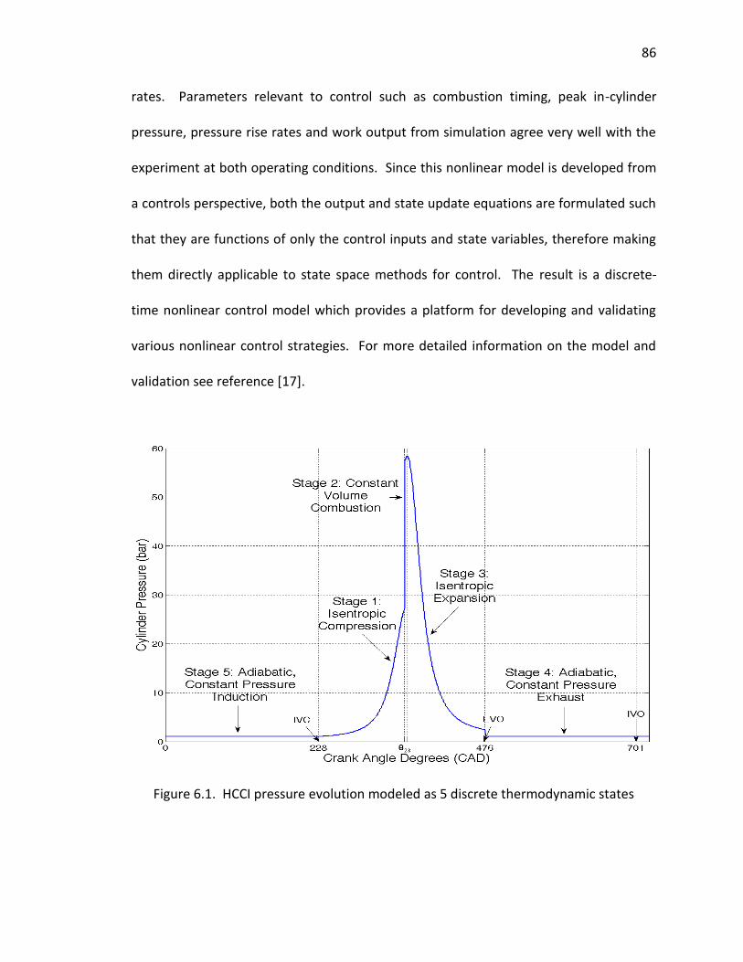
86
rates. Parameters relevant to control such as combustion timing, peak in-cylinder
pressure, pressure rise rates and work output from simulation agree very well with the
experiment at both operating conditions. Since this nonlinear model is developed from
a controls perspective, both the output and state update equations are formulated such
that they are functions of only the control inputs and state variables, therefore making
them directly applicable to state space methods for control. The result is a discrete-
time nonlinear control model which provides a platform for developing and validating
various nonlinear control strategies. For more detailed information on the model and
validation see reference [17].
Figure 6.1. HCCI pressure evolution modeled as 5 discrete thermodynamic states
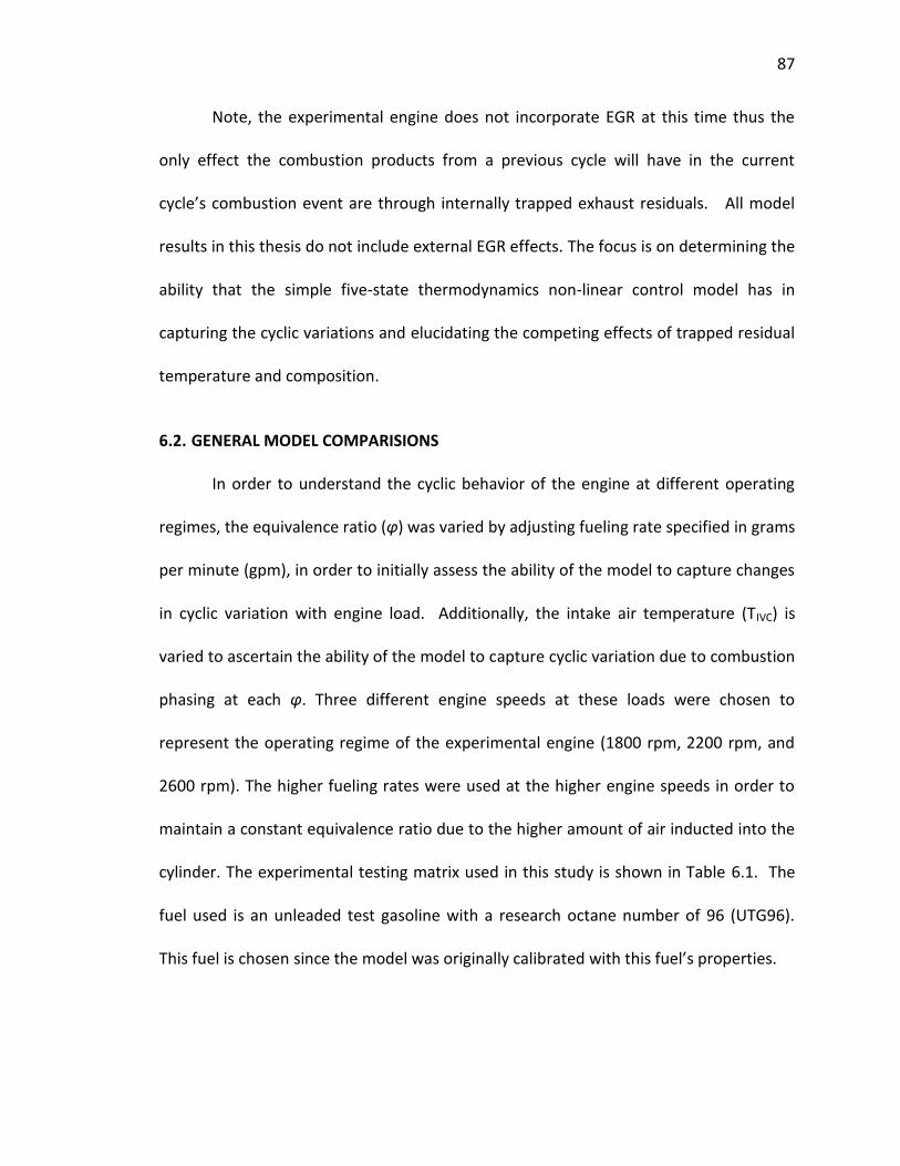
87
Note, the experimental engine does not incorporate EGR at this time thus the
only effect the combustion products from a previous cycle will have in the current
cycle’s combustion event are through internally trapped exhaust residuals. All model
results in this thesis do not include external EGR effects. The focus is on determining the
ability that the simple five-state thermodynamics non-linear control model has in
capturing the cyclic variations and elucidating the competing effects of trapped residual
temperature and composition.
6.2. GENERAL MODEL COMPARISIONS
In order to understand the cyclic behavior of the engine at different operating
regimes, the equivalence ratio (φ) was varied by adjusting fueling rate specified in grams
per minute (gpm), in order to initially assess the ability of the model to capture changes
in cyclic variation with engine load. Additionally, the intake air temperature (TIVC) is
varied to ascertain the ability of the model to capture cyclic variation due to combustion
phasing at each φ. Three different engine speeds at these loads were chosen to
represent the operating regime of the experimental engine (1800 rpm, 2200 rpm, and
2600 rpm). The higher fueling rates were used at the higher engine speeds in order to
maintain a constant equivalence ratio due to the higher amount of air inducted into the
cylinder. The experimental testing matrix used in this study is shown in Table 6.1. The
fuel used is an unleaded test gasoline with a research octane number of 96 (UTG96).
This fuel is chosen since the model was originally calibrated with this fuel’s properties.
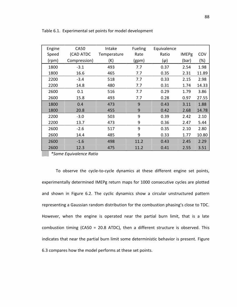
88
Table 6.1. Experimental set points for model development
Engine Speed
CA50 (CAD ATDC
Intake Temperature
Fueling Rate
Equivalence Ratio IMEPg COV
(rpm) Compression) (K) (gpm) (φ) (bar) (%)
1800 -3.1 493 7.7 0.37 2.54 1.98
1800 16.6 465 7.7 0.35 2.31 11.89
2200 -3.4 518 7.7 0.33 2.15 2.98
2200 14.8 480 7.7 0.31 1.74 14.33
2600 0.1 516 7.7 0.29 1.79 3.86
2600 15.8 493 7.7 0.28 0.97 27.55
1800 0.4 473 9 0.43 3.11 1.88
1800 20.8 455 9 0.42 2.68 14.78
2200 -3.0 503 9 0.39 2.42 2.10
2200 13.7 473 9 0.36 2.47 5.44
2600 -2.6 517 9 0.35 2.10 2.80
2600 14.4 485 9 0.33 1.77 10.80
2600 -1.6 498 11.2 0.43 2.45 2.29
2600 12.3 475 11.2 0.41 2.55 3.51
*Same Equivalence Ratio
To observe the cycle-to-cycle dynamics at these different engine set points,
experimentally determined IMEPg return maps for 1000 consecutive cycles are plotted
and shown in Figure 6.2. The cyclic dynamics show a circular unstructured pattern
representing a Gaussian random distribution for the combustion phasing’s close to TDC.
However, when the engine is operated near the partial burn limit, that is a late
combustion timing (CA50 = 20.8 ATDC), then a different structure is observed. This
indicates that near the partial burn limit some deterministic behavior is present. Figure
6.3 compares how the model performs at these set points.
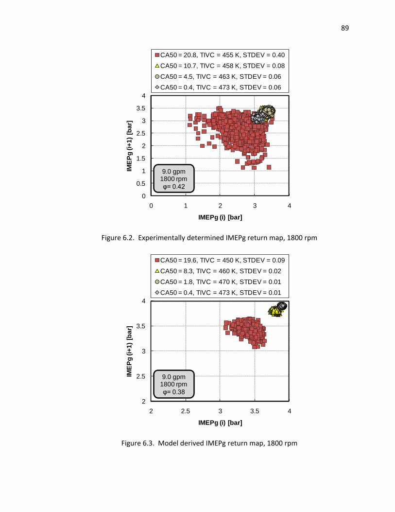
89
Figure 6.2. Experimentally determined IMEPg return map, 1800 rpm
Figure 6.3. Model derived IMEPg return map, 1800 rpm
0
0.5
1
1.5
2
2.5
3
3.5
4
0 1 2 3 4
IME
Pg
(i+
1)
[ba
r]
IMEPg (i) [bar]
CA50 = 20.8, TIVC = 455 K, STDEV = 0.40
CA50 = 10.7, TIVC = 458 K, STDEV = 0.08
CA50 = 4.5, TIVC = 463 K, STDEV = 0.06
CA50 = 0.4, TIVC = 473 K, STDEV = 0.06
9.0 gpm 1800 rpm
φ= 0.42
2
2.5
3
3.5
4
2 2.5 3 3.5 4
IME
Pg
(i+
1)
[ba
r]
IMEPg (i) [bar]
CA50 = 19.6, TIVC = 450 K, STDEV = 0.09
CA50 = 8.3, TIVC = 460 K, STDEV = 0.02
CA50 = 1.8, TIVC = 470 K, STDEV = 0.01
CA50 = 0.4, TIVC = 473 K, STDEV = 0.01
9.0 gpm 1800 rpm
φ= 0.38
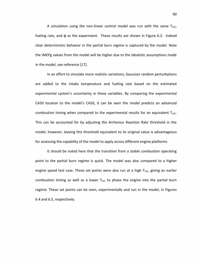
90
A simulation using the non-linear control model was run with the same TIVC,
fueling rate, and φ as the experiment. These results are shown in Figure 6.3. Indeed
clear deterministic behavior in the partial burn regime is captured by the model. Note
the IMEPg values from the model will be higher due to the idealistic assumptions made
in the model, see reference [17].
In an effort to simulate more realistic variations, Gaussian random perturbations
are added to the intake temperature and fueling rate based on the estimated
experimental system’s uncertainty in these variables. By comparing the experimental
CA50 location to the model’s CA50, it can be seen the model predicts an advanced
combustion timing when compared to the experimental results for an equivalent TIVC.
This can be accounted for by adjusting the Arrhenius Reaction Rate threshold in the
model, however, leaving this threshold equivalent to its original value is advantageous
for assessing the capability of the model to apply across different engine platforms.
It should be noted here that the transition from a stable combustion operating
point to the partial burn regime is quick. The model was also compared to a higher
engine speed test case. These set points were also run at a high TIVC, giving an earlier
combustion timing as well as a lower TIVC to phase the engine into the partial burn
regime. These set points can be seen, experimentally and run in the model, in Figures
6.4 and 6.5, respectively.
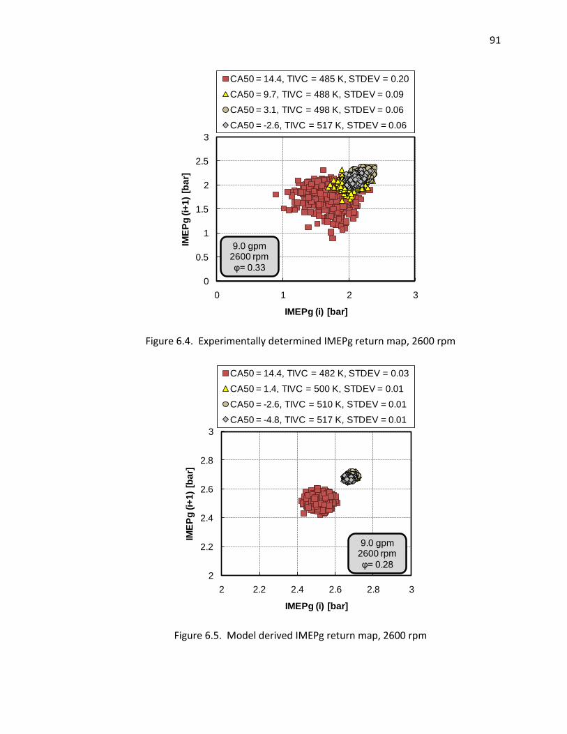
91
Figure 6.4. Experimentally determined IMEPg return map, 2600 rpm
Figure 6.5. Model derived IMEPg return map, 2600 rpm
0
0.5
1
1.5
2
2.5
3
0 1 2 3
IME
Pg
(i+
1)
[ba
r]
IMEPg (i) [bar]
CA50 = 14.4, TIVC = 485 K, STDEV = 0.20
CA50 = 9.7, TIVC = 488 K, STDEV = 0.09
CA50 = 3.1, TIVC = 498 K, STDEV = 0.06
CA50 = -2.6, TIVC = 517 K, STDEV = 0.06
9.0 gpm 2600 rpm
φ= 0.33
2
2.2
2.4
2.6
2.8
3
2 2.2 2.4 2.6 2.8 3
IME
Pg
(i+
1)
[ba
r]
IMEPg (i) [bar]
CA50 = 14.4, TIVC = 482 K, STDEV = 0.03
CA50 = 1.4, TIVC = 500 K, STDEV = 0.01
CA50 = -2.6, TIVC = 510 K, STDEV = 0.01
CA50 = -4.8, TIVC = 517 K, STDEV = 0.01
9.0 gpm 2600 rpm
φ= 0.28
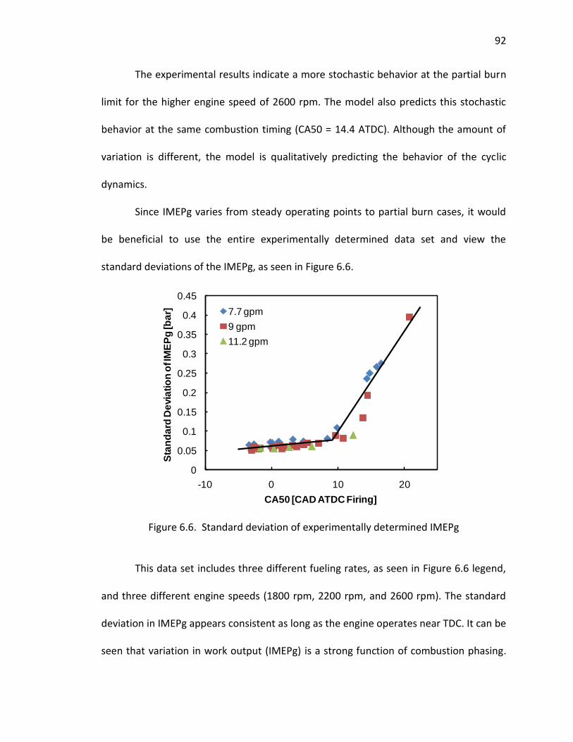
92
The experimental results indicate a more stochastic behavior at the partial burn
limit for the higher engine speed of 2600 rpm. The model also predicts this stochastic
behavior at the same combustion timing (CA50 = 14.4 ATDC). Although the amount of
variation is different, the model is qualitatively predicting the behavior of the cyclic
dynamics.
Since IMEPg varies from steady operating points to partial burn cases, it would
be beneficial to use the entire experimentally determined data set and view the
standard deviations of the IMEPg, as seen in Figure 6.6.
Figure 6.6. Standard deviation of experimentally determined IMEPg
This data set includes three different fueling rates, as seen in Figure 6.6 legend,
and three different engine speeds (1800 rpm, 2200 rpm, and 2600 rpm). The standard
deviation in IMEPg appears consistent as long as the engine operates near TDC. It can be
seen that variation in work output (IMEPg) is a strong function of combustion phasing.
0
0.05
0.1
0.15
0.2
0.25
0.3
0.35
0.4
0.45
-10 0 10 20
Sta
nd
ard
De
via
tio
n o
f IM
EP
g [b
ar]
CA50 [CAD ATDC Firing]
7.7 gpm
9 gpm
11.2 gpm
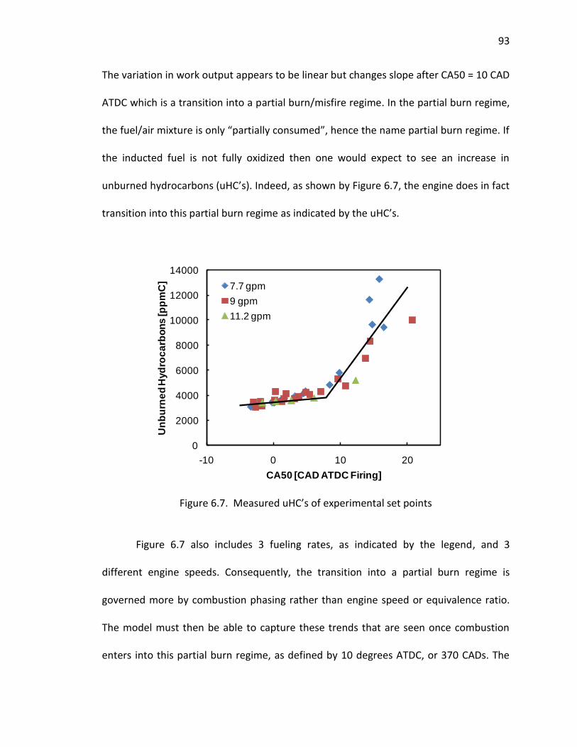
93
The variation in work output appears to be linear but changes slope after CA50 = 10 CAD
ATDC which is a transition into a partial burn/misfire regime. In the partial burn regime,
the fuel/air mixture is only “partially consumed”, hence the name partial burn regime. If
the inducted fuel is not fully oxidized then one would expect to see an increase in
unburned hydrocarbons (uHC’s). Indeed, as shown by Figure 6.7, the engine does in fact
transition into this partial burn regime as indicated by the uHC’s.
Figure 6.7. Measured uHC’s of experimental set points
Figure 6.7 also includes 3 fueling rates, as indicated by the legend, and 3
different engine speeds. Consequently, the transition into a partial burn regime is
governed more by combustion phasing rather than engine speed or equivalence ratio.
The model must then be able to capture these trends that are seen once combustion
enters into this partial burn regime, as defined by 10 degrees ATDC, or 370 CADs. The
0
2000
4000
6000
8000
10000
12000
14000
-10 0 10 20
Un
bu
rne
d H
yd
roc
arb
on
s [p
pm
C]
CA50 [CAD ATDC Firing]
7.7 gpm
9 gpm
11.2 gpm
94
misfire limit is when combustion does not occur and none of the fuel is consumed,
causing the residuals for that cycle to be comprised completely of unburned fuel. This
limit is set at 20 degrees ATDC, or 380 CADs. This is chosen as the engine experimentally
has been found to lose combustion at or slightly before this location.
6.3. MODELING THE UNBURNED RESIDUAL
Recall that HCCI combustion is governed by two main parameters: the
concentrations of fuel and oxygen, and the temperature. This means that changing the
concentration and/or the temperature of the intake charge will cause the combustion
phasing to change. The fact that the residual gas fraction directly affects both the
reactant concentrations and the temperature, makes it an important parameter when
trying to model combustion timing in an HCCI engine. Therefore, a practical and
accurate model for predicting the residual gas fraction αr is needed in order to
accurately predict the combustion timing.
The predictive model used was taken from [18]. This model predicts the overall
residual gas fraction as a combination of two components: the contribution of back-
flow from the exhaust to the cylinder during valve overlap, and the trapped gas in the
cylinder at exhaust valve closing. This back-flow contributes significantly to the residual
gas fraction for each engine cycle. Recall that the parameter often used to describe this
back-flow is the valve overlap factor (OF) [34] and is shown in Equation 24 in §4.3. Once
the overlap factor, OF, is known, an expression for the overall residual gas fraction can
be determined. The empirical expression from [18] is also given in in §4.3 as Equation
25. This resulting model relates the residual gas fraction to six independent parameters:
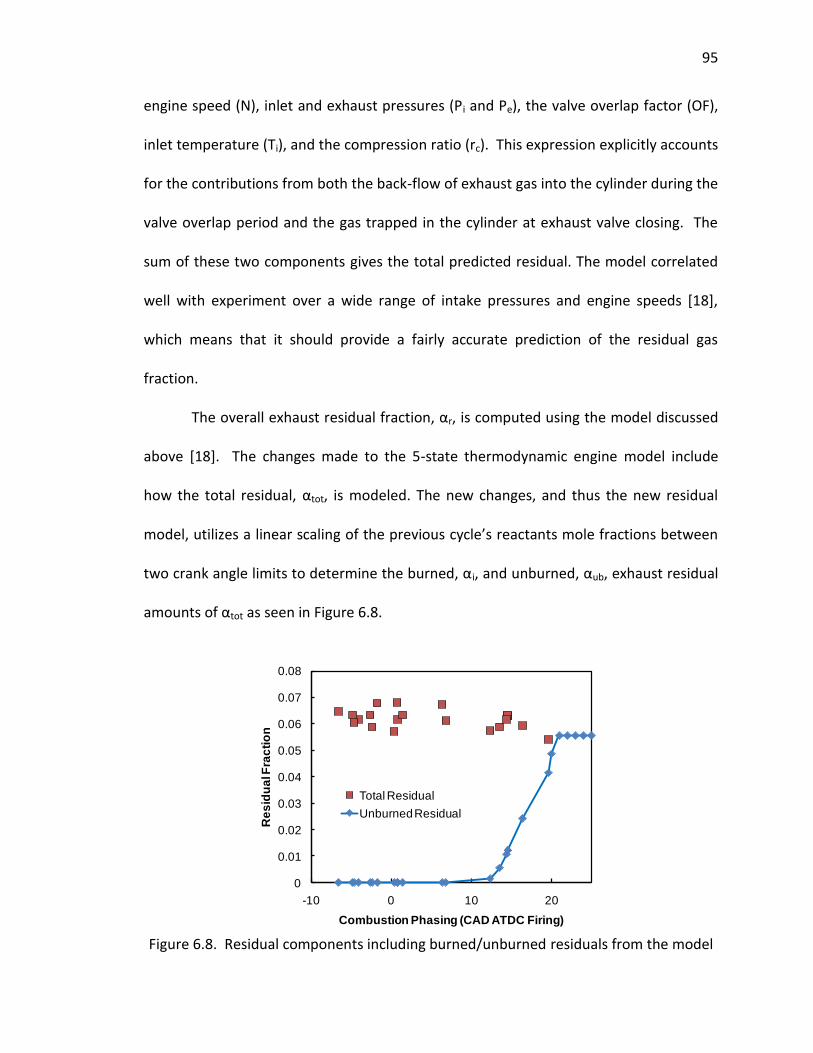
95
engine speed (N), inlet and exhaust pressures (Pi and Pe), the valve overlap factor (OF),
inlet temperature (Ti), and the compression ratio (rc). This expression explicitly accounts
for the contributions from both the back-flow of exhaust gas into the cylinder during the
valve overlap period and the gas trapped in the cylinder at exhaust valve closing. The
sum of these two components gives the total predicted residual. The model correlated
well with experiment over a wide range of intake pressures and engine speeds [18],
which means that it should provide a fairly accurate prediction of the residual gas
fraction.
The overall exhaust residual fraction, αr, is computed using the model discussed
above [18]. The changes made to the 5-state thermodynamic engine model include
how the total residual, αtot, is modeled. The new changes, and thus the new residual
model, utilizes a linear scaling of the previous cycle’s reactants mole fractions between
two crank angle limits to determine the burned, αi, and unburned, αub, exhaust residual
amounts of αtot as seen in Figure 6.8.
Figure 6.8. Residual components including burned/unburned residuals from the model
0
0.01
0.02
0.03
0.04
0.05
0.06
0.07
0.08
-10 0 10 20
Re
sid
ua
l Fra
cti
on
Combustion Phasing (CAD ATDC Firing)
Total Residual
Unburned Residual
96
The limits are defined as the crank angle degree at which an initial partial burn
limit is seen, CAPB, and a complete misfire limit that is observed, CAMF. The choice of
CAPB and CAMF will effectively set the lean combustion limits of the model. The crank
angle limits represent the onset of partial burn and misfire as discussed at the end of
the previous section and are set to 370 and 380, respectively. The unburned residual
fraction, αub, is scaled linearly proportional to the exhaust residual fraction, αi, based on
the following relationships:
The residual temperature is computed by scaling the exhaust temperature by a
residual heat transfer factor, X. Composition effects of the residual are captured
through the thermodynamic properties of the mixture, specifically through the specific
heat capacity of the residual. Note the inclusion of αub impacts the fuel and air in the
reactants considered during computation for ignition while αi influences only the
amount of oxidizer present for combustion. The composition effect of including αub is
through the specific heat capacity of high temperature unburned reactants and not
from properties of individual chemical species. Other than the inclusion of unburned
reactants, the model always assumes complete combustion products with excess
oxygen.
{
[
]
(26)
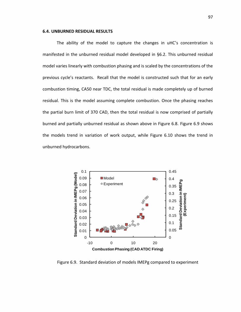
97
6.4. UNBURNED RESIDUAL RESULTS
The ability of the model to capture the changes in uHC’s concentration is
manifested in the unburned residual model developed in §6.2. This unburned residual
model varies linearly with combustion phasing and is scaled by the concentrations of the
previous cycle’s reactants. Recall that the model is constructed such that for an early
combustion timing, CA50 near TDC, the total residual is made completely up of burned
residual. This is the model assuming complete combustion. Once the phasing reaches
the partial burn limit of 370 CAD, then the total residual is now comprised of partially
burned and partially unburned residual as shown above in Figure 6.8. Figure 6.9 shows
the models trend in variation of work output, while Figure 6.10 shows the trend in
unburned hydrocarbons.
Figure 6.9. Standard deviation of models IMEPg compared to experiment
0
0.05
0.1
0.15
0.2
0.25
0.3
0.35
0.4
0.45
0
0.01
0.02
0.03
0.04
0.05
0.06
0.07
0.08
0.09
0.1
-10 0 10 20
Sta
nd
ard
De
via
tio
n in
IME
Pg
(E
xp
eri
me
nt)
Sta
nd
ard
De
via
tio
n in
IME
Pg
(M
od
el)
Combustion Phasing (CAD ATDC Firing)
Model
Experiment
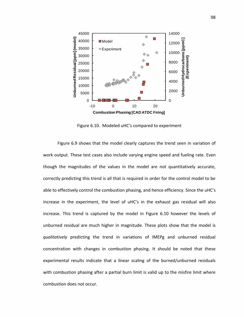
98
Figure 6.10. Modeled uHC’s compared to experiment
Figure 6.9 shows that the model clearly captures the trend seen in variation of
work output. These test cases also include varying engine speed and fueling rate. Even
though the magnitudes of the values in the model are not quantitatively accurate,
correctly predicting this trend is all that is required in order for the control model to be
able to effectively control the combustion phasing, and hence efficiency. Since the uHC’s
increase in the experiment, the level of uHC’s in the exhaust gas residual will also
increase. This trend is captured by the model in Figure 6.10 however the levels of
unburned residual are much higher in magnitude. These plots show that the model is
qualitatively predicting the trend in variations of IMEPg and unburned residual
concentration with changes in combustion phasing. It should be noted that these
experimental results indicate that a linear scaling of the burned/unburned residuals
with combustion phasing after a partial burn limit is valid up to the misfire limit where
combustion does not occur.
0
2000
4000
6000
8000
10000
12000
14000
0
5000
10000
15000
20000
25000
30000
35000
40000
45000
-10 0 10 20
Un
bu
rne
d H
yd
roc
arb
on
s [p
pm
C]
(Ex
pe
rim
en
t)
Un
bu
rne
d R
es
idu
al [
pp
m] (m
od
el)
Combustion Phasing [CAD ATDC Firing]
Model
Experiment
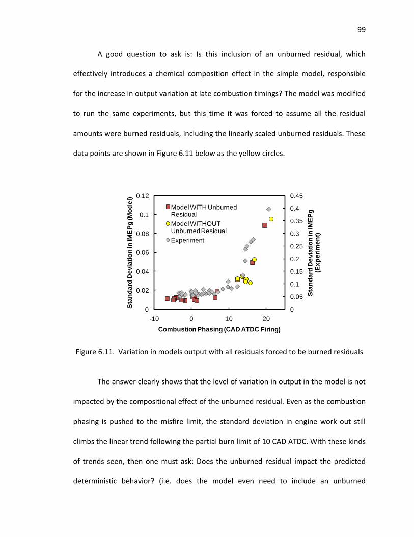
99
A good question to ask is: Is this inclusion of an unburned residual, which
effectively introduces a chemical composition effect in the simple model, responsible
for the increase in output variation at late combustion timings? The model was modified
to run the same experiments, but this time it was forced to assume all the residual
amounts were burned residuals, including the linearly scaled unburned residuals. These
data points are shown in Figure 6.11 below as the yellow circles.
Figure 6.11. Variation in models output with all residuals forced to be burned residuals
The answer clearly shows that the level of variation in output in the model is not
impacted by the compositional effect of the unburned residual. Even as the combustion
phasing is pushed to the misfire limit, the standard deviation in engine work out still
climbs the linear trend following the partial burn limit of 10 CAD ATDC. With these kinds
of trends seen, then one must ask: Does the unburned residual impact the predicted
deterministic behavior? (i.e. does the model even need to include an unburned
0
0.05
0.1
0.15
0.2
0.25
0.3
0.35
0.4
0.45
0
0.02
0.04
0.06
0.08
0.1
0.12
-10 0 10 20
Sta
nd
ard
De
via
tio
n in
IME
Pg
(E
xp
eri
me
nt)
Sta
nd
ard
De
via
tio
n in
IME
Pg
(M
od
el)
Combustion Phasing (CAD ATDC Firing)
Model WITH Unburned Residual
Model WITHOUT Unburned Residual
Experiment
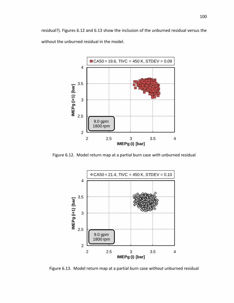
100
residual?). Figures 6.12 and 6.13 show the inclusion of the unburned residual versus the
without the unburned residual in the model.
Figure 6.12. Model return map at a partial burn case with unburned residual
Figure 6.13. Model return map at a partial burn case without unburned residual
2
2.5
3
3.5
4
2 2.5 3 3.5 4
IME
Pg
(i+
1)
[ba
r]
IMEPg (i) [bar]
CA50 = 19.6, TIVC = 450 K, STDEV = 0.09
9.0 gpm 1800 rpm
2
2.5
3
3.5
4
2 2.5 3 3.5 4
IME
Pg
(i+
1)
[ba
r]
IMEPg (i) [bar]
CA50 = 21.4, TIVC = 450 K, STDEV = 0.10
9.0 gpm 1800 rpm
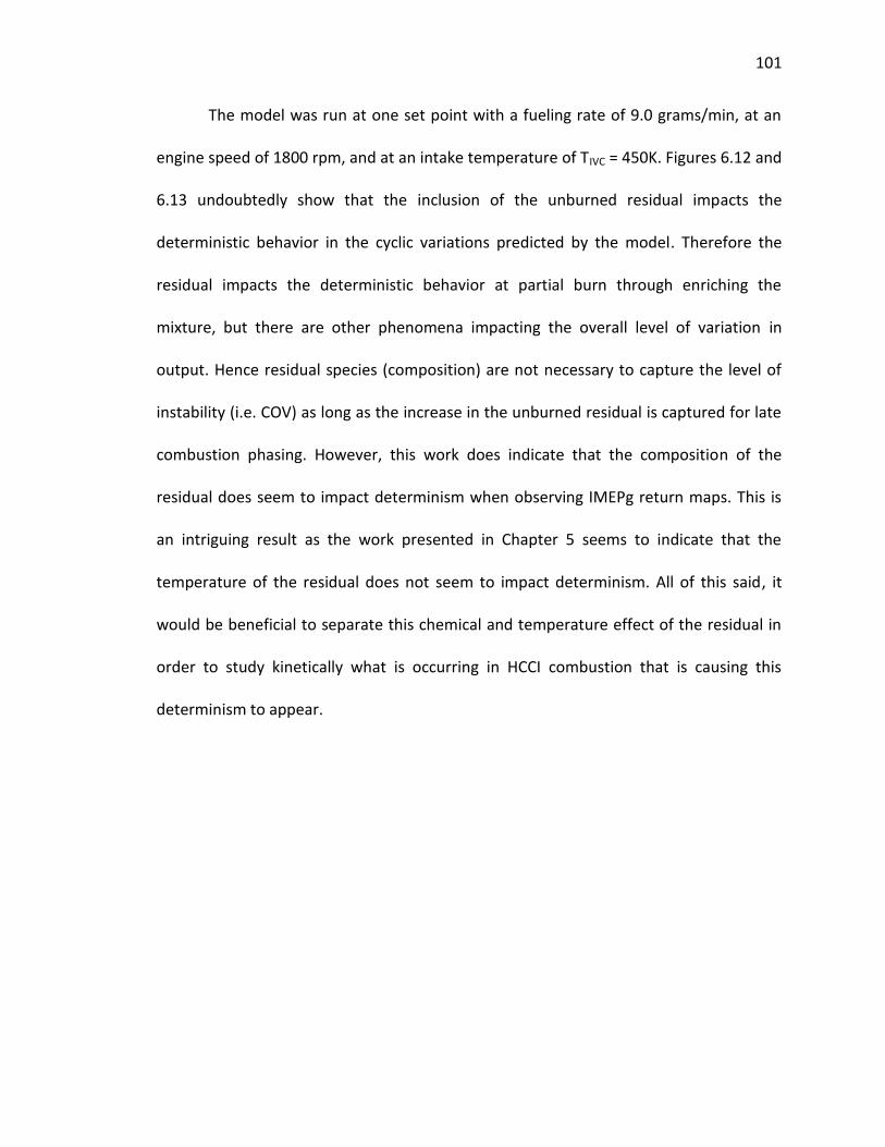
101
The model was run at one set point with a fueling rate of 9.0 grams/min, at an
engine speed of 1800 rpm, and at an intake temperature of TIVC = 450K. Figures 6.12 and
6.13 undoubtedly show that the inclusion of the unburned residual impacts the
deterministic behavior in the cyclic variations predicted by the model. Therefore the
residual impacts the deterministic behavior at partial burn through enriching the
mixture, but there are other phenomena impacting the overall level of variation in
output. Hence residual species (composition) are not necessary to capture the level of
instability (i.e. COV) as long as the increase in the unburned residual is captured for late
combustion phasing. However, this work does indicate that the composition of the
residual does seem to impact determinism when observing IMEPg return maps. This is
an intriguing result as the work presented in Chapter 5 seems to indicate that the
temperature of the residual does not seem to impact determinism. All of this said, it
would be beneficial to separate this chemical and temperature effect of the residual in
order to study kinetically what is occurring in HCCI combustion that is causing this
determinism to appear.
102
7. REACTIVE SPECIES GAS INJECTION
Since the occurrence of HCCI combustion relies on chemical kinetics, we know
that the thermodynamic state and the dilution levels of the charge mixture will directly
affect the start of combustion process. A more complete understanding is sought on the
role of residual gas properties on the next cycle’s start of combustion and heat release
rate. Work presented in Chapters 5 and 6 demonstrates that the deterministic effect
seen in the partial burn regime is more due to chemical composition of the residual than
the temperature of the residual gas. A more complete understanding is sought of the
role of this chemical composition effect on the kinetics of HCCI combustion
development. This chapter outlines preliminary results of the underlying cycle-by-cycle
dynamic impacts of carefully controlled in-cylinder injections of perturbation gases, in
this case carbon monoxide, using a residual gas injector (RGI) on an individual cycle
basis. By directly injecting a reactive species gas, like carbon monoxide or hydrogen, one
can isolate the chemical composition effects of the residuals from the thermal effects in
order to explore the extent of the non-linear effects seen in the regions of instability.
7.1. FLOW BENCH TESTING
Mass injections of certain percentages are to be added to the inlet fuel/air
charge during the intake stroke. The hardware and details about the RGI can be found in
§3.1.4. This section outlines how the RGI was benchmarked off the engine test stand in
order to verify that the mass being injected into the cylinder was the correct amount
thought to be injected. The RGI works on having back pressure from the reactive species
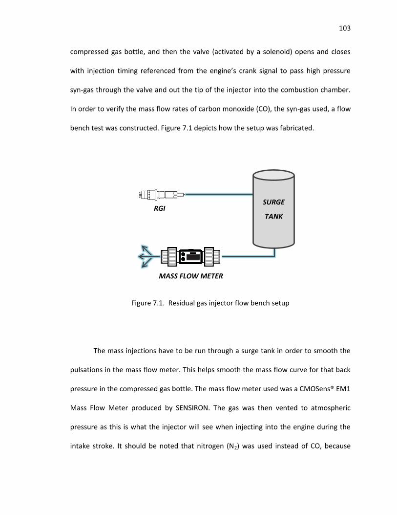
103
compressed gas bottle, and then the valve (activated by a solenoid) opens and closes
with injection timing referenced from the engine’s crank signal to pass high pressure
syn-gas through the valve and out the tip of the injector into the combustion chamber.
In order to verify the mass flow rates of carbon monoxide (CO), the syn-gas used, a flow
bench test was constructed. Figure 7.1 depicts how the setup was fabricated.
Figure 7.1. Residual gas injector flow bench setup
The mass injections have to be run through a surge tank in order to smooth the
pulsations in the mass flow meter. This helps smooth the mass flow curve for that back
pressure in the compressed gas bottle. The mass flow meter used was a CMOSens® EM1
Mass Flow Meter produced by SENSIRON. The gas was then vented to atmospheric
pressure as this is what the injector will see when injecting into the engine during the
intake stroke. It should be noted that nitrogen (N2) was used instead of CO, because
RGI SURGE
TANK
MASS FLOW METER
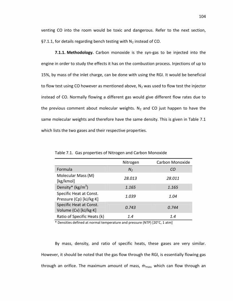
104
venting CO into the room would be toxic and dangerous. Refer to the next section,
§7.1.1, for details regarding bench testing with N2 instead of CO.
7.1.1. Methodology. Carbon monoxide is the syn-gas to be injected into the
engine in order to study the effects it has on the combustion process. Injections of up to
15%, by mass of the inlet charge, can be done with using the RGI. It would be beneficial
to flow test using CO however as mentioned above, N2 was used to flow test the injector
instead of CO. Normally flowing a different gas would give different flow rates due to
the previous comment about molecular weights. N2 and CO just happen to have the
same molecular weights and therefore have the same density. This is given in Table 7.1
which lists the two gases and their respective properties.
Table 7.1. Gas properties of Nitrogen and Carbon Monoxide
Nitrogen Carbon Monoxide
Formula N2 CO
Molecular Mass (M) [kg/kmol]
28.013 28.011
Density* (kg/m3) 1.165 1.165
Specific Heat at Const. Pressure (Cp) [kJ/kg·K]
1.039 1.04
Specific Heat at Const. Volume (Cv) [kJ/kg·K]
0.743 0.744
Ratio of Specific Heats (k) 1.4 1.4
* Densities defined at normal temperature and pressure (NTP) [20°C, 1 atm]
By mass, density, and ratio of specific heats, these gases are very similar.
However, it should be noted that the gas flow through the RGI, is essentially flowing gas
through an orifice. The maximum amount of mass, ṁmax, which can flow through an
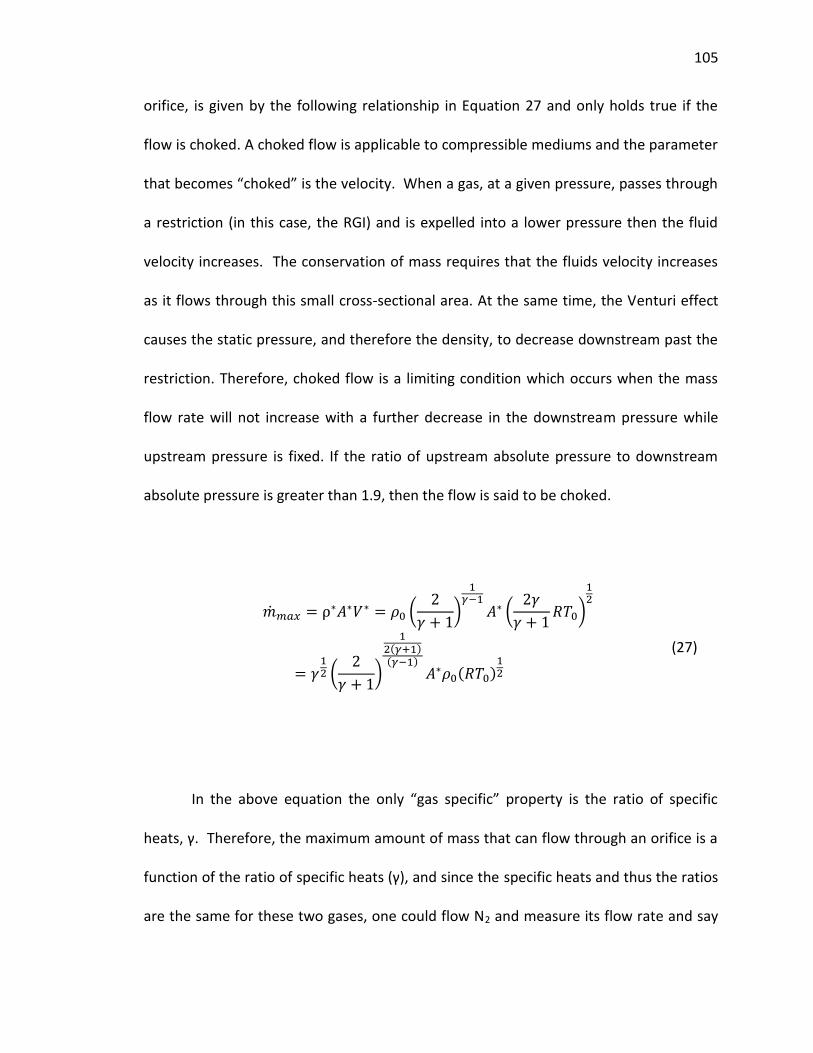
105
orifice, is given by the following relationship in Equation 27 and only holds true if the
flow is choked. A choked flow is applicable to compressible mediums and the parameter
that becomes “choked” is the velocity. When a gas, at a given pressure, passes through
a restriction (in this case, the RGI) and is expelled into a lower pressure then the fluid
velocity increases. The conservation of mass requires that the fluids velocity increases
as it flows through this small cross-sectional area. At the same time, the Venturi effect
causes the static pressure, and therefore the density, to decrease downstream past the
restriction. Therefore, choked flow is a limiting condition which occurs when the mass
flow rate will not increase with a further decrease in the downstream pressure while
upstream pressure is fixed. If the ratio of upstream absolute pressure to downstream
absolute pressure is greater than 1.9, then the flow is said to be choked.
In the above equation the only “gas specific” property is the ratio of specific
heats, γ. Therefore, the maximum amount of mass that can flow through an orifice is a
function of the ratio of specific heats (γ), and since the specific heats and thus the ratios
are the same for these two gases, one could flow N2 and measure its flow rate and say
(
)
(
)
(
)
( )( )
( )
(27)
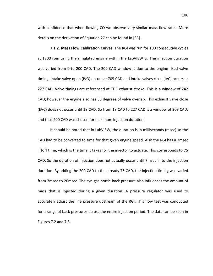
106
with confidence that when flowing CO we observe very similar mass flow rates. More
details on the derivation of Equation 27 can be found in [33].
7.1.2. Mass Flow Calibration Curves. The RGI was run for 100 consecutive cycles
at 1800 rpm using the simulated engine within the LabVIEW vi. The injection duration
was varied from 0 to 200 CAD. The 200 CAD window is due to the engine fixed valve
timing. Intake valve open (IVO) occurs at 705 CAD and intake valves close (IVC) occurs at
227 CAD. Valve timings are referenced at TDC exhaust stroke. This is a window of 242
CAD; however the engine also has 33 degrees of valve overlap. This exhaust valve close
(EVC) does not occur until 18 CAD. So from 18 CAD to 227 CAD is a window of 209 CAD,
and thus 200 CAD was chosen for maximum injection duration.
It should be noted that in LabVIEW, the duration is in milliseconds (msec) so the
CAD had to be converted to time for that given engine speed. Also the RGI has a 7msec
liftoff time, which is the time it takes for the injector to actuate. This corresponds to 75
CAD. So the duration of injection does not actually occur until 7msec in to the injection
duration. By adding the 200 CAD to the already 75 CAD, the injection timing was varied
from 7msec to 26msec. The syn-gas bottle back pressure also influences the amount of
mass that is injected during a given duration. A pressure regulator was used to
accurately adjust the line pressure upstream of the RGI. This flow test was conducted
for a range of back pressures across the entire injection period. The data can be seen in
Figures 7.2 and 7.3.
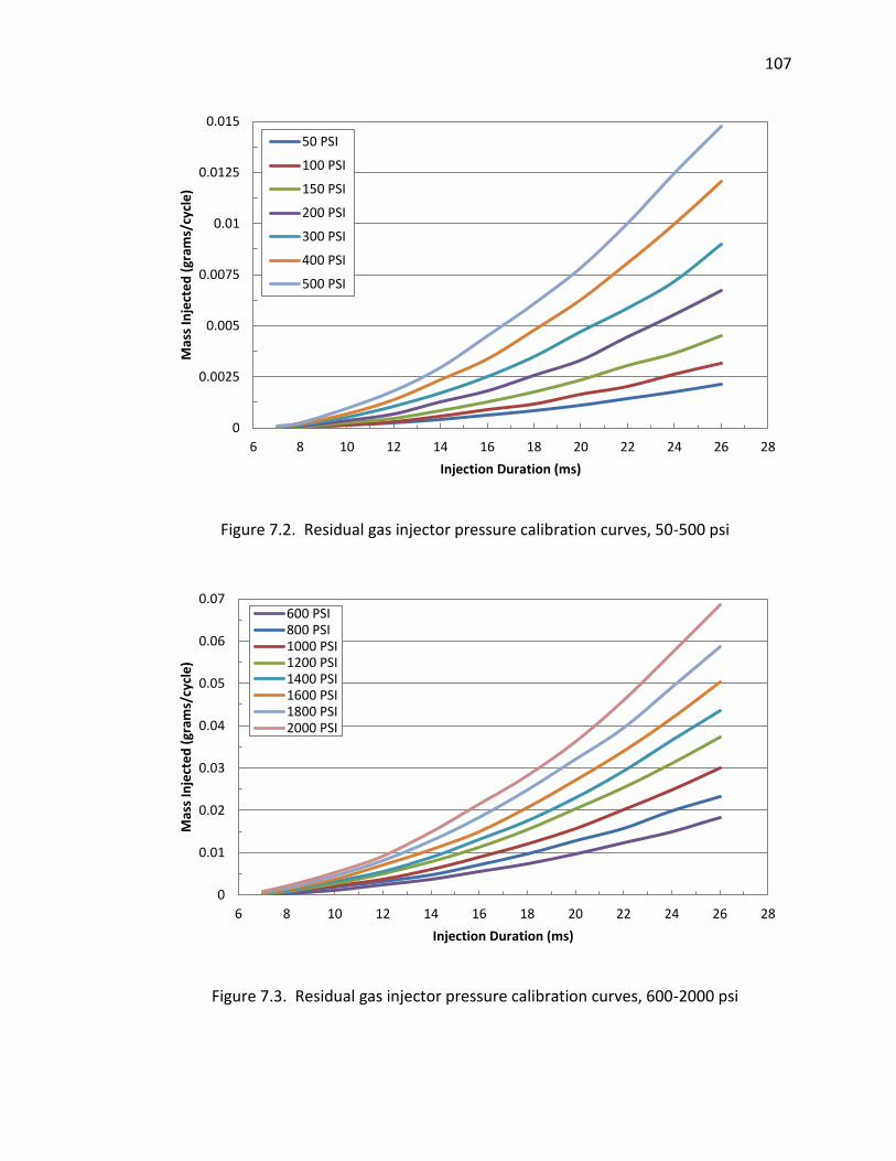
107
Figure 7.2. Residual gas injector pressure calibration curves, 50-500 psi
Figure 7.3. Residual gas injector pressure calibration curves, 600-2000 psi
0
0.0025
0.005
0.0075
0.01
0.0125
0.015
6 8 10 12 14 16 18 20 22 24 26 28
Mas
s In
ject
ed
(gr
ams/
cycl
e)
Injection Duration (ms)
50 PSI
100 PSI
150 PSI
200 PSI
300 PSI
400 PSI
500 PSI
0
0.01
0.02
0.03
0.04
0.05
0.06
0.07
6 8 10 12 14 16 18 20 22 24 26 28
Mas
s In
ject
ed
(gr
ams/
cycl
e)
Injection Duration (ms)
600 PSI800 PSI1000 PSI1200 PSI1400 PSI1600 PSI1800 PSI2000 PSI
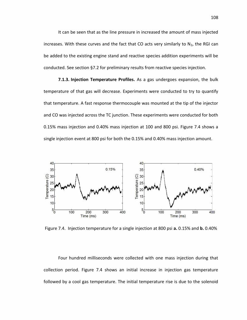
108
It can be seen that as the line pressure in increased the amount of mass injected
increases. With these curves and the fact that CO acts very similarly to N2, the RGI can
be added to the existing engine stand and reactive species addition experiments will be
conducted. See section §7.2 for preliminary results from reactive species injection.
7.1.3. Injection Temperature Profiles. As a gas undergoes expansion, the bulk
temperature of that gas will decrease. Experiments were conducted to try to quantify
that temperature. A fast response thermocouple was mounted at the tip of the injector
and CO was injected across the TC junction. These experiments were conducted for both
0.15% mass injection and 0.40% mass injection at 100 and 800 psi. Figure 7.4 shows a
single injection event at 800 psi for both the 0.15% and 0.40% mass injection amount.
Figure 7.4. Injection temperature for a single injection at 800 psi a. 0.15% and b. 0.40%
Four hundred milliseconds were collected with one mass injection during that
collection period. Figure 7.4 shows an initial increase in injection gas temperature
followed by a cool gas temperature. The initial temperature rise is due to the solenoid
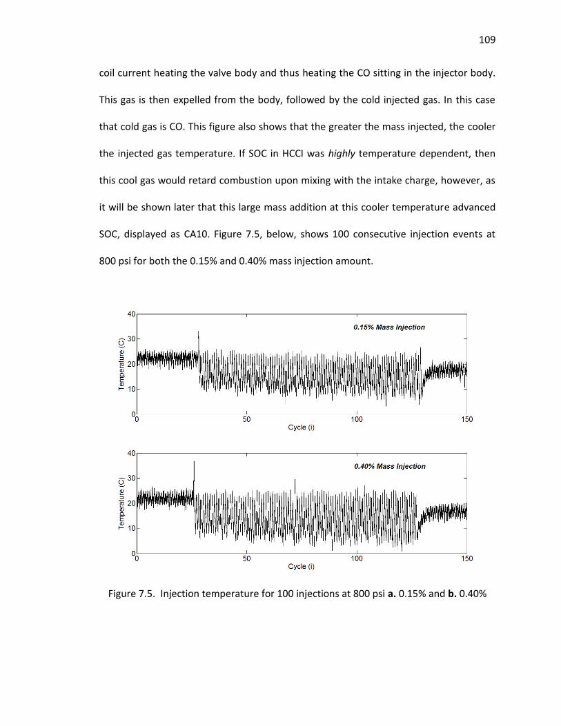
109
coil current heating the valve body and thus heating the CO sitting in the injector body.
This gas is then expelled from the body, followed by the cold injected gas. In this case
that cold gas is CO. This figure also shows that the greater the mass injected, the cooler
the injected gas temperature. If SOC in HCCI was highly temperature dependent, then
this cool gas would retard combustion upon mixing with the intake charge, however, as
it will be shown later that this large mass addition at this cooler temperature advanced
SOC, displayed as CA10. Figure 7.5, below, shows 100 consecutive injection events at
800 psi for both the 0.15% and 0.40% mass injection amount.
Figure 7.5. Injection temperature for 100 injections at 800 psi a. 0.15% and b. 0.40%
110
Again, Figure 7.5 reaffirms that the initial gas within the valve body is being
heated by the solenoid and once it is expelled, it is not seen again. The 100 consecutive
cycles show that average injected CO gas temperature at 0.15% mass injection is
approximately 7°C and the 0.40% mass injection is approximately 4°C. Since the gas is
expanding from 800 psi to atmospheric, these injection pressures will result in the
coolest gas temperature, therefore the 100 psi injection temperature profiles are not
shown here as the temperature of the gas is closer to room temperature than the
higher pressure cases. Injecting a cold gas into the cylinder would affect the overall
temperature of the bulk gas however in this case only 0.15-0.40% by mass is being
injected therefore the overall temperature should not be significantly changed. In fact,
by looking at the worst case (0.40% injection at 4°C) scenario by adding CO to 195°C bulk
gas temperature of the inlet charge through adiabatic mixing, only reduces the bulk gas
temperature to 194.2°C. Therefore the cooling effect on the bulk gas temperature is
negligible at these percent mass additions.
7.1.4. Thermochemistry Mass Balance. As mentioned above, the RGI can inject
up to 15%, by CO mass, of the inlet charge. Mass fuel flow rate (grams/min) is known
from bench testing the low flow metering pump for precise fuel flow rate into the fuel
atomizer. Emission gas concentrations of CO2 (%), CO (%), O2 (%), uHC (ppm), and NOX
(ppm) are collected using exhaust gas analyzers. The CO2, CO, and O2 data are taken
from a dry gas analyzer while the remaining species are each collected from wet gas
analyzers. The H2O concentration (%) is not collected during engine tests and thus must
111
be calculated. This is completed using some of the other collected emissions data and
the following equation from [16]:
Where [ ] = molar concentration present. In the above equation, K is defined as
the water-gas reaction equilibrium constant. A generally accepted empirical
determination of K is the constant 3.8. This water-gas reaction is used in conjunction
with the atom balances of the global reaction to derive the (H2O) equation. The
thermochemistry balance equation for the oxidation of fuel and air is given by,
The amount of fuel consumed in the above reaction can be calculated from a
Spindt exhaust gas analysis [16]. The make-up of combustion products, or exhaust gas
concentrations, are measured and therefore the amount of fuel consumed can be
determined. Previous investigations [35] have concluded that Spindt analyses return
values within 0.1 air-to-fuel ratio of the true value if the engine is run on gasoline and
the sampling location is before an exhaust catalyst. Since these two conditions are met
in this experimental setup, the Spindt analyses are deemed appropriate.
The Spindt method calculates the equivalence ratio based on a wet uHC and dry
inorganic gas analysis. This is the most accurate for the experimental engine stand due
[ ] (
)(( ) ( )
( )[ ( )]
)
(28)
( ) (29)
112
to the inorganic gas concentrations (CO2, CO, and O2) being determined from a dry gas
analyzer while the uHC concentration is given in a wet gas analysis. The following
formulas were used for this computation [16].
Where,
(O2 molecules required for complete combustion of fuel CxHy)
(Total moles of exhaust products)
This plus the air-fuel ratio calculated in §3.2 are used in conjunction to determine
the amount of mass that is introduced into the cylinder. The inlet mass is determined
( )(
)
(30)
(31)
( ) (32)
( )(
) (33)
[
( ) ( )(
)]
(34)
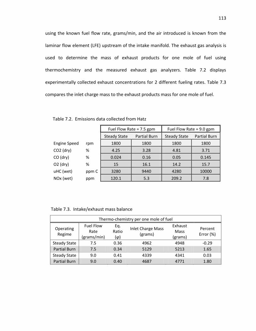
113
using the known fuel flow rate, grams/min, and the air introduced is known from the
laminar flow element (LFE) upstream of the intake manifold. The exhaust gas analysis is
used to determine the mass of exhaust products for one mole of fuel using
thermochemistry and the measured exhaust gas analyzers. Table 7.2 displays
experimentally collected exhaust concentrations for 2 different fueling rates. Table 7.3
compares the inlet charge mass to the exhaust products mass for one mole of fuel.
Table 7.2. Emissions data collected from Hatz
Fuel Flow Rate = 7.5 gpm Fuel Flow Rate = 9.0 gpm
Steady State Partial Burn Steady State Partial Burn
Engine Speed rpm 1800 1800 1800 1800
CO2 (dry) % 4.25 3.28 4.81 3.71
CO (dry) % 0.024 0.16 0.05 0.145
O2 (dry) % 15 16.1 14.2 15.7
uHC (wet) ppm C 3280 9440 4280 10000
NOx (wet) ppm 120.1 5.3 209.2 7.8
Table 7.3. Intake/exhaust mass balance
Thermo-chemistry per one mole of fuel
Operating Regime
Fuel Flow Rate
(grams/min)
Eq. Ratio (φ)
Inlet Charge Mass (grams)
Exhaust Mass
(grams)
Percent Error (%)
Steady State 7.5 0.36 4962 4948 -0.29
Partial Burn 7.5 0.34 5129 5213 1.65
Steady State 9.0 0.41 4339 4341 0.03
Partial Burn 9.0 0.40 4687 4771 1.80
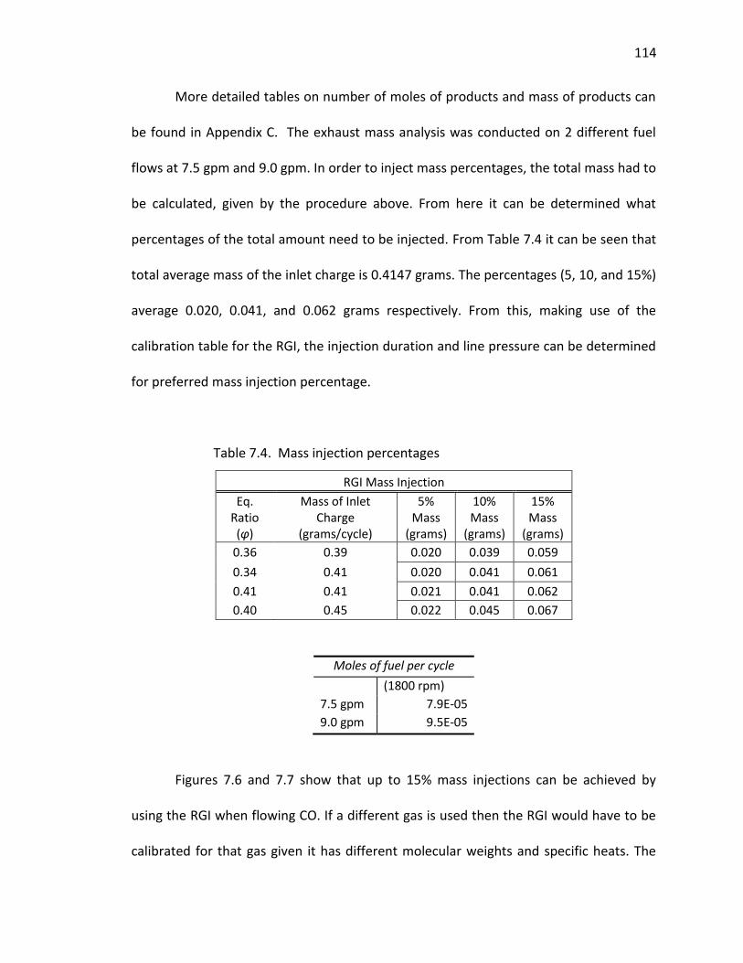
114
More detailed tables on number of moles of products and mass of products can
be found in Appendix C. The exhaust mass analysis was conducted on 2 different fuel
flows at 7.5 gpm and 9.0 gpm. In order to inject mass percentages, the total mass had to
be calculated, given by the procedure above. From here it can be determined what
percentages of the total amount need to be injected. From Table 7.4 it can be seen that
total average mass of the inlet charge is 0.4147 grams. The percentages (5, 10, and 15%)
average 0.020, 0.041, and 0.062 grams respectively. From this, making use of the
calibration table for the RGI, the injection duration and line pressure can be determined
for preferred mass injection percentage.
Table 7.4. Mass injection percentages
RGI Mass Injection
Eq. Ratio (φ)
Mass of Inlet Charge
(grams/cycle)
5% Mass
(grams)
10% Mass
(grams)
15% Mass
(grams)
0.36 0.39 0.020 0.039 0.059
0.34 0.41 0.020 0.041 0.061
0.41 0.41 0.021 0.041 0.062
0.40 0.45 0.022 0.045 0.067
Moles of fuel per cycle
(1800 rpm)
7.5 gpm 7.9E-05
9.0 gpm 9.5E-05
Figures 7.6 and 7.7 show that up to 15% mass injections can be achieved by
using the RGI when flowing CO. If a different gas is used then the RGI would have to be
calibrated for that gas given it has different molecular weights and specific heats. The
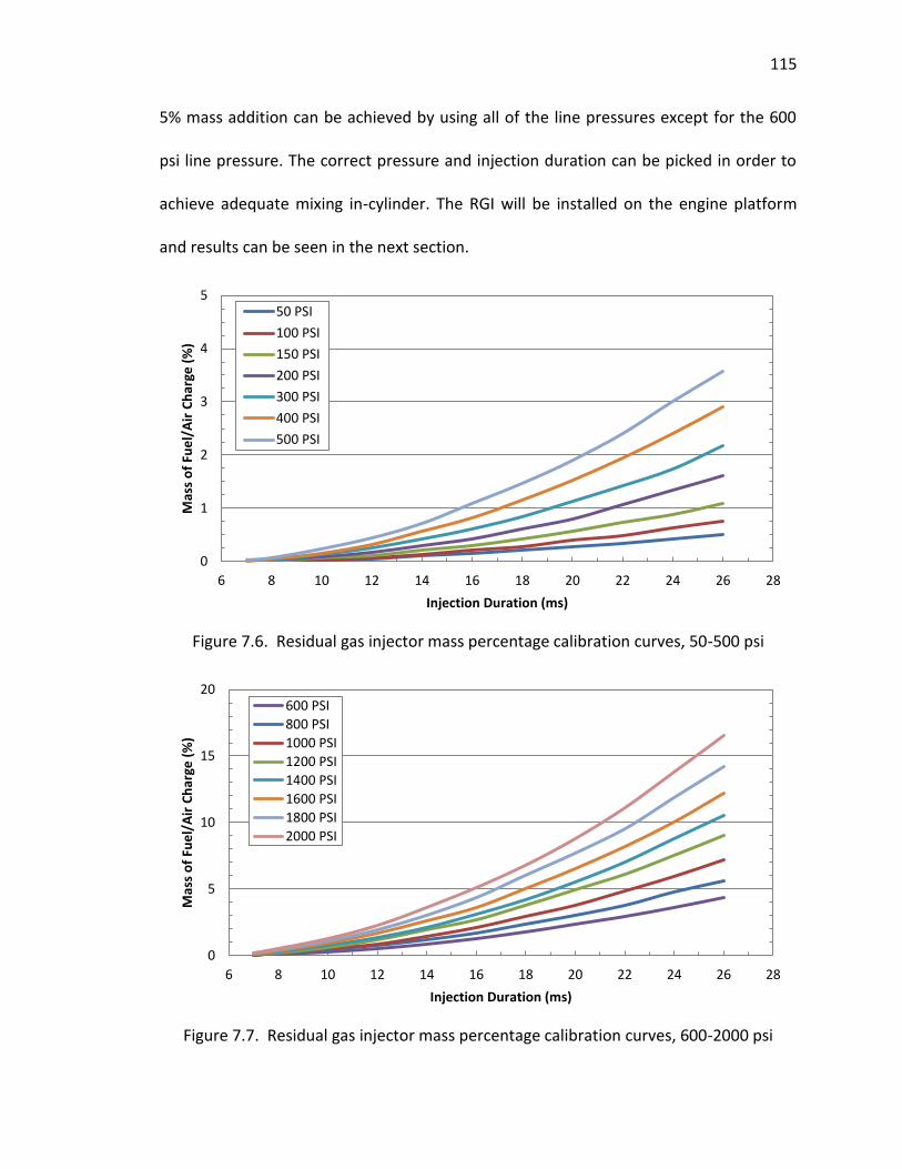
115
5% mass addition can be achieved by using all of the line pressures except for the 600
psi line pressure. The correct pressure and injection duration can be picked in order to
achieve adequate mixing in-cylinder. The RGI will be installed on the engine platform
and results can be seen in the next section.
Figure 7.6. Residual gas injector mass percentage calibration curves, 50-500 psi
Figure 7.7. Residual gas injector mass percentage calibration curves, 600-2000 psi
0
1
2
3
4
5
6 8 10 12 14 16 18 20 22 24 26 28
Mas
s o
f Fu
el/
Air
Ch
arge
(%
)
Injection Duration (ms)
50 PSI
100 PSI
150 PSI
200 PSI
300 PSI
400 PSI
500 PSI
0
5
10
15
20
6 8 10 12 14 16 18 20 22 24 26 28
Mas
s o
f Fu
el/
Air
Ch
arge
(%
)
Injection Duration (ms)
600 PSI
800 PSI
1000 PSI
1200 PSI
1400 PSI
1600 PSI
1800 PSI
2000 PSI
116
7.2. REAL-TIME ENGINE RESULTS
With the injector on the engine running in real-time, it was found that 5% mass
injections would significantly affect the engine’s combustion development and could
lead to damage of the engine/piston/connecting rod structure. Thus the amounts were
adjusted and found that mass injections of around 0.1% - 0.5% were acceptable to add
cyclically to the inlet charge in order to observe significant changes in the engine’s
behavior. This section presents the results seen from onboard reactive species mass
injection and draws conclusions on these test cases.
7.2.1. Carbon Monoxide Mass Injection Results. CO injections were added at
two different injection pressures for the same amount of mass. Mass percent injections
of 0.15% and 0.40% were used as these set points affected the engine’s performance
with respect to a high and low injection amount. The pressures were determined from
the calibration tables and found to be 800 psi and 100 psi. The duration of injection was
kept under 200 CAD and injected before IVC at 227 CAD. This allowed injections to occur
after EVC at 18 CAD. The durations found to fit the criteria were 8ms (800 psi, 0.15%
injected), 10ms (800 psi, 0.40% injected), 14ms (100 psi, 0.15% injected), and 20ms (100
psi, 0.40% injected). It should be noted that the valve required 7ms of inherent delay to
actuate so start of injection signal (SOI) was triggered 75 degrees (7ms at 1800 rpm)
before actual mass SOI occurred. The engine was run at a steady operating speed of
1800 rpm and a fuel flow rate of 7.5 grams/min. Also, the intake temperature was held
at a constant 195°C, or 468 K. Table 7.5 lists the averaged data collected from the
different test cases.
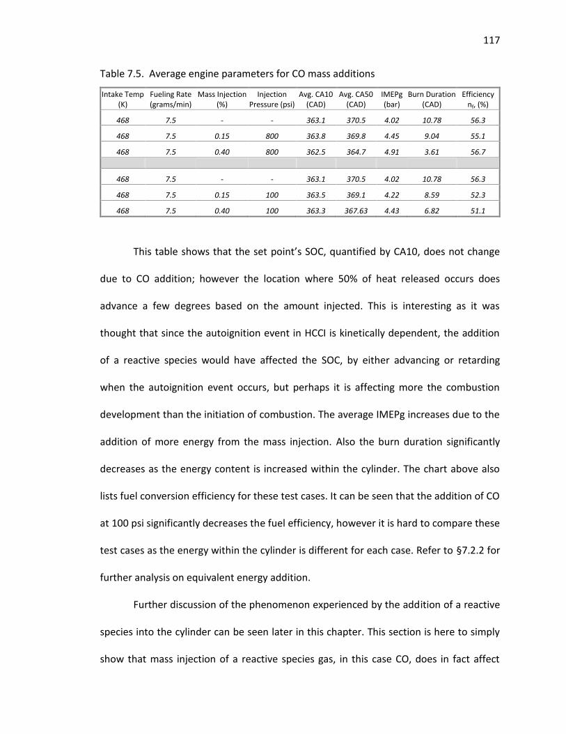
117
Table 7.5. Average engine parameters for CO mass additions
Intake Temp (K)
Fueling Rate (grams/min)
Mass Injection (%)
Injection Pressure (psi)
Avg. CA10 (CAD)
Avg. CA50 (CAD)
IMEPg (bar)
Burn Duration (CAD)
Efficiency nf, (%)
468 7.5 - - 363.1 370.5 4.02 10.78 56.3
468 7.5 0.15 800 363.8 369.8 4.45 9.04 55.1
468 7.5 0.40 800 362.5 364.7 4.91 3.61 56.7
468 7.5 - - 363.1 370.5 4.02 10.78 56.3
468 7.5 0.15 100 363.5 369.1 4.22 8.59 52.3
468 7.5 0.40 100 363.3 367.63 4.43 6.82 51.1
This table shows that the set point’s SOC, quantified by CA10, does not change
due to CO addition; however the location where 50% of heat released occurs does
advance a few degrees based on the amount injected. This is interesting as it was
thought that since the autoignition event in HCCI is kinetically dependent, the addition
of a reactive species would have affected the SOC, by either advancing or retarding
when the autoignition event occurs, but perhaps it is affecting more the combustion
development than the initiation of combustion. The average IMEPg increases due to the
addition of more energy from the mass injection. Also the burn duration significantly
decreases as the energy content is increased within the cylinder. The chart above also
lists fuel conversion efficiency for these test cases. It can be seen that the addition of CO
at 100 psi significantly decreases the fuel efficiency, however it is hard to compare these
test cases as the energy within the cylinder is different for each case. Refer to §7.2.2 for
further analysis on equivalent energy addition.
Further discussion of the phenomenon experienced by the addition of a reactive
species into the cylinder can be seen later in this chapter. This section is here to simply
show that mass injection of a reactive species gas, in this case CO, does in fact affect
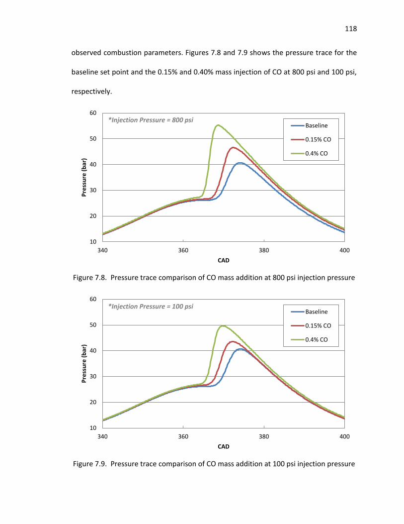
118
observed combustion parameters. Figures 7.8 and 7.9 shows the pressure trace for the
baseline set point and the 0.15% and 0.40% mass injection of CO at 800 psi and 100 psi,
respectively.
Figure 7.8. Pressure trace comparison of CO mass addition at 800 psi injection pressure
Figure 7.9. Pressure trace comparison of CO mass addition at 100 psi injection pressure
10
20
30
40
50
60
340 360 380 400
Pre
ssu
re (
bar
)
CAD
Baseline
0.15% CO
0.4% CO
10
20
30
40
50
60
340 360 380 400
Pre
ssu
re (
bar
)
CAD
Baseline
0.15% CO
0.4% CO
*Injection Pressure = 800 psi
*Injection Pressure = 100 psi
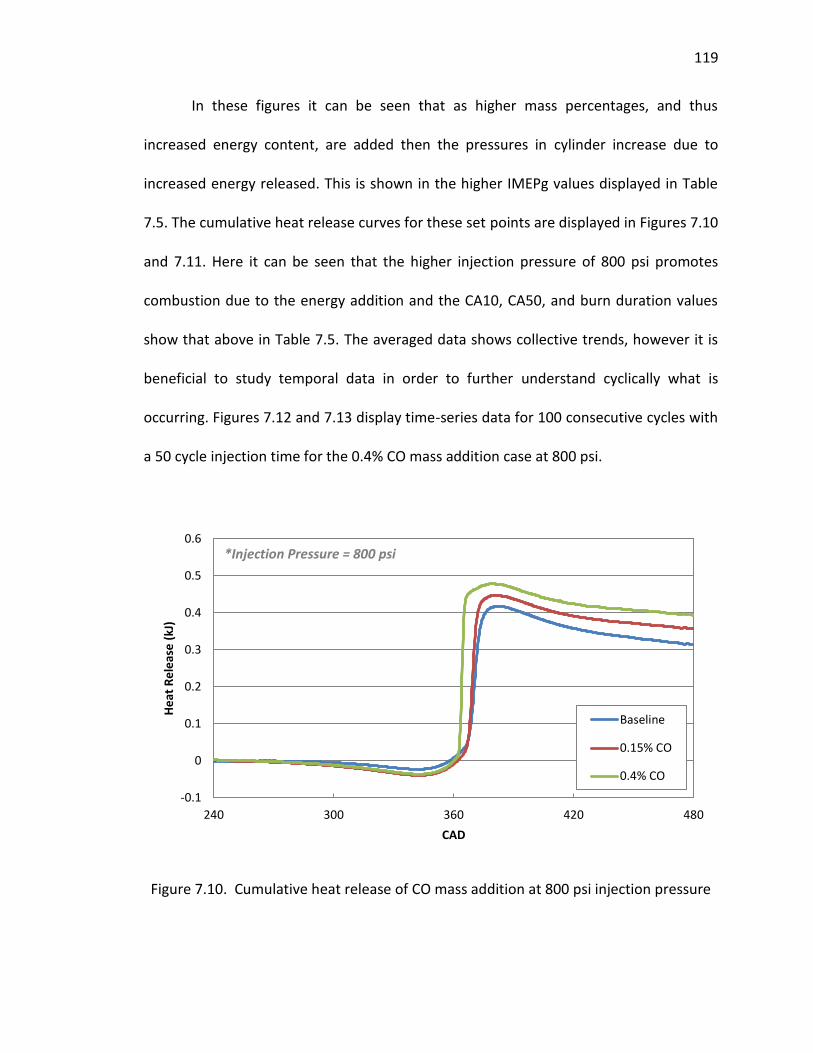
119
In these figures it can be seen that as higher mass percentages, and thus
increased energy content, are added then the pressures in cylinder increase due to
increased energy released. This is shown in the higher IMEPg values displayed in Table
7.5. The cumulative heat release curves for these set points are displayed in Figures 7.10
and 7.11. Here it can be seen that the higher injection pressure of 800 psi promotes
combustion due to the energy addition and the CA10, CA50, and burn duration values
show that above in Table 7.5. The averaged data shows collective trends, however it is
beneficial to study temporal data in order to further understand cyclically what is
occurring. Figures 7.12 and 7.13 display time-series data for 100 consecutive cycles with
a 50 cycle injection time for the 0.4% CO mass addition case at 800 psi.
Figure 7.10. Cumulative heat release of CO mass addition at 800 psi injection pressure
-0.1
0
0.1
0.2
0.3
0.4
0.5
0.6
240 300 360 420 480
He
at R
ele
ase
(kJ
)
CAD
Baseline
0.15% CO
0.4% CO
*Injection Pressure = 800 psi
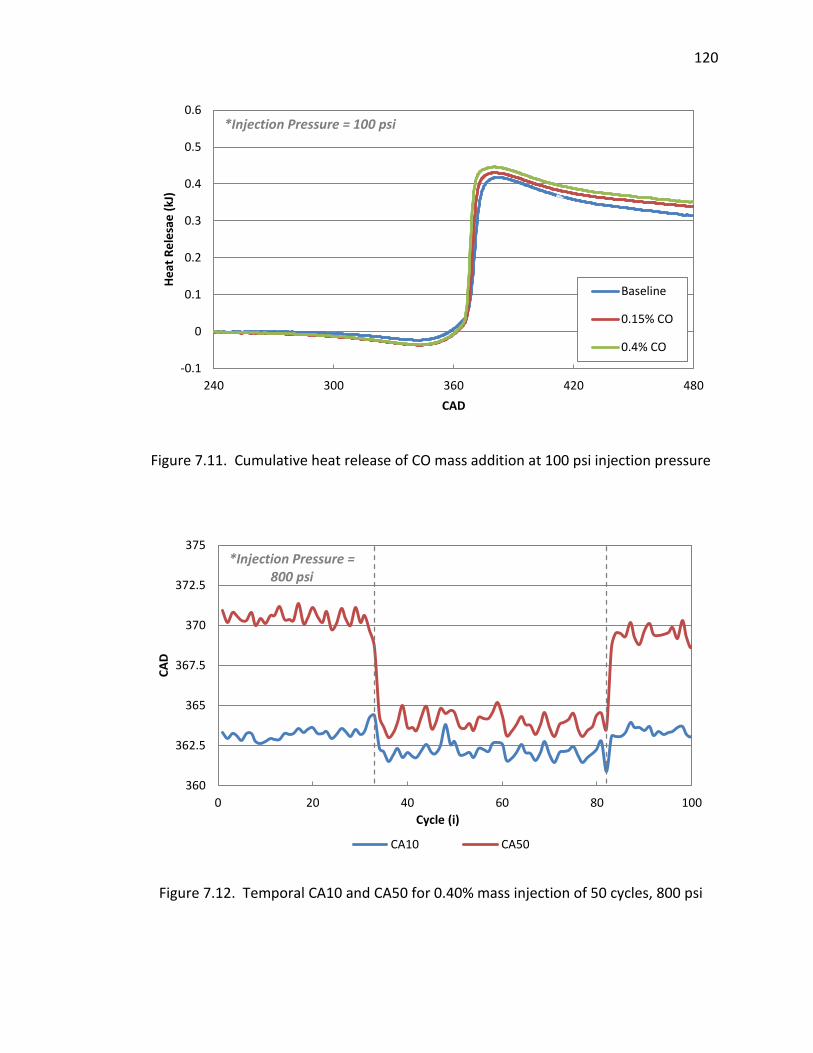
120
Figure 7.11. Cumulative heat release of CO mass addition at 100 psi injection pressure
Figure 7.12. Temporal CA10 and CA50 for 0.40% mass injection of 50 cycles, 800 psi
-0.1
0
0.1
0.2
0.3
0.4
0.5
0.6
240 300 360 420 480
He
at R
ele
sae
(kJ
)
CAD
Baseline
0.15% CO
0.4% CO
360
362.5
365
367.5
370
372.5
375
0 20 40 60 80 100
CA
D
Cycle (i)
CA10 CA50
*Injection Pressure = 100 psi
*Injection Pressure = 800 psi
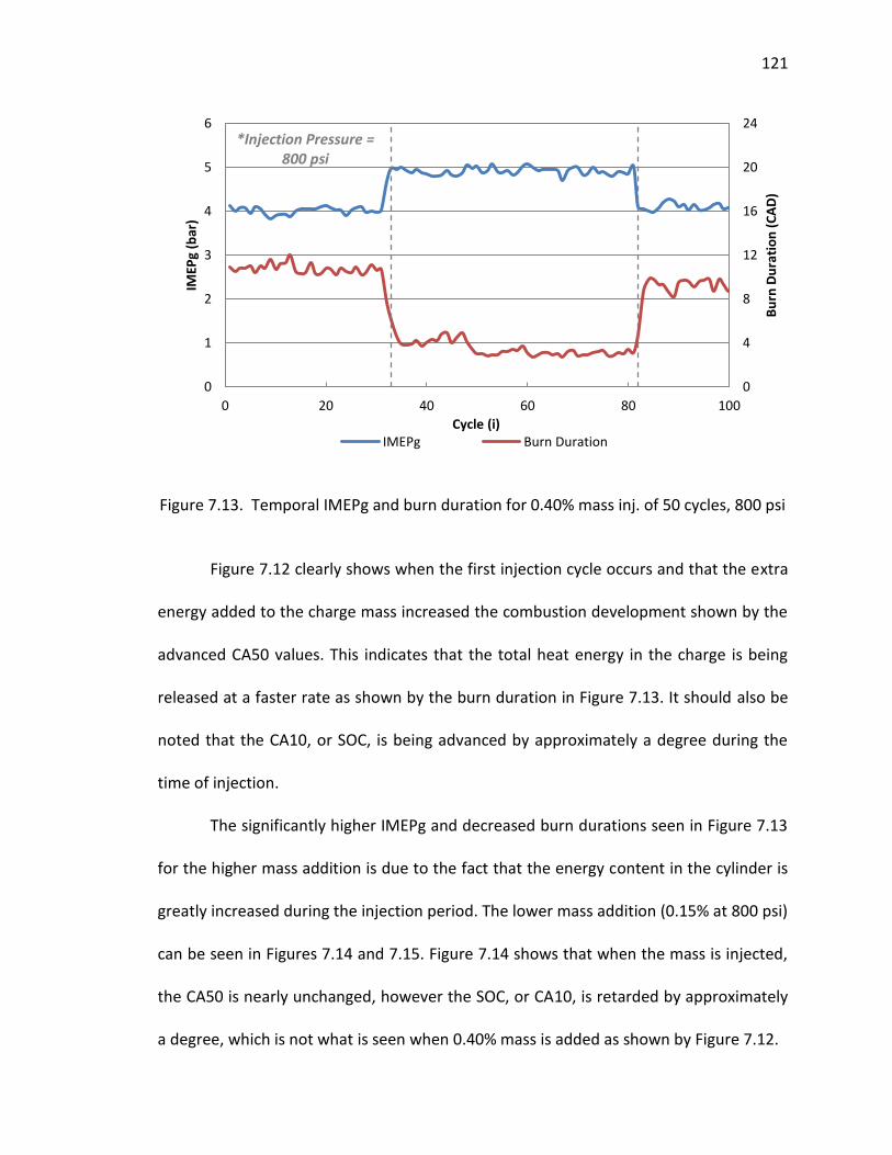
121
Figure 7.13. Temporal IMEPg and burn duration for 0.40% mass inj. of 50 cycles, 800 psi
Figure 7.12 clearly shows when the first injection cycle occurs and that the extra
energy added to the charge mass increased the combustion development shown by the
advanced CA50 values. This indicates that the total heat energy in the charge is being
released at a faster rate as shown by the burn duration in Figure 7.13. It should also be
noted that the CA10, or SOC, is being advanced by approximately a degree during the
time of injection.
The significantly higher IMEPg and decreased burn durations seen in Figure 7.13
for the higher mass addition is due to the fact that the energy content in the cylinder is
greatly increased during the injection period. The lower mass addition (0.15% at 800 psi)
can be seen in Figures 7.14 and 7.15. Figure 7.14 shows that when the mass is injected,
the CA50 is nearly unchanged, however the SOC, or CA10, is retarded by approximately
a degree, which is not what is seen when 0.40% mass is added as shown by Figure 7.12.
0
4
8
12
16
20
24
0
1
2
3
4
5
6
0 20 40 60 80 100
Bu
rn D
ura
tio
n (
CA
D)
IMEP
g (b
ar)
Cycle (i) IMEPg Burn Duration
*Injection Pressure = 800 psi
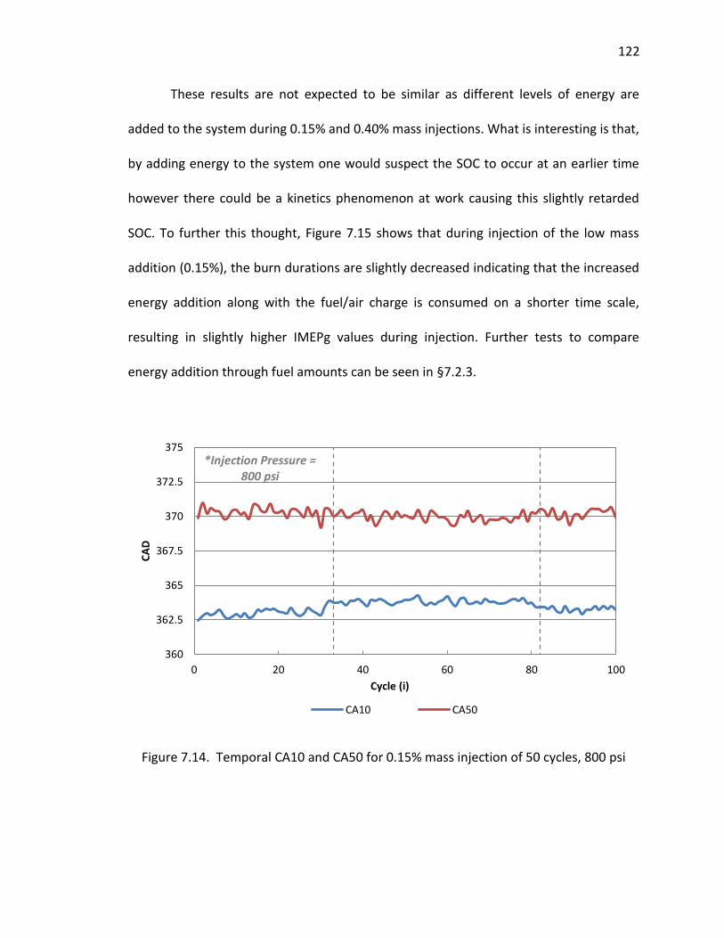
122
These results are not expected to be similar as different levels of energy are
added to the system during 0.15% and 0.40% mass injections. What is interesting is that,
by adding energy to the system one would suspect the SOC to occur at an earlier time
however there could be a kinetics phenomenon at work causing this slightly retarded
SOC. To further this thought, Figure 7.15 shows that during injection of the low mass
addition (0.15%), the burn durations are slightly decreased indicating that the increased
energy addition along with the fuel/air charge is consumed on a shorter time scale,
resulting in slightly higher IMEPg values during injection. Further tests to compare
energy addition through fuel amounts can be seen in §7.2.3.
Figure 7.14. Temporal CA10 and CA50 for 0.15% mass injection of 50 cycles, 800 psi
360
362.5
365
367.5
370
372.5
375
0 20 40 60 80 100
CA
D
Cycle (i)
CA10 CA50
*Injection Pressure = 800 psi
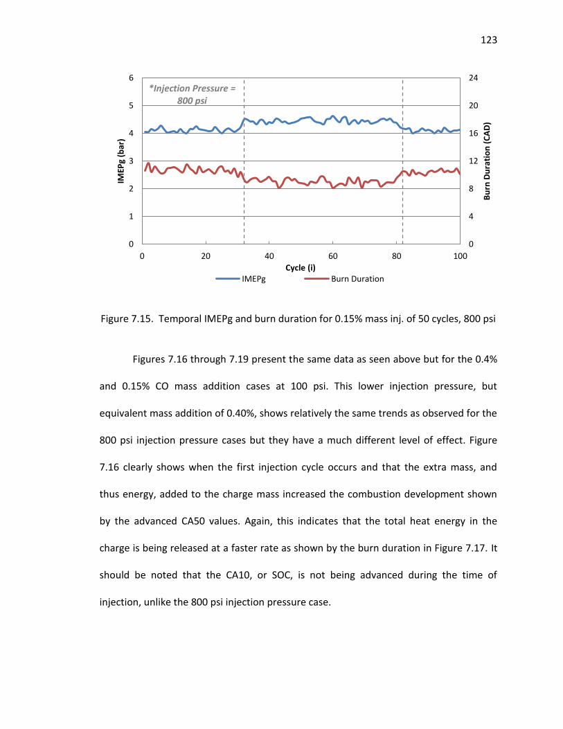
123
Figure 7.15. Temporal IMEPg and burn duration for 0.15% mass inj. of 50 cycles, 800 psi
Figures 7.16 through 7.19 present the same data as seen above but for the 0.4%
and 0.15% CO mass addition cases at 100 psi. This lower injection pressure, but
equivalent mass addition of 0.40%, shows relatively the same trends as observed for the
800 psi injection pressure cases but they have a much different level of effect. Figure
7.16 clearly shows when the first injection cycle occurs and that the extra mass, and
thus energy, added to the charge mass increased the combustion development shown
by the advanced CA50 values. Again, this indicates that the total heat energy in the
charge is being released at a faster rate as shown by the burn duration in Figure 7.17. It
should be noted that the CA10, or SOC, is not being advanced during the time of
injection, unlike the 800 psi injection pressure case.
0
4
8
12
16
20
24
0
1
2
3
4
5
6
0 20 40 60 80 100
Bu
rn D
ura
tio
n (
CA
D)
IMEP
g (b
ar)
Cycle (i) IMEPg Burn Duration
*Injection Pressure = 800 psi
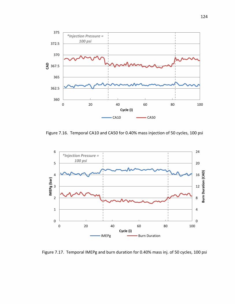
124
Figure 7.16. Temporal CA10 and CA50 for 0.40% mass injection of 50 cycles, 100 psi
Figure 7.17. Temporal IMEPg and burn duration for 0.40% mass inj. of 50 cycles, 100 psi
360
362.5
365
367.5
370
372.5
375
0 20 40 60 80 100
CA
D
Cycle (i)
CA10 CA50
0
4
8
12
16
20
24
0
1
2
3
4
5
6
0 20 40 60 80 100
Bu
rn D
ura
tio
n (
CA
D)
IMEP
g (b
ar)
Cycle (i)
IMEPg Burn Duration
*Injection Pressure = 100 psi
*Injection Pressure = 100 psi
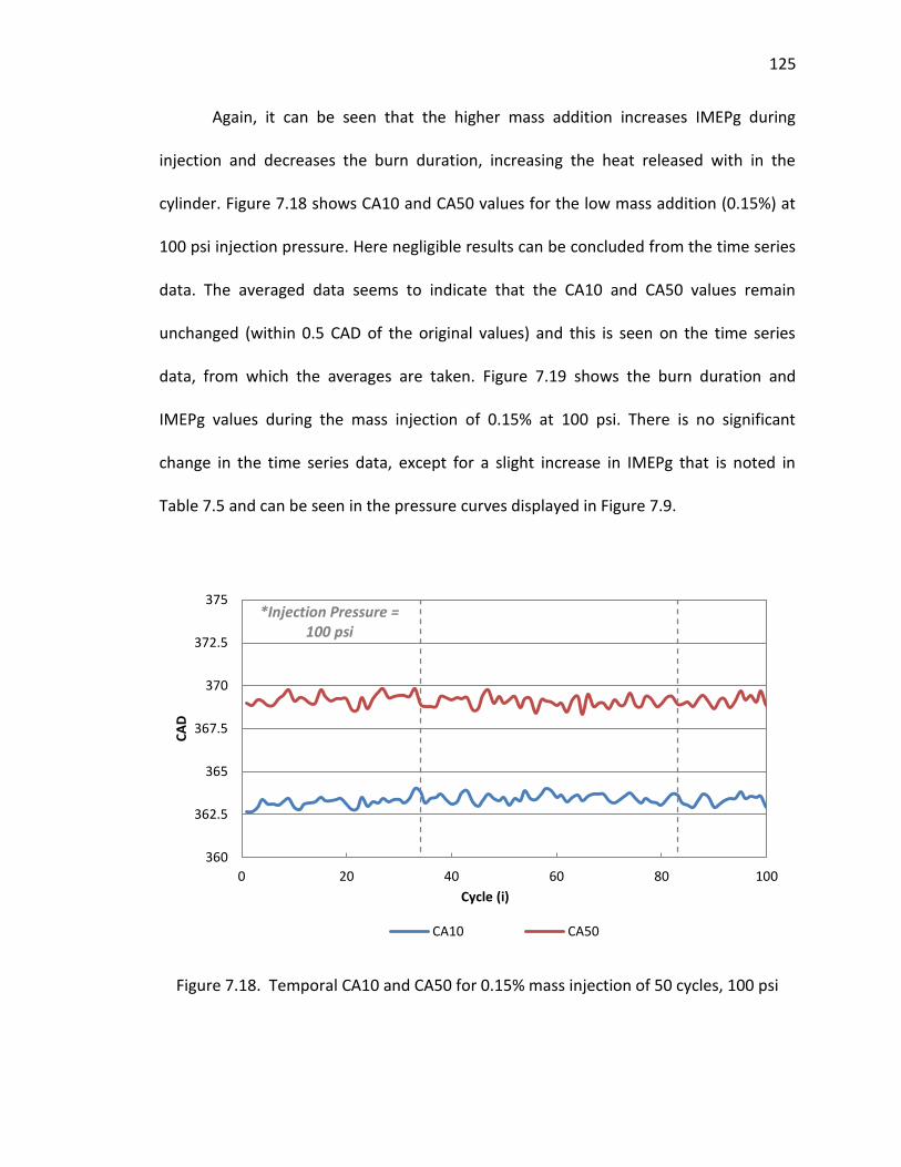
125
Again, it can be seen that the higher mass addition increases IMEPg during
injection and decreases the burn duration, increasing the heat released with in the
cylinder. Figure 7.18 shows CA10 and CA50 values for the low mass addition (0.15%) at
100 psi injection pressure. Here negligible results can be concluded from the time series
data. The averaged data seems to indicate that the CA10 and CA50 values remain
unchanged (within 0.5 CAD of the original values) and this is seen on the time series
data, from which the averages are taken. Figure 7.19 shows the burn duration and
IMEPg values during the mass injection of 0.15% at 100 psi. There is no significant
change in the time series data, except for a slight increase in IMEPg that is noted in
Table 7.5 and can be seen in the pressure curves displayed in Figure 7.9.
Figure 7.18. Temporal CA10 and CA50 for 0.15% mass injection of 50 cycles, 100 psi
360
362.5
365
367.5
370
372.5
375
0 20 40 60 80 100
CA
D
Cycle (i)
CA10 CA50
*Injection Pressure = 100 psi
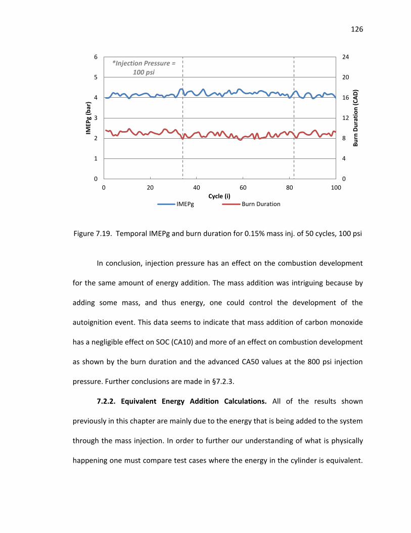
126
Figure 7.19. Temporal IMEPg and burn duration for 0.15% mass inj. of 50 cycles, 100 psi
In conclusion, injection pressure has an effect on the combustion development
for the same amount of energy addition. The mass addition was intriguing because by
adding some mass, and thus energy, one could control the development of the
autoignition event. This data seems to indicate that mass addition of carbon monoxide
has a negligible effect on SOC (CA10) and more of an effect on combustion development
as shown by the burn duration and the advanced CA50 values at the 800 psi injection
pressure. Further conclusions are made in §7.2.3.
7.2.2. Equivalent Energy Addition Calculations. All of the results shown
previously in this chapter are mainly due to the energy that is being added to the system
through the mass injection. In order to further our understanding of what is physically
happening one must compare test cases where the energy in the cylinder is equivalent.
0
4
8
12
16
20
24
0
1
2
3
4
5
6
0 20 40 60 80 100
Bu
rn D
ura
tio
n (
CA
D)
IMEP
g (b
ar)
Cycle (i) IMEPg Burn Duration
*Injection Pressure = 100 psi
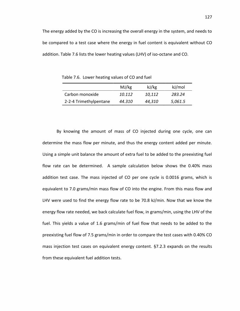
127
The energy added by the CO is increasing the overall energy in the system, and needs to
be compared to a test case where the energy in fuel content is equivalent without CO
addition. Table 7.6 lists the lower heating values (LHV) of iso-octane and CO.
Table 7.6. Lower heating values of CO and fuel
MJ/kg kJ/kg kJ/mol
Carbon monoxide 10.112 10,112 283.24
2-2-4 Trimethylpentane 44.310 44,310 5,061.5
By knowing the amount of mass of CO injected during one cycle, one can
determine the mass flow per minute, and thus the energy content added per minute.
Using a simple unit balance the amount of extra fuel to be added to the preexisting fuel
flow rate can be determined. A sample calculation below shows the 0.40% mass
addition test case. The mass injected of CO per one cycle is 0.0016 grams, which is
equivalent to 7.0 grams/min mass flow of CO into the engine. From this mass flow and
LHV were used to find the energy flow rate to be 70.8 kJ/min. Now that we know the
energy flow rate needed, we back calculate fuel flow, in grams/min, using the LHV of the
fuel. This yields a value of 1.6 grams/min of fuel flow that needs to be added to the
preexisting fuel flow of 7.5 grams/min in order to compare the test cases with 0.40% CO
mass injection test cases on equivalent energy content. §7.2.3 expands on the results
from these equivalent fuel addition tests.
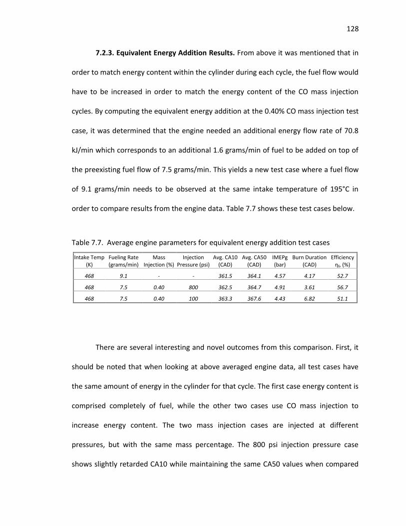
128
7.2.3. Equivalent Energy Addition Results. From above it was mentioned that in
order to match energy content within the cylinder during each cycle, the fuel flow would
have to be increased in order to match the energy content of the CO mass injection
cycles. By computing the equivalent energy addition at the 0.40% CO mass injection test
case, it was determined that the engine needed an additional energy flow rate of 70.8
kJ/min which corresponds to an additional 1.6 grams/min of fuel to be added on top of
the preexisting fuel flow of 7.5 grams/min. This yields a new test case where a fuel flow
of 9.1 grams/min needs to be observed at the same intake temperature of 195°C in
order to compare results from the engine data. Table 7.7 shows these test cases below.
Table 7.7. Average engine parameters for equivalent energy addition test cases
Intake Temp (K)
Fueling Rate (grams/min)
Mass Injection (%)
Injection Pressure (psi)
Avg. CA10 (CAD)
Avg. CA50 (CAD)
IMEPg (bar)
Burn Duration (CAD)
Efficiency ηf, (%)
468 9.1 - - 361.5 364.1 4.57 4.17 52.7
468 7.5 0.40 800 362.5 364.7 4.91 3.61 56.7
468 7.5 0.40 100 363.3 367.6 4.43 6.82 51.1
There are several interesting and novel outcomes from this comparison. First, it
should be noted that when looking at above averaged engine data, all test cases have
the same amount of energy in the cylinder for that cycle. The first case energy content is
comprised completely of fuel, while the other two cases use CO mass injection to
increase energy content. The two mass injection cases are injected at different
pressures, but with the same mass percentage. The 800 psi injection pressure case
shows slightly retarded CA10 while maintaining the same CA50 values when compared
129
to the baseline energy addition case (9.1 grams/min fuel flow). This is explained by the
energy within the cylinder being released at a faster rate and within a smaller time
scale, as shown by burn duration. The most important point to take away however is the
fact that engine power output significantly increases at this test case allowing for a 4%
increase in fuel conversion efficiency. Either the mixing effects from the high pressure
injection of CO or the chemical kinetics that are interacting between the CO and the
fuel/air mixture is allowing for this faster release of energy, causing more of the charge
energy to be converted to work instead of heat transfer and hence increase fuel
conversion efficiency. This is exciting as IMEPg values of around 5 bar could not have
been achieved by purely using fuel energy while keeping a pressure rise rate limit of 10
bar/CAD and these low of intake temperatures. On the other side, when looking at the
100 psi injection case, CA10 is retarded by 2 CAD and the CA50 is pushed later in the
cycle. This is also confirmed by the longer burn durations that are seen at this set point.
What is interesting to note is that the same amount of fuel energy is introduced into the
cylinder as the baseline test, yet by injecting this mass at 100 psi, the burn durations are
prolonged giving a longer combustion development, while retarding SOC. It is important
to note that the engine’s gross power out per displacement volume (IMEPg) is slightly
less than the baseline test at 4.43 bar, but maintains this output given longer burn
durations. The fuel conversion efficiency suffers by 1.6%. At this test case it is either the
kinetics interaction between the CO and fuel/air mixture or the mixing effects that are
introduced into the cylinder that are different than the 800 psi case causing combustion
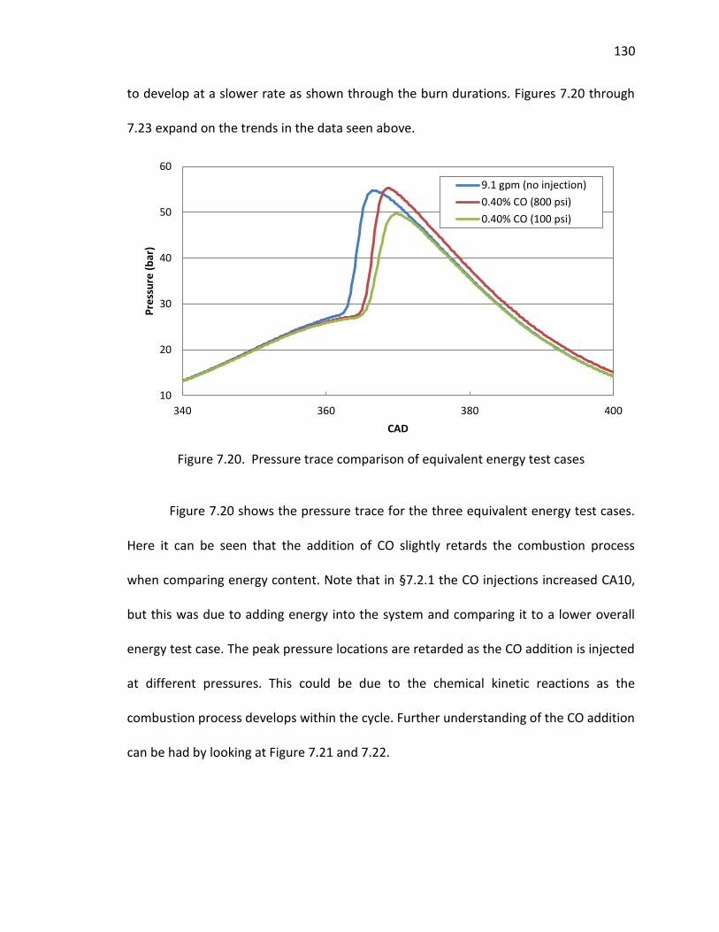
130
to develop at a slower rate as shown through the burn durations. Figures 7.20 through
7.23 expand on the trends in the data seen above.
Figure 7.20. Pressure trace comparison of equivalent energy test cases
Figure 7.20 shows the pressure trace for the three equivalent energy test cases.
Here it can be seen that the addition of CO slightly retards the combustion process
when comparing energy content. Note that in §7.2.1 the CO injections increased CA10,
but this was due to adding energy into the system and comparing it to a lower overall
energy test case. The peak pressure locations are retarded as the CO addition is injected
at different pressures. This could be due to the chemical kinetic reactions as the
combustion process develops within the cycle. Further understanding of the CO addition
can be had by looking at Figure 7.21 and 7.22.
10
20
30
40
50
60
340 360 380 400
Pre
ssu
re (
bar
)
CAD
9.1 gpm (no injection)
0.40% CO (800 psi)
0.40% CO (100 psi)
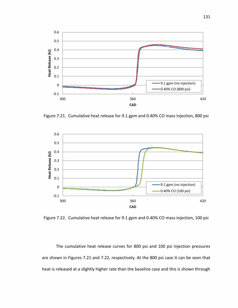
131
Figure 7.21. Cumulative heat release for 9.1 gpm and 0.40% CO mass injection, 800 psi
Figure 7.22. Cumulative heat release for 9.1 gpm and 0.40% CO mass injection, 100 psi
The cumulative heat release curves for 800 psi and 100 psi injection pressures
are shown in Figures 7.21 and 7.22, respectively. At the 800 psi case it can be seen that
heat is released at a slightly higher rate than the baseline case and this is shown through
-0.1
0
0.1
0.2
0.3
0.4
0.5
0.6
300 360 420
He
at R
ele
ase
(kJ
)
CAD
9.1 gpm (no injection)
0.40% CO (800 psi)
-0.1
0
0.1
0.2
0.3
0.4
0.5
0.6
300 360 420
He
at R
ele
ase
(kJ
)
CAD
9.1 gpm (no injection)
0.40% CO (100 psi)
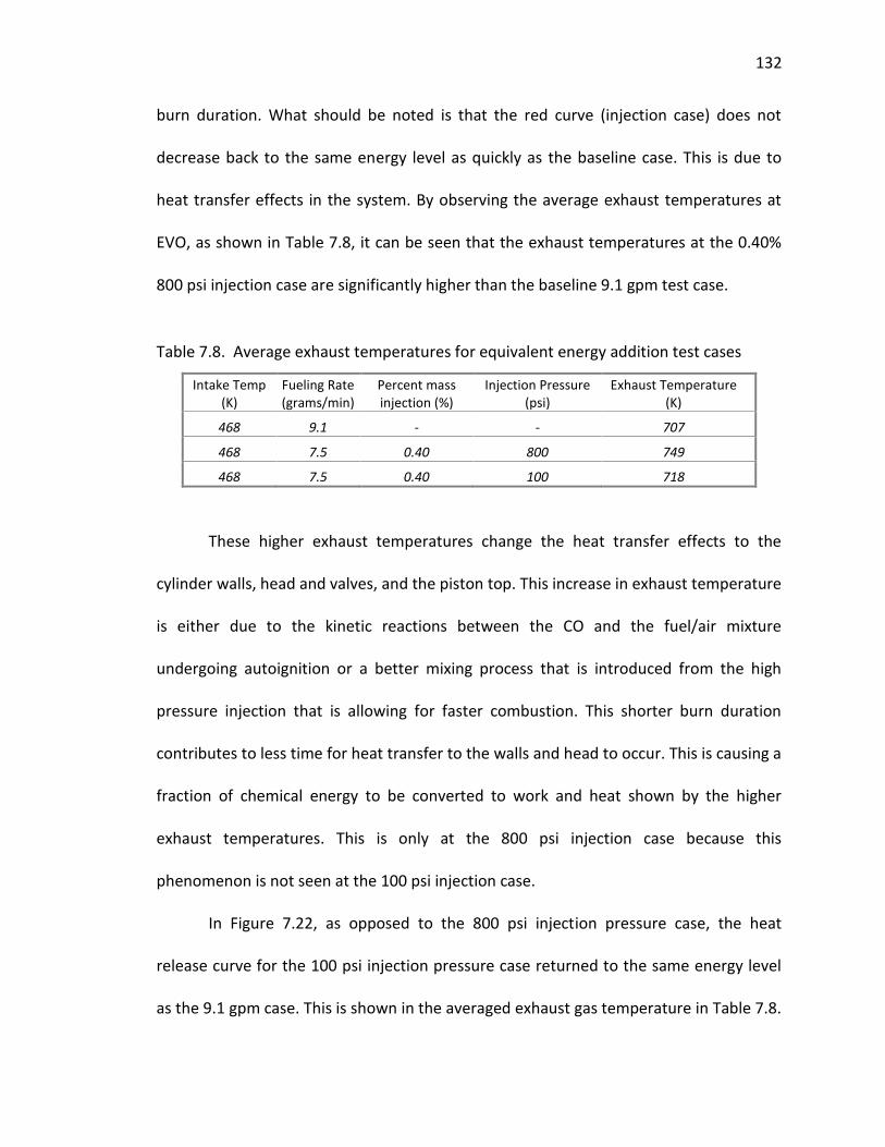
132
burn duration. What should be noted is that the red curve (injection case) does not
decrease back to the same energy level as quickly as the baseline case. This is due to
heat transfer effects in the system. By observing the average exhaust temperatures at
EVO, as shown in Table 7.8, it can be seen that the exhaust temperatures at the 0.40%
800 psi injection case are significantly higher than the baseline 9.1 gpm test case.
Table 7.8. Average exhaust temperatures for equivalent energy addition test cases
Intake Temp (K)
Fueling Rate (grams/min)
Percent mass injection (%)
Injection Pressure (psi)
Exhaust Temperature (K)
468 9.1 - - 707
468 7.5 0.40 800 749
468 7.5 0.40 100 718
These higher exhaust temperatures change the heat transfer effects to the
cylinder walls, head and valves, and the piston top. This increase in exhaust temperature
is either due to the kinetic reactions between the CO and the fuel/air mixture
undergoing autoignition or a better mixing process that is introduced from the high
pressure injection that is allowing for faster combustion. This shorter burn duration
contributes to less time for heat transfer to the walls and head to occur. This is causing a
fraction of chemical energy to be converted to work and heat shown by the higher
exhaust temperatures. This is only at the 800 psi injection case because this
phenomenon is not seen at the 100 psi injection case.
In Figure 7.22, as opposed to the 800 psi injection pressure case, the heat
release curve for the 100 psi injection pressure case returned to the same energy level
as the 9.1 gpm case. This is shown in the averaged exhaust gas temperature in Table 7.8.
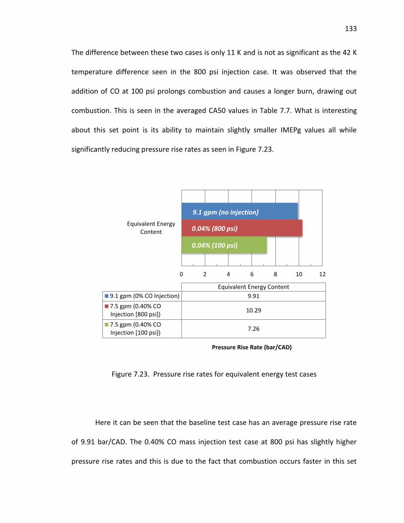
133
The difference between these two cases is only 11 K and is not as significant as the 42 K
temperature difference seen in the 800 psi injection case. It was observed that the
addition of CO at 100 psi prolongs combustion and causes a longer burn, drawing out
combustion. This is seen in the averaged CA50 values in Table 7.7. What is interesting
about this set point is its ability to maintain slightly smaller IMEPg values all while
significantly reducing pressure rise rates as seen in Figure 7.23.
Figure 7.23. Pressure rise rates for equivalent energy test cases
Here it can be seen that the baseline test case has an average pressure rise rate
of 9.91 bar/CAD. The 0.40% CO mass injection test case at 800 psi has slightly higher
pressure rise rates and this is due to the fact that combustion occurs faster in this set
0 2 4 6 8 10 12
Equivalent EnergyContent
Pressure Rise Rate (bar/CAD)
Equivalent Energy Content
9.1 gpm (0% CO Injection) 9.91
7.5 gpm (0.40% COInjection [800 psi])
10.29
7.5 gpm (0.40% COInjection [100 psi])
7.26
9.1 gpm (no injection)
0.04% (800 psi)
0.04% (100 psi)
134
point than at the baseline as shown by the burn durations. However, this slightly higher
pressure rise rate does not account for the fact that IMEPg values saw a 7.5% increase,
and the fuel conversion efficiency saw a 4% increase. This means that the addition of CO
at 800 psi allows for a more efficient conversion of energy into work due to either the
kinetics at work throughout the combustion development, which is near instantaneous
or a more complete mixing caused by the high injection pressure of a reactive gas.
When looking at the 0.40% CO mass injection test case at 100 psi, it can be seen that the
pressure rise rates are significantly reduced from the baseline case. This is interesting as
the engine’s IMEPg only saw a 3.1% decrease for this test case, and the fuel conversion
efficiency was reduced by 1.6%. This work shows that pressure rise rates can be
significantly reduced without suffering major losses in power output from the engine.
These results indicate that reactive species gas injection could be used for onboard
cyclic control of HCCI combustion in order to perturb the system and push the engine
away from regions of instability, as seen in the partial burn regime.
135
8. CONCLUSIONS AND FUTURE WORK
8.1. CONCLUSIONS
Cycle-to-cycle dynamics play a role in HCCI combustion, especially when the
engine is operated in the partial burn regime near the misfire limit. This thesis outlines
the impact that internally trapped exhaust gas residuals have on the combustion
parameters in this operating zone. This work also introduces a simple burned/ unburned
residual model into a much larger 5-state physics based thermodynamic control model
in order to capture and correctively predict the cycle-to-cycle dynamics regarding the
operational regime of an HCCI engine. Lastly, this work explores preliminary data
captured that shows the effect of cyclically injecting syn-gas as a possible control
scheme in HCCI combustion. This syn-gas has a profound effect based on injection
pressure, amount of mass (and thus energy) injected, and species injected.
In conclusion, work presented in this thesis has explored the effect that the
internally trapped exhaust gas residual temperature has on the next cycle, through start
of combustion represented by CA10. In order to assess the cycle-to-cycle variations in
work output, quantified by IMEPg, return maps of 400/1000 consecutive engine cycles
at steady state and partial burn operating regimes were plotted and compared. These
experimental return maps show that the engine’s cyclic variations display stochastic
behavior when the combustion phasing is near top dead center and more deterministic
behavior near the misfire limit in the partial burn regime. More importantly, it was
observed that the measured exhaust gas temperature appears to have limited
correlation to the next cycle’s start of combustion, quantified by CA10 when considering
136
simple correlation plots. There appears to be some determinism shown in the return
map of CA10 for all three set points.
The exhaust gas residual also affects the composition of the new charge through
its composition. From here, the exhaust manifold pressure was increased, and hence
more residuals were retained in the cylinder to be carried over to the next cycle. Again,
in order to assess the cycle-to-cycle variations in work output, quantified by IMEPg,
return maps of the partial burn operating regime were compared. It was observed that
with increased exhaust gas residual amounts, the engine could operate longer in the
partial burn regime; however this caused a larger dispersion in the IMEPg data collected.
The return maps for CA10 at these set points also showed some slight determinism
indicating that the current cycle’s (i) CA10 is correlated to the next cycle’s (i+1) CA10
through some feed forward mechanism. By increasing the residual gas fraction from
increased exhaust manifold pressure and hence the thermal effect of these residuals on
the fresh charge, one would expect to see a stronger correlation between the current
cycle’s measured exhaust gas temperature and the next cycle’s start of combustion
however it was observed that these two parameters once again show a limited
correlation. This indicates that the HCCI start of combustion event is not near as
dependent on temperature as originally conceived, and even more so at the higher load
case which contains hotter exhaust gas temperatures did not display any determinism,
despite having these hot residual temperatures. This goes to say that the next cycle’s
combustion event is more dependent on the chemistry and composition of the residuals
than the thermal effect of the residual gas fraction. It was also observed that the
137
increased residual amount is not affecting SOC; however it is affecting how the
combustion develops within the cylinder.
This work has also explored the capability of a five-state thermodynamics non-
linear control model to qualitatively capture the cyclic dynamics of an HCCI engine. In
order to assess the cycle-to-cycle variations in work output, quantified by IMEPg, return
maps of 1000 consecutive engine cycles of experimental and simulated data were
plotted and compared. The experimental return maps show the engine’s cyclic
variations display very stochastic behavior when combustion phasing is near top dead
center and more deterministic behavior near the partial burn limit. The simulated
results show that the non-linear model is capable of capturing this stochastic and
deterministic behavior but only through the inclusion of unburned exhaust residual (i.e.
chemical composition) effects. Therefore, it is shown that exhaust residual composition
effects through inclusion of an unburned gas residual impacts the ability of the model to
predict deterministic behavior at the partial burn limit.
In an attempt to expand on the aforementioned conclusions, a residual gas
injector was developed to cyclically inject a reactive species gas, in this case carbon
monoxide, in order to perturb the fresh intake charge through its chemical composition.
This perturbation allowed the chemical effects to be separated from the thermal effects
in order to study the kinetics behind HCCI combustion development. It was observed
that injecting CO at the same fueling rate would increase CA50 and IMEPg while
decreasing the burn duration. This was an expected result as adding a reactive gas
increases energy content of the charge. The interesting result from this experiment was
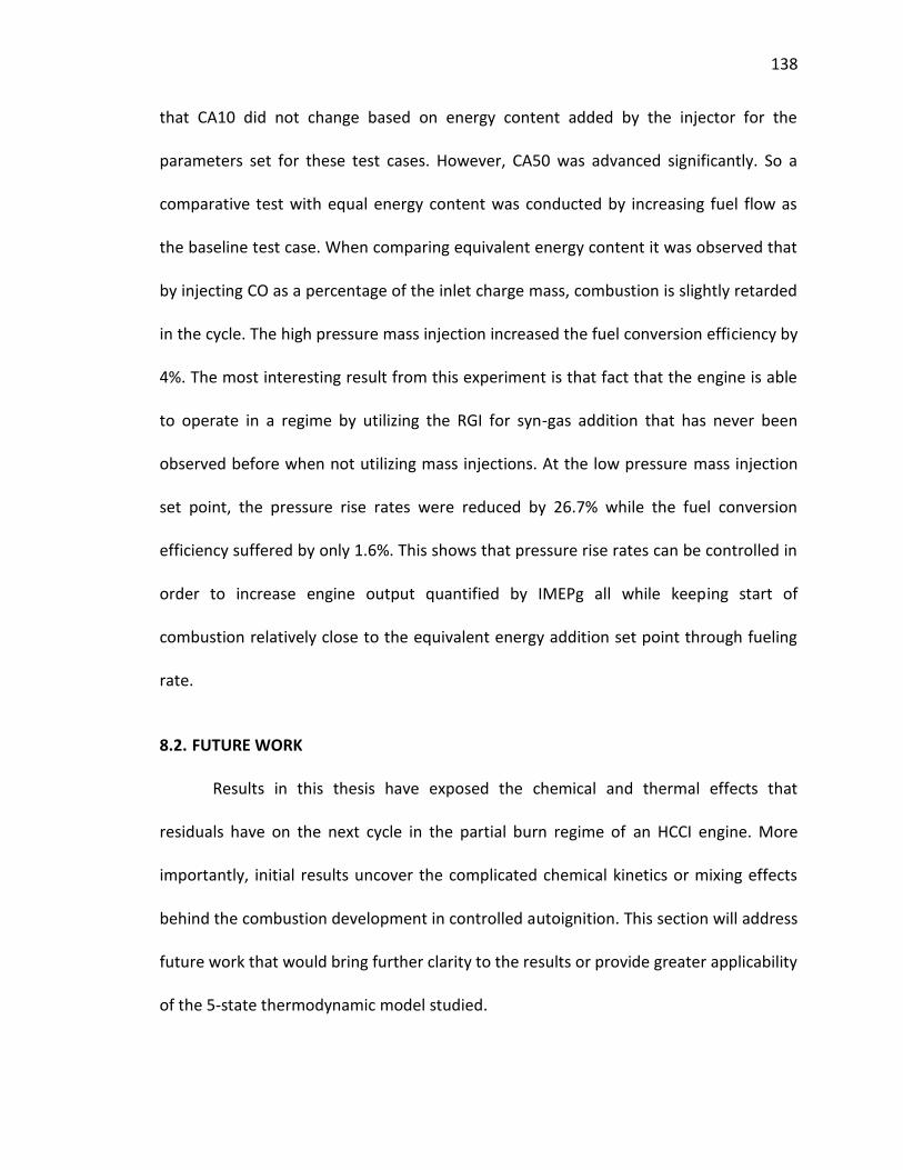
138
that CA10 did not change based on energy content added by the injector for the
parameters set for these test cases. However, CA50 was advanced significantly. So a
comparative test with equal energy content was conducted by increasing fuel flow as
the baseline test case. When comparing equivalent energy content it was observed that
by injecting CO as a percentage of the inlet charge mass, combustion is slightly retarded
in the cycle. The high pressure mass injection increased the fuel conversion efficiency by
4%. The most interesting result from this experiment is that fact that the engine is able
to operate in a regime by utilizing the RGI for syn-gas addition that has never been
observed before when not utilizing mass injections. At the low pressure mass injection
set point, the pressure rise rates were reduced by 26.7% while the fuel conversion
efficiency suffered by only 1.6%. This shows that pressure rise rates can be controlled in
order to increase engine output quantified by IMEPg all while keeping start of
combustion relatively close to the equivalent energy addition set point through fueling
rate.
8.2. FUTURE WORK
Results in this thesis have exposed the chemical and thermal effects that
residuals have on the next cycle in the partial burn regime of an HCCI engine. More
importantly, initial results uncover the complicated chemical kinetics or mixing effects
behind the combustion development in controlled autoignition. This section will address
future work that would bring further clarity to the results or provide greater applicability
of the 5-state thermodynamic model studied.
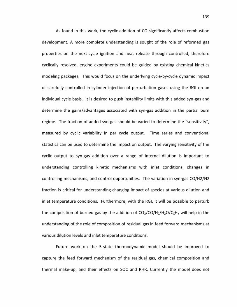
139
As found in this work, the cyclic addition of CO significantly affects combustion
development. A more complete understanding is sought of the role of reformed gas
properties on the next-cycle ignition and heat release through controlled, therefore
cyclically resolved, engine experiments could be guided by existing chemical kinetics
modeling packages. This would focus on the underlying cycle-by-cycle dynamic impact
of carefully controlled in-cylinder injection of perturbation gases using the RGI on an
individual cycle basis. It is desired to push instability limits with this added syn-gas and
determine the gains/advantages associated with syn-gas addition in the partial burn
regime. The fraction of added syn-gas should be varied to determine the “sensitivity”,
measured by cyclic variability in per cycle output. Time series and conventional
statistics can be used to determine the impact on output. The varying sensitivity of the
cyclic output to syn-gas addition over a range of internal dilution is important to
understanding controlling kinetic mechanisms with inlet conditions, changes in
controlling mechanisms, and control opportunities. The variation in syn-gas CO/H2/N2
fraction is critical for understanding changing impact of species at various dilution and
inlet temperature conditions. Furthermore, with the RGI, it will be possible to perturb
the composition of burned gas by the addition of CO2/CO/H2/H2O/CXHY will help in the
understanding of the role of composition of residual gas in feed forward mechanisms at
various dilution levels and inlet temperature conditions.
Future work on the 5-state thermodynamic model should be improved to
capture the feed forward mechanism of the residual gas, chemical composition and
thermal make-up, and their effects on SOC and RHR. Currently the model does not
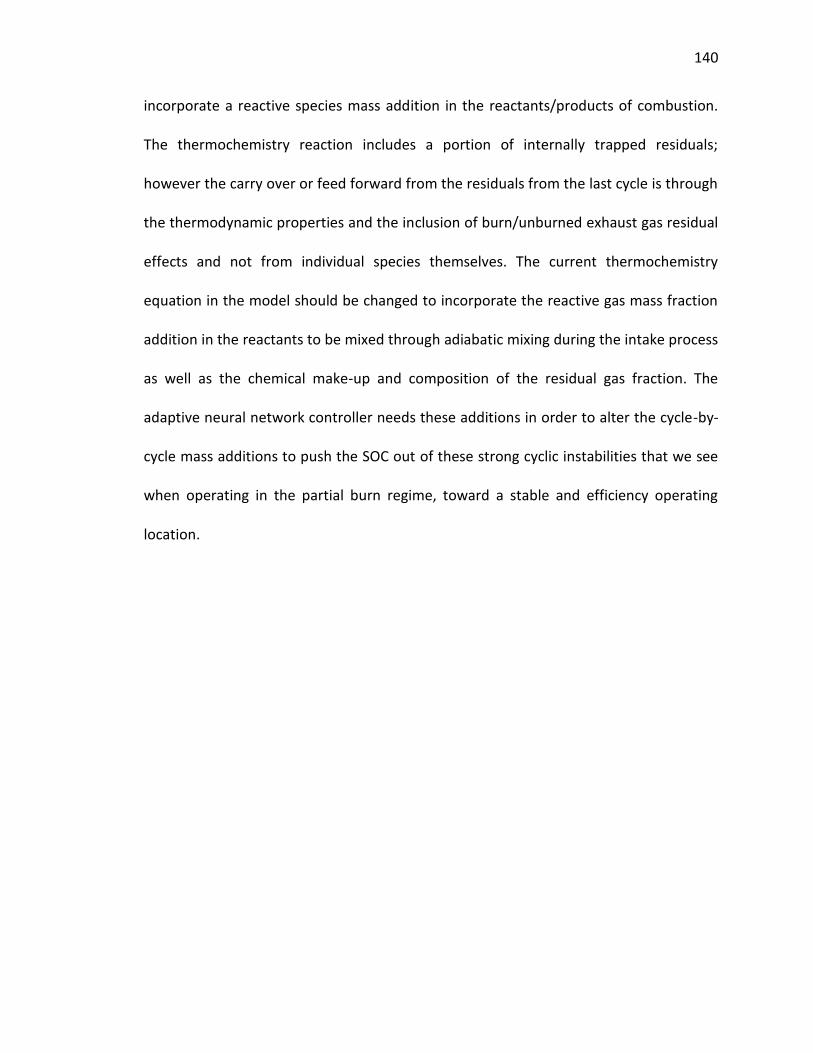
140
incorporate a reactive species mass addition in the reactants/products of combustion.
The thermochemistry reaction includes a portion of internally trapped residuals;
however the carry over or feed forward from the residuals from the last cycle is through
the thermodynamic properties and the inclusion of burn/unburned exhaust gas residual
effects and not from individual species themselves. The current thermochemistry
equation in the model should be changed to incorporate the reactive gas mass fraction
addition in the reactants to be mixed through adiabatic mixing during the intake process
as well as the chemical make-up and composition of the residual gas fraction. The
adaptive neural network controller needs these additions in order to alter the cycle-by-
cycle mass additions to push the SOC out of these strong cyclic instabilities that we see
when operating in the partial burn regime, toward a stable and efficiency operating
location.

141
APPENDIX A
RESIDUAL GAS INJECTOR DRAWINGS
142
Figure A-1. OEM Diesel Injector a. actual and b. solid model
Figure A-2. Residual Gas Injector solid modeled a. assembled view and b. exploded view
Figure A-3. Residual Gas Injector prototype a. assembled and b. exploded
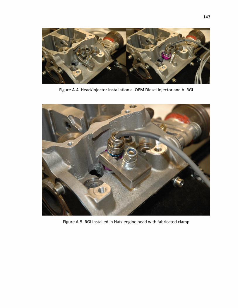
143
Figure A-4. Head/injector installation a. OEM Diesel Injector and b. RGI
Figure A-5. RGI installed in Hatz engine head with fabricated clamp
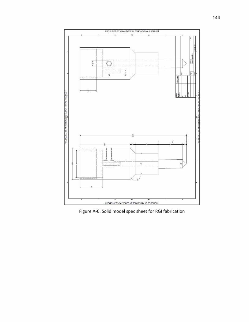
144
Figure A-6. Solid model spec sheet for RGI fabrication

145
APPENDIX B
EXPERIMENTAL TESTING MATRICIES
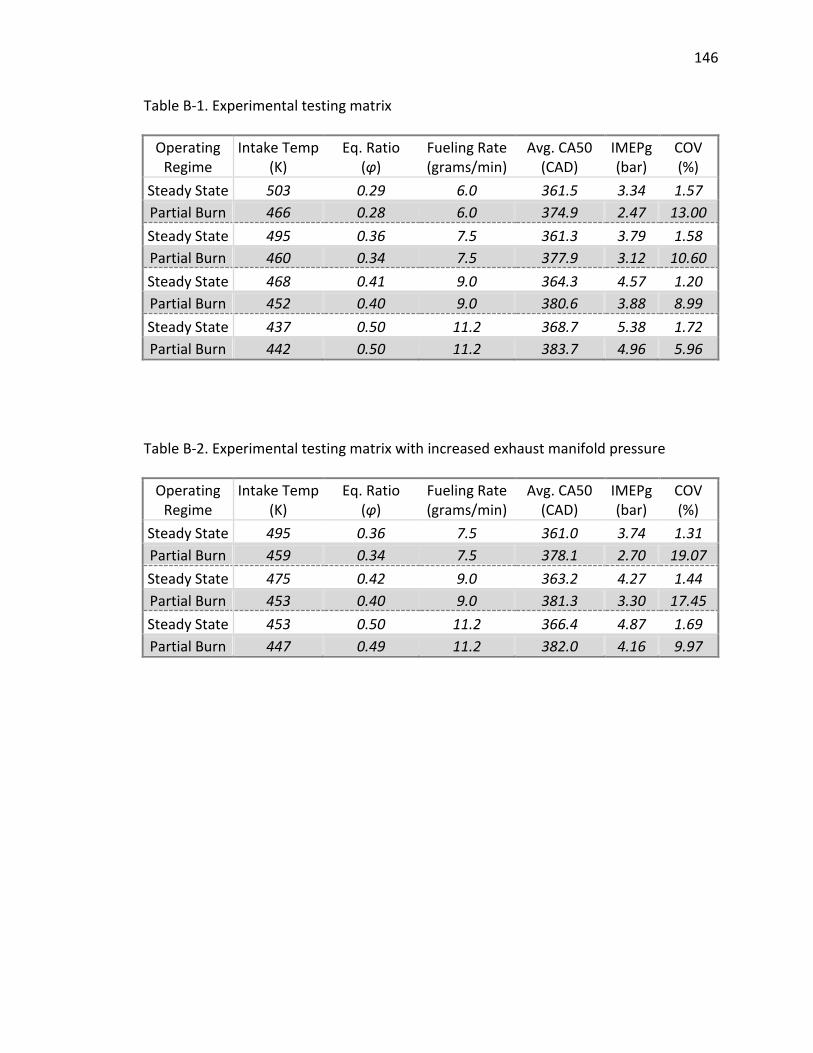
146
Table B-1. Experimental testing matrix
Operating Regime
Intake Temp (K)
Eq. Ratio (φ)
Fueling Rate (grams/min)
Avg. CA50 (CAD)
IMEPg (bar)
COV (%)
Steady State 503 0.29 6.0 361.5 3.34 1.57
Partial Burn 466 0.28 6.0 374.9 2.47 13.00
Steady State 495 0.36 7.5 361.3 3.79 1.58
Partial Burn 460 0.34 7.5 377.9 3.12 10.60
Steady State 468 0.41 9.0 364.3 4.57 1.20
Partial Burn 452 0.40 9.0 380.6 3.88 8.99
Steady State 437 0.50 11.2 368.7 5.38 1.72
Partial Burn 442 0.50 11.2 383.7 4.96 5.96
Table B-2. Experimental testing matrix with increased exhaust manifold pressure
Operating Regime
Intake Temp (K)
Eq. Ratio (φ)
Fueling Rate (grams/min)
Avg. CA50 (CAD)
IMEPg (bar)
COV (%)
Steady State 495 0.36 7.5 361.0 3.74 1.31
Partial Burn 459 0.34 7.5 378.1 2.70 19.07
Steady State 475 0.42 9.0 363.2 4.27 1.44
Partial Burn 453 0.40 9.0 381.3 3.30 17.45
Steady State 453 0.50 11.2 366.4 4.87 1.69
Partial Burn 447 0.49 11.2 382.0 4.16 9.97
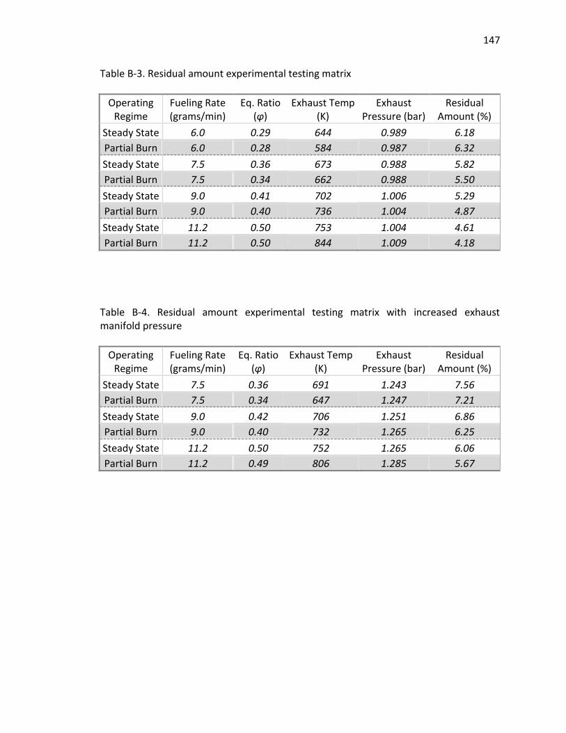
147
Table B-3. Residual amount experimental testing matrix
Operating Regime
Fueling Rate (grams/min)
Eq. Ratio (φ)
Exhaust Temp (K)
Exhaust Pressure (bar)
Residual Amount (%)
Steady State 6.0 0.29 644 0.989 6.18
Partial Burn 6.0 0.28 584 0.987 6.32
Steady State 7.5 0.36 673 0.988 5.82
Partial Burn 7.5 0.34 662 0.988 5.50
Steady State 9.0 0.41 702 1.006 5.29
Partial Burn 9.0 0.40 736 1.004 4.87
Steady State 11.2 0.50 753 1.004 4.61
Partial Burn 11.2 0.50 844 1.009 4.18
Table B-4. Residual amount experimental testing matrix with increased exhaust manifold pressure
Operating Regime
Fueling Rate (grams/min)
Eq. Ratio (φ)
Exhaust Temp (K)
Exhaust Pressure (bar)
Residual Amount (%)
Steady State 7.5 0.36 691 1.243 7.56
Partial Burn 7.5 0.34 647 1.247 7.21
Steady State 9.0 0.42 706 1.251 6.86
Partial Burn 9.0 0.40 732 1.265 6.25
Steady State 11.2 0.50 752 1.265 6.06
Partial Burn 11.2 0.49 806 1.285 5.67
148
APPENDIX C
THERMOCHEMISTRY INTAKE/EXHAUST MASS CALCULATION TABLES
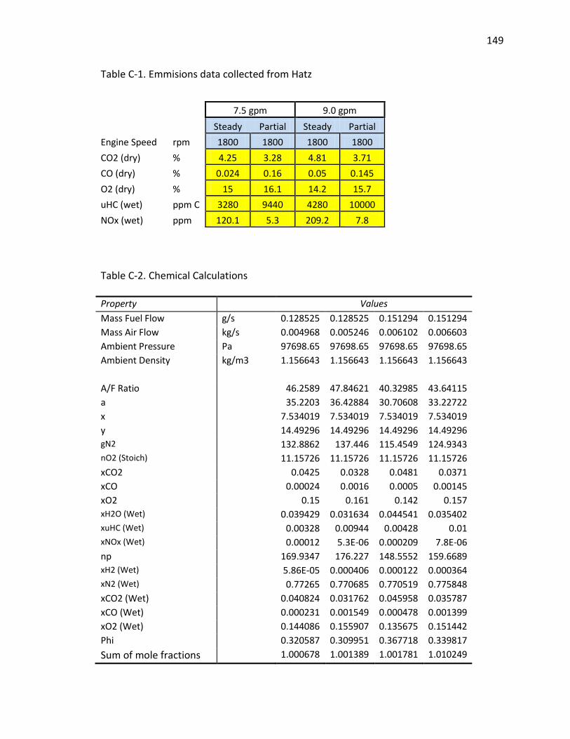
149
Table C-1. Emmisions data collected from Hatz
7.5 gpm 9.0 gpm
Steady Partial Steady Partial
Engine Speed rpm 1800 1800 1800 1800
CO2 (dry) % 4.25 3.28 4.81 3.71
CO (dry) % 0.024 0.16 0.05 0.145
O2 (dry) % 15 16.1 14.2 15.7
uHC (wet) ppm C 3280 9440 4280 10000
NOx (wet) ppm 120.1 5.3 209.2 7.8
Table C-2. Chemical Calculations Property Values
Mass Fuel Flow g/s 0.128525 0.128525 0.151294 0.151294
Mass Air Flow kg/s 0.004968 0.005246 0.006102 0.006603
Ambient Pressure Pa 97698.65 97698.65 97698.65 97698.65
Ambient Density kg/m3 1.156643 1.156643 1.156643 1.156643
A/F Ratio 46.2589 47.84621 40.32985 43.64115
a 35.2203 36.42884 30.70608 33.22722
x 7.534019 7.534019 7.534019 7.534019
y 14.49296 14.49296 14.49296 14.49296
gN2 132.8862 137.446 115.4549 124.9343
nO2 (Stoich) 11.15726 11.15726 11.15726 11.15726
xCO2 0.0425 0.0328 0.0481 0.0371
xCO 0.00024 0.0016 0.0005 0.00145
xO2 0.15 0.161 0.142 0.157
xH2O (Wet) 0.039429 0.031634 0.044541 0.035402
xuHC (Wet) 0.00328 0.00944 0.00428 0.01
xNOx (Wet) 0.00012 5.3E-06 0.000209 7.8E-06
np 169.9347 176.227 148.5552 159.6689
xH2 (Wet) 5.86E-05 0.000406 0.000122 0.000364
xN2 (Wet) 0.77265 0.770685 0.770519 0.775848
xCO2 (Wet) 0.040824 0.031762 0.045958 0.035787
xCO (Wet) 0.000231 0.001549 0.000478 0.001399
xO2 (Wet) 0.144086 0.155907 0.135675 0.151442
Phi 0.320587 0.309951 0.367718 0.339817
Sum of mole fractions 1.000678 1.001389 1.001781 1.010249
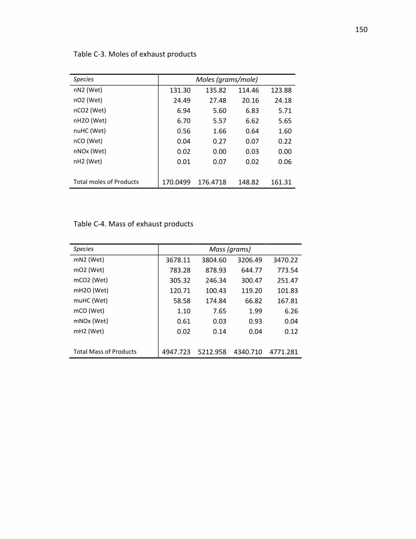
150
Table C-3. Moles of exhaust products
Species Moles (grams/mole)
nN2 (Wet) 131.30 135.82 114.46 123.88
nO2 (Wet) 24.49 27.48 20.16 24.18
nCO2 (Wet) 6.94 5.60 6.83 5.71
nH2O (Wet) 6.70 5.57 6.62 5.65
nuHC (Wet) 0.56 1.66 0.64 1.60
nCO (Wet) 0.04 0.27 0.07 0.22
nNOx (Wet) 0.02 0.00 0.03 0.00
nH2 (Wet) 0.01 0.07 0.02 0.06
Total moles of Products 170.0499 176.4718 148.82 161.31
Table C-4. Mass of exhaust products
Species Mass (grams)
mN2 (Wet) 3678.11 3804.60 3206.49 3470.22
mO2 (Wet) 783.28 878.93 644.77 773.54
mCO2 (Wet) 305.32 246.34 300.47 251.47
mH2O (Wet) 120.71 100.43 119.20 101.83
muHC (Wet) 58.58 174.84 66.82 167.81
mCO (Wet) 1.10 7.65 1.99 6.26
mNOx (Wet) 0.61 0.03 0.93 0.04
mH2 (Wet) 0.02 0.14 0.04 0.12
Total Mass of Products 4947.723 5212.958 4340.710 4771.281
151
BIBLIOGRAPHY
[1] Zhao, Fuquan, Thomas N. Asmus, Dennis N. Assanis, James A. Dec, and Paul M. Najt. "Homogeneous Charge Compression Ignition (HCCI) Engines.” SAE International, 2003.
[2] Zhao, H., Z. Peng, and N. Ladommatos. “Understanding of controlled autoignition combustion in a four-stroke gasoline engine.” Journal of Automobile Engineering 215 (2001): 1297-1310.
[3] Dec, John E. “Advanced compression-ignition engines – understanding the in-cylinder processes.” Proc. of the Combustion Institute 32 (2009): 2727-2742.
[4] Koopmans, Lucien, Ove Backlund, and Ingemar Denbratt. “Cycle to Cycle Variations: Their Influence on Cycle Resolved Gas Temperature and Unburned Hydrocarbons from a Camless Gasoline Compression Ignition Engine.” SAE Paper 2002-01-0110.
[5] Persson, H., R. Pfeiffer, A. Hultqvist, B. Johansson, and H. Ström. “Cylinder-to-Cylinder and Cycle-toCycle Variations at HCCI Operation With Trapped Residuals.” SAE Paper 2005-01-0130.
[6] Xingcai, Lu, Ji Libin, Ma Junjun, and Huang Zhen. “Experimental study on the cycle-by-cycle variations of homogeneous charge compression ignition combustion using primary reference fuels and their mixtures.” Journal of Automobile Engineering (2007): 859-866.
[7] Shahbakhti, Mahdi, Robert Lupul, and Charles Robert Koch. “Cyclic Variations of Ignition Timing in an HCCI Engine.” Proc. of the ASME/IEEE Joint Rail Conference and Internal Combustion Engine Spring Technical Conference (2007): 405-415.
[8] Shahbakhti, M., and C. R. Koch. “Characterizing the cyclic variability of ignition timing in a homogeneous charge compression ignition engine fuelled with n-heptane/iso-octane blend fuels.” International Journal of Engine Research 9 (2008): 361-397.
152
[9] Maurya, Rakesh Kumar, and Avinash Kumar Agarwal. “Experimental investigation on the effect of intake air temperature and air-fuel ratio on cycle-to-cycle variations of HCCI combustion and performance parameters.” Journal of Applied Energy 88 (2011): 1153-1163.
[10] Agarwal, Avinash Kumar. “Experimental Investigations on Intake Air Temperature and Air-Fuel Ratio Dependence of Random and Deterministic Cyclic Variability in a Homogeneous Charge Compression Ignition Engine.” SAE Paper 2011-01-1183.
[11] Wagner, Robert M., K. Dean Edwards, C. Stuart Daw, Johney B. Green Jr., and Bruce G. Bunting. “On the Nature of Cyclic Dispersion in Spark Assisted HCCI Combustion.” SAE Paper 2006-01-0418.
[12] Daw, C. Stuart, Robert M. Wagner, K. Dean Edwards, and Johney B. Green Jr. “Understanding the transition between conventional spark-ignited combustion and HCCI in a gasoline engine.” Proc. of the Combustion Institute 31 (2007): 2887-2894.
[13] Daw, C. Stuart, K. Dean Edwards, Robert M. Wagner, and Johney B. Green Jr. “Modeling Cyclic Variability in Spark-Assisted HCCI.” Journal of Engineering for Gas Turbines and Power 130 (2008): 052801 1-6.
[14] Sen, A.K., G. Litak, K.D. Edwards, C.E.A. Finney, C.S. Daw, and R.M. Wagner. “Characteristics of cyclic heat release variability in the transition from spark ignition to HCCI in a gasoline engine.” Journal of Applied Energy 88 (2011): 1649-1655.
[15] Hyvönen, Jari, Göran Haraldsson, and Bengt Johansson. “Operating Conditions Using Spark Assisted HCCI Combustion During Combustion Mode Transfer to SI in a Multi-Cylinder VCR-HCCI Engnie.” SAE Paper 2005-01-0109.
[16] Heywood, J.B. “Internal Combustion Engine Fundamentals.” McGraw-Hill, 1988.
[17] Bettis, Josh B. “Thermodynamic Modeling for Nonlinear Control of Combustion Phasing in HCCI Engines.” Thesis. Missouri University of Science and Technology, 2010.
153
[18] Waero, Rolf R. “The Effect of Spark Timing on Residual Gas Fraction.” Thesis. Massachusetts Institute of Technology, 2000.
[19] Morey, Francis, Patrice Seers. “Comparison of cycle-by-cycle variation of
measured exhaust-gas temperature and in-cylinder pressure measurements.” Journal of Applied Thermal Engineering 30 (2010): 487-491.
[20] Chiang, Chia-Jui, Anna Stefanopoulou, and Mrdjan Janković. “Nonlinear
Observer-Based Control of Load Transitions in Homogeneous Charge Compression Ignition Engines.” IEEE Transactions on Control Systems Technology 15.3 (2007): 438-448.
[21] Chiang, Chia-Jui, and Anna Stefanopoulou. “Sensitivity Analysis of Combustion Timing of Homogeneous Charge Compression Ignition Gasoline Engines.” Journal of Dynamic Systems, Measurement, and Control 131 (2009): 014506 1-5.
[22] Shahbakhti, M., A. Ghazimirsaied, and C. R. Koch. "Experimental Study of Exhaust Temperature Variation in an HCCI Engine." Journal of Automobile Engineering 224 (2010): 1177-1197.
[23] Fathi, Morteza, R. Khoshbakhti Saray, and M. David Checkel. “The influence of Exhaust Gas Recirculation (EGR) on combustion and emissions of n-heptane/natural gas fueled Homogeneous Charge Compression Ignition (HCCI) engines.” Journal of Applied Energy 88 (2011): 4719-4724.
[24] Lee, Donghoon, Anna G. Stefanopoulou, Satheesh Makkapati, and Mrdjan Janković. “Modeling and Control of a Heated Air Intake Homogeneous Charge Compression Ignition (HCCI) Engine.” Proc. of the American Controls Conference (2010): 3817-3823.
[25] Yu, X. R., X. S. Bai, A. Vressner, A. Hultqvist, B. Johansson, J. Olofsson, H. Seyfried, J. Sjöholm, M. Richter, and M. Aldén. “Effect of Turbulence on HCCI Combustion.” SAE Paper 2007-01-0183.
[26] He, X., M.T. Donovan, B.T. Zigler, T.R. Palmer, S.M. Walton, M.S. Wooldridge, and A. Atreya. “An experimental and modeling study of iso-octane ignition delay times under homogeneous charge compression ignition conditions.” Journal of Combustion and Flame 142 (2005): 266-275.
154
[27] Dubreuil, A., F. Foucher, and C. Mounaïm-Rousselle. “Effect of EGR Chemical Components and Intake Temperature on HCCI Combustion Development.” SAE Paper 2006-32-0044.
[28] Subramanian, G., A. Pires Da Cruz, R. Bounaceur, and L. Vervisch. “Chemical Impact of CO and H2 Addition on the Auto-Ignition Delay of Homogeneous n-Heptane/Air Mixtures.” Combustion Science and Technology 179 (2007): 1937-1962
[29] Hosseini, Vahid, and M. David Checkel. “Effect of Reformer Gas on HCCI Combustion – Part 1: High Octane Fuels.” SAE Paper 2007-01-0208.
[30] Hosseini, Vahid, and M. David Checkel. “Reformer Gas Composition Effect on
HCCI Combustion of n-Heptane, iso-Octane, and Natural Gas.” SAE Paper 2008-01-0049.
[31] Hosseini, Vahid, W. Stuart Neill, and M. David Checkel. “Controlling n-Heptane
HCCI Combustion with Partial Reforming: Experimental Results and Modeling Analysis.” Journal of Engineering for Gas Turbines and Power 131 (2009): 052801 1-11
[32] Ghazimirsaied, Ahmad, and Charles Robert Koch. "Controlling cyclic combustion timing variations using a symbol-statistics predictive approach in an HCCI engine." Journal of Applied Energy 92 (2012): 133-146.
[33] White, Frank M. “Fluid Mechanics.” McGraw-Hill, 1979.
[34] Fox, Jonathan W., Wai K. Cheng, and John B. Heywood. “A Model for Predicting Residual Gas Fraction in Spark-Ignition Engines.” SAE Paper 931025.
[35] Alkidas, A. C. “The Use of Availability and Energy Balances in Diesel Engines.” SAE Paper 890822.
155
VITA
Aaron David Attebery was born in Springdale, Arkansas to David and Sherrie
Attebery on August 20, 1988. He graduated from North Callaway High School in
Kingdom City, Missouri in May 2006. He worked as an Engineering Technician for the
City of Fulton during the summer of 2007. During the summers of 2008, 2009, and 2010
he worked as an Engineering Intern for Ameren UE at Callaway Nuclear Power Plant in
Fulton, Missouri. In December 2010, he received his B.S. with Honors in Mechanical
Engineering from Missouri University of Science and Technology (formerly known as
University of Missouri – Rolla). In April 2012, Aaron was awarded first place in the
Chancellor’s Fellowship Research Poster Competition. During the summer of 2012, he
spent two weeks studying abroad on the topic of Intercultural Communications at the
University of Western Cape in Cape Town, South Africa. In December 2012, Aaron
received his M.S. degree in Mechanical Engineering from Missouri University of Science
and Technology.

156