INTRODUCTION TO CONTROL SYSTEMS

Kamran IqbalUniversity of Arkansas at Little Rock

University of Arkansas at Little Rock

Introduction to Control Systems

Kamran Iqbal

This text is disseminated via the Open Education Resource (OER) LibreTexts Project (https://LibreTexts.org) and like the hundredsof other texts available within this powerful platform, it is freely available for reading, printing and "consuming." Most, but not all,pages in the library have licenses that may allow individuals to make changes, save, and print this book. Carefullyconsult the applicable license(s) before pursuing such effects.

Instructors can adopt existing LibreTexts texts or Remix them to quickly build course-specific resources to meet the needs of theirstudents. Unlike traditional textbooks, LibreTexts’ web based origins allow powerful integration of advanced features and newtechnologies to support learning.

The LibreTexts mission is to unite students, faculty and scholars in a cooperative effort to develop an easy-to-use online platformfor the construction, customization, and dissemination of OER content to reduce the burdens of unreasonable textbook costs to ourstudents and society. The LibreTexts project is a multi-institutional collaborative venture to develop the next generation of open-access texts to improve postsecondary education at all levels of higher learning by developing an Open Access Resourceenvironment. The project currently consists of 14 independently operating and interconnected libraries that are constantly beingoptimized by students, faculty, and outside experts to supplant conventional paper-based books. These free textbook alternatives areorganized within a central environment that is both vertically (from advance to basic level) and horizontally (across different fields)integrated.

The LibreTexts libraries are Powered by MindTouch and are supported by the Department of Education Open Textbook PilotProject, the UC Davis Office of the Provost, the UC Davis Library, the California State University Affordable Learning SolutionsProgram, and Merlot. This material is based upon work supported by the National Science Foundation under Grant No. 1246120,1525057, and 1413739. Unless otherwise noted, LibreTexts content is licensed by CC BY-NC-SA 3.0.

Any opinions, findings, and conclusions or recommendations expressed in this material are those of the author(s) and do notnecessarily reflect the views of the National Science Foundation nor the US Department of Education.

Have questions or comments? For information about adoptions or adaptions contact info@LibreTexts.org. More information on ouractivities can be found via Facebook (https://facebook.com/Libretexts), Twitter (https://twitter.com/libretexts), or our blog(http://Blog.Libretexts.org).

This text was compiled on 07/18/2022

®

1

TABLE OF CONTENTS

1: Mathematical Models of Physical Systems

1.0: Prelude to Mathematical Models of Physical Systems1.1: Model Variables and Element Types1.2: First-Order ODE Models1.3: Second-Order ODE Models1.4: An Electro-Mechanical System Model1.5: Industrial Process Models1.6: State Variable Models1.7: Linearization of Nonlinear ModelsOcatve examplesR ExamplesOctave examples

2: Transfer Function Models

2.0: Prelude to Transfer Function Models2.1: System Poles and Zeros2.2: System Natural Response2.3: System Stability2.4: The Step Response2.5: Sinusoidal Response of a SystemBlank

3: Feedback Control System Models

3.0: Prelude to Feedback Control System Models3.1: Static Feedback Controller3.2: First-Order Dynamic Controllers3.3: PI, PD, and PID Controllers3.4: Rate Feedback ControllersBlank

4: Control System Design Objectives

4.0: Prelude to Control System Design Objectives4.1: Stability of the Closed-Loop System4.2: Transient Response Improvement4.3: Steady-State Error Improvement4.4: Disturbance Rejection4.5: Sensitivity and Robustness

5: Control System Design with Root Locus

5.0: Prelude to Control System Design with Root Locus5.1: Root Locus Fundamentals5.2: Static Controller Design5.3: Transient Response Improvement

2

5.4: Steady-State Error Improvement5.5: Transient and Steady-State Improvement5.6: Controller Realization

6: Compensator Design with Frequency Response Methods

6.0: Prelude to Compensator Design with Frequency Response Methods6.1: Frequency Response Plots6.2: Measures of Performance6.3: Frequency Response Design6.4: Closed-Loop Frequency Response

7: Design of Sampled-Data Systems

7.0: Prelude to Design of Sampled-Data Systems7.1: Models of Sampled-Data Systems7.2: Pulse Transfer Function7.3: Sampled-Data System Response7.4: Stability of Sampled-Data Systems7.5: Closed-Loop System Response7.6: Digital Controller Design by Emulation7.7: Root Locus Design of Digital Controllers

8: State Variable Models

8.0: Prelude to State Variable Models8.1: State Variable Models8.2: State-Transition Matrix and Asymptotic Stability8.3: State-Space Realization of Transfer Function Models8.4: Linear Transformation of State Variables

9: Controllers for State Variable Models

9.0: Prelude to Controllers for State Variable Models9.1: Controller Design in Sate-Space9.2: Tracking with Feedforward Controller9.3: Tracking PI Controller Design

10: Controllers for Discrete State Variable Models

10.0: Prelude to Controllers for Discrete State Variable Models10.1: State Variable Models of Sampled-Data Systems10.2: Controllers for Discrete State Variable Models

Index

Index

Glossary

Thumbnail: A block diagram of a PID controller. (CC BY-SA 3.0 Unported; TravTigerEE via Wikipedia)

3

Book: Introduction to Control Systems (Iqbal) is shared under a CC BY-NC-SA 4.0 license and was authored, remixed, and/or curated by KamranIqbal.

1

CHAPTER OVERVIEW

1: Mathematical Models of Physical Systems

1. Obtain a mathematical model of a physical system.2. Obtain system transfer function from its differential equation model.3. Obtain a physical system model in the state variable form.4. Linearize a nonlinear dynamic system model about an operating point.

1.0: Prelude to Mathematical Models of Physical Systems1.1: Model Variables and Element Types1.2: First-Order ODE Models1.3: Second-Order ODE Models1.4: An Electro-Mechanical System Model1.5: Industrial Process Models1.6: State Variable Models1.7: Linearization of Nonlinear ModelsOcatve examplesR ExamplesOctave examples

1: Mathematical Models of Physical Systems is shared under a CC BY-NC-SA 4.0 license and was authored, remixed, and/or curated by KamranIqbal.

Learning Objectives

1.0.1 https://eng.libretexts.org/@go/page/24453

1.0: Prelude to Mathematical Models of Physical SystemsThis chapter describes the process of obtaining the mathematical description of a dynamic system, i.e., a system whose behaviorchanges over time. The system is assumed to be assembled from components. The system model is based on the physical laws thatgovern the behavior of various system components.

Physical systems of interest to engineers include, for example, electrical, mechanical, electromechanical, thermal, and fluidsystems. By using lumped parameter assumption, their behavior is mathematically described in terms of ordinary differentialequation (ODE) models. These equations are nonlinear, in general, but can be linearized about an operating point for analysis anddesign purposes.

Models of interconnected components are assembled from individual component describptions. The components in electricalsystems include resistors, capacitors, and inductors. The components used in mechanical systems include inertial masses, springs,and dampers (or friction elements). For thermal systems, these include thermal capacitance and thermal resistance. For hydraulicand fluid systems, these include reservoir capacity and flow resistance.

In certain physical systems, properties (or entities) flow in and out of a system boundary, e.g., a hydraulic reservoir, or thermalchamber. The dynamics of such systems is described by conservation laws and/or balance equations. In particular, let Q representan accumulated property, and represent the inflow and outflow rates, then the model is described as:

where and denote the internal generation and consumption of that property.

The Laplace transform converts a linear differential equation into an algebraic equation, which can be manipulated to obtain aninput-output description described as a transfer function. The transfer function forms the basis of analysis and design of controlsystems using conventional methods. In contrast, the modern control theory is established on time-domain analysis involving thestate equations, that describe system behavior as time derivatives of a set of state variables.

Linearization of nonlinear models is accomplished using Taylor series expansion about a critical point, where the linear behavior isrestricted to the neighborhood of the critical point. The linear systems theory is well-estabished and serves as the basic tool forcontroller design.

1.0: Prelude to Mathematical Models of Physical Systems is shared under a CC BY-NC-SA 4.0 license and was authored, remixed, and/or curatedby LibreTexts.

qin qout

= − +g−cdQ

dtqin qout (1.0.1)

g c

1.1.1 https://eng.libretexts.org/@go/page/24382

1.1: Model Variables and Element Types

Flow and Across Variables

Modeling of a physical system involves two kinds of variables: flow variables that ‘flow’ through the components, and acrossvariables that are measured across those components.

For example, in electric circuits, potential (voltage) is measured across elements, whereas electrical charge (current) flows throughthe circuit elements.

In mechanical linkage systems, displacement and velocity are measured across elements, whereas force or effort ‘flows’ throughthe linkages.

In thermal and fluid systems, heat and mass serve as the flow variables, whereas temperature and pressure constitute the acrossvariables.

A physical element is characterized by the relationship between flow and across variables. The three basic types are the resistive,inductive, and capacitive elements. The terminology, taken from electrical circuits, extends to other types of physical systems aswell.

While the resistive element dissipates energy, both the capacitive and inductive elements store energy. For example, a capacitorstores electrical energy and a moving mass stores kinetic energy. The energy storage accords memory to the element that accountsfor it dynamic behavior modeled by an ODE.

Let denote a flow variable and denote an across variable associated with an element; then, the element type is defined bytheir mutual relationships, described as follows:

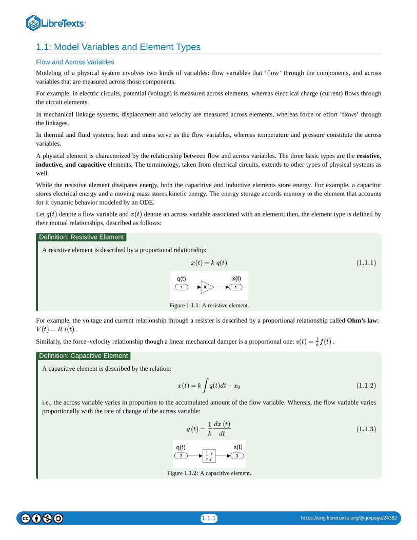
A resistive element is described by a proportional relationship:

Figure : A resistive element.

For example, the voltage and current relationship through a resister is described by a proportional relationship called Ohm’s law: .

Similarly, the force–velocity relationship though a linear mechanical damper is a proportional one: .

A capacitive element is described by the relation:

i.e., the across variable varies in proportion to the accumulated amount of the flow variable. Whereas, the flow variable variesproportionally with the rate of change of the across variable:

Figure : A capacitive element.

q(t) x(t)

Definition: Resistive Element

x(t) = k q(t) (1.1.1)

1.1.1

V (t) =R i(t)

v(t) = f(t)1b

Definition: Capacitive Element

x(t) = k∫ q(t)dt+x0 (1.1.2)

q (t) =1

k

dx (t)

dt(1.1.3)

1.1.2

1.1.2 https://eng.libretexts.org/@go/page/24382

For example, the voltage and current relationship through a capacitor is given as: . Since the currentintegral represents the accumulation of electrical charge, we have: . The inverse relationship is described as: .

Similarly, the force–velocity relationship that governs the movement of an inertial mass is described as: .

Its inverse is the familiar Newton’s second law of motion: .

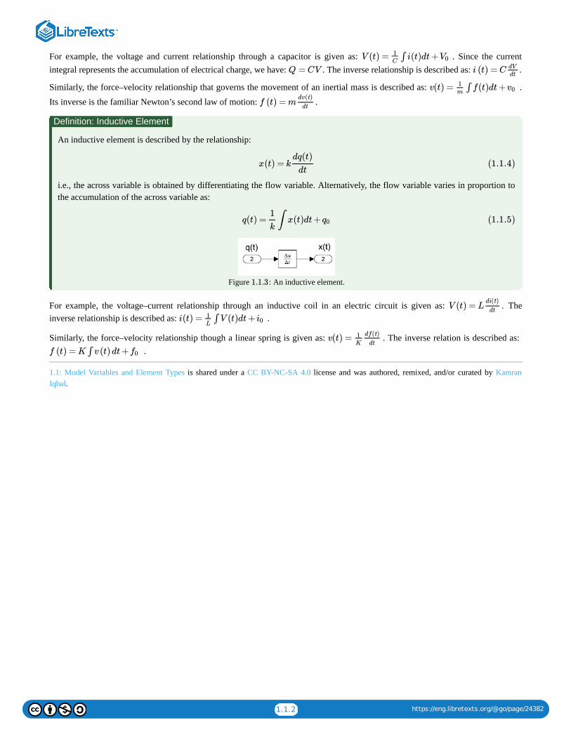
An inductive element is described by the relationship:

i.e., the across variable is obtained by differentiating the flow variable. Alternatively, the flow variable varies in proportion tothe accumulation of the across variable as:

Figure : An inductive element.

For example, the voltage–current relationship through an inductive coil in an electric circuit is given as: . Theinverse relationship is described as: .

Similarly, the force–velocity relationship though a linear spring is given as: . The inverse relation is described as: .

1.1: Model Variables and Element Types is shared under a CC BY-NC-SA 4.0 license and was authored, remixed, and/or curated by KamranIqbal.

V (t) = ∫ i(t)dt+1C

V0

Q =CV i (t) =C dV

dt

v(t) = ∫ f(t)dt+1m

v0

f (t) =mdv(t)

dt

Definition: Inductive Element

x(t) = kdq(t)

dt(1.1.4)

q(t) = ∫ x(t)dt+1

kq0 (1.1.5)

1.1.3

V (t) =Ldi(t)

dt

i(t) = ∫ V (t)dt+1L

i0

v(t) = 1K

df(t)

dt

f (t) =K ∫ v(t)dt+f0

1.2.1 https://eng.libretexts.org/@go/page/24383

1.2: First-Order ODE Models

First-Order ODE ModelsElectrical, mechanical, thermal, and fluid systems that contain a single energy storage element are described by first-order ODEmodels.Let denote a generic input, denote a generic output, and denote the time constant; then, a generic first-order ODEmodel is expressed as:

The time constant, , denotes the time when the system response to a constant input rises to 63.2% of its final value. The timeconstant is measured in .

Examples

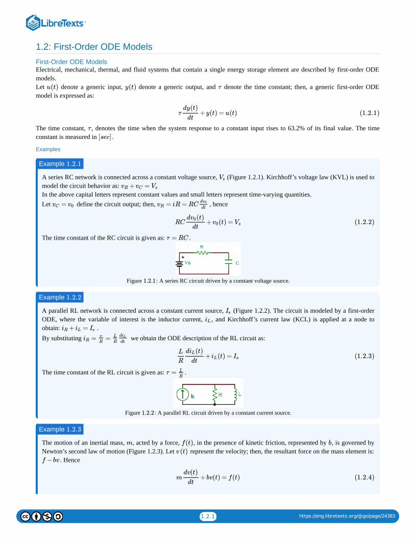
A series RC network is connected across a constant voltage source, (Figure 1.2.1). Kirchhoff’s voltage law (KVL) is used tomodel the circuit behavior as: In the above capital letters represent constant values and small letters represent time-varying quantities.Let define the circuit output; then, , hence

The time constant of the RC circuit is given as: .

Figure : A series RC circuit driven by a constant voltage source.

A parallel RL network is connected across a constant current source, (Figure 1.2.2). The circuit is modeled by a first-orderODE, where the variable of interest is the inductor current, , and Kirchhoff’s current law (KCL) is applied at a node toobtain: .By substituting we obtain the ODE description of the RL circuit as:

The time constant of the RL circuit is given as: .

Figure : A parallel RL circuit driven by a constant current source.

The motion of an inertial mass, , acted by a force, , in the presence of kinetic friction, represented by , is governed byNewton’s second law of motion (Figure 1.2.3). Let represent the velocity; then, the resultant force on the mass element is:

. Hence

u(t) y(t) τ

τ +y(t) = u(t)dy(t)

dt(1.2.1)

τ

[sec]

Example 1.2.1

Vs

+ =vR vC Vs

=vC v0 = iR = RCvRdv0

dt

RC + (t) =d (t)v0

dtv0 Vs (1.2.2)

τ = RC

1.2.1

Example 1.2.2

Is

iL+ =iR iL Is

= =iRv

R

L

R

diL

dt

+ (t) =L

R

d (t)iL

dtiL Is (1.2.3)

τ = L

R

1.2.2

Example 1.2.3

m f(t) b

v(t)

f −bv

m +bv(t) = f(t)dv(t)

dt(1.2.4)

1.2.2 https://eng.libretexts.org/@go/page/24383

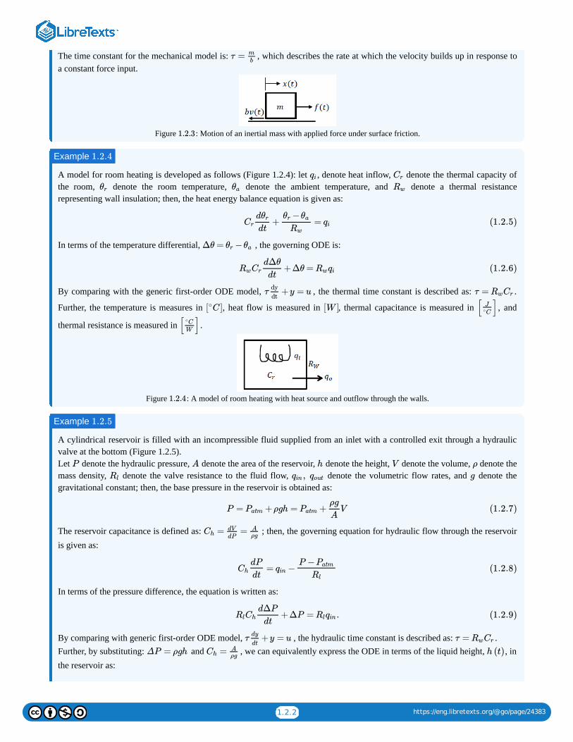
The time constant for the mechanical model is: , which describes the rate at which the velocity builds up in response toa constant force input.

Figure : Motion of an inertial mass with applied force under surface friction.

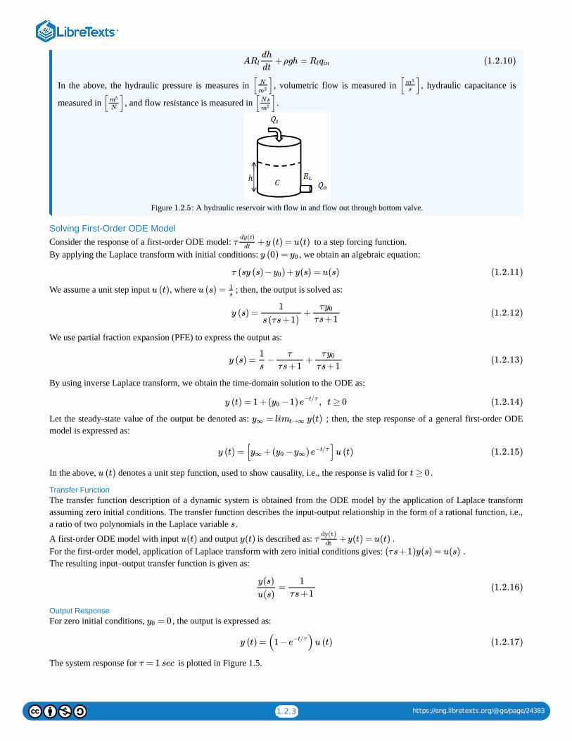
A model for room heating is developed as follows (Figure 1.2.4): let , denote heat inflow, denote the thermal capacity ofthe room, denote the room temperature, denote the ambient temperature, and denote a thermal resistancerepresenting wall insulation; then, the heat energy balance equation is given as:

In terms of the temperature differential, , the governing ODE is:

By comparing with the generic first-order ODE model, , the thermal time constant is described as: .

Further, the temperature is measures in , heat flow is measured in , thermal capacitance is measured in , and

thermal resistance is measured in .

Figure : A model of room heating with heat source and outflow through the walls.

A cylindrical reservoir is filled with an incompressible fluid supplied from an inlet with a controlled exit through a hydraulicvalve at the bottom (Figure 1.2.5).Let denote the hydraulic pressure, denote the area of the reservoir, denote the height, denote the volume, denote themass density, denote the valve resistance to the fluid flow, denote the volumetric flow rates, and denote thegravitational constant; then, the base pressure in the reservoir is obtained as:

The reservoir capacitance is defined as: ; then, the governing equation for hydraulic flow through the reservoiris given as:

In terms of the pressure difference, the equation is written as:

By comparing with generic first-order ODE model, , the hydraulic time constant is described as: .Further, by substituting: and , we can equivalently express the ODE in terms of the liquid height, , inthe reservoir as:

τ = m

b

1.2.3

Example 1.2.4

qi Cr

θr θa Rw

+ =Cr

dθr

dt

−θr θa

Rw

qi (1.2.5)

Δθ = −θr θa

+Δθ =RwCr

dΔθ

dtRwqi (1.2.6)

τ +y = udy

dtτ = RwCr

[ C]∘ [W ] [ ]J

C∘

[ ]C∘

W

1.2.4

Example 1.2.5

P A h V ρ

Rl ,qin qout g

P = +ρgh = + VPatm Patm

ρg

A(1.2.7)

= =ChdV

dP

Aρg

= −Ch

dP

dtqin

P −Patm

Rl

(1.2.8)

+ΔP = .RlCh

dΔP

dtRlqin (1.2.9)

τ +y = udy

dtτ = RwCr

ΔP = ρgh =ChAρg

h (t)

1.2.3 https://eng.libretexts.org/@go/page/24383

In the above, the hydraulic pressure is measures in , volumetric flow is measured in , hydraulic capacitance is

measured in , and flow resistance is measured in .

Figure : A hydraulic reservoir with flow in and flow out through bottom valve.

Solving First-Order ODE Model Consider the response of a first-order ODE model: to a step forcing function.By applying the Laplace transform with initial conditions: , we obtain an algebraic equation:

We assume a unit step input , where ; then, the output is solved as:

We use partial fraction expansion (PFE) to express the output as:

By using inverse Laplace transform, we obtain the time-domain solution to the ODE as:

Let the steady-state value of the output be denoted as: ; then, the step response of a general first-order ODEmodel is expressed as:

In the above, denotes a unit step function, used to show causality, i.e., the response is valid for .

Transfer FunctionThe transfer function description of a dynamic system is obtained from the ODE model by the application of Laplace transformassuming zero initial conditions. The transfer function describes the input-output relationship in the form of a rational function, i.e.,a ratio of two polynomials in the Laplace variable .

A first-order ODE model with input and output is described as: .For the first-order model, application of Laplace transform with zero initial conditions gives: .The resulting input–output transfer function is given as:

Output ResponseFor zero initial conditions, , the output is expressed as:

The system response for is plotted in Figure 1.5.

A +ρgh =Rl

dh

dtRlqin (1.2.10)

[ ]N

m2 [ ]m3

s

[ ]m5

N[ ]Ns

m5

1.2.5

τ +y (t) = u(t)dy(t)

dt

y (0) = y0

τ (sy (s) − ) +y(s) = u(s)y0 (1.2.11)

u (t) u (s) = 1s

y (s) = +1

s (τs+1)

τy0

τs+1(1.2.12)

y (s) = − +1

s

τ

τs+1

τy0

τs+1(1.2.13)

y (t) = 1 +( −1) ,   t ≥ 0y0 e−t/τ (1.2.14)

= y(t) y∞ limt→∞

y (t) = [ +( − ) ]u (t)y∞ y0 y∞ e−t/τ (1.2.15)

u (t) t ≥ 0

s

u(t) y(t) τ +y(t) = u(t)dy(t)

dt

(τs+1)y(s) = u(s)

=y(s)

u(s)

1

τs+1(1.2.16)

= 0y0

y (t) = (1 − )u (t)e−t/τ (1.2.17)

τ = 1 sec

1.2.4 https://eng.libretexts.org/@go/page/24383

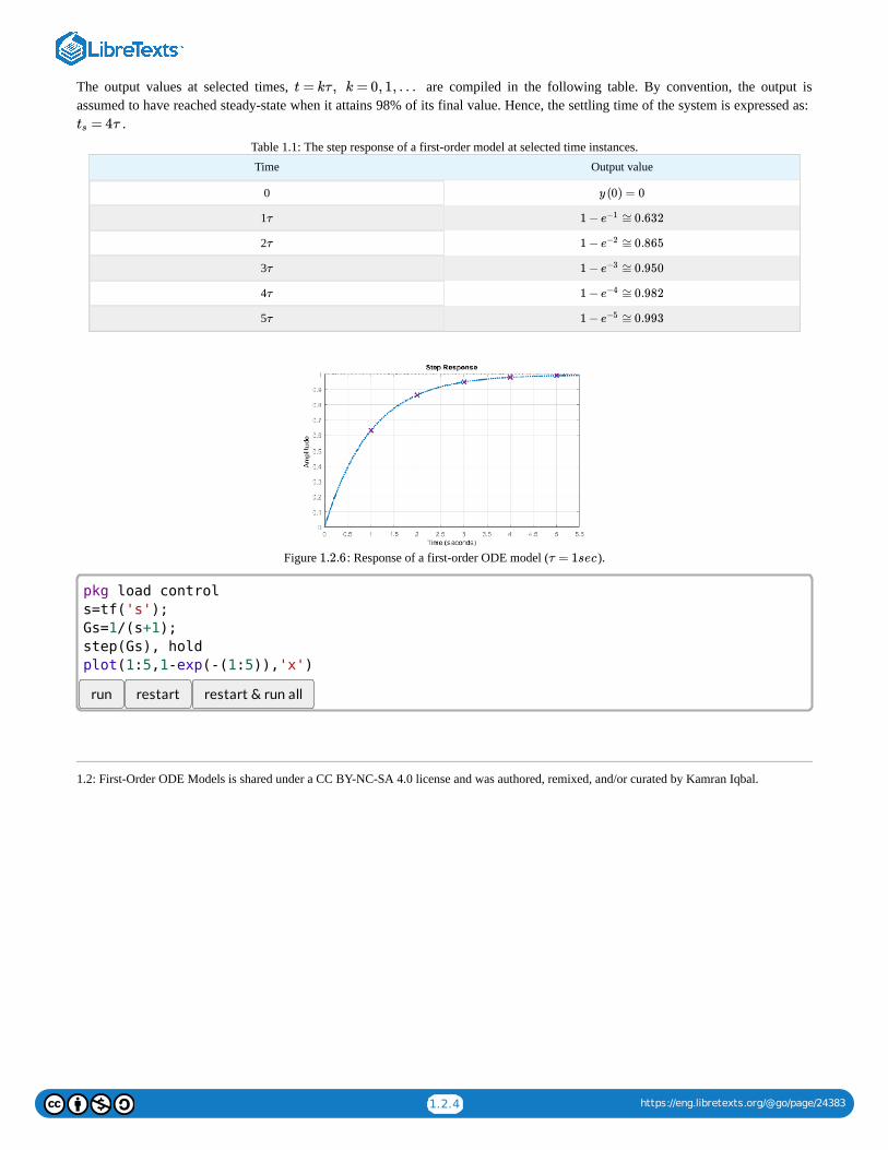
The output values at selected times, are compiled in the following table. By convention, the output isassumed to have reached steady-state when it attains 98% of its final value. Hence, the settling time of the system is expressed as:

.

Table 1.1: The step response of a first-order model at selected time instances.Time Output value

0

1

2

3

4

5

Figure : Response of a first-order ODE model ( ).

run restart restart & run all

1.2: First-Order ODE Models is shared under a CC BY-NC-SA 4.0 license and was authored, remixed, and/or curated by Kamran Iqbal.

t = kτ ,   k = 0, 1, …

= 4τts

y (0) = 0

τ 1 − ≅0.632e−1

τ 1 − ≅0.865e−2

τ 1 − ≅0.950e−3

τ 1 − ≅0.982e−4

τ 1 − ≅0.993e−5

1.2.6 τ = 1sec

pkg load control

s=tf('s');

Gs=1/(s+1);

step(Gs), hold

plot(1:5,1-exp(-(1:5)),'x')

1.3.1 https://eng.libretexts.org/@go/page/24385

1.3: Second-Order ODE Models

Second-Order ODE Models A physical system that contains two energy storage elements is described by a second-order ODE. Examples of second-ordermodels are discussed below:

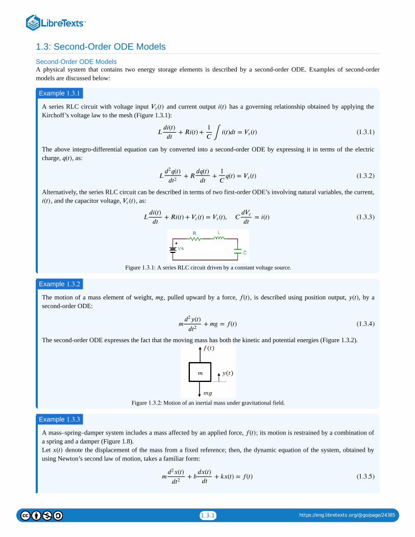
A series RLC circuit with voltage input and current output has a governing relationship obtained by applying theKirchoff’s voltage law to the mesh (Figure 1.3.1):

The above integro-differential equation can by converted into a second-order ODE by expressing it in terms of the electriccharge, , as:

Alternatively, the series RLC circuit can be described in terms of two first-order ODE’s involving natural variables, the current,, and the capacitor voltage, , as:

Figure : A series RLC circuit driven by a constant voltage source.

The motion of a mass element of weight, , pulled upward by a force, , is described using position output, , by asecond-order ODE:

The second-order ODE expresses the fact that the moving mass has both the kinetic and potential energies (Figure 1.3.2).

Figure : Motion of an inertial mass under gravitational field.

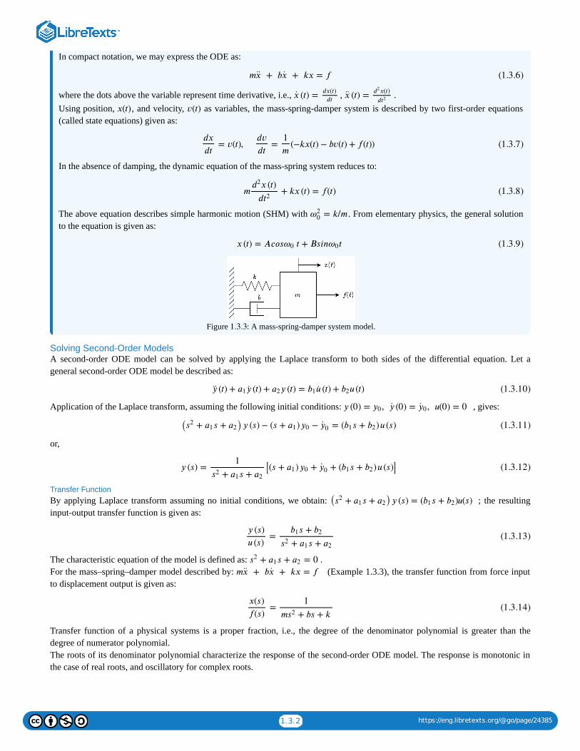
A mass–spring–damper system includes a mass affected by an applied force, ; its motion is restrained by a combination ofa spring and a damper (Figure 1.8).Let denote the displacement of the mass from a fixed reference; then, the dynamic equation of the system, obtained byusing Newton’s second law of motion, takes a familiar form:

Example 1.3.1

(𝑡)𝑉𝑠 𝑖(𝑡)

𝐿 +𝑅𝑖(𝑡) + ∫ 𝑖(𝑡)𝑑𝑡 = (𝑡)𝑑𝑖(𝑡)

𝑑𝑡

1

𝐶𝑉𝑠 (1.3.1)

𝑞(𝑡)

𝐿 +𝑅 + 𝑞(𝑡) = (𝑡)𝑞(𝑡)𝑑2

𝑑𝑡2

𝑑𝑞(𝑡)

𝑑𝑡

1

𝐶𝑉𝑠 (1.3.2)

𝑖(𝑡) (𝑡)𝑉𝑐

𝐿 +𝑅𝑖(𝑡) + (𝑡) = (𝑡),      𝐶 = 𝑖(𝑡)𝑑𝑖(𝑡)

𝑑𝑡𝑉𝑐 𝑉𝑠

𝑑𝑉𝑐

𝑑𝑡(1.3.3)

1.3.1

Example 1.3.2

𝑚𝑔 𝑓(𝑡) 𝑦(𝑡)

𝑚 + 𝑚𝑔 = 𝑓(𝑡)𝑦(𝑡)𝑑2

𝑑𝑡2(1.3.4)

1.3.2

Example 1.3.3

𝑓(𝑡)

𝑥(𝑡)

𝑚 + 𝑏 + 𝑘𝑥(𝑡) = 𝑓(𝑡)𝑥(𝑡)𝑑2

𝑑𝑡2

𝑑𝑥(𝑡)

𝑑𝑡(1.3.5)

1.3.2 https://eng.libretexts.org/@go/page/24385

In compact notation, we may express the ODE as:

where the dots above the variable represent time derivative, i.e., , .Using position, , and velocity, as variables, the mass-spring-damper system is described by two first-order equations(called state equations) given as:

In the absence of damping, the dynamic equation of the mass-spring system reduces to:

The above equation describes simple harmonic motion (SHM) with . From elementary physics, the general solutionto the equation is given as:

Figure : A mass-spring-damper system model.

Solving Second-Order Models A second-order ODE model can be solved by applying the Laplace transform to both sides of the differential equation. Let ageneral second-order ODE model be described as:

Application of the Laplace transform, assuming the following initial conditions: , gives:

or,

Transfer FunctionBy applying Laplace transform assuming no initial conditions, we obtain: ; the resultinginput-output transfer function is given as:

The characteristic equation of the model is defined as: .For the mass–spring–damper model described by: (Example 1.3.3), the transfer function from force inputto displacement output is given as:

Transfer function of a physical systems is a proper fraction, i.e., the degree of the denominator polynomial is greater than thedegree of numerator polynomial.The roots of its denominator polynomial characterize the response of the second-order ODE model. The response is monotonic inthe case of real roots, and oscillatory for complex roots.

𝑚 + 𝑏 + 𝑘𝑥 = 𝑓�� �� (1.3.6)

(𝑡) =��𝑑𝑥(𝑡)

𝑑𝑡(𝑡) =��

𝑥(𝑡)𝑑2

𝑑𝑡2

𝑥(𝑡) 𝑣(𝑡)

= 𝑣(𝑡),       = (−𝑘𝑥(𝑡)− 𝑏𝑣(𝑡) + 𝑓(𝑡))𝑑𝑥

𝑑𝑡

𝑑𝑣

𝑑𝑡

1

𝑚(1.3.7)

𝑚 + 𝑘𝑥 (𝑡) = 𝑓(𝑡)𝑥 (𝑡)𝑑2

𝑑𝑡2(1.3.8)

= 𝑘/𝑚𝜔20

𝑥 (𝑡) = 𝐴𝑐𝑜𝑠  𝑡 + 𝐵𝑠𝑖𝑛 𝑡 𝜔0 𝜔0 (1.3.9)

1.3.3

(𝑡) + (𝑡) + 𝑦 (𝑡) = (𝑡) + 𝑢 (𝑡)�� 𝑎1 �� 𝑎2 𝑏1 �� 𝑏2 (1.3.10)

𝑦 (0) = ,    (0) = ,   𝑢(0) = 0𝑦0 �� ��0

( + 𝑠 + )𝑦 (𝑠)− (𝑠 + ) − = ( 𝑠 + )𝑢 (𝑠)𝑠2 𝑎1 𝑎2 𝑎1 𝑦0 ��0 𝑏1 𝑏2 (1.3.11)

𝑦 (𝑠) = [(𝑠 + ) + + ( 𝑠 + )𝑢 (𝑠)]1

+ 𝑠 +𝑠2 𝑎1 𝑎2𝑎1 𝑦0 ��0 𝑏1 𝑏2 (1.3.12)

( + 𝑠 + )𝑦 (𝑠) = ( 𝑠 + )𝑢(𝑠)𝑠2 𝑎1 𝑎2 𝑏1 𝑏2

=𝑦 (𝑠)

𝑢 (𝑠)

𝑠 +𝑏1 𝑏2

+ 𝑠 +𝑠2 𝑎1 𝑎2(1.3.13)

+ 𝑠 + = 0𝑠2 𝑎1 𝑎2

𝑚 + 𝑏 + 𝑘𝑥 = 𝑓�� ��

=𝑥(𝑠)

𝑓(𝑠)

1

𝑚 + 𝑏𝑠 + 𝑘𝑠2(1.3.14)

1.3.3 https://eng.libretexts.org/@go/page/24385

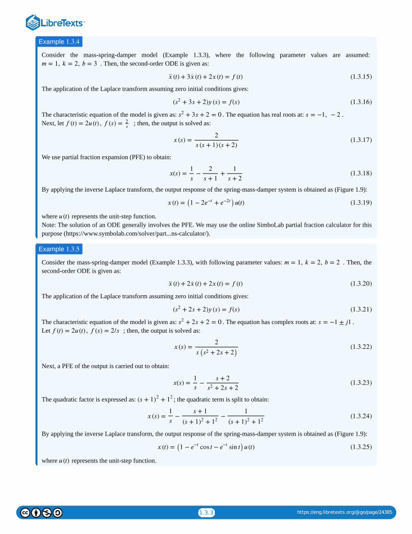
Consider the mass-spring-damper model (Example 1.3.3), where the following parameter values are assumed: . Then, the second-order ODE is given as:

The application of the Laplace transform assuming zero initial conditions gives:

The characteristic equation of the model is given as: . The equation has real roots at: .Next, let ; then, the output is solved as:

We use partial fraction expansion (PFE) to obtain:

By applying the inverse Laplace transform, the output response of the spring-mass-damper system is obtained as (Figure 1.9):

where represents the unit-step function.Note: The solution of an ODE generally involves the PFE. We may use the online SimboLab partial fraction calculator for thispurpose (https://www.symbolab.com/solver/part...ns-calculator/).

Consider the mass-spring-damper model (Example 1.3.3), with following parameter values: . Then, thesecond-order ODE is given as:

The application of the Laplace transform assuming zero initial conditions gives:

The characteristic equation of the model is given as: . The equation has complex roots at: .Let ; then, the output is solved as:

Next, a PFE of the output is carried out to obtain:

The quadratic factor is expressed as: ; the quadratic term is split to obtain:

By applying the inverse Laplace transform, the output response of the spring-mass-damper system is obtained as (Figure 1.9):

where represents the unit-step function.

Example 1.3.4

𝑚 = 1,  𝑘 = 2,  𝑏 = 3

(𝑡) + 3 (𝑡) + 2𝑥 (𝑡) = 𝑓 (𝑡)�� �� (1.3.15)

( + 3𝑠 + 2)𝑦 (𝑠) = 𝑓(𝑠)𝑠2 (1.3.16)

+ 3𝑠 + 2 = 0𝑠2 𝑠 = −1,  − 2

𝑓 (𝑡) = 2𝑢 (𝑡) ,  𝑓 (𝑠) = 2𝑠

𝑥 (𝑠) =2

𝑠 (𝑠 + 1)(𝑠 + 2)(1.3.17)

𝑥(𝑠) = − +1

𝑠

2

𝑠 + 1

1

𝑠 + 2(1.3.18)

𝑥 (𝑡) = (1 − 2 + )𝑢(𝑡)𝑒−𝑡 𝑒−2𝑡 (1.3.19)

𝑢 (𝑡)

Example 1.3.5

𝑚 = 1,  𝑘 = 2,  𝑏 = 2

(𝑡) + 2 (𝑡) + 2𝑥 (𝑡) = 𝑓 (𝑡)�� �� (1.3.20)

( + 2𝑠 + 2)𝑦 (𝑠) = 𝑓(𝑠)𝑠2 (1.3.21)

+ 2𝑠 + 2 = 0𝑠2 𝑠 = −1 ± 𝑗1

𝑓 (𝑡) = 2𝑢 (𝑡) ,  𝑓 (𝑠) = 2/𝑠

𝑥 (𝑠) =2

𝑠 ( + 2𝑠 + 2)𝑠2(1.3.22)

𝑥(𝑠) = −

1

𝑠

𝑠 + 2

+ 2𝑠 + 2𝑠2(1.3.23)

+(𝑠 + 1)212

𝑥 (𝑠) = − −

1

𝑠

𝑠 + 1

+(𝑠 + 1)2 12

1

+(𝑠 + 1)2 12(1.3.24)

𝑥 (𝑡) = (1 − cos 𝑡 − sin 𝑡)𝑢 (𝑡)𝑒−𝑡

𝑒−𝑡

(1.3.25)

𝑢 (𝑡)

1.3.4 https://eng.libretexts.org/@go/page/24385

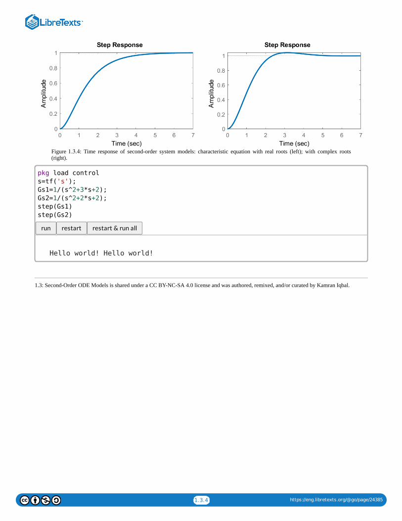
Figure : Time response of second-order system models: characteristic equation with real roots (left); with complex roots(right).

run restart restart & run all

1.3: Second-Order ODE Models is shared under a CC BY-NC-SA 4.0 license and was authored, remixed, and/or curated by Kamran Iqbal.

1.3.4

Hello world! Hello world!

pkg load control

s=tf('s');

Gs1=1/(s^2+3*s+2);

Gs2=1/(s^2+2*s+2);

step(Gs1)

step(Gs2)

1.4.1 https://eng.libretexts.org/@go/page/24388

1.4: An Electro-Mechanical System Model

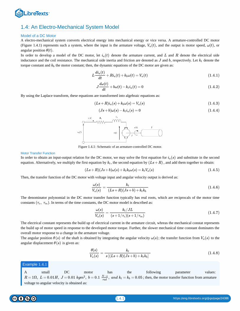
Model of a DC MotorA electro-mechanical system converts electrical energy into mechanical energy or vice versa. A armature-controlled DC motor(Figure 1.4.1) represents such a system, where the input is the armature voltage, , and the output is motor speed, , orangular position .In order to develop a model of the DC motor, let denote the armature current, and and denote the electrical sideinductance and the coil resistance. The mechanical side inertia and friction are denoted as and , respectively. Let denote thetorque constant and the motor constant; then, the dynamic equations of the DC motor are given as:

By using the Laplace transform, these equations are transformed into algebraic equations as:

Figure : Schematic of an armature-controlled DC motor.

Motor Transfer FunctionIn order to obtain an input-output relation for the DC motor, we may solve the first equation for and substitute in the secondequation. Alternatively, we multiply the first equation by , the second equation by , and add them together to obtain:

Then, the transfer function of the DC motor with voltage input and angular velocity output is derived as:

The denominator polynomial in the DC motor transfer function typically has real roots, which are reciprocals of the motor timeconstants . In terms of the time constants, the DC motor model is described as:

The electrical constant represents the build up of electrical current in the armature circuit, whreas the mechanical constat representsthe build up of motor speed in response to the developed motor torque. Further, the slower mechanical time constant dominates theoverall motor response to a change in the armature voltage.The angular position of the shaft is obtained by integrating the angular velocity ; the transfer function from to theangular displacement is given as:

A small DC motor has the following parameter values: ; then, the motor transfer function from armature

voltage to angular velocity is obtained as:

(t)Va ω(t)

θ(t)

(t)ia L R

J b ktkb

L +R (t) + ω(t) = (t)d (t)ia

dtia kb Va (1.4.1)

J +bω(t) − (t) = 0dω(t)

dtktia (1.4.2)

(Ls+R) (s) + ω(s) = (s)ia kb Va (1.4.3)

(Js+b)ω(s) − (s) = 0ktia (1.4.4)

1.4.1

(s)iakt (Ls+R)

(Ls+R)(Js+b)ω(s) + ω(s) = (s)ktkb ktVa (1.4.5)

=ω(s)

(s)Va

kt

(Ls+R)(Js+b) +ktkb(1.4.6)

( , )τe τm

=ω(s)

(s)Va

/JLkt

(s+1/ )(s+1/ )τe τm(1.4.7)

θ (s) ω(s) (s)Vaθ (s)

=θ(s)

(s)Va

kt

s [(Ls+R)(Js+b) + ]ktkb(1.4.8)

Example 1.4.1

R = 1Ω, L = 0.01H, J = 0.01 kg , b = 0.1 , and = = 0.05m2 N−s

radkt kb

1.4.2 https://eng.libretexts.org/@go/page/24388

The two motor time constants are given as: , where matches the time constant of an RL circuit () and matches the time constant of inertial mass in the presence of friction ( ).

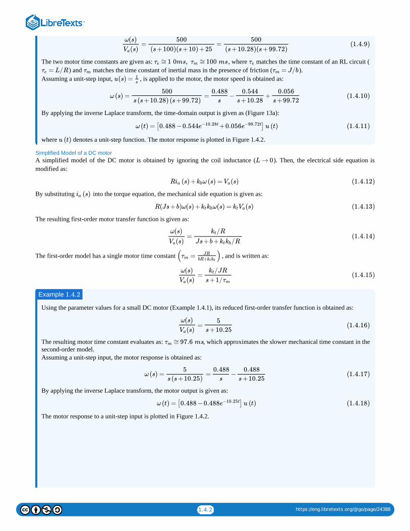
Assuming a unit-step input, , is applied to the motor, the motor speed is obtained as:

By applying the inverse Laplace transform, the time-domain output is given as (Figure 13a):

where denotes a unit-step function. The motor response is plotted in Figure 1.4.2.

Simplified Model of a DC motor A simplified model of the DC motor is obtained by ignoring the coil inductance ( ). Then, the electrical side equation ismodified as:

By substituting into the torque equation, the mechanical side equation is given as:

The resulting first-order motor transfer function is given as:

The first-order model has a single motor time constant , and is written as:

Using the parameter values for a small DC motor (Example 1.4.1), its reduced first-order transfer function is obtained as:

The resulting motor time constant evaluates as: , which approximates the slower mechanical time constant in thesecond-order model.Assuming a unit-step input, the motor response is obtained as:

By applying the inverse Laplace transform, the motor output is given as:

The motor response to a unit-step input is plotted in Figure 1.4.2.

= =ω(s)

(s)Va

500

(s+100)(s+10) +25

500

(s+10.28)(s+99.72)(1.4.9)

≅1 0ms, ≅100 msτe τm τe= L/Rτe τm = J/bτm

u(s) = 1s

ω (s) = = − +500

s (s+10.28) (s+99.72)

0.488

s

0.544

s+10.28

0.056

s+99.72(1.4.10)

ω (t) = [0.488 −0.544 +0.056 ] u (t)e−10.28t e−99.72t (1.4.11)

u (t)

L → 0

R (s) + ω (s) = (s)ia kb Va (1.4.12)

(s)ia

R(Js+b)ω(s) + ω(s) = (s)ktkb ktVa (1.4.13)

=ω(s)

(s)Va

/Rkt

Js+b+ /Rktkb(1.4.14)

( = )τmJR

bR+ktkb

=ω(s)

(s)Va

/JRkt

s+1/τm(1.4.15)

Example 1.4.2

=ω(s)

(s)Va

5

s+10.25(1.4.16)

≅97.6 msτm

ω (s) = = −5

s (s+10.25)

0.488

s

0.488

s+10.25(1.4.17)

ω (t) = [0.488 −0.488 ] u (t)e−10.25t (1.4.18)

1.4.3 https://eng.libretexts.org/@go/page/24388

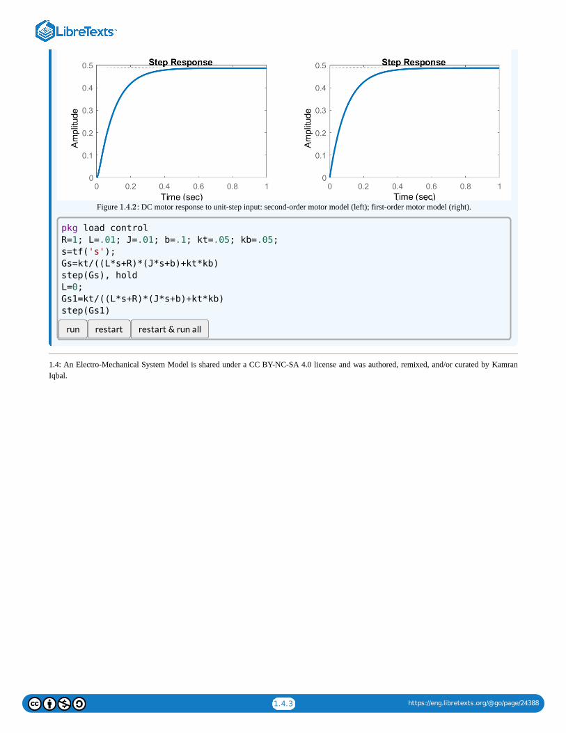
Figure : DC motor response to unit-step input: second-order motor model (left); first-order motor model (right).

run restart restart & run all

1.4: An Electro-Mechanical System Model is shared under a CC BY-NC-SA 4.0 license and was authored, remixed, and/or curated by KamranIqbal.

1.4.2

pkg load control

R=1; L=.01; J=.01; b=.1; kt=.05; kb=.05;

s=tf('s');

Gs=kt/((L*s+R)*(J*s+b)+kt*kb)

step(Gs), hold

L=0;

Gs1=kt/((L*s+R)*(J*s+b)+kt*kb)

step(Gs1)

1.5.1 https://eng.libretexts.org/@go/page/24389

1.5: Industrial Process Models

Industrial Process Models Industrial processes comprise exchange of chemical, electrical or mechanical energy in the manufacturing of industrial products.An industrial process model in its simplified form is represented by a first-order lag with a dead-time that represents the time delaybetween the application of input and the appearance of the process output.Let represent the time constant associated with an industrial process, represent the dead-time, and represent the process dcgain; then, simplified industrial process dynamics are represented by the following delay-differential equation:

Application of the Laplace transform produces the following first-order-plus-dead-time (FOPDT) model of an industrial process:

where the process parameters , can be identified from the process response to inputs. An rational process model isobtained by using a Taylor series approximation of the delay term, . Typical such approximations include:

The last expression is termed as first-order Pade’ approximation and is often preferred. Higher order approximations can also beused.

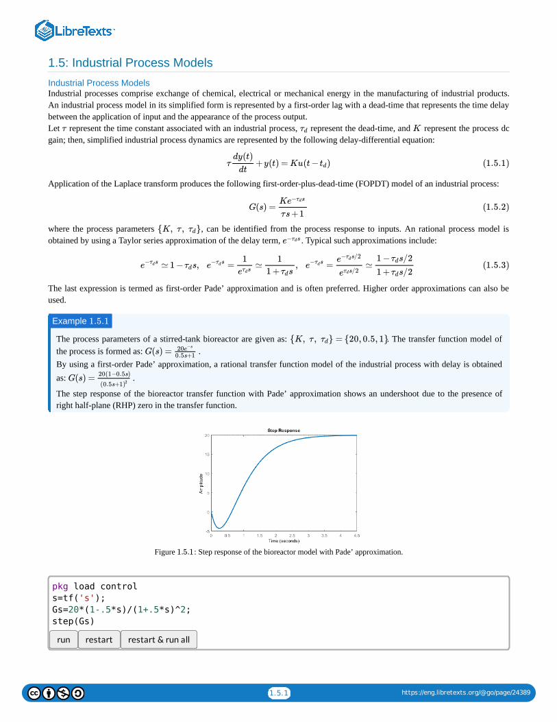
The process parameters of a stirred-tank bioreactor are given as: . The transfer function model ofthe process is formed as: .By using a first-order Pade’ approximation, a rational transfer function model of the industrial process with delay is obtainedas: .

The step response of the bioreactor transfer function with Pade’ approximation shows an undershoot due to the presence ofright half-plane (RHP) zero in the transfer function.

Figure : Step response of the bioreactor model with Pade’ approximation.

run restart restart & run all

τ τd K

τ +y(t) = Ku(t− )dy(t)

dttd (1.5.1)

G(s) =Ke− sτd

τs+1(1.5.2)

{K, τ , }τde− sτd

≃ 1 − s,     = ≃ ,     = ≃e− sτd τd e− sτd1

e sτd

1

1 + sτde− sτd

e− s/2τd

e s/2τd

1 − s/2τd

1 + s/2τd(1.5.3)

Example 1.5.1

{K, τ , } = {20, 0.5, 1}τd

G(s) = 20e−s

0.5s+1

G(s) =20(1−0.5s)

(0.5s+1)2

1.5.1

pkg load control

s=tf('s');

Gs=20*(1-.5*s)/(1+.5*s)^2;

step(Gs)

1.5.2 https://eng.libretexts.org/@go/page/24389

1.5: Industrial Process Models is shared under a CC BY-NC-SA 4.0 license and was authored, remixed, and/or curated by Kamran Iqbal.

1.6.1 https://eng.libretexts.org/@go/page/24390

1.6: State Variable Models

State Variable Models

State variable models are time-domain models that express system behavior as time derivatives of state variables, i.e., the variablesto express the process state. The state variables are typically selected as the natural variables associated with the energy storageelements in the process, but alternate variables can also be used. The state equations of the system describe the time derivatives ofthe state variables. When the state equations are linear, they are expressed in a vector-matrix form.

In the case of electrical networks, capacitor voltages and inductor currents serve as natural state variables. In the case of mechanicalsystems, positions and velocities of inertial masses serve as natural state variables. In thermal systems, heat flow is a natural statevariable. In hydraulic systems, the head (height of the liquid in the reservoir) is a natural state variable.

The number of state variables determines the system order, however, the choice of state variables for a system model is not unique.For example, in a mechanical system model, position and momentum can serve as state variables in place of position and velocity.

A series RLC circuit driven by a constant voltage source contains two energy storage elements, an inductor and a capacitor.Accordingly, let the inductor current, , and the capacitor voltage, , serve as state variables. Then, the circuit behavioris represented by the following equations:

In vector-matrix form, the state equations are represented as:

Let denote the circuit output; then, the output equation is formed as:

The dynamic equation of the mass–spring–damper system is given as:

Let the position, , and velocity, serve as the state variables, and let represent the output; then, the stateand output equations for the model are given as:

The dynamic equations for the DC motor are given as:

Example 1.6.1

i(t) (t)vc

C = i, L = − −Ridvc

dt

di

dtVs vc (1.6.1)

[ ] = [ ][ ]+[ ]d

dt

vc

i

0

−1/L

1/C

−R/L

vc

i

0

1/LVs (1.6.2)

vc

= [ ] [ ]vc 1 0vc

i(1.6.3)

Example 1.6.2

m +b +kx(t) = f(t)x(t)d2

dt2

dx(t)

dt(1.6.4)

x(t) v(t) = (t)x x(t)

[ ] = [ ][ ]+[ ] fd

dt

x

v

0

−k/m

1

−b/m

x

v

0

1/m(1.6.5)

x = [ ] [ ]1 0x

v(1.6.6)

Example 1.6.3

L +R (t) + ω(t) = (t)d (t)ia

dtia kb Va (1.6.7)

J +bω(t) − (t) = 0dω(t)

dtktia (1.6.8)

1.6.2 https://eng.libretexts.org/@go/page/24390

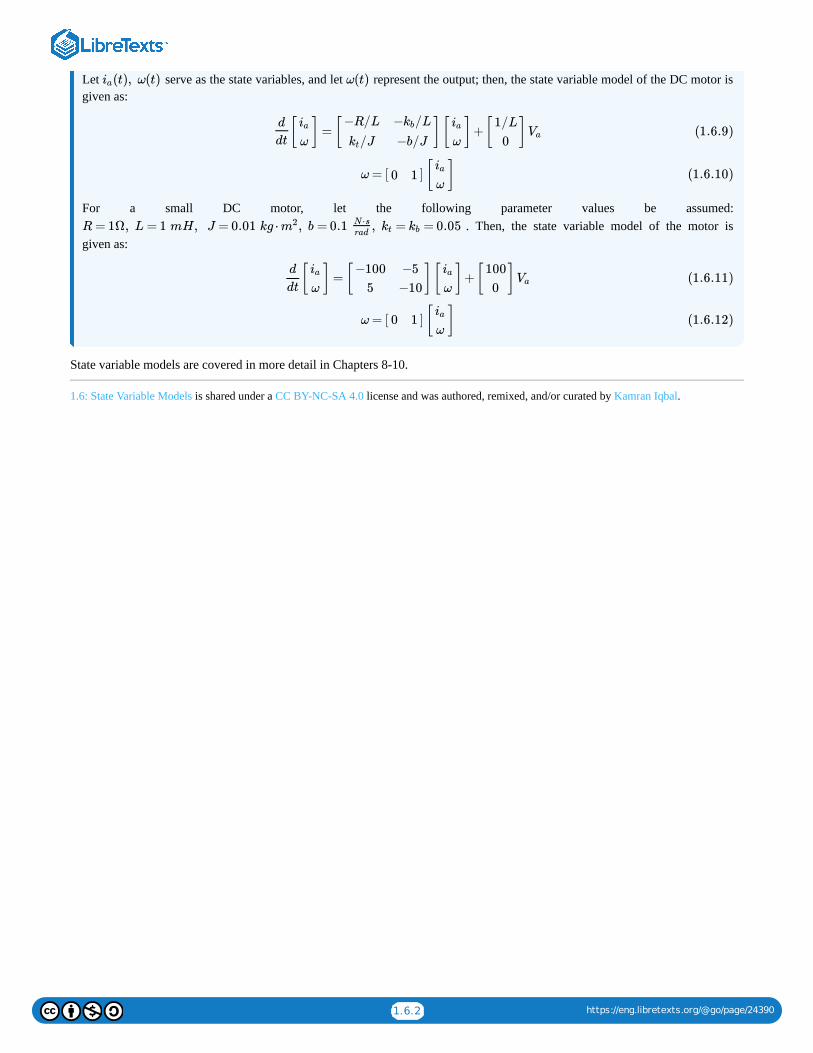
Let serve as the state variables, and let represent the output; then, the state variable model of the DC motor isgiven as:

For a small DC motor, let the following parameter values be assumed:. Then, the state variable model of the motor is

given as:

State variable models are covered in more detail in Chapters 8-10.

1.6: State Variable Models is shared under a CC BY-NC-SA 4.0 license and was authored, remixed, and/or curated by Kamran Iqbal.

(t), ω(t)ia ω(t)

[ ] = [ ][ ]+[ ]d

dt

ia

ω

−R/L

/Jkt

− /Lkb

−b/J

ia

ω

1/L

0Va (1.6.9)

ω = [ ] [ ]0 1ia

ω(1.6.10)

R = 1Ω, L = 1 mH, J = 0.01 kg ⋅ , b = 0.1 , = = 0.05m2 N ⋅srad

kt kb

[ ] = [ ][ ]+[ ]d

dt

ia

ω

−100

5

−5

−10

ia

ω

100

0Va (1.6.11)

ω = [ ] [ ]0 1ia

ω(1.6.12)

1.7.1 https://eng.libretexts.org/@go/page/24391

1.7: Linearization of Nonlinear Models

Linearization of Nonlinear Functions

The behavior of a nonlinear system, described by , in the vicinity of a given operating point, , can be approximatedby plotting a tangent line to the graph of at that point.

Analytically, linearization of a nonlinear function involves first-order Taylor series expansion about the operative point.

Let represent the variation from the operating point; then the Taylor series of a function of single variable is writtenas:

The resulting first order model is described by:

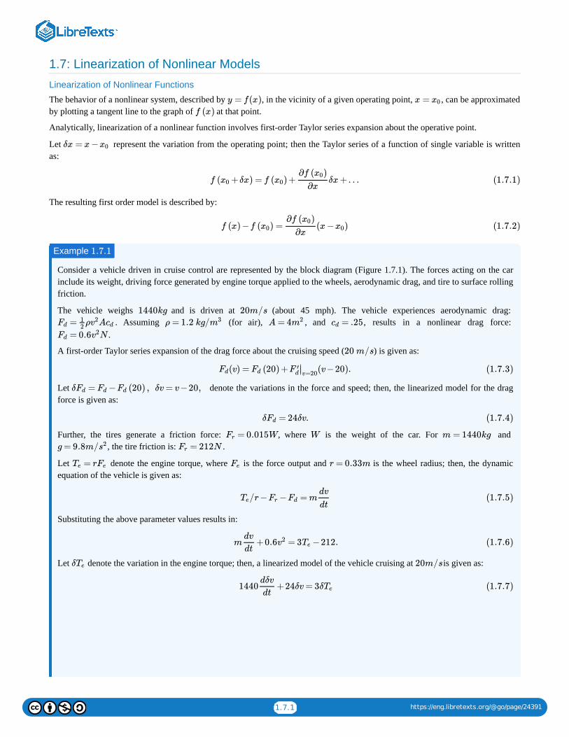
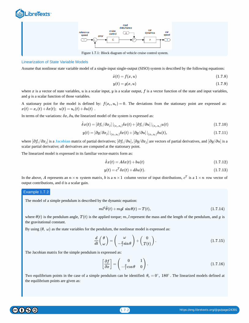
Consider a vehicle driven in cruise control are represented by the block diagram (Figure 1.7.1). The forces acting on the carinclude its weight, driving force generated by engine torque applied to the wheels, aerodynamic drag, and tire to surface rollingfriction.

The vehicle weighs and is driven at (about 45 mph). The vehicle experiences aerodynamic drag: . Assuming (for air), , and , results in a nonlinear drag force:

.

A first-order Taylor series expansion of the drag force about the cruising speed ( ) is given as:

Let denote the variations in the force and speed; then, the linearized model for the dragforce is given as:

Further, the tires generate a friction force: , where is the weight of the car. For and , the tire friction is: .

Let denote the engine torque, where is the force output and is the wheel radius; then, the dynamicequation of the vehicle is given as:

Substituting the above parameter values results in:

Let denote the variation in the engine torque; then, a linearized model of the vehicle cruising at is given as:

y = f(x) x = x0

f (x)

δx = x−x0

f ( +δx) = f ( ) + δx+…x0 x0

∂f ( )x0

∂x(1.7.1)

f (x) −f ( ) = (x− )x0

∂f ( )x0

∂xx0 (1.7.2)

Example 1.7.1

1440kg 20m/s

= ρ AFd12

v2 cd ρ = 1.2 kg/m3 A = 4m2 = .25cd

= 0.6 NFd v2

20 m/s

(v) = (20) + (v−20).Fd Fd F ′d∣∣v=20

(1.7.3)

δ = − (20) ,   δv= v−20,Fd Fd Fd

δ = 24δv.Fd (1.7.4)

= 0.015WFr W m = 1440kg

g = 9.8m/s2 = 212NFr

= rTe Fe Fe r = 0.33m

/r− − = mTe Fr Fd

dv

dt(1.7.5)

m +0.6 = 3 −212.dv

dtv2 Te (1.7.6)

δTe 20m/s

1440 +24δv= 3δdδv

dtTe (1.7.7)

1.7.2 https://eng.libretexts.org/@go/page/24391

Figure : Block diagram of vehicle cruise control system.

Linearization of State Variable Models

Assume that nonlinear state variable model of a single-input single-output (SISO) system is described by the following equations:

where is a vector of state variables, is a scalar input, is a scalar output, is a vector function of the state and input variables,and is a scalar function of those variables.

A stationary point for the model is defined by: . The deviations from the stationary point are expressed as: .

In terms of the variations: , the linearized model of the system is expressed as:

where is a Jacobian matrix of partial derivatives; are vectors of partial derivatives, and is ascalar partial derivative; all derivatives are computed at the stationary point.

The linearized model is expressed in its familiar vector-matrix form as:

In the above, represents an system matrix, is a column vector of input distributions, is a row vector ofoutput contributions, and d is a scalar gain.

The model of a simple pendulum is described by the dynamic equation:

where is the pendulum angle, is the applied torque; represent the mass and the length of the pendulum, and isthe gravitational constant.

By using as the state variables for the pendulum, the nonlinear model is expressed as:

The Jacobian matrix for the simple pendulum is expressed as:

Two equilibrium points in the case of a simple pendulum can be identified: . The linearized models defined atthe equilibrium points are given as:

1.7.1

(t) = f(x, u)x (1.7.8)

y(t) = g(x, u) (1.7.9)

x u y f

g

f( , ) = 0xe uex(t) = (t) +δx(t); u(t) = (t) +δu(t)xe ue

δx, δu

x(t) = [∂ /∂ ] δx(t) +[∂ /∂u] u(t)δ fi xj |( , )xe uefi |( , )xe ue

(1.7.10)

y(t) = [∂g/∂ ] δx(t) +[∂g/∂u] δu(t),xj |( , )xe ue|( , )xe ue

(1.7.11)

[∂ /∂ ]fi xj [∂ /∂u], [∂g/∂ ]fi xj [∂g/∂u]

x(t) = Aδx(t) +bu(t)δ (1.7.12)

y(t) = δx(t) +dδu(t).cT (1.7.13)

A n×n b n×1 cT 1 ×n

Example 1.7.2

m (t) +mgl sinθ(t) = T (t),l2 θ (1.7.14)

θ(t) T (t) m, l g

(θ, ω)

( ) =( )+( ) .d

dt

θ

ω

ω

− sinθg

l

0

T (t)(1.7.15)

[ ] =( ) .∂f

∂x

0

− cosθg

l

1

0(1.7.16)

= ,θe 0∘ 180∘

1.7.3 https://eng.libretexts.org/@go/page/24391

The output equation in both cases is given as: .

1.7: Linearization of Nonlinear Models is shared under a CC BY-NC-SA 4.0 license and was authored, remixed, and/or curated by Kamran Iqbal.

= 0 : [ ] = [ ] [ ]+[ ]Tθe∘ d

dt

θ

ω

0

−g

l

1

0

θ

ω

0

1(1.7.17)

= 180 : [ ] = [ ] [ ]+[ ]Tθe∘ d

dt

θ

ω

0g

l

1

0

θ

ω

0

1(1.7.18)

θ (t) = [ ] [ ]1 0θ

ω

1 https://eng.libretexts.org/@go/page/24384

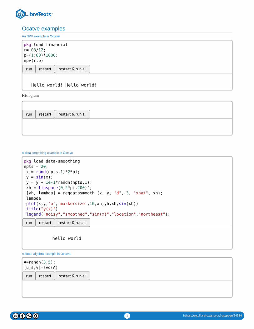
Ocatve examplesAn NPV example in Octave

run restart restart & run all

Histogram

run restart restart & run all

A data smoothing example in Octave

run restart restart & run all

A linear algebra example in Octave

run restart restart & run all

Hello world! Hello world!

 

hello world

 

pkg load financial

r=.03/12;

p=(1:60)*1000;

npv(r,p)

pkg load data-smoothing

npts = 20;

x = rand(npts,1)*2*pi;

y = sin(x);

y = y + 1e-1*randn(npts,1);

xh = linspace(0,2*pi,200)';

[yh, lambda] = regdatasmooth (x, y, "d", 3, "xhat", xh);

lambda

plot(x,y,'o','markersize',10,xh,yh,xh,sin(xh))

title("y(x)")

legend("noisy","smoothed","sin(x)","location","northeast");

A=randn(3,5);

[u,s,v]=svd(A)

2 https://eng.libretexts.org/@go/page/24384

Ocatve examples is shared under a CC BY-NC-SA 4.0 license and was authored, remixed, and/or curated by Kamran Iqbal.

1 https://eng.libretexts.org/@go/page/24386

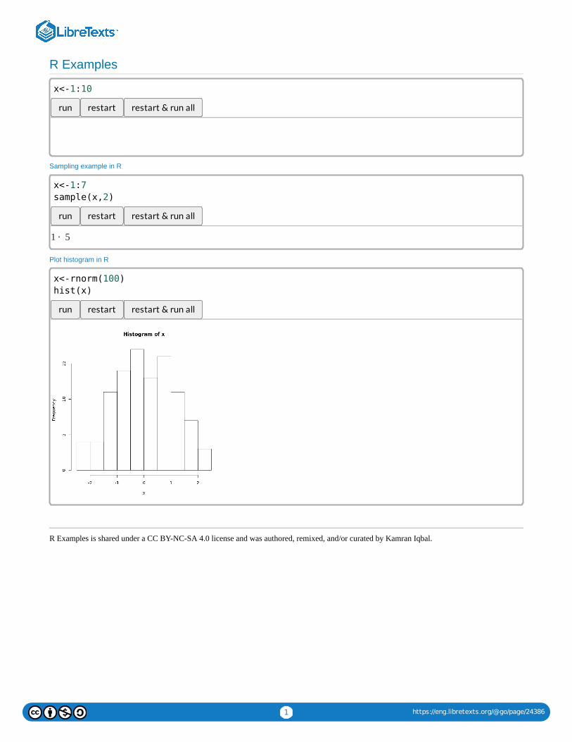
R Examples

run restart restart & run all

Sampling example in R

run restart restart & run all

Plot histogram in R

run restart restart & run all

R Examples is shared under a CC BY-NC-SA 4.0 license and was authored, remixed, and/or curated by Kamran Iqbal.

 

1 · 5

x<-1:10

x<-1:7

sample(x,2)

x<-rnorm(100)

hist(x)

1 https://eng.libretexts.org/@go/page/24387

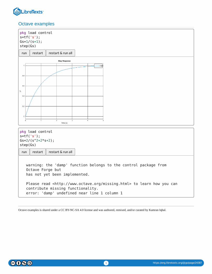
Octave examples

run restart restart & run all

run restart restart & run all

Octave examples is shared under a CC BY-NC-SA 4.0 license and was authored, remixed, and/or curated by Kamran Iqbal.

warning: the 'damp' function belongs to the control package from

Octave Forge but

has not yet been implemented.

Please read <http://www.octave.org/missing.html> to learn how you can

contribute missing functionality.

error: 'damp' undefined near line 1 column 1

pkg load control

s=tf('s');

Gs=1/(s+1);

step(Gs)

pkg load control

s=tf('s');

Gs=2/(s^2+2*s+2);

step(Gs)

1

CHAPTER OVERVIEW

2: Transfer Function Models

1. Analyze transfer function models of dynamic systems.2. Characterize the natural response of the system model.3. Characterize the stability of the system model.4. Obtain system response to step, impulse, and sinusoidal inputs.5. Visualize the frequency response of the system.

2.0: Prelude to Transfer Function Models2.1: System Poles and Zeros2.2: System Natural Response2.3: System Stability2.4: The Step Response2.5: Sinusoidal Response of a SystemBlank

2: Transfer Function Models is shared under a CC BY-NC-SA 4.0 license and was authored, remixed, and/or curated by Kamran Iqbal.

Learning Objectives

2.0.1 https://eng.libretexts.org/@go/page/24452

2.0: Prelude to Transfer Function ModelsThis chapter analyzes the transfer function models of physical systems developed in Chapter 1. The transfer function is obtained bythe application of Laplace transform to the linear differential equation description of the system. The transfer function, denoted by

, is a rational function of a complex frequency variable, . Given the transfer function and an input, , the response of thesystem can be computed as:

The transfer function is a ratio of two polynomials is s. The zeros of the transfer function, i.e., those frequencies that elicit zerosystem response, are represented by the roots of numerator polynomial. The poles of the transfer function, i.e., those frequencieswhere the system response is undefined, are represented by the roots of denominator polynomial.

The system impulse response, i.e., its response to a unit-impulse input, contains the natural modes of system response. The naturalresponse includes terms of the form , where is a pole of the transfer function. The natural response of a stable system dies outwith time.

The system step response, i.e., its response to a unit-step input, comprises both natural and forced responses, where the forcedresponse is a constant value. Once system's natural response dies out, the output reaches a steady-state. The dc gain of the systemdenotes its gain to a constant input.

System stability refers to the system being well-behaved and predictable under various operating conditions. The bounded-inputbounded-output (BIBO) stability refers to the system response staying finite to every finite input, i.e., if

. The BIBO stability requires that the poles of the system transfer function are located in the open left-half of thecomplex -plane.

The frequency response function of a system, obtained by substituting in the transfer function, characterizes its response tosinusoidal inputs in the steady-state, which is a sinusoid at the input frequency. Further, the magnitude of the response is scaled bythe gain of the system transfer function evaluated at the input frequency, and it has a phase contribution from the system transferfunction. The frequency response function can be visualized on a Bode plot.

2.0: Prelude to Transfer Function Models is shared under a CC BY-NC-SA 4.0 license and was authored, remixed, and/or curated by LibreTexts.

G(s) s u (s)

y (s) = G(s) u (s) . (2.0.1)

e tpi pi

|y(t)| < N < ∞

|u(t)| < M < ∞

s

s = jω

2.1.1 https://eng.libretexts.org/@go/page/24393

2.1: System Poles and Zeros

System Poles and Zeros

The transfer function, , is a rational function in the Laplace transform variable, . It is expressed as the ratio of the numerator

and the denominator polynomials, i.e., .

The roots of the numerator polynomial, , define system zeros, i.e., those frequencies at which the system response is zero.Thus, is a zero of the transfer function if

The roots of the denominator polynomial, , define system poles, i.e., those frequencies at which the system response isinfinite. Thus, is a pole of the transfer function if

The poles and zeros of first and second-order system models are described below.

First-Order System

A first-order system has a generic ODE description: , where and denote the input and the output,and is the system time constant. By applying the Laplace transform, a first-order transfer function is obtained as:

The transfer function has no finite zeros and a single pole located at in the complex plane.

The reduced-order model of a DC motor with voltage input and angular velocity output (Example 1.4.3) is described by thedifferential equation: .

The DC motor has a transfer function: where is the motor time constant.

For the following parameter values: , the motortransfer function evaluates as:

The transfer function has a single pole located at: with associated time constant of .

Second-Order System with an Integrator

A first-order system with an integrator is described by the transfer function:

The system has no finite zeros and has two poles located at and in the complex plane.

The DC motor modeled in Example 2.1.1 above is used in a position control system where the objective is to maintain a certainshaft angle . The motor equation is given as: ; its transfer function is given as: .

Using the above parameter values in the reduced-order DC motor model, the system transfer function is given as:

G(s) s

G(s) =n(s)

d(s)

Definition: Transfer Function Zeros

n(s)z0 G( ) = 0.z0

Definition: Transfer Function Poles

d(s)p0 G( ) = ∞.p0

τ (t) +y (t) = u(t)y u (t) y (t)τ

G(s) =K

τs+1(2.1.1)

s = − 1τ

Example 2.1.1

τ (t) +ω(t) = (t)ω Va

G(s) = K

s+1τmτm

R = 1Ω, L = 0.01H, J = 0.01 kg , b = 0.1 , and = = 0.05m2 N−s

radkt kb

G(s) = = =ω(s)

(s)Va

5

s+10.25

0.49

0.098s+1(2.1.2)

s = −10.25 0.098sec

G(s) =K

s(τs+1)(2.1.3)

s = 0 s = − 1τ

Example 2.1.2

θ(t) τ (t) + (t) = (t)θ θ Va G(s) = K

s(τs+1)

G(s) = = =θ(s)

(s)Va

5

s(s+10.25)

0.49

s(0.098s+1)(2.1.4)

2.1.2 https://eng.libretexts.org/@go/page/24393

The transfer function has no finite zeros and poles are located at: .

Second-Order System with Real Poles

A second-order system with poles located at is described by the transfer function:

From Section 1.4, the DC motor transfer function is described as:

Then, system poles are located at: and , where and represent the electrical and mechanical timeconstants of the motor.

For the following parameter values: , thetransfer function from armature voltage to angular velocity is given as:

The transfer function poles are located at: .

The motor time constants are given as: .

Second-Order System with Complex Poles

A second-order model with its complex poles located at: is described by the transfer function:

Equivalently, the second-order transfer function with complex poles is expressed in terms of the damping ratio, , and the naturalfrequency, , of the complex poles as:

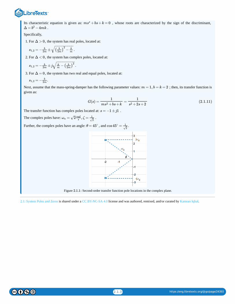
The transfer function poles are located at: , where (Figure 2.1.1).

As seen from the figure, equals the magnitude of the complex pole, and , where is the angle subtended by thecomplex pole at the origin.

The damping ratio, , is a dimensionless quantity that characterizes the decay of the oscillations in the system’s natural response.The damping ratio is bounded as: .

1. As , the complex poles are located close to the imaginary axis at: . The resulting impulse response displayspersistent oscillations at system’s natural frequency, .

2. As , the complex poles are located close to the real axis as . The resulting impulse response has nooscillations and exponentially decays to zero resembling the response of a first-order system.

A spring–mass–damper system has a transfer function:

s = 0, −10.25

s = − ,   −σ1 σ2

G(s) =1

(s+ ) (s+ )σ1 σ2(2.1.5)

Example 2.1.3

G(s) =K

(s+1/ )(s+1/ )τe τm(2.1.6)

= −s11τm

= −s21τe

τe τm

R = 1Ω, L = 0.01H, J = 0.01 kg , b = 0.1 , and = = 0.05m2 N−s

radkt kb

= =ω(s)

(s)Va

500

(s+100)(s+10) +25

500

(s+10.28)(s+99.72)(2.1.7)

s = −10.28, −99.72

≅ = 10 ms, ≅ = 100 msτeL

Rτm

J

b

s = −σ±jω

G(s) = .K

+(s+σ)2 ω2(2.1.8)

ζ

ωn

G(s) =K

(s+ζ + (1 − )ωn)2 ω2n ζ2

(2.1.9)

= −ζ ±js1,2 ωn ωd =ωd ωn 1 −ζ2− −−−−

√

ωn ζ = = cosθσ

ωnθ

ζ

0 < ζ < 1

ζ → 0 s ≅±jωn

ωn

ζ → 1 ≅−ζs1,2 ωn

Example 2.1.4

G(s) = .1

m +bs+ks2(2.1.10)

2.1.3 https://eng.libretexts.org/@go/page/24393

Its characteristic equation is given as: , whose roots are characterized by the sign of the discriminant, .

Specifically,

1. For the system has real poles, located at:

2. For the system has complex poles, located at:

3. For , the system has two real and equal poles, located at:

Next, assume that the mass-spring-damper has the following parameter values: ; then, its transfer function isgiven as:

The transfer function has complex poles located at: .

The complex poles have: .

Further, the complex poles have an angle: , and .

Figure : Second-order transfer function pole locations in the complex plane.

2.1: System Poles and Zeros is shared under a CC BY-NC-SA 4.0 license and was authored, remixed, and/or curated by Kamran Iqbal.

m +bs+k = 0ss

Δ = −4mkb2

Δ > 0,

= − ± .s1,2b

2m−( )b

2m

2 k

m

− −−−−−−−−√

Δ < 0,

= − ±j .s1,2b

2m−k

m( )b

2m

2− −−−−−−−−

√

Δ = 0

= − .s1,2b

2m

m = 1, b = k = 2

G(s) = =1

m +bs+ks2

1

+2s+2s2(2.1.11)

s = −1 ±j1

= , ζ =ωn 2–

√ rads

12√

θ = 45∘ cos =45∘ 12√

2.1.1

2.2.1 https://eng.libretexts.org/@go/page/24394

2.2: System Natural Response

System Natural ResponseThe transfer function of a dynamic linear time-invariant (LTI) system is given as a ratio of polynomials: . The poles ofthe transfer function are the roots of the denominator polynomial .The poles of the transfer function characterize the natural response modes of the system. Thus, if is a pole of the transferfunction, , then constitutes a natural response mode.

A real pole: , contributes a term to system natural response.A pair of complex poles: , contributes oscillatory terms of the form to thenatural response.

The natural response of the system is a weighted sum of the natural response modes, i.e., . Further, the naturalresponse is reflected in the impulse response of a system.

The impulse response of a system, represented by , is defined as system response to a unit-impulse input, , when theinitial conditions are zero.

Let ; then, the impulse response is computed as: ; in the time-domain, the impulse response isgiven as: .To proceed further, let the system transfer function be represented in the factored form as:

where is the numerator polynomial, and , are the system poles, assumed to be distinct and may include a singlepole at the origin. Using partial fraction expansion (PFE), the impulse response is given as:

Using the inverse Laplace transform, the impulse response of the system is computed as:

where represents the unit-step function, used here to indicate that the expression for is valid for .

Impulse Response of Low Order Systems

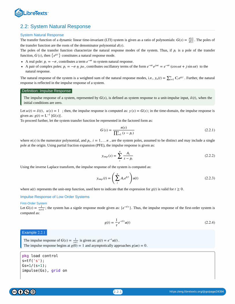
First-Order System Let ; the system has a signle response mode given as: . Thus, the impulse response of the first-order system iscomputed as:

The impulse response of is given as: .The impulse response begins at and asymptotically approaches .

𝐺(𝑠) =𝑛(𝑠)

𝑑(𝑠)

𝑑(𝑠)

𝑝𝑖

𝐺 (𝑠) { }𝑒 𝑡𝑝𝑖= −𝜎𝑝𝑖 𝑒−𝜎𝑡

= −𝜎 ± 𝑗𝜔𝑝𝑖 = (cos𝜔𝑡 + 𝑗 sin𝜔𝑡)𝑒−𝜎𝑡𝑒𝑗𝜔𝑡 𝑒−𝜎𝑡

(𝑡) =𝑦𝑛 ∑𝑛𝑖=1 𝐶𝑖𝑒𝑡𝑝𝑖

Definition: Impulse Response

𝐺(𝑠) 𝛿 (𝑡)

𝑢 (𝑡) = 𝛿 (𝑡) ,   𝑢 (𝑠) = 1 𝑦 (𝑠) = 𝐺(𝑠)

𝑔(𝑡) = [𝐺(𝑠)]L−1

𝐺 (𝑠) =𝑛(𝑠)

(𝑠 − )∏𝑛𝑖=1 𝑝𝑖(2.2.1)

𝑛(𝑠) ,  𝑖 = 1,…𝑛𝑝𝑖

(𝑠) =𝑦𝑖𝑚𝑝 ∑𝑖

𝑛𝐴𝑖

𝑠 − 𝑝𝑖(2.2.2)

(𝑡) = ( ) 𝑢(𝑡)𝑦𝑖𝑚𝑝 ∑𝑖

𝑛

𝐴𝑖𝑒𝑡𝑝𝑖 (2.2.3)

𝑢(𝑡) 𝑔(𝑡) 𝑡 ≥ 0

𝐺(𝑠) =1

𝜏𝑠+1{ }𝑒−𝑡/𝜏

𝑔(𝑡) = 𝑢(𝑡)1

𝜏𝑒−𝑡/𝜏

(2.2.4)

Example 2.2.1

𝐺(𝑠) =1

𝑠+1𝑔(𝑡) = 𝑢(𝑡)𝑒−𝑡

𝑔(0) = 1 𝑔(∞) = 0

pkg load control

s=tf('s');

Gs=1/(s+1);

impulse(Gs), grid on

2.2.2 https://eng.libretexts.org/@go/page/24394

run restart restart & run all

The time constant, , describes the time when, starting from unity, the natural response decays to , or 37% of itsinitial value. For a first-order system, with a real pole, , the time constant is given as: .

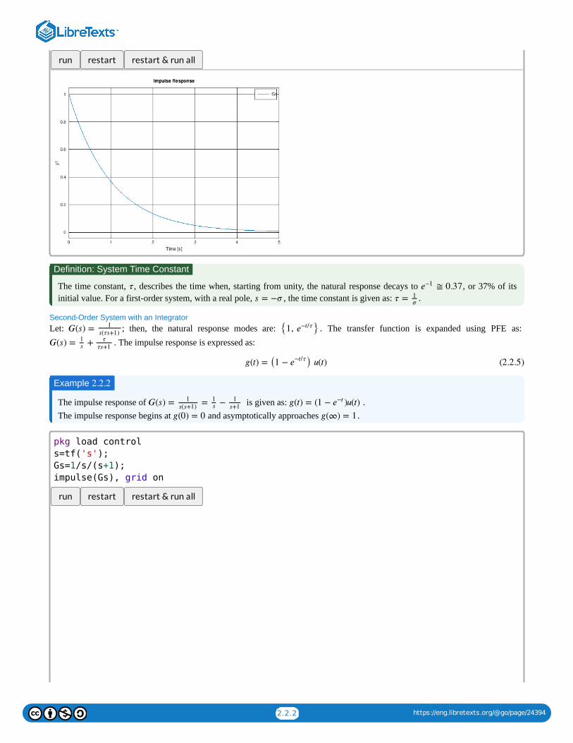
Second-Order System with an Integrator Let: ; then, the natural response modes are: . The transfer function is expanded using PFE as:

. The impulse response is expressed as:

The impulse response of is given as: .The impulse response begins at and asymptotically approaches .

run restart restart & run all

Definition: System Time Constant

𝜏 ≅ 0.37𝑒−1

𝑠 = −𝜎 𝜏 = 1𝜎

𝐺(𝑠) =1

𝑠(𝜏𝑠+1) {1,   }𝑒−𝑡/𝜏

𝐺(𝑠) = +1𝑠

𝜏

𝜏𝑠+1

𝑔(𝑡) = (1 − ) 𝑢(𝑡)𝑒−𝑡/𝜏

(2.2.5)

Example 2.2.2

𝐺(𝑠) = = −1

𝑠(𝑠+1)

1𝑠

1

𝑠+1𝑔(𝑡) = (1 − )𝑢(𝑡)𝑒−𝑡

𝑔(0) = 0 𝑔(∞) = 1

pkg load control

s=tf('s');

Gs=1/s/(s+1);

impulse(Gs), grid on

2.2.3 https://eng.libretexts.org/@go/page/24394

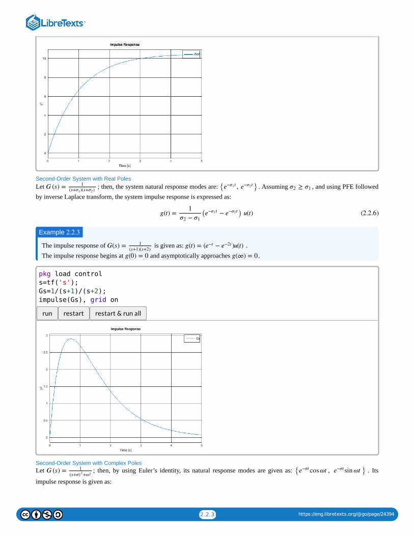
Second-Order System with Real Poles Let ; then, the system natural response modes are: . Assuming , and using PFE followedby inverse Laplace transform, the system impulse response is expressed as:

The impulse response of is given as: .The impulse response begins at and asymptotically approaches .

run restart restart & run all

Second-Order System with Complex Poles Let ; then, by using Euler’s identity, its natural response modes are given as: . Its

impulse response is given as:

𝐺 (𝑠) =1

(𝑠+ )(𝑠+ )𝜎1 𝜎2 { ,   }𝑒− 𝑡𝜎1 𝑒− 𝑡𝜎2 ≥𝜎2 𝜎1

𝑔(𝑡) = ( − ) 𝑢(𝑡)1

−𝜎2 𝜎1𝑒− 𝑡𝜎1 𝑒− 𝑡𝜎2 (2.2.6)

Example 2.2.3

𝐺(𝑠) = 1

(𝑠+1)(𝑠+2)𝑔(𝑡) = ( − )𝑢(𝑡)𝑒−𝑡 𝑒−2𝑡

𝑔(0) = 0 𝑔(∞) = 0

𝐺 (𝑠) = 1

+(𝑠+𝜎)2 𝜔2 { cos𝜔𝑡 ,    sin𝜔𝑡 }𝑒−𝜎𝑡 𝑒−𝜎𝑡

pkg load control

s=tf('s');

Gs=1/(s+1)/(s+2);

impulse(Gs), grid on

2.2.4 https://eng.libretexts.org/@go/page/24394

The oscillatory natural response is contained in the envelope defined by: . The effective time constant of a second-ordersystem is given as: .The natural response is of the form: can be alternatively expressed as:

where and .

The impulse response of is given as:

The impulse response begins at and asymptotically approaches .

run restart restart & run all

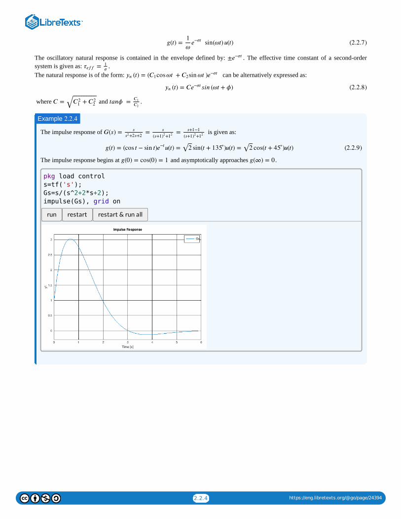
𝑔(𝑡) = sin(𝜔𝑡) 𝑢(𝑡)1

𝜔𝑒−𝜎𝑡

(2.2.7)

±𝑒−𝜎𝑡

=𝜏𝑒𝑓𝑓1𝜎

(𝑡) = ( cos𝜔𝑡  + sin𝜔𝑡 )𝑦𝑛 𝐶1 𝐶2 𝑒−𝜎𝑡

(𝑡) = 𝐶 𝑠𝑖𝑛 (𝜔𝑡 + 𝜙)  𝑦𝑛 𝑒−𝜎𝑡 (2.2.8)

𝐶 = +𝐶21 𝐶22

⎯ ⎯⎯⎯⎯⎯⎯⎯⎯⎯⎯⎯⎯⎯

√ 𝑡𝑎𝑛𝜙  =𝐶1𝐶2

Example 2.2.4

𝐺(𝑠) = = =𝑠

+2𝑠+2𝑠2𝑠

(𝑠+1 +)2 12𝑠+1−1(𝑠+1 +)2 12

𝑔(𝑡) = (cos 𝑡 − sin 𝑡) 𝑢(𝑡) = sin(𝑡 + )𝑢(𝑡) = cos(𝑡 + )𝑢(𝑡)𝑒−𝑡

2⎯⎯

√ 135∘

2⎯⎯

√ 45∘

(2.2.9)

𝑔(0) = cos(0) = 1 𝑔(∞) = 0

pkg load control

s=tf('s');

Gs=s/(s^2+2*s+2);

impulse(Gs), grid on

2.2.5 https://eng.libretexts.org/@go/page/24394

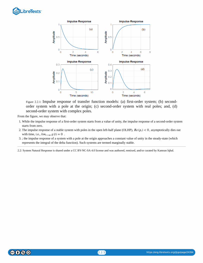
Figure : Impulse response of transfer function models: (a) first-order system; (b) second-order system with a pole at the origin; (c) second-order system with real poles; and, (d)second-order system with complex poles.

From the figure, we may observe that:

1. While the impulse response of a first-order system starts from a value of unity, the impulse response of a second-order systemstarts from zero.

2. The impulse response of a stable system with poles in the open left-half plane (OLHP), , asymptotically dies outwith time, i.e., .

3. ; the impulse response of a system with a pole at the origin approaches a constant value of unity in the steady-state (whichrepresents the integral of the delta function). Such systems are termed marginally stable.

2.2: System Natural Response is shared under a CC BY-NC-SA 4.0 license and was authored, remixed, and/or curated by Kamran Iqbal.

2.2.1

𝑅𝑒 ( ) < 0𝑝𝑖

𝑔 (𝑡) = 0 𝑙𝑖𝑚𝑡→∞

2.3.1 https://eng.libretexts.org/@go/page/24396

2.3: System StabilityStability is a desired characteristic of any dynamic system; it refers to the system being well behaved and in control under variousoperating conditions. Stability may be categorized in multiple ways, some of which are discussed below.

Bounded-Input Bounded-Output Stability (BIBO)

The bounded-input bounded-output (BIBO) stability implies that for every bounded input, the outputof the system stays bounded, that is, .

The output of the system in time-domain is given in terms of the convolution integral:

where is the impulse response of the system. Hence, a necessary condition for BIBO stability is that the impulse response diesout with time, that is, .

The impulse response contains the modes of system natural response and is given as:

where is a pole of the system transfer function. Hence, a necessary condition for BIBO stability is: .

Physically, the condition implies the presence of damping in the system, where the damping terms in the transferfunction indicate dissipation of residual energy with time.

Marginal Stability

The imaginary axis on the complex plane serves as the stability boundary. A system with poles in the open left-half plane (OLHP)is stable.

If the system transfer function has simple poles that are located on the imaginary axis, it is termed as marginally stable. Theimpulse response of such systems does not go to zero as , but stays bounded in the steady-state.

As an example, a simple harmonic oscillator is described by the ODE: , where represents the natural frequencyand the system has no damping. The oscillator transfer function, has simple poles on the -axis.

The natural response of the simple harmonic oscillator contains the response mode: . Its impulseresponse displays persisting oscillations at the natural frequency.

Internal Stability

The notion of internal stability requires that all signals within a control system remain bounded for every bounded input. It furtherimplies that all relevant transfer functions between input–output pairs in a feedback control system are BIBO stable.

Internal stability is a stronger notion than BIBO stability. It is so because the internal modes of system response may include thosemodes not be reflected in the input-output transfer function.

In the case of linear system models involving feedback, the internal stability requirements are met if the closed-loop characteristicpolynomial is stable and any pole-zero cancelations appearing in the loop gains are restricted to the OLHP.

In particular, for a single-input single-output (SISO) feedback control system, the loop gain includes the product of the plant andthe controller transfer functions.

Suppose the plant transfer function is: , and the controller is given as: ; then,

, which includes an OLHP pole-zero cancelation. However, the closed-loop characteristic polynomial:

has stable roots for . Hence, the closed-loop system is internally stable for .

Asymptotic Stability

For a general nonlinear system model, , stability refers to the stability of an equilibrium point defined by: .

u(t) : |u(t)| < < ∞,M1

y(t) : |y(t)| < < ∞M2

y(t) = g(t−τ)u(τ)dτ∫∞

0

(2.3.1)

g(t)

g(t) = 0limt→∞

g(t) =∑i=1

n

Aietpi (2.3.2)

pi Re [ ] < 0pi

Re[ ] < 0pi

t → ∞

+ y = 0y ω2n ωn

G(s) = 1

+s2 ω2n

( = ±j )p1,2 ωn jω

= cos t+jsin tej tωn ωn ωn

G(s) = 1s+1

K(s) = K( )s+1s+10

K(s)G(s) =K(s+1)

(s+1)(s+10)

Δ(s) = s+10 +K K > −10 K > −10

(t) = f (x, u)x ( , )xe uef ( , ) = 0xe ue

2.3.2 https://eng.libretexts.org/@go/page/24396

In particular, the equilibrium point is said to be stable if a system trajectory, , that starts in the vicinity of stays close to .The equilibrium point is said to be asymptotically stable if a system trajectory that starts in the vicinity of converges to .

For linear system models, defined by: , the origin serves as an equilibrium point. In such cases, theasymptotic stability requires that the poles of the system transfer function (equivalently, the eigenvalues of the system matrix) lie inthe open left-half plane, or , and there are no RHP pole-zero cancelations.

2.3: System Stability is shared under a CC BY-NC-SA 4.0 license and was authored, remixed, and/or curated by Kamran Iqbal.

x (t) xe xex (t) xe xe

= Ax(t) +Bu(t)x = 0xe

Re [ ] < 0pi

2.4.1 https://eng.libretexts.org/@go/page/24395

2.4: The Step Response

Step ResponseThe impulse and step inputs are among prototype inputs used to characterize the response of the systems. The unit-step input isdefined as:\[ u(x)=\begin{cases}0, &\;x<0 \\ 1,&\; x\ge 0\end{cases} \]

The step response of a system is defined as its response to a unit-step input, \(u(t)\), or \(u(s)=\frac{1}{s}\).

Let \(G(s)\) describe the system transfer function; then, the unit-step response is obtained as: \(y(s)\, \, =\, \, G(s)\frac{1}{s}\).Its inverse Laplace transform leads to: \(y\left(t\right)={\mathcal{L}}^{-1}\left[\frac{G\left(s\right)}{s}\right]\).Alternatively, the step response can be obtained by integrating the impulse response: \(y(t)=\int_0^t g(t-\tau)d\tau\).The unit-step response of a stable system starts from some initial value: \(y\left(0\right)=y_0\), and settles at a steady-state value: \(y_{\infty }={\lim_{t\to \infty } y\left(t\right)\ }\).Further, from the application of the final value theorem (FVT): \(y_{\infty }=G{\left(s\right)|}_{s=0}\).

Step Response of Low Order SystemsThe unit-step response in the case of the first- and second-order systems is described below.

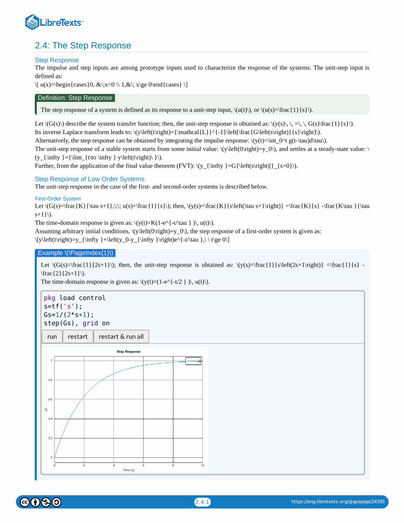
First-Order System Let \(G(s)=\frac{K}{\tau s+1},\;\; u(s)=\frac{1}{s}\); then, \(y(s)=\frac{K}{s\left(\tau s+1\right)} =\frac{K}{s} -\frac{K\tau }{\taus+1}\).The time-domain response is given as: \(y(t)=K(1-e^{-t/\tau } )\, u(t)\).Assuming arbitrary initial conditions, \(y\left(0\right)=y_0\), the step response of a first-order system is given as:\[y\left(t\right)=y_{\infty }+\left(y_0-y_{\infty }\right)e^{-t/\tau },\ \ t\ge 0\]

Let \(G(s)=\frac{1}{2s+1}\); then, the unit-step response is obtained as: \(y(s)=\frac{1}{s\left(2s+1\right)} =\frac{1}{s} -\frac{2}{2s+1}\).The time-domain response is given as: \(y(t)=(1-e^{-t/2 } )\, u(t)\).

run restart restart & run all

Definition: Step Response

Example \(\PageIndex{1}\)

pkg load control

s=tf('s');

Gs=1/(2*s+1);

step(Gs), grid on

2.4.2 https://eng.libretexts.org/@go/page/24395

Figure \(\PageIndex{1}\): Step response of first-order DC motor model.

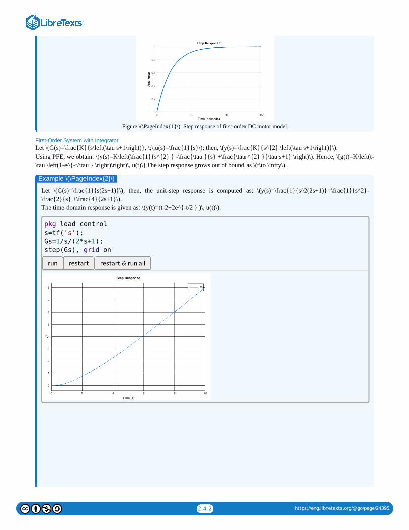
First-Order System with IntegratorLet \(G(s)=\frac{K}{s\left(\tau s+1\right)}, \;\;u(s)=\frac{1}{s}\); then, \(y(s)=\frac{K}{s^{2} \left(\tau s+1\right)}\).Using PFE, we obtain: \(y(s)=K\left(\frac{1}{s^{2} } -\frac{\tau }{s} +\frac{\tau ^{2} }{\tau s+1} \right)\). Hence, \[g(t)=K\left(t-\tau \left(1-e^{-t/\tau } \right)\right)\, u(t)\] The step response grows out of bound as \(t\to \infty\).

Let \(G(s)=\frac{1}{s(2s+1)}\); then, the unit-step response is computed as: \(y(s)=\frac{1}{s^2(2s+1)}=\frac{1}{s^2}-\frac{2}{s} +\frac{4}{2s+1}\).The time-domain response is given as: \(y(t)=(t-2+2e^{-t/2 } )\, u(t)\).

run restart restart & run all

Example \(\PageIndex{2}\)

pkg load control

s=tf('s');

Gs=1/s/(2*s+1);

step(Gs), grid on

2.4.3 https://eng.libretexts.org/@go/page/24395

Figure \(\PageIndex{2}\): Step-response of a second-order model with a pole at the origin.

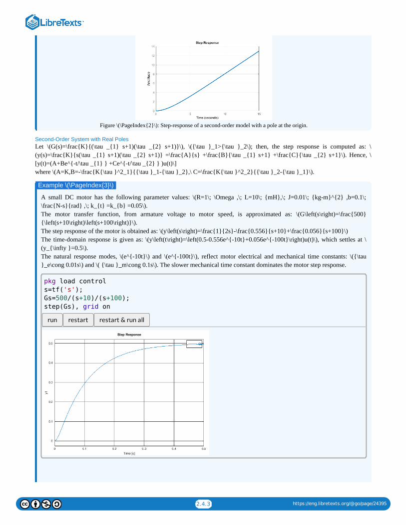
Second-Order System with Real Poles Let \(G(s)=\frac{K}{(\tau _{1} s+1)(\tau _{2} s+1)}\), \({\tau }_1>{\tau }_2\); then, the step response is computed as: \(y(s)=\frac{K}{s(\tau _{1} s+1)(\tau _{2} s+1)} =\frac{A}{s} +\frac{B}{\tau _{1} s+1} +\frac{C}{\tau _{2} s+1}\). Hence, \[y(t)=(A+Be^{-t/\tau _{1} } +Ce^{-t/\tau _{2} } )u(t)\]where \(A=K,B=-\frac{K{\tau }^2_1}{{\tau }_1-{\tau }_2},\ C=\frac{K{\tau }^2_2}{{\tau }_2-{\tau }_1}\).

A small DC motor has the following parameter values: \(R=1\; \Omega ,\; L=10\; {mH},\; J=0.01\; {kg-m}^{2} ,b=0.1\;\frac{N-s}{rad} ,\; k_{t} =k_{b} =0.05\).The motor transfer function, from armature voltage to motor speed, is approximated as: \(G\left(s\right)=\frac{500}{\left(s+10\right)\left(s+100\right)}\).The step response of the motor is obtained as: \(y\left(s\right)=\frac{1}{2s}-\frac{0.556}{s+10}+\frac{0.056}{s+100}\)The time-domain response is given as: \(y\left(t\right)=\left(0.5-0.556e^{-10t}+0.056e^{-100t}\right)u(t)\), which settles at \(y_{\infty }=0.5\).The natural response modes, \(e^{-10t}\) and \(e^{-100t}\), reflect motor electrical and mechanical time constants: \({\tau}_e\cong 0.01s\) and \( {\tau }_m\cong 0.1s\). The slower mechanical time constant dominates the motor step response.

run restart restart & run all

Example \(\PageIndex{3}\)

pkg load control

s=tf('s');

Gs=500/(s+10)/(s+100);

step(Gs), grid on

2.4.4 https://eng.libretexts.org/@go/page/24395

Figure \(\PageIndex{3}\): Step response of DC motor model with real poles.

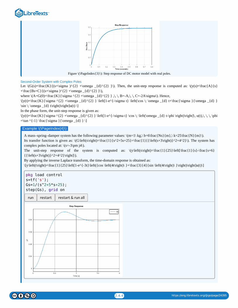
Second-Order System with Complex Poles Let \(G(s)=\frac{K}{(s+\sigma )^{2} +\omega _{d}^{2} }\). Then, the unit-step response is computed as: \(y(s)=\frac{A}{s}+\frac{Bs+C}{(s+\sigma )^{2} +\omega _{d}^{2} }\),where \(A=G(0)=\frac{K}{\sigma ^{2} +\omega _{d}^{2} } ,\, \, B=-A,\, \, C=-2A\sigma\). Hence,\[y(t)=\frac{K}{\sigma ^{2} +\omega _{d}^{2} } \left[1-e^{-\sigma t} \left(\cos \; \omega _{d} t+\frac{\sigma }{\omega _{d} }\sin \; \omega _{d} t\right)\right]u(t) \]In the phase form, the unit-step response is given as:\[y(t)=\frac{K}{\sigma ^{2} +\omega _{d}^{2} } \left[1-e^{-\sigma t} \cos \; \left(\omega _{d} t-\phi \right)\right]\, u(t),\, \, \, \phi=\tan ^{-1} \frac{\sigma }{\omega _{d} } \]

A mass–spring–damper system has the following parameter values: \(m=1\ kg,\ b=6\frac{Ns}{m},\ k=25\frac{N}{m}\).Its transfer function is given as: \(G\left(s\right)=\frac{1}{s^2+5s+25}=\frac{1}{{\left(s+3\right)}^2+4^2}\). The system hascomplex poles located at: \(s=-3\pm j4\).The unit-step response of the system is computed as: \(y\left(s\right)=\frac{1}{25}\left[\frac{1}{s}-\frac{s+6}{{\left(s+3\right)}^2+4^2}\right]\).By applying the inverse Laplace transform, the time-domain response is obtained as:\[y\left(t\right)=\frac{1}{25}\left[1-e^{-3t}\left({cos \left(4t\right)\ }+\frac{3}{4}{sin \left(4t\right)\ }\right)\right]u(t)\]

run restart restart & run all

Example \(\PageIndex{4}\)

pkg load control

s=tf('s');

Gs=1/(s^2+5*s+25);

step(Gs), grid on

2.4.5 https://eng.libretexts.org/@go/page/24395

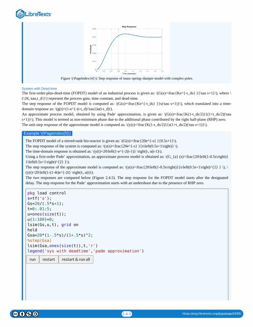
Figure \(\PageIndex{4}\): Step response of mass–spring–damper model with complex poles.

System with Dead-time The first-order-plus-dead-time (FOPDT) model of an industrial process is given as: \(G(s)=\frac{Ke^{-t_ds} }{\tau s+1}\), where \(\{K,\tau,t_d\}\) represent the process gain, time constant, and dead-time.The step response of the FOPDT model is computed as: \(G(s)=\frac{Ke^{-t_ds} }{s(\tau s+1)}\), which translated into a time-domain response as: \(g(t)=(1-e^{-(t-t_d)/\tau})u(t-t_d)\).An approximate process model, obtained by using Pade' approximation, is given as: \(G(s)=\frac{K(1-t_ds/2)}{(1+t_ds/2)(\taus+1)}\). This model is termed as non-minimum phase due to the additional phase contributed by the right half-plane (RHP) zero.The unit-step response of the approximate model is computed as: \(y(s)=\frac{K(1-t_ds/2)}{s(1+t_ds/2)(\tau s+1)}\).

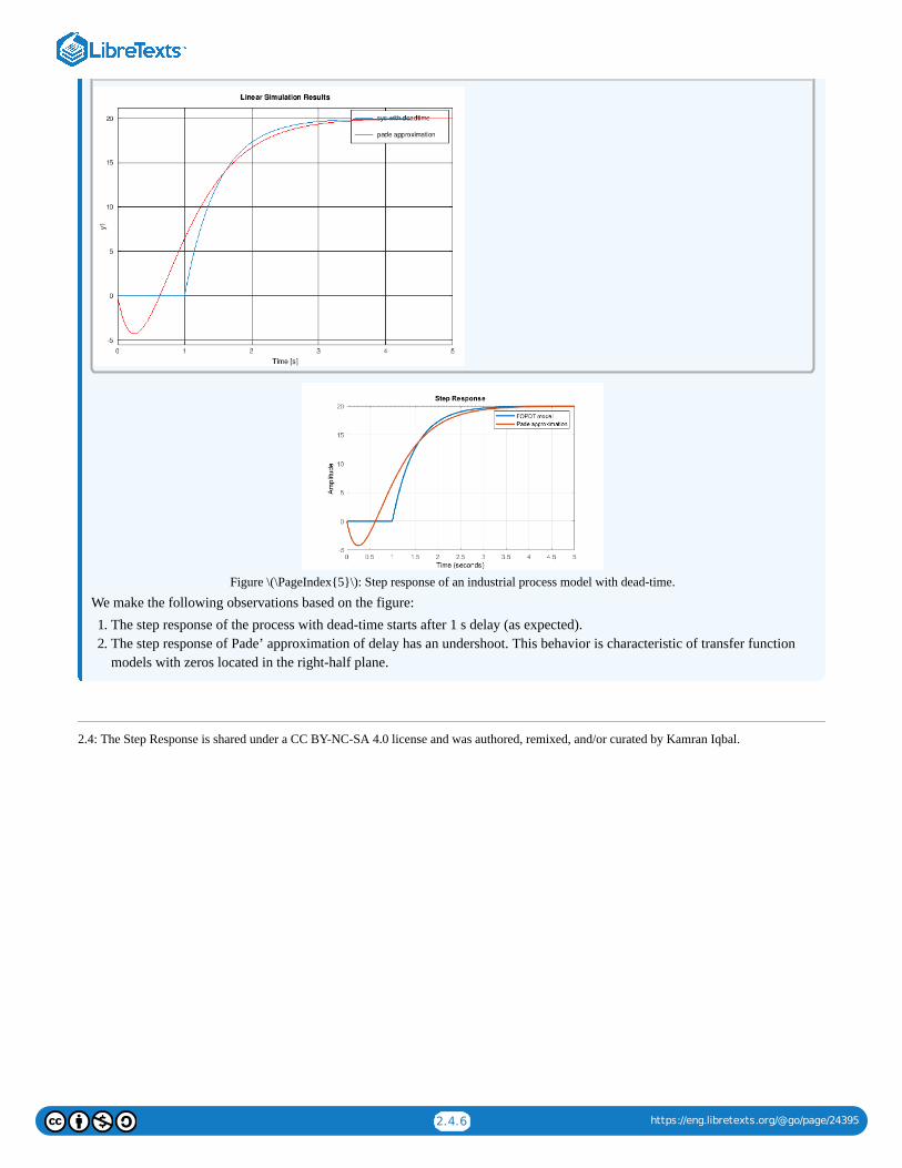
The FOPDT model of a stirred-tank bio-reactor is given as: \(G(s)=\frac{20e^{-s} }{0.5s+1}\).The step response of the system is computed as: \(y(s)=\frac{20e^{-s} }{s\left(0.5s+1\right)} \).The time-domain response is obtained as: \(y(t)=20\left(1-e^{-2(t-1)} \right)\, u(t-1)\).Using a first-order Pade’ approximation, an approximate process model is obtained as: \(G_{a} (s)=\frac{20\left(1-0.5s\right)}{\left(0.5s+1\right)^{2} }\).The step response of the approximate model is computed as: \(y(s)=\frac{20\left(1-0.5s\right)}{s\left(0.5s+1\right)^{2} } \), \(y(t)=20\left(1-(1-4t)e^{-2t} \right)\, u(t)\).The two responses are compared below (Figure 2.4.5). The step response for the FOPDT model starts after the designateddelay. The step response for the Pade’ approximation starts with an undershoot due to the presence of RHP zero.

run restart restart & run all

Example \(\PageIndex{5}\)

pkg load control

s=tf('s');

Gs=20/(.5*s+1);

t=0:.01:5;

u=ones(size(t));

u(1:100)=0;

lsim(Gs,u,t), grid on

hold

Gsa=20*(1-.5*s)/(1+.5*s)^2;

%step(Gsa)

lsim(Gsa,ones(size(t)),t,'r')

legend('sys with deadtime','pade approximation')

2.4.6 https://eng.libretexts.org/@go/page/24395

Figure \(\PageIndex{5}\): Step response of an industrial process model with dead-time.

We make the following observations based on the figure:1. The step response of the process with dead-time starts after 1 s delay (as expected).2. The step response of Pade’ approximation of delay has an undershoot. This behavior is characteristic of transfer function

models with zeros located in the right-half plane.

2.4: The Step Response is shared under a CC BY-NC-SA 4.0 license and was authored, remixed, and/or curated by Kamran Iqbal.

2.5.1 https://eng.libretexts.org/@go/page/24397

2.5: Sinusoidal Response of a System

Response to Sinusoidal Input

The sinusoidal response of a system refers to its response to a sinusoidal input: or .

To characterize the sinusoidal response, we may assume a complex exponential input of the form: .

Then, the system output is given as: .

To proceed, let , where , denote the poles of the transfer function; then, using PFE, the system

response is given as:

where . The time response of the system is given as:

Assuming BIBO stability, i.e., , the transient response component dies out with time. Then, the steady-state response isdescribed as:

The frequency response function, for a given transfer function is defined as: .

The frequency response function is described in the magnitude-phase form as:

When computed at a particular frequency, , the frequency response function, is a complex number.

Then, the steady-state response to a complex sinusoid is given as:

By Euler’s identity, we have: ; therefore, the steady-state response to is given as:

Similarly, the steady-state response to is given as:

Thus, the steady-state response to sinusoid of a certain frequency is a sinusoid at the same frequency, scaled by the magnitude ofthe frequency response function; the response includes a phase contribution from the frequency response function.

Examples

A small DC motor model is approximated as: .

Its frequency response function is given as: .

Let ; then, in the steady-state, the sinusoidal response is given as: .

The sinusoidal response of the DC motor is plotted in Figure 2.5.1.

u(t) = cos tω0 u(t) = sin tω0

u (t) = ,   u (s) =ej tω0 1s−jω0

 y (s) =G(s)

s−jω0

G(s) =n(s)

(s− )∏ni=1 pi

,  i = 1, … npi

y (s) = +A0

s −jω0∑i=1

n Ai

s −pi

(2.5.1)

= G(j )A0 ω0

y (t) = G(j ) +ω0 ej tω0 ∑i=1

n

Aietpi (2.5.2)

Re [ ] < 0pi

(t) = G(j )yss ω0 ej tω0 (2.5.3)

Definition: Frequency Response Function

G(s) G(jω) = G(s)|s=jω

G(jω) = |G(jω)| .e∠G(jω)

ω = ω0 G(j )ω0

u(t) = ej tω0

(t) = |G(j )|yss ω0 e∠G(j )ω0 ej tω0 (2.5.4)

= cos( t) +j sin( t)ej tω0 ω0 ω0 u(t) = cos tω0

(t) = |G(j )| cos( t +∠G(j ))yss ω0 ω0 ω0 (2.5.5)

u(t) = sin tω0

(t) = |G(j )| sin( t +∠G(j ))yss ω0 ω0 ω0 (2.5.6)

Example 2.5.1

G(s) = 500(s+10)(s+100)

G(jω) = 0.5(0.01ω+1)(0.1ω+1)

u(t) = sin10t (t) = 0.35 sin(10t −50 ) yss∘

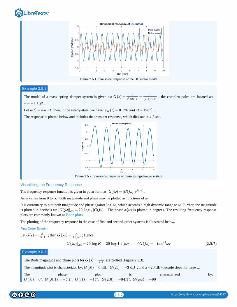
2.5.2 https://eng.libretexts.org/@go/page/24397

Figure : Sinusoidal response of the DC motor model.

The model of a mass–spring–damper system is given as: ; the complex poles are located at:

.

Let ; then, in the steady-state, we have: .

The response is plotted below and includes the transient response, which dies out in 4-5 sec.

Figure : Sinusoidal response of mass-spring-damper system.

Visualizing the Frequency Response

The frequency response function is given in polar form as: .

As varies from to , both magnitude and phase may be plotted as functions of .

It is customary to plot both magnitude and phase against , which accords a high dynamic range to . Further, the magnitudeis plotted in decibels as: . The phase is plotted in degrees. The resulting frequency responseplots are commonly known as Bode plots.

The plotting of the frequency response in the case of first and second-order systems is illustrated below.

First-Order System

Let ; then ; Hence,

The Bode magnitude and phase plots for are plotted (Figure 2.5.3).

The magnitude plot is characterized by: , and a slope for large .

The phase plot is characterized by: .

2.5.1

Example 2.5.2

G(s) = =1+2s+5s2

1

+(s+1)2 22

s = −1 ±j2

u(t) = sin πt (t) = 0.126 sin(πt −128 ) yss∘

2.5.2

G(jω) = |G(jω)|ejϕ(ω)

ω 0 ∞ ω

log ω  ω

|G(jω) = 20 |G(jω)||dB log10 ϕ(ω)

G(s) = K

τs+1G(jω) = K

1+jωτ

= 20 log K  −20 log|1 +jωτ | , ∠G(jω) = − ωτ  |G(jω)|dB tan−1 (2.5.7)

Example 2.5.3

G(s) = 1s+1

G(j0) = 0 dB,   G(j1) = −3 dB −20 dB/decade ω

G(j0) = 0 ,  G(j0.1) = −5.7 ,  G(j1) = −45 ,   G(j10) = −84.3 ,  G(j∞) = −90∘ ∘ ∘ ∘ ∘

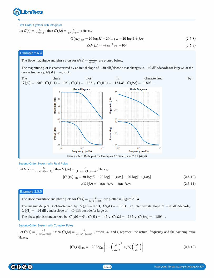
2.5.3 https://eng.libretexts.org/@go/page/24397

First-Order System with Integrator

Let ; then ; Hence,

The Bode magnitude and phase plots for are plotted below.

The magnitude plot is characterized by an initial slope of that changes to for large ; at thecorner frequency, .

The phase plot is characterized by: .

Figure : Bode plot for Examples 2.5.3 (left) and 2.5.4 (right).

Second-Order System with Real Poles

Let ; then ; Hence,

The Bode magnitude and phase plots for are plotted in Figure 2.5.4.

The magnitude plot is characterized by: , an intermediate slope of , , and a slope of for large .

The phase plot is characterized by: .

Second-Order System with Complex Poles

Let ; then , where and represent the natural frequency and the damping ratio.

Hence,

G(s) = K

s(τs+1)G(jω) = K

jω(1+jωτ)

= 20 log K  −20 log ω  −20 log|1 +jωτ | |G(jω)|dB (2.5.8)

∠G(jω) = − ωτ   −90tan−1 ∘ (2.5.9)

Example 2.5.4

G(s) = 1s(s+1)

−20 dB/decade −40 dB/decade ω

G(j1) = −3 dB

G(j0) = −90 ,  G(j0.1) = −96 ,  G(j1) = −135 ,   G(j10) = −174.3 ,  G(j∞) = −180∘ ∘ ∘ ∘ ∘

2.5.3

G(s) = K

( s+1)( s+1)τ1 τ2G(jω) = K

(1+jω )(1+jω )τ1 τ2

= 20 log K  −20 log|1 +jω |  −20 log|1 +jω | |G(jω)|dB τ1 τ2 (2.5.10)

∠G(jω) = − ω   − ω  tan−1 τ1 tan−1 τ2 (2.5.11)

Example 2.5.5

G(s) = 2(s+1)(s+2)

G(j0) = 0 dB,   G(j1) = −3 dB −20 dB/decadeG(j2) = −14 dB −40 dB/decade ω

G(j0) = 0 ,  G(j1) = −45 ,   G(j2) = −135 ,   G(j∞) = −180∘ ∘ ∘ ∘

G(s) =ω2

n

+2ζ s+s2 ωn ω2n

G(jω) =ω2

n

− +j2ζωω2n ω2 ωn

ωn ζ

= −20 1 − +j2ζ( )  |G(jω)|dB log10

∣

∣∣ ( )

ω

ωn

2 ω

ωn

∣

∣∣ (2.5.12)

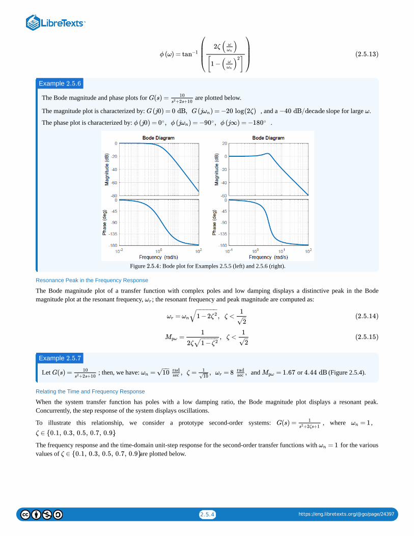
2.5.4 https://eng.libretexts.org/@go/page/24397

The Bode magnitude and phase plots for are plotted below.

The magnitude plot is characterized by: , and a slope for large .

The phase plot is characterized by: .

Figure : Bode plot for Examples 2.5.5 (left) and 2.5.6 (right).

Resonance Peak in the Frequency Response

The Bode magnitude plot of a transfer function with complex poles and low damping displays a distinctive peak in the Bodemagnitude plot at the resonant frequency, ; the resonant frequency and peak magnitude are computed as:

Let ; then, we have: and or (Figure 2.5.4).

Relating the Time and Frequency Response

When the system transfer function has poles with a low damping ratio, the Bode magnitude plot displays a resonant peak.Concurrently, the step response of the system displays oscillations.

To illustrate this relationship, we consider a prototype second-order systems: , where , .

The frequency response and the time-domain unit-step response for the second-order transfer functions with for the variousvalues of are plotted below.

ϕ (ω) =  tan−1

⎛

⎝

⎜⎜⎜

2ζ ( )ω

ωn

[1 − ]( )ω

ωn

2

⎞

⎠

⎟⎟⎟

(2.5.13)

Example 2.5.6

G(s) = 10+2s+10s2

G(j0) = 0 dB,   G(j ) = −20 log(2ζ) ωn −40 dB/decade ω

ϕ (j0) = 0 ,   ϕ (j ) = −90 ,   ϕ (j∞) = −180∘ ωn∘ ∘

2.5.4

ωr

= , ζ <ωr ωn 1 −2ζ2− −−−−−

√1

2–

√(2.5.14)

= , ζ <Mpω

1

2ζ 1 −ζ2− −−−−

√

1

2–

√(2.5.15)

Example 2.5.7

G(s) = 10+2s+10s2 = , ζ = , = 8 ,ωn 10

−−√ rad

sec110√

ωrradsec = 1.67Mpω 4.44 dB

G(s) = 1+2ζs+1s2 = 1ωn

ζ ∈ {0.1, 0.3, 0.5, 0.7, 0.9}

= 1ωn

ζ ∈ {0.1, 0.3, 0.5, 0.7, 0.9}

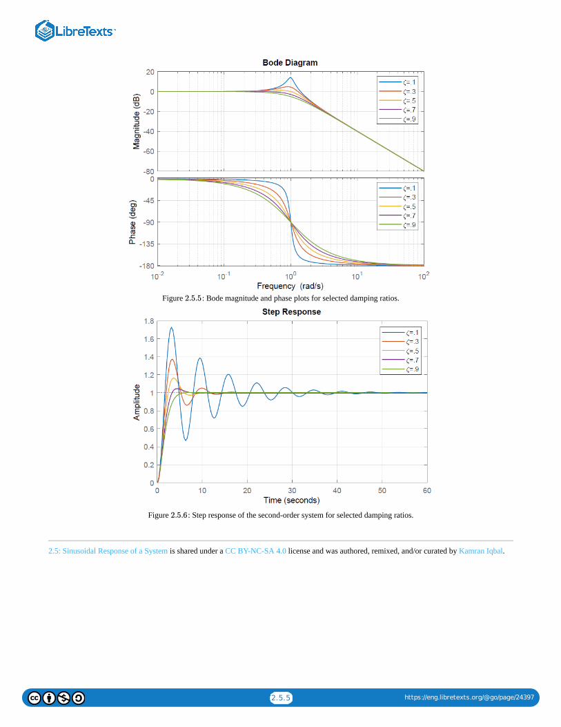
2.5.5 https://eng.libretexts.org/@go/page/24397

Figure : Bode magnitude and phase plots for selected damping ratios.

Figure : Step response of the second-order system for selected damping ratios.

2.5: Sinusoidal Response of a System is shared under a CC BY-NC-SA 4.0 license and was authored, remixed, and/or curated by Kamran Iqbal.

2.5.5

2.5.6

1 https://eng.libretexts.org/@go/page/27706

Welcome to the Engineering Library. This Living Library is a principal hub of the LibreTexts project, which is a multi-institutionalcollaborative venture to develop the next generation of open-access texts to improve postsecondary education at all levels of higherlearning. The LibreTexts approach is highly collaborative where an Open Access textbook environment is under constant revisionby students, faculty, and outside experts to supplant conventional paper-based books.

Home is shared under a not declared license and was authored, remixed, and/or curated by LibreTexts.

1

CHAPTER OVERVIEW

3: Feedback Control System Models

1. Characterize the static controller in a feedback control system.2. Characterize first-order dynamic controllers for feedback back control systems.3. Characterize the PID controller in terms of the three basic control modes.4. Characterize rate feedback controllers for single-input single-output systems.

3.0: Prelude to Feedback Control System Models3.1: Static Feedback Controller3.2: First-Order Dynamic Controllers3.3: PI, PD, and PID Controllers3.4: Rate Feedback ControllersBlank

3: Feedback Control System Models is shared under a CC BY-NC-SA 4.0 license and was authored, remixed, and/or curated by Kamran Iqbal.

Learning Objectives

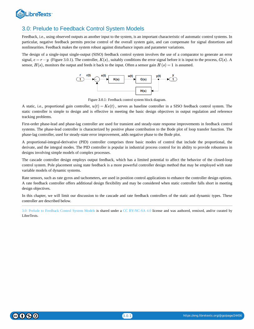
3.0.1 https://eng.libretexts.org/@go/page/24456

3.0: Prelude to Feedback Control System ModelsFeedback, i.e., using observed outputs as another input to the system, is an important characteristic of automatic control systems. Inparticular, negative feedback permits precise control of the overall system gain, and can compensate for signal distortions andnonlinearities. Feedback makes the system robust against disturbance inputs and parameter variations.

The design of a single-input single-output (SISO) feedback control system involves the use of a comparator to generate an errorsignal, (Figure 3.0.1). The controller, , suitably conditions the error signal before it is input to the process, . Asensor, , monitors the output and feeds it back to the input. Often a sensor gain is assumed.

Figure : Feedback control system block diagram.

A static, i.e., proportional gain controller, , serves as baseline controller in a SISO feedback control system. Thestatic controller is simple to design and is effective in meeting the basic design objectives in output regulation and referencetracking problems.

First-order phase-lead and phase-lag controller are used for transient and steady-state response improvements in feedback controlsystems. The phase-lead controller is characterized by positive phase contribution to the Bode plot of loop transfer function. Thephase-lag controller, used for steady-state error improvement, adds negative phase to the Bode plot.

A proportional-integral-derivative (PID) controller comprises three basic modes of control that include the proportional, thederivate, and the integral modes. The PID controller is popular in industrial process control for its ability to provide robustness indesigns involving simple models of complex processes.

The cascade controller design employs output feedback, which has a limited potential to affect the behavior of the closed-loopcontrol system. Pole placement using state feedback is a more powerful controller design method that may be employed with statevariable models of dynamic systems.

Rate sensors, such as rate gyros and tachometers, are used in position control applications to enhance the controller design options.A rate feedback controller offers additional design flexibility and may be considered when static controller falls short in meetingdesign objectives.

In this chapter, we will limit our discussion to the cascade and rate feedback controllers of the static and dynamic types. Thesecontroller are described below.

3.0: Prelude to Feedback Control System Models is shared under a CC BY-NC-SA 4.0 license and was authored, remixed, and/or curated byLibreTexts.

e = r −y K(s) G(s)

H(s) H (s) = 1

3.0.1

u(t) = Ke(t)

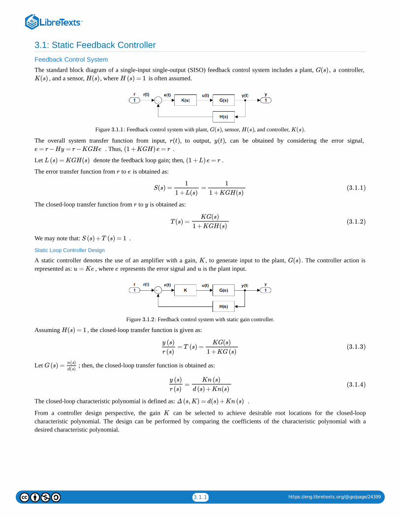
3.1.1 https://eng.libretexts.org/@go/page/24399

3.1: Static Feedback Controller

Feedback Control System

The standard block diagram of a single-input single-output (SISO) feedback control system includes a plant, , a controller, , and a sensor, , where is often assumed.

Figure : Feedback control system with plant, , sensor, , and controller, .

The overall system transfer function from input, , to output, , can be obtained by considering the error signal, . Thus, .

Let denote the feedback loop gain; then, .

The error transfer function from to is obtained as:

The closed-loop transfer function from to is obtained as:

We may note that: .

Static Loop Controller Design

A static controller denotes the use of an amplifier with a gain, , to generate input to the plant, . The controller action isrepresented as: , where represents the error signal and is the plant input.

Figure : Feedback control system with static gain controller.

Assuming , the closed-loop transfer function is given as:

Let ; then, the closed-loop transfer function is obtained as:

The closed-loop characteristic polynomial is defined as: .

From a controller design perspective, the gain can be selected to achieve desirable root locations for the closed-loopcharacteristic polynomial. The design can be performed by comparing the coefficients of the characteristic polynomial with adesired characteristic polynomial.

G(s)

K(s) H(s) H (s) = 1

3.1.1 G(s) H(s) K(s)

r(t) y(t)

e = r−Hy = r−KGHe (1 +KGH)e = r

L (s) = KGH(s) (1 +L)e = r

r e

S(s) = =1

1 +L(s)

1

1 +KGH(s)(3.1.1)

r y

T (s) =KG(s)

1 +KGH(s)(3.1.2)

S (s) +T (s) = 1

K G(s)

u = Ke e u

3.1.2

H(s) = 1

= T (s) =y (s)

r (s)

KG(s)

1 +KG(s)(3.1.3)

G(s) =n(s)

d(s)

=y (s)

r (s)

Kn (s)

d (s) +Kn(s)(3.1.4)

Δ (s,K) = d(s) +Kn (s)

K

3.1.2 https://eng.libretexts.org/@go/page/24399

The model for an environmental control system is given as: .

Assuming a static gain controller, the closed-loop characteristic polynomial is obtained as: .

Suppose a desired characteristic polynomial is selected as: . Then, by comparing the coefficients, weobtain the static controller as: .

The model for a position control system is given as: .

Assuming a static gain controller, the characteristic polynomial is obtained as: .

Suppose a desired characteristic polynomial is selected as: . Then, by comparing thecoefficients, we obtain the static controller as: .

3.1: Static Feedback Controller is shared under a CC BY-NC-SA 4.0 license and was authored, remixed, and/or curated by Kamran Iqbal.

Example 3.1.1

G(s) = 120s+1

Δ (s,K) = 20s+1 +K

(s) = 4(5s+1)Δdes

K = 3

Example 3.1.2

G(s) = 1

s(0.1s+1)

Δ (s,K) = s(0.1s+1) +K

(s) = 0.1( +10s+50)Δdes s2

K = 5

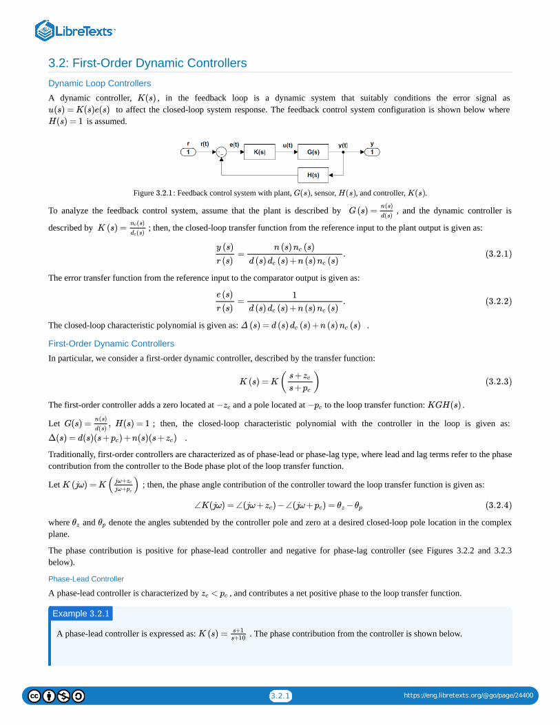
3.2.1 https://eng.libretexts.org/@go/page/24400

3.2: First-Order Dynamic Controllers

Dynamic Loop Controllers

A dynamic controller, , in the feedback loop is a dynamic system that suitably conditions the error signal as to affect the closed-loop system response. The feedback control system configuration is shown below where

is assumed.

Figure : Feedback control system with plant, , sensor, , and controller, .

To analyze the feedback control system, assume that the plant is described by , and the dynamic controller is

described by ; then, the closed-loop transfer function from the reference input to the plant output is given as:

The error transfer function from the reference input to the comparator output is given as:

The closed-loop characteristic polynomial is given as: .

First-Order Dynamic Controllers

In particular, we consider a first-order dynamic controller, described by the transfer function:

The first-order controller adds a zero located at and a pole located at to the loop transfer function: .

Let ; then, the closed-loop characteristic polynomial with the controller in the loop is given as:

.

Traditionally, first-order controllers are characterized as of phase-lead or phase-lag type, where lead and lag terms refer to the phasecontribution from the controller to the Bode phase plot of the loop transfer function.

Let ; then, the phase angle contribution of the controller toward the loop transfer function is given as:

where and denote the angles subtended by the controller pole and zero at a desired closed-loop pole location in the complexplane.

The phase contribution is positive for phase-lead controller and negative for phase-lag controller (see Figures 3.2.2 and 3.2.3below).

Phase-Lead Controller

A phase-lead controller is characterized by , and contributes a net positive phase to the loop transfer function.

A phase-lead controller is expressed as: . The phase contribution from the controller is shown below.

K(s)

u(s) = K(s)e(s)

H(s) = 1

3.2.1 G(s) H(s) K(s)

G(s) =n(s)

d(s)

K (s) =(s)nc

(s)dc

= .y (s)

r (s)

n (s) (s)nc

d (s) (s) +n (s) (s)dc nc

(3.2.1)

= .e (s)

r (s)

1

d (s) (s) +n (s) (s)dc nc

(3.2.2)

Δ (s) = d (s) (s) +n (s) (s)dc nc

K (s) = K( )s+zc

s+pc(3.2.3)

−zc −pc KGH(s)

G(s) = , H(s) = 1n(s)

d(s)

Δ(s) = d(s)(s+ ) +n(s)(s+ )pc zc

K (jω) = K( )jω+zc

jω+pc

∠K(jω) = ∠(jω+ ) −∠(jω+ ) = −zc pc θz θp (3.2.4)

θz θp

<zc pc

Example 3.2.1

K (s) = s+1s+10

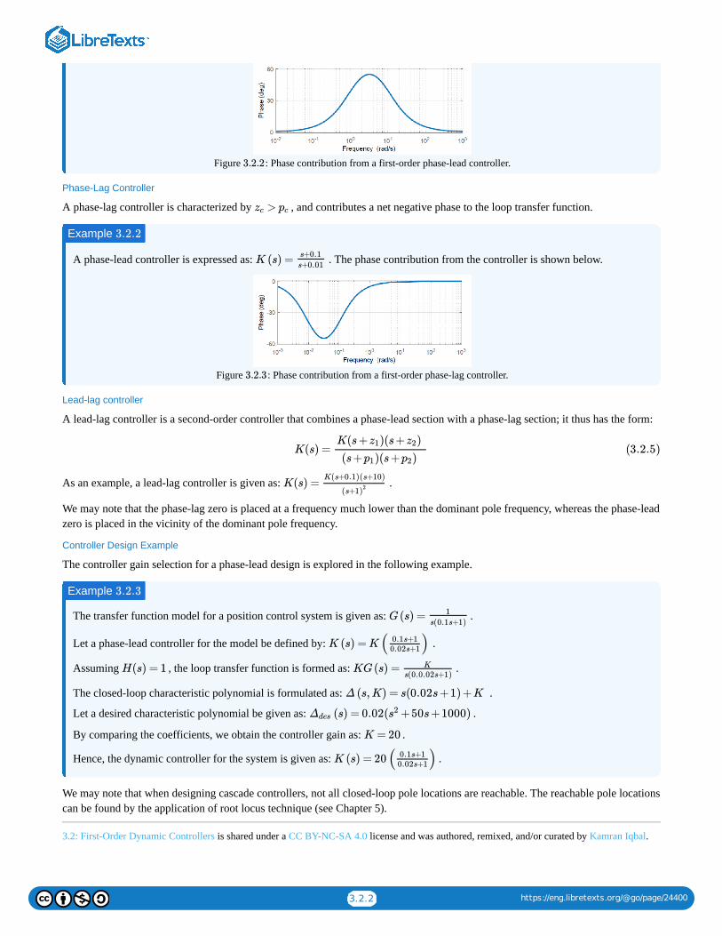
3.2.2 https://eng.libretexts.org/@go/page/24400

Figure : Phase contribution from a first-order phase-lead controller.

Phase-Lag Controller

A phase-lag controller is characterized by , and contributes a net negative phase to the loop transfer function.

A phase-lead controller is expressed as: . The phase contribution from the controller is shown below.

Figure : Phase contribution from a first-order phase-lag controller.

Lead-lag controller

A lead-lag controller is a second-order controller that combines a phase-lead section with a phase-lag section; it thus has the form:

As an example, a lead-lag controller is given as: .

We may note that the phase-lag zero is placed at a frequency much lower than the dominant pole frequency, whereas the phase-leadzero is placed in the vicinity of the dominant pole frequency.

Controller Design Example

The controller gain selection for a phase-lead design is explored in the following example.

The transfer function model for a position control system is given as: .

Let a phase-lead controller for the model be defined by: .

Assuming , the loop transfer function is formed as: .

The closed-loop characteristic polynomial is formulated as: .

Let a desired characteristic polynomial be given as: .

By comparing the coefficients, we obtain the controller gain as: .

Hence, the dynamic controller for the system is given as: .

We may note that when designing cascade controllers, not all closed-loop pole locations are reachable. The reachable pole locationscan be found by the application of root locus technique (see Chapter 5).

3.2: First-Order Dynamic Controllers is shared under a CC BY-NC-SA 4.0 license and was authored, remixed, and/or curated by Kamran Iqbal.

3.2.2

>zc pc

Example 3.2.2

K (s) =s+0.1

s+0.01

3.2.3

K(s) =K(s+ )(s+ )z1 z2

(s+ )(s+ )p1 p2

(3.2.5)

K(s) =K(s+0.1)(s+10)

(s+1)2

Example 3.2.3

G(s) = 1

s(0.1s+1)

K (s) = K( )0.1s+10.02s+1

H(s) = 1 KG(s) = K

s(0.0.02s+1)

Δ (s,K) = s(0.02s+1) +K

(s) = 0.02( +50s+1000)Δdes s2

K = 20

K (s) = 20( )0.1s+10.02s+1

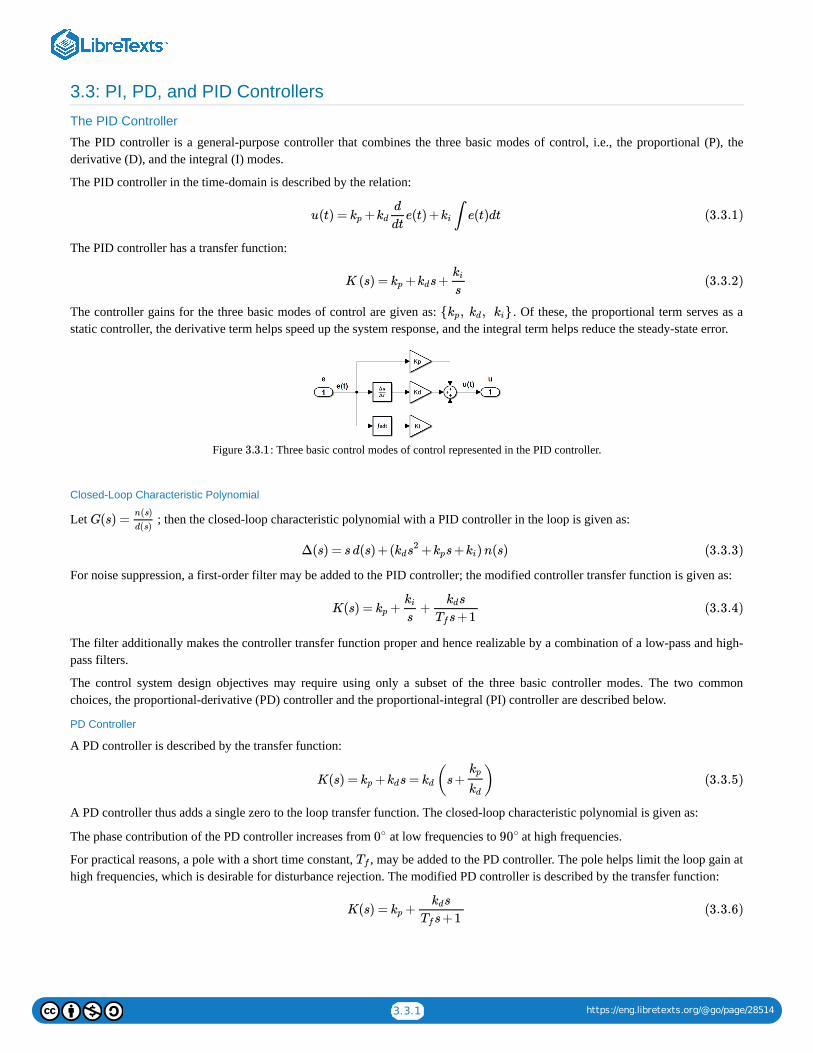
3.3.1 https://eng.libretexts.org/@go/page/28514

3.3: PI, PD, and PID Controllers

The PID Controller

The PID controller is a general-purpose controller that combines the three basic modes of control, i.e., the proportional (P), thederivative (D), and the integral (I) modes.

The PID controller in the time-domain is described by the relation:

The PID controller has a transfer function:

The controller gains for the three basic modes of control are given as: . Of these, the proportional term serves as astatic controller, the derivative term helps speed up the system response, and the integral term helps reduce the steady-state error.

Figure : Three basic control modes of control represented in the PID controller.

Closed-Loop Characteristic Polynomial

Let ; then the closed-loop characteristic polynomial with a PID controller in the loop is given as:

For noise suppression, a first-order filter may be added to the PID controller; the modified controller transfer function is given as:

The filter additionally makes the controller transfer function proper and hence realizable by a combination of a low-pass and high-pass filters.

The control system design objectives may require using only a subset of the three basic controller modes. The two commonchoices, the proportional-derivative (PD) controller and the proportional-integral (PI) controller are described below.

PD Controller

A PD controller is described by the transfer function:

A PD controller thus adds a single zero to the loop transfer function. The closed-loop characteristic polynomial is given as:

The phase contribution of the PD controller increases from at low frequencies to at high frequencies.

For practical reasons, a pole with a short time constant, , may be added to the PD controller. The pole helps limit the loop gain athigh frequencies, which is desirable for disturbance rejection. The modified PD controller is described by the transfer function:

u(t) = + e(t) + ∫ e(t)dtkp kdd

dtki (3.3.1)

K (s) = + s+kp kdki

s(3.3.2)

{ ,   ,    }kp kd ki

3.3.1

G(s) =n(s)

d(s)

Δ(s) = s d(s) +( + s+ )n(s)kds2 kp ki (3.3.3)

K(s) = + +kpki

s

skd

s+1Tf(3.3.4)

K(s) = + s = (s+ )kp kd kdkp

kd(3.3.5)

0∘ 90∘

Tf

K(s) = +kpskd

s+1Tf(3.3.6)

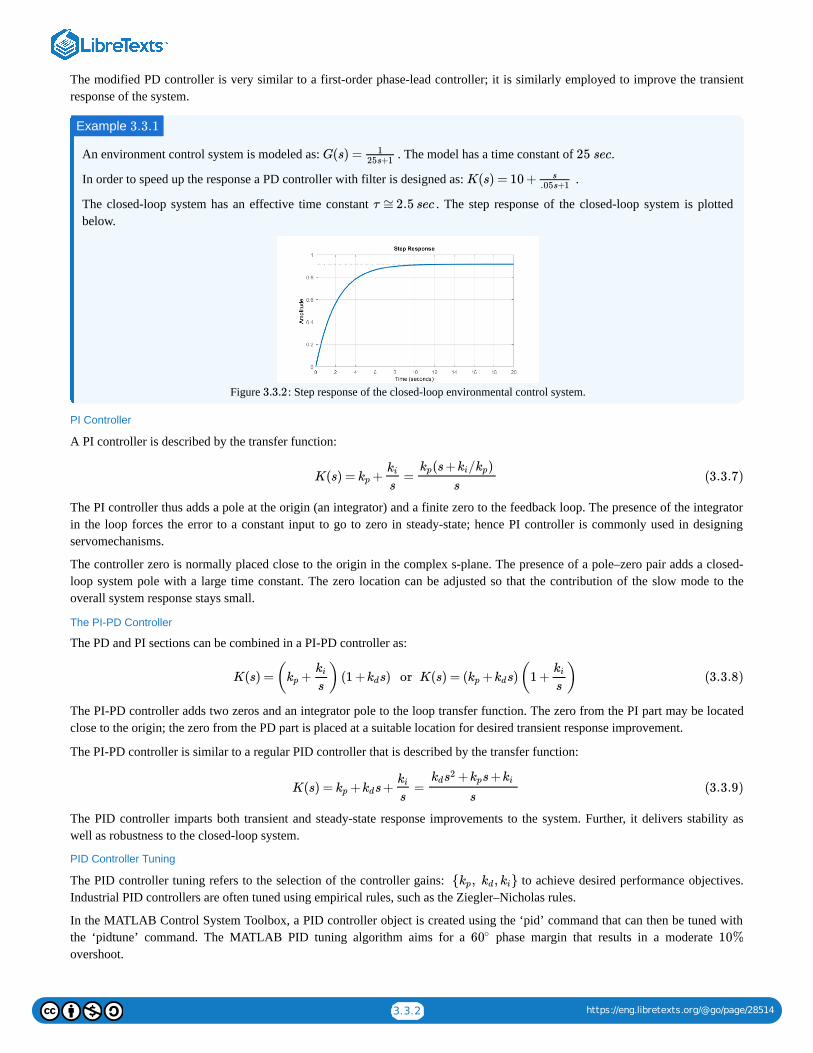
3.3.2 https://eng.libretexts.org/@go/page/28514

The modified PD controller is very similar to a first-order phase-lead controller; it is similarly employed to improve the transientresponse of the system.

An environment control system is modeled as: . The model has a time constant of .

In order to speed up the response a PD controller with filter is designed as: .

The closed-loop system has an effective time constant . The step response of the closed-loop system is plottedbelow.

Figure : Step response of the closed-loop environmental control system.

PI Controller

A PI controller is described by the transfer function:

The PI controller thus adds a pole at the origin (an integrator) and a finite zero to the feedback loop. The presence of the integratorin the loop forces the error to a constant input to go to zero in steady-state; hence PI controller is commonly used in designingservomechanisms.

The controller zero is normally placed close to the origin in the complex s-plane. The presence of a pole–zero pair adds a closed-loop system pole with a large time constant. The zero location can be adjusted so that the contribution of the slow mode to theoverall system response stays small.

The PI-PD Controller

The PD and PI sections can be combined in a PI-PD controller as:

The PI-PD controller adds two zeros and an integrator pole to the loop transfer function. The zero from the PI part may be locatedclose to the origin; the zero from the PD part is placed at a suitable location for desired transient response improvement.

The PI-PD controller is similar to a regular PID controller that is described by the transfer function:

The PID controller imparts both transient and steady-state response improvements to the system. Further, it delivers stability aswell as robustness to the closed-loop system.

PID Controller Tuning

The PID controller tuning refers to the selection of the controller gains: to achieve desired performance objectives.Industrial PID controllers are often tuned using empirical rules, such as the Ziegler–Nicholas rules.

In the MATLAB Control System Toolbox, a PID controller object is created using the ‘pid’ command that can then be tuned withthe ‘pidtune’ command. The MATLAB PID tuning algorithm aims for a phase margin that results in a moderate overshoot.

Example 3.3.1

G(s) = 125s+1

25 sec

K(s) = 10 + s.05s+1

τ ≅2.5 sec

3.3.2

K(s) = + =kpki

s

(s+ / )kp ki kp

s(3.3.7)

K(s) =( + ) (1 + s) or K(s) = ( + s)(1 + )kpki

skd kp kd

ki

s(3.3.8)

K(s) = + s+ =kp kdki

s

+ s+kds2 kp ki

s(3.3.9)

{ , , }kp kd ki

60∘ 10%

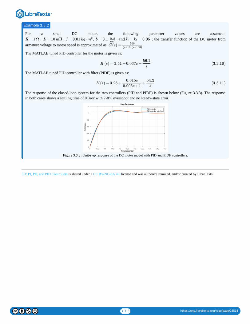
3.3.3 https://eng.libretexts.org/@go/page/28514

For a small DC motor, the following parameter values are assumed: ; the transfer function of the DC motor from

armature voltage to motor speed is approximated as: .

The MATLAB tuned PID controller for the motor is given as:

The MATLAB tuned PID controller with filter (PIDF) is given as:

The response of the closed-loop system for the two controllers (PID and PIDF) is shown below (Figure 3.3.3). The responsein both cases shows a settling time of 0.3sec with 7-8% overshoot and no steady-state error.

Figure : Unit-step response of the DC motor model with PID and PIDF controllers.

3.3: PI, PD, and PID Controllers is shared under a CC BY-NC-SA 4.0 license and was authored, remixed, and/or curated by LibreTexts.

Example 3.3.2

R = 1 Ω , L = 10 mH, J = 0.01 kg ⋅ , b = 0.1 , and = = 0.05m2 N ⋅srad

kt kb

G(s) = 500

(s+10)(s+100)

K (s) = 3.51 +0.037s+56.2

s(3.3.10)

K (s) = 3.26 + +0.015s

0.005s+1

54.2

s(3.3.11)

3.3.3

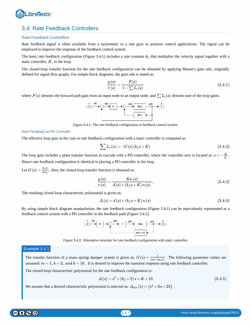
3.4.1 https://eng.libretexts.org/@go/page/28513

3.4: Rate Feedback Controllers

Rate Feedback Controllers

Rate feedback signal is often available from a tachometer or a rate gyro in position control applications. The signal can beemployed to improve the response of the feedback control system.

The basic rate feedback configuration (Figure 3.4.1) includes a rate constant that multiplies the velocity signal together with astatic controller, , in the loop.

The closed-loop transfer function for the rate feedback configuration can be obtained by applying Mason’s gain rule, originallydefined for signal flow graphs. For simple block diagrams, the gain rule is stated as:

where denotes the forward path gain from an input node to an output node, and denotes sum of the loop gains.

Figure : The rate feedback configuration in feedback control system.

Rate Feedback as PD Controller

The effective loop gain in the case or rate feedback configuration with a static controller is computed as:

The loop gain includes a plant transfer function in cascade with a PD controller, where the controller zero is located at: .

Hence rate feedback configuration is identical to placing a PD controller in the loop.

Let then, the closed-loop transfer function is obtained as:

The resulting closed-loop characteristic polynomial is given as:

By using simple block diagram manipulation, the rate feedback configuration (Figure 3.4.1) can be equivalently represented as afeedback control system with a PD controller in the feedback path (Figure 3.4.2).

Figure : Alternative structure for rate feedback configuration with static controller.

The transfer function of a mass–spring–damper system is given as: . The following parameter values areassumed: . It is desired to improve the transient response using rate feedback controller.

The closed-loop characteristic polynomial for the rate feedback configuration is:

We assume that a desired characteristic polynomial is selected as: .

kfK

=y (s)

r (s)

F (s)

1 −∑ (s)Li

(3.4.1)

F (s) ∑ (s)Li

3.4.1

∑ (s) = −G(s) ( s+K)Li kf (3.4.2)

s = − K

kf

G(s) = ;n(s)

d(s)

= ,y (s)

r (s)

Kn (s)

d (s) +( s+K)n (s)kf(3.4.3)

Δ (s) = d (s) +( s+K)n (s)kf (3.4.4)

3.4.2

Example 3.4.1

G(s) = 1

m +bs+ks2

m = 1, b = 2,  and k = 10

Δ (s) = +( +2)s+K+10s2 kf (3.4.5)

(s) = ( +6s+25)Δdes s2

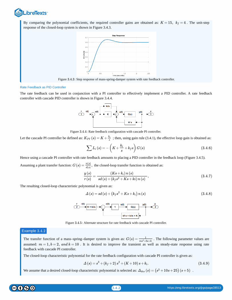
3.4.2 https://eng.libretexts.org/@go/page/28513

By comparing the polynomial coefficients, the required controller gains are obtained as: . The unit-stepresponse of the closed-loop system is shown in Figure 3.4.3.

Figure : Step response of mass-spring-damper system with rate feedback controller.

Rate Feedback as PID Controller

The rate feedback can be used in conjunction with a PI controller to effectively implement a PID controller. A rate feedbackcontroller with cascade PID controller is shown in Figure 3.4.4.

Figure : Rate feedback configuration with cascade PI controller.

Let the cascade PI controller be defined as: ; then, using gain rule (3.4.1), the effective loop gain is obtained as:

Hence using a cascade PI controller with rate feedback amounts to placing a PID controller in the feedback loop (Figure 3.4.5).

Assuming a plant transfer function: the closed-loop transfer function is obtained as:

The resulting closed-loop characteristic polynomial is given as:

Figure : Alternate structure for rate feedback with cascade PI controller.

The transfer function of a mass–spring–damper system is given as: . The following parameter values areassumed: . It is desired to improve the transient as well as steady-state response using ratefeedback with cascade PI controller.

The closed-loop characteristic polynomial for the rate feedback configuration with cascade PI controller is given as:

We assume that a desired closed-loop characteristic polynomial is selected as: .

K = 15,    = 4kf

3.4.3

3.4.4

(s) = K+KPIkis

∑ (s) = −(K+ + s)G(s)Li

ki

skf (3.4.6)

G(s) = ,n(s)

d(s)

= ,y (s)

r (s)

(Ks+ )n (s)ki

sd (s) +( +Ks+ki)n (s)kfs2(3.4.7)

Δ (s) = sd (s) +( +Ks+ )n (s)kfs2 ki (3.4.8)

3.4.5

Example 3.4.2

G(s) = 1

m +bs+ks2

m = 1, b = 2,  and k = 10

Δ (s) = +( +2) +(K+10)s+ .s3 kf s2 ki (3.4.9)

(s) = ( +10s+25) (s+5)Δdes s2

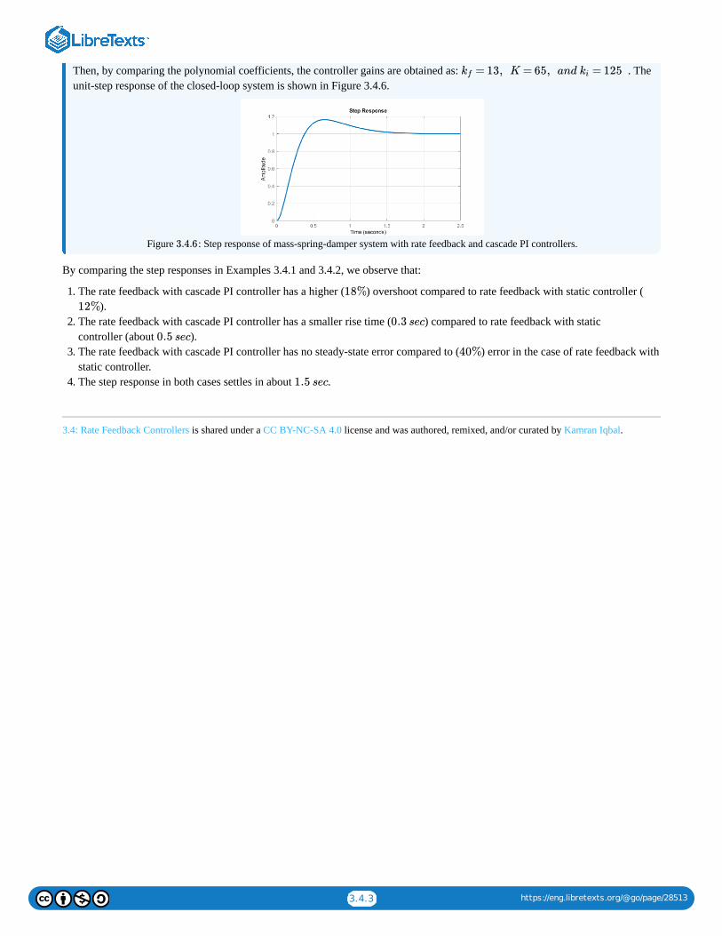
3.4.3 https://eng.libretexts.org/@go/page/28513

Then, by comparing the polynomial coefficients, the controller gains are obtained as: . Theunit-step response of the closed-loop system is shown in Figure 3.4.6.

Figure : Step response of mass-spring-damper system with rate feedback and cascade PI controllers.

By comparing the step responses in Examples 3.4.1 and 3.4.2, we observe that:

1. The rate feedback with cascade PI controller has a higher ( ) overshoot compared to rate feedback with static controller ().

2. The rate feedback with cascade PI controller has a smaller rise time ( ) compared to rate feedback with staticcontroller (about ).

3. The rate feedback with cascade PI controller has no steady-state error compared to ( ) error in the case of rate feedback withstatic controller.

4. The step response in both cases settles in about .

3.4: Rate Feedback Controllers is shared under a CC BY-NC-SA 4.0 license and was authored, remixed, and/or curated by Kamran Iqbal.

= 13,   K = 65,   and  = 125kf ki

3.4.6

18%

12%

0.3 sec

0.5 sec

40%

1.5 sec

1 https://eng.libretexts.org/@go/page/28512

Welcome to the Engineering Library. This Living Library is a principal hub of the LibreTexts project, which is a multi-institutionalcollaborative venture to develop the next generation of open-access texts to improve postsecondary education at all levels of higherlearning. The LibreTexts approach is highly collaborative where an Open Access textbook environment is under constant revisionby students, faculty, and outside experts to supplant conventional paper-based books.

Home is shared under a not declared license and was authored, remixed, and/or curated by LibreTexts.

1

CHAPTER OVERVIEW

4: Control System Design Objectives

1. Characterize closed-loop stability in a feedback control system model.2. Characterize performance objectives for transient and steady-state improvement.3. Characterize the disturbance rejection problem in feedback control systems.4. Determine the sensitivity of the closed-loop system to parameter variations.

4.0: Prelude to Control System Design Objectives4.1: Stability of the Closed-Loop System4.2: Transient Response Improvement4.3: Steady-State Error Improvement4.4: Disturbance Rejection4.5: Sensitivity and Robustness

4: Control System Design Objectives is shared under a CC BY-NC-SA 4.0 license and was authored, remixed, and/or curated by Kamran Iqbal.

Learning Objectives

4.0.1 https://eng.libretexts.org/@go/page/24457

4.0: Prelude to Control System Design ObjectivesIn a feedback control system, the controller is designed to achieve certain objective. The first and foremost among them is closed-loop system stability. The next is good dynamic stability displayed by an acceptable transient response. In tracking systems, theelimination of tracking error in desired. Further, the controlled system is required to mitigate disturbances entering the system andguard it against parameter variations and unmodeled dynamics. Hence we will discuss the ways to achieve the following objectivesin this chapter:

1. Closed-loop stability2. Acceptable transient response3. Acceptable steady-state error4. Sensitivity and robustness

In control system design, the stability of the closed-loop characteristic polynomial can be ascertained by algebraic methods, such asthe Routh’s array. These method can be applied toward the design of static controller. Stability can also be determined from theBode plot of the loop transfer function.

The transient response is commonly evaluated in terms of time-domain performance metrics applied to the step response of theclosed-loop system. The design specifications specify limits on the settling time of the system response and/or damping ratio ofclosed-loop roots. A phase-lead or PD/PID controller can be employed to obtain transient response improvements.

The steady-state error to prototype (step and ramp) inputs is measured in terms of position and velocity error constants of the looptransfer function. Generally speaking, high loop gain reduces steady-state error, but also makes the system prone to oscillations.The steady-state error can be eliminated by placing a PI/PID controller in the feedback loop.

Disturbance inputs are unavoidable in the operation of physical systems. Common examples of disturbance inputs include roadbumps while driving, turbulence in the airplanes, and machinery vibrations in industrial plants, etc. Effective disturbance rejectionrequires high loop gain in the frequency range of disturbance.

Aging in the physical system causes changes in the plant transfer function thus reducing the effectiveness of the controller. A well-designed control system is desired to have robustness against unmodeled dynamics as well as low sensitivity to parametervariations.

The control system design objectives involve inherent trade-offs. For example, a static controller cannot simultaneously improvethe transient response and reduce steady-state error to a constant input. Similarly, disturbance rejection and reference tracking poseconflicting design objectives. When faced with such situations, it is not always easy to find the right balance in meeting andprioritizing design objectives. Hence, the control system design is more of an art than an exact science, i.e., it relies much on theskills of the designer.

4.0: Prelude to Control System Design Objectives is shared under a CC BY-NC-SA 4.0 license and was authored, remixed, and/or curated byLibreTexts.

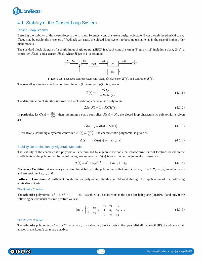
4.1.1 https://eng.libretexts.org/@go/page/24402

4.1: Stability of the Closed-Loop System

Closed-Loop Stability

Ensuring the stability of the closed-loop is the first and foremost control system design objective. Even though the physical plant, , may be stable, the presence of feedback can cause the closed-loop system to become unstable, as in the case of higher order

plant models.

The standard block diagram of a single-input single-output (SISO) feedback control system (Figure 4.1.1) includes a plant, , acontroller, , and a sensor, , where is assumed.

Figure : Feedback control system with plant, , sensor, , and controller, .

The overall system transfer function from input, , to output, , is given as:

The determination of stability is based on the closed-loop characteristic polynomial:

In particular, let ; then, assuming a static controller: , the closed-loop characteristic polynomial is given

as:

Alternatively, assuming a dynamic controller, , the characteristic polynomial is given as:

Stability Determination by Algebraic Methods

The stability of the characteristic polynomial is determined by algebraic methods that characterize its root locations based on thecoefficients of the polynomial. In the following, we assume that is an th order polynomial expressed as:

Necessary Condition. A necessary condition for stability of the polynomial is that coefficients , are all nonzeroand are positive, i.e., .

Sufficient Condition. A sufficient condition for polynomial stability is obtained through the application of the followingequivalent criteria:

The Hurwitz Criterion

The th order polynomial, is stable, i.e., has its roots in the open left-half plane (OLHP), if and only if thefollowing determinants assume positive values:

The Routh’s Criterion

The th order polynomial, is stable, i.e., has its roots in the open left-half plane (OLHP), if and only if allentries in the Routh's array are positive.

G(s)

G(s)K(s) H(s) H (s) = 1

4.1.1 G(s) H(s) K(s)

r(t) y(t)

T (s) =KG(s)

1 +KGH(s)(4.1.1)

Δ(s,K) = 1 +KGH(s). (4.1.2)

G(s) =n(s)

d(s)K(s) = K

Δ(s,K) = d(s) +Kn(s) (4.1.3)

K (s) = (s)nC

(s)dC

Δ(s) = d(s) (s) +n(s) (s)dC nC (4.1.4)

Δ(s) n

Δ(s) = + +… + s+sn a1sn−1 an−1 an (4.1.5)

, i = 1, 2, ⋯ ,nai> 0ai

n + +⋯ +sn a1sn−1 an

| | , , , …a1∣∣∣a1

1a3

a2

∣∣∣

∣

∣

∣∣

a1

10

a3

a2

a1

a5

a4

a3

∣

∣

∣∣ (4.1.6)

n + +⋯ +sn a1sn−1 an

4.1.2 https://eng.libretexts.org/@go/page/24402

The first two rows in the Routh's array are filled by alternating the coefficients of the polynomial. The entries appearing in the thirdand subsequent rows are computed as follows:

, etc.

The Routh’s stability criterion states that the number of unstable roots of the polynomial equals the number of sign changes in thefirst column of the Routh’s array.

Stability Determination for Low-Order Polynomials

Low-order polynomials (i.e., polynomials of degree ) are often encountered in model-based control system design. TheRouth or Hurwitz can be simplified when applied to such polynomials.

The stability criteria for second and third-order polynomials are given below:

Second-order polynomial: ( ): .

Third-order polynomial: ( ):

Controller Gain Selection

The stability conditions can be used to determine the range of controller gain, , to ensure that the roots of the closed-loopcharacteristic polynomial, , lie in the open left-half plane (OLHP).

Let , ; then, . By using the above stability criteria, is stable for

.

Let . By using the above stability criteria, is stable if the following conditions are met: and . Accordingly, the range of for closed-loop stablity is given as .

The simplified model of a small DC motor is given as:

A PID controller for the motor model is defined as: . The closed-loop characteristic polynomial isgiven as:

The constraints on the PID controller gains to ensure the stability of the third-order polynomial are given as:

We may choose, e.g., to meet the stability requirements.

sn

sn−1

⋮

s1

s0

∣

∣

∣∣∣∣∣∣∣

1a1

b1

c1

……

a2

a3

b2

c2

…………

(4.1.7)

= − , = − , = −b11a1

∣∣∣

1a1

a3

a2

∣∣∣ b2

1a3

∣∣∣a2

a3

a4

a5

∣∣∣ c1

1b1

∣∣∣a1

b1

a3

b2

∣∣∣

n = 2, 3

n = 2 > 0, > 0a1 a2

n = 3 > 0, > 0, > 0, − > 0.a1 a2 a3 a1a2 a3

K

Δ(s,K)

Example 4.1.1

G(s) = K

s(s+2)H (s) = 1 Δ(s,K) = +2s+Ks2 Δ(s)

K > 0

Example 4.1.2

Δ(s,K) = +3 +2s+Ks3 s2 Δ(s)K > 0 6 −K > 0 K 0 < K < 6

Example 4.1.3

= .θ(s)(s)Va

10s(s+6)

K(s) = + s+kp kdkp

s

Δ(s) = (s+6) +10( + s+ ) = +(6 +10 ) +10 s+10 .s2 kds2 kp ki s3 kd s2 kp ki (4.1.8)

, , 6 +10 > 0kp ki kd (4.1.9)

(6 +10 ) − > 0kp kd ki (4.1.10)

= 1, = 1, = 1kp ki kd

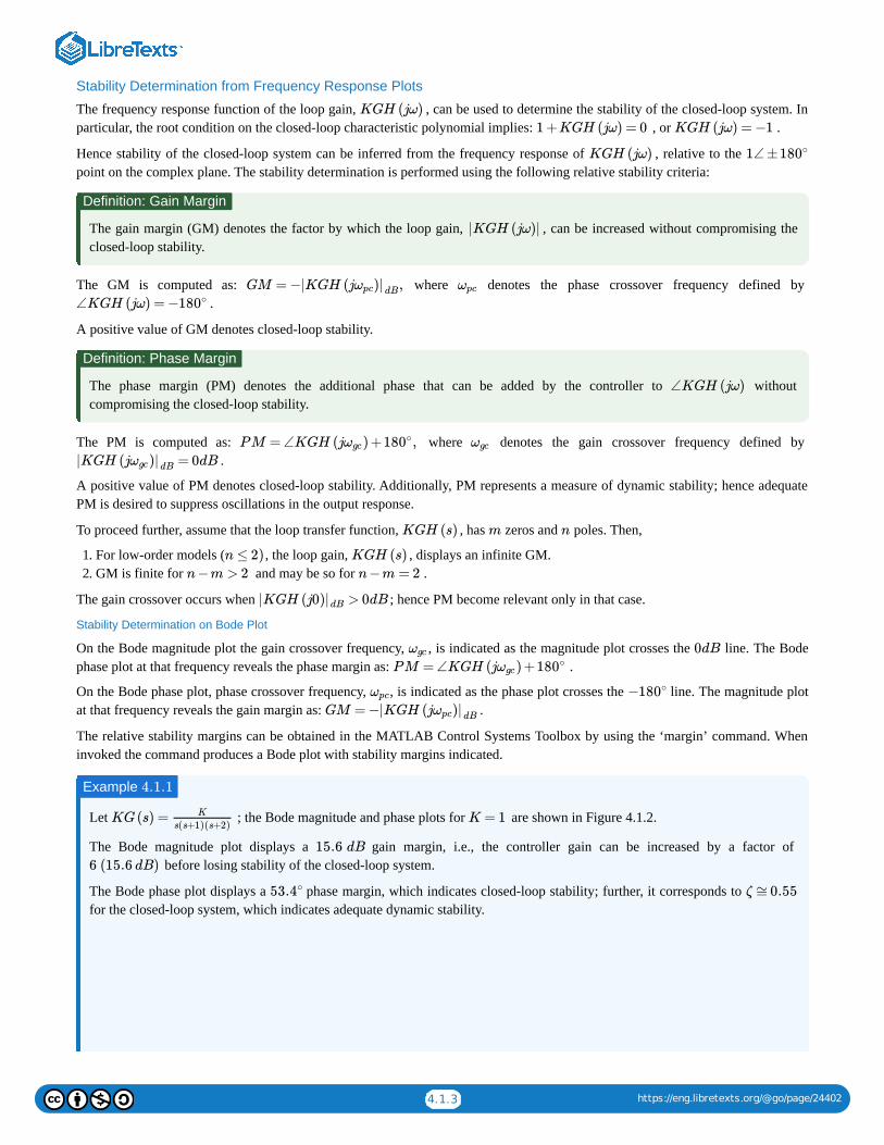
4.1.3 https://eng.libretexts.org/@go/page/24402

Stability Determination from Frequency Response Plots

The frequency response function of the loop gain, , can be used to determine the stability of the closed-loop system. Inparticular, the root condition on the closed-loop characteristic polynomial implies: , or .

Hence stability of the closed-loop system can be inferred from the frequency response of , relative to the point on the complex plane. The stability determination is performed using the following relative stability criteria:

The gain margin (GM) denotes the factor by which the loop gain, , can be increased without compromising theclosed-loop stability.

The GM is computed as: where denotes the phase crossover frequency defined by .

A positive value of GM denotes closed-loop stability.

The phase margin (PM) denotes the additional phase that can be added by the controller to withoutcompromising the closed-loop stability.

The PM is computed as: where denotes the gain crossover frequency defined by .

A positive value of PM denotes closed-loop stability. Additionally, PM represents a measure of dynamic stability; hence adequatePM is desired to suppress oscillations in the output response.

To proceed further, assume that the loop transfer function, , has zeros and poles. Then,

1. For low-order models ( , the loop gain, , displays an infinite GM.2. GM is finite for and may be so for .

The gain crossover occurs when ; hence PM become relevant only in that case.

Stability Determination on Bode Plot

On the Bode magnitude plot the gain crossover frequency, , is indicated as the magnitude plot crosses the line. The Bodephase plot at that frequency reveals the phase margin as: .

On the Bode phase plot, phase crossover frequency, , is indicated as the phase plot crosses the line. The magnitude plotat that frequency reveals the gain margin as: .

The relative stability margins can be obtained in the MATLAB Control Systems Toolbox by using the ‘margin’ command. Wheninvoked the command produces a Bode plot with stability margins indicated.

Let ; the Bode magnitude and phase plots for are shown in Figure 4.1.2.

The Bode magnitude plot displays a gain margin, i.e., the controller gain can be increased by a factor of before losing stability of the closed-loop system.

The Bode phase plot displays a phase margin, which indicates closed-loop stability; further, it corresponds to for the closed-loop system, which indicates adequate dynamic stability.

KGH (jω)1 +KGH (jω) = 0 KGH (jω) = −1

KGH (jω) 1∠ ±180∘

Definition: Gain Margin

  |KGH (jω)|

GM = − ,|KGH (j )|ωpc dB ωpc

∠KGH (jω) = −180∘

Definition: Phase Margin

∠KGH (jω)

PM = ∠KGH (j ) +180 ,ωgc∘ ωgc

= 0dB|KGH (j )|ωgc dB

KGH (s) m n

n ≤ 2) KGH (s)n−m > 2 n−m = 2

> 0dB|KGH (j0)|dB

ωgc 0dBPM = ∠KGH (j ) +180ωgc

∘

ωpc −180∘

GM = −|KGH (j )|ωpc dB

Example 4.1.1

KG(s) = K

s(s+1)(s+2)K = 1

15.6 dB

6 (15.6 dB)

53.4∘ ζ ≅0.55

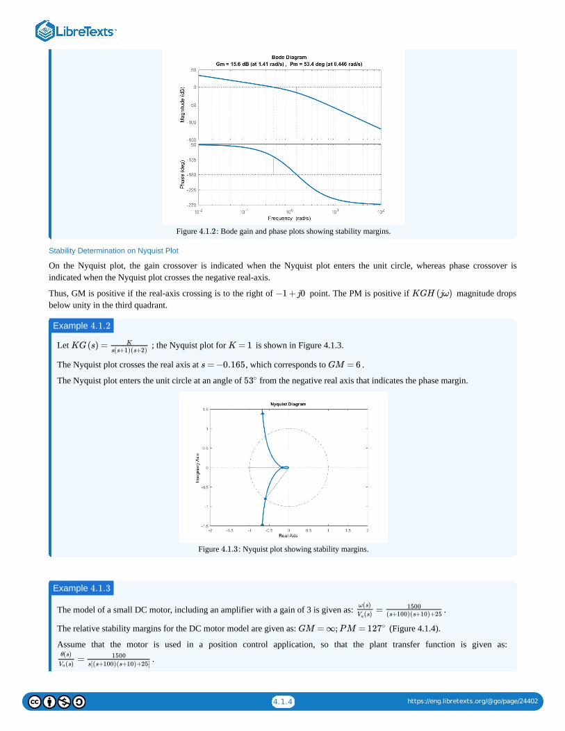
4.1.4 https://eng.libretexts.org/@go/page/24402

Figure : Bode gain and phase plots showing stability margins.

Stability Determination on Nyquist Plot

On the Nyquist plot, the gain crossover is indicated when the Nyquist plot enters the unit circle, whereas phase crossover isindicated when the Nyquist plot crosses the negative real-axis.

Thus, GM is positive if the real-axis crossing is to the right of point. The PM is positive if magnitude dropsbelow unity in the third quadrant.

Let ; the Nyquist plot for is shown in Figure 4.1.3.

The Nyquist plot crosses the real axis at , which corresponds to .

The Nyquist plot enters the unit circle at an angle of from the negative real axis that indicates the phase margin.

Figure : Nyquist plot showing stability margins.

The model of a small DC motor, including an amplifier with a gain of 3 is given as: .

The relative stability margins for the DC motor model are given as: (Figure 4.1.4).

Assume that the motor is used in a position control application, so that the plant transfer function is given as:

.

4.1.2

−1 +j0 KGH (jω)

Example 4.1.2

KG(s) = K

s(s+1)(s+2)K = 1

s = −0.165 GM = 6

53∘

4.1.3

Example 4.1.3

=ω(s)

(s)Va

1500(s+100)(s+10)+25

GM = ∞;PM = 127∘

=θ(s)

(s)Va

1500s[(s+100)(s+10)+25]

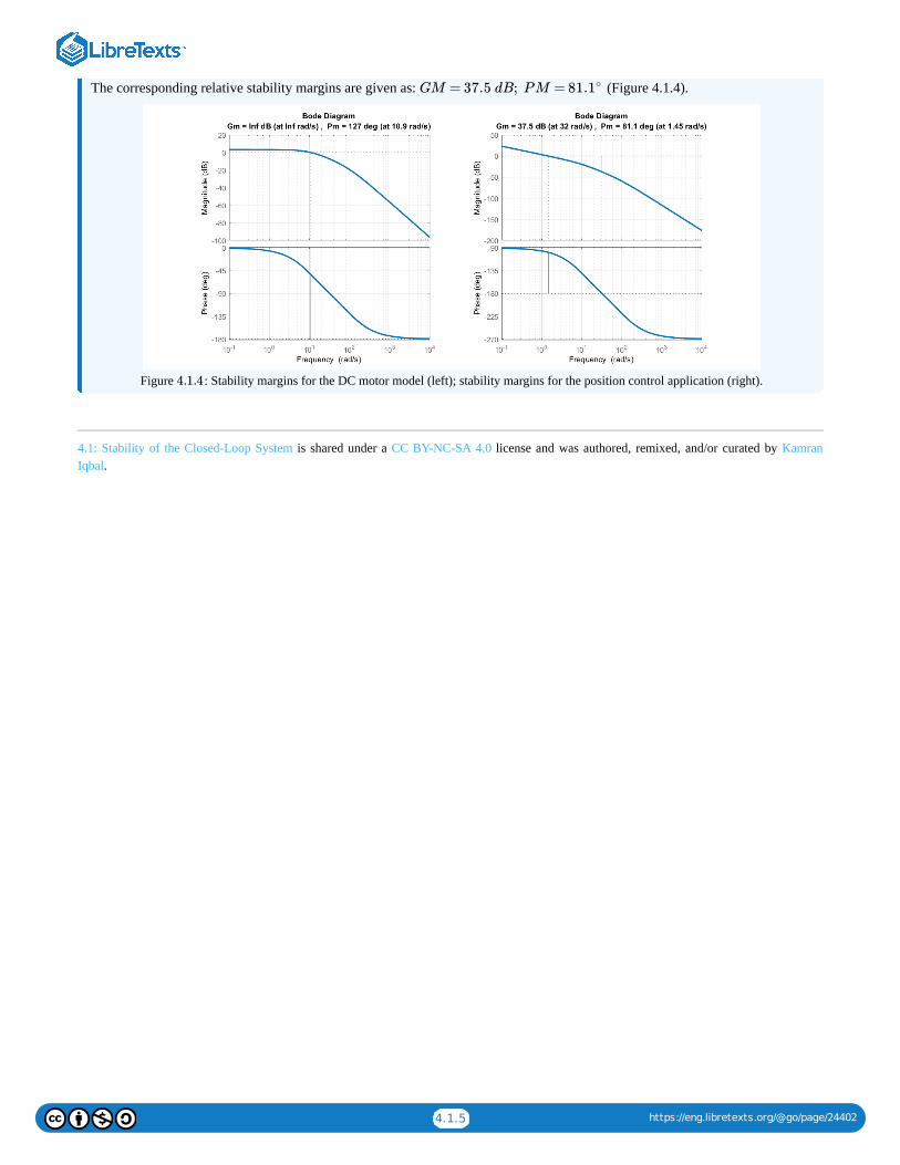
4.1.5 https://eng.libretexts.org/@go/page/24402

The corresponding relative stability margins are given as: (Figure 4.1.4).

Figure : Stability margins for the DC motor model (left); stability margins for the position control application (right).

4.1: Stability of the Closed-Loop System is shared under a CC BY-NC-SA 4.0 license and was authored, remixed, and/or curated by KamranIqbal.

GM = 37.5 dB;  PM = 81.1∘

4.1.4

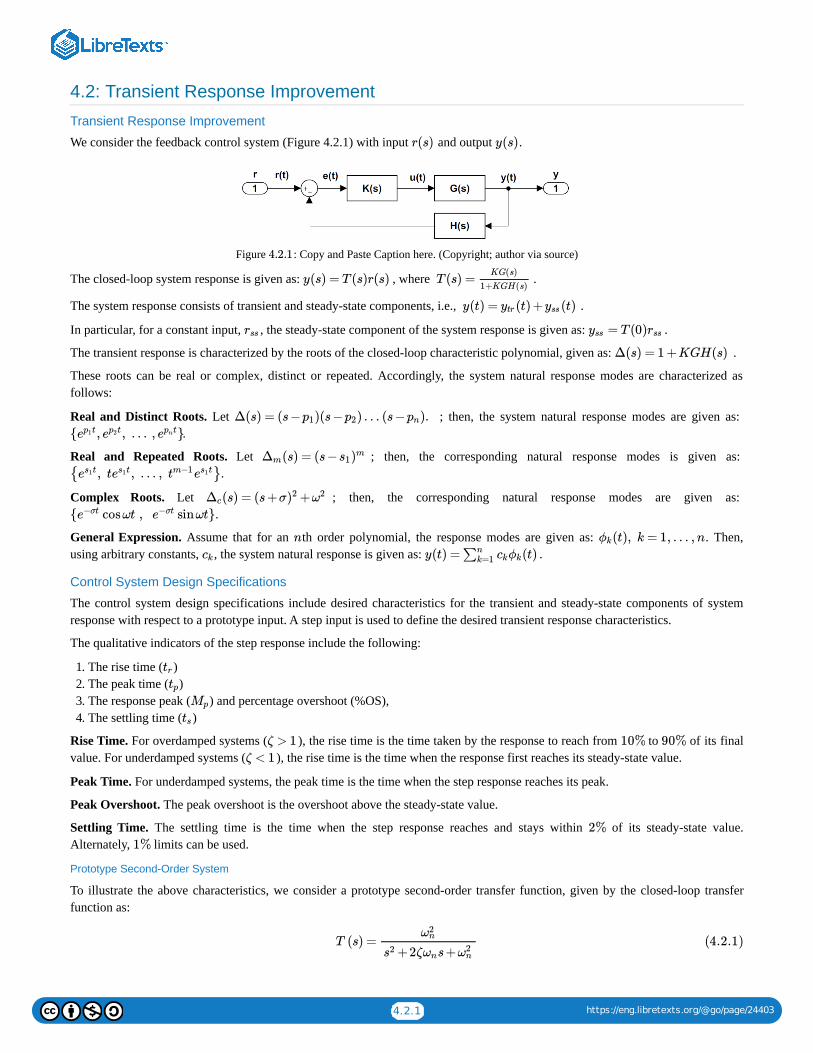
4.2.1 https://eng.libretexts.org/@go/page/24403

4.2: Transient Response Improvement

Transient Response Improvement

We consider the feedback control system (Figure 4.2.1) with input and output .

Figure : Copy and Paste Caption here. (Copyright; author via source)

The closed-loop system response is given as: , where .

The system response consists of transient and steady-state components, i.e., .

In particular, for a constant input, , the steady-state component of the system response is given as: .

The transient response is characterized by the roots of the closed-loop characteristic polynomial, given as: .

These roots can be real or complex, distinct or repeated. Accordingly, the system natural response modes are characterized asfollows:

Real and Distinct Roots. Let ; then, the system natural response modes are given as: .

Real and Repeated Roots. Let ; then, the corresponding natural response modes is given as: .

Complex Roots. Let ; then, the corresponding natural response modes are given as: .

General Expression. Assume that for an th order polynomial, the response modes are given as: . Then,using arbitrary constants, , the system natural response is given as: .

Control System Design Specifications

The control system design specifications include desired characteristics for the transient and steady-state components of systemresponse with respect to a prototype input. A step input is used to define the desired transient response characteristics.

The qualitative indicators of the step response include the following:

1. The rise time ( )2. The peak time ( )3. The response peak ( ) and percentage overshoot (%OS),4. The settling time ( )

Rise Time. For overdamped systems ( ), the rise time is the time taken by the response to reach from to of its finalvalue. For underdamped systems ( ), the rise time is the time when the response first reaches its steady-state value.

Peak Time. For underdamped systems, the peak time is the time when the step response reaches its peak.

Peak Overshoot. The peak overshoot is the overshoot above the steady-state value.

Settling Time. The settling time is the time when the step response reaches and stays within of its steady-state value.Alternately, limits can be used.

Prototype Second-Order System

To illustrate the above characteristics, we consider a prototype second-order transfer function, given by the closed-loop transferfunction as:

r(s) y(s)

4.2.1

y(s) = T (s)r(s) T (s) =KG(s)

1+KGH(s)

y(t) = (t) + (t)ytr yss

rss = T (0)yss rss

Δ(s) = 1 +KGH(s)

Δ(s) = (s− )(s− ) … (s− ).p1 p2 pn{ , , … , }e tp1 e tp2 e tpn

(s) = (s−Δm s1)m

{ , t , … , }e ts1 e ts1 tm−1e ts1

(s) = (s+σ +Δc )2 ω2

{ cosωt , sinωt}e−σt e−σt

n (t), k = 1, … ,nϕk

ck y(t) = (t)∑nk=1 ckϕk

trtp

Mp

ts

ζ > 1 10% 90%

ζ < 1

2%

1%

T (s) =ω2n

+2ζ s+s2 ωn ω2n

(4.2.1)

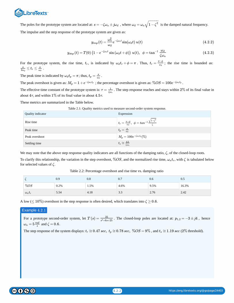
4.2.2 https://eng.libretexts.org/@go/page/24403

The poles for the prototype system are located at: , where is the damped natural frequency.

The impulse and the step response of the prototype system are given as:

For the prototype system, the rise time, , is indicated by . Thus, ; the rise time is bounded as: .

The peak time is indicated by ; thus, .

The peak overshoot is given as: ; the percentage overshoot is given as: .

The effective time constant of the prototype system is: . The step response reaches and stays within of its final value inabout , and within of its final value in about .

These metrics are summarized in the Table below.

Table 2.1: Quality metrics used to measure second-order system response.Quality indicator Expression

Rise time

Peak time

Peak overshoot

Settling time

We may note that the above step response quality indicators are all functions of the damping ratio, , of the closed-loop roots.

To clarify this relationship, the variation in the step overshoot, , and the normalized rise time, , with is tabulated belowfor selected values of .

Table 2.2: Percentage overshoot and rise time vs. damping ratio

0.9 0.8 0.7 0.6 0.5

0.2% 1.5% 4.6% 9.5% 16.3%

5.54 4.18 3.3 2.76 2.42

A low ( ) overshoot in the step response is often desired, which translates into

For a prototype second-order system, let . The closed-loop poles are located at: , hence and .

The step response of the system displays: , and ( threshold).

s = −ζ ±jωn ωd =ωd ωn 1 −ζ2− −−−−

√

(t) = sin( t) u(t)yimp

ω2n

ωd

e−ζ tωn ωd (4.2.2)

(t) = T (0)(1 − sin ( t+ϕ)) u(t), ϕ =ystep e−ζ tωn ωd tan−1 ωd

ζωn

(4.2.3)

tr +ϕ = πωdtr =trπ−ϕ

ωd

≤ ≤π2ωd

trπωd

= πωdtp =tpπ

ωd

= 1 +Mp e−ζωntp %OS = 100e−ζωntp

τ = 1ζωn

2%

4τ 1% 4.5τ

= ,  ϕ =  trπ−ϕ

ωdtan−1

1−ζ2√

ζ

=tpπωd

= 100 (%)Mp e−ζωntp

≅ts4.5ζωn

ζ

%OS ωntr ζ

ζ

ζ

%OS

ωntr

≤ 10% ζ ≥ 0.6.

Example 4.2.1

T (s) = 25

+6s+25s2 = −3 ±j4p1,2

= 5ωnrad

sζ = 0.6

≅0.47 sec, ≅0.78 sec, %OS = 9%tr tp ≅1.19 sects 2%

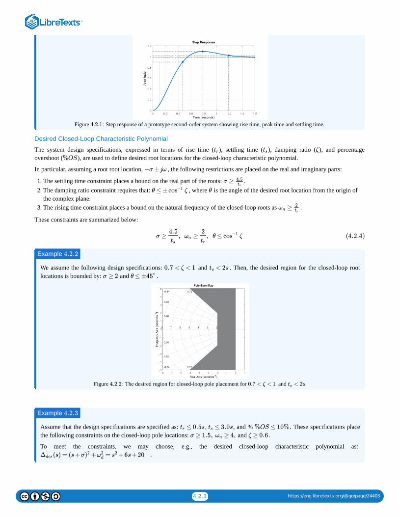
4.2.3 https://eng.libretexts.org/@go/page/24403

Figure : Step response of a prototype second-order system showing rise time, peak time and settling time.

Desired Closed-Loop Characteristic Polynomial

The system design specifications, expressed in terms of rise time ( ), settling time ( ), damping ratio ( ), and percentageovershoot ( ), are used to define desired root locations for the closed-loop characteristic polynomial.

In particular, assuming a root root location, , the following restrictions are placed on the real and imaginary parts:

1. The settling time constraint places a bound on the real part of the roots: .2. The damping ratio constraint requires that: , where is the angle of the desired root location from the origin of

the complex plane.3. The rising time constraint places a bound on the natural frequency of the closed-loop roots as .

These constraints are summarized below:

We assume the following design specifications: and . Then, the desired region for the closed-loop rootlocations is bounded by: and .

Figure : The desired region for closed-loop pole placement for and s.

Assume that the design specifications are specified as: , , and % . These specifications placethe following constraints on the closed-loop pole locations: and .

To meet the constraints, we may choose, e.g., the desired closed-loop characteristic polynomial as: .

4.2.1

tr ts ζ

%OS

−σ±jω

σ ≥ 4.5ts

θ ≤ ± ζcos−1 θ

≥ωn2tr

σ ≥ ,    ≥ ,   θ ≤ ζ4.5

tsωn

2

trcos−1 (4.2.4)

Example 4.2.2

0.7 < ζ < 1 < 2stsσ ≥ 2 θ ≤ ±45∘

4.2.2 0.7 < ζ < 1 < 2ts

Example 4.2.3

≤ 0.5str ≤ 3.0sts %OS ≤ 10%

σ ≥ 1.5,   ≥ 4,ωn ζ ≥ 0.6

(s) = (s+σ + = +6s+20Δdes )2 ω2d s2

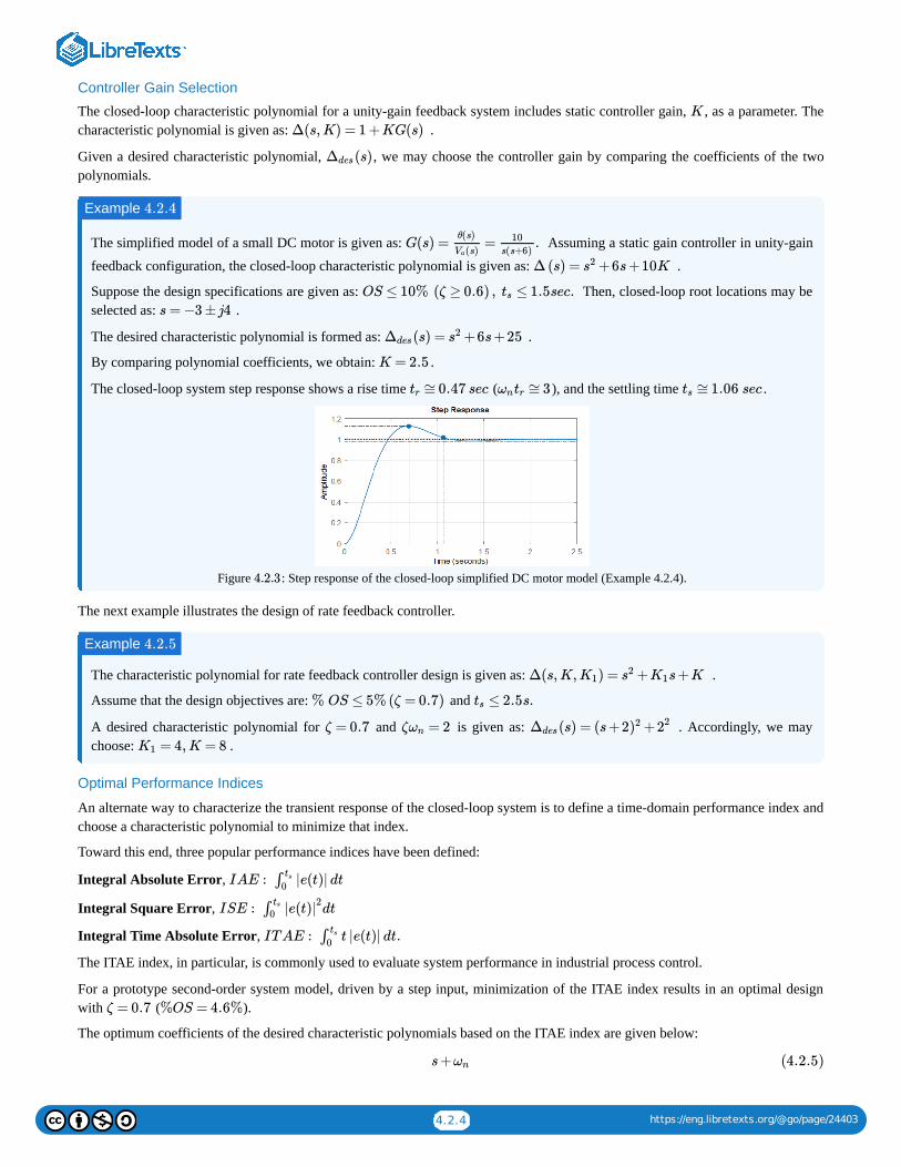
4.2.4 https://eng.libretexts.org/@go/page/24403

Controller Gain Selection

The closed-loop characteristic polynomial for a unity-gain feedback system includes static controller gain, , as a parameter. Thecharacteristic polynomial is given as: .

Given a desired characteristic polynomial, , we may choose the controller gain by comparing the coefficients of the twopolynomials.

The simplified model of a small DC motor is given as: Assuming a static gain controller in unity-gain

feedback configuration, the closed-loop characteristic polynomial is given as: .

Suppose the design specifications are given as: Then, closed-loop root locations may beselected as: .

The desired characteristic polynomial is formed as: .

By comparing polynomial coefficients, we obtain: .

The closed-loop system step response shows a rise time ( ), and the settling time .

Figure : Step response of the closed-loop simplified DC motor model (Example 4.2.4).

The next example illustrates the design of rate feedback controller.

The characteristic polynomial for rate feedback controller design is given as: .

Assume that the design objectives are: and

A desired characteristic polynomial for and is given as: . Accordingly, we maychoose: .

Optimal Performance Indices

An alternate way to characterize the transient response of the closed-loop system is to define a time-domain performance index andchoose a characteristic polynomial to minimize that index.

Toward this end, three popular performance indices have been defined:

Integral Absolute Error,

Integral Square Error,

Integral Time Absolute Error,

The ITAE index, in particular, is commonly used to evaluate system performance in industrial process control.

For a prototype second-order system model, driven by a step input, minimization of the ITAE index results in an optimal designwith ( ).

The optimum coefficients of the desired characteristic polynomials based on the ITAE index are given below:

K

Δ(s,K) = 1 +KG(s)

(s)Δdes

Example 4.2.4

G(s) = = .θ(s)

(s)Va

10

s(s+6)

Δ (s) = +6s+10Ks2

OS ≤ 10%  (ζ ≥ 0.6) ,   ≤ 1.5sec.tss = −3 ±j4

(s) = +6s+25Δdes s2

K = 2.5

≅0.47 sectr ≅3ωntr ≅1.06 sects

4.2.3

Example 4.2.5

Δ(s,K, ) = + s+KK1 s2 K1

% OS ≤ 5% (ζ = 0.7) ≤ 2.5s.ts

ζ = 0.7 ζ = 2ωn (s) = (s+2 +Δdes )2 22

= 4,K = 8K1

IAE : |e(t)| dt∫ ts0

ISE : dt∫ ts0 |e(t)|

2

ITAE : t |e(t)| dt.∫ ts0

ζ = 0.7 %OS = 4.6%

s+ωn (4.2.5)

4.2.5 https://eng.libretexts.org/@go/page/24403

The first-order-plus-dead-time (FOPDT) model of an industrial process is given as: . By using first-order Pade’approximation: , we obtain a rational approximation as: .

The closed-loop characteristic polynomial for a unity-gain feedback control system is: .

Using the ITAE index, a desired second-order polynomial is selected as: .

By comparing the polynomial coefficients, we obtain two equations that are solved to obtain: and .

4.2: Transient Response Improvement is shared under a CC BY-NC-SA 4.0 license and was authored, remixed, and/or curated by Kamran Iqbal.

+1.4 s+s2 ωn ω2n (4.2.6)

+1.75 +2.15 s+s3 ωns2 ω2

n ω3n (4.2.7)

+2.1 +3.4 +2.7 s+ .s4 ωns3 ω2

ns2 ω2

n ω3n (4.2.8)

Example 4.2.6

G(s) = e−s

s+1

≅e−s 2−s

2+sG(s) ≅ 2−s

(s+1)(s+2)

Δ (s) = (s+1) (s+2) +K(2 −s)

(s) = +1.4 s+Δdes s2 ωn ω2n

= 1.76ωnrad

sK = 0.54

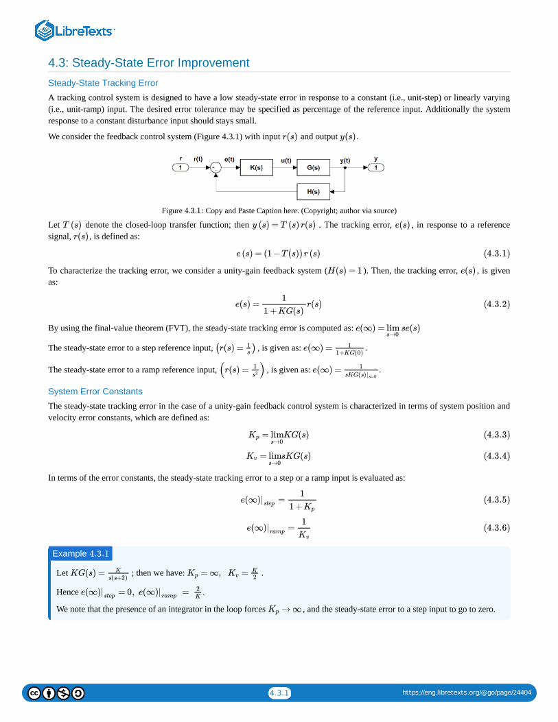
4.3.1 https://eng.libretexts.org/@go/page/24404

4.3: Steady-State Error Improvement

Steady-State Tracking Error

A tracking control system is designed to have a low steady-state error in response to a constant (i.e., unit-step) or linearly varying(i.e., unit-ramp) input. The desired error tolerance may be specified as percentage of the reference input. Additionally the systemresponse to a constant disturbance input should stays small.

We consider the feedback control system (Figure 4.3.1) with input and output .

Figure : Copy and Paste Caption here. (Copyright; author via source)

Let denote the closed-loop transfer function; then . The tracking error, , in response to a referencesignal, , is defined as:

To characterize the tracking error, we consider a unity-gain feedback system ( ). Then, the tracking error, , is givenas:

By using the final-value theorem (FVT), the steady-state tracking error is computed as:

The steady-state error to a step reference input, , is given as:

The steady-state error to a ramp reference input, , is given as:

System Error Constants

The steady-state tracking error in the case of a unity-gain feedback control system is characterized in terms of system position andvelocity error constants, which are defined as:

In terms of the error constants, the steady-state tracking error to a step or a ramp input is evaluated as:

Let ; then we have: .

Hence

We note that the presence of an integrator in the loop forces , and the steady-state error to a step input to go to zero.

r(s) y(s)

4.3.1

T (s) y (s) = T (s) r(s) e(s)

r(s)

e (s) = (1 −T (s)) r (s) (4.3.1)

H(s) = 1 e(s)

e(s) = r(s)1

1 +KG(s)(4.3.2)

e(∞) = se(s)lims→0

(r(s) = )1s

e(∞) = .11+KG(0)

(r(s) = )1

s2 e(∞) = .1

sKG(s)|s=0

= KG(s)Kp lims→0

(4.3.3)

= sKG(s)Kv lims→0

(4.3.4)

=e(∞)|step1

1 +Kp

(4.3.5)

=e(∞)|ramp

1

Kv

(4.3.6)

Example 4.3.1

KG(s) = K

s(s+2)= ∞, =Kp Kv

K2

= 0, = .e(∞)|step e(∞)|ramp2K

→ ∞Kp

4.3.2 https://eng.libretexts.org/@go/page/24404

The approximate model of a small DC motor is given as:

Then we have: , and .

Hence

Integral control, , is often employed to reduce the steady-state tracking error. The presence of an integrator in theloop forces , and the steady-state error to a step input to go to zero.

Steady-State Error to Ramp Input

Assuming that the feedback loop contains an integrator, so that the steady-state error to a step input is zero, the steady-state error toa ramp input is expressed as:

The error is evaluated by the application of FVT:

By using the L’ Hospital’s rule, we obtain: .

To evaluate the RHS, we use the natural logarithm to write:

Since by the integrator assumption, we have: .

Next, assume that is expressed as:

Then, we have: and

It follows that:

where and denote the zeros and poles of the closed-loop system.

Let ; then, the closed-loop characteristic polynomial is: .

Assuming a value of , the closed-loop poles are located at: .

The resulting steady-state error to a ramp input is given as: .

For verification, the closed-loop system response is plotted in Figure 4.3.1.

Example 4.3.2

KG(s) =500K

(s+10) (s+100)(4.3.7)

= 0.5KKp = 0Kv

= , = ∞.e(∞)|step2K

e(∞)|ramp

K (s) =kis

→ ∞Kp

e(s) = [1 −T (s)] r(s); r(s) = .1

s2(4.3.8)

= .e(∞)|ramp lims→0

1−T (s)

s

= (− )e(∞)|ramp lims→0

dT (s)

ds

lnT (s) = .d

ds

1T (s)

dT (s)

ds

T (s) = 1lims→0

lnT (s) =lims→0

d

dslims→0

dT (s)

ds

T (s) T (s) = .K(s− )…(s− )z1 zm

(s− )…(s− )p1 pn

lnT (s) = lnK+ (s− ) − (s− ),∑ln zi ∑ln pi

lnT (s) = lnK+∑ −∑d

ds

1

s−zi

1

s−pi(4.3.9)

=∑ −∑e(∞)|ramp

1

pi

1

zi(4.3.10)

zi pi

Example 4.3.3

KG(s) = K

s(s+2)Δ (s) = +2s+Ks2

K = 1 = −1,   −1s1,2

=∑ = 2e(∞)|ramp1pi

4.3.3 https://eng.libretexts.org/@go/page/24404

Figure : Steady-state error to a ramp input (Example 4.3.3).

4.3: Steady-State Error Improvement is shared under a CC BY-NC-SA 4.0 license and was authored, remixed, and/or curated by Kamran Iqbal.

4.3.1

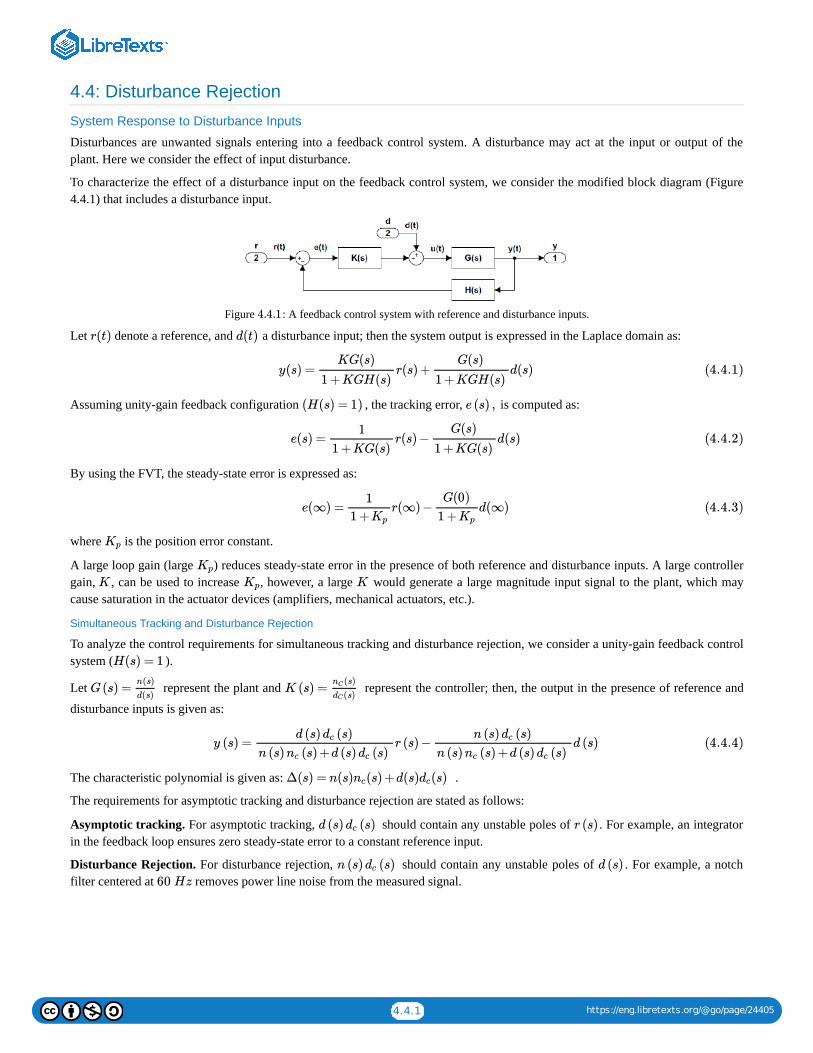
4.4.1 https://eng.libretexts.org/@go/page/24405

4.4: Disturbance Rejection

System Response to Disturbance Inputs

Disturbances are unwanted signals entering into a feedback control system. A disturbance may act at the input or output of theplant. Here we consider the effect of input disturbance.

To characterize the effect of a disturbance input on the feedback control system, we consider the modified block diagram (Figure4.4.1) that includes a disturbance input.

Figure : A feedback control system with reference and disturbance inputs.

Let denote a reference, and a disturbance input; then the system output is expressed in the Laplace domain as:

Assuming unity-gain feedback configuration , the tracking error, is computed as:

By using the FVT, the steady-state error is expressed as:

where is the position error constant.

A large loop gain (large ) reduces steady-state error in the presence of both reference and disturbance inputs. A large controllergain, , can be used to increase , however, a large would generate a large magnitude input signal to the plant, which maycause saturation in the actuator devices (amplifiers, mechanical actuators, etc.).

Simultaneous Tracking and Disturbance Rejection

To analyze the control requirements for simultaneous tracking and disturbance rejection, we consider a unity-gain feedback controlsystem ( ).

Let represent the plant and represent the controller; then, the output in the presence of reference and

disturbance inputs is given as:

The characteristic polynomial is given as: .

The requirements for asymptotic tracking and disturbance rejection are stated as follows:

Asymptotic tracking. For asymptotic tracking, should contain any unstable poles of . For example, an integratorin the feedback loop ensures zero steady-state error to a constant reference input.

Disturbance Rejection. For disturbance rejection, should contain any unstable poles of . For example, a notchfilter centered at removes power line noise from the measured signal.

4.4.1

r(t) d(t)

y(s) = r(s) + d(s)KG(s)

1 +KGH(s)

G(s)

1 +KGH(s)(4.4.1)

(H(s) = 1) e (s) ,

e(s) = r(s) − d(s)1

1 +KG(s)

G(s)

1 +KG(s)(4.4.2)

e(∞) = r(∞) − d(∞)1

1 +Kp

G(0)

1 +Kp

(4.4.3)

Kp

Kp

K Kp K

H(s) = 1

G(s) =n(s)

d(s)K (s) =

(s)nC

(s)dC

y (s) = r (s) − d (s)d (s) (s)dc

n (s) (s) +d (s) (s)nc dc

n (s) (s)dc

n (s) (s) +d (s) (s)nc dc(4.4.4)

Δ(s) = n(s) (s) +d(s) (s)nc dc

d (s) (s)dc r (s)

n (s) (s)dc d (s)60 Hz

4.4.2 https://eng.libretexts.org/@go/page/24405

A small DC motor has the following component values:

The DC motor transfer function is given as: .

Since with a static controller, the position error constant is: . The steady-state error in the presence ofreference and disturbance inputs is given as:

We may choose a large to reduce the steady-state tracking error as well as improve the disturbance rejection. A large valueof K, however, reduces system damping and results in an oscillatory response of the DC motor.

For a static controller, the closed-loop characteristic polynomial is given as: Theresulting damping ratio is: .

In order to limit the damping to, say , the controller gain is limited to: . We may choose, for example, , which results in the following steady-state error to reference and disturbance inputs:

4.4: Disturbance Rejection is shared under a CC BY-NC-SA 4.0 license and was authored, remixed, and/or curated by Kamran Iqbal.

Example 4.4.1

R = 1 Ω, L = 10 mH, J = 0.01 kg , b = 0.1 , = = 0.05.m2 Nsrad

kt kb

G(s) = 500+110s+1025s2

G(0) ≅0.5, = 0.5KKp

e(∞) = r(∞) − d(∞).1

1 +0.5K

0.5

1 +0.5K

K

Δ(s,K) = +110s+1025 +500K.s2

ζ = 551025+500K√

ζ ≤ 0.6 K ≤ 14.75

K = 14 e(∞) = r(∞) − d(∞).18

116

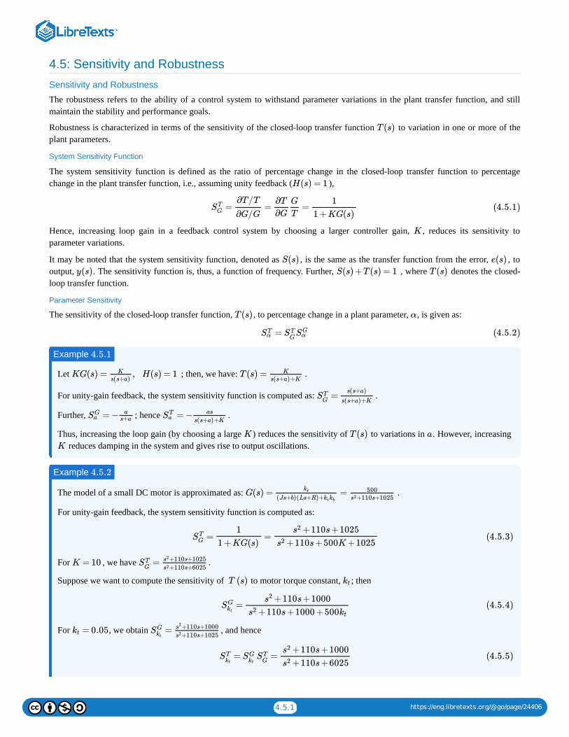
4.5.1 https://eng.libretexts.org/@go/page/24406

4.5: Sensitivity and Robustness

Sensitivity and Robustness

The robustness refers to the ability of a control system to withstand parameter variations in the plant transfer function, and stillmaintain the stability and performance goals.

Robustness is characterized in terms of the sensitivity of the closed-loop transfer function to variation in one or more of theplant parameters.

System Sensitivity Function

The system sensitivity function is defined as the ratio of percentage change in the closed-loop transfer function to percentagechange in the plant transfer function, i.e., assuming unity feedback ( ),

Hence, increasing loop gain in a feedback control system by choosing a larger controller gain, , reduces its sensitivity toparameter variations.

It may be noted that the system sensitivity function, denoted as , is the same as the transfer function from the error, , tooutput, . The sensitivity function is, thus, a function of frequency. Further, , where denotes the closed-loop transfer function.

Parameter Sensitivity

The sensitivity of the closed-loop transfer function, , to percentage change in a plant parameter, , is given as:

Let ; then, we have: .

For unity-gain feedback, the system sensitivity function is computed as: .

Further, ; hence .

Thus, increasing the loop gain (by choosing a large ) reduces the sensitivity of to variations in . However, increasing reduces damping in the system and gives rise to output oscillations.

The model of a small DC motor is approximated as: .

For unity-gain feedback, the system sensitivity function is computed as:

For , we have .

Suppose we want to compute the sensitivity of to motor torque constant, ; then

For , we obtain , and hence

T (s)

H(s) = 1

= = =STG

∂T /T

∂G/G

∂T

∂G

G

T

1

1 +KG(s)(4.5.1)

K

S(s) e(s)

y(s) S(s) +T (s) = 1 T (s)

T (s) α

=STα ST

GSG

α (4.5.2)

Example 4.5.1

KG(s) = , H(s) = 1K

s(s+a)T (s) = K

s(s+a)+K

=STG

s(s+a)

s(s+a)+K

= −SGa

as+a = −ST

aas

s(s+a)+K

K T (s) a

K

Example 4.5.2

G(s) = =kt

(Js+b)(Ls+R)+ktkb

500+110s+1025s2

= =STG

1

1 +KG(s)

+110s +1025s2

+110s +500K +1025s2(4.5.3)

K = 10 =STG

+110s+1025s2

+110s+6025s2

T (s) kt

=SGkt

+110s +1000s2

+110s +1000 +500s2 kt

(4.5.4)

= 0.05kt =SGkt

+110s+1000s2

+110s+1025s2

= =STkt

SGkt

STG

+110s +1000s2

+110s +6025s2(4.5.5)

4.5.2 https://eng.libretexts.org/@go/page/24406

A Bode magnitude plot of the sensitivity function is shown in Fig. 4.5.1.

Figure : Bode magnitude plot of the sensitivity function.

4.5: Sensitivity and Robustness is shared under a CC BY-NC-SA 4.0 license and was authored, remixed, and/or curated by Kamran Iqbal.

4.5.1

1

CHAPTER OVERVIEW

5: Control System Design with Root Locus

1. Sketch the root locus of a transfer function with respect to the controller gain K.2. Use root locus technique to design a static controller for a transfer function model.3. Use root locus technique to design first-order phase-lead and phase-lag controllers.4. Realize the controller design using operational amplifiers and filters.

5.0: Prelude to Control System Design with Root Locus5.1: Root Locus Fundamentals5.2: Static Controller Design5.3: Transient Response Improvement5.4: Steady-State Error Improvement5.5: Transient and Steady-State Improvement5.6: Controller Realization

5: Control System Design with Root Locus is shared under a CC BY-NC-SA 4.0 license and was authored, remixed, and/or curated by KamranIqbal.

Learning Objectives

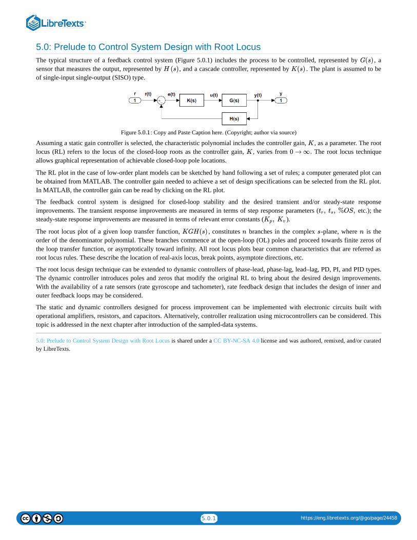
5.0.1 https://eng.libretexts.org/@go/page/24458

5.0: Prelude to Control System Design with Root LocusThe typical structure of a feedback control system (Figure 5.0.1) includes the process to be controlled, represented by , asensor that measures the output, represented by , and a cascade controller, represented by . The plant is assumed to beof single-input single-output (SISO) type.

Figure : Copy and Paste Caption here. (Copyright; author via source)

Assuming a static gain controller is selected, the characteristic polynomial includes the controller gain, , as a parameter. The rootlocus (RL) refers to the locus of the closed-loop roots as the controller gain, , varies from . The root locus techniqueallows graphical representation of achievable closed-loop pole locations.

The RL plot in the case of low-order plant models can be sketched by hand following a set of rules; a computer generated plot canbe obtained from MATLAB. The controller gain needed to achieve a set of design specifications can be selected from the RL plot.In MATLAB, the controller gain can be read by clicking on the RL plot.

The feedback control system is designed for closed-loop stability and the desired transient and/or steady-state responseimprovements. The transient response improvements are measured in terms of step response parameters ( etc.); thesteady-state response improvements are measured in terms of relevant error constants ( ).

The root locus plot of a given loop transfer function, , constitutes branches in the complex -plane, where is theorder of the denominator polynomial. These branches commence at the open-loop (OL) poles and proceed towards finite zeros ofthe loop transfer function, or asymptotically toward infinity. All root locus plots bear common characteristics that are referred asroot locus rules. These describe the location of real-axis locus, break points, asymptote directions, etc.

The root locus design technique can be extended to dynamic controllers of phase-lead, phase-lag, lead–lag, PD, PI, and PID types.The dynamic controller introduces poles and zeros that modify the original RL to bring about the desired design improvements.With the availability of a rate sensors (rate gyroscope and tachometer), rate feedback design that includes the design of inner andouter feedback loops may be considered.

The static and dynamic controllers designed for process improvement can be implemented with electronic circuits built withoperational amplifiers, resistors, and capacitors. Alternatively, controller realization using microcontrollers can be considered. Thistopic is addressed in the next chapter after introduction of the sampled-data systems.

5.0: Prelude to Control System Design with Root Locus is shared under a CC BY-NC-SA 4.0 license and was authored, remixed, and/or curatedby LibreTexts.

G(s)

H (s) K(s)

5.0.1

K

K 0 → ∞

,   ,  %OS,tr ts

,  Kp Kv

KGH(s) n s n

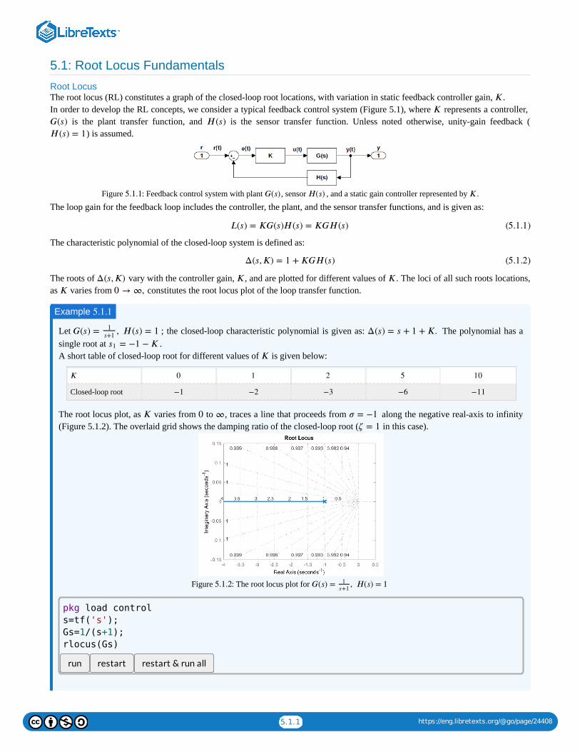
5.1.1 https://eng.libretexts.org/@go/page/24408

5.1: Root Locus Fundamentals

Root LocusThe root locus (RL) constitutes a graph of the closed-loop root locations, with variation in static feedback controller gain, .In order to develop the RL concepts, we consider a typical feedback control system (Figure 5.1), where represents a controller,

is the plant transfer function, and is the sensor transfer function. Unless noted otherwise, unity-gain feedback () is assumed.

Figure : Feedback control system with plant , sensor , and a static gain controller represented by .

The loop gain for the feedback loop includes the controller, the plant, and the sensor transfer functions, and is given as:

The characteristic polynomial of the closed-loop system is defined as:

The roots of vary with the controller gain, , and are plotted for different values of . The loci of all such roots locations,as varies from constitutes the root locus plot of the loop transfer function.

Let ; the closed-loop characteristic polynomial is given as: The polynomial has asingle root at .A short table of closed-loop root for different values of is given below:

Closed-loop root

The root locus plot, as varies from to , traces a line that proceeds from along the negative real-axis to infinity(Figure 5.1.2). The overlaid grid shows the damping ratio of the closed-loop root ( in this case).

Figure : The root locus plot for

run restart restart & run all

𝐾

𝐾

𝐺(𝑠) 𝐻(𝑠)

𝐻(𝑠) = 1

5.1.1 𝐺(𝑠) 𝐻(𝑠) 𝐾

𝐿(𝑠) = 𝐾𝐺(𝑠)𝐻(𝑠) = 𝐾𝐺𝐻(𝑠) (5.1.1)

Δ(𝑠,𝐾) = 1 +𝐾𝐺𝐻(𝑠) (5.1.2)

Δ(𝑠,𝐾) 𝐾 𝐾

𝐾 0 →∞,

Example 5.1.1

𝐺(𝑠) = , 𝐻(𝑠) = 11

𝑠+1Δ(𝑠) = 𝑠 + 1 +𝐾.

= −1 −𝐾𝑠1

𝐾

𝐾 0 1 2 5 10

−1 −2 −3 −6 −11

𝐾 0 ∞ 𝜎 = −1𝜁 = 1

5.1.2 𝐺(𝑠) = , 𝐻(𝑠) = 11

𝑠+1

pkg load control

s=tf('s');

Gs=1/(s+1);

rlocus(Gs)

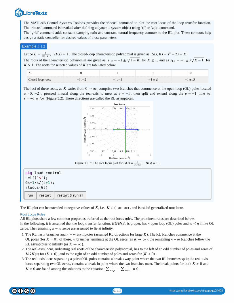
5.1.2 https://eng.libretexts.org/@go/page/24408

The MATLAB Control Systems Toolbox provides the ‘rlocus’ command to plot the root locus of the loop transfer function.The ‘rlocus’ command is invoked after defining a dynamic system object using ‘tf’ or ‘zpk’ command.The ‘grid’ command adds constant damping ratio and constant natural frequency contours to the RL plot. These contours helpdesign a static controller for desired values of those parameters.

Let . The closed-loop characteristic polynomial is given as:

The roots of the characteristic polynomial are given as: for , and as for . The roots for selected values of are tabulated below.

Closed-loop roots

The loci of these roots, as varies from , comprise two branches that commence at the open-loop (OL) poles locatedat , proceed inward along the real-axis to meet at , then split and extend along the line to

(Figure 5.2). These directions are called the RL asymptotes.

Figure : The root locus plot for .

run restart restart & run all

The RL plot can be extended to negative values of , i.e., , and is called generalized root locus.

Root Locus RulesAll RL plots share a few common properties, referred as the root locus rules. The prominent rules are described below.In the following, it is assumed that the loop transfer function, , is proper, has open loop (OL) poles and finite OLzeros. The remaining zeros are assumed to lie at infinity.

1. The RL has branches and asymptotes (assumed RL directions for large ). The RL branches commence at theOL poles (for ); of these, branches terminate at the OL zeros (as ); the remaining branches follow theRL asymptotes to infinity (as ).

2. The real-axis locus, indicating real roots of the characteristic polynomial, lies to the left of an odd number of poles and zeros of for , and to the right of an odd number of poles and zeros for .

3. The real-axis locus separating a pair of OL poles contains a break-away point where the two RL branches split; the real-axislocus separating two OL zeros, contains a break-in point where the two branches meet. The break points for both and

are found among the solutions to the equation: .

Example 5.1.2

𝐺(𝑠) = , 𝐻(𝑠) = 11

𝑠(𝑠+2)Δ(𝑠,𝐾) = + 2𝑠 +𝐾.𝑠2

= −1 ±𝑠1,2 1 −𝐾⎯ ⎯⎯⎯⎯⎯⎯⎯⎯⎯

√ 𝐾 ≤ 1 = −1 ± 𝑗𝑠1,2 𝐾 − 1⎯ ⎯⎯⎯⎯⎯⎯⎯⎯⎯

√𝐾 > 1 𝐾

𝐾 0 1 2 10

−1,−2 −1,−1 −1 ± 𝑗1 −1 ± 𝑗3

𝐾 0 →∞{0, −2} 𝜎 = −1 𝜎 = −1

𝑠 = −1 ± 𝑗∞

5.1.3 𝐺(𝑠) = , 𝐻(𝑠) = 11

𝑠(𝑠+2)

𝐾 𝐾 ∈ (−∞, ∞)

𝐾𝐺𝐻(𝑠) 𝑛 𝑚 ≤ 𝑛𝑛 − 𝑚

𝑛 𝑛 − 𝑚 𝐾

𝐾 = 0 𝑚 𝐾 →∞ 𝑛 − 𝑚𝐾 →∞

𝐾𝐺𝐻(𝑠) (𝐾 > 0) (𝐾 < 0)

𝐾 > 0

𝐾 < 0 ∑ −∑ = 01𝜎−𝑝𝑖

1𝜎−𝑧𝑖

pkg load control

s=tf('s');

Gs=1/s/(s+1);

rlocus(Gs)

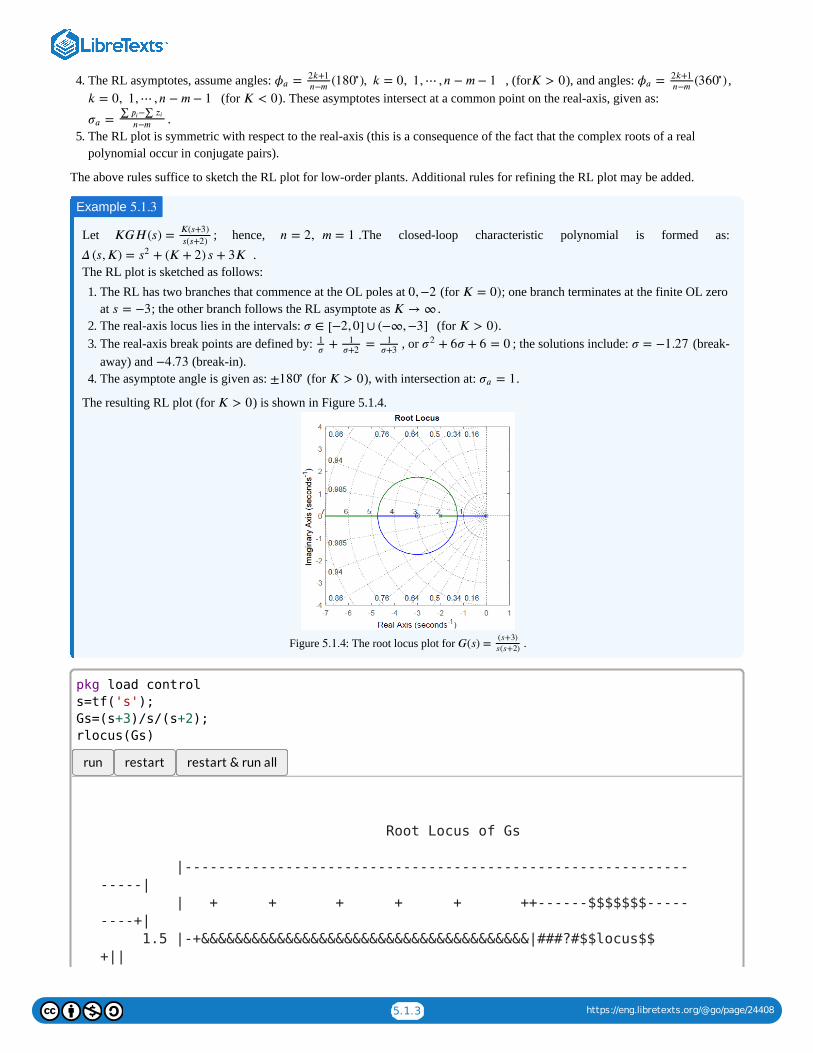
5.1.3 https://eng.libretexts.org/@go/page/24408

4. The RL asymptotes, assume angles: , (for ), and angles: , (for ). These asymptotes intersect at a common point on the real-axis, given as:

.5. The RL plot is symmetric with respect to the real-axis (this is a consequence of the fact that the complex roots of a real

polynomial occur in conjugate pairs).

The above rules suffice to sketch the RL plot for low-order plants. Additional rules for refining the RL plot may be added.

Let ; hence, .The closed-loop characteristic polynomial is formed as: .

The RL plot is sketched as follows:1. The RL has two branches that commence at the OL poles at (for ; one branch terminates at the finite OL zero

at ; the other branch follows the RL asymptote as .2. The real-axis locus lies in the intervals: (for .3. The real-axis break points are defined by: , or ; the solutions include: (break-

away) and (break-in).4. The asymptote angle is given as: (for ), with intersection at: .

The resulting RL plot (for ) is shown in Figure 5.1.4.

Figure : The root locus plot for .

run restart restart & run all

= ( ), 𝑘 = 0, 1,⋯ ,𝑛 − 𝑚− 1𝜙𝑎2𝑘+1

𝑛−𝑚 180∘ 𝐾 > 0 = ( )𝜙𝑎

2𝑘+1

𝑛−𝑚 360∘

𝑘 = 0, 1,⋯ ,𝑛 − 𝑚− 1 𝐾 < 0

=𝜎𝑎∑ −∑𝑝𝑖 𝑧𝑖

𝑛−𝑚

Example 5.1.3

𝐾𝐺𝐻(𝑠) =𝐾(𝑠+3)

𝑠(𝑠+2)𝑛 = 2,   𝑚 = 1

Δ (𝑠,𝐾) = + (𝐾 + 2)𝑠 + 3𝐾𝑠2

0,−2 𝐾 = 0)

𝑠 = −3 𝐾 →∞𝜎 ∈ [−2,0] ∪ (−∞,−3] 𝐾 > 0)

+ =1𝜎

1𝜎+2

1𝜎+3

+ 6𝜎 + 6 = 0𝜎2 𝜎 = −1.27−4.73

±180∘ 𝐾 > 0 = 1𝜎𝑎

𝐾 > 0

5.1.4 𝐺(𝑠) =(𝑠+3)

𝑠(𝑠+2)

Root Locus of Gs

|------------------------------------------------------------

-----|

| + + + + + ++------$$$$$$$-----

----+|

1.5 |-+&&&&&&&&&&&&&&&&&&&&&&&&&&&&&&&&&&&&&&&|###?#$$locus$$

+||

pkg load control

s=tf('s');

Gs=(s+3)/s/(s+2);

rlocus(Gs)

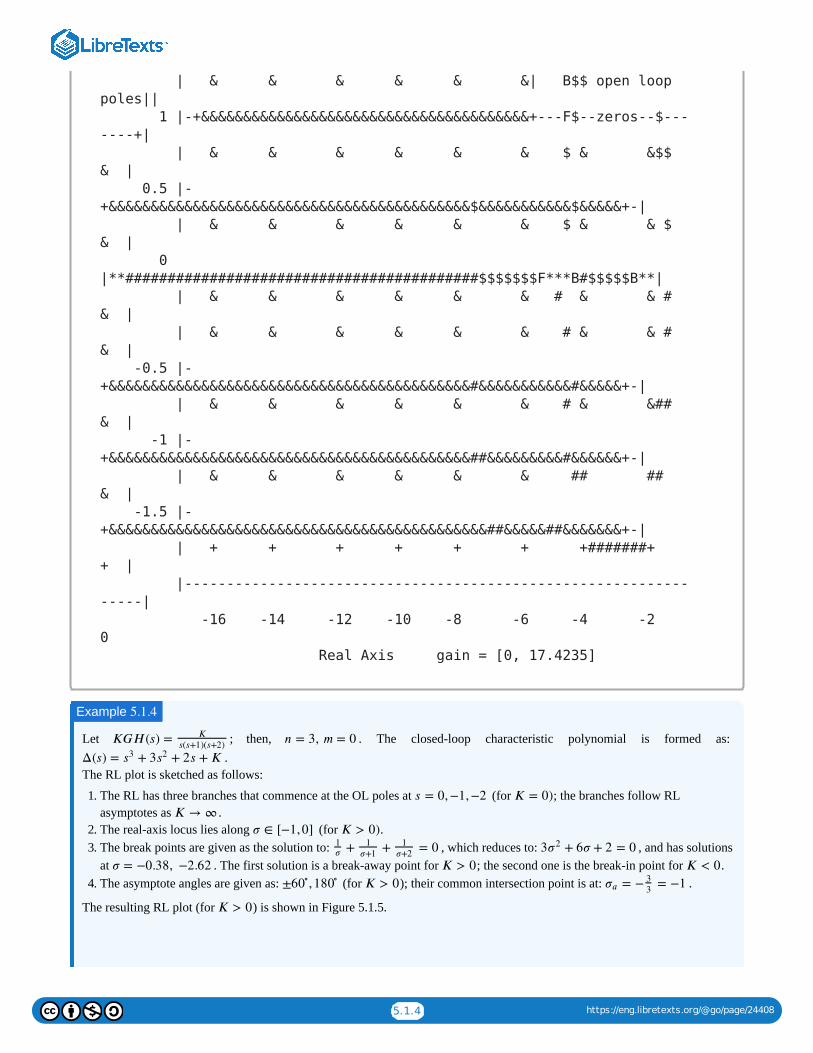
5.1.4 https://eng.libretexts.org/@go/page/24408

Let ; then, . The closed-loop characteristic polynomial is formed as: .

The RL plot is sketched as follows:

1. The RL has three branches that commence at the OL poles at (for ; the branches follow RLasymptotes as .

2. The real-axis locus lies along (for .3. The break points are given as the solution to: , which reduces to: , and has solutions

at . The first solution is a break-away point for ; the second one is the break-in point for .4. The asymptote angles are given as: (for ); their common intersection point is at: .

The resulting RL plot (for ) is shown in Figure 5.1.5.

| & & & & & &| B$$ open loop

poles||

1 |-+&&&&&&&&&&&&&&&&&&&&&&&&&&&&&&&&&&&&&&&+---F$--zeros--$---

----+|

| & & & & & & $ & &$$

& |

0.5 |-

+&&&&&&&&&&&&&&&&&&&&&&&&&&&&&&&&&&&&&&&&&&&$&&&&&&&&&&&$&&&&&+-|

| & & & & & & $ & & $

& |

0

|**##########################################$$$$$$$F***B#$$$$$B**|

| & & & & & & # & & #

& |

| & & & & & & # & & #

& |

-0.5 |-

+&&&&&&&&&&&&&&&&&&&&&&&&&&&&&&&&&&&&&&&&&&&#&&&&&&&&&&&#&&&&&+-|

| & & & & & & # & &##

& |

-1 |-

+&&&&&&&&&&&&&&&&&&&&&&&&&&&&&&&&&&&&&&&&&&&##&&&&&&&&&#&&&&&&+-|

| & & & & & & ## ##

& |

-1.5 |-

+&&&&&&&&&&&&&&&&&&&&&&&&&&&&&&&&&&&&&&&&&&&&&##&&&&&##&&&&&&&+-|

| + + + + + + +#######+

+ |

|------------------------------------------------------------

-----|

-16 -14 -12 -10 -8 -6 -4 -2

0

Real Axis gain = [0, 17.4235]

Example 5.1.4

𝐾𝐺𝐻(𝑠) =𝐾

𝑠(𝑠+1)(𝑠+2)𝑛 = 3,  𝑚 = 0

Δ(𝑠) = + 3 + 2𝑠 +𝐾𝑠3 𝑠2

𝑠 = 0,−1,−2 𝐾 = 0)

𝐾 →∞𝜎 ∈ [−1,0] 𝐾 > 0)

+ + = 01𝜎

1

𝜎+1

1

𝜎+23 + 6𝜎 + 2 = 0𝜎2

𝜎 = −0.38, −2.62 𝐾 > 0 𝐾 < 0

± ,60∘180

∘𝐾 > 0 = − = −1𝜎𝑎

3

3

𝐾 > 0

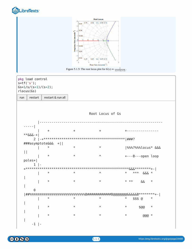
5.1.5 https://eng.libretexts.org/@go/page/24408

Figure : The root locus plot for .

run restart restart & run all

5.1.5 𝐺(𝑠) = 1

𝑠(𝑠+1)(𝑠+2)

Root Locus of Gs

|--------------------------------------------------------------

-----|

| + + + +----------------

**&&&-+|

2 |-+*****************************************|###?

###asymptote&&& +||

| * * * |%%%?%%%locus* &&&

||

| * * * +---B---open loop

poles+|

1 |-

+****************************************************&&&********+-|

| * * * * *** &&& *

|

| * * * * ** && *

|

0

|##%%%%%%%%%%%%%%%%%%%%%%%%%%%%B############B@@@@@@@&&&&&B********+-|

| * * * * $$$ @ *

|

| * * * * $@@ *

|

| * * * * @@@ *

|

-1 |-

pkg load control

s=tf('s');

Gs=1/s/(s+1)/(s+2);

rlocus(Gs)

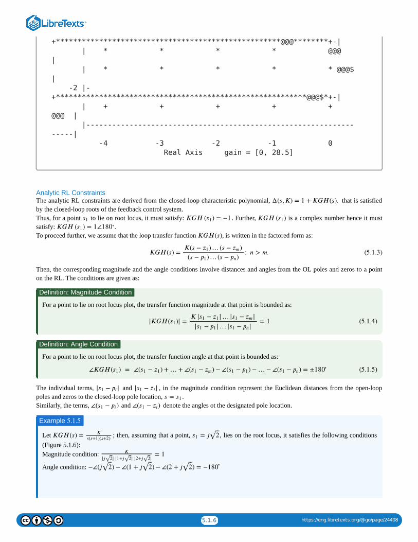
5.1.6 https://eng.libretexts.org/@go/page/24408

Analytic RL ConstraintsThe analytic RL constraints are derived from the closed-loop characteristic polynomial, that is satisfiedby the closed-loop roots of the feedback control system.Thus, for a point to lie on root locus, it must satisfy: . Further, is a complex number hence it mustsatisfy: .To proceed further, we assume that the loop transfer function , is written in the factored form as:

Then, the corresponding magnitude and the angle conditions involve distances and angles from the OL poles and zeros to a pointon the RL. The conditions are given as:

For a point to lie on root locus plot, the transfer function magnitude at that point is bounded as:

For a point to lie on root locus plot, the transfer function angle at that point is bounded as:

The individual terms, and , in the magnitude condition represent the Euclidean distances from the open-looppoles and zeros to the closed-loop pole location, .Similarly, the terms, and denote the angles ot the designated pole location.

Let ; then, assuming that a point, , lies on the root locus, it satisfies the following conditions(Figure 5.1.6):Magnitude condition:

Angle condition:

+****************************************************@@@********+-|

| * * * * @@@

|

| * * * * * @@@$

|

-2 |-

+**********************************************************@@@$*+-|

| + + + + +

@@@ |

|--------------------------------------------------------------

-----|

-4 -3 -2 -1 0

Real Axis gain = [0, 28.5]

Δ(𝑠,𝐾) = 1 +𝐾𝐺𝐻(𝑠).

𝑠1 𝐾𝐺𝐻 ( ) = −1𝑠1 𝐾𝐺𝐻 ( )𝑠1

𝐾𝐺𝐻 ( ) = 1∠180𝑠1∘

𝐾𝐺𝐻(𝑠)

𝐾𝐺𝐻(𝑠) = ; 𝑛 > 𝑚.𝐾(𝑠 − )…(𝑠 − )𝑧1 𝑧𝑚

(𝑠 − )…(𝑠 − )𝑝1 𝑝𝑛(5.1.3)

Definition: Magnitude Condition

|𝐾𝐺𝐻( )| = = 1𝑠1𝐾 | − |… | − |𝑠1 𝑧1 𝑠1 𝑧𝑚

| − |… | − |𝑠1 𝑝1 𝑠1 𝑝𝑛(5.1.4)

Definition: Angle Condition

∠𝐾𝐺𝐻( ) = ∠( − ) +…+ ∠( − )− ∠( − )−…− ∠( − ) = ±𝑠1 𝑠1 𝑧1 𝑠1 𝑧𝑚 𝑠1 𝑝1 𝑠1 𝑝𝑛 180∘ (5.1.5)

| − |𝑠1 𝑝𝑖 | − |𝑠1 𝑧𝑖

𝑠 = 𝑠1

∠( − )𝑠1 𝑝𝑖 ∠( − )𝑠1 𝑧𝑖

Example 5.1.5

𝐾𝐺𝐻(𝑠) =𝐾

𝑠(𝑠+1)(𝑠+2)= 𝑗𝑠1 2

⎯⎯

√

= 1𝐾

|𝑗 | |1+𝑗 | |2+𝑗 |2√ 2√ 2√

−∠(𝑗 )− ∠(1 + 𝑗 )− ∠(2 + 𝑗 ) = −2⎯⎯

√ 2⎯⎯

√ 2⎯⎯

√ 180∘

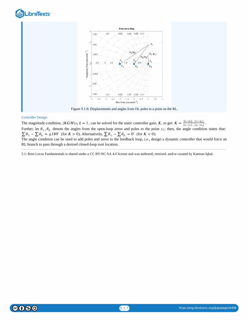
5.1.7 https://eng.libretexts.org/@go/page/24408

Figure : Displacements and angles from OL poles to a point on the RL.

Controller Design

The magnitude condition, , can be solved for the static controller gain, , to get: .Further, let denote the angles from the open-loop zeros and poles to the point ; then, the angle condition states that:

(for ). Alternatively, (for ).The angle condition can be used to add poles and zeros to the feedback loop, i.e., design a dynamic controller that would force anRL branch to pass through a desired closed-loop root location.

5.1: Root Locus Fundamentals is shared under a CC BY-NC-SA 4.0 license and was authored, remixed, and/or curated by Kamran Iqbal.

5.1.6

|𝐾𝐺𝐻( )| = 1𝑠1 𝐾 𝐾 =− …| − |||𝑠1 𝑝1 || 𝑠1 𝑝𝑛

| − |…| − |𝑠1 𝑧1 𝑠1 𝑧𝑚

,𝜃𝑧𝑖 𝜃𝑝𝑖 𝑠1

∑ −∑ = ±𝜃𝑧𝑖 𝜃𝑝𝑖 180∘ 𝐾 > 0 ∑ −∑ =𝜃𝑧𝑖 𝜃𝑝𝑖 0∘ 𝐾 < 0

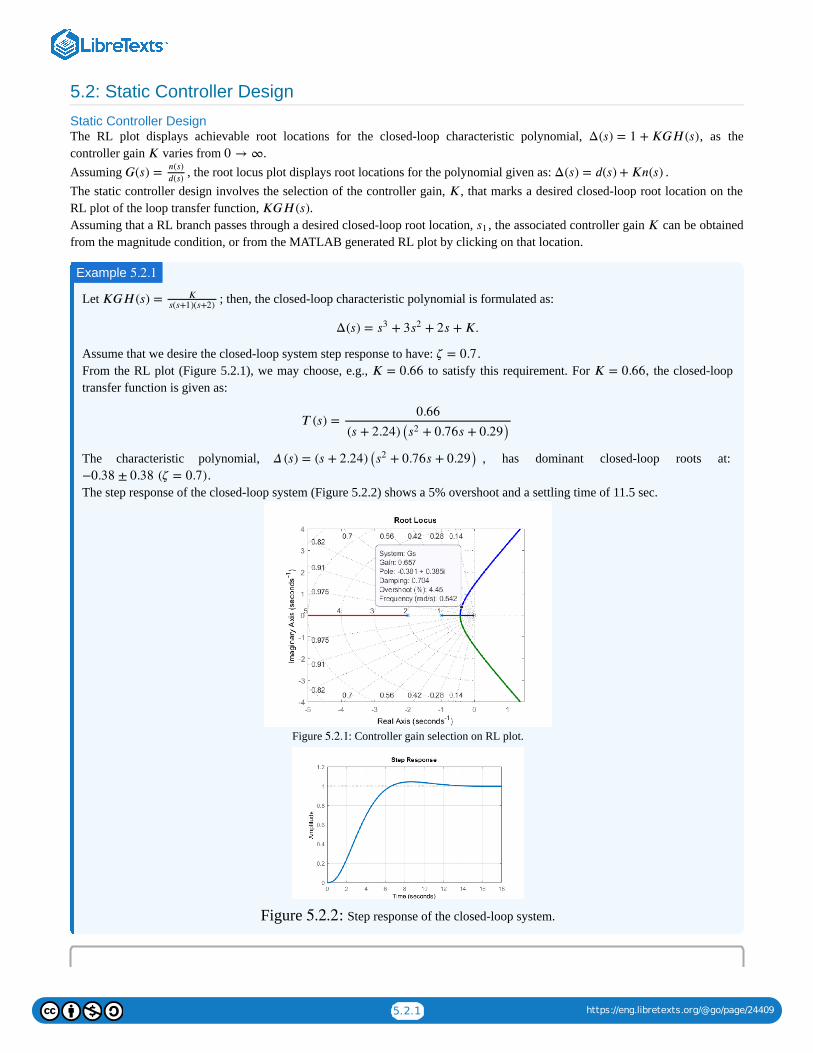
5.2.1 https://eng.libretexts.org/@go/page/24409

5.2: Static Controller Design

Static Controller DesignThe RL plot displays achievable root locations for the closed-loop characteristic polynomial, , as thecontroller gain varies from .Assuming , the root locus plot displays root locations for the polynomial given as: .The static controller design involves the selection of the controller gain, , that marks a desired closed-loop root location on theRL plot of the loop transfer function, .Assuming that a RL branch passes through a desired closed-loop root location, , the associated controller gain can be obtainedfrom the magnitude condition, or from the MATLAB generated RL plot by clicking on that location.

Let ; then, the closed-loop characteristic polynomial is formulated as:

Assume that we desire the closed-loop system step response to have: .From the RL plot (Figure 5.2.1), we may choose, e.g., to satisfy this requirement. For the closed-looptransfer function is given as:

The characteristic polynomial, , has dominant closed-loop roots at: .

The step response of the closed-loop system (Figure 5.2.2) shows a 5% overshoot and a settling time of 11.5 sec.

Figure : Controller gain selection on RL plot.

Figure : Step response of the closed-loop system.

Δ(𝑠) = 1 +𝐾𝐺𝐻(𝑠)

𝐾 0 →∞𝐺(𝑠) =

𝑛(𝑠)

𝑑(𝑠)Δ(𝑠) = 𝑑(𝑠) +𝐾𝑛(𝑠)

𝐾

𝐾𝐺𝐻(𝑠)

𝑠1 𝐾

Example 5.2.1

𝐾𝐺𝐻(𝑠) = 𝐾𝑠(𝑠+1)(𝑠+2)

Δ(𝑠) = + 3 + 2𝑠 +𝐾.𝑠3 𝑠2

𝜁 = 0.7

𝐾 = 0.66 𝐾 = 0.66,

𝑇 (𝑠) =0.66

(𝑠 + 2.24)( + 0.76𝑠 + 0.29)𝑠2

Δ (𝑠) = (𝑠 + 2.24)( + 0.76𝑠 + 0.29)𝑠2

−0.38 ± 0.38 (𝜁 = 0.7)

5.2.1

5.2.2

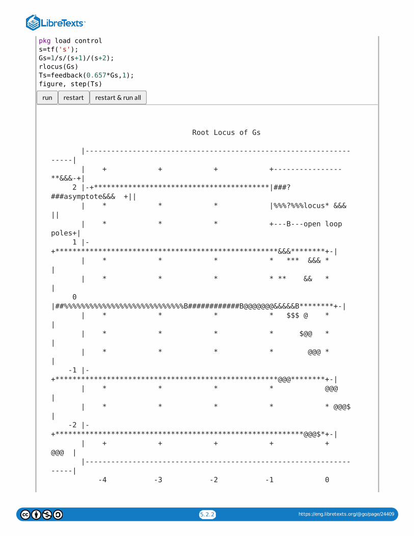
5.2.2 https://eng.libretexts.org/@go/page/24409

run restart restart & run all

Root Locus of Gs

|--------------------------------------------------------------

-----|

| + + + +----------------

**&&&-+|

2 |-+*****************************************|###?

###asymptote&&& +||

| * * * |%%%?%%%locus* &&&

||

| * * * +---B---open loop

poles+|

1 |-

+****************************************************&&&********+-|

| * * * * *** &&& *

|

| * * * * ** && *

|

0

|##%%%%%%%%%%%%%%%%%%%%%%%%%%%%B############B@@@@@@@&&&&&B********+-|

| * * * * $$$ @ *

|

| * * * * $@@ *

|

| * * * * @@@ *

|

-1 |-

+****************************************************@@@********+-|

| * * * * @@@

|

| * * * * * @@@$

|

-2 |-

+**********************************************************@@@$*+-|

| + + + + +

@@@ |

|--------------------------------------------------------------

-----|

-4 -3 -2 -1 0

pkg load control

s=tf('s');

Gs=1/s/(s+1)/(s+2);

rlocus(Gs)

Ts=feedback(0.657*Gs,1);

figure, step(Ts)

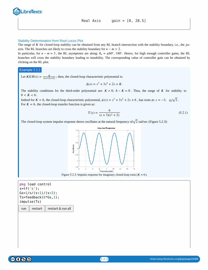
5.2.3 https://eng.libretexts.org/@go/page/24409

Stability Determination from Root Locus Plot The range of for closed-loop stability can be obtained from any RL branch intersection with the stability boundary, i.e., the -axis. The RL branches are likely to cross the stability boundary for .In particular, for , the RL asymptotes are along: . Hence, for high enough controller gains, the RLbranches will cross the stability boundary leading to instability. The corresponding value of controller gain can be obtained byclicking on the RL plot.

Let ; then, the closed-loop characteristic polynomial is:

The stability conditions for the third-order polynomial are: . Thus, the range of for stability is: .

Indeed for the closed-loop characteristic polynomial, , has roots at: .For the closed-loop transfer function is given as:

The closed-loop system impulse response shows oscillates at the natural frequency of rad/sec (Figure 5.2.3):

Figure : Impulse response for imaginary closed-loop roots ( ).

run restart restart & run all

Real Axis gain = [0, 28.5]

𝐾 𝑗𝜔

𝑛 − 𝑚 > 2𝑛 − 𝑚 = 3 = ±60 ,  180𝜃𝑎

∘ ∘

Example 5.2.2

𝐾𝐺𝐻(𝑠) = 𝐾𝑠(𝑠+1)(𝑠+2)

Δ(𝑠) = + 3 + 2𝑠 +𝐾.𝑠3 𝑠2

𝐾 > 0, 6 −𝐾 = 0 𝐾

0 < 𝐾 < 6

𝐾 = 6, Δ (𝑠) = + 3 + 2𝑠 + 6𝑠3 𝑠2 𝑠 = −3, ±𝑗 2⎯⎯

√𝐾 = 6,

𝑇 (𝑠) =6

(𝑠 + 3)( + 2)𝑠2(5.2.1)

2⎯⎯

√

5.2.3 𝐾 = 6

pkg load control

s=tf('s');

Gs=1/s/(s+1)/(s+2);

Ts=feedback(6*Gs,1);

impulse(Ts)

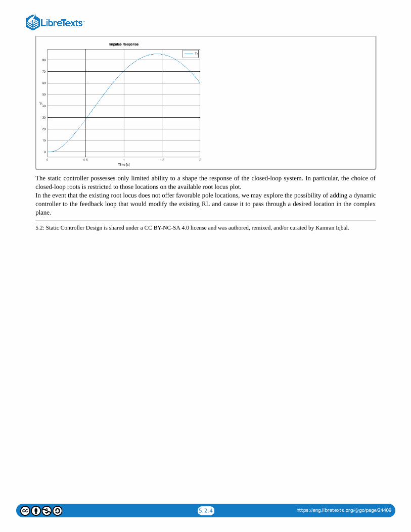
5.2.4 https://eng.libretexts.org/@go/page/24409

The static controller possesses only limited ability to a shape the response of the closed-loop system. In particular, the choice ofclosed-loop roots is restricted to those locations on the available root locus plot.In the event that the existing root locus does not offer favorable pole locations, we may explore the possibility of adding a dynamiccontroller to the feedback loop that would modify the existing RL and cause it to pass through a desired location in the complexplane.

5.2: Static Controller Design is shared under a CC BY-NC-SA 4.0 license and was authored, remixed, and/or curated by Kamran Iqbal.

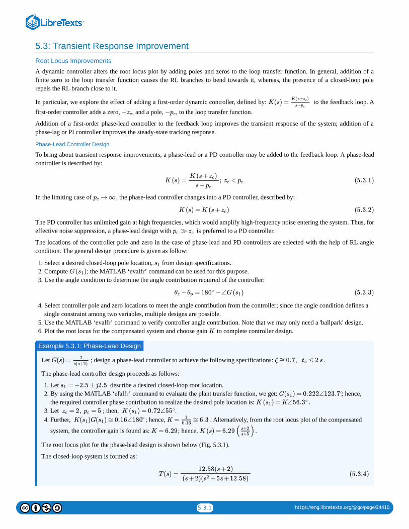
5.3.1 https://eng.libretexts.org/@go/page/24410

5.3: Transient Response Improvement

Root Locus Improvements

A dynamic controller alters the root locus plot by adding poles and zeros to the loop transfer function. In general, addition of afinite zero to the loop transfer function causes the RL branches to bend towards it, whereas, the presence of a closed-loop polerepels the RL branch close to it.

In particular, we explore the effect of adding a first-order dynamic controller, defined by: to the feedback loop. Afirst-order controller adds a zero, , and a pole, , to the loop transfer function.

Addition of a first-order phase-lead controller to the feedback loop improves the transient response of the system; addition of aphase-lag or PI controller improves the steady-state tracking response.

Phase-Lead Controller Design

To bring about transient response improvements, a phase-lead or a PD controller may be added to the feedback loop. A phase-leadcontroller is described by:

In the limiting case of , the phase-lead controller changes into a PD controller, described by:

The PD controller has unlimited gain at high frequencies, which would amplify high-frequency noise entering the system. Thus, foreffective noise suppression, a phase-lead design with is preferred to a PD controller.

The locations of the controller pole and zero in the case of phase-lead and PD controllers are selected with the help of RL anglecondition. The general design procedure is given as follow:

1. Select a desired closed-loop pole location, from design specifications.2. Compute ; the MATLAB ‘evalfr’ command can be used for this purpose.3. Use the angle condition to determine the angle contribution required of the controller:

4. Select controller pole and zero locations to meet the angle contribution from the controller; since the angle condition defines asingle constraint among two variables, multiple designs are possible.

5. Use the MATLAB ‘evalfr’ command to verify controller angle contribution. Note that we may only need a 'ballpark' design.6. Plot the root locus for the compensated system and choose gain to complete controller design.

Let ; design a phase-lead controller to achieve the following specifications: .

The phase-lead controller design proceeds as follows:

1. Let describe a desired closed-loop root location.2. By using the MATLAB ‘efalfr’ command to evaluate the plant transfer function, we get: ; hence,

the required controller phase contribution to realize the desired pole location is: . 3. Let ; then, .4. Further, ; hence, . Alternatively, from the root locus plot of the compensated

system, the controller gain is found as: ; hence, .

The root locus plot for the phase-lead design is shown below (Fig. 5.3.1).

The closed-loop system is formed as:

K(s) =K(s+ )zc

s+pc

−zc −pc

K (s) = ;   <K (s+ )zc

s+pczc pc (5.3.1)

→ ∞pc

K (s) = K (s+ )zc (5.3.2)

≫pc zc

s1

G( )s1

− = 180 −∠G( )θz θp∘ s1 (5.3.3)

K

Example : Phase-Lead Design5.3.1

G(s) = 2

s(s+2)ζ ≅0.7, ≤ 2 sts

= −2.5 ±j2.5s1

G( ) = 0.222∠123.7s1∘

K ( ) = K∠56.3s1∘

= 2,   = 5zc pc K ( ) = 0.72∠55s1∘

K( )G( ) ≅0.16∠s1 s1 180∘ K = ≅6.310.16

K = 6.29 K (s) = 6.29( )s+2s+5

T (s) =12.58(s+2)

(s+2)( +5s+12.58)s2(5.3.4)

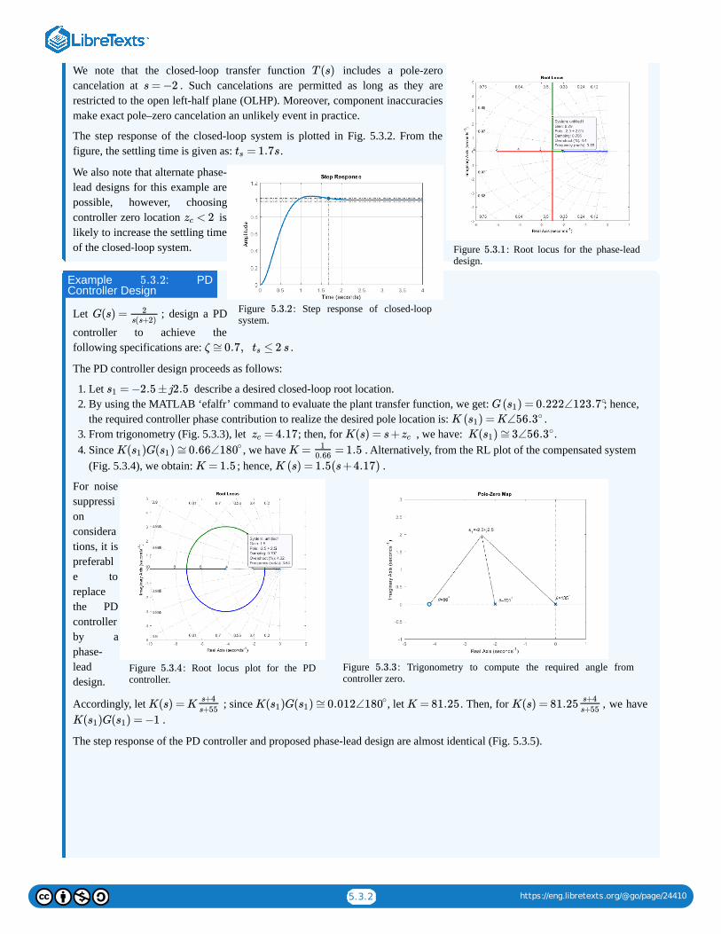
5.3.2 https://eng.libretexts.org/@go/page/24410

Figure : Trigonometry to compute the required angle fromcontroller zero.

Figure : Root locus plot for the PDcontroller.

Figure : Root locus for the phase-leaddesign.

Figure : Step response of closed-loopsystem.

We note that the closed-loop transfer function includes a pole-zerocancelation at . Such cancelations are permitted as long as they arerestricted to the open left-half plane (OLHP). Moreover, component inaccuraciesmake exact pole–zero cancelation an unlikely event in practice.

The step response of the closed-loop system is plotted in Fig. 5.3.2. From thefigure, the settling time is given as: .

We also note that alternate phase-lead designs for this example arepossible, however, choosingcontroller zero location islikely to increase the settling timeof the closed-loop system.

Let ; design a PD

controller to achieve thefollowing specifications are: .

The PD controller design proceeds as follows:

1. Let describe a desired closed-loop root location.2. By using the MATLAB ‘efalfr’ command to evaluate the plant transfer function, we get: ; hence,

the required controller phase contribution to realize the desired pole location is: . 3. From trigonometry (Fig. 5.3.3), let ; then, for , we have: .4. Since , we have . Alternatively, from the RL plot of the compensated system

(Fig. 5.3.4), we obtain: ; hence, .

For noisesuppressionconsiderations, it ispreferable toreplacethe PDcontrollerby aphase-leaddesign.

Accordingly, let ; since , let . Then, for , we have .

The step response of the PD controller and proposed phase-lead design are almost identical (Fig. 5.3.5).

5.3.1

T (s)

s = −2

= 1.7sts

5.3.2

< 2zc

Example : PDController Design

5.3.2

G(s) = 2s(s+2)

ζ ≅0.7, ≤ 2 sts

= −2.5 ±j2.5s1

G( ) = 0.222∠123.7s1∘

K ( ) = K∠56.3s1∘

= 4.17zc K(s) = s+zc K( ) ≅3∠56.3s1∘

K( )G( ) ≅0.66∠s1 s1 180∘ K = = 1.510.66

K = 1.5 K (s) = 1.5(s+4.17)

5.3.35.3.4

K(s) = Ks+4

s+55K( )G( ) ≅0.012∠s1 s1 180∘ K = 81.25 K(s) = 81.25

s+4

s+55

K( )G( ) = −1s1 s1

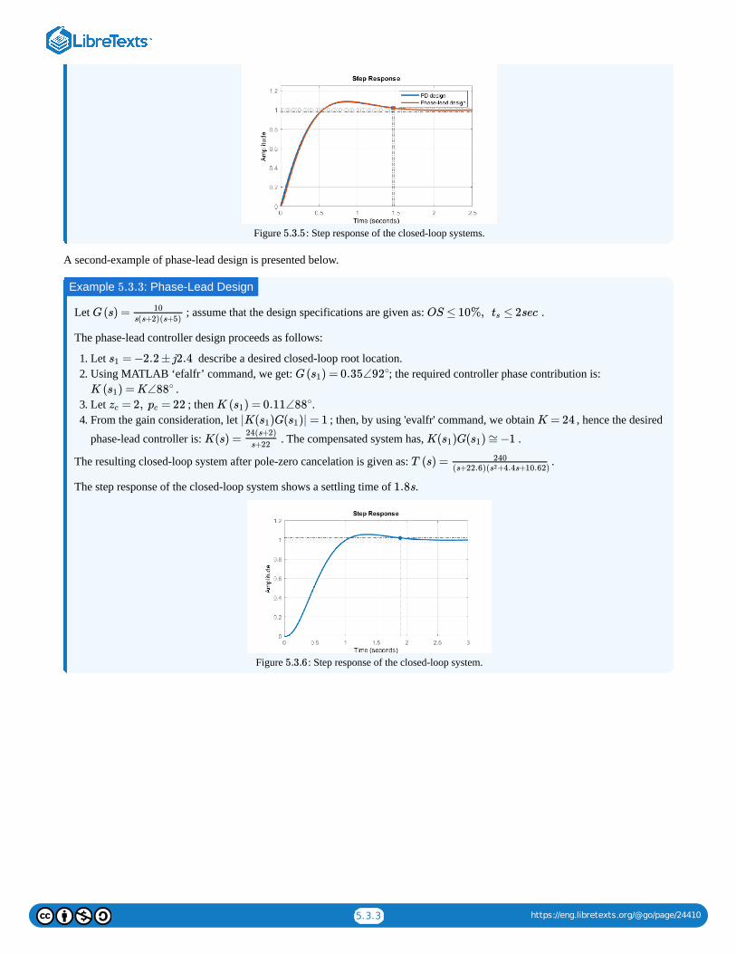
5.3.3 https://eng.libretexts.org/@go/page/24410

Figure : Step response of the closed-loop systems.

A second-example of phase-lead design is presented below.

Let ; assume that the design specifications are given as: .

The phase-lead controller design proceeds as follows:

1. Let describe a desired closed-loop root location.2. Using MATLAB ‘efalfr’ command, we get: ; the required controller phase contribution is:

.3. Let ; then .4. From the gain consideration, let ; then, by using 'evalfr' command, we obtain , hence the desired

phase-lead controller is: . The compensated system has, .

The resulting closed-loop system after pole-zero cancelation is given as: .

The step response of the closed-loop system shows a settling time of .

Figure : Step response of the closed-loop system.

5.3.5

Example : Phase-Lead Design5.3.3

G(s) = 10

s(s+2)(s+5)OS ≤ 10%,    ≤ 2sects

= −2.2 ±j2.4s1

G( ) = 0.35∠92s1∘

K ( ) = K∠88s1∘

= 2,   = 22zc pc K ( ) = 0.11∠88s1∘

|K( )G( )| = 1s1 s1 K = 24

K(s) =24(s+2)

s+22K( )G( ) ≅−1s1 s1

T (s) = 240(s+22.6)( +4.4s+10.62)s2

1.8s

5.3.6

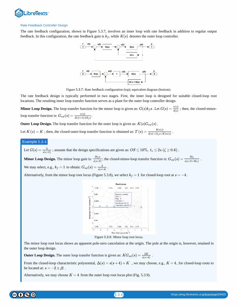
5.3.4 https://eng.libretexts.org/@go/page/24410

Rate Feedback Controller Design

The rate feedback configuration, shown in Figure 5.3.7, involves an inner loop with rate feedback in addition to regular outputfeedback. In this configuration, the rate feedback gain is , while denotes the outer loop controller.

Figure : Rate feedback configuration (top); equivalent diagram (bottom).

The rate feedback design is typically performed in two stages. First, the inner loop is designed for suitable closed-loop rootlocations. The resulting inner loop transfer function serves as a plant for the outer loop controller design.

Minor Loop Design. The loop transfer function for the minor loop is given as: . Let ; then, the closed-minor-

loop transfer function is:

Outer Loop Design. The loop transfer function for the outer loop is given as: .

Let ; then, the closed-outer-loop transfer function is obtained as: .

Let ; assume that the design specifications are given as: .

Minor Loop Design. The minor loop gain is: ; the closed-minor-loop transfer function is: .

We may select, e.g., to obtain: .

Alternatively, from the minor loop root locus (Figure 5.3.8), we select for closed-loop root at .

Figure : Minor loop root locus.

The minor loop root locus shows an apparent pole-zero cancelation at the origin. The pole at the origin is, however, retained inthe outer loop design.

Outer Loop Design. The outer loop transfer function is given as: .

From the closed-loop characteristic polynomial, , we may choose, e.g., , for closed-loop roots tobe located at: .

Alternatively, we may choose from the outer loop root locus plot (Fig. 5.3.9).

kf K(s)

5.3.7

G(s) skf G(s) =n(s)

d(s)

(s) = .Gmln(s)

d(s)+n(s) skf

K(s) (s)Gml

K (s) = K T (s) =Kn(s)

d(s)+( s+K)n(s)kf

Example 5.3.4

G(s) = 2

s(s+2)OS ≤ 10%, ≤ 2s (ζ ≥ 0.6)ts

2 skf

s(s+2)(s) =Gml

2kf

s(s+2+2 )kf

= 1kf (s) =Gml2

s(s+4)

= 1kf s = −4

5.3.8

K (s) =Gml2K

s(s+4)

Δ(s) = s(s+4) +K K = 4

s = −2 ±j2

K = 4

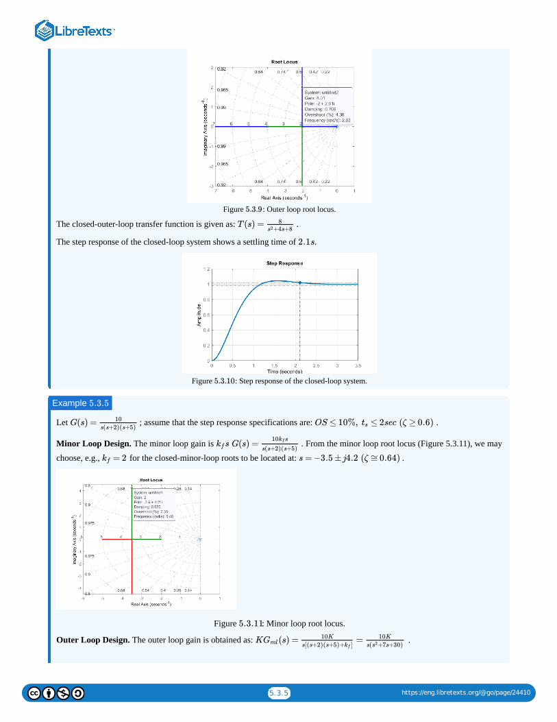
5.3.5 https://eng.libretexts.org/@go/page/24410

Figure : Outer loop root locus.

The closed-outer-loop transfer function is given as: .

The step response of the closed-loop system shows a settling time of .

Figure : Step response of the closed-loop system.

Let ; assume that the step response specifications are: .

Minor Loop Design. The minor loop gain is . From the minor loop root locus (Figure 5.3.11), we may

choose, e.g., for the closed-minor-loop roots to be located at: .

Figure : Minor loop root locus.

Outer Loop Design. The outer loop gain is obtained as: .

5.3.9

T (s) = 8+4s+8s2

2.1s

5.3.10

Example 5.3.5

G(s) = 10

s(s+2)(s+5)OS ≤ 10%,   ≤ 2sec (ζ ≥ 0.6)ts

s G(s) =kf10 skf

s(s+2)(s+5)

= 2kf s = −3.5 ±j4.2 (ζ ≅0.64)

5.3.11

K (s) = =Gml10K

s[(s+2)(s+5)+ ]kf

10K

s( +7s+30)s2

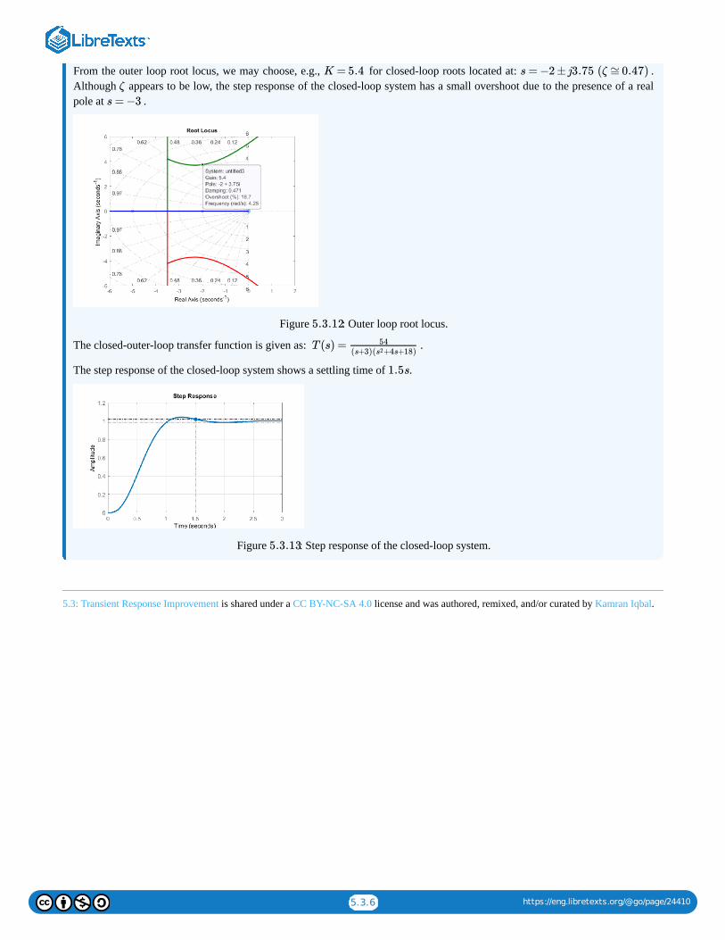
5.3.6 https://eng.libretexts.org/@go/page/24410

From the outer loop root locus, we may choose, e.g., for closed-loop roots located at: .Although appears to be low, the step response of the closed-loop system has a small overshoot due to the presence of a realpole at .

Figure : Outer loop root locus.

The closed-outer-loop transfer function is given as: .

The step response of the closed-loop system shows a settling time of .

Figure : Step response of the closed-loop system.

5.3: Transient Response Improvement is shared under a CC BY-NC-SA 4.0 license and was authored, remixed, and/or curated by Kamran Iqbal.

K = 5.4 s = −2 ±j3.75 (ζ ≅0.47)

ζ

s = −3

5.3.12

T (s) = 54(s+3)( +4s+18)s2

1.5s

5.3.13

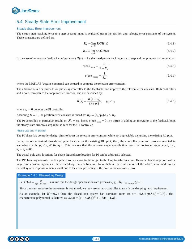
5.4.1 https://eng.libretexts.org/@go/page/28538

5.4: Steady-State Error Improvement

Steady-State Error Improvement

The steady-state tracking error to a step or ramp input is evaluated using the position and velocity error constants of the system.These constants are defined as:

In the case of unity-gain feedback configuration ( ), the steady-state tracking error to step and ramp inputs is computed as:

where the MATLAB 'dcgain' command can be used to compute the relevant error constant.

The addition of a first-order PI or phase-lag controller to the feedback loop improves the relevant error constant. Both controllersadd a pole–zero pair to the loop transfer function, and are described by:

where denotes the PI controller.

Assuming , the position error constant is raised as: .

The PI controller, in particular, results in: , hence . By virtue of adding an integrator to the feedback loop,the steady state error to a step input is zero for the PI controller.

Phase-Lag and PI Design

The PI/phase-lag controller design aims to boost the relevant error constant while not appreciably disturbing the existing RL plot.

Let denote a desired closed-loop pole location on the existing RL plot; then, the controller pole and zero are selected inaccordance with: . This ensures that the adverse angle contribution from the controller stays small, i.e.,

.

The actual pole-zero locations for phase-lag and zero location for PI can be arbitrarily selected.

The PI/phase-lag controller adds a pole-zero pair close to the origin to the loop transfer function. Hence a closed-loop pole with alarge time constant appears in the closed-loop transfer function. Nevertheless, the contribution of the added slow mode to theoverall system response remains small due to the close proximity of the pole to the controller zero.

Let ; assume that the design specifications are given as:

Since transient response improvement is not aimed, we may use a static controller to satisfy the damping ratio requirement.

As an example, let ; then, the closed-loop system has dominant roots at: . Thecharacteristic polynomial is factored as: .

= KGH(s)Kp lims→0

(5.4.1)

= sKGH(s)Kv lims→0

(5.4.2)

H(s) = 1

=e(∞)|step

1

1 +Kp

(5.4.3)

=e(∞)|ramp

1

Kv

(5.4.4)

K(s) = , <K(s + )zc

(s + )pc

pc zc (5.4.5)

= 0pc

K = 1 = ( / ) >K′

p zc pc Kp Kp

= ∞K′

p = 0e(∞)|step

s1

< ≪ Re( )pc zc s1

− ≈θz θp 0∘

Example : Phase-Lag Design5.4.1

G(s) = 10

s(s+2)(s+5)ζ ≥ 0.6,    ≤ 0.1.|ess ramp

K = 0.7 s = −0.8 ±j0.8 (ζ = 0.7)

Δ (s) = (s +5.38)( +1.62s +1.3)s2

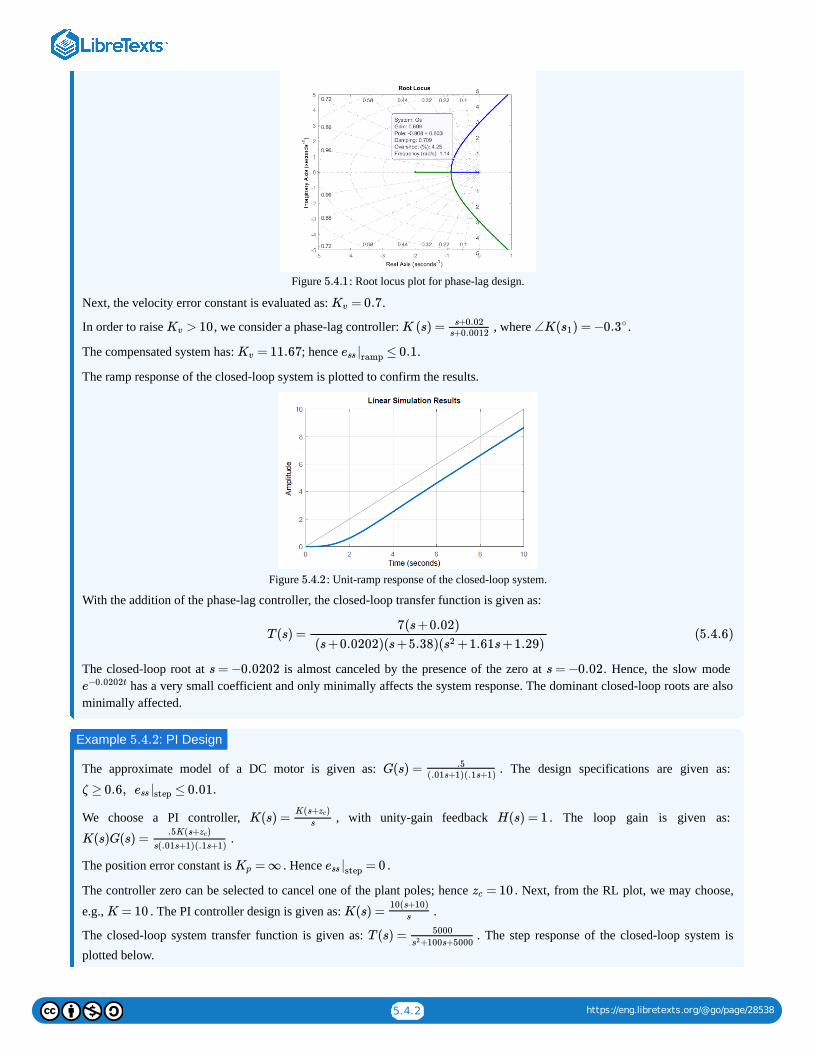
5.4.2 https://eng.libretexts.org/@go/page/28538

Figure : Root locus plot for phase-lag design.

Next, the velocity error constant is evaluated as: .

In order to raise , we consider a phase-lag controller: , where .

The compensated system has: ; hence .

The ramp response of the closed-loop system is plotted to confirm the results.

Figure : Unit-ramp response of the closed-loop system.

With the addition of the phase-lag controller, the closed-loop transfer function is given as:

The closed-loop root at is almost canceled by the presence of the zero at . Hence, the slow mode has a very small coefficient and only minimally affects the system response. The dominant closed-loop roots are also

minimally affected.

The approximate model of a DC motor is given as: . The design specifications are given as:

We choose a PI controller, , with unity-gain feedback . The loop gain is given as:

.

The position error constant is . Hence .

The controller zero can be selected to cancel one of the plant poles; hence . Next, from the RL plot, we may choose,

e.g., . The PI controller design is given as: .

The closed-loop system transfer function is given as: . The step response of the closed-loop system isplotted below.

5.4.1

= 0.7Kv

> 10Kv K (s) = s+0.02s+0.0012

∠K( ) = −0.3s1∘

= 11.67Kv ≤ 0.1|ess ramp

5.4.2

T (s) =7(s +0.02)

(s +0.0202)(s +5.38)( +1.61s +1.29)s2(5.4.6)

s = −0.0202 s = −0.02

e−0.0202t

Example : PI Design5.4.2

G(s) = .5(.01s+1)(.1s+1)

ζ ≥ 0.6,    ≤ 0.01.|ess step

K(s) =K(s+ )zc

s H(s) = 1

K(s)G(s) =.5K(s+ )zc

s(.01s+1)(.1s+1)

= ∞Kp = 0|ess step

= 10zc

K = 10 K(s) =10(s+10)

s

T (s) = 5000

+100s+5000s2

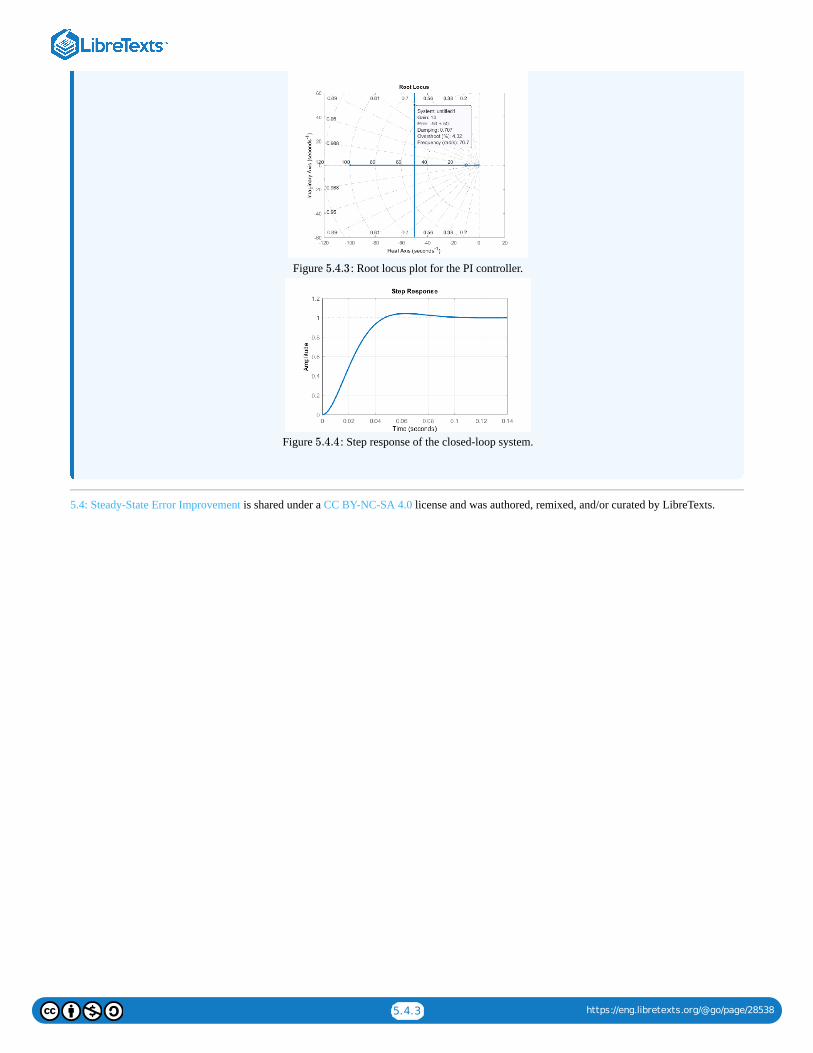
5.4.3 https://eng.libretexts.org/@go/page/28538

Figure : Root locus plot for the PI controller.

Figure : Step response of the closed-loop system.

5.4: Steady-State Error Improvement is shared under a CC BY-NC-SA 4.0 license and was authored, remixed, and/or curated by LibreTexts.

5.4.3

5.4.4

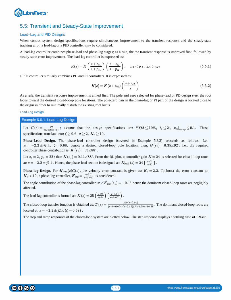
5.5.1 https://eng.libretexts.org/@go/page/28539

5.5: Transient and Steady-State Improvement

Lead–Lag and PID Designs

When control system design specifications require simultaneous improvement to the transient response and the steady-statetracking error, a lead-lag or a PID controller may be considered.

A lead-lag controller combines phase-lead and phase-lag stages; as a rule, the the transient response is improved first, followed bysteady-state error improvement. The lead-lag controller is expressed as:

a PID controller similarly combines PD and PI controllers. It is expressed as:

As a rule, the transient response improvement is aimed first. The pole and zero selected for phase-lead or PD design steer the rootlocus toward the desired closed-loop pole locations. The pole-zero pair in the phase-lag or PI part of the design is located close tothe origin in order to minimally disturb the existing root locus.

Lead-Lag Design

Let ; assume that the design specifications are: These

specifications translate into: .

Phase-Lead Design. The phase-lead controller design (covered in Example 5.3.3) proceeds as follows: Let denote a desired closed-loop pole location; then, , i.e., the required

controller phase contribution is: .

Let ; then . From the RL plot, a controller gain is selected for closed-loop roots

at: . Hence, the phase-lead section is designed as: .

Phase-lag Design. For , the velocity error constant is given as: . To boost the error constant to , a phase-lag controller, is considered.

The angle contribution of the phase-lag controller is: hence the dominant closed-loop roots are negligiblyaffected.

The lead-lag controller is formed as: .

The closed-loop transfer function is obtained as: . The dominant closed-loop roots are

located at: .

The step and ramp responses of the closed-loop system are plotted below. The step response displays a settling time of .

K(s) = K( )( ) , < , >s +zc1

s +pc1

s +zc2

s +pc2zc1 pc1 zc2 pc2 (5.5.1)

K(s) = K (s + )( )zc1s +zc2

s(5.5.2)

Example : Lead-Lag Design5.5.1

G(s) = 10s(s+2)(s+5)

%OS ≤ 10%, ≤ 2s, ≤ 0.1.ts ess|ramp

ζ ≥ 0.6,  σ ≥ 2,   ≥ 10Kv

= −2.2 ±j2.4, ζ = 0.68,s1 G( ) = 0.35∠92s1∘

K ( ) = K∠88s1∘

= 2,   = 22zc pc K ( ) = 0.11∠88s1∘ K = 24

s = −2.2 ±j2.4 (s) = 24( )Kleads+2s+22

(s)G(s)Klead = 2.2Kv

> 10Kv =Klags+0.01

s+0.002

∠ ( ) = −0.1Klag s1∘

K (s) = 25( )( )s+2

s+24

s+0.01

s+0.002

T (s) =240(s+0.01)

(s+0.01004)(s+22.6)( +4.39s+10.58)s2

s = −2.2 ±j2.4 (ζ = 0.68)

1.9sec

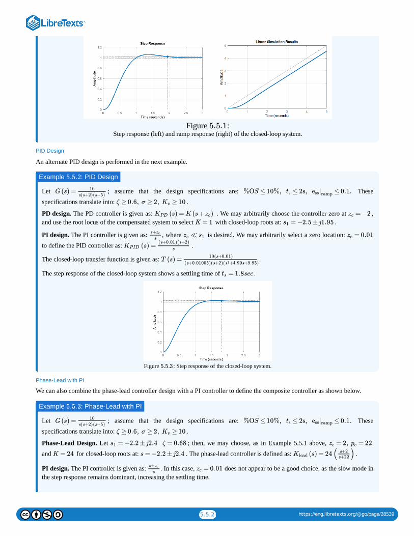
5.5.2 https://eng.libretexts.org/@go/page/28539

Figure :Step response (left) and ramp response (right) of the closed-loop system.

PID Design

An alternate PID design is performed in the next example.

Let ; assume that the design specifications are: These

specifications translate into: .

PD design. The PD controller is given as: . We may arbitrarily choose the controller zero at ,and use the root locus of the compensated system to select with closed-loop roots at: .

PI design. The PI controller is given as: , where is desired. We may arbitrarily select a zero location:

to define the PID controller as: .

The closed-loop transfer function is given as: .

The step response of the closed-loop system shows a settling time of .

Figure : Step response of the closed-loop system.

Phase-Lead with PI

We can also combine the phase-lead controller design with a PI controller to define the composite controller as shown below.

Let ; assume that the design specifications are: These

specifications translate into: .

Phase-Lead Design. Let ; then, we may choose, as in Example 5.5.1 above,

and for closed-loop roots at: . The phase-lead controller is defined as: .

PI design. The PI controller is given as: . In this case, does not appear to be a good choice, as the slow mode inthe step response remains dominant, increasing the settling time.

5.5.1

Example : PID Design5.5.2

G(s) = 10

s(s+2)(s+5)%OS ≤ 10%, ≤ 2s, ≤ 0.1.ts ess|ramp

ζ ≥ 0.6,  σ ≥ 2,   ≥ 10Kv

(s) = K (s + )KPD zc = −2zc

K = 1 = −2.5 ±j1.95s1

s+zc

s≪zc s1 = 0.01zc

(s) =KPID(s+0.01)(s+2)

s

T (s) =10(s+0.01)

(s+0.01005)(s+2)( +4.99s+9.95)s2

= 1.8sects

5.5.3

Example : Phase-Lead with PI5.5.3

G(s) = 10

s(s+2)(s+5)%OS ≤ 10%, ≤ 2s, ≤ 0.1.ts ess|ramp

ζ ≥ 0.6,  σ ≥ 2,   ≥ 10Kv

= −2.2 ±j2.4 ζ = 0.68s1 = 2,   = 22zc pc

K = 24 s = −2.2 ±j2.4 (s) = 24( )Kleads+2s+22

s+zc

s= 0.01zc

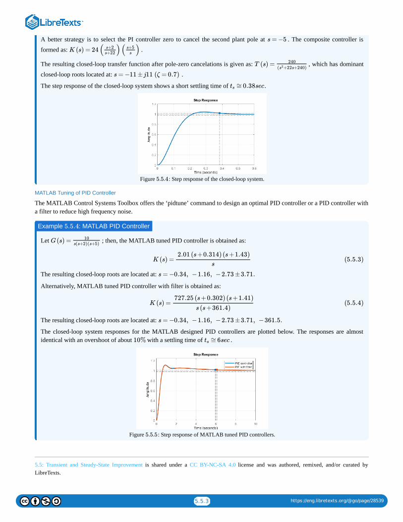
5.5.3 https://eng.libretexts.org/@go/page/28539

A better strategy is to select the PI controller zero to cancel the second plant pole at . The composite controller is

formed as: .

The resulting closed-loop transfer function after pole-zero cancelations is given as: , which has dominant

closed-loop roots located at: .

The step response of the closed-loop system shows a short settling time of .

Figure : Step response of the closed-loop system.

MATLAB Tuning of PID Controller

The MATLAB Control Systems Toolbox offers the ‘pidtune’ command to design an optimal PID controller or a PID controller witha filter to reduce high frequency noise.

Let ; then, the MATLAB tuned PID controller is obtained as:

The resulting closed-loop roots are located at:

Alternatively, MATLAB tuned PID controller with filter is obtained as:

The resulting closed-loop roots are located at:

The closed-loop system responses for the MATLAB designed PID controllers are plotted below. The responses are almostidentical with an overshoot of about with a settling time of .

Figure : Step response of MATLAB tuned PID controllers.

5.5: Transient and Steady-State Improvement is shared under a CC BY-NC-SA 4.0 license and was authored, remixed, and/or curated byLibreTexts.

s = −5

K (s) = 24( )( )s+2s+22

s+5s

T (s) = 240

( +22s+240)s2

s = −11 ±j11 (ζ = 0.7)

≅0.38sects

5.5.4

Example : MATLAB PID Controller5.5.4

G(s) = 10s(s+2)(s+5)

K (s) =2.01 (s +0.314) (s +1.43)

s(5.5.3)

s = −0.34,   −1.16,   −2.73 ±3.71.

K (s) =727.25 (s +0.302) (s +1.41)

s (s +361.4)(5.5.4)

s = −0.34,   −1.16,   −2.73 ±3.71,   −361.5.

10% ≅6sects

5.5.5

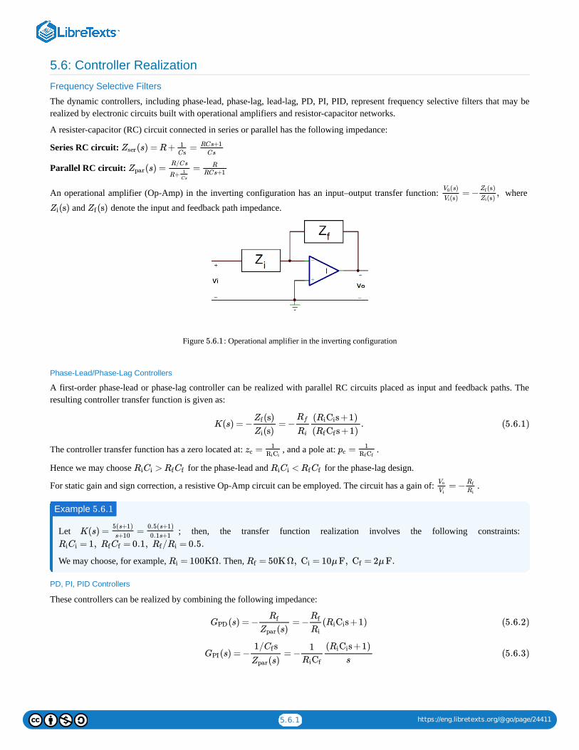
5.6.1 https://eng.libretexts.org/@go/page/24411

5.6: Controller Realization

Frequency Selective Filters

The dynamic controllers, including phase-lead, phase-lag, lead-lag, PD, PI, PID, represent frequency selective filters that may berealized by electronic circuits built with operational amplifiers and resistor-capacitor networks.

A resister-capacitor (RC) circuit connected in series or parallel has the following impedance:

Series RC circuit:

Parallel RC circuit:

An operational amplifier (Op-Amp) in the inverting configuration has an input–output transfer function: where

and denote the input and feedback path impedance.

Figure : Operational amplifier in the inverting configuration

Phase-Lead/Phase-Lag Controllers

A first-order phase-lead or phase-lag controller can be realized with parallel RC circuits placed as input and feedback paths. Theresulting controller transfer function is given as:

The controller transfer function has a zero located at: , and a pole at: .

Hence we may choose for the phase-lead and for the phase-lag design.

For static gain and sign correction, a resistive Op-Amp circuit can be employed. The circuit has a gain of: .

Let ; then, the transfer function realization involves the following constraints:

We may choose, for example, . Then,

PD, PI, PID Controllers

These controllers can be realized by combining the following impedance:

(s) = R + =Zser1

Cs

RCs+1

Cs

(s) = =ZparR/Cs

R+1

Cs

R

RCs+1

= − ,(s)V0

(s)Vi

(s)Zf

(s)Zi

(s)Zi (s)Zf

5.6.1

K(s) = − = − .(s)Zf

(s)Zi

Rf

Ri

( s +1)RiCi

( s +1)Rf Cf

(5.6.1)

=zc1

RiCi=pc

1Rf Cf

>RiCi Rf Cf <RiCi Rf Cf

= −Vo

Vi

Rf

Ri

Example 5.6.1

K(s) = =5(s+1)

s+10

0.5(s+1)

0.1s+1

= 1, = 0.1, / = 0.5.RiCi Rf Cf Rf Ri

= 100KΩRi = 50K Ω, = 10μ F, = 2μ F.Rf Ci Cf

(s) = − = − ( s +1)GPDRf

(s)Zpar

Rf

Ri

RiCi (5.6.2)

(s) = − = −GPI

1/ sCf

(s)Zpar

1

RiCf

( s +1)RiCi

s(5.6.3)

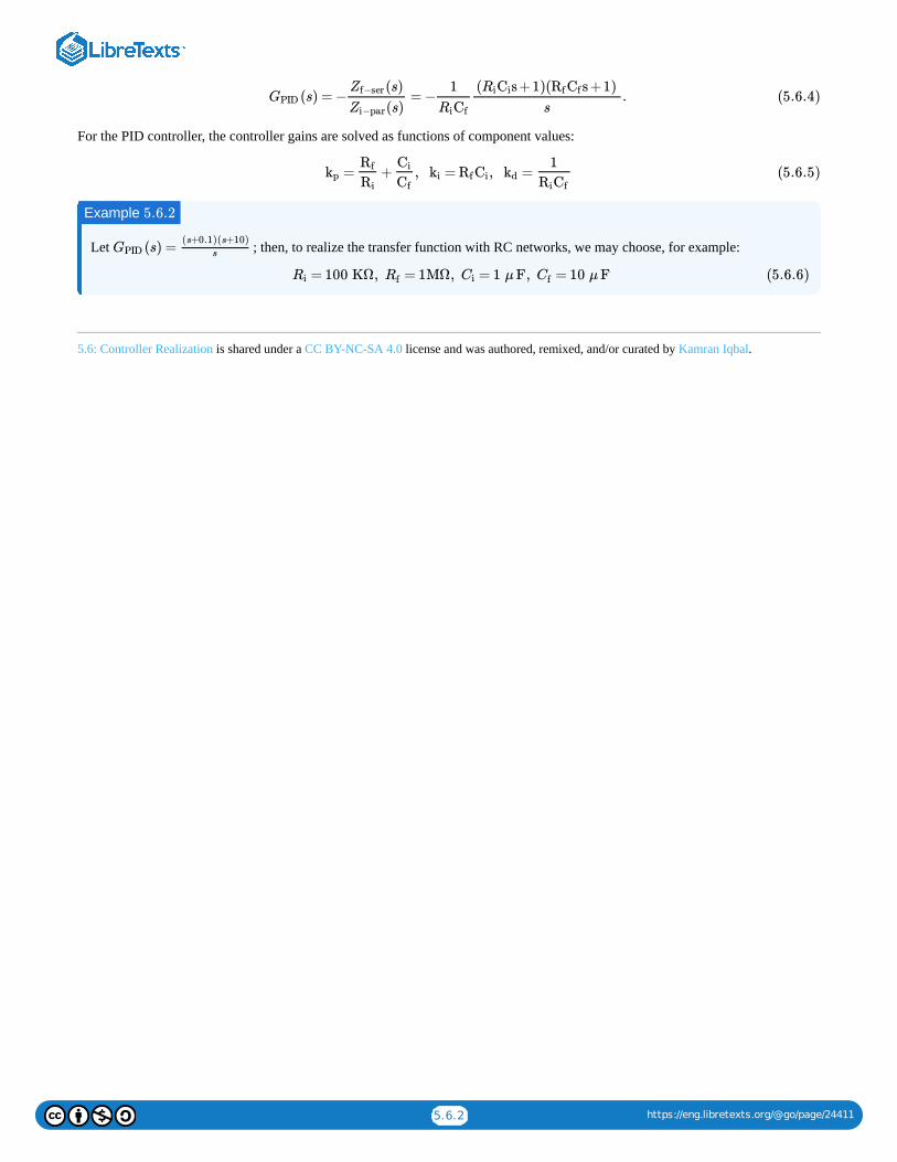
5.6.2 https://eng.libretexts.org/@go/page/24411

For the PID controller, the controller gains are solved as functions of component values:

Let ; then, to realize the transfer function with RC networks, we may choose, for example:

5.6: Controller Realization is shared under a CC BY-NC-SA 4.0 license and was authored, remixed, and/or curated by Kamran Iqbal.

(s) = − = − .GPID(s)Zf−ser

(s)Zi−par

1

RiCf

( s +1)( s +1)RiCi Rf Cf

s(5.6.4)

= + , = , =kpRf

Ri

Ci

Cfki Rf Ci kd

1

RiCf(5.6.5)

Example 5.6.2

(s) =GPID(s+0.1)(s+10)

s

= 100 KΩ, = 1MΩ, = 1 μ F, = 10 μ FRi Rf Ci Cf (5.6.6)

1

CHAPTER OVERVIEW

6: Compensator Design with Frequency Response Methods

1. Characterize and plot the frequency response of transfer function models.2. State the performance criteria for controller design in the frequency domain.3. Design compensators for dynamic system models using frequency response methods.4. Characterize the closed-loop frequency response of the compensated system.

6.0: Prelude to Compensator Design with Frequency Response Methods6.1: Frequency Response Plots6.2: Measures of Performance6.3: Frequency Response Design6.4: Closed-Loop Frequency Response

6: Compensator Design with Frequency Response Methods is shared under a CC BY-NC-SA 4.0 license and was authored, remixed, and/orcurated by Kamran Iqbal.

Learning Objectives

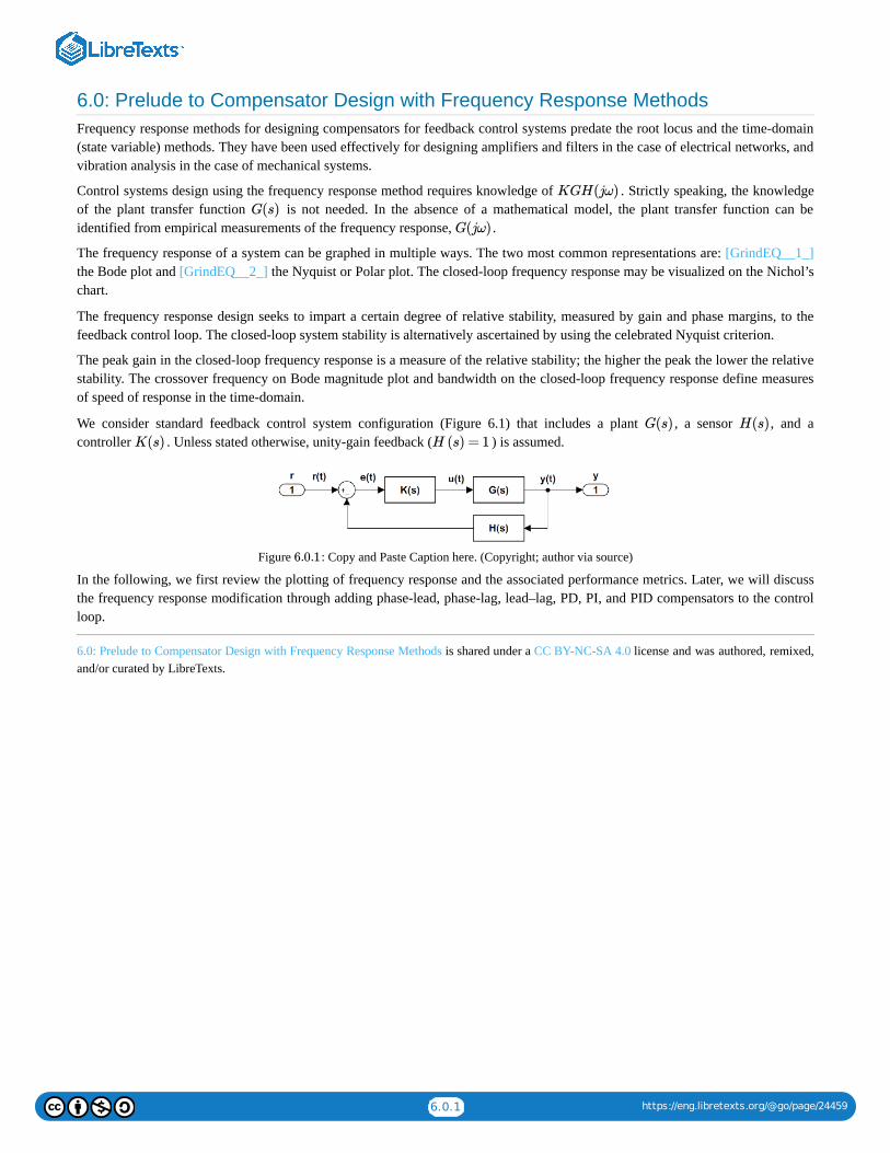
6.0.1 https://eng.libretexts.org/@go/page/24459

6.0: Prelude to Compensator Design with Frequency Response MethodsFrequency response methods for designing compensators for feedback control systems predate the root locus and the time-domain(state variable) methods. They have been used effectively for designing amplifiers and filters in the case of electrical networks, andvibration analysis in the case of mechanical systems.

Control systems design using the frequency response method requires knowledge of . Strictly speaking, the knowledgeof the plant transfer function is not needed. In the absence of a mathematical model, the plant transfer function can beidentified from empirical measurements of the frequency response, .

The frequency response of a system can be graphed in multiple ways. The two most common representations are: [GrindEQ__1_]the Bode plot and [GrindEQ__2_] the Nyquist or Polar plot. The closed-loop frequency response may be visualized on the Nichol’schart.

The frequency response design seeks to impart a certain degree of relative stability, measured by gain and phase margins, to thefeedback control loop. The closed-loop system stability is alternatively ascertained by using the celebrated Nyquist criterion.

The peak gain in the closed-loop frequency response is a measure of the relative stability; the higher the peak the lower the relativestability. The crossover frequency on Bode magnitude plot and bandwidth on the closed-loop frequency response define measuresof speed of response in the time-domain.

We consider standard feedback control system configuration (Figure 6.1) that includes a plant , a sensor , and acontroller . Unless stated otherwise, unity-gain feedback ( ) is assumed.

Figure : Copy and Paste Caption here. (Copyright; author via source)

In the following, we first review the plotting of frequency response and the associated performance metrics. Later, we will discussthe frequency response modification through adding phase-lead, phase-lag, lead–lag, PD, PI, and PID compensators to the controlloop.

6.0: Prelude to Compensator Design with Frequency Response Methods is shared under a CC BY-NC-SA 4.0 license and was authored, remixed,and/or curated by LibreTexts.

KGH(jω)

G(s)

G(jω)

G(s) H(s)

K(s) H (s) = 1

6.0.1

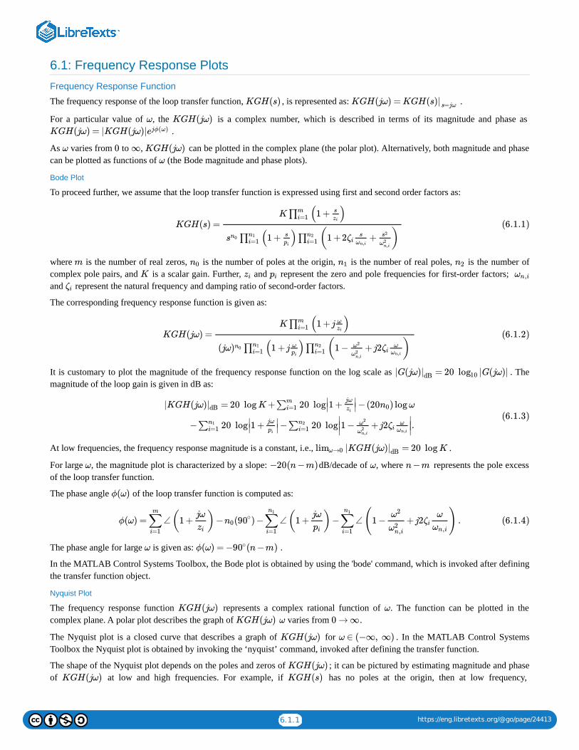
6.1.1 https://eng.libretexts.org/@go/page/24413

6.1: Frequency Response Plots

Frequency Response Function

The frequency response of the loop transfer function, , is represented as: .

For a particular value of , the is a complex number, which is described in terms of its magnitude and phase as .

As varies from to , can be plotted in the complex plane (the polar plot). Alternatively, both magnitude and phasecan be plotted as functions of (the Bode magnitude and phase plots).

Bode Plot

To proceed further, we assume that the loop transfer function is expressed using first and second order factors as:

where is the number of real zeros, is the number of poles at the origin, is the number of real poles, is the number ofcomplex pole pairs, and is a scalar gain. Further, and represent the zero and pole frequencies for first-order factors; and represent the natural frequency and damping ratio of second-order factors.

The corresponding frequency response function is given as:

It is customary to plot the magnitude of the frequency response function on the log scale as . Themagnitude of the loop gain is given in dB as:

At low frequencies, the frequency response magnitude is a constant, i.e., .

For large , the magnitude plot is characterized by a slope: dB/decade of , where represents the pole excessof the loop transfer function.

The phase angle of the loop transfer function is computed as:

The phase angle for large is given as: .

In the MATLAB Control Systems Toolbox, the Bode plot is obtained by using the 'bode' command, which is invoked after definingthe transfer function object.

Nyquist Plot

The frequency response function represents a complex rational function of . The function can be plotted in thecomplex plane. A polar plot describes the graph of varies from .

The Nyquist plot is a closed curve that describes a graph of for . In the MATLAB Control SystemsToolbox the Nyquist plot is obtained by invoking the ‘nyquist’ command, invoked after defining the transfer function.

The shape of the Nyquist plot depends on the poles and zeros of ; it can be pictured by estimating magnitude and phaseof at low and high frequencies. For example, if has no poles at the origin, then at low frequency,

KGH(s) KGH(jω) = KGH(s)| s=jω

ω KGH(jω)KGH(jω) = |KGH(jω)|ejϕ(ω)

ω 0 ∞ KGH(jω)ω

KGH(s) =K (1 + )∏m

i=1s

zi

(1 + ) (1 +2 + )sn0 ∏n1

i=1s

pi∏n2

i=1 ζis

ωn,i

s2

ω2n,i

(6.1.1)

m n0 n1 n2

K zi pi ωn,i

ζi

KGH(jω) =K (1 +j )∏m

i=1ωzi

(jω (1 +j ) (1 − +j2 ))n0 ∏n1

i=1ωpi∏n2

i=1ω2

ω2n,i

ζiωωn,i

(6.1.2)

|G(jω) = 20 |G(jω)||dB log10

|KGH(jω) = 20 logK+ 20 log 1 + −(20 ) logω|dB ∑mi=1

∣∣

jω

zi∣∣ n0

− 20 log 1 + − 20 log 1 − +j2 .∑n1

i=1∣∣

jω

pi

∣∣ ∑n2

i=1∣∣∣ ω2

ω2n,i

ζiωωn,i

∣∣∣

(6.1.3)

|KGH(jω) = 20 logKlimω→0 |dB

ω −20(n−m) ω n−m

ϕ(ω)

ϕ(ω) = ∠(1 + )− ( ) − ∠(1 + )− ∠(1 − +j2 ) .∑i=1

m jω

zin0 90∘ ∑

i=1

n1 jω

pi∑i=1

n1 ω2

ω2n,i

ζiω

ωn,i(6.1.4)

ω ϕ(ω) = − (n−m)90∘

KGH(jω) ω

KGH(jω) ω 0 → ∞

KGH(jω) ω ∈ (−∞,  ∞)

KGH(jω)KGH(jω) KGH(s)

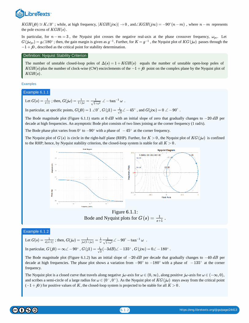
6.1.2 https://eng.libretexts.org/@go/page/24413

; while, at high frequency, , and , where representsthe pole excess of .

In particular, for , the Nyquist plot crosses the negative real-axis at the phase crossover frequency, . Let ; then, the gain margin is given as . Further, for , the Nyquist plot of passes through the

, described as the critical point for stability determination.

The number of unstable closed-loop poles of equals the number of unstable open-loop poles of plus the number of clock-wise (CW) encirclements of the point on the complex plane by the Nyquist plot of.

Examples

Let ; then, .

In particular, at specific points, , , and .

The Bode magnitude plot (Figure 6.1.1) starts at with an initial slope of zero that gradually changes to perdecade at high frequencies. An asymptotic Bode plot consists of two lines joining ar the corner frequency (1 rad/s).

The Bode phase plot varies from to with a phase of at the corner frequency.

The Nyquist plot of is circle in the right-half plane (RHP). Further, for , the Nyquist plot of is confinedto the RHP; hence, by Nyquist stability criterion, the closed-loop system is stable for all .

Figure :Bode and Nyquist plots for .

Let ; then, .

In particular, , , .

The Bode magnitude plot (Figure 6.1.2) has an initial slope of per decade that gradually changes to perdecade at high frequencies. The phase plot shows a variation from to with a phase of at the cornerfrequency.

The Nyquist plot is a closed curve that travels along negative -axis for , along positive -axis for ,and scribes a semi-circle of a large radius for . As the Nyquist plot of stays away from the critical point( ) for positive values of , the closed-loop system is projected to be stable for all .

KGH(j0) ≅K∠0∘ |KGH(j∞)| → 0 ∠KGH(j∞) = − (n−m)90∘ n−m

KGH(s)

n−m = 3 ωpc

G(j ) = g∠180ωpc∘ g−1 K = g−1 KG(jω)

−1 +j0

Definition: Nyquist Stability Criterion

Δ(s) = 1 +KGH(s)KGH(s) −1 +j0KGH(s)

Example 6.1.1

G(s) = 1s+1

G(jω) = = ∠ − ω11+jω

1

1+ω2√tan−1

G(j0) = 1 ∠0∘ G(j1) = ∠ −4512√

∘ G(j∞) = 0 ∠ −90∘

0 dB −20 dB

0∘ −90∘   −45∘

G(s) K > 0 KG(jω)K > 0

6.1.1G(s) = 1

s+1

Example 6.1.2

G(s) = 1s(s+1)

G(jω) = = ∠ − − ω1jω(1+jω)

1ω

1

1+ω2√90∘ tan−1

G(j0) = ∞∠ −90∘ G(j1) = (−3dB)∠ −13512√

∘ G(j∞) = 0∠ −180∘

−20 dB −40 dB−90∘ −180∘   −135∘

jω ω ∈ (0, ∞) jω ω ∈ (−∞, 0)ω ∈ ( , )0− 0+ KG(jω)

−1 +j0 K K > 0

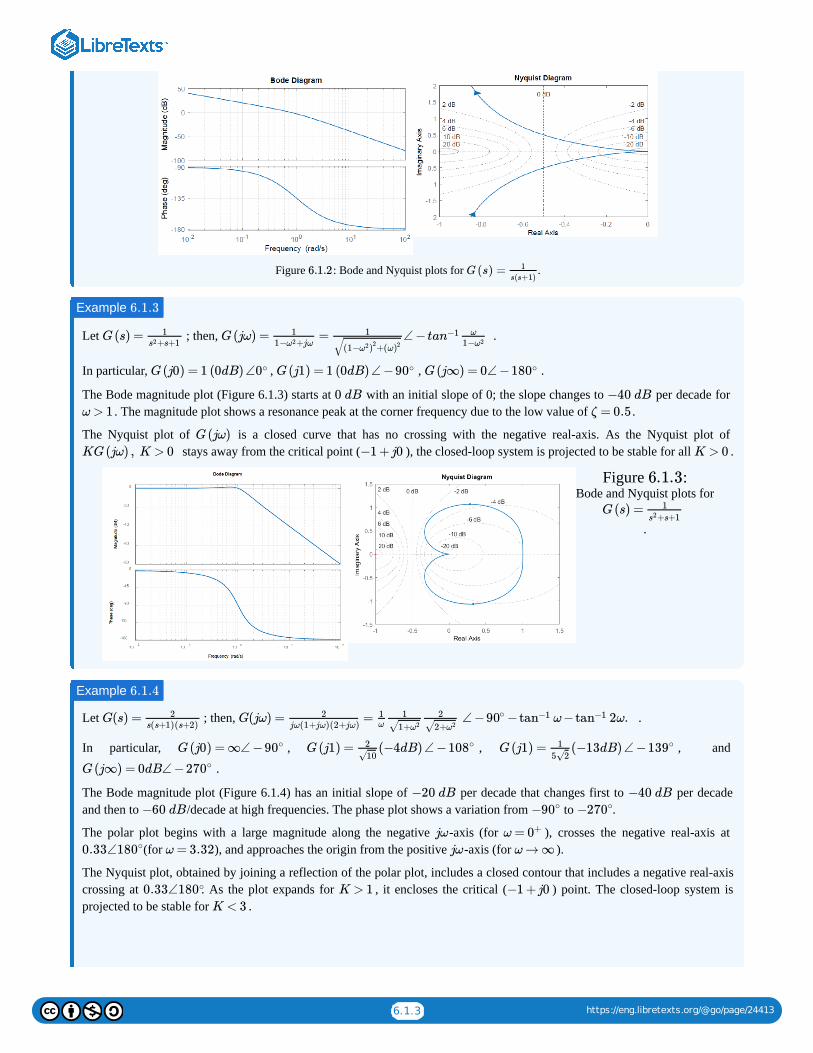
6.1.3 https://eng.libretexts.org/@go/page/24413

Figure : Bode and Nyquist plots for .

Let ; then, .

In particular, , , .

The Bode magnitude plot (Figure 6.1.3) starts at with an initial slope of 0; the slope changes to per decade for . The magnitude plot shows a resonance peak at the corner frequency due to the low value of .

The Nyquist plot of is a closed curve that has no crossing with the negative real-axis. As the Nyquist plot of stays away from the critical point ( ), the closed-loop system is projected to be stable for all .

Figure :Bode and Nyquist plots for

.

Let ; then, .

In particular, , , , and

.

The Bode magnitude plot (Figure 6.1.4) has an initial slope of per decade that changes first to per decadeand then to /decade at high frequencies. The phase plot shows a variation from to .

The polar plot begins with a large magnitude along the negative -axis (for ), crosses the negative real-axis at (for ), and approaches the origin from the positive -axis (for ).

The Nyquist plot, obtained by joining a reflection of the polar plot, includes a closed contour that includes a negative real-axiscrossing at . As the plot expands for , it encloses the critical ( ) point. The closed-loop system isprojected to be stable for .

6.1.2 G (s) = 1s(s+1)

Example 6.1.3

G(s) = 1+s+1s2

G(jω) = = ∠ −11− +jωω2

1

+(1− )ω2 2(ω)2√

tan−1 ω

1−ω2

G(j0) = 1 (0dB) ∠0∘ G(j1) = 1 (0dB) ∠ −90∘ G(j∞) = 0∠ −180∘

0 dB −40 dBω > 1 ζ = 0.5

G(jω)KG(jω) ,  K > 0 −1 +j0 K > 0

6.1.3

G(s) = 1+s+1s2

Example 6.1.4

G(s) = 2s(s+1)(s+2)

G(jω) = = ∠ − − ω− 2ω.2jω(1+jω)(2+jω)

1ω

1

1+ω2√2

2+ω2√90∘ tan−1 tan−1

G(j0) = ∞∠ −90∘ G(j1) = (−4dB) ∠ −108210√

∘ G(j1) = (−13dB) ∠ −13915 2√

∘

G(j∞) = 0dB∠ −270∘

−20 dB −40 dB−60 dB −90∘ −270∘

jω ω = 0+

0.33∠180∘ ω = 3.32 jω ω → ∞

0.33∠180∘ K > 1 −1 +j0K < 3

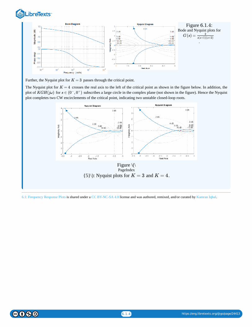
6.1.4 https://eng.libretexts.org/@go/page/24413

Figure :Bode and Nyquist plots for

.

Further, the Nyquist plot for passes through the critical point.

The Nyquist plot for crosses the real axis to the left of the critical point as shown in the figure below. In addition, theplot of for subscribes a large circle in the complex plane (not shown in the figure). Hence the Nyquistplot completes two CW encirclements of the critical point, indicating two unstable closed-loop roots.

Figure \(\PageIndex

{5}\): Nyquist plots for and .

6.1: Frequency Response Plots is shared under a CC BY-NC-SA 4.0 license and was authored, remixed, and/or curated by Kamran Iqbal.

6.1.4

G(s) = 2s(s+1)(s+2)

K = 3

K = 4KGH(jω) s ∈ ( , )0− 0+

K = 3 K = 4

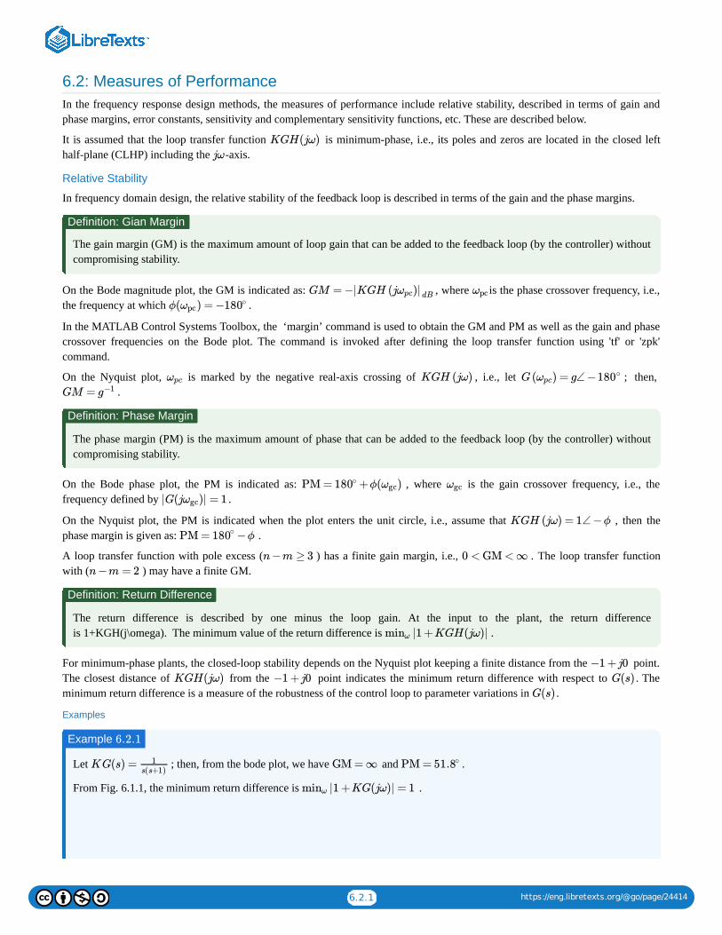
6.2.1 https://eng.libretexts.org/@go/page/24414

6.2: Measures of PerformanceIn the frequency response design methods, the measures of performance include relative stability, described in terms of gain andphase margins, error constants, sensitivity and complementary sensitivity functions, etc. These are described below.

It is assumed that the loop transfer function is minimum-phase, i.e., its poles and zeros are located in the closed lefthalf-plane (CLHP) including the -axis.

Relative Stability

In frequency domain design, the relative stability of the feedback loop is described in terms of the gain and the phase margins.

The gain margin (GM) is the maximum amount of loop gain that can be added to the feedback loop (by the controller) withoutcompromising stability.

On the Bode magnitude plot, the GM is indicated as: , where is the phase crossover frequency, i.e.,the frequency at which .

In the MATLAB Control Systems Toolbox, the ‘margin’ command is used to obtain the GM and PM as well as the gain and phasecrossover frequencies on the Bode plot. The command is invoked after defining the loop transfer function using 'tf' or 'zpk'command.

On the Nyquist plot, is marked by the negative real-axis crossing of , i.e., let ; then, .

The phase margin (PM) is the maximum amount of phase that can be added to the feedback loop (by the controller) withoutcompromising stability.

On the Bode phase plot, the PM is indicated as: , where is the gain crossover frequency, i.e., thefrequency defined by .

On the Nyquist plot, the PM is indicated when the plot enters the unit circle, i.e., assume that , then thephase margin is given as: .

A loop transfer function with pole excess ( ) has a finite gain margin, i.e., . The loop transfer functionwith ( ) may have a finite GM.

The return difference is described by one minus the loop gain. At the input to the plant, the return differenceis 1+KGH(j\omega). The minimum value of the return difference is .

For minimum-phase plants, the closed-loop stability depends on the Nyquist plot keeping a finite distance from the point.The closest distance of from the point indicates the minimum return difference with respect to . Theminimum return difference is a measure of the robustness of the control loop to parameter variations in .

Examples

Let ; then, from the bode plot, we have and .

From Fig. 6.1.1, the minimum return difference is .

KGH(jω)

jω

Definition: Gian Margin

GM = −|KGH (j )|ωpc dB ωpc

ϕ( ) = −ωpc 180∘

ωpc KGH (jω) G( ) = g∠ −180ωpc∘

GM = g−1

Definition: Phase Margin

PM = +ϕ( )180∘ ωgc ωgc

|G(j )| = 1ωgc

KGH (jω) = 1∠ −ϕ

PM = −ϕ180∘

n−m ≥ 3 0 < GM < ∞

n−m = 2

Definition: Return Difference

|1 +KGH(jω)|minω

−1 +j0

KGH(jω) −1 +j0 G(s)

G(s)

Example 6.2.1

KG(s) = 1s(s+1)

GM = ∞ PM = 51.8∘

|1 +KG(jω)| = 1minω

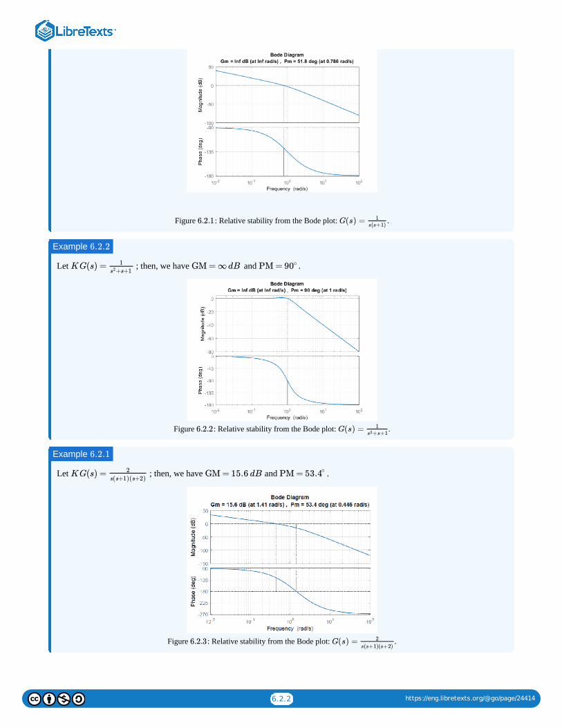
6.2.2 https://eng.libretexts.org/@go/page/24414

Figure : Relative stability from the Bode plot: .

Let ; then, we have and .

Figure : Relative stability from the Bode plot: .

Let ; then, we have and .

Figure : Relative stability from the Bode plot: .

6.2.1 G(s) = 1s(s+1)

Example 6.2.2

KG(s) = 1

+s+1s2 GM = ∞dB PM = 90∘

6.2.2 G(s) = 1+s+1s2

Example 6.2.1

KG(s) = 2

s(s+1)(s+2)GM = 15.6 dB PM = 53.4∘

6.2.3 G(s) = 2

s(s+1)(s+2)

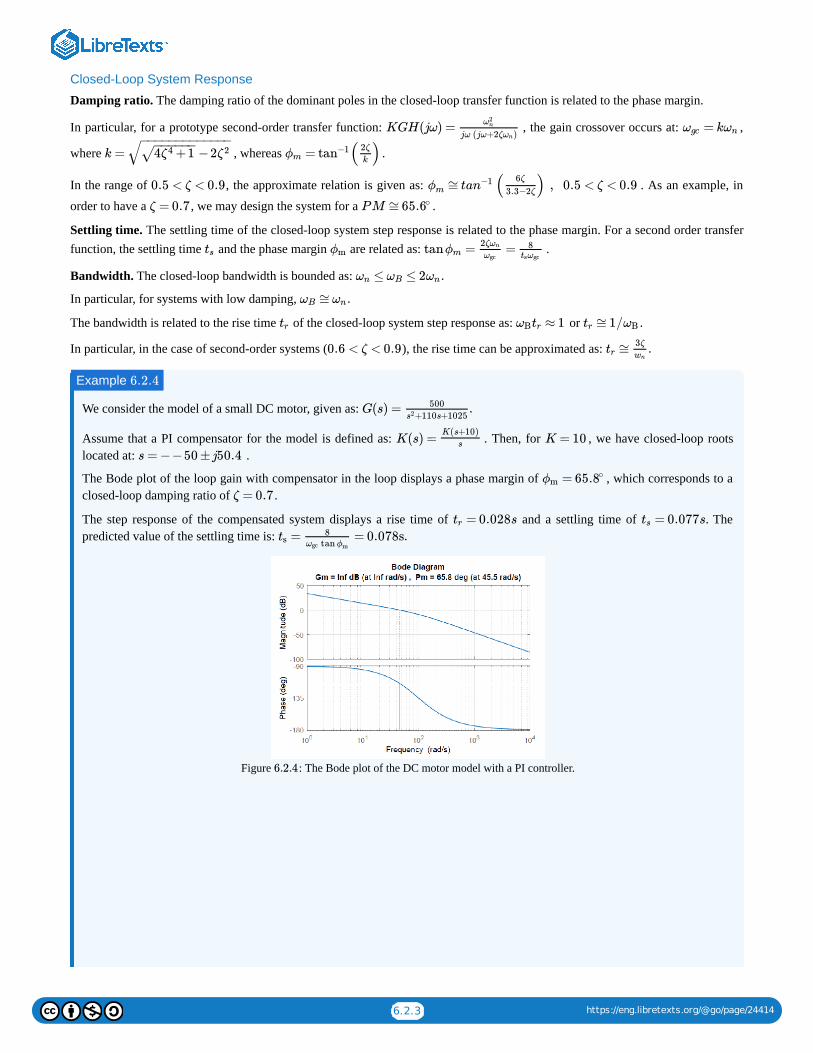
6.2.3 https://eng.libretexts.org/@go/page/24414

Closed-Loop System Response

Damping ratio. The damping ratio of the dominant poles in the closed-loop transfer function is related to the phase margin.

In particular, for a prototype second-order transfer function: , the gain crossover occurs at: ,

where , whereas .

In the range of , the approximate relation is given as: . As an example, in

order to have a , we may design the system for a .

Settling time. The settling time of the closed-loop system step response is related to the phase margin. For a second order transferfunction, the settling time and the phase margin are related as: .

Bandwidth. The closed-loop bandwidth is bounded as:

In particular, for systems with low damping,

The bandwidth is related to the rise time of the closed-loop system step response as: or .

In particular, in the case of second-order systems ( ), the rise time can be approximated as:

We consider the model of a small DC motor, given as:

Assume that a PI compensator for the model is defined as: . Then, for , we have closed-loop rootslocated at: .

The Bode plot of the loop gain with compensator in the loop displays a phase margin of , which corresponds to aclosed-loop damping ratio of .

The step response of the compensated system displays a rise time of and a settling time of . Thepredicted value of the settling time is:

Figure : The Bode plot of the DC motor model with a PI controller.

KGH(jω) =ω2n

jω (jω+2ζ )ωn= kωgc ωn

k = −24 +1ζ4− −−−−−√ ζ2− −−−−−−−−−−−−

√ = ( )ϕm tan−1 2ζ

k

0.5 < ζ < 0.9 ≅ ( )  , 0.5 < ζ < 0.9ϕm tan−1 6ζ

3.3−2ζ

ζ = 0.7 PM ≅65.6∘

ts ϕm tan = =ϕm2ζωn

ωgc

8tsωgc

≤ ≤ 2 .ωn ωB ωn

≅ .ωB ωn

tr ≈ 1ωBtr ≅1/tr ωB

0.6 < ζ < 0.9 ≅ .tr3ζ

wn

Example 6.2.4

G(s) = .500

+110s+1025s2

K(s) =K(s+10)

s K = 10

s = −−50 ±j50.4

=ϕm 65.8∘

ζ = 0.7

= 0.028str = 0.077sts= = 0.078s.ts

8tanωgc ϕm

6.2.4

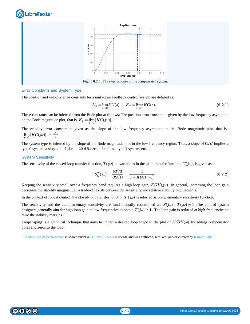
6.2.4 https://eng.libretexts.org/@go/page/24414

Figure : The step response of the compensated system.

Error Constants and System Type

The position and velocity error constants for a unity-gain feedback control system are defined as:

These constants can be inferred from the Bode plot at follows: The position error constant is given by the low frequency asymptoteon the Bode magnitude plot, that is, .

The velocity error constant is given as the slope of the low frequency asymptote on the Bode magnitude plot, that is,

The system type is inferred by the slope of the Bode magnitude plot in the low frequency region. Thus, a slope of implies atype system; a slope of , i.e., /decade implies a type system, etc.

System Sensitivity

The sensitivity of the closed-loop transfer function, , to variations in the plant transfer function, , is given as:

Keeping the sensitivity small over a frequency band requires a high loop gain, . In general, increasing the loop gaindecreases the stability margins, i.e., a trade-off exists between the sensitivity and relative stability requirements.

In the context of robust control, the closed-loop transfer function is referred as complementary sensitivity function.

The sensitivity and the complementary sensitivity are fundamentally constrained as: .The control systemdesigners generally aim for high loop gain at low frequencies to obtain . The loop gain is reduced at high frequencies toraise the stability margins.

Loopshaping is a graphical technique that aims to impart a desired loop shape to the plot of by adding compensatorpoles and zeros to the loop.

6.2: Measures of Performance is shared under a CC BY-NC-SA 4.0 license and was authored, remixed, and/or curated by Kamran Iqbal.

6.2.5

= KG(s) , = sKG(s).Kp lims→0

Kv lims→0

(6.2.1)

= |KG(jω)|Kp lims→0

|KG(jω)| = .lims→0

Kv

ω

0dB

0 −1 −20 dB 1

T (jω) G(jω)

(jω) = =STG

∂T/T

∂G/G

1

1 +KGH(jω)(6.2.2)

KGH(jω)

T (jω)

S(jω) +T (jω) = 1

T (jω) ≅1

KGH(jω)

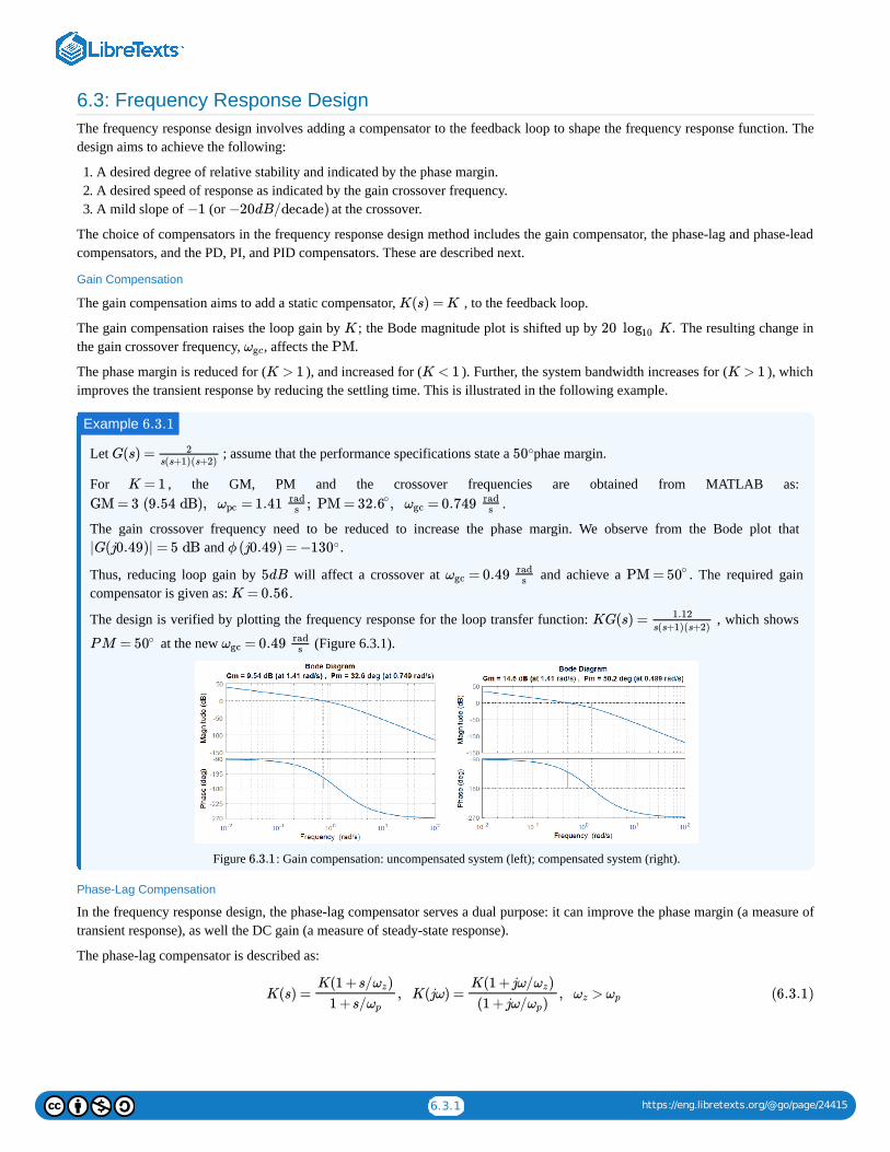
6.3.1 https://eng.libretexts.org/@go/page/24415

6.3: Frequency Response DesignThe frequency response design involves adding a compensator to the feedback loop to shape the frequency response function. Thedesign aims to achieve the following:

1. A desired degree of relative stability and indicated by the phase margin.2. A desired speed of response as indicated by the gain crossover frequency.3. A mild slope of (or at the crossover.

The choice of compensators in the frequency response design method includes the gain compensator, the phase-lag and phase-leadcompensators, and the PD, PI, and PID compensators. These are described next.

Gain Compensation

The gain compensation aims to add a static compensator, , to the feedback loop.

The gain compensation raises the loop gain by ; the Bode magnitude plot is shifted up by The resulting change inthe gain crossover frequency, , affects the .

The phase margin is reduced for ( ), and increased for ( ). Further, the system bandwidth increases for ( ), whichimproves the transient response by reducing the settling time. This is illustrated in the following example.

Let ; assume that the performance specifications state a phae margin.

For , the GM, PM and the crossover frequencies are obtained from MATLAB as: .

The gain crossover frequency need to be reduced to increase the phase margin. We observe from the Bode plot that and .

Thus, reducing loop gain by will affect a crossover at and achieve a . The required gaincompensator is given as: .

The design is verified by plotting the frequency response for the loop transfer function: , which shows

at the new (Figure 6.3.1).

Figure : Gain compensation: uncompensated system (left); compensated system (right).

Phase-Lag Compensation

In the frequency response design, the phase-lag compensator serves a dual purpose: it can improve the phase margin (a measure oftransient response), as well the DC gain (a measure of steady-state response).

The phase-lag compensator is described as:

−1 −20dB/decade)

K(s) = K

K 20 K.log10

ωgc PM

K > 1 K < 1 K > 1

Example 6.3.1

G(s) = 2s(s+1)(s+2)

50∘

K = 1

GM = 3 (9.54 dB), = 1.41 ; PM = , = 0.749ωpcrad

s 32.6∘ ωgcrad

s

|G(j0.49)| = 5 dB ϕ (j0.49) = −130∘

5dB = 0.49ωgcrad

s PM = 50∘

K = 0.56

KG(s) = 1.12s(s+1)(s+2)

PM = 50∘ = 0.49ωgcrad

s

6.3.1

K(s) = , K(jω) = , >K(1 +s/ )ωz

1 +s/ωp

K(1 +jω/ )ωz

(1 +jω/ )ωp

ωz ωp (6.3.1)

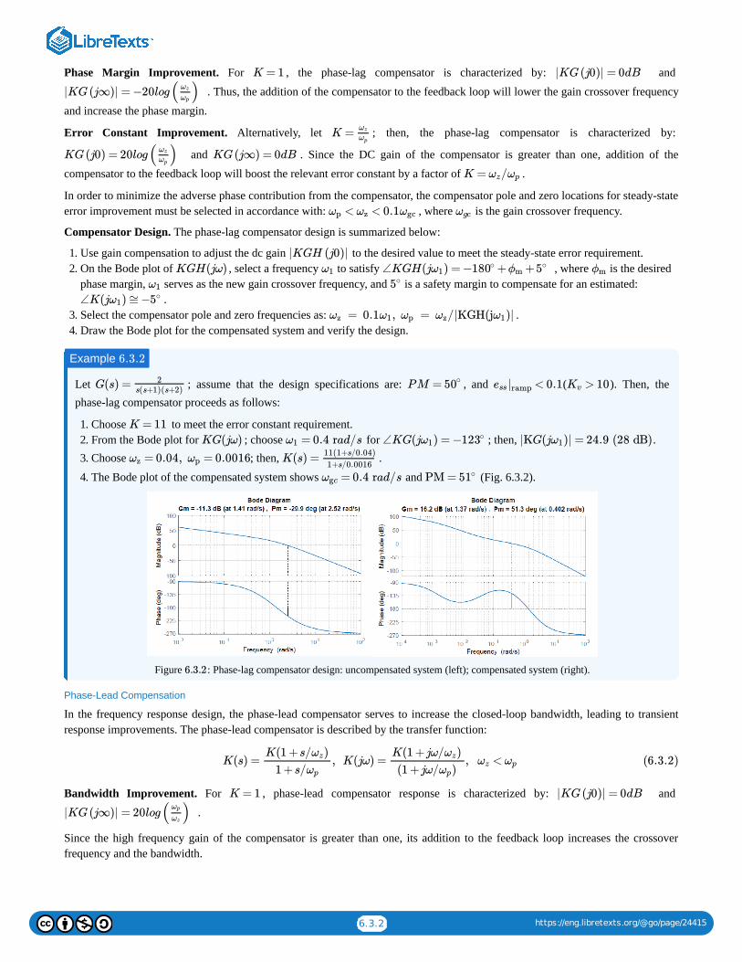
6.3.2 https://eng.libretexts.org/@go/page/24415

Phase Margin Improvement. For , the phase-lag compensator is characterized by: and

. Thus, the addition of the compensator to the feedback loop will lower the gain crossover frequency

and increase the phase margin.

Error Constant Improvement. Alternatively, let ; then, the phase-lag compensator is characterized by:

and . Since the DC gain of the compensator is greater than one, addition of the

compensator to the feedback loop will boost the relevant error constant by a factor of .

In order to minimize the adverse phase contribution from the compensator, the compensator pole and zero locations for steady-stateerror improvement must be selected in accordance with: , where is the gain crossover frequency.

Compensator Design. The phase-lag compensator design is summarized below:

1. Use gain compensation to adjust the dc gain to the desired value to meet the steady-state error requirement.2. On the Bode plot of , select a frequency to satisfy , where is the desired

phase margin, serves as the new gain crossover frequency, and is a safety margin to compensate for an estimated: .

3. Select the compensator pole and zero frequencies as: .4. Draw the Bode plot for the compensated system and verify the design.

Let ; assume that the design specifications are: , and ( ). Then, thephase-lag compensator proceeds as follows:

1. Choose to meet the error constant requirement.2. From the Bode plot for ; choose for ; then, .3. Choose ; then, .

4. The Bode plot of the compensated system shows and (Fig. 6.3.2).

Figure : Phase-lag compensator design: uncompensated system (left); compensated system (right).

Phase-Lead Compensation

In the frequency response design, the phase-lead compensator serves to increase the closed-loop bandwidth, leading to transientresponse improvements. The phase-lead compensator is described by the transfer function:

Bandwidth Improvement. For , phase-lead compensator response is characterized by: and

.

Since the high frequency gain of the compensator is greater than one, its addition to the feedback loop increases the crossoverfrequency and the bandwidth.

K = 1 |KG(j0)| = 0dB

|KG(j∞)| = −20log( )  ωz

ωp

K =ωz

ωp

KG(j0) = 20log( )  ωz

ωpKG(j∞) = 0dB

K = /ωz ωp

< < 0.1ωp ωz ωgc ωgc

|KGH (j0)|KGH(jω) ω1 ∠KGH(j ) = − + +ω1 180∘ ϕm 5∘ ϕm

ω1 5∘

∠K(j ) ≅−ω1 5∘

= 0.1 , = /|KGH(j )|ωz ω1 ωp ωz ω1

Example 6.3.2

G(s) = 2s(s+1)(s+2)

PM = 50∘ < 0.1ess |ramp > 10Kv

K = 11KG(jω) = 0.4 rad/sω1 ∠KG(j ) = −ω1 123∘ |KG(j )| = 24.9 (28 dB)ω1

= 0.04, = 0.0016ωz ωp K(s) =11(1+s/0.04)

1+s/0.0016

= 0.4 rad/sωgc PM = 51∘

6.3.2

K(s) = , K(jω) = , <K(1 +s/ )ωz

1 +s/ωp

K(1 +jω/ )ωz

(1 +jω/ )ωp

ωz ωp (6.3.2)

K = 1 |KG(j0)| = 0dB

|KG(j∞)| = 20log( )  ωp

ωz

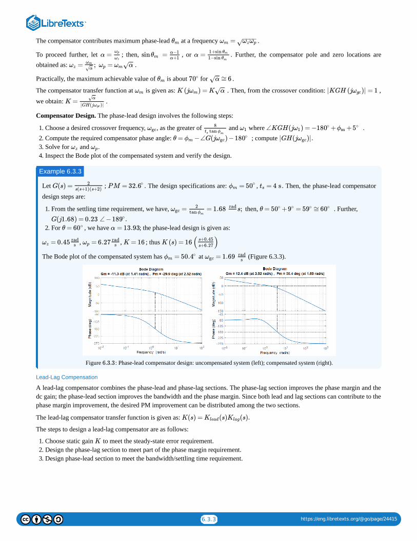
6.3.3 https://eng.libretexts.org/@go/page/24415

The compensator contributes maximum phase-lead at a frequency .

To proceed further, let ; then, , or . Further, the compensator pole and zero locations areobtained as: .

Practically, the maximum achievable value of is about for .

The compensator transfer function at is given as: . Then, from the crossover condition: ,

we obtain: .

Compensator Design. The phase-lead design involves the following steps:

1. Choose a desired crossover frequency, , as the greater of and where .2. Compute the required compensator phase angle: ; compute 3. Solve for and .4. Inspect the Bode plot of the compensated system and verify the design.

Let ; . The design specifications are: , . Then, the phase-lead compensator

design steps are:

1. From the settling time requirement, we have, then, . Further,

2. For , we have ; the phase-lead design is given as:

, , ; thus

The Bode plot of the compensated system has at (Figure 6.3.3).

Figure : Phase-lead compensator design: uncompensated system (left); compensated system (right).

Lead-Lag Compensation

A lead-lag compensator combines the phase-lead and phase-lag sections. The phase-lag section improves the phase margin and thedc gain; the phase-lead section improves the bandwidth and the phase margin. Since both lead and lag sections can contribute to thephase margin improvement, the desired PM improvement can be distributed among the two sections.

The lead-lag compensator transfer function is given as:

The steps to design a lead-lag compensator are as follows:

1. Choose static gain to meet the steady-state error requirement.2. Design the phase-lag section to meet part of the phase margin requirement.3. Design phase-lead section to meet the bandwidth/settling time requirement.

θm =ωm ωzωp− −−−

√

α =ωp

ωzsin =θm

α−1α+1

α =1+sin θm

1−sin θm

= ; =ωzωm

α√ωp ωm α−−√

θm 70∘ ≅6α−−√

ωm K (j ) = Kωm α−−√ |KGH (j )| = 1ωgc

K =α√

|GH(j )|ωgc

ωgc8

tants ϕm

ω1 ∠KGH(j ) = − + +ω1 180∘ ϕm 5∘

θ = −∠G(j ) −ϕm ωgc 180∘ |GH(j )|.ωgc

ωz ωp

Example 6.3.3

G(s) = 2s(s+1)(s+2)

PM = 32.6∘ =ϕm 50∘ = 4 sts

= = 1.68 s;ωgc2

tan ϕm

rad θ = + = ≅50∘ 9∘ 59∘ 60∘

G(j1.68) = 0.23 ∠ − .189∘

θ = 60∘ α = 13.93

= 0.45ωzrad

s = 6.27ωprad

s K = 16 K (s) = 16( )s+0.45s+6.27

=ϕm 50.4∘ = 1.69ωgcrad

s

6.3.3

K(s) = (s) (s).Klead Klag

K

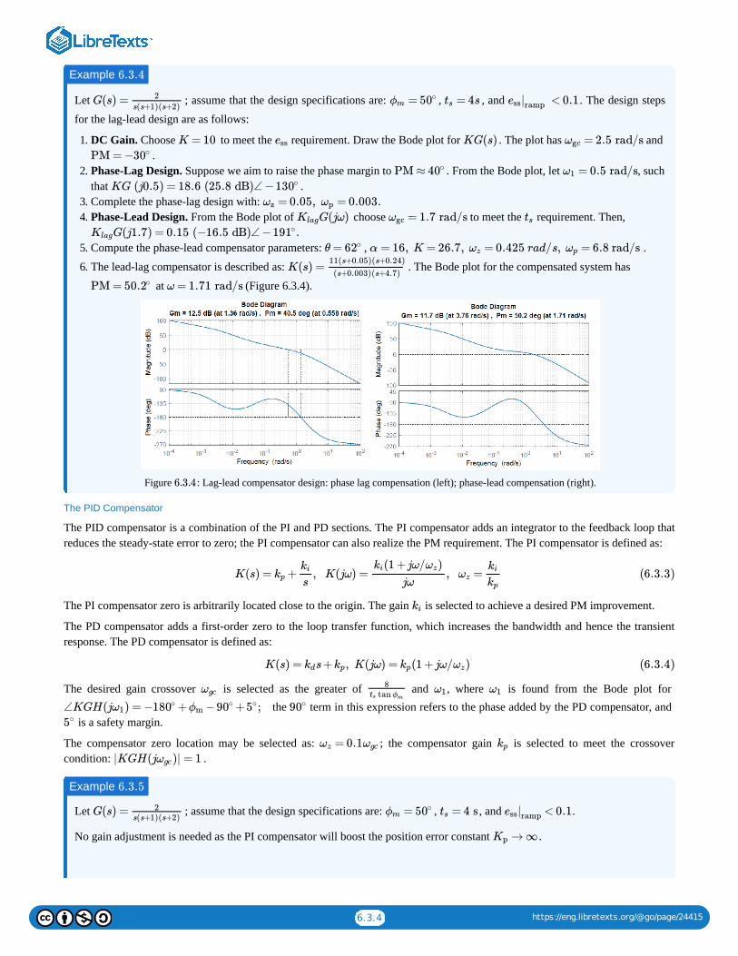
6.3.4 https://eng.libretexts.org/@go/page/24415

Let ; assume that the design specifications are: , , and . The design steps

for the lag-lead design are as follows:

1. DC Gain. Choose to meet the requirement. Draw the Bode plot for . The plot has and .

2. Phase-Lag Design. Suppose we aim to raise the phase margin to . From the Bode plot, let , suchthat .

3. Complete the phase-lag design with: 4. Phase-Lead Design. From the Bode plot of choose to meet the requirement. Then,

5. Compute the phase-lead compensator parameters: , .

6. The lead-lag compensator is described as: . The Bode plot for the compensated system has

at (Figure 6.3.4).

Figure : Lag-lead compensator design: phase lag compensation (left); phase-lead compensation (right).

The PID Compensator

The PID compensator is a combination of the PI and PD sections. The PI compensator adds an integrator to the feedback loop thatreduces the steady-state error to zero; the PI compensator can also realize the PM requirement. The PI compensator is defined as:

The PI compensator zero is arbitrarily located close to the origin. The gain is selected to achieve a desired PM improvement.

The PD compensator adds a first-order zero to the loop transfer function, which increases the bandwidth and hence the transientresponse. The PD compensator is defined as:

The desired gain crossover is selected as the greater of and , where is found from the Bode plot for the term in this expression refers to the phase added by the PD compensator, and

is a safety margin.

The compensator zero location may be selected as: ; the compensator gain is selected to meet the crossovercondition: .

Let ; assume that the design specifications are: , , and .

No gain adjustment is needed as the PI compensator will boost the position error constant .

Example 6.3.4

G(s) = 2s(s+1)(s+2)

=ϕm 50∘ = 4sts < 0.1ess|ramp

K = 10 ess KG(s) = 2.5 rad/sωgc

PM = −30∘

PM ≈ 40∘ = 0.5 rad/sω1

KG (j0.5) = 18.6 (25.8 dB)∠ −130∘

= 0.05, = 0.003.ωz ωp

G(jω)Klag = 1.7 rad/sωgc tsG(j1.7) = 0.15 (−16.5 dB)∠ − .Klag 191∘

θ = 62∘ α = 16,  K = 26.7,   = 0.425 rad/s,   = 6.8 rad/sωz ωp

K(s) =11(s+0.05)(s+0.24)

(s+0.003)(s+4.7)

PM = 50.2∘ ω = 1.71 rad/s

6.3.4

K(s) = + , K(jω) = , =kpki

s

(1 +jω/ )ki ωz

jωωz

ki

kp(6.3.3)

ki

K(s) = s+ , K(jω) = (1 +jω/ )kd kp kp ωz (6.3.4)

ωgc8

tants ϕmω1 ω1

∠KGH(j ) = − + − + ;ω1 180∘ ϕm 90∘ 5∘ 90∘

5∘

= 0.1ωz ωgc kp|KGH(j )| = 1ωgc

Example 6.3.5

G(s) = 2s(s+1)(s+2)

=ϕm 50∘ = 4 sts < 0.1ess|ramp

→ ∞Kp

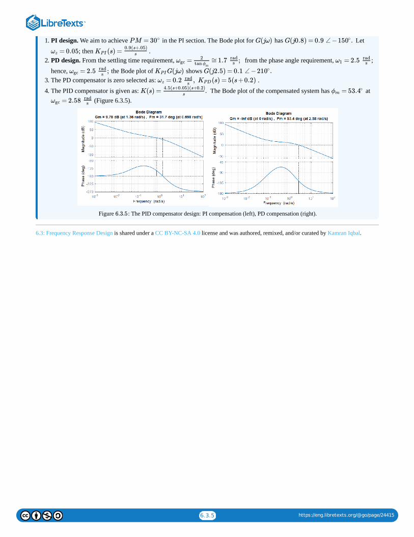
6.3.5 https://eng.libretexts.org/@go/page/24415

1. PI design. We aim to achieve in the PI section. The Bode plot for has Let

; then .2. PD design. From the settling time requirement, from the phase angle requirement, ;

hence, the Bode plot of shows 3. The PD compensator is zero selected as: .

4. The PID compensator is given as: The Bode plot of the compensated system has at (Figure 6.3.5).

Figure : The PID compensator design: PI compensation (left), PD compensation (right).

6.3: Frequency Response Design is shared under a CC BY-NC-SA 4.0 license and was authored, remixed, and/or curated by Kamran Iqbal.

PM = 30∘ G(jω) G(j0.8) = 0.9 ∠ − .150∘

= 0.05ωz (s) =KPI0.9(s+.05)

s

= ≅1.7 ;ωgc2

tan ϕm

rads = 2.5ω1

rads

= 2.5 ;ωgcrad

sG(jω)KPI G(j2.5) = 0.1 ∠ − .210∘

= 0.2 , (s) = 5(s+0.2)ωzrad

sKPD

K(s) = .4.5(s+0.05)(s+0.2)

s=ϕm 53.4∘

= 2.58ωgcrad

s

6.3.5

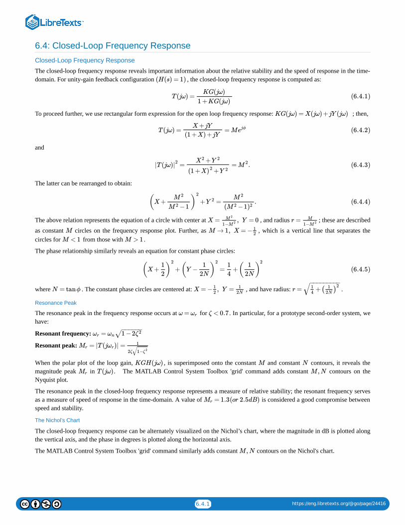
6.4.1 https://eng.libretexts.org/@go/page/24416

6.4: Closed-Loop Frequency Response

Closed-Loop Frequency Response

The closed-loop frequency response reveals important information about the relative stability and the speed of response in the time-domain. For unity-gain feedback configuration , the closed-loop frequency response is computed as:

To proceed further, we use rectangular form expression for the open loop frequency response: ; then,

and

The latter can be rearranged to obtain:

The above relation represents the equation of a circle with center at , and radius ; these are described

as constant circles on the frequency response plot. Further, as , which is a vertical line that separates thecircles for from those with .

The phase relationship similarly reveals an equation for constant phase circles:

where . The constant phase circles are centered at: , and have radius: .

Resonance Peak

The resonance peak in the frequency response occurs at for . In particular, for a prototype second-order system, wehave:

Resonant frequency:

Resonant peak:

When the polar plot of the loop gain, , is superimposed onto the constant and constant contours, it reveals themagnitude peak in . The MATLAB Control System Toolbox 'grid' command adds constant contours on theNyquist plot.

The resonance peak in the closed-loop frequency response represents a measure of relative stability; the resonant frequency servesas a measure of speed of response in the time-domain. A value of is considered a good compromise betweenspeed and stability.

The Nichol’s Chart

The closed-loop frequency response can be alternately visualized on the Nichol’s chart, where the magnitude in dB is plotted alongthe vertical axis, and the phase in degrees is plotted along the horizontal axis.

The MATLAB Control System Toolbox 'grid' command similarly adds constant contours on the Nichol's chart.

(H(s) = 1)

T (jω) =KG(jω)

1 +KG(jω)(6.4.1)

KG(jω) = X(jω) +jY (jω)

T (jω) = = MX+jY

(1 +X) +jYejϕ (6.4.2)

= = .|T (jω)|2 +X2 Y 2

+(1 +X)2 Y 2M 2 (6.4.3)

+ = .(X+ )M 2

−1M 2

2

Y 2 M 2

( −1M 2 )2(6.4.4)

X = , Y = 0M 2

1−M 2 r = M

1−M 2

M M → 1, X = − 12

M < 1 M > 1

+ = +(X+ )1

2

2

(Y − )1

2N

21

4( )

1

2N

2

(6.4.5)

N = tanϕ X = − , Y =12

12N

r = +14

( )12N

2− −−−−−−−−

√

ω = ωr ζ < 0.7

=ωr ωn 1 −2ζ2− −−−−−√

= |T (j )| =Mr ωr1

2ζ 1−ζ 2√

KGH(jω) M N

Mr T (jω) M ,N

= 1.3Mr (or 2.5dB)

M ,N

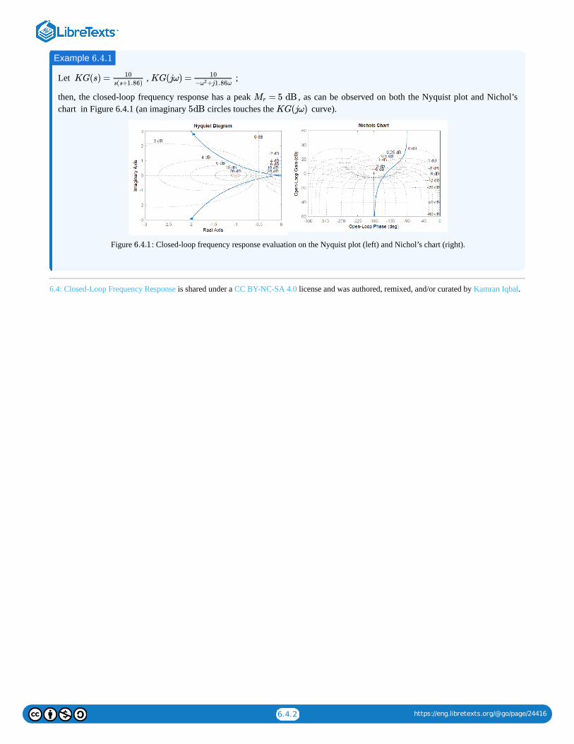
6.4.2 https://eng.libretexts.org/@go/page/24416

Let , ;

then, the closed-loop frequency response has a peak , as can be observed on both the Nyquist plot and Nichol’schart in Figure 6.4.1 (an imaginary circles touches the curve).

Figure : Closed-loop frequency response evaluation on the Nyquist plot (left) and Nichol’s chart (right).

6.4: Closed-Loop Frequency Response is shared under a CC BY-NC-SA 4.0 license and was authored, remixed, and/or curated by Kamran Iqbal.

Example 6.4.1

KG(s) = 10

s(s+1.86)KG(jω) = 10

− +j1.86ωω2

= 5 dBMr

5dB KG(jω)

6.4.1

1

CHAPTER OVERVIEW

7: Design of Sampled-Data Systems

1. Understand and analyze the sampled-data systems models.2. Solve difference equation models of sampled-data systems by iteration.3. Analyze the stability of closed-loop sampled-data systems.4. Design/emulate controllers for the sampled-data system models.

7.0: Prelude to Design of Sampled-Data Systems7.1: Models of Sampled-Data Systems7.2: Pulse Transfer Function7.3: Sampled-Data System Response7.4: Stability of Sampled-Data Systems7.5: Closed-Loop System Response7.6: Digital Controller Design by Emulation7.7: Root Locus Design of Digital Controllers

7: Design of Sampled-Data Systems is shared under a CC BY-NC-SA 4.0 license and was authored, remixed, and/or curated by Kamran Iqbal.

Learning Objectives

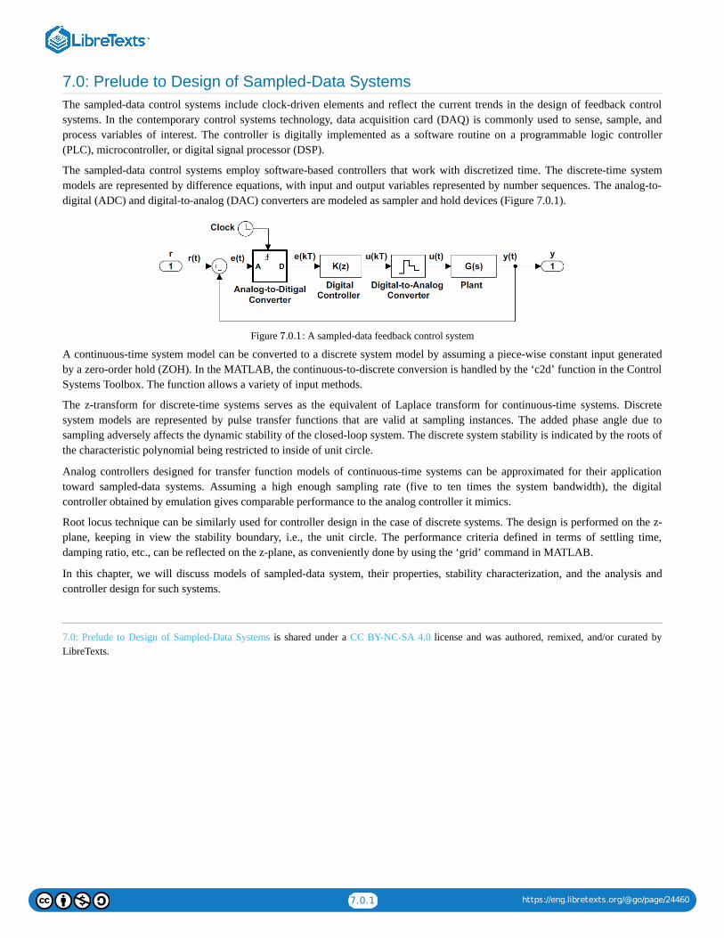
7.0.1 https://eng.libretexts.org/@go/page/24460

7.0: Prelude to Design of Sampled-Data SystemsThe sampled-data control systems include clock-driven elements and reflect the current trends in the design of feedback controlsystems. In the contemporary control systems technology, data acquisition card (DAQ) is commonly used to sense, sample, andprocess variables of interest. The controller is digitally implemented as a software routine on a programmable logic controller(PLC), microcontroller, or digital signal processor (DSP).

The sampled-data control systems employ software-based controllers that work with discretized time. The discrete-time systemmodels are represented by difference equations, with input and output variables represented by number sequences. The analog-to-digital (ADC) and digital-to-analog (DAC) converters are modeled as sampler and hold devices (Figure 7.0.1).

Figure : A sampled-data feedback control system

A continuous-time system model can be converted to a discrete system model by assuming a piece-wise constant input generatedby a zero-order hold (ZOH). In the MATLAB, the continuous-to-discrete conversion is handled by the ‘c2d’ function in the ControlSystems Toolbox. The function allows a variety of input methods.

The z-transform for discrete-time systems serves as the equivalent of Laplace transform for continuous-time systems. Discretesystem models are represented by pulse transfer functions that are valid at sampling instances. The added phase angle due tosampling adversely affects the dynamic stability of the closed-loop system. The discrete system stability is indicated by the roots ofthe characteristic polynomial being restricted to inside of unit circle.

Analog controllers designed for transfer function models of continuous-time systems can be approximated for their applicationtoward sampled-data systems. Assuming a high enough sampling rate (five to ten times the system bandwidth), the digitalcontroller obtained by emulation gives comparable performance to the analog controller it mimics.

Root locus technique can be similarly used for controller design in the case of discrete systems. The design is performed on the z-plane, keeping in view the stability boundary, i.e., the unit circle. The performance criteria defined in terms of settling time,damping ratio, etc., can be reflected on the z-plane, as conveniently done by using the ‘grid’ command in MATLAB.

In this chapter, we will discuss models of sampled-data system, their properties, stability characterization, and the analysis andcontroller design for such systems.

7.0: Prelude to Design of Sampled-Data Systems is shared under a CC BY-NC-SA 4.0 license and was authored, remixed, and/or curated byLibreTexts.

7.0.1

7.1.1 https://eng.libretexts.org/@go/page/24418

7.1: Models of Sampled-Data Systems

7.1.1 Sampled-Data Systems

The sampled-data systems operate on discrete-time, represented as integral multiples of the sampling time ( ).

To model the sampled-data systems, we consider an ideal sampler that samples a physical signal every seconds andgenerates a series of impulses with weights

Mathematically, the sampler output, , represents multiplication of with an impulse train, given as:

By applying the Laplace transform to the sampled signal , we obtain:

Since sampling time, , is constant, we can change the variable to: , to represent the sampled signal as:

where defines the -transform of the sampled signal, .

7.1.2 The z-transform

The -transform is the Laplace transform equivalent in the case of sampled-data systems. The domain of the -transform includesreal- or complex-valued number sequences.

Assuming the number sequence, , is obtained by sampling a real-valued signal , the time dependence may be suppressedto represent the sequence as: . The z-transformed sequence is given as:

The transformed sequence, , represents a rational function of a complex variable .

The -transform of a unit-step sequence: is given as:

The convergence of the above geometric series is conditioned on: , or which defines its region of convergence(ROC); the ROC is outside of the unit-circle: in the complex -plane.

Let ; then . Hence,

The ROC is outside of the circle of radius in the complex -plane.

In digital signal processing (DSP) applications, the index ' ' is commonly used to represent a real-valued sequenc, i.e., the z-transform of a sequence, is given as: .

T

r(t) T

r(kT ), k = 0, 1, … .

(t)r∗ r(t)

(t) = r(kT )δ(t −kT )r∗ ∑k=0

∞

(7.1.1)

(t)r∗

(s) = r(kT )r∗ ∑0

∞

e−skT (7.1.2)

T z = esT

r(z) = r(kT )∑0

∞

z−k (7.1.3)

r(z) z r(kT )

z z

r(kT ) r (t)

r (k) = {r (0) , r (1) , …}

r(z) = z[r(kT )] = r(k)∑0

∞

z−k (7.1.4)

r(z) z = |z| ejθ

Example 7.1.1

z u(k) = {1, 1, …}

u(z) = = ; | | < 1∑0

∞

z−k 1

1 −z−1z−1 (7.1.5)

| | < 1z−1 |z| > 1

,  0 ≤ θ < 2πejθ z

Example 7.1.2

r(t) = u(t)e−at r(kT ) = {1, , , …}e−aT e−2aT

r(z) = = ; | | < 1∑0

∞

e−akT z−k 1

1 −e−aT z−1e−aT z−1 (7.1.6)

e−aT z

n

r(n) = u(n)an r(z) = 11−az−1

7.1.2 https://eng.libretexts.org/@go/page/24418

Let then . Hence,

The ROC is outside of the unit-circle in the complex -plane.

The -transforms of the sampled sinusoidal signals are obtained by applying the Euler’s identity to the above -transform of and separating the real and imaginary parts. Thus

The -transforms of other complex signals may be obtained by using its properties of linearity, differentiation, and translation, etc.

Inverse z-Transform

Given the z-transform of a composite signal, the underlying sequence can be recovered by long division. Alternatively, partialfraction expansion (PFE) can be used to obtain first and second-order factors that can be inverse transformed with the help of z-transform tables.

Let represent the output of a feedback control system; then, the output sequence can be recovered by

the following methods:

1. Expand in partial fractions to obtain: . Hence, .2. Alternatively, use long division to obtain: . Hence,

.

7.1: Models of Sampled-Data Systems is shared under a CC BY-NC-SA 4.0 license and was authored, remixed, and/or curated by Kamran Iqbal.

Example 7.1.3

r(t) = u(t);ejωt r(kT ) = {1, , , …}ejωT e2jωT

r(z) = = ; | | = | | < 1∑0

∞

ejkωT z−k 1

1 −ejωT z−1ejωT z−1 z−1 (7.1.7)

z

z z ejkωT

sin(kωT ) ↔z sin(ωT ) z

−2 cos(ωT ) +1z2(7.1.8)

cos(kωT )↔z z(z −cos(ωT ) )

−2 cos(ωT) +1z2(7.1.9)

sin(kωT )e−akT ↔z sin(ωT )ze−aT

−2 cos(ωT ) +z2 e−aT e−2aT(7.1.10)

cos(kωT ) .e−akT ↔z z(z − cos(ωT ))e−aT

−2 cos(ωT ) +z2 e−aT e−2aT(7.1.11)

z

Example 7.1.4

y (z) =0.2z(z+0.9)

(z−1)(z−0.6)(z−0.9)

y(z)

zy (z) = − +4.75z

z−16z

z−0.91.25

z−0.6y (k) = 4.75 −6 +1.25(0.9)k (0.6)k

y (z) = 0.1 +0.34 +0.65 +0.98 +…z−1 z−2 z−3 z−4

y (k) = {0,  0.1,  0.34,  0.65,  0.98,   …}

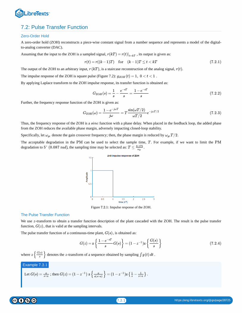
7.2.1 https://eng.libretexts.org/@go/page/28725

7.2: Pulse Transfer Function

Zero-Order Hold

A zero-order hold (ZOH) reconstructs a piece-wise constant signal from a number sequence and represents a model of the digital-to-analog converter (DAC).

Assuming that the input to the ZOH is a sampled signal, , its output is given as:

The output of the ZOH to an arbitrary input, , is a staircase reconstruction of the analog signal, .

The impulse response of the ZOH is square pulse (Figure 7.2): .

By applying Laplace transform to the ZOH impulse response, its transfer function is obtained as:

Further, the frequency response function of the ZOH is given as:

Thus, the frequency response of the ZOH is a function with a phase delay. When placed in the feedback loop, the added phasefrom the ZOH reduces the available phase margin, adversely impacting closed-loop stability.

Specifically, let denote the gain crossover frequency; then, the phase margin is reduced by

The acceptable degradation in the can be used to select the sample time, . For example, if we want to limit the degradation to , the sampling time may be selected as: .

Figure : Impulse response of the ZOH.

The Pulse Transfer Function

We use -transform to obtain a transfer function description of the plant cascaded with the ZOH. The result is the pulse transferfunction, , that is valid at the sampling intervals.

The pulse transfer function of a continuous-time plant, , is obtained as:

where denotes the -transform of a sequence obtained by sampling .

Let ; then

r(kT ) = r(t)|t=kT

r(t) = r((k−1)T ) for (k−1)T ≤ t < kT (7.2.1)

r (kT ) r(t)

(t) = 1, 0 < t < 1gZOH

(s) = − =GZOH

1

s

e−sT

s

1 −e−sT

s(7.2.2)

(ω) = = TGZOH1 −e−jωT

jω

sin(ωT/2)

ωT/2e−jωT/2 (7.2.3)

sinc

ωgc T/2.ωgc

PM T PM

(0.087 rad)5∘ T ≤ 0.175ωgc

7.2.1

z

G(z)

G(s)

G(z) = z{ G(s)} = (1 − )z{ }1 −e−sT

sz−1

G(s)

s(7.2.4)

z{ }G(s)

sz ∫ g (t)dt

Example 7.2.1

G(s) = as+a

G(z) = (1 − ) z{ } = (1 − )z{ − } .z−1 a

s(s+a)z−1 1

s1

s+a

7.2.2 https://eng.libretexts.org/@go/page/28725

By using the -transform table, we obtain: .

As an example, let . Then, the pulse transfer function is obtained as: , or

.

Let ; then .

By using the z-transform table, we obtain: .

As an example, let then, the pulse transfer function is obtained as: .

From the above examples, we observe that:

1. The order of the pulse transfer function, i.e., the degree of the denominator polynomial in , matches that of the continuous-time transfer function, .

2. The poles of the pulse transfer function are related to the transfer function poles as: .3. The pulse transfer functions of the second and higher order systems additionally includes finite zeros.

In the MATLAB Control Systems Toolbox, the pulse transfer function is obtained by using the “c2d” command and specifying asampling time ( ). The command is invoked after defining the continuous-time transfer function model.

The choice of the sampling time is guided by the natural frequency of the system. In particular, we may choose , where represents the natural frequency.

7.2: Pulse Transfer Function is shared under a CC BY-NC-SA 4.0 license and was authored, remixed, and/or curated by LibreTexts.

z G(z) = ( − ) =z−1z

z

z−1z

z−e−aT

1−e−aT

z−e−aT

G(s) = , T = 0.2s1s+1

G(z) = 0.181z−0.819

G(z) = 1−e−0.2

z−e−0.2

Example 7.2.2

G(s) = a

s(s+a)G(z) = (1 − ) z{ } = (1 − )z{ − + }z−1 a

(s+a)s2 z−1 1

s2

1/a

s

1/a

s+a

G(z) = [ − ( − )] =z−1z

Tz

(z−1)2

1a

z

z−1z

z−e−aT

aT (z− )−(z−1)(1− )e−aT e−aT

a(z−1)(z− )e−aT

G(s) = , T = 0.2s;1

s(s+1)G(z) =

0.0187(z+0.936)

(z−1)(z−0.819)

G(z)

G(s)

=zi e Tsi

Ts

≪ 1/Ts ωn

ωn

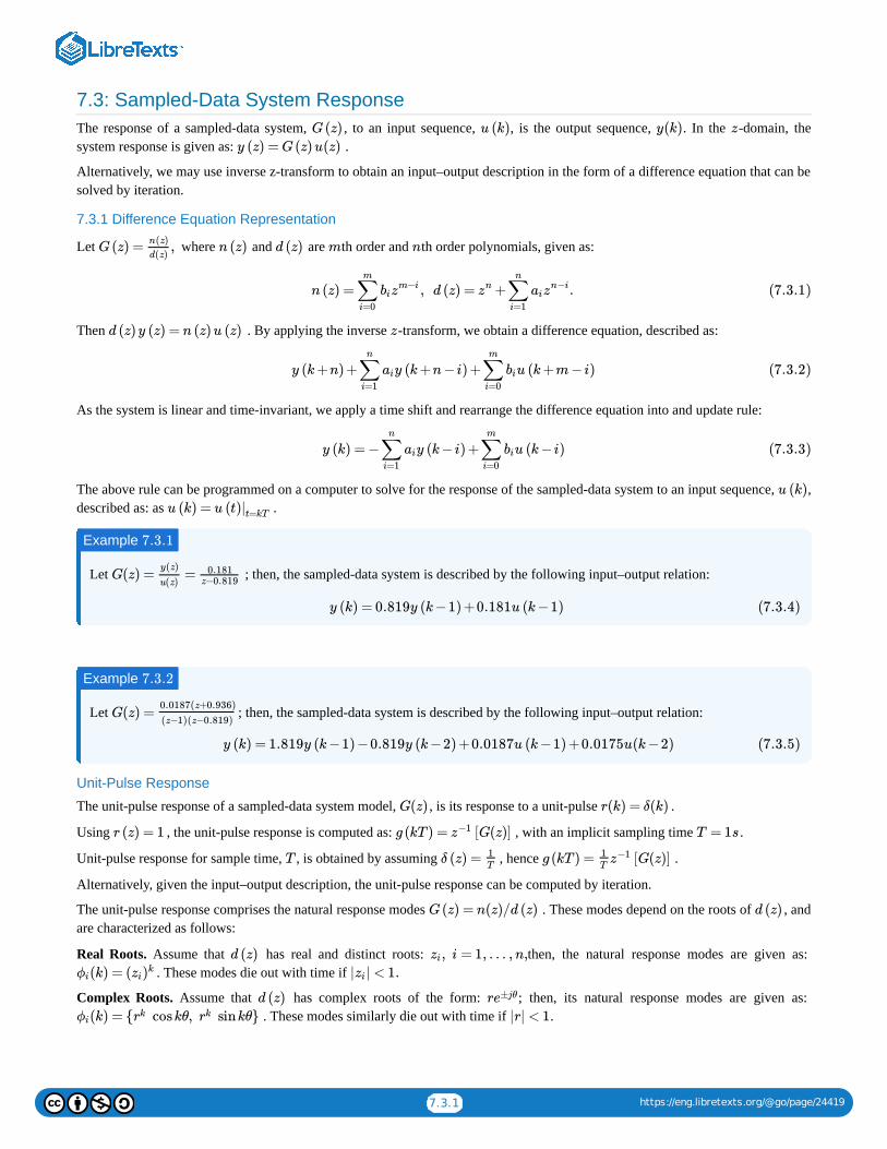
7.3.1 https://eng.libretexts.org/@go/page/24419

7.3: Sampled-Data System ResponseThe response of a sampled-data system, , to an input sequence, , is the output sequence, . In the -domain, thesystem response is given as: .

Alternatively, we may use inverse z-transform to obtain an input–output description in the form of a difference equation that can besolved by iteration.

7.3.1 Difference Equation Representation

Let where and are th order and th order polynomials, given as:

Then . By applying the inverse -transform, we obtain a difference equation, described as:

As the system is linear and time-invariant, we apply a time shift and rearrange the difference equation into and update rule:

The above rule can be programmed on a computer to solve for the response of the sampled-data system to an input sequence, ,described as: as .

Let ; then, the sampled-data system is described by the following input–output relation:

Let ; then, the sampled-data system is described by the following input–output relation:

Unit-Pulse Response

The unit-pulse response of a sampled-data system model, , is its response to a unit-pulse .

Using , the unit-pulse response is computed as: , with an implicit sampling time .

Unit-pulse response for sample time, , is obtained by assuming , hence .

Alternatively, given the input–output description, the unit-pulse response can be computed by iteration.

The unit-pulse response comprises the natural response modes . These modes depend on the roots of , andare characterized as follows:

Real Roots. Assume that has real and distinct roots: then, the natural response modes are given as: . These modes die out with time if

Complex Roots. Assume that has complex roots of the form: ; then, its natural response modes are given as: . These modes similarly die out with time if .

G(z) u (k) y(k) z

y (z) = G(z)u(z)

G(z) = ,n(z)

d(z)n (z) d (z) m n

n (z) = ,   d (z) = + .∑i=0

m

bizm−i zn ∑

i=1

n

aizn−i (7.3.1)

d (z)y (z) = n (z)u (z) z

y (k+n) + y (k+n− i) + u (k+m− i)∑i=1

n

ai ∑i=0

m

bi (7.3.2)

y (k) = − y (k− i) + u (k− i)∑i=1

n

ai ∑i=0

m

bi (7.3.3)

u (k)

u (k) = u (t)|t=kT

Example 7.3.1

G(z) = =y(z)

u(z)0.181

z−0.819

y (k) = 0.819y (k−1) +0.181u (k−1) (7.3.4)

Example 7.3.2

G(z) =0.0187(z+0.936)

(z−1)(z−0.819)

y (k) = 1.819y (k−1) −0.819y (k−2) +0.0187u (k−1) +0.0175u(k−2) (7.3.5)

G(z) r(k) = δ(k)

r (z) = 1 g (kT ) = [G(z)]z−1 T = 1s

T δ (z) = 1T

g (kT ) = [G(z)]1Tz−1

G(z) = n(z)/d (z) d (z)

d (z) , i = 1, … ,n,zi(k) = (ϕi zi)

k | | < 1.zi

d (z) re±jθ

(k) = { coskθ, sinkθ}ϕi rk rk |r| < 1

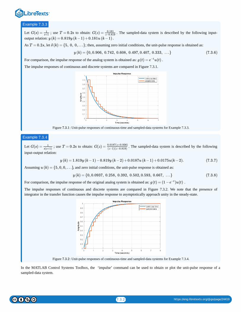
7.3.2 https://eng.libretexts.org/@go/page/24419

Let ; use to obtain: . The sampled-data system is described by the following input-output relation:

As , let ; then, assuming zero initial conditions, the unit-pulse response is obtained as:

For comparison, the impulse response of the analog system is obtained as: .

The impulse responses of continuous and discrete systems are compared in Figure 7.3.1.

Figure : Unit-pulse responses of continuous-time and sampled-data systems for Example 7.3.3.

Let ; use to obtain: . The sampled-data system is described by the following

input-output relation:

Assuming , and zero initial conditions, the unit-pulse response is obtained as:

For comparison, the impulse response of the original analog system is obtained as: .

The impulse responses of continuous and discrete systems are compared in Figure 7.3.2. We note that the presence ofintegrator in the transfer function causes the impulse response to asymptotically approach unity in the steady-state.

Figure : Unit-pulse responses of continuous-time and sampled-data systems for Example 7.3.4.

In the MATLAB Control Systems Toolbox, the ‘impulse’ command can be used to obtain or plot the unit-pulse response of asampled-data system.

Example 7.3.3

G(s) = 1s+1

T = 0.2s G(z) = 0.181z−0.819

y (k) = 0.819y (k−1) +0.181u (k−1) .

T = 0.2s δ (k) = {5,  0,  0, …}

y (k) = {0, 0.906,  0.742,  0.608,  0.497, 0.407,  0.333,   …} (7.3.6)

g (t) = u(t)e−t

7.3.1

Example 7.3.4

G(s) = 1s(s+1)

T = 0.2s G(z) =0.0187(z+0.936)

(z−1)(z−0.819)

y (k) = 1.819y (k−1) −0.819y (k−2) +0.0187u (k−1) +0.0175u(k−2). (7.3.7)

u (k) = {5, 0, 0, …}

y (k) = {0, 0.0937,  0.258,  0.392,  0.502, 0.593,  0.667,   …} (7.3.8)

g (t) = (1 − )u(t)e−t

7.3.2

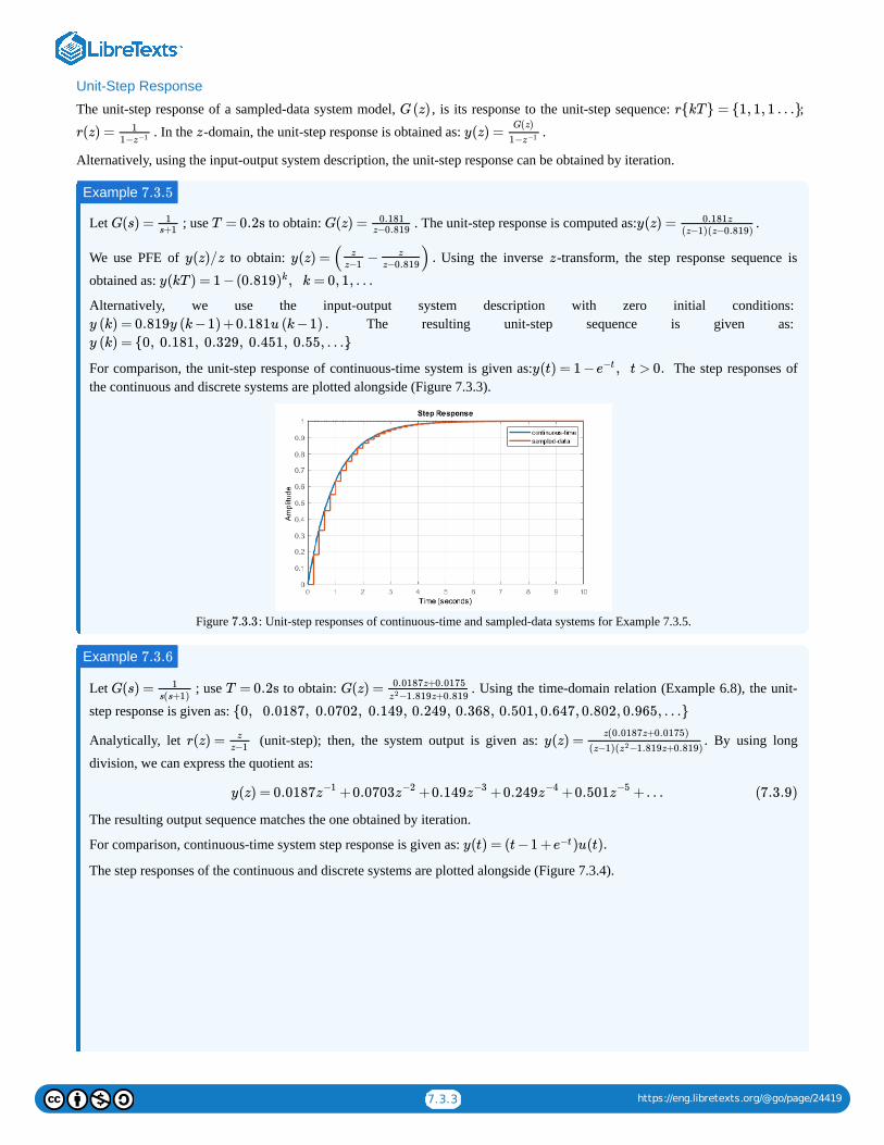
7.3.3 https://eng.libretexts.org/@go/page/24419

Unit-Step Response

The unit-step response of a sampled-data system model, , is its response to the unit-step sequence: ;

. In the -domain, the unit-step response is obtained as: .

Alternatively, using the input-output system description, the unit-step response can be obtained by iteration.

Let ; use to obtain: . The unit-step response is computed as: .

We use PFE of to obtain: Using the inverse -transform, the step response sequence is

obtained as:

Alternatively, we use the input-output system description with zero initial conditions: The resulting unit-step sequence is given as:

.

For comparison, the unit-step response of continuous-time system is given as: The step responses ofthe continuous and discrete systems are plotted alongside (Figure 7.3.3).

Figure : Unit-step responses of continuous-time and sampled-data systems for Example 7.3.5.

Let ; use to obtain: . Using the time-domain relation (Example 6.8), the unit-

step response is given as:

Analytically, let (unit-step); then, the system output is given as: . By using long

division, we can express the quotient as:

The resulting output sequence matches the one obtained by iteration.

For comparison, continuous-time system step response is given as:

The step responses of the continuous and discrete systems are plotted alongside (Figure 7.3.4).

G(z) r{kT} = {1, 1, 1 …}

r(z) = 11−z−1 z y(z) =

G(z)

1−z−1

Example 7.3.5

G(s) = 1s+1

T = 0.2s G(z) = 0.181z−0.819

y(z) = 0.181z(z−1)(z−0.819)

y(z)/z y(z) = ( − ) .z

z−1z

z−0.819z

y(kT ) = 1 −(0.819 , k = 0, 1, …)k

y (k) = 0.819y (k−1) +0.181u (k−1) .

y (k) = {0,  0.181,  0.329,  0.451,  0.55, …}

y(t) = 1 − , t > 0.e−t

7.3.3

Example 7.3.6

G(s) = 1s(s+1)

T = 0.2s G(z) = 0.0187z+0.0175

−1.819z+0.819z2

{0, 0.0187, 0.0702, 0.149, 0.249, 0.368, 0.501, 0.647, 0.802, 0.965, …}

r(z) = z

z−1y(z) =

z(0.0187z+0.0175)

(z−1)( −1.819z+0.819)z2

y(z) = 0.0187 +0.0703 +0.149 +0.249 +0.501 +…z−1 z−2 z−3 z−4 z−5 (7.3.9)

y(t) = (t−1 + )u(t).e−t

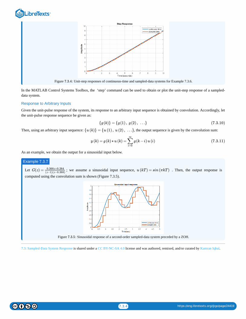
7.3.4 https://eng.libretexts.org/@go/page/24419

Figure : Unit-step responses of continuous-time and sampled-data systems for Example 7.3.6.

In the MATLAB Control Systems Toolbox, the ‘step’ command can be used to obtain or plot the unit-step response of a sampled-data system.

Response to Arbitrary Inputs

Given the unit-pulse response of the system, its response to an arbitrary input sequence is obtained by convolution. Accordingly, letthe unit-pulse response sequence be given as:

Then, using an arbitrary input sequence: , the output sequence is given by the convolution sum:

As an example, we obtain the output for a sinusoidal input below.

Let ; we assume a sinusoidal input sequence, . Then, the output response is

computed using the convolution sum is shown (Figure 7.3.5).

Figure : Sinusoidal response of a second-order sampled-data system preceded by a ZOH.

7.3: Sampled-Data System Response is shared under a CC BY-NC-SA 4.0 license and was authored, remixed, and/or curated by Kamran Iqbal.

7.3.4

{g (k)} = {g (1) ,  g (2) ,   …} (7.3.10)

{u (k)} = {u (1) ,  u (2) ,   …}

y (k) = g (k) ∗ u (k) = g (k− i)u (i)∑i=0

∞

(7.3.11)

Example 7.3.7

G(z) = 0.368z+0.264

(z−1)(z−0.368)u (kT ) = sin (πkT )  

7.3.5

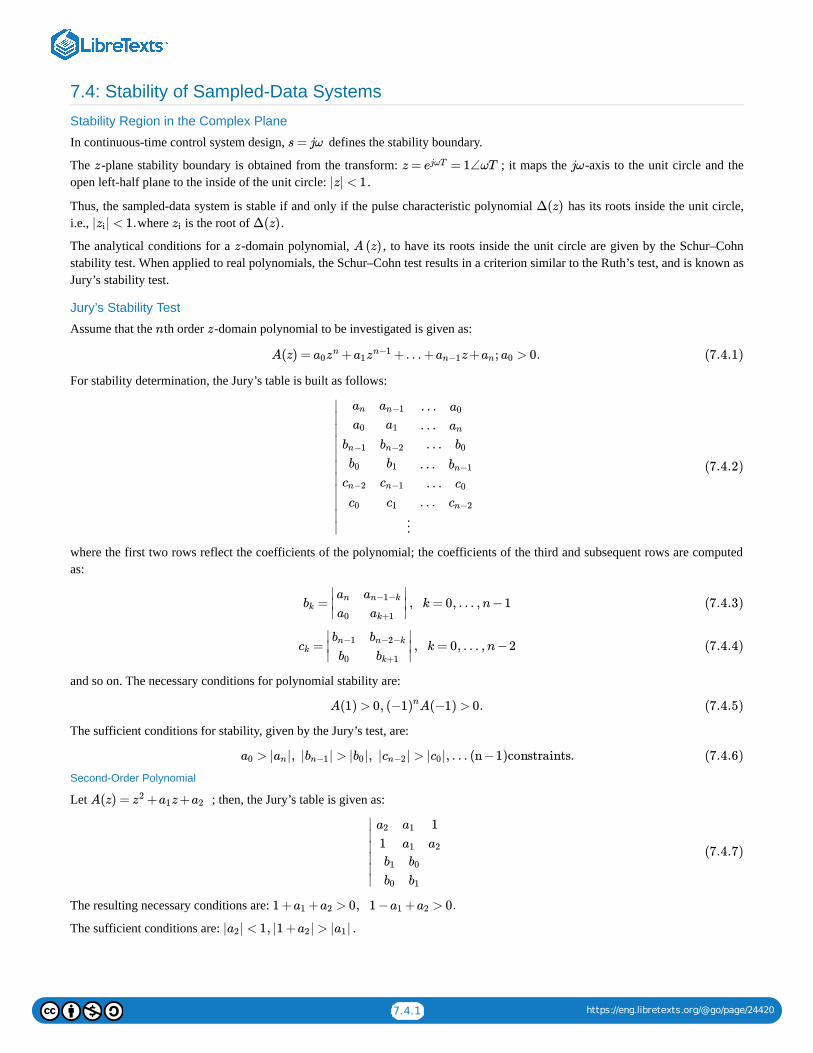
7.4.1 https://eng.libretexts.org/@go/page/24420

7.4: Stability of Sampled-Data Systems

Stability Region in the Complex Plane

In continuous-time control system design, defines the stability boundary.

The -plane stability boundary is obtained from the transform: ; it maps the -axis to the unit circle and theopen left-half plane to the inside of the unit circle: .

Thus, the sampled-data system is stable if and only if the pulse characteristic polynomial has its roots inside the unit circle,i.e., where is the root of .

The analytical conditions for a -domain polynomial, , to have its roots inside the unit circle are given by the Schur–Cohnstability test. When applied to real polynomials, the Schur–Cohn test results in a criterion similar to the Ruth’s test, and is known asJury’s stability test.

Jury’s Stability Test

Assume that the th order -domain polynomial to be investigated is given as:

For stability determination, the Jury’s table is built as follows:

where the first two rows reflect the coefficients of the polynomial; the coefficients of the third and subsequent rows are computedas:

and so on. The necessary conditions for polynomial stability are:

The sufficient conditions for stability, given by the Jury’s test, are:

Second-Order Polynomial

Let ; then, the Jury’s table is given as:

The resulting necessary conditions are:

The sufficient conditions are: .

s = jω

z z = = 1∠ωTejωT jω

|z| < 1

Δ(z)| | < 1.zi zi Δ(z)

z A (z)

n z

A(z) = + +… + z+ ; > 0.a0zn a1z

n−1 an−1 an a0 (7.4.1)

∣

∣

∣∣∣∣∣∣∣∣∣

an

a0

an−1

a1

… a0

… an

bn−1

b0

bn−2

b1

… b0

… bn−1

cn−2

c0

cn−1

c1

… c0

… cn−2

⋮

(7.4.2)

= , k = 0, … ,n−1bk∣∣∣an

a0

an−1−k

ak+1

∣∣∣ (7.4.3)

= , k = 0, … ,n−2ck∣∣∣bn−1

b0

bn−2−k

bk+1

∣∣∣ (7.4.4)

A(1) > 0, (−1 A(−1) > 0.)n (7.4.5)

> | |, | | > | |, | | > | |, … (n−1)constraints.a0 an bn−1 b0 cn−2 c0 (7.4.6)

A(z) = + z+z2 a1 a2

∣

∣

∣∣∣∣

a2

1a1

a1

1a2

b1

b0

b0

b1

(7.4.7)

1 + + > 0, 1 − + > 0.a1 a2 a1 a2

| | < 1, |1 + | > | |a2 a2 a1

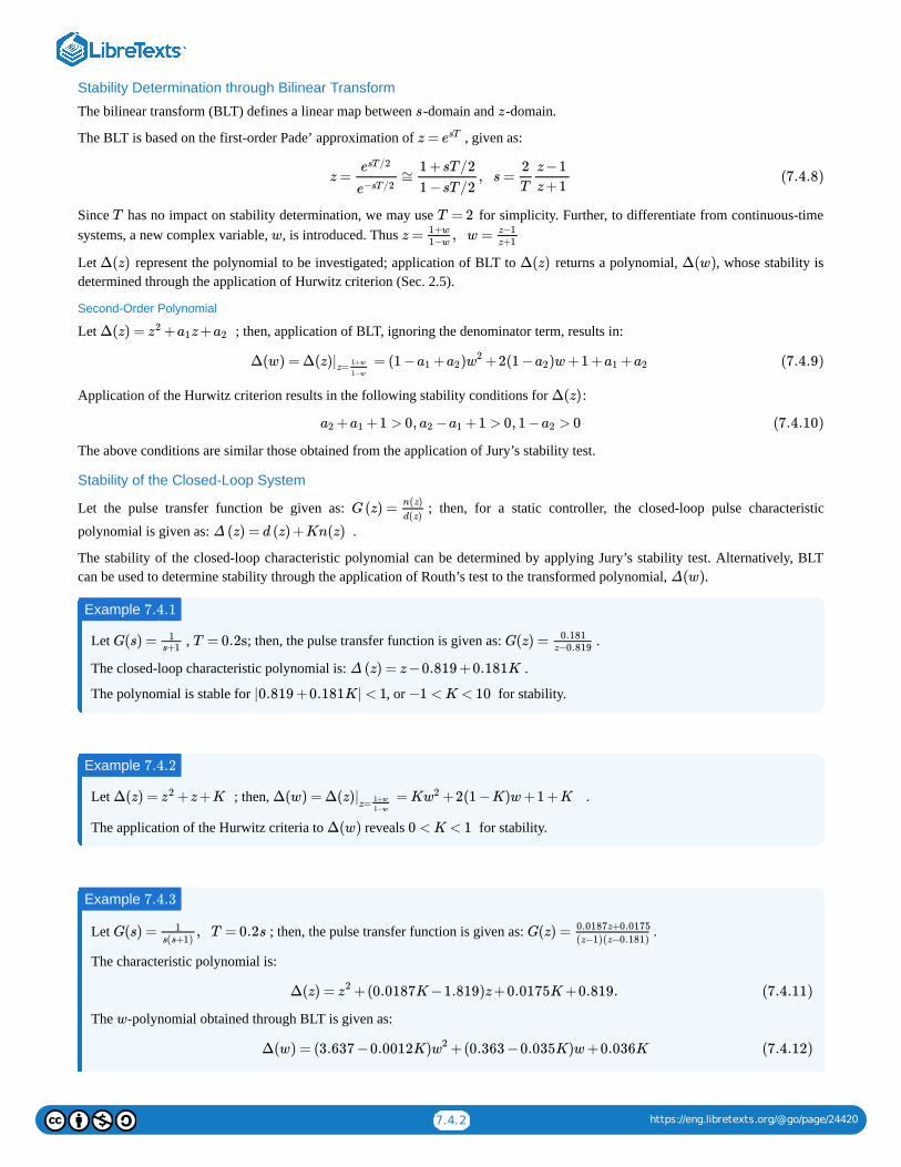
7.4.2 https://eng.libretexts.org/@go/page/24420

Stability Determination through Bilinear Transform

The bilinear transform (BLT) defines a linear map between -domain and -domain.

The BLT is based on the first-order Pade’ approximation of , given as:

Since has no impact on stability determination, we may use for simplicity. Further, to differentiate from continuous-timesystems, a new complex variable, , is introduced. Thus

Let represent the polynomial to be investigated; application of BLT to returns a polynomial, , whose stability isdetermined through the application of Hurwitz criterion (Sec. 2.5).

Second-Order Polynomial

Let ; then, application of BLT, ignoring the denominator term, results in:

Application of the Hurwitz criterion results in the following stability conditions for :

The above conditions are similar those obtained from the application of Jury’s stability test.

Stability of the Closed-Loop System

Let the pulse transfer function be given as: ; then, for a static controller, the closed-loop pulse characteristic

polynomial is given as: .

The stability of the closed-loop characteristic polynomial can be determined by applying Jury’s stability test. Alternatively, BLTcan be used to determine stability through the application of Routh’s test to the transformed polynomial, .

Let , ; then, the pulse transfer function is given as: .

The closed-loop characteristic polynomial is: .

The polynomial is stable for , or for stability.

Let ; then, .

The application of the Hurwitz criteria to reveals for stability.

Let ; then, the pulse transfer function is given as: .

The characteristic polynomial is:

The -polynomial obtained through BLT is given as:

s z

z = esT

z = ≅ , s =esT/2

e−sT/2

1 +sT/21 −sT/2

2T

z−1z+1

(7.4.8)

T T = 2w z = , w =1+w

1−w

z−1z+1

Δ(z) Δ(z) Δ(w)

Δ(z) = + z+z2 a1 a2

Δ(w) = Δ(z) = (1 − + ) +2(1 − )w+1 + +|z= 1+w

1−w

a1 a2 w2 a2 a1 a2 (7.4.9)

Δ(z)

+ +1 > 0, − +1 > 0, 1 − > 0a2 a1 a2 a1 a2 (7.4.10)

G(z) = n(z)d(z)

Δ (z) = d (z) +Kn(z)

Δ(w)

Example 7.4.1

G(s) = 1s+1 T = 0.2s G(z) = 0.181

z−0.819

Δ (z) = z−0.819 +0.181K

|0.819 +0.181K| < 1 −1 < K < 10

Example 7.4.2

Δ(z) = +z+Kz2 Δ(w) = Δ(z) = K +2(1 −K)w+1 +K|z= 1+w

1−w

w2

Δ(w) 0 < K < 1

Example 7.4.3

G(s) = , T = 0.2s1s(s+1)

G(z) = 0.0187z+0.0175(z−1)(z−0.181)

Δ(z) = +(0.0187K−1.819)z+0.0175K+0.819.z2 (7.4.11)

w

Δ(w) = (3.637 −0.0012K) +(0.363 −0.035K)w+0.036Kw2 (7.4.12)

7.4.3 https://eng.libretexts.org/@go/page/24420

The application of the Hurwitz criteria to gives for stability.

7.4: Stability of Sampled-Data Systems is shared under a CC BY-NC-SA 4.0 license and was authored, remixed, and/or curated by Kamran Iqbal.

Δ(w) 0 < K < 10.34

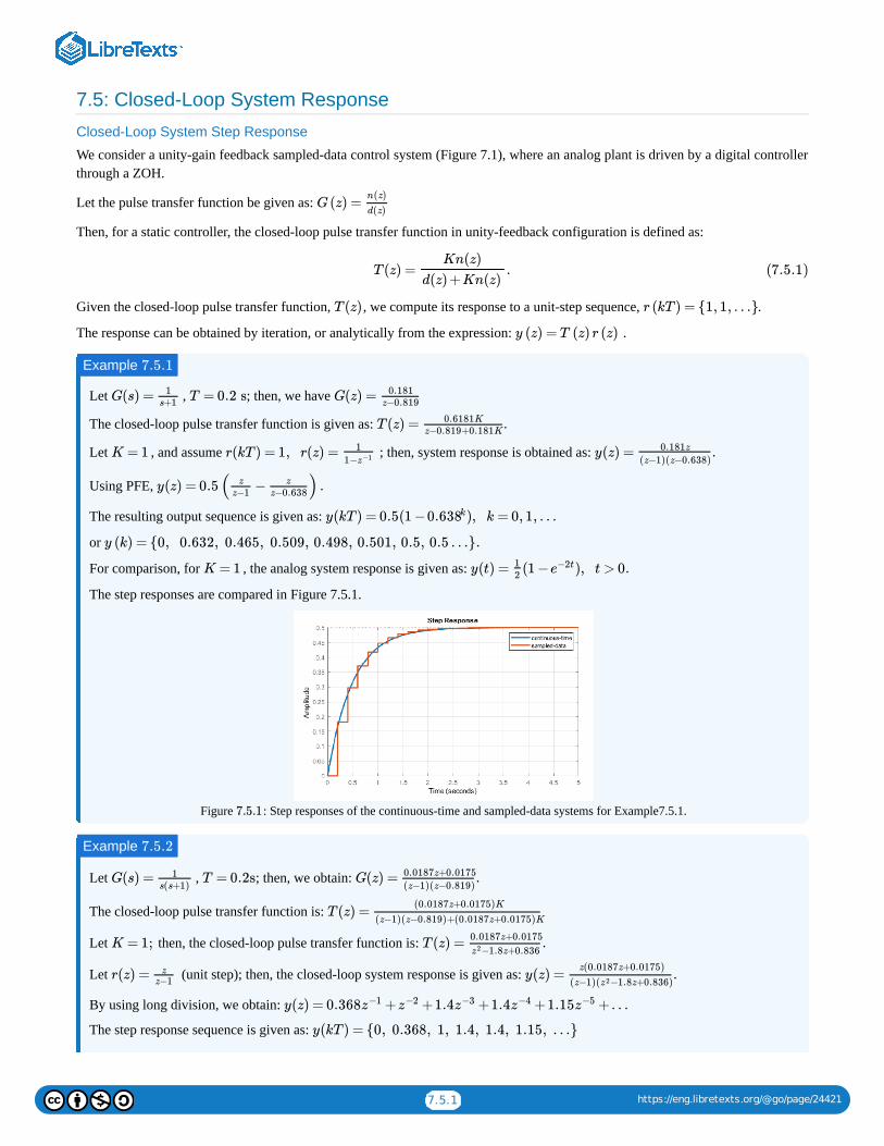
7.5.1 https://eng.libretexts.org/@go/page/24421

7.5: Closed-Loop System Response

Closed-Loop System Step Response

We consider a unity-gain feedback sampled-data control system (Figure 7.1), where an analog plant is driven by a digital controllerthrough a ZOH.

Let the pulse transfer function be given as:

Then, for a static controller, the closed-loop pulse transfer function in unity-feedback configuration is defined as:

Given the closed-loop pulse transfer function, , we compute its response to a unit-step sequence, .

The response can be obtained by iteration, or analytically from the expression: .

Let , ; then, we have

The closed-loop pulse transfer function is given as:

Let , and assume ; then, system response is obtained as:

Using PFE,

The resulting output sequence is given as:

or

For comparison, for , the analog system response is given as:

The step responses are compared in Figure 7.5.1.

Figure : Step responses of the continuous-time and sampled-data systems for Example7.5.1.

Let , ; then, we obtain:

The closed-loop pulse transfer function is:

Let then, the closed-loop pulse transfer function is:

Let (unit step); then, the closed-loop system response is given as:

By using long division, we obtain:

The step response sequence is given as:

G(z) =n(z)

d(z)

T (z) = .Kn(z)

d(z) +Kn(z)(7.5.1)

T (z) r (kT ) = {1, 1, …}

y (z) = T (z) r (z)

Example 7.5.1

G(s) = 1s+1

T = 0.2 s G(z) = 0.181z−0.819

T (z) = .0.6181Kz−0.819+0.181K

K = 1 r(kT ) = 1, r(z) = 1

1−z−1 y(z) = .0.181z

(z−1)(z−0.638)

y(z) = 0.5( − ) .z

z−1z

z−0.638

y(kT ) = 0.5(1 − ), k = 0, 1, …0.638k

y (k) = {0, 0.632, 0.465, 0.509, 0.498, 0.501, 0.5, 0.5 …}.

K = 1 y(t) = (1 − ), t > 0.12

e−2t

7.5.1

Example 7.5.2

G(s) = 1s(s+1)

T = 0.2s G(z) = .0.0187z+0.0175

(z−1)(z−0.819)

T (z) =(0.0187z+0.0175)K

(z−1)(z−0.819)+(0.0187z+0.0175)K

K = 1; T (z) = .0.0187z+0.0175

−1.8z+0.836z2

r(z) = zz−1

y(z) = .z(0.0187z+0.0175)

(z−1)( −1.8z+0.836)z2

y(z) = 0.368 + +1.4 +1.4 +1.15 +…z−1 z−2 z−3 z−4 z−5

y(kT ) = {0, 0.368, 1, 1.4, 1.4, 1.15, …}

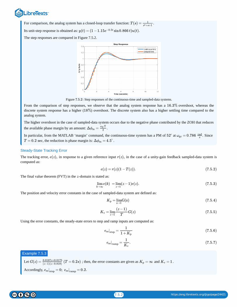
7.5.2 https://eng.libretexts.org/@go/page/24421

For comparison, the analog system has a closed-loop transfer function:

Its unit-step response is obtained as:

The step responses are compared in Figure 7.5.2.

Figure : Step responses of the continuous-time and sampled-data systems.

From the comparison of step responses, we observe that the analog system response has a overshoot, whereas thediscrete system response has a higher ( ) overshoot. The discrete system also has a higher settling time compared to theanalog system.

The higher overshoot in the case of sampled-data system occurs due to the negative phase contributed by the ZOH that reducesthe available phase margin by an amount:

In particular, from the MATLAB ‘margin’ command, the continuous-time system has a PM of at . Since , the reduction is phase margin is: .

Steady-State Tracking Error

The tracking error, in response to a given reference input in the case of a unity-gain feedback sampled-data system iscomputed as:

The final value theorem (FVT) in the -domain is stated as:

The position and velocity error constants in the case of sampled-data system are defined as:

Using the error constants, the steady-state errors to step and ramp inputs are computed as:

Let ; then, the error constants are given as and .

Accordingly,

T (s) = .1+s+1s2

y(t) = (1 −1.15 sin0.866 t)u(t).e−0.5t

7.5.2

16.3%

18%

Δ = .ϕmTωgc

2

52∘ = 0.786ωgcrad

s

T = 0.2 sec Δ =ϕm 4.5∘

e(z), r(z),

e(z) = r(z)(1 −T (z)). (7.5.2)

z

e(k) = (z−1)e(z).limk→∞

limz→1

(7.5.3)

= G(z)Kp limz→1

(7.5.4)

= G(z)Kv limz→1

(z−1)

T(7.5.5)

=|ess step

1

1 +Kp(7.5.6)

= .|ess ramp

1

Kv(7.5.7)

Example 7.5.3

G(z) = (T = 0.2s)0.0187z+0.0175

(z−1)(z−0.819)= ∞Kp = 1Kv

= 0; = 0.2.|ess step |ess ramp

7.5.3 https://eng.libretexts.org/@go/page/24421

Let with ; then, we have

Accordingly,

7.5: Closed-Loop System Response is shared under a CC BY-NC-SA 4.0 license and was authored, remixed, and/or curated by Kamran Iqbal.

Example 7.5.4

G(z) =0.368z+0.264

(z−1)(z−0.368)T = 1s = ∞, = 1.Kp Kv

= 0; = 1.|ess step |ess ramp

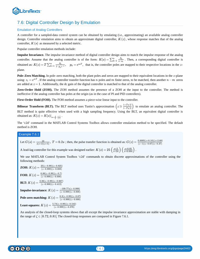
7.6.1 https://eng.libretexts.org/@go/page/24422

7.6: Digital Controller Design by Emulation

Emulation of Analog Controllers

A controller for a sampled-data control system can be obtained by emulating (i.e., approximating) an available analog controllerdesign. Controller emulation aims to obtain an approximate digital controller, , whose response matches that of the analogcontroller, as measured by a selected metric.

Popular controller emulation methods include:

Impulse Invariance. The impulse invariance method of digital controller design aims to match the impulse response of the analogcontroller. Assume that the analog controller is of the form: . Then, a corresponding digital controller is

obtained as: that is, the controller poles are mapped to their respective locations in the -

plane.

Pole–Zero Matching. In pole–zero matching, both the plant poles and zeros are mapped to their equivalent locations in the -planeusing: . If the analog controller transfer function has poles and finite zeros, to be matched, then another zerosare added at . Additionally, the dc gain of the digital controller is matched to that of the analog controller.

Zero-Order Hold (ZOH). The ZOH method assumes the presence of a ZOH at the input to the controller. The method isineffective if the analog controller has poles at the origin (as in the case of PI and PID controllers).

First-Order Hold (FOH). The FOH method assumes a piece-wise linear input to the controller.

Bilinear Transform (BLT). The BLT method uses Tustin’s approximation to emulate an analog controller. The

BLT method is quite effective when used with a high sampling frequency. Using the BLT, an equivalent digital controller isobtained as:

The ‘c2d’ command in the MATLAB Control Systems Toolbox allows controller emulation method to be specified. The defaultmethod is ZOH.

Let ; then, the pulse transfer function is obtained as:

A lead-lag controller for this example was designed earlier: .

We use MATLAB Control System Toolbox ‘c2d’ commands to obtain discrete approximations of the controller using thefollowing methods:

ZOH:

FOH:

BLT:

Impulse-invariance:

Pole-zero matching:

Least-squares:

An analysis of the closed-loop systems shows that all except the impulse invariance approximation are stable with damping inthe range of . The closed-loop responses are compared in Figure 7.6.1.

K (z)

K (s)

K(s) =∑nk=1

Ak

s−sk

K(z) = T , = ,∑nk=1

Ak

1−pkz−1

pk e Tsk z

z

=zi e Tsi n m n−m

z = 1

(z ≅ )1+Ts/2

1−Ts/2

K(z) = K(s) .|s= 2

T

z−1

z+1

Example 7.6.1

G(s) = ,  T = 0.2s10s(s+2)(s+5)

G(z) =0.0095(z+0.18)(z+2.68)

(z−1)(z−0.67)(z−0.37)

K (s) = 25( )( )s+2s+24

s+0.05s+0.004

K (z) =25(z−0.99)(z−0.925)

(z−0.999)(z−0.008)

K (z) =6.86(z−0.99)(z−0.7)

(z−0.999)(z−0.008)

K (z) =8.86(z−0.99)(z−0.667)

(z−0.999)(z−0.412)

K (z) =−109.77z(z−0.999)

(z−0.999)(z−0.008)

K (z) =6.3(z−0.99)(z−0.67)

(z−0.999)(z−0.008)

K (z) =5.74(z−0.99)(z−0.542)

(z−0.999)(z−0.376)

ζ ∈ [0.72, 0.81]

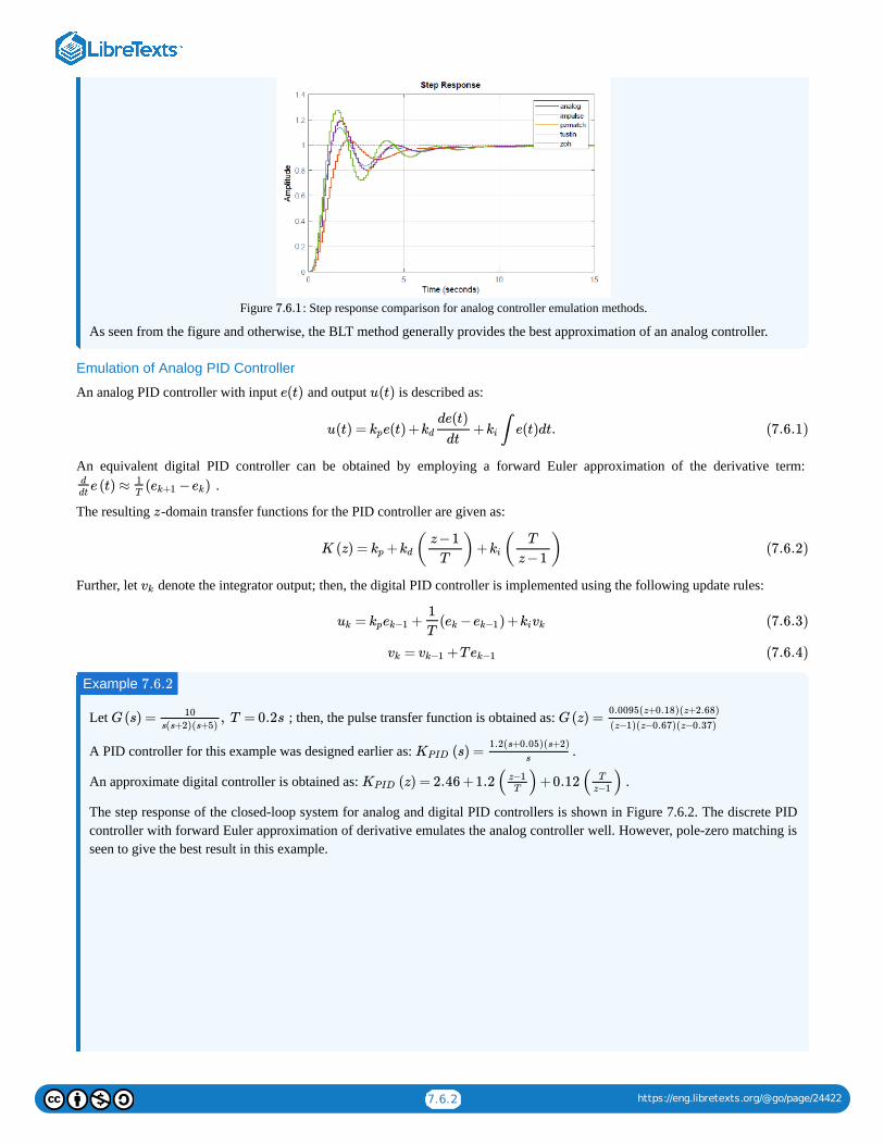
7.6.2 https://eng.libretexts.org/@go/page/24422

Figure : Step response comparison for analog controller emulation methods.

As seen from the figure and otherwise, the BLT method generally provides the best approximation of an analog controller.

Emulation of Analog PID Controller

An analog PID controller with input and output is described as:

An equivalent digital PID controller can be obtained by employing a forward Euler approximation of the derivative term: .

The resulting -domain transfer functions for the PID controller are given as:

Further, let denote the integrator output; then, the digital PID controller is implemented using the following update rules:

Let ; then, the pulse transfer function is obtained as:

A PID controller for this example was designed earlier as: .

An approximate digital controller is obtained as: .

The step response of the closed-loop system for analog and digital PID controllers is shown in Figure 7.6.2. The discrete PIDcontroller with forward Euler approximation of derivative emulates the analog controller well. However, pole-zero matching isseen to give the best result in this example.

7.6.1

e(t) u(t)

u(t) = e(t) + + ∫ e(t)dt.kp kdde(t)

dtki (7.6.1)

e (t) ≈ ( − )d

dt

1T

ek+1 ek

z

K (z) = + ( )+ ( )kp kdz−1

Tki

T

z−1(7.6.2)

vk

= + ( − ) +uk kpek−11

Tek ek−1 kivk (7.6.3)

= +Tvk vk−1 ek−1 (7.6.4)

Example 7.6.2

G(s) = ,  T = 0.2s10

s(s+2)(s+5)G(z) =

0.0095(z+0.18)(z+2.68)

(z−1)(z−0.67)(z−0.37)

(s) =KPID1.2(s+0.05)(s+2)

s

(z) = 2.46 +1.2( )+0.12( )KPIDz−1T

T

z−1

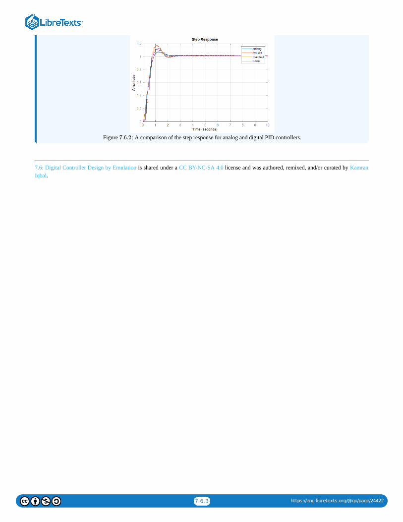
7.6.3 https://eng.libretexts.org/@go/page/24422

Figure : A comparison of the step response for analog and digital PID controllers.

7.6: Digital Controller Design by Emulation is shared under a CC BY-NC-SA 4.0 license and was authored, remixed, and/or curated by KamranIqbal.

7.6.2

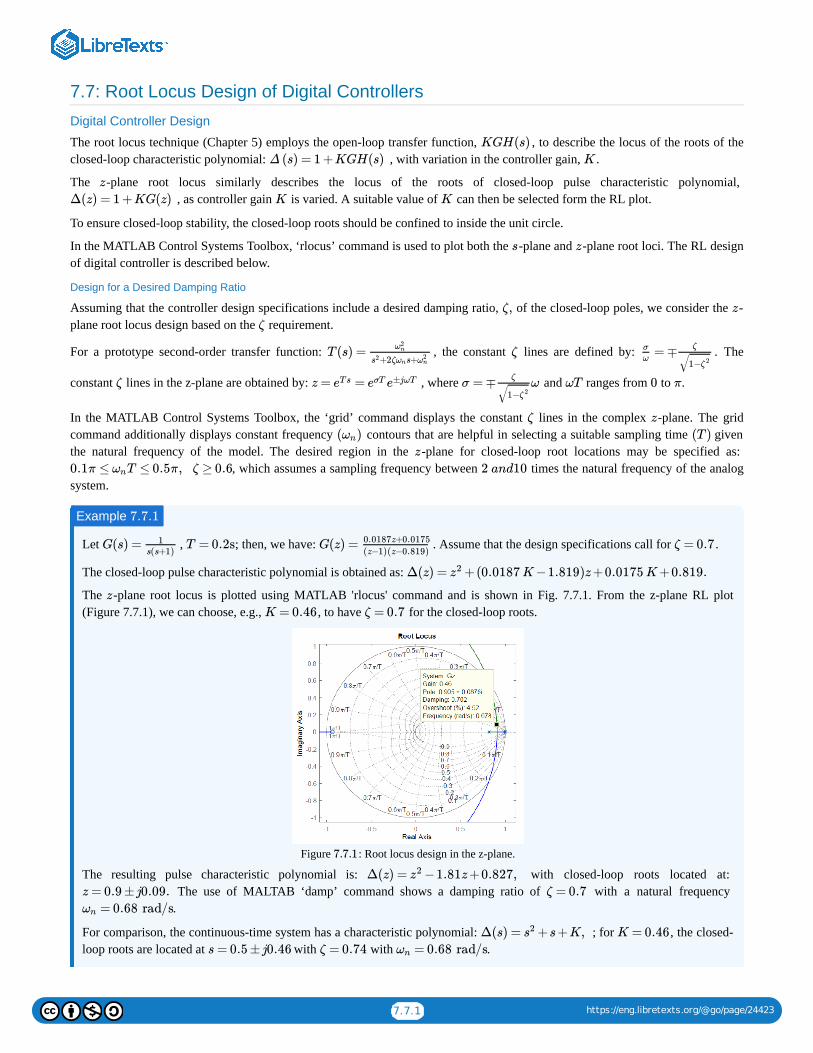
7.7.1 https://eng.libretexts.org/@go/page/24423

7.7: Root Locus Design of Digital Controllers

Digital Controller Design

The root locus technique (Chapter 5) employs the open-loop transfer function, , to describe the locus of the roots of theclosed-loop characteristic polynomial: , with variation in the controller gain, .

The -plane root locus similarly describes the locus of the roots of closed-loop pulse characteristic polynomial, , as controller gain is varied. A suitable value of can then be selected form the RL plot.

To ensure closed-loop stability, the closed-loop roots should be confined to inside the unit circle.

In the MATLAB Control Systems Toolbox, ‘rlocus’ command is used to plot both the -plane and -plane root loci. The RL designof digital controller is described below.

Design for a Desired Damping Ratio

Assuming that the controller design specifications include a desired damping ratio, of the closed-loop poles, we consider the -plane root locus design based on the requirement.

For a prototype second-order transfer function: , the constant lines are defined by: . The

constant lines in the z-plane are obtained by: , where and ranges from to .

In the MATLAB Control Systems Toolbox, the ‘grid’ command displays the constant lines in the complex -plane. The gridcommand additionally displays constant frequency contours that are helpful in selecting a suitable sampling time giventhe natural frequency of the model. The desired region in the -plane for closed-loop root locations may be specified as:

, which assumes a sampling frequency between times the natural frequency of the analogsystem.

Let , ; then, we have: . Assume that the design specifications call for .

The closed-loop pulse characteristic polynomial is obtained as:

The -plane root locus is plotted using MATLAB 'rlocus' command and is shown in Fig. 7.7.1. From the z-plane RL plot(Figure 7.7.1), we can choose, e.g., , to have for the closed-loop roots.

Figure : Root locus design in the z-plane.

The resulting pulse characteristic polynomial is: with closed-loop roots located at: The use of MALTAB ‘damp’ command shows a damping ratio of with a natural frequency .

For comparison, the continuous-time system has a characteristic polynomial: ; for , the closed-loop roots are located at with with .

KGH(s)

Δ (s) = 1 +KGH(s) K

z

Δ(z) = 1 +KG(z) K K

s z

ζ, z

ζ

T (s) =ω2n

+2ζ s+s2 ωn ω2n

ζ = ∓σ

ω

ζ

1−ζ 2√

ζ z = =eTs eσT e±jωT σ = ∓ ωζ

1−ζ 2√ωT 0 π

ζ z

( )ωn (T )

z

0.1π ≤ T ≤ 0.5π, ζ ≥ 0.6ωn 2 and10

Example 7.7.1

G(s) = 1s(s+1)

T = 0.2s G(z) = 0.0187z+0.0175

(z−1)(z−0.819)ζ = 0.7

Δ(z) = +(0.0187 K−1.819)z+0.0175 K+0.819.z2

z

K = 0.46 ζ = 0.7

7.7.1

Δ(z) = −1.81z+0.827,z2

z = 0.9 ±j0.09. ζ = 0.7

= 0.68 rad/sωn

Δ(s) = +s+K,s2 K = 0.46

s = 0.5 ±j0.46 ζ = 0.74 = 0.68 rad/sωn

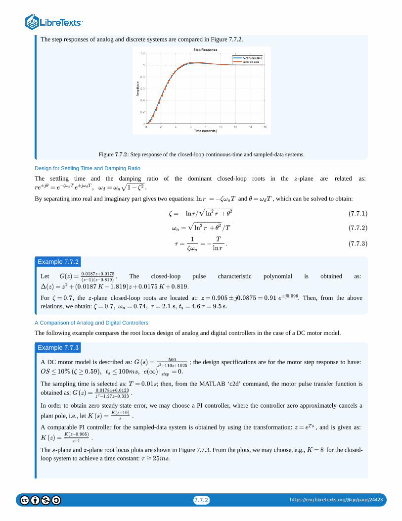
7.7.2 https://eng.libretexts.org/@go/page/24423

The step responses of analog and discrete systems are compared in Figure 7.7.2.

Figure : Step response of the closed-loop continuous-time and sampled-data systems.

Design for Settling Time and Damping Ratio

The settling time and the damping ratio of the dominant closed-loop roots in the -plane are related as:

By separating into real and imaginary part gives two equations: and , which can be solved to obtain:

Let . The closed-loop pulse characteristic polynomial is obtained as:

For , the -plane closed-loop roots are located at: . Then, from the aboverelations, we obtain:

A Comparison of Analog and Digital Controllers

The following example compares the root locus design of analog and digital controllers in the case of a DC motor model.

A DC motor model is described as: ; the design specifications are for the motor step response to have:

The sampling time is selected as: ; then, from the MATLAB ‘c2d’ command, the motor pulse transfer function isobtained as: .

In order to obtain zero steady-state error, we may choose a PI controller, where the controller zero approximately cancels a

plant pole, i.e., let .

A comparable PI controller for the sampled-data system is obtained by using the transformation: , and is given as:

.

The -plane and -plane root locus plots are shown in Figure 7.7.3. From the plots, we may choose, e.g., for the closed-loop system to achieve a time constant: .

7.7.2

z

r = , = .e±jθ e−ζ Tωn e±j Tωd ωd ωn 1 −ζ2− −−−−

√

lnr = −ζ Tωn θ = Tωd

ζ = −lnr/ r +ln2 θ2− −−−−−−−

√ (7.7.1)

= /Tωn r +ln2 θ2− −−−−−−−

√ (7.7.2)

τ = = − .1

ζωn

T

lnr(7.7.3)

Example 7.7.2

G(z) = 0.0187z+0.0175

(z−1)(z−0.819)

Δ(z) = +(0.0187 K−1.819)z+0.0175 K+0.819.z2

ζ = 0.7 z z = 0.905 ±j0.0875 = 0.91 e±j0.096

ζ = 0.7, = 0.74, τ = 2.1 s, = 4.6 τ = 9.5 s.ωn ts

Example 7.7.3

G(s) = 500

+110s+1025s2

OS ≤ 10% (ζ ≥ 0.59),    ≤ 100ms,   e = 0.ts (∞) |step

T = 0.01s

 G(z) = 0.0178z+0.0123

−1.27z+0.333z2

K (s) =K(s+10)

s

z = eTs

K (z) =K(z−0.905)

z−1

s z K = 8

τ ≅25ms

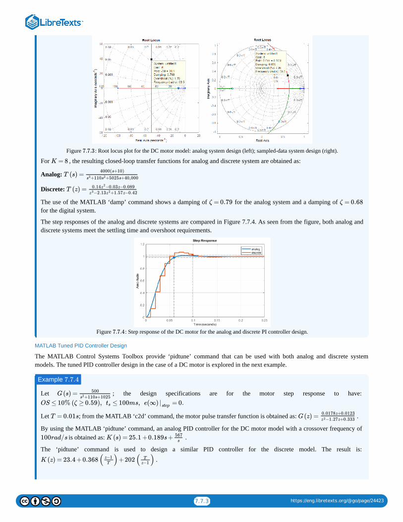
7.7.3 https://eng.libretexts.org/@go/page/24423

Figure : Root locus plot for the DC motor model: analog system design (left); sampled-data system design (right).

For , the resulting closed-loop transfer functions for analog and discrete system are obtained as:

Analog:

Discrete:

The use of the MATLAB ‘damp’ command shows a damping of for the analog system and a damping of for the digital system.

The step responses of the analog and discrete systems are compared in Figure 7.7.4. As seen from the figure, both analog anddiscrete systems meet the settling time and overshoot requirements.

Figure : Step response of the DC motor for the analog and discrete PI controller design.

MATLAB Tuned PID Controller Design

The MATLAB Control Systems Toolbox provide ‘pidtune’ command that can be used with both analog and discrete systemmodels. The tuned PID controller design in the case of a DC motor is explored in the next example.

Let ; the design specifications are for the motor step response to have:

Let ; from the MATLAB ‘c2d’ command, the motor pulse transfer function is obtained as: .

By using the MATLAB ‘pidtune’ command, an analog PID controller for the DC motor model with a crossover frequency of is obtained as: .

The ‘pidtune’ command is used to design a similar PID controller for the discrete model. The result is:

.

7.7.3

K = 8

T (s) =4000(s+10)

+110 +5025s+40,000s3 s2

T (z) = 0.14 −0.03z−0.089z2

−2.13 +1.57z−0.42z3 z2

ζ = 0.79 ζ = 0.68

7.7.4

Example 7.7.4

G(s) = 500

+110s+1025s2

OS ≤ 10% (ζ ≥ 0.59),    ≤ 100ms,   e = 0.ts (∞) |step

T = 0.01s  G(z) =0.0178z+0.0123

−1.27z+0.333z2

100rad/s K (s) = 25.1 +0.189s+ 567s

K (z) = 23.4 +0.368( )+202( )z−1T

Tz−1

7.7.4 https://eng.libretexts.org/@go/page/24423

The unit-step responses of the closed-loop systems for the analog and discrete models are compared in Figure 7.7.5. Bothcontroller achieve a settling time with no steady-state error. However, in this case, the tuned digital PID controllerhas a lower settling time.

Figure : Step response of the DC motor for the analog and discrete PID controller design.

7.7: Root Locus Design of Digital Controllers is shared under a CC BY-NC-SA 4.0 license and was authored, remixed, and/or curated by KamranIqbal.

< 0.1sts

7.7.5

1

CHAPTER OVERVIEW

8: State Variable Models

1. Analyze the state variable models of single-input single-output dynamic systems.2. Solve state equations in time-domain using the state-transition matrix.3. Obtain the modal matrix and determine the stability of the model.4. Obtain state-space realization of a transfer function model in alternate forms.

8.0: Prelude to State Variable Models8.1: State Variable Models8.2: State-Transition Matrix and Asymptotic Stability8.3: State-Space Realization of Transfer Function Models8.4: Linear Transformation of State Variables

8: State Variable Models is shared under a CC BY-NC-SA 4.0 license and was authored, remixed, and/or curated by Kamran Iqbal.

Learning Objectives

8.0.1 https://eng.libretexts.org/@go/page/24461

8.0: Prelude to State Variable ModelsThis chapter discusses algebraic methods to analyze the state variable models of dynamic systems. These models comprise a set offirst-order linear differential equations that describe the system behavior using system state variables. A common choice includesthe natural variables associated with the energy storage elements present in the system. Alternate variables in equal number canalso be selected.

The state equations include a set of coupled first-order ODE’s that describe the behavior of the system. The state equations can becollectively integrated using a matrix exponential, i.e., the state-transition matrix, as an integrating factor. The state-transitionmatrix contains natural modes of system response and plays a fundamental role in the evolution of system trajectories. The generalsolution to the homogeneous state equations is a weighted sum of the columns of the state-transition matrix.

Given a state variable model of the system, a transfer function representation can be obtained by applying the Laplace transform.Generally, the degree of the denominator polynomial in the transfer function model equals the number of state variables used torepresent it. A pole-zero cancellation in the transfer function would, however, cause some of the response modes to be absent fromthe input-output system description.

A given transfer function model can be realized into a state variable model in multiple ways. Different choices of state variablesaccord different structures to the system matrix. Specific realization structures may be preferred for ease of computing the systemresponse or determining its stability characteristics.

The modal realization reveals the natural modes of system response. The controller realization facilitates the controller design usingstate variable methods. The diagonal representation decouples the system variables into a set of independent first-order ordinarydifferential equations (ODEs) that can be easily integrated. The state variable vectors for these alternate models are related throughbilinear transformations.

This chapter describes the analysis techniques for state variable models of the continuous-time systems. The discrete-time systemmodels are covered later in Chapter 8. The analysis is restricted to the single-input single-output (SISO) systems, that exhibit arational transfer function, . The methods, however, can be generalized to include multi-input multi-output (MIMO) systems.

8.0: Prelude to State Variable Models is shared under a CC BY-NC-SA 4.0 license and was authored, remixed, and/or curated by LibreTexts.

G(s)

8.1.1 https://eng.libretexts.org/@go/page/24425

8.1: State Variable Models

The State Equations

The state variable model of a dynamic system comprises first-order ODEs that describe time derivatives of a set of state variables.The number of state variables represents the order of the system, which is assumed to match the degree of the denominatorpolynomial in its transfer function description.

The natural variables associated with the energy storing elements are commonly used as state variables, though alternate variablescan be selected. The natural variables include, for example, capacitor voltage and inductor current in the electrical networks, andposition and velocity of the inertial mass in the mechanical systems.

Let describe a vector of state variables, describe a scalar input, and describe a scalar output; then the state variablemodel of a linear time-invariant (LTI) single-input single-output (SISO) system is written in its generic form as:

In the above, is an matrix, is a column vector that distributes the inputs, is a row vector that combines the statevariables to form the output, and is a scalar feedforward term contributing to the output.

The state variable model of a multi-input multi-output (MIMO) system with inputs and outputs is described by the state andoutput equations given as:

In the above, the variable dimensions are: ; the matrices have the following dimensions:.

In the following, we restrict our attention to models of SISO systems. Unless noted otherwise, is assumed, whichcorresponds to a strictly proper transfer function description of the system.

Solution to the State Equations

In order to explore a time-domain solution to the state equations, we begin with a scalar differential equation:

Using an integrating factor, , the equation is written as total differential:

Next, assuming an initial conditions: , we integrate from to to obtain:

Hence, the solution to the scalar ODE in terms of is obtained as:

Further, the solution to homogeneous equation: is given as:

Next, we explore the possibility to generalize this solution to the matrix case. For this purpose, we define a matrix exponentialfunction as:

x(t) u(t) y(t)

(t) = Ax(t) +bu(t)x (8.1.1)

y(t) = x(t) +du(t)cT (8.1.2)

A n×n b cT

d

m p

(t) = Ax(t) +Bu(t)x (8.1.3)

y(t) = x(t) +Du(t)CT (8.1.4)

x ∈ ,  u ∈ ,   and y ∈Rn

Rm

Rp

A ∈ ,  B ∈ ,  C ∈ ,  and D ∈Rn×n

Rn×m

Rp×n

Rp×m

d = 0

(t) = ax(t) +bu(t).x (8.1.5)

e−at

( x(t)) = bu(t)d

dte−at e−at (8.1.6)

x (0) = x0 τ = 0 τ = t

x(t) − = bu(τ)dτe−at x0 ∫τ

0

e−aτ (8.1.7)

x(t)

x(t) = + bu(τ)dτeatx0 ∫τ

0

ea(t−τ) (8.1.8)

(t) = ax (t)x x (t) = .eatx0

= = I +At+…eAt ∑i=0

∞A

iti

i!(8.1.9)

8.1.2 https://eng.libretexts.org/@go/page/24425

The infinite series converges in the case of systems that are well-behaved. Further, the matrix exponential obeys the matrixdifferential equation:

Using the matrix exponential, the solution to the matrix differential equation, , is written as:

The above solution has two parts: the first term describes the system response to initial conditions , while the second termdescribes the system response to an input, .

Laplace Transform Solution

Consider the state equation:

Apply the Laplace transform to obtain:

The state variable vector is solved as:

where denote an identity matrix.

The matrix is called the characteristic matrix of .

Its determinant defines the characteristic polynomial of , i.e., .

The roots of the characteristic polynomial are the eigenvalues of .

The matrix is called the resolvent matrix of . The resolvent of can be computed as an infinite series:

By comparing the Laplace transform solution with the time-domain solution, we arrive at the following relations:

The first equation above can be used to compute the matrix exponential:

The second equation is used to solve for the output response when initial conditions are zero:

The State-Transition Matrix

Consider the homogenous system of equations: .

The solution to the homogenous state equation is given as: .

The matrix exponential that relates to is termed as the state-transition matrix. The state-transition matrix contains thenatural modes of system response.

Transfer Function

The output response of the state variable model defines the transfer function: , where

( ) = A = Ad

dteAt eAt eAt (8.1.10)

(t) = Ax(t) +bu(t)x

x(t) = + bu(τ)dτeAtx0 ∫τ

0

eA(t−τ) (8.1.11)

x0

u(t)

(t) = Ax(t) +bu(t), x (0) = ;x x0 (8.1.12)

sx(s) − = Ax(s) +bu(s).x0 (8.1.13)

x(s) = (sI −A +(sI − A bu(s),)−1x0 )−1 (8.1.14)

I n×n

n×n (sI − A) A

A Δ(s) = |sI −A|

A

n×n (sI −A)−1 A A

(sI −A = (I + A +…))−1 s−1 s−1 (8.1.15)

L[ ] = (sI −AeAt )−1 (8.1.16)

L[ bu(τ)dτ] = (sI −A bu(s)∫τ

0

eA(t−τ) )−1 (8.1.17)

= [(sI −A ]eAt L−1 )−1 (8.1.18)

y(s) = (sI −A bu(s)cT )−1 (8.1.19)

(t) = Ax(t) and x(0) =x x0

x(t) = eAtx0

eAt x0 x(t)

y(s) = G(s)u(s)

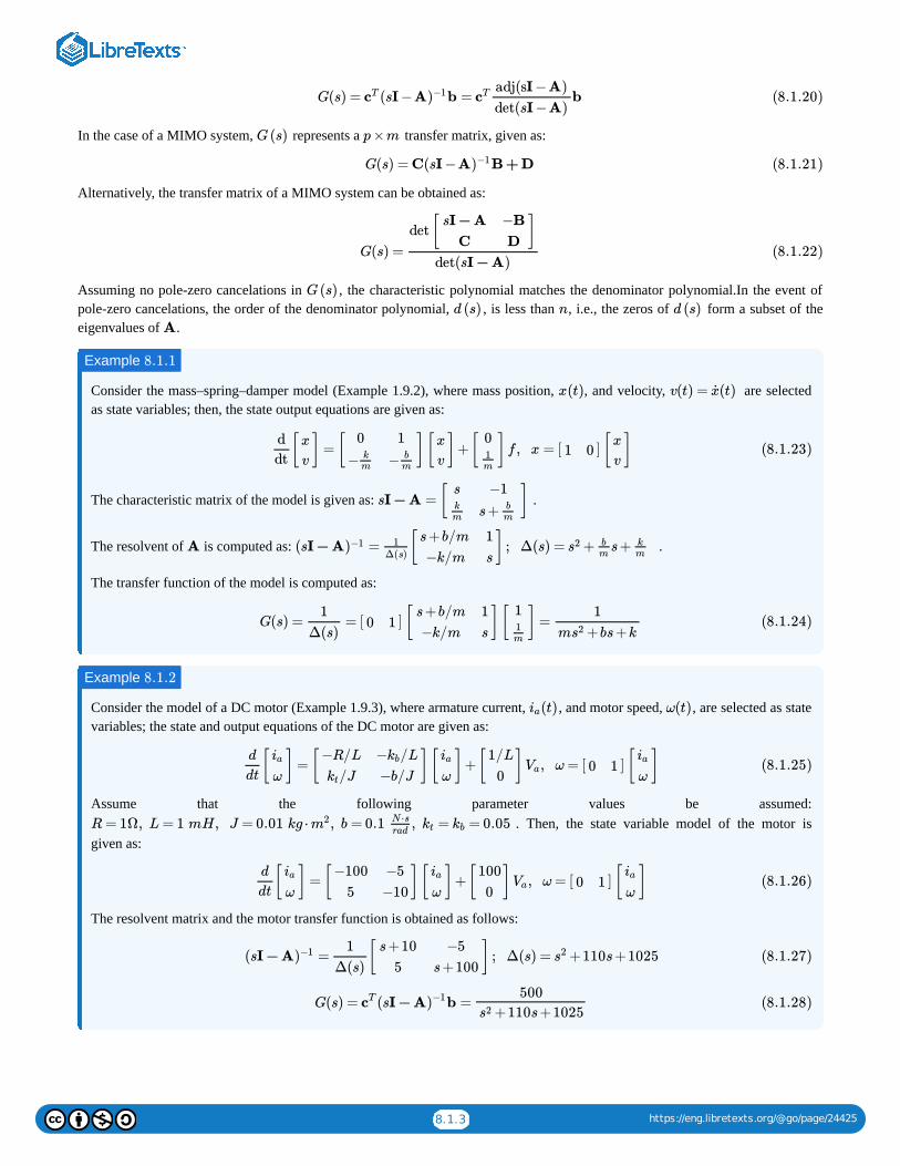
8.1.3 https://eng.libretexts.org/@go/page/24425

In the case of a MIMO system, represents a transfer matrix, given as:

Alternatively, the transfer matrix of a MIMO system can be obtained as:

Assuming no pole-zero cancelations in , the characteristic polynomial matches the denominator polynomial.In the event ofpole-zero cancelations, the order of the denominator polynomial, , is less than , i.e., the zeros of form a subset of theeigenvalues of .

Consider the mass–spring–damper model (Example 1.9.2), where mass position, , and velocity, are selectedas state variables; then, the state output equations are given as:

The characteristic matrix of the model is given as: .

The resolvent of is computed as: .

The transfer function of the model is computed as:

Consider the model of a DC motor (Example 1.9.3), where armature current, , and motor speed, , are selected as statevariables; the state and output equations of the DC motor are given as:

Assume that the following parameter values be assumed:. Then, the state variable model of the motor is

given as:

The resolvent matrix and the motor transfer function is obtained as follows:

G(s) = (sI −A b = bcT )−1 cTadj(sI −A)

det(sI −A)(8.1.20)

G(s) p×m

G(s) = C(sI −A B + D)−1 (8.1.21)

G(s) =

det[ ]sI − A

C

−B

D

det(sI − A)(8.1.22)

G(s)

d (s) n d (s)

A

Example 8.1.1

x(t) v(t) = (t)x

[ ] = [ ][ ]+[ ] f , x = [ ] [ ]d

dt

x

v

0

− km

1

− bm

x

v

01m

1 0x

v(8.1.23)

sI − A = [ ]skm

−1

s+ bm

A (sI − A = [ ] ; Δ(s) = + s+)−1 1Δ(s)

s+b/m

−k/m

1

ss2 b

mkm

G(s) = = [ ] [ ][ ] =1

Δ(s)0 1

s+b/m

−k/m

1

s

11m

1

m +bs+ks2(8.1.24)

Example 8.1.2

(t)ia ω(t)

[ ] = [ ][ ]+[ ] , ω = [ ] [ ]d

dt

ia

ω

−R/L

/Jkt

− /Lkb

−b/J

ia

ω

1/L

0Va 0 1

ia

ω(8.1.25)

R = 1Ω, L = 1 mH, J = 0.01 kg ⋅ , b = 0.1 , = = 0.05m2 N ⋅srad

kt kb

[ ] = [ ][ ]+[ ] , ω = [ ] [ ]d

dt

ia

ω

−100

5

−5

−10

ia

ω

100

0Va 0 1

ia

ω(8.1.26)

(sI − A = [ ] ; Δ(s) = +110s+1025)−1 1

Δ(s)

s+10

5

−5

s+100s2 (8.1.27)

G(s) = (sI − A b =cT )−1 500

+110s+1025s2(8.1.28)

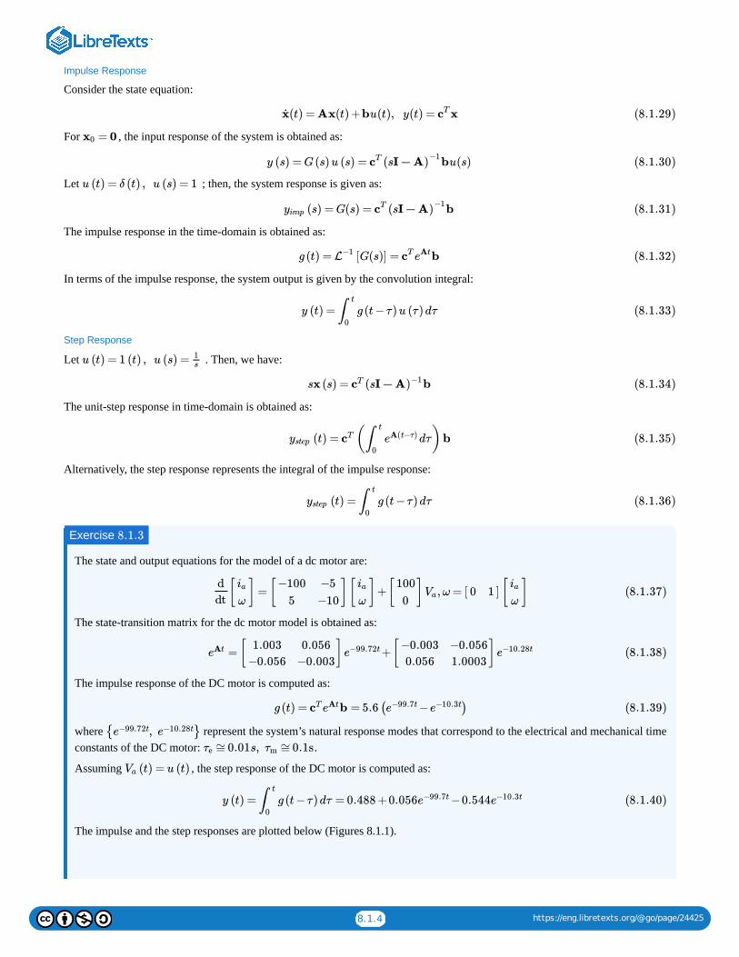
8.1.4 https://eng.libretexts.org/@go/page/24425

Impulse Response

Consider the state equation:

For , the input response of the system is obtained as:

Let ; then, the system response is given as:

The impulse response in the time-domain is obtained as:

In terms of the impulse response, the system output is given by the convolution integral:

Step Response

Let . Then, we have:

The unit-step response in time-domain is obtained as:

Alternatively, the step response represents the integral of the impulse response:

The state and output equations for the model of a dc motor are:

The state-transition matrix for the dc motor model is obtained as:

The impulse response of the DC motor is computed as:

where represent the system’s natural response modes that correspond to the electrical and mechanical timeconstants of the DC motor: .

Assuming , the step response of the DC motor is computed as:

The impulse and the step responses are plotted below (Figures 8.1.1).

(t) = Ax(t) +bu(t), y(t) = xx cT (8.1.29)

= 0x0

y (s) = G(s)u (s) = bu(s)cT (sI − A)

−1(8.1.30)

u (t) = δ (t) ,   u (s) = 1

(s) = G(s) = byimp cT (sI − A)

−1(8.1.31)

g (t) = [G(s)] = bL−1

cT eAt (8.1.32)

y (t) = g (t−τ)u (τ)dτ∫t

0

(8.1.33)

u (t) = 1 (t) ,   u (s) = 1s

sx (s) = bcT (sI − A)−1 (8.1.34)

(t) = ( dτ)bystep cT ∫t

0

eA(t−τ) (8.1.35)

(t) = g (t−τ)dτystep ∫t

0

(8.1.36)

Exercise 8.1.3

[ ] = [ ][ ]+[ ] ,ω = [ ] [ ]d

dt

ia

ω

−100

5

−5

−10

ia

ω

100

0Va 0 1

ia

ω(8.1.37)

= [ ] +[ ]eAt 1.003

−0.056

0.056

−0.003e−99.72t −0.003

0.056

−0.056

1.0003e−10.28t (8.1.38)

g (t) = b = 5.6 ( − )cT eAt e−99.7t e−10.3t (8.1.39)

{ , }e−99.72t e−10.28t

≅0.01s, ≅0.1sτe τm

(t) = u (t)Va

y (t) = g (t−τ)dτ = 0.488 +0.056 −0.544∫t

0

e−99.7t e−10.3t (8.1.40)

8.1.5 https://eng.libretexts.org/@go/page/24425

Figure : The DC motor model: impulse response (left); step response (right).

8.1: State Variable Models is shared under a CC BY-NC-SA 4.0 license and was authored, remixed, and/or curated by Kamran Iqbal.

8.1.1

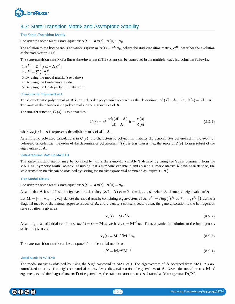
8.2.1 https://eng.libretexts.org/@go/page/28736

8.2: State-Transition Matrix and Asymptotic Stability

The State-Transition Matrix

Consider the homogenous state equation: .

The solution to the homogenous equation is given as: , where the state-transition matrix, , describes the evolutionof the state vector, .

The state-transition matrix of a linear time-invariant (LTI) system can be computed in the multiple ways including the following:

1. 2. 3. By using the modal matrix (see below)4. By using the fundamental matrix5. By using the Cayley–Hamilton theorem

Characteristic Polynomial of A

The characteristic polynomial of is an th order polynomial obtained as the determinant of , i.e., .The roots of the characteristic polynomial are the eigenvalues of .

The transfer function, , is expressed as:

where represents the adjoint matrix of .

Assuming no pole-zero cancelations in , the characteristic polynomial matches the denominator polynomial.In the event ofpole-zero cancelations, the order of the denominator polynomial, , is less than , i.e., the zeros of form a subset of theeigenvalues of .

State-Transition Matrix in MATLAB

The state-transition matrix may be obtained by using the symbolic variable 't' defined by using the 'syms' command from theMATLAB Symbolic Math Toolbox. Assuming that a symbolic variable 't' and an numeric matrix have been defined, thestate-transition matrix can be obtained by issuing the matrix exponential command as: .

The Modal Matrix

Consider the homogenous state equation: .

Assume that has a full set of eigenvectors, that obey , where denotes an eigenvalue of .

Let denote the modal matrix containing eigenvectors of , define adiagonal matrix of the natural response modes of , and denote a constant vector; then, the general solution to the homogenousstate equation is given as:

Assuming a set of initial conditions: ; we have, . Then, a particular solution to the homogenoussystem is given as:

The state-transition matrix can be computed from the modal matrix as:

Modal Matrix in MATLAB

The modal matrix is obtained by using the ‘eig’ command in MATLAB. The eigenvectors of obtained from MATLAB arenormalized to unity. The 'eig' command also provides a diagonal matrix of eigenvalues of . Given the modal matrix ofeigenvectors and the diagonal matrix of eigenvalues, the state-transition matrix is obtained as .

(t) = Ax(t), x(0) =x x0

x(t) = eAtx0 eAt

x (t)

= [(sI −A ]eAtL

−1 )−1

=eAt ∑∞0

Aiti

i !

A n (sI −A) Δ(s) = |sI −A|

A

G(s)

G(s) = b =cTadj(sI −A)

|sI −A|

n (s)

d (s)(8.2.1)

adj(sI −A) sI −A

G(s)

d (s) n d (s)

A

nxn A

expm(t ∗ A)

(t) = Ax(t), x(0) =x x0

A ( I −A) = 0,   i = 1, … ,nλi vi λi A

M = [ ,   , ⋯ , ]v1 v2 vn A = diag([ , , ⋯ , ])eΛt e tλ1 e tλ2 e tλn

A c

(t) = M cxh eΛt (8.2.2)

(0) = = Mcxh x0 c = M−1

x0

(t) = Mxh eΛtM−1x0 (8.2.3)

= MeAt eΛtM−1 (8.2.4)

A

A M

D M ∗ expm(t ∗ D)/M

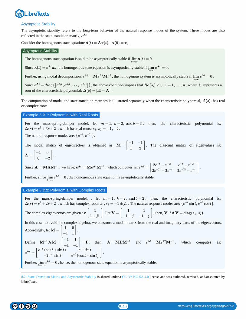
8.2.2 https://eng.libretexts.org/@go/page/28736

Asymptotic Stability

The asymptotic stability refers to the long-term behavior of the natural response modes of the system. These modes are alsoreflected in the state-transition matrix, .

Consider the homogenous state equation: .

The homogenous state equation is said to be asymptotically stable if .

Since , the homogenous state equation is asymptotically stable if .

Further, using modal decomposition, , the homogenous system is asymptotically stable if .

Since , the above condition implies that , where represents aroot of the characteristic polynomial: .

The computation of modal and state-transition matrices is illustrated separately when the characteristic polynomial, , has realor complex roots.

For the mass-spring-damper model, let ; then, the characteristic polynomial is: , which has real roots: .

The natural response modes are: .

The modal matrix of eigenvectors is obtained as: . The diagonal matrix of eigenvalues is:

.

Since , we have: , which computes as: .

Further, since , the homogenous state equation is asymptotically stable.

For the mass-spring-damper model, , let ; then, the characteristic polynomial is: , which has complex roots: . The natural response modes are: .

The complex eigenvectors are given as: . Let ; then, .

In this case, to avoid the complex algebra, we construct a modal matrix from the real and imaginary parts of the eigenvectors.

Accordingly, let .

Define ; then, and , which computes as:

.

Further, ; hence, the homogenous state equation is asymptotically stable.

8.2: State-Transition Matrix and Asymptotic Stability is shared under a CC BY-NC-SA 4.0 license and was authored, remixed, and/or curated byLibreTexts.

eAt

(t) = Ax(t), x(0) =x x0

Asymptotic Stability

x(t) = 0limt→∞

x(t) = eAtx0 = 0limt→∞

eAt

= MeAt eΛtM−1 = 0limt→∞

eΛt

= diag([ , , ⋯ , ])eΛt e tλ1 e tλ2 e tλn Re [ ] < 0,  i = 1, … ,nλi λi

Δ(s) = |sI − A|

Δ(s)

Example : Polynomial with Real Roots8.2.1

m = 1, k = 2, and b = 3

Δ(s) = +3s+2s2 , = −1, −2s1 s2

{ , }e−t e−2t

M = [ ]−1

1

−1

2

Λ = [ ]−1

0

0

−2

A = MΛM−1 = MeAt eΛtM−1 = [ ]eAt 2 −e−t e−2t

2 −2e−2t e−t

−e−t e−2t

2 −e−2t e−t

= 0limt→∞

eAt

Example : Polynomial with Complex Roots8.2.2

m = 1, k = 2, and b = 2

Δ(s) = +2s+2s2 , = −1 ±j1s1 s2 { sin t, cos t}e−t e−t

[ ]1

1 ±j1V = [ ]

1

−1 +j

1

−1 −jAV = diag( , )V−1 s1 s2

M = [ ]1

−1

0

1

AM = [ ] = ΓM−1 −1

−1

1

−1A = MΓM−1 = MeAt eΓtM−1

= [ ]eAt (cos t+sin t)e−t

−2 sin te−t

sin te−t

(cos t−sin t)e−t

= 0limt→∞

eAt

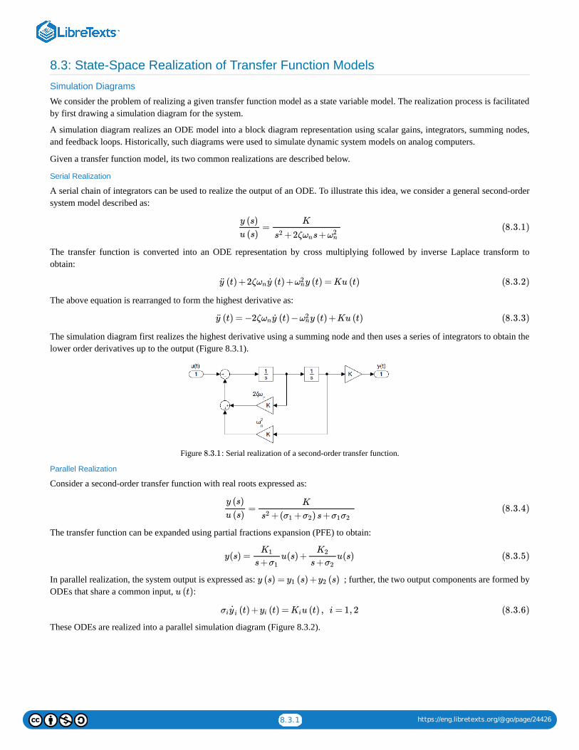
8.3.1 https://eng.libretexts.org/@go/page/24426

8.3: State-Space Realization of Transfer Function Models

Simulation Diagrams

We consider the problem of realizing a given transfer function model as a state variable model. The realization process is facilitatedby first drawing a simulation diagram for the system.

A simulation diagram realizes an ODE model into a block diagram representation using scalar gains, integrators, summing nodes,and feedback loops. Historically, such diagrams were used to simulate dynamic system models on analog computers.

Given a transfer function model, its two common realizations are described below.

Serial Realization

A serial chain of integrators can be used to realize the output of an ODE. To illustrate this idea, we consider a general second-ordersystem model described as:

The transfer function is converted into an ODE representation by cross multiplying followed by inverse Laplace transform toobtain:

The above equation is rearranged to form the highest derivative as:

The simulation diagram first realizes the highest derivative using a summing node and then uses a series of integrators to obtain thelower order derivatives up to the output (Figure 8.3.1).

Figure : Serial realization of a second-order transfer function.

Parallel Realization

Consider a second-order transfer function with real roots expressed as:

The transfer function can be expanded using partial fractions expansion (PFE) to obtain:

In parallel realization, the system output is expressed as: ; further, the two output components are formed byODEs that share a common input, :

These ODEs are realized into a parallel simulation diagram (Figure 8.3.2).

=y (s)u (s)

K

+2ζ s+s2 ωn ω2n

(8.3.1)

(t) +2ζ (t) + y (t) = Ku (t)y ωn y ω2n (8.3.2)

(t) = −2ζ (t) − y (t) +Ku (t)y ωn y ω2n (8.3.3)

8.3.1

=y (s)u (s)

K

+( + )s+s2 σ1 σ2 σ1σ2(8.3.4)

y(s) = u(s) + u(s)K1

s+σ1

K2

s+σ2(8.3.5)

y (s) = (s) + (s)y1 y2

u (t)

(t) + (t) = u (t) ,   i = 1, 2σi y i yi Ki (8.3.6)

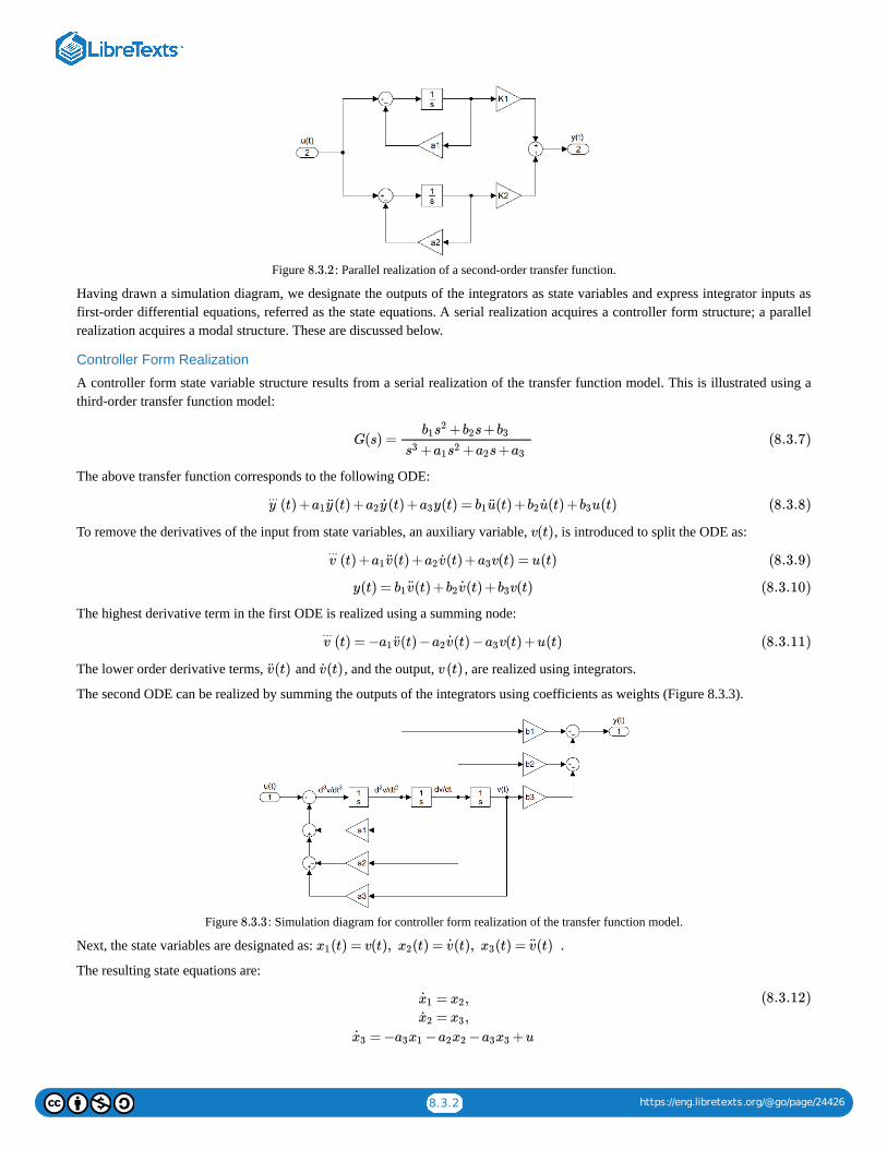
8.3.2 https://eng.libretexts.org/@go/page/24426

Figure : Parallel realization of a second-order transfer function.

Having drawn a simulation diagram, we designate the outputs of the integrators as state variables and express integrator inputs asfirst-order differential equations, referred as the state equations. A serial realization acquires a controller form structure; a parallelrealization acquires a modal structure. These are discussed below.

Controller Form Realization

A controller form state variable structure results from a serial realization of the transfer function model. This is illustrated using athird-order transfer function model:

The above transfer function corresponds to the following ODE:

To remove the derivatives of the input from state variables, an auxiliary variable, , is introduced to split the ODE as:

The highest derivative term in the first ODE is realized using a summing node:

The lower order derivative terms, and , and the output, , are realized using integrators.

The second ODE can be realized by summing the outputs of the integrators using coefficients as weights (Figure 8.3.3).

Figure : Simulation diagram for controller form realization of the transfer function model.

Next, the state variables are designated as: .

The resulting state equations are:

8.3.2

G(s) =+ s+b1s

2 b2 b3

+ + s+s3 a1s2 a2 a3(8.3.7)

(t) + (t) + (t) + y(t) = (t) + (t) + u(t)y...

a1 y a2 y a3 b1u b2u b3 (8.3.8)

v(t)

(t) + (t) + (t) + v(t) = u(t)v...

a1 v a2 v a3 (8.3.9)

y(t) = (t) + (t) + v(t)b1 v b2 v b3 (8.3.10)

(t) = − (t) − (t) − v(t) +u(t)v...

a1 v a2 v a3 (8.3.11)

(t)v (t)v v(t)

8.3.3

(t) = v(t), (t) = (t), (t) = (t)x1 x2 v x3 v

= ,x1 x2

= ,x2 x3

= − − − +ux3 a3x1 a2x2 a3x3

(8.3.12)

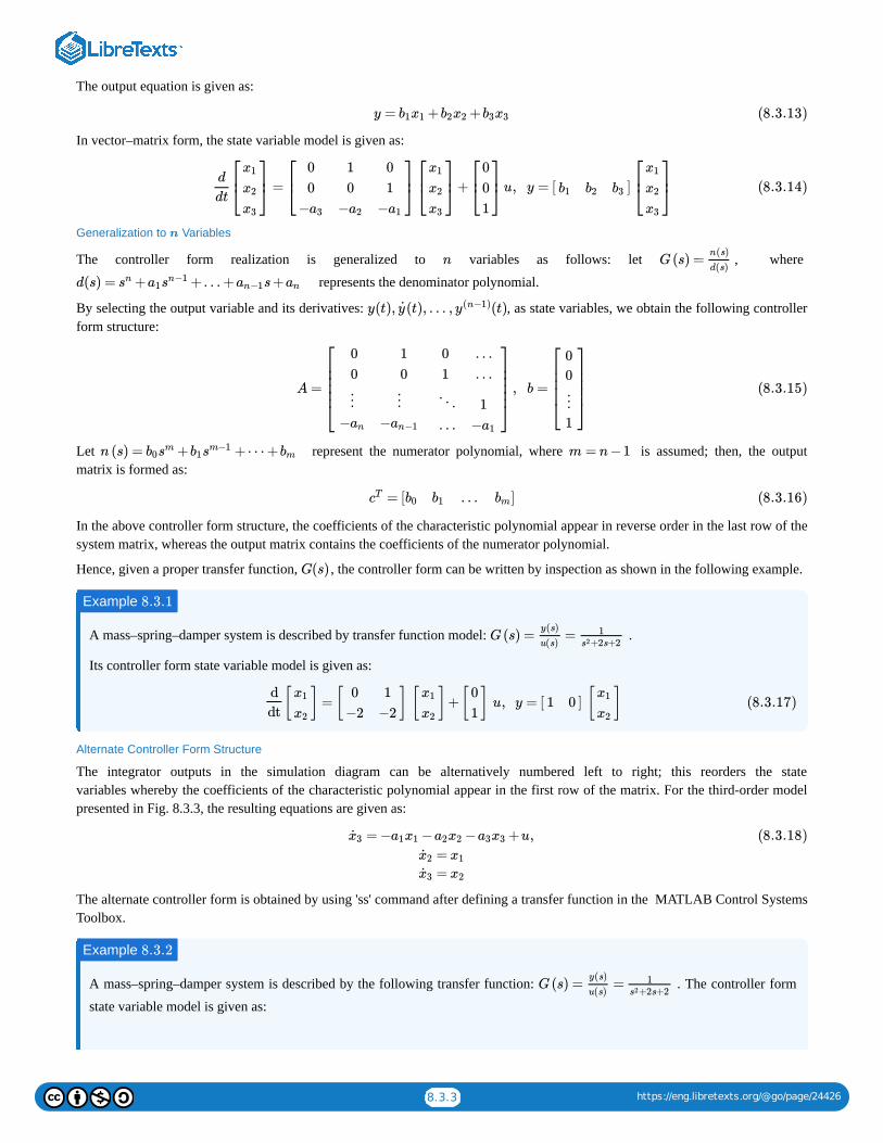
8.3.3 https://eng.libretexts.org/@go/page/24426

The output equation is given as:

In vector–matrix form, the state variable model is given as:

Generalization to Variables

The controller form realization is generalized to variables as follows: let , where

represents the denominator polynomial.

By selecting the output variable and its derivatives: , as state variables, we obtain the following controllerform structure:

Let represent the numerator polynomial, where is assumed; then, the outputmatrix is formed as:

In the above controller form structure, the coefficients of the characteristic polynomial appear in reverse order in the last row of thesystem matrix, whereas the output matrix contains the coefficients of the numerator polynomial.

Hence, given a proper transfer function, , the controller form can be written by inspection as shown in the following example.

A mass–spring–damper system is described by transfer function model: .

Its controller form state variable model is given as:

Alternate Controller Form Structure

The integrator outputs in the simulation diagram can be alternatively numbered left to right; this reorders the statevariables whereby the coefficients of the characteristic polynomial appear in the first row of the matrix. For the third-order modelpresented in Fig. 8.3.3, the resulting equations are given as:

The alternate controller form is obtained by using 'ss' command after defining a transfer function in the MATLAB Control SystemsToolbox.

A mass–spring–damper system is described by the following transfer function: . The controller form

state variable model is given as:

y = + +b1x1 b2x2 b3x3 (8.3.13)

= + u, y = [ ]d

dt

⎡

⎣⎢

x1

x2

x3

⎤

⎦⎥

⎡

⎣⎢

00

−a3

10

−a2

01

−a1

⎤

⎦⎥⎡

⎣⎢

x1

x2

x3

⎤

⎦⎥

⎡

⎣⎢

001

⎤

⎦⎥ b1 b2 b3

⎡

⎣⎢

x1

x2

x3

⎤

⎦⎥ (8.3.14)

n

n G(s) =n(s)

d(s)

d(s) = + +… + s+sn a1sn−1 an−1 an

y(t), (t), … , (t)y y(n−1)

A = , b =

⎡

⎣

⎢⎢⎢⎢⎢

00

10

⋮−an

⋮−an−1

01

……

⋱…

1−a1

⎤

⎦

⎥⎥⎥⎥⎥

⎡

⎣

⎢⎢⎢⎢

00

⋮1

⎤

⎦

⎥⎥⎥⎥

(8.3.15)

n (s) = + +⋯ +b0sm b1s

m−1 bm m = n−1

= [ … ]cT b0 b1 bm (8.3.16)

G(s)

Example 8.3.1

G(s) = =y(s)

u(s)1

+2s+2s2

[ ] = [ ] [ ]+[ ] u, y = [ ] [ ]ddt

x1

x2

0−2

1−2

x1

x2

01

1 0x1

x2(8.3.17)

= − − − +u,x3 a1x1 a2x2 a3x3

=x2 x1

=x3 x2

(8.3.18)

Example 8.3.2

G(s) = =y(s)

u(s)1

+2s+2s2

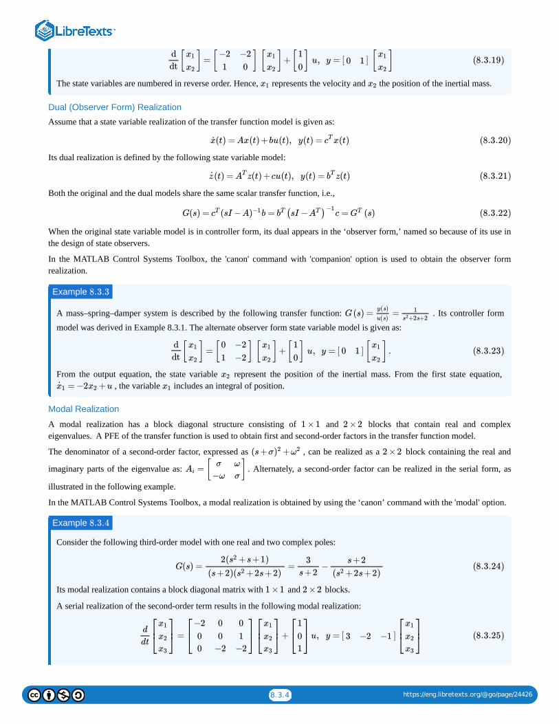
8.3.4 https://eng.libretexts.org/@go/page/24426

The state variables are numbered in reverse order. Hence, represents the velocity and the position of the inertial mass.

Dual (Observer Form) Realization

Assume that a state variable realization of the transfer function model is given as:

Its dual realization is defined by the following state variable model:

Both the original and the dual models share the same scalar transfer function, i.e.,

When the original state variable model is in controller form, its dual appears in the ‘observer form,’ named so because of its use inthe design of state observers.

In the MATLAB Control Systems Toolbox, the 'canon' command with 'companion' option is used to obtain the observer formrealization.

A mass–spring–damper system is described by the following transfer function: . Its controller form

model was derived in Example 8.3.1. The alternate observer form state variable model is given as:

From the output equation, the state variable represent the position of the inertial mass. From the first state equation, , the variable includes an integral of position.

Modal Realization

A modal realization has a block diagonal structure consisting of and blocks that contain real and complexeigenvalues. A PFE of the transfer function is used to obtain first and second-order factors in the transfer function model.

The denominator of a second-order factor, expressed as , can be realized as a block containing the real and

imaginary parts of the eigenvalue as: . Alternately, a second-order factor can be realized in the serial form, as

illustrated in the following example.

In the MATLAB Control Systems Toolbox, a modal realization is obtained by using the ‘canon’ command with the 'modal' option.

Consider the following third-order model with one real and two complex poles:

Its modal realization contains a block diagonal matrix with and blocks.

A serial realization of the second-order term results in the following modal realization:

[ ] = [ ] [ ]+[ ] u, y = [ ] [ ]ddt

x1

x2

−21

−20

x1

x2

10

0 1x1

x2(8.3.19)

x1 x2

(t) = Ax(t) +bu(t), y(t) = x(t)x cT (8.3.20)

(t) = z(t) +cu(t), y(t) = z(t)z AT bT (8.3.21)

G(s) = (sI −A b = c = (s)cT )−1 bT (sI − )AT −1GT (8.3.22)

Example 8.3.3

G(s) = =y(s)

u(s)1

+2s+2s2

[ ] = [ ] [ ]+[ ] u, y = [ ] [ ] .ddt

x1

x2

01

−2−2

x1

x2

10

0 1x1

x2(8.3.23)

x2

= −2 +ux1 x2 x1

1 ×1 2 ×2

(s+σ +)2 ω2 2 ×2

= [ ]Aiσ

−ω

ω

σ

Example 8.3.4

G(s) = = −2( +s+1)s2

(s+2)( +2s+2)s2

3s+2

s+2( +2s+2)s2

(8.3.24)

1 ×1 2 ×2

= + u, y = [ ]d

dt

⎡

⎣⎢

x1

x2

x3

⎤

⎦⎥

⎡

⎣⎢

−200

00

−2

01

−2

⎤

⎦⎥⎡

⎣⎢

x1

x2

x3

⎤

⎦⎥

⎡

⎣⎢

101

⎤

⎦⎥ 3 −2 −1

⎡

⎣⎢

x1

x2

x3

⎤

⎦⎥ (8.3.25)

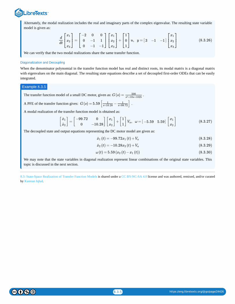
8.3.5 https://eng.libretexts.org/@go/page/24426

Alternately, the modal realization includes the real and imaginary parts of the complex eigenvalue. The resulting state variablemodel is given as:

We can verify that the two modal realizations share the same transfer function.

Diagonalization and Decoupling

When the denominator polynomial in the transfer function model has real and distinct roots, its modal matrix is a diagonal matrixwith eigenvalues on the main diagonal. The resulting state equations describe a set of decoupled first-order ODEs that can be easilyintegrated.

The transfer function model of a small DC motor, given as: .

A PFE of the transfer function gives: .

A modal realization of the transfer function model is obtained as:

The decoupled state and output equations representing the DC motor model are given as:

We may note that the state variables in diagonal realization represent linear combinations of the original state variables. Thistopic is discussed in the next section.

8.3: State-Space Realization of Transfer Function Models is shared under a CC BY-NC-SA 4.0 license and was authored, remixed, and/or curatedby Kamran Iqbal.

= + u, y = [ ]d

dt

⎡

⎣⎢

x1

x2

x3

⎤

⎦⎥

⎡

⎣⎢

−200

0−1−1

01

−1

⎤

⎦⎥⎡

⎣⎢

x1

x2

x3

⎤

⎦⎥

⎡

⎣⎢

101

⎤

⎦⎥ 3 −1 −1

⎡

⎣⎢

x1

x2

x3

⎤

⎦⎥ (8.3.26)

Example 8.3.5

G(s) = 500+10s+1025s2

 G(s) = 5.59 [ − ]1s+10.28

1s+99.72

[ ] = [ ][ ]+[ ] , ω = [ ] [ ]x1

x2

−99.720

0−10.28

x1

x2

11

Va −5.59 5.59x1

x2(8.3.27)

(t) = −99.72 (t) +x1 x1 Va (8.3.28)

(t) = −10.28 (t) +x2 x2 Va (8.3.29)

ω (t) = 5.59 ( (t) − (t))x2 x1 (8.3.30)

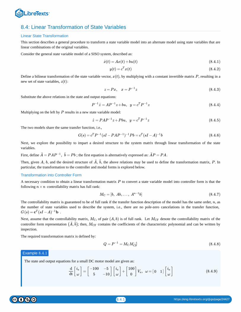
8.4.1 https://eng.libretexts.org/@go/page/24427

8.4: Linear Transformation of State Variables

Linear State Transformation

This section describes a general procedure to transform a state variable model into an alternate model using state variables that arelinear combinations of the original variables.

Consider the general state variable model of a SISO system, described as:

Define a bilinear transformation of the state variable vector, , by multiplying with a constant invertible matrix , resulting in anew set of state variables, :

Substitute the above relations in the state and output equations:

Multiplying on the left by results in a new state variable model:

The two models share the same transfer function, i.e.,

Next, we explore the possibility to impart a desired structure to the system matrix through linear transformation of the statevariables.

First, define ; the first equation is alternatively expressed as: .

Then, given , and the desired structure of , the above relations may be used to define the transformation matrix, . Inparticular, the transformation to the controller and modal forms is explored below.

Transformation into Controller Form

A necessary condition to obtain a linear transformation matrix to convert a state variable model into controller form is that thefollowing controllability matrix has full rank:

The controllability matrix is guaranteed to be of full rank if the transfer function description of the model has the same order, , asthe number of state variables used to describe the system, i.e., there are no pole-zero cancelations in the transfer function,

.

Next, assume that the controllability matrix, , of pair is of full rank. Let denote the controllability matrix of thecontroller form representation ; then, contains the coefficients of the characteristic polynomial and can be written byinspection.

The required transformation matrix is defined by:

The state and output equations for a small DC motor model are given as:

(t) = Ax(t) +bu(t)x (8.4.1)

y(t) = x(t)cT (8.4.2)

x(t) P

z(t)

z = P x, x = zP −1 (8.4.3)

= A z +bu, y = zP −1 z P −1 cT P −1 (8.4.4)

P

= P A z +P bu, y = zz P −1 cT P −1 (8.4.5)

G(s) = (sI −P A P b = (sI −A bcT P −1 P −1)−1 cT )−1 (8.4.6)

= P A , = P bA P −1 b P = P AA

A, b ,A b P

P

n ×n

= [b, Ab, … , b]MC An−1 (8.4.7)

n

G(s) = (sI −A bcT )−1

MC (A, b) MCF

( , )A b MCF

Q = =P −1 MCM −1CF (8.4.8)

Example 8.4.1

[ ] = [ ][ ]+[ ] , ω = [ ] [ ]d

dt

ia

ω

−100

5

−5

−10

ia

ω

100

0Va 0 1

ia

ω(8.4.9)

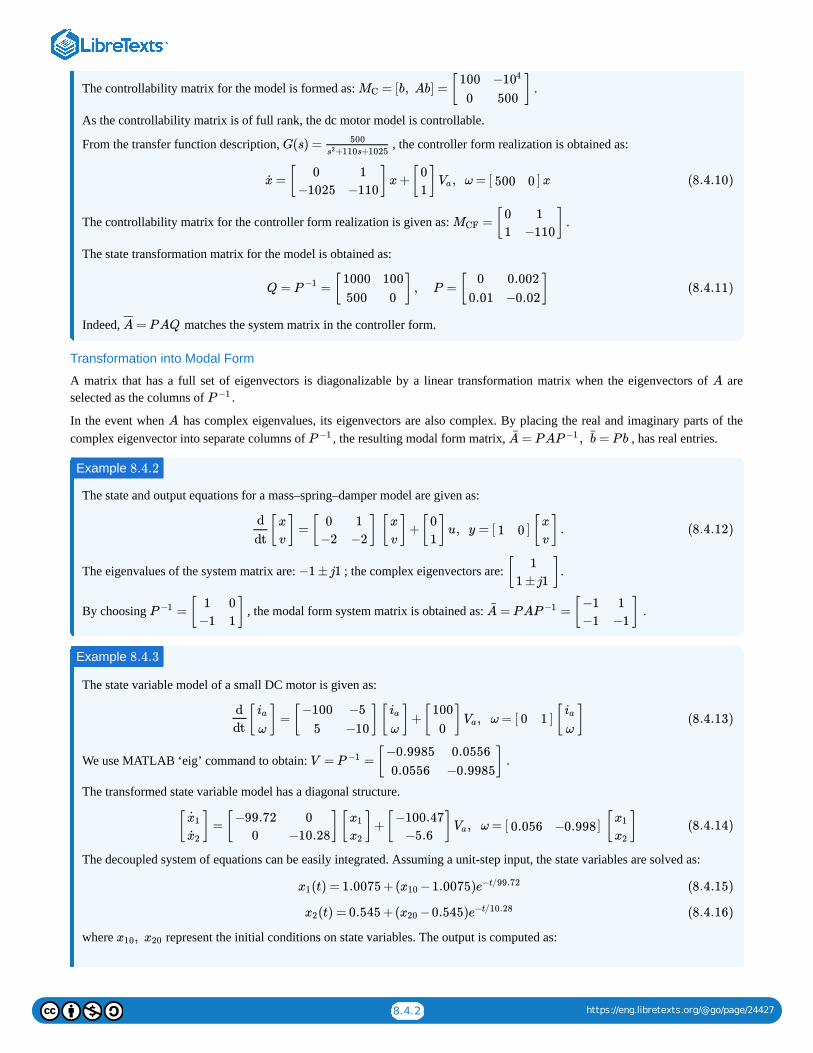
8.4.2 https://eng.libretexts.org/@go/page/24427

The controllability matrix for the model is formed as: .

As the controllability matrix is of full rank, the dc motor model is controllable.

From the transfer function description, , the controller form realization is obtained as:

The controllability matrix for the controller form realization is given as: .

The state transformation matrix for the model is obtained as:

Indeed, matches the system matrix in the controller form.

Transformation into Modal Form

A matrix that has a full set of eigenvectors is diagonalizable by a linear transformation matrix when the eigenvectors of areselected as the columns of .

In the event when has complex eigenvalues, its eigenvectors are also complex. By placing the real and imaginary parts of thecomplex eigenvector into separate columns of , the resulting modal form matrix, , has real entries.

The state and output equations for a mass–spring–damper model are given as:

The eigenvalues of the system matrix are: ; the complex eigenvectors are: .

By choosing , the modal form system matrix is obtained as: .

The state variable model of a small DC motor is given as:

We use MATLAB ‘eig’ command to obtain: .

The transformed state variable model has a diagonal structure.

The decoupled system of equations can be easily integrated. Assuming a unit-step input, the state variables are solved as:

where represent the initial conditions on state variables. The output is computed as:

= [b, Ab] = [ ]MC100

0

−104

500

G(s) = 500

+110s+1025s2

= [ ]x +[ ] , ω = [ ] xx0

−1025

1

−110

0

1Va 500 0 (8.4.10)

= [ ]MCF0

1

1

−110

Q = = [ ] , P = [ ]P −1 1000

500

100

0

0

0.01

0.002

−0.02(8.4.11)

= P AQA¯ ¯¯

A

P −1

A

P −1 = P A , = P bA P −1 b

Example 8.4.2

[ ] = [ ] [ ]+[ ]u, y = [ ] [ ] .d

dt

x

v

0

−2

1

−2

x

v

0

11 0

x

v(8.4.12)

−1 ±j1 [ ]1

1 ±j1

= [ ]P −1 1

−1

0

1= P A = [ ]A P −1 −1

−1

1

−1

Example 8.4.3

[ ] = [ ][ ]+[ ] , ω = [ ] [ ]d

dt

ia

ω

−100

5

−5

−10

ia

ω

100

0Va 0 1

ia

ω(8.4.13)

V = = [ ]P −1 −0.9985

0.0556

0.0556

−0.9985

[ ] = [ ][ ]+[ ] , ω = [ ] [ ]x1

x2

−99.72

0

0

−10.28

x1

x2

−100.47

−5.6Va 0.056 −0.998

x1

x2

(8.4.14)

(t) = 1.0075 +( −1.0075)x1 x10 e−t/99.72 (8.4.15)

(t) = 0.545 +( −0.545)x2 x20 e−t/10.28 (8.4.16)

,x10 x20

8.4.3 https://eng.libretexts.org/@go/page/24427

The original state variables are recovered as: , i.e.,

8.4: Linear Transformation of State Variables is shared under a CC BY-NC-SA 4.0 license and was authored, remixed, and/or curated by KamranIqbal.

ω(t) = 0.056 (t) −0.998 (t)x1 x2 (8.4.17)

[ ] = [ ]ia

ωP −1 x1

x2

(t) = −0.9985 (t) +0.0556 (t)ia x1 x2 (8.4.18)

ω (t) = 0.0556 (t) −0.9985 (t)x1 x2 (8.4.19)

1

CHAPTER OVERVIEW

9: Controllers for State Variable Models

1. Perform controller design for state variable models.2. Perform pole placement design using a variety of techniques.3. Design reference tracking controllers for state variable models.

9.0: Prelude to Controllers for State Variable Models9.1: Controller Design in Sate-Space9.2: Tracking with Feedforward Controller9.3: Tracking PI Controller Design

9: Controllers for State Variable Models is shared under a CC BY-NC-SA 4.0 license and was authored, remixed, and/or curated by Kamran Iqbal.

Learning Objectives

9.0.1 https://eng.libretexts.org/@go/page/24462

9.0: Prelude to Controllers for State Variable ModelsThe state variable models of dynamic systems comprises first-order differential equations that express the time derivatives of a setof state variables. For linear time-invariant (LTI) systems, these equations are commonly expressed in vector-matrix form.

The controller design for the state variable models involves feeding back all the state variables using appropriate weights togenerate the error signal. State feedback allows arbitrary placement of roots of the closed-loop characteristic polynomial. It is morepowerful and offers greater flexibility than the output feedback that allows only selective placement of closed-loop roots. Statefeedback assumes that the complete set of state variables are availabe for feedback.

The pole placement design refers to the selection of feedback gains for placing the roots of the closed-loop characteristicpolynomial at the desired locations in the complex plane. The pole placement design is performed with ease when the state variablemodel is in the controller form. Alternately, Ackermann’s and Bass-Gura formulas, or the Sylvester’s equation can be used for thispurpose.

Output regulation refers to finding a control law to asymptotically track prescribed refernce signals and/or asymptotically rejectundesired disturbance inputs. It includes imparting desired degree of dynamic stability to the system through arbitrary selection ofthe closed-loop characteristic polynomial.

The tracking system design involves reducing the steady-state error to a given reference input to zero. Though reference signal canbe used to cancel the tracking error, the design is not robust against parameter variations. A more robust design involves integratingthe error signal inside the feeback loop to form an augmented system model, which can used for pole placement. The augmentedmodel includes the differential equation describing the out put of the integrator.

The state-space design methods primarily cater to the design of multi-input multi-output (MIMO) systems. This chapter, however,introduces the state-space design methods using examples from single-input single-output (SISO) systems.

9.0: Prelude to Controllers for State Variable Models is shared under a CC BY-NC-SA 4.0 license and was authored, remixed, and/or curated byLibreTexts.

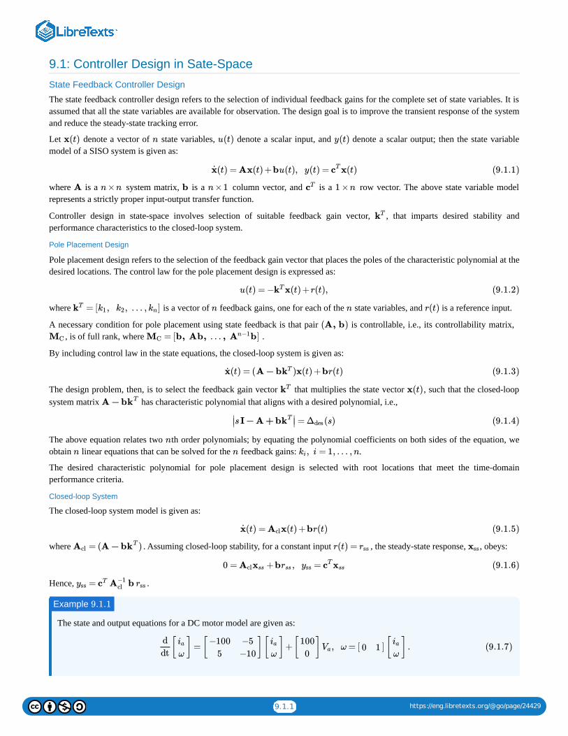
9.1.1 https://eng.libretexts.org/@go/page/24429

9.1: Controller Design in Sate-Space

State Feedback Controller Design

The state feedback controller design refers to the selection of individual feedback gains for the complete set of state variables. It isassumed that all the state variables are available for observation. The design goal is to improve the transient response of the systemand reduce the steady-state tracking error.

Let denote a vector of state variables, denote a scalar input, and denote a scalar output; then the state variablemodel of a SISO system is given as:

where is a system matrix, is a column vector, and is a row vector. The above state variable modelrepresents a strictly proper input-output transfer function.

Controller design in state-space involves selection of suitable feedback gain vector, , that imparts desired stability andperformance characteristics to the closed-loop system.

Pole Placement Design

Pole placement design refers to the selection of the feedback gain vector that places the poles of the characteristic polynomial at thedesired locations. The control law for the pole placement design is expressed as:

where is a vector of feedback gains, one for each of the state variables, and is a reference input.

A necessary condition for pole placement using state feedback is that pair is controllable, i.e., its controllability matrix, , is of full rank, where .

By including control law in the state equations, the closed-loop system is given as:

The design problem, then, is to select the feedback gain vector that multiplies the state vector , such that the closed-loopsystem matrix has characteristic polynomial that aligns with a desired polynomial, i.e.,

The above equation relates two th order polynomials; by equating the polynomial coefficients on both sides of the equation, weobtain linear equations that can be solved for the feedback gains: .

The desired characteristic polynomial for pole placement design is selected with root locations that meet the time-domainperformance criteria.

Closed-loop System

The closed-loop system model is given as:

where . Assuming closed-loop stability, for a constant input , the steady-state response, , obeys:

Hence, .

The state and output equations for a DC motor model are given as:

x(t) n u(t) y(t)

(t) = Ax(t) +bu(t), y(t) = x(t)x cT (9.1.1)

A n ×n b n ×1 cT 1 ×n

kT

u(t) = − x(t) +r(t),kT (9.1.2)

= [ , , … , ]kT k1 k2 kn n n r(t)

(A, b)MC = [ b]MC b, Ab, … , An−1

(t) = ( )x(t) +br(t)x A − bkT (9.1.3)

kT x(t)A − bk

T

s = (s)∣∣ I − A + bkT ∣∣ Δdes (9.1.4)

n

n n , i = 1, … , nki

(t) = x(t) +br(t)x Acl (9.1.5)

= ( )Acl A − bkT r(t) = rss xss

0 = +b , =Aclxss rss yss cT

xss (9.1.6)

= byss cT A−1cl rss

Example 9.1.1

[ ] = [ ][ ]+[ ] , ω = [ ] [ ] .ddt

ia

ω

−1005

−5−10

ia

ω

1000

Va 0 1ia

ω(9.1.7)

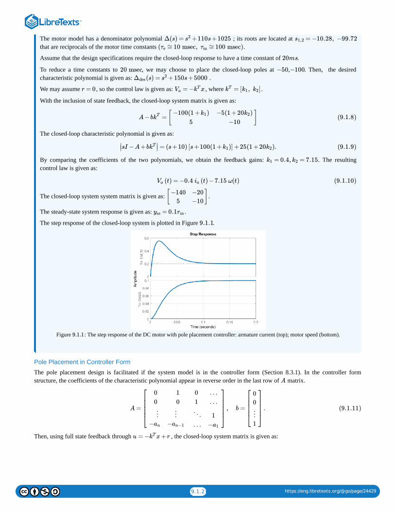
9.1.2 https://eng.libretexts.org/@go/page/24429

The motor model has a denominator polynomial ; its roots are located at that are reciprocals of the motor time constants .

Assume that the design specifications require the closed-loop response to have a time constant of .

To reduce a time constants to , we may choose to place the closed-loop poles at , . Then, the desiredcharacteristic polynomial is given as: .

We may assume , so the control law is given as: , where .

With the inclusion of state feedback, the closed-loop system matrix is given as:

The closed-loop characteristic polynomial is given as:

By comparing the coefficients of the two polynomials, we obtain the feedback gains: . The resultingcontrol law is given as:

The closed-loop system system matrix is given as: .

The steady-state system response is given as: .

The step response of the closed-loop system is plotted in Figure .

Figure : The step response of the DC motor with pole placement controller: armature current (top); motor speed (bottom).

Pole Placement in Controller Form

The pole placement design is facilitated if the system model is in the controller form (Section 8.3.1). In the controller formstructure, the coefficients of the characteristic polynomial appear in reverse order in the last row of matrix.

Then, using full state feedback through , the closed-loop system matrix is given as:

Δ(s) = +110s +1025s2 = −10.28, −99.72s1,2

( ≅10 msec, ≅100 msec)τe τm

20ms

20 msec −50 −100(s) = +150s +5000Δdes s2

r = 0 = − xVa kT = [ , ]kT k1 k2

A −b = [ ]kT −100(1 + )k1

5−5(1 +20 )k2

−10(9.1.8)

sI −A +b = (s +10) [s +100(1 + )] +25(1 +20 ).∣∣ kT ∣∣ k1 k2 (9.1.9)

= 0.4, = 7.15k1 k2

(t) = −0.4  (t) −7.15 ω(t)Va ia (9.1.10)

[ ]−140

5−20−10

= 0.1yss rss

9.1.1

9.1.1

A

A = , b = .

⎡

⎣

⎢⎢⎢⎢⎢

00

10

⋮−an

⋮−an−1

01

……

⋱…

1−a1

⎤

⎦

⎥⎥⎥⎥⎥

⎡

⎣

⎢⎢⎢⎢

00

⋮1

⎤

⎦

⎥⎥⎥⎥

(9.1.11)

u = − x +rkT

9.1.3 https://eng.libretexts.org/@go/page/24429

The closed-loop characteristic polynomial can be written by inspection, and is given as:

Let the desired characteristic polynomial be defined as:

By comparing the coefficients, the desired feedback gains are computed as:

Since the state variables in the controller form include system output and its derivatives, pole placement using state feedback is ageneralization of proportional-derivative (PD) and rate feedback controllers.

The state variable model of a mass–spring–damper is given as:

Assume that the design specifications require raising the damping to .

Since the system model is in controller form, its characteristic polynomial can be written by inspection, and is given as: .

In order to improve the damping, a desired characteristic polynomial is selected as: .

The desired feedback gains can be written by inspection, and are given as: .

Pole Placement using Bass-Gura Formula

The Bass-Gura formula describes a simple expression to compute the state feedback controller gains from the coefficients of theavailable and desired closed-loop characteristic polynomials. To proceed, let the state variable model be given as:

Assuming that pair is controllable, its controllability matrix is given as: .

The model is transformed into controller form by a linear transformation, ; the transformed model is described as:

The controllability matrix of the controller form representation is given as: The matrixcomprises the coefficients of the characteristic polynomial, , and can be written by inspection.

The required linear transformation matrix is obtained from the following relation:

The state feedback control law in the controller form is defined as:

In terms of polynomial coefficients, the controller gains are given as: .

The controller gains for the original state variable model are obtained as: .

Hence, the Bass-Gura formula is obtained as:

A −b = .kT

⎡

⎣

⎢⎢⎢⎢⎢

00

10

⋮− −an k1

⋮− −an−1 kn−1

01

……

⋱…

1− −a1 kn

⎤

⎦

⎥⎥⎥⎥⎥(9.1.12)

Δ(s) = +( + ) +… + +sn a1 kn sn−1 an k1 (9.1.13)

(s) = + +… + s + .Δdes sn a1sn−1 an−1 an (9.1.14)

= − , = − , … , = − .k1 an an k2 an−1 an−1 kn a1 a1 (9.1.15)

Example 9.1.2

[ ] = [ ][ ]+[ ] f , x = [ ] [ ] .ddt

x

v

0−10

1−1

x

v

01

1 0x

v(9.1.16)

ζ = 0.6

Δ(s) = +s +10s2

(s) = +4s +10Δdes s2

= [0 3]kT

(t) = Ax(t) +bu(t), y(t) = x(t)x cT (9.1.17)

(A, b) = [b, Ab, … , b]MC An−1

z = P x

(t) = z(t) + u(t), y(t) = z(t)z ACF bCF cTCF (9.1.18)

= [ , , … , ].MCF bCF ACFbCF ACFn−1bCF

Δ (s) = |sI −A|

= , P = .P −1 MCM −1CF MCFM −1

C (9.1.19)

u = − z(t) = − P x(t).kCFT kCF

T (9.1.20)

= [ ]kCFT −an an −an−1 an−1 ⋯ −a1 a1

= PkT kCFT

9.1.4 https://eng.libretexts.org/@go/page/24429

The state equations for a DC motor model are given as:

Assume that the design specifications require a time constant of .

The characteristic polynomial of the model is:

The controllability matrix of the model is formed as: .

The controller form representation for the model is developed as:

The controllability matrix for the controller form representation is: .

Assume that the desired characteristic polynomial is selected as: .

The feedback gains for the controller form representation are obtained as: .

Using the Bass-Gura formula, the state feedback controller gains for the DC motor model are computed as: .

The resulting state feedback control law is given as: .

Pole Placement using Ackermann’s Formula

The Ackermann’s formula is, likewise, a simple expression to compute the state feedback controller gains for pole placement. Todevelop the formula, let an -dimensional state variable model be given as:

The controllability matrix of the model is formed as:

Assume that a desired characteristic polynomial is given as: .

Next, we evaluate the following matrix polynomial that involves the system matrix:

where denotes an identity matrix. The state feedback controller gains are obtained from the following Ackermann’sformula:

The state equations for a DC motor model are given as:

Let the desired characteristic polynomial be given as: .

The controllability matrix for the model is computed as: .

The matrix polynomial used in the formula is evaluated as: .

= [ ]kT −an an −an−1 an−1 ⋯ −a1 a1 MCFM −1C (9.1.21)

Example 9.1.3

[ ] = [ ][ ]+[ ]ddt

ia

ω

−1005

−5−10

ia

ω

1000

Va (9.1.22)

20ms

|sI −A| = +110s +1025.s2

= [b, Ab] = [ ]MC100

0−104

500

[ ] = [ ][ ]+[ ]ddt

x1

x2

0−1025

1−110

x1

x2

01

Va (9.1.23)

= [ ]MCF01

1−110

(s) = +150s +5000Δdes s2

= [ ]kCFT 3975 40

= = [ ]kT kCFT MCFM −1

C 0.4 7.15

= −0.4 −7.15ωVa ia

n

(t) = Ax(t) +bu(t)x (9.1.24)

= [b, Ab, … , b].MC An−1

(s) = + +… + s +Δdes sn a1sn−1 an−1 an

(A) = + +… + A + I.Δdes An a1An−1 an−1 an (9.1.25)

I n ×n

= [ ] (A)kT 0 ⋯ 0 1 MC−1Δdes (9.1.26)

Example 9.1.4

[ ] = [ ][ ]+[ ]ddt

ia

ω

−1005

−5−10

ia

ω

1000

Va (9.1.27)

(s) = +150s +5000Δdes s2

= [b, Ab] = [ ]MC100

0−104

500

(A) = [ ]Δdes−25200

−2003575

9.1.5 https://eng.libretexts.org/@go/page/24429

Using the Ackermann’s formula, the pole placement controller is computed as: .

The resulting state feedback control law is given as: .

The MATLAB Control System Toolbox includes the ‘place’ command that uses Ackermann’s formula for pole placement design.The command is invoked by entering the system matrix, the input vector, and a vector of desired roots of the characteristicpolynomial. The function returns the feedback gain vector that places the eigenvalues of , at the desired root locations.

Pole Placement using Sylvester’s Equation

The Sylvester equation in linear algebra is a matrix equation, given as: , where and are square matrices of notnecessarily equal dimensions, and is a matrix of appropriate dimensions. The solution matrix is of the same dimension as .

In order to apply the Sylvester equation for pole placement design, let an -dimensional state variable model be given as:

The pair is assumed to be controllable.

Let represent the closed-loop system matrix; assume that a diagonalizing similarity transform is defined as:

The matrix is diagonal and contains the desired eigenvalues; it may be assumed in modal form for complex eigenvalues.

Let ; then, the Sylvester eqution is formulated as:

A unique solution to the Sylvester’s equation exists if the eigenvalues of and are distinct, i.e., .

The design procedure for pole placement using Sylvester’s equation is given as follows:

1. Choose a matrix of desired eigenvalues in modal form. Choose any and solve for .2. Recover the feedback gain vector from . If is not invertible, choose a different and repeat the procedure.

The state equation for the mass–spring–damper model is described as:

Let a desired characteristic polynomial be selected as: ; then, the modal matrix of the desired

eigenvalues is: .

Let ; then, . The solution to Sylvester’s equation is obtained as: .

The feedback controller gains are computed as: .

9.1: Controller Design in Sate-Space is shared under a CC BY-NC-SA 4.0 license and was authored, remixed, and/or curated by Kamran Iqbal.

= [ ]kT 0.4 7.15

= −0.4 −7.15ωVa ia

A −bkT

AX +XB = C A B

C X C

n

(t) = Ax(t) +bu(t)x (9.1.28)

(A, b)

A −bkT

(A −b )X = ΛX−1 kT (9.1.29)

Λ

X =kT gT

AX −XΛ = bgT (9.1.30)

X A Λ (A) − (Λ) ≠ 0λi λj

Λ gT AX −XΛ = bgT X

=kT gT X−1 X gT

Example 9.1.5

[ ] = [ ][ ]+[ ] fddt

x

v

0−10

1−1

x

v

01

(9.1.31)

(s) = +4s +10Δdes s2

Λ = [ ]−2

− 6–√6–√

−2

= [1 0]gT b = [ ]gT 01

00

X = [ ]−0.0670.333

−0.0820.0

= [0 3]kT

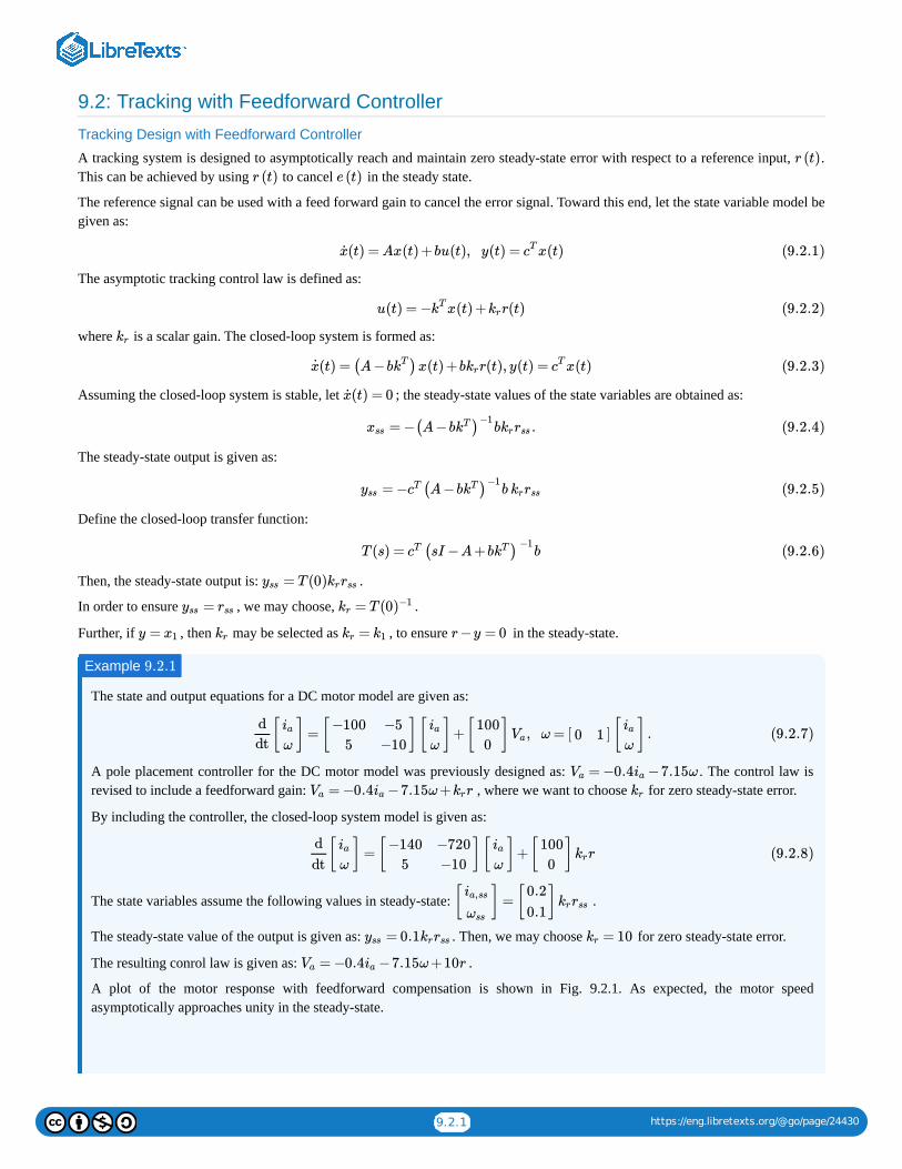
9.2.1 https://eng.libretexts.org/@go/page/24430

9.2: Tracking with Feedforward Controller

Tracking Design with Feedforward Controller

A tracking system is designed to asymptotically reach and maintain zero steady-state error with respect to a reference input, .This can be achieved by using to cancel in the steady state.

The reference signal can be used with a feed forward gain to cancel the error signal. Toward this end, let the state variable model begiven as:

The asymptotic tracking control law is defined as:

where is a scalar gain. The closed-loop system is formed as:

Assuming the closed-loop system is stable, let ; the steady-state values of the state variables are obtained as:

The steady-state output is given as:

Define the closed-loop transfer function:

Then, the steady-state output is: .

In order to ensure , we may choose, .

Further, if , then may be selected as , to ensure in the steady-state.

The state and output equations for a DC motor model are given as:

A pole placement controller for the DC motor model was previously designed as: . The control law isrevised to include a feedforward gain: , where we want to choose for zero steady-state error.

By including the controller, the closed-loop system model is given as:

The state variables assume the following values in steady-state: .

The steady-state value of the output is given as: . Then, we may choose for zero steady-state error.

The resulting conrol law is given as: .

A plot of the motor response with feedforward compensation is shown in Fig. 9.2.1. As expected, the motor speedasymptotically approaches unity in the steady-state.

r (t)

r (t) e (t)

(t) = Ax(t) +bu(t), y(t) = x(t)x cT (9.2.1)

u(t) = − x(t) + r(t)kT kr (9.2.2)

kr

(t) = (A −b )x(t) +b r(t), y(t) = x(t)x kT kr cT (9.2.3)

(t) = 0x

= − b .xss (A −b )kT −1krrss (9.2.4)

= − byss cT (A −b )kT −1krrss (9.2.5)

T (s) = bcT (sI −A +b )kT −1(9.2.6)

= T (0)yss krrss

=yss rss = T (0kr )−1

y = x1 kr =kr k1 r −y = 0

Example 9.2.1

[ ] = [ ][ ]+[ ] , ω = [ ] [ ] .d

dt

ia

ω

−100

5

−5

−10

ia

ω

100

0Va 0 1

ia

ω(9.2.7)

= −0.4 −7.15ωVa ia

= −0.4 −7.15ω + rVa ia kr kr

[ ] = [ ][ ]+[ ] rd

dt

ia

ω

−140

5

−720

−10

ia

ω

100

0kr (9.2.8)

[ ] = [ ]ia,ss

ωss

0.2

0.1krrss

= 0.1yss krrss = 10kr

= −0.4 −7.15ω +10rVa ia

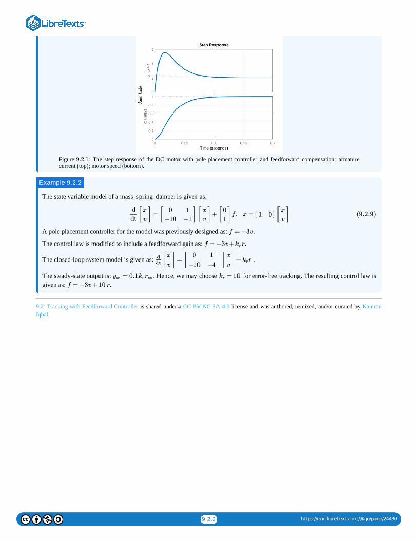
9.2.2 https://eng.libretexts.org/@go/page/24430

Figure : The step response of the DC motor with pole placement controller and feedforward compensation: armaturecurrent (top); motor speed (bottom).

The state variable model of a mass–spring–damper is given as:

A pole placement controller for the model was previously designed as: .

The control law is modified to include a feedforward gain as:

The closed-loop system model is given as: .

The steady-state output is: . Hence, we may choose for error-free tracking. The resulting control law isgiven as:

9.2: Tracking with Feedforward Controller is shared under a CC BY-NC-SA 4.0 license and was authored, remixed, and/or curated by KamranIqbal.

9.2.1

Example 9.2.2

[ ] = [ ][ ]+[ ] f , x = [ ] [ ]d

dt

x

v

0

−10

1

−1

x

v

0

11 0

x

v(9.2.9)

f = −3v

f = −3v+ r.kr

[ ] = [ ][ ]+ rddt

x

v

0

−10

1

−4

x

vkr

= 0.1yss krrss = 10kr

f = −3v+10 r.

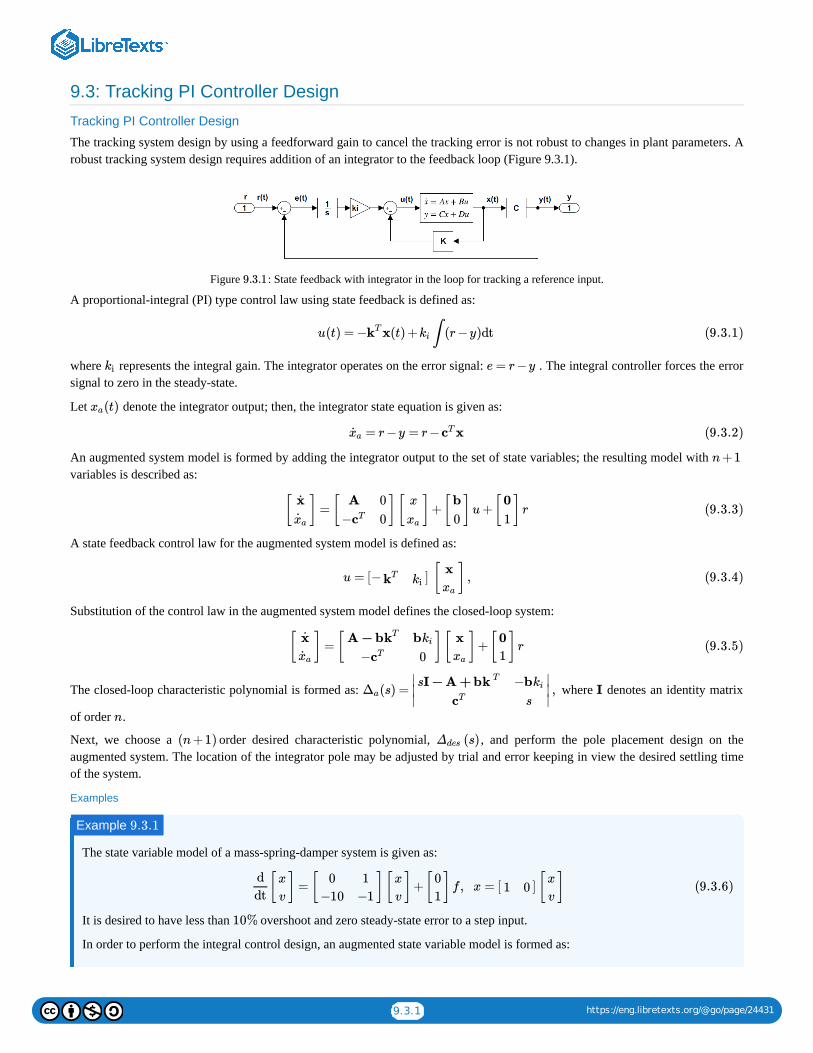
9.3.1 https://eng.libretexts.org/@go/page/24431

9.3: Tracking PI Controller Design

Tracking PI Controller Design

The tracking system design by using a feedforward gain to cancel the tracking error is not robust to changes in plant parameters. Arobust tracking system design requires addition of an integrator to the feedback loop (Figure 9.3.1).

Figure : State feedback with integrator in the loop for tracking a reference input.

A proportional-integral (PI) type control law using state feedback is defined as:

where represents the integral gain. The integrator operates on the error signal: . The integral controller forces the errorsignal to zero in the steady-state.

Let denote the integrator output; then, the integrator state equation is given as:

An augmented system model is formed by adding the integrator output to the set of state variables; the resulting model with variables is described as:

A state feedback control law for the augmented system model is defined as:

Substitution of the control law in the augmented system model defines the closed-loop system:

The closed-loop characteristic polynomial is formed as: where denotes an identity matrix

of order .

Next, we choose a order desired characteristic polynomial, , and perform the pole placement design on theaugmented system. The location of the integrator pole may be adjusted by trial and error keeping in view the desired settling timeof the system.

Examples

The state variable model of a mass-spring-damper system is given as:

It is desired to have less than overshoot and zero steady-state error to a step input.

In order to perform the integral control design, an augmented state variable model is formed as:

9.3.1

u(t) = − x(t) + ∫ (r−y)dtkT ki (9.3.1)

ki e = r−y

(t)xa

= r−y = r− xxa cT (9.3.2)

n+1

[ ] = [ ][ ]+[ ]u+[ ] rx

xa

A

−cT

0

0

x

xa

b

0

0

1(9.3.3)

u = [− ] [ ] ,kT ki

x

xa(9.3.4)

[ ] = [ ][ ]+[ ] rx

xa

A − bkT

−cT

bki

0

x

xa

0

1(9.3.5)

(s) = ,Δa

∣

∣∣sI − A + bk

T

cT

−bki

s

∣

∣∣ I

n

(n+1) (s)Δdes

Example 9.3.1

[ ] = [ ][ ]+[ ] f , x = [ ] [ ]d

dt

x

v

0

−10

1

−1

x

v

0

11 0

x

v(9.3.6)

10%

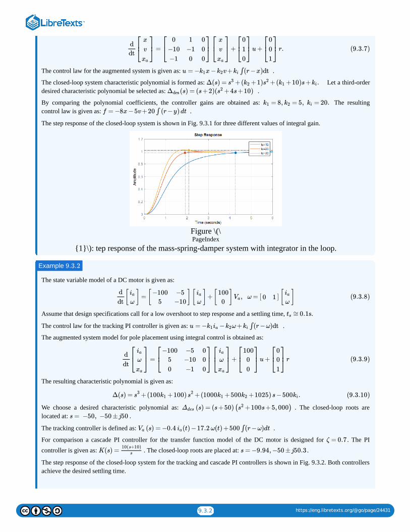
9.3.2 https://eng.libretexts.org/@go/page/24431

The control law for the augmented system is given as: .

The closed-loop system characteristic polynomial is formed as: Let a third-orderdesired characteristic polynomial be selected as: .

By comparing the polynomial coefficients, the controller gains are obtained as: The resultingcontrol law is given as: .

The step response of the closed-loop system is shown in Fig. 9.3.1 for three different values of integral gain.

Figure \(\PageIndex

{1}\): tep response of the mass-spring-damper system with integrator in the loop.

The state variable model of a DC motor is given as:

Assume that design specifications call for a low overshoot to step response and a settling time, .

The control law for the tracking PI controller is given as: .

The augmented system model for pole placement using integral control is obtained as:

The resulting characteristic polynomial is given as:

We choose a desired characteristic polynomial as: . The closed-loop roots arelocated at: .

The tracking controller is defined as: .

For comparison a cascade PI controller for the transfer function model of the DC motor is designed for . The PI

controller is given as: . The closed-loop roots are placed at: .

The step response of the closed-loop system for the tracking and cascade PI controllers is shown in Fig. 9.3.2. Both controllersachieve the desired settling time.

= + u+ r.d

dt

⎡

⎣⎢

x

v

xa

⎤

⎦⎥

⎡

⎣⎢

0

−10

−1

1

−1

0

0

0

0

⎤

⎦⎥⎡

⎣⎢

x

v

xa

⎤

⎦⎥

⎡

⎣⎢

0

1

0

⎤

⎦⎥

⎡

⎣⎢

0

0

1

⎤

⎦⎥ (9.3.7)

u = − x− v+ ∫(r−x)dtk1 k2 ki

Δ(s) = +( +1) +( +10)s+ .s3 k2 s2 k1 ki(s) = (s+2)( +4s+10)Δdes s2

= 8, = 5, = 20.k1 k2 kif = −8x−5v+20 ∫ (r−y)dt

Example 9.3.2

[ ] = [ ][ ]+[ ] , ω = [ ] [ ]d

dt

ia

ω

−100

5

−5

−10

ia

ω

100

0Va 0 1

ia

ω(9.3.8)

≅0.1sts

u = − − ω+ ∫(r−ω)dtk1ia k2 ki

= + u+ rd

dt

⎡

⎣⎢ia

ω

xa

⎤

⎦⎥

⎡

⎣⎢

−100

5

0

−5

−10

−1

0

0

0

⎤

⎦⎥⎡

⎣⎢ia

ω

xa

⎤

⎦⎥

⎡

⎣⎢

100

0

0

⎤

⎦⎥

⎡

⎣⎢

0

0

1

⎤

⎦⎥ (9.3.9)

Δ(s) = +(100 +100) +(1000 +500 +1025)s−500 .s3 k1 s2 k1 k2 ki (9.3.10)

(s) = (s+50)( +100s+5, 000)Δdes s2

s = −50, −50 ±j50

(s) = −0.4 (t) −17.2 ω(t) +500 ∫(r−ω)dtVa ia

ζ = 0.7

K(s) =10(s+10)

s s = −9.94, −50 ±j50.3

9.3.3 https://eng.libretexts.org/@go/page/24431

Figure : The step response of the DC motor model for cascade and tracking PI controllers.

9.3: Tracking PI Controller Design is shared under a CC BY-NC-SA 4.0 license and was authored, remixed, and/or curated by Kamran Iqbal.

9.3.2

1

CHAPTER OVERVIEW

10: Controllers for Discrete State Variable Models

1. Analyze state variable models of sampled-data systems.2. Solve discrete-time state equations by iteration.3. Perform pole placement controller design for sampled-data systems.4. Perform tracking controller desing for sampled-data systems.

10.0: Prelude to Controllers for Discrete State Variable Models10.1: State Variable Models of Sampled-Data Systems10.2: Controllers for Discrete State Variable Models

10: Controllers for Discrete State Variable Models is shared under a CC BY-NC-SA 4.0 license and was authored, remixed, and/or curated byKamran Iqbal.

Learning Objectives

10.0.1 https://eng.libretexts.org/@go/page/24463

10.0: Prelude to Controllers for Discrete State Variable ModelsThe state variable model of a dynamic system comprises a set of first-order differential equations that express the system behavioras time derivatives of the selected variables. The controller design for state state variable model involves selecting feedback gainsfor each (or a selection) of the state variables. The state feedback controller offers greater flexibility in system design compared tothe output feedback controllers designed with transfer function models.

The continuous-time state variable model of a linear time-invariant (LTI) system can be converted to a discrtete-time LTI model byassuming a piece-wise constant input to the system. The conversion is easily done in MATLAB by using the ‘c2d’ command. Theassumed sampling frequency should be five to ten times higher than the system bandwidth.

The control system design methods used with continuous-time systems can be extended to digital controller design of sampled-datasystems that include sample and hold elements. The time-domain description of a sampled-data system comprisess a set ofdifference equations that can be easily solved by iteration.

The pole placement design using full state feedback can be similarly performed on discrete state variable models. The desiredcharacteristic polynomial in the discrete case should have its roots inside the unit circle to ensure the stability of the closed-loopsystem. A discrete system model addionally allow the design of a deadbeat controller that places all roots of the closed-loopcharacteristic polynomial at the origin. The deadbeat controller ensures that the system response reaches steady state in exactly iterations.

Compared to the root locus design that allows selective placement of the closed-loop poles of the characteristic polynomial,arbitrary pole placement is made possible through the use of state feedback design in the case of state variable models. In thefollowing, we assume that the system to be controlled is of single-input single-output (SISO) type.

10.0: Prelude to Controllers for Discrete State Variable Models is shared under a CC BY-NC-SA 4.0 license and was authored, remixed, and/orcurated by LibreTexts.

n

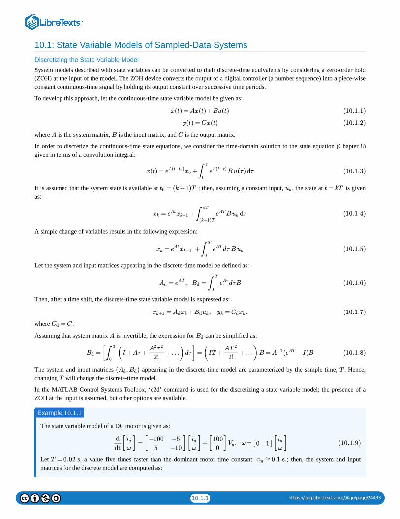
10.1.1 https://eng.libretexts.org/@go/page/24433

10.1: State Variable Models of Sampled-Data Systems

Discretizing the State Variable Model

System models described with state variables can be converted to their discrete-time equivalents by considering a zero-order hold(ZOH) at the input of the model. The ZOH device converts the output of a digital controller (a number sequence) into a piece-wiseconstant continuous-time signal by holding its output constant over successive time periods.

To develop this approach, let the continuous-time state variable model be given as:

where is the system matrix, is the input matrix, and is the output matrix.

In order to discretize the continuous-time state equations, we consider the time-domain solution to the state equation (Chapter 8)given in terms of a convolution integral:

It is assumed that the system state is available at ; then, assuming a constant input, , the state at is givenas:

A simple change of variables results in the following expression:

Let the system and input matrices appearing in the discrete-time model be defined as:

Then, after a time shift, the discrete-time state variable model is expressed as:

where

Assuming that system matrix is invertible, the expression for can be simplified as:

The system and input matrices appearing in the discrete-time model are parameterized by the sample time, . Hence,changing will change the discrete-time model.

In the MATLAB Control Systems Toolbox, ‘c2d’ command is used for the discretizing a state variable model; the presence of aZOH at the input is assumed, but other options are available.

The state variable model of a DC motor is given as:

Let , a value five times faster than the dominant motor time constant: ; then, the system and inputmatrices for the discrete model are computed as:

(t) = Ax(t) +Bu(t)x (10.1.1)

y(t) = Cx(t) (10.1.2)

A B C

x(t) = + Bu(τ) dτeA(t− )t0 x0 ∫τ

t0

eA(t−τ) (10.1.3)

= (k−1)Tt0 uk t = kT

= + B dτxk eAtxk−1 ∫kT

(k−1)TeAT uk (10.1.4)

= + dτ Bxk eAtxk−1 ∫T

0eAT uk (10.1.5)

= , = dτBAd eAT Bd ∫T

0eAτ (10.1.6)

= + , = .xk+1 Adxk Bduk yk Cdxk (10.1.7)

= C.Cd

A Bd

= [ (I +Aτ + +…) dτ] =(IT + +…)B = ( −I)BBd ∫T

0

A2τ 2

2!AT 2

2!A−1 eAT (10.1.8)

( , )Ad Bd T

T

Example 10.1.1

[ ] = [ ][ ]+[ ] , ω = [ ] [ ]ddt

ia

ω

−1005

−5−10

ia

ω

1000

Va 0 1ia

ω(10.1.9)

T = 0.02 s ≅0.1 s.τm

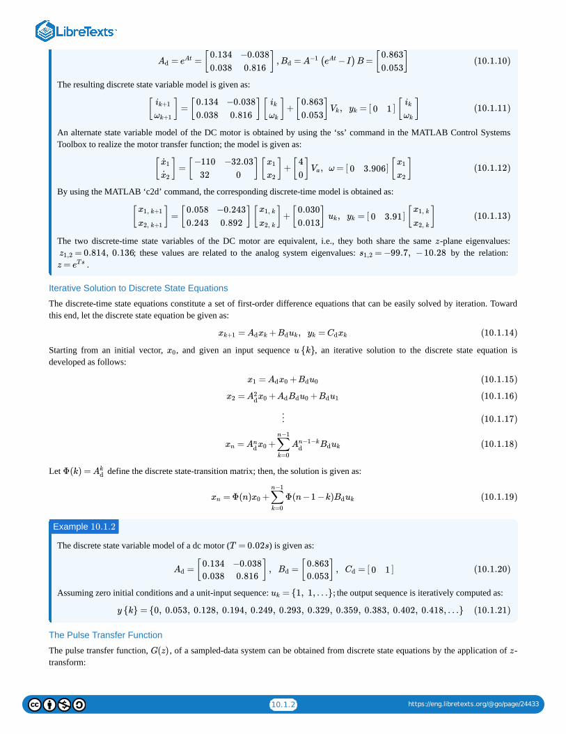
10.1.2 https://eng.libretexts.org/@go/page/24433

The resulting discrete state variable model is given as:

An alternate state variable model of the DC motor is obtained by using the ‘ss’ command in the MATLAB Control SystemsToolbox to realize the motor transfer function; the model is given as:

By using the MATLAB ‘c2d’ command, the corresponding discrete-time model is obtained as:

The two discrete-time state variables of the DC motor are equivalent, i.e., they both share the same -plane eigenvalues:; these values are related to the analog system eigenvalues: by the relation:

.

Iterative Solution to Discrete State Equations

The discrete-time state equations constitute a set of first-order difference equations that can be easily solved by iteration. Towardthis end, let the discrete state equation be given as:

Starting from an initial vector, , and given an input sequence , an iterative solution to the discrete state equation isdeveloped as follows:

Let define the discrete state-transition matrix; then, the solution is given as:

The discrete state variable model of a dc motor ( ) is given as:

Assuming zero initial conditions and a unit-input sequence: the output sequence is iteratively computed as:

The Pulse Transfer Function

The pulse transfer function, , of a sampled-data system can be obtained from discrete state equations by the application of -transform:

= = [ ] , = ( −I)B = [ ]Ad eAt0.1340.038

−0.0380.816

Bd A−1 eAt0.8630.053

(10.1.10)

[ ] = [ ][ ]+[ ] , = [ ] [ ]ik+1

ωk+1

0.1340.038

−0.0380.816

ik

ωk

0.8630.053

Vk yk 0 1ik

ωk

(10.1.11)

[ ] = [ ][ ]+[ ] ,   ω = [ ] [ ]x1

x2

−11032

−32.030

x1

x2

40

Va 0 3.906x1

x2(10.1.12)

[ ] = [ ][ ]+[ ] , = [ ] [ ]x1, k+1

x2, k+1

0.0580.243

−0.2430.892

x1, k

x2, k

0.0300.013

uk yk 0 3.91x1, k

x2, k(10.1.13)

z

  = 0.814,  0.136z1,2 = −99.7,   −10.28s1,2

z = eTs

= + , =xk+1 Adxk Bduk yk Cdxk (10.1.14)

x0 u {k}

= +x1 Adx0 Bdu0 (10.1.15)

= + +x2 A2dx0 AdBdu0 Bdu1 (10.1.16)

⋮ (10.1.17)

= +xn Andx0 ∑

k=0

n−1

An−1−kd Bduk (10.1.18)

Φ(k) = Akd

= Φ(n) + Φ(n−1 −k)xn x0 ∑k=0

n−1

Bduk (10.1.19)

Example 10.1.2

T = 0.02s

= [ ] , = [ ] , = [ ]Ad0.1340.038

−0.0380.816

Bd0.8630.053

Cd 0 1 (10.1.20)

= {1, 1, …};uk

y {k} = {0,  0.053,  0.128,  0.194,  0.249,  0.293,  0.329,  0.359,  0.383,  0.402,  0.418, …} (10.1.21)

G(z) z

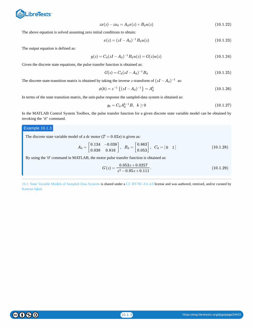
10.1.3 https://eng.libretexts.org/@go/page/24433

The above equation is solved assuming zero initial conditions to obtain:

The output equation is defined as:

Given the discrete state equations, the pulse transfer function is obtained as:

The discrete state-transition matrix is obtained by taking the inverse -transform of as:

In terms of the state transition matrix, the unit-pulse response the sampled-data system is obtained as:

In the MATLAB Control System Toolbox, the pulse transfer function for a given discrete state variable model can be obtained byinvoking the ‘tf’ command.

The discrete state variable model of a dc motor ( ) is given as:

By using the 'tf' command in MATLAB, the motor pulse transfer function is obtained as:

10.1: State Variable Models of Sampled-Data Systems is shared under a CC BY-NC-SA 4.0 license and was authored, remixed, and/or curated byKamran Iqbal.

zx(z) −z = x(z) + u(z)x0 Ad Bd (10.1.22)

x(z) = (zI − u(z)Ad)−1Bd (10.1.23)

y(z) = (zI − u(z) = G(z)u(z)Cd Ad)−1Bd (10.1.24)

G(z) = (zI −Cd Ad)−1Bd (10.1.25)

z (zI −Ad)−1

ϕ(k) = {(zI − } =z−1 Ad)−1 Akd (10.1.26)

= B, k ≥ 0gk CdAk−1d (10.1.27)

Example 10.1.3

T = 0.02s

= [ ] , = [ ] , = [ ]Ad0.1340.038

−0.0380.816

Bd0.8630.053

Cd 0 1 (10.1.28)

G(z) = .0.053z+0.0257

−0.95z+0.111z2(10.1.29)

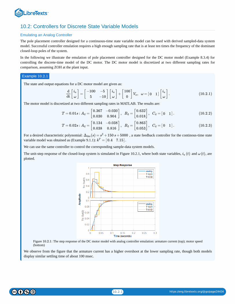
10.2.1 https://eng.libretexts.org/@go/page/24434

10.2: Controllers for Discrete State Variable Models

Emulating an Analog Controller

The pole placement controller designed for a continuous-time state variable model can be used with derived sampled-data systemmodel. Successful controller emulation requires a high enough sampling rate that is at least ten times the frequency of the dominantclosed-loop poles of the system.

In the following we illustrate the emulation of pole placement controller designed for the DC motor model (Example 8.3.4) forcontrolling the discrete-time model of the DC motor. The DC motor model is discretized at two different sampling rates forcomparison, assuming ZOH at the plant input.

The state and output equations for a DC motor model are given as:

The motor model is discretized at two different sampling rates in MATLAB. The results are:

For a desired characteristic polynomial: , a state feedback controller for the continous-time statevariable model was obtained as (Example 9.1.1): .

We can use the same controller to control the corresponding sample-data system models.

The unit-step response of the closed-loop system is simulated in Figure 10.2.1, where both state variables, and , areplotted.

Figure : The step response of the DC motor model with analog controller emulation: armature current (top); motor speed(bottom)

We observe from the figure that the armature current has a higher overshoot at the lower sampling rate, though both modelsdisplay similar settling time of about 100 msec.

Example 10.2.1

[ ] = [ ][ ]+[ ] , ω = [ ] [ ] .d

dt

ia

ω

−100

5

−5

−10

ia

ω

100

0Va 0 1

ia

ω(10.2.1)

T = 0.01s : = [ ] , = [ ] , = [ ] .Ad0.367

0.030

−0.030

0.904Bd

0.632

0.018Cd 0 1 (10.2.2)

T = 0.02s : = [ ] , = [ ] , = [ ] .Ad0.134

0.038

−0.038

0.816Bd

0.863

0.053Cd 0 1 (10.2.3)

(s) = +150 s +5000Δdes s2

= [ ]kT 0.4 7.15

(t)ia ω (t)

10.2.1

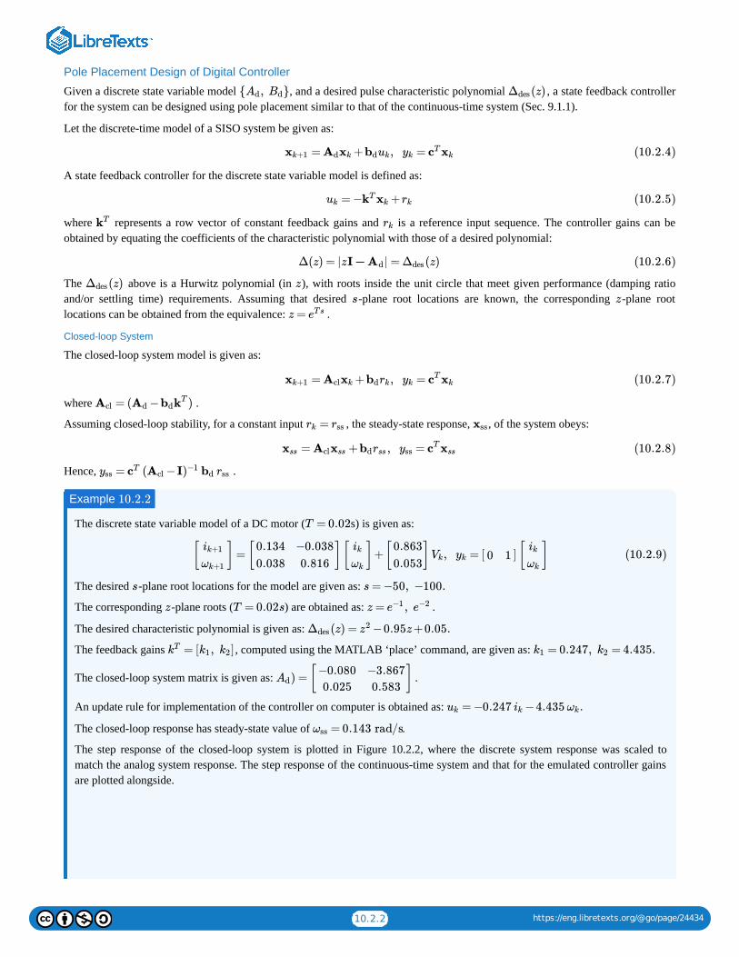
10.2.2 https://eng.libretexts.org/@go/page/24434

Pole Placement Design of Digital Controller

Given a discrete state variable model , and a desired pulse characteristic polynomial , a state feedback controllerfor the system can be designed using pole placement similar to that of the continuous-time system (Sec. 9.1.1).

Let the discrete-time model of a SISO system be given as:

A state feedback controller for the discrete state variable model is defined as:

where represents a row vector of constant feedback gains and is a reference input sequence. The controller gains can beobtained by equating the coefficients of the characteristic polynomial with those of a desired polynomial:

The above is a Hurwitz polynomial (in ), with roots inside the unit circle that meet given performance (damping ratioand/or settling time) requirements. Assuming that desired -plane root locations are known, the corresponding -plane rootlocations can be obtained from the equivalence: .

Closed-loop System

The closed-loop system model is given as:

where .

Assuming closed-loop stability, for a constant input , the steady-state response, , of the system obeys:

Hence, .

The discrete state variable model of a DC motor ( s) is given as:

The desired -plane root locations for the model are given as:

The corresponding -plane roots ( ) are obtained as: .

The desired characteristic polynomial is given as:

The feedback gains , computed using the MATLAB ‘place’ command, are given as:

The closed-loop system matrix is given as: .

An update rule for implementation of the controller on computer is obtained as:

The closed-loop response has steady-state value of .

The step response of the closed-loop system is plotted in Figure 10.2.2, where the discrete system response was scaled tomatch the analog system response. The step response of the continuous-time system and that for the emulated controller gainsare plotted alongside.

{ ,   }Ad Bd (z)Δdes

= + , =xk+1 Adxk bduk yk cT

xk (10.2.4)

= − +uk kT

xk rk (10.2.5)

kT rk

Δ(z) = |z | = (z)I − Ad Δdes (10.2.6)

(z)Δdes z

s z

z = eT s

= + , =xk+1 Aclxk bdrk yk cT

xk (10.2.7)

= ( − )Acl Ad bdkT

=rk rss xss

= + , =xss Aclxss bdrss yss cT

xss (10.2.8)

= ( −Iyss cT

Acl )−1bd rss

Example 10.2.2

T = 0.02

[ ] = [ ][ ]+[ ] , = [ ] [ ]ik+1

ωk+1

0.134

0.038

−0.038

0.816

ik

ωk

0.863

0.053Vk yk 0 1

ik

ωk

(10.2.9)

s s = −50, −100.

z T = 0.02s z = ,e−1 e−2

(z) = −0.95z +0.05.Δdes z2

= [ , ]kT k1 k2 = 0.247, = 4.435.k1 k2

) = [ ]Ad−0.080

0.025

−3.867

0.583

= −0.247 −4.435 .uk ik ωk

= 0.143 rad/sωss

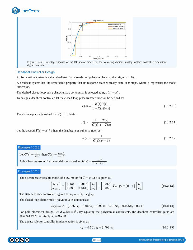
10.2.3 https://eng.libretexts.org/@go/page/24434

Figure : Unit-step response of the DC motor model for the following choices: analog system; controller emulation;digital controller.

Deadbeat Controller Design

A discrete-time system is called deadbeat if all closed-loop poles are placed at the origin .

A deadbeat system has the remarkable property that its response reaches steady-state in -steps, where represents the modeldimension.

The desired closed-loop pulse characteristic polynomial is selected as .

To design a deadbeat controller, let the closed-loop pulse transfer function be defined as:

The above equation is solved for to obtain:

Let the desired ; then, the deadbeat controller is given as:

Let then .

A deadbeat controller for the model is obtained as: .

The discrete state variable model of a DC motor for is given as:

The state feedback controller is given as: .

The closed-loop characteristic polynomial is obtained as:

For pole placement design, let . By equating the polynomial coefficients, the deadbeat controller gains areobtained as: .

The update rule for controller implementation is given as:

10.2.2

(z = 0)

n n

(z) =Δdes zn

T (z) =K(z)G(z)

1 +K(z)G(z)(10.2.10)

K(z)

K(z) =1

G(z)

T (z)

1 −T (z)(10.2.11)

T (z) = z−n

K(z) =1

G(z)( −1)zn(10.2.12)

Example 10.2.3

G(s) = ;1s+1

G(z) = 1−e−T

z−e−T

K(z) = z−e−T

(1− )(z−1)e−T

Example 10.2.4

T = 0.02 s

[ ] = [ ][ ]+[ ] , = [ ] [ ]ik+1

ωk+1

0.134

0.038

−0.038

0.816

ik

ωk

0.863

0.053Vk yk 0 1

ik

ωk

(10.2.13)

= −[ , ]uk k1 k2 xk

Δ(z) = +(0.863 +0.053 −0.95)z −0.707 +0.026 +0.111z2 k1 k2 k1 k2 (10.2.14)

(z) =Δdes z2

= 0.501, = 9.702k1 k2

= 0.501 +9.702uk ik ωk (10.2.15)

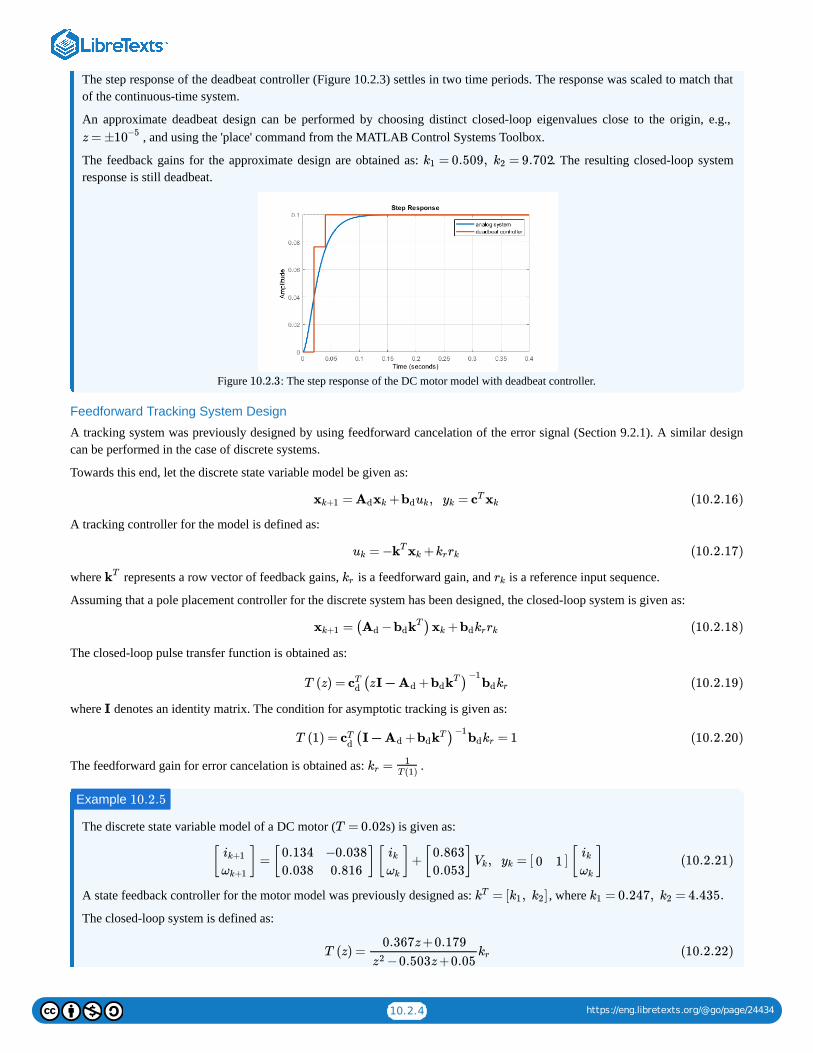
10.2.4 https://eng.libretexts.org/@go/page/24434

The step response of the deadbeat controller (Figure 10.2.3) settles in two time periods. The response was scaled to match thatof the continuous-time system.

An approximate deadbeat design can be performed by choosing distinct closed-loop eigenvalues close to the origin, e.g., , and using the 'place' command from the MATLAB Control Systems Toolbox.

The feedback gains for the approximate design are obtained as: . The resulting closed-loop systemresponse is still deadbeat.

Figure : The step response of the DC motor model with deadbeat controller.

Feedforward Tracking System Design

A tracking system was previously designed by using feedforward cancelation of the error signal (Section 9.2.1). A similar designcan be performed in the case of discrete systems.

Towards this end, let the discrete state variable model be given as:

A tracking controller for the model is defined as:

where represents a row vector of feedback gains, is a feedforward gain, and is a reference input sequence.

Assuming that a pole placement controller for the discrete system has been designed, the closed-loop system is given as:

The closed-loop pulse transfer function is obtained as:

where denotes an identity matrix. The condition for asymptotic tracking is given as:

The feedforward gain for error cancelation is obtained as: .

The discrete state variable model of a DC motor ( s) is given as:

A state feedback controller for the motor model was previously designed as: , where

The closed-loop system is defined as:

z = ±10−5

= 0.509, = 9.702k1 k2

10.2.3

= + , =xk+1 Adxk bduk yk cT

xk (10.2.16)

= − +uk kT

xk krrk (10.2.17)

kT kr rk

= ( − ) +xk+1 Ad bdkT

xk bdkrrk (10.2.18)

T (z) = cTd (z + )I − Ad bdk

T −1bdkr (10.2.19)

I

T (1) = = 1cTd( + )I − Ad bdk

T −1bdkr (10.2.20)

=kr1

T (1)

Example 10.2.5

T = 0.02

[ ] = [ ][ ]+[ ] , = [ ] [ ]ik+1

ωk+1

0.134

0.038

−0.038

0.816

ik

ωk

0.863

0.053Vk yk 0 1

ik

ωk

(10.2.21)

= [ , ]kT k1 k2 = 0.247, = 4.435.k1 k2

T (z) =0.367z +0.179

−0.503z +0.05z2kr (10.2.22)

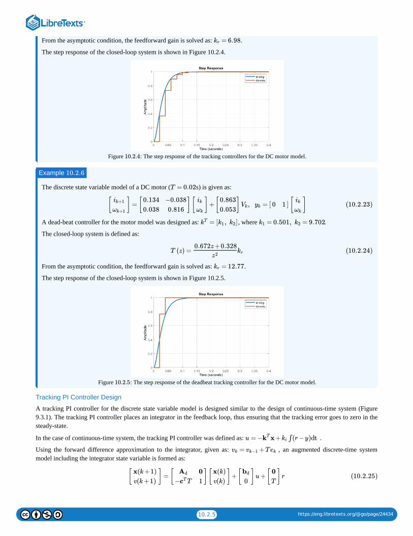
10.2.5 https://eng.libretexts.org/@go/page/24434

From the asymptotic condition, the feedforward gain is solved as: .

The step response of the closed-loop system is shown in Figure 10.2.4.

Figure : The step response of the tracking controllers for the DC motor model.

The discrete state variable model of a DC motor ( s) is given as:

A dead-beat controller for the motor model was designed as: , where .

The closed-loop system is defined as:

From the asymptotic condition, the feedforward gain is solved as: .

The step response of the closed-loop system is shown in Figure 10.2.5.

Figure : The step response of the deadbeat tracking controller for the DC motor model.

Tracking PI Controller Design

A tracking PI controller for the discrete state variable model is designed similar to the design of continuous-time system (Figure9.3.1). The tracking PI controller places an integrator in the feedback loop, thus ensuring that the tracking error goes to zero in thesteady-state.

In the case of continuous-time system, the tracking PI controller was defined as: .

Using the forward difference approximation to the integrator, given as: , an augmented discrete-time systemmodel including the integrator state variable is formed as:

= 6.98kr

10.2.4

Example 10.2.6

T = 0.02

[ ] = [ ][ ]+[ ] , = [ ] [ ]ik+1

ωk+1

0.134

0.038

−0.038

0.816

ik

ωk

0.863

0.053Vk yk 0 1

ik

ωk

(10.2.23)

= [ , ]kT k1 k2 = 0.501, = 9.702k1 k2

T (z) =0.672z +0.328

z2kr (10.2.24)

= 12.77kr

10.2.5

u = − x + ∫(r −y)dtkT ki

= +Tvk vk−1 ek

[ ] = [ ][ ]+[ ]u +[ ] rx(k +1)

v(k +1)

Ad

− TcT

0

1

x(k)

v(k)

bd

0

0

T(10.2.25)

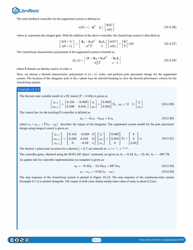
10.2.6 https://eng.libretexts.org/@go/page/24434

The state feedback controller for the augmented system is defined as:

where represents the integral gain. With the addition of the above controller, the closed-loop system is described as:

The closed-loop characteristic polynomial of the augmented system is formed as:

where denotes an identity matrix of order .

Next, we choose a desired characteristic polynomial of order, and perform pole placement design for the augmentedsystem. The location of the integrator pole in the -plane may be selected keeping in view the desired peformance criteria for theclosed-loop system.

The discrete state variable model of a DC motor ( s) is given as:

The control law for the tracking PI controller is defined as:

where describes the output of the integrator. The augmented system model for the pole placementdesign using integral control is given as:

The desired -plane pole locations for a desired are selected as: .

The controller gains, obtained using the MATLAB ‘place’ command, are given as:

An update rule for controller implementation on computer is given as:

The step response of the closed-loop system is plotted in Figure 10.2.6. The step response of the continuous-time system(Example 9.1.1) is plotted alongside. The output in both cases attains steady-state value of unity in about 0.12sec.

u(k) = [ ] [ ]−kT ki

x(k)

v(k)(10.2.26)

ki

[ ] = [ ][ ]+[ ] r(k)x(k +1)

v(k +1)

−Ad bdkT

− TcT

bdki

1

x(k)

v(k)

0

T(10.2.27)

(z) =Δa

∣

∣∣

z +I − Ad bdkT

− TcTd

−bdki

z −1

∣

∣∣ (10.2.28)

I n

(n +1)

z

Example 10.2.6

T = 0.02

[ ] = [ ][ ]+[ ] ,    = [ ] [ ]ik+1

ωk+1

0.134

0.038

−0.038

0.816

ik

ωk

0.863

0.053Vk ωk 0 1

ik

ωk

(10.2.29)

= − − +uk k1ik k2ωk kivk (10.2.30)

= +T ( − )vk vk−1 rk ωk

= + +⎡

⎣⎢

ik+1

ωk+1

vk+1

⎤

⎦⎥

⎡

⎣⎢

0.134

0.038

0

−0.038

0.816

−0.02

0

0

1

⎤

⎦⎥⎡

⎣⎢

ik

ωk

vk

⎤

⎦⎥

⎡

⎣⎢

0.863

0.053

0

⎤

⎦⎥Vk

⎡

⎣⎢

0

0

0.02

⎤

⎦⎥ rk (10.2.31)

z ζ = 0.7 z = ,e−1 e−1±j1

= 0.43, = 15.44, = −297.79.k1 k2 ki

= −0.43 −15.44 +297.8uk ik ωk vk (10.2.32)

= +0.02 ( − )vk vk−1 rk ωk (10.2.33)

10.2.7 https://eng.libretexts.org/@go/page/24434

Figure : Tracking PI control of the DC motor model: closed-loop response for the analog and discrete systems.

10.2: Controllers for Discrete State Variable Models is shared under a CC BY-NC-SA 4.0 license and was authored, remixed, and/or curated byKamran Iqbal.

10.2.6

1 https://eng.libretexts.org/@go/page/24443

IndexBBode plot

2.5: Sinusoidal Response of a System 6.1: Frequency Response Plots

Ccontroller form

9.1: Controller Design in Sate-Space

Ddamping ratio

2.1: System Poles and Zeros DC motor

1.4: An Electro-Mechanical System Model

Ffinal value theorem

7.5: Closed-Loop System Response frequency response function

2.5: Sinusoidal Response of a System 6.1: Frequency Response Plots

Ggain compensation

6.3: Frequency Response Design

HHurwitz criterion

4.1: Stability of the Closed-Loop System

Iimpulse response

2.4: The Step Response ITAE index

4.2: Transient Response Improvement

JJury’s stability test

7.4: Stability of Sampled-Data Systems

NNichol’s chart

6.4: Closed-Loop Frequency Response

Ppole placement design

9.1: Controller Design in Sate-Space

RRouth test

4.1: Stability of the Closed-Loop System

Ruth’s test7.4: Stability of Sampled-Data Systems

SSchur–Cohn stability test

7.4: Stability of Sampled-Data Systems sinusoidal response

2.5: Sinusoidal Response of a System step function

2.4: The Step Response step response

2.4: The Step Response Sylvester equation

9.1: Controller Design in Sate-Space system poles

2.1: System Poles and Zeros system sensitivity function

4.5: Sensitivity and Robustness

Ttracking control system

4.3: Steady-State Error Improvement tracking error

4.3: Steady-State Error Improvement transfer function

2.1: System Poles and Zeros

1 https://eng.libretexts.org/@go/page/29164

IndexBBode plot

2.5: Sinusoidal Response of a System 6.1: Frequency Response Plots

Ccontroller form

9.1: Controller Design in Sate-Space

Ddamping ratio

2.1: System Poles and Zeros DC motor

1.4: An Electro-Mechanical System Model

Ffinal value theorem

7.5: Closed-Loop System Response frequency response function

2.5: Sinusoidal Response of a System 6.1: Frequency Response Plots

Ggain compensation

6.3: Frequency Response Design

HHurwitz criterion

4.1: Stability of the Closed-Loop System

Iimpulse response

2.4: The Step Response ITAE index

4.2: Transient Response Improvement

JJury’s stability test

7.4: Stability of Sampled-Data Systems

NNichol’s chart

6.4: Closed-Loop Frequency Response

Ppole placement design

9.1: Controller Design in Sate-Space

RRouth test

4.1: Stability of the Closed-Loop System

Ruth’s test7.4: Stability of Sampled-Data Systems

SSchur–Cohn stability test

7.4: Stability of Sampled-Data Systems sinusoidal response

2.5: Sinusoidal Response of a System step function

2.4: The Step Response step response

2.4: The Step Response Sylvester equation

9.1: Controller Design in Sate-Space system poles

2.1: System Poles and Zeros system sensitivity function

4.5: Sensitivity and Robustness

Ttracking control system

4.3: Steady-State Error Improvement tracking error

4.3: Steady-State Error Improvement transfer function

2.1: System Poles and Zeros

1 https://eng.libretexts.org/@go/page/38088

GlossarySample Word 1 | Sample Definition 1