introduction to business economics introduction to business economics
TRANSCRIPT
Introduction to Business EconomicsIntroduction to Business Economics

Topics to be Discussed• Aims and objectives of the module• Module structure• The Themes of Microeconomics• What Is a Market?• What Is a Market?• Real Versus Nominal Prices• Why Study Microeconomics?

Aim of the module
• To analyse the principles of microeconomics and their application to business
Introductory ideas
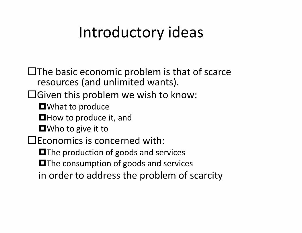
The basic economic problem is that of scarce resources (and unlimited wants).
Given this problem we wish to know:What to produceHow to produce it, and How to produce it, and Who to give it to
Economics is concerned with:The production of goods and servicesThe consumption of goods and servicesin order to address the problem of scarcity
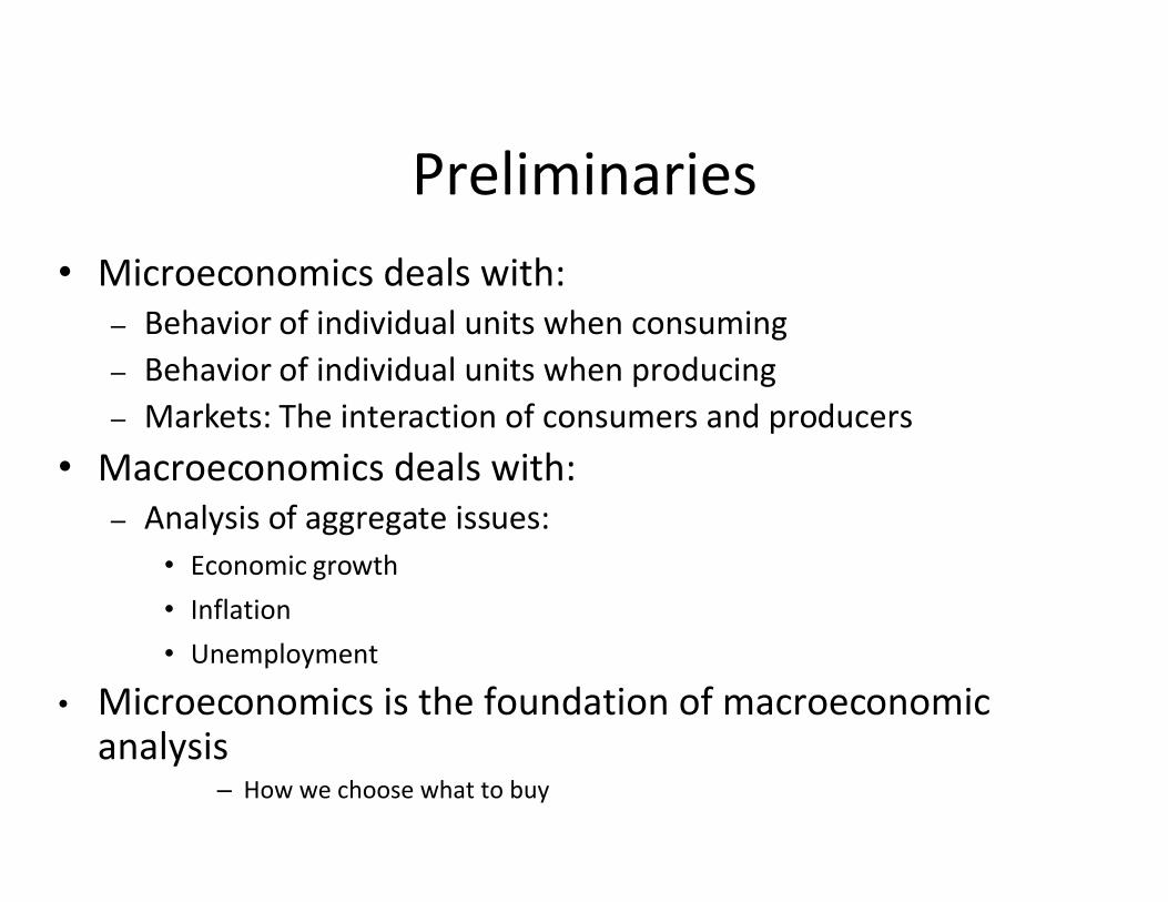
Preliminaries• Microeconomics deals with:
– Behavior of individual units when consuming– Behavior of individual units when producing– Markets: The interaction of consumers and producers
• Macroeconomics deals with:• Macroeconomics deals with:– Analysis of aggregate issues:
• Economic growth• Inflation• Unemployment
• Microeconomics is the foundation of macroeconomic analysis
– How we choose what to buy

Positive and normative economics
Positive statements (description)• What is, was or will be• Alleged facts about the universeNormative statements (prescription)Normative statements (prescription)• What ought to be• Require judgement about good and bad• Depend on philosophical, cultural & religious positions
Positive and normative economics
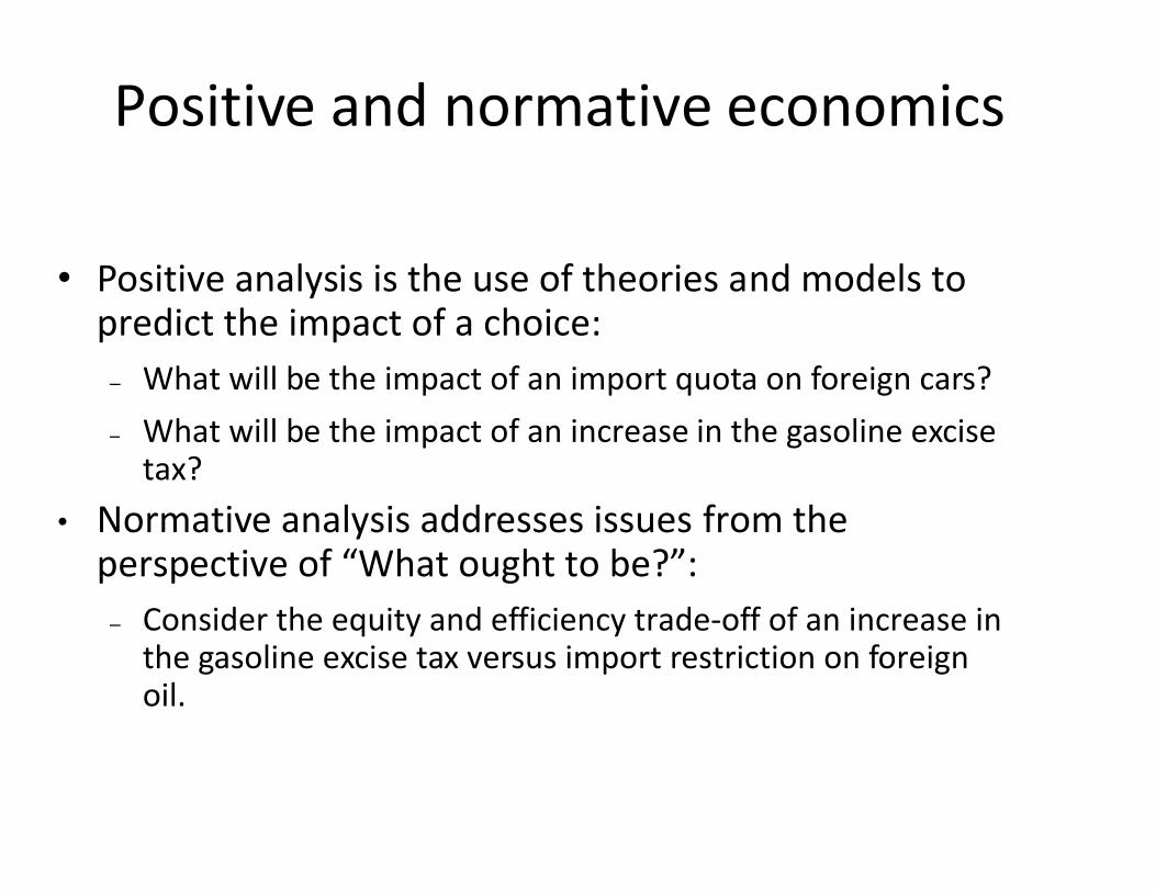
• Positive analysis is the use of theories and models to predict the impact of a choice:
– What will be the impact of an import quota on foreign cars?– What will be the impact of an increase in the gasoline excise – What will be the impact of an increase in the gasoline excise
tax?• Normative analysis addresses issues from the
perspective of “What ought to be?”:– Consider the equity and efficiency trade-off of an increase in
the gasoline excise tax versus import restriction on foreign oil.
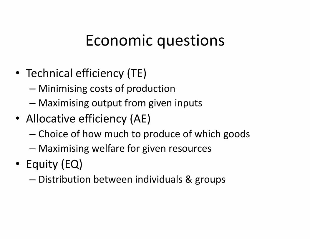
Economic questions
• Technical efficiency (TE)– Minimising costs of production– Maximising output from given inputs
• Allocative efficiency (AE)• Allocative efficiency (AE)– Choice of how much to produce of which goods– Maximising welfare for given resources
• Equity (EQ)– Distribution between individuals & groups

The Themes of Microeconomics
• Allocation of Scarce Resources and Trade-offs– In a planned economy– In a market economy
• Microeconomics and Optimal Trade-offs1. Consumer Theory1. Consumer Theory2. Workers3. Theory of the Firm
• Microeconomics and Prices– The role of prices in a market economy– How prices are determined
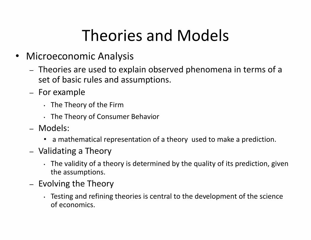
Theories and Models• Microeconomic Analysis
– Theories are used to explain observed phenomena in terms of a set of basic rules and assumptions.
– For example• The Theory of the Firm • The Theory of Consumer Behavior• The Theory of Consumer Behavior
– Models:• a mathematical representation of a theory used to make a prediction.
– Validating a Theory• The validity of a theory is determined by the quality of its prediction, given
the assumptions.
– Evolving the Theory• Testing and refining theories is central to the development of the science
of economics.
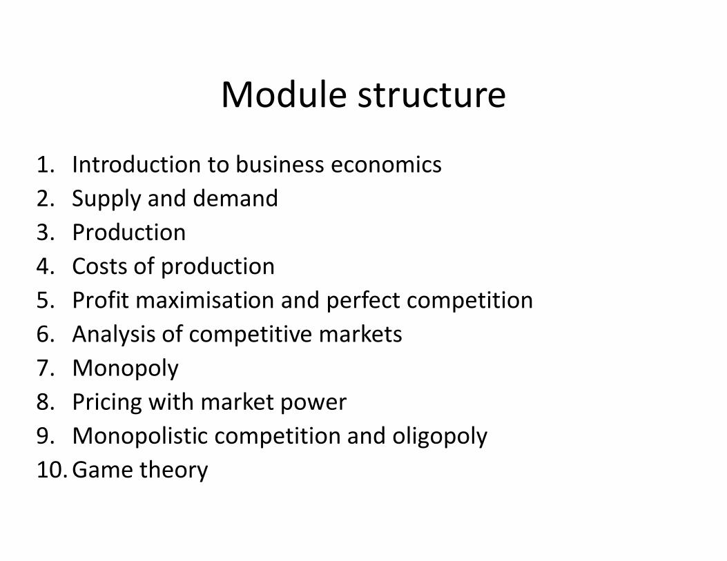
Module structure
1. Introduction to business economics2. Supply and demand3. Production4. Costs of production4. Costs of production5. Profit maximisation and perfect competition6. Analysis of competitive markets7. Monopoly8. Pricing with market power9. Monopolistic competition and oligopoly10. Game theory
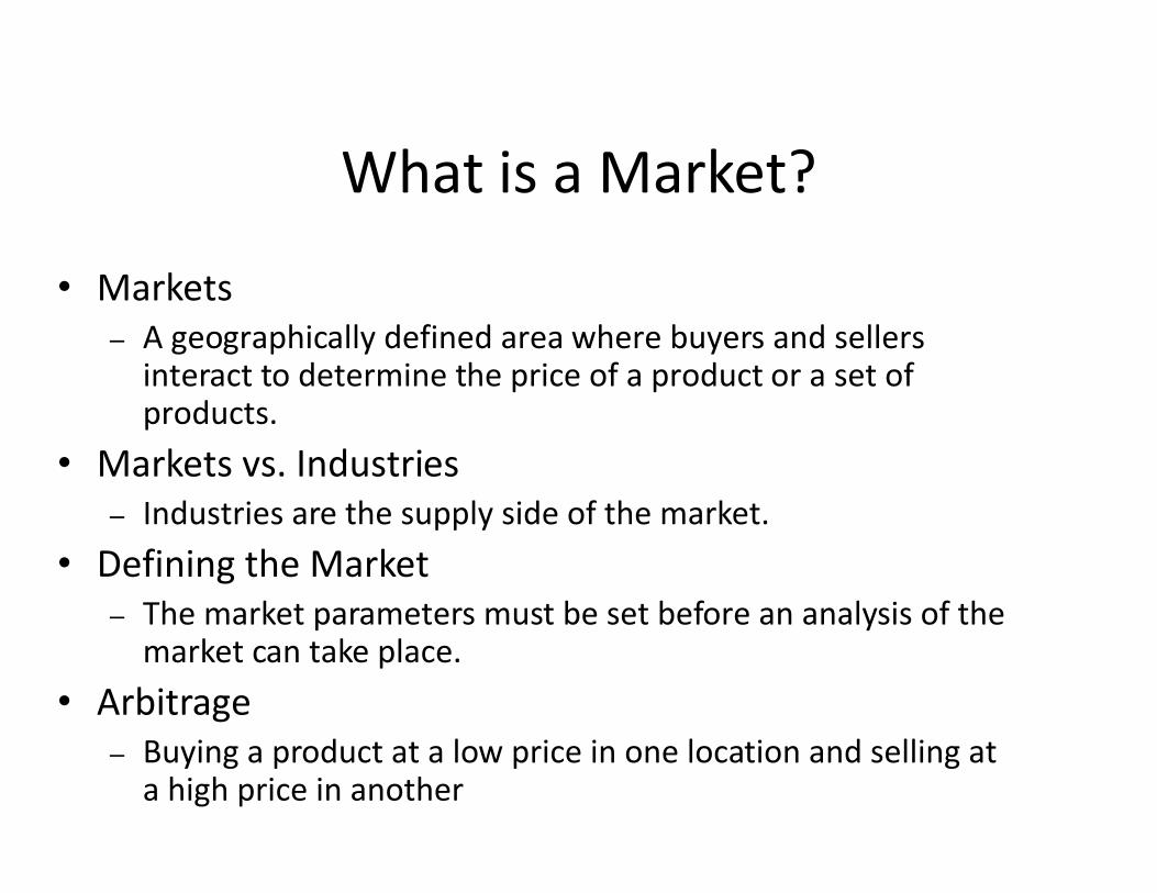
What is a Market?
• Markets– A geographically defined area where buyers and sellers
interact to determine the price of a product or a set of products.
• Markets vs. Industries• Markets vs. Industries– Industries are the supply side of the market.
• Defining the Market– The market parameters must be set before an analysis of the
market can take place.• Arbitrage
– Buying a product at a low price in one location and selling at a high price in another
Competitive vs. NoncompetitiveMarkets
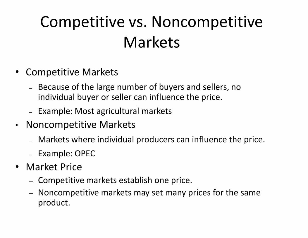
• Competitive Markets– Because of the large number of buyers and sellers, no
individual buyer or seller can influence the price.– Example: Most agricultural markets
Noncompetitive Markets• Noncompetitive Markets– Markets where individual producers can influence the price.– Example: OPEC
• Market Price– Competitive markets establish one price.– Noncompetitive markets may set many prices for the same
product.
Real Versus Nominal Prices• Nominal price is the absolute or current price of a
good or service when it is sold.• Real price is the price relative to an aggregate
measure of prices or constant price.measure of prices or constant price.
Real Versus Nominal Prices• The Consumer Price Index (CPI) is an aggregate
measure.– Real prices are emphasized to permit the analysis of
relative prices. relative prices.
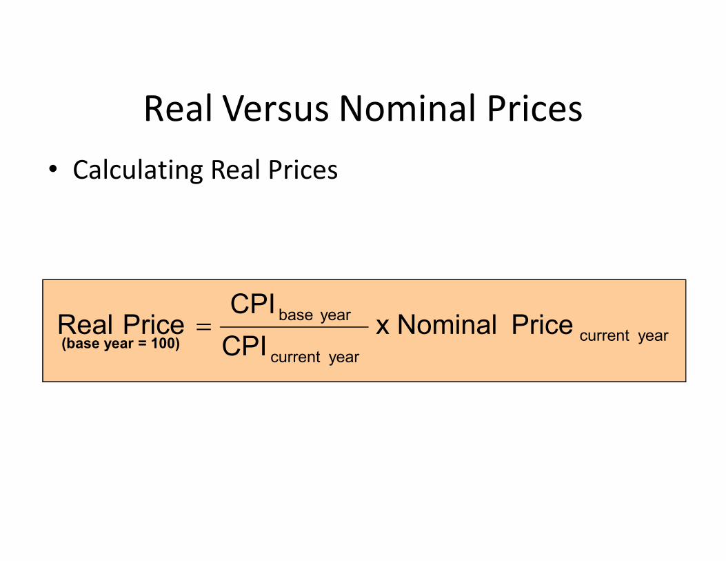
Real Versus Nominal Prices• Calculating Real Prices
yearcurrent yearcurrent
yearbase PriceNominal x CPI
CPIPriceReal
(base year = 100)

Example: the Real Price of Milk
Nominal Price Real Price of MilkYear of Milk CPI in 1970 dollars
1970 .40 38.8 .40 = 38.8/38.8 x .40
1980 .65 82.4 .31 = 38.8/82.4 x .65
1999 1.05 167.0 .24 = 38.8/167.0 x 1.05
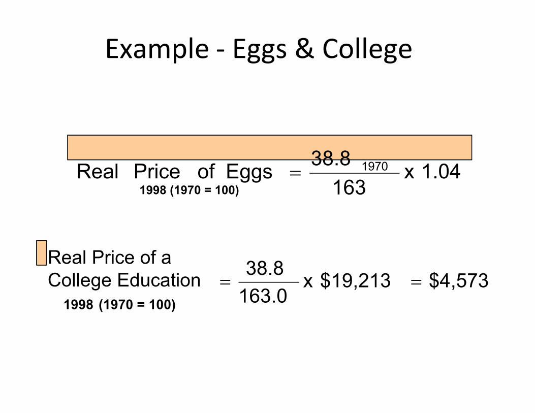
Example - Eggs & College
1.04x163
38.8EggsofPriceReal 1970
1998 (1970 = 100)
$4,573$19,213x 163.0
38.8
Real Price of a College Education
1998 (1970 = 100)
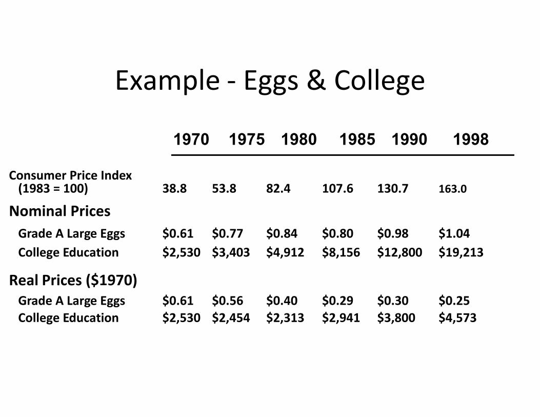
Example - Eggs & College
Consumer Price Index(1983 = 100) 38.8 53.8 82.4 107.6 130.7 163.0
Nominal Prices
1970 1975 1980 1985 1990 1998
Nominal PricesGrade A Large Eggs $0.61 $0.77 $0.84 $0.80 $0.98 $1.04College Education $2,530 $3,403 $4,912 $8,156 $12,800 $19,213
Real Prices ($1970)Grade A Large Eggs $0.61 $0.56 $0.40 $0.29 $0.30 $0.25College Education $2,530 $2,454 $2,313 $2,941 $3,800 $4,573

Why Study Microeconomics?• Microeconomic concepts are used by everyone to
assist them in making choices as consumers and producers.
Two Examples
• Ford and the development of its SUV’s• Public Policy Design: Automobile emission
standards for the 21st century

Ford and the development of itsSUV’s
• Issues– Consumer acceptance and demand– Production cost– Pricing strategy– Pricing strategy– Risk analysis– Organizational decisions– Government regulation
Auto emission standards for the 21stcentury
• Issues– Impact on consumers– Impact on producers– How to enforce the standards– How to enforce the standards– What are the benefits and costs?
Summary• Microeconomics is concerned with the decisions
made by small economic units.• Microeconomics relies heavily on the use of
theory and models.theory and models.

Summary• Microeconomics is concerned with positive
questions and normative analysis.• A market refers to a collection of buyers and
sellers who interact and to the possibility for sales sellers who interact and to the possibility for sales and purchases that results from that interaction.
Summary
• The market price is established by the interaction of buyers and sellers.
• A market’s geographic boundaries and range of products must be defined. A market’s geographic boundaries and range of products must be defined.
• To eliminate the effects of inflation we measure real prices, rather than nominal prices.

Supply and demandSupply and demand

Topics to Be Discussed
• Supply and Demand
• The Market Mechanism
• Changes in Market Equilibrium• Changes in Market Equilibrium
• Elasticities of Supply and Demand
• Effects of Government Intervention - Price Controls

Introduction• Applications of Supply and Demand Analysis
– Understanding and predicting how world economic conditions affect market price and production
– Analyzing the impact of government price controls, minimum wages, price supports, and production incentivesminimum wages, price supports, and production incentives
– Analyzing how taxes, subsidies, and import restrictions affect consumers and producers
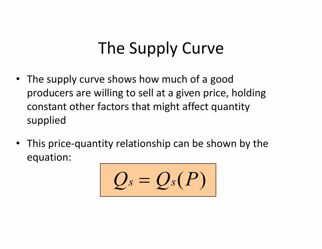
The Supply Curve
• The supply curve shows how much of a good producers are willing to sell at a given price, holding constant other factors that might affect quantity suppliedsupplied
• This price-quantity relationship can be shown by the equation:
)(PQQ ss
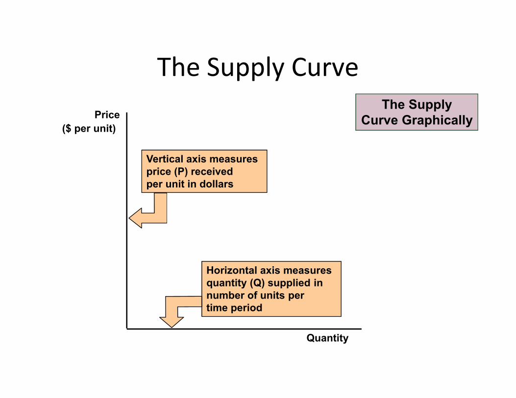
Vertical axis measures price (P) receivedper unit in dollars
The Supply CurveThe Supply
Curve GraphicallyPrice($ per unit)
Horizontal axis measures quantity (Q) supplied innumber of units per time period
Quantity
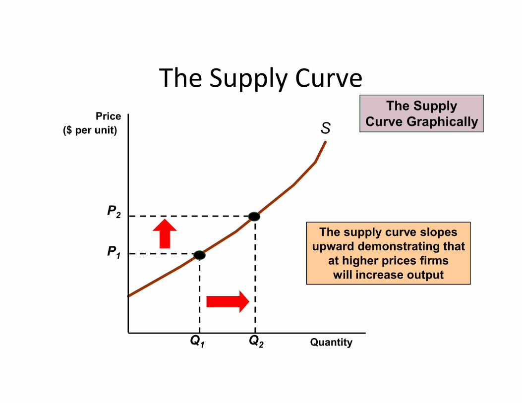
The Supply Curve
S
The SupplyCurve GraphicallyPrice
($ per unit)
The supply curve slopesupward demonstrating that
at higher prices firmswill increase output
Quantity
P1
Q1
P2
Q2
The Supply Curve• Non-price Determining Variables of Supply
– Costs of Production• Labor
• Capital• Capital
• Raw Materials

The Supply Curve• The cost of raw
materials falls– At P1, produce Q2
P S
Change in Supply
S’
– At P2, produce Q1
– Supply curve shifts right to S’
– More produced at any price on S’ than on S
Q
P1
P2
Q1Q0 Q2
The Supply Curve
• Supply - A Review– Supply is determined by non-price supply-
determining variables such as the cost of labor, capital, and raw materials.capital, and raw materials.
– Changes in supply are shown by shifting the entire supply curve.
– Changes in quantity supplied are shown by movements along the supply curve and are caused by a change in the price of the product.

The Demand Curve
• The demand curve shows how much of a good consumers are willing to buy as the price per unit changes holding non-price factors constant.constant.
• This price-quantity relationship can be shown by the equation:
(P)QQ DD
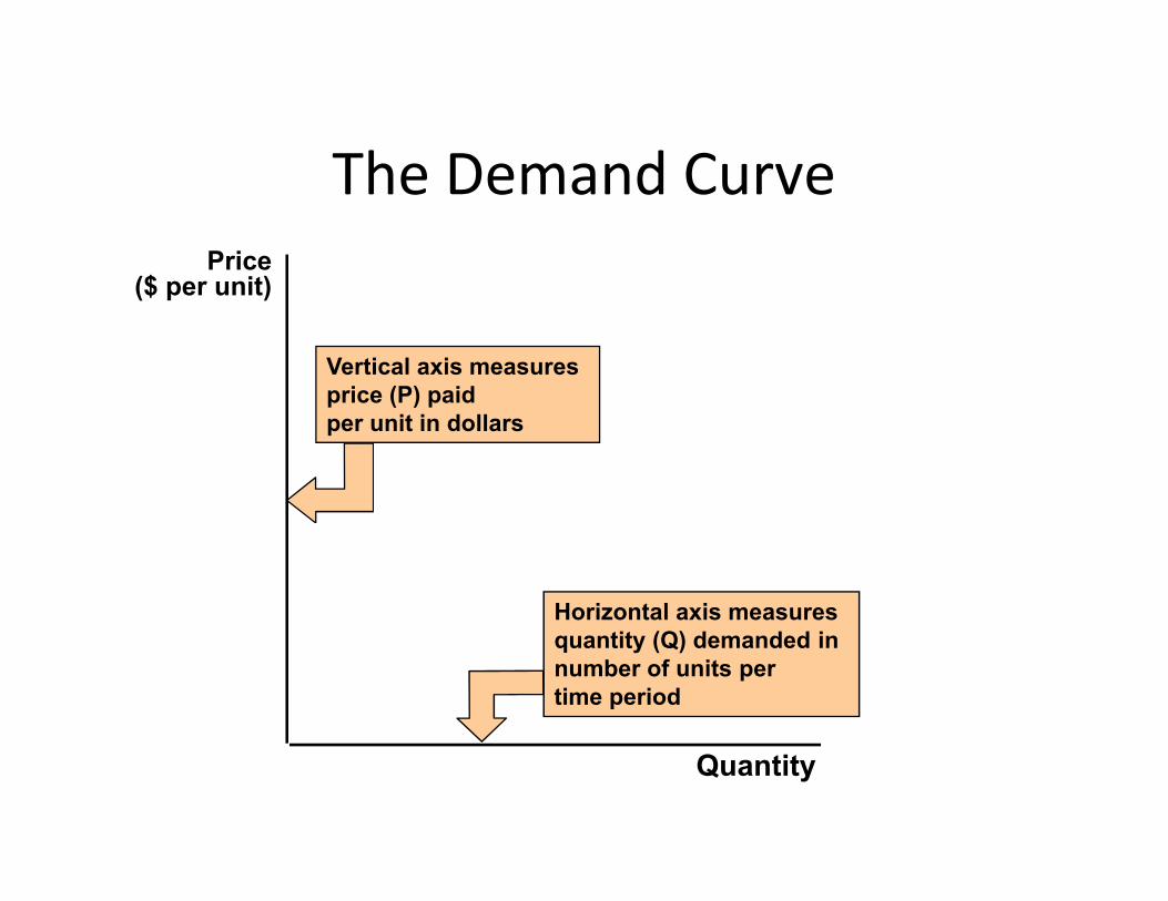
The Demand Curve
Vertical axis measures price (P) paidper unit in dollars
Price($ per unit)
Quantity
Horizontal axis measures quantity (Q) demanded innumber of units per time period
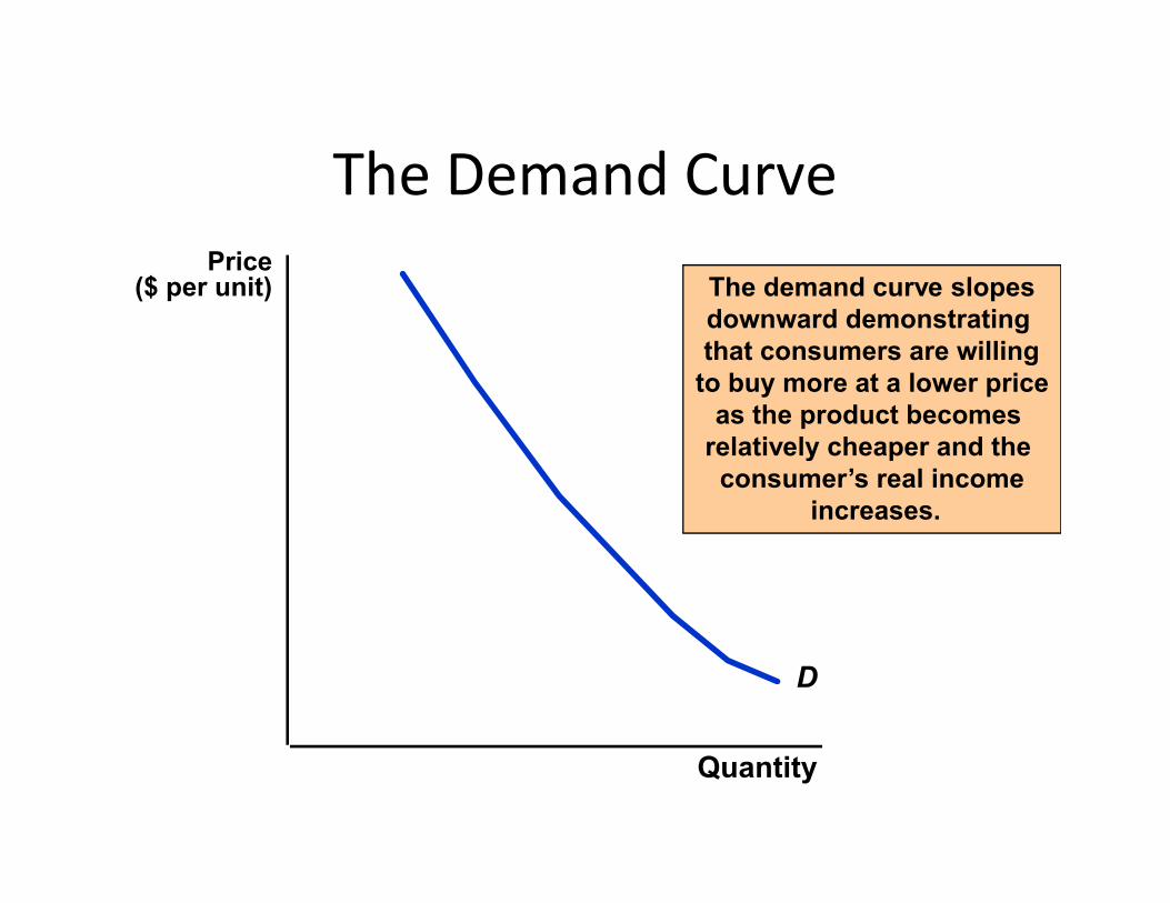
The Demand Curve
The demand curve slopesdownward demonstrating that consumers are willing
to buy more at a lower priceas the product becomes
relatively cheaper and the
Price($ per unit)
D
relatively cheaper and the consumer’s real income
increases.
Quantity

The Demand Curve• Non-price Determining Variables of Demand
– Income– Consumer Tastes– Price of Related Goods– Price of Related Goods
• Substitutes• Complements
DP
P2
D’
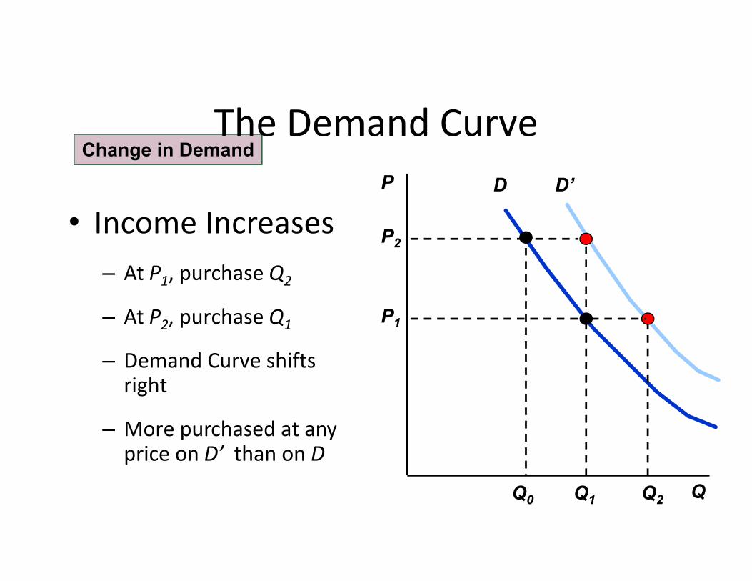
Change in DemandThe Demand Curve
• Income Increases– At P1, purchase Q2
QQ1Q0
P1
Q2
– At P2, purchase Q1
– Demand Curve shifts right
– More purchased at any price on D’ than on D
The Demand Curve• Demand - A Review
– Demand is determined by non-price demand-determining variables, such as, income, price of related goods, and tastes.goods, and tastes.
– Changes in demand are shown by shifting the entire demand curve.
– Changes in quantity demanded are shown by movements along the demand curve.

The Market MechanismS
The curves intersect atequilibrium, or market-
clearing, price. At P0 the
Price($ per unit)
Quantity
D
clearing, price. At P0 thequantity supplied is equalto the quantity demanded
at Q0 .
P0
Q0

The Market Mechanism
• Characteristics of the equilibrium or market clearing price:– QD = QS
– No shortage– No shortage– No excess supply– No pressure on the price to change

The Market MechanismS
If price is above equilibrium:
1) Price is above the
P1
Surplus
Price($ per unit)
Quantity
D
P0
Q0
1) Price is above themarket clearing price
2) Qs > Qd
3) Price falls to themarket-clearing price
The Market Mechanism
• The market price is above equilibrium– There is excess supply
A Surplus
– There is excess supply– Producers lower prices– Quantity demanded increases and quantity
supplied decreases– The market continues to adjust until the
equilibrium price is reached.
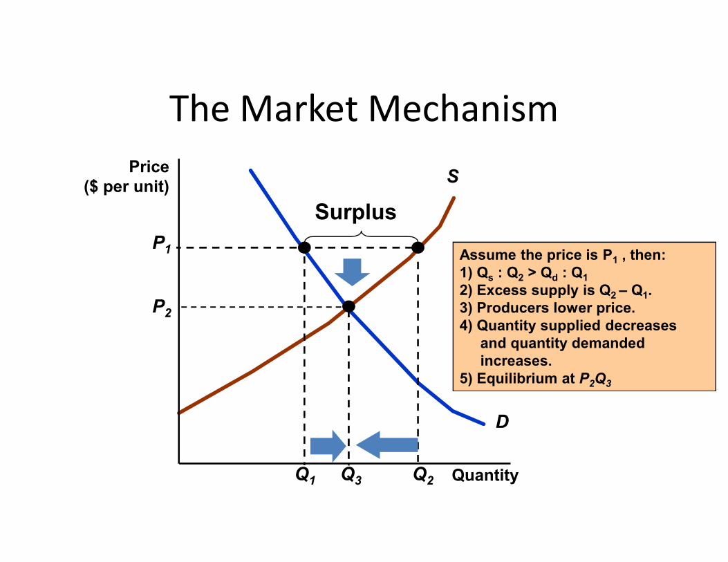
The Market MechanismS
Assume the price is P1 , then:1) Qs : Q2 > Qd : Q1
P1
Surplus
Price($ per unit)
D
Q1
s 2 d 1
2) Excess supply is Q2 – Q1.3) Producers lower price.4) Quantity supplied decreases
and quantity demanded increases.
5) Equilibrium at P2Q3
Q2 Quantity
P2
Q3

The Market Mechanism
• The market price is below equilibrium:– There is a shortage
Shortage
– There is a shortage– Producers raise prices– Quantity demanded decreases and quantity
supplied increases– The market continues to adjust until the new
equilibrium price is reached.
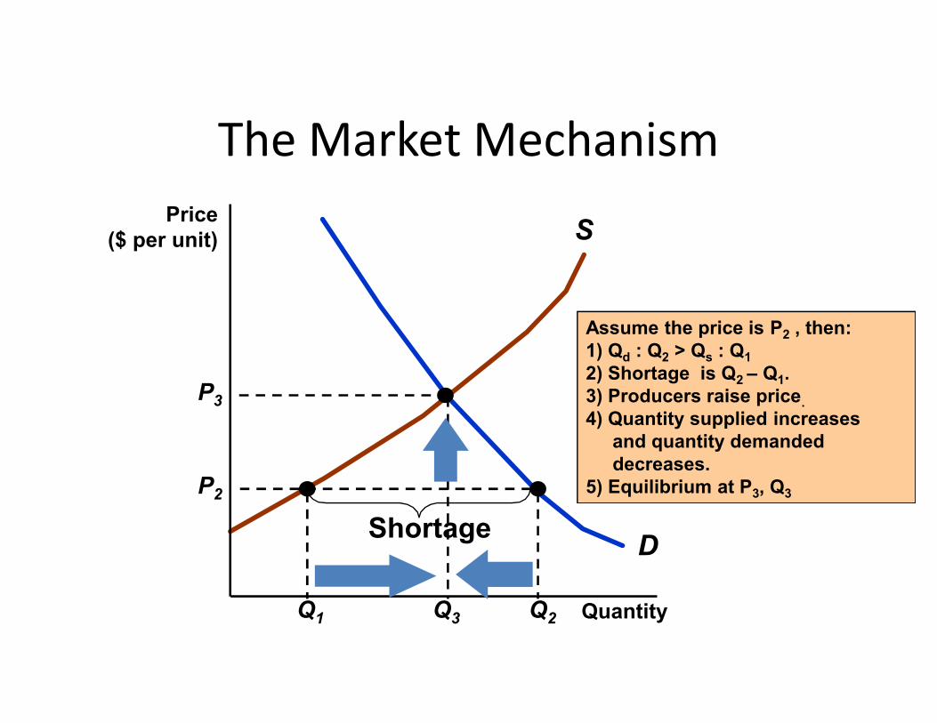
The Market Mechanism
SPrice
($ per unit)
Assume the price is P2 , then:1) Qd : Q2 > Qs : Q1
D
Q1 Q2
P2
Shortage
Quantity
d 2 s 1
2) Shortage is Q2 – Q1.3) Producers raise price.
4) Quantity supplied increases and quantity demanded decreases.
5) Equilibrium at P3, Q3
Q3
P3
The Market Mechanism
• Market Mechanism Summary
1) Supply and demand interact to determine the market-clearing price.
2) When not in equilibrium, the market will adjust to alleviate a shortage or surplus and return the market to equilibrium.
3) Markets must be competitive for the mechanism to be efficient.

Changes In Market Equilibrium
• Equilibrium prices are determined by the relative level of supply and demand.
• Supply and demand are determined by particular values of supply and demand determining variables.values of supply and demand determining variables.
• Changes in any one or combination of these variables can cause a change in the equilibrium price and/or quantity.
S’
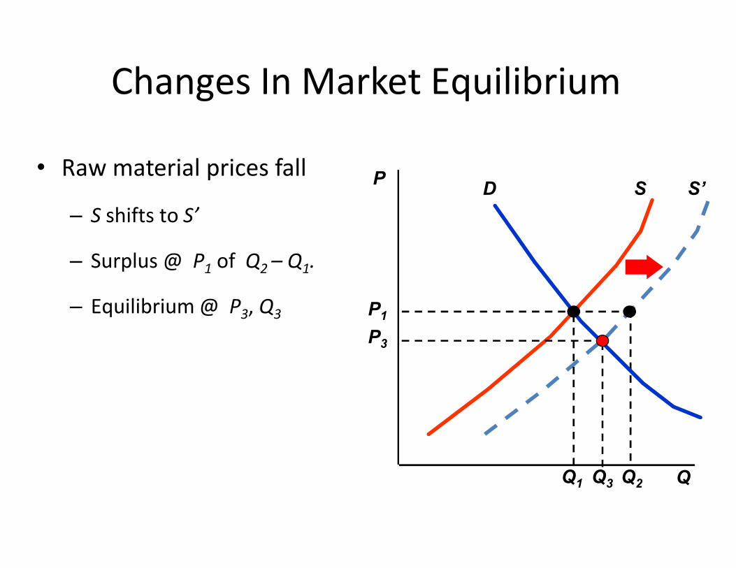
Changes In Market Equilibrium
• Raw material prices fall
– S shifts to S’
– Surplus @ P1 of Q2 – Q1.
P SD
Q2
– Equilibrium @ P3, Q3
Q
P3
Q3Q1
P1
D’ SD
P3
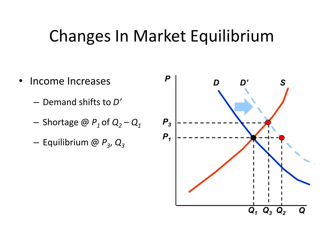
Changes In Market Equilibrium
• Income Increases
– Demand shifts to D’
– Shortage @ P1 of Q2 – Q1
P
Q3
P3– Shortage @ P1 of Q2 – Q1
– Equilibrium @ P3, Q3
QQ2Q1
P1
D’ S’
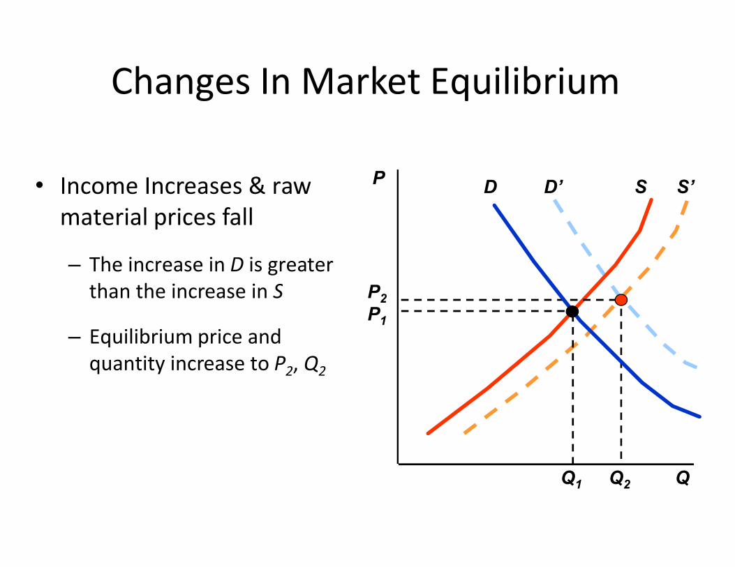
Changes In Market Equilibrium
• Income Increases & raw material prices fall
– The increase in D is greater than the increase in S
P S
P
D
than the increase in S
– Equilibrium price and quantity increase to P2, Q2
Q
P2
Q2
P1
Q1
Shifts in Supply and Demand• When supply and demand change simultaneously,
the impact on the equilibrium price and quantity is determined by:
1) The relative size and direction of the change1) The relative size and direction of the change
2) The shape of the supply and demand curves
The Price of Eggs and College Education Revisited
• The real price of eggs fell 59% from 1970 to 1998.
• Supply increased due to the increased mechanization of poultry farming and the reduced cost of production.
• Demand decreased due to the increasing consumer concern over the health and cholesterol consequences of eating eggs.
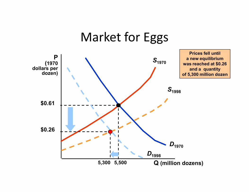
Market for EggsP
(1970dollars per
dozen)
S1970
S1998
Prices fell untila new equilibrium
was reached at $0.26and a quantity
of 5,300 million dozen
Q (million dozens)
D1970
$0.61
5,500
D1998
$0.26
5,300
The Price of a College Education
• The real price of a college education rose 68 percent from 1970 to 1995.
• Supply decreased due to higher costs of equipping and maintaining modern classrooms, laboratories and maintaining modern classrooms, laboratories and libraries, and higher faculty salaries.
• Demand increased due to a larger percentage of a growing number of high school graduates attending college.
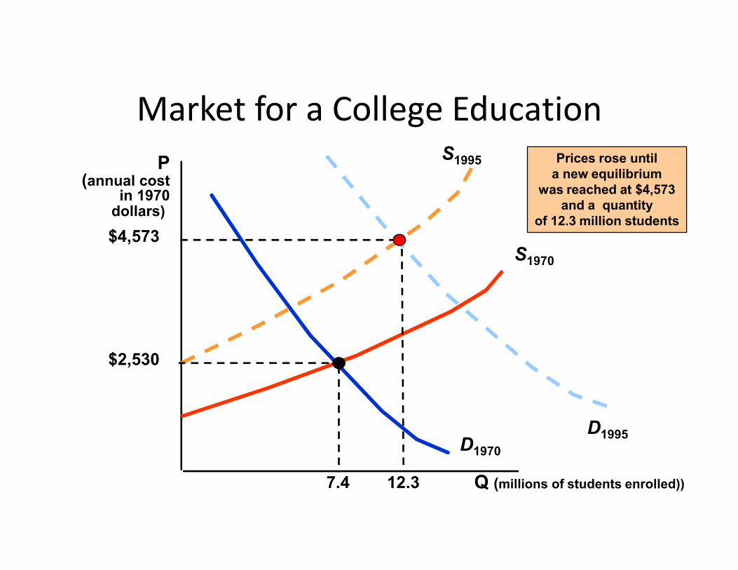
Market for a College EducationP
(annual costin 1970
dollars)
S1970
S1995
$4,573
Prices rose untila new equilibrium
was reached at $4,573and a quantity
of 12.3 million students
Q (millions of students enrolled))
D1970
D1995
12.3
$2,530
7.4
Elasticities of Supply and Demand
• Generally, elasticity is a measure of the sensitivity of one variable to another.
• It tells us the percentage change in one variable • It tells us the percentage change in one variable in response to a one percent change in another variable.
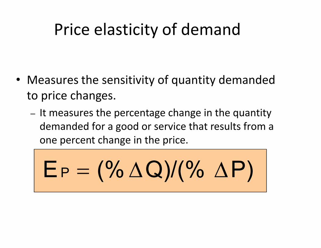
Price elasticity of demand
• Measures the sensitivity of quantity demanded to price changes.– It measures the percentage change in the quantity
demanded for a good or service that results from a demanded for a good or service that results from a one percent change in the price.
P)Q)/(%(%E P
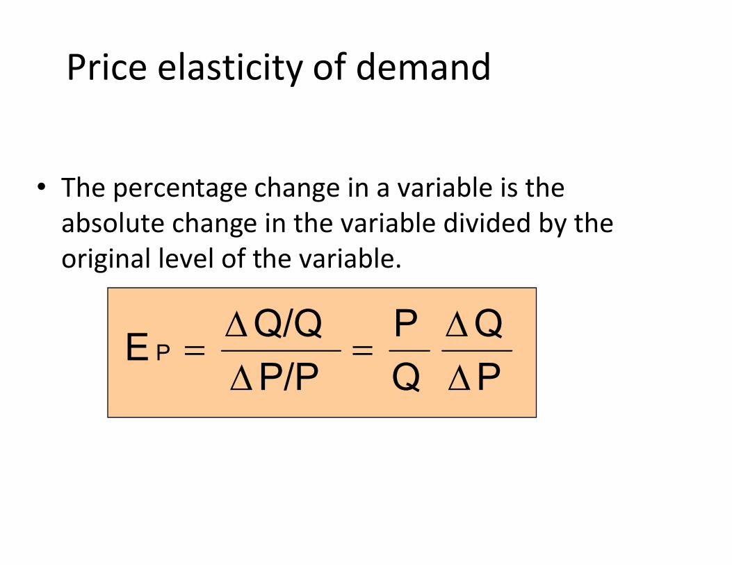
Price elasticity of demand
• The percentage change in a variable is the absolute change in the variable divided by the original level of the variable.
P
Q
Q
P
P/P
Q/QE P
Price elasticity of demand• Interpreting Price Elasticity of Demand
1) Because of the inverse relationship between P and Q; EP is negative.
2) If |EP| > 1, the percent change in quantity is greater than the percent change in price. We
say the demand is price elastic.
3) If |EP| < 1, the percent change in quantity is less than the percent change in price.
We say the demand is price inelastic.
Price elasticity of demand
• The primary determinant of price elasticity of demand is the availability of substitutes.– Many substitutes: demand is price elastic– Few substitutes: demand is price inelastic
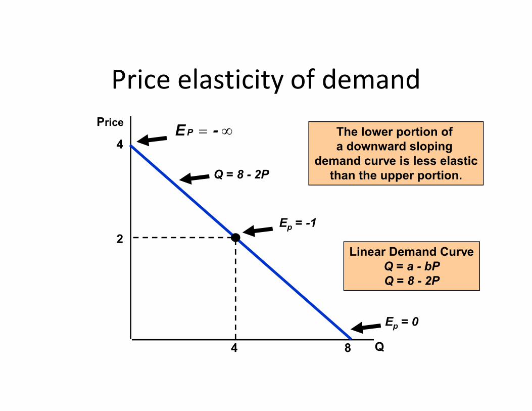
Price elasticity of demandPrice
Q = 8 - 2P
-EP The lower portion of a downward sloping
demand curve is less elasticthan the upper portion.
4
Q
Ep = -1
Ep = 0
8
2
4
Linear Demand CurveQ = a - bPQ = 8 - 2P
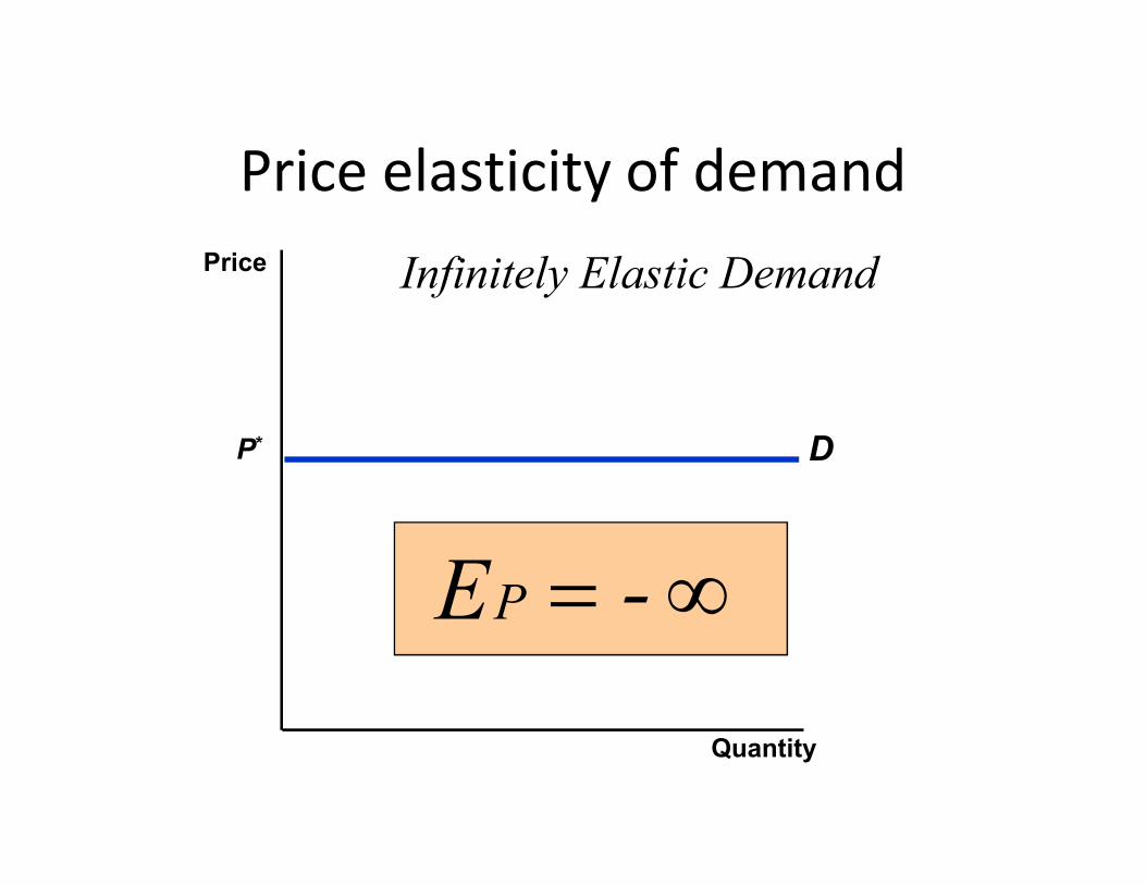
Price elasticity of demand
DP*
Price Infinitely Elastic Demand
DP*
-EP
Quantity
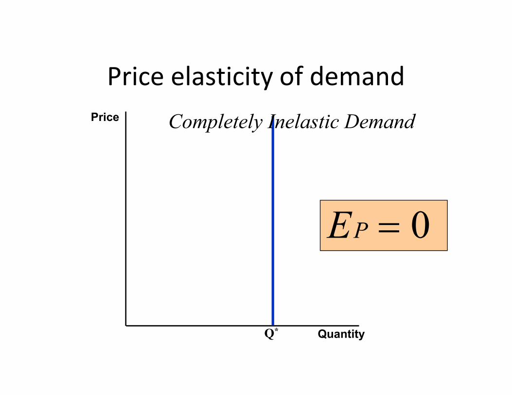
Price elasticity of demandPrice Completely Inelastic Demand
Q*
0EP
Quantity
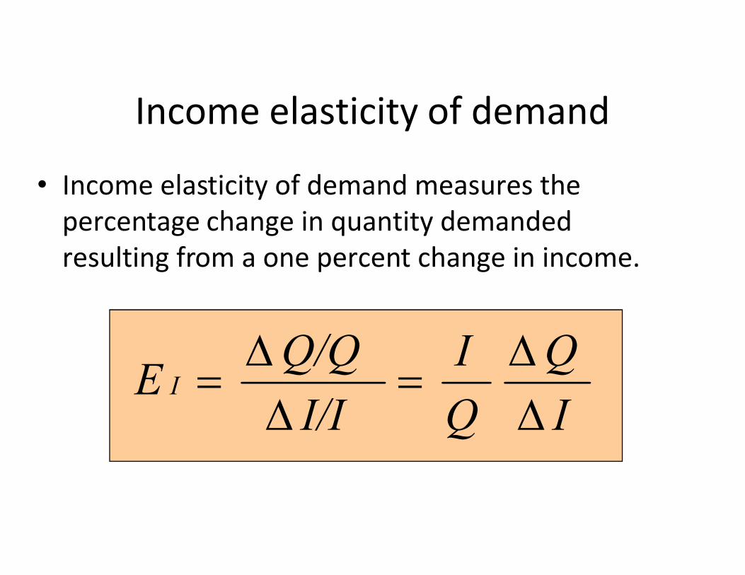
Income elasticity of demand
• Income elasticity of demand measures the percentage change in quantity demanded resulting from a one percent change in income.
I
Q
Q
I
I/I
Q/QE I
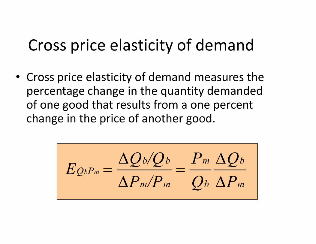
Cross price elasticity of demand
• Cross price elasticity of demand measures the percentage change in the quantity demanded of one good that results from a one percent change in the price of another good.change in the price of another good.
m
b
b
m
mm
bbPQ
P
Q
Q
P
/PP
/QQE mb

Price elasticity of demand• Price elasticity of supply measures the percentage change
in quantity supplied resulting from a 1 percent change in price.
• The elasticity is usually positive because price and quantity • The elasticity is usually positive because price and quantity supplied are positively related.
– Higher price gives producers an incentive to increase output
• We can refer to elasticity of supply with respect to interest rates, wage rates, and the cost of raw materials.
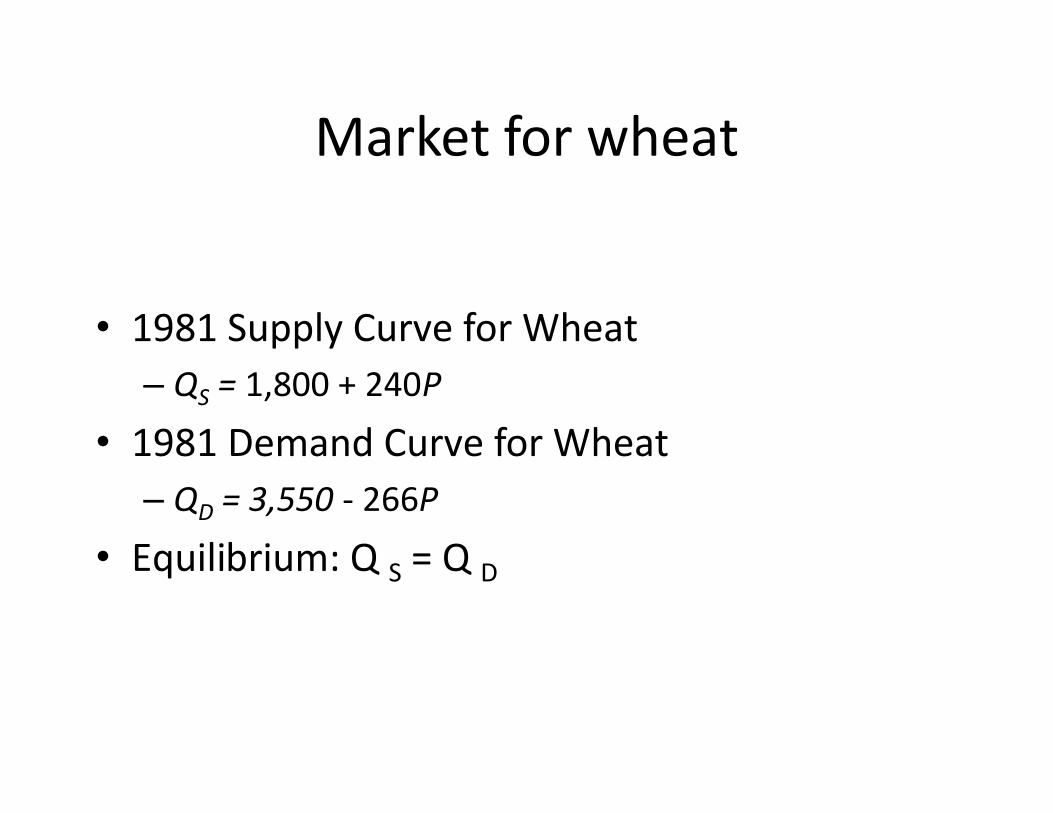
Market for wheat
• 1981 Supply Curve for Wheat– QS = 1,800 + 240PS
• 1981 Demand Curve for Wheat– QD = 3,550 - 266P
• Equilibrium: Q S = Q D
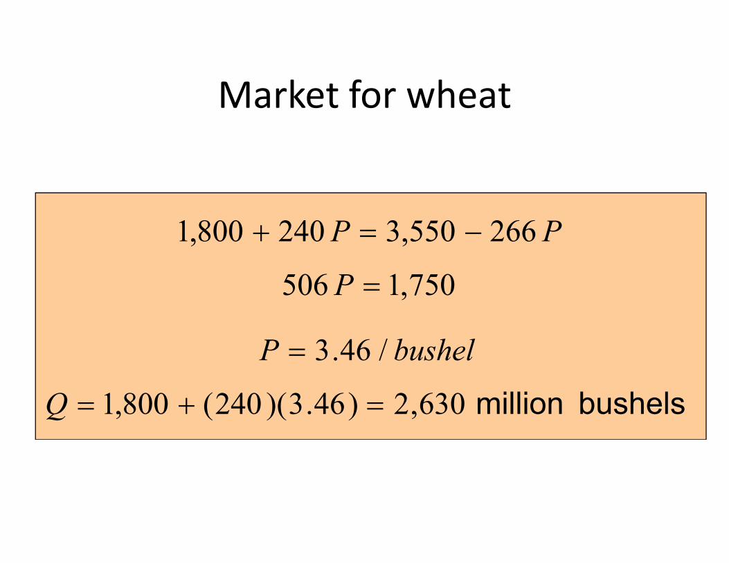
Market for wheat
PP 266550,3240800,1
750,1506 P 750,1506 P
bushelP /46.3
bushelsmillion630,2)46.3)(240(800,1 Q
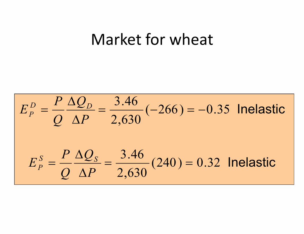
Market for wheat
Inelastic 35.0)266(630,2
46.3
P
Q
Q
PE DD
P 630,2PQP
Inelastic 32.0)240(630,2
46.3
P
Q
Q
PE SS
P
Market for wheat
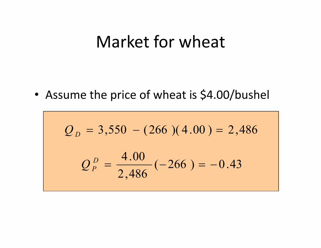
• Assume the price of wheat is $4.00/bushel
486,2)00.4)(266(550,3 Q 486,2)00.4)(266(550,3 DQ
43.0)266(486,2
00.4D
PQ
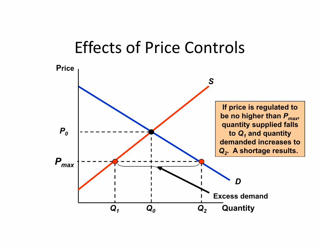
Effects of Price ControlsPrice
S
If price is regulated tobe no higher than Pmax,quantity supplied falls
D
Quantity
P0
Q0
Pmax
Excess demand
quantity supplied fallsto Q1 and quantity
demanded increases toQ2. A shortage results.
Q1 Q2
Price Controls and Natural GasShortages
• In 1954, the federal government began regulating the wellhead price of natural gas.
• In 1962, the ceiling prices that were imposed • In 1962, the ceiling prices that were imposed became binding and shortages resulted.

Price Controls and Natural GasShortages
• Price controls created an excess demand of 7 trillion cubic feet.
• Price regulation was a major component of U.S. • Price regulation was a major component of U.S. energy policy in the 1960s and 1970s, and it continued to influence the natural gas markets in the 1980s.
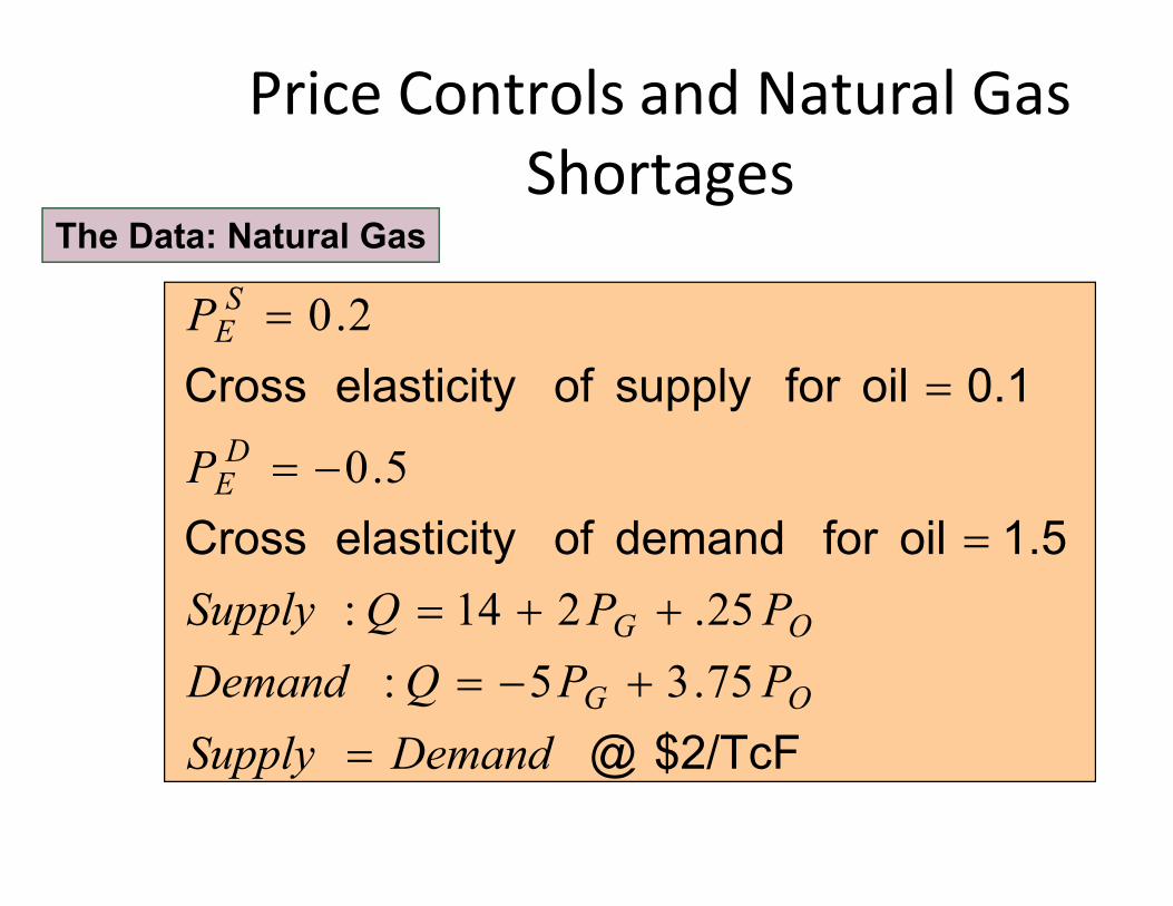
0.1oilforsupply ofelasticityCross
P
P
D
SE
5.0
2.0
Price Controls and Natural GasShortages
The Data: Natural Gas
$2/TcF@
1.5oilfordemandofelasticityCross
DemandSupply
PPQDemand
PPQSupply
P
OG
OG
DE
75.35:
25.214:
5.0
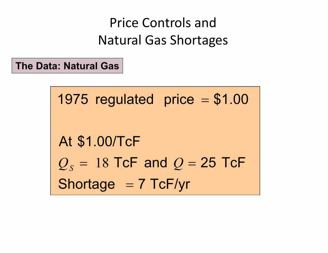
Price Controls andNatural Gas Shortages
The Data: Natural Gas
$1.00priceregulated1975
TcF/yr7Shortage
TcF25andTcF
$1.00/TcFAt
QQS 18
Summary• Supply-demand analysis is a basic tool of
microeconomics.
• The market mechanism is the tendency for supply and demand to equilibrate, so that there is neither excess demand nor excess supplydemand nor excess supply
• Elasticities describe the responsiveness of supply and demand to changes in price, income, and other variables. They pertain to a time frame.
• If we can estimate the supply and demand curves for a particular market, we can calculate the market clearing price.
ProductionProduction

Topics to be Discussed• The Technology of Production
• Isoquants
• Production with One Variable Input (Labor)• Production with One Variable Input (Labor)
• Production with Two Variable Inputs
• Returns to Scale
Introduction
• Our focus is the supply side.
• The theory of the firm addresses:
– How a firm makes cost-minimizing production decisions
– How cost varies with output
– Characteristics of market supply
– Issues of business regulation
The Technology of Production
• The Production Process– Combining inputs or factors of production to achieve an output
• Categories of Inputs (factors of production)– Labor– Materials– Capital

The Technology of Production
• Production Function:
– Indicates the highest output that a firm can produce for every specified combination of inputs given the state of technology.state of technology.
– Shows what is technically feasible when the firm operates efficiently.
The Technology of Production
• The production function for two inputs:
Q = F(K,L)
Q = Output, K = Capital, L = LaborQ = Output, K = Capital, L = Labor
• For a given technology
Isoquants• Curves showing all possible combinations of inputs
that yield the same output
• Assumptions
– Food producer has two inputs, Labor (L) & Capital (K)– Food producer has two inputs, Labor (L) & Capital (K)
• Observations:
– For any level of K, output increases with more L.
– For any level of L, output increases with more K.
– Various combinations of inputs produce the same output.

Production Function for Food
1 20 40 55 65 75
2 40 60 75 85 90
Capital Input 1 2 3 4 5
Labor Input
2 40 60 75 85 90
3 55 75 90 100 105
4 65 85 100 110 115
5 75 90 105 115 120

Production with Two Variable Inputs(L,K)
4
5
The isoquants are derivedfrom the production
function for output of
ECapitalper year The Isoquant Map
Labor per year
1
2
3
1 2 3 4 5
Q1 = 55
function for output ofof 55, 75, and 90.A
D
B
Q2 = 75
Q3 = 90
C
Short-run versus Long-run
• Short-run:– Period of time in which quantities of one or more
production factors cannot be changed.
– These inputs are called fixed inputs.
• Long-run– Amount of time needed to make all production
inputs variable.

Amount Amount Total Average Marginalof Labor (L) of Capital (K) Output (Q) Product Product
Production with One Variable Input(Labour)
0 10 0 --- ---
1 10 10 10 10
2 10 30 15 20
3 10 60 20 303 10 60 20 30
4 10 80 20 20
5 10 95 19 15
6 10 108 18 13
7 10 112 16 4
8 10 112 14 0
9 10 108 12 -4
10 10 100 10 -8
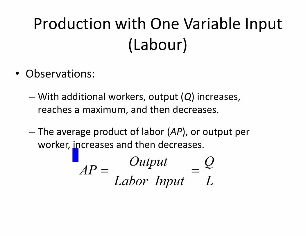
Production with One Variable Input(Labour)
• Observations:
– With additional workers, output (Q) increases, reaches a maximum, and then decreases.
– The average product of labor (AP), or output per worker, increases and then decreases.
L
Q
InputLabor
OutputAP
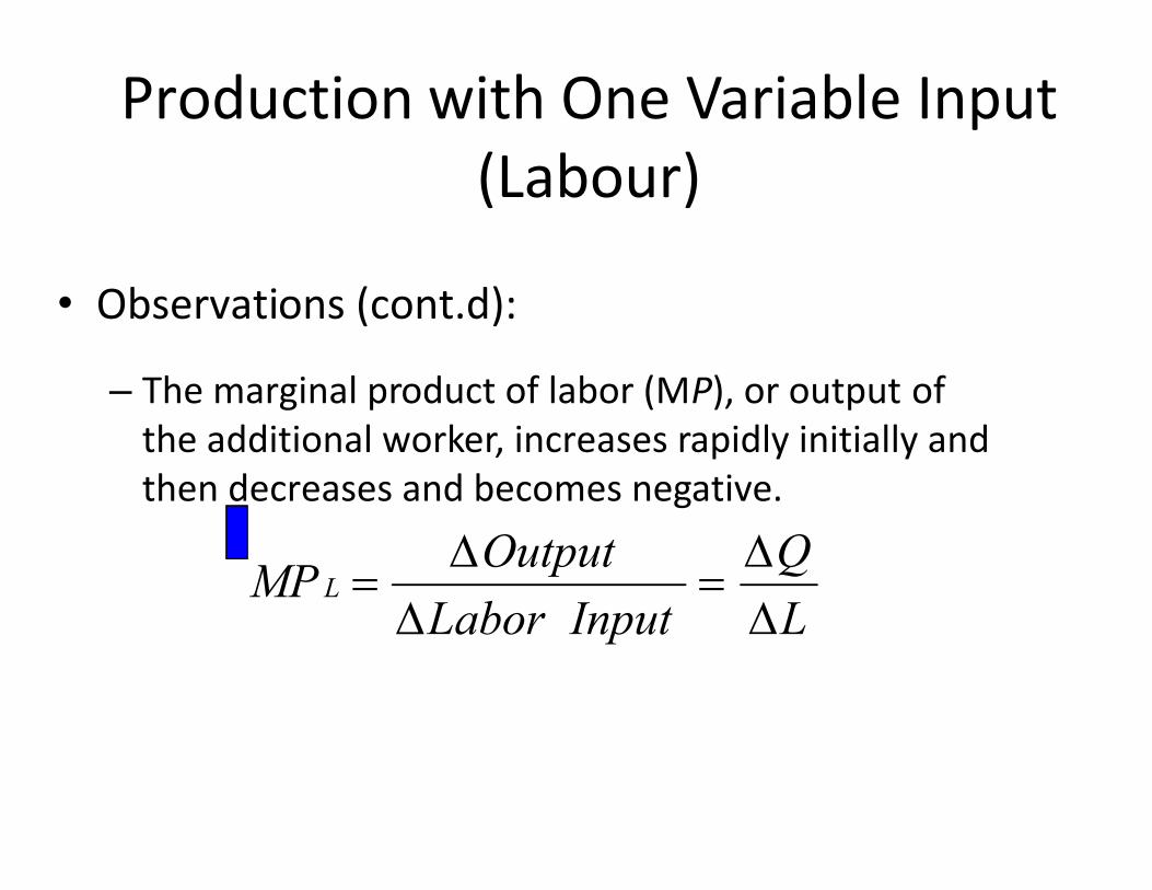
Production with One Variable Input(Labour)
• Observations (cont.d):
– The marginal product of labor (MP), or output of the additional worker, increases rapidly initially and the additional worker, increases rapidly initially and then decreases and becomes negative.
L
Q
InputLabor
OutputMP L
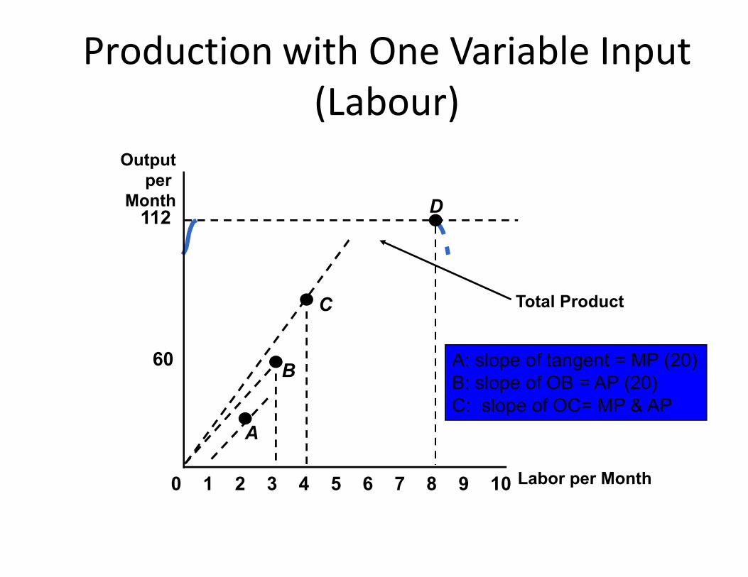
Outputper
Month112
D
Production with One Variable Input(Labour)
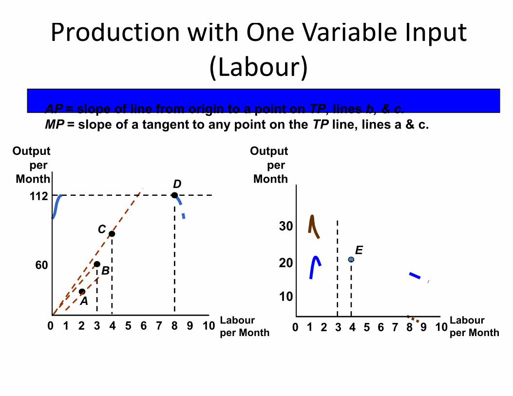
Total Product
A: slope of tangent = MP (20)B: slope of OB = AP (20)C: slope of OC= MP & AP
Labor per Month
60
0 2 3 4 5 6 7 8 9 101
A
B
C
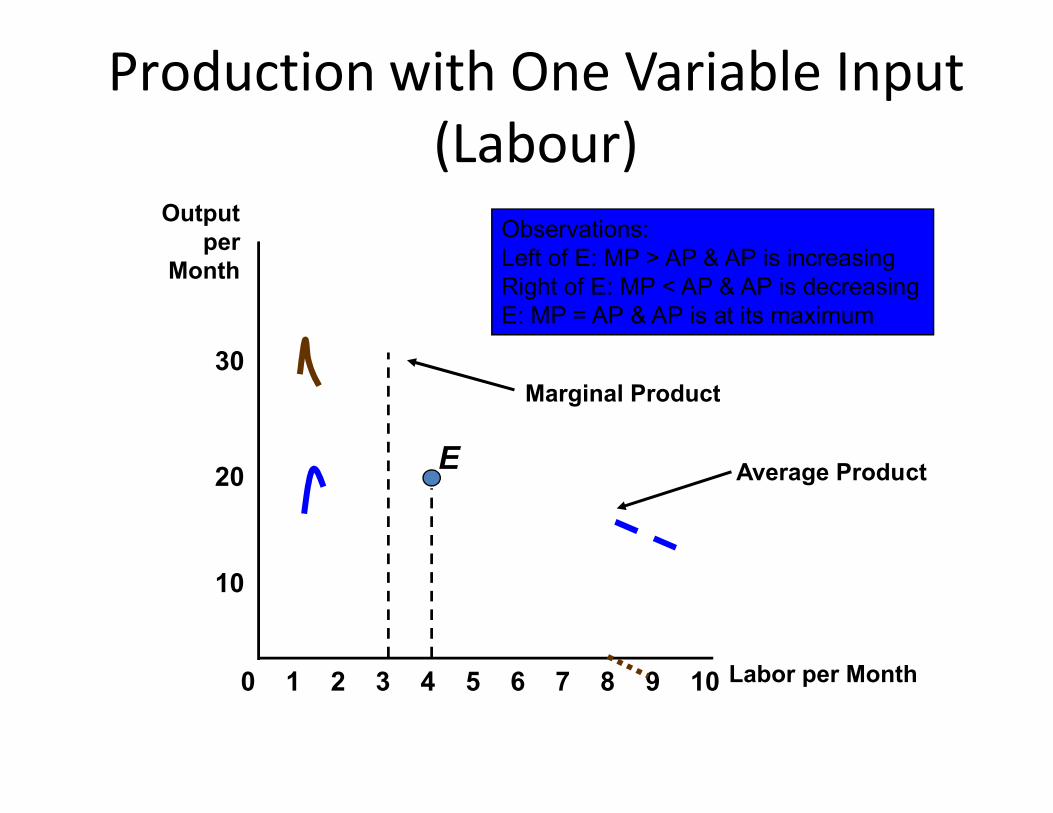
Production with One Variable Input(Labour)
Outputper
Month
30Marginal Product
Observations:Left of E: MP > AP & AP is increasingRight of E: MP < AP & AP is decreasingE: MP = AP & AP is at its maximum
Average Product
8
10
20
0 2 3 4 5 6 7 9 101 Labor per Month
E
Marginal Product
Production with One Variable Input(Labour)
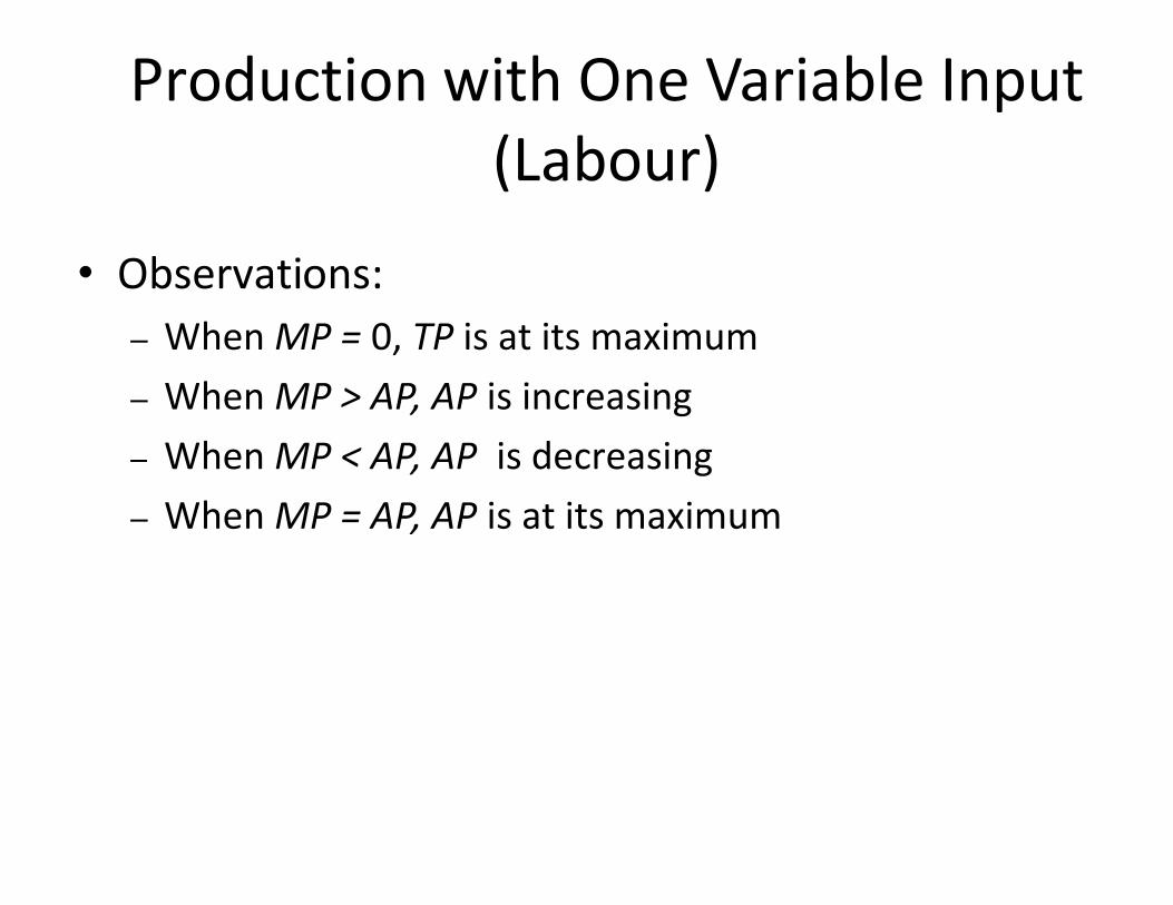
• Observations:– When MP = 0, TP is at its maximum– When MP > AP, AP is increasing– When MP < AP, AP is decreasing– When MP < AP, AP is decreasing– When MP = AP, AP is at its maximum
Production with One Variable Input(Labour)
AP = slope of line from origin to a point on TP, lines b, & c.MP = slope of a tangent to any point on the TP line, lines a & c.
112D
Outputper
Month
Outputper
Month
Labourper Month
60
112
0 2 3 4 5 6 7 8 9 101
A
B
C
8
10
20E
0 2 3 4 5 6 7 9 101
30
Labourper Month

Law of diminishing marginal returns
• As the use of an input increases in equal increments, a point will be reached at which the resulting additions to output decreases (i.e. MP declines):
– When the labor input is small, MP increases due to – When the labor input is small, MP increases due to specialization.
– When the labor input is large, MP decreases due to inefficiencies.
• Assumes technology and the quality of the variable input is constant
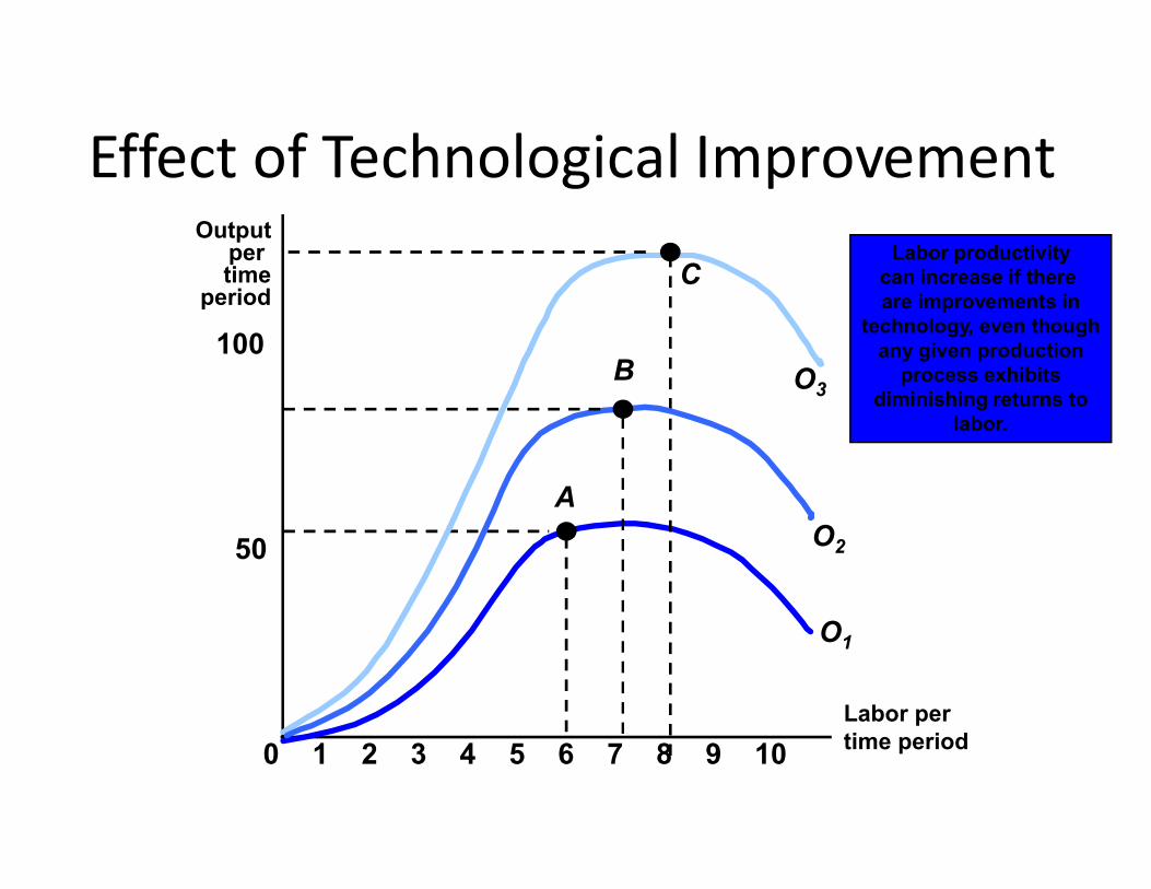
Effect of Technological ImprovementOutput
per time
period
100
C
O3B
Labor productivitycan increase if there are improvements in
technology, even thoughany given production
process exhibitsdiminishing returns to
labor.
Labor pertime period
50
0 2 3 4 5 6 7 8 9 101
A
O1
O2

Malthus and the Food Crisis
• Malthus predicted mass hunger and starvation as diminishing returns limited agricultural output and the population continued to grow.
• Why did Malthus’ prediction fail?

Index of World Food Consumption PerCapita
1948-1952 1001960 1151970 123
Year Index
1970 1231980 1281990 1371995 1351998 140
Malthus and the Food Crisis
• The data show that production increases have exceeded population growth.
• Malthus did not take into consideration the potential impact of technology which has allowed the supply of impact of technology which has allowed the supply of food to grow faster than demand.
• Technology has created surpluses and driven the price down.
Production with Two Variable Inputs• There is a relationship between production and
productivity.
• Long-run production K& L are variable.Long-run production K& L are variable.
• Isoquants analyze and compare the different combinations of K & L and output
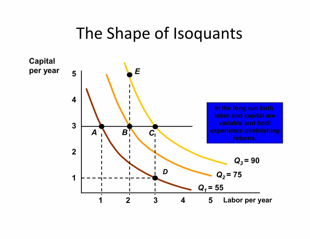
The Shape of Isoquants
4
5
In the long run both labor and capital are
variable and both
Capitalper year E
Labor per year
1
2
3
1 2 3 4 5
variable and bothexperience diminishing
returns.
Q1 = 55
Q2 = 75
Q3 = 90
A
D
B C
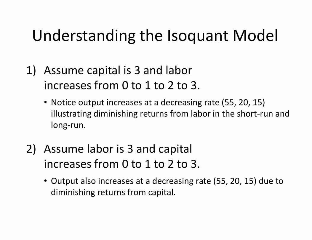
Understanding the Isoquant Model
1) Assume capital is 3 and labor increases from 0 to 1 to 2 to 3.• Notice output increases at a decreasing rate (55, 20, 15)
illustrating diminishing returns from labor in the short-run and long-run.long-run.
2) Assume labor is 3 and capital increases from 0 to 1 to 2 to 3.• Output also increases at a decreasing rate (55, 20, 15) due to
diminishing returns from capital.
Substituting Among Inputs
• Managers want to determine what combination of inputs to use.
• They must deal with the trade-off between inputs.
• The slope of each isoquant gives the trade-off between two inputs while keeping output constant.
Substituting Among Inputs
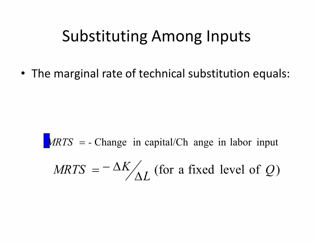
• The marginal rate of technical substitution equals:
inputlabor in angecapital/Chin Change-MRTS
)oflevelfixeda(for QLKMRTS
Marginal Rate of TechnicalSubstitution
4
5Capitalper year
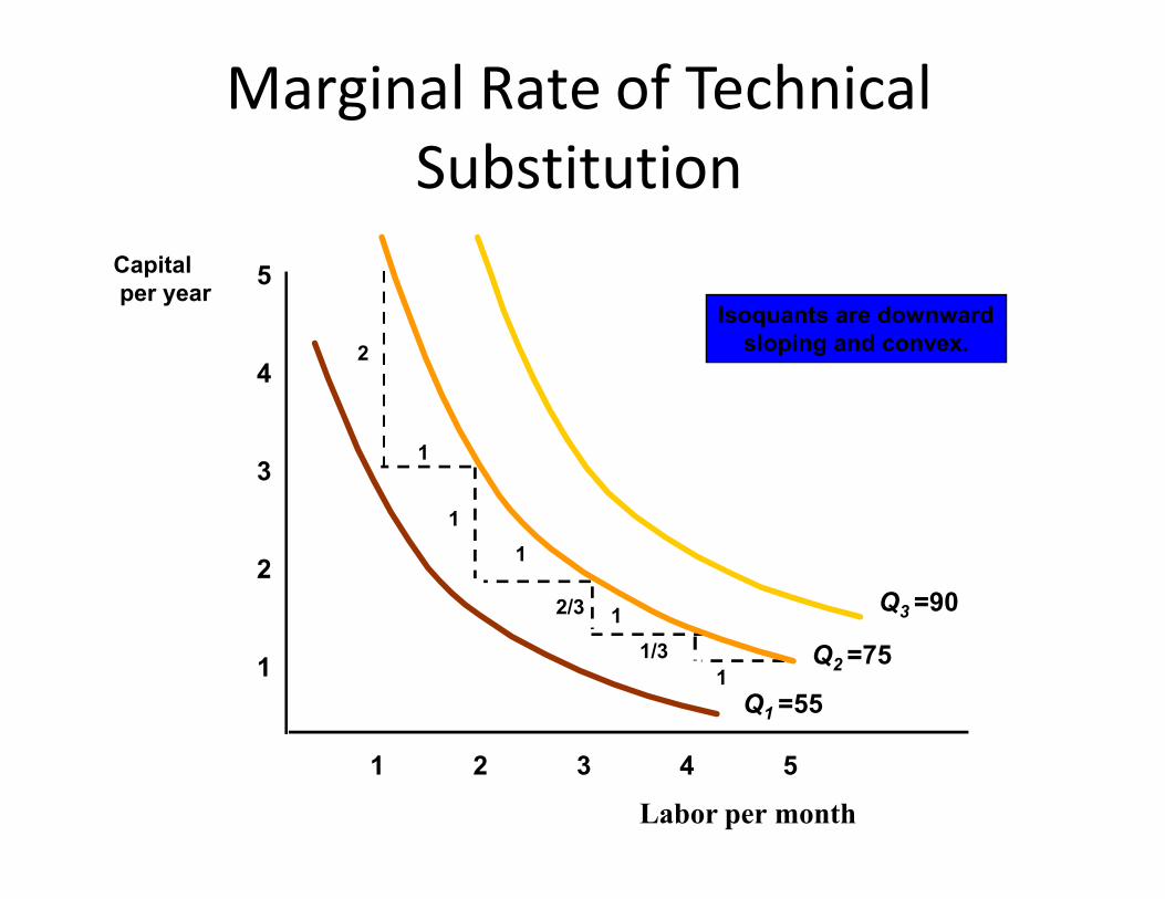
Isoquants are downwardsloping and convex.
1
2
Labor per month
1
2
3
1 2 3 4 5
1
1
1
1
1
2/3
1/3
Q1 =55
Q2 =75
Q3 =90
Marginal Rate of TechnicalSubstitution
• Observations:
1) Increasing labour in one unit increments from 1 to 5 results in a decreasing MRTS from 2 to 1/3.1/3.
2) Diminishing MRTS occurs because of diminishing returns and implies isoquants are convex.
MRTS and Marginal Productivity
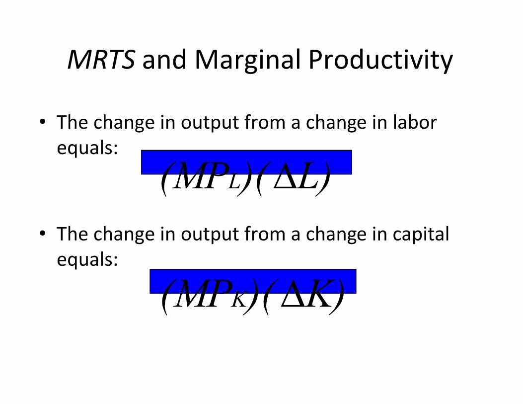
• The change in output from a change in labor equals:
L))((MPL • The change in output from a change in capital
equals:
K))((MPK
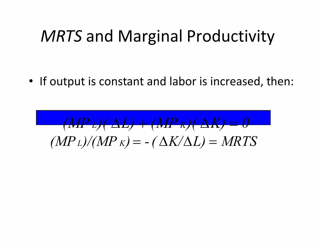
MRTS and Marginal Productivity
• If output is constant and labor is increased, then:
0K))((MPL))((MP KL 0K))((MPL))((MP KL MRTSL)K/(-))/(MP(MP KL
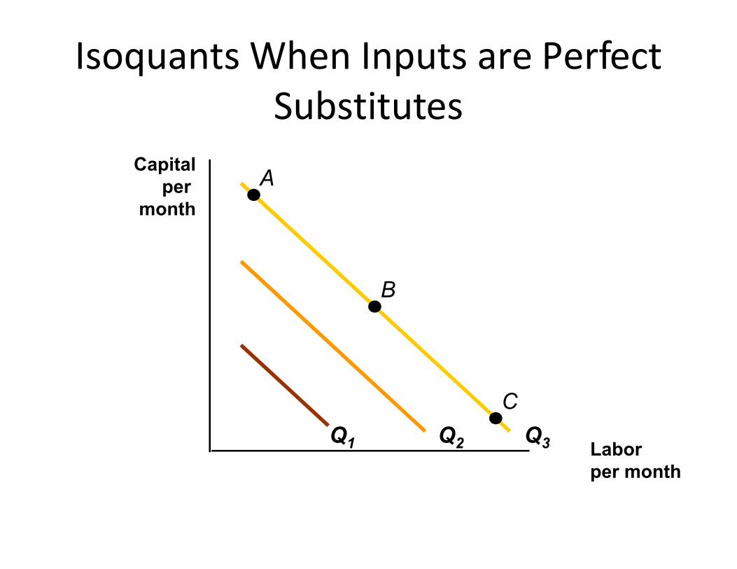
Isoquants When Inputs are PerfectSubstitutes
Capitalper
month
A
B
Laborper month
Q1 Q2 Q3
B
C

Production with Two Variable Inputs
• When inputs are perfectly substitutable:
1) The MRTS is constant at all points on the
Perfect Substitutes
1) The MRTS is constant at all points on the isoquant.
2) For a given output, any combination of inputs can be chosen (A, B, or C) to generate the same level of output (e.g. toll booths & musical instruments)
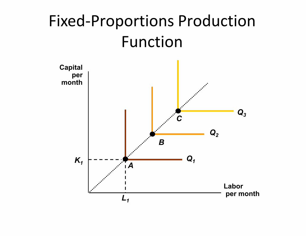
Fixed-Proportions ProductionFunction
Capitalper
month
Q3C
Laborper month
L1
K1Q1
Q2
A
B
C
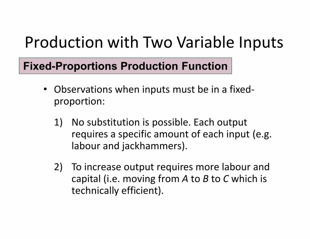
Production with Two Variable Inputs
• Observations when inputs must be in a fixed-proportion:
1) No substitution is possible. Each output
Fixed-Proportions Production Function
1) No substitution is possible. Each output requires a specific amount of each input (e.g. labour and jackhammers).
2) To increase output requires more labour and capital (i.e. moving from A to B to C which is technically efficient).
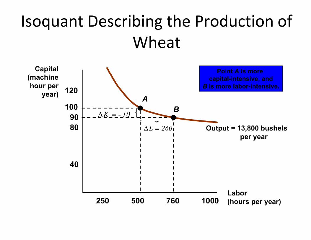
Isoquant Describing the Production ofWheat
Capital(machinehour per
year) 120
10090
AB
10-K
Point A is more capital-intensive, and
B is more labor-intensive.
Labor(hours per year)250 500 760 1000
40
8090
Output = 13,800 bushelsper year
260L
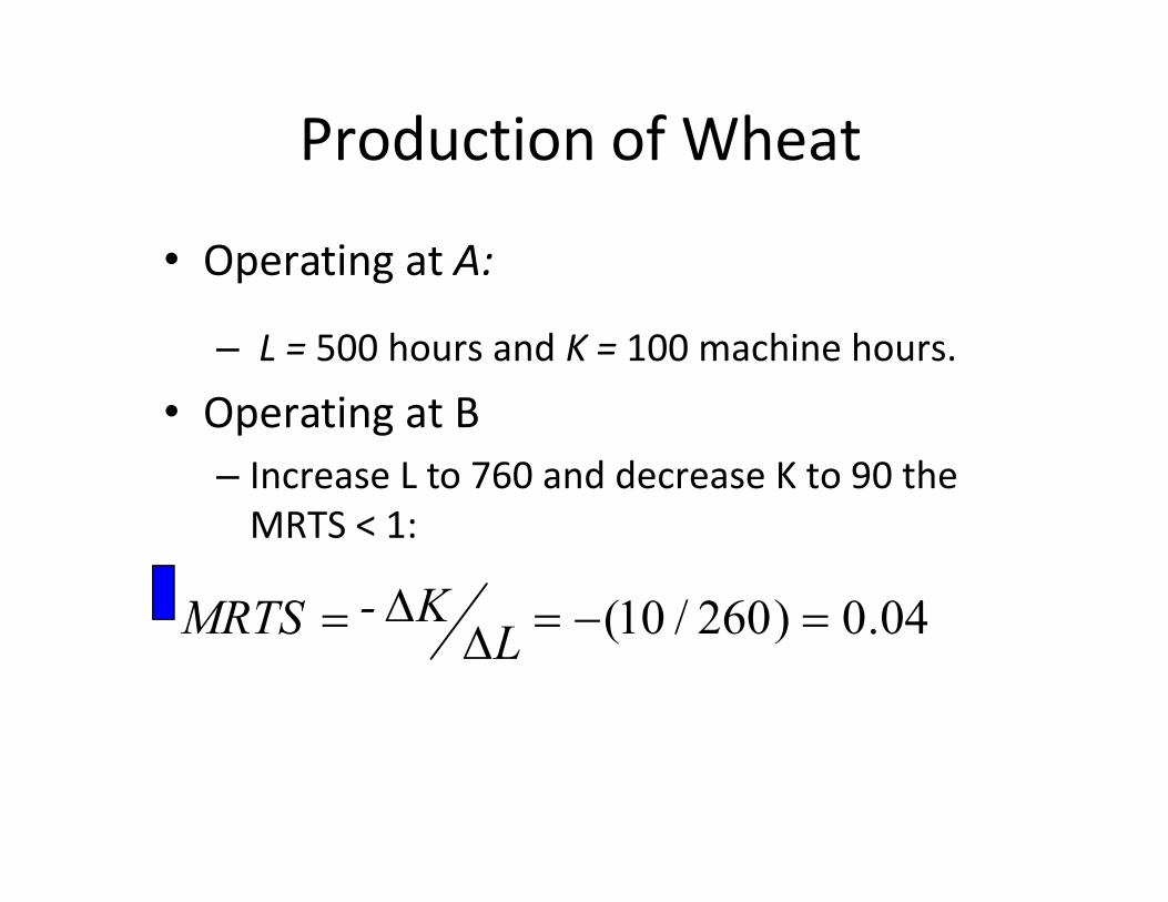
Production of Wheat
• Operating at A:
– L = 500 hours and K = 100 machine hours.
• Operating at BIncrease L to 760 and decrease K to 90 the – Increase L to 760 and decrease K to 90 the MRTS < 1:
04.0)260/10( L
K-MRTS
Production of Wheat
• MRTS < 1, therefore the cost of labor must be less than capital in order for the farmer substitute labor for capital.
• If labor is expensive, the farmer would use more capital (e.g. U.S.).
• If labor is inexpensive, the farmer would use more labor (e.g. India).
Returns to Scale• Measuring the relationship between the scale
(size) of a firm and output
• Increasing returns to scale: output more than doubles when all inputs are doubleddoubles when all inputs are doubled– Larger output associated with lower cost (autos)
– One firm is more efficient than many (utilities)
– The isoquants get closer together

Increasing returns to Scale
Capital(machine
hours)
Increasing Returns:The isoquants move closer together
A
Labor (hours)
10
20
30
5 10
2
4
0
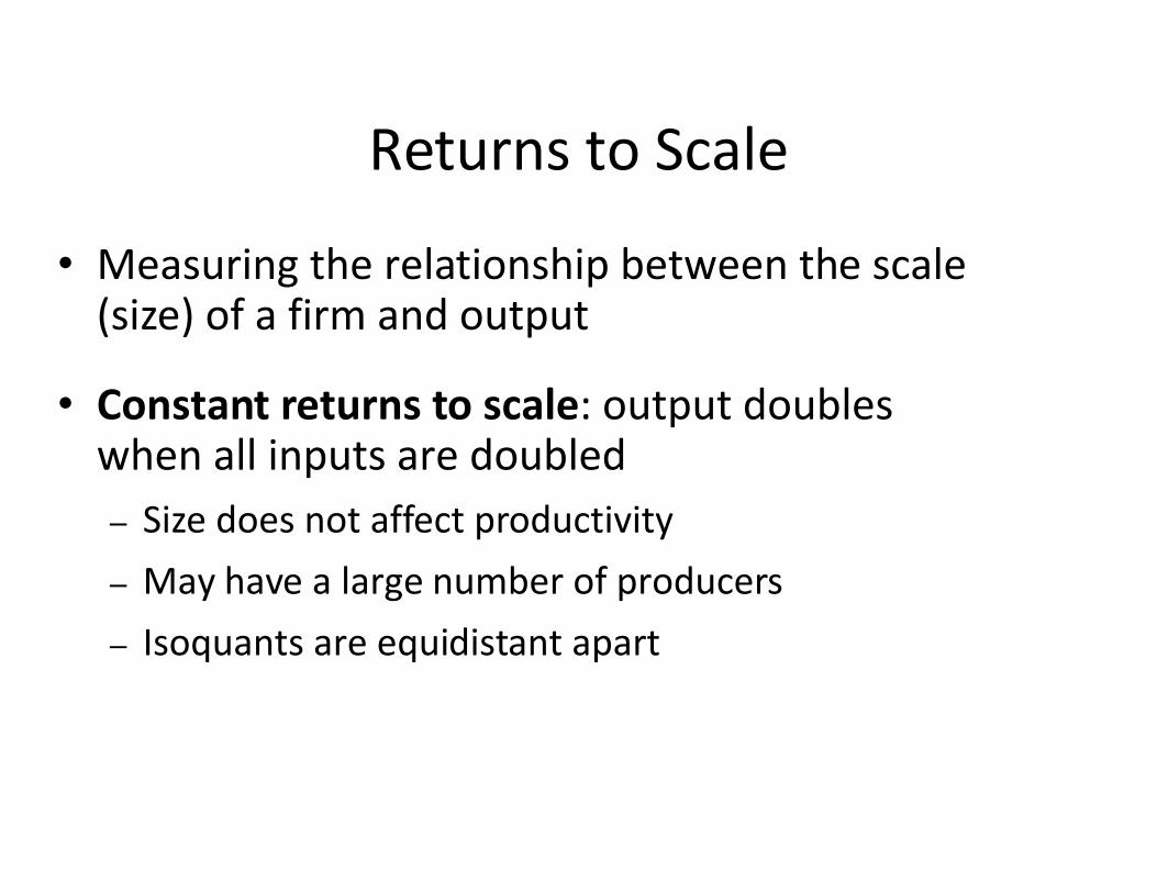
Returns to Scale
• Measuring the relationship between the scale (size) of a firm and output
• Constant returns to scale: output doubles when all inputs are doubledwhen all inputs are doubled– Size does not affect productivity– May have a large number of producers– Isoquants are equidistant apart
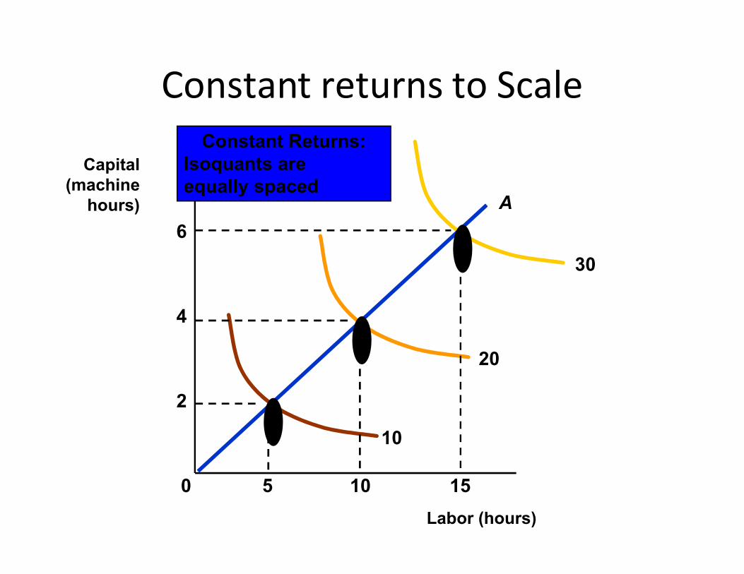
Constant returns to Scale
Capital(machine
hours)
Constant Returns:Isoquants are equally spaced
30
A
6
Labor (hours)
10
20
155 10
2
4
0
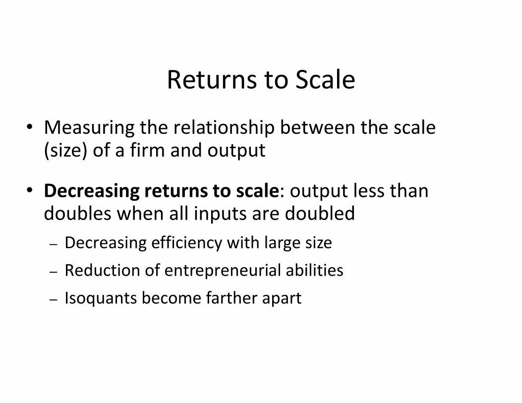
Returns to Scale
• Measuring the relationship between the scale (size) of a firm and output
• Decreasing returns to scale: output less than doubles when all inputs are doubled
• Decreasing returns to scale: output less than doubles when all inputs are doubled– Decreasing efficiency with large size– Reduction of entrepreneurial abilities– Isoquants become farther apart
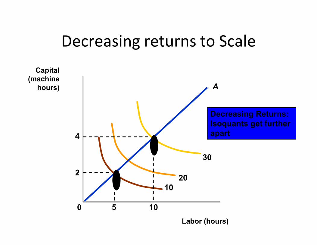
Decreasing returns to ScaleCapital
(machinehours)
Decreasing Returns:Isoquants get further
A
Labor (hours)
Isoquants get further apart
1020
30
5 10
2
4
0

Returns to Scale in the U.S. CarpetIndustry
• The carpet industry has grown from a small industry to a large industry with some very large firms.
• Can the growth be explained by the presence of economies to scale?
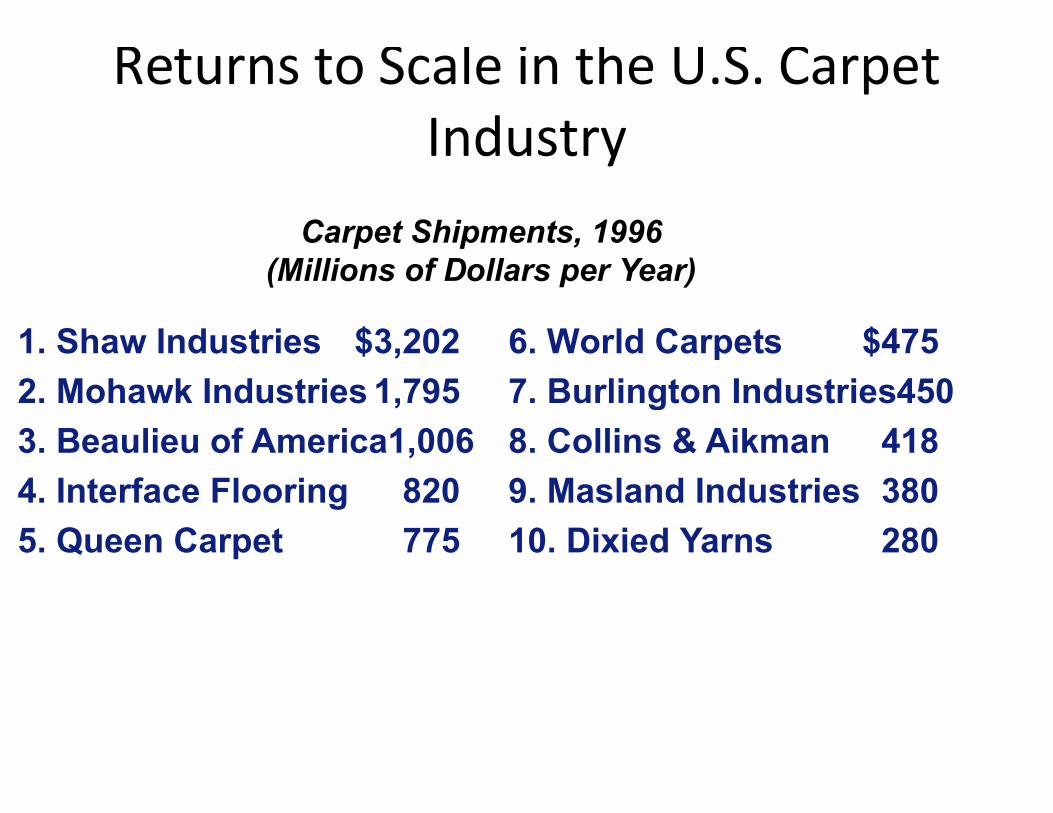
Returns to Scale in the U.S. CarpetIndustry
Carpet Shipments, 1996(Millions of Dollars per Year)
1. Shaw Industries $3,202 6. World Carpets $475
2. Mohawk Industries 1,795 7. Burlington Industries4502. Mohawk Industries 1,795 7. Burlington Industries450
3. Beaulieu of America1,006 8. Collins & Aikman 418
4. Interface Flooring 820 9. Masland Industries 380
5. Queen Carpet 775 10. Dixied Yarns 280
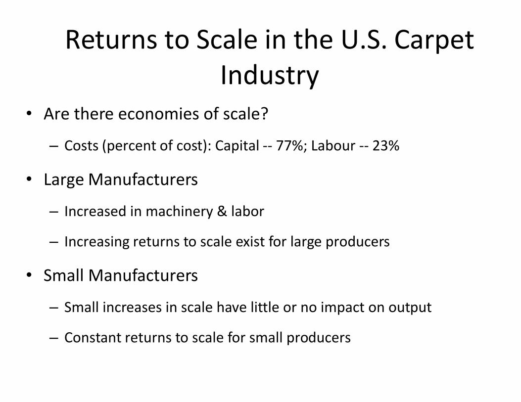
Returns to Scale in the U.S. CarpetIndustry
• Are there economies of scale?
– Costs (percent of cost): Capital -- 77%; Labour -- 23%
• Large Manufacturers
– Increased in machinery & labor
– Increasing returns to scale exist for large producers
• Small Manufacturers
– Small increases in scale have little or no impact on output
– Constant returns to scale for small producers

Summary• A production function describes the maximum output
a firm can produce for each specified combination of inputs.
• An isoquant is a curve that shows all combinations of • An isoquant is a curve that shows all combinations of inputs that yield a given level of output.
• Average product of labor measures the productivity of the average worker, whereas marginal product of labor measures the productivity of the last worker added.
Summary
• The law of diminishing returns explains that the marginal product of an input eventually diminishes as its quantity is increased.
• Isoquants always slope downward because the • Isoquants always slope downward because the marginal product of all inputs is positive.
• In long-run analysis, we tend to focus on the firm’s choice of its scale or size of operation.
Costs of productionCosts of production

Topics to be Discussed
• Measuring Cost: Which Costs Matter?
• Cost in the Short Run
• Cost in the Long Run• Cost in the Long Run
• Long-Run Versus Short-Run Cost Curves
Introduction• The production technology measures the relationship
between input and output.
• Given the production technology, managers must choose how to produce.choose how to produce.
• To determine the optimal level of output and the input combinations, we must convert from the unit measurements of the production technology to dollar measurements or costs.
Economic cost versus Accountingcost
• Accounting Cost– Actual expenses plus depreciation charges for
capital equipmentcapital equipment
• Economic Cost– Cost to a firm of utilizing economic resources in
production, including opportunity cost
Opportunity cost
• Cost associated with opportunities that are foregone when a firm’s resources are not put to their highest-value use.
• E.g.:
– A firm owns its own building and pays no rent for office space
– Does this mean the cost of office space is zero?
Sunk Cost
• Expenditure that has been made and cannot be recovered
• Should not influence a firm’s decisions.
• E.g.:• E.g.:
– A firm pays $500,000 for an option to buy a building.
– The cost of the building is $5 million or a total of $5.5 million.
– The firm finds another building for $5.25 million.
– Which building should the firm buy?
Fixed and variable costs
• Total output is a function of variable inputs and fixed inputs.
• Therefore, the total cost of production equals • Therefore, the total cost of production equals the fixed cost (the cost of the fixed inputs) plus the variable cost (the cost of the variable inputs), or…
VCFCTC

Fixed and variable costs
• Fixed Cost
– Does not vary with the level of output
• Variable Cost
– Cost that varies as output varies
Fixed versus sunk costs
• Fixed Cost
– Cost paid by a firm that is in business regardless of the level of output
• Sunk Cost
– Cost that has been incurred and cannot be recovered
Some examples
• Personal Computers: most costs are variable
– Components, labour
• Software: most costs are sunk• Software: most costs are sunk
– Cost of developing the software
• Pizza: most costs are fixed
– Largest cost component is fixed
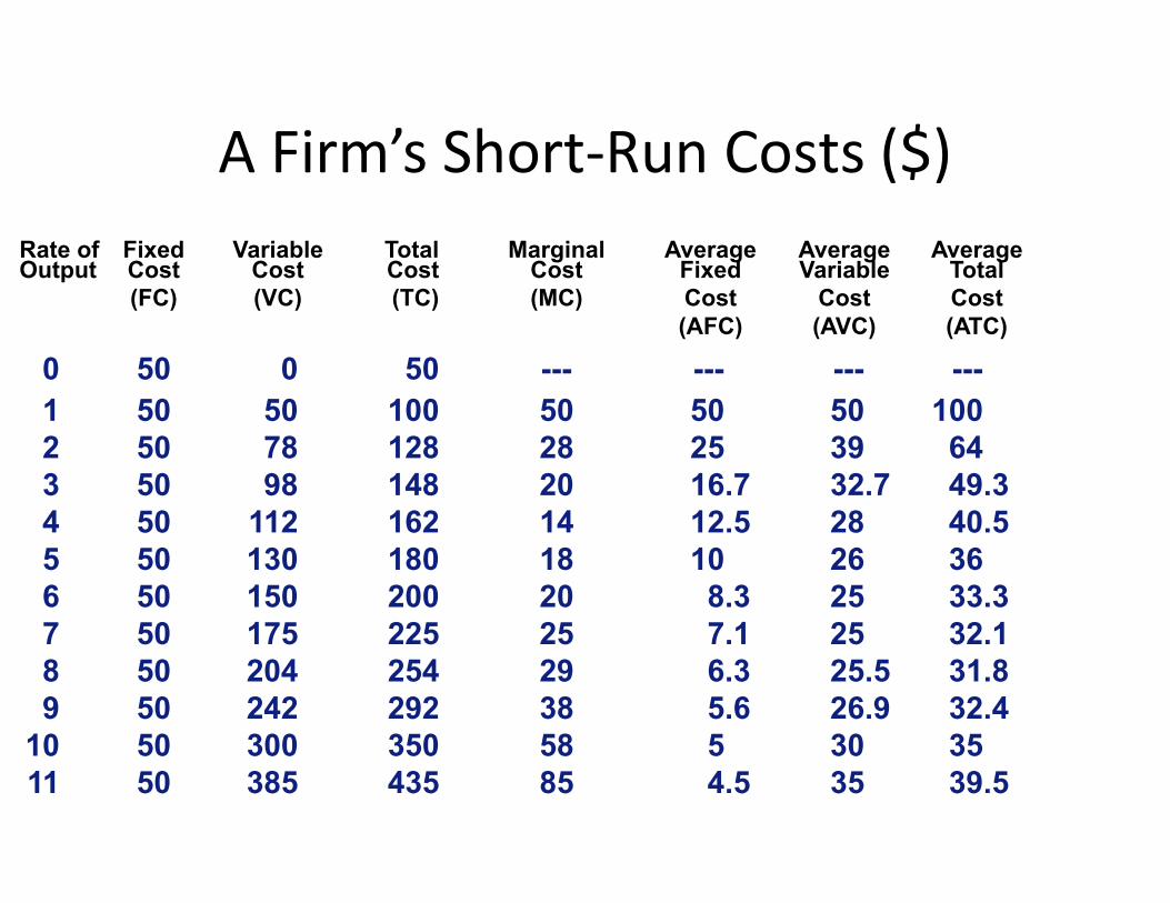
A Firm’s Short-Run Costs ($)
0 50 0 50 --- --- --- ---1 50 50 100 50 50 50 1002 50 78 128 28 25 39 64
Rate of Fixed Variable Total Marginal Average Average AverageOutput Cost Cost Cost Cost Fixed Variable Total
(FC) (VC) (TC) (MC) Cost Cost Cost(AFC) (AVC) (ATC)
2 50 78 128 28 25 39 643 50 98 148 20 16.7 32.7 49.34 50 112 162 14 12.5 28 40.55 50 130 180 18 10 26 366 50 150 200 20 8.3 25 33.37 50 175 225 25 7.1 25 32.18 50 204 254 29 6.3 25.5 31.89 50 242 292 38 5.6 26.9 32.4
10 50 300 350 58 5 30 3511 50 385 435 85 4.5 35 39.5
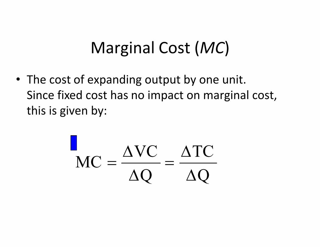
Marginal Cost (MC)
• The cost of expanding output by one unit. Since fixed cost has no impact on marginal cost, this is given by:
Q
TC
Q
VCMC
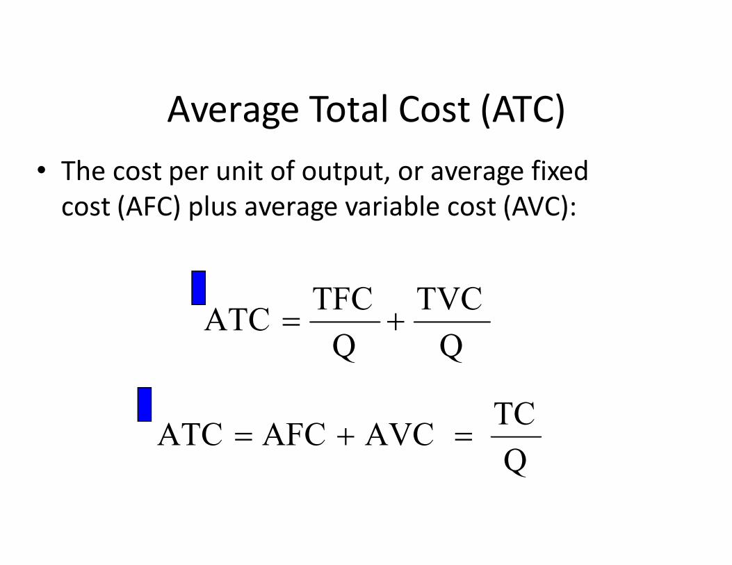
Average Total Cost (ATC)• The cost per unit of output, or average fixed
cost (AFC) plus average variable cost (AVC):
TVCTFC
Q
TVC
Q
TFCATC
Q
TC AVCAFCATC

The Determinants of Short-RunCost
• The relationship between the production function and cost is determined be whether there are increasing or decreasing returns to inputs.
• Increasing returns and cost– With increasing returns, output is increasing relative to input and
variable cost and total cost will fall relative to output.• Decreasing returns and cost
– With decreasing returns, output is decreasing relative to input and variable cost and total cost will rise relative to output.
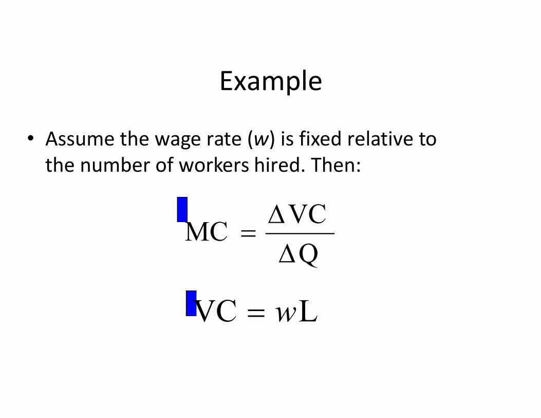
Example
• Assume the wage rate (w) is fixed relative to the number of workers hired. Then:
VCQ
VCMC
LVC w
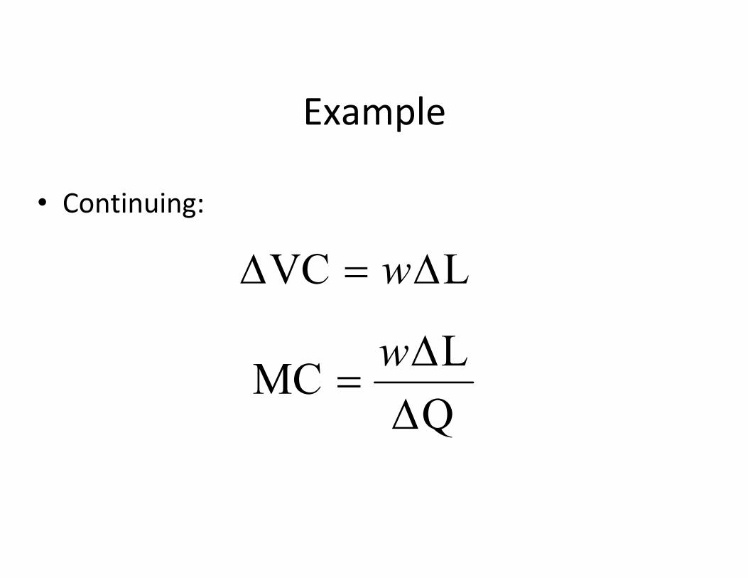
Example
• Continuing:
LVC w LVC w
Q
LMC
w
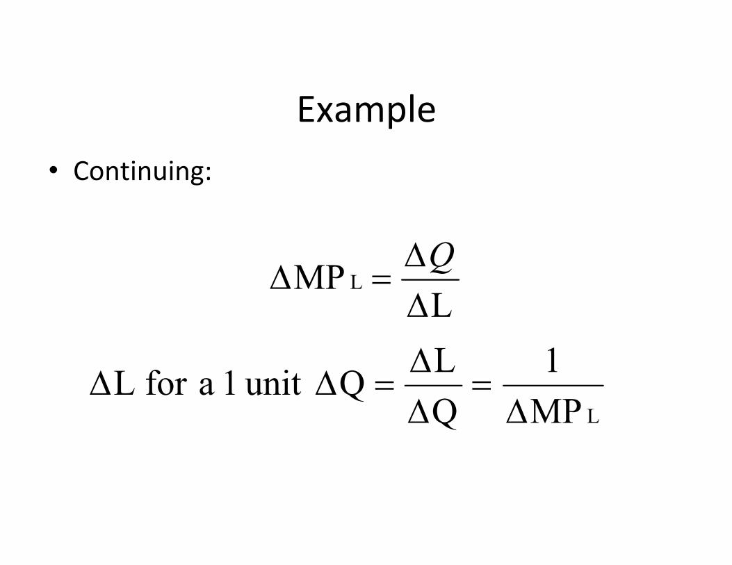
Example• Continuing:
MP L
Q
LMP L
LMP
1
Q
LQunit1aforL
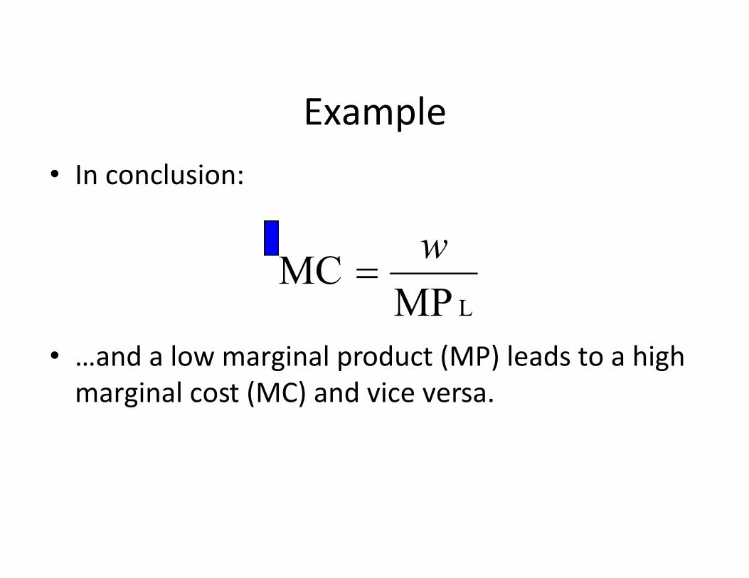
Example• In conclusion:
MPMC
w
• …and a low marginal product (MP) leads to a high marginal cost (MC) and vice versa.
LMPMC
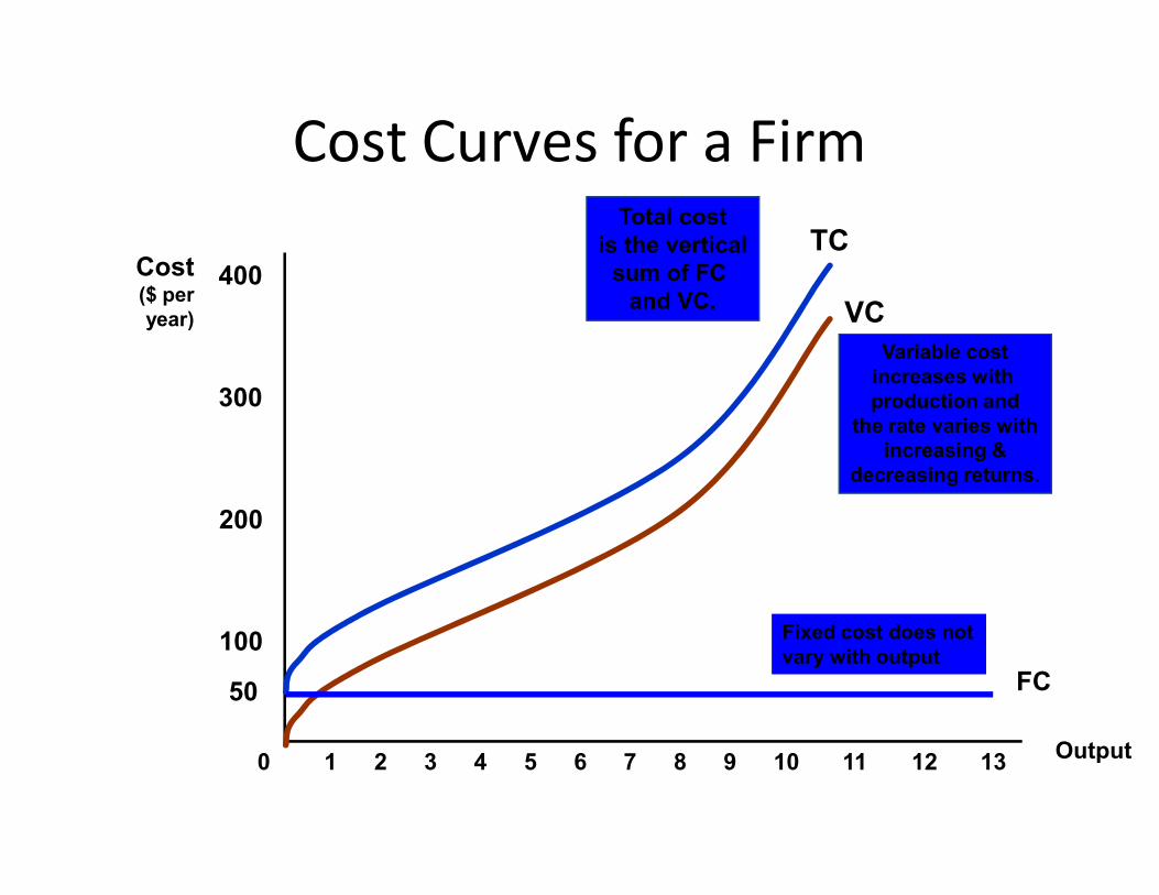
Cost Curves for a Firm
Cost($ peryear)
300
400
VCVariable cost
increases with production and
the rate varies withincreasing &
TCTotal cost
is the verticalsum of FC
and VC.
Output
100
200
0 1 2 3 4 5 6 7 8 9 10 11 12 13
increasing &decreasing returns.
FC50
Fixed cost does notvary with output

Cost Curves for a FirmCost($ perunit)
75
100
MC
Output (units/yr.)
25
50
0 1 2 3 4 5 6 7 8 9 10 11
ATC
AVC
AFC
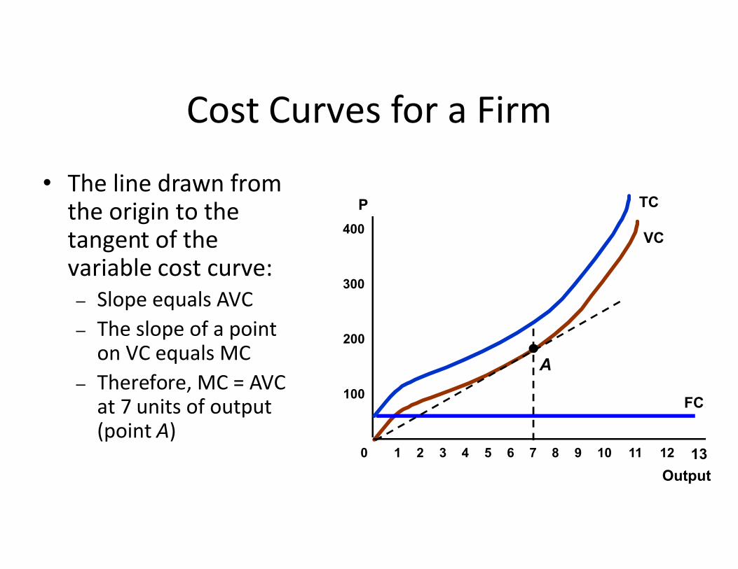
Cost Curves for a Firm
• The line drawn from the origin to the tangent of the variable cost curve:
P
300
400VC
TC
– Slope equals AVC– The slope of a point
on VC equals MC– Therefore, MC = AVC
at 7 units of output (point A)
Output
100
200
300
0 1 2 3 4 5 6 7 8 9 10 11 12 13
FC
A
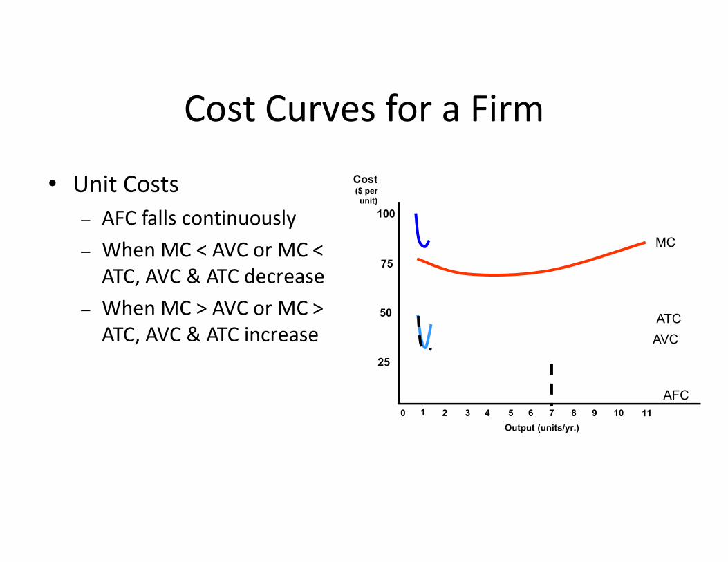
Cost Curves for a Firm
• Unit Costs– AFC falls continuously– When MC < AVC or MC <
ATC, AVC & ATC decrease
Cost($ perunit)
75
100
MC
ATC, AVC & ATC decrease– When MC > AVC or MC >
ATC, AVC & ATC increase
Output (units/yr.)
25
50
0 1 2 3 4 5 6 7 8 9 10 11
ATC
AVC
AFC
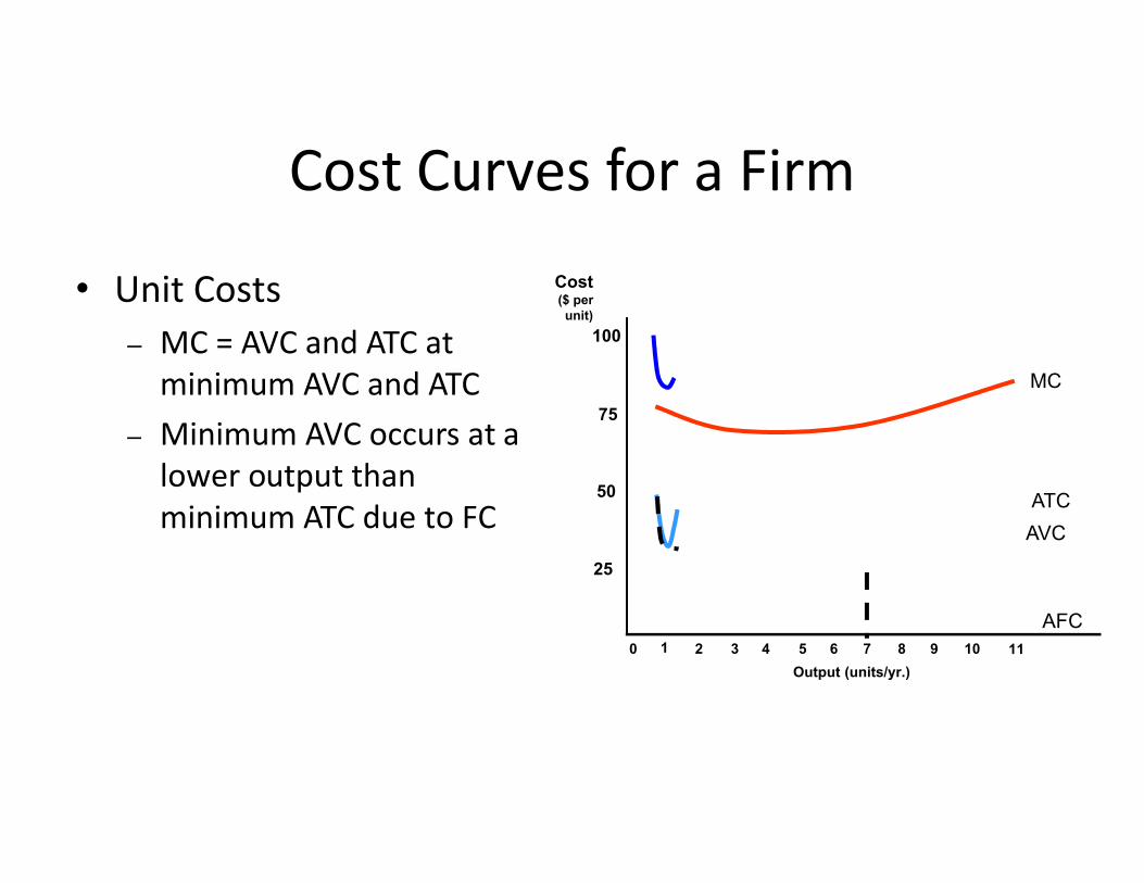
Cost Curves for a Firm
• Unit Costs– MC = AVC and ATC at
minimum AVC and ATC– Minimum AVC occurs at a
Cost($ perunit)
75
100
MC
– Minimum AVC occurs at a lower output than minimum ATC due to FC
Output (units/yr.)
25
50
0 1 2 3 4 5 6 7 8 9 10 11
ATC
AVC
AFC
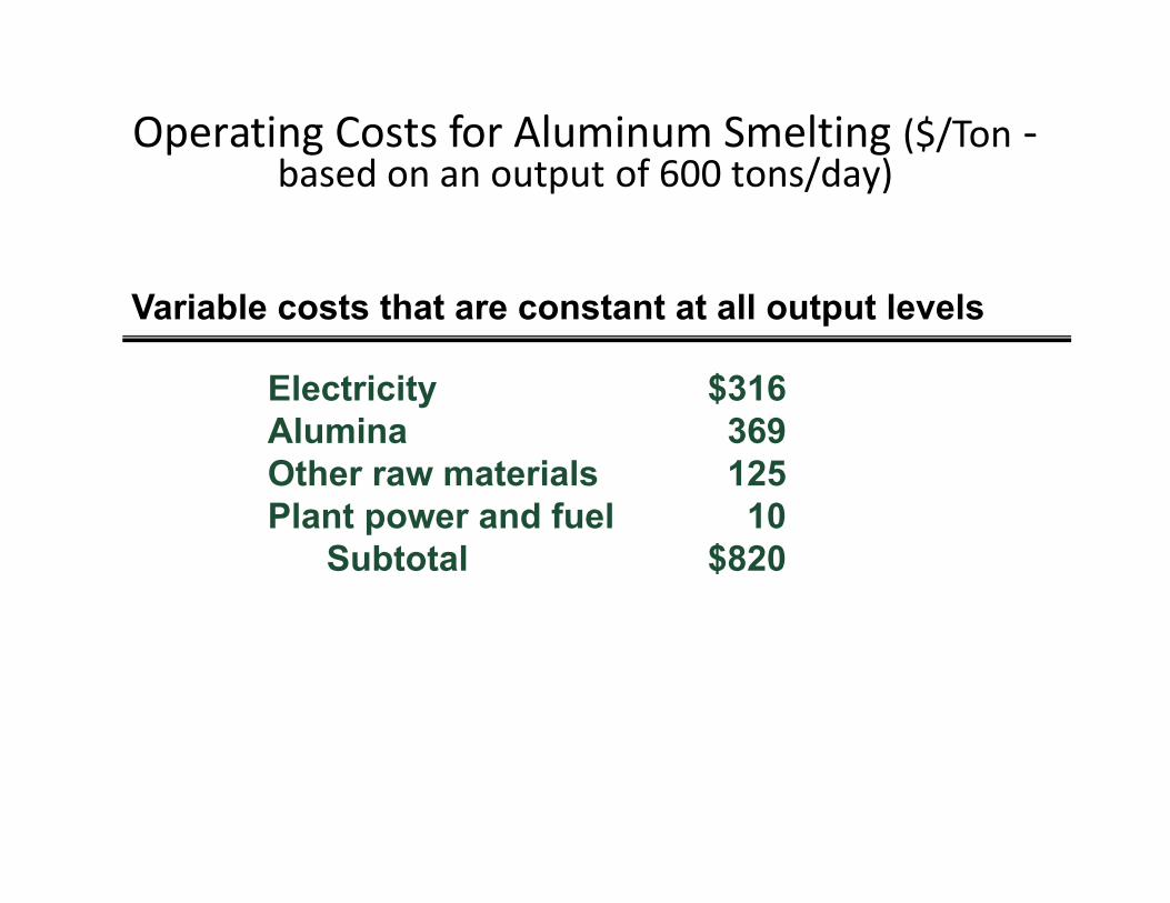
Operating Costs for Aluminum Smelting ($/Ton -based on an output of 600 tons/day)
Variable costs that are constant at all output levels
Electricity $316Alumina 369Other raw materials 125Plant power and fuel 10
Subtotal $820
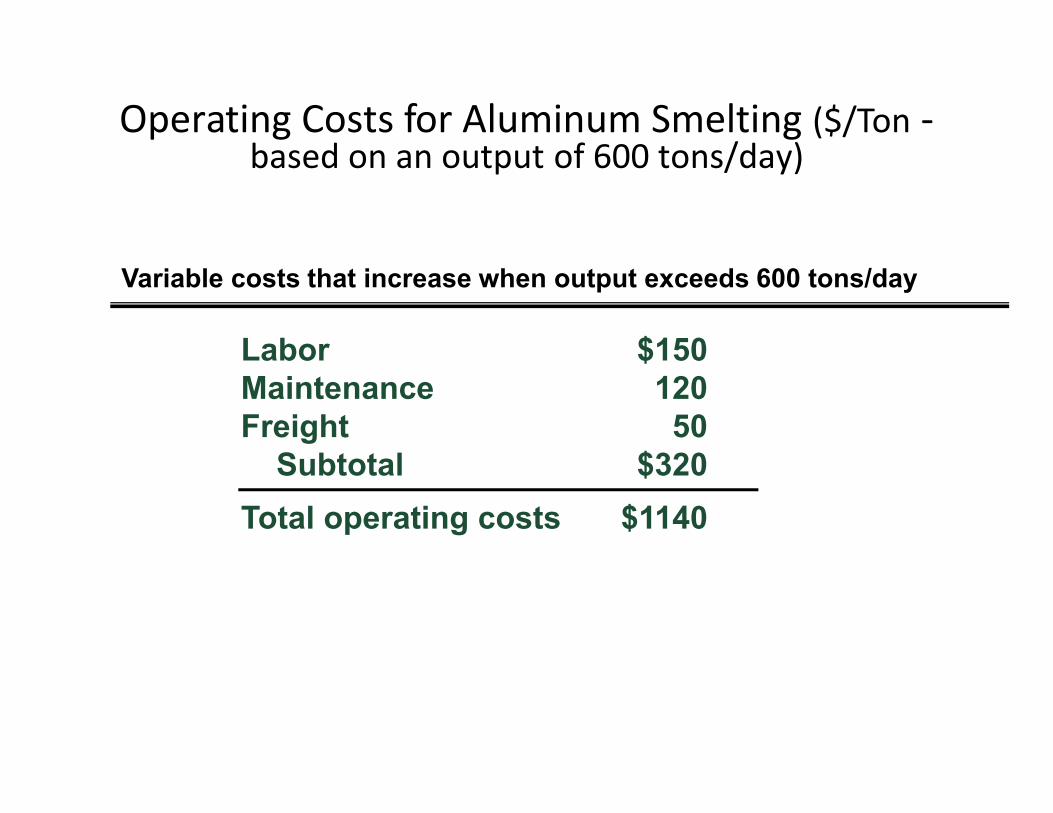
Operating Costs for Aluminum Smelting ($/Ton -based on an output of 600 tons/day)
Variable costs that increase when output exceeds 600 tons/day
Labor $150Maintenance 120Freight 50
Subtotal $320
Total operating costs $1140
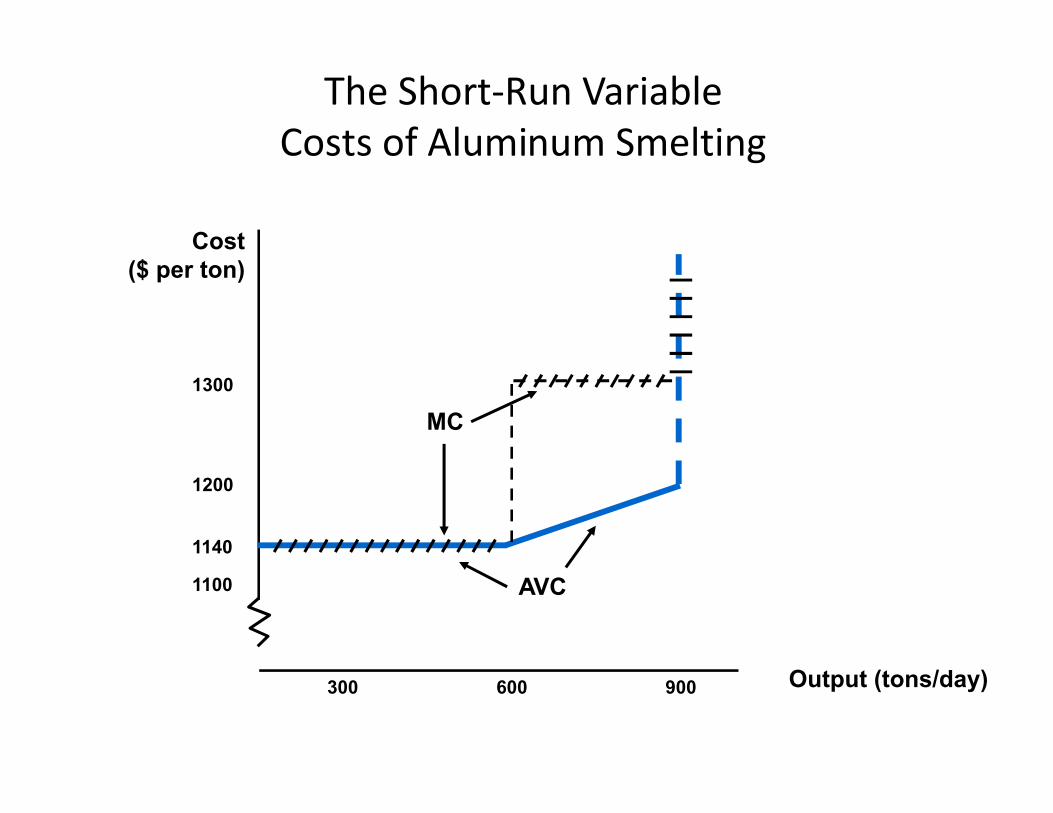
The Short-Run VariableCosts of Aluminum Smelting
Cost($ per ton)
1300
Output (tons/day)
1100
1200
300 600 900
1140
MC
AVC
Cost in the Long Run
• Assumptions
– Two Inputs: Labor (L) & capital (K)
– Price of labor: wage rate (w)
The Cost Minimizing Input Choice
– The price of capital: R = depreciation rate + interest rate

Cost in the Long Run
• The Isocost Line– C = wL + rK
The User Cost of CapitalThe Cost Minimizing Input Choice
– C = wL + rK
– Isocost: A line showing all combinations of L & Kthat can be purchased for the same cost
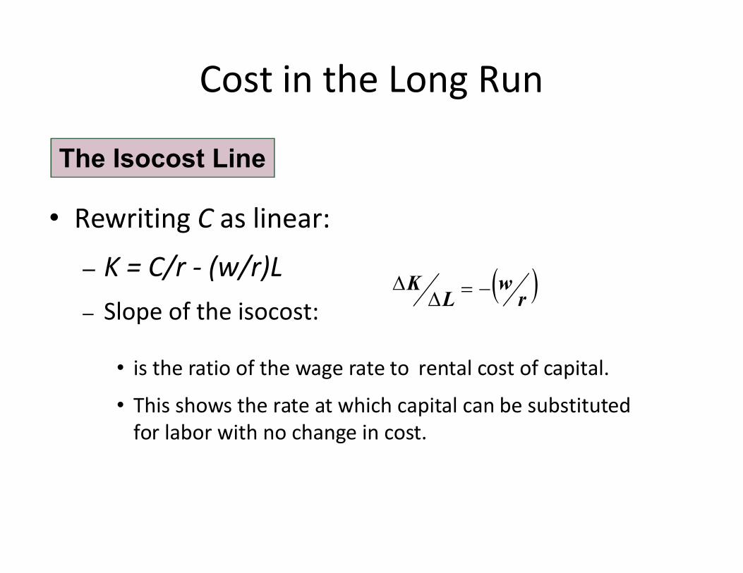
Cost in the Long Run
• Rewriting C as linear:
– K = C/r - (w/r)L wK
The Isocost Line
– Slope of the isocost:
• is the ratio of the wage rate to rental cost of capital.
• This shows the rate at which capital can be substituted for labor with no change in cost.
rw
LK

Choosing Inputs• We will examine how to minimize cost for a given
level of output (by combining isocosts with isoquants)

Producing a Given Output atMinimum Cost
Capitalper
year
Isocost C2 shows quantity Q can be produced with
Q1 is an isoquantfor output Q1.
Isocost curve C0 showsall combinations of K and L
that cost C0.
CO C1 C2 are
K2
Labour per year
Q1 can be produced withcombination K2L2 or K3L3.
However, both of theseare higher cost combinations
than K1L1.
Q1
C0 C1 C2
CO C1 C2 arethree
isocost lines
AK1
L1
K3
L3L2
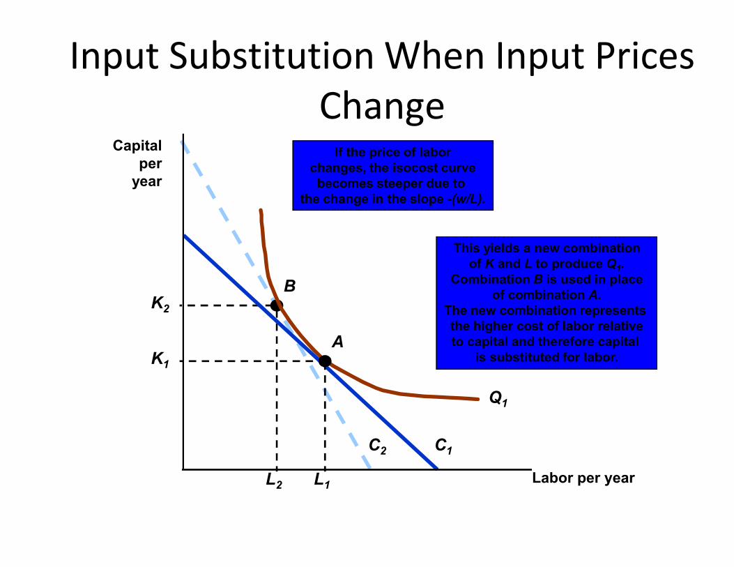
Input Substitution When Input PricesChange
This yields a new combinationof K and L to produce Q1.
Combination B is used in placeB
If the price of laborchanges, the isocost curvebecomes steeper due to
the change in the slope -(w/L).
Capitalper
year
C2
Combination B is used in placeof combination A.
The new combination represents the higher cost of labor relativeto capital and therefore capital
is substituted for labor.
K2
L2
B
C1
K1
L1
A
Q1
Labor per year
Cost in the Long Run
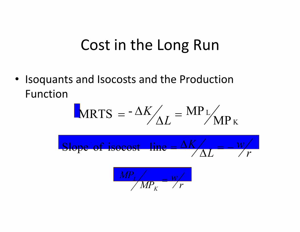
• Isoquants and Isocosts and the Production Function
LMP
MP-MRTS L
KK
LMP
MP-MRTS L
K
rw
LK
lineisocost ofSlope
rw
MPMP
K
L
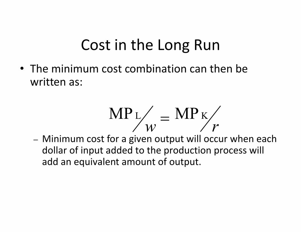
Cost in the Long Run• The minimum cost combination can then be
written as:
KL MPMP – Minimum cost for a given output will occur when each
dollar of input added to the production process will add an equivalent amount of output.
rwKL MPMP

Effect of Effluent Fees on Input Choices
• Firms that have a by-product to production produce an effluent.
• An effluent fee is a per-unit fee that firms must • An effluent fee is a per-unit fee that firms must pay for the effluent that they emit.
• How would a producer respond to an effluent fee on production?
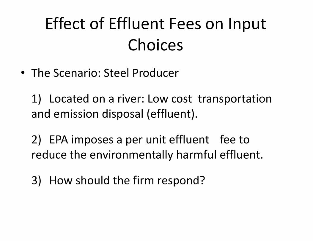
Effect of Effluent Fees on InputChoices
• The Scenario: Steel Producer
1) Located on a river: Low cost transportation and emission disposal (effluent).and emission disposal (effluent).
2) EPA imposes a per unit effluent fee to reduce the environmentally harmful effluent.
3) How should the firm respond?
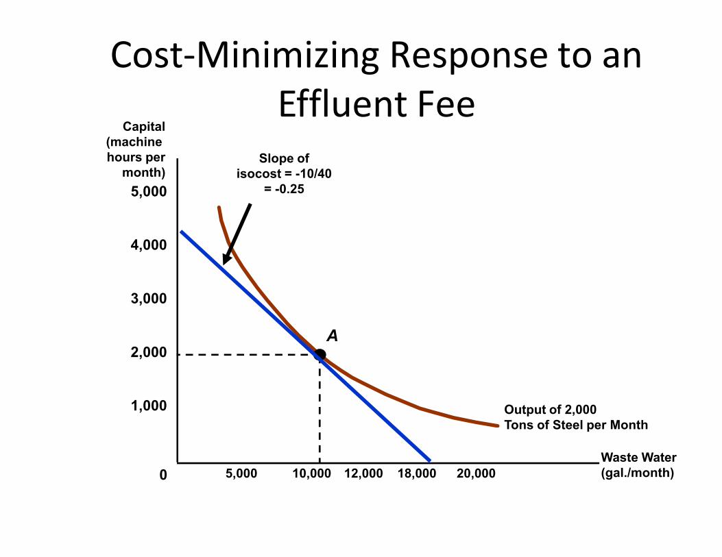
Cost-Minimizing Response to anEffluent Fee
Capital(machine hours per
month)Slope of
isocost = -10/40 = -0.25
4,000
5,000
Waste Water(gal./month)
Output of 2,000Tons of Steel per Month
A
10,000 18,000 20,0000 12,000
2,000
1,000
3,000
5,000
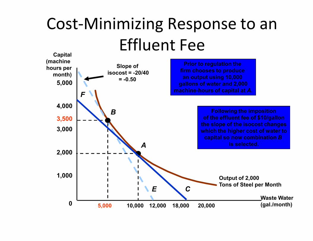
Cost-Minimizing Response to anEffluent Fee
4,000
5,000
Capital(machine hours per
month)
3,500
Slope ofisocost = -20/40
= -0.50
B Following the impositionof the effluent fee of $10/gallon
Prior to regulation the firm chooses to produce an output using 10,000
gallons of water and 2,000machine-hours of capital at A.
F
Output of 2,000Tons of Steel per Month
2,000
1,000
3,000
10,000 18,000 20,0000 12,000
E
5,000
3,500 of the effluent fee of $10/gallonthe slope of the isocost changeswhich the higher cost of water to
capital so now combination Bis selected.A
CWaste Water(gal./month)
Effect of Effluent Fees on InputChoices
• The more easily factors can be substituted, the more effective the fee is in reducing the effluent.
• The greater the degree of substitutes, the less the firm will have to pay (for example: $50,000 with firm will have to pay (for example: $50,000 with combination B instead of $100,000 with combination A)
Costs in the Long Run
• Cost minimization with Varying Output Levels– A firm’s expansion path shows the minimum cost
combinations of labor and capital at each level of output.output.
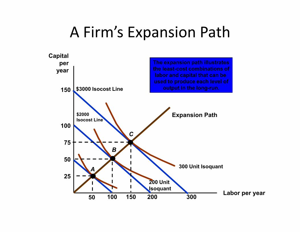
A Firm’s Expansion PathCapital
peryear
Expansion Path
The expansion path illustratesthe least-cost combinations oflabor and capital that can be used to produce each level of
output in the long-run.150
$2000
$3000 Isocost Line
Labor per year
Expansion Path
25
50
75
100
10050 150 300200
A
$2000Isocost Line
200 UnitIsoquant
B
300 Unit Isoquant
C
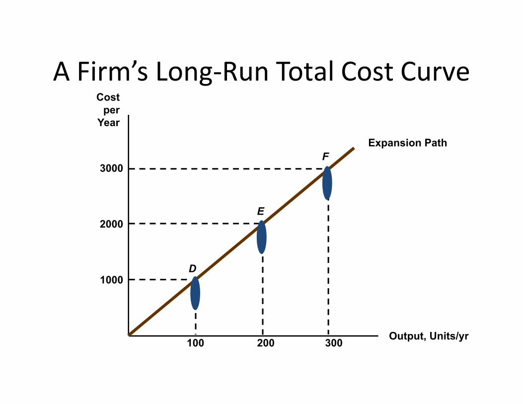
A Firm’s Long-Run Total Cost CurveCost
perYear
Expansion Path
3000F
Output, Units/yr
1000
100 300200
2000
D
E

Long-Run Versus Short-Run CostCurves
• What happens to average costs when both inputs are variable (long run) versus only having one input that is variable (short run)?
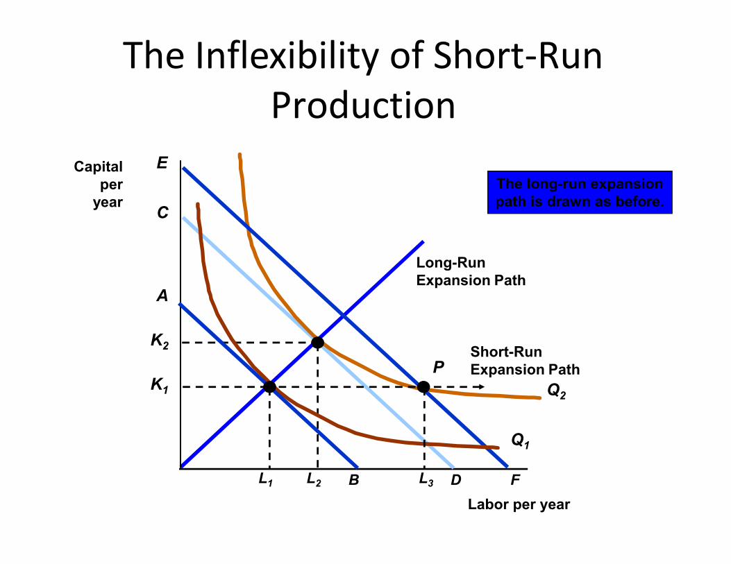
Long-RunExpansion Path
The long-run expansionpath is drawn as before.
The Inflexibility of Short-RunProduction
Capitalper
yearC
E
Expansion Path
Labor per year
L2
Q2
K2
D F
Q1
A
BL1
K1
L3
PShort-RunExpansion Path
Long-Run Average Cost (LAC)
• Constant Returns to Scale– If input is doubled, output will double and average cost is
constant at all levels of output.• Increasing Returns to ScaleIncreasing Returns to Scale
– If input is doubled, output will more than double and average cost decreases at all levels of output.
• Decreasing Returns to Scale– If input is doubled, the increase in output is less than twice
as large and average cost increases with output.• In the long-run:
– Firms experience increasing and decreasing returns to scale and therefore long-run average cost is “U” shaped.
Long-run marginal cost
• Long-run marginal cost leads long-run average cost:– If LMC < LAC, LAC will fall
– If LMC > LAC, LAC will rise
– Therefore, LMC = LAC at the minimum of LAC

Long-run average and marginal cost
Cost($ per unitof output
LAC
LMC
Output
A
Economies and Diseconomies ofScale
• Economies of Scale– Increase in output is greater than the increase in
inputs.
• Diseconomies of Scale• Diseconomies of Scale– Increase in output is less than the increase in
inputs.
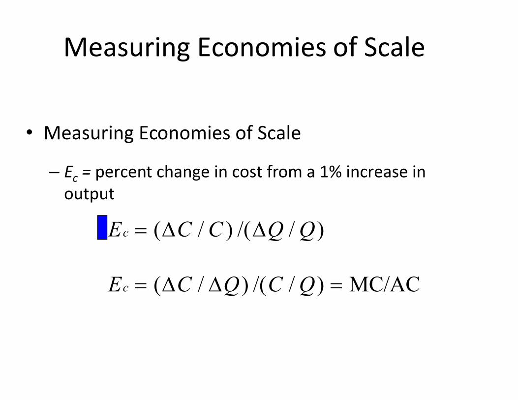
Measuring Economies of Scale
• Measuring Economies of Scale
– Ec = percent change in cost from a 1% increase in outputoutput
)//()/( QQCCEc
MC/AC)//()/( QCQCEc
Measuring Economies of Scale
• EC < 1: MC < AC– economies of scale
• EC = 1: MC = AC• EC = 1: MC = AC– constant economies of scale
• EC > 1: MC > AC– diseconomies of scale
Long-Run Versus Short-Run CostCurves
• The Relationship Between Short-Run and Long-Run Cost– We will use short and long-run cost to determine the
optimal plant sizeoptimal plant size
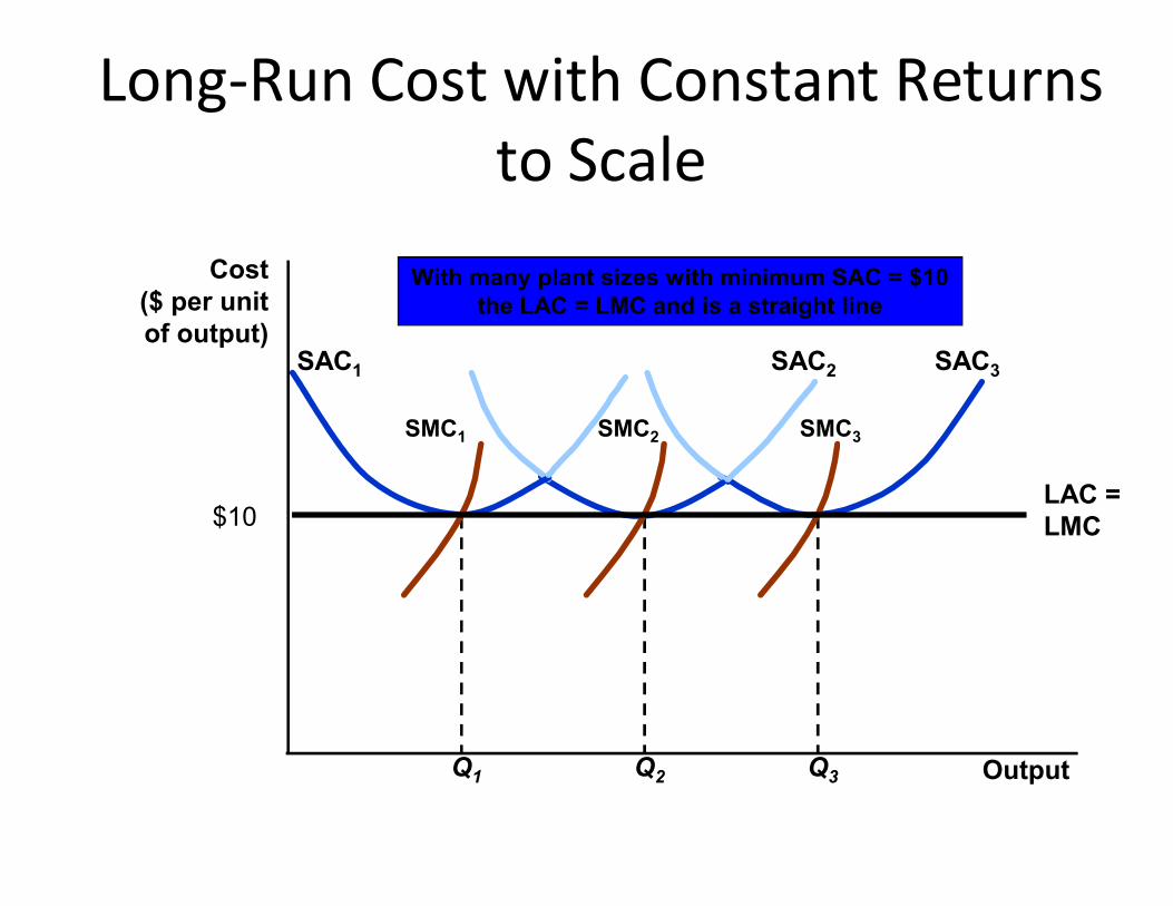
Long-Run Cost with Constant Returnsto Scale
Cost($ per unitof output)
SAC3
SMC3
SAC2
SMC2
SAC1
SMC1
With many plant sizes with minimum SAC = $10the LAC = LMC and is a straight line
OutputQ3Q2Q1
LAC =LMC$10
Long-Run Cost with Constant Returns toScale
• The optimal plant size will depend on the anticipated output (e.g. Q1 choose SAC1,etc).
• The long-run average cost curve is the envelope of The long-run average cost curve is the envelope of the firm’s short-run average cost curves.

Long-Run Cost with Economies and Diseconomies of Scale
Cost($ per unitof output
SAC1
SAC2
$10
$8B
A
LAC SAC3
Output
SMC1
SMC2LMC
If the output is Q1 a managerwould chose the small plant
SAC1 and SAC $8.Point B is on the LAC because
it is a least cost plant for a given output.
Q1
B
SMC3
Long-Run Cost with Economies and Diseconomies of Scale
• What is the firms’ long-run cost curve?– Firms can change scale to change output in the long-
run.– The long-run cost curve is the dark blue portion of the – The long-run cost curve is the dark blue portion of the
SAC curve which represents the minimum cost for any level of output.
Summary
• Managers, investors, and economists must take into account the opportunity cost associated with the use of the firm’s resources.
• Firms are faced with both fixed and variable costs • Firms are faced with both fixed and variable costs in the short-run.
• When there is a single variable input, as in the short run, the presence of diminishing returns determines the shape of the cost curves.
Summary• In the long run, all inputs to the production process
are variable.
• The firm’s expansion path describes how its cost-minimizing input choices vary as the scale or output of minimizing input choices vary as the scale or output of its operation increases.
• The long-run average cost curve is the envelope of the short-run average cost curves.
• A firm enjoys economies of scale when it can double its output at less than twice the cost.

Profit maximisation and perfectProfit maximisation and perfectcompetition
Objectives
• Perfectly competitive markets• Profit maximisation• Marginal revenue, marginal cost and profit
maximisationmaximisation• Choosing output in the short-run and in the long-
run
Topics to be Discussed• Perfectly Competitive Markets
• Profit Maximization
• Marginal Revenue, Marginal Cost, and Profit Maximization
• Choosing Output in the Short-Run• Choosing Output in the Short-Run
• The Competitive Firm’s Short-Run Supply Curve
• Short-Run Market Supply
• Choosing Output in the Long-Run
• The Industry’s Long-Run Supply Curve
Perfectly Competitive Markets
• Characteristics of Perfectly Competitive Markets
1) Price taking1) Price taking
2) Product homogeneity
3) Free entry and exit
Perfectly Competitive Markets
• Price Taking
– The individual firm sells a very small share of the total market output and, therefore, cannot influence market price.influence market price.
– The individual consumer buys too small a share of industry output to have any impact on market price.
Perfectly Competitive Markets
• Product Homogeneity
– The products of all firms are perfect substitutes.
– Examples: Agricultural products, oil, copper, iron, – Examples: Agricultural products, oil, copper, iron, lumber
Perfectly Competitive Markets
• Free Entry and Exit
– Buyers can easily switch from one supplier to another.another.
– Suppliers can easily enter or exit a market.
Profit Maximization• Do firms maximize profits?
• Possibility of other objectives?– Revenue maximization?– Revenue maximization?
– Dividend maximization?
– Short-run profit maximization?
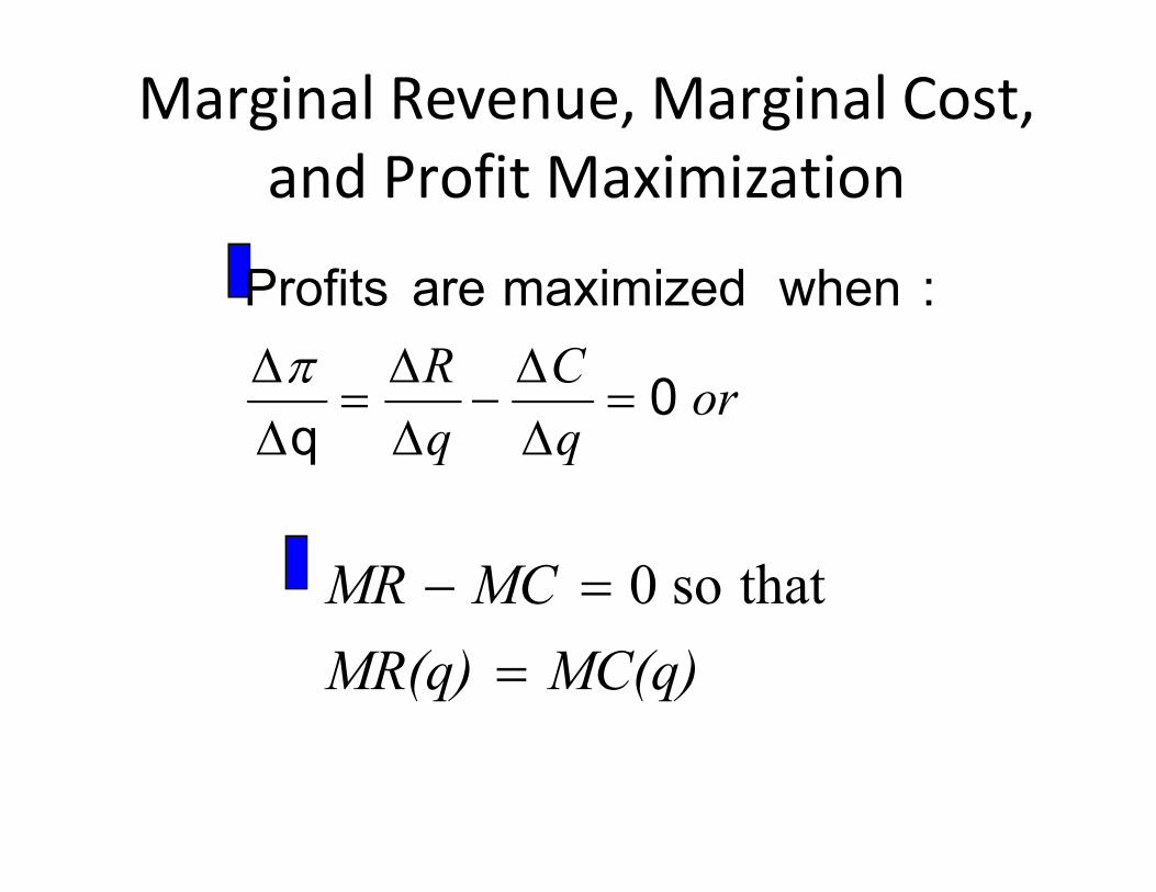
Marginal Revenue, Marginal Cost,and Profit Maximization
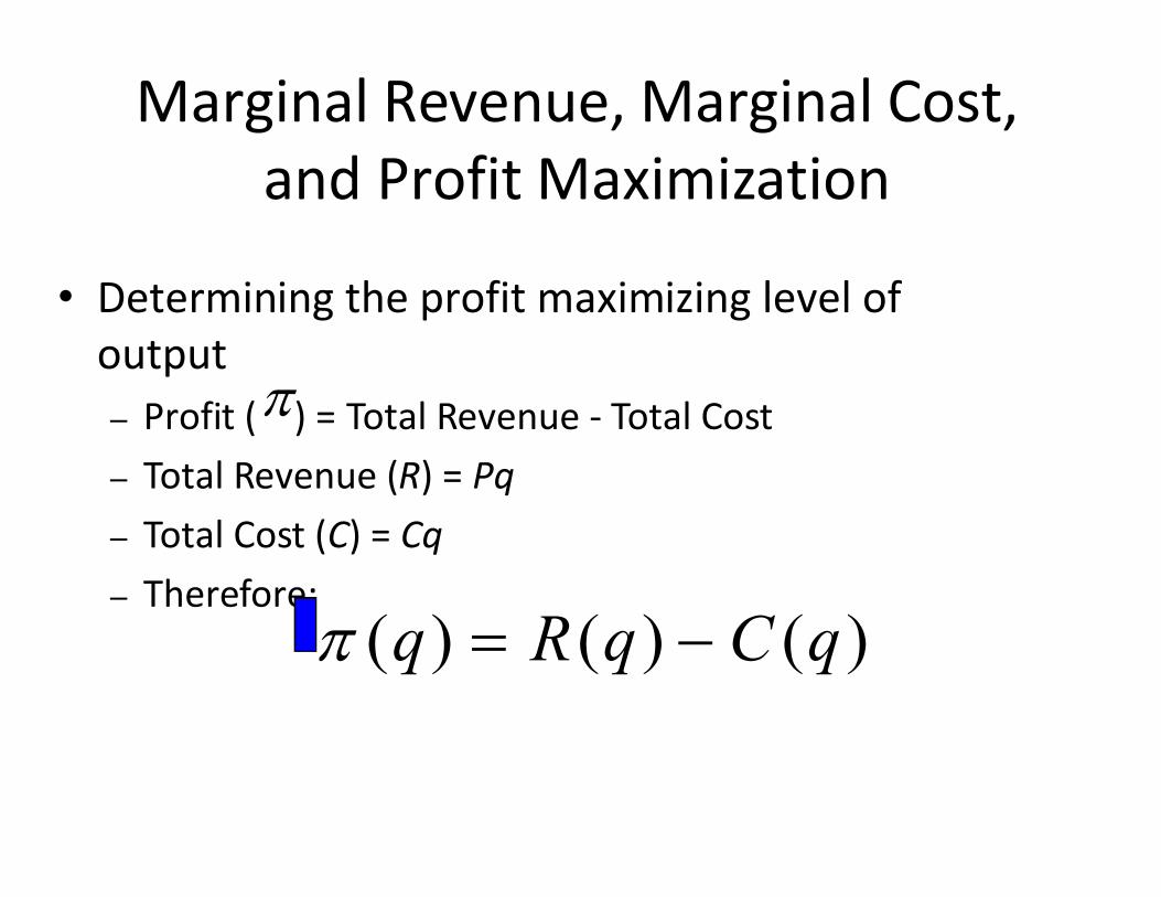
• Determining the profit maximizing level of output– Profit ( ) = Total Revenue - Total Cost– Total Revenue (R) = Pq– Total Cost (C) = Cq– Therefore:
)()()( qCqRq
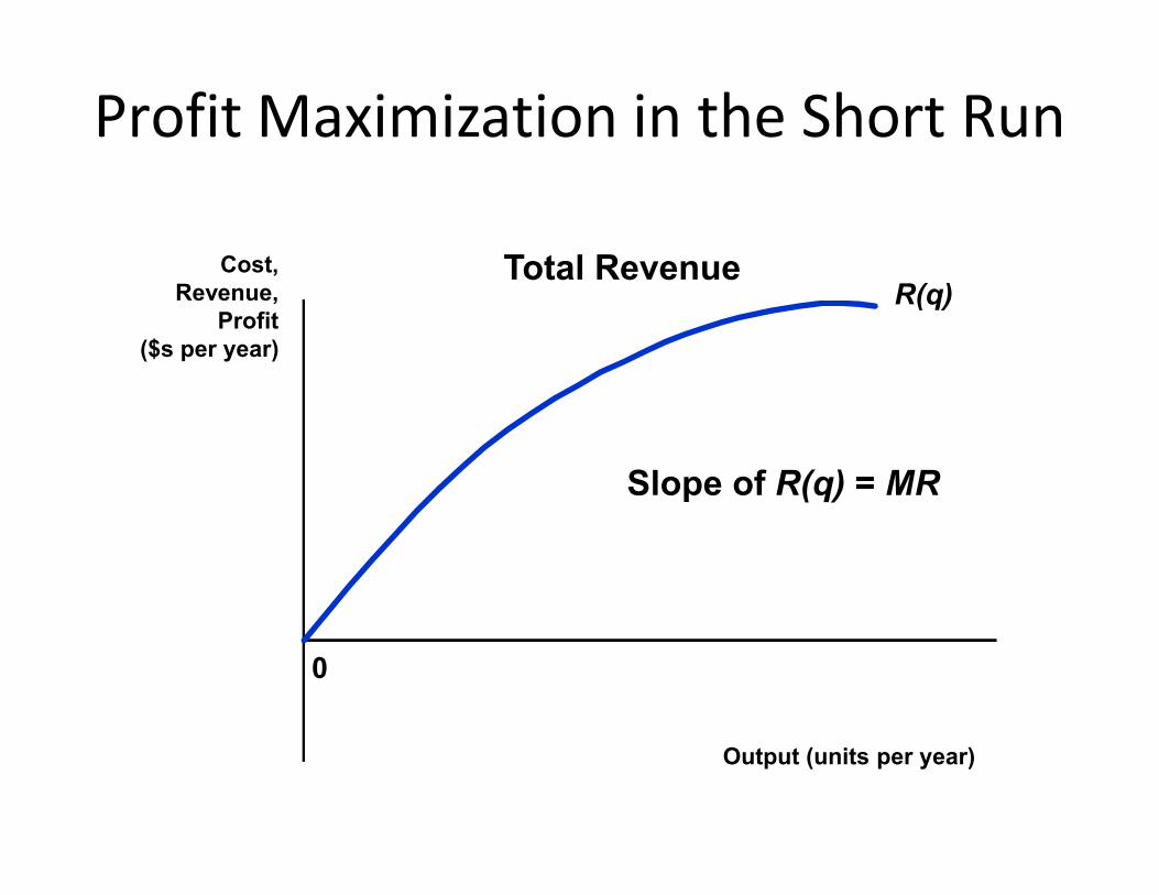
Profit Maximization in the Short Run
Cost,Revenue,
Profit($s per year)
R(q)Total Revenue
0
Output (units per year)
Slope of R(q) = MR
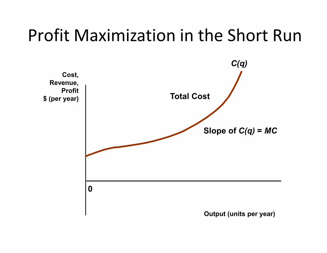
Cost,Revenue,
Profit$ (per year)
Profit Maximization in the Short RunC(q)
Total Cost
Slope of C(q) = MC
0
Output (units per year)
Slope of C(q) = MC
Marginal Revenue and Marginal Cost
• Marginal revenue is the additional revenue from producing one more unit of output.
• Marginal cost is the additional cost from Marginal cost is the additional cost from producing one more unit of output.
Marginal Revenue, Marginal Cost,and Profit Maximization
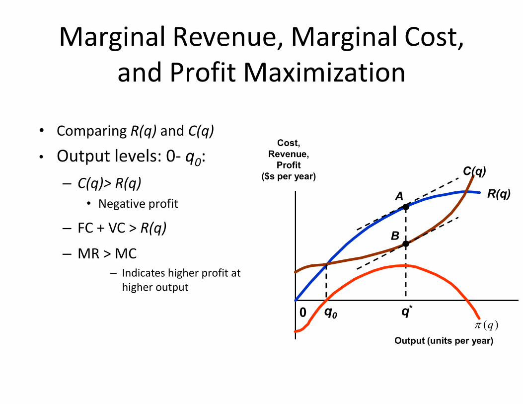
• Comparing R(q) and C(q)
• Output levels: 0- q0: – C(q)> R(q)
• Negative profit
Cost,Revenue,
Profit($s per year)
R(q)
C(q)
A• Negative profit
– FC + VC > R(q)
– MR > MC– Indicates higher profit at
higher output
0
Output (units per year)
A
B
q0 q*
)(q
Marginal Revenue, Marginal Cost,and Profit Maximization
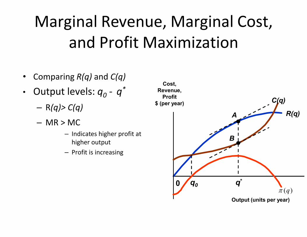
• Comparing R(q) and C(q)
• Output levels: q0 - q*
– R(q)> C(q)
– MR > MCR(q)
Cost,Revenue,
Profit$ (per year) C(q)
A– MR > MC
– Indicates higher profit at higher output
– Profit is increasing
0
Output (units per year)
A
B
q0 q*
)(q
Marginal Revenue, Marginal Cost,and Profit Maximization
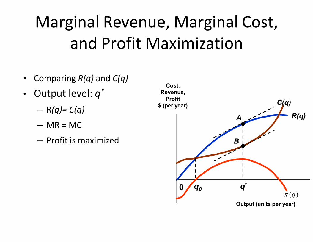
• Comparing R(q) and C(q)
• Output level: q*
– R(q)= C(q)
– MR = MCR(q)
Cost,Revenue,
Profit$ (per year) C(q)
A– MR = MC
– Profit is maximized
0
Output (units per year)
A
B
q0 q*
)(q
Marginal Revenue, Marginal Cost,and Profit Maximization
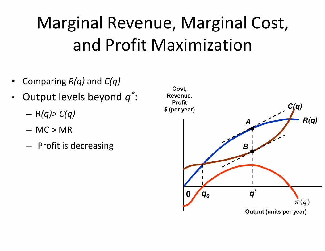
• Comparing R(q) and C(q)
• Output levels beyond q*: – R(q)> C(q)
– MC > MRR(q)
Cost,Revenue,
Profit$ (per year) C(q)
A– MC > MR
– Profit is decreasing
0
Output (units per year)
A
B
q0 q*
)(q

C-Rq
RMR
Marginal Revenue, Marginal Cost,and Profit Maximization
C-Rq
q
CMC
orq
C
q
R0
q
: whenmaximizedareProfits
Marginal Revenue, Marginal Cost,and Profit Maximization
qqq
MC(q)MR(q)
MCMR
thatso0
Demand and MR
• The Competitive Firm
– Price taker
– Market output (Q) and firm output (q)– Market output (Q) and firm output (q)
– Market demand (D) and firm demand (d)
– R(q) is a straight line
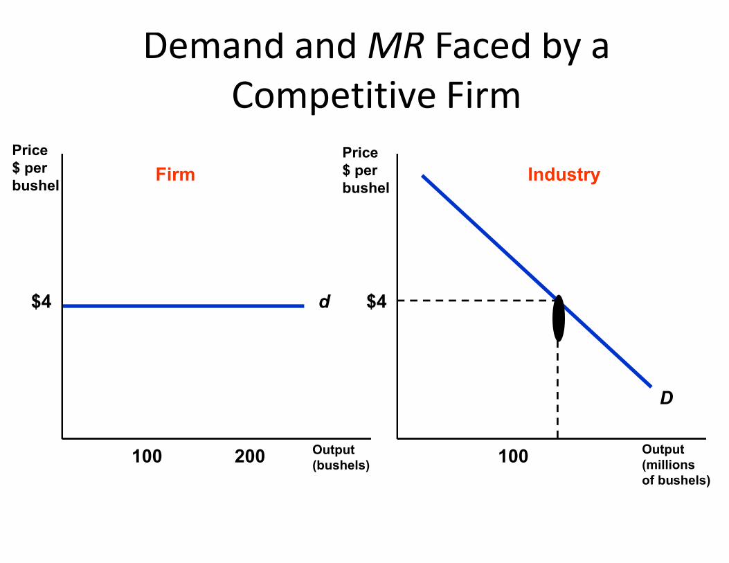
Demand and MR Faced by aCompetitive Firm
Price$ per bushel
Firm IndustryPrice$ per bushel
Output (bushels)
Output (millions of bushels)
d$4
100 200 100
D
$4
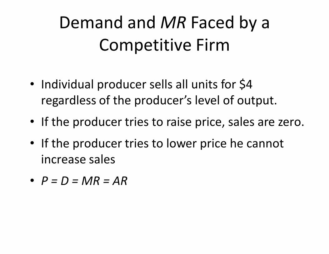
Demand and MR Faced by aCompetitive Firm
• Individual producer sells all units for $4 regardless of the producer’s level of output.
• If the producer tries to raise price, sales are zero.• If the producer tries to raise price, sales are zero.
• If the producer tries to lower price he cannot increase sales
• P = D = MR = AR
Choosing Output in the Short Run
• We will combine production and cost analysis with demand to determine output and profitability.
Lost profit forqq < q*
Lost profit forq2 > q*
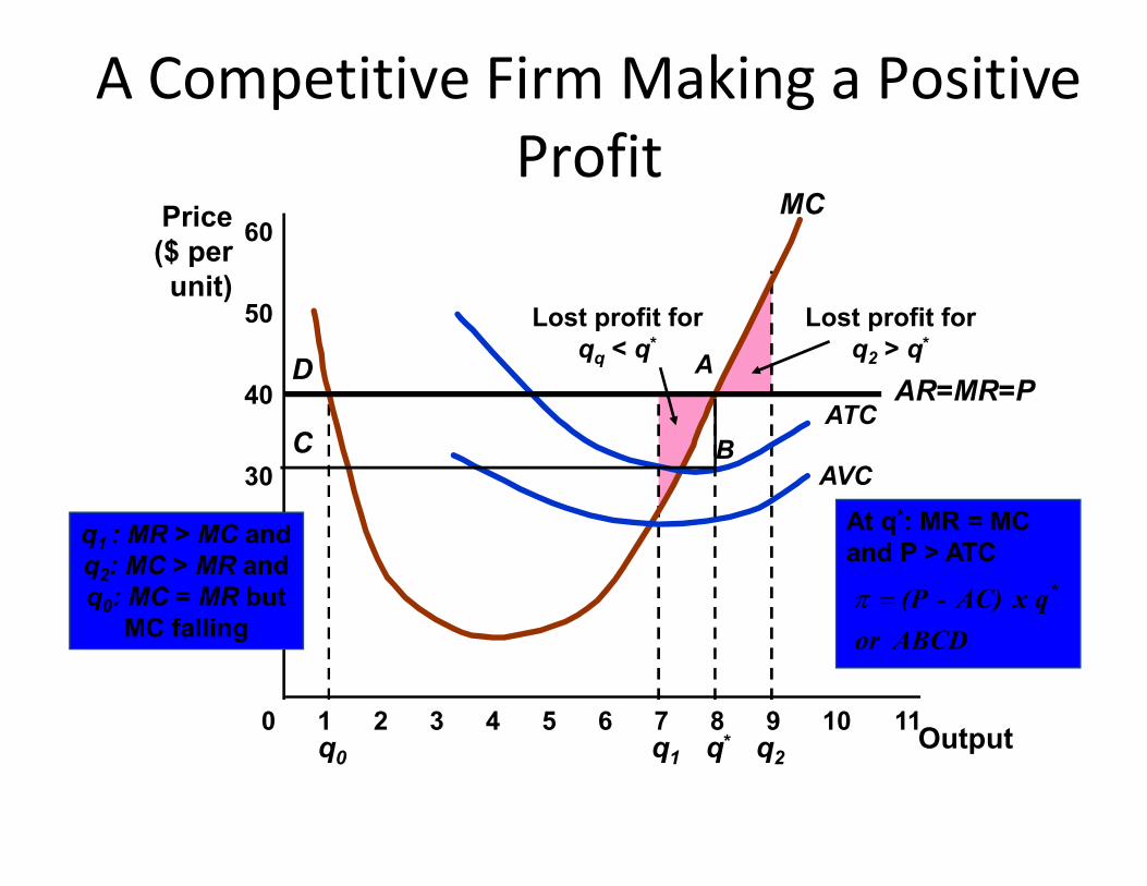
A Competitive Firm Making a PositiveProfit
40
Price($ perunit)
50
60MC
ATCAR=MR=P
D A
BC
q0 q1 q2
10
20
30
0 1 2 3 4 5 6 7 8 9 10 11
AVC
Outputq*
At q*: MR = MCand P > ATC
ABCDor
qx AC) -(P *
BC
q1 : MR > MC andq2: MC > MR andq0: MC = MR but
MC falling
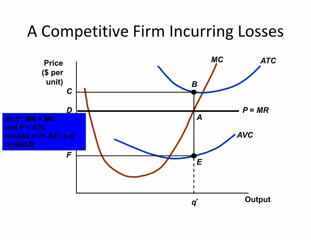
A Competitive Firm Incurring Losses
Price($ perunit)
ATCMC
P = MR
BC
AD
At q*: MR = MC
Output
AVC
q*
F
A
E
At q*: MR = MCand P < ATCLosses = (P- AC) x q*
or ABCD
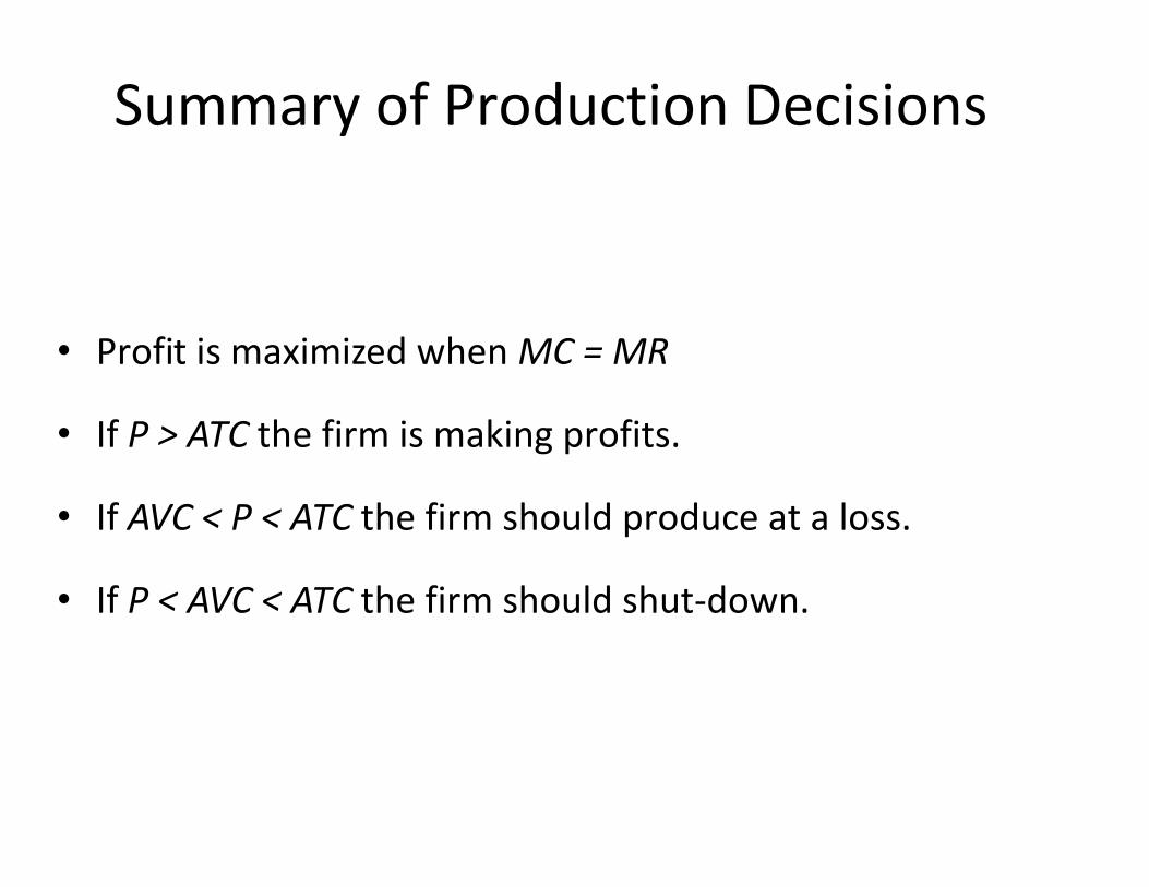
Summary of Production Decisions
• Profit is maximized when MC = MR
• If P > ATC the firm is making profits.• If P > ATC the firm is making profits.
• If AVC < P < ATC the firm should produce at a loss.
• If P < AVC < ATC the firm should shut-down.
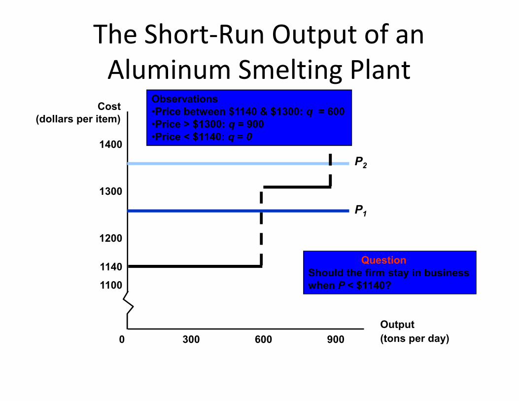
The Short-Run Output of anAluminum Smelting Plant
Cost(dollars per item)
1300
1400
P2
Observations•Price between $1140 & $1300: q = 600•Price > $1300: q = 900•Price < $1140: q = 0
Output (tons per day)300 600 9000
1100
1200
1140
P1
QuestionShould the firm stay in businesswhen P < $1140?
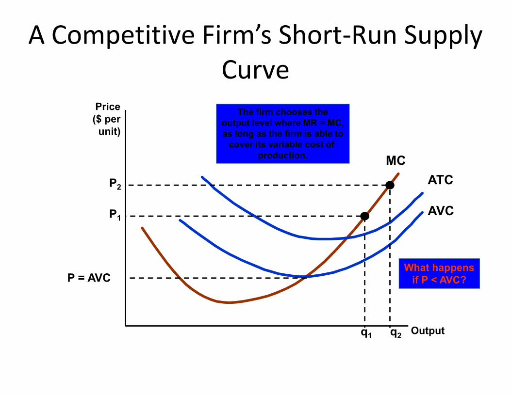
A Competitive Firm’s Short-Run SupplyCurve
Price($ per
unit)
MC
ATCP2
The firm chooses theoutput level where MR = MC,as long as the firm is able to
cover its variable cost of production.
Output
AVC
P = AVCWhat happens
if P < AVC?
q2
P1
q1
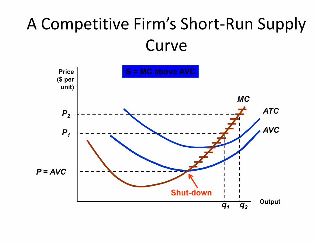
Price($ per
unit)
MC
ATCP2
S = MC above AVC
A Competitive Firm’s Short-Run SupplyCurve
Output
AVC
P = AVC
P1
q1 q2
Shut-down
A Competitive Firm’s Short-Run SupplyCurve
• Supply is upward sloping due to diminishing returns.• Higher price compensates the firm for higher cost of
additional output and increases total profit because it applies to all units.applies to all units.
• When the price of a firm’s input changes, the firm changes its output level, so that the marginal cost of production remains equal to the price.
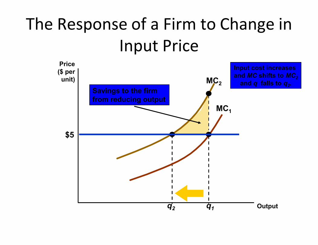
MC2
Input cost increases and MC shifts to MC2
and q falls to q2.
MC1
The Response of a Firm to Change inInput Price
Price($ per
unit)
Savings to the firmfrom reducing output
q2 q1 Output
$5

The Short-Run Production ofPetroleum Products
Cost($ per
barrel)
26
27 SMC
The MC of producinga mix of petroleum products
from crude oil increasessharply at several levelsof output as the refinery
shifts from one processingunit to another.
Output(barrels/day)
8,000 9,000 10,000 11,000
23
24
25How much wouldbe produced if
P = $23? P = $24-$25?
MC3
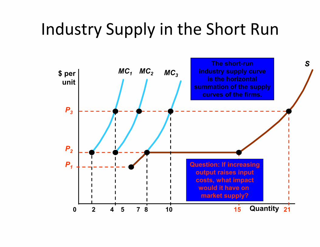
Industry Supply in the Short Run
$ perunit
MC1
SSThe short-runindustry supply curve
is the horizontalsummation of the supply
curves of the firms.
MC2
P3
0 2 4 8 105 7 15 21Quantity
P1
P2
Question: If increasingoutput raises inputcosts, what impactwould it have on market supply?
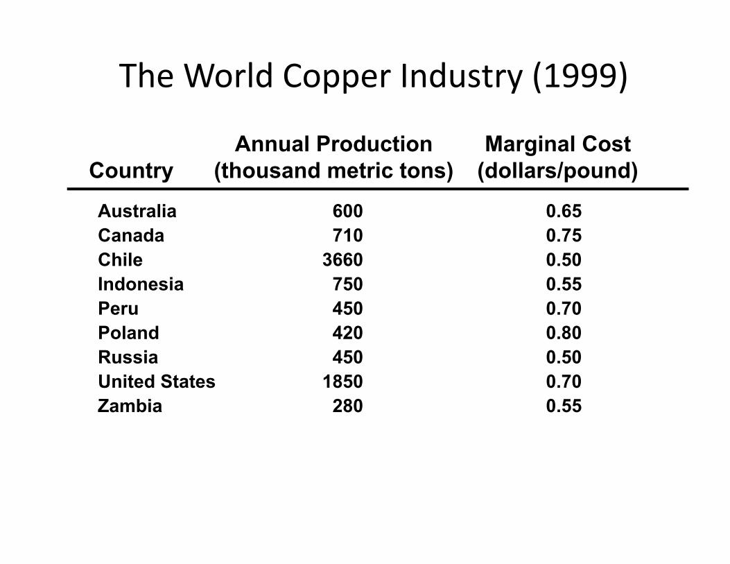
The World Copper Industry (1999)
Annual Production Marginal CostCountry (thousand metric tons) (dollars/pound)
Australia 600 0.65Canada 710 0.75Chile 3660 0.50Indonesia 750 0.55Indonesia 750 0.55Peru 450 0.70Poland 420 0.80Russia 450 0.50United States 1850 0.70Zambia 280 0.55

The Short-Run World Supply ofCopper
Price($ per pound)
0.80
0.90
MC ,MC
MCCa
MCPo
Production (thousand metric tons)0 2000 4000 6000 8000 10000
0.40
0.50
0.60
0.70
MCC,MCR
MCJ,MCZ
MCA
MCP,MCUS
Choosing Output in the Long Run
• In the long run, a firm can alter all its inputs, including the size of the plant.
• We assume free entry and free exit.We assume free entry and free exit.
AD
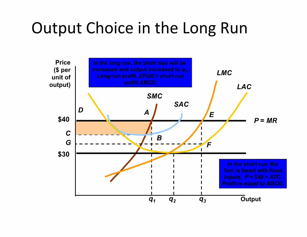
Output Choice in the Long Run
Price($ per
unit ofoutput)
P = MR$40
SACSMC
In the long run, the plant size will be increased and output increased to q3.
Long-run profit, EFGD > short runprofit ABCD.
LAC
E
LMC
q1
BC
In the short run, thefirm is faced with fixedinputs. P = $40 > ATC.
Profit is equal to ABCD.
Output
P = MR$40
q3q2
G F$30
E
Choosing Output in the Long Run
• Zero-Profit– If R > wL + rK, economic profits are positive
Long-Run Competitive Equilibrium
– If R > wL + rK, economic profits are positive– If R = wL + rK, zero economic profits, but the firm is
earning a normal rate of return; indicating the industry is competitive
– If R < wL + rK, consider going out of business
Choosing Output in the Long Run
• Entry and Exit– The long-run response to short-run profits is to
Long-Run Competitive Equilibrium
– The long-run response to short-run profits is to increase output and profits.
– Profits will attract other producers.– More producers increase industry supply which
lowers the market price.
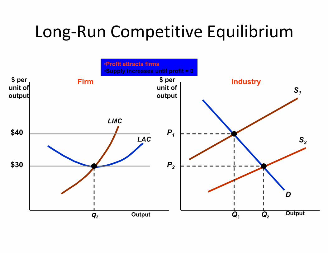
Long-Run Competitive Equilibrium
S1
$ per unit ofoutput
$ per unit ofoutput
LMC
Firm Industry
•Profit attracts firms•Supply increases until profit = 0
Output Output
$40LAC
D
S2
P1
Q1q2
$30
Q2
P2
Long-Run Competitive Equilibrium
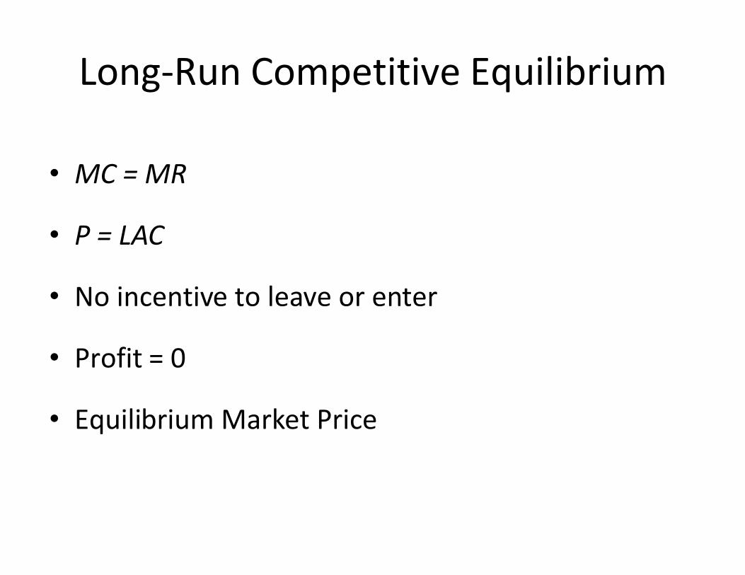
• MC = MR
• P = LAC
• No incentive to leave or enter• No incentive to leave or enter
• Profit = 0
• Equilibrium Market Price
The Industry’s Long-Run Supply Curve
• The shape of the long-run supply curve depends on the extent to which changes in industry output affect the prices the firms must pay for inputs.
• To determine long-run supply, we assume:• To determine long-run supply, we assume:
– All firms have access to the available production technology.
– Output is increased by using more inputs, not by invention.
– The market for inputs does not change with expansions and contractions of the industry.
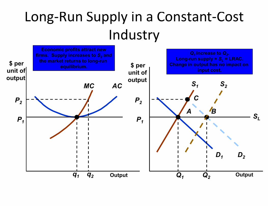
Long-Run Supply in a Constant-CostIndustry
ACMC S1
CP2P2
S2
Economic profits attract newfirms. Supply increases to S2 and
the market returns to long-run equilibrium. $ per
unit ofoutput
Q1 increase to Q2.Long-run supply = SL = LRAC.
Change in output has no impact on input cost.
$ per unit ofoutput
AP1 P1
q1
D1
Q1
D2
P2P2
q2
B
Q2Output Output
SL
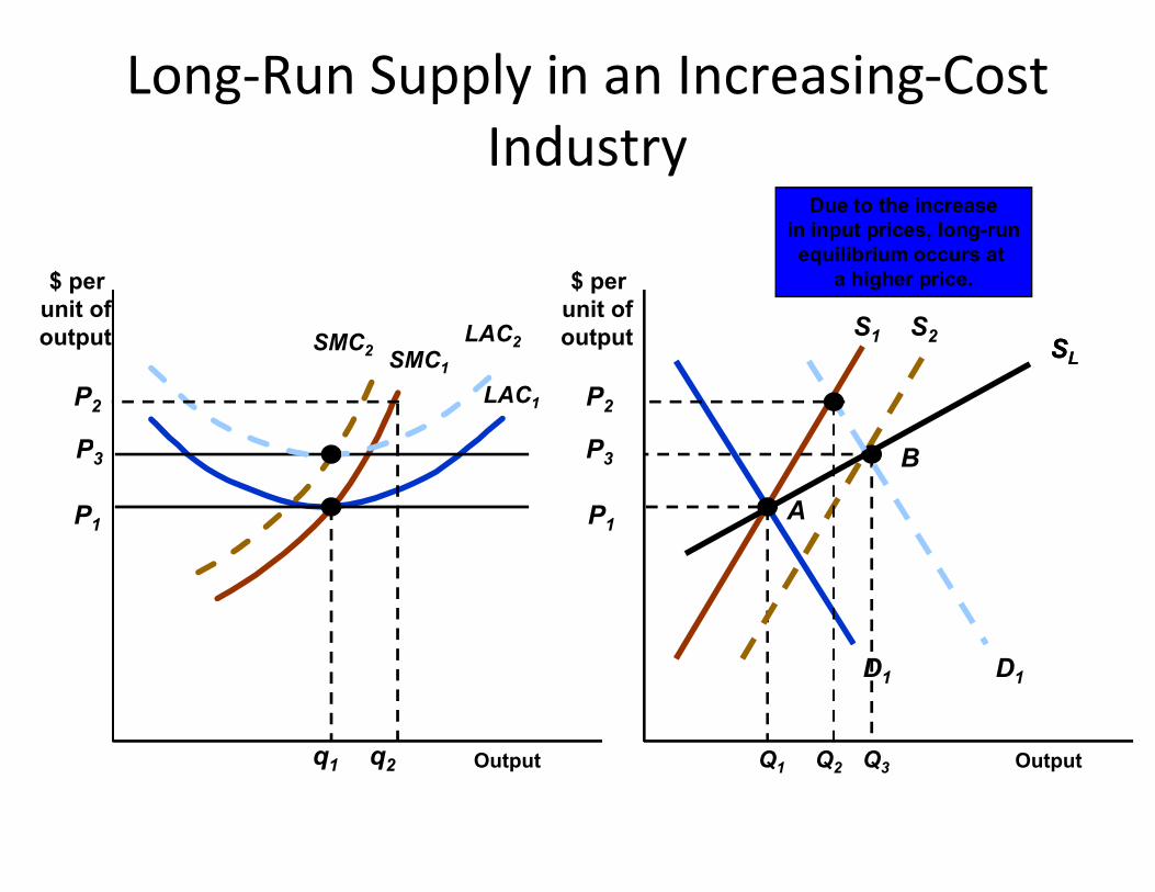
Long-Run Supply in an Increasing-Cost Industry
$ per unit ofoutput
$ per unit ofoutput S1
LAC1
SMC1SSLL
P
SMC2
Due to the increasein input prices, long-runequilibrium occurs at
a higher price.
LAC2
B
S2
P
P2 P2
Output Output
D1
P1 P1
q1 Q1
A
P3 BP3
Q3q2
D1
Q2

Long-Run Supply in an Decreasing-Cost Industry
S2
SMC2
Due to the decreasein input prices, long-runequilibrium occurs at
a lower price.$ per unit ofoutput
$ per unit ofoutput
SMC1
S1
LAC1
P2 P2
B
SL
P3
Q3
P3
LAC2
Output Output
P1P1
A
D1
Q1q1 Q2q2
P2 P2
D2
Long-Run Supply
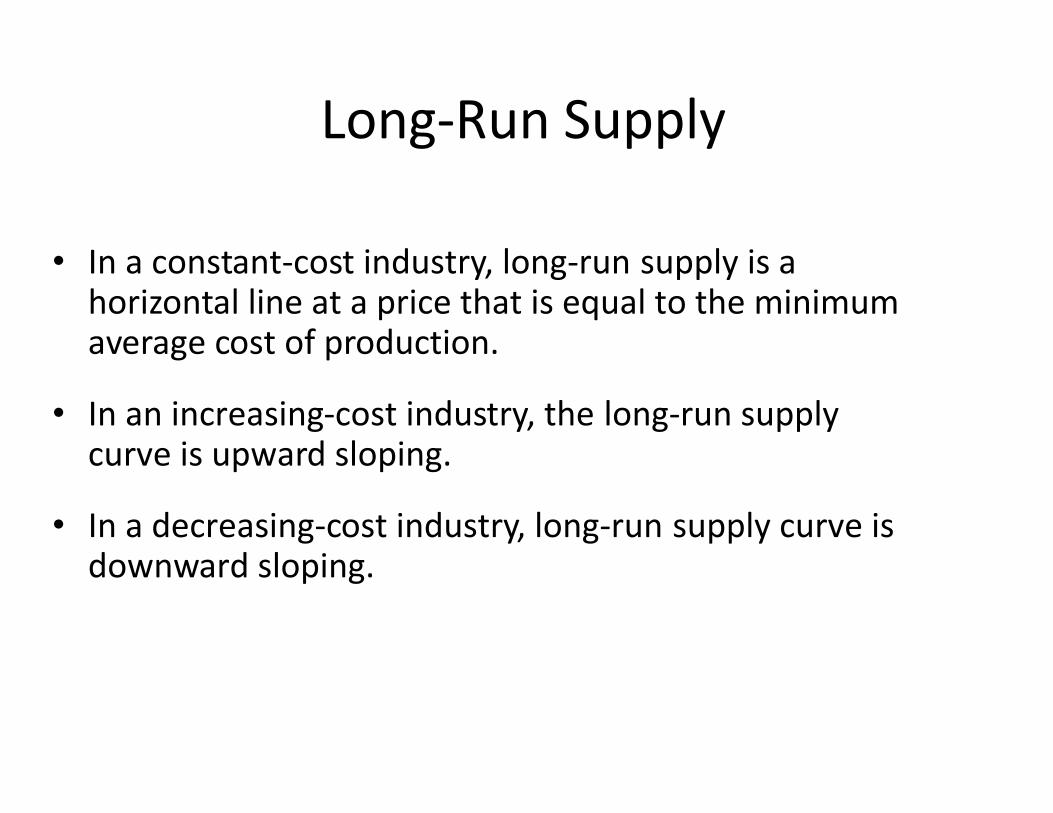
• In a constant-cost industry, long-run supply is a horizontal line at a price that is equal to the minimum average cost of production.
• In an increasing-cost industry, the long-run supply • In an increasing-cost industry, the long-run supply curve is upward sloping.
• In a decreasing-cost industry, long-run supply curve is downward sloping.
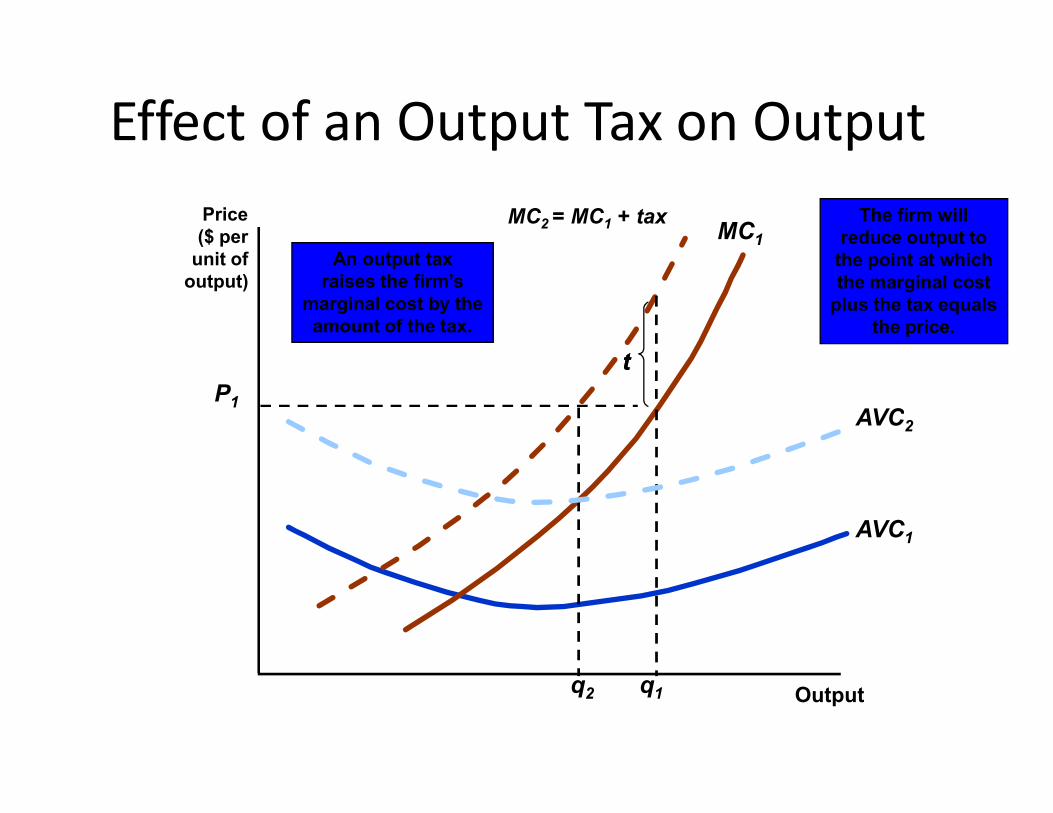
Effect of an Output Tax on OutputPrice($ per
unit ofoutput)
MC1
P1
The firm willreduce output to
the point at whichthe marginal cost
plus the tax equalsthe price.
tt
MC2 = MC1 + tax
AVC
An output taxraises the firm’s
marginal cost by theamount of the tax.
Output
AVC1
P1
q1q2
AVC2

Effect of an Output Tax on OutputPrice($ per
unit ofoutput) SS1
P
SS2 = S1 + t
t
Output
DD
P1
Q1
P2
Q2
t
Tax shifts S1 to S2 andoutput falls to Q2. Price
increases to P2.
Summary• The managers of firms can operate in accordance with a
complex set of objectives and under various constraints.
• A competitive market makes its output choice under the assumption that the demand for its own output is horizontal.
• In the short run, a competitive firm maximizes its profit by choosing an output at which price is equal to (short-run) marginal cost.
• The short-run market supply curve is the horizontal summation of the supply curves of the firms in an industry.
Summary
• In the long-run, profit-maximizing competitive firms choose the output at which price is equal to long-run marginal cost.
• The long-run supply curve for a firm can be horizontal, upward sloping, or downward sloping.

Analysis of competitive marketsAnalysis of competitive markets

Topics to be Discussed• Evaluating the Gains and Losses from Government Policies-
-Consumer and Producer Surplus
• The Efficiency of a Competitive Market
• Minimum Prices• Minimum Prices
• Price Supports and Production Quotas
• Import Quotas and Tariffs
• The Impact of a Tax or Subsidy
Consumer and Producer Surplus
• Consumer surplus is the total benefit or value that consumers receive beyond what they pay for the good.
• Producer surplus is the total benefit or revenue • Producer surplus is the total benefit or revenue that producers receive beyond what it cost to produce a good.

Consumer and Producer Surplus
ConsumerSurplus
Price
S
10
7 Between 0 and Q0
consumers A and B
ProducerSurplus
Between 0 and Q0
producers receive a net gain from
selling each product--producer surplus.
Quantity0
D
5
Q0
Consumer CConsumer BConsumer A
consumers A and Breceive a net gain from
buying the product--consumer surplus
Consumer and Producer Surplus
• To determine the welfare effect of a government policy we can measure the gain or loss in consumer and producer surplus.
• Welfare Effects
– Gains and losses caused by government intervention in the market.
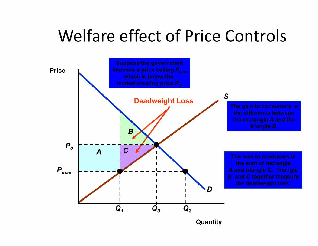
The gain to consumers isthe difference betweenthe rectangle A and the
Deadweight Loss
Welfare effect of Price Controls
Price
S
Suppose the governmentimposes a price ceiling Pmax
which is below the market-clearing price P0.
The loss to producers isthe sum of rectangle
A and triangle C. TriangleB and C together measure
the deadweight loss.
B
A C
triangle B.
Quantity
D
P0
Q0
Pmax
Q1 Q2

Welfare effect of Price Controls
• The total loss is equal to area B + C.• The total change in surplus =
(A - B) + (-A - C) = -B - C
The deadweight loss is the inefficiency of the price • The deadweight loss is the inefficiency of the price controls.– The loss of producer surplus exceeds the gain from
consumer surplus.
Welfare effect of Price Controls
• Consumers can experience a net loss in consumer surplus when the demand is sufficiently inelastic
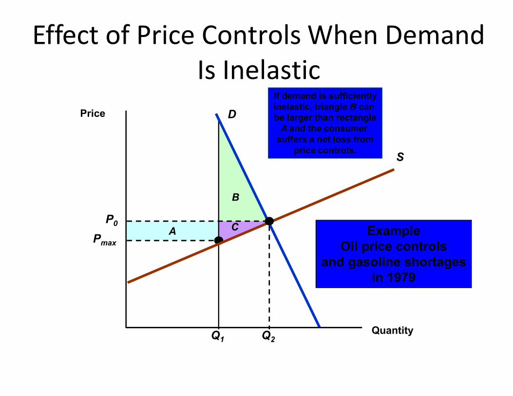
B
If demand is sufficientlyinelastic, triangle B can be larger than rectangle
A and the consumer suffers a net loss from
price controls.S
D
Effect of Price Controls When DemandIs Inelastic
Price
B
APmax
C
Q1
ExampleOil price controls
and gasoline shortagesin 1979
Quantity
P0
Q2

Price Controls and Natural Gas Shortages
• 1975 U.S.price controls created a shortage of natural gas.
• What was the deadweight loss?What was the deadweight loss?
Price Controls and Natural Gas Shortages
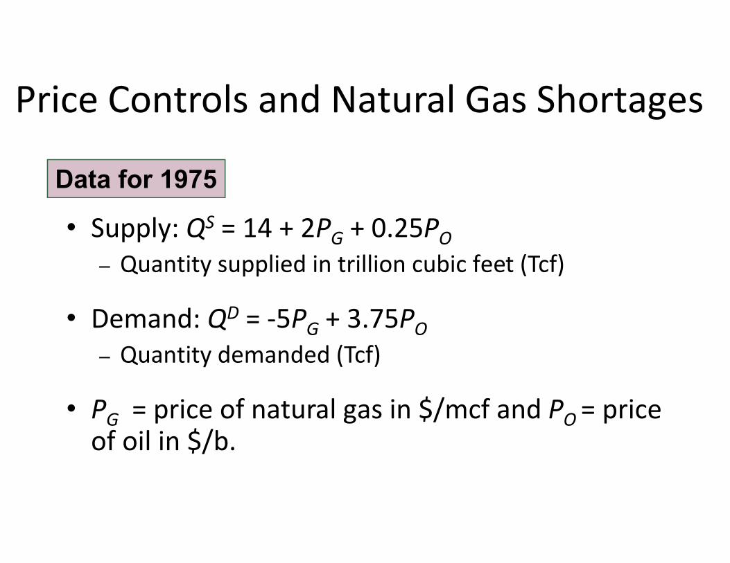
• Supply: QS = 14 + 2PG + 0.25PO– Quantity supplied in trillion cubic feet (Tcf)
Data for 1975
• Demand: QD = -5PG + 3.75PO– Quantity demanded (Tcf)
• PG = price of natural gas in $/mcf and PO = price of oil in $/b.

Price Controls and Natural Gas Shortages
• PO = $8/b
• Equilibrium P = $2/mcf and Q = 20 Tcf
Data for 1975
• Equilibrium PG = $2/mcf and Q = 20 Tcf
• Price ceiling set at $1
• This information can be seen graphically:
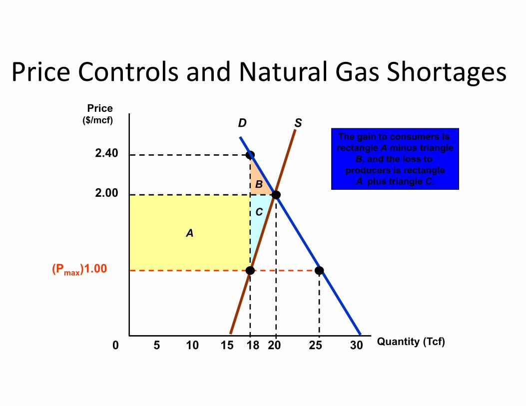
B
2.40
The gain to consumers is rectangle A minus triangle
B, and the loss to producers is rectangle
A plus triangle C.
SD
2.00
Price($/mcf)
Price Controls and Natural Gas Shortages
A
C
Quantity (Tcf)0 5 10 15 20 25 3018
(Pmax)1.00
Price Controls and Natural Gas Shortages
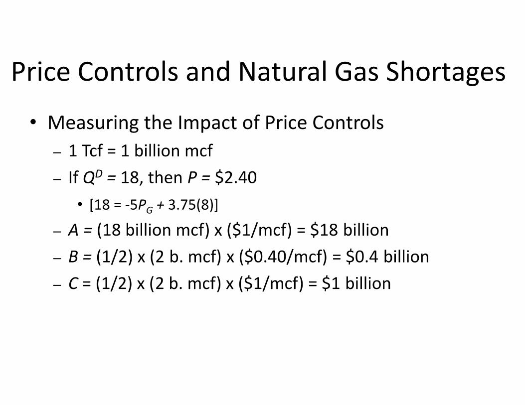
• Measuring the Impact of Price Controls– 1 Tcf = 1 billion mcf– If QD = 18, then P = $2.40
• [18 = -5P + 3.75(8)]• [18 = -5PG + 3.75(8)]
– A = (18 billion mcf) x ($1/mcf) = $18 billion– B = (1/2) x (2 b. mcf) x ($0.40/mcf) = $0.4 billion– C = (1/2) x (2 b. mcf) x ($1/mcf) = $1 billion
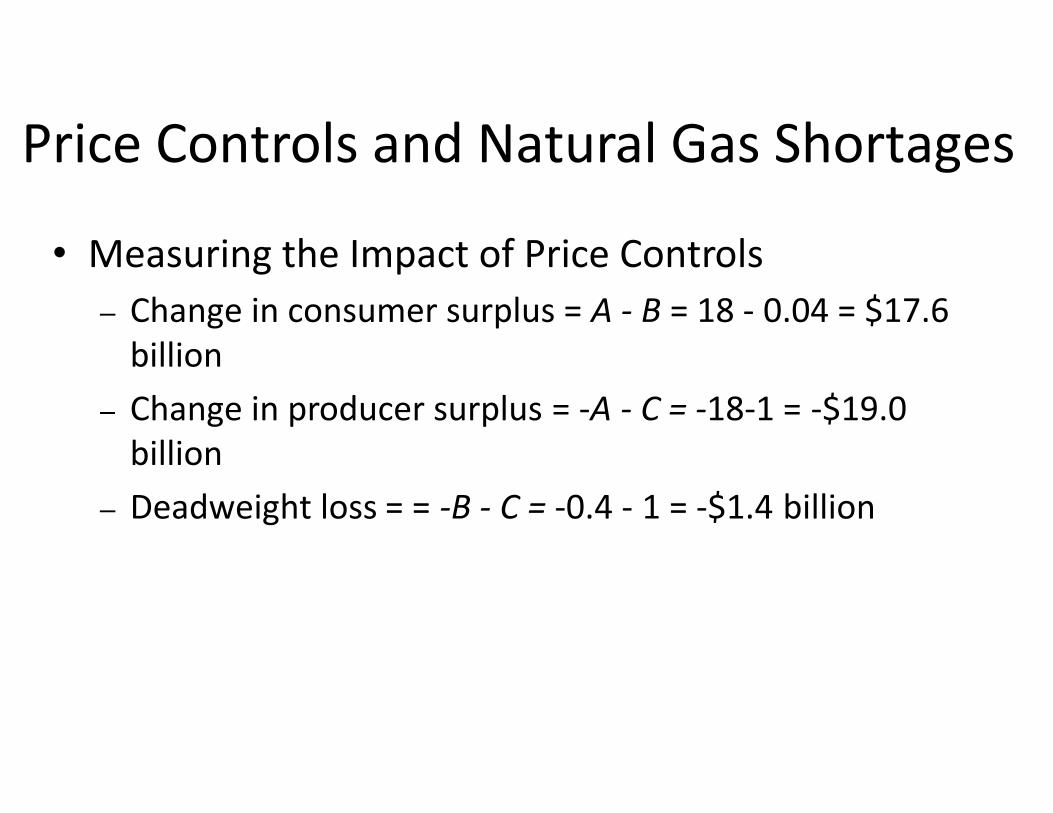
Price Controls and Natural Gas Shortages
• Measuring the Impact of Price Controls– Change in consumer surplus = A - B = 18 - 0.04 = $17.6
billion– Change in producer surplus = -A - C = -18-1 = -$19.0 – Change in producer surplus = -A - C = -18-1 = -$19.0
billion– Deadweight loss = = -B - C = -0.4 - 1 = -$1.4 billion
Market failure and governmentintervention
• When do competitive markets generate an inefficient allocation of resources or market failure?
– Externalities (Costs or benefits that do not show up as part of the market price (e.g. pollution))
– Lack of Information (Imperfect information prevents consumers from making utility-maximizing decisions.)
• Government intervention in these markets can increase efficiency.
• Government intervention without a market failure creates inefficiency or deadweight loss
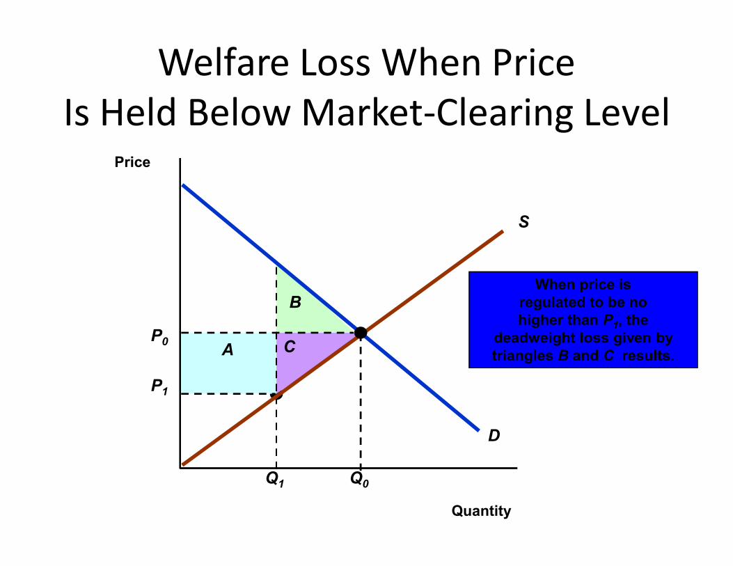
When price is
Welfare Loss When PriceIs Held Below Market-Clearing Level
Price
S
P1
Q1
A
B
C
When price is regulated to be no higher than P1, the
deadweight loss given by triangles B and C results.
Quantity
D
P0
Q0
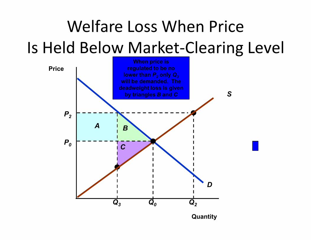
P2
When price is regulated to be no
lower than P2 only Q3
will be demanded. Thedeadweight loss is given
by triangles B and C
Price
S
Welfare Loss When PriceIs Held Below Market-Clearing Level
Q3
A B
C
Q2
Quantity
D
P0
Q0

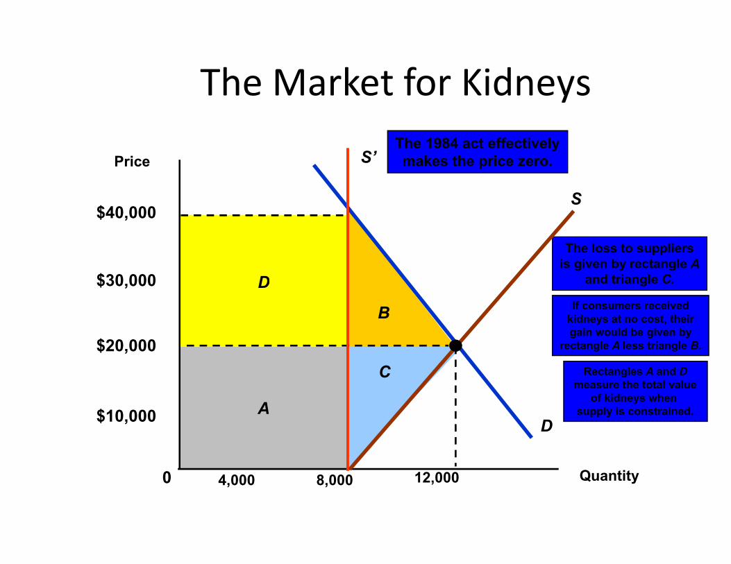
The Market for Human Kidneys
• The 1984 U.S. National Organ Transplantation Act prohibits the sale of organs for transplantation.
• Analyzing the Impact of the Act– Supply: QS = 8,000 + 0.2P
• If P = $20,000, Q = 12,000
– Demand: QD = 16,000 - 0.2P
D
The loss to suppliersis given by rectangle A
and triangle C.
The Market for Kidneys
Price
$30,000
$40,000S
S’The 1984 act effectivelymakes the price zero.
D
Rectangles A and Dmeasure the total value
of kidneys when supply is constrained.A
C
and triangle C.
Quantity8,0004,0000
$10,000
$30,000
B If consumers receivedkidneys at no cost, theirgain would be given by
rectangle A less triangle B.
D
12,000
$20,000
The Market for Human Kidneys
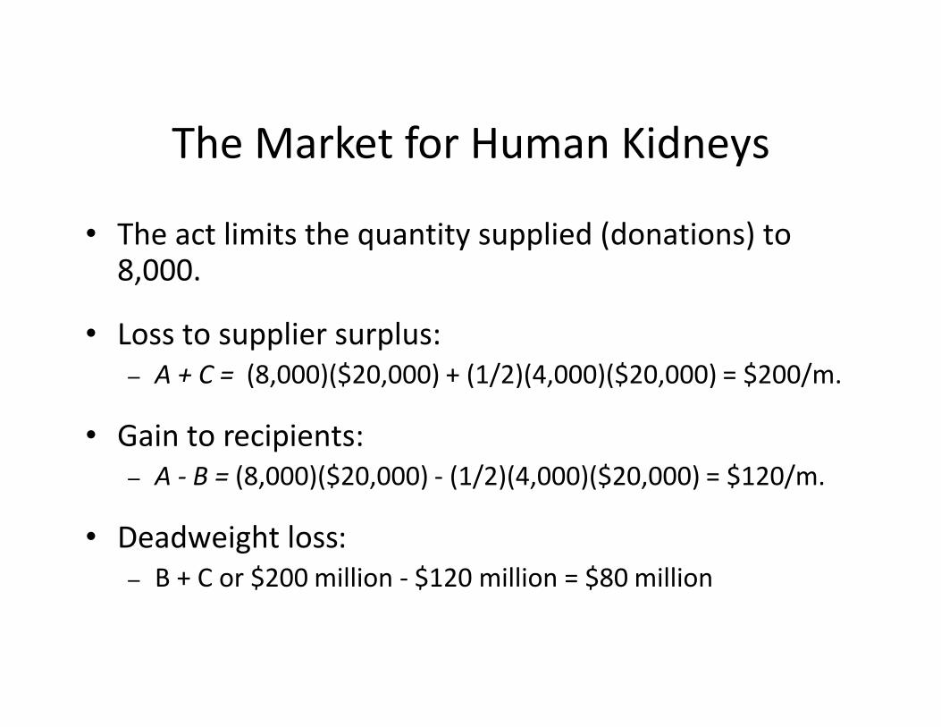
• The act limits the quantity supplied (donations) to 8,000.
• Loss to supplier surplus:A + C = (8,000)($20,000) + (1/2)(4,000)($20,000) = $200/m.– A + C = (8,000)($20,000) + (1/2)(4,000)($20,000) = $200/m.
• Gain to recipients:– A - B = (8,000)($20,000) - (1/2)(4,000)($20,000) = $120/m.
• Deadweight loss:– B + C or $200 million - $120 million = $80 million
Minimum Prices• Periodically government policy seeks to raise
prices above market-clearing levels.
• We will investigate this by looking at a price We will investigate this by looking at a price minimum (floor) and the minimum wage.
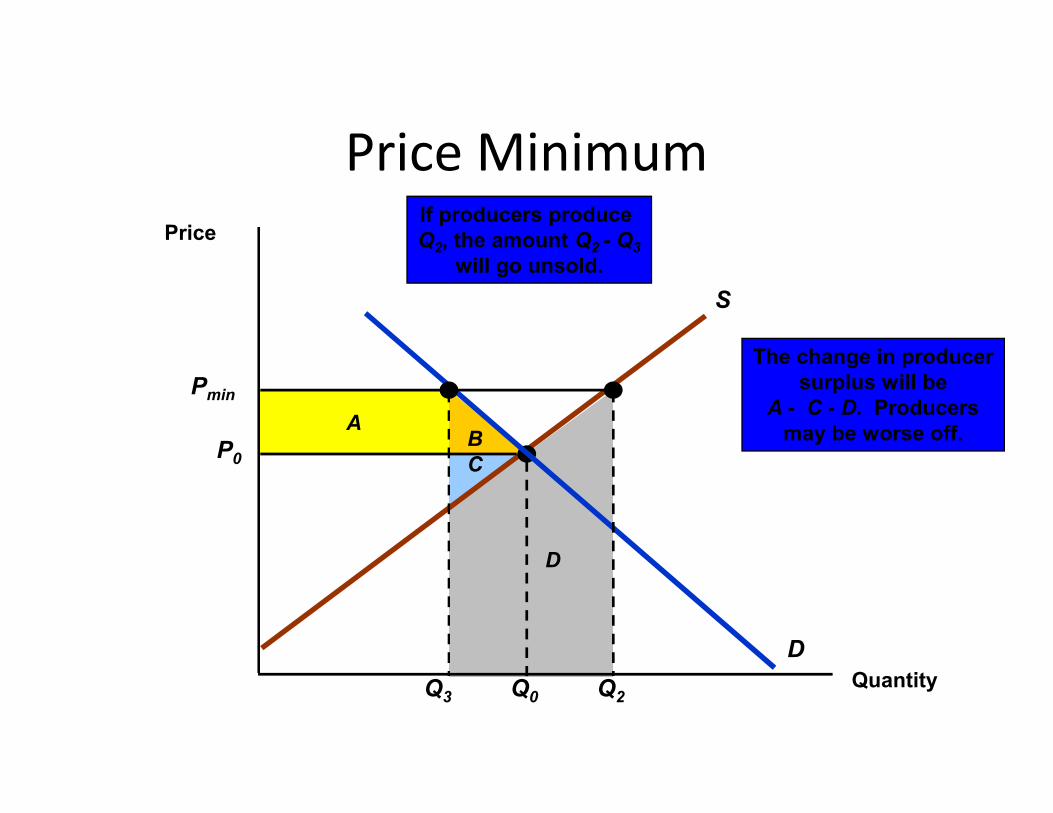
The change in producersurplus will be
A - C - D. Producers
Price MinimumPrice
S
Pmin
If producers produce Q2, the amount Q2 - Q3
will go unsold.
BA
A - C - D. Producersmay be worse off.
C
D
Quantity
D
P0
Q0Q3 Q2

wmin
Firms are not allowed topay less than wmin. This
results in unemployment.
S
The Minimum Wagew
B The deadweight lossis given by
triangles B and C.C
A
L1 L2
UnemploymentD
w0
L0L

Airline Regulation• During 1976-1981 the airline industry in the U.S.
changed dramatically.
• Deregulation lead to major changes in the industry.industry.
• Some airlines merged or went out of business as new airlines entered the industry.
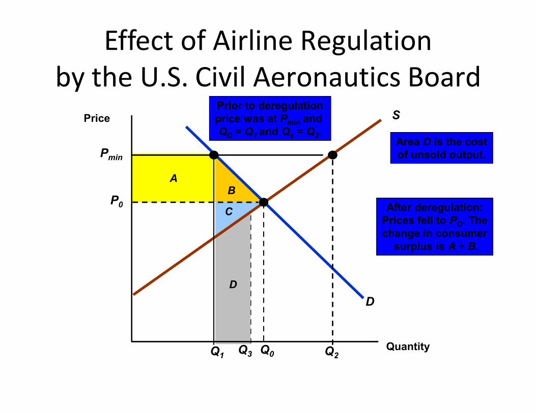
BA
C After deregulation:
Area D is the costof unsold output.
Effect of Airline Regulationby the U.S. Civil Aeronautics Board
Price S
P0
Pmin
Prior to deregulationprice was at Pmin and QD = Q1 and Qs = Q3.
C After deregulation:Prices fell to PO. Thechange in consumer
surplus is A + B.
Q3
D
Quantity
D
P0
Q0Q1 Q2
Price Supports and Production Quotas
• Much of agricultural policy is based on a system of price supports.
– This is support price is set above the equilibrium price and the government buys the surplus.and the government buys the surplus.
• This is often combined with incentives to reduce or restrict production
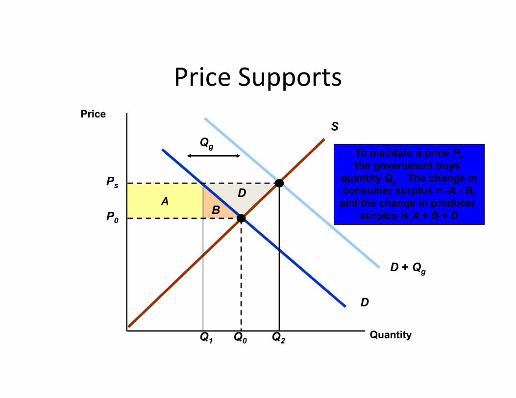
DA
To maintain a price Ps
the government buys quantity Qg . The change inconsumer surplus = -A - B,
and the change in producer
Qg
Price SupportsPrice
S
Ps
B
DA and the change in producer
surplus is A + B + D
D + Qg
Quantity
D
P0
Q0 Q2Q1

Qg
A
Price Supports
PriceS
Ps
The cost to the government is the speckled rectangle
Ps(Q2-Q1)
DTotal welfare loss
D-(Q2-Q1)ps
D + Qg
BA
Quantity
D
P0
Q0 Q2Q1
TotalWelfare
Loss
2 1 s
Production Quotas
• The government can also cause the price of a good to rise by reducing supply.
• E.g.: E.g.: – controlling entry into the taxicab market– controlling the number of liquor licenses
D
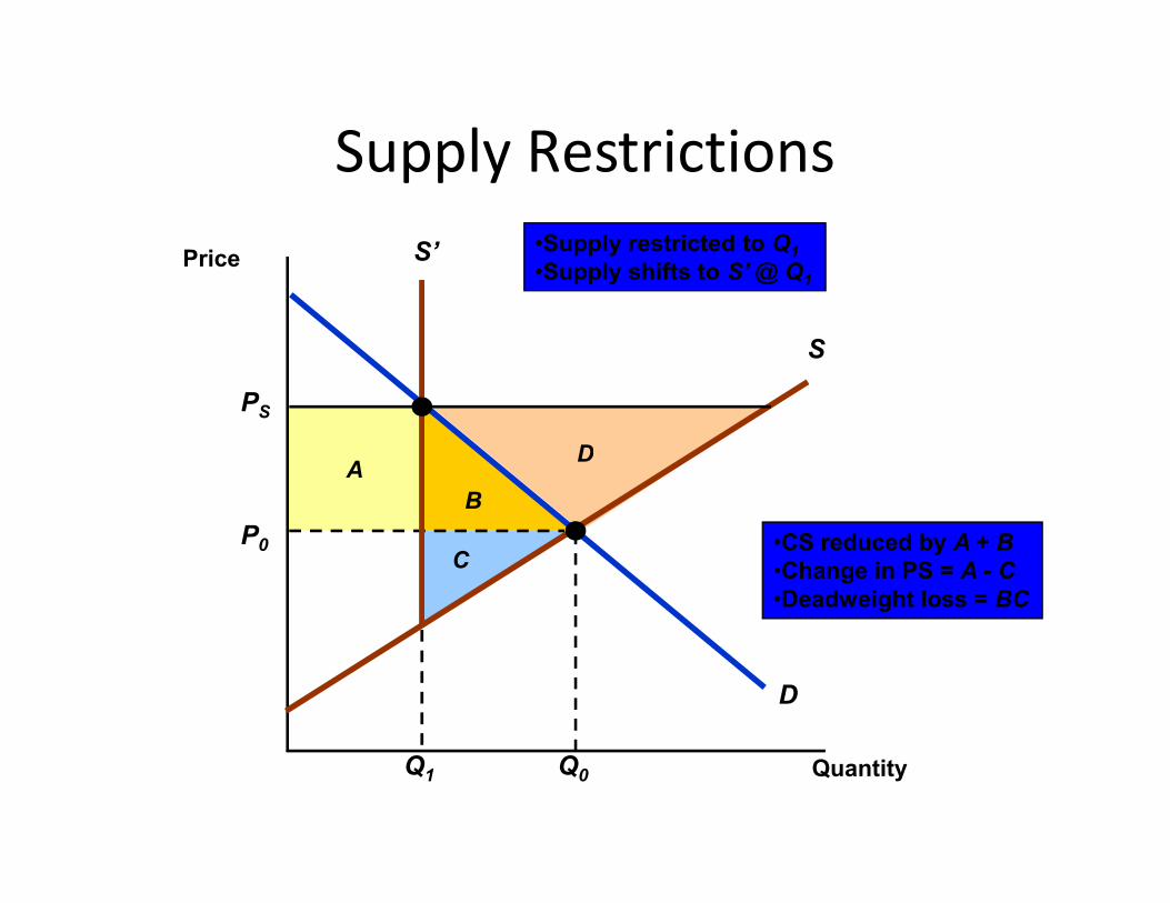
Supply RestrictionsPrice
S
PS
S’ •Supply restricted to Q1
•Supply shifts to S’ @ Q1
BA
•CS reduced by A + B•Change in PS = A - C•Deadweight loss = BC
C
D
Quantity
D
P0
Q0Q1
D
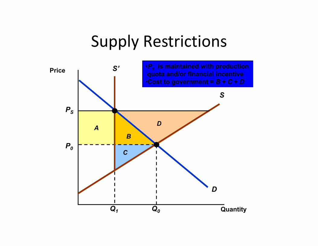
Price
S
PS
S’ •Ps is maintained with productionquota and/or financial incentive•Cost to government = B + C + D
Supply Restrictions
BA
C
D
Quantity
D
P0
Q0Q1
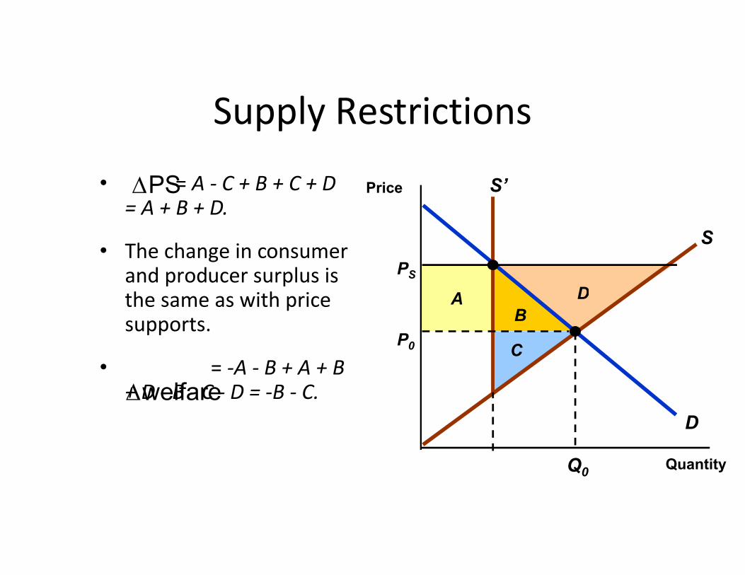
Supply Restrictions
• = A - C + B + C + D = A + B + D.
• The change in consumer and producer surplus is the same as with price
Price
PS
S
S’
D
PS
and producer surplus is the same as with price supports.
• = -A - B + A + B + D - B - C - D = -B - C.
BA
Quantity
D
P0
Q0
D
C
welfare
Import Quotas and Tariffs• Many countries use import quotas and tariffs to
keep the domestic price of a product above world levels
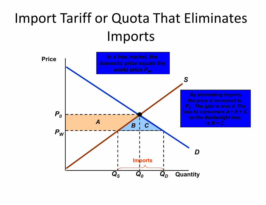
By eliminating imports,the price is increased to
Import Tariff or Quota That EliminatesImports
Price
S
In a free market, the domestic price equals the
world price PW.
QS QD
PW
Imports
AB C
the price is increased to PO. The gain is area A. The
loss to consumers A + B + C,so the deadweight loss
is B + C.
Quantity
D
P0
Q0
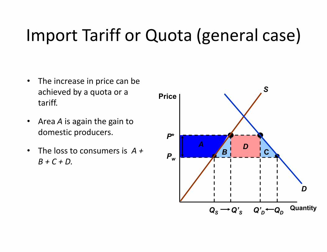
Import Tariff or Quota (general case)
• The increase in price can be achieved by a quota or a tariff.
• Area A is again the gain to
PriceS
DCB
QS QDQ’S Q’D
AP*
Pw
• Area A is again the gain to domestic producers.
• The loss to consumers is A + B + C + D.
Quantity
D

Import Tariff or Quota (general case)
• If a tariff is used the government gains D, so the net domestic product loss is B + C.
• If a quota is used instead,
SPrice
• If a quota is used instead, rectangle D becomes part of the profits of foreign producers, and the net domestic loss is B + C + D.
DCB
QS QDQ’S Q’D
AP*
Pw
Quantity
D
The Impact of a Tax or Subsidy
• The burden of a tax (or the benefit of a subsidy) falls partly on the consumer and partly on the producer.
• We will consider a specific tax which is a tax of a certain amount of money per unit sold.
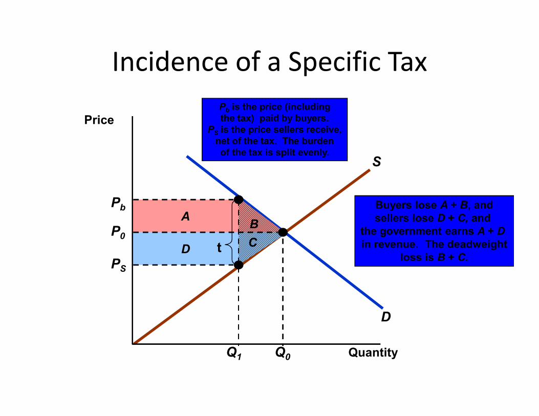
S
Buyers lose A + B, and
Incidence of a Specific Tax
Price
Pb
Pb is the price (includingthe tax) paid by buyers.
PS is the price sellers receive,net of the tax. The burdenof the tax is split evenly.
D
B
D
ABuyers lose A + B, andsellers lose D + C, and
the government earns A + D in revenue. The deadweight
loss is B + C.C
Quantity
P0
Q0Q1
PS
Pb
t
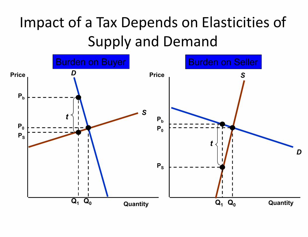
Impact of a Tax Depends on Elasticities of Supply and Demand
Price
S
D S
Pb
t P
Burden on Buyer Burden on SellerPrice
Quantity Quantity
D
Q0
P0 P0
Q0Q1
PS
t
Q1
Pb
PS
t

The Effects of a Subsidy
• A subsidy can be analyzed in much the same way as a tax.
• It can be treated as a negative tax.It can be treated as a negative tax.
• The seller’s price exceeds the buyer’s price.
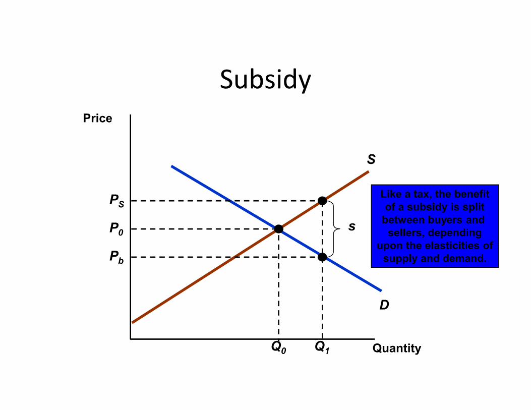
S
SubsidyPrice
PSLike a tax, the benefitof a subsidy is split
D
Quantity
P0
Q0 Q1
PS
Pb
s
of a subsidy is splitbetween buyers and
sellers, dependingupon the elasticities of
supply and demand.

Summary• Simple models of supply and demand can be used
to analyze a wide variety of government policies.
• In each case, consumer and producer surplus are In each case, consumer and producer surplus are used to evaluate the gains and losses to consumers and producers.
Summary
• When government imposes a tax or subsidy, price usually does not rise or fall by the full amount of the tax or subsidy.
• Government intervention generally leads to a • Government intervention generally leads to a deadweight loss.
• Government intervention in a competitive market is not always a bad thing.

MonopolyMonopoly

Topics to be Discussed• Monopoly
• Monopoly Power
• Sources of Monopoly Power• Sources of Monopoly Power
• The Social Costs of Monopoly Power
• Limiting Market Power

Review of Perfect Competition
• P = LMC = LRAC• Normal profits or zero economic profits in the long run• Large number of buyers and sellers• Homogenous product• Homogenous product• Perfect information• Firm is a price taker
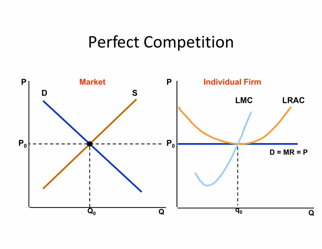
Perfect Competition
P PMarket Individual FirmD S
LRACLMC
Q QQ0
P0 P0D = MR = P
q0
Monopoly• Monopoly
1) One seller - many buyers
2) One product (no good substitutes)2) One product (no good substitutes)
3) Barriers to entry

Monopoly• The monopolist is the supply-side of the market
and has complete control over the amount offered for sale.
• Profits will be maximized at the level of output where marginal revenue equals marginal cost.
Monopoly• Finding Marginal Revenue
– As the sole producer, the monopolist works with the market demand to determine output and price.
– Assume a firm with demand:– Assume a firm with demand:• P = 6 - Q
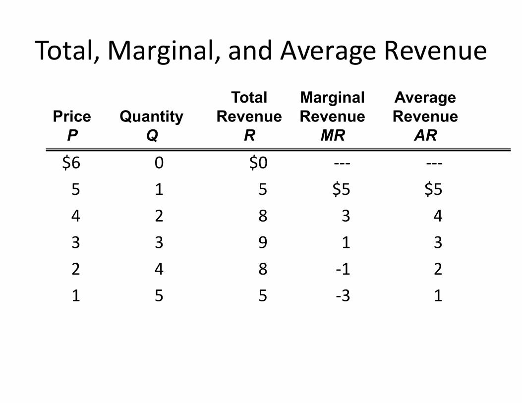
Total, Marginal, and Average Revenue
$6 0 $0 --- ---5 1 5 $5 $5
Total Marginal AveragePrice Quantity Revenue Revenue Revenue
P Q R MR AR
4 2 8 3 43 3 9 1 32 4 8 -1 21 5 5 -3 1
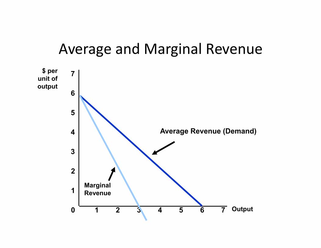
Average and Marginal Revenue$ per
unit ofoutput
5
6
7
Output0
1
2
3
1 2 3 4 5 6 7
4 Average Revenue (Demand)
MarginalRevenue
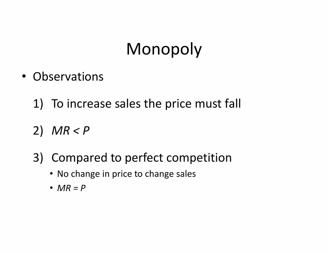
Monopoly• Observations
1) To increase sales the price must fall
2) MR < P2) MR < P
3) Compared to perfect competition• No change in price to change sales• MR = P
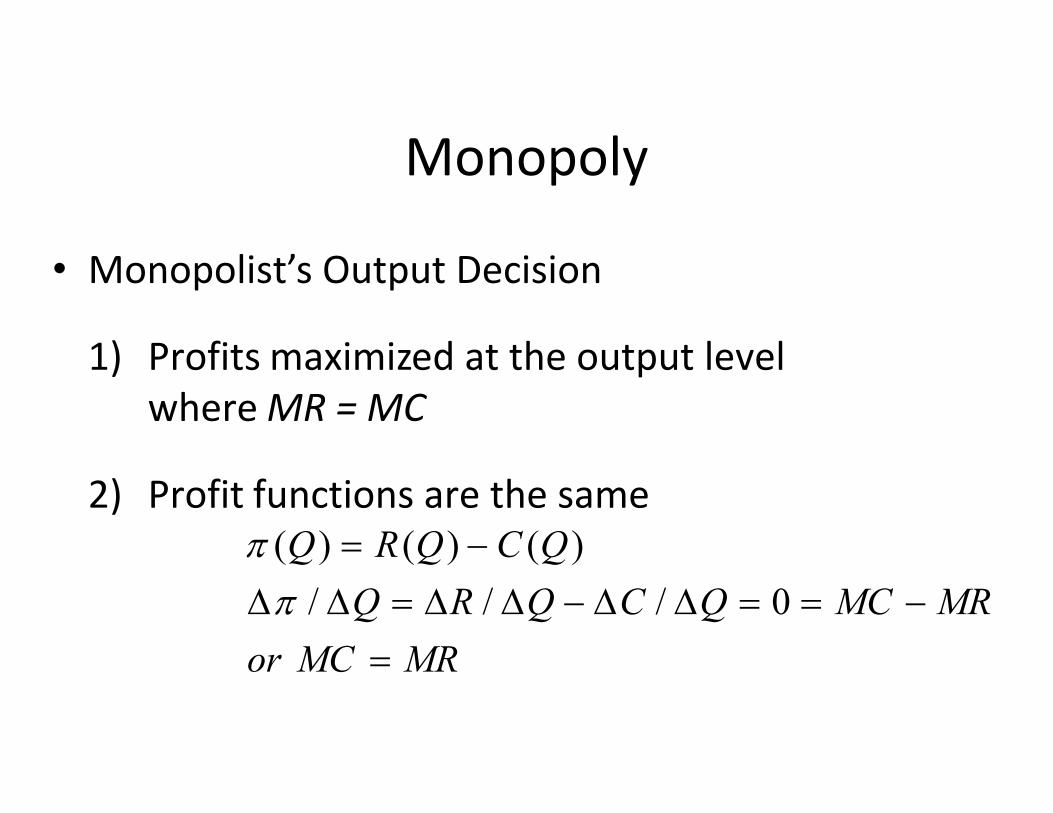
Monopoly
• Monopolist’s Output Decision
1) Profits maximized at the output level where MR = MCwhere MR = MC
2) Profit functions are the same
MRMCor
MRMCQCQRQ
QCQRQ
0///
)()()(
The monopolists output decision
• Moving to output levels below MR = MC the decrease in revenue is greater than the decrease in cost (MR > MC).decrease in cost (MR > MC).
• Moving to output levels above MR = MC the increase in cost is greater than the decrease in revenue (MR < MC)
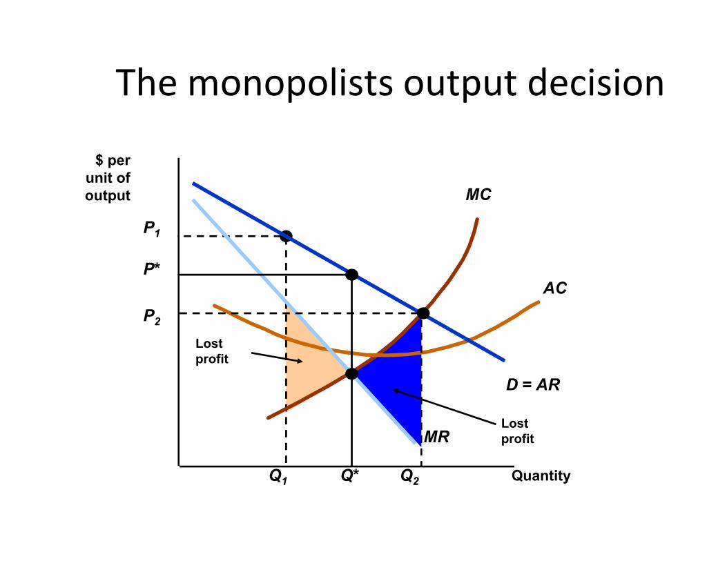
P1
MC
AC
$ perunit ofoutput
P*
The monopolists output decision
Lostprofit
Q1
Lostprofit
AC
Quantity
D = AR
MR
Q*
P2
Q2
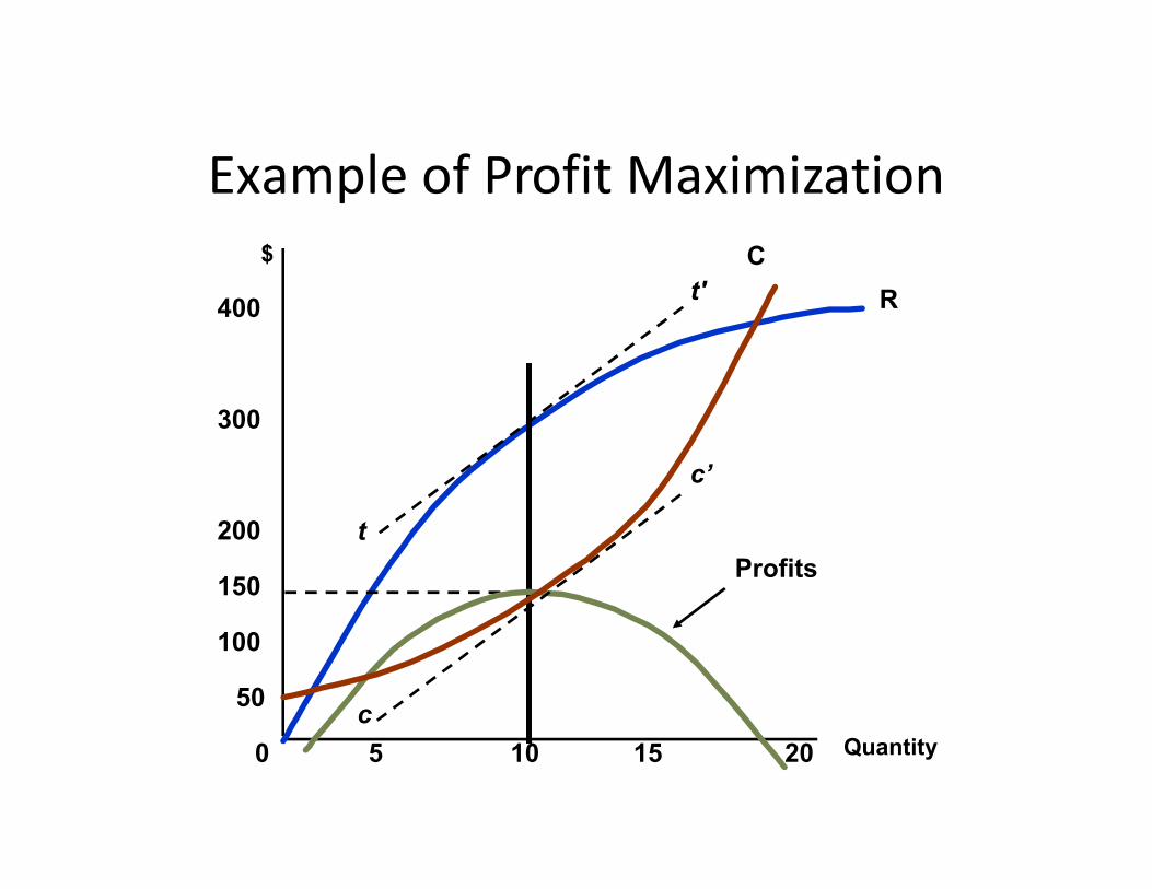
$
300
400 Rt'
Example of Profit MaximizationC
Quantity0 5 10 15 20
100
150
200
50
Profits
t
c
c’
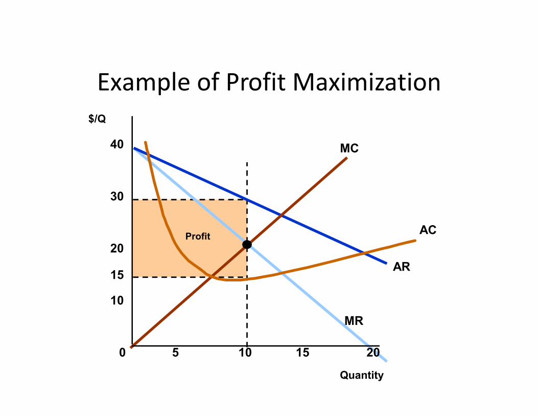
MC
Example of Profit Maximization$/Q
30
40
Profit
AR
MR
AC
Quantity
0 5 10 15 20
10
20
15

Monopoly• Monopoly pricing compared to perfect
competition pricing:– Monopoly
P > MCP > MC
– Perfect CompetitionP = MC
Monopoly Power• Pure monopoly is rare.• However, a market with several firms, each facing
a downward sloping demand curve will produce so that price exceeds marginal cost.that price exceeds marginal cost.
Monopoly Power• Scenario:
– Four firms with equal share (5,000) of a market for 20,000 toothbrushes at a price of $1.50.
– The demand curve for and one firm (e.g. Firm A)– The demand curve for and one firm (e.g. Firm A)depends on how much their product differs, and how the firms compete.
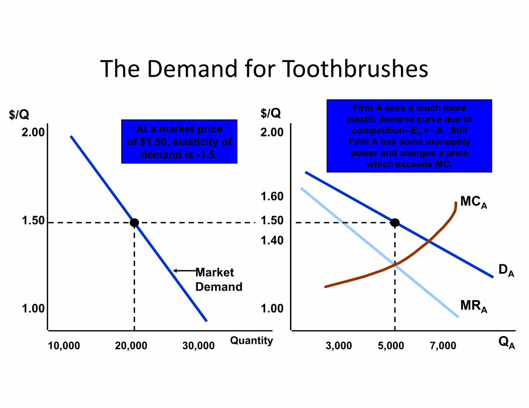
The Demand for Toothbrushes
At a market priceof $1.50, elasticity of
demand is -1.5.
2.00
$/Q
2.00
1.60
Firm A sees a much more elastic demand curve due tocompetition--Ed = -.6. Still
Firm A has some monopoly power and charges a price
which exceeds MC.
MCA
$/Q
Quantity10,000 QA
1.50
1.00
20,000 30,000 3,000 5,000 7,000
1.50
1.00
1.40
DA
MRA
Market Demand
MCA
Sources of Monopoly Power• Why do some firm’s have considerable monopoly
power, and others have little or none?• A firm’s monopoly power is determined by the
firm’s elasticity of demand.firm’s elasticity of demand.
Sources of Monopoly Power• The firm’s elasticity of demand is determined by:
1) Elasticity of market demand2) Number of firms3) The interaction among firms3) The interaction among firms
The Social Costs of Monopoly Power
• Monopoly power results in higher prices and lower quantities.
• However, does monopoly power make consumers and producers in the aggregate better or worse and producers in the aggregate better or worse off?
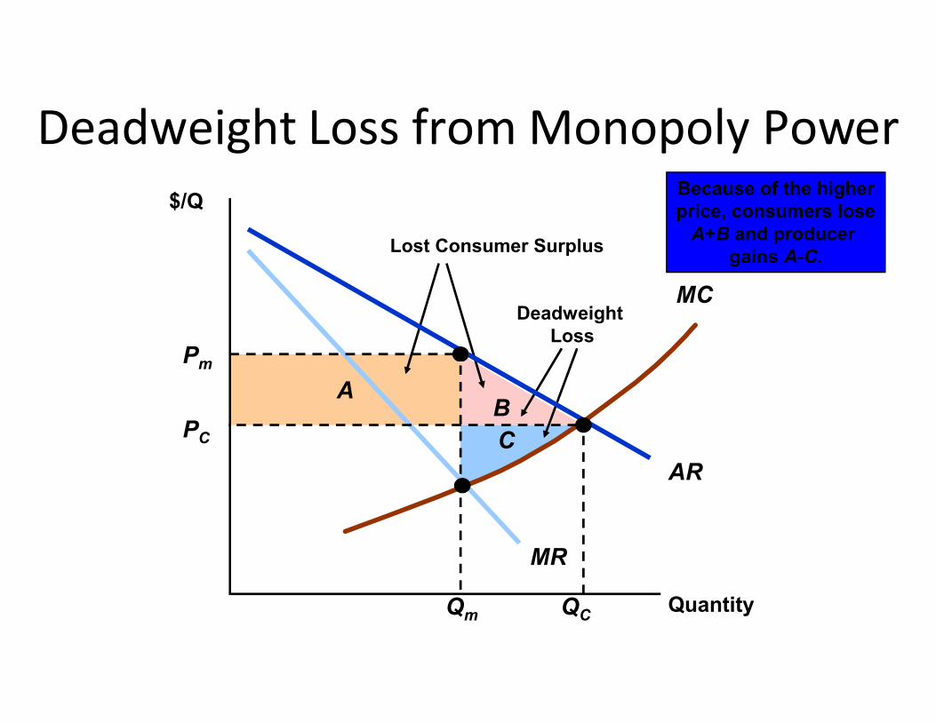
Lost Consumer Surplus
Deadweight Loss
Because of the higherprice, consumers lose
A+B and producer gains A-C.
Deadweight Loss from Monopoly Power
MC
Pm
$/Q
BA
C
Quantity
AR
MR
QC
PC
Pm
Qm
The Social Costs of Monopoly Powerc
• Firms may spend to gain monopoly power– Lobbying– Advertising– Building excess capacity– Building excess capacity
The Social Costs of Monopoly Power
• Price Regulation– Recall that in competitive markets, price regulation
created a deadweight loss.
• Question:• Question:– What about a monopoly?
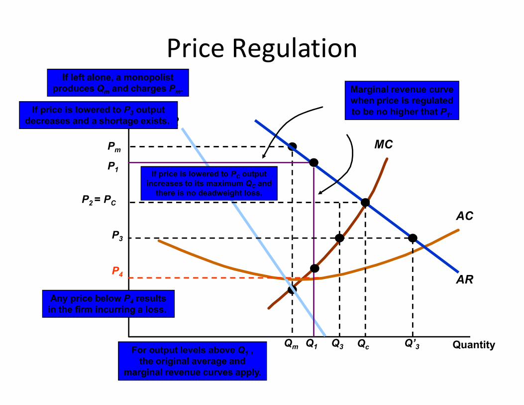
MCPm
MR
If left alone, a monopolistproduces Qm and charges Pm.
Price Regulation
$/Q
If price is lowered to PC outputincreases to its maximum QC and
there is no deadweight loss.P2 = PC
P1
Marginal revenue curvewhen price is regulatedto be no higher that P1.If price is lowered to P3 output
decreases and a shortage exists.
Qm
AC
AR
Quantity
P2 = PC
Qc
Any price below P4 resultsin the firm incurring a loss.
P4
Q1For output levels above Q1 ,the original average and
marginal revenue curves apply.
P3
Q3 Q’3
Natural Monopoly• A firm that can produce the entire output of an
industry at a cost lower than what it would be if there were several firms.
• Natural monopolies occur because of extensive • Natural monopolies occur because of extensive economies of scale

$/Q
Setting the price at Pr
If the price were regulated to be PC,the firm would lose money
and go out of business.
Pm
Unregulated, the monopolistwould produce Qm and
charge Pm.
Regulating the Price of a NaturalMonopoly
MC
AC
ARMR
Quantity
Setting the price at Pr
yields the largest possibleoutput; profit is zero.
Qr
Pr
PC
QCQm
Regulation in Practice
• It is very difficult to estimate the firm's cost and demand functions because they change with evolving market conditions
• An alternative pricing technique---rate-of-return regulation allows the firms to set a maximum price regulation allows the firms to set a maximum price based on the expected rate or return that the firm will earn:
• P = AVC + (D + T + sK)/Q, where – P = price, AVC = average variable cost– D = depreciation, T = taxes– s = allowed rate of return, K = firm’s capital stock
Limiting Market Power: Antitrust Laws
• Promote a competitive economy• Rules and regulations designed to promote a
competitive economy by:competitive economy by:– Prohibiting actions that restrain or are likely to
restrain competition– Restricting the forms of market structures that are
allowable

Limiting Market Power: Antitrust Laws
• Two Examples– American Airlines -- Price fixing– Microsoft– Microsoft
• Monopoly power• Predatory actions• Collusion
Summary
• Market power is the ability of sellers (or buyers) to affect the price of a good.
• Monopoly power is determined in part by the number of firms competing in the market.of firms competing in the market.
• Market power can impose costs on society.• Sometimes, scale economies make pure monopoly desirable.• We rely on the antitrust laws to prevent firms from obtaining
excessive market power.

Pricing with market powerPricing with market power

Topics to be Discussed
• Capturing Consumer Surplus
• Price Discrimination
• Intertemporal Price Discrimination and Peak-Load Pricing
• The Two-Part Tariff
Introduction
• Pricing without market power (perfect competition) is determined by market supply and demand.
• The individual producer must be able to forecast the market and then concentrate on managing production (cost) to maximize profits.
Introduction
• Pricing with market power requires the individual producer to know much more about the characteristics of demand as well as manage production.manage production.
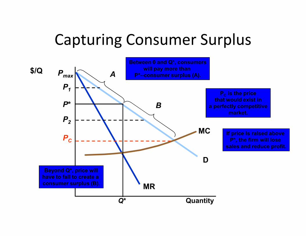
Capturing Consumer Surplus
$/Q Pmax
PC is the pricethat would exist in
a perfectly competitivemarket.
A
P*
P1
Between 0 and Q*, consumerswill pay more than
P*--consumer surplus (A).
B
P
Quantity
D
MR
MC If price is raised above P*, the firm will lose
sales and reduce profit.
PC
Q*
P2
Beyond Q*, price willhave to fall to create a consumer surplus (B).
Capturing Consumer Surplus• Price discrimination is the charging of different
prices to different consumers for similar goods.

Price Discrimination• First Degree Price Discrimination
– Charge a separate price to each customer: the maximum or reservation price they are willing to pay.
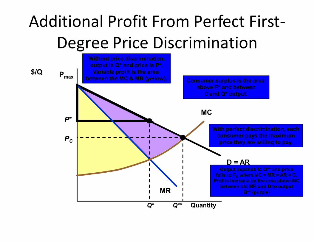
P*
Without price discrimination,output is Q* and price is P*.Variable profit is the area
between the MC & MR (yellow).
Additional Profit From Perfect First-Degree Price Discrimination
$/Q PmaxConsumer surplus is the area
above P* and between0 and Q* output.
MCP*
Q* Quantity
With perfect discrimination, eachconsumer pays the maximumprice they are willing to pay.
D = AR
MR
Output expands to Q** and pricefalls to PC where MC = MR = AR = D.
Profits increase by the area above MCbetween old MR and D to output
Q** (purple)
Q**
PC
Additional Profit From Perfect First-Degree Price Discrimination
• Question– Why would a producer have difficulty in achieving first-
degree price discrimination?
• Answer• Answer
1) Too many customers (impractical)
2) Could not estimate the reservation price for each customer
First Degree Price Discrimination
• Examples of imperfect price discrimination where the seller has the ability to segregate the market to some extent and charge different prices for the same product:prices for the same product:– Lawyers, doctors, accountants– Car salesperson (15% profit margin)– Colleges and universities
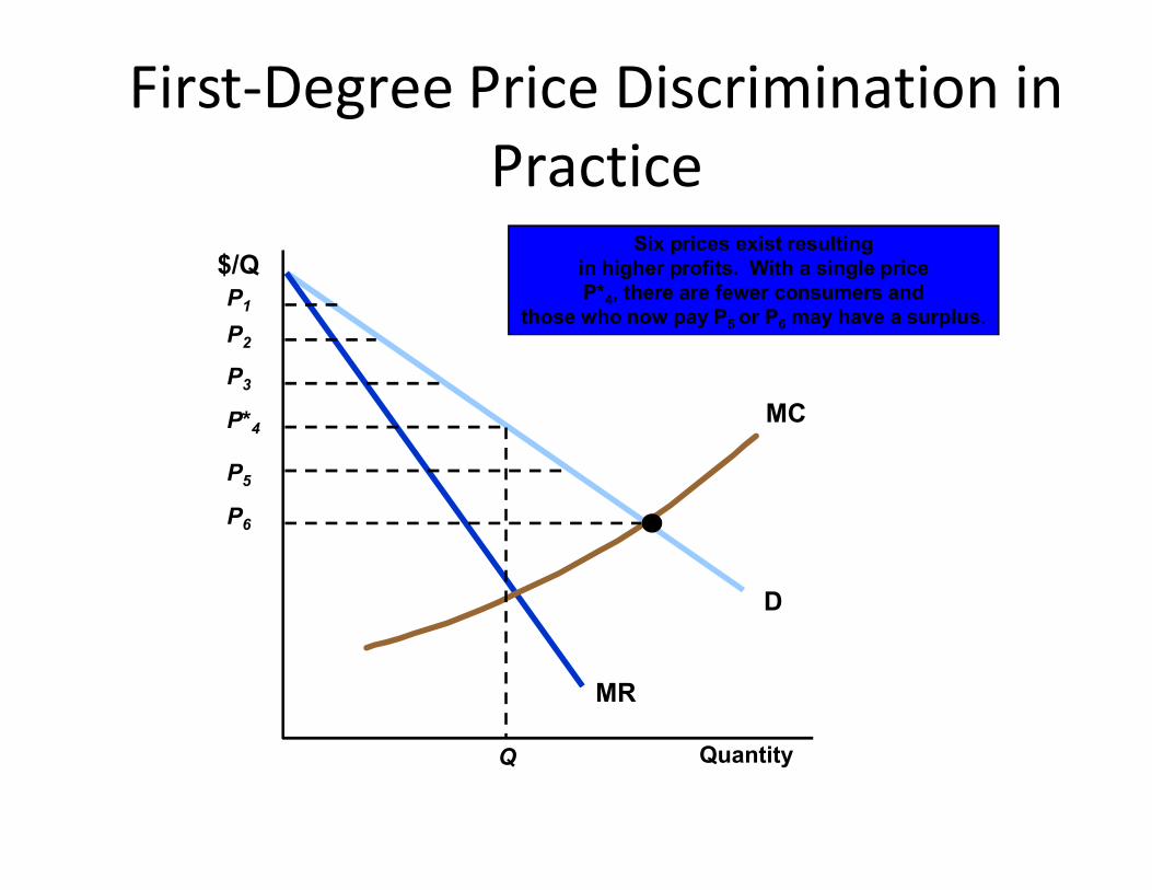
First-Degree Price Discrimination inPractice
MC
$/Q
P2
P3
P*4
P1
Six prices exist resultingin higher profits. With a single priceP*4, there are fewer consumers and
those who now pay P5 or P6 may have a surplus.
Quantity
D
MR
P5
P6
Q
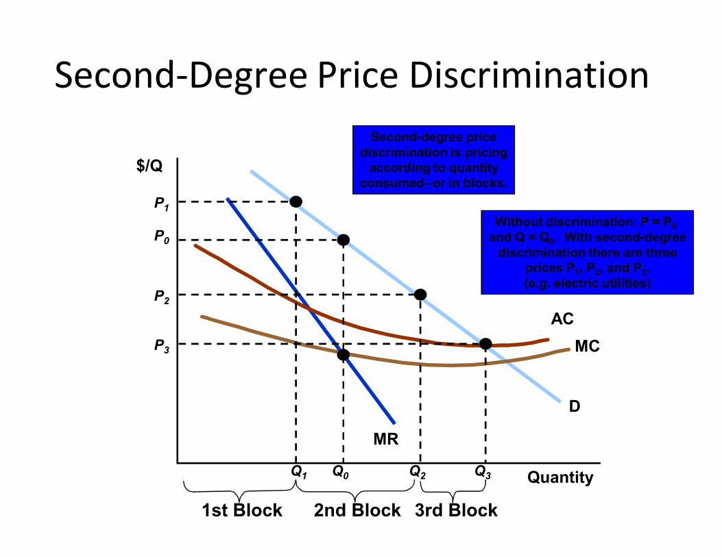
Second-Degree Price Discrimination
$/Q
P0
Without discrimination: P = P0
and Q = Q0. With second-degreediscrimination there are three
prices P1, P2, and P3.(e.g. electric utilities)
P1
Second-degree pricediscrimination is pricing
according to quantityconsumed--or in blocks.
Quantity
D
MR
MC
AC
Q0
(e.g. electric utilities)
Q1
1st Block
P2
Q2
P3
Q3
2nd Block 3rd Block
Third Degree Price Discrimination
• Divides the market into two-groups.
• Each group has its own demand function.
• Most common type of price discrimination.– Examples: airlines, liquor, vegetables, discounts to
students and senior citizens.
Third Degree Price Discrimination
• Is feasible when the seller can:
– separate his/her market into groups
– who have different price elasticities of demand (e.g. – who have different price elasticities of demand (e.g. business air travelers versus vacation air travelers)
• Pricing: Charge higher price to group with a low demand elasticity
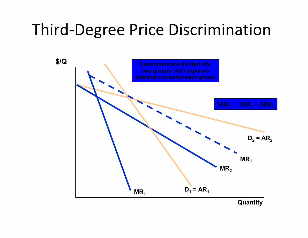
Third-Degree Price Discrimination
$/Q Consumers are divided intotwo groups, with separate
demand curves for each group.
MRT = MR1 + MR2
Quantity
D2 = AR2
MR2
D1 = AR1MR1
MRT
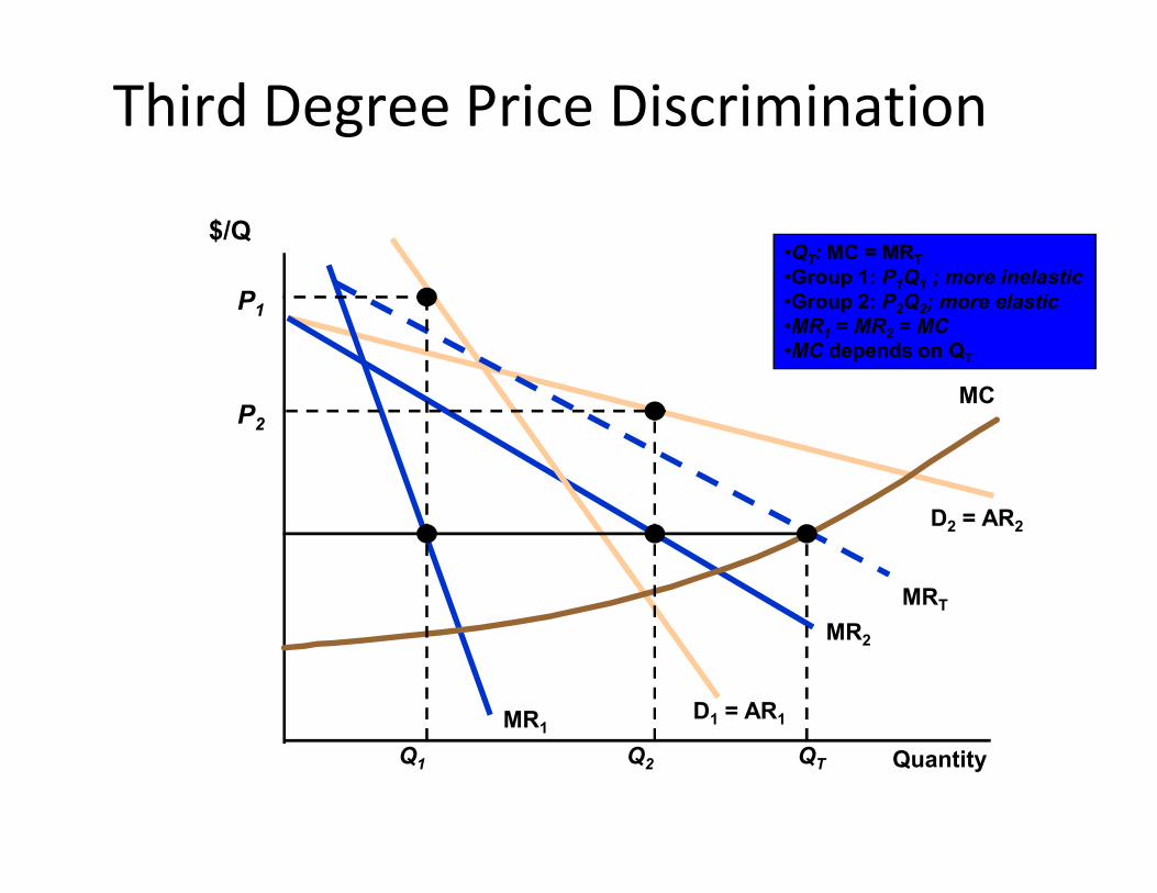
$/Q
MCP2
•QT: MC = MRT
•Group 1: P1Q1 ; more inelastic•Group 2: P2Q2; more elastic•MR1 = MR2 = MC•MC depends on QT
P1
Third Degree Price Discrimination
Quantity
D2 = AR2
MR2
D1 = AR1MR1
MRT
Q2 QTQ1

The Economics of Coupons and Rebates
• Those consumers who are more price elastic will tend to use the coupon/rebate more often will tend to use the coupon/rebate more often when they purchase the product than those consumers with a less elastic demand.
• Coupons and rebate programs allow firms to price discriminate.
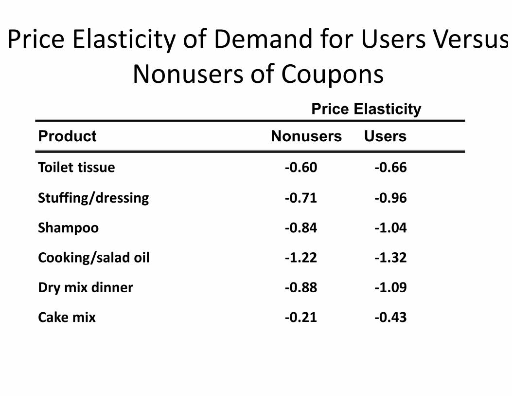
Price Elasticity of Demand for Users VersusNonusers of Coupons
Toilet tissue -0.60 -0.66
Stuffing/dressing -0.71 -0.96
Price Elasticity
Product Nonusers Users
Stuffing/dressing -0.71 -0.96
Shampoo -0.84 -1.04
Cooking/salad oil -1.22 -1.32
Dry mix dinner -0.88 -1.09
Cake mix -0.21 -0.43
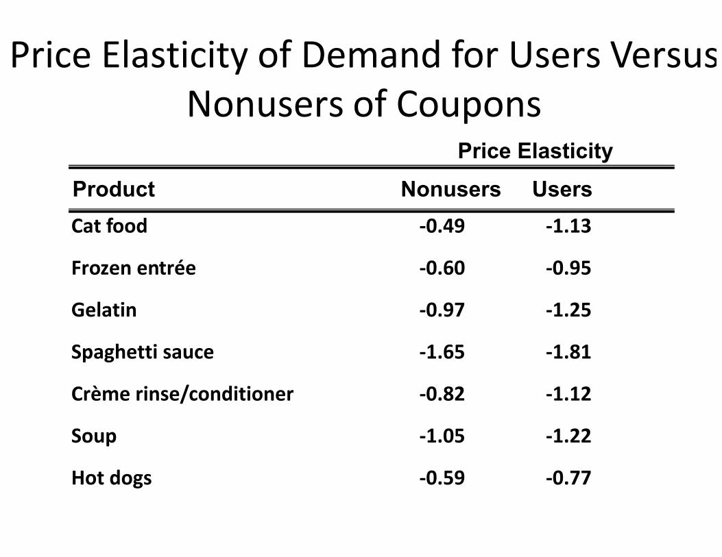
Price Elasticity of Demand for Users VersusNonusers of Coupons
Cat food -0.49 -1.13
Frozen entrée -0.60 -0.95
Price Elasticity
Product Nonusers Users
Frozen entrée -0.60 -0.95
Gelatin -0.97 -1.25
Spaghetti sauce -1.65 -1.81
Crème rinse/conditioner -0.82 -1.12
Soup -1.05 -1.22
Hot dogs -0.59 -0.77

Airline Fares• Differences in elasticities imply that some
customers will pay a higher fare than others.
• Business travelers have few choices and their Business travelers have few choices and their demand is less elastic.
• Casual travelers have choices and are more price sensitive.
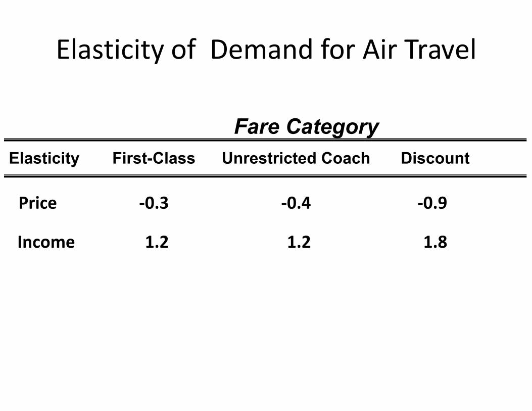
Elasticity of Demand for Air Travel
Price -0.3 -0.4 -0.9
Fare CategoryElasticity First-Class Unrestricted Coach Discount
Price -0.3 -0.4 -0.9
Income 1.2 1.2 1.8
Airline Fares• The airlines separate the market by setting various
restrictions on the tickets.– Less expensive: notice, stay over the weekend, no
refundrefund– Most expensive: no restrictions
Intertemporal Price Discrimination
• Separating the Market With Time• Initial release of a product, the demand is inelastic
– Book– Computer– Computer
• Once this market has yielded a maximum profit, firms lower the price to appeal to a general market with a more elastic demand – Paper back books– Discount computers

Intertemporal Price Discrimination
$/Q
Over time, demand becomesmore elastic and price
is reduced to appeal to the mass market.
D2 = AR2
P2
P1
Consumers are dividedinto groups over time.
Initially, demand is lesselastic resulting in a
price of P1 .
Quantity
AC = MC
Q2
MR2
D2 = AR2
D1 = AR1MR1
Q1
Peak-Load Pricing
• Demand for some products may peak at particular times.particular times.– Rush hour traffic– Electricity - late summer afternoons– Amusement parks on weekends

MC
P1
Peak-load price = P1 .
Peak-Load Pricing$/Q
MR1
D1 = AR1
Q1 Quantity
MR2
D2 = AR2
Off- peak price = P2 .
Q2
P2
The Two-Part Tariff• The purchase of some products and services can be
separated into two decisions, and therefore, two prices.
• Examples:• Examples:
– Amusement Park
– Tennis club
– Razor
– Polaroid camera and film
The Two-Part Tariff
• Pricing decision is setting the entry fee (T) and the usage fee (P).
• Choosing the trade-off between free-entry and • Choosing the trade-off between free-entry and high use prices or high-entry and zero use prices.
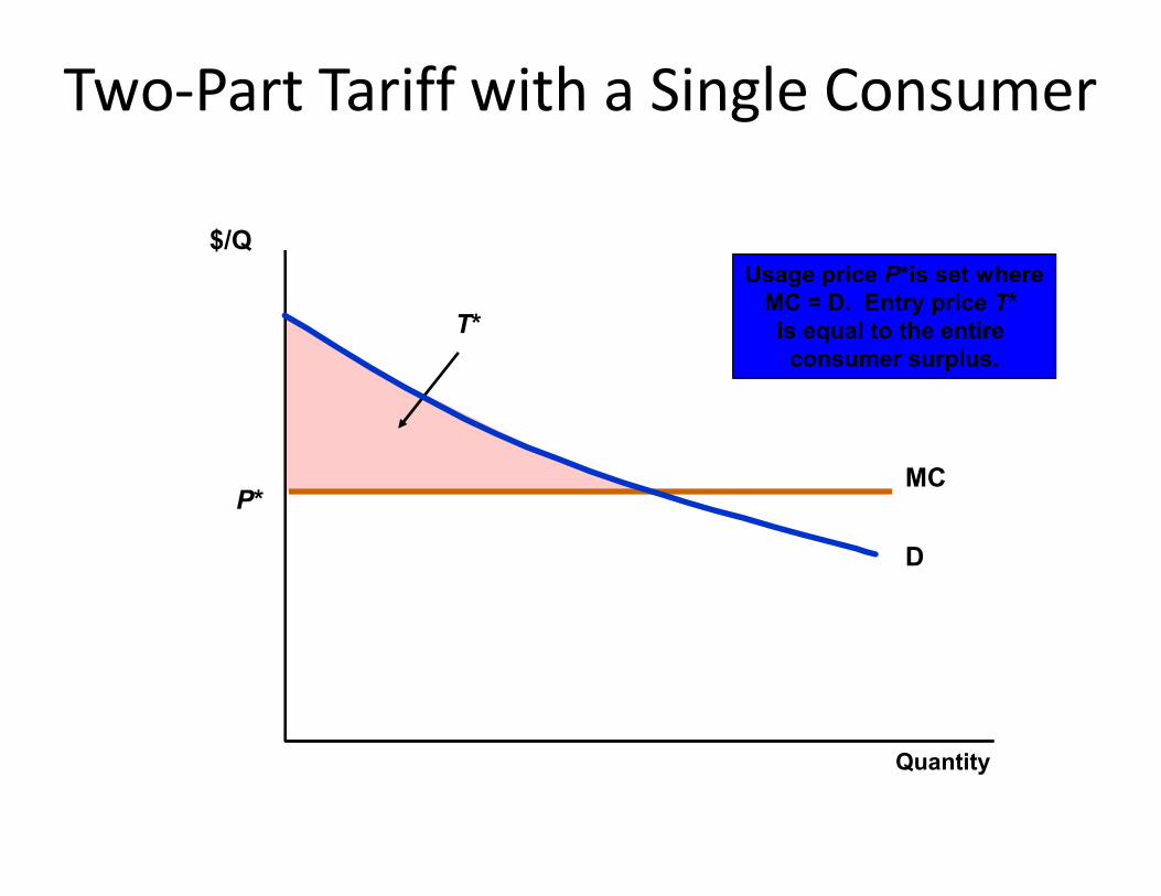
Usage price P*is set whereMC = D. Entry price T*is equal to the entire consumer surplus.
T*
Two-Part Tariff with a Single Consumer
$/Q
Quantity
MCP*
D
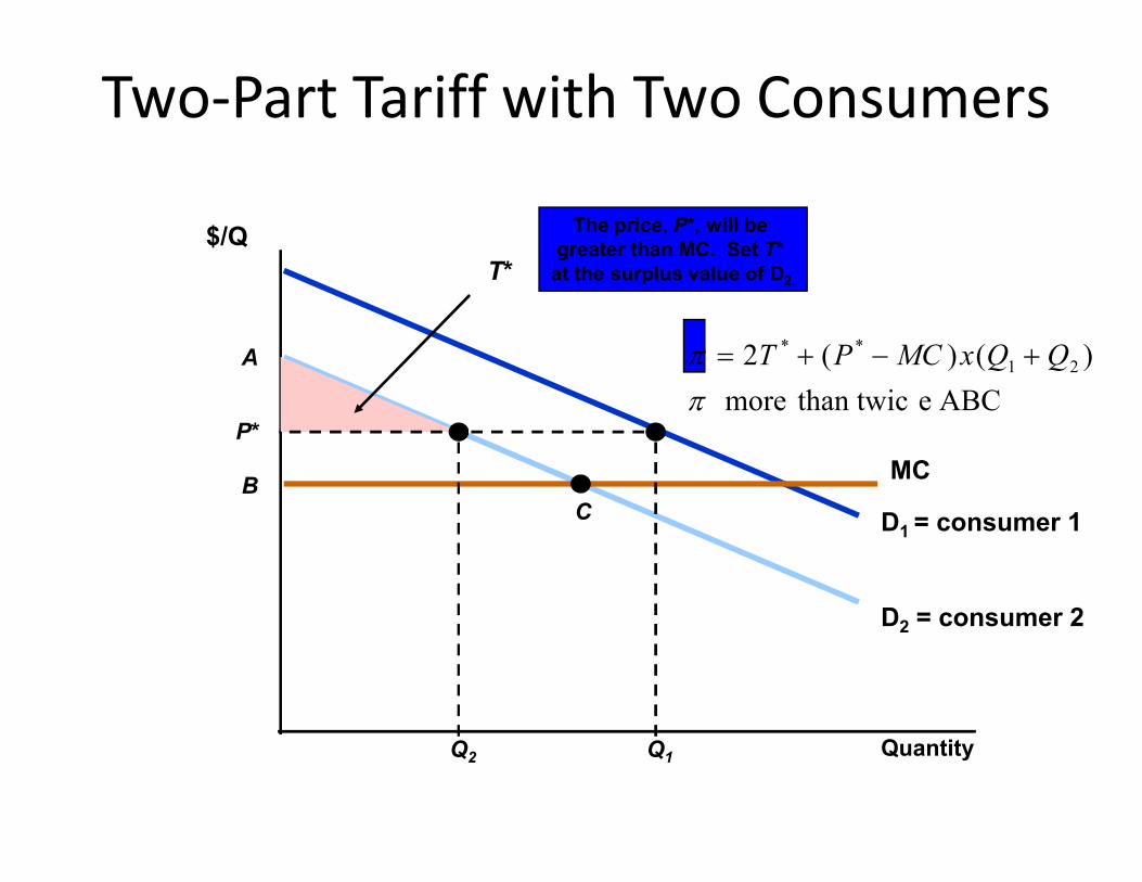
Two-Part Tariff with Two Consumers
$/Q
A
ABCe than twicmore
)()(2 21**
QQxMCPT
The price, P*, will be greater than MC. Set T*
at the surplus value of D2.T*
P*
D2 = consumer 2
D1 = consumer 1
Quantity
MCB
C
Q1Q2
P*
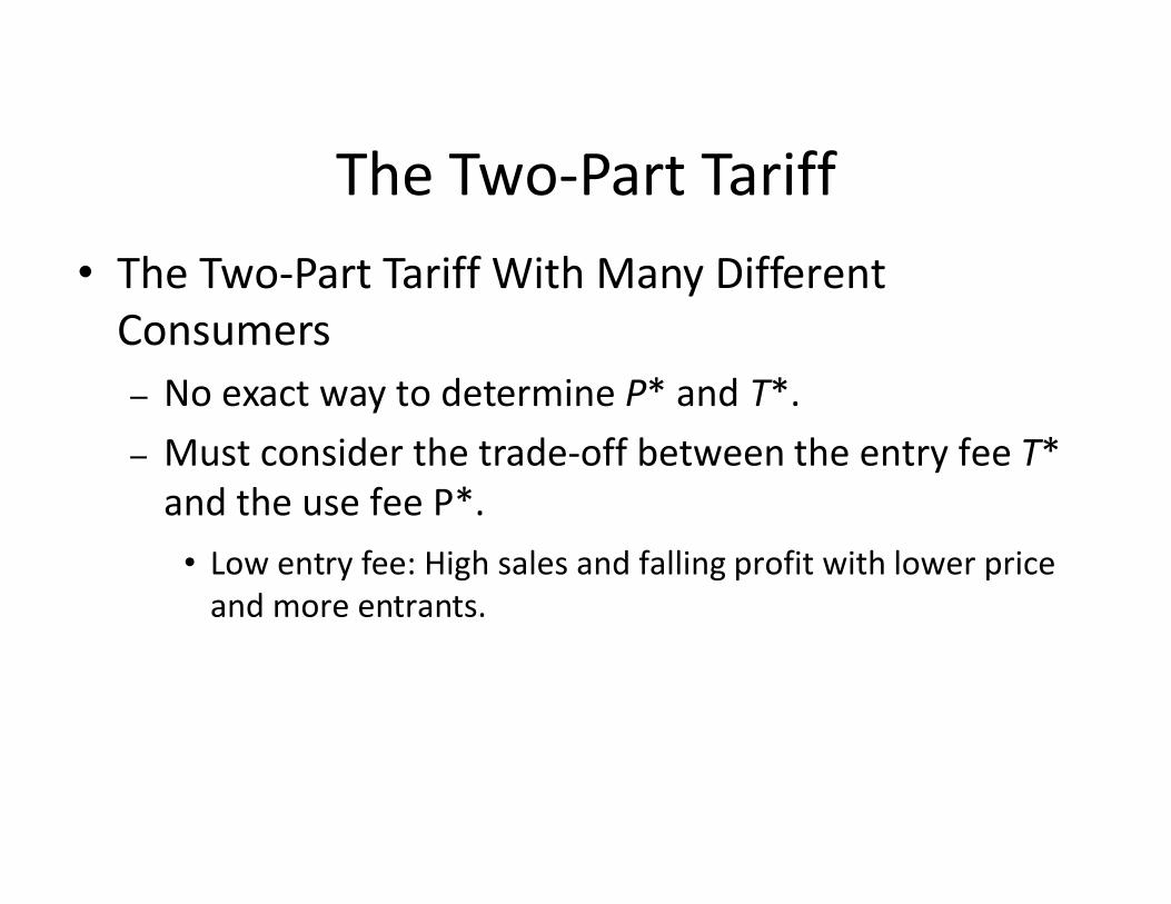
The Two-Part Tariff• The Two-Part Tariff With Many Different
Consumers– No exact way to determine P* and T*.– Must consider the trade-off between the entry fee T* – Must consider the trade-off between the entry fee T*
and the use fee P*.• Low entry fee: High sales and falling profit with lower price
and more entrants.
The Two-Part Tariff• The Two-Part Tariff With Many Different
Consumers– To find optimum combination, choose several
combinations of P,T.combinations of P,T.– Choose the combination that maximizes profit.
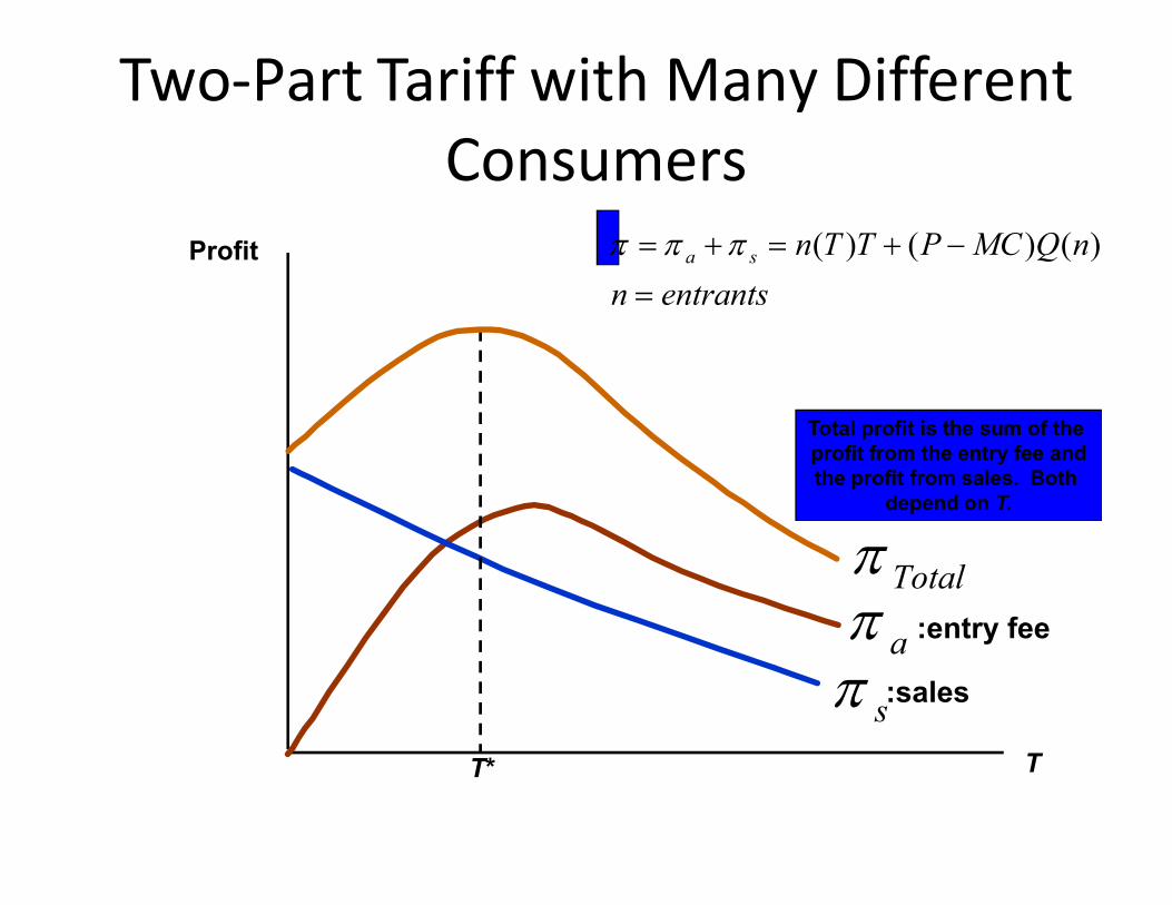
Two-Part Tariff with Many DifferentConsumers
Profit
Total profit is the sum of the profit from the entry fee and
entrantsn
nQMCPTTnsa
)()()(
T
a :entry fee
s :sales
Total
T*
profit from the entry fee andthe profit from sales. Both
depend on T.

The Two-Part Tariff• Rule of Thumb
– Similar demand: Choose P close to MC and high T– Dissimilar demand: Choose high P and low T.

Pricing Cellular Phone Service
• Question– Why do cellular phone providers offer several different
plans instead of a single two-part tariff with an access fee and per-unit charge?fee and per-unit charge?
Summary
• Firms with market power are in an enviable position because they have the potential to earn large profits, but realizing that potential may depend critically on the firm’s pricing strategy.the firm’s pricing strategy.
• A pricing strategy aims to enlarge the customer base that the firm can sell to, and capture as much consumer surplus as possible.
Summary• Ideally, the firm would like to perfectly price
discriminate.
• The two-part tariff is another means of capturing The two-part tariff is another means of capturing consumer surplus.
Monopolistic competition andMonopolistic competition andoligopoly

Topics to be Discussed
• Monopolistic Competition
• Collusive Oligopoly
• Cartels• Cartels
• Non-collusive oligopoly
• The prisoners’ dilemma
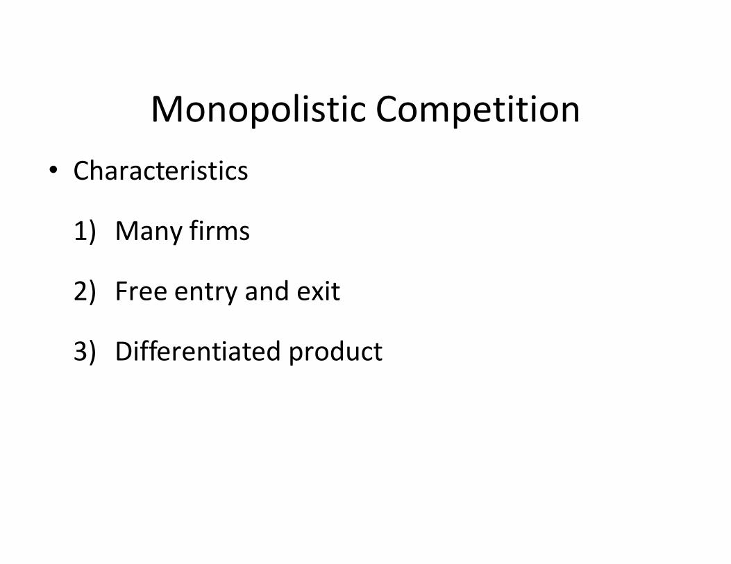
Monopolistic Competition• Characteristics
1) Many firms
2) Free entry and exit2) Free entry and exit
3) Differentiated product
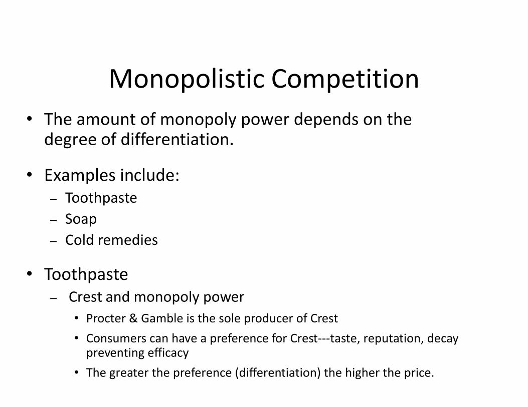
Monopolistic Competition• The amount of monopoly power depends on the
degree of differentiation.
• Examples include:– Toothpaste– Toothpaste– Soap– Cold remedies
• Toothpaste– Crest and monopoly power
• Procter & Gamble is the sole producer of Crest• Consumers can have a preference for Crest---taste, reputation, decay
preventing efficacy• The greater the preference (differentiation) the higher the price.
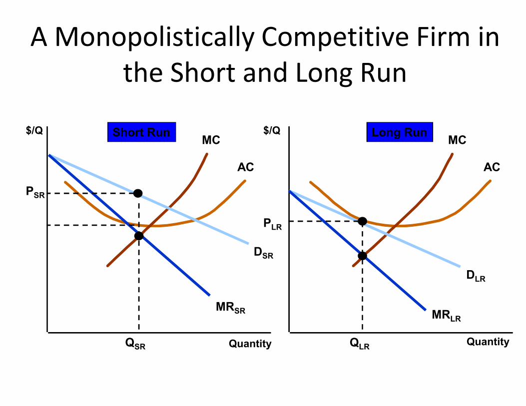
A Monopolistically Competitive Firm inthe Short and Long Run
$/Q $/QMC
AC
MC
AC
PSR
Short Run Long Run
Quantity Quantity
DSR
MRSR
DLR
MRLR
QSR QLR
PLR
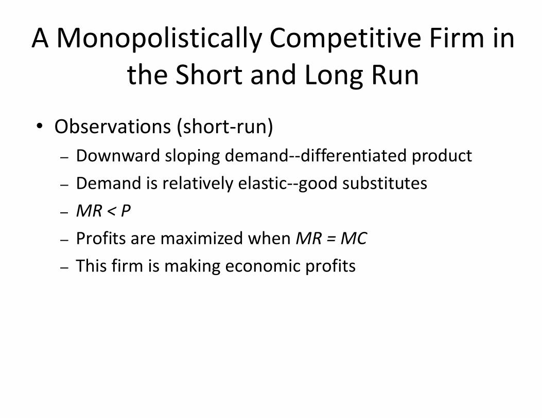
A Monopolistically Competitive Firm inthe Short and Long Run
• Observations (short-run)– Downward sloping demand--differentiated product– Demand is relatively elastic--good substitutes– MR < P– MR < P– Profits are maximized when MR = MC– This firm is making economic profits
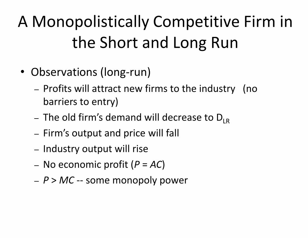
A Monopolistically Competitive Firm inthe Short and Long Run
• Observations (long-run)– Profits will attract new firms to the industry (no
barriers to entry)– The old firm’s demand will decrease to DLR– The old firm’s demand will decrease to DLR
– Firm’s output and price will fall– Industry output will rise– No economic profit (P = AC)– P > MC -- some monopoly power
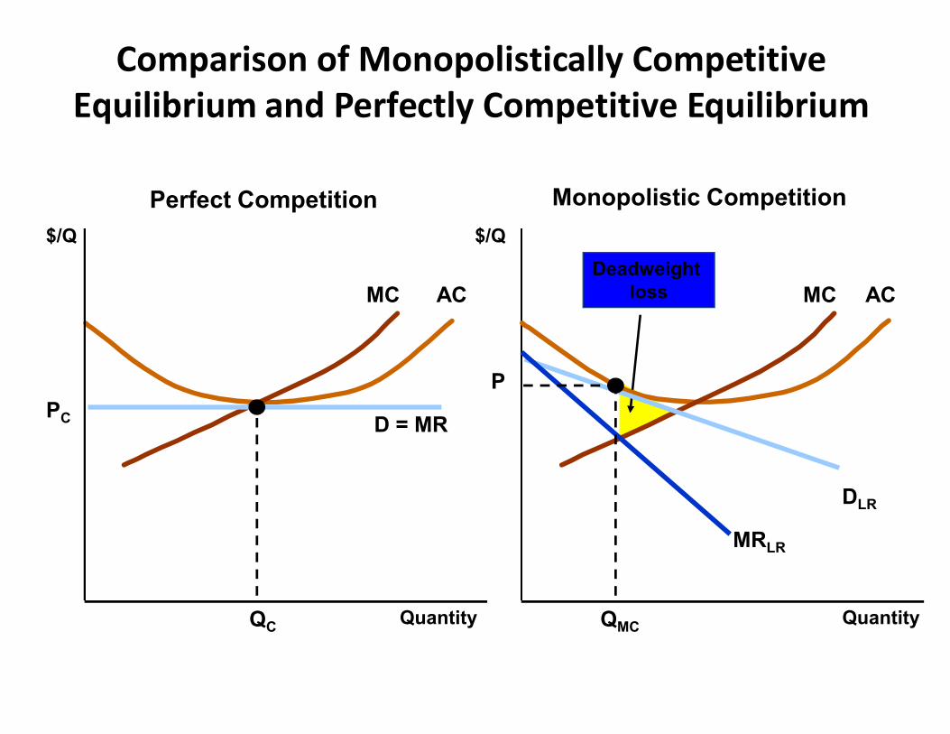
Comparison of Monopolistically CompetitiveEquilibrium and Perfectly Competitive Equilibrium
Deadweight lossMC AC
$/Q $/Q
MC AC
Perfect Competition Monopolistic Competition
Quantity
D = MR
QC
PC
DLR
MRLR
QMC
P
Quantity
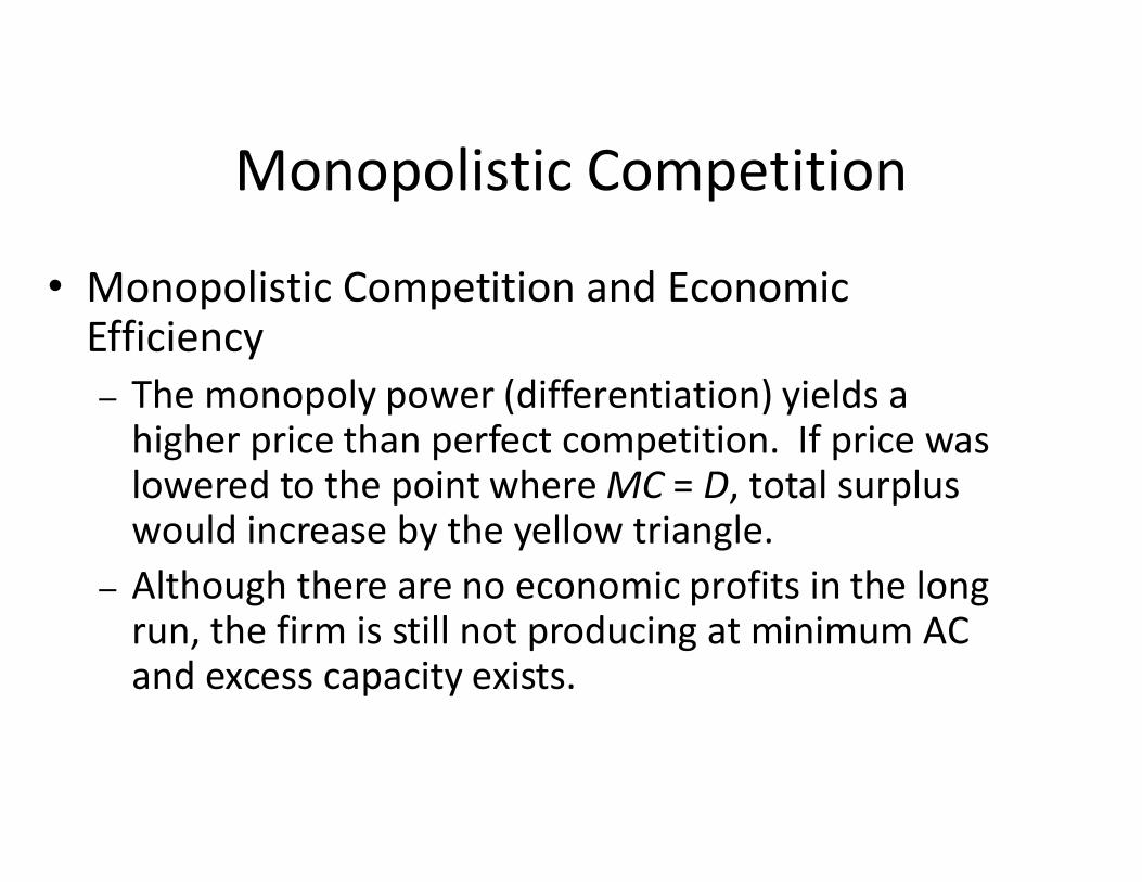
Monopolistic Competition
• Monopolistic Competition and Economic Efficiency– The monopoly power (differentiation) yields a
higher price than perfect competition. If price was higher price than perfect competition. If price was lowered to the point where MC = D, total surplus would increase by the yellow triangle.
– Although there are no economic profits in the long run, the firm is still not producing at minimum AC and excess capacity exists.
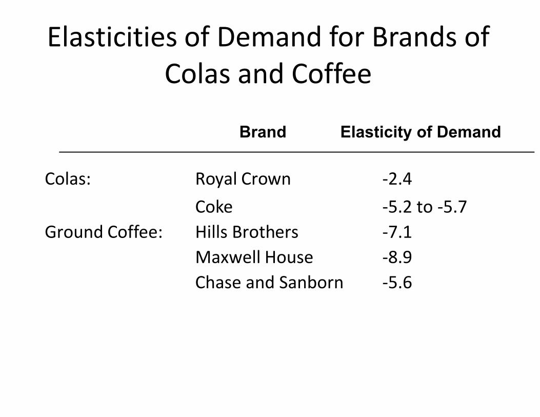
Elasticities of Demand for Brands ofColas and Coffee
Colas: Royal Crown -2.4Coke -5.2 to -5.7
Brand Elasticity of Demand
Coke -5.2 to -5.7Ground Coffee: Hills Brothers -7.1
Maxwell House -8.9Chase and Sanborn -5.6
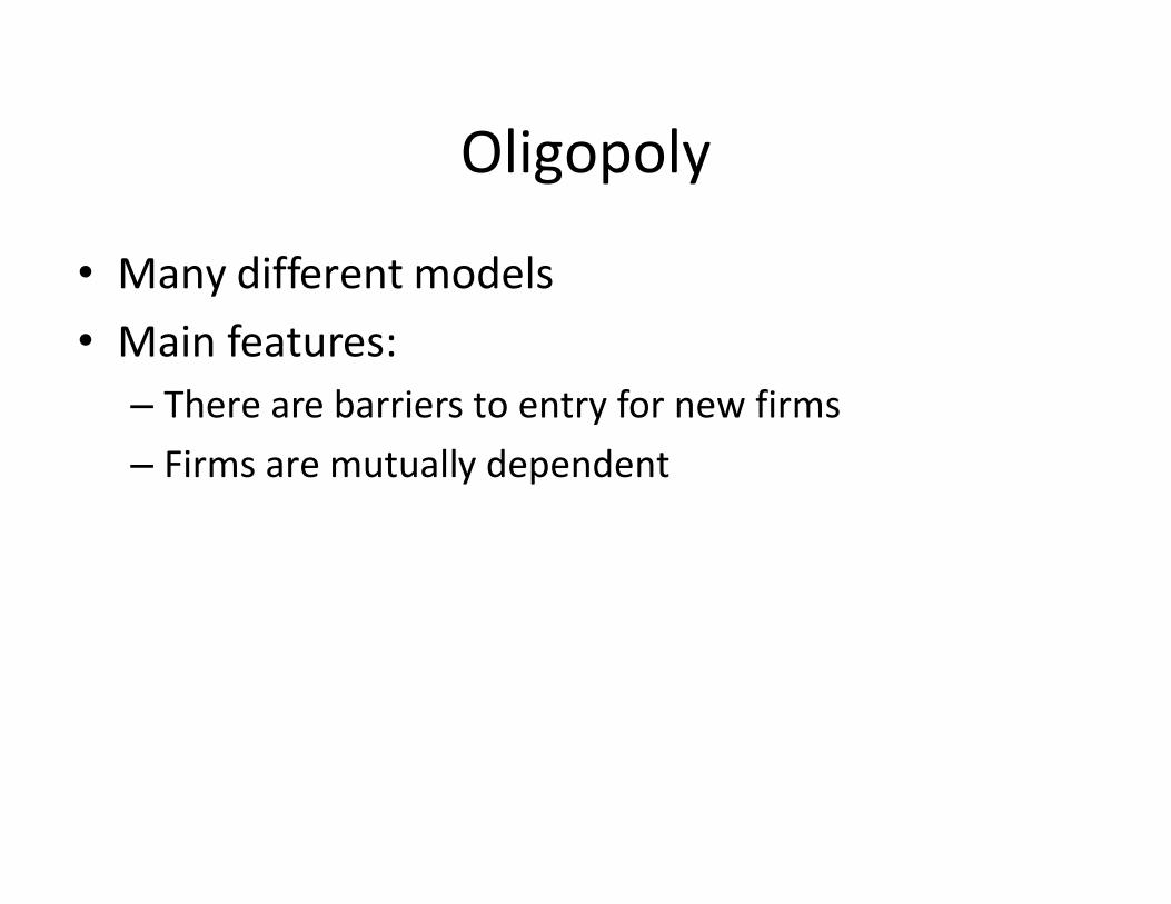
Oligopoly
• Many different models• Main features:
– There are barriers to entry for new firms – Firms are mutually dependent – Firms are mutually dependent
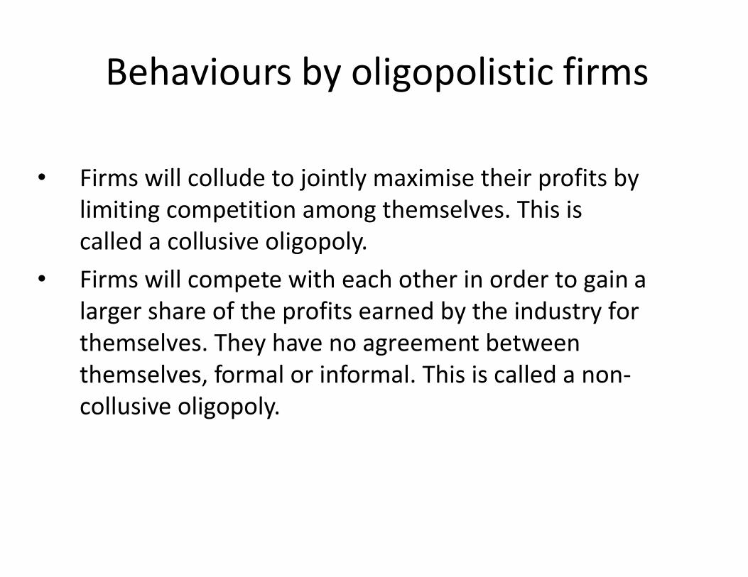
Behaviours by oligopolistic firms
• Firms will collude to jointly maximise their profits by limiting competition among themselves. This is called a collusive oligopoly.
• Firms will compete with each other in order to gain a • Firms will compete with each other in order to gain a larger share of the profits earned by the industry for themselves. They have no agreement between themselves, formal or informal. This is called a non-collusive oligopoly.
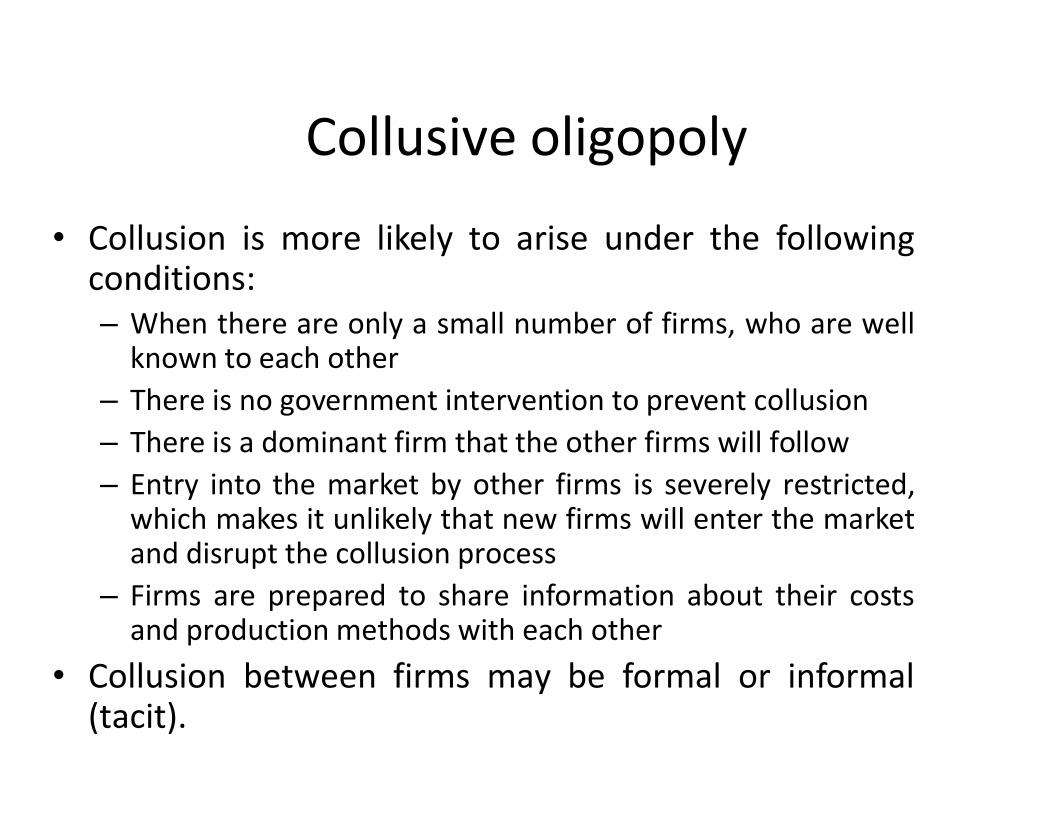
Collusive oligopoly
• Collusion is more likely to arise under the followingconditions:– When there are only a small number of firms, who are well
known to each other– There is no government intervention to prevent collusion– There is no government intervention to prevent collusion– There is a dominant firm that the other firms will follow– Entry into the market by other firms is severely restricted,
which makes it unlikely that new firms will enter the marketand disrupt the collusion process
– Firms are prepared to share information about their costsand production methods with each other
• Collusion between firms may be formal or informal(tacit).
Formal collusion
• A formal collusive agreement is called a cartel. • A cartel attempts to act like a monopoly, behaving
as if it is a single firm
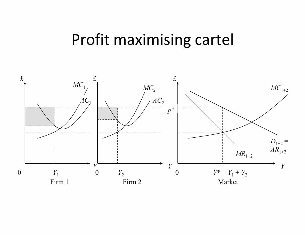
Profit maximising cartel
£MC1
AC1 AC2
£MC1+2
£MC2
p*
Y YY0 0 0
Firm 1
D1+2 = AR1+2MR1+2
Firm 2 MarketY* = Y1 + Y2Y2Y1
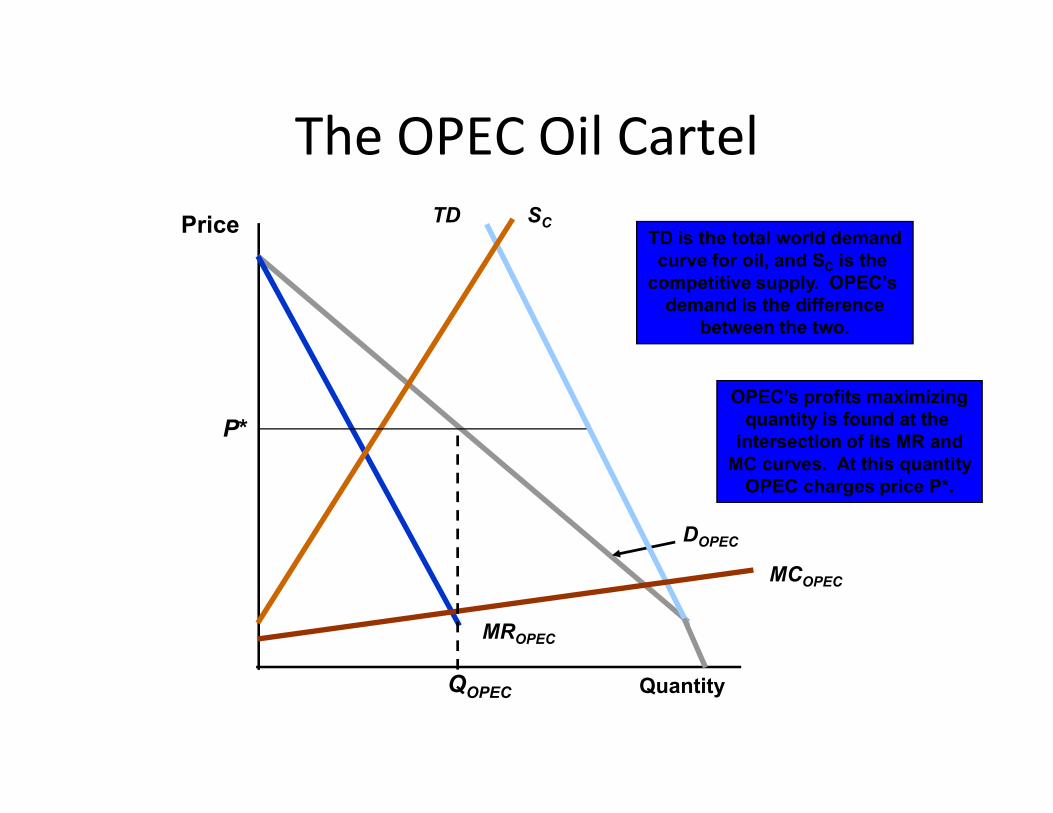
The OPEC Oil CartelPrice TD SC
TD is the total world demandcurve for oil, and SC is the
competitive supply. OPEC’s demand is the difference
between the two.
OPEC’s profits maximizing
Quantity
MROPEC
DOPEC
MCOPEC
QOPEC
P*
OPEC’s profits maximizingquantity is found at the
intersection of its MR andMC curves. At this quantity
OPEC charges price P*.
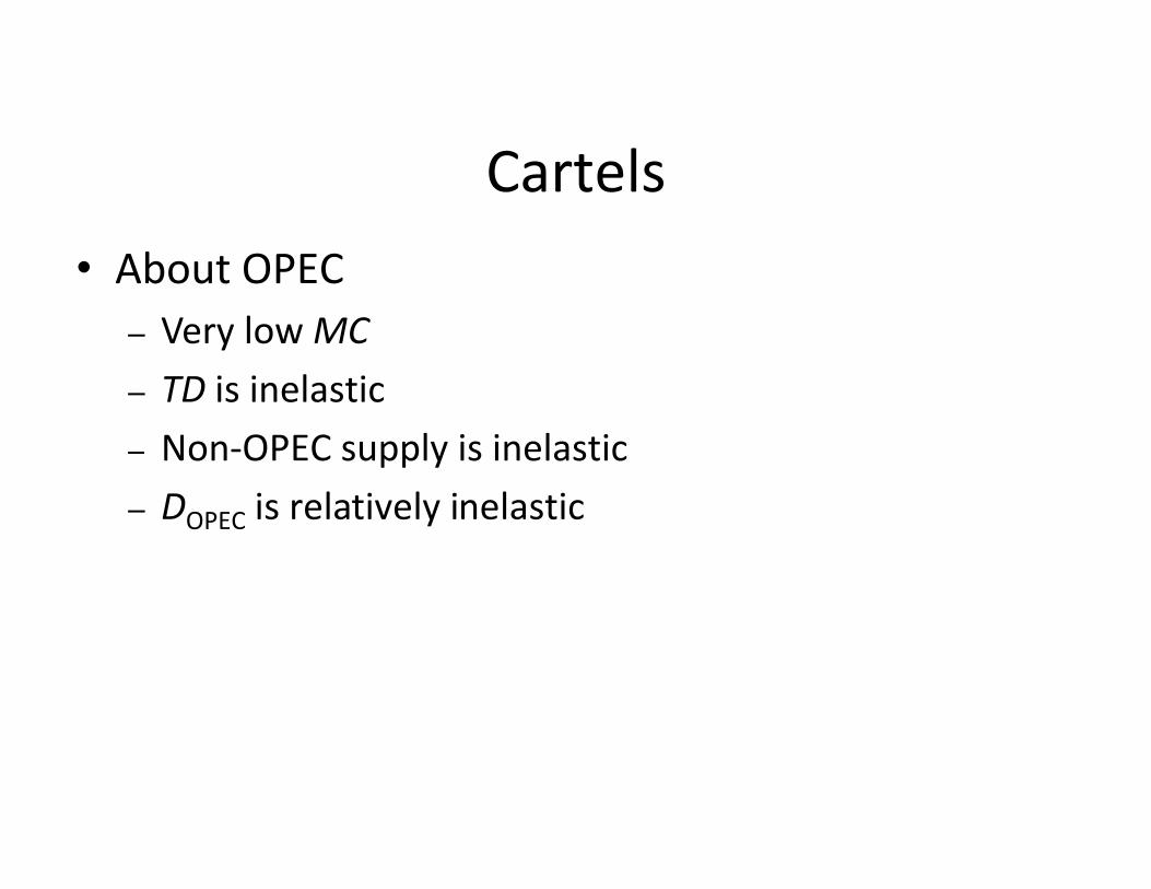
Cartels• About OPEC
– Very low MC– TD is inelastic– Non-OPEC supply is inelastic– Non-OPEC supply is inelastic– DOPEC is relatively inelastic
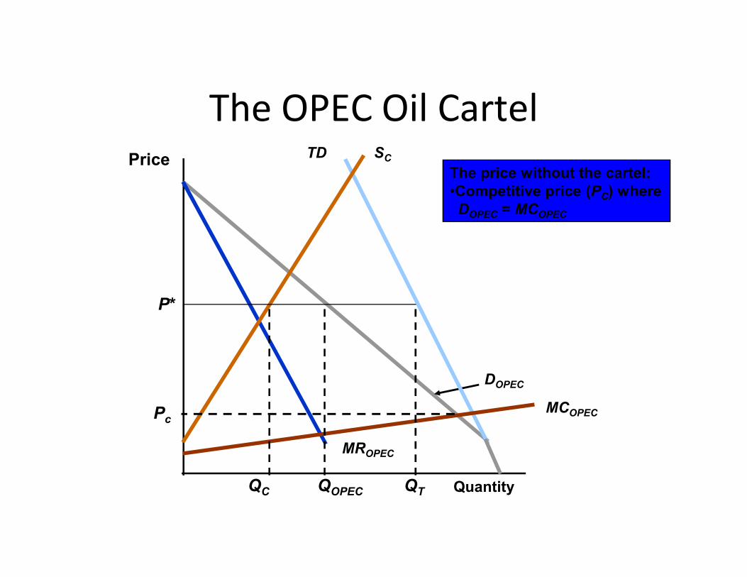
The OPEC Oil CartelPrice TD SC
The price without the cartel:•Competitive price (PC) where
DOPEC = MCOPEC
Quantity
MROPEC
DOPEC
MCOPEC
QOPEC
P*
QC QT
Pc
Tacit collusion
• Informal or tacit collusion will usually take the form of price leadership, where firms follow the price set either by:– a dominant firm in the market (dominant firm price
leadership), or a dominant firm in the market (dominant firm price leadership), or
– a firm considered to be a reliable gauge of market conditions (barometric firm price leadership)
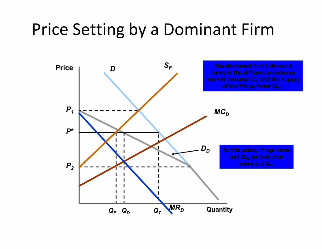
Price Setting by a Dominant Firm
Price D
P1 MCD
SF The dominant firm’s demandcurve is the difference between
market demand (D) and the supplyof the fringe firms (SF).
Quantity
DD
QD
P*
At this price, fringe firmssell QF, so that total
sales are QT.
QF QT
P2
MRD
Non-collusive oligopoly
• In the case of a non-collusive oligopoly there is no agreement, formal or informal, between firms.
• With no collusion price competition between firms is more likely to occur.
• Due to the interdependence of oligopolistic firms, non-collusive oligopolists are required to devise pricing strategies which take into account the impact of their actions on the behaviour of their rivals.
• Therefore the behaviour of a firm will depend on how it believes its rivals will react to its policies.

Non-collusive oligopoly• Equilibrium in an Oligopolistic Market
– In perfect competition, monopoly, and monopolistic competition the producers did not have to consider a rival’s response when choosing output and price.
– In oligopoly the producers must consider the response of – In oligopoly the producers must consider the response of competitors when choosing output and price.
– Defining Equilibrium• Firms do the best they can and have no incentive to change their
output or price• All firms assume competitors are taking rival decisions into account
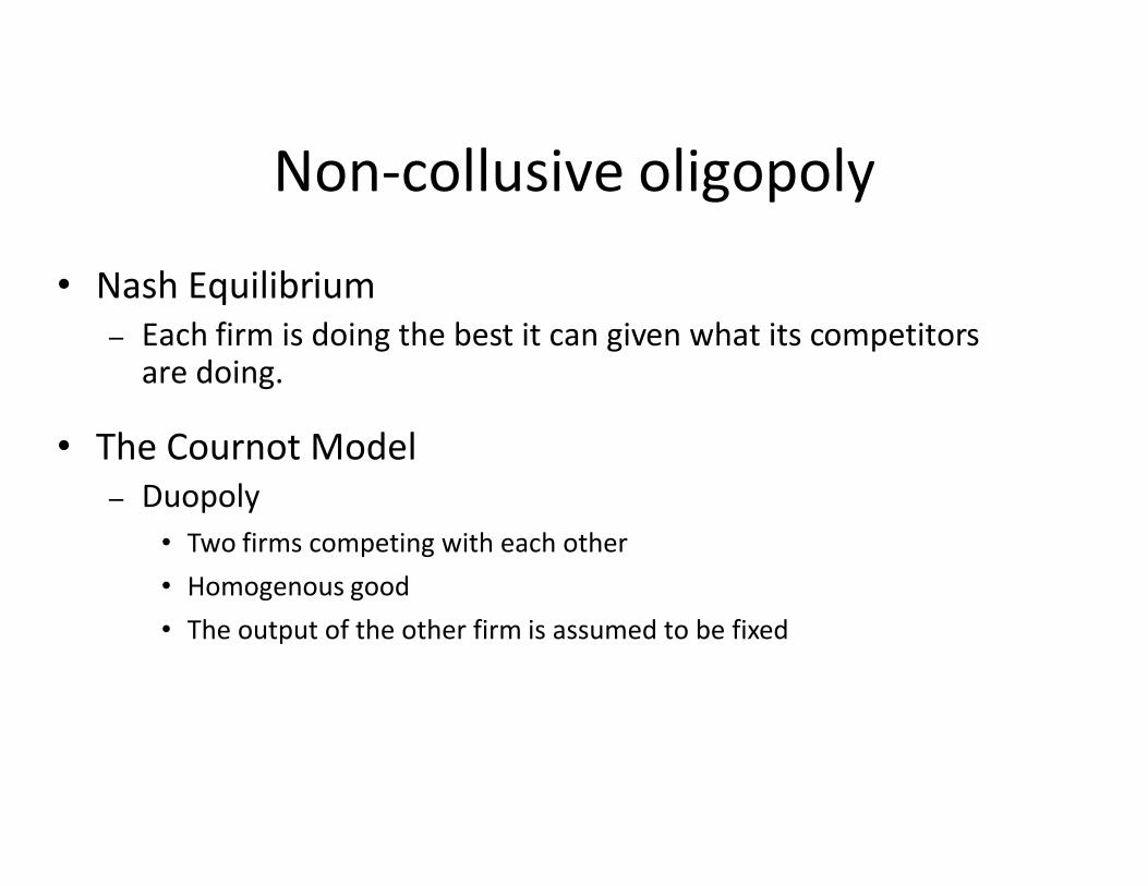
Non-collusive oligopoly
• Nash Equilibrium– Each firm is doing the best it can given what its competitors
are doing.
• The Cournot Model• The Cournot Model– Duopoly
• Two firms competing with each other• Homogenous good• The output of the other firm is assumed to be fixed

If Firm 1 thinks Firm 2 will produce
Firm 1’s Output Decision
P1
D1(0)
If Firm 1 thinks Firm 2 will produce nothing, its demand
curve, D1(0), is the market demand curve.
If Firm 1 thinks Firm 2 will produce50 units, its demand curve is
shifted to the left by this amount.
MC1
50
MR1(75)
D1(75)
12.5
If Firm 1 thinks Firm 2 will produce75 units, its demand curve is
shifted to the left by this amount.
Q1
MR1(0)
D1(50)MR1(50)
25
Non-collusive oligopoly• The Reaction Curve
– A firm’s profit-maximizing output is a decreasing schedule of the expected output of Firm 2.
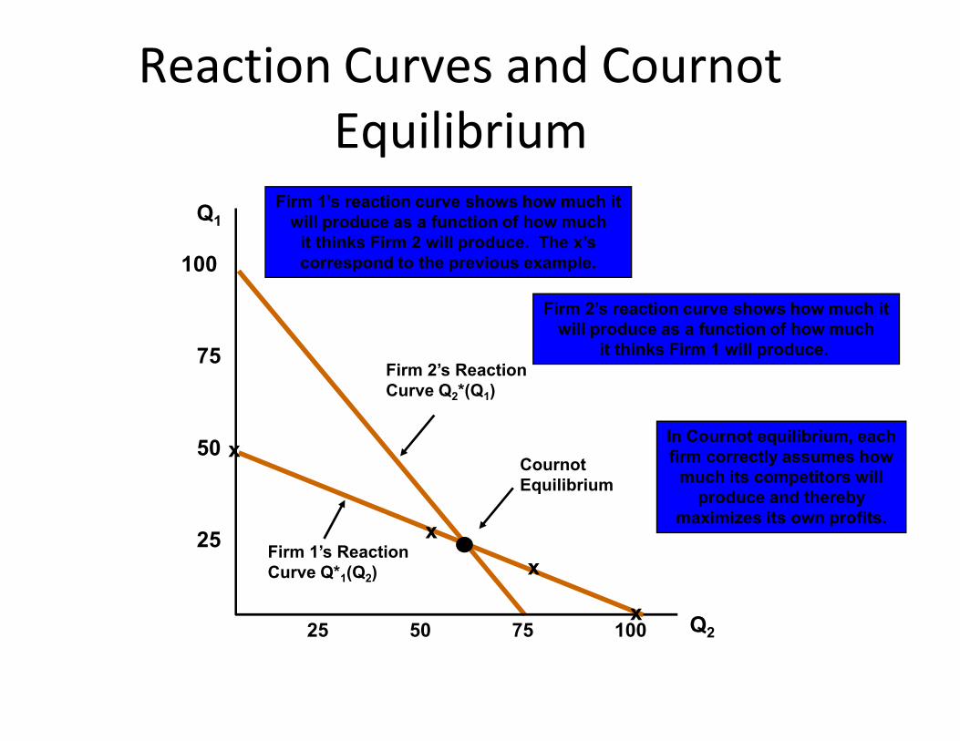
Firm 2’s Reaction
Firm 2’s reaction curve shows how much itwill produce as a function of how much
it thinks Firm 1 will produce.
Reaction Curves and CournotEquilibrium
Q1
75
100
Firm 1’s reaction curve shows how much itwill produce as a function of how much
it thinks Firm 2 will produce. The x’s correspond to the previous example.
Firm 2’s ReactionCurve Q2*(Q1)
Q225 50 75 100
25
50
Firm 1’s ReactionCurve Q*1(Q2)
x
x
x
x
In Cournot equilibrium, eachfirm correctly assumes how
much its competitors willproduce and thereby
maximizes its own profits.
CournotEquilibrium
Game theory
• Game theory, is one approach that can be used to examine the optimal strategy of the firm, depending on its views about how its rivals will behave.
• Oligopolistic firms are treated as players in a game where • Oligopolistic firms are treated as players in a game where for each action by one player another player may choose among several possible reactions.
• The reactions of rivals are uncertain, yet it may be possible, under certain circumstances to choose a strategy that will maximise the firms expected gain after making due allowance for the effects of rivals’ probable reactions.
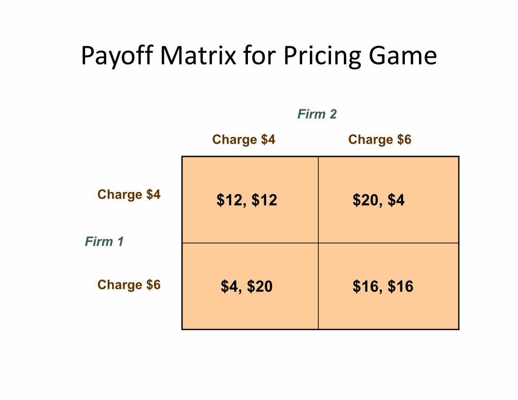
Payoff Matrix for Pricing Game
Firm 2
Charge $4 Charge $6
Charge $4 $12, $12 $20, $4
Firm 1
Charge $4
Charge $6
$12, $12 $20, $4
$16, $16$4, $20

The Prisoners’ Dilemma
• An example in game theory, called the Prisoners’ Dilemma, illustrates the problem oligopolistic firms face.
• Scenario• Scenario– Two prisoners have been accused of collaborating in a crime.– They are in separate jail cells and cannot communicate.– Each has been asked to confess to the crime.
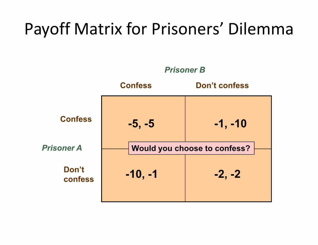
-5, -5 -1, -10
Payoff Matrix for Prisoners’ Dilemma
Confess Don’t confess
Confess
Prisoner B
-5, -5 -1, -10
-2, -2-10, -1
Prisoner A
Confess
Don’tconfess
Would you choose to confess?

Non-collusion and the kinked demandcurve
• Under non-collusion, oligopolists will typically face a kinked demand curve:
– demand is more price elastic above the current price than it is below it.
– This reflects the view that if the firm lowers its price it will expect its competitors to follow suit, matching the price reduction. The rivals are forced to do this to avoid losing customers. If however the firm increases its price it will not expect its rivals to do likewise, since by keeping their prices the same the rivals will gain customers.
• Explains why prices will tend to remain fixed under non-collusive oligopoly.
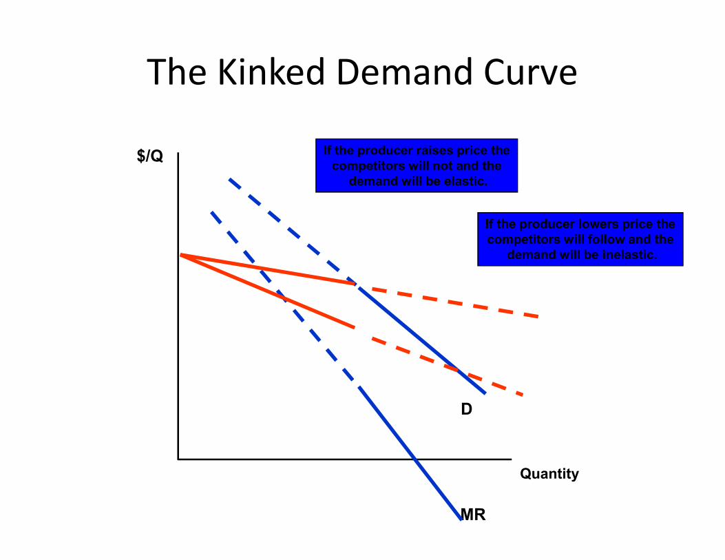
The Kinked Demand Curve
$/Q
If the producer lowers price thecompetitors will follow and the
demand will be inelastic.
If the producer raises price thecompetitors will not and the
demand will be elastic.
Quantity
MR
D
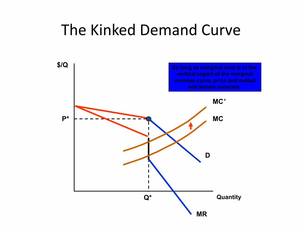
$/Q
P* MC
MC’
So long as marginal cost is in the vertical region of the marginal
revenue curve, price and output will remain constant.
The Kinked Demand Curve
D
P*
Q*
MC
MR
Quantity
Summary• In a monopolistically competitive market, firms
compete by selling differentiated products, which are highly substitutable.
• In an oligopolistic market, only a few firms account for • In an oligopolistic market, only a few firms account for most or all of production.
• Oligopolistic firms may collude to jointly maximise their profits by limiting competition among themselves, or they may compete with each other in order to gain a larger share of the profits earned by the industry for themselves.
Summary
• Collusion may be tacit or formal.
• Due to the interdependence of oligopolistic firms, non-collusive oligopolists are required to devise pricing strategies which take into account the impact pricing strategies which take into account the impact of their actions on the behaviour of their rivals.
• Game theory is one approach that can be used to examine the optimal strategy of the firm
Game theoryGame theory

Topics to be Discussed• Gaming and Strategic Decisions
• Dominant Strategies
• The Nash Equilibrium Revisited
Repeated Games• Repeated Games
• Sequential Games
• Threats, Commitments, and Credibility
• Bargaining Strategy
• Entry Deterrence

Gaming and Strategic Decisions
• “If I believe that my competitors are rational and act to maximize their own profits, how should I take their behavior into account when making my own profit-maximizing decisions?”own profit-maximizing decisions?”

Non-cooperative versus CooperativeGames
• Cooperative Game– Players negotiate binding contracts that allow them
to plan joint strategies
Non-cooperative Game• Non-cooperative Game– Negotiation and enforcement of a binding contract
are not possibleBinding contracts are possible

Non-cooperative versus CooperativeGames
• “The strategy design is based on understanding your opponent’s point of view, and (assuming you opponent is rational) deducing how he or she is likely to respond to your actions”likely to respond to your actions”
Dominant Strategies• Dominant Strategy
– One that is optimal no matter what an opponent does.
– An Example– An Example
• A & B sell competing products
• They are deciding whether to undertake advertising campaigns

Payoff Matrix for Advertising Game
Advertise
Don’tAdvertise
Advertise
Firm B
10, 5 15, 0
Firm A
Don’tAdvertise 10, 26, 8
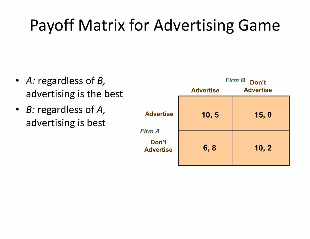
AdvertiseDon’t
Advertise
Advertise
Firm B
10, 5 15, 0
Payoff Matrix for Advertising Game
• A: regardless of B, advertising is the best
• B: regardless of A,advertising is best
Firm A
Don’tAdvertise 10, 26, 8
advertising is best
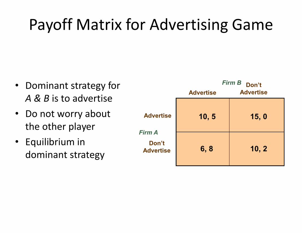
AdvertiseDon’t
Advertise
Advertise
Firm B
10, 5 15, 0
Payoff Matrix for Advertising Game
• Dominant strategy for A & B is to advertise
• Do not worry about
Firm A
Advertise
Don’tAdvertise
10, 5 15, 0
10, 26, 8
• Do not worry about the other player
• Equilibrium in dominant strategy
Game Without Dominant Strategy
• The optimal decision of a player without a dominant strategy will depend on what the other player does.
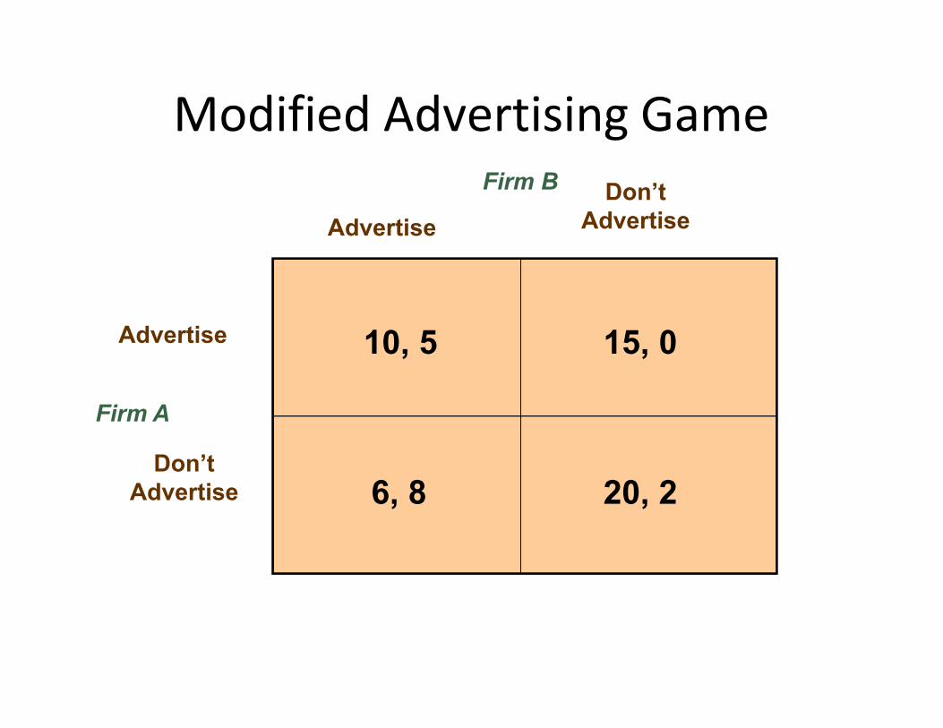
10, 5 15, 0
Advertise
Don’tAdvertise
Advertise
Firm B
Modified Advertising Game
20, 26, 8
Firm A
Don’tAdvertise
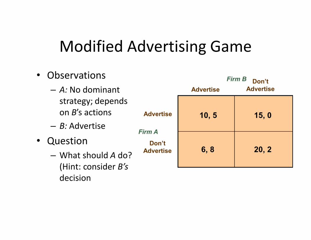
10, 5 15, 0
AdvertiseDon’t
Advertise
Advertise
Firm B
Modified Advertising Game
• Observations– A: No dominant
strategy; depends on B’s actions
20, 26, 8
Firm A
Don’tAdvertise
– B: Advertise
• Question– What should A do?
(Hint: consider B’sdecision

The Nash Equilibrium Revisited
• Dominant Strategies– “I’m doing the best I can no matter what you do.”– “You’re doing the best you can no matter what I do.”
• Nash Equilibrium– “I’m doing the best I can given what you are doing”– “You’re doing the best you can given what I am doing.”
The Nash Equilibrium Revisited
• Examples With A Nash Equilibrium– Two cereal companies
Product Choice Problem
– Two cereal companies– Market for one producer of crispy cereal– Market for one producer of sweet cereal– Each firm only has the resources to introduce one
cereal– Noncooperative
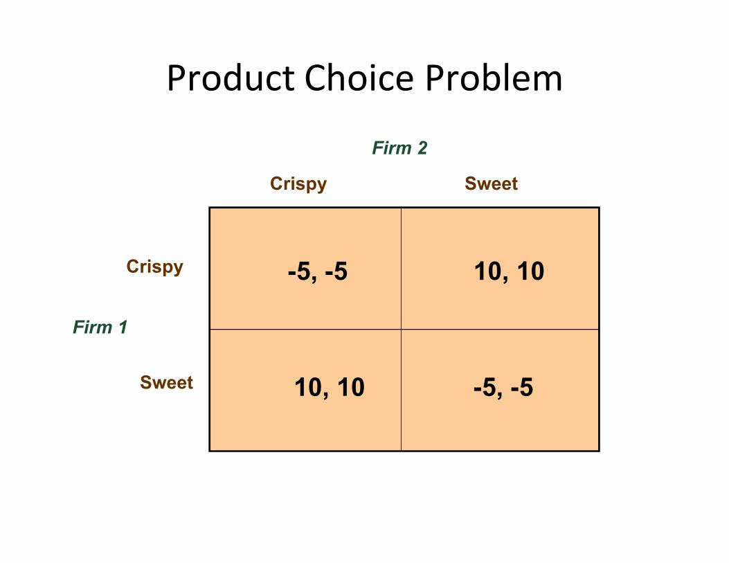
Product Choice Problem
Crispy Sweet
Crispy
Firm 2
-5, -5 10, 10
Firm 1
Sweet
-5, -5 10, 10
-5, -510, 10
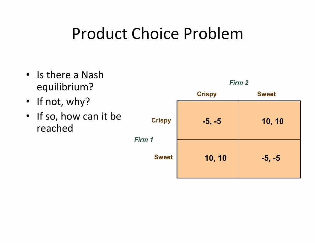
Crispy Sweet
Crispy
Firm 2
-5, -5 10, 10
Product Choice Problem
• Is there a Nash equilibrium?
• If not, why?• If so, how can it be
reachedFirm 1
Crispy
Sweet
-5, -5 10, 10
-5, -510, 10
• If so, how can it be reached
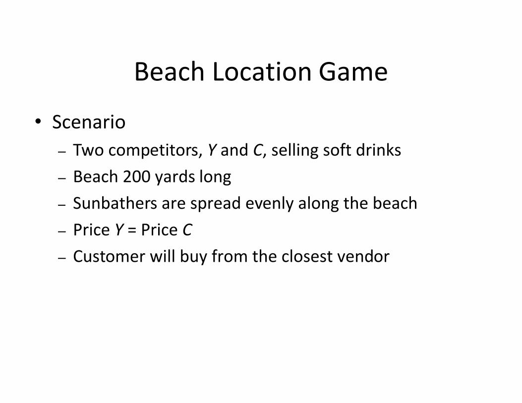
Beach Location Game
• Scenario– Two competitors, Y and C, selling soft drinks– Beach 200 yards long– Sunbathers are spread evenly along the beach– Sunbathers are spread evenly along the beach– Price Y = Price C– Customer will buy from the closest vendor
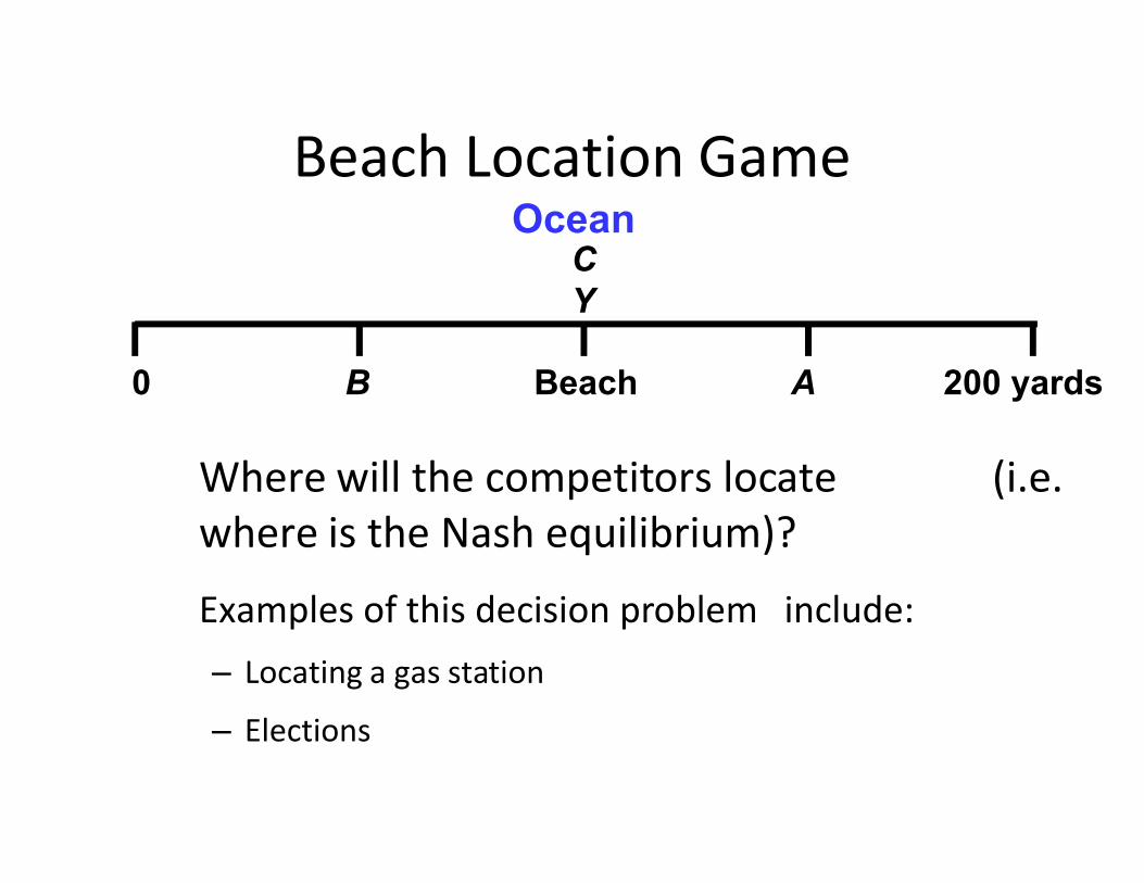
Beach Location GameOcean
0 B Beach A 200 yards
CY
Where will the competitors locate (i.e. where is the Nash equilibrium)?
Examples of this decision problem include:– Locating a gas station
– Elections
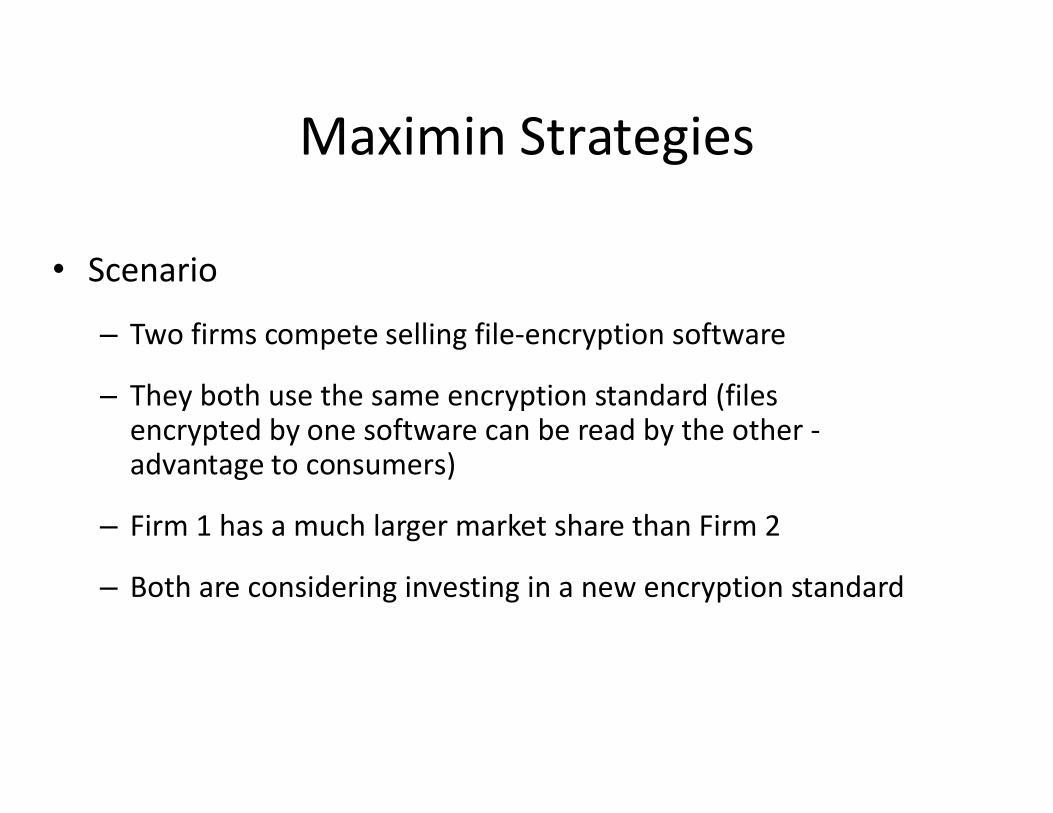
Maximin Strategies
• Scenario
– Two firms compete selling file-encryption software
– They both use the same encryption standard (files – They both use the same encryption standard (files encrypted by one software can be read by the other -advantage to consumers)
– Firm 1 has a much larger market share than Firm 2
– Both are considering investing in a new encryption standard

Don’t invest InvestFirm 2
0, 0 -10, 10Don’t invest
Maximin Strategies
Firm 1
20, 10-100, 0Invest
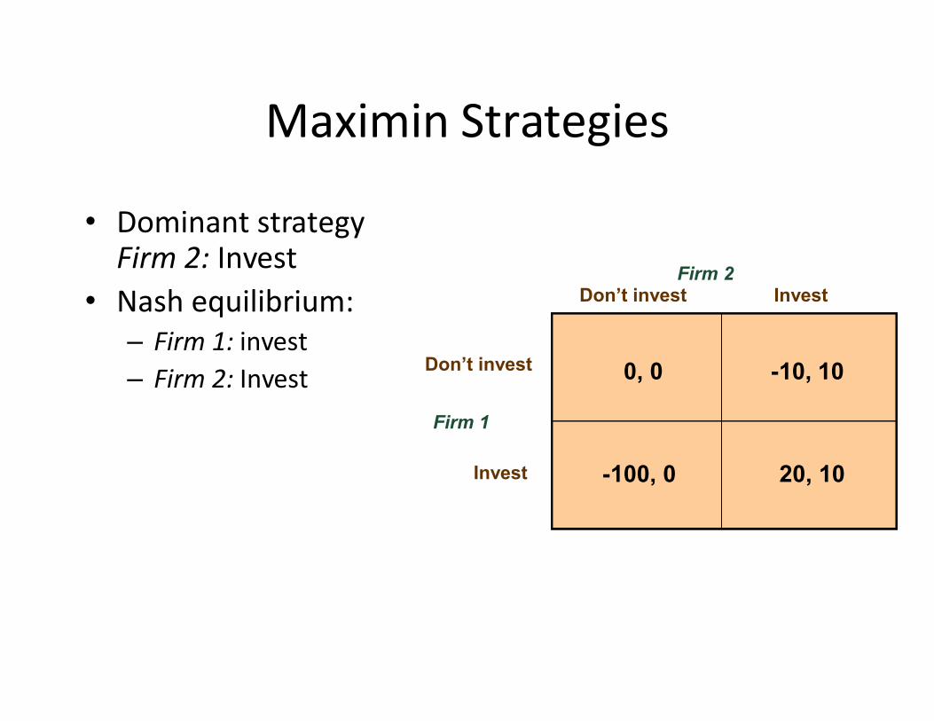
Don’t invest InvestFirm 2
0, 0 -10, 10Don’t invest
Maximin Strategies
• Dominant strategy Firm 2: Invest
• Nash equilibrium:– Firm 1: invest
Firm 1
0, 0 -10, 10
20, 10-100, 0
Don’t invest
Invest
– Firm 2: Invest
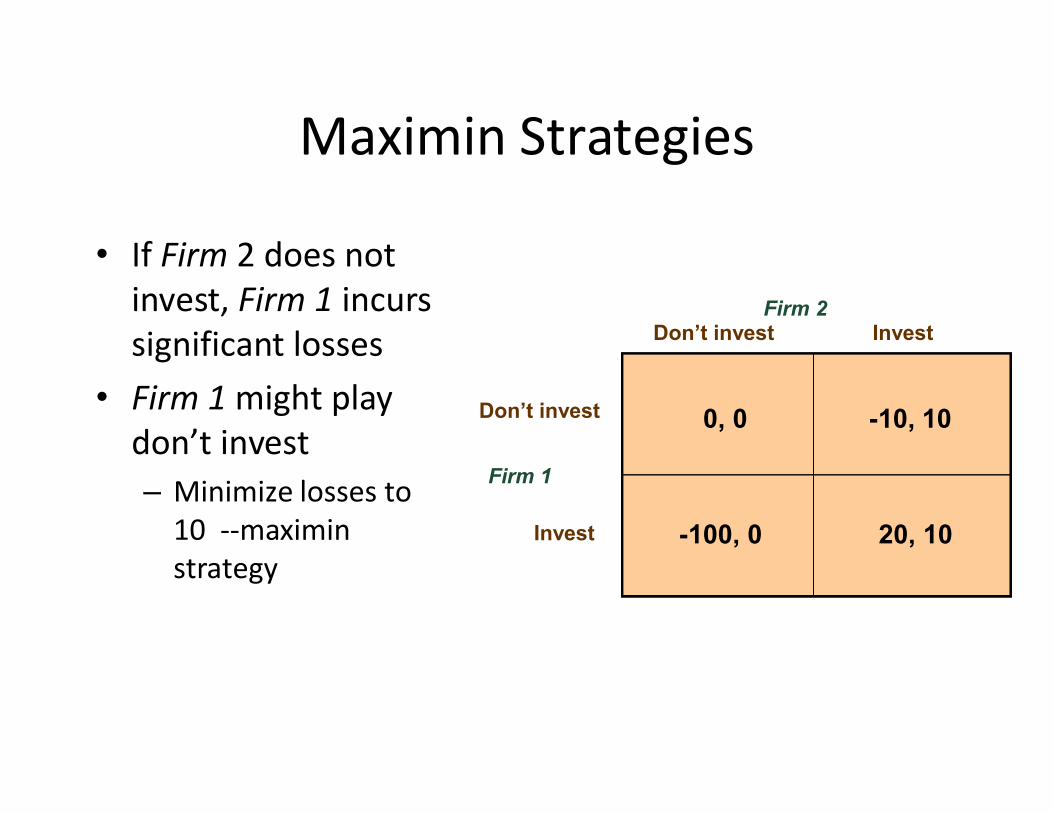
Don’t invest InvestFirm 2
0, 0 -10, 10Don’t invest
Maximin Strategies
• If Firm 2 does not invest, Firm 1 incurs significant losses
• Firm 1 might play
Firm 1
0, 0 -10, 10
20, 10-100, 0
Don’t invest
Invest
• Firm 1 might play don’t invest– Minimize losses to
10 --maximin strategy
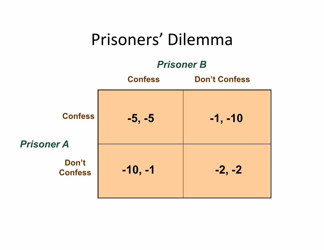
Prisoners’ Dilemma
Confess Don’t Confess
Confess
Prisoner B
-5, -5 -1, -10
Prisoner A
Don’tConfess -2, -2-10, -1
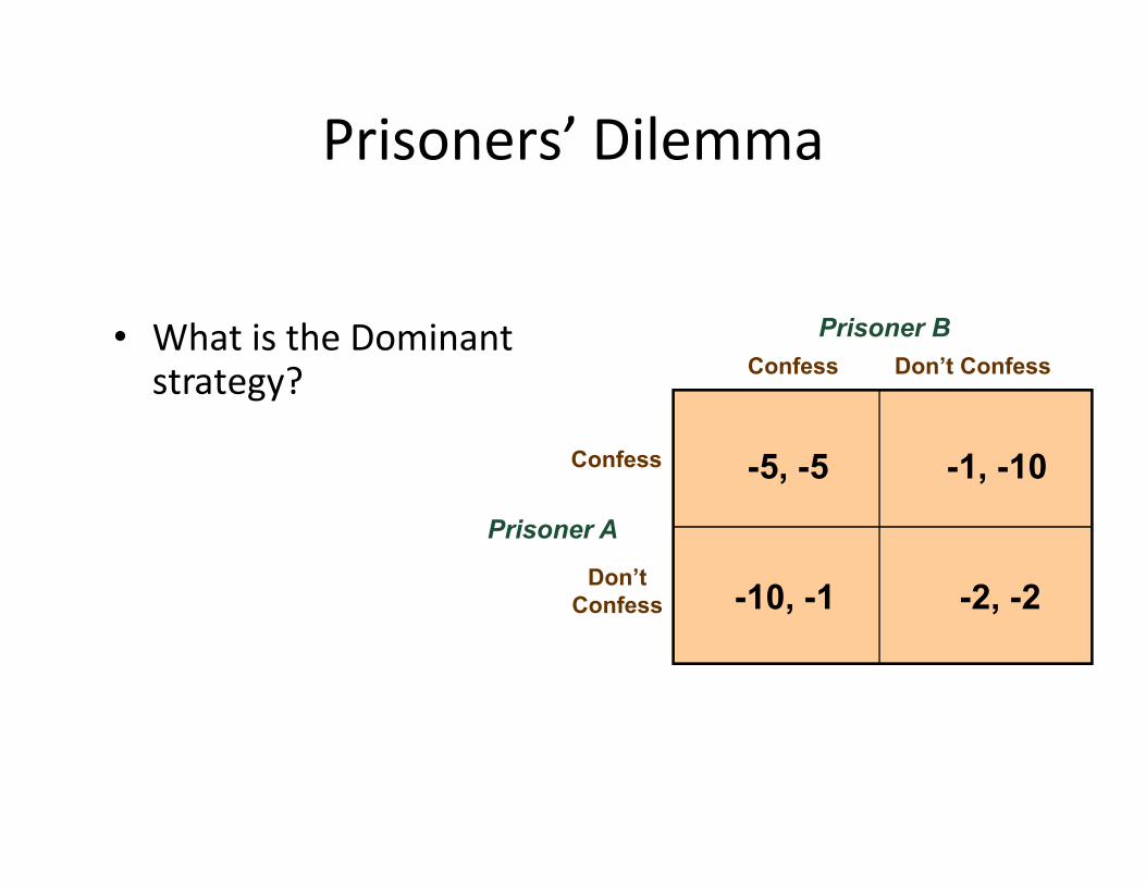
Confess Don’t Confess
Prisoner B
Prisoners’ Dilemma
• What is the Dominant strategy?
Prisoner A
Confess
Don’tConfess
-5, -5 -1, -10
-2, -2-10, -1

Repeated Games• Oligopolistic firms play a repeated game.
• With each repetition of the Prisoners’ Dilemma, firms can develop reputations about their firms can develop reputations about their behavior and study the behavior of their competitors.
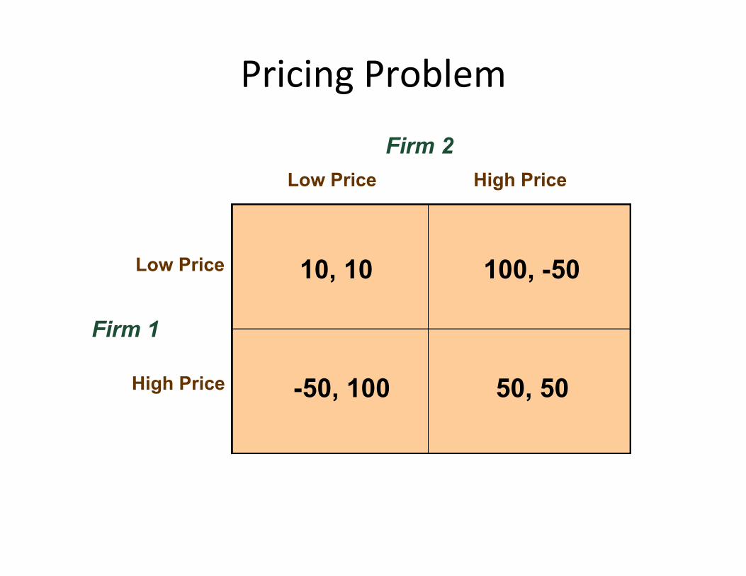
Pricing Problem
Low Price High Price
Low Price
Firm 2
10, 10 100, -50
Firm 1
High Price 50, 50-50, 100
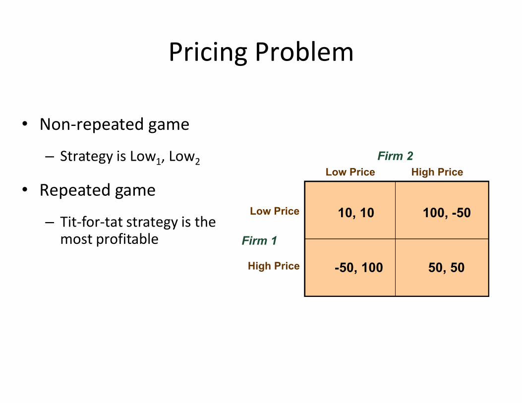
Low Price High Price
Firm 2
Pricing Problem
• Non-repeated game
– Strategy is Low1, Low2
• Repeated game
Firm 1
Low Price
High Price
10, 10 100, -50
50, 50-50, 100
– Tit-for-tat strategy is the most profitable

Oligopolistic Cooperation in the U.S.Water Meter Industry
• Characteristics of the Market– Four Producers
• Rockwell International (35%), Badger Meter, Neptune Water Meter Company, and Hersey Products (Badger, Neptune, and Hersey combined have about a 50 to 55% share)
Very inelastic demand– Very inelastic demand• Not a significant part of the budget
– Stable demand– Long standing relationship between consumer and producer
• Barrier
– Economies of scale• Barrier
Oligopolistic Cooperation in the U.S.Water Meter Industry
• This is a Prisoners’ Dilemma– Lower price to a competitive level
– Cooperate– Cooperate
• Repeated Game
• Question– Why has cooperation prevailed?

Sequential Games• Players move in turn
• Players must think through the possible actions and rational reactions of each player
• Examples– Responding to a competitor’s ad campaign– Entry decisions– Responding to regulatory policy

Sequential Games
• Scenario– Two new (sweet, crispy) cereals– Successful only if each firm produces one cereal– Successful only if each firm produces one cereal– Sweet will sell better– Both still profitable with only one producer
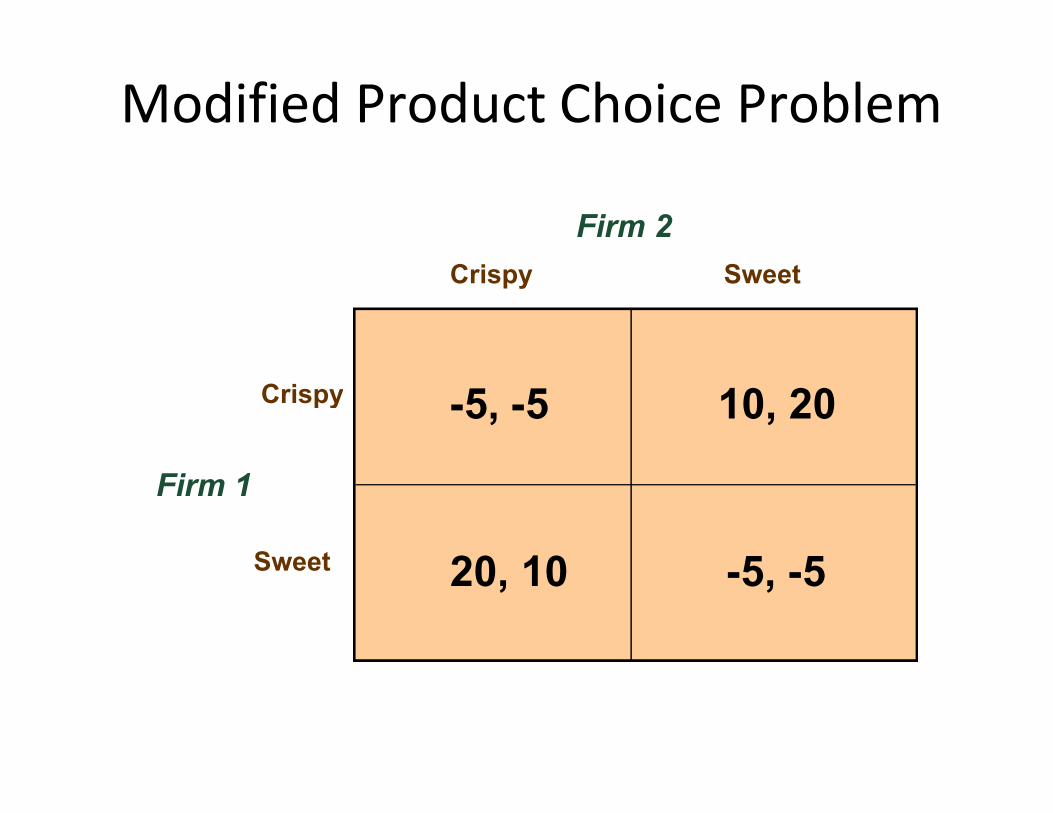
Modified Product Choice Problem
Crispy Sweet
Crispy
Firm 2
-5, -5 10, 20
Firm 1
Crispy
Sweet
-5, -5 10, 20
-5, -520, 10
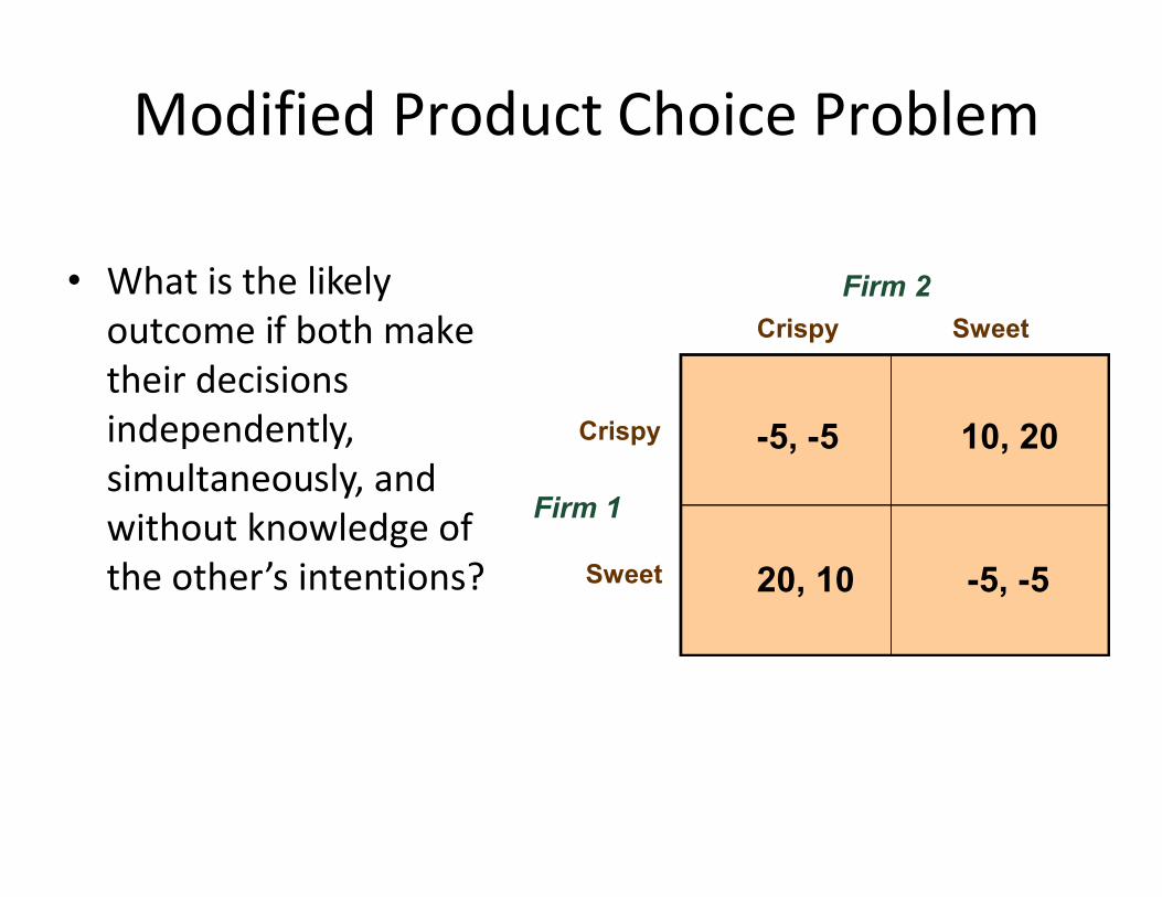
Crispy Sweet
Crispy
Firm 2
-5, -5 10, 20
Modified Product Choice Problem
• What is the likely outcome if both make their decisions independently,
Firm 1
Sweet
-5, -5 10, 20
-5, -520, 10
independently, simultaneously, and without knowledge of the other’s intentions?

Modified Product Choice Problem
• Assume that Firm 1 will introduce its new cereal first (a sequential game).
• Question• Question– What will be the outcome of this game?
• The Extensive Form of a Game– Using a decision tree
• Work backward from the best outcome for Firm 1
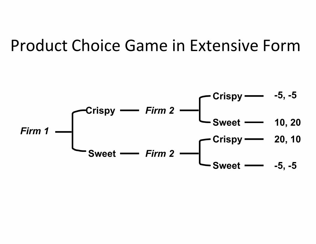
Product Choice Game in Extensive Form
Crispy
Sweet
-5, -5
10, 20Crispy Firm 2
Sweet
Crispy
Sweet
10, 20
20, 10
-5, -5
Firm 1
Sweet Firm 2

Sequential Games• The Advantage of Moving First
– In this product-choice game, there is a clear advantage to moving first.
Threats, Commitments, and Credibility
• Strategic Moves– What actions can a firm take to gain advantage in
the marketplace?Deter entry• Deter entry
• Induce competitors to reduce output, leave, raise price
• Implicit agreements that benefit one firm
Threats, Commitments, and Credibility
• How To Make the First Move– Demonstrate Commitment– Firm 1 must constrain his behavior to the extent
Firm 2 is convinced that he is committed
• Empty Threats– E.g. if a firm will be worse off if it charges a low
price, the threat of a low price is not credible in the eyes of the competitors.

Empty threats: Pricing of Computersand Word Processors
High Price Low Price
Firm 2
Firm 1
High Price
Low Price
100, 80 80, 100
10, 2020, 0
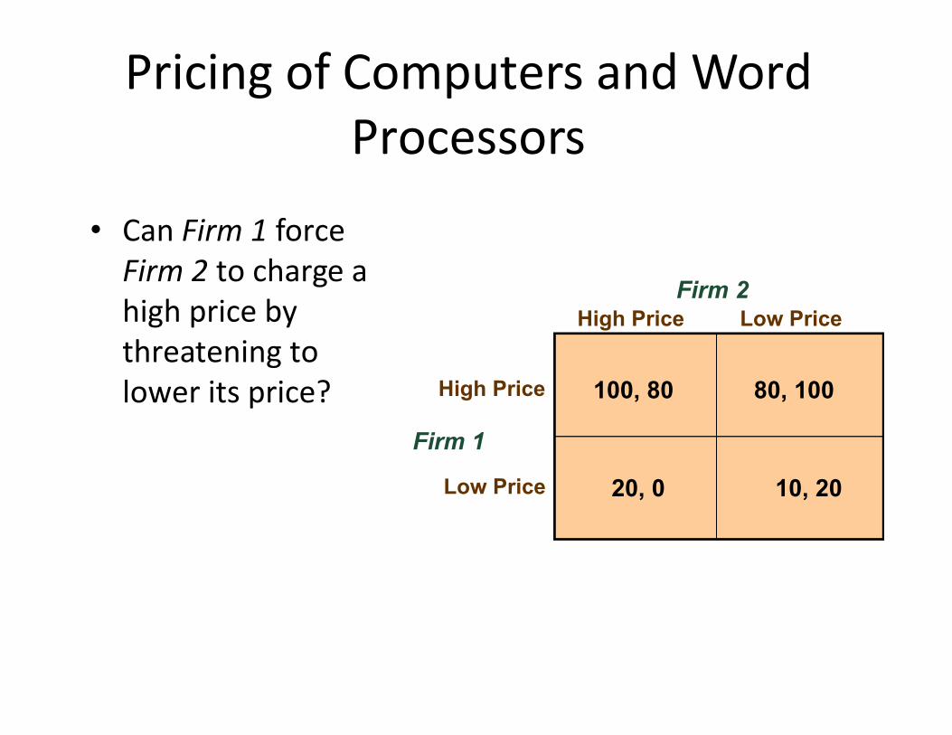
Pricing of Computers and WordProcessors
• Can Firm 1 force Firm 2 to charge a high price by threatening to
High Price Low PriceFirm 2
threatening to lower its price?
Firm 1
High Price
Low Price
100, 80 80, 100
10, 2020, 0
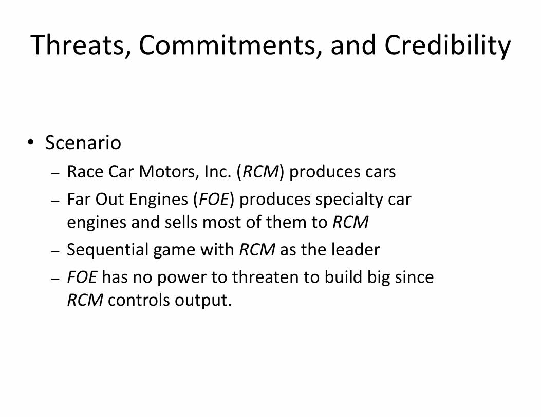
Threats, Commitments, and Credibility
• Scenario– Race Car Motors, Inc. (RCM) produces cars– Far Out Engines (FOE) produces specialty car Far Out Engines (FOE) produces specialty car
engines and sells most of them to RCM– Sequential game with RCM as the leader– FOE has no power to threaten to build big since
RCM controls output.
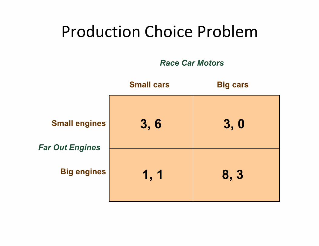
Production Choice Problem
Small cars Big cars
Small engines
Race Car Motors
3, 6 3, 0
Far Out Engines
Small engines
Big engines
3, 6 3, 0
8, 31, 1

Threats, Commitments, and Credibility
• Question– How could FOE force RCM to shift to big cars?
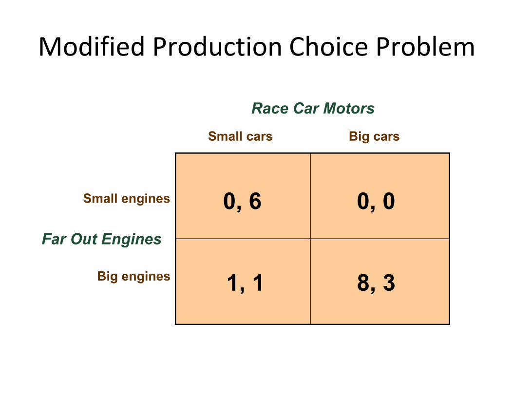
Modified Production Choice Problem
0, 6 0, 0
Small cars Big cars
Small engines
Race Car Motors
0, 6 0, 0
8, 31, 1
Far Out Engines
Small engines
Big engines
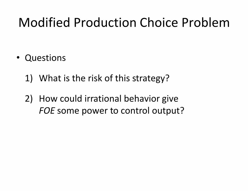
Modified Production Choice Problem
• Questions
1) What is the risk of this strategy?
2) How could irrational behavior give 2) How could irrational behavior give FOE some power to control output?
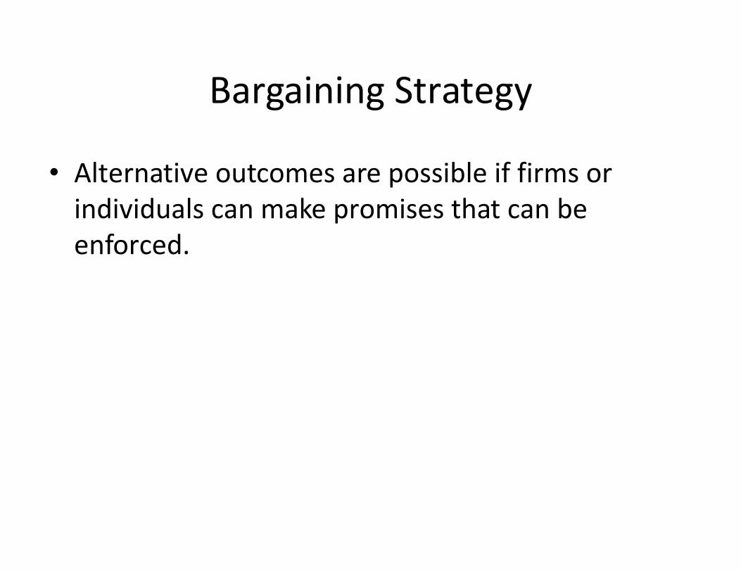
Bargaining Strategy
• Alternative outcomes are possible if firms or individuals can make promises that can be enforced.
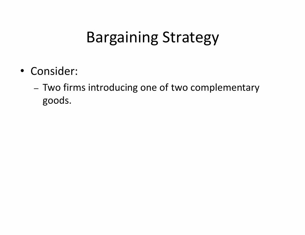
Bargaining Strategy
• Consider:– Two firms introducing one of two complementary
goods.
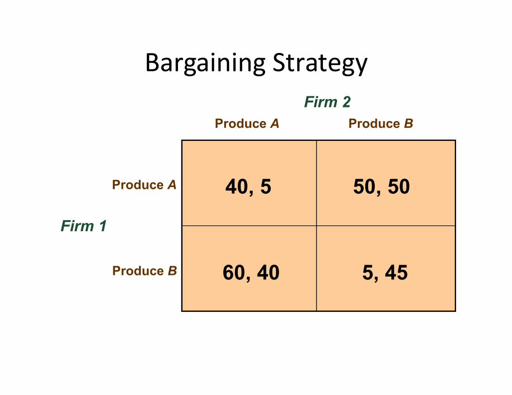
Produce A Produce B
Produce A
Firm 2
40, 5 50, 50
Bargaining Strategy
Firm 1
Produce B
40, 5 50, 50
5, 4560, 40
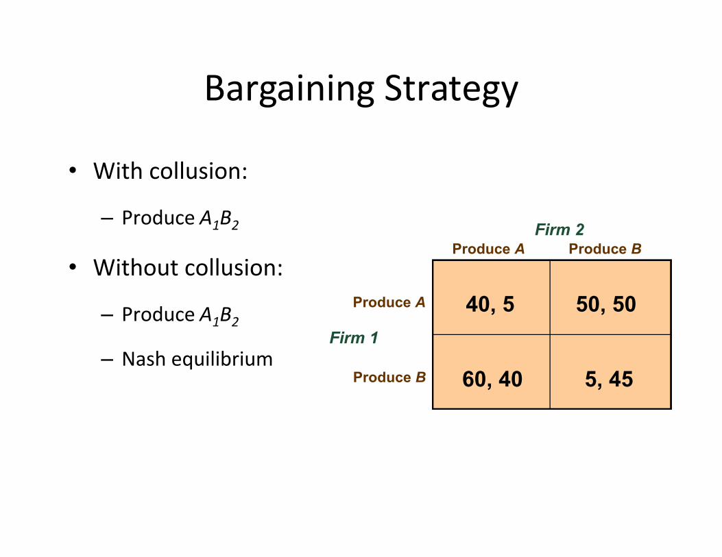
Produce A Produce BFirm 2
Bargaining Strategy
• With collusion:
– Produce A1B2
• Without collusion:
Firm 1
Produce A
Produce B
40, 5 50, 50
5, 4560, 40
• Without collusion:
– Produce A1B2
– Nash equilibrium
Bargaining Strategy
• Suppose– Each firm is also bargaining on the decision to join in a
research consortium with a third firm.
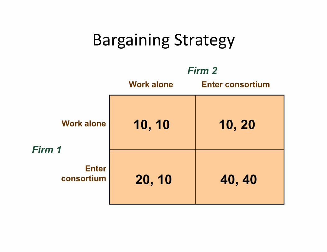
Work alone Enter consortium
Work alone
Firm 2
10, 10 10, 20
Bargaining Strategy
Firm 1
Work alone
Enterconsortium
10, 10 10, 20
40, 4020, 10
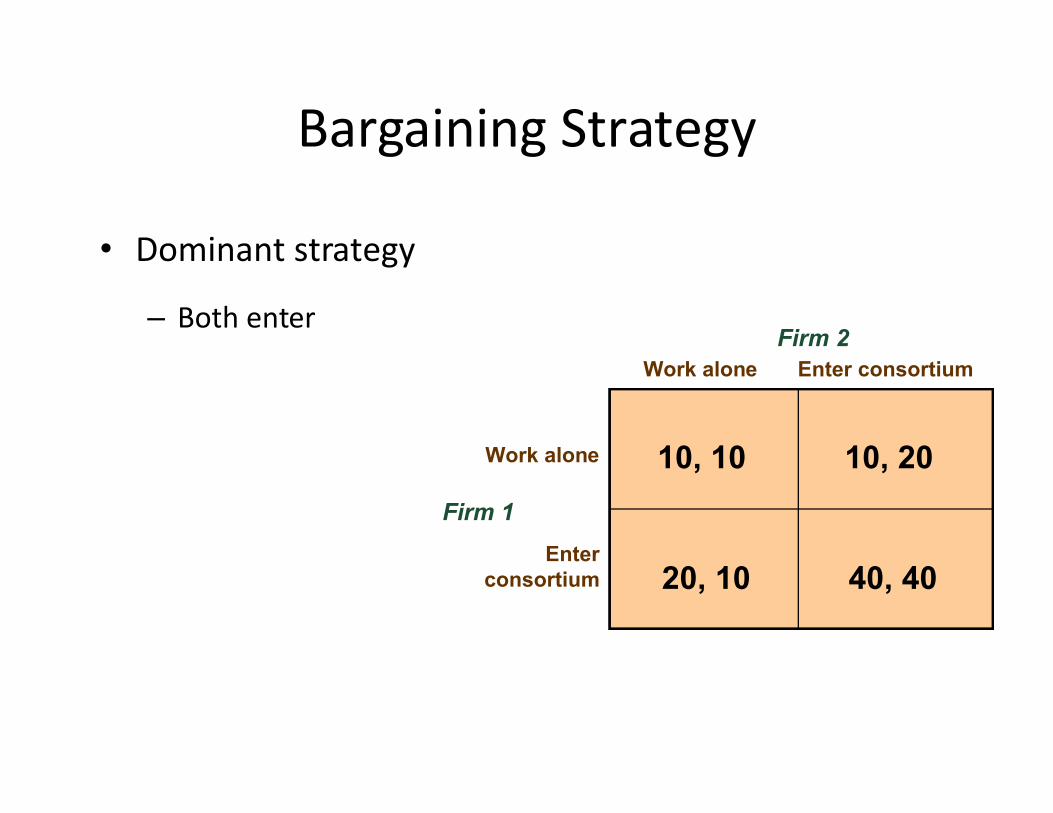
Work alone Enter consortium
Firm 2
Bargaining Strategy
• Dominant strategy
– Both enter
Firm 1
Work alone
Enterconsortium
10, 10 10, 20
40, 4020, 10
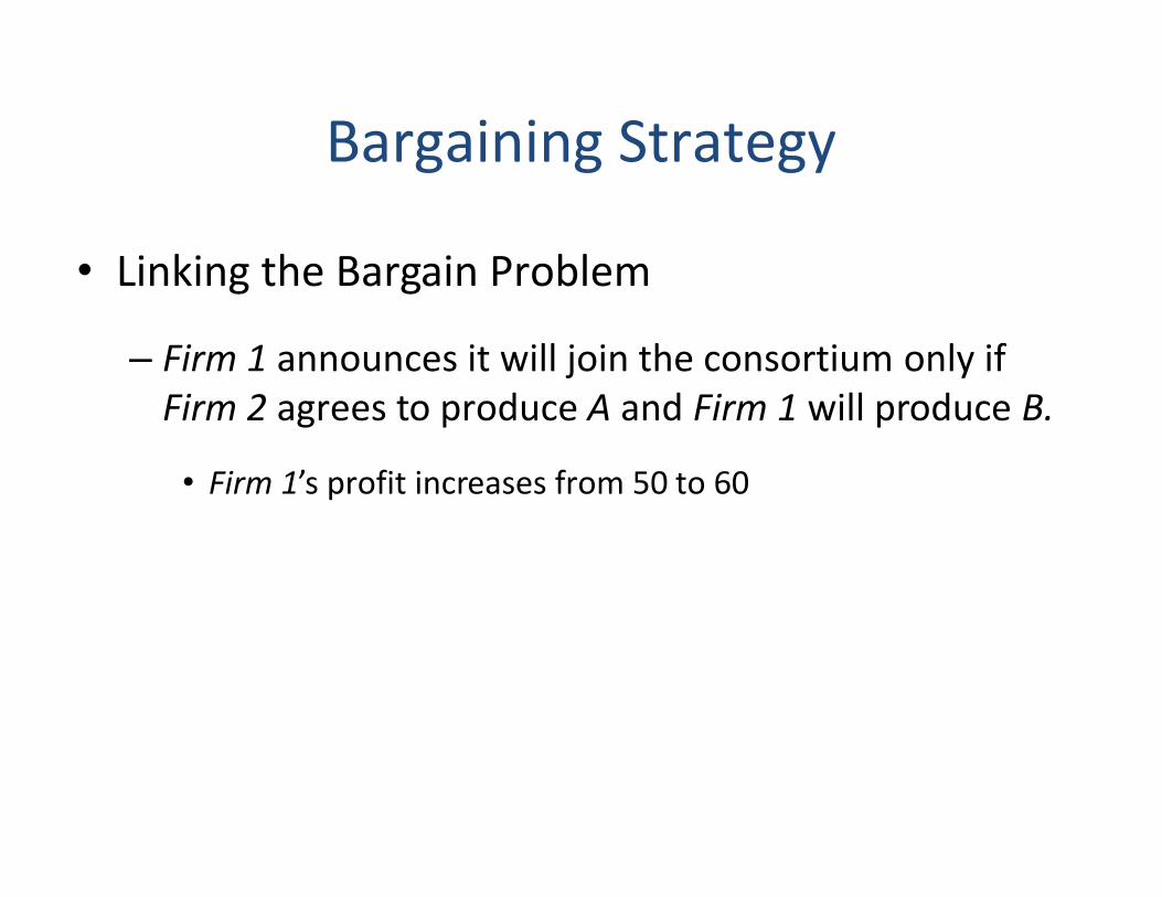
• Linking the Bargain Problem
– Firm 1 announces it will join the consortium only if Firm 2 agrees to produce A and Firm 1 will produce B.
Bargaining Strategy
• Firm 1’s profit increases from 50 to 60

Bargaining Strategy
• Strengthening Bargaining Power– Credibility– Reducing flexibility
Wal-Mart Stores’ Preemptive InvestmentStrategy
• Analysis of how Wal-Mart became the largest retailer in the U.S. when many established retail chains were closing their doors
• How did Wal-Mart gain monopoly power?– Preemptive game with Nash equilibrium
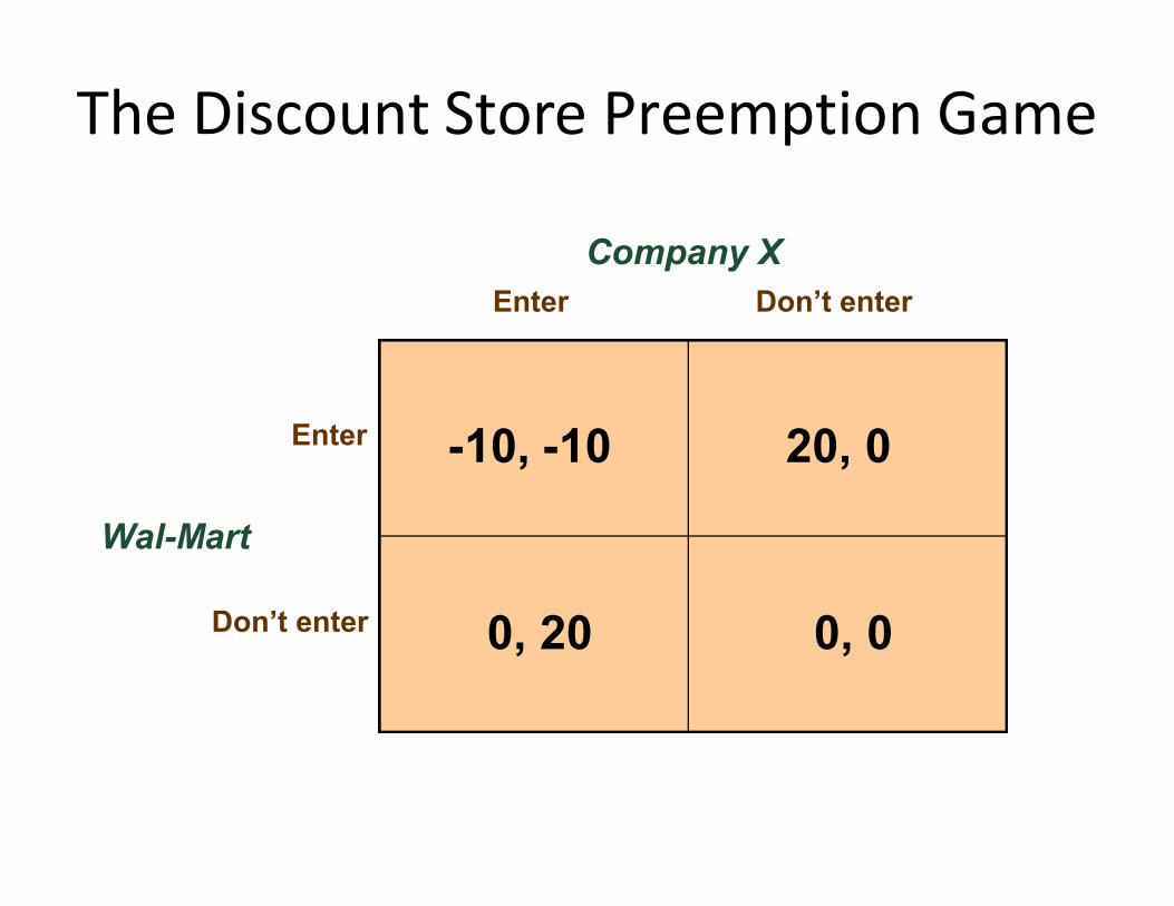
The Discount Store Preemption Game
Enter Don’t enter
Enter
Company X
-10, -10 20, 0
Wal-Mart
Don’t enter
-10, -10 20, 0
0, 00, 20
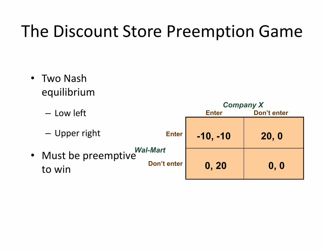
Enter Don’t enterCompany X
The Discount Store Preemption Game
• Two Nash equilibrium
– Low left
Wal-Mart
Enter
Don’t enter
-10, -10 20, 0
0, 00, 20
– Upper right
• Must be preemptive to win
Entry Deterrence
• To deter entry, the incumbent firm must convince any potential competitor that entry will be unprofitable.

Entry Possibilities
Enter Stay out
High price(accommodation)
Potential Entrant
100, 20 200, 0
Incumbent
(accommodation)
Low Price(warfare)
100, 20 200, 0
130, 070, -10
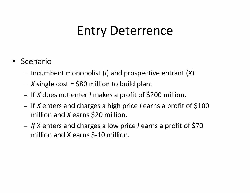
Entry Deterrence
• Scenario– Incumbent monopolist (I) and prospective entrant (X)– X single cost = $80 million to build plant– If X does not enter I makes a profit of $200 million.– If X does not enter I makes a profit of $200 million.– If X enters and charges a high price I earns a profit of $100
million and X earns $20 million.– If X enters and charges a low price I earns a profit of $70
million and X earns $-10 million.
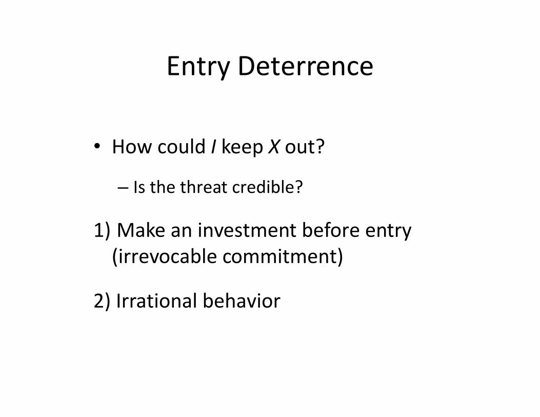
Entry Deterrence
• How could I keep X out?
– Is the threat credible?
1) Make an investment before entry (irrevocable commitment)
2) Irrational behavior
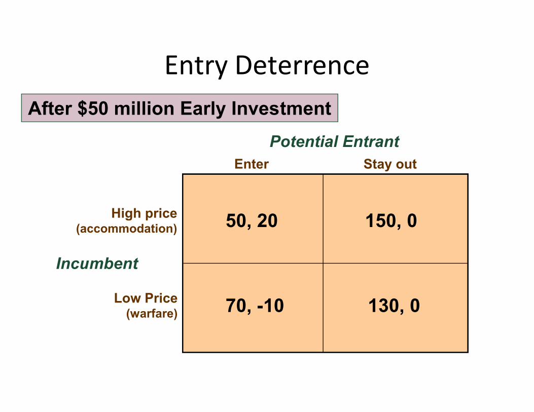
Enter Stay out
High price
Potential Entrant
After $50 million Early Investment
Entry Deterrence
Incumbent
High price(accommodation)
Low Price(warfare)
50, 20 150, 0
130, 070, -10
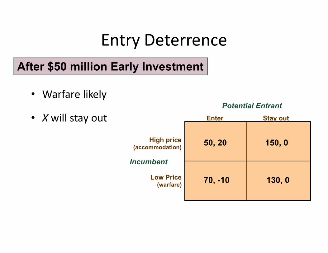
Enter Stay out
Potential Entrant
After $50 million Early Investment
Entry Deterrence
• Warfare likely
• X will stay out
Incumbent
High price(accommodation)
Low Price(warfare)
50, 20 150, 0
130, 070, -10
Entry Deterrence
• Airbus vs. Boeing– Without Airbus being subsidized, the payoff matrix for
the two firms would differ significantly from one showing subsidization. showing subsidization.

Development of a New Aircraft
Produce Don’t produce
Airbus
-10, -10 100, 0Produce
Boeing
-10, -10 100, 0
0, 00, 100
Produce
Don’t produce
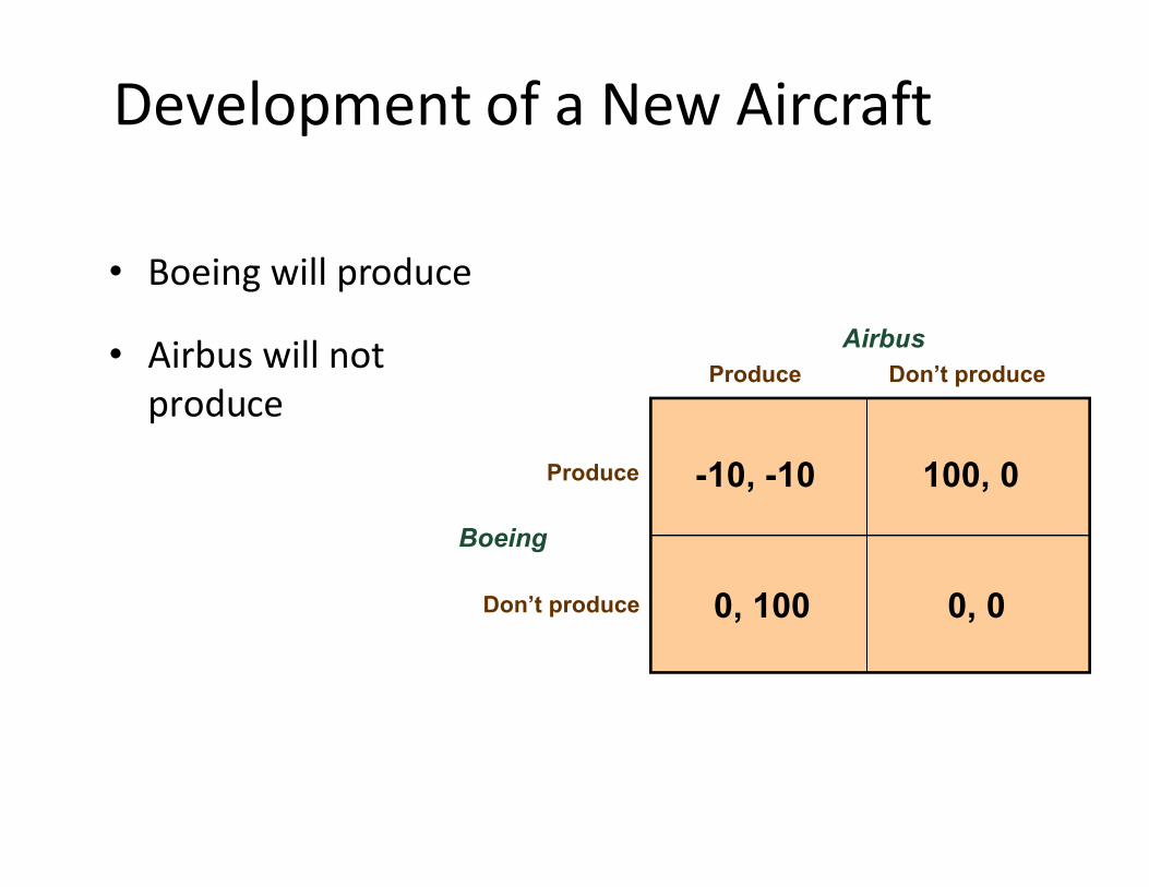
Development of a New Aircraft
• Boeing will produce
• Airbus will not produce
Produce Don’t produce
Airbus
Boeing
-10, -10 100, 0
0, 00, 100
Produce
Don’t produce
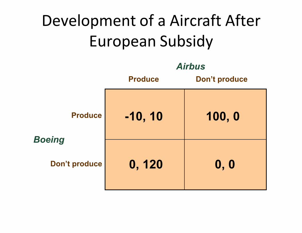
Development of a Aircraft AfterEuropean Subsidy
Produce Don’t produce
Airbus
-10, 10 100, 0Produce
Boeing
-10, 10 100, 0
0, 00, 120
Produce
Don’t produce
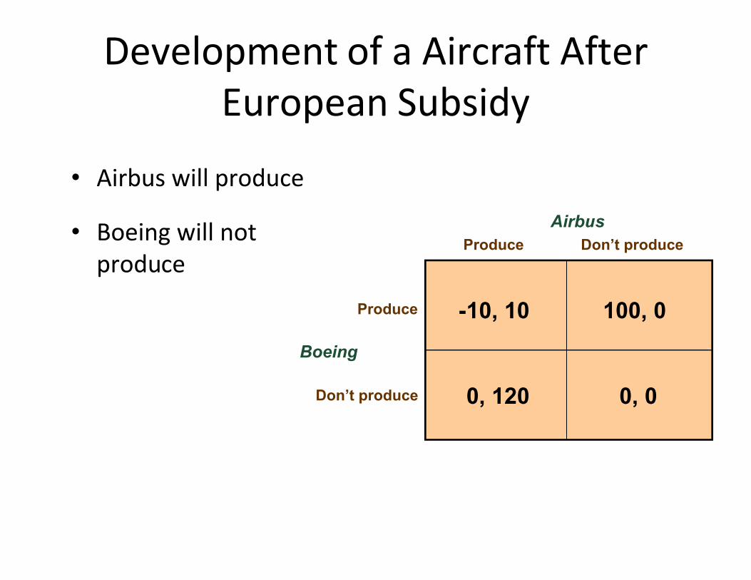
Produce Don’t produce
Airbus
Development of a Aircraft AfterEuropean Subsidy
• Airbus will produce
• Boeing will not produce
Boeing
-10, 10 100, 0
0, 00, 120
Produce
Don’t produce
Summary• A game is cooperative if the players can
communicate and arrange binding contracts; otherwise it is noncooperative.
• A Nash equilibrium is a set of strategies such that all players are doing their best, given the strategies of the other players.
Summary• Strategies that are not optimal for a one-shot
game may be optimal for a repeated game.
• In a sequential game, the players move in turn.In a sequential game, the players move in turn.

Summary• An empty threat is a threat that one would have
no incentive to carry out.
• To deter entry, an incumbent firm must convince any potential competitor that entry will be any potential competitor that entry will be unprofitable.
• Bargaining situations are examples of cooperative games.