Monopolistic Competition

Monopolistic competition: refers to the market situation in which a relatively large number of small producers or suppliers are differentiated products and sofaces a downward sloping demand curve for its own product.

Features of monopolistic competition few sellers i.e. from anything between 25 to just over a 100 Product differentiation Small market share No collusion Independent actions Free entry Eg: furniture, petrol

The theory: assumptions1. Each firm produces one specific variety or brand of the industry’s

differentiated product Each firm thus faces a demand curve that, although negatively sloped, is highly elastic because many close substitutes are sold by other firms

2. The industry contains so many firms that each one ignores the possible reactions of its many competitors when its makes its own price and output decisionsEach firm makes decisions based on its own demand and cost conditions and doesn’t take into account the reactions of its competitors, like a firm would if it was operating in a duopoly

3. there is freedom of entry and exit into the industry if existing firms are earning profits, new firms have an incentive to enter. When they do, the demand for the industry’s product must be shared among more brands

4. there is symmetry when a new firm enters the industry, selling a new version of the differentiated product, it takes customers equally from all existing firms. For example, a new entrant that captured 5% of the existing market would do so by capturing 5% of the sales of each existing firm.

Unexploited scale economiesMany firms in imperfectly competitive industries appear to be operating from a downward sloping portions of their long run average cost curves (although this is possible under monopoly, firms in perfect competition must, in the long run,be at their minimum point of their long run average cost curves). One reason for this is the high development costs and short product lives of many modern products. Many software products (eg) did not exist five years ago and will have been superseded in five years time. A computer program takes a lot of timeto write, but further efforts of it can be produced very cheaply. In such cases, firms face steeply falling long run average cost curves. The more units sold, the lower the fixed costs per unit. Given perfect competition, these firms would go on increasing outputs and sales until rising marginal costs of production just balanced their falling average fixed costs, bringing their

average total cost to a minimum. As it is, they often face falling average total cost curves throughout each product lifecycle.

2

Monopolistic competition: short run equilibrium

demand function = market share demand function downward sloping because of substitutes and other competitors

EquilibriumBecause each firm’s product as some features that are different from those of competitors, each firm faces a negatively sloped demand curve. But the curve israther elastic because similar products sold by other firms provide many close substitutes. The negative slope of the demand curve provides the potential for monopoly profits in the short run.

Short run: profits or losses The firm will maximise its profits or minimise its losses in the short run by

producing at MR = MC The economic profits will induce new firms to enter, causing the profits to

be competed away. o Profits encourage entry o Increases the number of products o Reduces the demand faced by each firmo Demand shifts to the left

The losses will cause an exodus of firms until normal profits are restored.

3

ECONOMICLOSS

DMR

MC

AC

Q

P

DMR

MC AC

Q

P

ECONOMICPROFIT

AC

P

AC

P

Monopolistic competition: long run equilibrium

NORMAL PROFIT: P = ATC P = TC QPQ = PC

Long run equilibrium in the short run a typical firm may make pure profits, but in the long run it

will only cover its costs the entry of new firms have pushed the existing firm’s demand curve to the

left until the curve is a tangent to ATC. Total costs are just being covered In the long run, equilibrium for monopolistic competition, prices are above marginal costs but economic

profits have been driven down to zero Freedom of entry and exist forces profits to be zero in the long run If existing firms in the industry are earning profits, new firms will enter

Excess capacity

Excess capacity: when firms produce at higher unit cost than minimum ATC at equilibrium

The absence of positive profits requires that each firm’s demand curve be nowhere near its long run average cost curve. The absence of losses, which would cause exit, requires that each firm be able to cover its costs. Thus average revenue must equal average cost at some output. Together these

4

DMR

MC

AC

Q

P = AC

DMR

MC AC

Q

P = AC

D2

Normal profit

D2

Normal profit

requirements imply that when a monopolistically competitive industry is in longrun equilibrium, each firm will be producing where its demand curve is tangent to its average total cost curves.Two curves that are tangent at a point have the same slope at that point. If a negatively sloped demand curve is to be tangent to the LRAC, the latter must also be negatively sloped at the point of tangency.

This is the excess capacity theorem of monopolistic competition. Each firm is producing its output at an average cost that is higher than it could achieve byproducing its capacity output. In other words, each firm has unused or excess capacity so:

The theory of monopolistic competition shows that an industry can be competitive, the sense of containing numerous competing firms and no pure profits, and yet contain unexploited scale economies, in the sense that each firm is producing on the negatively sloped portion of its average total cost curve.

Is excess capacity wasteful?The long run equilibrium of a monopolistically competitive industry might seem inefficient. Production costs are not as low as they could be if firms producedat the lowest point on their average cost curves, and firms typically invest insome capacity that goes unused. But this is not necessarily inefficient, because people value diversity and areprepared to pay for it. For eg: each brand of shampoo, car, denim jeans etc hasits sincere devotees. Increasing the number of differentiated products has two effects. First, it increases the amount of excess capacity in the production ofeach product, because the total demand must be divided among more products. Second, the increased diversity available products will better satisfy diverse tastes. How will consumers satisfaction be maximised in these circumstances?

Consumer’s satisfaction is maximised when the number of differentiated products is increased until the marginal gain in consumers’ satisfaction from an increase in diversity equals the loss from having to produce each existing product at higher cost.

For this reason (among others), the belief that a large group of monopolistic competition would lead to inefficiency in the use of resources is not proven.

5

DMR

MCAC

Q

P

Mark-up

Excess capacity Q

P

MC

AC

MR

Efficient production – no excess capacity

Excess capacity: the differences between the amount produced by a firm and the amount that could be efficiently produced.

Mark up: (over marginal cost)The tangency solutionThe tangency solution is an economic proof used to show that in the long run, amonopolistically competitive firm will realise only a normal profit because theprofit maximising output will occur when its demand curve is at a tangent to its ATC curve.

Losses to productive efficiency must be traded off against gains for the welfare of society through increased level of consumer choice resulting from product differentiation.

OligopolyOligopoly: the situation when the number of firms in the industry is so smallthat each must consider the reactions of its rivals when formulating price

policies.

Key features the tension between cooperation and self interest; cooperation means

colluding and acting like a monopolist by restricting output and price. Self interest means being interested in your own profit such that there are powerful incentives to hinder the formation of a monopoly

each firm has enough market power to prevent it being a price taker, but eachfirm is subject to enough inter-firm rivalry to prevent it considering the market demand curve as its own

oligopolies face few competitors because there are only a few firms in the industry, each firm realises that

its competitors may respond to any price movements the behaviour of the oligopolist is strategic, i.e. they must take explicit

account of the impact of their decisions on competing firms and of the reactions they expect from competing firms

high industry concentration ratio

6

significant barriers to entry that may be derived through legislation, economies of scale / scope, control of raw materials, the size of start up costs, sunk costs, and / or the strategic behaviour of market participants.

Suppliers control information about the industry, cost structures, prices andtechnologies

Price stability, and non price competition. Non-price competition is based upon factors other than price, eg image, packaging, advertising, technological development, location etc. Non price competition has two advantages over price competition. Firstly, it can produce a relatively permanent competitive advantage over rivals that cant be achieved with price competition. Secondly, non price competition is under the control of each competitor and takes considerable time to implement

Collusive behaviour in the form of:o The establishment of a monopoly selling organisation (cartel)o Price leadershipo ‘gentlemen’s’ agreements: informal verbal agreements o Market sharing

Factors to why so few large firms dominate the industry Natural causesEconomies of scale Larger firms can afford to produce more and engage in large scale production. Through doing so, the larger the scale of production, the lower the average variable costs of production

Fixed costsIt is costly to design, prove and market a new product. However fixed costs in product development must be recovered in the revenues from sales of the product. The larger the firms sales the lower the cost that has to be recoveredform each unit sold.

Economies of scopeEconomies of scope apply to multi-product firm from the fact that some resources of the firms can be shared between different product areas. Economiesof scope exist if production of several different products within one firm leads to lower unit costs of production of each product being lower than if they had been produced in independent firms.

Artificial causes (firm created)The number of firms in an industry may be decreased while the average size of the survivors rises, as a result of the strategic behaviour of the firms themselves. Firms may grow by acquisitions or mergers; or by driving rivals into bankruptcy through predatory practices.In this way the size and market shares of the survivors increase and may, by reducing competitive behaviour, allow them to earn larger profit margins. But these high profits will attract new entrants unless the surviving firms can create and sustain barriers to entry. Although most firms would like to behave in this manner, it is no easy tasks to create effective entry barriers when natural ones don’t exist.

7

The Game Theory

Game theory: is concerned with the study of optimal strategies to maximise payoffs, given the risks involved in judging the responses of adversaries and also the conditions under which there is a unique solution.

Example: prisoners dilemma

They know what the optimal level is, but they would choose the sub-optimal level because they are uncertain of the other’s move.

Outcome

Nash equilibrium: a situation when all the participants in a game are each pursuing their best possible strategy in the knowledge of the strategies of allother participants.

Dominant strategy: a strategy that is the best for a player in a game regardless of the strategies chosen by other players.

Co-operation?The prisoner’s dilemma shows that cooperation is difficult to achieve. Some times players can solve prisoner dilemma’s because the game is played more thanonce. They may give rise to the co-operative equilibrium. Each player knows that the other plays will punish cheating eg: tit for tat strategy.

Mutual independence

Mutual independence: the situation where the fate of one firm lies partially orwholly with the performance or decisions of other firms in the same industry.

8

8 years

8 years

SUB-OPTIMAL

20 years

0 years

DOMINANT STRATEGY

0 years

20 years

1 year

1 year

OPTIMAL

Confess

Clyde’sstrategy

Bonnie’s strategy

Confess

Collusive tendencies

Collusion: this term denotes a situation in which two or more firms jointly settheir prices or outputs, divide the market among themselves or make other business decisions jointly.

When oligopolists can collude to maximise their joint profits, taking into account their mutual interdependence, they will produce the monopoly output and price and earn the monopoly profit.

Cartel: an organisation of independent firms, producing similar products, that work together to raise prices and restrict output.

The cartel is the most extreme form of collusive agreement. Each individual supplier agrees to accept an output and price decision decided by the central selling organisation. The behaviour of cartels is for example observed in the pricing and output decisions of OPEC and medical and other professional associations.

The central organisation, having achieved control over all supply firms’ outputdecisions, act to produce a monopoly solution. It determines that the industry’s output level will be at a level where the industry’s marginal cost is equal to the industry’s marginal revenue. This output level will maximise the industry’s profit level.

Market sharing Firms compromising an oligopoly decide on some occasions to divide the market on a geographical line. This has been the experience in the taxi, beer, and newsagents industries at different points in time. The division of the market allows each individual supplier to act as a monopolist, producing a profit maximising economic profit, not achieving economic efficiency and producing an output that is not allocatively efficient. This is market sharing.

Maximin strategies and optimal pricing strategy

Maximin strategies: strategies chosen by players in a game to maximise their minimum expected payoff form the game.

Kinked demand curve

Kinked demand curve: this model assumes that firms believe that rivals will match any price cut but will not follow price increases.

the assumption results in the demand curve displaying a kink at the current price

the segment above the kink will be highly elastic the segment below the kink will be highly inelastic

9

an implication of this model is that prices will be inflexible over the business cycle.

Demand is relatively inelastic If an oligopolist lowers its price, competitors will follow. Thus as price falls quantity demanded increases slowly.

10

Demand is relatively elastic If an oligopolist raises price, competitors will most likely not raise their prices. Thus as price rises, quantity demanded falls rapidly.

choose the MR line that corresponds with the demand line MR no longer straight because D is no longer straight To maximise profits in the usual way: MR = MC If the MC curve intersects the discontinuous portion of the MR schedule,

price and output will remain the same, at P and Q This leads to price rigidity or tends to cause rigidity in oligopoly pricing

11

P

MR

MR1D

D1

D

MR

MC1

MR2

P

Q

For every demand curve, there is a corresponding marginal revenue curve. The marginal revenue curve is located midway between the price axis and the average revenue (demand) curve.

Two marginal revenue curves are associated with the kinked demand curve. The first is associated with the demand curve above the kink and the second with the demand curve below the kink.

The important sections of each marginal revenue curve are those associated with the demand curve that is relevant to the curve.

The overall effect of the gap in the marginal revenue curve is that there maybe substantial increases in marginal costs with no change in the price or output level of the firm and the industry.

This situation will continue, as long as the new marginal cost curve does notcut the continuous sections of the marginal revenue curve. If it does, a new kink is established.

Price inflexibility The kinked demand schedule gives each oligopolist good reason to believe that any change in price will be for the worst. Many of the firm’s customers will desert it if it raises prices. If it lowers price, its sales at best will increase very modestly. Worse yet, a price cut by firm A may be more than met by firm’s B and C. that is, firms A’s initial price cut may precipitate a pricewar, so the amount sold by firm A may actually decline as its rival firms charge still lower prices.

The other reason for price inflexibility under non-collusive oligopoly works from the cost side. The broken marginal revenue curve that accompanies the kinked demand curve suggests that, within limits, substantial cost changes willhave no effect on output and price. Any shift in the marginal cost between MC1 and MC2 will result in no change in price or output. MR will continue to equal MC at output Q at which price QP will be charged.

CriticismsThe kinked demand analysis is subject to two major criticisms. 1. It doesn’t explain why the current price is at PQ in the first place Rather is helps to explain only why oligopolists may be reluctant to deviate from an existing price that yields that a ‘satisfactory’ or ‘reasonable’ profit.

2.When the macro-economy is unstable, oligopoly prices are not as rigidParticularly in an upward direction – as the kinked demand theory suggests.Particularly during inflationary periods such as the late 1980s, oligopolist

producers raised their prices frequently and substantially.

12

Market failureMarket failure Market failure occurs with the presence of any of the following: monopolies public goods externalities

When these occur: we produce the wrong amount of goods and services fail to allocate any resources at all to the production of certain goods

Public goods

Public goods: goods and services that are not provided by the market system, asthey are indivisible and often bound by the exclusion principle

Exclusion principle: when those who do not pay for a product are excluded from its benefit.

Pure public goods: goods and services that are both indivisible and not subject to theexclusion principle.

Free-rider problem: when people receive benefits from the consumption of a goodor service without contributing directly to its costs.

Rival goods: a good that no two people can consume eg: apples, seat on an aeroplane

Determining the efficient provision of a public good

Marginal benefit: the additional benefit from one unit increase in the provision of a public good Marginal cost: the additional cost of the provision of one unit of the public good

13

MB

MCMB

MC

Q*QPG

Point ofallocativeefficiency

Private provision of a public good?Would the private sector provide Q* amount of the public good? NO! To provide it, the private sector would need to collect at least (total cost/population) to cover its costs and individuals have an incentive to free ride. Private provision is thus likely to be inefficient.

14

The market works best when goods and services are rivalrous and excludable Private firms can produce and sell them. Furthermore, these firms will fulfilthe condition for allocative efficiency by operating where marginal cost equals price as long as they are price takers.

TaxationTo raise revenue to fund the provision of public goods the government collects taxes (among other revenue measures) – for example, income tax and excise duties. Tax rates (those relating to excise taxes) vary depending on the price elasticity of demand for the good. Goods that have a low elasticity are taxed more heavily than those which have a higher elasticity. Why?? Deadweight lossesfor the former case are smaller.

Externalities

Externality (spill over): is a benefit or a cost associated with the consumption or production of a good or service which is obtained by or inflicted without compensation upon a party other than the buyer or seller of the good or service.

The externality is not reflected in the market supply curve, which only includes marginal private costs. Industrial pollution is a cost to society. In this case, marginal social costs (MSC) will exceed marginal private costs (MPC)by the amount of the marginal external costs (MEC) and the market solution of price and output will not be economically efficient. Thus:

MSC = MPC + MEC

External benefits The benefits obtained neither by producers nor by consumers of the product but without compensation by a third party (society). Eg: benefits to shops from theconstruction of a cinema complex or education. Spillover benefits cause an under-allocation of resources in that the optimum output exceeds the equilibrium output.

15

S

S1

D1

P

Benefit

The market demand curve shows the impact of external benefits on resource allocation. The market demand curve reflects only marginal private benefit – the private benefit derived at the margin by individuals. This understates the marginal social benefit available to society as a whole from consumption of each successive unit of the good or service. The market demand curve fails to capture all the benefits associated with the provision and consumption of goodsand services that involve external benefits.

D indicates the marginal benefits that private individuals derive from education, D1 is drawn to include these private benefits plus the additional external benefits. Whilst D and S would yield an educational output of Qe, this output would be less than the optimum output Qo. The market system would not produce enough education, (resources would be underallocated). Efficiency requires an increase in the allocations of resources to the production of education services and an increase in output of these services of QeQo. At Qo, the marginal social benefit (equal the marginal private benefit plus B) will beequal to the marginal social cost of production of education services, as shownby the height of supply curve SS.

External costsThe costs of producing a product borne by neither producer or consumer of the product but without compensation by a third party. Eg: pollution. External costs affect the allocation of resources. When external costs occur, producers shift some of their costs onto the community and their production costs are lower than otherwise. That is, the supply curve which shows marginal private cost of production, does not include or ‘capture’, all the costs that can be legitimately associated with the production of the good. Hence the producer’s supply curve S, understates the marginal social cost of production and therefore liesbelow the supply curve, that would include all costs to society of producing additional units of output, S1. By polluting (that is by creating an external cost), the firm enjoys lower costs and the supply curve S.

16

Qe Qo

D

S1

S

P

Q Qo

Qe

Cost (T)

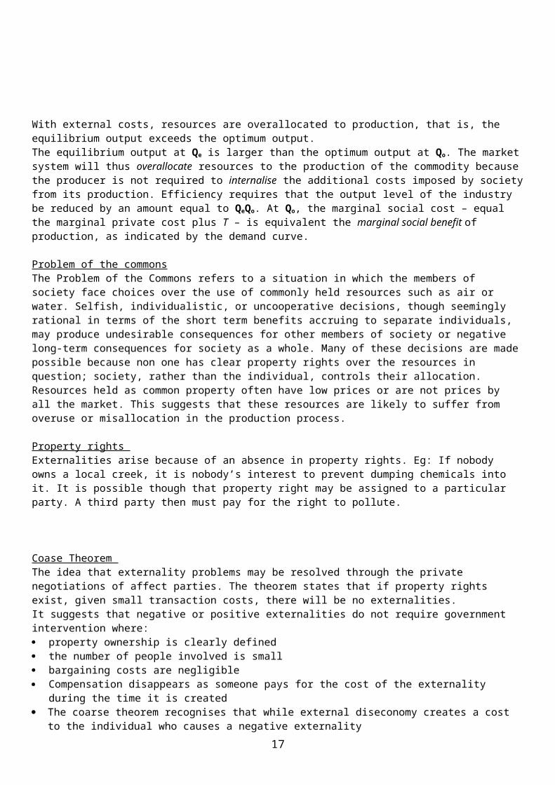
With external costs, resources are overallocated to production, that is, the equilibrium output exceeds the optimum output. The equilibrium output at Qe is larger than the optimum output at Qo. The marketsystem will thus overallocate resources to the production of the commodity becausethe producer is not required to internalise the additional costs imposed by societyfrom its production. Efficiency requires that the output level of the industry be reduced by an amount equal to QeQo. At Qo, the marginal social cost – equal the marginal private cost plus T – is equivalent the marginal social benefit of production, as indicated by the demand curve.

Problem of the commonsThe Problem of the Commons refers to a situation in which the members of society face choices over the use of commonly held resources such as air or water. Selfish, individualistic, or uncooperative decisions, though seemingly rational in terms of the short term benefits accruing to separate individuals, may produce undesirable consequences for other members of society or negative long-term consequences for society as a whole. Many of these decisions are madepossible because non one has clear property rights over the resources in question; society, rather than the individual, controls their allocation. Resources held as common property often have low prices or are not prices by all the market. This suggests that these resources are likely to suffer from overuse or misallocation in the production process.

Property rights Externalities arise because of an absence in property rights. Eg: If nobody owns a local creek, it is nobody’s interest to prevent dumping chemicals into it. It is possible though that property right may be assigned to a particular party. A third party then must pay for the right to pollute.

Coase Theorem The idea that externality problems may be resolved through the private negotiations of affect parties. The theorem states that if property rights exist, given small transaction costs, there will be no externalities. It suggests that negative or positive externalities do not require government intervention where: property ownership is clearly defined the number of people involved is small bargaining costs are negligible Compensation disappears as someone pays for the cost of the externality

during the time it is created The coarse theorem recognises that while external diseconomy creates a cost

to the individual who causes a negative externality17

It was created by Ronald Coarse who tried to get rid of the impact of externalities

A solution therefore would be choose the action that produces the least cost to society – measuring the benefits of payment along with the costs

Resources therefore, should be allocated to solving the problems of externalities, only to the extent that the marginal cost of the solution equals to the marginal benefit gained by the solution

Government should confine its role under these circumstances to encourage bargaining between affected individuals or groups. Because the economic self interests of the parties are at stake, bargaining with one another will enable them to find an acceptable solution to the problem. Property rights enable the parties to place a price tag on an externality through negotiation, creating opportunities for both.

Under this arrangement, the owner of the property rights can negotiate with thepart causing the negative externality. The owner will seek compensation for thecost of the externality – T (refer to diagram above). This additional cost to the party causing the negative externality leads to a reduction in output to the socially desirable level at Qo. A strong incentive thus emerges for the party tosolve their externality problem.

Marketable permits

Procedure: allocate each firm a permit to pollute a certain amount and allow the permits to be bought and sold.

E.g.: suppose there are two firms (a heavy polluter and a low polluter) Permits are allocated evenly

18

Marketable rights for pollution A market for pollution rights requires the establishment of an allowable

amount of pollution – in line with the ability of the environment to recycle – by a pollution control agency. This would be associated with the development of a set of ‘rights’ (permits) to create units of pollution.

These rights would be sold or auctioned in the market Polluters would bid for pollution rights up to the point at which the cost of

the pollution right exceeds the private cost of pollution abatement A market for pollution rights ensures an efficient allocation of rights

between producers reflecting the marginal cost to each of controlling its output of pollution, and hence the marginal benefit attained from the right to pollute

Marketable permits

Taxes and pollution

19

10

5MPB

2 5 Emissions

Low Polluter

MPB

15

10

5 8Emissions

Heavy polluter

Cost and benefits

Cost and benefits

10Emissions

MPB

MSC

Economy Cost and benefits

PERMITS ALLOTTED

MSC

MPC

A

P1

P2

P0

P3

Price, cost and

External costs

Efficient point

If everybody looked after their own interest (MPB=MPC), Q0 is produced. However MSC is higher than P1. The MC imposed on others is P1 – P0.

If the government imposes a tax equal to the external cost, price increases from P0 to P2 and quantity falls from Q0 to Q2. This is a point of efficiency (MPB=MSC). This is point A on the diagram

Other strategies of solving market failure (caused by externalities) Correcting for externalities

Legislation – such as with pollution passing limitations which prohibitor limit the amount if it works effectively it should decrease supply

A specific tax – a tax on an industry or a firm which will push up the cost, encouraging more efficient means of production

Property rights and individual bargaining – explored above

Correcting for external benefits Subsidise buyers – reduce the private cost on household income Subsidise producers – acts as a grant, however not all of it is put

towards the produce

Externalities and knowledge There are three devices by which the government can capitalise on the external benefits arsing from knowledge (assume its education), in order to achieve an efficient allocation of resources. subsidies below cost provision patents Suppose we have provision of education by a private institution Suppose that the MC of providing education is shown by the MSC curve and the

demand for education is represented by a MPB curve Competitive equilibrium is Point A However it is generally the case that education exhibits external benefit.

This implies that the MSB curve lies to the right of the MPB curve

20

D = MPB

Q2

MSC

MSBD = MPBA

B

Cost and price

P3

P1

P2

Q1 Efficient

Point of efficiency

Competitive equilibrium

Point of Efficiency – Point B

At point B the efficient output level is Q2 so long as tuition costs $P2 But since the MC at point B is P3, to attain efficient quantities of

enrolments the government must subsidise private institutions by an amount equal to P3 – P2

Aggregate DemandWhat is Macroeconomics? The study of the whole economic system aggregating over the functioning of

individuals economic units More specifically, it is the study of national economies and determination of

national income

Measuring Aggregate Output

GDP (Gross Domestic Product): The total market value of all final goods and services produced in the economy during a specified period of time

GDP is a measure of production, and, accordingly, the higher GDP is, the greater will be the quantity of goods and services available for purchase by citizens of the country concerned

GDP = C + I + G + (X - M)

Real vs. Nominal GDP Real GDP – data inflated or deflated to account for price level changes Nominal GDP – GDP measured in dollars of the period

Many of the current criticisms of GDP, are not concerned with its role as a being a measure of production, instead they address whether GDP is an accurate

21

indicator of economic welfare, and accordingly, whether policies should be directed to maximising GDP

National Accounts – measuring GDP The ABS collects data for the measurement of GDP which it publishes in the

National Income and Expenditure Accounts Credit Side: Records of receipts from sales of goods and services, increases

in stocks, exports and imports – GDP(I); Debit Side: records the costs of production including factor income like

wages and salaries – GDP(E) Conceptually GDP(I) and GDP (E) are equivalent

Real GDP = nominal GDP x 100 CPI

o real GDP = GDP at constant prices o nominal GDP = GDP at current prices o all the figures substituted are from the same year

22

National income equilibrium level of national income in the 3 sector model:

C + I = C + S

GDP can be measured in the following ways:1. GDP (P) – production measure which calculates the value added by each

stage of production in the production of goods and services2. GDP (E) – expenditure measure which calculates GDP according to the

total expenditure by consumers, businesses, and governments on final output (i.e. sales receipts on final g/s)

3. GDP (I) – total incomes received by the owners of productive resources who contribute resources to the production of g/s (i.e. wages, salaries, supplements and gross operating surplus)

4. GDP (A) – average of the GDP (P), (E), and (I) measures of GDP to achieve a standard average measure of the rate of economic growth

GDP Measurement Problems Double Counting: the separate inclusion of intermediate consumption in the

value of final goods and services – value adding is not taken into account Past Production: measures value of current production only. Does not include

sale of second hand cars etc Exclusion of non-market Production and Activity: e.g. home maintenance,

leisure etc Cash Economy: legal transactions paid in cash to avoid tax liabilities Errors in Measurement: most of which appears to be measurement errors in

investment Government Goods and Services: usually measured at their cost of production

not market value

Business Cycles Fluctuations in economic activity are generally referred to as business

cycles There are 3 characteristics

Economic fluctuations are irregular and unpredictable Most macroeconomic quantities fluctuate together As output falls, unemployment rises

Cycles are only the one of the movements that business activity is subject to– other movements include trends, seasonal fluctuations, and stochastic movements

Trends refer to the long run direction of movement of business activity Seasonal fluctuations reflect movements in the economy that are

influenced by the season of the year, or national customs Stochastic movements are the result of random and unpredictable factors

Specific economic variables also display cyclical movements Lead indicators - Some variables have the characteristics that they

consistently hit their peak before the business cycle peak and hit their trough before the business cycle trough

23

The most reliable leading indicators are grouped together into the Index of Leading indicators, a well-known forecasting tool

24

Aggregate demand We can analyse economic fluctuations with the use of the aggregate supply and demand model. On the vertical axis is a measure of the overall prices in the economy. On the horizontal axis is the overall quantity of goods and services.Caution: this model is not a scaled up version of the demand and supply model of microeconomics. The microeconomic model of demand, for example, allowed for substitution from one market to another, but this is not possible in the aggregate demand model.

Aggregate demand: AD – is the total level of expenditure in the economy over a given period of time. Includes consumption, investment, government spending, next export spending

AD = C + I + G + (X-M)

AD = aggregate demandC = consumer spending by householdsI = investment spending by businessesG = government spendingX = export revenueM = spending on imports

Ceteris paribus, a fall in the economy’s overall price level tends to raise thequantity of goods and services demanded

25

Relationship between AD and P Interest Rate Effect

Interest rate effect: as the price level rises, so do nominal interest rates, rising interest rates cause reductions in certain kinds of consumption, and most importantly, investment spending.

Assuming prices increase, an increase in price increase marginal total revenue (which for a given marginal supply will mean marginal demand > marginalsupply), increase in interest rates, decrease in consumer spending by households, decrease investment spending by businesses and a decrease in aggregate demand

Bracket CreepIncrease in prices greater proportion of tax payers pushed into higher tax brackets decrease income, decrease aggregate demand

Real-balances (wealth) effect

Real-balances effect: at a higher price level, the real value or purchasing power of the accumulated financial assets held by the public falls; the fall inreal wealth of the public leads to a reduction in consumption expenditures.

Foreign-purchases effect Ceteris paribus, a rise in our domestic price level increases our imports and reduces our exports, thereby reducing the net exports component of aggregate demand. The impact on aggregate demand of these changes in referred to as the foreign purchases effect. The aggregate demand curve shows the total quantity of goods and services

that will be purchased at different price levels It slopes downwards for three reasons

The interest rate effect indicates that people will demand more money when the nominal value of goods and services rises as a result of an increase in the price level

The real balances effect works through a change in the real value of financial assets – as the price level goes up, so the purchasing power of such assets goes down decrease in consumption – a fall has the opposite effect

The foreign purchases effect causes an increase in the domestic price level relative to foreign prices to reduce Australian exports and increase imports into Australia a decrease has the opposite effect

26

$P

Aggregate demand

Quantity

Shifts in aggregate demandCaused by other things, not the Australian price level. Factors shifting demandinclude:

Change in private consumption expenditure change in wealth eg: decrease in real wages (housing etc) increase in savings

and decrease in consumption = decrease in aggregate demand (curve shifts left)

change in taxes eg: decrease in taxes, increase in income = increase in aggregate demand

change in expectations: expecting future increases in income increase in consumption = increase in aggregate demand (shifts right)

Change in government expenditure decrease spending economy contracts spending decreases saving

increases = aggregate demand decreases

Change in investment expenditure change in business taxes change in interest rates if interest rates increase, investment decreases

and aggregate demand shifts to the left change in expectations of profits increase of investment (today) and

decrease in aggregate demand change in technology

Changes in net export spending e.g. a change in the AUD. $AUD appreciates decrease in exports and

increase in imports thus weakening of net exports aggregate demand shifts to the left

Shifts in the supply curveDemand pull inflationary shock (eg investment or export boom)

Demand pull inflation: inflations associated with purely with shifts in aggregate demand, resulting from changes in the components of aggregate expenditures, along a stable short run supply curve.

27

28

LRAS SRAS

LRAS SRAS

$P

Quantity

B

A

QNR

When AD shifts to the right, both Q and P increase. Prices increase faster as output approaches full employment. Here unemployment is above the natural rate.

B

A

QNR Quantity

$P When Ad shifts the

right, the economy moves above the potential level of output in the short run. Here

The impact of an increase in aggregate demand will depend on which of three ranges of the aggregate supply curve the increase takes place over

If the increase is in the horizontal range of the aggregate supply curve then output increases but the price level remains unchanged

An increase in aggregate demand in the vertical range of the aggregate supply curve increases the price level with no change in output

Finally, an increase in aggregate demand in the intermediate range of the aggregate supply curve leads to an increase in both real domestic output and the price level

A decrease in aggregate demand may not reduce prices because they tend to be downwardly inflexible – this is because wages tend to be downwardly inflexible and because firms have enough monopoly power to resist the price reductions

A decrease in aggregate supply will produce upward pressure on the price level while causing a reduction in real domestic output

An increase in supply, on the other hand, has the double benefit of reducing the price level at the same time as increasing the real domestic output and level and employment

The Ratchet Effect

The ratchet effect: the result of the tendency for prices of both products and resources to be individually ‘sticky’ or inflexible in a downward direction, leading to a loss in downward flexibility of the general level of prices.

Causes WagesAn assumption of the SRAS curve is that wages are fixed over the short term period. Because wages which typically constitute 70% or more of a firms total costs, are inflexible downwards, it may be extremely difficult to reduce their prices and remain profitable.

Employers’ interests Wage inflexibility is reinforced by the fact that employers may not want to reduce employment levels in the face of a temporary decline in demand. Redundancies may well have an adverse impact on worker morale and hence on labour productivity (output per worker). Although lower employment levels wouldtend to lower labour cost per unit of output, lower worker productivity obviously tends to increase unit labour costs.

Monopoly power Many industries have sufficient monopolistic power to resist price cuts when demand declines. Such firms may instead accept large cuts in production and employment as an alternative to price reductions.

Menu costsPrice changes are often costly to implement. Customers must be notified of

changes, computer systems updated etc. the costs of implementing price changes

29

– “menu costs” – discourage firms from changing prices in the short run. Thuswe expect price changes to be less frequent, and the costs of implementing

these changes traded off against the profits forgone because of the sales lostover the period.

30

Aggregate SupplyAggregate supply: short run

Aggregate supply: indicates the level of real domestic output that will produced at each possible price level.

Upward slope Firstly though the short run aggregate demand curve slopes upward because a

change in the price level causes output to deviate from its long-run level for a short period of time

The New Classical Misperceptions Theory When the price level unexpectedly falls, suppliers only notice that he price oftheir particular product has fallen. Hence they mistakenly believe that there has been a fall in the relative price of their product, causing them to reduce the quantity of goods / services supplied.

The Keynesian Sticky Wage TheorySuppose firms and workers agree on a nominal wage contract based on what they expect the price level to be. If the price level falls below what was expected,the real wage W/P rises, rasing the cost of production and lowering profits, causing the firm to hire less labour and reduce the quantity of goods and services supplied. The upward slope in the supply curve is due to short run nominal age stickiness

Real wages rise above what the firm wants to pay and therefore less staff are hired reducing supply

This is more complex though for example. Suppose firms and workersagree on a nominal wage contract based on what they expect the price level will be

If the price level falls below what is expected, the real wage W/P rises, raising the cost of production and lowering profit which then leads to less employment

The New Keynesian Sticky Price Theory

31

$P

Aggregate supply

Quantity

Because there is a cost to the firms for changing prices, some firms will resist reducing their prices when the price level unexpectedly falls. Thus, their prices are ‘too high’ and their sales decline causing the quantity of goods and services supplied to fall.The upward sloping AS curve may be due to the costs involved in adjusting prices (menu costs)

Adverse economic conditions induce some firms to reduce their prices when others lag behind the change. These laggings firms experience a fall in sales , which they react to be cutting back production

Firms will overall resist reducing their prices when the price level unexpectedly falls and then sales will decline as their prices are considered to high

Shape of the aggregate supply short run curve Shape: The AS function increases in slope because

At low Q’s – there is excess capacity in the economy At High Q’s – excess capacity falls and increases in output comes only

with higher prices Demonstration – suppose the economy is operating at the Natural Rate of

Unemployment (NRU) – total of frictional and structural rates of unemploymentin the economy (QNR) then

To increase the output, you need to increase labour and therefore aggregate change increase in quantity leads to a decrease in the unemployment rate

Eg: if prices increase increase in profits increase in output decrease in unemployment

Types of unemployment Frictional – moving between jobs Structural – mismatch of skills Cyclical – follows with the components of the business cycle Season – regular season changes Underemployment - seeking more work Frictional and structural make up the natural rate of unemployment

Shifts in Aggregate Supply

A shift rightward indicates that at each average price level businesses will produce more real output

The factors which shift these curves are Change in input prices: increase in input prices increase costs of

production decrease in aggregate supply (shifts left

Change in taxes: by the amount of the tax

32

Change in productivity increases in productivity, shifts the

AS curve to the right Change in government regulation: regulation tends to increase per unit

costs and shifts the AS curve to the left

What should policy makers do?Do nothing? Wait until wages, perceptions and prices adjust to higher production costs.

33

Q QNR Quantity

LRAS SRAS2

SRAS1

AD

B

$P

A

Q QNR Quantity

LRAS SRAS2

SRAS1

B

$P

A

C

Affect aggregate demand? Policy makers may stimulate AD by monetary or fiscal policy. Policy makers are said to accommodate shifts in As. The cost of this policy is larger levels of inflation.

Long run aggregate supply

The LRAS curve is vertical because, in the long run, the supply of goods and services depends on the supply of capital and labour, and production technology, and is independent of the level of prices. It is the embodiment of the classical dichotomy and monetary neutrality. That is, if the price level rises and all prices rise together, there should be no impact on output or any other real variable.

In the long run neither input prices nor capital are fixed Repeating the scenario for increases in prices but for the LRAS

1) Increase Price – move from A (at QNR) to B (see figure)2) Workers demand increases in wages to compensate for the increase in price3) This shifts the AS curve to the left (reflecting expectations that higher prices will continue) until QNR is restored C

Result – A vertical long run AS curve

Equilibrium

AD = I + G + X = S + T + M (injections = leakages)Y = C + S + T

34

$P

Quantity QNR

SRAS2

SRAS1

LRAS

A

BC

Y = AD Equilibrium

Equilibrium real domestic output and price level occur at the intersection of the aggregate demand and aggregate supply curves. If actual output produced exceeds the equilibrium level of output, then producers will experience rising inventories and interpret this as a signal to cut back output. This process continues until the equilibrium level is attained. The opposite happens when actual output produced falls short of the equilibrium level.

Case Study – Oil Prices

Oil shocks have a significant effect on economic fluctuations in Australia An oil shock (falls in supply) shift the AS function to the left

1973-75 oil prices doubled. Many countries experience stagflation 1978 – 81 oil prices more than double

Outcomes 1986 – Squabbling between OPEC countries. Many countries reneged on

agreement to restrict oil supply. AS shifts to the right as prices fall Inflation in many countries fell and employment grew

35

LRAS

SRAS

$P

Surplus

Equilibrium Pe

Qe QNR Quantity Unemployment is above NRU

Macro and Micro tools Macroeconomics

Fiscal policy: refers to the decisions that determine the governments budget including the amount and composition of government expenditures.

Rationale for macroeconomic policies: stabilisation and shifts in aggregate demandMacroeconomic policies refer to policies directed at stabilizing the overall or

aggregate level of economic activity or output. Main tools:

fiscal policy monetary policy

Fiscal policy: refers to the government’s use of the federal budge to affect the level of economic activity, through the governments’ manipulation of the two budgetary instruments of taxation and government spending.

Monetary: refers to the governments’ ability through its monetary authority, the RBA, to affect the level of interest rates in an economy. Changes in interest rates will indirectly affect the growth and cost of credit, thereby influencingspending, output, prices and employment in the economy.

Macroeconomic policies operate on the demand side of the economy – changes in the settings or stances of macroeconomic polices will impact the growth of aggregate demand. Changes in the growth of aggregate demand impact on the growth of output (GDP), employment and prices. Changes in macroeconomic policy settings may occur when the economy’s equilibrium level of income or output doesn’t coincide with the full employment level of income.

If AD > AS at full employment level of income an inflationary gap may emerge in the economy and result in a rising price level.

If AS > AD at the full employment level of income, a deflationary gap may occur in the economy and result in a rise of unemployment

36

ASAD2

AD

AD1

Deflationary gapExpenditure

Deflationary gap: measured by the shortfall in aggregate spending between AD and AD1. This situation could arise if there was a recession in the business cycle. The government could attempt to close the deflationary gap by easing the settings of monetary policy and fiscal policies to encourage more spending, increasing aggregate demand from AD1 to AD. This could be achieved through more expansionary stances of monetary / fiscal policy.

Inflationary gap: measured by the excess of aggregate spending between AD and AD2. This situation would arise if there was a boom in the business cycle causing over full employment. The government could attempt to close the inflationary gap by tightening the settings of monetary and fiscal policies to discourage spending and decreasing aggregate demand from AD2 to AD. This could be achieved by a more concretionary setting of monetary or fiscal policy.

The macroeconomic policy mix - Fiscal policy – less active role within the macroeconomic policy mix - Budgets main role has become to minimise the public borrowing and

implementing specific policy changes in targeted areas of the economy - Monetary policy now the major role in economic management – more

flexible

Limitations on Policy implementations- number of limitations / constraints that block or impede the effective

use of attempts to achieve the governments goals - Time lags: exists in implementing the changes and waiting for these new

changes to have an impact on the economy:- Recognition lag : period of time which elapses between when a problem

occurs and when it is recognized that action is required eg: inflation figures are released at 2.8% and they realise that there is an issue – time that they recognize there is a problem

- Decision lag: time that is taken between recognition of the need to do something and the actual policy decision. Eg: RBA realizes there is an issue with inflation – time it takes to implement thepolicy

- Action lag : gap between the policy decision and the implementation - Outcome lag: time between the policy implementation and the effects

it has on the economy - Global economy: as the Australian economy is integrated into the world

trade and financial markets – we are more susceptible to external shopseg: recession in the US is easily transmitted to us via world commodity

37

Inflationary gap

Ye1 Yf Ye2

National income

prices and the value of the $A. Australia’s commitment to internationalorganisations have a significant impact on policy formation in Australia

- Political constraints: - economic decisions are made within a political context eg:

reductions in wheat subsidies in the US may not be reduced because of political consequences.

- Sometimes the economic decisions go through because the government believe that the economic outcome is worth the political backlash.

- The structure of the government can also be a constraint. The senate need stop pass bills to become laws – they can also block legislation

- Interest groups can also influence government policy making eg: environmental groups eg the Kyoto Protocol

- Social constraints:- Occur because of culture, traditions and beliefs of a society - Eg: workplace reform 1997 – waterfront battle with Patrick’s

attempting to introduce contracts in 1997 – disappearance of ‘jobfor life’ tradition in Australian society (as you were a member of a union) – all the issues (such as introduction of enterprise bargaining and decline in trade unionism)

Microeconomic policiesRationale for microeconomic policies including shifts in aggregate supply, efficiencyMicroeconomic policy is action taken by the govt to improve resource allocationbetween firms and industries, in order to maximise output from scarce resources. It seeks to improve the efficiency and productivity of producers.

Microeconomic policies refer to government policies designed to raise the economy’s level of productivity and international competitiveness. At the microeconomic level of activity, firms, markets and governments produce and distribute goods and services to the community. Microeconomic reform polices aim to improve the efficiency of production, distribution and exchange by strengthening the market competition and the use of the latest technology. Theyare supply side policies aimed at increasing the economy’s long run aggregate supply curve or productive capacity.

Microeconomic policies include attempts to raise labour and capital productivity by encouraging firms to use the latest technology and more efficient work practices. They also involves less government regulation of markets (i.e. deregulation) which encourages a more efficient allocation of theeconomy’s resources.

38

Microeconomic policies are complementary to the governments macroeconomic strategy. If a government can achieve an internal and external balance in the short to medium term by using macroeconomic policies, microeconomic policies can operate to simultaneously improve the efficiency of resources allocation inthe long term. This involves changing the structure of the economy to make it more productive, efficient and competitive.

Three types of potential efficiency gains - Technical / Productive: refers to firms producing output using the least

cost combination of resources. This means producing at the maximum outputat the minimum average cost (technical optimum)

- Allocative efficiency: involves firms charging prices which reflect the marginal cost of production so that resources are allocated in such a wayas to reflect consumer preferences for goods and services

- Dynamic efficiency: refers to firms adapting to changing economic circumstances by using the latest cost reducing technology to meet changing consumer preferences. This is also known as intertemporal efficiency as firms responder to changes in the domestic and global markets over time producing output at a minimum cost.

Rationale for microeconomic policies including shifts in aggregate supply, efficiency

Microeconomic reform is central to the govt’s long-term aim of addressing the CAD and inflation, which are the main constraints on economic growth.

Microeconomic reform has reflected a change in the focus of eco managementfrom influencing demand towards measures to influence supply. This is known as supply side economics.

Macroeconomic policies mainly affect the level of demand in the economy, causing Govts to turn to policies that focus on increasing the aggregate supply level by improving the competitiveness, efficiency and productivityof Australian industries.

Overall aim of microeconomic policy: to encourage the efficient operation of market – to lift productivity, improve flexibility and responsiveness to change.

Fiscal policy

39

Federal Government Budgets and budget outcomes

Balanced budget: G = T

Budget Deficit = G > T

Budget Surplus = G < T

Stances of fiscal policy Neutral: a balanced budget, G = T. Government spending is fully funded by

tax revenue and overall the budget outcome has a neutral effect on the level of economic activity

Expansionary: budget deficit. G > T. Expansionary policy will lead to an increase in economic activity. Used by Keynes to boost aggregate demand to close the deflationary gap, where equilibrium income was below full employment income.

Contractionary: budget surplus. G < T. Contractionary policy will lead to a decrease in economic activity. Used by Keynes to reduce aggregate demand to close an inflationary gap, where equilibrium income was above full employment income.

Discretionary: the deliberate manipulation of taxes and spending by government for the purpose of altering real GDP and employment, controlling inflation and stimulating economic growth.

Structural and cyclical components of the budget outcome 1. Structural / discretionary: deliberate changes in government spending and

/ or tax that affect the budget outcome.2. Cyclical / non discretionary: changes in government spending and / or

revenue which are caused by the changes in the level of economic activitythat affect the budget outcome.

Automatic stabilisers Part of the budgetary framework involves automatic changes to revenue

collections and outlays which occur when the level of economic activity changes. These are known as automatic or inbuilt stabilizers which help to offset the extremes of the business cycle without the government needed to change the stance of the fiscal policy. The two main automatic stabilizers are progressive taxation and spending on transfer payments.- Progressive taxation: taxpayers pay an increasing proportion of their income in

tax as income rises- Expenditure on unemployment benefits: rises when unemployment increases to support

the unemployed 40

Built in stability

If tax revenues vary directly with GDP, then the deficits that tend to occur automatically during the recession help to alleviate that recession. Converselythe surpluses that tend to occur automatically during expansion help to offset possible inflation.

The budget and the business cycle There is a close connection between the budget and the unemployment rate.

When unemployment increases so does the deficit and vice versa. Why?? Automatic stabilizers. When the economy is in an upswing, wages are rising, consumption is increases, bracket creep occurs and thus, more taxation revenue for the government. More tax revenue means a small deficit or larger surplus. Unemployment is decreasing as more jobs are becoming available as businesses produce more in an attempt to cope with rising demand.

However, when the economy is in a trough or downswing, taxation revenue falls as wages start to decline. With a fall in taxation the deficit increases or surplus decreases. More people become unemployed as businesses retrench workers as they are no longer required due to decreased production (because of

41

Deficit

Surplus

Tax revenue

Governmentspending

Government expenditure and tax revenue ($billion)

GDP3 GDP1 GDP2

Real GDP

falling demand). Simultaneously, the government has to spend more on welfare benefits for the rising unemployed.

Annual or cyclical balanced budgets?Annual balanced budgetDuring a recession, unemployment increase sand tax revenue declines. Attempts to balance the budget by increasing tax revenue, either by increasing taxes or decreasing government expenditure, the recession with get deeper.

Cyclically balanced budget During a recession, the government can stimulate growth through decreasing taxes and/or increasing spending, thus increasing the deficit. Then in periods of inflationary tightening fiscal policy will increase revenue from which the government can retire some of its earlier debt.

Classical economists argued that the budget should be balanced annually. The pursuit of this strategy would however, have a destabilizing effect on the economy. An alternative view is that the budget should be balanced over the period of the business cycle. This view raises a number of practical difficulties arising from the different length and magnitude of the various phases of the business cycle. A third view on budget policy argues that the pursuit of policy goals should take precedence over considerations of whether or not the budget is balanced. Known as the functional finance approach, this view is criticized to the extent that is lessens fiscal discipline.

A further notion of budget policy is the cyclically adjusted budget. This approach judges whether fiscal policy is sufficiently expansionary or Contractionary by comparing actual government expenditure with the tax revenue which would be forthcoming at a desired high employment level of GDP. Whether the cyclically adjusted budget will achieve the desired level of GDP will depend on the level of private consumption and investment spending.

Methods of financing deficits The private sector - selling Commonwealth Government Securities in domestic financial markets

deficit/bond/debt financing and requires the government to pay it back in the future with interest

Advantages - Advantage of this method – no change in the money supply, as money borrowed

from the private sector causes a fall in bank deposits but the money returnsto the private sector as the government spends the money, increasing bank deposits to their previous level.

- Advantage of this method – no increase in the net foreign debt Disadvantages- May cause a rise in interest rates and ‘financial crowding out’ of financial

investments – therefore selling government securities will only be successful if the interest rate offered is competitive with market interest rates on other securities

42

- Higher interest rates may increase capital inflow, raising the exchange rate reducing international competitiveness of Australian exports. This may lead to a rise in imports at the expense of exports and is known as ‘international crowding out’

- Deficit financing leads to the accumulation of national debt by the government and sets up future obligations in the form of public debt interest

Reserve Bank of Australia - instructing the RBA to simply print money to cover the shortfall in budget

revenue - known as monetary financing or ‘printing money’ - the government sells new government securities to the RBA which the RBA is

obliged to buy and then credits the government’s account with the cash whichis then used to finance the deficit

Advantages- no change in interest rates- no accumulation of public debt

Disadvantages- increase in the money supply- danger of rising inflation if the economy is at full employment - if used frequently may cause a reduction in business and consumer confidence

in the government’s economic management - since 1980s and deregulation of financial markets, the government as not

used monetary finance as it can enter financial markets and raise finance there through issuing government securities

Overseas financial markets - getting the RBA to sell new government securities in return for foreign

currency - RBA holds the foreign currency in its reserves and credits the Australian

dollar equivalent to the loan to the government’s account – government then makes payments from its account to meet the commitments in the budget

Advantages- no increase in domestic interest rates

Disadvantages - government accumulates foreign debt – adding to the CAD because the interest

payments on the borrowings increase in the income component of the CAD (maindisadvantage)

Use of a surplusReduce debt with the private sector - can reduce debt with the private sector by retiring or redeeming debt - most preferred method of using a budget surplus as it means that debts

accumulated from the past borrowings are repaid, reducing future debt obligations

43

- advantage of reducing domestic debt – government’s debt interest is reduce which is a significant item of recurrent expenditure on the budget

Howard Government REDUCE debt:$96 281m – 18.2% GDP 1996-1997

To $24 563m – 2.9% GDP 2004 – 2005

Finance expenditure- accumulate the surplus to finance the expenditure in the future or to fund

tax cuts in the present (2000-2001 budget, 2003-2004 and 2005 budgets)- increase its ownership of productive assets such as infrastructure –

unlikely with current trend towards complete / partial privatisation of public assets

- use accumulated surpluses to raise public savings as a means of raising national savings and reducing Australia’s call on foreign savings – helps reduce size of CAD

Repay debt - use surplus to repay accumulated debt with overseas lenders - done through RBA using foreign currency reserves on behalf of the Government - advantage: reduction in the part of the net external debt owed by the

Australian government reduces interest payable overseas and the size of future net income deficits inthe CAD of the balance of payments

Aggregate supply & fiscal policy: complications to managing aggregate demand

The Crowding Out Effect The crowding out effect of the sale of treasury bonds is that these additional bonds take funds away from private borrowers who would otherwise contribute to aggregate demand.

When bonds are sold to banks, so bank reserves and thus the total amount of bank credit remains unchanged, banks must cut down on the volume of loans made to the private sector of the economy. This reduces the private capital expenditures that might have been financed by these loans.

If there were no increase in the money supply, rates of return would have to rise in order to induce persons to hold more bonds, stocks and physical assets relative to their money holdings. But the higher rates of return would reduce the supply of these other assets because higher rates of return are more difficult to earn. As a result, the issue of government securities would tend to be offset by a reduction in private investment.

44

Proceeds from sale of Telstra used. Future budget surpluses will be used to reduce the debt to 0% by 2007 – 2008

SRASAD2AD1

LRAS $P

Q

NO CROWDING OUT

Q

$P

LRAS SRAS

AD

CROWDING OUT

Shocks from abroad

Net export effectSuppose expansionary fiscal policy increase interest rates (crowding out) increase capital inflow (assuming overseas interest rates are unchanged) appreciation of the $AUD decrease exports (more expensive) and increase imports (cheaper) so decrease net exports. This shifts the aggregate demand curve to the left.

Effect: decrease in next exports leads to a diminishing effect of the expansionary fiscal policy.

45

Q

$P

SRAS

LRAS

AD3

AD2

AD1

C

B

A

The government uses fiscal policy to increase aggregate demand from A to B. Supposetrading partners increase their expenditures increaseour net exports increase aggregate demand from B to C generating demand pull inflation.

Supply side effect

46

Q

$P

LRAS SRAS2

AD2

CROWDING OUT

SRAS1

QNR

A

B

C

Suppose a loosening of fiscal policy by a decrease in tax rates:

Increase in business profitability stimulated work incentives and new entrants into the work force increase in financial capital spent onnew production methods shift of aggregate supply to the right

Problems with fiscal policyTiming Recognition lag: refers to the time that elapses between the beginning of a recession or an inflation and the recognition that is occurring. The economy may be several months into a recession or an inflation before this fact shows up in relevant statistics and its acknowledged. Administrative lag: time between policy that is decided to be used and the timethat it is implemented Operational lag: time between implementation and effect

PoliticalOther goals: economic stability is not the sole objective of government spending and tax policies. The government is also concerned with the provision of public goods and services and the redistribution of income. Expansionary bias: deficits tend to be politically attractive and surpluses politically painful. Fiscal policy may embody an expansionary-inflationary bias. Why might this be the case? Tax reductions tend to be politically popular. And so are increases in government spending, provided that the given politicians constituents share liberally in the benefits. Tax reductions tend to be politically popular and so are increases in government spending. But higher taxes upset votes and reduce government spending can be politically precarious.A political business cycle: a cynical viewpoint that politicians can manipulatefiscal policy for population gain and so they get re-elected.

Deficits and public debts

Public debt: is the sum of all the federal government’s budget deficits minus surpluses over time.

Foreign debt: is total borrowings of the public and private sector from overseas sources.

Economists point to some real and sometimes contentious issues surrounding the debt: It can add to income inequality; the need to finance the interest out of taxes may act as a disincentive to work, save and invest; the attempt to finance the interest burden through borrowing may increase interest rates and crowd out private sector spending; and, if it is to be incurred then it should be for productive (investment) purposes. It is often argued that the public debt has risen as a means of financing government consumption spending so that Australians ‘live beyond their means’.

Source of growth in public debt47

The principal sources of public debt has been wars and recessions. In January 2001 the public debt was 96 billion. However, although the figure is large, so is our economy: Debt to GDP ratio: a large economy has the ability to finance a large public

debt. In Australia the debt to GDP ration has declined significantly Interest payments on debt: annual interest charges, which, for Australia as a

percentage of GDP has declined.

Private debt in Australia is about 7 times larger than public debt.

48

Functions and supply of money

Functions of money medium of exchange unit of account (money allows for a relative comparison of heterogeneous

goods) store of value

Money supplyThe RBA publishes to measures of the money supply:

M3: the sum of currency, current (or demand) deposits in banks on which chequescan be drawn and non-current deposits in banks (eg savings accounts).

Broad money: M3 + the borrowings from the private sector of non-bank financial institutions (NBFIs) – holdings of currency and bank deposits by the NBFIs (to avoid double counting).

Money demand

Transaction demand: demand for money as a medium of exchange

Asset demand: demand for money as a financial asset or as a store of wealth

Asset demandThis function is downward sloping because of the inverse relationship between bond prices and interest rates. Example: Suppose we have a bond that is never repaid (‘consols’) and that the price of the bond (Pb) is given as follows:

Pb = C R

Since C (coupon payment) is fixed, Pb and R (interest rate) are inversely related. Now if R is expected to fall in the future, Pb is expected to rise and

49

InterestRate Transactions

Md1

InterestRate Asset

Md

InterestRate

Md1 Md

+ =

speculators buy bonds now (hence Md fall). So a high R now implies a low Md andvice versa.

50

Monetary policy

Monetary policy: is a macroeconomic policy that aims to influence the cost and supply of money in the economy in order to influence economic outcomes such as economic growth and inflation. The RBA administers monetary policy by influencing the level of interest rates.

Purpose of monetary policy to influence the interest rates in the economy in order to stabilise the

economy expansionary monetary policy is employed when economy is in a downswing Contractionary monetary policy is employed when an economy is in a boom is not a long term policy – it is a medium term frame work maintain full employment stabilise the exchange rate maintain prosperity and welfare of all Australians since 1993 – the target of 2-3% of inflation was seen as a practical

expression of these objectives

Implementation of monetary policy — Reserve Bank of Australia The main tool of monetary policy is the RBA’s use of domestic market

operations to influence the overnight cash rate. Manipulation of the cash rate is the RBA’s main instrument for changing the

stance of monetary policy The RBA is responsible for formulating and implementing monetary policy Obligations with respect to monetary policy are lair out in the RBA Act 1959-

1966 The RBA acts independently of the Government RBA meets first Tuesday of every month aside from January – decide the stance

on monetary policy for that month. It is announced in a media release – states the new target for the cash rate together with reasons why the Board decided to change it

Exchange settlement accounts Each bank has an ESA with the RBA which must be kept in credit at all times. Balances on these ESA are known as ES funds. Banks manage these funds through; crediting another banks ESA when settlement is required or; if the bank did nothave ES funds in the ESA, it could borrow funds from another bank. Therefore total ES funds in the system remain unchanged. When borrowing does take place it is secured by instruments known as Repos (repurchase agreements). Eg: Holderof securities sells these for cash agreeing to repurchase them at a fixed priceat a specified date and time. So even long term bonds can be used to generate short term liquidity.

51

Repurchase agreements: agreement detailing the price, timing and conditions under which the banks and the RBA may exchange government securities. Account for 90% of transactions.

Banks settle transactions with each other an the RBA through their ESAs. Banks prefer to keep these accounts as close to zero as possible. It follows therefore that if a bank is faced with heavy withdrawals, it will have to acquire ESF quickly to ensure that its ESA does not get overdrawn. Similarly ifa bank receives a large number of deposits, it will want to offload these fundsin to the short term money market to earn interest income. NOTE: non-banks do not have ES funds. Settlement between non-banks take place bybank cheque. So it is the ES accounts at banks that eventually transfer funds.

Domestic Market Operations (DMO’s) / (open market operations - OMOs) influence the cash rate essentially works through the demand and supply for funds in the overnight /

short term money market the RBA can exercise direct control over the supply of funds in the overnight

money market by buying and selling second hand Commonwealth Government Securities with participating financial institutions

all participating financial institutions hold exchange settlements accounts with RBA. They draw on these daily to settle payments with other banks eg: ifat the end of a day’s trading Westpac owed the Commonwealth Bank $4 million because of cheques written by account holders of Westpac to accounts holders of the Commonwealth, then funds would be transferred using their ESA’s

If the RBA enters into OMO sales, the cash rate goes up. The higher the price of funds is a result of their short supply. Given that the funds constitute a significant portion of banks reserves, this has implications for their lending activities. To boost reserves, banks must seek funds from elsewhere. Most notable among these other sources of funds is the bank bill market, where banks borrow for short periods, typically 90 days. As demand for funds here is higher because ofthe shortage of funds in the short term money market, the cost of borrowing is higher, and the banks have no alternative to increase the rates they charge on personal loans, mortgages, business loans and so on. Herein lies the key to thetransmission of monetary policy to the real economy, as these lending rates have a strong influence on the decisions of businesses and households to borrowand spend.

ExamplesSuppose Sesf = Desf. If tax payments add to the demand for ES funds, the demand curve shifts to the right. To ensure the same cash rate the RBA increase the supply of ES funds by purchasing securities.

Raising interest rates

52

RBA sell securities banks buy securities less money in their actual banks (more money in the Exchange Settlement Accounts) the value of ‘cash’ increases overnight cash rate increases interest rates go up

Decreasing interest ratesRBA buys securities banks sell securities more money in the banks (less inthe ESA’s) the value of ‘cash’ decreases overnight cash rate declines interest rates go down

RBA transactions with the banking systemFederal government Tax payments flow of funds out of the banking system. The ES funds held by banks reduces

Sale of FOREX If RBA sells $USD for $AUD the banks purchasing use their ES funds. The ES funds held by banks reduces

Market operations (DMO’s etc)Repos / DMO’s etc

THE RBA IS A MONOPOLY SUPPLIER OF ES FUNDS. IT IS THIS MONOPOLY THAT CONTROLSTHE CASH RATE.

Strengths and weakness of monetary policy Strengths: speed and flexibility political acceptability – more subtle and more politically conservative than

fiscal policy Weaknesses cyclical asymmetry - effective when tight compared to loose impact on investment – may be more discriminatory on small business treasurer has final say if RBA and treasury disagree on policy cost push inflation

The transmission mechanism Changes in the interest rates affect economic activity and inflation with

much longer lags This is because it takes time for individuals and businesses to adjust their

behavior There are distinct channels through which changes in interest rates

ultimately affect prices (and thus inflation) in the economy)

Movements in the cash rate are passed though quite quickly to the whole structure of lending and deposit rates. However, changes in these interest rates affect economic activity and inflation with much longer lags. This is because it takes time for individuals and businesses to adjust their behaviour.

53

There are several distinct channels through which changes in interest rates ultimately affect prices (and hence inflation) in the economy.

The transmission mechanism is what economists call the process where MP impactsupon the economy.

- a fall in the level of interest rates should encourage borrowing by both business and consumers

- reduced interest rates cost of servicing debt becomes cheaper borrowingneeding less money to service loans additional spending increase the demand for money, which will be accommodated by the RBA rasing the supply of money

- fall in interest rates discourages financial inflow into Australia depreciation of currency Australian goods more competitive (domestically and o/s) fall in levels of interest rates stimulates aggregate demand and economic activity increase inflation and/or a higher output and employment and/or higher prices and wages if the economy is close to full employment

The yield curve The yield curve is simply a summary of the interest rates that apply at a givenpoint in time to interest bearing securities of similar credit quality but of different terms to maturity. It thus provides us with a maturity profile of theinterest rates in the economy.

We may explain the link between the cash rate and other short term interest rates in the economy in two complementary ways. Firstly to recognise the relationship between the cahs rate and the banks short term cost of funds. Secondly, to recognise that all financial assets of similar maturities are substitutable for each other to some degree.

Changes in the cash rate change of funds for banks. This flows through to a change in the cost of credit (loans) provided by the banks. Changes in the price of one financial asset tend to lead to similar changes in the prices of other financial assets with similar maturities. The substitutability of financial assets of close maturities helps to ensure this to at least some degree.

54

Tightening and Loosening of Monetary Policy MP can be either tightened/loosened depending of whether the government wishes to dampen or boost the level of economic activity

- A tightening of MP would involve DMO putting upward pressure on interest rates, which would have the effect of dampening consumer and investment spending, resulting in a lower level of economic activity, with lower inflation and the possibility of higher unemployment

- A loosening of MP would put downward pressure on interest rates, boosting consumer and investment spending, resulting in a higher level of economic activity, with falling unemployment, and often an increase in inflationarypressures

MP stance DMO’s Overnight cash market (STMM)

Cash Rate

Market interest rates

Tightening RBA sells CGS

Shortage of borrowable funds

Rises Rise

Loosening RBA buys CGS Excess of borrowable funds

Falls Fall

Graphical explanation – LOOSENING of monetary policy

55

Cash rate

S1 S1 S2

CR1

CR2

D D QESF

QESF

Current stance of Monetary Policy July 1996 – December 1998:

- cash rate remained stable – inflation and CAD pressures eased- inflation stable, unemployment 8% - RBA loosened policy – 7.5% (1996)

to 4.75% (1998)- designed to keep the economy growing despite the Asian Economic Crisis

November 1999 – August 2000:- global growth strengthened, as did the US economy - tightening to cut inflation and reduce CAD – rises 1999-2000 1.5% -

reflected global tightening of monetary policy - August 6.25%

2001:- easing – total cuts of 1.75% (February – December) – December 4.25%

2002-2003- tightening (May 2002 – December 2003) – increase of 1%

2003: - tightened - 0.25% increase in November and December

2005:- tightened - 0.25% increase in March – 5.50% - Remained unchanged since then- Considered a ‘neutral level’ – interest rates between 5 – 6 % making

the stance neither Contractionary or expansionary

Factors influencing the stance of monetary policy Stronger economic growth globally:

56

- global economy grew at 5.1% 2004 - upswing continued into 2005 – led mainly by the USA and China - US recovery is in its 4th year- Rapid expansion of economic growth in China - Performance of the Japan and the Euro area has been disappointing –

they are two of our main trading partners – their declination in growthcould affect our exports

- China revalued its currency (July 2005) – consequently Australia’s imports from China will be more expensive – adding to inflationary pressure – in conjunction with the prediction in the May Budget of inflation increase close to 3% - could result in another interest rate rise

Levels of household debt - currently running at a very high levels - 2005 household credit growth as been around 1% per month – 13% p.a. - Less than 2003 but still high - Household savings ratio hitting a low of -2.% late 2004 – questions the

sustainability of the debt - Business credit growth has also been strengthening

Unemployment levels - dropped to a low of 5.1% - prediction of May 2005 Budget – drop to 5% by 2006

Strong economic growth in Australia - economy has experienced prolonged expansion phase of 14 years - prediction for 2005- 2006 is slightly slower growth although still

strong at 3%

Wages growth - real wages in Australia increased by 20% since 1991 - only 1% over the 1980s - current wage growth is around 4% p.a. - this could add to inflationary pressures in the economy and prompt the

need for higher interest rates

Drought- dampening effect on exports - this, to some extent is counter balance with higher export prices - Australia is currently experiencing the highest TOT since the mid 1970s

Levels of business and consumer confidence - both are positive at the moment – although sentiments has weakened

lately due to the oil price rises - strong business sentiment does have the negative effect of stronger

borrowing and involvement in the global equity market

Low levels of inflation - within the 2-3% target range and inflationary expectations 0 predicted

to rise to 2.75% over 2005-2006 – still within the band 57

Record high levels of CAD - $47 billion in 2003-2004 (6.5% GDP)- Expected to fall to 5.25% of GDP in 2005-2006, lessening the pressure

on interest rates

Low levels of domestic savings - household savings ration -2% which leads to an increase in the use of

foreign capital

Currency fluctuations - a weak $A will lead to high import prices and added inflationary

pressure - housing boom and the effect that this was having on asset prices – the

‘wealth effect’

Effects of monetary policy on the exchange rate – “net export effect”The net export effect reflects the impact of changes in interest rates on the value of the currency under the floating exchange rate system. An increase in interest rates tends to lead to exchange rate appreciation and a fall in net exports. A decrease in interest rates leads to a depreciation of the exchange rate and increase in net exports. Thus the net export effect acts to reinforce the domestic impact of monetary policy.

58

Comparative Advantage

Absolute advantage

Absolute Advantage: when a nation can produce a greater quantity of a particular good or service than another nation using fewer resources.

ExampleWool Shoes

Australia 100 150Bangladesh 50 200Total production

150 350

o Aust has an absolute advantage in wool productiono Bangladesh has an absolute advantage in shoe productionAust should specialise in wool production and Bangladesh in shoe production andthe 2 countries should trade

Comparative advantage

Comparative Advantage: a nation has a comparative advantage in the production of a particular good or service if it can produce it at a lower opportunity cost than the other nation.

ExampleWool Shoes

Australia 200 100Bangladesh 50 75

59

Opportunity cost for wool:Aust: 200:100 = 1:½Bangladesh: 50:75 = 1:1½

o Aust has an absolute advantage in theproduction of both goods

o Aust has a comparative advantage in the production of wool as the opportunity cost is lower

o Bangladesh has a comparative advantage in the production of shoes

Opportunity cost for shoes:Aust: 100:200 = 1:2Bangladesh: 75:50 = 1:⅔

The balance of paymentsAustralia’s balance of payments The balance of payments summarises all transactions that Australia has with therest of the world over a given period of time. All money that flows out is referred to as a debit and all money that flows in is referred to as a credit.

Balance of payments accounting Any payment to a country’s residents is recorded as a surplus

o Pensions received from Australians abroad o Tourists

Any payment to foreign residents is record as a deficit entry o Imports of foreign cars or purchase land abroad o Use of foreign shipping by Australians

Structure

Current account The current account shows the money flow from all exports and imports of goods and services, income and current transfers for a period of one year. In effect,the current account covers external transactions that are not reversible.

Net Goods

The difference between exports and imports i.e.:

Net goods = exports – imports

Three possible outcomes 1. balance exports = imports 2. surplus exports > imports 3. deficit exports < imports

Net services

The difference between service credits and service debits i.e.:

Net services = service credits – services debits

Balance on goods and services = net goods + net services

Net income Refers to earnings on investments interest payments on borrowings and returns on other foreign investments

60

when foreigners invest in Australia, income in the form of rent, profits and dividends flow overseas

when Australians invest overseas there is a flow of income back into Australia

Net income = income inflows - income outflows

Net current transfers transfers occur when products of financial resources are provided without a

specific good or service being provided in return little significance in the overall balance of payments includes:

o payouts on insurance claims o foreign aid (which is NOT being used for infrastructure)o pensions received by residents from foreign governments

Balance on current account =Balance on goods and services + Net income +Net current transfers

Capital and financial account Concerned with the financial assets and liabilities – the money flows that result from:- international borrowing - lending and purchasing of assets eg: shares Major feature is that these transacts ARE reversible – eg: borrowings can be repaid etc

Capital account Consists of capital transfers with 3 main elements:

1. capital transfers from people migrating into or out of Australia 2. capital transfers in the from of foreign aid (which is used for

infrastructure)3. entries for the purchase and sale of non produced, non-financial

assets (mainly intellectual property and franchises)

Total Capital account = debits + credits

61

The Current Account The CAD A country consistently running a deficit on its CA is importing more than it isexporting. If it has a persistent surplus on its CA, foreign residents are accumulating Australian assets faster than the Australian residents are accumulating foreign assets. This implies that the rest of the world is financing our CA.

Australia has experienced persistently large current account deficits since the mid 1980s

Each year, Australia has paid out considerably more for goods and services than it has received

Best measure of the CAD is; as a proportion of GDP Statistics:

o CAD was 2.5% of GDP in the mid 1980so Since then: increased to 4% GDP – one of the highest out of advanced

economies Key economic issue – whether this CAD is sustainable:

o The CAD can be a result of high levels of direct investment that would allow for higher economic growth and exports in the longer term

Trends and composition - 1980s – 2004 o Since mid 1980s – CAD has been higher on average as a % of GDP (ranging

between 3 – 6%)o During the 1980s – deterioration in the deficit – associated with dramatic

increase in Australia’s foreign liabilities and higher servicing costs duringthat decade

o During 1990s – CAD -4.4% of GDP

o 1990 – 1991 – CAD -5.5% of GDP

o 1991 – 1992 – CAD declined due to world recession and lower income deficit

o 1993 – 1994 – grew steadily as economic growth recovered in Australia and imports rose faster than exports

o 1994 – 1994 – CAD peaked -6% of GDP $22 840million Net income: 68% of CAD Goods deficit: $8, 216 million – higher import spending

o 1995 – 1998 – CAD became more sustainable as did the rate of domestic economic growth

o 1998 – 2000 – the Asia Financial Crisis (1997) reduced exports, domestic growth of over 4% - leading to a strong demand for imports.

o 1999 – 2000 – CAD -5.3% of GDP – unsustainable contractionary monetary policy stance slowed economic growth rate – fall in demand for imports.

62

o 2000 – 2001 – CAD reached lowest level of past two decades -2.7% of GDP. Combined with strong growth in exports –

Trade deficit: - $217 million CAD: -$18 560 million

o 2001 – 2002 – CAD -3.25% of GDP – sustainable Goods balance: -$852 million CAD: grew by 16% to -$21 523 million

o 2002 – 2003 – CAD doubled as a result of cyclical factors -5.3% GDP Weak $US and global economic recoveries reduced export demand (value

falling by 4.2%). Value of import spending increased by 10% due to strong domestic growth Goods Deficit: increased

Drought reduced farm exports by 25% Export income fell from $121 090 million (2001-2002) to $115 961

million weak global growth and drought

o 2003 – 2004 – soaring import levels – CAD rise -6% of GDP (highest since 1995)

Ongoing effects of the drought on farm production and exports combined with below average growth in the global economy to reduce export income– further 5.8% decline in exports

$A appreciation against $US reduced export competitiveness Domestic growth above world growth – import spending increased along

with the goods deficit – a 29% increase from 2002-2003 Net income stable but contributed around 50% of CAD

Is the CAD a problem for the Australian Economy? not a problem if that borrowing is used to drive economic growth – i.e.

“productive investment” if there is no investment, foreign borrowings would lead to a slow growing

economy could be a problem if $A has a real depreciation problem if Australia is undersaving lack of government incentives to save – forced savings eg: super may

discourage using monetary policy to eliminate CAD’s by raising savings wont work under a

flexible exchange rate system – higher interest rates lead to an appreciationof the $A which undermines other benefits from increasing savings

Is a CAD of 6% of GDP “safe”? Australia’s more flexible economy could cope with a CAD as high as 7 – 8% of

GDP if the CAD was fuelled by “productive investment”

What is the impact of free trade on the CAD?o problem in that our export contracts are increasingly written in foreign

currencies, not $A. With depreciation this worsens our trade position o in 2003 – CAD of $A31 billion and a huge foreign debt

63

Structural improvements in CAD – how it helped Australia’s resilience to Asia Financial Crisis o Australia’s success in avoiding repercussions from Asian financial crisis

helped it grow faster than its trading partners o In the 1980s the CAD was viewed as a constraint on Australia’s economic

growth o Late 1990s – turned around so that the government surpluses and increased

savings, low inflation in the economy and microeconomic reform contributed tostructural improvements in the CAD

Should Australia worry about its CAD?o Pitchford (1989) argued that most of Australia’s CAD was attributed to the

difference between private investment and private savings o Other economists argue – in the 1990s Australia’s CAD and consequent rising

external debt was becoming unsustainableo In order to remove the excess CAD and service Australia’s NFL national

savings must increase

Reasons for these trends – factors underlying CAD Cyclical when the domestic economy grows faster than the world economy or the

economies of our trading partners – import demand exceeds export demand if the world economy is recording slow growth (2003 – 2004) – commodity

prices for exports fall – reducing export income import spending (may therefore) rise more quickly than export income, causing

the goods balance to deteriorate – adding to the CAD if the world economy or economies of our trading patterns grows faster than

domestic economy – export demand exceeds import demand – leads to export income rising faster than import expenditure – goods balance improves – reducing or stabilising CAD

2003 – 2004 – cyclical deficit in goods and services led to much higher CAD than in other years

Generally – changes in income and the level of savings

Structural underlying problem of CAD is the size of the net income deficit reflects

the cost of servicing both debt and equity borrowings (total external liabilities) in the Australian economy

(above) means payment of interest, profit, dividends and royalties to foreignlenders and investors exceeds the receipt of income from Australian investment and lending overseas (2003 – 2004 – net income deficit 49.1% of CAD)

2003 – 2004 – ongoing underlying structural cause of the CAD was the relativesize of the net income deficit 50% of CAD

External declining TOT in the 1980s slower growth in exports

Internal fall in domestic savings relative to investment strong growth in imports fuelled by economic growth

64

Exchange ratesExchange rates

Exchange rate: the rate of exchange of one country’s currency in terms of another

Measurement of relative exchange rates Exchange rates cab be determined by the market forces of demand and

supply, or fixed by the government or central banking authority. Australia adopted a floating exchange rate in 1983

To other individual currencies bilateral or cross rates measure the value of a unit domestic currency

relative to another currency (usually that of a major trading partner eg: Australia relative to the US)

change in relative exchange rates over time measure the rise and fall in the $A relative purchasing power

a rise in purchasing power – appreciation of $A fall in purchasing power – depreciation of $A

Trade weighted index

Trade Weighted Index (TWI): measures movements in the Australian dollar againsta basket of currencies of Australia’s trading partners weighted according to their importance in Australia’s trade

the TWI includes 22 currencies of countries that account for approx. 99% of Australia’s trade

TWI is an accurate and important measure of the $A purchasing power than bilateral exchange rates because it is trade weighted and related to Australia’s balance of payments performance over time

Limitation of the TWI is that it is weighted according to volumes of traderegardless of what currency export and import contracts are invoiced in

The foreign exchange market (forex)

65

Exchange rate:Price of $A in terms of $US

S

D

70c

Qe

With a floating exchange rate, demand and supply factors largely determine the equilibrium exchange rate. Changes in demand and supply are influenced by transactions in the current and capital and financial accounts of the B.O.P

Demand The demand for a country’s currency in FOREX markets is derived demand. It is derived from the demand for a country’s exports of goods, services and assets.

Demand for the $A is represented by all those people who wish to buy $A

Factors:i. demand for exports

a. changes in commodity prices and in the T.O.T have tended to havean immediate affect on the dollar

b. influenced by degree of international competitiveness c. changes in global economic conditions will also influence

overseas demand for exports d. tastes and preferences of overseas consumers for Australian

exports ii. demand for Australian assets iii. size of financial flows into Australia from foreign investors iv. speculations of a future appreciation of the $A

Current account influences on the demand for exports and imports i. relative inflation rate differentials affect the relative prices

or competitiveness of exports and imports – measured in the real exchange rate

ii. movement in Australia’s T.O.T iii. relative rates of domestic and world economic growth

Capital and financial account influences on the demand for Australian and foreign assets i. interest rate differentials and changes in investment

expectations can affect capital flows and influence the exchange rate in the short term – causing it to be volatile

ii. exchange rate expectations about the future value of the exchangerate

SupplyThe supply of a country’s currency is derived from the demand by a country’s residents for foreign goods, services and assets.

The supply of $A is represented by all those people who wish to sell $A

Factors:i. domestic demand for imports

a. level of domestic income – income increases, spending on imports increase therefore supply $A increases

b. domestic inflation rate and competitiveness of domestic firms thatcompete with imports

c. tastes and preferences of domestic consumers ii. demand for foreign assets eg: shares by Australian consumers

66

iii. level of financial flows out of Australia iv. speculators in the FOREX market who expect the value of $A to

depreciate

Appreciation (shifts in demand and supply)If the value of our currency goes up it is called an appreciation of the $A. when this happens:

67

value of exports rise imports cheaper $A value of debt decreases International competitiveness

decreases

Increase T.O.T Decrease inflationary pressure Increase investor confidence

Depreciation (shifts in demand and supply)If the value of our currency falls, it is called a depreciation of the $A. when this happens: exports cheaper importers more expensive international competitiveness

improves debt in terms of $A increases decrease demand for exports decrease capital inflow decrease investor confidence increase capital outflow decrease domestic demand for

imports

Q2

S

D

0.70

D$A

$US

0.65

Q1 0

Q$A

$US

0.65

Q1 0

Q$A

S

D

0.70

S$A

Floating / flexible exchange rate systemNB: RBA = central bank or government of the economy

In this system the exchange rate is determined solely by the market forces of supply and demand.

The RBA plays not direct role in settling the exchange rate. A clean float is where there is no intervention

In a managed of dirty float the RBA intervenes to smoothout short term fluctuations in the exchange rate whilst not attempting to go against the long term trend of market forces

It is possible for the RBA to influence the exchange rateindirectly through the monetary policy. Higher interest rates attract capital inflow and so put upward pressure on the $A. Likewise, lowering the interest rates may leadto capital outflow and weakening for the $A.

Advantages of a floating exchange rate achieves a realistic price for the currency that reflect

the fundamentals of the economy discourages speculation about the future value of the

currency – seeing as it isn’t fixed by the government allows government to pursue a more effective and

independent monetary policy because the B.O.P surpluses and deficits would not impact on the money supply causing

$US

0.70

0.60

Q1

Q 0

S

D

$US

0.70

0.60

Q1 0

Q$A

the conduct of monetary policy to be less effective in controlling inflation

floating exchange rate provides some insulation properties for the economy from external real and financial shocks by moving to new equilibrium positions

Disadvantages of a floating exchange rate increase volatility

Fixed exchange rate system country’s exchange rate is fixed by the RBA usually on a

daily basis to another currency fixed rate is either above or below the equilibrium

exchange rate would be under market conditions, the RBA has to buy or sell foreign currency to keep the exchange rate at the predetermined level – this involves having sufficient reserve assets

Advantages certainty about the immediate short term value of the

exchange rate which assists exports and importers in their decision making and allows the RBA to conduct monetary policy similar to that of the country to which it has pegged its currency

Disadvantages speculation increases since the exchange rate is not

market determined central bank must hold large foreign exchange reserves to

keep the exchange rate at its predetermined value country does not react to external structural changes as

the exchange rate does not respond directly to changes inmarket forces, external real or financial shocks

B.O.P impacts on the domestic money supply o CAD surpluses increase the money supply and cause

inflation o CAD deficits can cause a fall in money supply, lower

economic growth and increase in unemployment Currency rises inevitably lead to devaluations /

revaluations or policy adjustments

Managed exchange rate system currency pegged or adjusted to variations in major

trading partners currency – similar to fixed the governments central bank sets the exchange rate daily

and keeps the exchange rate within a ‘targeted band’ or ‘zone of intervention’

The influence of the RBA on exchange rates o The RBA may intervene directly in the FOREX market in an

attempt to influence the value of the exchange rate – this is known as a dirty float. They may intervene because:

S$A

D$A

0.70

$US

0.75

Q$Abill. 18 22

FIXED EXCHANGE RATE S$A

D$A

0.70

$US

0.65

Q$A bill. 16 21

FIXED EXCHANGE RATE

If the RBA wanted to maintain an exchange rate above the market equilibrium they would need to buy $A4 billion

Qd = $18 billion

Qs = $22 billion

If the RBA wanted to maintain an exchange rate below the market equilibrium they would need to sell $A5 billion

Qd = $16 billion

Qs = $21 billion

i. If the exchange rate deviates from its long run equilibrium path as suggested by the fundamentals in the economy (eg: growth and B.O.P). A serious misalignment of the exchange rate with other currencies may have adverse effects on macroeconomic variables such as inflation, employment and GDP.

ii. The RBA authorities may view the FOREX market as inefficient if excessive speculation occurs, leading to exchange rate volatility or the exchangerate overshooting or undershooting its equilibrium path. Here the RBA may intervene as a buyer or seller of FOREX to ‘smooth’ or ‘test’ sentiment in the FOREX market

iii. The RBA authorities may intervene to prevent excessive depreciation (which could lead tohigher import prices and inflation) or excessive appreciation (leading to higher export prices and loss of international competitiveness) and ‘buy’ time to re-evaluate economic policy. This would represent heavy direct intervention by the RBA, using its FOREX reserves to influence the value of the exchange rate

Three policies which the Government (through RBA) can use to influence exchange rate

i. RBA can intervene directly in the FOREX market as buyer / seller. This is usually carried out to ‘smooth’ or ‘test’ the market to reduce what is deemedto be excessive volatility caused by misinformed speculation, i.e. not based on fundamental indicators of Australia’s economic performance

ii. RBA intervenes by changing the level of interest ratesthrough its market operations. This will alter the interest rate differential between Australia and the rest of the world. A rise in interest rates relative to overseas will encourage capital inflow and thus increase the demand for $A – this action may be taken to prevent an excessive deprecation (and reverse for supply)

iii. Government may use mixture of macroeconomicpolicies to either increase or decrease the rate of

economic growth in Australia relative to the rest of the world. Contractionary monetary, fiscal, and industrial relations polices may reduce the aggregate demand, including the demand for imports, and lower economic growth, thereby raising the exchange rate (and vice versa)

Direct intervention by the RBA in the FOREX market has potential implications for domestic liquidity. Intervention can be sterilised to offset its effects on domestic liquidity and interest rates, or unsterilised, allowing the interventionto affect interest rates and liquidity.

Sterilisation: when the central bank offsets its FOREX market intervention by buying or selling the equivalent amount of government securities, leaving the monetary liabilities of thecentral bank unchanged.

Unsterilisation: involves no offsetting purchase or sale of government securities. Therefore leading to a fall / rise in the money supply and a fall / rise in interest rates.

The RBA has always undertaken sterilised intervention. It doesthis by 2 means:

buying CGS’s in its domestic market operations arranging a foreign currency swap by exchanging one

currency for another in the present (spot market) and agreeing to reverse the transaction at a future date at an agreed price or exchange rate (in the forward / futures market)

Effects of fluctuations on the economy Appreciation Negatives:

currency more expensive to buy exports more expensive decrease international competitiveness fall in exports higher CAD

foreign currency cheaper to buy imports cheaper increased spending on imports higher CAD

lower financial flows more expensive to invest in Australia

Positives

reduce the $A value of foreign debt and the interest payments reduce outflow on the net income account reduce CAD

inflationary pressure declines – imports cheaper

Depreciation Negatives

increases the cost of foreign debt increases the interest servicing cost of foreign debt negative impact on CAD – imports more expensive increase the deficit on the balance of goods and services

in the current account inflationary pressure increases – imports more expensive sudden large depreciation may increase interest rates

reduce domestic investment, consumption and aggregate demand

Positives exports become cheaper on world markets increase

export income increase international competitiveness imports more expensive discourage spending

potentially improve CAD foreign investors – less to invest in Australia

increase financial inflow investment overseas and domestically will be encouraged

because of improved international competitiveness in the economy

steady deprecation foster a higher level of economic growth (Australian products more competitive) not definite