Intrinsic Variability in Group and Individual

Decision-Making

Tigran Melkonyan1 and Zvi Safra2

October 9, 2014

1University of Warwick2University of Warwick

Abstract

The paper analyzes choice behavior that is frequently observed in real life and experimental

settings and that seems to exhibit intransitivity of the underlying preferences. We exam-

ine the random preference model, which can explain inherent variability of preferences in

managerial and individual decision-making and provide axiomatizations for the utility com-

ponents of two such models differentiated by the structure of core preferences: expected

utility and betweenness-like preferences. We then examine the possibility of violations of

weak stochastic transitivity for these models and for a model with core dual-EU preferences.

Such violations correspond to the existence of Condorcet cycles and, therefore, the analysis

has implications for managerial decision-making and for majority rule voting. The paper

also investigates implications of its findings for two popular experimental settings.

1 Introduction

Transitivity of preferences is at the core of most models of decision-making. It is also

frequently cast in normative light on the grounds that decision-makers with transitive pref-

erences, whether they are individuals or organizations, are immune to money pumps (Danan

2010). Yet, intransitive choices are frequently observed both in real life and in experimental

settings. Moreover, groups of individuals, such as management teams and boards of directors,

that use majority voting to choose between pairs of alternatives, may be prone to making

intransitive choices (Condorcet, 1785). On the individual level, there exists an abundant

experimental evidence of decision-makers who choose a given lottery A over a certain sum

x while, not much later, choose to accept a smaller sum y over the same lottery A. More-

over, in retrospect, decision-makers are often not bothered by these seemingly contradicting

choices. The observation that decision-makers frequently act differently on similar occasions

of choices, even when faced with conditions that are deliberately crafted to be identical, has

focused some of the economics and psychology literature on finding explanations for this

‘within-subject’variability of choices (Hey, 1995, Otter et al., 2008). Such ‘within-subject’

variability naturally arises when the decision-making entity is comprised of several individ-

uals, as in the case of decision-making by management teams and social choice problems

(see the illustrative example in Section 2). It then follows that in order to accommodate the

observed variability that is exhibited by decision-makers over time, contexts, and occasions,

the assumption that choices are deterministic must be relaxed.

Several competing theories have been suggested to explain non-deterministic behavior.

In this paper we focus on the random preference model (Luce and Suppes 1965; see also

Loomes and Sugden 1995) because it frequently outperforms the other models and because

it is considered to be one of the most promising among them (see, e.g., Regenwetter et al.

2011, Butler et al. 2012, Cavagnaro and Davis-Stober 2013).1 In the random preference

model, a decision-maker has a set of deterministic transitive preference orders, called core

preferences, and choices are made according to a preference order that may seem to be drawn

at random from the set of these preferences. For management teams, the deterministic

1Regenwetter et al. (2011) utilize the term mixture model instead of the random preference model.

1

preference relations represent the various team members. For individual decision-makers,

they may correspond to different states of mind, or to reflect various parameters that are

hidden from the outside observer. When a decision-maker weighs up various attributes of a

choice problem, it may seem as if her decision-making pendulum swings in one direction on

one occasion and in the other direction on another occasion.2 Thus, the random preference

approach allows for certain variation in decision-makers’evaluation of different alternatives.

The existing literature provides very little axiomatic footing for the random preference

model. This limits the practical exports of the model by hindering hypothesis generation and

further development of theory. We fill this gap in the literature by providing axiomatizations

for the utility components of two classes of models with multiple core preferences. The two

classes are differentiated by the structure of core preferences. The first class of models entails

core preferences that have an expected utility form. These models are the most common ones

in this literature. The second class entails a more general set of core preferences satisfying

the betweenness property (Chew 1989 and Dekel 1986). The need for this extension arises

from consistent observed violations of the independence axiom, which is the corner stone

of all expected utility models. In addition to these two classes of preference structures, we

analyze random preference models where core preferences have dual expected utility form

(see Yaari 1987 and Chew Karni and Safra 1987), which is particularly useful for analyzing

portfolio choice problems.

The framework developed here is directly applicable to the model of Csaszar and Eggers

(2013) which compares three decision-making mechanisms frequently used by management

teams. They study the performance of majority voting, delegation, and averaging of opinions

in a dynamic model with differential flows of information across team members. All of the

team members in their model have the same preferences but different knowledge base. In

our framework, the reverse holds but the tools developed here can be easily implemented in

their framework. The relationship of the majority voting in Csaszar and Eggers (2013) to

our model is elaborated later while their delegation procedure is in exact correspondence to

the model developed in the present paper.

2There are several alternative interpretations of random choice models including limited cognitive ability

and limited attention.

2

To empirically isolate systematic violations of transitivity and, at the same time, to ac-

count for the intrinsic variability in choice behavior, the literature has put forth several prob-

abilistic analogues of transitivity. In this paper we study weak stochastic transitivity (WST)

(Vail 1953, Davidson and Marschak 1959). Assume there exists a probability distribution ψ

over the set of core preferences and let ψ (X � Y ) denote the probability that the prefer-

ence chosen ranks X over Y (see Section 4). Then WST requires that, if ψ (X � Y ) > 0.5

(i.e., the probability that X is chosen over Y exceeds one half) and ψ (Y � Z) > 0.5 (the

probability that Y is chosen over Z exceeds one half), then ψ (X � Z) > 0.5 (the proba-

bility that X is chosen over Z should also be greater than one half). Thus, this condition

characterizes preferences that are transitive in probabilistic sense. WST has a prominent

role among probabilistic variants of transitivity. For example, Rieskamp et al. (2006, p.648)

argue that “the principle of weak stochastic transitivity should generally be retained as a

bound of rationality”.

While it is widely acknowledged that the random preference model can violate WST

(see, e.g., Fishburn 1999, Regenwetter et al. 2011), very little is known about the scenarios

where the model always satisfies WST or which factors cause its violations. Without such

knowledge, we could be conducting empirical analysis of naturally occurring and laboratory

data under conditions that preclude violations of WST under the random preference model.

To avoid looking for something that may not exist, we relate potential violations of WST to

the “commonality”of core preferences and “dimensionality”of the choice problem. We find

that WST is always satisfied when the set of possible outcomes does not exceed three and all

core preferences are monotonic with respect to first-order stochastic dominance or are either

all risk averse or all risk loving. We also demonstrate that when the set of possible outcomes

is greater than three, violations of WST are in general possible even if one assumes both

types of commonality of core preferences.

Although this dimensionality restriction may seem overly restrictive, it is pertinent for a

number of popular experiments. We demonstrate it by examining an experiment that consists

of a sequence of 2-alternative forced choices where for each element of the sequence a decision-

maker chooses between a binary lottery and some certain amount of money (Cohen, Jaffray

and Said 1987, Holt and Laury 2002). Although on surface this environment may seem not

3

to meet our dimensionality restriction, we demonstrate that it is effectively two-dimensional

and, hence, WST is satisfied because one of our commonality conditions is satisfied. Thus,

satisfaction of WST in this, as well as in certain other popular settings, cannot be regarded

as evidence against the approach proposed in the present paper.

In contrast, experiments used to elicit the preference reversal phenomenon (Lichtenstein

and Slovic 1971, Lindman 1971, Grether and Plott 1979) violate the dimensionality re-

striction. We find that in this environment WST can be violated which is consistent with

preference reversals frequently observed in this type of experiments. We should note, how-

ever, that violations of WST are rare in some other experimental settings (see, e.g., the

discussion in Rieskamp et al. 2006) which was one of the reasons we set out to explore forces

that may lead to satisfaction of WST.

There is another practical benefit from identifying conditions under which WST is ex-

pected to hold for the random preference model.3 Violations of WST are problematic for

elicitation of net benefits to inform various organizational policies because they may lead

to systematic cyclic choices. If cycles exist, then policy prescriptions may be sensitive to

the specifics of an elicitation procedure including the sequence of choices made during the

procedure and whether different policies are compared directly versus through their elicited

certainty equivalents.

Our interest in WST also stems from its central role in collective choice. When a group of

individuals uses Condorcet’s procedure, a sequential choice between pairs of alternatives via

majority voting, WST ensures that there are no Condorcet cycles.4 If a cycle exists then, for

example, the member of a management team that sets the agenda for sequentially discarding

alternatives via majority voting will be able to induce any alternative in the cycle as the

overall winner of Condorcet’s procedure. Our dimensionality and commonality conditions

illuminate when such agenda setting can be avoided. These conditions are distinct from the

3Note that even when WST is satisfied, a finite sample of repeated choices may not only exhibit cycles

but may also violate transitivity expressed in terms of frequencies of different choices. However, if WST is

satisfied and the observed data form an independent and identically distributed random sample, then the

“frequentist”version of transitivity will be satisfied asymptotically.4A Condorcet cycle materializes when a majority of the voters choose alternative A over B, B over C,

but C over A.

4

existing conditions, such as single-peakedness, value restriction, and net value restriction,

that ensure transitivity of collective choice using Condorcet’s procedure (see, e.g., Gehrlein,

1981, 1997, 2002; Gehrlein and Fishburn, 1980; Gehrlein and Lepelley, 1997; Mueller, 2003;

Riker, 1982; Sen, 1969, 1970, 1999; Tangian, 2000).

We structure the paper as follows. We begin by presenting an illustrative example which is

used to motivate our modeling approach and to demonstrate our findings in a later section of

the paper. Then, we introduce the framework and present the two representation theorems.

We proceed to explore the implications of commonality of core preferences for violations

of WST. We then derive implications of our analysis for two experimental settings. After

providing an analysis of selected cases of core non-EU preferences, we conclude with some

final remarks.

2 Illustrative Example

As an illustrative example for a group decision-making that may seem to reflect random

behavior, consider the following choice problem faced by a team of top managers of a company

producing electronic tablets and mobile phones. The choice problem pertains to an allocation

of a fixed advertising budget between the firm’s two product lines. Suppose, for concreteness

sake, the team makes this decision on a monthly basis, the monthly advertising budget is

US$30m, and every month the team chooses between two of the following three options.5

Under option A, $20m is spent on advertising the tablets while the rest is spent on phone ads.

Option B is characterized by an equal spending on ads for the two product lines. Finally,

under option C, $13m is spent on tablet ads and $17m on phone ads.

Naturally, each of these three options involves a considerable level of uncertainty. It is

hard to envision a scenario where the management team can perfectly forecast whether an ad

will work and, more generally, what the precise effect of different advertisement expenditures

will be. Thus, the selection process is akin to a choice from a set of lotteries.

To demonstrate, suppose that for each product type there are two possible changes in

5We assume away learning that might take place between different occasions of the choice problem and

other forms of history dependence.

5

the revenue for that product net of all costs except for advertising. The feasible changes in

the revenue for the tablets are $14m and $22m. For the phones, the feasible changes in the

revenue are $12m and $20m. Thus, there are four possible contingencies, y1 =($14m,$12m),

y2 =($14m,$20m), y3 =($22m,$12m) and y4 =($22m,$20m) where, for example, ($14m,$20m)

represents the scenario under which the change in the tablet revenue is $14m while the

change in the phone revenue is $20m. Which of these four contingencies materializes is

uncertain. Each of the three options i = A,B,C results in some distinct probability dis-

tribution pi ≡ (pi1, pi2, p

i3, p

i4) over these contingencies, when the corresponding advertising

costs are subtracted. Thus, choosing option i = A,B,C is equivalent to choosing one the

following gambles over the changes in the profits for the two product types:

Option A :((-$6m,$2m) , pA1 ; (-$6m,$10m) , pA2 ; ($2m,$2m) , pA3 ; ($2m,$10m) , pA4

)Option B :

((-$1m,-$3m) , pB1 ; (-$1m,$5m) , pB2 ; ($7m,-$3m) , pB3 ; ($7m,$5m) , pB4

)Option C :

(($1m,-$5m) , pC1 ; ($1m,$3m) , pC2 ; ($9m,-$5m) , pC3 ; ($9m,$3m) , pC4

) (1)

where, for example, the first element under option B corresponds to y1−($15m,$15m), i.e.,

to the event that the change in the tablet profits is $14-$15=-$1m while the change in the

phone profits is $12-$15=-$3 (and its probability is given by pB1 ).

The team may have different rankings of the three alternatives on different occasions of

the choice problem. A plethora of characteristics unobservable to an outside observer may

contribute to the attractiveness of different options to the team. In addition to uncertainties

surrounding the team’s deliberation process on each occasion, the unobservable character-

istics may include market conditions, behavior of competitors, and new innovations that

occur over the period of repeated decision-making. For simplicity of interpretation, imagine

a scenario where this information pertains to “exogenous”factors, such as long-run market

share, image, and reputation, rather than probabilities of different outcomes and associated

net profits. Then, this information may change the ranking of the three options even with-

out affecting the way they are seen by an outside observer (that is, the representations that

appear in (1)). Hence for example, on one occasion, the team may possess information that

favors spending most of the budget on advertising the tablets. In this case, the team will

prefer option A to B to C. On another occasion, the team may have information suggesting

that equally sharing the budget is the best option and that spending on phone ads is a better

6

investment than spending on tablet ads. In this case, the team will prefer option B to C to

A. In theory, each of the six possible rankings of the three options seems conceivable.

Therefore one can also easily envision the following scenario. When choosing between

options A and B the team picks the former option. On a different occasion, when the team’s

choice set is comprised of options B and C, it chooses the former option. Finally, when the

team chooses between options A and C, it may select the latter. Formally, this sequence of

decisions exhibits non-transitivity or, in other words, forms a cycle: option A is chosen over

B, B is chosen over C, but C is chosen over A.

A violation of transitivity in a deterministic and stationary world, where the choice

environment remains constant and all of its aspects are publicly known, will lead to foregone

benefits and exploitation by other parties. However here, because of the inherent variability

in choice data, a criterion like WST (that requires that choices satisfy transitivity in a

probabilistic sense) is considered by many researchers to be more satisfactory.

There is an alternative and equally interesting interpretation of the example of this section

and WST. It also demonstrates the importance of the implications of our analysis for the

collective choice literature. Suppose that the team uses the Condorcet procedure to choose

among the three alternatives. The procedure involves sequential choice between pairs of

alternatives via majority voting. Thus, in each stage of the sequence option X is chosen over

option Y (X, Y ∈ {A,B,C}) if the majority of the team members prefer the former option.

Note that WST is equivalent to the absence of Condorcet cycles under the interpretation

of ψ (X � Y ) as the share of the team members that strictly prefer option X to option Y

(Luce and Suppes, 1965). In other words, transitive collective preference of the team under

Condorcet procedure is exactly the requirement of WST for the first interpretation of our

example. The former requirement is at the center stage of the social choice theory. For our

example and, more generally, for decision-making by management teams, it is important

because of its implications for agenda setting; if cycles exist, then the identity of the overall

winner of the procedure will be sensitive to the sequence in which pairs of alternatives are

presented to team members.

As was explained in the Introduction, one of our main objectives is to determine con-

ditions on the set of feasible alternatives (in our example, options A, B, and C) and the

7

structure of the preferences over different alternatives that ensure satisfaction of WST (ab-

sence of Condorcet cycles for the second interpretation). After we introduce our model

and determine these conditions, we return to the example in this section to elucidate the

implications of our formal findings.

Finally, note that befitting illustrative examples of our model are ubiquitous. They

include an introduction of a new design/model for a product, allocation of an R&D budget

across different divisions/product lines, choice of suppliers by retail stores, hiring of personnel

by a committee, allocation of funds across different colleges/departments by a university

administration, and many others.

3 Representation Theorems

We consider a finite set of n distinct outcomes X = {x1, x2, ..., xn}, and the set L = ∆ (X) of

all lotteries over it (with the induced topology of Rn). For a lottery p ∈ L we use the notation

pi = p (xi). We consider decision-makers who, when confronted with a choice between two

lotteries, must make up their mind and choose one of the two lotteries. This assumption

reflects many real life situations and it is in agreement with most experimental designs. A

decision-maker (DM) is represented by a binary relation < over L with the interpretationthat a lottery p is related to a lottery q if there are situations in which p is chosen over q. As

an example consider a DM who, when asked to make a choice between two lotteries p and

q, draws one utility from the set {u1, u2, u3} (defined over X) according to some probability

distribution and may choose p if the expected utility of p is not smaller than that of q for that

utility. That is, p < q if there exists j = 1, 2, 3 such that∑n

i=1 uj (xi) pi ≥

∑ni=1 u

j (xi) qi.

The strict asymmetric part � and the symmetric part ∼ are defined as usual: p � q if

p < q and ¬ (q < p); p ∼ q if both p < q and q < p. For the DM discussed above, p � q

if for all uj∑n

i=1 uj (xi) pi >

∑ni=1 u

j (xi) qi and p ∼ q if there exist two utilities uj, uk (not

necessarily identical) such that both∑n

i=1 uj (xi) pi ≥

∑ni=1 u

j (xi) qi and∑n

i=1 uk (xi) pi ≤∑n

i=1 uk (xi) qi hold.

8

3.1 Probabilistic DMs with core Expected Utility preferences

We start with assumptions on < that characterize DMs of this type.

(A.1) (Completeness) For all p, q ∈ L either p < q or q < p.

Completeness follows from our basic requirement that a choice must always be executed. It

implies the equivalence of the two relations ¬ < and ≺. Note that transitivity of < is notassumed.

(A.2) (Continuity) For all q ∈ L the sets {p ∈ L |p < q} and {p ∈ L |q < p} are closed.

(A.3) (Independence) For all p, q, r ∈ L and α ∈ [0, 1],

p < q ⇐⇒ αp+ (1− α) r < αq + (1− α) r .

This is the familiar independence axiom of the Expected Utility (EU) model.

(A.4) (Mixture domination) For all p, q, r ∈ L and α ∈ [0, 1],

p ≺ q and r ≺ q =⇒ αp+ (1− α) r ≺ q .

This axiom is closely related to the Independence axiom. It requires that if the lotteries p

and r are certainly strictly worse than q, then so is the compound lottery that either yields p

with probability α or r with probability 1−α. It can be shown that given the other axioms,

Mixture domination is equivalent to the transitivity of ≺. Our preference for (A.4) stems

from its role in proving our second, and more general, representation theorem. Lehrer and

Teper (2011) use another equivalent assumption to derive a similar representation result in a

different framework. The role of our set of possible utilities is played by a set of probabilities

(or beliefs) in their paper. A representation theorem that is more similar to ours, but in a

framework where behavior is characterized by a choice correspondence, is provided by Heller

(2012).

We now state our first representation theorem.

9

Theorem 1 A binary relation < satisfies (A.1)-(A.4) if and only if there exists a convex

cone of utility functions U such that

p < q ⇐⇒ ∃u ∈ U :n∑i=1

u (xi) pi ≥n∑i=1

u (xi) qi . (2)

Proof: See Appendix

Note that the strict relation � satisfies

p � q ⇐⇒ ∀u ∈ Un∑i=1

u (xi) pi >

n∑i=1

u (xi) qi, (3)

which is derived by taking negations of both sides of (2).

To understand the structure of the set U note that if u satisfies the right hand side

inequality of (2), then so does every function v that is derived from u through multiplication

by a positive scalar (that is, v = au, for some a > 0). This explains why U is a cone.

Similarly, convexity of U is a consequence of the weak inequality on the right hand side of

(2). Finally, it is easy to verify that any positive affi ne transformation of u (v = au+ t, a > 0

and t arbitrary) would also satisfy the right hand side of (2). This explains why, following

Dubra, Maccheroni and Ok (2004), the cones U and U ′ satisfy (2) if and only if the following

holds

{u+ te | u ∈ U , t ∈ R} = {u′ + te | u′ ∈ U ′, t ∈ R} ,

where e ≡ (1, ..., 1). This property generalizes the uniqueness property (up to positive affi ne

transformation) of the classical expected utility theorem.

Few special cases are worth mentioning. One extreme case corresponds to the scenario

where U = RX , so that the cone U consists of all real functions defined on X. In this

case, < is trivial in the sense that p ∼ q for all p, q ∈ L (for every p and q it is possible

to find u satisfying∑n

i=1 u (xi) pi ≥∑n

i=1 u (xi) qi and u′ satisfying the converse inequality)

and, moreover, < is transitive. Another extreme case materializes when the cone U is a ray.This is the only situation in which < is transitive while � is non-trivial and is, in fact, thestandard, transitive, expected utility preference (in which case there is no real randomness

over U). Two other interesting cases occur when the set of alternatives satisfies X ⊂ R (i.e.,

all xis are sums of money). If U consists of all strictly increasing functions then, by (3), �

10

is equal to the strong first-order stochastic dominance partial relation >1 defined by

p >1 q if

j∑i=1

pi <

j∑i=1

qi for all j=1, ..., n− 1,

where we assume, without loss of generality, that x1 < x2 < · · · < xn. Similarly, if U consists

of all concave functions then � is equal to a strong version of the second-order stochastic

dominance partial relation.

We will call a DM who acts as if she draws a utility function from a given set of utilities

a Probabilistic DM (denoted PDM). To reflect the fact that PDMs who are characterized

by Theorem 1 satisfy the Independence axiom, we refer to them as PDMs with core EU

preferences. The set U is called the PDM’s core utilities and elements of U may be thought

of as (possible) identities of the PDM. In Sections 4 and 5 we supplement the preference

structure with an additional component, a probability distribution ψ over U according to

which the PDM seems to draw a utility function from U before she makes her decision. Our

modeling of the probability distribution function ψ may seem rather ad hoc in the sense that

it is not generated by some behavioral axioms similar to those presented above. However,

our results do not depend on the specific structure of the assumed probability distributions.

The existing literature does offer some representation results along these lines but in

different, and often more complex, frameworks. This literature was originated by Kreps

(1979) who, in the context of preferences over menus, derived a subjective (non-unique)

mental state space that is analogous to our set of core utilities U . Dekel, Lipman and

Rustichini (2001; see also Dekel et al., 2007) axiomatized the existence and uniqueness

of Kreps’ subjective state space but their model did not pin down a unique probability

distribution function (the analogue of ψ) over this space. Gul and Pesendorfer (2006) took

a different approach and gave necessary and suffi cient conditions for a random choice rule to

maximize a random utility function. Finally, Ahn and Sarver (2013) synthesized the menu

choice model of Dekel, Lipman and Rustichini (2001) and the random choice model of Gul

and Pesendorfer (2006) to obtain a representation of a two-stage decision process in which,

in the first stage, decision-makers choose among menus according to the former model and,

in the second stage, they make a stochastic choice from the chosen menu according to the

11

latter representation. The probability distribution function ψ is assumed to be equal to the

empirical distribution observed by the experimenter in the second stage.

Note that each u ∈ U characterizes an EU functional V u defined by V u (p) =∑n

i=1 u (xi) pi

and that for such PDMs p < q if and only if there exists u ∈ U such that V u (p) ≥ V u (q).

Similarly, p � q if and only if, for all u ∈ U , V u (p) > V u (q). Clearly, PDMs satisfying (A.1)-

(A.4) become the usual EU decision-makers when the transitivity of < is also required.Our framework in this section is also related to recent models of incomplete preferences

(Dubra, Maccheroni and Ok 2004, Ok, Ortoleva and Riella 2012, Galaabaatar and Karni

2013) where decision-makers are represented by sets of EU preferences but choose an alter-

native if and only if all of these preferences agree that the alternative is preferred to all of the

other feasible alternatives. Although there are similarities at a formal level, the behavioral

content of our model is very different.

3.2 Probabilistic DMs with core Betweenness-like preferences

Models of probabilistic choice based on PDMs with core EU preferences cannot cope with

many violations of the usual (transitive) EU model. For example, let X = {0, 3000, 4000}

and consider a PDM who is first asked to choose between p = (0, 1, 0) (3000 for cer-

tain) and q = (0.2, 0, 0.8) (a lottery with a 0.8 chance of winning 4000) and then, in-

dependent of her first choice, between p = (0.75, 0.25, 0) (0.25 chance of winning 3000)

and q = (0.8, 0, 0.2) (0.2 chance of winning 4000). Let u ≡ (u1, u2, u3) be an abbrevi-

ation for u (x) = (u (x1) , u (x2) , u (x3)), let ψ be the PDM distribution over U and let

λ = ψ (u ∈ U : u · p > u · q) be the probability of drawing a utility u that ranks lottery p

strictly higher than lottery q, where ‘·’denotes the inner product. Since u · p > u · q if and

only if u · p > u · q, the probability ψ (u ∈ U : u · p > u · q) is, by construction, also equal to

λ. Hence, for every PDM with core EU preferences, the probability that the chosen pair is

(p, q) must be equal to the probability that it is (p, q) since both are equal to λ (1− λ) . How-

ever, this contradicts persistent experimental evidence showing that the former probability

is much greater than the latter which is immediately recognized as the famous common-ratio

12

effect.6

To address such violations of the EU model, we turn to a more general representation

theorem in which the utility set U still exists but depends on the lotteries at which choice is

made. These violations prompt us to replace the Independence axiom (A.3) with a weaker

betweenness assumption:

(B.3) (Betweenness) For all p, q ∈ L, r = p, q and α ∈ [0, 1],

p < q ⇐⇒ αp+ (1− α) r < αq + (1− α) r.

To see that this assumption is essentially identical to the Betweenness axiom used in gener-

alized EU models (see Chew 1989 and Dekel 1986), note that, assuming transitivity, (B.3)

holds if and only if for all p, q ∈ L, α ∈ [0, 1] and β ∈ (0, 1)

p < q =⇒ p < αp+ (1− α) r < q,

p � q =⇒ p � βp+ (1− β) r � q.

The statement in (B.3) was chosen because it emphasizes its relation to (A.3).

Theorem 2 A binary relation < satisfies (A.1), (A.2), (B.3) and (A.4) if and only if foreach q ∈ L there exists a convex cone of utility functions U q such that

p < q ⇐⇒ ∃u ∈ U q :n∑i=1

u (xi) pi ≥n∑i=1

u (xi) qi (4)

and

p � q ⇐⇒ ∀u ∈ U qn∑i=1

u (xi) pi >n∑i=1

u (xi) qi. (5)

Proof: See Appendix

As in Theorem 1, for each q ∈ L the cones U q are unique up to affi ne operator described

above. It should be noted that equivalence (5) is different from (4) and is not implied by it.

6See Loomes and Pogrebna (2014) for a recent paper that shows similar violations of the Independence

axiom.

13

To verify this, note that taking negations of both sides of (4) and changing the roles of p

and q yields

p � q ⇐⇒ ∀u ∈ Upn∑i=1

u (xi) pi >n∑i=1

u (xi) qi, (6)

where Up replaces the set U q in equivalence (5). The following example demonstrates how

these cones can vary with the lottery q.

Example Let X = {x1, x2, x3} = {0, 1, 2} and let pi denote the probability of outcome xi.

Consider the binary relation satisfying betweenness and defined by

p < q ⇐⇒ Vj (p) > Vj (q) for some j = 1, 2,

where

V1 (p) =

∑i∈X pi+1w (i) i∑i∈X pi+1w (i)

, w (1) = 1, w (0) = w (2) = 0.5,

is a weighted utility function that ranks outcome 2 at the top and outcome 0 at the bottom

and

V2 (p) =∑i∈X

pi+1i

is a function that ranks lotteries according to the expected value of the outcome. As can be

seen in Figure 1, drawn in the (p1, p3) plane (where p2 = 1− p1 − p3 is omitted), the cones

U q vary with the lottery q. At q′ = (0.25, 0.25), the cone U q′ satisfies

U q′ =

{λ

(−1

8, 0,

1

8

)| λ > 0

}.

The cone U ′ in Figure 1, with a vertex at q′ and spanned by the utility vector u′ =(−18, 18

),

is the projection of U q′ into the (p1, p3) plane. At q′′ = (0.1, 0.7), the cone U q′′ satisfies

U q′′ =

{λ1

(−1

8, 0,

1

8

)+ λ2

(− 1

15, 0,

1

5

)| λ1, λ2 > 0

},

while its projection U ′′ emanates from q′′ and it is spanned by u′ =(−18, 18

)and u′′ =(

− 115, 15

). Finally, at q′′′ = (0.7, 0.1), the cone U q′′′ satisfies

U q′′′ =

{λ1

(−1

8, 0,

1

8

)+ λ2

(−1

5, 0,

1

15

)| λ1, λ2 > 0

}.

Its projection U ′′′ is spanned by the utility vectors u′ =(−18, 18

)and u′′′ =

(−15, 115

)and is

depicted as the cone with a vertex at q′′′.

14

Place Figure 1 here

We say that PDMs characterized by Theorem 4 have core Betweenness-like preferences.

This reflects the role the Betweenness axiom plays in deriving the representation. Also,

similarly to the relation between EU and Betweenness transitive preferences, the ‘better

than’sets for the latter are defined by positive convex cones (like those of PDMs with core

EU utilities) but with (possibly) varying slopes of their boundaries. Moreover, it is immediate

to verify that our PDMs become the usual Betweenness decision-makers when a transitivity

requirement on < is added to (A.1), (A,2), (B.3) and (A.4). Note however that, unlike theEU case, a PDM characterized by Theorem 4 may not necessarily be represented by a set of

usual transitive Betweenness preferences. In fact, such representation cannot be achieved if

transitivity of the strict relation is not assumed (see Safra, 2014).

4 WST with core EU preferences

4.1 Preliminaries

In this section we consider PDMs who are characterized by Theorem 1. That is, a typical

PDM has core EU preferences given by a set U ⊆ Rn. To examine WST, we supplement the

preference structure of the preceding section with an additional component, a probability

distribution ψ over U according to which the PDM draws a utility function from U before

she makes her decision.7

Let u ≡ (u1, u2, ...., un) be an abbreviation for u (x) = (u (x1) , u (x2) , ...., u (xn)) .With a

slight abuse of notation, we denote the probability that lottery p ∈ L is preferred to lottery

q ∈ L by ψ (p � q) = ψ (u ∈ U : u · p > u · q) . That is, the binary choice probability ψ (p � q)

is the measure of the set of utilities for which the expected utility of p is strictly greater than

the expected utility of q. In incomplete expected utility models, lottery p is chosen over

lottery q if and only if the expected utility of p is strictly greater than the expected utility

of q for all EU functions in U , i.e. ψ (p � q) = 1. In contrast, in the models of probabilistic

7In what follows, it is assumed, without any loss of generality, that the support of ψ is equal to U .

15

choice p may be chosen over q even if ψ (p � q) is strictly less than one. In the latter models,

the nature of the function ψ (p � q) is of key interest. More specifically, consider the relation

between p and q defined by ψ (p � q) > 0.5 (see Davidson and Marschak 1959 and Tversky

1969). This relation is irreflexive and continuous but its transitivity is not guaranteed. In

the existing literature on decision-making, transitivity of this relation is referred to as WST.

Formally:

Definition 3 A PDM with a distribution function ψ satisfies weak stochastic transitivity

(WST) with respect to the set of lotteries P ⊂ L if ∀p, q, r ∈ P

ψ (p � q) > 0.5 and ψ (q � r) > 0.5 =⇒ ψ (p � r) ≥ 0.5.

Thus, WST requires that a PDM whose probability of choosing p over q is greater than

0.5 and probability of choosing q over r is greater than 0.5 will have a probability of choosing

p over r that also exceeds 0.5.8 Researchers who assume that behavior has random elements

consider violation of WST to be a more severe deviation from rationality than intransitivity.

In our framework, WST can be violated unless a combination of restrictions is imposed

on the probability distribution ψ and on the set of feasible lotteries P . That is, absent

such restrictions there exists a family of EU preferences, a probability distribution over that

family, and a collection of three distinct lotteries that will lead to a violation of WST.

To illustrate, consider a Condorcet-like situation with the set of utilities

u1 = (3, 2, 1) , u2 = (1, 3, 2) , u3 = (2, 1, 3)

and the set of degenerate lotteries {ei}3i=1 ⊂ L, where ei is the ith unit vector of R3 (hence a

vertex of L). It is easy to verify that a uniform probability distribution over {ui}3i=1 violates

WST with respect to the set of lotteries {ei}3i=1. Under the uniform distribution, the proba-

bility that the PDM will choose lottery e1 over lottery e2 is equal to 23

(ψ (e1 � e2) = 2

3

), the

probability that the PDMwill choose lottery e2 over lottery e3 is equal to 23

(ψ (e2 � e3) = 2

3

),

8A typical definition of WST involves only weak inequalities. Our slighly unconventional definition of

WST with two strict inequalities is used to avoid technicalities related to tie-breaking in making choices.

16

while the probability that the PDM will choose lottery e3 over lottery e1 is also equal to 23(

ψ (e3 � e1) = 23

).9

It should be noted, however, that not all violations of WST need to involve the vertices of

L. Moreover, a probability distribution over preferences can violate WST without exhibiting

such a violation with respect to the vertices of L. For example, let n = 3 and consider

the preferences u1 = (72, 36, 0), u2 = (60, 54, 0) and u3 = (0, 54, 252). As both u1 and

u2 prefer x1 to x2 to x3, any probability distribution over {u1, u2, u3} will satisfy WST

with respect to the vertices {e1, e2, e3}. However, as the following table demonstrates, a

uniform probability distribution over {u1, u2, u3} violates WST with respect to the lotteries

p1 =(69, 29, 19

), p2 =

(39, 69, 0)and p3 =

(29, 79, 0):

u1 · p1 = 56 > u1 · p2 = 48 > u1 · p3 = 44

u2 · p2 = 56 > u2 · p3 = 5513

> u2 · p1 = 52

u3 · p3 = 42 > u3 · p1 = 40 > u3 · p2 = 36

.

Thus, two out of the three core preferences rank p1 over p2, two rank p2 over p3, and two

rank p3 over p1. Note that all three utility functions {u1, u2, u3} in this example are single

peaked with respect to the (linear) order x1 � x2 � x3. However, WST is still violated.

Thus, single peakedness of preferences over the set of deterministic outcomes X does not

preclude the possibility of encountering violations of WST in the much richer lottery space

L.

Both of the above examples feature a finite number of core preferences for the PDM.

Appendix contains an example with a continuum of identities that violates WST.

As we have argued above, WST cannot be guaranteed without imposing restrictions on

the probability distribution ψ and/or the set of feasible lotteries P. Our main focus in the

following subsection is in investigating such restrictions.

9Note that the uniform distribution is not the only one that violates WST. There is a continuum of other

distributions over{u1, u2, u3

}that don’t satisfy WST. On the other hand, if, for example, ψ (·) places almost

all of the weight on one of the core preferences of the PDM, WST will be satisfied.

17

4.2 Commonality of preferences

Here we maintain the assumption that PDMs have core EU preferences but we restrict them

to satisfy a certain property. First, we examine the case where all preferences in U agree on

some common directions. Then, we suppose that all have similar risk attitudes (in the sense

that will be defined below). Finally, we juxtapose the main results of these two environments.

4.2.1 Comonotonic preferences

Denote the EU preference relation for the utility function u ∈ U by<u, where the asymmetricand symmetric parts are denoted by �u and ∼u, respectively. Suppose that all preference

relations in U agree on the order of the basic outcomes. That is, there exists a permutation

{ij}nj=1 of {1, ..., n} such that xi1 �u xi2 �u · · · �u xin for all u ∈ U . PDMs who satisfy

this condition are called comonotonic. A special case of comonotonic PDMs occurs when

all xis are monetary outcomes and money is desired. The main result here is that WST is

satisfied as long as the PDM is comonotonic and the set of available lotteries P is at most

two-dimensional.10

Proposition 4 Suppose there are no more than three outcomes. A comonotonic PDM with

core EU preferences satisfies WST with respect to all distributions ψ and all sets of lotteries.

Proof: See Appendix

Note that the condition that there are no more than three outcomes is necessary. See

subsection 4.2.3 for an example with a discrete U and Appendix for a continuous U . To

understand the main point of the proof note that if WST is violated, that is, if there exist

three lotteries p, q, r ∈ L such that ψ (p � q) > 0.5, ψ (q � r) > 0.5 and ψ (r � p) > 0.5,

then there must exist three utilities u, v, w ∈ U such that u ·p > u ·q > u ·r, v ·q > v ·r > v ·p

and w · r > w · p > w · q are satisfied. However, this is impossible when the utilities are

comonotonic.10The set P ⊆ L has dimension k if the convex hull of P is k-dimensional. For example, the set P is

(k − 1)-dimensional if it contains exactly k of the n vertices of L.

18

4.2.2 Common risk attitude

In this subsection all xis are taken to be monetary outcomes and the notion of risk aversion

that we use is the usual one: a preference relation exhibits risk aversion (or, risk seeking)

if the expected value of every non-degenerate lottery is strictly preferred (less preferred) to

that lottery. This is equivalent to the strict concavity (convexity) of the corresponding utility

function as well as to the PDM preference being strictly decreasing (increasing) with respect

to mean-preserving spreads. PDMs for whom all core EU preferences display risk aversion

(risk seeking) are called risk averse PDMs (risk seeking PDMs).

We use the structure imposed by common risk attitude to prove that, when the set P is

two-dimensional, risk averse and risk seeking PDMs always satisfy WST.

Proposition 5 Suppose there are no more than three outcomes. Risk averse (risk seeking)

PDMs with core EU preferences satisfy WST with respect to all distributions ψ and all sets

of lotteries.

Proof: See Appendix

To better understand the mechanism through which common risk aversion ensures WST

for a two-dimensional set P, let there be three outcomes and a family of risk averse pref-

erences {ui}3i=1 and consider the possibility of violating WST with respect to the three

deterministic outcomes. Assume, without any loss of generality, that x1 > x2 > x3.

If there exists a probability distribution over {ui}3i=1 that violates WST with respect to

{ei}3i=1, then there must exist a utility uj, j ∈ {1, 2, 3}, that ranks x2 the lowest (that

is, uj (x2) < Min {uj (x1) , uj (x3)}). Let t satisfy x2 = tx1 + (1− t)x3 and note that the

concavity of uj implies

uj (x2) = ui (tx1 + (1− t)x3)

> tuj (x1) + (1− t)uj (x3)

≥ Min{uj (x1) , u

j (x3)}.

A contradiction.

19

4.2.3 Comonotonicity and common risk attitude

Since separately requiring either comonotonicity or risk aversion (seeking) of core preferences

ensures WST for any two-dimensional set P, a natural question to ask is whether requiring

both warrants WST for sets of lotteries that are of dimension higher than 2. As the following

example demonstrates, this is not the case. Consider a situation with four possible outcomes

given by (x1, x2, x3, x4) = (10, 19, 25, 40), so that the dimension of P is equal to 3, and utility

set U that consists of

u1 =(u11, u

12, u

13, u

14

)= (0, 160, 210, 240) ,

u2 =(u21, u

22, u

23, u

24

)= (0, 114, 186, 240) ,

u3 =(u31, u

32, u

33, u

34

)= (0, 114, 168, 240) .

A PDM with U = {u1, u2, u3} is comonotonic and risk averse. Now consider the lotteries

p1 =(p11, p

12, p

13, p

14

)=

(1

2,1

2, 0, 0

),

p2 =(p21, p

22, p

23, p

24

)=

(2

3, 0,

1

3, 0

),

p3 =(p31, p

32, p

33, p

34

)=

(3

4, 0, 0,

1

4

).

and observe that the following inequalities are satisfied

u1 · p1 = 80 > u1 · p2 = 70 > u1 · p3 = 60,

u2 · p2 = 62 > u2 · p3 = 60 > u2 · p1 = 57,

u3 · p3 = 60 > u3 · p1 = 57 > u3 · p2 = 56.

Hence, a PDM with a uniform distribution ψ over U violates WST with respect to these

lotteries. Thus, a combination of comonotonicity and common risk attitude does not have

a bite in terms of ensuring WST for any probability distribution ψ and any set P that has

more than two dimensions.

4.3 Experimental violations of WST

The empirical literature on possible violations of WST in experimental settings is rather

vast. While some studies (e.g., Tversky, 1969, Myung et al., 2005) find violations of WST by

20

considerable proportions of experimental subjects, others (e.g., Iverson and Falmagne, 1985,

Regenwetter, Dana, Davis-Stober, 2011) challenge these findings. The key reasons behind

this diversity are the differences in statistical procedures used to test for violations of WST

and significant diffi culties associated with finding an appropriate statistical test.11

The model of decision-making developed in the present paper allows for violations of

WST. Sceptics of empirical violations of WST, guided by concerns for a model’s predictive

power, might favor a framework that always satisfies WST.12 If WST is indeed satisfied, then

such a model could potentially be more effective in terms of making theoretical and empirical

predictions. As we demonstrate in this section, such concerns are not fully warranted because

(by Propositions 4 and 5), when there are fewer than three outcomes, WST is satisfied by

any comonotonic or risk averse PDM with EU preferences. It turns out that for many

popular experimental settings, the choice problems are effectively two-dimensional. Thus,

satisfaction of WST in such settings cannot be regarded as evidence against the approach

proposed in the present paper.

In the following subsection, we present such an example: an experiment to elicit certainty

equivalents of binary lotteries. We then relate violations of WST to the preference reversal

phenomenon. In this section we maintain the assumptions that the outcomes are monetary,

the PDM’s core preferences are EU, and all their utility functions are increasing in income.

11A related literature tests WST in collective choice problems (e.g., Felsenthal, Maoz, and Rapoport, 1990,

1993; Regenwetter and Grofman, 1998; Regenwetter et al., 2006, 2009, Regenwetter, 2009). These studies

typically use election data to test for presence of Condorcet cycles.12A number of models preclude violations of WST. For example, most simple fixed utility models (Becker,

Degroot, and Marschak, 1963 and Luce and Suppes, 1965) always satisfy WST. However, these models may

suffer from violations of first-order stochastic dominance. Recently, Blavatskyy (2011) introduced a model

derived from a set of axioms, which include WST and monotonicity with respect to first-order stochastic

dominance. However, Loomes, Rodríguez-Puerta, Pinto-Prades (2014) argue that Blavatskyy’s (2011) model

cannot explain the common consequence effect and certain common ratio effects. In contrast, the random

preference model with core betweenness-like preferences, axiomatized in Section 3.2 of the present paper,

allows for all such behavioral phenomena.

21

4.3.1 Experiments with binary choice lists

Consider a choice problem where a PDM chooses between a sure income of y and a non-

degenerate lottery, denoted by B ≡ (x, q; z, 1− q) paying x with probability q and z with

(1− q), where x, y, z ∈[y, y]⊆ R. Assume, as in many actual experiments, that y varies in[

y, y]while B is fixed when the PDM chooses between ys and B. It is also assumed that

the PDM has core EU preferences that are continuous on the interval[y, y]. That is, we

consider a popular experimental design with binary choice lists (Cohen et al. 1987, Holt and

Laury 2002). Typically the objective of the experiment is to find the certainty equivalent of

lottery B.

For this experimental setup, the overall space is the Cartesian product of the interval[y, y]and the probability interval [0, 1], which is a 2-dimensional set. Since an element

(y, p) ∈[y, y]× [0, 1] represents the compound lottery (B, p; y, 1− p), the set of pairs (y, p)

can be identified with the probability simplex over the alternatives y, y, and B. Denote

this set by ∆(y,B, y

)and note that, as in the case of 3-outcome lotteries, the set is 2-

dimensional. Also note that, for any increasing vNM utility u ∈ U , first-order stochastic

dominance implies u(y)< u (B) < u (y) (where u (B) stands for the expected utility of B).

Hence, assuming that more money is better, all core EU preferences over ∆(y,B, y

)are

comonotonic.

Finally, to be able to use Proposition 4 we need to demonstrate that, for every u ∈ U ,

indifference curves of the derived expected utility preference are parallel straight lines. This,

however, is implied by the Independence axiom (as it enables us to replace the lottery B

by its certainty equivalent u−1 (u (B)); the formal development of this claim is omitted due

to space considerations). Hence, Proposition 4 implies that WST over ∆(y,B, y

)must be

satisfied and, therefore, violations of WST cannot be observed in this popular experimental

setting.

4.3.2 $-bet versus P-bet type experiments

In this section we examine the implications of our analysis for an experiment that exhibits

the “preference reversal phenomenon”(Lichtenstein and Slovic 1971, Lindman 1971, Grether

22

and Plott 1979). Two lotteries are presented to experimental subjects. A ‘$-bet’offers a

relatively high payoff, denoted by x1, with a relatively small probability, denoted by p1. In a

typical experiment, p1 is well below 0.5. A ‘P-bet’offers a relatively small payoff, denoted by

x2, with a relatively high probability, denoted by p2. The probability of winning for the P-bet

is higher than the probability of winning for the $-bet: p2 > p1. In the experiment, certainty

equivalents (CEs) of the $-bet and P-bet are elicited from the subjects. We denote these

certainty equivalents by CE$ and CEP , respectively. Most experimental subjects choose the

P-bet over the S-bet while revealing a strictly higher certainty equivalent for the $-bet than

for the P-bet. Thus, a typical ordering is as follows; x1 > x2 > CE$ > CEP > 0.

For this setting, the overall space can be identified with the space ∆ (0, x1, x2)× [0, x1] ,

where ∆ (0, x1, x2) denotes the probability simplex over alternatives 0, x1, and x2. But this

implies that lotteries are drawn from a space that is at least three dimensional. It then

follows from the results in the preceding sections and the example in the Appendix that our

model does not preclude violations of WST in this case.

Our findings are in concert with the relatively high frequency of cycles reported for

a variety of $-bet versus P-bet type experiments (see, e.g., Loomes Starmer and Sugden

1991). Note, however, that most studies of the preference reversal phenomenon do not

involve repeated choices or have too few repetitions. This makes it often impossible to assess

whether individual subjects satisfy WST. Recently, Loomes and Pogrebna (2013) conducted

an experimental study of the preference reversal phenomenon in a setting where subjects

made the same choice repeatedly. They have found modest violations of WST (about 7-10%

of their subjects). Since our focus is on exploring the possibility of violations of WST rather

on finding a lower bound on the frequency of their occurrence, a relatively small but positive

proportion of violations can be used to support the validity of our approach in comparison

to alternatives that assume WST from the outset.

5 WST with core non-EU preferences

In this section we provide further results for lottery sets that are two dimensional (n = 3) but

where PDMs have certain types of non-EU core preferences. Some of the results we obtain

23

here are for a framework with three outcomes where L is the two dimensional unit simplex.

However, there are other cases of interest that fall under the category of two dimensional

lotteries. For example, consider a world with two possible states of nature s1 and s2, and

with the corresponding fixed probabilities p1 and p2. Here the probabilities are fixed but the

outcomes zi can vary, and lotteries are given by the pairs (z1, z2). Since there is a one-to-one

correspondence between this space and the set of lotteries L in our basic setup, our results

apply to this case.

5.1 Three monetary outcomes and betweenness preferences

By Propositions 4 and 5, a PDM satisfiesWST if all core EU preferences are either comonotonic

or share the same risk attitude. We now extend these results by relaxing the assumption that

core preferences are of the EU type. We say that a PDM has core Betweenness preferences

if there exists a set of transitive Betweenness functionals {V τ}τ∈T such that each satisfies

V τ (p) ≥ V τ (q)⇔ V τ (p) ≥ V τ (αp+ (1− α) q) ≥ V τ (q) for all p, q and α ∈ [0, 1] (see Chew

1989 and Dekel 1986) and the PDM may choose p over q if and only if there exists τ ∈ T

such that V τ (p) ≥ V τ (q). Note that these PDMs fall under the category of preferences

characterized by Theorem 4.

As with transitive EU preferences, indifference sets of the Betweenness functionals V τ

are (n− 2)-dimensional hyperplanes in L (not necessarily parallel to each other). Hence,

for every p ∈ L there exists a vector uτp ∈ Rn, perpendicular to the indifference hyperplane

through p, that satisfies

∀p, q ∈ L V τ (p) ≥ V τ (q)⇐⇒ uτp · p ≥ uτp · q.

Following Machina 1982, uτp can be called the local utility of Vτ at p. Note that the following

two properties hold for Betweenness functionals: (1) V τ is increasing with respect to the

relation of first-order stochastic dominance if, and only if, all uτps are increasing and (2) Vτ

displays risk aversion if, and only if, all uτps are concave. We now state our result:

Proposition 6 Suppose there are no more than three outcomes. Then

(1) A comonotonic PDM with core Betweenness preferences satisfies WST with respect to all

24

distributions ψ and all sets of lotteries and

(2) A risk averse (risk seeking) PDM with core Betweenness preferences satisfies WST with

respect to all distributions ψ and all sets of lotteries.

Proof: See Appendix

5.2 Two states of nature and increasing dual EU preferences

Consider a world with two states of Nature s1 and s2. The probabilities of the two states are

fixed and given by p1 and p2, respectively. The pair (p1, p2) belongs to the one dimensional

unit-simplex but, as probabilities are fixed and only outcomes vary, the relevant elements

are identified with pairs of the form (z1, z2) where zi denotes the outcome received in state

si. We assume that p1 = p2 = 12and, as this implies the equivalence of (z1, z2) and (z2, z1),

our relevant space is given by Y = {(z1, z2) ∈ R2 : z1 ≥ z2}. The preference relations we

consider belong to the dual EU set (see Yaari 1987 and Quiggin 1982). On the set Y , these

preferences are represented by a function of the form

V (z1, z2) = f

(1

2

)z1 +

(1− f

(1

2

))z2,

where f : [0, 1] → [0, 1] is increasing, f (0) = 0, and f (1) = 1. Note that f is the dual

analog of the EU utility function. As in the EU case, a dual EU preference relation <can be identified with the vector f = (f1, f2) =

(f(12

), 1− f

(12

))and hence the following

relationship holds

∀z, z′ ∈ Y z < z′ ⇐⇒ f · z ≥ f · z′.

By construction, all dual EU preferences are increasing with respect to the relation of first-

order stochastic dominance. Risk aversion is characterized by the convexity of the function

f , which in our case is equivalent to f(12

)< 1

2(see Yaari 1987 and Chew Karni and Safra

1987). The next result deals with PDMs with core dual EU preferences. We do not provide

a representation result for these PDMs as it is an immediate corollary of Theorem 1 (by

swapping the roles of outcomes and probabilities; see Maccheroni 2004).

25

Proposition 7 Suppose the state space is two-dimensional. A PDM with core dual EU

preferences satisfies WST with respect to all distributions ψ and all sets of lotteries in Y.

Proof: See Appendix

6 Illustrative Example Revisited

We now return to the illustrative example of Section 2 to demonstrate the implications

of our findings. First, consider a scenario where, for all possible identities of the team,

attractiveness of options A, B, and C depends only on the probability distribution over the

total profits from the two product lines. One could expect such a restriction on possible

rankings if, for example, all monetary and non-monetary benefits of all team members were

tied solely to the total profitability of the company and, as a result, the team’s identity

respected monotonicity with respect to the total profits on each occasion a decision was

made. This, of course, does not imply that the options A, B, and C will be ranked similarly

by all identities of the team. Feasible core preferences may have different attitudes to risk

and, consequently, rank the three options differently.

The probability distributions over the total profits for the three options are given by:

Option A :(-$4m, pA1 ; $4m, pA2 + pA3 ; $12m, pA4

),

Option B :(-$4m, pB1 ; $4m, pB2 + pB3 ; $12m, pB4

),

Option C :(-$4m, pC1 ; $4m, pC2 + pC3 ; $12m, pC4

).

Thus, effectively there are three outcomes, -$4m, $12m, $12m, under this scenario and the

three options correspond to different probability distributions over these three outcomes.

In addition, all of the core preferences are comonotonic. It then follows immediately from

Proposition 4 that WST will be satisfied for any probability distribution ψ over different

identities and any probability distributions for options A,B, and C.13 The corresponding

implication for the example’s interpretation in terms of the Condorcet procedure is that the

13If the team members disagree on the probabilities of the respective outcomes then the chances of violating

WST increase. However, as long as these disagreements are not severe, our commonality and dimensionality

restrictions still apply.

26

procedure will be void of Condorcet cycles as long as all of the voting members of the team

care only about the total profits.

Suppose now that appeal of different options does not stem solely from the likelihoods

of the total profits. Rather, some core preferences put more weight on the tablet profits

while others favor the division that produces the phones. Under this scenario and absent

any additional information, one cannot reduce the set of relevant outcomes to three as in the

previous scenario and all twelve outcome pairs should be considered. But then our arguments

and the example in subsection 4.2.3 imply that even if all core preferences were comonotonic

and had similar risk attitudes (all were risk averse or all were risk loving), a violation of

WST would be possible. Correspondingly, the Condorcet procedure may exhibit cycles and

there may very well be room for agenda setting.

7 Conclusions

A large body of empirical literature (see, e.g., Hey 1995, Otter et al. 2008) reports that the

same experimental subject may choose differently in exactly the same choice situation on

different occasions even when the interval between different decisions is very short. Proba-

bilistic theories of preferential choice account for what seems like an inherent variability of

preferences and can also explain observed variability in managerial decision-making. We ex-

amine a subclass of such theories, random preference models, which fall into the category of

random utility models (see, e.g., Becker DeGroot and Marschak 1963 and Luce and Suppes

1965). In the random preference model considered in the present paper, a decision-maker

(either an individual or a group) is characterized by multiple rational preference structures

and behaves as if her choice is made according to the preference ranking randomly drawn

from the set of core preferences. We axiomatize the utility components of two classes of

models with multiple preference rankings. For the first, core preferences have an expected

utility form. The second is the more general preference structure where core preferences

satisfy the betweenness condition.

WST is frequently used to detect “true violations”of transitivity in environments char-

acterized by intrinsic variability of choices. We examine the possibility of violations of WST

27

for the cases where core preferences have EU form, betweenness-like form, and dual EU form.

Finally, we present the implications of our results for two popular experimental settings. As

violations of WST are related to existence of Condorcet cycles, the analysis has implications

to managerial decision-making and to the social choice literature dealing with majority rule

voting.

28

8 Appendix

Proof of Theorem 1: Verifying the validity of the ‘if’part is immediate (for (A.2) note

that, as elements of U are unique up to positive transformations, a compact subset can

chosen to represent it). For the converse, first note that if ≺ is empty then (2) trivially

holds for U =Rn. Hence assume that ≺ is non-empty and note that, by (A.3), the relation

≺ satisfies the Independence assumption: that is, for all p, q, r ∈ L and α ∈ [0, 1],

p ≺ q ⇐⇒ αp+ (1− α) r ≺ αq + (1− α) r. (7)

Now fix a lottery q in the interior of L and consider the set

W (q) = {λ (p− q) |λ > 0, p ∈ L, p ≺ q} ⊆ H,

where H = {y ∈ Rn|∑yi = 0}. Note that for all p ∈ L, p ≺ q ⇔ p − q ∈ W (q). One

direction in this equivalence follows from the definition of W (q), by taking λ = 1. For the

converse, consider p− q ∈ W (q). By construction there exists p′ and λ > 0 such that p′ ≺ q

and p − q = λ (p′ − q). If λ ∈ (0, 1] then p = λp′ + (1− λ) q and the relation p ≺ q follows

from (7) by taking r = q. If λ > 1 then p′ = 1λp +

(1− 1

λ

)q and p ≺ q follows from (7) by

taking r = q and α = 1λ.

Clearly (A.4) yields the convexity of the strictly positive cone W (q). To show that

W (q) is independent of q for interior points of L, consider q, q′, p ∈ L such that q, q′ are

interior points and p ≺ q. By construction, there exists q′′ ∈ L and α ∈ (0, 1) such that

q′ = αq + (1− α) q′′. Denote p′ = αp+ (1− α) q′′ and note that, by (7),

p ≺ q ⇒ p′ = αp+ (1− α) q′′ ≺ αq + (1− α) q′′ = q′.

But as p − q = 1α

(p′ − q′), W (q) ⊆ W (q′) for all such q, q′, which implies W (q) = W (q′).

Note that for a boundary point q (of L) we would still have W (q) ⊆ W (q′).

Being a strictly positive convex cone in H, W (q) is equal to the intersection of a family

of open half spaces {r ∈ H|u · r < 0}u∈U , where U ⊆ H is a uniquely defined strictly positive

convex cone (see Rockafellar 1970) and u · r stands for the Euclidean inner product. That is,

p− q ∈ W (q) ⇐⇒ ∀u ∈ U u · p < u · q

29

or, all p ∈ L,

p ≺ q ⇐⇒ ∀u ∈ U u · p < u · q

and

p < q ⇐⇒ ∃u ∈ U : u · p ≥ u · q.

�

Proof of Theorem 2: The proof of the ‘only if’part is similar to that of the corresponding

part of Theorem 1. If ≺ is empty then (4) trivially holds for U q=Rn, for all q ∈ L. Hence

assume that ≺ is non-empty and note that (B.3) is equivalent to the following: for all

p, q ∈ L, r = p, q and α ∈ [0, 1],

p ≺ q ⇐⇒ αp+ (1− α) r ≺ αq + (1− α) r. (8)

As in the former proof, fix a lottery q in the interior of L, consider the set

W (q) = {λ (p− q) |λ > 0, p ∈ L, p ≺ q} ⊆ H,

where H = {y ∈ Rn|∑yi = 0} and note that, again, for all p ∈ L, p ≺ q ⇔ p− q ∈ W (q).

Utilizing (A.4), W (q) is a strictly positive convex cone and hence is equal to the intersection

of a family of open half spaces {r ∈ H|u · r < 0}u∈Uq , where U q ⊆ H is a uniquely defined

positive convex cone. Hence,

p− q ∈ W (q) ⇐⇒ ∀u ∈ U q u · p < u · q

or, for p ∈ L,

p ≺ q ⇐⇒ ∀u ∈ U q u · p < u · q

equivalently,

p < q ⇐⇒ ∃u ∈ U q : u · p ≥ u · q.

Next we show that (5) holds. Let p satisfy p � q. Since q is an interior point, there exist

p′ and α ∈ (0, 1) such that q = αp′ + (1− α) p. By (7),

q = αp′ + (1− α) p ≺ αp+ (1− α) p = p =⇒ p′ ≺ p

30

and

p′ ≺ p =⇒ p′ = (1− α) p′ + αp′ ≺ (1− α) p+ αp′ = q,

hence p′ − q ∈ W (q) and u · p′ < u · q for all u ∈ U q. But u · q = α (u · p′) + (1− α) (u · p)

clearly implies u · p > u · q for all u ∈ U q. Conversely, let p satisfy u · p > u · q for all

u ∈ U q and choose p′ and α ∈ (0, 1) such that q = αp′ + (1− α) p. It then follows that

u · p′ < u · q for all u ∈ U q, hence p′ ≺ q and, by applying (7), p � q. Hence (5) is satisfied.

Next we prove the ‘if’part. If p < q does not hold then q � p and, by (5), q < p;

hence (A.1). (A.2) and (A.4) are immediate to verify. Finally, by (6) p � q implies p �

αp+ (1− α) q � q; hence (7) (which is equivalent to (B.3)) follows. �

Continuous example of necessity of condition n ≤ 3 in Proposition 4 for WST:

Suppose that utility vectors are drawn from a uniform probability distribution ψ and the

set U is given by a triangle with the following vertices:

uA = (0, 0.370, 0.465, 1) ,

uB = (0, 0.417, 0.805, 1) ,

uC = (0, 0.713, 0.98, 1) .

Note that the utility of the worst outcome is set to 0 while the utility of the best outcome

is set to 1. Given that these preferences respect monotonicity with regard to first-order

stochastic dominance, these restrictions are without any loss of generality. Figure 2 depicts

the projection of the support of the probability distribution into the space of intermediate

utility levels (the second and third components of the utility vectors). Since the triangle in

Figure 2 lies entirely above the 450 line, all of the utility vectors in U satisfy monotonicity

with respect to first-order stochastic dominance.

Place Figure 2 here

31

Consider the following set of lotteries:

p1 =(p11, p

12, p

13, p

14

)=

(1

2,1

2, 0, 0

),

p2 =(p21, p

22, p

23, p

24

)=

(2

3, 0,

1

3, 0

),

p3 =(p31, p

32, p

33, p

34

)=

(3

4, 0, 0,

1

4

).

The probability ψ (pi � pj) that lottery pi is preferred to lottery pj has a simple graphical

representation under monotonicity and four possible outcomes. For our example, the vertical

straight line at u2 = 0.5 in Figure 2 represents the set of vectors (u2, u3) for which the

expected utility of lottery p1 is equal to the expected utility of lottery p3 :

(0, u2, u3, 1) · p1 = (0, u2, u3, 1) · p3 if and only if u2 = 0.5.

Moreover, (0, u2, u3, 1) · p1 ≤ (0, u2, u3, 1) · p3 if and only if u2 ≤ 0.5. Thus, if the area

of the triangle to the left of the vertical line at 0.5 is greater than the area to the right

then ψ (p3 � p1) ≥ 0.5. Similarly, ψ (p1 � p2) ≥ 0.5 if and only if the area below the line

u3 = 1.5u2 is larger than the area above it while ψ (p2 � p3) ≥ 0.5 if and only if the area

above the horizontal line u3 = 0.75 is larger than the area below it. Calculating these areas

we obtain

ψ(p1 � p2

)= 0.556,

ψ(p2 � p3

)= 0.536,

ψ(p3 � p1

)= 0.52.

Thus, the probability distribution ψ violates WST for lotteries p1, p2, and p3. In this ex-

ample, all preference structures in the support of the uniform probability distribution are

comonotonic. However, since there are four possible outcomes we were able to find a proba-

bility distribution that led to a violation of WST with respect to P. Similar examples can

be constructed for sets P of higher dimensions.

Proof of Proposition 4: Consider a comonotonic PDM. Without any loss of generality

assume that for all u ∈ U , u (x1) > u (x2) > u (x3) and that U ⊂ H = {y ∈ R3|∑yi = 0}.

Since all u satisfy u · e1 > u · e3, U is a subset of the half plane {y ∈ R3| (e1 − e3) · y ≥ 0}.

32

Assume, by way of negation, that WST is violated. Then there exist three lotteries

p, q, r ∈ L such that ψ (p � q) > 0.5, ψ (q � r) > 0.5 and ψ (r � p) > 0.5. The first two

inequalities imply ψ (p � q � r) > 0 and hence the existence of a utility u ∈ U satisfying

u · p > u · q > u · r. Similarly, the last two inequalities imply ψ (q � r � p) > 0 and hence

the existence of a utility v ∈ U satisfying v · q > v · r > v · p. Finally, the first and last

inequalities imply ψ (r � p � q) > 0 and hence the existence of a utility w ∈ U satisfying

w · r > w · p > w · q.

This, however, cannot hold: as all utilities belong to a half plane then, without any loss

of generality, there exist α, β > 0 such that w = αu+ βv; this implies

w · q = α (u · q) + β (v · q) > α (u · r) + β (v · r) = w · r.

A contradiction. �

Proof of Proposition 5: Consider a risk averse PDM. Without loss of generality assume

that U ⊂ H = {y ∈ R3|∑yi = 0} and that the outcomes xi are ordered as x1 > x2 > x3 (this

does not imply that their utilities are ordered). Let t ∈ (0, 1) satisfy tx1 + (1− t)x3 = x2

and consider the lotteries e2 and q = (t, 0, 1− t) (the lottery that yields x1 with probability t

and x3 with probability (1− t)) in L. By risk aversion, every EU preference with utility in U

prefers to move from q to e2, hence U is a subset of the half plane {y ∈ R3| (e2 − q) · y ≥ 0}.

Next, assume that WST is violated. Then, similar to the proof of Proposition 4 there exist

three lotteries p, q, r ∈ L and three utilities u, v, w ∈ U satisfying u · p > u · q > u · r,

v · q > v · r > v · p and w · r > w · p > w · q. But as, without any loss of generality,

w = αu+ βv for some α, β > 0, we get

w · q = α (u · q) + β (v · q) > α (u · r) + β (v · r) = w · r.

A contradiction.

The case of a risk seeking PDM is similar. �

Proof of Proposition 6: Assume, by way negation, that WST is violated. Hence there

exists a triplet of Betweenness functionals {V τ i}3i=1 and lotteries {p, q, r} that satisfy the

33

following rankings

V τ1 (p) > V τ1 (q) > V τ1 (r) ,

V τ2 (q) > V τ2 (r) > V τ2 (p) ,

V τ3 (r) > V τ3 (p) > V τ3 (q) .

By betweenness, the corresponding local utilities uτ3p , uτ1q and uτ2r then satisfy

uτ1q · p > uτ1q · q > uτ1q · r, (9)

uτ2r · q > uτ2r · r > uτ2r · p,

uτ3p · r > uτ3p · p > uτ3p · q.

Hence, A PDM with core EU preferences defined by uτ3p , uτ1q and uτ2r violates WST with

respect to lotteries {p, q, r} when the uniform probability distribution ψ is considered.

To see that part (1) holds, note that if all V τ is are increasing with respect to the relation

of first-order stochastic dominance then uτ3p , uτ1q and uτ2r are increasing functions. Together

with (9), this contradicts Proposition 4. Finally, part (2) holds because if all <τ is are riskaverse (risk seeking) then uτ3p , u

τ1q and uτ2r are concave (convex) functions. Combining this

with (9), we obtain a contradiction to Proposition 5. �

Proof of Proposition 7: Assume, by way negation, that a PDM with core dual EU

preferences violates WST. Then there exists three dual EU preference relations {f i}3i=1 that

form a cycle with respect to three lotteries {zi}3i=1. We show that this contradicts Proposition

4. Assume, without any loss of generality, that 0 ≤ zij ≤ M for all i = 1, 2, 3 and j = 1, 2,

where M is some suffi ciently large constant. Consider the function h that maps points of

the triangle formed by the vertices (0, 0), (M, 0) and (M,M) onto the two dimensional unit

simplex:

h(z1, z2) =

(z2M,z1 − z2M

, 1− z1M

).

We have that h(M,M) = e1, h(M, 0) = e2 and h(0, 0) = e3. Clearly h is one-to-one, onto,

and affi ne function. Moreover, if the monetary outcomes xi associated with the unit vectors

ei satisfy x1 > x2 > x3, then h is order preserving. We will show that this is the case.

34

Consider a function v that operates on the vectors f from the dual EU representation and

transforms them into vectors u of the EU representation:

v(f1, f2) = ((f1 + f2)M, f1M, 0)) .

The resulting vector is interpreted as the utility vector u satisfying u(x1) = (f1 + f2)M ,

u(x2) = f1M and u(x3) = 0. Note also that this implies that all these us are comonotonic.

Next observe that for all z and f ,

v(f1, f2) · h(z1, z2) = ((f1 + f2)M, f1M, 0) ·(z2M,z1 − z2M

, 1− z1M

)= f1z1 + f2z2 = (f1, f2) · (z1, z2).

Hence, for all zi1 , zi2 and f j

f j · zi1 ≥ f j · zi2 ⇔ v(f j) · h(zi1) ≥ v(f j) · h(zi2).

As this property enables us to transform statements about dual EU preferences (on Y ) into

statements about EU preferences (over the two dimensional unit simplex), it now follows that

a comonotonic PDM with a uniform probability distribution over the core EU preference

relations {v(f i)}3i=1 violates WST with respect to the lotteries {h(zi)}3i=1; a contradiction.�

35

References

[1] Ahn, D.S., T. Sarver. 2013. Preference for Flexibility and Random Choice. Econometrica

81(1) 341—361.

[2] Becker, G., M. H. DeGroot, J. Marschak. 1963. Probabilities of choices among very

similar objects: An experiment to decide between two models.”Behav. Sci. 8(4) 306—

11.

[3] Blavatskyy, P. R. 2011. A Model of probabilistic choice satisfying first-order stochastic

dominance. Management Sci. 57(3) 542—548.

[4] Butler, D.J., A. Isoni, G. Loomes. 2012. Testing the ‘standard’model of stochastic

choice under risk. J. Risk Uncert. 45(3) 191-213.

[5] Cavagnaro, D. R., C. P. Davis-Stober. 2013. Transitive in our preferences, but transitive

in different ways: An analysis of choice variability. Working Paper.

[6] Chew, S.H. 1989. Axiomatic utility theories with the betweenness property. Ann. Oper.

Res. 19(1) 273-298.

[7] Chew, S.H., E. Karni, Z. Safra. 1987. Risk aversion in the theory of expected utility

with rank dependent probabilities. J. Econ. Theory 42(2) 370-381.

[8] Cohen, M., J. Y. Jaffray, T. Said. 1987. Experimental comparison of individual behavior

under risk and under uncertainty for gains and for losses. Organiz. behav. and human

decis. proc. 39(1) 1-22.

[9] Condorcet, M. 1785. Essai sur l’application de l’analyse à la probabilité des décisions

rendues à la pluralité des voix [Essay on the application of the probabilistic analysis of

majority vote decisions]. Paris, France: Imprimerie Royale.

[10] Csaszar, F. A., J. P. Eggers. 2013. Organizational decision making: An information

aggregation view. Management Sci. 59(10) 2257-2277.

36

[11] Danan, E. 2010. Randomization vs. selection: How to choose in the absence of prefer-

ence? Management Sci. 56(3) 503—518.

[12] Davidson, D., J. Marschak. 1959. Experimental tests of a stochastic decision theory.

Measurement: definitions and theories. 233-69.

[13] Dekel, E. 1986. An axiomatic characterization of preferences under uncertainty. J. Econ.

Theory 40(2) 304-318.

[14] Dekel, E., B. D. Lipman, A. Rustichini. 2001. Representing preferences with unique

subjective state space. Econometrica 69 891-934.

[15] Dekel, E., B. D. Lipman, A. Rustichini, T. Sarver. 2007. Representing preferences with

a unique subjective state space: A corrigendum. Econometrica 75 591-600.

[16] Dubra, J., F. Maccheroni, E. A. Ok. 2004. Expected utility theory without the com-

pleteness axiom. J. Econ. Theory 115(1) 118—133.

[17] Felsenthal, D. S., Z. Maoz, A. Rapoport. 1990. The Condorcet-effi ciency of sophisticated

voting under the plurality and approval procedures. Behav. Sci. 35(1) 24—33.

[18] Felsenthal, D. S., Z. Maoz, A. Rapoport. 1993. An empirical evaluation of six voting

procedures - do they really make any difference? British J. of Polit. Sci. 23(01) 1—27.

[19] Fishburn, P. 1999. Stochastic utility. In: S. Barbara, P. Hammond & C. Seidl (Eds),

Handbook of utility theory (1) 273—320. Berlin: Springer.

[20] Galaabaatar, T., E. Karni. 2013. Subjective expected utility with incomplete prefer-

ences. Econometrica 81(1) 255-284.

[21] Gehrlein, W. V. 1981. Expected probability of Condorcet’s paradox. Econ. Letters 7(1)

33—37.

[22] Gehrlein, W. V. 1997. Condorcet’s paradox and the Condorcet effi ciency of voting rules.

Mathematica Japonica 45(1) 173—199.

37

[23] Gehrlein, W. V. 2002. Condorcet’s paradox and the likelihood of its occurrence: Differ-

ent perspectives on balanced preferences. Theory and Decision 52(2) 171—199.

[24] Gehrlein, W. V., P. C. Fishburn. 1980. Social homogeneity and Condorcet’s paradox.

Public Choice 35(4) 403—419.

[25] Gehrlein, W. V., D. Lepelley. 1997. Condorcet’s paradox under the maximal culture

condition. Econ. Letters 55(1) 85—89.

[26] Grether, D. M., C. Plott. 1979. Economic theory of choice and the preference reversal

phenomenon. Amer. Econ. Rev. 69(4) 623-638.

[27] Gul, F. and W. Pesendorfer. 2006. Random expected utility. Econometrica 74 121-146.

[28] Heller, Y. 2012. Justifiable choice. Games Econ. Behav. 76(2) 375-390.

[29] Hey, J. 1995. Experimental investigations of errors in decision making under risk. Eur.

Econ. Rev. 39(3/4) 633—640.

[30] Holt, C. A., S. K. Laury. 2002. Risk aversion and incentive effects. Amer. Econ. Rev.

92(5) 1644-1655.

[31] Iverson, G. J., J.-C. Falmagne. 1985. Statistical issues in measurement. Math. Soc. Sci.

10(2) 131—153.

[32] Kreps, D. M. 1979. A representation theorem for ‘preference for flexibility’. Economet-

rica 47 565-576.

[33] Lehrer, E., R. Teper. 2011. Justifiable preferences. J. Econ. Theory 146(2) 762—774.

[34] Lichtenstein, S., P. Slovic. 1971. Reversals of preference between bids and choices in

gambling decisions. J. Experim. Psych. 89(1) 46-55.

[35] Lindman, H. R. 1971. Inconsistent preferences among gambles. J. Experim. Psych. 89(2)

390-397.

[36] Loomes, G., C. Starmer, R. Sugden. 1991. Observing violations of transitivity by ex-

perimental methods. Econometrica 59(2) 425-439.

38

[37] Loomes, G., R. Sugden. 1995. Incorporating a stochastic element into decision theories.

Eur. Econ. Rev. 39(3/4) 641—648.

[38] Loomes, G., G. Pogrebna. 2013. Preference reversals and probabilistic preferences.

Working Paper, University of Warwick.

[39] Loomes, G., G. Pogrebna. 2014. Testing for independence while allowing for probabilistic

choice. forthcoming in J. of Risk and Uncertainty.

[40] Loomes, G., I. Rodríguez-Puerta, J.-L. Pinto-Prades. 2014. Comment on “A Model of

Probabilistic Choice Satisfying First-Order Stochastic Dominance”by Pavlo Blavatskyy.

Management Sci. 60(5) 1346-1350.

[41] Luce, R. D., P. Suppes. 1965. Preference, Utility, and Subjective Probability. In Hand-

book of Mathematical Psychology, Vol. 3, ed. R. D. Luce, R. B. Bush.

[42] Maccheroni, F. 2004. Yaari’s dual theory without the completeness axiom. Econ. Theory

23(3) 701-714.

[43] Machina, M. J. 1982. “Expected utility” analysis without the independence axiom.

Econometrica 50(2) 277-323.

[44] Mueller, D. C. 2003. Public Choice III. Cambridge University Press, Cambridge, UK.

[45] Myung, J., G. Karabatsos, G. Iverson. 2005. A Bayesian approach to testing decision

making axioms. J. of Math. Psych. 49(3) 205-225.

[46] Ok, E. A., P. Ortoleva, G. Riella. 2012. Incomplete preferences under uncertainty: In-

decisiveness in beliefs versus tastes. Econometrica 80(4) 1791-1808.

[47] Otter, T., J. Johnson, J. Rieskamp, G. M. Allenby, J. D. Brazell, A. Diedrich, J. W.

Hutchinson, S. MacEachern, S. Ruan, J. Townsend. 2008. Sequential sampling models

of choice: Some recent advances. Market. Lett. 19 255-267.

[48] Quiggin, J. 1982. A theory of anticipated utility. J. Econ. Behav. Organ. 3(4) 323-343.

39

[49] Regenwetter, M. 2009. Perspectives on preference aggregation. Persp. on Psych. Sci.

4(4) 403—407.

[50] Regenwetter, M., J. Dana, C. P. Davis-Stober. 2010. Testing transitivity of preferences

on two-alternative forced choice data. Quant. Psych. and Measur. 1, 148.

[51] Regenwetter, M., J. Dana, C. P. Davis-Stober. 2011. Transitivity of preferences. Psych.

Rev. 118(1) 42—56.

[52] Regenwetter, M., B. Grofman. 1998. Approval voting, Borda winners and Condorcet

winners: Evidence from seven elections. Management Sci. 44(4) 520—533.

[53] Regenwetter, M., B. Grofman, A. Marley, I. Tsetlin. 2006. Behavavioal Social Choice.

Cambridge University Press, Cambridge, UK.

[54] Regenwetter, M., B. Grofman, A. Popova, W. Messner, C. P. Davis-Stober, D. R.

Cavagnaro. 2009. Behavioural social choice: A status report. Phil. Trans. of the Royal

Society of London B: Biol. Sci. 364(1518) 833—843.

[55] Riesekamp, J., J. R. Busemeyer, B. A. Mellers. 2006. Extending the bounds of rational-

ity: Evidence and theories of preferential choice. J. Econ. Lit. 44(3) 631—661.

[56] Rockafellar, R. T., 1970. Convex Analysis. Princeton University Press, New Jersey.

[57] Safra, Z., 2014. On betweenness, completeness and transitivity. Working paper, Univer-

sity of Warwick.

[58] Sen, A. K. 1969. Quasi-transitivity, rational choice and collective decisions. Rev. Econ.

Stud. 36(3) 381—393.

[59] Sen, A. K. 1970. Collective Choice and Social Welfare. Holden-Day, San Fransisco.

[60] Sen, A. K. 1999. The possibility of social choice. Amer. Econ. Rev. 89(3) 349—378.

[61] Tangian, A. 2000. Unlikelihood of Condorcet’s paradox in a large society. Social Choice

and Welfare 17(2) 337—365.

40

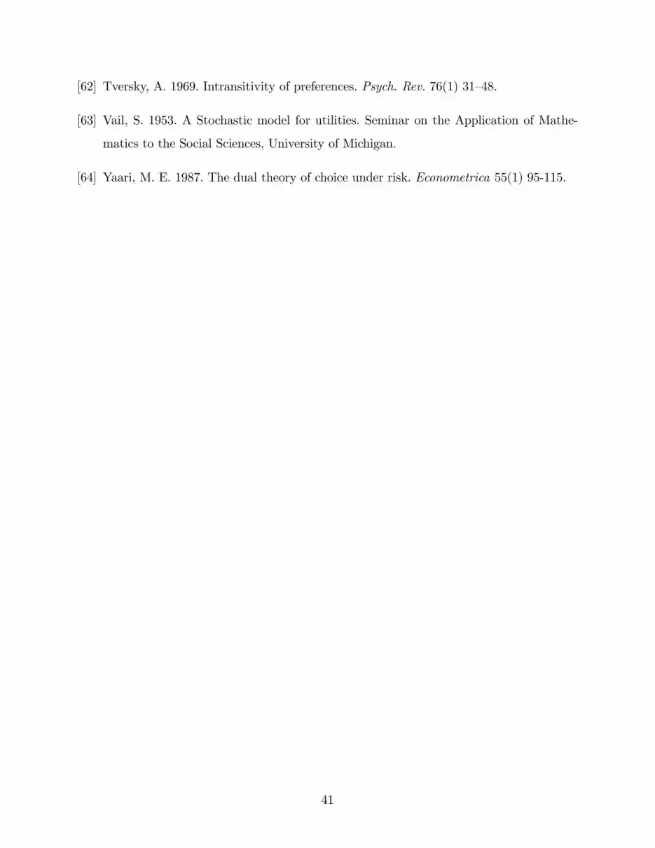
[62] Tversky, A. 1969. Intransitivity of preferences. Psych. Rev. 76(1) 31—48.

[63] Vail, S. 1953. A Stochastic model for utilities. Seminar on the Application of Mathe-

matics to the Social Sciences, University of Michigan.

[64] Yaari, M. E. 1987. The dual theory of choice under risk. Econometrica 55(1) 95-115.

41

0

Figure 1 The utility cones U' , U'' and U''', of the points q', q''

and q''', respectively, are depicted .

p1

1

1

q'

U '

q''

p3

0.25

0.70.25

0.7

q'''0.1

0.1

u'

u'

u'u''

u'''

U ''

U '''

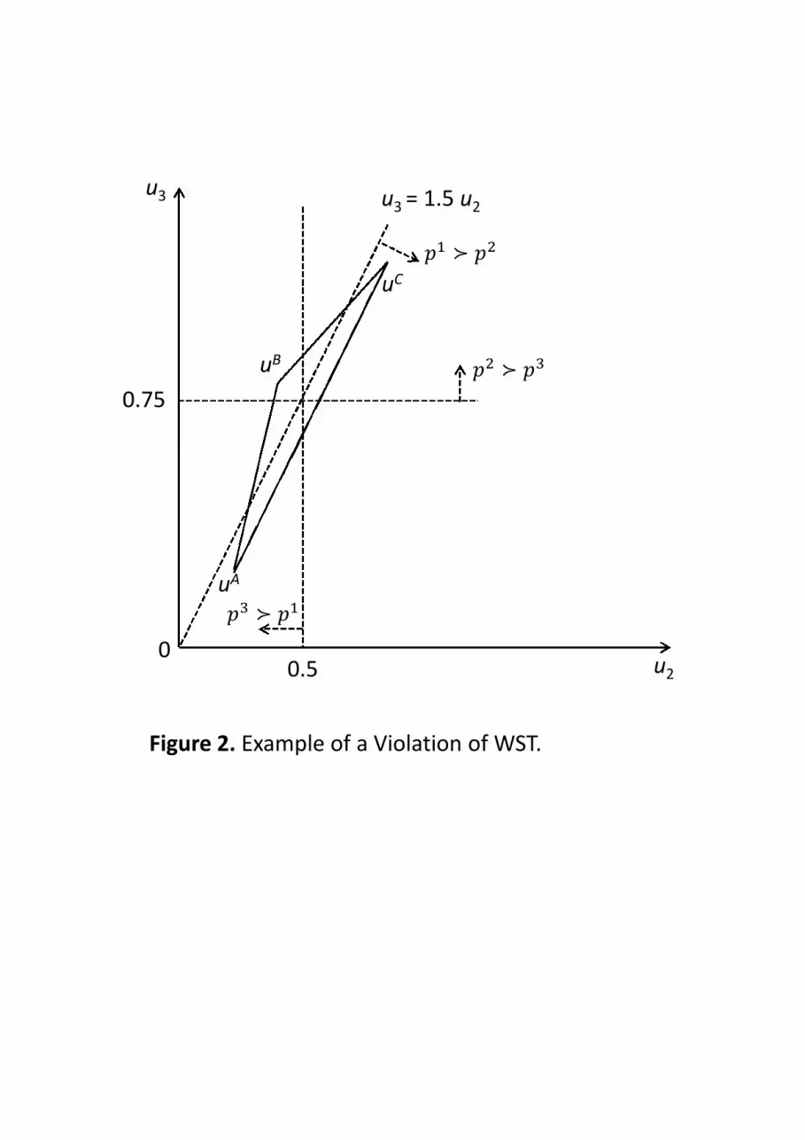
0.75

0.50

uC

u3

Figure 2. Example of a Violation of WST.

u3 = 1.5 u2

ଷ ≻ ଵ

ଶ ≻ ଷ

ଵ ≻ ଶ

uA

uB

u2