international journal of production research calculating the benefits of vendor managed inventory in...

Full Terms & Conditions of access and use can be found athttp://www.tandfonline.com/action/journalInformation?journalCode=tprs20

Download by: [University of Waterloo] Date: 15 October 2015, At: 09:57

International Journal of Production Research

ISSN: 0020-7543 (Print) 1366-588X (Online) Journal homepage: http://www.tandfonline.com/loi/tprs20

Calculating the benefits of vendor managedinventory in a manufacturer-retailer system

James H. Bookbinder , Mehmet Gümüş & Elizabeth M. Jewkes

To cite this article: James H. Bookbinder , Mehmet Gümüş & Elizabeth M. Jewkes(2010) Calculating the benefits of vendor managed inventory in a manufacturer-retailer system, International Journal of Production Research, 48:19, 5549-5571, DOI:10.1080/00207540903095434

To link to this article: http://dx.doi.org/10.1080/00207540903095434

Published online: 03 Sep 2009.

Submit your article to this journal

Article views: 481

View related articles

Citing articles: 24 View citing articles

http://www.tandfonline.com/action/journalInformation?journalCode=tprs20

http://www.tandfonline.com/loi/tprs20

http://www.tandfonline.com/action/showCitFormats?doi=10.1080/00207540903095434

http://dx.doi.org/10.1080/00207540903095434

http://www.tandfonline.com/action/authorSubmission?journalCode=tprs20&page=instructions

http://www.tandfonline.com/action/authorSubmission?journalCode=tprs20&page=instructions

http://www.tandfonline.com/doi/mlt/10.1080/00207540903095434

http://www.tandfonline.com/doi/mlt/10.1080/00207540903095434

http://www.tandfonline.com/doi/citedby/10.1080/00207540903095434#tabModule

http://www.tandfonline.com/doi/citedby/10.1080/00207540903095434#tabModule

International Journal of Production ResearchVol. 48, No. 19, 1 October 2010, 5549–5571

Calculating the benefits of vendor managed inventory

in a manufacturer-retailer system

James H. Bookbinder*, Mehmet Gumus� and Elizabeth M. Jewkes

Department of Management Sciences, University of Waterloo, Waterloo,Ontario, Canada N2L 3G1

(Received 5 November 2008; final version received 21 May 2009)

Firms such as Wal-Mart and Campbell’s Soup have successfully implementedvendor managed inventory (VMI). Articles in the trade press and academicliterature often begin with the premise that VMI is ‘beneficial’; but beneficial towhich party and under what conditions? We consider in this paper a vendor Vthat manufactures a particular product at a unique location. That item is sold toa single retailer, the customer C. Three cases are treated in detail: independentdecision making (no agreement between the parties); VMI, whereby the supplierV initiates orders on behalf of C; and central decision making (both vendor andcustomer are controlled by the same corporate entity). Values of some costparameters may vary between the three cases and each case may cause a differentactor to be responsible for particular expenses. Under a constant demand rate,optimal solutions are obtained analytically for the customer’s order quantity, thevendor’s production quantity, hence the parties’ individual and total costs in thethree cases. Inequalities are obtained to delineate those situations in which VMI isbeneficial.

Keywords: direct replenishment; logistics; supplier managed inventory;supply chain

1. Introduction

A supply chain implies interactions of different firms that seek decreased costs and greatermarket share. However, when the companies are managed independently, decisions madeby individual firms downstream in the chain can impose constraints on those upstream,resulting in additional costs. Consider the simplest example of a supply chain in which amanufacturer (called the vendor, V ) supplies materials or products, and a customer Corders from V (Figure 1). When each party makes decisions independently, the customerdetermines a replenishment that minimises his own operational costs. However, becausethe customer’s decisions on timing and quantity neglect the vendor’s costs, the resultingquantities might not be preferred by the vendor.

On the other hand, co-ordinated decision making (Figure 2) fosters potential benefitsfor the individual organisations. It may reduce the need for inventories and lower theshipping costs, or enable improved utilisation of resources at the manufacturer.

Two forms of co-ordination identified in the literature are vertical and virtualintegration. In the former, one supply chain member acquires the others or various

*Corresponding author. Email: [email protected]

ISSN 0020–7543 print/ISSN 1366–588X online

� 2010 Taylor & Francis

DOI: 10.1080/00207540903095434

http://www.informaworld.com

Dow

nloa

ded

by [

Uni

vers

ity o

f W

ater

loo]

at 0

9:57

15

Oct

ober

201

5

members merge. However, that ends the independence of the firms, and can fail (Aviv andFedergruen 1998) because of behavioural difficulties in integrating distinct organisational

cultures.The second form of co-ordination, virtual integration, maintains the independence of

those firms but harmonises their decisions by means of a business arrangement betweenthem. Chapters included in Tayur et al. (1999) discuss a number of such approaches.Vendor managed inventory (VMI), the subject of the present paper, is one example.

VMI, also referred to as a program of supplier-managed inventory or directreplenishment, emerged in the late 1980s as a partnership to co-ordinate replenishmentdecisions in a supply chain while maintaining the independence of chain members. In this

relationship between a vendor and customer, it is the vendor that decides when and inwhat quantity the customer’s stock is replenished. VMI was successfully implemented bynumerous firms including Wal-Mart and Procter & Gamble (Waller et al. 1999), CampbellSoup Company (Clark 1994), Barilla SpA (Hammond 1994), Intel (Kanellos 1998), and

Shell Chemical (Hibbard 1998).Despite the range of such examples of VMI relationships, there are researchers who

question whether VMI is beneficial to all parties. For example, Burke (1996) claims thatvendors are unwillingly forced into VMI agreements by powerful customers. Saccomano(1997) argues that VMI is just a way to transfer the risks involved in inventory

management from customers to vendors. Betts (1994) mentions that the vendor may beoverwhelmed since, to make VMI work, more technological investment is required therethan at the customer. According to Copacino (1993), a poorly designed VMI agreementcan harm the supplier that ships more often to satisfy the inventory turns required by theretailer.

Disputes over the benefits of VMI arise because few quantitative analyses are available,

and in those, general attributes of the agreements are fully understood in only someinstances. That research gap makes it difficult to assess and justify even conceptual modelsof VMI contracts.

Our aim in this paper is thus to develop and compare replenishment models byconsidering carefully the costs incurred by the vendor and the customer in various settings.

CVFinal-demand

Decision

Shipment

Information

Figure 2. Co-ordinated decision making.

Final-demand

CV

Decision

Shipment

Figure 1. Independent decision making.

5550 J.H. Bookbinder et al.

Dow

nloa

ded

by [

Uni

vers

ity o

f W

ater

loo]

at 0

9:57

15

Oct

ober

201

5

We start with the traditional unco-ordinated scenario in which the customer makes theordering decisions and the vendor reacts (Case 1).

Without a VMI agreement, the customer is responsible for inventory holding cost,transportation expense, and ordering charges: the cost of issuing the order and the cost ofreceiving those goods. ‘Issuing the order’ relates to writing up the purchase request anddetermining the size of order and thus it is the cost of authority over replenishmentplanning. The vendor’s expenses are those of production setup, inventory holding, andshipment release.

We next assume that the vendor is not content in simply reacting, and wants to getinvolved in replenishment decision-making. With VMI (Case 2), the vendor takes over theordering decision and hence the issuing-cost related to it, which might not be the same aswhat the customer used to pay. We determine the circumstances in which VMI is beneficialfor one of the parties, or for both.

Ignoring any organisational difficulty or investment implication, we finally considercentral decision making (Case 3). We will also describe this as ‘vertical integration’, whereboth parties are assumed to belong to the same company. Cost differences between verticalintegration and VMI, and between vertical integration and independent decision making,are then explored.

There are publications that investigate how certain types of VMI agreement impactsupply chain co-ordination. Examples include Aviv and Federgruen (1998), who analyseVMI in terms of information sharing, and find that VMI with information sharing isalways more beneficial than information sharing alone. Cachon (2001) suggests fixedtransfer payments in addition to VMI in a single supplier and multi-retailer setting.Bernstein and Federgruen (2003) study a partially centralised VMI model and concludethat channel co-ordination can be achieved under VMI.

Our research, in contrast, analyses tradeoffs between independent versus co-ordinateddecision making. In a broader context, we try to understand what VMI is, and in whatcircumstances it works or fails.

In addition, VMI has been conceived as a means of enabling operational benefits.Through the ‘flexibility’ that VMI offers, the supplier may combine routes from multipleorigins (Campbell et al. 1998, Kleywegt et al. 2002), delay stock assignments, consolidateshipments to two or more customers (Cheung and Lee 2002), or postpone a decision on thequantity destined for each of them (Cetinkaya and Lee 2000). Issues concerning VMI mayalso arise in a transportation-inventory problem whose tradeoffs are investment ininventory, delivery rates and shortages (Chaouch 2001), or in a simulation study thatanalyses the impacts of demand variability, limited manufacturing capacity, and partialchannel co-ordination (Waller et al. 1999). Some of those same impacts upon VMI areexamined by Sari (2007). Within a Newsvendor framework, Lee and Chu (2005) considerseveral ‘new mechanisms,’ including VMI, in which stock-level and ordering decisions aretransferred from customer to vendor. Nachiappan et al. (2007) develop a genetic algorithmto address the non-linear integer programme arising in their two-echelon VMI model.

The preceding stream of literature, ‘VMI for operational benefits,’ investigates thegains when decisions are supported by a presumed contract. However, few publications onVMI consider the cost implications of changing the decision-making authority from oneparty to another.

One exception is Yao et al. (2007). Our work is in a similar spirit to theirs. However,total costs, including transportation costs, are emphasised to a greater extent in the presentarticle. Our paper characterises the system results in detail, by delineating those cases

International Journal of Production Research 5551

Dow

nloa

ded

by [

Uni

vers

ity o

f W

ater

loo]

at 0

9:57

15

Oct

ober

201

5

where one party or the other, or both or neither, are better off under VMI. This will beseen as follows in Propositions 2 to 4. We obtain a result (Proposition 5) on the sidepayment necessary to turn a potentially-efficient VMI system into an efficient one. Totalcosts are again stressed in our discussions of Sections 8 and 9.

The joint economic lot-sizing (JELS) problem, though not apparently related to VMI,forms the starting point of our analysis, and can be considered a form of co-ordinateddecision making. Also referred to as ‘integrated vendor-buyer models,’ research in thiscategory minimises the overall cost of a two-echelon inventory system composed of asingle supplier and one or multiple customers. The cost function of the parties at eachechelon is the sum of inventory holding and ordering costs. Instead of separatelyoptimising each party’s cost, studies in this area minimise a total-cost function and add thecosts to each of them.

Banarjee (1986) was first to analyse the integrated vendor-buyer case, examining a lot-for-lot model in which Vmanufactures each shipment as a separate batch. As an extension,Goyal (1988) formulated a joint total-relevant-cost model for a single vendor and customerproduction-inventory system, where V’s lot size is an integer multiple of C’s order size.

Lu (1995) extended Goyal’s (1988) work by allowing the vendor to supply somequantity to the purchaser before completing the entire lot. Lu gives an optimal solution forthe case of a single vendor and buyer, and investigates heuristics for the single-vendor,multiple-buyer problem. Goyal (1995) employed the example provided by Lu for the singlevendor and buyer, but showed that a different shipment policy could give a better solution.

Hill (1997, 1998) considers a single vendor that manufactures a product at a finite rateand in batches, and supplies a sole buyer whose external demand is level and fixed. Eachbatch is sent to the buyer in a number of shipments. The vendor incurs a batch setup costand a fixed order or delivery cost associated with each shipment. Hill’s policy assumes thatsuccessive shipment sizes increase by a factor whose value lies between one and the ratio ofthe manufacturing rate to the product’s demand rate. Hill (1997) concludes that, althoughGoyal’s (1995) policy may perform much better than Lu’s equal-size shipment policy, hisown policy outperforms all. Goyal (2000) proposes a procedure to modify the shipmentsize in Hill (1997) to obtain a still lower cost.

Studies on general co-ordination are not always conclusive. Suitable incentives for co-ordination may not have been discussed, and numerical examples in these papers showthat cost reduction might not be that significant. Total cost of the co-ordinated systemmight have been underestimated, such as by ignoring the customer’s expense for ordering.That situation often occurs (e.g. Hill 1997), resulting in unrealistically lower costs. We alsonote that changes to any system require adjustments in the relevant parameters.

Moreover, the sharing of cost-related information by two independent parties rarelyoccurs unless C and V belong to the same firm, making general co-ordination difficult toachieve. A VMI contract, on the other hand, enables co-ordination based on costreallocation, and leaves each party still independent.

Having thus summarised the several important streams of literature with ties to ourresearch, the following sections will amplify the types of models we analyse. Before doingso, we distinguish between VMI and consignment inventory (CI). Under CI, the vendorstill owns the products shipped, until the customer sells those items. Gumus� et al. (2008)obtain conditions under which CI is beneficial. As opposed to Dong and Xu (2002), whostudy the economics of consignment inventory in the long-term and short-term, we adoptthe point of view of Gumus� et al., namely that consignment inventory should be treateddistinctly from VMI. Consignment inventory will be considered no further in what follows.


Dow

nloa

ded

by [

Uni

vers

ity o

f W

ater

loo]

at 0

9:57

15

Oct

ober

201

5

2. Problem definition and research scope

Our models will pertain to one vendor V who produces a single product at onemanufacturing plant, and furnishes it to a particular customer (retailer). The customer Cfaces a constant, deterministic demand that is known. Suppose there is no lead time and allcustomer orders are transmitted instantaneously to the vendor. At any moment in time,the vendor’s plant is either idle (actually, producing other SKUs not part of this analysis),or manufacturing the given item at a constant production rate. The vendor thus producesin batches at a finite rate. When the customer is replenished, those units are shipped fromthe vendor’s inventory to the customer’s.

The reader may be wondering about our use of a deterministic model and the seemingneglect of potential savings involving safety stock under VMI. VMI, as a contractualrelationship, is a medium- to long-term decision. For that time frame, annual demand andmean demand rates are appropriate.

Suppose the vendor V and customer C share the demand information and agree on aproper service measure. They would then concur on the particular level of safety stock (SS).This quantity of SS is (almost) constant throughout the year: when we need some, we use it,but immediately replenish that given amount. When there is a VMI agreement, perhaps thelevel of SS will change from the traditional way of doing business. If so, we feel this is a resultof information sharing, not through VMI as such (e.g. Aviv and Federgruen 1998).

We thus argue that for VMI, most of the total costs (ordering, inventory holding,transportation, etc.) pertain to the management and shipment of cycle stocks. And thatcan be well studied through a deterministic model.

We now continue the development of that model. Because of constant prices, thevendor’s total production cost and the customer’s overall revenue are both linear, and willbe omitted since all demands have to be satisfied. We assume that the vendor’s fixed costsof setup and of shipment dispatch, and the customer’s fixed cost per order, areindependent of the quantities involved. Both parties’ inventory costs are directlyproportional to the average stock levels. The performance criterion we use in each caseis the total cost of inventory holding plus ordering.

Independent decision making (Case 1) is the traditional way of doing business betweenthe vendor and the customer. Taking this as the base case and carefully identifying the costparameters of each party, we aim to develop and analyse quantitative cost models toestimate the economic value of VMI agreements. In light of those calculations, we willprovide insights on desirable agreements.

Inventory control policies for the following cases will be investigated in this paper:

(1) No agreement between the parties. Vendor and customer act separately. Hence,each independent party is responsible for its own inventory control. The customerdetermines a replenishment quantity and passes it to the vendor. The vendor thenoptimises her production quantity to satisfy the customer’s order. But the actorsare otherwise engaged in independent decision making.

(2) VMI. The vendor and customer are governed by a VMI agreement: each party isresponsible for its own inventory holding costs, but the vendor establishes andmanages the inventory control policy of the customer. The VMI case thus requiresshifting some costs from the customer to the vendor. We compare to the case withno agreement to determine if VMI is efficient (both parties realise cost savings),potentially efficient (system-wide cost savings are achieved although one party isworse off), or inefficient (no system-wide cost savings).


Dow

nloa

ded

by [

Uni

vers

ity o

f W

ater

loo]

at 0

9:57

15

Oct

ober

201

5

(3) Central decision making. The vendor and the customer belong to the samecorporate entity that manages the inventory of both parties. The model consideredis similar to JELS models, and our aim is to identify any potential benefits in thisvertical integration compared with no agreement (independent decision making)and VMI.

These cases will be analysed in Sections 4 to 6, and then numerical examples and furtherinterpretation will follow in Sections 7 and 8. In the final section, we provide a summaryand conclusions.

3. Notation

Let us begin with the basic notation that will be employed throughout our models.

Ac Customer’s fixed cost of ordering ($ per order). Ac¼ aoþ atþ ar, whereao cost of issuing the order;at transportation cost;ar cost of receiving the goods ordered.

hc Annual cost to carry one unit in stock at customer’s retail store ($/unit/year). This has two parts in it, vizh cost of capital per item;hs physical storage cost of an item.

The customer’s inventory holding cost is thus hc¼ hþ hs.

S Vendor’s fixed production setup cost incurred at the start of each cycle($ per setup).

av Vendor’s cost per shipment release ($ per shipment to the customer).hv Annual cost of holding a unit in inventory at the vendor’s production site

($/unit/year).p Vendor’s annual production rate (units/year).d Annual demand rate at the customer (units/year).ki Number of shipments to customer between successive production runs

(i.e. during the vendor’s cycle time) in Case i, i¼ 1, 2, 3.

For feasibility, it is assumed throughout that p� d. But unlike JELS models in general,we do not require hc� hv. Note that any type of agreement between the parties mayrequire a shift in expenses from one actor to the other. Unless explicitly stated, itshould not be assumed that a cost parameter of the vendor includes another one of thecustomer.

The cost of receiving the goods shipped is incurred by the customer, independent ofwhich party initiates the replenishment order. That expense includes the costs related tothe arrival of product at the store, receipt of the vendor’s invoice, and further processing(by the customer) of that invoice. Likewise, the vendor pays the costs related to receipt ofthe order information and the processing of it, and is charged for release of goods to thecustomer.

We begin in the next section by looking at the traditional way of doing businessbetween the vendor and the customer. We call it ‘independent decision making,’ with noagreement between parties. That case is the building block for VMI analyses.


Dow

nloa

ded

by [

Uni

vers

ity o

f W

ater

loo]

at 0

9:57

15

Oct

ober

201

5

4. Independent decision making (Case 1)

This first case thus assumes that C and V separately plan their own replenishments or

production, respectively. End-user demand d is realised at the customer, who must decide,

based on that demand, how often and in what quantity he should order from the vendor.

While doing so, the customer considers the ordering cost Ac and inventory holding cost hc.In light of the preceding costs, the customer in Case 1 orders from the vendor a

quantity equal to ffiffiffiffiffiffiffiffiffiffi2Acd

hc

s¼ EOQ ¼ q �1 ,

C’s optimal replenishment quantity. It follows that the customer’s total cost in Case 1 is

TC �c1¼ffiffiffiffiffiffiffiffiffiffiffiffiffiffiffi2Acdhcp

. Now, the vendor is informed by the customer of the ordering quantity

q �1 . The vendor has production rate p� d, and should satisfy the customer’s order fully

because no backorders are allowed. In choosing her batch size Q1, the vendor considers

the production setup cost (S), inventory holding cost (hv), and the cost per shipment

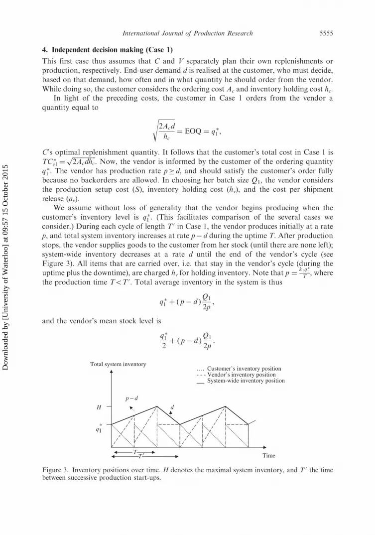
release (av).We assume without loss of generality that the vendor begins producing when the

customer’s inventory level is q �1 . (This facilitates comparison of the several cases we

consider.) During each cycle of length T 0 in Case 1, the vendor produces initially at a rate

p, and total system inventory increases at rate p� d during the uptime T. After production

stops, the vendor supplies goods to the customer from her stock (until there are none left);

system-wide inventory decreases at a rate d until the end of the vendor’s cycle (see

Figure 3). All items that are carried over, i.e. that stay in the vendor’s cycle (during the

uptime plus the downtime), are charged hv for holding inventory. Note that p ¼k1q

�1

T , where

the production time T5T 0. Total average inventory in the system is thus

q �1 þ ð p� d ÞQ1

2p,

and the vendor’s mean stock level is

q �12þ ð p� d Þ

Q1

2p:

Time

Total system inventory

*1q

H

dp −d

T ′

…. Customer’s inventory position - - - Vendor’s inventory position

System-wide inventory position

T

Figure 3. Inventory positions over time. H denotes the maximal system inventory, and T 0 the timebetween successive production start-ups.


Dow

nloa

ded

by [

Uni

vers

ity o

f W

ater

loo]

at 0

9:57

15

Oct

ober

201

5

Since we require Q1� q �1 , we state that there is a number of shipments k1 from thevendor to customer during the vendor’s cycle: Q1¼ k1q

�1 . Note also that the transportation

cost is paid by the customer, but the vendor pays av for every shipment released. Then, thevendor’s total cost is

TCv1 ¼ d ½S=Q1 þ av=q�1 � þ hv ½q

�1 þ 1� d=pð ÞQ1�=2: ð1Þ

The first two terms in (1) correspond to production setup and shipment release costs,and the third and fourth to inventory carrying cost. The only variable in that equation isQ1. Treating the number of shipments as continuous, rather than discrete (which will bethe assumption throughout; see also Proposition 1), the optimal production quantity inone cycle is

Q �1 ¼

ffiffiffiffiffiffiffiffiffiffiffiffiffiffiffiffiffiffiffiffiffiffiffi2Sd

hvð1� d=pÞ

s¼ EPQ:

Let K denote the set

EPQ=q �1� �

, EPQ=q �1� ��

:

Because TCv1 is a strictly convex function in the interval ð0,1Þ, the optimal integer valuefor k is

kint ¼ argmink2K

TCv1ðkÞ:

Based on the values of Q �1 and q �1 , we then have

TC �v1 ¼ffiffiffiffiffiffiffiffiffiffiffiffiffiffiffiffiffiffiffiffiffiffiffiffiffiffiffiffiffiffiffi2Sdhvð1� d=pÞ

pþ

davffiffiffiffiffiffiffiffiffiffiffiffiffiffiffiffiffi2Acd=hc

p þ hvffiffiffiffiffiffiffiffiffiffiffiffiffiffiffiffiffi2Acd=hc

p=2:

Letting � ¼ avAc

and � ¼ hvhc, and denoting C 0 ¼

ffiffiffiffiffiffiffiffiffiffiffiffiffiffiffiffiffiffiffiffiffiffiffiffiffiffiffiffiffiffiffi2Sdhvð1� d=pÞ

p, the result is

TC �v1 ¼ C 0 þ ð� þ �Þ

ffiffiffiffiffiffiffiffiffiffiffiffidAchc2

r:

Let us consider once more

We remark that Q �1 is constant no matter what quantity q �1 the customer orders, henceC 0 is constant and independent of q �1 . The second (circled) part of this total cost is a‘forced’ cost: the vendor has no influence over it. The customer’s decision q �1 determineshow much the vendor must pay. This explains a major motivation behind a VMIagreement, whereby V seeks a way to get involved in ordering decisions to see if thatsecond part of her total cost can be decreased.

Although the customer’s decision could be near optimal, we will suppose that thevendor is not happy with the customer’s order quantity and wants to make replenishmentdecisions herself. V then offers C a VMI partnership that states: the vendor will makereplenishment decisions on behalf of the customer, and will be responsible to pay any cost


Dow

nloa

ded

by [

Uni

vers

ity o

f W

ater

loo]

at 0

9:57

15

Oct

ober

201

5

associated with it. Here, an ‘associated cost’ does not include the expense fortransportation, which is still assumed to be paid by the customer (that will be relaxedlater in our analysis).

5. Vendor-managed inventory (Case 2)

With VMI, the vendor takes over from the customer the responsibility for replenishment.The customer does not place orders, hence pays no ordering charge, though the customerdoes pay its cost of holding stock.

The expense associated with the replenishment decision (i.e. the cost of issuing anorder) was ao, as paid by the customer when he makes that decision. This parameter mightbe a different value for the vendor. Under the proposed VMI partnership, we suppose thatV pays �1ao for issuing an order, where �1� 0 can be interpreted as the vendor’s efficiencyfactor (C will then be exempt from paying ao).

Under VMI, the vendor pays �1ao plus her costs as discussed in Case 1. As such, thecustomer pays all his costs from Case 1 except ao. The proposed VMI partnership does notinclude sharing the transportation cost; it is still paid by the customer. Let Q2 be theproduction quantity in Case 2 and q2 be the replenishment quantity, which is nowdetermined by the vendor on behalf of the customer. The vendor can find optimal valuesof Q2 and q2 that minimise her total cost TCv2, where

TCv2 ¼d

Q2Sþ k2ðav þ �1a0Þ½ � þ

1

2hv q2 þ ð1� d=pÞQ2½ �:

Note that q2 is now also a decision variable for the vendor.

Proposition 1: For a continuous number of shipments k2, the optimal values areQ �2 ¼Q �1 ¼EPQ, independent of q2, the minimum system-wide inventory.

Proof: Replace k2 by Q2=q2. Then, TCv2 ¼ f ðQ2Þ þ�f ðq2Þ, where

f ðQ2Þ ¼ dS=Q2 þhvð1� d=pÞQ2

2, and �f ðq2Þ ¼ d ðav þ �1aoÞ=q2 þ

hvq22:

These functions, each convex over ð0,1Þ, can be optimised separately. The optimal valuefor f thus occurs when

Q �2 ¼


hvð1� d=pÞ

s: h

Minimising �f ðq2Þ, the vendor finds the replenishment quantity under VMI to be

q �2 ¼

ffiffiffiffiffiffiffiffiffiffiffiffiffiffiffiffiffiffiffiffiffiffiffiffiffiffiffi2ðav þ �1aoÞd

hv

s:

Let

�1 ¼aoAc:


Dow

nloa

ded

by [

Uni

vers

ity o

f W

ater

loo]

at 0

9:57

15

Oct

ober

201

5

We previously defined

� ¼avAc

and � ¼hvhc:

Then

q �2 ¼

ffiffiffiffiffiffiffiffiffiffiffiffiffiffiffiffiffiffi� þ �1�1

�

sq �1 ¼ mq �1 ,

where we define

m ¼

ffiffiffiffi

�

sand ¼ � þ �1 �1:

Now we want to find the optimal TCv2 and TCc2, and see how they compare with

results from Case 1. We want to know if this VMI partnership can help achieve some of

the following:

(i) TCv25TCv1: Cost saving for the vendor.(ii) TCc25TCc1: Cost saving for the customer.(iii) TCv2 þ TCc25TCv1 þ TCc1: System-wide cost savings.

To categorise the results of the two systems, we state that

. VMI is an efficient system if both the vendor and the customer are better off

compared to Case 1: both (i) and (ii) hold. The VMI partnership is clearly

acceptable to both parties.. In a potentially-efficient system, one party is better off while the other is worse off,

and VMI achieves system-wide cost savings: both (iii), and either (i) or (ii), hold.

If so, we can look for a way to adjust the partnership so that no party is worse off.. An inefficient system means the system-wide cost under VMI exceeds that of

Case 1, hence (iii) does not hold.

Note that each statement (i)–(iii) is a strict inequality. We shall often emphasise this by

referring to ‘positive cost savings’. On the basis of cost comparisons, we can infer

Propositions 2 to 5, proofs of which are contained in the Appendix. In reading the

propositions, it may help to recall that � denotes the ratio of vendor’s cost per ship-

ment release to the customer’s fixed cost of ordering. Similarly, � is the ratio of holding

costs hv/hc.Following the statement of each proposition, we make several comments regarding its

interpretation. In those remarks, when we refer to the value of a particular parameter as

small or large, we shall mean respectively that it is�1 or�1, i.e. much less than or much

greater than one.

Proposition 2: Under VMI, the vendor achieves positive cost savings if and only if

� þ �42ffiffiffi�p ffiffiffiffiffiffiffiffiffiffiffiffiffiffiffiffiffiffi

� þ �1�1p

, i.e. if and only if �4ð2m� 1Þ�.

A vendor is more likely to prefer VMI to traditional sourcing if a particular ratio is large

or small. For example, the vendor will usually benefit from VMI if the customer’s

replenishment choice under traditional sourcing either causes the vendor to ship frequently


Dow

nloa

ded

by [

Uni

vers

ity o

f W

ater

loo]

at 0

9:57

15

Oct

ober

201

5

when �(av/Ac)� 1, or the customer forces the vendor to send large amounts less often

when � � hv=hc� 1.In those cases, the vendor in a VMI agreement can specify replenishment quantities

that balance her inventory and ordering costs. Alternatively, suppose � or � is quite small.

VMI can then be employed by the vendor to choose replenishment quantities to decrease

her inventory holding cost (if �� 1) or ordering cost (�� 1).

Proposition 3: Under VMI, the customer achieves positive cost savings if and only if

2ffiffiffi�p ffiffiffiffiffiffiffiffiffiffiffiffiffiffiffiffiffiffi

� þ �1�1p

4� ð�2 þ �3Þ þ � þ �1 �1, that is, if and only if �14ðm� 1Þ2, where

�2 ¼ at=Ac, �3 ¼ ar=Ac, and �1 þ �2 þ �3 ¼ 1. Equivalently, for a fixed value of �1, the

customer will achieve positive cost savings under VMI if and only if 1�ffiffiffiffi�1p

5m5 1þffiffiffiffi�1p

.

If the ratios � and � are large or small, the customer is less likely to achieve positive cost

savings under VMI: he does not pay the cost of issuing an order. If the vendor’s cost per

shipment release is very high (�� 1), she prefers to ship large quantities. This in turn

increases the customer’s inventory holding cost, often to a value greater than his savings

from not issuing an order. Alternatively, if �� 1, the vendor would tend to arrange

frequent shipments in small quantities, thereby increasing the customer’s cost of

transportation and shipments received. Very large or very small values of � lead to

similar results.

Proposition 4: If � þ �1 �15� when �4�, or if �5� when � þ �1�14�, then VMI will

yield positive system-wide cost savings. That is, VMI will enable positive system-wide cost

savings if and only if ð2�þ 1Þm2 � ð� þ �þ 2Þmþ 1� �150.

System-wide benefits of VMI depend on the relative efficiency of the vendor’s or the

customer’s operational costs. For example, when �4�, overall cost savings can be realised

under VMI if the vendor’s ‘effective’ cost per shipment release (av þ �1ao) is still low

enough to enable more frequent shipments, which in turn decrease the system-wide

inventory costs.

Lemma 1: If �5�1, both parties cannot simultaneously be better off.

Proof: A necessary (but not sufficient) condition that both parties are better off together is

� þ �4� ð�2 þ �3Þ þ � þ �1�1

) �4� ð1� �1Þ þ �1 �1, which implies �4�1: h

We remark that if �1¼ 1, VMI cannot be an efficient system if the vendor’s inventory

holding cost is smaller than the customer’s. That is, both parties cannot be simultaneously

better off. This result is interesting because many lot-sizing studies assume hv 5 hc before

proposing a model.

Note also that, to tell when (i) and (ii) hold together requires knowledge of at least the

ranges of parameters. We provide examples subsequently.Consider the case when (iii) is true, but only (i) or (ii) holds. This scenario means either

. The customer is better off: a VMI partnership is not applicable here because V

(who offered the partnership) is worse off, and there is no incentive for C to

share his cost savings with the vendor (the customer already pays the

transportation cost).


Dow

nloa

ded

by [

Uni

vers

ity o

f W

ater

loo]

at 0

9:57

15

Oct

ober

201

5

. The vendor is better off: C, now worse off, will not consent to VMI unless V offers

an additional incentive so that the customer’s cost is no greater than in Case 1.

One such incentive is ‘transportation cost sharing’: the vendor shares C’s

transportation cost (at) so that, overall, the customer does not suffer under VMI.

That is, the vendor pays ð1� �2Þat, and the customer pays �2at per shipment,

where 05�251.

Proposition 5: A potentially-efficient VMI arrangement, where the vendor is better off, can

be turned into an efficient system by setting

1� �2 ¼ � þ �1�1 þ �ð1� �1Þ � 2ffiffiffi�

p ffiffiffiffiffiffiffiffiffiffiffiffiffiffiffiffiffiffi� þ �1�1

ph i 1

��2¼

m� 1ð Þ2��1

�2: h

Note that when the customer pays just the fraction �2 of transportation cost, he is now no

worse off than in Case 1; the vendor is still better off, and all the savings are captured by

the vendor.Proposition 5 thus describes how to share transportation cost to convince a worse-off

customer. For any manufacturer-customer pair, the portion of transportation cost that is

suitably allocated to each party can be obtained numerically by substituting values of

parameters in the result of the proposition.As another way of sharing the cost savings, consider a payment from the vendor to the

customer in the form of a price discount. Suppose that the customer (originally) pays $ c

per item purchased. A discount of y% offered by the vendor will make VMI an efficient

system when

y ¼100

cdðTCc2 � TCc1Þ:

Such a price discount is an alternative to the sharing of transportation cost. Either

incentive can turn a potentially-efficient VMI system, where the vendor is better off, into

an efficient one that benefits both actors. (We remark that, in light of our cost

assumptions, those two incentives are the only means available to share the savings in

total cost.)Our analyses thus far have been for a vendor and customer that were independent

decision makers in a supply chain. We played the role of an outside observer to determine

the impacts of VMI. That is, we investigated if it was possible to keep the independence of

the actors and achieve efficiency at the same time.Let us next assume that there is a third party who has control over both vendor and

customer, and also has enough information about each of their particular cost parameters.

This will be true if the vendor and customer belong to a single corporate entity, hence are

vertically integrated.

6. Central decision making (Case 3)

We now analyse the system from the point of view of this third party, and call it ‘central

decision making’. As in JELS models, there is a single total cost function denoted by TCsys

that includes all expenses of both the vendor and customer. Assume also that �1¼ 1 when


Dow

nloa

ded

by [

Uni

vers

ity o

f W

ater

loo]

at 0

9:57

15

Oct

ober

201

5

comparing Cases 2 and 3, because a vertical integration implies the capture of all possibleefficiencies created by any of the supply chain members. Total cost in Case 3 is then

TCsys ¼dS

Q3þ1

2hvð1� d=pÞQ3 þ

d ðAc þ avÞ

q3þ1

2ðhc þ hvÞq3:

Observe that Proposition 1 still holds. When TCsys is minimised, optimal production andreplenishment quantities are then

Q �3 ¼


hvð1� d=pÞ

s¼ EPQ, and q �3 ¼

ffiffiffiffiffiffiffiffiffiffiffiffiffiffiffiffiffiffiffiffiffiffiffiffi2ðAc þ avÞd

hc þ hv

s¼

ffiffiffiffiffiffiffiffiffiffiffi1þ �

1þ �

sq �1 :

Note that if � ¼ �, then q �3 ¼ q �1 : the customer is replenishing at the system-wideoptimal quantity anyway. There is then no need for a contract to decrease overall totalcosts; they are already at their minimum. Comparing Case 3 and Case 1, we see that


p�


p 2 ffiffiffiffiffiffiffiffiffiffiffiffiAcdhc2

r¼ TC �v1 þ TC �c1 � TC �sys � 0:

Computing the total costs in Case 3 and Case 2, it is found that


p ffiffiffiffiffiffiffiffiffiffiffiffiffi� þ �1

p�

ffiffiffi�

p ffiffiffiffiffiffiffiffiffiffiffi1þ �

p 2 ffiffiffiffiffiffiffiffiffiffiffiffiffiffiffiffiffiffiffiffiffiffiAcdhc

2�ð� þ �1Þ

s¼ TC �v2 þ TC �c2 � TC �sys � 0:

Both of the equations above show that the lowest system-wide cost can be achievedthrough central decision making. In the next section, computational examples willhighlight this point as well as the previous analytical results.

7. Numerical examples

We now consider a series of examples to contrast Cases 1 to 3. The following values areused throughout: �1 ¼ 0:2, Ac ¼ $100 per order, hc ¼ $1.5 per item stored, p ¼ 1600 items/year and d¼ 1300 items/year in each example. Dollar values of total costs require only thepreceding parameters, plus of course the ‘ratios’ defined in our analysis: �, �, �1. InFigures 4 to 11, generally two of those ratios are fixed, while the third is varied. In eachcase, the range of variation encompasses a factor of 40: 0:1 0:1ð Þ 4½ �, i.e. between the valuesof 0.1 and 4.0 in steps of 0.1.

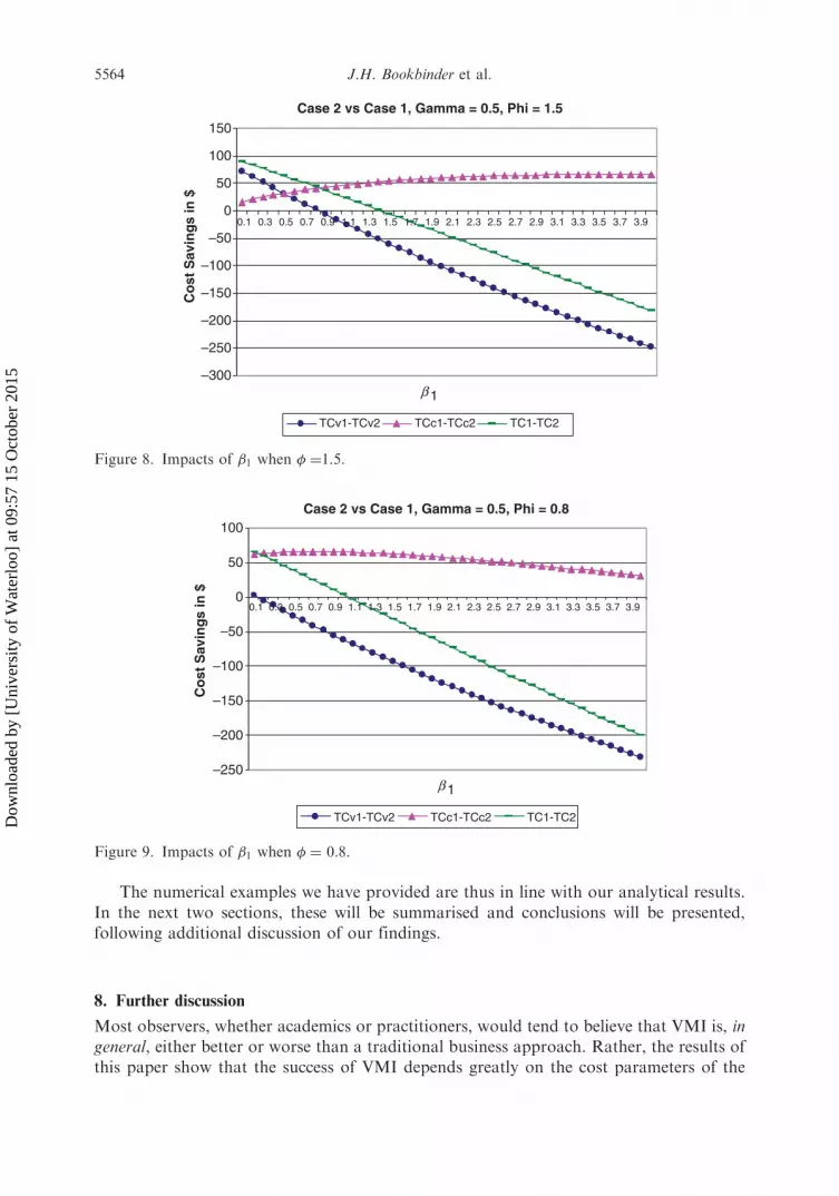
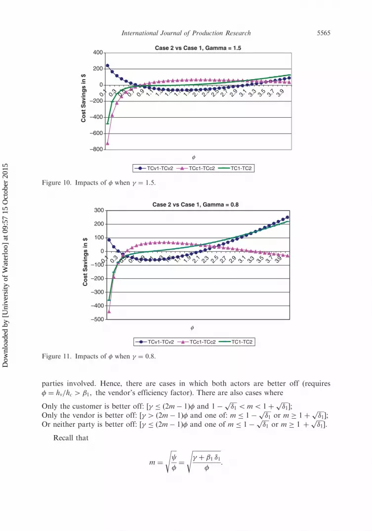
When a ratio, say �, is fixed at level �1 in one set of graphs, it may be fixed at level �2 inthe next set. The levels �1 , �2 (and similarly for the �i in their respective graphs) arechosen strategically, such that qualitatively different behaviour is observed for �1 vs �2.(We remark that �1¼1 in every figure except Figures 8 and 9.) In discussing Figures 4 to11, we usually first compare Case 2 to Case 1 and then comment on the differencesbetween each of those and Case 3. In those figures, TCi denotes the total system costfor Case i.

VMI versus independent decision making

Example 1:

� ¼ 1:5, � ¼ ½0:1 ð0:1Þ 4�:


Dow

nloa

ded

by [

Uni

vers

ity o

f W

ater

loo]

at 0

9:57

15

Oct

ober

201

5

Because �41, hv4hc. It is then possible to observe some intervals where both parties

are better off. Figure 4 shows that VMI is an efficient system if � is within [0.3, 0.4] or [2.6,

2.9]. It is inefficient when � lies within [1.4, 2] but potentially efficient for the remaining �.

Example 2:

� ¼ 0:8, � ¼ ½0:1 ð0:1Þ 4�:

Here, hv5hc, so VMI cannot be efficient (Figure 5). System-wide cost savings occur

when � is within [0.1, 0.6] or [2, 4]. In these ranges, there are two possibilities:

. C is better off while V is worse off: � 2 [0.1, 0.6]. Not much can be done, since (as

discussed before) there is no incentive for the customer to share his cost savings.

Case2 vs Case1, hv> hc

–100

–50

0

50

100

150

200

0.1

0.4

0.7 1 1.

31.

61.

92.

22.

52.

83.

13.

43.

7 4

Co

st s

avin

gs

in $

TCv1 - TCv2 TCc1-TCc2 TC1-TC2

γ

Figure 4. Comparison of Cases 1 and 2; �¼ 1.5.

Case2 vs Case1, hv<hc

–300

–200

–100

0

100

200

300

400

0.1

0.4 0.7 1 1.3

1.6

1.9

2.2

2.5

2.8

3.1

3.4

3.7 4

Co

st s

avin

gs

in $

TCv1 - TCv2 TCc1-TCc2 TC1-TC2

γ

Figure 5. Comparison of Cases 1 and 2; �¼ 0.8.


Dow

nloa

ded

by [

Uni

vers

ity o

f W

ater

loo]

at 0

9:57

15

Oct

ober

201

5

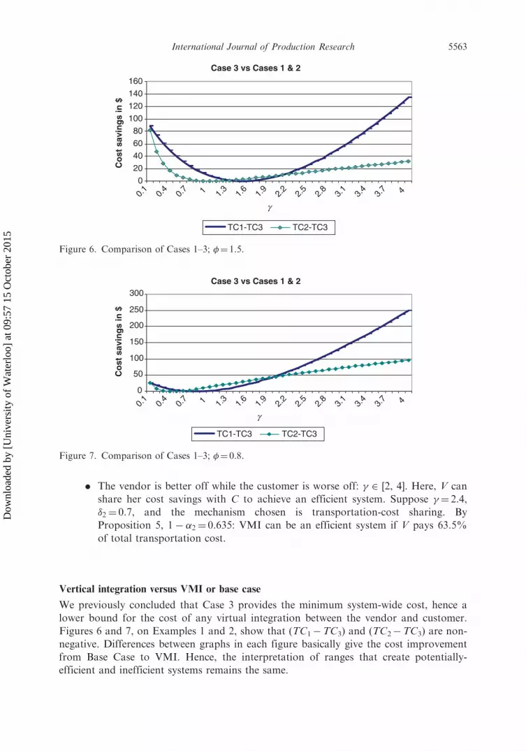
. The vendor is better off while the customer is worse off: � 2 [2, 4]. Here, V can

share her cost savings with C to achieve an efficient system. Suppose �¼ 2.4,

�2¼ 0.7, and the mechanism chosen is transportation-cost sharing. By

Proposition 5, 1� �2¼ 0.635: VMI can be an efficient system if V pays 63.5%

of total transportation cost.

Vertical integration versus VMI or base case

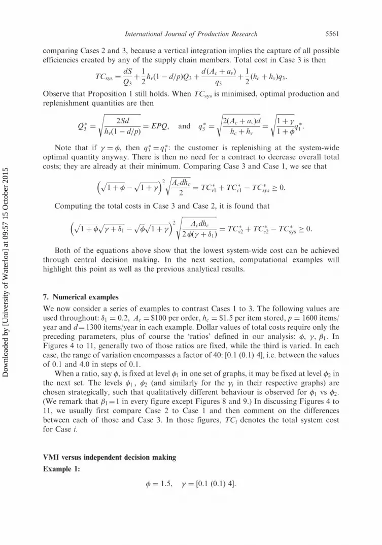
We previously concluded that Case 3 provides the minimum system-wide cost, hence a

lower bound for the cost of any virtual integration between the vendor and customer.

Figures 6 and 7, on Examples 1 and 2, show that (TC1�TC3) and (TC2�TC3) are non-

negative. Differences between graphs in each figure basically give the cost improvement

from Base Case to VMI. Hence, the interpretation of ranges that create potentially-

efficient and inefficient systems remains the same.

Case 3 vs Cases 1 & 2

0

20

40

60

80

100

120

140

160

0.1

0.4

0.7 1 1.

31.

61.

92.

22.

52.

83.

13.

43.

7 4

Co

st s

avin

gs

in $

TC1-TC3 TC2-TC3

γ

Figure 6. Comparison of Cases 1–3; �¼ 1.5.

Case 3 vs Cases 1 & 2

0

50

100

150

200

250

300

0.1

0.4

0.7 1 1.

31.

61.

92.

22.

52.

83.

13.

43.

7 4

Co

st s

avin

gs

in $

TC1-TC3 TC2-TC3

γ

Figure 7. Comparison of Cases 1–3; �¼ 0.8.


Dow

nloa

ded

by [

Uni

vers

ity o

f W

ater

loo]

at 0

9:57

15

Oct

ober

201

5

The numerical examples we have provided are thus in line with our analytical results.In the next two sections, these will be summarised and conclusions will be presented,following additional discussion of our findings.

8. Further discussion

Most observers, whether academics or practitioners, would tend to believe that VMI is, ingeneral, either better or worse than a traditional business approach. Rather, the results ofthis paper show that the success of VMI depends greatly on the cost parameters of the

–300

–250

–200

–150

–100

–50

0

50

100

150

3.9

Co

st S

avin

gs

in $

TCv1-TCv2 TCc1-TCc2 TC1-TC2

1β

Case 2 vs Case 1, Gamma = 0.5, Phi = 1.5

0.1 0.3 0.5 0.7 0.9 1.1 1.3 1.5 1.7 1.9 2.1 2.3 2.5 2.7 2.9 3.1 3.3 3.5 3.7

Figure 8. Impacts of �1 when � ¼1.5.

–250

–200

–150

–100

–50

0

50

100

Co

st S

avin

gs

in $


1β

Case 2 vs Case 1, Gamma = 0.5, Phi = 0.8

3.90.1 0.3 0.5 0.7 0.9 1.1 1.3 1.5 1.7 1.9 2.1 2.3 2.5 2.7 2.9 3.1 3.3 3.5 3.7

Figure 9. Impacts of �1 when � ¼ 0.8.


Dow

nloa

ded

by [

Uni

vers

ity o

f W

ater

loo]

at 0

9:57

15

Oct

ober

201

5

parties involved. Hence, there are cases in which both actors are better off (requires

� ¼ hv=hc 4�1, the vendor’s efficiency factor). There are also cases where

Only the customer is better off: � ð2m� 1Þ½ � and 1�ffiffiffiffi�1p

5m5 1þffiffiffiffi�1p�;

Only the vendor is better off: �4 ð2m� 1Þ½ � and one of: m 1�ffiffiffiffi�1p

or m � 1þffiffiffiffi�1p�;

Or neither party is better off: � ð2m� 1Þ½ � and one of m 1�ffiffiffiffi�1p

or m � 1 þffiffiffiffi�1p�.

Recall that

m ¼

ffiffiffiffi

�

s¼

ffiffiffiffiffiffiffiffiffiffiffiffiffiffiffiffiffiffi� þ �1 �1

�

s:

–500

–400

–300

–200

–100

0

100

200

300

0.1

0.3

0.5 0.7

0.9

1.1 1.3

1.5

1.7 1.9

2.1

2.3 2.5

2.7 2.9 3.1

3.3 3.5 3.7

3.9

Co

st S

avin

gs

in $


φ

Case 2 vs Case 1, Gamma = 0.8

Figure 11. Impacts of � when � ¼ 0.8.

–800

–600

–400

–200

0

200

400

0.1

0.3

0.5

0.7

0.9

1.1

1.3

1.5

1.7

1.9

2.1

2.3

2.5

2.7

2.9

3.1

3.3

3.5

3.7

3.9

Co

st S

avin

gs

in $


φ

Case 2 vs Case 1, Gamma = 1.5

Figure 10. Impacts of � when � ¼ 1.5.


Dow

nloa

ded

by [

Uni

vers

ity o

f W

ater

loo]

at 0

9:57

15

Oct

ober

201

5

We emphasise that each of the conditions in square brackets is both necessary andsufficient for that particular case. Those general inequalities can be verified on the givenregions in any of Figures 4 to 11.

More can be said, in terms of individual cost parameters, if we go back to our closed-form results of Propositions 2 to 5. We are particularly interested in outcome (iii), system-wide cost savings under VMI, where the vendor’s costs have decreased more than thecustomer’s costs have increased. This situation is more likely if � is much larger than

� ¼ av�Ac

� which can be seen after some algebra. That is, the customer’s efforts to decrease his owninventory carrying costs, combined with VMI, result in greater savings.

VMI may be efficient, potentially efficient, or inefficient, when � and � have otherrelative values. In those cases, the difference in system costs due to VMI depends stronglyon �1. This is observed in Figures 8 and 9, where �=� is respectively 3.0 and 1.6.

Recall that when the vendor orders on behalf of the customer, it costs her �1ao,compared with simply ao when the customer orders on his own. It is thus reasonable toview ð1� �1Þ as the degree to which the vendor is ‘more efficient’.

We see that in Figure 8, even when �1 ¼ 1:4, there are system-wide cost savings. Thatsituation, namely a potentially efficient system under VMI, requires in Figure 9 that thevendor V be at least as efficient as the customer C.

As V becomes more efficient, i.e. as �1 decreases, her costs clearly decrease. System-wide costs decrease as well. In fact, the latter is true even when the customer’s savings areincreasing in �1 (Figure 8). As far as the vendor’s savings, we observe in Figure 8 that Vneed only be 20% more efficient than C, to achieve savings for herself. Contrast this withFigure 9, where she must be 90% more efficient.

Let us now turn to the impact of �. This parameter is allowed to vary in Figures 10and 11, where � is fixed at 1.5 and 0.8, respectively, and all other data remain unchangedfrom previous examples. In both figures, the VMI system is inefficient for �5 1:0 or so.Figure 10 exhibits a wider range of � for which the system is potentially efficient. The widerrange in Figure 11 corresponds to the system being efficient: The smaller value of � permitsthe savings of each party under VMI to respond more quickly to an increment in �.

9. Summary and conclusions

We have considered a VMI agreement between a vendor V and customer C who initiallyact independently. With that agreement, V could make replenishment decisions on behalfof C, but would incur the cost to issue an order. We identified three possible outcomesof VMI:

. An efficient system in which both the vendor and the customer are better off. Thisis possible only when �4�1.

. A potentially-efficient system if there are system-wide cost savings, and either thecustomer or the vendor is better off. If we get a potentially-efficient system, wecan turn it into an efficient one (when the vendor is the better-off party) throughtransportation-cost sharing or a price discount.

. An inefficient system if TCc1 þ TCv15TCc2 þ TCv2. VMI causes an increase in thesystem’s total cost.


Dow

nloa

ded

by [

Uni

vers

ity o

f W

ater

loo]

at 0

9:57

15

Oct

ober

201

5

Assuming there are no regulations against vertical integration, Case 3 (central decision

making) would provide the best possible system-wide cost. Table 1 summarises the

analytical results we obtained in the three cases.We remark that our findings are ‘general’, in the following sense. The formulations

account for relevant cost parameters of each party; no inequalities between parameter

values have been assumed in advance. In a particular application, there will be specific

numerical figures. The preceding results permit determination of whether VMI is efficient

or potentially efficient or not.In many instances our analyses indicate that either the customer alone or the vendor

alone captures the savings generated by VMI. Even so, a change from independent decision

making is often worthwhile. Specifically, VMI is beneficial overall (Proposition 4) if and

only if

2�þ 1ð Þm2 � � þ �þ 2ð Þmþ 1� �1 5 0:

The better-off vendor can compensate the customer to the point that his losses are

neutralised (Proposition 5).Future researchmight include several products or customers. If there were two products,

both managed under VMI by V for C, consolidated shipments of a mixed load could be

dispatched to C. But the non-VMI case now is also more interesting. This could involve

‘co-ordinated inventory control’, i.e. joint replenishment by C of SKUs ordered from the

same supplier V.In the case of two customers C1, C2, even a single product could be shipped from V to

a cross-dock (CD; e.g. Gumus� and Bookbinder 2004), followed by transport over shorter

distances to each Ci individually. And whether or not a CD is employed, a route that

combines deliveries to the two Ci is a separate option.The point is that two products and/or two customers would allow additional

economies in inventory or transportation decisions, both for VMI and non-VMI. To

capitalise on the richness of the new examples will again require precise treatment of the

cost parameters, and care in allocating particular expenses to each actor.Let us close with the following thought. The reader may have wondered, since both the

customer and vendor can benefit from VMI, why wouldn’t the customer do this without

Table 1. Summary of analytical results.

Case 1 Case 2 Case 3

q�i

ffiffiffiffiffiffiffiffiffiffiffi2Ac d

hc

s¼ EOQ mq�1


1þ �

sq�1

Q�i


hvð1� d=pÞ

s¼ EPQ Q�1 Q�1

Customer’scost TC�ci

ffiffiffiffiffiffiffiffiffiffiffiffiffiffiffiffiffi2Ac d hcp m2 þ 1� �1

2m

� �TC�c,1

Vendor’s costy �þ�2

� TC�c,1 m�TC�c, 1

System-widecosty

TC�sys,1 ¼ 1þ� þ �

2

� �TC�c,1

m2 2�þ 1ð Þ þ 1� �1ð Þ

m � þ �þ 2ð Þ

� �TC�sys,1

ffiffiffiffiffiffiffiffiffiffiffiffiffiffiffiffiffiffiffiffiffiffiffiffiffiffiffiffiffið1þ �Þð1þ �Þ

pTC�c,1

yExcludes the fixed cost C 0.


Dow

nloa

ded

by [

Uni

vers

ity o

f W

ater

loo]

at 0

9:57

15

Oct

ober

201

5

VMI? Couldn’t he just set the order quantity at the same level as for VMI? The answer isthat the advantages of VMI result from more than a change in order quantities. At a cost�1 ao, the vendor can initiate an order on the customer’s behalf, an order that would costthe customer ao to place with the vendor. For small �1 (e.g. see Lemma 1 and Figure 8),VMI can enable total system costs to be lowered while both parties are better off.

Acknowledgement

Research supported by NSERC.

References

Aviv, Y. and Federgruen, A., 1998. The operational benefits of information sharing and vendor

managed inventory (VMI) programs. Working paper. Washington University, St. Louis.Banarjee, A., 1986. A joint economic lot size model for purchaser and vendor. Decision Sciences,

17 (3), 292–311.

Bernstein, F. and Federgruen, A., 2003. Pricing and replenishment strategies in a distribution system

with competing retailers. Operations Research, 51 (3), 409–426.Betts, M., 1994. Manage my inventory or else! Computerworld, 28, 93–95.Burke, M., 1996. It’s time for vendor managed inventory. Industrial Distribution, 85, 90.Cachon, G., 2001. Stock wars: inventory competition in a two-echelon supply chain with multiple

retailers. Operations Research, 49 (5), 658–674.

Campbell, A., et al., 1998. The inventory routing problem, In: T.G. Crainic and G. Laporte, eds.

Fleet management and logistics. Boston: Kluwer, 95–112.Cetinkaya, S. and Lee, C.Y., 2000. Stock replenishment and shipment scheduling for vendor-

managed inventory systems. Management Science, 46 (2), 217–232.Chaouch, B.A., 2001. Stock levels and delivery rates in vendor-managed inventory programs.

Production and Operations Management, 10 (1), 31–44.

Cheung, K.L. and Lee, H.L., 2002. The inventory benefit of shipment coordination and stock

rebalancing in a supply chain. Management Science, 48 (2), 300–306.Clark, T., 1994. Campbell Soup Company: a leader in continuous replenishment innovations.

Harvard Business School Case, Harvard Business School.Copacino, W.C., 1993. How to get with the program. Traffic Management, 32, 23–24.

Dong, Y. and Xu, K., 2002. A supply chain model of vendor managed inventory. Transportation

Research E, 38 (1), 75–95.Goyal, S.K., 1988. A joint economic lot size model for purchaser and vendor: a comment. Decision

Sciences, 19 (1), 236–241.Goyal, S.K., 1995. A one-vendor multi-buyer integrated inventory model: a comment. European

Journal of Operational Research, 82 (1), 209–210.

Goyal, S.K., 2000. On improving the single-vendor single-buyer integrated production inventory

model with a generalised policy. European Journal of Operational Research, 125 (2),

429–430.Gumus� , M. and Bookbinder, J.H., 2004. Cross-docking and its implications in location-distribution

systems. Journal of Business Logistics, 25 (2), 199–228.Gumus� , M., Jewkes, E.M., and Bookbinder, J.H., 2008. Impact of consignment inventory and

vendor managed inventory for a two-party supply chain. International Journal of Production

Economics, 113 (2), 502–517.

Hammond, J., 1994. Barilla SpA (A) and (B). Harvard Business School Cases, Harvard Business

School.


Dow

nloa

ded

by [

Uni

vers

ity o

f W

ater

loo]

at 0

9:57

15

Oct

ober

201

5

Hibbard, J., 1998. Supply-side economics. Informationweek, 707, 85–87.Hill, R.M., 1997. The single-vendor single-buyer integrated production inventory model with

a generalised policy. European Journal of Operational Research, 97 (3), 493–499.Hill, R.M., 1998. Erratum: the single-vendor single-buyer integrated production-inventory model

with a generalised policy. European Journal of Operational Research, 107 (1), 236.Kanellos, M., 1998. Intel to manage PC inventories [online]. CNET News.com. Available from:

http://www.cnet.comKleywegt, A.J., Nori, V.S., and Savelsbergh, M.P, 2002. The stochastic inventory routing problem

with direct deliveries. Transportation Science, 36 (1), 94–118.Lee, C.C. and Chu, W.H.J., 2005. Who should control inventory in a supply chain? European

Journal of Operational Research, 164 (1), 158–172.Lu, L., 1995. A one-vendor multi-buyer integrated inventory model. European Journal of Operational

Research, 81 (2), 312–323.Nachiappan, S.P., Gunasekaran, A., and Jawahar, N., 2007. Knowledge management system for

operating parameters in two-echelon VMI supply chains. International Journal of Production

Research, 45 (11), 2479–2505.

Saccomano, A., 1997. Risky business. Traffic World, 250, 48.Sari, K., 2007. Exploring the benefits of vendor managed inventory. International Journal of Physical

Distribution & Logistics Management, 37 (7), 529–545.Tayur, S., Ganeshan, R., and Magazine, M., 1998. Quantitative models for supply chain management.

Boston: Kluwer Academic Publishers.Waller, M., Johnson, M.E., and Davis, T., 1999. Vendor-managed inventory in the retail supply

chain. Journal of Business Logistics, 20 (1), 183–203.Yao, Y., Evers, P.T., and Dresner, M.E., 2007. Supply chain integration in vendor-managed

inventory. Decision Support Systems, 43 (2), 663–674.

Appendix

Proof of Proposition 2: We showed (Section 4) that

TC �v1 ¼ C 0 þ ð� þ �Þ

ffiffiffiffiffiffiffiffiffiffiffiffiAcdhc2

r:

Also,

TCv2 ¼ C 0 þd ðav þ �1aoÞ

q2þ1

2hv q2:

Since

q �2 ¼

ffiffiffiffiffiffiffiffiffiffiffiffiffiffiffiffiffiffi� þ �1 �1

�

s ffiffiffiffiffiffiffiffiffiffi2Acd

hc

s, ao ¼ �1Ac, av ¼ �Ac, and hv ¼ �hc,

we have

TC �v2 ¼ C 0 þffiffiffiffiffiffiffiffiffiffiffiffiffiffiffiffiffiffiffiffiffiffiffiffi�ð� þ �1 �1Þ

p ffiffiffiffiffiffiffiffiffiffiffiffiffiffiffi2Acdhc

p:

Let TC �v1 � TC �v2 ¼ � �v denote the vendor’s savings, the decrease in costs due to VMI.

BecauseffiffiffiffiffiffiffiffiffiffiffiffiAcdhcp

40, � �v 4 0 if and only ifffiffiffi1

2

rð� þ �Þ �

ffiffiffi2p ffiffiffiffiffiffiffiffiffiffiffiffiffiffiffiffiffiffiffiffiffiffiffiffi

�ð� þ �1 �1Þp

4 0:


Dow

nloa

ded

by [

Uni

vers

ity o

f W

ater

loo]

at 0

9:57

15

Oct

ober

201

5

That is, the vendor’s savings are positive if and only if � þ �4 2ffiffiffi�p ffiffiffiffiffiffiffiffiffiffiffiffiffiffiffiffiffiffi

� þ �1 �1p

, i.e. if and onlyif �4 2m� 1ð Þ�. œ

Proof of Proposition 3:

TC �c1 ¼ffiffiffiffiffiffiffiffiffiffiffiffiffiffiffi2Ac dhc

pand TCc2 ¼

d ðar þ atÞ

q2þ1

2hc q2 ¼

d ðAc � aoÞ

q2þ1

2hcq2:

Based on q �2 as well as �1 þ �2 þ �3 ¼ 1,

TC �c2 ¼ ½� þ �1�1 þ �ð1� �1Þ�

ffiffiffiffiffiffiffiffiffiffiffiffiffiffiffiffiffiffiffiffiffiffiffiffiffiffiAcdhc

2�ð� þ �1�1Þ

s:

Let TC �c1 � TC �c2 ¼ � �c denote the customer’s savings under VMI. We find � �c 4 0 if and only if

2ffiffiffiffiffiffiffiffiffiffiffiffiffiffiffiffiffiffiffiffiffiffiffiffiffi� ð� þ �1 �1Þ

p� ½� þ �1 �1 þ � ð1� �1Þ�40, i.e. if and only if �1 4 ðm� 1Þ2. The latter is clearly

equivalent to 1�ffiffiffiffi�1p

5m5 1þffiffiffiffi�1p

. œ

Proof of Proposition 4: The system’s overall savings are � �sys ¼ ðTC�v1 þ TC �c1Þ � ðTC

�v2 þ TC �c2Þ,

which is

� �sys ¼

ffiffiffiffiffiffiffiffiffiffiffiffiffiAc dhc

2

rð� þ �Þ þ 2�

2�ð� þ �1 �1Þ þ � þ �1 �1 þ � ð1� �1Þffiffiffiffiffiffiffiffiffiffiffiffiffiffiffiffiffiffiffiffiffiffiffiffiffi� ð� þ �1 �1Þ

p !" #

:

We have � �sys40 (system–wide cost savings) if and only if ð� þ �þ 2Þffiffiffiffiffiffiffi� p

� ð2�þ 1Þ þ½

� ð1� �1Þ�40. That condition is equivalent to

ffiffiffi�

p�

ffiffiffiffiffiffiffiffiffiffiffiffiffiffiffiffiffiffi� þ �1�1

p ffiffiffiffiffiffiffiffiffiffiffiffiffiffiffiffiffiffi� þ �1�1

pð�þ 1Þ �

ffiffiffi�

pð� þ 1Þ

4��1ð�1 � 1Þ ð2Þ

One sees from the right-hand side of (2) that, if �1 ¼ 1, a necessary and sufficient condition forsystem-wide cost savings is that both factors on the left have the same sign. When both factors arepositive, necessary and sufficient condition reduces to

�þ 1

� þ 14

ffiffiffi�pffiffiffiffiffiffiffiffiffiffiffiffiffiffiffiffiffiffi

� þ �1 �1p 4 1, ð3Þ

whereas if both factors are negative, the corresponding condition is

�þ 1

� þ 15

ffiffiffi�pffiffiffiffiffiffiffiffiffiffiffiffiffiffiffiffiffiffi

� þ �1 �1p 5 1: ð4Þ

When �151, the right-hand side of inequality (2) is negative, so each of conditions (3) and (4) issufficient but not necessary for system-wide cost savings. In the case that �141, inequalities (3) and(4) are now alternative statements of necessary (but not sufficient) conditions for overall cost savingsunder VMI.

To combine the three cases, recall that m ¼ffiffiffi �

q. After some algebra, VMI enables positive

system–wide cost savings if and only if

2�þ 1ð Þm2 � � þ �þ 2ð Þmþ 1� �1 5 0:

œ

Proof of Proposition 5: Initially, T �c2 � T �c140. Now the vendor pays ð1� �2Þ at, so that thecustomer is not worse off than in Case 1. Then,

ð1� �2Þ atd

q �2¼ TC �c2 � TC �c1 ¼

½� þ �1 �1 þ � ð1� �1Þ�ffiffiffiffiffiffiffiffiffiffiffiffiffiffiffiffiffiffiffiffiffiffiffiffiffiffiffiffi2� ð� þ �1 �1Þ

p ffiffiffiffiffiffiffiffiffiffiffiffiffiAc dhc

p�

ffiffiffiffiffiffiffiffiffiffiffiffiffiffiffi2Ac dhc

p:


Dow

nloa

ded

by [

Uni

vers

ity o

f W

ater

loo]

at 0

9:57

15

Oct

ober

201

5

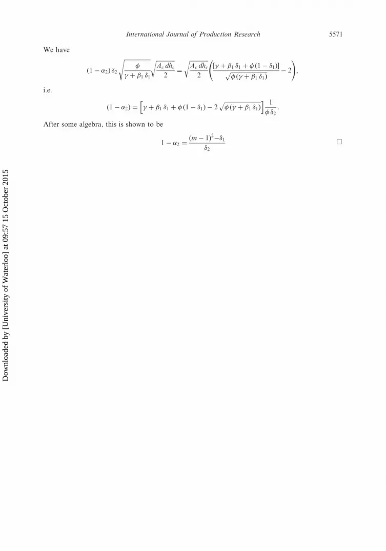
We have

ð1� �2Þ �2

ffiffiffiffiffiffiffiffiffiffiffiffiffiffiffiffiffiffi�

� þ �1 �1

s ffiffiffiffiffiffiffiffiffiffiffiffiffiAc dhc

2

r¼

ffiffiffiffiffiffiffiffiffiffiffiffiffiAc dhc

2

r½� þ �1 �1 þ � ð1� �1Þ�ffiffiffiffiffiffiffiffiffiffiffiffiffiffiffiffiffiffiffiffiffiffiffiffiffi

� ð� þ �1 �1Þp � 2

!,

i.e.

ð1� �2Þ ¼ � þ �1 �1 þ � ð1� �1Þ � 2ffiffiffiffiffiffiffiffiffiffiffiffiffiffiffiffiffiffiffiffiffiffiffiffiffi� ð� þ �1 �1Þ

ph i 1

� �2:

After some algebra, this is shown to be

1� �2 ¼m� 1ð Þ

2��1

�2h


Dow

nloa

ded

by [

Uni

vers

ity o

f W

ater

loo]

at 0

9:57

15

Oct

ober

201

5

international journal of production research calculating the benefits of vendor managed inventory in...

Documents