instrument choice for environmental protection when technological innovation is endogenous

Instrument Choice for EnvironmentalProtection When TechnologicalInnovation is Endogenous

Carolyn FischerIan W. H. ParryWilliam A. Pizer

Discussion Paper 99-04

October 1998

1616 P Street, NWWashington, DC 20036Telephone 202-328-5000Fax 202-939-3460Internet: http://www.rff.org

© 1998 Resources for the Future. All rights reserved.No portion of this paper may be reproduced withoutpermission of the authors.

Discussion papers are research materials circulated by theirauthors for purposes of information and discussion. Theyhave not undergone formal peer review or the editorialtreatment accorded RFF books and other publications.

ii

Instrument Choice for Environmental ProtectionWhen Technological Innovation is Endogenous

Carolyn Fischer, Ian W. H. Parry, and William A. Pizer

Abstract

This paper presents an analytical and numerical comparison of the welfare impacts ofalternative instruments for environmental protection in the presence of endogenoustechnological innovation. We analyze emissions taxes and both auctioned and free(grandfathered) emissions permits.

We find that under different sets of circumstances each of the three policies mayinduce a significantly higher welfare gain than the other two policies. In particular, therelative ranking of policy instruments can crucially depend on the ability of adopting firms toimitate the innovation, the costs of innovation, the slope and level of the marginalenvironmental benefit function, and the number of firms producing emissions. Moreover,although in theory the welfare impacts of policies differ in the presence of innovation,sometimes these differences are relatively small. In fact, when firms anticipate that policieswill be adjusted over time in response to innovation, certain policies can become equivalent.

Our analysis is simplified in a number of respects; for example, we assumehomogeneous and competitive firms. Nonetheless, our preliminary results suggest there is noclear-cut case for preferring any one policy instrument on the grounds of dynamic efficiency.

Key Words: technological innovation, externalities, environmental policies, welfare impacts

JEL Classification Numbers: Q28, O38, H23

iii

Table of Contents

1. Introduction ................................................................................................................. 1

2. Theoretical Analysis .................................................................................................... 4

A. The Basic Model .................................................................................................... 4

(i) Abatement Cost Minimization ........................................................................ 5

(ii) The Technology Adoption Choice .................................................................. 6

(iii) The Innovation Decision ................................................................................ 7

(iv) The First-Best Outcome ................................................................................10

B. Comparing Policy Instruments ..............................................................................10

(i) Innovation Incentives ....................................................................................10

(ii) Welfare Effects .............................................................................................14

(iii) Policy Adjustment .........................................................................................15

3. Numerical Analysis ....................................................................................................16

A. Functional Forms and Model Calibration ..............................................................16

B. Numerical Results .................................................................................................19

(i) Benchmark Results: The Role of the Imitation Effect ....................................19

(ii) The Implications of Declining Marginal Environmental Benefits ..................20

(iii) Alternative Scenarios for Innovation Costs ...................................................22

(iv) Number of Firms and Benefit Level ..............................................................23

(v) Further Sensitivity Analysis ..........................................................................24

C. Lessons for Policy .................................................................................................25

4. Conclusion .................................................................................................................26

References ..........................................................................................................................28

List of Tables and Figures

Table 1 Determinants of the Incentives for Innovation ...................................................... 9Table 2 Relative Incentives for Innovation .......................................................................14Table 3 Appendix: Interaction of Alternative Parameter Values .......................................27Figure 1 Appropriable Gains to Innovation with a Tax ......................................................11Figure 2 Appropriable Gains to Innovation with Auctioned Permits ..................................12Figure 3 Benchmark Simulations of Alternative Policies ...................................................19Figure 4 Effect of Marginal Benefit Slope on Welfare Gains ............................................21Figure 5 Effect of R&D Costs on Welfare Gains ...............................................................23Figure 6 Effect of Number of Firms and Benefit Level on Welfare Gain ...........................24

1

INSTRUMENT CHOICE FOR ENVIRONMENTAL PROTECTIONWHEN TECHNOLOGICAL INNOVATION IS ENDOGENOUS

Carolyn Fischer, Ian W. H. Parry, and William A. Pizer*

1. INTRODUCTION

Policy makers must often choose amongst alternative policy instruments for protectingthe environment. A key consideration affecting this choice is the impact of different policieson firm incentives to develop cleaner production technologies.1 Over the long run, thecumulative effect of technological innovation may greatly ameliorate what in the short runcan appear to be serious conflicts between economic activity and environmental quality(Jaffee and Stavins, 1995; Kneese and Schultz, 1975). This effect is especially pertinent inthe context of global climate change, where governments have so far been unwilling toimplement measures to substantially reduce emissions of greenhouse gases due to thepotential economic costs of these measures.

In environmental economics a strand of literature, mainly theoretical, has explored theeffects of environmental policies on technological innovation.2 Several early studies in thisliterature showed that emissions taxes and emissions permits generally provide moreincentives for technological innovation than "command and control" policies (such asperformance standards and technology mandates) in a single-firm setting.3 However manyinnovations are applicable to more than a single firm. Indeed at the heart of most R&Dmodels in the industrial organization literature is the spillover benefits of innovation to otherfirms, and the inability of innovators to fully appropriate the rents from innovation. Thus,more recent studies in environmental economics have expanded the earlier models toincorporate the diffusion of new technologies to other firms in the industry.

* Carolyn Fischer and Ian W. H. Parry, Fellows, Energy and Natural Resources Division, Resources for theFuture; William A. Pizer, Fellow, Quality of the Environment Division, Resources for the Future. The authorsare grateful to Tim Brennan, Raymond Prince and Mike Toman for helpful comments and suggestions. Theauthors also thank the Environmental Protection Agency (Grant CX 82625301) for financial support.Corresponding author: Ian Parry, email [email protected], phone (202) 328-5151.1 A number of other factors affect this choice. For example, the ease of monitoring and enforcement, politicalfeasibility, and the expected costs of policy instruments in the presence of uncertainty, firm heterogeneity andpre-existing tax distortions. For a review of the literature see Cropper and Oates (1992).2 Innovation incentives are frequently listed as an important consideration in the choice among environmentalpolicy instruments (see e.g. Stavins, 1998; Bohm and Russell, 1985). However the amount of analysis of thisissue--particularly empirical analysis--is surprisingly limited.3 See e.g. Downing and White (1986), Magat (1978) and Zerbe (1970).

Fischer, Parry, and Pizer RFF 99-04

2

The most comprehensive study of innovation in a multi-firm setting was Milliman andPrince (1989) (hereafter MP).4 An important finding in their analysis was that--when policiesare fixed at their "Pigouvian" levels over a period of time--incentives for innovation aregreater under an emissions tax than under free (grandfathered) emissions permits, and higherstill under auctioned emissions permits (see also Jung et al., 1996). Two effects underliethese results.

First, the amount of emissions abatement is greater after innovation under theemissions tax than under emissions permits. Innovation reduces the (marginal) cost ofemissions abatement, which induces more emissions abatement under a tax, while underpermits the industry-level amount of emissions by definition remains constant. Since firmsreduce emissions by a larger amount under the tax, they are willing to pay more forinnovations that reduce the costs of abatement. We refer to the industry-level reduction inabatement costs brought about by innovation as the abatement cost effect. Thus the abatementcost effect is larger under the emissions tax than under emissions permits.

The second effect arises from the impact of innovation on reducing the equilibriumpermit price. To the extent that firms purchase permits to cover their emissions--as they dounder auctioned permits--they gain from the fall in permit price. We refer to the reduction inpayments on firm emissions caused by innovation as the emissions payment effect. This effectis absent under a fixed emissions tax and (in the aggregate) free permits. In MP the emissionspayment effect is generally sufficient to raise the overall incentives for innovation underauctioned permits above those under the emissions tax.

Our paper differs from MP in three main respects. First, we alter some of theassumptions regarding the process of adoption and the spillover mechanism. MP assume thatinnovators can appropriate a constant fraction of the private gains to all firms in the industryfrom a new technology. In our analysis, we assume a competitive equilibrium where non-innovating firms pay a royalty for the new technology. The royalty level is endogenouslydetermined by the desire of the innovator to attract payment from the marginal, non-innovating firm.5 An important consequence of this assumption under a permit system is thatthe innovator cannot appropriate any of the emission payment effect accruing to non-innovators because the marginal firm has no effect on the equilibrium permit price. As aresult, the extra incentives for innovation from auctioning permits rather than grandfatheringthem are typically lower in our analysis than in MP.

4 Other studies following MP have examined different aspects of the innovation process. For example Jung etal. (1996) and Biglaiser and Horrowitz (1995) consider environmental policies in a setting where firms differ inabatement costs and their willingness to pay for new technologies. Jaffe and Stavins (1995) find someeconometric evidence for the superiority of market-based environmental policies at promoting innovation overcommand and control policies. For more discussion of the literature see Kemp (1997) and Ulph (1998).5 Indeed in our analysis the rate of appropriation of the overall industry gains from a new technology--which isobviously crucial for innovation incentives--is endogenously determined under all policy instruments, rather thanbeing exogenous as in other studies.


3

Second, we provide a numerical--as well as analytical--comparison of policyinstruments. Thus, we investigate the types of situations where the gains from using oneinstrument over others may be important and when they are not. Our analysis focuses onemissions taxes and auctioned and free emissions permits.6 For the most part we assume thatthese policies are set at their (ex ante) Pigouvian levels--the standard recommendation fromstatic analyses.7

Third, previous studies have tended to focus on the impact of policies on the demandfor innovation. However, from a welfare perspective, more innovation is desirable only if thebenefits outweigh the costs. Our analysis explicitly models the costs of using environmentalpolicies to induce innovation; therefore, we are able to examine the overall impacts of policieson social welfare.

In contrast with some earlier studies our results do not suggest a general preference forauctioned permits over emissions taxes--and emissions taxes over free permits--either on thecriterion of welfare gains or the induced amount of innovation. Instead, our tentativeconclusion is that a more pragmatic approach to instrument choice in the presence of inducedinnovation may be appropriate. Under different sets of circumstances, we find that each of thethree policies may generate a substantially higher welfare gain than the other two policies. Inparticular, the relative welfare ranking of policy instruments can crucially depend on fourimportant factors: the ability of adopting firms to imitate the innovation, the cost of innovation,the shape of the environmental benefit function, and the number of firms producing emissions.In certain situations, however, these welfare differences are small enough to be of little practicalrelevance for the choice of policy instruments. Thus, an evaluation of the circumstancesspecific to a particular pollutant seems to be required in order to judge whether a case for oneinstrument over the other two instruments can be made on dynamic efficiency grounds.8

To give some flavor of our results, we find that when innovators can effectivelyappropriate a large fraction of the rents from innovation, an emissions tax may induce asignificantly greater amount of innovation than free and auctioned permits, due in part to thelarger abatement cost effect under the tax. Assuming marginal environmental benefits are

6 These policy instruments are generally advocated by economists over command and control policies on thegrounds of their static efficiency properties (see for example Stavins, 1998). A free tradable emissions programwas implemented in the U.S. in 1990 to reduce sulfur emissions. All three policy instruments have beenproposed as a means to achieving the limits on carbon emissions agreed at the recent conference in Kyoto.7 Static models that assume the state of technology is exogenous do not capture the welfare gain frominnovation. In this sense they understate the overall welfare gains from environmental policies. However, theoptimal level of environmental regulation in the presence of innovation is not necessarily greater than thePigouvian amount. For more discussion of this see Parry (1995).8 Some of our results complement a recent study by Parry (1998). He showed that the welfare gain from usingan emissions tax over free emissions permits is only likely to be significant in the case of "major" innovations.Our analysis generalizes that in Parry (1998) in a number of respects. We provide a much more comprehensivecomparison of policy instruments. In addition we broaden the choice of policy instruments to include auctionedemissions permits, we vary the number of firms producing emissions, and we allow for convex as well as linearenvironmental benefits. Our analysis also reconciles the results from earlier studies.


4

relatively flat, this greater amount of innovation is socially desirable and welfare is alsosignificantly greater under the tax. However when appropriation is weak (due to theavailability of imitation technologies) the emissions payment effect at the innovating firmbecomes relatively more important, and both the innovation level and welfare gains can behighest under auctioned permits. The welfare gain from induced innovation is also morelikely to be greatest under emissions permits when the marginal environmental benefit curveis steeply sloped relative to the marginal abatement cost curve. Moreover, we find that thewelfare discrepancies between policies are only significant when the amount of innovationover the period for which policies are fixed is large enough to reduce abatement costs by asignificant amount (around 10 percent or more). In this connection, the flexibility of policyinstruments over time is important. If policies can be adjusted at regular intervals (and firmsanticipate this) the welfare discrepancies between instruments are less important.

A number of important caveats are in order. For example, we mainly assumeenvironmental policies are fixed at today's (pre-innovation) Pigouvian levels. As alreadymentioned, innovation incentives can differ when firms anticipate frequent policy adjustmentsin response to innovation. In addition, our assumption of a Nash equilibrium in the market fornew technologies may or may not be more realistic than the constant appropriations rateapproach in MP. Clearly, joint ventures or some other form of cooperation or bargainingbetween innovators and non-innovators are possible. However, we do believe that ourapproach provides an important competitive-equilibrium benchmark that is amenable to futureextensions while also providing policy guidance based on numerical simulations. The resultscan then be used to gauge the quantitative importance of incorporating more complexfeatures, such as imperfectly competitive behavior.

The rest of the paper is organized as follows. Section 2 develops an analyticalframework that decomposes the determinants of innovation incentives under alternativepolicy instruments. This framework is used to explain our numerical results, which arepresented in Section 3. Section 4 concludes and suggests extensions for future research.

2. THEORETICAL ANALYSIS

In this section, we first develop the basic model of induced technological change.Then we compare in general terms the differences between different environmental policieswith respect to their impacts on innovation and on welfare.

A. The Basic Model

We model a three-stage process of innovation, diffusion and emissions abatementinvolving a fixed number of n identical, competitive firms.9 One of these firms is an

9 The industrial organization literature on innovation has tended to focus on strategic models involving a smallnumber of firms where monopoly rents, timing and preemption are important (see e.g. the survey in Tirole, 1988).While appropriate for major R&D industries such as pharmaceuticals, these studies may be less appropriate whereenvironmental issues are concerned. Major pollutants like sulfur dioxide, nitrogen oxides, particulates and carbon


5

innovator. In the first stage, the innovating firm decides how much to invest in R&D todevelop an emissions abatement technology. In the second stage, the other n-1 firms decidewhether to adopt this technology in return for a royalty fee. Alternatively, they can use animitation technology that is not fully equivalent to the original innovation. In the third stage,all n firms choose emissions abatement to minimize costs given an emission tax or a permitprice. The environmental policy is set prior to innovation, although implementation (includingany auctioning of permits) takes place in the last stage. The model is best solved backwards.

(i) Abatement Cost Minimization

The abatement cost function for a firm in the third stage is ),( kaC , where a is firm-

level emissions abatement and k represents the state of technology for reducing emissions.10

Abatement costs are assumed to be increasing and convex in a and decreasing in k withdiminishing returns to technology: Ca>0, Caa>0, kC <0, kkC >0, akC <0, Ca(0, k)=0.

Technological innovation (k) is determined in the first stage and therefore is exogenous in thethird stage. An augmented state of technology (higher k) reduces the slope of the marginalabatement cost function.11

Let t denote the "price" of emissions. Under an emissions tax this is simply the taxrate. Alternatively it represents the equilibrium permit price under an emissions permitpolicy. Firms are competitive in the market for emissions; i.e., they take the emissions priceas given when making abatement decisions.In the third stage each firm solves

=),( tkµ { })(),(min aetkaCa

−+ , (2.1)

where e is what emissions would be in the absence of abatement. Firms choose emissionsabatement to minimize the sum of (i) abatement costs and (ii) tax payments on actualemissions, or alternatively the cost of purchasing (or forgoing sales) of emissions permits.This cost minimization yields the following first order condition:

tkaCa =),( . (2.2)

dioxide are produced by large numbers of firms. See Oates and Strassmann (1984) for a defense of the competitiveassumption in models of environmental policy.10 Abatement reduces emissions per unit of output and represents the substitution of cleaner inputs for pollutinginputs in production, or the installation of end-of-pipe clean-up technologies. In practice emissions also fall asindustry output contracts in response to higher pollution abatement costs. For simplicity we do not incorporatethis effect. For many pollutants this may be a reasonable approximation because abatement costs are typicallyonly around 2 percent of total production costs (Robison, 1985). Indeed, Goulder et al. (1998) find that around98 percent of NOX emissions reductions come from firms reducing emissions per unit of output and only 2percent from reductions in industry output.11 An increase in k may represent, for example, a new process for blending cleaner fuels in production, or amore effective technology for "scrubbing" air pollutants or cleaning water pollutants. The impact of successiveincreases in innovation on reducing abatement costs is declining, since there is a limit on the ability to reduceabatement costs (costs cannot become negative).


6

In other words, marginal abatement costs equal the price of emissions.

(ii) The Technology Adoption Choice

Typically innovators can only partially appropriate the spillover benefits to other firmsfrom new technologies. In particular, other firms may use the new information to developalternative technologies to the original innovation. We represent imperfect appropriation byassuming that the new innovation is patented but other firms can (imperfectly) imitate aroundthe patent. Thus in the second stage non-innovators decide whether to pay a fixed-fee royaltyY for licensing the technology (k) developed in the first stage. Alternatively, they can use animitation that improves their technology level by σk rather than k, where 10 ≤≤ σ . A firmwill adopt the patented technology if its costs (including the royalty payment) are no higherthan costs with the imitation.12

Each firm makes its decision of whether to adopt given the adoption decisions of allthe other firms and the prevailing price of emissions. We assume the royalty is set such thatin the resulting Nash equilibrium, all firms adopt the original innovation rather than use animitation.13 Thus, the maximum royalty that the innovator can charge just leaves the lastadopting firm indifferent between the new technology and the imitation:14

),(),( tktkY σµµ −= . (2.3)

Thus, while in equilibrium no one chooses to imitate, the threat of imitation limits theability of the innovator to appropriate the social benefits from innovation.15

From (1) and (3), the maximum royalty can be expressed:

{ } ))((),(),()( 11 σσ σ aaktkaCkaCkY −+−= , (2.4)

12 For simplicity, we assume zero costs to imitation. Allowing for positive imitation costs would raise thewillingness to pay for the patented technology and hence the rate of appropriability. Thus, incorporatingimitation costs would be equivalent to lowering the value of σ in our model. In addition we could assume thatthe alternative technology was also invented and patented by one firm. However allowing for multiple (andcompeting) patented technologies would have the same impact on reducing innovation incentives as imitation (orσ) does in our model (Bigliaser and Horrowitz, 1995).13 We ignore the possibility that pricing the technology such that only some portion of non-innovating firmsadopt is the profit-maximizing outcome.14 We prohibit the possibility of price-discrimination in royalties according to the order of adoption, since in thatcase every firm would want to be the last to adopt.15 Allowing for the possibility of imitation is one way to introduce imperfect appropriation into the model. Analternative approach would be to allow for firm heterogeneity and the cost reduction from adopting theinnovation to differ across firms. The innovator cannot charge different royalties to different firms and thereforewould be unable to appropriate the full social benefits from the innovation (see Bigliaser and Horrowitz, 1995).Imperfect appropriability also arises when one firm's R&D in one period raises the productivity of another firm'sR&D in future periods. Also the assumptions that new technologies are patented and licensed to all firms are notcrucial. Often, when the number of potential users of a new technology is small, innovators may choose not topatent a new technology. Our assumptions simply enable us to represent imperfect appropriability, and inSection 3 we consider a wide range of possible scenarios for the appropriation rate.


7

where superscripts σ and 1 denote the solution to condition (2.2) for a firm with technologylevel σk and k respectively. From equation (2.4), the willingness to pay for adopting thepatented technology rather than using the imitation consists of two components. First, thesavings in abatement costs from using the better technology over the imitationis ),(),( 1 kaCkaC −σσ . Second, tax payments (or payments for emissions permits) on

emissions net of abatement with the patented technology )))((( 1aekt − are less than the

corresponding payments if the imitation were used )))((( σaekt − . Thus, using the patented

technology over the imitation reduces these payments by ))(( 1 σaakt − .

Our assumption of adopting firms being competitive in the market for emissionsimplies that no one firm believes its abatement and adoption decisions can affect price ofemissions. However, changes in (marginal) abatement costs aggregated over all firms canaffect the price of emissions, and our innovator does recognize this implication oftechnological diffusion. In the case of fixed permits, this adjustment occurs through changes inthe permit price; thus, we write t = t(k). Under a fixed emissions tax, the price of emissionsdoes not change with aggregate abatement cost reductions (although we also briefly consider acase where the tax rate is adjusted in response to innovation). To the extent that emissionsprices fall due to aggregate marginal cost reductions, adopting firms will benefit from lowerpayments on their inframarginal emissions. However, since any one firm can enjoy this benefitwhether it adopts or not, given an equilibrium where every other firm is adopting, the innovatorcannot appropriate these gains. Still, any adjustments in the price of emissions continue toaffect the maximum royalty, since it affects the relative value of the imitation option.

Differentiating (2.4) with respect to k gives the marginal change in individual royaltypayments:

))((),(),()( 11 σσ σσ aaktkaCkaCkY kk −′+−=′ . (2.5)

(iii) The Innovation Decision

We assume that innovation results from investments in R&D activity by one firm.16

The cost of the R&D necessary for technological innovation is F(k), where F′>0, F′′ ≥ 0. Inthe first stage the innovator chooses R&D (or, equivalently, the amount of technologicalinnovation) to maximize profits:17

))(()(),()()1()( 11 eaektkFkaCkYnk −−−−−−=π . (2.6)

16 Other studies have explored the implications of innovation by more than one firm. In those settings, innovationmay be socially excessive. This is because firms do not take into account the potential effect of their researchefforts on reducing the likelihood of innovation rents at other firms (see Wright (1983) for a good discussion).17 Thus we simplify by assuming that innovation is continuous rather than discrete. "Innovation" in our analysiseffectively represents the aggregate amount of innovation over a given period, and in this sense it is more reasonableto regard it as a continuos variable. An alternative formulation would be to assume that firms invest in R&D toincrease the probability of successfully inventing a discrete technology (see e.g. Wright, 1983; Parry, 1998).


8

Innovator profits equal royalties from the other n−1 firms minus the sum of own abatementcosts, innovation costs and payments on own emissions, either in the form of tax payments orpermit purchases. e is the (exogenous) permit allocation of the innovating firm under thefree permits policy ( e = 0 for the emissions tax and auctioned permits policies).18

Maximizing (2.6) with respect to k gives

))((),()()1()( 11 eaektkaCkYnkF k −−′−−′−=′ . (2.7)

Substituting (2.5) in (2.7) gives the following condition that determines the privately optimalamount of innovation:

=′ )(kF −43421

effectcostabatement

kanCk ),( 11 + 444 3444 21

effectimitation

kaCn k ),()1( σσ σ− (2.8)

44 344 21

effectpaymentemissions

eaekt ))(( 1 −−′− +444 3444 21

effect price adoption

aaktn ))(()1( 1 σ−′−

Equation (2.8) equates the marginal cost and marginal private benefit of innovation,where the latter is decomposed into four components. First, the (marginal) abatement costeffect is the increased willingness to pay for the new technology across all firms due to theimpact of (incremental) innovation on reducing firm abatement costs. Second, the (marginal)imitation effect is the reduction in the willingness of non-innovators to pay for the newtechnology, due to the impact of (incremental) innovation on increasing the possibility ofabatement cost-reducing imitation.

The third and fourth components are present when emissions prices adjust to changesin marginal abatement costs, e.g., permit policies or policies adjusted ex post. The (marginal)emissions payment effect represents the reduction in payments for permits to cover theinnovator's (infra-marginal) emissions, net of current permit holdings, due to the effect ofinnovation on reducing the permit price. Under auctioned permits, the innovator must coverall inframarginal emissions (e−a1) and the corresponding reduction in payments can be asignificant additional incentive to innovate. Under free permits, if the permit allocation e isless (greater) than emissions ( 1ae − ), the innovator is a net buyer (seller) of permits. Thus,by driving down the emissions price, innovation produces a private gain (loss) for the innovatorif he is a net buyer (seller) of permits. We simplify by assuming that all firms receive the samepermit allocation. Therefore, since in our symmetric equilibrium all firms produce the sameamount of emissions, no buying or selling of permits actually occurs and, correspondingly,no emissions payment effect exists under free permits.19 Although non- innovators who 18 e does not appear in equation (2.1) or (2.3), since firm decisions about emissions and technology adoptiondo not affect the price of emissions, and hence the rents obtained from permit allocations.19 More generally, if the innovator is a net buyer of permits, the amount of induced innovation will lie betweenthe amount under our free and auctioned permit cases. If the innovator is a net permit seller, innovation will bebelow that in our free permit case.


9

are net buyers of permits also gain from an emissions payment effect, the innovator cannotappropriate this benefit, which accrues regardless of any one firm's choice to adopt thepatented technology or the imitation. In other words, non-innovators free ride on the fall inpermit price.20

The final component in equation (2.8) is the adoption price effect. Under free orauctioned permits, if a non-innovator were to use the imitation instead of the patentedtechnology, it would have higher emissions and would pay ))(( 1 σaakt − for the additional

permits. By reducing the permit price, innovation reduces these extra payments and hence theroyalty that non-innovators will pay for the new technology. Again, no corresponding effectexists under an emissions tax, unless the policy maker reduces the emissions tax in responseto innovation.21 We summarize the determinants of the incentives for innovation underalternative policies in Table 1.

Table 1: Determinants of the Incentives for Innovation

Emissions tax Free permits Auctioned permits

abatement cost effect + + +

imitation effect − − −emissions payment effect 0a 0 +

adoption price effect 0a − −a Our main focus is on a fixed emissions tax. In the case when marginal environmental benefits aredeclining and the Pigouvian tax is adjusted downwards in response to innovation, the emissions paymenteffect is positive and the adoption price effect is negative, as with auctioned permits.

20 In contrast MP effectively assume that innovators appropriate an (exogenous) fraction of the emissionspayment effect at other firms. This assumption seems more applicable when the number of non-innovating firmsis relatively small. In this case the decision of non-innovators about whether to adopt the patented technology orthe imitation may affect the equilibrium permit price. In addition the innovator could bargain with all otherfirms as a group and threaten not to license the new technology to the group unless non-innovators pay for partof the emissions payment benefit. With fewer firms there is also greater scope for collusion over innovationstrategies and sharing the (private) industry-wide benefits from innovation. Note that in these cases theappropriable fraction of the emissions payment effect at other firms will be complex and difficult to estimateempirically. It will depend, among other things, on the number of firms and the form of imperfect competition. Our assumption of Nash equilibrium implicitly implies that firms have rational expectations about the finalequilibrium permit price. If this is not the case, some licensing of the new technology may occur atdisequilibrium prices (that is, before complete diffusion of the new technology). However so long as non-innovators are price-takers in the permit market the innovator is still unable to appropriate the emissionspayment effect at other firms.21 It is possible that an innovating firm will be an outside supplier. That is the firm is engaged in developingnew technologies but does not produce pollution itself. In this case there is no emissions payment effect at theinnovating firm, and auctioned permits would be equivalent to free permits in our analysis.


10

(iv) The First-Best Outcome

In order to investigate the welfare properties of these policies, we first need to defineoutcomes in the first-best or social planning version of the model. We assume thatenvironmental benefits from emissions abatement by the n firms is B(na) where B′>0 andB′′ ≤ 0 and a continues to represent firm-level emission abatement. Social welfare equalsenvironmental benefits, less abatement costs across the n firms, less innovation costs:

)(),()( kFkanCnaBW −−= . (2.9)

Maximizing this expression with respect to a and k gives

)(),( *** naBkaCa ′= , (2.10)

and

),()( *** kanCkF k−=′ . (2.11)

In other words, Equation (2.10) shows that a social planner would equate firm-levelmarginal abatement costs per firm with marginal environmental benefits. In Equation (2.11),the planner equates the marginal cost of innovation with the marginal benefit in terms ofreducing abatement costs across all firms.

B. Comparing Policy Instruments

We now compare the impacts of alternative policies on innovation and welfare. Forthe most part we assume that policies are fixed at their "Pigouvian" levels, since this is thestandard recommendation from static analyses.22 We illustrate the important points usingFigures 1 and 2. These figures show the gains from innovation at the innovating firm (upperpanels) and the royalty received from non-innovators (lower panels), under the tax (Figure 1)and permit policies (Figure 2). )0,(aCa , ),( kaCa σ and ),( kaCa are the marginal cost of

abatement prior to innovation, with the imitation, and with the patented technologyrespectively.

(i) Innovation Incentives

Under the emissions tax, firms reduce emissions until the tax rate equals marginalabatement costs. Therefore, abatement per firm increases as marginal costs shift down,depicted in Figure 1 by 0a , taσ and 1a with the original technology, the imitation and the

patented technology, respectively. The innovator gains the full abatement cost effect for itself,the shaded area 0hj in the top panel. However, non-innovators, although they realize the samecost savings, are only willing to pay the shaded area 0lj to adopt the patented technology.

22 That is, policies are set to equate the marginal environmental benefits and marginal abatement costs prior toinnovation.

11

(a) From the Innovator

0 a0 a1

Ca(a,0)

Ca(a,k)h s

Emissions, e Abatement, a

t j

(b) From a Non-Innovator

Ca(a,s k)

l

0

Ca(a,0)

Ca(a,k)h j s


t

a0 aFt a1

Figure 1: Appropriable Gains to Innovation with a Tax

i

i

12

(b) From a Non-Innovator

Ca(a,s k)

0

Ca(a,0)

Ca(a,k)


t(0)

t(k)

aFp

k

l

qu

h

i

js

r

a0

wt(s k)

(a) From the Innovator

0 a0

Ca(a,0)

Ca(a,k)


sht(0)

t(k)i r

j

Figure 2: Appropriable Gains to Innovation with Auctioned Permits


13

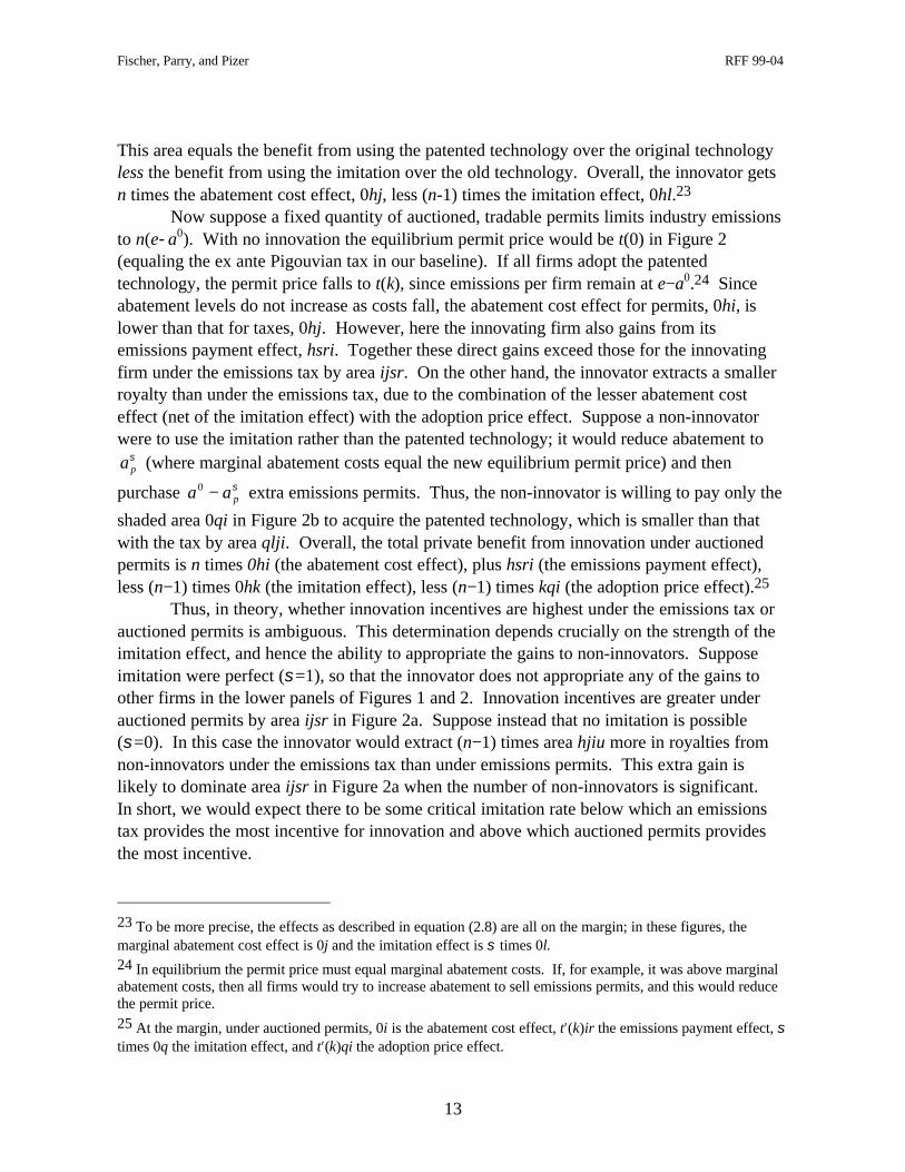
This area equals the benefit from using the patented technology over the original technologyless the benefit from using the imitation over the old technology. Overall, the innovator getsn times the abatement cost effect, 0hj, less (n-1) times the imitation effect, 0hl.23

Now suppose a fixed quantity of auctioned, tradable permits limits industry emissionsto n(e−a0). With no innovation the equilibrium permit price would be t(0) in Figure 2(equaling the ex ante Pigouvian tax in our baseline). If all firms adopt the patentedtechnology, the permit price falls to t(k), since emissions per firm remain at e−a0.24 Sinceabatement levels do not increase as costs fall, the abatement cost effect for permits, 0hi, islower than that for taxes, 0hj. However, here the innovating firm also gains from itsemissions payment effect, hsri. Together these direct gains exceed those for the innovatingfirm under the emissions tax by area ijsr. On the other hand, the innovator extracts a smallerroyalty than under the emissions tax, due to the combination of the lesser abatement costeffect (net of the imitation effect) with the adoption price effect. Suppose a non-innovatorwere to use the imitation rather than the patented technology; it would reduce abatement to

σpa (where marginal abatement costs equal the new equilibrium permit price) and then

purchase σpaa −0 extra emissions permits. Thus, the non-innovator is willing to pay only the

shaded area 0qi in Figure 2b to acquire the patented technology, which is smaller than thatwith the tax by area qlji. Overall, the total private benefit from innovation under auctionedpermits is n times 0hi (the abatement cost effect), plus hsri (the emissions payment effect),less (n−1) times 0hk (the imitation effect), less (n−1) times kqi (the adoption price effect).25

Thus, in theory, whether innovation incentives are highest under the emissions tax orauctioned permits is ambiguous. This determination depends crucially on the strength of theimitation effect, and hence the ability to appropriate the gains to non-innovators. Supposeimitation were perfect (σ=1), so that the innovator does not appropriate any of the gains toother firms in the lower panels of Figures 1 and 2. Innovation incentives are greater underauctioned permits by area ijsr in Figure 2a. Suppose instead that no imitation is possible(σ=0). In this case the innovator would extract (n−1) times area hjiu more in royalties fromnon-innovators under the emissions tax than under emissions permits. This extra gain islikely to dominate area ijsr in Figure 2a when the number of non-innovators is significant.In short, we would expect there to be some critical imitation rate below which an emissionstax provides the most incentive for innovation and above which auctioned permits providesthe most incentive.

23 To be more precise, the effects as described in equation (2.8) are all on the margin; in these figures, themarginal abatement cost effect is 0j and the imitation effect is σ times 0l.24 In equilibrium the permit price must equal marginal abatement costs. If, for example, it was above marginalabatement costs, then all firms would try to increase abatement to sell emissions permits, and this would reducethe permit price.25 At the margin, under auctioned permits, 0i is the abatement cost effect, t′(k)ir the emissions payment effect, σtimes 0q the imitation effect, and t′(k)qi the adoption price effect.


14

Finally, suppose that permits were given out for free. In this case the incentives forinnovation are less than under auctioned permits since the emissions payment effect at theinnovating firm (rectangle hsri) is absent. Free permits therefore also induce less innovationthan the emissions tax, since both the abatement cost effect and the royalty received fromnon-innovators is smaller.

Table 2 summarizes these results. Innovation under the emissions tax is less than thefirst-best amount (due to the imitation effect), except possibly when marginal environmentalbenefits are declining. Innovation under free permits is always less than under auctionedpermits or the tax. Under auctioned permits, innovation could be greater or less than underthe tax, depending on the relative strength of the emissions payment effect.

Table 2: Relative Incentives for Innovation

Level of policyinstrumentsa

Marginalenvironmental

benefits

Innovation underemissions tax

relative to first-best innovation

Innovation underauctioned permits

relative toinnovation under

emissions tax

Innovation underfree permits relativeto innovation under

emissions tax

constant less greater or less less1. Ex antePigouvian policies declining greater or less greater or less less

constant less same same2. Ex postPigouvian policies declining greater or less same less

a Our main focus is on ex ante Pigouvian policies.

(ii) Welfare Effects

High levels of innovation are not always indicative of welfare maximization.Innovation is costly and therefore only desirable to the extent that the marginal gains frominnovation exceed the cost. In particular a social planner will weigh the decrease inabatement costs, net of any change in the optimal abatement level, against the innovation cost.While decentralized policies provide similar incentives to innovate, they are potentiallydistorted by the imitation, emission payment, and adoption price effects, as well as policystickiness. As a result, the welfare ranking of the different policies is even more ambiguousthan the ranking of innovations incentives, particularly when the slope of marginal benefits istaken into account.

Suppose first that marginal environmental benefits are constant and equal to t inFigure 1 (or t(0) in Figure 2). The total social benefit from innovation (gross of innovationcosts) in the first-best outcome is n times triangle 0hj. Society gains both from reducingabatement costs at the ex ante optimal abatement level a0 and from additional environmentalbenefits (net of costs) from increasing abatement to a1. These gains exceed the private benefit


15

from innovation under the Pigouvian emissions tax by the amount of the imitation effectaggregated over the (n-1) firms. As a result, the induced amount of innovation under the taxis less than the socially optimal level. However, given the amount of innovation, emissionsabatement is optimal, since the emissions tax (and hence marginal abatement costs) equalsmarginal environmental benefits.

As discussed above, innovation under free permits is less than under the emissions taxand hence even further below the socially optimal amount. In addition, the ex post abatementlevel is also sub-optimal since abatement does not increase as marginal abatement costs fall.Therefore, welfare is unambiguously lower than under the emissions tax, when marginalenvironmental benefits are constant.

As shown in section 3, welfare is typically lower under auctioned permits than underthe emissions tax with constant marginal environmental benefits. The exception is the casewhen innovation is greater under auctioned permits than under the emissions tax, and thewelfare gain from this extra innovation more than outweighs the welfare loss from sub-optimal (ex post) abatement levels.

Now suppose marginal environmental benefits decline monotonically, and therefore arelower at a1 than a0 in Figure 1. Thus, starting with Pigouvian tax t, given any positive amountof innovation, the emissions abatement under a tax will be socially excessive, because marginalabatement costs will exceed marginal environmental benefits. In addition, innovation maynow exceed the first-best amount, if the excessive demand for innovation from the abatementcost effect more than outweighs the negative influence of the imitation effect.

Under free emissions permits innovation is necessarily below the socially optimalamount. This is because emissions abatement is less (not greater) than ex post optimal levels,and because of the imitation effect. Insufficient innovation is also likely under auctionedpermits, except possibly when the emissions payment effect is relatively strong. Overallwelfare may be greater under any of the three policies, depending on which policy inducesabatement and innovations levels that are closer to first-best levels. As illustrated below, thiscrucially depends on the relative slope of the marginal environmental function and thestrength of the imitation effect.

(iii) Policy Adjustment

Finally, we consider very briefly what happens when policies are perfectly flexibleand are adjusted to the new Pigouvian levels following innovation.26 Suppose the tax, orquantity of permits, are adjusted such that emissions abatement is optimal given the ex poststate of technology. When the innovator anticipates this policy adjustment, taxes andauctioned permits become functionally equivalent policies. When marginal environmentalbenefits are constant, free permits are equivalent as well. Ex post abatement levels, and hence

26 We do not consider optimal (second-best) policies because they would be difficult to implement in practice.To estimate optimal policies would require information on the costs and benefits of both innovation andpollution abatement.


16

the abatement cost effect, are identical under all policies. In addition, the quantity of permitsis reduced to prevent the emissions price from falling and hence there are no emissionspayment or adoption price effects. However, innovation is still below the first-best level ineach case to the extent that there is an imitation effect.

When marginal environmental benefits are declining, abatement does not expand asmuch relative to the constant marginal benefits case, and the abatement cost effect becomessmaller on the margin. At the same time, the emissions price falls under each policy followinginnovation. The resulting adoption price effect causes appropriable gains to fall even more.For the tax and auctioned permits, where the innovator is liable for his or her own inframarginalemissions, the emissions payment effect provides some added inducement to innovate.However, this effect is absent under free permits, causing innovation to be lower for this policy.

Thus, the welfare discrepancies between policies would tend to disappear if policiescould be continuously adjusted to their Pigouvian levels in response to every new innovation(except in the case when the emissions payment effect is significant and leads to lessinnovation under free permits). In practice, policy instruments are not perfectly flexible--theycan only be adjusted at discrete points in time. Nonetheless, in general, the smaller theamount of innovation during the period for which policies are fixed, the smaller is the relativewelfare discrepancy between policies.

3. NUMERICAL ANALYSIS

We now explore the quantitative importance of the results in Section 2 by specifyingfunctional forms for the previous model and solving numerically. This procedure is describedin Subsection A. Subsection B presents the simulation results of the numerical model.Subsection C summarizes some tentative policy lessons from our findings.

A. Functional Forms and Model Calibration

We assume the following functional forms:

2

)(),(

2anekanC k−= (3.1)

2)(

2kfkF = (3.2)

2)(2

)( anbbananB −−=α

(3.3)

where k is the innovation level, a is the emissions abatement level for each firm, n is thenumber of firms and f, b and α are parameters.

Equation (3.1) specifies emission abatement costs with ),( kaC representing the

abatement costs at a single firm. The costs of abatement decline exponentially withinnovation, k. Thus, it becomes increasingly difficult to generate additional reductions in


17

abatement costs through innovation as abatement costs fall towards zero. For a given state oftechnology, emissions abatement costs are quadratic.27 Equation (3.2) specifies the costs ofinnovation. These costs are also quadratic and the parameter f determines the slope of themarginal cost of innovation.28 Finally, equation (3.3) specifies environmental benefits fromemissions abatement. When α=0, marginal environmental benefits are constant, and whenα>0, marginal environmental benefits are declining.

Equations (3.1)−(3.3) can be combined to form an expression for welfare that isanalogous to equation (2.9):

22

2

22

)()(

2)(),()(),( k

fnaeanbbankFkanCanBkanW k −−−−=−−= −α

(3.4)

The numerical model maximizes this expression by solving first order conditions analogous toequations (2.10) and (2.11), yielding the first-best outcome a* and k *. Writing the optimalabatement level in the absence of innovation as a0, we define the welfare gain frominnovation as:

)()0,(),( *0

** kFnaWknaW −−

That is, environmental benefits net of abatement costs with innovation (a = a*, k = k*), lessenvironmental benefits net of abatement costs with no innovation (a = a0, k = 0), lessinnovation costs.29

To obtain the outcomes under alternative policies, we first note that the cost functionper firm defined by (3.1), namely 2/),( 2anekaC k−= , can be used to solve for firm-level

abatement in response to a tax or permit price t and at a particular innovation level k:

knet

tka−

=),(

Using this expression, we write out the profit function for the innovator. From (2.4) and (2.6)this is:

)(kπ )())(()1())((),()1(),( kFaaktneaektkaCnkanC −−−+−−−−+−= σσ σ (3.5)

27 We normalize the slope of the industry-wide marginal abatement cost function to unity. That is, the secondderivative of aggregate costs nC(a, k) with respect to aggregate abatement na is one (when k = 0). We normalizecosts in this way so that the socially optimal level of aggregate abatement and innovation is independent of thenumber of firms. Otherwise, in our examination of the effect of market size on policy choice, it would bedifficult to vary the number of firms without simultaneously affecting the degree to which optimal innovationshifts the marginal abatement cost curve.28 The assumption of increasing marginal costs from innovation seems plausible, due to the increasing scarcityof specialized inputs, such as scientists and engineers, at higher levels of research activity. However, our resultsare not sensitive to assuming constant marginal costs of innovation.29 This welfare gain corresponds to n times area 0hj in Figure 1, less innovation costs.


18

where ))(,( ktkaa σσσ = and ))(,( ktkaa = . As before, σ is the degree to which other firms

can imitate the innovation, e is the uncontrolled emission level, and e is the number ofpermits freely given to each firm. For the emissions tax, t is a constant and set equal to

¢B a n( )0 where ¢ =B a n C aa( ) ( , )0 0 0 ; this marginal benefit defines the Pigouvian tax prior toinnovation (see Figure 1). Under permits the quantity of abatement is fixed at a0, and thepermit price is endogenously determined. e equals 0ae − in the case of free permits, and is

zero for the other two policies. We substitute (3.1)−(3.3) into (3.5) and the profit functionsunder alternative policies are maximized numerically to determine the innovation level k. Thewelfare gain from innovation under each policy, )()0,(),( 0 kFnaWknaW −− , is then

computed and expressed as a fraction of the welfare gain in the first-best outcome (thus, therelative welfare gain cannot exceed unity).

In this model, the relative welfare impacts of alternative policies depend on fiveimportant parameters: (i) the extent of imitation, σ; (ii) the innovation cost parameter f; (iii)the initial level of abatement/environmental benefits, b; (iv) the relative slope of the marginalenvironmental benefit curve, α; (v) the number of firms, n. We begin by creating abenchmark scenario. The choice of initial parameter values for this benchmark is necessarilysomewhat arbitrary. However we subsequently explore how each parameter affects thewelfare ranking of alternative policies, under a wide range of assumed values.

We begin by assuming a flat marginal environmental benefit curve, α = 0, and we setb = 0.2 to imply an optimal emissions reduction of 20 percent before innovation.30 Theparameter f is chosen to imply that innovation in the first-best outcome would reduceabatement costs by 20 percent over the period (f = 0.11).31 We assume n = 100 toapproximate a competitive market (thus the innovator's emissions are small relative to totalemissions). Finally, we begin by considering all possible values for σ ( )10 ≤≤ σ and

subsequently a "high imitation" case (σ = 0.25) and a "low imitation" case (σ = 0.75).32

30 This translates further into a0 = 0.2 under the permit policies ( e = 0.8 for free permits) and t = 0.2 under theemissions tax. The assumption of flat marginal environmental benefits appears to be a reasonable approximationfor a number of pollutants including sulfur dioxide (Burtraw et al., 1997) and carbon dioxide (Pizer, 1998).31 It is very difficult to estimate ex ante the costs of developing cleaner production technologies. Instead, weassume different scenarios for the amount of innovation (in the first-best case), and infer the value of f thatwould generate these innovation levels.32 Under the emissions tax the innovator appropriates approximately 1−σ of the private benefits to other firmsfrom innovation. The appropriation rate is somewhat less than 1−σ under auctioned emissions permits, since thebenefits to other firms include the (non-appropriable) emissions payment effect. Studies for commercial (or non-environmental) innovations suggest that appropriation rates vary considerably over different types ofinnovations, with an average rate of around 50 percent. See Griliches (1992) and Nadiri (1993).


19

B. Numerical Results

(i) Benchmark Results: The Role of the Imitation Effect

Our first simulations highlight the role of the imitation effect. The left-hand panel ofFigure 3 compares the welfare gain from innovation under each policy instrument, expressedrelative to that in the first-best outcome, using our benchmark parameter values. Theserelative welfare gains are shown as a function of the imitation rate, varying from 0 to 100percent.33 The right hand panel indicates the corresponding amount of innovation under eachpolicy, again expressed relative to the first-best amount of innovation. Figure 3 displaysseveral noteworthy features.

Figure 3: Benchmark Simulations of Alternative Policies

0 0.2 0.4 0.6 0.8 10

0.2

0.4

0.6

0.8

1

degree of imitation (σ)

wel

fare

gai

n re

lativ

e to

fir

st b

est

tax

auctionedpermit

freepermit

0 0.2 0.4 0.6 0.8 10

0.2

0.4

0.6

0.8

1

degree of imitation (σ)

R&

D le

vel r

elat

ive

to f

irst

bes

ttax

auctionedpermit

freepermit

First, and not surprisingly, the absolute amount of, and welfare gain from, innovationunder each policy falls dramatically as the imitation effect increases. For example, under theemissions tax the amount of, and welfare gain from, innovation declines from 100 percent ofthe first best levels when σ = 0 to practically zero percent when σ = 1. A stronger imitationeffect reduces the ability of the innovator to capture the benefits of innovation to other firms.34

Second, however, the relative performance of policy instruments also criticallydepends on the imitation effect. With no imitation (s = 0), taxes provide a much greaterincentive to innovate than free or auctioned permits in our benchmark scenario: innovationunder free and auctioned emissions permits is less than 60 percent of that under the emissions

33 When there is no imitation (σ=0), the innovator appropriates 100 percent of the private gains from innovationto other firms under the emissions tax and free permits, and somewhat less than 100 percent under auctionedpermits (see previous footnote). When there is perfect imitation (σ=1), the innovator obtains none of the benefitsto other firms under all policies.34 As mentioned earlier when more than one firm conducts R&D, competition for innovation can be excessive.Parry (1998) discusses to what extent this effect may mitigate the negative incentives from imperfect appropriation.


20

tax. Essentially, the emissions tax induces additional emissions abatement as (marginal)abatement costs fall, while emissions permits do not. With more abatement over which togarnish cost savings under the tax, the abatement cost effect is larger and the willingness topay for improved abatement technologies is greater. Under our benchmark assumptions offlat marginal environmental benefits, this additional abatement is also socially efficient.

As the potential for other firms to imitate increases, the innovator appropriates less ofthe abatement cost effect of other firms. This imitation effect has a disproportionate impactunder the emissions tax since the abatement cost effect is larger under this policy. As a result,this policy loses its relative advantage, as all policies underprovide innovation. Furthermore,the emissions payment effect from auctioned permits becomes relatively more importantwhen the innovator appropriates very little from other firms. Indeed, at some rate ofimitation, innovation and welfare are highest under auctioned permits. However in absoluteterms any gain from using auctioned permits over other instruments is never very substantialin our benchmark scenario. Figure 3 illustrates a counter-example to previous theoreticalstudies which appear to imply a general preference for auctioned permits over otherinstruments on the grounds of innovation incentives.35

(ii) The Implications of Declining Marginal Environmental Benefits

Figure 4 illustrates the welfare implications of declining marginal environmentalbenefits. On the horizontal axes we vary the (magnitude of the) slope of the marginalenvironmental benefit curve between one tenth and ten times the slope of the marginalabatement cost curve. We do this by pivoting the marginal environmental benefit curve aboutthe initial Pigouvian abatement level of 20 percent (a0 in Figures 1 and 2). The level of policyinstruments--and hence the induced amount of innovation and abatement--are constant in thisexercise: varying marginal environmental benefits affects first-best outcomes but not thepolicy-induced outcomes. The left and right hand panels in Figure 4 correspond to our lowand high imitation scenarios respectively.

The left-hand panel illustrates that the relative slope of the marginal environmentalbenefit function crucially influences the welfare ranking of alternative policies. When themarginal environmental benefit curve is flatter than the marginal abatement cost curve (α<1),welfare is significantly higher under the tax; when marginal environmental benefits arerelatively steep (α>1), welfare is higher under the permit policies, possibly by a dramatic

35 It should be noted that while policy rankings according to innovation level and welfare are the same inFigure 3, this is not always the case. Since welfare depends on both abatement and innovation level, as shown in(3.2), one policy might induce the right level of innovation and another the right level of abatement. In ourbenchmark case, the tax always induces the correct level of abatement since marginal environmental benefits areequal to the tax rate. In order for a permit scheme to have a higher welfare gain than a tax scheme, not only mustthe innovation level under a permit scheme be closer to the socially optimal level, but it must be closer by amargin large enough to offset the incorrect abatement level under the permit scheme. This explains why, in ourscenario, innovation is higher under auctioned permits when σ>0.70, but welfare is greater under auctionedpermits only when σ>0.73.


21

amount. The emissions tax is better than permits at approximating the marginal environmentalbenefit curve when this curve is relatively flat. Thus, the extra emissions abatement andwillingness to pay for abatement technologies under the tax is socially efficient in this case.However, when the marginal environmental benefit curve is relatively steep, innovation andemissions abatement under the permit policies, though sub-optimal, are still closer to the first-best levels than under the emissions tax. Under the emissions tax, the abatement cost effect is"too large," and more than compensating for the imitation effect in the left-hand panel. Thus,innovation and ex post abatement levels are both socially excessive.

Figure 4: Effect of Marginal Benefit Slope on Welfare Gains

0

0.2

0.4

0.6

0.8

1

slope of marginal benefit schedule (α)(low imitation scenario, σ = 0.25)

wel

fare

gai

n re

lativ

e to

fir

st b

est

taxauctioned

permit

freepermit

0.1 1 10

0.1 1 100.2

0.3

0.4

0.5

0.6

0.7

slope of marginal benefit schedule (α)(high imitation scenario, σ = 0.75)

wel

fare

gai

n re

lativ

e to

fir

st b

est

tax

auctionedpermit

freepermit

In the high imitation scenario the incentives for innovation are sub-optimal under allpolicies and the welfare gain curves are shifted down (the right hand panel of Figure 4).Again, as the marginal environmental benefit curve becomes steeper it becomes more likelythat welfare is higher under permits than under the tax.36 Auctioned emissions permits inducea more substantial welfare gain over free permits in this case. This result reflects the relativeimportance of the emissions payment effect at the innovating firm when the innovatorappropriates only a small amount of the benefits to other firms.37

Figure 4 illustrates the potential danger from ranking environmental policies based onhow much innovation they induce, rather than their overall welfare impact. When the imitation

36 However, note that welfare under taxes exceeds that under free permits over a wider range of values for α inthe right hand panel than the left-hand panel. Even when marginal environmental benefits are relatively steepand abatement is excessive under the emissions tax, up to a point this policy may still be more efficient overallthan free emissions permits. This is because the greater incentives for innovation under the tax, due to the higherabatement cost effect, now serves to mitigate the inadequate incentives due to high imitation (in contrast in thelow imitation scenario this higher abatement cost effect is more likely to induce excessive innovation).37 Indeed auctioned permits perform slightly better than the emissions tax even when marginal environmentalbenefits are relatively flat. In this case abatement under the tax is closer to the first-best level. However,innovation is closer to the first-best level under auctioned permits because of the emissions payment effect.


22

effect is relatively weak, as in the left panel, the emissions tax induces the most innovation.However, when the marginal environmental benefit curve is steeper than the marginalabatement cost curve the emissions tax produces the smallest welfare gain. This result isreminiscent of Weitzman's (1974) result concerning instrument choice in the presence ofuncertainty: steep marginal benefits favor permits. The reason is the same: when marginal costsare shifting after policy has been set--either due to random shocks or to innovation--the policythat most closely mimics the relative slope of the marginal benefit curve will perform better.

(iii) Alternative Scenarios for Innovation Costs

Figure 5 illustrates how the cost of innovation affects the relative welfare ranking(returning to our benchmark assumption of flat marginal environmental benefits). As thecosts of innovation (f) increase both the amount of innovation under each policy and thedownward shift in the marginal abatement cost curve decline. This reduces the relativeimportance of the larger abatement cost effect and willingness to pay for abatementtechnologies under the emissions tax. Consequently, the relative welfare discrepancy betweenthe tax and permits policies is smaller as firms in the low imitation scenario (the left-handpanel of Figure 1). As the amount of induced innovation becomes very small the welfareimpacts of the policies almost converge.38 Conversely, when the potential for innovation islarge there is a much greater welfare discrepancy between the tax and emissions permits.39

In the right-hand panel of Figure 5, the stronger imitation effect reduces the amountof, and hence the welfare gain from, innovation under all three policies. The proportionatereduction in welfare is greater under the emissions tax, because the imitation effect isrelatively more important under this policy due to the higher level of abatement. Auctionedpermits typically induce the highest welfare gain in this high imitation scenario, since theemissions payment effect is relatively more important.40

As discussed in Section 2, all the policies would induce the same welfare gain if theycould be instantly adjusted to their ex post level in response to innovation (at least when

38 Nordhaus (1997) makes the point that the amount of induced innovation is likely to be small if emissions aretied directly to input usage and if the price change in the polluting input is small. For example, in the case ofcarbon dioxide abatement is directly related to reduced energy use. Since energy is already priced in themarketplace, firms already have an incentive to find energy (and carbon) saving innovations. Governmentpolicies to reduce carbon dioxide emissions simply add to this incentive. Therefore without substantial increasesin the price of energy, he argues it is unlikely that induced innovation will be large.39 For example, in our benchmark, f=0.11, optimally inducing a 20 percent reduction in abatement costs. Whenf=0.07, innovation reduces abatement costs by nearly 35 percent under the tax, and the induced welfare gain istwice as large as under emissions permits. When f = 1, on the other hand, innovation reduces abatement costs byless than 3 percent under all policies.40 Note that the amount of innovation need not be large in order for there to be important welfare discrepanciesamong policies. When f=1 welfare is 20 percent higher under auctioned permits than under the tax and freepermits in the right hand panel of Figure 5. The discrepancy would be even larger if marginal environmentalbenefits were declining. Thus concern about proper policy choice in the presence of innovation need not focuson large amounts of innovation.


23

marginal environmental benefits are constant). In practice, policy instruments can only beadjusted at discrete points in time rather than on a continuous basis. "Innovation" in ouranalysis effectively represents the cumulative amount of innovation over the period for whichenvironmental policies are fixed (at their Pigouvian levels). At least for the emissions tax andfree emissions permits, Figure 5 indicates that the welfare discrepancies between policyinstruments are less significant when there is less innovation. Thus, in practice the welfareloss from using free emissions permits over an emissions tax may not be very important iflittle innovation is occurring.

Figure 5: Effect of R&D Costs on Welfare Gains

10.4

0.5

0.6

0.7

0.8

0.9

1

0.1cost of R&D ( f )

(low imitation scenario, σ = 0.25)

wel

fare

gai

n re

lativ

e to

fir

st b

est

taxauctionedpermit

freepermit

0.1 10

0.1

0.2

0.3

0.4

0.5

cost of R&D ( f )(high imitation scenario, σ = 0.75)

wel

fare

gai

n re

lativ

e to

fir

st b

est

tax

auctionedpermit

freepermit

(iv) Number of Firms and Benefit Level

Figure 6 highlights the importance of both market size (left panel) and the level ofenvironmental benefits/initial abatement (right panel). Both panels show cases where theemissions payment effect under auctioned permits becomes large relative to the otherdeterminants of innovation incentives, leading to dramatically higher levels of innovation and,in the extreme, too much innovation. With only a few firms, the emission payment effectbecomes large because the innovator is purchasing a significant fraction of the auctionedpermits. We also observe that innovation and welfare rise for both taxes and free permitssince the imitation effect is smaller when there are fewer firms to imitate. The initial level ofabatement/marginal environmental benefits works in a slightly different way. Rather thanaffecting the size of the emissions payment effect, this variation changes the abatement costeffect: when abatement and benefits are low, the abatement cost effect is necessarily small.The emissions payment effect then becomes relatively more important and can, in theextreme, induce too much innovation. At high initial abatement/environmental benefit levels,


24

we see effects similar to the effect of low innovation costs: considerable innovation and anincreasing preference for taxes under the benchmark assumption of flat marginal benefits.41

Figure 6: Effect of Number of Firms and Benefit Level on Welfare Gain

0

0.2

0.4

0.6

0.8

1

1 10 100

number of firms (n)(high imitation scenario, σ = 0.75)

wel

fare

gai

n re

lativ

e to

fir

st b

est

tax

auctionedpermit

freepermit

0 0.05 0.1 0.15 0.2 0.250

0.2

0.4

0.6

0.8

1

marginal benefits (b)= pre R&D abatement level

(high imitation scenario, σ = 0.75)

wel

fare

gai

n re

lativ

e to

fir

st b

est

tax

auctionedpermit

freepermit

(v) Further Sensitivity Analysis

Varying each parameter individually as we have done above may obscure some importantinteractions among parameter combinations. For the interested reader we provide Table 3 in theappendix that illustrates the implications of varying all parameters simultaneously. For eachparameter we consider "high" and "low" values, and for each combination of parameter valueswe show both innovation and welfare under each policy relative to the corresponding levels inthe first-best outcome.

There are several points in this table worth noting that have not already been mentioned.For example, so far we have only seen situations where either taxes or auctioned permits arepreferred. Consider the case of high imitation, steeply sloped marginal environmental benefits,low innovation costs, a small number of firms, and high benefits/abatement, as shown in the lastline of Table 3 (case #32). Free permits outperform both taxes and auctioned permits. In thissituation, auctioned permits lead to too much innovation while taxes lead to too much abatement.We can also see those situations where the emissions payment effect generates far too muchinnovation, namely when there are a small number of firms and a small level of initial abatement(cases #3, 7, 11, 15, 19, 23, 27, and 31). As noted in the last section, each of these situations by

41 These results are obviously interdependent as discussed below. At higher initial levels of abatement, a smallnumber of firms will not necessarily lead to an excessive emissions payment effect. Similarly, with a largenumber of firms, low initial abatement will not as easily diminish the abatement cost effect to the point where itis dwarfed by emissions payment effect. In the case of market size, the results may also be sensitive to ourassumption that innovators behave competitively. This assumption is less plausible when the number of firmsproducing emissions is very small.


25

themselves generates a relatively large emissions payment effect. Together, the consequencesare extremely adverse. Finally, we can see cases where taxes induce far too much innovation:when marginal benefits are steep and innovation incentives are large (low innovation costs andhigh abatement/benefit levels). A relatively weak imitation effect induces more than twice thefirst-best amount of innovation and leads to large negative welfare consequences (cases #14 and#16). If the imitation effect is relatively strong this is not as much of a problem since theinnovation level is already too low.

C. Lessons for Policy

The above discussion illustrates that no unambiguous case can be made for preferringone environmental policy instrument over other instruments in the presence of endogenoustechnological innovation. Under certain circumstances (i.e. combinations of parametervalues) one policy instrument can perform significantly better than the other instruments,while under other circumstances that instrument may be significantly worse than the otherinstruments. Nonetheless, we can still draw some rough policy guidelines.

First, in cases where imitation opportunities are low and diffusion is wide, what mattersis inducing the optimal level of emissions abatement over time. If marginal environmentalbenefits are relatively flat an emissions tax is the most efficient instrument for this. If marginalenvironmental benefits are steep relative to the marginal cost of emissions abatement then freeor auctioned permits are the more efficient policies.

Second, when imitation rates are high and gains to adopters are hard to appropriate,auctioned emissions permits may induce the highest welfare gain. However, the danger existsthat this policy may induce excessive innovation when the number of polluters or the initialabatement level is small.

Third, the welfare discrepancies between policies are generally less important whenless innovation is performed during the period for which policy instruments are "sticky".Conversely, if policy instruments can be adjusted at regular intervals over time in response toinnovation, the choice of specific policy instrument will matter less. However, while regularadjustment will ensure greater ex post efficiency, some innovation incentives risk beingcompromised when the innovating firm rationally expects the policy adjustments. Essentially,endogenous policy adjustments create an adoption price effect which, in aggregate, canoutweigh the emissions price effect to the innovating firm and reduce innovation incentives.In some cases, the extra innovation incentive of a fixed tax can outweigh the ex postefficiency loss from over-abatement and provide a higher welfare gain than the adjustedpolicy. However, our initial simulations indicate that this improved performance is slightcompared to the gains from adjusted taxes or auctioned permits when the naive policies areperforming poorly.


26

4. CONCLUSION

In this paper we present an analytical and numerical comparison of the welfareimpacts in the innovation market induced by emissions taxes and both free and auctionedemissions permits. Contrary to earlier theoretical work we do not find a general preferencefor auctioned permits over emissions taxes, and emissions taxes over free permits, on thegrounds of their incentives for innovation. Under different circumstances, either auctionedpermits or taxes can induce larger amounts of innovation but, more importantly, any of thethree policies can have significantly greater welfare gains than the other two policies. Inparticular, the relative ranking of policy instruments can crucially depend on a number of keyfactors: the scope for imitation, the costs of innovation, the relative level and slope of themarginal environmental benefit function, and the number of firms producing emissions.Thus, a more pragmatic approach to instrument choice, one that evaluates the circumstancesspecific to a particular pollutant, appears to be more appropriate.

For practical purposes, sometimes the welfare discrepancies between policy instrumentsare not very important. This situation is more likely the smaller the amount of innovation thatoccurs during the period for which the level of regulation is fixed. Thus, the intertemporalflexibility of policy instruments is important. The welfare discrepancy between the most andleast efficient policies may be quantitatively unimportant, if policies can be adjusted at regularintervals in response to innovation. However, policy adjustments, when expected, may trade offex post abatement efficiency against some ex ante innovation incentives.

Our analysis ignores a number of complications that might be worth exploring in futureresearch. We abstract from heterogeneity in the willingness of firms to pay for cleanertechnologies and the possibility of strategic behavior. We also assume the innovation processis deterministic. In reality, the fruits of innovation investments can be highly uncertain.42 Ouranalysis compares policies on welfare grounds. Sometimes (particularly when environmentalbenefits are highly uncertain) the policy objective may be to minimize the cost of stabilizingenvironmental quality at a target level. This alternative criterion may affect the appropriatechoice of policy instrument. We also assume that technological innovation results exclusivelyfrom deliberate investments in innovation activity. More generally, firms may "learn bydoing" and become more efficient at pollution abatement as they gain more experience overtime.43 Finally, if pollution damages depend on the stock of pollution rather than the annualflow, the relative timing of and policy emphasis on innovation versus abatement activities maybe an important issue.

42 For a discussion of how uncertainty over the costs and benefits of R&D may affect the relative efficiency ofresearch (as opposed to environmental) policies see Wright (1983).43 Goulder and Mathai (1998) model technological innovation arising from both R&D investments and learningby doing in the context of optimal carbon taxes. Although there are some subtle differences between these twoformulations, they find that in practice there is little difference between the optimal tax in each case.


27

APPENDIX

Table 3: Interaction of Alternative Parameter Values

optimal welfare innovation levelshift (relative to 1st best) (relative to 1st best)

case in MC tax auction free tax auction free1 low low high high low 0.02 0.94 0.95 0.89 0.75 0.87 0.702 low low high high high 0.25 0.93 0.57 0.56 0.73 0.43 0.413 low low high low low 0.02 0.97 -22.69 0.92 0.83 5.70 0.784 low low high low high 0.25 0.97 0.20 0.60 0.82 1.15 0.475 low low low high low 0.06 0.94 0.87 0.81 0.75 0.77 0.636 low low low high high 0.77 0.99 0.13 0.13 0.95 0.16 0.157 low low low low low 0.06 0.97 -14.31 0.85 0.83 4.55 0.718 low low low low high 0.77 0.99 0.11 0.14 0.96 0.41 0.189 low high high high low 0.02 0.93 0.97 0.91 0.77 0.89 0.72

10 low high high high high 0.19 0.72 0.76 0.73 0.98 0.58 0.5511 low high high low low 0.02 0.96 -23.25 0.95 0.85 5.85 0.8012 low high high low high 0.19 0.63 0.26 0.79 1.10 1.55 0.6413 low high low high low 0.06 0.92 0.93 0.86 0.80 0.82 0.6714 low high low high high 0.41 -15.90 0.59 0.58 2.62 0.44 0.4215 low high low low low 0.06 0.93 -15.30 0.91 0.89 4.87 0.7616 low high low low high 0.41 -15.88 0.48 0.64 2.67 1.15 0.5117 high low high high low 0.02 0.44 0.65 0.43 0.25 0.42 0.2518 high low high high high 0.25 0.39 0.35 0.30 0.21 0.20 0.1719 high low high low low 0.02 0.75 -20.90 0.72 0.50 5.52 0.4820 high low high low high 0.25 0.69 0.29 0.49 0.44 1.10 0.3321 high low low high low 0.06 0.43 0.61 0.40 0.25 0.39 0.2322 high low low high high 0.77 0.16 0.09 0.08 0.14 0.09 0.0823 high low low low low 0.06 0.74 -13.63 0.67 0.49 4.47 0.4524 high low low low high 0.77 0.39 0.11 0.13 0.38 0.41 0.1425 high high high high low 0.02 0.45 0.67 0.44 0.26 0.43 0.2526 high high high high high 0.19 0.47 0.46 0.40 0.29 0.27 0.2327 high high high low low 0.02 0.75 -21.42 0.74 0.51 5.66 0.4928 high high high low high 0.19 0.74 0.38 0.65 0.59 1.47 0.4429 high high low high low 0.06 0.46 0.65 0.43 0.27 0.42 0.2530 high high low high high 0.41 0.51 0.40 0.35 0.39 0.25 0.2131 high high low low low 0.06 0.75 -14.57 0.72 0.52 4.78 0.4832 high high low low high 0.41 -0.28 0.49 0.56 1.05 1.14 0.40

MB

leve

l

imita

tion

leve

l

MB

slo

pe

inno

vatio

nco

sts

num

ber

of fi

rms


28

REFERENCES

Biglaiser, Gary and John K. Horrowitz. 1995. "Pollution Regulation and Incentives forPollution Control Research," Journal of Economics and Management Strategy 3,pp. 663−684.

Bohm, Peter and Clifford F. Russell. 1985. "Comparative Analysis of Alternative PolicyInstruments," in A. V. Kneese and J. L. Sweeney, eds., Handbook of Natural Resourceand Energy Economics (Amsterdam: North-Holland).

Burtraw, Dallas, Alan J. Krupnick, Erin Mansur, David Austin, and Deirdre Farrell. 1997.The Costs and Benefits of Reducing Acid Rain, Discussion Paper 97-31, Resources for theFuture, Washington, D.C.

Cropper Maureen, L. and Wallace E. Oates. 1992. "Environmental Economics: A Survey,"Journal of Economic Literature 30, pp. 675-740.

Downing, Paul G. and Lawrence J. White. 1986. "Innovation in Pollution Control," Journalof Environmental Economics and Management 13, pp. 18-29.

Goulder, Lawrence H. and Koshy Mathai. 1997. "Optimal CO2 Abatement in the Presence ofInduced Technological Change," unpublished manuscript, Stanford University,California.

Goulder, Lawrence H., Ian W. H. Parry, Roberton C. Williams, and Dallas Burtraw. 1998."The Cost-Effectiveness of Alternative Instruments for Environmental Protection in aSecond-best Setting," Journal of Public Economics, forthcoming.

Griliches, Zvi. 1992. "The Search for R&D Spillovers," Scandinavian Journal of Economics94 (supplement), pp. S29-S47.

Jaffe, Adam B. and Robert N. Stavins. 1995. "Dynamic Incentives for EnvironmentalRegulations: The Effects of Alternative Policy Instruments on Technology Diffusion,"Journal of Environmental Economics and Management 29, pp. S43-S63.

Jung, Chulho, Kerry Krutilla, and Roy Boyd. 1996. "Incentives for Advanced PollutionAbatement Technology at the Industry Level: An Evaluation of Policy Alternatives,"Journal of Environmental Economics and Management 30, pp. 95-111.

Kemp, Rene. 1997. Environmental Policy and Technical Change: A Comparison of theTechnological Impact of Policy Instruments (Cheltenham, U.K.: Edward Elgar).

Kneese, Alan and Charles Schultz. 1975. Pollution, Prices, and Public Policy (Washington,D.C.: Brookings Institution).

Magat, Wesley A. 1978. "Pollution Control and technological Advance: A Dynamic Modelof the Firm," Journal of Environmental Economics and Management 5, pp. 1-25.

Milliman, Scott R. and Raymond Prince. 1989. "Firm Incentives to Promote TechnologicalChange in Pollution Control," Journal of Environmental Economics and Management 17,pp. 247-265.


29

Nadiri, M. Ishaq. 1993. "Innovations and Technological Spillovers," Working Paper 4423,National Bureau of Economic Research, Cambridge, Massachusetts.

Nordhaus, William D. 1997. "Modeling Induced Innovation in Climate-Change Policy,"working paper, Yale University, New Haven, Connecticut.

Oates, Wallace E. and Diana L. Strassmann. 1984. "Effluent Fees and Market Structure,"Journal of Public Economics 24, pp. 29-46

Parry, Ian W. H. 1998. "Pollution Regulation and the Efficiency Gains from TechnologicalInnovation," Journal of Regulatory Economics, forthcoming.

Parry, Ian W. H. 1995. "Optimal Pollution Taxes and Endogenous Technological Progress,"Resource and Energy Economics 17, pp. 69-85.

Pizer, William A. 1997. Prices vs. Quantities: The Case of Climate Change, DiscussionPaper 98-02, Resources for the Future, Washington, D.C. (October).

Robison, H. David. 1985. "Who Pays for Industrial Pollution Abatement?" Review ofEconomics and Statistics 67, pp. 702-706.

Stavins, Robert N. 1998. Market-Based Environmental Policies, Discussion Paper 98-26,Resources for the Future, Washington, D.C. (March).

Tirole, Jean. 1988. The Theory of Industrial Organization (Cambridge, Mass., MIT Press).

Ulph, David. 1998. "Environmental Policy and Technological Innovation," forthcoming inC. Carraro and D. Siniscalaco, eds., Frontiers of Environmental Economics (Cheltenham,U.K.: Edward Elgar).

Weitzman, Martin L. 1974. "Prices vs. Quantities," Review of Economic Studies 41, pp. 477-491.

Wright, Brian D. 1983. "The Economics of Invention Incentives: Patents, Prizes andResearch Contracts," American Economic Review 73, pp. 691-707.

Zerbe, Richard O. 1970. "Theoretical Efficiency in Pollution Control," Western EconomicJournal 8, pp. 364-376.

instrument choice for environmental protection when technological innovation is endogenous

Documents