Infrastructure of Water and Waste Management

WATER NETWORK MODELING USING EPANET 2.0

Nasser A. S. Tuqan

Student No.: pg24849

Submitted to:

Professora Manuela Lemos Lima

Universidade do Minho - Departamento de Engenharia Civil - 14/06/2014

1

Introduction and Overview:

As life standards go higher, quality of services has to go in the same track. Water, which is a vital element for human being in general and for modern life style specifically, has to be provided sufficiently with the highest possible quality. However, this puts a huge responsibility over water engineers’ shoulders. In urban and inhabited areas, water is distributed by WDNs (Water Distribution Networks) to assure accessibility and availability of water for each single point of demand (i.e. a house). WDNs consist basically of two main components, Nodes and Links. Those two components are used to represent all the variables in the network, where:

- Nodes: represent points of supply, demand of water, and any change of flow rate within the network (i.e. tanks, reservoirs, neighborhood, etc.). Quality requirements of service are judged in the nodes.

- Links: match between nodes, they have special requirements and limitations that all affect service quality. Usually links are pipes in a WDN. Many types of materials can be used.

However, additional components can (must, at some cases) be used in the WDN to improve the service quality. Basically, valves and pumps are the most common. WDN can be formed of loops and/or branches. The formation is determined by the designer (i.e. water engineer) depending on the topography of the area, the purpose and needs from the network and other technical and financial factors. The flow rate path of distribution inside the network should be studied, in order to expect and fix any hydraulic or other types of problems. This is implemented using hydraulic concepts and equations. Two basic concepts are used:

- Continuity (flow rate conservation at any node) - Energy conservation (summation of head loss at any point equals zero)

The larger and more complex the network goes, more equations and unknown variables will result. In order to solve this mathematical problem, computer software of modeling are used to model the whole system and to solve equations. This project is trying to implement all of these mentioned ideas by doing two networks for the same area of study, fully looped and fully branched using computer software, EPANET 2.0, which is provided by US EPA (Environmental Protection Agency).

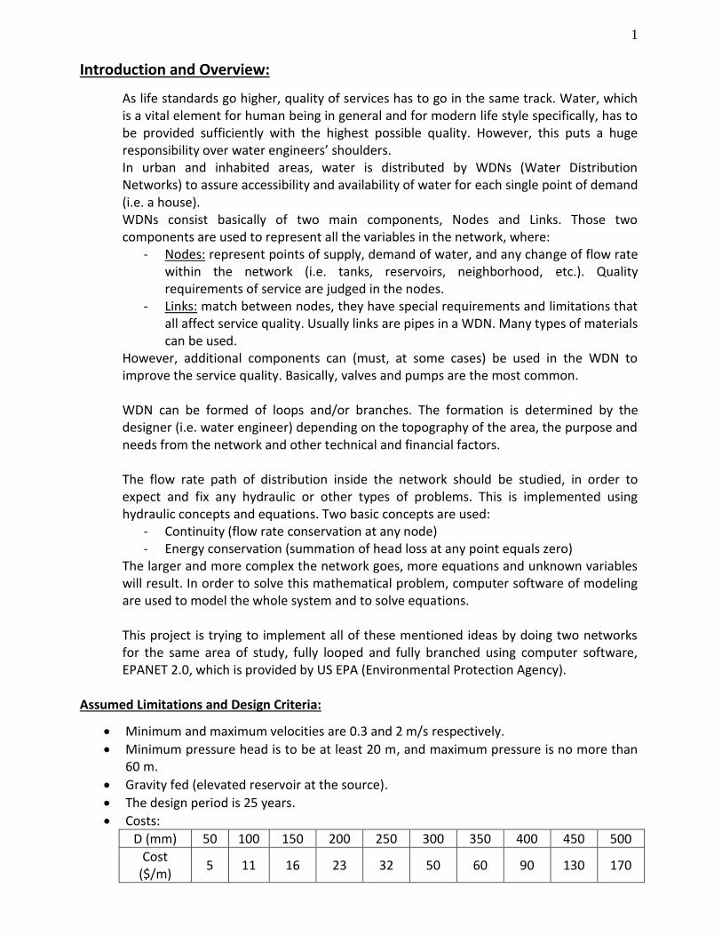
Assumed Limitations and Design Criteria:

Minimum and maximum velocities are 0.3 and 2 m/s respectively.

Minimum pressure head is to be at least 20 m, and maximum pressure is no more than 60 m.

Gravity fed (elevated reservoir at the source).

The design period is 25 years.

Costs:

D (mm) 50 100 150 200 250 300 350 400 450 500

Cost ($/m)

5 11 16 23 32 50 60 90 130 170

2

Moreover:

Average per capita daily water demand used equals 100 l/c.d.

Hazen-Williams formula used for head loss calculations.

For all pipes, roughness = 100

Minor losses are neglected

Maximum daily peaking factor is used.

Annual population growth rate is 2%.

Fire flow is neglected.

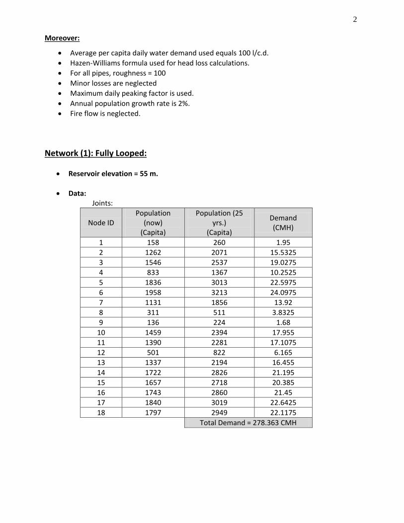
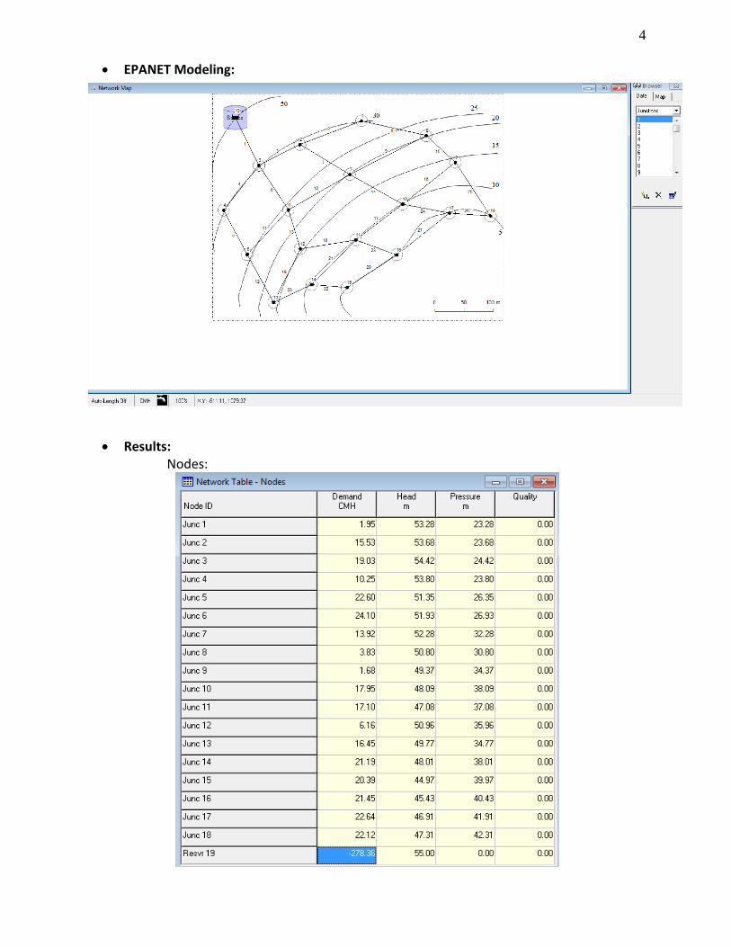
Network (1): Fully Looped:

Reservoir elevation = 55 m.

Data: Joints:

Node ID Population

(now) (Capita)

Population (25 yrs.)

(Capita)

Demand (CMH)

1 158 260 1.95

2 1262 2071 15.5325

3 1546 2537 19.0275

4 833 1367 10.2525

5 1836 3013 22.5975

6 1958 3213 24.0975

7 1131 1856 13.92

8 311 511 3.8325

9 136 224 1.68

10 1459 2394 17.955

11 1390 2281 17.1075

12 501 822 6.165

13 1337 2194 16.455

14 1722 2826 21.195

15 1657 2718 20.385

16 1743 2860 21.45

17 1840 3019 22.6425

18 1797 2949 22.1175

Total Demand = 278.363 CMH

3

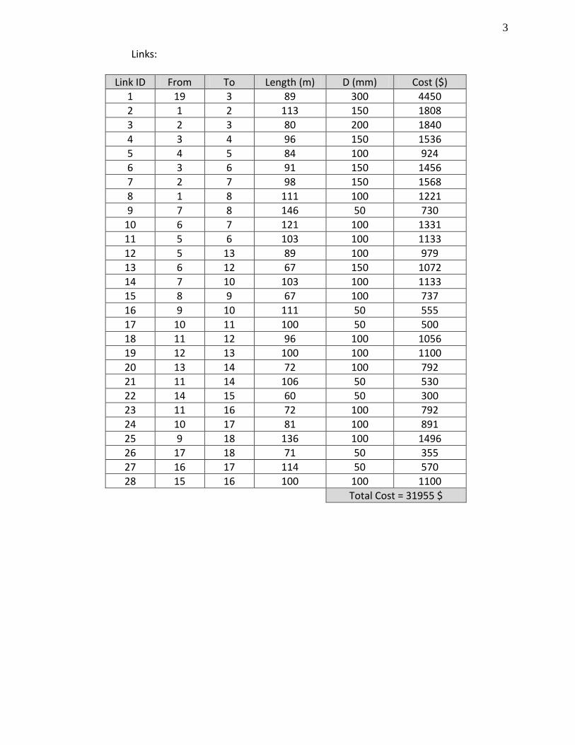
Links:

Link ID From To Length (m) D (mm) Cost ($)

1 19 3 89 300 4450

2 1 2 113 150 1808

3 2 3 80 200 1840

4 3 4 96 150 1536

5 4 5 84 100 924

6 3 6 91 150 1456

7 2 7 98 150 1568

8 1 8 111 100 1221

9 7 8 146 50 730

10 6 7 121 100 1331

11 5 6 103 100 1133

12 5 13 89 100 979

13 6 12 67 150 1072

14 7 10 103 100 1133

15 8 9 67 100 737

16 9 10 111 50 555

17 10 11 100 50 500

18 11 12 96 100 1056

19 12 13 100 100 1100

20 13 14 72 100 792

21 11 14 106 50 530

22 14 15 60 50 300

23 11 16 72 100 792

24 10 17 81 100 891

25 9 18 136 100 1496

26 17 18 71 50 355

27 16 17 114 50 570

28 15 16 100 100 1100

Total Cost = 31955 $

4

EPANET Modeling:

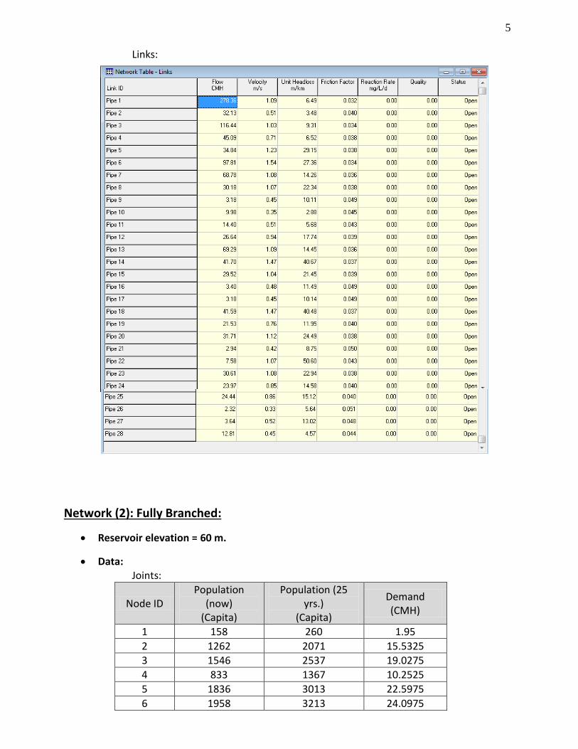
Results: Nodes:

5

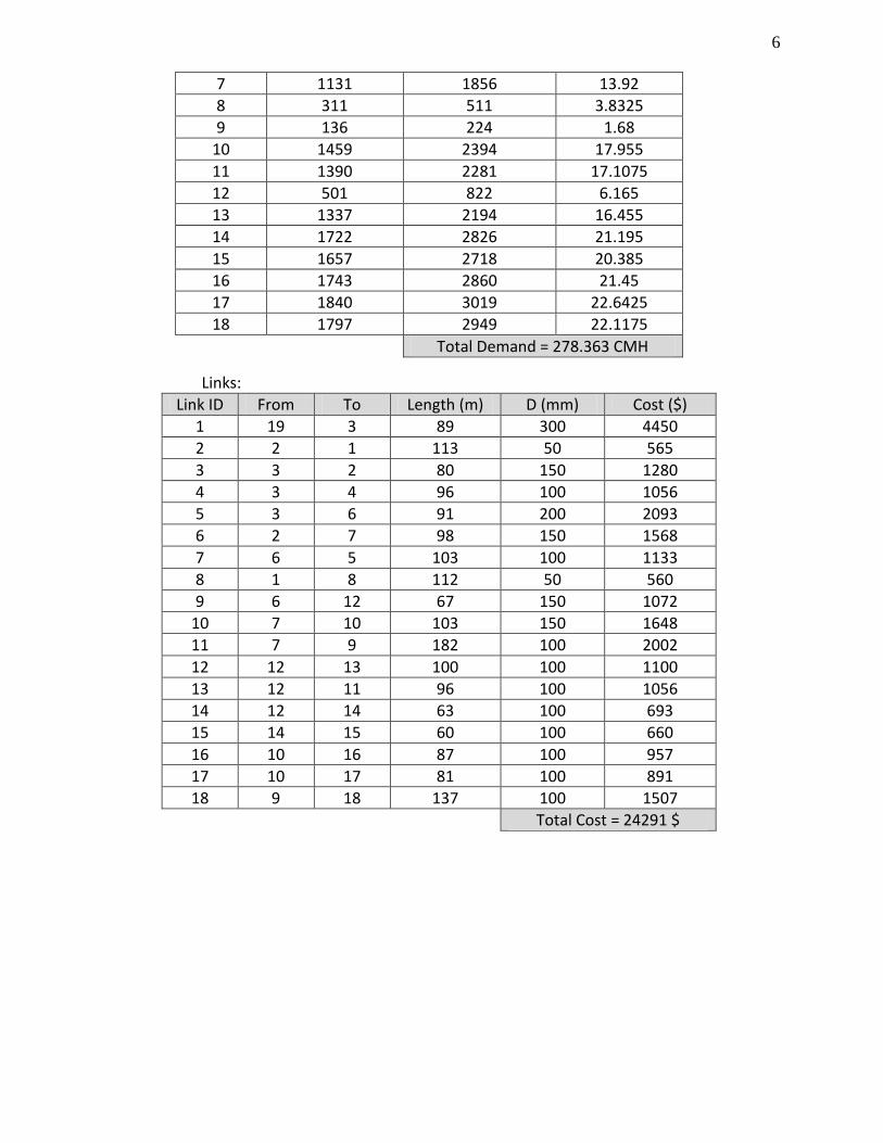
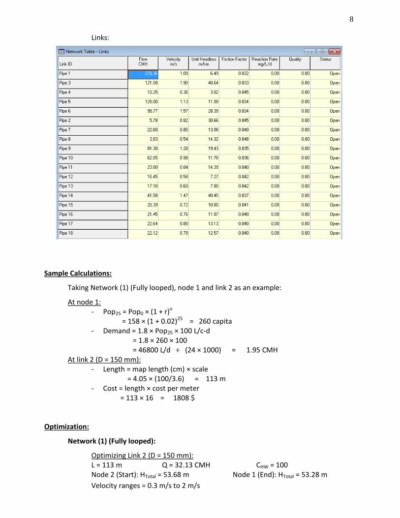
Links:

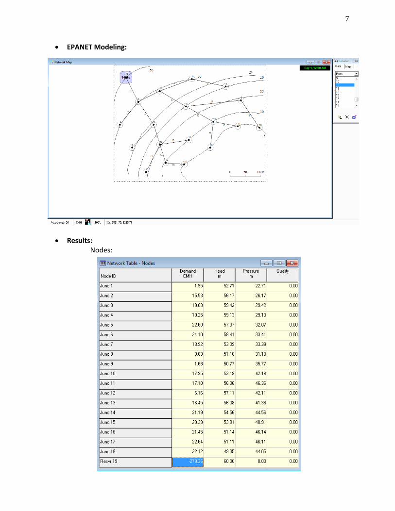
Network (2): Fully Branched:

Reservoir elevation = 60 m.

Data: Joints:

Node ID Population

(now) (Capita)

Population (25 yrs.)

(Capita)

Demand (CMH)

1 158 260 1.95

2 1262 2071 15.5325

3 1546 2537 19.0275

4 833 1367 10.2525

5 1836 3013 22.5975

6 1958 3213 24.0975

6

7 1131 1856 13.92

8 311 511 3.8325

9 136 224 1.68

10 1459 2394 17.955

11 1390 2281 17.1075

12 501 822 6.165

13 1337 2194 16.455

14 1722 2826 21.195

15 1657 2718 20.385

16 1743 2860 21.45

17 1840 3019 22.6425

18 1797 2949 22.1175

Total Demand = 278.363 CMH

Links:

Link ID From To Length (m) D (mm) Cost ($)

1 19 3 89 300 4450

2 2 1 113 50 565

3 3 2 80 150 1280

4 3 4 96 100 1056

5 3 6 91 200 2093

6 2 7 98 150 1568

7 6 5 103 100 1133

8 1 8 112 50 560

9 6 12 67 150 1072

10 7 10 103 150 1648

11 7 9 182 100 2002

12 12 13 100 100 1100

13 12 11 96 100 1056

14 12 14 63 100 693

15 14 15 60 100 660

16 10 16 87 100 957

17 10 17 81 100 891

18 9 18 137 100 1507

Total Cost = 24291 $

7

EPANET Modeling:

Results: Nodes:

8

Links:

Sample Calculations:

Taking Network (1) (Fully looped), node 1 and link 2 as an example:

At node 1: - Pop25 = Pop0 × (1 + r)n

= 158 × (1 + 0.02)25 = 260 capita - Demand = 1.8 × Pop25 × 100 L/c-d

= 1.8 × 260 × 100 = 46800 L/d ÷ (24 × 1000) = 1.95 CMH

At link 2 (D = 150 mm): - Length = map length (cm) × scale

= 4.05 × (100/3.6) = 113 m - Cost = length × cost per meter

= 113 × 16 = 1808 $

Optimization:

Network (1) (Fully looped):

Optimizing Link 2 (D = 150 mm): L = 113 m Q = 32.13 CMH CHW = 100 Node 2 (Start): HTotal = 53.68 m Node 1 (End): HTotal = 53.28 m

Velocity ranges = 0.3 m/s to 2 m/s

9

Maximum allowable diameter = 150 mm

HL = 53.68 – 53.28 = 0.4 m

But, HL = 162.5 × (Q/CHW)1.825 × D-4.87 × L 0.4 = 162.5 × (32.13/100)1.825 × D-4.87 × 113 Dexact = 5.33 in Dexact = 135.3 mm So, Choose: D1 = 100 mm & D2 = 150 mm Equation 1: X100 + X150 = 113 m Equation 2: J100X100 + J150X150 = 0.4 m

0.0143X100 + 0.002X150 = 0.4 m After solving: X100 = 14.3 m & X150 = 98.7 m

Network (2) (Fully Branched):

Optimizing Link 4 (D = 100 mm): L = 96 m Q = 10.25 CMH CHW = 100 Node 3 (Start): HTotal = 59.42 m Node 4 (End): HTotal = 59.13 m

Velocity ranges = 0.3 m/s to 2 m/s Maximum allowable diameter = 100 mm

HL = 59.42 – 59.13 = 0.29 m

But, HL = 162.5 × (Q/CHW)1.825 × D-4.87 × L 0.4 = 162.5 × (10.25/100)1.825 × D-4.87 × 96 Dexact = 3.56 in Dexact = 90.5 mm So, Choose: D1 = 50 mm & D2 = 100 mm Equation 1: X50 + X100 = 96 m Equation 2: J50X50 + J100X100 = 0.29 m

0.0503X50 + 0.00172X100 = 0.29 m After solving: X50 = 2.6 m & X100 = 93.4 m

Scenarios:

1. Demand Pattern:

Water consumption varies during the day (being lower at night), from day to day during the week, from week to week during the month and from month to month during the year. Water demand generally fluctuates being below the average daily demand in the early‐morning hours and above the average daily demand during the midday hours. On a typical day in most communities, water use is lowest at night (11 pm to 5 am when most people are asleep. Water use rises rapidly in the morning (5 am to 11 am) followed by moderate usage through midday (11 am to 6 pm). Then, use increases in the evening (6 pm to 10 pm) and drops rather quickly around 10 pm.

10

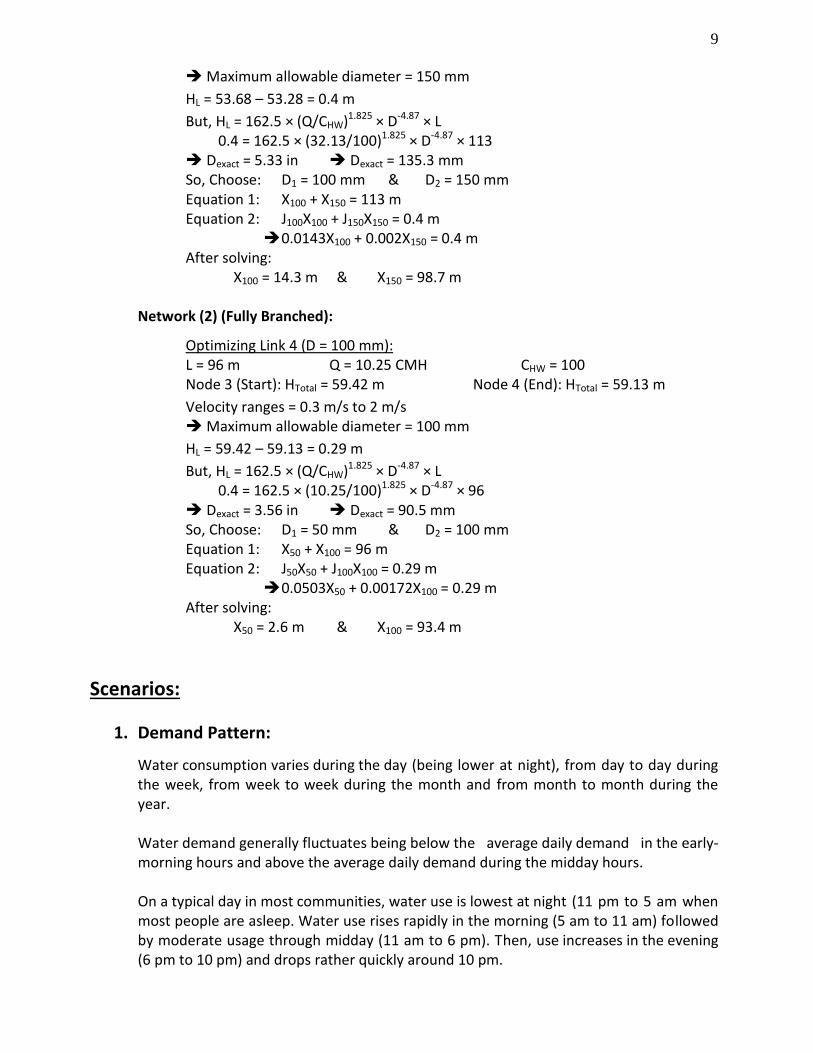
To model and present the mentioned variation in water use, we will create a Time Pattern that makes demands at the nodes vary in a periodic way over the course of a day using EPANET, assuming the following multipliers values:

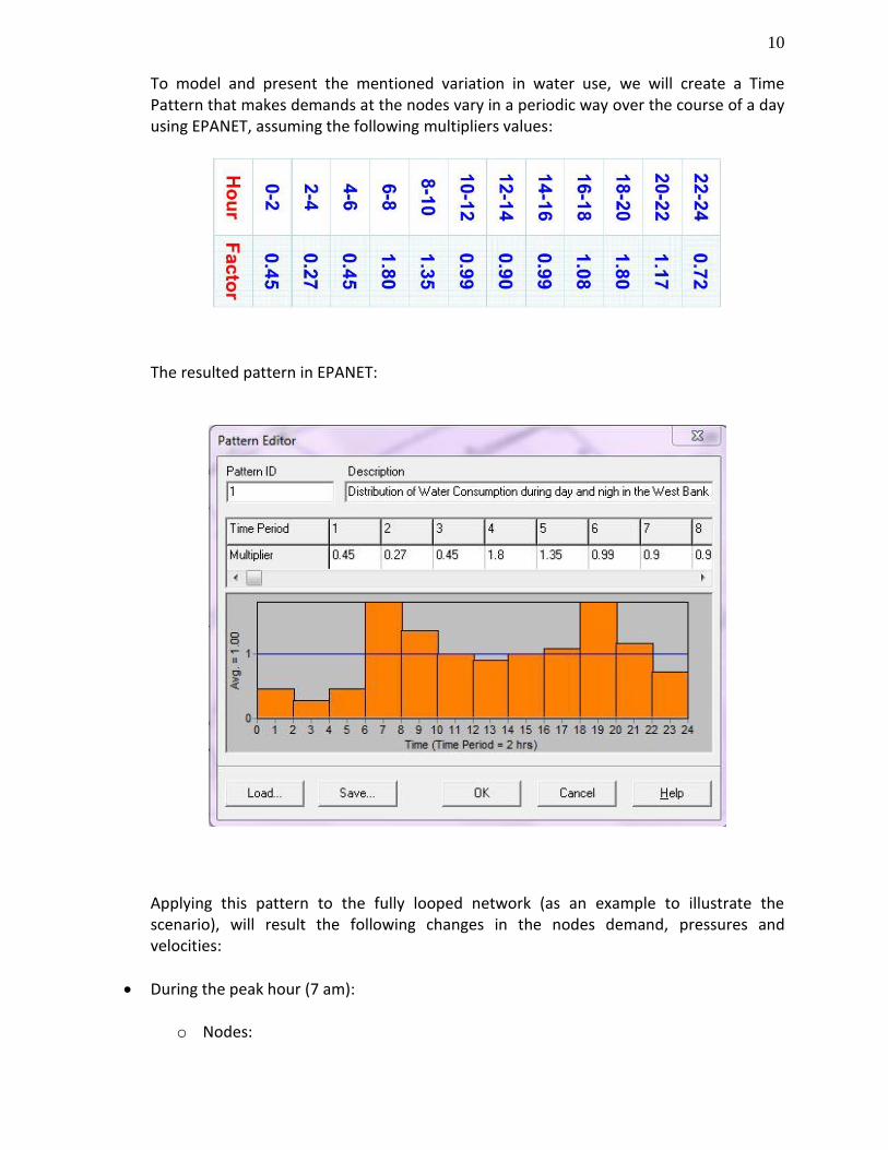
The resulted pattern in EPANET:

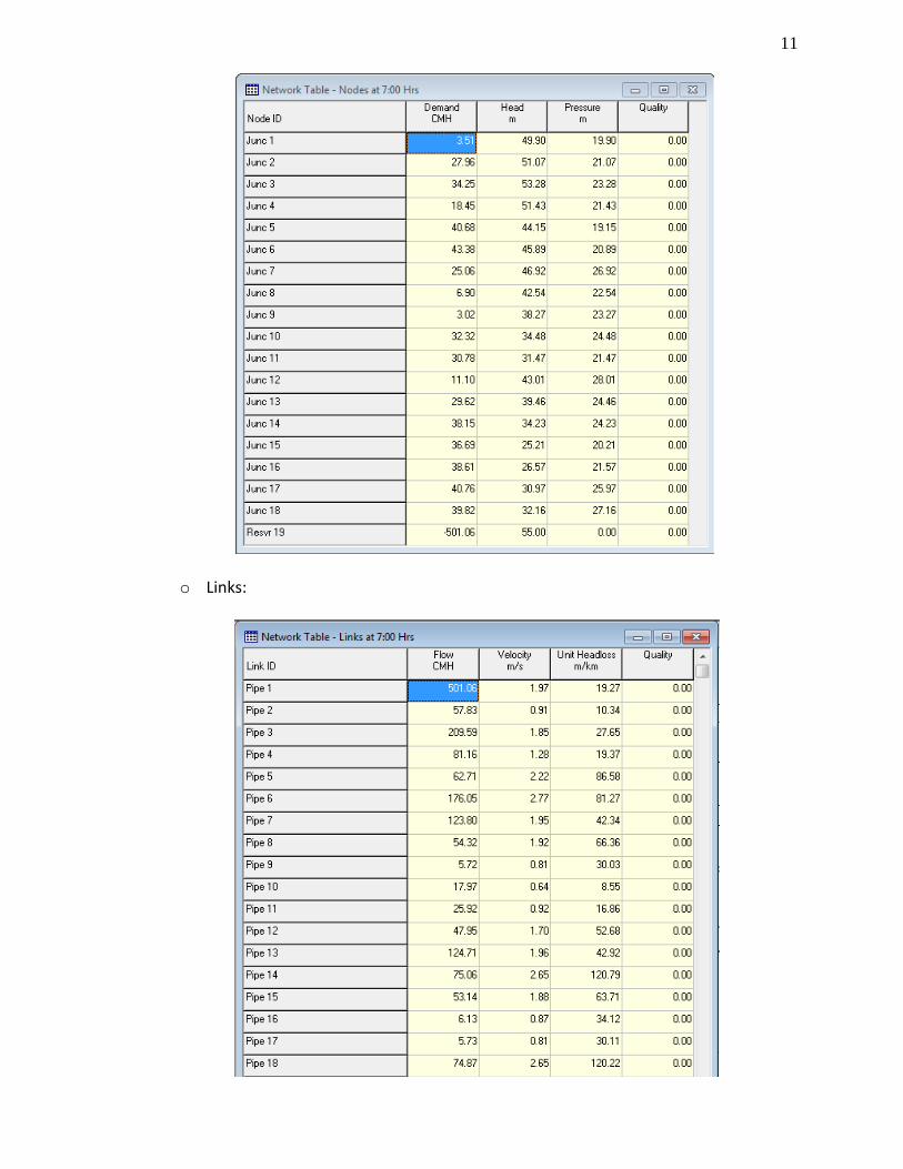
Applying this pattern to the fully looped network (as an example to illustrate the scenario), will result the following changes in the nodes demand, pressures and velocities:

During the peak hour (7 am):

o Nodes:

11

o Links:

12

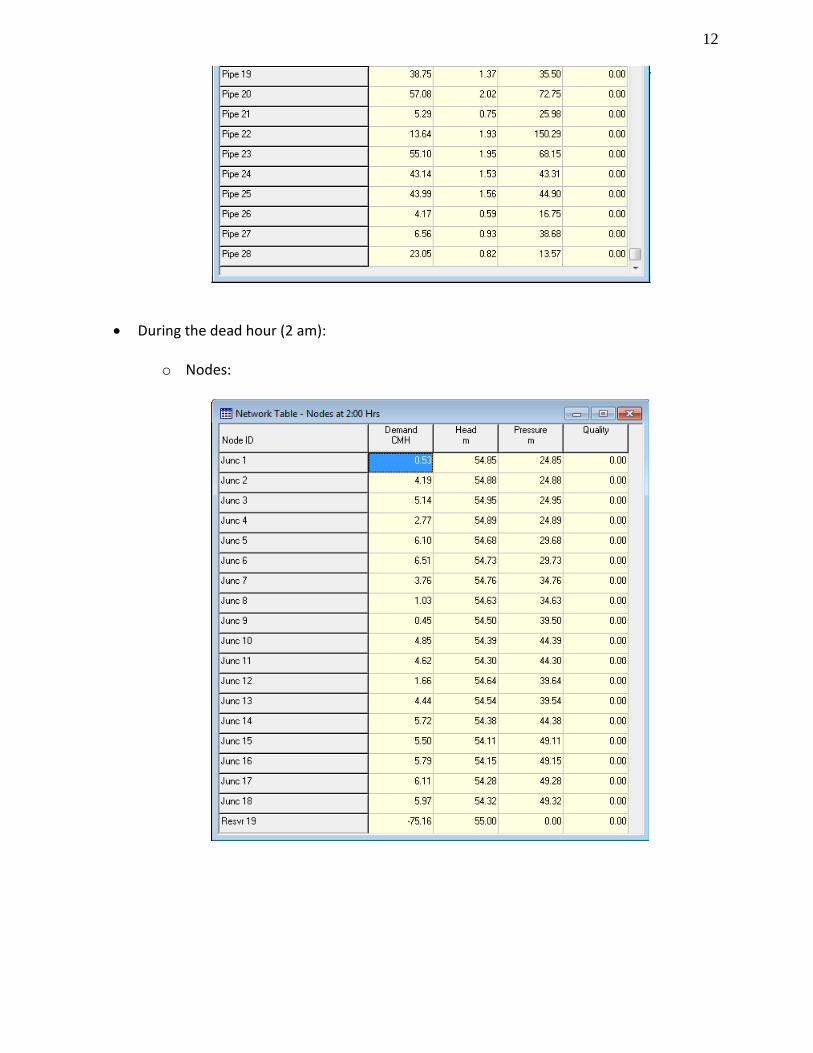
During the dead hour (2 am):

o Nodes:

13

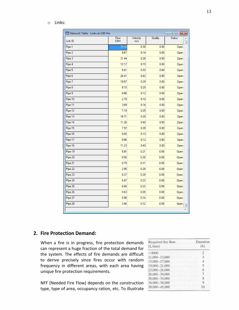
o Links:

2. Fire Protection Demand:

When a fire is in progress, fire protection demands can represent a huge fraction of the total demand for the system. The effects of fire demands are difficult to derive precisely since fires occur with random frequency in different areas, with each area having unique fire protection requirements. NFF (Needed Fire Flow) depends on the construction type, type of area, occupancy ration, etc. To illustrate

14

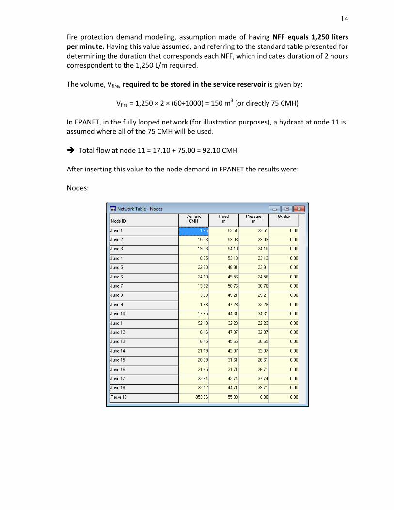
fire protection demand modeling, assumption made of having NFF equals 1,250 liters per minute. Having this value assumed, and referring to the standard table presented for determining the duration that corresponds each NFF, which indicates duration of 2 hours correspondent to the 1,250 L/m required. The volume, Vfire, required to be stored in the service reservoir is given by:

Vfire = 1,250 × 2 × (60÷1000) = 150 m3 (or directly 75 CMH) In EPANET, in the fully looped network (for illustration purposes), a hydrant at node 11 is assumed where all of the 75 CMH will be used. Total flow at node 11 = 17.10 + 75.00 = 92.10 CMH After inserting this value to the node demand in EPANET the results were: Nodes:

15

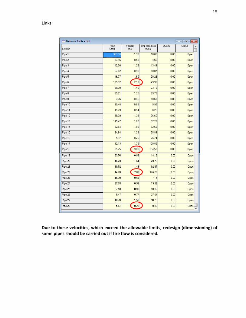
Links:

Due to these velocities, which exceed the allowable limits, redesign (dimensioning) of some pipes should be carried out if fire flow is considered.

16

Water Quality Analysis:

Water Age:

The cumulative residence time of water in the system, or water age, has come to be

regarded as a reliable surrogate for water quality. Water age is of particular concern

when quantifying the effect of storage tank turnover on water quality. It is also beneficial

for evaluating the loss of disinfectant residual and the formation of disinfection by-

products in distribution systems. The water age analysis reports the cumulative residence

time for each parcel of water moving through the network.

The constituent analysis is performed assuming a zero-order reaction with a k value

equal to +1 [(mg/l)/s]. Thus, constituent concentration growth is directly proportional to

time, and the cumulative residence time along the transport pathways in the network is

numerically summed.

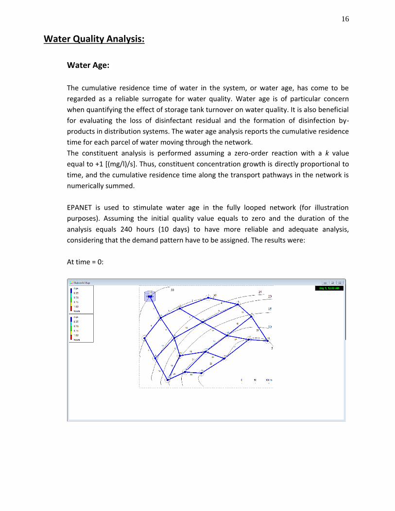
EPANET is used to stimulate water age in the fully looped network (for illustration

purposes). Assuming the initial quality value equals to zero and the duration of the

analysis equals 240 hours (10 days) to have more reliable and adequate analysis,

considering that the demand pattern have to be assigned. The results were:

At time = 0:

17

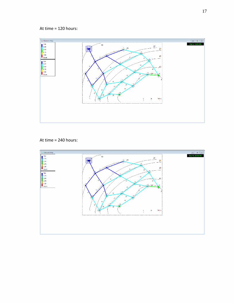
At time = 120 hours:

At time = 240 hours:

18

Chlorine Transport and Decay:

After water leaves the treatment plant and enters the distribution system, it is subject to

many complex physical and chemical processes, some of which are poorly understood,

and most of which are not modeled. The most commonly used reaction model is the first

order decay model. This has been applied to chlorine decay, radon decay, and other

decay processes. A first order decay is equivalent to an exponential decay, represented

by the equation:

Ct = Co e-kt

Where: Ct = concentration at time t (M/L3)

Co = initial concentration (at time zero)

k = reaction rate (1/T)

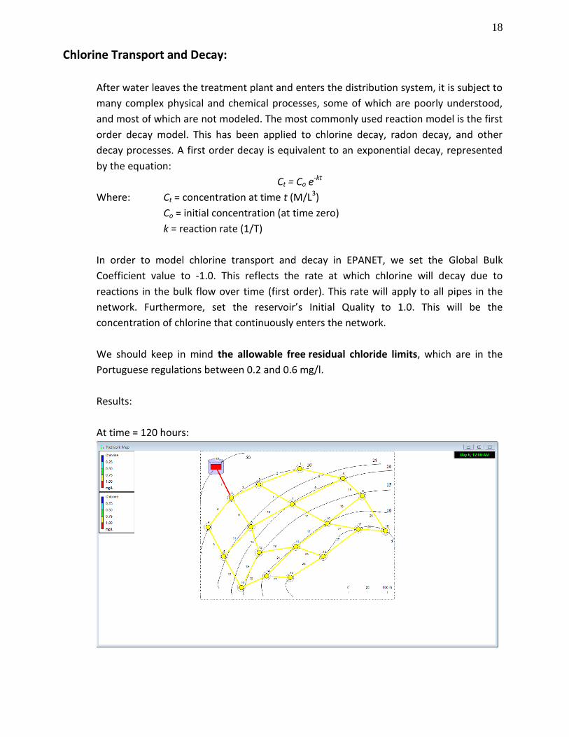
In order to model chlorine transport and decay in EPANET, we set the Global Bulk

Coefficient value to -1.0. This reflects the rate at which chlorine will decay due to

reactions in the bulk flow over time (first order). This rate will apply to all pipes in the

network. Furthermore, set the reservoir’s Initial Quality to 1.0. This will be the

concentration of chlorine that continuously enters the network.

We should keep in mind the allowable free residual chloride limits, which are in the

Portuguese regulations between 0.2 and 0.6 mg/l.

Results:

At time = 120 hours:

19

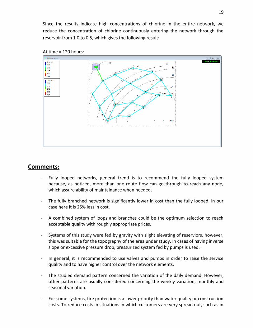
Since the results indicate high concentrations of chlorine in the entire network, we

reduce the concentration of chlorine continuously entering the network through the

reservoir from 1.0 to 0.5, which gives the following result:

At time = 120 hours:

Comments:

- Fully looped networks, general trend is to recommend the fully looped system because, as noticed, more than one route flow can go through to reach any node, which assure ability of maintainance when needed.

- The fully branched network is significantly lower in cost than the fully looped. In our case here it is 25% less in cost.

- A combined system of loops and branches could be the optimum selection to reach acceptable quality with roughly appropriate prices.

- Systems of this study were fed by gravity with slight elevating of reserviors, however, this was suitable for the topography of the area under study. In cases of having inverse slope or excessive pressure drop, pressurized system fed by pumps is used.

- In general, it is recommended to use valves and pumps in order to raise the service quality and to have higher control over the network elements.

- The studied demand pattern concerned the variation of the daily demand. However, other patterns are usually considered concerning the weekly variation, monthly and seasonal variation.

- For some systems, fire protection is a lower priority than water quality or construction costs. To reduce costs in situations in which customers are very spread out, such as in

20

rural areas, the network may not be designed to provide fire protection. Instead, the fire departments rely on water tanker trucks or other sources for water to combat fires (for example, ponds constructed specifically for that purpose).

- Both water age simulation and chlorine transport and decay simulation use the same modeling concepts. Anyhow, water age is a very useful tool that can be generlized to simulate different chemical processes that may affect distribution system water quality, which are a function of water chemistry and the physical characteristics of the distribution system itself.

- Water quality modeling can be used to helpimprove the performance of distribution system modifications meant toreduce hydraulic residence times, and as a tool for improving the management of disinfectant residuals and other water qualityrelated operations.

Bibliography - Rossman, L. A. (2000). EPANET 2 USERS MANUAL. CINCINNATI, OH: U.S.

ENVIRONMENTAL PROTECTION AGENCY.

- Walski, T. M., Chase, D. V., Savic, D. A., Grayman, W., Beckwith, S., & Koelle, E. (2003). ADVANCED WATER DISTRIBUTION MODELING AND MANAGEMENT. Waterbury, CT: Haestad Methods.