information sharing for the semantic web -a schema transformation approach

Information Sharing for the Semantic Web —

a Schema Transformation Approach

Version 2

Lucas Zamboulis and Alexandra Poulovassilis

School of Computer Science and Information Systems,

Birkbeck College, University of London, London WC1E 7HX

{lucas,ap}@dcs.bbk.ac.uk

June 30, 2005

Abstract

This paper proposes a set of algorithms for the transformation and integration of heterogeneous

XML data sources which make use of correspondences from them to ontologies expressed in the form

of RDFS schemas. Our algorithms generate schema transformation/integration rules which are im-

plemented in the AutoMed heterogeneous data integration system. These rules can then be used to

perform virtual or materialised transformation and integration of the XML data sources. The paper

first illustrates how correspondences to a single ontology can be exploited. The approach is then ex-

tended to the more general setting where correspondences may refer to multiple ontologies, themselves

interconnected via schema transformation pathways. The contribution of this research is a set of au-

tomatic, XML-specific algorithms for the transformation and integration of XML data, making use of

RDFS ontologies as a ‘semantic bridge’.

1 Introduction

The emergence of several new standards from the World Wide Web Consortium has provided a strong

basis for enhancing the interoperability of web-based applications. XML is emerging as the common

data interchange format, while RDF [26], RDFS [25] and OWL [24] provide a framework for assigning

meaning to heterogenous web-based data. The Semantic Web aims to become an extension of the current

Web, in which applications will be able to share and reuse information in an automated way. This

1

kind of information sharing requires the transformation and/or integration of data from heterogeneous

data sources in a form that is suitable for the target applications. The development of algorithms that

automate these tasks is essential to many domains: examples range from generic frameworks, such as for

XML messaging and component-based development, to applications and services in e-business, e-science,

entertainment, leisure and e-learning.

This paper proposes an approach to the transformation and integration of heterogeneous XML data

sources by using correspondences from them to ontologies expressed in the form of RDFS schemas. There

are two main advantages of this approach, compared with say constructing pairwise mappings between the

data sources, or between each data source and some known global XML format. Firstly, known semantic

correspondences between data sources and domain and other ontologies can be utilised for transforming

and/or integrating the data sources. Secondly, changes in a data source, or addition or removal of a

data source, do not affect the other sets of correspondences, thus promoting the reusability of sets of

correspondences.

Our framework provides a set of algorithms for the transformation and integration of heterogeneous

XML data sources by exploiting correspondences between them to ontologies expressed as RDFS schemas.

Our algorithms generate schema transformation/integration rules which are implemented in the AutoMed

heterogeneous data integration system1. These rules can be used to transform an XML data source into

a target format, or to integrate a set of heterogeneous XML data sources into a common format. The

transformation or integration may be virtual, in the sense that it allows queries posed on the target

or common format to be answered by using the transformation rules and the data sources. Or the

transformation/integration may be materialised, in the sense that the transformation rules can be used

to generate from the data sources equivalent XML data that conforms to the target/common format.

Paper outline: Section 2 compares our approach with related work. Section 3 gives an overview of

AutoMed to the level of detail necessary for the purposes of this paper. Section 4 presents the process

of transforming and integrating XML data sources which conform to the same ontology, while Section 5

extends this to the more general case of conformance to different ontologies. Section 6 gives our concluding

remarks and plans for future work.1See http://www.doc.ic.ac.uk/automed/

2

2 Related Work

The work in [4, 5] also undertakes data integration through the use of ontologies. However, this is by

transforming the source data into a common RDF format, in contrast to our integration approach in

which the common format is an XML schema. In [10], mappings from DTDs to RDF ontologies are used

in order to reformulate path queries expressed over a global ontology to equivalent XML data sources.

In [1], an ontology is used as a global virtual schema for heterogeneous XML data sources using LAV

mapping rules. SWIM [3] uses mappings from various data models (including XML and relational) to

RDF, in order to integrate data sources modelled in different modelling languages. In [11], XML Schema

constructs are mapped to OWL constructs and evaluation of queries on the virtual OWL global schema

are supported.

In contrast to all of these approaches, we use RDFS schemas merely as a ‘semantic bridge’ for trans-

forming (or integrating) XML data, and the target (or global) schema is in all cases an XML schema.

Other approaches to transforming or integrating XML data which do not make use of RDF/S or OWL

include [17, 19, 20, 21, 27]. Clio [17] translates data source schemas, XML or relational, into an internal

representation and the mappings between the source and the target schemas are semi-automatically de-

rived. Xyleme [19] also takes a mapping-based approach to XML data integration; it uses a tree structure

as the global schema and source schemas are mapped to this via path mappings. DIXSE [20] transforms

the DTD specifications of a set of source XML documents into an internal representation, using some

heuristics to capture semantics as well as input from domain experts. Another DTD-dependent approach

is presented in [21] which transforms XML documents using a set of transformations on documents’ DTDs,

encoded in a transformation script; the target document is produced using this script and XSLT. The ap-

proach in [27] uses XML-specific transformations for XML schema integration, similarly to our approach.

However, the semantics of these transformations are not captured within queries, as ours are, and they

do not generate elements to preserve data that would have otherwise been lost during the transformation.

Finally, our own earlier work in [28, 29] has also discussed the transformation and integration of XML

data sources. However, this work was in the absence of any correspondences between the data sources and

ontologies. The approach we present here is able to use information that identifies an element/attribute

in one data source to be equivalent to, a superclass of, or a subclass of an element/attribute in another

data source. This information is generated from the correspondences between the data sources and

ontologies. This allows more semantic relationships to be inferred between the data sources, and hence

3

more information to be retained from a data source when it is transformed into a target format.

3 Overview of AutoMed

AutoMed is a heterogeneous data transformation and integration system which offers the capability to

handle virtual, materialised and indeed hybrid data integration across multiple data models. It supports

a low-level hypergraph-based data model (HDM) and provides facilities for specifying higher-level

modelling languages in terms of this HDM. An HDM schema consists of a set of nodes, edges and

constraints, and each modelling construct of a higher-level modelling language is specified as some com-

bination of HDM nodes, edges and constraints. For any modelling language M specified in this way (via

the API of AutoMed’s Model Definitions Repository) AutoMed provides a set of primitive schema trans-

formations that can be applied to schema constructs expressed in M. In particular, for every construct of

M there is an add and a delete primitive transformation which add to/delete from a schema an instance

of that construct. For those constructs of M which have textual names, there is also a rename primitive

transformation.

Instances of modelling constructs within a particular schema are identified by means of their scheme

enclosed within double chevrons 〈〈. . .〉〉. AutoMed schemas can be incrementally transformed by applying

to them a sequence of primitive transformations, each adding, deleting or renaming just one schema con-

struct (thus, in general, AutoMed schemas may contain constructs of more than one modelling language).

We term a sequence of primitive transformations from one schema S1 to another schema S2 a pathway

from S1 to S2 and denote it by S1 → S2. All source, intermediate, and integrated schemas, and the

pathways between them, are stored in AutoMed’s Schemas & Transformations Repository.

Each add and delete transformation is accompanied by a query specifying the extent of the added

or deleted construct in terms of the rest of the constructs in the schema. This query is expressed in a

functional query language, IQL2.

Also available are extend and contract primitive transformations which behave in the same way as

add and delete except that they state that the extent of the new/removed construct cannot be pre-

cisely derived from the other constructs present in the schema. More specifically, each extend/contract

transformation takes a pair of queries that specify a lower and an upper bound on the extent of the new

construct. The lower bound may be Void and the upper bound may be Any, which respectively indicate2IQL is a comprehensions-based functional query language and we refer the reader to [8] for details of its syntax, semantics

and implementation. Such languages subsume query languages such as SQL and OQL in expressiveness [2].

4

no known information about the lower or upper bound of the extent of the new construct.

The queries supplied with add, extend, delete and contract can be used to automatically translate

queries or data along a transformation pathway S1 → S2 by means of query unfolding: for translating

a query on S1 to a query on S2 the delete, contract and rename steps are used, while for translating

data from S1 to data on S2 the add, extend and rename steps are used — we refer the reader to [15] for

details.

The queries supplied with primitive transformations also provide the necessary information for these

transformations to be automatically reversible, in that each add/extend transformation is reversed by a

delete/contract transformation with the same arguments, while each rename is reversed by a rename

with the two arguments swapped.

As discussed in [16], this means that AutoMed is a both-as-view (BAV) data integration system:

the add and extend steps in a transformation pathway correspond to Global-As-View (GAV) rules since

they incrementally define target schema constructs in terms of source schema constructs; while the delete

and contract steps correspond to Local-As-View (LAV) rules since they define source schema constructs

in terms of target schema constructs. If a GAV view is derived from solely add steps it will be exact in the

terminology of [12]. If, in addition, it is derived from one or more extend steps using their lower-bound

(upper-bound) queries, then the GAV view will be sound (complete) in the terminology of [12]. Similarly,

if a LAV view is derived solely from delete steps it will be exact. If, in addition, it is derived from one or

more contract steps using their lower-bound (upper-bound) queries, then the LAV view will be complete

(sound) in the terminology of [12].

We refer the reader to [9] for a discussion of how GAV view definitions for global schema constructs

can be generated from the queries in the pathways between a global schema and a set of data source

schemas. AutoMed’s Global Query Processor (GQP) can use these view definitions in order to evaluate

an IQL query formulated with respect to the global schema: the view definitions are substituted into the

query in order to reformulate it into an IQL query expressed on the data source schemas. This query

is then optimised, and the GQP then interacts with the data source Wrappers, submitting to them IQL

subqueries which they translate into the local query language for evaluation, returning subquery results

back to the GQP for any further necessary post-processing and merging. Currently, the AutoMed toolkit

includes wrappers for relational, XML and flat-file data sources.

An in-depth comparison of BAV with the GAV, LAV and also the GLAV [6, 14] approaches to data

integration can be found in [9], while [15] discusses the use of BAV for peer-to-peer data integration.

5

3.1 Representing XML schemas in AutoMed

The standard schema definition languages for XML are DTD [22] and XML Schema [23]. However, both of

these provide grammars to which conforming documents adhere, and do not abstract the tree structure of

the actual documents. In our schema transformation and integration context, schemas with this property

are preferable as this facilitates schema traversal, structural comparison between a source and a target

schema, and restructuring of the source schema(s) that are to be transformed and/or integrated. Moreover,

such a schema type means that the queries supplied with the AutoMed primitive transformations are

essentially path queries, which are easily generated. It is also possible that an XML file may have no

referenced DTD or XML Schema.

We have therefore defined a simple modelling language called XML DataSource Schema (XMLDSS)

which summarises the structure of an XML document. XMLDSS schemas consist of four kinds of con-

structs (here, we describe these somewhat informally and refer the reader to [28] for their formal specifi-

cation in terms of the HDM):

Element: Elements, e, are identified by a scheme 〈〈e〉〉. An XMLDSS element is represented by a node

in the HDM.

Attribute: Attributes, a, belonging to elements, e, are identified by a scheme 〈〈e, a〉〉. They are repre-

sented by a node in the HDM, representing the attribute; an edge between this node and the node

representing the element e; and a cardinality constraint stating that an instance of e can have at

most one instance of a associated with it, and that an instance of a can be associated with one or

more instances of e.

NestList: NestLists are parent-child relationships between two elements ep and ec and are identified by

a scheme 〈〈ep, ec, i〉〉, where i is the position of ec within the list of children of ep. In the HDM, they

are represented by an edge between the nodes representing ep and ec; and a cardinality constraint

that states that each instance of ep is associated with zero or more instances of ec, and each instance

of ec is associated with precisely one instance of ep. Note that i is used for ordering purposes only

within XMLDSS schemas, as the list-based nature of IQL means that ordering of children instances

of ec under parent instances of ep is preserved within the extent of NestList 〈〈ep, ec, i〉〉; therefore,

queries supplied within transformations may use the short-hand notation 〈〈ep, ec〉〉 for NestLists.

PCData: In any XMLDSS schema there is one construct with scheme 〈〈PCData〉〉, representing all the

6

instances of PCData within an XML document.

In an XML document there may be elements with the same name occurring at different positions in

the tree. To avoid ambiguity, in XMLDSS schemas we use an identifier of the form elementName$count

for each element, where count is a counter incremented every time the same elementName is encoun-

tered in a depth-first traversal of the schema. If the suffix $count is omitted from an element name,

then the suffix $1 is assumed. For the XML documents themselves, we use an identifier of the form

elementName&sid$count instanceCount for each element, where instanceCount is a counter identify-

ing each instance of elementName$count in the document and sid is a number identifying the schema to

which the element construct belongs in the AutoMed repository. Using the schema id as part of the ele-

ment instance identifier is necessary in a data integration setting in order to disambiguate between element

instances from different data sources which may have the same elementName, count and instanceCount

values.

The XMLDSS schema, S, of an XML document, D, is extracted by means of a depth-first traversal

of D as follows:

1. Create an element r as the root element of S.

2. Create an element ES as a child of r by copying the root element of D, ED, together with any

attributes it may have (but not their values). If ED has PCData, create a NestList construct

linking ES to PCData in S.

3. For every child element, CD, of ED do:

(a) • If an element with the same name as CD does not appear in the list of children of ES , copy

CD and its attributes (without their values), and append this new element to the current

list of children of ES .

• Otherwise, if there is an element CS within the list of children of ES with the same name

as CD, copy any attributes of CD that do not appear as attributes of CS to CS .

• If CD has PCData, create a NestList construct linking CD to PCData in S, if such a link

does not already exist.

(b) Let ED be CD and recursively perform step 3.

In step 1 above, a new root for the XMLDSS schema is created. This is not strictly necessary but it

guarantees that the root element of any XMLDSS schema has a specific label. This is useful in adopting a

7

more uniform approach in the schema restructuring and the schema integration algorithms (Sections 4.2

and 4.3 respectively) by not having to consider whether the input schemas have the same or different

roots.

We observe that the complexity of this algorithm is O(N × F ) where N is the number of elements

in the source XML document and F is the average fan-out of elements in the extracted schema. We

note that the XMLDSS schema is equivalent to the tree resulting as an intermediate step in the creation

of a minimal DataGuide [7]. However, unlike DataGuides, we do not merge common sub-trees and the

resulting schema remains a tree rather than a DAG.

To illustrate XMLDSS schemas, consider the following XML document, named UniversityOfAthens.xml:

<university><school name="School of Law">

<academic><name>Dr. Nicholas Petrou</name><office>123</office>

</academic><academic>

<name>Prof. George Lazos</name><office>111</office>

</academic></school><school name="School of Economics">

<academic><name>Dr. Anna Georgiou</name><office>321</office>

</academic></school>

</university>

The XMLDSS schema extracted from this document is S1 in Figure 1. The extent of each of the

constructs of schema S1 are listed in Table 1. For each construct, this extent is the result that would be

returned by AutoMed’s Global Query Processor for an IQL query consisting of just that construct. In

particular, the unique identifiers of the form elementName&sid$count instanceCount for XML elements

are automatically generated by the XMLDSS Wrapper interacting with the UniversityOfAthens.xml doc-

ument.

As mentioned earlier, after a modelling languageM has been specified in terms of the HDM, AutoMed

automatically makes available a set of primitive transformations for transforming schemas defined in M.

Thus, for XMLDSS schemas there are transformations addElement(〈〈e〉〉,query), addAttribute(〈〈e, a〉〉,query), addNestList(〈〈ep, ec, i〉〉,query), and similar transformations for the extend, delete, contract

and rename of Element, Attribute and NestList constructs.

8

Table 1: Schema S1 constructs and their extents.Construct Extent

〈〈r〉〉 [r&1$1 1]〈〈r, university, 1〉〉 [{r&1$1 1, university&1$1 1}]〈〈university〉〉 [university&1$1 1]〈〈school〉〉 [school&1$1 1, school&1$1 2]〈〈university, school, 1〉〉 [{university&1$1 1, school&1$1 1}, {university&1$1 2, school&1$1 2}]〈〈school, name〉〉 [{school&1$1 1,′ School of Law′}, {school&1$1 2,′ School of Economics′}]〈〈academic〉〉 [academic&1$1 1, academic&1$1 2, academic&1$1 3]〈〈school, academic, 1〉〉 [{school&1$1 1, academic&1$1 1}, {school&1$1 1, academic&1$1 2},

{school&1$1 2, academic&1$1 3}]〈〈name〉〉 [name&1$1 1, name&1$1 2, name&1$1 3]〈〈academic, name, 1〉〉 [{academic&1$1 1, name&1$1 1}, {academic&1$1 2, name&1$1 2},

{academic&1$1 3, name&1$1 3}]〈〈office〉〉 [office&1$1 1, office&1$1 2, office&1$1 3]〈〈academic, office, 2〉〉 [{academic&1$1 1, office&1$1 1}, {academic&1$1 2, office&1$1 2},

{academic&1$1 3, office&1$1 3}]〈〈name, PCData, 1〉〉 [{name&1$1 1,′Dr. Nicholas Petrou′}, {name&1$1 2,′ Prof. George Lazos′},

{name&1$1 3,′Dr. Anna Georgiou′}]〈〈office, PCData, 1〉〉 [{office&1$1 1,′ 123′}, {office&1$1 2,′ 111′}, {office&1$1 3,′ 321′}]

3.2 Representing RDFS in AutoMed

RDF is a language for representing metadata about Web resources [26]. RDFS is a schema definition

language for RDF which constrains the classes and properties that can be used to create RDF metadata,

and indicates the relationships between these constructs [25]. An RDFS schema can be represented in

AutoMed using the following five kinds of constructs:

Class: A class, c, is identified by a scheme 〈〈c〉〉. An RDFS class is represented by a node in the HDM.

Property: The rdfs:property class and its rdfs:domain and rdfs:range attributes are represented

as a single construct. In particular, a property with name p, applying to instances of class cd, and

allowed to take values that are instances of class cr, is identified by a scheme 〈〈p, cd, cr〉〉. In the

HDM, a property is represented by an edge with label p between the nodes representing cd and cr.

subClassOf: The rdfs:subClassOf RDFS schema construct is identified by a scheme 〈〈csub, csup〉〉. In

the HDM, this is represented by a constraint stating that class csub is a subclass of class csup.

subPropertyOf: The rdfs:subPropertyOf RDFS schema construct is identified by a scheme

〈〈psub, cd1 , cr1 , psup, cd2 , cr2〉〉. In the HDM, this is represented by a constraint stating that property

〈〈psub, cd1 , cr1〉〉 is a subproperty of property 〈〈psup, cd2 , cr2〉〉.

9

Literal: In any AutoMed RDFS schema there is one construct with scheme 〈〈Literal〉〉, representing all

the instances of text. To link it with a class, we treat it as a class and use the Property construct.

For example, the RDFS schema R1 in Figure 1 is represented by Class constructs 〈〈University〉〉,〈〈College〉〉, 〈〈School〉〉, 〈〈Staff〉〉, 〈〈AcademicStaff〉〉, 〈〈AdminStaff〉〉, Property constructs

〈〈belongs, College, University〉〉, 〈〈belongs,School, College〉〉, 〈〈belongs, Staff,School〉〉, 〈〈name, University, Literal〉〉,〈〈name, College, Literal〉〉, 〈〈name, School, Literal〉〉, 〈〈name,Staff, Literal〉〉, 〈〈office,Staff, Literal〉〉,〈〈teachesIn, Staff, Literal〉〉, and subClassOf constructs 〈〈AcademicStaff, Staff〉〉,〈〈AdminStaff, Staff〉〉.

Primitive transformations are available on AutoMed RDFS schemas for the add, extend, delete,

contract and rename of Class and Property constructs, and for the add and delete of subClassOf and

subPropertyOf constructs.

4 Transforming and Integrating XML Data Sources

In this section we consider first a scenario in which two XMLDSS schemas S1 and S2 are each semantically

linked to an RDFS schema by means of a set of correspondences. These correspondences may be defined

by a domain expert or extracted by a process of schema matching from the XMLDSS schemas and/or

underlying XML data, e.g. using the techniques described in [18]. Each correspondence maps an XMLDSS

Element or Attribute construct to an IQL query over the RDFS schema.

In Section 4.1 we first present a renaming algorithm which uses these correspondences to generate a

transformation pathway from S1 to an intermediate schema IS1, and a pathway from S2 to an intermediate

schema IS2. The schemas IS1 and IS2 are ‘conformed’ in the sense that they use the same terms for the

same RDFS concepts.

Due to the bidirectionality of BAV, from these two pathways S1 → IS1 and S2 → IS2 can be

automatically derived the reverse pathways IS1 → S1 and IS2 → S2.

In Section 4.2 we then describe a schema restructuring algorithm which automatically generates a

transformation pathway from IS1 → IS2. An overall transformation pathway from S1 to S2 can finally

be obtained by composing the pathways S1 → IS1, IS1 → IS2 and IS2 → S2.

This pathway can subsequently be used to automatically translate queries expressed on S2 to operate

on S1, using the XMLDSS Wrapper for S1 to return the query results. Or the pathway can be used to

automatically transform data that conforms to S1 to conform to S2 and an XML document conforming

to S2 can be output.

10

S 2

staffMember

PCData

IS 2

S 1

academic

office

2

name

1

PCData

1 1

IS 1

University.belongs.College.belongs.

School.belongs. AcademicStaff

2 University.belongs. College.belongs.

School.belongs.

AcademicStaff.

name

1

PCData

1 1

school 1

University

University.belongs.College.

belongs. School 1

university 1

1

University.belongs. College.belongs.

School.belongs.

AcademicStaff.

office

office

1

college

R 1

College

School

Staff name

teachesIn

name

name

Literal office

University belongs

name

belongs belongs

Academic Staff

subClass

Admin Staff

subClass

name 1

2 name


School.belongs. Staff

PCData


School.belongs. Staff. office 1

1

2 University.belongs.

College. name

University.belongs. College.belongs.School.

belongs. Staff. name

University.belongs. College

name


School. name

r

1

r

1

r

1

r

1

Figure 1: XMLDSS schemas S1 and S2, RDFS schema R1 and conformed schemas IS1 and IS2

In Section 4.3 we present an algorithm for the automatic integration of a number of XML data

sources described by XMLDSS schemas S1, . . . , Sn, each semantically linked to an RDFS schema by a

set of correspondences. This schema integration algorithm uses the algorithms of Sections 4.1 and 4.2 to

integrate schemas S1, . . . , Sn into a single global XMLDSS schema. This global schema can subsequently

be queried, using AutoMed’s Global Query Processor in cooperation with the data source XMLDSS

Wrappers. Or the global schema can be materialised and an integrated XML document generated.

4.1 Renaming algorithm

In our context, a correspondence defines an Element or Attribute of an XMLDSS schema by means of an

IQL path query over an RDFS schema. In particular, an Element e may map either to a Class c, or to a

11

Table 2: Correspondences between XMLDSS schema S1 and R1

S1 R1

〈〈university〉〉〈〈University〉〉〈〈school〉〉 [s | {c, u} ← 〈〈belongs,College, University〉〉;

{s, c} ← 〈〈belongs, School, College〉〉]〈〈school, name〉〉 [{s, l}|{c, u} ← 〈〈belongs, College,University〉〉;

{s, c} ← 〈〈belongs, School, College〉〉;{s, l} ← 〈〈name, School, Literal〉〉])]

〈〈academic〉〉 [s2 | {c, u} ← 〈〈belongs, College, University〉〉;{s1, c} ← 〈〈belongs, School,College〉〉;{s2, s1} ← 〈〈belongs,Staff, School〉〉;member s2 〈〈AcademicStaff〉〉]

〈〈name〉〉 [o | o ← generateElemUID ′name′

(count [l|{c, u} ← 〈〈belongs, College, University〉〉;{s1, c} ← 〈〈belongs, School,College〉〉;{s2, s1} ← 〈〈belongs, Staff,School〉〉;member s2 〈〈AcademicStaff〉〉;{s2, l} ← 〈〈name, Staff, Literal〉〉])]

〈〈office〉〉 [o | o ← generateElemUID ′office′

(count [l|{c, u} ← 〈〈belongs, College, University〉〉;{s1, c} ← 〈〈belongs, School,College〉〉;{s2, s1} ← 〈〈belongs, Staff,School〉〉;member s2 〈〈AcademicStaff〉〉;{s2, l} ← 〈〈office, Staff, Literal〉〉])]

path ending with a class-valued property of the form 〈〈p, c1, c2〉〉, or to a path ending with a literal-valued

property of the form 〈〈p, c, Literal〉〉; additionally, the correspondence may state that the instances of a

class are constrained by membership in some subclass. An Attribute may map either to a literal-valued

property or to a path ending with a literal-valued property.

For example, Tables 2 and 3 show the correspondences between the XMLDSS schemas S1 and S2 in Fig-

ure 1 and and the RDFS schema R1 in the same figure. In Table 2 the first correspondence maps element

〈〈university〉〉 to class 〈〈University〉〉. The second correspondence states that the extent of element 〈〈school〉〉corresponds to the instances of class School derived from the join of properties 〈〈belongs, College, University〉〉and 〈〈belongs,School, College〉〉 on their common class construct, College3. In the third correspondence, the

attribute 〈〈school, name〉〉 corresponds to the instances of property 〈〈name, School, Literal〉〉 derived from the

specified path expression. In the fourth correspondence, element 〈〈academic〉〉 corresponds to the instances

of class Staff derived from the specified path expression and that are also members of AcademicStaff. In the

fifth correspondence, the IQL function generateElemUID generates as many instances for element 〈〈name〉〉3The IQL query defining this correspondence may be read as “return all values s such that the pair of values {c, u}

is in the extent of construct 〈〈belongs, College, University〉〉 and the pair of values {s, c} is in the extent of construct〈〈belongs, School, College〉〉”.

12

Table 3: Correspondences between XMLDSS schema S2 and R1

S2 R1

〈〈staffMember, name〉〉 [{s2, l}|{c, u} ← 〈〈belongs, College, University〉〉;{s1, c} ← 〈〈belongs, School, College〉〉;{s2, s1} ← 〈〈belongs,Staff, School〉〉;{s2, l} ← 〈〈name,Staff, Literal〉〉]

〈〈staffMember〉〉 [s2 | {c, u} ← 〈〈belongs, College,University〉〉;{s1, c} ← 〈〈belongs, School, College〉〉;{s2, s1} ← 〈〈belongs, Staff, School〉〉]

〈〈office〉〉 [o |o ← generateElemUID ′office′

(count [{s2, l}|{c, u} ← 〈〈belongs, College, University〉〉;{s1, c} ← 〈〈belongs, School, College〉〉;{s2, s1} ← 〈〈belongs, Staff, School〉〉;{s2, l} ← 〈〈office, Staff, Literal〉〉])]

〈〈college, name〉〉 [{c, l}|{c, u} ← 〈〈name, College, University〉〉;{c, l} ← 〈〈name,College, Literal〉〉]

〈〈college〉〉 [c | {c, u} ← 〈〈belongs, College, University〉〉]

as specified by its second argument i.e. the number of instances of the property 〈〈name, Staff, Literal〉〉 in

the path expression specified as the argument to the count function, that are also members of class

〈〈AcademicStaff〉〉. The remaining correspondences in Tables 2 and 3 are similar.

Conforming a pair of XMLDSS schemas S1 and S2 to equivalent XMLDSS schemas IS1 and IS2 that

represent the same RDFS concepts in the same way is achieved by applying the renaming algorithm

given below to S1 and to S2. Note that not all constructs of the XMLDSS schemas S1 and S2 need be

mapped by correspondences to an ontology. Such constructs are not affected by the renaming algorithm

and are treated as-is by the subsequent schema restructuring phrase (described in Section 4.2 below).

For every correspondence i in the set of correspondences between an XMLDSS schema S and an

ontology R, the renaming algorithm does the following:

1. If i concerns an Element e:

(a) If e maps directly to a Class c, rename e to c. If the instances of c are constrained by

membership in a subclass csub of c, rename e to csub.

(b) Else, if e maps to a path in R ending with a class-valued Property, rename e to s, where s is

the concatenation of the labels of the Class and Property constructs of the path, separated

by ‘.’. If the instances of a Class c in this path are constrained by membership in a subclass,

then the label of the subclass is used instead within s.

(c) Else, if e maps to a path in R ending with a literal-valued Property 〈〈p, c, Literal〉〉, rename e

13

as in step 1b, but without appending the label Literal to s.

2. If i concerns an Attribute a, then a must map to a path in R ending with a literal-valued Property

〈〈p, c, Literal〉〉, and it is renamed as Element e in step 1c.

The application of this algorithm to schemas S1 and S2 in Figure 1 produces schemas IS1 and IS2

shown in that figure.

4.2 Schema restructuring

In order to next transform schema IS1 to have the same structure as schema IS2, we have developed

a restructuring algorithm that, given a source XMLDSS schema S and a target XMLDSS schema

T , transforms S to the structure of T . This algorithm is able to use information that identifies an

element/attribute in S to be equivalent to, a superclass of, or a subclass of an element/attribute in T .

This information may be produced by, for example, a schema matching tool or, in our context here, via

correspondences to an RDFS ontology.

Our restructuring algorithm consists of a growing phase where S is augmented with any constructs

from T that it is missing, followed by a shrinking phase where it is reduced to remove any constructs

that are now redundant. The algorithm for the growing phase is illustrated in Panels 1 and 2.

In the growing phase, every element e in the target XMLDSS schema T is visited in a depth-first

fashion. If e is present in the source schema S, but under a different parent element than in T , a NestList

construct is inserted from the correct parent to e in S (line 4) — the existing incoming NestList construct

to e in S will be removed later on in the shrinking phase. If e is not present in S, the missing element is

inserted (line 6) in one of four ways (lines 9-16). First, we search the equivalent of parent(e, T )4 in S for

an attribute a with the same name as e; if the search succeeds, an attribute-to-element transformation is

performed (line 10). If no suitable attribute exists, but S contains elements corresponding to subclasses

of the class to which e corresponds, e is inserted with an add transformation, using these elements to

populate its extent (line 12). Otherwise, if S contains elements corresponding to superclasses of e, e is

inserted with an extend transformation, using Void as the lower-bound query, while for the upper-bound

query the element corresponding to the class that is the lowest in the class hierarchy is used (line 14).

If all else fails, e is inserted with an extend transformation using Void as the lower-bound query, while

the upper-bound query synthetically generates an extent for e (lines 16); this synthetic extent is used to4parent(e, T ) denotes the parent element of element e in target schema T .

14

// ----------------------Growing Phase----------------------//for every element e in T , corresponding to class c, in a depth-first fashion do1

- Let pT be the parent element of e in T and pS the element with the same label as pT in S.2

if e is present in S and the parent of e in S is not pS then3

Insert a NestList from pS to e in S, populating its extent using the existing path from pS4

to e.else if e is not present in S then5

InsertMissingElement(e)6

ProcessPCDataLink(e)7

ProcessAttributes(e)8

// ----------------InsertMissingElement(e)----------------//if pS has an attribute a with the same label as e and pS has the same label as pT then9

AttributeToElement(‘e’,〈〈pS, a〉〉,〈〈pS〉〉)10

else if there are elements e1 . . . en in S, corresponding to subclasses of c, c1 . . . cn, n ≥ 1 then11

AddElementUsingSubClasses(e, 〈〈e1〉〉 . . . 〈〈en〉〉)12

else if S contains one or more elements corresponding to superclasses of c, choose element e′13

corresponding to the class that is the lowest in the class hierarchy thenExtendElementUsingSuperClass(e,e’)14

else15

ExtendElement(e,〈〈pS〉〉)16

// -----------------ProcessPCDataLink(e)-----------------//if e in T is connected to the PCData construct with a NestList construct while e in S is not then17

Insert a NestList construct from e to the PCDataconstruct in S using the constants Void and18

Any

// -----------------ProcessAttributes(e)-----------------//for each attribute a of element e in T , corresponding to literal-valued property pa do19

if a is not present in e in S then20

if there is an element e′ in S, that has the same label as a, is connected to the PCData21

construct and also the parent element of e′, pe′ has the same label with e thenElementToAttribute(e,〈〈pe′ , e

′〉〉,〈〈e′,PCData〉〉)22

else if there is no construct in S with the same label as a then23

if S contains attribute constructs ni that correspond to subproperties of pa then24

AddAttributeUsingSubProperties(e, a, n1 . . . nn)25

else if S contains attribute constructs ni that correspond to superproperties of pa,26

choose attribute n corresponding to the property that is the lowest in the hierarchy thenExtendAttributeUsingSuperProperties(e, a, n)27

Panel 1: Schema Restructuring Algorithm: Growing Phase (part 1)

ensure that if e has child nodes or contains attributes, their extent will not be lost 5.

Next, if there is a link from e to the PCData construct in T , one is also inserted in S, if not already

present (line 7). The attributes of e in T are then processed (line 8). These are treated in a similar5If the user does not wish for synthetic extent generation, this option can be disabled.

15

// -----------------AttributeToElement(‘e’,〈〈pS, a〉〉,〈〈pS〉〉)-----------------//- add e in S and a NestList from pS to e, populating their extents with queries that use the28

extents of 〈〈pS, a〉〉 and 〈〈pS〉〉if e in T is connected to the PCData construct then29

add a NestList from e to the PCData construct, using a query that generates its extent using30

the extents of 〈〈e〉〉 and 〈〈pS, a〉〉// ---------------AddElementUsingSubClasses(e, 〈〈e1〉〉 . . . 〈〈en〉〉)---------------//- add e in S, populating its extent with the union of the extents of the elements ei.31

- Insert a NestList from pS to e, populating its extent with the union of the extents derived from32

each path from pS to each element ei.if e in T is connected to the PCData construct and elements ei are connected to the PCData33

construct with NestList constructs ni thenadd a NestList from e to the PCData construct, using a query that populates its extent with34

the union of the extents of ni.// -----------------ExtendElementUsingSuperClass(e,e’ )-----------------//- Insert e in S with an extend transformation. The lower-bound query supplied with the35

transformation is the constant Void, while the upper-bound one is the extent of e′, with itsinstances renamed to have the same name as e.- Insert a NestList from pS to e with an extend transformation. The lower-bound query supplied36

with the transformation is the constant Void, while the upper-bound one is the path from pS to e.- Insert a NestList from pS to e, populating its extent with the union of the extents derived from37

each path from pS to each element ei.if both e in T and e′ in S are connected to the PCData construct then38

Insert a NestList from e in S to the PCData construct with an extend transformation. The39

lower-bound query supplied with the transformation is the constant Void, while theupper-bound query uses the extents of 〈〈e〉〉 and 〈〈e′, PCData〉〉.

// -----------------------ExtendElement(e,〈〈pS〉〉)-----------------------//- Insert element e into S using an extend transformation. The lower-bound query supplied with40

the transformation is the constant Void, while the upper-bound one is a a query that generates anextent for e of the same size as pS .- Insert a NestList from pS to e with an extend transformation. The lower-bound query supplied41

with the transformation is the constant Void, while the upper-bound one is a query that generatesits extent using the extents of 〈〈pS〉〉 and 〈〈e〉〉.// -------------ElementToAttribute(e,〈〈pe′ , e

′〉〉,〈〈e′,PCData〉〉)-------------//- add 〈〈e′, a〉〉 in S, using the extents of 〈〈pe′ , e

′〉〉 and 〈〈e′, PCData〉〉 and to populate its extent.42

// -------------AddAttributeUsingSubProperties(e, n1 . . . nn)-------------//- add 〈〈e, a〉〉 in S using the extents of constructs ni to populate its extent.43

// --------------AddAttributeUsingSuperProperties(e, a, n)--------------//- Insert attribute 〈〈e, a〉〉 with an extend transformation; the lower-bound query supplied with the44

transformation is the constant Void, while the upper-bound one uses the extent of n.Panel 2: Schema Restructuring Algorithm: Growing Phase (part 2)

manner to elements, in that if an attribute of e in T is not present in e in S, an element-to-attribute

transformation is first attempted (line 22), otherwise the attribute is inserted using subclasses (line 25)

or a superclass (line 27) to populate its extent. If all else fails, there is no need to insert the attribute

with an extend transformation and a synthetic extent (as is the case with elements), as missing attributes

16

cannot cause further loss of data.

Note that in line 4, an add or an extend transformation is issued, depending on the edges in the

path from parent(e, T ) in S to e. In particular, if this path contains at some point an edge from a child

element B to a parent element A then an extend transformation will be used to insert the NestList from

parent(e, T ) in S to e, otherwise an add transformation will be used. The reason an extend transformation

is used in the first case is that in the data source of S there may be instances of A that do not have

instances of B as children. In such cases, it is possible to complete 6 the existing schemes 〈〈B〉〉 and

〈〈A, B〉〉 so as to generate for each such instance of A a new instance of B as a child, and then issue an add

transformation for the NestList. Alternatively, if such behaviour is not desired, the user has the option

of instructing the algorithm to just issue an extend transformation for the NestList.

The transformation of line 4 inserts a NestList from the correct parent of e in source schema S to e;

together with the transformation of the shrinking phase that removes the old link to element e in S, these

transformations perform a move operation. Consider a subtree within S, under element e1, while in target

schema T the same subtree is under element e2. The move operation allows us to move the subtree under

element e2 with two primitive transformations, a NestList insertion and a NestList removal, rather

than having to first reconstruct the whole subtree under e2 and then remove the old subtree from under

e1.

The shrinking phase of the restructuring algorithm does the converse of the growing phase: S is

now traversed in a depth-first fashion, and every construct present in S but not in T is removed with a

delete transformation, if it is possible to describe its extent using the rest of the constructs of S, or with a

contract transformation otherwise. In order to preserve the consistency of schemas, before removing any

Element, its Attribute and incoming and outgoing NestList constructs are first removed. For reasons

of space, and because the shrinking phase operates similarly to the growing phase, we have not given the

pseudocode of this phase.

The separation of the growing phase from the shrinking phase ensures the completeness of our restruc-

turing algorithm: since data transformation occurs within the queries supplied with the transformations,

inserting all new schema constructs before removing any redundant constructs ensures that the constructs

needed to define the extent of a new construct are present in the schema. Finally, we note that this re-

structuring algorithm has a worst-case complexity of O(NS ×NT ), where NS and NT are the number of

element and attribute constructs of S and T , respectively.6complete is a composite transformation that replaces a construct c with an identical construct with a larger extent.

17

After growing phase


School.belongs. AcademicStaff


School.belongs.

AcademicStaff.

name

1

PCData

1 1

University

University.belongs.College.

belongs. School 1

1


School.belongs.

AcademicStaff.

office


School. name

r


School.belongs. Staff


School.belongs. Staff. office

1

1

2

University.belongs.

College. name

University.belongs. College.belongs.School.

belongs. Staff. name

University.belongs. College

1

Figure 2: Applying the growing phase to schema IS1.

In our running example, the transformations applied by the schema restructuring algorithm on schema

IS1 in order to transform it to schema IS2 are illustrated in Table 4. In the growing phase, the first

block of transformations is concerned with the root element of IS2, 〈〈Staff〉〉. This element is inserted in

IS1 using Element 〈〈AcademicStaff〉〉, which corresponds to a class that is a subclass of the class 〈〈Staff〉〉corresponds to in the RDFS ontology. After that, a NestList is inserted, linking 〈〈Staff〉〉 to its parent,

which is the root r. Since there is no existing path from r to 〈〈Staff〉〉, IQL function generateNestLists

is used to generate the extent of this construct 7. 〈〈Staff〉〉 in T is not linked to the PCData construct,

and therefore its attribute is handled next. The addAttribute transformation performs an element-to-

attribute transformation by inserting Attribute 〈〈Staff, name〉〉 using the extents of NestList constructs

〈〈AcademicStaff, name〉〉 and 〈〈name, PCData〉〉. The following block of transformations insert Element

〈〈Staff.office〉〉 along with its incoming and outgoing NestList constructs in a similar manner. Then the last

block of transformations insert Element 〈〈College〉〉 along with its Attribute and its incoming NestList.

Since there is no information relevant to the extents of these constructs in S, extend transformations

are used, with Void as the lower-bound query. Note however that the upper-bound query generates a

synthetic extent for both the 〈〈College〉〉 Element and its incoming NestList; this is to make sure that if7Generally, function generateNestLists either accepts Element schemes 〈〈a〉〉 and 〈〈b〉〉, with equal size of extents, and

generates the extent of NestList construct 〈〈a, b〉〉; or, it accepts Element schemes 〈〈a〉〉 and 〈〈b〉〉, where the extent of 〈〈a〉〉 isa single instance, and generates the extent of NestList construct 〈〈a, b〉〉.

18

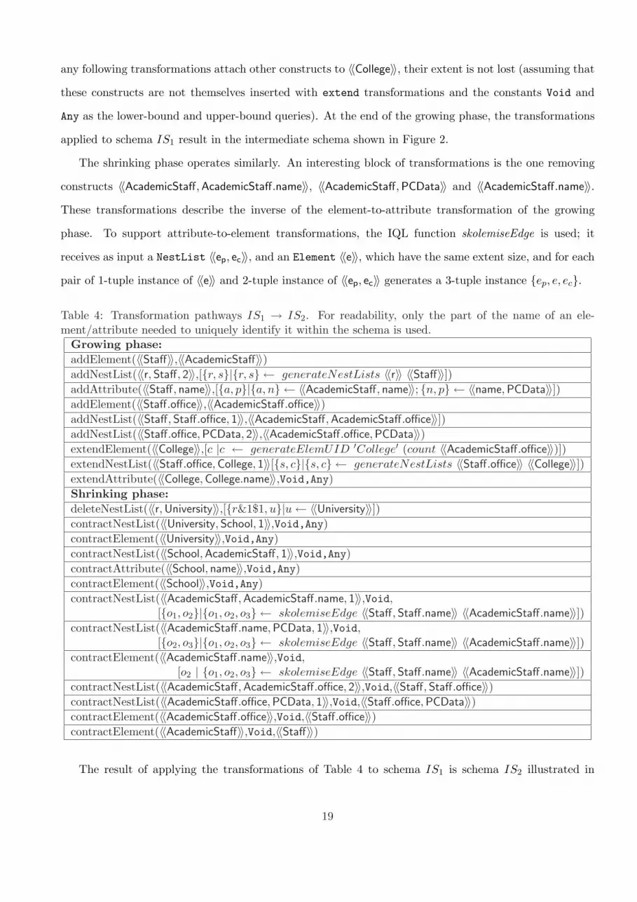
any following transformations attach other constructs to 〈〈College〉〉, their extent is not lost (assuming that

these constructs are not themselves inserted with extend transformations and the constants Void and

Any as the lower-bound and upper-bound queries). At the end of the growing phase, the transformations

applied to schema IS1 result in the intermediate schema shown in Figure 2.

The shrinking phase operates similarly. An interesting block of transformations is the one removing

constructs 〈〈AcademicStaff, AcademicStaff.name〉〉, 〈〈AcademicStaff,PCData〉〉 and 〈〈AcademicStaff.name〉〉.These transformations describe the inverse of the element-to-attribute transformation of the growing

phase. To support attribute-to-element transformations, the IQL function skolemiseEdge is used; it

receives as input a NestList 〈〈ep, ec〉〉, and an Element 〈〈e〉〉, which have the same extent size, and for each

pair of 1-tuple instance of 〈〈e〉〉 and 2-tuple instance of 〈〈ep, ec〉〉 generates a 3-tuple instance {ep, e, ec}.

Table 4: Transformation pathways IS1 → IS2. For readability, only the part of the name of an ele-ment/attribute needed to uniquely identify it within the schema is used.

Growing phase:addElement(〈〈Staff〉〉,〈〈AcademicStaff〉〉)addNestList(〈〈r, Staff, 2〉〉,[{r, s}|{r, s} ← generateNestLists 〈〈r〉〉〈〈Staff〉〉])addAttribute(〈〈Staff, name〉〉,[{a, p}|{a, n} ← 〈〈AcademicStaff, name〉〉; {n, p} ← 〈〈name, PCData〉〉])addElement(〈〈Staff.office〉〉,〈〈AcademicStaff.office〉〉)addNestList(〈〈Staff, Staff.office, 1〉〉,〈〈AcademicStaff, AcademicStaff.office〉〉])addNestList(〈〈Staff.office, PCData, 2〉〉,〈〈AcademicStaff.office, PCData〉〉)extendElement(〈〈College〉〉,[c |c ← generateElemUID ′College′ (count 〈〈AcademicStaff.office〉〉)])extendNestList(〈〈Staff.office, College, 1〉〉[{s, c}|{s, c} ← generateNestLists 〈〈Staff.office〉〉〈〈College〉〉])extendAttribute(〈〈College,College.name〉〉,Void,Any)Shrinking phase:deleteNestList(〈〈r, University〉〉,[{r&1$1, u}|u ← 〈〈University〉〉])contractNestList(〈〈University, School, 1〉〉,Void,Any)contractElement(〈〈University〉〉,Void,Any)contractNestList(〈〈School,AcademicStaff, 1〉〉,Void,Any)contractAttribute(〈〈School, name〉〉,Void,Any)contractElement(〈〈School〉〉,Void,Any)contractNestList(〈〈AcademicStaff,AcademicStaff.name, 1〉〉,Void,

[{o1, o2}|{o1, o2, o3} ← skolemiseEdge 〈〈Staff, Staff.name〉〉〈〈AcademicStaff.name〉〉])contractNestList(〈〈AcademicStaff.name, PCData, 1〉〉,Void,

[{o2, o3}|{o1, o2, o3} ← skolemiseEdge 〈〈Staff, Staff.name〉〉〈〈AcademicStaff.name〉〉])contractElement(〈〈AcademicStaff.name〉〉,Void,

[o2 | {o1, o2, o3} ← skolemiseEdge 〈〈Staff, Staff.name〉〉〈〈AcademicStaff.name〉〉])contractNestList(〈〈AcademicStaff,AcademicStaff.office, 2〉〉,Void,〈〈Staff, Staff.office〉〉)contractNestList(〈〈AcademicStaff.office, PCData, 1〉〉,Void,〈〈Staff.office, PCData〉〉)contractElement(〈〈AcademicStaff.office〉〉,Void,〈〈Staff.office〉〉)contractElement(〈〈AcademicStaff〉〉,Void,〈〈Staff〉〉)

The result of applying the transformations of Table 4 to schema IS1 is schema IS2 illustrated in

19

Figure 1. There now exists a transformation pathway S1 → IS1 → IS2 → S2, which can be used to

query S2, obtaining data from the data source corresponding to schema S1. The query on S2 is translated

by means of query unfolding using the queries within the delete, contract and rename steps in the

reverse pathway S2 → IS2 → IS1 → S1 to an equivalent query on S1. For example, if the data source

corresponding to S1 is the UniversityOfAthens.xml document listed in Section 3.1, the IQL query

[{n, p}|{s, n} ← 〈〈staffMember, name〉〉; {s, o} ← 〈〈staffMember, office〉〉; {o, p} ← 〈〈office, PCData〉〉]posed on S2 is translated by AutoMed’s Global Query Processor into the following equivalent query on

S1

[{n, p}|{s, n} ← [{a, p}|{a, n} ← 〈〈academic, name, 1〉〉; {n, p} ← 〈〈name,PCData, 1〉〉];{s, o} ← 〈〈academic, office〉〉; {o, p} ← 〈〈office,PCData〉〉]

which is then rewritten by the GQP as

[{n, p}|{s, n1} ← 〈〈academic, name, 1〉〉; {n1, n} ← 〈〈name, PCData, 1〉〉;{s, o} ← 〈〈academic, office〉〉; {o, p} ← 〈〈office,PCData〉〉]

and returns the following result:

[{′Dr. Nicholas Petrou′,′ 123′}, {′Prof. George Lazos′,′ 111′}, {′Dr. Anna Georgiou′,′ 321′}]We can also use the pathway S1 → IS1 → IS2 → S2 to materialise S2 using the data from the data

source corresponding to S1. For this, the add, extend and rename steps in the pathway are used to

incrementally define the output document from the source data — see [29] for details of this process. The

result is the following XML document:

<r><staffMember name="Dr. Nicholas Petrou">

<office>123<college name=""/>

</office></staffMember><staffMember name="Prof. George Lazos">


</office></staffMember><staffMember name="Dr. Anna Georgiou">


</office></staffMember>

20

</r>

We note that the above XML document has a single root element. If strict conformance to the target

XML format is required, the materialisation algorithm can produce multiple XML documents, one for

each instance of the 〈〈staffMember〉〉 root element.

4.3 Schema integration

The previous sections described algorithms for the translation of a source XMLDSS schema S1 into a

target XMLDSS schema S2. The resulting pathway S1 → S2 can subsequently be used to automatically

translate queries expressed on S2 to operate on S1, or to automatically transform data that conforms to

S1 to conform to S2.

Consider now a setting where we need to integrate a set of XMLDSS schemas S1, . . . , Sn all conforming

to some ontology R into a global XMLDSS schema. The renaming algorithm of Section 4.1 can first be used

to produce intermediate XMLDSS schemas IS1, . . . , ISn. We now need to integrate these intermediate

schemas into a single global schema. This can be done as follows.

The initial global schema, GS1, is IS1. A schema integration algorithm (see below) is then applied

to IS2 and GS1, producing a new global schema GS2. IS2 is then restructured to match GS2 by applying

the schema restructuring algorithm to IS2 as the source and GS2 as the target schema. Schemas IS3,

. . . , ISn are integrated similarly: for each ISi, we first apply the schema integration algorithm to ISi and

GSi−1, producing the new global schema GSi; we then restructure ISi to match the GSi, by applying the

schema restructuring algorithm to ISi and GSi.

The schema integration algorithm applied to each pair ISi and GSi−1 has a growing and a

shrinking phase. In the growing phase, the algorithm recreates the structure of ISi under the root of GSi

by issuing add or extend transformations. In the shrinking phase, the algorithm removes any duplicate

constructs now present in the global schema, using delete transformations.

We note that the structure of the final global schema GSn depends on the order of integration of

IS1, . . . , ISn, in that it will be identical to IS1 successively augmented with missing constructs appearing

in IS2, . . . , ISn. If a different integration order is chosen, then the structure of the final global schema

will be different, though containing the same Element and Attribute constructs.

The resulting global schema GSn can subsequently be queried, using AutoMed’s Global Query Proces-

sor (GQP) in cooperation with the XMLDSS wrappers for the data sources corresponding to the source

XMLDSS schemas S1, . . . , Sn. At present, the XMLDSS wrappers translate IQL subqueries submitted to

21

them by the GQP into XPath. Future plans include XQuery support, both within the XMLDSS wrappers,

and on the global XMLDSS schema.

Alternatively, the global schema GSn can be materialised and an integrated XML document conform-

ing to it can be generated. We refer the reader to [29] for details of how a global XMLDSS schema can

be materialised by using the GQP to incrementally generate the integrated XML document.

5 Handling Multiple Ontologies

Section 4 presented algorithms for the translation of a source XMLDSS schema S into a target XMLDSS

schema T and for the integration of schemas S1, . . . , Sn under a single global schema. In both cases,

it was assumed that all XMLDSS schemas conform to the same ontology. We now briefly discuss how

our approach can also cater for XMLDSS schemas that conform to different ontologies. These may be

connected either directly via an AutoMed transformation pathway, or via another ontology (e.g. an

‘upper’ ontology) to which both ontologies are connected by an AutoMed pathway.

Consider in particular two XMLDSS schemas S1 and S2 that are semantically linked by two sets of

correspondences C1 and C2 to two ontologies R1 and R2. Suppose that there is an articulation between

R1 and R2, in the form of an AutoMed pathway between them. This may be a direct pathway R1 → R2.

Alternatively, there may be two pathways R1 → RGeneric and R2 → RGeneric linking R1 and R2 to

a more general ontology RGeneric, from which we can derive a pathway R1 → RGeneric → R2 (due

to the reversibility of pathways). In both cases, the pathway R1 → R2 can be used to transform the

correspondences C1 expressed w.r.t. R1 to a set of correspondences C ′1 expressed on R2. This is using the

query translation algorithm mentioned in Section 3 which performs query unfolding using the the delete,

contract and rename steps in R1 → R2.

The result is two XMLDSS schemas S1 and S2 that are semantically linked by two sets of correspon-

dences C ′1 and C2 to the same ontology R2. Our algorithms described in Section 4 can now be applied.

There is a proviso here that the new correspondences C ′1 must conform syntactically to the correspon-

dences accepted as input by the renaming algorithm of Section 4.1. It is easy to show that this will be the

case if R1 → R2 maps classes in R1 to classes in R2 and properties in R1 to path expressions in R2, with

the additional proviso that if a property in R1 is literal-valued then the path in R2 ends in a literal-valued

property.

22

6 Concluding Remarks

This paper has presented algorithms for the transformation and integration of XML data sources that

make use of known correspondences between them and one or more ontologies expressed as RDFS schemas.

Our algorithms generate schema transformation/integration rules which are implemented in the AutoMed

heterogeneous data integration system. These rules can then be used to perform virtual or materialised

transformation and integration of the XML data sources.

The novelty of our approach lies in the use of XML-specific graph restructuring techniques in com-

bination with correspondences from XML schemas to the same or different ontologies. We envisage our

algorithms as being particularly useful in peer-to-peer data sharing and data integration environments.

There are several directions of further work. We are currently evaluating empirically the scalability

of our algorithms for different sizes and numbers of input XML documents and their XMLDSS schemas.

We also plan to evaluate empirically the extensibility of our approach, for example if a source or global

XMLDSS schema evolves, or if an ontology and the set of correspondences to it evolve. Another issue

is incrementally maintaining a materialised global XMLDSS schema, if the data or schema of a data

source changes. One specific application testbed that we are involved with that exhibits all of these

requirements is biological data integration, both materialised and virtual, in the context of the BIOMAP 8

and ISPIDER 9 projects. The former is building a data warehouse from diverse biological data sources

while the latter is building a ‘proteomic grid’ based on web/grid service technologies. Reference [13]

discusses our early experiences in using XMLDSS as a unifying data model for XML and relational

biological data sources, and using our XMLDSS schema restructuring algorithm for their automatic

transformation and integration.

References

[1] B. Amann, C. Beeri, I. Fundulaki, and M. Scholl. Ontology-based integration of XML web resources.

In Proc. International Semantic Web Conference 2002, pages 117–131, 2002.

[2] P. Buneman, L. Libkin, D. Suciu, V. Tannen, and L. Wong. Comprehension syntax. SIGMOD

Record, 23(1):87–96, 1994.8http://www.biochem.ucl.ac.uk/bsm/biomap/9http://www.dcs.bbk.ac.uk/∼lucas/projects/ispider/

23

[3] V. Christophides, G. Karvounarakis, I. Koffina, G. Kokkinidis, A. Magkanaraki, D. Plexousakis,

G. Serfiotis, and V. Tannen. The ICS-FORTH SWIM: A powerful Semantic Web integration mid-

dleware. In Proc. SWDB’03, 2003.

[4] I. F. Cruz and H. Xiao. Using a layered approach for interoperability on the Semantic Web. In Proc.

WISE’03, pages 221–231, 2003.

[5] I. F. Cruz, H. Xiao, and F. Hsu. An ontology-based framework for XML semantic integration. In

Proc. IDEAS’04, pages 217–226, 2004.

[6] M. Friedman, A. Levy, and T. Millstein. Navigational plans for data integration. In Proc. of the 16th

National Conference on Artificial Intelligence, pages 67–73. AAAI, 1999.

[7] R. Goldman and J. Widom. DataGuides: enabling query formulation and optimization in semistruc-

tured databases. In Proc. VLDB’97, pages 436–445, 1997.

[8] E. Jasper, A. Poulovassilis, and L. Zamboulis. Processing IQL queries and migrating data in the

AutoMed toolkit. AutoMed Technical Report 20, June 2003.

[9] E. Jasper, N. Tong, P. Brien, and A. Poulovassilis. View generation and optimisation in the AutoMed

data integration framework. In Proc. 6th International Baltic Conference on Databases & Information

Systems, Riga, Latvia, June 2004.

[10] L. V. S. Lakshmanan and F. Sadri. XML interoperability. In In Proc. of WebDB’03, pages 19–24,

June 2003.

[11] P. Lehti and P. Fankhauser. XML data integration with OWL: Experiences and challenges. In Proc.

Symposium on Applications and the Internet (SAINT 2004), Tokyo, 2004.

[12] M. Lenzerini. Data integration: A theoretical perspective. In Proc. PODS’02, pages 233–246, 2002.

[13] G. Rimon N. Martin M. Maibaum, L. Zamboulis and A. Poulovassilis.

[14] J. Madhavan and A.Y. Halevy. Composing mappings among data sources. In Proc. VLDB’03, pages

572–583, 2003.

[15] P. McBrien and A.Poulovassilis. Defining peer-to-peer data integration using both as view rules.

In Proc. Proc. Workshop on Databases, Information Systems and Peer-to-Peer Computing (at

VLDB’03), Berlin, 2003.

24

[16] P. McBrien and A. Poulovassilis. Data integration by bi-directional schema transformation rules. In

Proc. ICDE’03. ICDE, March 2003.

[17] L. Popa, Y. Velegrakis, R.J. Miller, M.A. Hernandez, and R. Fagin. Translating web data. In Proc.

VLDB’02, pages 598–609, 2002.

[18] E. Rahm and P. Bernstein. A survey of approaches to automatic schema matching. VLDB Journal,

10(4):334–350, 2001.

[19] C. Reynaud, J.P. Sirot, and D. Vodislav. Semantic integration of XML heterogeneous data sources.

In Proc. IDEAS, pages 199–208, 2001.

[20] P. Rodriguez-Gianolli and J. Mylopoulos. A semantic approach to XML-based data integration. In

Proc. ER’01, pages 117–132, 2001.

[21] H. Su, H. Kuno, and E. A. Rudensteiner. Automating the transformation of XML documents. In

Proc. WIDM’01, pages 68–75, 2001.

[22] W3C. Guide to the W3C XML Specification (“XMLspec”) DTD, Version 2.1.

http://www.w3.org/XML/1998/06/xmlspec-report-v21.htm#AEN56, June 1998.

[23] W3C. XML Schema Specification. http://www.w3.org/XML/Schema, May 2001.

[24] W3C. OWL Web Ontology Language Overview. http://www.w3.org/TR/owl-features/, August

2003.

[25] W3C. RDF Vocabulary Description Language 1.0: RDF Schema. http://www.w3.org/TR/rdf-

schema/, February 2004.

[26] W3C. Resource Description Framework (RDF): Concepts and Abstract Syntax.

http://www.w3.org/TR/rdf-concepts/, February 2004.

[27] X. Yang, M.L. Lee, and T.W.Ling. Resolving structural conflicts in the integration of XML schemas:

A semantic approach. In Proc. ER’03, pages 520–533, 2003.

[28] L. Zamboulis. XML data integration by graph restructuring. In Proc. BNCOD’04, LNCS 3112, 2004.

[29] L. Zamboulis and A. Poulovassilis. Using AutoMed for XML data transformation and integration.

In Proc. DIWeb’04 (at CAiSE’04), Riga, Latvia, June 2004.

25

information sharing for the semantic web -a schema transformation approach

Documents