schema matching and mapping
TRANSCRIPT

123
Schema Matching and Mapping
| | | | | | | | | | | | | | | | | | | | | | | | | | | | | | | | | | | | | | | | | | |
| | | | | | | | | | | | | | | | | | | | | | | | | | | | | | | | | | | | | | | | | | | | | | |
| | | | | | | | | | | | | | | | | | | | | | | | | | | | | | | | | | | | | | | | | | | | | | |
| | | | | | | | | | | | | | | | | | | | | | | | | | | | | | | | | | | | | | | | | | | | | | | | | | |
| | | | | | | | | | | | | | | | | | | | | | | | | | | | | | | | | | | | | | | | | | | | | | | | | | | | | |
Zohra BellahseneAngela BonifatiErhard Rahm (Eds.)
DCSA

Data-Centric Systems and Applications
Series Editors
M.J. CareyS. Ceri
Editorial Board
P. BernsteinU. Dayal
C. FaloutsosJ.C. FreytagG. Gardarin
W. JonkerV. Krishnamurthy
M.-A. NeimatP. ValduriezG. Weikum
K.-Y. WhangJ. Widom
For further volumes:http://www.springer.com/series/5258

•

Zohra Bellahsene � Angela BonifatiErhard RahmEditors
Schema Matchingand Mapping
123

EditorsZohra BellahseneLIRMM CNRS/Univ. Montpellier 2Rue Ada 16134392 [email protected]
Erhard RahmUniversitat LeipzigInst. InformatikAugustusplatz 10-1104109 [email protected]
Angela BonifatiConsiglio Nazionale delleRicerche (CNR)Via P. Bucci 41/C87036 [email protected]
ISBN 978-3-642-16517-7 e-ISBN 978-3-642-16518-4DOI 10.1007/978-3-642-16518-4Springer Heidelberg Dordrecht London New York
Library of Congress Control Number: 2011922131
ACM Computing Classification (1998): H.2, I.2, F.4
c� Springer-Verlag Berlin Heidelberg 2011This work is subject to copyright. All rights are reserved, whether the whole or part of the material isconcerned, specifically the rights of translation, reprinting, reuse of illustrations, recitation, broadcasting,reproduction on microfilm or in any other way, and storage in data banks. Duplication of this publicationor parts thereof is permitted only under the provisions of the German Copyright Law of September 9,1965, in its current version, and permission for use must always be obtained from Springer. Violationsare liable to prosecution under the German Copyright Law.The use of general descriptive names, registered names, trademarks, etc. in this publication does notimply, even in the absence of a specific statement, that such names are exempt from the relevant protectivelaws and regulations and therefore free for general use.
Cover design: KuenkelLopka GmbH
Printed on acid-free paper
Springer is part of Springer Science+Business Media (www.springer.com)
Preface
This book provides an overview about the state-of-the-art solutions and the mostrecent advances in schema matching and mapping, both recognized as key areas ofmetadata management. Tasks involving metadata are indeed pervasive in databasesand information systems and include schema evolution, schema and ontology inte-gration and matching, XML message mapping, as well as data migration and dataexchange. While research on these complex problems has been performed since sev-eral decades, we have witnessed significant progress especially in the last decade. Inparticular, research addressed the metadata problems in a more abstract and genericway rather than focusing on specific applications and data models. A cornerstoneof this new line of research is the notion of schema mappings, i.e., expressivemappings interrelating schemas (or other metadata models such as ontologies).Furthermore, powerful operators to manipulate schemas and mappings (e.g., match-ing and merging of schemas or composition of mappings) have been investigatedfor solving various kinds of metadata-related tasks. Raising the level of abstrac-tion for metadata management was a vision first articulated by Phil Bernstein etal. in A vision for management of complex models, ACM Sigmod Record 2000.Since then, many steps have been performed towards the various goals of match-ing and mapping different kinds of design artifacts (i.e., a relational schema, aweb site, or a data mart), thus motivating a flurry of recent research, which wesurvey in this book. The book consists of ten comprehensive chapters groupedwithin three parts: large-scale and knowledge-driven schema matching, quality-driven schema mapping and evolution and evaluation and tuning of matchingtasks.
The first part deals with schema matching, i.e., the semi-automatic findingof semantic correspondences between elements of two schemas or two ontolo-gies. Schema matching implements a Match operator that is often the first stepto determine schema mappings, e.g., for schema evolution, data integration anddata exchange. The typically high semantic heterogeneity of the schemas makesschema matching an extremely difficult problem. The separation of Match fromother metadata management tasks such as Merge helped to address the match prob-lem better than in the past. Numerous powerful prototypes for schema and ontologymatching have been developed in the last decade and automatic match functionalityfound already its way into commercial products. The four chapters in the first
v

vi Preface
part cover the achieved state of the art and point out areas where more work isneeded, in particular support for large-scale match problems and improved userinteraction. Further chapters deal with proposed extensions to enhance the seman-tic power of match correspondences and to deal with the uncertainty of matchdecisions.
The second part of the book also consists of four chapters and focuses onschema mappings and their use for schema evolution and schema merging. Thefirst chapter of the second part surveys the existing schema mapping algorithmsand the most recent developments towards realizing efficient, optimized and correctschema mapping transformations. Two further chapters deal with the use of schemamappings for schema evolution. One of these introduces the requirements for effec-tive schema evolution support and provides an overview of proposed evolutionapproaches for diverse kinds of schemas and ontologies. The other evolution-relatedchapter focuses on the automatic adaptation of mappings after schema changesby presenting two first-class operators on schema mappings, namely compositionand inversion. The final chapter surveys the state of the art on mapping-basedmerging of schemas by discussing the key works in this area and identifying theircommonalities and differences.
The third part of the book consists of two chapters devoted to the evaluationand tuning of schema matching and mapping systems. The first of these chaptersprovides a comprehensive overview of existing evaluation efforts for data trans-formation tasks, by providing a brand-new perspective under which the variousapproaches are being/have been evaluated. Such perspective allows the authors toidentify the pitfalls of current evaluations and brings them to discuss open problemsfor future research in this area. The last chapter deals with the complex problem oftuning schema matching tools to optimize their quality and efficiency with a limitedamount of configuration effort. An overview of proposed tuning efforts includingthe use of machine learning techniques is provided.
To the best of our expectations, this book provides:
1. A comprehensive survey of current and past research on schema matching andmapping.
2. An up-to-date source of reference about schema and ontology evolution andschema merging.
3. Scholarly written chapters enabling a learning experience to both experts andnon-experts whenever they would like to enhance their knowledge or build itfrom the scratch; the chapters have been conceived in such a way to be readableindividually or altogether by following the book table-of-contents.
As such, we hope that the book proves to be a useful reference to researchers as wellas graduate students and advanced professionals. We thank the editors of the DCSAbook series, Mike Carey and Stefano Ceri, for their support of our book project andall authors for preparing their chapters and revisions within a few months. With-out them, this project would not have been possible. Further thanks go the referees

Preface vii
of the individual chapters for their insightful comments and to Ralf Gerstner fromSpringer-Verlag for his professional assistance during all the stages of the bookproduction.
September 2010 Zohra BellasehneAngela Bonifati
Erhard Rahm

•

Contents
Part I Large-Scale and Knowledge-Driven Schema Matching
1 Towards Large-Scale Schema and Ontology Matching . . . . . . . . . . . . . . . . . . 3Erhard Rahm
2 Interactive Techniques to Support Ontology Matching . . . . . . . . . . . . . . . . . . 29Sean M. Falconer and Natalya F. Noy
3 Enhancing the Capabilities of Attribute Correspondences . . . . . . . . . . . . . . 53Avigdor Gal
4 Uncertainty in Data Integration and Dataspace SupportPlatforms . . . . . . . . . . . . . . . . . . . . . . . . . . . . . . . . . . . . . . . . . . . . . . . . . . . . . . . . . . . . . . . . . . . . . . 75Anish Das Sarma, Xin Luna Dong, and Alon Y. Halevy
Part II Quality-Driven Schema Mapping and Evolution
5 Discovery and Correctness of Schema MappingTransformations . . . . . . . . . . . . . . . . . . . . . . . . . . . . . . . . . . . . . . . . . . . . . . . . . . . . . . . . . . . . . .111Angela Bonifati, Giansalvatore Mecca, Paolo Papotti,and Yannis Velegrakis
6 Recent Advances in Schema and Ontology Evolution . . . . . . . . . . . . . . . . . . . .149Michael Hartung, James Terwilliger, and Erhard Rahm
7 Schema Mapping Evolution Through Compositionand Inversion . . . . . . . . . . . . . . . . . . . . . . . . . . . . . . . . . . . . . . . . . . . . . . . . . . . . . . . . . . . . . . . . . .191Ronald Fagin, Phokion G. Kolaitis, Lucian Popa,and Wang-Chiew Tan
8 Mapping-Based Merging of Schemas . . . . . . . . . . . . . . . . . . . . . . . . . . . . . . . . . . . . . .223Rachel Pottinger
ix

x Contents
Part III Evaluating and Tuning of Matching Tasks
9 On Evaluating Schema Matching and Mapping . . . . . . . . . . . . . . . . . . . . . . . . . .253Zohra Bellahsene, Angela Bonifati, Fabien Duchateau,and Yannis Velegrakis
10 Tuning for Schema Matching . . . . . . . . . . . . . . . . . . . . . . . . . . . . . . . . . . . . . . . . . . . . . . .293Zohra Bellahsene and Fabien Duchateau
Index . . . . . . . . . . . . . . . . . . . . . . . . . . . . . . . . . . . . . . . . . . . . . . . . . . . . . . . . . . . . . . . . . . . . . . . . . . . . . . . . .317

Contributors
Zohra Bellahsene LIRMM – CNRS/Universite Montpellier II, 161 Rue Ada,34095 Montpellier Cedex 5, France, [email protected]
Angela Bonifati ICAR-CNR, Rende, [email protected]
Xin Luna Dong Data Management Department, AT&T Labs – Research, Bld 103,Rm B281, 180 Park Ave., Florham Park, NJ 07932, USA, [email protected]
Fabien Duchateau CWI, Amsterdam, The [email protected]
Ronald Fagin IBM Almaden Research Center, Dept. K53/B2, 650 Harry Road,San Jose, CA 95120, USA, [email protected]
Sean Falconer Stanford University, Stanford, CA 94305-5479, [email protected]
Avigdor Gal Faculty of Industrial Engineering and Management, Technion –Israel Institute of Technology, Technion City, Haifa 32000, Israel, [email protected]
Alon Halevy Google Inc., 1600 Amphitheatre Blvd, Mountain View, CA 94043,USA, [email protected]
Michael Hartung Department of Computer Science, University of Leipzig,P.O. Box 100920, 04109 Leipzig, Germany, [email protected]
Phokion Kolaitis IBM Almaden Research Center, 650 Harry Road, San Jose, CA95120, USAandUniversity of California Santa Cruz, 1156 High Street, Santa Cruz, CA 95064,USA, [email protected]
Giansalvatore Mecca Dipartimento di Matematica e Informatica, Universitadella Basilicata, c.da Macchia Romana, 85100 Potenza, Italy, [email protected]
xi

xii Contributors
Natalya Noy Stanford University, Stanford, CA 94305-5479, USAandMedical School Office Building, Room X-215, 251 Campus Drive, Stanford, CA94305-5479, USA, [email protected]
Paolo Papotti Dipartimento di Informatica e Automazione, Universita Roma Tre,Via della Vasca Navale 79, 00146 Rome, Italy, [email protected]
Lucian Popa 8CC/B1, IBM Almaden Research Center, 650 Harry Road,San Jose, CA 95120, USA, [email protected]
Rachel Pottinger Department of Computer Science, University of BritishColumbia, 201-2366 Main Mall, Vancouver, BC, Canada V6T 1Z4, [email protected]
Erhard Rahm Department of Computer Science, University of Leipzig, P.O. Box100920, 04109 Leipzig, Germany, [email protected]
Anish Das Sarma Yahoo! Research, 2-GA 2231, Santa Clara, CA 95051, USA,[email protected]
Wang-Chiew Tan E3-406, IBM Almaden Research Center, 650 Harry Road,San Jose, CA 95120, USAandUniversity of California Santa Cruz, 1156 High Street, Santa Cruz, CA 95064,USA, [email protected]
James F.Terwilliger Microsoft Research, Redmond, WA, USA, [email protected]
Yannis Velegrakis DISI – University of Trento, Via Sommarive 14, 38123 Trento,Italy, [email protected]

Part ILarge-Scale and Knowledge-Driven
Schema Matching
Schema matching is the task of finding semantic correspondences between ele-ments of two schemas. It is needed in many metadata-intensive applications, such asXML message mapping, integration of web data sources, catalogue integration, datawarehouse loading and peer-to-peer data management. The typically high seman-tic heterogeneity of the schemas make schema matching an extremely difficultproblem.
Currently, such matching tasks are largely performed manually by domainexperts, at best supported by some GUI, and therefore they are time consuming,tedious and error prone. Approaches for automating the schema and ontologymatching tasks as much as possible are needed to simplify and speed up thedevelopment, maintenance and use of metadata-intensive applications.
In the last decade semi-automatic schema matching and related variants such asontology matching have attracted a huge amount of research effort and considerableprogress has been achieved. In particular, powerful schema matching prototypeshave been developed and successfully applied to a large variety of match prob-lems. These prototypes typically allow the combined execution of multiple matchalgorithms to improve overall match quality. Furthermore, initial schema match-ing capabilities found their way into middleware platforms from IBM, Microsoft(Biztalk) and SAP (Netweaver). Still, the current solutions are not yet sufficientbut need improvements to deal with large-scale match problems, to improve userinteraction and to enhance the semantic power of mappings.
The introductory part of the book reviews the current state of the art and recentresearch efforts in these directions. Chapter 1 written by Erhard Rahm describesapproaches to match large schemas and ontologies. He discusses advanced strategiesand techniques for improving the match quality and the runtime efficiency for suchlarge-scale match tasks.
Chapter 2 by Sean Falconer and Natasha Noy deals with recent approaches forimproving the crucial user interaction for schema matching. They present visualiza-tion techniques for assisting users with mapping generation and discuss wiki-basedtechniques for collaborative schema matching.

Chapter 3 by Avi Gal focuses on the generation of enhanced match results thatare not limited to simple 1:1 attribute correspondences. In particular, he considerssemantically refined correspondences by taking the context of schema elements andontological relationships into account.
Das Sarma, Dong and Halevy discuss in Chap. 4 recent work on supporting prob-abilistic mappings to deal with the inherent uncertainty of data integration. Theyfocus on dataspace-oriented environments for which probabilistic mappings andprobabilistic mediated schemas can help minimize the amount of upfront modellingeffort for data integration.
Chapter 1Towards Large-Scale Schema and OntologyMatching
Erhard Rahm
Abstract The purely manual specification of semantic correspondences betweenschemas is almost infeasible for very large schemas or when many different schemashave to be matched. Hence, solving such large-scale match tasks asks for auto-matic or semiautomatic schema matching approaches. Large-scale matching needsespecially to be supported for XML schemas and different kinds of ontologiesdue to their increasing use and size, e.g., in e-business and web and life sci-ence applications. Unfortunately, correctly and efficiently matching large schemasand ontologies are very challenging, and most previous match systems have onlyaddressed small match tasks. We provide an overview about recently proposedapproaches to achieve high match quality or/and high efficiency for large-scalematching. In addition to describing some recent matchers utilizing instance andusage data, we cover approaches on early pruning of the search space, divide andconquer strategies, parallel matching, tuning matcher combinations, the reuse ofprevious match results, and holistic schema matching. We also provide a briefcomparison of selected match tools.
1 Introduction
Schema matching aims at identifying semantic correspondences between metadatastructures or models, such as database schemas, XML message formats, and ontolo-gies. Solving such match problems is a key task in numerous application fields,particularly to support data exchange, schema evolution, and virtually all kinds ofdata integration. Unfortunately, the typically high degree of semantic heterogeneityreflected in different schemas makes schema matching an inherently complex task.Hence, most current systems still require the manual specification of semantic corre-spondences, e.g., with the help of a GUI. While such an approach is appropriate for
E. RahmUniversity of Leipzig, Ritterstraße 26, 04109 Leipzig, Germanye-mail: [email protected]
Z. Bellahsene et al. (eds.), Schema Matching and Mapping, Data-Centric Systemsand Applications, DOI 10.1007/978-3-642-16518-4 1,c� Springer-Verlag Berlin Heidelberg 2011
3

4 E. Rahm
matching a few small schemas, it is enormously time-consuming and error-pronefor dealing with large schemas encompassing thousands of elements or to matchmany schemas. Therefore, automatic or semiautomatic approaches to find semanticcorrespondences with minimal manual effort are especially needed for large-scalematching. Typical use cases of large-scale matching include:
– Matching large XML schemas, e.g., e-business standards and message formats(Rahm et al. 2004; Smith et al. 2009)
– Matching large life science ontologies describing and categorizing biomedicalobjects or facts such as genes, the anatomy of different species, diseases, etc.(Kirsten et al. 2007; Zhang et al. 2007)
– Matching large web directories or product catalogs (Avesani et al. 2005; Nandiand Bernstein 2009)
– Matching many web forms of deep web data sources to create a mediated searchinterface, e.g., for travel reservation or shopping of certain products (He andChang 2006; Su et al. 2006).
Schema matching (including its ontology matching variant) has been a very activeresearch area, especially in the last decade, and numerous techniques and prototypesfor automatic matching have been developed (Rahm and Bernstein 2001; Euzenatand Shvaiko 2007). Schema matching has also been used as a first step to solve dataexchange, schema evolution, or data integration problems, e.g., to transform corre-spondences into an executable mapping for migrating data from a source to a targetschema (Fagin et al. 2009). Most match approaches focus on 2-way or pairwiseschema matching where two related input schemas are matched with each other.Some algorithms have also been proposed for n-way or holistic schema matching(He and Chang 2006), to determine the semantic overlap in many schemas, e.g.,to build a mediated schema. The result of pairwise schema matching is usually anequivalence mapping containing the identified semantic correspondences, i.e., pairsof semantically equivalent schema elements. Some ontology matching approachesalso try to determine different kinds of correspondences, such as is-a relationshipsbetween ontologies (Spiliopoulos et al. 2010). Due to the typically high semanticheterogeneity of schemas, algorithms can only determine approximate mappings.The automatically determined mappings may thus require the inspection and adap-tation by a human domain expert (deletion of wrong correspondences, addition ofmissed correspondences) to obtain the correct mapping.
Despite the advances made, current match systems still struggle to deal withlarge-scale match tasks as those mentioned above. In particular, achieving both goodeffectiveness and good efficiency are two major challenges for large-scale schemamatching. Effectiveness (high match quality) requires the correct and complete iden-tification of semantic correspondences, and the larger the search space, the moredifficult it is to achieve. For pairwise schema matching, the search space increases atleast quadratically with the number of elements. Furthermore, the semantic hetero-geneity is typically high for large-scale match tasks, e.g., the schemas may largelydiffer in their size and scope, making it difficult to find all correspondences. Fur-thermore, elements often have several equivalent elements in the other schema that

1 Towards Large-Scale Schema and Ontology Matching 5
are more difficult to identify than 1:1 correspondences that are more likely for smallmatch tasks. Some large-scale problems in the ontology alignment evaluation ini-tiative (OAEI) contest on ontology matching are still not satisfactorily solved afterseveral years. For example, the best F-measure1 result for the catalog test to matchweb directories (71%) was achieved in 2007; in 2009, the best participating sys-tem achieved merely 63%; the average F-measure was around 50% (Euzenat et al.2009).
Efficiency is another challenge for large-scale matching. Current match systemsoften require the schemas and intermediate match results to fit in main memory,thereby limiting their applicability for large-scale match tasks. Furthermore, eval-uating large search spaces is time consuming, especially if multiple matchers needto be evaluated and combined. For some OAEI match tasks and systems, executiontimes in the order of several hours or even days are observed (Euzenat et al. 2009).For interactive use of schema matching systems, such execution times are clearlyunacceptable.
In this book chapter, we provide an overview of recent approaches to improveeffectiveness and efficiency for large-scale schema and ontology matching. We onlybriefly discuss further challenges such as support for sophisticated user interactionor the evaluation of match quality, but these are treated in more detail in other chap-ters of this book (Falconer and Noy 2011; Bellahsene et al. 2011). For example,advanced GUIs should be supported to visualize large schemas and mappings, tospecify automatic match strategies (selection of matchers, parameter tuning), toincrementally start automatic schema matching and adapt match results, etc.
In the next section, we introduce the kinds of matchers used in current matchsystems as well as a general workflow to combine the results of multiple match-ers for improved match quality. We also discuss performance optimizations forsingle matchers and present recently proposed approaches for instance-based andusage-based matching. In Sect. 3, we present several match strategies that we con-sider as especially promising for large-scale matching: early pruning of the searchspace, partition-based matching, parallel matching, self-tuning match workflows,and reuse-based matching. We also discuss briefly approaches for n-way (holistic)schema matching. Section 4 contains a short discussion of match support in com-mercial systems and a comparison of selected research prototypes that have beenapplied to large match problems.
2 Matchers and Match Workflows
The developed systems for schema and ontology matching typically support severalmatch algorithms (or matchers) and combine their results for improved match qual-ity. There exists a large spectrum of possible matchers and different implementations
1 F-Measure combines Recall and Precision, two standard measures to evaluate the effectivenessof schema matching approaches (Do et al. 2003).

6 E. Rahm
as surveyed in (Rahm and Bernstein 2001; Euzenat and Shvaiko 2007), particularlymetadata-based and instance-based matchers. Metadata-based matchers are mostcommon and exploit characteristics of schema or ontology elements such as theirnames, comments, data types, as well as structural properties. Instance-based match-ers determine the similarity between schema elements from the similarity of theirinstances; this class of matchers has recently been studied primarily for matchinglarge ontologies and will be discussed in more detail below.
Further matching techniques exploit different kinds of auxiliary (background)information to improve or complement metadata- and instance-based matchers.For example, name matching for both schema elements and instance values canbe enhanced by general thesauri such as Wordnet or, for improved precision,domain-specific synonym lists and thesauri (e.g., UMLS as a biomedical reference).Furthermore, search engines can be used to determine the similarity between names,e.g., by using the relative search result cardinality for different pairs of names as asimilarity indicator (Gligorov et al. 2007). At the end of this section, we will brieflydiscuss a further kind of match technique, the recently proposed consideration ofusage information for matching.
Efficiently matching large schemas and ontologies implies that every matchershould impose minimal CPU and memory requirements. For improving linguis-tic matching, many techniques for efficiently computing string similarities canbe exploited, e.g., for tokenization and indexing (Koudas et al. 2004). Structuralmatching can be optimized by precollecting the predecessors and children of everyelement, e.g., in database tables, instead of repeatedly traversing large graph struc-tures (Algergawy et al. 2009). Such an approach can also avoid the need of keepinga graph representation of the schemas in memory that can become a bottleneck withlarge schemas. The results of matchers are often stored within similarity matricescontaining a similarity value for every combination of schema elements. With largeschemas, these matrices may require millions of entries and thus several hundredsof MB memory. To avoid a memory bottleneck, a more space-efficient storage ofmatcher results becomes necessary, e.g., by using hash tables (Bernstein et al. 2004).In Sect. 3, we will discuss further performance techniques such as parallel matcherexecution.
In the following, we first describe a general workflow-like approach to applymultiple matchers and to combine their results. We then discuss approaches forinstance-based ontology matching and usage-based matching.
2.1 Match Workflows
Figure 1.1a shows a general workflow for automatic, pairwise schema matching asbeing used in many current match systems. The schemas are first imported into aninternal processing format. Further preprocessing may be applied such as analysisof schema features or indexing name tokens to prepare for a faster computation ofname similarities. The main part is a subworkflow to execute several matchers each

1 Towards Large-Scale Schema and Ontology Matching 7
S2
S1ResultMapping
Pre-processing
Input schemas
Combination ofmatcher results
Selection ofcorrespondences
Matcher 1
Matcher 2
Matcher 3
Matcher 1 Matcher 2 … Matcher 1
Matcher
Matcher
Matcher
General workflow for pairwise schema matching
Principal matcher sub-workflows
Sequential matchers Parallel (independent)matchers
Mixed strategy
a
b
MatcherExecution
(sub-workflow)
Fig. 1.1 General match workflows
of which determines a preliminary set of correspondences. After the execution of thematcher subworkflow, there are typically several postprocessing steps, particularlythe combination of the individual matcher results and finally the selection of thecorrespondences from the combined result.
As indicated in Fig. 1.1b, the individual matchers may either be executed sequen-tially, independently (in parallel), or in some mixed fashion. In the sequentialapproach, the matchers are not executed independently, but the results of initialmatchers are used as input by subsequent matchers. A common strategy, e.g., usedin Cupid (Madhavan et al. 2001), is to first execute a linguistic matcher to comparethe names of schema elements and then use the obtained similarities as input forstructure-based matching. In the parallel matcher strategy, individual matchers areautonomous and can be independently executed from other matchers. This supportsa high flexibility to select matchers for execution and combination. Furthermore,these matchers may also physically be executed in parallel, e.g., on multicore ormultiserver hardware. On the other hand, the autonomy of individual matchers mayintroduce redundant computations, e.g., of name similarities to be used for structuralmatching. The mixed strategy combines sequential and parallel matcher executionand is thus most complex.
There are different methods to combine match results of individual matchers,e.g., by performing a union or intersection of the correspondences or by aggregatingindividual similarity values, e.g., by calculating a weighted average of the individualsimilarities. Similarly, there are different methods to finally select the correspon-dences. Typically, correspondences need to exceed some predetermined thresholdbut may also have to meet additional constraints for improved precision. So it isreasonable for 1:1 mappings to enforce the so-called stable marriages, i.e., a corre-spondence c1� c10 is only accepted if c10 is the most similar element for c1 andvice versa. Some ontology matching systems such as ASMOV enforce additionalconstraints regarding is-a relationships (see Sect. 4.2).

8 E. Rahm
For interactive schema matching, the user may interact with the system and thematch workflow in different ways (not shown in Fig. 1.1), preferably via a user-friendly GUI. She typically has to specify the workflow configuration, e.g., whichmatchers should be executed and which strategy/parameters should be applied forthe final combination and selection steps. The final results are typically only sug-gested correspondences that the user can confirm or correct. The match workflowitself could be executed on the whole input schemas or incrementally for selectedschema parts or even individual elements (Bernstein et al. 2006). The latter approachis a simple but reasonable way to better deal with large schemas as it reduces theperformance requirements compared to matching the whole schemas. Furthermore,the determined correspondences can better be visualized avoiding that the user isoverwhelmed with huge mappings. Shi et al. (2009) propose an interesting variationfor interactive matching where the system asks the user for feedback on specificcorrespondences that are hard to determine automatically and that are valuable asinput for further matcher executions.
2.2 Instance-Based and Usage-Based Matching
2.2.1 Instance-Based Ontology Matching
Instance-based ontology matching determines the similarity between ontology con-cepts from the similarity of instances associated to the concepts. For example,two categories of a product catalog can be considered as equivalent if their prod-ucts are largely the same or at least highly similar. One can argue that instancescan characterize the semantics of schema elements or ontology concepts very welland potentially better than a concept name or comment. Therefore, instance-basedmatching holds the promise of identifying high-quality correspondences. On theother hand, obtaining sufficient and suitable instance data for all ontologies and allontology concepts to be matched is a major problem, especially for large ontologies.Hence, we consider instance-based approaches primarily as a complementary, albeitsignificant, match approach to be used in addition to metadata-based matchers.
As indicated in Fig. 1.2, two main cases for instance-based ontology match-ing can be distinguished depending on whether or not the existence of commoninstances is assumed. The existence of the same instances for different ontologies(e.g., the same web pages categorized in different web directories, the same prod-ucts offered in different product catalogs, or the same set of proteins described indifferent life science ontologies) simplifies the determination of similar concept. Inthis case, two concepts may be considered as equivalent when their instances over-lap significantly. Different set similarity measures can be used to measure such aninstance overlap, e.g., based on Dice, Jaccard, or cosine similarity. The instanceoverlap approach has been used to match large life science ontologies (Kirsten et al.2007) and product catalogs (Thor et al. 2007).

1 Towards Large-Scale Schema and Ontology Matching 9
a b
02
Commoninstances
?
ontologyassociations
Common instances(separate from ontologies)
0101 02
01instances
?
02instances
Ontology-specific instances
?
Fig. 1.2 Two cases for instance-based ontology matching
The more broadly applicable case is when only similar but potentially differentinstances are used to determine correspondences (Fig. 1.2b). In this case, determin-ing concept similarity requires determining the similarity between sets of instances,which is a variation of the well-studied problem of object matching or entity res-olution (Elmagarmid et al. 2007; Koepcke and Rahm 2010). One approach foraddressing this task is to combine all instances of a concept into a virtual document.Matching is then implemented by comparing such virtual documents with each otherbased on some document similarity measure, e.g., TF/IDF. This approach is sup-ported in several match prototypes including Rimom and ComaCC (see Sect. 4.2).Massmann and Rahm (2008) evaluate instance-based matching for web directoriesutilizing a virtual document approach for website names and descriptions as well asan instance overlap approach for website URLs. The approaches achieve an aver-age F-measure of about 60% (79% in combination with metadata-based matching)for different match tasks; the largest directory had more than 3,000 categories. TheOAEI contest also includes a web directory match task, however, without provid-ing instance data, thereby limiting the achievable match quality (as mentioned inthe introduction, the participating systems could not improve on this task in recentyears; the best F-measure in 2009 was 63%).
An alternate approach for instance-based matching using machine learning hasbeen implemented in the GLUE and SAMBO systems (Doan et al. 2003; Lambrixet al. 2008). The SAMBO approach focuses on matching life science ontologiesbased on the similarity of publications (Pubmed abstracts) referring to the ontol-ogy concepts. Both GLUE and SAMBO perform a training phase per ontologyto learn concept classifiers for the available instances. These classifiers are thenmutually applied to the instances from the other ontology to determine the conceptsan instance is predicted to belong to. The instance-concept associations are aggre-gated, e.g., by a Jaccard-based set similarity measure, to derive concept similaritiesand concept correspondences. The approaches do not require shared instances butonly similar ones for classification. Furthermore, they can utilize many existing

10 E. Rahm
instances in applications such as matching product catalogs or web directories. Onthe other hand, the classification problem becomes inherently more difficult to solvefor increasing numbers of concepts. The GLUE evaluation in Doan et al. (2003)was restricted to comparatively small match tasks with ontology sizes between 31and 331 concepts. The SAMBO approach was evaluated for even smaller (sub-)ontologies (10–112 concepts). Effectiveness and efficiency of the machine learn-ing approaches to large-scale match tasks with thousands of concepts is thus anopen issue.
2.2.2 Usage-Based Matching
Two recent works propose the use of query logs to aid in schema matching. InElmeleegy et al. (2008), SQL query logs are analyzed to find attributes with similarusage characteristics (e.g., within join conditions or aggregations) and occurrencefrequencies as possible match candidates for relational database schemas. TheHamster approach (Nandi and Bernstein 2009) uses the click log for keywordqueries of an entity search engine to determine the search terms, leading to instancesof specific categories of a taxonomy (e.g., product catalog or web directory). Cate-gories of different taxonomies sharing similar search queries are then considered asmatch candidates. Different search terms referring to the same categories are alsopotential synonyms that can be utilized not only for matching but also for otherpurposes such as the improvement of user queries.
A main problem of usage-based matching is the difficulty to obtain suitable usagedata, which is likely more severe than the availability of instance data. For example,the click logs for the Hamster approach are only available to the providers of searchengines. Furthermore, matching support can primarily be obtained for categories orschema elements receiving many queries.
3 Techniques for Large-Scale Matching
In this section, we provide an overview about recent approaches for large-scale pair-wise matching that go beyond specific matchers but address entire match strategies.In particular, we discuss approaches in four areas that we consider as especiallypromising and important:
– Reduction of search space for matching (early pruning of dissimilar elementpairs, partition-based matching)
– Parallel matching– Self-tuning match workflows– Reuse of previous match results
We also discuss proposed approaches for holistically matching n schemas.

1 Towards Large-Scale Schema and Ontology Matching 11
3.1 Reduction of Search Space
The standard approach for pairwise schema matching is to compare every elementof the first schema with every element with the second schema to determine match-ing schema elements, i.e., evaluation of the cross join. Such an approach has at leasta quadratic complexity with respect to schema size and does not scale well. Thereare not only efficiency problems for large schemas but the large search space makesit also very difficult to correctly identify matching element pairs. Hence, it is impor-tant for large match tasks to reduce the search space in order to improve at leastefficiency and, potentially, match quality.
To reduce the search space for matching, we can adopt similar approaches as inthe area of entity resolution (or object matching), where the number of objects andthus the search space is typically much larger than for schema matching. The initialstep to reduce the search space for entity matching has been called blocking, andthere exist numerous approaches for this task, e.g., based on clustering on selectedobject attributes (Elmagarmid et al. 2007).
For schema and ontology matching, two main types of approaches have beenconsidered to reduce the search space that we discuss in the following:
� Early pruning of dissimilar element pairs� Partition-based matching
3.1.1 Early Pruning of Dissimilar Element Pairs
The idea is to limit the evaluation of the cartesian product to at most a few initialsteps in the match workflow, e.g., one matcher, and to eliminate all element pairswith very low similarity from further processing since they are very unlikely tomatch. This idea is especially suitable for workflows with sequential matchers wherethe first matcher can evaluate the cartesian product, but all highly dissimilar elementpairs are excluded in the evaluation of subsequent matchers and the combination ofmatch results.
Quick ontology matching (QOM) was one of the first approaches to implementthis idea (Ehrig and Staab 2004). It iteratively applies a sequence of matchers andcan restrict the search space for every matcher. The considered approaches to restrictthe search space include focusing on elements with similar names (labels) or similarstructural properties. The authors showed that the runtime complexity of QOM canbe reduced to .O.n � log.n// instead of O.n2/ for ontologies of size n.
Peukert et al. (2010a) propose the use of filter operators within match work-flows to prune dissimilar element pairs (whose similarity is below some minimalthreshold) from intermediate match results. The threshold is either statically pre-determined or dynamically derived from the similarity threshold used in the matchworkflow to finally select match correspondences. Peukert et al. (2010a) also pro-pose a rule-based approach to rewrite match workflows for improved efficiency,particularly to place filter operators within sequences of matchers.

12 E. Rahm
3.1.2 Partition-Based Matching
Partition-based matching is a divide-and-conquer strategy to first partition the inputschemas/ontologies and then perform a partition-wise matching. The idea is to per-form partitioning in such a way that every partition of the first schema has to bematched with only a subset of the partitions (ideally, only with one partition) ofthe second schema. This results in a significant reduction of the search space andthus improved efficiency. Furthermore, matching the smaller partitions reduces thememory requirements compared to matching the full schemas. To further improveperformance, the partition-based match tasks may be performed in parallel.
There are many possible ways to perform partitioning, and finding the most effec-tive approaches is still an open research problem. COMACC was one of the firstsystems to support partition-based schema matching by a so-called fragment match-ing (Aumueller et al. 2005; Do and Rahm 2007). Fragment matching works in twophases. In the first phase, the fragments of a specified type (e.g., user-specified frag-ments or subschemas such as relational tables or message formats in large XMLschemas) are determined and compared with each other to identify the most similarfragments from the other schema worth to be fully matched later. The search forsimilar fragments is some kind of light-weight matching, e.g., based on the sim-ilarity of the fragment roots. In the second phase, each pair of similar fragmentsis independently matched to identify correspondences between their elements. Thefragment-based match results are finally merged to obtain the complete output map-ping. In the evaluation for large XML schemas in (Do and Rahm 2007), fragmentmatching not only improved execution times significantly but also led to a slightimprovement of match quality.
The ontology matching system Falcon-AO also supports partition-based match-ing to reduce the search space (Hu et al. 2008). The approach is similar to fragmentmatching but uses a structural clustering to initially partition the ontologies into rel-atively small, disjoint blocks. Matching is then restricted to the most similar blocksfrom the two ontologies. To determine the block similarity, Falcon-AO utilizes theso-called anchors. Anchors are highly similar element pairs that are determinedbefore partitioning by a combined name/comment matcher. Figure 1.3 illustratesthe idea to limit matching to pairs of similar partitions sharing at least one anchor.In the shown example, only partitions of the same color are matched with each other(e.g., BS2 with BT2), while partitions without shared anchor .BT3/ are excluded frommatching. An extension of the Falcon approach has been proposed for the Taxomapsystem (Hamdi et al. 2009). They first partition only one of the ontologies like inFalcon and then try to partition the second ontology accordingly. In particular, it istried to achieve that the anchors per partition can be localized in few partitions ofthe other ontology to reduce the number of pairs to be matched.
The taxonomy matching system AnchorFlood implements a dynamic partition-based matching that avoids the a-priori partitioning of the ontologies (Hanif andAono 2009). It also utilizes anchors (similar concept pairs) but takes them as a start-ing point to incrementally match elements in their structural neighborhood until nofurther matches are found or all elements are processed. Thus the partitions (called

1 Towards Large-Scale Schema and Ontology Matching 13
C8
C9
C2
C3
C4
C10
C5
C11
C6
C12
C1
C7
C13
C8C9
C2 C3
C4
C10
C5
C1
C7
C6
OSource OTargetAnchors
BS1 BS2
BS3
BT1BT2BT3
Fig. 1.3 Partition-based matching in Falcon-AO and Taxomap (from Hamdi et al. (2009))
segments) are located around the anchors, and their size depends on the continuedsuccess of finding match partners for the considered elements.
Zhong et al. (2009) focus on the case when a small ontology is matched with amuch larger one, e.g., one that is obtained from merging several others. They deter-mine the subontology (partition) from the larger ontology that is most similar to thesmaller ontology and consider only this subontology for matching to improve effi-ciency. Finding the subontology is performed in two steps. First, a name matcher isapplied on the Cartesian product of elements to determine the most similar ontologyelements from the large ontology. Then, the subontology is determined by evaluatingthe subgraphs around the similar elements found in the first step.
3.2 Parallel Matching
A relatively straight-forward approach to reduce the execution time of large-scalematching is to run match processes in parallel on several processors. As discussedin Gross et al. (2010), two main kinds of parallel matching are applicable: inter-and intra-matcher parallelization. Inter-matcher parallelization enables the paral-lel execution of independently executable (parallel) matchers in match workflows.This kind of parallelism is easy to support and can utilize multiple cores of a singlecomputing node or multiple nodes. However, inter-matcher parallelization is limitedby the number of independent matchers and not applicable for sequential matchers.Furthermore, matchers of different complexity may have largely different execu-tion times limiting the achievable speedup (the slowest matcher determines overallexecution time). Moreover, the memory requirements for matching are not reducedsince matchers evaluate the complete ontologies.

14 E. Rahm
Intra-matcher parallelization is more versatile and deals with internal paralleliza-tion of matchers, typically based on a partitioning of the schemas or ontologies tobe matched. Partitioning leads to many smaller match tasks that can be executedin parallel with reduced memory requirements per task. By choosing appropri-ate partition sizes, the approach becomes very flexible and scalable. Furthermore,intra-matcher parallelism can be applied for sequential as well as independentlyexecutable matchers, i.e., it can also be combined with inter-matcher parallelism.
The partition-based matching discussed in Sect. 3.1 inherently supports intra-matcher parallelization as well as a reduction of the search space by limitingmatching to pairs of similar partitions. However, intra-matcher parallelization couldalso be applied without reduced search space by matching all partition pairs, i.e., toevaluate the Cartesian product in parallel. As discussed in Gross et al. (2010), sucha simple, generic parallelization is applicable for virtually all element-level match-ers (e.g., name matching) but can also be adapted for structural matching. In thiscase, one can also choose a very simple, size-based partitioning (same number ofelements per partition) supporting good load balancing.
3.3 Self-Tuning Match Workflows
The match workflows in most current systems need to be manually defined and con-figured. This affects the choice of matchers to be applied and specification of themethods to combine matcher results and to finally select match correspondences.Obviously, these decisions have a significant impact on both effectiveness and effi-ciency and are thus especially critical for large-scale match tasks. Unfortunately,the huge number of possible configurations makes it very difficult even for expertusers to define suitable match workflows. Hence, the adoption of semi-automatictuning approaches becomes increasingly necessary and should especially considerthe challenges of matching large schemas.
The companion book chapter (Bellahsene and Duchateau 2011) provides anoverview of recent approaches including tuning frameworks such as Apfel andeTuner (Ehrig et al. 2005; Lee et al. 2007). Most previous approaches for automatictuning apply supervised machine learning methods. They use previously solvedmatch tasks as training to find effective choices for matcher selection and parame-ter settings such as similarity thresholds and weights to aggregate similarity values,e.g., Duchateau et al. (2009). A key problem of such approaches is the difficulty ofcollecting sufficient training data that may itself incur a substantial effort. A furtherproblem is that even within a domain, the successful configurations for one matchproblem do not guarantee sufficient match quality for different problems, especiallyfor matching large schemas. Therefore, one would need methods to preselect suit-able and sufficient training correspondences for a given match task, which is an openchallenge.
Tan and Lambrix (2007) propose an alternative approach that recommends apromising match strategy for a given match problem. They first select a limited

1 Towards Large-Scale Schema and Ontology Matching 15
number of pairs of small segments from the schemas to be matched (e.g., subgraphswith identically named root concepts) and determine the perfect match result forthese segments. These results are used to comparatively evaluate the effectivenessand efficiency of a predetermined number of match strategies from which the bestperforming one is recommended for the complete match task. The approach thusrequires manual “training” for matching the preselected segment pairs; this effortpays off if it helps to avoid a larger amount of manual postprocessing. On the otherhand, the number of reasonable match strategies can be very high (many combina-tions of available matchers, many possible similarity thresholds, etc.), so that likelyonly a small subset of them can be evaluated (in the evaluation merely 30 strategiesare considered).
Several match systems first analyze the schemas to be matched and determinetheir linguistic and structural similarity. These similarity characteristics are thenused to select matchers or to weigh the influence of different matchers in the com-bination of matcher results (Pirro and Talia 2010). The Rimom system (Li et al.2009) uses such similarity factors for dynamically selecting matchers for a spe-cific match task. For example, they use string measures for name matching only ifthe input schemas have highly similar names; otherwise, they rely on thesauri suchas Wordnet. Similarly, they apply structural matching only if the input schemasare deeply structured and structurally similar. Falcon-AO uses the linguistic andstructural similarities to combine matcher results, particularly to optimize individ-ual similarity (cutoff) thresholds (Hu et al. 2008). For example, if the linguisticsimilarity is high, Falcon-AO uses lower thresholds for linguistic matchers so thatmore of their correspondences are considered.
A versatile approach to combine the results of individual matchers is to determinea weighted average of the individual matcher similarities per correspondence and toaccept a correspondence if the combined similarity exceeds some threshold. Severalapproaches try to tune matcher combination by applying task-specific weights andcombination methods, e.g., by favoring higher similarity values (Ehrig and Staab2004; Mao et al. 2008; Mork et al. 2008). For example, the approach of Mao et al.(2008), used in the PRIORCmatch prototype, combines similarity values accordingto the matchers’ so-called harmony value that is defined as the ratio of element pairsfor which a matcher achieved the top similarity values. The comparative analysisin Peukert et al. (2010b) showed that such combination approaches can be effectivein some cases but that they are mostly less effective and less robust than genericapproaches such as taking the average matcher similarity.
Optimizing complete match workflows is so far an open challenge, especiallysince most match systems prescribe workflows of a fixed structure, e.g., regardingwhich matchers can be executed sequentially or in parallel. As discussed in Sect. 3.1,(Peukert et al. 2010a) propose a first approach for tuning match workflows focusingon reducing the search space for improved efficiency.

16 E. Rahm
3.4 Reuse of Previous Match Results
A promising approach to improve both the effectiveness and efficiency of schemamatching is the reuse of previous match results to solve a new but similar match task(Rahm and Bernstein 2001). An ideal situation for such a reuse is the need to adapta mapping between two schemas after one of them evolves to a new schema version.By reusing the previous match mapping for the unchanged schema parts, a signifi-cant amount of match effort can likely be saved. The reuse of previously determinedcorrespondences and match results may also be applicable in other cases, especiallywhen different schemas share certain elements or substructures, such as standard-ized address information. Exploiting the reuse potential requires a comprehensiveinfrastructure, particularly a repository to maintain previously determined corre-spondences and match results. Furthermore, methods are necessary to determinethe schema elements and fragments for which match reuse is applicable. Reuse canbe exploited at three mapping granularities: for individual element correspondences,for mappings between common schema fragments, and for complete mappings andschemas.
Coma and its successor ComaCC support the reuse of complete match map-pings (Do and Rahm 2002). They apply a so-called MatchCompose operator for ajoin-like combination of two or more match mappings to indirectly match schemas.For example, a mapping between schemas S1 and S3 can be obtained by combin-ing preexisting S1–S2 and S2–S3 mappings involving another schema S2. For twoschemas to be matched, the reuse matcher of Coma searches the repository for allapplicable mapping paths connecting the two schemas and combines the composi-tion results just like other matcher results. The reuse matcher can also be combinedwith regular matchers. Furthermore, the compose approach allows the adaptationof an old mapping after one of the schema evolves. Figure 1.4 shows a ComaCCscreenshot for such a reuse scenario where the target schema (shown on the right)has been slightly changed. The mapping between the source schema and the old tar-get schema (shown in the middle) can be reused by composing it with the mappingbetween the old and the new target schema. The latter mapping has to be newlydetermined, but this is easy when the two schema versions are highly similar as inthe example. The evaluations in (Do and Rahm 2002) and (Do 2006) showed thehigh effectiveness and efficiency of the reuse approach even when only completelyautomatically determined match results are composed.
The corpus-based match approach of Madhavan et al. (2005) uses a domain-specific corpus of schemas and match mappings and focuses on the reuse ofelement correspondences. They augment schema elements with matching elementsfrom the corpus and assume that two schema elements match if they match withthe same corpus element(s). They use a machine learning approach to find matchesbetween schema and corpus elements. In particular, for each corpus element c, amodel based on several matchers is learned to decide whether schema elements smatch c. The approach thus requires a substantial effort for learning the models andapplying the models to determine the matches, especially for a large corpus andlarge schemas.

1 Towards Large-Scale Schema and Ontology Matching 17
Fig. 1.4 ComaCC reuse scenario after the evolution of the target schema
There are several other attempts to provide repositories of schemas and mappingsfor matching or information integration, in general. For example, the OpenII projectis developing an infrastructure for information integration that includes a repositoryof schemas and mappings to permit their reuse (Seligman et al. 2010). While theOpenII schema matcher, Harmony, does not yet exploit this reuse potential, thereare several other tools to explore and visualize the schemas and mappings. In par-ticular, the Schemr search tool determines a ranked list of schemas in the repositorythat are similar to a given schema fragment or list or keywords (Chen et al. 2009).For this purpose, Schemr uses an index on schema element names to first find repos-itory schemas that are linguistically similar to the search input. In a second step, thecandidate schemas are matched with the input schema to obtain refined schema sim-ilarities used for ranking. The search tool could thus be useful to determine relevantschemas for reuse.
A new project at the IBM Almaden research center investigates the repository-based reuse of schema fragments and mappings, particularly for enhancing schemamatching (Alexe et al. 2009). The repository stores conceptual schema fragmentscalled unified famous objects (UFOs) such as address or employee structures thatare in use or relevant for different applications and schemas. By maintaining map-pings between similar UFOs in the repository, these mappings may be reused whenmatching schemas that contain the respective UFOs. Successfully implementingsuch an idea is promising but also highly complex and apparently not yet finished.First, the repository has to be built and populated; a first design is sketched inGubanov et al. (2009). For schema matching, the schemas to be matched have tobe analyzed whether they include schema fragments from the repository for whichmappings exist. Finally, the fragment mappings need to be properly assembled (and

18 E. Rahm
combined with the results of other matchers) in order to obtain a complete schemamapping. Saha et al. (2010) focuses on the second step and describes an approachcalled schema covering to partition the input schemas such that the partitions canbe matched to schema fragments in the repository. They first apply a filter stepto determine relevant repository fragments with some similarity with the schemasto be matched. Then for each of the remaining repository fragments, the maximalsubgraphs in the schemas are determined that can be covered by the fragment.To speed-up the similarity computations, filtering and subgraph identification uti-lize a predetermined index of the schema element names and their positions in therepository schemas and the schemas to be matched.
SAP also works on an ambitious project called Warp10 to exploit the reuse ofXML schemas and mappings for business integration including improved schemamatching (SAP 2010). As indicated in Fig. 1.5, the key idea is to maintain acentral repository maintaining a global schema (called consolidated data model)that includes semantically consolidated versions of individual schemas or schemafragments. Consolidation is based on the UN/CEFACT core component technicalspecification (CCTS) rules for uniformly naming and structuring concepts. Theglobal schema is initially populated by standard business schemas and data types(e.g., from SAP) and can be semiautomatically and collaboratively extended byintegrating specific schemas. The correct integration of such schemas is likely acomplex merge operation needing the control by domain experts. Once mappingsbetween schemas and the global schema are established, they can be reused forquickly solving new integration tasks, particularly for matching between schemas(to match schemas S1 with S2, one has to compose their mappings with the globalschema G, S1–G and G–S2). Unfortunately, the details about how the global schemais maintained are not yet published.
Fig. 1.5 Mappings between schemas and the consolidated data model in Warp10 (from SAP(2010))

1 Towards Large-Scale Schema and Ontology Matching 19
3.5 Holistic Schema Matching
While most of the previous match work focuses on pairwise matching, there has alsobeen some work on the generalized problem of matching n schemas. Typically, thegoal is to integrate or merge the n schemas such that all matching elements of then schemas are represented only once in the integrated (mediated) schema. N -waymatching can be implemented by a series of 2-way match steps, and some systemssuch as Porsche follow such an approach and incrementally merge schemas (Saleemet al. 2008). The alternative is a holistic matching that clusters all matching schemaelements at once.
The holistic approach has primarily been considered for the use case of match-ing and integrating web forms for querying deep web sources (He et al. 2004; Heand Chang 2006; Su et al. 2006). While there are typically many web forms to inte-grate in a domain, the respective schemas are mostly small and simple, e.g., a list ofattributes. Hence, the main task is to group together all similar attributes. Matchingis primarily performed on the attribute names (labels) but may also use additionalinformation such as comments or sample values. A main observation utilized inholistic schema matching is the correlation of attribute names, particularly that sim-ilar names between different schemas are likely matches but similar names withinthe same schema are usually mismatches. For example, the attribute’s first name andlast name do not match if they co-occur in the same source.
The dual correlation mining (DCM) approach of He and Chang (2006) utilizesthese positive and negative attribute correlations for matching. It also utilizes neg-ative correlations to derive complex relationships, e.g., that attribute name matchesthe combination of both first name and last name. The HSM approach of Su et al.(2006) extends the DCM scheme for improved accuracy and efficiency. HSM alsoutilizes that the vocabulary of web forms in a domain tends to be relatively smalland that terms are usually unambiguous in a domain (e.g., title in a book domain).A main idea is to first identify such shared attributes (and their synonyms) in theinput schemas and exclude such attributes from matching the remaining attributesfor improved efficiency and accuracy.
Das Sarma et al. (2008) propose to determine a so-called probabilistic mediatedschema from n input schemas, which is in effect a ranked list of several mediatedschemas. The approach observes the inherent uncertainty of match decisions butavoids any manual intervention by considering not only one but several reasonablemappings. The resulting set of mediated schemas was shown to provide queries withpotentially more complete results than with a single mediated schema. The proposedapproach only considers the more frequently occurring attributes for determiningthe different mediated schemas, i.e., sets of disjoint attribute clusters. Clustering isbased on the pairwise similarity between any of the remaining attributes exceedinga certain threshold as well as the co-occurrence of attributes in the same source. Thesimilarity between attributes can also be considered as uncertain by some error mar-gin, which leads to different possibilities to cluster such attributes within differentmediated schemas. The probabilistic mapping approach is further described in thecompanion book chapter (Das Sarma et al. 2011).

20 E. Rahm
We finally note that some of the partition-based and reuse-based match appro-aches discussed above dealt with multiple subschemas, so they also implement someform of n-way schema matching. An important building block in such advancedmatch strategies is to search a collection of n (sub) schemas for the schema that ismost similar to a given schema. There are many other applications for the schemasearch problem, e.g., finding similar peer schemas in P2P data integration or thediscovery of suitable web services (Dong et al. 2004; Algergawy et al. 2010).
4 Selected Match Systems
To further illustrate the state of the art, we discuss in this section the schemamatching capabilities in commercial tools as well as in selected research proto-types. For better comparability, we restrict ourselves on systems for pairwise schemamatching.
4.1 Commercial Match Tools
In commercial tools, schema matching is typically a first step for generating exe-cutable mappings (e.g., for data transformation) between schemas, particularlyXML schemas or relational database schemas. Systems such as IBM InfosphereData Architect, Microsoft Biztalk server, SAP Netweaver Process Integration, orAltova MapForce provide a GUI-based mapping editor but still require a largelymanual specification of the match correspondences. In recent years, support forautomatic matching has improved and all mentioned systems can present usersequally named schema elements (typically within preselected schema fragments) asmatch candidates. The Infosphere mapping editor also supports approximate namematching and the use of external thesauri for linguistic matching. The mapping toolof Microsoft Biztalk server 2010 has significantly improved for better matchinglarge schemas (www.microsoft.com/biztalk). It supports an enhanced user interfaceto better visualize complex mappings similar as described in Bernstein et al. (2006).Furthermore, it supports approximate name matching by a new search functionalitycalled “indicative matching.”
The increasing support in commercial tools underlines the high practical impor-tance of automatic schema matching. However, the tools need much further improv-ement to reduce the manual mapping effort especially for large match tasks. Forexample, commercial tools do neither support structural matching nor any of theadvanced techniques discussed in Sect. 3.

1 Towards Large-Scale Schema and Ontology Matching 21
4.2 Research Prototypes
As already discussed in the previous sections, in research, more advanced appro-aches for semiautomatic schema and ontology matching have been developed. Infact, hundreds of prototypes and algorithms for schema and ontology matchinghave been developed in the last decade, many of which are surveyed in Euzenatand Shvaiko (2007). To illustrate the state of the art in current tools, we brieflycompare a few recent prototypes that have successfully been applied to large-scalematch problems, particularly within the OAEI benchmark competition (http://oaei.ontologymatching.org). Table 1.1 provides a rough comparison between six matchprototypes. All of them are capable of matching (OWL) ontologies, and two systems(ComaCC, Harmony) can also match relational and XML schemas. The shownyears of introduction are estimates based on the oldest publication found per system.
The table indicates that all systems include linguistic and structural matchers.Linguistic matching can always be performed either on element names and com-ments; furthermore, external dictionaries such as synonym lists or thesauri can beutilized. Most systems (except Falcon and Harmony) also support instance-basedmatching. A comprehensive GUI for interactive matching is provided by ComaCC,AgreementMaker, and Harmony; for the other systems, no specific details on thisissue could be found. The individual matchers may either be executed indepen-dently or sequentially within a predetermined, fixed match workflow (not mentionedin Table 1.1). Partitioning of large schemas is currently supported by two of theconsidered systems (ComaCC, Falcon), a self-tuning by dynamically selectingthe matchers to execute only by Rimom. ComaCC is the only system supportingthe reuse of previous mappings for matching. All systems except Harmony have
Table 1.1 Comparison of match prototypes (AM AgreementMaker)
COMACC Falcon Rimom Asmov AM Harmony
Year of introduction 2002/2005 2006 2006 2007 2007 2008Input
relational schemasp
– – – –p
XML schemasp
– – – .p/
pontologies
p p p p p pCompreh. GUI
p.p/ ? ?
p pMatchers
Linguisticp p p p p p
structurep p p p p p
Instancep
–p p p
–Use of ext.dictionaries
p?
p p p pSchema partitioning
p p– – – –
Parallel matching – – – – – –Dyn. matcher selection – –
p– – –
Mapping reusep
– – – – –OAEI participation
p p p p p–

22 E. Rahm
successfully participated in OAEI ontology matching contests; some systems evenimplemented specific extensions to better solve certain contest tasks. Not shown inthe table is that most systems focus on 1:1 correspondences, although the elementsof a schema may participate in several such correspondences (the fact that elementName in one schema matches to the combination of Firstname and Lastname in thesecond schema can thus not directly be determined). Parallel matching (Sect. 3.2) isalso not yet supported in the tools.
In the following, we provide some specific details for the considered prototypes.
4.2.1 ComaCC
ComaCC (Aumueller et al. 2005; Do and Rahm 2007) and its predecessor Coma(Do and Rahm 2002) are generic prototypes for schema and ontology matchingdeveloped at the University of Leipzig, Germany. They were among the first sys-tems to successfully support the multimatcher architecture and match workflowsas introduced in Sect. 2. Initially, the focus was on a metadata-based matching;instance-based matching was added in 2006. ComaCC supports the partitioningand reuse approaches discussed in the previous section.
ComaCC is available for free for research purposes, and hundreds of insti-tutes worldwide have used and evaluated the prototype. Surprisingly, the defaultmatch workflow of ComaCC (combining four metadata-based matchers) provedto be competitive in many diverse areas, particularly for matching XML schemas(Algergawy et al. 2009), web directories (Avesani et al. 2005), or even meta-modelsderived from UML (Kappel et al. 2007). ComaCC successfully participated in theontology matching contest OAEI 2006.
4.2.2 Falcon
Falcon-AO is an ontology matching prototype developed at the Southeast Universityin Nanjing, China (Hu et al. 2008). As discussed in Sect. 3.1, it supports a partition-ing approach to reduce the search space and uses coefficients of the linguistic andstructural schema similarity to control the combination of matcher results. Instance-based matching is not yet provided. In the OAEI contests from 2005–2007, it wasamong the best performing systems.
4.2.3 Rimom
Rimom is an ontology matching prototype developed at Tsinghua University inBeijing, China (Li et al. 2009). It was one of the first systems implementing adynamic selection of matchers, as discussed in Sect. 3.3. The schema elements andtheir instances are first linguistically matched; structural matching is only appliedif the schemas exhibit sufficient structural similarity. There are several methods for

1 Towards Large-Scale Schema and Ontology Matching 23
linguistic matching including one that uses a virtual document per element consist-ing of the name, comments, and instance values of the element. Rimom is amongthe best performing prototypes in the OAEI contests until 2009.
4.2.4 Asmov
Automated semantic matching of ontologies with verification (ASMOV) proto-type (Jean-Mary et al. 2009) is among the best performing systems at the recentOAEI match contests. Its most distinctive feature is an extensive postprocess-ing of the combined matcher results to eliminate potential inconsistencies amongthe set of candidate correspondences. Five different kinds of inconsistencies arechecked including the avoidance of the so-called crisscross correspondences, e.g.,to prevent that for a correspondence between classes c1 and c10, there is anothercorrespondence mapping – a child of c1 to a parent of c10.
4.2.5 AgreementMaker
This ontology matching prototype is developed at the University of Illinois atChicago (Cruz et al. 2009). It provides a sophisticated GUI so that the user cancontrol the iterative execution of matchers. AgreementMaker was among the bestperforming systems in the OAEI 2009 contest.
4.2.6 Harmony
Harmony is the match component within the Open Information Integration project ondeveloping a publicly available infrastructure for information integration (Seligmanet al. 2010). It provides many of the known features of previous match prototypesas well as a GUI. Instance-based matching is not yet supported. The combination ofmatcher results uses a nonlinear combination of similarity values to favor matcherswith higher similarity values (Mork et al. 2008) as briefly discussed in Sect. 3.3.According to Smith et al. (2009), Harmony is able to match larger schemas withabout 1,000 elements each. However, so far, no detailed evaluation of Harmony’seffectiveness and efficiency has been published.
5 Conclusions
We have provided an overview of selected approaches and current implementationsfor large-scale schema and ontology matching. Commercial systems increasinglysupport automatic matching but still have to improve much to better handle largeschemas. The current research prototypes share many similarities, particularly a

24 E. Rahm
multimatcher architecture with support for combining linguistic, structural, andinstance-based matching. We discussed first approaches in several areas that seempromising for large-scale matching, particularly partition-based matching, paral-lel matching, self-tuning of match workflows, and reuse of previously determinedmatch mappings. Such techniques are not yet common in current match systems,and more research is needed in all these areas.
Research on holistic (n-way) schema matching mostly focused on very simpleschemas such as web forms. More research is therefore needed for n-way matching(clustering) of more complex schemas. An important variation of this problem issearching the most similar schemas for a given schema. Within advanced matchstrategies for large schemas, such search approaches are also needed for findingrelevant subschemas.
Fully automatic schema matching is possible and may provide sufficient matchquality for simple schemas such as web forms. This is especially the case for theidea of probabilistic mediated schemas considering several alternatives for cluster-ing attributes. For large schemas and ontologies, on the other hand, user interactionremains necessary to configure match workflows, perform incremental matching onselected schema portions, and to provide feedback on the correctness of match can-didates. Integrating the various match techniques within a usable and effective dataintegration infrastructure is challenging and also requires much more work.
References
Alexe B, Gubanov M, Hernandez MA, Ho H, Huang JW, Katsis Y, Popa L, Saha B, Stanoi I (2009)Simplifying information integration: Object-based flow-of-mappings framework for integra-tion. In: Proceedings of BIRTE08 (business intelligence for the real-time enterprise) workshop.Lecture Notes in Business Information Processing, vol 27. Springer, Heidelberg, pp 108–121
Algergawy A, Schallehn E, Saake G (2009) Improving XML schema matching performance usingPrufer sequences. Data Knowl Eng 68(8):728–747
Algergawy A et al. (2010) Combining schema and level-based matching for web service discovery.In: Proceedings of 10th international conference on web engineering (ICWE). Lecture Notesin Computer Science, vol 6189. Springer, Heidelberg, pp 114–128
Aumueller D, Do HH, Massmann S, Rahm E (2005) Schema and ontology matching withCOMACC. In: Proceedings of ACM SIGMOD conference, demo paper. ACM, NY, pp 906–908
Avesani P, Giunchiglia F, Yatskevich M (2005) A large scale taxonomy mapping evaluation. In:Proceedings of international conference on semantic web (ICSW). LNCS, vol 3729. Springer,Heidelberg, pp 67–81
Bellahsene Z, Duchateau F (2011) Tuning for schema matching. In: Bellahsene Z, Bonifati A,Rahm E (eds) Schema matching and mapping, Data-Centric Systems and Applications Series.Springer, Heidelberg
Bellahsene Z, Bonifati A, Duchateau F, Velegrakis Y (2011) On evaluating schema matching andmapping. In: Bellahsene Z, Bonifati A, Rahm E (eds) Schema matching and mapping, Data-Centric Systems and Applications Series. Springer, Heidelberg
Bernstein PA, Melnik S, Petropoulos M, Quix C (2004) Industrial-strength schema matching. ACMSIGMOD Rec 33(4):38–43

1 Towards Large-Scale Schema and Ontology Matching 25
Bernstein PA, Melnik S, Churchill JE (2006) Incremental schema matching. In: Proceedings ofVLDB, demo paper. VLDB Endowment, pp 1167–1170
Chen K, Madhavan J, Halevy AY (2009) Exploring schema repositories with Schemr. In:Proceedings of ACM SIGMOD Conference, demo paper. ACM, NY, pp 1095–1098
Cruz IF, Antonelli FP, Stroe C (2009) AgreementMaker: Efficient matching for large real-worldschemas and ontologies. In: PVLDB, vol 2(2), demo paper. VLDB Endowment, pp 1586–1589
Das Sarma A, Dong X, Halevy AY (2008) Bootstrapping pay-as-you-go data integration systems.In: Proceedings of ACM SIGMOD conference. ACM, NY, pp 861–874
Das Sarma A, Dong X, Halevy AY (2011) Uncertainty in data integration and dataspace supportplatforms. In: Bellahsene Z, Bonifati A, Rahm E (eds) Schema matching and mapping, Data-Centric Systems and Applications Series. Springer, Heidelberg
Do HH (2006) Schema Matching and Mapping-based Data Integration. Dissertation, Dept ofComputer Science, Univ. of Leipzig
Do HH, Rahm E (2002) COMA – A System for Flexible Combination of Schema MatchingApproaches. Proceedings VLDB Conf., pp 610–621
Do HH, Rahm E (2007) Matching large schemas: Approaches and evaluation. Inf Syst 32(6):857–885
Do HH, Melnik S, Rahm E (2003) Comparison of schema matching evaluations. In: web, web-services, and database systems, LNCS, vol 2593. Springer, Heidelberg
Doan A, Madhavan J, Dhamankar R, Domingos P, Halevy AY (2003) Learning to match ontologieson the semantic web. VLDB J 12(4):303–319
Dong X, Halevy AY, Madhavan J, Nemes E, Zhang J (2004) Similarity search for web services. In:Proceedings of VLDB conference. VLDB Endowment, pp 372–383
Duchateau F, Coletta R, Bellahsene Z, Miller RJ (2009) (Not) yet another matcher. In: Proceedingsof CIKM, poster paper. ACM, NY, pp 1537–1540
Ehrig M, Staab S (2004) Quick ontology matching. In: Proceedings of international conferencesemantic web (ICSW). LNCS, vol 3298. Springer, Heidelberg, pp 683–697
Ehrig M, Staab S, Sure Y (2005) Bootstrapping ontology alignment methods with APFEL. In:Proceedings of international conference on semantic web (ICSW). LNCS, vol 3729. Springer,Heidelberg, pp 1148–1149
Elmagarmid AK, Ipeirotis PG, Verykios VS (2007) Duplicate record detection: A survey. IEEETrans Knowl Data Eng 19(1):1–16
Elmeleegy H, Ouzzani M, Elmagarmid AK (2008): Usage-based schema matching. In: Proceed-ings of ICDE conference. IEEE Computer Society, Washington, DC, pp 20–29
Euzenat J, Shvaiko P (2007) Ontology matching. Springer, HeidelbergEuzenat J et al. (2009) Results of the ontology alignment evaluation initiative 2009. In: Proceedings
of the 4th international workshop on Ontology Matching (OM-2009)Fagin R, Haas LM, Hernandez MA, Miller RJ, Popa L, Velegrakis Y (2009) Clio: Schema mapping
creation and data exchange. In: Conceptual modeling: Foundations and applications. LNCS, vol5600. Springer, Heidelberg
Falconer SM, Noy NF (2011) Interactive techniques to support ontology mapping. In:Bellahsene Z, Bonifati A, Rahm E (eds) Schema matching and mapping. Data-Centric Systemsand Applications Series. Springer, Heidelberg
Gligorov R, ten Kate W, Aleksovski Z, van Harmelen F (2007) Using Google distance to weightapproximate ontology matches. In: Proceedings WWW Conf., pp 767–776
Gross A, Hartung M, Kirsten T, Rahm E (2010) On matching large life science ontologies inparallel. In: Proceedings of 7th international conference on data integration in the life sciences(DILS). LNCS, vol 6254. Springer, Heidelberg
Gubanov M et al (2009) IBM UFO repository: Object-oriented data integration. PVLDB, demopaper. VLDB Endowment, pp 1598–1601
Hamdi F, Safar B, Reynaud C, Zargayouna H (2009) Alignment-based partitioning of large-scaleontologies. In: Advances in knowledge discovery and management. Studies in ComputationalIntelligence Series. Springer, Heidelberg

26 E. Rahm
Hanif MS, Aono M (2009) An efficient and scalable algorithm for segmented alignment ofontologies of arbitrary size. J Web Sem 7(4):344–356
He B, Chang KC (2006) Automatic complex schema matching across Web query interfaces: Acorrelation mining approach. ACM Trans. Database Syst 31(1):346–395
He H, Meng W, Yu CT, Wu Z (2004) Automatic integration of Web search interfaces with WISE-Integrator. VLDB J 13(3):256–273
Hu W, Qu Y, Cheng G (2008) Matching large ontologies: A divide-and-conquer-approach. DataKnowl Eng 67(1):140–160
Jean-Mary YR, Shironoshita EP, Kabuka MR (2009) Ontology matching with semantic verifica-tion. J Web Sem 7(3):235–251
Kappel G et al. (2007) Matching metamodels with semantic systems – An experience report. In:Proceedings of BTW workshop on model management, pp 1–15
Kirsten T, Thor A, Rahm E (2007) Instance-based matching of large life science ontologies.In: Proceedings of data integration in the life sciences (DILS). LNCS, vol 4544. Springer,Heidelberg, pp 172–187
Koepcke H, Rahm E (2010) Frameworks for entity matching: A comparison. Data Knowl Eng69(2):197–210
Koudas N, Marathe A, Srivastava D (2004) Flexible string matching against large databases inpractice. In: Proceedings of VLDB conference. VLDB Endowment, pp 1078–1086
Lambrix P, Tan H, Xu W (2008) Literature-based alignment of ontologies. In: Proceedings of the3rd International Workshop on Ontology Matching (OM-2008)
Lee Y, Sayyadian M, Doan A, Rosenthal A (2007) eTuner: Tuning schema matching softwareusing synthetic scenarios. VLDB J 16(1):97–122
Li J, Tang J, Li Y, Luo Q (2009) RiMOM: A dynamic multistrategy ontology alignment framework.IEEE Trans Knowl Data Eng 21(8):1218–1232
Madhavan J, Bernstein P A, Rahm E (2001) Generic Schema Matching with Cupid. In: ProceedingsVLDB Conf., pp 49–58
Madhavan J, Bernstein PA, Doan A, Halevy AY (2005) Corpus-based schema matching. In:Proceedings of ICDE conference. IEEE Computer Society, Washington, DC, pp 57–68
Mao M, Peng Y, Spring M (2008) A harmony based adaptive ontology mapping approach. In:Proceedings of international conference on semantic web and web services (SWWS), pp 336–342
Massmann S, Rahm E (2008) Evaluating instance-based matching of web directories. In: Proceed-ings of 11th international Workshop on the Web and Databases (WebDB 2008)
Mork P, Seligman L, Rosenthal A, Korb J, Wolf C (2008) The harmony integration workbench.J Data Sem 11:65–93
Nandi A, Bernstein PA (2009) HAMSTER: Using search clicklogs for schema and taxonomymatching. PVLDB, vol 2(1), pp 181–192
Peukert E, Berthold H, Rahm E (2010a) Rewrite techniques for performance optimization ofschema matching processes. In: Proceedings of 13th international conference on extendingdatabase technology (EDBT). ACM, NY, pp 453–464
Peukert E, Massmann S, Konig K (2010b) Comparing similarity combination methods for schemamatching. In: Proceedings of 40th annual conference of the German computer society (GI-Jahrestagung). Lecture Notes in Informatics 175, pp 692–701
Pirro G, Talia D (2010) UFOme: An ontology mapping system with strategy prediction capabilities.Data Knowl Eng 69(5):444–471
Rahm E, Bernstein PA (2001) A survey of approaches to automatic schema matching. VLDB J10(4):334–350
Rahm E, Do, HH, Massmann S (2004) Matching large XML schemas. SIGMOD Rec 33(4):26–31Saha B, Stanoi I, Clarkson KL (2010) Schema covering: A step towards enabling reuse in
information integration. In: Proceedings of ICDE conference, pp 285–296Saleem K, Bellahsene Z, Hunt E (2008) PORSCHE: Performance oriented SCHEma mediation.
Inf Syst 33(7–8):637–657

1 Towards Large-Scale Schema and Ontology Matching 27
SAP (2010) Warp10 community-based integration. https://cw.sdn.sap.com/cw/docs/DOC-120470(white paper), https://cw.sdn.sap.com/cw/community/esc/cdg135. Accessed April 2010
Seligman L, Mork P, Halevy AY et al (2010) OpenII: An open source information integrationtoolkit. In: Proceedings of ACM SIGMOD conference. ACM, NY, pp 1057–1060
Shi F, Li J et al (2009) Actively learning ontology matching via user interaction. In: Proceedingsof international conference on semantic web (ICSW). Springer, Heidelberg, pp 585–600
Smith K, Morse M, Mork P et al (2009) The role of schema matching in large enterprises. In:Proceedings of CIDR
Spiliopoulos V, Vouros GA, Karkaletsis V (2010) On the discovery of subsumption relations forthe alignment of ontologies. J Web Sem 8(1):69–88
Su W, Wang J, Lochovsky FH (2006) Holistic schema matching for web query interfaces. In:Proceedings of international conference on extending database technology (EDBT). Springer,Heidelberg, pp 77–94
Tan H, Lambrix P (2007) A method for recommending ontology alignment strategies. In: Pro-ceedings of international conference on semantic web (ICSW). LNCS, vol 4825. Springer,Heidelberg
Thor A, Kirsten T, Rahm E (2007) Instance-based matching of hierarchical ontologies. In: Proceed-ings of 12th BTW conference (Database systems for business, technology and web). LectureNotes in Informatics 103, pp 436–448
Zhang S, Mork P, Bodenreider O, Bernstein PA (2007) Comparing two approaches for aligningrepresentations of anatomy. Artif Intell Med 39(3):227–236
Zhong Q, Li H et al. (2009) A gauss function based approach for unbalanced ontology matching.In: Proceedings of ACM SIGMOD conference. ACM, NY, pp 669–680

Chapter 2Interactive Techniques to Support OntologyMatching
Sean M. Falconer and Natalya F. Noy
Abstract There are many automatic approaches for generating matches betweenontologies and schemas. However, these techniques are far from perfect and whenthe use case requires an accurate matching, humans must be involved in the process.Yet, involving the users in creating matchings presents its own problems. Users havetrouble understanding the relationships between large ontologies and schemas andtheir concepts, remembering what they have looked at and executed, understandingoutput from the automatic algorithm, remembering why they performed an oper-ation, reversing their decisions, and gathering evidence to support their decisions.Recently, researchers have been investigating these issues and developing tools tohelp users overcome these difficulties. In this chapter, we present some of the lat-est work related to human-guided ontology matching. Specifically, we discuss thecognitive difficulties users face with creating ontology matchings, the latest visualtools for assisting users with matching tasks, Web 2.0 approaches, common themes,challenges, and the next steps.
1 Introduction
As ontologies become more commonplace and their number grows, so does theirdiversity and heterogeneity. As a result, research on ontology matching has becomea prominent topic in the Semantic Web and ontology communities. There are rig-orous evaluations that compare the effectiveness of different algorithms [Euzenat etal., 2009], and researchers have proposed a standard matching language [Euzenat,2006]. As the results of the evaluations show, ontology matching is far from beinga fully automated task. In most cases where high precision is required, manualintervention will be necessary to verify or fine-tune the matchings produced by theautomatic algorithms.
S.M. Falconer (B) and N.F. NoyStanford University, Stanford, CA 94305, USAe-mail: [email protected],[email protected]
Z. Bellahsene et al. (eds.), Schema Matching and Mapping, Data-Centric Systemsand Applications, DOI 10.1007/978-3-642-16518-4 2,c� Springer-Verlag Berlin Heidelberg 2011
29

30 S.M. Falconer and N.F. Noy
In many areas of science, researchers are investigating how best to pair humaninput with automated procedures. For example, in the area of intelligent robotdesign, some researchers believe that the future of the field lies not in the devel-opment of fully automated robots, but in the development of partially automatedones [Coradeschi and Saffiotti, 2006]. Some tasks, such as classification and patternrecognition, are very difficult and robots need help from humans in performing thesetasks. At the same time, robots can help humans with tedious and repetitive tasks.Similarly, in ontology matching, humans have access to vast amounts of backgroundknowledge, which they can use to help make inductive judgments about potentialcorrespondences.
In general, potential matching correspondences produced by a matching toolmust be examined by a domain or ontology expert. The expert must determinethe correspondences that are correct, remove false positives, and create additionalcorrespondences missed by the automated procedure. This process is both time con-suming and cognitively demanding. It requires understanding of both ontologies thatare being mapped and how they relate to each other. Furthermore, both the ontolo-gies and the number of candidate matching correspondences that the tools producecan be very large. Researchers have largely focused on improving the performanceof the algorithms themselves. However, recently there has been a growing trendtoward a more human-centered approach to ontology matching.
Examining and supporting the symbiosis between tool and user has been gainingmore prominence and more tools that support a semiautomatic process are becom-ing available. Shvaiko et al. discuss ten challenges for ontology matching, three ofwhich directly relate to the user: user involvement, explanation of matching results,and social and collaborative ontology matching [Shvaiko and Euzenat, 2008]. Oneapproach researchers have been exploring to help support user involvement is infor-mation visualization techniques, such as those used by AlViz [Lanzenberger andSampson, 2006] and COGZ [Falconer and Storey, 2007b]. The International Work-shop on Ontology Alignment and Visualization1 was created as a platform forresearchers to share and explore new visual techniques to support the matchingprocess. Another growing trend is the use of Web 2.0 approaches to help supportthe social and collaborative matching process. Researchers are exploring the util-ity of crowdsourcing to help facilitate the process of generating many matchingcorrespondences [Noy et al., 2008, Zhdanova, 2005].
These new trends in ontology matching research offer an exciting and interestingalternative to completely manual or completely automated processes. The researchemphasis is shifting. New research is investigating how to gain a better understand-ing of the cognitive demands placed on the user during a matching procedure, howcommunities of users can work together to create more comprehensive and precisematchings, and how to make the most effective use of automation. Research onthese topic areas is still in its infancy, but the future of the field lies in a joint effortbetween human and machine.
1 http://www.ifs.tuwien.ac.at/?mlanzenberger/OnAV10/.

2 Interactive Techniques to Support Ontology Matching 31
In this chapter, we explore research and tools that support the visual and inter-active ontology matching process. We begin by discussing the cognitive difficultieswith creating an ontology matching (Sect. 2). In Sects. 3–5, we discuss interactivetools for ontology matching, schema matching, and Web 2.0 approaches. In Sect. 6,we present several user-oriented evaluations and experiments that researchers in thisarea have carried out. We discuss common themes in Sect. 7, challenges and futuredirections for this field in Sect. 8. We conclude the chapter in Sect. 9.
2 Why is Ontology Matching Difficult?
Reconciling different ontologies and finding correspondences between their con-cepts is likely to be a problem for the foreseeable future. In fact, every self-assessment of database research has listed interoperability of heterogeneous dataas one of the main research problems [Bernstein and Melnik, 2007]. Despite yearsof research on this topic, ontology and schema matching is far from being a fullyautomated task. In general, a user must interact with an ontology-matching toolto examine candidate matchings produced by the tool and to indicate which onesare correct, which ones are not, and to create additional correspondences that thetool has missed. However, this validation process is a difficult cognitive task. Itrequires tremendous patience and an expert understanding of the ontology domain,terminology, and semantics.
Obtaining this understanding is very difficult. Languages are known to be locallyambiguous, meaning that a sentence may contain an ambiguous portion that is nolonger ambiguous once the whole sentence is considered [PPP, 2006]. Humans usedetailed knowledge about the world to infer unspoken meaning [NLP, 2002]. How-ever, an ontology often lacks sufficient information to infer the intended meaning.The concepts are largely characterized by a term or a small set of terms, which maybe ambiguous.
The underlying data format that is used for specifying the ontology also intro-duces potential problems. The language used (e.g., OWL, RDF, XSD) constrainsthe expressiveness of the data representation. For example, many formats lackinformation relating to units of measure or intended usage [Bernstein and Melnik,2007].
Ontologies are also developed for different purposes and by users with potentiallyopposing world views or different requirements. As a result, two ontologies maydescribe the same concept with different levels of granularity or the same conceptwith different intended application or meaning. All of these issues make discoveringand defining matchings a very challenging problem for both man and machine.
As a consequence, to create accurate matchings in a reasonable amount of time,users and tools must be paired together. This process, usually referred to as semi-automatic ontology matching, typically follows an iterative process that is similarto the one that we describe in Fig. 2.1. Recently, this approach has received greaterattention and an increasingly larger number of semiautomatic tools are becoming

32 S.M. Falconer and N.F. Noy
Selectontologies
Alignmentalgorithm
Potentialmappings
Mappingcomplete
Verifiedmappings
Fig. 2.1 Example of semiautomatic matching process. A user is involved in iteration with the tool.As the user evaluates potential matching correspondences, their decisions are used by the tool tomake other suggestions about correspondences. This iteration continues until the user determinesthe matching is complete
available (more discussion in Sect. 3). Beyond tool design, some researchers havestarted to carry out behavioral studies in an attempt to identify the cognitivedifficulties with validating matching correspondences.
Falconer and Storey have used results from several studies to propose a “cog-nitive support framework” [Falconer and Storey, 2007b, Falconer, 2009] that helpsguide the design of ontology matching tools. They also used their experiments touncover several themes that describe human and tool limitations: human memorylimitations, decision-making difficulty, problems searching and filtering for infor-mation, issues with navigating the ontologies, understanding the progress of thetask, and trusting the results from the automated procedure [Falconer and Storey,2007a].
In another study, Yamauchi demonstrated that humans tend to bias their induc-tive judgments based on class-inclusion labels [Yamauchi, 2007]. In this work,Yamauchi carried out several studies examining how human subjects classify prop-erties and class-labels for randomly generated cartoon images. Using the resultsfrom these experiments, he drew several interesting conclusions directly relating toontology construction and matching. For example, because people tend to overuseclass-labels for comparison, even when other information is available, the impactbetween the similarity of concept labels between two ontological concepts may biasthe decision made by user of an ontology matching tool.
Research exploring the cognitive challenges of resolving data heterogeneity isstill very new. Such research provides theoretical foundations for the design andevaluation of ontology matching tools. In the next three sections, we provide a shortsurvey of different tools and approaches for ontology and schema matching.

2 Interactive Techniques to Support Ontology Matching 33
3 Existing Tools
Researchers have developed a number of tools that enable users to find matchingcorrespondences between ontologies. For example, Euzenat et al. discuss more than20 different algorithms and tools [Euzenat et al., 2004b]. In this section, we focusour discussion on semiautomatic tools that follow an iterative process that is similarto the one shown in Fig. 2.1. The user selects the ontologies to be mapped, an algo-rithm runs to compute an initial set of correspondences, the user interacts with thetool to validate the matching correspondences, and the tool uses this information toprovide other possible matches. Some of the projects that we discuss in this chapterare no longer under active development; and some of the projects are still in theearly research prototype phase and are not available for public use. However, eachsystem provides an interesting example of the variety of approaches available forsupporting semiautomatic ontology matching.
COMACC [Do, 2006] automatically generates matchings between source andtarget schemas (XML or OWL), and draws lines between potentially matchingterms (see Fig. 2.2). Users can define their own term matches by interacting withthe schema trees. Hovering over a potential correspondence displays a confidencelevel about the match as a numerical value between zero and one. COMACC
Fig. 2.2 Screenshot of COMACC interface

34 S.M. Falconer and N.F. Noy
Fig. 2.3 Screenshot of PROMPT plugin while matching two university ontologies
contains several different matching algorithms in its library and the library is exten-sible. It also assumes interaction with a user: as a user approves of certain matches,COMACC uses this information to make further suggestions.
PROMPT [Noy and Musen, 2003] (see Fig. 2.3) is a plugin for the popularontology editor Protege.2 The plugin supports tasks for managing multiple ontolo-gies including ontology differencing, extraction, merging, and matching. PROMPT
begins the matching procedure by allowing the user to specify a source and tar-get ontology. It then computes an initial set of candidate correspondences basedlargely on lexical similarity between the ontologies. The user then works with thislist of correspondences to verify the recommendations or to create correspondencesthat the algorithm missed. Once a user has verified a correspondence, PROMPT’salgorithm uses this information to perform structural analysis based on the graphstructure of the ontologies. This analysis usually results in further correspondencesuggestions. This process is repeated until the user determines that the matching iscomplete. PROMPT saves verified correspondences as instances in a matching ontol-ogy [Crubezy and Musen, 2003]. The matching ontology provides a framework forexpressing transformation rules for ontology matchings. The transformation rulesupport depends on the matching plugin and ontology used. In the default matchingplugin, the matching ontology simply describes the source and target correspon-dence components and metadata, such as the date, who created the correspondence,and a user-defined comment.
Like COMACC, PROMPT is extensible via its own plugin framework [Falconeret al., 2006]. However, while COMACC supported extensibility only at the
2 http://protege.stanford.edu.

2 Interactive Techniques to Support Ontology Matching 35
Algorithm forinitial
comparison
Iterativecomparisonalgorithm
Visualizationsupport forcomparingconcepts
Presentationof candidate
mappings
Fine-tuningand saving
of mappings
Executionof mappings
Fig. 2.4 Configurable steps in the PROMPT framework. Developers can replace any component inthe figure with their own implementation
algorithm level, PROMPT supports a much more comprehensive set of extensions. Itdecomposes the matching process into several steps: an algorithm for comparison,the presentation of matching correspondences, fine-tuning and saving of correspon-dences, and execution of a matching (see Fig. 2.4). These steps represent pluginextension points in PROMPT: a new plugin can replace or augment any of thesesteps.
COGZ is an interactive visual plugin for PROMPT. Figure 2.5 presents the mainCOGZ interface. Like COMACC, COGZ uses a visual metaphor for the represen-tation of matching correspondences. Candidate correspondences are represented bydotted, red arcs, while validated correspondences are represented by solid, blackarcs. The tool supports incremental search and filtering of both source and targetontologies and generated correspondences. For example, as a user types in a searchterm for the source ontology, after each keystroke, the tree representation of theontology is filtered to show only terms and hierarchy that matches the search cri-teria. Other filtering is available that allow a user to focus on certain parts of thehierarchy or help hide unwanted information from the display.
COGZ uses highlight propagation to assist users with understanding and navigat-ing matching correspondences. When a user selects an ontology term, all matchingsexcept those relevant to the selected term are semitransparent, while the relevantmatchings are highlighted. To support navigation of large ontologies, a fish-eyezoom is available. The fish-eye zoom creates a distortion effect on the source andtarget trees such that selected terms are shown in a normal font size while otherterms are shown progressively smaller depending on their relevance to the selectedvalues (see Fig. 2.6).
Similar to PROMPT, AlViz [Lanzenberger and Sampson, 2006] is a plugin forProtege, however the tool is primarily in an early research phase. AlViz was devel-oped specifically for visualizing ontology alignments. It applies multiple-views

36 S.M. Falconer and N.F. Noy
Fig. 2.5 The COGZ perspective in PROMPT. (A) and (B) show the source and target ontologies.Concepts with “C” icons represent terms with candidate correspondences that were discoveredautomatically, while concepts with “M” icons (e.g., Article) are terms that have been validated andmapped. (C) shows a visual representation of correspondences. (D) shows the main toolbar. Eachontology has a set of buttons for applying filters, moving through the correspondences, and repre-senting the overall progress. Finally, (E) shows three tabs. The first tab displays all the candidate orsuggested correspondences found automatically. The second tab displays only the correspondencesvalidated by the user. The final tab displays a side by side visual comparison between the conceptsselected in the source and target ontologies
through a cluster graph visualization along with synchronized navigation withinstandard tree controls (see Fig. 2.7). The tool attempts to facilitate user under-standing of the ontology matching results [Lanzenberger and Sampson, 2006] byproviding an overview of the ontologies in the form of clusters. The clusters rep-resent an abstraction of the original ontology graph; moreover, clusters are coloredbased on their potential concept similarity with the other ontology.
OWL Lite Alignment (OLA) is a tool for automated matching construction aswell as an environment for manipulating matching correspondences [Euzenat et al.,2004a]. The tool supports parsing and visualization of ontologies, automated com-puting of similarities between ontology entities, manual construction, visualization,and comparison of matching correspondences (see Fig. 2.8). OLA supports onlyOWL Lite ontologies and uses the Alignment API specified in Euzenat [2006] todescribe a matching. The matching algorithm finds correspondences by analyzing

2 Interactive Techniques to Support Ontology Matching 37
Fig. 2.6 Example of COGZ fisheye distortion effect
the structural similarity between the ontologies using graph-based similarity tech-niques. This information is combined with label similarity measures (e.g., Euclideandistance, Hamming distance, substring distance) to produce a list of matchingcorrespondences.
Muse is a matching design wizard that uses data examples to help guide a userthrough the matching design process [Alexe et al., 2008]. Like AlViz, Muse is stillin the early research phase and is not available for public download. The Muse tooltakes a different approach to user support by attempting to compile a small set ofyes/no questions that a designer can answer. The answers allow Muse to infer thedesired semantics of a potential matching correspondence. Muse also constructsexamples based on ontology instance data to help a user disambiguate a potentialcorrespondence with multiple interpretations.
The NeOn toolkit [Le Duc et al., 2008], developed as an Eclipse plugin,3 is anenvironment for managing ontologies within the NeOn project.4 NeOn supports runtime and design time ontology matching support and can be extended via plugins.The toolkit includes a matching editor called OntoMap, which allows a user to createand edit matchings (see Fig. 2.9). Similar to the previously mentioned tools, NeOnsupports OWL ontologies; however it also supports RDF and F-Logic. The toolkitcan convert a variety of sources (e.g., databases, file systems, UML diagrams) intoan ontology to be used for matching.
3 http://www.eclipse.org.4 http://www.neon-project.org.

38 S.M. Falconer and N.F. Noy
Fig. 2.7 Screenshot of AlViz plugin while matching two tourism ontologies [Lanzenberger andSampson, 2006]
These are just a few of the visual and interactive tools available for ontologymatching. In the next section, we discuss similar tools that have been developed tosupport the related problem of schema matching.
4 Schema Matching
Typically in schema matching the goal is to map entities from relational databaseschemas, XML schemas, Web catalogs, or directories rather than entities of anontology. While the process of schema matching is very similar to the process ofontology matching, there are some significant differences. For example, there arefundamental differences in terms of the representational semantics of a databaseschema versus an ontology. An ontology is a representation of the concepts for adomain of discourse, which is often developed independent from an application.A database or XML schema is usually modeled to represent data with a particu-lar application in mind. Moreover, ontologies are often constructed and published

2 Interactive Techniques to Support Ontology Matching 39
Fig. 2.8 Screenshot of OLA visualization of an OWL ontology
publicly with sharing in mind. In contrast, schemas are often internal to a particularapplication and are not available for others to consume or re-use. In terms of match-ing, the focus in ontology matching is usually to create semantic links between twoindependent ontologies that can later be used for various applications. With data-specific schemas, data translation or integration is often the focus. Thus, a lot ofschema-matching tools support sophisticated methods for constructing transforma-tion rules to translate data from a source schema to a target. Finally, while ontologymatching has primarily been confined to research laboratories, there is a number ofcommercial tools available for schema matching. Microsoft, IBM, and Oracle arejust a few of the companies that have commercial tools available.
Many of these tools have been developed through successful collaborationsbetween researchers and industry. Clio, one of the first and most sophisticatedschema matching tools, was a research prototype developed through a collaborationat IBM’s Almaden Research Center and the University of Toronto [Miller et al.,2001]. Clio can automatically generate a view to reformulate queries from oneschema to another or transform data from one representation to another to facilitatedata exchange.
Like the previously discussed ontology matching tools, Clio proposes a semi-automatic approach and supports a visual matching representation similar toCOMACC, COGZ, and OntoMapper (see Fig. 2.10). Users can draw arrows

40 S.M. Falconer and N.F. Noy
Fig. 2.9 Screenshot of NeOn toolkit matching editor [NE08, 2008]
between the source and target schema elements and these arrows are interpreted asmatchings and translated into a query. The heart of Clio is its incremental matchingengine, which uses information about the matching that is input from a user to inferand re-rank correspondences. The Clio project has been in development since 1999,and a product version is now available as part of the Rational Data Architect.5
MapForce is part of Altova’s XML suite of tools.6 Similar to Clio, users candraw matching correspondences between the source and target schemas and theseare used to automatically generate queries to support data integration. For XMLand database matchings, the matching can be saved as XSLT, XQuery, or generatedas programming language code (e.g., Java). MapForce supports a feature to “autoconnect matching children.” When a parent element is manually connected, childrenwith the same name are automatically mapped.
Similar to MapForce, the Stylus Studio contains an XML matching tool that sup-ports visual matching between XML, relational databases, and web service data.7
Users can drag and drop lines between source and target elements and matching
5 http://www-01.ibm.com/software/data/optim/data-architect/.6 http://www.altova.com/mapforce.html.7 http://www.stylusstudio.com/xml to xml mapper.html.

2 Interactive Techniques to Support Ontology Matching 41
Fig. 2.10 Screenshot of the Schema Viewer from http://www.almaden.ibm.com/cs/projects/criollo/(2009)
correspondences can be interpreted as XSLT or XQuery code. This tool also onlysupports manual creation of matching correspondences.
Finally, like the Clio project, Microsoft’s BizTalk mapper8 has had both aresearch and commercial focus. BizTalk mapper provides similar functionalityas MapForce and the matching tools in the Stylus Studio, however, work fromMicrosoft’s Research has been incorporated to allow the matching tool to work moreeffectively for large schemas.
Robertson et al. discuss visual enhancements that were made to BizTalk mapperas well as a user evaluation [Robertson et al., 2005]. The tool uses the same visualmetaphor for matching as many of the previously mentioned tools (see Fig. 2.11)and many of the visual enhancements are similar to features of the COGZ tool.
One of the problems with such a visual metaphor is that the interface can quicklybecome unmanageable as the number of matchings increases. To help alleviate thisissue, Robertson et al. made several small enhancements to the interface that ledto great impact in terms of usability. First, like COGZ, highlight propagation wasincorporated to make it easier to follow the correspondences for a particular schemaentity. This feature simply highlights all the relevant correspondences for a selectedentity, while all other correspondences are made semitransparent. Moreover, auto-scrolling was incorporated so that when a user selects a source entity, the target
8 http://www.microsoft.com/biztalk/en/us/product-documentation.aspx.

42 S.M. Falconer and N.F. Noy
Fig. 2.11 Screenshot of the BizTalk mapper [Bernstein et al., 2006]
schema tree is automatically scrolled to display the area of the target most likelyto have a correspondence of interest. As with the COGZ tool, features were intro-duced to help users deal with a large number of entities in the schema. Insteadof zooming or distortion effects, tree coalescing is used to automatically collapseand hide entities deemed to be nonrelevant to the current selected and highlightedelements. Finally, search enhancements were incorporated to support incrementalsearch. Unlike COGZ’s incremental search that filters to display results, BizTalkmapper uses scrollbar highlighting. The scrollbar highlighting is used to mark areasof the tree that have search hits.
Besides visualization research, the BizTalk mapper developers have incorpo-rated research for workflow enhancements [Bernstein et al., 2006]. In this research,Bernstein et al. argued that presenting all schema matching correspondences to auser at once is too overwhelming and in fact annoys the user as they become frus-trated sifting through all the false positives. Alternatively, the authors suggest thatan incremental approach is necessary, where a user can select an entity of interestand then be presented with just the candidate correspondences for that entity. Thecorrespondences are ranked based on their match likelihood, and the user can easilynavigate between the candidates. Once a decision is reached and committed by theuser, this information can be incorporated into further incremental suggestions.
Each of these tools uses similar visual interaction techniques as the ontologymatching tools that we discussed in Sect. 3. However, there is more focus on datatranslation rule construction than with the ontology-related tools. In the next section,we discuss a different interaction approach, one based on creating matchings byharnessing the power of a community of users.

2 Interactive Techniques to Support Ontology Matching 43
5 Web 2.0 Approaches
Besides interactive desktop tools, researchers have started to explore how to usecommunities of users to develop ontology matchings collaboratively and to sharethem. Crowdsourcing – outsourcing of a task to a community of motivated individ-uals – has had huge success in projects such as Wikipedia and social bookmarkingsites such as Digg. Similar wisdom of the crowd approaches are beginning to gaintraction in the matching community.
Zhdanova and Shvaiko developed an online application to support and collectcommunity-driven matchings [Zhdanova, 2005]. The web application allowed usersto upload ontologies and to use online tools to perform an automatic matchingbetween the ontologies. Once the users generated the matching, they could save andshare it with other members of the community. Realizing that matchings can oftenbe subjective, the authors designed their application to collect information about theusers of the community in terms of their expertise, experience levels with particularontologies, and their goals for a particular matching. Other members of the com-munity could therefore make informed decisions about whether or not to rely on anuploaded matching. The application also stored information about the relationshipbetween users of the community.
Similarly, the OntoMediate Project, as part of their research initiative, has beenexploring to what extent collaborative online environments can help to facilitatethe specification of ontology matchings [Correndo et al., 2008b]. The prototypesystem supports the matching of local ontologies to already uploaded ontologiesand matchings. Furthermore, the automated procedures make use of the existingmatchings to improve the quality of suggested matchings. The tools exploit socialinteraction to help improve matching quality. Users of the community that workwith similar data can socially interact with each other to help validate matchings,spot errors, provide feedback, and propose alternatives [Correndo et al., 2008a].
McCann et al. have also been exploring Web 2.0 approaches. They have proposedan interesting approach to engage the user community [Robert McCann et al., 2008].In their research, they have been investigating how to gather feedback from users inthe form of simple questions in which the answers are used to improve the accuracyof the underlying algorithms. The goal is to pose questions to users that will have asignificant impact on the tool’s accuracy, as well as be questions that are easy for ahuman to answer but difficult for a machine. For example, an automated proceduremay guess that a particular attribute is of type date, but may not be completely confi-dent about the choice. User-expertise can be exploited in this circumstance to clarifywhether the particular attribute is a date or not, leading to significant improvementin the algorithm choices.
In BioPortal,9 an online tool for accessing and sharing biomedical ontologies,researchers have been exploring the impact of supporting matchings as a form ofontology metadata. Users can upload matchings that are generated offline as well as
9 http://bioportal.bioontology.org/.

44 S.M. Falconer and N.F. Noy
create matchings interactively through the web application. The online communitycan comment on the matchings, discuss and refine them. There is currently morethan 30,000 such matchings available [Noy et al., 2008].
One important aspect of BioPortal’s matching support is that both the ontologiesand the matchings are available via web services. This is an important distinctionfrom the early work of Zhdanova and Shvaiko. By making the consumption ofthese resources readily available to anyone that wishes to make use of this infor-mation, it greatly lowers the barrier of entry for applications that need matchings.The consuming applications do not need to be concerned with updates to the ontolo-gies or matchings, as those are handled by BioPortal and immediately available viathe services. The services also potentially help promote feedback and improvementabout the matchings in BioPortal as it is in consuming application’s best interest toimprove the matchings. However, without the services, if the matchings were simplydownloaded, consumers could make local changes without contributing those backto the community.
There is great potential with a community web-based approach for collecting andsharing matchings. However, this area of study is still very new. To the best of ourknowledge, researchers have not yet performed any evaluation to determine whetherusers can be motivated to contribute to such projects and whether such an approachis feasible. In the next section, we survey existing user-based evaluations and exper-iments that have been carried out in the ontology matching community. Theseexperiments have mostly been focused on the differences between two tools or howusers interpret the automatic suggestions computed by the underlying algorithms.
6 Experiments and Evaluation
As our survey of tools in this chapter demonstrates, the development of semi-automatic tools for ontology matching has been gaining momentum. However,evaluation of such tool is still very much in its infancy. There has been only a hand-ful of user-based evaluations carried out in this area. All of these experiments haveinvolved the PROMPT system.
The first experiment was led by the authors of the PROMPT tool. The experimentconcentrated on evaluating the correspondence suggestions provided by the tool byhaving several users merge two ontologies. The researchers recorded the numberof steps, suggestions followed, suggestions that were not followed, and what theresulting ontologies looked like. Precision and recall were used to evaluate the qual-ity of the suggestions: precision was the fraction of the tool’s suggestions that theusers followed and recall was the fraction of the operations performed by the usersthat were suggested by the tool. The experiment only involved four users, whichwas too small to draw any meaningful conclusions. The authors stated that, “[w]hatwe really need is a larger-scale experiment that compares tools with similar sets ofpragmatic criteria [Noy and Musen, 2002, p. 12].”

2 Interactive Techniques to Support Ontology Matching 45
Lambrix and Edberg [Lambrix and Edberg, 2003] performed a user evaluation ofthe matching tools PROMPT and Chimaera [McGuinness et al., 2000] for the spe-cific use case of merging ontologies in bioinformatics. The user experiment involvedeight users, four with computer science backgrounds and four with biology back-grounds. The participants were given a number of tasks to perform, a user manualon paper, and the software’s help system for support. They were also instructed to“think aloud” and an evaluator took notes during the experiment. Afterward, theusers were asked to complete a questionnaire about their experience. The tools wereevaluated with the same precision and recall measurements as used in the previouslydescribed PROMPT experiment [Noy and Musen, 2002], while the user interfaceswere evaluated using the REAL (Relevance, Efficiency, Attitude, and Learnability)[Lowgren, 1994] approach. Under both criteria, PROMPT outperformed Chimaera,however, the participants found learning how to merge ontologies in either toolwas equally difficult. The participants found it particularly difficult to performnon-automated procedures in PROMPT, such as creating user-defined merges.
The third experiment evaluated PROMPT and the alternative user-interfaceCOGZ. The experiment focused on evaluating the cognitive support providedby the tools in terms of their effectiveness, efficiency, and satisfaction [Falconer,2009]. Researchers assigned eighteen matching and comprehension tasks to partic-ipants that they had to perform using each tool (nine per tool). The evaluators thenmeasured the time that it took a participant to complete the task and accuracy withwhich they performed the task. They measured the participant satisfaction via exitinterviews and the System Usability Scale [Brooke, 1996].
This last experiment was significantly more comprehensive than the previousstudies. Researchers used quantitative analysis to analyze the differences in par-ticipant performance across the tasks. They used qualitative approaches to helpexplain the differences in participant task performance. Furthermore, the designof the experiment was guided by an underlying theory that the authors previouslyproposed [Falconer and Storey, 2007b].
7 Discussion
In this section, we return to the ontology tools discussed in our survey. We pro-vide a brief summary of these tools in terms of their visual paradigms, plugins, andalgorithm support (see Table 2.1).
Table 2.1 provides a high-level comparison between the surveyed tools. However,more details of comparison and evaluation are needed. In the next section, we dis-cuss this need more deeply as well as other challenges facing the area of interactivetechniques for ontology matching.

46 S.M. Falconer and N.F. Noy
Table 2.1 Tool comparison
Tool Visual and interaction paradigm Pluggable Algorithm support
COMACC Line-based representation of matchings.Tree-based representation of ontologies.Strength of correspondence (numberbetween zero and one). Line colorindicates similarity strength
Plugin supportformatchingalgorithms
A variety of automaticmatchers
PROMPT List representation of matchings.Tree-based representation of ontologies.Interaction is synchronized with thesource and target ontology trees.Strength of correspondence (descriptionof the “reason for suggestion”)
Extensivepluginarchitecture
Default algorithm islexical based.Verification of acorrespondence isused to infer newsuggestions
COGZ Line-based representation of matchings.Tree-based representation of ontologies.Interaction is synchronized betweensearch, ontology browsing, andcorrespondence browsing. Strength ofcorrespondence (description of the“reason for suggestion”)
AlViz Tree-based representation of ontologies.Small world graphs representation ofmatchings. Interaction synchronizedwith Protege class browser. Color isused to represent the types ofcorrespondences (e.g., equal, similar,broader than). The cluster display can befiltered by selecting particular entities inthe source
No pluggablearchitecture
FOAM algorithm
OLA Graph-based visualization of ontologies.The source and target ontologies can becompared side by side. Interactionsynchronized between the two ontologydisplays
No pluggablearchitecture
A custom algorithmthat combinessimilarity metricsbased on lexicalsimilarity,neighbor nodesimilarity, anddescriptive features
Muse Interaction based on wizards that help auser disambiguate matchingcorrespondences
No pluggablearchitecture
A custom algorithmthat incorporatesuser feedback andautomaticallygenerates questionsand examples forthe user
OntoMap Drag and drop, line-based representationfor matchings. Filters for datatransformation can be createdinteractively based on a particularmatching correspondence
No pluggablearchitecture
Does not supportautomaticgeneration ofmatchings

2 Interactive Techniques to Support Ontology Matching 47
8 Challenges and Next Steps
As our survey in this chapter demonstrates, workers are developing more and moreinteractive approaches for supporting semiautomatic ontology matching. Manydesktop tools for both ontology and schema matching make use of a similar visualrepresentation of matchings – the line-based metaphor for representing a corre-spondence. This approach is attractive because it is easy to understand what thevisualization is attempting to convey. However, previous studies have indicated largevariation in the usability of such an approach [Falconer and Storey, 2007a, Falconer,2009]. It appears that visual support for matching is not as simple as copying thisparticular interface style. It is a combination of features and support techniques thatassist with a user’s workflow that is ultimately needed to help matching users makeefficient and effective matching decisions.
Most of the tools in this research area have not been based on theoretical find-ings from behavioral user studies. They have instead often evolved from a needfor some level of interaction with the underlying algorithm. However, without toolevaluations or underlying theories, it is impossible to pinpoint the exact featuresthat lead to a more usable tool. Researchers must address this lack of evaluation andtheoretical foundations.
In 2005, a group of researchers started the Ontology Alignment Evaluation Ini-tiative (OAEI)10 to help provide a standard platform for developers to compare andevaluate their ontology matching approaches. OAEI provides benchmark match-ing datasets that enable developers of different matching systems to compare theirresults. At the moment, OAEI evaluates only automatic approaches. We must extendthis evaluation framework to compare and contrast interactive tools as well.
Such evaluation will require the development of a standardized comparisonframework and evaluation protocols. Comparing interactive tools is more chal-lenging than comparing automatic tools for several reasons: First, the evaluationof interactive tools is more expensive because it requires participation of domainexperts in creating the matchings. Second, participation of humans in the evaluationintroduces the inevitable bias and differences in the level of expertise and interestsof those users who perform the matchings. Familiarity with some tools might biasusers toward particular approaches and paradigms. Third, as our survey shows, thetools vary significantly in the types of input that they take and the types of analysisthat they perform during the interactive stages. To compare the tools, we must notonly characterize these differences but also develop protocols that would allow usto evaluate unique aspects of the tools, while keeping the comparison meaningful.There will need to be common interfaces that would enable evaluators to providesimilar initial conditions for the tools, such as the initial set of matchings and tocompare the results, such as the matchings produced by the users.
This evaluation would also face some of the same challenges that OAEI faces.For example, there are many strong tools from both industry and research, yet manyare not publicly available, making even informal comparisons challenging.
10 http://oaei.ontologymatching.org.

48 S.M. Falconer and N.F. Noy
One of the contributions of OAEI was the development of a framework that iden-tified various features of the tools, and enabled researchers to understand whichtools works best under which circumstances. We hope that a similar frameworkcan be developed for interactive tools, where there is an even greater variabilityin capabilities and workflows supported by the tools. Some interaction and visualparadigms only work well for small-scale ontologies, however, depending on a par-ticular use case, these approaches may be appropriate. It would be useful to evaluatethis criteria and make such information publicly available.
The criteria for evaluation of matching tools needs to be specified. This shouldinclude usability features, technical details about what ontologies are supported, aswell as criteria for evaluating the scalability of the approach.
Besides desktop tools, researchers are exploring web applications that make useof crowdsourcing techniques. This paradigm introduces new directions in interac-tion, such as social interactions between users, interactions to upload and shareontologies, and services for consuming the matchings. This is a growing researchdirection and it will take time to determine how to motivate users to contribute tosuch projects. Also, evaluation will be important to help determine the quality ofmatchings that are contributed in this way, compared to more closed settings.
Such an approach is very attractive given the success of many existing crowd-sourcing applications. This technique is one possible approach for helping deal withthe scalability issue of generating a matching. It is a difficult and time-consumingprocess for a single individual to create the entire matching between two largeontologies. Crowdsourcing potentially alleviates some of this burden by allowingany Web user to contribute.
Researchers who work on the tools for interactive ontology matching, must focusmore attention on the issues of scalability of the tools. As the sizes of the ontologiesgrows (e.g., some biomedical ontologies have tens of thousands of classes), so dothe computational demands on the tools: they must be able to work with ontologiesthat may not load into memory or may take huge computational resources to pro-cess. Scalability of visualization techniques is another issue that must be addressedby the tools. As the ontologies become larger, some of the visualization paradigmsthat worked very well for small ontologies, with all the classes fitting on a singlecomputer screen, simply may not work for ontologies where only a small fractionof the classes will fit on the screen. Both incremental matching [Bernstein et al.,2006] and ontology modularization [Stuckenschmidt et al., 2009] are approachesthat potentially address this problem. They have the potential to help reduce cog-nitive overload during the matching process by restricting the focus of the user toparticular areas of the ontology.
Finally, we still must explore new questions in interactive ontology matching,such as how to match the expertise of the user with particular areas of the ontol-ogy, where the best location to begin a matching process is, and how to best locatecandidate-heavy areas of two ontologies.

2 Interactive Techniques to Support Ontology Matching 49
9 Conclusion
There are many exciting questions to address in the growing research field of inter-active techniques for matching. Industry and research has been attempting to addressproblems of data heterogeneity for many years, yet this problem is ever more preva-lent. When precision is necessary, we must rely on human reasoning and domainexpertise to help contribute to the matching process. Yet, it is important that weassist users with the process by designing tools that give them access to the infor-mation they require to make good decisions, by not hindering the process withoverwhelming information, and by automating parts of the procedure when pos-sible. From a research perspective, it is important that we address the lack of toolevaluation by carrying out more user-based evaluations. Heuristic evaluation proce-dures could also be useful for comparing feature sets of matching tools. There alsoneeds to be more effort to make such findings and tools publicly available to helpwith evaluation.
We need evaluation to help distinguish what features and approaches are usefulfor particular use cases. We need theories to help explain these differences. Toolsencode a workflow process and this process must align with the user’s own internalprocess. By aligning these processes, we will be able to assist rather than hinder theuser. We must incorporate a “human in the loop,” where the human is an essentialcomponent in the matching process. Helping to establish and harness this symbi-otic relationship between human processes and the tool’s automated process willallow people to work more efficiently and effectively, and afford them the time toconcentrate on difficult tasks that are not easily automated.
References
Alexe et al. (2008) Muse: Mapping understanding and design by example. In: internationalconference on data engineering, Cancun, 7–12 April 2008, pp 10–19
Bernstein PA, Melnik S (2007) Model management 2.0: Manipulating richer mappings. In: ACMspecial interest group on management of data (SIGMOD), Beijing, China, September 2007.ACM, NY, pp 1–12
Bernstein et al. (2006) Incremental schema matching. In: VLDB ’06: Proceedings of the 32ndinternational conference on very large databases, Seoul, Korea, September 2006. VLDBEndowment, pp 1167–1170
Brooke J (1996) Usability evaluation in industry. In: Jordan PW, Thomas B, Weerdmeester BA,McClelland IL (eds) SUS: A quick and dirty usability scale. Taylor & Francis, London, pp184–194
Coradeschi S, Saffiotti A (2006) Symbiotic robotic systems: Humans, robots, and smartenvironments. IEEE Intell Syst 21(3):82–84. doi:http://doi.ieeecomputersociety.org/10.1109/MIS.2006.59
Correndo et al. (2008a) Collaborative support for community data sharing. In: 2nd workshop oncollective intelligence in semantic web and social networks, Sydney, Australia, 12 December2008
Correndo et al. (2008b) A community based approach for managing ontology alignments. In:Ontology matching workshop, Karlsruhe, Germany, 26–30 October 2008

50 S.M. Falconer and N.F. Noy
Crubezy M, Musen MA (2003) Ontologies in support of problem solving. In: Staab S, Studer R(eds) Handbook on ontologies. Springer, Heidelberg, pp 321–342
Do HH (2006) Schema matching and mapping-based data integration. PhD thesis, Department ofComputer Science, Universitat Leipzig
Euzenat J (2006) An API for ontology alignment (version 2.1). http://gforge.inria.fr/docman/view.php/117/251/align.pdf
Euzenat et al. (2004a) Ontology alignment with OLA. In: Proceedings of the 3rd evaluation ofontologies for the web (EON) workshop. CEUR-WS, pp 59–68
Euzenat et al. (2004b) State of the art on ontology alignment. deliverable d2.2.3. Tech. Rep. ISTKnowledge Web NoE
Euzenat et al. (2009) Results of the ontology alignment evaluation initiative 2009. In: Proceedingsof the 4th international workshop on Ontology Matching (OM-2009)
Falconer SM (2009) Cognitive support for semi-automatic ontology mapping. PhD thesis, Univer-sity of Victoria
Falconer SM, Noy NF, Storey MA (2006) Towards understanding the needs of cognitive sup-port for ontology mapping. In: International workshop on ontology matching at ISWC-2006,Athens, GA
Falconer SM, Storey MA (2007a) Cognitive support for human-guided mapping systems. Tech.Rep. DCS-318-IR, University of Victoria, Victoria, BC, Canada
Falconer SM, Storey MA (2007b) A cognitive support framework for ontology mapping. In: Pro-ceedings of international semantic web conference, Busan, Korea, November 2007. Springer,Heidelberg, pp 114–127
Lambrix P, Edberg A (2003) Evaluation of ontology merging tools in bioinformatics. In:Proceedings pacific symposium on biocomputing, pp 589–600
Lanzenberger M, Sampson J (2006) Alviz – a tool for visual ontology alignment. In: Proceedings ofthe conference on information visualization (IV), London, July 2006. IEEE Computer Society,Washington, DC, pp 430–440. doi:http://dx.doi.org/10.1109/IV.2006.18
Le Duc et al. (2008) Matching ontologies for context: The neon alignment plug-in. Tech. Rep.Deliverable 3.3.2, IST NeOn IP, NeOn. ftp://ftp.inrialpes.fr/pub/exmo/reports/neon-332.pdf
Lowgren J (1994) Human-computer interaction. What every system developer should know.Chartwell-Bratt, England
McGuinness et al. (2000) The chimaera ontology environment. In: Proceedings of the 17th nationalconference on artificial intelligence and 12th conference on innovative applications of artificialintelligence, Austin, TX, 30 July–3 August 2000. AAAI, CA, pp 1123–1124
Miller et al. (2001) The clio project: Managing heterogeneity. SIGMOD Record 30(1):78–83NE08 (2008) Neon wiki. http://www.neon-toolkit.org/wiki/index.phpNLP (2002) An introduction to NLP. http://www.cs.bham.ac.uk/ pxc/nlpa/2002/AI-HO-
IntroNLP.html, http://www.cs.bham.ac.uk/�pxc/nlpa/2002/AI-HO-IntroNLP.htmlNoy NF, Musen MA (2002) Evaluating ontology-mapping tools: Requirements and experience. In:
Proceedings of OntoWeb-SIG3 workshop, Siguenza, Spain, October 2002, pp 1–14Noy NF, Musen MA (2003) The PROMPT suite: Interactive tools for ontology merging and
mapping. Int J Hum Comput Stud 59(6):983–1024Noy et al. (2008) Collecting community-based mappings in an ontology repository. Tech. Rep.
BMIR-2008-1310, Stanford Center For Biomedical Informatics ResearchPPP (2006) Performance, Parsing and Pragmatics. http://www.phon.ucl.ac.uk/home/marco/
Principles of Linguistics Handout2006-2007.htmRobert McCann et al. (2008) Matching schemas in online communities: A web 2.0 approach.
In: Proceedings of the 2008 IEEE 24th international conference on data engineering. IEEEComputer Society, Washington, DC, pp 110–119
Robertson et al. (2005) Visualization of mappings between schemas. In: CHI ’05: Proceedings ofthe SIGCHI conference on human factors in computing systems, Portland, OR, April 2005.ACM, NY, pp 431–439. doi:http://doi.acm.org/10.1145/1054972.1055032
Shvaiko P, Euzenat J (2008) Ten challenges for ontology matching. In: ODBASE, Monterrey,Mexico, November 2008. Springer, Heidelberg, pp 1164–1182

2 Interactive Techniques to Support Ontology Matching 51
Stuckenschmidt et al. (2009) Modular ontologies – Concepts, theories, and techniques forknowledge modularization. Springer, Heidelberg
Yamauchi T (2007) The semantic web and human inference: A lesson from cognitive science.In: Proceedings of ISWC/ASWC, Busan, Korea, 13 November 2007. Springer, Heidelberg,pp 609–622
Zhdanova AV (2005) Towards a community-driven ontology matching. In: K-CAP ’05,Banff, AB, Canada, October 2005. ACM, NY, pp 221–222. doi:http://doi.acm.org/10.1145/1088622.1088678
http://www.almaden.ibm.com/cs/projects/criollo/ (2009). Website on Clio and schema man-agement

Chapter 3Enhancing the Capabilities of AttributeCorrespondences
Avigdor Gal
Abstract In the process of schema matching, attribute correspondence is the asso-ciation of attributes in different schemas. Increased importance of attribute corre-spondences led to new research attempts that were devoted to improve attributecorrespondences by extending their capabilities. In this chapter, we describe recentadvances in the schema matching literature that attempt to enhance the capabil-ities of attribute correspondences. We discuss contextual schema matching as amethod for introducing conditional correspondences, based on context. The useof semantic matching is proposed to extend attribute correspondences to results inan ontological relationship. Finally, probabilistic schema matching generates mul-tiple possible models, modeling uncertainty about which one is correct by usingprobability theory.
1 Introduction
In the process of schema matching, attribute correspondence is the association ofattributes in different schemas. Creating attribute correspondences is considereda basic step in schema matching. Attribute correspondences serve the communitywell. For example, they are useful as input to a manual refinement, especially if notlimited to 1 W 1 constraint matching. Also, in ontology matching, attribute correspon-dences are used to express the relatedness of product categories or bioinformaticsconcepts. Finally, attribute correspondences can be used for recommending schemamatchings for restricting query search space or as input for ontology merging.
Given two schemas, a matcher first evaluates the level of confidence in the corre-spondence of any pair of attributes. Then, decisions are made as to which attributecorrespondences should be retained as part of a schema matching outcome. In recentyears, new applications have emerged, putting more and more emphasis on the
A. GalTechnion – Israel Institute of Technology, Haifa 32000, Israele-mail: [email protected]
Z. Bellahsene et al. (eds.), Schema Matching and Mapping, Data-Centric Systemsand Applications, DOI 10.1007/978-3-642-16518-4 3,c� Springer-Verlag Berlin Heidelberg 2011
53

54 A. Gal
attribute correspondence selection process. Such applications involve data exchangein data spaces and integration in the Semantic Web. Matching requires more automa-tion, as the time frame for reaching matching decisions shrinks. Also, the role ofthe human designer is changing, as data is being scraped from sources to whichno human designer is available for evaluating the matching correctness. Finally,the sheer amount of data integration decisions that need to be taken require thedevelopment of methods for nonexperts.
As a result of this setting change, several research attempts were devoted toimprove attribute correspondences by extending their capabilities, as illustrated inFig. 3.1. In this chapter, we describe recent advances in the schema matching lit-erature that attempt to enhance the capabilities of attribute correspondences. Wediscuss contextual schema matching (Sect. 3) that can express that attribute corre-spondences hold under certain instance conditions. For example, a code attribute inone schema may refer to an ISBN attribute in another schema only if the sold item isa book. Semantic matching is introduced in Sect. 4, extending attribute correspon-dences to support ontological constructs. Traditionally, attribute correspondencesare limited to the ontological construct known as synonym. However, correspon-dences may be of various types. For example, a pair of attributes may correspondthrough a hyperonym relationship, where one attribute represents a more generalconcept than another. As a concrete example, consider two databases for sellingelectronic products. The correspondence between an attribute digitalCamera andan attribute PhotoAndCamera is that of subsumption and not equivalence. Finally,probabilistic schema matching (Sect. 5) extends attribute correspondences to con-currently assume the validity of attribute correspondences, which were consideredconflicting in the past. For example, a 1 W 1 matching constraint may hold valid, yetunder the probabilistic approach an attribute may (probabilistically) be associated
AttributeA
AttributeA
AttributeA
AttributeB1
AttributeB2
AttributeB3
0.2
0.5
0.3
AttributeA
AttributeB
AttributeB
AttributeB
hyperonym
R.CreditCardlnfo.type= ‘RoomsRUs’
SemanticAttribute
Correspondence
ProbabilisticAttribute
Correspondence
ContextualAttribute
Correspondence
Fig. 3.1 Extensions to attribute correspondences

3 Enhancing the Capabilities of Attribute Correspondences 55
with more than one attribute from another schema. We conclude with a discussion ofhow to combine these three directions into a new, more powerful model of attributecorrespondences.
2 A Model for Attribute Correspondences
In this section, we present a simple model of attribute correspondences as a basisfor the proposed extensions. The model is based on Marie and Gal [2008]. We shallaccompany the description with a specific simplified case study that will assist usin demonstrating the three extensions to the basic attribute correspondence model.The case study is about the design of a hotel reservation portal. The portal mergesvarious hotel information databases, adding a mashup applications that assists inpositioning hotels on a geographical map.
We consider three relational databases, and we now provide a partial descriptionof the databases, as illustrated in Table 3.1. Database R contains three relations,CardInfo, HotelInfo, and reservation information in the relation Reservations.Database S stores data of a hotel chain RoomsRUs that separates informationof a store credit card from information of major credit cards. Therefore, S con-tains the following two relations, CardInformation and HotelCardInformation.It also contains reservation information in the relation ReserveDetails. Finally, adatabase T contains urban information with two relations, CityInfo and Subway.CityInfo provides information about neighborhoods in cities and their approximateGPS positioning whereas Subway provides similar information for subway stations.
In what follows, we use a path representation. An attributeA of a given relationRin a given databaseD is referred to asD:R:A. For example, R.CardInfo.cardNum.
Table 3.1 Sample database schema description
Database R
CardInfo type cardNum lastName firstName securityCodeexpiryMonth expiryYear
HotelInfo hotelName neighborhood cityReservations lastName firstName arrivalDate numberOfDaysDatabase SCardInformation type cardNum securityCode expiryMonth expiryYearHotelCardInformation clientNum expiryMonth expiryYearReserveDetails clientNum name checkInDay checkOutDayDatabase TCityInfo city neighborhood GPSPositionSubway city station GPSPosition

56 A. Gal
2.1 Model
Let schema S D fA1; A2; : : : ; Ang be a finite set of attributes. Attributes can beboth simple and compound, compound attributes should not necessarily be disjoint,etc. For example, an attribute in a schema of a hotel reservation Web site may belastName and firstName. A compound attribute may be creditCardInfo combin-ing four other attributes, type, cardNum, securityCode, and expiry (which couldalso be a compound attribute, representing month and year of expiration). We definean attribute to be categorical if its domain contains a closed set of categories, e.g., atype attribute.
This model captures the essence of schema matching, namely matching ofattributes, and therefore a richer representation of data models is not needed. There-fore, if we aim at matching simple attributes (such as lastName and firstName) weneed not represent their composition into a compound attribute called name. If thegoal of our schema matching process is to match XML paths (see, e.g., Vinson et al.2007), then XML paths are the elements we define as attributes in our schemata.
For any schemata pair S and S 0, let S D S�S 0 be the set of all possible attributecorrespondences between S and S 0. S is a set of attribute pairs (e.g., (arrivalDate,checkInDay)). Let M.S; S 0/ be an n � n0 similarity matrix over S, where Mi;j
represents a degree of similarity between the i th attribute of S and the j th attributeof S 0. The majority of works in the schema matching literature define Mi;j to be areal number in Œ0; 1�. M.S; S 0/ is a binary similarity matrix if for all 1 � i � n and1 � j � n0, Mi;j 2 f0; 1g. That is, a binary similarity matrix accepts only 0 and 1as possible values.
Similarity matrices are generated by schema matchers. Schema matchers areinstantiations of the schema matching process [Euzenat and Shvaiko, 2007, Galand Shvaiko, 2009]. They differ mainly in the measures of similarity they employ,yielding different similarity matrices. These measures can be arbitrarily complex,and may use various techniques for, e.g., name matching and structure matching(such as XML hierarchical representation). Schema matchers use the applicationsemantics in many different ways. Some matchers (e.g., He and Chang 2003, Suet al. 2006) assume similar attributes are more likely to have similar names. Othermatchers (e.g., Gal et al. 2005b, Madhavan et al. 2001) assume similar attributesshare similar domains. Others yet (e.g., Berlin and Motro 2001, Doan et al. 2001)take instance similarity as an indication to attribute similarity.
Example 1. To illustrate our model and for completeness sake, we now present afew examples of schema matchers, representative of many other, similar matchers.Detailed description of these matchers can be found in Gal et al. [2005b] and Marieand Gal [2007]:
Term: Term matching compares attribute names to identify syntactically similarattributes. To achieve better performance, names are preprocessed using sev-eral techniques originating in IR research. Term matching is based on eithercomplete words or string comparison. As an example, consider the attributesCreditCardInfo and HotelCardInformation. The maximum common substring

3 Enhancing the Capabilities of Attribute Correspondences 57
is CardInfo, and the similarity of the two terms is length.CardInfo/length.HotelCardInfomation/
D 820D
40%.Value: Value matching utilizes domain constraints (e.g., drop lists, check boxes,
and radio buttons). It becomes valuable when comparing two attributes thatdo not exactly match through their names. For example, consider attributesarrivalDate and checkInDay. These two attributes have associated valuesets f.Select/; 1; 2; : : : ; 31g and f.Day/; 1; 2; : : : ; 31g respectively, and thus theircontent-based similarity is 31
33D 94%, which improves significantly over their
term similarity ( 2.Da/11.arrivalDate/
D 18%).
Let the power-set ˙ D 2S be the set of all possible schema matchings betweenthe schema pair and let � W ˙ ! f0; 1g be a Boolean function that captures theapplication-specific constraints on schema matchings, for example, cardinality con-straints and inter-attribute correspondence constraints (see Miller et al. [2000] andPopa et al. [2002] for constraint enforcing mechanisms). Given a constraint spec-ification � , the set of all valid schema mappings in ˙ is given by ˙� D f� 2˙ j � .�/ D 1g. We define � here as a general constraint model, where � .�/ D 1means that the mapping � can be accepted by a designer.
To conclude this section, we introduce schema mappings. Let S and T be rela-tional schemas. A relation mappingM is a triple .S; T;m/, where S is a relation inS , T is a relation in T , andm is a set of attribute correspondences between S and T .A schema mappingM is a set of one-to-one relation mappings between relations inS and in T , where every relation in either S or T appears at most once.
2.2 Monotonicity: Tying Expert Opinionwith Automatic Matching
The evaluation of schema matchings is performed with respect to an exact match-ing, based on expert opinions. The most common evaluation metrics are precision,recall, and their derivations such as F-measure and overall. Depending of the match-ing task at hand, one may wish to measure a matching using a combined metricof precision and recall, such as F-mesaure, or optimize to one metric, possiblyconstraining the other to some minimal threshold.
The monotonicity measure, first presented in Gal et al. [2005a], aims at identify-ing a general principle that can differentiate good from bad matchers. It is based notonly on the evaluation metric itself, but rather observes the ability of a matcher toassign an increasingly better performance to more accurate schema matchings. Themonotonicity principle serves as a basis for improvements to attribute correspon-dences and we therefore demonstrate it here. As a metric of choice we use precision.We note that a similar analysis can be done using precision with bounded recall,recall, F-Measure, and any other measure a designer deems suitable for assessingmatcher performance.

58 A. Gal
The monotonicity principle refers to the performance of complete schema match-ings from which the performance of individual attribute correspondences can bederived. Assume that out of the n� n0 attribute matchings, there are c � n� n0 cor-rect attribute matchings, with respect to the exact matching. Also, let t � c be thenumber of matchings, out of the correct matchings, that were chosen by the match-ing algorithm and f � n � n0 � c be the number of incorrect attribute matchings.Then, precision is computed to be t
tCfand recall is computed as t
c. Clearly, higher
values of both precision and recall are desired. From now on, we shall focus on theprecision measure, where p.�/ denotes the precision of a schema matching � .
We first create equivalence schema matching classes on 2S . Two matchings � 0and � 00 belong to a class p if p.� 0/ D p.� 00/ D p, where p 2 Œ0; 1�. For eachtwo matchings � 0 and � 00, such that p.� 0/ < p.� 00/, we can compute their schemamatching level of certainty,˝.� 0/ and ˝.� 00/. We say that a matching algorithm ismonotonic if for any two such matchings p.� 0/ < p.� 00/! ˝.� 0/ < ˝.� 00/. Intu-itively, a matching algorithm is monotonic if it ranks all possible schema matchingsaccording to their precision level.
A monotonic matching algorithm easily identifies the exact matching. Let �� bethe exact matching, then p.��/ D 1. For any other matching � 0, p.� 0/ < p.��/.Therefore, if p.� 0/ < p.��/, then from monotonicity˝.� 0/ < ˝.��/. All one hasto do then is to devise a method for finding a matching �� that maximizes ˝ .1
Figure 3.2 provides an illustration of the monotonicity principle using a matchingof a simplified version of two Web forms. Both schemata have nine attributes, all ofwhich are matched under the exact matching. Given a set of matchings, each value
Fig. 3.2 Illustration of the monotonicity principle
1 In Gal et al. [2005a], where the monotonicity principle was originally introduced, it was shownthat while such a method works well for fuzzy aggregators (e.g., weighted average) it does notwork for t-norms such as min.

3 Enhancing the Capabilities of Attribute Correspondences 59
on the x-axis represents a class of schema matchings with a different precision. Thez-axis represents the similarity measure. Finally, the y-axis stands for the number ofschema matchings from a given precision class and with a given similarity measure.
Two main insights are available from Fig. 3.2. First, the similarity measures ofmatchings within each schema matching class form a “bell” shape, centered arounda specific similarity measure. Such a behavior indicates a certain level of robust-ness of a schema matcher, assigning close similarity measures to matchings withineach class. Second, the “tails” of the bell shapes overlap. Therefore, a schemamatching from a class of a lower precision may receive a higher similarity mea-sure than a matching from a class of a higher precision. This, of course, contradictsthe monotonicity definition. However, the first observation serves as a motivationfor a definition of a statistical monotonicity, first introduced in Gal et al. [2005a], asfollows:
Let˙ D f�1; �2; : : : ; �mg be a set of matchings over schemata S1 and S2 with n1
and n2 attributes, respectively, and define n D max.n1; n2/. Let ˙1; ˙2; : : : ; ˙nC1
be subsets of ˙ such that for all 1 � i � n C 1; � 2 ˙i iff i�1n� p.�/ < i
n.
We define Mi to be a random variable, representing the similarity measure of arandomly chosen matching from ˙i . ˙ is statistically monotonic if the followinginequality holds for any 1 � i < j � nC 1:
N .Mi / < N .Mj /;
where N .M/ stands for the expected value of M .Intuitively, a schema matching algorithm is statistically monotonic with respect
to given two schemata if the expected certainty level increases with precision.Statistical monotonicity can assist us in explaining certain phenomena in schemamatching (e.g., why schema matcher ensembles work well [Gal and Sagi, 2010])and also to serve as a guideline in finding better ways to use schema matchingalgorithms.
3 Contextual Attribute Correspondences
Attribute correspondences may hold under certain instance conditions. With con-textual attribute correspondences, selection conditions are associated with attributecorrespondences. Therefore, a contextual attribute correspondence is a triplet ofthe form .Ai ; Aj ; c/, where Ai and Aj are attributes and c is a condition whosestructure is defined in Sect. 3.1.
Example 2. With contextual attribute correspondences, we could state that R.Card-Info.cardNum is the same as S.HotelCardInfo.clientNum if R.CardInfo.typeis assigned with the value RoomsRUs. For all other type values, R.Card-Info.cardNum is the same as S.CardInfo.cardNum. These contextual attributecorrespondences are given as follows.

60 A. Gal
.R:CardInfo:cardNum;S:HotelCardInfo:clientNum;R:CardInfo:typeD ‘RoomsRUs’/
.R:CardInfo:cardNum;S:CardInfo:cardNum;R:CardInfo:type¤ ‘RoomsRUs’/
Contextual attribute correspondences are useful in overcoming various aspectsof structural heterogeneity. A typical example of such heterogeneity involvesdesigner’s decision regarding the interpretation of subtypes. In the example above,database R was designed to include all credit card subtypes in a single relation,with type as a differentiating value. Database S refines this decision by allocating aseparate relation to one of the subtypes.
In Bohannon et al. [2006], a selection condition is defined as a logical condi-tion, with the added benefit of serving as a basis for the schema mapping process[Barbosa et al., 2005, Bohannon et al., 2005, Fagin, 2006, Fagin et al., 2007].
At the basis of contextual attribute correspondences is the use of instance valuesas a differentiator between possible correspondences. Therefore, the ability of iden-tifying contextual attribute correspondences depends on the ability of a matcher totake into account instance values. For example, the Term matching technique, givenearlier as an example, will not change its estimation of the amount of similarity oftwo attributes based on context. Instance values are used in many of the methodsthat apply machine learning techniques to schema matching. Autoplex [Berlin andMotro, 2001], LSD [Doan et al., 2001], and iMAP [Dhamankar et al., 2004] use anaıve Bayes classifier to learn attribute correspondence probabilities using instancetraining set. Also, sPLMap [Nottelmann and Straccia, 2007] use naıve Bayes, kNN,and KL-distance as content-based classifiers.
3.1 Modeling Contextual Attribute Correspondences
Contextual attribute correspondences are specified in terms of a condition on thevalue assignments of attributes. A k-context of an attribute correspondence is acondition that involves k database attributes. For k D 0, a contextual attribute corre-spondence becomes a common attribute correspondence. For k D 1, the condition issimple, of the form a D v, where a is an attribute and v is a constant in a’s domain.For example, R.CardInfo.type=‘RoomsRUs’. Disjunctive, conjunctive, and gen-eral k-contexts generalize simple conditions in the usual way. For example, simpledisjunctive k-context for k D 1 is a condition of the form a 2 fv1; v2; : : : ; vkg.
Contextual attribute correspondences can be modeled with similarity matrices.An entry in the similarity matrix Mi;j is extended to be a tuple hv; ci, wherev 2 Œ0; 1� is a similarity value and c is a context as defined above. This model-ing allows a smooth extension of contextual attribute correspondences to matcherensembles [Domshlak et al., 2007, He and Chang, 2005], in which matchers arecombined to improve the quality of the outcome of the matching process. For exam-ple, Do et al. [2002] and Domshlak et al. [2007] proposed several ways to combinesimilarity matrices, generated by different matchers, into a single matrix. Such com-bination, which was based solely on aggregating similarity scores, can be extended

3 Enhancing the Capabilities of Attribute Correspondences 61
to also handle condition algebra as proposed in Bohannon et al. [2006]. For example,assume that matcher A matches
.R:CardInfo:cardNum;S:HotelCardInformation:clientNum;R:CardInfo:type D ‘RoomsRUs’/
with a certainty of 0:8 and matcher B matches
.R:CardInfo:cardNum;S:HotelCardInformation:clientNum;Null/
with a certainty of 0:5. If we use max as the aggregation function, then the entry
.R:CardInfo:cardNum;S:HotelCardInformation:clientNum/
in the combined similarity matrix will contain the tuple h0:8;R:CardInfo:type D‘RoomsRUs’i.
Both context conditions and the constraint function � serve in constraining thepossible space of correct matchings. Traditionally, � was assumed to be given bythe designer (e.g., a 1 W 1 matching constraint or a user feedback after an iterationof the matching process). Context, on the other hand, is learned from the domain.However, there is no dichotomy here. One can assume that certain context condi-tions are given by the designer while some matching constraints are learned fromthe application. A decision on whether a constraint should be specified in the simi-larity matrix or as part of the constraint function can be based on the following twoobservations:
1. The similarity matrix captures information that is inherently uncertain while �is defined to be deterministic. Therefore, a context provided by a designer canbe considered deterministic and become part of � while learned contexts can beembedded at the matrix level.
2. The similarity matrix inherently captures attribute correspondence informationwhile � can handle schema level constraints. For example, using only thesimilarity matrix, one can assume that the contextual attribute correspondence
.R:CardInfo:cardNum;S:HotelCardInformation:clientNum;R:CardInfo:type D ‘RoomsRUs’/
can coexist with the attribute correspondence
.R:CardInfo:cardNum;S:CardInformation:cardNum/
simply because both entries have a nonzero similarity measure. It is only at theconstraint function level � that such coexistence can be explicitly forbidden.Therefore, schema level contextual constraint should be modeled using � whileattribute level constraints are modeled as part of the similarity matrix.

62 A. Gal
3.2 Finding Contextual Attribute Correspondences
A few challenges arise when designing an algorithm for finding contextual attributecorrespondences. First, one may risk overfitting the correspondences to the train-ing data. For example, it is possible that one could find a contextual attributecorrespondence stating
.R:CardInfo:expiryMonth;S:HotelCardInformation:expiryMonth;R:CardInfo:securityCode > 333/ ;
which is clearly inappropriate, since the security code is associated with the cardnumber and not with its expiry. A naıve classifier may fall into this trap simply bysome bias in the training dataset that assigns more cards with higher values of thesecurityCode attribute.
A second challenge involves situations in which the contextual attribute corre-spondences are not specializations of (noncontextual) attribute correspondences andtherefore, cannot be identified as refinements of the outcome of existing matchers.As an example, consider our case study application. R.HotelInfo.neighborhoodprovides neighborhood information for medium-size cities. However, for biggercities, it prefers a more accurate positioning of the hotel, using subway stationnames as the neighborhood information. Therefore, a possible contextual attributecorrespondence may be
.R:HotelInfo:neighborhood;T:Subway:station;R:HotelInfo:city D ‘Moscow’/:
However, this is not a refinement of an attribute correspondence .R:HotelInfo:neighborhood;T:Subway:station/.
An approach for discovering contextual matches was introduced in Bohannonet al. [2006]. Let Mi;j be the score of matching attributes S:Ai with S:Aj . Givena condition c, a matcher can use the subset of the instance problem that satisfies cto provide a new score M c
i;j . The differenceM ci;j �Mi;j is the improvement of the
contextual attribute correspondence. Given the set of conditions C , we can createa contextual attribute correspondence using the condition c� that maximizes theimprovement measure. Using an improvement threshold can solve the overfittingchallenge. However, thresholds are always tricky. A threshold that is set too lowintroduces false positives while a threshold that is too high may introduce falsenegatives. Using machine learning techniques to tune thresholds has proven to beeffective in schema matching [Lee et al., 2007]. However, as was shown in Gal[2006], it is impossible to set thresholds that will avoid this false negative/falsepositive trade-off.
It has been proposed in Bohannon et al. [2006] that k-contexts with k > 1
will yield more trustworthy contextual attribute correspondences. The algorithmfirst determines an initial list of 1-context conditions. Then, it creates and evalu-ates disjunctive conditions that are generated from the original 1-context conditions.The generation of conditions is carried out using view selection. Views are chosen

3 Enhancing the Capabilities of Attribute Correspondences 63
as promising whenever the data values of some non-categorical attributes are wellclassified by a categorical attribute. Example 2 provides such a case, where values ofR.CardInfo.cardNum have many identical values in S.HotelCardInfo.clientNumwhenever the categorical attribute R.CardInfo.type is assigned with the valueRoomsRUs.
To avoid false positives, the measureM ci;j�Mi;j is tested for significance against
a naıve classifier, which chooses the most common value of a categorical attribute.The number of correct classifications between instances of matched attributes, givena categorical value v, is distributed binomially, with an estimated parameter
p D jvjntr
the ratio is the percentage of occurrences of the value v in the training set. Theexpected score of such a correspondence is
� D ntsp
(with nts being the size of the test set) and its standard deviation is
� Dpntsp.1 � p/
A threshold for the significance of a correspondence is commonly set to be
˚�c � �
�
�
(the complementary value of the probability of the null hypothesis), with c beingthe actual score of the contextual correspondence.
3.3 Identifying Candidate Attributes
A major performance concern is the determination of candidate attributes forcontextual attribute correspondences. The approach above is based on context iden-tification using categorical attributes. Clearly, with more categorical attributes, anexhaustive search of all categorical values becomes more expensive. However, evenwith a small set of categorical values, the attribute candidates for correspondencesdepends on the number of attributes in the target database.
To improve the run-time of an algorithm for identifying candidate attributes, wepropose the use of an algorithm for finding top-K attribute correspondences. Suchalgorithms were proposed in the literature [Bernstein et al., 2006, Domshlak et al.,2007, Gal et al., 2005a, Gal, 2006], offering a ranked set of attribute correspon-dences and schema matchings. Empirical results showed the top-K list to be aquality set of candidates for schema matching. Therefore, by taking the top-K

64 A. Gal
matchings, one can generate a quality, restricted set of candidate attributes againstwhich the algorithm for finding contextual candidate attributes can be tested.
3.4 Discussion
Contextual correspondences improve on noncontextual correspondences in twomain aspects. First, it allows the specification of alternative correspondences forthe same attribute, under different conditions. Second, its refined definition of a cor-respondence allows it to connect attributes via correspondences in cases where acommon correspondence is too “weak” to be considered valid.
The way contextual correspondences are defined, they are deterministic, notallowing a probabilistic interpretation of a correspondence. Therefore, contextualcorrespondences are meant to resolve an issue of uncertainty by finding a morerefined, yet deterministic, correspondence. It is worth noting, however, that an intro-duction of stochastic analysis already exists in the form of statistical significance,which can be extended to handle probabilistic mappings as well.
4 Semantic Attribute Correspondences
Traditionally, attribute correspondences are limited to the ontological constructknown as synonym. The model of semantic matching, introduced in the realm ofthe semantic Web [Euzenat and Shvaiko, 2007], extends attribute correspondencesin that pairwise matching results in an ontological relationship (e.g., equivalenceand subsumption) between attributes. Therefore, a semantic attribute correspon-dence is a triplet of the form .ai ; aj ; r/, where ai and aj are attributes and r isan ontological relationship. The S-Match system [Giunchiglia et al., 2005] definesfour types of such relationships, equivalence (D), subsumption (v), disjointness(?), and unknown (idk). The latter was referred to as intersection (\) in Magnaniet al. [2005]. We shall use S-Match to illustrate the semantic extension to attributecorrespondences.
S-Match separates labels from concepts. A label (referred to as concept at labelin Magnani et al. [2005]) represents its meaning in the real world while a concept isa composite term that considers the label within its path in the semantic graph (e.g.,ontology, classification tree). To illustrate the difference, consider the case studyand Fig. 3.3. The relational model schema can be interpreted as a semantic graph, inwhich a relation name is linked with its attribute through a part-of relationship and aprimary key is related to its foreign key through a special, foreign-key, relationship.We note here that in Giunchiglia et al. [2005] the type of the semantic link is ignoredwhen computing semantic attribute correspondences. In our case study example,the label city appears multiple times and is considered to have the same real worldmeaning(s). However, the concept city is different when part of HotelInfo or part ofSubway.

3 Enhancing the Capabilities of Attribute Correspondences 65
CreditCardlnfo
type
cardNumber
securityCode
expiryMontho
expiryYear
city
neighborhood
hotelName
Hotellnfo
R
Fig. 3.3 A partial example of a semantic relationship graph
4.1 Finding Semantic Attribute Correspondence
S-Match takes two trees as input and provides for any pair of nodes from the twotrees the strongest semantic relation that holds between concepts. A lattice of rela-tionship strength is introduced in Giunchiglia et al. [2005], where for example,equivalence is considered stronger than subsumption. This is performed in fourstages, the first two can be performed once for each schema, while the last twoare performed whenever two schemas are matched.
The first step identifies the concept of a node. It starts with the node label, whichis tokenized and lemmatized. Then, using a thesaurus, such as Wordnet,2 all sensesof the processed label (termed synsets in Wordnet) are retrieved. Finally, after somefiltering, a formal statement that defines the node concept is built using disjunctionsto separate senses and multiple word labels. For example, consider the relation nameHotelInfo. Assume that we can separate this label into Hotel and Info, using capi-talization as a hint. Using Wordnet, Hotel has senses such as resort (hyponym) andbuilding (hypernym). Info is recognized as a synonym for information with sensessuch as fact (hyponym), and message (hypernym), creating the following concept:
hotel _ resort _ building _ info _ information _ fact _message _ :::
In the second step, a node is recognized within its path in the graph. Its conceptis extended to be a conjunction of all the node concepts leading from the root to
2 http://wordnet.princeton.edu/.

66 A. Gal
the node. Therefore, the concept of the node HotelInfo.city is the conjunction of theconcept HotelInfo and the concept city.
The third step involves the creation of a semantic relationship matrix for eachpair of atomic concepts, based on node information only. This can be done eitherby using common string matching techniques or by using a thesaurus such as Word-net. For the latter, equivalence is determined if there is at least one sense that isdefined as a synonym. Subsumption is determined if a sense in one concept is ahypernym or holonym of a sense in the other concept. Disjointness is defined if twosenses of the two concepts are different hyponyms of the same synonym set or ifthey are antonyms. For example, assume the use of string matching and Wordnet.HotelInfo and HotelCardInformation will be (mistakenly) considered to be equiv-alent, both because of the identical Hotel label and because Info and Informationare synonyms.
The fourth step takes all pairs of nodes and computes a semantic relationshipmatrix based on the positioning of nodes within their own ontologies. Semanticrelations are translated into propositional connectives, with equivalence being trans-lated into equivalence, subsumption into implication, and disjointness into negation.Then, the following formula is checked for satisfiability:
C ! rel.Ci ; Cj /:
Ci and Cj are the concepts of nodes i and j in the two schemas, as generated in thefirst step and C is the conjunction of all the relations that hold between concepts oflabels mentioned in Ci and Cj (this includes all nodes on the path to nodes i and j ).This is done by using a SAT solver to test unsatisfiability. It is worth noting thatthe unsatisfiability problem is known to be CO-NP, yet modern SAT solvers haveshown very good performance in solving such problems. To reason about relationsbetween concepts of nodes, a set of premises (axioms) is built as a conjunction of theconcepts of labels computed in the third step. For example, R.CardInfo.type willbe defined to be subsumed by S.CardInformation while an equivalence semanticrelationship is defined between R.CardInfo.type and S.CardInformation.type.
4.2 Discussion
A few other methods for finding semantic attribute correspondences were suggestedin the literature. For example, Chimaera [McGuinness et al., 2000] finds equiv-alences, subsumptions, and disjointness among attributes (ontology terms in thiscase). As another example, FCA-Merge [Stumme and Maedche, 2001] identifiessubsumptions using a natural language document corpus.
Semantic attribute correspondences can be modeled using the similarity matrixmodel (see Sect. 2). Each ontological relationship is modeled as a separate matrix(one matrix for equivalence, one for subsumption, etc.). These matrices representthe confidence level in an ontological relationships, as generated in the first two

3 Enhancing the Capabilities of Attribute Correspondences 67
steps of the S-Match algorithm. Steps 3 and 4 of S-Match generate a set of binarymatrices, where 1 represents relationship existence and 0 represents no relationship,using some thresholds. During this process, and as part of a constraint enforcer, ifthe same entry in two matrices is computed to be 1, a lattice of relationships strengthdetermines which values are to remain 1 and which will be lowered to 0. As a finalstep, any entry for which a 0 value is recorded in all matrices, is assigned 1 for the idkmatrix. We observe that such modeling may be of much practical value, especially ifsemantic matching is combined with quantity-based methods (e.g., based on stringmatching) to create matcher ensembles.
5 Probabilistic Attribute Correspondences
There are many scenarios where a precise schema mapping may not be available.For instance, a comparison search “bot” that tracks comparative prices from dif-ferent web sites has – in real time – to determine which attributes at a particularlocation correspond to which attributes in a database at another URL. In many cases,users querying two databases belonging to different organizations may not knowwhat is the right schema mapping. The common model of attribute correspondencesassumes a unique and deterministic possible correspondence to each attribute andthus incapable of modeling multiple possibilities.
Probabilistic attribute correspondences extend attribute correspondences by gen-erating multiple possible models, modeling uncertainty about which one is correctby using probability theory. Such probabilities can then be combined to representpossible schema mappings, based on which query processing can be performed.
Example 3. For illustration purposes, consider the case study from Sect. 2. We nowdescribe a scenario, which we dub semantic shift, according to which a relation in adatabase, which was intended for one semantic use, changes its semantic role in theorganization database over the years. For example, the relation HotelCardInforma-tion was initially designed to hold information of RoomsRUs credit cards. Over theyears, the hotel chain has outsourced the management of its credit cards to an exter-nal company, and as a result, the differentiation between hotel credit cards and othercredit cards became vague, and new credit cards may be inserted in some arbitraryway to the two relations CardInformation and HotelCardInformation.
Probabilistic attribute correspondences can state that R.CardInfo.cardNummatches S.CardInformation.cardNum with a probability of 0.7 and S.HotelCard-Information.clientNum with a probability of 0.3.
This robust model allows the provision, in the case of aggregate queries, not onlya ranking of the results, but also the expected value of the aggregate query outcomeand the distribution of possible aggregate values.
The model of probabilistic attribute correspondences is based on the modelof probabilistic schema mapping [Dong et al., 2007], extending the concept of

68 A. Gal
schema mapping with probabilities. Let S and T be relational schemas. A prob-abilistic mapping pM is a triple .S; T;m/, where S 2 S , T 2 T , and m is a setf.m1; P r.m1//; : : : ; .ml ; P r.ml//g, such that
� For i 2 Œ1; l�, mi is a one-to-one relation mapping between S and T , and forevery i; j 2 Œ1; l�, i ¤ j ) mi ¤ mj .
� P r.mi / 2 Œ0; 1� andPl
iD1 P r.mi / D 1.
A schema probabilistic mapping pM is a set of probabilistic mappings betweenrelations in S and in T , where every relation in either S or T appears in at most oneprobabilistic mapping.
A probabilistic attribute correspondence .Ai ; Aj ; p/ is any attribute correspon-dence in a probabilistic schema mapping.
The intuitive interpretation of a probabilistic schema mapping is that there isuncertainty about which of the mappings is the right one. Such uncertainty was jus-tified [Miller et al., 2000] by the fact that “the syntactic representation of schemasand data do not completely convey the semantics of different databases,” i.e., thedescription of a concept in a schema can be semantically misleading. As proposed inDong et al. [2007], there are two ways in which this uncertainty can be interpreted:either a single mapping should be applied to the entire set of tuples in the sourcerelation, or a choice of a mapping should be made for each of these tuples. Theformer is referred to as the by-table semantics, and the latter as the by-tuple seman-tics. The by-tuple semantics represents a situation in which data is gathered frommultiple sources, each with a potentially different interpretation of a schema. Anexample that can illustrate the by-tuple semantics is presented in Sect. 3.2. There,R.HotelInfo.neighborhood provides neighborhood information for medium-sizecities and subway stations for bigger cities. Here, the semantics is clearly by-tupleand not by-table.
5.1 Finding Probabilistic Attribute Correspondences
Uncertainty in schema matching gives rise to alternative matchings. It was argued(e.g., Gal et al. 2005a, Heß and Kushmerick 2003) that under certain conditions(e.g., monotonicity [Gal et al., 2005a], see Sect. 2.2), top-K matchings, the Kmatchings with the highest similarity measures, are the preferred choice of alterna-tive matchings. Intuitively speaking, a schema matcher is monotonic if its ranking ofall possible matchings is “similar” to that of some oracle, ranking matchings accord-ing to the Num of correct attribute correspondences in a matching. Therefore, if thetop-K matchings contain many correct attribute correspondences while matchingswith lower similarities do not contain as many correct attribute correspondences, thematcher performs monotonically.
As already mentioned earlier, algorithms for identifying top-K correspon-dences and matchings were proposed in the literature (see Bernstein et al. 2006,

3 Enhancing the Capabilities of Attribute Correspondences 69
Domshlak et al. 2007, Gal et al. 2005a, Gal 2006), offering a ranked set of attributecorrespondences and schema matchings.
We argue that the probability that can be assigned to an attribute correspondencedepends on two main factors. First, it depends on the amount of similarity that thematcher(s) of choice assign with this attribute correspondences. This is a naturalassumption that lies at the basis of all matching techniques. Second, such probabil-ity also depends on the ability of the two attributes to be matched together giventhe constraints of the matching task (modeled using the � function, see Sect. 2). Toillustrate this point, consider Example 3. R.CardInfo.cardNum can match well withboth S.CardInformation.cardNum and S.HotelCardInformation.clientNum.However, if the application enforces 1 W 1 matching, then despite the high similaritythat is assigned with both matches, they will have to “share” the same probabilityspace when matched with R.CardInfo.cardNum.
We use the work of Domshlak et al. [2007] to demonstrate a method for com-puting probabilistic attribute correspondences. A generic computational framework,Schema Meta-Matching was introduced in Domshlak et al. [2007]. This frame-work computes the top-K matchings using a “consensus” ranking of matchers inan ensemble. The similarity of attribute correspondences is provided by membersof a schema matching ensemble and combined to generate a consensus ranking. Forexample, an ensemble may include a string-matching matcher (e.g., Term) and adomain-based matcher (e.g., Value).
Each member in an ensemble uses a local aggregation function (such as average)to generate a schema matching similarity measure from the similarity measures ofthe attribute correspondences. Local similarity measures can then be aggregatedusing a global similarity measure (e.g., max) to become the ensemble similaritymeasure.
A Meta-Matching algorithm is used to generate the Top-K schema matchingsaccording to this similarity measure. The work in Domshlak et al. [2007] supportsfour algorithms for top-K schema matching alternative generation. The Thresholdalgorithm, originally proposed in the context of database middleware [Fagin et al.,2003], is applied almost as is, yet may require time exponential in the size of thematched schemata. For a certain wide class of problems, the Matrix-Direct algo-rithm, a simple variation of the COMA algorithm [Do and Rahm, 2002], was intro-duced. The time complexity of the Matrix-Direct algorithm is polynomial in the sizeof the matched schemata and the requiredK . Subsequently, the Matrix-Direct-with-Bounding algorithm was introduced, which draws upon both the Matrix-Direct andthe Threshold algorithms, addressing matching scenarios where the Matrix-Directalgorithm is inapplicable. It was shown in Domshlak et al. [2007] that the Thresh-old and Matrix-Direct-with-Bounding algorithms are (complexity-wise) mutuallyundominated – that is, there exist problem instances in which one algorithm per-forms dramatically better than the other. To enjoy the best of both worlds and evento improve upon them, the CrossThreshold algorithm was introduced, a hybridversion of these two algorithms, based on their in-parallel, mutually enhancingexecution.

70 A. Gal
Given a user defined K or a threshold on the minimum certainty, the system canproduce alternative matchings and assign a probability estimate of correctness toeach of them. The probability is based on the similarity measure, as assigned by anensemble of matchers. To justify this method, we use the monotonicity principle, asdiscussed before.
Equipped with the monotonicity principle, one can generate a probability spaceover a set of K matchings, as follows. Let .�1; �2; : : : ; �k/ be the similarity mea-sures of the top-K matchings .�1; �2; : : : ; �k/ and�1 > 0. The probability assignedwith matching i is computed to be:
pi D �iPk
j D1 �j
pi is well defined (since �1 > 0). Each pi is assigned with a value in Œ0; 1� andPkj D1 pi D 1. Therefore, .p1; p2; : : : ; pk/ forms a probability space over the set
of top-K matchings. For completeness, we argue that an appropriate interpretationof this probability space is to consider it to be the conditional probability, given thatthe exact matching is known to be within the top-K matchings.
We can create the probability that is assigned with an attribute correspondence.Ai ; Aj / by summing all probabilities of schema matchings in which .Ai ; Aj /
appears. That is, for a probabilistic attribute correspondence .Ai ; Aj ; p/ we com-pute p to be:
p DX
�l j.Ai ;Aj /2�l
pl
It is worth noting that methods for assigning attributes to alternative schemamappings were also suggested by other researchers, such as Magnani et al. [2005].
6 Conclusions
This chapter introduces three recent advances to the state-of-the-art, extendingthe abilities of attribute correspondences. Contextual attribute correspondencesassociate selection conditions with attribute correspondences. Semantic matchingextends attribute correspondences to be specified in terms of ontological relation-ship. Finally, probabilistic attribute correspondences extend attribute correspon-dences by generating multiple possible models, modeling uncertainty about whichone is correct by using probability theory.
These three extensions are individually powerful in extending the expressivepower of attribute correspondences. However, combining them together can gen-erate an even more powerful model. For example, combining all the three, onecan declare that attribute A subsumes attribute B if the condition C D c holdstrue. If C ¤ c, then there is a 70% chance that attribute A is actually subsumedby attribute B and 30% chance that they are disjoint. Therefore, we conclude byidentifying the challenges and benefits of putting these extensions together.

3 Enhancing the Capabilities of Attribute Correspondences 71
The first observation is that top-K schema matchings play a pivotal role in iden-tifying attribute correspondences. We have shown that top-K matchings can servein identifying both good candidates for contextual attribute correspondences andprobabilistic attribute correspondences. In this research direction, there are stillmany open questions, first of which is the ability to identify top-K matchings inpolynomial time.
A model was proposed in Magnani et al. [2005] for combining semantic andprobabilistic attribute correspondences using constructs of uncertain semantic rela-tionships in an ER model. An uncertain semantic relationship is a distribution ofbeliefs over the set of all possible semantic relationships, using belief functions[Shafer, 1976]. The set of possible semantic relations serve as the frame of discern-ment (marked �), based on which two functions are defined, namely belief andplausability. Both functions assign a value to a subset of the frame of discernment,starting from the basic probability mass that is assigned with each element in theframe of discernment. Belief of a set A 2� sums the probability mass of all subsetsB � A. Plausability of a set A is the sum of all subsets that intersect with A, i.e., allB such that A\ B ¤ ¿.
Combining semantic and probabilistic attribute correspondences (as proposed inMagnani et al. [2005], for example) can be easily captured by the matrix abstrac-tion. In Sect. 4.2, we have outlined the way semantic attribute correspondences canbe captured using similarity matrices. When using the model proposed in Magnaniet al. [2005], the aggregator can be Dempster’s combination rule [Shafer, 1976].Consider now that entries in each such matrix are in Œ0; 1�, reflecting probability(or plausability) of this semantic attribute correspondence to hold. This will opena new challenge of querying a database that uses probabilistic semantic attributecorrespondences. First, the notion of querying using semantic attribute correspon-dences should be examined carefully. Then analysis, similar to the analysis donein Dong et al. [2007] and Gal et al. [2009], where possible worlds semantics wascarefully defined for probabilistic schema mapping, can be extended to the case ofprobabilistic semantic attribute correspondences. It is worth noting that the analysisin Magnani et al. [2005] described a de-facto set of possible worlds, each worldrepresented by a different ER schema.
Contextual and by-tuple probabilistic attribute correspondences seem to be com-plementary. A by-tuple probabilistic attribute correspondence represents a situationin which there is uncertainty as to whether a given tuple should be interpretedusing one correspondence or the other. Contextual attribute correspondences modelsexactly such knowledge. Therefore, By-tuple probabilistic attribute correspondenceis needed whenever no information regarding the contextual attribute correspon-dence is available. Whenever contextual attribute correspondence is gathered auto-matically, using statistical methods as described in Sect. 3.2, another layer of uncer-tainty is added to the modeling. Therefore, contextual attribute correspondencesshould also be extended to provide probabilistic alternative versions.
Acknowledgments I thank Wenfei Fan, Pavel Shvaiko, Luna Dong, and Tomer Sagi for usefulcomments. The views and conclusions contained in this chapter are those of the author.

72 A. Gal
References
Barbosa D, Freire J, Mendelzon A (2005) Designing information-preserving mapping schemesfor xml. In: Proceedings of the international conference on very large data bases (VLDB),Trondheim, Norway, August 2005. VLDB Endowment, pp 109–120
Berlin J, Motro A (2001) Autoplex: Automated discovery of content for virtual databases.In: Batini C, Giunchiglia F, Giorgini P, Mecella M (eds) Cooperative information systems,9th international conference, CoopIS 2001, Trento, Italy, 5–7 September 2001. Proceedings,Lecture Notes in Computer Science, vol 2172. Springer, Heidelberg, pp 108–122
Bernstein P, Melnik S, Churchill J (2006) Incremental schema matching. In: Proceedings of theinternational conference on very large data bases (VLDB), Seoul, Korea, September 2006.VLDB Endowment, pp 1167–1170
Bohannon P, Fan W, Flaster M, Narayan P (2005) Information preserving xml schema embedding.In: Proceedings of the international conference on very large data bases (VLDB), Trondheim,Norway, August 2005. VLDB Endowment, pp 85–96
Bohannon P, Elnahrawy E, Fan W, Flaster M (2006) Putting context into schema matching. In:Proceedings of the international conference on very large data bases (VLDB), Seoul, Korea,September 2006. VLDB Endowment, pp 307–318
Dhamankar R, Lee Y, Doan A, Halevy A, Domingos P (2004) iMAP: Discovering complexmappings between database schemas. In: Proceedings of the ACM-SIGMOD conference onmanagement of data (SIGMOD), Paris, France, June 2004. ACM, NY, pp 383–394
Do H, Rahm E (2002) COMA – a system for flexible combination of schema matching approaches.In: Proceedings of the international conference on very large data bases (VLDB), Hong Kong,China, August 2002. VLDB Endowment, pp 610–621
Do H, Melnik S, Rahm E (2002) Comparison of schema matching evaluations. In: Proceedings ofthe 2nd international workshop on web databases, German Informatics Society, 2002. citeseer.nj.nec.com/do02comparison.html
Doan A, Domingos P, Halevy A (2001) Reconciling schemas of disparate data sources: A machine-learning approach. In: Aref WG (ed) Proceedings of the ACM-SIGMOD conference onmanagement of data (SIGMOD), Santa Barbara, CA, June 2001. ACM, CA, pp 509–520
Domshlak C, Gal A, Roitman H (2007) Rank aggregation for automatic schema matching. IEEETrans Knowl Data Eng (TKDE) 19(4):538–553
Dong X, Halevy A, Yu C (2007) Data integration with uncertainty. In: Proceedings of the interna-tional conference on very large data bases (VLDB), Vienna, Austria, September 2007. VLDBEndowment, pp 687–698
Euzenat J, Shvaiko P (2007) Ontology matching. Springer, HeidelbergFagin R (2006) Inverting schema mappings. In: Proceedings of the ACM SIGACT-SIGMOD-
SIGART symposium on principles of database systems (PODS), Chicago, IL, June 2006. ACM,NY, pp 50–59
Fagin R, Lotem A, Naor M (2003) Optimal aggregation algorithms for middleware. J Comput SystSci 66:614–656
Fagin R, Kolaitis P, Popa L, Tan W (2007) Quasi-inverses of schema mappings. In: Proceedings ofthe ACM SIGACT-SIGMOD-SIGART symposium on principles of database systems (PODS),Beijing, China, June 2007. ACM, NY, pp 123–132
Gal A (2006) Managing uncertainty in schema matching with top-k schema mappings. J DataSemant 6:90–114
Gal A, Sagi T (2010) Tuning the ensemble selection process of schema matchers. Inform Syst35(8):845–859
Gal A, Shvaiko P (2009) Advances in ontology matching. In: Dillon TS, Chang E, Meersman R,Sycara K (eds) Web services and applied semantic web. Springer, Heidelberg, pp 176–198
Gal A, Anaby-Tavor A, Trombetta A, Montesi D (2005a) A framework for modeling and evaluatingautomatic semantic reconciliation. VLDB J 14(1):50–67

3 Enhancing the Capabilities of Attribute Correspondences 73
Gal A, Modica G, Jamil H, Eyal A (2005b) Automatic ontology matching using applicationsemantics. AI Mag 26(1):21–32
Gal A, Martinez M, Simari G, Subrahmanian V (2009) Aggregate query answering under uncer-tain schema mappings. In: Proceedings of the IEEE CS international conference on dataengineering, Shanghai, China, March 2009. IEEE Computer Society, Washington, DC, pp940–951
Giunchiglia F, Shvaiko P, Yatskevich M (2005) Semantic schema matching. In: Proceedings of the10th international conference on cooperative information systems (CoopIS 2005), pp 347–365
He B, Chang KC (2005) Making holistic schema matching robust: An ensemble approach. In:Proceedings of the 11th ACM SIGKDD international conference on knowledge discovery anddata mining, Chicago, IL, 21–24 August 2005. ACM, NY, pp 429–438
He B, Chang KCC (2003) Statistical schema matching across Web query interfaces. In: Proceed-ings of the ACM-SIGMOD conference on management of data (SIGMOD), San Diego, CA,June 2003. ACM, NY, pp 217–228
Heß A, Kushmerick N (2003) Learning to attach semantic metadata to web services. In: Proceed-ings of the 2nd semantic web conference, Sanibel Island, FL, 2003. Springer, Heidelberg, pp258–273
Lee Y, Sayyadian M, Doan A, Rosenthal A (2007) eTuner: Tuning schema matching softwareusing synthetic scenarios. VLDB J 16(1):97–122
Madhavan J, Bernstein P, Rahm E (2001) Generic schema matching with cupid. In: Proceedings ofthe international conference on very large data bases (VLDB), Rome, Italy, September 2001.Morgan Kaufmann, CA, pp 49–58
Magnani M, Rizopoulos N, McBrien P, Montesi D (2005) Schema integration based on uncertainsemantic mappings. In: Delcambre LML, Kop C, Mayr HC, Mylopoulos J, Pastor O (eds) ER.LNCS, vol 3716. Springer, Heidelberg, pp 31–46
Marie A, Gal A (2007) On the stable marriage of maximumweight royal couples. In: Proceedingsof AAAI workshop on information integration on the web (IIWeb’07), Vancouver, BC, Canada
Marie A, Gal A (2008) Boosting schema matchers. In: Proceedings of the 13th international con-ference on cooperative information systems (CoopIS 2008), Monterrey, Mexico, November2008. Springer, Heidelberg, pp 283–300
McGuinness D, Fikes R, Rice J, Wilder S (2000) An environment for merging and testing largeontologies. In: Proceedings of the 7th international conference on principles of knowledge rep-resentation and reasoning (KR2000), Breckenridge, CO, April 2000. Morgan Kaufmann, CA,pp 483–493
Miller R, Haas L, Hernandez M (2000) Schema mapping as query discovery. In: Abbadi AE,Brodie M, Chakravarthy S, Dayal U, Kamel N, Schlageter G, Whang KY (eds) Proceedingsof the international conference on very large data bases (VLDB), September 2000. MorganKaufmann, CA, pp 77–88
Nottelmann H, Straccia U (2007) Information retrieval and machine learning for probabilisticschema matching. Inform Process Manag 43(3):552–576
Popa L, Velegrakis Y, Miller R, Hernandez M, Fagin R (2002) Translating web data. In: Pro-ceedings of the international conference on very large data bases (VLDB), Hong Kong, China,August 2002. VLDB Endowment, pp 598–609
Shafer G (ed) (1976) A mathematical theory of evidence. Princeton University Press, NJStumme G, Maedche A (2001) Ontology merging for federated ontologies in the semantic web.
In: Proceedings of the international workshop for foundations of models for informationintegration (FMII-2001), Viterbo, Italy, pp 413–418
Su W, Wang J, Lochovsky F (2006) Aholistic schema matching for web query interfaces. In:Advances in database technology – EDBT 2006, 10th international conference on extendingdatabase technology, Munich, Germany, 26–31 March 2006. Proceedings, pp 77–94
Vinson A, Heuser C, da Silva A, de Moura E (2007) An approach to xml path matching. In: WIDM’07: Proceedings of the 9th annual ACM international workshop on Web information and datamanagement. ACM, NY, pp 17–24. doi:http://doi.acm.org/10.1145/1316902.1316906

Chapter 4Uncertainty in Data Integration and DataspaceSupport Platforms
Anish Das Sarma, Xin Luna Dong, and Alon Y. Halevy
Abstract Data integration has been an important area of research for several years.However, such systems suffer from one of the main drawbacks of database systems:the need to invest significant modeling effort upfront. Dataspace support platforms(DSSP) envision a system that offers useful services on its data without any setupeffort and that improves with time in a pay-as-you-go fashion. We argue that tosupport DSSPs, the system needs to model uncertainty at its core. We describe theconcepts of probabilistic mediated schemas and probabilistic mappings as enablingconcepts for DSSPs.
1 Introduction
Data integration and exchange systems offer a uniform interface to a multitude ofdata sources and the ability to share data across multiple systems. These systemshave recently enjoyed significant research and commercial success (Halevy et al.2005, 2006b). Current data integration systems are essentially a natural extensionof traditional database systems in that queries are specified in a structured formand data are modeled in one of the traditional data models (relational, XML). Inaddition, the data integration system has exact knowledge of how the data in thesources map to the schema are used by the data integration system.
A.D. Sarma (B)Yahoo! Research, 2-GA 2231, Santa Clara, CA 95051, USAe-mail: [email protected]
X.L. DongAT&T Labs – Research, 180 Park Ave., Florham Park, NJ 07932, USAe-mail: [email protected]
A.Y. HalevyGoogle Inc., 1600 Amphitheatre Blvd, Mountain View, CA 94043, USAe-mail: [email protected]
Z. Bellahsene et al. (eds.), Schema Matching and Mapping, Data-Centric Systemsand Applications, DOI 10.1007/978-3-642-16518-4 4,c� Springer-Verlag Berlin Heidelberg 2011
75

76 A.D. Sarma et al.
In this chapter, we argue that as the scope of data integration applications broad-ens, such systems need to be able to model uncertainty at their core. Uncertainty canarise for multiple reasons in data integration. First, the semantic mappings betweenthe data sources and the mediated schema may be approximate. For example, inan application like Google Base (GoogleBase 2005) that enables anyone to uploadstructured data, or when mapping millions of sources on the deep Web (Madhavanet al. 2007), we cannot imagine specifying exact mappings. In some domains (e.g.,bioinformatics), we do not necessarily know what the exact mapping is. Second,data are often extracted from unstructured sources using information extractiontechniques. Since these techniques are approximate, the data obtained from thesources may be uncertain. Third, if the intended users of the application are notnecessarily familiar with schemata, or if the domain of the system is too broad tooffer form-based query interfaces (such as Web forms), we need to support key-word queries. Hence, another source of uncertainty is the transformation betweenkeyword queries and a set of candidate structured queries. Finally, if the scope ofthe domain is very broad, there can even be uncertainty about the concepts in themediated schema.
Another reason for data integration systems to model uncertainty is to supportpay-as-you-go integration. Dataspace Support Platforms (Halevy et al. 2006a) envi-sion data integration systems where sources are added with no effort and the systemis constantly evolving in a pay-as-you-go fashion to improve the quality of semanticmappings and query answering. This means that as the system evolves, there willbe uncertainty about the semantic mappings to its sources, its mediated schema, andeven the semantics of the queries posed to it.
This chapter describes some of the formal foundations for data integration withuncertainty. We define probabilistic schema mappings and probabilistic mediatedschemas and show how to answer queries in their presence. With these foundations,we show that it is possible to completely automatically bootstrap a pay-as-you-gointegration system.
This chapter is largely based on previous papers (Dong et al. 2007; Sarma et al.2008). The proofs of the theorems we state and the experimental results validatingsome of our claims can be found there in. We also place several other works onuncertainty in data integration in the context of the system we envision. In the nextsection, we describe an architecture for data integration system that incorporatesuncertainty.
2 Overview of the System
This section describes the requirements from a data integration system that supportsuncertainty and the overall architecture of the system.

4 Uncertainty in Data Integration and Dataspace Support Platforms 77
2.1 Uncertainty in Data Integration
A data integration system needs to handle uncertainty at four levels.
Uncertain mediated schema: The mediated schema is the set of schema terms inwhich queries are posed. They do not necessarily cover all the attributes appearingin any of the sources, but rather the aspects of the domain that the application builderwishes to expose to the users. Uncertainty in the mediated schema can arise for sev-eral reasons. First, as we describe in Sect. 4, if the mediated schema is automaticallyinferred from the data sources in a pay-as-you-go integration system, there will besome uncertainty about the results. Second, when domains get broad, there will besome uncertainty about how to model the domain. For example, if we model allthe topics in Computer Science, there will be some uncertainty about the degree ofoverlap between different topics.
Uncertain schema mappings: Data integration systems rely on schema mappingsfor specifying the semantic relationships between the data in the sources and theterms used in the mediated schema. However, schema mappings can be inaccu-rate. In many applications, it is impossible to create and maintain precise mappingsbetween data sources. This can be because the users are not skilled enough to pro-vide precise mappings, such as in personal information management (Dong andHalevy 2005), since people do not understand the domain well and thus do not evenknow what correct mappings are, such as in bioinformatics, or since the scale of thedata prevents generating and maintaining precise mappings, such as in integratingdata of the Web scale (Madhavan et al. 2007). Hence, in practice, schema mappingsare often generated by semiautomatic tools and not necessarily verified by domainexperts.
Uncertain data: By nature, data integration systems need to handle uncertain data.One reason for uncertainty is that data are often extracted from unstructured orsemistructured sources by automatic methods (e.g., HTML pages, emails, blogs).A second reason is that data may come from sources that are unreliable or not up todate. For example, in enterprise settings, it is common for informational data such asgender, racial, and income level to be dirty or missing, even when the transactionaldata are precise.
Uncertain queries: In some data integration applications, especially on the Web,queries will be posed as keywords rather than as structured queries against a well-defined schema. The system needs to translate these queries into some structuredform so that they can be reformulated with respect to the data sources. At thisstep, the system may generate multiple candidate structured queries and have someuncertainty about which is the real intent of the user.

78 A.D. Sarma et al.
2.2 System Architecture
Given the previously discussed requirements, we describe the architecture of a dataintegration system we envision that manages uncertainty at its core. We describe thesystem by contrasting it to a traditional data integration system.
The first and most fundamental characteristic of this system is that it is based ona probabilistic data model. This means that we attach probabilities to the following:
� Tuples that we process in the system� Schema mappings� Mediated schemas� Possible interpretations of keyword queries posed to the system
In contrast, a traditional data integration system includes a single mediated schemaand a single (and supposed to be correct) schema mapping between the mediatedschema and each source. The data in the sources are also assumed to be correct.
Traditional data integration systems assume that the query is posed in a structuredfashion (i.e., can be translated to some subset of SQL). Here, we assume that queriescan be posed as keywords (to accommodate a much broader class of users and appli-cations). Hence, whereas traditional data integration systems begin by reformulatinga query onto the schemas of the data sources, a data integration system with uncer-tainty needs to first reformulate a keyword query into a set of candidate structuredqueries. We refer to this step as keyword reformulation. Note that keyword refor-mulation is different from techniques for keyword search on structured data (e.g.,Agrawal et al. 2002; Hristidis and Papakonstantinou 2002) in that (a) it does notassume access to all the data in the sources or that the sources support keywordsearch and (b) it tries to distinguish different structural elements in the query topose more precise queries to the sources (e.g., realizing that in the keyword query“Chicago weather,” “weather” is an attribute label and “Chicago” is an instancename). That being said, keyword reformulation should benefit from techniques thatsupport answering keyword search on structured data.
The query answering model is different. Instead of necessarily finding allanswers to a given query, our goal is typically to find the top-k answers andrank these answers most effectively.
The final difference from traditional data integration systems is that our queryprocessing will need to be more adaptive than usual. Instead of generating a queryanswering plan and executing it, the steps we take in query processing will dependon results of previous steps. We note that adaptive query processing has been dis-cussed quite a bit in data integration (Alon Levy 2000), where the need for adaptivityarises from the fact that data sources did not answer as quickly as expected or thatwe did not have accurate statistics about their contents to properly order our opera-tions. In our work, however, the goal for adaptivity is to get the answers with highprobabilities faster.
The architecture of the system is shown in Fig. 4.1. The system contains a numberof data sources and a mediated schema (we omit probabilistic mediated schemasfrom this figure). When the user poses a query Q, which can be either a structured

4 Uncertainty in Data Integration and Dataspace Support Platforms 79
Mediated Schema
Q
Q1,...Qm
KeywordReformulation
QueryReformulation
D1
D2
D3
D4
Dk
...
QueryPocessor
Q11,...Q1n,…,Qk1,...Qkn
Qk1,...QknQ11,...Q1n
Fig. 4.1 Architecture of a data-integration system that handles uncertainty
query on the mediated schema or a keyword query, the system returns a set of answertuples, each with a probability. If Q is a keyword query, the system first performskeyword reformulation to translate it into a set of candidate structured queries onthe mediated schema. Otherwise, the candidate query is Q itself.
2.3 Source of Probabilities
A critical issue in any system that manages uncertainty is whether we have a reliablesource of probabilities. Whereas obtaining reliable probabilities for such a system isone of the most interesting areas for future research, there is quite a bit to buildon. For keyword reformulation, it is possible to train and test reformulators onlarge numbers of queries such that each reformulation result is given a probabilitybased on its performance statistics. For information extraction, current techniquesare often based on statistical machine learning methods and can be extended to com-pute probabilities of each extraction result. Finally, in the case of schema matching,it is standard practice for schema matchers to also associate numbers with the can-didates they propose (e.g., Berlin and Motro 2002; Dhamankar et al. 2004; Do andRahm 2002; Doan et al. 2002; He and Chang 2003; Kang and Naughton 2003; Rahmand Bernstein 2001; Wang et al. 2004). The issue here is that the numbers are meantonly as a ranking mechanism rather than true probabilities. However, as schemamatching techniques start looking at a larger number of schemas, one can imagineascribing probabilities (or estimations thereof) to their measures.

80 A.D. Sarma et al.
2.4 Outline of the Chapter
We begin by discussing probabilistic schema mappings in Sect. 3. We also discusshow to answer queries in their presence and how to answer top-k queries. In Sect. 4,we discuss probabilistic mediated schemas. We begin by motivating them and show-ing that in some cases they add expressive power to the resulting system. Then,we describe an algorithm for generating probabilistic mediated schemas from acollection of data sources.
3 Uncertainty in Mappings
The key to resolving heterogeneity at the schema level is to specify schema map-pings between data sources. These mappings describe the relationship between thecontents of the different sources and are used to reformulate a query posed overone source (or a mediated schema) into queries over the sources that are deemedrelevant. However, in many applications, we are not able to provide all the schemamappings upfront. In this section, we describe how we use probabilistic schemamappings (p-mappings, defined in Definition 3 in Chap. 3) to capture uncertainty onmappings between schemas.
We start by presenting a running example for this section that also motivatesp-mappings (Sect. 3.1). Then, Sect. 3.2 formally defines its semantics in queryanswering. After that, Sect. 3.3 describes algorithms for query answering withrespect to probabilistic mappings and discusses the complexity. Next, Sect. 3.4shows how to leverage previous work on schema matching to automatically cre-ate probabilistic mappings. In the end, Sect. 3.5 briefly describes various extensionsto the basic definition, and Sect. 3.6 describes other types of approximate schemamappings that have been proposed in the literature.
3.1 Motivating Probabilistic Mappings
Example 1. Consider a data source S , which describes a person by her emailaddress, current address, and permanent address, and the mediated schema T , whichdescribes a person by her name, email, mailing address, home address, and officeaddress:
S=(pname, email-addr, current-addr, permanent-addr)T=(name, email, mailing-addr, home-addr, office-addr)
A semiautomatic schema-mapping tool may generate three possible mappingsbetween S and T , assigning each a probability. Whereas the three mappingsall map pname to name, they map other attributes in the source and the tar-get differently. Figure 4.2a describes the three mappings using sets of attributecorrespondences. For example, mapping m1 maps pname to name, email-addr

4 Uncertainty in Data Integration and Dataspace Support Platforms 81
to email, current-addr to mailing-addr, and permanent-addr to home-addr.Because of the uncertainty about which mapping is correct, we consider all of thesemappings in query answering.
Suppose the system receives a query Q composed on the mediated schema andasking for people’s mailing addresses:
Q: SELECT mailing-addr FROM T
Using the possible mappings, we can reformulateQ into different queries:
Q1: SELECT current-addr FROM SQ2: SELECT permanent-addr FROM SQ3: SELECT email-addr FROM S
If the user requires all possible answers, the system generates a single aggrega-tion query based on Q1;Q2, and Q3 to compute the probability of each returnedtuple and sends the query to the data source. Suppose the data source contains atable DS as shown in Fig. 4.2b, the system will retrieve four answer tuples, eachwith a probability, as shown in Fig. 4.2c.
If the user requires only the top-1 answer (i.e., the answer tuple with the highestprobability), the system decides at runtime which reformulated queries to execute.For example, after executing Q1 and Q2 at the source, the system can alreadyconclude that (“Sunnyvale”) is the top-1 answer and can skip queryQ3. ut
Possible Mapping Probf(pname, name), (email-addr, email),
m1 =(current-addr, mailing-addr), (permanent-addr, home-addr)g 0.5
f(pname, name), (email-addr, email),m2 =
(permanent-addr, mailing-addr), (current-addr, home-addr)g 0.4
f(pname, name), (email-addr, mailing-addr),m3 =
(current-addr, home-addr)g 0.1
(a)pname email-addr current-addr permanent-addrAlice alice@ Mountain View SunnyvaleBob bob@ Sunnyvale Sunnyvale
(b)Tuple (mailing-addr) Prob
(’Sunnyvale’) 0.9(’Mountain View’) 0.5
(’alice@’) 0.1(’bob@’) 0.1
(c)
Fig. 4.2 The running example: (a) a probabilistic schema mapping between S and T ; (b) a sourceinstance DS ; (c) the answers of Q over DS with respect to the probabilistic mapping

82 A.D. Sarma et al.
3.2 Definition and Semantics
3.2.1 Schema Mappings and p-Mappings
We begin by reviewing nonprobabilistic schema mappings. The goal of a schemamapping is to specify the semantic relationships between a source schema and atarget schema. We refer to the source schema as NS , and a relation in NS as S Dhs1; : : : ; smi. Similarly, we refer to the target schema as NT , and a relation in NT asT D ht1; : : : ; tni.
We consider a limited form of schema mappings that are also referred to asschema matching in the literature. Specifically, a schema matching contains a set ofattribute correspondences. An attribute correspondence is of the form cij D .si ; tj /,where si is a source attribute in the schema S and tj is a target attribute in theschema T . Intuitively, cij specifies that there is a relationship between si and tj .In practice, a correspondence also involves a function that transforms the value ofsi to the value of tj . For example, the correspondence (c-degree, temperature)can be specified as temperatureDc-degree �1:8 C 32, describing a transforma-tion from Celsius to Fahrenheit. These functions are irrelevant to our discussion,and therefore, we omit them. This class of mappings are quite common in practiceand already expose many of the novel issues involved in probabilistic mappings. InSect. 3.5, we will briefly discuss extensions to a broader class of mappings.
Formally, relation mappings and schema mappings are defined as follows.
Definition 1 (Schema Mapping). Let NS and NT be relational schemas. A relationmappingM is a triple .S; T;m/, where S is a relation in NS , T is a relation in NT , andm is a set of attribute correspondences between S and T .
When each source and target attribute occurs in at most one correspondence inm, we call M a one-to-one relation mapping.
A schema mappingM is a set of one-to-one relation mappings between relationsin NS and in NT , where every relation in either NS or NT appears at most once. ut
A pair of instancesDS andDT satisfies a relation mappingm if for every sourcetuple ts 2 DS , there exists a target tuple tt 2 Dt , such that for every attributecorrespondence .s; t/ 2 m, the value of attribute s in ts is the same as the value ofattribute t in tt .
Example 2. Consider the mappings in Example 1. The source database in Fig. 4.2b(repeated in Fig. 4.3a) and the target database in Fig. 4.3b satisfy m1. ut
Intuitively, a probabilistic schema mapping describes a probability distributionof a set of possible schema mappings between a source schema and a target schema.For completeness, we repeat its definition as follows (also see Definition 3 inChap. 3).
Definition 2 (Probabilistic Mapping). Let NS and NT be relational schemas. A prob-abilistic mapping (p-mapping),pM , is a triple .S; T;m/, where S 2 NS , T 2 NT , andm is a set f.m1;Pr.m1//; : : : ; .ml ;Pr.ml//g, such that

4 Uncertainty in Data Integration and Dataspace Support Platforms 83
pname email-addr current-addr permanent-addrAlice alice@ Mountain View SunnyvaleBob bob@ Sunnyvale Sunnyvale
(a)name email mailing-addr home-addr office-addrAlice alice@ Mountain View Sunnyvale officeBob bob@ Sunnyvale Sunnyvale office
(b)name email mailing-addr home-addr office-addrAlice alice@ Sunnyvale Mountain View officeBob email bob@ Sunnyvale office
(c)Tuple (mailing-addr) Prob
(’Sunnyvale’) 0.9(’Mountain View’) 0.5
(’alice@’) 0.1(’bob@’) 0.1
(d)
Tuple (mailing-addr) Prob(’Sunnyvale’) 0.94
(’Mountain View’) 0.5(’alice@’) 0.1(’bob@’) 0.1
(e)
Fig. 4.3 Example 3: (a) a source instance DS ; (b) a target instance that is by-table consistentwith DS and m1; (c) a target instance that is by-tuple consistent with DS and < m2;m3 >; (d)Qtable.DS /; (e) Qtuple.DS/
� For i 2 Œ1; l�, mi is a one-to-one mapping between S and T , and for everyi; j 2 Œ1; l�, i ¤ j ) mi ¤ mj .
� Pr.mi / 2 Œ0; 1� andPl
iD1 Pr.mi / D 1.
A schema p-mapping, pM , is a set of p-mappings between relations in NS and inNT , where every relation in either NS or NT appears in at most one p-mapping. ut
We refer to a nonprobabilistic mapping as an ordinary mapping. A schemap-mapping may contain both p-mappings and ordinary mappings. Example 1 showsa p-mapping (see Fig. 4.2a) that contains three possible mappings.
3.2.2 Semantics of Probabilistic Mappings
Intuitively, a probabilistic schema mapping models the uncertainty about which ofthe mappings in pM is the correct one. When a schema matching system producesa set of candidate matches, there are two ways to interpret the uncertainty: (1) asingle mapping in pM is the correct one, and it applies to all the data in S , or (2)several mappings are partially correct, and each is suitable for a subset of tuplesin S , though it is not known which mapping is the right one for a specific tuple.Figure 4.3b illustrates the first interpretation and applies mappingm1. For the sameexample, the second interpretation is equally valid: some people may choose to usetheir current address as mailing address, while others use their permanent address

84 A.D. Sarma et al.
as mailing address; thus, for different tuples, we may apply different mappings sothat the correct mapping depends on the particular tuple.
We define query answering under both interpretations. The first interpretationis referred to as the by-table semantics, and the second one is referred to as theby-tuple semantics of probabilistic mappings. Note that one cannot argue for oneinterpretation over the other; the needs of the application should dictate the appro-priate semantics. Furthermore, the complexity results for query answering, whichwill show advantages to by-table semantics, should not be taken as an argument inthe favor of by-table semantics.
We next define query answering with respect to p-mappings in detail, and thedefinitions for schema p-mappings are the obvious extensions. Recall that given aquery and an ordinary mapping, we can compute certain answers to the query withrespect to the mapping. Query answering with respect to p-mappings is defined as anatural extension of certain answers, which we next review.
A mapping defines a relationship between instances of S and instances of T thatare consistent with the mapping.
Definition 3 (Consistent Target Instance). Let M D .S; T;m/ be a relationmapping and DS be an instance of S .
An instance DT of T is said to be consistent with DS and M , if for each tuplets 2 DS there exists a tuple tt 2 DT , such that for every attribute correspondence.as ; at / 2 m the value of as in ts is the same as the value of at in tt . ut
For a relation mappingM and a source instanceDS , there can be an infinite num-ber of target instances that are consistent withDS andM . We denote by TarM .DS /
the set of all such target instances. The set of answers to a queryQ is the intersectionof the answers on all instances in TarM .DS /.
Definition 4 (Certain Answer). Let M D .S; T;m/ be a relation mapping. Let Qbe a query over T and let DS be an instance of S .
A tuple t is said to be a certain answer of Q with respect to DS and M , if forevery instance DT 2 TarM .DS /, t 2 Q.DT /. ut
By-table semantics: We now generalize these notions to the probabilistic setting,beginning with the by-table semantics. Intuitively, a p-mapping pM describes a setof possible worlds, each with a possible mapping m 2 pM . In by-table semantics,a source table can fall in one of the possible worlds, that is, the possible mappingassociated with that possible world applies to the whole source table. Following thisintuition, we define target instances that are consistent with the source instance.
Definition 5 (By-table Consistent Instance). Let pM D .S; T;m/ be ap-mapping andDS be an instance of S .
An instance DT of T is said to be by-table consistent with DS and pM , if thereexists a mappingm 2 m such that DS and DT satisfy m. ut

4 Uncertainty in Data Integration and Dataspace Support Platforms 85
Given a source instance DS and a possible mapping m 2 m, there can be aninfinite number of target instances that are consistent withDS andm. We denote byTarm.DS / the set of all such instances.
In the probabilistic context, we assign a probability to every answer. Intuitively,we consider the certain answers with respect to each possible mapping in isolation.The probability of an answer t is the sum of the probabilities of the mappings forwhich t is deemed to be a certain answer. We define by-table answers as follows:
Definition 6 (By-table Answer). Let pM D .S; T;m/ be a p-mapping. Let Q bea query over T and let DS be an instance of S .
Let t be a tuple. Let Nm.t/ be the subset of m, such that for each m 2 Nm.t/ andfor each DT 2 Tarm.DS /, t 2 Q.DT /.
Let p DPm2 Nm.t/ Pr.m/. If p > 0, then we say .t; p/ is a by-table answer of Q
with respect to DS and pM . ut
By-tuple semantics: If we follow the possible-world notions, in by-tuple semantics,different tuples in a source table can fall in different possible worlds, that is, differentpossible mappings associated with those possible worlds can apply to the differentsource tuples.
Formally, the key difference in the definition of by-tuple semantics from thatof by-table semantics is that a consistent target instance is defined by a mappingsequence that assigns a (possibly different) mapping in m to each source tuple inDS . (Without losing generality, to compare between such sequences, we assignsome order to the tuples in the instance.)
Definition 7 (By-tuple Consistent Instance). Let pM D .S; T;m/ be ap-mapping and let DS be an instance of S with d tuples.
An instance DT of T is said to be by-tuple consistent with DS and pM , if thereis a sequence hm1; : : : ; md i such that d is the number of tuples inDS and for every1 � i � d ,
� mi 2 m, and� For the i th tuple of DS , ti , there exists a target tuple t 0i 2 DT such that for each
attribute correspondence .as ; at / 2 mi , the value of as in ti is the same as thevalue of at in t 0i . utGiven a mapping sequence seq D hm1; : : : ; md i, we denote by Tarseq.DS / the
set of all target instances that are consistent with DS and seq. Note that if DT isby-table consistent with DS and m, then DT is also by-tuple consistent with DS
and a mapping sequence in which each mapping is m.We can think of every sequence of mappings seq D hm1; : : : ; md i as a separate
event whose probability is Pr.seq/ D ˘diD1Pr.mi /. (Section 3.5 relaxes this inde-
pendence assumption and introduces conditional mappings.) If there are l mappingsin pM , then there are ld sequences of length d , and their probabilities add up to1. We denote by seqd .pM/ the set of mapping sequences of length d generatedfrom pM .

86 A.D. Sarma et al.
Definition 8 (By-tuple Answer). Let pM D .S; T;m/ be a p-mapping. Let Q bea query over T and DS be an instance of S with d tuples.
Let t be a tuple. Let seq.t/ be the subset of seqd .pM/, such that for each seq 2seq.t/ and for each DT 2 Tarseq.DS /, t 2 Q.DT /.
Let p DPseq2seq.t/ Pr.seq/. If p > 0, we call .t; p/ a by-tuple answer ofQ with
respect to DS and pM . utThe set of by-table answers forQ with respect to DS is denoted byQtable.DS /
and the set of by-tuple answers forQ with respect toDS is denoted byQtuple.DS /.
Example 3. Consider the p-mappingpM , the source instanceDS , and the queryQin the motivating example.
In by-table semantics, Fig. 4.3b shows a target instance that is consistent withDS (repeated in Fig. 4.3a) and possible mapping m1. Figure 4.3d shows the by-table answers of Q with respect to DS and pM . As an example, for tuple t D(“Sunnyvale”), we have Nm.t/ D fm1; m2g, so the possible tuple (“Sunnyvale,” 0.9)is an answer.
In by-tuple semantics, Fig. 4.3c shows a target instance that is by-tuple consistentwith DS and the mapping sequence < m2; m3 >. Figure 4.3e shows the by-tupleanswers of Q with respect to DS and pM . Note that the probability of tuple t D(“Sunnyvale”) in the by-table answers is different from that in the by-tuple answers.We describe how to compute the probabilities in detail in the next section. ut
3.3 Query Answering
This section studies query answering in the presence of probabilistic mappings. Westart with describing algorithms for returning all answer tuples with probabilities,and discussing the complexity of query answering in terms of the size of the data(data complexity) and the size of the p-mapping (mapping complexity). We thenconsider returning the top-k query answers, which are the k answer tuples with thetop probabilities, and answering aggregate queries.
3.3.1 By-table Query Answering
In the case of by-table semantics, answering queries is conceptually simple. Givena p-mapping pM D .S; T;m/ and an SPJ query Q, we can compute the cer-tain answers of Q under each of the mappings m 2 m. We attach the probabilityP r.m/ to every certain answer underm. If a tuple is an answer toQ under multiplemappings in m, then we add up the probabilities of the different mappings.
Algorithm BYTABLE takes as input an SPJ query Q that mentions the relationsT1; : : : ; Tl in the FROM clause. Assume that we have the p-mappingpMi associatedwith the table Ti . The algorithm proceeds as follows.

4 Uncertainty in Data Integration and Dataspace Support Platforms 87
Step 1: We generate the possible reformulations of Q (a reformulation query com-putes all certain answers when executed on the source data) by considering everycombination of the form .m1; : : : ; ml/, where mi is one of the possible mappingsin pMi . Denote the set of reformulations by Q0
1; : : : ;Q0k
. The probability of areformulationQ0 D .m1; : : : ; ml/ is ˘ l
iD1P r.mi /.
Step 2: For each reformulation Q0, retrieve each of the unique answers from thesources. For each answer obtained by Q0
1 [ : : : [ Q0k, its probability is computed
by summing the probabilities of the Q0’s in which it is returned.Importantly, note that it is possible to express both steps as an SQL query with
grouping and aggregation. Therefore, if the underlying sources support SQL, wecan leverage their optimizations to compute the answers.
With our restricted form of schema mapping, the algorithm takes time poly-nomial in the size of the data and the mappings. We, thus, have the followingcomplexity result.
Theorem 1. Let pM be a schema p-mapping and let Q be an SPJ query.Answering Q with respect to pM in by-table semantics is in PTIME in the size
of the data and the mapping. ut
3.3.2 By-tuple Query Answering
To extend the by-table query-answering strategy to by-tuple semantics, we wouldneed to compute the certain answers for every mapping sequence generated by pM .However, the number of such mapping sequences is exponential in the size of theinput data. The following example shows that for certain queries, this exponentialtime complexity is inevitable.
Example 4. Suppose that in addition to the tables in Example 1, we also haveU(city) in the source and V(hightech) in the target. The p-mapping for V containstwo possible mappings: (f(city, hightech)g, 0.8) and (;, 0.2).
Consider the following query Q, which decides if there are any people living ina high-tech city.
Q: SELECT ‘true’FROM T, VWHERE T.mailing-addr = V.hightech
An incorrect way of answering the query is to first execute the following twosubqueries Q1 and Q2 and then join the answers of Q1 and Q2, and summing upthe probabilities.
Q1: SELECT mailing-addr FROM TQ2: SELECT hightech FROM V
Now, consider the source instance D, where DS is shown in Fig. 4.2a, and DU
has two tuples (“Mountain View”) and (“Sunnyvale”). Figure 4.4a,b showQtuple1 .D/

88 A.D. Sarma et al.
Tuple (mailing-addr) Pr(’Sunnyvale’) 0.94
(’Mountain View’) 0.5(’alice@’) 0.1(’bob@’) 0.1
(a)
Tuple (mailing-addr) Pr(’Sunnyvale’) 0.8
(’Mountain View’) 0.8(b)
Fig. 4.4 Example 4: (a) Qtuple1 .D/ and (b) Qtuple
2 .D/
andQtuple2 .D/. If we join the results ofQ1 andQ2, we obtain for the true tuple the
following probability: 0:94�0:8C0:5�0:8 D 1:152. However, this is incorrect. Byenumerating all consistent target tables, we in fact compute 0.864 as the probability.The reason for this error is that on some target instance that is by-tuple consistentwith the source instance, the answers to both Q1 and Q2 contain tuple (“Sunny-vale”) and tuple (“Mountain View”). Thus, generating the tuple (“Sunnyvale”) as ananswer for both Q1 and Q2 and generating the tuple (“Mountain View”) for bothqueries are not independent events, and so simply adding up their probabilities leadsto incorrect results.
Indeed, it is not clear if there exists a better algorithm to answer Q than byenumerating all by-tuple consistent target instances and then answering Q on eachof them. ut
In fact, it is proved that in general, answering SPJ queries in by-tuple semanticswith respect to schema p-mappings is hard.
Theorem 2. Let Q be an SPJ query and let pM be a schema p-mapping. Theproblem of finding the probability for a by-tuple answer to Q with respect to pMis #P-complete with respect to data complexity and is in PTIME with respect tomapping complexity. ut
Recall that #P is the complexity class of some hard counting problems (that is,e.g., counting the number of variable assignments that satisfy a Boolean formula). Itis believed that a #P-complete problem cannot be solved in polynomial time, unlessP D NP .
Although by-tuple query answering in general is hard, there are two restricted butcommon classes of queries for which by-tuple query answering takes polynomialtime. The first class of queries are those that include only a single subgoal beingthe target of a p-mapping; here, we refer to an occurrence of a table in the FROMclause of a query as a subgoal of the query. Relations in the other subgoals are eitherinvolved in ordinary mappings or do not require a mapping. Hence, if we only haveuncertainty with respect to one part of the domain, our queries will typically fallin this class. The second class of queries can include multiple subgoals involved inp-mappings but return the join attributes for such subgoals. We next illustrate thesetwo classes of queries and query answering for them using two examples.

4 Uncertainty in Data Integration and Dataspace Support Platforms 89
Example 5. Consider rewritingQ in the motivating example, repeated as follows:
Q: SELECT mailing-addr FROM T
To answer the query, we first rewrite Q into queryQ0 by adding the id column:
Q’: SELECT id, mailing-addr FROM T
We then invoke BYTABLE and generate the following SQL query to computeby-table answers for Q0:
Qa: SELECT id, mailing-addr, SUM(pr)FROM (
SELECT DISTINCT id, current-addrAS mailing-addr, 0.5 AS pr
FROM SUNION ALLSELECT DISTINCT id, permanent-addr
AS mailing-addr, 0.4 AS prFROM SUNION ALLSELECT DISTINCT id, email-addr
AS mailing-addr, 0.1 AS prFROM S)
GROUP BY id, mailing-addr
Finally, we generate the results using the following query.
Qu: SELECT mailing-addr, NOR(pr) AS prFROM QaGROUP BY mailing-addr
where for a set of probabilities pr1; : : : ; prn, NOR computes 1 �˘niD1.1 � pri /.ut
Example 6. Consider the schema p-mapping in Example 4. If we revise Q slightlyby returning the join attribute, shown as follows, we can answer the query inpolynomial time.
Q’: SELECT V.hightechFROM T, VWHERE T.mailing-addr = V.hightech
We answer the query by dividing it into two subqueries,Q1 andQ2, as shown inExample 4. We can computeQ1 with queryQu (shown in Example 5) and computeQ2 similarly with a queryQ0
u. We compute by-tuple answers of Q0 as follows:
SELECT Qu’.hightech, Qu.pr*Qu’.prFROM Qu, Qu’WHERE Qu.mailing-addr = Qu’.hightect
ut

90 A.D. Sarma et al.
3.3.3 Top-k Query Answering
The main challenge in designing the algorithm for returning top-k query answers isto only perform the necessary reformulations at every step and halt when the top-kanswers are found. We focus on top-k query answering for by-table semantics, andthe algorithm can be modified for by-tuple semantics.
Recall that in by-table query answering, the probability of an answer is the sum ofthe probabilities of the reformulated queries that generate the answer. Our goal is toreduce the number of reformulated queries we execute. The algorithm we describenext proceeds in a greedy fashion: it executes queries in descending order of prob-abilities. For each tuple t , it maintains the upper bound pmax.t/ and lower boundpmin.t/ of its probability. This process halts when it finds k tuples whose pmin valuesare higher than pmax of the rest of the tuples.
TOPKBYTABLE takes as input an SPJ query Q, a schema p-mapping pM , aninstance DS of the source schema, and an integer k, and outputs the top-k answersin Qtable.DS /. The algorithm proceeds in three steps.
Step 1: Rewrite Q according to pM into a set of queries Q1; : : : ;Qn, each with aprobability assigned in a similar way as stated in Algorithm BYTABLE.
Step 2: ExecuteQ1; : : : ;Qn in descending order of their probabilities. Maintain thefollowing measures:
� The highest probability, PMax, for the tuples that have not been generated yet.We initialize PMax to 1; after executing query Qi and updating the list ofanswers (see third bullet), we decrease PMax by P r.Qi /;
� The threshold th determining which answers are potentially in the top-k. Weinitialize th to 0; after executing Qi and updating the answer list, we set th tothe kth largest pmin for tuples in the answer list;
� A list L of answers whose pmax is no less than th, and bounds pmin and pmax foreach answer in L. After executing query Qi , we update the list as follows: (1)for each t 2 L and t 2 Qi .DS /, we increase pmin.t/ by P r.Qi /; (2) for eacht 2 L but t 62 Qi .DS /, we decrease pmax.t/ by P r.Qi /; (3) if PMax th, foreach t 62 L but t 2 Qi .DS /, insert t to L, set pmin to P r.Qi /, and set pmax.t/
to PMax.� A list T of k tuples with top pmin values.
Step 3: When th > PMax and for each t 62 T , th > pmax.t/, halt and return T .
Example 7. Consider Example 1 where we seek for top-1 answer. We answer thereformulated queries in order of Q1;Q2;Q3. After answeringQ1, for tuple (“Sun-nyvale”) we have pmin D 0:5 and pmax D 1, and for tuple (“Mountain View”) wehave the same bounds. In addition, PMax D 0:5 and th D 0:5.
In the second round, we answer Q2. Then, for tuple (“Sunnyvale”), we havepmin D 0:9 and pmax D 1, and for tuple (“Mountain View”), we have pmin D 0:5
and pmax D 0:6. Now PMax D 0:1 and th D 0:9.Because th > PMax and th is above the pmax for the (“Mountain View”) tuple,
we can halt and return (“Sunnyvale”) as the top-1 answer. ut

4 Uncertainty in Data Integration and Dataspace Support Platforms 91
3.3.4 Answering Aggregate Queries
Finally, we discuss queries with aggregate operators: COUNT, SUM, AVG,MAX, and MIN based on results from Gal et al. (2009). We consider three commonextensions to semantics with aggregates and probabilistic information: the rangesemantics returns the range of the aggregate (i.e., the minimum and the maximumvalue); the expected-value semantics returns the expected value of the aggregate,and the distribution semantics returns all possible values with their probabilities.Note that the answer under the former two semantics can be derived from that underthe last semantics; in other words, the distribution semantics is the richest one. Wenext formally define the three semantics.
Definition 9 (Semantics of Aggregate Query). Let pM D .S; T;m/ be a p-mapping, Q be an aggregate query over T , and DS be an instance of S . Let NVbe the set of result values of evaluating Q on DS w.r.t. pM under by-table (resp.by-tuple) semantics and P r.v/ be the probability of value v 2 NV .
1. Range semantics: The result is the interval Œmin. NV /;max. NV /�.2. Expected-value semantics: The result is
Pv2 NV P r.v/ � v.
3. Distribution semantics: The result is a random variable X , s.t. for each distinctvalue v 2 NV , P r.X D v/ D P r.v/. utAccording to the definition, there are six combinations of semantics for aggre-
gate queries w.r.t. a p-mapping. Since results under the range or expected-valuesemantics can be derived from the results under the distribution semantics in poly-nomial time, the complexity of query answering w.r.t. to the former two semantics isno higher than that w.r.t. to the distribution semantics; in fact, in some cases, queryanswering w.r.t. to the former two semantics can be computed more efficiently with-out obtaining the distribution. Table 4.1 summarizes the complexity results for eachaggregate operator, and we now explain them briefly.
� In by-table query answering, we can enumerate all answers and compute theirprobabilities in polynomial time; thus, query answering is in PTIME for allsemantics.
� In by-tuple query answering, we can enumerate all answers (without computingtheir probabilities) in polynomial time; thus, query answering under the rangesemantics (where we do not need to know the probabilities of each answer) is inPTIME.
Table 4.1 Complexity of answering aggregate queries under different semantics
Semantics Operator Range Expected-value Distribution
By-table COUNT, SUM, AVG, MIN, MAX PTIME PTIME PTIMEBy-tuple COUNT PTIME PTIME PTIME
SUM PTIME PTIME ?AVG, MIN, MAX PTIME ? ?

92 A.D. Sarma et al.
� We can prove that under the expected-value semantics, the answer for the SUMoperator under by-table and by-tuple semantics is the same; thus, query answer-ing for SUM under the by-tuple and expected-value semantics is in PTIME.
� For the COUNT operator, even query answering under the by-tuple semantics isPTIME for the distribution semantics and thus also for other semantics. We nextillustrate this using an example.
� For the rest of the combinations, we conjecture that query answering cannotbe finished in polynomial time and the complexity of query answering remainsopen.
Example 8. Continue with the running example (Fig. 4.2) and consider the follow-ing query.
Qc: SELECT COUNT(*) FROM SWHERE mailing-addr = ’Sunnyvale’
Table 4.2 shows how the probability of each answer value changes after we pro-cess each source tuple under the by-tuple semantics. After processing the first tuple,the probability of COUNT D 0 is 0:5C0:1 D 0:6 (m1; m3) and that of COUNT D 1is 0:4 (m2). After processing the second tuple, the probability of COUNT D 0
is the probability that COUNT D 0 after the first tuple times the probability ofapplying m3 to the second tuple, so 0:6 � 0:1 D 0:06. That of COUNT D 1 is0:6� .0:5C0:4/C0:4�0:1 D 0:58, that is, either COUNT D 0 after we process thefirst tuple and we applym1 orm2 to the second tuple, or COUNT D 1 after the firsttuple and we apply m3 to the third tuple. Similarly, the probability of COUNT D 2is 0:4 � .0:5C 0:4/ D 0:36. ut
3.4 Creating p-Mappings
We now address the problem of generating a p-mapping between a source schemaand a target schema. We begin by assuming that we have a set of weighted corre-spondences between the source attributes and the target attributes. These weightedcorrespondences are created by a set of schema matching modules. However, as weexplain shortly, there can be multiple p-mappings that are consistent with a givenset of weighted correspondences, and the question is which of them to choose. Wedescribe an approach to creating p-mappings that is based on choosing the mappingthat maximizes the entropy of the probability assignment.
Table 4.2 Trace of query answering in Example 8
TupleID COUNT D 0 COUNT D 1 COUNT D 2
1 0:6 0:4 –2 0:06 0:58 0.36

4 Uncertainty in Data Integration and Dataspace Support Platforms 93
3.4.1 Computing Weighted Correspondences
A weighted correspondence between a pair of attributes specifies the degree ofsemantic similarity between them. Let S.s1; : : : ; sm/ be a source schema andT .t1; : : : ; tn/ be a target schema. We denote by Ci;j ; i 2 Œ1;m�; j 2 Œ1; n�; theweighted correspondence between si and tj and by wi;j the weight of Ci;j . Thefirst step is to compute a weighted correspondence between every pair of attributes,which can be done by applying existing schema-matching techniques.
Although weighted correspondences tell us the degree of similarity between pairsof attributes, they do not tell us which target attribute a source attribute should mapto. For example, a target attribute mailing-address can be both similar to the sourceattribute current-addr and to permanent-addr, so it makes sense to map either ofthem to mailing-address in a schema mapping. In fact, given a set of weightedcorrespondences, there could be a set of p-mappings that are consistent with it. Wecan define the one-to-many relationship between sets of weighted correspondencesand p-mappings by specifying when a p-mapping is consistent with a set of weightedcorrespondences.
Definition 10 (Consistent p-mapping). A p-mapping pM is consistent with aweighted correspondence Ci;j between a pair of source and target attributes if thesum of the probabilities of all mappingsm 2 pM containing correspondence .i; j /equals wi;j ; that is,
wi;j DX
m2pM;.i;j /2m
Pr.m/:
A p-mapping is consistent with a set of weighted correspondences C if it isconsistent with each weighted correspondence C 2 C. utHowever, not every set of weighted correspondences admits a consistent p-mapping.The following theorem shows under which conditions a consistent p-mapping exists,and it establishes a normalization factor for weighted correspondences that willguarantee the existence of a consistent p-mapping.
Theorem 3. Let C be a set of weighted correspondences between a source schemaS.s1; : : : ; sm/ and a target schema T .t1; : : : ; tn/.
� There exists a consistent p-mapping with respect to C if and only if (1) for everyi 2 Œ1;m�, Pn
j D1 wi;j � 1 and (2) for every j 2 Œ1; n�, PmiD1 wi;j � 1.
� Let
M 0 D maxfmaxi fnX
j D1
wi;j g; maxj fmX
iD1
wi;j gg:
Then, for each i 2 Œ1;m�, Pnj D1
wi;j
M 0� 1 and for each j 2 Œ1; n�, Pm
iD1wi;j
M 0�1.ut
Based on Theorem 3, we normalize the weighted correspondences we generatedas described previously by dividing them by M 0, that is,
w0i;j D
wi;j
M 0 :

94 A.D. Sarma et al.
3.4.2 Generating p-Mappings
To motivate our approach to generate p-mappings, consider the following example.Consider a source schema .A;B/ and a target schema .A0; B 0/. Assume that wehave computed the following weighted correspondences between source and targetattributes: wA;A0 D 0:6 and wB;B0 D 0:5 (the rest are 0).
As we explained above, there are an infinite number of p-mappings that are con-sistent with this set of weighted correspondences and below we list two of them:pM1:
m1: (A,A’), (B,B’): 0.3 m2: (A,A’): 0.3 m3:(B,B’): 0.2 m4: empty: 0.2
pM2:
m1: (A,A’), (B,B’): 0.5m2: (A,A’): 0.1m3: empty: 0.4
In a sense, pM1 seems better than pM2 because it assumes that the similaritybetween A and A0 is independent of the similarity between B and B 0.
In the general case, among the many p-mappings that are consistent with a setof weighted correspondences C, we choose the one with the maximum entropy, thatis, the p-mappings whose probability distribution obtains the maximum value ofPl
iD1�pi � logpi . In the above example, pM1 obtains the maximum entropy.The intuition behind maximum entropy is that when we need to select among
multiple possible distributions on a set of exclusive events, we choose the one thatdoes not favor any of the events over the others. Hence, we choose the distributionthat does not introduce new information that we did not have a priori. The prin-ciple of maximum entropy is widely used in other areas such as natural languageprocessing.
To create the p-mapping, we proceed in two steps. First, we enumerate all pos-sible one-to-one schema mappings between S and M that contain a subset ofcorrespondences in C. Second, we assign probabilities on each of the mappingsin a way that maximizes the entropy of our result p-mapping.
Enumerating all possible schema mappings given C is trivial: for each subsetof correspondences, if it corresponds to a one-to-one mapping, we consider themapping as a possible mapping.
Given the possible mappings m1; : : : ; ml , we assign probabilities p1; : : : ; pl tom1; : : : ; ml by solving the following constraint optimization problem (OPT):
maximizePl
kD1�pk � logpk subject to:
1. 8k 2 Œ1; l�; 0 � pk � 1;2.
PlkD1 pk D 1, and
3. 8i; j WPk2Œ1;l�;.i;j /2mkpk D wi;j .

4 Uncertainty in Data Integration and Dataspace Support Platforms 95
We can apply existing technology in solving the OPT optimization problem.Although finding maximum-entropy solutions in general is costly, the experimentsdescribed in Sarma et al. (2008) show that the execution time is reasonable for aone-time process.
3.5 Broader Classes of Mappings
In this section, we describe several practical extensions to the basic mapping lan-guage. The query answering techniques and complexity results we have describedcarry over to these techniques.
GLAV mappings: The common formalism for schema mappings, GLAV (a.k.a.tuple-generating dependencies), is based on expressions of the form
m W 8x.'.x/! 9y .x; y//:
In the expression, ' is the body of a conjunctive query over NS , and is the body of aconjunctive query over NT . A pair of instancesDS andDT satisfies a GLAV mappingm if for every assignment of x in DS that satisfies ' there exists an assignment of yin DT that satisfies .
We define general p-mappings to be triples of the form pGM D . NS; NT ; gm/,where gm is a set f.gmi ; P r.gmi // j i 2 Œ1; n�g, such that for each i 2 Œ1; n�, gmi
is a general GLAV mapping. The definition of by-table semantics for such mappingsis a simple generalization of Definition 6, and query answering can be conducted inPTIME. Extending by-tuple semantics to arbitrary GLAV mappings is much trickierthan by-table semantics and would involve considering mapping sequences whoselength is the product of the number of tuples in each source table, and the results aremuch less intuitive.
Theorem 4. Let pGM be a general p-mapping between a source schema NS and atarget schema NT . Let DS be an instance of NS . Let Q be an SPJ query with onlyequality conditions over NT . The problem of computing Qtable.DS / with respect topGM is in PTIME in the size of the data and the mapping. utComplex mappings: Complex mappings map a set of attributes in the source to aset of attributes in the target. For example, we can map the attribute address to theconcatenation of street, city, and state.
Formally, a set correspondence between S and T is a relationship between asubset of attributes in S and a subset of attributes in T . Here, the function associatedwith the relationship specifies a single value for each of the target attributes given avalue for each of the source attributes. Again, the actual functions are irrelevant toour discussion. A complex mapping is a triple .S; T; cm/, where cm is a set of setcorrespondences, such that each attribute in S or T is involved in at most one setcorrespondence. A complex p-mapping is of the form pCM D f.cmi ; P r.cmi // ji 2 Œ1; n�g, where
PniD1 Pr.cmi / D 1.

96 A.D. Sarma et al.
Theorem 5. Let pCM be a complex schema p-mapping between schemas NS andNT . Let DS be an instance of NS . Let Q be an SPJ query over NT . The data com-
plexity and mapping complexity of computingQtable.DS / with respect to pCM arePTIME. The data complexity of computingQtuple.DS / with respect to pCM is #P-complete. The mapping complexity of computing Qtuple.DS / with respect to pCMis in PTIME. ut
Union mapping: Union mappings specify relationships such as both attribute home-address and attribute office-address can be mapped to address. Formally, aunion mapping is a triple .S; T; Nm/, where Nm is a set of mappings between S and T .Given a source relation DS and a target relation DT , we say DS and DT are con-sistent with respect to the union mapping if for each source tuple t andm 2 Nm thereexists a target tuple t 0, such that t and t 0 satisfym. A union p-mapping is of the formpUM D f. Nmi ; P r. Nmi // j i 2 Œ1; n�g, where
PniD1 Pr. Nmi / D 1.
Both by-table and by-tuple semantics apply to probabilistic union mappings.
Theorem 6. Let pUM be a union schema p-mapping between a source schema NSand a target schema NT . Let DS be an instance of NS . Let Q be a conjunctive queryover NT . The problem of computing Qtable.DS / with respect to pUM is in PTIMEin the size of the data and the mapping; the problem of computingQtuple.DS / withrespect to pUM is in PTIME in the size of the mapping and #P-complete in the sizeof the data. ut
Conditional mappings: In practice, our uncertainty is often conditioned. For exam-ple, we may want to state that daytime-phone maps to work-phone with prob-ability 60% if age � 65, and maps to home-phone with probability 90% ifage > 65.
We define a conditional p-mapping as a set cpM Df.pM1;C1/; : : :; .pMn;Cn/g,where pM1; : : : ; pMn are p-mappings, and C1; : : : ; Cn are pairwise disjoint con-ditions. Intuitively, for each i 2 Œ1; n�, pMi describes the probability distributionof possible mappings when condition Ci holds. Conditional mappings make moresense for by-tuple semantics. The following theorem shows that the complexityresults carry over to such mappings.
Theorem 7. Let cpM be a conditional schema p-mapping between NS and NT . LetDS be an instance of NS . Let Q be an SPJ query over NT . The problem of computingQtuple.DS / with respect to cpM is in PTIME in the size of the mapping and #P-complete in the size of the data. ut
3.6 Other Types of Approximate Schema Mappings
There have been various models proposed to capture uncertainty on mappingsbetween attributes. Gal et al. (2005b) proposes keeping the top-K mappingsbetween two schemas, each with a probability (between 0 and 1) of being true.

4 Uncertainty in Data Integration and Dataspace Support Platforms 97
Gal et al. (2005a) proposes assigning a probability for matching of every pair ofsource and target attributes. This notion corresponds to weighted correspondencesdescribed in Sect. 3.4.
Magnani and Montesi (2007) have empirically shown that top-k schema map-pings can be used to increase the recall of a data integration process, and Gal(2007) described how to generate top-k schema matchings by combining the match-ing results generated by various matchers. The probabilistic schema mappings wedescribed above are different as they contain all possible schema mappings that con-form to the schema-matching results and assigns probabilities to these mappings toreflect the likelihood that each mapping is Nottelmann and Straccia (2007) pro-posed generating probabilistic schema matchings that capture the uncertainty oneach matching step. The probabilistic schema mappings we create not only cap-ture our uncertainty on results of the matching step but also take into considerationvarious combinations of attribute correspondences and describe a distribution ofpossible schema mappings where the probabilities of all mappings sum up to 1.
There have also been work studying how to use probabilistic models to captureuncertainty on mappings of schema object classes, such as DatabasePapers andAIPapers. Query answering can take such uncertainty into consideration in com-puting the coverage percentage of the returned answers and in ordering informationsources to maximize the likelihood of obtaining answers early. Specifically, considertwo object classes A and B . The goal of the probabilistic models is to capture theuncertainty on whether A maps to B . One method (Florescu et al. 1997) uses prob-ability P.BjA/, which is the probability that an instance of A is also an instance ofB . Another method (Magnani and Montesi 2007) uses a tuple < A;B;R;P >,where R is a set of mutually exclusive relationships between A and B , and Pis a probability distribution over R. The possible relationships considered in thismodel include equivalentD, subset-subsumption, superset-subsumption�, over-lapping\, disjointness 6 \, and incompatibility 6�. In the relational model, an objectclass is often represented using a relational table; thus, these probabilistic modelsfocus on mapping between tables rather than attributes in the tables.
4 Uncertainty in Mediated Schema
The mediated schema is the set of schema terms (e.g., relations, attribute names) inwhich queries are posed. They do not necessarily cover all the attributes appearingin any of the sources, but rather the aspects of the domain that are important for theintegration application. When domains are broad and there are multiple perspec-tives on them (e.g., a domain in science that is constantly evolving), there will beuncertainty about which is the correct mediated schema and about the meaning ofits terms. Also, when the mediated schema is created automatically by inspectingthe sources in a pay-as-you-go system, there will be uncertainty about the mediatedschema.

98 A.D. Sarma et al.
In this section, we first motivate the need for probabilistic mediated schemas(p-med-schemas) with an example (Sect. 4.1). In Sect. 4.2, we formally definep-med-schemas and relate them with p-mappings in terms of expressive power andsemantics of query answering. Then, in Sect. 4.3, we describe an algorithm for creat-ing a p-med-schema from a set of data sources. Finally, Sect. 4.4 gives an algorithmfor consolidating a p-med-schema into a single schema that is visible to the user ina pay-as-you-go system.
4.1 P-med-Schema Motivating Example
Let us begin with an example motivating p-med-schemas. Consider a setting inwhich we are trying to automatically infer a mediated schema from a set of datasources, where each of the sources is a single relational table. In this context, themediated schema can be thought of as a “clustering” of source attributes, with sim-ilar attributes being grouped into the same cluster. The quality of query answerscritically depends on the quality of this clustering. Because of the heterogeneity ofthe data sources being integrated, one is typically unsure of the semantics of thesource attributes and in turn of the clustering.
Example 9. Consider two source schemas both describing people:
S1(name, hPhone, hAddr, oPhone, oAddr)S2(name, phone, address)
In S2, the attribute phone can either be a home phone number or be an officephone number. Similarly, address can either be a home address or be an officeaddress.
Suppose we cluster the attributes of S1 and S2. There are multiple ways to clusterthe attributes, and they correspond to different mediated schemas. Below we list afew of them:
M1(fnameg, fphone, hPhone, oPhoneg, faddress, hAddr, oAddrg)M2(fnameg, fphone, hPhoneg, foPhoneg, faddress, oAddrg, fhAddrg)M3(fnameg, fphone, hPhoneg, foPhoneg, faddress, hAddrg, foAddrg)M4(fnameg, fphone, oPhoneg, fhPhoneg, faddress, oAddrg, fhAddrg)M5(fnameg, fphoneg, fhPhoneg, foPhoneg, faddressg, fhAddrg, foAddrg)
None of the listed mediated schemas is perfect. Schema M1 groups multipleattributes from S1.M2 seems inconsistent because phone is grouped with hPhonewhile address is grouped with oAddress. Schemas M3;M4, and M5 are partiallycorrect, but none of them captures the fact that phone and address can be eitherhome phone and home address, or office phone and office address.
Even if we introduce probabilistic schema mappings, none of the listed mediatedschemas will return ideal answers. For example, using M1 prohibits returning cor-rect answers for queries that contain both hPhone and oPhone because they are

4 Uncertainty in Data Integration and Dataspace Support Platforms 99
taken to be the same attribute. As another example, consider a query that containsphone and address. Using M3 or M4 as the mediated schema will unnecessar-ily favor home address and phone over office address and phone or vice versa. Asystem with M2 will incorrectly favor answers that return a person’s home addresstogether with office phone number. A system with M5 will also return a person’shome address together with office phone and does not distinguish such answersfrom answers with correct correlations.
A probabilistic mediated schema will avoid this problem. Consider a probabilis-tic mediated schema M that includes M3 and M4, each with probability 0.5. Foreach of them and each source schema, we generate a probabilistic mapping (Sect. 3).For example, the set of probabilistic mappings pM for S1 is shown in Fig. 4.5a, b.
Now consider an instance of S1 with a tuple
(’Alice’, ’123-4567’, ’123, A Ave.’,’765-4321’, ’456, B Ave.’)
and a query
Possible Mapping Probabilityf(name, name), (hPhone, hPPhone), (oPhone, oPhone),
(hAddr, hAAddr), (oAddr, oAddr)g 0.64
f(name, name), (hPhone, hPPhone), (oPhone, oPhone),(oAddr, hAAddr), (hAddr, oAddr)g 0.16
f(name, name), (oPhone, hPPhone), (hPhone, oPhone),(hAddr, hAAddr), (oAddr, oAddr)g 0.16
f(name, name), (oPhone, hPPhone), (hPhone, oPhone),(oAddr, hAAddr), (hAddr, oAddr)g 0.04
(a)Possible Mapping Probability
f(name, name), (oPhone, oPPhone), (hPhone, hPhone),(oAddr, oAAddr), (hAddr, hAddr)g 0.64
f(name, name), (oPhone, oPPhone), (hPhone, hPhone),(hAddr, oAAddr), (oAddr, hAddr)g 0.16
f(name, name), (hPhone, oPPhone), (oPhone, hPhone),(oAddr, oAAddr), (hAddr, hAddr)g 0.16
f(name, name), (hPhone, oPPhone), (oPhone, hPhone),(hAddr, oAAddr), (oAddr, hAddr)g 0.04
(b)Answer Probability
(’Alice’, ’123-4567’, ’123, A Ave.’) 0.34(’Alice’, ’765-4321’, ’456, B Ave.’) 0.34(’Alice’, ’765-4321’, ’123, A Ave.’) 0.16(’Alice’, ’123-4567’, ’456, B Ave.’) 0.16
(c)
Fig. 4.5 The motivating example: (a) p-mapping for S1 and M3, (b) p-mapping for S1 and M4,and (c) query answers w.r.t. M and pM. Here we denote fphone, hPhoneg by hPPhone, fphone,oPhoneg by oPPhone, faddress, hAddrg by hAAddr, and faddress, oAddrg by oAAddr

100 A.D. Sarma et al.
SELECT name, phone, addressFROM People
The answer generated by our system with respect to M and pM is shown in Fig. 4.5c.(As we describe in detail in the following sections, we allow users to composequeries using any attribute in the source.) Compared with using one of M2 to M5
as a mediated schema, our method generates better query results in that (1) it treatsanswers with home address and home phone and answers with office address andoffice phone equally, and (2) it favors answers with the correct correlation betweenaddress and phone number. ut
4.2 Probabilistic Mediated Schema
Consider a set of source schemas fS1; : : : ; Sng. We denote the attributes in schemaSi ; i 2 Œ1; n�; by at t r.Si /, and the set of all source attributes as A , that is, A Dat t r.S1/ [ � � � [ at t r.Sn/. We denote a mediated schema for the set of sourcesfS1; : : : ; Sng by M D fA1; : : : ; Amg, where each of the Ai ’s is called a mediatedattribute. The mediated attributes are sets of attributes from the sources, i.e., Ai �A ; for each i; j 2 Œ1;m�; i ¤ j ) Ai \ Aj D ;.
Note that whereas in a traditional mediated schema an attribute has a name, wedo not deal with naming of an attribute in our mediated schema and allow usersto use any source attribute in their queries. (In practice, we can use the most fre-quent source attribute to represent a mediated attribute when exposing the mediatedschema to users.) If a query contains an attribute a 2 Ai ; i 2 Œ1;m�, then whenanswering the query, we replace a everywhere with Ai .
A probabilistic mediated schema consists of a set of mediated schemas, eachwith a probability indicating the likelihood that the schema correctly describesthe domain of the sources. We formally define probabilistic mediated schemas asfollows.
Definition 11 (Probabilistic Mediated Schema). Let fS1; : : : ; Sng be a set ofschemas. A probabilistic mediated schema (p-med-schema) for fS1; : : : ; Sng is aset
M D f.M1; P r.M1//; : : : ; .Ml ; P r.Ml//g;where
� For each i 2 Œ1; l�, Mi is a mediated schema for S1; : : : ; Sn, and for eachi; j 2 Œ1; l�; i ¤ j , Mi and Mj correspond to different clusterings of the sourceattributes;
� P r.Mi / 2 .0; 1�, and˙ liD1P r.Mi / D 1. ut
Semantics of queries: Next, we define the semantics of query answering with respectto a p-med-schema and a set of p-mappings for each mediated schema in thep-med-schema. Answering queries with respect to p-mappings returns a set of

4 Uncertainty in Data Integration and Dataspace Support Platforms 101
answer tuples, each with a probability indicating the likelihood that the tuple occursas an answer. We consider by-table semantics here. Given a query Q, we computeanswers by first answering Q with respect to each possible mapping and then foreach answer tuple t by summing up the probabilities of the mappings with respectto which t is generated.
We now extend this notion for query answering that takes p-med-schema intoconsideration. Intuitively, we compute query answers by first answering the querywith respect to each possible mediated schema and then for each answer tuple bytaking the sum of its probabilities weighted by the probabilities of the mediatedschemas.
Definition 12 (Query Answer). Let S be a source schema and M D f.M1; P r
.M1//; : : : ; .Ml ; P r.Ml//g be a p-med-schema. Let pM DfpM.M1/, : : : ; pM
.Ml/g be a set of p-mappings where pM.Mi / is the p-mapping between S andMi .Let D be an instance of S and Q be a query.
Let t be a tuple. Let P r.t jMi /; i 2 Œ1; l�; be the probability of t in the answer ofQ with respect to Mi and pM.Mi/. Let p D ˙ l
iD1P r.t jMi / � P r.Mi /. If p > 0,then we say .t; p/ is a by-table answer with respect to M and pM.
We denote all by-table answers by QM;pM.D/. utWe say that query answers A1 and A2 are equal (denoted A1 D A2) if A1 and
A2 contain exactly the same set of tuples with the same probability assignments.
Expressive power: A natural question to ask at this point is whether probabilisticmediated schemas provide any added expressive power compared to deterministicones. Theorem 8 shows that if we consider one-to-many schema mappings, whereone source attribute can be mapped to multiple mediated attributes, then any combi-nation of a p-med-schema and p-mappings can be equivalently represented using adeterministic mediated schema with p-mappings, but may not be represented using ap-med-schema with deterministic schema mappings. Note that we can easily extendthe definition of query answers to one-to-many mappings, as one mediated attributecan correspond to no more than one source attribute.
Theorem 8 (Subsumption). The following two claims hold.
1. Given a source schema S , a p-med-schema M, and a set of p-mappings pMbetween S and possible mediated schemas in M, there exists a deterministicmediated schema T and a p-mapping pM between S and T , such that 8D;Q WQM;pM.D/ D QT;pM .D/.
2. There exists a source schema S , a mediated schema T , a p-mappingpM betweenS and T , and an instance D of S , such that for any p-med-schema M and anyset m of deterministic mappings between S and possible mediated schemas inM, there exists a query Q such that QM;m.D/ ¤ QT;pM .D/. ut
In contrast, Theorem 9 shows that if we restrict our attention to one-to-one map-pings, then a probabilistic mediated schema does add expressive power.

102 A.D. Sarma et al.
Theorem 9. There exists a source schema S , a p-med-schema M, a set of one-to-one p-mappings pM between S and possible mediated schemas in M, and aninstance D of S , such that for any deterministic mediated schema T and anyone-to-one p-mapping pM between S and T , there exists a query Q such thatQM;pM.D/ ¤ QT;pM .D/. utConstructing one-to-many p-mappings in practice is much harder than construct-ing one-to-one p-mappings. And when we are restricted to one-to-one p-mappings,p-med-schemas grant us more expressive power while keeping the process ofmapping generation feasible.
4.3 P-med-Schema Creation
We now show how to create a probabilistic mediated schema M. Given source tablesS1; : : : ; Sn, we first construct the multiple schemas M1; : : : ;Mp in M, and thenassign each of them a probability.
We exploit two pieces of information available in the source tables: (1) pairwisesimilarity of source attributes, and (2) statistical co-occurrence properties of sourceattributes. The former is used for creating multiple mediated schemas and the latterfor assigning probabilities on each of the mediated schemas.
The first piece of information tells us when two attributes are likely to be similarand is generated by a collection of schema matching modules. This information istypically given by some pairwise attribute similarity measure, say s. The similar-ity s.ai ; aj / between two source attributes ai and aj depicts how closely the twoattributes represent the same real-world concept.
The second piece of information tells us when two attributes are likely to bedifferent. Consider for example, source table schemas
S1: (name,address,email-address)S2: (name,home-address)
Pairwise string similarity would indicate that attribute address can be similar toboth email-address and home-address. However, since the first source table con-tains address and email-address together, they cannot refer to the same concept.Hence, the first table suggests address is different from email-address, making itmore likely that address refers to home-address.
Creating multiple mediated schemas: The creation of the multiple mediated schemasconstituting the p-med-schema can be divided conceptually into three steps. First,we remove infrequent attributes from the set of all source attributes, that is, attributenames that do not appear in a large fraction of source tables. This step ensures thatour mediated schema contains only information that is relevant and central to thedomain. In the second step, we construct a weighted graph whose nodes are theattributes that survived the filter of the first step. An edge in the graph is labeled

4 Uncertainty in Data Integration and Dataspace Support Platforms 103
with the pairwise similarity between the two nodes it connects. Finally, several pos-sible clusterings of nodes in the resulting weighted graph give the various mediatedschemas.
Algorithm 1 describes the various steps in detail. The input is the set of sourceschemas creating S1; : : : ; Sn and a pairwise similarity function s, and the output isthe multiple mediated schemas in M. Steps 1–3 of the algorithm find the attributesthat occur frequently in the sources. Steps 4 and 5 construct the graph of these high-frequency attributes. We allow an error � on the threshold � for edge weights. We,thus, have two kinds of edges: certain edges, having weight at least � C �, anduncertain edges, having weight between � � � and � C �.
Steps 6–8 describe the process of obtaining multiple mediated schemas. Specif-ically, a mediated schema in M is created for every subset of the uncertain edges.For every subset, we consider the graph resulting from omitting that subset fromthe graph. The mediated schema includes a mediated attribute for each connectedcomponent in the resulting graph. Since, in the worst case, the number of resultinggraphs is exponential in the number of uncertain edges, the parameter � needs to bechosen carefully. In addition, Step 6 removes uncertain edges that when omitted willnot lead to different mediated schemas. Specifically, we remove edges that connecttwo nodes already connected by certain edges. Also, we consider only one amonga set of uncertain edges that connect a particular node with a set of nodes that areconnected by certain edges.
Probability assignment: The next step is to compute probabilities for possible medi-ated schemas that we have generated. As a basis for the probability assignment,we first define when a mediated schema is consistent with a source schema. Theprobability of a mediated schema in M will be the proportion of the number ofsources with which it is consistent.
0: Input: Source schemas S1; : : : ; Sn.Output: A set of possible mediated schemas.
1: Compute A D fa1; : : : ; amg, the set of all source attributes;2: for each (j 2 Œ1; m�)
Compute frequency f .aj / D jfi2Œ1;n�jaj2Sigj
n;
3: Set A D faj jj 2 Œ1; m�; f .aj / � g; // is a threshold4: Construct a weighted graph G.V;E/, where (1) V D A , and (2) for each aj ; ak 2
A ; s.aj ; ak/ � � � �, there is an edge .aj ; ak/ with weight s.aj ; ak/;5: Mark all edges with weight less than � C � as uncertain;6: for each (uncertain edge e D .a1; a2/ 2 E)
Remove e from E if (1) a1 and a2 are connected by a path with only certain edges, or (2)there exists a3 2 V , such that a2 and a3 are connected by a path with only certain edges andthere is an uncertain edge .a1; a3/;
7: for each (subset of uncertain edges)Omit the edges in the subset and compute a mediated schema where each connected
component in the graph corresponds to an attribute in the schema;8: return distinct mediated schemas.
Algorithm 1: Generate all possible mediated schemas

104 A.D. Sarma et al.
0: Input: Possible mediated schemas M1; : : : ;Ml and source schemas S1; : : : ; Sn.Output: P r.M1/; : : : ; P r.Ml /.
1: for each (i 2 Œ1; l�)Count the number of source schemas that are consistent with Mi , denoted as ci ;
2: for each (i 2 Œ1; l�) Set P r.Mi/ D ciPliD1 ci
.
Algorithm 2: Assign probabilities to possible mediated schemas
0: Input: Mediated schemas M1; : : : ;Ml .Output: A consolidated single mediated schema T .
1: Set T = M1.2: for (i D 2; : : : ; l) modify T as follows:3: for each (attribute A0 inMi )4: for each (attribute A in T )5: Divide A into A\ A0 and A� A0;6: return T .
Algorithm 3: Consolidate a p-med-schema
Definition 13 (Consistency). LetM be a mediated schema for sources S1; : : : ; Sn.We say M is consistent with a source schema Si ; i 2 Œ1; n�; if there is no pair ofattributes in Si that appears in the same cluster in M .
Intuitively, a mediated schema is consistent with a source only if it does notgroup distinct attributes in the source (and hence distinct real-world concepts) intoa single cluster. Algorithm 2 shows how to use the notion of consistency to assignprobabilities on the p-med-schema.
4.4 Consolidation
To complete the fully automatic setup of the data integration system, we considerthe problem of consolidating a probabilistic mediated schema into a single mediatedschema and creating p-mappings to the consolidated schema. We require that theanswers to queries over the consolidated schema be equivalent to the ones over theprobabilistic mediated schema.
The main reason to consolidate the probabilistic mediated schema into a singleone is that the user expects to see a single schema. In addition, consolidating to asingle schema has the advantage of more efficient query answering: queries nowneed to be rewritten and answered based on only one mediated schema. We notethat in some contexts, it may be more appropriate to show the application buildera set of mediated schemas and let her select one of them (possibly improving on itlater on).
Consolidating a p-med-schema: Consider a p-med-schema MDf.M1;
P r.M1//; : : : ; .Ml ; P r.Ml//g. We consolidate M into a single mediated schemaT . Intuitively, our algorithm (see Algorithm 3)generates the “coarsest refinement”of the possible mediated schemas in M such that every cluster in any of the Mi ’s

4 Uncertainty in Data Integration and Dataspace Support Platforms 105
0: Input: Source S with p-mappings pM1; : : : ; pMl for M1; : : : ;Ml .Output: Single p-mapping pM between S and T .
1: For each i 2 Œ1; l�, modify p-mapping pMi : Do the following for every possible mapping min pMi :
� For every correspondence .a; A/ 2 m between source attribute a and mediated attributeA in Mi , proceed as follows. (1) Find the set of all mediated attributes B in T such thatB � A. Call this set B . (2) Replace .a; A/ inm with the set of all .a; B/’s, where B 2 B .
Call the resulting p-mapping pM 0
i .2: For each i 2 Œ1; l�, modify probabilities in pM 0
i : Multiply the probability of every schemamapping in pM 0
i by P r.Mi/, which is the probability of Mi in the p-med-schema. (Note thatafter this step the sum of probabilities of all mappings in pM 0
i is not 1.)3: Consolidate pM 0
i ’s: Initialize pM to be an empty p-mapping (i.e., with no mappings). Foreach i 2 Œ1; l�, add pM 0
i to pM as follows:
� For each schema mapping m in pM 0
i with probability p: if m is in pM , with probabilityp0, modify the probability of m in pM to .p C p0/; if m is not in pM , then add m to pMwith probability p.
4: Return the resulting consolidated p-mapping, pM ; the probabilities of all mappings in pMadd to 1.
Algorithm 4: Consolidating p-mappings
is equal to the union of a set of clusters in T . Hence, any two attributes ai and aj
will be together in a cluster in T if and only if they are together in every mediatedschema of M. The algorithm initializes T to M1 and then modifies each cluster ofT based on clusters fromM2 to Ml .
Example 10. Consider a p-med-schema M D fM1;M2g, where M1 containsthree attributes fa1; a2; a3g, fa4g, and fa5; a6g, and M2 contains two attributesfa2; a3; a4g and fa1; a5; a6g. The target schema T would then contain fourattributes: fa1g, fa2; a3g, fa4g, and fa5; a6g. utNote that in practice the consolidated mediated schema is the same as the mediatedschema that corresponds to the weighted graph with only certain edges. Here, weshow the general algorithm for consolidation, which can be applied even if we donot know the specific pairwise similarities between attributes.
Consolidating p-mappings: Next, we consider consolidating p-mappings specifiedw.r.t. M1; : : : ;Ml to a p-mapping w.r.t. the consolidated mediated schema T . Con-sider a source S with p-mappings pM1; : : : ; pMl forM1; : : : ;Ml , respectively. Wegenerate a single p-mapping pM between S and T in three steps. First, we modifyeach p-mappingpMi ; i 2 Œ1; l�; between S andMi to a p-mappingpM 0
i between Sand T . Second, we modify the probabilities in each pM 0
i . Third, we consolidate allpossible mappings in pM 0
i ’s to obtain pM . The details are specified in Algorithm 4,as follows.
Note that the second part of Step 1 can map one source attribute to multiplemediated attributes; thus, the mappings in the result pM are one-to-many mappingsand so typically different from the p-mapping generated directly on the consoli-dated schema. The following theorem shows that the consolidated mediated schema

106 A.D. Sarma et al.
and the consolidated p-mapping are equivalent to the original p-med-schema andp-mappings.
Theorem 10 (Merge Equivalence). For all queries Q, the answers obtainedby posing Q over a p-med-schema M D fM1; : : : ;Mlg with p-mappingspM1; : : : ; pMl is equal to the answers obtained by posingQ over the consolidatedmediated schema T with consolidated p-mapping pM . ut
4.5 Other Approaches
He and Chang (2003) considered the problem of generating a mediated schema fora set of Web sources. Their approach was to create a mediated schema that is sta-tistically maximally consistent with the source schemas. To do so, they assume thatthe source schemas are created by a generative model applied to some mediatedschema, which can be thought of as a probabilistic mediated schema. (Some otherworks, e.g., (He et al. 2004; He and Chang 2006), have considered correlationsfor schema matching as well.) The probabilistic mediated schema we described inthis chapter has several advantages in capturing heterogeneity and uncertainty in thedomain. We can express a wider class of attribute clusterings, and in particular clus-terings that capture attribute correlations. Moreover, we are able to combine attributematching and co-occurrence properties for the creation of the probabilistic medi-ated schema, allowing for instance two attributes from one source to have a nonzeroprobability of being grouped together in the mediated schema. Also, the approachfor p-med-schema creation described in this chapter is independent of a specificschema-matching technique, whereas the approach in He and Chang (2003) is tunedfor constructing generative models and hence must rely on statistical properties ofsource schemas.
Magnani et al. (2005), proposed generating a set of alternative mediated schemasbased on probabilistic relationships between relations (such as an Instructor rela-tion intersects with a Teacher relation but is disjoint with a Student relation)obtained by sampling the overlapping of data instances. Here, we focus on match-ing attributes within relations. In addition, our approach allows exploring varioustypes of evidence to improve matching, and we assign probabilities to the mediatedschemas we generate.
Chiticariu et al. (2008), studied the generation of multiple mediated schemas foran existing set of data sources. They consider multitable data sources, not consideredin this chapter, but explore interactive techniques that aid humans in arriving at themediated schemas.
There has been quite a bit of work on automatically creating mediated schemasthat focused on the theoretical analysis of the semantics of merging schemas andthe choices that need to be made in the process (Batini et al. 1986; Buneman et al.1992; Hull 1984; Kalinichenko 1990; Miller et al. 1993; Pottinger and Bernstein2002). The goal of these works was to make as many decisions automatically aspossible, but where some ambiguity arises, refer to input from a designer.

4 Uncertainty in Data Integration and Dataspace Support Platforms 107
4.6 Conclusions
This chapter introduced the notion of a probabilistic mediated schema, and providedalgorithms for constructing them automatically by analyzing the source schemas.This allows for automatically establishing a fairly advanced starting point for dataintegration systems. We believe that the foundation of modeling uncertainty laid outhere will also help pinpoint where human feedback can be most effective in improv-ing the semantic integration in the system. In the future, we shall consider suchimprovement of data integration over time, as well as extensions of our techniquesto deal with multiple-table sources.
References
Agrawal S, Chaudhuri S, Das G (2002) DBXplorer: A system for keyword-based search overrelational databases. In: ICDE, February 2002. IEEE Computer Society, Washington, DC, p 5
Batini C, Lenzerini M, Navathe SB (1986) A comparative analysis of methodologies for databaseschema integration. ACM Comput Surv 18(4):323–364
Berlin J, Motro A (2002) Database schema matching using machine learning with feature selec-tion. In: Proceedings of the 14th international conference on advanced information systemsengineering (CAiSE02), May 2002. Springer, London, pp 452–466
Buneman P, Davidson S, Kosky A (1992) Theoretical aspects of schema merging. In: Proceedingsof EDBT, March 1992. Springer, London, pp 152–167
Chiticariu L, Kolaitis PG, Popa L (2008) Interactive generation of integrated schemas. In:Proceedings of ACM SIGMOD, Vancouver, Canada, June 2008. ACM, NY, pp 833–846
Dhamankar R, Lee Y, Doan A, Halevy AY, Domingos P (2004) iMAP: Discovering complexsemantic matches between database schemas. In: Proceedings of ACM SIGMOD, Paris,France, June 2004. ACM, NY, pp 383–394
Do H, Rahm E (2002) COMA – a system for flexible combination of schema matching approaches.In: Proceedings of VLDB, Hong Kong, China, August 2002. VLDB Endowment, pp 610–621
Doan A, Madhavan J, Domingos P, Halevy AY (2002) Learning to map between ontologies onthe Semantic Web. In: Proceedings of the international WWW conference, Honolulu, HI, May2002. ACM, NY, pp 662–673
Dong X, Halevy AY (2005) A platform for personal information management and integration. In:Proceedings of Conference on Innovative Data Research (CIDR), Asilomar, CA
Dong X, Halevy AY, Yu C (2007) Data integration with uncertainty. In: Proceedings of VLDB,Vienna, Austria, September 2007. VLDB Endowment, pp 687–698
Florescu D, Koller D, Levy AY (1997) Using probabilistic information in data integration. In:Proceedings of VLDB, August 1997. Morgan Kaufmann, CA, pp 216–225
Gal A (2007) Why is schema matching tough and what can we do about it? SIGMOD Rec35(4):2–5
Gal A, Anaby-Tavor A, Trombetta A, Montesi D (2005a) A framework for modeling and evaluatingautomatic semantic reconciliation. VLDB J 14(1):50–67
Gal A, Modica G, Jamil H, Eyal A (2005b) Automatic ontology matching using applicationsemantics. AI Mag 26(1):21–31
Gal A, Martinez M, Simari G, Subrahmanian V (2009) Aggregate query answering under uncertainschema mappings. In: Proceedings of ICDE, Shanghai, China, March 2009. IEEE ComputerSociety, Washington, DC, pp 940–951
GoogleBase (2005) GoogleBase. http://base.google.com/

108 A.D. Sarma et al.
Halevy AY, Ashish N, Bitton D, Carey MJ, Draper D, Pollock J, Rosenthal A, Sikka V (2005)Enterprise information integration: Successes, challenges and controversies. In: SIGMOD,Baltimore, MD, June 2005. ACM, NY, pp 778–787
Halevy AY, Franklin MJ, Maier D (2006a) Principles of dataspace systems. In: PODS, Chicago,IL, June 2006. ACM, NY, pp 1–9
Halevy AY, Rajaraman A, Ordille JJ (2006b) Data integration: The teenage years. In: VLDB, Seoul,Korea, September 2006. VLDB Endowment, pp 9–16
He B, Chang KC (2003) Statistical schema matching across web query interfaces. In: Proceedingsof ACM SIGMOD, San Diego, CA, June 2003. ACM, NY, pp 217–228
He B, Chang KCC (2006) Automatic complex schema matching across web query interfaces: Acorrelation mining approach. TODS 31(1):346–395
He B, Chang KCC, Han J (2004) Discovering complex matchings across web query interfaces: acorrelation mining approach. In: KDD
Hristidis V, Papakonstantinou Y (2002) DISCOVER: Keyword search in relational databases. In:Proceedings of VLDB, Seattle, WA, August 2004. ACM, NY, pp 148–157
Hull R (1984) Relative information capacity of simple relational database schemata. In: Proceed-ings of ACM PODS, Waterloo, ON, April 1984. ACM, NY, pp 97–109
Kalinichenko LA (1990) Methods and tools for equivalent data model mapping construction. In:Proceedings of EDBT, Venice, Italy, March 1990. Springer, NY, pp 92–119
Kang J, Naughton J (2003) On schema matching with opaque column names and data values. In:Proceedings of ACM SIGMOD, San Diego, CA, June 2003. ACM, NY, pp 205–216
Levy A (ed) (2000) Special issue on adaptive query processing. IEEE Data Eng Bull 23(2), IEEEComputer Society, Washington, DC
Madhavan J, Cohen S, Dong X, Halevy A, Jeffery S, Ko D, Yu C (2007) Web-scale data integration:You can afford to pay as you go. In: Proceedings of CIDR, pp 342–350
Magnani M, Montesi D (2007) Uncertainty in data integration: current approaches and openproblems. In: VLDB workshop on management of uncertain data, pp 18–32
Magnani M, Rizopoulos N, Brien P, Montesi D (2005) Schema integration based on uncer-tain semantic mappings. Lecture Notes in Computer Science, vol 3716. Springer, Heidelberg,pp 31–46
Miller RJ, Ioannidis Y, Ramakrishnan R (1993) The use of information capacity in schema inte-gration and translation. In: Proceedings of VLDB, August 1993. Morgan Kaufmann, CA,pp 120–133
Nottelmann H, Straccia U (2007) Information retrieval and machine learning for probabilisticschema matching. Inform Process Manag 43(3):552–576
Pottinger R, Bernstein P (2002) Creating a mediated schema based on initial correspondences.IEEE Data Eng Bull 25:26–31
Rahm E, Bernstein PA (2001) A survey of approaches to automatic schema matching. VLDB J10(4):334–350
Sarma AD, Dong L, Halevy A (2008) Bootstrapping pay-as-you-go data integration systems. In:Proceedings of ACM SIGMOD, Vancouver, Canada, June 2008. ACM, NY, pp 861–874
Wang J, Wen J, Lochovsky FH, Ma W (2004) Instance-based schema matching for Web databasesby domain-specific query probing. In: Proceedings of VLDB, Toronto, Canada, August 2004.VLDB Endowment, pp 408–419

Part IIQuality-Driven Schema Mapping
and Evolution
A fundamental problem in information integration is to derive precisely the rela-tionships between elements and structures in heterogeneous schemas. Such processis called schema mapping and may utilize the results output by schema matchingtools, or simply rely on the correspondences manually provided by the user. In bothcases, the correspondences are not by themselves guarantee of good quality andadequacy to the intended semantics. Although there exist several schema mappingtools and techniques, only recently our community is looking at the problem ofverification and optimization of the transformations output using those tools andtechniques. This part surveys the existing schema mapping algorithms and the mostrecent developments towards realizing efficient, optimized and correct schema map-ping transformations. Along these lines, it also deals with the problem of adaptingsuch mappings when schemas change and evolve, and discusses the impact thatschema evolution has on the mapping operators and their composition and inver-sion. Besides the semantics and the algorithmic issues of schema evolution, this partalso analyzes the problems of change specification, evolution transparency, auto-mated generation of evolving mappings, and migration of a predictable instancethat minimizes data loss and manual intervention.
Finally, schemas and other related structures often need to be merged. This hap-pens for many reasons such as view integration, data integration or data warehousecreation. This part compares and contrast different approaches for schema mergingand schema integration, and mapping creation thereof.
Chapter 5 by Angela Bonifati, Giansalvatore Mecca, Paolo Papotti and YannisVelegrakis surveys the state of the art of schema mapping approaches. It discussesthe advances towards the efficiency of the mapping transformations, their correct-ness, minimality and optimality. It also underlines the importance of utilizing suchmappings in all data transformation stages beyond the specific tool boundaries.
Chapters 6 and 7 deal with mapping-based support for schema evolution.Chapter 6 by Michael Hartung, James Terwilliger and Erhard Rahm introducesthe schema evolution problem and the requirements for its effective treatmentsuch as support for a rich set of changes, evolution transparency by providingschema versions and views, and the automated generation of evolution mappings.

Furthermore, it describes how and to what degree recently proposed approachesmeet the requirements for a variety of schemas, in particular relational and XMLschemas.
Chapter 7 by Ronald Fagin, Phokion G. Kolaitis, Lucian Popa, and Wang-ChiewTan complements the previous chapter by focusing on the problem of mappingadaptation when schemas evolve. In particular, they survey the recent work onfundamental operators on schema mapping, such as inversion and composition,while discussing the most important developments of their semantics, algorithmsand implementation.
Chapter 8 by Rachel Pottinger focuses on the problem of schema merging, map-ping creation and schema integration, by surveying their key developments. Inparticular, generic approaches are considered, along with view integration and dataintegration techniques that have been important milestones in our field.

Chapter 5Discovery and Correctness of Schema MappingTransformations
Angela Bonifati, Giansalvatore Mecca, Paolo Papotti, and Yannis Velegrakis
Abstract Schema mapping is becoming pervasive in all data transformation,exchange, and integration tasks. It brings to the surface the problem of differencesand mismatches between heterogeneous formats and models, respectively, used insource and target databases to be mapped one to another. In this chapter, we startby describing the problem of schema mapping, its background, and technical impli-cations. Then, we outline the early schema mapping systems, along with the newgeneration of schema mapping tools. Moving from the former to the latter entaileda dramatic change in the performance of mapping generation algorithms. Finally,we conclude the chapter by revisiting the query answering techniques allowedby the mappings, and by discussing useful applications and future and currentdevelopments of schema mapping tools.
1 Introduction
Currently there are many kinds of scenarios in which heterogeneous systems needto exchange, transform, and integrate data. These include “Extract, Transformand Load” (ETL) applications, object-relational mapping systems, “Enterprise
A. Bonifati (B)ICAR-CNR, Italye-mail: [email protected]
G. MeccaUniversita of Basilicata, Potenza, Italye-mail: [email protected]
P. PapottiUniversita Roma Tre, Rome, Italye-mail: [email protected]
Y. VelegrakisUniversita di Trento, Trento, Italye-mail: [email protected]
Z. Bellahsene et al. (eds.), Schema Matching and Mapping, Data-Centric Systemsand Applications, DOI 10.1007/978-3-642-16518-4 5,c� Springer-Verlag Berlin Heidelberg 2011
111

112 A. Bonifati et al.
a b
Fig. 5.1 Mapping company information
Information Integration” (EII) systems, and “Enterprise Application Integration”(EAI) frameworks.
A common feature of all of these applications is that data is organized accordingto different descriptions, typically based on a variety of data models and formats. Togive one example, consider the scenario in Fig. 5.1.
The inputs to the problem are three data sources about companies, potentiallyorganized according to rather different formats and models: (1) a list of companiesfrom the New York Stock Exchange, (NYSE); (2) a public database concerning com-panies and grants (Public-Companies, Public-Grants); (3) and database of grantsfrom the National Scientific Foundation (NSF-Grantee, NSF-Grant). Notice that,for the purpose of this section, we shall assume that source data are relationaltables. However, as it will be clear in the following, they might easily be organizedaccording to more complex data models, for example as nested XML documents.
The expected output is an instance of a target database with the followingschema: two tables, Company and Grant, a key constraint on the Company.nameattribute, and a foreign-key constraint from Grant.company to Company.id. Assum-ing the source data are those in Fig. 5.1a, it is natural to expect that the target instanceobtained by the translation process is the one in Fig. 5.1b. In fact, informally speak-ing, such instance has a number of desirable properties: (1) it is a legal instance forthe target database; (2) it is “complete,” in the sense that it contains all of the infor-mation that is in the source tables; (3) at the same time, it is “non-redundant,” i.e.,no piece of information is reported twice.
It can be seen from this example that computing an output solution requires thedefinition of some form of mapping from the source repository to the target repos-itory. Generally speaking, mappings, also called schema mappings, are expressionsthat specify how an instance of the source repository should be translated into aninstance of the target repository. To be useful in practical applications, they shouldhave an executable implementation – for example, under the form of SQL queriesfor relational data, or XQuery scripts for XML.

5 Discovery and Correctness of Schema Mapping Transformations 113
There are many ways in which such a transformation can be implemented. Often,this is done in a rather procedural fashion, and developers are forced to write quitea lot of code to glue together the various sources. To give an example, in an ETLapplication a developer would be forced to manually construct a script made ofpotentially large number of simpler data-transformation steps. In other cases, suchas commercial EII systems, transformation steps are often expressed using program-ming language (such as Java). This procedural style of specifying the mapping hasmade the problem of exchanging data across different repositories quite a burden,as discussed in Haas (2007).
To alleviate developers from this burden, we can identify two key requirementsthat a mapping system should have:
� A first key requirement is represented by ease of use and productivity. Developersshould not be required to manually specify all of the details about the map-ping; on the contrary, users would like to specify only a high-level, abstract anddeclarative representation of the mapping; then, based on this input, the mappingsystem should be able to generate the actual mappings, by working out the miss-ing details. To support this process, mapping systems usually provide a graphicaluser interface using which developers may specify the mapping as a set of valuecorrespondences, i.e., correspondences among schema elements. In our example,the input provided to the mapping system would be that shown in Fig. 5.2;
� A second essential requirement is concerned with the generation of the targetinstances, i.e., with the quality and efficiency in the generation of solutions.
In this respect, database researchers have identified two main problems: (1) thefirst one is that of schema mapping generation, largely inspired by the seminal Cliopapers (Miller et al. 2000; Popa et al. 2002); this is the problem of generating a setof mappings based on the correspondences provided as input by the user; (2) the
Fig. 5.2 An abstract specification of the mapping as a set of correspondences (dashed arrowsdenote foreign-key constraints)

114 A. Bonifati et al.
second one is that of solving the actual data exchange problem; originally formal-ized in Fagin et al. (2005a), this consists in assigning a clear semantics to a givenset of mappings, to turn them into executable queries on the source, and updates onthe target that generate the desired target instance.
Another important application of schema mappings is query answering (Abite-boul and Duschka 1998). In particular, given a fixed data exchange scenario, targetquery answering aims at computing the set of answers to a query posed on the targetschema. In our example, this amounts to take a query initially expressed on the targettables in Fig. 5.1b, and to reformulate it according to the source tables in Fig. 5.1a.
In recent years, research on schema mappings, data exchange, and query answer-ing have provided quite a lot of building blocks toward this goal. Interestingly,the majority of bulk theoretical ideas for solving the data exchange problem wereintroduced several years after the first mapping generation techniques had beendeveloped. The main motivation was that of providing a clear theoretical founda-tion for schema mappings, i.e., a solid formalism that systems could use to reasonabout mappings and their properties, to optimize them, and to guarantee that dataare exchanged in an optimal way.
In the following sections, we provide an overview of these contributions. Morespecifically:
� Section 2 provides an overview of data exchange theory, and more specificallyof the notions of dependencies, mapping scenario, and solution;
� Section 3 introduces the seminal ideas about schema mapping generation, andthe early algorithms developed in the framework of the Clio project (Miller et al.2000; Popa et al. 2002);
� Section 4 describes the recent advancements in terms of schema mapping rewrit-ing techniques that were introduced to improve the quality of solutions;
� Section 5 provides an overview of the complexity results and algorithms devel-oped for query answering over schema mappings;
� Section 6 discusses a number of other interesting developments and applicationsof schema mapping techniques;
� Finally, Sect. 7 concludes the chapter by discussing the open problems in thisarea.
2 Preliminaries
To provide a common formalism to be used across the chapter, we first introducethe data model we adopt as a reference. Data exchange was originally formalized forthe relation model, so we focus on this data model. Nested sources will be discussedseparately in the following sections.
In all of the data exchange theory, databases are considered as collections ofrelations on two distinct and disjoint domains: a set of constants, CONST, a set oflabeled nulls, NULLS. Labeled nulls are used during the generation of solutions to“invent” new values in the target that do not appear in the source database. One way

5 Discovery and Correctness of Schema Mapping Transformations 115
to generate labeled nulls through Skolem functions (Hull and Yoshikawa 1990). ASkolem function is an injective function and can be used to produce unique identi-fiers. It takes one or more arguments and it has the property of producing a uniquevalue for each different set of arguments.
This said, we can formalize the relational model as follows. We fix a set of labelsfA0; A1 : : :g, and a set of relation symbols fR0;R1; : : :g. With each relation symbolR, we associate a relation schema R.A1; : : : ; Ak/. A schema S D fR1; : : : ;Rng is acollection of relation schemas. An instance of a relation schema R.A1; : : : ; Ak/ is afinite set of tuples of the form R.A1 W v1; : : : ; Ak W vk/, where, for each i , vi is eithera constant or a labeled null. An instance of a schema S is a collection of instances,one for each relation schema in S. In the following, we will interchangeably usethe positional and nonpositional notation for tuples and facts; also, with an abuseof notation, we will often blur the distinction between a relation symbol and thecorresponding instance.
Dependencies and mapping scenarios: Data exchange systems rely on embeddeddependencies (Beeri and Vardi 1984) to specify mappings. These dependencies arelogical formulas of two forms: tuple-generating dependencies (tgds) or equality-generating dependencies (egds); each of them has a precise role in the mapping.Informally speaking (the formal definition are reported below):
� Source-to-target tgds (s-t tgds), i.e., tgds that use source relations in the premise,and target relations in the conclusion, are used to specify which tuples should bepresent in the target based on the tuples that appear in the source; they representthe core of the mapping, since they state how to “move” data from the source tothe target;
� Target tgds, i.e., tgds the only use target symbols; these are typically used tospecify foreign-key constraints on the target;
� Target egds, in turn, are typically used to encode key constraints on the targetdatabase.
In our example, the desired mapping can be expressed using the following depen-dencies:
SOURCE-TO-TARGET TGDS
m1: 8s; nW NYSE.s; n/! 9I W Company.I; n; s/m2: 8n; c; a; pi W Public-Company.n; c/ ^ Public-Grant.a; pi; n/!
9I; S W Company.I; n; S/ ^Grant.a; I /m3: 8i; n; sW NSF-Grantee.i; n; s/! Company.i; n; s/m4: 8a; cW NSF-Grant.a; c/! Grant.a; c/TARGET TGDS
t1: 8a; cW Grant.a; c/! 9N;S W Company.c;N; S/TARGET EGDS
e1: 8n; n0; i; i 0; sW Company.i; n; s/ ^ Company.i 0; n0; s/! .i D i 0/ ^ .n D n0/
Intuitively, each of the s-t tgds specifies how to map the organization of a portionof the source tables to that of a portion of the target tables. In particular, mapping

116 A. Bonifati et al.
m1 copies company names and symbols in the NYSE source table to the Companytable in the target. In doing this, the mapping requires that some value – representedby the I existentially quantified variable – is assigned to the id attribute of the Com-pany table. The Public source contains two relations with companies names andgrants that are assigned to them; these information are copied to the target tables bymapping m2; in this case, a value – again denoted by the I existentially quantifiedvariable – must be “invented” to correlate a tuple in Grant with the correspondingtuple in Company. Finally, mappingsm3 andm4 copy data in the NSF source tablesto the corresponding target tables; note that in this case we do not need to invent anyvalues.
The target tgd encode the foreign key on the target. The target egd simply statesthat symbol is key for Company.
To formalize, given two schemas, S and T, an embedded dependency (Beeri andVardi 1984) is a first-order formula of the form 8x..x/ ! 9y. .x; y///, wherex and y are vectors of variables, .x/ is a conjunction of atomic formulas suchthat all variables in x appear in it, and .x; y/ is a conjunction of atomic formulas..x/ and .x; y/ may contain equations of the form vi D vj , where vi and vj arevariables.
An embedded dependency is a tuple-generating dependency if .x/ and .x; y/only contain relational atoms. It is an equality generating dependency (egd) if .x; y/ contains only equations. A tgd is called a s-t tgds if .x/ is a formulaover S and .x; y/ over T. It is a target tgd if both .x/ and .x; y/ are formulasover T.
A mapping scenario (also called a data exchange scenario or a schema mapping)is a quadruple M D .S;T; ˙st ; ˙t /, where S is a source schema, T is a targetschema, ˙st is a set of s-t tgds, and ˙t is a set of target dependencies that maycontain tgds and egds. If the set of target dependencies˙t is empty, we will use thenotation .S;T; ˙st /.
Solutions. We can now introduce the notion of a solution for a mapping scenario. Todo this, given two disjoint schemas, S and T, we shall denote by hS;Ti the schemafS1 : : : Sn;T1 : : : Tmg. If I is an instance of S and J is an instance of T, then the pairhI; J i is an instance of hS;Ti.
A target instance J is a solution of M and a source instance I (denoted J 2Sol.M ; I /) iff hI; J i ˆ ˙st [˙t , i.e., I and J together satisfy the dependencies.
Given a mapping scenario M D .S;T; ˙st ; ˙t /, with s-t and target dependen-cies, we find it useful to define a notion of a pre-solution for M and a source instanceI as a solution over I for scenario Mst D .S;T; ˙st /, obtained from M by remov-ing target constraints. In essence, a pre-solution is a solution for the s-t tgds only,and it does not necessarily enforce the target constraints.
Figure 5.3 shows several solutions for our example scenario on the sourceinstance in Fig. 5.1. In particular, solution (a) is a pre-solution, since it satisfiesthe s-t tgds but it does not comply with the key constraints and therefore it doesnot satisfy the egds. Solution (b) is a solution for both the s-t tgds and the egds.We want, however, to note that a given scenario may have multiple solutions on agiven source instance. This is a consequence of the fact that each tgd only states an

5 Discovery and Correctness of Schema Mapping Transformations 117
a b c d
Fig. 5.3 Several solutions for the companies scenario
inclusion constraint, but it does not fully determine the content of the target. To givean example, besides solution (b) in Fig. 5.3, the two target instances (c) and (d) arealso solutions for the same source instance.
By looking at these solutions, we notice two things: (1) solution (c) is morecompact than solution (b); it can be seen that the grayed tuples in solution (b) aresomehow “redundant,” since they do not add any information to that contained insolution (c); (2) solution (d) contains a tuple (the one with a gray background) witha ground value (80;000) that does not belong to the source instance. In essence, thespace of solutions is quite various: on one side, solutions may have different sizes;intuitively, we prefer those of smaller size; on the other side, some of them maycontain some “arbitrary” values that do not really follow from the content of thesource instance and from the constraints in ˙st [˙t .
It is natural to state a couple of quality requirements for solutions to a mappingscenario:
� First, we would like to restrict our attention to those solutions – which we calluniversal – that only contain information that follows from I and˙st [˙t ;
� Among universal solutions, we would like to select the ones of the smallest size –called the core universal solutions.
To formalize these two notions, we introduce the notion of a homomorphism amongsolutions. Given two instances J , J 0 over a schema T, a homomorphism h W J ! J 0is a mapping of the values of dom.J / to the values in dom.J 0/ such that it maps eachconstant to itself, i.e., for each c 2 const().J /, h.c/ D c, and it maps each tuple inJ to a tuple in J 0, i.e., for each t D R.A1 W v1; : : : ; Ak W vk/ in J it is the case thath.t/ D R.A1 W h.v1/; : : : ; Ak W h.vk// belongs to J 0. h is called an endomorphismif J 0 � J ; if J 0 J it is called a proper endomorphism.
In essence, a homomorphism is a constant-preserving mapping that can be usedto turn one instance into a subset of another. Whenever a homomorphism h turns

118 A. Bonifati et al.
a tuple t of J into a tuple t 0 of J 0, we may be certain that t 0 contains at least “asmuch information as” t . Similarly, if h maps J into J 0, then J 0 contains at least asmuch information as J . If, on the contrary, there exists a tuple t in J that contains aconstant (like 80;000 in our example) that does not appear in J 0, i.e., if J containssome “extra” information that is not in J 0, then there cannot be any homomorphismof t into a tuple of J 0 and therefore no homomorphism of J itself into J 0.
This allows us to formalize the notion of a universal solution. A solution J for Mand source instance I is universal (Fagin et al. 2005a) (denoted J 2 USol.M ; I /)iff for every other solutionK for M and I there is an homomorphism from J toK .In the following, we shall only consider universal solutions.
Among these, we prefer those of minimal size. Given a scenario M , and aninstance I , a core universal solution (Fagin et al. 2005b) J 2 USol.M ; I /, denotedC 2 Core.M ; I /, is a subinstance C� J such that there is a homomorphism fromJ to C, but there is no homomorphism from J to a proper subinstance of C. Coresof universal solutions are themselves universal solutions (Fagin et al. 2005b), andthey are all isomorphic to each other. It is therefore possible to speak of the coresolution as the “optimal” solution, in the sense that it is the universal solution ofminimal size (Fagin et al. 2005b).
The chase. A natural question is how it is possible to derive universal solutionsfor a mapping scenario and a source instance. It turns out that this can be done byresorting to the classical chase procedure (Fagin et al. 2005a).
The chase works differently for tgds and egds. Given a vector of variables v, anassignment for v is a mapping a W v ! CONST [ NULLS that associates with eachuniversal variable a constant in CONST. Given a formula .x/ with free variables x,and an instance I , we write I ˆ .a.x//, whenever I satisfies the formula .a.x//,that is whenever I contains all the atoms in .a.x//.
Given instances I; J , during the naive chase (ten Cate et al. 2009)1 a tgd .x/!9y. .x; y// is fired for all assignments a such that I ˆ .a.x//; to fire the tgd, ais extended to y by injectively assigning to each yi 2 y a fresh null, and then addingthe facts in .a.x/; a.y// to J . Consider tgdm2 in our example:
m2: 8n; c; a; pi; nW Public-Company.n; c/ ^ Public-Grant.a; pi; n/!9I; S W Company.I; n; S/ ^ Grant.a; I /:
On source tuples Public-Company(Adobe, SJ), Public-Grant(Adobe., Anne C.,50,000) it will generate two target tuples, Company.N1; Adobe;N2/, andGrant.50;000;N1/, where N1; N2 are fresh nulls.
A solution generated by the (naive) chase is called a canonical solution. It ispossible to prove (Fagin et al. 2005a) that each canonical solution is a universal solu-tion. Chasing the s-t tgds in our example scenario generates the canonical, universal
1 We refer to naive chase rather than to the standard chase used in Fagin et al. (2005a), sincethe naive chase is much simpler and rather straightforward to implement in SQL. Such chase issometimes calles oblivious chase, e.g., in Marnette (2009).

5 Discovery and Correctness of Schema Mapping Transformations 119
pre-solution in Fig. 5.3a. In Fagin et al. (2005a), the notion of a weakly-acyclic set oftgds was introduced to guarantee that the chase terminates and generates a universalsolution.
After a canonical pre-solution has been generated by chasing the s-t tgds, togenerate an actual universal solution it is necessary to chase the target dependencies.Notice that the chase of target tgds can be defined exactly in the same way, with thevariant that it only works for assignments such that J ˆ .a.x//. However, in thisexample, there is no need to chase the target tgd: the pre-solution is also a solutionfor tgd t1. In fact, the target tgd states that, whenever a tuple is inserted into theGrant table, a corresponding tuple must exist in the the Company table, and this isthe case in our pre-solution. Generating tgds that have this property is one of themain intuitions behind the Clio algorithms Miller et al. (2000); Popa et al. (2002),which will be discussed in more detail in Sect. 3.
To chase an egd .x/ ! .xi D xj / over an instance J , for each assignment asuch that J ˆ .a.x//, if h.xi / ¤ h.xj /, the chase tries to equate the two values.We distinguish two cases: (1) both h.xi / and h.xj / are constants; in this case, thechase procedure fails, since it attempts to identify two different constants; (2) at leastone of h.xi /, h.xj / is a null – say h.xi / – in this case chasing the egd generates anew instance J 0 obtained from J by replacing all occurrences of h.xi / by h.xj /. Togive an example, consider egd e1:
e1: 8n; n0; i; i 0; sW Company.i; n; s/ ^ Company.i 0; n0; s/! .i D i 0/ ^ .n D n0/:
On the two tuples generated by chasing the tgds, Company .23;YahooŠ;YHOO/,Company .N2;YahooŠ;YHOO/, chasing the egd equates N2 to the constant 23,based on the same value for the symbol attribute, YHOO. Chasing the egds returnsthe canonical universal solution in Fig. 5.3b. Notice how the canonical universalsolution is not the core universal solution, which in turn is represented in Fig. 5.3c.
Based on these ideas, it is possible to introduce the following procedure to solvea mapping scenario M given a source instance I :
� First, chase the s-t tgds in ˙st on I to generate a canonical pre-solution, Jpre;� Then, chase the target constraints (target tgds and especially egds) on Jpre to
generate a canonical universal solution, J ;� Minimize J by looking for endomorphic subsets that are still universal solutions
to generate the core universal solution, J0
There currently exist chase engines capable of doing this (Savenkov and Pichler2008), which we will discuss thoroughly in the remainder of this chapter.
Chasing with SQL. As an alternative, the naive chase of a set of tgds on a givensource instance I can be naturally implemented using SQL. Given a tgd .x/ !9y. .x; y//, to chase it over I we may see .x/ as a first-order query Q� withfree variables x over S. We may execute Q�.I / using SQL to find all vectors ofconstants that satisfy the premise.
We now need to insert the appropriate tuples into the target instance to satisfy .x; y/. However, to do this, we need to find a way to properly “invent” some fresh

120 A. Bonifati et al.
nulls for y. To do this, Skolem functions (Hull and Yoshikawa 1990) are typicallyused. Given a vector of k universally quantified variables x, a Skolem term2 over xis a term of the form f .x/, where f is a function symbol of arity k. Skolem termsare used to create fresh labeled nulls on the target. Given an assignment of values afor x, with the Skolem term above we (injectively) associate a labeled nullNf .a.x//.
Based on this, to implement the chase by means of SQL statements, as a prelim-inary step we replace existential variables in the conclusion by means of Skolemterms. More specifically, for each tgd m W .x/! 9y. .x; y//, we use a differentSkolem function fm;yi
for each variable yi 2 y, and take as argument all universalvariables that appear in the conclusion.
To give an example of how the process works, consider tgdm2 above.
m2: 8n; c; a; pi; nW Public-Company.n; c/ ^ Public-Grant.a; pi; n/!9I; S W Company.I; n; S/ ^Grant.a; I /:
To implement the chase in SQL, the tgd is first rewritten using Skolem terms asfollows:
m02: 8n; c; a; pi; nW Public-Company.n; c/ ^ Public-Grant.a; pi; n/!
9I; S W Company.fI .n; a/; n; fS .n; a// ^ Grant.a; fI .n; a//:
As an example, we show below one of the two SQL statements to which m02 is
translated (we omit the second on Grant for space reasons):
INSERT into CompanySELECT append(‘fI(’,c.name, ‘,’, g.amount, ‘)’), c.n,
append(‘fS(’,c.name, ‘,’, g.amount, ‘)’)FROM Public-Company c, Public-Grant gWHERE c.name = g.company
3 Schema Mappings: The Early Years
The design of mappings had for a long time been a manual task. Transformationdesigners had to express their mappings in complex transformation languages andscripts, and this only after they had obtained a good knowledge and understand-ing of the semantics of the schemas and of the desired transformation. As schemasstarted to become larger and more complex, it was soon realized that the manualdesign of the mappings was at the same time laborious, timeconsuming, and error-prone. While seeking support for mapping designers, mapping tools were createdwith the intention of raising the level of abstraction and the automated part of the
2 While Skolem terms are usually nested, for the sake of simplicity here we only consider flatterms.

5 Discovery and Correctness of Schema Mapping Transformations 121
tasks. This section provides an overview of the developments in mapping gener-ation since the very first need of data transformations, until the development ofthe first schema mapping tools under the form they are widely understood today.Having defined the data exchange problem, this section describes how a mappingscenario can be constructed. The presented algorithm, which is the basis of theClio (Popa et al. 2002) mapping scenario generation mechanism, has the additionaladvantage that generates scenarios in which the mappings respect the target schemaconstraints. In that sense, generating the target instance can be done by taking intoconsideration only the mappings of the mapping scenario and not the target schemaconstraints. This kind of mappings are more expressive that other formalisms suchas simple correspondence lines (Rahm and Bernstein 2001) or morphisms (Melniket al. 2005).
3.1 The First Data Translation Systems
Since the beginning of data integration, a major challenge has been the ability totranslate data from one format to another. This problem of data translation hasbeen studied for many years, in different variants and under different assumptions.One of the first systems was EXPRESS (Shu et al. 1977), a system developed byIBM. A series of similar but more advanced tools have followed EXPRESS. TheTXL language (Abu-Hamdeh et al. 1994), initially designed to describe syntacticsoftware transformations, offered a richer set of operations and soon became pop-ular in the data management community. It was based on transformation rules thatwere fired upon successful parsing of the input data. The problem became morechallenging when data had to be transformed across different data models, a situa-tion that was typically met in wrapper construction (Tork-Roth and Schwarz 1997).MDM (Atzeni and Torlone 1997) was a system for this kind of transformations thatwas based on patterns (Atzeni and Torlone 1995).
Some later works (Beeri and Milo 1999) proposed a tree-structured data modelfor describing schemas, and showed that the model was expressive enough to rep-resent relational and XML schemas, paving the way for the later introduction oftree-based transformations. A formal foundation for data translation was created,alongside a declarative framework for data translation (Abiteboul et al. 1997). Basedon this work, the TranScm system (Milo and Zohar 1998) used a library of transfor-mation rules and pattern matching techniques to select the most applicable rulesbetween two schemas, in an effort to automate the whole data translation task.Other transformation languages developed in parallel emphasized on the type check-ing (Cluet et al. 1998) task or on integrity constraint satisfaction (Davidson andKosky 1997).

122 A. Bonifati et al.
3.2 Correspondences
The first step toward the creation of mappings between two schemas was to under-stand how the elements of the different schemas relate to each other. This relation-ship had to be expressed in some high level specification. That specification wasmaterialized in the form of correspondences.
A correspondence maps atomic elements of a source schema to atomic elementsof the target schema. This specification is independent of logical design choicessuch as the grouping of elements into tables (normalization choices), or the nestingof records or tables (for example, the hierarchical structure of an XML schema). Inother words, one need not specify the logical access paths (join or navigation) thatdefine the associations between the elements involved. Therefore, even users thatare unfamiliar with the complex structure of the schema can easily specify them.Correspondences can be represented graphically through simple arrows or lines thatconnect the elements of the two schemas.
The efficacy of using element-to-element correspondences is greatly increasedby the fact that they need not be specified by a human user. They could be in fact theresult of an automatic component that matches the elements of the two schemas, andthen the mapping designer simply verifies the correctness of the results. This taskis found in the literature under the name schema matching and has received consid-erable attention, and has led into a variety of methodologies and techniques (Rahmand Bernstein 2001).
A correspondence can be formally described as a tgd with one and only oneexistentially quantified variable being equal to one of the universally quantified vari-ables, and one term on each side of the dependency (for the case of the relationalschemas). The correspondence states that every value of the source schema elementrepresented by the first variable should also exist in the instance values of targetschema element represented by the second.
In certain cases, correspondences that involve more than one source schemaelements may exist, but there should always be one existentially quantified vari-able whose value is determined as a function of the universally quantified variablesrepresenting the participated source schema elements.
Consider the example of Fig. 5.4a, which is a variation of the example presentedpreviously. Here, the first source consists of only the three relational tables Public-Company, Public-Grant, and Contact, while the target consists of only the tableCompany. As before, the intra-schema lines represent schema constraints, and inthe particular example are foreign key constraints. The red dotted inter-schemalines represent the correspondences. Note that the appearance of an attribute withthe same or similar name in both schemas does not necessarily mean that the twoattributes represent the same fact. For instance, consider the attributes symbol andid. Although in the companies world these terms may be used interchangingly, inthe specific example, the lack of a line among them may be justified by a case inwhich the attribute id may represent the fiscal number of the company while theattribute symbol may be the symbol with which the company appears in the stockexchange.

5 Discovery and Correctness of Schema Mapping Transformations 123
a b
Fig. 5.4 Two schema matching examples
The line v1 from the attribute name of the Public-Company table to the attributename of the Company table represents a correspondence declaring that the latterhas to be populated with values from the former. Its tgd representation is:
v1 W 8na; sy Public�Company.na; sy/ !9na2; id; fi; am2; sc; ph2 Company.na2; id; fi; am2; sc; ph2/; na2 D na :
It can be seen in the above logical expression that among all the existential variablesof its right-hand side, only the value of the na2 is determined by a source variable,i.e., one of the universally quantified.
A situation that demonstrate the case in which an attribute value in the targetschema is created by a combination of attribute values from the source is the oneof amount. Although the attribute amount appears in both schemas, it may be thecase that in the first, amount means the amount of an installment while in the secondamount may mean the total figure. In that case, the value of the latter is composedby the value of the former multiplied by the number of installments that is stored inthe attribute installments. The tgd of the correspondence is:
v3 W 8gi; am; in; co; re;ma; as Public� Grant.gi; am; in; co; re;ma; as/!9na2; id; fi; am2; sc; ph2 Company.na2; id; fi; am2; sc; ph2/; am2 D am � in
Note that even in this case, there is only one target schema variable whose value isdetermined by source variable values.
While easy to create, understand, and manipulate, element correspondences arenot expressive enough to describe the full semantics of a transformation. As a con-sequence, they are inherently ambiguous. There may be many mappings that areconsistent with a set of correspondences, and still, not all of them have the samesemantics. A mapping generation tool needs to be able to identify what the mappingdesigner had in mind when he/she provided a given set of correspondences, and

124 A. Bonifati et al.
generate plausible interpretations to produce a precise and faithful representationof the transformation, i.e., the mappings. For instance, in the schema mapping sce-nario of Fig. 5.4a, consider only the correspondence v1. One possible mapping thatthis correspondence alone describes is that for each Public-Company in the sourceinstance, there should be in the target instance a Company with the same name.Based on a similar reasoning for correspondence v2, for every Public-Grant withidentifier gid in the source instance, it is expected that there should be a Companytuple in the target instance with that grant identifier as attribute fid. By noticing that aPublic-Grant is related to a Public-Company through the foreign key on attributecompany, one can easily realized that a more natural interpretation of these twocorrespondences is that every public grant identifier found in a target schema tupleof table Company should have as an associated company name the name of therespective public company that the public grant is associated in the source. Yet, it isnot clear, whether public companies with no associated grants should appear in thetarget table Company with a null fid attribute, or should not appear at all. Further-more, note that the target schema relation has an attribute phone that is populatedfrom the homonym attribute from the source. This value should not be random butsomehow related to the company and the grant. However, note that the Contacttable in which the phone is located is related to the grant information through twodifferent join paths, i.e., one on the manager and one on the assistant. The informa-tion provided by the correspondence on the phone is not enough to specify whetherthe target should be populated with the phone of the manager or the phone of theassistant.
The challenging task of interpreting the ambiguous correspondences gave raiseto the schema mapping problem as it has been introduced in Sect. 2.
3.3 Schema Mapping as Query Discovery
One of the first mapping tools to systematically study the schema mapping problemwas Clio (Miller et al. 2000), a tool developed by IBM. The initial algorithm of thetool considers each target schema relation independently. For each relation Ri , itcreates a set V Ri of all the correspondences that are on a target schema element thatbelongs to the relation Ri . Naturally, all these sets are mutually disjoint. For eachsuch set, a query QV Ri will be constructed to populate the relation Ri . The latterquery is constructed as follows. The set V Ri of correspondences is further dividedinto maximal subsets such that each such maximal subset M V Ri
kcontains at most
one correspondence for each attribute of the respective target schema relation. Forall the source schema elements used by the correspondences in each such subset,the possible join paths connecting them are discovered, and combined to form theunion of join queries. These queries are then combined together through an outerunion operator to form the queryQV Ri .

5 Discovery and Correctness of Schema Mapping Transformations 125
3.4 Schema Mapping as Constraint Discovery
The algorithm for managing the schema mapping problem as query discovery failedto handle two important cases. The first, was the complex nesting schema situations,and the second was the management of unspecified attributes, i.e., attributes in thetarget schema for which there is no correspondence to specify their value, yet, thetarget schema specification either does not permit a null value, or even if it does, itsuse will lead to loss of information. Furthermore, it became clear that the schemainformation in conjunction will the correspondences could not always lead into a fullspecification of the target instance, but only into a constraint relationship betweenthe source and the target instance. Thus, the notion of a mapping stopped beingthe actual transformation script and became this notion of inter-schema constraint,expressed as a tgd. This is a more natural view of the mapping problem since withschemas being heterogeneous, it is natural to expect that not all the informationrepresented in the source can also exist in the target, and vice versa. Since a mappingdescribes only the data that is to be exchanged between the schemas, the informationdescribed by the mapping is a subset of the information described by the schemas.
Consider the example of Fig. 5.4b. The situation is more or less the same as theone on its left, with the small difference that the target schema has all the grantinformation grouped and nested within the company in which the grant belongs.Furthermore, the amount of the grand is not stored within the grand but separately inthe FinancialData structure. Note that the Grant structure has an attribute fdid usedby no correspondence, thus it could have remained null, if the target schema spec-ification permits it. If not, a random value could have been generated to deal withthis restriction. Unfortunately, either of the two actions would break the relationshipof the funding information with its amount, since the attribute fdid is actually theforeign key relationship that connects their respective structures.
To discover the intended meaning of the correspondences and generate the map-pings, it is important to realize how the elements within a schema relate to eachother. This relationship will guide the combination of correspondences into groupsand the creation of the expected mappings. The idea for doing so comes from thework on the universal relation (Maier et al. 1984). The universal relation providesa single-relation view of the whole database in a way that the user does not haveto specify different tables and join paths. The construction of the universal relationis based on the notion of logical access paths, or connections, as they were initiallyintroduced, and are groups of attributes connected either by being in the same tableor by following foreign key constraints (Maier et al. 1984).
A generalized notion of a connection is that of the association (Popa et al. 2002).Intuitively, an association represents a set of elements in the same schema alongsidetheir relationships. An association is represented as a logical query whose head con-sists of a relation with all the attributes mentioned in the body. For simplicity, thehead of the association is most of the time omitted. As an example, the followinglogical query body:
A.x; y; z/; B.u; v;w/; x D u

126 A. Bonifati et al.
represents an association that consists of the six attributes of the tables A and B , forwhich the first is equal to the fourth. Obviously, not all associations are semanticallymeaningful. In database systems, there are many ways one can specify seman-tic relationships between schema elements, but three are the most prevalent, theschema structure, the schema constraints, and the user specification, which definethree respective kinds of associations.
The structural associations are based on the aggregation of schema elements as ithas been specified by the database designer. For instance, the placement of a numberof attributes in the same tables means that these attributes are related to each other,most probably by describing different characteristics of the entity that the respectivetable represents. In a relational schema, there is one structural association for eachset of attributes in a table. For a nested schema, there is a structural association foreach set element, at any level of nesting. The association is constructed by collectingall the nonset subelements of the set element alongside all the nonset subelements ofevery set element ancestor. Due to the way structural associations are constructed innested schemas, they are also known broadly as primary paths. The source schemaof Fig. 5.4a has the following three primary paths: (1) Public�Company.na; sy/, (2)Public-Grant.gi; am; in; co; re;ma; as/, and (3) Contact.ci; ph/, while the targetschema has only the Company.na2; id; f i; am; sc; ph2/.
For the scenario of Fig. 5.4b, the primary paths of the source schema are the same,while those of the target schema are: (1) Company.na2; id/, (2) Company.na2;id;Grant/, Grant.f i; sc; fd/, and (3) FinancialData.fd2; am2; ph2/. Note thatthe structural association that contains the elements of the set element Grant, thoseof the set element Company are also included since the former is nested within thelatter.
Schema formalisms may not always be enough to describe the full semantics ofthe data. A data administrator may have some knowledge about sets of attributesthat are associated that is nowhere recorded. Based on this user knowledge, anassociation can be constructed. These kinds of associations are known as userassociations (Velegrakis 2005).
Apart from the schema structure, another way database designers can specifysemantic relationships between schema elements is the use of schema constraints.This lead to the form of association called the logical associations. A logical asso-ciation is a maximal set of schema elements that are related either through userspecification (user association), or through structural construction (structural asso-ciation), or through constraints. Since logical associations are based on constraints,they can be used as an alternative for computing different join paths on the schema.
Logical associations, also known in the literature, as logical relations, are com-puted by using the chase (Maier et al. 1979), a classical method that has been usedin query optimization (Popa and Tannen 1999), although originally introduced totest implications of functional dependencies. A chase procedure is a sequence ofchase steps. A chase step is an enhancement of an association using a schemaconstraint. In particular, when the left part of the tgd that expresses a referentialconstraint is logically implied by the logical representation of the association, thenthe latter is enhanced with the terms and the conditions of the right-hand side of

5 Discovery and Correctness of Schema Mapping Transformations 127
the tgd of the constraint. This intuitively means that the association is expandedto include the referenced attributes of the constraint. The procedure is repeateduntil no more schema constraints can be applied, in which case the associationhas become maximal. This maximal association is a logical association. Maieret al. (Maier et al. 1979) have shown that for the relational model, two differ-ent chase sequences with the same set of dependencies, i.e., constraints, generateidentical results. Popa (Popa 2000) has shown a similar result for the case of thenested relational model. These two results mean that the the result of the chase of auser or a structural association with a set of constraints is unique. To illustrate howthe logical relations are computed, consider again the example on Fig. 5.4b. LetA represent the structural association Public�Grant.gi; am; co; in;ma; as/. Thetgd expressing the foreign key constraint from the attribute company to name isPublic�Grant.gi; am; co; in;ma; as/! Public�Company.na; sy/, na D co. Itsleft-hand side is the same as A, thus, the question on whether it is logically impliedby A is yes, which means that a chase step can be applied on A using the specificconstraint. This will enhanceA with the contents of the right-hand side of the tgd ofthe constraint, bringing the association into the form:
Public�Grant.gi; am; co; in;ma; as/; Public�Company.na; sy/; na D co
Further chase steps on the association using the foreign key constraints on theattributes manager and assistant will further expand the association into the form:
Public�Grant.gi; am; co; in;ma; as/; Public�Company.na; sy/;
Contact.cim; phm/; Contact.cia; pha/; na D co ^ cim D ma ^ cia D as :
Since no other constraint can be further applied to it A, A in its last form is a logicalassociation.
Associations form the basis for understanding how the correspondences can becombined together to form groups that will produce semantically meaningful map-pings. The technique presented here forms the basis of the Clio (Fagin et al. 2009)mapping tool. Given a set of correspondences, Clio generates a mapping scenariowith nested tgds. Similar technique has also been adapted by other tools, such asSpicy (Bonifati et al. 2008a) or HePToX (Bonifati et al. 2005). This is done by con-sidering pairs of source and target logical associations. For each such pair, the set ofcorrespondences covered by the pair is discovered. A correspondence is said to becovered by the pair A;B of a source and a target association, if its left and right part(apart from the equality condition) are logically implied by A and B , respectively.A mapping is formed by creating a tgd whose left-hand side consists of associationA, and whose right-hand side is the association B enhanced with the conditionsof the covered correspondences. Note that the covering of a correspondence isbased on the notion of homomorphism. If there are multiple homomorphisms, thenthere are multiple alternative mappings. Consider, for instance, the source-targetlogical association pair Public�Company.na; sy/ and Company.na2; id;Grand/.

128 A. Bonifati et al.
Only the correspondence v1 is covered by this pair. This leads to the mapping m1:Public�Company.na; sy/!Company.na2; id;Grand/, na2 D na, where the lastequation is the one that was on the tgd representation of the correspondence v1.
For the source-target logical association pair A and B , where A is
Public�Grant.gi; am; co; in;ma; as/; Public�Company.na; sy/;
Contact.cim; phm/; Contact.cia; pha/; naDco ^ cimDma ^ ciaDas
and B is
Company.na2; id;Grand/; Grant.fi; sc; sd/;
FinancialData.fd2; am2; ph2/; fd2Dfd;
all the correspondences illustrated in Fig. 5.4 are covered. However, for v5 there aretwo ways that it can be covered, which leads to two different mappings. The first is:
Public�Grant.gi; am; co; in;ma; as/; Public�Company.na; sy/;
Contact.cim; phm/; Contact.cia; pha/; naDco ^ cimDma ^ ciaDas
! Company.na2; id;Grand/; Grant.fi; sc; sd/;
FinancialData.fd2; am2; ph2/; fd2Dfd ^na2Dna ^ fiDgi ^ am2Dam ^ reDsc ^ ph2Dpha :
The second mapping is exactly the same with the only difference that the lastequality is ph2Dphm instead of ph2Dpha.
Note that through the right-hand side conditions, the mappings guarantee to gen-erate data that does not violate the constraints of the target schema, which is whyfinding a solution to a Clio generated scenario does not need to take into considera-tion the target schema constraints, since they have been taken into consideration inthe source-to-target tgd construction.
3.5 Data Exchange and Query Generation
Once the mapping scenario has been constructed, the next step it to find a solution(see Sect. 2). Clio (Popa et al. 2002) was the first tool to consider mappings in anested relational setting, thus offering not only mappings that were nested tgds, butalso an algorithm for generating nested universal solutions.
The algorithm mainly starts by creating a graph of the target schema in whichevery node corresponds to a schema element, i.e., a table or an attribute in the caseof a relational schema. Then, the nodes are annotated with source schema elementsfrom where the values will be derived. These annotations propagate to other nodesbased on the nested relationship and on integrity constraint associations. The value

5 Discovery and Correctness of Schema Mapping Transformations 129
for the unspecified elements is the result if a Skolem function that gets as argumentsthe values of all the source schema elements of the source. The annotations thathave been made on the set elements are used to create Skolem functions that drivethe right nesting. More details can be found in Fagin et al. (2009).
At this point, the final queries, or transformation scripts in general, can beconstructed. First, the variable of every unspecified target schema element in themapping is replaced by its Skolem function expression. In its simplest brute-forceform, the final query is generated by first executing the query described on the left-hand side of the mapping tgd expression for every nesting level, i.e., for every setelement of any nesting depth of the target. Then, the Skolem functions that havebeen computed for the set elements of the target are used to partition the result setof these queries and place them nested under the right elements. The full details ofthis task can be found in Fagin et al. (2009).
4 Second-Generation Mapping Systems
Inspired by the seminal papers about the first schema mapping system (Miller et al.2000; Popa et al. 2002), in the following years a rich body of research has pro-posed algorithms and tools to improve the easiness of use of mapping systems (Anet al. 2007; Raffio et al. 2008; Cabibbo 2009; Mecca et al. 2009b) (see Sect. 7 andChap. 9) and the quality of the solutions they produce. As experimentally shownin Fuxman et al. (2006); Mecca et al. (2009a), different solutions for the same sce-nario may differ significantly in size and for large source instances the amount ofredundancy in the target produced by first generation mapping systems may be verylarge, thus impairing the efficiency of the exchange and the query answering pro-cess. Since the core is the smallest among the solutions that preserve the semanticsof the exchange, it is considered a desirable requirement for a schema mappingsystem to generate executable scripts that materialize core solutions for a mappingscenario.
In this section, we present results related to this latest issue and we showhow novel algorithms for mapping generation and rewriting have progressivelyaddressed the challenge of producing the best solution for data exchange.
4.1 Problems with Canonical Solutions
To see how translating data with mapping systems from a given source databasemay bring to a certain amount of redundancy into the target data, consider againthe mapping scenario in Fig. 5.2 and its source instance in Fig. 5.1. To simplifythe discussion, in the following we drop the target egd constraints as they are nothandled by most mapping systems during the schema mapping generation. Based onthe schemas and the correspondences in the scenario, a constraint-driven mapping

130 A. Bonifati et al.
system such as Clio would rewrite the target tgd constraints into a set of s-t tgds(using the logical associations described in Sect. 3), like the ones below.
m1: 8s; nW NYSE.s; n/! 9I W Company.I; n; s/m2: 8n; c; a; pi W Public-Company.n; c/ ^ Public-Grant.a; pi; n/!
9I; S W Company.I; n; S/ ^Grant.a; I /m3: 8i; n; sW NSF-Grantee.i; n; s/! Company.i; n; s/m4: 8a; cW NSF-Grant.a; c/! 9M;S W Company.c;M; S/ ^Grant.a; c/ :
Notice that these expressions are different from those in Sect. 2. In fact, themapping tool is taking care of the foreign key constraint in m4 and produces thecanonical universal solution in Fig. 5.5a. While this instance satisfies the s-t tgds(and the original target tgd), still it contains many redundant tuples, those with agray background.
Consider, for example, the tuple t1 D (N2, Yahoo!, YHOO) in the Company table;it can be seen that the tuple is redundant since the target contains another tuple t2 D(23, Yahoo!, YHOO) for the same company, which in addition to the company namealso gives information about its id in the target database (i.e., there is an homomor-phism from t1 to t2). A similar argument holds for the tuples (I2, Adobe, S2) and(50,000, I2), where I2 and S2 are the values invented by executing tgd m2, whilethere are tuples with real id and symbol values for the same company and grant. Thecore in this example is the solution reported in Fig. 5.5b.
Therefore, a natural requirement for a schema mapping system becomes that ofmaterializing core solutions. We now review the algorithms that have been proposedto compute the core solution in a relational data exchange setting.
a b
Fig. 5.5 Canonical and core solutions for the mapping scenario

5 Discovery and Correctness of Schema Mapping Transformations 131
4.2 Theoretical Results on Core Computation
The first approach that has been studied to generate the core for a relational dataexchange problem is to generate the canonical solution, and then to apply a post-processing algorithm for its core identification. It is known that computing the coreof an arbitrary relational instance with variables is NP-complete, as many NP-complete problems (e.g., computing the core of a graph (Fagin et al. 2005b; Helland Nesetril 1992) or conjunctive query optimization (Chandra and Merlin 1977))can be reduced to it. In contrast with the case of computing the core of an arbitraryinstance, computing the core of a universal solution in data exchange can be donein polynomial time.
In Fagin et al. (2005b), an algorithm is presented that computes the core inpolynomial time in a restricted setting, that is, for a data exchange problem whosesource-to-target constraints are tgds and whose target constraints consist of arbitraryegds only. More specifically, they proved that the core of a universal solution can becomputed in polynomial time in two settings: (1) when the set of target constraintsis empty, (2) when the set of target constraints contains egds only. To address thesegoals, two different methods are provided.
A greedy algorithm, given a source instance I , first computes an universal solu-tion J for I , if it exists, and then computes its core by successively removing tuplesfrom J , as long as I and the instance resulting in each step satisfy the s-t tgdsand the target constraints. Although the greedy algorithm is conceptually simple, itrequires the availability of the source instance I for the execution of the algorithm.
The blocks method does not require the availability of the source instance and isbased on the relationships among the labeled nulls of a canonical solution J . TheGaifman graph of the nulls of J is an undirected graph in which the nodes are thenulls of J and there exists an edge between two labeled nulls whenever there existssome tuple in some relation of J in which both labeled nulls occur. A block ofnulls is the set of nulls in a connected component of the Gaifman graph of the nulls.Given J as the result of applying the s-t tgds to a ground source instance S , the blockmethod starts from the observation that the Gaifman graph of the labeled nulls ofthe result instance J consists of connected components whose size is bounded by aconstant b. The main step of the algorithm relies on the observation that checkingwhether there is a homomorphism from any J 2 K , whereK is any set of instanceswith such bound b, into any arbitrary other instance J0 is feasible in polynomialtime. The algorithm works also for the case where the target constraints consist ofegds, which, when applied, can merge blocks by equating variables from differentblocks. Thus, after chasing J with egds, the resulting J 0 can lost the bounded block-size property. However, the authors show an algorithm that looks at the nulls in Jand computes its core by successively finding and applying a sequence of smalluseful endomorphisms; where useful means that at least one null disappears. Morepractically, (1) the algorithm starts computing a canonical universal solution J0, (2)then it recursively generates a sequence of intermediate instances such that, giventhe intermediate instance Ji , there is a useful endomorphism that is the identityeverywhere except for a block from Ji to JiC1; (3) when the algorithm stops, the

132 A. Bonifati et al.
instance Ji is the core solution. The polynomial-time bound is due to the total num-ber of endomorphisms that the algorithm explores, which is at most nb for eachblock of J0, where b is the maximum number of existentially quantified variablesover all the s-t tgds and n is the number of tuples in J0.
Gottlob and Nash (2008) extended previous results by introducing an algorithmthat computes, still in polynomial time, the core solution of a data exchange problemwhose target constraints are (weakly-acyclic) tgds and arbitrary egds. The authorsintroduce novel technical intuitions to compute the core of universal solutions andprove two complexity bounds. Using an exhaustive enumeration algorithm, they getan upper bound of O.vmjdom.J /jb/, where v is the number of variables in thecanonical solution J , m is the size of J , and b is the block size of J . There existcases where a better bound can be achieved by relying on hypertree decompositiontechniques. In such cases, the upper bound is O.vmŒb=2�C2/, with special benefits ifthe target constraints of the data exchange scenario are LAV tgds.
The main algorithm in Gottlob and Nash (2008) has been revised in Savenkovand Pichler (2008) (by removing the simulation of egds with full tgds) and in Mar-nette (2009) (by replacing a key component of the algorithm with a faster one). Also,an implementation of the core-computation algorithm in Gottlob and Nash (2008)has been developed (Savenkov and Pichler 2008): the prototype uses a relationalDBMS to chase tgds and egds, and a specialized engine to find endomorphisms andminimize the universal solution.
The algorithms above provide a very general solution to the problem of com-puting core solutions for a data exchange setting and made significant steps towardthe goal of integrating core computations into schema mapping systems. However,experience with these algorithms shows that, although polynomial, they requirevery high computing times since they look for all possible endomorphisms amongtuples in the canonical solution (Savenkov and Pichler 2008; Mecca et al. 2009a).As a consequence, recursive algorithms iterating on intermediate instances hardlyscale to large mapping scenarios: the necessity to study more scalable solutions thanpostprocessing approaches motivated the works that follow.
4.3 Generating Core Solutions with SQL Scripts
The fact that s-t tgds produced by first-generation schema mapping systems maygenerate redundancy in the target has motivated several practical proposals towardthe goal of removing such redundant data. Unfortunately, some of these works areapplicable only in some cases and do not represent a general solution to the problem.Only recently, there have been proposals for general rewriting techniques that areable to obtain core solution with executable scripts. As we discuss next, all themapping systems that attempted to reduce the redundancy in the solutions startedfrom the formalism and the algorithms in Popa et al. (2002).
Early attempts. Nested mappings (Fuxman et al. 2006) are s-t tgds that extend thelanguage of s-t tgds allowing the arbitrary nesting of mapping formulas within other

5 Discovery and Correctness of Schema Mapping Transformations 133
mapping formulas. As an example, the schema mapping from the example in theright-hand side of Fig. 5.4 can be defined by means of nested s-t tgds. We omit thequantifiers for the sake of readability (variables on the right that do not appear onthe left are existentially quantified), while the atomic variables are in lowercase andthe set variables start with uppercase, as follows:
m01: Public-Company.sn; ss/! ŒCompany.sn; ti; Grant/^ŒPublic-Grant.sg; sa; sn; sr; sm; sa/ ^ Contact.sm; ph/ ^ Contact.sa; ph2/!
Grant.sg; sr; tf / ^ FinancialData.tf; sa; ph/�� :
The second mapping is exactly the same with the only difference that the lastvariable in atom FinancialData is ph2 instead of ph.
Intuitively, whenever a tgdm1 writes into a target relationR1 and a tgdm2 writesinto a relation R2 nested into R1, it is possible to “correlate” the two mappingsby nesting m2 into m1. The correlation among inner and outer mappings can beobserved by the variable sn both in Public-Company and in Public-Grant in theexample above. This rewritten mapping reduces the amount of redundant tuples inthe target, since the same data is not mapped twice in the generated target instance.The same intuition applies if R2 contains a foreign key pointing to relation R1.Nested mappings are correlated in a rewriting step based on a nestable property fora given pair of mappings. The property is verified with a syntactical check basedon the structures of the schemas involved in the mappings and the correspondencesbetween them. Once the property has been verified for all the mappings composinga scenario, the nesting algorithm constructs a DAG, where a node is a mappinghaving edges to other mappings for which it is nestable. The DAG represents allthe possible ways in which mappings can be nested under other mappings. Thealgorithm identifies root mappings for the DAG (mappings that are not nestable), foreach root mapping traverses the DAG to identify a tree of mappings, and generatesa nested mapping for each tree rewriting the variables accordingly to the structure.
As nested mappings factor out common subexpressions, there are many bene-fits in their use: (1) it is possible to produce more efficient translation queries byreducing the number of passes over the source; (2) the generated data have lessredundancy as the same data are not mapped repeatedly by s-t tgds sharing commonparts.
Another attempt to reduce the redundancy generated by basic mappings has beenproposed by Cabibbo (2009). The work introduced a revision of both the mappingand the query generation algorithms. In the mapping generation phase, the pres-ence of nullable attributes is considered to introduce an extended notion of logicalassociations, a modified chase procedure to compute them, and novel pruning rulesused together with the subsumption and implication rules from Popa et al. (2002).The query generation algorithm is also revised to ensure the satisfaction of targetkey constraints or to unveil unsatisfiability of such keys. Moreover, when there arekey conflicts between groups of logical mappings with the same target relation, analgorithm tries to resolve those conflicts by rewriting conflicting logical mappingsin queries with negations. Such interaction between mapping and query generation

134 A. Bonifati et al.
algorithms allows to have similar benefits to those gained by nested mappings indifferent relational settings. In particular, those techniques generate target data withless redundancy, as source data involved in the same target key constraints is copiedby the generated queries only once.
Unfortunately, the approaches above are applicable only in some specific cases:the above techniques benefits apply only when schemas and correspondences obeyto certain structures or require the presence of key constraints to reduce the redun-dancy in the output. Therefore, those approaches do not represent a general solutionto the problem of generating neither core nor compact universal solutions.
SQL core-generation algorithms. The following systems introduce core computa-tion algorithms that, given a set of s-t tgds, enable a more efficient implementationby means of executable scripts that scale well to large databases. This problemhas been first approached in Chiticariu (2005), where an algorithm is presentedfor schema mappings specified by the limited class of s-t tgds with single atomicformulas (without repetition of existential quantified variables) in the conclusions.
The first complete proposal of an algorithm for rewriting s-t tgds to generatecore solutions was introduced in Mecca et al. (2009a). This work is based on theexploiting of two key ideas: the notion of homomorphism among formulas and theuse of negation to rewrite tgds.
m1: 8s; nW NYSE.s; n/! 9I W Company.I; n; s/m2: 8n; c; a; pi W Public-Company.n; c/ ^ Public-Grant.a; pi; n/!
9I; S W Company.I; n; S/ ^Grant.a; I /m3: 8i; n; sW NSF-Grantee.i; n; s/! Company.i; n; s/m4: 8a; cW NSF-Grant.a; c/! Grant.a; c/ :
The first intuition is that it is possible to analyze the set of formulas to recognizewhen two tgds may generate redundant tuples in the target. This happens when itis possible to find a homomorphism between the right-hand sides of the two tgds.Consider the right-hand sides of the s-t tgdsm1 andm3 from the Example in Sect. 2reported here for convenience; with an abuse of notation, we treat the two formu-las as sets of tuples, with existentially quantified variables that correspond to nulls.It can be seen that the conclusion Company.I; n; s/ of m1 can be mapped into theconclusion Company.i; n; s/ of m3 by the following mapping of variables: I ! i ,n! n, s ! s; in this case, they say thatm3 subsumesm1. This gives a condition tointercept possible redundancy that is general (i.e., key constraint on the target is notrequired to identify causes of redundancy) and necessary, since the actual generationof endomorphisms among facts in the target data depends on values coming fromthe source. From the complexity viewpoint, checking for the presence of homomor-phisms among formulas, i.e., conclusions of tgds, is completely different than doingthe same check among instance tuples: since the number of tgds is typically orderof magnitudes smaller than the size of an instance, the check among formulas canbe carried out very quickly.

5 Discovery and Correctness of Schema Mapping Transformations 135
Based on these ideas, the algorithm finds all possible homomorphisms amongs-t tgd conclusions. More specifically, it looks for variable mappings that transformatoms in the conclusion of one tgd into atoms belonging to the conclusions of othertgds, with the constraint that universal variables are mapped to universal variables.There are two homomorphisms of this form in the running example. The first one isfrom the right hand side ofm1 to the rhs ofm3, as discussed above. The second oneis from the rhs ofm2 to the union of the conclusions ofm3 andm4 by the followingmapping: I ! i , n! n, S ! s, a! a, I ! c; in this case, the homomorphismsto be valid imply a condition i D c and they say that m3; m4 cover m2.
A second intuition is that, whenever two tgds m, m0 such that m subsumes m0are identified, it is possible to prevent the generation of redundant tuples in thetarget instance by executing them according to the following strategy: first, gener-ate the target tuples for m, the “more informative” mapping; then, generate for m0only those tuples that actually add some new content to the target. In the runningexample, the original s-t tgds can be rewritten as follows:
m3: 8i; n; sW NSF-Grantee.i; n; s/! Company.i; n; s/m4: 8a; cW NSF-Grant.a; c/! Grant.a; c/m0
2: 8n; c; a; pi; s; i W Public-Company.n; c/ ^ Public-Grant.a; pi; n/^^:.NSF-Grantee.i; n; s/ ^ NSF-Grant.a; i//!
9I; S W Company.I; n; S/ ^ Grant.a; I /m0
1: 8s; n; i W NYSE.s; n/ ^ :.NSF-Grantee.i; n; s//! 9I W Company.I; n; s/ :
Once the original tgds have been rewritten in this form, which are called core schemamappings, it is easy to generate an executable transformation under the form ofrelational algebra expressions where negations become difference operators. Thealgebraic expressions can then be implemented in an executable script, to be run inany database engine. The authors experimentally show that, in the computation ofthe target instance, with executable scripts there is a gain in efficiency of orders ofmagnitude with respect to the postprocessing algorithms (Fagin et al. 2005b; Gottloband Nash 2008; Savenkov and Pichler 2008).
In ten Cate et al. (2009), the authors independently developed an algorithm torewrite a set of s-t tgds as a laconic mapping, that is, a new set of dependenciesfrom which to generate an SQL script that computes core solutions for the origi-nal scenario. The algorithm is more general than the one proposed in Mecca et al.(2009a), since it can be applied to dependencies that make use of arbitrary first-orderformulas in the premises, and not only conjunctive formulas.
The main algorithm to rewrite schema mappings as laconic is composed of fourstep. In the first step, it constructs a finite list of potential patterns of tuples inthe core. This step is done by an exhaustive analysis of the target right hand sideof each s-t tgd in the input mapping. The number of patterns is finite, but expo-nential in the size of the schema mapping in general. In the running example, thepatterns are the right hand sides of the four original mappings. In the second step,the main algorithm computes for each pattern a precondition: a first-order formulaover the source schema that is able to identify the cases when the core solution

136 A. Bonifati et al.
will contain the current pattern. This crucial task is done by relying on a proce-dure called certain(), which rewrites the certain answers of a query on the targetas a query on the source. Given a source instance I , a schema mapping M , anda query q on the target schema, the set of certain answers to q in I with respectto M , is the intersection of the results from the query q.Ji / over all the possiblesolutions Ji to the mapping. The authors introduce a practical version of the algo-rithm in which certain() relies on a variant of the MiniCon algorithm (Pottinger andHalevy 2001), which works for conjunctive formulas, and they also announce (tenCate and Kolaitis 2009) a more general algorithm to compute certain() on arbitraryFO queries. In the example, the precondition for the pattern Company.I; n; s/ is theleft hand side of mappingm0
1 above. In the third step, the algorithm generates addi-tional side-conditions to handle special cases with self-joins in the conclusion, i.e.,s-t tgds in which the same relation symbols occurs more than once in the right-handside. Side-conditions are Boolean combination of formulas with inequalities. In ourexample, side-conditions are not generated as there are not self-joins. In the finalstep, the algorithm put together the laconic schema mapping with preconditions andside-conditions in the left-handside and the respective pattern in the right-handside,thus generating mappings such as m0
1 above.In terms of dependencies generated by the algorithm, laconic mappings from the
algorithm in ten Cate et al. (2009) tend to contain a lower number of dependencieswith more complex premises with respect to the core schema mappings from Meccaet al. (2009a), which typically contain more rules. In fact, laconic mappings rea-son on patterns at a “global” level, while the rewriting algorithm for core schemamappings works at a “local” level, i.e., at the tgd level.
5 Query Answering in Mapping Scenarios
An important application of schema mappings arises in all the scenarios in whichqueries are formulated against one of the two schemas connected by the mappingsand need to be translated against the other schema. In the early years, the semanticsof query answering in indefinite databases adopted the notion of “certain answers.”This notion has also been adopted in data exchange (Fagin et al. 2005a), while study-ing the computational complexity of target query answering, i.e., the problem ofcomputing certain answers for a target query q.
As already explained in Sect. 4.3, to represent all possible databases, we mustconsider the set of all possible target instances Ji consistent with M and the sourceinstance I . Since there may be several target instances Ji , we must consider theintersection
TJiq.Ji /, the intersection being called the set of the certain answers
of q.In Fagin et al. (2005a), the semantics of query answering has been defined by
considering the universal solutions. Indeed, it is important to ascertain whethercertain answers of a query can be computed by query evaluation on the “good”target instance that has been chosen for materialization. In Sect. 2, we have already
5 Discovery and Correctness of Schema Mapping Transformations 137
introduced universal solutions for a data exchange scenario. Sufficient conditionsfor the existence of a universal solution have been defined for weakly acyclictgds (Fagin et al. 2005a). In this special case, polynomial-time algorithms can bedefined to determine whether a solution exists and to produce a particular solution,the canonical universal solution (as defined in Sect. 2). By analyzing query answer-ing issues in greater detail, Fagin et al. (2005a) focuses on determining which targetqueries can be answered using solely the materialized target instance, and studiesthe computational complexity of computing certain answers for target queries.
Given a fixed data exchange scenario M D .S;T; ˙st ; ˙t /, for each target queryq, the problem is to study the computational complexity of the following problem:given a source instance I , find the certain answers of q with respect to I . If qis a union of conjunctive queries, the certain answers of q can be computed onan arbitrary canonical universal solution. Having this solution homomorphisms toall solutions, and being computable in polynomial time, it implies that the certainanswers of q as union of conjunctive queries can also be computed in polyno-mial time. However, if conjunctive queries have inequalities, computing the certainanswers becomes a coNP-complete problem (Abiteboul and Duschka 1998). In par-ticular, in Fagin et al. (2005a), it is shown that computing the certain answers ofunions of conjunctive queries with at most two equalities per disjunct is a coNP-complete problem. Beyond the intractability result for the case with two or moreinequalities, Fagin et al. (2005a) show that there is a polynomial time algorithm forcomputing certain answers of queries with at most one inequality per disjunct (thusovercoming the result in Abiteboul and Duschka (1998)).
Fagin et al. (2005a) focus on the relational case, whereas Yu and Popa (2004)extend the target query answering to the XML data model, by also covering thepresence of target constraints (also called nested equality-generating dependen-cies (NEGDS). The latter presence further complicates the problem of definingthe correct query answering semantics, since merging rules at the target have tobe taken into account. In Yu and Popa (2004), a nested extension of the relationalchase (Fagin et al. 2005a) is used to accomodate XML target instances. A basicquery rewriting algorithm is presented that consists of four phases, precisely rulegeneration, query translation, query optimization, and query assembly. The basicversion ignores the presence of target constraints. Rule generation is done by cre-ating a rule for each root of the target schema, and by taking the mappings intoconsideration. The goal of this phase is to set of mapping rules that fully specifythe target in terms of the sources, and to prepare the target expressions that willbe substituted by source expressions in the next phase. Query translation is doneby translating the target query into a set of decorrelated source queries, by exploit-ing the set of mappings. Optimization is then performed to eliminate equal Skolemterms that have been introduced in the previous phase and to guarantee the min-imization of the rewriting, as one of the cases in Deutsch et al. (1999). Finally,decorrelated queries get assembled into nested source queries.
The above steps are modified when target constraints are present, since the abovequery rewriting becomes incomplete. A resolution step needs to be performed beforequery optimization takes place, to exhaustively explore all possible rewritings and

138 A. Bonifati et al.
the application of resolution to them. The computation is a tree, whose branchingfactor corresponds to the multiple ways of applying a resolution step to a query. Theresolution step terminates if the set of source constraints obtained by translating thetarget constraints is acyclic.
However, the query rewriting algorithm may still be incomplete, as it explicitlyavoids recursion. The validity of the incomplete results is proved experimentally, bymeasuring their approximation with respect to the complete set of certain answers.However, it is still an open problem how to bridge the completeness gap in anefficient way.
Target query answering is addressed in HePToX (Bonifati et al. 2010) as back-ward translation, i.e., translation of a query q over the target schema and against thedirection of the mappings. In HePToX, the opposite direction of query translation,namely the forward translation, is also considered, to highlight the importance ofhaving bidirectional mappings, which can be traversed either ways. A key compli-cation in forward translation is that �, the mapping that transforms instances of Sto those of T, may not be invertible (Fagin 2007). In this direction, the semanticsof query answering is still based on certain answers over all possible pre-images I k
for which J D �.I k/. This direction is novel and has not been handled in previouswork.
To handle this translation, the query q posed against S is transformed into a treepattern (for simplicity, only one tree pattern is considered, although the query trans-lation module can handle joins of tree patterns). The tree pattern is matched againsteach of the rule bodies in˙st ; this phase is called expansion. The tree pattern, possi-bly augmented with dummy nodes at the end of the expansion, is translated againstthe rules in ˙st , leading to the translation phase. Several translated tree patternsmay be merged in the stitching phase, and dummy and redundant nodes may beeliminated in the contraction phase.
6 Developments and Applications
In this chapter, we discuss the recent developments and applications of schemamapping. Schema mapping is widely known as the “AI-complete” problem ofdata management, and, as such, exhibits strong theoretical foundations, as it hasbeen highlighted in the previous sections. However, the question we ask ourselvesis: what are the real application scenarios in which schema mapping is used? isschema mapping an everyday life problem? All the scenarios that entail the accessto multiple heterogenous datasets represent natural applications of schema map-ping (Halevy 2010). For instance, executing a Web search leads to dispatch therequest to several web sites that are differently structured and have possible over-lapping content. Thus, providing a common semantic layer that lets obtain a uniformanswer from multiple sites, by means of explicit or implicit correspondences, is thecommon objective of schema mapping tools. There are several directions on whichresearchers have focused their attention, and achieved promising results, namely:
5 Discovery and Correctness of Schema Mapping Transformations 139
(1) extending the expressiveness of schema mappings to cover data-metadata con-flicts (Bonifati et al. 2010, 2005; Hernandez et al. 2008); (2) extending them tocomplex data models, such as XML (Arenas and Libkin 2008; Amano et al. 2009)and ontologies (Calı et al. 2009b,a); (3) using mappings in large-scale distributedscenarios (Bonifati et al. 2010, 2005; Ives et al. 2004); (4) normalizing and optimiz-ing schema mappings (Gottlob et al. 2009; Fagin et al. 2008). We underline that allthe above achievements correspond to the need of addressing problems that arise inreal life applications. Indeed, if we focus on the first direction, we can easily thinkof heterogeneus data management scenarios in which instances and schemas con-tain the same content and need to be bridged (Bonifati et al. 2010, 2005; Hernandezet al. 2008). As an example, health care environments have typically the informa-tion about patients, diseases, and therapy. However, such information is structuredquite differently across the various health care databases. Whereas in one database,the diseases are data instances, it may happen that such values become schemacomponents in another database. Such conflicts, known as data-metadata conflicts,may arise in various other situations, such as multimedia databases, data-intensiveweb sites, heterogeneous parallel, and distributed databases. We illustrate the impli-cations of dealing with data-metadata conflicts, and discuss the schema mappingtools that support data-metadata mappings in Sect. 6.1. Whereas data integrationand exchange tasks have been extensively studied for relational schema mappings,only recently a similar theory has been developed for XML schema mappings (Jianget al. 2007). Such mappings allow navigational queries with joins and tree patterns,thus enlarging the scope of relational queries (Arenas and Libkin 2008; Amanoet al. 2009). Along the same line, disparate data sources may be expressed bymeans of ontological languages, which are more or less expressive fragments ofOWL-2 (OWL-Full 2004). Such languages rely on expressive constructs, in whichsophisticate semantic relationships are better represented and go far beyond theexpressive power of the relational and XML models. Notwithstanding the com-plexity of handling such languages to express instances, they are becoming moreand more important in data modeling, information integration, and development ofthe Semantic Web. In particular, there has been in the latest years a paradigm shiftfrom decidability issues on ontologies to scalable query answering for suitable frag-ments, such as Datalog˙ (Calı et al. 2009a,b). We discuss the issues behind thetreatment of both XML and ontological instances and schema mappings tailored tosuch instances in Sect. 6.2. Third, we focus on the mapping scalability issues thatarise in real scenarios exhibiting distributed heterogeneous data. In such cases, notonly the semantic of mappings should be correctly interpreted, but also the effi-ciency of data exchange and query answering should be guaranteed. Examples ofsuch distributed architectures are numerous if we think of Internet-scale applica-tions and novel highly distributed peer-to-peer systems. In Sect. 6.3, we introducethe systems that so far have addressed this problem, discuss their differences, andthe future work in this area. Fourth, schema mappings expressed as source-to-targetdependencies may be redundant, due to the presence of unnecessary atoms, andunrelated variables. Recent efforts have aimed at simplifying such dependencies, byobtaining a normal form (Gottlob et al. 2009) and by identifying various classes of

140 A. Bonifati et al.
equivalences (Fagin et al. 2008). These optimizations are very important in appli-cations, in which mappings are required to be minimal, for efficiency reasons. Wediscuss the recent approaches (Gottlob et al. 2009; Fagin et al. 2008) in Sect. 6.4.
6.1 Bridging Data and Metadata
HePToX (Bonifati et al. 2010, 2005) has been the first system to introduce data-metadata correspondences that drive the trasformation from the schema componentsin the source schema to the instance values in the target schema and vice-versa. Suchnovel correspondences enrich the semantics of the transformation, while at the sametime posing new research challenges. HePToX uses a Datalog-based mapping lan-guage called TreeLog; being an extension of SchemaLog, it is capable of handlingschema and data at par. TreeLog expressions have been inferred from arrows andboxes between elements in the source schema and instances in the target schemathat rely on an ad-hoc graphical notation. By virtue of a bidirectional semantics forquery answering, correspondences also involving data-metadata conflicts can be tra-versed by collecting the necessary components to answer the queries. Queries areexpressed in XQuery and the underlying data is expressed in XML to maintain theconnection with TreeLog expressions, which are intrinsically nested.
Recently, MAD (MetadatA-Data) mappings (Hernandez et al. 2008) have beenstudied as useful extensions in Clio (Popa et al. 2002), which extend the basic map-pings expressed as s-t tgds. Contrary to HePToX, such mappings are used for dataexchange. To this purpose, output dynamic schemas are defined, since the result ofdata exchange cannot be determined a priori whenever it depends on the instances.MAD mappings in Clio are also generated from visual specifications, similarly toHePToX and then translated to executable trasformations. The translation algorithmis a two-step algorithm in which the first step “shreds” the source data into views thatoffer a relational partitioning of the target schema, and the second step restructuresthe result of the previous step by also taking into account user-defined grouping intarget schema with nested sets.
To summarize, Clio derives a set of MAD mappings from a set of lines between asource schema and a target schema. Applying these transformations computes a tar-get instance that adheres to the target schema and to the correspondences. Similarly,HePToX derives a set of TreeLog mapping rules from element correspondences (i.e.,boxes and arrows) between two schemas. TreeLog rules are similar in spirit to s-ttgds, although TreeLog has a second-order syntax. However, the problems solved byClio and HePToX are different. In Clio, the goal is data exchange, while in HePToXturns to be query reformulation in a highly distributed setting, as we will furtherdiscuss in Sect. 6.3.

5 Discovery and Correctness of Schema Mapping Transformations 141
6.2 Extending Schema Mappings to Complex Data Models
We have recently seen research aiming to study the extensions needed to handlethe XML data model for schema mapping (Arenas and Libkin 2008; Amano et al.2009), data transformation (Jiang et al. 2007), and query rewriting (Yu and Popa2004). The latter (Yu and Popa 2004) starts from proposing novel algorithms toreformulate target queries against the source schemas, based on the mappings andon the target constraints. Given that the data is at the sources, such queries needto be efficiently evaluated and this work considers for the first time both relationaland XML schemas. The presence of the target constraints make the problem waysmore complicated by the fact that the data transformed according to the mappingneeds to be “merged” afterward. A further complication bears from the fact thatthe target constraints can enable each other in a recursive way and interact with themappings as well. A canonical target instance is defined that takes into account thepresence of target constraints and mappings, and the semantics of query answeringis decided upon this target instance. Moreover, a basic query rewriting algorithmfocuses on only mappings first, and extends to XML queries and XML mappingsthe relational techniques for query rewriting using views. The target constraints,namely the NEGDS, covering XML schema key constraints among the others, arethen considered in a query resolution algorithm. Schema mapping for XML data hasbeen studied in Jiang et al. (2007), as an extension of the Clio system. In particular,data transformations involving such a complex data model require more complextransformation primitives than previously relational efforts. For instance, a key chal-lenge arises with XML-to-XML data transformation if the target data is generatedas a hierarchy with multiple levels of grouping (as in Fig. 5.4b in Sect. 3). In sucha case, a deep union operator must be natively implemented in the transformationengine (and this is done in Clio), as XML query languages, such as XQuery, XSLT,and SQL/XML, are not yet suitable for such task of hierarchically merging XMLtrees. Reasoning about the full structure of XML documents and developing a the-ory of expressive XML schema mapping has been only recently tackled (Arenas andLibkin 2008; Amano et al. 2009). In particular, Arenas and Libkin (2008) focus onextending the theory of data exchange to XML, and introduced the XML tree pat-terns as XML schema mappings. Along the same lines, (Amano et al. 2009) presentan analog of source-to-target dependencies for XML schema mappings, discusstheir properties, including their complexity, and present static analysis techniquesfor determining the “consistency” between source schemas and target schemas.The problem of consistency was also dealt with in Arenas and Libkin (2008), andin Amano et al. (2009) it is extended to consider all forms of navigational axes andjoins for XML query languages.
Recently, database vendors are extending their products to support ontologi-cal reasoning capabilities. Following this direction, research on schema mappingand query rewriting (Calı et al. 2009a,b) is focusing on the extension of classicallogical formalisms, such as Datalog, to support query answering over ontologies.DatalogC enriches Datalog with existential quantifiers in the rule head, and allowsa set of restrictions to guarantee efficient ontology querying. In particular, the

142 A. Bonifati et al.
tractable fragment of Description Logics, namely DL-Lite[15] can be representedwith DatalogC by filling the gap between databases and the Semantic Web. Suitablefragments of DatalogC are embodied by: (1) guarded TGDs (GTGDs); (2) linearTGDs (LTGDs); (3) (1) or (2) with equation-generating dependencies and negativeconstraints. A tgd � is guarded iff it contains an atom in its body that has all univer-sally quantified variables of � . A subset of GTGDs is represented by LTGDs, iff itcontains only a singleton body atom. If we look at the s-t tgds illustrated in Sect. 2,thenm1,m3, andm4 are LTGDs (and, thus, guarded) andm2 is a nonguarded TGD.The main result of Calı et al. (2009b) is that query answering with (3) that do notconflict with the tgds is feasible in polynomial time in the data complexity and thusis first-order rewritable.
6.3 Distributing Schema Mappings Across Several Sites
We are currently witnessing a substantial interest in distributed database manage-ment systems, called PDMS that are based on highly decentralized P2P infrastruc-tures. Such PDMSs might share heterogeneous data and exchange such data in aseamless fashion.
In Piazza (Ives et al. 2004), each peer stores semantic mappings and storagedescriptions. Semantic mappings are equalities or subsumptions between queryexpressions, provided in XQuery. Storage descriptions are equalities or subsump-tions between a query and one or more relations stored on a peer. In Piazza,semantic mappings are first used to do query rewriting using the MiniCon algo-rithm (Pottinger and Halevy 2001). When semantic mappings cannot be appliedfurther, storage descriptions are used to do query reformulation. The result of thisphase is a reformulation of peer relations into stored relations, which can be eitherin GAV or in LAV style. Query routing in Piazza requires a centralized index thatstores all the mappings at a global level.
In HePToX (Bonifati et al. 2005, 2010), the exact mapping rules are derivedautomatically from correspondences, which are intuitively displayed in a peer-basedGUI. In contrast to Piazza, HePToX is totally decentralized and its scalability is lessthan linear (i.e., logarithmic, as in DHT-based systems). Thus, mappings are locallystored on each peer and used at need when doing query reformulation.
HePToX query rewriting can be done in both directions, along and againstthe mappings, leading to forward and backward query translations. The seman-tics of HePToX’s forward query translation is similar to answering queries usingviews (Levy et al. 1995). However, HePToX can leverage Skolem functions andthe form of the mapping rules to perform forward translation efficiently. Backwardquery translation is totally new and was never defined in other systems.
Orchestra (Ives et al. 2008) extends PDMSs for life scientists. It focuses onprovenance, trust, and updates. While it can be extended to XML, it uses the rela-tional model. Orchestra’s mapping rules translate from tgds to Datalog, rather thanHePToX’s mapping rules which translate from a visual language to TreeLog. UnlikeHePToX, which supports the user in easily creating the mapping between schemas,Orchestra relies on other systems to create the initial mappings. Moreover, the Q

5 Discovery and Correctness of Schema Mapping Transformations 143
system, which is the query module in Orchestra, focuses on keywords queries ratherthan on XQuery queries.
Calvanese et al. (2004) address data interoperability in P2P systems using expres-sive schema mappings, also following the GAV/LAV paradigm, and show that theproblem is in PTIME only when mapping rules are expressed in epistemic logic.
6.4 Normalizing Schema Mappings
Schema mappings, as high-level specifications describing the relationships betweentwo database schemas, are subject to optimization. Fagin et al. (2008) lay the foun-dations of schema mapping optimization, by introducing three kinds of equivalence:(1) logical equivalence, stating that two schema mappings M D .S;T; ˙/ andM 0 D .S;T; ˙ 0/3 are logically equivalent if for every source instance I and targetinstance J , we have that .I; J / ˆ ˙ if and only if .I; J / ˆ ˙ 0; (2) data-exchangeequivalence, if for every source instance I , the set of universal solutions for I underM coincides with the set of universal solutions for I under M 0; (3) conjunctive-query equivalence, if for every target conjunctive query Q and for every sourceinstance I , the set of solutions for I under M is empty if and only if the set ofsolutions for I under M 0 is empty, and, whenever they are not empty, the set ofcertain answers of Q on I under M coincides with the set of certain answersof Q on I under M 0. Equivalences (2) and (3) coincide with equivalence (1)when ˙ D ˙st , but differ on richer classes of equivalences, such as second-ordertgds and sets of both ˙st and ˙t . The assumption of logical equivalence has alsobeen done in Gottlob et al. (2009), which focuses on the normalization of schemamappings with respect to four optimality criteria, precisely cardinality-minimality,antecedent-minimality, conclusion-minimality, and variable-minimality. Followingthese criteria, given a set of st-tgds in ˙ , the total number of st-tgds in this set,the total number of atoms in the antecedent and conclusion of each st-tgd shallbe minimal, along with the total number of existentially quantified variables in theconclusion. The presence of egds is not considered in Gottlob et al. (2009) and rep-resents a natural extension. Other than that, much work remains to be done towarddefining new heuristics for schema mapping optimization, extending the above cri-teria to larger classes of rules, and considering the impact of all the equivalencesdiscussed above.
7 Conclusions and Future Work
In this chapter, we have discussed the state of the art of schema mapping algorithms,along with their most recent developments and applications.
We believe that there are quite a lot of open problems in this area, which weattempt to briefly discuss below.
3 We do not distinguish here between ˙st and ˙t and consider ˙ as a set of generic constraints.

144 A. Bonifati et al.
First of all, within the data exchange theory the core has been studied only forrelational settings, to date there is no formal definition of core solutions for nestedscenarios. We believe such a notion is needed in many practical scenarios.
Postprocessing algorithms (Fagin et al. 2005b; Gottlob and Nash 2008; Savenkovand Pichler 2008; Marnette 2009) can handle scenarios with arbitrary target con-straints, while by using the rewriting algorithms in Mecca et al. (2009a); ten Cateet al. (2009), the best we can achieve is to generate a solution that does not considertarget tgds and edgs. This is especially unsatisfactory for egds, since the obtainedsolution violates the required key constraints and it is not even a legal instance forthe target. As shown in Marnette et al. (2010), this may lead to a high level ofredundancy, which can seriously impair both the efficiency of the translation andthe quality of answering queries over the target database.
In fact, handling egds is a complicated task. As conjectured in ten Cate et al.(2009), it has recently been shown (Marnette et al. 2010) that it is not possible, ingeneral, to get an universal solution that enforces a set of egds using a first-orderlanguage as SQL. For the class of target egds that correspond to functional depen-dencies, the most common in practical settings Marnette et al. (2010) introduceda best-effort rewriting algorithm that takes as input a scenario with s-t tgds andegds and, whenever this is possible, it rewrites it into a new scenario without egds.Moreover, this algorithm can be combined with existing mapping rewriting algo-rithms (Mecca et al. 2009a; ten Cate et al. 2009) to obtain SQL scripts that generatecore solutions. The paper shows that handling target egds efficiently is possible inmany practical cases. This is particularly important in real-world applications ofmappings, where key constraints are often present and play an important role.
Another important open problem concerns the expressibility of the GUI of aschema mapping tool. Indeed, many GUIs are limited in the set of primitives theyuse to specify the mapping scenarios and need to be enriched in several ways. Forinstance, it would be useful to be able to duplicate sets in the source and in the targetand, thus, handle tgds that contain duplicate tables. To a further extent, full controlover joins in the two data sources becomes a crucial requirement of schema mappingGUIs, in addition to those corresponding to foreign key constraints; by using thisfeature, users can specify arbitrary join paths, like self-joins themselves.
This richer set of primitives poses some challenges with respect to the mappinggeneration and rewriting algorithms as well. In particular, duplications in the targetcorrespond to different ways of contributing tuples to the same set. As we discussedabove, this makes the generation of core solutions more delicate, since there existtgds that write more than one tuple at a time in the same target table, and thereforeredundancy can be generated not only across different tgds, but also by firing asingle tgd (Mecca et al. 2009a; ten Cate et al. 2009).
Second generation mapping systems have certainly enlarged the class of map-pings scenarios that can be handled using a GUI, but a formal characterization ofthe exact class of mappings that can be expressed with them is still missing. Forinstance, it is still unclear if every mapping made of conjunctive queries can beexpressed by existing GUIs.

5 Discovery and Correctness of Schema Mapping Transformations 145
Finally, another important problem is the use of mappings in practical user sce-narios and applications, thus making them the building blocks of general-purposedata transformation tools. Although previous attempts have been done in thisdirection (as explained in Sect. 6), more work is still left to fill this gap.
References
Abiteboul S, Duschka OM (1998) Complexity of answering queries using materialized views. In:PODS. ACM, NY, pp 254–263
Abiteboul S, Cluet S, Milo T (1997) Correspondence and translation for heterogeneous data. In:ICDT, Delphi, Greece. Springer, London, pp 351–363
Abu-Hamdeh R, Cordy J, Martin T (1994) Schema translation using structural transformation. In:CASCON. IBM Press, pp 202–215
Amano S, Libkin L, Murlak F (2009) XML schema mappings. In: PODS. ACM, NY, pp 33–42An Y, Borgida A, Miller R, Mylopoulos J (2007) In: Proceedings of the 23rd International Con-
ference on Data Engineering, ICDE 2007, April 15–20, 2007, The Marmara Hotel, Istanbul,Turkey
Arenas M, Libkin L (2008) XML data exchange: Consistency and query answering. J ACM55(2):1–72
Atzeni P, Torlone R (1995) Schema translation between heterogeneous data models in a latticeframework. In: Data semantics conference. Chapman & Hall, London, pp 345–364
Atzeni P, Torlone R (1997) MDM: A multiple-data model tool for the management of heteroge-neous database schemes. In: SIGMOD. ACM, NY, pp 528–531
Beeri C, Milo T (1999) Schemas for intergration and translation of structured and semi-structureddata. In: ICDT. Springer, London, pp 296–313
Beeri C, Vardi M (1984) A proof procedure for data dependencies. J ACM 31(4):718–741Bonifati A, Chang EQ, Ho T, Lakshmanan L, Pottinger R (2005) HePToX: Marrying XML and
heterogeneity in your P2P databases. In: VLDB. VLDB Endowment, pp 1267–1270Bonifati A, Mecca G, Pappalardo A, Raunich S, Summa G (2008) Schema mapping verification:
The spicy way. In: EDBT. ACM, NY, pp 85–96Bonifati A, Chang EQ, Ho T, Lakshmanan L, Pottinger R, Chung Y (2010) Schema mapping and
query translation in heterogeneous P2P XML databases. VLDB J 19(2):231–256Cabibbo L (2009) On keys, foreign keys and nullable attributes in relational mapping systems. In:
EDBT. ACM, NY, pp 263–274Calı A, Gottlob G, Lukasiewicz T (2009a) Datalog˙: A unified approach to ontologies and
integrity constraints. In: ICDT. ACM, NY, pp 14–30Calı A, Gottlob G, Lukasiewicz T (2009b) A general datalog-based framework for tractable query
answering over ontologies. In: PODS. ACM, NY, pp 77–86Calvanese D, De Giacomo G, Lenzerini M, Rosati R (2004) Logical foundations of peer-to-peer
data integration. In: ACM PODS. ACM, NY, pp 241–251Chandra AK, Merlin PM (1977) Optimal implementation of conjunctive queries in relational data
bases. In: STOC. ACM, NY, pp 77–90Chiticariu L (2005) Computing the core in data exchange: Algorithmic issues. MS Project Report,
unpublished manuscriptCluet S, Delobel C, Simeon J, Smaga K (1998) Your mediators need data conversion! In: SIGMOD.
ACM, NY, pp 177–188Davidson S, Kosky A (1997) IEEE Computer Society. In: Proceedings of the Thirteenth Interna-
tional Conference on Data Engineering, April 7–11, 1997 Birmingham UKDeutsch A, Popa L, Tannen V (1999) Physical data independence, constraints, and optimization
with universal plans. In: VLDB. Morgan Kaufmann, CA, pp 459–470

146 A. Bonifati et al.
Fagin R (2007) Inverting schema mappings. ACM TODS 32(4)Fagin R, Kolaitis P, Miller R, Popa L (2005a) Data exchange: Semantics and query answering.
TCS 336(1):89–124Fagin R, Kolaitis P, Popa L (2005b) Data exchange: Getting to the core. ACM TODS 30(1):
174–210Fagin R, Kolaitis P, Nash A, Popa L (2008) Towards a theory of schema-mapping optimization. In:
ACM PODS. ACM, NY, pp 33–42Fagin R, Haas LM, Hernandez M, Miller RJ, Popa L, Velegrakis Y (2009) Clio: Schema mapping
creation and data exchange. In: Borgida A, Chaudhri V, Giorgini P, Yu E (eds) Conceptualmodeling: Foundations and applications. Springer, Heidelberg, pp 198–236
Fuxman A, Hernandez MA, Howard CT, Miller RJ, Papotti P, Popa L (2006) Nested mappings:Schema mapping reloaded. In: VLDB. VLDB Endowment, pp 67–78
Gottlob G, Nash A (2008) Efficient core computation in data exchange. J ACM 55(2):1–49Gottlob G, Pichler R, Savenkov V (2009) Normalization and optimization of schema mappings.
PVLDB 2(1):1102–1113Haas LM (2007) Lecture Notes in Computer Science, vol. 4353. In: ICDT, Springer.Halevy AY (2010) Technical perspective – schema mappings: Rules for mixing data. Commun
CACM 53(1):100Hell P, Nesetril J (1992) The core of a graph. Discrete Math 109(1–3):117–126Hernandez MA, Papotti P, Tan WC (2008) Data exchange with data-metadata translations. PVLDB
1(1):260–273Hull R, Yoshikawa M (1990) ILOG: Declarative creation and manipulation of object identifiers.
In: VLDB. Morgan Kaufmann, CA, pp 455–468Ives ZG, Halevy AY, Mork P, Tatarinov I (2004) Piazza: Mediation and integration infrastructure
for semantic web data. J Web Sem 1(2):155–175Ives ZG, Green TJ, Karvounarakis G, Taylor NE, Tannen V, Talukdar PP, Jacob M, Pereira F
(2008) The orchestra collaborative data sharing system. SIGMOD Rec 37(3):26–32Jiang H, Ho H, Popa L, Han W (2007) Mapping-driven XML transformation. In: WWW
conference. ACM, NY, pp 1063–1072Levy AY, Mendelzon A, Sagiv Y, Srivastava D (1995) Proceedings of the fourteenth ACM
SIGACT-SIGMOD-SIGART symposium on principles of database systems. ACM Press, SanJose, California, May 22–25, 1995
Maier D, Mendelzon AO, Sagiv Y (1979) Testing implications of data dependencies. ACM TODS4(4):455–469
Maier D, Ullman JD, Vardi MY (1984) On the foundations of the universal relation model. ACMTODS 9(2):283–308
Marnette B (2009) Generalized schema mappings: From termination to tractability. In: ACMPODS. ACM, NY, pp 13–22
Marnette B, Mecca G, Papotti P (2010) Scalable data exchange with functional dependencies.PVLDB 3(1):106–116
Mecca G, Papotti P, Raunich S (2009a) Core schema mappings. In: SIGMOD. ACM, NY,pp 655–668
Mecca G, Papotti P, Raunich S, Buoncristiano M (2009b) Concise and expressive mappings withCSPICY. PVLDB 2(2):1582–1585
Melnik S, Bernstein P, Halevy A, Rahm E (2005) Supporting executable mappings in modelmanagement. In: SIGMOD. ACM, NY, pp 167–178
Miller RJ, Haas LM, Hernandez MA (2000) Schema mapping as query discovery. In: VLDB.Morgan Kaufmann, CA, pp 77–99
Milo T, Zohar S (1998) Using schema matching to simplify heterogeneous data translation. In:VLDB. Morgan Kaufmann, CA, pp 122–133
OWL-Full (2004) OWL web ontology language reference. http://www.w3.org/TR/owl-ref/#OWLFull
Popa L (2000) Object/relational query optimization with chase and backchase. PhD thesis,University of Pennsylvania

5 Discovery and Correctness of Schema Mapping Transformations 147
Popa L, Tannen V (1999) An equational chase for path-conjunctive queries, constraints, and views.In: ICDT. Springer, London, pp 39–57
Popa L, Velegrakis Y, Miller RJ, Hernandez MA, Fagin R (2002) Translating web data. In: VLDB.VLDB Endowment, pp 598–609
Pottinger R, Halevy A (2001) Minicon: A scalable algorithm for answering queries using views.VLDB J 10(2–3):182–198
Raffio A, Braga D, Ceri S, Papotti P, Hernandez MA (2008) Clip: A visual language for explicitschema mappings. In: ICDE. IEEE Computer Society, Washington, DC, pp 30–39
Rahm E, Bernstein PA (2001) A survey of approaches to automatic schema matching. VLDB J10:334–350
Savenkov V, Pichler R (2008) Towards practical feasibility of core computation in data exchange.In: LPAR. Springer, Heidelberg, pp 62–78
Shu NC, Housel BC, Taylor RW, Ghosh SP, Lum VY (1977) EXPRESS: A data extraction,processing and restructuring system. ACM TODS 2(2):134–174
ten Cate B, Kolaitis PG (2009) Structural characterizations of schema-mapping languages. In:ICDT. ACM, NY, pp 63–72
ten Cate B, Chiticariu L, Kolaitis P, Tan WC (2009) Laconic schema mappings: Computing coreuniversal solutions by means of SQL queries. PVLDB 2(1):1006–1017
Tork-Roth M, Schwarz PM (1997) Don’t scrap it, wrap it! A wrapper architecture for legacy datasources. In: VLDB. Morgan Kaufmann, CA, pp 266–275
Velegrakis Y (2005) Managing schema mappings in highly heterogeneous environments. PhDthesis, University of Toronto
Yu C, Popa L (2004) Constraint-based XML query rewriting for data integration. In: SIGMODconference. ACM, NY, pp 371–382

Chapter 6Recent Advances in Schema and OntologyEvolution
Michael Hartung, James Terwilliger, and Erhard Rahm
Abstract Schema evolution is the increasingly important ability to adapt deployedschemas to changing requirements. Effective support for schema evolution is chal-lenging since schema changes may have to be propagated, correctly and efficiently,to instance data and dependent schemas, mappings, or applications. We introducethe major requirements for effective schema and ontology evolution, including sup-port for a rich set of change operations, simplicity of change specification, evolutiontransparency (e.g., by providing and maintaining views or schema versions), auto-mated generation of evolution mappings, and predictable instance migration thatminimizes data loss and manual intervention. We then give an overview about thecurrent state of the art and recent research results for the evolution of relationalschemas, XML schemas, and ontologies. For numerous approaches, we outline howand to what degree they meet the introduced requirements.
1 Introduction
Schema evolution is the ability to change deployed schemas, i.e., metadata struc-tures formally describing complex artifacts such as databases, messages, applicationprograms, or workflows. Typical schemas thus include relational database schemas,conceptual ER or UML models, ontologies, XML schemas, software interfaces, andworkflow specifications. Obviously, the need for schema evolution occurs very oftenin order to deal with new or changed requirements, to correct deficiencies in thecurrent schemas, to cope with new insights in a domain, or to migrate to a newplatform.
M. Hartung (B) and E. RahmUniversity of Leipzig, Ritterstraße 26, 04109 Leipzig, Germanye-mail: [email protected], [email protected]
J. TerwilligerMicrosoft Research, Redmond, WA, USAe-mail: [email protected]
Z. Bellahsene et al. (eds.), Schema Matching and Mapping, Data-Centric Systemsand Applications, DOI 10.1007/978-3-642-16518-4 6,c� Springer-Verlag Berlin Heidelberg 2011
149

150 M. Hartung et al.
Effective support for schema evolution is challenging since schema changes mayhave to be propagated, correctly and efficiently, to instance data, views, applica-tions, and other dependent system components. Ideally, dealing with these changesshould require little manual work and system unavailability. For instance, changesto a database schema S should be propagated to instance data and views defined onS with minimal human intervention. On the other hand, without sufficient supportschema evolution is difficult and time-consuming to perform and may break run-ning applications. Therefore, necessary schema changes may be performed too lateor not at all resulting in systems that do not adequately meet requirements.
Schema evolution has been an active research area for a long time and it isincreasingly supported in commercial systems. The need for powerful schema evo-lution has been increasing. One reason is that the widespread use of XML, webservices, and ontologies has led to new schema types and usage scenarios ofschemas for which schema evolution must be supported. The main goals of thissurvey chapter are as follows:
� To introduce requirements for schema evolution support.� To provide an overview about the current state of the art and recent research
results on schema evolution in three areas: relational database schemas, XMLschemas, and ontologies. For each kind of schema, we outline how and to whatdegree the introduced requirements are served by existing approaches.
While we cover more than 20 recent implementations and proposals, there are manymore approaches that can be evaluated in a similar way than we do in this chapter.We refer the reader to the online bibliography on schema evolution under http://se-pubs.dbs.uni-leipzig.de (Rahm and Bernstein 2006) for additional related work.Book chapter 7 (Fagin et al. 2011) complements our paper by focusing on recentwork on mapping composition and inversion that support the evolution of schemamappings.
In Sect. 2, we introduce the main requirements for effective schema and ontologyevolution. Sections 3 and 4 deal with the evolution of relational database schemasand of XML schemas, respectively. In Sect. 5, we outline proposed approaches forontology evolution and conclude in Sect. 6.
2 Schema Evolution Requirements
Changes to schemas and ontologies affect the instances described by these metadatastructures as well as other dependent system components. Figure 6.1 illustrates someof these dependencies for the evolution of database schemas that are always tightlyconnected with the instances of the database. So when the schema S of a databasewith instances D, described by S, is changed to schema S0 the instances must beadapted accordingly, e.g., to reflect changed data types or added and deleted struc-tures in S0. We assume that schema changes from S to S0 are described by a so-calledevolution mapping (e.g., a set of incremental changes or a higher-level abstraction).

6 Recent Advances in Schema and Ontology Evolution 151
DD
derivedschema (view)
view mapping v
D¢D¢
S S ¢Schema
Instances
V
Evolutionmapping
Instancemapping
v ′
Fig. 6.1 Schema evolution scenario
Similarly, instance changes/migration can be specified by an instance mapping, e.g.,a sequence of SQL operations. A main requirement for database schema evolu-tion is thus to propagate the schema changes to the instances, i.e., to derive andexecute an instance mapping correctly and efficiently implementing the changesspecified in the evolution mapping. Changes to schema S can also affect all otherusages of S, in particular the applications using S or other schemas and views relatedto S. Schema changes may thus have to be propagated to dependent schemas andmappings. To avoid the costly adaptation of applications they should be isolatedfrom schema changes as much as possible, e.g., by the provision of stable schemaversions or views. For example, applications using view V remain unaffected bythe change from S to S0 if the view schema V can be preserved, e.g., by adapt-ing view mapping v to v0 (Fig. 6.1). There are similar evolution requirements forXML schemas and ontologies, although they are less tightly connected to instancedata and have different usage forms than database schemas as we will see (e.g.,XML schemas describing web service interfaces; ontologies may only provide acontrolled vocabulary).
In the following sections, we discuss in detail general and more specific desider-ata and requirements for effective schema and ontology evolution. These require-ments are then used in the subsequent sections to review and compare existing andproposed evolution approaches.
We see the following general desiderata for a powerful schema evolution support:
– Completeness: There should be support for a rich set of schema changes and theircorrect and efficient propagation to instance data and dependent schemas.
– Minimal user intervention: To the degree possible, ensure that the schema evolu-tion description is the only input to the system and that other artifacts co-evolveautomatically.
– Transparency: Schema evolution should result into minimal or no degradationof availability or performance of the changed system. Furthermore, applicationsand other schema consumers should largely be isolated from the changes, e.g.,by support for backward compatibility, versioning, or views.

152 M. Hartung et al.
The general desiderata are hard to meet and imply support for a series of morespecific, interrelated features:
– Rich set of simple and complex changes: Simple changes refer to the addi-tion, modification, or deletion of individual schema constructs (e.g., tables andattributes of relational databases), while complex changes refer to multiple suchconstructs (e.g., merging or partitioning tables) and may be equivalent to multi-ple simple changes. There are two main ways to specify such changes and bothshould ideally be supported. The straightforward approach is to explicitly specifyschema modification statements to incrementally update a schema. Alternatively,one can provide the evolved schema, thereby providing an implicit specificationof the changes compared to the old schema. This approach is attractive since itis easy to use and since the updated schema version may contain several changesto apply together.
– Backward compatibility: For transparency reasons, schema changes should min-imally impact schema consumers and applications. We therefore require supportfor backward compatibility meaning that applications/queries of schema S shouldcontinue to work with the changed schema S0. This requires that schema changesdo not result in an information loss but preserve or extent the so-called informa-tion capacity of schemas (Miller et al. 1994). Changes that are potentially lossy(e.g., deletes) should therefore be either avoided or limited to safe cases, i.e., toschema elements that have not yet been used. As we see, the view concept andschema versioning in combination with schema mappings are main approachesto support backward compatibility.
– Mapping support: To automatically propagate schema changes to instances anddependent or related schemas, it is necessary to describe the evolution itself aswell as schema dependencies (such as view mappings) by high-level, declara-tive schema mappings. In the simplest case, the evolution mapping between theoriginal schema S and the evolved schema S0 consists of the set of incrementalchanges specified by the schema developer. In case the changes are specified byproviding the evolved schema S0, the evolution mapping between S and S0 stillneeds to be determined. Ideally, this mapping is (semi-)automatically determinedby a so-called Diff(erence) computation that can be based on schema matching(Rahm and Bernstein 2001; Rahm 2011) but also has to take into account the(added/deleted) schema elements that exist in only one of the two schemas.
There are different possibilities to represent evolution mappings and other schemamappings. A high flexibility and expressive power is achieved by using differentkinds of logical and algebraic mapping expressions that have been the focus of asubstantial amount of theoretical research (Cate and Kolaitis 2010). The mappingrepresentation should at least be expressive enough to enable the semi-automaticgeneration of corresponding instance (data migration) mappings. Further mappingdesiderata include the ability to support high-level operations such as compositionand inversion of mappings (Bernstein 2003) that support the evolution (adaptation)of mappings after schema changes. In the example of Fig. 6.1, such operations can

6 Recent Advances in Schema and Ontology Evolution 153
be used to derive the changed view mapping v0 by composing the inverse of theevolution mapping with the view mapping v.
– Automatic instance migration: Instances of a changed schema or ontology shouldautomatically be migrated to comply with the specified changes. This may beachieved by executing an instance-level mapping (e.g., in SQL or XQuery)derived from the evolution mapping. Database schema evolution also requiresthe adaptation of affected index structures and storage options (e.g., clusteringor partitioning), which should be performed without reducing the availability ofthe database (online reorganization). There are different options to perform suchinstance and storage structure updates: either in place or on a copy of the orig-inal data. The copy approach is conceptually simpler and keeping the originaldata simplifies undoing an erroneous evolution. On the other hand, copying isinherently slow for a large amount of data most of which are likely unaffectedby the schema change. Furthermore, data migration can be performed eagerly(expensive, but fast availability of changes) or lazily. Instance migration shouldbe undoable if anything goes wrong, which can be achieved by running it undertransactional control.
– Propagation of schema changes to related mappings and schemas: Schemas arefrequently related to other schemas (by mappings) so that schema changes mayhave to be propagated to these related schemas. This should be performed ina largely automatic manner supporting a maximum of backward compatibil-ity. Important use cases of this general requirement include the maintenance ofviews, integrated (global) schemas, and conceptual schemas. As discussed viewschemas may be kept stable for information-preserving changes by adapting theview mapping according to a schema change; deleted or added schema compo-nents on the other hand may also require the adaptation of views. Data integrationarchitectures typically rely on mappings between source schemas and a globaltarget (mediator or warehouse) schema and possibly between source schemas anda shared ontology. Again, some schema changes (e.g., renames) may be coveredby only adapting the mappings, while other changes such as the provision of newinformation in a source schema may have to be propagated to the global schema.Finally, interrelating database schemas with their conceptual abstractions, e.g., inUML or the entity/relationship (ER) model, require evolution support. Changesin the UML or ER model should thus be consistently propagated to the databaseschema and vice versa (reverse engineering).
– Versioning support: Supporting different explicit versions for schemas and onto-logies and possibly for their associated instances supports evolution transparency.This is because schema changes are reflected in new versions leaving formerversions that are in use in a stable state. Different versioning approaches are fea-sible, e.g., whether only a sequence of versions is supported or whether one canderive different versions in parallel and merge them later on. For full evolutiontransparency, it is desirable to not only support backward compatibility (appli-cations/queries of the old schema version S can also use S0) but also forwardcompatibility between schema versions S and S0, i.e., applications of S0 can alsouse S.

154 M. Hartung et al.
– Powerful schema evolution infrastructure: The comprehensive support for sch-ema evolution discussed before requires a set of powerful and easily usable tools,in particular to determine the impact of intended changes, to specify incremen-tal changes, to determine Diff evolution mappings, and to perform the specifiedchanges on the schemas, instances, mappings, and related schemas.
3 Relational Schema Evolution Approaches
By far, the most predominantly used model for storing data is the relational model.One foundation of relations is a coupling between instances and schema, whereall instances follow a strict regular pattern; the homogeneous nature of relationalinstances is a foundational premise of nearly every advantage that relational systemsprovide, including query optimization and efficient physical design. As a conse-quence, whenever the logical scheme for a table changes, all instances must followsuit. Similarly, whenever the set of constraints on a database changes, the set ofinstances must be validated against the new set of constraints, and if any violationsare found, either the validations must be resolved in some way or, more commonly,the schema change is rejected.
An additional complication is the usually tight coupling between applications andrelational databases or at least between the data access tier and the database. Becausethe SQL query language is statically typed, application queries and business logicapplied to query results are tightly coupled to the database schema. Consequently,after a database schema is upgraded to a new version, multiple applications maystill attempt access to that database concurrently. The primary built-in support pro-vided by SQL for such schema changes is external schemas, known more commonlyas views. When a new version of an application has different data requirements,one has several options. First, one can create views to support the new applica-tion version leaving existing structures intact for older versions. Or, one can adaptthe existing schema for the new application and maintain existing views to pro-vide backward compatibility for existing applications. In both cases, the views maybe virtual, in which case they are subject to the stringent rules governing updatableviews, or they may be materialized, in which case the application versions are essen-tially communicating with different database versions. However, the different viewshave no semantic relationship and no intrinsic notion of schema version, and thusno clean interoperability.
For the rest of this section, we first consider the current state of the art inrelational database systems regarding their support for schema evolution. We exam-ine their language, tool, and scenario support. We then consider recent researchrevelations in support for relational schema evolution. Finally, we use Table 6.1to summarize the schema evolution support of the considered approaches w.r.t.requirements introduced in Sect. 2.

6 Recent Advances in Schema and Ontology Evolution 155
Tab
le6.
1C
hara
cter
isti
csof
syst
ems
for
rela
tion
alsc
hem
aev
olut
ion
Ora
cle
Mic
roso
ftSQ
LSe
rver
IBM
DB
2Pa
nta
Rhe
i,PR
ISM
Cur
ino
etal
.(20
08)
HE
CA
TAE
US
Papa
stef
anat
oset
al.
(200
8,20
10)
DB
-MA
IN/M
eDE
AH
ick
and
Hai
naut
(200
6),D
omın
guez
etal
.(20
08)
Des
crip
tion
/foc
usof
wor
kC
omm
erci
alre
lati
onal
data
base
syst
em
Com
mer
cial
rela
tion
alda
taba
sesy
stem
Com
mer
cial
rela
tion
alda
taba
sesy
stem
Evo
luti
onm
appi
ngla
ngua
geal
low
ing
mul
tipl
eve
rsio
nsof
appl
icat
ions
toru
nco
ncur
rent
ly
Prop
agat
ion
ofev
olut
ion
prim
itiv
esbe
twee
nde
pend
ent
data
base
obje
cts
Con
cept
ual
mod
elin
gin
terf
ace,
allo
win
gm
odel
-dri
ven
evol
utio
nC
hang
es(1
)R
ichn
less
(sim
ple,
com
plex
)(1
)O
nly
sim
ple
chan
ges
(SQ
LD
DL
)
(1)
Onl
ysi
mpl
ech
ange
s(S
QL
DD
L)
(1)
Onl
ysi
mpl
ech
ange
s(S
QL
DD
L)
(1)
Sim
ple
and
com
plex
chan
ges
(tab
lem
ergi
ng/
part
itio
ning
)
(1)
Sim
ple
chan
ges
(SQ
LD
DL
).C
reat
est
atem
ent
anno
tate
dw
ith
prop
agat
ion
poli
cies
(1)
Sim
ple
chan
ges
(add
/mod
ify/
drop
enti
tyty
pe,
rela
tion
ship
,at
trib
ute,
etc.
)
(2)
Spec
ifica
tion
(inc
rem
enta
l,ne
wsc
hem
a)
(2)
Incr
emen
tal
orne
wsc
hem
a(t
able
rede
finit
ion)
(2)
Incr
emen
tal
(2)
Incr
emen
tal
(2)
Incr
emen
tal
(2)
Incr
emen
tal
(2)
Incr
emen
tal
Evo
luti
onm
appi
ng(1
)R
epre
sent
atio
n(1
)C
olum
nm
appi
ngbe
twee
nol
dan
dne
wsi
ngle
tabl
eor
seto
fin
crem
enta
lch
ange
s
(1)
Seto
fin
crem
enta
lch
ange
s(S
QL
DD
L)
(1)
Seto
fin
crem
enta
lch
ange
s(S
QL
DD
L)
(1)
Form
allo
gic
and
SQL
map
ping
s,bo
thfo
rwar
dan
dba
ckw
ard
(1)
Non
ebe
yond
stan
dard
DD
Lex
ecut
ion
(1)
Seto
fin
crem
enta
lch
ange
sba
sed
onco
ncep
tual
mod
el
(Con
tinu
ed)

156 M. Hartung et al.
Tab
le6.
1(C
onti
nued
) Ora
cle
Mic
roso
ftSQ
LSe
rver
IBM
DB
2Pa
nta
Rhe
i,PR
ISM
Cur
ino
etal
.(20
08)
HE
CA
TAE
US
Papa
stef
anat
oset
al.
(200
8,20
10)
DB
-MA
IN/M
eDE
AH
ick
and
Hai
naut
(200
6),D
omın
guez
etal
.(20
08)
(2)
DIF
Fco
mpu
tati
on(2
)C
ompa
riso
nfu
ncti
onal
ity
for
two
sche
ma
vers
ions
(dif
fex
pres
sed
inSQ
LD
DL
)
(2)–
(2)–
(2)–
(2)–
(2)–
Upd
ate
prop
agat
ion
(1)
Inst
ance
s(1
)N
on-
tran
sact
iona
l,in
stan
ces
mig
rate
ifno
othe
rob
ject
sde
pend
onch
ange
dta
ble
(1)
Tra
nsac
tion
alD
DL
,aut
omat
icin
stan
cetr
ansl
atio
nfo
rob
ject
sw
ith
node
pend
ents
(1)
Tra
nsac
tion
alD
DL
,aut
omat
icin
stan
cetr
ansl
atio
nfo
rob
ject
sw
ith
node
pend
ents
(1)–
(1)–
(1)
Tra
nsla
tion
ofin
stan
ceda
taby
aex
trac
t-tr
ansf
orm
-lo
adw
orkfl
ow
(2)
Dep
ende
ntsc
hem
as(2
)–(2
)–(2
)–(2
)Q
uery
rew
riti
ngw
hen
poss
ible
,no
tific
atio
nif
quer
ies
inva
lid
beca
use
oflo
ssy
evol
utio
n
(2)
Poli
cies
dete
rmin
eho
wan
dw
hen
toau
tom
atic
ally
upda
tede
pend
ent
obje
cts
such
asvi
ews
and
quer
ies
(2)–

6 Recent Advances in Schema and Ontology Evolution 157
Ver
sion
ing
supp
ort
Edi
tions
supp
ort
mul
tipl
eve
rsio
nsof
nonp
ersi
sten
tob
ject
s,w
ith
trig
gers
,etc
.,fo
rin
tera
ctin
gw
ith
tabl
es
Onl
yin
tern
alve
rsio
ning
duri
ngin
stan
cem
igra
tion
Onl
yin
tern
alve
rsio
ning
duri
ngin
stan
cem
igra
tion
Gen
erat
esvi
ews
tosu
ppor
tbo
thfo
rwar
dan
dba
ckw
ard
com
pati
bili
ty,w
hen
form
ally
poss
ible
––
Infr
astr
uctu
re/G
UI
Ora
cle
chan
gem
anag
emen
tpa
ck–
com
pare
ssc
hem
as,
bund
les
chan
ges,
pred
icts
erro
rs
SSM
Scr
eate
sch
ange
scri
pts
from
desi
gner
chan
ges.
DA
Cpa
cks
supp
ort
sche
ma
diff
and
in-p
lace
inst
ance
mig
rati
onfo
rpa
ckag
edda
taba
ses
Opt
imda
tast
udio
adm
inis
trat
or–
bund
les
chan
ges,
pred
icts
evol
utio
ner
rors
Web
-bas
edto
olfo
rde
mon
stra
ting
quer
yre
wri
ting
and
view
gene
rati
on
–G
UI-
base
dto
ols
used
toca
ptur
eus
erac
tion
sw
hile
mod
ifyi
ngsc
hem
as

158 M. Hartung et al.
3.1 Commercial Relational Systems
Relational database systems, both open-source and proprietary, rely on the DDLstatements from SQL (CREATE, DROP, and ALTER) to perform schema evolution,though the exact dialect may vary from system to system (Turker 2000). So, to addan integer-valued column C to a table T, one uses the following syntax:
ALTER TABLE T ADD COLUMN C int;
Other changes are differently specified in commercial DBMS. For instance, renam-ing a table in Oracle is performed using the following syntax:
ALTER TABLE foo RENAME TO bar;
SQL Server uses a stored procedure for that particular change:sp rename ‘foo’, ‘bar’, ‘TABLE’;
Schema evolution primitives in the SQL language and in commercial DBMS areatomic in nature. Unless there is a proprietary extension to the language, each state-ment describes a simple change to a schema. For instance, individual tables may beadded or dropped, individual columns may be added or dropped from a table, andindividual constraints may be added or dropped. Additionally, individual propertiesof a single object may be changed; so, one can rename a column, table, or constraint;one can change individual properties of columns, such as their maximum length orprecision; and one can change the data type of a column under the condition that theconversion of data from the old type to the new type can be done implicitly.
However, one cannot specify more complex, compound tasks such as horizontalor vertical splitting or merging of tables in commercial DBMS. Such actions may beaccomplished as a sequence of atomic actions – a horizontal split, for instance, maybe represented as creating each of the destination tables, copying rows to their newtables, and then dropping the old table. Using this piecemeal approach is alwayspossible; however, it loses the original intent that treats the partition action as a sin-gle action with its own properties and semantics, including knowing that horizontalmerge is its inverse.
The approach that has been taken by and large by commercial vendors is toinclude at most a few small features in the DBMS itself and then provide robusttooling that operates above the database. One feature that is fairly common acrosssystems is transactional DDL; CREATE, ALTER, and DROP statements can bebundled inside transactions and undone via a rollback. A consequence of this fea-ture is that multiple versions of schemas at a time may be maintained for each tableand potentially for rows within the table for concurrent access. Even though multipleversions of schema may exist internally within the engine, there is still only a singleversion available to the application. PostgreSQL, SQL Server, and DB2 all supportthis feature; in Oracle, DDL statements implicitly mark a transaction boundary andrun independently.
Commercial systems automatically perform update propagation for the simplechanges they support. Simple actions, such as column addition, deletion, or type

6 Recent Advances in Schema and Ontology Evolution 159
changes, can frequently be performed while also migrating existing instance data(provided new columns are allowed to be null). Furthermore, online reorganizationis increasingly supported to avoid server downtime for update propagation. So, forinstance, DB2 offers a feature where renaming or adjusting the type of a columndoes not require any downtime to complete, and existing applications can still accessdata in the table mid-evolution (IBM 2009b). The transactional DDL and internalversioning features also promote high server uptime, as alterations may be madelazily after the transaction has completed while allowing running applications accessto existing data.
On the other hand, there is little support to propagate schema changes to depen-dent schema objects, such as views, foreign keys, and indexes. When one alters atable, either the dependent objects must themselves be manually altered in someway, or the alteration must be aborted. The latter approach takes the majority of thetime. For instance, SQL Server aborts any attempt to alter a column if it is part ofany index, unless the alteration is within strict limits – namely, the alteration is awidening of a text or binary column. Dropped columns simply cannot participate inany index. DB2 has similar restrictions; Oracle invalidates dependent objects likeviews so that they must be revalidated on next use and fails to execute them if theydo not compile against the new schema version.
Commercial DBMS do not support abstract schema mappings but only SQL forspecifying view mappings and evolution mappings. There is no support for multipleexplicit schema and database versions. Once the DDL statements of an evolutionstep have been executed, the previous version of the evolved objects is gone. Thereis no support for applications that were developed against previous versions of thedatabase.
For the rest of this subsection, we will focus on vendor-specific features that goabove and beyond the standard DDL capabilities for schema evolution.
Oracle provides a tool called Change Management Pack that allows some high-level schema change operations. One can compare two database schemas, batchchanges to existing database objects, and determine statically if there will be anypossible impacts or errors that may need to be mitigated such as insufficient priv-ileges. The tool then creates scripts comprising SQL DDL statements from theschema difference. This capability is similar to those offered by other commerciallyavailable schema difference engines (e.g., Altova DiffDog (Altova 2010)), but doesnot offer the same level of automatic matching capabilities that can be found inschema-matching research tools.
Since the release of version 9i, Oracle also provides a schema evolution featurecalled redefinition (Oracle Database 10g Release 2 2005). Redefinition is performedon single tables and allows the DBA to specify and execute multiple schema orsemantic modifications on a table. Changes such as column addition or deletion,changing partitioning options, or bulk data transformation can be accomplishedwhile the table is still available to applications until the final steps of the updatepropagation.
Redefinition is a multistep process. It involves creating an interim table with theshape and properties that the table is to have post-redefinition and then interlinking

160 M. Hartung et al.
the interim table with the original table by a column mapping specified as a SQLquery. The DBA can periodically synchronize data between the two tables accordingto the query before finally finishing the redefinition. At the end of the redefinitionprocess, the interim table takes the place of the original table. Only the final steprequires the table to go offline.
Finally, Oracle supports a feature called editions (Oracle Edition-Based Redefi-nition 2009). An edition is a logical grouping of database objects such as views andtriggers that are provided to applications for accessing a database. Using editions,database objects are partitioned into two sets – those that can be editioned and thosethat cannot. Any object that has a persistent extent, in particular tables and indexes,cannot be editioned. So, an edition is a collection of primarily views and triggersthat provide an encapsulated version of the database.
To illustrate the use of editions, consider a simple scenario of a database thathandles data about people (Fig. 6.2). In version 1, the database has a table TPersonwith a single column Name. Edition 1 also provides applications with an editionedview 1 over TPerson that includes the name column. Schema evolution is triggeredby the need to break apart Name into FirstName and LastName. So, version 2 ofthe database adds two new columns – FirstName and LastName – to TPerson, butleaves column Name present. Edition 2 of the database includes a new view 2 thatleaves out Name but includes FirstName and LastName. A background task, runconcurrently with the creation of the edition, copies existing data in Name into thenew columns but leaves existing data intact. Furthermore, Edition 2 includes twotriggers written by the developer to resolve the differences between the two versions.The forward trigger applies to edition 2 and all future editions and takes the datafrom FirstName and LastName on inserts and updates and applies the data to Name.The reverse trigger applies to all strictly older editions and translates Name data intoFirstName and LastName on insert and update. Note that view 1 is still supportedon the changed schema so that its applications continue to work.
The resulting database presents two different external faces to different appli-cation versions. Version 1 sees edition 1 with a Name column; and version 2 (andbeyond) sees edition 2 with FirstName and LastName columns. Both versions can
TPerson
View 1View 1 View 2
TableOld
New
Edition 1, with a view, above the table TPerson
Editions 1 and 2 of the view, with changes to the table and triggers translating between old and new columns TPerson
Fig. 6.2 Editions in Oracle

6 Recent Advances in Schema and Ontology Evolution 161
create and consume data about a person’s name, and that data are visible to the otherversion as well.
While editions solve a significant process problem, it does not solve data seman-tics problems. For instance, there is no guarantee that the forward and reversetriggers are in any way inverses of one another and are both essentially opaqueprogram codes to the database system.
SQL Server ships with a tool called SQL Server Management Studio (SSMS) thatserves as the GUI front end for a database. The tool can present a database diagramfor a given database; the developer can then make changes directly to that diagram,such as adding foreign keys or dropping columns, and the changes are then propa-gated to the database when the diagram is saved. SSMS also has a generate changescript feature. While editing a table in a designer, SSMS will track the changes thatthe developer has made on the table. SSMS packages those changes into a scripteither on demand or whenever the designer is saved or closed.
SQL Server also includes a feature called Data-Tier Applications (MicrosoftSQL Server 2008 R2 Data-Tier Applications 2010). At the core of the feature is adistributable file called a DAC pack. A DAC pack is essentially a deployable imageof a single version of an application database schema. A typical use case is that adeveloper packages an application with the schema of a database within such a DACpack. Initially, when a customer installs the DAC pack an empty database is createdwith the respective table definitions, views, indexes, etc., from the schema. Whenthe developer creates a new version of the application with an evolved version of thedatabase schema, it is again bundled in a DAC (the old schema version is not con-sidered). When the customer installs the new DAC, the existing database is detectedand evolved (upgraded) to the new schema version. The current SQL server versiondoes not do any sophisticated schema-matching heuristics, but also does not makeany guesses. If a table has the same name in both the before and after versions, andhas columns that are named the same, the upgrade will attempt to transfer the datafrom the old to the new, failing with a rollback if there are errors like incompat-ible data types. The resulting evolution process is effectively able to add or dropany objects – tables, columns, indexes, constraints, etc. – but unable to perform anyaction that requires user intent to capture semantics, such as object renaming (whichto an automated process appears like a drop followed by an add). What the approachthus supports are common evolution scenarios of schema element adds and drops forwhich instance data can be migrated without either developer or user intervention.
IBM DB2 includes a tool called Optim Data Studio Administrator, which is aworkbench tool for displaying, creating, and editing database objects with a liveconnection to a database (IBM 2009a). The interface has a largely hierarchical lay-out, with databases at the top of the hierarchy moving down to tables and displayedcolumn properties. One can use the tool to manually edit schema objects and committhem to the database. Data Studio Administrator can batch changes together into ascript that can subsequently be deployed independently. The script can be staticallychecked to determine whether the operation can be performed without error. Forinstance, when changing a column’s data type, the default operation is to unload thedata from the column’s table, make the change to the type, and then reload the data.
162 M. Hartung et al.
If the type changes in such a way that will cause data type conflicts, Data StudioAdministrator will alert the user that an error exists and offer the potential solutionof casting the column’s data on reload.
3.2 Research Approaches
PRISM (Curino et al. 2008) is a tool that is part of a larger project called PantaRhei, a joint project between UCLA, UC San Diego, and Politecnico di Milanoinvestigating schema evolution tools. The PRISM tool is one product of that jointventure that focuses on relational evolution with two primary goals: allow the userto specify schema evolution with more semantic clarity and data preservation andgrant multiple versions of the same application concurrent access to the same data.
One contribution of the work on PRISM is a language of schema modifica-tion operators (SMOs). The SMO language closely resembles the DDL languagein the SQL standard in that it is a textual, declarative language. The two languagesalso share some constructs, including “CREATE TABLE” and “ADD COLUMN.”However, the two languages have two fundamental distinctions.
First, for every statement expressed using the SMO language, there are for-mal semantics associated with it that describe forward and reverse translation ofschemas. The reverse translation defines, for each statement, the “inverse” actionthat effectively undoes the translation. The only SMO statements that lack theseforward and reverse translations are the CREATE TABLE and DROP TABLE oper-ations; logical formalism for these statements is impossible, since one is effectivelystating that a tuple satisfies a predicate in the before or after state, but that thepredicate itself does not exist in the other state. The work on PRISM describes“quasi-inverses” of such operations; for instance, if one had copied the table beforedropping it, one could recover the dropped information from other sources. PRISMoffers some support for allowing a user to manually specify such inverses.
Second, SMO and SQL DDL have a different philosophy for what constitutesan atomic change. SQL DDL has a closure property – one can alter any schema Sinto another schema S0 using a sequence of statements in the language. The state-ments may be lossy to data, but such a sequence will always be possible. The SMOstatements have a different motivation, namely, each statement represents a commondatabase restructuring action that requires data migration. Rather than set the unit ofchange to be individual changes to individual database elements, the unit of changein PRISM more closely matches high-level refactoring constructs such as verticalor horizontal partitioning. For instance, consider the following statements:
MERGE TABLE R, S INTO TPARTITION TABLE T INTO S WITH T.X < 10, TCOPY TABLE R INTO T
These three statements merge two tables, partition a table into two based on apredicate, and copy a table, respectively. Each statement and its inverse can be rep-resented as a logical formula in predicate calculus as well as SQL statements that

6 Recent Advances in Schema and Ontology Evolution 163
describe the alteration of schema and movement of data. For instance, the mergestatement above may be represented in SQL as follows:
CREATE TABLE T (the columns from either R or S)INSERT INTO TSELECT � FROM RUNIONSELECT � FROM S
DROP TABLE RDROP TABLE S
The second major contribution of PRISM is support for database versioning withbackward and forward compatibility. When starting with version N of a database, ifone uses SMOs to create version NC1 of the database, PRISM will provide at leastone of the following services to applications whenever the SMOs are deemed to beinvertible or the user provides a manual workaround:
– Automatic query rewriting of queries specified against version N into semanti-cally equivalent queries against schema NC 1, and vice versa.
– Views that expose version N of the schema using version NC 1 as a base.
The authors examine the entire schema edit history of the database behind Wikipediaand create a classification of high-level restructuring that covers the vast majority ofchanges that have occurred in the history of that data repository.
HECATAEUS (Papastefanatos et al. 2010) focuses on the dependencies betweenschema components and artifacts such as views and queries. Recall that commercialsystems have tight restrictions on schema evolution when dependencies exist; onecannot drop a column from a table if a view has been created that references thattable. Using HECATAEUS, the developer is given fine-grained control over whento propagate schema changes to an object to the queries, statements, and views thatdepend on it.
A central construct in HECATAEUS is an evolution policy (Papastefanatos et al.2008). Policies may be specified on creation of tables, views, constraints, or queries.One specifies an evolution policy using a syntactic extension to SQL. For instance,consider the following table definition:
CREATE TABLE Person (Id INT PRIMARY KEY,Name VARCHAR(50),DateOfBirth DATE,Address VARCHAR(100),ON ADD Attribute TO Person THEN Propagate)
This DDL statement constructs a table with a policy that states that any addedattribute should be automatically added as well to any dependent object. For ins-tance, consider the following view:
CREATE VIEW BobPeople ASSELECT Id, DateOfBirth, Address FROM PersonWHERE Name D ‘Bob’

164 M. Hartung et al.
If one were to subsequently add a new column “City” to the Person table, theBobPeople view definition would be automatically updated with an additionalcolumn Person as well.
Policies are specified on the object to be updated, not the dependent objects.Each policy has three enforcement options: propagate (automatically propagate thechange to all dependents), block (which prevents the change from being propagatedto dependents), or prompt (meaning the user is asked for each change which actionto take). For both propagate and block options, queries are rewritten to either take thenew schema semantics into account or preserve the original semantics. The availablepolicies depend on the object being created; for instance, tables may have policiesadded for adding, dropping, or renaming attributes; drop or rename the relation; oradd, drop, or modify constraint.
DB-MAIN is a conceptual modeling platform that offers services that connectmodels and databases. For instance, one can reverse engineer from a database aconceptual model in an entity–relationship model with inheritance, or one can for-ward engineer a database to match a given model. The relationship between suchmodels and databases is generally straightforward – constructs like inheritance thatexist in the model that have no direct analog in the relational space map to certainpatterns like foreign keys in predictable ways (and detectable, in the case of reverseengineering a model from a database).
Research over the last decade from DB-MAIN includes work on ensuring thatedits to one of those artifacts can be propagated to the other (Hick and Hainaut2006). So, for instance, changes to a model should propagate to the database ina way that evolves the database and maintains the data in its instance rather thandropping the database and regenerating a fresh instance. The changes are made in anonversioning fashion in that, like vanilla DDL statements, the changes are intendedto bring the database to its next version and support applications accessing the newversion without any guarantee of backward compatibility.
Because DB-MAIN is a tool, it can maintain the history of operations madeto the graphical representation of a model. Graphical edits include operations likeadding or dropping elements (entity types, relationships, attributes, etc.) as well as“semantics-preserving” operations like translating an inheritance relationship intoa standard relationship or reifying a many-to-many relationship into an entity type.Each model transformation is stored in a history buffer and replayed when it istime to deploy the changes to a database instance. A model transformation is cou-pled with a designated relational transformation as well as a script for translatinginstance data – in essence, a small extract-transform-load workflow. The set of avail-able translations is specified against the conceptual model rather than the relationalmodel, so while it is not a relational schema evolution language by definition, it hasthe effect of evolving relational schemas and databases by proxy.
MeDEA (Domınguez et al. 2008) is a tool that, like DB-MAIN, exposes rela-tional databases as conceptual models and then allows edits to the conceptual modelto be propagated back to schema changes on the relational database. A key distinc-tion between MeDEA and DB-MAIN is that MeDEA has neither a fixed modeling

6 Recent Advances in Schema and Ontology Evolution 165
language nor a fixed mapping to the database. For instance, the conceptual modelfor a database may be constructed in UML or an extended ER diagram.
As a result, the relationship between model and database is fluid as well inMeDEA. Given a particular object in the conceptual model, there may be multi-ple ways to represent that object as schema in the database. Consequently, whenone adds a new object to an existing model (or an empty one), the developerhas potentially many valid options for persistence. A key concept in MeDEA isthe encapsulation of those evolution choices in rules. For each incremental modelchange, the developer chooses an appropriate rule that describes the characteristicsof the database change. For instance, consider adding to an ER model a new entitytype that inherits from an existing entity type. The developer in that situation maychoose as follows:
– To add a new relational table with the primary key of the hierarchy and the newattributes of the type as column, plus a foreign key to the parent type’s table (the“table-per-type” mapping strategy).
– To add a new relational table with columns corresponding to all attributes of thenew type including inherited attributes (the “table-per-concrete class” mappingstrategy).
– To add columns to the table of the parent type, along with a discriminator ora repurposing of an existing discriminator column (the “table-per-hierarchy”mapping strategy).
Each of these strategies may be represented as a rule that may be applied whenadding a new type.
Impact Analysis (Maule et al. 2008) is an approach that attempts to bridge theloose coupling of application and schema when the database schema changes. Therough idea is to inform the application developer of potential effects of a schemachange at application design time. A complicating factor is that the SQL that isactually passed from application to database may not be as simple as a static string;rather, the application may build such queries or statements dynamically. The workuses dataflow analysis techniques to estimate what statements are being generatedby the application, as well as the state of the application at the time of execution soas to understand how the application uses the statement’s results.
The database schema evolution language is assumed to be SQL in this work.Schema changes are categorized by their potential impact according to existing lit-erature on database refactoring (Ambler and Sadalage 2006). For instance, droppinga column will cause statements that refer to that column to throw errors when exe-cuted, and as such is an error-level impact. Impact analysis attempts to recognizethese situations at design time and register an error rather than rely on the appli-cation throwing an error at runtime. On the other hand, adding a default value to acolumn will trigger a warning-level impact notice for any statement referring to thatcolumn because the semantics of that column’s data has now changed – the defaultvalue may now be used in place of null – but existing queries and statements willstill compile without incident. DB-MAIN and MeDea focus on propagating changesbetween relational schemas and conceptual models.

166 M. Hartung et al.
A significant amount of research has recently been dedicated to automatic map-ping adaptation (Yu and Popa 2005) to support schema evolution and is surveyed inchapter 7 (Fagin et al. 2011). This work mostly assumed relational or nested rela-tional schemas and different kinds of logical schema mappings. For these settings,the definition and implementation of two key operators, composition and inversionof mapping, have been studied. These operators are among those proposed in thecontext of model management, a general framework to manipulate schemas andmappings using high-level operators to simplify schema management tasks such asschema evolution (Bernstein 2003; Bernstein and Melnik 2007). A main advantageof composition and inversion is that they permit the reuse of existing mappings andtheir adaptation after a schema evolves. The proposed approaches for mapping adap-tation still have practical limitations with respect to a uniform mapping language,mapping functionality, and performance so that more research is needed before theirbroader usability.
3.3 Summary
Table 6.1 shows a side-by-side comparison of most of the approaches described inthis section for key requirements of Sect. 2. With the exception of the Panta Rheiproject, all solutions focus on the simple (table) changes of SQL DDL. Oracle is theonly system that also allows the specification of changes by providing a new versionof a table to be changed as well as a column mapping. Commercial GUIs exist thatcan support simple diffing and change bundling, but eventually output simple SQLDDL without version mappings or other versioning support. Oracle’s edition con-cept makes versioning less painful to emulate, though underlying physical structuresare still not versioned. Overall, commercial DBMS support only simple schemachanges and incur a high manual effort to adapt dependent schemas and to ensurebackward compatibility. PRISM adds value by enabling versioning through inter-version mappings, forward and backward compatibility, and formal guarantees ofinformation preservation when applicable. HECATAEUS improves flexibility byspecifying how to update dependent schema objects in a system when underlyingobjects evolve.
4 XML Schema Evolution
XML as a data model is vastly different than the relational model. Relations arehighly structured, where schema is an intrinsic component of the model and anintegral component in storage. On the other hand, XML is regarded as a semi-structured model. Instances of XML need not conform to any schema, and mustonly conform to certain well-formed-ness properties, such as each start elementhaving an end tag, attributes having locally distinct names, etc. Individual elements

6 Recent Advances in Schema and Ontology Evolution 167
may contain structured content, wholly unstructured content, or a combination ofboth. In addition, the initial purpose and still dominant usage of XML is as a doc-ument structure and communication medium and not a storage model, and as such,notions of schema for XML are not nearly as intrinsic to the model as with relations.However, a notion of schema for XML is important for application interoperabilityto establish common communication protocols.
Given that the very notion of XML schemas is relatively new, the notion ofschema evolution in XML is equally new. While there have been many proposedschema languages for XML, two have emerged as dominant – Document typedefinitions (DTDs) and XML Schema, with XML Schema now being the W3Crecommendation. Each schema language has different capabilities and expressivepower and as such has different ramifications on schema evolution strategies. Noneof the proposed XML schema languages, including DTDs and XML Schema, havean analogous notion of an “ALTER” statement from SQL allowing incremental evo-lution. Also unlike the relational model, XML does have a candidate language forreferring to schema elements called component designators (W3C 2010); however,while the language has been used in research for other purposes, it has to datenot been used in the context of schema evolution. Currently, XML schema evolu-tion frameworks either use a proprietary textual or graphical language to expressincremental schema changes or require the developer to provide the entire newschema.
The W3C – the official owners of the XML and XML Schema recommenda-tions – have a document describing a base set of use cases for evolution of XMLSchemas (W3C 2006). The document does not provide any language or frame-work for mitigating such evolutions, but instead prescribes what the semantics andbehavior should be for certain kinds of incremental schema evolution and how appli-cations should behave when faced with the potential for data from multiple schemaversions. For instance, Sect. 2.3 lists use cases where the same element in differ-ent versions of a schema contains different elements. Applications are instructed to“ignore what they don’t expect” and be able to “add extra elements without breakingthe application.”
All of the use cases emphasize application interoperability above all other con-cerns, and in addition that each application be allowed to have a local understandingof schema. Each application should be able to both produce and consume dataaccording to the local schema. This perspective places the onus on the database ormiddle tier to handle inconsistencies, in sharp contrast to the static, structured natureof the relational model, which generally assumes a single working database schemawith homogeneous instances that must be translated with every schema change.Thus, commercial and research systems have taken both approaches from the outset;some systems (e.g., Oracle) assume uniform instances like a relational system, whileother systems (e.g., DB2) allow flexibility and versioning within a single collectionof documents.
A key characteristic of a schema language such as DTDs and XML Schemasis that it determines what elements may be present in instance documents and inwhat order and multiplicity. Proprietary schema alteration languages thus tend to

168 M. Hartung et al.
have analogous primitive statements, e.g., change an element’s multiplicity, reorderelements, rename an element, insert or remove elements from the sequence, etc.Researchers have created a taxonomy of possible incremental changes to an XMLschema (Moto et al. 2007) that is useful for evaluating evolution support in existingsystems:
1. Add a new optional or required element to a type.2. Delete an element from a type.3. Add new top-level constructs like complex types.4. Remove top-level constructs.5. Change the semantics of an element without changing its syntax – for instance,
if the new version of an application treats the implicit units of a column to be inmetric where previous versions did not.
6. Refactor a schema in a way that does not affect instance validation – forinstance, factoring out common local type definitions into a single global typedefinition.
7. Nest a collection of elements inside another element.8. Flatten an element by replacing it by its children.9. Rename an element or change its namespace.
10. Change an element’s maximum or minimum multiplicity.11. Modify an element’s type, either by changing it from one named type to another
or adding or changing a restriction or extension.12. Change an element’s default value.13. Reorder elements in a type.
For each class of change, Moto et al. (2007) describe under what conditions a changein that class will preserve forward and backward compatibility. For instance, if inversion 2 of a schema one adds optional element X to a type from version 1, anyapplication running against version 1 will be able to successfully run against ver-sion 2 and vice versa so long as version 2 applications do not generate documentswith element X. If element X is required rather than optional, the two versions are nolonger interoperable under this scheme. The same logic can be applied to instances:an instance of schema version 1 will validate against version 2 if X is optional andwill not if X is required.
For the rest of this section, we will describe the current state of the art in XMLschema evolution as present in commercially available systems and research works.For each solution, in addition to comparing the solution against the requirementsoutlined in Sect. 2, we describe the classes of incremental changes that the solutionsupports and in what way it mitigates changes that must be made to either appli-cations or instances. Table 6.2 shows the characteristics of the main approachesconsidered, which are discussed at the end of this section.

6 Recent Advances in Schema and Ontology Evolution 169
Tab
le6.
2C
hara
cter
isti
csof
XM
Lsc
hem
aev
olut
ion
syst
ems
Ora
cle
Mic
roso
ftSQ
LSe
rver
IBM
DB
2A
ltova
Dif
fD
ogX
EM
Kra
mer
(200
1),S
uet
al.
(200
1)
Mod
el-b
ased
appr
oach
es(X
-Evo
lutio
n,C
oDE
X,U
ML
)
Tem
pora
lXM
Lsc
hem
a
Des
crip
tion/
focu
sof
wor
kC
omm
erci
alre
latio
nal
syst
emw
ithX
ML
supp
ort
Com
mer
cial
rela
tiona
lsy
stem
with
XM
Lsu
ppor
t
Com
mer
cial
rela
tiona
lsy
stem
with
XM
Lsu
ppor
t
Com
mer
cial
tool
for
XM
Lsc
hem
adi
ffing
DT
D-b
ased
incr
emen
tal
chan
ges
tosc
hem
a
Vie
wX
ML
sche
ma
ina
conc
eptu
alm
odel
Allo
wtim
e-va
ryin
gin
stan
ces
tova
lidat
eag
ains
ttim
e-va
ryin
gsc
hem
aC
hang
ety
pes
(1)
Ric
hnes
s(s
impl
e,co
mpl
ex)
(1)
Sim
ple,
e.g.
,ad
ditio
nof
anop
tiona
lele
men
tor
attr
ibut
e
(1)–
(1)–
(1)
Sim
ple
chan
ges
like
rena
me,
elem
ent
reor
deri
ng(a
dditi
ons
and
mul
tiplic
itych
ange
sun
clea
r)
(1)
Cha
nges
dete
rmin
edby
DT
Dda
tam
odel
,e.g
.,ad
del
emen
tor
attr
ibut
e
(1)
Cha
nges
dete
rmin
edby
conc
eptu
alm
odel
,e.g
.,re
nam
ety
peor
chan
geca
rdin
ality
(1)–
(2)
Spec
ifica
tion
(inc
rem
enta
l,ne
wsc
hem
a)
(2)
Incr
emen
tal
usin
gdi
ffX
ML
lang
uage
orsp
ecifi
catio
nof
new
sche
ma
(2)
Add
ition
ofne
wsc
hem
asto
exis
ting
sche
ma
sets
(2)
New
sche
ma
vers
ions
are
spec
ified
asne
wsc
hem
as
(2)
Supp
lyof
old/
new
sche
ma
(2)
Incr
emen
tal
(2)
Incr
emen
tal
(2)
New
vers
ions
are
adde
dto
runn
ing
tem
pora
lsc
hem
a(C
onti
nued
)

170 M. Hartung et al.
Tab
le6.
2(C
onti
nued
) Ora
cle
Mic
roso
ftSQ
LSe
rver
IBM
DB
2A
ltova
Dif
fD
ogX
EM
Kra
mer
(200
1),S
uet
al.
(200
1)
Mod
el-b
ased
appr
oach
es(X
-Evo
lutio
n,C
oDE
X,U
ML
)
Tem
pora
lXM
Lsc
hem
a
Evo
lutio
nm
appi
ng(1
)R
epre
sent
atio
n(1
)Se
tof
chan
ges
base
don
diff
XM
Lup
date
lang
uage
(1)–
(1)–
(1)
Seto
fel
emen
t-el
emen
tco
rres
pond
ence
s
(1)
Seto
fin
crem
enta
lch
ange
s
(1)
Seto
fin
crem
enta
lch
ange
s
(1)–
(2)
DIF
Fco
mpu
tatio
n(2
)M
anua
llysp
ecifi
edor
XM
Ldi
fffu
nctio
n
(2)–
(2)–
(2)
Sem
i-au
tom
atic
ally
deri
ved
(man
ual
corr
ectio
nvi
aG
UI
poss
ible
)
(2)–
(2)–
(2)–
Upd
ate
prop
agat
ion
(1)
Inst
ance
s(1
)Sp
ecifi
edin
XSL
T(c
opyE
volv
epr
oced
ure)
(1)
Non
e–
docu
men
tsm
ust
valid
ate
agai
nst
new
and
old
sche
mas
(1)
Non
e–
docu
men
tsm
ust
valid
ate
agai
nst
the
new
vers
ion
that
exis
tsat
inse
rtio
n
(1)
Gen
erat
ion
ofX
SLT
totr
ansf
orm
docu
men
ts
(1)
Eac
hsc
hem
ach
ange
isco
uple
dw
itha
seri
esof
XM
Lda
tach
ange
ssu
chas
addD
ataE
lor
dest
royD
ataE
l
(1)
Eac
hsc
hem
ach
ange
isco
uple
dw
itha
seri
esof
XM
Lda
tach
ange
sus
ing
XQ
uery
Upd
ate
orpr
opri
etar
yup
date
lang
uage
s
(1)
No
need
–do
cum
ents
valid
ate
agai
nst
the
vers
ion
ofth
edo
cum
enta
ta
give
ntim
esl
ice

6 Recent Advances in Schema and Ontology Evolution 171
(2)
Dep
ende
ntsc
hem
as(2
)–(2
)–(2
)–(2
)–(2
)–(2
)–(2
)–
Ver
sion
ing
supp
ort
––
All
docu
men
tsva
lidat
eag
ains
tth
eir
orig
inal
sche
ma
vers
ion
––
–D
ocum
ents
and
sche
mas
are
both
allo
wed
tobe
vers
ione
dIn
fras
truc
ture
/GU
IL
ibra
ries
exis
tto
diff
two
sche
mas
atan
XM
Ldo
cum
ent
leve
l
––
GU
Ito
perf
orm
diff
and
tom
anua
llyco
rrec
tm
atch
resu
lts
–To
ol-b
ased
gene
ratio
nof
chan
ges,
capt
ure
user
actio
ns
–

172 M. Hartung et al.
4.1 Commercial DBMS Systems
All three of the leading commercial database systems at the time of publication –Oracle, Microsoft SQL Server, and IBM DB2 – provide support for storage of XMLdata validated against an XML schema. Both of the major open-source relationaldatabase offerings – PostgreSql and MySql – have support for storing XML, but donot yet support schema validation in their standard configurations. We now brieflydescribe how each of the three major vendors supports XML schemas in generalas well as how each vendor handles changes to those schemas. Furthermore, wediscuss evolution support in the native XML database system Tamino.
Oracle offers two very different ways to evolve an XML schema (Oracle XMLSchema Evolution 2008). The first is a copy-based mechanism that allows a greatdeal of flexibility. Data from an XML document collection are copied to a temporarylocation, then transformed according to a specification, and finally replaced in itsoriginal location. The second is an in-place evolution that does not require any datacopying but only supports a limited set of possible schema changes.
Oracle has supported XML in tables and columns since version 9i (9.0.1) aspart of XML DB, which comes packaged with Oracle since version 9.2. One canspecify a column to have type XMLType, in which case each row of the table willhave a field that is an XML document, or one can specify a table itself to havetype XMLType, where each row is itself an XML document. In both cases, one canspecify a single schema for the entire collection of documents. For instance, one canspecify an XML column to have a specified given schema as follows:
CREATE TABLE table with xml column(id NUMBER, xml document XMLType)XMLTYPE COLUMN xml documentELEMENT "http://tempuri.com/temp.xsd#Global1";
Note that when specifying a schema for an XML column or document, one mustalso specify a single global element that must serve as the document root for eachdocument instance. In the example above, schema temp.xsd has a global elementGlobal1 against which all document roots must validate.
The copy-based version of schema evolution is performed using the DBMSXMLSCHEMA.copyEvolve stored procedure. The procedure takes as input threearrays: a list of schema URLs representing the schemas to evolve, a list of XMLschema documents describing the new state of each schema in the first list, and alist of transformations expressed in XSLT. Each transformation corresponds to aschema based on its position in the list; so, the first transformation on the list isused to translate all instances of the first schema to conform to the first new schemadefinition, and so on.
There are a few restrictions on the usage of copyEvolve. For instance, thelist of input schemas must include all dependent schemas of anything in the list,even if those schemas have not changed. There are also some additional stepsthat must be performed whenever global element names change. However, from anexpressiveness perspective, one can use the procedure to migrate any schema to any

6 Recent Advances in Schema and Ontology Evolution 173
other schema. There is no correctness validation that the specified transformationsactually provide correct instance translation, so in the event that translated doc-uments do not actually conform to the new schema, an error is thrown mid-translation.
The second in-place method of evolution is performed using a different pro-cedure called DBMS XMLSCHEMA.inPlaceEvolve. Because the evolution isperformed in place, the procedure does not have any parameters guiding physicalmigration, given that there is none. The in-place evolution procedure has much lessexpressive power than the copy version – for this procedure, there is a full reverse-compatibility restriction in place. It is not just the case that all existing instances ofthe old schema must also conform to the new schema without alteration; it must bethe case that all possible instances of the old schema must conform to the new oneas well. Therefore, the restriction can be statically determined from the schemasand is not a property of the documents currently residing in the database. So, forinstance, schema elements cannot be reordered, and elements that are currently sin-gletons cannot be changed to collections and vice versa. The restriction guaranteesthat the relational representation of the schema does not change, which ensures thatthe in-place migration does not impose relational disk layout changes.
The kinds of changes that in-place migration does support include as follows:
– Add a new optional element or attribute (a subset of change class 1 from earlierin the section).
– Add a new domain value to an enumeration (subset of change class 11).– Add a new global element, attribute, or type (change class 3).– Change the type of an element from a simple type to a complex type with simple
content (change class 6).– Delete a global type, if it does not leave elements orphaned (subset of change
class 4).– Decrease the minOccurs for an instance, or increase the maxOccurs (subset of
change class 10).
This list is not comprehensive, but is representative. It is clear from these changesthat any valid instance of the old schema will still be valid after any of these changes.To specify these incremental changes, Oracle has a proprietary XML difference lan-guage called diffXML that is not specific to schemas but rather describe a diffgrambetween two XML document instances (and XML schemas are, of course, XMLdocuments themselves). Expressions in diffXML loosely resemble expressions inXML update facility in that they have primitives that append, delete, or insert nodesin an XML document. However, diffXML expressions are XML documents ratherthan XQuery expressions. For instance, one can change the MaxLength restrictionfacet to 28 in a type using the following sequence of nodes:
<xd:delete-node xpathD"/schema/complexType[@name’Foo’]//maxLength/>
<xd:append-nodeparent-xpath D "/schema/complexType[@nameD’Foo’]//restriction"

174 M. Hartung et al.
node-type D "element"><xd:content><xs:maxLength value D "28"/>
</xd:content>< =xd:append-node>
Note that the expression language used to navigate an XML schema is vanilla XPath.The xd namespace is the namespace for the diffXML language, and xd:contentnodes contain fragments of XML schema using the xs namespace.
One can specify a diffXML document manually, or one can generate it from theXMLDiff function, available both in Oracle’s SQL dialect and Java. As mentionedearlier, XMLDiff operates on any XML documents, not just XML schemas, so thein-place evolution is essentially migrating schema by incrementally modifying theschema documents as instances under a guarantee that there will be no cascadingeffects of the migration.
Microsoft SQL Server, like Oracle, supports storing a collection of homogeneousXML documents in a relation column (Pal et al. 2006). Whereas instances in anXML-typed column or table in Oracle must conform to a specific schema with aspecific global element as root, an XML-typed column in SQL Server validatesagainst any schema in a collection of schemas and allows any global element as root.One specifies an XML Schema Collection in SQL server using a DDL statement:
CREATE XML SCHEMA COLLECTION [<relational schema>.]sql identifier AS Expression
Once a schema collection has been created, it can be assigned to be the schemafor any column whose type is XML. Also, once the collection is created, there areonly two operations that can be done on it – drop it or alter it by adding new con-structs. The ALTER statement is the only form of schema evolution that SQL Serverallows without manually dropping the schema, manually translating instances, andreestablishing the schema. The ALTER statement has only one form:
ALTER XML SCHEMA COLLECTION [relational schema.]sql identifier ADD Expression
For both the CREATE and ALTER statements, the expression must be a forest ofvalid XML schema documents. The ALTER statement can add schema elements tonamespaces that already exist in the collection or to new namespaces.
The monotonic nature of alterations to a schema collection X means that, for themost part, documents that conform to collection X will continue to validate againstthe collection after alteration (maintaining the same reverse-compatibility restrictionof the in-place evolution in Oracle). The one exception is if the collection contains alax validation wildcard or any element whose type is xs:anyType. In such a case, theaddition of new global elements to the schema collection could cause documentsto fail validation. So, if any existing schema elements include such a construct,revalidation of existing documents will happen any time new global elements areadded, and if the revalidation fails, the action is aborted.

6 Recent Advances in Schema and Ontology Evolution 175
IBM DB2 takes a different approach to XML schema validation, one that embr-aces the XML notion of interoperability rather than instance homogeneity (Beyeret al. 2005). Rather than apply a single schema or schema set against an entirecollection of documents in a table or column, DB2 schema validation occurs on aper-document basis. XML documents may be validated against a schema at the timeof insertion; however, the schema against which to validate the document is notdetermined by the schema associated with the column, since there by definition isno such schema. Rather, the schema is determined by attributes within the documentto be inserted, or by manually specifying a schema as an argument to the XMLVal-idate function. Once a document has been validated, the document is adorned withmetadata that verifies that the document was validated as well as information to helpoptimize query processing.
Like Oracle’s schema registration service and SQL Server’s schema collections,DB2 requires one to register XML schemas in the system prior to use:
register xmlSchema ’foo://tempuri.com/schema.xsd’from ’schema-v1.xsd’ as schemaV1 complete
DB2 has no support for schema evolution per se, as different versions of the sameschema appear in the database repository as unconnected documents. One also doesnot update document instances from one version of a schema to another, similar toSQL Server. Researchers from IBM have described how to support schema version-ing using a complete scenario (Beyer et al. 2005); the scenario involves a relationaltable that correlates the currently registered schemas (and thus schema versions)with the applications currently using them. All of the mitigation of schema version-ing is handled by the tables and protocols set up in the scenario rather than insidethe engine.
Since the engine does not enforce document homogeneity, it allows documentsfrom multiple schemas and thus multiple schema versions to coexist in a singlecorpus with full fidelity. Rather than automatically evolve instances, the documentsexist in their original form, associated with its original schema.
Native XML databases, unlike relational systems, are built from the ground upto support XML storage. Relatively few of these systems support XML schemas orschema evolution. One notable exception is Tamino (Software AG 2006).
Like Oracle, Tamino can store XML data in a fashion that is XML schemadependent, i.e., the physical structures may be optimized, possibly by mapping torelations, knowing that the XML data is regularly structured in some way. Alsosimilarly to Oracle, Tamino allows schemas to evolve under the same restrictionsas Oracle’s in-place migration mechanism. One specifies a new schema versionwholesale – no mapping or incremental changes are possible – providing the entireschema document, and passing it to the same define command to define an initialversion.
Where Tamino differs from Oracle is that Tamino allows the stored data to deter-mine reverse compatibility rather than the schema document versions themselves.One can pass a parameter to the define command to attempt to do some staticvalidation first – determining just from the documents themselves whether it is pos-sible for reverse compatibility to be guaranteed – but eventually all documents are

176 M. Hartung et al.
validated against the new schema at evolution time and, if any fail validation, thechange is rejected.
4.2 Mapping Tools
Altova (Altova 2010) does specialize in XML-specific tools for document and datamanagement. Altova provides a tool called DiffDog that can perform XML schemamatching and diffing. The tool takes as input two XML schema instances and per-forms element-to-element matching. The tool’s result can be manually modified toaccommodate renames that the automatic algorithm does not immediately catch.From a diff result, the tool generates an XSLT script that translates valid docu-ments of one schema into valid documents of the other schema. The tool can thushandle renaming and reordering of elements in a fairly straightforward manner. Itis unclear from documentation whether the tool can handle addition of requiredelements or changes in multiplicity; such changes would not be straightforward inthe user interface of the tool. There is also no mechanism to incrementally alterschemas – schemas are diffed wholesale. A related tool Altova MapForce is used togenerate XSLT mappings between different XML schemas that are not in an evo-lution relationship but may differ to a larger extent. The initial schema matching istherefore to be provided by a human user.
Research on schema matching and mapping has also resulted in several tools tosemi-automatically determine executable mappings such as Clio, e.g., for instancemigration after schema evolution (Jiang et al. 2007; Bonifati et al. 2011). The toolsdo not provide for incremental evolutions per se, but map between the old and theevolved schema. None of the existing mapping-based tools provide full support forall of the features of XML Schema; for instance, Clio supports a significant subsetof XML Schema but not element order, choice particles, or element multiplicityrestrictions other than zero, one, or unbounded.
4.3 Research Approaches
As of the year 2000, the DTD was the predominant method for schematizing XMLdocuments. As the decade progressed, XML Schema became the dominant schema-tizing technology for XML. That same trend has been mirrored in research; schemaevolution techniques introduced earlier in the decade focused more on changes to aDTD, while more recent publications cover the far more expressive XML Schemarecommendation.
XEM (Kramer 2001; Su et al. 2001) – XML Evolution Management – is a frame-work introduced by Worcester Polytechnic Institute in 2001 describing evolutionmanagement in DTDs. The approach predates schema evolution in any of the com-mercial systems introduced in the previous section. The work provides a sound and

6 Recent Advances in Schema and Ontology Evolution 177
complete set of change operations. The set is sound in that each evolution prim-itive is guaranteed to maintain all validity and integrity properties; post-evolution,all documents will still be well-formed XML and will still validate against the DTD.The set is complete in that one can start with any DTD and arrive at any other validDTD using only changes from the set. The set of schema changes is as follows:
– Create a DTD element type (change class 3).– Delete a DTD element type (change class 4).– Insert DTD element or attribute into an existing element type (change class 1).– Remove an element or attribute from an existing element type (change class 2).– Change the quantifier on an element in a type (change class 10, limited to the
kinds that DTD is capable of).– Nest a set of adjacent elements in a type beneath a new element (change class 7).– Flatten a nested element (change class 8).
Each individual change to a DTD induces a change on all valid documents to main-tain document validity. For instance, if one adds a new required element or changesthe quantifier on an element so that it becomes required, XEM will automaticallyadd a default element to all instances that lack the element. Note that this evolu-tion scheme takes a relational approach to evolution in the sense that all instancesmust evolve to match the new schema rather than allowing documents to belong tomultiple versions simultaneously.
DTD-Diff (Leonardi et al. 2007) is an algorithm and tool for detecting changesbetween versions of a DTD. The algorithm takes as input two DTD instances andreturns a list of changes from the following categories:
– Adding or deleting element, attribute, or entity declarations (change classes 3and 4).
– Change the content of an element type by adding, removing, or reordering nodes(change classes 1, 2, 11, and 13).
– Change element cardinality (change class 10, limited to DTD support).– Update attribute or entity facets such as changing a default value of an attribute or
updating the replacement text of an entity declaration (change classes 5 and 12).
The set of supported changes explicitly does not include construct renaming, due tothe fully automated nature of the difference engine – one could imagine adding sup-port for allowing the result of a matching graph as additional input to handle suchrenaming, though. The authors claim that applying existing XML document changedetection algorithms to instances of XML Schema (which are themselves XMLdocuments) does not necessarily yield semantically correct or optimal changes.
Diagram-based evolution (Domınguez et al. 2005) is a way to bypass the absenceof a standard evolution language by allowing the developer to express evolutionintent using a tool. One such effort uses UML diagrams as a front end for an XMLschema; in turn, changes to a diagram translate to changes on the associated schema.In that framework, a UML diagram is used as a conceptual model for an XMLschema and its corresponding documents. The UML diagrams supported by the

178 M. Hartung et al.
framework do not have the same expressive power as the full XML schema lan-guage, and so the work focuses on the subset of XML Schema to which the UMLlanguage maps cleanly. Changes to the UML diagrams within a tool then inducechanges to the underlying schema and instances in the form of deployable XSLTdocuments.
The set of changes that the UML framework supports is thus heavily influ-enced by the tooling support. For instance, the change that is described in depthin Domınguez et al. (2005) is a refactoring operation that translates an attribute in aUML class into its own class:
Employee:
- Name
- Address
- Department
Employee:
- Name
- Address
Department:
- Department
Attributeto Class
*
1..1
In general, each class corresponds to a type in an XML schema with an elementand a key. Attributes correspond to nested elements, while associations map to keyreferences. The refactoring operation above therefore results in removing the nestedelement from the Employee type, creating a new type and element with a key forDepartment, and a key reference between the two types. An XSLT stylesheet is alsogenerated to migrate data to ensure Department data is not lost.
A similar and more recent approach is CoDEX (Klettke 2007), which uses aconceptual model that is closely aligned with XML Schema rather than using UML.Again, incremental changes made to the conceptual model result in changes to theassociated schema and valid documents. The work on CoDEX also describes analgebra that does preprocessing on incremental changes. As the user edits the model,a log of actions is recorded, which can subsequently be optimized using reductionrules. For instance, adding a new element then renaming it is equivalent to simplyadding the element with the new name to begin with.
X-Evolution (Guerrini and Mesiti 2009; Mesiti et al. 2006) is another frameworkthat defines incremental schema evolution in terms of a tool, in this case a graph rep-resentation of the schema. Like CoDEX and the UML tools, X-Evolution supports aset of evolution primitives; the list is too long to mention in-line, but covers changeclasses except 7, 8, and 13 from our running list (and the algorithm in X-Evolutioncould be altered in a fairly straightforward way to accommodate them). X-Evolutionis also able to handle a kind of change not listed in the change taxonomy at all –specifically, changing a content particle’s type, say, from ALL to SEQUENCE orCHOICE. A subset of the list of incremental evolutions is classified as having noeffect on validation, such as the removal of a global type that has no current elementinstances. With any such evolution, no document revalidation is necessary – this listof validation-less changes tracks with the research done in Moto et al. (2007).

6 Recent Advances in Schema and Ontology Evolution 179
A key contribution of the work on X-Evolution is incremental repudiation andrevalidation. Given an incremental change to a schema, X-Evolution runs one of twoalgorithms at the user’s request – one that tests valid documents to see if they are stillvalid post-validation and one that alters valid documents to make them valid withrespect to the new schema. Both algorithms are incremental, as the documents arenot re-validated en masse. Instead, only the parts of the document that correspondto the altered part of the document are re-validated (or altered).
Temporal XML Schema (Currim et al. 2009) – also referred to as �XSchema –is a way to formalize the temporal nature of schema and document versioning. Theframework is assembled by the same research group that helped develop the tem-poral extensions to SQL. In all other frameworks discussed to date, the relationshipbetween versions of schemas and documents are informal if they exist at all; twoversions of the same schema version are considered to be two separate schemas,related to each other only by whatever point-in-time script was used to performthe migration. £XSchema makes evolution over time a first-class concept, modelingdifferent versions of the same conventional XML schema in the same document.£XSchema enforces the standard constraints of an XML schema. Assuming that
a temporal document is valid with respect to a temporal schema, restricting the doc-ument to a single point in time produces a document that is valid with respect toits XML schema at that same point in time. Any conventional schema constraintmust be valid at all points in time as well, such as keys, key references, and datatype restrictions. In addition, temporal documents and schemas are still valid XMLdocuments with additional elements and attributes added to reflect temporal char-acteristics; £XSchema provides extensions to existing XML tools that perform theadditional temporal validation of documents.
4.4 Summary
Table 6.2 shows a comparison of most of the previously mentioned approaches toXML evolution relative to the characteristics laid out in Sect. 2. In general, commer-cial options support evolution where instances may need to be revalidated but neednot be updated. The exception is Oracle, where one can specify XSLT scripts tomigrate instances. There is no commonly supported evolution language to spec-ify incremental updates, a shortcoming that research approaches circumvent byinventing proprietary solutions. XEM and model-based solutions attempt to cou-ple incremental schema changes with incremental data changes, which often resultsin empty or default element generation to fill gaps where a document no longervalidates. None of the solutions explicitly support versioning unless they supportmultiple versions appearing side by side physically in persistent storage, as IBM andtemporal XSchema do. Altova presents a dedicated diffing tool with noncompletecapabilities, and model-driven approaches offer a GUI-based method to specifyincremental changes. Mapping tools such as Clio also support diff computation andinstance migration for XML-like schemas. Currently, there is not yet any supportfor adapting dependent mappings/schemas for XML schema evolution.

180 M. Hartung et al.
5 Ontology Evolution
Gruber (1993) characterizes an ontology as the explicit specification of a concep-tualization of domain. While there are different kinds of ontologies, they typicallyprovide a shared/controlled vocabulary that is used to model a domain of interestusing concepts with properties and relationships between concepts. In the recentpast, such ontologies have been increasingly used in different domains to seman-tically describe objects and to support data integration applications. For example,there are a growing number of life science ontologies, e.g., the ontologies managedin the open biomedical ontologies (OBO) Foundry (Smith et al. 2007). The exist-ing ontologies are not static but are frequently evolved to incorporate the newestknowledge of a domain or to adapt to changing application requirements.
There are several differences between ontologies and relational schemas thatinfluence their evolution:
� Ontologies are conceptually more abstract models than database schemas andcome in different variations ranging from controlled vocabularies and thesauriover is-a hierarchies/taxonomies and directed a-cyclic graphs (DAG) to frame-based and formal representations (Lassila and McGuinness 2001). For instance,ontology languages such as RDF or OWL allow the specification of concepthierarchies with multiple inheritance, cardinality constraints, inverse or transitiveproperties, and disjoint classes. The kind and expressiveness of ontologies deter-mine the kind of changes that should be supported for ontology evolution. Forinstance, Noy and Klein (2004) propose a set of 22 simple and complex ontol-ogy change operations such as concept creation, reclassification of a concept, ormerge/split of concepts.
� The role of instances differs between ontologies and relational schemas. Forexample, many ontologies include instances but do not clearly separate themfrom other parts of the ontologies such as concepts and relationships. In othercases, instances are described by ontologies but are maintained outside the ontol-ogy within separate data sources. These differences impact update propagationof ontology changes since the separately maintained instances may not be underthe control of the ontology editors.
� In contrast to database schemas, the development and evolution of ontologiesis often a collaborative and decentralized process. Furthermore, new ontologiesoften reuse existing ones, i.e., an ontology engineer uses a common ontology asthe basis for domain-specific extensions. These aspects lead to new synchroniza-tion requirements for ontology changes. Furthermore, ontologies serving a wholedomain likely introduce many usage dependencies, although ontology providersusually do not know which applications/users utilize their ontology. Supportingdifferent ontology versions is a main approach to provide stability for ontologyapplications. For example, there are daily new versions for the popular GeneOntology.
Despite these differences, it is easy to see that the schema evolution requirementsintroduced in Sect. 2 also apply to ontology evolution, in particular support for a rich

6 Recent Advances in Schema and Ontology Evolution 181
set of changes, expressive mappings, update propagation to instances and dependentschemas/ontologies, versioning, and user-friendly tools.
For the rest of this section, we will describe representative approaches onontology evolution and how they meet the introduced requirements. Table 6.3comparatively shows selected approaches that are discussed at the end of the section.
5.1 Research Approaches
The Protege system supports different kinds of collaborative ontology evolutionmeeting varying functional requirements (Noy et al. 2006). First, ontologies can bemodified synchronously or asynchronously. Synchronous editing is performed ona centrally stored ontology that can be modified concurrently by several develop-ers. For asynchronous editing collaborators check out the latest ontology version,change it offline, and merge their changes into a common version later on. Sec-ond, ontologies may internally be versioned or not. Ontologies may so periodicallybe archived with the possibility to roll back to a former version. Alternatively, allchanges are continuously directed to a single (the most recent) ontology version.Third, ontology changes may be subject to the approval of designated curators toresolve potential problems and maintain a high quality. Usually, such a curation isperformed before releasing a new version of an ontology. Finally, ontology changesmay be monitored (logged) or not.
The ontology evolution framework supports a rich set of simple and complexchanges that can be annotated (Noy et al. 2006). These changes are classified withina change and annotation ontology (CHAO). Annotation includes the type of ontol-ogy change, the class/property/instance that was changed, the user and date/timewhen the change was performed. The two main approaches to specify changes aresupported: specification (and logging) of incremental change operations and the pro-vision of a new ontology version. In the latter case, the Diff evolution mapping issemi-automatically determined.
Protege uses the PROMPTDIFF algorithm (Noy and Musen 2002) to deter-mine an evolution mapping between two input ontology versions. The two versionsV1 and V2 are compared using an iterative algorithm combining different heuris-tic matchers (e.g., single unmatched sibling, unmatched inverse slots, or sametype/name) until no more changes are found. The found changes are presented ina so-called difference table containing a set of tuples that interrelate elements ofV1 with elements of V2. Each tuple specifies a change operation (add, delete, split,merge, and map) and its parameters.
The different kinds of ontology evolution are implemented in the Protege ontol-ogy editor within two plugins: Change-management plugin and the PROMPTplugin. The Change-management plugin can be used to access a list of changes,allows users to add annotations, and enables to study the history of concepts, i.e.,users can examine what modifications happened on a particular concept in the his-tory. The PROMPT plugin implements the PROMPTDIFF algorithm and provides

182 M. Hartung et al.
Tab
le6.
3C
hara
cter
isti
csof
sele
cted
onto
logy
evol
utio
nsy
stem
s
Prot
ege
Noy
etal
.(20
04,
2006
),N
oyan
dM
usen
(200
2)
KA
ON
Stoj
anov
icet
al.
(200
2)O
ntoV
iew
Kle
inet
al.(
2002
)O
nEX
Har
tung
etal
.(20
08,
2009
,201
0),K
irst
enet
al.
(200
9)
Des
crip
tion
/foc
usof
wor
kFl
exib
lefr
amew
ork
for
onto
logy
man
agem
enta
ndev
olut
ion
Proc
ess
for
cons
iste
nton
tolo
gyev
olut
ion
Ver
sion
man
agem
enta
ndco
mpa
riso
nfo
rR
DF-
base
don
tolo
gies
Qua
ntit
ativ
eev
olut
ion
anal
ysis
for
life
scie
nce
onto
logi
esan
dm
appi
ngs
Supp
orte
don
tolo
gyfo
rmat
sR
DF/
OW
L,f
urth
erfo
rmat
svi
aim
port
plug
ins
RD
F/O
WL
RD
FO
BO
,RD
F,C
SV;f
urth
erfo
rmat
svi
aad
apta
ble
impo
rtC
hang
ety
pes
(1)
Ric
hnes
s(s
impl
e,co
mpl
ex)
(1)
Sim
ple
and
com
plex
(sib
ling
sm
ove,:::)
(1)
Sim
ple
and
com
plex
(mer
ge,c
opy,:::)
(1)
Sim
ple
(1)
Sim
ple
and
com
plex
(mer
ge,s
plit
,:::
)(2
)Sp
ecifi
cati
on(i
ncre
men
tal,
new
sche
ma)
(2)
Incr
emen
talo
rsp
ecifi
cati
onof
new
onto
logy
vers
ion
(2)
Incr
emen
tal
(2)
Inte
grat
ion
ofne
wve
rsio
ns(2
)In
tegr
atio
nof
new
vers
ions
Evo
luti
onm
appi
ng(1
)R
epre
sent
atio
n(1
)In
crem
enta
lcha
nges
ordi
ffer
ence
tabl
efo
rtw
ove
rsio
ns
(1)
Incr
emen
talc
hang
es(1
)Se
tof
chan
ges
inte
rrel
atin
gtw
ove
rsio
ns(1
)Se
tof
chan
ges
inte
rrel
atin
gtw
ove
rsio
ns
(2)
DIF
Fco
mpu
tati
on(2
)PR
OM
PTD
IFF
algo
rith
m(2
)–(2
)R
ule-
base
ddi
ffco
mpu
tati
on(2
)M
atch
ing
and
rule
-bas
eddi
ffco
mpu
tati
on

6 Recent Advances in Schema and Ontology Evolution 183
Upd
ate
prop
agat
ion
(1)
Inst
ance
s(1
)–(1
)M
igra
tion
ofin
stan
ces
man
aged
wit
hth
eon
tolo
gy(1
)–(1
)A
dapt
atio
nof
anno
tati
ons
affe
cted
byon
tolo
gych
ange
(2)
Dep
ende
ntsc
hem
as(2
)–(2
)R
ecur
sive
appl
icat
ion
ofev
olut
ion
proc
ess
onde
pend
ent
onto
logi
es
(2)–
(2)–
Ver
sion
ing
supp
ort
Sequ
enti
alve
rsio
ning
–Se
quen
tial
vers
ioni
ngba
sed
onC
VS
Supp
orts
exis
ting
sequ
enti
alon
tolo
gyve
rsio
nsIn
fras
truc
ture
/GU
IPr
oteg
eon
tolo
gyed
itor
wit
hPR
OM
PTan
dch
ange
man
agem
entp
lugi
n
GU
I-ba
sed
edit
orin
KA
ON
infr
astr
uctu
reW
eb-b
ased
appl
icat
ion
toac
cess
,com
pare
,and
vers
ion
onto
logi
es
Web
-bas
edap
plic
atio
nto
expl
ore
chan
ges
inli
fesc
ienc
eon
tolo
gies

184 M. Hartung et al.
facilities to accept/reject performed changes for curators. Besides these two plugins,the Protege environment provides functionality for editing in a client–server modeas well as transaction and undo support.
The KAON prototype (Karlsruhe Ontology and Semantic Web Tool Suite) pro-viding a graphical user interface for incrementally editing ontologies within aprocess of six phases (Stojanovic et al. 2002). For each change, the followingsequential phases are needed: (1) Change Capturing, (2) Change Representation,(3) Semantics of Change, (4) Change Implementation, (5) Change Propagation, and(6) Change Validation. The evolution process can be cyclic, i.e., after the last phase,the process can be re-executed for further ontology changes.
In the first phase (Change Capturing), the ontology engineer decides about thenecessary ontology changes, e.g., to delete a concept. In phase 2 (Change Repre-sentation), such change requests are translated into a formal change representation.The approach distinguishes between elementary (simple) as well as composite(complex) changes that can be expressed by a series of elementary ones. In total,16 elementary changes (additions/deletions/modifications of concepts, properties,axioms, and subclass relationships) and 12 composite changes (merging and movingof concepts, concept duplication/extraction, etc.) are distinguished.
Phase 3 uses the formal change representation to identify potential problems(inconsistencies) that the intended changes can introduce within the ontology. Forexample, the deletion of a concept C impacts its children and instances. Differentevolution strategies can be specified to deal with such situations, e.g., one can deletethe children as well or move the children to be subconcepts of C’s parent concept.To reduce the manual effort for such decisions, different default evolution strategiescan be specified. Furthermore, the evolution strategies to resolve inconsistenciesmay be automatically determined controlled by general goals such as minimizingthe number of ontology changes or keeping the ontologies flat.
The resulting changes are presented to the user for confirmation and are thenimplemented in phase 4. All performed changes are logged in a version log; anexplicit versioning does not take place. The following phase 5 (Propagation) isresponsible to propagate the ontology changes to dependent applications or otherontologies that extend the modified ontology. This approach assumes that the con-sumers of the ontology are known and that the ontology evolution process can berecursively applied on the dependent ontologies. The final Validation phase givesontology engineers the possibility to review the performed changes with the optionof undoing changes. Moreover, she can initiate further change requests by startinganother evolution cycle.
The OntoView system (Klein et al. 2002) focuses on versioning support forRDF-based ontologies. The system is inspired by the concurrent versioning sys-tem (CVS), which is used in collaborative software development. One of its corefunctions is to structurally compare ontology versions to determine different typesof changes (representing a Diff evolution mapping). Nonlogical changes denotechanges in the label or comment of a concept. Logical definition changes may affectthe formal semantics of a concept, e.g., modifications on subClassOf, domain/rangeof properties, or property restrictions. Further change types include identifier

6 Recent Advances in Schema and Ontology Evolution 185
changes and the addition/deletion of definitions. More complex changes suchas merges or splits of concepts are not supported.
The detection algorithm is inspired by the UNIX diff operation but uses the ontol-ogy graph structure and RDF triples<subject, predicate, object> as the basis for theversion comparison. Change detection between two graphs is based on IF–THENrules that specify conditions on triples in the old/new ontology and produce resultingchanges if the conditions are fulfilled. The authors argue that they can specify anddetect almost every change type using this mechanism except identifier changes.
Ontology evolution explorer (OnEX) is a web-based system for exploring chan-ges in numerous life science ontologies (Hartung et al. 2009). It uses existingontology versions and identifies the differences between succeeding versions of anontology. The differences are represented by evolution mappings consisting of sim-ple changes (adds, deletes, updates of concepts/relationships, and attributes) that areidentified by comparing the unambiguous accession numbers of elements availablein life science ontologies (Hartung et al. 2008). OnEX can be used to determinethe stability and specific change history of ontologies and selected concepts ofinterest. Furthermore, one can determine whether given annotations referring to anontology version have been invalidated, e.g., due to deletes. Such annotations canthen be semi-automatically migrated to be consistent with the newest version of therespective ontology.
OnEX uses a tailored storage model to efficiently store all ontology versions inits repository by utilizing that succeeding ontology version differ only to a smalldegree (Kirsten et al. 2009). Currently, OnEX provides access to about 700 versionsof 16 life science ontologies.
The ontology diff algorithm proposed in Hartung et al. (2010) determines anevolution mapping between two ontology versions. The evolution mapping consistsof a set of simple as well as complex ontology changes (e.g., merging or splitting ofconcepts). The approach is based on an initial matching of the ontology version andapplies so-called Change Operation Generating Rules (COG rules) for deriving thechange operations of the evolution mapping. For instance, the rule for determininga merge of multiple concepts looks as follows:
9mapC.a; c/ ^ 9mapC.b; c/ ^ :9mapC.a; d/ ^ :9mapC.b; e/
^a ¤ b ^ c ¤ d ^ c ¤ e ! createŒmerge.fag; c/�; createŒmerge.fbg; c/�
The rule derives that concepts a and b are merged into concept c if there are twomatch correspondences mapC(a,c) and mapC(b,c) and if a and b are not con-nected to any other concept. The approach could be validated for different kindsof ontologies.
Change detection using a version log: Plessers and De Troyer (2005) buildsupon the KAON ontology evolution process (Stojanovic et al. 2002). The pro-posed evolution process consists of five phases: (1) Change Request, (2) ChangeImplementation, (3) Change Detection, (4) Change Recovery, and (5) Change Prop-agation. The main difference is in the Change Detection phase where additionalimplicit changes are detected based on the history (log) of previous changes as well

186 M. Hartung et al.
as the so-called version log containing the different versions of ontology conceptsduring their lifetime.
Changes are either basic (simple) or composite and defined declaratively usingthe change definition language (CDL), which is based on RDF/OWL. Both kindsof changes are determined by evaluating the old and new ontology versions w.r.t.rule-based change definitions. For example, the change definition
8 p 2 P;A 2 C W addDomain.p;A/ :hasDomain.p;A; vi�1/
^ hasDomain.p;A; vi /
specifies that the basic change addDomain(p, A) to add A as the domain of propertyp has occurred when this domain has not been in the old version vi�1 but in thechanged version vi . Composite changes are more difficult to determine since theyinvolve several ontology elements that may be subject to changes themselves thatmay have to be taken into account. The correct identification of such changes isimportant to correctly adapt instances of the ontology. For instance, we may havetwo basic changes to move property p from class C1 to class C2 followed by asubclass addition between C1 and C2. Treating these changes independently wouldfirst delete all properties p in instances of C1. However, the following addition of asubclass relationship between C1 and C2 would require the addition of property pto the C1 instances. By finding out that the two basic changes realize the compositechange of moving up p in the class hierarchy, the unnecessary deletions of p valuescan be avoided.
Detection of high-level changes in RDF/S ontologies: Papavassiliou et al. (2009)focuses on the detection of high-level changes (diff) between two RDF/S-basedontology versions. Their framework uses a formal language to define changes anddistinguishes between basic, composite, and heuristic changes. Heuristic changesrefer to changes that are detected by matchers employing heuristic techniques todetermine that classes have been renamed, merged, or split. The proposed algorithmfocuses on the detection of basic and composite changes and utilizes the so-calledlow-level delta containing the RDF triples that have been added and deleted betweentwo versions V1 and V2 of a RDF/S knowledge base. Changes are described bytriples consisting of (1) required added RDF triples, (2) required deleted RDFtriples, and (3) a set of conditions that need to be fulfilled. For instance, the changeDelete Superclass(x,y), which removes the is-a relationship between x and y, canbe described as follows: (1) no added triple exists, (2) the deletion of a triple (x, sub-ClassOf, y) exists, and (3) x is a class in V1. The detection algorithm first uses thelow-level delta and the change descriptions to find potential changes between V1and V2. The second step then iteratively selects changes that meet the conditionsand reduces the set of changes in the low-level delta. The algorithm first identifiescomposite changes and then basic ones.

6 Recent Advances in Schema and Ontology Evolution 187
5.2 Summary
Table 6.3 shows a comparison of most systems that are discussed. While the firsttwo systems Protege and KAON support complete processes for ontology evolu-tion, OntoView and OnEX focus on the management of existing ontology versionsdeveloped elsewhere. Supported ontology formats are primarily RDF and OWL;Protege and OnEX can integrate further formats (e.g., OBO). With the exceptionof OntoView, all systems support both simple and complex changes. The represen-tation and determination of an evolution mapping between two ontology versionsdiffers among the systems. Protege is most flexible for specifying ontology changesby supporting both incremental changes and the provision of a new ontology ver-sion; the other systems follow only one of the two possibilities. A Diff computationis supported by all systems except KAON. The update propagation to instancesand related data is partially supported in KAON and OnEX. KAON uses evolutionstrategies to adapt instances managed together with the ontology. OnEX supports theidentification and migration of annotations affected by ontology changes. With theexception of KAON, all systems support sequential versioning. Graphical user inter-faces are provided by all systems: Protege and KAON are editor-like applications,while OntoView and OnEX are web-based.
6 Conclusions
Effective schema evolution is a long-standing problem that is difficult to addresssince schema changes impact existing instances, index and storage structures as wellas applications, and other schema consumers. We introduced the main requirementsfor effective schema evolution and provided an overview about the current state ofthe art on the evolution of relational schemas, XML schemas, and ontologies. Morethan 20 approaches have been analyzed against the introduced requirements and weused several tables to compare most of these approaches side by side. The introducedmethodology should be similarly applicable to evaluate further schema or ontologyevolution approaches. We summarize some of our observations as follows.
Commercial DBMS currently restrict their support for evolving relational sch-emas to simple incremental changes and instance migration, while there is not yetsupport to semi-automatically propagate changes to dependent schemas, mappings,and applications. Filling this gap requires support for the determination and pro-cessing of expressive schema mappings that have been studied in recent researchapproaches such as Pantha Rei/Prism and in model management research (Bernsteinand Melnik 2007).
The evolution of XML schemas is easier than for relational schemas since theschemas can be extended by optional components that do not invalidate exist-ing instances. Due to the absence of a standard schema modification language,schema changes are usually specified by providing a new version of the schema.In research approaches, schema matching and mapping techniques are being used

188 M. Hartung et al.
to semi-automatically derive the evolution mapping between two schema versionsand to derive a corresponding instance-level mapping for instance migration. Sup-port for propagating changes of XML schemas to dependent schemas or applicationshave not yet been studied sufficiently.
Research on ontology evolution considers both the adoption of incrementalchanges and the provision of new schema versions to specify several changes atonce. Several approaches have been proposed to semi-automatically determine Diffevolution mappings by comparing two ontology versions. These mappings are usu-ally represented by sets of simple or complex changes. While instance migration hasbeen considered to some extent, the propagation of ontology changes to dependentontologies/schemas, or applications have not yet found sufficient attention.
Despite recent progress, we therefore see a need for substantially more researchon schema evolution, also in areas not discussed in this chapter. For example, dis-tributed architectures with many schemas and mappings need powerful mappingand evolution support, e.g., to propagate changes of a data source schema to merged(global) schemas. New challenges are also posed by dynamic settings such as streamsystems where the data to be analyzed may change its schema, e.g., by providingnew or changed attributes. A first approach in this area is Fernandez-Moctezumaet al. (2009). They propose certain extensions for schema consumers such as queryoperators to deal with changed schemas.
References
Altova DiffDog (2010) http://www.altova.com/diffdogAmbler SW, Sadalage PJ (2006) Refactoring databases: Evolutionary database design. Addison
Wesley, MABernstein PA (2003) Applying model management to classical meta data problems. In: Proceedings
of Conference on Innovative Database Research (CIDR) 2003. ACM, NY, pp 209–220Bernstein PA, Melnik S (2007) Model management 2.0: manipulating richer mappings. In:
Proceedings of ACM SIGMOD conference. ACM, NY, pp 1–12Beyer K, Oezcan F, Saiprasad S, Van der Linden B (2005) DB2/XML: Designing for evolution. In:
Proceedings of ACM SIGMOD conference. ACM, NY, pp 948–952Bonifati A, Mecca G, Papotti P, Velegrakis Y (2011) Discovery and correctness of schema mapping
transformations. In: Bellahsene Z, Bonifati A, Rahm E (eds) Schema matching and mapping,Data-Centric Systems and Applications Series. Springer, Heidelberg
Cate BT, Kolaitis PG (2010) Structural characterizations of schema-mapping languages. CommACM 53(1):101–110
Curino CA, Moon HJ, Zaniolo C (2008) Graceful database schema evolution: The PRISMworkbench. In: Proceedings of VLDB conference. VLDB Endowment. pp 761–772
Currim F, Currim S, Dyreson CE, Joshi S, Snodgrass RT, Thomas SW, Roeder E (2009) tXSchema:Support for data-and schema-versioned XML documents. TimeCenter Technical Report TR-91,Aalborg University, Denmark
Domınguez E, Lloret J, Rubio AL, Zapata, MA (2005) Evolving XML schemas and documentsusing UML class diagrams. In: Proceedings of DEXA conference. Springer, Heidelberg
Domınguez E, Lloret J, Rubio AL, Zapata MA (2008) MeDEA: A database evolution architecturewith traceability. Data Knowl Eng 65(3):419–441

6 Recent Advances in Schema and Ontology Evolution 189
Fagin R, Kolaitis PG, Popa L, Tan W (2011) Schema mapping evolution through compositionand inversion. In: Bellahsene Z, Bonifati A, Rahm E (eds) Schema matching and mapping,Data-Centric Systems and Applications Series. Springer, Heidelberg
Fernandez-Moctezuma R, Terwilliger JF, Delcambre LML, Maier D (2009) Toward formal seman-tics for data and schema evolution in data stream management systems. In: Proceedings of ERworkshops. Springer, Heidelberg, pp 85–94
Gruber TR (1993) A translation approach to portable ontology specifications. In: Knowledgeacquisition, vol 5(2). Academic, London, pp 199–220
Guerrini G, Mesiti M (2009) XML schema evolution and versioning: current approaches andfuture trends. In: Open and novel Issues in XML database applications. Future directions andadvanced technologies. IDEA Group, pp 66–87
Hartung M, Kirsten T, Rahm E (2008) Analyzing the evolution of life science ontologies andmappings. In: Proceedings of 5th international workshop data integration in the life sciences(DILS). LNCS, vol 5109. Springer, Heidelberg
Hartung M, Kirsten T, Gross A, Rahm E (2009) OnEX – Exploring changes in life scienceontologies. BMC Bioinformatics 10:250
Hartung M, Gross A, Rahm E (2010) Rule-based determination of Diff evolution mappingsbetween ontology versions. Technical report, University of Leipzig
Hick JM, Hainaut JL (2006) Database application evolution: a transformational approach. DataKnowl Eng 59(3):534–558
IBM (2009a) Database version control with IBM Optim Database Administrator V2.2. http://www.ibm.com/developerworks/data/library/techarticle/dm-0704henry/index.html
IBM (2009b) DB2 9.7: Online schema change. http://www.ibm.com/developerworks/data/library/techarticle/dm-0907db2outages/index.html
Jiang H, Ho H, Popa L, Han WS (2007) Mapping-driven XML transformation. In: Proceedings ofWWW conference. ACM, NY, pp 1063–1072
Kirsten T, Hartung M, Gross A, Rahm E (2009) Efficient management of biomedical ontology ver-sions. In: Proceedings on the move to meaningful internet systems (OTM) workshops. Springer,Heidelberg, pp 574–583
Klein M, Fensel D, Kiryakov A, Ognyanov D (2002) Ontology versioning and change detectionon the web. In: Proceedings of 13th international conference on knowledge engineering andknowledge management. Ontologies and the semantic web. Springer, Heidelberg
Klettke M (2007) Conceptual XML schema evolution – the CoDEX approach for design andredesign. In: Proceedings of BTW workshops, pp 53–63
Kramer D (2001) XEM: XML evolution management. Master’s Thesis, Worcester PolytechnicInstitute
Lassila O, McGuinness, D (2001) The role of frame-based representation on the semantic web.Knowledge Systems Laboratory Report KSL-01-02, Stanford University
Leonardi E, Hoaia TT, Bhowmicka SS, Madria S (2007) DTD-Diff: A change detection algorithmfor DTDs. Data Knowl Eng 61(2):384–402
Maule A, Emmerich W, Rosenblum DS (2008) Impact analysis of database schema changes.In: Proceedings of international conference on software engineering (ICSE). ACM, NY,pp 451–460
Mesiti M, Celle R, Sorrenti, MA, Guerrini G (2006) X-Evolution: A system for XML schemaevolution and document adaptation. In: Proceedings of EDBT, 2006. Springer, Heidelberg
Microsoft SQL Server 2008 R2 Data-Tier Applications (2010) http://msdn.microsoft.com/en-us/library/ee240739(SQL.105).aspx
Miller R, Ioannidis YE, Ramakrishnan R (1994) Schema equivalence in heterogeneous systems:Bridging theory and practice. Inform Syst 19(1):3–31
Moto MM, Malaika S, Lim L (2007) Preserving XML queries during schema evolution. In:Proceedings of WWW conference. ACM, NY, pp 1341–1342
Noy NF, Klein M (2004) Ontology evolution: Not the same as schema evolution. Knowl InformSyst 6(4):428–440

190 M. Hartung et al.
Noy NF, Musen MA (2002) PromptDiff: A fixed-point algorithm for comparing ontology versions.In: Proceedings of the national conference on artificial intelligence. American Association forArtificial Intelligence, CA, pp 744–750
Noy NF, Kunnatur S, Klein M, Musen, MA (2004) Tracking changes during ontology evolu-tion. In: Proceedings of international semantic web conference (ISWC). Springer, Heidelberg,pp 259–273
Noy NF, Chugh A, Liu W, Musen, MA (2006) A framework for ontology evolution in collaborativeenvironments. In: Proceedings of international semantic web conference (ISWC). Springer,Heidelberg, pp 544–558
Oracle Database 10g Release 2 (2005) Online data reorganization & redefinition, white paper.May 2005
Oracle Edition-Based Redefinition (2009) Whitepaper. Available at http://www.oracle.com/technology/deploy/availability/pdf/edition based redefinition.pdf
Oracle XML Schema Evolution (2008) Chapter 9 of Oracle XML DB, Developer’s Guide, 11gRelease, May 2008
Pal S, Tomic D, Berg B, Xavier J (2006) Managing collections of XML schemas in Microsoft SQLServer 2005. In: Proceedings of EDBT conference. Springer, Heidelberg, pp 1102–1105
Papastefanatos G, Vassiliadis P, Simitsis A, Aggistalis K, Pechlivani F, Vassiliou Y (2008) Lan-guage extensions for the automation of database schema evolution. In: Proceedings of the 10thinternational conference on enterprise information systems (ICEIS). INSTICC, pp 74–81
Papastefanatos G, Vassiliadis P, Simitsis A, Vassiliou Y (2010) HECATAEUS: Regulating schemaevolution. In: Proceedings of ICDE, pp 1181–1184
Papavassiliou V, Flouris G, Fundulaki I, Kotzinos D, Christophides V (2009) On detecting high-level changes in RDF/S KBs. In: Proceedings of 8th international semantic web conference(ISWC). Springer, Heidelberg, pp 473–488
Plessers P, De Troyer O (2005) Ontology change detection using a version log. In: Proceedings of4th international semantic web conference (ISWC). Springer, Heidelberg, pp 578–592
Rahm E (2011) Towards large-scale schema and ontology matching. In: Bellahsene Z, Bonifati A,Rahm E (eds) Schema matching and mapping, Data-Centric Systems and Applications Series.Springer, Heidelberg
Rahm E, Bernstein PA (2001) A survey of approaches to automatic schema matching. VLDB J10(4):334–350
Rahm E, Bernstein PA (2006) An online bibliography on schema evolution. SIGMOD Rec35(4):30–31
Smith B, Ashburner M, Rosse C et al (2007) The OBO Foundry: coordinated evolution ofontologies to support biomedical data integration. Nat Biotechnol 25(11):1251–1255
Software AG (2006) Tamino XML schema user guide 4.4.1. http://documentation.softwareag.com/crossvision/ins441 j/print/tsl.pdf
Stojanovic L, Maedche A, Motik B, Stojanovic N (2002) User-driven ontology evolution man-agement. In: Proceedings of 13th international conference on knowledge engineering andknowledge management. Springer, London, pp 285–300
Su H, Rundensteiner E, Kramer D, Chen L, Claypool K (2001) XEM: Managing the evolu-tion of XML documents. In: Proceedings international workshop on research issues in dataengineering (RIDE). IEEE Computer Society, Washington, DC
Turker C (2000) Schema evolution in SQL-99 and commercial (object-) relational DBMS.Database schema evolution and meta-modeling. LNCS, vol 2065. Springer, Heidelberg,pp 1–32
W3C (2006) XML schema versioning use cases. Framework for discussion of versioning, 2006.http://www.w3.org/XML/2005/xsd-versioning-use-cases
W3C (2010) XML component designators, 2010 http://www.w3.org/TR/xmlschema-ref/Yu C, Popa L (2005) Semantic adaptation of schema mappings when schemas evolve. In:
Proceedings VLDB conference. VLDB Endowment, pp 1006–1017

Chapter 7Schema Mapping Evolution ThroughComposition and Inversion
Ronald Fagin, Phokion G. Kolaitis, Lucian Popa, and Wang-Chiew Tan
Abstract Mappings between different representations of data are the essentialbuilding blocks for many information integration tasks. A schema mapping is ahigh-level specification of the relationship between two schemas, and represents auseful abstraction that specifies how the data from a source format can be trans-formed into a target format. The development of schema mappings is laborious andtime consuming, even in the presence of tools that facilitate this development. Atthe same time, schema evolution inevitably causes the invalidation of the existingschema mappings (since their schemas change). Providing tools and methods thatcan facilitate the adaptation and reuse of the existing schema mappings in the con-text of the new schemas is an important research problem.
In this chapter, we show how two fundamental operators on schema mappings,namely composition and inversion, can be used to address the mapping adaptationproblem in the context of schema evolution. We illustrate the applicability of thetwo operators in various concrete schema evolution scenarios, and we survey themost important developments on the semantics, algorithms, and implementation ofcomposition and inversion. We also discuss the main research questions that stillremain to be addressed.
1 Introduction
Schemas and schema mappings are two fundamental metadata components that areat the core of heterogeneous data management. Schemas describe the structure ofthe various databases, while schema mappings describe the relationships between
R. Fagin (B) and L. PopaIBM Almaden Research Center, San Jose, CA, USAe-mail: [email protected], [email protected]
P.G. Kolaitis and W.-C. TanIBM Almaden Research Center, San Jose, CA, USAandUC Santa Cruz, Santa Cruz, CA 95064, USAe-mail: [email protected], [email protected]
Z. Bellahsene et al. (eds.), Schema Matching and Mapping, Data-Centric Systemsand Applications, DOI 10.1007/978-3-642-16518-4 7,c� Springer-Verlag Berlin Heidelberg 2011
191

192 R. Fagin et al.
them. Schema mappings can be used either to transform data between two differ-ent schemas (a process typically called data exchange [Fagin et al., 2005a] or datatranslation [Shu et al., 1977]) or to support processing of queries formulated overone schema when the data is physically stored under some other schemas (a pro-cess typically encountered in data integration [Lenzerini, 2002] and also in schemaevolution [Curino et al., 2008]).
A schema mapping is typically formalized as a triple .S;T; ˙/, where S is asource schema, T is a target schema, and ˙ is a set of dependencies (or con-straints) that specify the relationship between the source schema and the targetschema. Schema mappings are necessarily dependent on the schemas they relate.Once schemas change (and this inevitably happens over time), the mappings becomeinvalid. A typical solution is to regenerate the mappings; however, this processcan be expensive in terms of human effort and expertise, especially for complexschemas. Moreover, there is no guarantee that the regenerated mappings will reflectthe original semantics of the mappings. A better solution is to provide principledsolutions that reuse the original mappings and adapt them to the new schemas, whilestill incorporating the original semantics. This general process was first describedin Velegrakis et al. [2003], which called it mapping adaptation and also provideda solution that applied when schemas evolve in small, incremental changes. In thispaper, we describe a more general formalization of the mapping adaptation prob-lem, where schema evolution can be specified by an arbitrary schema mapping.Under this formalization, which is in the spirit of model management [Bernstein,2003], the new, adapted mapping is obtained from the original mapping through theuse of schema mapping operators.
The two operators on schema mappings that we need to consider are composi-tion [Bernstein et al., 2008, Fagin et al., 2005b, Madhavan and Halevy, 2003, Nashet al., 2005] and inversion [Arenas et al., 2008, Fagin, 2007, Fagin et al., 2008b,2009b]. These operators turn out to be quite fundamental, with many applications inmetadata management [Bernstein, 2003] and for schema evolution. In particular, thetwo operators of composition and inversion provide a principled way to solving theproblem of adapting a schema mapping when schemas evolve. We will use Fig. 7.1to describe, at a high-level, the operators of composition and inversion, and theirapplication in the context of schema evolution. First, assume that we are given aschema mapping M (the “original” schema mapping) that describes a relationshipor a transformation from a source schema S to a target schema T. To “reuse” theoriginal schema mapping M when schemas evolve, we need to handle changes ineither the target schema or the source schema.
Target schema evolution. Assume that the target schema evolves to a new targetschema T0, and that we model this evolution as a schema mapping M0 from Tto T0. Intuitively, M0 is a new data transformation that converts instances of T toinstances of T0. Note that generating such M0 is an instance of the general schemamapping creation problem and can be done manually or with the help of tools suchas Clio, described elsewhere [Fagin et al., 2009a]. Based on M and M0, we canthen obtain a new mapping from S to T0 by applying the composition operator.Composition operates, in general, on two consecutive schema mappings M and

7 Schema Mapping Evolution Through Composition and Inversion 193
Schema S
Schema S¢¢
Schema T Schema T¢
M
M†
M† o M o M¢
M¢¢ Mo M¢
M¢
Fig. 7.1 Application of composition and inversion in schema evolution
M0, where the target schema of M is the source schema of M0. The result is aschema mapping MıM0 that has the same effect as applying first M and then M0.For our schema evolution context, M ıM0 combines the original transformationM with the evolution mapping M0.
Source schema evolution. Assume now that the source schema evolves to a newsource schema S00, and that we model this evolution as a schema mapping M00 fromS to S00. Intuitively, M00 represents a data transformation that converts instances ofS to instances of S00. We need to obtain a new schema mapping that reflects theoriginal schema mapping M (or rather M ıM0 after target schema evolution) butuses S00 as the source schema. Note that in this case we cannot directly combineM00 with M ıM0 via composition, since M00 and M ıM0 are not consecutive.To be able to apply composition, we need first to apply the inversion operator andobtain a schema mapping M� that “undoes” the effect of M00. Once we obtain asuitable M�, we can then apply the composition operator to produceM�ıMıM0.The resulting schema mapping, which is now from S00 to T0, is an adaptation of theoriginal schema mapping M that works on the evolved schemas.
While the composition of two schema mappings (under a fairly natural seman-tics [Fagin et al., 2004, Melnik, 2004]) always exists and it is “only” a matter ofexpressing the composition in a suitable language for schema mappings, the situa-tion is worse for inversion. In general, a schema mapping may lose information and,as a result, it may not be possible to revert the transformation in a way that recoversthe original data. Hence, an exact inverse [Fagin, 2007] may not exist, and one needsto look beyond such exact inverses. As a result, there are several notions of “approxi-mations” of inverses that have recently been developed: quasi-inverses [Fagin et al.,2008b], maximum recoveries [Arenas et al., 2008], maximum extended recover-ies [Fagin et al., 2009b]. In this paper, motivated by the applications to schemaevolution, we take a more pragmatic approach for the treatment of the variousnotions of inverse and emphasize the operational aspect behind them. In particu-lar, we focus on two types of inverses, which were first introduced in Fagin et al.[2009b] and which have a clear operational semantics based on the notion of chasethat makes them attractive from a practical point of view. The first type of such oper-ational inverses, which are called chase-inverses, can be used to recover the original

194 R. Fagin et al.
data (without loss) via the chase. In general, this recovery is up to homomorphicequivalence due to the presence of nulls; in the ideal case when the original sourceinstance is recovered exactly, we call the chase-inverse an exact chase-inverse. Thesecond type of operational inverses, which we call relaxed chase-inverses,1 arerelaxations of chase-inverses that work in situations where there is information lossand, hence, chase-inverses do not exist. Intuitively, a relaxed chase-inverse recoversthe original source data as well.
In this chapter, we use various concrete examples of schema evolution toillustrate the main developments and challenges behind composition and inver-sion and their applications to schema evolution. We note that we are focusedhere on composition and inversion; a companion book chapter [Hartung et al.,2011] will give a separate overview of the schema evolution area in gen-eral. In our survey, we illustrate the concept of composition, and then discussthe two flavors of operational inverses mentioned above. At the same time,we discuss the languages in which such composition and inversion can beexpressed. In the context of the schema evolution scenarios that we consider,these languages vary in complexity from GAV schema mappings to LAV andGLAV schema mappings (the latter are also known as source-to-target tuple-generating dependencies, or s-t tgds [Fagin et al., 2005a]) and then to mappingsspecified by second-order (SO) tgds [Fagin et al., 2005b]. During the exposi-tion, we will proceed from simpler, easier scenarios of schema evolution tomore challenging scenarios, and illustrate how composition and inversion tech-niques can be put together into a framework that deals with schema evolutionproblems.
In a separate section, we examine in detail two systems that implement one orboth of the above schema mapping operators to deal with aspects of schema evo-lution. The first one is an implementation of mapping composition [Yu and Popa,2005] that is part of the Clio system is based on the SO tgds introduced in Faginet al. [2005b] and is specifically targeted at the problem of mapping adaptation in thecontext of schema evolution. The second system is the PRISM workbench [Curinoet al., 2008] for query migration in the presence of schema evolution. This sys-tem is based on query rewriting under constraints and in particular on the chaseand backchase framework [Deutsch et al., 1999]. However, before it can apply suchquery rewriting, the PRISM system needs to implement both mapping compositionand inversion. The notion chosen here for inversion is based on quasi-inverses [Faginet al., 2008b].
We end the paper with a discussion of the main open research questions thatstill remain to be solved. Perhaps the most important open issue here is to find aunifying schema-mapping language that is closed under both composition and thevarious flavors of inverses, and, additionally, has good algorithmic properties.
1 These were introduced in Fagin et al. [2009b] under a different name: universal-faithful inverses.However, the term relaxed chase-inverses, which we use in this paper, is a more suggestive termthat also reflects the relationship with the chase-inverses.

7 Schema Mapping Evolution Through Composition and Inversion 195
2 Preliminaries
A schema R is a finite sequence hR1; : : : ; Rki of relation symbols, where each Ri
has a fixed arity. An instance I over R is a sequence .RI1 ; : : : ; R
Ik/, where each RI
i
is a finite relation of the same arity as Ri . We shall often use Ri to denote both therelation symbol and the relation RI
i that instantiates it. We assume that we have acountably infinite set Const of constants and a countably infinite set Var of labelednulls that is disjoint from Const. A fact of an instance I (over R) is an expressionRI
i .v1; : : : ; vm/ (or simply Ri .v1; : : : ; vm/), where Ri is a relation symbol of Rand v1; : : : ; vm are constants or labeled nulls such that .v1; : : : ; vm/ 2 RI
i . Theexpression .v1; : : : ; vm/ is also sometimes referred to as a tuple of Ri . An instanceis often identified with its set of facts.
A ground instance over some schema is an instance such that all values occurringin its relations are constants. In general, however, instances over a schema may haveindividual values from Const [ Var; thus, some of the values in the instances maybe nulls representing unknown information. Such (non-ground) instances naturallyarise in data integration, data exchange and also schema evolution. We will seeexamples of instances with nulls all throughout this paper.
Next, we define the concepts of homomorphism and homomorphic equivalence,which we use frequently throughout this paper. Let I1 and I2 be instances over aschema R. A function h from Const[Var to Const[Var is a homomorphism fromI1 to I2 if for every c in Const, we have that h.c/ D c, and for every relation symbolR in R and every tuple .a1; : : : ; an/ 2 RI1 , we have that .h.a1/; : : : ; h.an// 2RI2 . We use the notation I1 ! I2 to denote that there is a homomorphism from I1
to I2. We say that I1 is homomorphically equivalent to I2 if I1 ! I2 and I2 ! I1,and we write this as I1 $ I2.
Schema mappings: A schema mapping is a triple M D .S;T; ˙/, where S is asource schema, T is a target schema, and ˙ is a set of constraints (typically, formu-las in some logic) that describe the relationship between S and T. We say that Mis syntactically specified by, or, expressed by ˙ . Furthermore, M is semanticallyidentified with the binary relation:
Inst.M/ D f.I; J / j I is an S-instance, J is a T-instance, .I; J / ˆ ˙g:
We will use the notation .I; J / 2M to denote that the ordered pair .I; J / satisfiesthe constraints of M; furthermore, we will sometimes define schema mappings bysimply defining the set of ordered pairs .I; J / that constitute M (instead of givinga set of constraints that specify M). If .I; J / 2M, we say that J is a solution of I(with respect to M).
In general, the constraints in ˙ are formulas in some logical formalism. Inthis chapter, we will focus on schema mappings specified by source-to-targettuple-generating dependencies.
An atom is an expression of the form R.x1; : : : ; xn/, where R is a relation sym-bol and x1; : : : ; xn are variables that are not necessarily distinct. A source-to-target

196 R. Fagin et al.
tuple-generating dependency (s-t tgd) is a first-order sentence ' of the form
8x.'.x/! 9y .x; y//;
where '.x/ is a conjunction of atoms over S, each variable in x occurs in at leastone atom in '.x/, and .x; y/ is a conjunction of atoms over T with variables in xand y. For simplicity, we will often suppress writing the universal quantifiers 8x inthe above formula. Another name for s-t tgds is global-and-local-as-view (GLAV)constraints (see Lenzerini 2002). They contain GAV and LAV constraints, which wenow define, as important special cases.
A global-as-view (GAV) constraint is an s-t tgd in which the right-hand side is asingle atom with no existentially quantified variables, that is, it is of the form
8x.'.x/! P.x//;
where P.x/ is an atom over the target schema. A local-as-view (LAV) constraint isan s-t tgd in which the left-hand side is a single atom, that is, it is of the form
8x.Q.x/! 9y .x; y//;
where Q.x/ is a atom over the source schema.2
We often write a LAV schema mapping to mean a schema mapping specifiedentirely by LAV s-t tgds. A strict LAV schema mapping is a LAV schema mappingwhere it is specified entirely by strict LAV s-t tgds. Similarly, a GAV schema map-ping (respectively, GLAV schema mapping) is a schema mapping specified entirelyby GAV s-t tgds (respectively, GLAV s-t tgds).
Chase. The chase procedure has been used in a number of settings over the years.Close to our area of interest, the chase procedure has been used in Fagin et al.[2005a] to give a natural, operational semantics for data exchange. Specifically,in data exchange, if M is a fixed schema mapping specified by s-t tgds, then thechase procedure can be used to compute, given a source instance I , a target instancechaseM.I / for I that has a number of desirable properties. First, chaseM.I / is auniversal solution [Fagin et al., 2005a] of I with respect to the schema mapping M.Universal solutions are the most general solutions that one can obtain for a givensource instance I with respect to M in the sense that a universal solution hashomomorphisms into every solution of I with respect to M. Second, chaseM.I / iscomputed in time bounded by a polynomial in the size of I .
There are several variants of the chase procedure. Here, we will consider thevariant of chase described in Fagin et al. [2005a]. The chase on I with a schemamapping M produces a target instance, denoted as chaseM.I /, as follows: For
2 A stricter version of LAV s-t tgds, where no repeated variables in the left-hand side Q.x/ areallowed and all variables in x appear in the right-hand side, is also used in literature. We refer tothis type of LAV s-t tgds as strict LAV s-t tgds.

7 Schema Mapping Evolution Through Composition and Inversion 197
every s-t tgd8x.'.x/! 9y .x; y//
in ˙ and for every tuple a of constants from the active domain of I , such that I ˆ'.a/, if there does not exist a tuple b of constants or labeled nulls, such that .a;b/exists in chaseM.I /, then we add to chaseM.I / all facts in .a;N/, where N is atuple of new, distinct labeled nulls interpreting the existential quantified variables y.We sometimes say that M has been applied to I to produce chaseM.I / to meanthat I has been chased with M to produce chaseM.I /.
We end this section by giving two examples of the chase in action. Variations ofthe schemas and the mappings used in these examples will appear throughout thepaper. First, let M1 be a LAV schema mapping specified by:
Takes .n;m; co/! 9s.Student .s; n;m/ ^ Enrolled .s; co//
Here, we assume that the source schema has a ternary relation symbol Takes andthe target schema has two binary relation symbols, Student and Enrolled. Themapping takes input tuples of the form .n;m; co/ in Takes, where n represents astudent name, m represents a major for the student, and co represents a course thatthe student takes. For each such input tuple, the mapping asserts the existence oftwo target tuples: a tuple .s; n;m/ in Student, and a tuple .s; co/ in Enrolled.These tuples are related by the fact that the same student id s occurs in both.
Let I be the source instance consisting of the following two facts:
Takes (John, CS, CS101),Takes (Ann, Math, MATH203).
The chase of I with M1 will then produce a target instance J that consists of thefollowing four facts:
Student .N1; John, CS/;Enrolled .N1;CS101/,Student .N2;Ann;Math/;Enrolled .N2;MATH203/.
In the above instance, N1 and N2 are nulls (representing student ids for John andAnn, respectively). The chase of I with M1 works by exhaustively determiningfacts in the source instance that can “trigger” the s-t tgd in M1 to generate newtarget facts. The first fact in I , namely, Takes.John;CS; CS101/, triggers the s-ttgd in M1, resulting in the addition of two target facts: Student.N1; John, CS/and Enrolled.N1; CS101/. Observe that this chase step instantiates the existen-tially quantified variable s in the tgd with the null N1, which effectively associatesthe newly created Student and Enrolled facts together. Similarly, the sec-ond source fact also triggers the s-t tgd in M1 to generate two target facts:Student.N2;Ann;Math/ and Enrolled.N2;MATH203/. After this, no othersource facts could trigger the s-t tgd in M1 to generate new target facts. Hence,the chase terminates with the target instance that consists of the above four facts.
As another example, let M2 be a GAV schema mapping specified by:
Student .s; n;m/ ^ Enrolled .s; co/! Takes0 .s; n; co/

198 R. Fagin et al.
This schema mapping combines information in Student and Enrolled intothe Takes0 relation. Observe that Takes0 contains information about student ids,name, and courses (as opposed to name, major, and course in Takes). Suppose Iconsists of the following facts:
Student .111; John; CS/;Enrolled .111; CS101/,Student .111; John;Math/;Enrolled .111;MATH101/.
The chase of I with M2 will produce the following target instance:
Takes0 .111; John;CS101/,Takes0 .111; John;MATH101/.
The source facts Student.111; John; CS/ and Enrolled.111;CS101/ togethertrigger the s-t tgd in M2 to produce Takes0.111; John;CS101/. In addition, thesource facts Student.111; John;Math/ and Enrolled.111;MATH101/ triggerthe s-t tgd in M2 to produce Takes0.111; John;MATH101/ in the target. Afterthis, even though the source facts Student.111; John;CS/ and Enrolled .111,MATH101/ also trigger the s-t tgd in M2, this chase step is not taken since the targetfact Takes .111, John, MATH101/ already exists in the target instance. It is easyto observe that no other source facts would trigger the s-t tgd in M2, and hence Jis the result of the chase. Also note that, as opposed to the previous example, thereis no need to generate nulls in the target, since M2 has no existentially quantifiedvariables (i.e., it is a GAV mapping).
3 An Ideal Scenario of Evolution
We start our exposition of the application of composition and inversion to schemaevolution, by considering first a relatively “simple” example of schema evolution.For this section, we will refer to the schema evolution scenario that is graphicallyillustrated in Fig. 7.2.
We first assume the existence of a schema mapping M from a source schema S,consisting of one relation Takes, to a target schema T, consisting of two relationsStudent and Enrolled. The Takes relation contains tuples relating student ids
Schema S″
Takes″Takes Takes′
Student
Enrolledsid
sidsidsid
sid
course
coursegrade
cid
cid
course
coursemajor
majormajor
major
Course
Schema S Schema T Schema T′
M¢¢ M¢M
Fig. 7.2 Our first scenario of schema evolution

7 Schema Mapping Evolution Through Composition and Inversion 199
with their majors and the courses they take. According to the mappingM, each tupleof Takes is split into two tuples, one in Student and the other in Enrolled, thatshare the same sid value. Formally, the schema mapping is given by the followingtwo assertions:
M W Takes .s;m; co/! Student .s;m/
Takes .s;m; co/! Enrolled .s; co/
Note that M is an example of both a GAV mapping and an (strict) LAV mapping.Also note that in this example we have a variation of the earlier M1 (in Sect. 2); inthis variation, the sid value in the target is not existentially quantified, but insteadit is copied directly from the source relation Takes.
We next address the issues of schema evolution, starting with the target schemafirst.
3.1 Target Evolution: GAV–GLAV Composition
Let us assume that the target schema evolves to a new schema T0 consisting of onerelation Takes0 that combines all the attributes in T (i.e., sid, major, course)and further includes an extra grade attribute. Moreover, assume that the evolutionmapping from T to T0 is:
M0 W Student .s;m/ ^ Enrolled .s; co/! 9G Takes0 .s;m; co; G/
In contrast to the original mapping M, the above M0 is an example of a moregeneral GLAV mapping: it is neither LAV (since there is more than one atom on theleft-hand side) nor GAV (since there is an existential quantifier on the right-handside).
Before we can show how to adapt the mapping M to the new target schema, weformally state what composition means.
Definition 1. (Composition of Schema Mappings [Fagin et al., 2005b]) LetM12 D (S1, S2, ˙12) and M23 D .S2;S3; ˙23/ be schema mappings suchthat the schemas S1, S2, and S3 have no relation symbol in common pairwise. Aschema mapping M13 D .S1;S3; ˙13/ is a composition of M12 and M23 (writtenM13 DM12 ıM23) if M13 D f.I1; I3/ j there exists I2 such that .I1; I2/ 2M12
and .I2; I3/ 2M23g.The important computational problem associated with mapping composition is
the following: Given two schema mappings M12 and M23 how do we compute,and in what language can we express, a set ˙13 of constraints that specifies thecomposition M13 of M12 and M23? The answer to the above question very muchdepends on the language in which the input schema mappings are specified.
For our running example, to adapt the above mapping M to the new targetschema, we must compose M with the evolution mapping M0. As it turns out,

200 R. Fagin et al.
we are in an “easy” case where we can express the result of this composition as aGLAV mapping. This is essentially due to the fact that the first mapping is GAV.(The second mapping M0 is a GLAV mapping.) We shall see that in cases whereM is LAV or GLAV the composition need not be first-order and we need a morepowerful language to express the composition. For the scenario in this section, thefact that the composition is a GLAV mapping follows from the next theorem.
Theorem 1 (Fagin et al. 2005b). Let M1 and M2 be two consecutive schemamappings. The following hold:
1. If M1 and M2 are GAV mappings, then M1 ıM2 can be expressed as a GAVmapping.
2. If M1 is a GAV mapping and M2 is a GLAV mapping then M1 ıM2 can beexpressed as a GLAV mapping.
As a more general result, we obtain the following corollary that applies to a chainof GAV mappings followed by a GLAV mapping.
Corollary 1. Let M1; : : : ;MkC1;Mk be consecutive schema mappings. If M1,: : : ;Mk are GAV mappings and MkC1 is a GLAV mapping, then the compositionM1 ı : : : ıMk ıMkC1 can be expressed as a GLAV mapping.
Concretely, for our scenario, it can be verified that the following GLAV mappingis the composition of M and M0:
M ıM0 W Takes .s;m; co/ ^ Takes .s;m0; co0/! 9G Takes0 .s;m; co0; G/
Observe that the self-join on Takes in the above composition is needed. This canbe traced to the fact that students can have multiple majors, in general. At the sametime, the Takes relation need not list all combinations of major and course fora given sid. However, the evolution mapping M0 requires all such combinations.The composition M ıM0 correctly accounts for all these subtle semantic aspects.
To see a concrete example, consider the following instance of Takes:
Takes .007;Math;MA201/Takes .007;CS;CS101/
In the above instance, 007 identifies a student (say,Ann) who has a double major (inMath and CS ) and takes two courses. Given the above instance, the compositionM ıM0 requires the existence of the following four Takes0 facts, to account forall the combinations between Ann’s majors and the courses that Ann took.
Takes0 .007;Math;MA201;G1/
Takes0 .007;Math;CS101;G2/
Takes0 .007;CS;MA201;G3/
Takes0 .007;CS;CS101;G4/
In practice, we would also have an additional target constraint (a functionaldependency) on Takes0 specifying that sid together with course functionally

7 Schema Mapping Evolution Through Composition and Inversion 201
determines grade. This functional dependency would then force the equality ofG1 and G3, and also the equality of G2 and G4 in the above instance.
Composition Algorithm. Next, we explain on our example how the compositionalgorithm of Fagin et al. [2005b] arrives at the formula that specifies M ıM0.We give an intuitive explanation of the algorithm rather than a complete and formalone. Recall that M is specified by the following GAV s-t tgds
M W Takes .s;m; co/! Student .s;m/
Takes .s;m; co/! Enrolled .s; co/
and that M0 is specified by the following GLAV s-t tgd
M0 W Student .s;m/ ^ Enrolled .s; co/! 9G Takes0 .s;m; co; G/:
Intuitively, the composition algorithm will replace each relation symbol from Tin M0 by relation symbols from S using the GAV s-t tgds of M. In this case, thefact Student.s;m/ that occurs on the left-hand side of M0 can be replaced bya Takes fact, according to the first GAV s-t tgd of M. Hence, we arrive at anintermediate tgd shown below:
Takes .s;m; co0/ ^ Enrolled .s; co/! 9G Takes0 .s;m; co; G/:
Observe that a new variable co0 in Takes is used instead of co. This avoids anotherwise unintended join with Enrolled, which also contains the variable co.(This is accomplished in the algorithm by a variable renaming step.)
Next, the composition algorithm will replace Enrolled.s; co/ with a Takesfact, based on the second GAV s-t tgd of M. We then obtain the following GLAVs-t tgd from the source schema S to the new target schema T0. This tgd3 specifiesthe composition M ıM0.
Takes .s;m; co0/ ^ Takes .s;m0; co/! 9G Takes0 .s;m; co; G/:
3.2 Source Evolution: The Case of a Lossless Mapping
Let us now assume that the source schema evolves to a new schema S00 consist-ing of the two relations Takes00 and Course shown in Fig. 7.2. Thus, in the newschema, courses are stored in a separate relation and are assigned ids (cid). Therelation Takes00 is similar to Takes except that course is replaced by cid. Letus assume that the source evolution is described by the following LAV mapping:
3 Note that it is logically equivalent to the earlier way we expressed M ı M0, and where the rolesof co and co0 were switched.

202 R. Fagin et al.
M00 W Takes .s;m; co/! 9C .Takes00 .s;m;C / ^ Course .C; co//:
Note first that in the figure the direction of M00 is the reverse of the direction ofthe original mappingM. Intuitively, the assertions ofM00 imply a data flow from theschema S to the schema S00, where facts over S00 are required to exist based on factsover S. To enable the application of the same composition techniques as we used fortarget evolution, we first need to invert the mapping M00. After inversion, we canthen combine the result, via composition, with the previously obtained M ıM0.
From a practical point of view, the important (and ideal) requirement that we needfrom an inverse is to be able to recover the original source instance. Concretely, if weapply the mapping M00 on some source instance I and then we apply the candidateinverse on the result of M00, we would like to obtain the original source instance I .Here, applying a schema mappingM to an instance I means generating the instancechaseM.I /. The next definition captures the requirements of such an inverse.
Definition 2 (Exact chase-inverse). Let M be a GLAV schema mapping from aschema S1 to a schema S2. We say that M� is an exact chase-inverse of M if M�is a GLAV schema mapping from S2 to S1 with the following property: for everyinstance I over S1, we have that I D chaseM�.chaseM.I //.
For our example, consider the following candidate inverse of M00:
M� W Takes00 .s;m; c/ ^ Course .c; co/! Takes .s;m; co/
As it turns out, this candidate inverse satisfies the above requirement of being ableto recover, exactly, the source instance. Indeed, it can be immediately verified thatfor every source instance I over S, we have that chaseM�.chaseM00.I // equals I .Thus, M� is an exact chase-inverse of M00.
Since M� is a GAV mapping, we can now apply Corollary 1 and composeM� with M ıM0 to obtain a schema mapping from S00 to T0. The result of thiscomposition is the following (GLAV) schema mapping:
M� ıM ıM0 W Takes00 .s;m; c/ ^ Course .c; co/ ^Takes00 .s;m0; c0/ ^ Course .c0; co0/
! 9G Takes0 .s;m0; co; G/
3.3 A More General Notion of Chase-Inverses
The schema mappingM� used in Sect. 3.2 is an exact chase-inverse in the sense thatit can recover the original source instance I exactly. In general, however, equalitywith I is too strong of a requirement, and all we need is a more relaxed form ofequivalence of instances, where intuitively the equivalence is modulo nulls. In thissection, we start with a concrete example to show the need for such relaxation. We

7 Schema Mapping Evolution Through Composition and Inversion 203
then give the general definition of a chase-inverse [Fagin et al., 2009b] and discussits properties and its application in the context of schema evolution.
We observe that the schema mapping M00 in Sect. 3.2 is similar to the followinggeneral pattern:
P.x; y/! 9z .Q.x; z/ ^Q0.z; y//:
Here, for simplicity, we focus on schema mappings on binary relations. (In partic-ular, M00 can be forced into this pattern if we ignore the major field in the tworelations Takes and Takes00.) The important point about this type of mappings isthat they always have an exact chase-inverse. Consider now a variation on the abovepattern, whereQ0 is the same asQ. Thus, let M be the following schema mapping:
M W P.x; y/! 9z .Q.x; z/ ^Q.z; y//:
The following schema mapping M� is a natural candidate inverse of M:
M� W Q.x; z/ ^Q.z; y/! P.x; y/:
Consider now the source instance I = fP.1; 2/; P.2; 3/g. Then the result of applyingM to I is
chaseM.I / D fQ.1; n1/;Q.n1; 2/;Q.2; n2/;Q.n2; 3/g;
where n1 and n2 are two nulls introduced by the chase (for the existentiallyquantified variable z). Furthermore, the result of applying M� to the previousinstance is
chaseM�.chaseM.I // D fP.1; 2/; P.2; 3/; P.n1; n2/g:
Thus, we recovered the two original facts of I but also the additional fact P.n1; n2/
(via joining Q.n1; 2/ and Q.2; n2/). Therefore, M� is not an exact chase-inverseof M. Nevertheless, since n1 and n2 are nulls, the extra fact P.n1; n2/ does not addany new information that is not subsumed by the other two facts. Intuitively, the lastinstance is equivalent (although not equal) to the original source instance I .
The above type of equivalence between instances with nulls is captured, ingeneral, by the notion of homomorphic equivalence. Recall that two instances I1
and I2 are homomorphically equivalent, with notation I1 $ I2, if there existhomomorphisms in both directions between I1 and I2.
We are now ready for the main definition in this section.
Definition 3 (Chase-inverse). Let M be a GLAV schema mapping from a schemaS1 to a schema S2. We say that M� is a chase-inverse of M if M� is a GLAVschema mapping from S2 to S1 with the following property: for every instance Iover S1, we have that I $ chaseM�.chaseM.I //.

204 R. Fagin et al.
Intuitively, the above definition uses homomorphic equivalence as a replacementfor the usual equality between instances. This is consistent with the fact that, inthe presence of nulls, the notion of homomorphism itself becomes a replacementfor the usual containment between instances. Note that when I1 and I2 are ground,I1 ! I2 is the same as I1 � I2. However, when I1 has nulls, these nulls are allowedto be homomorphically mapped to other values (constants or nulls) inside I2. Thisreflects the fact that nulls represent unknown information.
The existence of a chase-inverse for M implies that M has no information loss,since we can recover an instance that is the same modulo homomorphic equivalenceas the original source instance. At the same time, a chase-inverse is a relaxationof the notion of an exact chase-inverse; hence, it may exist even when an exactchase-inverse does not exist.
Both examples of chase-inverses that we have given, namely M� in Sect. 3.2and M� in this section, are GAV mappings. This is not by accident. As the follow-ing theorem shows, we do not need the full power of GLAV mappings to expressa chase-inverse: whenever there is a chase-inverse, there is a GAV chase-inverse.The main benefit of this theorem is that it may keep composition simpler. In par-ticular, we may still be able to apply Corollary 1 as opposed to the more complexcomposition techniques of Sect. 4.
Theorem 2 (Fagin et al. 2010). Let M be a GLAV schema mapping. If M has achase-inverse, then M has a GAV chase-inverse.
We remark that other, more general notions of inverses exist that are not basedon the chase. The first notion of an “exact” inverse, capturing the case of no loss ofinformation, was introduced by Fagin [Fagin, 2007]. An exact inverse M� of Mis a schema mapping M� satisfying the equation M ıM� D Id where Id is the“identity” GLAV schema mapping that maps each relation in a schema to a copyof it. Subsequently, extended inverses [Fagin et al., 2009b] were introduced as anextension of exact inverses that is able to handle instances with nulls (i.e., non-ground instances). Without giving the exact definition of extended inverses here,we point out that chase-inverses coincide with the extended inverses that are speci-fied by GLAV constraints. Thus, from a practical point of view, chase-inverses areimportant special cases of extended inverses, with good algorithmic properties.
We conclude this section with a corollary that summarizes the applications ofchase-inverses together with the earlier Corollary 1 to our schema evolution context.
Corollary 2. Let M, M0, and M00 be schema mappings as in Fig. 7.1 such thatM is a GAV mapping and M0 and M00 are GLAV mappings. Assume that M00 hasa chase-inverse, and let M� be a GAV chase-inverse of M00. Then the mappingM� ıM ıM0 can be expressed as a GLAV mapping.
We note that a chase-inverse may not exist in general, since a schema mappingmay lose information and hence it may not be possible to find a chase-inverse. Theabove corollary depends on the fact that the schema mapping M00 has a chase-inverse. In Sect. 5, we shall address the more general case where M00 has no chase-inverse.

7 Schema Mapping Evolution Through Composition and Inversion 205
The other important restriction in the above corollary is that the original schemamapping M must be GAV and not GLAV. We shall lift this restriction in the nextsection.
4 Composition: The Need for Second-Order TGDs
In this section, we discuss a more general schema mapping language as well as amore general composition result that enables us, in particular, to handle the generalcase of composing GLAV mappings. In particular, in our schema evolution context,we show how to handle the case where M is a GLAV mapping instead of a GAVmapping. We start by showing first that the compositionMıM0 becomes challeng-ing in such a case. We then illustrate the necessity of SO tgds [Fagin et al., 2005b]as a more powerful language needed to express such a composition.
For this section, we shall consider a very simple scenario [Fagin et al., 2005b] thatis graphically illustrated in Fig. 7.3. In this scenario, the source schema S consists ofone relation Emp with a single attribute for employee id (eid). The target schemaT consists of one relation Reports that associates each employee with his/hermanager. In the target relation, mgr is itself an employee id (the employee id of themanager). Assume that we have the following schema mapping that describes therelationship between a database over S and a database over T:
M W Emp.e/! 9M Reports.s;M/
Note that the above mapping is a very simple example of a LAV mapping that is nota GAV mapping.
Let us assume that the target schema evolves to a new schema T0 consisting ofthe two relations Manager and SelfMgr shown in Fig. 7.3. Moreover, assumethat the evolution mapping from T to T0 is given by:
M0 W Reports.e;m/! Manager.e;m/
Reports.e; e/! SelfMgr.e/
eid
EmpReports
Manager
SelfMgr
eid
eid
eid = mgr
mgr
eidmgr
Schema S Schema T Schema T′
M M¢
Fig. 7.3 A target evolution scenario that needs SO tgds

206 R. Fagin et al.
Thus, in the new schema, the relation Manager of T0 is intended to be a copy ofthe relation Reports of T, while the relation SelfMgr is intended to contain allemployees who are their own managers, that is, employees for which the eid fieldequals the mgr field in the relation Reports of T. Note that the evolution mappingM0 is a GAV mapping.
To express the composition M ıM0 for this example, it turns out that we cannotuse GLAV constraints. It is shown in Fagin et al. [2005b] that there is no (finite orinfinite) set of GLAV constraints that specifies MıM0. However, the following SOtgd specifies the composition M ıM0:
9f . 8e.Emp.e/! Manager.e; f .e///^ 8e.Emp.e/ ^ .e D f .e//! SelfMgr.e///.
We will formally define SO tgds shortly. For now, we note that SO tgds strictlyinclude GLAV constraints and make essential use of function symbols. In par-ticular, the above SO tgd uses a function symbol f and an equality e D f .e/.The use of both equalities and function symbols is, in general, necessary. As itcan be seen, the above SO tgd consists of two inner implications, 8e.Emp.e/ !Manager.e; f .e/// and 8e.Emp.e/ ^ .e D f .e//! SelfMgr.e//, which sharea universally quantified unary function symbol f . Intuitively, the first part of the SOtgd states that every employee in Emp has a manager who is given by the value f .e/.The second part of the SO tgd states that if an employee e in Emp has a managerequal to itself (i.e., e D f .e/), then this employee must appear in the SelfMgrrelation in the target.
Next, we provide the precise definition of an SO tgd and give an informal descrip-tion of the composition algorithm of Fagin et al. [2005b] that derives SO tgds suchas the above one. The definition of an SO tgd makes use of the concept of a term,which we define first.
Given a collection x of variables and a collection f of function symbols, a term(based on x and f) is defined inductively as follows:
1. Every variable in x is a term.2. If f is a k-ary function symbol in f and t1; : : : ; tk are terms, then f .t1; : : : ; tk/
is a term.
Definition 4. (Second-order tuple generating dependencies [Fagin et al., 2005b])Let S be a source schema and T a target schema. A second-order tuple-generatingdependency (SO tgd) is a formula of the form:
9f..8x1.1 ! 1/ ^ : : : ^ 8xn.n ! n///;
where
1. Each member of f is a function symbol.2. Each i is a conjunction of
� Atomic formulas of the form S.y1; :::; yk /, where S is a k-ary relation symbolof schema S and y1; :::; yk are variables in xi , not necessarily distinct, and
� Equalities of the form t D t 0, where t and t 0 are terms based on xi and f.

7 Schema Mapping Evolution Through Composition and Inversion 207
3. Each i is a conjunction of atomic formulas T .t1; :::; tl /, where T is an l-aryrelation symbol of schema T and t1; :::; tl are terms based on xi and f.
4. Each variable in xi appears in some atomic formula of i .
Composition algorithm for SO tgds. We now illustrate the steps of the compositionalgorithm using the schema mappings M and M0 in this section. For the completedetails of the algorithm, we refer the reader to Fagin et al. [2005b]. The first step ofthe algorithm is to transform M and M0 into schema mappings that are specifiedby SO tgds (if they are not already given as SO tgds). Each GLAV constraint can betransformed into an SO tgd by skolemization, that is, by replacing each existentiallyquantified variable by a Skolem term. For our example, we transform M into aschema mapping specified by the following SO tgd:
9f .8e.Emp.e/! Reports.e; f .e////:
Here, f is an existentially quantified function and the term f .e/ replaces the earlierexistentially quantified variable M . The second mapping M0 needs no skolemiza-tion since there are no existentially quantified variables. The corresponding SO tgdfor M0 is simply one with no existentially quantified functions and consisting of theconjunction of the two constraints that specify M0.
After this, we initialize two sets, S and S 0, to consist of all the implications ofthe SO tgds in M and, respectively, M0.
S W Emp.e0/! Reports.e0; f .e0//
S 0 W Reports.e;m/! Manager.e;m/; Reports.e; e/! SelfMgr.e/
Observe that the existential quantifiers of function symbols as well as the universalquantifiers in front of the implications are omitted, for convenience. Additionally,we have renamed the variables in S so that they are disjoint from the variables usedin S 0.
Next, for each implication in S 0, we consider each relational atom on the left-hand side of the implication and replace that atom based on all the implicationsin S whose right-hand side have an atom with the same relation symbol. For ourexample, we will replace Reports(e,m) of the first implication in S 0 using the soleimplication in S, whose right-hand side also has a Reports atom. Replacementproceeds by equating the terms in corresponding positions of Reports
�e0, f .e0/
�
and Reports(e,m), and then adding the left-hand side of the implication in S. Inthis case, we obtain the equalities e0 D e and f .e0/ D m and we add the relationalatom Emp(e0). Hence, the first implication of S 0 becomes:
�1 W Emp.e0/ ^ .e0 D e/ ^ .f .e0/ D m/! Manager.e;m/:
Similarly, the second implication of S23 becomes:
�2 W Emp.e0/ ^ .e0 D e/ ^ .f .e0/ D e/! SelfMgr.e/:

208 R. Fagin et al.
The implications�1 and �2 can be simplified by replacing every occurrence of e0
with e (according to the equality e0 D e). In addition, �1 can be further simplifiedby replacingm with f .e/. We obtain:
�1: Emp.e/! Manager.e; f .e//�2: Emp.e/ ^ .f .e/ D e/! SelfMgr.e/.
At this point, the resulting implications describe a relationship between relationsymbols of S and relation symbols of T0. The final SO tgd that describes the com-position M ıM0 is obtained by adding all the needed universal quantifiers in frontof each implication and then by adding in all the existentially quantified functions(at the beginning of the formula). For our example, we obtain:
9f .8e �1 ^ 8e �2/:
The following theorem states that SO tgds suffice for composition of GLAV map-pings. Moreover, SO tgds are closed under composition. Thus, we do not need to gobeyond SO tgds for purposes of composition.
Theorem 3 (Fagin et al. 2005b). Let M and M0 be two consecutive schemamappings.
1. If M and M0 are GLAV, then M ıM0 can be expressed by an SO tgd.2. If M and M0 are SO tgds, then M ıM0 can be expressed by an SO tgd.
Moreover, it is shown in Fagin et al. [2005b] that SO tgds form a minimal lan-guage for the composition of GLAV mappings, in the sense that every schemamapping specified by an SO tgd is the composition of a finite number of GLAVschema mappings.
The above theorem has an immediate consequence in the context of targetschema evolution. As long as the original schema mapping M is GLAV or givenby an SO tgd, and as long as we represent the target evolution M0 by a similar typeof mapping, the new adapted mapping can be obtained by composition and can beexpressed as an SO tgd.
Additionally, the above theorem also applies in the context of source schemaevolution, provided that the source evolution mapping M00 has a chase-inverse. Wesummarize the applicability of Theorem 3 to the context of schema evolution asfollows.
Corollary 3. Let M, M0, and M00 be schema mappings as in Fig. 7.1 such thatM and M0 are SO tgds (or, in particular GLAV mappings) and M00 is a GLAVmapping. If M00 has a chase-inverse M�, then the mapping M� ıM ıM0 can beexpressed as an SO tgd.
The important remaining restriction in the above corollary is that the sourceevolution mapping M00 must have a chase-inverse and, in particular, that M00 isa lossless mapping. We address next the case where M00 is lossy and, hence, achase-inverse does not exist.

7 Schema Mapping Evolution Through Composition and Inversion 209
5 The Case of Lossy Mappings
We have seen earlier that chase-inverses, when they exist, can be used to recover theoriginal source data either exactly, in the case of exact chase-inverses, or modulohomomorphic equivalence, in general. However, chase-inverses do not always exist.Intuitively, a schema mapping may drop some of the source information, by eitherprojecting or filtering the data, and hence it is not possible to recover the sameamount of information. In this section, we look at relaxations of chase-inverses,which we call relaxed chase-inverses [Fagin et al., 2009b], and which are intendedfor situations where there is information loss. Intuitively, a relaxed chase-inverserecovers the original source data as well as possible.
5.1 Relaxed Chase-Inverses
We consider a variation of the scenario described in Fig. 7.2. In this variation, theevolved source schema S00 is changed so that it no longer contains the major field.The new source evolution scenario is illustrated graphically in Fig. 7.4a. The sourceevolution mapping M00 is now given as:
M00 W Takes.s;m; co/! 9C .Takes00.s; C / ^ Course.C; co//:
The natural “inverse” that one would expect here is the following mapping:
M� W Takes00.s; c/ ^ Course.c; co/! 9M Takes.s;M; co/:
First of all, it can be verified that M� is not a chase-inverse for M00. In particular, ifwe start with a source instance I for Takes where the source tuples contain someconstant values for the major field, and then apply the chase with M00 and then thereverse chase with M�, we obtain another source instance U for Takes where the
sidsidmajorcourse
cid
cidcourse
Course
Schema S′′a b
Takes′′Takes
J = chaseM″(I)
I
Takes′′ (007, c1, CS101)
Takes (007, CS, CS101)
Takes (007, X, CS101)
U = chaseM†(J)Course (c1, CS101)
Schema S
M†
M¢¢
M¢¢
Fig. 7.4 (a) A case where M00 is a lossy mapping. (b) Recovery of an instance U such thatU $M00 I

210 R. Fagin et al.
tuples have nulls in the major position. Consequently, the resulting source instanceU cannot be homomorphically equivalent to the original source instance I . To givea concrete example, consider the source instance I over the schema S that is shownin Fig. 7.4b. If we apply the chase with M00 on I , we obtain the instance J shown inthe same figure. Here, c1 is a null that is assigned as the course id for CS101. If wenow apply M� to J , we obtain another source instance U , where a null X is usedin place of a major.
As it can be seen, the recovered source instanceU is not homomorphically equiv-alent to the original source instance: there is a homomorphism from U to I , but nohomomorphism can map the constant CS in I to the null X in U . Intuitively, thereis information loss in the evolution mapping M00, which does not export the majorfield. Later on, in Sect. 5.2, we will show that in fact M00 has no chase-inverse; thus,we cannot recover a homomorphically equivalent source instance.
At the same time, it can be argued, intuitively, that the source instance U that isrecovered by M� in this example is the “best” source instance that can be recovered,given the circumstances. We will make this notion precise in the next paragraphs,leading to the definition of a relaxed chase-inverse. In particular, we will show thatM� is a relaxed chase-inverse.
Data exchange equivalence. First, we observe that the source instance U that isrecovered by M� contains all the information that has been present in the originalsource instance I and has been exported by M00. Indeed, if we now apply the map-ping M00 on U , we obtain via the chase an instance that is the same as J modulonull renaming (i.e., the chase may generate a different null c2 instead of c1). Thus,the following holds:
chaseM00.U /$ chaseM00.I /;
where recall that$ denotes homomorphic equivalence of instances. Intuitively, theabove equivalence says thatU is as good as I from the point of view of the data theyexport via M00. Thus, intuitively, U and I are also equivalent, although in a weakersense. This weaker notion of equivalence is captured by the following definition,which was first given in Fagin et al. [2008b].
Definition 5. Let M be a GLAV schema mapping from S1 to S2. Let I and I 0be two instances over S1. We say that I and I 0 are data exchange equivalentwith respect to M if chaseM.I / $ chaseM.I 0/. We also write in such case thatI $M I 0.
For our example, we have that U $M00 I . At this point, we could take such acondition (i.e., the recovery of an instance U that is data exchange equivalent to I )to be the requirement for a relaxation of a chase-inverse. Such relaxation would beconsistent with the earlier notion of chase-inverse and lead into a natural hierarchyof inverses. More precisely, if M is a GLAV schema mapping, then we could havethree types of chase-based inverses M�, which increasingly relax the equivalencerequirement between I and chaseM�.chaseM.I //:
1. I D chaseM�.chaseM.I // (exact chase-inverse)2. I $ chaseM�.chaseM.I // (chase-inverse)3. I $M chaseM�.chaseM.I //.

7 Schema Mapping Evolution Through Composition and Inversion 211
Somewhat surprisingly, having just the third condition is too loose of a require-ment for a good notion of a relaxation of a chase-inverse. As we show next, we needto add an additional requirement of homomorphic containment.
Relaxed chase-inverse: Stronger requirement. We illustrate the need for the extracondition by using our example. Refer again to the schema mappingM00 in Fig. 7.4aand the natural candidate inverse M� introduced earlier. As shown in Fig. 7.4b,given the source instance I , the mapping M� recovers an instance U such that Uand I are data exchange equivalent with respect to M00. However, there can be manyother instances that are data exchange equivalent to I but intuitively are incorrect.Consider, for example, the following instance:
U 0 D fTakes.007; 007; CS101/g
Like U , the instance U 0 is data exchange equivalent to I with respect to M00. (Theonly difference from U is in the major field, which is not used by the chase withM00.) Furthermore, such instance U 0 would be obtained if we use the following“inverse” instead of M�:
M�1 W Takes00.s; c/ ^ Course.c; co/! Takes.s; s; co/:
Intuitively, the instanceU 0 and the mappingM�1 are not what we would expect from
a natural inverse. In the instance U 0, the sid value 007 is artificially copied into themajor field, and the resulting Takes fact represents extra information that didnot appear in the original source instance I . We can rule out bad “inverses” suchas M�
1 by requiring any recovered instance to also have a homomorphism into I .Intuitively, this is a soundness condition saying that the recovered instance does nothave extra facts that were not present in I . Note that the earlier instance U doeshave a homomorphism into I .
Putting it all together, we now formally capture the two desiderata discussedabove (data exchange equivalence and homomorphic containment) into the follow-ing definition of a relaxed chase-inverse.
Definition 6 (Relaxed chase-inverse). Let M be a GLAV schema mapping from aschema S1 to a schema S2. We say that M� is a relaxed chase-inverse of M if M�is a GLAV schema mapping from S2 to S1 such that, for every instance I over S1,the following properties hold for the instance U D chaseM�.chaseM.I //:
(a) U $M I (data exchange equivalence w.r.t. M),(b) U ! I (homomorphic containment).
The notion of relaxed chase-inverse originated in Fagin et al. [2009b], under thename of universal-faithful inverse. The definition given in Fagin et al. [2009b] had,however, a third condition called universality, which turned out to be redundant(and equivalent to homomorphic containment). Thus, the formulation given here fora relaxed chase-inverse is simpler.

212 R. Fagin et al.
Coming back to our example, it can be verified that the above M� satisfies theconditions of being a relaxed chase-inverse of M00, thus reflecting the intuition thatM� is a good “approximation” of an inverse in our scenario.
Since M� is a GLAV mapping, we can now apply the composition of M� withMıM0 to obtain an SO tgd that specifies M�ıMıM0. This SO tgd is the result ofadapting the original schema mapping M to the new schemas S00 and T0. We leavethe full details to the reader.
5.2 More on Relaxed Chase-Inverses
It is fairly straightforward to see that every chase-inverse is also a relaxed chase-inverse. This follows from a well-known property of the chase that implies thatwhenever U $ I we also have that U $M I . Thus, the notion of relaxedchase-inverse is a generalization of the notion of chase-inverse; in fact, it is a strictgeneralization, since the schema mapping M� in Sect. 5.1 is a relaxed chase-inverseof M00 but not a chase-inverse of M00. However, for schema mappings that have achase-inverse, the notions of a chase-inverse and of a relaxed chase-inverse coin-cide, as stated in the following theorem, which can be derived from results in Faginet al. [2009b].
Theorem 4. Let M be a GLAV schema mapping from a schema S1 to a schemaS2 that has a chase-inverse. Then the following statements are equivalent for everyGLAV schema mapping M� from S2 to S1:
(i) M� is a chase-inverse of M.(ii) M� is a relaxed chase-inverse of M.
As an immediate application of the preceding theorem, we conclude that theschema mapping M00 in Sect. 5.1 has no chase-inverse, because M� is a relaxedchase-inverse of M00 but not a chase-inverse of M00.
In Sect. 3.3, we pointed out that chase-inverses coincide with the extendedinverses that are specified by GLAV constraints. For schema mappings that haveno extended inverses, a further relaxation of the concept of an extended inversehas been considered, namely, the concept of a maximum extended recovery [Faginet al., 2009b]. It follows from results established in Fagin et al. [2009b] that relaxedchase-inverses coincide with the maximum extended recoveries that are specified byGLAV constraints.
6 Implementations and Systems
In this section, we examine systems that implement composition and inversion andapply them to the context of schema evolution. We do not attempt to give here acomplete survey of all the existing systems and implementations but rather focus

7 Schema Mapping Evolution Through Composition and Inversion 213
on two systems that are directly related to the concepts described earlier and alsotargeted at schema evolution.
The first system that we will discuss is an implementation of mapping composi-tion that is reported in Yu and Popa [2005] and is targeted at the mapping adaptationproblem in the context of schema evolution. This implementation is part of the Cliosystem [Fagin et al., 2009a] and builds on the schema mapping framework of Clio.In particular, it is focused on schema mappings that are expressed as SO tgds [Faginet al., 2005b]. A different implementation of mapping composition that is worth not-ing, but which we do not discuss in detail in here, is the one reported in Bernsteinet al. [2008]. This system allows a schema mapping to contain not only source-to-target constraints, but also target constraints, source constraints, and target-to-sourceconstraints. Furthermore, the focus is on expressing the composition as a first-orderformula (when possible). In this approach, a significant effort is spent on eliminatingsecond-order features (via deskolemization). As a result, the composition algorithmis inherently complex and may not always succeed in finding a first-order formula,even when one exists.
The second system that we will discuss in this section is a more recent one,reported in Curino et al. [2008], and includes both composition and inversion as partof a framework for schema evolution. This system is focused on the query migration(or adaptation) problem in the context of schema evolution.
6.1 Mapping Composition and Evolution in Clio
The system described in Yu and Popa [2005] is part of the larger Clio system [Faginet al., 2009a] and is the first reported implementation of mapping composition in thecontext of schema evolution. In this system, both source schema evolution and tar-get schema evolution are described through mappings, which are given in the samelanguage as the original schema mapping (that is to be adapted). However, differ-ently from the earlier diagram shown in Fig. 7.1, the source evolution is requiredto be given as a schema mapping from S00 to S, and not from S to S00. (The latterwould, intuitively, be a more natural way to describe an evolution of S into S00.)The main reason for this requirement is that the system described in Yu and Popa[2005] preceded the work on mapping inversion. Thus, the only way to apply map-ping composition techniques was to require that all mappings form a chain, as seenin Fig. 7.5.
In the system implemented in Yu and Popa [2005], the schema mapping languagethat is used to specify the input mappings (i.e., the original mapping M and theevolution mappings M0 and M00) are based on SO tgds [Fagin et al., 2005b]. Onereason for this choice is that, as discussed earlier, GLAV mappings are not closedunder composition, while SO tgds form a more expressive language that includesGLAV mappings and, moreover, is closed under composition. Another reason is thatSO tgds, independently of mapping composition, include features that are desirablefor any schema mapping language. In particular, the Skolem terms that can be used

214 R. Fagin et al.
Schema S Schema T Schema T¢
Schema S¢¢
M
M″ MoM¢
M¢
M″ o M o M¢
Fig. 7.5 Using composition (only) in schema evolution
Takes Takes′
Student
Enrolled
sid
sid
sid
coursecourse
course
majormajorname
name
name
Schema S Schema T Schema T′
M¢M
Fig. 7.6 Example to illustrate SO tgd-based composition and minimization
in SO tgds enable a much finer control over the creation of new data values (e.g.,ids) in the process of data exchange. We shall give such example shortly. A relatedpoint is that the language used in Yu and Popa [2005] (and also in the larger Cliosystem) is actually a nested relational extension of SO tgds that can handle XMLschemas and can be compiled into XQuery and XSLT. We will not elaborate on theXML aspect here and refer the interested readers to either Haas et al. [2005] or Yuand Popa [2005].
Another main ingredient of the system described in Yu and Popa [2005] is theuse of an operational semantics of mapping composition that is based on the chase.Under this semantics, the composition algorithm needs to find an expression thatis chase-equivalent only, rather than logically equivalent, to the composition of thetwo input mappings. (We define shortly what chase-equivalence means.) In turn, theuse of this chase-based semantics of composition enables syntactic minimizationof the outcome of mapping composition. For schema evolution, such minimizationis shown to be essential in making the outcome of mapping adaptation intuitive(and presentable) from a user point of view. This is especially true for the largerschemas that arise in practice, where the outcome of mapping composition (underthe general semantics) is complex, contains many self-joins, and it is generally hardto understand.
To make the above ideas more concrete, consider the following schema evolu-tion scenario depicted in Fig. 7.6. This scenario is a variation on the earlier schemaevolution scenario described in Fig. 7.2. In the new scenario, we focus on the target

7 Schema Mapping Evolution Through Composition and Inversion 215
schema evolution alone. Furthermore, there are several changes in the schemas aswell as the mappings. We assume that the source schema S consists of one rela-tion Takes where instead of a student id (sid) we are given a student name(name). However, the target schema T, consisting of the two relations Studentand Enrolled, still requires a student id that must relate the two relations. Theschema mapping that relates the two schemas is now given as the following SO tgd:
M W 9f . Takes.n;m; co/! Student.f .n/; n;m/
^ Takes.n;m; co/! Enrolled.f .n/; co/ /
In the above SO tgd, f is an existentially quantified Skolem function and, foreach student name n, the Skolem term f .n/ represents the associated student idthat is used to populate both Student and Enrolled tuples. The use of suchSkolem terms offer fine control over the creation of target values. By changing theparameters given to the Skolem function, one can change how the target values arepopulated. For example, if we know that a student name does not uniquely identifya student, but the student name together with the major does, then we can changef .n/ to f .n;m/ to reflect such dependency.
Assume now that the target schema evolves to a new schema T0 that consistsof a single relation Takes0 that keeps the association between sid, name, andcourse, while dropping the major. The target evolution can be described by thefollowing mapping:
M0 W Student.s; n;m/ ^ Enrolled.s; co/! Takes0.s; n; co/:
It can be verified that the composition of M and M0 is expressed by the followingSO tgd:
� W 9f . Takes.n;m; co/ ^ Takes.n0; m0; co0/ ^ .f .n/ D f .n0//! Takes0.f .n0/; n0; co/ /
This mapping is surprisingly complex, but still correct (i.e., � expresses M ıM0).It accounts for the fact that, given a source instance I over S and a target instanceJ over T, two different student names n and n0 occurring in different tuples of Imay relate to the same sid in J . In other words, the function f that is existentiallyquantified by the original mapping M may have the property that f .n/ D f .n0/for some distinct names n and n0. To account for such possibility, the composition� includes a self-join on Takes and the test f .n/ D f .n0/.
Minimization of SO tgds under chase-equivalence. If we now take the operationalview behind schema mappings, the above � can be drastically simplified. Under theoperational view, a mapping M does not describe an arbitrary relationship betweeninstances I and J over two schemas but rather a transformation which, given asource instance I , generates the target instance J D chaseM.I /. We refer thereader to Fagin et al. [2005b] for the definition of the chase with SO tgds. Here,

216 R. Fagin et al.
we point out that an important property of this chase is that it always generatesdifferent values (nulls) for different arguments to the Skolem functions. Hence, forour example, the equality f .n/ D f .n0/ can happen only if n D n0. As a result, theabove � reduces to the following SO tgd:
�0 W 9f . Takes.n;m; co/! Takes0.f .n/; n; co/ /:
The above SO tgd is much simpler and more intuitive than the earlier � . Just bylooking at the diagram in Fig. 7.6, one would expect the overall adapted mappingfrom S to T0 to be as close as possible to an identity schema mapping. The SO tgd �0
accomplishes this desideratum while still incorporating the id generation behaviorvia f .n/ that is given in the original mapping M.
The reduction algorithm implemented in Yu and Popa [2005] systematicallyreplaces every equality between two Skolem terms with the same function sym-bol by the equalities of their arguments, until all equalities that involve such Skolemterms are eliminated. The algorithm also eliminates every implication where theleft-hand side contains an equality between two Skolem terms that use differentSkolem functions. Intuitively, such equalities cannot be satisfied during the chase;hence, the implications that contain them can be dropped. Finally, the algorithm usesconjunctive-query minimization [Chandra and Merlin, 1977] type of techniques toeliminate any redundant relational atoms in the resulting mappings. For example,in the above � , once we replace f .n/ D f .n0/ with n D n0, the second Takesatom becomes Takes.n;m0; co0/; it can then be eliminated, since it is subsumed bythe first Takes atom, and neither m0 nor co0 is used in the right-hand side of theimplication.
The main observation behind this reduction algorithm is that its output SO tgd(e.g., �0) is chase-equivalent to the input SO tgd (e.g., �).
Definition 7. Let M1 and M2 be two schema mappings from S to T that are spec-ified by SO tgds (or in particular by GLAV mappings). We say that M1 and M2
are chase-equivalent if, for every source instance I , we have that chaseM1.I / $
chaseM2.I /.
Theorem 5 (Yu and Popa 2005). Every SO tgd � is chase-equivalent to its reducedform �0.
We note that the above �0 is not logically equivalent to the input � . In general, thenotion of chase-equivalence is a relaxation of the concept of logical equivalence. Asystematic study of relaxed notions of equivalence of schema mappings appearedlater in Fagin et al. [2008a]. For schema mappings specified by GLAV mappings or,more generally, by SO tgds, the above notion of chase-equivalence turns out to bethe same as the notion of CQ-equivalence of schema mappings studied in Fagin et al.[2008a]. There, two schema mappings M1 and M2 are CQ-equivalent if for everysource instance I , the certain answers of a conjunctive query q are the same underboth M1 and M2. For our example, the CQ-equivalence of �0 and � is anotherargument of why we can use �0 instead of � .

7 Schema Mapping Evolution Through Composition and Inversion 217
We also note that �0 represents a relaxation of the composition M ı M0(since �0 is chase-equivalent but not logically equivalent to � , which expressesM ıM0). Such relaxation of composition appears early in the work of Madhavanand Halevy [Madhavan and Halevy, 2003].4 The concept used there is based, implic-itly, on CQ-equivalence; however, their results are limited to GLAV mappings,which, in general, are not powerful enough to express composition (even under therelaxed form) [Fagin et al., 2005b].
Since schemas can be quite large in practice, mapping composition as well asmapping reduction can be expensive. Therefore, a great deal of the work in Yu andPopa [2005] is spent on developing pruning techniques that identify the parts of aschema mapping that are not affected by the changes in the schemas, and hence donot need to be involved in the process of composition and reduction. We refer theinterested reader to Yu and Popa [2005] for more details on this.
6.2 The PRISM Workbench: Query Adaptation
The PRISM project, described in Curino et al. [2008], has the overall goal ofautomating as much as possible the database administration work that is neededwhen schemas evolve. Under this general umbrella, one of the main concrete goalsin PRISM is to support migration (or adaptation) of queries from old (legacy)schemas to the new evolved schemas. Similar to the Clio-based schema evolutionsystem in Yu and Popa [2005], PRISM also uses schema mappings (although in arestricted form) to describe the evolution of schemas. However, differently from theClio-based system, the focus in PRISM is not on mapping adaptation but on queryadaptation. More concretely, in the Clio-based system, we are given a schema map-ping from S to T and the goal is to adapt it when either S or T changes, whilein PRISM we are given a query q over a schema S and the goal is to adapt itwhen S changes. Because it is targeted at queries, PRISM makes prominent useof query rewriting. In particular, it applies the chase and backchase algorithm intro-duced in Deutsch et al. [1999] for query rewriting under constraints. Additionally,PRISM also makes use of the schema mapping operations that we described ear-lier (i.e., composition and inversion) to enable the application of the query rewritingalgorithm and to optimize its application.
We use Fig. 7.7 to illustrate the type of functionality that PRISM aims to achieve.There, schema S represents an initial (legacy) schema that goes through severalsteps of change, forming a schema evolution chain: from S to S1, then to S2, andso on. Each of the evolution steps can be described by a mapping. However, thesemappings are not arbitrary and must correspond to a set of predefined schema modi-fication operations (SMOs) that allow only for certain type of schema modifications.Examples of such modifications are: copying of a table, renaming of a table or ofa column, taking the union of two tables into one, decomposing a table into two,
4 In fact, that is how Madhavan and Halevy defined composition of schema mappings.

218 R. Fagin et al.
Schema S
Query rewriting
Schema evolution
Schema S1 Schema S2
q q1 q2
M¢1
M1 M2
M¢2
Fig. 7.7 Schema evolution and query rewriting in PRISM
and others. These operations are chosen carefully so that they represent the mostcommon forms of schema evolution that arise in practice, but also to allow for invert-ibility. More precisely, each of the evolution mappings that are allowed in PRISMis guaranteed to have a quasi-inverse [Fagin et al., 2008b]. Thus, in Fig. 7.7, M0
1
is a quasi-inverse of M1, and M02 is a quasi-inverse of M2. The main reason for
why each evolution mapping must have a reverse mapping is that the presence ofmappings in both directions (i.e., from S to S1, and from S1 to S) is essential for theapplication of query reformulation algorithms, as we explain next.
More concretely, query reformulation in PRISM can be phrased as follows. Weare given a query q over the original schema S. We assume one step of evolution,with mappingM1 from S to S1 and reverse mappingM0
1 from S1 to S. The problemis to find a query q1 over the schema S1 such that q1 is equivalent to q, whereequivalence is interpreted over the union S[ S1 of the two schemas and where M1
and M01 form constraints on the larger schema. In other words, we are looking for
a query q1 to satisfy q.K/ D q1.K/, for every instance K over S [ S1 such that Ksatisfies the union of the constraints in M1 and M0
1. In turn, this is an instance ofthe general problem of query reformulation under constraints [Deutsch et al., 2006],which can be solved by the chase and backchase method [Deutsch et al., 1999].The application of the chase and backchase method in this context consists of, first,applying the chase on q with the constraints in M1, and then on applying the (back)chase with the reverse constraints in M0
1 to find equivalent rewritings of q.Before we concretely illustrate on an example the application of the chase and
backchase in the PRISM context, we need to point out that for multiple evolutionsteps, the query reformulation problem needs to take into account all the direct andreverse mappings alongs the chain (e.g., M1, M2, M0
1, and M02 for two evolu-
tion steps). Thus, as the evolution chain becomes longer, the number of constraintsinvolved in query reformulation becomes larger. To reduce the number of constraintsneeded for rewriting, PRISM makes repeated use of composition to replace twoconsecutive schema mappings by one schema mapping. Since PRISM restricts map-pings such as M1 and M2 to always be GAV schema mappings, the compositionM1 ıM2 can also be expressed as a GAV mapping (see our earlier Theorem 1,

7 Schema Mapping Evolution Through Composition and Inversion 219
Schema S Schema S1
TakesStudent
Enrolledsid
sidsid
course
course
q(s,c) :- Takes(s,“CS”,c)
majormajor
M1
Fig. 7.8 Example of schema evolution with a query to be rewritten
part 1). The same cannot be done for the reverse schema mappings (e.g., M01
and M02), which are quasi-inverses of the direct mappings, and require in general
a more complex language that includes disjunction (see Fagin et al. 2008b). Theexact language in which to express composition of such schema mappings (i.e.,with disjunction) is an open research problem.
To make the above ideas more concrete, consider the following schema evolutionexample shown in Fig. 7.8. This example is based on two of our earlier schemas (seeS and T in Fig. 7.2). Here, the schema S represents the “old” schema, which thenevolves into a “new” schema S1. The evolution step from S to S1 can be describedby one of the SMOs that the PRISM workbench allows. In particular, this evolutionstep is an application of the Decompose operator where the table Takes is splitinto two tables Student and Enrolled that share the common attribute sid.The application of the Decompose operator in this case can be represented bythe following GAV mapping (this is the same as the earlier M in Sect. 3):
M1 W Takes.s;m; co/! Student.s;m/
Takes.s;m; co/! Enrolled.s; co/:
Assume now that we have a legacy query q that is formulated in terms of the oldschema. This query, shown in Fig. 7.8, retrieves all pairs of student id and course,where the major is “CS.” The goal is to adapt, via query rewriting, the query q intoa new query q1 that is formulated in terms of the new schema S1 and is equivalentto q.
The first step is to retrieve a quasi-inverseM01 of M1. As mentioned earlier, each
evolution step in PRISM is an instance of one of the predetermined SMOs. Thus, aquasi-inverse always exists and can be chosen by the system or by the user. In thiscase, the following is a quasi-inverse of M1:
M01 W Student.s;m/ ^ Enrolled.s; co/! Takes.s;m; co/:
The next step is to apply the chase and backchase algorithm to find rewritings of qthat are equivalent given the union of the constraints in M1 and M0
1. The followingquery over schema S1 is such an equivalent rewriting and will be returned by the

220 R. Fagin et al.
chase and backchase algorithm.
q1.s; c/ W � Student.s; “CS”/ ^ Enrolled.s; c/:
The above quasi-inverse M01 also happens to be a chase-inverse of M1. In general,
however, quasi-inverses differ from chase-inverses (or relaxed chase-inverses), andone may find quasi-inverses with nonintuitive behavior (e.g., a quasi-inverse thatis not a chase-inverse, even when a chase-inverse exists). We note that the PRISMdevelopment preceded the development of chase-inverses or relaxed chase-inverses.
We also remark that the language needed to express quasi-inverses requires dis-junction. As a result, PRISM uses an extension of the chase and backchase algorithmthat is able to handle disjunctive dependencies; this extension was developed as partof MARS [Deutsch and Tannen, 2003]. Finally, we note that we may not alwayssucceed in finding equivalent reformulations, depending on the input query, the evo-lution mappings and also on the quasi-inverses that are chosen. Hence, PRISM muststill rely on a human DBA to solve exceptions.
7 Other Related Work
We have emphasized in this paper the operational view of schema evolution, wherea schema mapping M is viewed as a transformation, which given an instance Iproduces chaseM.I /. Under this view, we have emphasized two types of opera-tional inverses: the chase-inverse (with its exact variation), which corresponds tothe absence of information loss, and the relaxed chase-inverse, which is designed forthe case of information loss. However, there is quite a lot of additional (and related)work on mapping inversion that studies more general, nonoperational notions ofinverses. These notions can be categorized into three main notions: inverses [Fagin,2007], quasi-inverses [Fagin et al., 2008b], and maximum recoveries [Arenas et al.,2008].
Most of the technical development on inverses, quasi-inverses, and maximumrecoveries was originally focused on the case when the source instances wereassumed to contain no nulls, that is, they were assumed to be ground. However,in practice, such an assumption is not realistic, since an instance with nulls caneasily arise as the result of another schema mapping. This is especially true inschema evolution scenarios, where we can have chains of mappings describingthe various evolution steps. To uniformly deal with the case where instances canhave nulls, the notions of inverses and of maximum recoveries were extendedin Fagin et al. [2009b] by systematically making use of the notion of homomorphismbetween instances with nulls as a replacement for the more standard containment ofinstances. In addition to their benefit in dealing with nonground instances, it turnsout that the two extended notions, namely extended inverses and maximum extendedrecoveries, have the operational counterpart that we want. More concretely, whenMis a GLAV mapping, we have that: (1) extended inverses that are also expressed asGLAV mappings coincide with chase-inverses, and (2) maximum extended recover-

7 Schema Mapping Evolution Through Composition and Inversion 221
ies that are also expressed as GLAV mappings coincide with relaxed chase-inverses(Note that extended inverses and maximum extended recoveries, or any of theother semantic notions of inverses, need not be expressible as GLAV mappings,in general). This correspondence between two very general semantic notions, onthe one hand, and two procedural and practical notions of inverses, on the other, isinteresting in itself.
Finally, we note that there are certain limitations to what composition and inver-sion can achieve in the context of schema evolution. For example, if we refer backto Fig. 7.1, it is conceivable that the composition M ıM0 does not always give the“complete” mapping from S to T0. Instead, the “complete” mapping from S to T0may require merging the schema mapping MıM0 with an additional mapping thatrelates directly S to T0. Such additional mapping may be defined separately by a userto account for, say, a schema element that occurs in both S and T0 but does not occurin T. The operation of merging two schema mappings appears in the model man-agement framework [Melnik et al., 2005] under the term Confluence; a more refinedversion of merge, together with an algorithm for it, appears in Alexe et al. [2010].
8 Concluding Remarks
In this chapter, we illustrated how the composition operator and the inverse operatoron schema mappings can be applied to schema evolution. The techniques presentedhere rely on the existence of chase-inverses or relaxed chase-inverses, which, inparticular, are required to be specified by GLAV constraints. Much more remainsto be done in the study of schema mappings for which no relaxed chase-inverseexists. In this direction, research issues include: (1) What is the exact language forexpressing maximum extended recoveries? (2) How does this language composewith SO tgds? (3) What do inverses of SO tgds look like? More broadly, is there aunifying schema-mapping language that is closed under both composition and thevarious flavors of inverses, and, additionally, has good algorithmic properties?
Acknowledgements The authors thank Erhard Rahm for reading an earlier version of this chapterand providing valuable feedback. The research of Kolaitis and Tan is supported by NSF grant IIS-0430994 and NSF grant IIS-0905276. Tan is also supported by NSF CAREER award IIS-0347065.
References
Alexe B, Hernandez MA, Popa L, Tan WC (2010) MapMerge: Correlating independent schemamappings. In: PVLDB, vol 3(1), pp 81–92
Arenas M, Perez J, Riveros C (2008) The recovery of a schema mapping: Bringing exchanged databack. In: PODS. ACM, NY, pp 13–22
Bernstein PA (2003) Applying model management to classical meta-data problems. In: Conferenceon innovative data systems research (CIDR), Asilomar, CA, pp 209–220
Bernstein PA, Green TJ, Melnik S, Nash A (2008) Implementing mapping composition. VLDB J17(2):333–353

222 R. Fagin et al.
Chandra AK, Merlin PM (1977) Optimal implementation of conjunctive queries in relational databases. In: ACM symposium on theory of computing (STOC). ACM, NY, pp 77–90
Curino C, Moon HJ, Zaniolo C (2008) Graceful database schema evolution: The PRISMworkbench. PVLDB 1(1):761–772
Deutsch A, Tannen V (2003) MARS: A system for publishing XML from mixed and redundantstorage. In: International conference on very large data bases (VLDB). VLDB Endowment,pp 201–212
Deutsch A, Popa L, Tannen V (1999) Physical data independence, constraints and optimizationwith universal plans. In: International conference on very large data bases (VLDB). MorganKaufmann, CA, pp 459–470
Deutsch A, Popa L, Tannen V (2006) Query reformulation with constraints. SIGMOD Rec35(1):65–73
Fagin R (2007) Inverting schema mappings. ACM Trans Database Syst (TODS) 32(4), ArticleNo. 11
Fagin R, Kolaitis PG, Popa L, Tan WC (2004) Composing schema mappings: Second-order depen-dencies to the rescue. In: ACM symposium on principles of database systems (PODS). ACM,NY, pp 83–94
Fagin R, Kolaitis PG, Miller RJ, Popa L (2005a) Data exchange: Semantics and query answering.Theor Comput Sci (TCS) 336(1):89–124
Fagin R, Kolaitis PG, Popa L, Tan WC (2005b) Composing schema mappings: Second-orderdependencies to the rescue. ACM Trans Database Syst (TODS) 30(4):994–1055
Fagin R, Kolaitis PG, Nash A, Popa L (2008a) Towards a theory of schema-mapping optimization.In: ACM symposium on principles of database systems (PODS). ACM, NY, pp 33–42
Fagin R, Kolaitis PG, Popa L, Tan WC (2008b) Quasi-inverses of schema mappings. ACM TransDatabase Syst (TODS) 33(2), Article No. 11
Fagin R, Haas LM, Hernandez MA, Miller RJ, Popa L, Velegrakis Y (2009a) Clio: Schemamapping creation and data exchange. In: Conceptual modeling: Foundations and applications,Essays in Honor of John Mylopoulos. Springer, Heidelberg, pp 198–236
Fagin R, Kolaitis PG, Popa L, Tan WC (2009b) Reverse data exchange: Coping with nulls. In:ACM symposium on principles of database systems (PODS). ACM, NY, pp 23–32
Fagin R, Kolaitis PG, Popa L, Tan WC (2010) Reverse data exchange: Coping with nulls. In: ACMsymposium on principles of database systems (PODS). ACM, NY, pp 23–32
Haas LM, Hernandez MA, Ho H, Popa L, Roth M (2005) Clio grows up: From research prototypeto industrial tool. In: SIGMOD. ACM, NY, pp 805–810
Hartung M, Terwilliger J, Rahm E (2011) Recent advances in schema and ontology evolution. In:Bellahsene Z, Bonifati A, Rahm E (eds) Schema matching and mapping. Data-Centric Systemsand Applications Series. Springer, Heidelberg
Lenzerini M (2002) Data integration: A theoretical perspective. In: ACM symposium on principlesof database systems (PODS). ACM, NY, pp 233–246
Madhavan J, Halevy AY (2003) Composing mappings among data sources. In: Internationalconference on very large data bases (VLDB). VLDB Endowment, pp 572–583
Melnik S (2004) Generic model management: Concepts and algorithms. Lecture Notes inComputer Science, vol 2967. Springer, Heidelberg
Melnik S, Bernstein PA, Halevy A, Rahm E (2005) Applying model management to executablemappings. In: SIGMOD, ACM, NY, pp 167–178
Nash A, Bernstein PA, Melnik S (2005) Composition of mappings given by embedded depen-dencies. In: ACM symposium on principles of database systems (PODS). ACM, NY,pp 172–183
Shu NC, Housel BC, Taylor RW, Ghosh SP, Lum VY (1977) EXPRESS: A data extraction,processing, amd restructuring system. ACM Trans Database Syst (TODS) 2(2):134–174
Velegrakis Y, Miller RJ, Popa L (2003) Mapping adaptation under evolving schemas. In:International conference on very large data bases (VLDB). VLDB Endowment, pp 584–595
Yu C, Popa L (2005) Semantic adaptation of schema mappings when schemas evolve. In: VLDB.VLDB Endowment, pp 1006–1017

Chapter 8Mapping-Based Merging of Schemas
Rachel Pottinger
Abstract Merging schemas or other structured data occur in many different datamodels and applications, including merging ontologies, view integration, data inte-gration, and computer supported collaborative work. This paper describes some ofthe key works in merging schemas and discusses some of the commonalities anddifferences.
1 Introduction
Schemas, ontologies and other related structures commonly need to be mergedin a number of different applications. This happens for a number of reasons. Forexample:
View integration: Different users have their own aspects of a common applicationthat they are interested in. For example, in creating a database for a university,the registrar has a different view from a professor, and both have different viewsfrom a student. In view integration, each user group creates its own “view” ofwhat should be in the schema and then these different views are combined tocreate one global schema in which the data is stored.
Data integration: Users may want to query over multiple databases. For exam-ple, a BioMedical researcher may want to query both HUGO and OMIM forinformation on genes, and then use the gene information to query SwissProt forwhich proteins those genes encode. Because the researcher does not want to learneach of the schemas, and yet creating a warehouse of the entire set of databases isinfeasible because of size and access restrictions, the user would like to just queryone schema once and have the system figure out how to translate the queries overthe sources. Such a system is called a data integration system.
R. PottingerUniversity of British Columbia, 201-2366 Main Mall, Vancouver, BC, Canada V6T 1Z4e-mail: [email protected]
Z. Bellahsene et al. (eds.), Schema Matching and Mapping, Data-Centric Systemsand Applications, DOI 10.1007/978-3-642-16518-4 8,c� Springer-Verlag Berlin Heidelberg 2011
223

224 R. Pottinger
Merging ontologies: An ontology describes the concepts in a domain and therelationships between those concepts [Fikes, 1996]. Ontologies are a common-place in varied domains such as anatomy and civil engineering. Often a domainhas more than one “standard” ontology for the same general concepts. Forexample, the foundational model of anatomy (FMA) [Rosse et al., 1998] isdesigned to model anatomy in great detail, whereas the Galen Common Ref-erence Model [Rector et al., 1994] is designed to model anatomy for clinicalapplications. Because these two ontologies serve different communities, theyhave different concepts even though the domain is roughly the same. Mergingthe two ontologies would allow users to understand how all the concepts arerelated.
All of these applications have the same problem: given the two or more struc-tured representations of data – which we often refer to as models [Bernstein et al.,2000] – combine the models to form one unified representation. These applicationsmay also seek to create the mappings between the unified version and the inputsmaller schemas/ontologies. Many different works have looked at these differentproblems, both alone and in consort. This paper surveys some of the works in thisarea. In particular, Sect. 2 begins by describing a number of theoretical works thatare relevant for multiple merging situations. Section 3 looks at works on view inte-gration. Section 4 looks at work on data integration. Section 5 looks at work onmerging ontologies. Section 6 looks at generic approaches for merging structureddata representations. Section 7 surveys work on a variation of the problem: the datato be merged has been modified from a common ancestor and now the changesmust be incorporated together. This variation is common both in file systems andin computer supportive collaborative work. Section 8 discusses commonalities anddifferences. Finally, Sect. 9 concludes.
Throughout this paper, we assume that the relationships between the schemashave already been created; this is beyond the scope of the paper. Interested readersin creating mappings are referred to existing surveys [Rahm and Bernstein, 2001,Doan and Halevy, 2004].
2 Theoretical Underpinnings
2.1 Information Capacity
The key notion of information capacity [Hull, 1984] is that when comparing twoschemas E and G, one can consider how much of the data in E can be accessedusing G and vice versa.
Miller et al. [1993] study which properties of information capacity are requiredfor both data integration and view integration. The key to understanding the require-ments is the definitions of equivalence and dominance:
To be information capacity preserving, a mapping I(S1)! I(S2) must be definedon every element in S1 and functional in both directions. If so, then S2 dominates

8 Mapping-Based Merging of Schemas 225
S1, denoted S1 � S2. If S1 � S2 and S2 � S1, then S1 and S2 are equivalent,denoted S2 S1, and I is an equivalence preserving mapping. Informally, thismeans that if S1 dominates S2, then it is possible to retrieve all the information fromS2 by accessing S1; if the two are equivalent, one can get all the information fromS2 by querying S1 and one can get all the information from S1 by querying S2.
Miller et al. show that in data integration, querying the source schemas fromthe integrated views requires that the integrated schema dominates the union oflocal schemas. In view integration, querying the integrated schema through the userviews requires that the union of user views dominates the integrated schema. Thisnotion of completeness in creating a merged or mediated schema is common, notjust for information capacity but in other generic merging algorithms such as thespecification by Buneman et al. [1992].
Ontology merging algorithms often use notions of completeness as well. How-ever, ontology merging algorithms do not use information capacity as a basis forcomparison since ontologies often lack data. Instead, they check to ensure that allconcepts from the input ontologies appear in the merged ontology.
2.2 Instance-Level Constraints and Schema Merging
One natural question when examining work on merging schemas is how to dealwith instance-level constraints such as key constraints and foreign keys. Unfortu-nately, as shown in Convent [1986] merging schemas is undecidable as soon asinstance-level constraints are considered, even with a very simple representation ofschemas. While Convent [1986] specifically considers relational view integrationwhere the integrity constraints are keys and foreign keys, it generalizes to otherschema merging areas as well.
Convent [1986] concentrates primarily on what it means to have incompatibleconstraints. Informally, this means that if users are trying to integrate views, thenfor each user’s view, it should be possible to access those instances from the globalschema – note that this is very similar to the information capacity requirement laidout in Sect. 2.1 by Miller et al. [1993]. Unfortunately, Convent [1986] shows thathaving incompatible constraints is undecidable even in this very basic case. Becauseof this early undecidability result, schema merging works typically do not considerinstance-level constraints.
3 View Integration
As mentioned in Sect. 1, view integration is the problem of integrating the views/requirements that different users have of a schema, and then creating one globalschema. Typically, this global schema is one in which the data is actually stored.Some systems may also allow the existing user views to persist, and then mappings

226 R. Pottinger
may be created from the user views to the global schema where the data is stored.This problem has been studied for quite some time, and is the subject of an earlysurvey [Batini et al., 1986]. Batini et al. [1986] categorizes view integration work astaking one or more of the following steps:
Preintegration: Deciding which schemas to be integrated, in which order the inte-gration should occur, and various preferences (e.g., if one of the schemas is“preferred” over the other).
Comparison of the schemas: Determining the correspondences and detecting thepossible conflicts. In this context, a conflict is when a concept is representeddifferently in the input schemas. For example, a simple conflict might be thatthere is an attribute “Last Name” in one schema that is represented by an attribute“LName” in another schema.
Conforming the schemas: resolving the conflicts between the schemas; theauthors note that automatic resolution is not typically possible in schemaconformation.
Merging and restructuring: Now that the schemas are ready to be superimposed,how should they be combined? Batini et al. [1986] offers the following qualitativecriteria to decide on the “correctness” of the merged schema:
� Completeness and correctness� Minimality� Understandability
These criteria are seen again and again in a number of different guises throughoutthe schema merging literature. As far as schema merging is concerned, this catego-rization is the main contribution of Batini, Lenzerini, and Navathe’s paper; the bulkof the remainder is concentrated on matching. Again, matching (i.e., determiningwhat concepts in one schema are related to the concepts in another schema) is out-side the scope of this paper and is surveyed in existing surveys (e.g., Rahm andBernstein 2001, Doan and Halevy 2004, Rahm 2011) (see also Chap. 2). Our workfocuses on the “merging and restructuring.”
The view integration problem was subsequently studied in many areas, includingER diagrams [Song et al., 1996, Lee and Ling, 2003], XML [Beeri and Milo, 1999,Tufte and Maier, 2001, Yang et al., 2003], semi-structured data [Bergamaschi et al.,1999], relational and object-oriented databases [Larson et al., 1989, Shu et al., 1975,Biskup and Convent, 1986, Navathe and Gadgil, 1982, Shoval and Zohn, 1991], andothers. The remainder of this section details a few of the schema merging algorithmsin the context of view integration.
3.1 Biskup and Convent
Biskup and Convent [1986] define a formal language for view integration and thenproceed to integrate based on that language. This fairly early work provides a list ofdetails need to be provided to create a view integration system:

8 Mapping-Based Merging of Schemas 227
� The data model.� A language specifying the constraints of how the schemas are related. In this
case, the authors use a variation on relational algebra. The precise constraintsthat are considered are described below.
� A formalization of conflicts. As in Batini, Lenzerini, and Navathe’s work, a con-flict is when a concept is represented differently in the input schemas (e.g., twocorresponding attributes being called “Last Name” and “Lname”).
� Some explanation of when the global schema will provide all the informationthat the users require (i.e., is it complete).
� A formal definition based on the concepts above.
After taking these items as input, the authors produce a global schema that meetsthose requirements, along with mappings that relate the global schema to the sourceschemas. The mappings between the views and the global schema are essentiallythe same as the language used to represent the constraints between the views formost of the constraints given. However, while the algorithm details what the globalschema should be, and an example shows what the view to global schema mappingwould look like, there is no algorithm given for creating the view to global schemamapping.
A key facet of their approach is that their constraints can only exist betweensingle relationships. They also assume that each attribute can be related to a singleother attribute. The set of constraints that they consider is entirely instancebased.These three restrictions combine to result in a fairly straightforward merge. Despitethese limitations, the paper is a large step forward, largely to the overall framework.Informally, the constraints that they consider are:
� Identity constraints – the key of one relation is the same as the key of anotherrelation, and their instances are the same.
� Selection constraints – the key of one relation is the same as the key of anotherrelation. The instances of the key of one relation can be expressed as a selectionof the instances of the key on the other relation.
� Disjoint constraints – the key of one relation is the same as the key of anotherrelation. The instances of the keys are disjoint.
� Containment constraint – the key of one relation is the same as the key of anotherrelation. The instance of one key is a subset of the instances of another relation.This relationship is like the selection constraint, but not easily quantifiable.
Unsurprisingly, given that one of the authors is also an author of the work on theundecidability of constraints in Sect. 2.2, they do not consider the case of conflictingconstraints.
The desired result is a global schema, G, that fits two criteria, both basedon Atzeni et al. [1982] notion of “weakly included.” In particular, it must be that:
� G can be queried using only relational algebra and exactly the same viewdefinitions will be retrieved.
� G is minimal – nothing that exists outside of the initial views is stored in G.

228 R. Pottinger
The first of these is similar to Hull’s notion of maintaining information capac-ity [Hull, 1984]; the second is one of the requirements in Batini et al. [1986].
Based on these requirements, the outcome of the merge is a set of relations, whereeach of the relations of the first three types of constraints (i.e., all but containmentconstraints) mean that the relations are combined, with all of their attributes presentin the global schema. For containment constraints, the two relations are left separate,since there can be no way of determining what relational algebra operator to use.
3.2 Casanova and Vidal
Casanova and Vidal [1983] describe a method for performing view integration. Inparticular, they break the problem into two parts: combination and optimization.
The combination phase consists of gathering all of the views, as well as deter-mining the dependencies between schemas. The optimization phase concentrateson both minimizing the schema and reducing redundancy. They concentrate on theoptimization phase, which is akin to the problem considered in semantic merge.
The kinds of dependencies that they consider are, as in Biskup and Convent[1986], instance based. They consider the following dependency types:
� Functional dependencies� An inclusion dependency says that one relation contains a subset of the tuples in
another� An exclusion dependency says that the instances of a relation are disjoint.� A union functional dependency essentially allows functional dependencies to be
declared valid across different schemas
The authors show that in general trying to optimize an integration with the abovedependencies is intractable, so they concentrate on a limited subset of schemas.Essentially, these restrictions limit where the different kinds of dependencies can beapplied, as well as assuming that the schemas are already in Boyce Codd NormalForm (BCNF).
Their goal is to create an optimization that is minimal in size, and also removesredundancy. They also want to ensure that any consistent state of the initial schemacan be mapped into a consistent state of the transformed schema and vice versa –a notion very similar to the idea of completeness. To achieve these goals, theirtransformation removes many inclusion dependencies or union functional depen-dencies (since they may be a source of redundancy), as well as vacuous exclusiondependencies.
They provide an algorithm that will perform the optimization for the limitedcases. Note that their algorithm creates the unified schema, but does not create themapping from the unified schema to the initial views.
There are a number of other schema merging works in the view integrationdomain around this period, including Shoval and Zohn [1991] and Navathe andGadgil [1982]. Generally, these works build on approximately the same foundation:define what it means to merge and what it means for there to be a conflict. Most

8 Mapping-Based Merging of Schemas 229
of these works assume that conflict resolution will be fully automatic. Additionally,most of these works assume that there is no structural conflict (e.g., that a mergedcolumn should belong to two different tables). This kind of more complex conflictresolution is explored more fully in the next section.
3.3 Spaccapietra and Parent
Spaccapietra and Parent [1994] work in the context of ERCC [Spaccapietra et al.,1992], which extends an early version of entity relationship diagrams [Chen, 1976].In ERCC, there are three basic types of objects: attributes, entities, and relation-ships. While there are differences between ERCC and Chen’s original ER diagram,for the purposes of this paper, the primary difference is that ERCC allows complexattributes (i.e., attributes can have subattributes) (Fig. 8.1).
Spaccapietra and Parent assume that the matching or aligning work has alreadybeen completed by the database administrator or some view integration tool. Theirmethod for merging the data once these mappings (based on Superviews [Motro,1987]) have been created is fully automatic. However, this is at least partially pos-sible because the authors do not consider constraints or ordering of any type, thusavoiding the undecidability result of Sect. 2.2.
Spaccapietra and Parent [1994] concentrates on rules for view integration, andthe merging algorithm that uses them. They have two overriding principles: (1) inte-gration rules should apply to both objects and the links between them, and (2) ifthere is a choice to be made, they choose the least restrictive option. According tothese principles, they have created 6 integration rules that can be combined for theirmerging algorithm. The rules, as named by Spaccapietra and Parent, are:
1. Elements integration rule: For any two matching elements that are not of thesame type, the resulting element is an entity type. If the two matching types are
Student
Ugrad Grad
Class
SAT Score
Verbal Math
Enrolled
Office
Name
Fig. 8.1 An example ERCC diagram. The entities are represented by rectangles, the relationshipsare represented by diamonds, and attributes are represented by plain text

230 R. Pottinger
not attributes and are of the same type, then the resulting element is of the originaltype.
2. Links integration rule: For any pair of elements that are matched to each other,if the elements are of the same type, then the links between them are of the sametype.
3. Paths integration rule: If there is a direct path between two nonattribute elementsin one model and an equivalent indirect path in the other model, choose the indi-rect path. The reason for this is that the indirect path contains more information,and the direct path can always be inferred from the indirect path.
4. Integration of attributes of corresponding elements: For elements that are alreadyintegrated, if each attribute pair in the original diagrams match, add the attributesto the resulting schema.
5. Attributes with path integration rule: If there is a direct path between an elementand an attribute in one model and an indirect path between the correspondingpair in the other model, choose the indirect path.
6. Add rule for elements and links without correspondent: Add all elements thatexist in one model and not in the other.
At a high level, their algorithm first merges the nonattribute elements, thenmerges the paths, and finally merges the attributes. The full algorithm is describedin Spaccapietra and Parent [1994].
This work is notable because it marks a departure of focus from the existingliterature: it concentrates on the fact that type information may conflict (rules 1 and2) as well as the fact that some relationships that exist explicitly in the input schemascan be represented implicitly in the resulting schema (rules 3 and 5). This use ofimplicit relationships is featured prominently in later work, particularly in genericschema merging (Sect. 6). It is probably not a coincidence that this work, like thegeneric work, is not based in the relational model: the more direct representationof relationships between schema elements allows the authors to deal with complexrelationships without running into the undecidability result in Convent [1986].
3.4 Rosenthal and Reiner
A contemporary work with Spaccapietra and Parent [1994] is The Database Designand Evaluation Workbench [Rosenthal and Reiner, 1994]. The workbench allowsusers to manipulate schemas, including combining multiple views into one schema.Their ER-based system largely focuses on “rearrangements,” which transform theinput but leave the content “equivalent” to the input. The primary transformationsthat they considered were:
� Duplicating the attributes of an entity to propagate to related entities, or alter-nately removing duplication if necessary.
� Simplifying relationships by decomposing them into two simpler relationships.

8 Mapping-Based Merging of Schemas 231
� Inferring constraints from existing constraints, or alternately removing duplicateconstraints.
� Creating keys.
The definition of equivalent, while different in a few details, is very similar to thenotion of information capacity in Sect. 2.1. One scenario that they tackle is that ofview integration. The authors state that their goals are much more pragmatic thansome of the existing work; as previously discussed [Batini et al., 1986, Biskup andConvent, 1986, Casanova and Vidal, 1983], take a more theoretical approach. Assuch, Rosenthal and Reiner concentrate on a usable tool: they only detect homonymsand synonyms, and such conflicts are presented to the user for resolution. They thenperform a duplicate removing union between the two schemas. No mappings arecreated between the schemas.
These works represent the type of focus on schema merging present in themore recent view integration literature. After this point, more of the databaseresearch in schema merging came from data integration (Sect. 4) and generic schemamanagement (Sect. 6).
4 Data Integration
As motivated in the introduction, in data integration, there exists a set of hetero-geneous, independent sources that contain related data. To have these sources bequeried efficiently, a mediated schema can be created. Because these sources areindependent, heterogeneous, and often change rapidly, it is not possible to thenimport all of the data into the mediated schema. Instead, the users query the medi-ated schema, and then the system translates the queries over the mediated schemainto queries over the sources.
While much of the time this mediated schema is created manually, there exist anumber of works that discuss creating the mediated schema based on the sources.
4.1 Data Warehousing
DWQ is a system for creating a data warehouse from the sources [Calvanese et al.,1999]. Calvanese et al. [2001] focuses on the data integration aspects of DWQ. Thispaper describes their system on how to use data integration in data warehousing.One issue with building a data warehouse is that it often has to be highly tuned forthe specific queries; e.g., one might want to have a star schema (i.e., a base “fact”table from which various dimensions measuring things such as time and locationradiate) for the data warehouse instead of whatever format just happens to be themerged result of the sources.

232 R. Pottinger
Their solution is to create a conceptual model, which “corresponds roughly tothe notion of integrated conceptual schema in the traditional approaches to schemaintegration.”
They consider that both the data warehouse and the source schema are viewsover the conceptual schema (i.e., local-as-view (LAV) [Vijayaraman et al., 1996]).As mappings they use “adorned queries,” where the adornment is an annotation onthe variables in the query; these are referred to as Reconciliation Correspondences.In particular, they consider three types of Reconciliation Correspondences: Con-version, Matching, and Merging Correspondences. Conversion Correspondencesmake data level transformations between the same real world objects. For example,one might use a Conversion Correspondence to translate between income definedmonthly and income defined yearly. Matching Correspondences specify the match-ing. The Merging Correspondences show how to merge the data based on theexisting Conversion and Matching Correspondences; they consist largely of callsto the Conversion and Matching Correspondences.
4.2 Pottinger and Bernstein
The authors of Pottinger and Bernstein [2008] take as input a pair of relationalsource schemas and a mapping between them, and then create a relational medi-ated schema and the mappings from the mediated schema to the source. They alsoshow how this can be extended to a larger set of schemas. The mappings that theyexpect between the sources is a set of conjunctive mappings similar to the onesin Madhavan and Halevy [2003] – i.e., a set of select-project-join queries.
For example, assume that there are two travel websites: TravelOn and GoTravel.Assume that TravelOn has the relations TravelOnGuide(Name, ID) and TravelOn-Bio(ID, Bio) for tour guides and their bios, respectively. GoTravel may, in contrast,have the single relation GoTravel-Guide(Name, Bio) to represent both thoseconcepts. One possible mapping between these sources is the following:
Guide(Name, Bio) :- TravelOn-Guide(Name, ID), TravelOn-Bio(ID, Bio)Guide(Name, Bio) :- GoTravel-Guide(Name, Bio).
This mapping holds the standard Datalog semantics: Guides can be found eitherby taking the join of TravelOn-Guide and TravelOn-Bio on ID, or by looking atGoTravel-Guide. Hence, it shows that the two concepts are mapped to each othersince instances of the same concept can be found by either conjunctive query. Thequestion is: what should be in the mediated schema?
Informally, Pottinger and Bernstein [2008] requires completeness, accessibilityto both all of the input relation (i.e., it preserves information capacity (see Sect. 2.1)),makes the concepts that are mentioned in the mappings accessible, does not combinerelations unless they are related by the mappings, and finally is minimal.

8 Mapping-Based Merging of Schemas 233
In the case of our guide relation, this means that the mediated schema shouldcontain the relation Guide(Name, ID, Bio). Additionally, there also needs to bemappings between the source schemas and the mediated schema. This is donethrough two sets of views. First, a set of views define an intermediate schema interms of the mediated schema. These are called LAV views after the data inte-gration architecture, where local sources are defined as views over the mediatedschema [Vijayaraman et al., 1996]. Continuing with our travel example, the LAVviews are:
I-TravelOn-Guide(Name, ID, Bio) :- Guide(Name, ID, Bio)I-GoTravel-Guide(Name, Bio):- Guide(Name, ID, Bio).
A separate set of views defines the intermediate schema in terms of the sources.These are called global-as-view (or GAV) mappings after the data integration archi-tecture, where the global sources are defined as views over the mediated schema(see [Lenzerini, 2002] for a discussion of GAV as well as how it relates to LAV).Our final set of views for our travel example is thus the GAV views:
I-TravelOnGuide(Name, ID, Bio):- TravelOn-Guide(Name, ID),TravelOn-Bio(ID, Bio)
I-GoTravel-Guide(Name, Bio) :- GoTravel-Guide(Name, Bio).
An interesting result of this paper is that the mappings that are created betweenthe mediated schema and the sources are a very limited form of global-local-as-view(GLAV) mappings [Friedman et al., 1999] (i.e., mappings where either the localor the global schema can be defined as the head of a view); in particular, the LAVviews each only have one subgoal in them. This is important because the LAV viewsrequire using answering queries using views (see [Halevy, 2001] for a survey), andhaving only one subgoal in the LAV view means that answering queries is very fast.This is particularly of note since the local sources will be related to each other in thisfashion – regardless of how the mediated schema is created – so this result showswhat we should expect even if the mediated schema is created in some other fashion.
4.3 BAV
Both-as-view (BAV) [Pidduck et al., 2002, McBrien and Poulovassilis, 2003] isa framework to support schema transformation and integration. Similar to GLAVmappings [Friedman et al., 1999], BAV allows the definition of views between themediated schema and the local sources in both direction – it treats both the globaland the local schemas as sources. A key focus of their work is the transformationsthat make this possible – how can the mediated schema be related to the sourceschemas. They additionally provide a method to update a mediated schema basedon the integration of new source schemas. To do so, they create a mapping thatdirectly calls for the addition, deletion, and renaming of attributes and relations inthe mediated schema.

234 R. Pottinger
5 Ontology Merging
An ontology specifies a domain-specific vocabulary of objects and a set of rela-tionships between the objects in the vocabulary [Fikes, 1996] (see also Chap. 2).In general, an ontology can be viewed as a graph of hierarchical objects that havespecific attributes and constraints on those attributes and objects. The hierarchiesin an ontology can be more than simple is-a generalizations and specializations –ontologies can also have notions of “containment” or “type of” or “part of.” For thepurposes of this paper, the different kinds of relationships do not matter; the factthat there are different kinds of relationships is the only part that is relevant. Theobjects in an ontology may have various structures; for the purpose of this paper, wecan think of them as either being classes with various attributes or instances. Whileconstraints may exist on attributes, classes, or instances, in general these constraintsare not treated in the ontology merging literature.
Two sample ontologies are shown in Fig. 8.2. The classes are shown as ovals. Theattributes are represented by text. A solid line represents inheritance. A dashed lineindicates that an attribute is a member of that class. An example constraint mightstate that “SAT score” is at most 1,600.
5.1 SMART and Prompt
One representative work on merging ontologies began with an algorithm calledSMART [Noy and Musen, 1999a,b] and was later renamed Prompt [Noy and Musen,2000].
SMART tackles the problems of both merging and aligning ontologies. Align-ment is the problem of taking two related ontologies and establishing links betweenthem to indicate where they match (much as in the database literature). Merging is
Student
Ugrad Grad
Name
OfficeSAT score
Ontology A
Student
Undergrad Grad
Name
LocationSAT score
Ontology B
Fig. 8.2 Two sample ontologies. The classes are shown as ovals. The attributes are represented bytext. A solid line represents inheritance. A dashed line represents that an attribute is a member ofthat class

8 Mapping-Based Merging of Schemas 235
the problem of taking two ontologies and combining them to form a third ontology.So, for example, alignment of the ontologies in Fig. 8.2 might tell us that elementpairs with the same name are aligned with each other, that “Ugrad” matches with“Undergrad,” and that “Office” matches with “Location.” Merging the two ontolo-gies would result in a single ontology with the same structure as both ontologies Aand B since the two are structurally identical, but there would be some resolution ofthe naming differences (e.g., a decision would have to be made as to what to call thenode that describes undergraduates).
SMART is used for both merging and alignment. The algorithm is not completelyautomatic for either operation; there are stages that must be performed by the user,even after the initial setup has occurred.
SMART keeps track of its state with two data structures: the Conflicts list andthe ToDo list. The Conflicts list details the inconsistencies in the current state of theprocess that must be resolved before the resulting ontology can be in a “logicallyconsistent state.” The ToDo list keeps track of operations which should be done butare not required in order for the resulting ontology to be in a logically consistent state(e.g., if an action results in two attributes in the same classes with a similar name,SMART might add to the ToDo list a suggestion that one of them be removed). Sincedetermining the source of a problem may enable the user to optimize the problem’sresolution, each item in the ToDo and Conflicts list contains a reference back to theoperation that triggered it. More details of SMART and Prompt, particularly on thematching and alignment aspects, can be found in Falconer and Noy [2011].
An outline of the SMART algorithm for merging is shown below. Note that themerging process requires also performing an alignment, so steps for both appear inthe algorithm:
1. The user performs setup by loading the ontologies, A and B and specifying someoptions such as specifying if there is a preferred ontology.The result, the ontologyC, is initialized to be a new ontology with a new root and A and B as that root’schildren.
2. SMART generates an initial list of suggestions of what should be aligned/merged.In this stage, SMART relies largely on content or syntactic information. Thenames of the objects are examined, but structural information (i.e., the positionof the classes or their participation in specific relations) is not used.
� For each pair of classes a 2 A and b 2 B with identical names SMART eithermerges the a and b in C or removes either a or b from C.
� For each pair of classes a 2 A and b 2 B with linguistically similar names alink is created between them in C. This means that both a and b are still in C,but SMART suggests that they may need to be merged by adding them to theToDo list.
3. The user selects and performs an operation such as merging a class or resolvingan item on the ToDo or Conflict lists.
4. SMART performs any automatic updates that it can and create new suggestions.It has the ability to:

236 R. Pottinger
a. Execute any changes automatically determined as necessary by SMART.b. Add any conflicts caused by the user’s actions in step 3 to the Conflicts list.c. Add to the ToDo list any other suggested operations or make new suggestions
based on linguistic or structural similarity.
5. Steps 3 and 4 are repeated until the ontologies are completely merged or aligned.
5.2 Chimæra
The Ontolingua Server [Farquhar et al., 1996] is designed to make all parts ofdealing with ontologies easier; they have a large collection of tools to allowusers to create, view, manipulate, publish, and share ontologies. One of the toolsis Chimæra[McGuinness et al., 2000], an environment for merging and testingontologies.
Their system, like SMART, is designed to help users merge their ontologies. Thedifference is that where SMART concentrates on actually merging ontologies (e.g.,automatically merging two classes with the same name), and Chimæra only pointsout the areas where merging is likely to be required. Their goal was to build a toolthat “focuses the attention of the editor on particular portions of the ontology that aresemantically interconnected and in need of repair or further merging.” [McGuinnesset al., 2000]
The authors identify a number of key features that a merging tool must sup-port [McGuinness et al., 2000]. They propose that a merging tool have support for:
� Searching for names across multiple ontologies,� Renaming in a systematic fashion,� Merging multiple terms into a single term,� Focusing the user’s attention on term merging based on term names,� Browsing classes and attributes,� Modifying subsumption relationships in classes and attributes, and� Recognizing logical inconsistencies introduced by merges and edits.
5.3 FCA Merge
FCA Merge [Nebel, 2001] from Stumme and Maedche merges ontologies based on alattice approach; they perform a match (in database terms) or an alignment (ontologyterms) automatically. The lattice describes both the structure of the merged docu-ment and which elements in the ontology match according to the classes’ semanticcontent. The created lattice may contain both nodes that are labeled with more thanone class (indicating that merging may be required) and nodes with no correspond-ing class in the original ontology (suggesting that the user may want to insert a new

8 Mapping-Based Merging of Schemas 237
class). Interestingly, the lattices are found automatically [Bouzeghoub et al., 2000],but the merging is largely manual. To determine how to merge a node in the lattice,they distinguish four cases:
� There is one class at the node: In this case, the answer is found automatically;there are no conflicts and the class at that node is added to the resulting mergedontology.
� There are two or more classes at the node: In this case, the user is asked whatshould be done.
� There are no classes at a nonroot node: Here, the user must decide whether toadd a class or not.
� There are no classes at a root node: In this final case, the user must decidewhether to add a new top level class to the resulting ontology.
As seen from the description, FCA Merge makes no attempt to resolve anyconflicts.
5.4 Ontology Merging Analysis
Each of the three systems, SMART, Chimæra, and FCA Merge, takes a very differ-ent approach to merging ontologies. Unlike database research (i.e., view integrationand data integration), all three systems view the problem of merge to intrinsicallyrequire user intervention. SMART takes the most automatic approach of the three bymerging some concepts from different ontologies without requiring any user inter-vention, but even this is limited: the user still must guide the system whenever thenames of the classes that match are too different. Even if the names are linguisti-cally similar, there is little that SMART can do automatically other than point theuser at any potential conflicts unless the choice is clear from the preferred ontology.Chimæra provides very little automatic support; it focuses the user’s attention onpossibly related classes but has no conflict resolution support. FCA Merge providesamazing support for automatically matching the classes in the ontologies includingdoing some very sophisticated linguistic checks, but provides very little support forautomatically merging classes in the ontology if any sort of conflict exists.
Together, these solutions define an overall compendium of interesting and usefulfeatures for ontology merging. SMART provides the notion of a preferred ontol-ogy that can help the system to work automatically. They also suggest the processof maintaining a list for the user of both where the user must perform an actionand where the user should perform an action with the Conflict and ToDo lists. TheChimæra system offers good guidelines on what interactions must be available tomerge ontologies. Finally, FCA Merge introduces the notion of additional nodesthat are not present in either original ontology but may make the structure of theresulting ontology more sensible.

238 R. Pottinger
6 Generic Schema Merging
6.1 Buneman, Davidson, and Kosky
Buneman et al. [1992] delve into some of the theory of schema merging. In particu-lar, they start once again with the assumption that elements are matched by name –i.e., they have avoided the matching problem entirely. The goal is to think of thisfrom a lattice perspective (much like the one later used by FCA Merge) and describetwo different theoretical perspectives: either the least upper bound (i.e., take every-thing that is available in either schema, which is rather like taking the union) or thegreatest lower bound (i.e., take everything that is available in both schemas, whichis rather like taking the intersection).
They, like most works here, focus on the least upper bound. Once having decidedthat the least upper bound is the correct semantics, the question is what kind ofconflicts should be resolved. They use a very basic meta-model to allow them to con-centrate on some very fundamental conflicts. In particular, their meta-model allowsfor elements which have only names as attributes. Their meta-model allows for twotypes of edges: is-a and has-a. They represent the fact that an element r Has-a ele-ment x of type y by an arrow from r to y with the label x. They do not considerconstraints on the instances. Given these limited types of edges, they can focus onwhat would happen if two elements are combined resulting in the merged elementhaving two types. For example, Fig. 8.3a says that element R has a Q of type Pand S. Naturally, this does not make sense. Hence, their solution is to say that thereshould be a new type, and that both of the original types inherit from this type, asshown in Fig. 8.3b.
This kind of work shows the fundamental issues that have to be explored to mergeschemas regardless of application or data model.
6.2 Model Management
Pottinger and Bernstein [2003] and Rondo [Melnik et al., 2003] both describemerge operators for Model Management [Bernstein et al., 2000]. The goal of Model
P R SQQ
aP R S
Q
T
b
Fig. 8.3 Buneman et al. [1992] show that one conflict that occurs during the merging of schemasis that if there are two elements in the resulting merge that have different types (a), then a new typecan be created which inherits from both original types (b)

8 Mapping-Based Merging of Schemas 239
Management is to allow structured representations of data – referred to as models –to be manipulated in bulk by using a set of generic and reusable operators. Becausethese works concentrate on the schema level rather than the data level, they do notconsider instance level constraints.
Rondo [Melnik et al., 2003] is a Model Management system prototype. As such,it fully explores all Model Management operators (e.g., Merge, Match, Compose,Diff) and includes a Merge definition based entirely on equality mappings. Two ele-ments can be declared to be equal, and each 1–1 mapping relationship can specify apreference for one element over another. Like Buneman et al. [1992], Rondo essen-tially creates the duplicate-free union of the elements and relationships involved. Aswith the view integration work in Sect. 3, both works consider schema-level con-flicts, where elements in one schema are represented differently from elements inanother schema (e.g., “Last Name” and “Lname”). Some conflicts require removingelements or relationships from the merged model (e.g., if an SQL column belongsto two tables in a merge result, it must be deleted from one of them). As in Pottingerand Bernstein [2003], Rondo’s Merge resolves such meta-model conflicts later in aseparate operator.
Pottinger and Bernstein [2003] concentrates on fully describing a Merge operatorfor Model Management. One if its contributions is defining three types of conflictsthat have to be resolved in combining two schemas:
� Representation conflicts: Representation conflicts occur when there are tworepresentations of the same real world concept. For example, the elements rep-resenting the concept of “name” may have different names. This corresponds to“comparison of the schemas” in Batini et al. [1986], and is resolved outside ofMerge (since it may occur in other operators as well).
� Meta-model conflicts: Meta-model conflicts occur when the resulting Merge vio-lates the constraints of a specific model, but not the constraints mandatory forall models. This is just like how in Rondo [Melnik et al., 2003] an SQL columncan belong to only one table: there is nothing inherent in having structured datathat says that a child must belong to only one parent. Similarly to Rondo, theseconflicts must be resolved elsewhere.
� Fundamental conflicts: Fundamental conflicts are conflicts that occur during aMerge and must be resolved for the resulting model to be valid in any model. Thisnotion of what must be true for any model is called the “meta-meta model” – forexample, a relational schema is a model, the relational model is the meta-model,and the meta-meta model restricts what must be true in any meta-model.
Unlike many existing works, the Merge in Pottinger and Bernstein [2003] (here-after Vanilla Merge after its meta-meta model, which is named Vanilla) allowscomplex mappings between elements in the model and many different types of rela-tionships between elements; in particular, the mapping is also a first-class model.The mapping resolves conflicts by first taking values from the mapping, then fromthe (optional) preferred model, then from any model. For example, Fig. 8.4 showstwo models (Model A and Model B) and a mapping (MapAB) between them. Thisexample extends an example in Pottinger and Bernstein [2003]. Figure 8.5 shows the

240 R. Pottinger
Actor
FirstName
ActIDLast
NameBio
Actor
ActorID
ActorName
Bio
Model A Model BMapA_B
m1
m3 m4
m5 m6
AllBios
m7Name =“Official”
m8Name=
“Unofficial”
Fig. 8.4 An example mapping for the merge in Pottinger and Bernstein [2003]
ActorID AllBios ActorName
LastNameFirstName
Actor
UnofficialOfficial
Fig. 8.5 The result of performing the merge in Pottinger and Bernstein [2003] on the models andmappings in Fig. 8.4
result of performing the merge in Fig. 8.4. The diamond-headed intra-model edgesindicate a containment relationship. The double arrowed inter-model relationshipsindicate equality between elements. Looking carefully at MapAB reveals that thereis an element All Bios, which is not mapped to by any element, but contains theBios from models A and B, both of which have been renamed.
This complex mapping allows users to generically yet accurately represent theway that the elements are related to each other. As with other mappings, creatingthis style of mapping is beyond the scope of this paper; [Wang and Pottinger, 2008]studies how to create these mappings.
Vanilla Merge defines what the output should be based on the principles laidout in many other papers referenced here, including the least upper bound notionfrom Buneman et al. [1992].
While Vanilla Merge defines that there may be other fundamental conflicts, thefundamental conflicts in the Vanilla meta-meta conflict are the one type conflict(an adjustment of the conflict discussed in Buneman et al. [1992] for the Vanillameta-meta-model) and acyclicity.
6.3 Providing Choices to Users
Chiticariu et al. [2008] concentrate more on how the user interacts with the system.In particular, the authors assume that they are trying to merge a set of schemas. Theymodel these schemas as graphs containing elements related by has-a relationships.

8 Mapping-Based Merging of Schemas 241
Like the model management work, they assume that they are given a set of inputmappings that relate the two schemas. Unlike previous work on graph-based mod-els, such as the ontology merging work in Sect. 5, the authors assume that if twoelements are marked as being a match, that this is a possible place that they shouldbe merged in the result. The goal of their system is to help users understand thespace of possibilities that arise when a pair of elements are combined – what is theimpact on the rest of the schema?
Radwan et al. [2009] build upon Chiticariu et al. [2008] by helping to automatethe process of choosing how the schemas should be merged and presenting thisresult to the user. They use some of the schema matcher’s internal information tohelp chose which possible elements to merge. A key feature of their system is thatlike Pottinger and Bernstein [2003] they create more complex edges than simpleequalities. In particular, if two concepts are deemed similar, then they are either (1)merged, or (2) related through a “has” edge – they make this choice if the similaritybetween two elements is quite high in one direction but low in the other.
Both works provide a valuable complement to the more theory-based papers thatmake up the bulk of the papers cited here, and also dovetail nicely with some of thework on user preference in ontology merging systems, e.g., SMART (see Sect. 5.1).
7 Three-Way Merge
A final version of the merge problem is when the user is trying to merge two objectsthat are derivatives of a common ancestor. This problem occurs in both computersupported collaborative work (CSCW) [Munson and Dewan, 1994, Berlage andGenau, 1993, Berger et al., 1998] and file merging [Balasubramaniam and Pierce,1998]. In these contexts, there is a common ancestor and the two later modelsmust be merged together based on the relationship between them and their com-mon ancestor. With the added information from the common ancestor, the initialmatching is much simpler, but the merging can be much more difficult.
For example, if there is a change that occurs only in one model, then the systemwill probably want to give preference to the changed model. This would seem tomake the problem easier, but there are likely to be other constraints (e.g., the othermodel is preferred because it was modeled by an expert), which actually make theproblem more difficult. Another example of this is that if both models diverge fromthe original, then it may be impossible to guess what the user wants. The presenceof this information means that there are additional semantic constraints that mustbe satisfied, but the incompleteness of the information and the possibility of contra-dicting other information means that these additional constraints must be satisfiedwith no guarantee of a clear resolution to any of the constraints.
The work in this area that is the most flexible and automatic is that by Munsonand Dewan [Munson and Dewan, 1994]. They propose a system that, dependingon the parameters that are specified, can be either manual, semiautomatic, or fullyautomatic. Users who choose a more automatic system are likely to receive a merged

242 R. Pottinger
result that does not correspond to exactly what they want, but they will not have tomanually guide the system. The model that they look at, while applicable to files,considers the general case of objects by encapsulating the differences in the objecttypes as described below.
They investigate two different types of merges, consolidation merges and rec-onciliation merges. In a consolidation merge, the assumption is that the changesmade in both models should be integrated; most changes will not conflict with oneanother too much, and that changes from both models should be incorporated intotheir system. In a reconciliation merge, the assumption is that the merge is being per-formed to resolve conflicts. The two different types of merges call for very differentoutcomes.
Their system operates using a number of merge matrices. A merge matrix fortwo models to be merged, say A and B, has the rows represent edits made to achievemodel A and the columns represent the edits needed to achieve model B. The matrixentries dictate how to merge the result of each (row, column) pair of edits. For exam-ple, a merge matrix for an object that is a sequence of elements may look like theone below (from Munson and Dewan 1994):
Sequence Insert element Delete element Change element No changeInsert element Both RowDelete element Row User RowChange element User Merge edits RowNo change Column Column Column
The blank entries represent situations that are either impossible (e.g., deleting anentry in one model and adding it in another) or where no change is required (e.g.,if the element stays the same in both models). The entries that specify “row” meanthat the version of the element from the model represented in the row should betaken, and similarly “column” indicates that the column’s version should be taken.So, for example, if a sequence were unchanged in model A and deleted in model B,the action would be dictated by the entry at (no change, delete element), which, inthis case is to delete the sequence since that is the action performed in model B, theone represented by the column.
The specification of these elements in the merge matrix is what allows for thealgorithm to move on the scale from manual to automatic merging; if there are noentries that require manual intervention, then the algorithm is fully automatic.
In addition to the algorithm, they also list the characteristics that a merge toolshould have. They state that a merge tool should support:
� Automatic merging,� Interactive merging,� Merging of both text files and more structured objects,� Use of the semantics of the objects to drive the merging (rather than just a
requirement that all objects merge in the same way), and� Specification of preferred policies by the user.

8 Mapping-Based Merging of Schemas 243
8 Discussion
These diverse areas differ greatly in terms of goal, context, data model and more,but there are a number of similarities. We now discuss some of the similaritiesand differences across these different research areas. Because evaluating the qual-ity of automatic merging algorithms is an open problem, we do not compare theapproaches based on quality.
8.1 Separation of Match and Merge
Ontology merging, view integration, and CSCW all separate matching and merg-ing. Ontology merging calls the difference alignment and merging [Noy and Musen,2000], but despite defining them as separate problems, the techniques that they usestill force the system to perform both actions at the same time. The work on viewintegration also requires a matching step to occur before the merging process canbegin. However, as it processes the matched elements, it may discover more matchesthat can be made to help with the merging process [Spaccapietra and Parent, 1994].CSCW and Model Management make a complete separation between matching andmerging. A question is thus how much less efficient does it become to completelydivorce the merging from the matching. In some cases, interleaving the matchingwith the merging (e.g., as in view integration) can cut down on the initial matchingthat needs to be done. However, there has been substantial work on schema match-ing as an independent problem (see [Rahm and Bernstein, 2001, Doan and Halevy,2004] for some surveys). This increases the likelihood that future works on mergingschemas will use the results of these matching algorithms as input and thus schemamerging and matching will become more, rather than less, distinct over time.
The work in Radwan et al. [2009] represents a pull in the other direction, as itexploits information about the potential matches to suggest merge results. It wouldbe interesting to see how the work in Radwan et al. [2009] can extend the work ofvarious schema matchers.
8.2 Treating Models Asymmetrically
One idea that occurs repeatedly in all of these works is that the models are treatedasymmetrically, allowing for the algorithms to function more automatically in thepresence of conflicting choices. This may be because one model is more general orstable than the other and thus assumed to be the “preferred” model [Noy and Musen,1999a]. This allows merging operations to proceed much more automatically bygiving it a clear indicator which element to prefer in the case of a conflict.

244 R. Pottinger
8.3 Data Model Differences
The different problems examined used very different data models (ontologies,ERCC diagrams, etc), but for the most part the subset of the data models that wereused were very similar. The authors largely ignored the parts of the data models thatcontained significant differences, (e.g., constraints in databases or ontologies).
All of the models that were considered were very simple; they essentially con-tained objects with subelements and these objects needed to be mapped; whetherthe subelement was a class or an attribute made very little difference.
The main difference that occurred was that in the merging of the ERCC dia-grams, the “relationship” elements had no real corresponding member in any of theother works. However, the relationships were treated in a fashion almost identical tothose as entities, and when there was a choice to be made, the result was to revert toan entity.
The similarity of the approaches emphasizes the underlying common structureof the many diverse approaches.
8.4 Structure vs. Content
Another issue addressed by each system was how much the merge is driven by thestructure vs. the content. Structure refers to the way that the objects relate to oneanother (e.g., class x is the parent of class y). Content refers to the data values fora given object (e.g., the name of the class is “Bob”). In most cases, the authorsconcentrated on the structure of models at least as much as the content, but bothwere necessary. An interesting point to note is that content is more likely to beneeded in performing a match than in performing a merge, and thus systems thatmatch and merge at the same time rely more on content than systems that make acleaner separation between the two.
Of the ontology merging systems, SMART, on the one hand, concentrates mainlyon resolving conflicts that arise by similar names, but it also looks to make sure thatthe children are merged. Chimæra, on the other hand, concentrates on structure overcontent. Two of its three modes of exploration rely entirely on structural searchingand leave the content checking to the user. The third, however, relies completelyon content. Both of these systems perform alignment at the same time as merging,however, so their dependence on content is not surprising.
In the third ontology merging system, FCA Merge, alignment is performedbefore the merge, and the merging pays very little attention to the content. In viewintegration, the problem is almost entirely structural if one considers paths to beentirely structural rather than content. The names are ignored almost completely asone would expect given that matching has already occurred.

8 Mapping-Based Merging of Schemas 245
8.5 Binary Merge vs. N-ary Merge
Many different situations, such as view integration, solve the problem of mergingmore than two models at the same time. However, in almost every case this is brokendown into a series of two way merges. Break down of an n-ary merge follows eithera ladder strategy, wherein a new component schema is integrated with an existingintermediate result at each step, or a balanced binary strategy wherein the modelsare divided into pairs at the start and are integrated in a symmetric pattern [Batiniet al., 1986]. Thus even in situations where n-ary merge would be appropriate, theproblem can be, and often is, broken down into a number of binary merges.
8.6 Can Merge be Fully Automatic?
One natural question is whether merge can be fully automatic. Based on these sys-tems, it would appear that it cannot. Even with the limited problems that the abovesystems address, most of them require user intervention or error handling eventhough most do not consider either constraints or ordering.
However, with enough parameters set to allow the system to resolve any conflictsthat arise, it is possible to have a largely if not entirely automatic version of merge.In addition to setting parameters to allow for the merge to be tailored to the abovesemantic differences, some of the parameters that should be considered are:
� Is there a preferred model and if so which one?� If there are two matched objects and one has a more restrictive type than the
other (e.g., an integer vs. a double), which would the user prefer? Both havetheir utilities; if there is an application built on top of the databases, it may be anadvantage to require the more restrictive type. However, the less restrictive typeallows more expressiveness.
A fully automatic system would not allow the different semantics and user desiresto be fully taken into account. A system that required too many knobs would beannoying and frustrating for the user. Thus, any merge system must strike a balance.The most solution is to allow the setting of a number of parameters but to providedefault settings to make the common case perform correctly.
8.7 User Interaction Requirements
Both the Chimæra ontology merger [McGuinness et al., 2000] and Munson andDewan’s work in CSCW [Munson and Dewan, 1994] describe interactions that theuser should be able to have with the tool when performing a merge. Combined, theylist a great number of the goals that any merge operator for Model Management

246 R. Pottinger
should provide. The combined list yields that a generic merge operator shouldsupport:
� Renaming in a systematic fashion� Merging multiple elements into a single element� Modifying subsumption relationships in objects� Automatic merging� Interactive merging� Merging many different types of objects� The semantics of the objects to drive the merging rather than just requiring that
all objects merge in the same way� The users to specify what policies they prefer
Allowing all of these interactions will give the users the control that they needover the merging process.
9 Conclusions
This paper surveyed what it means to merge complex structures, such as relationalschemas or ontologies, through a variety of applications, including view integration,data integration, and computer supported collaborative work. The work has a longhistory. Advances in other areas such as schema matching are likely to mean thatwork on merging continues to be a fruitful and interesting subject for the foreseeablefuture.
Acknowledgements Thanks are given to Phil Bernstein and Alon Halevy for their previous workand discussion with the author on the subject and to Jamila Salari, Steve Wolfman, and the editorsfor reading earlier drafts of this paper.
References
Atzeni P, Ausiello G, Batini C, Moscarini M (1982) Inclusion and equivalence between relationaldatabase schemata. Theor Comp Sci 19:267–285
Balasubramaniam S, Pierce BC (1998) What is a file synchronizer? In: ACM/IEEE internationalconference on mobile computing and networking (MOBICOM). pp 98–108
Batini C, Lenzerini M, Navathe S (1986) A comparative analysis of methodologies for databaseschema integration. ACM Comput Surveys 18(4):323–364
Beeri C, Milo T (1999) Schemas for integration and translation of structured and semi-structureddata. In: International conference on database theory (ICDT). Springer, Heidelberg, pp 296–313
Bergamaschi S, Castano S, Vincini M (1999) Semantic integration of semistructured and structureddata sources. SIGMOD Rec 28(1):54–59
Berger M, Schill A, Voksen G (1998) Coordination technology for collaborative applications:Organizations, processes, and agents. Springer, London
Berlage T, Genau A (1993) A framework of shared applications with a replicated architecture. In:ACM symposium on user interface software and technology. ACM, NY, pp 249–257
Bernstein PA, Halevy AY, Pottinger R (2000) A vision of management of complex models.SIGMOD Rec 29(4):55–63

8 Mapping-Based Merging of Schemas 247
Biskup J, Convent B (1986) A formal view integration method. In: ACM SIGMOD internationalconference on management of data (SIGMOD). ACM, NY, pp 398–407
Bouzeghoub M, Klusch M, Nutt W, Sattler U (eds) (2000) Proceedings of the 7th internationalworkshop on knowledge representation meets databases (KRDB 2000). CEUR WorkshopProceedings, vol. 29. CEUR-WS.org, Berlin, Germany, August 21, 2000
Buneman P, Davidson SB, Kosky A (1992) Theoretical aspects of schema merging. In: Interna-tional conference on extending database technology (EDBT). Springer, London, pp 152–167
Calvanese D, Giacomo GD, Lenzerini M, Nardi D, Rosati R (1999) Data integration and reconcil-iation in data warehousing: Conceptual modeling and reasoning support. Network Inform Syst2:413–432
Calvanese D, de Giomo G, Lenzerini M, Nardi D, Rosati R (2001) Data integration in datawarehousing. Int J Cooper Inform Syst 10:237–271
Casanova M, Vidal V (1983) Towards a sound view integration methodology. In: PODS. ACM,NY, pp 36–47
Chen PP (1976) Entity relation model – toward a unified view of the data. ACM Trans DatabaseSyst 1(1):9–36
Chiticariu L, Kolaitis P, Popa L (2008) Interactive generation of integrated schemas. In: SIGMOD.ACM, NY, pp 833–846
Convent B (1986) Unsolvable problems related to the view integration approach. In: ICDT.Springer, NY, pp 141–156
Doan A, Halevy AY (2004) Semantic integration research in the database community: A briefsurvey. AI Mag 25(1):109–112
Falconer SM, Noy N (2011) Interactive techniques to support ontology matching. In: Bellah-sene Z, Bonifati A, Rahm E (eds) Schema matching and mapping. Data-Centric Systems andApplications. Springer, Heidelberg
Farquhar A, Fikes R, Rice J (1996) The ontolingua server: A tool for collaborative ontology con-struction. Technical Report KSL-96-26 KSL-96-26, Stanford University Knowledge SystemsLaboratory
Fikes R (1996) Ontologies: What are they, and where’s the research? In: Principles of knowledgerepresentation and reasoning (KR), pp 652–653
Friedman M, Levy A, Millstein T (1999) Navigational plans for data integration. In: Proceedingsof the national conference on artificial intelligence (AAAI). American Association for ArtificialIntelligence, CA, pp 67–73
Halevy AY (2001) Answering queries using views: A survey. VLDB J 10(4):270–294Hull R (1984) Relative information capacity of simple relational database schemata. In: Sympo-
sium on principles of database systems (PODS). ACM, NY, pp 97–109Larson JA, Navathe SB, Elmasri R (1989) A theory of attribute equivalence in databases with
application to schema integration. Trans Software Eng 15(4):449–463Lee ML, Ling TW (2003) A methodology for structural conflict resolution in the integration of
entity-relationship schemas. Knowl Inform Syst 5(2):225–247Lenzerini M (2002) Data integration: A theoretical perspective. In: Symposium on principles of
database systems (PODS). ACM, NY, pp 233–246Madhavan J, Halevy AY (2003) Composing mappings among data sources. In: Very large data
bases conference (VLDB). VLDB Endowment, pp 572–583McBrien P, Poulovassilis A (2002) Schema evolution in heterogenous database architectures,a schema transformation approach. In: International conference on advanced informationsystems engineering (CAiSE), pp 484–499
McBrien P, Poulovassilis A (2003) Data integration by bi-directional schema transformation rules.In: International conference on data engineering (ICDE). Springer, London, pp 227–238
McGuinness DL, Fikes R, Rice J, Wilder S (2000) An environment for merging and testing largeontologies. In: Principles of knowledge representation and reasoning (KR), pp 483–493
Melnik S, Rahm E, Bernstein PA (2003) Rondo: A programming platform for generic model man-agement. In: ACM SIGMOD international conference on management of data (SIGMOD).ACM, NY, pp 193–204

248 R. Pottinger
Miller RJ, Ioannidis YE, Ramakrishnan R (1993) The use of information capacity in schema inte-gration and translation. In: Very large data bases conference (VLDB). Morgan Kaufmann, CA,pp 120–133
Motro A (1987) Superviews: Virtual integration of multiple databases. Trans Software Eng SE-13(7):785–798
Munson JP, Dewan P (1994) A flexible object merging framework. In: Conference on computersupported cooperative work (CSCW). ACM, NY, pp 231–242
Navathe SB, Gadgil SG (1982) A methodology for view integration in logical database design. In:VLDB. Morgan Kaufmann, CA, pp 142–164
Nebel B (ed) (2001) Proceedings of the seventeenth international joint conference on artificialintelligence, IJCAI 2001. Morgan Kaufmann, Seattle, Washington, USA, August 4–10, 2001
Noy NF, Musen MA (1999a) An algorithm for merging and aligning ontologies: automation andtool support. In: Proceedings of the Workshop on ontology management at sixteenth nationalconference on artificial intelligence (AAAI-99), Orlando, FL. Available as SMI technical reportSMI-1999-0799
Noy NF, Musen MA (1999b) SMART: Automated support for ontology merging and alignment.In: Proceedings of the twelfth workshop on knowledge acquisition, modeling and management,Banff, Canada. Available as SMI technical report SMI-1999-0813
Noy NF, Musen MA (2000) Proceedings of the seventeenth national conference on artificialintelligence and twelfth conference on innovative applications of artificial intelligence. AAAIPress/The MIT Press, Austin, Texas, USA, July 30 – August 3, 2000
Pidduck AB, Mylopoulos J, Woo CC, Ozsu MT (eds) (2002) Advanced information systemsengineering, 14th international conference, CAiSE 2002, Toronto, Canada, May 27–31, 2002,Proceedings, Lecture Notes in Computer Science, vol. 2348, Springer, Heidelberg
Pottinger R, Bernstein PA (2008) Schema merging and mapping creation for relational sources. In:EDBT. ACM, NY, pp 73–84
Pottinger RA, Bernstein PA (2003) Merging models based on given correspondences. In: Verylarge data bases conference (VLDB). VLDB Endowment, pp 862–873
Radwan A, Popa L, Stanoi IR, Younis A (2009) Top k generation of integrated schemas based ondirected and weighted correspondences. In: SIGMOD. ACM, NY, pp 641–654
Rahm E (2011) Schema matching and mapping. Bellahsene Z, Bonifati A, Rahm E (eds) Towardslarge-scale schema and ontology matching. Data-Centric Systems and Applications. Springer,Heidelberg
Rahm E, Bernstein PA (2001) A survey of approaches to automatic schema matching. VLDB J10(4):334–350
Rector AL, Gangemi A, Galeazzi E, Glowinski AJ, Rossi-Mori A (1994) The GALEN COREmodel schemata for anatomy: towards a re-usable application-independent model of med-ical concepts. In: Twelfth international congress of the European Federation for MedicalInformatics, MIE-94, Lisbon, Portugal, pp. 229–233
Rosenthal A, Reiner D (1994) Tools and transformations – rigorous and otherwise – for practicaldatabase design. ACM Trans Database Syst 19(2):167–211
Rosse C, Shapiro LG, Brinkley JF (1998) The digital anatomist foundational model: principles fordefining and structuring its concept domain. Proc AMIA Symp 1998:820–824
Shoval P, Zohn S (1991) Binary-relationship integration methodology. Data Knowl Eng 6:225–250Shu NC, Housel BC, Lum VY (1975) Convert: A high level translation definition language for data
conversion. Commun ACM 18(10):557–567Song WW, Johannesson P, Bubenko J Janis A (1996) Semantic similarity relations in schema
integration. Data Knowl Eng 19(1):65–97Spaccapietra S, Parent C (1994) View integration: A step forward in solving structural conflicts.
IEEE Trans Data Knowl Data Eng (TKDE) 6(2):258–274Spaccapietra S, Parent C, Dupont Y (1992) Model independent assertions for integration of
heterogeneous schemas. VLDB J 1(1):81–126Tufte K, Maier D (2001) Aggregation and accumulation of xml data. IEEE Data Eng Bull 24:34–39

8 Mapping-Based Merging of Schemas 249
Vijayaraman TM, Buchmann AP, Mohan C, Sarda NL (eds) (1996) VLDB’96, Proceedings of 22thinternational conference on very large data bases. Morgan Kaufmann, Mumbai, September 3–6,1996
Wang T, Pottinger R (2008) Semap: A generic mapping construction system. In: EDBT. ACM, NY,pp 97–108
Yang X, Lee ML, Ling TW (2003) Resolving structural conflicts in the integration of XMLschemas: A semantic approach. In: ER. Springer, Heidelberg, pp 520–533

Part IIIEvaluating and Tuning of Matching Tasks
The increasing demand of matching and mapping tasks in modern integration sce-narios has led to a plethora of tools for facilitating these tasks. While the plethoramade these tools available to a broader audience, it led to some form of confusionregarding the exact nature, goals, core functionalities expected features and basiccapabilities of these tools. This great diversity makes comparative performance eval-uations a difficult task. Thus, the development of comparison standards that willallow the evaluation of the tools becomes necessary.
These standards are particularly important for mapping and matching systemusers since they allow them to evaluate the relative merits of the systems and takethe right business decisions. They are also important for mapping system developers,since they offer a way of comparing the system against competitors, and motivatingimprovements and further development. Finally, they are important to researcherssince they serve as illustrations of the existing system limitations, triggering furtherresearch in the area.
Tuning schema matching tools is another important means to improve the qualityof mappings and performance time. Most matching tools are semi-automatic mean-ing that to perform well, an expert must tune some (matcher-specific) parameters(i.e., thresholds, weights, etc.). Often this tuning can be a difficult task as the mean-ing of these parameters and their effect on matching quality can only be seen throughtrial and error. Indeed, studies have shown how important and difficult tuning is, andthat without tuning most matchers perform poorly.
Part III of this book includes two chapters, which are devoted to evaluation andtuning techniques of schema matching and mapping systems.
Chapter 9 written by Yannis Velegrakis et al. provides a generic overview of theexisting efforts on benchmarking schema matching and mapping tools. It offers acomprehensive description of the problem, lists the basic comparison criteria andtechniques and provides a description of the main functionalities and characteristicsof existing tools.
Chapter 10 written by Zohra Bellahsene et al. is devoted to tuning aspectof schema matching tools. After describing the principles of the main tuningtechniques, this chapter covers the latest approaches and tools that have beendesigned for tuning purpose and discusses their capabilities in terms of flexibilityand extensibility.

Chapter 9On Evaluating Schema Matching and Mapping
Zohra Bellahsene, Angela Bonifati, Fabien Duchateau, and Yannis Velegrakis
Abstract The increasing demand of matching and mapping tasks in modern inte-gration scenarios has led to a plethora of tools for facilitating these tasks. While theplethora made these tools available to a broader audience, it led to some form ofconfusion regarding the exact nature, goals, core functionalities, expected features,and basic capabilities of these tools. Above all, it made performance measurementsof these systems and their distinction a difficult task. The need for design anddevelopment of comparison standards that will allow the evaluation of these toolsis becoming apparent. These standards are particularly important to mapping andmatching system users, since they allow them to evaluate the relative merits of thesystems and take the right business decisions. They are also important to mappingsystem developers, since they offer a way of comparing the system against com-petitors, and motivating improvements and further development. Finally, they areimportant to researchers as they serve as illustrations of the existing system limi-tations, triggering further research in the area. In this work, we provide a genericoverview of the existing efforts on benchmarking schema matching and mappingtasks. We offer a comprehensive description of the problem, list the basic compar-ison criteria and techniques, and provide a description of the main functionalitiesand characteristics of existing systems.
Z. BellahseneUniversity of Montpellier II, 34000 Montpellier, Francee-mail: [email protected]
A. Bonifati (B)ICAR-CNR, Italye-mail: [email protected]
F. DuchateauCWI, Amsterdam, The Netherlandse-mail: [email protected]
Y. VelegrakisUniversity of Trento, Trento, Italye-mail: [email protected]
Z. Bellahsene et al. (eds.), Schema Matching and Mapping, Data-Centric Systemsand Applications, DOI 10.1007/978-3-642-16518-4 9,c� Springer-Verlag Berlin Heidelberg 2011
253

254 Z. Bellahsene et al.
1 Introduction
The Web has become the world’s largest database. Daily, thousands of organiza-tions and individuals are making their repositories available online. To exploit thefull potential of these sources, modern information systems and Web applicationsmust be able to retrieve, integrate, and exchange data. Unfortunately, the repositoriesand applications are developed by different people, at different times, with varyingrequirements in mind. Thus, the underlying data is inherently highly heterogeneous.To cope with the heterogeneity and achieve interoperability, a fundamental require-ment is the ability to match and map data across different formats. These two tasksare found in the literature under the names matching [Rahm and Bernstein, 2001]and mapping [Miller et al., 2000], respectively. A match is an association betweenindividual structures in different data sources. Matches are the required componentsfor every mapping task. The mappings are the products of the latter. A mapping, inparticular, is an expression that describes how the data of some specific format isrelated to data of another. The relationship forms the basis for translating the data inthe first format into data in the second.
Mappings can be found in almost every aspect of data management. In infor-mation integration systems [Lenzerini, 2002], mappings are used to specify therelationships between every local and the global schema. In schema integration,mappings specify how an integrated schema is constructed from the individual inputschemas [Batini et al., 1986]. In data exchange [Fagin et al., 2005] and P2P set-tings [Halevy et al., 2003, Bernstein et al., 2002], mappings are used to describehow data in one source are to be translated into data conforming to the schema ofanother. A similar use is found in schema evolution [Lerner, 2000] where mappingsdescribe the relationship between the old and new version of an evolved schema.
Mapping generation had been for a long time a manual task, performed mainlyby data professionals with good understanding of the semantics of the differentschemas and with expertise in the transformation language. But as schemas havestarted to become larger and more complicated, the process has become laborious,time-consuming and error-prone. On top of that, the modern mashup technolo-gies [Wun, 2009] have given to regular Internet users the ability to build their ownintegration applications, systems, and services. In this process, these users haveto strive with the complexities of the schemas, the peculiarities of the transfor-mation language, and the many other technical details of the data transformationspecification. The need for designing and developing tools to support the map-ping designer in the mapping specification task has been apparent. Those toolsare known as mapping tools, and they offer support in different styles and fla-vors. Certain tools raise the abstraction level by providing sophisticated graphicalinterfaces [Altova, 2008] or high-level mapping languages [Bernstein and Melnik,2007]. Others offer advanced algorithms performing part of the reasoning the map-ping designer has to make [Popa et al., 2002, Do and Rahm, 2002, Mecca et al.,2009, Madhavan et al., 2001], while some offer designer guidance [Alexe et al.,2008a]. Today, there exists a plethora of such systems, including the Altova Map-force [Altova, 2008], IBM Rational Data Architect [IBM, 2006], Microsoft BizTalk

9 On Evaluating Schema Matching and Mapping 255
Mapper, which is embedded in Microsoft Visual Studio [Microsoft, 2005], StylusStudio[Stylus Studio, 2005], BEA AquaLogic [Carey, 2006], and the research proto-types Rondo [Do and Rahm, 2002], COMACC [Aumueller et al., 2005], Harmony[Mork et al., 2008], S-Match [Giunchiglia et al., 2005], Cupid [Madhavan et al.,2001], Clio [Popa et al., 2002], Tupelo [Fletcher and Wyss, 2006], Spicy [Bonifatiet al., 2008a], and HePToX [Bonifati et al., 2010].
Despite the availability of the many mapping tools, no generally accepted bench-mark has been developed for comparing and evaluating them. As it is the case withother benchmarks, such a development is of major importance for assessing the rel-ative merits of the tools. This can help customers in making the right investmentdecisions and selecting among the many alternatives the tools that better fit theirbusiness needs. A benchmark can also help the mapping tool developers as it offersthem a common metric to compare their own achievements against those of the com-petitors. Such comparisons can boost competition and drive the development towardsystems of higher quality. A benchmark is also offering the developers a generallyaccepted language for talking to customers and describing the advantages of theirtools through well-known features that determine performance, effectiveness, andusability. Furthermore, the benchmark can highlight limitations of the mapping toolsor unsupported features that may not have been realized by the developers. Finally,a benchmark is also needed in research community [Bertinoro, 2007]. Apart from acommon platform for comparison, a benchmark allows researchers to evaluate theirachievements not only in terms of performance but also in terms of applicability inreal-world situations.
In this work, we summarize and present in a systematic way existing effortstoward the characterization and evaluation of mapping tools, and the establishmentof a benchmark. After a quick introduction of the architecture and main functionalityof matching and mapping tools in Sect. 2, we describe the challenges of building amatching/mapping system benchmark in Sect. 3. Section 4 presents existing effortsin collecting real-world test cases with the intention of using them in evaluating thematching and mapping systems. Section 5 addresses the issue of creating synthetictest cases that are targeting the evaluation of specific features of the mapping sys-tems. Finally, Sects. 6 and 7 present different metrics that have been proposed inthe literature for measuring the efficiency and effectiveness of matching/mappingsystems, respectively.
2 The Matching and Mapping Problem
Matching is the process that takes as input two schemas, referred to as the sourceand the target, and produces a number of matches, aka correspondences, betweenthe elements of these two schemas [Rahm and Bernstein, 2001]. The term schemais used with the broader sense and includes database schemas [Madhavan et al.,2001], ontologies [Giunchiglia et al., 2009], or generic models [Atzeni and Torlone,1995]. A match is defined as a triple hSs,Et,ei, where Ss is a set of elements from

256 Z. Bellahsene et al.
the source,Et is an element of the target schema, and e is a matching expression thatspecifies a relationship between the elementEt and the elements in Ss. Note that theexpression e does not specify how the elements in Ss relate to each other. Most ofthe time, a match is as simple as an equality or a set-inclusion relationship betweenan element of the source and an element of the target. There are, however, cases inwhich the relationship can be more complex, e.g., a concatenation function, somearithmetic operation, a relationship over scalars like D or �, a conceptual modelrelationship such as the part-of, or some set-oriented relationships, such as overlapsor contains. Schema matching tools employ a number of different techniques to dis-cover this kind of relationships. They can range from structural [Madhavan et al.,2001] and name similarities to semantic closeness [Giunchiglia et al., 2004] and datavalue analysis [Doan et al., 2001, 2004]. A schema matching tool accepts as inputthe two schemas and generates the set of matches. Since any schema matching pro-cess is based on semantics, its final output needs to be verified by a human expert.The matching process can be roughly divided into three phases: the prematch, thematch, and the postmatch phase. During the first phase, the matcher performs somecomputations and processes the data. Typically, this involves the training of theclassifiers in the case of machine learning-based matchers, the configuration of thevarious parameters like thresholds and weight values used by the matching algo-rithm, and the specification of auxiliary information, such as domain synonyms andconstraints [Giunchiglia et al., 2009]. During the second phase, the actual discoveryof the matches takes place. At the end, the matcher outputs the matches betweenelements of these data sources. During the postmatch phase, the users may checkand modify the displayed matches if needed.
Given a source and a target schema, a mapping is a relationship, i.e., a constraint,that must hold between their respective instances. For the mappings to be generated,a fundamental requirement are the matches between the elements of the schemas.These matches can be either generated automatically through a matching process orcan be manually provided by an expert user. In contrast to matches, which specifyhow instance values of individual source and target schema elements relate to eachother, a mapping additionally specifies how the values within the same instancerelate to each other. For example, a match may specify that the dollar price of aproduct in the target corresponds to the multiplication of the price of the productin the source (expressed in some foreign currency) multiplied by the exchange rate.The mapping is the one that specifies that the exchange rate with which the productprice in the source is multiplied is the exchange rate of the currency in which theprice of the product is expressed. The mapping does so by specifying the right joinpath between the price and the exchange rate attributes.
Mappings can be used in many different ways. In the case in which the targetschema is a virtual, i.e., not materialized, database as in virtual information integra-tion systems, in P2P applications, or in data repositories that publish an interfaceschema, the mappings can be used for query answering by driving the translationof queries on the target schema to queries on the source [Lenzerini, 2002]. Anothermajor application of mappings is data exchange [Fagin et al., 2003] in which givena source instance, the mappings are used to drive the materialization of a target

9 On Evaluating Schema Matching and Mapping 257
Fig. 9.1 Overview of the matching, mapping, and data exchange tasks
instance. Since mappings are interschema constraints, they may not be enough tofully specify the target instance. In other words, given a source instance and a setof mappings between a source and a target schema, there may be multiple targetinstances that satisfy the mappings. Finding the best target instance is known in theliterature as the data exchange problem [Fagin et al., 2005]. Once the right targetinstance is decided, the mappings can be converted into a transformation script thattranslates an instance of the source schema into some target schema representation.This transformation script is typically expressed in some executable language suchas XQuery, XSLT, or SQL.
A mapping tool is a tool that assists the mapping designer in generating the map-pings using less effort, in less time and with fewer mistakes. Mapping tools can beclassified into two large categories based on what they consider as a mapping. Thefirst category is the one that makes a clear distinction between mapping generation,

258 Z. Bellahsene et al.
i.e., the generation of the interschema constraints, and the data exchange, i.e., thegeneration of the transformation script. Tools in this category include the researchprototypes Clio [Popa et al., 2002] and SpicyCC [Mecca et al., 2009]. Their maingoal is the generation of the mappings in the form of constraints, which can then beused either for information integration or for data exchange. To facilitate the lattercase, the tools may be equipped with a data exchange module that converts the gen-erated mappings into some transformation script that can be executed on the sourceinstance to produce the target. The generated mappings are typically expressedthrough some declarative specification in a logic formalism. The most widely usedsuch formalism is the tuple generating dependency, or tgd in short [Abiteboul et al.,1995]. The second large class of mapping tools are those that make no distinc-tion between mapping generation and data exchange. For these tools, the notionof mapping generation is actually the creation in some native language of the finaltransformation script that provides a full specification of the target instance in termsof a source instance. Characteristic representatives in this category are the com-mercial tools Altova MapForce [Altova, 2008] and Stylus Studio [Stylus Studio,2005].
In what follows, we use the term mapping tool to describe a tool in either cate-gory, and the term mapping to describe the output of such a tool, no matter whether itis an interschema constraint or a transformation script. In case we want to emphasizethat a mapping is not a transformation script, we use the term mapping dependency.
The design of existing mapping tools is based on the idea of providing themapping designer with a graphical representation of the two schemas and a setof graphical constructs representing high-level transformation abstractions. Usingthese graphical constructs, the mapping designer provides a specification of thedesired mappings. The level of abstraction of the graphical objects may vary fromdirect correspondences [Popa et al., 2002, Mecca et al., 2009], i.e., matches, tographical representations of primitive operations of the transformation script lan-guage [Altova, 2008, Stylus Studio, 2005]. The high-level graphical constructsprovided by the mapping designer are easy to use, but they are inherently ambigu-ous. The mapping tool will have to interpret them and make an educated guess of atransformation that the mapping designer had in mind to create [Velegrakis, 2005].An a posteriori verification is then necessary to ensure that the generated mappingsare indeed those intended by the designer. Clearly, the simpler the graphical con-structs are, the easier the task is for the designer, but at the same time, the more theintelligence required by the tool to interpret these constructs and infer the desiredmappings.
A number of mapping tools are equipped with a matching module, which canbe used by the mapping designer to suggest possible matches. One such tool isClio [Popa et al., 2002] whose matching component is based on attribute fea-ture analysis [Naumann et al., 2002]. It generates matches in the form of attributecorrespondences, i.e., interschema lines connecting atomic type schema elements,annotated with some value transformation functions. Other tools [Bernstein andMelnik, 2007] have the matching task not as an add-on component, but as a fullyintegrated and indistinguishable part of the tool. Spicy [Bonifati et al., 2008a] is

9 On Evaluating Schema Matching and Mapping 259
between these two alternatives. It has a matching module similar to the one in Cliobut is used as an integral part of the tool, allowing it to accept as input only the pairof source and target schema, if needed.
Since matching and mapping tools try to guess the intentions of the designerbased on the provided input, it is natural to assume that their output is not alwaysthe one anticipated by the designer. As already mentioned, an a posteriori verifi-cation is necessary. Nevertheless, there is a significant number of tools that allowthe active participation of the designer in the matching/mapping generation phaseto guide the whole process and arrive faster at the desired result. For example, oncesome matchings/mappings have been generated, the designer can verify their cor-rectness. If she feels unsatisfied by the result, she can go back and modify someintermediate steps, for instance, she can tune the matcher, select a fraction of theset of the generated matches, enhance the matches by introducing new matches notautomatically generated by the matcher, tune the mapping generation process byaccepting only a fraction of the generated mappings, or even edit directly the map-pings. User participation is highly active in Tupelo [Fletcher and Wyss, 2006] wheremapping generation is studied as a search problem driven by input data examples.Domain knowledge, that is usually an input to the matcher, is also used as input tothe mapping discovery module. User feedback can be used to improve the effective-ness of the discovered semantic functions, i.e., the matches, and of the structuralrelationships, i.e., the mapping dependencies, that in turn can be entrusted to a datamapping module for generating the final transformation query.
Many mapping tools are used as schema integration tools. Schema integrationis the process of merging multiple source schemas into one integrated schema, akathe global or mediated schema. The integrated schema serves as a uniform inter-face for querying the data sources. Nowadays, construction of integrated schemashas become a laborious task mainly due to the number, size, and complexity of theschemas. On the other hand, decision makers need to understand, combine, andexploit in a very short time all the information that is available to them beforeacting [Smith et al., 2009]. This reality requires the rapid construction of largeprototypes and the flexible evolution of existing integrated schemas from userswith limited technical expertise. Matching and mapping tools facilitate that goal.A mapping designer may be presented with a number of source schemas and anempty target. Through a graphical interface, source schema elements can be selectedand “dropped” into the target. When the elements are dropped into the target, themappings specifying how the target elements are related to those in the sourcesare automatically or semiautomatically generated. This functionality is graphicallydepicted in Fig. 9.2. Note that schema integration involves additional tasks; however,here we concentrate only on the part related to matching and mapping.
A special case of mapping tools are the ETL systems. An ETL system is a tooldesigned to perform large-scale extract–transform–load operations. The transfor-mation performed by an ETL system is typically described by a graph flowchartin which each node represents a specific primitive transformation and the edgesbetween the nodes represent flow of data produced as a result of a primitive oper-ator and fed as input in another. Figure 9.3 illustrates such a data flowchart. The

260 Z. Bellahsene et al.
Fig. 9.2 Overview of the schema integration task
Fig. 9.3 An ETL data flowchart
triangles represent transformation operators, and the cylinders represent data storedin some media. Although ETL systems are typically not considered mapping tools,they share many similarities with them. First, their main goal is also to facilitate thedesigner in describing a data transformation from one format to another. Second,they often provide a graphical interface, and they produce as a final output trans-formation scripts. Finally, there are mapping tools currently in the market [StylusStudio, 2005] that operate very close to the ETL model. Their graphical interfaceprovides a set of primitive transformations that the designer can combine togetherto provide a full specification of the transformation that needs to be applied on the

9 On Evaluating Schema Matching and Mapping 261
data. Their output looks like an ETL flowchart. ETL systems require no large intel-ligent capabilities, since the input provided by the designer is so detailed that onlya limited form of reasoning is necessary. Similar to ETL systems are mashup edi-tors [Heinzl et al., 2009] that try to facilitate the mashup designer. The operationalgoals of mashup editors are similar to those of ETL systems, so we do not considerthem as a separate category.
We use the term matching or mapping scenario to refer to a particular instanceof the matching or mapping problem, respectively. A scenario is represented bythe input provided to the matching or mapping tool. More specifically, a matchingscenario is a pair of source and target schema. A mapping scenario is a pair of sourceand target schema alongside a specification of the intented mappings. A solution toa scenario is a set of matches, respectively mappings, that satisfy the specificationsset by the scenario.
3 Challenges in Matching and Mapping System Evaluation
A fundamental requirement for providing universal evaluation of matching andmapping tools is the existence of benchmarks. A benchmark for a computer appli-cation or tool is based on the idea of evaluation scenarios, i.e., a standardizedset of problems or tests serving as a basis for comparison.1 An evaluation sce-nario for a matching/mapping tool is a scenario alongside the expected outputof the tool, i.e., the expected solution. Unfortunately, and unlike benchmarks forrelational database management tools, such as, TPC-H [Transaction Processing Per-formance Council, 2001], or for XML query engines, such as, XMach [Bohme andRahm, 2001], X007 [Bressan et al., 2001], MBench [Runapongsa et al., 2002],XMark [Schmidt et al., 2002], and XBench [Yao et al., 2004], the design of a bench-mark for matching/mapping tools is fundamentally different and significantly morechallenging [Okawara et al., 2006], mainly due to the different nature, goals, andoperational principles of the tool.
One of the differences is the fact that given a source and a target schema, thereis not always one “correct” set of matches or mappings. In query engines [Transac-tion Processing Performance Council, 2001, Bohme and Rahm, 2001], the correctanswer to a given query is uniquely specified by the semantics of the query lan-guage. In matching/mapping tools, on the other hand, the expected answer dependsnot only on the semantics of the schemas, which by nature may be ambiguous, butalso on the transformation that the mapping designer was intending to make. Thesituation reminisces the case of Web search engines, where there are many docu-ments returned as an answer to a given keyword query, others more and others lessrelated to the query, but which document is actually the correct answer can only be
1 Source: Merriam Webster dictionary.

262 Z. Bellahsene et al.
decided by the user that posed the keyword query. For that reason, many evaluationsof matching or mapping tools are performed by human experts.
Another difficulty faced during the design of evaluation techniques for mappingtools is the lack of a clear specification of the input language, i.e., a standardized for-malism with well-defined semantics. In contrast to benchmarks for relational [Trans-action Processing Performance Council, 2001] and XML systems [Bohme andRahm, 2001] that could leverage from the respective SQL and XQuery standardquery languages, it is still not clear how to describe a scenario. Formally describ-ing the schemas is not an issue, but describing the intended transformation, i.e., theinput that the designer needs to provide, is. The best way to unambiguously specifythe intended transformation is through a transformation language script, or a map-ping in some formalism, but there are two main issues with this option. First, thereare no guarantees that the mapping tool will be able to accept the specific formal-ism as input, or at least that there will be an unambiguous translation of the inputfrom the formalism into the input language supported by the mapping tool. Thesecond issue is that such an approach beats the purpose of a mapping tool, which isintended to shield the mapping designer from the complexity and the peculiarities ofthe transformation language. It is actually for that reason that mapping tool devel-opers have opted for simpler, higher-level specification languages, such as visualobjects, direct lines between schema elements, or the output of the matching pro-cess in general. Unfortunately, such specification is by nature ambiguous. Considerone of the already identified [Alexe et al., 2008c] ambiguous situations, describedin Fig. 9.4. It is a simple scenario in which the mapping designer needs to copythe company data from the source into organizations data in the target. To specifythis, the designer draws the two interschema lines illustrated in Fig. 9.4. When theseare fed to a popular commercial mapping tool, the tool generates a transformationscript, which generates the target instance illustrated in Fig. 9.5a when executed onthe instance of Fig. 9.4. A different tool, for the same input, produces a transforma-tion script that generates the instance illustrated in Fig. 9.5b. A third one produces ascript that generates the instance of Fig. 9.5c, which is most likely the one the map-ping designer had in mind to create. These differences are not an error from the sideof the tools, rather a consequence of the fact that in the absence of a global agree-ment on the semantics of the matches, or the input language in general, differenttools may interpret them differently and may require different inputs for generat-ing the same mappings. In the above example, the tool that generated the instancein Fig. 9.5a could have also produced the instance of Fig. 9.5c, if the designer hadprovided one more match from the element Company to the element Organization.This match (which is between nonleaf elements) is not allowed at all in the tool thatcreated the instance of Fig. 9.5c. The issue is also highly related to the level of intel-ligence and reasoning capabilities that the tools are offering. Some tools may requirea minimum input from the user, and through advanced reasoning they may be able togenerate the intended mappings [Bonifati et al., 2008b, Fagin et al., 2009a]. Othersmay require the designer to be more explicit when describing the transformation shehas in mind to create [Altova, 2008, Stylus Studio, 2005]. Even by considering only

9 On Evaluating Schema Matching and Mapping 263
<Source><Company>
<Name>IBM</Title><Location>NY</Address>
</Company><Company>
<Name>MS</Title><Location>WA</Address>
</Company></Source>
Source
Company Organization
Target
NameLocation Address
Title
Fig. 9.4 A simple mapping scenario and the source schema instance
<Target><Organization>
<Title>IBM</Title><Title>MS</Title><Address>NY</Address><Address>WA</Address>
</Organization></Target>
<Target><Organization>
<Title>IBM</Title><Address>NY</Address>
</Organization></Target>
<Target><Organization><Title>IBM</Title><Address>NY</Address>
</Organization><Organization><Title>IBM</Title><Address>NY</Address>
</Organization></Target>
(a) (b) (c)
Fig. 9.5 Three different target instances generated by different tools
matches, there is a large variety of specification options as a recent classification ofmapping tools illustrates [Legler and Naumann, 2007].
The input problem goes even further. Some mapping tools allow the designer toedit the generated mappings or transformation scripts to correct or enhance them.In that way, the generated output is restricted only by the expressive power of themapping language or of the transformation script. Under such circumstances, a sce-nario should be extended to include, apart from the two schemas and the intendedmapping specification, the modifications/corrections that the designer does on thegenerated output. However, allowing the designer to edit the output makes unfairany comparison to mapping tools that operate under the principle that the designercan only use the high-level graphical input language [Altova, 2008].
Another issue of inconsistency across different matching and mapping tools isthe lack of a standardized output. Some matching tools generate only 1–1 identityfunction matches, i.e., simple interschema correspondences, while others generatemore complex relationships. Furthermore, some mapping tools generate mappingsas interschema dependencies only, while others produce also the transformationscripts. The problem is becoming more crucial due to the fact that there is nounique way of generating a target instance. Two different mapping tools may pro-duce completely different transformation scripts and yet generate the same targetinstance.
Deciding the metrics with which success is measured is another challenging task.Since a general goal of a mapping tool is to reduce the required programming effort,

264 Z. Bellahsene et al.
measuring the effort spent for a matching or a mapping task using a tool can serve asan indication of the success of the tool. Unfortunately, such metrics are not broadlyaccepted, since they highly depend on the user interface. An advanced user interfacewill lead to good evaluation results, which means that the evaluation of a mappingtool is actually a graphical interface evaluation. Furthermore, the fact that there isno global agreement on the expressive power of the interface poses limits on theevaluation scenarios that can be run. A mapping tool with a simple interface mayrequire less designer effort but may also be limited on the kind of mappings or trans-formations it can generate. This has led a number of researchers and practitionersinto considering as an alternative metric the expressive power of the mappings thatthe tool can generate, while others talked about the quality of the mappings them-selves [Bonifati et al., 2008b] or the quality of the integrated schema, for the case inwhich the mapping tool is used for schema integration. The quality of the integratedschema is important for improving query execution time, successful data exchange,and accurate concept sharing. Unfortunately, there is no broadly accepted agreementon how mapping quality is measured; thus, to provide meaningful comparisons, anevaluation method should consider a number of different metrics for that purpose.
Developing evaluation techniques for mapping tools is also limited by the nondeterministic output of the scenarios. In contrast to query engines, different map-ping tools may generate different results for the same input, without any of theresults being necessarily wrong. In particular, for a given high-level mapping speci-fication, there may be different interpretation alternatives, and each tool may chooseone over another. The ability to effectively communicate to the mapping designerthe semantics of the generated output is of major importance to allow the designer toeffectively guide the tool toward the generation of the desired mappings. One way todo so is to present the designer with the target instance that the generated mappingscan produce. This is not always convenient, practical, or even feasible, especially forlarge complicated instances. Presenting the mapping to the designer seems prefer-able [Velegrakis, 2005], yet it is not always convenient, since the designer maynot be familiar with the language in which the mappings are expressed. An attrac-tive alternative [Alexe et al., 2008a] is to provide carefully selected representativesamples of the target instance or synthetic examples that effectively illustrate thetransformation modeled by the generated mappings. This option is becoming par-ticularly appealing nowadays that more and more systems are moving away fromexact query semantics toward supporting keyword [Bergamaschi et al., 2010] andapproximate queries, or queries that embrace uncertainty in the very heart of thesystem [Ioannou et al., 2010].
4 Real-World Evaluation Scenarios
A close look at popular benchmarks can reveal a common design pattern. Thebenchmark provides a number of predefined test cases that the tool under eval-uation is called to successfully execute. The tool is then evaluated based on the

9 On Evaluating Schema Matching and Mapping 265
number of these cases that were indeed implemented successfully. The TPC-Hbenchmark [Transaction Processing Performance Council, 2001], for instance, con-sists of a set of predefined queries on a given database, with each of these queriestesting a specific feature of the query language that the query engine is expected tosupport. For each such query, the benchmark provides the expected correct answeragainst which the results of the query execution on the under evaluation enginecan be compared. Accordingly, a mapping tool benchmark should provide a set ofevaluation scenarios, i.e., scenarios alongside the expected result.
There has been a number of efforts toward building collections of evaluationscenarios. There is an unquestionable value to these collections. The ability of amapping method or tool to successfully execute the evaluation scenarios is a clearindication of its practical value. By successful execution, we mean that the toolis able to generate the expected output as described by the evaluation scenario.Although these collections are built based on criteria such as popularity, commu-nity acceptance, or by contributions of interested parties and by the user base, theyoften lack systematic categorization of the cases they test. For instance, they mayhave multiple evaluation scenarios testing the same feature of the tool, or they mayprovide no generalized test patterns. For that reason, this kind of collections aretypically termed as testbeds or standardized tests.
A complete and generic benchmark should go beyond a simple set of test cases.It should offer a systematic organization of tests that is consistent, complete, andminimal. Consistent means that the existence of every test case should be justifiedby some specific feature upon which the tool or technique is evaluated through thetest case. Complete means that for every important feature of the mapping tool underevaluation there is a test case. Minimal means that there are no redundant test cases,i.e., more than one test case for the same feature.
To evaluate a matching tool on a given evaluation scenario, the scenario is pro-vided to the tool that produces a solution. That generated solution, which in thecase of a matching tool is a set of matches, is then compared against the expectedset of matches that the evaluation scenario contains. If the two sets are the same,then the tool is said to be successful for this scenario. The evaluation scenarios aretypically designed to check a specific matching situation. Success or failure to aspecific scenario translates into the ability or inability of the matching tool underevaluation to handle the specific matching situation. This kind of evaluation is theone for which testbeds are designed for. The Ontology Alignment Evaluation Ini-tiative [Euzenat et al., 2006], OAEI in short, is a coordinated international initiativethat every year organizes a matching competition for ontologies. Ontologies can beseen as semantic schemas; thus, ontology matching is considered part of the generalmatching problem. The initiative provides the contesters with a set of matching testscenarios with which the contesters test their tools. Throughout the year, individualsmay also submit to the initiative various scenarios they meet in practice. As a result,the collected scenarios of the initiative constitute a good representation of the real-ity. In some recent evaluation of a number of matching tools [Kopcke and Rahm,2010], the number of real-world test problems that the matching tool could handlefeatured as one of the main comparison criteria. The OAEI scenarios may be further

266 Z. Bellahsene et al.
enhanced with datasets. In a recent effort [Giunchiglia et al., 2009], an extensionwas proposed that contains 4,500 matches between three different Web directoriesand has three important features, namely, it is error-free, has a low complexity, andhas a high discriminative capability, a notion that is explained later. Unfortunately,despite the fact that there is a strong need for comparing matchers using identicalevaluation scenarios,2 there has been no broadly accepted agreement until today onwhat these evaluation scenarios should be.
The XBenchMatch [Duchateau et al., 2007] is a benchmark for matching tools.It defines a set of criteria for testing and evaluating matching tools. It may focusmostly on the assessment of the matching tools in terms of matching quality andtime performance but provides a testbed involving ten datasets that can be used toquickly benchmark new matching algorithms [Duchateau, 2009]. These matchingscenarios have been classified according to the tasks they reflect, either at the datalevel, e.g., the structure or the degree of heterogeneity, or at the matching processlevel, e.g., the scale. Although collaborative work can help providing new datasetswith their correct set of matches, the creation of such a large and complete set stillremains a challenge.
It is important to add here that one of the challenges during the creation of testscenarios is deciding what the correct matches will be. As mentioned in the previ-ous section, for a given matching scenario, there may be multiple correct answers.Opting for one of them may not be fair for the others. For this reason, in cases likeOAEI, the test scenarios designers perform a careful selection so that the scenarioshave no multiple alternatives, or in the case that they have, the one that is consideredas the correct answer to the chosen scenario is the one that is most obvious or theone that the exclusive majority of matching users would have considered as correct.
One of the first benchmarks for mapping tools is the STBenchmark [Alexe et al.,2008c]. It contains a list of basic test scenarios, each consisting of a source schema,a target schema, and a transformation query expressed in XQuery. The choice ofdescribing the mapping specification in XQuery was made to avoid any misinter-pretation of the mapping that needs to be achieved. This, of course, does not meanthat the mappings that the mapping tool will generate will have to be necessarily inXQuery, but they have to describe an equivalent mapping. Furthermore, the selec-tion of XQuery as a mapping specification language causes no major issues to themapping tool evaluators, since such users are in general more experienced than reg-ular mapping designers. They can easily understand the full details of the expectedtransformation, and by using the mapping tool interface, they can try to material-ize it. For mapping tools that accept matches as input, conversion from XQuery tomatches is a straightforward task.
Each STBenchmark mapping scenario is carefully designed to test the abilityof the mapping tool to create transformations of a specific kind. The evaluatoris expected to understand first the desired transformation by studying the trans-formation script, and then try to implement it through the interface provided by
2 Netrics HD blog, April 2010: http://www.netrics.com/blog/a-data-matching-benchmark.

9 On Evaluating Schema Matching and Mapping 267
Fig. 9.6 A mapping scenario for vertical partition
the mapping tool that wants to be evaluated. Some of the scenarios provided bySTBenchmark are related to copying structures, constant value generation, horizon-tal and vertical partitioning, key generation, nesting and unnesting of structures,different join path selection, aggregation, value combination, and many others.Figure 9.6 illustrates an example of one of these scenarios. The list of scenarioshas been collected by a study of the related information integration literature andmany practical applications. Definitely, one cannot build an exhaustive set of testingscenarios. There will always be cases that remain untested. This is the case evenwith query engine benchmarks. However, what is important for a benchmark is tocover the majority of the cases that are met in practice [Alexe et al., 2008b].
An important issue that must be brought here is that general-purpose evalua-tion tools should contain examples from the domains the tool is intended to beused [Kopcke and Rahm, 2010]. It is a known fact that certain matching or map-ping tools perform well on data with certain characteristics. Thus, such tools shouldbe evaluated using scenarios from that area. General-purpose benchmarks shouldprovide scenarios from different domains. Each STBenchmark test scenario, forinstance, is accompanied by a source instance with data extracted from the DBLPbibliographic server,3 the BioWarehouse4 collection, and other similar real sources.
The approach of using predefined evaluation scenarios is also followed byThalia [Hammer et al., 2005], a benchmark for evaluating integration tools. Recallthat in the schema integration task, the input to the tool is a set of source schemasfor which the mapping designer is called to generate the integrated schema andthe mappings that populate it from source data. Thalia provides a rich set of testdata for integration problems exhibiting a wide variety of syntactic and semantic
3 http://www.informatik.uni-trier.de/ ley/db/.4 biowarehouse.ai.sri.com.

268 Z. Bellahsene et al.
heterogeneities. It also provides twelve test queries, each requiring the resolution ofa particular type of heterogeneity.
5 Synthetic Evaluation Scenarios
An important issue for a benchmark is to have not only fixed evaluation scenarios butalso scenarios representing generic patterns. In a world where the data is becomingincreasingly complicated, it is crucial to stress-test the tools for data and schemas ofdifferent sizes. This means that matching and mapping benchmarks should supportdynamic generation of evaluation scenarios of different sizes with which one cantest how the tool under evaluation scale up.
Unfortunately, such a pluralism may be hard to find in real-world applications,mainly due to privacy reasons, or because they typically originate from a singledomain that restricts their pluralism and makes them unsuitable for general-purposeevaluations. Thus, a benchmark should be able to create synthetic test cases in asystematic way that stress-test the mapping tools and allow the evaluation of theirperformance under different situations.
In the case of a matching tool, generation of a synthetic test scenario involvesthe creation of a source and a target schema, alongside the expected matches. Theconstruction of the two schemas should be done in parallel so that for every part ofthe source schema, the part of the target schema with which it matches is known.For the case of a mapping tool, the situation is similar, but instead of the expectedmatches, the synthetic test scenario should have the expected transformation. Theconstruction of the latter should also be orchestrated with the construction of thetwo schemas. For mapping tools in schema integration, a test scenario consists of aset of source schemas, the expected integrated schema, and the specification on howthe expected integrated schema is related to the individual source schemas.
Generation of synthetic scenarios has in general followed two main approaches:the top-down and the bottom-up approach. The former starts with some large sce-nario and by removing parts of it generates other smaller scenarios. The latterconstructs each scenario from scratch. Both approaches can be applied in the caseof synthetic scenario generation for matching and mapping tools.
The top-down approach starts with an existing large source and target schema,and systematically removes components to generate smaller scenarios satisfyingspecific properties. The properties depend on the features of the matching or map-ping task that needs to be evaluated. An example of an ontology matching evaluationdataset that has been built using the top-down approach is TaxME2 [Giunchigliaet al., 2009]. In TaxME2, a set of original ontologies are initially constructed out ofthe Google, Yahoo, and Looksmart Web directories. In the sequel, matches acrossthese ontologies are also defined and characterized. For every pair of ontologies,portions are cut out alongside matches using elements from these portions. Theremaining parts of the two ontologies are used as the source and the target, andthe remaining matches form the expected correct matches. The process is repeatedmultiple times, each time using a different portion that leads to the creation of a

9 On Evaluating Schema Matching and Mapping 269
new matching evaluation scenario. The selection of the portions was done in a waythat preserved five main properties: (1) the complexity of the matching operators,(2) the incrementality, i.e., the ability to reveal weaknesses of the matching toolunder evaluation, (3) the ability to distinguish among the different matching solu-tions, (4) the quality preservation, meaning that any matching quality measurecalculated on the subset of the schemas did not differ substantially from the measurecalculated on the whole dataset, and (5) the correctness, meaning that any matchesconsidered were correct.
A top-down approach has also been proposed for data exchange systems[Okawara et al., 2006] and is the model upon which the THALIA [Hammer et al.,2005] integration benchmark is based. In particular, Thalia provides a large datasetand the filters that can select portions of this dataset in terms of values and schemas.
eTuner [Lee et al., 2007] is a tool for automatically tuning matchers that utilizesthe instance data in conjunction with the schema information and can also be usedto create synthetic scenarios in the top-down fashion. It starts with an initial schema,and splits it into two, each keeping the same structure but half of the instance data.The correct matches between the schemas generated by the split are known, and theidea is to apply transformations to one of the two schemas to create a new schema.The transformations are based on rules at three levels: (1) modifications on the struc-ture of the schema, (2) changes of the schema element names, and (3) perturbationsof the data. The matchings between schema elements are traced through the wholeprocess so that they are known at the end and are used for evaluating the matchers.A limitation of eTuner is that the user needs to create or find a reference ontology.Furthermore, the set of modifications that can be performed on the data is limited,making the perturbated data look less similar to natural real-world data.
In the bottom-up approach of synthetic scenario generation, some small scenariois used as a seed for the construction of more complex scenarios. STBench-mark [Alexe et al., 2008b] is based on this idea to provide synthetic mapping testscenarios, i.e., a synthetic source schema, a target schema, an expected mappingbetween the source and the target schema, and an instance of the source schema.The seeds it uses are its basic scenarios that were mentioned in the previous sec-tion. Given a basic scenario, STBenchmark constructs an expanded version of it.The expanded version is an image of the original scenario but on a larger scale.The scale is determined by dimensions specified through configuration parametersrepresenting characteristics of the schemas and the mappings. For instance, in acopy basic scenario, the configuration parameters are the average nesting depth ofthe schemas and the average number of attributes of each element. In the verticalpartition scenario (ref. Fig. 9.6), on the other hand, the configuration parametersinclude additionally the length of join paths, the type of the joins, and the number ofattributes involved in each such join. Expanded scenarios can then be concatenatedto produce even larger mapping scenarios. Figure 9.7a illustrates an expanded unnestbasic mapping scenario, and Fig. 9.7b illustrates how a large synthetic scenario iscreated by concatenating smaller scenarios. STBenchmark5 has also the ability to
5 www.stbenchmark.org.

270 Z. Bellahsene et al.
a b
Fig. 9.7 Basic scenario expansion and synthetic scenario generation
create synthetic mapping scenarios that involve complex transformations comingfrom a combination of transformations that the basic mapping scenarios describe.For the generation of the instance of the source schema, STBenchmark generates aToXGene [Barbosa et al., 2002] configuration template with which one can invokeToXGene to produce the data of the source instance.
In the area of schema matching, the ISLab Instance Matching Benchmark[Ferrara et al., 2008] is also following a bottom-up approach. It uses several algo-rithms to create different data sets. It initially requires the creation of a referenceontology for a specific domain. Then, this ontology is populated with instances byquerying Web sites. For example, IMDB enables the population of a movie ontology.Subsequently, a number of modifications on the data takes place, with three goalsin mind: (1) to introduce variations in the data values, e.g., typographical errors,(2) to introduce structural heterogeneity, e.g., properties represented by differentstructural levels, aggregations, and others, and (3) to introduce local heterogeneity,which mainly includes semantic variations that requires ontological reasoning tocope with. Once the modifications have been performed, the benchmark users areprovided with the initial reference ontology and the modified one, against whichthey evaluate matching tools.
6 Measuring Efficiency
6.1 Matching/Mapping Generation Time
Since one of the goals of mapping tools is to assist the matching/mapping designerin performing the time-consuming matching and mapping tasks faster, time plays amajor role in measuring the performance of matching/mapping tools. Nevertheless,mapping tools like Spicy [Bonifati et al., 2008b], HePToX [Bonifati et al., 2005], orClio [Popa et al., 2002], in their evaluation experiments, make only a small reference

9 On Evaluating Schema Matching and Mapping 271
to mapping generation time, and evaluation techniques proposed by Spicy [Bonifatiet al., 2008a] or STBenchmark [Alexe et al., 2008c] do not elaborate extensively onthe issue. This is not an omission on their behalf. It reflects the fact that it is hard tomeasure time when human participation, in our specific case for the verification andguidance of the mapping tool, is part of the process. The time required by humansto understand the mappings generated by the tool and provide feedback is orders ofmagnitude higher than the one the tool requires for computing the mappings.
The situation is slightly different in matching tools where there is limited humanintervention. Although computation time is still a central factor, it is not as impor-tant as the quality of the generated matches. A recent evaluation on a number ofmatching tools [Yatskevich, 2003] has extended previous evaluations [Do et al.,2003] by adding time measures for matching tasks on real-world matching scenar-ios. Unfortunately, these metrics have yet to be materialized in an a benchmark. Ina more recent comparison [Kopcke and Rahm, 2010] of state-of-the-art matchingtools, generation time has been one of the main comparison criteria and is also oneof the metrics used by matching evaluation tools like XBenchMatch [Duchateauet al., 2007] and the ISLab Instance Matching Benchmark [Ferrara et al., 2008].
6.2 Data Translation Performance
It has already been mentioned that one of the popular uses of mappings is to translatedata from one source to another, i.e., the data exchange task. This translation isdone by materializing the target or integrated instance from the data of one or moresource instances according to the mappings. Data sources typically contain a largenumber of records. This means that if the mappings are numerous and describecomplex transformations, then the time required to materialize the target instancemay be significant. Based on this observation, it is clear that one of the factors tocharacterize the quality of a mapping tool is by the performance of the executionof the transformations described by the generated mappings. Metrics that can beused to measure such performance are the overall execution time and the degree ofparallelization.
[Time] The most general-purpose metric is the time required to perform the over-all transformation time. Although this parameter is not explicitly stated in anymatching or mapping evaluation effort, certain extensive experiments found in theliterature [Alexe et al., 2008c] illustrate its importance. The generation of goodtransformation scripts is actually a way to characterize good mapping tools. Notethat to avoid falling into the trap of evaluating the query execution engine instead ofthe mapping tool, when measuring the performance of the generated transformationscripts, all the comparison and evaluation experiments should be performed on thesame transformation engine.
There has been an increasing interest toward efficient methods for generating theright target instance given a mapping scenario, and more specifically in generating

272 Z. Bellahsene et al.
the core. The core [Fagin et al., 2003] is a minimum universal solution [Fagin et al.,2005]. Core identification has been shown to be a co-NP hard problem [Fagin et al.,2005] for certain mapping dependencies. Despite these complexity results, therehave been successful developments of efficient techniques that given two schemasand a set of mapping dependencies between them, in the form of tuple generatingdependencies, produce a set of transformation scripts, e.g., in XSLT or SQL, whoseexecution efficiently generates a core target instance [Mecca et al., 2009, ten Cateet al., 2009].
Time performance is becoming particularly critical in ETL tools that typicallydeal with large volumes of data. Recent ETL benchmarks [Simitsis et al., 2009]consider it as one of the major factors of every ETL tool evaluation. Other simi-lar factors that are also mentioned in ETL benchmarks are the workflow executionthroughput, the average latency per tuple, and the workflow execution throughputunder failures. The notion of time performance in ETL tools extends beyond the endof the ETL workflow construction by considering, apart from the data translationtime, the time required to answer business-level queries on the transformed data.
[Parallelization] One way to improve the data transformation time is to increaseparallelization by generating mappings with minimum interdependencies. There arein general two broad categories of parallel processing: pipelining and partitioning.In pipelining, different parts of the transformation are executed in parallel in a sys-tem with more than one processor, and the data generated by one component areconsumed immediately by another component without the need of waiting for thefirst component to fully complete its task. Pipelining works well for transformationsthat do not involve extremely large amounts of data. If this is not the case, a differentparallelization mechanism called partitioning is preferable. In partitioning, the datais first divided into different parts, and then, the transformation described by themappings is applied on each partition independently of the others [Simitsis et al.,2009].
6.3 Human Effort
Since the goal of a matching or mapping tool is to alleviate the designer from thelaborious task of matching and mapping specification, it is natural to consider as oneof the evaluation metrics of such a tool the effort required by the mapping designer.
In a schema matching task, the input consists of only the two schemas. Since thetask involves semantics, the designer must go through all the produced matches andverify their correctness. Consequently, the effort the designer needs to spend duringa matching task can be naively quantified by the number of matches produced bythe matcher and by their complexity.
A matcher may produce not only false positives but also false negatives, whichthe matching designer will have to add manually to the result of the matcher, orwill have to tune the tool to generate them. Two metrics have been proposed in theliterature for quantifying this effort. One is the overall, which is also found under

9 On Evaluating Schema Matching and Mapping 273
the name accuracy [Melnik et al., 2002] and is defined by the formula that follows:
Overall D Recall��2 � 1
Precision
�(9.1)
Recall and precision are metrics that are presented later and evaluate the accuracy ofthe generated matches intuitively. The overall metric evaluates the amount of workan expert must provide to remove irrelevant matches (false positives) and to addthose relevant that were not discovered (false negatives) [Do et al., 2003]. The metricreturns a value between �1 and 1. The greater the overall value is, the less effortthe designer has to provide. It is a general belief [Do et al., 2003] that a precisionbelow 50% implies that more effort is required from the designer to remove the falsematches and add those missing than to manually do the matching. This is why suchsituations have a negative overall value. A limitation of the overall metric is that itassumes equal effort for removing an irrelevant match and for adding a missing one,which is rarely the case in the real world.
Another metric to measure the human effort is the human-spared resources(HSR) [Duchateau, 2009]. It counts the number of designer interactions requiredto correct both precision and recall, i.e., to manually obtain a 100% f-measure, aquality metric that is discussed later. In other words, HSR takes into account notonly the effort to validate or invalidate the discovered matches but also the effortto discover those missing. HSR is sufficiently generic, can be expresse in the rangeof Œ0; 1� or in time units (e.g., seconds), and does not require any input other thanthe one for computing precision, recall, f-measure, or overall. The only limitation isthat it does not take into account the fact that some matching tools may return thetop-K matches instead of all of them.
In the schema mapping process, if the mapping specification is provided by thedesigner and is not taken from the output of an automatic matching task, the situationis different. The designer is required to provide input to the mapping tool throughits interface, not only at the beginning but also throughout the mapping genera-tion process, since the designer will have to continuously verify the tool-generatedmappings and provide the respective modifications. Thus, the effort of the mappingdesigner can be measured by the number of inputs the designer provides to the tool.
This evaluation criterion is essentially an evaluation of the graphical interface ofthe tool. It is true that the more intelligence a tool incorporates in interpreting themapping designer input, the less input effort is required by the designer. However,certain interfaces may be so well designed that even if there are many tasks themapping designer needs to do, the human effort is kept to the minimum.
STBenchmark introduces a simple usability (SU) model, intended to provide afirst-cut measure on the amount of effort required for a mapping scenario. It is basedon a rough counting of the mouse clicks and keystrokes to quantify effort. This isimportant even if the time required for the mapping specification is much smaller incomparison to the time needed by the generated mappings to become transformationscripts and be executed. The click log information describing a mapping design forSTBenchmark looks like this: Right mouse click to pull up menu, left mouse clickto select a schema element, typing a function into a box, etc. Since different actions

274 Z. Bellahsene et al.
may require more effort than others [MacKenzie et al., 1991], for example, a point-and-click is much easier than dragging or typing, weights can be assigned to eachtype of action to build a cost model for quantifying the total required effort.
One of the limitations of the above model is that it does not distinguish betweenclicks leading to the final mapping design and corrective actions, such as, undo ordelete operations. It assumes that the mapping designer is familiar with the mappingtool and makes no mistakes. Another limitation is that the model does not capturethe time the designer spends on thinking. A mapping tool that requires the designerthink for long time before designing the mapping with only few clicks should not beconsidered more efficient than others that require less thinking by the designer buta few more clicks. A final limitation of this idea is that the model does not considerfeatures such as presentation layout, visual aids, access to frequently used tasks, etc.
In the area of schema integration, the Thalia benchmark [Hammer et al., 2005]can be used for objectively evaluating the capabilities of integration technologyby taking into account, besides the correctness of the solution, the amount of pro-grammatic effort (i.e., the complexity of external functions) needed to resolve anyheterogeneity. For a fair comparison, any measurement of the needed effort must bedone on the implementation of the twelve queries that Thalia provides. However,Thalia, does not provide any specifications on how this “effort” is to be measured.
7 Measuring Effectiveness
Measuring the effectiveness of a mapping or matching tool means measuringwhether (or how much) the tool can fulfill its expectations for a given task. In thecase of matching, an expert user typically knows what the correct matches are, andthe matching tool is expected to find them. Thus, evaluating its effectiveness boilsdown to a comparison between the expected set of matchings and the set of match-ings that the tool generated. The situation is slightly different for the case of mappingsystems. Since the expected output of a mapping system is a set of mappings thatis used to generate the target (or global) instance, evaluating whether the mappingsystem has fulfilled its expectations can be done by checking whether the generatedmappings can produce the expected target instance, or how close to the expectedinstance is the one that the generated mappings produce. This comparison can bedone either extensionally, by comparing instances, or intensionally, by comparingthe generated transformation expressions, i.e., the mappings. In this section, we pro-vide an overview of metrics that have been used in the literature for measuring sucheffectiveness.
7.1 Supported Scenarios
One way to evaluate a matching or mapping tool is by counting the percentage ofscenarios it can successfully implement from a provided list of scenarios. A basicassumption is that there is an oracle providing the ground truth for each of these

9 On Evaluating Schema Matching and Mapping 275
scenarios, i.e., the set of expected matches/mappings. This oracle is typically anexpert user. A match/mapping generated by a tool is characterized as correct if it ispart of the ground truth, or incorrect, otherwise. The successful implementation ofa scenario by a tool is the generation of the expected matches/mappings.
Provided with a rich set of mapping scenarios, one can test different aspects ofa mapping tool. The effectiveness of the tool is the percentage of these scenariosthat the tool could successfully implement. This approach is the one followed bySTBenchmark [Alexe et al., 2008b]. The scenarios the benchmark provides havebeen collected from the related scientific literature and real-world applications.
The characterization of the effectiveness of a tool based on the notion of thesuccessful or unsuccessful implementation of scenarios may not be the optimalapproach especially in the case of systems. Very often, a mapping tool may notbe able to produce exactly the expected mappings, yet it may be able to generate apretty good approximation of them, or mappings that produce a target instance veryclose to the expected one. Under the above model, such a tool will be unfairly penal-ized as unsuccessful, even though the final result is very close to the one expected.For this reason, a metric measuring proximity of the produced results to the expectedis becoming an increasingly popular alternative.
7.2 Quality of the Generated Matchings/Mappings
Four metrics that have been used extensively in the area of matching tool eval-uation are the precision, recall, f-measure, and the fallout [Euzenat and Shvaiko,2007]. They are all intended to quantify the proximity of the results generated bya matching tool to those expected. They are based on the notions of true positives,false positives, true negatives, and false negatives. Given two schemas S and T ,let M represent the set of all possible matches that can exist between their respec-tive elements. Assume that an oracle provides the list of expected matches. Thesematches are referred to as relevant, and all the other matches in M as irrelevant. Thematching tool provides a list of matches that it considers true. These are the tool rel-evant matches, while the remaining matches in M are the tool irrelevant matches.A match in M is characterized as true positive, false positive, true negative, or falsenegative, depending on which of the above sets it belongs. The respective definitionsare illustrated in Table 9.1.
The precision, recall, and f-measure [Van-Risbergen, 1979] are well known fromthe information retrieval domain. They return a real value between 0 and 1 andhave been used in many matching evaluation efforts [Duchateau et al., 2007, Doet al., 2002]. Figure 9.8 depicts a matching example. It illustrates two schemas
Table 9.1 Contingency table forming the base of evaluation measures
Relevant matches Irrelevant matches
Tool relevant matches TP (true positive) FP (false positive)Tool irrelevant matches FN (false negative) TN (true negative)

276 Z. Bellahsene et al.
(a) COMACC
(b) Similarity Flooding
Fig. 9.8 Correspondences discovered by two schema matchers

9 On Evaluating Schema Matching and Mapping 277
related to hotel reservations and the relevant matches (illustrated by the interschemalines) generated by two matching tools, COMACC [Aumueller et al., 2005] andSimilarity Flooding [Melnik et al., 2002], denoted as SF in short. COMACC hasdiscovered 9 matches, while SF has discovered 7. Note that for SF, the matchesbetween the root elements of the schemas are not considered.
[Precision] The precision calculates the proportion of relevant matches discoveredby the matching tool with respect to all those discovered. Using the notation ofTable 9.1, the precision is defined as
Precision D TP
TPC FP
An 100% precision means that all the matches discovered by the tool are relevant.In the particular example of Fig. 9.8, both tools achieve a 100% precision:
PrecisionCOMACC D 9
9C 0 D 100% PrecisionSF D 7
7C 0 D 100%
[Recall] Recall is another broadly used metric. It computes the proportion ofmatches discovered by the tool with respect to all the relevant matches. It is definedby the formula
Recall D TP
TPC FN
A 100% recall means that all relevant matches have been found by the tool. Forthe scenario of Fig. 9.8, COMACC has discovered 9 matches but missed 4 rele-vant matches. These missed matches are the false negatives. SF, on the other hand,discovered 7 relevant matches out of the 13. These results give the following recallvalues:
RecallCOMACC D 9
9C 4 D 69% RecallSF D 7
7C 6 D 54%
[F-measure] F-measure is a trade-off between precision and recall. It is defined asfollows:
f � measure.ˇ/ D .ˇ2 C 1/ � Precision � Recall
.ˇ2 � Precision/C Recall
The ˇ parameter regulates the respective influence of precision and recall. It is oftenset to 1 to give the same weight to these two evaluation measures. Back to ourrunning example, using a ˇ equal to 1, the f-measure values obtained for COMACCand SF are, respectively, as follows:

278 Z. Bellahsene et al.
f � measureCOMACC D 2 � 1 � 0:691C 0:69 D 82%
and
f �measureSF D 2 � 1 � 0:541C 0:54 D 70%
[Fallout] Another metric that is often used in the literature is the fallout [Euzenatet al., 2006] [Ferrara et al., 2008]. It computes the rate of incorrectly discoveredmatches out of the number of those nonexpected ones. Intuitively, it measures theprobability that a irrelevant match is discovered by the tool. The fallout is definedby the following formula:
Fallout D FP
FPC TN
In the running example of Fig. 9.8, the number of nonexpected, i.e., irrelevant,matches equals 253 (there exist a total of 266 possible matches including the 13that are relevant). However, since neither tool discovered any irrelevant match, theirfallout equals to 0%.
FalloutCOMACC D 0
0C 253 D 0% FalloutSF D 0
0C 253 D 0%
The matching benchmark XBenchMatch [Duchateau et al., 2007] and the ontol-ogy alignment API [Euzenat, 2004] are based on the above metrics to evaluate theeffectiveness of matching tools. They assume the availability of the expected set ofmatches through an expert user. Based on that set and the matches that the matchingtool produces, the various values of the metrics are computed.
A limitation of the above metrics is that they do not take into consideration anypostmatch user effort, for instance, tasks that the user may need to do to guide thematching tool in the matching process, or any iterations the user may perform toverify partially generated results.
Measuring the quality of mappings turns out to be more challenging than mea-suring the quality of the matches. The reason is that it requires comparisons amongmappings, which is not a straightforward task. Finding whether a generated map-ping belongs to the set of expected mappings requires a comparison between thismapping and every other mapping in that set. This comparison boils down to queryequivalence. Apart from the fact that query equivalence is a hard task per se, itis also the case that a transformation described by a mapping may be also imple-mented through a combination of more than one different mapping. This meansthat it is not enough to compare with individual mappings only, but combinationsof mappings should also be considered. For this reason, direct mapping compari-son has typically been avoided as evaluation method of mapping tools. Researchers

9 On Evaluating Schema Matching and Mapping 279
have instead opted for a comparison of the results of the mappings, e.g., the targetinstances.
Nevertheless, the precision, recall, and the f-measure can be used to evaluate thelarge class of tools that do not differentiate among the matching and the mappingprocess but consider the whole task as a monolithic procedure. Spicy [Bonifati et al.,2008a] is an example of such tools, as it pipelines a matching module and a map-ping generation module and allows the mapping designer to reiterate between thetwo processes to improve the quality of the generated mappings. In Spicy, the map-ping tasks were designed in such a way that the source always contains a mappingthat covers the entire target, meaning that no subset of the target schema remainsunmapped. The set of mapping scenarios in the system are built in such a way thatfor a target schema, the correct set of matches that will generate a given predeter-mined mapping is internally identified. These matches are called the ideal matchMid. At this point, the mapping generation algorithm can be run, and a singletransformation, Tbest, i.e., the mapping that has the best scores in terms of instancesimilarity (cfr. next section for details), can be generated. Then, the matches MTbest
on which this mapping is based upon are identified. In the ideal case, these matchesare the same as the ideal match Mid. The quality of the tool can be measured interms of precision and recall of MTbest with respect to Mid. However, Spicy reportsquality only in terms of precision. The reason is that in all cases, the tool returns anumber of matches that is equal to the size of the target, as mentioned above. As aconsequence, precision and recall are both equal to the number of correct matchesin MTbest
over the size of the target, which means that either precision or recallsuffices to characterize the quality of the generated mappings.
The cases in which the source does not contain a mapping that covers the entiretarget are more complex and have not so far been addressed. It is believed that themost general case in which the target schema is not entirely covered by the mappingentails a new class of mapping tasks in which the target instance is partially filledwith data exchanged with the source and partially filled with its own data.
The problem of characterizing mappings in a quantitative way has also been stud-ied [Fagin et al., 2009b] through the notion of information loss, which is introducedto measure how much a schema mapping deviates from an ideal invertible mapping.An invertible mapping is a mapping that given the generated target instance can beused to regenerate the original source instance. A first definition of invertibility hasconsidered only constants in the source instance and constants alongside labelednulls in the target (cfr. [Fagin et al., 2011]). Labeled nulls are generated values forelements in the target that require a value, but the mapping provides no specifica-tion for that value. In the inversion, these labeled nulls can propagate in the sourceinstance, resulting into an instance that has less information that the original one. Tocapture in a precise way such an information loss, the notion of maximum extendedrecovery has been introduced for tgds with disjunction and inequalities [Fagin et al.,2009b]. This new metric clearly identifies a viable approach to precisely compareschema mappings, but the full potential of this metric in benchmarking mappingtools still remains to be explored.

280 Z. Bellahsene et al.
Another step toward the design of meaningful and high-quality schema mappingshas been tackled recently [Alexe et al., 2010a] by using a MapMerge operator tomerge multiple small mappings into large ones. The evaluation of such an operator isdone by using a novel similarity metric that is able to capture the extent to which dataassociations are preserved by the transformation from a source to a target instance.The metric depends on the natural associations that exist among data values in thesource instance, discovered by looking at the schema structures and by followingthe schema referential integrity constraints. The idea behind the metric is that theseassociations must be preserved by the transformation that the mapping describes.
7.3 Quality of the Generated Target Instance
In systems that do not differentiate between the matching and the mapping task,an alternative to measuring precision, recall, or f-measure would be preferable.One such approach is to use the final expected result of the mapping process,which is the actual target instance generated by the transformation described bythe mappings. This kind of evaluation is also useful in cases where one needs toavoid comparisons between mappings for reasons like those provided earlier. Theexpected target instance is typically provided by an expert user. Once the expectedtarget instance is available, the success of a mapping task can be measured by com-paring it to the actual target instance produced by the generated mappings. Theapproach constitutes an appealing verification and validation method, mainly due toits simplicity.
The comparison between the actual and the expected target instance can bedone by considering an ad hoc similarity function, such as tree edit distance, or byemploying a general-purpose comparison technique [Bonifati et al., 2008a]. Defin-ing such a customized comparison technique is a promising direction for futuredevelopments in this area. The Spicy system offers a comparison method based oncircuit theory [Bonifati et al., 2008a], called structural analysis. Figure 9.9 shows anexample of a circuit generated by the tree representation of a schema, as shown onthe left-hand side. The circuit is based on building blocks corresponding to atomicattributes. More specifically, for each intermediate node n in the schema tree, aresistance value r.n/ is defined. Such a value cannot be based on instances, sinceintermediate nodes of the tree represent higher structures, but it is rather based onthe topology of the tree. In particular, r.n/ D k � level.n/, where k is a constantmultiplicative factor, and level.n/ is the level of n in the tree, defined as follows: (1)leaves have level 0 (2) an intermediate node with children n0; n1; : : : nk has levelmax.level.n0/; level.n1/; : : : level.nk//C 1.
The complete circuit is defined by means of a circuit mapping function, circ.t/over a tree t . For a leaf node A, circ.A/ is defined by mapping a sampled attributeto a circuit. Intuitively, circ.A/ is assembled by assigning a set of features to anumber of resistors and voltage generators. For a tree t rooted at node n withchildren n0; n1; : : : nk , circ.t/ is the circuit obtained by connecting in parallel

9 On Evaluating Schema Matching and Mapping 281
flat structure
r(project) = k
r(projectDB) = 3 k
name: string
amount: real
company: string
project: tuple
circ(company)
Schema
circ(name)
nested structure
r(project) = 2 k
r(company) = k
name : string
amount: real
company: tuple
project: tuple
projectDB: set
cname: string
budget: real
circ(name) circ(amount)
circ(cname) circ(budget)
circ(amount)
Corresponding circuit
Fig. 9.9 Examples of circuits for flat and nested structures
circ.n0/; circ.n1/; : : : circ.nk/ between ground and an intermediate circuit nodentop, and then adding a resistor of value r.n/ from node ntop to the output. Exam-ples of such transformation are illustrated in Fig. 9.9. Note that the circuit mappingfunction makes the resulting circuits isomorphic to the original trees.
In Spicy, similarly to the opaque schema matching [Kang and Naughton, 2003],labels are ignored by the circuit mapping function, and values are basically treatedas uninterpreted strings. Furthermore, values correspond to alphanumeric data inthe underlying Spicy data model. The circuit features discussed above reflect thischoice. However, the circuit model is sufficiently flexible to allow the treatment ofspecial data, like large texts or multimedia, as discussed in other orthogonal usageof circuits [Palmer and Faloutsos, 2003].
Given two trees t1 and t2, a measure of their similarity can be computed by map-ping t1 and t2 to the corresponding circuits, circ.t1/; circ.t2/, as depicted in Fig. 9.9,solving the two circuits to determine their currents and voltages, and choosing anumber of descriptive features of the corresponding circuits, f0; f1; : : : fi . A notionof comparator for each feature fi as a module that computes the index of similar-ity �i between the two structures with respect to feature fi is defined in Spicy asfollows:�i D abs.fi .circ.t1//�fi .circ.t2///=fi .circ.t1//. Finally, the overall sim-ilarity of the two trees is computed based on the values of �0; �1; : : : �i [Bonifatiet al., 2008a].

282 Z. Bellahsene et al.
The quality of the target instance is also an important factor in the case of ETLsystems. For these systems, the quality is typically determined by the data fresh-ness, the resiliency to occasional failures, and the easy of maintenance [Simitsiset al., 2009]. Data freshness means that the effect of any modification in the sourceinstance is also implemented in the target. Resiliency to failures measures whetherdifferent transformation routes or recovery procedures can guarantee that in casethat a part of the transformation fails, the data that was to be generated can begenerated either through different routes or by repetition of the failed procedure.Finally, the maintainability is affected, among others, by the simplicity of thetransformation. A simple ETL transformation is more maintainable, whereas in acomplex transformation it is more difficult to keep track of the primitive transfor-mations that take place. Occasionally, the compliance to business rules is also oneof the considered factors for measuring the quality of an ETL system.
7.4 Data Examples
Generating the expected target instance for evaluating a mapping system may notalways be the most desired method. The size of the target schema may be pro-hibitively large, and its generation at mapping design time may not be feasible. Evenif its generation is possible, due to its size, even an expert mapping designer mayfind hard to understand the full semantics of the generated transformation, since itis practically impossible to always obtain a full view of the target data. The gen-erated mappings between a source and the target schema may also be numerous,ambiguous, and complicated to a degree that the designer is not able to understandwhat and how some target data was created from data in the source. To cope withthese issues and help the designer in quickly and fully understanding the seman-tics of the mapping-system-generated transformations and validate them, carefullyselected representative samples of the target instance can be used. Samples of theexpected target instance can be used to drive the mapping process, while samplesof the generated target instance can be used to communicate to the designer thesemantics of the mappings the system has generated.
The importance of data examples in mapping generation has long ago beenrecognized [Yan et al., 2001]. In the specific work, each mapping is considereda transformation query and is interpreted as an indirectly connected graph G D.N;E/, where the set of nodes N is a subset of the relations of the source schemaand the set of edgesE represents conjunctions of join predicates on attributes of thesource relations. Typically, joins are inner joins, but they can also be considered asouter joins or combinations of inner and outer joins. Given a query graphG, the fulland the possible data associations can be computed. A data association is a relationthat contains the maximum number of attributes whose data are semantically relatedthrough structural or constraint, e.g., foreign key, constructs. A full data associationofG is computed by an inner join query overG, and it involves all nodes inG. Givenan induced, connected subgraphs of G, a data association can be constructed in thesame way, but since it is based on a subgraph of G, the data association is referred

9 On Evaluating Schema Matching and Mapping 283
to as a possible association. Full and possible data associations can be leveraged tounderstand what information needs to be included in a mapping.
From a different perspective, one could think of a wizard or a debugging toolthat allows to better understand the semantics of the mappings by illustrating theflow of tuples from source to target in a schema mapping task. The notion ofroutes [Chiticariu and Tan, 2006] captures this idea and is useful in the mappingdebugging process to understand the behavior of mappings. Routes can be createdbetween original source and target instances or between illustrative data examples.Ultimately, routes can be used in conjunction with data examples to help the userdig in the semantics of a mapping.
To understand what a data example represents, assume a mapping generation sit-uation with a source schema S , a target schema T , and a set of mappings ˙ . It issaid that a data example .I; J / is satisfied by the set of mappings ˙ , denoted as.I; J / ˆ ˙ , if I is a fraction of an instance of S , J is a fraction of an instanceof T , and there is a mapping m 2 ˙ such that m.I/ D J . Such a data example iscalled a positive data example. If I is a fraction of an instance of S , J is a fractionof an instance of T , but .I; J / 6ˆ ˙ , then the data example is called negative. Posi-tive examples are used to illustrate intended transformed data in the instance, whilenegative examples can be used to describe undesired mapping transformations.
In the special case that the data J of a data example .I; J / is a universal solu-tion (cfr. [Bonifati et al., 2011]), the example is called a universal data example.Universal data examples are of major importance due to their generality. A recentstudy [Alexe et al., 2010b] has highlighted that if the only kind of mappings con-sidered are source-to-target tgds, a mapping can be characterized by a finite set ofpositive and negative data examples if and only if the source and the target schemacontain only unary relation symbols. Nevertheless, the study has also shown thatthe universal examples may characterize the entire class of local-as-view [Lenzerini,2002] source-to-target tgds.
In short, data examples have already found their way into mapping systems as away of helping the designer understand and refine the generated mappings [Alexeet al., 2008a] and in certain cases select a subset of those mappings that the mappingsystem produces [Yan et al., 2001]. They can also become an asset in mapping sys-tem evaluation as indicated by some first efforts toward this direction [Alexe et al.,2010b]. In particular, the mapping system Clio is employing debugging tools likeRoutes [Chiticariu and Tan, 2006] to build a mapping designer evaluation frame-work that is based on data examples. There are still many challenging research issuesaround that topic, for instance, a deeper study of the use of positive, negative, anduniversal examples.
7.5 Quality of the Generated Target Schema
When the mapping system is used to create an integrated (or target) schema, atechnique to evaluate the quality of the system is to measure the quality of the gen-erated integrated schema. This can be done mainly by measuring its relationship

284 Z. Bellahsene et al.
to the schema that the designer had in mind to create, i.e., the intended integratedschema. The relationship can be measured in terms like the amount of informationin the source schema that is also described in the integrated schema, the differ-ence in the schema structures, etc. Three metrics have been recently proposed: thecompleteness, minimality, and structurality.
Completeness. Let Sitool represent the target schema generated by the mapping tooland Siint the intended target schema that models the integration. The notation jS j isused to refer to the number of elements in a schema S . The completeness [Batistaand Salgado, 2007] is a metric in the range of 0 to 1, which intuitively measureshow many of the concepts that can be modeled by the source schema(s) can also bemodeled by the target schema, i.e., the integration. More formally,
Completeness D jStool \ SintjjSintj
Minimality. The minimality [Batista and Salgado, 2007] is another metric also in therange of 0 to 1, which indicates the redundancy that may appear in the integratedschema. The higher the minimality, the lower the redundancy. Minimality is definedby the following expression, which basically calculates the percentage of extra ele-ments in the integrated schema produced by the mapping tool with respect to theintended instance. In particular:
Minimality D 1 � jStoolj � jStool \ SintjjSintj
Structurality. The structurality has been introduced [Duchateau, 2009] to intuitivelymeasure the qualities of the structure an object possesses.6 In the case of schemas,this notion is translated to the set of ancestors of a schema structure. In other words,the structurality measures whether the elements of the generated and the intendedschema contain the same set of ancestors. To compute structurality, the schemasare viewed as trees. Let Sint and Sgen denote the intended and the generated targetschema, respectively. Assume also that in the tree representation of a schema S ,PS .e/ is the set of elements in the path from the root to the element e, exclusively.The structurality of an element e is defined as follows:
Structurality.e/ D max
�0;˛jPSint .e/\ PSgen .e/j � .jPSgen .e/j � jPSint .e/\ PSgen .e/j/
˛jPSint .e/j�
Intuitively, the formula checks that an element shares most ancestors both inthe generated and intended integrated schemas. Besides, it takes into account theinsertion of incorrect ancestors in the generated integrated schema. Note that the
6 http://en.wiktionary.org/wiki/structurality.

9 On Evaluating Schema Matching and Mapping 285
structurality of an element e of the intended schema that does not appear in theschema generated by the tool is zero. The parameter ˛ is a constant factor thatallows higher importance to be given to ancestors that have been created in thegenerated schema, as opposed to those that have not. Since the number of ancestorsPgen may be large, an element structurality may become negative, which explainsthe existence of the max function in the above formula. A negative value would bedifficult to interpret by end users, as this is the case for the overall measure whendealing with matching quality.
The structurality of a schema Sgen generated by the mapping tool is the averageof the structuralities of the individual elements in the intended schema, i.e.,
Structurality of Sgen DP
e2SintStructurality.e/
jSintjThe completeness, minimality, and structurality metrics can be combined into a
weighted sum to provide an overall metric for the proximity of the generated schemaand the intended scheme, i.e.,
Proximity D w1 � CompletenessC w2 �MinimalityC w3 � Structurability
with w1 C w2 C w3 D 1.To illustrate the above metrics, consider the abstract schema shown on the left-
hand side of Fig. 9.10, and assume that it is the schema generated by the mappingtool. The schema that was intended to be created is the one on the right-hand sideof the same figure. The number of common schema elements between these twoschemas are 6, thus, CompletenessD 6
7and MinimalityD 1�8�6
7D 5
7. Assuming an
˛ factor with value 2, the structuralities of the elements of the intended schema areillustrated in Table 9.2. According to these values, the structurality of the generated
schema with respect to the intended schema is1C1C1C0C 1
4C 1
2
6D 0:625. Giving
equal weight to completeness, minimality, and structurality, the overall proximity ofthe generated schema to the intended is as follows: 0:86C0:71C0:625
3D 0:73.
BB
DD
C
C
EE
FF
GX
Z
(generated) (intended)
AA
Fig. 9.10 An abstract example of a schema generated by a mapping tool (left) and the intended

286 Z. Bellahsene et al.
Table 9.2 Element structuralities for the intended schema of Fig. 9.10
Element Pint Pgen Element structurality
B A A max.0; 2�1�.1�1/
2�1/ D 1
D A A max.0; 2�1�.1�1/
2�1/ D 1
E A,D A,D max.0; 2�2�.2�2/
2�2/ D 1
G A,D ; max.0; 2�0�.0�0/
2�2/ D 0
C A,B A,D max.0; 2�1�.2�1/
2�2/ D 1
4
F A,D A max.0; 2�1�.1�1/
2�2/ D 1
2
There has been an interesting set of experimental results [Duchateau, 2009] oncomputing the above metrics using a number of different datasets with the twopopular matching systems: COMACC [Aumueller et al., 2005] and SimilarityFlooding [Melnik et al., 2002]. The former system builds integrated schemas usingan ASCII-tree format (then converted into XSD using a script [Duchateau et al.,2007]), while the latter system directly generates an XSD integrated schema. Thematches discovered by the tools before building the integrated schema have not beenchecked. The experiments include a dataset extracted from the XCBL7 and OAGI8
collections, a dataset on university courses provided by the Thalia benchmark [Ham-mer et al., 2005], a Biology dataset from Uniprot9 and GeneCards,10 a currency andsms dataset,11 and a university department dataset [Duchateau et al., 2008]. Thesedatasets present various features that reflect real-world scenarios. For instance, thebiology dataset contains a specific vocabulary that is not usually found in commondictionaries. The dataset about university courses describes a case in which manyschemas have to be integrated. A part of the experimental results obtained from thateffort is illustrated in Fig. 9.11. It has been noticed that the tools can obtain a highcompleteness in most cases, mainly because the tools promote precision during thematching phase. On the contrary, the minimality is more difficult to achieve, sinceit depends on the recall. Finally, structurality is mostly preserved because the toolstry to keep the same structure that they find in the source schemas.
8 Conclusion
We have presented a retrospective on key contributions in the area of evaluatingmatching and mapping tools. Schema matching and mapping is a relatively newarea that has received considerable attention in the last few years. Since these
7 www.xcbl.org.8 www.oagi.org.9 http://www.ebi.uniprot.org/support/docs/uniprot.xsd.10 http://www.geneontology.org/GO.downloads.ontology.shtml.11 www.seekda.com.

9 On Evaluating Schema Matching and Mapping 287
Val
ue in
%
0 %
20 %
40 %
60 %
COMA +++
Betting Dataset
SF
CompletenessMinimalityStructuralityScbema-Protimity
80 %
100 %
COMA +++
Currency Dataset
SF
CompletenessMinimalityStructuralityScbema-Proximity
Val
ue in
%
0 %
20 %
40 %
60 %
80 %
100 %
SMS Dataset
COMA +++ SF
CompletenessMinimalityStructuralitySchema-Proximity
Val
ue in
%
0 %
20 %
40 %
60 %
80 %
100 %
COMA +++ SF
CompletenessMinimalityStructuralitySchema-Protimity
University Courses Dataset
Val
ue in
%
0 %
20 %
40 %
60 %
80 %
100 %
Fig. 9.11 Experimental results for the evaluation of the target schema quality
notions may not have yet matured in the minds of researchers and of the commercialdevelopers and users, and to avoid confusions, we have first attempted to provide acomplete description of the architectural components, tasks, and goals of matchingand mapping tools. Then, we have motivated the importance of evaluation methodsand benchmarks for researchers, developers, businesses, and users.
Schema matching is a topic that has been extensively studied. There is already along list of research prototypes and tools. Since the matching task involves seman-tics, evaluating the correctness of the output of a matching tool is a task requiringhuman intervention. The major issue in all these matching cases is deciding what isthe correct answer, i.e., the intended matches. This is a challenging task since, due tothe semantic heterogeneity, different perspectives may give different answers. Eval-uation techniques for matching tasks have focused on the development of metricsthat will allow a common evaluation base and effective communication of the eval-uation results. We have provided a description of these metrics and have highlightedfeatures and limitations.
Schema mapping seems to be a problem for which there is still some confusionas to what constitutes a mapping tool, what is its input, in what form, and what is itsoutput. Different research prototypes and commercial tools have followed differentapproaches, something that makes their direct comparison and evaluation difficult.We have attempted to provide a definition of what a mapping tool is and the param-eters one should consider when evaluating such tools. We have highlighted the lackof evaluation standards and have provided a complete picture of what an evalua-tion standard (or benchmark) should contain, alongside existing efforts toward thecreation of such a standard.

288 Z. Bellahsene et al.
Mapping tools have been mainly designed for data exchange. Nevertheless, theyhave been extensively used in integration systems for constructing an integratedglobal schema. Based on this dimension, we have also provided a number of metricsfor measuring the success of the schema integration task performed by mappingtools.
Acknowledgements We are grateful to B. Alexe, L. Chiticariu, A. Kementsietsidis, E. Rahm, andP. Shvaiko for their valuable comments and suggestions.
References
Abiteboul S, Hull R, Vianu V (1995) Foundations of databases. Addison-Wesley, MAAlexe B, Chiticariu L, Miller RJ, Tan WC (2008a) Muse: Mapping understanding and deSign by
example. In: ICDE. IEEE Computer Society, Washington, DC, pp 10–19Alexe B, Tan WC, Velegrakis Y (2008b) Comparing and evaluating mapping systems with
STBenchmark. Proc VLDB 1(2):1468–1471Alexe B, Tan WC, Velegrakis Y (2008c) STBenchmark: Towards a benchmark for mapping
systems. Proc VLDB 1(1):230–244Alexe B, Hernandez M, Popa L, Tan WC (2010a) MapMerge: Correlating independent schema
mappings. Proceedings of VLDB, vol 3(1). VLDB Endowment, pp 81–92Alexe B, Kolaitis PG, Tan W (2010b) Characterizing schema mappings via data examples. In:
PODS. ACM, NY, pp 261–272Altova (2008) MapForce. http://www.altova.comAtzeni P, Torlone R (1995) Schema translation between heterogeneous data models in a lattice
framework. In: Data semantics conference. Chapman & Hall, London, pp 345–364Aumueller D, Do HH, Massmann S, Rahm E (2005) Schema and ontology matching with
COMACC. In: SIGMOD. ACM, NY, pp 906–908Barbosa D, Mendelzon AO, Keenleyside J, Lyons KA (2002) ToXgene: A template-based data
generator for XML. In: SIGMOD. ACM, NY, p 616Batini C, Lenzerini M, Navathe SB (1986) A comparative analysis of methodologies for database
schema integration. ACM Comp Surv 18(4):323–364Batista M, Salgado A (2007) Information Quality Measurement in Data Integration Schemas. In:
Workshop on Quality in Databases, pp 61–72Bergamaschi S, Domnori E, Guerra F, Orsini M, Lado RT, Velegrakis Y (2010) Keymantic: Seman-
tic keyword based searching in data integration systems. Proceedings of VLDB, vol 3(2), pp1637–1640
Bernstein PA, Melnik S (2007) Model management 2.0: Manipulating richer mappings. In:SIGMOD. ACM, NY, pp 1–12
Bernstein PA, Giunchiglia F, Kementsietsidis A, Mylopoulos J, Serafini L, Zaihrayeu I (2002) Datamanagement for peer-to-peer computing: A vision. In: WebDB, pp 89–94
Bertinoro (ed) (2007) Bertinoro workshop on information integration, www.dis.uniroma1.it/˜lenzerin/INFINT2007
Bohme T, Rahm E (2001) XMach-1: A benchmark for XML data management. In: BTW. Springer,London, pp 264–273
Bonifati A, Chang EQ, Ho T, Lakshmanan LV, Pottinger R (2005) HePToX: Marrying XML andheterogeneity in your P2P databases. In: VLDB. VLDB Endowment, pp 1267–1270
Bonifati A, Mecca G, Pappalardo A, Raunich S, Summa G (2008a) Schema mapping verification:The spicy way. In: EDBT. ACM, NY, pp 85–96
Bonifati A, Mecca G, Pappalardo A, Raunich S, Summa G (2008b) The spicy system: Towards anotion of mapping quality. In: SIGMOD. ACM, NY, pp 1289–1294

9 On Evaluating Schema Matching and Mapping 289
Bonifati A, Chang EQ, Ho T, Lakshmanan LVS, Pottinger R, Chung Y (2010) Schema mappingand query translation in heterogeneous P2P XML databases. VLDB J 19(2): 231–256
Bonifati A, Mecca G, Papotti P, Velegrakis Y (2011) Discovery and correctness of schema mappingtransformations. In: Bellahsene Z, Bonifati A, Rahm E (eds) Schema matching and mapping.Data-Centric Systems and Applications Series. Springer, Heidelberg
Bressan S, Dobbie G, Lacroix Z, Lee M, Li YG, Nambiar U, Wadhwa B (2001) X007: Applying007 benchmark to XML query processing tool. In: CIKM. ACM, NY, pp 167–174
Carey MJ (2006) Data delivery in a service-oriented world: The BEA aquaLogic data servicesplatform. In: SIGMOD. ACM, NY, pp 695–705
ten Cate B, Chiticariu L, Kolaitis P, Tan WC (2009) Laconic schema mappings: Computing coreuniversal solutions by means of SQL queries. Proc VLDB 2(1):1006–1017
Chiticariu L, Tan WC (2006) Debugging schema mappings with routes. In: VLDB. VLDBEndowment, pp 79–90
Do HH, Rahm E (2002) COMA – A system for flexible combination of schema matchingapproaches. In: VLDB. VLDB Endowment, pp 610–621
Do HH, Melnik S, Rahm E (2002) Comparison of schema matching evaluations. In: Web, web-services, and database systems. ACM, NY, pp 221–237
Do HH, Melnik S, Rahm E (2003) Comparison of schema matching evaluations. In: Revised papersfrom the NODe 2002 web and database-related workshops on web, web-services, and databasesystems. Springer, London, pp 221–237
Doan A, Domingos P, Halevy AY (2001) Reconciling schemas of disparate data sources: Amachine-learning approach. In: SIGMOD. ACM, NY, pp 509–520
Doan A, Madhavan J, Domingos P, Halevy AY (2004) Ontology matching: A machine learningapproach. In: Handbook on ontologies. Springer, Heidelberg, pp 385–404
Duchateau F (2009) Towards a generic approach for schema matcher selection: Leveraging userpre- and post-match effort for improving quality and time performance. PhD thesis, UniversiteMontpellier II - Sciences et Techniques du Languedoc
Duchateau F, Bellahsene Z, Hunt E (2007) XBenchMatch: A benchmark for XML schemamatching tools. In: VLDB. VLDB Endowment, pp 1318–1321
Duchateau F, Bellahsene Z, Roche M (2008) Improving quality and performance of schemamatching in large scale. Ingenierie des Systemes d’Information 13(5):59–82
Euzenat J (2004) An API for ontology alignment. In: ISWC, pp 698–712Euzenat J, Shvaiko P (2007) Ontology matching. Springer, HeidelbergEuzenat J, Mochol M, Shvaiko P, Stuckenschmidt H, Svab O, Svatek V, van Hage WR, Yatskevich
M (2006) Results of the ontology alignment evaluation initiative. In: Proceedings of the 1stInternational Workshop on Ontology Matching (OM-2006)
Fagin R, Kolaitis PG, Popa L (2003) Data exchange: Getting to the core. In: PODS. ACM, NY,pp 90–101
Fagin R, Kolaitis PG, Miller RJ, Popa L (2005) Data exchange: Semantics and query answering.Theor Comp Sci 336(1):89–124
Fagin R, Haas LM, Hernandez M, Miller RJ, Popa L, Velegrakis Y (2009a) Clio: Schema mappingcreation and data exchange. In: Borgida A, Chaudhri V, Giorgini P, Yu E Conceptual modeling:Foundations and applications. Springer, Heidelberg, pp 198–236
Fagin R, Kolaitis PG, Popa L, Tan WC (2009b) Reverse data exchange: Coping with nulls. In:PODS. ACM, NY, pp 23–32
Fagin R, Kolaitis P, Popa L, Tan W (2011) Schema mapping evolution through composition andinversion. In: Bellahsene Z, Bonifati A, Rahm E (eds) Schema matching and mapping. Data-Centric Systems and Applications Series. Springer, Heidelberg
Ferrara A, Lorusso D, Montanelli S, Varese G (2008) Towards a benchmark for instance matching.In: Proceedings of the 3rd International Workshop on Ontology Matching (OM-2008)
Fletcher GHL, Wyss CM (2006) Data mapping as search. In: EDBT. Springer, Heidelberg,pp 95–111
Giunchiglia F, Shvaiko P, Yatskevich M (2004) S-Match: An algorithm and an implementation ofsemantic matching. In: ESWS. Springer, Heidelberg, pp 61–75

290 Z. Bellahsene et al.
Giunchiglia F, Shvaiko P, Yatskevich M (2005) S-Match: An algorithm and an implementation ofsemantic matching. In: Dagstuhl seminar proceedings semantic interoperability and integration2005
Giunchiglia F, Yatskevich M, Avesani P, Shvaiko P (2009) A large dataset for the evaluation ofontology matching. Knowl Eng Rev 24(2):137–157
Halevy AY, Ives ZG, Suciu D, Tatarinov I (2003) Schema mediation in peer data managementsystems. In: Proceedings of international conference on data engineering (ICDE), pp 505–516
Hammer J, Stonebraker M, Topsakal O (2005) THALIA: Test harness for the assessment of legacyinformation integration approaches. In: ICDE, pp 485–486
Heinzl S, Seiler D, Unterberger M, Nonenmacher A, Freisleben B (2009) MIRO: A mashup editorleveraging web, grid and cloud services. In: iiWAS. ACM, NY, pp 17–24
IBM (2006) Rational data architect. www.ibm.com/software/data/integration/rdaIoannou E, Nejdl W, Niederee C, Velegrakis Y (2010) On-the-fly entity-aware query processing in
the presence of linkage. Proceedings of VLDB, vol 3(1). VLDB Endowment, pp 429–438Kang J, Naughton JF (2003) On schema matching with opaque column names and data values. In:
SIGMOD. ACM, NY, pp 205–216Kopcke H, Rahm E (2010) Frameworks for entity matching: A comparison. DKE 69(2):197–210Lee Y, Sayyadian M, Doan A, Rosenthal A (2007) eTuner: Tuning schema matching software
using synthetic scenarios. VLDB J 16(1):97–122Legler F, Naumann F (2007) A classification of schema mappings and analysis of mapping tools.
In: Proceedings BTW Conf., Aachen, pp 449–464Lenzerini M (2002) Data integration: A theoretical perspective. In: PODS. ACM, NY, pp 233–246Lerner BS (2000) A model for compound type changes encountered in schema evolution. TPCTC
25(1):83–127MacKenzie IS, Sellen A, Buxton W (1991) A comparison of input devices in elemental pointing
and dragging tasks. In: CHI. ACM, NY, pp 161–166Madhavan J, Bernstein PA, Rahm E (2001) Generic schema matching with cupid. In: VLDB.
Morgan Kaufmann, CA, pp 49–58Mecca G, Papotti P, Raunich S (2009) Core schema mappings. In: SIGMOD. ACM, NY,
pp 655–668Melnik S, Garcia-Molina H, Rahm E (2002) Similarity flooding: A versatile graph matching algo-
rithm and its application to schema matching. In: ICDE. IEEE Computer Society, Washington,DC, pp 117–128
Microsoft (2005) Visual studio. Msdn2.microsoft.com/en-us/ie/bb188238.aspxMiller RJ, Haas LM, Hernandez MA (2000) Schema mapping as query discovery. In: VLDB.
Morgan Kaufmann, CA, pp 77–88Mork P, Seligman L, Rosenthal A, Korb J, Wolf C (2008) The harmony integration workbench.
JODS 11:65–93Naumann F, Ho CT, Tian X, Haas LM, Megiddo N (2002) Attribute classification using feature
analysis. In: ICDE. IEEE Computer Society, Washington, DC, p 271Okawara T, Morishima A, Sugimoto S (2006) An approach to the benchmark development for data
exchange tools. In: Databases and applications. ACTA Press, CA, pp 19–25Palmer C, Faloutsos C (2003) Electricity based external similarity of categorical attributes. In:
Proceedings of PAKDD. Springer, Heidelberg, pp 486–500Popa L, Velegrakis Y, Miller RJ, Hernandez MA, Fagin R (2002) Translating web data. In: VLDB.
VLDB Endowment, pp 598–609Rahm E, Bernstein PA (2001) A survey of approaches to automatic schema matching. VLDB J
10(4):334–350Runapongsa K, Patel JM, Jagadish HV, Al-Khalifa S (2002) The Michigan benchmark:
A microbenchmark for XML query processing systems. In: EEXTT. Springer, London,pp 160–161
Schmidt AR, Waas F, Kersten ML, Carey MJ, Manolescu I, Busse R (2002) XMark: A benchmarkfor XML data management. In: VLDB. VLDB Endowment, pp 974–985

9 On Evaluating Schema Matching and Mapping 291
Simitsis A, Vassiliadis P, Dayal U, Karagiannis A, Tziovara V (2009) Benchmarking ETLworkflows. In: TPCTC. Springer, Heidelberg, pp 199–220
Smith K, Morse M, Mork P, Li M, Rosenthal A, Allen D, Seligman L (2009) The role of schemamatching in large enterprises. In: CIDR
Stylus Studio (2005) XML Enterprise Suite. www.stylusstudio.comTransaction Processing Performance Council (2001) TPC-H Benchmark. Tpc.orgVan-Risbergen C (1979) Information retrieval, 2nd edn. Butterworths, LondonVelegrakis Y (2005) Managing schema mappings in highly heterogeneous environments. PhD
thesis, University of ToronroWun A (2009) Mashups. In: Encyclopedia of database systems. Springer, Heidelberg, pp 1696–
1697Yan L, Miller RJ, Haas LM, Fagin R (2001) Data-driven understanding and refinement of schema
mappings. In: Proceedings of SGMOD conf. ACM, NY, pp 485–496Yao B, Ozsu T, Khandelwal N (2004) XBench benchmark and performance testing of XML
DBMSs. In: Proceedings of international conference on data engineering (ICDE). IEEEComputer Society, Washington, DC, pp 621–633
Yatskevich M (2003) Preliminary evaluation of schema matching systems. Tech. Rep. DIT-03-028,University of Trento

Chapter 10Tuning for Schema Matching
Zohra Bellahsene and Fabien Duchateau
Abstract Schema matching has long been heading towards complete automation.However, the difficulty arising from heterogeneity in the data sources, domain speci-ficity or structure complexity has led to a plethora of semi-automatic matching tools.Besides, letting users the possibility to tune a tool also provides more flexibility,for instance to increase the matching quality. In the recent years, much work hasbeen carried out to support users in the tuning process, specifically at higher levels.Indeed, tuning occurs at every step of the matching process. At the lowest level,similarity measures include internal parameters which directly impact computedsimilarity values. Furthermore, a common filter to present mappings to users arethe thresholds applied to these values. At a mid-level, users can adopt one or morestrategies according to the matching tool that they use. These strategies aim at com-bining similarity measures in an efficient way. Several tools support the users inthis task, mainly by providing state-of-the-art graphical user interfaces. Automat-ically tuning a matching tool at this level is also possible, but this is limited to afew matching tools. The highest level deals with the choice of the matching tool.Due to the proliferation of these approaches, the first issue for the user is to find theone which would best satisfies his/her criteria. Although benchmarking availablematching tools with datasets can be useful, we show that several approaches havebeen recently designed to solve this problem.
Z. Bellahsene (B)University of Montpellier II, 34000 Montpellier, Francee-mail: [email protected]
F. DuchateauCWI, Amsterdam, The Netherlandse-mail: [email protected]
Z. Bellahsene et al. (eds.), Schema Matching and Mapping, Data-Centric Systemsand Applications, DOI 10.1007/978-3-642-16518-4 10,c� Springer-Verlag Berlin Heidelberg 2011
293

294 Z. Bellahsene and F. Duchateau
1 Introduction
The gap between manual schema matching and semi-automatic schema matchinghas been filled in early, especially because of the need to handle large schemasand to accelerate the matching process [Carmel et al., 2007]. The next step towardsautomatic schema matching is mainly motivated by the lack of human experts, forinstance in dynamic environments. In all cases, tuning is mainly required to improvequality results and/or time performance. We illustrate this statement with Fig. 10.1,on which four schema matchers (YAM, COMA, Similarity Flooding and YAM withtuning) have been run on the same scenario. Only one of them has been tuned andthis plot compares the number of user interactions to obtain a 100% F-measure man-ually. In brief, a user interaction is a user (in)validation for a given pair of schemaelements [Bellahsene et al., 2011]. When a tool discovers many relevant correspon-dences, the user has less interactions to correct and find the missing ones. The plotclearly shows that the tuned matcher improves quality and consequently reducespost-match effort.
Tuning, either automatic or manual, is performed during the pre-match phase ofthe schema matching process. The main motivation for tuning a schema matcherdeals with the difficulty to know in advance, even for a human expert, the best con-figuration of the parameters for a given set of schemas. The heterogeneity, structureand domain specificity encompassed in every set of schemas to be matched make itmore difficult for a schema matcher to achieve acceptable results in all cases. Thus,tuning enables schema matchers to provide flexibility and customization to copewith the different features of each set of schemas.
0
10
20
30
40
50
60
70
80
90
100
0 500 1000 1500 2000 2500
f-m
easu
re
number of interactions
YAMYAM-tuned
COMA++SF
Fig. 10.1 A tuned matcher mainly improves matching quality

10 Tuning for Schema Matching 295
However, tuning the parameters to fulfil this goal is not an easy task for the user.Indeed, it has recently been pointed out that the main issue is how to select the mostsuitable similarity measures to execute for a given domain and how to adjust themultiple parameters [Lee et al., 2007]. Due to the numerous possible configurationsof the parameters, it is not possible to try them all. Besides, they require specificknowledge from the users. Let us imagine that a user has to choose one similaritymeasure for matching his/her schemas and to assign a threshold to this measure.Selecting the appropriate similarity measure first implies that the user is a domainexpert. Further, assigning the threshold means that the user has some backgroundknowledge about the chosen measure, e.g., its value distribution.
One of the ten challenges for ontology matching focuses on the tuning issue[Shvaiko and Euzenat, 2008]. Authors claim that this tuning is splitted in three cate-gories: (1) matcher selection, (2) matcher tuning and (3) combination strategy of thesimilarity measures. In the first category, we distinguish manual selection from auto-matic selection. In the former, evaluation of different matchers and benchmarkingtools facilitate the choice of a matcher for a given task [Yatskevich, 2003, Do et al.,2002, Duchateau et al., 2007, Ferrara et al., 2008]. On the contrary, there exist afew tools that automatically select and build a schema matcher according to variousparameters (YAM [Duchateau et al., 2009a,b]). The second category is mainly dedi-cated to tools such as eTuner [Lee et al., 2007], which automatically tunes a schemamatcher with its best configuration for a given set of schemas. Any schema matcherwhich provides the possibility to change manually the value of one or more of itsparameters also falls in this catagory. The last category gathers the matchers whichprovide a manual combination of similarity measures (e.g., COMACC [Aumuelleret al., 2005], BMatch [Duchateau et al., 2008b]) and those which automaticallycombines these measures (SMB [Anan and Avigdor, 2008] and MatchPlanner fromDuchateau [2009]). Note that in the rest of this chapter, we consider that the combi-nation strategy is one parameter that can be tuned. In other words, the third categoryis merged into the second one.
The rest of the chapter is a survey about most popular parameters in schemamatching and the tuning systems. We have gathered these parameters according tothe entities against which they are applied: input data, similarity measures, combi-nation of similarity measures and finally the matcher. This means that a tool may bedescribed at different levels, according to the parameters that they enable to tune.Thus, the chapter is organized as follows: Section 2 covers the main notions abouttuning. We then present the different parameters that one might face when usinga matcher. These parameters have been sorted in four categories: in Sect. 3, wepresent the parameters related to input data and user preferences. Then, we describein Sect. 4 low-level parameters involved in the schema matching process, namelythose dealing with the similarity measures. One level higher, we find parameterswhich aim at combining the similarity measures. They are presented in Sect. 5. Thehighest level is the matcher selection and the involved parameters are discussed inSect. 6. Finally, we conclude and we outline perspectives in Sect. 7.

296 Z. Bellahsene and F. Duchateau
2 Preliminaries
For many systems, tuning is an important step to obtain expected results or to opti-mize either matching quality or execution time. In the schema matching context,this statement is easily checkable due to the large amount and the diversity of avail-able parameters provided by schema matchers. We now formalize the problem oftuning a schema matcher. As depicted by Fig. 10.2, the schema matching processrequires as inputs at least two schemas, and optional parameters which can be givena value. These values belong to a specific domain. We mainly distinguish three typesof domains:
� A finite (multi-)valued set, e.g., a list of synonyms<(author, writer), : : : ; (book,volume)>
� An unordered discrete domain, e.g., mapping cardinality can be 1:1, 1:n, n:1, orn:m
� An ordered continuous domain, e.g., a threshold for a similarity measure in therange [0, 1]
Similarly to Lee et al. [2007], we call knob a parameter with an associated value.However, we do not restrict knobs to have values from a finite valued set. Here areexamples of knobs: (mapping cardinality, 1:1) and (thresholdtrigrams, 0.15).
More formally, we define S D< s1, s2, : : : ; sn > the set of input schemasthat the user wants to match. The parameters are represented by the set P D< p1,p2, : : : ; pk >. The value domains are gathered in a set D D< d1, d2, : : : ; dn >
where each di 2 D is a set < valuei 1, valuei 2, : : : ; valuei t >. Finally,K D< k1, k2, : : : ; kl > stands for the set of knobs or the configuration of aschema matcher. With these definitions, we propose a Match function which usesany schema matcher with a configuration k to match a set of schemas s. The outputof the Match function with the configuration k is a set of correspondencesmk .
Match(s, k)D mk
schema-1
schema-n
param-1 = value-1
param-k = value-k
SCHEMA
Set of Matches
MATCHER
Fig. 10.2 Inputs and outputs of the schema matching process

10 Tuning for Schema Matching 297
As described in Bellahsene et al. [2011], it is possible to measure the quality ofthis set of correspondences, e.g., precision, recall and F-measure. We note Fmes theF-measure applied to a set of correspondencesmk .
Fmes(mk) :D [0, 1]
Thus, an optimal tuning k in this context consists of finding a configurationfunction applied to parameters and domains so that the output of the schemamatcher mk is optimal given the input schemas. In other words, the configurationof the knobs would be perfectly tuned to achieve the best matching quality. That is,changing the value of any knob would decrease the matching quality.
Given that (s, p, d)D k and Match(s, k)D mk ,À zD (s, p, d) and Match(s, z)D mz with Fmes(mz) > Fmes(mk).
Likely, the measure of satisfaction over the ouput deals with quality (F-measure).But it is also possible to tune a schema matcher to optimize time performance, forinstance with decision trees [Duchateau et al., 2008a].
In the next sections, we discuss the different parameters that one may face withwhen using a schema matcher, based on these definitions.
3 Input and Data Parameters
In this section, we gather the data and input parameters that one may have to con-figure when using a schema matcher. We do not consider that the input schemasbelong to the tuning parameters. Indeed, a set of input schemas is compulsory torun the matcher. Thus, this section is dedicated to parameters that may side alongwith the input schemas (e.g., expert correspondences, data instances) or parametersrelated to techniques used by the matcher (e.g., machine learning, external resourcesused by a similarity measure). Indeed, most of these parameters directly affect thequality or the time performance. Deciding whether to provide any of them, as wellas the choice of the parameters’ values, is inherent to the tuning phase. The section isorganized according to the type of parameters. First, data parameters include expertfeedback. Such a reliable knowledge aims at improving the matching quality byreusing entities that have been checked by a domain expert. This feedback, as wellas data instances, is often combined with machine learning techniques to exploitthem. These machine learning techniques hold various parameters to be efficientand/or flexible, and we study them in the second part. The third category gathersexternal resources, which mainly consist of providing an ontology or dictionary.Finally, due to the complexity of the matching process and the design of numerousmatchers, there exist very specific parameters that one may only face by using agiven tool.

298 Z. Bellahsene and F. Duchateau
3.1 Expert feedback
Expert feedback mainly consists of correct mappings between the schemas to bematched. These mappings can be seen as a bootstrap for the schema matcher, i.e.,knowledge is taken as input by machine learning algorithms to classify schemainstances. It may be a compulsory parameter such as in LSD/Glue [Doan et al.,2001, 2003] and APFEL [Ehrig et al., 2005].
Conversely, providing mappings is an extra option to improve matching qualitywith tools such as YAM. As explained in Duchateau et al. [2009a,b], each schemais built with a given “design methodology” (e.g., naming labels using underscoresbetween tokens, using labels from an ontology). Consequently, by providing correctmappings, the system is able to infer, during the learning process, which simi-larity measures are the most efficient between elements of the mappings. Since aschema designer mainly keeps the same “design methodology” to build the whole(sub)schema, the similarity measures which have been detected as efficient with thecorrect mappings may also be efficient to discover new mappings.
Other tools have been designed to store correspondences and reuse them later[Madhavan et al., 2005]. This is called a reuse strategy in matchers such asCOMACC [Aumueller et al., 2005] or Quickmig [Drumm et al., 2007]. Actu-ally, these tools are able to derive new correspondences when different successivematching processes involve the same schema. This feature is specifically usefulwhen one of the schemas has been modified.
3.2 Machine Learning Parameters
Many schema matchers (partly) rely on machine learning techniques to discover cor-respondences between schemas. We distinguish two use cases of machine learningtechniques: (1) as a similarity measure or (2) as a “matcher” to combine measures.
3.2.1 Parameters at the Similarity Measure Level
In most cases, these learning techniques are applied against schema instances as partof a similarity measure. We can cite many works, which have at least one such mea-sure [Drumm et al., 2007, Li and Clifton, 2000, Berlin and Motro, 2002, Hernandezet al., 2002, Doan et al., 2003, Dhamankar et al., 2004].
The most common machine learning parameter deals with the training data. First,a suitable set of training data is a crucial issue common for all machine learn-ing approaches. Second, users also have to cope with the number of training data.Matching tools are either provided with a knowledge base, thus enabling the stor-age and reuse of these data or the tools do not require too many training data to be

10 Tuning for Schema Matching 299
Table 10.1 Impact of the number of training data on the matching quality with Apfel’sdecision tree
Dataset Number of training data Precision Recall F-measure
Russia 20 83% 48% 60%50 82% 47% 60%150 72% 59% 65%
Biblio 20 01% 28% 01%50 46% 25% 32%150 63% 38% 47%
efficient, since this woud not be realistic. For example, if a user needs to match 100data sources, (s)he can manually find the mappings for a few data sources and LSDdiscovers the others for the remaining sources [Doan et al., 2001]. Due to the avail-ability of training data and the classifier used, tuning this parameter is complicated.To illustrate this, we have partly reproduced a table from Ehrig et al. [2005], shownas Table 10.1. We have limited this excerpt to two matching datasets (Russia andbiblio) and to one Apfel’s classifier (the decision tree). It depicts how the numberof training data has a significant impact on the matching quality (in terms of preci-sion, recall and F-measure). For instance, we notice that providing 20 training datain the Russia dataset enables the best precision (83%). This precision value tends todecrease with more training data. On the contrary, using 20 training data with thebiblio dataset is clearly not sufficient.
Not only the number of training data may be crucial, but their validity also. Forinstance, APFEL [Ehrig et al., 2005] uses both positive and negative examples fortraining its classifiers. In this context, it is easier to provide sufficient training data tothe system: authors explain that an initial matcher performs a matching over sampledata and let users rate the discovered correspondences. The rated list of correspon-dences is then given as input to APFEL. From this list, the tools determines heuristicweights and threshold levels using various machine learning techniques, namelydecision trees, neural networks, and support vector machines.
Another work aims at classifying candidate correspondences (either as relevantor not) by analysing their features [Naumann et al., 2002]. The features representboolean properties over data instance, such as presence of delimiters. Thus, selectingan appropriate feature set is a first parameter to deal with. The choice of a classifieris also important, and authors propose, by default, the Naive Bayes classifier forcategorical data and quantile-based classifier for numerical data.
Similarity measures based on machine learning may not always stand for themost effective. The ASID matcher [Bozovic and Vassalos, 2008] considers its NaiveBayes classifier (against schema instances) as a less credible similarity measure,which is applied after user (in)validation of initial results provided by more reliablemeasures (Jaro and TF/IDF). We think that this credibility of machine learning-based similarity measures heavily depends on the quality of their training data.

300 Z. Bellahsene and F. Duchateau
3.2.2 Parameters at the Matcher Level
The second category of matchers use machine learning techniques to combine sim-ilarity measures. However, they share almost the same parameters than the firstcategory.
SMB [Anan and Avigdor, 2008] is based on the Boosting algorithm. In additionto training data, this approach also needs two parameters. The former is a hypothesisspace, which is in this case a pair of similarity measures chosen among a pool. Itappears that the similarity measures that perform well when used alone are mainlynot included in the hypothesis space when combined with another one. The latter isan error measure, which aims at both stopping the algorithm (when the computederror value reaches a threshold, 0:5 by default) and selecting at each iteration thesimilarity measure which produced less errors. The authors have noticed that thiserror value is quickly reached, and therefore have added a pre-processing step toremove all pairs of schema elements that have been classified as irrelevant by allclassifiers.
In YAM [Duchateau et al., 2009a,b], the number of training data, extracted froma knowledge base, is either provided by users or chosen according to empirical eval-uation results. This tool can also be trained with similar schemas. This means thatusers may already have schemas that have been matched and could be reused toimprove the results. Similarly, authors indicate that the schemas belong to eitherthe same domain (e.g., biology, business) or share some features (e.g., degree ofheterogeneity, nested structure).
3.3 External Resources
External resources have long been useful to bring reliable knowledge into theschema matching process. In addition to the availability and security issues, usershould check the adequacy of the resource content for the given matching taskand its integration within the matcher. Different types of resources are acceptedby schema matchers. The simplest one is a list of similar labels, also called list ofsynonyms. COMACC [Aumueller et al., 2005] and Porsche [Saleem et al., 2008]let users fill in these resources. List of abbreviations are very common to extendthe labels of ambiguous schema elements, such as in COMACC [Aumueller et al.,2005].
Another type of external resources is the domain ontology, used by Quickmig[Drumm et al., 2007] for instance. Similarly, Porsche [Saleem and Bellahsene, 2009]is enhanced by data mining techniques applied to many domain ontologies to extractmini-taxonomies, that are finally used to discover complex mappings.
The Wordnet dictionary [Wordnet, 2007] is also used in different fashions:it facilitates the discovery of various relationships (e.g., synonyms, antonyms)in approaches such as YAM [Duchateau et al., 2009a,b] and S-MATCH/S-MATCHCC [Giunchiglia et al., 2004, Avesani et al., 2005]. A dictionary canalso become the core of the system against which all schema elements are matched,as performed by AUTOPLEX/AUTOMATCH [Berlin and Motro, 2001, 2002].
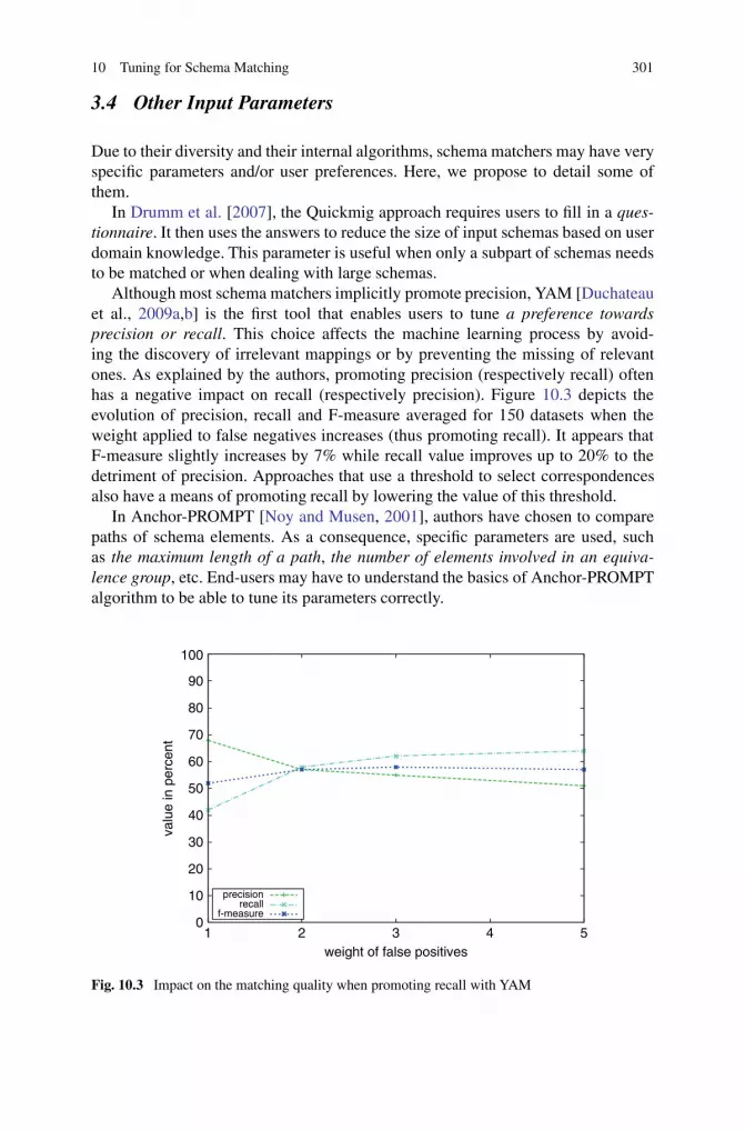
10 Tuning for Schema Matching 301
3.4 Other Input Parameters
Due to their diversity and their internal algorithms, schema matchers may have veryspecific parameters and/or user preferences. Here, we propose to detail some ofthem.
In Drumm et al. [2007], the Quickmig approach requires users to fill in a ques-tionnaire. It then uses the answers to reduce the size of input schemas based on userdomain knowledge. This parameter is useful when only a subpart of schemas needsto be matched or when dealing with large schemas.
Although most schema matchers implicitly promote precision, YAM [Duchateauet al., 2009a,b] is the first tool that enables users to tune a preference towardsprecision or recall. This choice affects the machine learning process by avoid-ing the discovery of irrelevant mappings or by preventing the missing of relevantones. As explained by the authors, promoting precision (respectively recall) oftenhas a negative impact on recall (respectively precision). Figure 10.3 depicts theevolution of precision, recall and F-measure averaged for 150 datasets when theweight applied to false negatives increases (thus promoting recall). It appears thatF-measure slightly increases by 7% while recall value improves up to 20% to thedetriment of precision. Approaches that use a threshold to select correspondencesalso have a means of promoting recall by lowering the value of this threshold.
In Anchor-PROMPT [Noy and Musen, 2001], authors have chosen to comparepaths of schema elements. As a consequence, specific parameters are used, suchas the maximum length of a path, the number of elements involved in an equiva-lence group, etc. End-users may have to understand the basics of Anchor-PROMPTalgorithm to be able to tune its parameters correctly.
0
10
20
30
40
50
60
70
80
90
100
1 2 3 4 5
valu
e in
per
cent
weight of false positives
precisionrecall
f-measure
Fig. 10.3 Impact on the matching quality when promoting recall with YAM

302 Z. Bellahsene and F. Duchateau
To the best of our knowledge, AgreementMaker [Cruz et al., 2007, 2009] is theonly tool that enables users to select a type of cardinality to be discovered. Giventwo input schemas, mapping cardinality is either 1:1, 1:n, n:1 or n:m. In a 1:1 con-figuration, the matcher is limited to discover mappings between one element of thefirst schema and one element in the other schema. Only a few matchers empha-size the complex mappings such as n:m, in which any number of elements in bothschemas can be involved in a mapping.
3.5 Conclusion
In this section, we have mainly presented user inputs, i.e., optional preferences andparameters applied to data. To sum up, the quality can be improved by using exter-nal resources and expert feedback. Several tools are based on machine learningtechniques either as a similarity measure (mostly at the instance level) or as a meansof combining the results of similarity measures. In both cases, training data is acrucial issue. Finally, many tools propose preferences or options which add moreflexibility or may improve the matching quality. The next section focuses on theparameters at the similarity measure level.
4 Similarity Measures Parameters
Similarity measures are the basic components of schema matchers. They can be usedas individual algorithms or combined with an aggregation function. Consequently,they may have internal parameters. In most cases, schema matchers do not enableusers to tune such low-level parameters. Another parameter applied to similaritymeasures is the threhold. It filters the pair of schema elements in different categories(e.g., is a correspondence, or should apply another type of similarity measure) basedon the output of the similarity measures. The last part of this section is dedicated toparameters specific to one or several matchers.
4.1 Internal Parameters
Similarity measures takes as input two schema elements, and it outputs a similaritybetween them. This similarity value may be a numerical value (e.g., a distance, areal in the range [0, 1]) or a relationship (e.g., equivalence, generalization). Similarto black-box algorithms, similarity measures can have internal parameters whichimpact the output. Due to the numerous available similarity measures, we do notintend to describe all of them with their parameters. Thus, we focus on two simpleexamples to illlustrate various types of such internal parameters.

10 Tuning for Schema Matching 303
The first example is the Levenhstein distance [Levenshtein, 1966] between twocharacter strings. It computes the minimal number of operations costs needed totransform one source string into the target string, where an operation is an insertion,deletion or substitution of a single character. Each operation may have a differentcost. For instance, a substitution can have a cost equal to 2, while insertions anddeletions may cost 1. Users can tune these costs according to their needs.
Between the two string dept and department, one requires six character inser-tions to transform dept into department. If an insertion costs 1, then the Levenhsteindistance between both strings is 6.
The second similarity measure that we study is Jaro Winkler [Winkler, 1999].This measure is also terminological and it compares two character strings. It extendsJaro measure by taking into account the order of the characters of both strings. Fur-thermore, it promotes higher similarity values between strings which share similarprefixes. Consequently, it includes two parameters. The first one is the length of theprefix substring while the second represents a constant scaling factor for how muchthe score is adjusted upwards for having common prefixes.
For further reading, we advise you to check the following list of resources[Cohen et al., 2003, Euzenat et al., 2004]. Several packages also describe similaritymeasures and their parameters, for instance SecondString1 or SimMetrics.2
4.2 Thresholds
Most similarity measures are normalized to return a value in the range [0, 1]. Amongall candidate pairs of schema elements, selecting the ones to propose as mappingscan be performed with a threshold. That is, all candidate pairs whose similarity value(from one measure or resulting from a combination of several measures) is abovea given threshold become mappings. Many tools [Avesani et al., 2005, Madhavanet al., 2001, Duchateau et al., 2008b, Drumm et al., 2007] have a threshold forselecting mappings. In most cases, a default value for the threshold is provided withthe tool, e.g., 0:6 for the string-matching threshold in S-Match [Giunchiglia et al.,2007]. COMACC [Aumueller et al., 2005] includes a threshold often combinedwith a top-K strategy (i.e., the best K correspondences are returned) and a MaxDeltastrategy (i.e., the best correspondence is returned with the closest ones, whose scoreonly differs by a Delta tolerance value). Conversely, APFEL [Ehrig et al., 2005] isa machine learning-based tools which features an automatic threshold tuning.
As the value distribution is very different from a similarity measure to another,a schema matcher can have one specific threshold for each similarity measure.This is the case with MatchPlanner [Duchateau et al., 2008a]. The extended ver-sion of this matcher enables the automatic learning of these thresholds, thanks to
1 SecondString (May 2010): http://sourceforge.net/projects/secondstring/.2 SimMetrics (May 2010): http://www.dcs.shef.ac.uk/�sam/stringmetrics.html.

304 Z. Bellahsene and F. Duchateau
machine learning techniques [Duchateau, 2009]. Similarly, Anchor-PROMPT [Noyand Musen, 2001] automatically computes the threshold values by averaging allsimilarity scores obtained on different runs with various parameter configurations.
In a broader way, authors of [Melnik et al., 2002] discuss the notion of fil-ters to select the mappings. These filters include not only the thresholds, but alsoconstraints between elements (types and cardinality) and a selection function.
Note that the threshold may be a parameter applied to a global similarity value,i.e., different similarity values are aggregated into a global one (given a strategy,see Sect. 5) and the threshold represents the decision-maker for accepting the pairof schema elements as a correspondence or not.
4.3 Various
Contrary to most aggregation-based approaches, Similarity Flooding/Rondo[Melnik et al., 2002, 2003] uses a graph propagation mechanism to refine simi-larities between schema elements. Thus, it holds specific parameters. The first oneis fixpoint formula, which enables the computation of updated similarities and theend of execution of the propagation. Different fixpoint formulas have been testedand evaluated in Melnik et al. [2002]. In addition, several filters are proposedto select among all candidate pairs the ones that Rondo displays as mappings.Constraints (on cardinality and types) or thresholds are examples of filters.
For a given schema element, we do not know in advance to how many elementsit should be matched [Avigdor, 2005]. However, approaches such as COMACC[Aumueller et al., 2005] or iMAP [Dhamankar et al., 2004] can display the top-Kcorrespondences (for future interactive mode), thus enabling users to disambiguatecomplex correspondences. Other works have been specifically designed to discovercomplex mappings, such as Porsche [Saleem and Bellahsene, 2009].
4.4 Conclusion
This section describes the parameters related to similarity measures. Although theyhave a significant impact, parameters inside the similarity measures are often setto default values. Schema matching tools let users tune the thresholds, which is atraditional decision maker for deciding what happens to a pair of schema elements.Finally, we have detailed specific parameters that users have to understand beforeoptimizing the matchers. In the next section, we reach one level up by studying theparameters related to the combination of similarity measures.

10 Tuning for Schema Matching 305
5 Parameters for Combining Similarity Measures
At a higher level, schema matchers have to combine the results computed by diff-erent similarity measures. This enables an increase of the matching quality inmost cases. However, the method for combining these results is crucial to derivehigh-quality mappings. The matcher first normalizes all similarity values. Differentstrategies are adopted to fulfil this goal. The first part of this section describes thesedifferent strategies. Several tools have been designed to enhance the interactivitywith users for selecting the best strategy. These tools are presented in the secondpart of this section. Finally, we focus on a specific strategy which is widely usedby matchers: the linear regression. It mainly encompasses weights to reflect eachsimilarity measure’s influence when combining them.
5.1 Strategy for Combining Similarity Measures
As many schema matchers use different similarity measures (based on string-matching, semantic, linguistics, structure, etc.), they need to adopt a strategy forcombining these measures. In most cases, schema matchers combine the resultscomputed by similarity measures, after a normalization step of the values (e.g., inthe range Œ0; 1�).
One of the simplest method to combine similarity values is the average function,used by tools such as ASID [Bozovic and Vassalos, 2008] or BMatch [Duchateauet al., 2008b]. Aggregating the similarity values using weights reflects the impact ofeach measure in the matching process. In other words, it is possible to promote mea-sures that are based on reliable resources (e.g., dictionaries, ontologies) by assigningthem a high weight (see Sect. 5.2 for more details).
More complex strategies are found within COMACC [Aumueller et al., 2005] inwhich similarity measures, types of nodes along with context, and fragments (parts)of the schema can be tuned. These strategies are then applied to the matrix built byCOMACC to deduce the correspondences that are displayed to the user. The threemain combination steps are aggregation (e.g., weighted, max or the default average),direction (e.g., unidirectional or stable marriage), and selection (e.g., threshold,maxN) [Do and Rahm, 2002]. A strategy is built by choosing a value for each ofthese three steps. Figure 10.4 depicts an overview of COMACC graphical interfacefor selecting a strategy. We also notice that a strategy may be performed on specificelements of the schemas (nodes, leaves, etc.).
MatchPlanner is a schema matcher based on decision trees to combine similaritymeasures. Although it has been extended by machine learning techniques to gen-erate these decision trees [Duchateau, 2009], users can provide their own decisiontrees to the system [Duchateau et al., 2008a]. There is no weight on the measures,but their order and position in the decision tree are crucial. Manually designing suchdecision trees is interesting when one wants to promote time performance or use aspecific similarity measure.

306 Z. Bellahsene and F. Duchateau
Fig. 10.4 COMACC user interface for selecting combination strategy
In SMB [Anan and Avigdor, 2008], the output of a weak similarity measure(called first-line matcher) is combined with a decision maker (or second-linematcher) to discover correspondences. The combination strategy depends on thedecision maker, which can be Maximum Weighted Bipartite Graph algorithm, StableMarriage, etc.
In YAM [Duchateau et al., 2009a,b], the combination of similarity measures isperformed by a machine learning classifier. Authors consider that any classifier isa matcher since it classifies pairs of schema elements as relevant or not. Thus, thecombination of the similarity measures depends on the type of classifier (decisiontree, Bayes network, neural network, etc.).
To sum up, many tools have designed their own strategies to combine similaritymeasures. However, most of them are based on weighted functions that the usersmay have to tune.
5.2 Weights in Formulas
Previously, we have detailed different types of strategies. One of the most com-mon strategy in the matching community is the linear regression to aggregate valuescomputed by similarity measures. In that case, the weights given to each measure isimportant according to the domain and the schemas to be matched. For instance, if adomain ontology is available, one may decide to give a high weight to the measures,which are able to use this ontology. However, tuning these weights manually stillrequires user expertise.

10 Tuning for Schema Matching 307
A simple example of aggregation function is demonstrated with BMatch[Duchateau et al., 2008b] or Cupid [Madhavan et al., 2001]. Their authors aggre-
gate the results of terminological measure with the ones computed by a structuralmeasure by varying the weights applied to each measure ( 1
2and 1
2, 1
3and 2
3, etc.).
In most tools, default values are given to these weights. They are mainly theresults of intensive experiments. For example, the default weights of COMACC’sname and data type similarity measures are 0:7 and 0:3, respectively [Do and Rahm,2002]. As explained in Glue [Doan et al., 2003] or APFEL [Ehrig et al., 2005], itis possible to tune the weights of an aggregation function automatically, thanks tomachine learning techniques.
To help tuning the weights in aggregating functions, we discuss the iMAPapproach [Dhamankar et al., 2004]. This matcher mainly provides a new set ofmachine learning-based measures for discovering specific types of complex map-pings (e.g., name is a concatenation of firstname and lastname). It also includes anexplanation module to clarify why a given correspondence has been discovered tothe detriment of another candidate. For instance, this module is able to describe thata string-matching classifier has a strong influence for a discovered correspondence.Thus, user can use this feedback to decrease the weight of this classifier.
5.3 Supporting Users to Revise Strategies
Although most matchers simply provide a graphical user interface to visualize theresults, recent works have pointed out a need for selecting the best strategy. Forinstance, including some mechanisms to easily update the weights of a function sothat users can directly analyse impacts of these changes.
Here, we describe recent works that aim at supporting users during the tasks ofselecting appropriate similarity measures and combining them. To combine themefficiently, weights have to be efficiently tuned. To support users during these tasks,two tools have been designed: AgreementMaker and Harmony. Whatever the tech-nique they use (interactions with users or strategy filters), they enable a revision ofthe current strategy by adding, removing or modifying parameters and similaritymeasures involved in the combination. We further describe each of these tools in therest of this part.
5.3.1 AgreementMaker
The originality of AgreementMaker [Cruz et al., 2007, 2009] is the capability ofmatching methods combination. Moreover, it provides facilities for tuning manuallythe quality of matches. Indeed, one of the interesting features of AgreementMaker isa comprehensive user interface supporting both advanced visualization techniquesand a control panel that drives the matching methods. This interface, depicted byFig. 10.5, provides the user facilities to evaluate the matching process, thus enablingthe user to be directly involved in the loop and evaluation strategies.

308 Z. Bellahsene and F. Duchateau
Fig. 10.5 AgreementMaker user interface for testing and comparing combination strategies
AgreementMaker provides a combination strategy based on the linear interpola-tion of the similarity values. The weights can be either user assigned or evaluatedthrough automatically determined quality measures. The system allows for serialand parallel composition where, respectively, the output of one or more methodscan be used as input to another one, or several methods can be used on the sameinput and then combined.
5.3.2 Harmony
Harmony schema matcher [Mork et al., 2008, Smith et al., 2009] combines mul-tiple matcher algorithms by using a vote merger. The vote merging principle isa weighted average of the match scores provided by each match voter. A matchvoter provides a confidence score for each pair of schema elements to be matched.Then, Similarity Flooding strategy [Melnik et al., 2002] is applied to adjust theconfidence scores based on structural information. Thus, positive confidence scorespropagate up the graph. An interesting feature of Harmony lies in its graphical userinterface for viewing and modifiying the discovered schema correspondences. Thisallows to assist the users to focus their attention on different ways. This assistanceis done through a filter, which is a predicate that is evaluated against each candidatecorrespondence. Harmony supports two kinds of filters. The first kind named linkfilters depends on the characteristics of a candidate correspondence. For example,applying the confidence filter will have an effect to graphically display those corre-spondences, whose match score falls within the specific range of values. The secondone named node filters is related to a schema element characteristics. This kind of

10 Tuning for Schema Matching 309
filters includes a depth and a sub-tree filter. For example, in Entity Relationshipschemas, entities appear at level 1, whereas attributes are at level 2. In this case, byusing the depth filter with value 1, the user may focus on matching entities, whilethe sub-tree filter is useful in tree based model such as XML schemas.
5.4 Discovering the Best Configuration
The previous section gathers tools that support users to manually find the beststrategy, i.e., the best method for combining similarity measures and its optionalparameters such as weights. This last part is dedicated to the tools that automaticallydiscover the best strategy: eTuner and YAM.
5.4.1 eTuner
eTuner [Lee et al., 2007] is not a schema matching tool, but it aims at automaticallytuning them. It proceeds as follows: from a given schema, it derives many schemaswhich are semantically equivalent. The mappings between the initial schema and itsderivations are stored. Then, a given matching tool (e.g., COMACC or SimilarityFlooding) is applied against the schemas and the results is compared with the storedset of mappings. This process is repeated until an optimal parameters configurationof the matching tool is found, i.e., the mappings discovered by the matching toolare mostly similar to those stored. eTuner strongly relies on the capabilities of thematching tool that it tunes. In most experiments, eTuner is able to improve matchingquality by 1 to 15% compared to the tools with their default configuration.
5.4.2 YAM
Similar to MatchPlanner, YAM [Duchateau et al., 2009a,b] takes some user inputsand it uses them to produce a schema matcher. Although MatchPlanner is limitedto combine the similarity measures with a decision tree, YAM is able to combinethem, thanks to any machine learning classifier. All low-level parameters such asweights and thresholds are therefore automatically tuned during the learning pro-cess. The combination of similarity measures only depends on the type of classifierselected by YAM. For instance, Fig. 10.6a, b depict two techniques for combiningsimilarity measures. The first one is based on a decision tree while the second oneuses NNge. With the decision tree, each pair of schema elements is matched withsimilarity measures from the root until a leaf node is reached, indicating whetherthe pair is a correspondence (T) or not (F). The value of the previously computedsimilarity measure is used to decide which edge (and consequently which similaritymeasure) should be executed next. Combining with a decision tree enables a sparingof resources since all similarity measures may not be computed for a given pair of

310 Z. Bellahsene and F. Duchateau
With a Decision Tree
a
With Nearest Neigbour Generalized Examples
b
Fig. 10.6 YAM: Examples of combination of similarity measures
schema elements. On the contrary, NNge classifier builds groups of nearest neigh-bour pairs of schema elements and then finds the best rule, expressed by booleanlogic, for each group. YAM currently includes 20 classifiers from the Weka library[Garner, 1995]. According to [Duchateau, 2009], experiments show that the tunedmatchers produced by YAM are able to improve F-measure by 20% over traditionalapproaches. Datasets mainly include average schemas from various domains, butalso two datasets involving large schemas. Similar to most machine learning-basedapproaches, authors have noticed the fact that the results may vary according totraining data, hence the need to perform different runs during experiments.
5.5 Conclusion
In this section, we have described the different strategies to combine similarity mea-sures and to tune them, mainly their weights. Fortunately, there exist several tools tohelp users revising or selecting the strategies. Visual tools support users for manu-ally configuring these strategies, mainly thanks to state-of-the-art GUI. Finally, wehave explored automatic approaches that are able to discover and tune the best strat-egy. In the following section, we are still heading one level higher. Indeed, the firstchoice of a user deals with the matching tool.
6 Matcher Selection
The selection of a schema matcher is obviously not a parameter: it does not fit withthe definitions provided in Sect. 2. But this is likely meta-tuning since one first needsto choose a schema matcher before tuning its parameters and using it. Furthermore,

10 Tuning for Schema Matching 311
some recent challenges directly refer to this issue [Shvaiko and Euzenat, 2008].The selection of a schema matcher may be guided by the results that it obtainsusing some benchmarking tools. In addition, a few recent works have been proposedto automatize this matcher selection. We describe each of them in the rest of thissection.
6.1 AHP
Authors of Malgorzata et al. [2006] have proposed to select a relevant and suit-able matcher for ontology matching. They have used Analytic Hierarchical Process(AHP) to fulfil this goal. They first define characteristics of the matching processdivided into six categories (inputs, approach, usage, output, documentation andcosts). Users then fill in a requirements questionnaire to set priorities for eachdefined characteristic. Finally, AHP is applied with these priorities and it outputsthe most suitable matcher according to user requirements. This approach has twodrawbacks: (1) there is no experiment demonstrating its effectiveness and (2) cur-rently there does not exist a listing of all characteristics for all matching tools. Thus,the user would have to manually fill in these characteristics.
6.2 RiMOM
RiMOM [Li et al., 2009] is a multiple strategy dynamic ontology matching system.Different matching strategies are applied to a specific type of ontology information.Based on the features of the ontologies to be matched, RiMOM selects the beststrategy (or strategy combination) to apply. When loading the ontologies, the toolalso compute three feature factors. The underlining idea is that if two ontologiesshare similar feature factors, then the strategies that use these factors should begiven a high weight when computing similarity values. For instance, if the labelmeaningful factor is low, then the Wordnet-based strategy will not be used. Eachstrategy produces a set of correspondences, and all sets are finally aggregated using alinear interpolation method. A last strategy dealing with ontology structure is finallyperformed to confirm discovered correspondences and to deduce new ones. Contraryto other approaches, RiMOM does not rely on machine learning techniques. It isquite similar to the AHP work by selecting an appropriate matcher based on input’sfeatures. RiMOM participated to the 2009 OAEI campaign [Zhang et al., 2009].Results show that the tool performed well in different tracks (anatomy, benchmark,instance matching). For instance, it achieves F-measures above 75% for all datasetsin the instance matching track.

312 Z. Bellahsene and F. Duchateau
6.3 YAM
Yet another matcher (YAM) [Duchateau et al., 2009a,b] enables the generation ofa la carte schema matchers according to user requirements. It uses a knowledgebase that includes a (possibly large) set of similarity measures and machine learn-ing classifiers. All classifiers are trained with scenarios from this knowledge base(and optionally provided by the users). Their individual results (precision, recall andF-measure), are computed and according to the adopted strategy, the classifier thatachieves the best quality is selected as schema matcher. The strategy mainly dependson user inputs. For instance, if (s)he wants to promote recall, then the classifier withthe best recall value is returned. If the user has provided expert mappings, then YAMselects as the schema matcher the classifier that obtains the best F-measure on thisset of expert mappings.
6.4 SMB
In Anan and Avigdor [2008], the authors propose a machine learning approach,SMB. It uses the Boosting algorithm to classify the similarity measures, dividedinto first-line and second-line matchers. The Boosting algorithm consists in iteratingweak classifiers over the training set while re-adjusting the importance of elementsin this training set. Thus, SMB automatically selects a pair of similarity measuresas a matcher by focusing on harder training data. An advantage of this algorithm isthe important weight given to misclassified pairs during the training. Although thisapproach makes use of several similarity measures, it mainly combines a similaritymeasure (first-line matcher) with a decision maker (second-line matcher). Empiri-cal results show that the selection of the pair does not depend on their individualperformance.
6.5 STEM
In a broader way, the STEM framework [Kopcke and Rahm, 2008] identifies themost interesting training data set which is then used to combine matching strate-gies and tune several parameters such as thresholds. First, training data is generated,either manually (i.e., an expert labels the entity pairs) or automatically (at random,using static-active selection or active learning). Then, similarity values are com-puted using pairs in the training data set to build a similarity matrix between eachpair and each similarity measure. Finally, the matching strategy is deduced fromthis matrix, thanks to supervised learned algorithm. The output is a tuned matchingstrategy (how to combine similarity measures and tune their parameters). The frame-work enables a comparative study of various similarity measures (e.g., Trigrams,Jaccard) combined with different strategies (e.g., decision tree, linear regression)whose parameters are either manually or automatically tuned.

10 Tuning for Schema Matching 313
6.6 Conclusion
This last section underlines the fact that selecting an appropriate schema matchingtool is the first issue to be considered. A few works have been proposed in thisdomain, which is recognized as one of the ten matching challenges for the nextdecade [Shvaiko and Euzenat, 2008]. If we exclude the AHP approach, for whichno experiment is provided, the remaining tools are all based on machine learningtechniques. This is an interesting feature since more datasets with correct corre-spondences are becoming available. However, discovering the features of a datasetto determine the most appropriate tool could be a challenging task.
7 Conclusion
In this chapter, we have provided an overview about what has been done for tuningschema matchers. At first, schema matchers enabled users to configure some oftheir low-level parameters (e.g., thresholds). They mainly allow to filter or selectthe output (the set of mappings). The next step deals with parameters for combiningsimilarity measures. They add more flexibility and the set of discovered mappingsdepends on the configuration of these parameters. More recently, some works wentup one level further by selecting the appropriate matcher for a given matching task.These tools lessen the burden of the user by automatically tuning most of the low-level parameters.
In the meanwhile, much effort has also been spent to integrate user preferencesor input data parameters. Most of them are based on machine learning techniques sothat schema instances or expert feedback can be used in the process. The integrationof such parameters is often an extra means for improving matching quality. Userpreferences such as the promotion of precision or recall let users choose how theyintend to manage post-match effort. These options are also interesting in contexts,where high dynamicity leads to a quick evolution of data sources, thus implyingthat a high precision is preferred. On the contrary, recall can be promoted when datasources are going to be fully integrated and manually checked.
Although a default configuration should still be proposed with a matcher, webelieve that we are heading towards a specific configuration of a schema matcherfor a given matching task. Namely, various properties of the matching scenario canbe computed by the tool. The latter can then deduce, based on previous experimentsor properties values, the best configuration. Visual tools have a strong impact on themanual post-match effort. By displaying the results of different matching strategies,one has sufficient information to check and (in)validate the mappings. Combinedwith user preferences, these tools would clearly reduce manual post-match effort. Tothe best of our knowledge, there are currently no works which study the impact ofthe tuning (during pre-match effort) over matching quality (and post-match effort).A balanced effort between parameters that would bring significant impact on thematching quality given a matching task might be further investigated.

314 Z. Bellahsene and F. Duchateau
Acknowledgements We thank our reviewers for their comments and corrections on this chapter.We are also grateful to colleagues who have accepted the publication of pictures from their tools.
References
Anan M, Avigdor G (2008) Boosting schema matchers. In: OTM ’08: Proceedings of the OTM2008 confederated international conferences, CoopIS, DOA, GADA, IS, and ODBASE 2008.Part I on on the move to meaningful internet systems. Springer, Heidelberg, pp 283–300.doi:http://dx.doi.org/10.1007/978-3-540-88871-0 20
Aumueller D, Do HH, Massmann S, Rahm E (2005) Schema and ontology matching withCOMACC. In: ACM SIGMOD. ACM, NY, pp 906–908
Avesani P, Giunchiglia F, Yatskevich M (2005) A large scale taxonomy mapping evaluation. In:ISWC 2005, Galway, pp 67–81
Avigdor G (2005) On the cardinality of schema matching. In: OTM workshops, pp 947–956Berlin J, Motro A (2001) Automated discovery of contents for virtual databases. In: CoopIS.
Springer, Heidelberg, pp 108–122Berlin J, Motro A (2002) Database schema matching using machine learning with feature selection.
In: CAiSE. Springer, London, pp 452–466Bellahsene Z, Bonifati A, Duchateau F, Velegrakis Y (2011) On evaluating schema matching and
mapping. In: Bellahsene Z, Bonifati A, Rahm E (eds) Schema matching and mapping. Data-694Centric Systems and Applications Series. Springer, Heidelberg
Bozovic N, Vassalos V (2008) Two-phase schema matching in real world relational databases. In:ICDE Workshops, pp 290–296
Carmel D, Avigdor G, Haggai R (2007) Rank aggregation for automatic schema matching. IEEETrans Knowl Data Eng 19(4):538–553. doi:http://dx.doi.org/10.1109/TKDE.2007.1010
Cohen W, Ravikumar P, Fienberg S (2003) A comparison of string distance metricsfor name-matching tasks. In: Proceedings of the IJCAI-2003. http://citeseer.ist.psu.edu/cohen03comparison.html
Cruz IF, Sunna W, Makar N, Bathala S (2007) A visual tool for ontology alignment to enablegeospatial interoperability. J Vis Lang Comput 18(3):230–254
Cruz IF, Antonelli FP, Stroe C (2009) Agreementmaker: Efficient matching for large real-worldschemas and ontologies. Proc VLDB Endow 2(2):1586–1589
Dhamankar R, Lee Y, Doan A, Halevy A, Domingos P (2004) iMAP: Discovering complexsemantic matches between database schemas. In: ACM SIGMOD. ACM, NY, pp 383–394
Do HH, Rahm E (2002) COMA – A system for flexible combination of schema matchingapproaches. In: VLDB. VLDB Endowment, pp 610–621
Do HH, Melnik S, Rahm E (2002) Comparison of schema matching evaluations. In: Web, web-services, and database systems workshop. Springer, London, pp 221–237
Doan A, Domingos P, Halevy AY (2001) Reconciling schemas of disparate data sources – Amachine learning approach. In: ACM SIGMOD. ACM, NY, pp 509–520
Doan A, Madhavan J, Dhamankar R, Domingos P, Halevy AY (2003) Learning to match ontologieson the semantic web. VLDB J 12(4):303–319
Drumm C, Schmitt M, Do HH, Rahm E (2007) Quickmig: Automatic schema matching fordata migration projects. In: CIKM. ACM, NY, pp 107–116. doi:http://doi.acm.org/10.1145/1321440.1321458
Duchateau F (2009) Towards a generic approach for schema matcher selection: Leveraging userpre- and post-match effort for improving quality and time performance. PhD thesis, Uni-versite Montpellier II – Sciences et Techniques du Languedoc. http://tel.archives-ouvertes.fr/tel-00436547/en/
Duchateau F, Bellahsene Z, Hunt E (2007) Xbenchmatch: A benchmark for xml schema matchingtools. In: VLDB. VLDB Endowment, pp 1318–1321

10 Tuning for Schema Matching 315
Duchateau F, Bellahsene Z, Coletta R (2008a) A flexible approach for planning schema matchingalgorithms. In: OTM Conferences (1), Springer, Heidelberg, pp 249–264
Duchateau F, Bellahsene Z, Roche M (2008b) Improving quality and performance of schemamatching in large scale. Ingenierie des Systemes d’Information 13(5):59–82
Duchateau F, Coletta R, Bellahsene Z, Miller RJ (2009a) (not) yet another matcher. In: CIKMACM, Hong Kong, pp 1537–1540
Duchateau F, Coletta R, Bellahsene Z, Miller RJ (2009b) Yam: A schema matcher factory. In:CIKM ACM, Hong Kong, pp 2079–2080
Ehrig M, Staab S, Sure Y (2005) Bootstrapping ontology alignment methods with APFEL. In:ISWC, ACM, NY, pp 1148–1149
Euzenat J, et al (2004) State of the art on ontology matching. Tech. Rep. KWEB/2004/D2.2.3/v1.2,Knowledge Web
Ferrara A, Lorusso D, Montanelli S, Varese G (2008) Towards a benchmark for instance match-ing. In: Shvaiko P, Euzenat J, Giunchiglia F, Stuckenschmidt H (eds) OM. CEUR-WS.org,CEUR workshop proceedings, vol 431. http://dblp.uni-trier.de/db/conf/semweb/om2008.html#FerraraLMV08
Garner SR (1995) Weka: The waikato environment for knowledge analysis. In: Proceedings of theNew Zealand computer science research students conference, pp 57–64
Giunchiglia F, Shvaiko P, Yatskevich M (2004) S-Match: An algorithm and an implementation ofsemantic matching. In: European semantic web symposium. ACM, NY, pp 61–75
Giunchiglia F, Shvaiko P, Yatskevich M (2007) Semantic matching: Algorithms and an implemen-tation. Tech. rep., DISI, University of Trento. http://eprints.biblio.unitn.it/archive/00001148/
Hernandez MA, Miller RJ, Haas LM (2002) Clio: A semi-automatic tool for schema mapping(software demonstration). In: ACM SIGMOD, Madison
Kopcke H, Rahm E (2008) Training selection for tuning entity matching. In: QDB/MUD, VLDB,Auckland, pp 3–12
Lee Y, Sayyadian M, Doan A, Rosenthal A (2007) etuner: Tuning schema matching software usingsynthetic scenarios. VLDB J 16(1):97–122
Levenshtein V (1966) Binary codes capable of correcting deletions, insertions and reversals. SovPhys Dokl 10:707
Li J, Tang J, Li Y, Luo Q (2009) Rimom: A dynamic multistrategy ontology alignment framework.IEEE Trans Knowl Data Eng 21(8):1218–1232. DOI http://dx.doi.org/10.1109/TKDE.2008.202
Li WS, Clifton C (2000) Semint: a tool for identifying attribute correspondences in heterogeneousdatabases using neural networks. Data Knowl Eng 33(1):49–84. DOI http://dx.doi.org/10.1016/S0169-023X(99)00044-0
Madhavan J, Bernstein PA, Rahm E (2001) Generic schema matching with cupid. In: VLDB.Morgan Kaufmann, CA, pp 49–58
Madhavan J, Bernstein PA, Doan A, Halevy AY (2005) Corpus-based schema matching. In:International conference on data engineering. IEEE Computer Society, Washington, DC, pp57–68
Malgorzata M, Anja J, Jerome E (2006) Applying an analytic method for matching approachselection. In: Shvaiko P, Euzenat J, Noy NF, Stuckenschmidt H, Benjamins VR, Uschold M(eds) Ontology matching. CEUR-WS.org, CEUR workshop proceedings, vol 225. http://dblp.uni-trier.de/db/conf/semweb/om2006.html#MocholJE06
Melnik S, Garcia-Molina H, Rahm E (2002) Similarity flooding: A versatile graph matching algo-rithm and its application to schema matching. In: ICDE. IEEE Computer Society, Washington,DC, pp 117–128
Melnik S, Rahm E, Bernstein PA (2003) Developing metadata-intensive applications with rondo.J Web Semant I:47–74
Mork P, Seligman L, Rosenthal A, Korb J, Wolf C (2008) The harmony integration workbench.J Data Semant 11:65–93
Naumann F, Ho CT, Tian X, Haas LM, Megiddo N (2002) Attribute classification using featureanalysis. In: ICDE. IEEE Computer Society, Washington, p 271

316 Z. Bellahsene and F. Duchateau
Noy N, Musen M (2001) Anchor-PROMPT: Using non-local context for semantic matching. In:Proceedings of IJCAI 2001 workshop on ontology and information sharing, Seattle, pp 63–70
Saleem K, Bellahsene Z (2009) Complex schema match discovery and validation throughcollaboration. In: OTM Conferences (1). Springer, Heidelberg, pp 406–413
Saleem K, Bellahsene Z, Hunt E (2008) Porsche: Performance oriented schema mediation. Inf Syst33(7–8):637–657
Shvaiko P, Euzenat J (2008) Ten challenges for ontology matching. In: OTM Conferences (2).Springer, Heidelberg, pp 1164–1182
Smith K, Morse M, Mork P, Li M, Rosenthal A, Allen D, Seligman L (2009) The role of schemamatching in large enterprises. In: CIDR, Asilomar
Winkler W (1999) The state of record linkage and current research problems. In: Statistics ofIncome Division, Internal Revenue Service Publication R99/04
Wordnet (2007) http://wordnet.princeton.eduYatskevich M (2003) Preliminary evaluation of schema matching systems. Tech. Rep. DIT-03-028,
Informatica e Telecomunicazioni, University of TrentoZhang X, Zhong Q, Shi F, Li J, Tang J (2009) Rimom results for OAEI 2009. http://oaei.
ontologymatching.org/2009/results/

Index
Accuracy, 273AgreementMaker, 21, 23, 302, 307AHP, 311Alignment API, 36, 278AlViz, 30, 35, 46AnchorFlood, 12Anchor-PROMPT, 301APFEL, 298, 299, 303, 307Approximate Schema Mappings, 96ASID, 299, 305ASMOV, 7, 21, 23Atoms, 116, 142, 195, 196, 199, 207, 216Attribute correspondences, 53–73AUTOPLEX/AUTOMATCH, 300
Backward compatibility, 152Benchmarks, 255, 261, 262, 265–268BioPortal, 44BizTalk mapper, 41, 42BMatch, 305, 307Both-as-view (BAV), 233
Certain answers, 136, 216Chase, 118, 196–198Chase-equivalent, 216Chase inverse, 203
exact, 202relaxed, 209–212
Chimaera, 66, 236, 237Clio, 39, 124, 127, 130, 140, 176, 213, 258,
270CoDEX, 169, 178Cognitive support framework, 32CogZ, 30, 35, 45, 46Collaborative ontology matching, 30COMA, 16, 22, 69
COMACC, 9, 12, 16, 17, 21, 22, 33, 35,46, 255, 276, 277, 286, 298, 300,303–305, 307
Combining similarity measures, 15, 305Completeness, 284Composition, 152, 166, 192, 199–201Conditional mapping, 96Configuration, 294, 297Constants, 114, 195Constraint Discovery, 125Contextual correspondences, 59–64Contextual schema matching, 54Core computation, 131Core universal solution, 118Correct mappings, 4, 77, 84, 298Correspondences, 113, 122, 255Crowdsourcing, 43Cupid, 7, 255, 307
Data exchange equivalent, 210Data exchange problem, 114Data integration, 40, 74–107, 121, 139, 231Data migration, 153Data translation performance, 271Data warehousing, 231Dataspace, 74–107DB2, 155, 158, 159, 161, 169, 175DB-MAIN, 155, 164DB-MeDEA, 155DCM, 19DIFF, 152, 156, 170, 181, 182, 185–188DiffDog, 169, 176DTD-Diff, 177DWQ, 231
Equality-generating dependencies, 115ETL system, 259, 272
317c� Springer-Verlag Berlin Heidelberg 2011
Z. Bellahsene et al. (eds.), Schema Matching and Mapping, Data-Centric Systemsand Applications, DOI 10.1007/978-3-642-16518-4,

318 Index
eTuner, 269, 309Evaluation, 5, 44, 49, 251, 253, 255, 261, 262,
264–266, 268, 269, 271–273, 275,277, 278, 280, 283, 287
Evolution mapping, 150, 152, 181, 184, 185,187, 191–222, 254–291
Exact chase inverse, 202Expert feedback, 298
F-measure, 5, 275, 277, 279Falcon-AO, 12, 15, 21, 22Fallout, 275, 278FCA Merge, 66, 236, 237Forward compatibility, 153Functional dependencies, 228
Global-as-view (GAV), 142, 196constraint, 196schema mapping, 196
Global-local-as-view (GLAV), 233constraint, 196schema mapping, 95, 196
GLUE, 9, 307Google Base, 76Ground instance, 195
Hamster, 10Harmony, 21, 23, 255, 308HECATAEUS, 155, 163HePToX, 127, 138, 140, 142, 270Holistic schema matching, 4, 19Homomorphic equivalence, 195Homomorphism, 117, 195HSM, 19Human effort, 272
IBM Infosphere Data Architect, 20iMAP, 304, 307Information capacity, 152, 224, 231Information loss, 279Instance, 112, 195
mapping, 151migration, 153
Instance-based ontology matching, 8Instance-level constraints, 225Interactive ontology matching, 31Interactive techniques, 29–51Inversion, 192ISLab, 270
KAON, 182, 184, 187
Labeled nulls, 114, 195Large-scale matching, 4–24Local-as-view (LAV), 132, 232
constraint, 196schema mapping, 196schema mapping, strict, 196s-t tgd, strict, 196
LSD, 299LSD/Glue, 298
Machine learning parameters, 298MapForce, 40MapMerge operator, 280Mapping adaptation, 166Mapping composition, 152Mapping inversion, 152Mapping system, 111, 129, 251Match workflow, 6–8Matcher selection, 15, 310Matching effectiveness, 4, 274Matching efficiency, 5, 270Matching quality, 5, 9, 43, 251, 266, 269, 285,
293, 294, 296–299, 301, 313MatchPlanner, 303, 305MeDEA, 164Merging, 221, 223–249
ontologies, 223schemas, 223
Meta-matching, 69Meta-tuning, 310Microsoft Biztalk, 20MiniCon algorithm, 136Minimality, 284Model management, 166, 187, 192, 238Monotonicity, 57–59Muse, 37, 46MySql, 172
NeOn toolkit, 37Nested equality-generating dependencies, 137Nested mappings, 132Nulls, labeled, 195
OnEX, 182, 185, 187Ontolingua server, 236Ontology, 180–186Ontology alignment evaluation initiative
(OAEI), 5, 9, 21, 47, 265

Index 319
Ontology changes, 180Ontology evolution, 180–186Ontology matching, 3–24, 29–51Ontology merging, 233Ontology modularization, 48Ontology versions, 180, 181OntoMap, 46OntoMediate Project, 43OntoView, 182, 184, 187Oracle, 155, 158–160, 169, 172–174, 179Overall metric, 273OWL Lite Alignment (OLA), 36, 46
P2P infrastructures, 142Parallel matching, 13, 22Parameters, 296, 297Partition-based matching, 12Pay-as-you-go, 76Performance, 251, 253, 255, 266, 268,
270–272Porsche, 19, 300, 304Post-match, 294PostgreSql, 172Precision, 275, 277, 279PRIORC, 15PRISM, 155, 162, 187, 217Probabilistic attribute correspondences, 67–70Probabilistic mapping, 19, 68, 74–107Probabilistic mediated schema, 74–107Probabilistic schema matching, 54Prompt, 34, 35, 44–46, 234PromptDiff, 181Protege, 34, 181, 182, 187Proximity, 285
Quality, 273, 275, 278, 280, 297, 299, 312Query answering, 86–92, 136Query discovery, 124Quickmig, 298, 300, 301Quick ontology matching (QOM), 11
Recall, 275, 277, 279Relational schema evolution, 154–166Relaxed chase inverse, 209–212Reuse of previous match results, 16RiMOM, 9, 15, 21, 311Rondo, 238, 239, 255, 304Routes, 283
SAMBO, 9
SAP Netweaver Process Integration, 20Schema evolution, 149–190Schema mapping, 111, 120, 195, 254, 256Schema mapping evolution, 191–222Schema mapping generation, 111, 113, 114,
129, 133, 254, 258, 259, 271, 279,282, 283
Schema matching, 3–24, 38–42, 53–73, 254,293, 295, 297, 299, 301, 303, 305,307, 309, 311, 313, 315
Second-order (SO) tgd, 206Self-tuning, 14Semantic attribute correspondences, 64–67Semantic matching, 53, 54, 70Similarity flooding, 276, 277, 286, 294Similarity matrix, 56Similarity measures, 302Smart, 234, 237S-Match, 67, 255, 300, 303SMB, 300, 306, 312SO tgd, 206Spicy, 127, 258, 271, 279SpicyCC, 258SQL server, 155, 158, 159, 161, 169, 174STBenchmark, 266, 267, 269, 271, 273, 275STEM, 312Stream systems, 188Strict LAV schema mapping, 196Strict LAV s-t tgd, 196Structurality, 284s-t tgd, 196Stylus Studio, 40
Tamino, 175TaxME2, 268Testbeds, 265THALIA, 269, 274Three-Way merge, 241Threshold parameters, 303Top-K correspondences, 63, 68Top-K schema matching, 71Training data, 298Tuning, 293, 295, 297, 299, 301, 303, 305,
307, 309, 311, 313, 315Tupelo, 255, 259Tuple generating dependency (tgd), 115, 196,
206, 258
Uncertain mappings, 80–97Uncertainty, 64, 67, 68Uncertainty in data integration, 77Universal solutions, 118, 128, 143

320 Index
Update propagation, 153, 156, 159, 170, 180,183, 187
Usage-based matching, 10User interaction, 245, 307User involvement, 30
Versioning, 153, 157, 171, 183View integration, 225
Warp10, 18Weights, 306
XBenchMatch, 266, 271, 278XEM, 169, 176, 179X-Evolution, 169, 178–179XML, 112, 137, 141XML schema evolution, 166–179XML schemas, 4, 12, 18, 22, 38, 121, 141, 167
Yet another matcher (YAM), 298, 300, 301,306, 309, 312