influence of mutation frequency on mutation profile in colon
TRANSCRIPT
University of ConnecticutOpenCommons@UConn
Doctoral Dissertations University of Connecticut Graduate School
12-21-2016
Influence of Mutation Frequency on MutationProfile in Colon CancerMichael J. [email protected]
Follow this and additional works at: https://opencommons.uconn.edu/dissertations
Recommended CitationGooch, Michael J., "Influence of Mutation Frequency on Mutation Profile in Colon Cancer" (2016). Doctoral Dissertations. 1338.https://opencommons.uconn.edu/dissertations/1338
Influence of Mutation Frequency on Mutation Profile in Colon Cancer
Michael James Gooch, PhD
University of Connecticut, 2017
Abstract
Colorectal cancers display a vast range in the number of mutations per tumor. It is
reasonable to assume that most mutations found in tumors are harmless passenger
mutations and that only a small fraction of mutations found in these tumors are driver
mutations that are responsible for initiation, progression and maintenance of the tumor.
My research project was to compare types of mutations, genes targeted and specificity
of gene targeting in high versus low mutation frequency tumors. My hypothesis is that
there are qualitative and quantitative differences in the mutation spectrum of
colorectal cancers that can be distinguished by the overall number of mutations
detected in the tumors. To address this hypothesis, I analyzed whole-genome
sequencing data from 223 colorectal cancers in the Cancer Genome Atlas. I compared
cancers with >1000 mutations per tumor to those that had 0-999 mutations per tumor. I
found that while the majority of genes mutated were found in both groups, distinct subsets
of mutated genes did occur in the two sample sets that were mutated more than expected
and more than in the other group. I found that those in the low mutation frequency set
had a high specificity for mutations in known cancer genes while those in the high
frequency set showed no significant clustering of mutations in known cancer genes.
Altogether my data supported that there were qualitative and quantitative differences in
the mutation spectrum of colorectal cancers based on the frequency of mutation in the
individual tumors.

i
Influence of Mutation Frequency on Mutation Profile in Colon Cancer
Michael James Gooch
B.S. Rutgers University, 2009
A Dissertation
Submitted in Partial Fulfillment of the
Requirements for the Degree of
Doctor of Philosophy
at the
University of Connecticut
2017

ii
Copyright by
Michael James Gooch
2017

iii
APPROVAL PAGE
Doctor of Philosophy Dissertation
Influence of Mutation Frequency on Mutation Profile in Colon Cancer
Presented by
Michael James Gooch, B.S.
Major Advisor Dr. Marc Hansen
Associate Advisor Dr. William Mohler
Associate Advisor Dr. Asis Das
Associate Advisor Dr. Christopher Heinen
Associate Advisor Dr. Gordon Carmichael
University of Connecticut
2017

iv
Acknowledgements
I have finally completed my PhD requirements, and would not have been able to do so
without the aid of many people. Both major labs I have been a member of during the
development of this research project contributed significantly to my experience and
successful completion of my dissertation.
My first thesis advisor, Dr. Richard Everson, helped me to develop the idea of examining
the spectrum of mutations in cancer, while other projects in his lab helped to increase my
experience and exposure to bioinformatics methods and available analysis software. He
and I share a vision of the significant role computational analysis of genetic data will play
in the future of biological and medical research.
My current thesis advisor, Dr. Marc Hansen, also helped me bring the ideas behind this
project into fruition. He helped me stay on course, and provided key guidance that
enabled me to solve problems that came up during analysis, and identify efficient and
accurate solutions.
Cynthia Alander, our lab technician, is a great resource, a good friend, and great moral
support. It was always a pleasure to share lab space with her.
I would like to thank Statisticians Dr. James Grady, and Dr. Yu-Bo Wang for their
significant assistance in choosing viable analytical methods which enabled a numerical
approach that created interesting results.
v
I would like to thank Dr. Ion Moraru and Jeffrey Dutton of CCAM for all of their technical
support and computational resources that I have used over the last several years. Their
help was instrumental in my acquisition of bioinformatics experience, and having access
to an environment capable of the computational demands of some projects.
I would like to thank Dr. Pramod Srivastiva and the Neag Cancer Center for continuing to
support me through my research and dissertation preparation. Without this aid I could not
have completed the program.
My committee members, Dr. Gordon Carmichael, Dr. Asis K. Das, Dr. Christopher D.
Heinen, and Dr. William Mohler, have also been an enormous resource for both my
dissertation work, and personal and professional development. Their questions and
observations improved the quality of my research in ways that should not be taken for
granted.
I also thank my friends and family for being supportive when times were difficult, and
being a significant source of motivation and moral support.

vi
I dedicate this dissertation to my wonderfully independent and cheerful daughter,
Kaelyn Siqi Gooch.
vii
Table of Contents
Approval page p. iii
Acknowledgements p. iv
Table of Contents p. v
List of Figures p. vi
Chapter 1. Genome sequencing, Cancer, The Cancer Genome Atlas,
Mutation Rates, and Mutation Profiles
p. 1
Chapter 2. Broad analysis of TCGA COAD Sample Populations, Sample
Grouping, and Differences Between Groups
p. 12
Chapter 3. Mutation Rate Group Differences in Mutation Types and Gene
Mutation Counts; Positively Deviating Outliers in Mutation
Count & Gene Length Trend
p. 37
Chapter 4. Kurtosis of mutation locations as a Possible Mutation Survey
Method and Detailed Analysis of Potentially Interesting Genes
p. 89
Chapter 5. Technical Difficulties Encountered During the Analysis p. 134
Chapter 6. Future Directions and Conclusion p. 139
References p. 148
viii
List of Figures
Chapter II
Figure 1. Number of mutations per tumor p. 18
Figure 2. Venn diagram of all mutated genes p. 20
Figure 3. Venn diagram of mutated genes, first ~100 p. 22
Figure 4. Venn diagram of mutated genes, first ~50 p. 24
Figure 5. List of ~100 most mutated genes p. 26-28
Figure 6. Tumor Staging p. 30
Figure 7. Genes related to repair and replication p. 32
Figure 8. DNA Microsatellite status of the samples p. 34
Figure 9. Venn Diagram of High and Low mutation groups split at 300
mutations.
p. 37
Figure 10. Venn Diagram of ~100 most mutated genes in High and
Low mutation groups split at 300 mutations.
p. 39
Figure 11. Venn Diagram of ~50 most mutated genes in High and Low
mutation groups split at 300 mutations.
p. 41
Chapter III
Figure 12. Low mutation count group mutation type counts p. 49-52
Figure 13. High mutation count group mutation type counts p. 53
Figure 14. Low mutation group mutation type count categories p. 55-58
Figure 15. High mutation group mutation type count categories p. 59
Figure 16. Low mutation group mutation type proportions p. 61-64
ix
Figure 17. Low mutation group mutation type category proportions p. 66--69
Figure 18. High mutation group mutation type (and category)
proportions
p. 71-73
Figure 19. Results of two-sided Welch two sample T test on mutation
type data
p. 75-77
Figure 20. Scatterplot of gene based counts from non-split data p. 79
Figure 21. Gene mutation counts derived from split data p. 81
Figure 22. Gene mutation counts derived from split data zoomed in p. 83
Figure 23. Gene counts with lengths from split populations p. 85-87
Figure 24. 100 Genes with highest studentized residuals from each
population
p. 90-92
Chapter IV
Figure 25. Illustrations of kurtosis shapes p. 101
Figure 26. Kurtosis values for Vogelstein Subtly mutated gene list for
TCGA data
p. 109-110
Figure 27. Kurtosis values for selected genes from linear regression
table
p. 113-115
Figure 28. Genes known to be associated with colon adenocarcinoma
their known mutations, and their kurtosis values in the high
and low mutation populations
p. 118-119
Figure 29. COAD mutations classified by types p. 121
Figure 30. Selected genes of interest p. 123
x
Figure 31. Known cancer related genes p. 126-128
Figure 32. Two keratin associated proteins found on chromosome 17 p. 130
Figure 33. ERICH6B / FAM194B p. 132
Figure 34. ZNF814 p. 134
Figure 35. DSPP p. 136-137

1
Chapter 1
Genome sequencing, Cancer, The Cancer Genome Atlas, Mutation Rates, and
Mutation Profiles
2
Introduction
There were three technological breakthroughs that were critical to the success of
my thesis project. The first of these was the successful completion of the human genome
sequencing project that provided the template upon which my project could be built.
Accompanying and enabling the human genome sequencing project was the
development of technologies that enabled rapid and accurate sequencing of entire
genomes. Finally, the development of highly curated databases storing both the normal
genome sequence as well as the variation within the “normal” human genome together
with the genomic sequences of human tumors was a critical preliminary step in my project.
Parallel with this technological development, there was the conceptual advance that
mutations in certain genes were critical in driving the process of tumorigenesis while
mutations in other genes were simply passengers that were carried along as part of a
stochastic process. Together these prior steps laid the foundation for my work.
History of Human Genome Sequencing Project
The Human Genome Project was initiated in 1990 with the goal of obtaining the
full human genomic DNA sequence (1). The project did not seek to sequence
heterochromatic regions such as centromeres or telomeres, but rather focused on
euchromatic regions (1,2). When the project began, the NIH Genome program was
headed by James Watson, who was succeeded by Francis Collins in 1993 (3).
There was also a privately funded quest launched by Craig Venter and the firm
Celera Genomics in 1998 (4). It was able to proceed much faster and more cheaply than
the publicly funded HGP by making use of data that was released by the HGP. This effort
was a profit seeking one, and Celera attempted to obtain patents on a large number of
3
genes (5). Celera promised to publish their results but there was suspicion that they would
not permit free redistribution or scientific use of the data (5–7). Their intentions compelled
the publicly funded project to publish their results first (6,7). In March 2000, then president
Bill Clinton announced that the human genome sequence should be made freely available
to all researchers and that access should be unencumbered (8).
Initial drafts of the human genome became available in June 2000 and working
drafts were completed by February 2001(1,6,7,9). The project was declared complete in
April 2003 (10). The sequencing speeds during this 13-year time period increased
dramatically as technologies improved, allowing the project to be completed 2 years
earlier than initially planned. The genomic sequence continues to be updated and revised
as directed by improvements in technology and accuracy of the underlying data (11).
Sequencing technologies
DNA sequencing technologies began being developed and used in the 1970s (12).
Initially, labor intensive processes like Maxam & Gilbert sequencing resulted in maximum
read lengths of about 100 bases at the time of its development (12). This was eventually
overtaken by Sanger’s enzyme-driven sequencing process, which was able to achieve
significantly reduced manual labor requirements and increased read lengths as
improvements in gel and dye technologies were developed (12,13). Successive
improvements have led to current processes including SOLiD and Illumina next
generation high throughput sequencing technologies (13–15), and very powerful variants
of Sanger’s original sequencing method that have been greatly improved by modern
technological advances (13,16). Parallel improvements in multiple technologies, including
electrophoresis gels, DNA base identification and detection, ranging from radiolabels, to
4
detecting pyrophosphate released during nucleobase-specific reactions, to various
technology-specific fluorescent dyes, while machine driven automation technologies have
brought DNA sequencing from a very labor intensive process resulting in very inefficient
output, to a relatively easier and much cheaper process that enables the sequencing of
enormous eukaryotic genomes within days, generating vast amounts of data that enable
the detection of mutations throughout the genome. Various read selection techniques like
exome sequencing (17,18), shotgun sequencing (19–21), cDNA sequencing of RNAs (19)
and others have been developed that make specific types of experimental analysis
possible.
The Sanger sequencing method can now make use of colored fluorescent dyes
allowing sequencing to proceed in a single reaction, paired with arrays of capillary gels in
re-usable capillaries that allow the use of more powerful electric fields resulting in faster
sequencing than could be achieved in slab gels (12,13). This technology was achieving
read lengths of about 1300 bp in about 2 hours in the year 2000 (12,13). The benefit of
these very long read lengths and arrays of capillaries allowing multiple samples to run at
once, analogous to parallel “lanes” in older slab gels, enabled the rapid completion of the
human genome project (13,16).
The current Next Generation high throughput methods such as Illumina
sequencing do not achieve the same long individual read lengths as Sanger sequencing
(13,16), but what they lack in length, they more than make up for in read numbers,
allowing sequencing runs to cover entire genomes with large numbers of reads per locus
(13). The paired end nature of the sequencing (13) also allows software analysis to
provide insights into phenomena such as alternative splicing, despite the shorter read
5
lengths. This technology can read 2 x 150bp in most current machines and 2 x 300bp on
the MiSeq series (14,22). (2 x N refers to the first N bp on each “side” of the DNA strands).
The machines range in output from 25 million reads per run to 6 billion reads per run, and
run times range from 4-24 hours to more than 3 days, depending on the sequencer
platform.
Implications for research in human disease
The completion of the human genome project’s main goal and the advent of these
sequencing technologies has been a boon for all biological research, but in particular it
enabled a much deeper probing of the genomic changes occurring in heritable diseases
and various kinds of cancers than had previously been possible.
History of TCGA
The Cancer Genome Atlas (TCGA) is an ambitious project that seeks to map
mutations and clinical characteristics of 33 types of human cancers (23). It was formed
as a collaboration between the National Cancer Institute and the National Human
Genome Research Institute. The TCGA dataset was generated by the TCGA Research
Network, which is composed of a broad coalition of different research centers and
laboratories. Much of the data has been made publicly available. Identifiable data,
including a portion of the patient information and any germ-line mutations or relevant
SNPs, as well as the raw sequencing data, require additional agreements and security
procedures from researchers and their institutions in order to gain access.
Across all tumor types, 11091 samples have been sent to the TCGA project for
analysis. Out of these, 11077 have data available in the database. These are not evenly
6
distributed amongst the tissue types, probably due to varying rates of incidence. 16 tumor
types have between 300-600 samples with data, 9 tumor types have between 100-300
samples with data, 8 tumor types have less than 100 samples with data, and just one,
breast invasive carcinoma has more than 600, with 1097 samples with data. I noticed that
34 rows were in the table of tumor types on the TCGA website. I believe that while colon
and rectal cancers are sometimes listed separately, the project treats them as the same
cancer type when they provide the value of 33 for the number of tumor types.
Concept of Drivers and passengers
One of the big questions in cancer research is how many mutations are necessary
to cause a tumor and what types of genes are involved (24). Bert Vogelstein and others
have long proposed that multiple steps are necessary during the tumorigenic process (25).
Early attempts to correlate mutations with tumor stage particularly in colon cancer
resulted in a linear multistep process now known as the Vogelstein model (26). It
proposed that each of three steps, initiation, promotion and progression could be
correlated with specific mutations (27). Although this model has now been shown to be
overly simplistic (28), it did provide the foundation for subsequent work on the concept of
driver mutations.
In two seminal papers by Sjöblom et al (29) and Wood et al (30) from Bert
Vogelstein’s group, they were some of the earliest to describe the use of genome
sequencing approaches to determine what mutations contribute to cancer pathogenesis,
and to classify them appropriately (31). Mutations that do not contribute to cancer
pathogenesis are called passengers, while the mutations that do contribute to cancer
pathogenesis are called drivers (32).
7
In addition to this concept they examined mutation patterns, and frequency of
mutations at different loci within populations of tumors (29–31). One of the ways they
visualize these mutations is a 3 dimensional histogram “map”. On one axis is the
chromosome number and on the other axis is the position along the chromosome. The
height of the peaks is determined by the number of mutations within the region. Using this
technique, they are able to find that certain genes are “gene mountains”, with very tall
peaks, some are “gene hills” which are mutated an intermediate amount, while other
genes are barely a blip on such a graph. They then examine how mutations cluster within
the protein structure of a gene product as well as where the mutated genes fit within
different signaling pathways.
While these efforts were groundbreaking, there are some important details
regarding how scientists might assign driver and passenger status to a mutation that need
to be further explored. It is the combination of which gene is mutated, at which location,
and the precise change, that actually determine whether the mutation will be pathogenic
or not. It isn’t sufficient to consider a mutation a driver, simply because it happens within
a gene known to have associations with cancer.
Additionally, it is possible that there are some mutations that may contribute
conditionally, if paired with other mutations. One such theoretical example would be Myc
mutations in Burkitt’s lymphoma described by Bauer et al (33). In this case, a driver
mutation in Myc leads to increased proliferation as well as increased rates of apoptosis.
The increased rate of apoptosis balances the increased rate of proliferation preventing
the tumor from increasing in size. A subsequent mutation in another gene that reduces
the rate of apoptosis would lead to an increased growth of the tumor. Thus the initial driver
8
mutation is dependent on the second driver mutation for there to be a benefit to
tumorigenesis. Other more complex scenarios may exist in genes that are part of
signaling pathways. For example, multiple mutations disrupting different parts of a
pathway might or might not produce a greater tumorigenic effect together than they would
by themselves.
Another example of conditional driver mutations would be a hemizygous mutation
in a tumor suppressor gene. If one copy of a tumor suppressor gene was mutated
somatically or was inherited with a defective sequence and did not produce a haplo-
insufficiency effect, and then a subsequent deletion or disruptive mutation that disabled
the remaining functional copy on the other chromosome would be required to produce the
tumorigenic effect. However, if only 1 such mutation occurred and the other functional
copy remained, this mutation would not contribute to tumorigenesis. Technically this kind
of mutation would rightly be considered a driver, but it would be a conditional driver, since
its driver effect is dependent on the absence of both functional alleles.
While silent mutations that do not affect the amino acid composition of a gene, or
functionally synonymous amino acid changes, would likely be passenger mutations (since
they do not affect the function of the gene), in some cases even mutations that destroy
the function of a gene could also be considered passenger mutations. If the tumorigenic
process requires a gain-of-function mutation in a gene to produce a tumorigenic effect,
then mutations that inactivate the protein would actually be passenger mutations.
I wanted to examine the effect that significant differences in mutation frequency
had on the patterns of mutations that were found in tumors. Heritable defects in genes
related to DNA mismatch repair are found in the familial syndrome, Lynch Syndrome (34),
9
which is known to cause very high rates of colon cancer (34), as well as broadly raise the
rates of cancers in other tissues as well (34). This same repair mechanism can also be
damaged or disabled in a somatic way in a subset of tumors in individuals that do not
have a heritable defect (34,35). For my thesis project, it seemed that colon cancer would
be a good model cancer type in which to examine mutation patterns to see if the idea that
variations in mutation frequency in each tumor would significantly affect which genes were
mutated in that tumor was plausible and to examine some details of the phenomenon if
the hypothesis was true.
Colon Cancer
Colon adenocarcinoma is the third most common cancer in the USA (36,37).
According to Cancer.org, 93,090 new cases of colon cancer and 39,610 new cases of
rectal cancer were predicted to occur in the U.S. in 2015 of which 49,700 deaths from
colon and rectal combined were anticipated (38). From 2003-2007 men showed an
incidence of 57.2/100,000 and mortality of 21.2/100,000 and women had an incidence of
42.5/100,000 and a mortality of 14.9/100,000. Understanding the defects that lead to
these cancers may give us better tools to manage disease and potentially make available
new avenues of attack to destroy tumors more effectively without serious harm to patients.
A fraction (25%) of colorectal cancers result from inherited mutations (36), while
the rest (75%) are a result of somatically acquired mutations. Colorectal cancers arise
through several different pathways. One commonly observed mechanism in colorectal
cancer involves defects in the DNA mismatch repair (MMR) pathway (39). MMR defects
account for 15% of colon cancers (36) while most other cases (~85%) are caused by
other processes involving chromosomal instability. In either case, cells that lose their
10
ability to repair replication errors and/or DNA damage have an increased mutation rate
many times greater than that of normal cells (40,41). Presumably, any condition that leads
cells to have either increased rate of mutation, an inability to recognize damage and
undergo apoptosis, or a reduced ability to repair DNA damage or replication errors would
increase the risk of cancer by contributing to tumor initiation, progression and metastasis.
Even before the discovery of specific mechanisms that caused increased genetic
instability and mutation rates, genetic instability had been considered to be highly
important in human cancers (42). While mechanisms of DNA repair, their mutations, and
the effects of mutations in these genes on colon cancers have been an area of intense
research (43–46), the patterns of mutations that occur with different repair defects are still
poorly understood (31). The specific types of mutations that occur could be significantly
affected by the identity of the initially disrupted repair gene or the nature of the mutation,
which could lead to distinct patterns of targeted mutations.
I was curious to determine whether the spectrum of genes in which somatic
mutations occurred in colorectal cancers differed depending upon the overall number of
mutations that occurred in each individual tumor. I wanted to know if separating tumors
with high numbers of mutations from those with relatively few mutations altered the
patterns of driver mutations in the tumors. To do this, I proposed to analyze whole genome
sequencing data from colorectal cancer tumors to test whether the tumors have different
patterns of mutated genes based on the overall number of mutations that occurred in the
tumors. My reasoning is that if I can show that there is a difference in types of mutations
or genes that are being mutated between tumors with a very large number of mutations
and those with a lower mutation frequency, future studies may discover that these

11
differences contain patterns that may be associated with the probability of recurrence,
effectiveness of treatments, and patient outcome.
12
Chapter 2
Broad analysis of TCGA COAD Sample Populations, Sample Grouping, and
Differences Between Groups
13
Introduction
In order to study the effect of mutation frequency on tumor genetics I needed to
choose a tumor mutation dataset to use as an example. The Cancer Genome Atlas
project has been collecting and analyzing tumor samples from numerous kinds of cancers
and collecting the data into a publicly accessible database (47). Of primary interest to me
was the effect of mutation rate on mutation spectrum in cancer. I chose to use colon
adenocarcinoma as the model system for my analysis due to its association with tumors
having genomic instability and high mutation rates (35,48).
Colorectal cancer in general has high rates of genomic instability (49–51). Colon
cancer genomic instability has previously been investigated in regard to diseases that
produce microsatellite instability, such as hereditary nonpolyposis colorectal cancer (52–
54), (Lynch Syndrome), and similar conditions associated with defects in DNA mismatch
repair proteins or failure to express them (35,55).
Ongoing clonal adaption is a common and necessary trait of cancers leading to
the concept that cancer is a Darwinian evolutionary process (50,56). As cancers and
precancerous tissues undergo random selection during initiation and progression, their
rates of mutation show variation (57,58). This variation in mutation rate drives the
deterministic mechanism for both passenger and driver mutations. As a consequence, it
is likely that those cancers that have lower mutation rates would likely show a
retrospective bias towards mutations that actually contribute to the cancer phenotype
while cancers that have a high rate of mutation would show a retrospective bias towards
more stochastic mutations. This is because a low rate of mutation would provide greater
opportunity for the developing tumor to undergo clonal selection before many mutations
14
accumulate. In my analysis, I lacked any physical access to any cells from the tumors
that I proposed to examine. Therefore, I could not measure the mutation rate in these
tumor cells directly. However, numbers of mutations occurring in each cancer could act
as a surrogate for mutation rate. Therefore, by comparing the number of mutations that
are found in individual tumors, it may be possible to correlate mutation frequency with its
effects on clonal selection.
Other factors may also have an effect on the retrospective bias for mutations.
There may be structural or chemical factors that could lead specific genes to be more
likely to experience mutation than others depending on the mechanisms driving the
change in rate of retained unrepaired mutation. It is also possible that the cancer staging
may correlate to how severely genetically damaged the tumor cells have become
although I did not actually expect later staging to correlate very strongly with mutations,
since high mutation rate tumors seemed to have more favorable outcomes in general
than normal tumors.
Together, these factors suggested to me that it was likely that there would be a
qualitative difference in the spectrum of genes that underwent mutation during cancer
that was dependent on the number of mutations in the individual tumors.
Hypothesis
As the number of mutations within a tumor increases, there will be a shift in which
genes undergo mutations in tumors collected from cancer patients. Tumors with low
numbers of mutations should show a bias towards mutations in cancer driver genes that
should not be apparent in tumors with high numbers of mutations.
15
Methods
The TCGA dataset mutation data is stored in MAF format. A program was prepared
to count mutation entries in the dataset according to sample ID, mutation type, and Gene
Symbol. Individual counting functions were prepared for each of these with corresponding
tab separated output. Originally there was a pair of files, with data resulting from SOLiD
sequencing being kept separate from data that resulted from Illumina sequencing. The
bulk of the data were in the Illumina dataset, so to avoid potential complication in the
analysis, I chose not to use the SOLiD file.
As noted, I lacked physical access to any cells from these tumors with which to
attempt to measure a mutation rate directly. The TCGA project itself did not include
measurement of mutation rate as one of their analysis methods either. As a result, I had
to use an indirect method to get a rough handle on the mutation rate. I decided to use the
total count of somatic mutations within the TCGA dataset as a proxy for this. I chose not
to analyze larger chromosomal structural changes as I felt that this would complicate the
analysis unnecessarily.
I wrote a program in Python to count single nucleotide mutation types (substitutions,
insertions, and deletions), separating the counts according to original base and resulting
base. I also enabled this tool to count mutations by Sample ID and Gene symbol. This
was accomplished using a counter object sub-classed into multiple other types defined to
use different counting rules. My method was to use strings in a map data type that stored
integers using strings as the key. Gene Symbol and Sample ID were used as keys, and I
constructed a key for the mutation types using the original and changed bases, using
16
dash as a placeholder for indels. The script allowed any combination of the counters to
be used simultaneously, each outputting their counts to separate files.
To determine the effect of the mutator phenotype on these counts, I also decided
to divide the tumors into two groups, a high mutation group and a low mutation group,
and ran the same counting process on the separated groups as I ran on the entire dataset
in the previous analysis. To accomplish this, I wrote an additional program to use the
output of the sample ID counting function in combination with integers provided by the
user, to split an MAF file, entry by entry, into grouped outputs. These output entries, still
in MAF format, were then run through the original counting script again and the results
were examined.
Count boundaries used to split the data were selected based on the location in a
sorted graph of total mutation counts where it seemed there was a significant difference
in the number. I did check the MSI status of these samples at a later time, and the results
of this split matched fairly well with this boundary. The MSI high samples mostly fell into
the higher mutation group where the MSI low were mostly in the lower mutation group.
Clinical staging was analyzed for correlation to mutation counts as well.
I requested clinical information alongside the somatic mutation data, when I first
obtained the TCGA dataset. These files were examined for their structure and information
content to determine where the relevant data were, and then were used to combine this
information into a useful table containing the information of concern. The sample IDs were
used to cross compare the various categorizations and mutation counts to determine if
there were any statistically significant correlations.
17
Results
Population Level Mutation Information
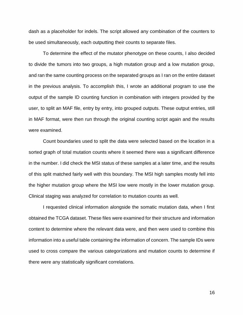
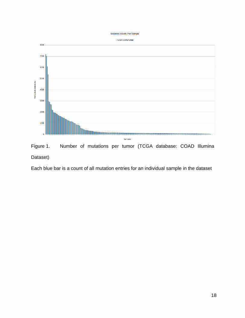
The first analysis performed was to count the number of mutations in each sample
and view this data. I chose to sort the results from highest to lowest and plot them in a
bar graph. The values of the mutations per tumor showed a distribution of samples with
a long trailing tail of lower value counts and a relatively shorter collection of samples with
very high count values. There seemed to be at least two different trends in the population,
which could be the result of shifts in mutation rate. If one was to draw trend lines for the
low mutation side of this plot, and the high mutation side of this plot, separately, they
would have very different slopes.
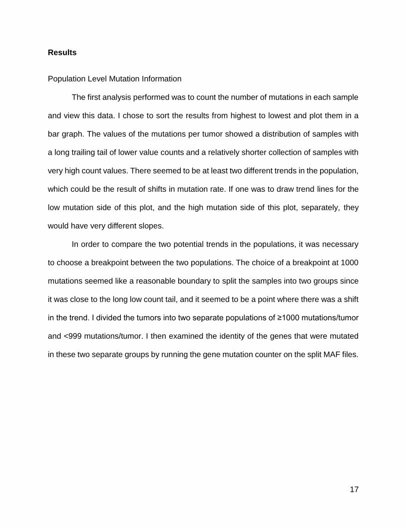
In order to compare the two potential trends in the populations, it was necessary
to choose a breakpoint between the two populations. The choice of a breakpoint at 1000
mutations seemed like a reasonable boundary to split the samples into two groups since
it was close to the long low count tail, and it seemed to be a point where there was a shift
in the trend. I divided the tumors into two separate populations of ≥1000 mutations/tumor
and <999 mutations/tumor. I then examined the identity of the genes that were mutated
in these two separate groups by running the gene mutation counter on the split MAF files.
18
Figure 1. Number of mutations per tumor (TCGA database: COAD Illumina
Dataset)
Each blue bar is a count of all mutation entries for an individual sample in the dataset

19
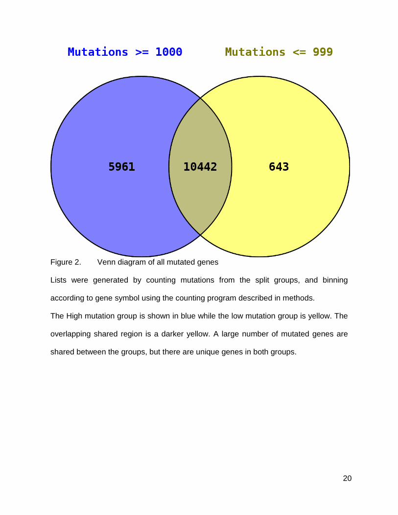
When looking at the results for all genes, since a very large portion of the human
genome was included in the set of genes with mutations, there was an expected
significant amount of overlap between the two groups of tumors. In total, both lists
represented 17,046 genes, which is a majority of the predicted 20,000 to 25,000 human
genes (2,59). However, even within this very large gene set, the two groups had distinct
sets of genes. So I decided to look at overlaps within smaller, more significantly mutated
subsets.
20
Figure 2. Venn diagram of all mutated genes
Lists were generated by counting mutations from the split groups, and binning
according to gene symbol using the counting program described in methods.
The High mutation group is shown in blue while the low mutation group is yellow. The
overlapping shared region is a darker yellow. A large number of mutated genes are
shared between the groups, but there are unique genes in both groups.
21
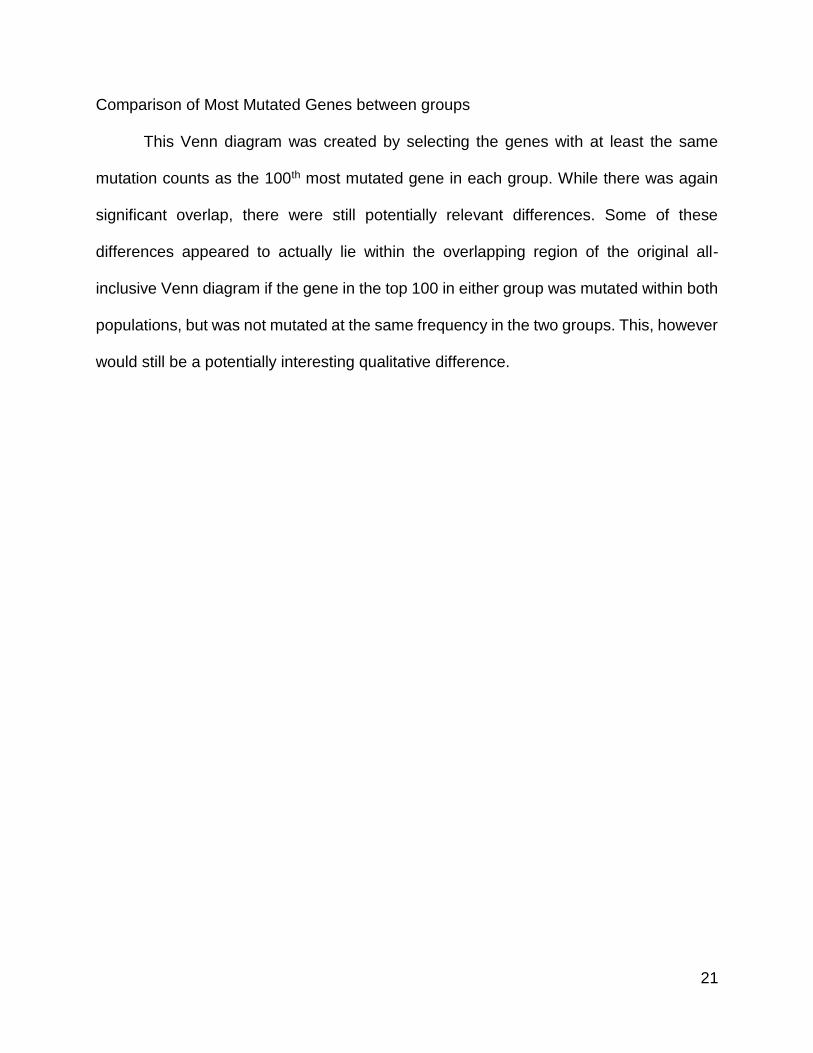
Comparison of Most Mutated Genes between groups
This Venn diagram was created by selecting the genes with at least the same
mutation counts as the 100th most mutated gene in each group. While there was again
significant overlap, there were still potentially relevant differences. Some of these
differences appeared to actually lie within the overlapping region of the original all-
inclusive Venn diagram if the gene in the top 100 in either group was mutated within both
populations, but was not mutated at the same frequency in the two groups. This, however
would still be a potentially interesting qualitative difference.

22
Figure 3. Venn Diagram of Mutated Genes, First ~100
Lists were generated by selecting all genes that had at least the same number of
mutations as the 100th after sorting by mutation count. The list of gene based counts
was generated using the counting program on the split data files. The High mutation
group is yellow, the low mutation group is red, and the overlap is orange.

23
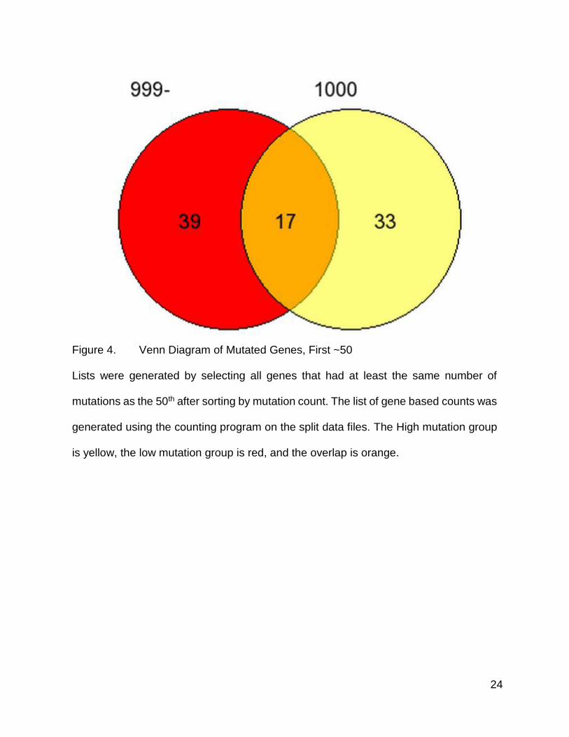
As in the previous diagram, this Venn diagram was created by selecting the genes
with at least the same mutation counts as the 50th most mutated gene in each group. This
smaller list again recapitulated the pattern observed in the larger previous lists. This same
pattern of overlapping and non-matching genes remains visible even when filtering the
list according to the most mutated genes. This resembles a chaotic equation plot, like a
fractal (60–62), where the appearance remains similar regardless of magnification.
24
Figure 4. Venn Diagram of Mutated Genes, First ~50
Lists were generated by selecting all genes that had at least the same number of
mutations as the 50th after sorting by mutation count. The list of gene based counts was
generated using the counting program on the split data files. The High mutation group
is yellow, the low mutation group is red, and the overlap is orange.
25
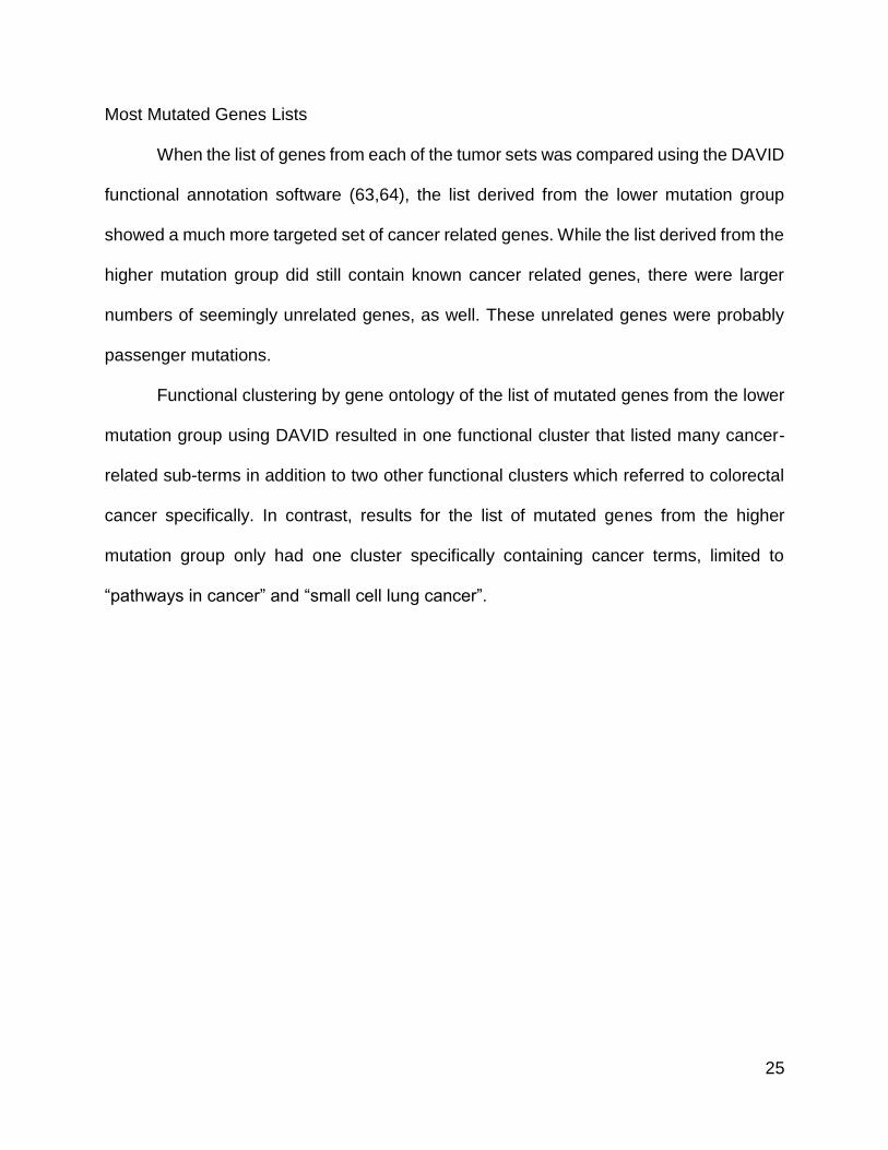
Most Mutated Genes Lists
When the list of genes from each of the tumor sets was compared using the DAVID
functional annotation software (63,64), the list derived from the lower mutation group
showed a much more targeted set of cancer related genes. While the list derived from the
higher mutation group did still contain known cancer related genes, there were larger
numbers of seemingly unrelated genes, as well. These unrelated genes were probably
passenger mutations.
Functional clustering by gene ontology of the list of mutated genes from the lower
mutation group using DAVID resulted in one functional cluster that listed many cancer-
related sub-terms in addition to two other functional clusters which referred to colorectal
cancer specifically. In contrast, results for the list of mutated genes from the higher
mutation group only had one cluster specifically containing cancer terms, limited to
“pathways in cancer” and “small cell lung cancer”.
26
27
28
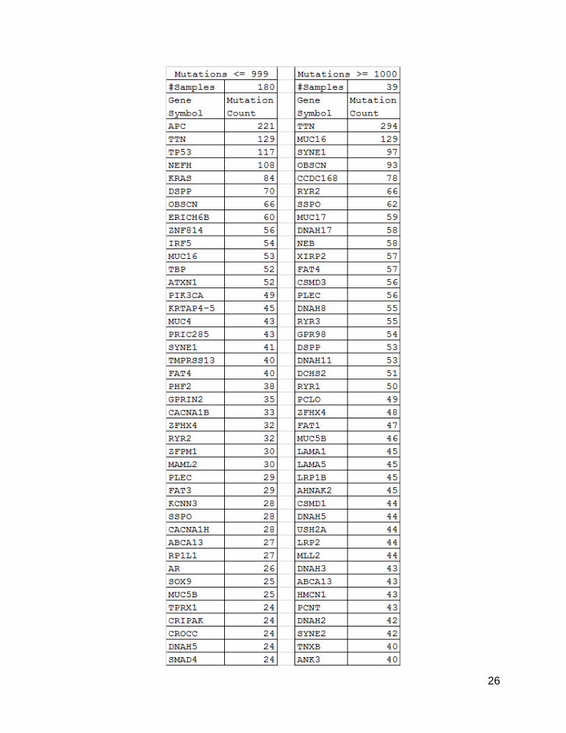
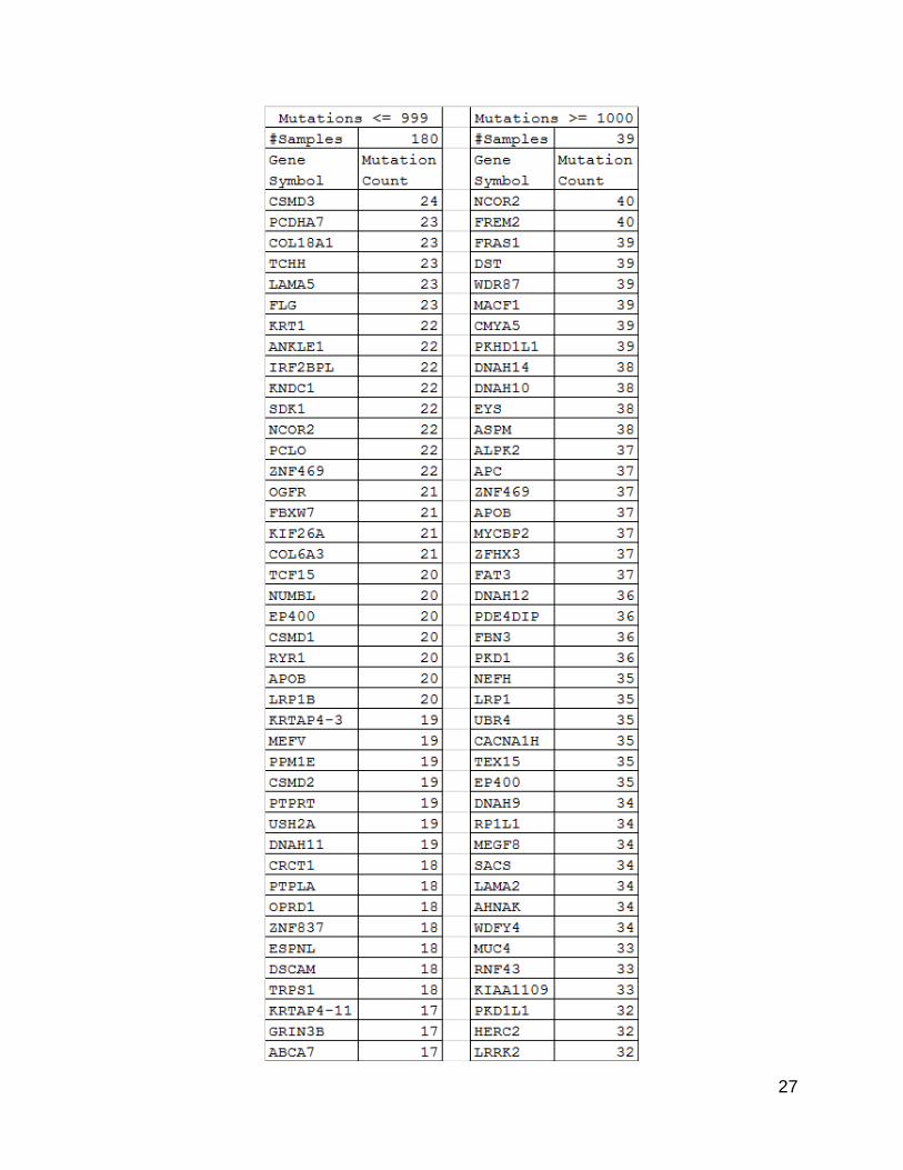
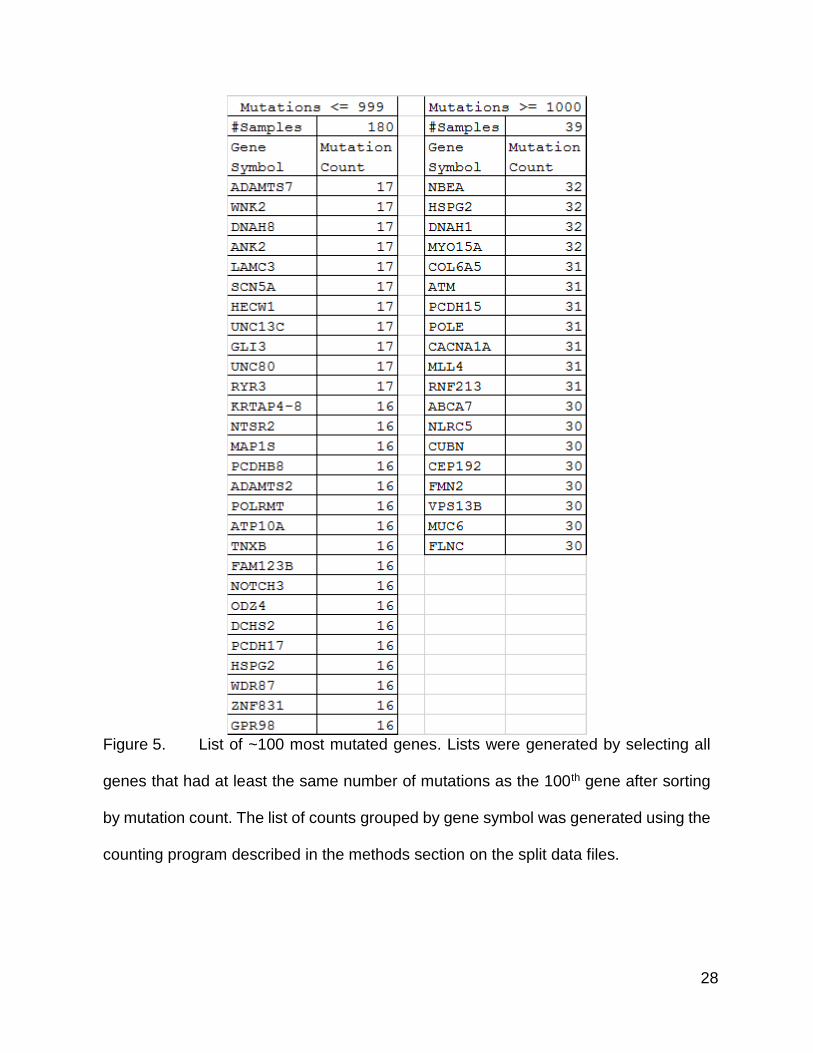
Figure 5. List of ~100 most mutated genes. Lists were generated by selecting all
genes that had at least the same number of mutations as the 100th gene after sorting
by mutation count. The list of counts grouped by gene symbol was generated using the
counting program described in the methods section on the split data files.
29
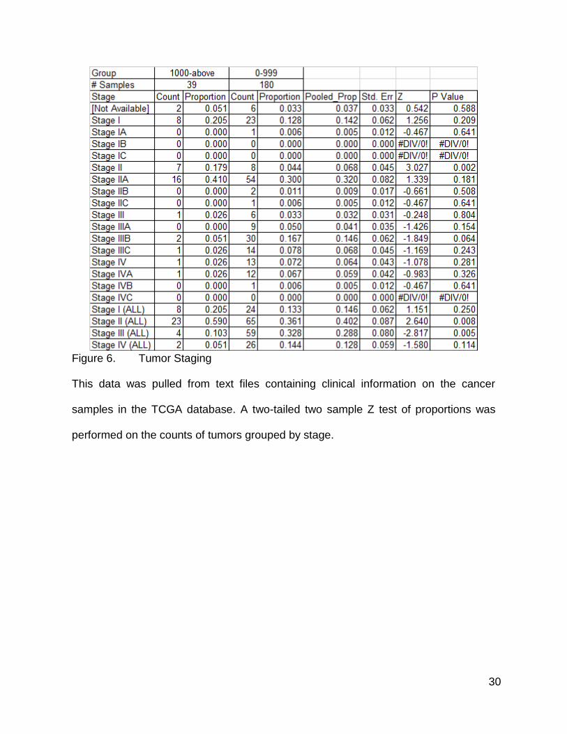
Correlation Between Mutation Count Group and Cancer Staging
During one of my Research in Progress meetings, someone from the audience
raised a question about correlation between tumor staging (65) and mutation rate. I chose
to examine this by pulling the publicly available clinical data and matching it with the
mutation counts. The high mutation count group has a higher proportion of Stage II and
Stage IIA tumors and a lower proportion of Stage III and IV tumors than the low mutation
count group (Figure 6). The proportion of Stage I tumors was very similar in the two
groups, but was slightly higher in the high mutation group (Figure 6). The differences for
Stage II (without a subtype) were statistically significant, as were the difference between
the pooled counts for all subtypes of Stage II together (Figure 6). Differences for Stage III
only showed statistical significance when pooled (Figure 6). Stage I and IV did not pass
requirements for statistical significance via a two tailed Z test of proportions (Figure 6).
30
Figure 6. Tumor Staging
This data was pulled from text files containing clinical information on the cancer
samples in the TCGA database. A two-tailed two sample Z test of proportions was
performed on the counts of tumors grouped by stage.
31
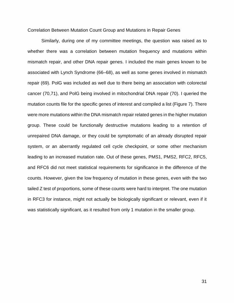
Correlation Between Mutation Count Group and Mutations in Repair Genes
Similarly, during one of my committee meetings, the question was raised as to
whether there was a correlation between mutation frequency and mutations within
mismatch repair, and other DNA repair genes. I included the main genes known to be
associated with Lynch Syndrome (66–68), as well as some genes involved in mismatch
repair (69). PolG was included as well due to there being an association with colorectal
cancer (70,71), and PolG being involved in mitochondrial DNA repair (70). I queried the
mutation counts file for the specific genes of interest and compiled a list (Figure 7). There
were more mutations within the DNA mismatch repair related genes in the higher mutation
group. These could be functionally destructive mutations leading to a retention of
unrepaired DNA damage, or they could be symptomatic of an already disrupted repair
system, or an aberrantly regulated cell cycle checkpoint, or some other mechanism
leading to an increased mutation rate. Out of these genes, PMS1, PMS2, RFC2, RFC5,
and RFC6 did not meet statistical requirements for significance in the difference of the
counts. However, given the low frequency of mutation in these genes, even with the two
tailed Z test of proportions, some of these counts were hard to interpret. The one mutation
in RFC3 for instance, might not actually be biologically significant or relevant, even if it
was statistically significant, as it resulted from only 1 mutation in the smaller group.
32
Figure 7. Genes Related to Repair and Replication
Lists of counts grouped by genes were searched for the entries corresponding to genes
of interest. A two-tailed two sample Z test of proportions was performed on the counts.
33
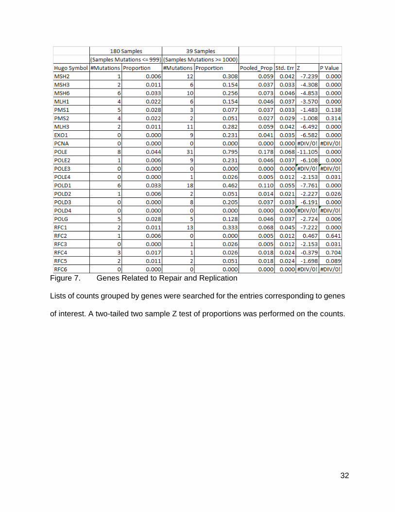
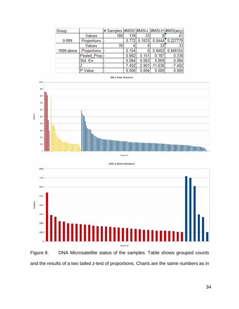
Following up the mismatch repair gene mutation list, I also looked into DNA
microsatellite instability status, which is associated with the mismatch repair deficiency
phenotype (46,54,72,73), as a mutation within these genes would not necessarily produce
the well characterized phenotype. The MSI status was also available within the clinical
data. The high mutation count population was enriched for tumors designated as MSI-H,
while the population with lower mutation counts was enriched for MSI stable tumors and
those categorized as MSI-L.
I plotted this breakdown of the tumors according to MSI categories (Figure 8) to
show the total somatic mutation count in a manner similar to Figure1. A few of the MSI-H
tumors had comparatively lower counts compared to the other MSI-H tumors while 1 MSI-
H tumor showed a very high mutation count in comparison to the others. Most of the MSI-
stable tumors were fairly low in mutation count, but a small number of them had between
300 and 600 mutations, which was significantly more than the rest (Figure 8).
A handful of MSI stable tumors had even more mutations than those in the low
mutation population (Figure 8). These samples ranged from more than 7 thousand
mutations to one with approximately 2000. Most of the MSI-H samples were between
1000 and 2000 mutations. A handful were between 2000 and 3000, and one was above
5000.
The difference in proportions between the high and low groups for all of these
classification groups were highly statistically significant according to a two tailed Z test.
34
Figure 8. DNA Microsatellite status of the samples. Table shows grouped counts
and the results of a two tailed z-test of proportions. Charts are the same numbers as in

35
Figure 1, but grouped by MSI status and split by mutation count group. The first bar
graph is the low mutation count group, and the second is the high mutation count group.
Red is MSI-H, Yellow is MSI-L, and Blue is MSS
36
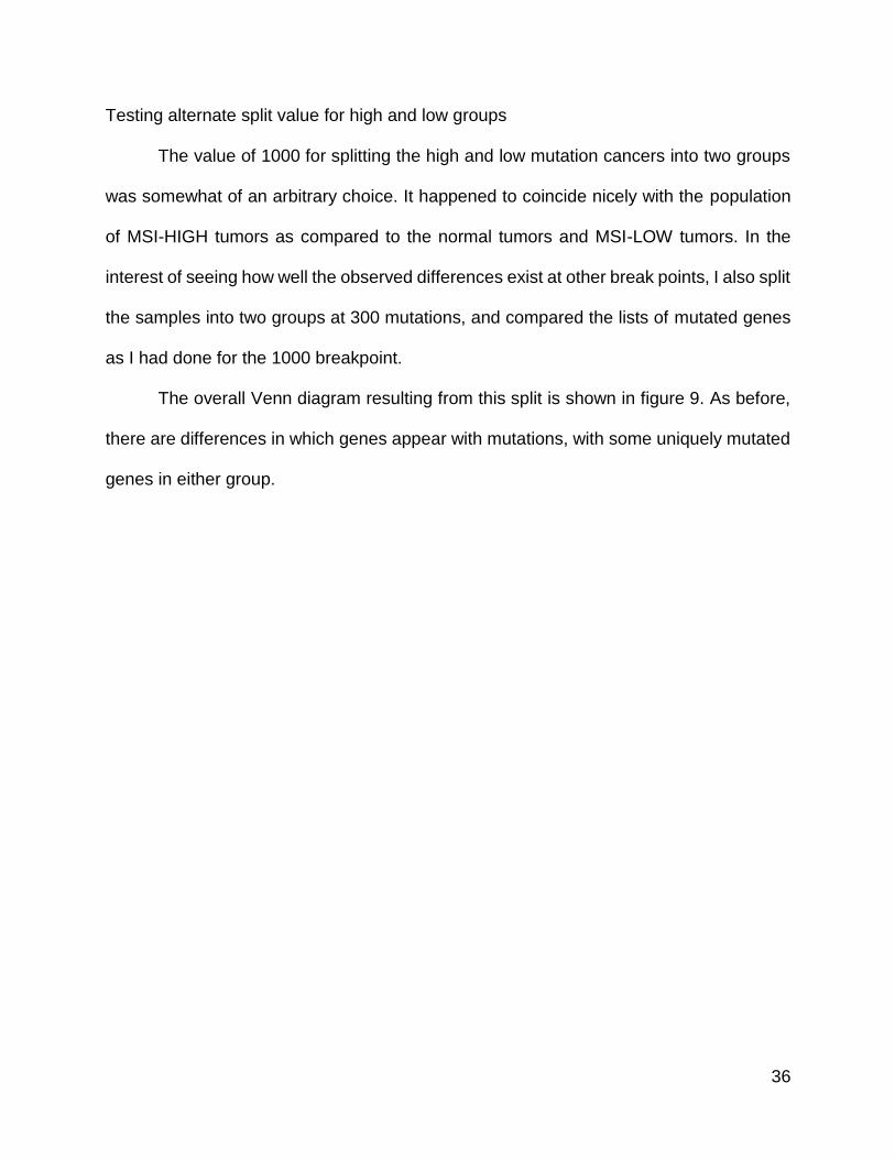
Testing alternate split value for high and low groups
The value of 1000 for splitting the high and low mutation cancers into two groups
was somewhat of an arbitrary choice. It happened to coincide nicely with the population
of MSI-HIGH tumors as compared to the normal tumors and MSI-LOW tumors. In the
interest of seeing how well the observed differences exist at other break points, I also split
the samples into two groups at 300 mutations, and compared the lists of mutated genes
as I had done for the 1000 breakpoint.
The overall Venn diagram resulting from this split is shown in figure 9. As before,
there are differences in which genes appear with mutations, with some uniquely mutated
genes in either group.
37
Figure 9. Venn Diagram of High and Low mutation groups split at 300 mutations.
38
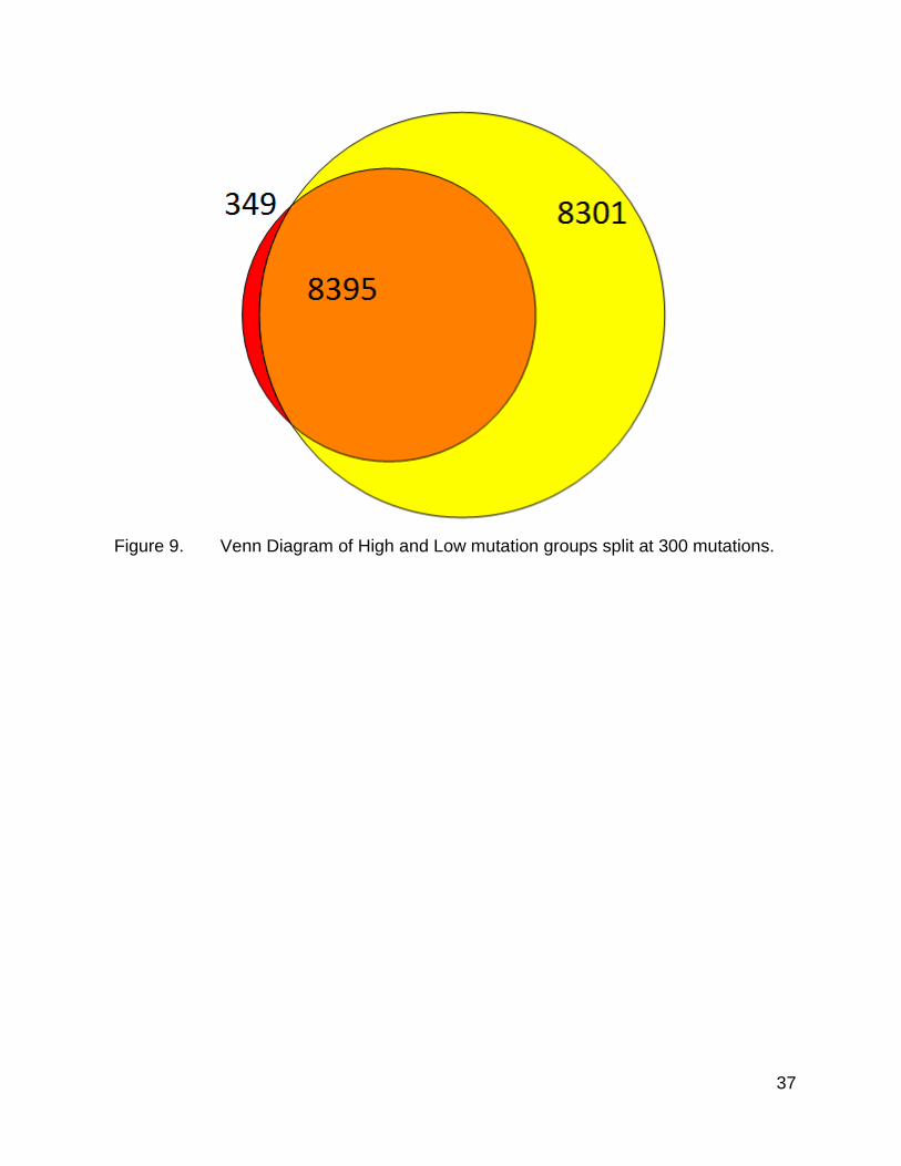
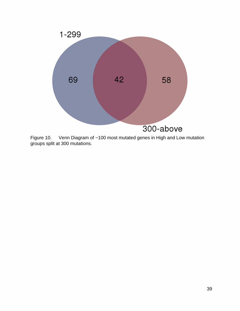
Figure 10 corresponds to Figure 3, but for the 300 mutation split point. As before,
when selecting the 100 most mutated genes from either group, there were shared genes
as well as significant numbers of unique genes. This pattern supports the idea that there
really are differences between the high and low mutation groups, and that the split point
of 1000 is not the only breakpoint that reveals these differences in mutation. There were
slightly more shared genes and fewer unique genes, although it was hard to determine
how significant this difference was, as the numbers are still very similar.
39
Figure 10. Venn Diagram of ~100 most mutated genes in High and Low mutation
groups split at 300 mutations.
40
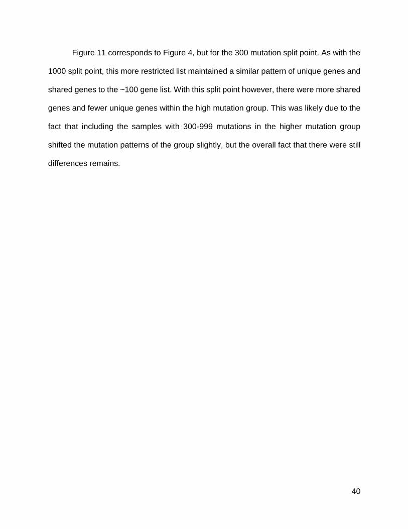
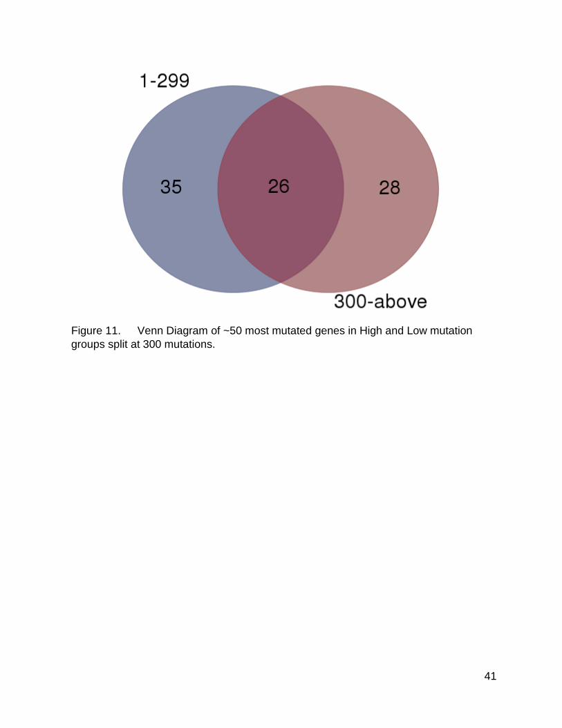
Figure 11 corresponds to Figure 4, but for the 300 mutation split point. As with the
1000 split point, this more restricted list maintained a similar pattern of unique genes and
shared genes to the ~100 gene list. With this split point however, there were more shared
genes and fewer unique genes within the high mutation group. This was likely due to the
fact that including the samples with 300-999 mutations in the higher mutation group
shifted the mutation patterns of the group slightly, but the overall fact that there were still
differences remains.
41
Figure 11. Venn Diagram of ~50 most mutated genes in High and Low mutation
groups split at 300 mutations.
42
Discussion
These tumors exhibited an interesting divide between the high and low mutation
frequency groups that held at both the large scale and when focusing on the most mutated
genes. There did appear to be a relationship to DNA mismatch repair genes in the high
mutation frequency group, and curiously, lower staging seems to correlate with the high
mutation frequency group tumors instead of higher staging as one might be inclined to
expect.
When looking broadly at the most mutated genes between these low and high
mutation groups, it was apparent that the lower mutation group exhibits a bias towards
mutations in cancer focused genes, while the higher mutation group had some cancer
genes in its list but also many other kinds of genes. It was apparent that there was indeed
a difference between these populations. Thus a more detailed examination of those
differences became of interest.

43
Chapter 3
Mutation Rate Group Differences in Mutation Types and Gene Mutation Counts;
Positively Deviating Outliers in Mutation Count & Gene Length Trend
44
Introduction
In the previous chapter, I had noticed when examining the counts of mutations by
Official Gene Symbol, that there was a general trend of mutation count with gene size.
As an example, Titin (TTN; OMIM 188840) was generally near the top of both lists when
sorted by mutation count. TTN is encoded by an 82kb mRNA making it one of the largest
genes in the human genome (74). This suggested that its mutation frequency might be a
consequence of its size. However, after examining other genes from annotation
databases I noticed that there were some other genes that appeared more frequently
than their size would dictate.
The concept of mutation spectrum, also called genome or mutation landscapes,
refers to the total of all mutations contained in the genome of tumor cells, usually classified
as passenger or driver mutations (28–32,75). It is sometimes visualized in a histogram-
like manner using mutation counts as the height variable, across the chromosomes on
one axis and the chromosome number on the other axis.
There are many types of mutations and each can have varying causes. Small scale
mutations include substitutions, insertions, and deletions each of which involves a single
nucleotide or multiple nucleotides, and small scale inversions, which would necessarily
involve more than one nucleotide. Large scale mutations, involving very large changes to
chromosomes including copy number changes, duplications, deletions, and movement of
large segments of DNA within or between chromosomes, or even gain or loss of entire
chromosomes, would require a more complex analysis and were not included in my
project.
45
Mutations within genes can have complications in their assignment. Due to splicing
of transcripts there are sometimes multiple transcript variants that use different
combinations of exons. A mutation may fall within one of the optional exons and only
affect some transcript variants.
I used an approach of examining at the gene scale rather than differentiating
between transcripts. There could perhaps be something of interest involving alternative
transcripts, but it would introduce complexities into my analysis that were not directly
relevant to answering the question I was seeking to answer.
Hypothesis
I hypothesized that the collection of genes mutated within the low mutation count
population would tend to be more selective and have a greater degree of cancer
specificity than the higher mutation count group. Further, in the higher mutation count
group, I expected the influence of gene length on mutation count to increase significantly
and the influence of selection, related to clonal evolution within the tumors, to be less
significant in the high mutation population compared to the low mutation population.
Methods
In an idealized mutation scenario without the influence of clonal selection, one
would expect a linear relationship between gene size and the number of mutations that
would appear in a population of cells over time. If the mutations found in the tumors were
to become more random and less selected, then there ought to be an increase in the
association between gene size and mutation count within a gene. I wanted to be able to
determine which genes were outliers from this trend. The impact of selection would place
46
some genes outside of this trend, in a positive direction if the mutations provided selective
benefit or negative direction if they were deleterious for the cells in some way. I am
primarily interested in those genes which had positive deviation from the trend.
I wrote a program to count mutation types both for the group as a whole and with
a breakdown by sample. I also wrote a program to perform two tailed t-tests on the
resulting tables of values, as well as their proportions against the total number of
mutations within each tumor using a matching table structure, and to perform a linear
regression on count data binned by gene symbol, and use that regression to obtain
studentized residuals for the mutation counts of each gene. These were used to assess
differences between the high mutation group and the low mutation group. The residuals
and linear regression aimed to reduce the impact of gene length on the ranking and to
identify genes that were positively deviated outliers in the roughly linear gene length and
mutation count relationship.
The results of mutation count grouped by gene symbol were used to plot gene size
against total mutation count. I used Excel’s trend-line feature to place a trend line on this
graph. Note that this trend line was not produced by the same software that performed
the linear regression, and so may not be exactly the same as the line that was used to
produce the residuals.
Files containing gene lengths were obtained from the genome browser table
viewer. These were matched up with the entries in the MAF files in order to normalize
against the effect of gene length. Genes with multiple transcript variants had isoform
lengths averaged. The counts were divided by the lengths and the number of samples in
their respective group.
47
I added these lengths to the selection of ~100 genes with the highest mutation
counts from the previous chapter to show the variation of the gene lengths at the high
end of the mutation counts. For these, I examined the 100th gene in the count-sorted list,
and included any others beyond that point which had the same number of counts, in each
group. I also repeated this using the studentized residual values instead of the counts, to
show the genes with the highest residuals.
Results
Differences in Mutation Types
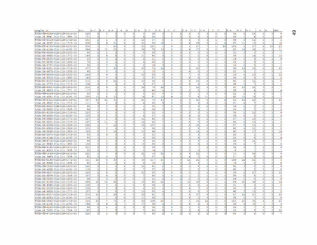
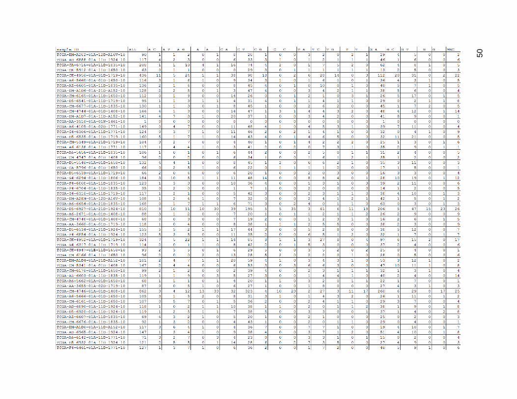
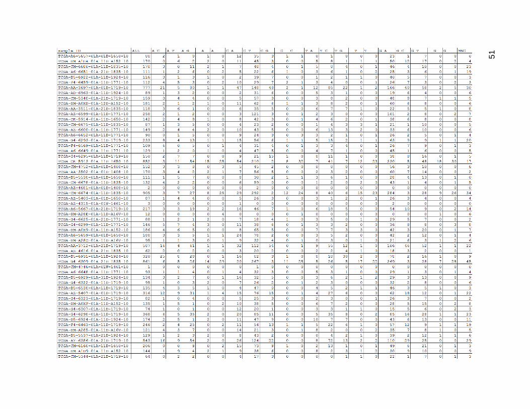
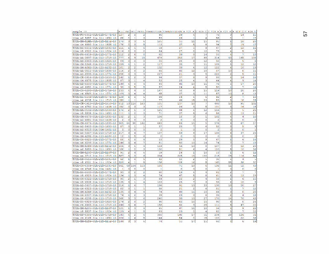
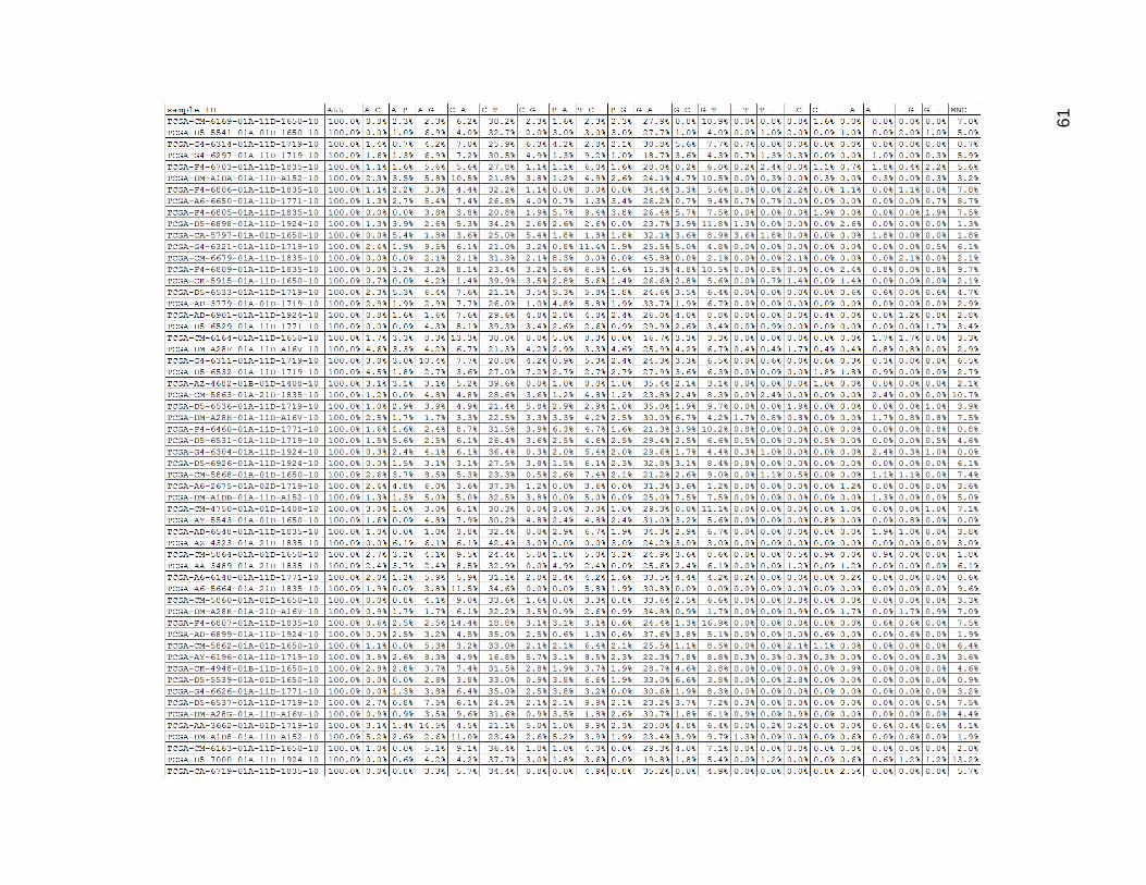
Figures 12,13,14, and 15 show the mutation type counts for the low and high
mutation count groups respectively. Figures 14 and 15 are calculated values based on
categories of mutation type, and mutations that are technically chemically
indistinguishable due to DNA’s base pairing. Figures 16, 17, and 18 show these values
converted into percentages based on the total sum of mutations within each sample.
Figure 18 corresponds to both Figures 14 and 15, which were kept separate due to size.
These mutations are labeled using a “reference_mutation” pattern, with a dash “-
“ standing in for missing bases in insertions or deletions. MNC stands for multi-nucleotide
change. Due to difficulty and complexity in the analysis of mutations involving more than
one base, I opted to bin these types of mutations into one category. These types of
mutations were less frequent than single base mutations in general, but are still prevalent
enough to be potentially important.
The raw data and some calculated values are being shown in Figures 12-18 to
facilitate explanation of some details about the mutation types, and because it was
48
feasible to fit these tables into this document, albeit in a very dense and compact form.
The results of the t-test are shown in Figure 19.
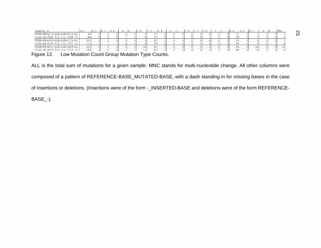
Figure 12 depicts the result of the uncategorized mutation counts within the low
mutation count group. There was quite a lot of variation in mutation count within this group,
and the tumors with low numbers of total mutations frequently had zeroes for certain
values. The values of corresponding mutations (such as C_T and G_A) usually matched
quite well within each row. C_T and G_A were the most common mutation type by far,
which was probably frequently the result of 5-methylcytosine deamination.
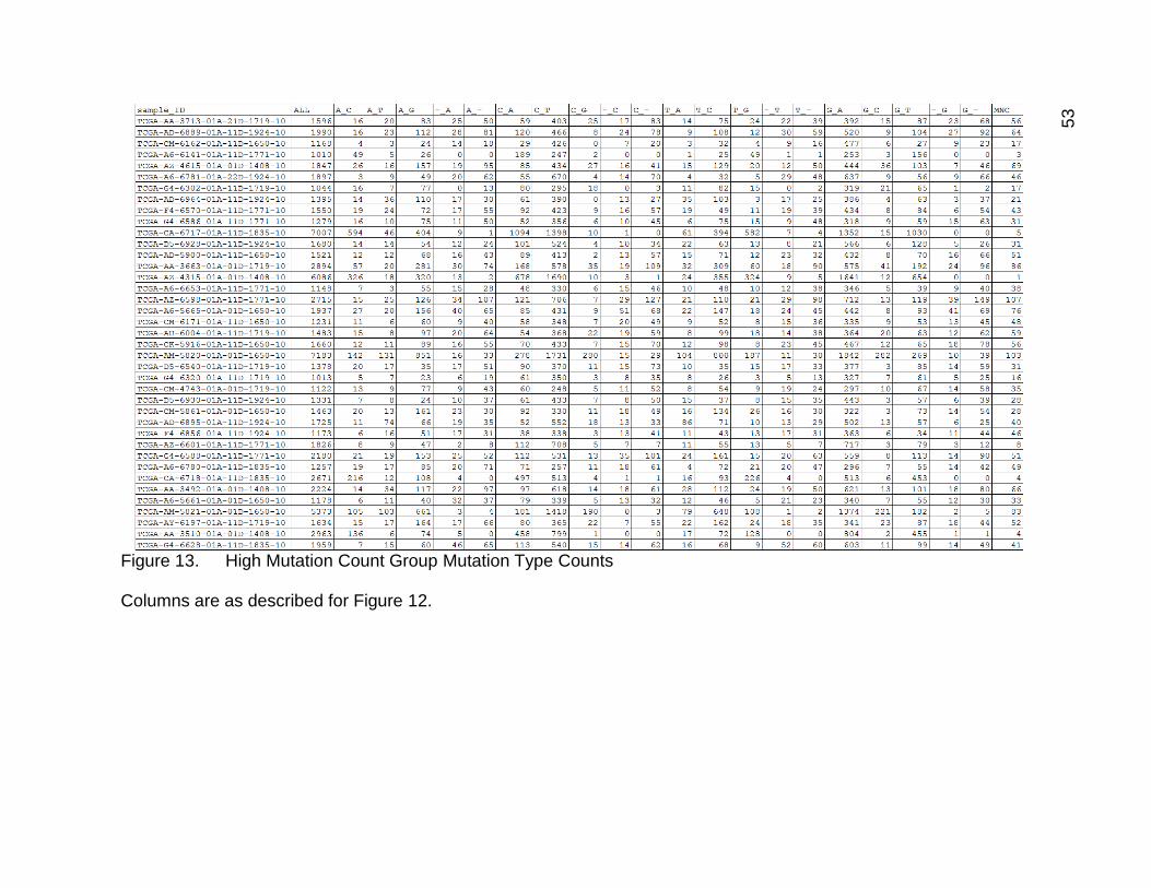
Figure 13 is the same type of table as Figure 12, but for the high mutation group.
The counts were broadly raised, but there was a subset of these tumors that had very
large counts for some types and not others. For instance, the 2nd to last row was a sample
that had 799 C_T mutations, but only 1 C_G mutation and very low numbers of insertion
mutations.
49
50
51
52
Figure 12. Low Mutation Count Group Mutation Type Counts.
ALL is the total sum of mutations for a given sample. MNC stands for multi-nucleotide change. All other columns were
composed of a pattern of REFERENCE-BASE_MUTATED-BASE, with a dash standing in for missing bases in the case
of insertions or deletions. (Insertions were of the form -_INSERTED-BASE and deletions were of the form REFERENCE-
BASE_-).
53
Figure 13. High Mutation Count Group Mutation Type Counts
Columns are as described for Figure 12.
54
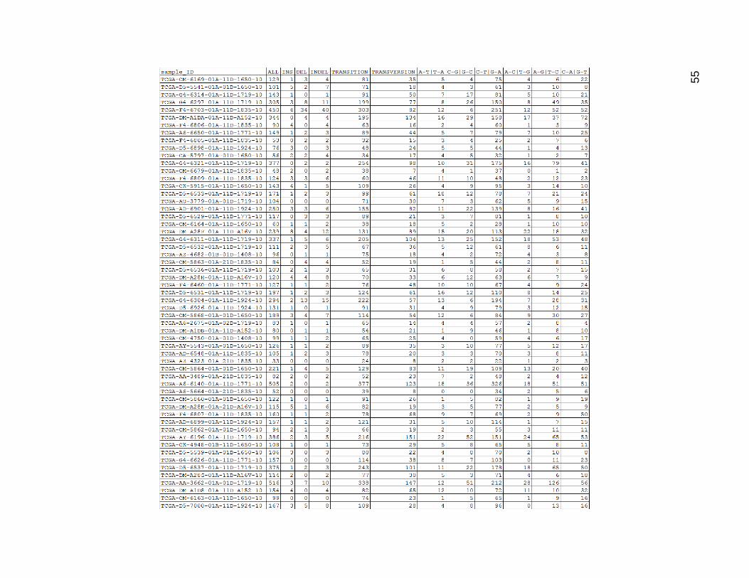
I created additional data columns based on potentially relevant categories by
adding together the values present in the above table. These values included insertions,
a sum of all single-base insertions, deletions, a sum of all single base deletions, indels, a
sum of both of those, transitions, and transversions, sums of the mutations that matched
these definitions, and a set of mutations that would be considered indistinguishable due
to double-strand base-pairing ({A-T and T-A}, {C-G and G-C}, {C-T and G-A}, {A-C and
T-G}, {A-G and T-C}, {C-A and G-T}). The values for these sums and their proportions
were also included in the t tests.
Figure 14 depicts these values for the low mutation group. Insertions and deletions
showed quite a bit of variability. In some tumors the insertions and deletions roughly
matched, while in others the numbers were very different. Indels in general were less
frequent than other single-base mutations. With the chemically matching mutations added
together, the dominance of the C_T mutation became even more apparent.
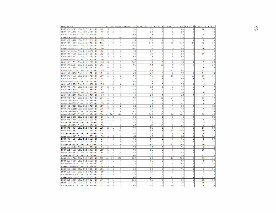
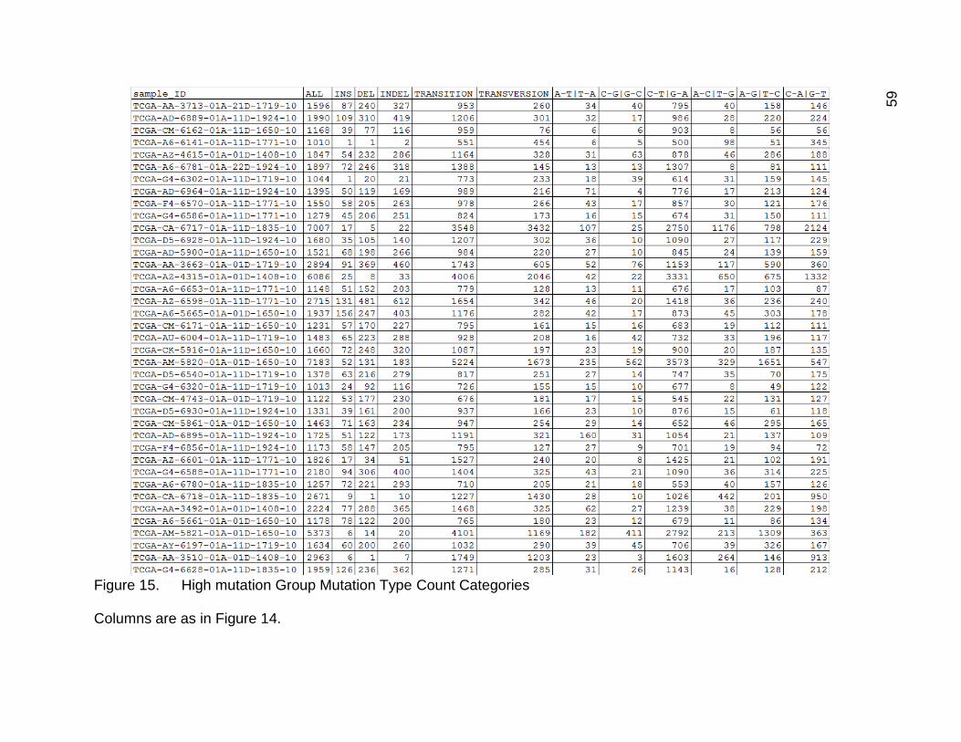
In Figure 15, the data for the high mutation group mutation type categories drive
home again how many more mutations these samples had on average than the others.
C-T and G_A were once again the most common, with C_A and G_T generally having
slightly more mutations than A_G and T_C. It was interesting that the other 3 mutation
types were still fairly low. There were quite a lot of single base indels in these samples as
well.
55
56
57
58
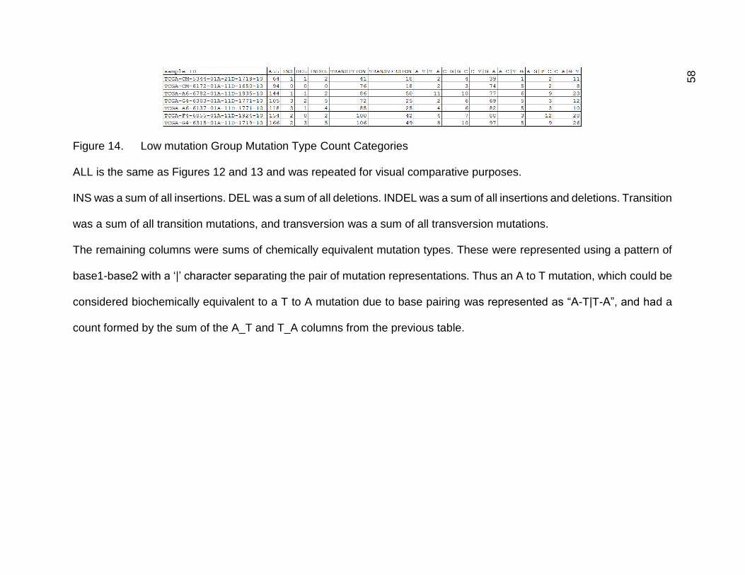
Figure 14. Low mutation Group Mutation Type Count Categories
ALL is the same as Figures 12 and 13 and was repeated for visual comparative purposes.
INS was a sum of all insertions. DEL was a sum of all deletions. INDEL was a sum of all insertions and deletions. Transition
was a sum of all transition mutations, and transversion was a sum of all transversion mutations.
The remaining columns were sums of chemically equivalent mutation types. These were represented using a pattern of
base1-base2 with a ‘|’ character separating the pair of mutation representations. Thus an A to T mutation, which could be
considered biochemically equivalent to a T to A mutation due to base pairing was represented as “A-T|T-A”, and had a
count formed by the sum of the A_T and T_A columns from the previous table.
59
Figure 15. High mutation Group Mutation Type Count Categories
Columns are as in Figure 14.
60
It was apparent that due to the difference in magnitude of the numbers between
the groups that most if not all of these mutation categories would have statistically
significant differences. I created equivalently structured tables where the values for each
sample were divided by the total number of mutations in that sample, to obtain percentage
proportions.
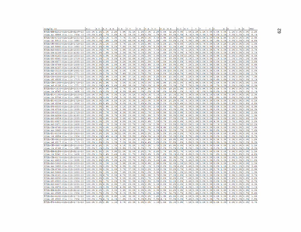
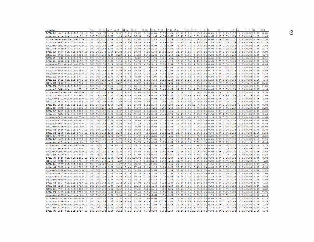
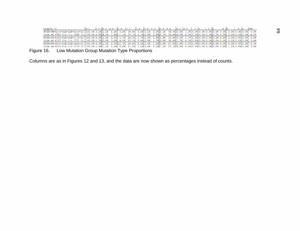
Figure 16 shows the proportions for the low mutation population. After controlling
for total mutation count by converting these numbers to percentages, the ratios were
much less variant for the C_T and G_A mutations. There were some variations among
other mutation types that might be more significant. MNC mutations were fairly
consistently in the single digit percentages, although were more frequent in some tumors.
61
62
63
64
Figure 16. Low Mutation Group Mutation Type Proportions
Columns are as in Figures 12 and 13, and the data are now shown as percentages instead of counts.
65
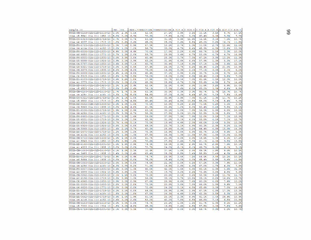
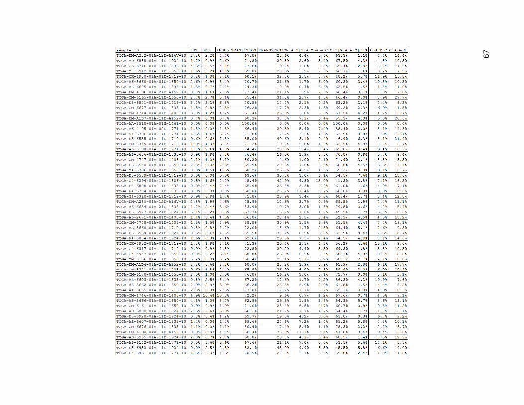
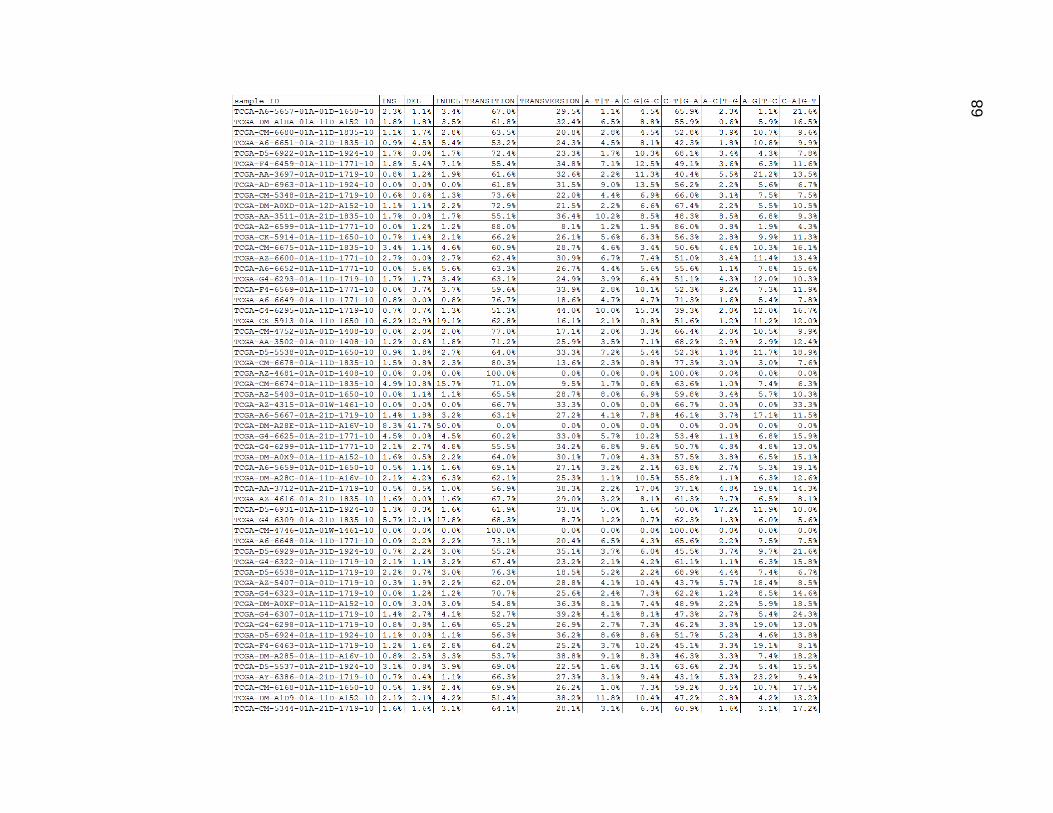
Cross comparing the indel percentages from Figure 17 and the MNC percentages
from Figure 16, it seems they had very similar values, although not always matched up in
magnitude within any one tumor. C_T and G_A mutations accounted for between 40%-
60% of the mutations in most of the samples. C_A and G_T mutations were somewhat
common single base changes, and accounted for about 10%-20% of the mutations in
most of the samples. The A_G and T_C mutations were slightly less common than that
with most ranging from 6%-20%, but tended to be low more often. The other three
mutation type categories mostly ranged between 0% and 5%, and were closer to values
between 3-5%.
66
67
68
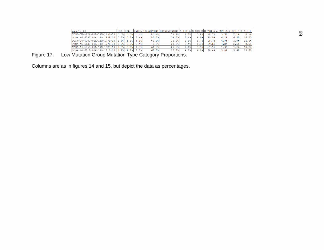
69
Figure 17. Low Mutation Group Mutation Type Category Proportions.
Columns are as in figures 14 and 15, but depict the data as percentages.

70
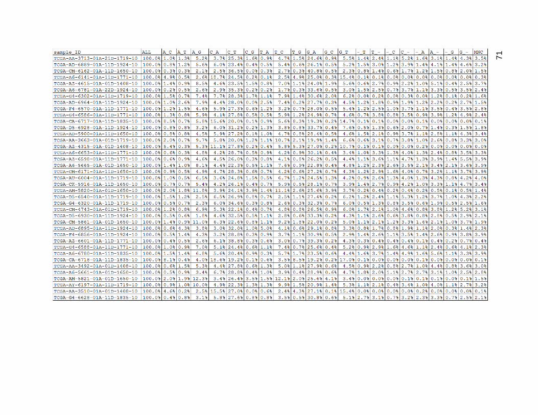
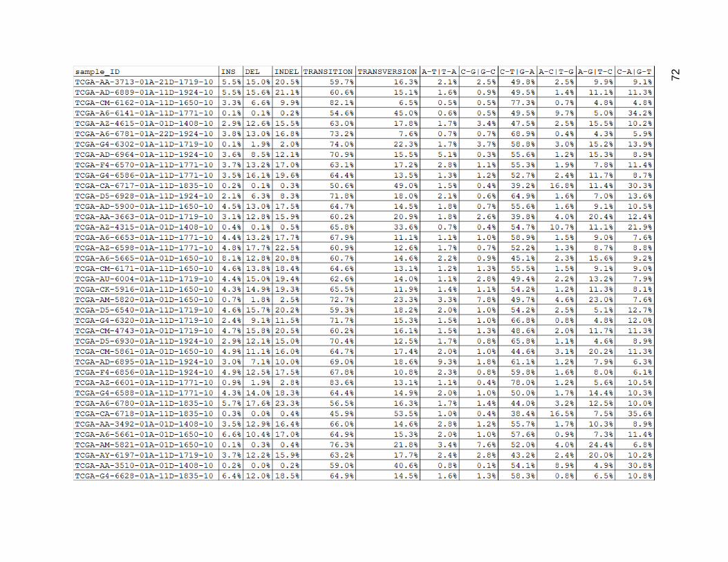
Figure 18 contains both the mutation type proportion table and the mutation
category proportion table for the high mutation group. The C-T and G_A mutations
seemed similar in the high group to what was found in the low group. The indels seemed
to be somewhat raised in general (although some of these tumors did not experience this).
The A_G and T_C mutations seemed to be a bit more common as well in this group. The
other three types were a bit less common than in the low mutation group. This was relative
to the total number of mutations, so the actual values were higher on average by quite a
lot than in the low mutation group, but the ratios did seem to be a bit different.
71
72

73
Figure 18. High Mutation Group Mutation Type (and Category) Proportions
Columns here are as shown in tables 9-14. These values are represented as proportions of total mutation counts per
sample.
74
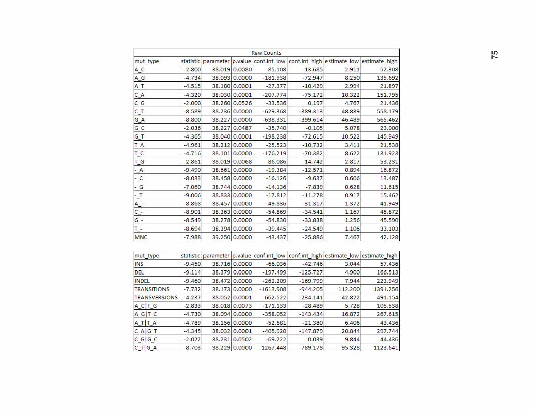
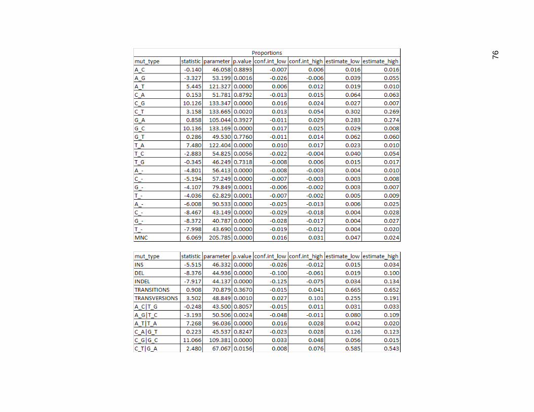
I then performed a t test on both the raw data and the proportions. C_G mutations
did not pass requirements for significance of difference base on counts, while its chemical
equivalent G_C did, but only barely. The combined category for these, also did not pass,
having a p value just slightly higher than 5%. All the rest of the count values were
significantly different, as expected.
In terms of proportions, several mutation types counted separately did not pass 5%
requirement for significance, including A_C, C_A, G_A, G_T, T_G. In the categories, the
A_C and T_G, the C_A and G_T, and the transitions categories did not pass requirements
for significance
75
76

77
Figure 19. Results of Two Sided Welch Two Sample T Test on Mutation Type Data
The first pair of tables is the result of the t test on the raw count values. The second pair of tables is the result of the t test
using proportions as input instead of the raw counts. Within each pair the first table contains the results for the individual
mutation types and the second table for the categories.

78
Differences in Mutated Genes
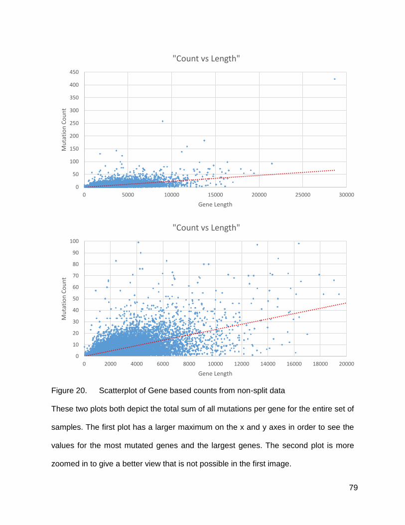
Plotting the mutation counts binned according to gene for the entire population of
tumors resulted in a scatterplot that was quite messy. It was apparent however that there
was a collection of a small number of genes that mutated significantly more than their
similarly sized counterparts. In the first plot, showing all of the points, one can see several
genes that mutated to the most extreme levels, and with the slightly more zoomed in
scatterplot, there were quite a number of highly mutated genes that deviated from the
general trend to a lesser, but still quite obvious, extent. I became interested in the
appearance of this kind of plot when produced using the split populations.
79
Figure 20. Scatterplot of Gene based counts from non-split data
These two plots both depict the total sum of all mutations per gene for the entire set of
samples. The first plot has a larger maximum on the x and y axes in order to see the
values for the most mutated genes and the largest genes. The second plot is more
zoomed in to give a better view that is not possible in the first image.
0
50
100
150
200
250
300
350
400
450
0 5000 10000 15000 20000 25000 30000
Mu
tati
on
Co
un
t
Gene Length
"Count vs Length"
0
10
20
30
40
50
60
70
80
90
100
0 2000 4000 6000 8000 10000 12000 14000 16000 18000 20000
Mu
tati
on
Co
un
t
Gene Length
"Count vs Length"

80
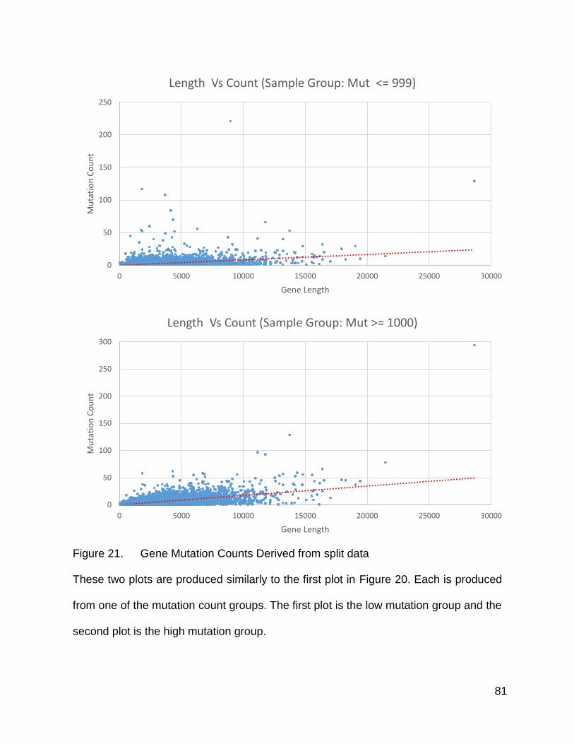
The one difference that became obvious right away was the number of mutations.
The population size of the high mutation group was 39, while the low mutation group was
180. These counts had not been normalized by population size, and yet the plots were
covering approximately the same region in terms of count values. Additionally, there were
not quite as many obvious outliers on the low-length side of this scatterplot in the higher
mutation count group. The dot near the top right corner, which happened to be TTN,
seemed to have approximately twice the number of mutations, indicating that it garnered
several mutations in several of the tumors.
81
Figure 21. Gene Mutation Counts Derived from split data
These two plots are produced similarly to the first plot in Figure 20. Each is produced
from one of the mutation count groups. The first plot is the low mutation group and the
second plot is the high mutation group.
0
50
100
150
200
250
0 5000 10000 15000 20000 25000 30000
Mu
tati
on
Co
un
t
Gene Length
Length Vs Count (Sample Group: Mut <= 999)
0
50
100
150
200
250
300
0 5000 10000 15000 20000 25000 30000
Mu
tati
on
Co
un
t
Gene Length
Length Vs Count (Sample Group: Mut >= 1000)
82
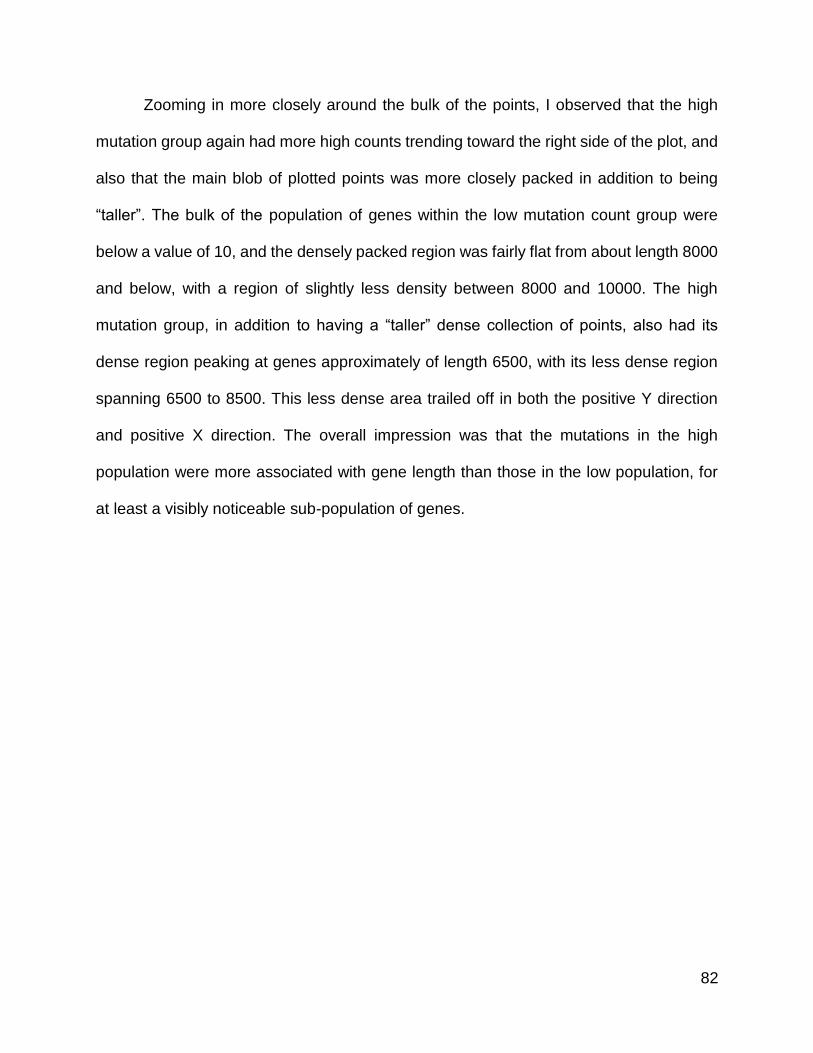
Zooming in more closely around the bulk of the points, I observed that the high
mutation group again had more high counts trending toward the right side of the plot, and
also that the main blob of plotted points was more closely packed in addition to being
“taller”. The bulk of the population of genes within the low mutation count group were
below a value of 10, and the densely packed region was fairly flat from about length 8000
and below, with a region of slightly less density between 8000 and 10000. The high
mutation group, in addition to having a “taller” dense collection of points, also had its
dense region peaking at genes approximately of length 6500, with its less dense region
spanning 6500 to 8500. This less dense area trailed off in both the positive Y direction
and positive X direction. The overall impression was that the mutations in the high
population were more associated with gene length than those in the low population, for
at least a visibly noticeable sub-population of genes.
83
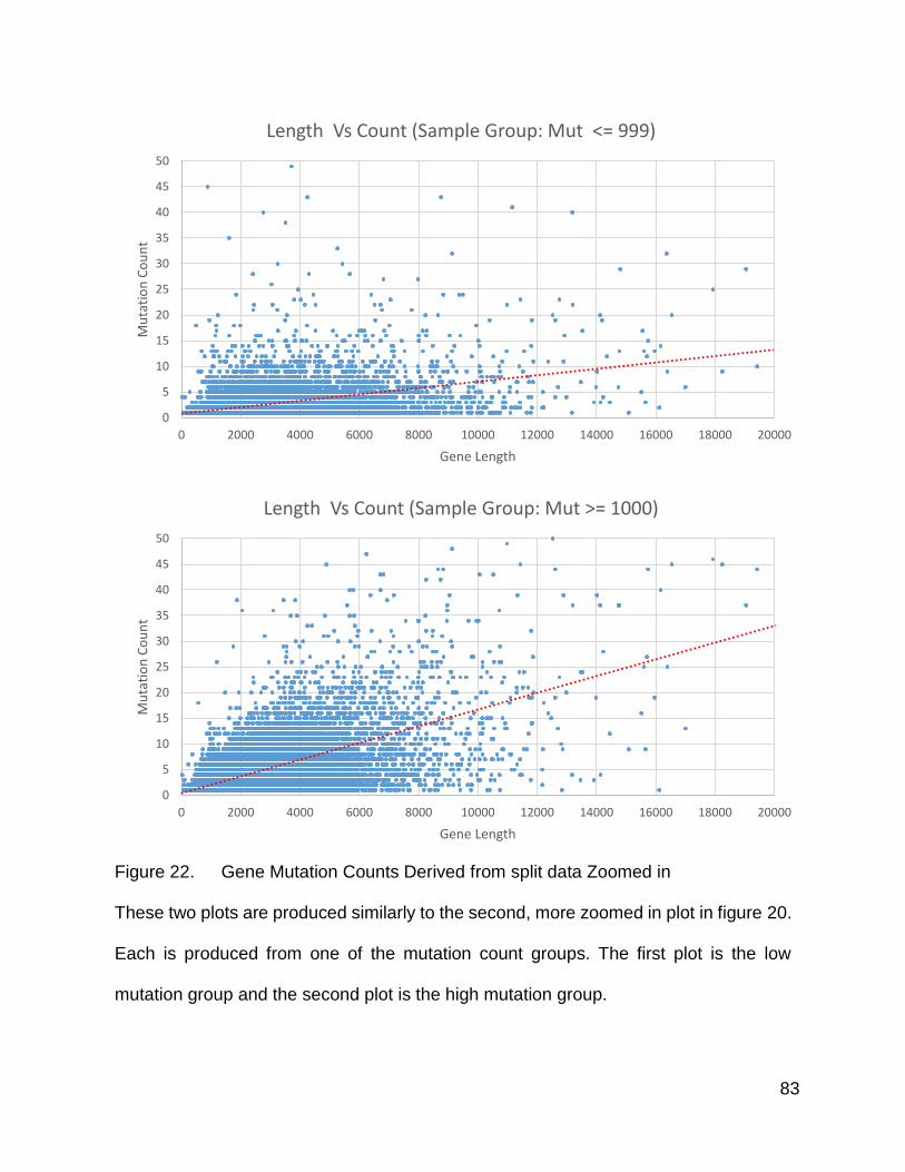
Figure 22. Gene Mutation Counts Derived from split data Zoomed in
These two plots are produced similarly to the second, more zoomed in plot in figure 20.
Each is produced from one of the mutation count groups. The first plot is the low
mutation group and the second plot is the high mutation group.
0
5
10
15
20
25
30
35
40
45
50
0 2000 4000 6000 8000 10000 12000 14000 16000 18000 20000
Mu
tati
on
Co
un
t
Gene Length
Length Vs Count (Sample Group: Mut <= 999)
0
5
10
15
20
25
30
35
40
45
50
0 2000 4000 6000 8000 10000 12000 14000 16000 18000 20000
Mu
tati
on
Co
un
t
Gene Length
Length Vs Count (Sample Group: Mut >= 1000)

84
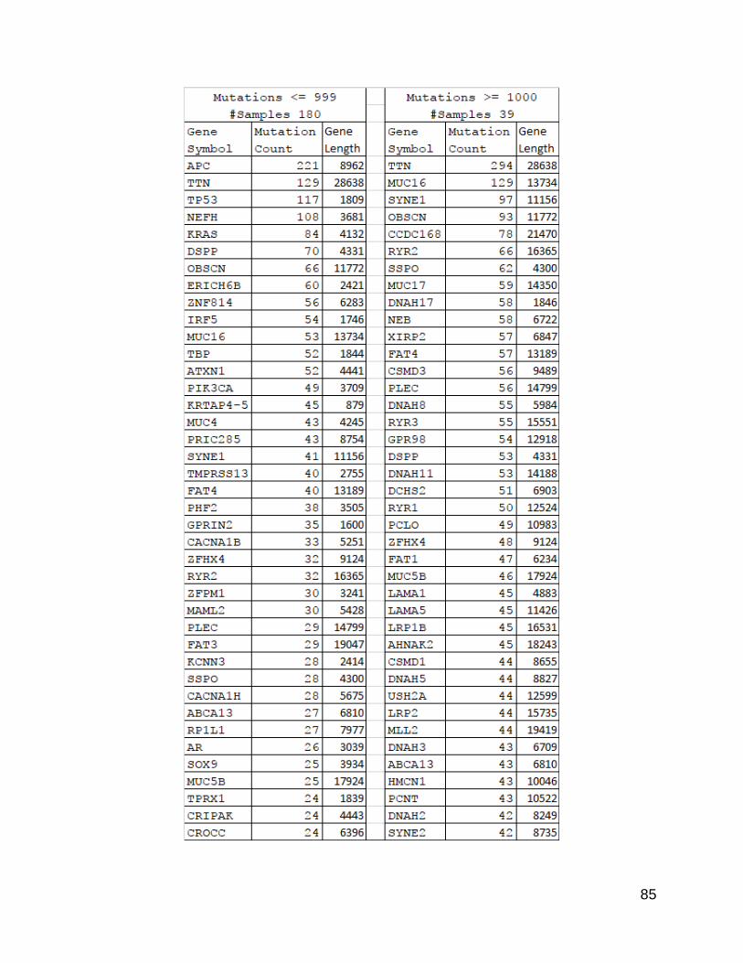
The next question was which genes were most significantly mutated. After I
returned to the list previously examined, and added in gene lengths, it became apparent
that there was a difference between the two lists in terms of gene lengths. The high
mutation population count list, when sorted by count value from high to low, showed a
stronger trend of the length values following a high to low order than the low mutation
count list. There were several genes that bucked this trend, which might be due to
mutational hot spots or the effects of clonal selection.
85
86
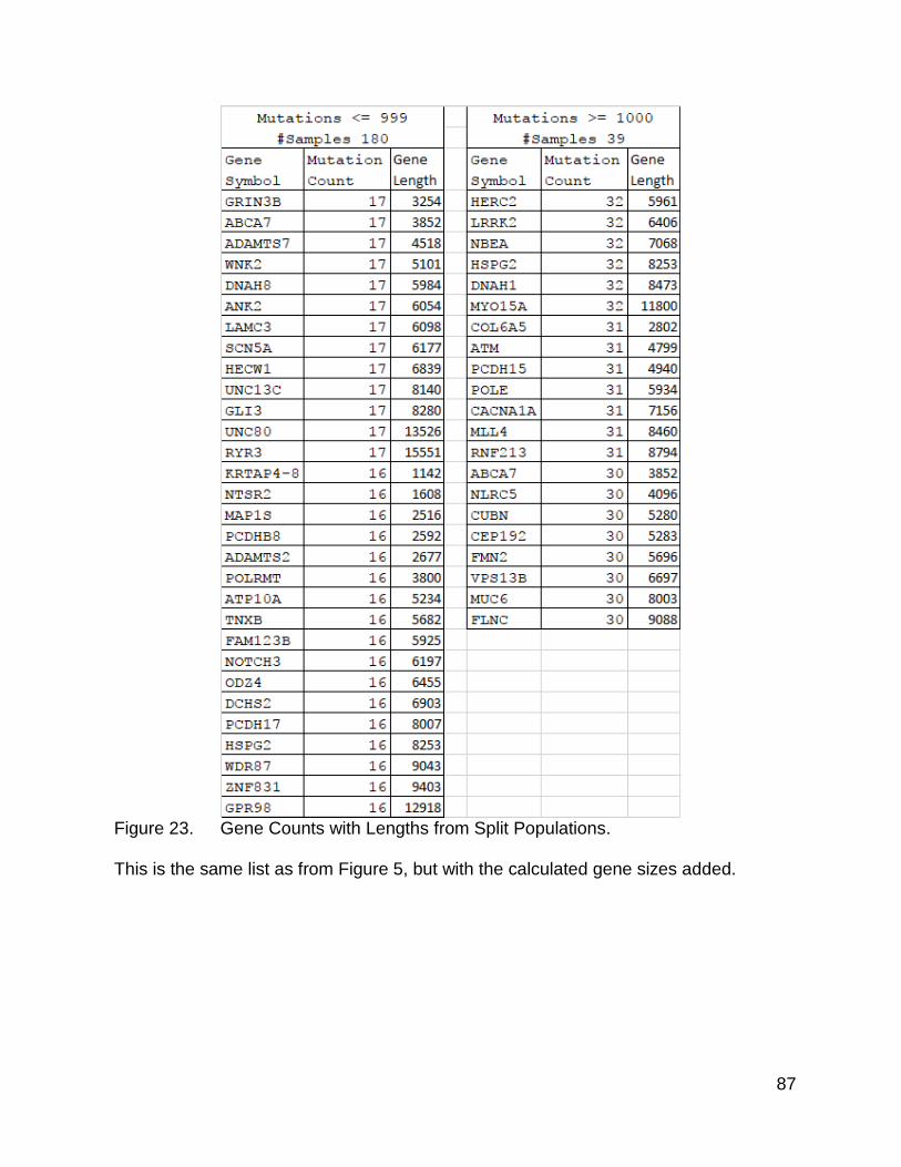
87
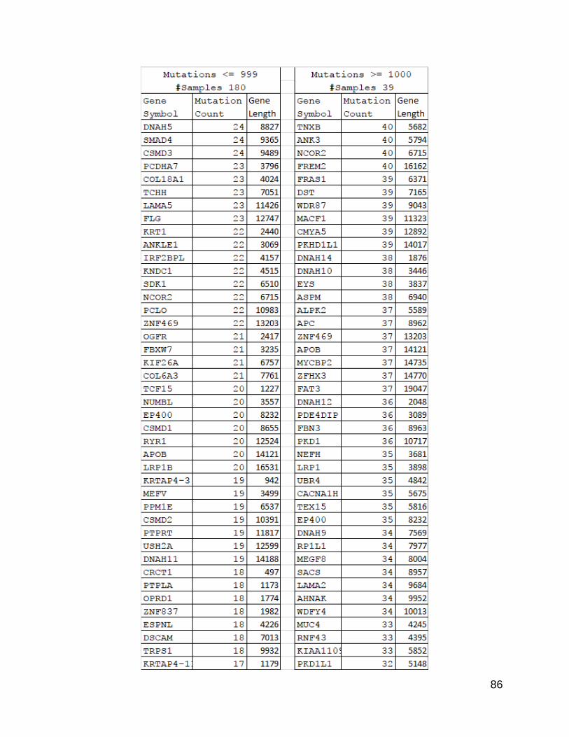
Figure 23. Gene Counts with Lengths from Split Populations.
This is the same list as from Figure 5, but with the calculated gene sizes added.
88
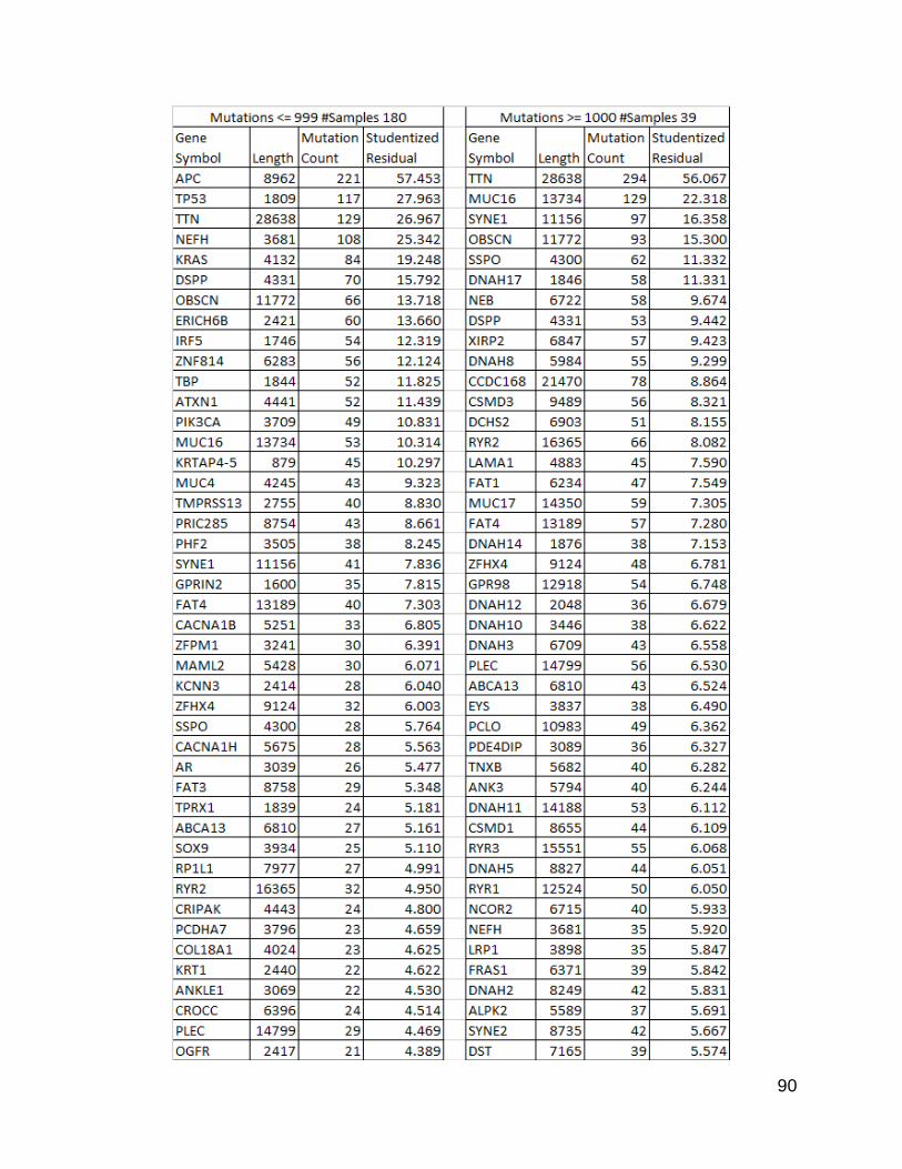
I decided to try some methods to reduce the effect of gene length, and after
speaking to Yu-Bo Wang and Dr. James Grady, both experts in statistics, I went with
using a linear regression to obtain studentized residuals. The values of these residuals
should reflect the degree to which the count was an outlier from the trend line for that
population, with negative values indicating a negative deviation from the trend and
positive values indicating a positive deviation from the trend. I compiled a list of these
computed residual values and sorted the list from high to low. The 100 highest values
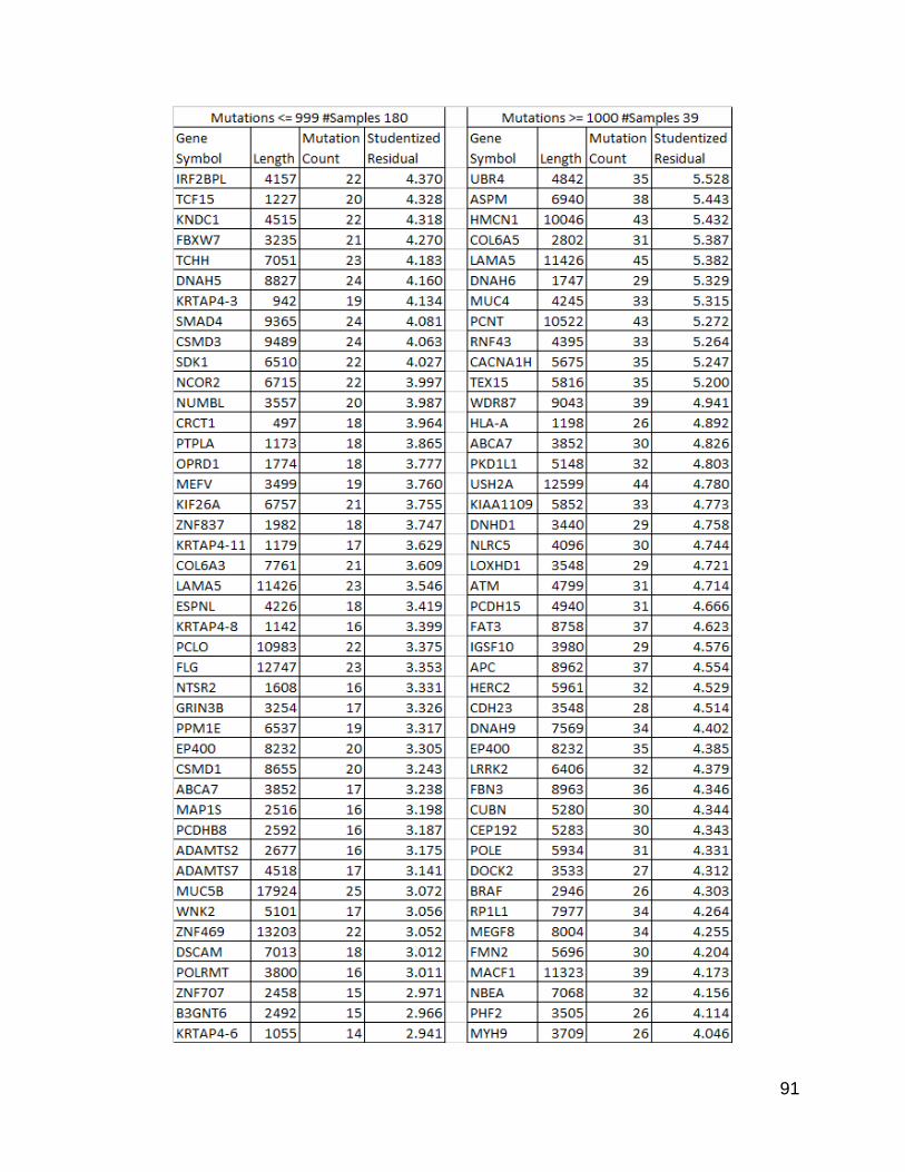
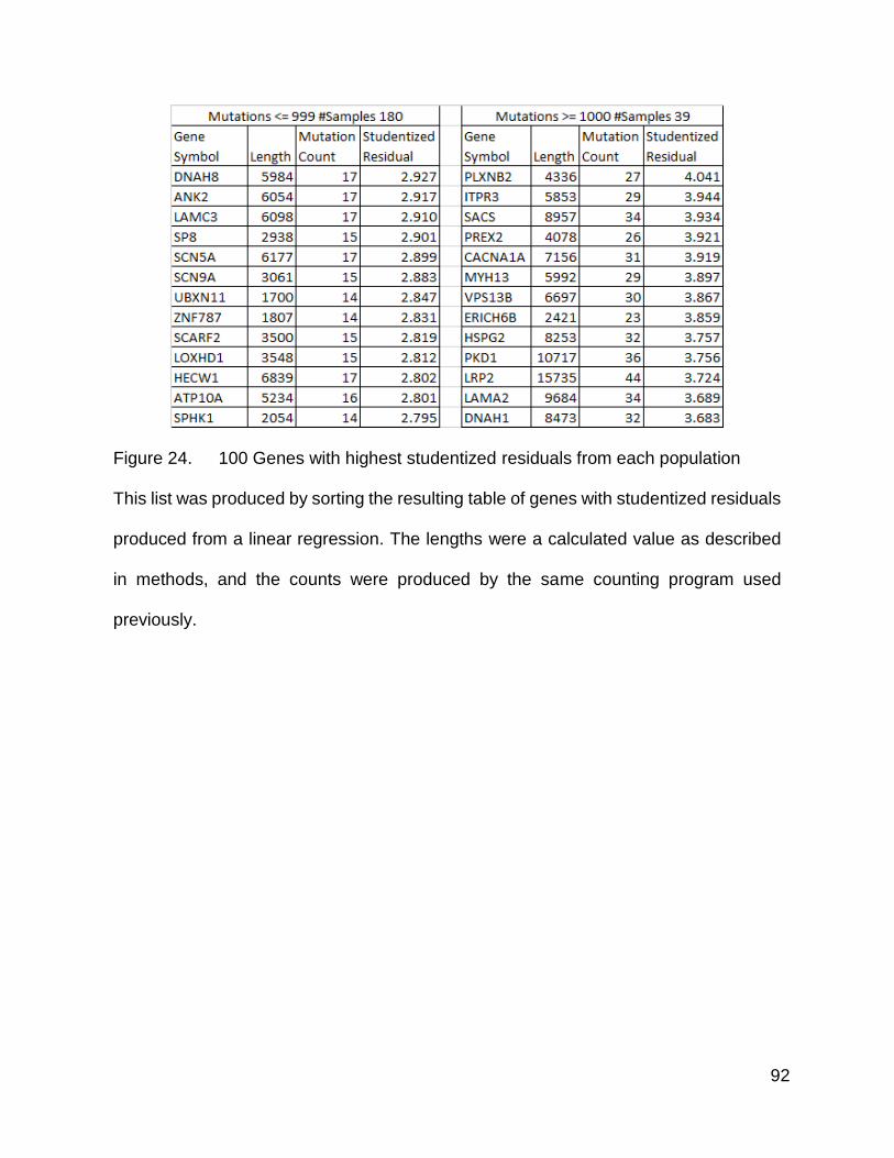
from each population are listed in Figure 24.
A more advanced statistical model than a linear regression might be desirable for
future analyses, as there were multiple overlapping effects other than just gene length.
Some genes would exhibit negative selection for damaging mutations, due to cell viability
needs and either show low mutation counts or zero counts. Other genes would have
positive selection in tumors from any deactivating mutations, due to not requiring subtle
mutations in order to contribute to the tumor phenotype.
Another set of genes would exhibit positive selection on very specific subtle
mutations, but negative selection or no selection at all (depending on the tumor’s existing
genetic background) for any deactivating mutations, making some mutations within this
class of genes passenger mutations despite the gene being a cancer-related gene.
If a tumor was already carrying a subtle mutation in one of these genes, then a
destructive change to the function of that gene would be unlikely to persist within the
tumor unless it occurred within the second copy of the gene on the other chromosome for
a gene where losing the remaining normal copy would not be detrimental to cell viability.
The chances of such a double mutation within the same gene on the same chromosome
89
were also remote for most genes, however this effect might also impact other required
genes downstream in the functional pathway from the subtly affected gene.
In addition to these effects from subtle mutations and disabling damaging
mutations in cancer related genes, there were also a very large number of mutations that
had little to no effect on the genes they occur in, due to being a redundant codon swap,
or causing a functionally synonymous amino acid change. These kinds of mutations
would inherently be passenger mutations, and it is important to note, they could also occur
within cancer related genes. There would also be a collection of mutations that were
destructive in terms of gene function, but which occurred in genes that were not
particularly important for tumor cell survival or competition. These mutations, too, would
be passenger mutations from a cancer genomics perspective. Realizing the possibility of
cancer genes experiencing mutations that ought to be classified as passenger mutations
rather than driver mutations, I became interested in looking at distribution of mutations
within single-genes.
These competing selective effects, in addition to other potential confounding
influences, made the data fairly noisy as a result. There was clearly a positive correlation
of gene length with mutation counts, but the scatterplot did not pack very tightly around
the trend line in either population.
90
91
92
Figure 24. 100 Genes with highest studentized residuals from each population
This list was produced by sorting the resulting table of genes with studentized residuals
produced from a linear regression. The lengths were a calculated value as described
in methods, and the counts were produced by the same counting program used
previously.
93
Discussion
In terms of the mutation types, there did appear to be some significant differences.
Some specific types of mutations did not pass significance tests such as the proportions
of C_A|G_T and A_C|T_G, and A_C, C_A, G_A, G_T, T_G proportions individually, and
the sum of all transitions as well as the non-proportional counts of the C_G|G_C mutations
and the C_G mutations individually (while G_C with a p value of 0.0487 just barely
passed), but most did, even when checking if the proportions were the same. Oddly, the
p value for G_A proportions was 0.39 while the p value for C_T proportions was much
lower at 0.002. This was probably the result of a relatively small number of samples within
the low population that had very few reported mutations in the MAF file, resulting in 0%
for several categories. Since these categories were fairly high in percentage (between
20-35%), these zero values may have lowered the mean values of the proportions enough
to cause a statistical significance between the populations.
When looking at which genes were affected by mutation, here again there were
differences. A primary driver of these differences appeared to be gene size, but when
sorting the lists by mutation counts and looking manually at the gene sizes, and when
using a linear regression and looking at the genes with the highest residuals there were
some differences that were not driven purely by gene size.
Having shown that there were indeed differences an obvious question that follows
is: “What is causing these differences”? I speculate that there are probably a combination
of structural, biological, and biochemical mechanisms behind these differences (40,76–
83). In addition to clonal selection, there may be mutational hot spots, such as
microsatellites within some genes and not others. These genes would be prone to mutate
94
more frequently if a condition causing microsatellite instability were to affect the cell.
Depending on the mutation or regulatory problem that led to the condition causing
increased mutation retention, certain types of DNA damage may become harder for the
cells to detect or to repair leading to a rise in mutations that result from that kind of damage
(45). In addition to this, expression seems to negatively correlate with mutation rates
across the genome (76). There is also the expected effect of larger genes being bigger
targets.
Other causes might broadly increase all types of mutation, due to affecting
detection of DNA damage or weakening the ability of the DNA mismatch repair
mechanism to locate and repair multiple types of damage (67,84–86).

95
Chapter 4
Kurtosis of mutation locations as a Possible Mutation Survey Method and
Detailed Analysis of Potentially Interesting Genes

96
Introduction
I next wanted to determine if the distinction between the two classes of tumors
based on the number of mutated genes carried within the tumors had an effect on the
mutations that were within the genes themselves. Were certain mutations within a given
gene more frequently found in the highly mutated group or the less mutated group? Were
the mutations more random in the high frequency group while those in the low frequency
group were more specific? The thinking behind my hypothesis is that mutations that act
as drivers in driver genes should be enriched in the low mutation group than the high,
while passenger mutations in driver genes should be relatively enriched in the high
mutation group.
An extension of this thinking is that within a specific cancer-associated gene,
specific mutations that enhance an activity that assists in producing the cancer phenotype
should exhibit an enrichment in the low mutation group and a diluted frequency in the high
mutation group.
I expected to see a decrease in specificity of mutations in the high mutation group,
such that even when oncogenes are mutated in the high mutation group, the correct gain-
of-function mutation would not be hit frequently, and that existing tumors or the pre-tumor
somatic lineage would instead acquire mutations in oncogenes at non-tumorigenic
locations. In contrast, inactivating mutations in tumor suppressor genes were far less
precise than the gain-of-function mutations in oncogenes. Thus a random mutation event
was far more likely to produce a tumor assisting (inactivating) mutation within a
suppressor than in an oncogene (assuming the given gene will be hit somewhere along
97
its length), and I expected that this effect would also be borne out if the locations of
mutations within genes were examined between the two groups. In simple terms, I
expected no dramatic difference in targeting of mutations to specific sites in tumor
suppressors between the low and high mutation groups (except that the low mutation
group may be enriched in nonsense or frameshift mutations relative to the high mutation
group), but that there would be a significant difference in distribution of mutations in
oncogenes between the low and high mutation groups with low mutation group showing
targeting of specific activating mutations and a higher degree of randomness in the high
mutation group.
Types of Cancer Driver Genes
Some cancer driver mutations achieve their effects by shutting down a gene which
when functionally normal acts against pathways that favor tumor formation or survival.
These genes with anti-tumor effects are classified as tumor suppressors (31,87). In genes
with this kind of function one will expect higher mutation rates to result in a broad targeting
of the gene sequence across all exons in any location where a disabling change can
occur. There may be peaks in codons that only require a single base change to become
STOP codons, especially if those require mutations are achievable with the most common
variety of mutations. Due to the less targeted nature of the cancer contributing changes
in tumor suppressors as compared to oncogenes, higher mutation rates would favor more
of these mutations having a possible effect just by chance.
Other cancer driver mutations result in a functional change in the function/activity
of a gene. These effects require that the gene still be expressed, but the mutation changes
the function of the gene in some way that supports tumor survival or helps create the
98
cancer phenotype. These genes which can acquire pro-tumor functional changes are
classified as oncogenes (31,32,87). Due to the requirement of conversion of proto-
oncogenes to oncogenes being a gain of function mutation, these genes will often exhibit
a mutational profile with specific locations where point mutations can have an activating
effect (87,88). Due to the highly specific nature of cancer driving mutations in these genes,
these genes would not be expected to be particularly enriched in tumors with a mutator
phenotype, as the chance that a mutation would land outside of the specific activating
targets that are pro-cancer is considerably larger than that of hitting the right spot with the
right mutation.
Assessing the Nature of Mutational Specificity: Kurtosis
Kurtosis (a word derived from Greek, meaning “curved, arching”) is a statistical
computation that is usually used to get a numeric value that indicates something about
the overall shape of a graph (89,90). It and skewness are often used when determining
whether a collection of data seem to fit a normal distribution or not (91). It is a measure
of “tailedness” of the probability distribution of a real-valued random variable. A peak at a
point would not be sufficient to raise kurtosis if a normal distribution surrounded that point.
A normal distribution with very small standard deviation would still have an excess
kurtosis of 0 (excess kurtosis is a calculation where the raw kurtosis value for the normal
distribution, usually 3, is subtracted from the raw kurtosis value). A value is leptokurtotic
(high kurtosis value) when there is a very strong peak that looks like a pointy spike, and/or
heavy tails. The opposing situation, platykurtosis, would exist in a distribution where there
was no pointy peak, and the peak was surrounded by a wide and rounded distribution, or
in more extreme cases, a very wide and very flat distribution. Mesokurtosis refers to

99
values that are less extreme. Normal distributions are mesokurtotic and have an excess
kurtosis of 0. A Bernoulli distribution with p=1/2, (a coin flip) has a kurtosis of -2. A discrete
uniform distribution (dice roll) has a kurtosis that varies according to the number of
possible values (number of faces on the die). At N=3 the excess kurtosis is -1.5, and it
approaches -1.2 asymptotically as N increases.
When dealing with genomic coordinates of mutations within a gene, I was not
dealing with a direct measure of probability of a single random variable, but those genes
in which there are specific hot spots could still be expected to produce a higher kurtosis
value than genes where there are no hot spots and mutations are randomly distributed
throughout the entire length of the gene. Dr. Yu-Bo Wang suggested trying to use kurtosis
values due to lack of a more obvious tailor-made method for detecting such differences,
so I decided to see what resulted from these calculations for the mutated genes in these
populations of tumors.
Kurtosis is a measure of the shape of a distribution (89,90). Technically, it is a
measurement of how weighty the tails of a distribution are, though in practical terms, for
distributions that have a bulk of their probability at the center of the distribution and that
are symmetrical, it can also be an indicator of sharpness, or pointy-ness.
There are three terms that generally describe graphs with different kinds of kurtosis.
The normal distribution, shown in gray on Figure 25, actually has a true kurtosis value of
3, but is used to define the concept of excess kurtosis, which subtracts the value of the
kurtosis of the normal distribution from the true kurtosis, which is what is usually reported
as kurtosis by various types of software, and is what many kurtosis estimation formulas
return, and as such the normal distribution is considered to have an excess kurtosis value

100
of 0. When I refer to kurtosis values in the latter parts of this document, I am actually
referring to excess kurtosis returned by an algorithm.
Leptokurtic distributions generally have a sharper peak, and heavier tails, such as
the laplace distribution shown in blue in Figure 25. Platykurtic distributions generally have
flatter peaks and lighter tails. The raise cosine distribution shown in yellow and the uniform
distribution shown in orange on Figure 25 are both platykurtic. The raised cosine
distribution has the typical qualities mentioned, and the uniform distribution has no peak
at all, and is all tail.
To explain this point, there is a probability distribution known as a U-quadratic
distribution, that is a continuous probability distribution over a defined range from a to b.
The quadratic that describes this distribution would be a U shaped parabola (with a focus
pointing in the positive direction) that is symmetrical about the midpoint between a and b,
and has total area under the curve of 1 between a and b. The excess kurtosis for such a
function is 3/112*(b-a)4. The longer the distance from b to a, the more kurtosis this
distribution would have, and yet it has no peak in the middle. Kurtosis values for this
distribution can approach zero for very small a to b intervals, but it will never be negative.
This does suggest that strongly positive kurtosis values obtained from mutation
locations across a gene would need to be examined for similar heavy tailed distributions
without a centralized probability peak. I do not expect that mutation distributions fitting a
very long and heavy tailed distribution with no peaks in the middle such as this would be
particularly common.
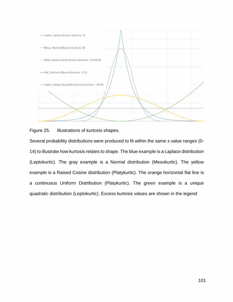
101
Figure 25. Illustrations of kurtosis shapes.
Several probability distributions were produced to fit within the same x value ranges (0-
14) to illustrate how kurtosis relates to shape. The blue example is a Laplace distribution
(Leptokurtic). The gray example is a Normal distribution (Mesokurtic). The yellow
example is a Raised Cosine distribution (Platykurtic). The orange horizontal flat line is
a continuous Uniform Distribution (Platykurtic). The green example is a unique
quadratic distribution (Leptokurtic). Excess kurtosis values are shown in the legend
102
Hypothesis
Within any cancer driver oncogene, specific activating or gain-of-function
mutations should be enriched in the low mutation group of tumors while non-specific or
passenger mutations should be enriched in the high mutation group of tumors. To detect
this difference, I examined the mutations within specific genes. I expected that within
oncogenes there are a small number of locations where subtle mutations lead to
constitutive activation of the resulting protein or other subtle alteration in its structure or
behavior that leads to a tumorigenic effect. This means that there ought to be a very
specific set of mutations in oncogenes that are capable of contributing to the cancer
phenotype within the selected tumor population. I expected therefore to see a very small
number of locations with high mutation counts in these genes when they present selective
advantage.
In contrast, I expected that tumor suppressor genes would show a profile where
mutations appear throughout the gene at any sites where they can deactivate the function
of the gene, perhaps with some hot spots where it is easier to create damaging mutations,
but with less precision than I would expect within oncogenes.
There is also the effect of the mutation rates to consider. My model is that the
highly increased rate of mutation in the high mutation group would create possibilities for
random mutations to occur outside the tumorigenesis process that wouldn’t exist at the
lower mutation rates in the low mutation group. As a result of this increased rate of
mutations in the high mutation group, there is an increased possibility of redundantly
affecting signaling pathways via multiple hits to more easily disabled gene targets in the
high mutation group instead of requiring a precise hit on a canonically important cancer-
103
related gene target. Also, the effect of the enhanced mutation rate would generally cause
a lot more passenger mutations. Therefore, in the high mutation group I would expect the
mutation accumulation peaks to be less pronounced in oncogenes, and for the oncogenes
that were mutated, there would be an increased number of non-tumorigenic mutations,
which would effectively be passenger mutations, in a significantly increased number of
samples. In contrast, I expect that there would not be very much difference to the
spectrum of mutations found in most tumor suppressor genes between the two groups
except possibly an enrichment of missense or silent mutations in the high mutation group.
In summary, the mutations found within many genes that require precise mutations
will likely be found to have more accurate targeting in the low mutation group, and less
accurate targeting in the high mutation group, while genes that simply require deactivation
will not experience much difference in the distribution of their mutations between the two
groups.
Given that mutations in hot-spots will create peaks at a specific point rather than
at an “average location”, these would tend to produce a leptokurtic scenario. If there are
multiple hot spots that are not localized to a particular section of the gene this would trend
toward producing a mesokurtic result, especially if there are also off target mutations
spread through the gene, or spanning multiple exons. If the gene has no hot spots and
no selective locations producing oncogenic traits, and sports very long “tails” of off target
mutations spread throughout the gene, this would be expected to produce platykurtic
values.
104
Methods
For a selected set of oncogenes with known effective mutation sites and a set of
suppressor genes, I examined the mutation locations that appeared within the two sample
groups. Counts were tallied per genomic location, and these counts were used in
conjunction with annotations of known effective sites to test the hypothesis.
I sought advice on how to discriminate between mutation profiles containing strong
peaks and mutation profiles with wide dispersal of mutations from statistics experts Drs.
James Grady and Yu-Bo Wang. Yu-Bo suggested that I try computing the kurtosis of the
genomic positions, and see if the kurtosis values signaled the position of strong peaks.
Based on my observation of some of the mutations lists and the resulting kurtosis values
this method has resulted in at least a partial success, although there are some caveats
to the method. Some distributions that have no peaks result in kurtosis values that
suggest there should be strong peaks. It did produce some interesting and potentially
useful results though.
I accomplished the kurtosis calculations using a python program to control function
calls in R using a module called rpy2. The kurtosis function from the R package e1071
was used. A list of start positions for each mutation within each gene was compiled, and
this list of numbers was fed to the kurtosis function. The resulting numbers were compiled
into a tab separated table as output.
For a selected set of genes, I pulled a list of the mutations out of the MAF file using
command line tools. I queried for the lines containing the requested gene symbol and
pulled out the relevant fields for the start and end locations. This was sorted and
duplicates were counted, producing a set of tables showing the number of mutations at
105
each position. For better comparison between the high and low mutation groups, I added
columns that divided the count values by the tumor population size.
Results
As expected, mutations in oncogenes showed a strong preference for specific sites
to a much higher degree than the mutations in tumor suppressors within the low mutation
population. The high mutation population showed a higher degree of randomness and
significantly less specificity. However, the results were not completely clean. In both the
low and high mutation groups, tumor suppressor genes still showed statistical
preferences for some sites. It is possible that this preference might have been due to
ease of mutational deactivation at these sites by creating premature stop codons or
significantly disrupting the action of the gene by disrupting normal folding or structural
integrity of the peptide at these enriched sites.
An exception to the higher degree of randomness in the mutations in the high
mutation group was found for the gene BRAF. This decreased randomness was
consistent with the previous observation that specific mutations in BRAF were associated
with and advantageous to the mutator phenotype (92–94). Thus I confirmed the possibility
of there being some exceptions to my hypothesis on a genome-wide basis if certain
mutations within specific oncogenes are strongly selective within the mutator phenotype.
Vogelstein et al. composed a list of cancer related genes classified as tumor
suppressor genes and oncogenes according to a scoring algorithm (31). I wanted to see
the mutation profiles of these genes and whether the kurtosis values for these genes
obeyed my model based on their Vogelstein classification. I found that the kurtosis values
106
were consistent with my model for both tumor suppressors and oncogenes and between
the low and high mutation frequency populations.
APC, short for Adenomatous polyposis coli, is a well-known tumor suppressor
gene that has been found to have very prominent involvement in colon cancer (95), and
was given a name based on that relationship. APC had high kurtosis values in both
populations, with a very strong value for the high population. This was not unexpected,
given that destructive mutations often cluster in important functional motifs, and due to
the very strong association of this gene with colon cancer. The increase in kurtosis in the
high mutation group could be due merely to the very high mutation rate, or might be the
result of random fluctuation in the locations where the mutations hit. Perhaps the gene
has hot spots for mutation that are more likely to mutate under the conditions present in
a cell with a mutator phenotype.
BRAF an oncogene with known association to tumors with DNA repair disorders,
(92,94) had very high kurtosis in the high mutation group, an expected result in this
population.
KRAS does not share an association with mutator phenotypes or DNA repair
disorders (96–98). It had high kurtosis in the low mutation group, showing very strong
selection for the oncogenic mutation locations. In contrast, KRAS was rarely mutated at
the oncogenic sites in the high mutation group.
Compared purely in terms of accumulated mutation count, APC had 84 mutations
in a population of 180 tumors in the low group (0.46 mutations/sample), and 15 mutations
out of a population of 39 (0.38 mutations/sample), but to focus on this alone would have
missed a very important aspect of how oncogenes like KRAS mutate. KRAS only
107
experiences oncogenic mutations as a result of specific changes at specific locations in
its sequence.
Position chr12:25398284 (in GRCh37/hg19), corresponding to the 2nd base in the
12th codon of KRAS, was the most mutated site, with 39 mutations. The codon at this site
is usually GGU (Glycine). There were 3 mutation variants found at this site. C to T (19
counts), changes the codon to GAU (Aspartic acid). C to A (15 counts), changes the
mRNA codon to GUU (Valine). C to G (5 counts), changes this codon to GCU (Alanine).
A site immediately adjacent at position chr12:25398285 which is the 1st base within the
same codon, had 11 mutations. C to T (5 counts) results in codon AGU (Arginine). C to
A (4 counts) results in codon UGU (Cysteine). C to G (2 counts) results in codon CGU
(Serine).
Another site, at position chr12:25398281 corresponds to the 2nd base in the 13th
codon which is usually GGC. This C to T mutation (16 counts) results in GAC (Aspartic
acid). The first base of this codon also experienced a C to A mutation to produce a UGC
codon (cysteine) in one sample.
It is unclear whether all of these amino acid changes result in an oncogenic protein.
Changes to codon 12 and 13 tend to be oncogenic (98,99), but mutations other known
locations were not particularly common in this type of tumor.
Limitations of the analysis
Kurtosis appeared to function well as a positive identifier, but its power in terms of
negative results was unreliable due to the relatively low mutation counts some genes
experience and the fact that some genes’ involvement in cancer is related to the tissue of
origin, and that some genes might exhibit a very platykurtic distribution if they are tumor

108
suppressors lacking hot spots. Thus its utility in identifying interesting genes lies solely in
comparative results (which group shows a higher value) and even so requires more
detailed follow-up analysis to interpret any positive results. It therefore can serve as a
useful flag for taking a further look at genes that show high kurtosis values.
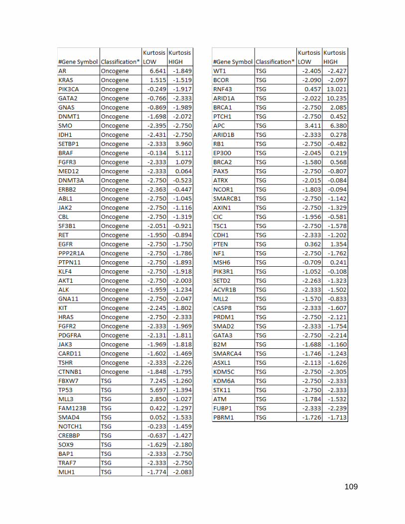
109
110
Figure 26. Kurtosis values for Vogelstein Subtly Mutated Gene List for TCGA data.
Genes that were found in the supplemental data of the 2013 Vogelstein paper on
Genomic Landscapes in Cancer (31) but which had no counts or not enough counts to
be able to compute kurtosis for either population were omitted from this table. The table
was sorted by the Vogelstein classification first, and as a secondary sorting rule the
genes with higher values in the LOW population than the HIGH population were sorted
toward the top.
111
Examining Outliers and Potentially Interesting Genes in More Detail
I examined a subset of genes that seemed particularly out of place in regard to
their size vs their mutation counts. I included a calculation for the absolute value of the
difference for the kurtosis value between the groups and sorted according to that
difference. My hope was the genes with the most different values would have significant
shifts in their mutation distribution, and perhaps would have a functional association with
cancer phenotypes. They might also have targeted locations that mutate and become
strongly positively selected. I included TTN on this list because despite its massive size,
it had many more mutations than its size ought to dictate based on the general trend, and
it is also a very good example of a gene that was computed to have low kurtosis on its
mutation locations, and actually deserves the negative result. The mutations in TTN do
not pile up at any particular spots. The mutations are spread out quite a bit, with all of the
locations only having 1 or 2 mutations, with counts of 2 being infrequent. Due to this very
spread out and sparse mutation pattern, I opted not to show TTN’s mutation locations in
detail.
In Figure 27, I highlighted in green those genes that were also contained within the
Vogelstein list of oncogenes and tumor suppressor genes known to be associated with
cancer phenotypes (31). Their results may also help in understanding these mutation
profiles and how the mutation rates affect them. There are clearly some genes with very
strong kurtosis values, and also some genes that only pile up enough to get positive
kurtosis in one group or the other. Interestingly, a good number of the genes showed a
higher degree of “pointiness”, as scored by kurtosis, in the high mutation group, where
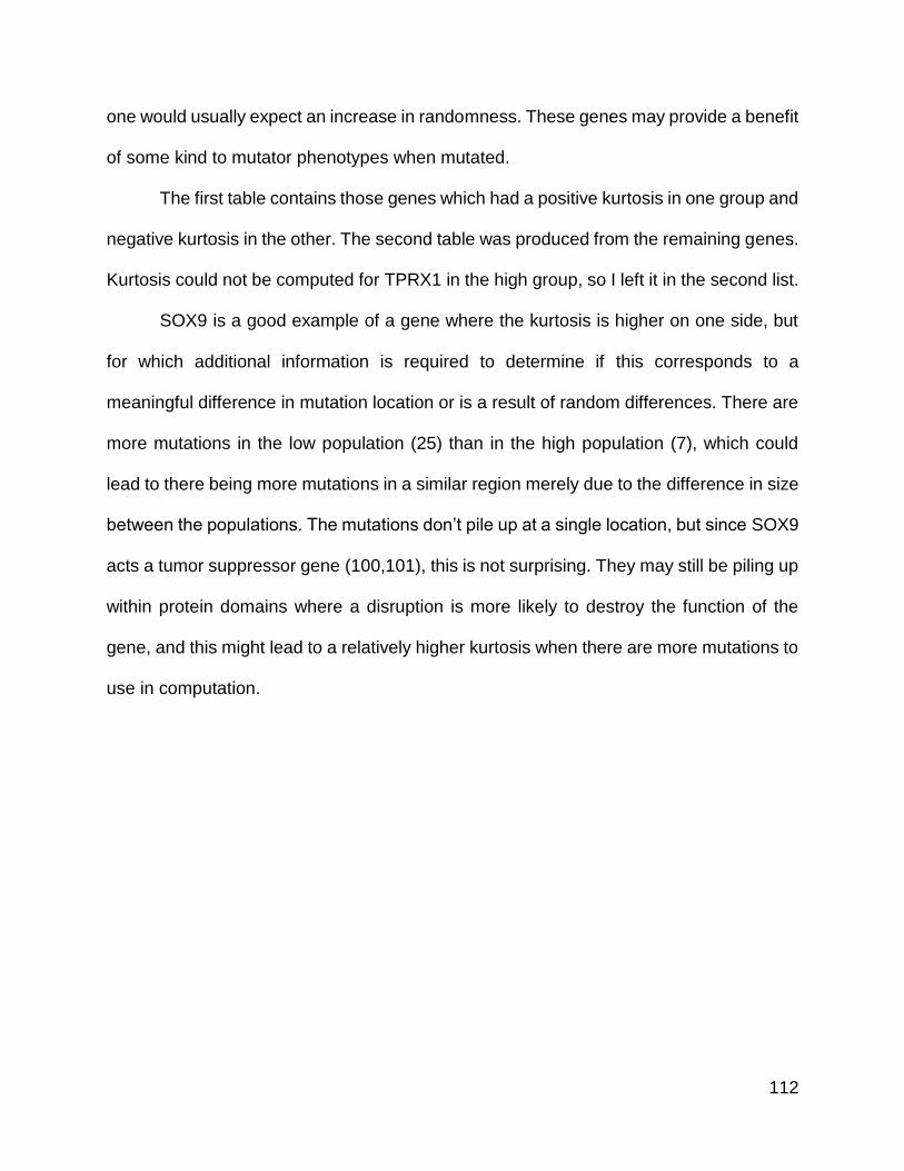
112
one would usually expect an increase in randomness. These genes may provide a benefit
of some kind to mutator phenotypes when mutated.
The first table contains those genes which had a positive kurtosis in one group and
negative kurtosis in the other. The second table was produced from the remaining genes.
Kurtosis could not be computed for TPRX1 in the high group, so I left it in the second list.
SOX9 is a good example of a gene where the kurtosis is higher on one side, but
for which additional information is required to determine if this corresponds to a
meaningful difference in mutation location or is a result of random differences. There are
more mutations in the low population (25) than in the high population (7), which could
lead to there being more mutations in a similar region merely due to the difference in size
between the populations. The mutations don’t pile up at a single location, but since SOX9
acts a tumor suppressor gene (100,101), this is not surprising. They may still be piling up
within protein domains where a disruption is more likely to destroy the function of the
gene, and this might lead to a relatively higher kurtosis when there are more mutations to
use in computation.
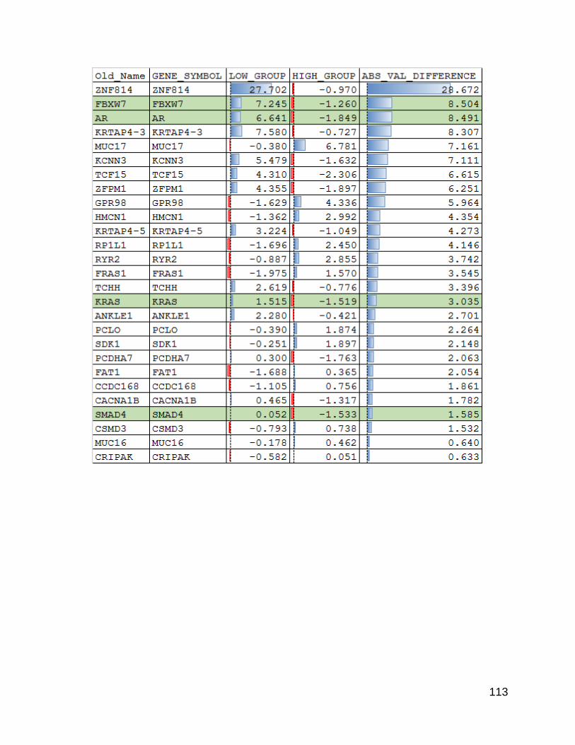
113
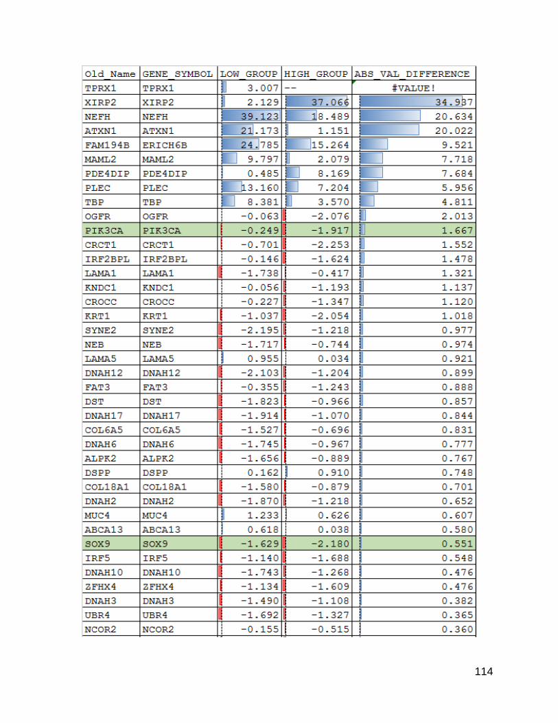
114
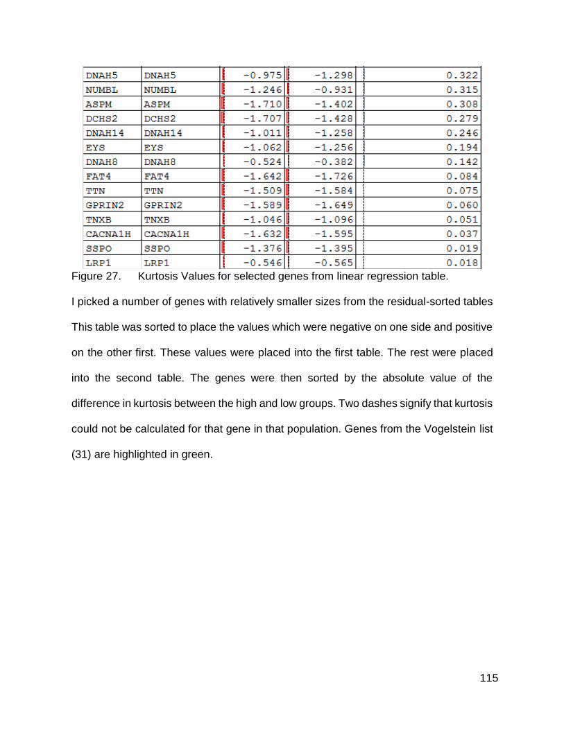
115
Figure 27. Kurtosis Values for selected genes from linear regression table.
I picked a number of genes with relatively smaller sizes from the residual-sorted tables
This table was sorted to place the values which were negative on one side and positive
on the other first. These values were placed into the first table. The rest were placed
into the second table. The genes were then sorted by the absolute value of the
difference in kurtosis between the high and low groups. Two dashes signify that kurtosis
could not be calculated for that gene in that population. Genes from the Vogelstein list
(31) are highlighted in green.
116
The cancer gene list (31), as a whole, contained genes that were not necessarily
expected to be associated with colon cancer, and thus resulted in many genes having
low kurtosis in both groups. It was interesting that so many genes had higher kurtosis for
the HIGH mutation group, where I generally expected more randomness. I then decided
to take a look at the genes canonically associated with colon cancer.
I compiled a table (shown in Figure 28) based on the list of mutations and genes
on mycancergenome.org (102). While it is a complex table, I structured it such that only
known mutations would be counted. It would show a dash for any value that was not
defined in the known mutation part of the table.
As mentioned previously, KRAS showed a strong preference for mutations in
codon 12 and 13, and to a lesser extent, codons 61 and 146, while other locations were
rarely mutated.
In BRAF there was strong tendency for changing codon 600 to code for Valine.
This BRAF mutation is highly associated with defects in DNA repair (92,93,96). This
targeting of the mutation to a specific location (V600E) was captured quite readily by the
difference in kurtosis.
PIK3CA is strongly associated with colon cancer (103,104) and showed a strong
tendency for mutation at codon 545, changing from Glycine to Lysine. There was a
concordant rise in kurtosis, but the number of off target mutations (and perhaps their
distance from this mutation peak), was sufficient to cause the resulting kurtosis to be
somewhat low. This is why the change in value between the same gene in both
populations is more important than the actual value of the kurtosis.
117
PTEN is another gene associated with microsatellite-stable colon cancer (104,105).
Its mutation spectrum was particularly interesting. It showed NONE of the three known
cancer-associated mutations (102), though one was very similar (there was a deletion
mutation at a position very close to the listed one found in both populations). There were
also a few other frame shift mutations at different locations and some nonsense mutations
as well. These could possibly all be oncogenic due to destroying the function of the
resulting PTEN protein or initiating nonsense-mediated decay (106) and resulting in no
protein being made at all.
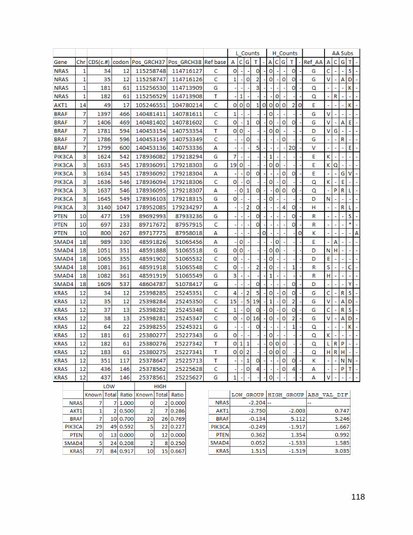
118
119
Figure 28. Genes known to be associated with colon adenocarcinoma (102), their
known mutations, and their kurtosis values in the high and low mutation populations.
The first table lists genomic position, codon number, CDS position, reference base,
original amino acid, the resulting amino acid for known mutations, and counts of
specified mutations within the high and low mutation groups.
Of the smaller tables, the one on the left shows counts of known mutations the total
number of mutations for that gene and a ratio of known mutations to total mutations.
The smaller table on the right shows the kurtosis values for these genes. (-- is a stand
in for a value that was unable to be computed due to there not being enough mutations)
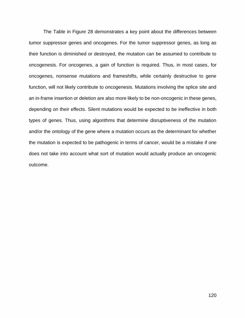
120
The Table in Figure 28 demonstrates a key point about the differences between
tumor suppressor genes and oncogenes. For the tumor suppressor genes, as long as
their function is diminished or destroyed, the mutation can be assumed to contribute to
oncogenesis. For oncogenes, a gain of function is required. Thus, in most cases, for
oncogenes, nonsense mutations and frameshifts, while certainly destructive to gene
function, will not likely contribute to oncogenesis. Mutations involving the splice site and
an in-frame insertion or deletion are also more likely to be non-oncogenic in these genes,
depending on their effects. Silent mutations would be expected to be ineffective in both
types of genes. Thus, using algorithms that determine disruptiveness of the mutation
and/or the ontology of the gene where a mutation occurs as the determinant for whether
the mutation is expected to be pathogenic in terms of cancer, would be a mistake if one
does not take into account what sort of mutation would actually produce an oncogenic
outcome.
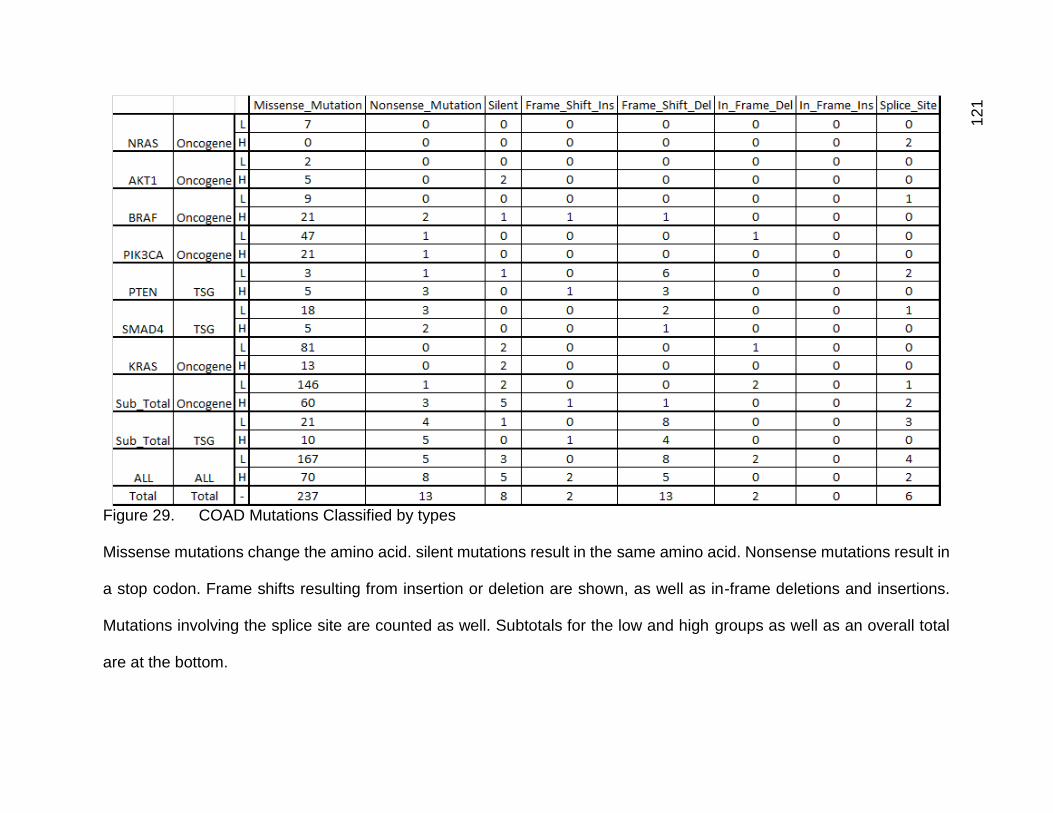
12
1
Figure 29. COAD Mutations Classified by types
Missense mutations change the amino acid. silent mutations result in the same amino acid. Nonsense mutations result in
a stop codon. Frame shifts resulting from insertion or deletion are shown, as well as in-frame deletions and insertions.
Mutations involving the splice site are counted as well. Subtotals for the low and high groups as well as an overall total
are at the bottom.
122
The genes in Figure 30 were of particular interest. BRAF, EGFR, HRAS, KRAS,
RB1, and TP53 are on this list due to being known for bearing canonical cancer driver
mutations. TTN was an example of a gene that was not expected to have any specific
mutations related to cancer. KRTAP4-3 (107,108), KRTAP4-5 (107,109) FAM194B
(110,111) (which has had its official symbol changed to ERICH6B), and DSPP (112–114)
were mutation count trend outliers that looked to have potentially interesting mutation
distributions.
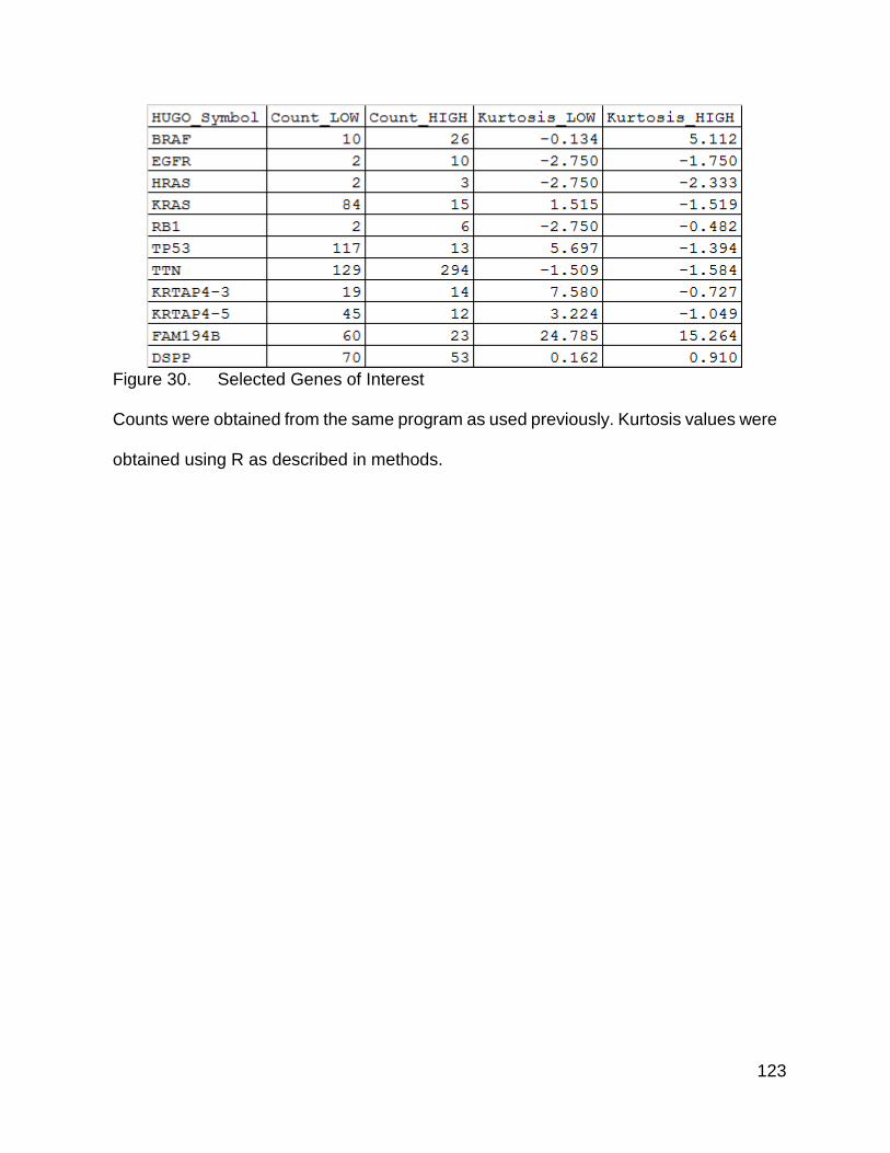
123
Figure 30. Selected Genes of Interest
Counts were obtained from the same program as used previously. Kurtosis values were
obtained using R as described in methods.
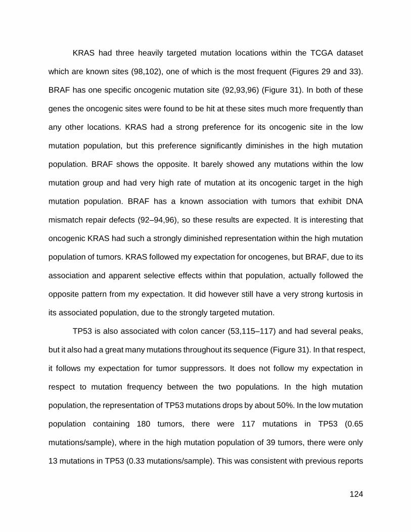
124
KRAS had three heavily targeted mutation locations within the TCGA dataset
which are known sites (98,102), one of which is the most frequent (Figures 29 and 33).
BRAF has one specific oncogenic mutation site (92,93,96) (Figure 31). In both of these
genes the oncogenic sites were found to be hit at these sites much more frequently than
any other locations. KRAS had a strong preference for its oncogenic site in the low
mutation population, but this preference significantly diminishes in the high mutation
population. BRAF shows the opposite. It barely showed any mutations within the low
mutation group and had very high rate of mutation at its oncogenic target in the high
mutation population. BRAF has a known association with tumors that exhibit DNA
mismatch repair defects (92–94,96), so these results are expected. It is interesting that
oncogenic KRAS had such a strongly diminished representation within the high mutation
population of tumors. KRAS followed my expectation for oncogenes, but BRAF, due to its
association and apparent selective effects within that population, actually followed the
opposite pattern from my expectation. It did however still have a very strong kurtosis in
its associated population, due to the strongly targeted mutation.
TP53 is also associated with colon cancer (53,115–117) and had several peaks,
but it also had a great many mutations throughout its sequence (Figure 31). In that respect,
it follows my expectation for tumor suppressors. It does not follow my expectation in
respect to mutation frequency between the two populations. In the high mutation
population, the representation of TP53 mutations drops by about 50%. In the low mutation
population containing 180 tumors, there were 117 mutations in TP53 (0.65
mutations/sample), where in the high mutation population of 39 tumors, there were only
13 mutations in TP53 (0.33 mutations/sample). This was consistent with previous reports

125
that colon tumors with microsatellite instability due to mutations in MMR genes are less
likely to have mutations in either KRAS or TP53 (72).
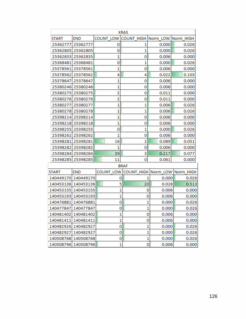
126
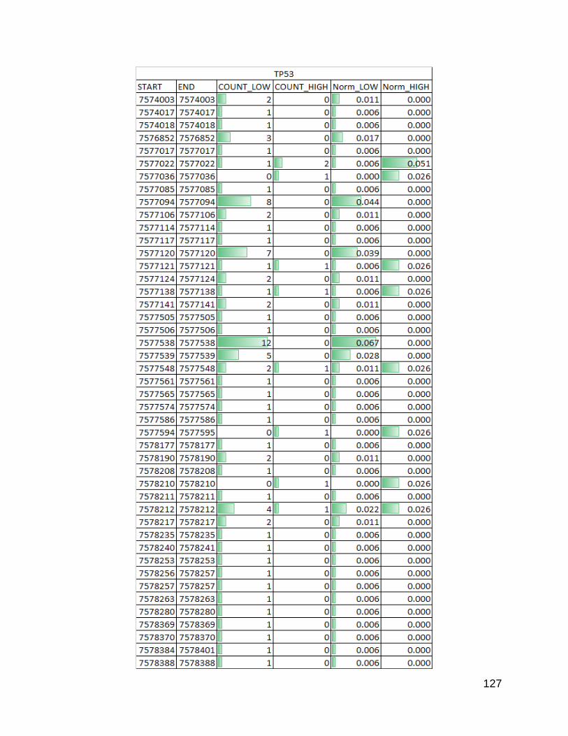
127
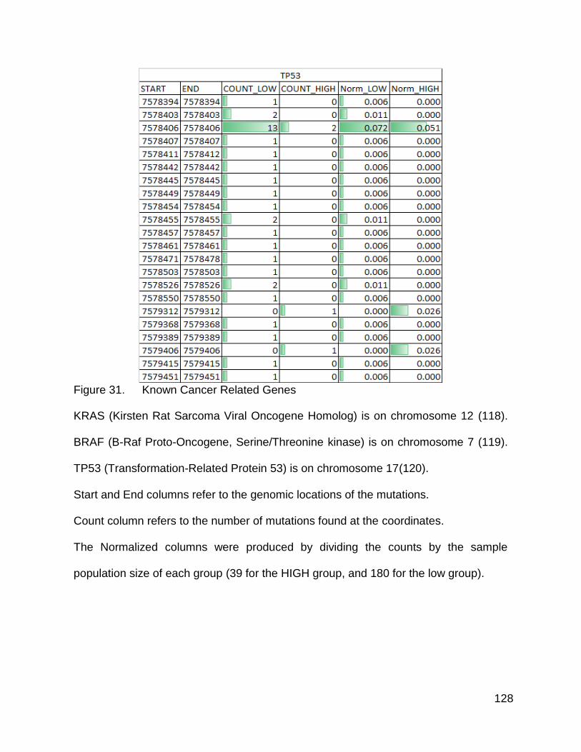
128
Figure 31. Known Cancer Related Genes
KRAS (Kirsten Rat Sarcoma Viral Oncogene Homolog) is on chromosome 12 (118).
BRAF (B-Raf Proto-Oncogene, Serine/Threonine kinase) is on chromosome 7 (119).
TP53 (Transformation-Related Protein 53) is on chromosome 17(120).
Start and End columns refer to the genomic locations of the mutations.
Count column refers to the number of mutations found at the coordinates.
The Normalized columns were produced by dividing the counts by the sample
population size of each group (39 for the HIGH group, and 180 for the low group).
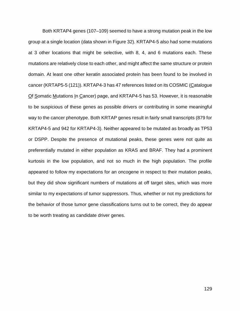
129
Both KRTAP4 genes (107–109) seemed to have a strong mutation peak in the low
group at a single location (data shown in Figure 32). KRTAP4-5 also had some mutations
at 3 other locations that might be selective, with 8, 4, and 6 mutations each. These
mutations are relatively close to each other, and might affect the same structure or protein
domain. At least one other keratin associated protein has been found to be involved in
cancer (KRTAP5-5 (121)). KRTAP4-3 has 47 references listed on its COSMIC (Catalogue
Of Somatic Mutations In Cancer) page, and KRTAP4-5 has 53. However, it is reasonable
to be suspicious of these genes as possible drivers or contributing in some meaningful
way to the cancer phenotype. Both KRTAP genes result in fairly small transcripts (879 for
KRTAP4-5 and 942 for KRTAP4-3). Neither appeared to be mutated as broadly as TP53
or DSPP. Despite the presence of mutational peaks, these genes were not quite as
preferentially mutated in either population as KRAS and BRAF. They had a prominent
kurtosis in the low population, and not so much in the high population. The profile
appeared to follow my expectations for an oncogene in respect to their mutation peaks,
but they did show significant numbers of mutations at off target sites, which was more
similar to my expectations of tumor suppressors. Thus, whether or not my predictions for
the behavior of those tumor gene classifications turns out to be correct, they do appear
to be worth treating as candidate driver genes.
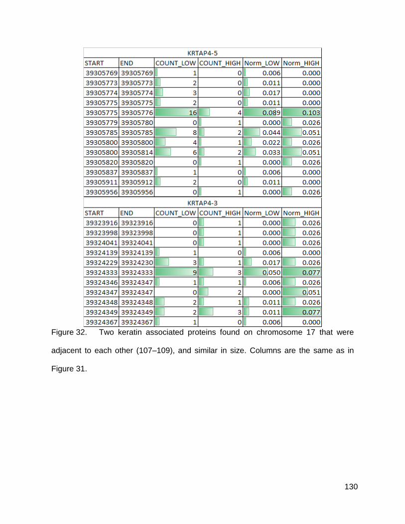
130
Figure 32. Two keratin associated proteins found on chromosome 17 that were
adjacent to each other (107–109), and similar in size. Columns are the same as in
Figure 31.
131
ERICH6B, formerly called FAM194B, has been reported as mutated in cancers
(110). Its COSMIC entry (which is still under its older name FAM194B), has 62 entries in
its references list. It showed a very targeted set of mutation peaks within a small genomic
region (data shown in Figure 33). These were about 11 bp in size, with 4 locations being
targets. There were not very many mutations within this gene outside of the targeted
location. It also seemed to be mutated at these targets to a proportionally larger degree
in the high mutation group. Its locus spans 81218 bases, but its exonic size is fairly small
containing ~2421 bases and resulting in a protein 696 amino acids in size. The profile
does seem to be more similar to a tumor suppressor than to my expectations for an
oncogene, but it is hard to use my model to suggest which classification this gene might
fit. The relative lack of mutations throughout the gene could simply be a function of how
small the spliced transcript is. The range of the mutation target suggests that the mutation
may be disrupting a structure in that area or a function that relies on that 11 bp region.
That domain might become inactivated due to these mutations, but I do not know how
that impacts the function of the gene as a whole. It still presents itself as an interesting
driver gene candidate.
132
Figure 33. ERICH6B / FAM194B. This gene, from chromosome 13, is named
ERICH6B. It was named FAM194B within the MAF file obtained from TCGA due to the
older annotation data the project used. The name has since been changed. The new
name stands for Glutamate rich 6B, while the old name stood for family with sequence
similarity 194, member B. Columns are the same as in Figure 31.

133
ZNF814 is a gene found on chromosome 19. It has a generic name based on its
high number of zinc finger motifs, and not much appears to be known about it. A ten base
pair region showed a high concentration of mutations in both groups, with 3 additional
locations relatively close to that region also showing involvement. It is unknown what
affect disrupting this region of the gene will do, but it does appear potentially interesting
as a candidate driver gene deserving further research.
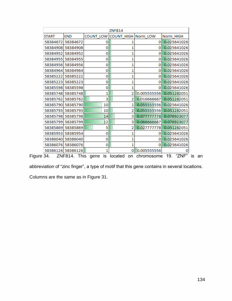
134
Figure 34. ZNF814. This gene is located on chromosome 19. “ZNF” is an
abbreviation of “zinc finger”, a type of motif that this gene contains in several locations.
Columns are the same as in Figure 31.
135
DSPP has also been associated with cancer in previous work (113,122). There are
93 entries in its COSMIC references page indicating it may have some involvement in
cancer. DSPP had a higher kurtosis value in the high mutation group. It showed a peak
of mutations in a 12 bp region targeting 4 locations (data shown in Figure 35). There was
also another peak that showed up within the low population 621 bp away from the other
cluster of mutations. This population lacked a peak at the second location, which might
be partly responsible. It demonstrated preferred sites, but the peaks were pretty
consistent within the high group and there were a lot of off target mutation locations all
through the gene as well. Its mutation profile superficially resembled that of TP53.
There were some targeted locations, but these were mostly silent mutations, and
there were also a very large number of mutation peak locations all through the gene. Thus
the fairly wide spread of mutation locations indicated that I should expect the gene to act
as a tumor suppressor if it has any involvement in cancer, but it turns out that a large
number of these mutations were silent. Due to the mutations mostly being silent, the gene
is less promising as a candidate driver gene, but it does deserve a deeper look given that
it has some degree of mutation frequency other than the mutation count peaks.
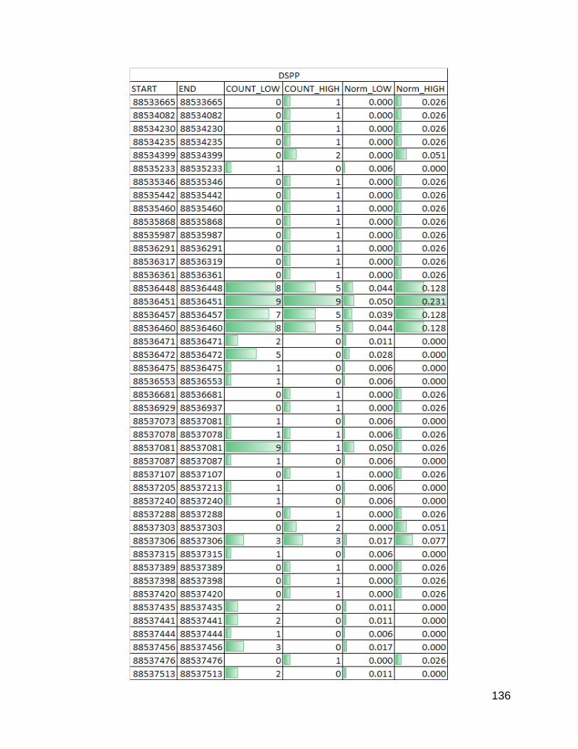
136

137
Figure 35. DSPP (Dentin sialophosphoprotein) is found on chromosome 4 (112).
Columns are the same as in Figure 31.
138
TP53, DSPP, ERICH6B, KRTAP4-3, and KRTAP4-5 were all found to be mutated
more often than their size should dictate, and have mutation patterns suggesting there is
a selective effect at some of these loci in tumors within the colon TCGA sample set. These
genes have also been previously reported in lists of affected genes or in cancer studies
previously. Many of the mentions involving these genes have been the result of genome
wide association studies in large lists of results as opposed to specific research into these
genes to characterize their function and possible contribution to cancer phenotypes.
Discussion
In summary, I found that some genes had differences in their mutation distribution
pattern between these groups. The kurtosis values as a survey method do appear to be
somewhat useful, but require careful analysis to interpret. My hypothesis regarding
targeted mutations concentrating the in the low mutation group did not hold for all genes,
but in the broad sense the expectation was still valid. Some of the genes known to be
associated with colon adenocarcinoma possessed many mutations in known locations,
however genes such as PTEN did not mutate in known locations at all and as predicted
by my model, there were more passenger mutations in several of the genes that I
examined closely in the high mutation group than there were in the low mutation group.
At least one gene, BRAF, had its targeted mutations concentrated in the high mutation
group, presumably because they offer these tumors some kind of selective benefit, and
either do not affect other types of tumors or present a selective detriment.
139
Alternative approaches
A more ideal method would be to develop a sophisticated bioinformatics model to
carry out this analysis. A statistical test for each site or for groupings of sites (if there are
multiple effective spots, vs useless spots in the case of oncogenes) could be programmed,
and each gene would require a designation as an oncogene (with an associated list of
effective mutation sites, and types of mutations that are known achieve the tumor driving
effects), or as a tumor suppressor, or a passenger (reasonable to conclude as uninvolved
with tumor phenotype) or an unknown status (where not enough is known about a gene
to make a determination). From there it could analyze the patterns of mutations found
within the gene against expectation values to produce an ability to cluster samples
according to similarity of mutation patterns, or even perhaps to set up a neural network
to recognize these patterns in future data sets.
Once the profiles of these genes are better understood, a similar algorithm could
be engineered to use these types of profiles to predict if a candidate gene is likely an
oncogene or a suppressor, based on the distribution of mutations within population splits
based on total mutation count in large datasets. A potential confounding factor is how to
differentiate preferred sites based on deactivation from those that are activating mutations.
The number of such sites within a gene tends to be much smaller for oncogenes, so the
probability could be assumed to be inversely correlated with the number of codons
affected, though genes with complicated folding pattern, or that participate in multi-protein
complexes could have multiple locations throughout their sequences that participate in
important enzymatic activities, ability of the protein to recognize and bind to substrates,
influence folding and structure, or even influence the protein’s ability to bind to a
140
multiprotein complex. My method of using kurtosis over the full set of mutation locations
might be unable to properly signal peaks in genes where these preferred sites are more
distant from one another. Perhaps a different statistic would be better, and perhaps
computing kurtosis, or a more specialized statistic, using a sliding window of some
number of nucleotides might prove to be a more powerful application of this idea to identify
locations where there is a mutation peak. This is an important improvement to seek,
because there may be cases where a range of nucleotides within a protein domain could
be modified and achieve similar effects rather than just a single location of small handful
of locations. For example, a gene that promotes cell survival or growth might be converted
to being more active by blocking the binding of an inhibitor by changing its binding site
via mutation. This could possibly be achieved by changing multiple nucleotides in the
sequence of its binding domain, while retaining the overall structure of the protein and
preserving its ability to carry out its biological activity. In such a case there wouldn’t just
be one peak, but rather a generally raised mutation rate over a wider genomic region.
Whether kurtosis calculations would pick up on this pattern would depend partly on the
size of the domain, how spread out the mutation sites are, and on the number and location
of any passenger mutations exist in the population being studied, but perhaps a more
sophisticated statistical model would be more sensitive and able to pick up on such a
pattern more easily.
If protein structure data is available, perhaps the 3-dimensional distance between
different amino acids and their associated codons could be used to determine if clusters
of mutation peaks at different locations within the transcript are affecting the same relative
physical location in a folded protein structure. Structure based algorithms would be

141
significantly more complex than simple sequence analysis, but could prove fruitful.
Unfortunately, this would require data that is not always available for genes of interest,
and would require an analytical method requiring a highly complex model and algorithm
that is not currently available.

142
Chapter 5
Technical Difficulties Encountered During the Analysis
143
Technical Difficulties Encountered During the Analysis
Database Issues
There were some issues that I encountered during this project that were related to
the way that the data was collected and formatted in the mutation database. When I was
performing the length and mutation count analysis in chapter 3, I had to obtain gene
lengths to use. I decided to use the transcript length since the MAF files did not include
mutations in intronic regions. For genes with multiple transcript lengths I opted for a simple
average. Since the MAF file was not making transcript distinctions, I would have had to
obtain and parse through a list of alternatively spliced genes and their exon locations.
This would have complicated the analysis quite a bit, and for a gain in accuracy that did
not seem to be very significant.
I used the UCSC table browser to pull down a table containing the information I
was looking for. However, when I tried to relate the information in the MAF files to the
information in the gene tables from UCSC I quickly noticed that there was a problem. The
gene symbols did not match for a number of the genes from the TCGA project. There had
been changes to quite a few of them. I used a combination of methods including checking
the current ID for the ENTREZ ID in the MAF file and checking databases of gene symbols
for previous and new names. To parse all of this output, I tagged on an Updated Symbols
column to the table. After doing this I was able to perform the length collection, and
averaging where necessary.
This would have been made significantly easier if there were a TSV file available
that I could have parsed through for old symbols and new symbols, but due to having to
144
cover for weaknesses and missed genes in each approach, it became a bit more difficult
than it ought to have been.
Problems with the COSMIC database
I had looked at the COSMIC (Catalogue Of Somatic Mutations In Cancer)
database, and noticed that there was a pair of columns in the table that included FATHMM
score and FATHMM prediction. I looked up the FATHMM software, and its webpage
states that it uses Hidden Markov models to score the probability that single nucleotide
coding and noncoding variants have functional consequences. It has options for inherited
diseases, cancer, and other disease specific options.
Intrigued by this, I set about writing a program to match up the entries from the
MAF file to the COSMIC database. A few things became apparent fairly quickly. The first
was that again, the gene symbols were not matching up, as had been the problem in
pulling the transcript lengths out of the genome database table. I used a similar solution
for the COSMIC file as I had used with the lengths. The next was ensuring that I was
matching up the correct mutation. The COSMIC database encodes its mutations in CDS
format. This format proved quite frustrating to read using programmed parsing, and
eventually I gave up trying in favor of another choice. I noticed that the VCF format
COSMIC files encoded the genomic location, in addition to the from and to nucleotide
sequence changes.
Due to a few quirks of the VCF format, I had to work out some minor mismatches
(under certain circumstances this format includes leading sequence homology of at least
1 base, and adjusts the sequences displayed and the indexes accordingly). It was still far
simpler to do this text manipulation and simple math than to match up the CDS formatting.
145
To my disappointment, I found that the FATHMM results appeared to be purely structural.
As an example, destructive mutations in known oncogenes were still being scored as
pathogenic, rendering the results significantly less useful than they could have been.
There were also cases of multiple entries for the same genomic location with the
same mutation. The COSMIC database is in need of some periodic manual or automated
curation to identify entries that ought to be merged. Perhaps there is a reason these
entries are being kept separated, such as being from tumors of different tissue origin,
despite being the same mutation. I am not aware of what justifications there may be, only
that it is not something that I had expected to find in such a large, ostensibly important
database for genomic research. It would also be nice if they added additional columns
that contained genomic coordinates and the “FROM” and “TO” DNA base characters
rather than requiring that one decipher the CDS string or read the VCF files.
As a consequence of these technical problems, I chose not to pursue this line of
analysis any further. Recall the classifications of tumorigenic genes that Vogelstein et. al
produced. Some genes were classified as tumor suppressors, and would be expected to
become tumorigenic via any disabling mutations, while others, called oncogenes,
required specific activating mutations to become tumorigenic. One possible way to
approach this problem with COSMIC classifications might be to try to use the Vogelstein
classifications and the COSMIC predictions together to come up with a merged result.
The problem in attempting to do this is that the one would need a list of gain-of-function
mutations for each oncogene in order to know the difference between the destructive
mutations and the gain-of-function mutations.

146
What might actually be better than trying to merge these results would be a more
strictly curated sub-database specifically dedicated to tracking known functional
mutations in cancer instead of all reported mutations. A database that could track the
class of cancer gene would help in making predictions of mutation consequence more
accurate and more comprehensive. This database could also usefully curate the
classification of the mutation’s effects, such as specifying gain-of-function, loss-of-
function, loss of ability to respond to regulatory signals, loss of critical protein domains or
other types of protein truncation, etc.

147
Chapter 6
Future Directions and Conclusion
148
Implications and Future Directions
In this last chapter, I would like to describe some future directions in which my
thesis work could be extended. These include both novel analytical and functional
avenues to examine the notion of differential targeting of genes based on mutation
frequency in the individual tumors.
Obtain access to the rest of the Samples, and Germline data, and use SOLiD sequencing
results
There were 54 samples in a separate MAF file that resulted from SOLiD
sequencing. I did not think the benefit of the small increase in numbers would warrant the
possible confounding influence by including these results so I did not utilize this file in this
analysis. However, according to the GDC data portal there are now 463 colon tumor
samples in the database. When I originally pulled the available data from the portal that
the TCGA project had previously made available, data from some of these samples were
not included. Perhaps analysis had not been completed on all of the samples, or perhaps
not all of the samples were made publicly available without a security agreement at the
time. Regardless of the reason, data from 193 samples was unavailable. In addition, none
of the germline data was available to me, since neither I nor the UCHC had gone through
the security agreement process in order to assure the TCGA that I will be able to adhere
to minimum security requirements. The data for 458 of the samples, including the samples
that were previously missing, has now become available from the GDC portal.
Before proceeding into other tissue types, the obvious follow-up to my work would
be to go through the required steps to gain access to the germline mutations and to
include these in the analysis. Additionally, the location of the mutation data for the
149
remaining 193 samples should be included. The germline mutations, when combined with
expression data also available in the database, would give clues as to which samples
were the result of heritable conditions like Lynch Syndrome or of sporadic mutation or
repression of known repair genes. There are also 172 cases of rectal cancer with sample
data in the database, of which 158 samples have nucleotide variation data available, that
could reasonably be combined into an analysis of colorectal cancer as a whole.
Extend analysis into other tumor types typically associated with either MMR or other kinds
of genomic instability.
A very common cause of tumors with very high mutation rates is a defect in one of
the genes that contributes to the DNA mismatch repair (MMR) pathway. Heritable
mutations in these genes lead to a condition known as hereditary nonpolyposis colorectal
cancer, or Lynch Syndrome. Somatic defects in these genes, including mutations and
aberrant epigenetic silencing, also occur.
Tumors of this type occur most commonly in colon and rectal tissue, but the
heritable conditions also cause a significant rise in tumors of other tissue types, which
would also have a chance of suffering sporadic mutations producing the same mutation
rate increasing condition. Expanding this analysis to include other tissue types might be
beneficial as it could help reveal the impact of tissue specificity of certain tumor genes,
and would also increase the number of samples significantly. The obvious first choice
would be to include the rectal tumor samples. With the larger dataset it would become
more feasible to see if the raised mutation rate tumors all have the same mutation profile,
or whether there are subtypes within the category. One possible distinction would be
tumors with defects in MMR vs those that have a large number of mutations despite an
150
apparent lack of defect in the MMR system. Classifying tumors this way would require
access to the germline mutation data to detect Lynch Syndrome, and would also require
scanning the expression data for the genes known to play a part in the mismatch repair
system. The colon tumors are already characterized in terms of microsatellite stability,
which is another diagnostic clue, but it is possible that not all of the other tumors would
have the results of such analysis included in their clinical data files.
Other tumors have been associated with Lynch Syndrome including gastric cancer,
endometrial and ovarian cancer, prostate cancer, hepatocellular cancer, pancreatic
cancer, urinary tract cancers, kidney and bile duct cancers and brain tumors. It would be
interesting to compare the frequency and patterns of mutations in these other Lynch
Syndrome-related tumors to the mutations that were found in the colon tumors. It is likely
that the same pattern of high and low frequency mutations would be detected in these
tumors and that like the colon tumors, there would be differences in the types of genes
that are altered in the high and low frequency mutation tumors. It would be interesting to
compare the mutations between these tumors and the colon tumors to see if MMR-related
tumors show preferences for types of genes that are mutated. It would also be interesting
to compare the types of genes mutated in the tumors with low numbers of mutations to
see what common pathways occur in the non-MMR-related examples of these tumors.
This would potentially be a way to discover common driver mutations that are associated
with sporadic forms of these tumors.
Extend analysis into other tumor types not typically associated with MMR
Finally, it would also be interesting to look at cancers that are outside of the Lynch
Syndrome cluster of tumors. Lung cancer, breast cancer, as well as the soft tissue and
151
bony sarcomas typically are not associated with Lynch Syndrome or mutations in the
MMR pathway. An analysis of these tumors would be interesting both to see if there are
differences in the frequency of mutations within the tumor samples for a particular cancer
and whether those tumors would also show a difference in the types of genes that are
mutated in the high and low frequency mutation groups.
Replace kurtosis with a more accurate scoring model
While kurtosis did turn out to be somewhat useful, it is also apparent that it has
strong weaknesses. It is liable to being confounded by spread out mutations and multiple
independent hot spots. While it could possibly detect clustering of mutations within a
protein domain, this is both a good and a bad thing. It would be more ideal if I could
differentiate what was contributing to the score. Peaks within specific codons and
mutations clustering within a small genomic region are different phenomena that would
be useful to identify.
As such, it would be ideal to construct a set of bioinformatics models to use for
scoring these mutations that would identify these different conditions. Different models
for detecting domain preference and specific codon preference would be needed. Use
ontology data and known mutation information where appropriate and available. Ideally
one would include gene ontology and classifications like whether a gene was an
oncogene, tumor suppressor gene, or of unknown status, in the analysis of mutations.
Then I could replace kurtosis with these scoring algorithms and gain a much more useful
and specific result.
152
Try to develop self-clustering methods based on mutation patterns
Early on in this project I became interested in the potential application of self-
directed clustering on these mutation patterns. One key problem is that most clustering
algorithms depend on numerical distance scores, and much of the mutation data is
Boolean in the sense of whether a mutation has occurred within a designated region, or
with a matching base change if one got specific enough. Different models for scoring
mutations between any two samples or any grouped set of samples and another sample
could be developed that calculate distance values based on this information. One part of
the algorithm could look at the mutation patterns in terms of the chemistry of which bases
are changing to which other bases, and another module could examine for selective
genes using information about the codons, known cancer mutations, and gene ontology
and systems biology pathway information. This could aid in discovering patterns in the
data that would be difficult to manually expose, and that might have biological or clinical
significance.
Identify new driver genes based on outlier status in the analysis
One potential future extension of this analysis and expansions of it into other
tissues, would be to use the results of this analysis in an effort to identify new tumor driver
genes from the positively deviating outliers in the mutation versus length analysis. The
kurtosis values or a replacement scoring algorithm might also provide additional clues in
terms of identifying genes with mutational hot spots that may prove to be interesting
candidates.
When these mutations at specific sites are identified as statistically common, one
could then induce or engineer cell lines to have the same mutations and examine what
153
effects these mutations have on cell phenotype, regulatory pathways, and expression
patterns.
Examine differences between selected genes and mutation incidence.
One of the potentially most interesting applications of this work might be to
examine the differences between potential driver and passenger genes and the mutation
incidence over time. Dr. Richard Lenski has been working on an ongoing long-term
evolution experiment in E. coli (123). This project, that began in 1988, involves keeping
12 populations of E. coli bacteria in continuous culture, storing samples of the strains at
regular intervals, and examining their genomes for mutations and changes in genotype
frequency over time. These 12 populations were initially the same strain. They have since
diverged and produced many new mutations and new traits. A similar experiment
examining mutations in human cell lines rather than just the overall effects of selection
under different culture conditions, might be useful to examine the effect of mutation rate
on mutation incidence and patterns.
With the addition of more samples from other tumor types, it would become more
feasible to try to differentiate between effects of selection on genes due to their benefit to
cancer cell survival, and the raw patterns of mutation that are imposed by the regulatory
or genetic conditions creating the higher mutation rates. Perhaps growing immortalized
cells with these mutation rate increasing disorders in culture and examining the mutations
that occur over time, similar to how the Lenski experiment in bacteria were performed,
would enable researchers to observe mutations in the cell populations as they occur. The
key difficulty in this is that if the mutations are not selective, they would either be neutral
or deleterious, and in either case may not spread to many cells, so the ability to detect
154
these changes in potentially one or two of thousands of cells requires very low sequencing
error, so that the detected base changes remain above minimal quality acceptance
criteria. Some of these cell lines are already heavily mutated, so it might be better to start
with the youngest stock cultures available, in terms of number of generations of cells since
collection from the patient or derivation of the cell line.
To some extent this experiment has already been done, albeit in an much less
controlled and methodical way than with the Lenksi E.coli project, with the long-term use
of immortalized human cell cultures such as HeLa cells. Samples from various time points
in the culturing of HeLa cells exist in labs all over the world, as does sequencing data for
many of these samples. This existing data could be mined to reconstruct a picture of what
has been happening, genomically, within these cells as they have been used in
experiments over the decades they have been in use. This data could also be used in
conjunction with a follow-up project keeping these cell lines in a more methodical
experimental setup. Some of the cultures could be given a starting DNA repair deficit by
deleting or mutating one or more of several known repair-related genes in such a way as
to significantly raise unrepaired mutation rates. Then the results between the different
cultures could be compared over time.
Concluding Thoughts
I have shown that there were differences in mutation pattern between tumors with
a lot of mutations and those will smaller numbers of mutations. I have examined some of
these differences in greater detail, and identified the genes that were most affected by
the conditions that led to this difference in amount of total mutation. Some of these genes
were clearly more affected due to size, but there also appeared to be a subset of cancer
155
related genes that were affected by selection in one population or the other. This
phenomenon needs further study to determine causative mechanisms of these
differences. It is also necessary to attempt to explain what is driving the genomic instability
of the microsatellite stable tumors with very high mutation counts.
I have also highlighted the importance of determining whether a mutation that is
structurally deleterious actually contributes to cancer. It is not sufficient for a gene to be
known to be cancer related, or part of a known tumorigenic pathway, or to have mutations
causing structural alterations, even destructive ones to be classified as a driver. For
example, in oncogenes, which require an activating mutation to cause cancer, a
deactivating mutation would simply be a passenger mutation. Many existing predictive
analysis programs lack the ability to make this important distinction and assign misleading
predictions based on gene ontology and/or structural predictions, but without
consideration for which specific mutations are actually capable of being tumor drivers and
which are not.
To this end there must be a greater effort to determine which genes appearing to
be frequently mutated in cancer are actually capable of being cancer drivers, whether
they are oncogenes or tumor suppressors, and where the activating mutations of
oncogenes are located.
156
Bibliography
1. Lander ES, Linton LM, Birren B, Nusbaum C, Zody MC, Baldwin J, et al. Initial
sequencing and analysis of the human genome. Nature [Internet]. Nature
Publishing Group; 2001 Feb 15 [cited 2016 Aug 15];409(6822):860–921.
Available from: http://www.nature.com/doifinder/10.1038/35057062
2. Human Genome Sequencing Consortium I. Finishing the euchromatic sequence
of the human genome. Nature [Internet]. Nature Publishing Group; 2004 Oct 21
[cited 2016 Aug 15];431(7011):931–45. Available from:
http://www.nature.com/doifinder/10.1038/nature03001
3. Kolata G. SCIENTIST AT WORK: Francis S. Collins; Unlocking the Secrets of the
Genome. The New York Times [Internet]. 1993; Available from:
http://www.nytimes.com/1993/11/30/science/scientist-at-work-francis-s-collins-
unlocking-the-secrets-of-the-genome.html?pagewanted=all
4. Belkin L. Splice Einstein and Sammy Glick. Add a Little Magellan. The New York
Times [Internet]. 1998; Available from:
http://www.nytimes.com/1998/08/23/magazine/splice-einstein-and-sammy-glick-
add-a-little-magellan.html?pagewanted=all
5. Williams H, Cohen W, Doyle J, Fetter D, Gentzkow M, Murray F, et al. Intellectual
property rights and innovation: Evidence from the human genome * the WEAI
meetings, and IFPRI. Several individuals from Celera, the Human Genome
Project, and related institutions provided invaluable guidance, including. 2010;
6. Celera Genomics Company Profile, Information, Business Description, History,
Background Information on Celera Genomics [Internet]. Available from:
157
http://www.referenceforbusiness.com/history/Ca-Ch/Celera-Genomics.html
7. The Human Genome Project Race | Genomics Institute [Internet]. Available from:
https://genomics.soe.ucsc.edu/research/hgp_race
8. Joint Statement - President Clinton & Prime Minister Blair [Internet]. 2000.
Available from: https://clinton4.nara.gov/WH/EOP/OSTP/html/00314.html
9. Venter JC, Adams MD, Myers EW, Li PW, Mural RJ, Sutton GG, et al. The
sequence of the human genome. Science [Internet]. American Association for the
Advancement of Science; 2001 Feb 16 [cited 2016 Aug 15];291(5507):1304–51.
Available from: http://www.ncbi.nlm.nih.gov/pubmed/11181995
10. Release: International Consortium Completes HGP [Internet]. 2003. Available
from: https://www.genome.gov/11006929/2003-release-international-consortium-
completes-hgp/
11. Genome Reference Consortium [Internet]. Available from:
http://www.ncbi.nlm.nih.gov/projects/genome/assembly/grc/
12. França LTC, Carrilho E, Kist TBL. A review of DNA sequencing techniques. Q
Rev Biophys. 2002;35(2):169–200.
13. Gužvić M. The History of DNA Sequencing / ISTORIJAT SEKVENCIRANJA DNK.
J Med Biochem [Internet]. De Gruyter Open; 2013;32(4):301–12. Available from:
http://10.2478/jomb-2014-
0004\nhttp://search.ebscohost.com/login.aspx?direct=true&db=a9h&AN=9155639
6&site=ehost-live
14. Sequencing Platforms Archives - AllSeq [Internet]. Available from:
http://allseq.com/knowledge-bank/kb-category/sequencing-platforms/
158
15. Rodríguez-Ezpeleta N, Hackenberg M, Aransay AM, editors. Bioinformatics for
High Throughput Sequencing [Internet]. New York, NY: Springer New York; 2012
[cited 2016 Aug 15]. Available from: http://link.springer.com/10.1007/978-1-4614-
0782-9
16. França LTC, Carrilho E, Kist TBL. A review of DNA sequencing techniques. Q
Rev Biophys. Cambridge University Press; 2002;35(2):169–200.
17. Choi M, Scholl UI, Ji W, Liu T, Tikhonova IR, Zumbo P, et al. Genetic diagnosis
by whole exome capture and massively parallel DNA sequencing. Proc Natl Acad
Sci U S A [Internet]. 2009;106(45):19096–101. Available from:
http://www.pnas.org/content/106/45/19096.full
18. Bashiardes S, Veile R, Helms C, Mardis ER, Bowcock AM, Lovett M. Direct
genomic selection. Nat Methods. 2005;2(1).
19. Jiang Z, Zhou X, Li R, Michal JJ, Zhang S, Dodson M V., et al. Whole
transcriptome analysis with sequencing: methods, challenges and potential
solutions. Cell Mol Life Sci [Internet]. Springer Basel; 2015 Sep 28 [cited 2016
Aug 15];72(18):3425–39. Available from: http://link.springer.com/10.1007/s00018-
015-1934-y
20. Simpson JT, Pop M. The Theory and Practice of Genome Sequence Assembly.
Annu Rev Genomics Hum Genet. 2015;16:153–72.
21. Staden R. A strategy of DNA sequencing employing computer programs. Nucleic
Acids Res [Internet]. 1979 [cited 2016 Aug 15];6(7):2601–10. Available from:
http://nar.oxfordjournals.org/lookup/doi/10.1093/nar/6.7.2601
22. Sequencing Systems | Sequencer Comparison Table [Internet]. Available from:
159
http://www.illumina.com/systems/sequencing.html
23. Cancers Selected for Study - TCGA [Internet]. Available from:
http://cancergenome.nih.gov/cancersselected
24. Hanahan D, Weinberg RA, Adams JM, Cory S, Aguirre-Ghiso JA, Ahmed Z, et al.
Hallmarks of Cancer: The Next Generation. Cell [Internet]. Elsevier; 2011 Mar
[cited 2016 Aug 15];144(5):646–74. Available from:
http://linkinghub.elsevier.com/retrieve/pii/S0092867411001279
25. Vogelstein B, Fearon ER, Hamilton SR, Kern SE, Preisinger AC, Leppert M, et al.
Genetic Alterations during Colorectal-Tumor Development. N Engl J Med
[Internet]. Massachusetts Medical Society ; 1988 Sep [cited 2016 Aug
15];319(9):525–32. Available from:
http://www.nejm.org/doi/abs/10.1056/NEJM198809013190901
26. Fearon ER, Vogelstein B. A genetic model for colorectal tumorigenesis. Cell
[Internet]. Cell Press; 1990 Jun [cited 2016 Aug 15];61(5):759–67. Available from:
http://linkinghub.elsevier.com/retrieve/pii/009286749090186I
27. Vogelstein B, Kinzler KW. The multistep nature of cancer. Trends Genet
[Internet]. Elsevier Current Trends; 1993 Apr [cited 2016 Aug 15];9(4):138–41.
Available from: http://linkinghub.elsevier.com/retrieve/pii/016895259390209Z
28. Ragusa M, Barbagallo C, Statello L, Condorelli AG, Battaglia R, Tamburello L, et
al. Non-coding landscapes of colorectal cancer. World J Gastroenterol [Internet].
Baishideng Publishing Group Inc; 2015 Nov 7 [cited 2016 Aug 15];21(41):11709–
39. Available from: http://www.ncbi.nlm.nih.gov/pubmed/26556998
29. Sjöblom T, Jones S, Wood LD, Parsons DW, Lin J, Barber TD, et al. The
160
consensus coding sequences of human breast and colorectal cancers. Science
[Internet]. 2006 Oct 13 [cited 2014 Jul 19];314(5797):268–74. Available from:
http://www.sciencemag.org/content/314/5797/268.full
30. Wood LD, Parsons DW, Jones S, Lin J, Sjöblom T, Leary RJ, et al. The genomic
landscapes of human breast and colorectal cancers. Science.
2007;318(5853):1108–13.
31. Vogelstein B, Papadopoulos N, Velculescu VE, Zhou S, Diaz LA, Kinzler KW, et
al. Cancer genome landscapes. Science [Internet]. American Association for the
Advancement of Science; 2013 Mar 29 [cited 2016 Aug 15];339(6127):1546–58.
Available from: http://www.ncbi.nlm.nih.gov/pubmed/23539594
32. Vogelstein B, Kinzler KW. The Path to Cancer — Three Strikes and You’re Out. N
Engl J Med [Internet]. Massachusetts Medical Society; 2015 Nov 12 [cited 2016
Aug 15];373(20):1895–8. Available from:
http://www.nejm.org/doi/10.1056/NEJMp1508811
33. Bauer B, Siebert R, Traulsen A. Cancer initiation with epistatic interactions
between driver and passenger mutations. J Theor Biol. 2014;358:52–60.
34. Lynch HT, Lynch PM, Lanspa SJ, Snyder CL, Lynch JF, Boland CR. Review of
the Lynch syndrome: history, molecular genetics, screening, differential diagnosis,
and medicolegal ramifications. Clin Genet [Internet]. NIH Public Access; 2009 Jul
[cited 2016 Aug 15];76(1):1–18. Available from:
http://www.ncbi.nlm.nih.gov/pubmed/19659756
35. Poulogiannis G, Frayling IM, Arends MJ. DNA mismatch repair deficiency in
sporadic colorectal cancer and Lynch syndrome. Histopathology [Internet].
161
Blackwell Publishing Ltd; 2010 Jan [cited 2016 Aug 15];56(2):167–79. Available
from: http://doi.wiley.com/10.1111/j.1365-2559.2009.03392.x
36. Horvat M, Stabuc B. Microsatellite instability in colorectal cancer. Radiol Oncol.
2011;45(2):75–81.
37. Timmermann B, Kerick M, Roehr C, Fischer A, Isau M, Boerno ST, et al. Somatic
mutation profiles of MSI and MSS colorectal cancer identified by whole exome
next generation sequencing and bioinformatics analysis. PLoS One.
2010;5(12):1–10.
38. What are the key statistics about colorectal cancer? [Internet]. [cited 2015 Apr 16].
Available from:
http://www.cancer.org/cancer/colonandrectumcancer/detailedguide/colorectal-
cancer-key-statistics
39. Zaanan A, Meunier K, Sangar F, Fléjou J-F, Praz F. Microsatellite instability in
colorectal cancer: from molecular oncogenic mechanisms to clinical implications.
Cell Oncol (Dordr). 2011;34(3):155–76.
40. Supek F, Lehner B. Differential DNA mismatch repair underlies mutation rate
variation across the human genome. Nature [Internet]. Nature Research; 2015
Feb 23 [cited 2016 Aug 16];521(7550):81–4. Available from:
http://www.nature.com/doifinder/10.1038/nature14173
41. de las Alas MM, Aebi S, Fink D, Howell SB, Los G. Loss of DNA mismatch repair:
effects on the rate of mutation to drug resistance. J Natl Cancer Inst [Internet].
1997 Oct 15 [cited 2016 Aug 16];89(20):1537–41. Available from:
http://www.ncbi.nlm.nih.gov/pubmed/9337351
162
42. Lengauer C, Kinzler KW, Vogelstein B. Genetic instability in colorectal cancers.
Nature [Internet]. 1997 Apr 10 [cited 2015 Mar 14];386(6625):623–7. Available
from: http://dx.doi.org/10.1038/386623a0
43. Li SKH, Martin A. Mismatch Repair and Colon Cancer: Mechanisms and
Therapies Explored. Trends Mol Med. 2016;22(4):274–89.
44. Torgovnick A, Schumacher B. DNA repair mechanisms in cancer development
and therapy. Front Genet [Internet]. Frontiers; 2015 Apr 23 [cited 2016 Aug
16];6:157. Available from:
http://journal.frontiersin.org/article/10.3389/fgene.2015.00157/abstract
45. Richman S. Deficient mismatch repair: Read all about it (Review). Int J Oncol.
Spandidos Publications; 2015;47(4):1189–202.
46. Zhang T, Boswell EL, McCall SJ, Hsu DS. Mismatch repair gone awry:
Management of Lynch syndrome. Crit Rev Oncol Hematol. 2015;93(3):170–9.
47. About TCGA - TCGA [Internet]. Available from:
http://cancergenome.nih.gov/abouttcga
48. Peltomaki P. Deficient DNA mismatch repair: a common etiologic factor for colon
cancer. Hum Mol Genet [Internet]. 2001;10(7):735–40. Available from:
http://hmg.oxfordjournals.org/content/10/7/735.abstract
49. Grady WM. Genomic instability and colon cancer. Cancer Metastasis Rev
[Internet]. 2004;23(1-2):11–27. Available from:
http://www.ncbi.nlm.nih.gov/pubmed/15000146
50. Sieber OM, Heinimann K, Tomlinson IPM. Genomic instability — the engine of
tumorigenesis? Nat Rev Cancer. 2003;3(9):701–8.
163
51. Ashktorab H, Schäffer A a., Daremipouran M, Smoot DT, Lee E, Brim H. Distinct
genetic alterations in colorectal cancer. PLoS One. 2010;5(1).
52. Hampel H, Frankel WL, Martin E, Arnold M, Khanduja K, Kuebler P, et al.
Screening for the Lynch syndrome (hereditary nonpolyposis colorectal cancer). N
Engl J Med [Internet]. 2005 May 5 [cited 2015 Mar 22];352(18):1851–60.
Available from: http://www.ncbi.nlm.nih.gov/pubmed/15872200
53. Lynch HT, de la Chapelle a. Genetic susceptibility to non-polyposis colorectal
cancer. J Med Genet. 1999;36(11):801–18.
54. Lynch HT, de la Chapelle A. Hereditary colorectal cancer. N Engl J Med [Internet].
2003 Mar 6 [cited 2015 Mar 16];348(10):919–32. Available from:
http://www.ncbi.nlm.nih.gov/pubmed/12621137
55. Liu B, Nicolaides NC, Markowitz S, Willson JK, Parsons RE, Jen J, et al.
Mismatch repair gene defects in sporadic colorectal cancers with microsatellite
instability. Vol. 9, Nature genetics. 1995. p. 48–55.
56. Swede H, Bartos JD, Chen N, Shaukat A, Dutt SS, McQuaid D a., et al. Genomic
profiles of colorectal cancers differ based on patient smoking status. Cancer
Genet Cytogenet. 2006;168(2):98–104.
57. Tomlinson IP, Novelli MR, Bodmer WF. The mutation rate and cancer. Proc Natl
Acad Sci U S A [Internet]. National Academy of Sciences; 1996 Dec 10 [cited
2016 Aug 16];93(25):14800–3. Available from:
http://www.ncbi.nlm.nih.gov/pubmed/8962135
58. Heng HH. Debating cancer : the paradox in cancer research. World Scientific
Publishing Company; 2015. 464 p.
164
59. Pennisi E. Genomics. ENCODE project writes eulogy for junk DNA. Science
[Internet]. American Association for the Advancement of Science; 2012 Sep 7
[cited 2016 Aug 17];337(6099):1159, 1161. Available from:
http://www.ncbi.nlm.nih.gov/pubmed/22955811
60. Fractals and Chaos Theory [Internet]. Available from:
http://faculty.mc3.edu/cvaughen/chaos/index.html
61. Green E. Table of Contents [Internet]. 1998. Available from:
http://pages.cs.wisc.edu/~ergreen/honors_thesis/contents.html
62. Lanius C. Cynthia Lanius’ Lessons: A Fractals Lesson - Introduction [Internet].
1996. Available from: http://math.rice.edu/~lanius/frac/
63. Huang DW, Sherman BT, Lempicki RA. Bioinformatics enrichment tools: paths
toward the comprehensive functional analysis of large gene lists. Nucleic Acids
Res [Internet]. 2009 Jan [cited 2016 Aug 16];37(1):1–13. Available from:
http://www.ncbi.nlm.nih.gov/pubmed/19033363
64. Huang DW, Sherman BT, Lempicki RA. Systematic and integrative analysis of
large gene lists using DAVID bioinformatics resources. Nat Protoc [Internet]. 2009
[cited 2016 Aug 16];4(1):44–57. Available from:
http://www.ncbi.nlm.nih.gov/pubmed/19131956
65. AJCC - Desk References [Internet]. Available from:
https://cancerstaging.org/references-tools/deskreferences/Pages/default.aspx
66. Fedier A, Fink D. Mutations in DNA mismatch repair genes: Implications for DNA
damage signaling and drug sensitivity (Review). Int J Oncol. Spandidos
Publications; 2004;24(4):1039–47.
165
67. Silva FCC da, Valentin MD, Ferreira F de O, Carraro DM, Rossi BM. Mismatch
repair genes in Lynch syndrome: a review. Sao Paulo Med J [Internet].
Associação Paulista de Medicina; 2009 Jan [cited 2016 Aug 16];127(1):46–51.
Available from: http://www.scielo.br/scielo.php?script=sci_arttext&pid=S1516-
31802009000100010&lng=en&nrm=iso&tlng=en
68. Peltomäki P. DNA mismatch repair gene mutations in human cancer. Environ
Health Perspect [Internet]. National Institute of Environmental Health Science;
1997 Jun [cited 2016 Aug 16];(Suppl 4):775–80. Available from:
http://www.ncbi.nlm.nih.gov/pubmed/9255561
69. Li G-M. Mechanisms and functions of DNA mismatch repair. Cell Res [Internet].
Nature Publishing Group; 2008 Jan [cited 2016 Aug 16];18(1):85–98. Available
from: http://www.nature.com/doifinder/10.1038/cr.2007.115
70. Linkowska K, Jawień A, Marszałek A, Skonieczna K, Grzybowski T. Searching for
association of the CAG repeat polymorphism in the mitochondrial DNA
polymerase gamma gene (POLG) with colorectal cancer. Acta Biochim Pol.
2015;62(3):625–7.
71. Linkowska K, Jawień A, Marszałek A, Malyarchuk BA, Tońska K, Bartnik E, et al.
Mitochondrial DNA Polymerase γ Mutations and Their Implications in mtDNA
Alterations in Colorectal Cancer. Ann Hum Genet [Internet]. 2015 Sep [cited 2016
Aug 16];79(5):320–8. Available from: http://doi.wiley.com/10.1111/ahg.12111
72. Boland CR, Goel A. Microsatellite Instability in Colorectal Cancer.
Gastroenterology [Internet]. Elsevier Inc.; 2010;138(6):2073–87.e3. Available
from: http://dx.doi.org/10.1053/j.gastro.2009.12.064
166
73. Hatch SB, Lightfoot HM, Garwacki CP, Moore DT, Calvo BF, Woosley JT, et al.
Microsatellite instability testing in colorectal carcinoma: Choice of markers affects
sensitivity of detection of mismatch repair-deficient tumors. Clin Cancer Res.
2005;11(6):2180–7.
74. Scherer S. Gene Structure [Internet]. 2010. Available from:
http://www.cshlp.org/ghg5_all/section/gene.shtml
75. Lee W, Jiang Z, Liu J, Haverty PM, Guan Y, Stinson J, et al. The mutation
spectrum revealed by paired genome sequences from a lung cancer patient.
Nature [Internet]. Nature Research; 2010 May 27 [cited 2016 Aug
16];465(7297):473–7. Available from:
http://www.nature.com/doifinder/10.1038/nature09004
76. Lawrence MS, Stojanov P, Polak P, Kryukov G V., Cibulskis K, Sivachenko A, et
al. Mutational heterogeneity in cancer and the search for new cancer-associated
genes. Nature [Internet]. Nature Research; 2013 Jun 16 [cited 2016 Aug
16];499(7457):214–8. Available from:
http://www.nature.com/doifinder/10.1038/nature12213
77. Schuster-Böckler B, Lehner B. Chromatin organization is a major influence on
regional mutation rates in human cancer cells. Nature [Internet]. Nature Research;
2012 Jul 22 [cited 2016 Aug 16];488(7412):504–7. Available from:
http://www.nature.com/doifinder/10.1038/nature11273
78. Chen CL, Rappailles A, Duquenne L, Huvet M, Guilbaud G, Farinelli L, et al.
Impact of replication timing on non-CpG and CpG substitution rates in mammalian
genomes. Genome Res [Internet]. Cold Spring Harbor Laboratory Press; 2010
167
Apr 1 [cited 2016 Aug 16];20(4):447–57. Available from:
http://genome.cshlp.org/cgi/doi/10.1101/gr.098947.109
79. Sima J, Gilbert DM. Complex correlations: replication timing and mutational
landscapes during cancer and genome evolution. Curr Opin Genet Dev.
2014;25:93–100.
80. Stamatoyannopoulos JA, Adzhubei I, Thurman RE, Kryukov G V, Mirkin SM,
Sunyaev SR. Human mutation rate associated with DNA replication timing. Nat
Genet [Internet]. 2009 [cited 2016 Aug 16];41(4):393–5. Available from:
http://www.nature.com/doifinder/10.1038/ng.363\nhttp://www.ncbi.nlm.nih.gov/pub
med/19287383\nhttp://www.pubmedcentral.nih.gov/articlerender.fcgi?artid=PMC2
914101
81. Waters LS, Walker GC. The critical mutagenic translesion DNA polymerase Rev1
is highly expressed during G2/M phase rather than S phase. Proc Natl Acad Sci
[Internet]. National Academy of Sciences; 2006 Jun 13 [cited 2016 Aug
16];103(24):8971–6. Available from:
http://www.pnas.org/cgi/doi/10.1073/pnas.0510167103
82. Liu L, De S, Michor F. DNA replication timing and higher-order nuclear
organization determine single-nucleotide substitution patterns in cancer genomes.
Nat Commun [Internet]. Nature Research; 2013 Feb 19 [cited 2016 Aug
16];4:1502. Available from:
http://www.nature.com/doifinder/10.1038/ncomms2502
83. Swami M. Mutation: It’s the CpG content that counts. Nat Rev Genet [Internet].
Nature Publishing Group; 2010 Jun 8 [cited 2016 Aug 16];11(7):456–7. Available
168
from: http://www.nature.com/doifinder/10.1038/nrg2820
84. Harris RS, Lawrence M, Stojanov P, Polak P, Kryukov G, Cibulskis K, et al.
Cancer mutation signatures, DNA damage mechanisms, and potential clinical
implications. Genome Med [Internet]. BioMed Central; 2013 [cited 2016 Aug
16];5(9):87. Available from:
http://genomemedicine.biomedcentral.com/articles/10.1186/gm490
85. Clancy S (2008) DD& RM for MDI. DNA Damage & Repair: Mechanisms for
Maintaining DNA Integrity. Nat Educ [Internet]. 2008;1(1):103. Available from:
http://www.nature.com/scitable/topicpage/dna-damage-repair-mechanisms-for-
maintaining-dna-344
86. Roberts SA, Gordenin DA. Hypermutation in human cancer genomes: footprints
and mechanisms. Nat Rev Cancer [Internet]. NIH Public Access; 2014 Dec [cited
2016 Aug 16];14(12):786–800. Available from:
http://www.ncbi.nlm.nih.gov/pubmed/25568919
87. Lodish H, Berk A, Zipursky SL, Matsudaira P, Baltimore D, Darnell J. Proto-
Oncogenes and Tumor-Suppressor Genes. In: Molecular Cell Biology 4th edition
[Internet]. 4th ed. New York: W. H. Freeman; 2000 [cited 2016 Aug 16]. Available
from: http://www.ncbi.nlm.nih.gov/books/NBK21662/
88. McClean P. The Eukaryotic Cell Cycle and Cancer [Internet]. 1997. Available
from: https://www.ndsu.edu/pubweb/~mcclean/plsc431/cellcycle/cellcycl5.htm
89. Runkel P. Why Kurtosis is Like Liposuction. And Why it Matters. [Internet]. 2014.
Available from: http://blog.minitab.com/blog/statistics-and-quality-data-
analysis/why-kurtosis-is-like-liposuction-and-why-it-matters
169
90. How skewness and kurtosis affect your distribution.
91. Ghasemi A, Zahediasl S. Normality tests for statistical analysis: a guide for non-
statisticians. Int J Endocrinol Metab [Internet]. Kowsar Medical Institute; 2012
[cited 2016 Aug 16];10(2):486–9. Available from:
http://www.ncbi.nlm.nih.gov/pubmed/23843808
92. Kumar K, Brim H, Giardiello F, Smoot DT, Nouraie M, Lee EL, et al. Distinct
BRAF (V600E) and KRAS mutations in high microsatellite instability sporadic
colorectal cancer in African Americans. Clin Cancer Res [Internet]. 2009 Feb 15
[cited 2015 Apr 14];15(4):1155–61. Available from:
http://www.pubmedcentral.nih.gov/articlerender.fcgi?artid=2713502&tool=pmcentr
ez&rendertype=abstract
93. Brim H, Mokarram P, Naghibalhossaini F, Saberi-Firoozi M, Al-Mandhari M, Al-
Mawaly K, et al. Impact of BRAF, MLH1 on the incidence of microsatellite
instability high colorectal cancer in populations based study. Mol Cancer.
2008;7:68.
94. Thiel A, Heinonen M, Kantonen J, Gylling A, Lahtinen L, Korhonen M, et al. BRAF
mutation in sporadic colorectal cancer and Lynch syndrome. Virchows Arch
[Internet]. Springer Berlin Heidelberg; 2013 Nov 21 [cited 2016 Aug
15];463(5):613–21. Available from: http://link.springer.com/10.1007/s00428-013-
1470-9
95. Aoki K, Taketo MM. Adenomatous polyposis coli (APC): a multi-functional tumor
suppressor gene. J Cell Sci [Internet]. The Company of Biologists Ltd; 2007 Oct 1
[cited 2016 Aug 17];120(Pt 19):3327–35. Available from:
170
http://www.ncbi.nlm.nih.gov/pubmed/17881494
96. Gonsalves WI, Mahoney MR, Sargent DJ, Nelson GD, Alberts SR, Sinicrope FA,
et al. Patient and tumor characteristics and BRAF and KRAS mutations in colon
cancer, NCCTG/Alliance N0147. J Natl Cancer Inst [Internet]. Oxford University
Press; 2014 Jul [cited 2016 Aug 17];106(7). Available from:
http://www.ncbi.nlm.nih.gov/pubmed/24925349
97. Hutchins G, Southward K, Handley K, Magill L, Beaumont C, Stahlschmidt J, et al.
Value of Mismatch Repair, KRAS, and BRAF Mutations in Predicting Recurrence
and Benefits From Chemotherapy in Colorectal Cancer. J Clin Oncol [Internet].
American Society of Clinical Oncology; 2011 Apr 1 [cited 2016 Aug
17];29(10):1261–70. Available from:
http://jco.ascopubs.org/cgi/doi/10.1200/JCO.2010.30.1366
98. Yoon HH, Tougeron D, Shi Q, Alberts SR, Mahoney MR, Nelson GD, et al. KRAS
codon 12 and 13 mutations in relation to disease-free survival in BRAF-wild-type
stage III colon cancers from an adjuvant chemotherapy trial (N0147 alliance). Clin
Cancer Res [Internet]. Clinical Cancer Research; 2014 Jun 1 [cited 2016 Aug
17];20(11):3033–43. Available from:
http://www.ncbi.nlm.nih.gov/pubmed/24687927
99. COSMIC: Gene analysis - KRAS [Internet]. Available from:
http://cancer.sanger.ac.uk/cosmic/gene/analysis?ln=KRAS
100. Wang H, Lian P, Zheng P-S, Wang H, Lian P, Zheng P-S. SOX9, a potential
tumor suppressor in cervical cancer, transactivates p21 WAF1/CIP1 and
suppresses cervical tumor growth. Oncotarget. Impact Journals;
171
2015;6(24):20711–22.
101. Prévostel C, Rammah-Bouazza C, Trauchessec H, Canterel-Thouennon L,
Busson M, Ychou M, et al. SOX9 is an atypical intestinal tumor suppressor
controlling the oncogenic Wnt/ß-catenin signaling. Oncotarget. Impact Journals;
2016;5(0).
102. Molecular Profiling of Colorectal Cancer - My Cancer Genome [Internet]. Available
from: https://mycancergenome.org/content/disease/colorectal-cancer/
103. Cathomas G. PIK3CA in Colorectal Cancer. Front Oncol [Internet]. Frontiers
Media SA; 2014 [cited 2016 Aug 17];4:35. Available from:
http://www.ncbi.nlm.nih.gov/pubmed/24624362
104. Naguib A, Cooke JC, Happerfield L, Kerr L, Gay LJ, Luben RN, et al. Alterations
in PTEN and PIK3CA in colorectal cancers in the EPIC Norfolk study:
associations with clinicopathological and dietary factors. BMC Cancer [Internet].
BioMed Central; 2011 Dec 7 [cited 2016 Aug 17];11(1):123. Available from:
http://bmccancer.biomedcentral.com/articles/10.1186/1471-2407-11-123
105. Nassif NT, Lobo GP, Wu X, Henderson CJ, Morrison CD, Eng C, et al. PTEN
mutations are common in sporadic microsatellite stable colorectal cancer.
Oncogene [Internet]. Nature Publishing Group; 2004 Jan 15 [cited 2016 Aug
17];23(2):617–28. Available from:
http://www.nature.com/doifinder/10.1038/sj.onc.1207059
106. Brogna S, Wen J. Nonsense-mediated mRNA decay (NMD) mechanisms. Nat
Struct Mol Biol [Internet]. Nature Publishing Group; 2009 Feb [cited 2016 Aug
17];16(2):107–13. Available from:
172
http://www.nature.com/doifinder/10.1038/nsmb.1550
107. Rogers MA, Langbein L, Winter H, Ehmann C, Praetzel S, Korn B, et al.
Characterization of a Cluster of Human High/Ultrahigh Sulfur Keratin-associated
Protein Genes Embedded in the Type I Keratin Gene Domain on Chromosome
17q12-21. J Biol Chem [Internet]. American Society for Biochemistry and
Molecular Biology; 2001 May 25 [cited 2016 Aug 17];276(22):19440–51. Available
from: http://www.jbc.org/cgi/doi/10.1074/jbc.M100657200
108. KRTAP4-3 Gene - GeneCards [Internet]. [cited 2016 Jan 8]. Available from:
http://www.genecards.org/cgi-bin/carddisp.pl?gene=KRTAP4-3
109. KRTAP4-5 Gene - GeneCards [Internet]. Available from:
http://www.genecards.org/cgi-bin/carddisp.pl?gene=KRTAP4-5
110. COSMIC: Gene analysis - FAM194B [Internet]. Available from:
http://cancer.sanger.ac.uk/cosmic/gene/analysis?ln=FAM194B
111. ERICH6B Gene - GeneCards [Internet]. Available from:
http://www.genecards.org/cgi-bin/carddisp.pl?gene=ERICH6B
112. DSPP Gene - GeneCards [Internet]. Available from:
http://www.genecards.org/cgi-bin/carddisp.pl?gene=DSPP
113. TAWFIK A, EDEH N, HSU S, DICKINSON D, OGBUREKE KU. DSPP
upregulation in oral squamous cell carcinoma suppresses caspase-14 expression.
2010;
114. MacDougall M, Simmons D, Luan X, Nydegger J, Feng J, Gu TT. Dentin
Phosphoprotein and Dentin Sialoprotein Are Cleavage Products Expressed from
a Single Transcript Coded by a Gene on Human Chromosome 4: DENTIN
173
PHOSPHOPROTEIN DNA SEQUENCE DETERMINATION. J Biol Chem
[Internet]. American Society for Biochemistry and Molecular Biology; 1997 Jan 10
[cited 2016 Aug 17];272(2):835–42. Available from:
http://www.jbc.org/cgi/doi/10.1074/jbc.272.2.835
115. Cancer T, Atlas G. Integrated genomic analyses of ovarian carcinoma. Nature.
2011;474(7353):609–15.
116. Zilfou JT, Lowe SW. Tumor suppressive functions of p53. Cold Spring Harb
Perspect Biol [Internet]. Cold Spring Harbor Laboratory Press; 2009 Nov [cited
2016 Aug 17];1(5):a001883. Available from:
http://www.ncbi.nlm.nih.gov/pubmed/20066118
117. Bieging KT, Mello SS, Attardi LD. Unravelling mechanisms of p53-mediated
tumour suppression. Nat Rev Cancer [Internet]. Nature Research; 2014 Apr 17
[cited 2016 Aug 17];14(5):359–70. Available from:
http://www.nature.com/doifinder/10.1038/nrc3711
118. KRAS Gene - GeneCard [Internet]. Available from: http://www.genecards.org/cgi-
bin/carddisp.pl?gene=KRAS
119. BRAF Gene - GeneCards [Internet]. Available from: http://www.genecards.org/cgi-
bin/carddisp.pl?gene=braf
120. TP53 Gene - GeneCards [Internet]. Available from: http://www.genecards.org/cgi-
bin/carddisp.pl?gene=tp53
121. Berens EB, Sharif GM, Schmidt MO, Yan G, Shuptrine CW, Weiner LM, et al.
Keratin-associated protein 5-5 controls cytoskeletal function and cancer cell
vascular invasion. Oncogene [Internet]. Nature Publishing Group; 2016 Jul 4
174
[cited 2016 Aug 17]; Available from:
http://www.nature.com/doifinder/10.1038/onc.2016.234
122. COSMIC: Gene analysis - DSPP [Internet]. Available from:
http://cancer.sanger.ac.uk/cosmic/gene/analysis?ln=DSPP
123. Tenaillon O, Barrick JE, Ribeck N, Deatherage DE, Blanchard JL, Dasgupta A, et
al. Tempo and mode of genome evolution in a 50,000-generation experiment.
Nature [Internet]. Nature Research; 2016 Aug 1 [cited 2016 Aug
12];536(7615):165–70. Available from:
http://www.nature.com/doifinder/10.1038/nature18959