Available online at www.sciencedirect.com

www.elsevier.com/locate/marpolbul

Marine Pollution Bulletin 56 (2008) 439–457

Industrial pollution at Bagnoli (Naples, Italy): Benthic foraminifera asa tool in integrated programs of environmental characterisation

Elena Romano a,*, Luisa Bergamin a, Maria Grazia Finoia a, Maria Gabriella Carboni b,c,Antonella Ausili a, Massimo Gabellini a

a ICRAM – Central Institute for Marine Research, Via di Casalotti, 300 – 00166 Rome, Italyb Earth Science Department, Sapienza University, P.le Aldo Moro, 5 – 00185 Rome, Italy

c IGAG, CNR – Institute of Environmental Geology and Geoengineering, c/o P.le Aldo Moro, 5 – 00185 Rome, Italy

Abstract

In the 20th century an important industrial plant operated on the coastal area of Bagnoli. After its closing, an integrated study ofenvironmental characterisation aimed at restoration started. The survey conducted was based on chemical and sedimentological analysesintegrated with benthic foraminifera analyses. Statistical analysis of the data shows sectors with a distinct type and degree of pollution.Particularly, pollution linked to the silty sediment fraction, mainly due to Pb and Zn, was recognised in front of the southern sector of theplant.

The study of benthic foraminifera provides evidence for a pollution-tolerant character in some species like Haynesina germanica andQuinqueloculina parvula. In addition, two species among the 113 recognised show high percentages of abnormal specimens. These per-centages show a statistical correlation with some pollutants (PAHs, Mn, Pb and Zn). In addition, Energy Dispersive Spectrometry showssmall amounts of Fe ions included in deformed tests of Miliolinella subrotunda. Because the number of these deformations is positivelycorrelated to the concentration of PAHs, Mn and Zn, the inability of some specimens to exclude the foreign elements from the crystallinereticulum of the test could be attributed to the potential toxic effect of these pollutants.� 2007 Published by Elsevier Ltd.

Keywords: Marine contaminated sediments; Benthic foraminifera; Bio-indicator; Steel plant; Bagnoli

1. Introduction

During the 20th century, the site of Bagnoli was used forseveral industrial activities including an important steelplant that was opened in 1910 and closed in 1991. Theindustrial area has been widely studied since the late1990s, when it was included in Italian national legislationfor environmental reclamation of disused and heavily pol-luted coastal sites. The study performed on the Bagnoliindustrial site represents the first Italian example of envi-ronmental characterisation aimed at the restoration of apolluted marine area.

0025-326X/$ - see front matter � 2007 Published by Elsevier Ltd.

doi:10.1016/j.marpolbul.2007.11.003

* Corresponding author. Fax: +39 06 61561906.E-mail address: e.romano@icram.org (E. Romano).

Chemical features of pollution at Bagnoli were studiedby Romano et al. (2004) and two different suites of pollu-tants were recognised: the first set was Pb, Zn and Cdand the second was Fe and Mn. Both the suites appeardirectly linked to industrial activity: the first one is con-nected to the southern sector of the area, while the secondone is regularly distributed along the coastline facing theplant.

The environmental characterisation, carried out usinggeochemical and sedimentological analyses, was integratedwith the study of benthic foraminifera because these organ-isms are recognised as excellent tools for pollution moni-toring in marine environments (for a review of this topicsee Yanko et al., 1999; Nigam et al., 2006).

A large number of studies dealing with pollution havebeen carried out on lagoonal/estuarine areas, which are

440 E. Romano et al. / Marine Pollution Bulletin 56 (2008) 439–457

subjected to significant temporal changes for salinity andother environmental parameters like temperature, pH,nutrients and oxygenation (e.g., Sharifi et al., 1991; Cocci-oni, 2000; Samir, 2000). This determines natural environ-mental stress on benthic foraminifera, with a responsesuperimposed onto the amount due to anthropic pollution(Geslin et al., 2000; Debenay et al., 2001a; Geslin et al.,2002). The Bagnoli industrial site is particularly suitablefor the pollution characterisation and determination ofenvironmental stress using benthic foraminifera for theabsence of rivers that directly flow in the study area. Inthe Bagnoli site, previous studies on foraminifera, associ-ated with chemical and grain-size analyses of marine sedi-ments, had already obtained the result of recognisingsome effects of pollution (mainly heavy metals). Bergaminet al. (2005) found in seven short cores collected from theshore line to 17 m water depth the complete absence offoraminifera near the plant. They also found that withincreased distance from the plant faunal abundanceincreased. In addition, two species were supposed to bebio-indicators for heavy metal pollution because theyshowed a significant percentage of irregular tests. The useof a comprehensive statistical approach, considering pollu-tant concentration and relative abundance of foraminiferal

Fig. 1. Study area and locat

species on 20 superficial samples, revealed a good toleranceto heavy metals for some taxa like Haynesina germanica,Miliolinella subrotunda and Quinqueloculina parvula (Berg-amin et al., 2003). Finally, using distribution patterns offoraminifera, pollutants and grain-size, three distinct mar-ine habitats with specific features regarding type of sedi-ment and type and degree of pollution were recognised(Romano et al., 2003).

The goal of this study was to quantitatively characterisechemical and ecological (foraminifera) features of the pol-luted area by using distributional trends of the ecologicalstress effects. The study also looked for the presence of pol-lution tolerant and pollution sensitive bio-indicators bycomparing the metal content in sediments and foraminiferacharacteristics. The bio-indicators response to pollutionmay consist both of increasing or decreasing their abun-dance and developing abnormal specimens over the naturalbackground levels.

2. The study area

The Bagnoli area was assigned to industrial use in 1904for steel production. The ILVA-Italsider was one of themost important Italian steel plants in the 20th century.

ion of sampling stations.

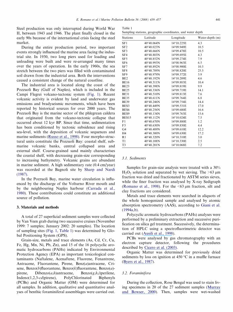
Table 1Sampling stations, geographic coordinates, and water depth

Stations Latitude Longitude Water-depth (m)

SF1 40�48.064N 14�10.225E 4.3SF2 40�48.023N 14�09.949E 10.5SF3 40�48.666N 14�09.478E 10.5SF4 40�48.803N 14�09.695E 4.3SF5 40�48.852N 14�09.274E 7.9SF6 40�48.993N 14�08.963E 6.5SF7 40�48.892N 14�08.900E 10.5SF8 40�48.789N 14�08.820E 25.5SF9 40�48.979N 14�09.372E 3.9BE2 40�48.192N 14�10.209E 4.6BE16 40�48.311N 14�09.883E 10.4BE23 40�48.398N 14�09.819E 9.9BE25 40�48.336N 14�09.719E 14.1BE31 40�48.510N 14�09.813E 7.6BE35 40�48.611N 14�09.764E 6.8BE39 40�48.246N 14�09.754E 14.4BES3 40�48.449N 14�09.531E 17.0BES6 40�48.256N 14�09.680E 16.6BES9 40�48.134N 14�09.763E 15.6BES15 40�48.112N 14�10.024E 7.5F1 40�48.670N 14�09.880E 1.2F3 40�48.630N 14�09.850E 4.4G4 40�48.489N 14�09.610E 12.2H4 40�48.300N 14�09.630E 17.2R1 40�48.320N 14�10.310E 3.0T1 40�48.108N 14�10.330E 2.5T3 40�48.201N 14�10.068E 7.2

E. Romano et al. / Marine Pollution Bulletin 56 (2008) 439–457 441

Steel production was only interrupted during World WarII, between 1943 and 1946. The plant finally closed in theearly 90s because of the international crisis facing the steelmarket.

During the entire production period, two importantevents strongly influenced the marine area facing the indus-trial site. In 1930, two long piers used for loading andunloading were built and were re-arranged many timesover the years of operation. In the early 1960s, the seastretch between the two piers was filled with contaminatedsoil drawn from the industrial area. Both the interventionscaused a consistent change of the natural coastline.

The industrial area is located along the coast of thePozzuoli Bay (Gulf of Naples), which is included in theCampi Flegrei volcano-tectonic system (Fig. 1). Recentvolcanic activity is evident by land and underwater gasemissions and bradyseismic movements, which have beenreported by historical sources for over 2000 years. ThePozzuoli Bay is the marine sector of the phlegrean calderathat originated from the volcano-tectonic collapse thatoccurred about 12 kyr BP. Since that time, sedimentationhas been conditioned by tectonic subsidence and risingsea-level, with the deposition of volcanic sequences andmarine sediments (Russo et al., 1998). Four morpho-struc-tural units constitute the Pozzuoli Bay: coastal shelf, sub-marine volcanic banks, central collapsed area andexternal shelf. Coarse-grained sand mainly characterisesthe coastal shelf, with decreasing grain-size correspondingto increasing bathymetry. Volcanic grains are abundantin marine sediment. A high sedimentary rate (0.4 cm/year)was recorded at the Bagnoli site by Sharp and Nardi(1987).

In the Pozzuoli Bay, marine water circulation is influ-enced by the discharge of the Volturno River mouth andby the neighbouring Naples harbour (Carrada et al.,1980). These contributions could constitute an additionalsource of pollution.

3. Materials and methods

A total of 27 superficial sediment samples were collectedby Van Veen grab during two successive cruises (November1999: 7 samples; January 2002: 20 samples). The locationof sampling sites (Fig. 1, Table 1) was determined by Glo-bal Positioning System (GPS).

Grain-size, metals and trace elements (As, Cd, Cr, Cu,Fe, Hg, Mn, Ni, Pb, Zn), and 15 of the 16 polycyclic aro-matic hydrocarbons (PAHs) indicated by EnvironmentalProtection Agency (EPA) as important toxicological con-taminants (Naftalene, Acenaftene, Fluorene, Fenantrene,Antracene, Fluorantene, Pirene, Benz(a)antracene, Cri-sene, Benzo(b)fluorantene, Benzo(k)fluorantene, Benzo(a)-pirene, Dibenzo(a,h)antracene, Benzo(g,h,i)perilene,Indeno(1,2,3-cd)pirene), PolyChlorinated Biphenyls(PCBs) and Organic Matter (OM) were determined forall samples. In addition, qualitative and quantitative anal-yses of benthic foraminiferal assemblages were carried out.

3.1. Sediments

Samples for grain-size analysis were treated with a 30%H2O2 solution and separated by wet sieving. The >63 lmfraction was dried and fractionated by ASTM series sieves,while the finer fraction was analysed by X-ray Sedigraph(Romano et al., 1998). For the <63 lm fraction, silt andclay fractions are considered.

Metals and trace elements were searched in aliquots ofthe whole homogenized sample and analysed by atomicabsorption spectrometry (AAS), according to Giani et al.(1994a,b).

Polycyclic aromatic hydrocarbons (PAHs) analyses wereperformed by a preliminary extraction and successive puri-fication on silica gel treatment. Successively, the determina-tion of HPLC using a spectrofluorimetric detector wascarried out (Ausili et al., 1998).

PCBs were analysed by gas chromatography with anelectron capture detector, following the proceduresdescribed by Cicero et al. (2003).

Organic Matter was determined for previously driedsediments by loss on ignition at 450 �C in a muffle furnace(Byers et al., 1987).

3.2. Foraminifera

During the collection, Rose Bengal was used to stain liv-ing specimens in 20 of the 27 sediment samples (Murrayand Bowser, 2000). Then, samples were wet-washed

442 E. Romano et al. / Marine Pollution Bulletin 56 (2008) 439–457

through 63 and 125 lm sieves and, due to the scarce or veryscarce content in pelite of the studied sediment, only thecoarser fraction was selected for quantitative analysis(Alve, 1991a,b; Coccioni, 2000; Ferraro et al., 2006).

Qualitative analysis was carried out on the finer fraction(63–125 lm) to detect the presence of additional species(Samir, 2000). Dry sediment was split into sub samplescontaining at least 300 specimens. Because of the low num-ber of living specimens, and the impossibility of performingseasonal samplings over a period of at least one year, thecount of total assemblage was considered for statisticalpurposes (Scott and Medioli, 1980). Rose Bengal was veryhelpful in recognising the living species as autochthonousspecies.

Faunal density was calculated using the number of testsfound in 1 g of dry sediment (Benthic Number – BN) (Coc-cioni, 2000). Species diversity was given by the number oftaxa (S), the a-index (Fisher et al., 1943) and the Shan-non–Weaver index (H) (Shannon and Weaver, 1963). Thea-index takes reliably into account for rare species andthere is only a small increase of values with increasing num-ber of counted specimens, but it assumes that the numberof individuals of each species follows a logarithmic series(Murray, 1968, 1991). The Shannon–Weaver index (H)gives additional information with respect to the a-index,because it accounts for both abundance and evenness ofspecies. This feature is also well described by Equitability(E), calculated by the ratio between H and the Hmax, (Mur-ray, 1991).

The diversity indices were calculated by means of thePAST – PAlaeontological STatistics data analysis package(version 1.38). In addition, the foraminifera abnormalityindex (FAI), corresponding to the total percentage ofabnormal foraminifera in each sample (Coccioni et al.,2005), was calculated. Loeblich and Tappan’s (1987) gen-eric classification was followed and most species weredetermined by comparison with those of Jorissen (1988),Cimerman and Langer (1991) and Sgarrella and Monchar-mont-Zei (1993). In regards to specific attribution, Quinqu-

eloculina dimidiata recognised by Bergamin et al. (2003),was considered in this paper to be Quinqueloculina lata

by comparison with the specimen figured by Debenayet al. (2001b).

Deformed specimens were carefully observed by meansof SEM. In addition, comparative analyses of someselected regular and deformed specimens of the same spe-cies were carried out to detect the presence of foreign ele-ments in the tests using the energy dispersivespectrometer (EDS) attached to SEM (Samir and El Din,2001).

3.3. Data processing

Data were organised into a matrix including sedimentparameters (grain-size and chemical analyses) and relativeabundance of commonly occurring species, i.e., the 28 spe-cies with greater than 5% abundance in at least one sample

(Fishbein and Patterson, 1993). Parameters obtained by thequantitative analysis on benthic foraminifera such as a-index, BN and FAI, were also included. Data with differentorders of magnitude were standardised (mean = 0 andSD = 1) before multivariate analysis, to assign the samenumerical weight to each variable.

Bivariate analysis like as bivariate correlation (BC) andmultivariate analysis like as Q-mode hierarchical clusteranalysis (HCA), principal component analysis (PCA) anddiscriminant canonical analysis (DCA) were carried outusing the softwares SPSS (version 12.0) and R (version2.0.1).

In order to find correlations between variable couplings,the BC was calculated by Pearson’s correlation. This coef-ficient is considered significant only when a linear correla-tion between two variables exists. In our study, it was usedto prove the correlation between relative abundance of asingle species and each chemical and sedimentologicalparameter (Debenay et al., 2001b). Additionally, the BCon a matrix including chemical data and the percentagesof deformed tests was performed in order to show a possi-ble correlation between heavy metal concentration andoccurrence of abnormalities.

The HCA, using Ward’s method as the amalgamationrule and the Squared Euclidean distance as a similaritymeasurement (Massart and Kaufman, 1989), was appliedfor searching the natural grouping among stations. ThePCA was used to examine the relationships among the vari-ables as a preliminary descriptive method. The DCA wasperformed on the PCA results, on the base of the a priorigroups pointed out by the HCA (Mahalanobis, 1936; Tom-assone et al., 1988), in order to eliminate redundancybetween the analysed variables.

4. Results

Results of grain size and chemical analyses are given inTables 2 and 3, respectively. Data from Table 2 show thatsediments are mainly constituted of sand, with significantgravel content (up to 38.0%), mainly in stations from thenorthern area. The content in pelite, mainly constitutedby silt, is higher (up to 21.1%) in front of the plant, betweenthe two piers.

The chemical results show high concentrations for con-taminants such as As, Pb, Zn, PAHs and PCBs. Except forAs, that’s high values could be caused by hydrothermalactivity of the area, the other parameters seem correlatedto the industrial plant. A comparison with some referencevalues of Mediterranean coastal areas (UNEP, 1996),background values of the area (Damiani et al., 1987),and adopted values by national regulatory guidelines legis-lation for monitoring Italian coastal marine areas (D.M.367/03) has been carried out. Almost all the parameters,except Cr and Ni that show very low concentrations(Table 3), exceed the reference values.

Particularly, Fe (up to 336,700 mg/kg d.w.), Pb (up to465 mg/kg d.w.), Zn (up to 2313 mg/kg d.w.), PAHs (up

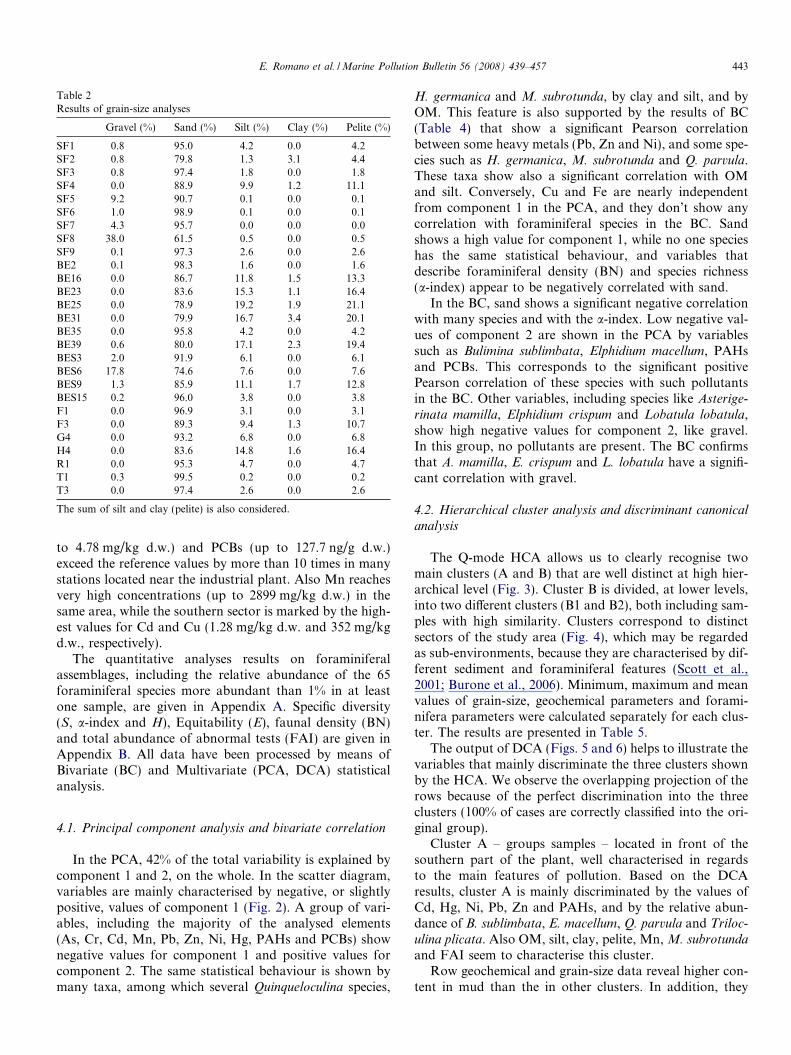
Table 2Results of grain-size analyses

Gravel (%) Sand (%) Silt (%) Clay (%) Pelite (%)

SF1 0.8 95.0 4.2 0.0 4.2SF2 0.8 79.8 1.3 3.1 4.4SF3 0.8 97.4 1.8 0.0 1.8SF4 0.0 88.9 9.9 1.2 11.1SF5 9.2 90.7 0.1 0.0 0.1SF6 1.0 98.9 0.1 0.0 0.1SF7 4.3 95.7 0.0 0.0 0.0SF8 38.0 61.5 0.5 0.0 0.5SF9 0.1 97.3 2.6 0.0 2.6BE2 0.1 98.3 1.6 0.0 1.6BE16 0.0 86.7 11.8 1.5 13.3BE23 0.0 83.6 15.3 1.1 16.4BE25 0.0 78.9 19.2 1.9 21.1BE31 0.0 79.9 16.7 3.4 20.1BE35 0.0 95.8 4.2 0.0 4.2BE39 0.6 80.0 17.1 2.3 19.4BES3 2.0 91.9 6.1 0.0 6.1BES6 17.8 74.6 7.6 0.0 7.6BES9 1.3 85.9 11.1 1.7 12.8BES15 0.2 96.0 3.8 0.0 3.8F1 0.0 96.9 3.1 0.0 3.1F3 0.0 89.3 9.4 1.3 10.7G4 0.0 93.2 6.8 0.0 6.8H4 0.0 83.6 14.8 1.6 16.4R1 0.0 95.3 4.7 0.0 4.7T1 0.3 99.5 0.2 0.0 0.2T3 0.0 97.4 2.6 0.0 2.6

The sum of silt and clay (pelite) is also considered.

E. Romano et al. / Marine Pollution Bulletin 56 (2008) 439–457 443

to 4.78 mg/kg d.w.) and PCBs (up to 127.7 ng/g d.w.)exceed the reference values by more than 10 times in manystations located near the industrial plant. Also Mn reachesvery high concentrations (up to 2899 mg/kg d.w.) in thesame area, while the southern sector is marked by the high-est values for Cd and Cu (1.28 mg/kg d.w. and 352 mg/kgd.w., respectively).

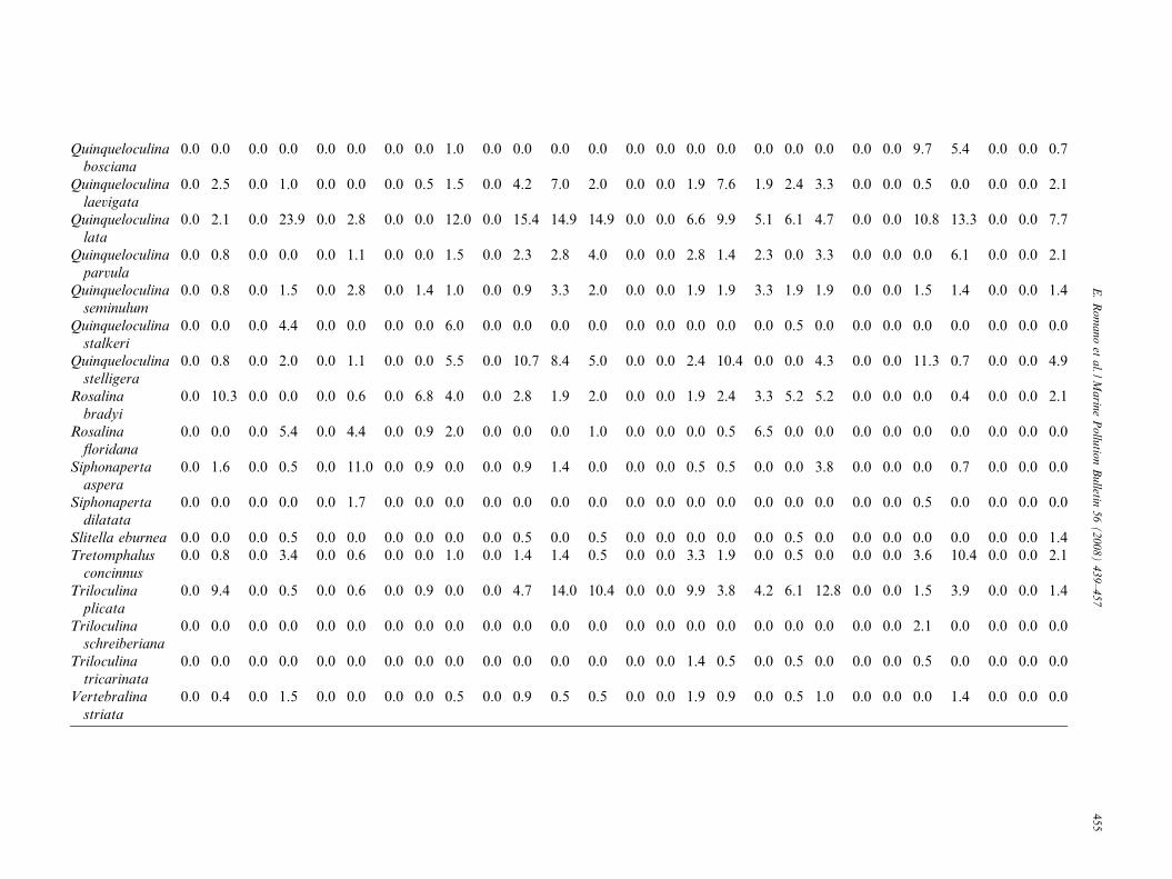
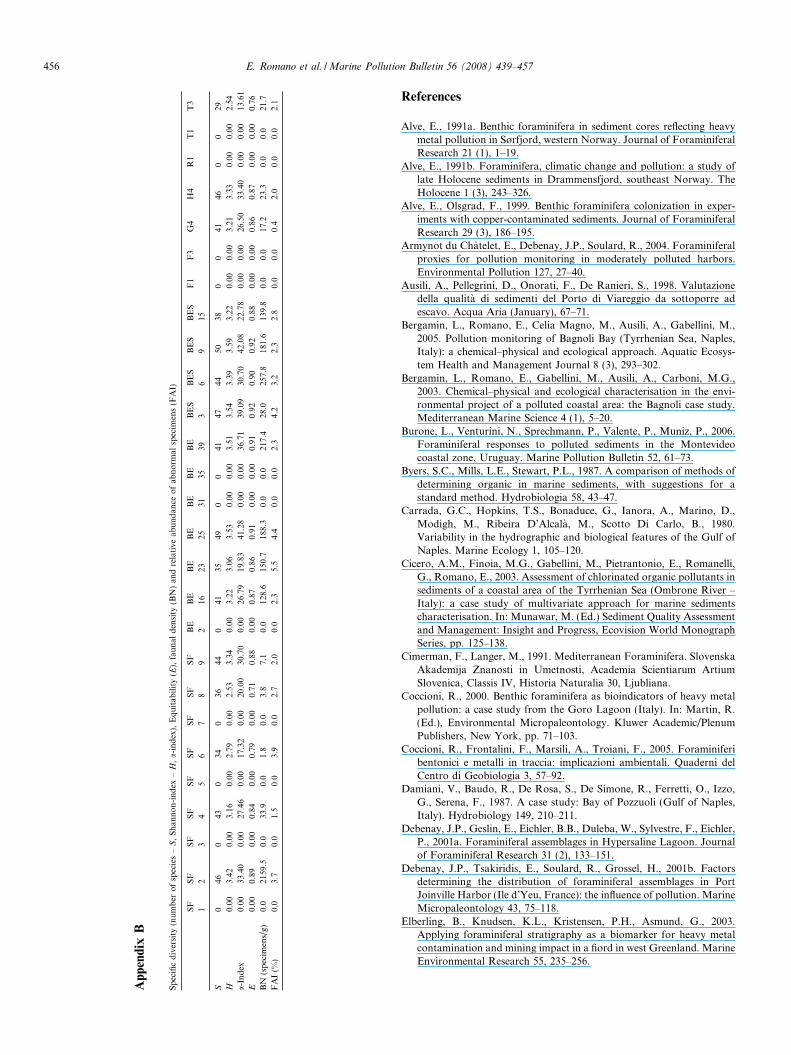
The quantitative analyses results on foraminiferalassemblages, including the relative abundance of the 65foraminiferal species more abundant than 1% in at leastone sample, are given in Appendix A. Specific diversity(S, a-index and H), Equitability (E), faunal density (BN)and total abundance of abnormal tests (FAI) are given inAppendix B. All data have been processed by means ofBivariate (BC) and Multivariate (PCA, DCA) statisticalanalysis.

4.1. Principal component analysis and bivariate correlation

In the PCA, 42% of the total variability is explained bycomponent 1 and 2, on the whole. In the scatter diagram,variables are mainly characterised by negative, or slightlypositive, values of component 1 (Fig. 2). A group of vari-ables, including the majority of the analysed elements(As, Cr, Cd, Mn, Pb, Zn, Ni, Hg, PAHs and PCBs) shownegative values for component 1 and positive values forcomponent 2. The same statistical behaviour is shown bymany taxa, among which several Quinqueloculina species,

H. germanica and M. subrotunda, by clay and silt, and byOM. This feature is also supported by the results of BC(Table 4) that show a significant Pearson correlationbetween some heavy metals (Pb, Zn and Ni), and some spe-cies such as H. germanica, M. subrotunda and Q. parvula.These taxa show also a significant correlation with OMand silt. Conversely, Cu and Fe are nearly independentfrom component 1 in the PCA, and they don’t show anycorrelation with foraminiferal species in the BC. Sandshows a high value for component 1, while no one specieshas the same statistical behaviour, and variables thatdescribe foraminiferal density (BN) and species richness(a-index) appear to be negatively correlated with sand.

In the BC, sand shows a significant negative correlationwith many species and with the a-index. Low negative val-ues of component 2 are shown in the PCA by variablessuch as Bulimina sublimbata, Elphidium macellum, PAHsand PCBs. This corresponds to the significant positivePearson correlation of these species with such pollutantsin the BC. Other variables, including species like Asterige-

rinata mamilla, Elphidium crispum and Lobatula lobatula,show high negative values for component 2, like gravel.In this group, no pollutants are present. The BC confirmsthat A. mamilla, E. crispum and L. lobatula have a signifi-cant correlation with gravel.

4.2. Hierarchical cluster analysis and discriminant canonical

analysis

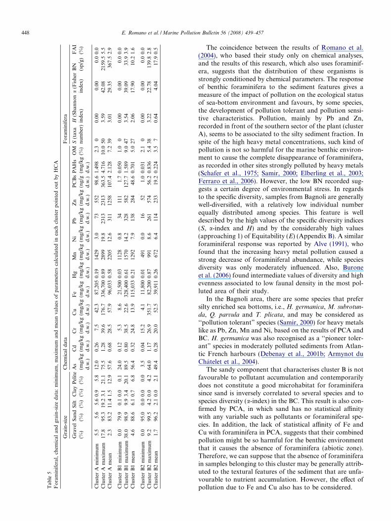
The Q-mode HCA allows us to clearly recognise twomain clusters (A and B) that are well distinct at high hier-archical level (Fig. 3). Cluster B is divided, at lower levels,into two different clusters (B1 and B2), both including sam-ples with high similarity. Clusters correspond to distinctsectors of the study area (Fig. 4), which may be regardedas sub-environments, because they are characterised by dif-ferent sediment and foraminiferal features (Scott et al.,2001; Burone et al., 2006). Minimum, maximum and meanvalues of grain-size, geochemical parameters and forami-nifera parameters were calculated separately for each clus-ter. The results are presented in Table 5.

The output of DCA (Figs. 5 and 6) helps to illustrate thevariables that mainly discriminate the three clusters shownby the HCA. We observe the overlapping projection of therows because of the perfect discrimination into the threeclusters (100% of cases are correctly classified into the ori-ginal group).

Cluster A – groups samples – located in front of thesouthern part of the plant, well characterised in regardsto the main features of pollution. Based on the DCAresults, cluster A is mainly discriminated by the values ofCd, Hg, Ni, Pb, Zn and PAHs, and by the relative abun-dance of B. sublimbata, E. macellum, Q. parvula and Triloc-

ulina plicata. Also OM, silt, clay, pelite, Mn, M. subrotunda

and FAI seem to characterise this cluster.Row geochemical and grain-size data reveal higher con-

tent in mud than the in other clusters. In addition, they

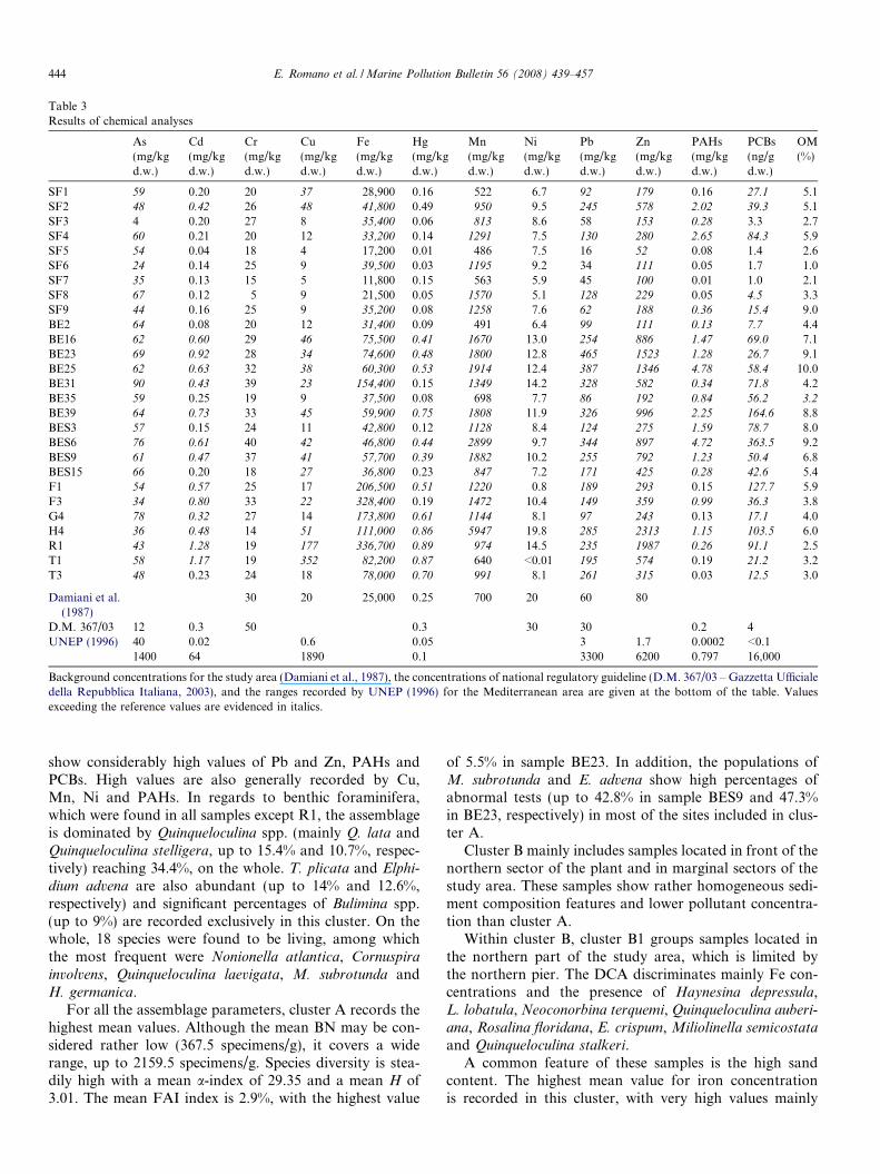
Table 3Results of chemical analyses

As(mg/kgd.w.)

Cd(mg/kgd.w.)

Cr(mg/kgd.w.)

Cu(mg/kgd.w.)

Fe(mg/kgd.w.)

Hg(mg/kgd.w.)

Mn(mg/kgd.w.)

Ni(mg/kgd.w.)

Pb(mg/kgd.w.)

Zn(mg/kgd.w.)

PAHs(mg/kgd.w.)

PCBs(ng/gd.w.)

OM(%)

SF1 59 0.20 20 37 28,900 0.16 522 6.7 92 179 0.16 27.1 5.1SF2 48 0.42 26 48 41,800 0.49 950 9.5 245 578 2.02 39.3 5.1SF3 4 0.20 27 8 35,400 0.06 813 8.6 58 153 0.28 3.3 2.7SF4 60 0.21 20 12 33,200 0.14 1291 7.5 130 280 2.65 84.3 5.9SF5 54 0.04 18 4 17,200 0.01 486 7.5 16 52 0.08 1.4 2.6SF6 24 0.14 25 9 39,500 0.03 1195 9.2 34 111 0.05 1.7 1.0SF7 35 0.13 15 5 11,800 0.15 563 5.9 45 100 0.01 1.0 2.1SF8 67 0.12 5 9 21,500 0.05 1570 5.1 128 229 0.05 4.5 3.3SF9 44 0.16 25 9 35,200 0.08 1258 7.6 62 188 0.36 15.4 9.0BE2 64 0.08 20 12 31,400 0.09 491 6.4 99 111 0.13 7.7 4.4BE16 62 0.60 29 46 75,500 0.41 1670 13.0 254 886 1.47 69.0 7.1BE23 69 0.92 28 34 74,600 0.48 1800 12.8 465 1523 1.28 26.7 9.1BE25 62 0.63 32 38 60,300 0.53 1914 12.4 387 1346 4.78 58.4 10.0BE31 90 0.43 39 23 154,400 0.15 1349 14.2 328 582 0.34 71.8 4.2BE35 59 0.25 19 9 37,500 0.08 698 7.7 86 192 0.84 56.2 3.2

BE39 64 0.73 33 45 59,900 0.75 1808 11.9 326 996 2.25 164.6 8.8BES3 57 0.15 24 11 42,800 0.12 1128 8.4 124 275 1.59 78.7 8.0BES6 76 0.61 40 42 46,800 0.44 2899 9.7 344 897 4.72 363.5 9.2BES9 61 0.47 37 41 57,700 0.39 1882 10.2 255 792 1.23 50.4 6.8BES15 66 0.20 18 27 36,800 0.23 847 7.2 171 425 0.28 42.6 5.4F1 54 0.57 25 17 206,500 0.51 1220 0.8 189 293 0.15 127.7 5.9F3 34 0.80 33 22 328,400 0.19 1472 10.4 149 359 0.99 36.3 3.8G4 78 0.32 27 14 173,800 0.61 1144 8.1 97 243 0.13 17.1 4.0H4 36 0.48 14 51 111,000 0.86 5947 19.8 285 2313 1.15 103.5 6.0R1 43 1.28 19 177 336,700 0.89 974 14.5 235 1987 0.26 91.1 2.5T1 58 1.17 19 352 82,200 0.87 640 <0.01 195 574 0.19 21.2 3.2T3 48 0.23 24 18 78,000 0.70 991 8.1 261 315 0.03 12.5 3.0

Damiani et al.(1987)

30 20 25,000 0.25 700 20 60 80

D.M. 367/03 12 0.3 50 0.3 30 30 0.2 4UNEP (1996) 40 0.02 0.6 0.05 3 1.7 0.0002 <0.1

1400 64 1890 0.1 3300 6200 0.797 16,000

Background concentrations for the study area (Damiani et al., 1987), the concentrations of national regulatory guideline (D.M. 367/03 – Gazzetta Ufficialedella Repubblica Italiana, 2003), and the ranges recorded by UNEP (1996) for the Mediterranean area are given at the bottom of the table. Valuesexceeding the reference values are evidenced in italics.

444 E. Romano et al. / Marine Pollution Bulletin 56 (2008) 439–457

show considerably high values of Pb and Zn, PAHs andPCBs. High values are also generally recorded by Cu,Mn, Ni and PAHs. In regards to benthic foraminifera,which were found in all samples except R1, the assemblageis dominated by Quinqueloculina spp. (mainly Q. lata andQuinqueloculina stelligera, up to 15.4% and 10.7%, respec-tively) reaching 34.4%, on the whole. T. plicata and Elphi-

dium advena are also abundant (up to 14% and 12.6%,respectively) and significant percentages of Bulimina spp.(up to 9%) are recorded exclusively in this cluster. On thewhole, 18 species were found to be living, among whichthe most frequent were Nonionella atlantica, Cornuspira

involvens, Quinqueloculina laevigata, M. subrotunda andH. germanica.

For all the assemblage parameters, cluster A records thehighest mean values. Although the mean BN may be con-sidered rather low (367.5 specimens/g), it covers a widerange, up to 2159.5 specimens/g. Species diversity is stea-dily high with a mean a-index of 29.35 and a mean H of3.01. The mean FAI index is 2.9%, with the highest value

of 5.5% in sample BE23. In addition, the populations ofM. subrotunda and E. advena show high percentages ofabnormal tests (up to 42.8% in sample BES9 and 47.3%in BE23, respectively) in most of the sites included in clus-ter A.

Cluster B mainly includes samples located in front of thenorthern sector of the plant and in marginal sectors of thestudy area. These samples show rather homogeneous sedi-ment composition features and lower pollutant concentra-tion than cluster A.

Within cluster B, cluster B1 groups samples located inthe northern part of the study area, which is limited bythe northern pier. The DCA discriminates mainly Fe con-centrations and the presence of Haynesina depressula,L. lobatula, Neoconorbina terquemi, Quinqueloculina auberi-

ana, Rosalina floridana, E. crispum, Miliolinella semicostata

and Quinqueloculina stalkeri.A common feature of these samples is the high sand

content. The highest mean value for iron concentrationis recorded in this cluster, with very high values mainly

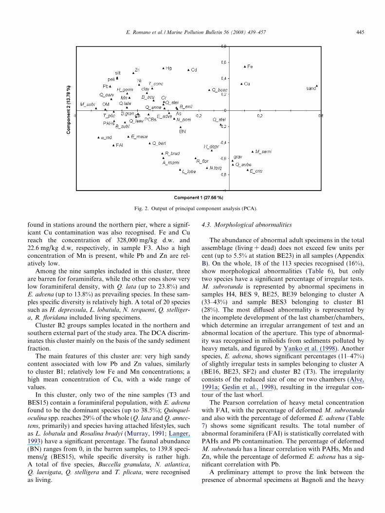
Fig. 2. Output of principal component analysis (PCA).

E. Romano et al. / Marine Pollution Bulletin 56 (2008) 439–457 445

found in stations around the northern pier, where a signif-icant Cu contamination was also recognised. Fe and Cureach the concentration of 328,000 mg/kg d.w. and22.6 mg/kg d.w, respectively, in sample F3. Also a highconcentration of Mn is present, while Pb and Zn are rel-atively low.

Among the nine samples included in this cluster, threeare barren for foraminifera, while the other ones show verylow foraminiferal density, with Q. lata (up to 23.8%) andE. advena (up to 13.8%) as prevailing species. In these sam-ples specific diversity is relatively high. A total of 20 speciessuch as H. depressula, L. lobatula, N. terquemi, Q. stelliger-

a, R. floridana included living specimens.Cluster B2 groups samples located in the northern and

southern external part of the study area. The DCA discrim-inates this cluster mainly on the basis of the sandy sedimentfraction.

The main features of this cluster are: very high sandycontent associated with low Pb and Zn values, similarlyto cluster B1; relatively low Fe and Mn concentrations; ahigh mean concentration of Cu, with a wide range ofvalues.

In this cluster, only two of the nine samples (T3 andBES15) contain a foraminiferal population, with E. advenafound to be the dominant species (up to 38.5%); Quinquel-

oculina spp. reaches 29% of the whole (Q. lata and Q. annec-

tens, primarily) and species having attached lifestyles, suchas L. lobatula and Rosalina bradyi (Murray, 1991; Langer,1993) have a significant percentage. The faunal abundance(BN) ranges from 0, in the barren samples, to 139.8 speci-mens/g (BES15), while specific diversity is rather high.A total of five species, Buccella granulata, N. atlantica,Q. laevigata, Q. stelligera and T. plicata, were recognisedas living.

4.3. Morphological abnormalities

The abundance of abnormal adult specimens in the totalassemblage (living + dead) does not exceed few units percent (up to 5.5% at station BE23) in all samples (AppendixB). On the whole, 18 of the 113 species recognised (16%),show morphological abnormalities (Table 6), but onlytwo species have a significant percentage of irregular tests.M. subrotunda is represented by abnormal specimens insamples H4, BES 9, BE25, BE39 belonging to cluster A(33–43%) and sample BES3 belonging to cluster B1(28%). The most diffused abnormality is represented bythe incomplete development of the last chamber/chambers,which determine an irregular arrangement of test and anabnormal location of the aperture. This type of abnormal-ity was recognised in miliolids from sediments polluted byheavy metals, and figured by Yanko et al. (1998). Anotherspecies, E. advena, shows significant percentages (11–47%)of slightly irregular tests in samples belonging to cluster A(BE16, BE23, SF2) and cluster B2 (T3). The irregularityconsists of the reduced size of one or two chambers (Alve,1991a; Geslin et al., 1998), resulting in the irregular con-tour of the last whorl.

The Pearson correlation of heavy metal concentrationwith FAI, with the percentage of deformed M. subrotunda

and also with the percentage of deformed E. advena (Table7) shows some significant results. The total number ofabnormal foraminifera (FAI) is statistically correlated withPAHs and Pb contamination. The percentage of deformedM. subrotunda has a linear correlation with PAHs, Mn andZn, while the percentage of deformed E. advena has a sig-nificant correlation with Pb.

A preliminary attempt to prove the link between thepresence of abnormal specimens at Bagnoli and the heavy

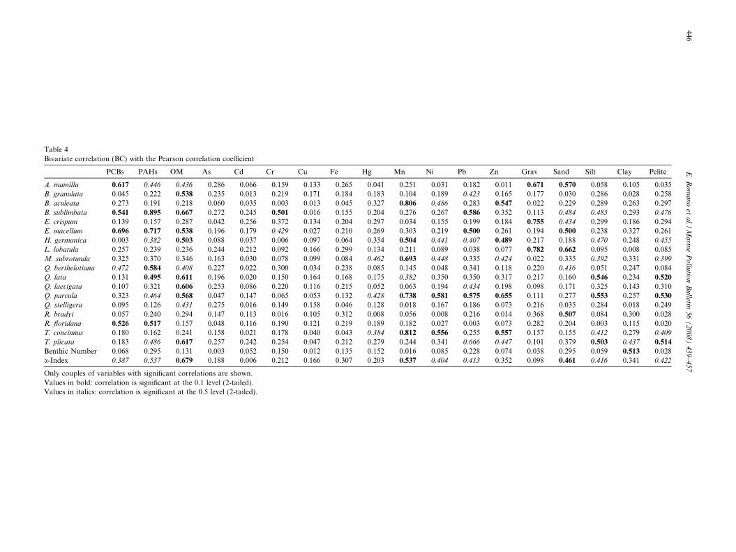
Table 4Bivariate correlation (BC) with the Pearson correlation coefficient

PCBs PAHs OM As Cd Cr Cu Fe Hg Mn Ni Pb Zn Grav Sand Silt Clay Pelite

A. mamilla 0.617 0.446 0.436 0.286 �0.066 0.159 �0.133 �0.265 �0.041 0.251 �0.031 0.182 �0.011 0.671 �0.570 0.058 �0.105 0.035B. granulata 0.045 0.222 0.538 0.235 0.013 0.219 �0.171 �0.184 0.183 0.104 0.189 0.423 0.165 �0.177 �0.030 0.286 0.028 0.258B. aculeata 0.273 0.191 0.218 �0.060 0.035 �0.003 0.013 �0.045 0.327 0.806 0.486 0.283 0.547 �0.022 �0.229 0.289 0.263 0.297B. sublimbata 0.541 0.895 0.667 0.272 0.245 0.501 �0.016 �0.155 0.204 0.276 0.267 0.586 0.352 0.113 �0.484 0.485 0.293 0.476

E. crispum �0.139 �0.157 �0.287 �0.042 �0.256 �0.372 �0.134 �0.204 �0.297 0.034 �0.155 �0.199 �0.184 0.755 �0.434 �0.299 �0.186 �0.294E. macellum 0.696 0.717 0.538 0.196 0.179 0.429 �0.027 �0.210 0.269 0.303 0.219 0.500 0.261 0.194 �0.500 0.238 0.327 0.261H. germanica 0.003 0.382 0.503 0.088 0.037 �0.006 �0.097 �0.064 0.354 0.504 0.441 0.407 0.489 �0.217 �0.188 0.470 0.248 0.455

L. lobatula 0.257 0.239 0.236 0.244 �0.212 �0.092 �0.166 �0.299 �0.134 0.211 �0.089 0.038 �0.077 0.782 �0.662 �0.095 �0.008 �0.085M. subrotunda 0.325 0.370 0.346 0.163 �0.030 0.078 �0.099 �0.084 0.462 0.693 0.448 0.335 0.424 �0.022 �0.335 0.392 0.331 0.399

Q. berthelotiana 0.472 0.584 0.408 0.227 0.022 0.300 �0.034 �0.238 0.085 0.145 0.048 0.341 0.118 0.220 �0.416 0.051 0.247 0.084Q. lata 0.131 0.495 0.611 0.196 0.020 0.150 �0.164 �0.168 0.175 0.382 0.350 0.350 0.317 �0.217 �0.160 0.546 0.234 0.520

Q. laevigata 0.107 0.321 0.606 0.253 0.086 0.220 �0.116 �0.215 0.052 0.063 0.194 0.434 0.198 �0.098 �0.171 0.325 0.143 0.310Q. parvula 0.323 0.464 0.568 0.047 0.147 0.065 �0.053 �0.132 0.428 0.738 0.581 0.575 0.655 �0.111 �0.277 0.553 0.257 0.530

Q. stelligera �0.095 0.126 0.431 0.275 �0.016 0.149 �0.158 �0.046 0.128 0.018 0.167 0.186 0.073 �0.216 0.035 0.284 �0.018 0.249R. bradyi 0.057 0.240 0.294 0.147 �0.113 0.016 �0.105 �0.312 �0.008 0.056 0.008 0.216 0.014 0.368 �0.507 �0.084 0.300 �0.028R. floridana 0.526 0.517 0.157 0.048 �0.116 0.190 �0.121 �0.219 �0.189 0.182 �0.027 0.003 �0.073 0.282 �0.204 �0.003 �0.115 �0.020T. concinnus 0.180 0.162 0.241 �0.158 0.021 �0.178 �0.040 �0.043 0.384 0.812 0.556 0.255 0.557 �0.157 �0.155 0.412 0.279 0.409

T. plicata 0.183 0.486 0.617 0.257 0.242 0.254 �0.047 �0.212 0.279 0.244 0.341 0.666 0.447 �0.101 �0.379 0.503 0.437 0.514

Benthic Number 0.068 0.295 0.131 �0.003 0.052 0.150 0.012 �0.135 0.152 �0.016 0.085 0.228 0.074 �0.038 �0.295 �0.059 0.513 0.028a-Index 0.387 0.537 0.679 0.188 �0.006 0.212 �0.166 �0.307 0.203 0.537 0.404 0.413 0.352 0.098 �0.461 0.416 0.341 0.422

Only couples of variables with significant correlations are shown.Values in bold: correlation is significant at the 0.1 level (2-tailed).Values in italics: correlation is significant at the 0.5 level (2-tailed).

446E

.R

om

an

oet

al./M

arin

eP

ollu

tion

Bu

lletin5

6(

20

08

)4

39

–4

57

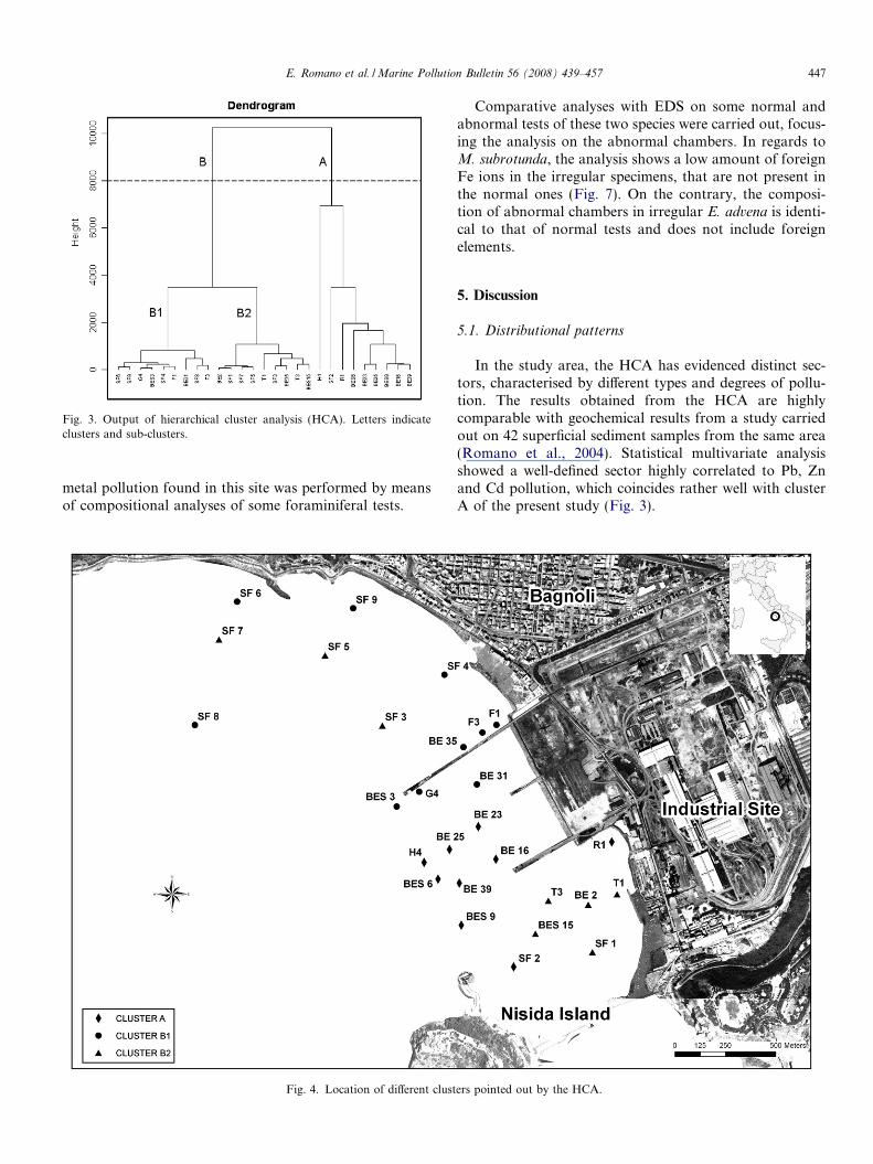
Fig. 3. Output of hierarchical cluster analysis (HCA). Letters indicateclusters and sub-clusters.

E. Romano et al. / Marine Pollution Bulletin 56 (2008) 439–457 447

metal pollution found in this site was performed by meansof compositional analyses of some foraminiferal tests.

Fig. 4. Location of different clust

Comparative analyses with EDS on some normal andabnormal tests of these two species were carried out, focus-ing the analysis on the abnormal chambers. In regards toM. subrotunda, the analysis shows a low amount of foreignFe ions in the irregular specimens, that are not present inthe normal ones (Fig. 7). On the contrary, the composi-tion of abnormal chambers in irregular E. advena is identi-cal to that of normal tests and does not include foreignelements.

5. Discussion

5.1. Distributional patterns

In the study area, the HCA has evidenced distinct sec-tors, characterised by different types and degrees of pollu-tion. The results obtained from the HCA are highlycomparable with geochemical results from a study carriedout on 42 superficial sediment samples from the same area(Romano et al., 2004). Statistical multivariate analysisshowed a well-defined sector highly correlated to Pb, Znand Cd pollution, which coincides rather well with clusterA of the present study (Fig. 3).

ers pointed out by the HCA.

Tab

le5

Fo

ram

inif

eral

,ch

emic

alan

dgr

ain

-siz

ed

ata:

min

imu

m,

max

imu

man

dm

ean

valu

eso

fp

aram

eter

sca

lcu

late

din

each

clu

ster

po

inte

do

ut

by

HC

A

Gra

in-s

ize

Ch

emic

ald

ata

Fo

ram

inif

era

Gra

vel

(%)

San

d(%

)S

ilt

(%)

Cla

y(%

)P

elit

e(%

)A

s(m

g/k

gd

.w.)

Cd

(mg/

kg

d.w

.)

Cr

(mg/

kg

d.w

.)

Cu

(mg/

kg

d.w

.)

Fe

(mg/

kg

d.w

.)

Hg

(mg/

kg

d.w

.)

Mn

(mg/

kg

d.w

.)

Ni

(mg/

kg

d.w

.)

Pb

(mg/

kg

d.w

.)

Zn

(mg/

kg

d.w

.)

PC

Bs

(ng/

gd

.w.)

PA

Hs

(mg/

kg

d.w

.)

OM

(%)

S(t

axa

nu

mb

er)

H(S

han

no

nin

dex

)a

(Fis

her

ind

ex)

BN

(sp

/g)

FA

I(%

)

Clu

ster

Am

inim

um

5.5

5.6

5.6

0.9

5.8

12.0

0.26

7.5

42.3

87,2

050.

1914

293.

073

552

98.6

1.49

82.

30

0.00

0.00

0.0

0.0

Clu

ster

Am

axim

um

17.8

95.3

19.2

3.1

21.1

75.5

1.28

39.6

176.

733

6,70

00.

8928

9919

.823

1323

1336

3.5

4.71

610

.050

3.59

42.0

821

59.5

5.5

Clu

ster

Am

ean

2.3

83.2

11.4

1.5

12.9

57.6

0.68

28.5

57.9

96,0

330.

5822

0512

.631

112

5810

7.4

2.12

87.

239

3.01

29.3

536

7.5

2.9

Clu

ster

B1

min

imu

m0.

079

.90.

10.

00.

124

.00.

125.

38.

621

,500

0.03

1128

0.8

3411

11.

70.

050

1.0

00.

000.

000.

00.

0C

lust

erB

1m

axim

um

38.0

98.9

9.9

3.4

20.1

89.5

0.80

38.5

22.6

328,

400

0.61

1570

14.2

328

582

127.

71.

589

9.0

473.

5439

.09

33.9

3.9

Clu

ster

B1

mea

n4.

688

.66.

10.

76.

856

.40.

3224

.813

.911

5,03

30.

2112

927.

913

828

448

.60.

701

5.0

272.

0617

.90

10.2

1.6

Clu

ster

B2

min

imu

m0.

095

.00.

00.

00.

03.

50.

0415

.24.

111

,800

0.01

491

0.0

1652

1.0

0.03

12.

10

0.00

0.00

0.0

0.0

Clu

ster

B2

max

imu

m9.

299

.54.

20.

04.

264

.01.

1726

.935

1.7

82,2

000.

8799

18.

626

157

456

.20.

836

5.4

383.

2222

.78

139.

82.

8C

lust

erB

2m

ean

1.7

96.2

2.1

0.0

2.1

49.4

0.28

20.0

52.5

39,9

110.

2667

26.

411

423

319

.20.

224

3.5

70.

644.

0417

.90.

5

448 E. Romano et al. / Marine Pollution Bulletin 56 (2008) 439–457

The coincidence between the results of Romano et al.(2004), who based their study only on chemical analyses,and the results of this research, which also uses foraminif-era, suggests that the distribution of these organisms isstrongly conditioned by chemical parameters. The responseof benthic foraminifera to the sediment features gives ameasure of the impact of pollution on the ecological statusof sea-bottom environment and favours, by some species,the development of pollution tolerant and pollution sensi-tive characteristics. Pollution, mainly by Pb and Zn,recorded in front of the southern sector of the plant (clusterA), seems to be associated to the silty sediment fraction. Inspite of the high heavy metal concentrations, such kind ofpollution is not so harmful for the marine benthic environ-ment to cause the complete disappearance of foraminifera,as recorded in other sites strongly polluted by heavy metals(Schafer et al., 1975; Samir, 2000; Elberling et al., 2003;Ferraro et al., 2006). However, the low BN recorded sug-gests a certain degree of environmental stress. In regardsto the specific diversity, samples from Bagnoli are generallywell-diversified, with a relatively low individual numberequally distributed among species. This feature is welldescribed by the high values of the specific diversity indices(S, a-index and H) and by the considerably high values(approaching 1) of Equitability (E) (Appendix B). A similarforaminiferal response was reported by Alve (1991), whofound that the increasing heavy metal pollution caused astrong decrease of foraminiferal abundance, while speciesdiversity was only moderately influenced. Also, Buroneet al. (2006) found intermediate values of diversity and highevenness associated to low faunal density in the most pol-luted area of their study.

In the Bagnoli area, there are some species that prefersilty enriched sea bottoms, i.e., H. germanica, M. subrotun-

da, Q. parvula and T. plicata, and may be considered as‘‘pollution tolerant” species (Samir, 2000) for heavy metalslike as Pb, Zn, Mn and Ni, based on the results of PCA andBC. H. germanica was also recognised as a ‘‘pioneer toler-ant” species in moderately polluted sediments from Atlan-tic French harbours (Debenay et al., 2001b; Armynot duChatelet et al., 2004).

The sandy component that characterises cluster B is notfavourable to pollutant accumulation and contemporarilydoes not constitute a good microhabitat for foraminiferasince sand is inversely correlated to several species and tospecies diversity (a-index) in the BC. This result is also con-firmed by PCA, in which sand has no statistical affinitywith any variable such as pollutants or foraminiferal spe-cies. In addition, the lack of statistical affinity of Fe andCu with foraminifera in PCA, suggests that their combinedpollution might be so harmful for the benthic environmentthat it causes the absence of foraminifera (abiotic zone).Therefore, we can suppose that the absence of foraminiferain samples belonging to this cluster may be generally attrib-uted to the textural features of the sediment that are unfa-vourable to nutrient accumulation. However, the effect ofpollution due to Fe and Cu also has to be considered.

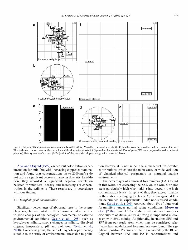
Fig. 5. Output of the discriminant canonical analysis (DCA). (a) Variables canonical weights. (b) Cosine between the variables and the canonical scores.This is the correlation between the variables and the discriminant axis. (c) Eigenvalues bar charts. (d) Plot of plain PCA axes projected into discriminantplain. (e) Gravity centre of classes. (f) Projection of the rows with ellipses and gravity centre of classes.

E. Romano et al. / Marine Pollution Bulletin 56 (2008) 439–457 449

Alve and Olsgrad (1999) carried out colonization exper-iments on foraminifera with increasing copper contamina-tion and found that concentrations up to 2000 mg/kg donot cause a significant decrease in species diversity. In addi-tion, they recorded a significant negative correlationbetween foraminiferal density and increasing Cu concen-tration in the sediments. These results are in accordancewith our findings.

5.2. Morphological abnormalities

Significant percentages of abnormal tests in the assem-blage may be attributed to the environmental stress dueto wide changes of the ecological parameters or extremeenvironmental conditions (Geslin et al., 1998), such ashypo/hyper salinity, strong changes in salinity, dissolvedoxygen, temperature, pH and pollution (Geslin et al.,2000). Considering this, the site of Bagnoli is particularlysuitable to the study of environmental stress due to pollu-

tion because it is not under the influence of fresh-watercontributions, which are the main cause of wide variationof chemical–physical parameters in marginal marineenvironments.

The percentages of abnormal foraminifera (FAI) foundin this work, not exceeding the 5.5% on the whole, do notseem particularly high when taking into account the highcontamination levels. In spite of this, they exceed, mainlyin the stations belonging to cluster A, the background lev-els determined in experiments under non-stressed condi-tions. Stouff et al. (1999) recorded about 1% of abnormalforaminifera under normal saline conditions. Morovanet al. (2004) found 1.75% of abnormal tests in a monospe-cific culture of Ammonia tepida living in unpolluted micro-cosm with 35‰ salinity. Additionally, in stations SF5 andSF7 from our study area, which may be considered rela-tively clean, no deformed foraminifera were found. The sig-nificant positive Pearson correlation recorded by the BC atBagnoli between FAI and PAHs concentrations and

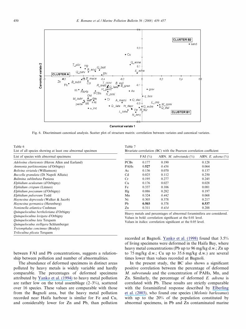
Fig. 6. Discriminant canonical analysis. Scatter plot of structure matrix: correlation between variates and canonical variates.

Table 6List of all species showing at least one abnormal specimen

List of species with abnormal specimens

Adelosina cliariesnsis (Heron Allen and Earland)Ammonia parkinsoniana (d’Orbigny)Bolivina striatula (Williamson)Buccella granulata (Di Napoli Alliata)Bulimina sublimbata PanizzaElphidium aculeatum (d’Orbigny)Elphidium crispum (Linneo)Elphidium poeyanum (d’Orbigny)Elphidium pulvereum ToddHaynesina depressula (Walker & Jacob)Haynesina germanica (Herenberg)Nonionella atlantica CushmanQuinqueloculina berthelotiana d’OrbignyQuinqueloculina levigata d’OrbignyQuinqueloculina lata TerquemQuinqueloculna stelligera SchlumbergerTretomphalus concinnus (Bradyi)Triloculina plicata Terquem

Table 7Bivariate correlation (BC) with the Pearson correlation coefficient

FAI (%) ABN. M. subrotunda (%) ABN. E. advena (%)

PCBs 0.177 0.190 �0.128PAHs 0.527 0.456 0.064As 0.136 0.070 0.137Cd 0.025 0.112 0.250Cr 0.195 0.277 0.245Cu �0.176 �0.027 �0.028Fe �0.337 �0.106 �0.081Hg 0.086 0.282 0.197Mn 0.324 0.442 0.068Ni 0.305 0.378 0.217Pb 0.503 0.378 0.537

Zn 0.311 0.414 0.288

Heavy metals and percentages of abnormal foraminifera are considered.Values in bold: correlation significant at the 0.01 level.Values in italics: correlation significant at the 0.05 level.

450 E. Romano et al. / Marine Pollution Bulletin 56 (2008) 439–457

between FAI and Pb concentrations, suggests a relation-ship between pollution and number of abnormalities.

The abundance of deformed specimens in distinct areaspolluted by heavy metals is widely variable and hardlycomparable. The percentages of deformed specimensattributed by Yanko et al. (1994) to heavy metal pollutionare rather low on the total assemblage (2–3%), scatteredover 16 species. These values are comparable with thosefrom the Bagnoli area, but the heavy metal pollutionrecorded near Haifa harbour is similar for Fe and Cu,and considerably lower for Zn and Pb, than pollution

recorded at Bagnoli. Yanko et al. (1998) found that 3.5%of living specimens were deformed in the Haifa Bay, whereheavy metal concentrations (Pb up to 96 mg/kg d.w.; Zn upto 75 mg/kg d.w.; Cu up to 35.6 mg/kg d.w.) are severaltimes lower than values recorded at Bagnoli.

In the present study, the BC also shows a significantpositive correlation between the percentage of deformedM. subrotunda and the concentration of PAHs, Mn, andZn. Similarly, the percentage of deformed E. advena iscorrelated with Pb. These results are strictly comparablewith the foraminiferal response described by Elberlinget al. (2003), who found one species (Melonis barleeanus)with up to the 20% of the population constituted byabnormal specimens, in Pb and Zn contaminated marine

E. Romano et al. / Marine Pollution Bulletin 56 (2008) 439–457 451

sediments. The percentage of deformed M. barleeanus

showed high correlation with Pb concentration and,consequently, this species was considered a usefulbiomarker.

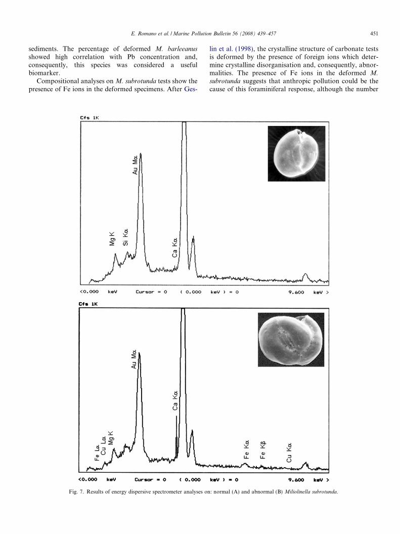
Compositional analyses on M. subrotunda tests show thepresence of Fe ions in the deformed specimens. After Ges-

Fig. 7. Results of energy dispersive spectrometer analyses on

lin et al. (1998), the crystalline structure of carbonate testsis deformed by the presence of foreign ions which deter-mine crystalline disorganisation and, consequently, abnor-malities. The presence of Fe ions in the deformed M.

subrotunda suggests that anthropic pollution could be thecause of this foraminiferal response, although the number

: normal (A) and abnormal (B) Miliolinella subrotunda.

452 E. Romano et al. / Marine Pollution Bulletin 56 (2008) 439–457

of abnormal M. subrotunda is not correlated to Fe concen-tration in sediments. Accordingly, Samir and El Din (2001)found relevant Cu, Zn, Cr and Pb concentrations indeformed foraminifera in the El-Mex Bay, with respect tonormal specimens of the same species, and they recognisedthat theses elements are absorbed, regardless of their con-centration in the surrounding medium. Also Sharifi et al.(1991) found that deformed specimens contain a higheramount of metals, particularly Cu and Zn, than non-deformed specimens, using Inductively Coupled PlasmaMass Spectrometry.

At Bagnoli, Fe is the only element, among the main pol-lutants, included in the crystalline reticulum of abnormalM. subrotunda, probably due its lower atomic number thanCu, Zn and, above all, Pb. Based on these results, we mayconsider M. subrotunda as a bio-indicator for Fe pollution.

The presence of foreign Fe ions in the composition ofabnormal M. subrotunda from Bagnoli confirms the roleplayed by metal pollution, also suggested by the statisticalanalysis, in the development of abnormal foraminifera. Thepositive Pearson correlation of deformed specimens withPAHs, Mn, and Zn indicates that high concentrations ofthese pollutants most likely favour the inclusion of Fe ions.This could be attributed to a potential toxic effect of thistypes of pollution, which determine the inability of M.

subrotunda to exclude foreign elements during the secretionof the test.

The non-recovery of foreign elements in deformed spec-imens of E. advena does not permit the attribution of thisfeature to metal pollution. Nevertheless, the strong statisti-cal correlation between E. advena deformation and Pb con-centration lets us suppose that deformation represents theresponse of this species to high Pb pollution. This type ofdeformation seems to be caused by a temporal perturba-tion that involves the construction of one single chamber,and no foreign elements are included in the crystallineframework. However, this temporal perturbation seemsto occur more frequently with high lead concentration.More studies with different analytical methods must be car-ried out to find the origin of this abnormality, which is notsignalled as frequent in natural environments.

6. Conclusions

In this research, benthic foraminifera gave a quantitativeevaluation of the ecological health of a benthic marinecoastal environment. The results of quantitative analyseson benthic assemblages, processed with geochemical andtextural sediment data, helped to characterise the studyarea by recognising distinct sectors, with different types

and degrees of pollution. The different response of foram-inifera let us recognise distinct kinds of pollution with dif-ferent effects on benthic environments. The strongpollution (primarily Pb and Zn), mainly located in frontof the steel plant, determines the environmental stress onthe foraminiferal population, shown by the low faunalabundance. In addition, this environment favours the pres-ence of some species such as H. germanica, M. subrotunda

and Q. parvula that may be considered to be pollution-tol-erant. Pollution due to Fe, generally associated to Cu,seems responsible for the highest environmental stress,until the disappearance of foraminifera, because no onespecies shows tolerance to such kinds of pollution. The pre-liminary analytical results performed on M. subrotundatests also suggest a ‘‘pollution-sensitive” character for thisspecies because it includes Fe ions in the crystalline reticu-lum, with the development of abnormal specimens. Never-theless, the abundance of abnormalities is not proportionalto the concentration of this metal in the sediment. Theinability to exclude foreign elements from the crystallinereticulum may be related to the potential toxic effect ofPAHs, Mn and Zn on M. subrotunda specimen, becausethe number of deformed tests is statistically correlated tothese pollutants.

The statistical correlation of deformed E. advena withPb let us suppose that this element plays a role in testsdeformation. Probably mechanisms other than crystallinedisorganisation are responsible for deformations and thiscould explain the lack of recovery of foreign elements indeformed tests.

This study showed that morphological abnormalitiescould be utilised in pollution monitoring, although thecomplexity of factors determining vital processes in naturalenvironments make it difficult to find a cause-effect rela-tionship between single pollutants and percentages ofabnormalities. The results are encouraging for the use ofbenthic foraminifera in an integrated program for pollu-tion monitoring.

Acknowledgement

The authors are very grateful to Maria Celia Magno andGiancarlo Pierfranceschi for their contribution on sedi-mentological analysis and to Andrea Salmeri and France-sco Venti for figure editing. Many thanks also toGiuseppina Ciuffa for determination of PAHs and to An-drea Colasanti for PCBs analyses. Particular thanks to Al-fredo Mancini for his assistance in SEM photographs andEDS analyses. Finally, many thanks to an anonymous ref-eree for his improving comments.

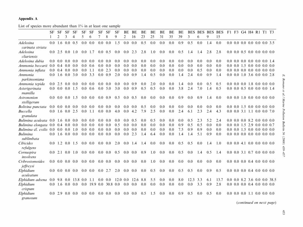
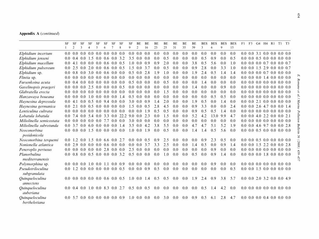
Appendix A

List of species more abundant than 1% in at least one sample

SF1

SF2

SF3

SF4

SF5

SF6

SF7

SF8

SF9

BE2

BE16

BE23

BE25

BE31

BE35

BE39

BES3

BES6

BES9

BES15

F1 F3 G4 H4 R1 T1 T3

Adelosinacarinata striata

0.0 1.6 0.0 0.5 0.0 0.0 0.0 0.0 1.5 0.0 0.0 0.5 0.0 0.0 0.0 0.9 0.5 0.0 1.4 0.0 0.0 0.0 0.0 0.0 0.0 0.0 3.5

Adelosina

cliariensis

0.0 2.5 0.0 1.0 0.0 1.7 0.0 0.5 0.0 0.0 2.3 2.8 1.0 0.0 0.0 0.5 1.4 1.4 2.8 2.8 0.0 0.0 0.5 0.0 0.0 0.0 0.0

Adelosina dubia 0.0 0.0 0.0 0.0 0.0 0.0 0.0 0.0 0.0 0.0 0.0 0.0 0.0 0.0 0.0 0.0 0.0 0.0 0.0 0.0 0.0 0.0 0.0 0.0 0.0 0.0 1.4Ammonia beccarii 0.0 0.4 0.0 0.0 0.0 0.6 0.0 0.0 0.0 0.0 0.0 0.0 0.0 0.0 0.0 0.0 0.0 0.0 0.0 0.0 0.0 0.0 1.5 0.0 0.0 0.0 0.0Ammonia inflata 0.0 0.4 0.0 0.0 0.0 1.1 0.0 2.3 0.0 0.0 0.0 0.0 0.0 0.0 0.0 0.0 0.0 0.5 0.0 0.0 0.0 0.0 0.0 0.0 0.0 0.0 0.0Ammonia

parkinsoniana

0.0 1.6 0.0 3.0 0.0 3.3 0.0 0.9 2.0 0.0 0.9 1.4 0.5 0.0 0.0 1.4 2.4 0.0 0.9 1.4 0.0 0.0 1.0 3.6 0.0 0.0 2.8

Ammonia tepida 0.0 2.5 0.0 0.0 0.0 0.0 0.0 0.0 0.0 0.0 0.9 0.0 2.0 0.0 0.0 1.4 0.0 0.0 0.5 0.5 0.0 0.0 0.0 1.8 0.0 0.0 0.0Asterigerinata

mamilla

0.0 0.0 0.0 1.5 0.0 0.6 0.0 5.0 3.0 0.0 0.9 0.5 0.5 0.0 0.0 3.8 2.4 7.0 1.4 0.5 0.0 0.0 0.5 0.0 0.0 0.0 1.4

Astrononion

stelligerum

0.0 0.0 0.0 1.5 0.0 0.0 0.0 0.9 0.5 0.0 0.5 0.0 0.0 0.0 0.0 0.9 0.0 0.9 1.4 0.0 0.0 0.0 1.0 0.0 0.0 0.0 0.0

Bolivina punctata 0.0 0.0 0.0 0.0 0.0 0.0 0.0 0.0 0.0 0.0 0.0 0.5 0.0 0.0 0.0 0.0 0.0 0.0 0.0 0.0 0.0 0.0 1.5 0.0 0.0 0.0 0.0Buccella

granulata

0.0 1.6 0.0 2.5 0.0 1.1 0.0 0.0 4.0 0.0 4.2 7.9 2.5 0.0 0.0 2.4 6.1 2.3 2.4 4.3 0.0 0.0 3.1 1.1 0.0 0.0 7.0

Bulimina aculeata 0.0 1.6 0.0 0.0 0.0 0.0 0.0 0.0 0.0 0.0 0.5 0.0 0.5 0.0 0.0 0.0 0.5 2.3 5.2 2.4 0.0 0.0 0.0 8.2 0.0 0.0 0.0Bulimina elongata 0.0 0.4 0.0 0.0 0.0 0.0 0.0 0.0 0.5 0.0 0.0 0.0 0.0 0.0 0.0 0.9 0.5 0.5 0.0 0.0 0.0 0.0 1.5 2.9 0.0 0.0 0.7Bulimina cf. exilis 0.0 0.0 0.0 1.0 0.0 0.0 0.0 0.0 0.0 0.0 0.0 0.0 0.0 0.0 0.0 7.5 0.9 0.9 0.0 0.0 0.0 0.0 1.5 0.0 0.0 0.0 0.0Bulimina

sublimbata

0.0 1.6 0.0 0.0 0.0 0.0 0.0 0.0 0.0 0.0 2.3 1.4 6.4 0.0 0.0 1.4 1.4 5.1 0.9 0.0 0.0 0.0 0.0 0.0 0.0 0.0 0.0

Cibicides

refulgens

0.0 1.2 0.0 1.5 0.0 0.0 0.0 0.0 2.0 0.0 1.4 1.4 0.0 0.0 0.0 0.5 0.5 0.0 1.4 1.0 0.0 0.0 4.1 0.0 0.0 0.0 0.0

Cornuspirainvolvens

0.0 2.1 0.0 1.0 0.0 0.0 0.0 0.0 0.5 0.0 0.0 0.9 1.0 0.0 0.0 0.5 0.0 1.4 0.5 1.4 0.0 0.0 3.1 0.7 0.0 0.0 0.0

Cribrostomoides

jeffreysi

0.0 0.0 0.0 0.0 0.0 0.0 0.0 0.0 0.0 0.0 0.0 0.0 1.0 0.0 0.0 0.0 0.0 0.0 0.0 0.0 0.0 0.0 0.0 0.4 0.0 0.0 0.0

Elphidium

aculeatum

0.0 0.0 0.0 0.0 0.0 0.0 0.0 2.7 2.0 0.0 0.0 0.0 0.5 0.0 0.0 0.5 0.5 0.0 0.9 0.5 0.0 0.0 0.0 0.4 0.0 0.0 0.0

Elphidium advena 0.0 9.8 0.0 13.8 0.0 1.1 0.0 0.0 12.0 0.0 12.6 8.8 5.5 0.0 0.0 8.0 12.3 3.3 6.1 13.7 0.0 0.0 8.2 3.6 0.0 0.0 38.5Elphidium

crispum

0.0 1.6 0.0 0.0 0.0 19.9 0.0 30.8 0.0 0.0 0.0 0.0 0.0 0.0 0.0 0.0 0.0 3.3 0.9 2.8 0.0 0.0 0.0 0.4 0.0 0.0 0.0

Elphidium

granosum

0.0 2.9 0.0 0.0 0.0 0.0 0.0 0.0 0.0 0.0 0.0 0.5 1.5 0.0 0.0 0.9 0.5 0.0 0.5 0.0 0.0 0.0 0.0 1.1 0.0 0.0 0.0

(continued on next page)

E.

Ro

ma

no

eta

l./Ma

rine

Po

llutio

nB

ulletin

56

(2

00

8)

43

9–

45

7453

Appendix A (continued)

SF1

SF2

SF3

SF4

SF5

SF6

SF7

SF8

SF9

BE2

BE16

BE23

BE25

BE31

BE35

BE39

BES3

BES6

BES9

BES15

F1 F3 G4 H4 R1 T1 T3

Elphidium incertum 0.0 0.0 0.0 0.0 0.0 0.0 0.0 0.0 0.0 0.0 0.0 0.0 0.0 0.0 0.0 0.0 0.0 0.0 0.0 0.0 0.0 0.0 3.1 0.0 0.0 0.0 0.0Elphidium jenseni 0.0 0.4 0.0 1.5 0.0 0.6 0.0 3.2 3.5 0.0 0.0 0.0 0.5 0.0 0.0 0.0 0.5 0.9 0.0 0.5 0.0 0.0 0.5 0.0 0.0 0.0 0.0Elphidium macellum 0.0 4.1 0.0 0.0 0.0 0.6 0.0 0.5 1.0 0.0 0.9 0.9 2.0 0.0 0.0 3.8 0.5 5.6 0.0 1.0 0.0 0.0 0.0 0.7 0.0 0.0 0.7Elphidium pulvereum 0.0 2.5 0.0 2.0 0.0 0.6 0.0 0.5 1.5 0.0 3.7 0.0 0.5 0.0 0.0 0.9 2.8 0.0 3.3 1.0 0.0 0.0 1.5 2.9 0.0 0.0 0.7Elphidium sp. 0.0 0.8 0.0 3.0 0.0 0.6 0.0 0.0 0.5 0.0 2.8 1.9 1.0 0.0 0.0 1.9 2.4 0.5 1.4 1.4 0.0 0.0 0.0 0.7 0.0 0.0 0.0Flintia sp. 0.0 0.0 0.0 0.0 0.0 0.0 0.0 0.0 0.0 0.0 0.0 0.0 0.0 0.0 0.0 0.0 0.0 0.0 0.0 0.0 0.0 0.0 0.0 1.4 0.0 0.0 0.0Fursenkoina acuta 0.0 0.4 0.0 0.0 0.0 0.0 0.0 0.0 0.5 0.0 0.0 0.0 0.5 0.0 0.0 0.0 1.4 0.0 0.0 0.0 0.0 0.0 0.0 0.0 0.0 0.0 0.0Gavelinopsis praegeri 0.0 0.0 0.0 2.5 0.0 0.0 0.0 0.5 0.0 0.0 0.0 0.0 0.0 0.0 0.0 1.4 0.0 0.0 0.9 0.0 0.0 0.0 0.0 0.0 0.0 0.0 0.0Glabratella erecta 0.0 0.0 0.0 0.0 0.0 0.0 0.0 0.0 0.0 0.0 0.0 0.0 1.5 0.0 0.0 0.0 0.0 0.0 0.0 0.0 0.0 0.0 0.0 0.0 0.0 0.0 0.0Hanzawaya boueana 0.0 0.0 0.0 1.0 0.0 0.0 0.0 1.4 0.5 0.0 0.0 0.0 0.0 0.0 0.0 0.0 0.0 0.5 0.5 0.0 0.0 0.0 0.0 0.0 0.0 0.0 0.0Haynesina depressula 0.0 4.1 0.0 0.5 0.0 9.4 0.0 0.0 3.0 0.0 0.9 1.4 2.0 0.0 0.0 1.9 0.5 0.0 1.4 0.0 0.0 0.0 2.1 0.0 0.0 0.0 0.0Haynesina germanica 0.0 2.1 0.0 0.5 0.0 0.0 0.0 0.0 1.5 0.0 0.5 2.8 4.5 0.0 0.0 0.9 3.3 0.0 0.0 2.4 0.0 0.0 2.6 4.7 0.0 0.0 1.4Lenticulina cultrata 0.0 0.0 0.0 0.0 0.0 0.0 0.0 0.0 0.0 0.0 1.9 0.5 0.5 0.0 0.0 0.9 0.5 0.5 1.4 0.0 0.0 0.0 0.0 0.0 0.0 0.0 0.0Lobatula lobatula 0.0 7.4 0.0 5.4 0.0 3.3 0.0 22.2 9.0 0.0 2.3 0.0 1.5 0.0 0.0 5.2 4.2 13.0 9.9 4.7 0.0 0.0 4.0 2.2 0.0 0.0 2.1Miliolinella semicostata 0.0 0.0 0.0 0.0 0.0 7.7 0.0 0.0 3.0 0.0 0.0 0.0 0.0 0.0 0.0 0.0 0.0 0.0 0.0 0.0 0.0 0.0 0.0 0.0 0.0 0.0 0.0Miliolinella subrotunda 0.0 3.7 0.0 6.0 0.0 0.0 0.0 1.4 3.5 0.0 4.2 3.8 5.5 0.0 0.0 4.7 4.7 5.1 5.2 1.9 0.0 0.0 4.6 9.7 0.0 0.0 2.8Neoconorbina

posidonicola

0.0 0.0 0.0 1.5 0.0 0.0 0.0 0.0 1.0 0.0 1.9 0.0 0.5 0.0 0.0 1.4 1.4 0.5 5.6 0.0 0.0 0.0 0.5 0.0 0.0 0.0 0.0

Neoconorbina terquemi 0.0 1.2 0.0 1.5 0.0 6.6 0.0 2.7 0.0 0.0 0.5 0.9 2.5 0.0 0.0 0.0 0.9 2.3 0.5 0.0 0.0 0.0 0.5 0.0 0.0 0.0 0.0Nonionella atlantica 0.0 2.9 0.0 0.0 0.0 0.6 0.0 0.0 0.0 0.0 3.7 3.3 2.5 0.0 0.0 1.4 0.5 0.0 0.9 1.4 0.0 0.0 1.5 2.2 0.0 0.0 2.8Peneroplis pertusus 0.0 0.0 0.0 0.0 0.0 2.8 0.0 0.0 2.5 0.0 0.0 0.0 0.0 0.0 0.0 0.0 0.0 0.9 0.0 0.0 0.0 0.0 0.0 0.0 0.0 0.0 0.0Planorbulina

mediterranensis

0.0 0.8 0.0 0.5 0.0 0.0 0.0 3.2 0.5 0.0 0.0 0.0 1.0 0.0 0.0 0.5 0.0 0.9 1.4 0.0 0.0 0.0 0.0 1.8 0.0 0.0 0.0

Polymorphina sp. 0.0 0.0 0.0 1.0 0.0 1.1 0.0 0.9 0.0 0.0 0.0 0.0 0.0 0.0 0.0 0.0 0.0 0.9 0.0 0.0 0.0 0.0 0.0 0.0 0.0 0.0 0.0Pseudotriloculina

subgranulata

0.0 1.2 0.0 0.0 0.0 0.0 0.0 0.5 0.0 0.0 0.9 0.5 0.0 0.0 0.0 0.0 0.0 0.0 0.0 0.5 0.0 0.0 1.5 0.0 0.0 0.0 0.0

Quinqueloculina

annectens

0.0 0.0 0.0 0.0 0.0 0.6 0.0 0.5 1.0 0.0 1.4 0.5 0.5 0.0 0.0 1.9 2.4 0.9 3.8 5.7 0.0 0.0 2.0 3.2 0.0 0.0 4.9

Quinqueloculina

auberiana

0.0 0.4 0.0 1.0 0.0 8.3 0.0 2.7 0.5 0.0 0.5 0.0 0.0 0.0 0.0 0.0 0.5 1.4 4.2 0.0 0.0 0.0 0.0 0.0 0.0 0.0 0.0

Quinqueloculina

berthelotiana

0.0 5.7 0.0 0.0 0.0 0.0 0.0 0.9 1.0 0.0 0.0 0.0 3.0 0.0 0.0 0.9 0.5 6.1 2.8 4.7 0.0 0.0 0.0 0.4 0.0 0.0 0.0

454E

.R

om

an

oet

al./M

arin

eP

ollu

tion

Bu

lletin5

6(

20

08

)4

39

–4

57

Quinqueloculina

bosciana

0.0 0.0 0.0 0.0 0.0 0.0 0.0 0.0 1.0 0.0 0.0 0.0 0.0 0.0 0.0 0.0 0.0 0.0 0.0 0.0 0.0 0.0 9.7 5.4 0.0 0.0 0.7

Quinqueloculina

laevigata

0.0 2.5 0.0 1.0 0.0 0.0 0.0 0.5 1.5 0.0 4.2 7.0 2.0 0.0 0.0 1.9 7.6 1.9 2.4 3.3 0.0 0.0 0.5 0.0 0.0 0.0 2.1

Quinqueloculina

lata

0.0 2.1 0.0 23.9 0.0 2.8 0.0 0.0 12.0 0.0 15.4 14.9 14.9 0.0 0.0 6.6 9.9 5.1 6.1 4.7 0.0 0.0 10.8 13.3 0.0 0.0 7.7

Quinqueloculina

parvula

0.0 0.8 0.0 0.0 0.0 1.1 0.0 0.0 1.5 0.0 2.3 2.8 4.0 0.0 0.0 2.8 1.4 2.3 0.0 3.3 0.0 0.0 0.0 6.1 0.0 0.0 2.1

Quinqueloculina

seminulum

0.0 0.8 0.0 1.5 0.0 2.8 0.0 1.4 1.0 0.0 0.9 3.3 2.0 0.0 0.0 1.9 1.9 3.3 1.9 1.9 0.0 0.0 1.5 1.4 0.0 0.0 1.4

Quinqueloculina

stalkeri

0.0 0.0 0.0 4.4 0.0 0.0 0.0 0.0 6.0 0.0 0.0 0.0 0.0 0.0 0.0 0.0 0.0 0.0 0.5 0.0 0.0 0.0 0.0 0.0 0.0 0.0 0.0

Quinqueloculina

stelligera

0.0 0.8 0.0 2.0 0.0 1.1 0.0 0.0 5.5 0.0 10.7 8.4 5.0 0.0 0.0 2.4 10.4 0.0 0.0 4.3 0.0 0.0 11.3 0.7 0.0 0.0 4.9

Rosalina

bradyi

0.0 10.3 0.0 0.0 0.0 0.6 0.0 6.8 4.0 0.0 2.8 1.9 2.0 0.0 0.0 1.9 2.4 3.3 5.2 5.2 0.0 0.0 0.0 0.4 0.0 0.0 2.1

Rosalina

floridana

0.0 0.0 0.0 5.4 0.0 4.4 0.0 0.9 2.0 0.0 0.0 0.0 1.0 0.0 0.0 0.0 0.5 6.5 0.0 0.0 0.0 0.0 0.0 0.0 0.0 0.0 0.0

Siphonaperta

aspera

0.0 1.6 0.0 0.5 0.0 11.0 0.0 0.9 0.0 0.0 0.9 1.4 0.0 0.0 0.0 0.5 0.5 0.0 0.0 3.8 0.0 0.0 0.0 0.7 0.0 0.0 0.0

Siphonaperta

dilatata

0.0 0.0 0.0 0.0 0.0 1.7 0.0 0.0 0.0 0.0 0.0 0.0 0.0 0.0 0.0 0.0 0.0 0.0 0.0 0.0 0.0 0.0 0.5 0.0 0.0 0.0 0.0

Slitella eburnea 0.0 0.0 0.0 0.5 0.0 0.0 0.0 0.0 0.0 0.0 0.5 0.0 0.5 0.0 0.0 0.0 0.0 0.0 0.5 0.0 0.0 0.0 0.0 0.0 0.0 0.0 1.4Tretomphalus

concinnus

0.0 0.8 0.0 3.4 0.0 0.6 0.0 0.0 1.0 0.0 1.4 1.4 0.5 0.0 0.0 3.3 1.9 0.0 0.5 0.0 0.0 0.0 3.6 10.4 0.0 0.0 2.1

Triloculina

plicata

0.0 9.4 0.0 0.5 0.0 0.6 0.0 0.9 0.0 0.0 4.7 14.0 10.4 0.0 0.0 9.9 3.8 4.2 6.1 12.8 0.0 0.0 1.5 3.9 0.0 0.0 1.4

Triloculinaschreiberiana

0.0 0.0 0.0 0.0 0.0 0.0 0.0 0.0 0.0 0.0 0.0 0.0 0.0 0.0 0.0 0.0 0.0 0.0 0.0 0.0 0.0 0.0 2.1 0.0 0.0 0.0 0.0

Triloculina

tricarinata

0.0 0.0 0.0 0.0 0.0 0.0 0.0 0.0 0.0 0.0 0.0 0.0 0.0 0.0 0.0 1.4 0.5 0.0 0.5 0.0 0.0 0.0 0.5 0.0 0.0 0.0 0.0

Vertebralina

striata

0.0 0.4 0.0 1.5 0.0 0.0 0.0 0.0 0.5 0.0 0.9 0.5 0.5 0.0 0.0 1.9 0.9 0.0 0.5 1.0 0.0 0.0 0.0 1.4 0.0 0.0 0.0

E.

Ro

ma

no

eta

l./Ma

rine

Po

llutio

nB

ulletin

56

(2

00

8)

43

9–

45

7455

Ap

pen

dix

B

Sp

ecifi

cd

iver

sity

(nu

mb

ero

fsp

ecie

s–

S,

Sh

ann

on

-in

dex

–H

,a-

ind

ex),

Eq

uit

abil

ity

(E),

fau

nal

den

sity

(BN

)an

dre

lati

veab

un

dan

ceo

fab

no

rmal

spec

imen

s(F

AI)

SF

1

SF

2

SF

3

SF

4

SF

5

SF

6

SF

7

SF

8

SF

9

BE

2

BE

16

BE

23

BE

25

BE

31

BE

35

BE

39

BE

S

3

BE

S

6

BE

S

9

BE

S

15

F1

F3

G4

H4

R1

T1

T3

S0

460

430

340

3644

041

3549

00

4147

4450

380

041

460

029

H0.

003.

420.

003.

160.

002.

790.

002.

533.

340.

003.

223.

063.

530.

000.

003.

513.

543.

393.

593.

220.

000.

003.

213.

330.

000.

002.

54

a-In

dex

0.00

33.4

00.

0027

.46

0.00

17.3

20.

0020

.00

30.7

00.

0026

.79

19.8

341

.28

0.00

0.00

36.7

139

.09

30.7

042

.08

22.7

80.

000.

0026

.50

33.4

00.

000.

0013

.61

E0.

000.

890.

000.

840.

000.

790.

000.

710.

880.

000.

870.

860.

910.

000.

000.

910.

920.

900.

920.

880.

000.

000.

860.

870.

000.

000.

76

BN

(sp

ecim

ens/

g)0.

021

59.5

0.0

33.9

0.0

1.8

0.0

3.8

7.1

0.0

128.

615

0.7

188.

30.

00.

021

7.4

28.0

257.

818

1.6

139.

80.

00.

017

.223

.30.

00.

021

.7

FA

I(%

)0.

03.

70.

01.

50.

03.

90.

02.

72.

00.

02.

35.

54.

40.

00.

02.

34.

23.

22.

32.

80.

00.

00.

42.

00.

00.

02.

1

456 E. Romano et al. / Marine Pollution Bulletin 56 (2008) 439–457

References

Alve, E., 1991a. Benthic foraminifera in sediment cores reflecting heavymetal pollution in Sørfjord, western Norway. Journal of ForaminiferalResearch 21 (1), 1–19.

Alve, E., 1991b. Foraminifera, climatic change and pollution: a study oflate Holocene sediments in Drammensfjord, southeast Norway. TheHolocene 1 (3), 243–326.

Alve, E., Olsgrad, F., 1999. Benthic foraminifera colonization in exper-iments with copper-contaminated sediments. Journal of ForaminiferalResearch 29 (3), 186–195.

Armynot du Chatelet, E., Debenay, J.P., Soulard, R., 2004. Foraminiferalproxies for pollution monitoring in moderately polluted harbors.Environmental Pollution 127, 27–40.

Ausili, A., Pellegrini, D., Onorati, F., De Ranieri, S., 1998. Valutazionedella qualita di sedimenti del Porto di Viareggio da sottoporre adescavo. Acqua Aria (January), 67–71.

Bergamin, L., Romano, E., Celia Magno, M., Ausili, A., Gabellini, M.,2005. Pollution monitoring of Bagnoli Bay (Tyrrhenian Sea, Naples,Italy): a chemical–physical and ecological approach. Aquatic Ecosys-tem Health and Management Journal 8 (3), 293–302.

Bergamin, L., Romano, E., Gabellini, M., Ausili, A., Carboni, M.G.,2003. Chemical–physical and ecological characterisation in the envi-ronmental project of a polluted coastal area: the Bagnoli case study.Mediterranean Marine Science 4 (1), 5–20.

Burone, L., Venturini, N., Sprechmann, P., Valente, P., Muniz, P., 2006.Foraminiferal responses to polluted sediments in the Montevideocoastal zone, Uruguay. Marine Pollution Bulletin 52, 61–73.

Byers, S.C., Mills, L.E., Stewart, P.L., 1987. A comparison of methods ofdetermining organic in marine sediments, with suggestions for astandard method. Hydrobiologia 58, 43–47.

Carrada, G.C., Hopkins, T.S., Bonaduce, G., Ianora, A., Marino, D.,Modigh, M., Ribeira D’Alcala, M., Scotto Di Carlo, B., 1980.Variability in the hydrographic and biological features of the Gulf ofNaples. Marine Ecology 1, 105–120.

Cicero, A.M., Finoia, M.G., Gabellini, M., Pietrantonio, E., Romanelli,G., Romano, E., 2003. Assessment of chlorinated organic pollutants insediments of a coastal area of the Tyrrhenian Sea (Ombrone River –Italy): a case study of multivariate approach for marine sedimentscharacterisation. In: Munawar, M. (Ed.) Sediment Quality Assessmentand Management: Insight and Progress, Ecovision World MonographSeries, pp. 125–138.

Cimerman, F., Langer, M., 1991. Mediterranean Foraminifera. SlovenskaAkademija Znanosti in Umetnosti, Academia Scientiarum ArtiumSlovenica, Classis IV, Historia Naturalia 30, Ljubliana.

Coccioni, R., 2000. Benthic foraminifera as bioindicators of heavy metalpollution: a case study from the Goro Lagoon (Italy). In: Martin, R.(Ed.), Environmental Micropaleontology. Kluwer Academic/PlenumPublishers, New York, pp. 71–103.

Coccioni, R., Frontalini, F., Marsili, A., Troiani, F., 2005. Foraminiferibentonici e metalli in traccia: implicazioni ambientali. Quaderni delCentro di Geobiologia 3, 57–92.

Damiani, V., Baudo, R., De Rosa, S., De Simone, R., Ferretti, O., Izzo,G., Serena, F., 1987. A case study: Bay of Pozzuoli (Gulf of Naples,Italy). Hydrobiology 149, 210–211.

Debenay, J.P., Geslin, E., Eichler, B.B., Duleba, W., Sylvestre, F., Eichler,P., 2001a. Foraminiferal assemblages in Hypersaline Lagoon. Journalof Foraminiferal Research 31 (2), 133–151.

Debenay, J.P., Tsakiridis, E., Soulard, R., Grossel, H., 2001b. Factorsdetermining the distribution of foraminiferal assemblages in PortJoinville Harbor (Ile d’Yeu, France): the influence of pollution. MarineMicropaleontology 43, 75–118.

Elberling, B., Knudsen, K.L., Kristensen, P.H., Asmund, G., 2003.Applying foraminiferal stratigraphy as a biomarker for heavy metalcontamination and mining impact in a fiord in west Greenland. MarineEnvironmental Research 55, 235–256.

E. Romano et al. / Marine Pollution Bulletin 56 (2008) 439–457 457

Ferraro, L., Sprovieri, M., Alberico, I., Lirer, F., Prevedello, L., Marsella,E., 2006. Benthic foraminifera and heavy metals distribution: a casestudy from the Naples Harbour (Tyrrhenian Sea, Southern Italy).Environmental Pollution 142, 274–287.

Fishbein, E., Patterson, T., 1993. Error-weighted maximum likeli-hood (EWML): a new statistically based method to cluster quantita-tive micropaleontological data. Journal of Paleontology 67 (3), 475–486.

Fisher, R.A., Corbet, A.S., Williams, C.B., 1943. The relation between thenumber of species and the number of individuals in a random sampleof an animal population. Journal of Animal Ecology 12, 42–58.

Giani, M., Gabellini, M., Pellegrini, D., Costantini, S., Beccaloni, E.,Giordano, R., 1994a. Concentration and partitioning of Cr, Hg and Pbin sediments of dredge and disposal sites of the northern Adriatic Sea.Science of Total Environment 158, 97–112.

Geslin, E., Debenay, J.P., Lesourd, M., 1998. Abnormal wall textures andtest deformation in Ammonia (hyaline foraminifer). Journal ofForaminiferal Research 28 (2), 148–156.

Geslin, E., Stouff, V., Debenay, J.P., Lesourd, M., 2000. Environmentalvariation and foraminiferal test abnormalities. In: Martin, R. (Ed.),Environmental Micropaleontology. Kluwer Academic/Plenum Pub-lishers, New York, pp. 91–215.

Geslin, E., Debenay, J.P., Duleba, W., Bonetti, C., 2002. Morphologicalabnormalities of foraminiferal tests in Brazilian environments: com-parison between polluted and non-polluted areas. Marine Micropale-ontology 45, 151–168.

Giani, M., Gabellini, M., Pellegrini, D., Costantini, S., Beccaloni, E.,Giordano, R., 1994b. Concentration and partitioning of Cr, Hg andPb in sediments of dredge and disposal sites of the northern Adriaticsea. Science of Total Environment 158, 97–112.

Jorissen, F.J., 1988. Benthic foraminifera from the Adriatic Sea: principlesof phenotypic variations. Utrecht Micropaleontological Bulletin 37, 1–174.

Langer, M.R., 1993. Epiphytic foraminifera. Marine Micropaleontology20, 235–265.

Loeblich, A.R., Tappan, H., 1987. Foraminiferal Genera and theirClassification. Van Nostrand Reinhold Comp., New York.

Mahalanobis, P.C., 1936. On the generalized distance in statistics.Proceedings of the National Institute of Sciences of India 12, 49–55.

Massart, D.L., Kaufman, L., 1989. Hierarchical clustering methods. In:Krieger, R.E. (Ed.), The Interpretation of Analytical Chemical data bythe use of Cluster Analysis. Krieger Publishing Co. Inc., Malabar, FL,pp. 75–99.

Ministero dell’Ambiente e della Tutela del Territorio 2003. D.M. n. 367del 6 novembre 2003. Regolamento concernente la fissazione distandard di qualita nell’ambiente acquatico per le sostanze pericolose,ai sensi dell’articolo 3, comma 4, del decreto legislativo 11 maggio1999, n. 152. Gazzetta Ufficiale della Repubblica Italiana, 8 Gennaio2004, 5, pp. 17–29.

Morovan, J., La Cadre, V., Jorissen, F., Debenay, J.P., 2004. Foraminif-era as potential bio-indicators of the”Erika‘‘ oil spill in the Bay ofBourgneuf: field and experimental studies. Aquatic Living Resources17, 317–322.

Murray, J.W., 1968. Living foraminifera of lagoons and estuaries.Micropaleontology 14, 435–455.

Murray, J.W., 1991. Ecology and Paleoecology of Benthic Foraminifera.Longman Scientific & Technical, New York.

Murray, J.W., Bowser, S.S., 2000. Mortality, protoplasm decay rate, andreliability of staining techniques to recognize ‘‘living” foraminifera: areview. Journal of Foraminiferal Research 30 (1), 66–70.

Nigam, R., Saraswat, R., Pancharng, R., 2006. Application of foramini-fers in ecotoxicology: retrospect, perspect and prospect. EnvironmentInternational 32, 273–283.

Romano, E., Ausili, A., Zaharova, N., Celia Magno, M., Pavoni, B.,Gabellini, M., 2004. Marine sediment contamination of an industrialsite at Port of Bagnoli, Gulf of Naples, Southern Italy. MarinePollution Bulletin 49, 487–495.

Romano, E., Bergamin, L., Finoia, M.G., Ausili, A., Di Mento, R.,Manfra, L., Celia Magno, M., Pierfranceschi, G., Gabellini, M., 2003.Environmental characterisation of contaminated marine sediments:the Bagnoli industrial site. In: Porta, A., Pellei, M. (Eds.), Proceedingsof the 2nd International Conference on Remediation of ContaminatedSediments, section G, paper 07.

Romano, E., Gabellini, M., Pellegrini, D., Ausili, A., Mellara, F., 1998.Metalli in tracce e contaminanti organici provenienti da differenti areemarine costiere in relazione alla movimentazione dei fondali. In:Proceedings of the 12th A.I.O.L (Associazione Italiana Oceanologia eLimnologia) Conference, vol. 2, pp. 473–486.

Russo, F., Calderoni, G., Lombardo, M., 1998. Evoluzione geomorfologiadella depressione Bagnoli-Fuorigrotta: periferia urbana della citta diNapoli. Bollettino della Societa geologica Italiana 117, 21–38.

Samir, A.M., 2000. The response of benthic foraminifera and ostracods tovarious pollution sources: a study from two lagoons in Egypt. Journalof Foraminiferal Research 30 (2), 83–98.

Samir, A.M., El Din, A.B., 2001. Benthic foraminiferal assemblages andmorphological abnormalities as pollution proxies in two Egyptianbays. Marine Micropaleontology 41, 193–227.

Scott, D.B., Medioli, F.S., 1980. Living vs total foraminiferal populations:their relative usefulness in paleoecology. Journal of Paleontology 54(4), 814–831.

Scott, D.B., Medioli, F.S., Schafer, C.T., 2001. Monitoring of Coastalenvironments using Foraminifera and Thecamoebian Indicators.Cambridge University Press.

Schafer, C.T., Wagner, F.J.E., Ferguson, C., 1975. Occurrence offoraminifera, molluscs and ostracods adjacent to the industrializedshoreline of Canso Strait, Nova Scotia. Water Air and Soil Pollution 2,79–96.

Sgarrella, F., Moncharmont-Zei, M., 1993. Benthic Foraminifera of theGulf of Naples (Italy): systematics and autoecology. Bollettino dellaSocieta Paleontologica Italiana 32 (2), 145–264.

Shannon, C.E., Weaver, W.W., 1963. The Mathematical Theory ofCommunication. University of Illinois Press, Urbana.

Sharp, W.E., Nardi, G., 1987. A study of the heavy-metal pollution in thebottom sediments at Porto di Bagnoli (Naples, Italy). Journal ofGeochemical Exploration 29, 31–48.

Sharifi, A.R., Croudace, J.W., Austin, R.L., 1991. Benthic foraminiferidsas pollution indicators in Southampton Water, southern England,U.K.. Journal of Micropaleontology 10 (1), 109–113.

Stouff, V., Geslin, E., Debenay, J.P., Lesourd, M., 1999. Origin ofmorphological abnormalities in Ammonia (Foraminifera): studies inlaboratory and natural environments. Journal of ForaminiferalResearch 29 (2), 152–170.

Tomassone, R., Danzard, M., Daudin, J.J., Masson, J.P., 1988. Discrim-ination et classement. Masson, Paris.

UNEP, 1996. State of marine and coastal environment in the Mediter-ranean region. MAP Technical Reports Series 100, UNEP, Athens.

Yanko, V., Ahmad, M., Kaminski, M., 1998. Morphological deformitiesof benthic foraminiferal tests in response to pollution by heavy metals:implications for pollution monitoring. Journal of ForaminiferalResearch 28 (3), 177–200.

Yanko, V., Kronfeld, J., Flexer, A., 1994. Response of benthic forami-nifera to various pollution sources: implications for pollution moni-toring. Journal of Foraminiferal Research 24 (1), 1–17.

Yanko, V., Arnold, A., Parker, W., 1999. Effect of marine pollution onbenthic foraminifera. In: Sen Gupta, B.K. (Ed.), Modern Foraminif-era. Kluver Academic, pp. 217–235.