1

INCREMENTAL DYNAMIC ANALYSIS APPLIED TO

SEISMIC FINANCIAL RISK ASSESSMENT OF BRIDGES

John B. Mander1*, Rajesh P. Dhakal1, Naoto Mashiko1, Kevin Solberg1

1Dept. of Civil Engineering, University of Canterbury, Private Bag 4800, Christchurch 8020, New Zealand

*Corresponding author: Ph +64-3-366 7001 ext 7395; Fax: +64-3-364 2758;

Email: john.mander@canterbury.ac.nz

ABSTRACT

Incremental Dynamic Analysis (IDA) is applied in a Performance-Based Earthquake Engineering context to investigate expected structural response, damage outcomes, and

financial loss from highway bridges. This quantitative risk analysis procedure consists of: adopting a suitable suite of ground motions and performing IDA on a nonlinear model of the prototype structure; summarize and parameterize the IDA results into various percentile performance bounds; and integrate the results with respect to hazard intensity-recurrence relations into a probabilistic risk format. An illustrative example of the procedure is given for reinforced concrete highway bridge piers, designed to New Zealand, Japan and Caltrans specifications. It is shown that bridges designed to a “Design Basis Earthquake” that has a 10 percent probability in 50 years with PGA =

0.4g, and detailed according to the specification of each country, should perform well without extensive damage. However, if a larger earthquake occurs, such as a maximum considered event which has a probability of 2 percent in 50 years, then extensive damage with the possibility of collapse may be expected. The financial implications of this

vulnerability are also given, revealing a four fold variation between the three countries.

KEYWORDS

Incremental Dynamic Analysis, Performance Based Earthquake Engineering (PBEE), expected annual loss, seismic risk assessment.

INTRODUCTION

Performance Based Earthquake Engineering procedures require the prediction of the seismic capacity of structures which is then compared to the local seismic demand. The interrelationship between the two gives an inference of the expected level of damage for a given level of ground shaking. In order to estimate structural performance under seismic loads, Vamvatsikos and Cornell [1] proposed a computational-based methodology called Incremental Dynamic Analysis (IDA). The IDA approach is a new methodology which can give a clear indication of the relationship between the seismic capacity and

the demand. With respect to seismological intensity measures (IM), such as peak ground acceleration (PGA), engineers can estimate principal response quantities in terms of governing engineering demand parameters (EDP), such as the maximum deflection or drift of the structure.

The IDA approach involves performing nonlinear dynamic analyses of a prototype structural

system under a suite of ground motion records, each scaled to several IM levels designed to force the structure all the way from elastic response to final global dynamic instability (collapse). From IDA curves, limit states can be defined. The probability of exceeding a specified limit state for a given IM (e.g. PGA) can also be found. The final results of IDA are thus in a suitable format to be conveniently

integrated with a conventional seismic hazard curve in order to calculate mean annual frequency of exceeding a certain damage limit-state capacity. This can be used to determine likely damage given a scenario earthquake event, or in a financial sense, the expected annual loss (EAL), incorporating the entire range of seismic scenarios.

This paper develops the IDA process specifically for bridge structures. What is new here is the way in which IDA results are quantitatively modelled and then integrated into a probabilistic risk analysis procedure whereby the seismic intensity-recurrence relationship (the seismic demand) is viewed with respect to the damage propensity of a specific bridge structure (structural capacity). Confidence intervals

and damage outcomes for given hazard intensity levels, such as the Design Basis Earthquake (DBE) or a Maximum Considered Earthquake (MCE), can be evaluated. In addition, a methodology for assessing the financial seismic vulnerability of bridges is introduced. The procedure will be demonstrated using a comparative study of bridge piers designed to three different countries’ standards.

2

IDA-BASED SEISMIC RISK ASSESSMENT

Step 1: Select ground motion records and Hazard–Recurrence Risk Relation

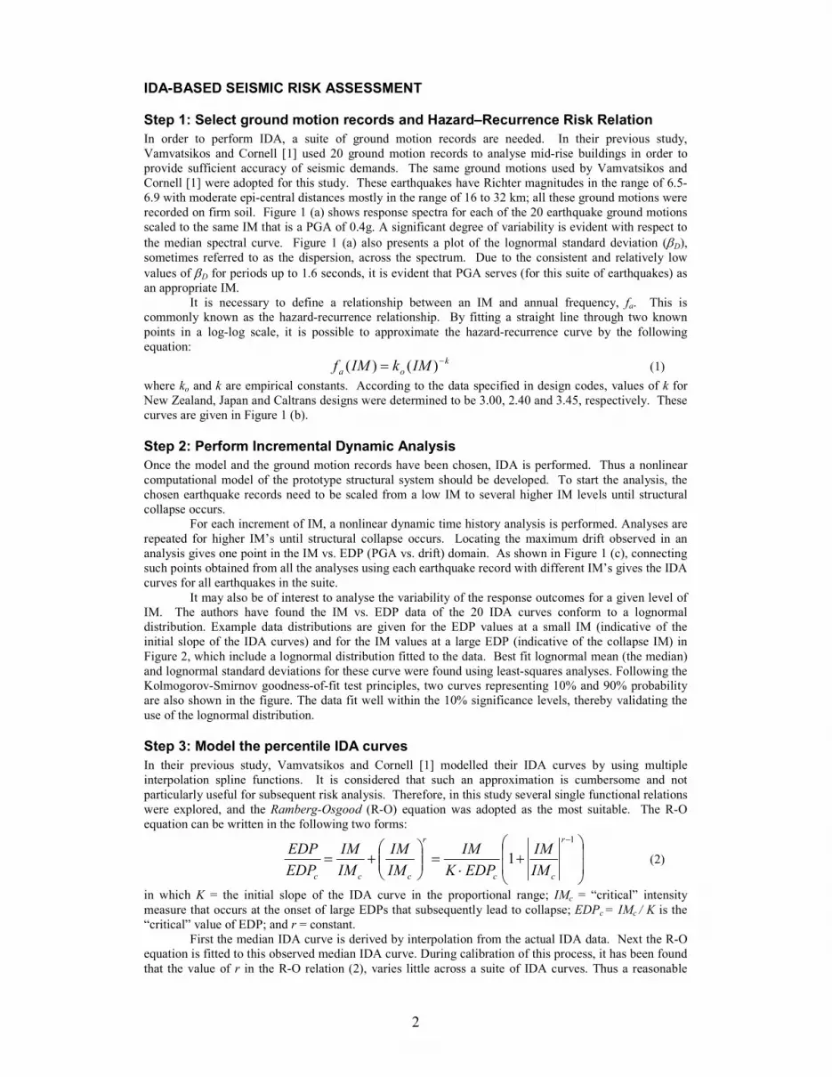
In order to perform IDA, a suite of ground motion records are needed. In their previous study, Vamvatsikos and Cornell [1] used 20 ground motion records to analyse mid-rise buildings in order to provide sufficient accuracy of seismic demands. The same ground motions used by Vamvatsikos and Cornell [1] were adopted for this study. These earthquakes have Richter magnitudes in the range of 6.5-6.9 with moderate epi-central distances mostly in the range of 16 to 32 km; all these ground motions were recorded on firm soil. Figure 1 (a) shows response spectra for each of the 20 earthquake ground motions scaled to the same IM that is a PGA of 0.4g. A significant degree of variability is evident with respect to

the median spectral curve. Figure 1 (a) also presents a plot of the lognormal standard deviation (βD), sometimes referred to as the dispersion, across the spectrum. Due to the consistent and relatively low

values of βD for periods up to 1.6 seconds, it is evident that PGA serves (for this suite of earthquakes) as an appropriate IM.

It is necessary to define a relationship between an IM and annual frequency, fa. This is commonly known as the hazard-recurrence relationship. By fitting a straight line through two known

points in a log-log scale, it is possible to approximate the hazard-recurrence curve by the following equation:

k

oa IMkIMf −= )()( (1)

where ko and k are empirical constants. According to the data specified in design codes, values of k for New Zealand, Japan and Caltrans designs were determined to be 3.00, 2.40 and 3.45, respectively. These curves are given in Figure 1 (b).

Step 2: Perform Incremental Dynamic Analysis

Once the model and the ground motion records have been chosen, IDA is performed. Thus a nonlinear

computational model of the prototype structural system should be developed. To start the analysis, the chosen earthquake records need to be scaled from a low IM to several higher IM levels until structural collapse occurs. For each increment of IM, a nonlinear dynamic time history analysis is performed. Analyses are

repeated for higher IM’s until structural collapse occurs. Locating the maximum drift observed in an analysis gives one point in the IM vs. EDP (PGA vs. drift) domain. As shown in Figure 1 (c), connecting such points obtained from all the analyses using each earthquake record with different IM’s gives the IDA curves for all earthquakes in the suite.

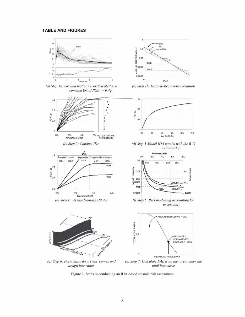
It may also be of interest to analyse the variability of the response outcomes for a given level of IM. The authors have found the IM vs. EDP data of the 20 IDA curves conform to a lognormal distribution. Example data distributions are given for the EDP values at a small IM (indicative of the initial slope of the IDA curves) and for the IM values at a large EDP (indicative of the collapse IM) in

Figure 2, which include a lognormal distribution fitted to the data. Best fit lognormal mean (the median) and lognormal standard deviations for these curve were found using least-squares analyses. Following the Kolmogorov-Smirnov goodness-of-fit test principles, two curves representing 10% and 90% probability are also shown in the figure. The data fit well within the 10% significance levels, thereby validating the

use of the lognormal distribution.

Step 3: Model the percentile IDA curves

In their previous study, Vamvatsikos and Cornell [1] modelled their IDA curves by using multiple interpolation spline functions. It is considered that such an approximation is cumbersome and not

particularly useful for subsequent risk analysis. Therefore, in this study several single functional relations were explored, and the Ramberg-Osgood (R-O) equation was adopted as the most suitable. The R-O equation can be written in the following two forms:

+

⋅=

+=

−1

1

r

cc

r

ccc IM

IM

EDPK

IM

IM

IM

IM

IM

EDP

EDP (2)

in which K = the initial slope of the IDA curve in the proportional range; IMc = “critical” intensity

measure that occurs at the onset of large EDPs that subsequently lead to collapse; EDPc = IMc / K is the “critical” value of EDP; and r = constant. First the median IDA curve is derived by interpolation from the actual IDA data. Next the R-O equation is fitted to this observed median IDA curve. During calibration of this process, it has been found

that the value of r in the R-O relation (2), varies little across a suite of IDA curves. Thus a reasonable

3

value of r is fixed and the other parameters K and IMC, and their associated dispersions βK and βIMc found by conducting a combined least squares analysis on interpolated 10th, 50th and 90th percentile curves. Figure 1 (d) illustrates the fit between the actual IDA data points and the fitted R-O curve for one specific

case, and Figure 1 (e) illustrates fitted continuous smooth IDA curves representing the 10th, 50th and 90th percentile response demand.

Step 4: Assign damage limit states

Once the three (10th, 50th and 90th percentile) lines have been generated, it is possible to determine the expected drift for an earthquake with a certain level of intensity. Emerging international best practice for

seismic design is tending to adopt a dual level intensity approach: (i) a DBE represented by a 10% in 50 years ground motion; and (ii) a MCE represented by a 2% in 50 years earthquake.

Several damage limit-states can be defined on the IDA curves developed. In their previous research, Vamvatsikos and Cornell [1] applied building use criteria of Immediate Occupancy (IO) and

Collapse Prevention (CP) limit-states to their IDA. In this study, the definitions of damage limit states were extended by adopting Mander and Basoz [3] definitions of damage states (DS) for bridges, as listed in Table 1, with the resulting limits given on a theoretical pushover curve in Figure 3.

The first damage state (DS1) can be defined at the onset of damage defined as the computed yield

drift (displacement) of the structure. This can be approximated considering elastic deformation of the pier and local curvature at yield. The final damage state, DS5, occurs when the structure becomes dynamically unstable and topples. This generally occurs when the lateral strength is exhausted as a result of longitudinal bar fracture from low cycle fatigue, or instability from the P-delta effect.

The other damage stages are more subjective in their definitions. It is suggested that the boundary separating DS=3 and DS=4 be defined at that level of drift where the structure would be deemed to have suffered irreparable damage such that the structure would likely be abandoned. This may be evidenced by: (i) excessive permanent (residual) drift at the end of the earthquake; (ii) severe damage to critical

elements such as buckling of longitudinal reinforcing bars or the fracture of transverse hoops and/or longitudinal reinforcing bars.

The boundary separating DS=2 and DS=3 should be defined as that level of damage that would necessitate repairs that need to be undertaken. Such repairs lead to temporary loss of functionality. For

reinforced concrete bridge substructures, this usually occurs when spalling of cover concrete is evident. This displacement can also be found from moment-curvature analysis when the cover concrete compression strain exceeds the spalling strain. At drifts below this boundary (i.e., DS=2) damage is considered to be slight and tolerable.

Step 5: Risk modelling and accounting for uncertainty

In the foregoing analysis it must be emphasized that the resulting variability in response results entirely

from the randomness of the input motion that is the seismic demand. This is because the computational modelling is conducted using crisp input data. However, the structural resistance both in terms of strength and displacement capacity is also inherently variable. Moreover, the computational modelling, although it may be sophisticated, is not exact; there is a measure of uncertainty that exists between the predicted and

the observed response.

To encompass the randomness of seismic demand along with the inherent randomness of the

structural capacity and the uncertainty due to inexactness of the computational modelling it is necessary to use an integrated approach as suggested by Kennedy et al. [4]. The composite dispersion value for the lognormal distribution can be expressed as

222

/ UDCDC ββββ ++= (3)

in which βD = lognormal standard deviation for the seismic demand which arises from record-to-record

randomness in the earthquake ground motion suite; βC = lognormal standard deviation for the capacity which arises as a result of the randomness of the material properties that affect strength, in the case of

reinforced concrete bridge columns this is due to randomness in the steel yield strength; and βU = lognormal dispersion parameter for modelling (i.e. epistemic) uncertainty.

Note that βC/D does not account for the uncertainty in hazard recurrence curve because hazard recurrence relation is assumed to be crisp, as represented by Equation (1). In other words, the variation in

the magnitude of earthquakes for a given probability is not accounted for because no basis exists for a reasonable approximation of the variability in the hazard relationship. Nevertheless, variation in the probable structural responses due to earthquakes of the same value of chosen intensity measure (represented by PGA) is explicitly taken into account in the form of record-to-record randomness (with

dispersion βD).

4

Following recommendations given by FEMA 350 [5], βC and βU are assumed to be 0.2 and 0.25,

respectively. The original sets of percentile IDA curves (that have the dispersion βD) can be modified by keeping the median (50th percentile) IDA curve intact and shifting away other curves such that the

dispersion becomes βC/D. The hazard recurrence curves that include both aleatory randomness and epistemic uncertainty can be seen plotted as the dotted 90th percentile line for βC/D=0.5 in Figure 1 (f).

Step 6: Calculate Expected Annual Loss

From the Pacific Earthquake Engineering Research (PEER) Center’s triple integral framework

equation [6], it is possible to perform an additional integration to give EAL [7]:

( ) ( ) ( ) ( ) aarr dffimdGimedpdGedpdmdGdmLdGLEAL ||||∫∫∫∫= (4)

in which fa = annual frequency; im = intensity measure (e.g. peak ground acceleration, spectral acceleration); edp = engineering demand parameter (e.g. column drift angle); dm = damage measure (e.g.

maximum drift without damage); dv = decision variable (e.g. loss ratio, repair cost, downtime); Lr = loss ratio (LR) defined as the cost to repair a structure divided by the total replacement cost; and G(x|y)=P(x<X|y=Y); the conditional complementary cumulative distribution function (CCDF). This formula, which is based on the total probability theorem, is the foundation of the EAL calculations

presented in this paper. The modified percentile IDA curves which consider uncertainty and randomness can be used to generate data points defining the probability of not exceeding a damage state given an annual frequency. This can be found by calculating the IM at each DS boundary for multiple percentile values of the

distribution, and converting that IM to annual frequency. This relationship can be expressed by hazard-survival curves; these curves are plotted along with LR’s as illustrated in Figure 1 (g). It is then possible to combine the multiple DS’s into a single total loss curve as given in Figure 1 (h). By numerically integrating the generated data, EAL can be found by from:

nLRfEAL

n

i

m

j

jai

1

1 1

∑∑= =

=

(5)

where n = number of earthquake records considered; m = number of damage states; LR = loss ratio; and j corresponds to each confidence bound. This formula represents the volume under the curves given in Figure 1 (g) or the area beneath the total loss curve given in Figure 1 (h).

CASE STUDY OF BRIDGE PIERS

Results of an analytical investigation on three bridge piers, initially designed to conduct a comparative study on different seismic design codes summarized by Tanabe [8], is presented herein. The three piers were designed for similar loading, material, and geological characteristics using governing specifications

of New Zealand, Japan and the California Department of Transportation (Caltrans). All three piers are 7m high and were taken from a “long” multi-span highway bridge on firm soil with a 40m longitudinal span and a 10m transverse width. The weight of the super-structure at each pier is assumed to be 7 MN. Elevation views of the whole bridge and piers together with the design parameters for the three piers are given in Figure 4.

IDA Procedures

Dynamic time history inelastic analyses were carried out for the 20 selected earthquake records using a nonlinear structural analysis program RUAUMOKO [9]. Prior to performing the IDA, pushover analyses were conducted to enable a single-degree of freedom model for each of the three reinforced concrete

circular bridge piers to be established. A modified Takeda rule [9] was adopted to model the hysteretic performance of the piers. Figure 5 (a) presents the data obtained from the IDA computational investigation which are plotted along with their respective dispersions for the three piers. The dispersions were calculated using standard statistical techniques (circles) or a least-squares analysis (triangles) when extreme (off-scale) data required fitting to an incomplete data set. Fitted IDA curves along with the actual IDA curves for the 10th, 50th and 90th percentile bands are shown for each bridge pier in Figure 5 (b). Also shown in Figure 5 (b) are the five damage state boundaries described above and listed in Table 1. The damage state boundaries were calculated from the mechanisms described earlier and

illustrated in Figure 2. The yield limit (DS=1) is calculated considering elastic deformation of the pier and yield curvature as defined by Priestley et al. [10]. Based on recommendations given in Pauley and Priestley [11], a compressive concrete strain of 0.008 was adopted to represent the spalling strain which was used to define the onset of DS3. The onset of longitudinal bar buckling was calculated based on a

performance model of bar buckling given in Berry and Eberhard [12]. Finally, DS5 was assumed to

5

occur at µDS5 = µDS4 + 2, where µ is defined as drift divided by the yield drift. In the present study, each of these limit state demarcation points have been verified through experiments on 30% scale models of all three bridge piers [13,14].

From the IDA results it is possible to identify those earthquakes that, in a probabilistic sense, inflict the most damage. It is, therefore, of interest to scrutinize the structural performance for a few selected ground motions that correspond to the desired performance bounds. Figure 6 illustrates this process for the New Zealand designed bridge pier [15]. Earthquake 13 (Imperial Valley) from the original

suite of 20 earthquakes [1] was found to represent a 90th percentile performance of the DBE – that is 10% in 50 year motion with an IM of PGA = 0.4g. From the results presented in Figure 6 (a) it is evident that the performance expectation results in only “slight” damage (i.e. DS2). Thus a high degree of confidence can be placed on achieving satisfactory performance under DBE-like motions. Similar conclusions can be drawn for both the Japanese and Caltrans designs. Under MCE—that is IM = 0.8g with a 2% probability in 50 years – two earthquakes, 4 (Loma Prieta) and 17 (Superstition Hills) in the original suite [1], have respectively been selected to represent the median (50th percentile) expected response and 90th percentile response for the New Zealand bridge pier.

It is of interest to examine the results in Figure 6 (b) and (c), respectively. These show dramatically different levels of behaviour from “slight” damage (DS2), to “complete” damage or toppling (DS5). This wide variability of response needs to be better understood.

Hazard-recurrence risk assessment

The diversity in seismic behaviour outcomes can be better understood by examining the responses in a

probabilistic risk sense. By transforming the IDA curves using Equation (1), hazard recurrence-drift-damage interrelationships can be obtained. This result is shown with the solid lines in Figure 7 (a). Note that these curves only display uncertainty due to the record-to-record randomness inherent in the suite of ground motions used in the IDA. To include all sources of uncertainty, Equation (3) with βC/D=0.5 is

applied to the 90th percentile hazard-drift damage curves, as shown by the dashed lines in Figure 7 (a). As modification of the hazard-drift damage curves to account for the increased uncertainty is done in this paper by pivoting the median (50th percentile) curve and widening the band, this approach may incur error for extreme percentile curves. However, the authors are not yet aware of a well-established methodology

to perform this modification more reliably and convincingly. Note that this approach has been used for all three piers so the relative outcome of this comparative study may not be affected by this assumption. Although this modification does not affect the expected outcome for the DBE level of shaking, it can markedly affect the degree of damage expected for the MCE. Note that when βC/D is used the response curves are asymptotic in the vicinity of the MCE.

Equations (1) and (2) along with the information in Table 2; i.e. R-O parameters for the 50th percentile (median) IDA curves and their dispersions βC along with the composite dispersion factor βC/D as given by Equation (3), can be used to plot a full set of different percentile hazard recurrence-drift-

damage curves. Figure 7 (b) presents 95th, 90th, 80th, 70th, 60th and 50th percentile curves for the three bridges. From this quantitative risk analysis it is evident that for each of the three bridge designs, one can be 90 percent confident of survival without collapse for a DBE with a 10 percent probability in 50 years. For a rarer event, such as an MCE that has a 2 percent probability of recurrence in 50 years, it is evident

that one’s confidence in the performance is substantially reduced. For the New Zealand design, one can only be some 70 percent confident that the bridge will survive without collapse—this implies there is a 30 percent chance of collapse.

Financial Risk Assessment

The EAL of the three bridge piers was found based on the methodology presented in Step 6 of the previous section. The assigned LR’s and DS limits are given in the last two columns of Table 1. The LR’s are based on actual repair data from the Northridge and Loma Prieta earthquakes as given by Mander and Basoz [3]. For consistency, the same values were assigned for all three piers. The hazard

survival curves and total loss curves for the piers are given in Figure 8 (a) and (b), respectively. The calculated EAL was found to be $4,260 per $1 Million of asset value for the New Zealand pier; $750 for the Japanese pier, and $2,840 for the Caltrans pier.

DISCUSSION

From the results of the analysis it is demonstrated that the designs for each country satisfy life-safety requirements. However, from an overall loss point-of-view, the results of this study suggest that the Japanese pier has a better performance than the other piers; and the NZ pier does not perform as well as the Caltrans pier does. Note, this hierarchy may not appear to agree with the general belief that the NZ concrete design specification with its sophisticated ductile detailing requirements should lead to superior

6

seismic performance. Nevertheless, when it comes to strength, it is obvious from the tabular data listed in Figure 2 for the three piers that a small section combined with a lower reinforcement ratio renders the NZ

pier significantly weaker than the other two. Furthermore, although the Japanese and Caltrans piers have the same cross-section, a higher reinforcement ratio makes the Japanese pier slightly stronger than its Caltrans counterpart. Ductility based designs permit inelastic response and hence damage to occur, as long as collapse

is prevented. It is thus not surprising to see the NZ pier resulting in a higher financial loss. This is mainly attributed to the repair cost of the minor to moderate damage states, DS2 and DS3. What is more worrying is that the implicit compromise of strength for additional ductility in the NZ code has resulted in rendering the NZ pier unable to withstand the 90th percentile MCE. In a PBEE context, as the hierarchies of seismic performance and potential financial risk exposure of these three piers are in the same order as their strength (and not ductility), the following provocative questions are raised: Is there merit in moving away from highly deformable piers based on designs for high ductility? Or, is there merit in moving towards a damage avoidance design philosophy? It should behove the structural and earthquake

engineering community to address these questions.

CONCLUSIONS

This paper has presented a study based on using IDA in the context of a quantitative seismic risk assessment. The following conclusions are drawn:

1. It is important to analyse bridge structures under a high level of shaking as large displacements can occur that can lead to structural collapse. The IDA approach is a systematic method for achieving this end. It is possible to parameterise the outcomes using the Ramberg-Osgood (R-O) function. Statistical analysis of the control parameters in the R-O equation gives a good indication of the level

of shaking needed to cause collapse. 2. A seismic risk analysis can be developed when IDA is combined with site-dependent hazard-

recurrence relations and compiled with damage indices. In this way, risk can be posed as the probability of the hazard times the consequential outcome for a given level shaking in terms of

structural damage for a level of confidence in that outcome. 3. A bridge designed to a “Design Basis Earthquake” that has a 10 percent probability in 50 years with

PGA = 0.4g, and detailed according to the specification of New Zealand, Japan, and the United States, should perform well without extensive damage. However, if a larger earthquake occurs, such as a

“maximum considered event” which has a probability of 2 percent in 50 years, then extensive damage with the possibility of collapse may be expected.

4. The financial implications of damage can be expressed by EAL. This parameter represents the median annual cost from seismic risk considering all possible earthquake scenarios; it is a good tool

for comparing the performance of different structural designs. Along with other relationships, IDA forms the basis from which EAL can be calculated.

5. The financial vulnerability of bridge piers from three countries was examined, revealing a four fold variation in performance. The EAL of piers designed to New Zealand, Japanese, and Caltrans

standards was found to be in the order of $4000, $1000, and $3000 per $1 Million of asset value, respectively. The principal reason the EAL for Japanese and New Zealand piers differ from the US-Caltrans pier is because they are respectively stronger and weaker. While ductility may have some effect on seismic safety and can be used to offset strength, ductility is no substitute for strength and hence the damage-potential of the structure where direct financial losses are concerned.

REFERENCES

1. Vamvatsikos D, Cornell CA. Incremental Dynamic Analysis. Earthquake Engineering and

Structural Dynamics 2002; 31:491-514. 2. Shome N, Cornell CA, Bazzurro P, Carballo JE. Earthquakes, records, and nonlinear responses.

Earthquake Spectra 1998; 14(3):469-500. 3. Mander JB, Basoz N. Seismic fragility curve theory for highway bridges in transportation lifeline

loss estimation. Optimizing Post-Earthquake Lifeline System Reliability. TCLEE Monograph No. 16, American Society of Civil Engineers: Reston, VA, USA, 1999.

4. Kennedy RP, Cornell CA, Campbell RD, Kaplan S, Perla HF. Probabilistic Seismic Safety Study of an Existing Nuclear Power Plant. Nuclear Engineering and Design 1980; 59:315-338.

5. Federal Emergency Management Agency (FEMA). Recommended seismic design criteria for new steel moment-frame buildings. Rep. No. FEMA-350, SAC Joint Venture: Washington, DC 2000.

6. Deierlein GG, Krawinkler H, Cornell CA. A Framework for Performance-based Earthquake Engineering. Pacific Conference on Earthquake Engineering, Christchurch, New Zealand 2003.

7

7. Dhakal RP and Mander JB. Financial Risk Assessment Methodology for Natural Hazards. Bulletin of the New Zealand Society of Earthquake Engineering 2006; 39(2):91-105.

8. Tanabe T. Comparative Performance of Seismic Design codes for Concrete Structures, Vol. 1, Elsevier, New York 1999.

9. Carr AJ. RUAUMOKO: Inelastic Dynamic Computer Program. Computer Program Library, Department of Civil Engineering, University of Canterbury, Christchurch, New Zealand 2004.

10. Priestley MJN, Seible F, and Calvi GM. Seismic Design and Retrofit of Bridges. Wiley, New York, NY 1986, 686 pp.

11. Paulay T, Priestley MJN. Seismic Design of Reinforced Concrete and Masonry Buildings. Wiley, New York, NY, 1992, 744 pp.

12. Berry MP, Eberhard MO. Practical performance model for bar buckling. Journal of Structural Engineering – ASCE 2005; 131(7):1060-1070.

13. Mashiko N. Comparative performance of ductile and damage protected bridge piers subjected to bi-direction earthquake attack. Master of Engineering Thesis. University of Canterbury,

Christchurch, New Zealand 2006. 14. Dhakal RP, Mander JB, Mashiko N. Performance of ductile highway bridge piers subjected to bi-

directional earthquake attacks. 8NCEE, San Francisco, April 17-21 2006. 15. Dhakal RP, Mander JB, Mashiko N. Identification of critical ground motions for seismic

performance assessment of structures. Earthquake Engineering and Structural Dynamics 2006; 35(8):989-1008

8

TABLE AND FIGURES

0

0.4

0.8

1.2

1.6

2

PGA (g)

Median

0

0.4

0.8

1.2

0 1 2 3 4 5Period (sec)

β

0.0001

0.001

0.01

0.1

1

0.1 1PGA

ANNUAL FREQUENCY,

f a i

DBE

MCE

-k

USA

NZ

JAPAN

(a) Step 1a: Ground motion records scaled to a

common IM of PGA = 0.4g

(b) Step 1b: Hazard–Recurrence Relation

0

0.4

0.8

1.2

0% 2% 4% 6%MAXIMUM DRIFT

PGA (g) i

0.2 0.4 0.6 0.8DISPERISON

0

0.4

0.8

1.2

0% 3% 6% 9% 12% 15%

Max Drift (%)PGA (g)

(c) Step 2: Conduct IDA (d) Step 3 Model IDA results with the R-O

relationship

DS1 DS2 DS3 DS4 DS5

0.0

0.4

0.8

1.2

0% 2% 4% 6%Maximum Drift

PGA (g) i

Pre-yield Slight Repairable Irrepairable Collapse

10th

50th

90th

10000

100

1000

DBE

MCE

DS2 DS3 DS4 DS5

0.0001

0.001

0.01

0.1

0% 2% 4% 6% 8%

Maximum Drift

Annual Frequency i

Return Period

90th (βC)

90th (βC/D)

50th

(e) Step 4: Assign Damages States (f) Step 5: Risk modelling accounting for

uncertainty

0

0.5

1

log ANNUAL FREQUENCY

TOTAL LOSS RATIO l i

AREA UNDER CURVE = EAL

ORDINATE =

SCENARIO EQ

PROBABLE LOSS

(g) Step 6: Form hazard-survival curves and

assign loss ratios (h) Step 7: Calculate EAL from the area under the

total loss curve

Figure 1. Steps in conducting an IDA-based seismic risk assessment

9

0

0.5

1

0% 1% 2% 3% 4% 5%

Drift

CDF i

IDA data fo r IM =0.4g

lognormal distribution

K-S Test

0

0.5

1

0 0.5 1 1.5IMc

CDF i

IM c interpolated at a drift o f 0.07

lognormal distribution

K-S Test

(a) (b)

Figure 2. Verification of the log normality of data for the purpose of fitting the R-O relation with a global

set of parameters: (a) shows the lognormal distribution fitted to one stripe of data at an IM=0.4g. This implies that 1/K in the R-O relation will similarly follow a lognormal distribution; and (b) shows the lognormal distribution fitted to the critical IM, IMc, at a drift of 0.07. This implies for higher drifts the

system becomes dynamically unstable. For both graphs the bounds for the K-S test are shown for a large data set for D10.

10

YIELD

COVER SPALLING LONGITUDINALBAR BUCKLING

RESIDUAL CAPACITYFROM ROCKING

DS2 DS3 DS4 DS5DS1

DRIFT

MOMENT

Mn

Figure 3. Damage state boundaries adopted in this study

11

40 TYP

200

Figure 4. The prototype bridge and pier details

N Z Japan Caltrans

D mm 1700 2000 2000 D’ mm 1540 1834 1838 PHZ mm 1700 4000 3000 P/Agf’c - 0.15 0.11 0.11 Bar - 28-D32 28-D51 32-D41 Mn kNm 11200 22400 19300

ρl - 0.99% 1.82% 1.34%

Spiral - R20@170 R20@115 R20@85

ρs - 0.49% 0.61% 0.78%

Tn s 0.86 0.61 0.66 ρl = the ratio of the longitudinal bars area to the pier’s cross sectional area ρs = the volume ratio of the volume of the spiral to the volume of the confined concrete

Tn = natural period

D D'

D

7000

PLASTIC HINGE ZONE

12

Figure 5. IDA results for the New Zealand, Japan, and Caltrans bridge piers

(a) IDA data (b) Fitted IDA Curves and Damage States

(1)

New

Zea

lan

d

0

0.4

0.8

1.2

0% 2% 4% 6%Maximum Drift

PGA (g) i

LEAST SQR

STATS

0.2 0.4 0.6 0.8

π

DS2 DS3 DS4 DS5

0.0

0.4

0.8

1.2

0% 2% 4% 6%Maximum Drift

PGA (g) i

R-0

IDA

Pre-yield

Slight Repairable Irrepairable

Collapse10th

50th

90th

DS1

(2)

Jap

an

0

0.4

0.8

1.2

0% 2% 4% 6%Maximum Drift

PGA (g) i

0.2 0.4 0.6 0.8

Η

DS2 DS4 DS5

0

0.4

0.8

1.2

0% 2% 4% 6%

Maximum DriftPGA (g) i

50th10th

DS3

90th

(3)

Ca

ltra

ns

0

0.4

0.8

1.2

0% 2% 4% 6%Maximum Drift

PGA (g) i

0.2 0.4 0.6 0.8

♦

0

0.4

0.8

1.2

0% 2% 4% 6%Maximum Drift

PGA (g) i DS1 DS2 DS3 DS4 DS5

10th 50th

90th

β

β

β

13

Time histories of input accelerations

and drift response

Lateral Load vs. Drift

response

EQ

13:

DB

E

(90

th p

erc

enti

le)

-0.8

-0.4

0

0.4

0.8

0 10 20 30 40Time (sec)

Input Acceleration (g)

-6%

-3%

0%

3%

6%

0 10 20 30 40

Time (sec)

Drift i Max 2.2%

EQ

4:

MC

E

(50

th p

erce

nti

le)

-0.8

-0.4

0

0.4

0.8

0 10 20 30 40Time (sec)

Input Acceleration (g)

-6%

-3%

0%

3%

6%

0 10 20 30 40

Time (sec)

Drift i Max 2.7%

EQ

17

:

MC

E

(90

th p

erce

nti

le)

-0.8

-0.4

0

0.4

0.8

0 10 20 30 40Time (sec)

Input Acceleration (g)

-6%

-3%

0%

3%

6%

0 10 20 30 40

Time (sec)

Drift i

Figure 6. Example dynamic analyses for the New Zealand bridge pier

-2000

-10000

1000

2000

-6%

-3%

0%

3%

6%

Drift

Lateral Load (kN) i

Max 2.2%

-2000

-10000

1000

2000

-6%

-3%

0%

3%

6%

Drift

Lateral Load (kN) i

Max 2.7%

-2000

-10000

1000

2000

-6%

-3%

0%

3%

6%

Drift

Lateral Load (kN) i

14

Figure 7. Risk assessment results for the New Zealand, Japan, and Caltrans bridge piers

(a) Hazard Recurrence-Drift-Damage

Curves

(b) Uncertainty-Modified Hazard

Recurrence-Drift-Damage Curves

(1)

New

Zea

land

100

10000

1000

DBE

MCE

DS2 DS3 DS4 DS5

0.0001

0.001

0.01

0.1

0% 2% 4% 6% 8%

Maximum Drift

Annual Frequency i

90th (βC/D)

90th (βC)

50th

Return Period

DBE

MCE

DS2 DS3 DS4 DS5

0.0001

0.001

0.01

0.1

0% 2% 4% 6% 8%Maximum Drift

Annual Frequency i

90

95

50

807060

(2)

Jap

an

10000

100

1000

DBE

MCE

DS2 DS3 DS4 DS5

0.0001

0.001

0.01

0.1

0% 2% 4% 6% 8%

Maximum Drift

Annual Frequency i

Return Period

90th (βC)

90th (βC/D)

50th

DBE

MCE

DS2 DS3 DS4 DS5

0.0001

0.001

0.01

0.1

0% 2% 4% 6% 8%Maximum Drift

Annual Frequency i

9590

80706050

(3)

Calt

ran

s

DBE

MCE

DS2 DS3 DS4 DS5

0.0001

0.001

0.01

0.1

0% 2% 4% 6% 8%

Maximum Drift

Annual Frequency i

1000

10000

100

Return Period

90th (βC/D)

90th (βC)50th

DBE

MCE

DS2 DS3 DS4 DS5

0.0001

0.001

0.01

0.1

0% 2% 4% 6% 8%

Maximum DriftAnnual Frequency i

95

90

80

706050

15

(a) Hazard-survival curves (b) Total loss curves and calculated EAL

(1)

New

Zeala

nd

0

0.5

1

0.00001 0.0001 0.001 0.01 0.1ANNUAL FREQUENCY, f a

SURVIVAL PROBABILITY l

DS1

LR=0

DS3

LR=0.08

DS2

LR=0.03

DS4

LR=0.25

DS5

LR=1

$4,260 per $1M

0

0.5

1

0.00001 0.0001 0.001 0.01 0.1ANNUAL FREQUENCY, f a

TOTAL LOSS RATIO l i

MCE DBE

(2)

Jap

an

0

0.5

1

0.00001 0.0001 0.001 0.01 0.1ANNUAL FREQUENCY, f a

SURVIVAL PROBABILITY l

DS1

LR=0

DS3

LR=0.08

DS2

LR=0.03

DS4

LR=0.25

DS5

LR=1

$750 per $1M

0

0.5

1

0.00001 0.0001 0.001 0.01 0.1

ANNUAL FREQUENCY, f a

TOTAL LOSS RATIO l i

MCE DBE

(3)

Ca

ltra

ns

0

0.5

1

0.00001 0.0001 0.001 0.01 0.1ANNUAL FREQUENCY, f a

SURVIVAL PROBABILITY l

DS1

LR=0

DS3

LR=0.08

DS2

LR=0.03

DS4

LR=0.25

DS5

LR=1

$2,840 per $1M

0

0.5

1

0.00001 0.0001 0.001 0.01 0.1ANNUAL FREQUENCY, f a

TOTAL LOSS RATIO l i

MCE DBE

Figure 8. Financial risk assessment results for the New Zealand, Japan, and Caltrans bridge piers

16

Table 1. Damage States adapted from HAZUS [3] and loss ratios assigned

Drift Limit (%) Damage State

Failure

Mechanism

Repair

required Outage

NZ Japan Caltrans

Loss Ratio

(%)

DS1 None Pre-Yielding None None -- -- -- 0

DS2 Minor/Slight Minor spalling Inspect, Patch < 3 days 0.62 0.53 0.53 3

DS3 Moderate Bar buckling Repair components

< 3 weeks 2.30 1.60 1.90 8

DS4 Major/Extensive Bar fracture Rebuild components

< 3 months 4.40 4.60 5.10 25

DS5 Complete/

Collapse Collapse

Rebuild

structure > 3 months 5.64 5.66 6.16 100

17

Table 2. R-O parameters representing different percentile IDA curves and their variability

New Zealand Japan Caltrans

IMc Κ r IMc Κ r IMc Κ r

50th [median] 0.98 25.4 12 1.34 43.0 6 1.41 38.2 6

β 0.43 0.50 - 0.40 0.40 - 0.42 0.42 -