improvement in industrial re-chromatography (recycling) procedure in solvent gradient bio-separation...

Journal of Chromatography A, 1195 (2008) 67–77

Contents lists available at ScienceDirect

Journal of Chromatography A

journa l homepage: www.e lsev ier .com/ locate /chroma

Improvement in industrial re-chromatography (recycling) procedure in solventgradient bio-separation processes

Abhijit Tarafder, Lars Aumann, Massimo Morbidelli ∗

cyclionlycarr

with ted thvity amentsteadout ath the sep

of grage, HI

ETH Zurich, Institute for Chemical and Bioengineering, CH-8093 Zurich, Switzerland

a r t i c l e i n f o

Article history:Received 15 February 2008Received in revised form 23 April 2008Accepted 25 April 2008Available online 13 May 2008

Keywords:Re-chromatographyRecycleOptimizationIndustrialSolvent gradientBio-separation

a b s t r a c t

Re-chromatography or rechromatography is commchromatography steps areyield comes as a trade-offhand, it has been suggestthe yield, but the productitechnology yet to be impleing a study made on non-practice. The results pointis necessary to improve botest case used here was ththe general methodologyprocesses like ion-exchan

1. Introduction

Recycling of poorly separated products in solvent gradient chro-matography is routinely done in industry. Understandably, this iscarried out only when the reclaimable product is more valuablethan the running cost of the re-chromatography step. Inherently,such improvement in product recovery, or yield, comes as a trade-off with the process productivity. On the other hand, in a recentstudy we have shown that with a steady-state recycling (SSR)scheme [1] one can considerably improve both the yield and theproductivity of a process [2] compared to the performance of abatch system. SSR, however, is a continuous process and one hasto modify the current facilities and develop technical expertise toput it in operation. Although not a significant investment, still itintroduces a new technology which needs effort to get through.In the current study, on the other hand, we have investigated theimprovement opportunities of the recycling mode which is alreadypracticed in industry.

The industrial recycling scheme is generally not developed as aserious process step. The main and the only focus during the devel-opment of separation methods stays on improving the batch yield

∗ Corresponding author. Tel.: +41 446323034; fax: +41 446321082.E-mail address: [email protected] (M. Morbidelli).

0021-9673/$ – see front matter © 2008 Elsevier B.V. All rights reserved.doi:10.1016/j.chroma.2008.04.079

ng impure products obtained from the batch runs of solvent gradientpracticed in industry to improve product yield. However, as the re-

ied out at the expense of running fresh batches, any improvement in thehe production time, and hence productivity. In recent studies, on the otherat with a properly designed recycling process one can not only improves well. That study, however, considered a steady-state recycling process, aed with bio-chromatographic systems. In the present paper we are report-y-state recycling or re-chromatography, as it is typically done in industrialn amendment to the standard way of designing solvent gradients, which

e yield and the productivity of an industrial run with recycle. Although thearation of an industrial peptide, Calcitonin, in a reversed-phase column,

dient manipulation, needless to say, is also valid for other solvent gradientC, etc.

© 2008 Elsevier B.V. All rights reserved.

to the maximum feasible extent, treating recycling as a supplemen-tary step to recover some product from the waste if needed. Thesame solvent gradient, which is used for the batch run, is employedin the recycle run as well, despite the fact that the recycled feedcompositions can be quite different. As in our previous study with
SSR [2], in this study as well, our main objective is to treat recyclingas an integral part of the overall separation process in the designstep. So, the main design alternatives which are investigated hereare based upon considerations of either an integrated recycle designor a supplementary recycle design.
To evaluate different design alternatives, we have carried outa series of optimization studies and compared the best of thedesign options. For all the cases, only the solvent gradient pro-files were considered as the manipulated variables, as in anindustrial situation the other operating parameters like flow rate,feed concentration, etc. may not be desirable to vary. It may bementioned here, that recycling in solvent gradient chromatog-raphy has different scopes compared to recycling in isocraticsystems. In gradient chromatography, the power of manipulat-ing the solvent strength enables a higher control over the elutiontimes of the components, and this is a great advantage. Thedisadvantage, however, is that before feeding back the recy-cled fraction, one has to typically dilute it to make the solutionstrength equal to that of the feed solution. This directly means anincrease in the feed time and hence a decrease in productivity.Another disadvantage is, in gradient chromatography the solvent

http://www.sciencedirect.com/science/journal/00219673

mailto:[email protected]

dx.doi.org/10.1016/j.chroma.2008.04.079

matog
68 A. Tarafder et al. / J. Chro
Fig. 1. Schematic diagram of an industrial recycling setup.

cannot be recycled, which may be quite un-economical with costlysolvents. In isocratic systems, on the other hand, the recycledfractions can be directly fed to the column and the solventscan be recycled. But isocratic systems, however, may lead toenormously high operation time if the components have widelydifferent adsorption behaviour. Since this is quite often the casein bio-separation, where multiple components may elute at widelydifferent times under isocratic condition, the advantage of gradientchromatography outweighs its collective disadvantages. As in thepresent study, recycling possibilities in bio-separation processesare investigated, recycling under gradient conditions only will beconsidered.

Three different alternatives of designing solvent gradients havebeen tested. Two of them follow the current practice, i.e. design-ing recycle as a supplementary step. The third one, on the otherhand, considers an integral design approach by trying to opti-mize the overall process of the batches and the recycle together,not caring whether the batch performance is the best possible ornot. A detailed description of the design alternatives are describedinside the text. Separation of Calcitonin, an industrial peptide,in a reversed-phase system was considered as the test case. Theoutcome of the study was quite insightful as the overall per-formance of the third alternative came out to be the best. Themain highlight of the study is, one should design the batch andthe recycle gradients in a way that the separation load is prop-erly distributed between the primary and the recycle purificationsteps.

2. Description of the recycling scheme and productidentification procedure

The schematic diagram of the recycling procedure investigatedin this work is described in Fig. 1. The approach is simple, but use-ful, and probably that is why, it has a wider practical appeal. First,a solvent gradient run is carried out in batch. Then, fractions of theeluted streams are collected and analysed for the purity of the tar-get product. The collected fractions whose purity is above certainpre-defined limit (say U) are retained as the collects (Co), the frac-tions whose purity are lower than another pre-defined limit (sayL) are removed as reject (Re) and the fractions whose purities arein between U and L are kept separately for re-chromatography orrecycling (Ry). There can be, however, different ways of identify-ing the collected fractions as Co, Re or Ry, e.g. as described by theequations below:

Puj〉U ⇒ collectL〈Puj〈U ⇒ recycle

Puj〈L ⇒ reject(1)

r. A 1195 (2008) 67–77

(Puj→k)ave〉U ⇒ collectL〈(Pul→j−1,k+1→m)ave〈U ⇒ recycle

(Pu1→l−1,m+1→N)ave〈L ⇒ reject(2)

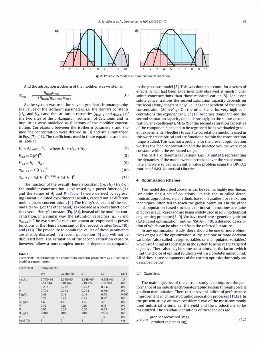
where Pu is the purity of target component (P) in a certain frac-tion, N is the total number of fractions collected and j, k, l and mare the indices of fractions used to mark the collect, recycle andreject. According to the method defined in Eq. (1), each fractionis evaluated individually to put a tag of Co or Ry or Re on it. Onthe other hand, following the method in Eq. (2), the fractions canbe mixed and the average purity of the mixed fractions evaluated.Fig. 2 provides a schematic example of these criteria. To elaboratethe example, let us consider that a total of 10 fractions were col-lected in the schematic profile, covering the target component andits two closely eluting impurities (Fig. 2). Let us also assume that alab analysis found that the fractions 1, 2, 9 and 10 contain almost noproduct (P) or very low percentage of P, so they can be sent to thereject. From the remaining of the fractions, one can either acceptone as a collect or send for recycling (Ry) depending on the purityconstraint on the collected product. Let us set U = 0.9 and L = 0.5.Based on this, one can identify the collect, on individual fractionbasis (e.g. Eq. (1) and Fig. 2a), as fractions 6 and 7, and the fractions3, 4, 5 and 8 as recycle. On the other hand, if the average purity ofthe collected fractions is considered (Eq. (2)) fractions 5, 6, 7 and 8can be treated as collect and fractions 3 and 4 as recycle. It may benoted that determining the average concentration of the collectedproduct is not difficult. An off-line mass balance of different com-binations of the fractions is sufficient to reach a close value. Forthe present study, the second type of fraction evaluation, whichconsiders average purity over a range, was adopted.

3. Mathematical model

The model of the chromatographic system used in the presentwork was developed based on a number of experimental studies,a detailed account of which is available elsewhere [3]. An outlineof the model and the model parameters is provided here. For mod-elling the multi-component mixture containing Calcitonin, only themain product P (Calcitonin), the modifier and one weakly adsorbed(W1) and two strong adsorbed (S1–S2) impurities, which elute clos-est to the main product, were considered. These three impuritiesrepresent an unknown mixture of components each, and are iden-tifiable only from the elution profiles of analytical chromatograms.A multi-component competitive bi-Langmuir isotherm was used
to define the adsorption behaviour of Calcitonin and its impuritiesand a non-competitive Langmuir isotherm is used for the modifier[3]. To simulate the column dynamics, a lumped kinetic model wasused by lumping the pore diffusion effect in the mass-transfer coef-ficient, Km. This saved computational time making it suitable foran optimization study without loosing the accuracy significantly.The effective diffusivity, Deff, was calculated as the column intersti-tial velocity multiplied by the axial dispersion coefficient, dax. Thevalue of dax was taken to be the same for all the solutes, as eachwere assumed to have similar molecular structure and weight. Themass balance for each component i was written as cf. [3]:
εi∂ci

∂t+ (1 − εi)

∂qi

∂t+ usf

∂ci

∂z= Deff

∂2ci

∂z2(3)

∂qi

∂t= Kmi[q

∗i − qi] (4)

The adsorption isotherm for Calcitonin and its impurities, fol-lowing the bi-Langmuir isotherm were written as

q∗i = H1,ici

1 + ∑ncompj=1 (H1,i/qsat,1,j)cj

+ H2,ici

1 +∑ncomp

j=1 (H2,i/qsat,2,j)cj

(5)

matog

f elut

A. Tarafder et al. / J. Chro

Fig. 2. Possible methods o

And the adsorption isotherm of the modifier was written as

q∗mod = Hmodcmod

1 + (Hmod/qsat,mod)cmod(6)

As the system was used for solvent gradient chromatography,the values of the isotherm parameters, i.e. the Henry’s constants(H1,i and H2,i) and the saturation capacities (qsat,1,i and qsat,2,i) ofthe two sites of the bi-Langmuir isotherm, of Calcitonin and itsimpurities were modelled as functions of the modifier concen-tration. Correlations between the isotherm parameters and themodifier concentration were derived in [3] and are summarisedin Eqs. (7)–(11). The coefficients used in these equations are listedin Table 1:

Hi = Ai[cACNL]Bi , where Hi = H1,i + H2,i (7)

H2,i = Ci[Hi]Di (8)

H1,i = Hi − H2,i (9)

qsat,1,i = Ei[H1,i]Fi (10)

qsat,2,i = Gi[H2,i]Mi+Nici + Oi[H2,i]

Ri (11)

The function of the overall Henry’s constant (i.e. H1,i + H2,i) onthe modifier concentration is expressed by a power function (7),and the values of Ai and Bi (Table 1) were derived by regress-ing isocratic diluted experimental results, carried out at differentmobile phase concentrations [4]. The Henry’s constant of the sec-ond site (H2,i), on the other hand, is expressed as a power function ofthe overall Henry’s constant (Eq. (8)), instead of the modifier con-centration. In a similar way, the saturation capacities (qsat,1,i andqsat,2,i) of the two sites for each component are expressed as powerfunctions of the Henry’s constant of the respective sites (Eqs. (10)and (11)). The procedure to obtain the values of these parametersare already discussed in a recent publication [5] and will not bediscussed here. The estimation of the second saturation capacity,however, follows a more complex functional dependence compared

Table 1Coefficients for estimating the equilibrium isotherm parameters as a function ofmodifier concentration

Coefficient Components

W1 Calcitonin S1 S2 Mod

A (L/g) 5.74E+44 2.34E+45 1.94E+46 4.58E+46 1.5B −18.644 −18.864 −19.224 −19.364 0.0C 0.232 0.232 0.232 0.232 0.0D 0.794 0.794 0.794 0.794 0.0E (g/L) 0.48 0.48 0.48 0.48 0.005F 0.27 0.27 0.27 0.27 0.0G (g/L) 4.6 4.6 4.6 4.6 0.0M 0.18 0.18 0.18 0.18 0.0N 0.05 0.05 0.05 0.05 0.0O (g/L) 2000 2000 2000 2000 0.0P −5 −5 −5 −5 0.0Feed (%) 3 91 3 3 var

r. A 1195 (2008) 67–77 69

ion fraction classification.

to the previous model [5]. This was done to account for a series ofeffects, which had been experimentally observed at much highersolute concentrations than those reported earlier [5]. For lessersolute concentrations the second saturation capacity depends onthe local Henry constant only, i.e. it is independent of the soluteconcentration (Mi � Nici). On the other hand, for very high con-centrations the exponent Nici of (11) becomes dominant and thesecond saturation capacity depends strongly on the solute concen-tration. The coefficients, Mi to Ri of the second saturation capacitiesof the components needed to be regressed from overloaded gradi-ent experiments. Needless to say, the correlation functions used inthis work are empirical and are functional within the concentrationrange studied. This was not a problem for the present optimizationwork as the feed concentration and the injected volume were keptconstant within the evaluated range.

The partial differential equations (Eqs. (3) and (4)) representingthe dynamics of the model were discretized over the space coordi-nate and were solved as an initial value problem using the DIVPAGroutine of IMSL Numerical Libraries.

4. Optimization schemes

The model described above, as can be seen, is highly non-linear.For optimizing a set of equations like this the so-called deter-ministic approaches, e.g. methods based on gradient or relaxationtechniques, often fail to reach the global optimum. On the otherhand, population-based stochastic optimization routines are quiteeffective in such cases and are being widely used in solving chemicalengineering problems [5–9]. We have used here a genetic algorithm
(GA)-based optimization routine, NSGA-II [10], a detailed descrip-tion of which can be obtained from the referred literature.
In any optimization study, there should be one or more objec-tives or goals of the optimization study, and one or more decisionvariables (also called design variables or manipulated variables)which are the agents of change in the system to achieve the targetedobjective. There also may be some constraints, i.e. the factors whichlimit the choice of optimal solutions within a predetermined limit.All of these three components of the current optimization study aredescribed below.

4.1. Objectives

The main objective of the current study is to improve the per-formance of an industrial chromatographic system through solventgradient manipulation. There can be several indices of performanceimprovement in chromatographic separation processes [11,12]. Inthe present study we have considered two of the most commonlyused industrial criteria, i.e. the yield and the productivity to bemaximized. The standard definitions of these indices are

yield = product recovered (mg)product injected (mg)

(12)

matog
productivity = product recovered (mg)process duration (min) × column volume (mL)

(13)

As in the current study we have investigated the performanceimprovement of a combination of batch and recycle processes, notof a single run of the process, the variables defined in yield andproductivity may need more explanation. Let us call the set of pro-cess runs comprising NB batches and one re-chromatography stepas one chromatographic cycle, and the time taken by this, as thecycle period. Considering that the operating conditions will remainthe same for all the batch operations and the same column will beused, we can assume that the chromatograms measured for eachrun will be the same. Thus, the amount of product collected in allthe batch runs per cycle will be equal that collected in one batchrun multiplied by NB. Similarly, the amount of solute mass to berecycled is equal to the recycle mass per batch multiplied by NB.Based on these assumptions, the formulation of the yield and theproductivity of a chromatographic cycle can be written as

YC =(YBcF

P,BQBtFB )NB + (YRcF

P,RQRtFR)

(cFP,BQBtF

B )NB(14)

Pr =(YBcF

P,BQBtB)NB + (YRcFP,RQRtR)

tCV(15)

The expression (YBcFP,BQBtF

B ) represents the mass of the product (P)

collected in the batch runs and (YRcFP,RQRtF

R) represents the samein the re-chromatography run, where YB and YR are the yields ofthe batch run and the recycle run, respectively. Thus, the combinedyield YC is determined by dividing the overall mass of P collectedin the batches and the re-chromatography runs by the net mass ofP fed to the batch runs. In Eq. (15), tC, which is the cycle period, isevaluated as

tC = tBNB + tR = (tFB + tE

B + tRgB )NB + (tF

R + tER + tRg

R ) (16)

In both the batch and the recycle runs, the column operationtime can be divided into three parts: (a) the feed time, (b) the elu-tion time and (c) the regeneration time, which are indicated bythe superscripts F, E and Rg, respectively. Because of gradient elu-tion, the modifier concentration in the recycled fractions was higherthan that in the feed solution. While preparing the recycled feed, themodifier concentration was adjusted to that of the feed by dilutionwith water [5]. Thus the typical values of tF

R are much higher than
tFB . A regeneration time, on the other hand, is needed to bring back
the column to the initial state after a solvent gradient operation.During regeneration, the column is washed with solvent having thesame modifier concentration as in the feed solution. The time isthe same for the batch and the recycle run and was taken as 10 min,which is approximately three times the column volume. For a bettervisualization, Fig. 3 shows schematic profiles of a typical batch anda typical recycle gradient, indicating the feed and the regenerationtimes.

For detecting the optimal solution, we have simultaneouslymaximized the above two objectives (yield and productivity) usinga multi-objective optimization approach. Usually the objectivesconsidered for a given study are clubbed into one entity throughsome formulation and a single objective optimization is carried out.On the other hand, with special optimization routines, like NSGA-II,one can address the objectives separately (no clubbing) producinga set of solutions representing the optimum trade-offs betweenthe counter-acting objectives, instead of a single pre-compromisedsolution. The results can be plotted in multi-dimensional space,called a Pareto optimal plot, which is a convenient way to representsuch results.

r. A 1195 (2008) 67–77

Fig. 3. Schematic profiles of typical batch and recycle gradients, with feeding andregeneration times.

4.2. Constraints

Sometimes, putting constraints in an optimization studybecomes necessary as all the possibilities of improving the objec-tive may not be of practical interest. Several constraints were putin this study, all originating from typical industrial requirements,and are described below.

4.2.1. Minimum product purityPurity of the target product was considered as a constraint as

typically in industry it is a manufacturing essential. The minimumpurity was taken as 97% and was defined as

purity = product in outlet (mg)(product + impurities) in outlet (mg)

(17)

4.2.2. Maximum impurity in collectIn many situations, the manufacturers, along with a certain

purity requirement for the main product, wants to ensure that thepresence of any single impurity is lower than a certain level. Themaximum presence of any impurity is taken as 2% in the presentstudy. The impurity is calculated in the same way as in (17).

4.2.3. Minimum product concentrationThis constraint mainly serves to limit the collected product

above a certain concentration to facilitate the product recoveryfrom the solvent solution. It has been taken as 1.5 g/L in the presentstudy.

There are a few other implicit constraints used in the study, suchas the elution time or the duration of the batch process. This wastaken as 480 min which is the typical duration of a shift in industry.Another constraint, the maximum allowable pressure drop in a col-umn, is automatically accounted for by properly fixing the valuesof all internal liquid flow rates.

4.3. Decision variables

The decision variables for process optimization are typicallyselected from the operating parameters so that their optimumvalues can be readily applied to the system. In solvent gradientchromatography, the main operating parameters are the solventflow rate, the feed injection volume and the coefficients definingthe gradient profile as a function of time. In the present study onlythe variables defining the gradient profile were considered as thedecision variables because in an industrial scenario changing theloading factor or the residence time may not always be a desirableoption. Even from academic point of view, the effects of manipu-lating feed volume and flow rate are already well understood, andso are not interesting.

matogr. A 1195 (2008) 67–77 71

Table 3The optimum yield (Y), productivity (Pr) and the decision variables obtained afteroptimizing a batch separation

# Y Pr �tmod,2 �tmod,3 cmod,2 cmod,3

21 0.7757 0.0368 91.53 16.47 196.95 340.0322 0.7774 0.0306 127.84 27.21 196.45 362.10

The serial number shown at the left most column of the table is used as a decisionvariable for selecting the batch gradients for BB and BR.

Each one of these Pareto points was given a serial number forspecific access (first column in Table 3). The recycle optimizationwas then carried out with two discrete decision variables. The firstone is an integer variable (representing the row numbers in Table 3),which defines the gradient profiles for the batch as well as the recy-


Fig. 4. Schematic diagram of a multi-linear gradient profile.

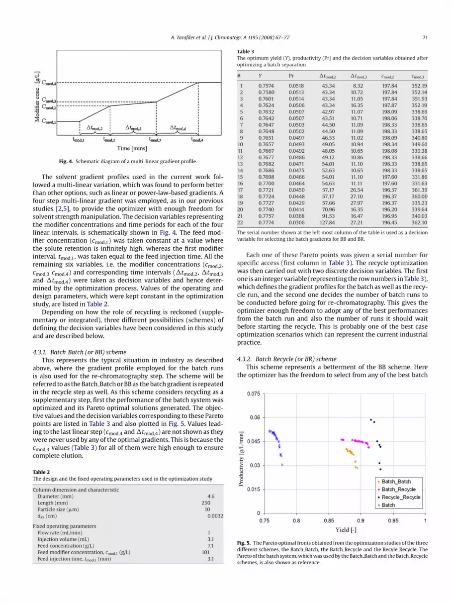
The solvent gradient profiles used in the current work fol-lowed a multi-linear variation, which was found to perform betterthan other options, such as linear or power-law-based gradients. Afour step multi-linear gradient was employed, as in our previousstudies [2,5], to provide the optimizer with enough freedom forsolvent strength manipulation. The decision variables representingthe modifier concentrations and time periods for each of the fourlinear intervals, is schematically shown in Fig. 4. The feed mod-ifier concentration (cmod,1) was taken constant at a value wherethe solute retention is infinitely high, whereas the first modifierinterval, tmod,1, was taken equal to the feed injection time. All theremaining six variables, i.e. the modifier concentrations (cmod,2,cmod,3 cmod,4) and corresponding time intervals (�tmod,2, �tmod,3and �tmod,4) were taken as decision variables and hence deter-mined by the optimization process. Values of the operating and
design parameters, which were kept constant in the optimizationstudy, are listed in Table 2.
Depending on how the role of recycling is reckoned (supple-mentary or integrated), three different possibilities (schemes) ofdefining the decision variables have been considered in this studyand are described below.

4.3.1. Batch Batch (or BB) schemeThis represents the typical situation in industry as described

above, where the gradient profile employed for the batch runsis also used for the re-chromatography step. The scheme will bereferred to as the Batch Batch or BB as the batch gradient is repeatedin the recycle step as well. As this scheme considers recycling as asupplementary step, first the performance of the batch system wasoptimized and its Pareto optimal solutions generated. The objec-tive values and the decision variables corresponding to these Paretopoints are listed in Table 3 and also plotted in Fig. 5. Values lead-ing to the last linear step (cmod,4 and �tmod,4) are not shown as theywere never used by any of the optimal gradients. This is because thecmod,3 values (Table 3) for all of them were high enough to ensurecomplete elution.

Table 2The design and the fixed operating parameters used in the optimization study

Column dimension and characteristicDiameter (mm) 4.6Length (mm) 250Particle size (�m) 10dax (cm) 0.0032

Fixed operating parametersFlow rate (mL/min) 1Injection volume (mL) 3.1Feed concentration (g/L) 7.1Feed modifier concentration, cmod,1 (g/L) 101Feed injection time, tmod,1 (min) 3.1

1 0.7574 0.0518 43.34 8.32 197.84 352.192 0.7580 0.0513 43.34 10.72 197.84 352.143 0.7601 0.0514 43.34 11.05 197.84 351.934 0.7624 0.0506 43.34 16.35 197.87 352.195 0.7632 0.0507 42.97 11.07 198.09 338.696 0.7642 0.0507 43.51 10.71 198.06 338.707 0.7647 0.0503 44.50 11.09 198.33 338.658 0.7648 0.0502 44.50 11.09 198.33 338.659 0.7651 0.0497 46.53 11.02 198.09 340.80

10 0.7657 0.0493 49.05 10.94 198.34 349.6011 0.7667 0.0492 48.05 10.65 198.08 339.3812 0.7677 0.0486 49.12 10.86 198.33 338.6613 0.7682 0.0471 54.01 11.10 198.33 338.6514 0.7686 0.0475 52.63 10.65 198.33 338.6515 0.7698 0.0466 54.01 11.10 197.60 331.8616 0.7700 0.0464 54.63 11.11 197.60 331.6317 0.7721 0.0450 57.17 26.54 196.37 361.3918 0.7724 0.0448 57.17 27.10 196.37 360.0019 0.7727 0.0429 57.66 27.97 196.37 335.2320 0.7740 0.0414 70.96 16.35 196.20 339.64

cle run, and the second one decides the number of batch runs tobe conducted before going for re-chromatography. This gives theoptimizer enough freedom to adopt any of the best performancesfrom the batch run and also the number of runs it should waitbefore starting the recycle. This is probably one of the best caseoptimization scenarios which can represent the current industrialpractice.

4.3.2. Batch Recycle (or BR) schemeThis scheme represents a betterment of the BB scheme. Here

the optimizer has the freedom to select from any of the best batch

Fig. 5. The Pareto optimal fronts obtained from the optimization studies of the threedifferent schemes, the Batch Batch, the Batch Recycle and the Recyle Recycle. ThePareto of the batch system, which was used by the Batch Batch and the Batch Recycleschemes, is also shown as reference.

matog

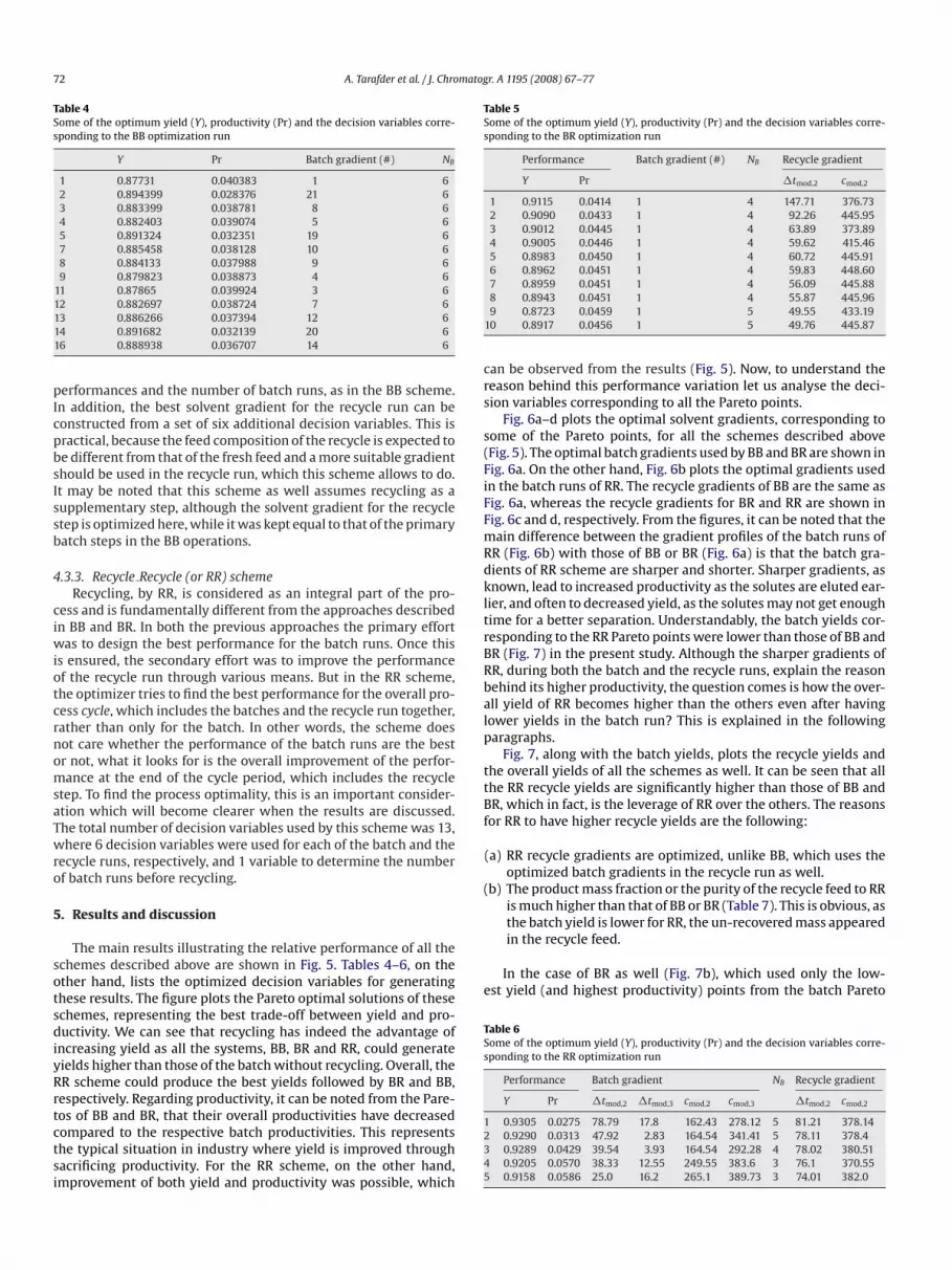
BR (Fig. 7) in the present study. Although the sharper gradients ofRR, during both the batch and the recycle runs, explain the reasonbehind its higher productivity, the question comes is how the over-all yield of RR becomes higher than the others even after havinglower yields in the batch run? This is explained in the followingparagraphs.

Fig. 7, along with the batch yields, plots the recycle yields andthe overall yields of all the schemes as well. It can be seen that allthe RR recycle yields are significantly higher than those of BB andBR, which in fact, is the leverage of RR over the others. The reasonsfor RR to have higher recycle yields are the following:


Table 4Some of the optimum yield (Y), productivity (Pr) and the decision variables corre-sponding to the BB optimization run

Y Pr Batch gradient (#) NB

1 0.87731 0.040383 1 62 0.894399 0.028376 21 63 0.883399 0.038781 8 64 0.882403 0.039074 5 65 0.891324 0.032351 19 67 0.885458 0.038128 10 68 0.884133 0.037988 9 69 0.879823 0.038873 4 6

11 0.87865 0.039924 3 612 0.882697 0.038724 7 613 0.886266 0.037394 12 614 0.891682 0.032139 20 616 0.888938 0.036707 14 6

performances and the number of batch runs, as in the BB scheme.In addition, the best solvent gradient for the recycle run can beconstructed from a set of six additional decision variables. This ispractical, because the feed composition of the recycle is expected tobe different from that of the fresh feed and a more suitable gradientshould be used in the recycle run, which this scheme allows to do.It may be noted that this scheme as well assumes recycling as asupplementary step, although the solvent gradient for the recyclestep is optimized here, while it was kept equal to that of the primarybatch steps in the BB operations.

4.3.3. Recycle Recycle (or RR) schemeRecycling, by RR, is considered as an integral part of the pro-

cess and is fundamentally different from the approaches describedin BB and BR. In both the previous approaches the primary effortwas to design the best performance for the batch runs. Once thisis ensured, the secondary effort was to improve the performanceof the recycle run through various means. But in the RR scheme,the optimizer tries to find the best performance for the overall pro-cess cycle, which includes the batches and the recycle run together,rather than only for the batch. In other words, the scheme doesnot care whether the performance of the batch runs are the bestor not, what it looks for is the overall improvement of the perfor-mance at the end of the cycle period, which includes the recyclestep. To find the process optimality, this is an important consider-ation which will become clearer when the results are discussed.The total number of decision variables used by this scheme was 13,
where 6 decision variables were used for each of the batch and therecycle runs, respectively, and 1 variable to determine the numberof batch runs before recycling.
5. Results and discussion

The main results illustrating the relative performance of all theschemes described above are shown in Fig. 5. Tables 4–6, on theother hand, lists the optimized decision variables for generatingthese results. The figure plots the Pareto optimal solutions of theseschemes, representing the best trade-off between yield and pro-ductivity. We can see that recycling has indeed the advantage ofincreasing yield as all the systems, BB, BR and RR, could generateyields higher than those of the batch without recycling. Overall, theRR scheme could produce the best yields followed by BR and BB,respectively. Regarding productivity, it can be noted from the Pare-tos of BB and BR, that their overall productivities have decreasedcompared to the respective batch productivities. This representsthe typical situation in industry where yield is improved throughsacrificing productivity. For the RR scheme, on the other hand,improvement of both yield and productivity was possible, which

r. A 1195 (2008) 67–77

Table 5Some of the optimum yield (Y), productivity (Pr) and the decision variables corre-sponding to the BR optimization run

Performance Batch gradient (#) NB Recycle gradient

Y Pr �tmod,2 cmod,2

1 0.9115 0.0414 1 4 147.71 376.732 0.9090 0.0433 1 4 92.26 445.953 0.9012 0.0445 1 4 63.89 373.894 0.9005 0.0446 1 4 59.62 415.465 0.8983 0.0450 1 4 60.72 445.916 0.8962 0.0451 1 4 59.83 448.607 0.8959 0.0451 1 4 56.09 445.888 0.8943 0.0451 1 4 55.87 445.969 0.8723 0.0459 1 5 49.55 433.19

10 0.8917 0.0456 1 5 49.76 445.87

can be observed from the results (Fig. 5). Now, to understand thereason behind this performance variation let us analyse the deci-sion variables corresponding to all the Pareto points.

Fig. 6a–d plots the optimal solvent gradients, corresponding tosome of the Pareto points, for all the schemes described above(Fig. 5). The optimal batch gradients used by BB and BR are shown inFig. 6a. On the other hand, Fig. 6b plots the optimal gradients usedin the batch runs of RR. The recycle gradients of BB are the same asFig. 6a, whereas the recycle gradients for BR and RR are shown inFig. 6c and d, respectively. From the figures, it can be noted that themain difference between the gradient profiles of the batch runs ofRR (Fig. 6b) with those of BB or BR (Fig. 6a) is that the batch gra-dients of RR scheme are sharper and shorter. Sharper gradients, asknown, lead to increased productivity as the solutes are eluted ear-lier, and often to decreased yield, as the solutes may not get enoughtime for a better separation. Understandably, the batch yields cor-responding to the RR Pareto points were lower than those of BB and

(a) RR recycle gradients are optimized, unlike BB, which uses theoptimized batch gradients in the recycle run as well.

(b) The product mass fraction or the purity of the recycle feed to RRis much higher than that of BB or BR (Table 7). This is obvious, asthe batch yield is lower for RR, the un-recovered mass appearedin the recycle feed.

In the case of BR as well (Fig. 7b), which used only the low-est yield (and highest productivity) points from the batch Pareto

Table 6Some of the optimum yield (Y), productivity (Pr) and the decision variables corre-sponding to the RR optimization run

Performance Batch gradient NB Recycle gradient

Y Pr �tmod,2 �tmod,3 cmod,2 cmod,3 �tmod,2 cmod,2

1 0.9305 0.0275 78.79 17.8 162.43 278.12 5 81.21 378.142 0.9290 0.0313 47.92 2.83 164.54 341.41 5 78.11 378.43 0.9289 0.0429 39.54 3.93 164.54 292.28 4 78.02 380.514 0.9205 0.0570 38.33 12.55 249.55 383.6 3 76.1 370.555 0.9158 0.0586 25.0 16.2 265.1 389.73 3 74.01 382.0

A. Tarafder et al. / J. Chromatogr. A 1195 (2008) 67–77 73

a) Shoand d

Fig. 6. The optimum gradients corresponding to the Pareto points shown in Fig. 5. ((b) Shows the optimum gradients corresponding to the batch performance of RR. (c

(Table 3), the reason behind increased recycle yield compared toBB can be understood following the same set of arguments. Theperformance of BR, however, was lower compared to RR becausethe later could increase the recycle yield even more through anoptimized compromise in the batch yield.

The above observation can be understood from a general pointof view as well. If a batch run has a lower yield (say YB), it willresult in higher feed purity in the recycle run, because of the reason
explained above. Now this higher feed purity (so lower impurity),with an appropriate gradient can lead to higher recycle yield (YR)because the product will have stronger displacement effect [11]on the lesser retained impurities, and lesser convergence with themore retained impurities. A higher YB, on the other hand, followingthe same line of arguments, may lead to lower YR. The dependenceof YR on YB, however, is highly non-linear in nature. For examplein the cases of BR and RR, both of which used optimized gradientsfor the recycle run, the recycle yields for RR could be made muchhigher than those of BR, although the batch yields of RR and BRare not wide apart (Fig. 7). In short, it can be said that batch yieldhas a strong influence on the recycle yield and a lower batch yieldcan lead to having higher recycle yield. Now to understand howthe yield of the recycle, which is run once against NB number ofbatches, can play a role in defining the overall yield, the followingexplanation is offered.
The overall yield, of a process with recycle, can be expressed asa function of the batch and the recycle yield in the following way:

YC = YB + YR(1 − YRe,B − YB) (18)

Table 7Representative comparison of recycle feed compositions between different schemes

Schemes Recycle feed mass fractions

W1 P S1 S2

BB 0.0708 0.7812 0.0656 0.0825BR 0.0652 0.7966 0.0623 0.0758RR 0.0411 0.8840 0.0364 0.0385

Values of the other points are in the similar range and hence not shown.

ws the optimum batch gradients, which was used by both the BB and BR schemes.) Shows the optimum recycle gradients used in the BR and the RR schemes.

This simple equation is a direct transformation of Eq. (14), withoutany approximation, including only one new term, YRe,B, which is thefraction of product mass in the reject of the batch runs. In fact, asin the batch runs most of the product is either taken in the collector in the recycle, the value of YRe,B can be ignored in Eq. (18) and amore simplified form for the overall yield can be written as

YC = YB + YR(1 − YB) = YB + YR − YBYR (19)

Eq. (19) clearly shows that the recycle yield has an equivalent impor-tance, as the batch yield, in defining the overall yield of a process.This explains why RR, even having lower batch yield, could generatehigher overall yield with the support of higher recycle yield.

It can be concluded from this observation that when there isa recycle step, one should distribute the separation load morejudiciously as both the batch and the recycle yields are equallyimportant. The standard design criterion of achieving the best batchyield puts unnecessarily high separation load on the batch pro-
cesses, ignoring the performance potential of the recycle step. Thisis the main point which makes BB perform worse than BR, and BRperform worse than the RR scheme. In BB (and to some extent forBR) the batch runs were made to perform the best, and to gain thelast few percents in the batch yields, the recycle yields were heavilysacrificed. On the other hand, for RR, following an integral designapproach, the optimizer could find the best sacrifice in batch yieldto improve the recycle yield substantially, resulting into a higheroverall yield.
6. Experimental verification

The conclusions made from the theoretical studies were to betested in a real system. To do that, the studied peptide, Calcitonin,was separated using some of the optimal gradients chosen from allthe schemes described before. A description of the experimentalsetup is provided below.

The experiments were carried out in a modular HPLC system,from Agilent (HP 1100), equipped with a gradient pump module,a degasser, a diode-array detector to monitor simultaneously sev-eral wavelengths and a column temperature controller. The solvent

74 A. Tarafder et al. / J. Chromatogr. A 1195 (2008) 67–77

tal study was to verify the conclusions made from the theoreticalanalysis. So, the operating conditions for the experiments were cho-sen from the results of all the three optimization schemes, markedwith circles in Fig. 8. The points were chosen such that they rep-resent an acceptable trade-off between the two objectives. Fig. 8also shows the experimental performance vis-a-vis the simulatedones. It can be seen that the experimental yields and productivi-ties are lower than their simulated counterparts, which was mainlybecause of the simplified assumptions made for the model. Themain point here, however, is that the nature of performance vari-ation between the different schemes remained unchanged, whichis what we actually looked for in the experimental studies as ver-ification. In the following paragraphs short accounts of the results

Fig. 7. Comparison between the batch yields, recycle yields and the overall yieldsfor the three different recycle schemes, BB, BR and RR.

flow rate used for all the experiments was 1 mL/min. The mobilephase was constructed by mixing two different solutions, the com-positions of which are shown in Table 8. De-ionized water, purifiedwith a “Synergy” water purification system of MILLIPORE and ace-tonitrile of FLUKA, no. 00692 had been used. The chromatographiccolumn used was a 0.46 cm × 25 cm column filled with reversed-phase resin DAISOGEL SP-120-10-ODS-B of 10 �m particle size.The experimental elution profiles, presented in this paper, wererecorded with a UV detector at 280 nm.

Table 8Solutions used for generating modifier gradient

Solutions Acetonitrile Water H3PO4

A 100.5 g 868.1 g 2 g/kgB 455.6 g 414.5 g 2 g/kg

Fig. 8. Comparison of the simulated vis-a-vis experimental performances of thethree schemes: BB, BR and RR. The circled points on the Paretos represent thepoints taken for simulation, whereas, the square points represent the experimentalperformance.

As mentioned earlier, the main motivation for the experimen-

of individual experiments are provided along with a summary oftheir performances.

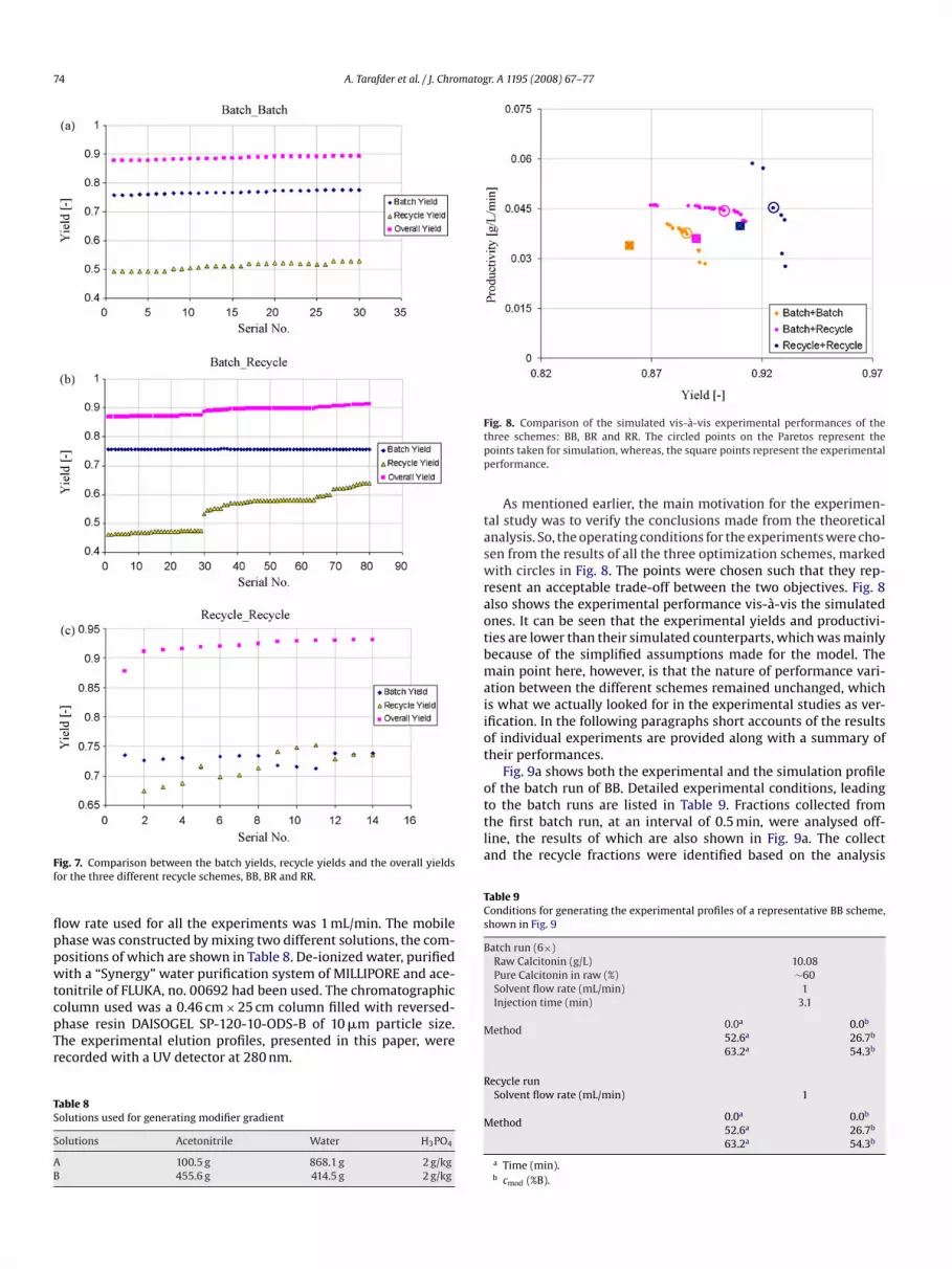
Fig. 9a shows both the experimental and the simulation profileof the batch run of BB. Detailed experimental conditions, leadingto the batch runs are listed in Table 9. Fractions collected fromthe first batch run, at an interval of 0.5 min, were analysed off-line, the results of which are also shown in Fig. 9a. The collectand the recycle fractions were identified based on the analysis

Table 9Conditions for generating the experimental profiles of a representative BB scheme,shown in Fig. 9

Batch run (6×)Raw Calcitonin (g/L) 10.08Pure Calcitonin in raw (%) ∼60Solvent flow rate (mL/min) 1Injection time (min) 3.1

Method 0.0a 0.0b

52.6a 26.7b

63.2a 54.3b

Recycle runSolvent flow rate (mL/min) 1

Method 0.0a 0.0b

52.6a 26.7b

63.2a 54.3b

a Time (min).b cmod (%B).

matog

me collectiopresen


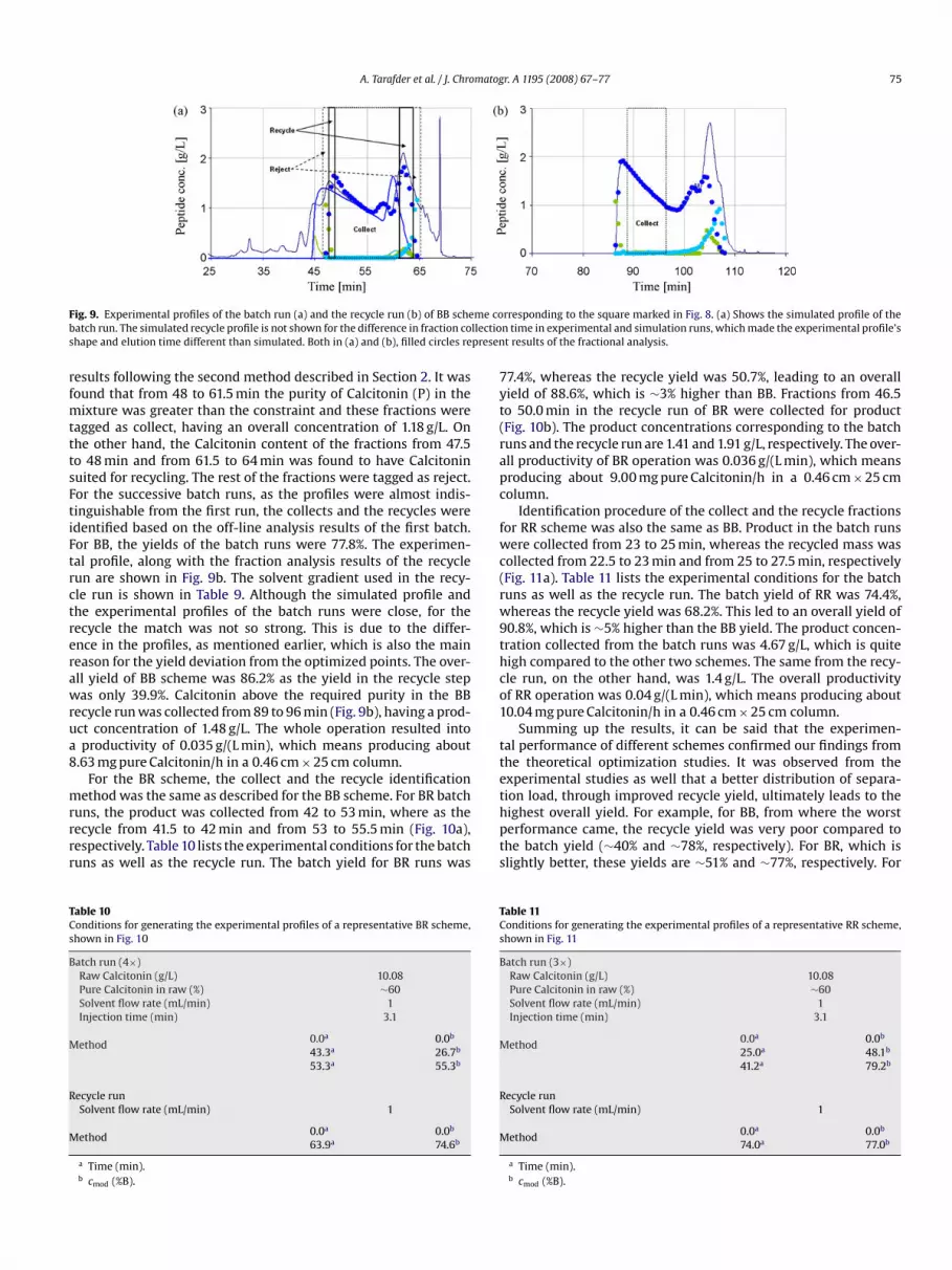
Fig. 9. Experimental profiles of the batch run (a) and the recycle run (b) of BB schebatch run. The simulated recycle profile is not shown for the difference in fraction coshape and elution time different than simulated. Both in (a) and (b), filled circles re

results following the second method described in Section 2. It wasfound that from 48 to 61.5 min the purity of Calcitonin (P) in themixture was greater than the constraint and these fractions weretagged as collect, having an overall concentration of 1.18 g/L. Onthe other hand, the Calcitonin content of the fractions from 47.5to 48 min and from 61.5 to 64 min was found to have Calcitoninsuited for recycling. The rest of the fractions were tagged as reject.For the successive batch runs, as the profiles were almost indis-tinguishable from the first run, the collects and the recycles wereidentified based on the off-line analysis results of the first batch.
For BB, the yields of the batch runs were 77.8%. The experimen-tal profile, along with the fraction analysis results of the recyclerun are shown in Fig. 9b. The solvent gradient used in the recy-cle run is shown in Table 9. Although the simulated profile andthe experimental profiles of the batch runs were close, for therecycle the match was not so strong. This is due to the differ-ence in the profiles, as mentioned earlier, which is also the mainreason for the yield deviation from the optimized points. The over-all yield of BB scheme was 86.2% as the yield in the recycle stepwas only 39.9%. Calcitonin above the required purity in the BBrecycle run was collected from 89 to 96 min (Fig. 9b), having a prod-uct concentration of 1.48 g/L. The whole operation resulted intoa productivity of 0.035 g/(L min), which means producing about8.63 mg pure Calcitonin/h in a 0.46 cm × 25 cm column.
For the BR scheme, the collect and the recycle identificationmethod was the same as described for the BB scheme. For BR batchruns, the product was collected from 42 to 53 min, where as therecycle from 41.5 to 42 min and from 53 to 55.5 min (Fig. 10a),respectively. Table 10 lists the experimental conditions for the batchruns as well as the recycle run. The batch yield for BR runs was

Table 10Conditions for generating the experimental profiles of a representative BR scheme,shown in Fig. 10


Method 0.0a 0.0b

43.3a 26.7b

53.3a 55.3b


Method 0.0a 0.0b

63.9a 74.6b


r. A 1195 (2008) 67–77 75

rresponding to the square marked in Fig. 8. (a) Shows the simulated profile of then time in experimental and simulation runs, which made the experimental profile’st results of the fractional analysis.

77.4%, whereas the recycle yield was 50.7%, leading to an overallyield of 88.6%, which is ∼3% higher than BB. Fractions from 46.5to 50.0 min in the recycle run of BR were collected for product(Fig. 10b). The product concentrations corresponding to the batchruns and the recycle run are 1.41 and 1.91 g/L, respectively. The over-all productivity of BR operation was 0.036 g/(L min), which meansproducing about 9.00 mg pure Calcitonin/h in a 0.46 cm × 25 cmcolumn.

Identification procedure of the collect and the recycle fractionsfor RR scheme was also the same as BB. Product in the batch runs
were collected from 23 to 25 min, whereas the recycled mass wascollected from 22.5 to 23 min and from 25 to 27.5 min, respectively(Fig. 11a). Table 11 lists the experimental conditions for the batchruns as well as the recycle run. The batch yield of RR was 74.4%,whereas the recycle yield was 68.2%. This led to an overall yield of90.8%, which is ∼5% higher than the BB yield. The product concen-tration collected from the batch runs was 4.67 g/L, which is quitehigh compared to the other two schemes. The same from the recy-cle run, on the other hand, was 1.4 g/L. The overall productivityof RR operation was 0.04 g/(L min), which means producing about10.04 mg pure Calcitonin/h in a 0.46 cm × 25 cm column.
Summing up the results, it can be said that the experimen-tal performance of different schemes confirmed our findings fromthe theoretical optimization studies. It was observed from theexperimental studies as well that a better distribution of separa-tion load, through improved recycle yield, ultimately leads to thehighest overall yield. For example, for BB, from where the worstperformance came, the recycle yield was very poor compared tothe batch yield (∼40% and ∼78%, respectively). For BR, which isslightly better, these yields are ∼51% and ∼77%, respectively. For

Table 11Conditions for generating the experimental profiles of a representative RR scheme,shown in Fig. 11


Method 0.0a 0.0b

25.0a 48.1b

41.2a 79.2b


Method 0.0a 0.0b

74.0a 77.0b


76 A. Tarafder et al. / J. Chromatogr. A 1195 (2008) 67–77

Fig. 10. Experimental profiles of the batch run (a) and the recycle run (b) of BR scheme corresponding to the square marked in Fig. 8. (a) Shows the simulated profile ofion co

circles

hemeion co

circles

the batch run. The simulated recycle profile is not shown for the difference in fractprofile’s shape and elution time different than simulated. Both in (a) and (b), filled

Fig. 11. Experimental profiles of the batch run (a) and the recycle run (b) of RR scthe batch run. The simulated recycle profile is not shown for the difference in fractprofile’s shape and elution time different than simulated. Both in (a) and (b), filled

RR, on the other hand, both the yields are at higher level, ∼68% and∼74%, respectively. As an added advantage, the methods of increas-ing overall yield also led to achieve the highest productivity andhighest product enrichment for the RR scheme, both of which areattractive from an industrial point of view.

7. Conclusions

Recycling is often done in the solvent gradient chromatographicsteps in industry. According to the standard procedure, the main
objective of designing the solvent gradients is to achieve the bestyield in the batch steps. The recycling step is used as a supplemen-tary, out of the design possessing, to reclaim some product fromthe impure fractions of the batch runs. The present work, however,shows through theoretical as well as experimental studies, that therecycle step can play a role which is equally as important as that ofthe batch steps. So, a design procedure which considers recyclingas an integrated part with the batch runs, will always lead to bet-ter performance in terms of both yield and productivity. The maindifference between the motives of these two alternatives is in theway the separation load is distributed between the batch and therecycle runs. The strategy of running the batches with the highestyield may lead to a poorer yield in the recycle step, making theoverall yield lesser than the achievable optimum. The integrateddesign approach, on the other hand, tries to improve the recycleyield, judiciously sacrificing the batch yield, to take the overallyield to a value not reachable through the batch-specific designprocedures.
The finding in this work can provide an important cue during thedesign of solvent gradients of the chromatographic steps. Even forthe current processes, one can bring improvement in the process

llection time in experimental and simulation runs, which made the experimentalrepresent results of the fractional analysis.

corresponding to the square marked in Fig. 8. (a) Shows the simulated profile ofllection time in experimental and simulation runs, which made the experimentalrepresent results of the fractional analysis.

performance just by modifying the operation method following theprocedure suggested in this work.

Nomenclature

A, B, C, D, E, F, G, M, N, O, R coefficients used in Eqs. (7)–(11)c liquid phase concentration (g/L)dax axial dispersion coefficient (cm)D diffusivity (cm2/min)
H Henry’s constantK equilibrium constant (L/g)Km mass-transfer coefficient (min−1)L purity of the lower limit of recyclem mass (g)NB number of batchesP product or the target componentPr productivity (g/(L min))Pu purity (%)q solid phase concentration (g/L)qsat saturation capacity of solid phase (g/L)q* equilibrium solid phase concentration (g/L)Q flow rate (mL/min)S stronger impuritiest time (min)u velocity (cm/min)U purity of the lower limit of collect or upper limit of recycleV column volume (mL)W weaker impuritiesx mass fractionY yield

matog
z column axis (cm)

Greek letters� differenceε column void fraction

Indicesave averageACNL acetonitrileB batch operationc collectivecolm columncum cumulativeC combined or overall yieldCo collected, the portion of the outlet having useful productCT Calcitonineff effectiveE elutionF feedi componentsj, k, l, m fraction indicesmod modifierncomp total number of componentsnsteps total number of time steps in simulationN total number of fractionsR recycle operation

[

[

[

r. A 1195 (2008) 67–77 77

Re reject, or the portion of the outlet which was wastedRg regenerationsat saturatedsf superficial

Acknowledgement

This work was financially supported by NOVARTIS Pharma AG,Basel, Switzerland.

References

[1] C.M. Grill, L. Miller, J. Chromatogr. A 827 (1998) 359.[2] A. Tarafder, G. Strohlein, L. Aumann, M. Morbidelli, J. Chromatogr. A 1183 (2008)

87.[3] L. Aumann, PhD Thesis, ETH Zurich, Switzerland, 2006.[4] L. Aumann, A. Butte, M. Mazzotti, M. Morbidelli, K. Buscher, B. Schenkel, Sep.

Sci. Technol., in press.[5] A. Tarafder, L. Aumann, T. Mueller-Spaeth, M. Morbidelli, J. Chromatogr. A 1167

(2007) 42.[6] A. Tarafder, B.C.S. Lee, A.K. Ray, G.P. Rangaiah, Ind. Eng. Chem. Res. 44 (2005)

124.[7] A. Tarafder, G.P. Rangaiah, A.K. Ray, Chem. Eng. Sci. 60 (2005) 347.[8] S. Majumdar, K. Mitra, S. Raha, Polymer 46 (2005) 11858.[9] A.D. Nandasana, A.K. Ray, S.K. Gupta, Ind. Eng. Chem. Res. 42 (2003) 4028.10] K. Deb, Multiobjective Optimization using Evolutionary Algorithms, John Wiley

and Sons, 2001.11] G. Guiochon, S.G. Shirazi, A. Katti, Fundamentals of Preparative and Nonlinear

Chromatography, Academic Press, 1994.12] A. Felinger, G. Guiochon, J. Chromatogr. A 752 (1996) 31.

improvement in industrial re-chromatography (recycling) procedure in solvent gradient bio-separation...

Documents