implementation of the “snakes and ladders” heuristic ... - addi

Bachelor Degree in Computer EngineeringComputation

Thesis

Implementation of the

“Snakes and Ladders” Heuristic

for solving the

Hamiltonian Cycle Problem

Author

Manuel Torralbo Lezana

2021

Abstract

The Hamiltonian Cycle Problem is a popular NP-complete problem belong-ing to the field of Graph Theory and an intrinsic part of the famous Travel-ling Salesman Problem. Both paradigms are highly regarded in Mathematicsand Computer Science due to the immense consequences that would supposeto achieve an optimal solution in investigation and research as well as in theoptimization of numerous real life scenarios. As a result, there is no lack ofmaterial engaging the issues from numerous mathematical approaches, one ofthem being the “Snakes and Ladders” Heuristic. First introduced in 2014, the“Snakes and Ladders” Heuristic is a state of the art polynomial-time determin-istic algorithm for solving the Hamiltonian Cycle Problem, which inspired bythe Lin-Kernighan Heuristic uses “k -opt” transformations to search for a possi-ble solution, achieving astounding results even with difficult graphs of differentcharacteristics. What follows in this document is a proposal for a functional im-plementation of the “Snakes and Ladders” Heuristic, including in-depth analysisof the process which took place in order to conceive it.

Acknowledgements

All credit regarding the conception of the “Snakes and Ladders” Heuristic goesto Pouya Baniasadi, Vladimir Ejov, Jerzy A. Filar, Michael Haythorpe andSerguei Rossomakhine, the authors of the algorithm [4].

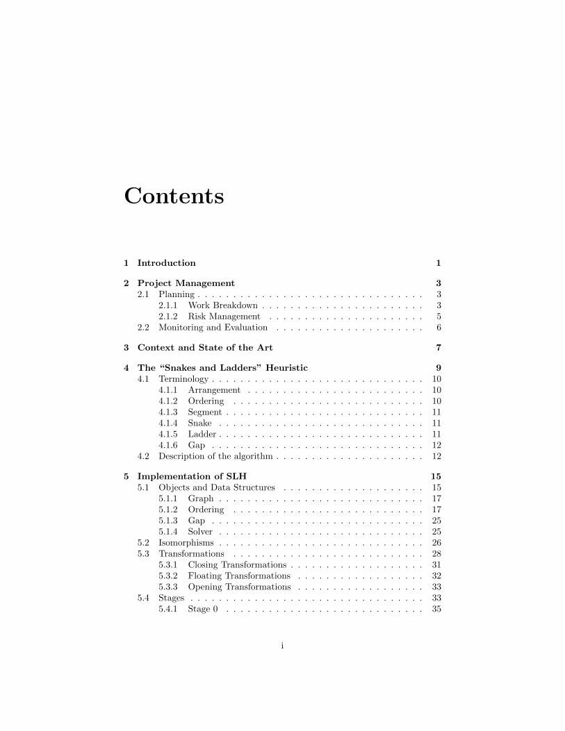
Contents

1 Introduction 1

2 Project Management 32.1 Planning . . . . . . . . . . . . . . . . . . . . . . . . . . . . . . . . 3

2.1.1 Work Breakdown . . . . . . . . . . . . . . . . . . . . . . . 32.1.2 Risk Management . . . . . . . . . . . . . . . . . . . . . . 5

2.2 Monitoring and Evaluation . . . . . . . . . . . . . . . . . . . . . 6

3 Context and State of the Art 7

4 The “Snakes and Ladders” Heuristic 94.1 Terminology . . . . . . . . . . . . . . . . . . . . . . . . . . . . . . 10

4.1.1 Arrangement . . . . . . . . . . . . . . . . . . . . . . . . . 104.1.2 Ordering . . . . . . . . . . . . . . . . . . . . . . . . . . . 104.1.3 Segment . . . . . . . . . . . . . . . . . . . . . . . . . . . . 114.1.4 Snake . . . . . . . . . . . . . . . . . . . . . . . . . . . . . 114.1.5 Ladder . . . . . . . . . . . . . . . . . . . . . . . . . . . . . 114.1.6 Gap . . . . . . . . . . . . . . . . . . . . . . . . . . . . . . 12

4.2 Description of the algorithm . . . . . . . . . . . . . . . . . . . . . 12

5 Implementation of SLH 155.1 Objects and Data Structures . . . . . . . . . . . . . . . . . . . . 15

5.1.1 Graph . . . . . . . . . . . . . . . . . . . . . . . . . . . . . 175.1.2 Ordering . . . . . . . . . . . . . . . . . . . . . . . . . . . 175.1.3 Gap . . . . . . . . . . . . . . . . . . . . . . . . . . . . . . 255.1.4 Solver . . . . . . . . . . . . . . . . . . . . . . . . . . . . . 25

5.2 Isomorphisms . . . . . . . . . . . . . . . . . . . . . . . . . . . . . 265.3 Transformations . . . . . . . . . . . . . . . . . . . . . . . . . . . 28

5.3.1 Closing Transformations . . . . . . . . . . . . . . . . . . . 315.3.2 Floating Transformations . . . . . . . . . . . . . . . . . . 325.3.3 Opening Transformations . . . . . . . . . . . . . . . . . . 33

5.4 Stages . . . . . . . . . . . . . . . . . . . . . . . . . . . . . . . . . 335.4.1 Stage 0 . . . . . . . . . . . . . . . . . . . . . . . . . . . . 35

i

5.4.2 Stage 1 . . . . . . . . . . . . . . . . . . . . . . . . . . . . 355.4.3 Stage 2 . . . . . . . . . . . . . . . . . . . . . . . . . . . . 355.4.4 Stage 3 . . . . . . . . . . . . . . . . . . . . . . . . . . . . 36

5.5 Run Time . . . . . . . . . . . . . . . . . . . . . . . . . . . . . . . 395.6 Possible Improvements . . . . . . . . . . . . . . . . . . . . . . . . 39

5.6.1 Ordering fingerprint . . . . . . . . . . . . . . . . . . . . . 395.6.2 Blind Improvement Space . . . . . . . . . . . . . . . . . . 405.6.3 Multithreading . . . . . . . . . . . . . . . . . . . . . . . . 41

6 Experimental Validation 426.1 Benchmarks . . . . . . . . . . . . . . . . . . . . . . . . . . . . . . 426.2 Results . . . . . . . . . . . . . . . . . . . . . . . . . . . . . . . . . 43

7 Web Application 46

8 Conclusions 51

ii

List of Figures

2.1 Work Breakdown Structure Diagram. . . . . . . . . . . . . . . . . 42.2 Gantt Diagram showing the time period each of the identified

tasks takes place. . . . . . . . . . . . . . . . . . . . . . . . . . . . 5

4.1 Example of the class equivalence of the two arrangements (Aand B) shown in the upper section. The bottom section provesthis equivalence by transforming arrangement A to B ; the firststep performs a reversal and the second a two position clockwiserotation. . . . . . . . . . . . . . . . . . . . . . . . . . . . . . . . . 11

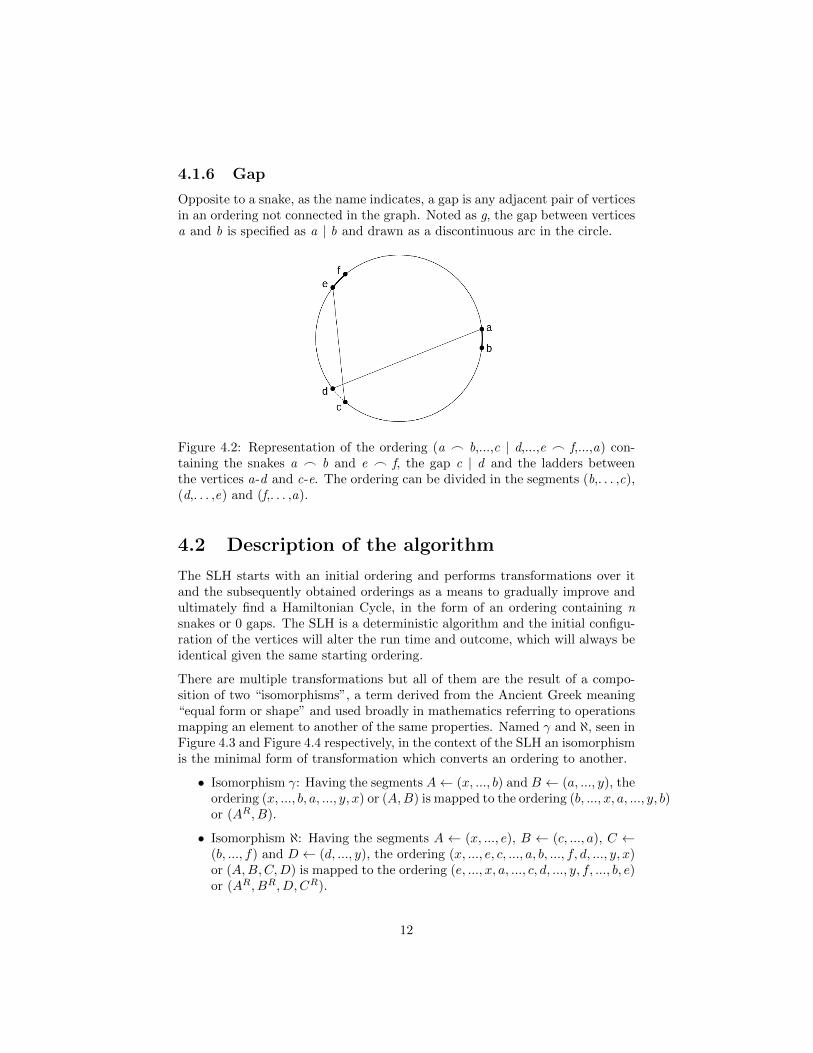
4.2 Representation of the ordering (a _ b,...,c | d,...,e _ f,...,a) con-taining the snakes a _ b and e _ f, the gap c | d and the laddersbetween the vertices a-d and c-e. The ordering can be dividedin the segments (b,. . . ,c), (d,. . . ,e) and (f,. . . ,a). . . . . . . . . . 12

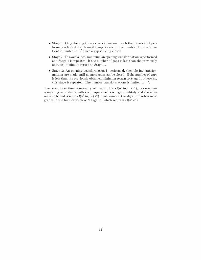
4.3 Isomorphism γ. . . . . . . . . . . . . . . . . . . . . . . . . . . . . 134.4 Isomorphism ℵ. . . . . . . . . . . . . . . . . . . . . . . . . . . . . 13

5.1 Class Diagram showing the relationships, properties, methodsand attributes of each of the classes in the implementation. . . . 16

5.2 Example of the arrays vertices and indices for the ordering (7,9,4,3,6,8,2,5,1,10,7). For the sake of clarity, the two arrays can beviewed as mirrors of each other since opposite to the verticesarray, the indices array has the vertices as indices and their po-sitions as values. . . . . . . . . . . . . . . . . . . . . . . . . . . . 18

5.3 Comparison of arrangements A (2,5,1,3,4,6,2) and B (5,4,3,1,6,2,5),where A > B. . . . . . . . . . . . . . . . . . . . . . . . . . . . . . 19

5.4 Effect of a segment reversal on the vertices array. . . . . . . . . . 225.5 Floating 4-flo type 1 transformation. . . . . . . . . . . . . . . . . 28

iii

5.6 State Diagram showing the transition between the different stagesof SLH. The conditions being as follows: A) An ordering with 0gaps found. B) The number of orderings in the stack is greaterthan n2 or no more floating transformations can be performed.C) An ordering with a new minimum number of gaps found. D)All opening transformations considering the ordering at the topof the stack and one of its gaps have been considered. E) Thenumber of orderings in the stack is greater that n3 or the orderingat top of the stack has no possible opening transformation. . . . 34

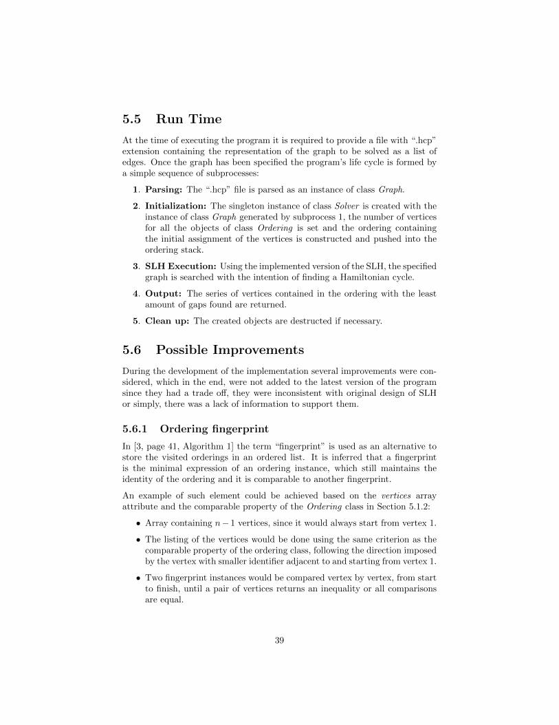
5.7 Comparison of fingerprints of orderings A (2,5,1,3,4,6,2) and B(5,4,3,1,6,2,5), where A > B. Same as Figure 5.3. . . . . . . . . . 40

7.1 SLH Web Application input window. . . . . . . . . . . . . . . . . 477.2 SLH Web Application loading screen. . . . . . . . . . . . . . . . . 487.3 SLH Web Application image gallery showing the initial ordering

for the symmetric cubic graph C2048.25. . . . . . . . . . . . . . . 497.4 SLH Web Application image gallery showing the final ordering of

the symmetric cubic graph C2048.25, which contains a Hamilto-nian cycle. . . . . . . . . . . . . . . . . . . . . . . . . . . . . . . . 50

List of Algorithms

1 Swap Segments . . . . . . . . . . . . . . . . . . . . . . . . . . . . 242 Isomorphism γ . . . . . . . . . . . . . . . . . . . . . . . . . . . . 263 Isomorphism ℵ . . . . . . . . . . . . . . . . . . . . . . . . . . . . 274 Floating 4-flo type 1 . . . . . . . . . . . . . . . . . . . . . . . . . 295 Stage 0 of SLH . . . . . . . . . . . . . . . . . . . . . . . . . . . . 356 Stage 1 of SLH . . . . . . . . . . . . . . . . . . . . . . . . . . . . 367 Stage 2 of SLH . . . . . . . . . . . . . . . . . . . . . . . . . . . . 378 Stage 3 of SLH . . . . . . . . . . . . . . . . . . . . . . . . . . . . 38

iv

List of Tables

5.1 SLH closing transformations in order of priority. Where k refersto the maximum degree of graph G. . . . . . . . . . . . . . . . . 31

5.2 SLH floating transformations in order of priority. Where k is themaximum degree of gap graph G and s is the length of segment(x, ..., a), see Figure 5.5 and Algorithm 4, lines 9-11. . . . . . . . 32

5.3 SLH opening transformation. Where k is the maximum degreeof graph G and s is the length of segment (x, ..., a) [see 4, page 9]. 33

6.1 Combined time required to solve all graphs in the TSPLIB chal-lenge set and the 795 symmetric cubic graphs containing Hamil-tonian cycles. . . . . . . . . . . . . . . . . . . . . . . . . . . . . . 43

6.2 Average time required for 10 different tests using random initialorderings for all TSPLIB graphs. . . . . . . . . . . . . . . . . . 43

6.3 Average time required for 10 different tests using random initialorderings for all the symmetric cubic graphs of 2048 vertices. . . 44

6.4 Five distinct runs of the first ten graphs in the Flinders HCPChallenge set using random initial orderings. All instances weresuccessfully solved. . . . . . . . . . . . . . . . . . . . . . . . . . . 44

v

Chapter 1

Introduction

The Hamiltonian Cycle Problem (HCP), named after the Irish mathematicianWilliam Rowan Hamilton who first presented and studied it alongside ThomasKirkman around 1856, is an NP-complete problem belonging to Graph Theoryand close relative of the widely known Travelling Salesman Problem (TSP).

Given a graph G containing n vertices, the HCP consists on proving whetherG is a Hamiltonian graph, by finding the existence of at least one Hamiltoniancycle, or on the contrary, if G is a non-Hamiltonian graph, assuring the absenceof any of such cycles. A Hamiltonian cycle being a sequence of n distinctinterconnected edges, visiting all n vertices once and starting and ending at thesame vertex.

The TSP goes a step beyond and determines of all Hamiltonian cycles presentin G, if there are any, which has the the minimal cost, given by the sum of theweights of the edges. If the edges of G are not weighted, or all have the sameweight for that matter, the TSP is simply reduced to the HCP. In other words,the HCP is an intrinsic part of the TSP, and a breakthrough in the first wouldinevitably affect the latter.

Such advancement would also have implications in Mathematics and ComputerScience, specially in the branches of Optimization and Complexity Theory. Notonly that, but these problems real world applications are numerous, just to namea few, these include logistics, data storage, circuitry, cytogenetics, etc. For thisreason, the HCP and TSP problems have been studied extensively and a vastamount of literature is available, engaging the issue from multiple mathematicalapproaches, some of which will be discussed further along in this document.

However, this work’s main focus is the state of the art “Snakes and Ladders”Heuristic (SLH) for solving the HCP. Presented for the first time in Baniasadi etal (2014) [4], SLH is a polynomial complexity deterministic algorithm inspiredby the Lin-Kernighan heuristic [10] for solving the TSP, the primary influence

1

being the usage of “k -opt” transformation techniques to transition and searchfor a Hamiltonian cycle making incremental improvements.

The lack of an available source code for the SLH brings up this project’s moti-vation; to propose and facilitate a functional implementation of the algorithm.Throughout this paper, in detail documentation of the implementation is pro-vided, alongside the rational process that took place in order to conceive it,which in some cases may open the opportunity to discuss further improvements.Subsequently, the implementation’s performance is tested against a large poolof graphs, varying in size and difficulty.

In addition, a web application with a user interface has been developed whichprovides a visual representation of the internal behaviour of the SLH.

2

Chapter 2

Project Management

The following chapter defines this projects scope and time constraints and themeasures taken to control the given limitations, reduce the risks and ultimatelysuccessfully complete the project.

2.1 Planning

Keep in mind that the planning process is being conceived at the early stagesof the project and may be subject to change during its course.

2.1.1 Work Breakdown

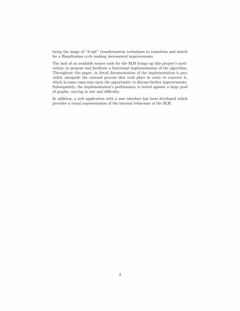
The project’s work load has been divided and the identified tasks have beenorganized for easier management. The Work Breakdown Structure can be seenin Figure 2.1 and, in addition, a brief explanation for each task is provided.Lastly, the time period which each task will take place is shown in the GanttDiagram, see Figure 2.2.

• T1 Research

– T1.1 SLH Research: Deep analysis of the “Snakes and Ladders”Heuristic.

– T1.2 “k -opt” Transformations: Study other algorithms which use“k -opt” transformation techniques.

– T1.3 Graph Test Set: Gather a set of graph of different qualities todebug and benchmark the implementation.

– T1.4 Flask WAF: Learn how to use “Flask” to develop the web ap-plication.

3

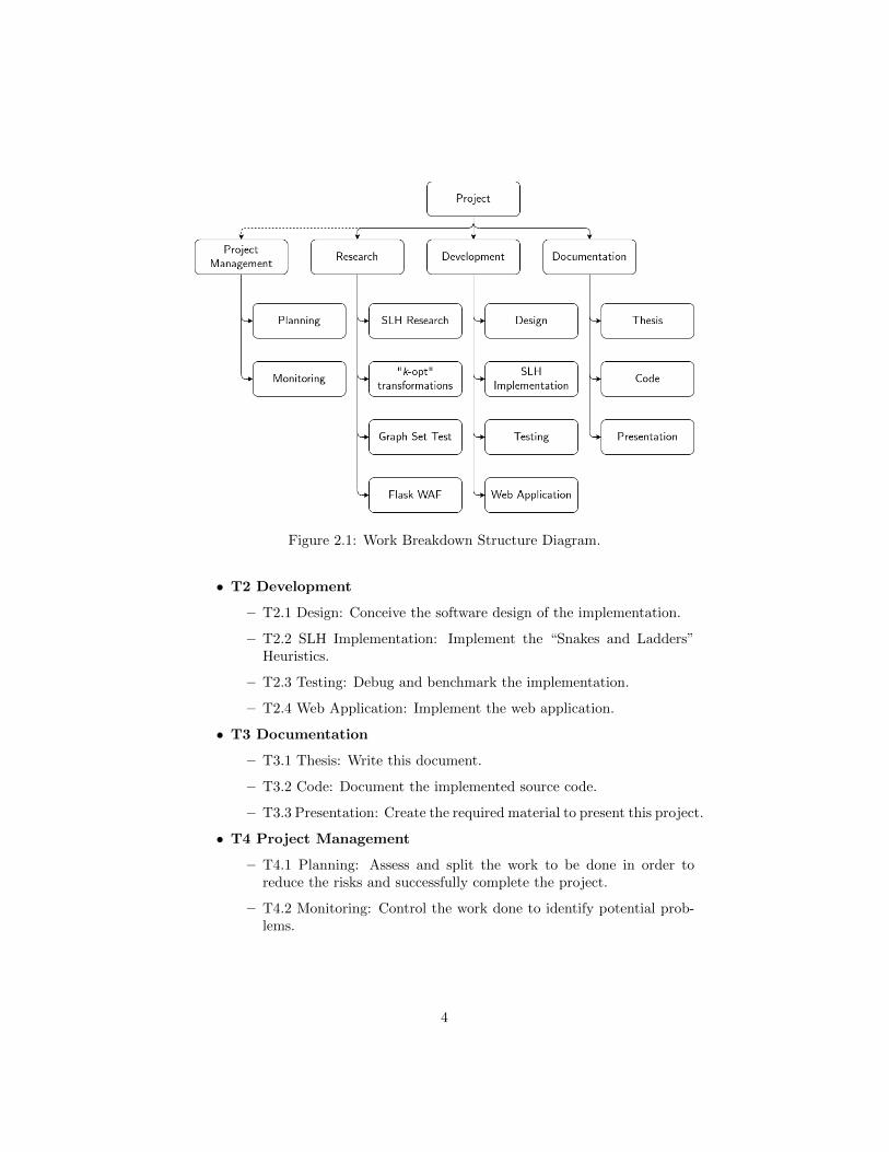
Figure 2.1: Work Breakdown Structure Diagram.

• T2 Development

– T2.1 Design: Conceive the software design of the implementation.

– T2.2 SLH Implementation: Implement the “Snakes and Ladders”Heuristics.

– T2.3 Testing: Debug and benchmark the implementation.

– T2.4 Web Application: Implement the web application.

• T3 Documentation

– T3.1 Thesis: Write this document.

– T3.2 Code: Document the implemented source code.

– T3.3 Presentation: Create the required material to present this project.

• T4 Project Management

– T4.1 Planning: Assess and split the work to be done in order toreduce the risks and successfully complete the project.

– T4.2 Monitoring: Control the work done to identify potential prob-lems.

4

Figure 2.2: Gantt Diagram showing the time period each of the identified taskstakes place.

2.1.2 Risk Management

The following risks have been identified and, if possible, a contingency plan hasbeen proposed:

• R1: As of January of 2021 the world is subject to a global pandemic of thevirus COVID-19 and the possibility of contagion and further quarantinesseems a likely scenario. Since this is a single person project, all the workwill be done from home and a lockdown situation would not pose a seriousthread. However, in the case of suffering grave symptoms the project couldbe delayed from one to two weeks.

• R2: The SLH is a state of the art algorithm with no available implemen-tation, the only available information being the one given by the authors.This means that the implementation must be done from scratch and fromjust one source, for which only the given results can be contrasted. Therisk of misunderstanding the authors guidance is probable and will in-evitably change the output of the resulting algorithm to a greater or lesserextent.

• R3: Providing a publicly accessible web application entails difficultiesfrom a couple of standpoints. Since the interface requires a user input,a secure parser and website is consequently needed. Furthermore, SLHmakes use of a considerable amount of computational power and space.Even if the chance of multiple concurrent users is disregarded, acquir-ing the necessary infrastructure may be problematic. For these reasons,

5

just making a local web application for demonstrative purposes is notdiscarded.

• R4: The period this project takes place coincides with the second schoolquadrimester, an excessive total workload may delay this project.

2.2 Monitoring and Evaluation

During the period in which the project took place several decision where madewhich affected the initially planned guidelines. At the time of writing this beingin the latest stages of the project the final outcome asks for a recapitulation andevaluation of the most significant events.

One of the mayor changes is a nearly three month delay of the project, untilSeptember of 2021. This is to a large extent due to risks already listed in theplanning phase. First of, as assessed in R4, the month of May was in its en-tirety dedicated to other projects and exams, which made impossible any realadvancement. Secondly, R2 posed to be even a harder challenge than expected;a working implementation of the SLH was achieved earlier in the project, how-ever, the acquired results did not meet the standard set in the projects scope.What followed where a series of optimizations and various versions of the imple-mentation, until the outcome was considered satisfactory enough. As of now, theimplementation exceeds the expectations regarding the time required to solvelarge graphs, nevertheless, it still lacks a consistent record of solving difficultinstances.

On another note, as predicted in R3, making a publicly accessible website,containing user inputs and needing a significant amount of infrastructure, dueto the computational requirements of the SLH, ended up being an unfeasibletask. Therefore, the web application made is set to be a local user interfacewith the sole purpose of showing how the SLH internally works.

6

Chapter 3

Context andState of the Art

As part of the mathematical branch of graph theory, many of the solutions pro-vided for the HCP base their approach solely in vertices and edges of a graphand the properties within them. There are even algorithms designed to exploitthe peculiarities of certain families of graphs. Such is the case with the al-gorithm proposed by Eppstein (2003) [6], which provides a list of all existingHamiltonian cycles in a cubic graph in time O(23n/8). Using a recursive back-tracking structure the algorithm takes advantage on the fact that the graph hasmaximum degree of three to discern if a certain edge will be considered in acycle or not.

Trying to solve the problem by other means, most notable are the studieswhich, given the structural similarities between the HCP and Markov chains,use the tools and techniques of Markov decision processes that graph theorydoes not have access to. The “Determinant Interior Point Algorithm” proposedby Haythorpe (2010) [8], embeds the HCP in a Markov decision process creatinga doubly-stochastic probability transition matrix containing the probabilities ofall vertices transitions between each other. The algorithm then is described asan optimization problem which tries to find a deterministic doubly-stochastictransition matrix representing a Hamiltonian cycle.

On another note, it is not possible to talk about the HCP without mentioningthe TSP, more so taking into account that any TSP solver available also tries tofind Hamiltonian cycles. Consider a graph with n vertices originally intendedfor the HCP, but the same weight w has been assigned to all of its edges. If thisvery graph is provided to an algorithm designed to solve the TSP and a tourwith a cost of n× w is returned, then the graph has a Hamiltonian cycle.

7

The highly regarded “Concorde TSP Solver” [2] is an exact algorithm, alwaysreturning the tour with the best cost, which poses the issue as a linear pro-gramming problem. Implemented as a complex branch and bound algorithm,Concorde uses cutting planes constraints to reduce the search space and correctitself as to produce a valid tour. However, it has to be noted that if the defaultconfiguration of Concorde is used, the initial solution from which the solver willbuild upon is constructed with the “Chained Lin-Kernighan” algorithm [1].

In the context of SLH, the “Lin-Kernighan Heuristic” [10] has mayor impor-tance, being the first algorithm which considered an exchange of edges over aTSP tour as a means to obtain a new one with better cost, a technique nowknown as “k -opt” transformation, k being the number of edges exchanged. Theidea was based on the basic approach of other heuristics for combinatorial opti-mization problems, which iteratively improved considering a random set of validsolutions.

Over the time multiple improvements have been proposed for the Lin-KernighanHeuristic, the most notable one being Helsgaun’s Lin-Kernighan implementation[9]. With an improved and more meticulous search strategy and an added in-depth analysis focusing and restricting the search space, the running times arehighly reduced compared to the original algorithm, specially in graphs withlarger amount of vertices.

8

Chapter 4

The “Snakes and Ladders”Heuristic

Having already available the full description of the SLH by the authors them-selves makes it unnecessary and redundant trying to capture in detail the al-gorithm here again. For this reason, only a brief explanation of the SLH willbe presented, emphasizing in the concepts that provide context to the proposedimplementation. The reader is of course referred to [4] for the detailed descrip-tion.

Let G be a graph containing n vertices, for which edges have neither directionnor weight. Conceptually, what the SLH does is arranging all vertices alongthe perimeter of a circle and then adding the edges in one of two ways. If thevertices which the edge joins are contiguous in the perimeter, the arc of thecircle connecting both vertices is underlined and will be called a “Snake”. If,on the contrary, the vertices are not next to another, a straight line is drawnbetween the two, making a chord in the circle, and will be called “Ladder”.Is this conceived image and its relative similarity to the popular board game“Snakes and Ladders” what gives name to the algorithm.

For any given configuration of the vertices, since the number of vertices is n,the total number of snakes can only be as many as n, and if that is the case,it would mean that all vertices along the perimeter are connected in G to theircontiguous two vertices, a Hamiltonian Cycle for that matter. Searching forsuch arrangement of vertices containing n snakes is the purpose of the SLH.

9

4.1 Terminology

In order to explain the SLH, and subsequently the proposed implementation, aparticular terminology and notation is introduced.

4.1.1 Arrangement

A permutation of all vertices contained in a graph placed along the perimeterof a circle. An arrangement has two directions, forward and backward, or morespecifically, clockwise and counterclockwise. Having the same number of verticesas the graph it refers to, two vertices are said to be adjacent in the arrangementif they are next to each other, or put in other words, if there is no additionalvertex between them.

If the contained vertices are to be specified, they are listed ordered clockwise,using commas and between parenthesis, repeating the initial vertex at the endto denote its cyclic nature and emphasize that it covers the entire perimeter ofthe circle. Three suspension points indicate an ellipsis of 0 or more vertices.

One example of this notation could be (a,b,. . . ,c,a); a being the initial vertexis adjacent and previous of vertex b, 0 or more vertices follows ending with thefinal vertex c.

4.1.2 Ordering

Quoting Baniasadi et al (2014) [see 4, page 4]:

“The arrangement of vertices on the circle form natural equivalence classes.Namely, two arrangements are said to be equivalent if either one can be trans-formed to the other via a rotation or reversal, or a composition of both. . . . .We use the term ordering, or cycle ordering to denote such an equivalence class,. . . ”.

To be able to test the class equivalence of different arrangements to begin with,they have to refer to the same graph, problem which is intrinsically solved sinceG is the only mentioned graph.

An ordering of G is noted as C. Listing all 2n possible arrangements of theequivalence class would be inefficient, therefore, just one of the members isused to represent the ordering. For this reason, the term ordering is also usedreferring to its representative arrangement when no confusion is possible. Lastly,the number of gaps in the ordering C in noted as g(C).

10

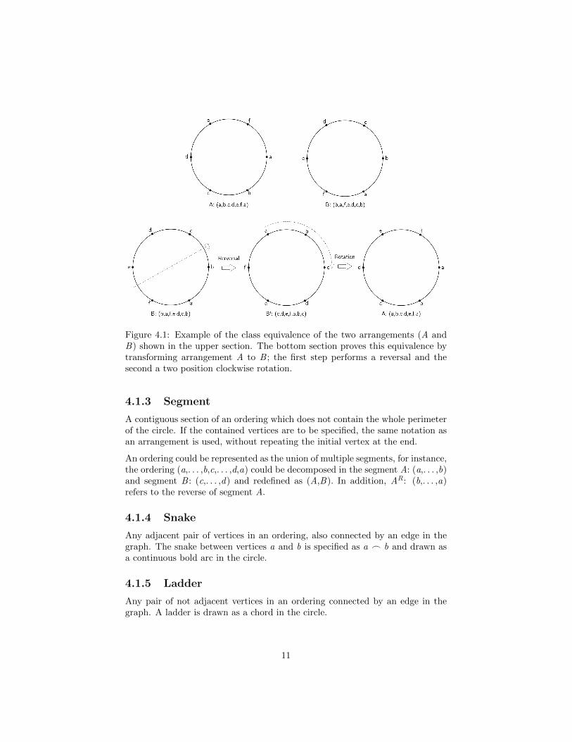
Figure 4.1: Example of the class equivalence of the two arrangements (A andB) shown in the upper section. The bottom section proves this equivalence bytransforming arrangement A to B ; the first step performs a reversal and thesecond a two position clockwise rotation.

4.1.3 Segment

A contiguous section of an ordering which does not contain the whole perimeterof the circle. If the contained vertices are to be specified, the same notation asan arrangement is used, without repeating the initial vertex at the end.

An ordering could be represented as the union of multiple segments, for instance,the ordering (a,. . . ,b,c,. . . ,d,a) could be decomposed in the segment A: (a,. . . ,b)and segment B : (c,. . . ,d) and redefined as (A,B). In addition, AR: (b,. . . ,a)refers to the reverse of segment A.

4.1.4 Snake

Any adjacent pair of vertices in an ordering, also connected by an edge in thegraph. The snake between vertices a and b is specified as a _ b and drawn asa continuous bold arc in the circle.

4.1.5 Ladder

Any pair of not adjacent vertices in an ordering connected by an edge in thegraph. A ladder is drawn as a chord in the circle.

11

4.1.6 Gap

Opposite to a snake, as the name indicates, a gap is any adjacent pair of verticesin an ordering not connected in the graph. Noted as g, the gap between verticesa and b is specified as a | b and drawn as a discontinuous arc in the circle.

Figure 4.2: Representation of the ordering (a _ b,...,c | d,...,e _ f,...,a) con-taining the snakes a _ b and e _ f, the gap c | d and the ladders betweenthe vertices a-d and c-e. The ordering can be divided in the segments (b,. . . ,c),(d,. . . ,e) and (f,. . . ,a).

4.2 Description of the algorithm

The SLH starts with an initial ordering and performs transformations over itand the subsequently obtained orderings as a means to gradually improve andultimately find a Hamiltonian Cycle, in the form of an ordering containing nsnakes or 0 gaps. The SLH is a deterministic algorithm and the initial configu-ration of the vertices will alter the run time and outcome, which will always beidentical given the same starting ordering.

There are multiple transformations but all of them are the result of a compo-sition of two “isomorphisms”, a term derived from the Ancient Greek meaning“equal form or shape” and used broadly in mathematics referring to operationsmapping an element to another of the same properties. Named γ and ℵ, seen inFigure 4.3 and Figure 4.4 respectively, in the context of the SLH an isomorphismis the minimal form of transformation which converts an ordering to another.

• Isomorphism γ: Having the segments A← (x, ..., b) and B ← (a, ..., y), theordering (x, ..., b, a, ..., y, x) or (A,B) is mapped to the ordering (b, ..., x, a, ..., y, b)or (AR, B).

• Isomorphism ℵ: Having the segments A ← (x, ..., e), B ← (c, ..., a), C ←(b, ..., f) and D ← (d, ..., y), the ordering (x, ..., e, c, ..., a, b, ..., f, d, ..., y, x)or (A,B,C,D) is mapped to the ordering (e, ..., x, a, ..., c, d, ..., y, f, ..., b, e)or (AR, BR, D,CR).

12

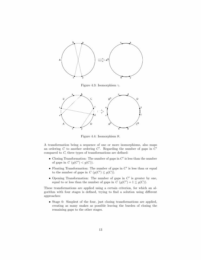
Figure 4.3: Isomorphism γ.

Figure 4.4: Isomorphism ℵ.

A transformation being a sequence of one or more isomorphisms, also mapsan ordering C to another ordering C ′. Regarding the number of gaps in C ′

compared to C, three types of transformations are defined:

• Closing Transformation: The number of gaps in C ′ is less than the numberof gaps in C (g(C ′) < g(C)).

• Floating Transformation: The number of gaps in C ′ is less than or equalto the number of gaps in C (g(C ′) ≤ g(C)).

• Opening Transformation: The number of gaps in C ′ is greater by one,equal to or less than the number of gaps in C (g(C ′) + 1 ≤ g(C)).

These transformations are applied using a certain criterion, for which an al-gorithm with four stages is defined, trying to find a solution using differentapproaches:

• Stage 0: Simplest of the four, just closing transformations are applied,creating as many snakes as possible leaving the burden of closing theremaining gaps to the other stages.

13

• Stage 1: Only floating transformation are used with the intention of per-forming a lateral search until a gap is closed. The number of transforma-tions is limited to n2 since a gap is being closed.

• Stage 2: To avoid a local minimum an opening transformation is performedand Stage 1 is repeated. If the number of gaps is less than the previouslyobtained minimum return to Stage 1.

• Stage 3: An opening transformation is performed, then closing transfor-mations are made until no more gaps can be closed. If the number of gapsis less than the previously obtained minimum return to Stage 1, otherwise,this stage is repeated. The number transformations is limited to n3.

The worst case time complexity of the SLH is O(n6 log(n) k4), however en-countering an instance with such requirements is highly unlikely and the morerealistic bound is set to O(n5 log(n) k4). Furthermore, the algorithm solves mostgraphs in the first iteration of “Stage 1”, which requires O(n4 k4).

14

Chapter 5

Implementation of SLH

The proposed implementation is designed as an object-oriented program and isavailable in both C++ and Python programming languages. Object-orientedprogramming (OOP) is based on the concept of objects which interact with oneanother and change their state with the use of their stored data, in the form ofattributes, and code, in the form of methods.

Applied to the SLH algorithm, an OPP approach makes possible, among otherthings, to create collections containing instances of classes representing elementssuch as gaps and orderings. An ordering instance in turn, also contains gapsand stores vertices in a specific order, giving it its identity. Is this relationshipbetween different objects and the joint stored data what defines the particularstate of the SLH algorithm.

Furthermore, OOP can make use of auxiliary objects, such as iterators, whichallow to transverse orderings despite being cyclic, and in conjunction with or-dering class methods, ease the implementation of SLH transformations.

The given explanation starts from the lower level notions, and as they are grad-ually acquired they are used as a means to build more complex and abstractalgorithms. Therefore, the employed objects and data structures are introducedfirst, and then, the SLH transformations and stages are described, in that order.

5.1 Objects and Data Structures

What comes ahead is a detailed description of the objects and data structuresused along the algorithm’s course, these being a global manager instance called“Solver” and the class representations of graphs, orderings and gaps. An overalldescription of each class and the relationship between each other can be seen inthe Class Diagram shown in Figure 5.1.

15

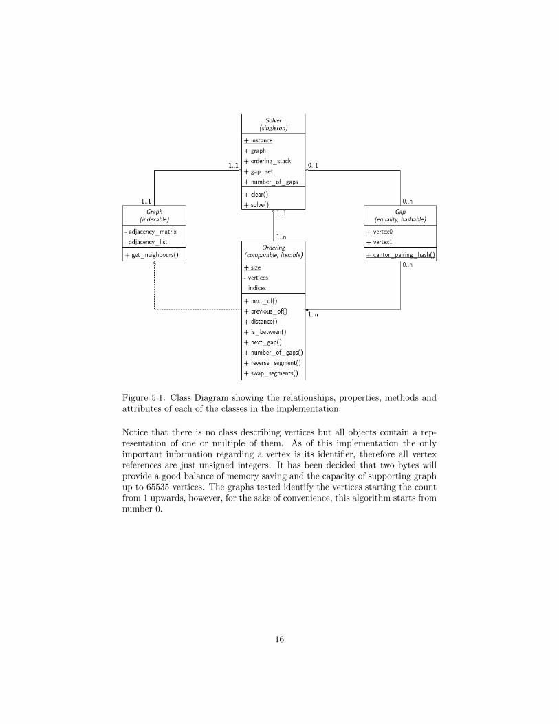
Figure 5.1: Class Diagram showing the relationships, properties, methods andattributes of each of the classes in the implementation.

Notice that there is no class describing vertices but all objects contain a rep-resentation of one or multiple of them. As of this implementation the onlyimportant information regarding a vertex is its identifier, therefore all vertexreferences are just unsigned integers. It has been decided that two bytes willprovide a good balance of memory saving and the capacity of supporting graphup to 65535 vertices. The graphs tested identify the vertices starting the countfrom 1 upwards, however, for the sake of convenience, this algorithm starts fromnumber 0.

16

5.1.1 Graph

Class representing the undirected and unweighted graph G by the connectionsbetween its n vertices. For time optimization purposes, explained further inSection 5.3, both the Adjacency Matrix and the Adjacency List of the graphare stored at the cost of having redundant information.

Attributes

Adjacency Matrix. Square n x n matrix such that the element located atrow i and column j indicates if there is a connection between vertices i and jfor 0 ≤ i, j < n. Stored as a bidimensional array of bits.

Adjacency List. Collection of lists such that the v -th list contains the neigh-bors of vertex v for 0 ≤ v < n. Stored as a bidimensional array of unsigned twobyte integers.

Properties

Indexable. In order to gain access to the adjacency matrix the class is twiceindexable, such that the expression G[i][j] returns a Boolean indicating if thereis a connection between vertices i and j for 0 ≤ i, j < n.

Time Complexity: Constant.

Methods

Get the neighbors of a vertex. Returns the list of neighbors for vertex v atthe Adjacency List.

Notation: get neighbours().

Arguments: Vertex v.


5.1.2 Ordering

Class representing an ordering by a particular arrangement of the equivalenceclass. All instances refer to the same graph G and, as a result, the same numberof vertices n.

Attributes

Vertices. Arrangement of vertices. Stored as an array of unsigned two byteintegers.

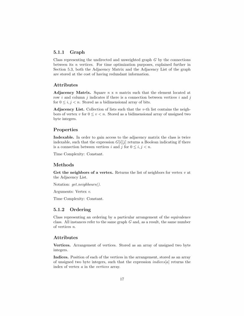
Indices. Position of each of the vertices in the arrangement, stored as an arrayof unsigned two byte integers, such that the expression indices[a] returns theindex of vertex a in the vertices array.

17

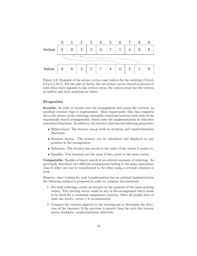
Figure 5.2: Example of the arrays vertices and indices for the ordering (7,9,4,3,6,8,2,5,1,10,7). For the sake of clarity, the two arrays can be viewed as mirrors ofeach other since opposite to the vertices array, the indices array has the verticesas indices and their positions as values.

Properties

Iterable. In order to iterate over the arrangement and access the vertices, anauxiliary iterator class is implemented. Most importantly, this class supportsthe cyclic nature of the orderings, internally traversing between both ends of thesequentially stored arrangements, which eases the implementation of otherwiseconvoluted functions. In addition, the iterator class has the following properties:

• Bidirectional. The iterator can go both in clockwise and counterclockwisedirections.

• Random Access. The iterator can be initialized and displaced to anyposition in the arrangement.

• Deference. The iterator has access to the value of the vertex it points to.

• Equality. Two iterators are the same if they point to the same vertex.

Comparable. Enables a binary search in an ordered container of orderings. Aspreviously described, two different arrangements belong to the same equivalenceclass if either one can be transformed to the other using a reversal, rotation orboth.

However, since looking for such transformation has no optimal implementationthe following method is proposed in order to compare two instances:

1. For both orderings, create an iterator at the position of the same startingvertex. This starting vertex could be any in the arrangement but it needsto be fixed for a consistent comparison criterion. Since all graphs have atleast one vertex, vertex 1 is recommended.

2. Compare the vertices adjacent to the starting one to determine the direc-tion of the iterators; if the previous is greater than the next the iteratormoves clockwise, counterclockwise otherwise.

18

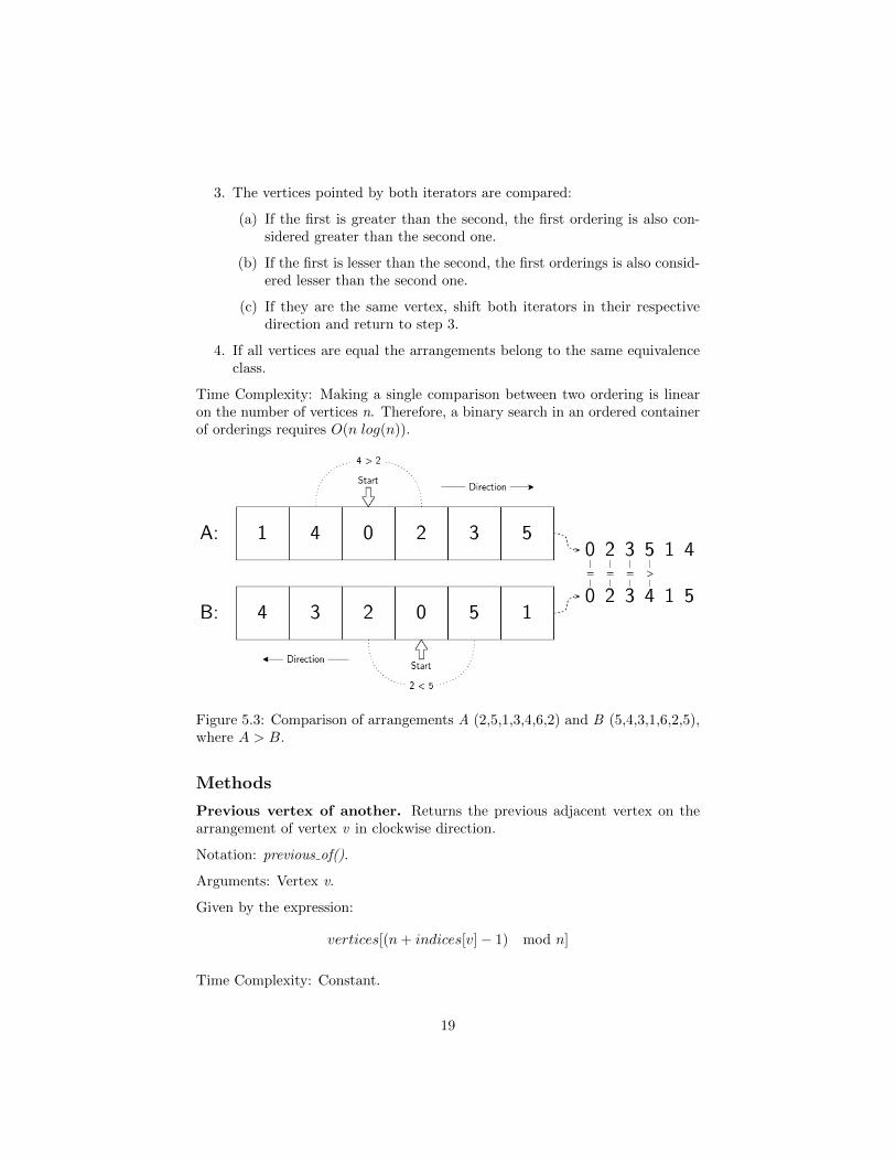
3. The vertices pointed by both iterators are compared:

(a) If the first is greater than the second, the first ordering is also con-sidered greater than the second one.

(b) If the first is lesser than the second, the first orderings is also consid-ered lesser than the second one.

(c) If they are the same vertex, shift both iterators in their respectivedirection and return to step 3.

4. If all vertices are equal the arrangements belong to the same equivalenceclass.

Time Complexity: Making a single comparison between two ordering is linearon the number of vertices n. Therefore, a binary search in an ordered containerof orderings requires O(n log(n)).

Figure 5.3: Comparison of arrangements A (2,5,1,3,4,6,2) and B (5,4,3,1,6,2,5),where A > B.

Methods

Previous vertex of another. Returns the previous adjacent vertex on thearrangement of vertex v in clockwise direction.

Notation: previous of().


Given by the expression:

vertices[(n+ indices[v]− 1) mod n]


19

Subsequent vertex of another. Returns the next adjacent vertex on thearrangement of vertex v in clockwise direction.

Notation: next of().



vertices[(indices[v] + 1) mod n]


Distance between two vertices. Returns the number of vertices on thearrangement between vertices v0 and v1, non inclusive and in clockwise direction.

Notation: distance().

Arguments: Vertices v0 and v1.


(n+ indices[v0]− indices[v1]− 1) mod n


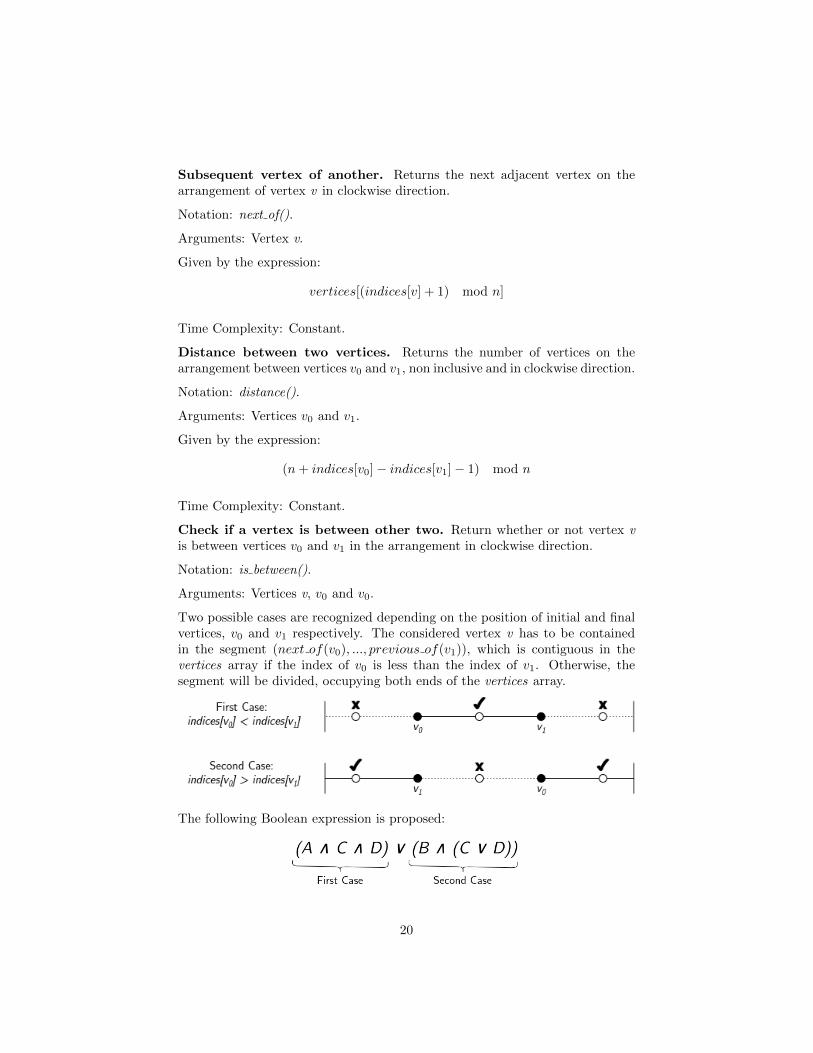
Check if a vertex is between other two. Return whether or not vertex vis between vertices v0 and v1 in the arrangement in clockwise direction.

Notation: is between().

Arguments: Vertices v, v0 and v0.

Two possible cases are recognized depending on the position of initial and finalvertices, v0 and v1 respectively. The considered vertex v has to be containedin the segment (next of(v0), ..., previous of(v1)), which is contiguous in thevertices array if the index of v0 is less than the index of v1. Otherwise, thesegment will be divided, occupying both ends of the vertices array.

The following Boolean expression is proposed:

20

Where:

• A : indices[v0] < indices[v1]

• B : indices[v0] > indices[v1]

• C : indices[v] < indices[v0]

• D : indices[v] > indices[v1]


Next gap given a position. Returns the next gap in the arrangement inclockwise direction starting from a position given by an iterator. If no iteratoris passed the position is assumed to be the start of the arrangement. Thepurpose of the iterator is not only to indicate the position, but also to store itbetween this method’s calls to efficiently iterate over gaps.

Notation: next gap().

Arguments: Optional iterator.

The following implementation is proposed:

1. Store the vertex pointed by the iterator.

2. Shift the iterator in clockwise direction.

3. If the vertex currently pointed by the iterator and the previously storedare not connected in the graph G, return the gap containing these twovertices, go back to step 1 otherwise.

4. If the end of the iterator is reached there is no gap.

Time Complexity: Linear on the number of vertices n.

Number of gaps. Returns the amount of gaps in the ordering.

Notation: number of gaps().

The following implementation is proposed:

1. Initialize a counter to 0.

2. Initialize an iterator at the start of the arrangement.

3. Call the method next gap() providing the iterator as an argument. If agap is returned, increment the the counter by 1 and repeat this step.

4. Return the counter.

Time complexity: Linear on the number of vertices n.

21

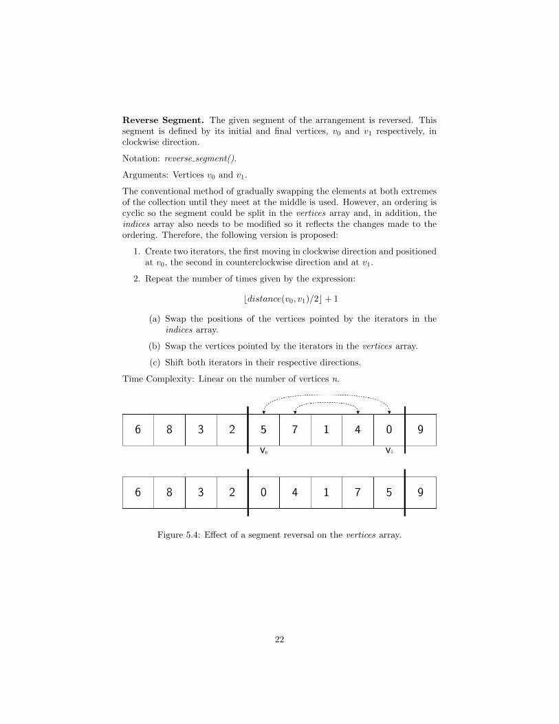
Reverse Segment. The given segment of the arrangement is reversed. Thissegment is defined by its initial and final vertices, v0 and v1 respectively, inclockwise direction.

Notation: reverse segment().

Arguments: Vertices v0 and v1.

The conventional method of gradually swapping the elements at both extremesof the collection until they meet at the middle is used. However, an ordering iscyclic so the segment could be split in the vertices array and, in addition, theindices array also needs to be modified so it reflects the changes made to theordering. Therefore, the following version is proposed:

1. Create two iterators, the first moving in clockwise direction and positionedat v0, the second in counterclockwise direction and at v1.

2. Repeat the number of times given by the expression:

bdistance(v0, v1)/2c+ 1

(a) Swap the positions of the vertices pointed by the iterators in theindices array.

(b) Swap the vertices pointed by the iterators in the vertices array.

(c) Shift both iterators in their respective directions.


Figure 5.4: Effect of a segment reversal on the vertices array.

22

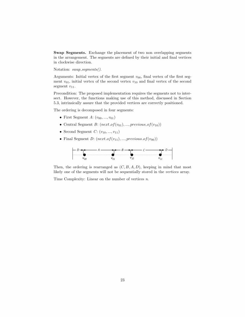
Swap Segments. Exchange the placement of two non overlapping segmentsin the arrangement. The segments are defined by their initial and final verticesin clockwise direction.

Notation: swap segments().

Arguments: Initial vertex of the first segment v00, final vertex of the first seg-ment v01, initial vertex of the second vertex v10 and final vertex of the secondsegment v11.

Precondition: The proposed implementation requires the segments not to inter-sect. However, the functions making use of this method, discussed in Section5.3, intrinsically assure that the provided vertices are correctly positioned.

The ordering is decomposed in four segments:

• First Segment A: (v00, ..., v01)

• Central Segment B : (next of(v01), ..., previous of(v10))

• Second Segment C : (v10, ..., v11)

• Final Segment D : (next of(v11), ..., previous of(v00))

Then, the ordering is rearranged as (C,B,A,D), keeping in mind that mostlikely one of the segments will not be sequentially stored in the vertices array.


23

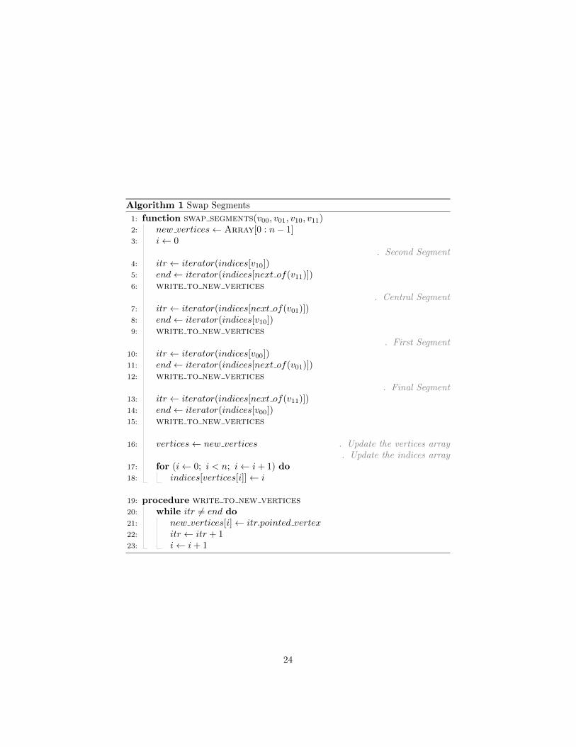
Algorithm 1 Swap Segments

1: function swap segments(v00, v01, v10, v11)2: new vertices← Array[0 : n− 1]3: i← 0

. Second Segment4: itr ← iterator(indices[v10])5: end← iterator(indices[next of(v11)])6: write to new vertices

. Central Segment7: itr ← iterator(indices[next of(v01)])8: end← iterator(indices[v10])9: write to new vertices

. First Segment10: itr ← iterator(indices[v00])11: end← iterator(indices[next of(v01)])12: write to new vertices

. Final Segment13: itr ← iterator(indices[next of(v11)])14: end← iterator(indices[v00])15: write to new vertices

16: vertices← new vertices . Update the vertices array. Update the indices array

17: for (i← 0; i < n; i← i+ 1) do18: indices[vertices[i]]← i

19: procedure write to new vertices20: while itr 6= end do21: new vertices[i]← itr.pointed vertex22: itr ← itr + 123: i← i+ 1

24

5.1.3 Gap

Representation of two adjacent vertices in an ordering, which are not connectedin the graph G.

Attributes

V0. First vertex.

V1. Second vertex.

Properties

Equality. Two gaps are said to be the same if they contain the same pair ofvertices, whatever the order. To test the equality of gaps g0 and g1 the followingexpression is proposed:

(g0.v0 = g1.v0 ∧ g0.v1 = g1.v1) ∨ (g0.v0 = g1.v1 ∧ g0.v1 = g1.g0)


Hashable. Enables the fast search and retrieval in hash based containers. TheCantor pairing function is used [11]:

Cantor : N× N→ N

Cantor(x, y) =1

2(x+ y)(x+ y + 1) + y

Applied to a gap, the following criterion is used:

• x = max(v0, v1)

• y = min(v0, v1)

Since the Cantor pairing function is bijective, it is also a perfect hash functionwith no possible hash collision.

Time Complexity: Constant for both computing the pairing function and search-ing a gap in a hash based container.

5.1.4 Solver

Attributes

Graph. Instance of class Graph, representing graph G.

Ordering Stack. LIFO container of instances of class Ordering.

Gap Set. Hash based container of unique instances of class Gap.

Number of Gaps. Unsigned two byte integer storing the minimum number ofgaps found in an ordering.

25

Properties

Singleton. Restricted instantiation of the class to a single instance for easieraccess.

Methods

Clear. Removes every single ordering from the ordering stack except the oneat the top and empties the gap set.

Notation: clear().

Solve. Runs the SLH algorithm controlling the logic flow between the differentstages.

Time Complexity: O(n6 log(n) k4), where n is the number of vertices and k isthe maximum degree of graph G. However, this is worst case scenario and it ishighly unlikely. O(n5 log(n) k4) is given as the more reasonable time complexity,or even O(n4 k4) if the graph solved at the early stages of the algorithm. SeeSection 5.4 for a detailed explanation.

5.2 Isomorphisms

Representative of the generative transformations [see 4, page 4], these are theonly processes that perform transformations over orderings. Implemented asblind functions which do not check any condition, they just change the config-uration of the vertices in an ordering, making direct use of the Ordering classmethods reverse segments() and swap segments(). As the actual isomorphisms,these functions can be applied sequentially to form complex transformations.

Isomorphism γ

Given an ordering C and two of its vertices x and b, the segment (x, ..., b) isreversed. In other words, considering the vertices y ← previous of(x) and a←next of(b) and the segments A← (x, ..., b) and B ← (a, ..., y), the ordering C =(x, ..., b, a, ...y, x) or (A,B) is transformed into (b, ..., x, a, ..., y, b) or (AR, B), seeFigure 4.3.

Arguments: Ordering C and vertices x and b.

Algorithm 2 Isomorphism γ

1: function isomorphism γ(C, x, b)2: C.reverse segment(x, b)

The function internally calls Ordering class method reverse segment(), there-fore, keep in mind that the reversed segment is defined in clockwise direction.However, if the ordering is being traversed in counterclockwise direction the

26

correct transformation can be achieved by simply interchanging vertices x andb at the time of calling the function.

Time Complexity: Linear in the number of vertices n.

Isomorphism ℵGiven ordering C and its vertices x, e, c, a, b, f , d and y, the following segmentsare considered:

• A← (x, ..., e)

• B ← (c, ..., a)

• C ← (b, ..., f)

• D ← (d, ..., y)

The ordering C = (x, ..., e, c, ..., a, b, ..., f, d, ..., y) or (A,B,C,D) is transformedinto the ordering (e, ..., x, a, ..., c, d, ..., y, f, ..., b, e) or (AR, BR, D,CR), see Fig-ure 4.4

Arguments: Ordering C and vertices x, e, c, a, b, f , d and y.

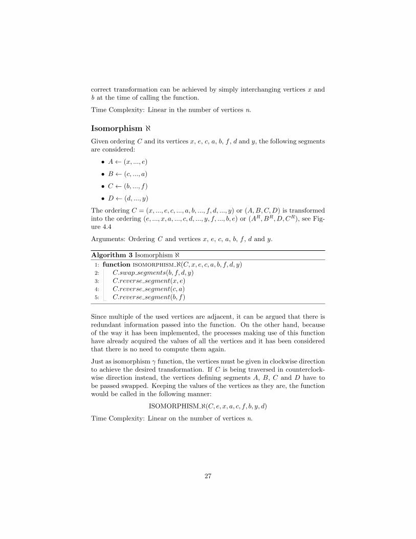
Algorithm 3 Isomorphism ℵ1: function isomorphism ℵ(C, x, e, c, a, b, f, d, y)2: C.swap segments(b, f, d, y)3: C.reverse segment(x, e)4: C.reverse segment(c, a)5: C.reverse segment(b, f)

Since multiple of the used vertices are adjacent, it can be argued that there isredundant information passed into the function. On the other hand, becauseof the way it has been implemented, the processes making use of this functionhave already acquired the values of all the vertices and it has been consideredthat there is no need to compute them again.

Just as isomorphism γ function, the vertices must be given in clockwise directionto achieve the desired transformation. If C is being traversed in counterclock-wise direction instead, the vertices defining segments A, B, C and D have tobe passed swapped. Keeping the values of the vertices as they are, the functionwould be called in the following manner:

ISOMORPHISM ℵ(C, e, x, a, c, f, b, y, d)


27

5.3 Transformations

A special combination of isomorphisms γ and ℵ, each of these complex transfor-mations requires a different set occurrences involving snakes, ladders and gapsto be present in an ordering so it can be transformed. They are implemented assearching algorithms which look for specific conditions and leave the actual con-version of the ordering to the isomorphism functions discussed in the previoussection.

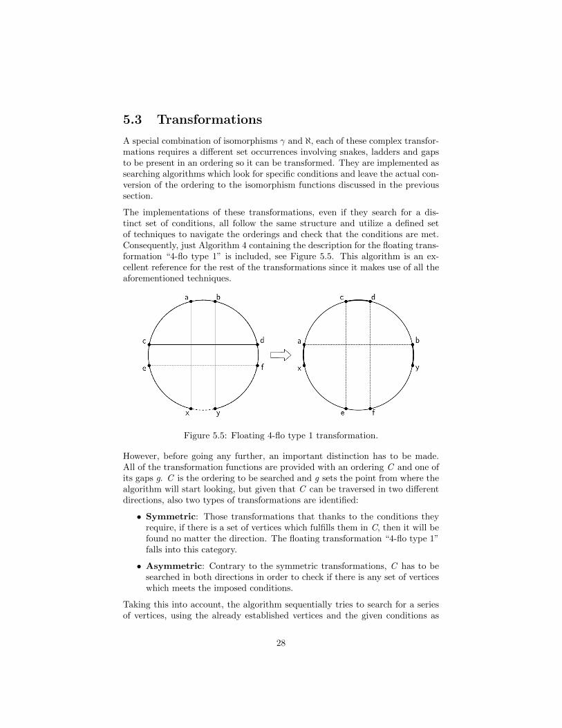
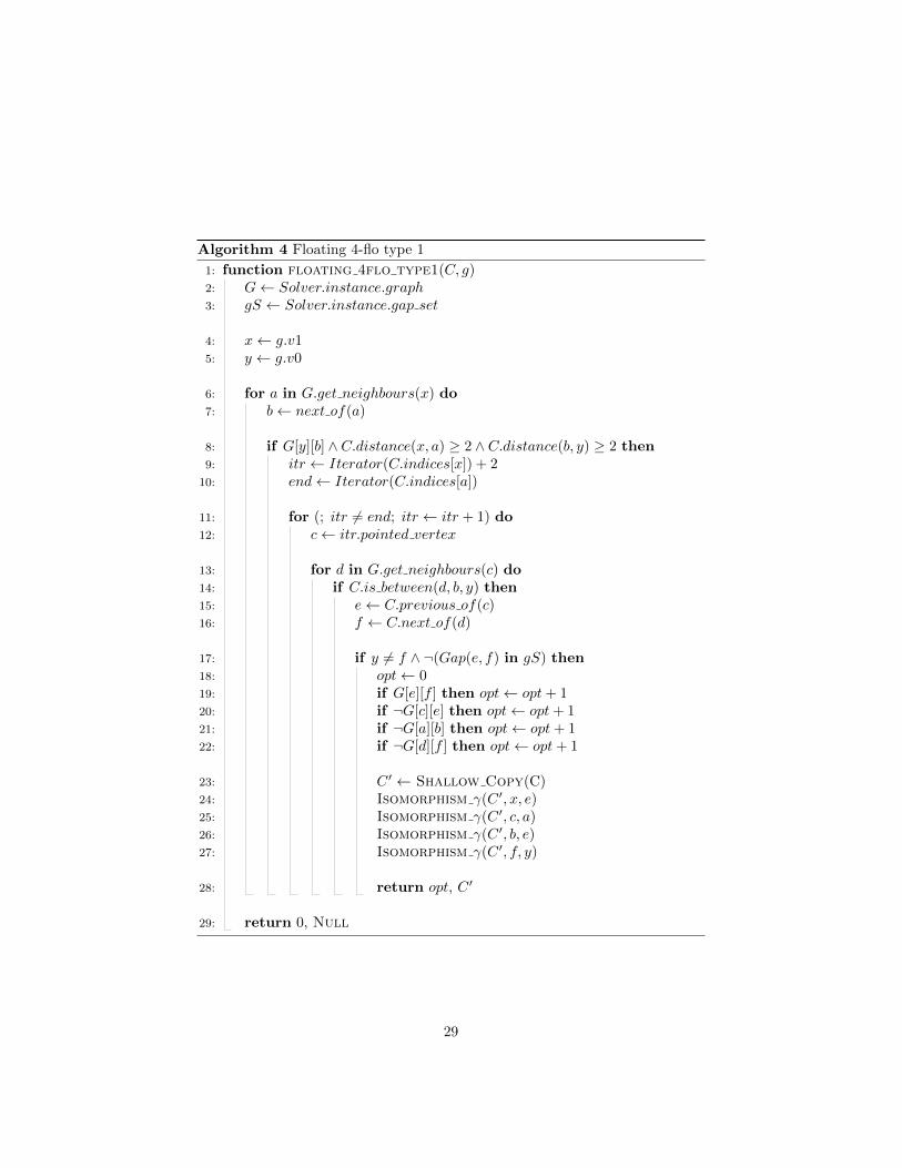
The implementations of these transformations, even if they search for a dis-tinct set of conditions, all follow the same structure and utilize a defined setof techniques to navigate the orderings and check that the conditions are met.Consequently, just Algorithm 4 containing the description for the floating trans-formation “4-flo type 1” is included, see Figure 5.5. This algorithm is an ex-cellent reference for the rest of the transformations since it makes use of all theaforementioned techniques.

Figure 5.5: Floating 4-flo type 1 transformation.

However, before going any further, an important distinction has to be made.All of the transformation functions are provided with an ordering C and one ofits gaps g. C is the ordering to be searched and g sets the point from where thealgorithm will start looking, but given that C can be traversed in two differentdirections, also two types of transformations are identified:

• Symmetric: Those transformations that thanks to the conditions theyrequire, if there is a set of vertices which fulfills them in C, then it will befound no matter the direction. The floating transformation “4-flo type 1”falls into this category.

• Asymmetric: Contrary to the symmetric transformations, C has to besearched in both directions in order to check if there is any set of verticeswhich meets the imposed conditions.

Taking this into account, the algorithm sequentially tries to search for a seriesof vertices, using the already established vertices and the given conditions as

28

Algorithm 4 Floating 4-flo type 1

1: function floating 4flo type1(C, g)2: G← Solver.instance.graph3: gS ← Solver.instance.gap set

4: x← g.v15: y ← g.v0

6: for a in G.get neighbours(x) do7: b← next of(a)

8: if G[y][b] ∧ C.distance(x, a) ≥ 2 ∧ C.distance(b, y) ≥ 2 then9: itr ← Iterator(C.indices[x]) + 2

10: end← Iterator(C.indices[a])

11: for (; itr 6= end; itr ← itr + 1) do12: c← itr.pointed vertex

13: for d in G.get neighbours(c) do14: if C.is between(d, b, y) then15: e← C.previous of(c)16: f ← C.next of(d)

17: if y 6= f ∧ ¬(Gap(e, f) in gS) then18: opt← 019: if G[e][f ] then opt← opt+ 120: if ¬G[c][e] then opt← opt+ 121: if ¬G[a][b] then opt← opt+ 122: if ¬G[d][f ] then opt← opt+ 1

23: C ′ ← Shallow Copy(C)24: Isomorphism γ(C ′, x, e)25: Isomorphism γ(C ′, c, a)26: Isomorphism γ(C ′, b, e)27: Isomorphism γ(C ′, f, y)

28: return opt, C ′

29: return 0, Null

29

guides to find the next vertex. The “anchor points”, as they will be called, arejust the vertices which for a given state of the algorithm have already been set.These anchor points, when possible, are used in conjunction with the requiredsnakes, ladders and gaps to obtain a new anchor point. If all anchor points havebeen positioned, then a set of vertices fulfilling the conditions exists and thetransformation can proceed.

The techniques or methods used to navigate the orderings in either directionfall into these three categories:

1. Adjacency in graph G: Provides the information regarding the exis-tence or absence of edges between vertices.

(a) Adjacency List: Allows to loop trough all the ladders of an anchorpoint. This can be seen in Algorithm 4 line 6, since there is a ladder(x−a) and vertex x, being part of g, is an anchor point, the algorithmiterates over all possible ladders of x in order to set vertex a.

(b) Adjacency Matrix: Returns in constant time whether or not twovertices are connected in G in order to check the existence of snakes,ladders and gaps.

Having both representations of graph G implies that there is redundantinformation stored. On the other hand, not having available one of the twomeans a suboptimal search. In the lack of the adjacency list, all n verticeswould have to be considered as possible ladders, and in the absence ofthe adjacency matrix, testing if two vertex are connected in G would costO(log(n)) at best if the neighbours of each vertex are stored in orderlymanner.

2. Ordering Iterators: Used as a last resort, they are necessary when thenext vertex to be found has no related anchor point. This situation can beseen at Algorithm 4, lines 9-11, where vertices x, y, a and b have alreadybeen set but not one of vertices c, d, e and f has a snake, ladder or gapwith any of the anchor points. Consequently, the vertices of an entiresegment have to be observed, in this case segment (x, .., a) in search forvertex c.

3. Relative position in ordering C : Provide early stopping conditions andmost importantly assure that the anchor points are correctly positionedbetween each other, leaving no room to contradictions.

(a) Previous and next of a vertex: They easily obtain the adjacent vertexof an anchor point in C. See Algorithm 4, line 7, where vertex b isjust the next of a, the previous in the case of the direction beingcounterclockwise.

(b) Distance between vertices: Considering the anchor points, it is usedto determine if the conditions are still feasible. See Algorithm 4, line8, once vertices a and b have been set there is no reason to continue if

30

in the segments (x,...,a) and (b,...,y) contain less than four vertices,since vertices e, c and d, f respectively, also have to be included.

(c) Vertex contained within a segment: Used in conjunction with tech-nique 1.a when the vertex at the end of a ladder starting from ananchor point has to be contained in a certain segment. See Algo-rithm 4, line 14, where considering the ladder (c− d) and the anchorpoint c the algorithm is trying to set vertex d. However, vertex d hasto be included in segment (b, ..., y) or otherwise it will be discarded.

Depending on the minimum number of gaps potentially closed there are threetypes of transformations: “closing”, “floating” and “opening” transformations.Furthermore, the “stages” defined at Section 5.4 do not ask for a particulartransformation, these functions request for any applicable transformation ofone given type instead, just specifying the ordering to transform. This meansthat for all gaps in the ordering and for all transformations falling in the giventype, any combination could be potentially applicable.

It is not specified the priority in which the transformations are tested, nor if allthe transformations are tested before continuing to the next gap or the otherway around. The approach taken in this implementation is based on one of theprinciples adopted in [3, page 38], which gives priority to the transformationsof lower computational cost. For that matter, the implementation iterates overthe transformations of the specified type, ordered from lower to higher compu-tational cost, and tries to apply the selected transformation with all the gapsin the ordering until an applicable combination is found, or going to the nexttransformation otherwise. Notice that this approach is just one of the possibleamong others and it could not be the same as the authors used.

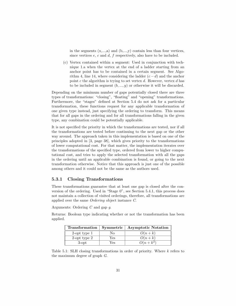
5.3.1 Closing Transformations

These transformations guarantee that at least one gap is closed after the con-version of the ordering. Used in “Stage 0”, see Section 5.4.1, this process doesnot maintain a collection of visited orderings, therefore, all transformations areapplied over the same Ordering object instance C.

Arguments: Ordering C and gap g.

Returns: Boolean type indicating whether or not the transformation has beenapplied.

Transformation Symmetric Asymptotic Notation

2-opt type 1 No O(n+ k)2-opt type 2 Yes O(n+ k)

3-opt Yes O(n+ k2)

Table 5.1: SLH closing transformations in order of priority. Where k refers tothe maximum degree of graph G.

31

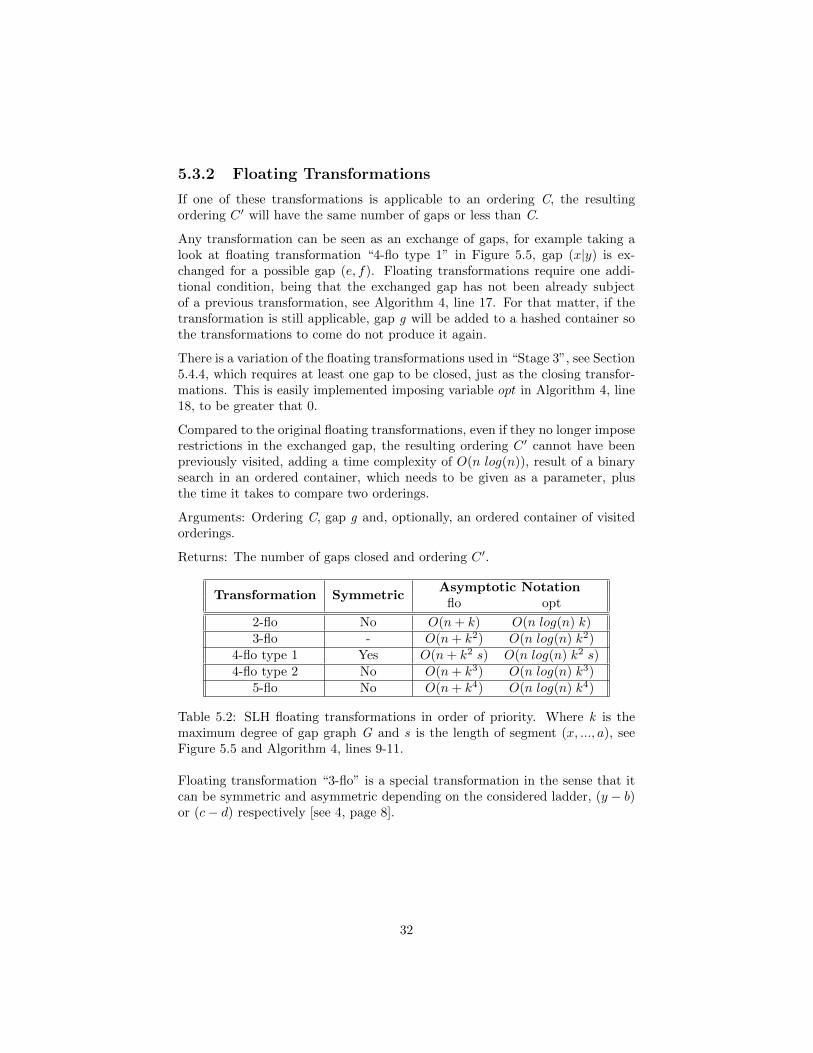
5.3.2 Floating Transformations

If one of these transformations is applicable to an ordering C, the resultingordering C ′ will have the same number of gaps or less than C.

Any transformation can be seen as an exchange of gaps, for example taking alook at floating transformation “4-flo type 1” in Figure 5.5, gap (x|y) is ex-changed for a possible gap (e, f). Floating transformations require one addi-tional condition, being that the exchanged gap has not been already subjectof a previous transformation, see Algorithm 4, line 17. For that matter, if thetransformation is still applicable, gap g will be added to a hashed container sothe transformations to come do not produce it again.

There is a variation of the floating transformations used in “Stage 3”, see Section5.4.4, which requires at least one gap to be closed, just as the closing transfor-mations. This is easily implemented imposing variable opt in Algorithm 4, line18, to be greater that 0.

Compared to the original floating transformations, even if they no longer imposerestrictions in the exchanged gap, the resulting ordering C ′ cannot have beenpreviously visited, adding a time complexity of O(n log(n)), result of a binarysearch in an ordered container, which needs to be given as a parameter, plusthe time it takes to compare two orderings.

Arguments: Ordering C, gap g and, optionally, an ordered container of visitedorderings.

Returns: The number of gaps closed and ordering C ′.

Transformation SymmetricAsymptotic Notation

flo opt

2-flo No O(n+ k) O(n log(n) k)3-flo - O(n+ k2) O(n log(n) k2)

4-flo type 1 Yes O(n+ k2 s) O(n log(n) k2 s)4-flo type 2 No O(n+ k3) O(n log(n) k3)

5-flo No O(n+ k4) O(n log(n) k4)

Table 5.2: SLH floating transformations in order of priority. Where k is themaximum degree of gap graph G and s is the length of segment (x, ..., a), seeFigure 5.5 and Algorithm 4, lines 9-11.

Floating transformation “3-flo” is a special transformation in the sense that itcan be symmetric and asymmetric depending on the considered ladder, (y − b)or (c− d) respectively [see 4, page 8].

32

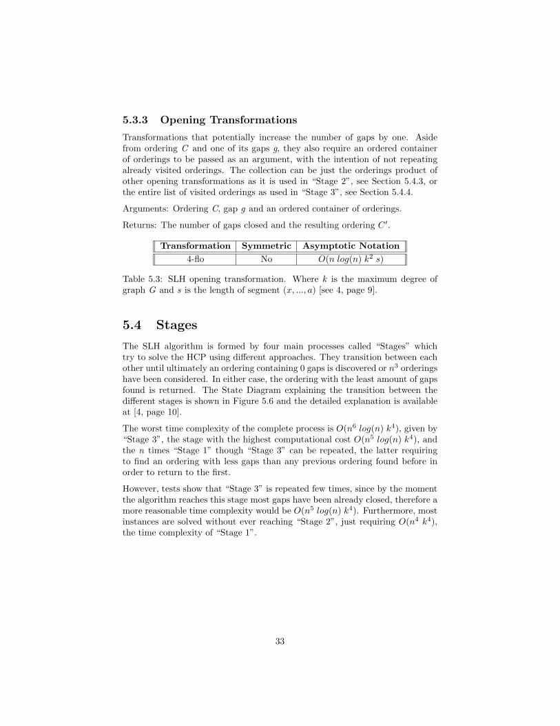
5.3.3 Opening Transformations

Transformations that potentially increase the number of gaps by one. Asidefrom ordering C and one of its gaps g, they also require an ordered containerof orderings to be passed as an argument, with the intention of not repeatingalready visited orderings. The collection can be just the orderings product ofother opening transformations as it is used in “Stage 2”, see Section 5.4.3, orthe entire list of visited orderings as used in “Stage 3”, see Section 5.4.4.

Arguments: Ordering C, gap g and an ordered container of orderings.

Returns: The number of gaps closed and the resulting ordering C ′.

Transformation Symmetric Asymptotic Notation

4-flo No O(n log(n) k2 s)

Table 5.3: SLH opening transformation. Where k is the maximum degree ofgraph G and s is the length of segment (x, ..., a) [see 4, page 9].

5.4 Stages

The SLH algorithm is formed by four main processes called “Stages” whichtry to solve the HCP using different approaches. They transition between eachother until ultimately an ordering containing 0 gaps is discovered or n3 orderingshave been considered. In either case, the ordering with the least amount of gapsfound is returned. The State Diagram explaining the transition between thedifferent stages is shown in Figure 5.6 and the detailed explanation is availableat [4, page 10].

The worst time complexity of the complete process is O(n6 log(n) k4), given by“Stage 3”, the stage with the highest computational cost O(n5 log(n) k4), andthe n times “Stage 1” though “Stage 3” can be repeated, the latter requiringto find an ordering with less gaps than any previous ordering found before inorder to return to the first.

However, tests show that “Stage 3” is repeated few times, since by the momentthe algorithm reaches this stage most gaps have been already closed, therefore amore reasonable time complexity would be O(n5 log(n) k4). Furthermore, mostinstances are solved without ever reaching “Stage 2”, just requiring O(n4 k4),the time complexity of “Stage 1”.

33

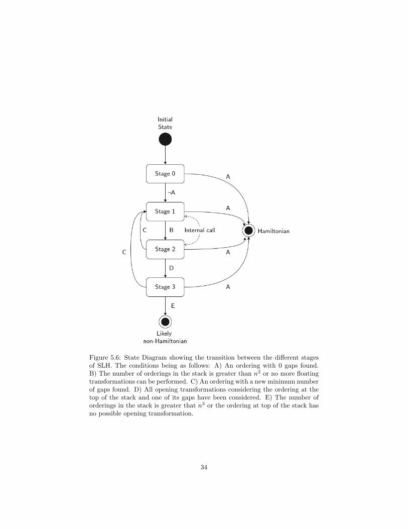
Figure 5.6: State Diagram showing the transition between the different stagesof SLH. The conditions being as follows: A) An ordering with 0 gaps found.B) The number of orderings in the stack is greater than n2 or no more floatingtransformations can be performed. C) An ordering with a new minimum numberof gaps found. D) All opening transformations considering the ordering at thetop of the stack and one of its gaps have been considered. E) The number oforderings in the stack is greater that n3 or the ordering at top of the stack hasno possible opening transformation.

34

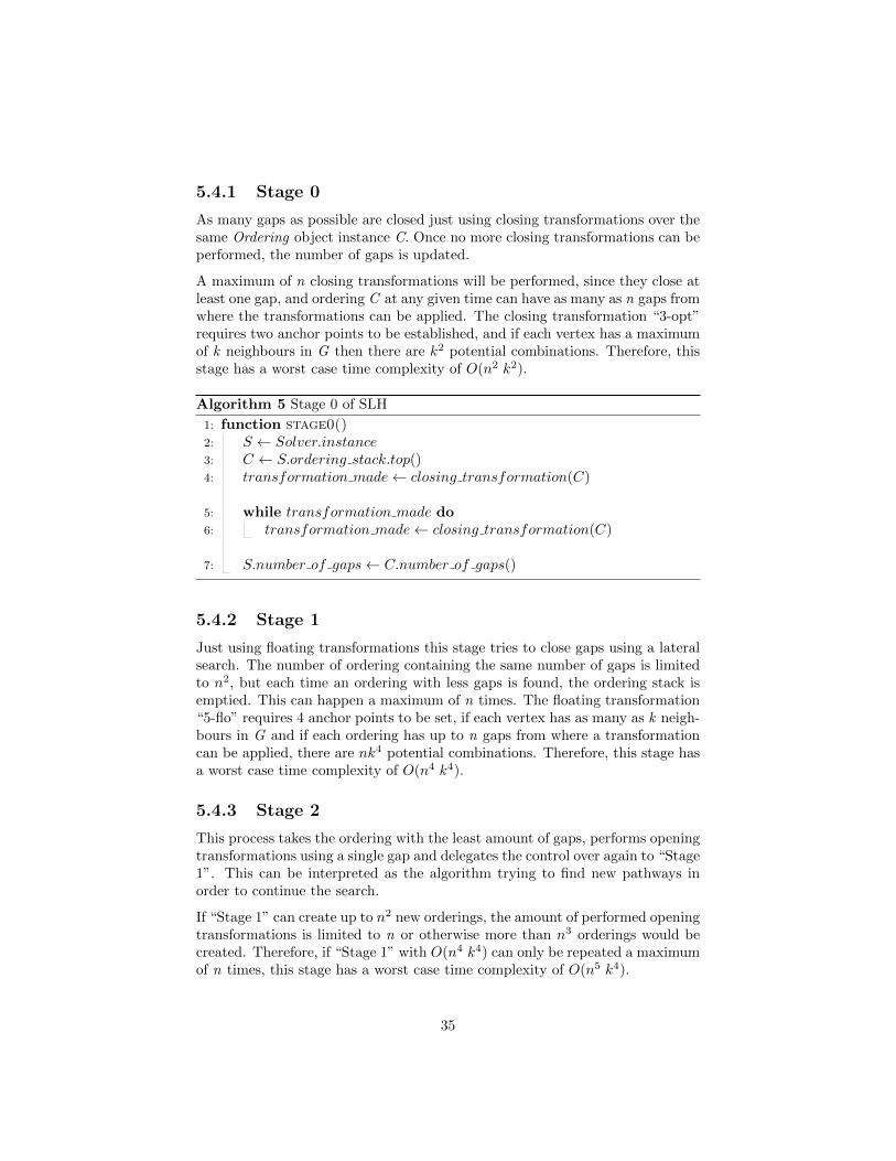
5.4.1 Stage 0

As many gaps as possible are closed just using closing transformations over thesame Ordering object instance C. Once no more closing transformations can beperformed, the number of gaps is updated.

A maximum of n closing transformations will be performed, since they close atleast one gap, and ordering C at any given time can have as many as n gaps fromwhere the transformations can be applied. The closing transformation “3-opt”requires two anchor points to be established, and if each vertex has a maximumof k neighbours in G then there are k2 potential combinations. Therefore, thisstage has a worst case time complexity of O(n2 k2).

Algorithm 5 Stage 0 of SLH

1: function stage0()2: S ← Solver.instance3: C ← S.ordering stack.top()4: transformation made← closing transformation(C)

5: while transformation made do6: transformation made← closing transformation(C)

7: S.number of gaps← C.number of gaps()

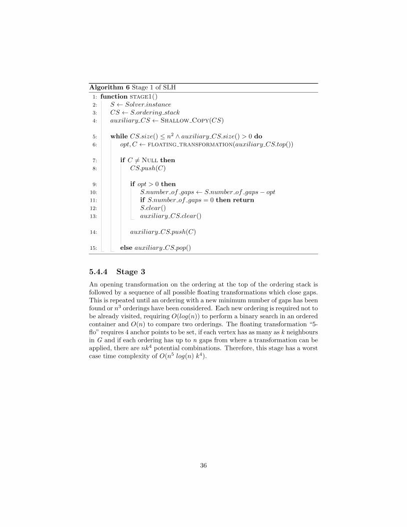
5.4.2 Stage 1

Just using floating transformations this stage tries to close gaps using a lateralsearch. The number of ordering containing the same number of gaps is limitedto n2, but each time an ordering with less gaps is found, the ordering stack isemptied. This can happen a maximum of n times. The floating transformation“5-flo” requires 4 anchor points to be set, if each vertex has as many as k neigh-bours in G and if each ordering has up to n gaps from where a transformationcan be applied, there are nk4 potential combinations. Therefore, this stage hasa worst case time complexity of O(n4 k4).

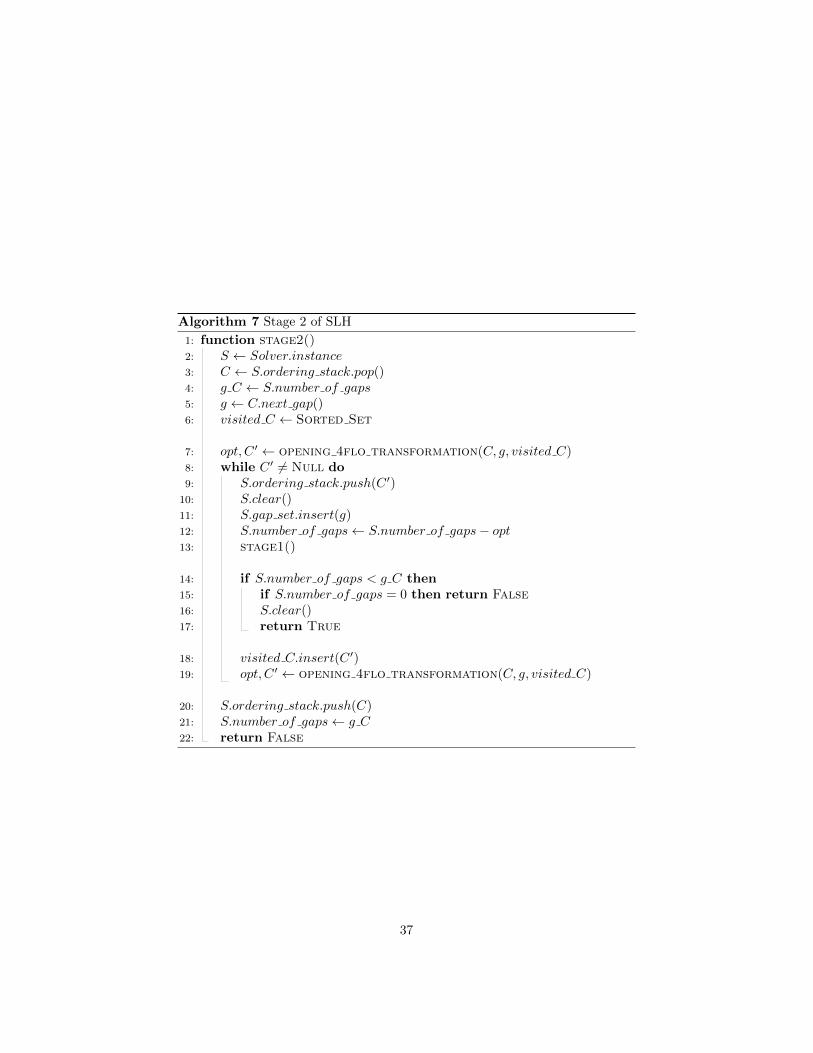
5.4.3 Stage 2

This process takes the ordering with the least amount of gaps, performs openingtransformations using a single gap and delegates the control over again to “Stage1”. This can be interpreted as the algorithm trying to find new pathways inorder to continue the search.

If “Stage 1” can create up to n2 new orderings, the amount of performed openingtransformations is limited to n or otherwise more than n3 orderings would becreated. Therefore, if “Stage 1” with O(n4 k4) can only be repeated a maximumof n times, this stage has a worst case time complexity of O(n5 k4).

35


1: function stage1()2: S ← Solver.instance3: CS ← S.ordering stack4: auxiliary CS ← Shallow Copy(CS)

5: while CS.size() ≤ n2 ∧ auxiliary CS.size() > 0 do6: opt, C ← floating transformation(auxiliary CS.top())

7: if C 6= Null then8: CS.push(C)

9: if opt > 0 then10: S.number of gaps← S.number of gaps− opt11: if S.number of gaps = 0 then return12: S.clear()13: auxiliary CS.clear()

14: auxiliary CS.push(C)

15: else auxiliary CS.pop()

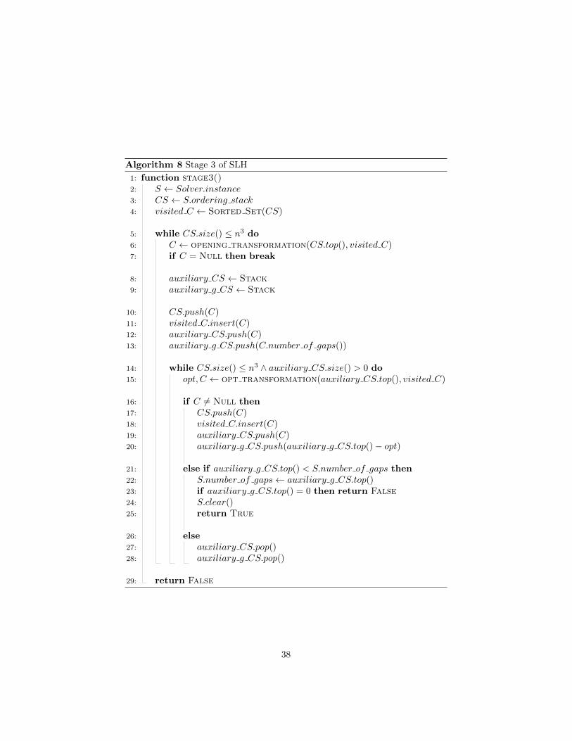
5.4.4 Stage 3

An opening transformation on the ordering at the top of the ordering stack isfollowed by a sequence of all possible floating transformations which close gaps.This is repeated until an ordering with a new minimum number of gaps has beenfound or n3 orderings have been considered. Each new ordering is required not tobe already visited, requiring O(log(n)) to perform a binary search in an orderedcontainer and O(n) to compare two orderings. The floating transformation “5-flo” requires 4 anchor points to be set, if each vertex has as many as k neighboursin G and if each ordering has up to n gaps from where a transformation can beapplied, there are nk4 potential combinations. Therefore, this stage has a worstcase time complexity of O(n5 log(n) k4).

36


1: function stage2()2: S ← Solver.instance3: C ← S.ordering stack.pop()4: g C ← S.number of gaps5: g ← C.next gap()6: visited C ← Sorted Set

7: opt, C ′ ← opening 4flo transformation(C, g, visited C)8: while C ′ 6= Null do9: S.ordering stack.push(C ′)

10: S.clear()11: S.gap set.insert(g)12: S.number of gaps← S.number of gaps− opt13: stage1()

14: if S.number of gaps < g C then15: if S.number of gaps = 0 then return False16: S.clear()17: return True

18: visited C.insert(C ′)19: opt, C ′ ← opening 4flo transformation(C, g, visited C)

20: S.ordering stack.push(C)21: S.number of gaps← g C22: return False

37


1: function stage3()2: S ← Solver.instance3: CS ← S.ordering stack4: visited C ← Sorted Set(CS)

5: while CS.size() ≤ n3 do6: C ← opening transformation(CS.top(), visited C)7: if C = Null then break

8: auxiliary CS ← Stack9: auxiliary g CS ← Stack

10: CS.push(C)11: visited C.insert(C)12: auxiliary CS.push(C)13: auxiliary g CS.push(C.number of gaps())

14: while CS.size() ≤ n3 ∧ auxiliary CS.size() > 0 do15: opt, C ← opt transformation(auxiliary CS.top(), visited C)

16: if C 6= Null then17: CS.push(C)18: visited C.insert(C)19: auxiliary CS.push(C)20: auxiliary g CS.push(auxiliary g CS.top()− opt)

21: else if auxiliary g CS.top() < S.number of gaps then22: S.number of gaps← auxiliary g CS.top()23: if auxiliary g CS.top() = 0 then return False24: S.clear()25: return True

26: else27: auxiliary CS.pop()28: auxiliary g CS.pop()

29: return False

38

5.5 Run Time

At the time of executing the program it is required to provide a file with “.hcp”extension containing the representation of the graph to be solved as a list ofedges. Once the graph has been specified the program’s life cycle is formed bya simple sequence of subprocesses:

1. Parsing: The “.hcp” file is parsed as an instance of class Graph.

2. Initialization: The singleton instance of class Solver is created with theinstance of class Graph generated by subprocess 1, the number of verticesfor all the objects of class Ordering is set and the ordering containingthe initial assignment of the vertices is constructed and pushed into theordering stack.

3. SLH Execution: Using the implemented version of the SLH, the specifiedgraph is searched with the intention of finding a Hamiltonian cycle.

4. Output: The series of vertices contained in the ordering with the leastamount of gaps found are returned.

5. Clean up: The created objects are destructed if necessary.

5.6 Possible Improvements

During the development of the implementation several improvements were con-sidered, which in the end, were not added to the latest version of the programsince they had a trade off, they were inconsistent with original design of SLHor simply, there was a lack of information to support them.

5.6.1 Ordering fingerprint

In [3, page 41, Algorithm 1] the term “fingerprint” is used as an alternative tostore the visited orderings in an ordered list. It is inferred that a fingerprintis the minimal expression of an ordering instance, which still maintains theidentity of the ordering and it is comparable to another fingerprint.

An example of such element could be achieved based on the vertices arrayattribute and the comparable property of the Ordering class in Section 5.1.2:

• Array containing n− 1 vertices, since it would always start from vertex 1.

• The listing of the vertices would be done using the same criterion as thecomparable property of the ordering class, following the direction imposedby the vertex with smaller identifier adjacent to and starting from vertex 1.

• Two fingerprint instances would be compared vertex by vertex, from startto finish, until a pair of vertices returns an inequality or all comparisonsare equal.

39

Figure 5.7: Comparison of fingerprints of orderings A (2,5,1,3,4,6,2) and B(5,4,3,1,6,2,5), where A > B. Same as Figure 5.3.

Applied to the proposed implementation, it would mean that each time anordering was recovered it would have to be reconstructed from the fingerprintin O(n) time, and that each time a transformation was made the producedordering had to be created following the fingerprint listing order.

On the other hand, the space in memory required to run the algorithm wouldbe approximately reduced by half in difficult instances, since just a compressedrepresentation of the orderings would have to be stored instead of the entireinstance.

5.6.2 Blind Improvement Space

Explained in detail in [3, page 23], a “Blind Improvement Space” (BIS) is a termused by “k -opt” transformation algorithms referring to a map that associates anon-optimal tour of a graph to a set of transformations which produce at leastone improved tour, closer to the optimal. The BIS of SLH is conformed by theset of stages and the order the transformations of each category are applied,having a lack of information regarding the latter.

It is probable that the BIS created by the proposed implementation is not thesame as the authors originally intended, which would explain the unreliableresults on the last two stages of the algorithm shown in Section 6.2. This wouldalso mean that optimizing the BIS of the implementation could significantlyincrease its performance in difficult graphs.

40

5.6.3 Multithreading

The current version of the algorithm is implemented as a single threaded pro-gram, however, some segments of the code could be ran in multiple threads asmeans to increase the computing power. The most notable segments being thesearches of applicable transformations for the different categories. If the CPUwould allow it, multiple threads could ran in parallel looking for new orderingsusing different combinations of gaps and transformations.

Notice that in this case, if the first eligible transformation found would be per-formed, the algorithm would no longer be deterministic, since the output couldvary between different executions depending on the state of the CPU and theoperating system. Therefore a priority system should be also implemented, onethat would make a thread wait if it has found an applicable transformation untilthe threads considering higher priority gaps and transformations had finished,which would nevertheless speed up the process in some situations.

41

Chapter 6

Experimental Validation

The goal of this chapter is to evaluate the proposed implementation using dif-ferent problem benchmarks.

All the times listed in this section where achieved running the C++ versionof the implemented SLH running in a custom desktop computer with a Ryzen7 2700X at 4.3GHz overclocked with Precision Boost Overdrive and 16GB ofRAM under Linux Debian 10.

6.1 Benchmarks

The graphs used to test the implementation are obtained from the TSPLIBwebsite’s specific HCP section [12], which provides 9 graph of up to 5000 vertices,a large set of 797 symmetric cubic graphs of up to 2048 vertices, accessible at [5]and lastly, from the Flinders HCP Challenge Set [7], a collection of 1001 difficultgraphs. All mentioned graphs contain Hamiltonian Cycles with the exception oftwo symmetric cubic graphs, C10.1 (the Petersen graph) and C28.1 (the Coxetergraph).

42

6.2 Results

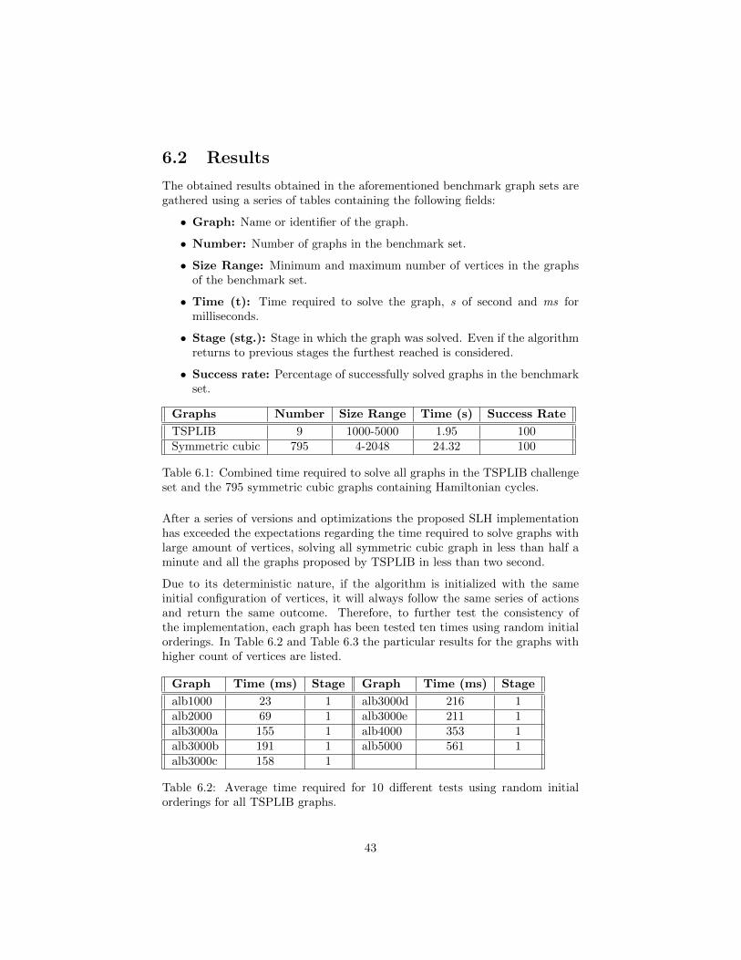
The obtained results obtained in the aforementioned benchmark graph sets aregathered using a series of tables containing the following fields:

• Graph: Name or identifier of the graph.

• Number: Number of graphs in the benchmark set.

• Size Range: Minimum and maximum number of vertices in the graphsof the benchmark set.

• Time (t): Time required to solve the graph, s of second and ms formilliseconds.

• Stage (stg.): Stage in which the graph was solved. Even if the algorithmreturns to previous stages the furthest reached is considered.

• Success rate: Percentage of successfully solved graphs in the benchmarkset.

Graphs Number Size Range Time (s) Success Rate

TSPLIB 9 1000-5000 1.95 100Symmetric cubic 795 4-2048 24.32 100

Table 6.1: Combined time required to solve all graphs in the TSPLIB challengeset and the 795 symmetric cubic graphs containing Hamiltonian cycles.

After a series of versions and optimizations the proposed SLH implementationhas exceeded the expectations regarding the time required to solve graphs withlarge amount of vertices, solving all symmetric cubic graph in less than half aminute and all the graphs proposed by TSPLIB in less than two second.

Due to its deterministic nature, if the algorithm is initialized with the sameinitial configuration of vertices, it will always follow the same series of actionsand return the same outcome. Therefore, to further test the consistency ofthe implementation, each graph has been tested ten times using random initialorderings. In Table 6.2 and Table 6.3 the particular results for the graphs withhigher count of vertices are listed.

Graph Time (ms) Stage Graph Time (ms) Stage

alb1000 23 1 alb3000d 216 1alb2000 69 1 alb3000e 211 1alb3000a 155 1 alb4000 353 1alb3000b 191 1 alb5000 561 1alb3000c 158 1

Table 6.2: Average time required for 10 different tests using random initialorderings for all TSPLIB graphs.

43

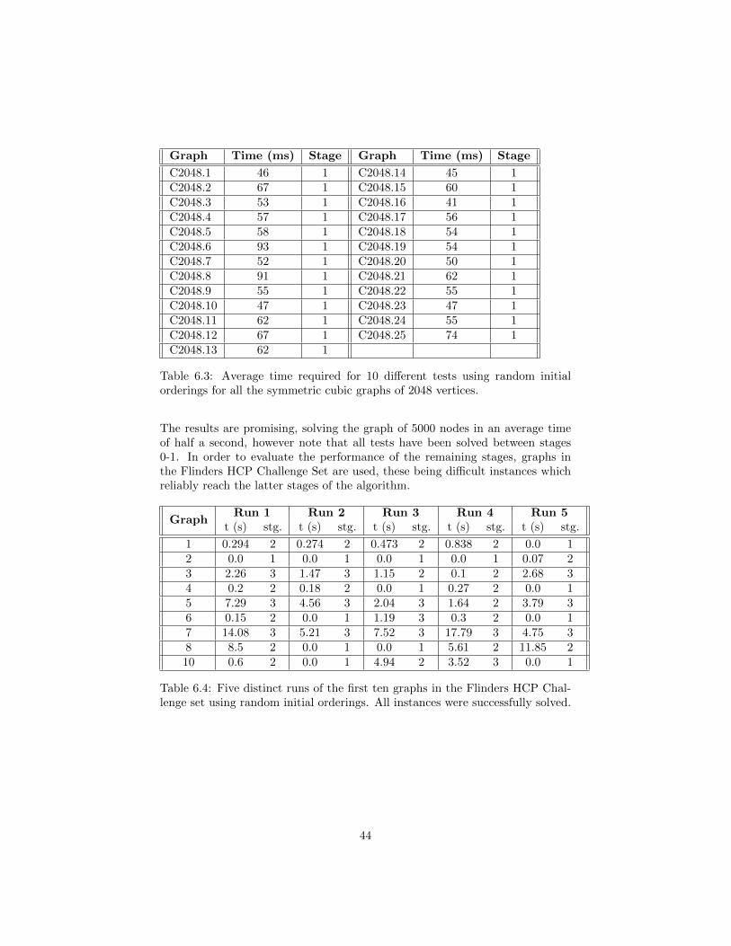
Graph Time (ms) Stage Graph Time (ms) Stage

C2048.1 46 1 C2048.14 45 1C2048.2 67 1 C2048.15 60 1C2048.3 53 1 C2048.16 41 1C2048.4 57 1 C2048.17 56 1C2048.5 58 1 C2048.18 54 1C2048.6 93 1 C2048.19 54 1C2048.7 52 1 C2048.20 50 1C2048.8 91 1 C2048.21 62 1C2048.9 55 1 C2048.22 55 1C2048.10 47 1 C2048.23 47 1C2048.11 62 1 C2048.24 55 1C2048.12 67 1 C2048.25 74 1C2048.13 62 1

Table 6.3: Average time required for 10 different tests using random initialorderings for all the symmetric cubic graphs of 2048 vertices.

The results are promising, solving the graph of 5000 nodes in an average timeof half a second, however note that all tests have been solved between stages0-1. In order to evaluate the performance of the remaining stages, graphs inthe Flinders HCP Challenge Set are used, these being difficult instances whichreliably reach the latter stages of the algorithm.

GraphRun 1 Run 2 Run 3 Run 4 Run 5

t (s) stg. t (s) stg. t (s) stg. t (s) stg. t (s) stg.

1 0.294 2 0.274 2 0.473 2 0.838 2 0.0 12 0.0 1 0.0 1 0.0 1 0.0 1 0.07 23 2.26 3 1.47 3 1.15 2 0.1 2 2.68 34 0.2 2 0.18 2 0.0 1 0.27 2 0.0 15 7.29 3 4.56 3 2.04 3 1.64 2 3.79 36 0.15 2 0.0 1 1.19 3 0.3 2 0.0 17 14.08 3 5.21 3 7.52 3 17.79 3 4.75 38 8.5 2 0.0 1 0.0 1 5.61 2 11.85 210 0.6 2 0.0 1 4.94 2 3.52 3 0.0 1

Table 6.4: Five distinct runs of the first ten graphs in the Flinders HCP Chal-lenge set using random initial orderings. All instances were successfully solved.

44

As shown in Table 6.4 the implementation is not reliable solving difficult in-stances. The algorithms shines in stages 0-1, however, when it transitions tostages 2 or 3 the time required to solve the graph rapidly increases, even moreso as the number of vertices grows. In addition, the state reached is highlydependant on the initial configuration of the vertices considered, an obviousexample being graph 8 which alternates between nearly instantly being solvedand requiring one of the longest time observed.

One of the observations made during multiple runs is that the algorithm oftenfalls to stage 3 when it has just gap left to be closed, meaning that the problemis stuck in this stage until it is being solved, since stage 3 requires at least onegap to be closed in order to transition. This can be, due to multiple reasons, anerror in the implementation, a misinterpreted guideline of the official algorithm,a suboptimal search space, etc.

45

Chapter 7

Web Application

As a means to show the internal behaviour of the SLH applied to real and com-plex graphs, a simple web application with a user interface has been developed.The application allows to drag and drop a “.hcp” file containing the representa-tion of the graph as a list of edges. Afterwards, the given graph is solved usingthe implementation made of the SLH. The algorithm, modified to periodicallyreserve the best ordering found at that given time, allows the web application torender the stored ordering using the same visual representation the algorithmwas based upon, arranging the sequence of vertices contained in the orderingalong the perimeter of a circle and subsequently drawing the snakes, laddersand gaps.

The ladders are painted in orange color, as chords in the circle between twonon adjacent vertices in the ordering. The snakes and gaps on the other side,are painted as arcs between all the adjacent vertices, in green and red colorrespectively, which in the end constitutes the entirety of the circle’s perimeter.All in all, the contrast between the colors combined with geometrical propertiesof some graphs and the patterns produced by the SLH transformations canultimately produce striking images. Furthermore, the user can go back andforth between distinct visual representation of the orderings, using an imagegallery, allowing to see how, over the course of the algorithm, the number ofgaps decreases as snakes increase.

The Web application has been built using Flask, HTML, JavaScript and theBootstrap framework for the CSS styles. The python implementation of theSLH, with the variations already mentioned, is used to solve the HCP instancesprovided by the “.hcp” files, and the visual representation of the graphs arerendered using the Pillow library.

46

Unfortunately, due to the space and computational requirements of the SLHimplementation, the web application has to remain as a local demonstrativeinterface. Moreover, the security measures required, given the user input file,and the concurrency of multiple users, distance even further a publicly accessibleweb site from this project’s scope.

Figure 7.1: SLH Web Application input window.

47

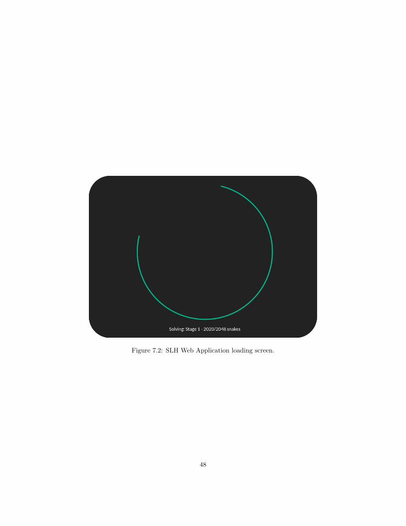
Figure 7.2: SLH Web Application loading screen.

48

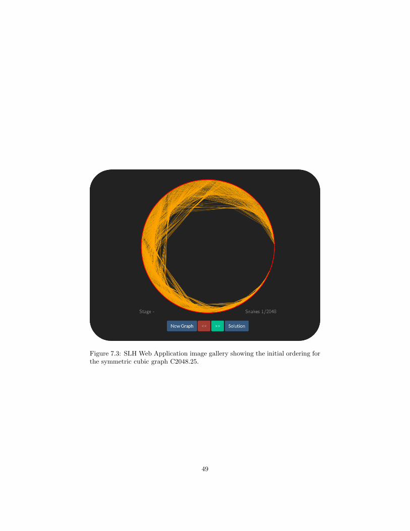
Figure 7.3: SLH Web Application image gallery showing the initial ordering forthe symmetric cubic graph C2048.25.

49

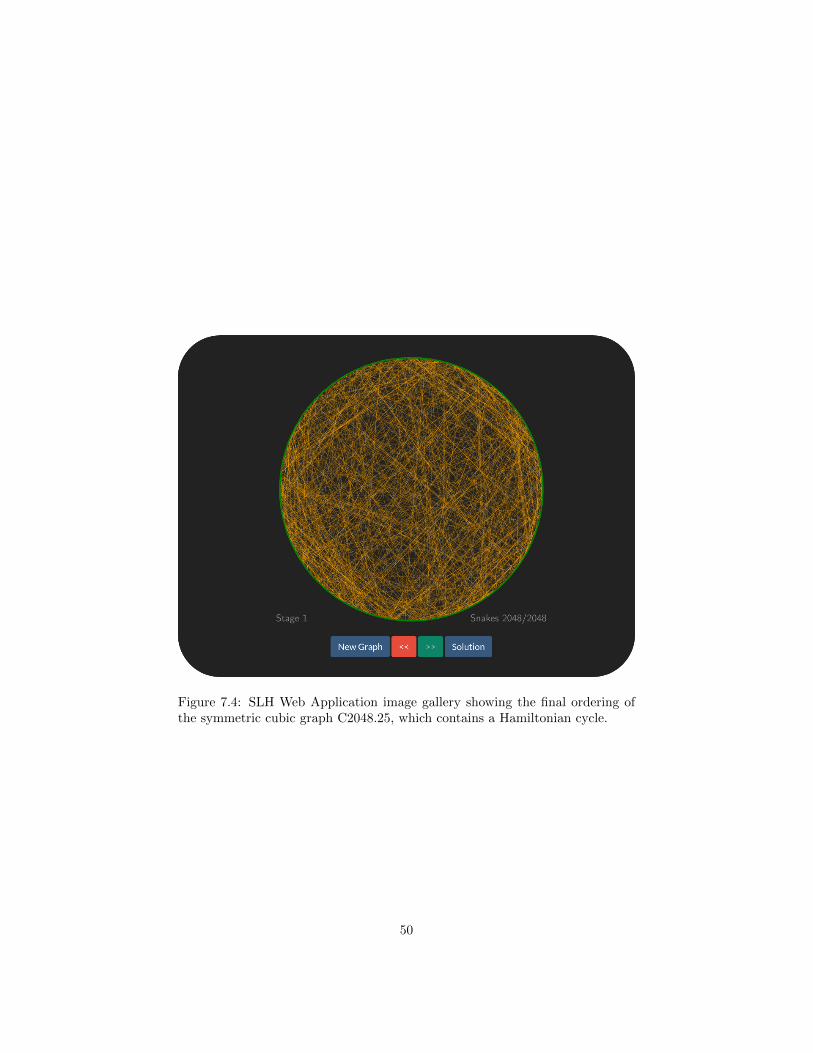
Figure 7.4: SLH Web Application image gallery showing the final ordering ofthe symmetric cubic graph C2048.25, which contains a Hamiltonian cycle.

50

Chapter 8

Conclusions

The course of this project has been at all times carried out under the context ofthe “Snakes and Ladders” Heuristic, a state of the art algorithm for the Hamil-tonian Cycle Problem. The main goal was to design and develop a functionalimplementation of the heuristic, which had to be built from the ground up justwith the help of the description provided by the authors.

After meticulous study and a series of optimizations a version of the algorithmwith excellent results in graphs of large number of vertices was conceived, whichcorroborated the incredible potential of the “Snakes and Ladders” Heuristic.

On the other side, there is no denying that the implementation proposed doesnot reliable solve difficult instances and is highly dependant on the initial con-figuration of the vertices. However, this is not discouraging, but rather reassuresthat there are improvements to be made.

The products derived from this project are two implementations, in pythonand C++, a web application, showing the internal behaviour of the algorithm,and most importantly, a detailed guideline of the designed program, allowinganyone who desires to build it on their own, or even better, improve the givenimplementation.

51

Bibliography

[1] David Applegate, William Cook, and Andre Rohe. “Chained Lin-Kernighanfor large traveling salesman problems”. In: INFORMS Journal on Com-puting 15.1 (2003), pp. 82–92.

[2] David Applegate et al. Concorde TSP Solver. http://www.math.uwaterloo.ca/tsp/concorde.html. 2003.

[3] Pouya Baniasadi. “Algorithms for Solving Variations of the TravelingSalesman Problem”. PhD thesis. Flinders University, College of Scienceand Engineering, 2019.

[4] Pouya Baniasadi et al. “Deterministic “Snakes and Ladders” Heuristic forthe Hamiltonian cycle problem”. In: Mathematical Programming Compu-tation 6.1 (2014), pp. 55–75.

[5] M. Conder. Trivalent (cubic) Symmetric Graphs on Up to 2048 Vertices.https://www.math.auckland.ac.nz/~conder/symmcubic2048list.

txt.[6] David Eppstein. “The traveling salesman problem for cubic graphs”. In:

(2003), pp. 307–318.[7] Michael Haythorpe. “FHCP Challenge Set: The first set of structurally

difficult instances of the Hamiltonian cycle problem”. In: arXiv preprintarXiv:1902.10352 (2019).

[8] Michael Haythorpe. “Finding Hamiltonian cycles using an interior pointmethod”. PhD thesis. Australian Mathematical Society, 2010.

[9] Keld Helsgaun. “An effective implementation of the Lin–Kernighan travel-ing salesman heuristic”. In: European journal of operational research 126.1(2000), pp. 106–130.

[10] Shen Lin and Brian W Kernighan. “An effective heuristic algorithm for thetraveling-salesman problem”. In: Operations research 21.2 (1973), pp. 498–516.

[11] Meri Lisi. “Some remarks on the Cantor pairing function”. In: Le Matem-atiche 62.1 (2007), pp. 55–65.

[12] TSPLIB. Hamiltonian Cycle Problem (HCP). http://comopt.ifi.uni-heidelberg.de/software/TSPLIB95/hcp/.

52

implementation of the “snakes and ladders” heuristic ... - addi

Documents