impacts on corn and soybean markets and crop rotation

Sustainable Agriculture Research; Vol. 5, No. 1; 2016 ISSN 1927-050X E-ISSN 1927-0518

Published by Canadian Center of Science and Education

1

Development of Corn Stover Biofuel: Impacts on Corn and Soybean Markets and Crop Rotation

Farzad Taheripour1, Julie Fiegel2 & Wallace E. Tyner1 1 Department of Agricultural Economics, Purdue University, West Lafayette, Indian, USA 2 HYLA Mobile, USA

Correspondence: Farzad Taheripour, Department of Agricultural Economics, Purdue University, 403 West State St., West Lafayette, IN 47907-2056, USA. Tel: 765-494-4612.

Received: August 21, 2015 Accepted: September 21, 2015 Online Published: October 26, 2015

doi:10.5539/sar.v5n1p1 URL: http://dx.doi.org/10.5539/sar.v5n1p1

Abstract What would be the impacts of a viable market for corn stover? A partial equilibrium model and a linear programing model were used to determine to what extent the existence of a viable market for corn stover would affect the traditional corn-soybean crop rotation in the US. We find that with government support production of biofuel from corn stover could significantly increase. That boosts profitability of farming corn in combination with harvesting corn stover versus soybeans. We show that if corn stover is demanded for biofuel, then a major shift will be observed in crop rotations in the US.

Keywords: soybeans, corn, corn stover, cellulosic biofuel, land use, corn-soybean rotation, partial equilibrium

1. Introduction 1.1 Importance First generation biofuels and their impacts on: 1) greenhouse gas emissions, 2) oil imports, and 3) markets for agricultural commodities and food prices have been examined from different angles in recent years. These studies showed that first generation biofuels, which are produced from food crops will not be able to replace a large portion of oil-based liquid fuels, because their rapid expansion could cause adverse impacts on food supply (Abbott, Hurt, & Tyner, 2008; Abbott, Hurt, & Tyner, 2011; Trostle, 2008; Zilberman et al., 2013) and/or induce major unintended land use changes which in turn will lead to increases in greenhouse gas emissions (Hertel, 2010; Tyner & Taheripour, 2012). Instead, second-generation biofuels produced from forest or crop residues such as wood chips, corn stover, or wheat straw offer an alternative to first generation biofuels. These residue-based biofuels could have minor impacts on both food prices and land use change. In addition, they could make a major contribution in greenhouse gas emission reduction targets if removed in a sustainable manner (English et al., 2013). Another advantage for second-generation biofuels produced from agricultural residues is that they provide a potential new source of income for farmers (Thompson & Tyner, 2013).

If second generation biofuels became economically viable and a massive volume of biofuels are produced from agricultural residues, it then can have major impacts on agricultural commodity markets. Corn stover is a major and abundant feedstock in the USA, which is expected to be used in biofuel production, if the technology becomes economically viable. Converting corn stover to biofuels, if a significant market develops, can affect profitability of corn production versus other crops produced in the USA, in particular. Thompson and Tyner suggest that if a viable corn stover market existed, it could have a large impact on farmers’ crop rotations and land allocation decisions. However, that research was done at the farm level with a given set of crop prices and ignored interactions between farm and market level variables. The purpose of this paper is to determine to what extent producing biofuels from corn stover can affect demands for and supplies of corn and soybeans and their market prices. In addition, it examines to what extent producing biofuels from corn stover could affect switching from corn-soybean rotation to continuous corn.

To determine how a corn stover market would impact corn and soybean markets, a partial equilibrium model was developed which links corn, soybeans, corn stover, ethanol, dried distiller grains, and gasoline markets at the USA national level and determines market-clearing prices at different crude oil prices. The resulting prices were used in a linear programming model to determine how farmers would allocate their land.

www.ccsen

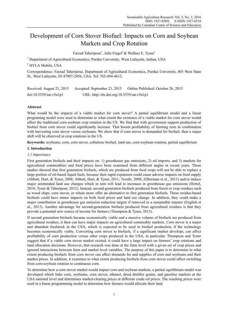
1.2 BackgrCorn and scrops has gtraditionalpest cycleincreased area of corthe soybea

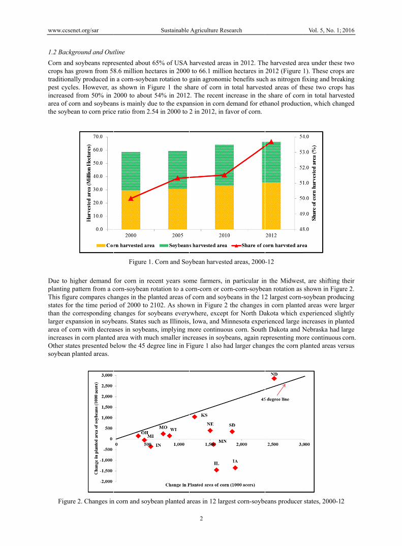
Due to higplanting paThis figurestates for tthan the clarger expaarea of corincreases iOther statesoybean pl

Figure

net.org/sar

round and Outsoybeans repregrown from 58ly produced ins. However, afrom 50% in rn and soybeanan to corn price

gher demand attern from a ce compares chthe time perioorresponding ansion in soybrn with decreain corn plantedes presented belanted areas.

2. Changes in

tline esented about 8.6 million hen a corn-soybeas shown in Fi2000 to aboutns is mainly due ratio from 2.

Figure 1

for corn in recorn-soybean ranges in the pld of 2000 to 2changes for so

beans. States suases in soybeand area with muelow the 45 de

n corn and soyb

Sustainable

65% of USA ctares in 2000an rotation to gigure 1 the sht 54% in 2012ue to the expan54 in 2000 to 2

. Corn and Soy

ecent years somrotation to a colanted areas of2102. As showoybeans everyuch as Illinois,ns, implying m

uch smaller incegree line in F

bean planted a

Agriculture Res

2

harvested area0 to 66.1 milliogain agronomi

hare of corn in2. The recent insion in corn d2 in 2012, in f

ybean harveste

me farmers, inorn-corn or cof corn and soyb

wn in Figure 2ywhere, except, Iowa, and Mmore continuoucreases in soybFigure 1 also ha

areas in 12 larg

search

as in 2012. Thon hectares in ic benefits sucn total harvestincrease in thedemand for ethfavor of corn.

ed areas, 2000

n particular inrn-corn-soybebeans in the 12

2 the changes it for North Dainnesota experus corn. South

beans, again read larger chan

gest corn-soybe

he harvested ar2012 (Figure h as nitrogen fted areas of the share of cornhanol producti

-12

n the Midwestan rotation as 2 largest corn-in corn plantedakota which exrienced large ih Dakota and Nepresenting monges the corn p

eans producer

Vol. 5, No. 1;

rea under these1). These cropfixing and breahese two cropn in total harvion, which cha

t, are shifting shown in Figu

-soybean produd areas were lxperienced slincreases in plaNebraska had ore continuousplanted areas v

states, 2000-1

2016

e two ps are aking s has ested

anged

their ure 2. ucing arger ghtly anted large corn.

ersus

2

www.ccsenet.org/sar Sustainable Agriculture Research Vol. 5, No. 1; 2016

3

Converting corn stover to biofuel could change relative profitability of corn and soybeans in favor of corn, when corn stover price is higher than its production costs. Production costs of corn stover include fertilizer costs to maintain productivity of land after stover removal and collection, storage, and transportation costs (Thompson & Tyner, 2013). These authors have concluded that if a viable corn stover market existed, it could have a large influence on farmer’s crop rotation in favor of corn-corn rotation. However, they ignored the fact that relative prices of corn and soybeans could be different in the presence of a viable market for corn stover.

Consider a case where converting corn stover to biofuel is profitable, either due to market forces or government supports. In this case, farmers who produce corn and soybeans will bring profitability of corn stover collection into account. When corn stover production is a profitable operation for a farmer, in each planting period he/she will compare gains from a joint production of corn and corn stover with profits from soybean production at given prices (Note 1). In this case, if the joint profits from corn production and corn stover is higher than the profit from soybean production, then corn will be produced. If a large group of farmers decides to follow this choice, then the corn-corn rotation will increase among farmers, which will lead to an increase in corn production and a reduction in soybean production, other factors being constant. This could affect relative prices of corn and soybeans at the market level.

In this paper we first develop a partial equilibrium model to examine impacts of converting corn stover to ethanol on markets for ethanol, gasoline, corn, corn stover, and soybeans at the USA aggregation level. The model developed in this paper is based on the model developed and used by (Tyner & Taheripour, 2008). Then we will feed the results of this model into the Purdue Crop/Livestock Linear Programing (PCLP) model (Doster et al., 2008) to examine farmers’ land allocation behavior in the presence of a viable market for corn stover. We test the sensitivity of the land allocation process at the farm level with respect to changes in key economic factors.

2. Method and Implemented Models 2.1 Partial Equilibrium Model The partial equilibrium model developed in this paper is an extended version of the model developed by and used in several other articles (Taheripour & Tyner, 2008; Tyner & Taheripour, 2007; Tyner, Taheripour, & Perkis 2010; Tyner, Taheripour, & Hurt August, 2012). The original model follows an integrated partial equilibrium modeling structure which displays linkages among crude oil, gasoline, ethanol, and corn markets. The model captures the demand and supply sides of the corn, corn ethanol, dried distiller grains, and gasoline markets. The demand side of the corn market consists of three major corn users: foreign users (qcxd), domestic uses for food and feed (qcdd), and the corn ethanol industry (qced). The foreign and domestic demands for food and feed are modeled using constant price elasticity functional forms. The corn demand for the ethanol industry is qced = y.qse. Here, y shows the corn-ethanol conversion factor and qse is quantity of ethanol supply. Hence, total demand for corn is: qcd = qcxd + qcdd + qced.

On the supply side, a constant return to scale Cobb-Douglas production function is used to model the supply side of the corn market. In this production function, capital, labor, land, and a composite input (which represent fertilizer, pesticides, seeds, energy and other items) are used to produce corn. In this function all inputs, except the composite input, are constant in the short-run. This production function is used to determine the supply for corn, qcs.

In this model, in the short-run the demand for liquid fuel, ggd, only responds to its own price using a constant price elasticity functional form. However, in the long-run, demand can grow with income and population. The supply side of the fuel market is comprised of gasoline producers and ethanol producers. Gasoline supply is produced from crude oil. The supply of gasoline, qgos, is a function of its price and the price of crude oil. It follows a constant elasticity functional form as well. Ethanol is produced from corn. The supply of ethanol, qes, is a function of its own price and the price of corn following a constant elasticity functional form as well. In this model it is assumed that every gallon of ethanol is presumed to contain 70% of the energy of a gallon of gasoline. Hence, total supply of gasoline equivalent is: qgs = qgos + 0.7*qes.

Distiller's Dried Grains with Solubles (DDGS) is a co-product of the ethanol industry. DDGS can be used as a substitute for corn and to some extent soybean meal in the livestock industry and also alleviate impacts of ethanol production on the corn market. DDGS can increase profitability of ethanol industry as well. As a substitute for corn, DDGS covers a portion of corn demand: qDDGS = ϒ.qced. Here qDDGS is the quantity of DDGS produced and ϒ is the corn-DDGS conversion factor. The model evaluates profitability of the ethanol industry and assumes that this industry will expand/contract until profits reach zero. Given this assumption and according to the predetermined supply and demand elasticities, the model determines equilibrium prices and their


4

corresponding quantities for corn, ethanol, and gasoline and other endogenous variables for given exogenous variables defined in the model (such as crude oil price).

Several new components are introduced into this partial equilibrium model to handle new markets for soybeans, corn stover, and a biofuel produced from corn stover. The first component added to the model is a drop-in biofuel named bio-gasoline. This drop-in biofuel can be produced from corn stover with the following supply function: qgstov = Aestov(ppg)gstov(pstov)-gstov. The energy content of bio-gasoline is assumed to be equal to the energy content of gasoline. In the presence of bio-gasoline, total supply of gasoline will be equal to: qgs = qgos + 0.7*qes+ qgstov. Similar to ethanol industry, the bio-gasoline industry will expand until profits reach zero. Profits per gallon of bio-gasoline are estimated by: πs = pg - capstov –varstov. Here, capstov and varstov are capital and variable costs per gallon of bio-gasoline. At equilibrium πs=0.

In the new model it is assumed that the capital costs of producing corn ethanol is zero when markets operate below the existing production capacity. However, if an expansion in capacity is required the model takes into account the required capital costs.

The supply of and demand for corn stover are added to the model as well. The supply of stover is presented by: qstov = Astov(pstov /cstov) estov. Here qstov and pstov represent supply and market price of stover, Astov is the constant term, cstov stands for production costs of stover per metric ton (including all costs items such as collection costs, costs to maintain land productivity, and transportation costs), and estov indicates price elasticity of supply. The production costs are divided into two segments of fixed and variable costs. The variable costs are assumed to be sensitive to changes in crude oil price to cover impacts of changes in crude oil price on collection and transportation costs of stover. The corn stover total production costs follows an increasing trend from $68 per ton at $60 per gallon of crude oil to about $100 per ton at $160 crude oil price. The demand for corn stover is determined by bio-gasoline production with the following equation: qdstov= qgstov (Vstov). Here Vstov is the conversion rate of corn stover to bio-gasoline. For details about the cost structure of the bio-gasoline industry and corn stover activity see Fiegel (Fiegel, 2012).

A market for soybeans is also added to the model. In this market, the demand for soybeans is defined as: qdsoy=Asoy(1/(psoy)esoy). Here qdsoy and psoy represent demand for soybeans and its price, Asoy shows the constant term of the demand function, and esoy indicates the own price elasticity of demand for soybeans. The model determines the supply of soybeans (qssoy) using the allocated land to this product (lsoy) from the following equation: qssoy=lsoy.yieldsoy. Here, yieldsoy represents soybean yield. The model assumes that total supply of land (ltot) for corn and soybean production is fixed in the short-run. Hence, it determines areas under soybean production using the following relationship: lsoy=ltot-( qcs /yieldcorn).

Finally, the model imposes a zero profit condition to allocate land between corn and soybeans. Indeed the model assumes that farmers maximize their profit when they allocate their land between corn and soybeans. It is assumed that at equilibrium: πsoy=πcorn+πstov.

The revised model is calibrated using data obtained for 2010 for the US economy. For details see Fiegel (Fiegel, 2012). Then the model is solved for several alternative crude oil prices (an exogenous key variable of the model) ranging from $60 per barrel to $160 per barrel. For each crude oil price two alternative policies are tested. The first policy assumes that the government will not support converting corn stover to biofuel. The second policy assumes that the government will pay a fixed subsidy of $1.01 per gallon of bio-gasoline. Note that in both cases mentioned here we assumed that the government pays no subsidy for corn ethanol.

2.2 Farm Level Model To examine impacts of having a viable market for corn stover on crop rotation at a farm level the PCLP model which was originally developed at Purdue University is used and modified. PCLP is a linear programming model which helps determine profit-maximizing decisions for a given farm according to its possible crop activities, its existing resources, and according to current prices of commodities and input costs. The PCLP model takes specific data such as land, labor, capital, crop yields, crop prices, and detailed input costs and determines activities which maximize farmer’s profits. To adapt this model a new activity called stover collection is added to this model. This activity covers all steps and their corresponding costs which are required to collect and sell corn stover to a bio-refinery at current prices. These steps and their corresponding costs are defined in detail in (Fiegel, 2012; Thompson & Tyner, 2013). Then the model is solved for a group of farmers who participated in the Top Crop Farmer Workshops in 2007-2010 under two alternative cases of with and without corn stover activity to find out their optimal choices under these two different cases. To tune the PCLP model with market conditions in the presence of corn stover activity, prices obtained from the partial equilibrium model are used. Then the sensitivity of the results with respect to changes in the assumptions and parameters behind the corn stover


5

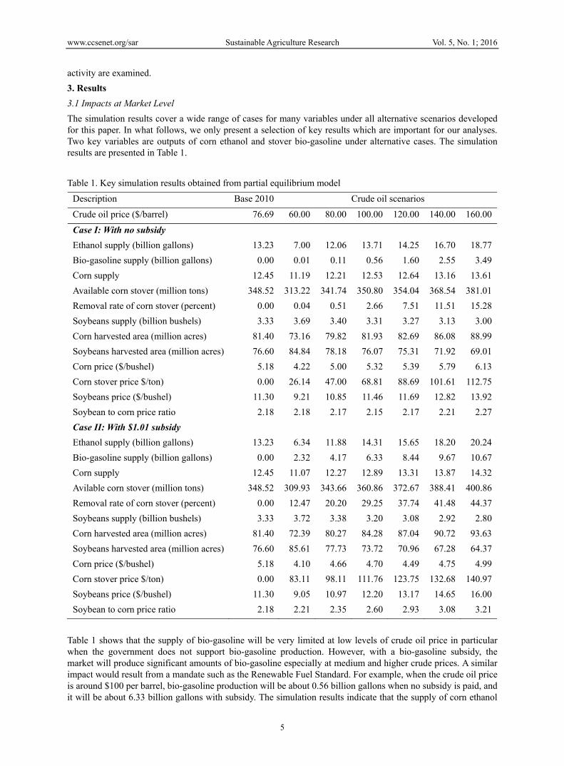
activity are examined. 3. Results 3.1 Impacts at Market Level The simulation results cover a wide range of cases for many variables under all alternative scenarios developed for this paper. In what follows, we only present a selection of key results which are important for our analyses. Two key variables are outputs of corn ethanol and stover bio-gasoline under alternative cases. The simulation results are presented in Table 1.

Table 1. Key simulation results obtained from partial equilibrium model

Description Base 2010 Crude oil scenarios

Crude oil price ($/barrel) 76.69 60.00 80.00 100.00 120.00 140.00 160.00

Case I: With no subsidy Ethanol supply (billion gallons) 13.23 7.00 12.06 13.71 14.25 16.70 18.77

Bio-gasoline supply (billion gallons) 0.00 0.01 0.11 0.56 1.60 2.55 3.49

Corn supply 12.45 11.19 12.21 12.53 12.64 13.16 13.61

Available corn stover (million tons) 348.52 313.22 341.74 350.80 354.04 368.54 381.01

Removal rate of corn stover (percent) 0.00 0.04 0.51 2.66 7.51 11.51 15.28

Soybeans supply (billion bushels) 3.33 3.69 3.40 3.31 3.27 3.13 3.00

Corn harvested area (million acres) 81.40 73.16 79.82 81.93 82.69 86.08 88.99

Soybeans harvested area (million acres) 76.60 84.84 78.18 76.07 75.31 71.92 69.01

Corn price ($/bushel) 5.18 4.22 5.00 5.32 5.39 5.79 6.13

Corn stover price $/ton) 0.00 26.14 47.00 68.81 88.69 101.61 112.75

Soybeans price ($/bushel) 11.30 9.21 10.85 11.46 11.69 12.82 13.92

Soybean to corn price ratio 2.18 2.18 2.17 2.15 2.17 2.21 2.27

Case II: With $1.01 subsidy

Ethanol supply (billion gallons) 13.23 6.34 11.88 14.31 15.65 18.20 20.24

Bio-gasoline supply (billion gallons) 0.00 2.32 4.17 6.33 8.44 9.67 10.67

Corn supply 12.45 11.07 12.27 12.89 13.31 13.87 14.32

Avilable corn stover (million tons) 348.52 309.93 343.66 360.86 372.67 388.41 400.86

Removal rate of corn stover (percent) 0.00 12.47 20.20 29.25 37.74 41.48 44.37

Soybeans supply (billion bushels) 3.33 3.72 3.38 3.20 3.08 2.92 2.80

Corn harvested area (million acres) 81.40 72.39 80.27 84.28 87.04 90.72 93.63

Soybeans harvested area (million acres) 76.60 85.61 77.73 73.72 70.96 67.28 64.37

Corn price ($/bushel) 5.18 4.10 4.66 4.70 4.49 4.75 4.99

Corn stover price $/ton) 0.00 83.11 98.11 111.76 123.75 132.68 140.97

Soybeans price ($/bushel) 11.30 9.05 10.97 12.20 13.17 14.65 16.00

Soybean to corn price ratio 2.18 2.21 2.35 2.60 2.93 3.08 3.21

Table 1 shows that the supply of bio-gasoline will be very limited at low levels of crude oil price in particular when the government does not support bio-gasoline production. However, with a bio-gasoline subsidy, the market will produce significant amounts of bio-gasoline especially at medium and higher crude prices. A similar impact would result from a mandate such as the Renewable Fuel Standard. For example, when the crude oil price is around $100 per barrel, bio-gasoline production will be about 0.56 billion gallons when no subsidy is paid, and it will be about 6.33 billion gallons with subsidy. The simulation results indicate that the supply of corn ethanol

www.ccsen

increases aon supply ethanol is the supplydue to the

In generalpresence obiofuel is 12.53 billconditions$100 per bonly collec

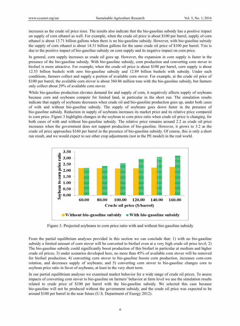
While bio-because coindicate thof with abio-gasolinto corn priboth casesincreases wcrude oil prun result,

From the subsidy a lThe bio-gacrude oil pfor biofuerotation, asoybean pr

In our partimpacts ofrelated to bio-gasolinaround $10

net.org/sar

as the crude oiof corn ethanoabout 13.71 b

y of corn ethanpositive impac

l, corn supply of the bio-gasomore attractivion bushels w

s, farmers collebarrel, the avaict about 29% o

-gasoline prodorn and soybe

hat supply of soand without bne subsidy. Reice. Figure 3 hs of with and when the govprice approachand we would

Figure 3. Pro

partial equiliblimited amounasoline subsidyprices; 3) undeel production; and decreases rice ratio in fav

tial equilibriumf converting co

crude price ne will not be00 per barrel in

il price rises. Tol as well. For illion gallons w

nol is about 14ct of bio-gasol

increases as coline subsidy. ve. For examplwith zero bio-ect and supplyilable corn stoof available co

duction elevateeans compete oybeans decre

bio-gasoline sueduction in suphighlights chan

without bio-gernment does

hes $160 per bad expect to see

ojected soybe

brium analysesnt of corn stovy could signifier scenarios de4) convertingsupply of so

vor of soybean

m analyses weorn stover to bi

of $100 per e produced witn the near futu

Sustainable

The results alsoexample, whe

when there is n4.31 billion galine subsidy on

crude oil goesWith bio-gasole, when the c-gasoline subsy a portion of ver is about 36

orn stover.

es demand for for limited l

eases when cruubsidy. The spply of soybeanges in the soygasoline subsid

not support parrel in the pre

e other crop adj

ans to corn pr

s provided in ver will be convficantly boost peveloped here, g corn stover toybeans; and 5ns, at least in th

e examined maio-gasoline on

barrel with thout the goveure (U.S. Depa

Agriculture Res

6

o indicate thaten the crude oino bio-gasolinllons for the sn corn supply a

s up. Howeveroline subsidy, crude oil price sidy and 12.8available corn60.86 million

and supply ofland, in particude oil and biosupply of soyans increases iybean to corn pdy. The relativproduction of esence of bio-gjustments (not

rice ratio with

this section wverted to biofuproduction of tno more than

to bio-gasoline5) converting he very short t

arket behavior n farmers’ beha

the bio-gasolernment subsidartment of Ener

search

t the bio-gasoliil price is aboune subsidy. Hosame crude oil and its negativ

r, the expansiocorn productiois about $100

89 billion busn stover. For etons with the b

f corn, it negatcular in the sh-gasoline prod

ybeans goes dits market pricprice ratio wheve price remainbio-gasoline. gasoline subsidt in the PE mod

h and without

we can concluuel even at a vthis biofuel in

n 45% of availae boosts corn corn stover t

term.

for a wide ranavior at farm leline subsidy. dy, and the crurgy 2012).

ine subsidy haut $100 per barwever, with biprice of $100

ve impact on co

on in corn supon and conver0 per barrel, coshels with subexample, at thebio-gasoline su

tively affects short run. The duction goes updown faster ine and its relati

en crude oil prins around 2.2However, it gdy. Of course, del) in the real

bio-gasoline s

ude that: 1) wivery high crud

particular at mable corn stovproduction, in

to bio-gasolin

nge of crude oevel we use theWe selected ude oil price w

Vol. 5, No. 1;

as a positive imrrel, supply ofio-gasoline sub

0 per barrel. Thorn price.

pply is faster inrting corn stovorn supply is absidy. Under e crude oil priubsidy, but far

supply of soybsimulation re

p, under both cn the presencive price compice is changing

2 as crude oil grows to 3.2 a

this is only a l world.

subsidy

ith no bio-gase oil price levemedium and h

ver will be remncreases corn-

ne changes cor

oil prices. To ae simulation rethis case bec

was expected

2016

mpact f corn bsidy his is

n the ver to about such ce of rmers

beans esults cases ce of pared g, for price

as the short

oline el; 2) igher

moved -corn rn to

ssess esults cause to be


7

3.2 Impacts at Farm Level To examine impacts of a viable market for corn stover at a farm level we tuned the PCLP model with market clearing prices obtained from the PE model as described above. We then made the following experiments for each farm to assess its response with respect to changes in key economic variables:

i. Base case, no stover removal,

ii. Base case, with stover removal with tuned market prices in the presence of bio-gasoline subsidy under status quo assumptions on tillage costs, soybean and corn yields, cost associated with corn stover activity, and harvesting technology,

iii. No saving in tillage costs,

iv. Change in yield due to change in rotation, known as yield drag,

v. Reduction in corn stover price

vi. Change in corn stover harvesting technologies,

vii. Impacts of new harvesting technology but no savings in tillage costs.

The first case provides a status quo situation where there is no market for corn stover. The second case evaluates impacts at farm level in the presence of a market for corn stover. In this case it is assumed that: 1) corn-corn rotation with stover removal reduces tillage costs by $25 per acre; 2) corn-corn rotation does not affect corn and soybean yields; 3) corn stover farm price and corn stover delivery price are about $85.40 per ton, and $111.80 per ton, respectively; and 4) farmers will use the rake and bale system to remove corn stover. In cases iii to vii these basic assumptions are relaxed. In case iii it is assumed that corn-corn rotation with stover removal does not reduce tillage costs. Case iv takes into account the fact that corn-corn rotation can affect yield. In case v the farm level and delivery prices used in the base case are reduced by 20%. Case vi investigates impacts of using a new technology to remove corn stover. This technology is known as the corn-rower. Compared to the rake and bale system, this technology eliminates the need to rake the stover after harvesting corn and in general reduces the costs of stover activity (Fiegel, 2012). Finally, the last case assumes that farmers will use the corn-rower technology to harvest corn stover, but this technology does not reduce tillage costs.

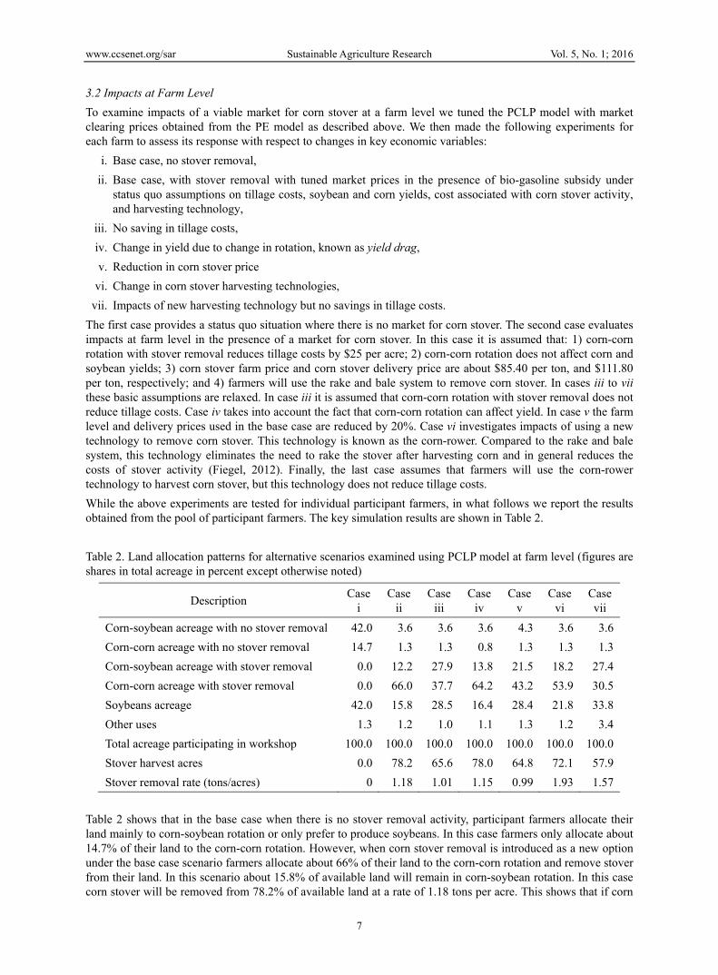
While the above experiments are tested for individual participant farmers, in what follows we report the results obtained from the pool of participant farmers. The key simulation results are shown in Table 2.

Table 2. Land allocation patterns for alternative scenarios examined using PCLP model at farm level (figures are shares in total acreage in percent except otherwise noted)

Description Case

i Case

ii Case

iii Case

iv Case

v Case

vi Case vii

Corn-soybean acreage with no stover removal 42.0 3.6 3.6 3.6 4.3 3.6 3.6

Corn-corn acreage with no stover removal 14.7 1.3 1.3 0.8 1.3 1.3 1.3

Corn-soybean acreage with stover removal 0.0 12.2 27.9 13.8 21.5 18.2 27.4

Corn-corn acreage with stover removal 0.0 66.0 37.7 64.2 43.2 53.9 30.5

Soybeans acreage 42.0 15.8 28.5 16.4 28.4 21.8 33.8

Other uses 1.3 1.2 1.0 1.1 1.3 1.2 3.4

Total acreage participating in workshop 100.0 100.0 100.0 100.0 100.0 100.0 100.0

Stover harvest acres 0.0 78.2 65.6 78.0 64.8 72.1 57.9

Stover removal rate (tons/acres) 0 1.18 1.01 1.15 0.99 1.93 1.57

Table 2 shows that in the base case when there is no stover removal activity, participant farmers allocate their land mainly to corn-soybean rotation or only prefer to produce soybeans. In this case farmers only allocate about 14.7% of their land to the corn-corn rotation. However, when corn stover removal is introduced as a new option under the base case scenario farmers allocate about 66% of their land to the corn-corn rotation and remove stover from their land. In this scenario about 15.8% of available land will remain in corn-soybean rotation. In this case corn stover will be removed from 78.2% of available land at a rate of 1.18 tons per acre. This shows that if corn

www.ccsen

stover is dscenarios case iii indbe used in will have emphasizeprice is 20the case ofstover remFinally, thessentially

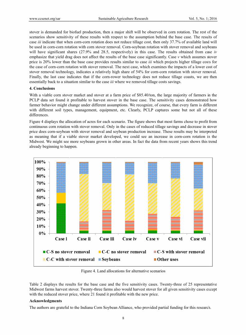
4. ConclusWith a viaPCLP datafarmer behwith diffedifferences

Figure 4 dcontinuousprice doesas meaninMidwest. Walready be

Table 2 diMidwest fwith the re

AcknowleThe author

net.org/sar

demanded for bshow sensitividicate that whecorn-corn rotasignificant sh

e that yield dra0% lower thanf corn-corn rot

moval technolohe last case iny back to a situ

sions able corn stovea set found it havior might cerent soil types.

displays the allos corn rotation corn-soybean

ng that if a viWe might see

eginning to hap

isplays the resfarms harvest seduced stover p

edgments rs are grateful

biofuel producity of these reen corn-corn ration with cornhares (27.9% ag does not affn the base casetation with sto

ogy, indicates andicates that ifuation similar t

er market andprofitable to

change under des, manageme

ocation of acren with stover ren with stover reiable stover mmore soybean

ppen.

Figure

sults for the bastover. Twentyprice, where 2

to the Indiana

Sustainable

ction, then a mesults with respotation does nn stover removand 28.5, res

fect the resultse provides resuver removal. Ta relatively higf the corn-rowto the case iii w

d stover at a faharvest stover

different assument, equipment

es for each sceemoval. Only emoval and so

market developns grown in oth

4. Land alloca

ase case and t-three farms al1 found it prof

a Corn Soybean

Agriculture Res

8

major shift wilpect to the as

not reduce tillaval. Corn-soybspectively) in s of the base cults similar to The next case, gh share of 54

wer technologywhere we remo

arm price of $r in the base

mptions. We ret, etc. Clearly

enario. The figin the cases of

oybean producped, we couldher areas. In f

ations for altern

the five sensitlso would harvfitable with the

n Alliance, wh

search

ll be observedsumption behi

age cost, then obean rotation w

this case. Thase significantcase iii whichwhich examin

4% for corn-coy does not redoved tillage co

85.40/ton, the case. The sen

ecognize, of coy, PCLP captu

gure shows thatf reduced tillag

ction increase.d see an increfact the data fro

native scenario

tivity cases. Twvest stover for e new price.

ho provided par

d in corn rotatiind the base conly 37.7% of with stover remhe results obtatly. Case v whh projects highnes the impactsorn rotation wduce tillage c

osts savings.

large majoritynsitivity cases ourse, that eveures some bu

t most farms cge savings andThese results

ease in corn-coom recent yea

os

wenty-three oall given sens

rtial funding fo

Vol. 5, No. 1;

ion. The rest ocase. The resulf available landmoval and soybained from cahich assumes sher tillage costs of a lower coith stover rem

coasts, we are

y of farmers idemonstrated ry farm is diff

ut not all of

chose to profit d decrease in smay be interporn rotation in

ars shows this

f 25 representsitivity cases ex

for this research

2016

of the lts of d will beans se iv tover ts for ost of

moval. then

n the how

ferent these

from tover reted n the trend

tative xcept

h.


9

References Abbott, P., Hurt, C., & Tyner, W. E. (2008). What’s Driving Food Prices?: Farm Foundation Issue Report.

Abbott, P., Hurt, C., & Tyner, W. E. (2011). What's Driving Food Prices in 2011? In Issue Report Farm Foundation.

Doster, D. H., Dobbins, C. L., Patrick, G. F., Miller, W. A., Preckel, P. V., Valentin, L., & Erickson, B. (2008). Purdue PC-LP Farm Plan B-21 Crop Input Form. Edited by Dept. of Agricultural Economics. West Lafayette, Indiana: Purdue University.

English, A., Tyner, W. E., Sesmero, J., Owens, P., & Muth, D. (2013). Environmental tradeoffs of stover removal and erosion in Indiana. Biofuels, Bioproducts, and Biorefining, 7(4), 78-88.

Fiegel, J. L. (2012). Development of Viable Corn Stover Market: Impacts on Corn and Soybean Markets, Department of Agricultural Economics, Purdue University, West Lafayette, IN.

Hertel, T., Golub, A., Jones, A., O'hare, M., Plevin, R., & Kammen, D. (2010). Effects of US Maize Ethanol on Global Land Use and Greenhouse Gas Emissions: Estimating Market-mediated Responses. Bioscience, 60(3), 223-231. http://dx.doi.org/10.1525/bop.2010.60.3.8

Taheripour, F., & Tyner, W. E. (2008). Ethanol Policy Analysis - What Have We Learned So Far? Choices, 23(3), 6-11.

Thompson, J., & Tyner, W. E. (2011). Corn Stover for Bioenergy Production: Cost Estimates and Farmer Supply Response, RE-3-W. Edited by Purdue Cooperative Extension Service. West Lafayette, IN: Purdue University.

Thompson, J., & Tyner, W. E. (2013). Corn Stover for Bioenergy Production: Cost Estimates and Farmer Supply Response. Biomass and Bioenergy, 62, 166-173. http://dx.doi.org/10.1016/j.biombioe.2013.12.020

Trostle, R. (2008). Global Agricultural Supply and Demand Factors Contributing to the Recent Increase in Food Commodity Prices. Edited by U.S. Department of Agriculture Economic Research Service. Washington, D.C.

Tyner, W. E., & Taheripour, F. (2007). Renewable Energy Policy Alternatives for the Future. American Journal of Agricultural Economics, 89(5), 1303-1310. http://dx.doi.org/10.1111/j.1467-8276.2007.01101.x

Tyner, W. E., & Taheripour, F. (2008). Policy Options for Integrated Energy and Agricultural Markets. Review of Agricultural Economics, 30(3), 387-396. http://dx.doi.org/10.1111/j.1467-9353.2008.00412.x

Tyner, W. E., & Taheripour, F. (2012). Land Use Changes and Consequent CO2 Emissions due to US Corn Ethanol Production. Encyclopedia of Biodiversity (2nd Ed.).

Tyner, W. E., Taheripour, F., & Hurt, C. (2012). Potential Impacts of a Partial Waiver of the Ethanol Blending Rules. Farm Foundation.

Tyner, W. E., Taheripour, F., & Perkis D. (2010). Comparison of Fixed Versus Variable Biofuels Incentives. Energy Policy, 38, 5530-5540. http://dx.doi.org/10.1016/j.enpol.2010.04.052

U.S. Department of Energy. (2012). Annual Energy Outlook 2013 - Early Release. Washington, D.C.

Zilberman, D., Hochman, G., Rajagopal, D., Sexton, R., & Timilsina. G. R. (2013). The Impact of Biofuels on Commodity Food Prices: Assessment of Findings. American Journal of Agricultural Economics, 95(2), 275-281. http://dx.doi.org/10.1093/ajae/aas037

Notes Note 1. In this paper it is assumed that corn and corn stover production is a single process and the farmer makes the decision at planting time. Of course a farmer can decide to produce corn at the planting time and later on he/she can decide whether to collect the corn stover or not.

Copyrights Copyright for this article is retained by the author(s), with first publication rights granted to the journal.

This is an open-access article distributed under the terms and conditions of the Creative Commons Attribution license (http://creativecommons.org/licenses/by/3.0/).

impacts on corn and soybean markets and crop rotation

Documents