imaging ahead of tunnel boring machines with dc
TRANSCRIPT
IMAGING AHEAD OF TUNNEL BORING MACHINES WITH DC
RESISTIVITY
FINAL PROJECT REPORT
by
Andrei Swidinsky1
Max Mifkovic1
Mike Mooney1 1 Colorado School of Mines
Sponsorship
UTC-UTI
For
University Transportation Center for
Underground Transportation Infrastructure
(UTC-UTI)
October 7, 2020
University Transportation Center for Underground Transportation Infrastructure 2
Disclaimer
The contents of this report reflect the views of the authors, who are responsible for the facts and
the accuracy of the information presented herein. This document is disseminated in the interest of
information exchange. The report is funded, partially or entirely, by a grant from the U.S.
Department of Transportation’s University Transportation Centers Program. However, the U.S.
Government assumes no liability for the contents or use thereof.
University Transportation Center for Underground Transportation Infrastructure 3
1. Report No. UTC-UTI 002 2. Government Accession No. 3. Recipient's Catalog No.
4. Title and Subtitle: IMAGING AHEAD OF TUNNEL BORING
MACHINE WITH DC RESISTIVITY
5. October 7, 2020
6. Performing Organization Code
7. Andrei Swidinsky, Max Mifkovic, Mike Mooney 8. Performing Organization Report
No. UTC-UTI 002
9. Performing Organization Name and Address
University Transportation Center for Underground Transportation
Infrastructure (UTC-UTI)
Tier 1 University Transportation Center
Colorado School of Mines
Coolbaugh 308, 1012 14th St., Golden, CO 80401
10. Work Unit No. (TRAIS)
11. Contract or Grant No.
69A355174711
12. Sponsoring Agency Name and Address
United States of America
Department of Transportation
Research and Innovative Technology Administration
13. Type of Report and Period
Covered
Final Project Report
14. Sponsoring Agency Code
15. Supplementary Notes
Report also available at: https://zenodo.org/communities/utc-uti
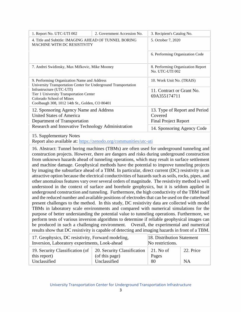
16. Abstract: Tunnel boring machines (TBMs) are often used for underground tunneling and
construction projects. However, there are dangers and risks during underground construction
from unknown hazards ahead of tunneling operations, which may result in surface settlement
and machine damage. Geophysical methods have the potential to improve tunneling projects
by imaging the subsurface ahead of a TBM. In particular, direct current (DC) resistivity is an
attractive option because the electrical conductivities of hazards such as soils, rocks, pipes, and
other anomalous features vary over several orders of magnitude. The resistivity method is well
understood in the context of surface and borehole geophysics, but it is seldom applied in
underground construction and tunneling. Furthermore, the high conductivity of the TBM itself
and the reduced number and available positions of electrodes that can be used on the cutterhead
present challenges to the method. In this study, DC resistivity data are collected with model
TBMs in laboratory scale environments and compared with numerical simulations for the
purpose of better understanding the potential value to tunneling operations. Furthermore, we
perform tests of various inversion algorithms to determine if reliable geophysical images can
be produced in such a challenging environment. Overall, the experimental and numerical
results show that DC resistivity is capable of detecting and imaging hazards in front of a TBM.
17. Geophysics, DC resistivity, Forward modeling,
Inversion, Laboratory experiments, Look-ahead
18. Distribution Statement
No restrictions.
19. Security Classification (of
this report)
Unclassified
20. Security Classification
(of this page)
Unclassified
21. No of
Pages
80
22. Price
NA
University Transportation Center for Underground Transportation Infrastructure 4
Table of Contents
CHAPTER 1 - INTRODUCTION………………………………………….…………………..…9
CHAPTER 2 - ELECTRICAL RESISTIVITY FUNDAMENTALS……………………………11
CHAPTER 3 - LABORATORY EXPERIMENT……………………………………………….13
Section 3.1 - Methods……………………………………………………………………13
Section 3.2 - Results.…………………………………………………………….……….15
CHAPTER 4 - FORWARD MODELLING EXPERIMENTS…………………………….….…19
Section 4.1 - Methods…………………………………………………………….………19
Section 4.2 - Results……………………………………………………………………..20
CHAPTER 5 – INVERSION AND IMAGING AHEAD OF A TBM…………………………23
Section 5.1 - Methods….……………………………………………………………........23
Section 5.2 - Results………………………………………………….…………………..25
CHAPTER 6 - SUMMARY AND CONCLUSIONS…………………………..………………...29
REFERENCES ………………………………………………………………...………………...31
APPENDIX A - TECHNOLOGY TRANSFER ACTIVITIES ………………….................…...34
APPENDIX B – DATA FROM THE PROJECT ………………………………………………..36
University Transportation Center for Underground Transportation Infrastructure 5
List of Figures
Figure 1. Cartoon diagram of probe-based Wenner array and dipole-dipole array on a
TBM……………………………………………………………………………………………...12
Figure 2. Various photographs of the laboratory TBM setup……………………………………13
Figure 3. Schematic of scale-model TBM…………………………………………………...…...14
Figure 4. Comparison of Wenner array data collected in the laboratory and numerically
simulated…………………………………………………………………………………………16
Figure 5. TBM Wenner array data collected in a homogeneous tank with the metal rod………..17
Figure 6. TBM dipole-dipole array data collected in a homogeneous tank with the metal rod….17
Figure 7. 3D mesh of model TBM and metal rod created with BERT and TetGen……………...20
Figure 8. Forward modeled Wenner data of a scale TBM in a tank………………………….......22
Figure 9. Forward modeled dipole-dipole data of a scale TBM in a tank………………………..22
Figure 10. DC resistivity survey design used for inversions………...…………………….……..24
Figure 11. Synthetic single-phase inversion results………………………………………………27
Figure 12. Synthetic time-lapse inversion results………………………………………………...28
University Transportation Center for Underground Transportation Infrastructure 6
List of Tables
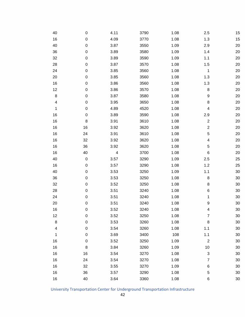
Table 1. Wenner array data for copper TBM model and no target in tank …………..……….… 36
Table 2. Wenner array data for plastic TBM model and no target in tank …………..………… 40
Table 3. Wenner array data for copper TBM model and metal rod in tank ………….………… 44
Table 4. Wenner array data for plastic TBM model and metal rod in tank ….………………… 48
Table 5. Dipole-dipole array data for copper TBM model and metal rod in tank …...……….… 56
Table 6. Dipole-dipole array data for plastic TBM model and no target in tank …….………… 60
Table 7. Wenner array data for copper TBM model and insulating sphere in tank …….……… 64
Table 8. Wenner array data for plastic TBM model and insulating sphere in tank ….………… 68
Table 9. Dipole-dipole array data for copper TBM model and insulating sphere in tank …....… 73
Table 10. Dipole-dipole array data for plastic TBM model and insulating sphere in tank …...... 77
University Transportation Center for Underground Transportation Infrastructure 7
List of Abbreviations
BEAM: Bore-tunneling, Electrical Ahead Monitoring
BERT: Boundless Electrical Resistivity Tomography
DC: Direct current
EM: Electromagnetic
FEM: Finite element method
GPR: Ground penetrating radar
IP: Induced polarization
PVC: Polyvinyl chloride
TBM: Tunnel boring machine
TEM: Time domain electromagnetic
University Transportation Center for Underground Transportation Infrastructure 8
EXCUTIVE SUMMARY
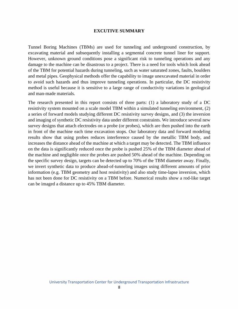
Tunnel Boring Machines (TBMs) are used for tunneling and underground construction, by
excavating material and subsequently installing a segmental concrete tunnel liner for support.
However, unknown ground conditions pose a significant risk to tunneling operations and any
damage to the machine can be disastrous to a project. There is a need for tools which look ahead
of the TBM for potential hazards during tunneling, such as water saturated zones, faults, boulders
and metal pipes. Geophysical methods offer the capability to image unexcavated material in order
to avoid such hazards and thus improve tunneling operations. In particular, the DC resistivity
method is useful because it is sensitive to a large range of conductivity variations in geological
and man-made materials.
The research presented in this report consists of three parts: (1) a laboratory study of a DC
resistivity system mounted on a scale model TBM within a simulated tunneling environment, (2)
a series of forward models studying different DC resistivity survey designs, and (3) the inversion
and imaging of synthetic DC resistivity data under different constraints. We introduce several new
survey designs that attach electrodes on a probe (or probes), which are then pushed into the earth
in front of the machine each time excavation stops. Our laboratory data and forward modeling
results show that using probes reduces interference caused by the metallic TBM body, and
increases the distance ahead of the machine at which a target may be detected. The TBM influence
on the data is significantly reduced once the probe is pushed 25% of the TBM diameter ahead of
the machine and negligible once the probes are pushed 50% ahead of the machine. Depending on
the specific survey design, targets can be detected up to 70% of the TBM diameter away. Finally,
we invert synthetic data to produce ahead-of-tunneling images using different amounts of prior
information (e.g. TBM geometry and host resistivity) and also study time-lapse inversion, which
has not been done for DC resistivity on a TBM before. Numerical results show a rod-like target
can be imaged a distance up to 45% TBM diameter.
University Transportation Center for Underground Transportation Infrastructure 9
CHAPTER 1 - INTRODUCTION
There has been a growing quantity of research on look-ahead methods for imaging in front of a
tunnel boring machine (TBM) for the purposes of hazard detection. Many techniques are
geophysical in nature and use elastic or electromagnetic field measurements to characterize the
material ahead of the TBM cutterface. Each method has its advantages and disadvantages based
on its sensitivity to different physical properties of the subsurface, the signal source, noise sources,
and the local geology. While most methods measuring elastic phenomena (elastic moduli and
density) in tunnels use passive seismic approaches (Poletto and Petronio, 2006) by taking
advantage of the natural mechanical signals being generated by the TBM itself as a source, there
has also been some research into active seismic methods using controlled sources (Bharadwaj et
al., 2017). The advantage of seismic imaging in the tunneling environment is that the method is
easy to implement and data can be collected continuously during excavation. However, not all
hazards ahead of the TBM have elastic moduli or density anomalies, and seismic instruments may
have poor coupling with the surrounding rock (Mooney et al., 2012). Other methods of geophysical
imaging in tunneling environments measure electromagnetic (EM) fields; such techniques include
ground penetrating radar (GPR) and transient EM (TEM). GPR is sensitive to dielectric
permittivity and magnetic permeability contrasts, and is particularly useful due to its high
resolution. Much research on the application of GPR in tunnels focuses on optimal survey and
antenna design to balance radar penetration depth with signal resolution (Wang et al., 2016; Simi
and Manacorda, 2016). The TEM method is sensitive to electrical conductivity contrasts and some
studies have suggested that the approach can detect anomalies as far as 60-80 meters away from a
TBM cutterface (Sun et al., 2012; Li et al., 2014; Jianlei and Xiu, 2016). However, EM methods
designed to image conductivity have limited resolution and signal-to-noise ratios in the tunneling
environment can be very poor.
Another geophysical approach that has been applied for TBM look-ahead imaging is direct current
(DC) resistivity, which is sensitive to the large range and contrasts of resistivity in different
geologies, fluids, and man-made materials (Zohdy et al., 1970; Ward, 1987; Loke, 2000). Research
in applying DC resistivity to TBMs dates back to the early 2000s and the first commercial
implementation to our knowledge is the Bore-tunnelling, Electrical Ahead Monitoring (BEAM)
system, produced by Geo Exploration Technologies. This method uses controlled, direct electrical
currents generated on the TBM to measure apparent resistivity and induced polarization (IP)
effects, and subsequently uses this information to make petrophysical classifications of the
material ahead of the cutterface (Kaus and Boening, 2008). BEAM uses in-house software and
foucses on hazard detection rather than full 3D imaging with quantitative interpretation. More
recently, other focused current methods similar to the BEAM technique have emerged (see, for
example, Bai-Yao et al., 2009). Furthermore, complex survey designs have arisen with multiple
electrode pairs located on the TBM face, the face and shield, or even using the shield as one giant
electrode (Mooney et al., 2013; Li et al., 2015).
At the Colorado School of Mines, a dissertation by Schaeffer (2016) and a follow-up paper
(Schaeffer and Mooney, 2016) studied DC resistivity methods on a TBM using a mix of numerical
University Transportation Center for Underground Transportation Infrastructure 10
and laboratory experiments. Schaeffer (2016) suggested attaching all electrodes to the TBM or the
tunnel liner, and our own laboratory experiment is largely inspired by his experimental design.
Schaeffer (2016) performed laboratory and numerical experiments with a large metal pipe
representing a tunneling hazard, and also carried out additional experiments on geologic planar
interfaces representing fault planes. Experimental results of this previous work indicated that a
metal pipe could be detected up to 3 TBM diameters away from the tunnel face, an observation
found to be in disagreement with numerical modeling. Our own results resolve the differences
between laboratory measurements and numerical simulations, and suggest a smaller detection
distance than established in Schaeffer (2016).
More recently, the idea of attaching electrodes onto probes extended in front of the TBM during
the ring-building phase has been explored (Lee et al., 2017; Park et al., 2017). Although this survey
design has only been numerically studied to date, it has many similarities to the ideas explored in
our own project. Lee et al. (2017) focused on computationally modeling and imaging a water
saturated vertical layer of bedrock with an electrode probe-based system - a much different
problem than trying to image a metal pipe or rod which presents a particular tunneling hazard.
Furthermore, Lee et al. (2017) focused on imaging the bedrock layer after it was located between
the two probes, rather than trying to image the target before the probes reached it. While their
results are promising, the ability to image ahead of the TBM is naturally limited by how far the
probes are inserted into the earth.
In this project, we extend previous work on DC resistivity methods by studying alternative probe-
based survey designs and their interpretation via state-of-the-art 3D inversion methods,
specifically for the purpose of imaging pipe-like hazards ahead of tunneling. There are three main
elements to the research described here: (1) DC measurements in a laboratory tunneling
environment complete with a scale model of a TBM and a metal rod target; (2) a numerical
modelling counterpart to the laboratory experiment; and (3) the application 3D DC resistivity
inversion methods for look-ahead TBM hazard imaging. We also examine the influence of the
electrically conductive TBM cutterface upon DC resistivity measurements and corresponding
inversion models.
University Transportation Center for Underground Transportation Infrastructure 11
CHAPTER 2- ELECTRICAL RESITIVITY FUNDAMENTALS
A DC resistivity survey is performed with at least four electrodes, often labeled A, B, M, and N.
Two common survey designs are the Wenner array and dipole-dipole array (Figure 1), which are
the focus of this project given the different current flow patterns they generate and measure. For
any survey design, current (I) is injected into the earth between the two source electrodes (A and
B) and the potential difference (∆V) is measured between the two potential electrodes (M and N).
The current and observed potential difference can be transformed to an apparent resistivity with a
geometric factor (k) (Herman, 2001; Zohdy et al., 1970; Loke, 2000; Ward, 1987), as in Equation
1:
a
Vk
I
= (1)
The geometric factor is dependent on the relative positions of the electrodes and is typically
derived for a survey at the surface of a halfspace representing a homogenous Earth. However, in
the TBM imaging problem the electrodes will likely be located in the subsurface near the tunnel;
in this case geometric factors are derived assuming a wholespace host and the apparent resistivity
transform in equation 1 can be written as
2a
Va
I
= (2)
and
2 ( 1)( 2)a
Vna n n
I
= + + (3)
for a Wenner array and dipole-dipole array, respectively (this wholespace assumption is later
justified in Chapter 3 by showing that the results are only sensitive to resistivity contrasts within
the tunneling profile). In equations 2 and 3, the variable a represents the basic distance scale of the
survey as indicated in Figure 1, and n is an integer multiple of this elemental spacing. In the event
where the electrode spacing between dipoles is the same as the electrode spacing within dipoles (n
= 1) as in Figure 1b, the apparent resistivity equation for a dipole-dipole array reduces to

University Transportation Center for Underground Transportation Infrastructure 12
12a
Va
I
= (4)
While the constant presence of the conductive TBM cutterface and resistive tunnel breaks
wholespace host assumption, the influence of these features is to produce a constant voltage signal
in the data, so apparent resistivity will always be offset by a constant quantity from the true
wholespace resistivity. The presence of a target will also break the wholespace assumption, but
the purpose of the wholespace geometric factor is precisely to measure such deviations from the
host resistivity. A more advanced method of 3D inversion is applied in Chapter 5 to directly solve
for the true resistivity distribution rather than simply apparent resistivity; inversion does not rely
on the assumption of a wholespace and can incorporate additional information, such as topography
and the known position of tunneling equipment.
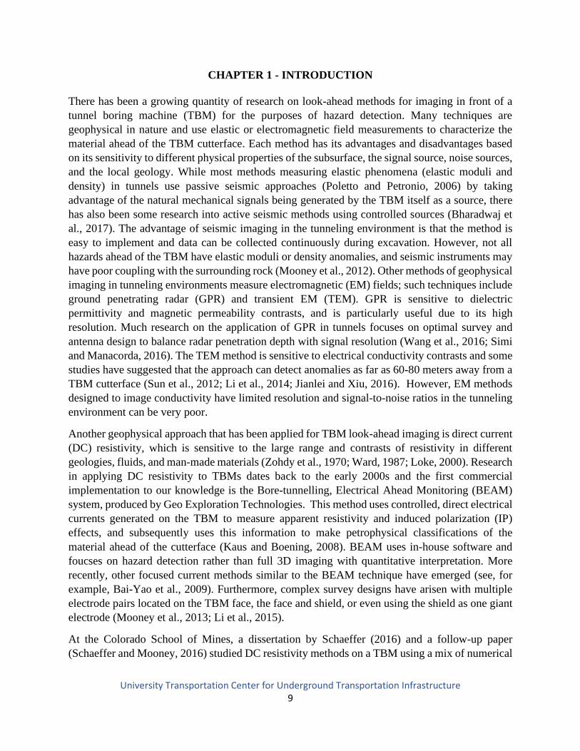
Figure 1: Cartoon diagram of probe-based (a) Wenner array and (b) dipole-dipole array on a TBM.
Each electrode is located at the end of a non-conductive probe. In both arrays, current flows from
University Transportation Center for Underground Transportation Infrastructure 13
electrode A to electrode B. While current is flowing through the earth, the potential difference is
measured between electrodes M and N. In the configurations shown here, the electrode spacing a
is constant between all adjacent electrodes.
CHAPTER 3- LABORATORY EXPERIMENT
Section 3.1 - Methods
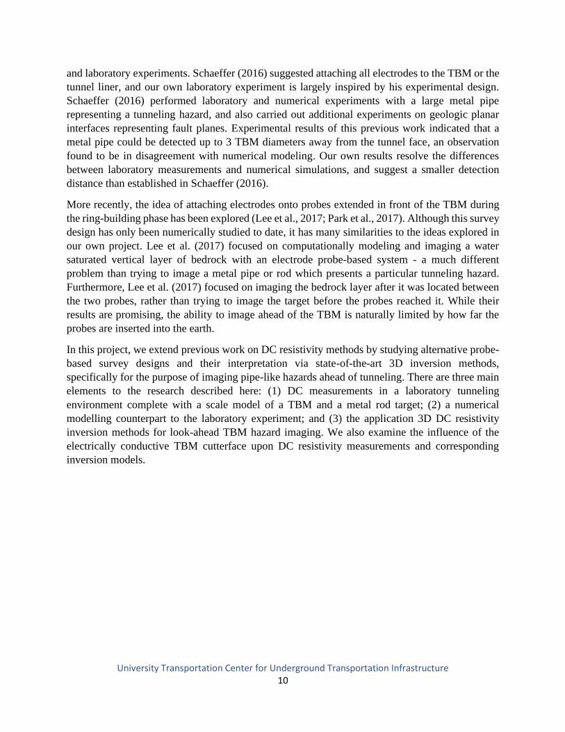
The laboratory environment, shown in Figure 2, consists of a large tank of water to mimic a
homogeneous host rock, a scale model TBM, and a miniature target. The tank measures 0.95m in
diameter. The tank was filled to a height of 1.2 with tap water that had a measured resistivity of
875 Ωm ± 5Ωm. Water was used in place of soil to improve experimental efficiency and is a
common method in geophysical scale-model experiments (Bleil, 1953; Frischknecht, 1988). Note
that Park et al. (2016) also explored DC resistivity in the context of mechanized tunneling and
performed their experiments in a water tank.
University Transportation Center for Underground Transportation Infrastructure 14
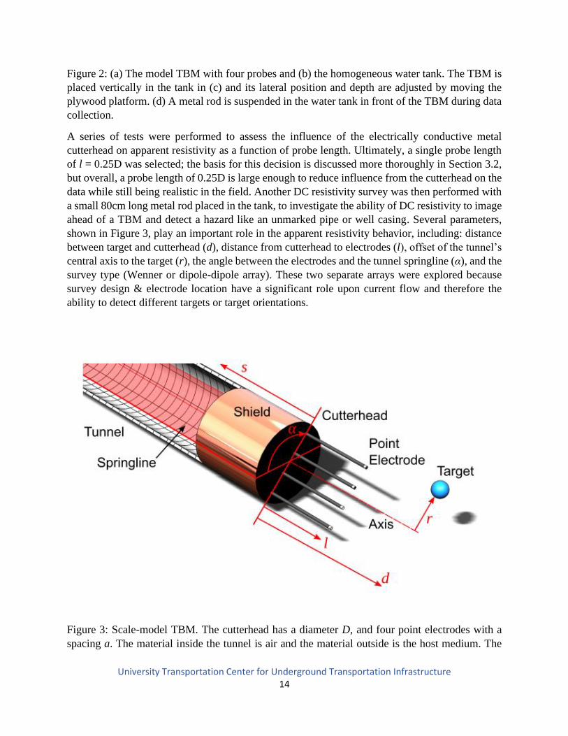
Figure 2: (a) The model TBM with four probes and (b) the homogeneous water tank. The TBM is
placed vertically in the tank in (c) and its lateral position and depth are adjusted by moving the
plywood platform. (d) A metal rod is suspended in the water tank in front of the TBM during data
collection.
A series of tests were performed to assess the influence of the electrically conductive metal
cutterhead on apparent resistivity as a function of probe length. Ultimately, a single probe length
of l = 0.25D was selected; the basis for this decision is discussed more thoroughly in Section 3.2,
but overall, a probe length of 0.25D is large enough to reduce influence from the cutterhead on the
data while still being realistic in the field. Another DC resistivity survey was then performed with
a small 80cm long metal rod placed in the tank, to investigate the ability of DC resistivity to image
ahead of a TBM and detect a hazard like an unmarked pipe or well casing. Several parameters,
shown in Figure 3, play an important role in the apparent resistivity behavior, including: distance
between target and cutterhead (d), distance from cutterhead to electrodes (l), offset of the tunnel’s
central axis to the target (r), the angle between the electrodes and the tunnel springline (α), and the
survey type (Wenner or dipole-dipole array). These two separate arrays were explored because
survey design & electrode location have a significant role upon current flow and therefore the
ability to detect different targets or target orientations.
Figure 3: Scale-model TBM. The cutterhead has a diameter D, and four point electrodes with a
spacing a. The material inside the tunnel is air and the material outside is the host medium. The

University Transportation Center for Underground Transportation Infrastructure 15
cutterhead can rotate about its center axis and the angle of rotation (α) is measured with respect to
the tunnel springline (the horizontal and transparent red plane in diagram). An example target (in
this case a resistive, spherical cavity) is located a distance d in front of the cutterhead and offset a
distance r radially from the center. The electrodes extend a distance l in front of the cutterhead and
are electrically isolated. The cutterhead is located a distance s from the tunnel entrance.
The scale-model TBM in Figure 2a was constructed to replicate a real TBM in both spatial
dimensions and material properties. The cutterhead has a diameter (D) equal to 89mm, a shield
that extends 1.125D into the tunnel and is made of copper (with resistivity on the order of 10-8
Ω·m) to mimic the high electrical conductivity of a real TBM. In addition, the cutterhead has a
section of PVC pipe (on the order of 10−13 Ω·m) inserted behind it to mimic a resistive, concrete
tunnel liner. The full model TBM (cutterhead, shield, and PVC tunnel liner) is then inserted
vertically into a tank of water as shown in Figure 2b, to mimic the tunneling environment.
The model TBM is equipped with four electrodes, extending directly in front of the cutterhead by
a distance of 0.25D (an appropriate distance as established by our target-free tests) and which are
electrically isolated from the TBM to act as point electrodes. Electrode separation a is 23mm and
used for both Wenner and dipole-dipole arrays. All data collected with the Wenner and dipole-
dipole survey designs are transformed into a wholespace apparent resistivity value with Equations
2 and 4, respectively. Unlike the survey used by Lee et al. (2017) which makes multiple
measurements from an array of electrodes on two probes, our design is intended to be performed
each time the TBM stops for the ring building phase.
The final component of the laboratory model is the target, a metal rod that is 4.8mm in diameter
(just greater than D/20), 0.8 meters (9D) long, and a resistivity on the order of 10-6 Ω·m. The target
is initially placed a distance 1.01D away from the TBM and is moved forward in 10mm increments
(0.11D) until it reaches the cutterhead. While a larger target can be detected from a greater
distance; the small diameter of 4.8mm was selected to maintain a realistic scale when considering
a common TBM diameter of 7 meters and the typical dimensions of pipes and well casings. We
also measured the response of a 108 Ω·m, 1.78cm diameter plastic sphere meant to represent a
resistive air-filled cavity: the data is provided in Appendix B but is not examined in this study.
Section 3.2 - Results
Figure 4 shows the influence of the electrically conductive metallic cutterhead upon apparent
resistivity as a function of l/D (raw data included in Appendix B, Table 1). When l/D is close to
zero, the data is highly sensitive to the copper cutterhead and over 99% of the electrical current
flows into the metal rather than into the tank water (or earth, in a full-scale experiment). As l/D
increases, the apparent resistivity approaches the true resistivity; once l = 0.5D, over 97% of the
current flows into the water (earth). However, extending the probes a distance of 0.5D during each
tunnel liner ring building phase in the field is technically challenging and time consuming, so a
majority of experiments in this paper fix the probe extension at l = 0.25D. This distance was
selected as a compromise between extending the electrodes as far ahead of the TBM as possible
and being feasible in the field. At this distance, a large majority (82%) of the electrical current is
flowing into the water (earth). For comparison (not shown here), we repeated this experiment
University Transportation Center for Underground Transportation Infrastructure 16
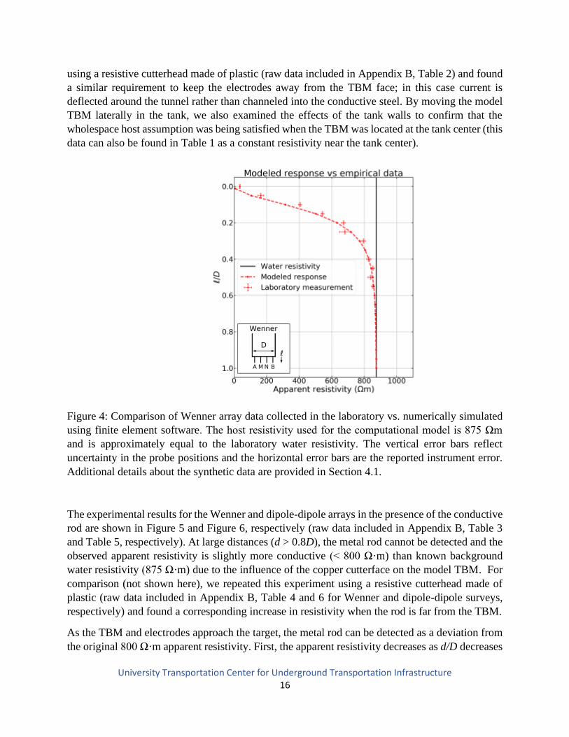
using a resistive cutterhead made of plastic (raw data included in Appendix B, Table 2) and found
a similar requirement to keep the electrodes away from the TBM face; in this case current is
deflected around the tunnel rather than channeled into the conductive steel. By moving the model
TBM laterally in the tank, we also examined the effects of the tank walls to confirm that the
wholespace host assumption was being satisfied when the TBM was located at the tank center (this
data can also be found in Table 1 as a constant resistivity near the tank center).
Figure 4: Comparison of Wenner array data collected in the laboratory vs. numerically simulated
using finite element software. The host resistivity used for the computational model is 875 Ωm
and is approximately equal to the laboratory water resistivity. The vertical error bars reflect
uncertainty in the probe positions and the horizontal error bars are the reported instrument error.
Additional details about the synthetic data are provided in Section 4.1.
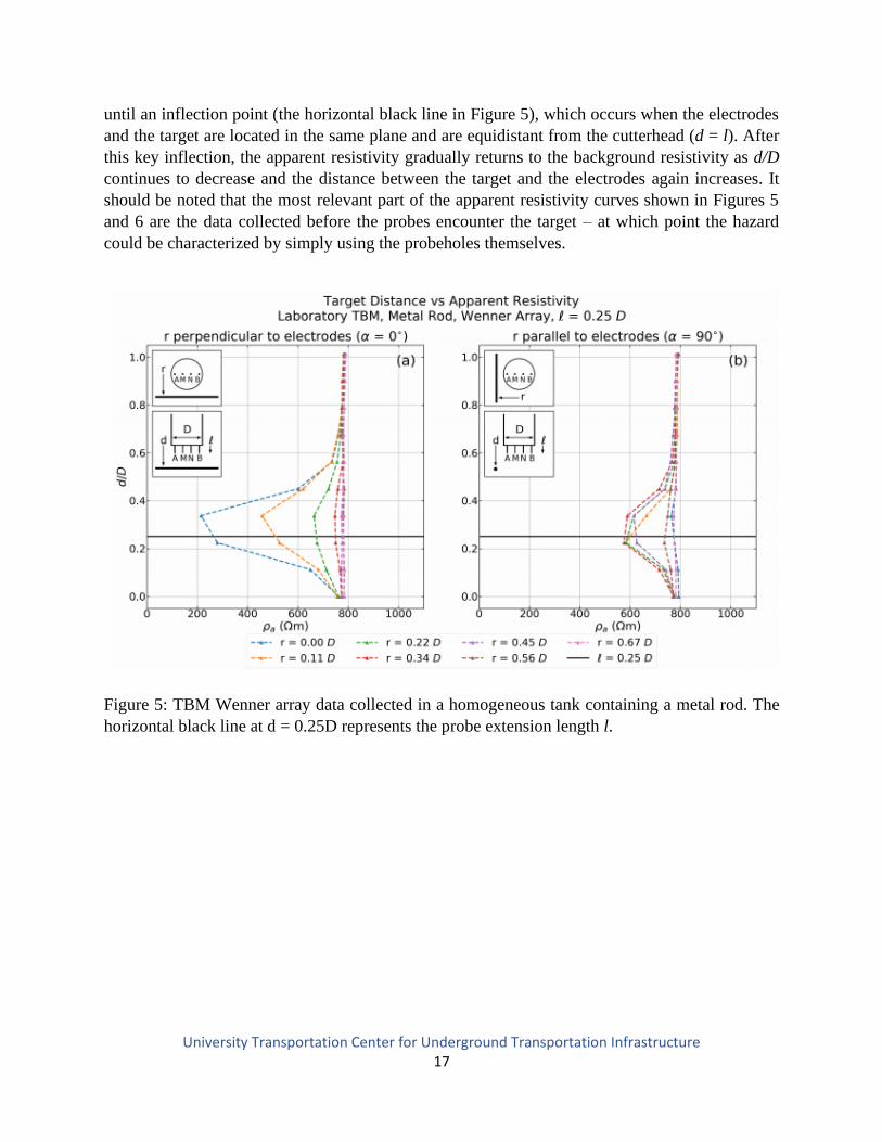
The experimental results for the Wenner and dipole-dipole arrays in the presence of the conductive
rod are shown in Figure 5 and Figure 6, respectively (raw data included in Appendix B, Table 3
and Table 5, respectively). At large distances (d > 0.8D), the metal rod cannot be detected and the
observed apparent resistivity is slightly more conductive (< 800 Ω·m) than known background
water resistivity (875 Ω·m) due to the influence of the copper cutterface on the model TBM. For
comparison (not shown here), we repeated this experiment using a resistive cutterhead made of
plastic (raw data included in Appendix B, Table 4 and 6 for Wenner and dipole-dipole surveys,
respectively) and found a corresponding increase in resistivity when the rod is far from the TBM.
As the TBM and electrodes approach the target, the metal rod can be detected as a deviation from
the original 800 Ω·m apparent resistivity. First, the apparent resistivity decreases as d/D decreases
University Transportation Center for Underground Transportation Infrastructure 17
until an inflection point (the horizontal black line in Figure 5), which occurs when the electrodes
and the target are located in the same plane and are equidistant from the cutterhead (d = l). After
this key inflection, the apparent resistivity gradually returns to the background resistivity as d/D
continues to decrease and the distance between the target and the electrodes again increases. It
should be noted that the most relevant part of the apparent resistivity curves shown in Figures 5
and 6 are the data collected before the probes encounter the target – at which point the hazard
could be characterized by simply using the probeholes themselves.
Figure 5: TBM Wenner array data collected in a homogeneous tank containing a metal rod. The
horizontal black line at d = 0.25D represents the probe extension length l.
University Transportation Center for Underground Transportation Infrastructure 18
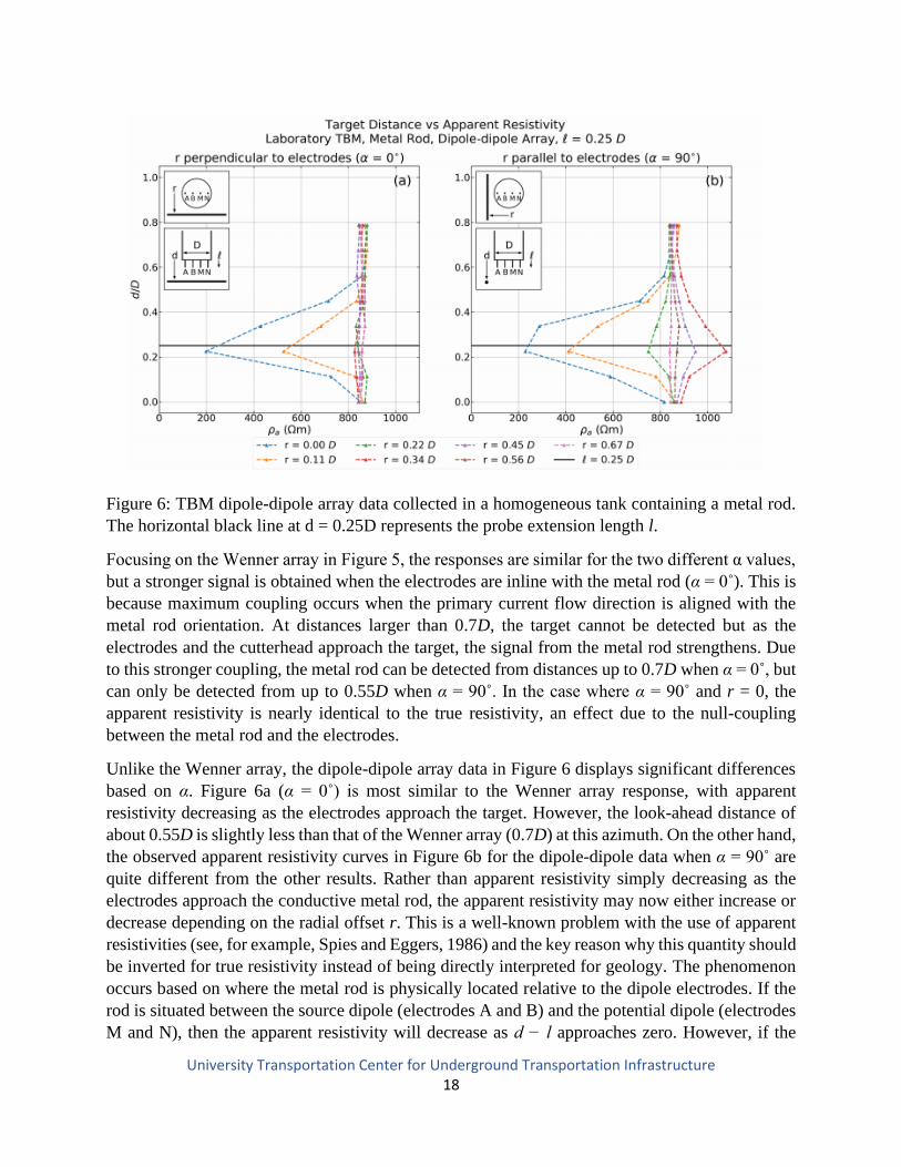
Figure 6: TBM dipole-dipole array data collected in a homogeneous tank containing a metal rod.
The horizontal black line at d = 0.25D represents the probe extension length l.
Focusing on the Wenner array in Figure 5, the responses are similar for the two different α values,
but a stronger signal is obtained when the electrodes are inline with the metal rod (α = 0˚). This is
because maximum coupling occurs when the primary current flow direction is aligned with the
metal rod orientation. At distances larger than 0.7D, the target cannot be detected but as the
electrodes and the cutterhead approach the target, the signal from the metal rod strengthens. Due
to this stronger coupling, the metal rod can be detected from distances up to 0.7D when α = 0˚, but
can only be detected from up to 0.55D when α = 90˚. In the case where α = 90˚ and r = 0, the
apparent resistivity is nearly identical to the true resistivity, an effect due to the null-coupling
between the metal rod and the electrodes.
Unlike the Wenner array, the dipole-dipole array data in Figure 6 displays significant differences
based on α. Figure 6a (α = 0˚) is most similar to the Wenner array response, with apparent
resistivity decreasing as the electrodes approach the target. However, the look-ahead distance of
about 0.55D is slightly less than that of the Wenner array (0.7D) at this azimuth. On the other hand,
the observed apparent resistivity curves in Figure 6b for the dipole-dipole data when α = 90˚ are
quite different from the other results. Rather than apparent resistivity simply decreasing as the
electrodes approach the conductive metal rod, the apparent resistivity may now either increase or
decrease depending on the radial offset r. This is a well-known problem with the use of apparent
resistivities (see, for example, Spies and Eggers, 1986) and the key reason why this quantity should
be inverted for true resistivity instead of being directly interpreted for geology. The phenomenon
occurs based on where the metal rod is physically located relative to the dipole electrodes. If the
rod is situated between the source dipole (electrodes A and B) and the potential dipole (electrodes
M and N), then the apparent resistivity will decrease as d − l approaches zero. However, if the
University Transportation Center for Underground Transportation Infrastructure 19
metal rod is located between the two electrodes of either dipole, then the apparent resistivity will
increase as d − l approaches zero. Aside from this peculiar behavior, it should be noted that this
dipole-dipole survey design and orientation can detect a metal rod from distances up to 0.7D,
which is better than the Wenner array when α = 90˚.
In all survey designs, maximum coupling occurs when both α and r are minimized. The dipole-
dipole array is less sensitive to α than the Wenner array, although the response is more variable
with respect to r. The different responses of the survey designs with α is beneficial for extracting
information about the target location and orientation. In both survey designs, the metal rod cannot
be detected if r < D/2, meaning that observations are only sensitive to conductive pipe-like hazards
within the tunneling profile.
In summary, our experiments have shown that DC resistivity is capable of detecting targets on a
model TBM in laboratory conditions. It is particularly important for electrodes to be located far
enough in front of the cutterhead to reduce the influence of the conductive steel on the data. A
minimum distance of l > 0.25D is suggested to sufficiently reduce the TBM and a distance of l >
0.5D for the influence of the TBM to be negligible. Although no data was collected using a value
for D other than 89mm, none of the results are expected to change for different TBM diameters
given the linear scaling relationships fundamental to the theory of DC resistivity.
CHAPTER 4- FORWARD MODELLING EXPERIMENTS
Section 4.1 - Methods
Forward modeling is the process of calculating the expected data from a given model and a set of
material properties for each region of the model. In the case of DC resistivity, the model is a map
of true resistivity (ρ) assigned to each region or voxel, and the resulting apparent resistivity data
(ρa) can be calculated from the model using Laplace’s equation in all source-free regions.
Due to the geometric complexity of modeling a TBM and its surrounding environment, the finite
element method (FEM) is used for the forward calculation. The models were created with the C++
library TetGen (Si, 2015) and with assistance from BERT (Boundless Electrical Resistivity
Tomography), a geophysical library that was also used to perform the forward modeling
calculations (Günther and Rücker, 2017). BERT is a FEM forward modeling and inversion
program that uses unstructured meshes to provide solutions for complex and irregular geometries
by outsourcing the mesh generation to other programs (such as the TetGen library used here) which
auto-generate tetrahedral meshes with specific parameters. The benefit of these unstructured
meshes is the ability to accurately model the TBM and metal rod, which are not rectilinear in
nature. BERT further improves modeling accuracy by separately calculating the primary and
secondary electrical potentials in order to remove numerical errors. Readers can refer to Rücker et
al. (2006) and Coggon (1971) for additional information on details concerning BERT.
University Transportation Center for Underground Transportation Infrastructure 20
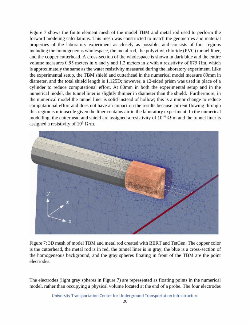
Figure 7 shows the finite element mesh of the model TBM and metal rod used to perform the
forward modeling calculations. This mesh was constructed to match the geometries and material
properties of the laboratory experiment as closely as possible, and consists of four regions
including the homogeneous wholespace, the metal rod, the polyvinyl chloride (PVC) tunnel liner,
and the copper cutterhead. A cross-section of the wholespace is shown in dark blue and the entire
volume measures 0.95 meters in x and y and 1.2 meters in z with a resistivity of 875 Ωm, which
is approximately the same as the water resistivity measured during the laboratory experiment. Like
the experimental setup, the TBM shield and cutterhead in the numerical model measure 89mm in
diameter, and the total shield length is 1.125D; however, a 12-sided prism was used in place of a
cylinder to reduce computational effort. At 80mm in both the experimental setup and in the
numerical model, the tunnel liner is slightly thinner in diameter than the shield. Furthermore, in
the numerical model the tunnel liner is solid instead of hollow; this is a minor change to reduce
computational effort and does not have an impact on the results because current flowing through
this region is minuscule given the liner contains air in the laboratory experiment. In the numerical
modelling, the cutterhead and shield are assigned a resistivity of 10−6 Ω·m and the tunnel liner is
assigned a resistivity of 106 Ω·m.
Figure 7: 3D mesh of model TBM and metal rod created with BERT and TetGen. The copper color
is the cutterhead, the metal rod is in red, the tunnel liner is in gray, the blue is a cross-section of
the homogeneous background, and the gray spheres floating in front of the TBM are the point
electrodes.
The electrodes (light gray spheres in Figure 7) are represented as floating points in the numerical
model, rather than occupying a physical volume located at the end of a probe. The four electrodes
University Transportation Center for Underground Transportation Infrastructure 21
are evenly spaced by 23mm in the x-direction and are centered about the TBM axis. For each
measurement, the electrodes are moved in the z-direction, beginning at 0.013D in front of the TBM
and then moving forward in 0.05D increments from 0.05D to 1.00D in front of the TBM, inclusive.
This is more comprehensive than the laboratory procedure, where l/D was fixed at 0.25D for all
experiments containing a target.
Finally, the metal rod was also approximated with a 12-sided prism, a length of 0.8 meters (or 9D),
a diameter of 4.8mm (just over D/20), and a resistivity of 10−6 Ω·m. As in the laboratory
experiment, the target begins at a distance of 1.01D away from the TBM and is moved toward the
TBM in 10mm increments (0.12D). A separate finite element mesh is used for each combination
of electrode positions, target distance, radial target offset, and target orientation to ensure that the
model space is properly discretized and convergence is obtained.
Section 4.2 – Results
Forward modeling was performed for both a Wenner array and a dipole-dipole array, and with and
without the metal rod. Figure 4 shows a comparison between the forward modeled response and
the laboratory measurements of a Wenner array in front of the TBM without the metal rod. This
comparison confirms that the numerical methods used are accurate, which was a concern because
of the possibility of singularities and numerical errors in the DC resistivity modelling problem (Li
and Spitzer, 2002). The comparison also confirms that the design of the numerical model in Figure
7 is satisfactory and provides a reassuring cross-check between laboratory and numerical results.
For the case of a metal rod target, numerical simulations were performed for all combinations of
d/D, r/D and α that were measured in the laboratory experiment. Numerical results are shown in
Figure 8 and Figure 9, and plotted in a similar manner to the experimental data in Figure 5 and
Figure 6. The numerical results strongly resemble the experimental results, providing additional
validation that the numerical code is correct and building confidence in the laboratory data. The
laboratory and numerical data differ at large distances (d > 0.8D), a result of uncertainties in the
experiment - such as the variation in the water tank resistivity over time, the precision required for
extending the electrodes to a distance of l = 0.25D, the differences between material properties in
the laboratory and in the computational model, and because the laboratory electrodes are slightly
larger than point electrodes.
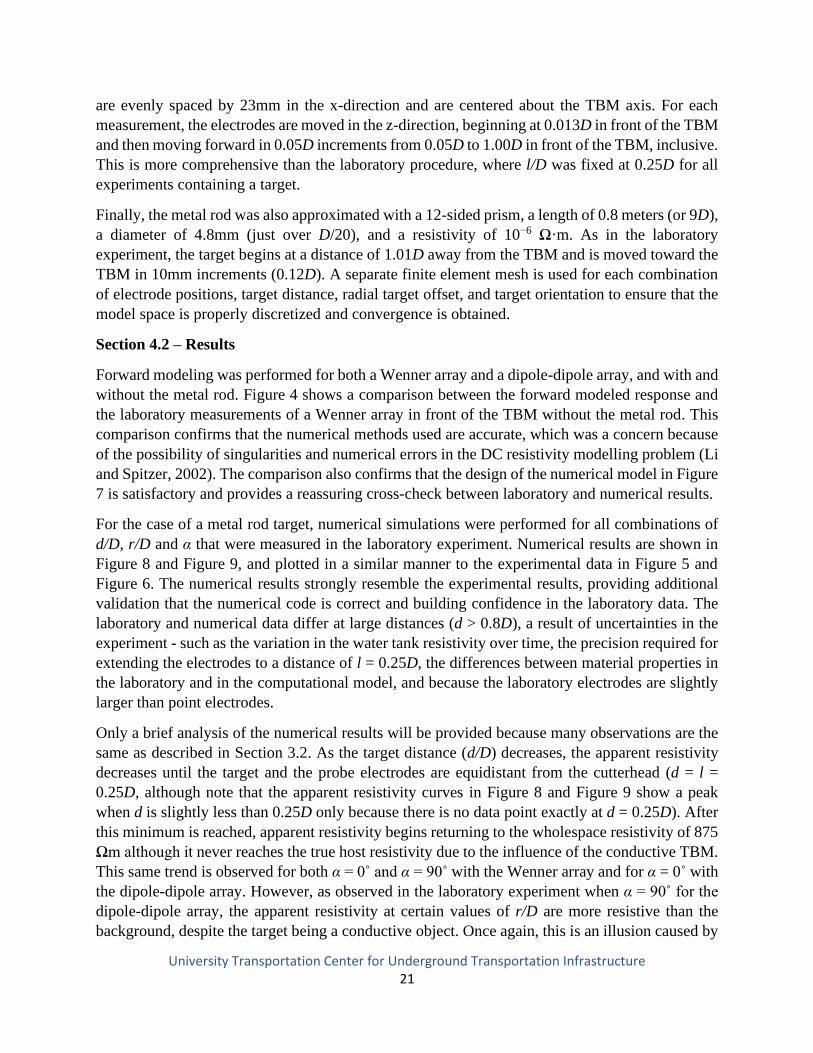
Only a brief analysis of the numerical results will be provided because many observations are the
same as described in Section 3.2. As the target distance (d/D) decreases, the apparent resistivity
decreases until the target and the probe electrodes are equidistant from the cutterhead (d = l =
0.25D, although note that the apparent resistivity curves in Figure 8 and Figure 9 show a peak
when d is slightly less than 0.25D only because there is no data point exactly at d = 0.25D). After
this minimum is reached, apparent resistivity begins returning to the wholespace resistivity of 875
Ωm although it never reaches the true host resistivity due to the influence of the conductive TBM.
This same trend is observed for both α = 0˚ and α = 90˚ with the Wenner array and for α = 0˚ with
the dipole-dipole array. However, as observed in the laboratory experiment when α = 90˚ for the
dipole-dipole array, the apparent resistivity at certain values of r/D are more resistive than the
background, despite the target being a conductive object. Once again, this is an illusion caused by
University Transportation Center for Underground Transportation Infrastructure 22
the relative positions of the metal rod and the electrode dipoles, and is an additional reason not to
directly use apparent resistivity as an interpretation tool to image hazards ahead of tunneling.
Figure 8: Forward calculation of Wenner data for a scale-model TBM in a tank, showing apparent
resistivity vs. the distance between the metal rod target and the TBM.

University Transportation Center for Underground Transportation Infrastructure 23
Figure 9: Forward calculation of dipole-dipole data for a scale-model TBM in a tank, showing
apparent resistivity vs. the distance between the metal rod target and the TBM.
CHAPTER 5- INVERSION AND IMAGING AHEAD OF A TBM
Section 5.1 - Methods
Inversion is a common technique in geophysics, typically used for producing physical property
images in one, two or three-dimensions. Forward modeling – as described in Chapter 4 - takes a
hypothetical model and applies known physics to calculate the expected data; in the case of DC
resistivity, the model is the true resistivity distribution and the data is apparent resistivity. Inversion
is the opposite process and attempts to reconstruct the original model by essentially mapping the
given data to a discretized physical property distribution. Difficulties arise in the inversion problem
due to the data space size (number of data points) often being smaller than the model space size
(number of voxels). Furthermore, non-uniqueness - meaning that there are an infinite number of
models that satisfy the data – is inherent in most geophysical inversion problems. Regularization
is often introduced to provide model constraints that incorporate prior information and to prevent
overfitting of the data, with the hope of producing more geologically realistic and unique models.
In addition, regularization allows information from other sources to be incorporated to reduce the
discrepancy between the data space size and the model space size. Such additional information
may include borehole data, other geophysical data, prior geologic knowledge and model
assumptions. In this report, such additional information includes the TBM structure, TBM material
properties, and in some cases the host resistivity.
University Transportation Center for Underground Transportation Infrastructure 24
In this chapter, we would like to assess how well a target can be identified using a survey design
as might be deployed in a field-scale TBM experiment. The survey geometries from the laboratory
and forward modeling experiments will not be used because there is not enough data to produce
reliable images without significant assumptions. This problem arises because there are only two
data points (the Wenner and dipole-dipole array measurements) for a given α value and tunneling
station, and the same four electrodes are used for each measurement. With such little information,
an inversion routine is seriously underdetermined and cannot discriminate whether the target is a
sphere, rod, or any other shape. Even with additional information from previous tunneling stations
or model assumptions (either about the host or target) the problem is still poorly posed. The
purpose of the survey designs introduced in this chapter is to reduce the number of possible
inversion solutions, by collecting more data and increasing data coverage ahead of the TBM. The
various surveys are also designed to be practical in the field given the challenging environment
expected during tunneling operations.
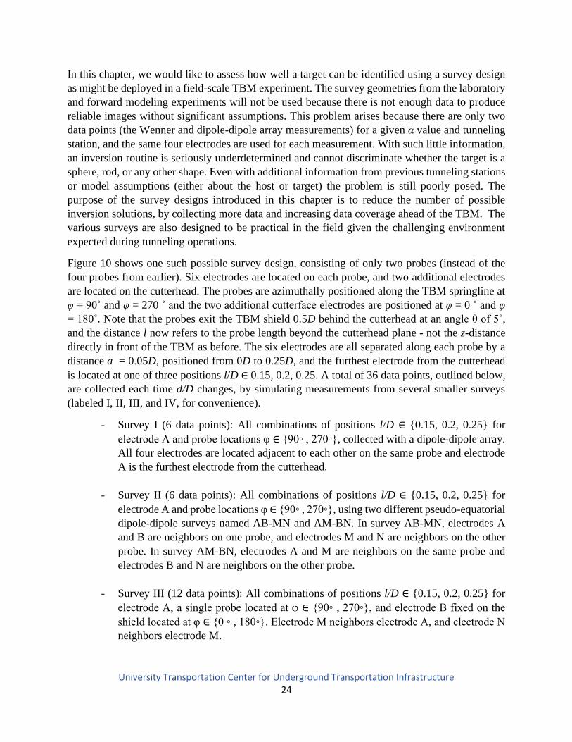
Figure 10 shows one such possible survey design, consisting of only two probes (instead of the
four probes from earlier). Six electrodes are located on each probe, and two additional electrodes
are located on the cutterhead. The probes are azimuthally positioned along the TBM springline at
φ = 90˚ and φ = 270 ˚ and the two additional cutterface electrodes are positioned at φ = 0 ˚ and φ
= 180˚. Note that the probes exit the TBM shield 0.5D behind the cutterhead at an angle θ of 5˚,
and the distance l now refers to the probe length beyond the cutterhead plane - not the z-distance
directly in front of the TBM as before. The six electrodes are all separated along each probe by a
distance a = 0.05D, positioned from 0D to 0.25D, and the furthest electrode from the cutterhead
is located at one of three positions l/D ∈ 0.15, 0.2, 0.25. A total of 36 data points, outlined below,
are collected each time d/D changes, by simulating measurements from several smaller surveys
(labeled I, II, III, and IV, for convenience).
- Survey I (6 data points): All combinations of positions l/D ∈ 0.15, 0.2, 0.25 for
electrode A and probe locations φ ∈ 90 , 270, collected with a dipole-dipole array.
All four electrodes are located adjacent to each other on the same probe and electrode
A is the furthest electrode from the cutterhead.
- Survey II (6 data points): All combinations of positions l/D ∈ 0.15, 0.2, 0.25 for
electrode A and probe locations φ ∈ 90 , 270, using two different pseudo-equatorial
dipole-dipole surveys named AB-MN and AM-BN. In survey AB-MN, electrodes A
and B are neighbors on one probe, and electrodes M and N are neighbors on the other
probe. In survey AM-BN, electrodes A and M are neighbors on the same probe and
electrodes B and N are neighbors on the other probe.
- Survey III (12 data points): All combinations of positions l/D ∈ 0.15, 0.2, 0.25 for
electrode A, a single probe located at φ ∈ 90 , 270, and electrode B fixed on the
shield located at φ ∈ 0 , 180. Electrode M neighbors electrode A, and electrode N
neighbors electrode M.
University Transportation Center for Underground Transportation Infrastructure 25
- Survey IV (12 data points): All combinations of positions l/D ∈ 0.15, 0.2, 0.25 for
electrodes A and M, electrode B positioned on the shield at φ ∈ 0 , 180, electrode
A located on one probe at φ ∈ 90 , 270, electrodes M and N neighboring each other
on the second probe, and a separation of ∆φ = 180 between the two probes.
Figure 10: Realistic survey design used for inversions. The probes are located 0.5D on the shield
behind the cutterhead and are flared outwards at an angle of 5˚. The complete survey is a
combination of surveys I, II, III, and IV (please refer to the text for a detailed description of each).
There are a total of 14 electrodes, used to collect 36 data points.
The forward modeling and inversion of this data is done with the same 3D tetrahedral mesh used
previously and the only difference is the electrode positions. The target is still a metal rod with a
resistivity of 10−6 Ωm and the host is homogeneous with a resistivity of 875 Ωm. More data could
have been simulated; however, the quantity was limited to what might be realistic in the field with
an instrument capable of measuring at multiple potential electrodes for each current injection
within the ring build time frame. A reasonable time requirement is to extend the probes in front of
the TBM, collect data, and retrieve the probes in less than 30 minutes. The inversion does not need
to be completed within this time window, but should be performed before the TBM has advanced
a significant distance. The maximum time allocated to performing an inversion depends on various
TBM parameters and the local geology, but completing the inversion and interpreting the results
within an additional 30 minutes should be a good rule of thumb. With this context, the inversions
presented here are performed with a focus more on run time rather than constructed model quality.
While model quality is still important, the model can only be used if it can be computed fast enough
in the field. All inversions in this paper were performed on a personal laptop (ASUS Q534UXK)
with the following specifications: Intel i7-7500U CPU, 16 GB of RAM, a Nvidia GeForce GTX
950M GPU, and running Windows 10.
Although we did not perform any field-scale experiments in this project, it is important to consider
how such a survey design as indicated in Figure 10 may be implemented in the field and identify
any limitations. One method is to attach the probes to hydraulics within the TBM and push them
University Transportation Center for Underground Transportation Infrastructure 26
into the surrounding earth, using the same equipment used to create exploratory probe holes and
perform jet grouting. However, this pushing method is only feasible in soft soils. Performing such
a routine in rock would require drilling a probe hole, which is a more time-intensive process that
cannot be done during each ring-building phase.
Section 5.2 – Results
The results from two separate sets of inversions for r/D = 0 and α = 0˚ are shown in Figure 11 and
Figure 12. The first set of inversions (Figure 11) include prior information of the TBM shape,
TBM material properties, and the background resistivity of the wholespace. The second set of
inversions (Figure 12) contain the same prior information and incorporates additional data from
previous TBM positions in a time-lapse inversion. Computations for the first set of inversions were
performed in 3 to 11 minutes and the time-lapse inversions were performed in under 18 minutes
(total time). Run time was largely a factor of how many iterations were required for the inversion
results to converge; more iterations were required when the target was closer (given the increasing
model complexity), and when time-lapse inversions were performed.
Prior information about the TBM was included by essentially extracting the 3D TBM mesh and its
material properties from the forward modeling and directly inputting it directly into the inverse
model solution. This is a valid approach because information on the TBM specifications are well
known in the field. It also has the benefit of decreasing the size of the model space, which also
decreases the inversion run time.
Prior information about the host background resistivity is not as well known in the field, but
boreholes, surface DC resistivity, and other on-site surveys can provide rough estimates of local
geology and electrical resistivity. Such models can be included in the inversion process to guide
the final results. This is different from including the TBM prior information, which is considered
a known value, whereas the geologic prior information is treated more as an initial best guess.
Additional prior information for an initial guess of the target size, shape, position, and resistivity
could also be included, but was not used because the goal here is to assess inversion & imaging
performance with the minimal amount of additional information.
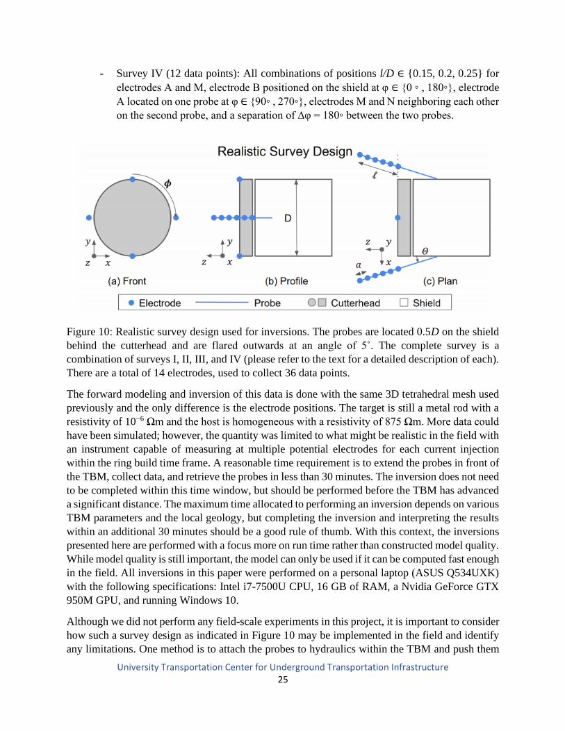
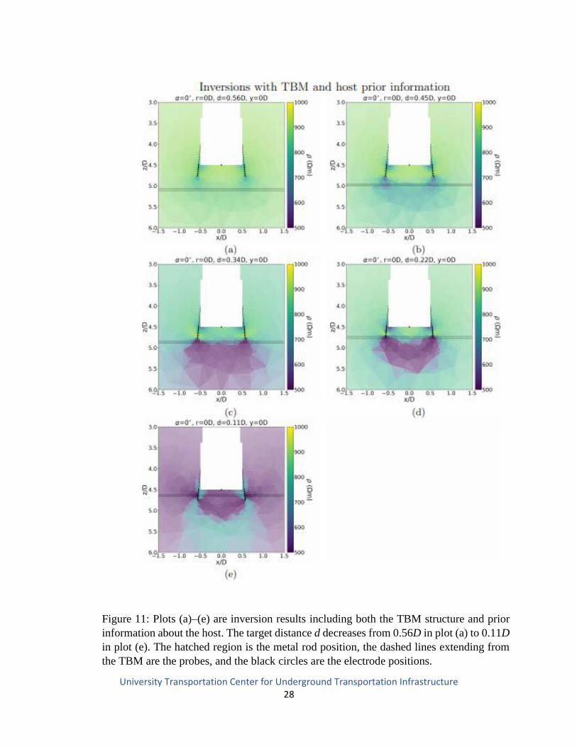
The results in Figure 11 show that the data can be successfully inverted to image the target. In
Figure 11c, when the metal rod is 0.34D in front of the TBM, the inversion successfully recovers
the background resistivity and obtains an oblong conductive body. Although, this recovered body
is larger than the metal rod, the envelope begins at the correct position in z. The inverted model at
d = 0.22D shows a similar result, but the resulting body is even more compact. Given the small
quantity of data and the inherent non-unique nature of the problem, these results are better than
expected.
However, as shown in Figure 11e (when d = 0.11D), the constructed model can also falsely appear
as a resistive body in a relatively conductive host. This is due to insufficient data coverage that
leads the inversion to interpret the very close and extremely conductive signal from the metal rod
as the background. This instability in the constructed model caused by the target position and
inadequate data quantity is an important reason for performing a time-lapse inversion.
University Transportation Center for Underground Transportation Infrastructure 27
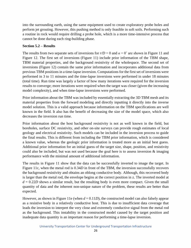
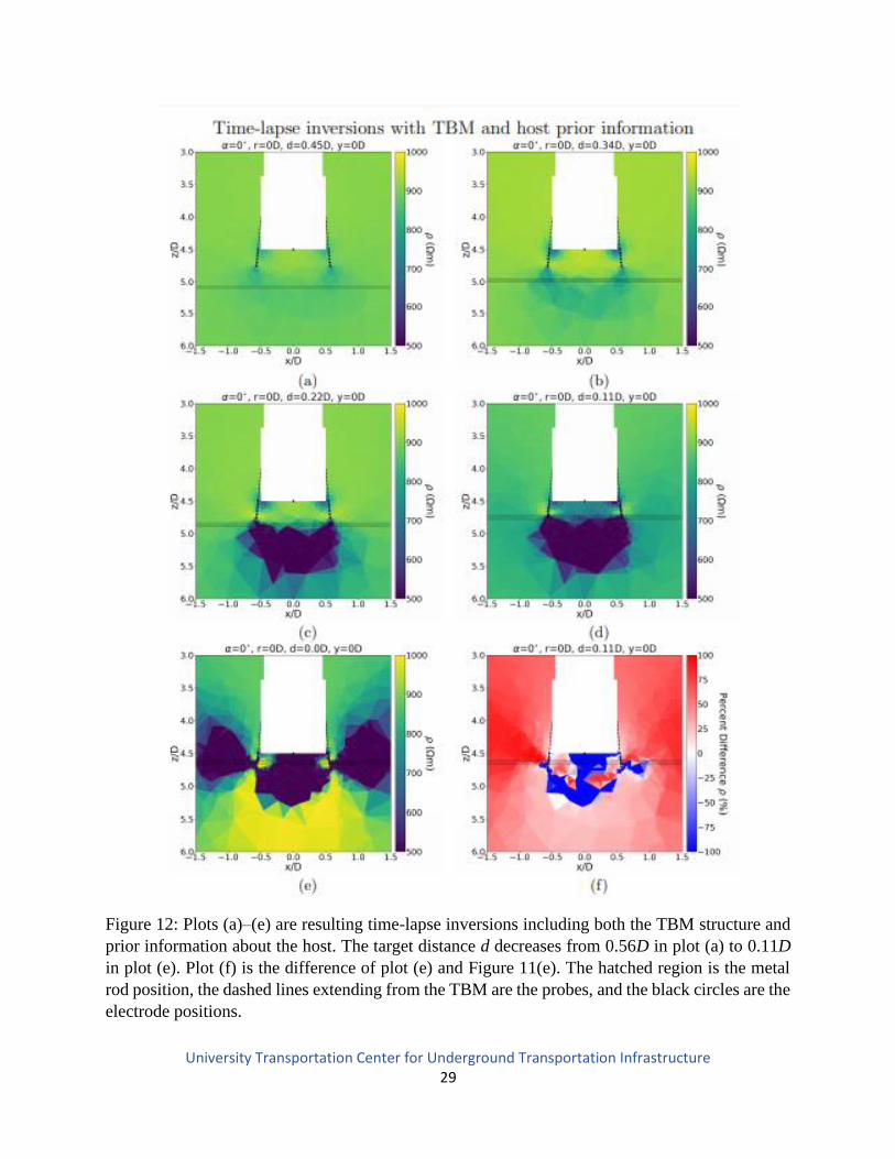
The advantage of a time-lapse inversion is that it improves imaging stability. At large distances,
such as d > 0.5D, the metal rod cannot be imaged, even though an apparent resistivity anomaly
can be detected (as indicated in Figures 5, 6, 8 and 9). When the target is at a distance of 0.45D it
can be faintly imaged, but noise in the field may obscure the result. As d/D continues decreasing,
similar results to the single-phase inversions are obtained. However, the background is better
constrained from the results of previous inversions, and the conductive body no longer displays as
much curvature in Figure 12d as we observe in Figure 11d. In the extreme case where the metal
rod distance is 0.11D, the constructed model in Figure 12e is significantly improved compared to
Figure 11e. This is largely because the background resistivity is better imaged from earlier stages
of the time-lapse process.
Hazard detection distance is limited by the presence of absence of an apparent resistivity anomaly,
while imaging quality is additionally limited by the quantity of data, the use of additional
information, and how well the inversion can be optimized in a time window. The maximum
imaging distance of 0.45D can be increased by further inserting the probes into the earth
(increasing l/D). Another approach is to use a model reference in the inversion, which is a best
guess of a possible target structure, to attempt to image a detected apparent resistivity anomaly.
However, as previously explained, the goal here is to understand the capabilities of an inversion
without resorting to the use of such additional information.
University Transportation Center for Underground Transportation Infrastructure 28
Figure 11: Plots (a)–(e) are inversion results including both the TBM structure and prior
information about the host. The target distance d decreases from 0.56D in plot (a) to 0.11D
in plot (e). The hatched region is the metal rod position, the dashed lines extending from
the TBM are the probes, and the black circles are the electrode positions.
University Transportation Center for Underground Transportation Infrastructure 29
Figure 12: Plots (a)–(e) are resulting time-lapse inversions including both the TBM structure and
prior information about the host. The target distance d decreases from 0.56D in plot (a) to 0.11D
in plot (e). Plot (f) is the difference of plot (e) and Figure 11(e). The hatched region is the metal
rod position, the dashed lines extending from the TBM are the probes, and the black circles are the
electrode positions.
University Transportation Center for Underground Transportation Infrastructure 30
CHAPTER 6 – SUMMARY AND CONCLUSIONS
In this paper, the capabilities of DC resistivity as a look-ahead geophysical imaging tool during
TBM operations have been explored through laboratory experiments, forward modeling, and
inversion. An initial four-probe study was performed experimentally and numerically to determine
the conductive metal cutterhead influence upon the apparent resistivity data in a wholespace.
Results verified expectations that apparent resistivity returns to the background resistivity as a
function of (l/D)2. Furthermore, it provided an important insight about how much electrical current
is flowing into the earth, rather than into the cutterhead. Ideally l would be greater than 0.5D to
increase the look-ahead distance and for the TBM influence upon the data to be negligible, but a
distance of 0.25D was used in further experiments to ensure a majority of the current (82%) flows
into the earth, while still being feasible in the field.
After this initial baseline study, Wenner and dipole-dipole surveys were experimentally performed
with the four-probe survey design to determine how well a conductive rod-like target could be
detected. With the Wenner array, the target produces a response from distances up to 0.7D when
α = 0˚, and from up to 0.55D when α = 90˚. With the dipole-dipole array, the target could be
detected from distances up to 0.55D when α = 0˚ and from up to 0.7D when α = 90˚. Other than l
and array configuration, this detection distance is also a function of target size, shape and
conductivity contrast with the background.
Both the Wenner and dipole-dipole array survey designs show response variation with α, which is
beneficial for detecting the orientation of asymmetric targets. Targets away from the tunnel axis
can also be detected, although such hazards are difficult to quantify from apparent resistivity data
alone. Directly interpreting the apparent resistivities is misleading in some cases, which reinforces
the need to invert for true resistivity prior to interpreting the impact of a potential target on an
underground construction project. Forward modeling results supported the laboratory data and
showed the same trends in apparent resistivity as a function of d/D, α, and r.
A more realistic survey design consisting of fewer probes and more data points was then studied
through the inversion of synthetic data. Such a design was chosen because there are is not enough
data (1–4 data points at each discrete value of d/D) in the original four probe method to properly
construct an image of the target through geophysical inversion. Initial results show that the target
can be imaged by including the TBM shape, its material properties, and some constraints on the
background resistivity. The inversion imaged a conductive rod as an elongated conductive body,
with the correct orientation. A more advanced time-lapse inversion, utilizing apparent resistivity
data from previous TBM positions, resulted in a more accurate background resistivity and also
produced more stable results closer to the TBM. However, while the target could be detected from
distances up to 0.7D, quantitative imaging the target cannot be performed until distances of less
than 0.45D. This imaging distance is smaller than the detection distance because the inversion
requires a certain amount of data coverage related to the target before converging on a meaningful
solution.

University Transportation Center for Underground Transportation Infrastructure 31
Overall, our experimental and numerical results were successful in showing how well DC
resistivity can be applied in a tunneling environment to detect and image targets; however, there
is still more research to be done. Studies should be performed on targets with different shapes or
material properties located off-axis from the cutterhead, to determine the extent of hazard
detectability. In addition, a field experiment on a full-scale TBM is recommended; such an
experiment would test the practicality of a probe-based survey during each ring building phase.
Finally, we suggest revisiting the topic of induced-polarization (IP), which has previously been
collected commercially (Kaus and Boening, 2008) and in the laboratory (Park et al., 2018) together
with DC resistivity data. Applying a probe-based IP survey design may provide additional
opportunities for data collection, and subsequent joint DC-IP inversion would be advantageous for
hazard detection and imaging.

University Transportation Center for Underground Transportation Infrastructure 32
REFERENCES
Bai-Yao, R., Xiao-Kang, D., Hai-Fei, L., Li, Z., 2009. Research on a new method of advanced
focus detection with DC resistivity in tunnels. Chinese Journal of Geophysics 52, 250–259.
Bharadwaj, P., Drijkoningen, G., Mulder, W., Thorbecke, J., Neducza, B., Jenneskens, R., 2017.
A shear-wave seismic system using full-waveform inversion to look ahead of a tunnel-boring
machine. Near Surface Geophysics 15, 210–224.
Bleil, D.F., 1953. Induced polarization: A method of geophysical prospecting. Geophysics 18,
636–661.
Coggon, J.H., 1971. Electromagnetic and electrical modeling by the finite element method.
Geophysics 36, 132–155.
Frischknecht, F.C., 1988. Electromagnetic methods in applied geophysics: Volume 1, theory.
Society of Exploration Geophysicists. chapter Electromagnetic Physical Scale Modeling. pp. 364–
441.
Günther, T., Rücker, C., 2017. Boundless Electrical Resistivity Tomography BERT 2 - the user
tutorial.
Herman, R., 2001. An introduction to electrical resistivity in geophysics. American Journal of
Physics 69, 943–952.
Jianlei, G., Xiu, L., 2016. Research of multi component response characteristics of array antenna
source transient electromagnetic tunnel detection, in: 7th International Conference on Environment
and Engineering Geophysics & Summit Forum of Chinese Academy of Engineering on
Engineering Science and Technology, Atlantis Press.
Kaus, A., Boening, W., 2008. BEAM - Geoelectric ahead monitoring of TBM-drives.
Geomechanics and Tunnelling 1, 442–449.
Lee, K.H., Park, J.H., Park, J., Lee, I.M., Lee, S.W., 2017. Electrical resistivity tomography survey
for prediction of anomaly ahead of tunnel face in mechanized tunneling, in: The 2017 World
Congress on Advances in Structural Engineering and Mechanics, ASEM17.
Li, S., Liu, B., Nie, L., Liu, Z., Tian, M., Wang, S., Su, M., Guo, Q., 2015. Detecting and
monitoring of water inrush in tunnels and coal mines using direct current resistivity method: A
review. Journal of Rock Mechanics and Geotechnical Engineering 7, 469–478.
Li, S., Sun, H., Lu, X., Li, X., 2014. Three-dimensional modeling of transient electromagnetic
responses of water-bearing structures in front of a tunnel face. Journal of Environmental and
Engineering Geophysics 19, 13–32.
University Transportation Center for Underground Transportation Infrastructure 33
Li, Y., Spitzer, K., 2002. Three-dimensional dc resistivity forward modelling using finite elements
in comparison with finite-difference solutions. Geophysical Journal International 151, 924–934.
Loke, M.H., 2000. Electrical imaging surveys for environmental and engineering studies.
http://pages.mtu.edu/ ctyoung/LOKENOTE.PDF.
Mooney, M.A., Karaoulis, M., Revil, A., 2013. Investigation of geoelectricwhile-tunneling
methods through numerical modeling. World Tunnel Congress.
Mooney, M.A., Walter, B., Frenzel, C., 2012. Real-time tunnel boring machine monitoring: A state
of the art review. North American Tunneling 2012 Proceedings.
Park, J., Lee, K., Kim, B., Choi, H., Lee, I., 2017. Predicting anomalous zone ahead of tunnel face
utilizing electrical resistivity: II. Field tests. Tunnelling and Underground Space Technology 68,
1–10.
Park, J., Lee, K., Park, J., Choi, H., Lee, I., 2016. Predicting anomalous zone ahead of tunnel face
utilizing electrical resistivity: I. Algorithm and measuring system development. Tunnelling and
Underground Space Technology 60, 141–150.
Park, J., Ryu, J., Choi, H., Lee, I., 2018. Risky ground prediction ahead of mechanized tunnel face
using electrical methods: Laboratory tests. KSCE Journal of Civil Engineering 22, 3663–3675.
Poletto, D., Petronio, L., 2006. Seismic interferometry with a tbm source of transmitted and
reflected waves. Society of Exploration Geophysicists 71, 85–93.
Rücker, C., Günther, T., Spitzer, K., 2006. Three-dimensional modelling and inversion of dc
resistivity data incorporating topography - i. modelling. Geophysics Journal International 166,
495–505.
Schaeffer, K., 2016. An experimental and computational investigation of electrical resistivity
imaging for prediction ahead of tunnel boring machines. Ph.D. thesis. Colorado School of Mines.
Schaeffer, K., Mooney, M., 2016. Examining the influence of tbmground interaction on electrical
resistivity imaging ahead of the tbm. Tunnelling and Underground Space Technology 58, 82–89.
doi:https://doi.org/10.1016/j.tust.2016.04.003.
Si, H., 2015. TetGen, a delaunay-based quality tetrahedral mesh generator. ACM Transactions on
Mathematical Software 41. Simi, A., Manacorda, G., 2016. The NeTTUN project: Design of a
GPR antenna for a TBM, in: 2016 16th International Conference on Ground Penetrating Radar
(GPR), IEEE. IEEE.
Spies, B.R., Eggers, D.E., 1986. The use and misuse of apparent resistivity in electromagnetic
methods. Journal of Geophysics 51, 1462–1471.
Sun, H., Li, X., Li, S., Qi, Z., Su, M., Xue, Y., 2012. Multi-component and multi-array TEM
detection in karst tunnels. Journal of Geophysics and Engineering 9, 359–373.
University Transportation Center for Underground Transportation Infrastructure 34
Wang, X., Sun, S., Wang, J., Yarovoy, A., Neducza, B., Manacorda, G., 2016. Real GPR signal
processing for target recognition with circular array antennas, in: 2016 URSI International
Symposium on Electromagnetic Theory (EMTS), IEEE. IEEE.
Ward, S.H., 1987. Electrical methods in geophysical prospecting. Methods in Experimental
Physics 24, 291–313.
Zohdy, A.A.R., Eaton, G.P., Mabey, D.R., 1970. Techniques of waterresources investigations of
the united states geological survey, in: Collection of environmental data. USGS. chapter
Application of surface geophysics to ground-water investigations, pp. 1–116.
University Transportation Center for Underground Transportation Infrastructure 35
APPENDIX A – TECHNOLOGY TRANSFER ACTIVITIES
1 Accomplishments
1.1 What was done? What was learned?
We performed scale-model laboratory experiments and numerical simulations to understand the
value of using DC resistivity on a Tunnel Boring Machine. Our laboratory data and forward
modeling results showed that using probes reduces interference caused by the metallic TBM body,
and increases the distance ahead of the machine at which a target may be detected. The TBM
influence on the data is significantly reduced once the probe is pushed 25% of the TBM diameter
ahead of the machine and negligible once the probes are pushed 50% ahead of the machine.
Depending on the specific survey design, targets can be detected up to 70% of the TBM diameter
away. We also inverted synthetic data to produce ahead-of-tunneling images using different
amounts of prior information (e.g. TBM geometry and host resistivity) and studied time-lapse
inversion, which has not been done for DC resistivity on a TBM before. Numerical results showed
a rod-like target can be imaged a distance up to 45% TBM diameter.
1.2 How have the results been disseminated?
Dissemination through 1 submitted journal publication, 1 international conference presentation
(and corresponding expanded abstract), 1 workshop presentation. Furthermore, Max Mifkovic’s
MS thesis was funded by the UTC-UTI and is archived at the Colorado School of Mines Library.
2 Participants and Collaborating Organizations
Name: Colorado School of Mines
Location: Golden, CO, 80401
Contribution: All research performed on campus
3 Outputs
Journal publications:
Mifkovic, M., Swidinsky, A., & Mooney, M., (in review): Imaging ahead of a Tunnel Boring
Machine with DC resistivity: A laboratory and numerical study. Tunneling and Underground
Space Technology. Submission number TUST_2020_166
Presentations
Mifkovic, M., Swidinsky, A., & Mooney, M., 2018: Imaging ahead of tunnel boring machines
with DC resistivity: A laboratory study: SEG conference, Anaheim, USA, October 14-19.
Major reports
University Transportation Center for Underground Transportation Infrastructure 36
Contributions to Three Program Progress Performance Reports (PPPRs) for the Department of
Transportation: “US DOT Tier 1 University Transportation Center for Underground
Transportation Infrastructure (UTC-UTI)” together with other UTC-UTI members.
Workshops
Presentation at the 1st UTC-UTI Workshop on February 18, 2018, hosted at the Colorado School
of Mines
4 Outcomes
Our experimental and numerical results have been successful in showing how DC resistivity can
be applied in a tunneling environment to detect and image potential hazards. Further studies should
be performed on targets with different shapes, material properties and locations around the
cutterhead to determine the limitations of TBM-based DC resistivity. Overall, we recommend a
field experiment on a real TBM to test the repeated use of a probe-based survey during each ring
building phase.
5 Impacts
The research contained in this report, submitted journal publication, conference presentation and
MS thesis provides the basis for a real DC resistivity experiment on a TBM. Our observations
concerning required probe lengths together with expectations for maximum cutterhead-hazard
detectability distances (both as a percentage of TBM diameter) will impact design of such large-
scale field experiments.
University Transportation Center for Underground Transportation Infrastructure 37
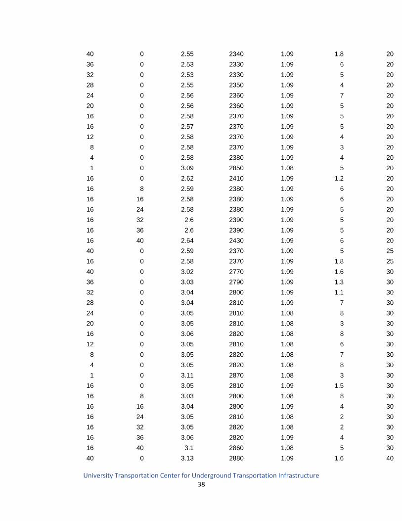
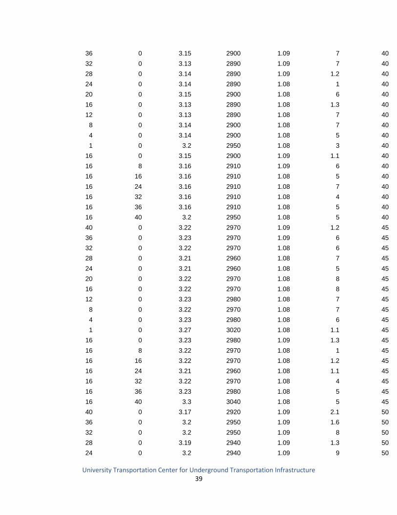
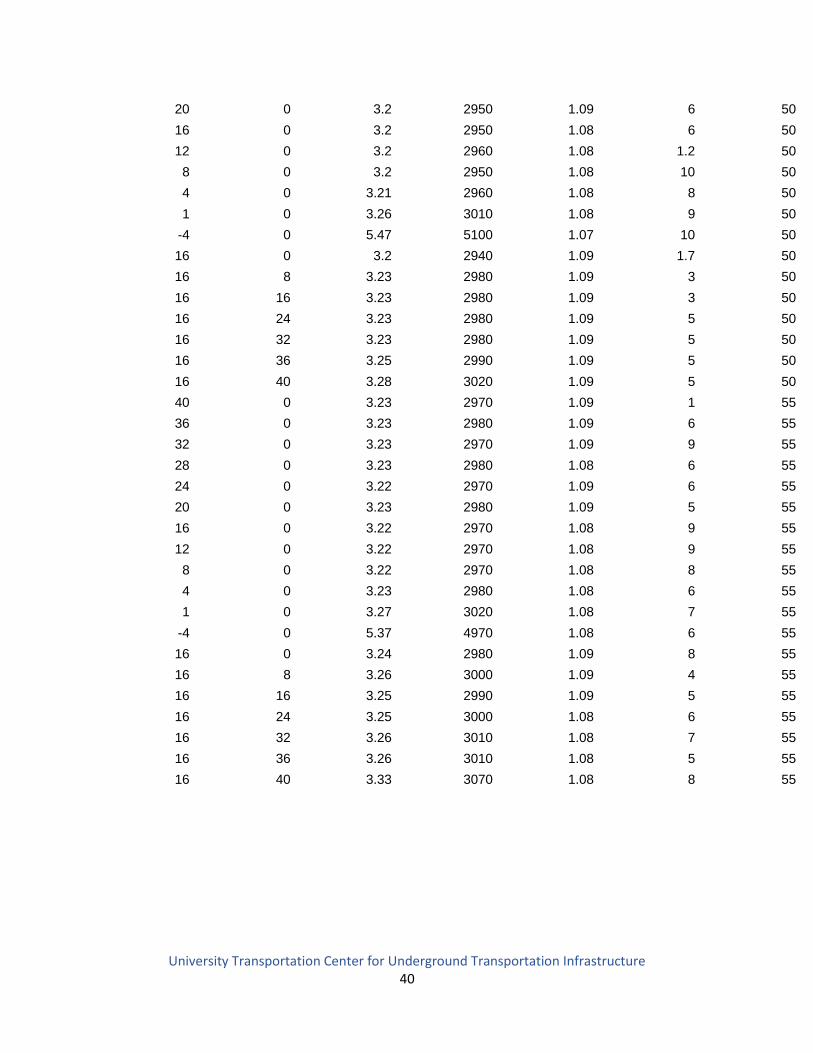
APPENDIX B - DATA FROM THE PROJECT
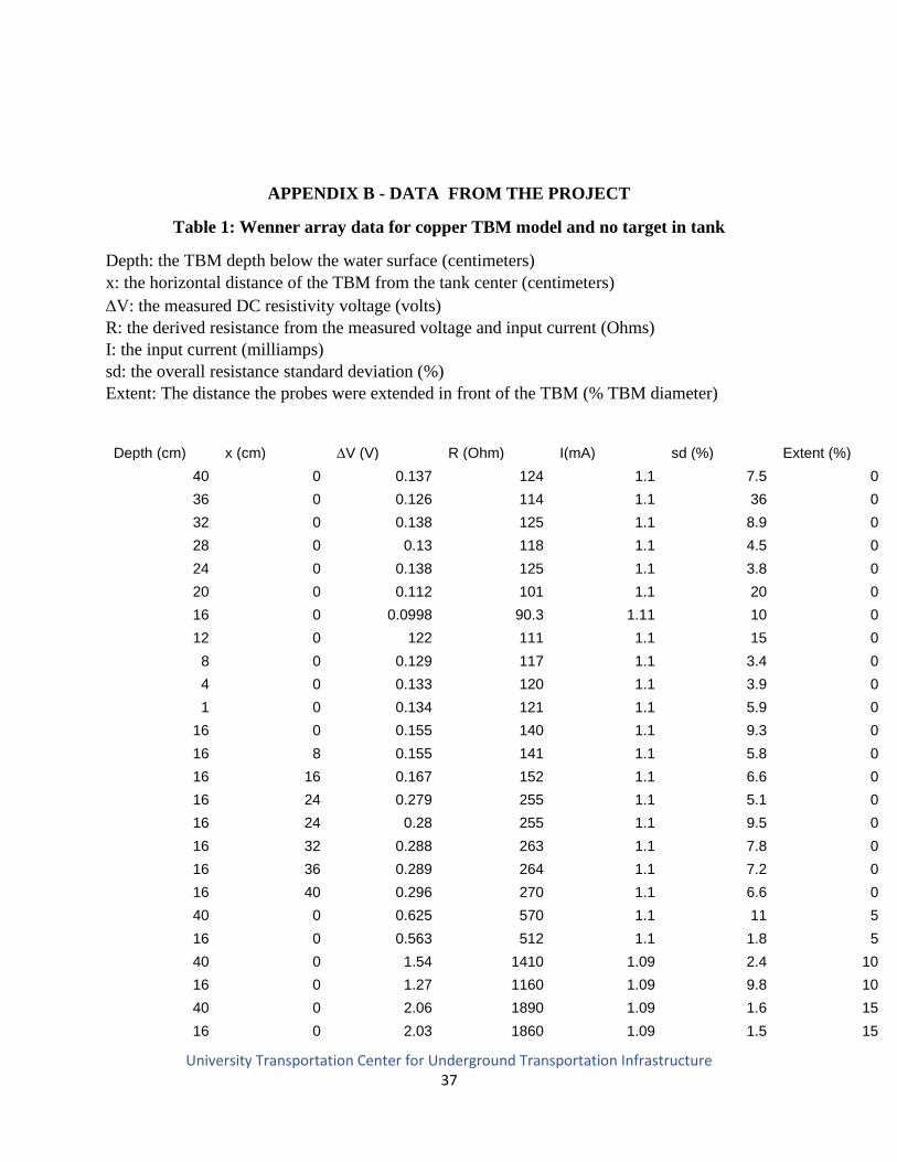
Table 1: Wenner array data for copper TBM model and no target in tank
Depth: the TBM depth below the water surface (centimeters)
x: the horizontal distance of the TBM from the tank center (centimeters)
V: the measured DC resistivity voltage (volts)
R: the derived resistance from the measured voltage and input current (Ohms)
I: the input current (milliamps)
sd: the overall resistance standard deviation (%)
Extent: The distance the probes were extended in front of the TBM (% TBM diameter)
Depth (cm) x (cm) V (V) R (Ohm) I(mA) sd (%) Extent (%)
40 0 0.137 124 1.1 7.5 0
36 0 0.126 114 1.1 36 0
32 0 0.138 125 1.1 8.9 0
28 0 0.13 118 1.1 4.5 0
24 0 0.138 125 1.1 3.8 0
20 0 0.112 101 1.1 20 0
16 0 0.0998 90.3 1.11 10 0
12 0 122 111 1.1 15 0
8 0 0.129 117 1.1 3.4 0
4 0 0.133 120 1.1 3.9 0
1 0 0.134 121 1.1 5.9 0
16 0 0.155 140 1.1 9.3 0
16 8 0.155 141 1.1 5.8 0
16 16 0.167 152 1.1 6.6 0
16 24 0.279 255 1.1 5.1 0
16 24 0.28 255 1.1 9.5 0
16 32 0.288 263 1.1 7.8 0
16 36 0.289 264 1.1 7.2 0
16 40 0.296 270 1.1 6.6 0
40 0 0.625 570 1.1 11 5
16 0 0.563 512 1.1 1.8 5
40 0 1.54 1410 1.09 2.4 10
16 0 1.27 1160 1.09 9.8 10
40 0 2.06 1890 1.09 1.6 15
16 0 2.03 1860 1.09 1.5 15
University Transportation Center for Underground Transportation Infrastructure 38
40 0 2.55 2340 1.09 1.8 20
36 0 2.53 2330 1.09 6 20
32 0 2.53 2330 1.09 5 20
28 0 2.55 2350 1.09 4 20
24 0 2.56 2360 1.09 7 20
20 0 2.56 2360 1.09 5 20
16 0 2.58 2370 1.09 5 20
16 0 2.57 2370 1.09 5 20
12 0 2.58 2370 1.09 4 20
8 0 2.58 2370 1.09 3 20
4 0 2.58 2380 1.09 4 20
1 0 3.09 2850 1.08 5 20
16 0 2.62 2410 1.09 1.2 20
16 8 2.59 2380 1.09 6 20
16 16 2.58 2380 1.09 6 20
16 24 2.58 2380 1.09 5 20
16 32 2.6 2390 1.09 5 20
16 36 2.6 2390 1.09 5 20
16 40 2.64 2430 1.09 6 20
40 0 2.59 2370 1.09 5 25
16 0 2.58 2370 1.09 1.8 25
40 0 3.02 2770 1.09 1.6 30
36 0 3.03 2790 1.09 1.3 30
32 0 3.04 2800 1.09 1.1 30
28 0 3.04 2810 1.09 7 30
24 0 3.05 2810 1.08 8 30
20 0 3.05 2810 1.08 3 30
16 0 3.06 2820 1.08 8 30
12 0 3.05 2810 1.08 6 30
8 0 3.05 2820 1.08 7 30
4 0 3.05 2820 1.08 8 30
1 0 3.11 2870 1.08 3 30
16 0 3.05 2810 1.09 1.5 30
16 8 3.03 2800 1.08 8 30
16 16 3.04 2800 1.09 4 30
16 24 3.05 2810 1.08 2 30
16 32 3.05 2820 1.08 2 30
16 36 3.06 2820 1.09 4 30
16 40 3.1 2860 1.08 5 30
40 0 3.13 2880 1.09 1.6 40
University Transportation Center for Underground Transportation Infrastructure 39
36 0 3.15 2900 1.09 7 40
32 0 3.13 2890 1.09 7 40
28 0 3.14 2890 1.09 1.2 40
24 0 3.14 2890 1.08 1 40
20 0 3.15 2900 1.08 6 40
16 0 3.13 2890 1.08 1.3 40
12 0 3.13 2890 1.08 7 40
8 0 3.14 2900 1.08 7 40
4 0 3.14 2900 1.08 5 40
1 0 3.2 2950 1.08 3 40
16 0 3.15 2900 1.09 1.1 40
16 8 3.16 2910 1.09 6 40
16 16 3.16 2910 1.08 5 40
16 24 3.16 2910 1.08 7 40
16 32 3.16 2910 1.08 4 40
16 36 3.16 2910 1.08 5 40
16 40 3.2 2950 1.08 5 40
40 0 3.22 2970 1.09 1.2 45
36 0 3.23 2970 1.09 6 45
32 0 3.22 2970 1.08 6 45
28 0 3.21 2960 1.08 7 45
24 0 3.21 2960 1.08 5 45
20 0 3.22 2970 1.08 8 45
16 0 3.22 2970 1.08 8 45
12 0 3.23 2980 1.08 7 45
8 0 3.22 2970 1.08 7 45
4 0 3.23 2980 1.08 6 45
1 0 3.27 3020 1.08 1.1 45
16 0 3.23 2980 1.09 1.3 45
16 8 3.22 2970 1.08 1 45
16 16 3.22 2970 1.08 1.2 45
16 24 3.21 2960 1.08 1.1 45
16 32 3.22 2970 1.08 4 45
16 36 3.23 2980 1.08 5 45
16 40 3.3 3040 1.08 5 45
40 0 3.17 2920 1.09 2.1 50
36 0 3.2 2950 1.09 1.6 50
32 0 3.2 2950 1.09 8 50
28 0 3.19 2940 1.09 1.3 50
24 0 3.2 2940 1.09 9 50
University Transportation Center for Underground Transportation Infrastructure 40
20 0 3.2 2950 1.09 6 50
16 0 3.2 2950 1.08 6 50
12 0 3.2 2960 1.08 1.2 50
8 0 3.2 2950 1.08 10 50
4 0 3.21 2960 1.08 8 50
1 0 3.26 3010 1.08 9 50
-4 0 5.47 5100 1.07 10 50
16 0 3.2 2940 1.09 1.7 50
16 8 3.23 2980 1.09 3 50
16 16 3.23 2980 1.09 3 50
16 24 3.23 2980 1.09 5 50
16 32 3.23 2980 1.09 5 50
16 36 3.25 2990 1.09 5 50
16 40 3.28 3020 1.09 5 50
40 0 3.23 2970 1.09 1 55
36 0 3.23 2980 1.09 6 55
32 0 3.23 2970 1.09 9 55
28 0 3.23 2980 1.08 6 55
24 0 3.22 2970 1.09 6 55
20 0 3.23 2980 1.09 5 55
16 0 3.22 2970 1.08 9 55
12 0 3.22 2970 1.08 9 55
8 0 3.22 2970 1.08 8 55
4 0 3.23 2980 1.08 6 55
1 0 3.27 3020 1.08 7 55
-4 0 5.37 4970 1.08 6 55
16 0 3.24 2980 1.09 8 55
16 8 3.26 3000 1.09 4 55
16 16 3.25 2990 1.09 5 55
16 24 3.25 3000 1.08 6 55
16 32 3.26 3010 1.08 7 55
16 36 3.26 3010 1.08 5 55
16 40 3.33 3070 1.08 8 55
University Transportation Center for Underground Transportation Infrastructure 41
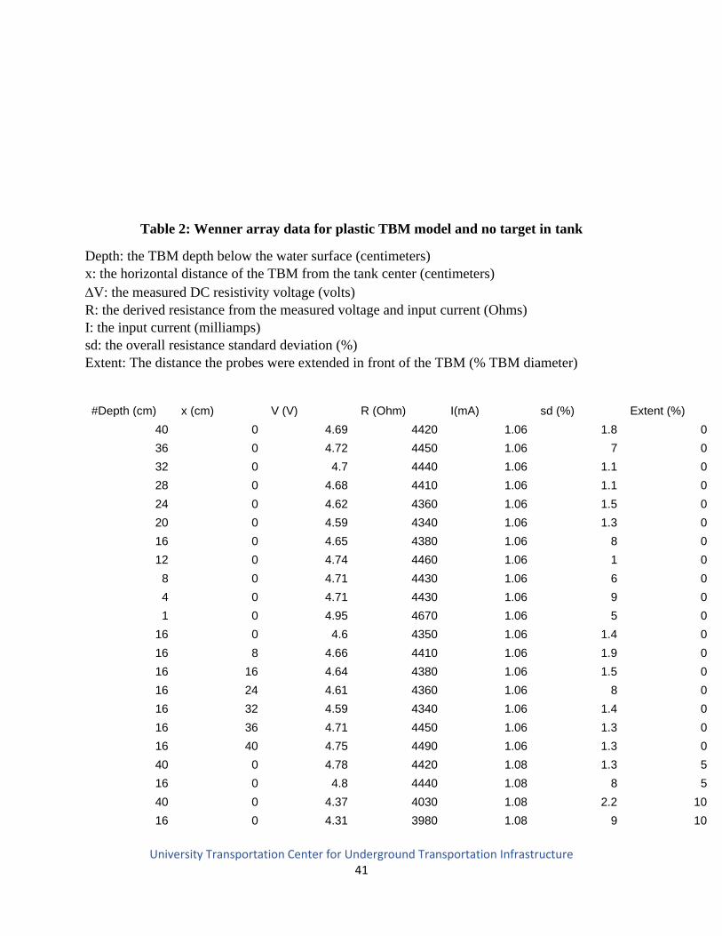
Table 2: Wenner array data for plastic TBM model and no target in tank
Depth: the TBM depth below the water surface (centimeters)
x: the horizontal distance of the TBM from the tank center (centimeters)
V: the measured DC resistivity voltage (volts)
R: the derived resistance from the measured voltage and input current (Ohms)
I: the input current (milliamps)
sd: the overall resistance standard deviation (%)
Extent: The distance the probes were extended in front of the TBM (% TBM diameter)
#Depth (cm) x (cm) V (V) R (Ohm) I(mA) sd (%) Extent (%)
40 0 4.69 4420 1.06 1.8 0
36 0 4.72 4450 1.06 7 0
32 0 4.7 4440 1.06 1.1 0
28 0 4.68 4410 1.06 1.1 0
24 0 4.62 4360 1.06 1.5 0
20 0 4.59 4340 1.06 1.3 0
16 0 4.65 4380 1.06 8 0
12 0 4.74 4460 1.06 1 0
8 0 4.71 4430 1.06 6 0
4 0 4.71 4430 1.06 9 0
1 0 4.95 4670 1.06 5 0
16 0 4.6 4350 1.06 1.4 0
16 8 4.66 4410 1.06 1.9 0
16 16 4.64 4380 1.06 1.5 0
16 24 4.61 4360 1.06 8 0
16 32 4.59 4340 1.06 1.4 0
16 36 4.71 4450 1.06 1.3 0
16 40 4.75 4490 1.06 1.3 0
40 0 4.78 4420 1.08 1.3 5
16 0 4.8 4440 1.08 8 5
40 0 4.37 4030 1.08 2.2 10
16 0 4.31 3980 1.08 9 10
University Transportation Center for Underground Transportation Infrastructure 42
40 0 4.11 3790 1.08 2.5 15
16 0 4.09 3770 1.08 1.3 15
40 0 3.87 3550 1.09 2.9 20
36 0 3.89 3580 1.09 1.4 20
32 0 3.89 3590 1.09 1.1 20
28 0 3.87 3570 1.08 1.5 20
24 0 3.85 3560 1.08 1 20
20 0 3.85 3560 1.08 1.3 20
16 0 3.86 3560 1.08 1.3 20
12 0 3.86 3570 1.08 8 20
8 0 3.87 3580 1.08 9 20
4 0 3.95 3650 1.08 8 20
1 0 4.89 4520 1.08 4 20
16 0 3.89 3590 1.08 2.9 20
16 8 3.91 3610 1.08 2 20
16 16 3.92 3620 1.08 2 20
16 24 3.91 3610 1.08 5 20
16 32 3.92 3620 1.08 4 20
16 36 3.92 3620 1.08 5 20
16 40 4 3700 1.08 6 20
40 0 3.57 3290 1.09 2.5 25
16 0 3.57 3290 1.08 1.2 25
40 0 3.53 3250 1.09 1.1 30
36 0 3.53 3250 1.08 8 30
32 0 3.52 3250 1.08 8 30
28 0 3.51 3240 1.08 6 30
24 0 3.51 3240 1.08 1 30
20 0 3.51 3240 1.08 9 30
16 0 3.52 3240 1.08 4 30
12 0 3.52 3250 1.08 7 30
8 0 3.53 3260 1.08 8 30
4 0 3.54 3260 1.08 1.1 30
1 0 3.69 3400 108 1.1 30
16 0 3.52 3250 1.09 2 30
16 8 3.84 3260 1.09 10 30
16 16 3.54 3270 1.08 3 30
16 24 3.54 3270 1.08 7 30
16 32 3.55 3270 1.09 6 30
16 36 3.57 3290 1.08 5 30
16 40 3.64 3360 1.08 6 30
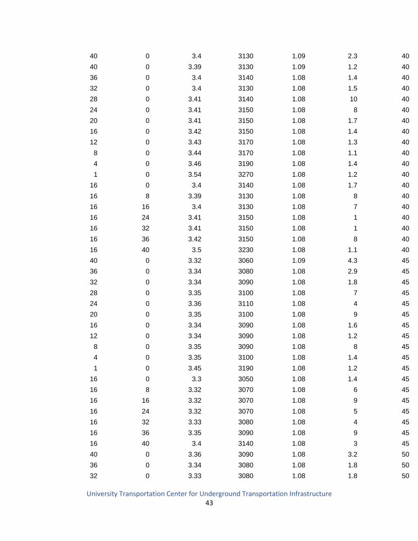
University Transportation Center for Underground Transportation Infrastructure 43
40 0 3.4 3130 1.09 2.3 40
40 0 3.39 3130 1.09 1.2 40
36 0 3.4 3140 1.08 1.4 40
32 0 3.4 3130 1.08 1.5 40
28 0 3.41 3140 1.08 10 40
24 0 3.41 3150 1.08 8 40
20 0 3.41 3150 1.08 1.7 40
16 0 3.42 3150 1.08 1.4 40
12 0 3.43 3170 1.08 1.3 40
8 0 3.44 3170 1.08 1.1 40
4 0 3.46 3190 1.08 1.4 40
1 0 3.54 3270 1.08 1.2 40
16 0 3.4 3140 1.08 1.7 40
16 8 3.39 3130 1.08 8 40
16 16 3.4 3130 1.08 7 40
16 24 3.41 3150 1.08 1 40
16 32 3.41 3150 1.08 1 40
16 36 3.42 3150 1.08 8 40
16 40 3.5 3230 1.08 1.1 40
40 0 3.32 3060 1.09 4.3 45
36 0 3.34 3080 1.08 2.9 45
32 0 3.34 3090 1.08 1.8 45
28 0 3.35 3100 1.08 7 45
24 0 3.36 3110 1.08 4 45
20 0 3.35 3100 1.08 9 45
16 0 3.34 3090 1.08 1.6 45
12 0 3.34 3090 1.08 1.2 45
8 0 3.35 3090 1.08 8 45
4 0 3.35 3100 1.08 1.4 45
1 0 3.45 3190 1.08 1.2 45
16 0 3.3 3050 1.08 1.4 45
16 8 3.32 3070 1.08 6 45
16 16 3.32 3070 1.08 9 45
16 24 3.32 3070 1.08 5 45
16 32 3.33 3080 1.08 4 45
16 36 3.35 3090 1.08 9 45
16 40 3.4 3140 1.08 3 45
40 0 3.36 3090 1.08 3.2 50
36 0 3.34 3080 1.08 1.8 50
32 0 3.33 3080 1.08 1.8 50
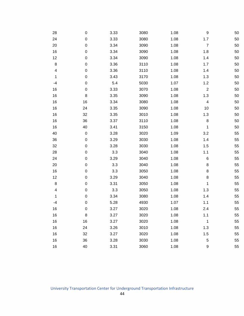
University Transportation Center for Underground Transportation Infrastructure 44
28 0 3.33 3080 1.08 9 50
24 0 3.33 3080 1.08 1.7 50
20 0 3.34 3090 1.08 7 50
16 0 3.34 3090 1.08 1.8 50
12 0 3.34 3090 1.08 1.4 50
8 0 3.36 3110 1.08 1.7 50
4 0 3.36 3110 1.08 1.4 50
1 0 3.43 3170 1.08 1.3 50
-4 0 5.4 5030 1.07 1.2 50
16 0 3.33 3070 1.08 2 50
16 8 3.35 3090 1.08 1.3 50
16 16 3.34 3080 1.08 4 50
16 24 3.35 3090 1.08 10 50
16 32 3.35 3010 1.08 1.3 50
16 36 3.37 3110 1.08 8 50
16 40 3.41 3150 1.08 1 50
40 0 3.28 3020 1.09 3.2 55
36 0 3.29 3030 1.08 1.4 55
32 0 3.28 3030 1.08 1.5 55
28 0 3.3 3040 1.08 1.1 55
24 0 3.29 3040 1.08 6 55
20 0 3.3 3040 1.08 8 55
16 0 3.3 3050 1.08 8 55
12 0 3.29 3040 1.08 8 55
8 0 3.31 3050 1.08 1 55
4 0 3.3 3050 1.08 1.3 55
1 0 3.34 3080 1.08 1.4 55
-4 0 5.28 4930 1.07 1.1 55
16 0 3.27 3020 1.08 2.4 55
16 8 3.27 3020 1.08 1.1 55
16 16 3.27 3020 1.08 1 55
16 24 3.26 3010 1.08 1.3 55
16 32 3.27 3020 1.08 1.5 55
16 36 3.28 3030 1.08 5 55
16 40 3.31 3060 1.08 9 55
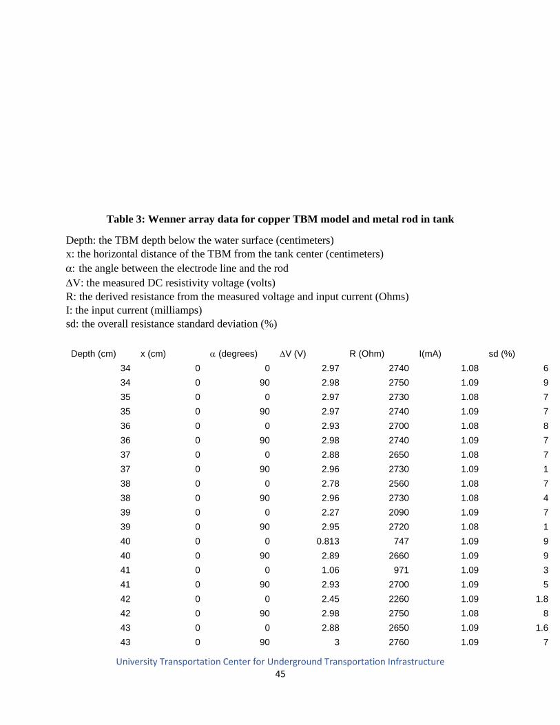
University Transportation Center for Underground Transportation Infrastructure 45
Table 3: Wenner array data for copper TBM model and metal rod in tank
Depth: the TBM depth below the water surface (centimeters)
x: the horizontal distance of the TBM from the tank center (centimeters)
the angle between the electrode line and the rod
V: the measured DC resistivity voltage (volts)
R: the derived resistance from the measured voltage and input current (Ohms)
I: the input current (milliamps)
sd: the overall resistance standard deviation (%)
Depth (cm) x (cm) (degrees) V (V) R (Ohm) I(mA) sd (%)
34 0 0 2.97 2740 1.08 6
34 0 90 2.98 2750 1.09 9
35 0 0 2.97 2730 1.08 7
35 0 90 2.97 2740 1.09 7
36 0 0 2.93 2700 1.08 8
36 0 90 2.98 2740 1.09 7
37 0 0 2.88 2650 1.08 7
37 0 90 2.96 2730 1.09 1
38 0 0 2.78 2560 1.08 7
38 0 90 2.96 2730 1.08 4
39 0 0 2.27 2090 1.09 7
39 0 90 2.95 2720 1.08 1
40 0 0 0.813 747 1.09 9
40 0 90 2.89 2660 1.09 9
41 0 0 1.06 971 1.09 3
41 0 90 2.93 2700 1.09 5
42 0 0 2.45 2260 1.09 1.8
42 0 90 2.98 2750 1.08 8
43 0 0 2.88 2650 1.09 1.6
43 0 90 3 2760 1.09 7
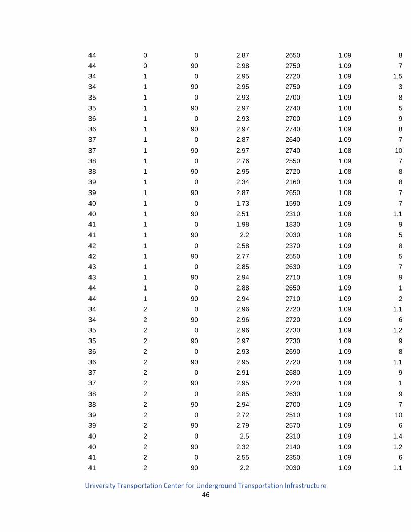
University Transportation Center for Underground Transportation Infrastructure 46
44 0 0 2.87 2650 1.09 8
44 0 90 2.98 2750 1.09 7
34 1 0 2.95 2720 1.09 1.5
34 1 90 2.95 2750 1.09 3
35 1 0 2.93 2700 1.09 8
35 1 90 2.97 2740 1.08 5
36 1 0 2.93 2700 1.09 9
36 1 90 2.97 2740 1.09 8
37 1 0 2.87 2640 1.09 7
37 1 90 2.97 2740 1.08 10
38 1 0 2.76 2550 1.09 7
38 1 90 2.95 2720 1.08 8
39 1 0 2.34 2160 1.09 8
39 1 90 2.87 2650 1.08 7
40 1 0 1.73 1590 1.09 7
40 1 90 2.51 2310 1.08 1.1
41 1 0 1.98 1830 1.09 9
41 1 90 2.2 2030 1.08 5
42 1 0 2.58 2370 1.09 8
42 1 90 2.77 2550 1.08 5
43 1 0 2.85 2630 1.09 7
43 1 90 2.94 2710 1.09 9
44 1 0 2.88 2650 1.09 1
44 1 90 2.94 2710 1.09 2
34 2 0 2.96 2720 1.09 1.1
34 2 90 2.96 2720 1.09 6
35 2 0 2.96 2730 1.09 1.2
35 2 90 2.97 2730 1.09 9
36 2 0 2.93 2690 1.09 8
36 2 90 2.95 2720 1.09 1.1
37 2 0 2.91 2680 1.09 9
37 2 90 2.95 2720 1.09 1
38 2 0 2.85 2630 1.09 9
38 2 90 2.94 2700 1.09 7
39 2 0 2.72 2510 1.09 10
39 2 90 2.79 2570 1.09 6
40 2 0 2.5 2310 1.09 1.4
40 2 90 2.32 2140 1.09 1.2
41 2 0 2.55 2350 1.09 6
41 2 90 2.2 2030 1.09 1.1
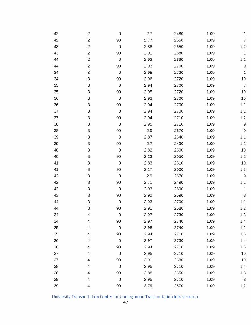
University Transportation Center for Underground Transportation Infrastructure 47
42 2 0 2.7 2480 1.09 1
42 2 90 2.77 2550 1.09 7
43 2 0 2.88 2650 1.09 1.2
43 2 90 2.91 2680 1.09 1
44 2 0 2.92 2690 1.09 1.1
44 2 90 2.93 2700 1.09 9
34 3 0 2.95 2720 1.09 1
34 3 90 2.96 2720 1.09 10
35 3 0 2.94 2700 1.09 7
35 3 90 2.95 2720 1.09 10
36 3 0 2.93 2700 1.09 10
36 3 90 2.94 2700 1.09 1.1
37 3 0 2.94 2700 1.09 1.1
37 3 90 2.94 2710 1.09 1.2
38 3 0 2.95 2710 1.09 9
38 3 90 2.9 2670 1.09 9
39 3 0 2.87 2640 1.09 1.1
39 3 90 2.7 2490 1.09 1.2
40 3 0 2.82 2600 1.09 10
40 3 90 2.23 2050 1.09 1.2
41 3 0 2.83 2610 1.09 10
41 3 90 2.17 2000 1.09 1.3
42 3 0 2.9 2670 1.09 9
42 3 90 2.71 2490 1.09 1.1
43 3 0 2.93 2690 1.09 1
43 3 90 2.92 2690 1.09 8
44 3 0 2.93 2700 1.09 1.1
44 3 90 2.91 2680 1.09 1.2
34 4 0 2.97 2730 1.09 1.3
34 4 90 2.97 2740 1.09 1.4
35 4 0 2.98 2740 1.09 1.2
35 4 90 2.94 2710 1.09 1.6
36 4 0 2.97 2730 1.09 1.4
36 4 90 2.94 2710 1.09 1.5
37 4 0 2.95 2710 1.09 10
37 4 90 2.91 2680 1.09 10
38 4 0 2.95 2710 1.09 1.4
38 4 90 2.88 2650 1.09 1.3
39 4 0 2.95 2710 1.09 8
39 4 90 2.79 2570 1.09 1.2
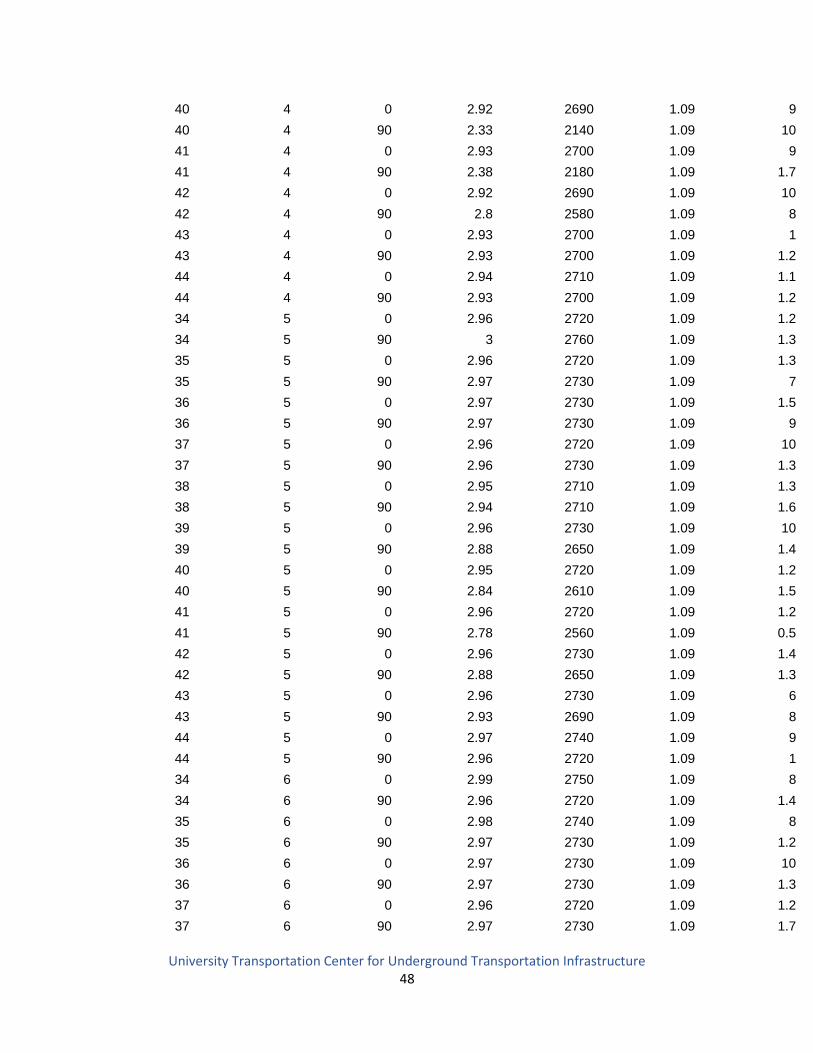
University Transportation Center for Underground Transportation Infrastructure 48
40 4 0 2.92 2690 1.09 9
40 4 90 2.33 2140 1.09 10
41 4 0 2.93 2700 1.09 9
41 4 90 2.38 2180 1.09 1.7
42 4 0 2.92 2690 1.09 10
42 4 90 2.8 2580 1.09 8
43 4 0 2.93 2700 1.09 1
43 4 90 2.93 2700 1.09 1.2
44 4 0 2.94 2710 1.09 1.1
44 4 90 2.93 2700 1.09 1.2
34 5 0 2.96 2720 1.09 1.2
34 5 90 3 2760 1.09 1.3
35 5 0 2.96 2720 1.09 1.3
35 5 90 2.97 2730 1.09 7
36 5 0 2.97 2730 1.09 1.5
36 5 90 2.97 2730 1.09 9
37 5 0 2.96 2720 1.09 10
37 5 90 2.96 2730 1.09 1.3
38 5 0 2.95 2710 1.09 1.3
38 5 90 2.94 2710 1.09 1.6
39 5 0 2.96 2730 1.09 10
39 5 90 2.88 2650 1.09 1.4
40 5 0 2.95 2720 1.09 1.2
40 5 90 2.84 2610 1.09 1.5
41 5 0 2.96 2720 1.09 1.2
41 5 90 2.78 2560 1.09 0.5
42 5 0 2.96 2730 1.09 1.4
42 5 90 2.88 2650 1.09 1.3
43 5 0 2.96 2730 1.09 6
43 5 90 2.93 2690 1.09 8
44 5 0 2.97 2740 1.09 9
44 5 90 2.96 2720 1.09 1
34 6 0 2.99 2750 1.09 8
34 6 90 2.96 2720 1.09 1.4
35 6 0 2.98 2740 1.09 8
35 6 90 2.97 2730 1.09 1.2
36 6 0 2.97 2730 1.09 10
36 6 90 2.97 2730 1.09 1.3
37 6 0 2.96 2720 1.09 1.2
37 6 90 2.97 2730 1.09 1.7
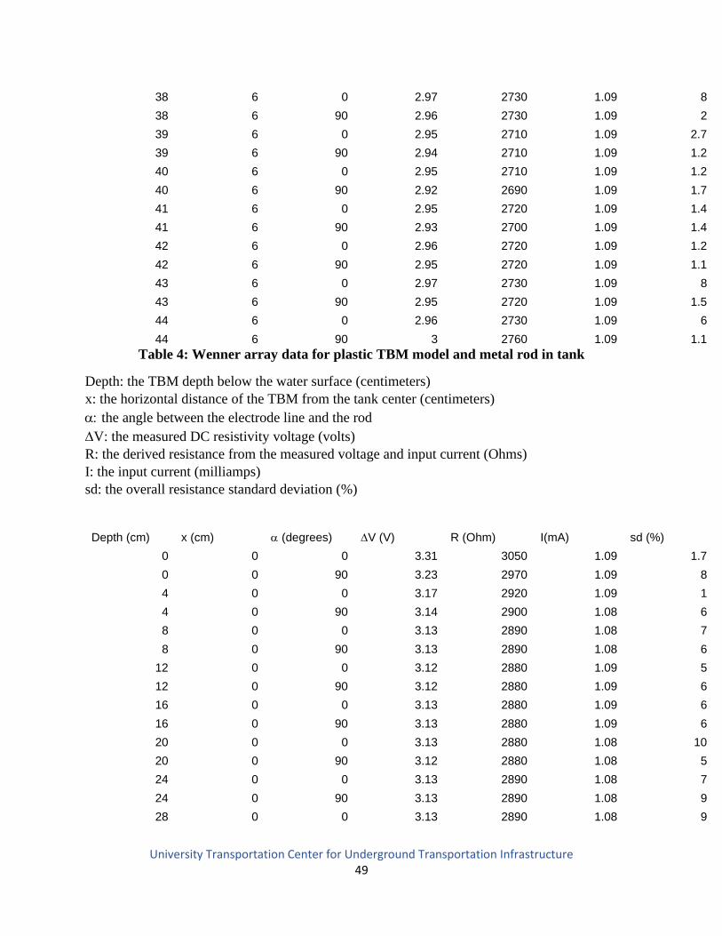
University Transportation Center for Underground Transportation Infrastructure 49
38 6 0 2.97 2730 1.09 8
38 6 90 2.96 2730 1.09 2
39 6 0 2.95 2710 1.09 2.7
39 6 90 2.94 2710 1.09 1.2
40 6 0 2.95 2710 1.09 1.2
40 6 90 2.92 2690 1.09 1.7
41 6 0 2.95 2720 1.09 1.4
41 6 90 2.93 2700 1.09 1.4
42 6 0 2.96 2720 1.09 1.2
42 6 90 2.95 2720 1.09 1.1
43 6 0 2.97 2730 1.09 8
43 6 90 2.95 2720 1.09 1.5
44 6 0 2.96 2730 1.09 6
44 6 90 3 2760 1.09 1.1
Table 4: Wenner array data for plastic TBM model and metal rod in tank
Depth: the TBM depth below the water surface (centimeters)
x: the horizontal distance of the TBM from the tank center (centimeters)
the angle between the electrode line and the rod
V: the measured DC resistivity voltage (volts)
R: the derived resistance from the measured voltage and input current (Ohms)
I: the input current (milliamps)
sd: the overall resistance standard deviation (%)
Depth (cm) x (cm) (degrees) V (V) R (Ohm) I(mA) sd (%)
0 0 0 3.31 3050 1.09 1.7
0 0 90 3.23 2970 1.09 8
4 0 0 3.17 2920 1.09 1
4 0 90 3.14 2900 1.08 6
8 0 0 3.13 2890 1.08 7
8 0 90 3.13 2890 1.08 6
12 0 0 3.12 2880 1.09 5
12 0 90 3.12 2880 1.09 6
16 0 0 3.13 2880 1.09 6
16 0 90 3.13 2880 1.09 6
20 0 0 3.13 2880 1.08 10
20 0 90 3.12 2880 1.08 5
24 0 0 3.13 2890 1.08 7
24 0 90 3.13 2890 1.08 9
28 0 0 3.13 2890 1.08 9
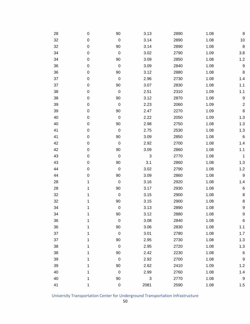
University Transportation Center for Underground Transportation Infrastructure 50
28 0 90 3.13 2890 1.08 8
32 0 0 3.14 2890 1.08 10
32 0 90 3.14 2890 1.08 8
34 0 0 3.02 2790 1.09 3.8
34 0 90 3.09 2850 1.08 1.2
36 0 0 3.09 2840 1.08 9
36 0 90 3.12 2880 1.08 8
37 0 0 2.96 2730 1.08 1.4
37 0 90 3.07 2830 1.08 1.1
38 0 0 2.51 2310 1.09 1.1
38 0 90 3.12 2870 1.08 9
39 0 0 2.23 2060 1.09 2
39 0 90 2.47 2270 1.09 8
40 0 0 2.22 2050 1.09 1.3
40 0 90 2.98 2750 1.08 1.3
41 0 0 2.75 2530 1.08 1.3
41 0 90 3.09 2850 1.08 6
42 0 0 2.92 2700 1.08 1.4
42 0 90 3.09 2860 1.08 1.1
43 0 0 3 2770 1.08 1
43 0 90 3.1 2860 1.08 1.3
44 0 0 3.02 2790 1.08 1.2
44 0 90 3.09 2860 1.08 9
28 1 0 3.16 2920 1.08 1.4
28 1 90 3.17 2930 1.08 6
32 1 0 3.15 2900 1.08 8
32 1 90 3.15 2900 1.08 8
34 1 0 3.13 2890 1.08 9
34 1 90 3.12 2880 1.08 9
36 1 0 3.08 2840 1.08 6
36 1 90 3.06 2830 1.08 1.1
37 1 0 3.01 2780 1.08 1.7
37 1 90 2.95 2730 1.08 1.3
38 1 0 2.95 2720 1.08 1.3
38 1 90 2.42 2230 1.08 6
39 1 0 2.92 2700 1.08 9
39 1 90 2.62 2410 1.09 1.2
40 1 0 2.99 2760 1.08 1.4
40 1 90 3 2770 1.08 9
41 1 0 2081 2590 1.08 1.5
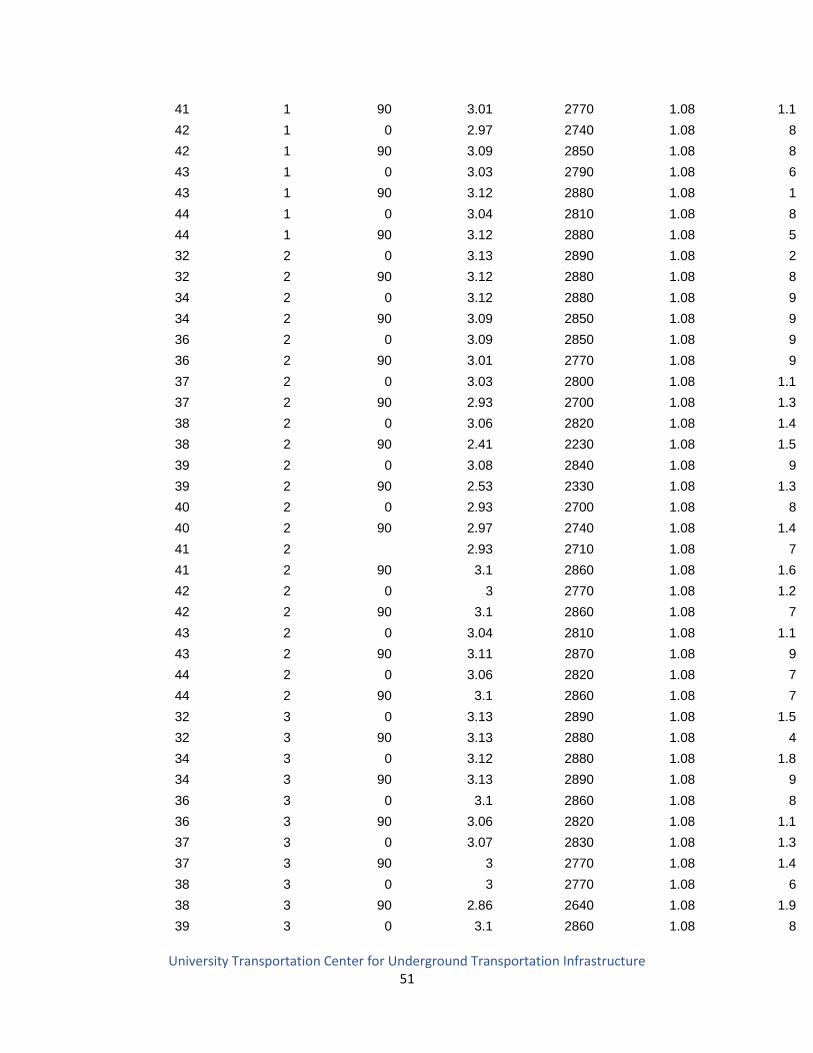
University Transportation Center for Underground Transportation Infrastructure 51
41 1 90 3.01 2770 1.08 1.1
42 1 0 2.97 2740 1.08 8
42 1 90 3.09 2850 1.08 8
43 1 0 3.03 2790 1.08 6
43 1 90 3.12 2880 1.08 1
44 1 0 3.04 2810 1.08 8
44 1 90 3.12 2880 1.08 5
32 2 0 3.13 2890 1.08 2
32 2 90 3.12 2880 1.08 8
34 2 0 3.12 2880 1.08 9
34 2 90 3.09 2850 1.08 9
36 2 0 3.09 2850 1.08 9
36 2 90 3.01 2770 1.08 9
37 2 0 3.03 2800 1.08 1.1
37 2 90 2.93 2700 1.08 1.3
38 2 0 3.06 2820 1.08 1.4
38 2 90 2.41 2230 1.08 1.5
39 2 0 3.08 2840 1.08 9
39 2 90 2.53 2330 1.08 1.3
40 2 0 2.93 2700 1.08 8
40 2 90 2.97 2740 1.08 1.4
41 2 2.93 2710 1.08 7
41 2 90 3.1 2860 1.08 1.6
42 2 0 3 2770 1.08 1.2
42 2 90 3.1 2860 1.08 7
43 2 0 3.04 2810 1.08 1.1
43 2 90 3.11 2870 1.08 9
44 2 0 3.06 2820 1.08 7
44 2 90 3.1 2860 1.08 7
32 3 0 3.13 2890 1.08 1.5
32 3 90 3.13 2880 1.08 4
34 3 0 3.12 2880 1.08 1.8
34 3 90 3.13 2890 1.08 9
36 3 0 3.1 2860 1.08 8
36 3 90 3.06 2820 1.08 1.1
37 3 0 3.07 2830 1.08 1.3
37 3 90 3 2770 1.08 1.4
38 3 0 3 2770 1.08 6
38 3 90 2.86 2640 1.08 1.9
39 3 0 3.1 2860 1.08 8
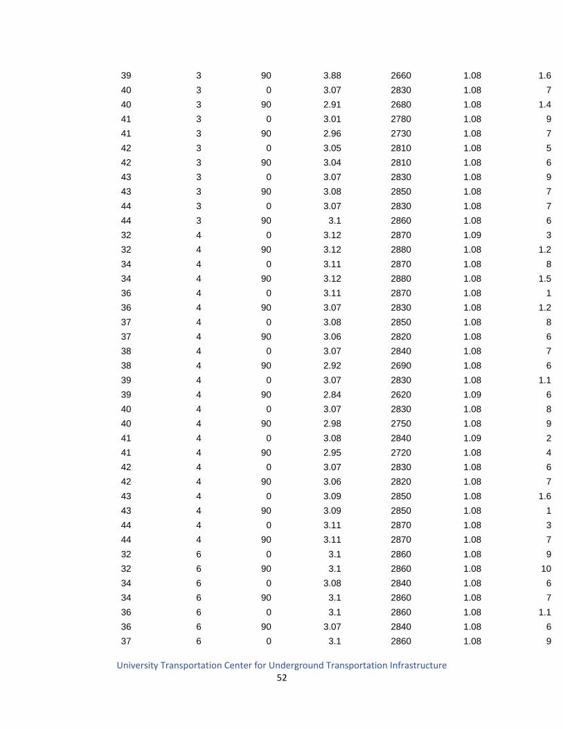
University Transportation Center for Underground Transportation Infrastructure 52
39 3 90 3.88 2660 1.08 1.6
40 3 0 3.07 2830 1.08 7
40 3 90 2.91 2680 1.08 1.4
41 3 0 3.01 2780 1.08 9
41 3 90 2.96 2730 1.08 7
42 3 0 3.05 2810 1.08 5
42 3 90 3.04 2810 1.08 6
43 3 0 3.07 2830 1.08 9
43 3 90 3.08 2850 1.08 7
44 3 0 3.07 2830 1.08 7
44 3 90 3.1 2860 1.08 6
32 4 0 3.12 2870 1.09 3
32 4 90 3.12 2880 1.08 1.2
34 4 0 3.11 2870 1.08 8
34 4 90 3.12 2880 1.08 1.5
36 4 0 3.11 2870 1.08 1
36 4 90 3.07 2830 1.08 1.2
37 4 0 3.08 2850 1.08 8
37 4 90 3.06 2820 1.08 6
38 4 0 3.07 2840 1.08 7
38 4 90 2.92 2690 1.08 6
39 4 0 3.07 2830 1.08 1.1
39 4 90 2.84 2620 1.09 6
40 4 0 3.07 2830 1.08 8
40 4 90 2.98 2750 1.08 9
41 4 0 3.08 2840 1.09 2
41 4 90 2.95 2720 1.08 4
42 4 0 3.07 2830 1.08 6
42 4 90 3.06 2820 1.08 7
43 4 0 3.09 2850 1.08 1.6
43 4 90 3.09 2850 1.08 1
44 4 0 3.11 2870 1.08 3
44 4 90 3.11 2870 1.08 7
32 6 0 3.1 2860 1.08 9
32 6 90 3.1 2860 1.08 10
34 6 0 3.08 2840 1.08 6
34 6 90 3.1 2860 1.08 7
36 6 0 3.1 2860 1.08 1.1
36 6 90 3.07 2840 1.08 6
37 6 0 3.1 2860 1.08 9
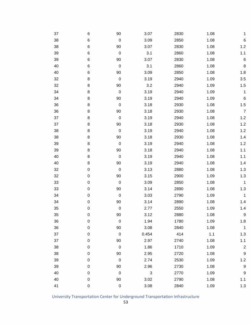
University Transportation Center for Underground Transportation Infrastructure 53
37 6 90 3.07 2830 1.08 1
38 6 0 3.09 2850 1.08 6
38 6 90 3.07 2830 1.08 1.2
39 6 0 3.1 2860 1.08 1.1
39 6 90 3.07 2830 1.08 6
40 6 0 3.1 2860 1.08 8
40 6 90 3.09 2850 1.08 1.8
32 8 0 3.19 2940 1.09 3.5
32 8 90 3.2 2940 1.09 1.5
34 8 0 3.19 2940 1.09 1
34 8 90 3.19 2940 1.09 6
36 8 0 3.18 2930 1.08 1.5
36 8 90 3.18 2930 1.08 7
37 8 0 3.19 2940 1.08 1.2
37 8 90 3.18 2930 1.08 1.2
38 8 0 3.19 2940 1.08 1.2
38 8 90 3.18 2930 1.08 1.4
39 8 0 3.19 2940 1.08 1.2
39 8 90 3.18 2940 1.08 1.1
40 8 0 3.19 2940 1.08 1.1
40 8 90 3.19 2940 1.08 1.4
32 0 0 3.13 2880 1.08 1.3
32 0 90 3.15 2900 1.09 1.3
33 0 0 3.09 2850 1.08 1
33 0 90 3.14 2890 1.08 1.3
34 0 0 3.03 2790 1.09 1
34 0 90 3.14 2890 1.08 1.4
35 0 0 2.77 2550 1.09 1.4
35 0 90 3.12 2880 1.08 9
36 0 0 1.94 1780 1.09 1.8
36 0 90 3.08 2840 1.08 1
37 0 0 0.454 414 1.1 1.3
37 0 90 2.97 2740 1.08 1.1
38 0 0 1.86 1710 1.09 2
38 0 90 2.95 2720 1.08 9
39 0 0 2.74 2530 1.09 1.2
39 0 90 2.96 2730 1.08 9
40 0 0 3 2770 1.09 9
40 0 90 3.02 2790 1.08 1.1
41 0 0 3.08 2840 1.09 1.3
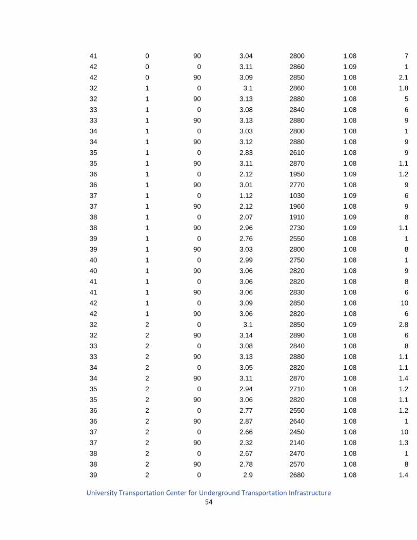
University Transportation Center for Underground Transportation Infrastructure 54
41 0 90 3.04 2800 1.08 7
42 0 0 3.11 2860 1.09 1
42 0 90 3.09 2850 1.08 2.1
32 1 0 3.1 2860 1.08 1.8
32 1 90 3.13 2880 1.08 5
33 1 0 3.08 2840 1.08 6
33 1 90 3.13 2880 1.08 9
34 1 0 3.03 2800 1.08 1
34 1 90 3.12 2880 1.08 9
35 1 0 2.83 2610 1.08 9
35 1 90 3.11 2870 1.08 1.1
36 1 0 2.12 1950 1.09 1.2
36 1 90 3.01 2770 1.08 9
37 1 0 1.12 1030 1.09 6
37 1 90 2.12 1960 1.08 9
38 1 0 2.07 1910 1.09 8
38 1 90 2.96 2730 1.09 1.1
39 1 0 2.76 2550 1.08 1
39 1 90 3.03 2800 1.08 8
40 1 0 2.99 2750 1.08 1
40 1 90 3.06 2820 1.08 9
41 1 0 3.06 2820 1.08 8
41 1 90 3.06 2830 1.08 6
42 1 0 3.09 2850 1.08 10
42 1 90 3.06 2820 1.08 6
32 2 0 3.1 2850 1.09 2.8
32 2 90 3.14 2890 1.08 6
33 2 0 3.08 2840 1.08 8
33 2 90 3.13 2880 1.08 1.1
34 2 0 3.05 2820 1.08 1.1
34 2 90 3.11 2870 1.08 1.4
35 2 0 2.94 2710 1.08 1.2
35 2 90 3.06 2820 1.08 1.1
36 2 0 2.77 2550 1.08 1.2
36 2 90 2.87 2640 1.08 1
37 2 0 2.66 2450 1.08 10
37 2 90 2.32 2140 1.08 1.3
38 2 0 2.67 2470 1.08 1
38 2 90 2.78 2570 1.08 8
39 2 0 2.9 2680 1.08 1.4
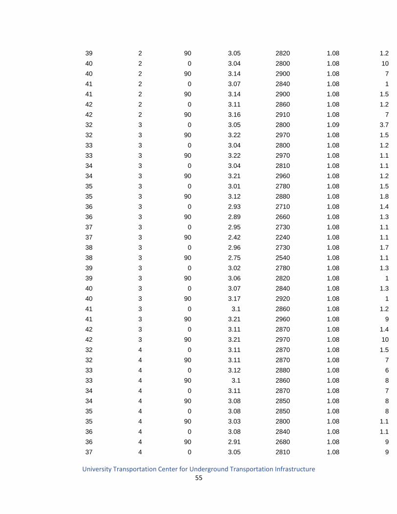
University Transportation Center for Underground Transportation Infrastructure 55
39 2 90 3.05 2820 1.08 1.2
40 2 0 3.04 2800 1.08 10
40 2 90 3.14 2900 1.08 7
41 2 0 3.07 2840 1.08 1
41 2 90 3.14 2900 1.08 1.5
42 2 0 3.11 2860 1.08 1.2
42 2 90 3.16 2910 1.08 7
32 3 0 3.05 2800 1.09 3.7
32 3 90 3.22 2970 1.08 1.5
33 3 0 3.04 2800 1.08 1.2
33 3 90 3.22 2970 1.08 1.1
34 3 0 3.04 2810 1.08 1.1
34 3 90 3.21 2960 1.08 1.2
35 3 0 3.01 2780 1.08 1.5
35 3 90 3.12 2880 1.08 1.8
36 3 0 2.93 2710 1.08 1.4
36 3 90 2.89 2660 1.08 1.3
37 3 0 2.95 2730 1.08 1.1
37 3 90 2.42 2240 1.08 1.1
38 3 0 2.96 2730 1.08 1.7
38 3 90 2.75 2540 1.08 1.1
39 3 0 3.02 2780 1.08 1.3
39 3 90 3.06 2820 1.08 1
40 3 0 3.07 2840 1.08 1.3
40 3 90 3.17 2920 1.08 1
41 3 0 3.1 2860 1.08 1.2
41 3 90 3.21 2960 1.08 9
42 3 0 3.11 2870 1.08 1.4
42 3 90 3.21 2970 1.08 10
32 4 0 3.11 2870 1.08 1.5
32 4 90 3.11 2870 1.08 7
33 4 0 3.12 2880 1.08 6
33 4 90 3.1 2860 1.08 8
34 4 0 3.11 2870 1.08 7
34 4 90 3.08 2850 1.08 8
35 4 0 3.08 2850 1.08 8
35 4 90 3.03 2800 1.08 1.1
36 4 0 3.08 2840 1.08 1.1
36 4 90 2.91 2680 1.08 9
37 4 0 3.05 2810 1.08 9
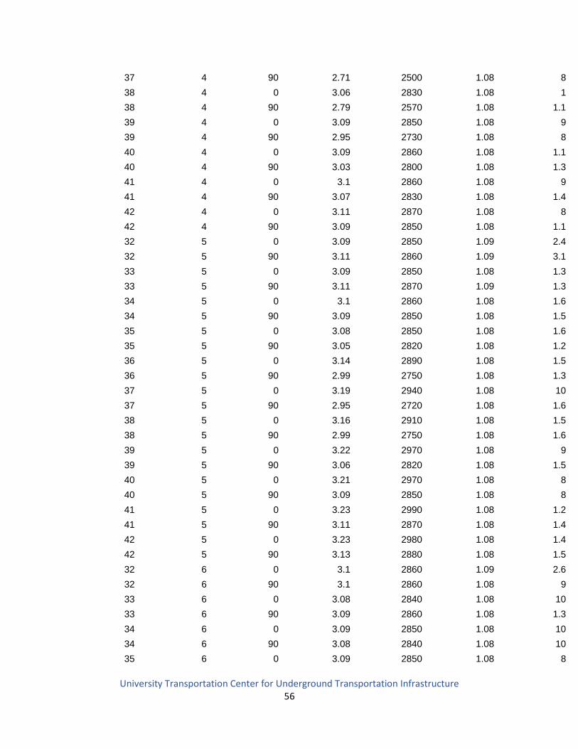
University Transportation Center for Underground Transportation Infrastructure 56
37 4 90 2.71 2500 1.08 8
38 4 0 3.06 2830 1.08 1
38 4 90 2.79 2570 1.08 1.1
39 4 0 3.09 2850 1.08 9
39 4 90 2.95 2730 1.08 8
40 4 0 3.09 2860 1.08 1.1
40 4 90 3.03 2800 1.08 1.3
41 4 0 3.1 2860 1.08 9
41 4 90 3.07 2830 1.08 1.4
42 4 0 3.11 2870 1.08 8
42 4 90 3.09 2850 1.08 1.1
32 5 0 3.09 2850 1.09 2.4
32 5 90 3.11 2860 1.09 3.1
33 5 0 3.09 2850 1.08 1.3
33 5 90 3.11 2870 1.09 1.3
34 5 0 3.1 2860 1.08 1.6
34 5 90 3.09 2850 1.08 1.5
35 5 0 3.08 2850 1.08 1.6
35 5 90 3.05 2820 1.08 1.2
36 5 0 3.14 2890 1.08 1.5
36 5 90 2.99 2750 1.08 1.3
37 5 0 3.19 2940 1.08 10
37 5 90 2.95 2720 1.08 1.6
38 5 0 3.16 2910 1.08 1.5
38 5 90 2.99 2750 1.08 1.6
39 5 0 3.22 2970 1.08 9
39 5 90 3.06 2820 1.08 1.5
40 5 0 3.21 2970 1.08 8
40 5 90 3.09 2850 1.08 8
41 5 0 3.23 2990 1.08 1.2
41 5 90 3.11 2870 1.08 1.4
42 5 0 3.23 2980 1.08 1.4
42 5 90 3.13 2880 1.08 1.5
32 6 0 3.1 2860 1.09 2.6
32 6 90 3.1 2860 1.08 9
33 6 0 3.08 2840 1.08 10
33 6 90 3.09 2860 1.08 1.3
34 6 0 3.09 2850 1.08 10
34 6 90 3.08 2840 1.08 10
35 6 0 3.09 2850 1.08 8
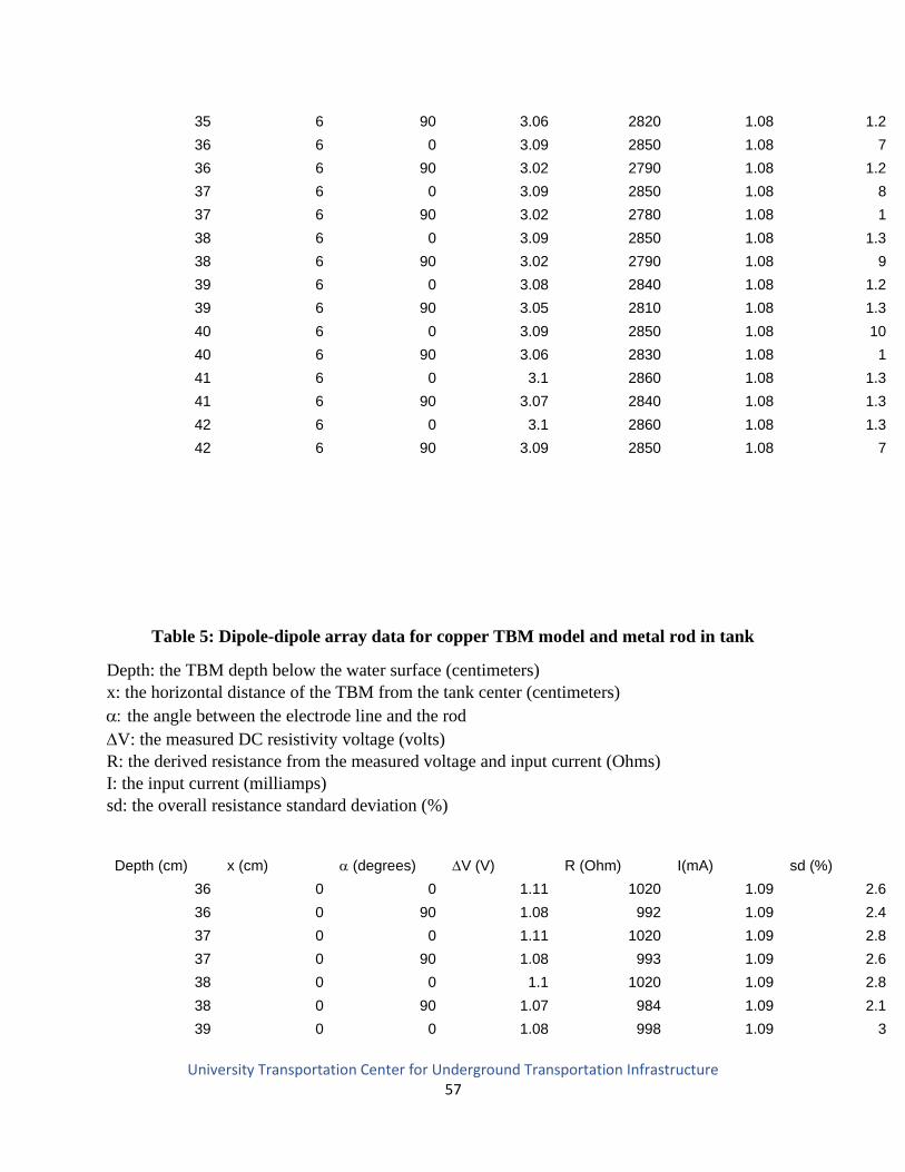
University Transportation Center for Underground Transportation Infrastructure 57
35 6 90 3.06 2820 1.08 1.2
36 6 0 3.09 2850 1.08 7
36 6 90 3.02 2790 1.08 1.2
37 6 0 3.09 2850 1.08 8
37 6 90 3.02 2780 1.08 1
38 6 0 3.09 2850 1.08 1.3
38 6 90 3.02 2790 1.08 9
39 6 0 3.08 2840 1.08 1.2
39 6 90 3.05 2810 1.08 1.3
40 6 0 3.09 2850 1.08 10
40 6 90 3.06 2830 1.08 1
41 6 0 3.1 2860 1.08 1.3
41 6 90 3.07 2840 1.08 1.3
42 6 0 3.1 2860 1.08 1.3
42 6 90 3.09 2850 1.08 7
Table 5: Dipole-dipole array data for copper TBM model and metal rod in tank
Depth: the TBM depth below the water surface (centimeters)
x: the horizontal distance of the TBM from the tank center (centimeters)
the angle between the electrode line and the rod
V: the measured DC resistivity voltage (volts)
R: the derived resistance from the measured voltage and input current (Ohms)
I: the input current (milliamps)
sd: the overall resistance standard deviation (%)
Depth (cm) x (cm) (degrees) V (V) R (Ohm) I(mA) sd (%)
36 0 0 1.11 1020 1.09 2.6
36 0 90 1.08 992 1.09 2.4
37 0 0 1.11 1020 1.09 2.8
37 0 90 1.08 993 1.09 2.6
38 0 0 1.1 1020 1.09 2.8
38 0 90 1.07 984 1.09 2.1
39 0 0 1.08 998 1.09 3

University Transportation Center for Underground Transportation Infrastructure 58
39 0 90 1.03 946 1.09 2.5
40 0 0 0.903 831 1.09 3
40 0 90 0.9 828 1.09 2.7
41 0 0 0.541 497 1.09 2.8
41 0 90 0.364 334 1.09 2.8
42 0 0 0.251 230 1.09 1.4
42 0 90 0.288 265 1.09 3
43 0 0 0.917 844 1.09 4
43 0 90 0.743 683 1.09 2.5
44 0 0 1.07 989 1.09 2.9
44 0 90 1.03 947 1.09 2.6
36 1 0 1.1 1010 1.09 2.8
36 1 90 1.1 1010 1.09 2.3
37 1 0 1.1 1010 1.09 1.9
37 1 90 1.1 1020 1.09 1.7
38 1 0 1.11 1020 1.09 2.3
38 1 90 1.1 1010 1.09 2.2
39 1 0 1.09 1010 1.09 2.4
39 1 90 1.06 975 1.09 2.1
40 1 0 1.05 969 1.09 2.3
40 1 90 0.94 866 1.09 2.1
41 1 0 0.862 794 1.09 2.6
41 1 90 0.677 622 1.09 2
42 1 0 0.664 610 1.09 2.7
42 1 90 0.519 476 1.09 1.4
43 1 0 1.05 962 1.09 2.2
43 1 90 0.986 907 1.09 3
44 1 0 1.09 1000 1.09 2.1
44 1 90 1.09 1000 1.09 1.9
36 2 0 1.11 1020 1.09 1.5
36 2 90 1.06 978 1.09 1.4
37 2 0 1.1 1020 1.09 1.8
37 2 90 1.06 972 1.09 7
38 2 0 1.1 1010 1.09 1.6
38 2 90 1.06 972 1.09 9
39 2 0 1.1 1010 1.09 1.6
39 2 90 1.06 975 1.09 1.1
40 2 0 1.1 1010 1.09 1.5
40 2 90 1.04 954 1.09 8
41 2 0 1.05 966 1.09 1.2
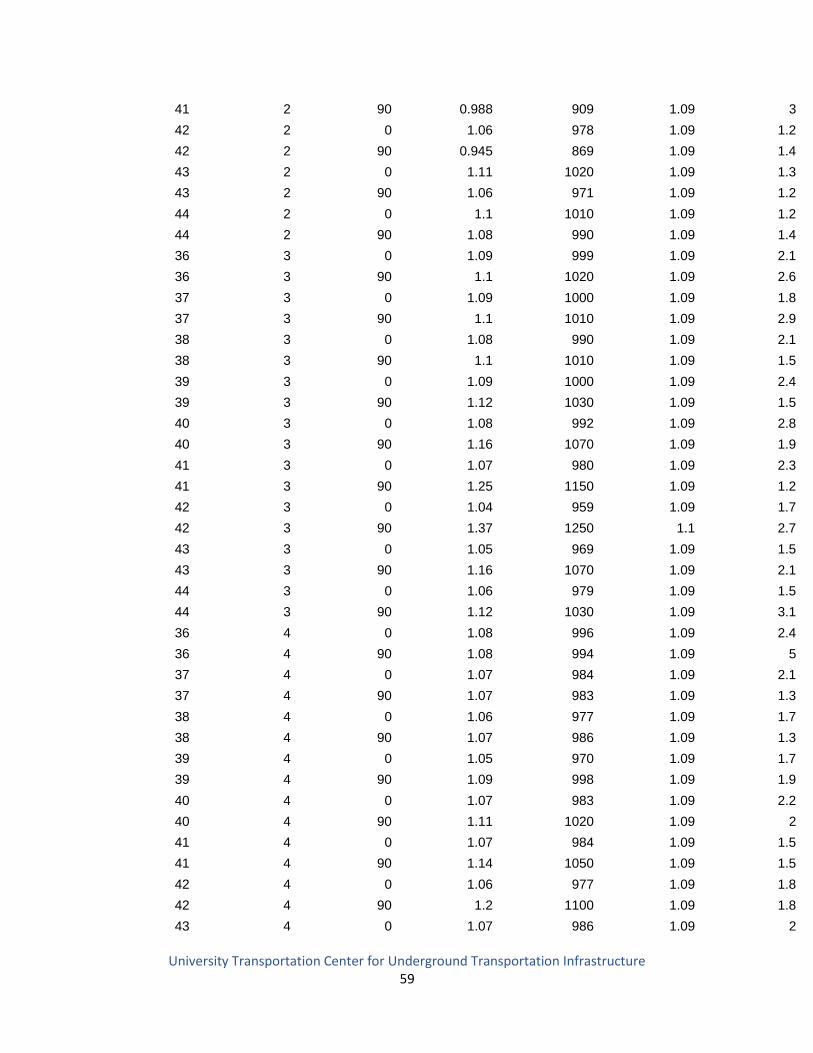
University Transportation Center for Underground Transportation Infrastructure 59
41 2 90 0.988 909 1.09 3
42 2 0 1.06 978 1.09 1.2
42 2 90 0.945 869 1.09 1.4
43 2 0 1.11 1020 1.09 1.3
43 2 90 1.06 971 1.09 1.2
44 2 0 1.1 1010 1.09 1.2
44 2 90 1.08 990 1.09 1.4
36 3 0 1.09 999 1.09 2.1
36 3 90 1.1 1020 1.09 2.6
37 3 0 1.09 1000 1.09 1.8
37 3 90 1.1 1010 1.09 2.9
38 3 0 1.08 990 1.09 2.1
38 3 90 1.1 1010 1.09 1.5
39 3 0 1.09 1000 1.09 2.4
39 3 90 1.12 1030 1.09 1.5
40 3 0 1.08 992 1.09 2.8
40 3 90 1.16 1070 1.09 1.9
41 3 0 1.07 980 1.09 2.3
41 3 90 1.25 1150 1.09 1.2
42 3 0 1.04 959 1.09 1.7
42 3 90 1.37 1250 1.1 2.7
43 3 0 1.05 969 1.09 1.5
43 3 90 1.16 1070 1.09 2.1
44 3 0 1.06 979 1.09 1.5
44 3 90 1.12 1030 1.09 3.1
36 4 0 1.08 996 1.09 2.4
36 4 90 1.08 994 1.09 5
37 4 0 1.07 984 1.09 2.1
37 4 90 1.07 983 1.09 1.3
38 4 0 1.06 977 1.09 1.7
38 4 90 1.07 986 1.09 1.3
39 4 0 1.05 970 1.09 1.7
39 4 90 1.09 998 1.09 1.9
40 4 0 1.07 983 1.09 2.2
40 4 90 1.11 1020 1.09 2
41 4 0 1.07 984 1.09 1.5
41 4 90 1.14 1050 1.09 1.5
42 4 0 1.06 977 1.09 1.8
42 4 90 1.2 1100 1.09 1.8
43 4 0 1.07 986 1.09 2
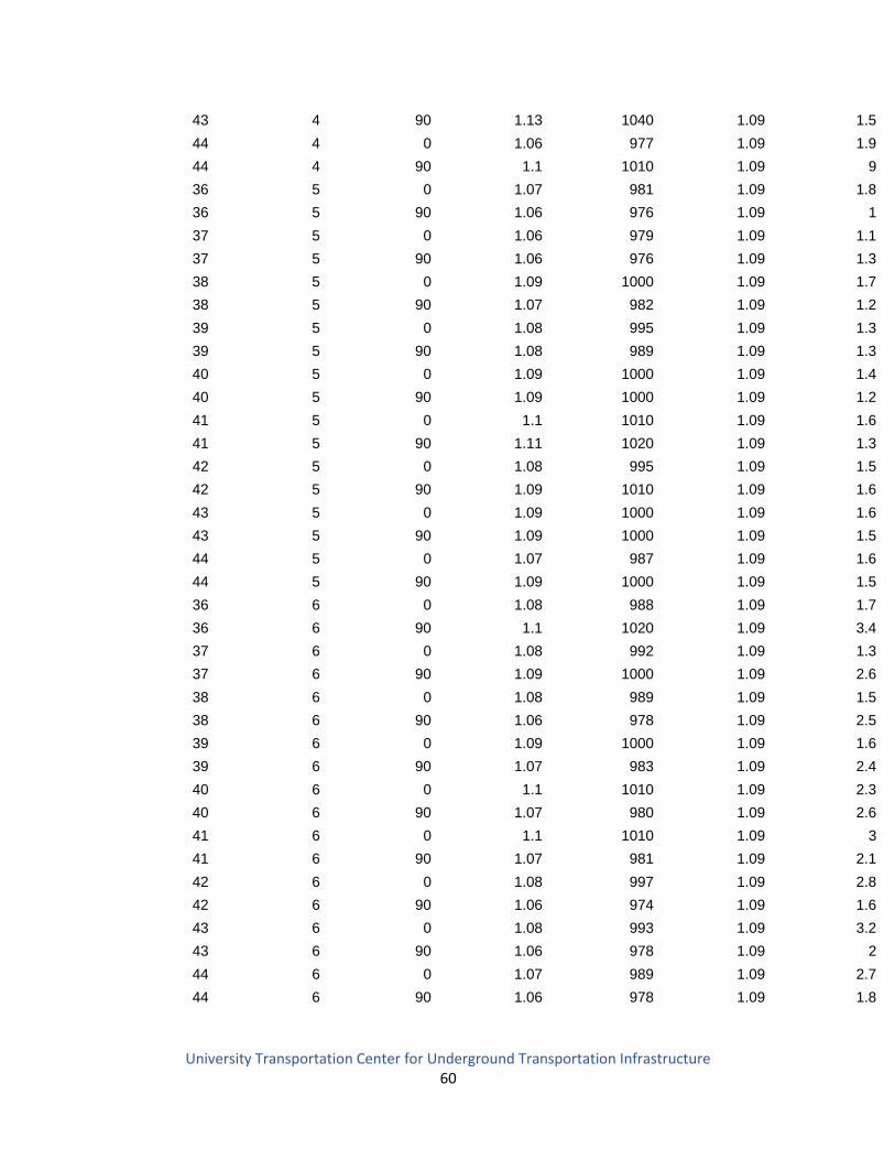
University Transportation Center for Underground Transportation Infrastructure 60
43 4 90 1.13 1040 1.09 1.5
44 4 0 1.06 977 1.09 1.9
44 4 90 1.1 1010 1.09 9
36 5 0 1.07 981 1.09 1.8
36 5 90 1.06 976 1.09 1
37 5 0 1.06 979 1.09 1.1
37 5 90 1.06 976 1.09 1.3
38 5 0 1.09 1000 1.09 1.7
38 5 90 1.07 982 1.09 1.2
39 5 0 1.08 995 1.09 1.3
39 5 90 1.08 989 1.09 1.3
40 5 0 1.09 1000 1.09 1.4
40 5 90 1.09 1000 1.09 1.2
41 5 0 1.1 1010 1.09 1.6
41 5 90 1.11 1020 1.09 1.3
42 5 0 1.08 995 1.09 1.5
42 5 90 1.09 1010 1.09 1.6
43 5 0 1.09 1000 1.09 1.6
43 5 90 1.09 1000 1.09 1.5
44 5 0 1.07 987 1.09 1.6
44 5 90 1.09 1000 1.09 1.5
36 6 0 1.08 988 1.09 1.7
36 6 90 1.1 1020 1.09 3.4
37 6 0 1.08 992 1.09 1.3
37 6 90 1.09 1000 1.09 2.6
38 6 0 1.08 989 1.09 1.5
38 6 90 1.06 978 1.09 2.5
39 6 0 1.09 1000 1.09 1.6
39 6 90 1.07 983 1.09 2.4
40 6 0 1.1 1010 1.09 2.3
40 6 90 1.07 980 1.09 2.6
41 6 0 1.1 1010 1.09 3
41 6 90 1.07 981 1.09 2.1
42 6 0 1.08 997 1.09 2.8
42 6 90 1.06 974 1.09 1.6
43 6 0 1.08 993 1.09 3.2
43 6 90 1.06 978 1.09 2
44 6 0 1.07 989 1.09 2.7
44 6 90 1.06 978 1.09 1.8
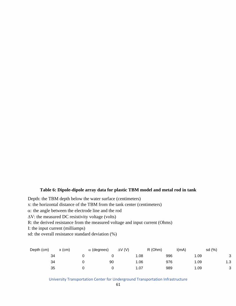
University Transportation Center for Underground Transportation Infrastructure 61
Table 6: Dipole-dipole array data for plastic TBM model and metal rod in tank
Depth: the TBM depth below the water surface (centimeters)
x: the horizontal distance of the TBM from the tank center (centimeters)
the angle between the electrode line and the rod
V: the measured DC resistivity voltage (volts)
R: the derived resistance from the measured voltage and input current (Ohms)
I: the input current (milliamps)
sd: the overall resistance standard deviation (%)
Depth (cm) x (cm) (degrees) V (V) R (Ohm) I(mA) sd (%)
34 0 0 1.08 996 1.09 3
34 0 90 1.06 976 1.09 1.3
35 0 0 1.07 989 1.09 3
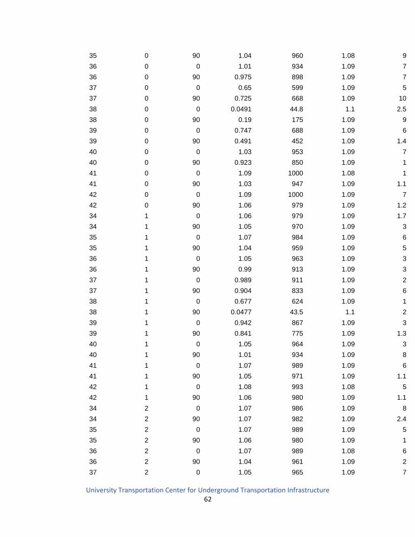
University Transportation Center for Underground Transportation Infrastructure 62
35 0 90 1.04 960 1.08 9
36 0 0 1.01 934 1.09 7
36 0 90 0.975 898 1.09 7
37 0 0 0.65 599 1.09 5
37 0 90 0.725 668 1.09 10
38 0 0 0.0491 44.8 1.1 2.5
38 0 90 0.19 175 1.09 9
39 0 0 0.747 688 1.09 6
39 0 90 0.491 452 1.09 1.4
40 0 0 1.03 953 1.09 7
40 0 90 0.923 850 1.09 1
41 0 0 1.09 1000 1.08 1
41 0 90 1.03 947 1.09 1.1
42 0 0 1.09 1000 1.09 7
42 0 90 1.06 979 1.09 1.2
34 1 0 1.06 979 1.09 1.7
34 1 90 1.05 970 1.09 3
35 1 0 1.07 984 1.09 6
35 1 90 1.04 959 1.09 5
36 1 0 1.05 963 1.09 3
36 1 90 0.99 913 1.09 3
37 1 0 0.989 911 1.09 2
37 1 90 0.904 833 1.09 6
38 1 0 0.677 624 1.09 1
38 1 90 0.0477 43.5 1.1 2
39 1 0 0.942 867 1.09 3
39 1 90 0.841 775 1.09 1.3
40 1 0 1.05 964 1.09 3
40 1 90 1.01 934 1.09 8
41 1 0 1.07 989 1.09 6
41 1 90 1.05 971 1.09 1.1
42 1 0 1.08 993 1.08 5
42 1 90 1.06 980 1.09 1.1
34 2 0 1.07 986 1.09 8
34 2 90 1.07 982 1.09 2.4
35 2 0 1.07 989 1.09 5
35 2 90 1.06 980 1.09 1
36 2 0 1.07 989 1.08 6
36 2 90 1.04 961 1.09 2
37 2 0 1.05 965 1.09 7
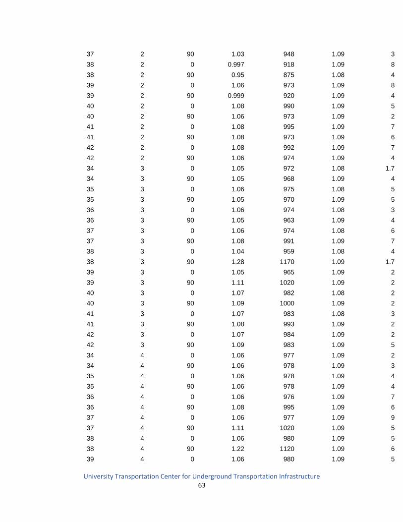
University Transportation Center for Underground Transportation Infrastructure 63
37 2 90 1.03 948 1.09 3
38 2 0 0.997 918 1.09 8
38 2 90 0.95 875 1.08 4
39 2 0 1.06 973 1.09 8
39 2 90 0.999 920 1.09 4
40 2 0 1.08 990 1.09 5
40 2 90 1.06 973 1.09 2
41 2 0 1.08 995 1.09 7
41 2 90 1.08 973 1.09 6
42 2 0 1.08 992 1.09 7
42 2 90 1.06 974 1.09 4
34 3 0 1.05 972 1.08 1.7
34 3 90 1.05 968 1.09 4
35 3 0 1.06 975 1.08 5
35 3 90 1.05 970 1.09 5
36 3 0 1.06 974 1.08 3
36 3 90 1.05 963 1.09 4
37 3 0 1.06 974 1.08 6
37 3 90 1.08 991 1.09 7
38 3 0 1.04 959 1.08 4
38 3 90 1.28 1170 1.09 1.7
39 3 0 1.05 965 1.09 2
39 3 90 1.11 1020 1.09 2
40 3 0 1.07 982 1.08 2
40 3 90 1.09 1000 1.09 2
41 3 0 1.07 983 1.08 3
41 3 90 1.08 993 1.09 2
42 3 0 1.07 984 1.09 2
42 3 90 1.09 983 1.09 5
34 4 0 1.06 977 1.09 2
34 4 90 1.06 978 1.09 3
35 4 0 1.06 978 1.09 4
35 4 90 1.06 978 1.09 4
36 4 0 1.06 976 1.09 7
36 4 90 1.08 995 1.09 6
37 4 0 1.06 977 1.09 9
37 4 90 1.11 1020 1.09 5
38 4 0 1.06 980 1.09 5
38 4 90 1.22 1120 1.09 6
39 4 0 1.06 980 1.09 5
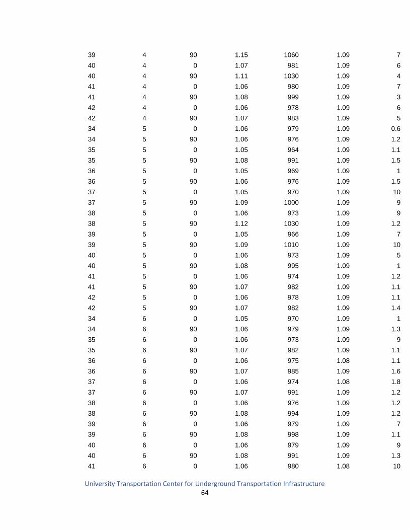
University Transportation Center for Underground Transportation Infrastructure 64
39 4 90 1.15 1060 1.09 7
40 4 0 1.07 981 1.09 6
40 4 90 1.11 1030 1.09 4
41 4 0 1.06 980 1.09 7
41 4 90 1.08 999 1.09 3
42 4 0 1.06 978 1.09 6
42 4 90 1.07 983 1.09 5
34 5 0 1.06 979 1.09 0.6
34 5 90 1.06 976 1.09 1.2
35 5 0 1.05 964 1.09 1.1
35 5 90 1.08 991 1.09 1.5
36 5 0 1.05 969 1.09 1
36 5 90 1.06 976 1.09 1.5
37 5 0 1.05 970 1.09 10
37 5 90 1.09 1000 1.09 9
38 5 0 1.06 973 1.09 9
38 5 90 1.12 1030 1.09 1.2
39 5 0 1.05 966 1.09 7
39 5 90 1.09 1010 1.09 10
40 5 0 1.06 973 1.09 5
40 5 90 1.08 995 1.09 1
41 5 0 1.06 974 1.09 1.2
41 5 90 1.07 982 1.09 1.1
42 5 0 1.06 978 1.09 1.1
42 5 90 1.07 982 1.09 1.4
34 6 0 1.05 970 1.09 1
34 6 90 1.06 979 1.09 1.3
35 6 0 1.06 973 1.09 9
35 6 90 1.07 982 1.09 1.1
36 6 0 1.06 975 1.08 1.1
36 6 90 1.07 985 1.09 1.6
37 6 0 1.06 974 1.08 1.8
37 6 90 1.07 991 1.09 1.2
38 6 0 1.06 976 1.09 1.2
38 6 90 1.08 994 1.09 1.2
39 6 0 1.06 979 1.09 7
39 6 90 1.08 998 1.09 1.1
40 6 0 1.06 979 1.09 9
40 6 90 1.08 991 1.09 1.3
41 6 0 1.06 980 1.08 10
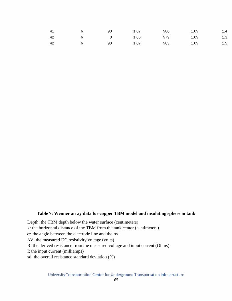
University Transportation Center for Underground Transportation Infrastructure 65
41 6 90 1.07 986 1.09 1.4
42 6 0 1.06 979 1.09 1.3
42 6 90 1.07 983 1.09 1.5
Table 7: Wenner array data for copper TBM model and insulating sphere in tank
Depth: the TBM depth below the water surface (centimeters)
x: the horizontal distance of the TBM from the tank center (centimeters)
the angle between the electrode line and the rod
V: the measured DC resistivity voltage (volts)
R: the derived resistance from the measured voltage and input current (Ohms)
I: the input current (milliamps)
sd: the overall resistance standard deviation (%)
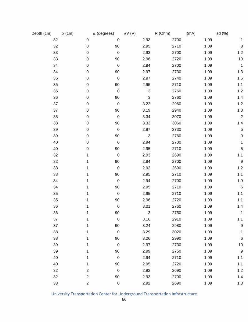
University Transportation Center for Underground Transportation Infrastructure 66
Depth (cm) x (cm) (degrees) V (V) R (Ohm) I(mA) sd (%)
32 0 0 2.93 2700 1.09 1
32 0 90 2.95 2710 1.09 8
33 0 0 2.93 2700 1.09 1.2
33 0 90 2.96 2720 1.09 10
34 0 0 2.94 2700 1.09 1
34 0 90 2.97 2730 1.09 1.3
35 0 0 2.97 2740 1.09 1.6
35 0 90 2.95 2710 1.09 1.1
36 0 0 3 2760 1.09 1.2
36 0 90 3 2760 1.09 1.4
37 0 0 3.22 2960 1.09 1.2
37 0 90 3.19 2940 1.09 1.3
38 0 0 3.34 3070 1.09 2
38 0 90 3.33 3060 1.09 1.4
39 0 0 2.97 2730 1.09 5
39 0 90 3 2760 1.09 9
40 0 0 2.94 2700 1.09 1
40 0 90 2.95 2710 1.09 5
32 1 0 2.93 2690 1.09 1.1
32 1 90 2.94 2700 1.09 9
33 1 0 2.92 2690 1.09 1.2
33 1 90 2.95 2710 1.09 1.1
34 1 0 2.94 2700 1.09 1.9
34 1 90 2.95 2710 1.09 6
35 1 0 2.95 2710 1.09 1.1
35 1 90 2.96 2720 1.09 1.1
36 1 0 3.01 2760 1.09 1.4
36 1 90 3 2750 1.09 1
37 1 0 3.16 2910 1.09 1.1
37 1 90 3.24 2980 1.09 9
38 1 0 3.29 3020 1.09 1
38 1 90 3.26 2990 1.09 6
39 1 0 2.97 2730 1.09 10
39 1 90 2.99 2750 1.09 9
40 1 0 2.94 2710 1.09 1.1
40 1 90 2.95 2720 1.09 1.1
32 2 0 2.92 2690 1.09 1.2
32 2 90 2.93 2700 1.09 1.4
33 2 0 2.92 2690 1.09 1.3
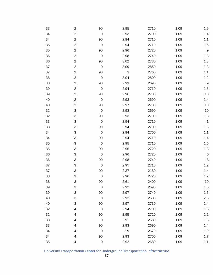
University Transportation Center for Underground Transportation Infrastructure 67
33 2 90 2.95 2710 1.09 1.5
34 2 0 2.93 2700 1.09 1.4
34 2 90 2.94 2710 1.09 1.1
35 2 0 2.94 2710 1.09 1.6
35 2 90 2.96 2720 1.09 9
36 2 0 2.98 2740 1.09 1.8
36 2 90 3.02 2780 1.09 1.3
37 2 0 3.09 2850 1.09 1.3
37 2 90 3 2760 1.09 1.1
38 2 0 3.04 2800 1.09 1.2
38 2 90 2.93 2690 1.09 9
39 2 0 2.94 2710 1.09 1.8
39 2 90 2.96 2730 1.09 10
40 2 0 2.93 2690 1.09 1.4
40 2 90 2.97 2730 1.09 10
32 3 0 2.93 2690 1.09 10
32 3 90 2.93 2700 1.09 1.8
33 3 0 2.94 2710 1.09 1
33 3 90 2.94 2700 1.09 1.5
34 3 0 2.94 2700 1.09 1.1
34 3 90 2.94 2710 1.09 1.4
35 3 0 2.95 2710 1.09 1.6
35 3 90 2.96 2720 1.09 1.8
36 3 0 2.96 2720 1.09 6
36 3 90 2.98 2740 1.09 8
37 3 0 2.95 2710 1.09 1.2
37 3 90 2.37 2180 1.09 1.4
38 3 0 2.96 2720 1.09 1.2
38 3 90 2.61 2400 1.09 10
39 3 0 2.92 2690 1.09 1.5
39 3 90 2.97 2740 1.09 1.5
40 3 0 2.92 2680 1.09 2.5
40 3 90 2.97 2730 1.09 1.4
32 4 0 2.94 2700 1.09 1.6
32 4 90 2.95 2720 1.09 2.2
33 4 0 2.91 2680 1.09 1.5
33 4 90 2.93 2690 1.09 1.4
34 4 0 2.9 2670 1.09 1.9
34 4 90 2.93 2700 1.09 1.7
35 4 0 2.92 2680 1.09 1.1
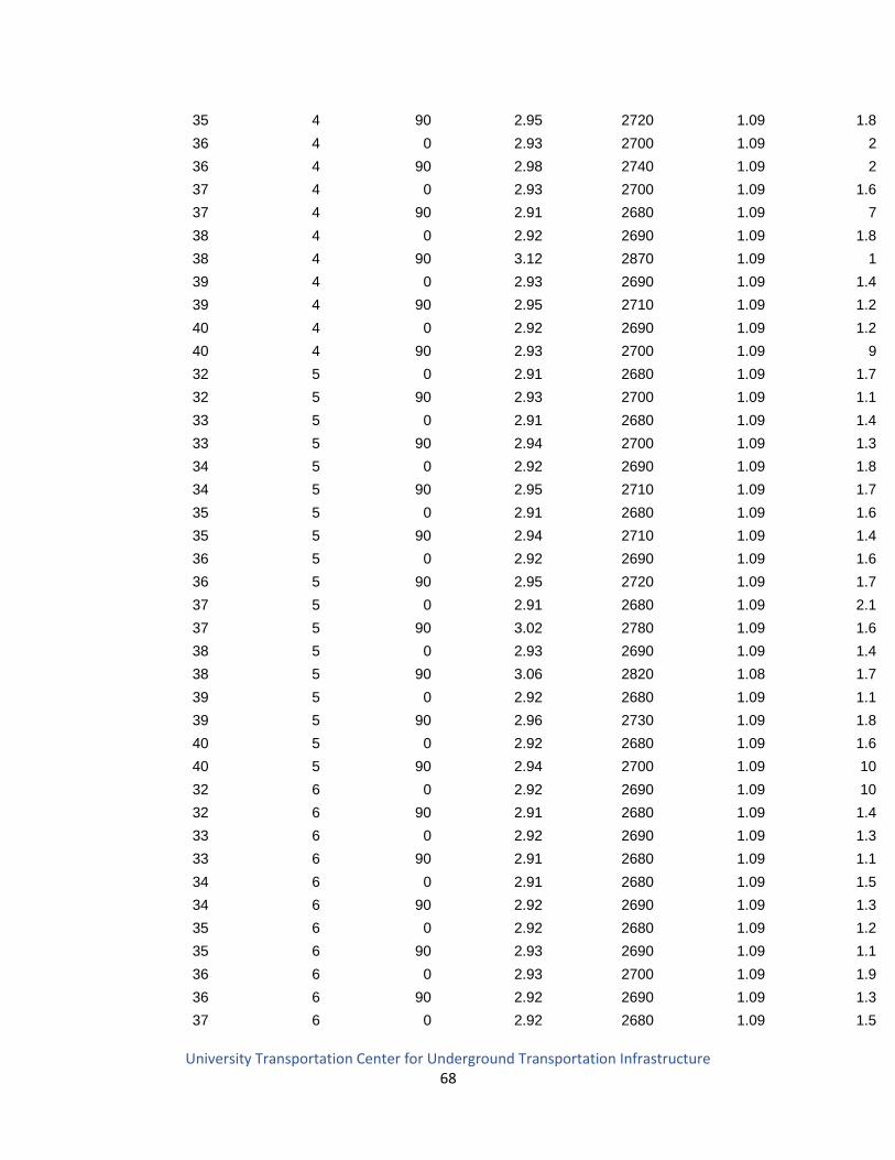
University Transportation Center for Underground Transportation Infrastructure 68
35 4 90 2.95 2720 1.09 1.8
36 4 0 2.93 2700 1.09 2
36 4 90 2.98 2740 1.09 2
37 4 0 2.93 2700 1.09 1.6
37 4 90 2.91 2680 1.09 7
38 4 0 2.92 2690 1.09 1.8
38 4 90 3.12 2870 1.09 1
39 4 0 2.93 2690 1.09 1.4
39 4 90 2.95 2710 1.09 1.2
40 4 0 2.92 2690 1.09 1.2
40 4 90 2.93 2700 1.09 9
32 5 0 2.91 2680 1.09 1.7
32 5 90 2.93 2700 1.09 1.1
33 5 0 2.91 2680 1.09 1.4
33 5 90 2.94 2700 1.09 1.3
34 5 0 2.92 2690 1.09 1.8
34 5 90 2.95 2710 1.09 1.7
35 5 0 2.91 2680 1.09 1.6
35 5 90 2.94 2710 1.09 1.4
36 5 0 2.92 2690 1.09 1.6
36 5 90 2.95 2720 1.09 1.7
37 5 0 2.91 2680 1.09 2.1
37 5 90 3.02 2780 1.09 1.6
38 5 0 2.93 2690 1.09 1.4
38 5 90 3.06 2820 1.08 1.7
39 5 0 2.92 2680 1.09 1.1
39 5 90 2.96 2730 1.09 1.8
40 5 0 2.92 2680 1.09 1.6
40 5 90 2.94 2700 1.09 10
32 6 0 2.92 2690 1.09 10
32 6 90 2.91 2680 1.09 1.4
33 6 0 2.92 2690 1.09 1.3
33 6 90 2.91 2680 1.09 1.1
34 6 0 2.91 2680 1.09 1.5
34 6 90 2.92 2690 1.09 1.3
35 6 0 2.92 2680 1.09 1.2
35 6 90 2.93 2690 1.09 1.1
36 6 0 2.93 2700 1.09 1.9
36 6 90 2.92 2690 1.09 1.3
37 6 0 2.92 2680 1.09 1.5
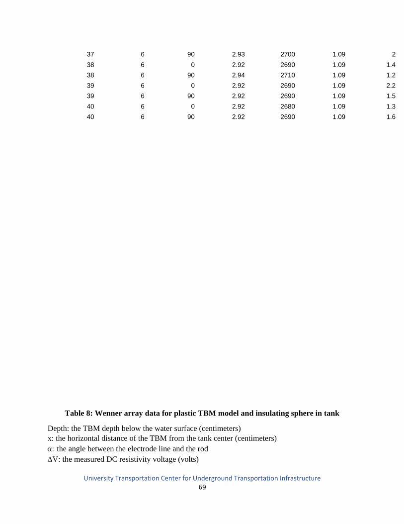
University Transportation Center for Underground Transportation Infrastructure 69
37 6 90 2.93 2700 1.09 2
38 6 0 2.92 2690 1.09 1.4
38 6 90 2.94 2710 1.09 1.2
39 6 0 2.92 2690 1.09 2.2
39 6 90 2.92 2690 1.09 1.5
40 6 0 2.92 2680 1.09 1.3
40 6 90 2.92 2690 1.09 1.6
Table 8: Wenner array data for plastic TBM model and insulating sphere in tank
Depth: the TBM depth below the water surface (centimeters)
x: the horizontal distance of the TBM from the tank center (centimeters)
the angle between the electrode line and the rod
V: the measured DC resistivity voltage (volts)
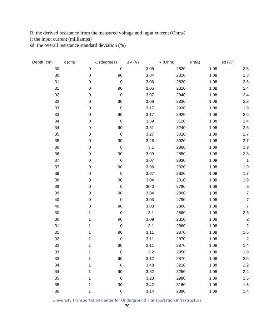
University Transportation Center for Underground Transportation Infrastructure 70
R: the derived resistance from the measured voltage and input current (Ohms)
I: the input current (milliamps)
sd: the overall resistance standard deviation (%)
Depth (cm) x (cm) (degrees) V (V) R (Ohm) I(mA) sd (%)
30 0 0 3.05 2820 1.08 2.5
30 0 90 3.04 2810 1.08 2.3
31 0 0 3.06 2820 1.08 2.6
31 0 90 3.05 2810 1.08 2.4
32 0 0 3.07 2840 1.08 2.4
32 0 90 3.06 2830 1.08 2.8
33 0 0 3.17 2920 1.08 1.9
33 0 90 3.17 2920 1.08 2.6
34 0 0 3.39 3120 1.08 2.4
34 0 90 3.51 3240 1.08 2.5
35 0 0 3.27 3010 1.09 1.7
35 0 90 3.28 3020 1.08 2.7
36 0 0 3.1 2860 1.09 1.9
36 0 90 3.09 2850 1.08 2.3
37 0 0 3.07 2830 1.09 1
37 0 90 3.06 2820 1.08 1.9
38 0 0 3.07 2820 1.09 1.7
38 0 90 3.04 2810 1.08 1.9
39 0 0 30.3 2790 1.09 5
39 0 90 3.04 2800 1.08 7
40 0 0 3.03 2790 1.08 7
40 0 90 3.03 2800 1.08 7
30 1 0 3.1 2860 1.08 2.6
30 1 90 3.09 2850 1.08 2
31 1 0 3.1 2860 1.08 2
31 1 90 3.11 2870 1.08 1.5
32 1 0 3.11 2870 1.08 2
32 1 90 3.11 2870 1.08 1.4
33 1 0 3.2 2950 1.08 1.9
33 1 90 3.12 2870 1.08 2.5
34 1 0 3.48 3210 1.08 2.2
34 1 90 3.52 3250 1.08 2.4
35 1 0 3.23 2980 1.09 1.5
35 1 90 3.42 3160 1.08 1.6
36 1 0 3.14 2890 1.09 1.4
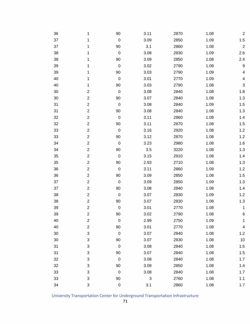
University Transportation Center for Underground Transportation Infrastructure 71
36 1 90 3.11 2870 1.08 2
37 1 0 3.09 2850 1.09 1.5
37 1 90 3.1 2860 1.08 2
38 1 0 3.08 2830 1.09 2.6
38 1 90 3.09 2850 1.08 2.4
39 1 0 3.02 2790 1.08 9
39 1 90 3.03 2790 1.09 4
40 1 0 3.01 2770 1.09 4
40 1 90 3.03 2790 1.08 3
30 2 0 3.08 2840 1.08 1.8
30 2 90 3.07 2840 1.08 1.3
31 2 0 3.08 2840 1.09 1.5
31 2 90 3.08 2840 1.08 1.3
32 2 0 3.11 2860 1.08 1.4
32 2 90 3.11 2870 1.08 1.5
33 2 0 3.16 2920 1.08 1.2
33 2 90 3.12 2870 1.08 1.2
34 2 0 3.23 2980 1.08 1.6
34 2 90 3.5 3220 1.08 1.3
35 2 0 3.15 2910 1.08 1.4
35 2 90 2.93 2710 1.08 1.3
36 2 0 3.11 2860 1.09 1.2
36 2 90 3.09 2850 1.08 1.5
37 2 0 3.09 2850 1.09 1.3
37 2 90 3.08 2840 1.08 1.4
38 2 0 3.07 2830 1.09 1.2
38 2 90 3.07 2830 1.08 1.3
39 2 0 3.01 2770 1.08 1
39 2 90 3.02 2790 1.08 6
40 2 0 2.99 2750 1.09 1
40 2 90 3.01 2770 1.08 4
30 3 0 3.07 2840 1.08 1.2
30 3 90 3.07 2830 1.08 10
31 3 0 3.08 2840 1.08 1.5
31 3 90 3.07 2840 1.08 1.5
32 3 0 3.08 2840 1.08 1.7
32 3 90 3.09 2850 1.08 1.4
33 3 0 3.08 2840 1.08 1.7
33 3 90 3 2760 1.08 1.1
34 3 0 3.1 2860 1.08 1.7
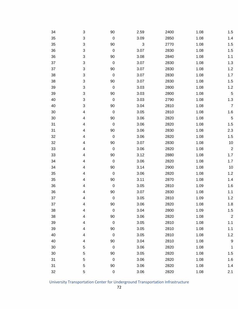
University Transportation Center for Underground Transportation Infrastructure 72
34 3 90 2.59 2400 1.08 1.5
35 3 0 3.09 2850 1.08 1.4
35 3 90 3 2770 1.08 1.5
36 3 0 3.07 2830 1.08 1.5
36 3 90 3.08 2840 1.08 1.1
37 3 0 3.07 2830 1.08 1.3
37 3 90 3.07 2830 1.08 1.2
38 3 0 3.07 2830 1.08 1.7
38 3 90 3.07 2830 1.08 1.5
39 3 0 3.03 2800 1.08 1.2
39 3 90 3.03 2800 1.08 5
40 3 0 3.03 2790 1.08 1.3
40 3 90 3.04 2810 1.08 7
30 4 0 3.05 2810 1.08 1.6
30 4 90 3.06 2820 1.08 5
31 4 0 3.06 2820 1.08 1.5
31 4 90 3.06 2830 1.08 2.3
32 4 0 3.06 2820 1.08 1.5
32 4 90 3.07 2830 1.08 10
33 4 0 3.06 2820 1.08 2
33 4 90 3.12 2880 1.08 1.7
34 4 0 3.06 2820 1.08 1.7
34 4 90 3.14 2900 1.08 10
35 4 0 3.06 2820 1.08 1.2
35 4 90 3.11 2870 1.08 1.4
36 4 0 3.05 2810 1.09 1.6
36 4 90 3.07 2830 1.08 1.1
37 4 0 3.05 2810 1.09 1.2
37 4 90 3.06 2820 1.08 1.8
38 4 0 3.04 2800 1.09 1.5
38 4 90 3.06 2820 1.08 2
39 4 0 3.05 2810 1.08 1.1
39 4 90 3.05 2810 1.08 1.1
40 4 0 3.05 2810 1.08 1.2
40 4 90 3.04 2810 1.08 9
30 5 0 3.06 2820 1.08 1
30 5 90 3.05 2820 1.08 1.5
31 5 0 3.06 2820 1.08 1.6
31 5 90 3.06 2820 1.08 1.4
32 5 0 3.06 2820 1.08 2.1
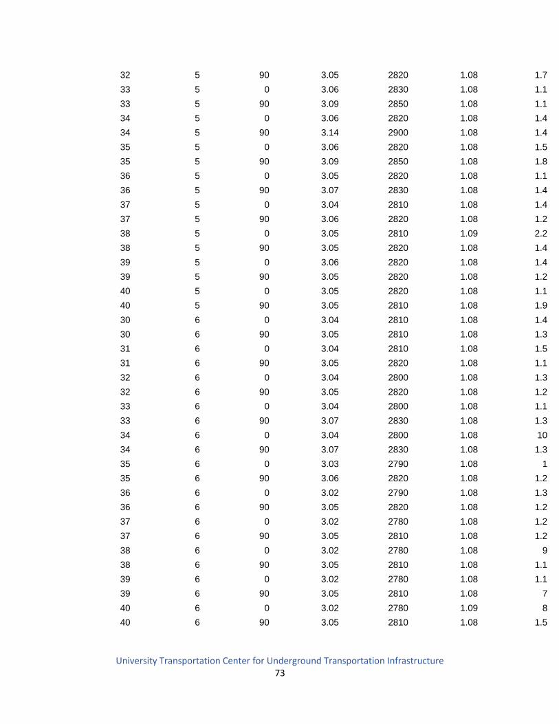
University Transportation Center for Underground Transportation Infrastructure 73
32 5 90 3.05 2820 1.08 1.7
33 5 0 3.06 2830 1.08 1.1
33 5 90 3.09 2850 1.08 1.1
34 5 0 3.06 2820 1.08 1.4
34 5 90 3.14 2900 1.08 1.4
35 5 0 3.06 2820 1.08 1.5
35 5 90 3.09 2850 1.08 1.8
36 5 0 3.05 2820 1.08 1.1
36 5 90 3.07 2830 1.08 1.4
37 5 0 3.04 2810 1.08 1.4
37 5 90 3.06 2820 1.08 1.2
38 5 0 3.05 2810 1.09 2.2
38 5 90 3.05 2820 1.08 1.4
39 5 0 3.06 2820 1.08 1.4
39 5 90 3.05 2820 1.08 1.2
40 5 0 3.05 2820 1.08 1.1
40 5 90 3.05 2810 1.08 1.9
30 6 0 3.04 2810 1.08 1.4
30 6 90 3.05 2810 1.08 1.3
31 6 0 3.04 2810 1.08 1.5
31 6 90 3.05 2820 1.08 1.1
32 6 0 3.04 2800 1.08 1.3
32 6 90 3.05 2820 1.08 1.2
33 6 0 3.04 2800 1.08 1.1
33 6 90 3.07 2830 1.08 1.3
34 6 0 3.04 2800 1.08 10
34 6 90 3.07 2830 1.08 1.3
35 6 0 3.03 2790 1.08 1
35 6 90 3.06 2820 1.08 1.2
36 6 0 3.02 2790 1.08 1.3
36 6 90 3.05 2820 1.08 1.2
37 6 0 3.02 2780 1.08 1.2
37 6 90 3.05 2810 1.08 1.2
38 6 0 3.02 2780 1.08 9
38 6 90 3.05 2810 1.08 1.1
39 6 0 3.02 2780 1.08 1.1
39 6 90 3.05 2810 1.08 7
40 6 0 3.02 2780 1.09 8
40 6 90 3.05 2810 1.08 1.5

University Transportation Center for Underground Transportation Infrastructure 74
Table 9: Dipole-dipole array data for copper TBM model and insulating sphere in tank
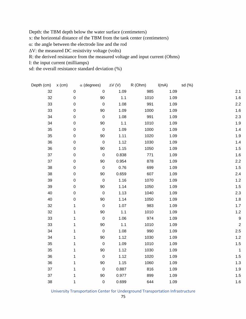
University Transportation Center for Underground Transportation Infrastructure 75
Depth: the TBM depth below the water surface (centimeters)
x: the horizontal distance of the TBM from the tank center (centimeters)
the angle between the electrode line and the rod
V: the measured DC resistivity voltage (volts)
R: the derived resistance from the measured voltage and input current (Ohms)
I: the input current (milliamps)
sd: the overall resistance standard deviation (%)
Depth (cm) x (cm) (degrees) V (V) R (Ohm) I(mA) sd (%)
32 0 0 1.09 985 1.09 2.1
32 0 90 1.1 1010 1.09 1.6
33 0 0 1.08 991 1.09 2.2
33 0 90 1.09 1000 1.09 1.6
34 0 0 1.08 991 1.09 2.3
34 0 90 1.1 1010 1.09 1.9
35 0 0 1.09 1000 1.09 1.4
35 0 90 1.11 1020 1.09 1.9
36 0 0 1.12 1030 1.09 1.4
36 0 90 1.15 1050 1.09 1.5
37 0 0 0.838 771 1.09 1.6
37 0 90 0.954 878 1.09 2.2
38 0 0 0.76 699 1.09 1.5
38 0 90 0.659 607 1.09 2.4
39 0 0 1.16 1070 1.09 1.2
39 0 90 1.14 1050 1.09 1.5
40 0 0 1.13 1040 1.09 2.3
40 0 90 1.14 1050 1.09 1.8
32 1 0 1.07 983 1.09 1.7
32 1 90 1.1 1010 1.09 1.2
33 1 0 1.06 974 1.09 9
33 1 90 1.1 1010 1.09 2
34 1 0 1.08 990 1.09 2.5
34 1 90 1.12 1030 1.09 1.2
35 1 0 1.09 1010 1.09 1.5
35 1 90 1.12 1030 1.09 1
36 1 0 1.12 1020 1.09 1.5
36 1 90 1.15 1060 1.09 1.3
37 1 0 0.887 816 1.09 1.9
37 1 90 0.977 899 1.09 1.5
38 1 0 0.699 644 1.09 1.6
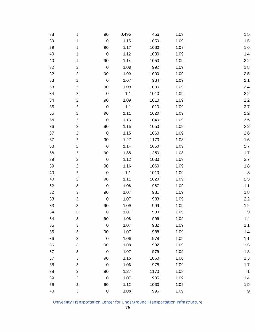
University Transportation Center for Underground Transportation Infrastructure 76
38 1 90 0.495 456 1.09 1.5
39 1 0 1.15 1050 1.09 1.5
39 1 90 1.17 1080 1.09 1.6
40 1 0 1.12 1030 1.09 1.4
40 1 90 1.14 1050 1.09 2.2
32 2 0 1.08 992 1.09 1.8
32 2 90 1.09 1000 1.09 2.5
33 2 0 1.07 984 1.09 2.1
33 2 90 1.09 1000 1.09 2.4
34 2 0 1.1 1010 1.09 2.2
34 2 90 1.09 1010 1.09 2.2
35 2 0 1.1 1010 1.09 2.7
35 2 90 1.11 1020 1.09 2.2
36 2 0 1.13 1040 1.09 3.5
36 2 90 1.15 1050 1.09 2.2
37 2 0 1.15 1060 1.09 2.6
37 2 90 1.27 1170 1.08 1.6
38 2 0 1.14 1050 1.09 2.7
38 2 90 1.35 1250 1.08 1.7
39 2 0 1.12 1030 1.09 2.7
39 2 90 1.16 1060 1.09 1.8
40 2 0 1.1 1010 1.09 3
40 2 90 1.11 1020 1.09 2.3
32 3 0 1.08 987 1.09 1.1
32 3 90 1.07 981 1.09 1.8
33 3 0 1.07 983 1.09 2.2
33 3 90 1.09 999 1.09 1.2
34 3 0 1.07 980 1.09 9
34 3 90 1.08 996 1.09 1.4
35 3 0 1.07 982 1.09 1.1
35 3 90 1.07 988 1.09 1.4
36 3 0 1.06 978 1.09 1.1
36 3 90 1.08 992 1.09 1.5
37 3 0 1.07 979 1.09 1.8
37 3 90 1.15 1060 1.08 1.3
38 3 0 1.06 978 1.09 1.7
38 3 90 1.27 1170 1.08 1
39 3 0 1.07 985 1.09 1.4
39 3 90 1.12 1030 1.09 1.5
40 3 0 1.08 996 1.09 9
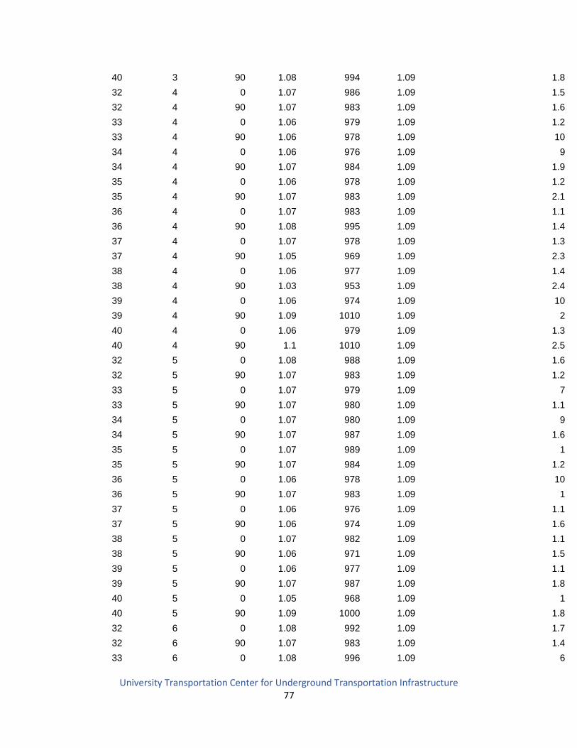
University Transportation Center for Underground Transportation Infrastructure 77
40 3 90 1.08 994 1.09 1.8
32 4 0 1.07 986 1.09 1.5
32 4 90 1.07 983 1.09 1.6
33 4 0 1.06 979 1.09 1.2
33 4 90 1.06 978 1.09 10
34 4 0 1.06 976 1.09 9
34 4 90 1.07 984 1.09 1.9
35 4 0 1.06 978 1.09 1.2
35 4 90 1.07 983 1.09 2.1
36 4 0 1.07 983 1.09 1.1
36 4 90 1.08 995 1.09 1.4
37 4 0 1.07 978 1.09 1.3
37 4 90 1.05 969 1.09 2.3
38 4 0 1.06 977 1.09 1.4
38 4 90 1.03 953 1.09 2.4
39 4 0 1.06 974 1.09 10
39 4 90 1.09 1010 1.09 2
40 4 0 1.06 979 1.09 1.3
40 4 90 1.1 1010 1.09 2.5
32 5 0 1.08 988 1.09 1.6
32 5 90 1.07 983 1.09 1.2
33 5 0 1.07 979 1.09 7
33 5 90 1.07 980 1.09 1.1
34 5 0 1.07 980 1.09 9
34 5 90 1.07 987 1.09 1.6
35 5 0 1.07 989 1.09 1
35 5 90 1.07 984 1.09 1.2
36 5 0 1.06 978 1.09 10
36 5 90 1.07 983 1.09 1
37 5 0 1.06 976 1.09 1.1
37 5 90 1.06 974 1.09 1.6
38 5 0 1.07 982 1.09 1.1
38 5 90 1.06 971 1.09 1.5
39 5 0 1.06 977 1.09 1.1
39 5 90 1.07 987 1.09 1.8
40 5 0 1.05 968 1.09 1
40 5 90 1.09 1000 1.09 1.8
32 6 0 1.08 992 1.09 1.7
32 6 90 1.07 983 1.09 1.4
33 6 0 1.08 996 1.09 6
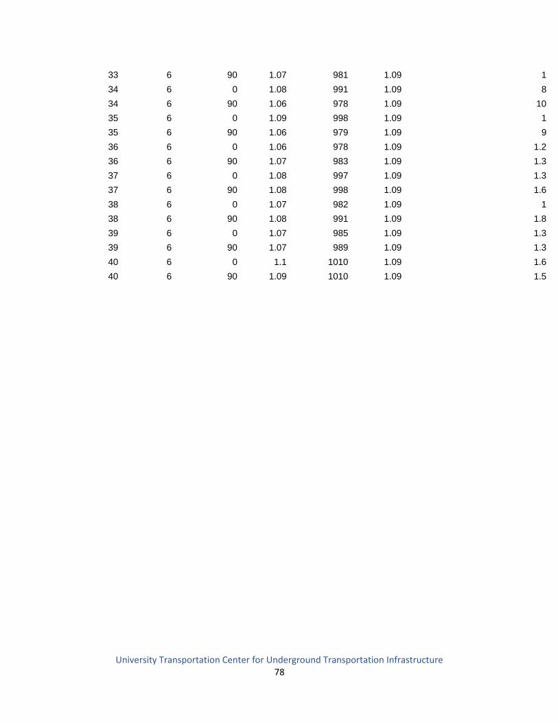
University Transportation Center for Underground Transportation Infrastructure 78
33 6 90 1.07 981 1.09 1
34 6 0 1.08 991 1.09 8
34 6 90 1.06 978 1.09 10
35 6 0 1.09 998 1.09 1
35 6 90 1.06 979 1.09 9
36 6 0 1.06 978 1.09 1.2
36 6 90 1.07 983 1.09 1.3
37 6 0 1.08 997 1.09 1.3
37 6 90 1.08 998 1.09 1.6
38 6 0 1.07 982 1.09 1
38 6 90 1.08 991 1.09 1.8
39 6 0 1.07 985 1.09 1.3
39 6 90 1.07 989 1.09 1.3
40 6 0 1.1 1010 1.09 1.6
40 6 90 1.09 1010 1.09 1.5
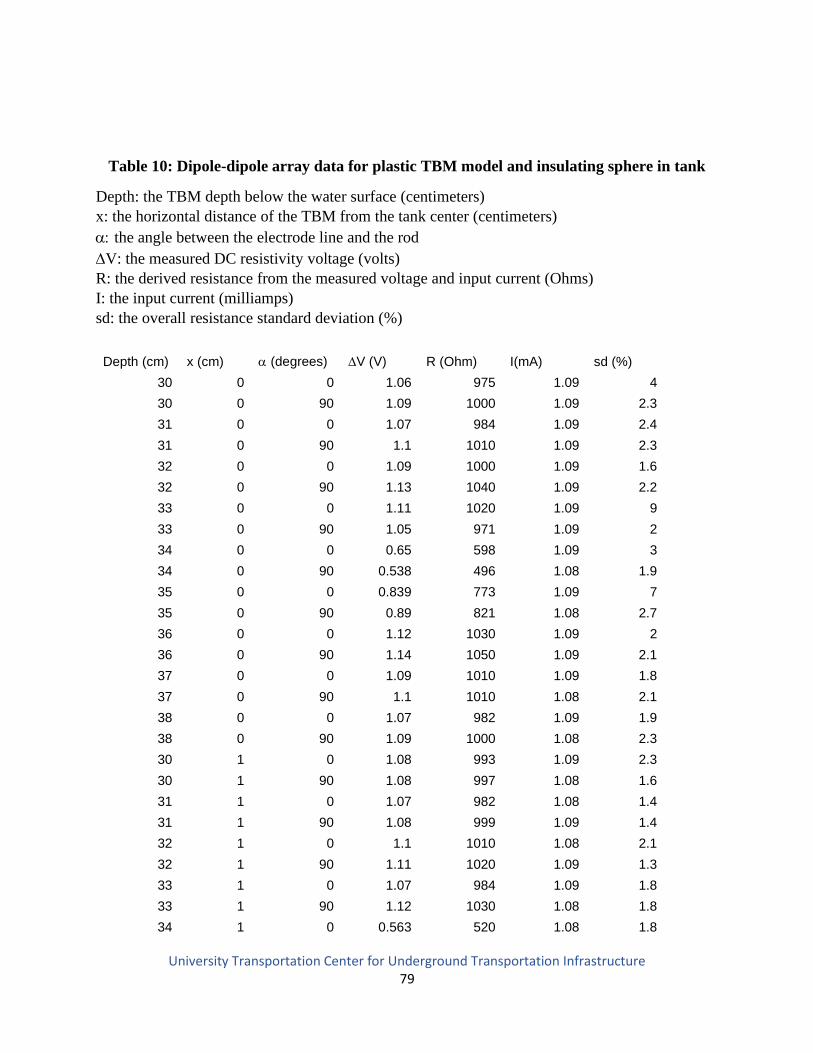
University Transportation Center for Underground Transportation Infrastructure 79
Table 10: Dipole-dipole array data for plastic TBM model and insulating sphere in tank
Depth: the TBM depth below the water surface (centimeters)
x: the horizontal distance of the TBM from the tank center (centimeters)
the angle between the electrode line and the rod
V: the measured DC resistivity voltage (volts)
R: the derived resistance from the measured voltage and input current (Ohms)
I: the input current (milliamps)
sd: the overall resistance standard deviation (%)
Depth (cm) x (cm) (degrees) V (V) R (Ohm) I(mA) sd (%)
30 0 0 1.06 975 1.09 4
30 0 90 1.09 1000 1.09 2.3
31 0 0 1.07 984 1.09 2.4
31 0 90 1.1 1010 1.09 2.3
32 0 0 1.09 1000 1.09 1.6
32 0 90 1.13 1040 1.09 2.2
33 0 0 1.11 1020 1.09 9
33 0 90 1.05 971 1.09 2
34 0 0 0.65 598 1.09 3
34 0 90 0.538 496 1.08 1.9
35 0 0 0.839 773 1.09 7
35 0 90 0.89 821 1.08 2.7
36 0 0 1.12 1030 1.09 2
36 0 90 1.14 1050 1.09 2.1
37 0 0 1.09 1010 1.09 1.8
37 0 90 1.1 1010 1.08 2.1
38 0 0 1.07 982 1.09 1.9
38 0 90 1.09 1000 1.08 2.3
30 1 0 1.08 993 1.09 2.3
30 1 90 1.08 997 1.08 1.6
31 1 0 1.07 982 1.08 1.4
31 1 90 1.08 999 1.09 1.4
32 1 0 1.1 1010 1.08 2.1
32 1 90 1.11 1020 1.09 1.3
33 1 0 1.07 984 1.09 1.8
33 1 90 1.12 1030 1.08 1.8
34 1 0 0.563 520 1.08 1.8
University Transportation Center for Underground Transportation Infrastructure 80
34 1 90 0.595 550 1.08 1.4
35 1 0 0.933 860 1.08 2.6
35 1 90 0.915 844 1.08 1.5
36 1 0 1.13 1040 1.08 1.8
36 1 90 1.14 1050 1.09 1.6
37 1 0 1.09 1010 1.08 1.8
37 1 90 1.1 1010 1.08 1.5
38 1 0 1.08 999 1.08 1.8
38 1 90 1.08 1000 1.09 1.1
30 2 0 1.06 975 1.09 2.6
30 2 90 1.07 990 1.09 1.4
31 2 0 1.07 981 1.09 8
31 2 90 1.08 994 1.09 1
32 2 0 1.09 1000 1.09 1.3
32 2 90 1.1 1010 1.09 1.2
33 2 0 1.12 1030 1.09 9
33 2 90 1.17 1080 1.09 1
34 2 0 1.13 1040 1.09 9
34 2 90 1.35 1240 1.08 8
35 2 0 1.12 1040 1.09 9
35 2 90 1.2 1110 1.08 1.4
36 2 0 1.1 1010 1.09 1.5
36 2 90 1.11 1020 1.09 1
37 2 0 1.08 993 1.09 1.1
37 2 90 1.08 997 1.09 8
38 2 0 1.08 993 1.09 1
38 2 90 1.08 995 1.09 9
30 3 0 1.07 987 1.09 1
30 3 90 1.07 989 1.09 9
31 3 0 1.07 985 1.09 9
31 3 90 1.07 987 1.09 8
32 3 0 1.07 989 1.09 9
32 3 90 1.07 989 1.09 1
33 3 0 1.08 989 1.09 9
33 3 90 1.08 1000 1.08 7
34 3 0 1.09 1000 1.09 8
34 3 90 1.19 1100 1.08 1.3
35 3 0 1.08 999 1.09 1.3
35 3 90 1.23 1130 1.08 1
36 3 0 1.08 991 1.09 1.5
University Transportation Center for Underground Transportation Infrastructure 81
36 3 90 1.12 1030 1.09 8
37 3 0 1.07 988 1.09 9
37 3 90 1.09 1000 1.09 8
38 3 0 1.07 990 1.09 1.3
38 3 90 1.07 990 1.09 1
30 4 0 1.08 992 1.09 2.1
30 4 90 1.08 997 1.09 7
31 4 0 1.09 1000 1.09 1.6
31 4 90 1.08 992 1.09 1.2
32 4 0 1.09 1000 1.08 1.2
32 4 90 1.08 991 1.09 1.2
33 4 0 1.09 1000 1.09 8
33 4 90 1.07 985 1.09 1
34 4 0 1.09 1000 1.09 8
34 4 90 1.05 965 1.08 1.1
35 4 0 1.08 999 1.09 1.1
35 4 90 1.06 974 1.08 1.1
36 4 0 1.08 998 1.09 1.2
36 4 90 1.07 988 1.09 1
37 4 0 1.08 999 1.09 1.1
37 4 90 1.07 989 1.09 9
38 4 0 1.09 1000 1.09 1.3
38 4 90 1.08 994 1.09 8
30 5 0 1.07 987 1.09 1.3
30 5 90 1.07 990 1.09 8
31 5 0 1.07 988 1.09 1.1
31 5 90 1.07 989 1.09 1.1
32 5 0 1.08 992 1.09 1.3
32 5 90 1.07 985 1.09 1.4
33 5 0 1.08 991 1.09 1
33 5 90 1.07 985 1.09 1
34 5 0 1.08 992 1.09 1.1
34 5 90 1.07 982 1.09 10
35 5 0 1.07 988 1.09 8
35 5 90 1.07 987 1.09 1.2
36 5 0 1.07 989 1.09 1.2
36 5 90 1.07 986 1.09 1
37 5 0 1.07 989 1.09 1.2
37 5 90 1.07 986 1.09 9
38 5 0 1.07 988 1.09 1.2
University Transportation Center for Underground Transportation Infrastructure 82
38 5 90 1.07 987 1.09 8
30 6 0 1.08 996 1.09 1.2
30 6 90 1.08 993 1.09 1.3
31 6 0 1.09 1000 1.09 1.3
31 6 90 1.08 991 1.09 1.7
32 6 0 1.08 993 1.09 1.8
32 6 90 1.07 988 1.09 9
33 6 0 1.09 999 1.09 1.4
33 6 90 1.07 986 1.09 1.2
34 6 0 1.08 991 1.09 2.6
34 6 90 1.07 988 1.09 1.4
35 6 0 1.08 997 1.09 1.8
35 6 90 1.07 987 1.09 1.1
36 6 0 1.08 999 1.09 1.7
36 6 90 1.07 989 1.09 1.2
37 6 0 1.08 997 1.09 2.3
37 6 90 1.07 988 1.09 1.1
38 6 0 1.08 992 1.09 1.8
38 6 90 1.07 990 1.09 1.4