qsoft documentation - ahead
TRANSCRIPT

Page 0 of 78
Document: AHEAD-WP8-D8.9-D43-QSOFT
AHEAD Workpackage 8 Deliverable D8.9 – D43 QSOFT Documentation
AHEAD Workpackage 8 JRA X-ray optics
Deliverable D8.9 – D43
QSOFT Documentation
Written by Richard Willingale (ULeic)
Checked by Vadim Burwitz (MPE)
Distribution List AHEAD Management Team
Vadim Burwitz WP8.0, WP8.1, WP8.3
Dick Willingale WP8.1
Rene Hudec WP8.1
Gianpiero Tagliaferri WP8.1, WP8.2
Distribution Date Draft version Dec 21, 2019
Final version Feb 26, 2019
Ref. Ares(2019)1371899 - 28/02/2019

QSOFT DocumentationRelease 9.0
Richard Willingale
Dec 21, 2018

CONTENTS
1 Build and Installation 3
2 Python, R and IDL 52.1 Python . . . . . . . . . . . . . . . . . . . . . . . . . . . . . . . . . . . . . . . . . . . . . . . . . . 52.2 RScript . . . . . . . . . . . . . . . . . . . . . . . . . . . . . . . . . . . . . . . . . . . . . . . . . . 52.3 IDL . . . . . . . . . . . . . . . . . . . . . . . . . . . . . . . . . . . . . . . . . . . . . . . . . . . . 6
3 qfits - Using FITS Files 73.1 Reading FITS Files . . . . . . . . . . . . . . . . . . . . . . . . . . . . . . . . . . . . . . . . . . . . 73.2 Writing FITS Files . . . . . . . . . . . . . . . . . . . . . . . . . . . . . . . . . . . . . . . . . . . . 83.3 qfits.functions . . . . . . . . . . . . . . . . . . . . . . . . . . . . . . . . . . . . . . . . . . . . . . 10
4 images - Image Processing 154.1 images.functions . . . . . . . . . . . . . . . . . . . . . . . . . . . . . . . . . . . . . . . . . . . . . 16
5 astro - Astronomy Applications 255.1 astro.functions . . . . . . . . . . . . . . . . . . . . . . . . . . . . . . . . . . . . . . . . . . . . . . 25
6 xscat - X-ray Physics 316.1 xscat.functions . . . . . . . . . . . . . . . . . . . . . . . . . . . . . . . . . . . . . . . . . . . . . . 31
7 xsrt - Sequential Ray Tracing 377.1 Example Scripts . . . . . . . . . . . . . . . . . . . . . . . . . . . . . . . . . . . . . . . . . . . . . 377.2 Optical Elements and Coordinates . . . . . . . . . . . . . . . . . . . . . . . . . . . . . . . . . . . . 397.3 Source and Detector . . . . . . . . . . . . . . . . . . . . . . . . . . . . . . . . . . . . . . . . . . . 407.4 Monte Carlo and Random Numbers . . . . . . . . . . . . . . . . . . . . . . . . . . . . . . . . . . . 417.5 Deformations . . . . . . . . . . . . . . . . . . . . . . . . . . . . . . . . . . . . . . . . . . . . . . . 417.6 Surface Quality, Reflectivity and Scattering . . . . . . . . . . . . . . . . . . . . . . . . . . . . . . . 417.7 X-ray Telescopes, Lens and Prism . . . . . . . . . . . . . . . . . . . . . . . . . . . . . . . . . . . . 427.8 Ray Tracing and Saving Rays . . . . . . . . . . . . . . . . . . . . . . . . . . . . . . . . . . . . . . 427.9 xsrt.functions . . . . . . . . . . . . . . . . . . . . . . . . . . . . . . . . . . . . . . . . . . . . . . . 44
8 Adding New Functions 638.1 Module Source Code . . . . . . . . . . . . . . . . . . . . . . . . . . . . . . . . . . . . . . . . . . . 638.2 The Ray Tracing Routines . . . . . . . . . . . . . . . . . . . . . . . . . . . . . . . . . . . . . . . . 648.3 New Surface Elements . . . . . . . . . . . . . . . . . . . . . . . . . . . . . . . . . . . . . . . . . . 66
9 Authors 69
Python Module Index 71
i

Index 73
ii

QSOFT Documentation, Release 9.0
QSOFT is a collection of data analysis and modelling applications for use in X-ray astronomy and related disciplines.
The applications are run as commands/functions within Python, R or IDL.
The core code is written in Fortran and C, compiled to produce shareable object libraries and imported as modules inPython or loaded by R or IDL.
The commands/functions are defined in Python modules, R or IDL scripts.
The QSOFT collection should be built using the gcc and gfortran compilers. The Python module f2py and/or R mustbe available to create the shareable objects.
CONTENTS 1

QSOFT Documentation, Release 9.0
2 CONTENTS

CHAPTER
ONE
BUILD AND INSTALLATION
The following software items are required for the build:
• Fortran compiler - GNU gfortran used in development
• C compiler - GNU gcc used in development
• Python module f2py - to build the modules for Python
• R - to build the shareable libraries for R and IDL
• Python module sphinx - to build the documentation
1. Download from GitHub
$ git clone git://github.com/dickwillingale/qsoft.git
This will create a directory qsoft/
2) Move into /your/files/top/qsoft/src
$ cd /your/files/top/qsoft/src
Edit the compile.config so that the compilers CC and F77 and R, F2PY and IDL point to the correctexecutables on your system. If you don’t have R or F2PY leave them blank. If your target is IDL youwill need R to compile the shareable library.
3. Move into /your/files/top/qsoft and execute build
$ cd /your/files/top/qsoft
$ ./build
This will check you have gcc gfortran and R and/or Python with f2py. It will then create thesrc/compiler.config file for make and compile the shareable objects.
4. Put the following line into your /home/.profile
. /your/files/top/qsoft/setup_q
Qsoft will be available when you launch a login terminal.
5. That’s it.
When you start R (or Rscript) it will automatically load the QSOFT applications using the/home/.Rprofile file.
The environment variable PYTHONPATH will point to the qsoft/python_modules directory so youcan load the modules into Python.
3

QSOFT Documentation, Release 9.0
4 Chapter 1. Build and Installation
CHAPTER
TWO
PYTHON, R AND IDL
All the Fortran functions can be called from Python, R or IDL. Because of peculiarities in the syntax and structure ofthe scripting languages there are minor differences in the way the functions are accessed.
The documentation of all the functions uses the Python implementation. Where there are significant differences in theR or IDL versions these are mentioned in the text.
2.1 Python
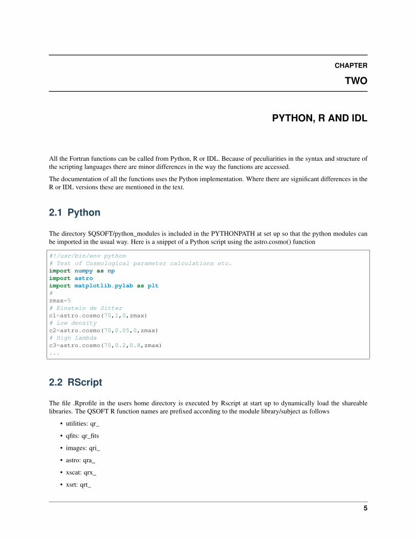
The directory $QSOFT/python_modules is included in the PYTHONPATH at set up so that the python modules canbe imported in the usual way. Here is a snippet of a Python script using the astro.cosmo() function
#!/usr/bin/env python# Test of Cosmological parameter calculations etc.import numpy as npimport astroimport matplotlib.pylab as plt#zmax=5# Einstein de Sitterc1=astro.cosmo(70,1,0,zmax)# Low densityc2=astro.cosmo(70,0.05,0,zmax)# High Lambdac3=astro.cosmo(70,0.2,0.8,zmax)...
2.2 RScript
The file .Rprofile in the users home directory is executed by Rscript at start up to dynamically load the shareablelibraries. The QSOFT R function names are prefixed according to the module library/subject as follows
• utilities: qr_
• qfits: qr_fits
• images: qri_
• astro: qra_
• xscat: qrx_
• xsrt: qrt_
5
QSOFT Documentation, Release 9.0
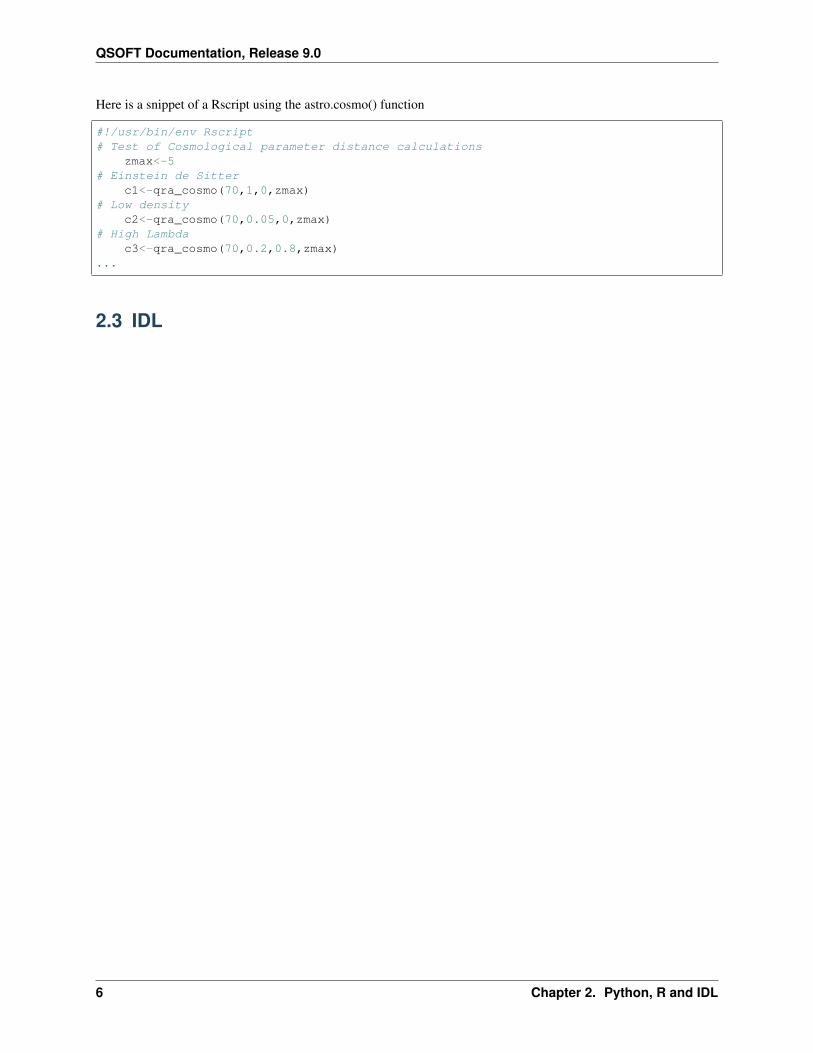
Here is a snippet of a Rscript using the astro.cosmo() function
#!/usr/bin/env Rscript# Test of Cosmological parameter distance calculations
zmax<-5# Einstein de Sitter
c1<-qra_cosmo(70,1,0,zmax)# Low density
c2<-qra_cosmo(70,0.05,0,zmax)# High Lambda
c3<-qra_cosmo(70,0.2,0.8,zmax)...
2.3 IDL
6 Chapter 2. Python, R and IDL
CHAPTER
THREE
QFITS - USING FITS FILES
The qfits interface has not yet been implemented in IDL.
Reading and writing of FITS files is available in Python and R.
3.1 Reading FITS Files
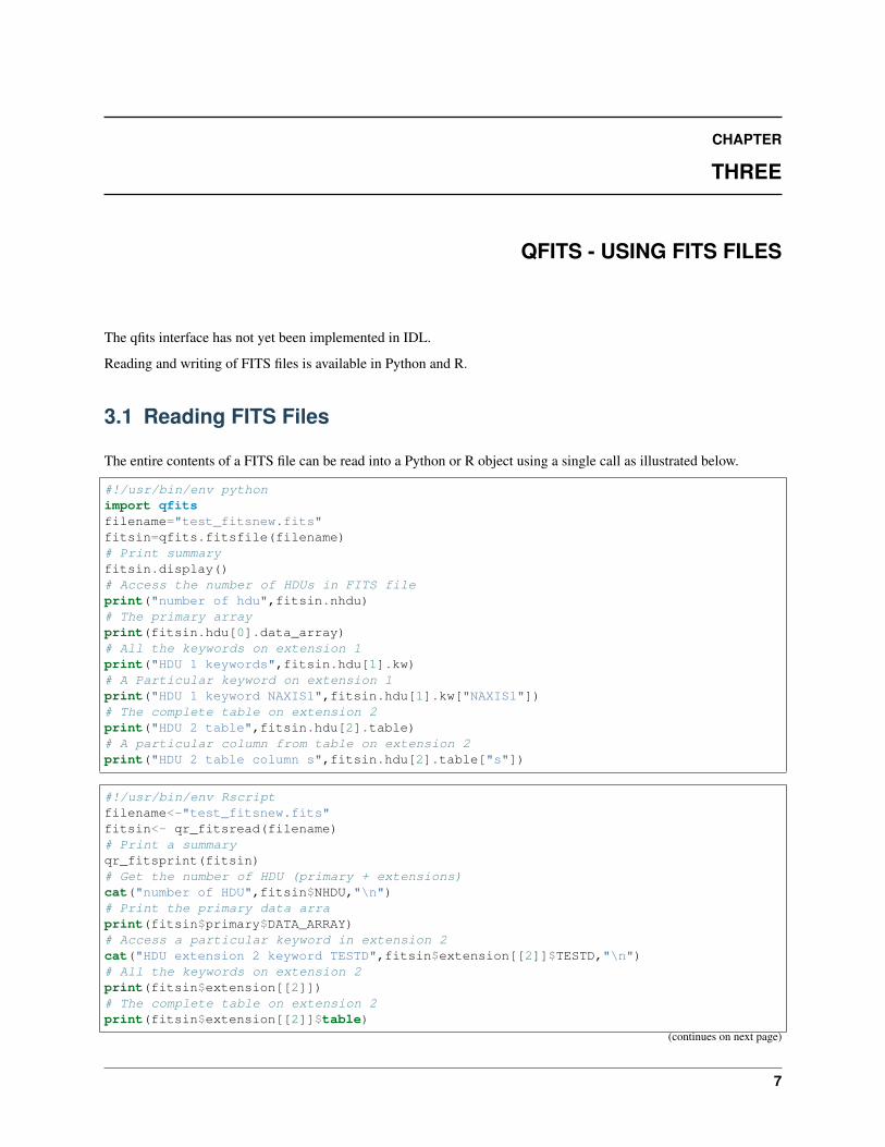
The entire contents of a FITS file can be read into a Python or R object using a single call as illustrated below.
#!/usr/bin/env pythonimport qfitsfilename="test_fitsnew.fits"fitsin=qfits.fitsfile(filename)# Print summaryfitsin.display()# Access the number of HDUs in FITS fileprint("number of hdu",fitsin.nhdu)# The primary arrayprint(fitsin.hdu[0].data_array)# All the keywords on extension 1print("HDU 1 keywords",fitsin.hdu[1].kw)# A Particular keyword on extension 1print("HDU 1 keyword NAXIS1",fitsin.hdu[1].kw["NAXIS1"])# The complete table on extension 2print("HDU 2 table",fitsin.hdu[2].table)# A particular column from table on extension 2print("HDU 2 table column s",fitsin.hdu[2].table["s"])
#!/usr/bin/env Rscriptfilename<-"test_fitsnew.fits"fitsin<- qr_fitsread(filename)# Print a summaryqr_fitsprint(fitsin)# Get the number of HDU (primary + extensions)cat("number of HDU",fitsin$NHDU,"\n")# Print the primary data arraprint(fitsin$primary$DATA_ARRAY)# Access a particular keyword in extension 2cat("HDU extension 2 keyword TESTD",fitsin$extension[[2]]$TESTD,"\n")# All the keywords on extension 2print(fitsin$extension[[2]])# The complete table on extension 2print(fitsin$extension[[2]]$table)
(continues on next page)
7
QSOFT Documentation, Release 9.0
(continued from previous page)
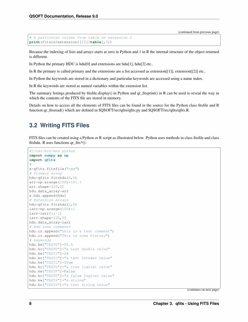
# A particular column from table on extension 2print(fitsin$extension[[2]]$table[,3])
Because the indexing of lists and arrays starts at zero in Python and 1 in R the internal structure of the object returnedis different.
In Python the primary HDU is hdu[0] and extensions are hdu[1], hdu[2] etc..
In R the primary is called primary and the extensions are a list accessed as extension[[1]], extension[[2]] etc..
In Python the keywords are stored in a dictionary and particular keywords are accessed using a name index.
In R the keywords are stored as named variables within the extension list.
The summary listings produced by fitsfile.display() in Python and qr_fitsprint() in R can be used to reveal the way inwhich the contents of the FITS file are stored in memory.
Details on how to access all the elements of FITS files can be found in the source for the Python class fitsfile and Rfunction qr_fitsread() which are defined in $QSOFT/src/qfits/qfits.py and $QSOFT/src/qfits/qfits.R.
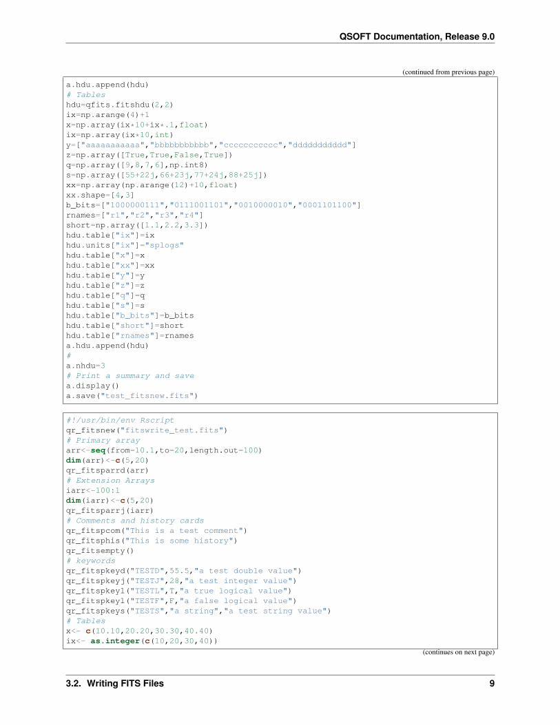
3.2 Writing FITS Files
FITS files can be created using a Python or R script as illustrated below. Python uses methods in class fitsfile and classfitshdu. R uses functions qr_fits*().
#!/usr/bin/env pythonimport numpy as npimport qfits#a=qfits.fitsfile("new")# Primary arrayhdu=qfits.fitshdu(0,0)arr=np.arange(100)+101.1arr.shape=[20,5]hdu.data_array=arra.hdu.append(hdu)# Extension Arrayshdu=qfits.fitshdu(1,0)iarr=np.arange(100)+1iarr=iarr[::-1]iarr.shape=[20,5]hdu.data_array=iarr# Add some commentshdu.cr.append("This is a test comment")hdu.cr.append("This is some history")# keywordshdu.kw["TESTD"]=55.5hdu.kc["TESTD"]="a test double value"hdu.kw["TESTJ"]=28hdu.kc["TESTJ"]="a test integer value"hdu.kw["TESTL"]=Truehdu.kc["TESTL"]="a true logical value"hdu.kw["TESTF"]=Falsehdu.kc["TESTF"]="a false logical value"hdu.kw["TESTS"]="a string"hdu.kc["TESTS"]="a test string value"
(continues on next page)
8 Chapter 3. qfits - Using FITS Files
QSOFT Documentation, Release 9.0
(continued from previous page)
a.hdu.append(hdu)# Tableshdu=qfits.fitshdu(2,2)ix=np.arange(4)+1x=np.array(ix*10+ix*.1,float)ix=np.array(ix*10,int)y=["aaaaaaaaaaa","bbbbbbbbbbb","ccccccccccc","ddddddddddd"]z=np.array([True,True,False,True])q=np.array([9,8,7,6],np.int8)s=np.array([55+22j,66+23j,77+24j,88+25j])xx=np.array(np.arange(12)+10,float)xx.shape=[4,3]b_bits=["1000000111","0111001101","0010000010","0001101100"]rnames=["r1","r2","r3","r4"]short=np.array([1.1,2.2,3.3])hdu.table["ix"]=ixhdu.units["ix"]="splogs"hdu.table["x"]=xhdu.table["xx"]=xxhdu.table["y"]=yhdu.table["z"]=zhdu.table["q"]=qhdu.table["s"]=shdu.table["b_bits"]=b_bitshdu.table["short"]=shorthdu.table["rnames"]=rnamesa.hdu.append(hdu)#a.nhdu=3# Print a summary and savea.display()a.save("test_fitsnew.fits")
#!/usr/bin/env Rscriptqr_fitsnew("fitswrite_test.fits")# Primary arrayarr<-seq(from=10.1,to=20,length.out=100)dim(arr)<-c(5,20)qr_fitsparrd(arr)# Extension Arraysiarr<-100:1dim(iarr)<-c(5,20)qr_fitsparrj(iarr)# Comments and history cardsqr_fitspcom("This is a test comment")qr_fitsphis("This is some history")qr_fitsempty()# keywordsqr_fitspkeyd("TESTD",55.5,"a test double value")qr_fitspkeyj("TESTJ",28,"a test integer value")qr_fitspkeyl("TESTL",T,"a true logical value")qr_fitspkeyl("TESTF",F,"a false logical value")qr_fitspkeys("TESTS","a string","a test string value")# Tablesx<- c(10.10,20.20,30.30,40.40)ix<- as.integer(c(10,20,30,40))
(continues on next page)
3.2. Writing FITS Files 9
QSOFT Documentation, Release 9.0
(continued from previous page)
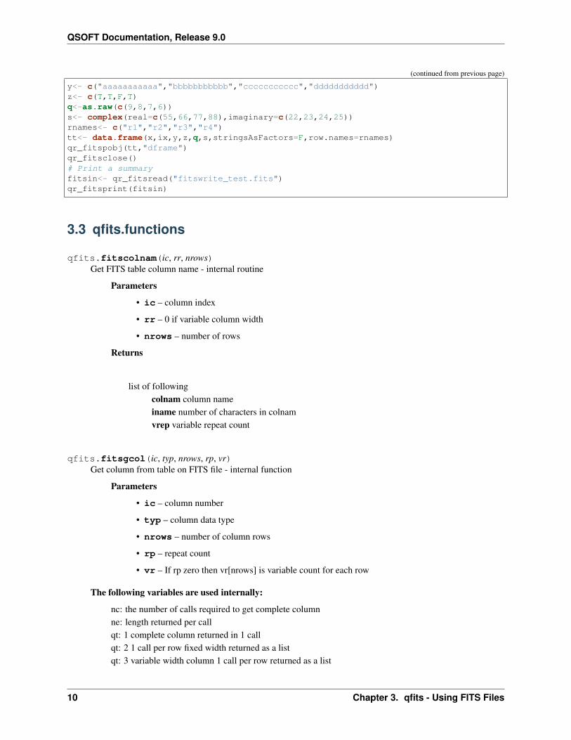
y<- c("aaaaaaaaaaa","bbbbbbbbbbb","ccccccccccc","ddddddddddd")z<- c(T,T,F,T)q<-as.raw(c(9,8,7,6))s<- complex(real=c(55,66,77,88),imaginary=c(22,23,24,25))rnames<- c("r1","r2","r3","r4")tt<- data.frame(x,ix,y,z,q,s,stringsAsFactors=F,row.names=rnames)qr_fitspobj(tt,"dframe")qr_fitsclose()# Print a summaryfitsin<- qr_fitsread("fitswrite_test.fits")qr_fitsprint(fitsin)
3.3 qfits.functions
qfits.fitscolnam(ic, rr, nrows)Get FITS table column name - internal routine
Parameters
• ic – column index
• rr – 0 if variable column width
• nrows – number of rows
Returns
list of followingcolnam column nameiname number of characters in colnamvrep variable repeat count
qfits.fitsgcol(ic, typ, nrows, rp, vr)Get column from table on FITS file - internal function
Parameters
• ic – column number
• typ – column data type
• nrows – number of column rows
• rp – repeat count
• vr – If rp zero then vr[nrows] is variable count for each row
The following variables are used internally:
nc: the number of calls required to get complete columnne: length returned per callqt: 1 complete column returned in 1 callqt: 2 1 call per row fixed width returned as a listqt: 3 variable width column 1 call per row returned as a list
10 Chapter 3. qfits - Using FITS Files
QSOFT Documentation, Release 9.0
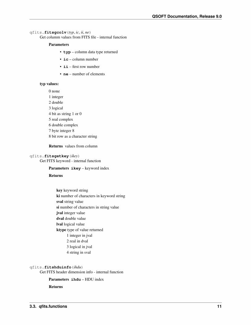
qfits.fitsgcolv(typ, ic, ii, ne)Get columm values from FITS file - internal function
Parameters
• typ – column data type returned
• ic – column number
• ii – first row number
• ne – number of elements
typ values:
0 none1 integer2 double3 logical4 bit as string 1 or 05 real complex6 double complex7 byte integer 88 bit row as a character string
Returns values from column
qfits.fitsgetkey(ikey)Get FITS keyword - internal function
Parameters ikey – keyword index
Returns
key keyword stringki number of characters in keyword stringsval string valuesi number of characters in string valuejval integer valuedval double valuelval logical valuektype type of value returned
1 integer in jval2 real in dval3 logical in jval4 string in sval
qfits.fitshduinfo(ihdu)Get FITS header dimension info - internal function
Parameters ihdu – HDU index
Returns
3.3. qfits.functions 11
QSOFT Documentation, Release 9.0
list of followinghdutype type of HDUnaxis number of dimensionsnaxes size of dimensions (nrows,ncols)nkeys number of keywords
qfits.fitsparr(arr)Put array onto fits file - internal function
Parameters arr – arr of data values
qfits.fitsptab(hdu)Create binary table HDU on FITS object
Parameters hdu – FITS HDU object
qfits.fitstypes(hdutype, ncols)Get FITS header data types - internal function
Parameters
• hdutype – type of HDU
• ncols – number of columns (if hdutype=0)
Returns
ctype column typerp column repeat count
qfits.fitsupdate(filename)Open FITS file for read/write
Parameters filename – FITS file name
Returns number of HDU in file
qfits.init()Initialize common blocks on import
class qfits.fitsfile(filename)
__init__(filename)Read object from FITS file or create new FITS object
Parameters filename – FITS filename (“new” to create new object)
display()List FITS object
save(filename)Save FITS object to file
Parameters filename – FITS file name
class qfits.fitshdu(ihdu, hdutype)
12 Chapter 3. qfits - Using FITS Files

QSOFT Documentation, Release 9.0
__init__(ihdu, hdutype)FITS HDU object
Parameters
• ihdu – HDU index
• hdutype – HDU type
display()List FITS HDU object
3.3. qfits.functions 13

QSOFT Documentation, Release 9.0
14 Chapter 3. qfits - Using FITS Files
CHAPTER
FOUR
IMAGES - IMAGE PROCESSING
Positions in images. The coordinates of an image field are set up using the function setfield(). The current positioncan be set using the function setpos(). This position is then used by functions like beam(). The position is given inpixel coordinates (a real scale running 0-NCOLS in X and 0-NROWS in Y) and local X,Y (usually taken as mm).If, in addition to setfield(), sky coordinates are set using the function setsky() the current position is also specified inlocal azimuth and elevation (degrees), Celestial RA,DEC (degrees J2000), Ecliptic EA,EL (degrees) and Galactic LII,BII (degrees). The sky coordinates can be set using different projections, Plate Carre, Aitoff (Hammer) or Lambert(equatorial aspect of Azimuthal equal-area).
• setfield() Set local coordinates for image field
• setsky() Set up sky coordinates for image field
• setpos() Set current position in image field
• getpos() Get current position in image field
• toxy() Convert position to local xy coordinates
• plt_show_locator() Get local coordinate positions using the cursor
Analysis of a beam containing a source or PSF. The beam is centred at the current positon (see above).
• beam() Analysis of source above background within a circular beam
• sqbeam() Analysis of source above background within a square beam
• lecbeam() Analysis of source above background in a lobster eye cross-beam
Creation of images from event lists or 2-d functions. In Python these function return a 2-d array. In R they return animage object which contains the array and ancillary information.
• binxy() x-y event binning to form an image array
• lebin() Create an image from an event list binning using lobster eye psf
• lecimage() Create an image array of the lobster eye cross-beam
• lepsf() Create an image of the lobster eye PSF
Drawing over images. The function hamgrid() and lamgrid() will only work if sky coordinates have been set up usingsetsky().
• rectangles() Draw rectangles
• hamgrid() Plot a Hammer projection grid on figure
• lamgrid() Plot a Lambert projection grid on figure
1-d profiles
• gaussian() Gaussian profile
15
QSOFT Documentation, Release 9.0
• king_profile() King function (modified Lorentzian) profile
• lorentzian() Lorentzian profile
Model function fitting using a statistic. Can be used for fitting of PSF profiles to image data or more generally forfitting data with a model function.
• srchmin() Search for minimum statistic and return best fit parameters and confidence limits of the parameters
• peakchisq() Chi-squared for image peak fitting
• quaderr() Quadratic estimator for confidence limit
4.1 images.functions
images.beam(arr, rbeam, blev, bvar)Analysis of source above background within a circular beam
Parameters
• arr – image array
• rbeam – radius of beam in pixels
• blev – average background level per pixel (to be subtracted)
• bvar – variance on blev (-ve for counting statistics)
Returns
list with the followingnsam: number of pixels in beambflux: background in beam (e.g. counts)bsigma: standard deviation of backgroundflux: source flux above background in beam (e.g. counts)fsigma: standard deviation of source fluxpeak: source x,y peak positioncen: source x,y centroid positiontha: angle (degrees) of major axis wrt x (x to y +ve)rmsa: source max rms width (major axis) (pixels)rmsb: source min rms width (minor axis) (pixels)fwhm: full width half maximum (pixels) about beam centrehew: half energy width (pixels) about beam centrew90: W90 (90% width) (pixels) about beam centrefwhmp: full width half maximum (pixels) about peakhewp: half energy width (pixels) about peakw90p: W90 (90% width) (pixels) about peakfwhmc: full width half maximum (pixels) about centroidhewc: half energy width (pixels) about centroidw90c: W90 (90% width) (pixels) about centroidfit: parameters from peak fit using peakchisq()
16 Chapter 4. images - Image Processing
QSOFT Documentation, Release 9.0
Fit performed if bvar!=0.Parameters are saved in the list fit (see function srchmin())
0: peak value (no error range calculated)1: peak X pixel position with 90% error range2: peak Y pixel position with 90% error range3: Lorentzian width including 90% upper and lower bounds
The position of the beam is the current position within the image.Use function setpos() to set the current position.
images.binxy(x, y, iq, w, xleft, xright, ybot, ytop, nx, ny)x-y event binning to form an image
Parameters
• x – array of x positions
• Y – array of y positions
• iq – array of quality values (0 for OK)
• w – array of weights
• xleft – minimum x value (left edge) for image array
• xright – maximum x value (rigth edge) for image array
• ybot – minimum y value (bottom edge) for image array
• ytop – maximum y value (top edge) for image array
• nx – size of 1st dimension of image array (number of rows)
• ny – size of 2nd dimension of image array (number of columns)
Returns
image arrayR version returns an image object - image array object$data_array
images.gaussian(x, p)Gaussian profile
Parameters
• x – array of x values
• p – array of fitting parameters
par 0: normalisation (value at peak)par 1: x-centre (pixel position)par 2: Gaussian full width half maximum (pixels)
Returns array of function values evaluated at x
4.1. images.functions 17
QSOFT Documentation, Release 9.0
images.getpos()Get current position in image field
Returns list with following
pix: pixel positionxyl: local positionaes: local azimuth,elevation degreesequ: Celestial RA,DEC degrees J2000ecl: Ecliptic EA,EL degreesgal: Galactic LII,BII degrees
images.hamgrid(pic)Plot a Hammer projection grid on figure
Parameters pic – figure object
images.init()Initialise common blocks on import
images.king_profile(x, p)King function (modified Lorentzian) profile
Parameters
• x – array of x values
• p – array of fitting parameters
par 0: normalisation (value at peak)par 1: x-centre (pixel position)par 2: full width half maximum (pixels)par 3: power index (1 for Lorentzian)
Returns array of function values evaluated at x
images.lamgrid(pic)Plot a Lambert projection grid on figure
Parameters pic – figure object
images.lebin(xe, ye, s, h, g, eta, nx, ny)Create an image from an event list binning using lobster eye psf
The image is effectively a cross-correlation of the event list with the lobster eye cross-beam.
Parameters
• xe – x event positions, pixels
• ye – y event positions, pixels
• s – size of cross-beam square area in pixels
• h – height of cross-arm triangle in pixels (=2d/L)
• g – width of Lorentzian central spot in pixels
18 Chapter 4. images - Image Processing
QSOFT Documentation, Release 9.0
• eta – cross-arm to peak ratio at centre
• nx – first dimension of array
• ny – second dimension of array
Returns image array
Event positions assumed to run:x: 0 left edge to nx right edgey: 0 bottom edge to ny top edge
Therefore centre of left bottom pixel is 0.5,0.5
images.lecbeam(arr, s, h, blev, bvar, nt)Analysis of source above background in a lobster eye cross-beam
Parameters
• arr – image array
• s – size of cross-beam square area in pixels
• h – height of cross-arm quadrant in pixels (=2d/L)
• blev – average background level per pixel (to be subtracted)
• bvar – variance on blev (-ve for counting statistics)
• nt – dimension of output quadrant flux distribution in pixels
Returns list of the following
qua: quadrant surface brightness distribution array nt by ntquan: quadrant pixel occupancy array nt by ntnsam: number of pixels in beambflux: background in beam (e.g. counts)bsigma: standard deviation of backgroundflux: source flux above background in beam (e.g. counts)fsigma: standard deviation of source fluxpeak: source x,y peak positioncen: source x,y centroid positionhew: half energy width (pixels)w90: W90 (90% width) (pixels)ahe: half energy area (sq pixels)aw9: W90 (90% width) area (sq pixels)fpeak: flux in peak pixel
The position of the beam is the current position within the image.Use function setpos() to set the current position.
images.lecimage(s, h, b, xcen, ycen, nx, ny)Create an image array of the lobster eye cross-beam
4.1. images.functions 19
QSOFT Documentation, Release 9.0
Parameters
• s – size of cross-beam square area in pixels
• h – height of cross-arm triangle in pixels (=2d/L)
• b – jwidth of cross-arm triangle in pixels
• xcen – centre pixel (see coords below)
• ycen – centre pixel (see coords below)
• nx – first dimension of array
• ny – second dimension of array
Returns image array
Coordinate system for xcen,ycen is:
x runs from 0.0 on left to nx on rightY runs from 0.0 on bottom to ny on topCentre of bottom left pixel is therefore 0.5,0.5Centre of top right pixel is nx-0.5,ny-0.5
images.lepsf(s, h, g, eta, xcen, ycen, nx, ny)Create an image of the lobster eye PSF
Parameters
• s – size of cross-beam square area in pixels
• h – height of cross-arm triangle in pixels (=2d/L)
• g – width of Lorentzian central spot in pixels
• eta – cross-arm to peak ratio at centre
• xcen – centre of PSF (see below for coords. system)
• ycen – centre of PSF (see below for coords. system)
• nx – first dimension of array
• ny – second dimension of array
Returns image array
Coordinate system for xcen,ycen is:
x runs from 0.0 on left to nx on rightY runs from 0.0 on bottom to ny on topCentre of bottom left pixel is therefore 0.5,0.5Centre of top right pixel is nx-0.5,ny-0.5
images.lorentzian(x, p)Lorentzian profile
Parameters
• x – array of x values
• p – array of fitting parameters
20 Chapter 4. images - Image Processing
QSOFT Documentation, Release 9.0
par 0: normalisation (value at peak)par 1: x-centre (pixel position)par 2: Lorentian width (pixels)
Returns array of function values evaluated at x
images.peakchisq(fpars)Chi-squared for image peak fitting
Parameters fpars – array of fitting parameters
par 0: normalisation (value at peak)par 1: x-centre (pixel position)par 2: y-centre (pixel position)par 3: Lorentian width (pixels) 24th Sept. 2017 RW
Returns Chi-squared value
Used by function beam() which loads Fortran common block BEAMFIT with image data.
images.plt_show_locator(fg, npos)Get local coordinate positions using the cursor
Parameters
• fg – figure id returned by plt.figure()
• npos – number of positions to be retured (clicked)
Returns xx,yy, 2 arrays containing npos local coordinates
This routine provides a basic level of interaction with a displayed figure. It is used in place of a simple plt.show()call so that npos local coordinate positions can be selected interactively using the cursor from a displayed imageand returned in arrays to the user.
images.quaderr(x0, y0, x1, y1, y)Quadratic estimator for confidence limit
Parameters
• x0 – parameter at minimum
• y0 – statistic at minimum
• x1 – parameter near minimum
• y1 – statistic near minimum
• y – required statistic value
Returns estimate of parameter corresponding to y
images.rectangles(x, y, w, h, t)Draw rectangles
Parameters
• x – centres in local x
• y – centres in local y
4.1. images.functions 21
QSOFT Documentation, Release 9.0
• w – widths
• h – heights
• t – rotation angles radians
images.reset()Reset common blocks to initial condition
images.setfield(nx, xleft, xright, ny, ybot, ytop)Set local coordinates for image field
Parameters
• nx – number of columns
• xleft – local x left edge
• xright – local x right edge
• ny – number of rows
• ybot – local y bottom edge
• ytop – local y top edge
images.setpos(ipos, p)Set current position in image field
Parameters
• ipos – coordinate index
• p – position coordinate pair
ipos values:
1: pixel 0-NCOLS, 0-NROWS2: local X,Y3: local azimuth,elevation degrees4: Celestial RA,DEC degrees J20005: Ecliptic EA,EL degrees6: Galactic LII,BII degrees
Returns current position using getpos()
images.setsky(xtodeg, ytodeg, ipr, mjd, ra, dec, roll)Set up sky coordinates for image field
Parameters
• xtodeg – scale from local x to degrees (usually -ve)
• ytodeg – scale from local y to degrees
• ipr – projection between local XY and local spherical
• mjd – Modified Julian date
• ra – Right Ascension (degrees J2000 at local origin)
• dec – Declination (degrees J2000 at local origin)
• roll – Roll angle (degrees from North to +ve elev. +ve clockwise)
22 Chapter 4. images - Image Processing
QSOFT Documentation, Release 9.0
ipr values:
0: Plate Carre1: Aitoff (Hammer)2: Lambert (equatorial aspect of Azimuthal equal-area projection)
images.sqbeam(arr, hbeam, blev, bvar)Analysis of source above background within a square beam
Parameters
• arr – image array
• hbeam – half width of square beam in pixels
• blev – average background level per pixel (to be subtracted)
• bvar – variance on blev (-ve for counting statistics)
Returns
list with the followingnx,ny: dimension of beam pixels (truncated if falls off edge)xpi,xpr: x output arrays, pixel position and fluxypi,ypr: y output arrays, pixel position and fluxbflux: background in beam (e.g. counts)bsigma: standard deviation of backgroundflux: source flux above background in beam (e.g. counts)fsigma: standard deviation of source fluxpeak: source x,y peak positioncen: source x,y centroid positionrmsx: rms width in x (pixels) about centroidrmsy: rms width in y (pixels) about centroidpi5: 5% x,y positionpi25: 25% x,y positionmed: median (50%) x,y positionpi75: 75% x,y positionpi95: 95% x,y positionhewx: HEW (half energy width) x (pixels)hewy: HEW (half energy width) y (pixels)w90x: W90 (90% width) x (pixels)w90y: W90 (90% width) y (pixels)fitx: parameters from x profile fit using king_profile()fity: parameters from y profile fit using king_profile()
Fits performed if bvar!=0.Parameters are saved in the lists fitx and fity
0: peak value (no error range calculated)1: peak X pixel position (no error range calculated)2: Lorentzian width including 90% upper and lower bounds
4.1. images.functions 23
QSOFT Documentation, Release 9.0
The position of the sqbeam is the current position within the image.Use function setpos() to set the current position.
images.srchmin(pars, pl, ph, stat, delstat, derr)Search for minimum statistic and return best fit parameters and confidence limits of the parameters
Parameters
• pars – initial parameter values
• pl – hard lower limit of parameter values
• ph – hard upper limit of parameter values
• stat – the statistic function to be minimised
• delstat – the change in statistic for confidence limits
• derr – initial error estimates for parameters, 0 fixed, >0 to estimate confidence range
Returns list from optim() plus confidence limits parlo and parhi
The statistic function call must return the value of a statistic with call of form stat(pars) (e.g. im-ages.peakchisq(pars))
images.toxy(ipos, p)Convert position to local xy coordinates
Parameters ipos – coordinate index
1: pixel 0-NCOLS, 0-NROWS2: local X,Y3: local azimuth,elevation degrees4: Celestial RA,DEC degrees J20005: Ecliptic EA,EL degrees6: Galactic LII,BII degrees
Returns position as local xy
24 Chapter 4. images - Image Processing

CHAPTER
FIVE
ASTRO - ASTRONOMY APPLICATIONS
X-ray spectra. X-ray spectral data are usually presented as histograms of X-ray counts vs. energy (keV). The functionsbtoc() and ctob() provide conversion between energies at n bin centres and n+1 bin boundaries.
• brems() Bremsstrahlung spectrum
• habs() X-ray absorption by a Hydrogen column density
• setabnd() Set abundances for XSPEC routines used in absorption and optical depth calculations
• btoc() Convert n+1 bin boundaries to n bin centres
• ctob() Convert n bin centres to n+1 bin boundaries
X-ray optical depth. The local ISM and cosmic IGM gas is modelled as a hydrogen column including heavier elementsat specified abundances and ionisation state.
• igmtau() X-ray optical depth of IGM gas
• iigmtau() X-ray optical depth of ionized IGM gas
• iigmtauvz() X-ray optical depth of ionized IGM gas vs. redshift
• ismtau() X-ray optical depth of cold ISM gas
• iismtau() X-ray optical depth of ionized ISM gas
• lyftau() X-ray optical depth of Lyman Forest
• lyftauvz() X-ray optical depth of Lyman Forest vs. redshift
Cosmology and redshift.
• cosmo() Calculation of cosmological quantities (luminosity distance etc.)
• kcorrb() K-correction using numerical integration of the Band function
5.1 astro.functions
astro.brems(ekev, t)Bremsstrahlung spectrum
Parameters
• ekev – array of photon energies keV
• t – temperature keV
Returns Bremsstrahlung continuum photons/keV at energies ekev
25

QSOFT Documentation, Release 9.0
astro.btoc(x)Convert n+1 bin boundaries to n bin centres
Parameters x – array of bin boundaries length n+1
Returns array of bin centres length n
astro.cosmo(h0, omegam, omegal, zmax)Calculation of cosmological quantities
Using equations from David Hogg astro-ph/9905116
Parameters
• h0 – cosmological H0 km s-1 Mpc-1
• omegam – cosmological omegam
• omegal – cosmological omegal
• zmax – maximum redshift
Returns list with following sampled at dz=0.01
z: redshift valuesez: scaling functiondc: comoving line-of-sight distancedm: transverse comoving distanceda: angular diameter distancedl: luminosity distancedistm: distance modulusdvc: comoving volume elementtlbak: look back timevc: integrated comoving volume over whole skythsec: Hubble time in secondsthgyr: Hubble time in Giga yearsdhmpc: Hubble length in Mpc
astro.ctob(x)Convert n bin centres to n+1 bin boundaries
Parameters x – array of bin centres length n
Returns array of bin boundaries length n+1
astro.habs(cd, ekev)X-ray absorption by a Hydrogen column density
Parameters
• cd – hydrogen column 10**21 cm-2
• ekev – array of photon energies keV
Returns array of absorption factors
26 Chapter 5. astro - Astronomy Applications
QSOFT Documentation, Release 9.0
astro.igmtau(n0, z, h0, omegam, omegal, ekev)X-ray optical depth of IGM gas
Parameters
• n0 – number density cm-3 at z=0
• z – redshift of source
• h0 – cosmological H0 km s-1 Mpc-1
• omegam – cosmological omegam
• omegal – cosmological omegal
• ekev – array of photon energies keV
Returns optical depth for each energy
astro.iigmtau(n0, pl, tk, ist, z, h0, omegam, omegal, ekev)X-ray optical depth of ionized IGM gas
Parameters
• n0 – number density cm-3 at z=0
• pl – powerlaw index of continuum spectrum
• tk – temperature Kelvin
• ist – ionization state L/nR^2
• z – redshift of source
• h0 – cosmological H0 km s-1 Mpc-1
• omegam – cosmological omegam
• omegal – cosmological omegal
• ekev – array of photon energies keV
Returns optical depth for each energy
astro.iigmtauvz(n0, dind, m0, mind, pl, tk, ist, h0, omegam, omegal, ekev, z)X-ray optical depth of ionized IGM gas vs. redshift
Parameters
• n0 – number density cm-3 at z=0
• dind – density index wrt z+1
• m0 – metalicity log[X/H] at z=0
• mind – metalicity log[X/H] index wrt z
• pl – powerlaw index of continuum spectrum
• tk – temperature Kelvin
• ist – ionization state = L/nR^2
• h0 – cosmological H0 km s-1 Mpc-1
• omegam – cosmological omegam
• omegal – cosmological omegal
• ekev – energy keV
5.1. astro.functions 27

QSOFT Documentation, Release 9.0
• z – array of redshift values
Returns optical depth at ekev for each redshift
astro.iismtau(nh, z, tk, pl, ist, ekev)X-ray optical depth of ionized ISM gas
Parameters
• nh – column density 10**21 cm-3 at redshift z
• z – redshift of source
• tk – temperature Kelvin
• pl – powerlaw index of continuum spectrum
• ist – ionization state = L/nR^2
• ekev – array of photon energies keV
Returns: optical depth for each energy
astro.init()Initialise common blocks on import
astro.ismtau(nh, z, ekev)X-ray optical depth of cold ISM gas
Parameters
• nh – column density 10**21 cm-2 at redshift z
• z – redshift of source
• ekev – array of photon energies keV
Returns optical depth for each energy
astro.kcorrb(e1src, e2src, e1obs, e2obs, z, gamma1, gamma2, ecobs)K-correction using numerical integration of Band function
Parameters
• e1src – lower source frame energy
• e2src – upper source frame energy
• e1obs – array of lower observed energies
• e2obs – array of upper observed energies
• z – array of redshifts
• gamma1 – array of observed photon indices below Ec
• gamma2 – array of observed photon indices above Ec
• ecobs – array of observed Ec energies
Returns list with the following for each object
kcorr: K-correction factorobint: integral over observed bandboint: integral over Eiso band in observed frame
28 Chapter 5. astro - Astronomy Applications
QSOFT Documentation, Release 9.0
astro.lyftau(n0, dind, m0, mind, z, h0, omegam, omegal, ekev)X-ray optical depth of Lyman Forest
Parameters
• n0 – number density cm-3 at z=0
• dind – density index wrt z+1
• m0 – metalicity log[X/H] at z=0
• mind – metalicity log[X/H] index wrt z
• z – redshift of source
• h0 – cosmological H0 km s-1 Mpc-1
• omegam – cosmological omegam
• omegal – cosmological omegal
• ekev – array of photon energies keV
Returns optical depth for each energy
astro.lyftauvz(n0, dind, m0, mind, h0, omegam, omegal, ekev, z)X-ray optical depth of Lyman Forest vs. z
Parameters
• n0 – number density cm-3 at z=0
• dind – density index wrt z+1
• m0 – metalicity log[X/H] at z=0
• mind – metalicity log[X/H] index wrt z
• h0 – cosmological H0 km s-1 Mpc-1
• omegam – cosmological omegam
• omegal – cosmological omegal
• ekev – photon energy keV
• z – array of redshifts
Returns optical depth at ekev for each redshift
astro.reset()Reset common blocks to initial condition
astro.setabund(abun, amet)Set abundances for XSPEC routines
Parameters
• abun – XSPEC abundance table
• amet – metalicity
5.1. astro.functions 29

QSOFT Documentation, Release 9.0
30 Chapter 5. astro - Astronomy Applications

CHAPTER
SIX
XSCAT - X-RAY PHYSICS
X-ray optical constants.
• xopt() X-ray optical properties of a material
• xfresnel() Calculate X-ray reflectivity using Fresnel’s equations
X-ray scattering by dust.
• dustrings() Model fitting to dust X-ray scattering halo rings
• duststat() Statistic of fit of model to dust rings
• dustthetascat() Scattering angle radians
• miev0() Wiscombe subroutine for Mie scattering calculations
6.1 xscat.functions
xscat.dustrings(data, derr, dsou, ekv, srate, dts, td, zd, amin, amax, qa, sig1)Model fitting to dust X-ray scattering halo rings
Parameters
• data – data array of rings surface brightness cts/s/str
• derr – array of errors on data
• dsou – distance to source PC
• ekv – array of energies keV (equally spaced across observed band)
• srate – source spectrum cts/s/keV
• dts – source burst duration
• td – delay time of observations secs
• zd – fraction of source distance to rings
• amin,amax – grain size radius range microns
• qa – grain size distribution index N(a)=A.a^-qa
• sig1 – differential cross-section of 1 grain cm2, 1 keV, 0.1 microns
Returns the following
angs: array of angles
31
QSOFT Documentation, Release 9.0
ndust: N dust columns cm-2edust: errors on N dust columns cm-2model: model cts/s/str in ringschisq: Chi-Squared between data and modelndof: ndof
class xscat.duststat(data, derr, dsou, ekv, srate, dts, td, zd, sig1)Statistic of fit of model to dust rings
xscat.dustthetascat(td, ds, zd)Scattering angle radians
Parameters
• td – delay time seconds after source flare (assumed delta function)
• ds – distance to source parsecs (convert to m - 3.086e16/parsec)
• zd – fractional distance to dust
Returns angle in radians
xscat.miev0(xx, crefin, pfct, mimc, anya, xmu, nmom, ipolzn, momd, prt)Wiscombe subroutine
Computes Mie scattering and extinction efficiencies; asymmetry factor; forward- and backscatter amplitude;scattering amplitudes vs. scattering angle for incident polarization parallel and perpendicular to the plane ofscattering; coefficients in the Legendre polynomial expansions of either the unpolarized phase function or thepolarized phase matrix; some quantities needed in polarized radiative transfer; and information about whetheror not a resonance has been hit.
Input and output variables are described in file MIEV.doc. Many statements are accompanied by commentsreferring to references in MIEV.doc, notably the NCAR Mie report which is now available electronically andwhich is referred to using the shorthand (Rn), meaning Eq. (n) of the report.
Parameters
• xx – Mie size parameter ( 2 * pi * radius / wavelength )
• crefin – Complex refractive index ( imag part can be + or -, but internally a negativeimaginary index is assumed ). If imag part is - , scattering amplitudes as in Van de Hulst arereturned; if imag part is + , complex conjugates of those scattering amplitudes are returned(the latter is the convention in physics). ** NOTE ** In the ‘PERFECT’ case, scatteringamplitudes in the Van de Hulst (Ref. 6 above) convention will automatically be returnedunless Im(CREFIN) is positive; otherwise, CREFIN plays no role.
• pfct – TRUE, assume refractive index is infinite and use special case formulas for Miecoefficients ‘a’ and ‘b’ ( see Kerker, M., The Scattering of Light and Other ElectromagneticRadiation, p. 90 ). This is sometimes called the ‘totally reflecting’, sometimes the ‘perfectlyconducting’ case. ( see CREFIN for additional information )
• mimc – (positive) value below which imaginary refractive index is regarded as zero (com-putation proceeds faster for zero imaginary index)
• anya – TRUE, any angles whatsoever may be input through XMU. FALSE, the angles aremonotone increasing and mirror symmetric about 90 degrees (this option is advantageousbecause the scattering amplitudes S1,S2 for the angles between 90 and 180 degrees areevaluable from symmetry relations, and hence are obtained with little added computationalcost.)
32 Chapter 6. xscat - X-ray Physics
QSOFT Documentation, Release 9.0
• numang – No. of angles at which scattering amplitudes S1,S2 are to be evaluated ( set= 0 to skip calculation of S1,S2 ). Make sure NUMANG does not exceed the parameterMAXANG in the program.
• xmu (N ) – Cosines of angles ( N = 1 TO NUMANG ) at which S1,S2 are to be evaluated. IfANYANG = FALSE, then (a) the angles must be monotone increasing and mirror symmetricabout 90 degrees (if 90-A is an angle, then 90+A must be also) (b) if NUMANG is odd, 90degrees must be among the angles
• nmom – Highest Legendre moment PMOM to calculate, numbering from zero ( NMOM =0 prevents calculation of PMOM )
• ipolzn – POSITIVE, Compute Legendre moments PMOM for the Mueller matrix ele-ments determined by the digits of IPOLZN, with 1 referring to M1, 2 to M2, 3 to S21,and 4 to D21 (Ref. 3). E.g., if IPOLZN = 14 then only moments for M1 and D21 will bereturned. 0, Compute Legendre moments PMOM for the npolarized unnormalized phasefunction. NEGATIVE, Compute Legendre moments PMOM for the Sekera phase quantitiesdetermined by the digits of ABS(IPOLZN), with 1 referring to R1, 2 to R2, 3 to R3, and 4to R4 (REF. 4). E.g., if IPOLZN = -14 then only moments for R1 and R4 will be returned. (NOT USED IF NMOM = 0 )
• momd – Determines first dimension of PMOM, which is dimensioned internally as PMOM(0:MOMDIM, * ) (second dimension must be the larger of unity and the highest digit inIPOLZN; if not, serious errors will occur). Must be given a value, even if NMOM = 0.Minimum: 1.
• prt (L) – Print flags (LOGICAL). L = 1 prints S1,S2, their squared absolute values, anddegree of polarization, provided NUMANG is non-zero. L = 2 prints all output variablesother than S1,S2.
Returns list containing the following
qext: (REAL) extinction efficiency factor ( Ref. 2, Eq. 1A )qsca: (REAL) scattering efficiency factor ( Ref. 2, Eq. 1B )gqsc: (REAL) asymmetry factor times scattering efficiency
( Ref. 2, Eq. 1C ) ( allows calculation of radiationpressure efficiency factor QPR = QEXT - GQSC )
NOTE – S1, S2, SFORW, SBACK, TFORW, AND TBACK are calculatedinternally for negative imaginary refractive index;for positive imaginary index, their complex conjugatesare taken before they are returned, to correspond tocustomary usage in some parts of physics ( in particular,in papers on CAM approximations to Mie theory ).
pmom(M,NP): (REAL) moments M = 0 to NMOM of unnormalized NP-thphase quantity PQ ( moments with M .GT. 2*NTRM arezero, where NTRM = no. terms in Mie series =XX + 4*XX**1/3 + 1 )
PQ( MU, NP ): = sum( M=0 to infinity ) ( (2M+1)* PMOM( M,NP ) * P-sub-M( MU ) )WHERE MU = COS( scattering angle )P-sub-M = M-th Legendre polynomialand the definition of ‘PQ’ is as follows:IPOLZN.GT.0: PQ(MU,1) = CABS( S1(MU) )**2
6.1. xscat.functions 33
QSOFT Documentation, Release 9.0
PQ(MU,2) = CABS( S2(MU) )**2PQ(MU,3) = RE( S1(MU)*CONJG( S2(MU) ) )PQ(MU,4) = - IM( S1(MU)*CONJG( S2(MU) ) )( called M1, M2, S21, D21 in literature )IPOLZN=0: PQ(MU,1) = ( CABS(S1)**2 + CABS(S2)**2 ) / 2( the unnormalized phase function )IPOLZN.LT.0: PQ(MU,1) = CABS( T1(MU) )**2PQ(MU,2) = CABS( T2(MU) )**2PQ(MU,3) = RE( T1(MU)*CONJG( T2(MU) ) )PQ(MU,4) = - IM( T1(MU)*CONJG( T2(MU) ) )( called R1, R2, R3, R4 in literature )The sign of the 4th phase quantity is a source ofconfusion. It flips if the complex conjugates ofS1,S2 or T1,T2 are used, as occurs when arefractive index with positive imaginary part isused (see discussion below). The definition aboveis consistent with a negative imaginary part.See Ref. 5 for correct formulae for PMOM ( Eqs. 2-5of Ref. 3 contain typographical errors ). Ref. 5 alsocontains numerous improvements to the Ref. 3 formulas.NOTE THAT OUR DEFINITION OF MOMENTS DIFFERS FROM REF. 3in that we divide out the factor (2M+1) and number themoments from zero instead of one.** WARNING ** Make sure the second dimension of PMOMin the calling program is at least as large as theabsolute value of IPOLZN.For small enough values of XX, or large enough valuesof M, PMOM will tend to underflow. Thus, it isunwise to assume the values returned are non-zero and,for example, to divide some quantity by them.
s1(N),s2(N): (COMPLEX) Mie scattering amplitudes at angles specifiedby XMU(N) ( N=1 to NUMANG ) ( Ref. 2, Eqs. 1d-e ).
sforw: (COMPLEX) forward-scattering amplitude S1 at0 degrees. ( S2(0 deg) = S1(0 deg) )
sback: (COMPLEX) backscattering amplitude S1 at180 degrees. ( S2(180 deg) = - S1(180 deg) )
tforw(I): (COMPLEX) values ofI=1: T1 = ( S2 - (MU)*S1 ) / ( 1 - MU**2 )I=2: T2 = ( S1 - (MU)*S2 ) / ( 1 - MU**2 )At angle theta = 0 ( MU = COS(theta) = 1 ), where theexpressions on the right-hand side are indeterminate.( these quantities are required for doing polarizedradiative transfer (Ref. 4, Appendix). )
tback(I): (COMPLEX) values of T1 (for I=1) or T2 (for I=2) atangle theta = 180 degrees ( MU = COS(theta) = - 1 ).
spike: (REAL) magnitude of the smallest denominator ofeither Mie coefficient (a-sub-n or b-sub-n),
34 Chapter 6. xscat - X-ray Physics
QSOFT Documentation, Release 9.0
taken over all terms in the Mie series pastN = size parameter XX. Values of SPIKE belowabout 0.3 signify a ripple spike, since thesespikes are produced by abnormally small denominatorsin the Mie coefficients (normal denominators are oforder unity or higher). Defaults to 1.0 when noton a spike. Does not identify all resonances(we are still working on that).
class xscat.mievsMie scattering and Rayleigh-Gans approximation for scattering by dust
list()List object
xscat.xfresnel(alpha, gamma, angs)Calculate X-ray reflectivity using Fresnel’s equations
Parameters
• alpha – real incremental part dielectric constant
• gamma – imaginary part of dielectric constant
• angs – incidence angles (degrees)
Returns
Return type list of following
rs: sigma reflectivityrp: pi reflectivityrunp: unpolarized reflectivity
If angs(I) out of range 0-90 degrees returns zero reflectivity
xscat.xopt(mspec, rho, ekev, itype)X-ray optical properties of a material
Parameters
• mspec – specification of composition
• rho – density gm/cm**3
• ekev – array of photon energies in keV
• itype – data source (0=Cromer, 1=Henke)
Returns list with the following
alpha: array of real parts dielectric constantgamm: array of imaginary parts dielectric constantabsl: array of absortion lengths cm-1f1: array of real parts scattering factor
6.1. xscat.functions 35

QSOFT Documentation, Release 9.0
f2: array of imaginary parts scattering factor
36 Chapter 6. xscat - X-ray Physics
CHAPTER
SEVEN
XSRT - SEQUENTIAL RAY TRACING
The code was written for modelling grazing incidence X-ray telescopes but it works at normal incidence and includesmany common optical elements.
The code is sequential in the sense that rays encounter the optical elements in the order that they are specified. How-ever, by setting flags associated with each element the sequence can be controlled dynamically to handle multipleinteractions, between different optical elements, in any sequence.
7.1 Example Scripts
The following Python and R scripts illustrate how the ray tracing is done.
The sequence of elements is:
source –> mirrors/stops/lenses/gratings/etc. –> detector
#!/usr/bin/env python# Use Swift XRT geometry as an examplefrom __future__ import print_functionimport sysimport numpy as npimport imagesimport xsrt# Useful vectorssn=np.array([1,0,0])nn=np.array([0,0,0])rx=np.array([0,1,0])# Set look-up table reflectivity to 1.0angs=np.array([0,90])refs=np.array([1,1])# Support spidersspi=np.array([3838.8,0,0])tp=np.array([3800,0,0])conea=10.05nsec=12cwid= 0.0awid= 3.0edf2=np.array([3200,0,0])edf1=np.array([3161.2,0,0])# Wolter I shell parametersfl= 3500ph= 3800hl= 3200ra= 1.0
(continues on next page)
37
QSOFT Documentation, Release 9.0
(continued from previous page)
ns= 13rj=np.array([146.880,140.980,135.320,129.890,124.670,119.660,114.850,110.240,105.810,101.560,97.490,93.560,90.833])tt=np.array([1.25,1.20,1.15,1.10,1.05,1.00,0.95,0.90,0.85,0.80,0.75,0.70,0.70])# Sourcedi=np.array([-1,0,0])rlim=np.array([92.0,151.0,0,0,0,0])nray= 10000# Detectorrdet= 30dlim=np.array([0,rdet,0,0])dpos=np.array([0,0,0])# image paramtersnx= 100ny= 100hwid= 5.0# Ray tracing callsxsrt.reset()xsrt.source(1,di,nn,spi,sn,rx,rlim,0.0,nray,0)xsrt.surface(1,2,0.0,0.0,0.0,0.0,0.0,0.0,angs,refs,0,0,0)xsrt.spider(-conea,spi,sn,rx,nsec,cwid,awid)xsrt.spider(0.0,tp,sn,rx,nsec,cwid,awid)xsrt.w1nest(fl,rj,ra,fl,ph,hl,fl,tt,tt,tt,sn,rx,nn,0,1,0)xsrt.spider(0.0,edf2,sn,rx,nsec,cwid,awid)xsrt.spider(conea,edf1,sn,rx,nsec,cwid,awid)xsrt.detector(1,dpos,sn,rx,dlim,0.0)results=xsrt.trace(0,rdet,-2)# Create an image of the detected areaXD,YD,ZD,XC,YC,ZC,XR,YR,ZR,YDET,ZDET,AREA,IREF=np.loadtxt("detected.dat",skiprows=1,→˓unpack=True)arr=images.binxy(YDET,ZDET,0,AREA,-hwid,hwid,-hwid,hwid,nx,ny)# Analyse beam to get total collecting areaimages.setfield(nx,-hwid,hwid,ny,-hwid,hwid)images.setpos(2,[0,0])bb=images.beam(a,hwid,0,0)area=bb.flux/100.print("area cm^2",area)
#!/usr/bin/env Rscript# Use Swift XRT geometry as an example# Useful vectorssn<-c(1,0,0)nn<-c(0,0,0)rx<-c(0,1,0)# Set look-up table reflectivity to 1.0angs<- c(0,90)refs<- c(1,1)# Support spidersspi<- c(3838.8,0,0)tp<- c(3800,0,0)conea<- 10.05nsec<- 12cwid<- 0.0awid<- 3.0edf2<- c(3200,0,0)edf1<- c(3161.2,0,0)
(continues on next page)
38 Chapter 7. xsrt - Sequential Ray Tracing
QSOFT Documentation, Release 9.0
(continued from previous page)
# Wolter I shell parametersfl<- 3500ph<- 3800hl<- 3200ra<- 1.0ns<- 13rj<- c(146.880,140.980,135.320,129.890,124.670,119.660,114.850,110.240,105.810,101.560,97.490,93.560,90.833)tt<- c(1.25,1.20,1.15,1.10,1.05,1.00,0.95,0.90,0.85,0.80,0.75,0.70,0.70)# Sourcedi<- c(-1,0,0)rlim<- c(92.0,151.0)nray<- 10000# Detectorrdet<- 30dlim=c(0,rdet,0,0)dpos<- c(0,0,0)# image paramtersnx<- 100ny<- 100hwid<- 5.0# Ray tracing callsqrt_reset()qrt_source(1,di,nn,spi,sn,rx,rlim,0.0,nray,0)qrt_surface(1,2,0.0,0.0,0.0,0.0,0.0,0.0,angs,refs,0,0,0)qrt_spider(-conea,spi,sn,rx,nsec,cwid,awid)qrt_spider(0.0,tp,sn,rx,nsec,cwid,awid)qrt_w1nest(fl,rj,ra,fl,ph,hl,fl,tt,tt,tt,sn,rx,nn,0,1,0)qrt_spider(0.0,edf2,sn,rx,nsec,cwid,awid)qrt_spider(conea,edf1,sn,rx,nsec,cwid,awid)qrt_detector(1,dpos,sn,rx,dlim,0.0)results<- qrt_trace(0,rdet,-2)# Create an image of the detected areadetpos<-read.table("detected.dat",header=TRUE)a<-qri_binxy(detpos$YDET,detpos$ZDET,0,detpos$AREA,-hwid,hwid,nx,-hwid,hwid,ny)# Analyse beam to get total collecting areabb<-qri_beam(a$data_array,hwid,0,0)area<-bb$flux/100.cat("area cm^2",area,"\n")
7.2 Optical Elements and Coordinates
Each of the elements, including the source and detector, are specified by:
• 3 surface reference vectors - origin position, surface normal at origin and reference tangent at origin
• The surface figure - planar, spherical or conic section - parameters to define the curvature etc. of the figure
• The surface boundary - circles or rectangles in local surface coordinates
• A surface quality - source of rays, detection, reflection, diffraction, scattering, refraction, absorption
• The surface deformation - a grid of displacements defined in local surface coordinates
A full list of all the currently defined elements is produced by the function srtlist().
Individual elements referenced by the surface element index can be shifted and rotated using shift() and rotate().
7.2. Optical Elements and Coordinates 39
QSOFT Documentation, Release 9.0
The data base of elements can be cleared to the initial condition (no elements defined) using the function reset(). Ifelements are repeatedly defined within a procedure (for instance within a loop) the safe and prefered option is to reset()everything and redefine all elements each time they are required.
Coordinates
There is no fixed coordinate system and elements can be set/defined at any orientation. However it is conventional touse the X-axis as the optical axis (which defines the direction of paraxial rays) and the Y-axis as the nominal tangentreference axis. Of course given elements may not be aligned exactly with the X-axis and Y-axis. In most cases thelocal coordinates in the detector plane are nominally aligned with the Y-axis and Z-axis. Rays are usually traced fromright to left travelling in the -X direction but this is not necessary and it is possible for rays to bounce back and forthas in, for example, a cassegrain system.
The source is always the first element in the sequence. All other elements are placed in sequence as they are defined. Ifthe source() function is used repeatedly the source specification will be overwritten each time. If the detector commandis used repeatedly a new detector will be added to the sequence each time and all detectors defined will be active.
Local surface coordinates are specified using the tangent plane to the surface at the point defined as the surface origin.For a sphere points on this tangent plane are projected onto the surface along the normal to the surface at the surfaceorigin (Lambert’s projection). The local x-axis is specified by a tangent vector at the surface origin. The local y-axisis the cross product of the normal and tangent vector at the surface origin.
The coordinates used for the limits of apertures and stops are given in the docstrings of the xsrt.aperture() function.
The local coordinates used for surfaces of revolution generated from conic sections (hyperbola, parabola, ellipse)depend on whether the surface is designated as being “normal” or “grazing” incidence. For normal incidence theyare defined in a similar way to the planar or spherical surfaces as given above. For grazing incidence a cylindricalcoordinate system is used where the axis is the normal to the surface at the surface origin and the azimuth is therotation about this axis with zero at the surface reference axis at the surface origin. Local coordinates are given asaxial position and azimuthal position (radians). The limits of such surfaces are specified by axial and/or radial limitscorresponding to the bottom and top edges of the surface of revolution.
7.3 Source and Detector
Source of Rays
The source of rays consists of an annular or rectangular aperture on a planar surface. The origin of each ray is arandom point within the aperture. The direction of the rays is specified either by a source at infinity, a source at a finitedistance or diffuse. For a source at infinity all rays are parallel with the direction set by direction cosines. A source ata finite distance is specified by a position vector somewhere behind the aperture. Diffuse rays are generated so as togive a uniform random distribution over a hemisphere. The total number of rays generated is either set explicitly or byusing an aperture area per ray.
Only one source can be specified. If the source command is used in a loop then the source will change on each passthrough the loop.
The deformation index is used to specify a pixel array which spreads out a point source into an angular distribution.The deformation data are set using two functions xsrt.deform() and xsrt.defmat(). If the source is at infinity the x andy sample arrays must be in radians measured from the direction sd along the reference axis ar and the other axis. (ancross ar). If the source is at a finite distance then x and y are displacements in mm (or whatever distance unit is used)of the position sp along the reference axis ar and the other axis (an cross ar).
Detector
The detector consists of an annular or rectangular aperture on a planar or spherical surface. More than one detectorcan be specified for an instrument. Each detector defined will occupy a given position within the sequence of opticalelements specified.
40 Chapter 7. xsrt - Sequential Ray Tracing
QSOFT Documentation, Release 9.0
7.4 Monte Carlo and Random Numbers
The starting positions of rays, X-ray scattering angles from surface roughness and some surface figure er-rors/deformations are generated using random numbers. The sequence of random numbers used will be differenteach run unless the random number seed is set using function rseed(). If the same seed value is set before callingthe function trace() exactly the same random sequence will be generated for the ray tracing and the results will beidentical.
7.5 Deformations
Deformations of surfaces can be specified using matricies which either span a grid of points in the local coordinatesystem of the surface or are indexed using integer labels for sectors or areas on a surface. A set of deformationspertaining to a single surface or group of related surfaces are given a deformation index (integer 1,2,3. . . ). Thepositions of the deformation grid points in local coordinates are specified by two 1-dimensional arrays.
Alternatively deformations can be specified using functions with parameters set separately for local x and y coordi-nates.
A surface deformation is applied along the normal to the surface. The deformation value is interpolated from the 2-dgrid of points.
Radial deformations for annula apertures are specified by a vector, sampling in 1-d in azimuth, and the deformation isapplied as a perturbation in the radial direction.
The function xsrt.deform() is used to set up the type and dimensionality of a particular deformation and must be thefirst call. The component matricies or function parameters are then set using calls to xsrt.defmat() or xsrt.defparxy().
If the deformation index, it, is -ve then uses abs(it) but expects a 2nd deformation to be defined which will be addedto the current deformation. By using a succession of -ve deformation indices a series of deformations can be addedtogether.
A deformation applied to the source() spreads the point source into a pixel array. See Source of Rays.
7.6 Surface Quality, Reflectivity and Scattering
Several surface qualities can be set up for the simulation of a given instrument. Each is referenced using a surfacequality index (integer 1,2,3. . . ). The type of surface can be reflecting (with reflectivity specified using Fresnel’sequations or a lookup table), refracting or diffracting. The roughness of the surface can also be specified using a powerlaw distribution.
The X-ray optical constants alpha and gamma can be calculated for a material of specified composition using thefunction xscat.xopt(). Within the ray tracing the reflectivity is calculated using these constants using the same code asin function xscat.xfresnel().
The reflectivity as a function of incidence angle in other energy bands can be calculated from the real and imaginarypart of the refractive index using the function fresnel().
Stops which are intended to block radiation have a surface quality index set to 0. When rays hit such surfaces theyare terminated (absorbed). Detectors have surface quality index -1. If a ray hits such a surface it is terminated(detected). The source aperture surface has quality index -2. The quality indices of the source, stops and detectorsare set automatically. As ray tracing proceeds rays are stored for further analysis. Each position along a ray where anintersection with a surface element occured is labelled with the quality index of the surface.
7.4. Monte Carlo and Random Numbers 41
QSOFT Documentation, Release 9.0
For a grating the surface type is it=4. In this case the ruling direction is specified by the surface element axis and dhubcontrols the geometry. dhub < 1 in-plane in which the dhub specifies the d-spacing gradient across the ruling and dhub> 1 off-plane where the d-spacing gradient along the ruling is determined from the distance to the hub.
7.7 X-ray Telescopes, Lens and Prism
Wolter Telescopes
A nest of Wolter I shells is set up using the function w1nest() and a conical approximation to the same by c1nest().A Wolter II telescope is set up using the function wolter2(). A Wolter I telescope manufactured as an array of SiliconPore Optics (like Athena) is set up using the function spoarr().
Lobster Eye and Kirkpatrick-Baez Telescopes
A lobster eye telscope is set up using the function sqmpoarr().
A silicon pore Kirkpatrick-Baez stack is defined using the function kbs().
A Schmidt configuration lobster eye telescope is set up using the function sle().
Apertures, stops, baffles and support structure
The function aperture() sets up stops with various geometries, single annulus, nested annuli, rectangular holes/blocks,rectangular grid, polar sectors, paralleogram. Cylindrical baffles in front of behind circular apertures are set up usingthe function baffle(). Spider support structures commomly used in Wolter systems are set up using the functionspider().
Lens and Prism
Refracting lens and prism are defined using functions lens() and prism().
7.8 Ray Tracing and Saving Rays
Once the source, detector and other elements have been defined rays can be traced through the instrument using thefunction trace(). The form of the output is controlled by the parameter iopt.
• -2 save traced.dat and detected.dat files
• -1 save detected.dat
• 0 don’t save files or adjust focus
• 1 adjust focus and save detected.dat
• 2 adjust focus and save detected.dat and traced.dat
• Only rays with iopt reflections are used in adjustment
The files traced.dat and detected.dat are ASCII tabulations.
When iopt is +ve then the detector position which gives the best focus is determined. Only rays which have ioptreflections and impact the detector within a radius riris of the centre of the detector are included in the analysis. Thedetector is shifted along the normal direction to find the axial position of minimum rms radial spread. The results ofthis analysis are returned as:
• area detected area within RIRIS
• dshft axial shift to optimum focus (0.0 if IOPT<=0)
• ybar y centroid of detected distribution
42 Chapter 7. xsrt - Sequential Ray Tracing
QSOFT Documentation, Release 9.0
• zbar z centroid of detected distribution
• rms rms radius of detected distribution
The file traced.dat contains the paths of all the rays. It can be very large so should not be saved unless required fordetailed analysis.
• RXP,RYP,RZP positions of points along each ray
• AREA aperture area associated with ray
• IQU quality index -2 at source, 1 reflected, 0 absorbed, -1 detected
Note: in the tabulation the beginning of each ray is identified using IQU=-2 and the end using IQU=0 absorbed orIQU=-1 detected. Using these data you can plot the paths of all the rays.
The file detected.dat contains information about the detected rays.
• XD,YD,ZD the detected position for each ray
• XC,YC,ZC the direction cosines for each ray
• XR,YR,ZR the position of the last interaction before detection
• YDET,ZDET the local detected position on detector
• AREA the aperture area associated with the ray
• IREF the number of reflections suffered by the ray
The position XR,YR,ZR is used to indicate where the ray came from.
The following snippets of code show how an image of the detected rays can be generated in Python or R.
import numpy as npimport imagesimport xsrt......# half width of image mmhwid=5.0# trace all the raysresults=xsrt.trace(0,rdet,-2)# Create an image of the detected areaXD,YD,ZD,XC,YC,ZC,XR,YR,ZR,YDET,ZDET,AREA,IREF=np.loadtxt("detected.dat",
skiprows=1,unpack=True)arr=images.binxy(YDET,ZDET,0,AREA,-hwid,hwid,-hwid,hwid,nx,ny)
# half width of image mmhwid<- 5.0# trace all the raysresults<- qrt_trace(0,rdet,-2)# Create an image of the detected areadetpos<-read.table("detected.dat",header=TRUE)aim<-qri_binxy(detpos$YDET,detpos$ZDET,0,detpos$AREA,-hwid,hwid,nx,-hwid,hwid,ny)
In Python arr is an image array. In R aim is an image object which contains the image array aim$data_array. Inboth cases the function images.binxy() is used to bin up the aperture area associated with each ray into an image (2-dhistogram). The effective area is found by summing up areas of the image.
7.8. Ray Tracing and Saving Rays 43
QSOFT Documentation, Release 9.0
7.9 xsrt.functions
Utility functions
• rotate() Rotate surface element
• shift() Shift position of surface element
• rseed() Set random number seed
• srtlist() List all current xsrt parameters
• setreset() Reset Fortran common blocks to inital condition
Apertures, baffles and support structure
• aperture() Set up an aperture stop
• baffle() Set up a cylindrical baffle
• spider() Set up a support spider
Wolter systems
• w1nest() Set up a Wolter Type I nest
• c1nest() Set up conical approximation to a Wolter type I nest
• sipore() Set up Silicon Pore Optics
• spoarr() Set up Silicon Pore Optics array
• wolter2() Set up Wolter Type II surfaces
Square pore and Kirkpatrick-Baez systems
• sqpore() Set up slumped square pore MPOs
• sqmpoarr() Set up an array of square pore MPOs
• kbs() Set up a Silicon Kirkpatrick-Baez stack array
• sle() Set up a Schmidt lobster eye stack
Common optical elements
• lens() Set up a lens
• prism() Set up a prism
• mirror() Set up a plane mirror
• elips() Set up elliptical grazing indidence mirror
• moa() Set up a cylindrical Micro Optic Array
• opgrat() Set up a single off-plane grating
Surface quality and deformations
• surface() Set surface quality parameters
• fresnel() Calculate reflectivity using Fresnel’s equations
• deform() Set up surface deformation dimensions
• defmat() Load deformation matrix
• defparxy() Set up deformation defined by parameters in x and y axes
44 Chapter 7. xsrt - Sequential Ray Tracing
QSOFT Documentation, Release 9.0
Source of rays, tracing rays, detecting rays
• source() Set up source of rays
• trace() Perform ray tracing
• detector() Set up detector
Tracing charged particles through magnetic fields
• bfield() Calculation of magnetic field for array of dipoles
• eltmxt() Trace electrons through SVOM MXT telescope with magnetic diverter
• prtathena() Trace proton through Athena telescope with magnetic diverter
xsrt.aperture(idd, idf, ap, an, ar, alim, nsurf)Set up an aperture stop
Parameters
• id – aperture type
• idf – deformation index
• ap – position of aperture
• an – normal to aperture plane
• ar – reference axis in aperture plane
• alim – limit values (depend on id see above)
• nsurf – number of subsequent surfaces per aperture (id=2)
id values:
1 Single annulus, radial limits (aref,rmin,rmax,0,0,0)2 Nested annuli, radial limits (aref,rmin1,rmax1,rmin2,0,0)
aref is an axial reference position used for deformation3 Hole Cartesian limits (xmin,ymin,xmax,ymax,0,0)4 Block Cartesian limits (xmin,ymin,xmax,ymax,0,0)5 Cartesian grid limits (pitchx pitchy ribx riby,0,0)6 Radial/azimuthal sector limits (rmin,rmax,amin,amax,0,0)
amin and amax in radians range 0-2pi7 Parallelogram limits (xmin,ymin,xmax,ymax,dx,0)
where dx is the shear in X over the distance ymax-ymin8 Aperture for MCO test station limits (hsize dols,0,0,0,0)
The parameter nsurf is used for radially nested apertures so that the code knows how many surface elements toskip if a ray penitrates a particular annulus.
If the limits are radial the deformation is defined as a vector (1-d sampless in azimuth) and is applied in theradial direction.
If the limits are cartesian, radial/azimuthal or parallelogram the deformation is defined over a matrix (2-d) andis applied in the direction of the normal.
No deformation is used for id=8.
xsrt.baffle(xmin, xmax, rad, ax, ar, rp, iq)Set up a cylindrical baffle
7.9. xsrt.functions 45
QSOFT Documentation, Release 9.0
Parameters
• xmin – axial position of base
• xmax – axial position of top
• rad – radius of cylinder
• ax – axis direction
• ar – reference direction perpendicular to axis
• rp – position of vertex
• iq – surface quality index
The axial positions of the base and top, xmin and xmax are local coordinates wrt ap along the ax direction.
xsrt.bfield(dm, pdx, pdy, pdz, ddx, ddy, ddz, px, py, pz)Calculation of magnetic field for array of dipoles
Parameters
• dm – dipole moments (Gauss cm3)
• pdx – x positions of dipoles (cm)
• pdy – y positions of dipoles (cm)
• pdz – z positions of dipoles (cm)
• ddx – x direction cosines of dipole moments
• ddy – y direction cosines of dipole moments
• ddz – z direction cosines of dipole moments
• px – x positions for calculation
• py – y positions for calculation
• pz – z positions for calculation
Returns
list of followingbf magnitude of B-field Gaussdx direction cosines of B-field in x directiondy direction cosines of B-field in y directiondz direction cosines of B-field in z directionrmin minimum distance from dipoles
xsrt.c1nest(ax, ar, ff, iq, ib, idf, pl, ph, hl, hh, rpl, rph, rhl, rhh, tin, tj, tout)Set up conical approximation to a Wolter type I nest
Parameters
• ax – optical axis
• ar – reference axis
• ff – position of focus
• pl – array of low axial position of parabola
46 Chapter 7. xsrt - Sequential Ray Tracing
QSOFT Documentation, Release 9.0
• ph – array of high axial position of parabola
• hl – array of low axial position of hyperbola
• hh – array of high axial position of hyperbola
• rp – array of radii parabola near join
• rp – array of radii parabola at input aperture
• rhl – array of radii hyperbola at exit aperture
• rjh – array of radii hyperbola near join
• tin – array of thicknesses of shells at input aperture
• tj – array of thicknesses of shells at join plane (or near join)
• tout – array of thicknesses of shells at the output aperture
The innermost shell is a dummy and provides an inner stop for the nest
Deformation: A deformation sub-matrix is required for each shell (not including the innermost shell) Eachmatrix covers a grid of points along the axis in mm and azimuth in radians. The axial range covers both the1st and 2nd reflection surfaces. The values in the matrices are radial displacments mm at the grid points.
xsrt.defmat(idd, im, xsam, ysam, zdef)Load deformation matrix
Parameters
• id – deformation index
• im – sub-matrix index (runs from 1-N)
• xsam – x values
• ysam – y values
• zdef – deformation matrix
Note for deformation of a surface of revolution X is axial direction and Y is azimuth.
Used when it=1 in deform().
xsrt.deform(idd, it, nm, nx, ny)Set up surface deformation dimensions
Parameters
• id – deformation index
• it – deformation type (1 matrix, 2 sin() in x and/or y)
• nm – number of sub-matrices
• nx – number of x samples
• ny – number of y samples
Note when it=2 the sin() function requires 3 parameters, amplitude (amp), wavelength (lam) and phase (phi)all in mm (or the same units) defx=amp.sin(2.pi.(x-phi)/lam)
If it -ve then uses abs(it) but expects a 2nd deformation to be defined which will be added to the currentdeformation.
xsrt.defparxy(idd, im, xpar, ypar)Sets parameters of deformation defined by parameters in x and y axes.
7.9. xsrt.functions 47
QSOFT Documentation, Release 9.0
Parameters
• idd – deformation index
• im – sub-surface index
• xpar – parameters of deformations in x axis
• ypar – parameters of deformations in y axis
Empty field [] can be used as xpar or ypar if there are no deformations in the corresponding axis.
Use this routine to set parameteric deformations, e.g. when it=2 in deform() the sin() function requires 3 param-eters, amplitude (amp), wavelength (lam) and phase (phi) all in mm (or the same units) defx=amp.sin(2.pi.(x-phi)/lam)
xsrt.detector(idd, dpos, dnml, drfx, dlim, radet)Set up detector
Parameters
• id – detector type
• dpos – detector position
• dnml – detector normal
• drfx – detector reference axis
• dlim – detector limits
• radet – radius of curvature of spherical detector
id values:
1 planar detector, radial limits2 planar detector, cartesian limits3 spherical detector, radial limits4 spherical detector, cartesian limits
xsrt.elips(org, axs, cen, xmin, xmax, amin, amax, smb, rab, ide, iq)Set up elliptical grazing indidence mirror
Parameters
• org – local origin on surface of ellipse
• axs – reference axis in aperture
• cen – focus of ellipse
• xmin – minimum axial position
• xmax – maximum axial position
• amin – minimum azimuth radians
• amax – maximum azimuth radians
• smb – conic coefficient
• rab – conic coefficient conic equation of form r**2=rab**2.x**2+smb**2
• ide – deformation index
• iq – reflecting surface quality
48 Chapter 7. xsrt - Sequential Ray Tracing
QSOFT Documentation, Release 9.0
xsrt.eltmxt(dm, pdx, pdy, pdz, ddx, ddy, ddz, ekv, tsig, xaper, xdiv, apy, apz, apsiz, wdiv, ddiv, sdet,maxst)
Trace electrons through SVOM MXT telescope with magnetic diverter
Parameters
• dm – dipole moments (Gauss cm3)
• pdx – x positions of dipoles (cm)
• pdy – y positions of dipoles (cm)
• pdz – z positions of dipoles (cm)
• ddx – x direction cosines of dipole moments
• ddy – y direction cosines of dipole moments
• ddz – z direction cosines of dipole moments
• ekv – proton energy keV
• tsig – rms width of beam degrees
• xaper – x position of mirror aperture cm (focal length)
• xdiv – x position of diverter input aperture cm
• apy – y centre of apertures cm
• apz – z centre of apertures cm
• apsiz – aperture size (3.8) cm
• wdiv – extra width of diverter apertures (0.2) cm
• ddiv – axial depth of diverter cm
• sdet – size of detector cm (axial position XDET=0.0)
• maxst – maximum number of steps along path
Returns
list of the followingnpath number of points along pathiqual type of path
0 hits active detector1 too close to dipole2 hits telescope tube3 hits mirror aperture4 hits diverter5 hits focal plane beyond detector6 hit maximum number of steps
xp x positions along path cmyp y positions along path cmzp z positions along path cm
xsrt.fresnel(nreal, kimag, angs)Calculate reflectivity using Fresnel’s equations
7.9. xsrt.functions 49
QSOFT Documentation, Release 9.0
Parameters
• nreal – real part of refractive index
• kimag – imaginary part of refractive index
• angs – array of incidence angles (degrees range 0-90)
Returns
list of followingrs sigma reflectivityrp pi reflectivityrunp unpolarized reflectivity
Reference “Handbook of Optical Constants of Solids” Ed. Edward D.PalikAcademic Press 1985, page 70If angs(I) out of range 0-90 degrees returns zero reflectivities
xsrt.init()Initialisation of Fortran common blocks
xsrt.kbs(pcen, pnor, raxi, ipack, rmin, rmax, flen, csize, pitch, wall, plmin, plmax, idf, iq)Set up a Silicon Kirkpatrick-Baez stack array
Parameters
• pcen – centre of telescope aperture
• pnor – normal to aperture
• razi – reference axis at centre of aperture
• ipack – packing 0 single module, 1 sunflower, 2 cartesian, 3 wide field cartesian
• rmin – minimum radius for aperture of constellation
• rmax – maximum radius for aperture of constellation
• flen – focal length (-ve for 2nd stack)
• csize – size of each module in constellation
• pitch – pitch of K-B slots
• wall – wall thickness of K-B slots
• plmin – minimum axial length of K-B slots
• plmax – maximum axial length of K-B slots
• idf – deformation index
• iq – surface quality index
Returns
rc radius of each modulepc azimuth of each module
50 Chapter 7. xsrt - Sequential Ray Tracing
QSOFT Documentation, Release 9.0
tc rotation of each moduleac axial length of each modulenset number of module coordinates returned
Deformation:
matrix is (5,nmod) specifying 5 deformations per module.1 displacement of module vertex in razi mm2 displacement of module vertex in pnor X razi mm3 displaement of module vertex in pnor mm4 rms Gaussian in-plane figure errors radians5 rms Gaussian out-of-plane figure errors radians
xsrt.lens(idd, idf, iq, anml, arfx, apos, rap, r1, r2, refind, thickq)Set up a lens
Parameters
• id – lens type 1 spherical, 2 cylindrical
• idf – deformation index
• iq – surface quality index
• anml – surface normal
• arfx – surface reference axis
• apos – surface reference position
• rap – radius of aperture
• r1,r2 – radii of curvature of lens surfaces
• refind – refractive index of lens material (or n2/n1)
• thick – lens thickness
Surface quality: This function sets up 2 surface qualities iq and iq+1 to represent the entrance and exit surfaces.
xsrt.mirror(idd, idf, iq, anml, arfx, apos, alim, nsurf)Set up a plane mirror
Parameters
• idd – aperture type
• idf – deformation index
• iq – surface quality index
• anml – surface normal
• arfx – surface reference axis
• apos – surface reference position
• alim – limits array (see aperture() )
• nsurf – number of subsequent surfaces ID=2
The aperture limits of the mirror are specified in the same way as for a top. See function aperture().
7.9. xsrt.functions 51
QSOFT Documentation, Release 9.0
xsrt.moa(pcen, pno, rax, rcur, xyap, pitch, wall, plen, idf, iq)Set up a cylindrical Micro Optic Array
Parameters
• pcen – centre of MOA
• pno – normal at centre of MOA
• rax – cylindrical axis of MOA
• rcur – radius of curvature of cylinder
• xyap – half width of MOA aperture
• pitchnput – pitch of slots
• wall – wall thickness between slots
• plen – depth of slots (thickness MOA)
• idf – deformation index
• iq – surface quality index
xsrt.opgrat(idd, defi, iq, al, fpos, zpos, gpos, alim)Set up a single off-plane grating
Parameters
• id – 1 radial, 2 nested rad., 4 cart., 6 slats
• defi – deformation index
• iq – surface quality index
• al – azimuthal exit angle of zeroth order on cone degrees
• fpos – position of primary focus (not reflected)
• zpos – position of zeroth order focus (reflected)
• gpos – position of centre of grating
• alim – limits on surface
Returns
adir grating normalrdir grating rulingdpos grating hubgraz grating grazing angle radiansgam grating cone angle radiansdhub grating hub distance
The grating parameters gpitch, dhub and order and the reflectivity as a function of incidence angle are set bythe surface quality (index iq).
xsrt.prism(idd, idf, iq, anml, arfx, apos, rap, d1, d2, refind, thick)Set up a prism
Parameters
• id – 1 small angle, 2 right-angle
52 Chapter 7. xsrt - Sequential Ray Tracing
QSOFT Documentation, Release 9.0
• idf – deformation index
• iq – quality index
• anml – entrance surface normal
• arfx – reference axis
• apos – reference position
• rap – aperture radius
• d1 – small angle radians on entry side (if ID=1)
• d2 – small angle radians on exit side (if ID=1)
• refind – refractive index of material or n2/n1
• thick – thickness
Surface quality: This function sets up 2 surface qualities iq and iq+1 to represent the entrance and exit surfaces.
xsrt.prtathena(dm, pdx, pdy, pdz, ddx, ddy, ddz, ekv, tsig, xaper, xdiv, rrings, trings, drings, rdet, maxst)Trace proton through Athena telescope with magnetic diverter
Parameters
• dm – dipole moments (Gauss cm3)
• pdx – x positions of dipoles (cm)
• pdy – y positions of dipoles (cm)
• pdz – z positions of dipoles (cm)
• ddx – x direction cosines of dipole moments
• ddy – y direction cosines of dipole moments
• ddz – z direction cosines of dipole moments
• ekv – proton energy keV
• tsig – rms width of beam degrees
• xaper – x position of mirror aperture cm (focal length)
• xdiv – x position of diverter input aperture cm
• nrings – number of rings in diverter
• rrings – radius of rings in diverter cm
• trings – radial thickness of rings in diverter cm
• drings – axial depth of rings in diverter cm
• rdet – radius of detector cm (axial position XDET=0.0)
• maxst – maximum number of steps along path
Returns
list of followingnpath number of points along pathiqual type of path
7.9. xsrt.functions 53
QSOFT Documentation, Release 9.0
0 hits active detector1 too close to dipole2 hits telescope tube3 hits mirror aperture4 hits diverter5 hits focal plane beyond detector6 hit maximum number of steps
xp x positions along path cmyp y positions along path cmzp z positions along path cm
xsrt.reset()Reseting of Fortran common blocks to initial condition
xsrt.rotate(iss, pl, ax, angle)Rotate surface element
Parameters
• iss – surface element index
• pl – position of rotation centre (x,y,z)
• ax – rotation axis (ax,ay,az)
• angle – rotation angle degrees
xsrt.rseed(iseed)Set random number seed
Parameters iseed – integer seed
xsrt.shift(iss, pl)Shift position of surface element
Parameters
• iss – surface element index
• pl – 3 vector shift (dx,dx,dz)
xsrt.sipore(pcen, pnorm, raxis, flen, rpitch, apitch, wall, rm, pm, tm, wm, hm, am, cm, gm, wfr, a2j, idf,iq)
Set up Silicon Pore Optics
Parameters
• pcen – position of centre of aperture (above join plane)
• rnorm – normal at centre of aperture
• raxis – reference axis at centre of aperture
• flen – focal length
• rpitch – pore radial pitch
• apitch – pore azimuthal pitch
• wall – wall thickness
• rm – array of module radii
54 Chapter 7. xsrt - Sequential Ray Tracing
QSOFT Documentation, Release 9.0
• pm – array of module azimuths (radians)
• tm – array of module rotations (radians normally 0)
• wm – array of module widths (radial mm)
• hm – array of module heights (azimuthal mm)
• am – array of module lengths (axial pore length mm)
• cm – array of module curvature signatures 0 conical, 1 Wolter, 2 curve-plane, 3 constant. . .
• gm – array of module grazing angle ratios
• wrf – module frame width (surrounding module aperture)
• a2j – aperture to join plane axial distance
• idf – deformation index
• iq – reflecting surface quality
xsrt.sle(pcen, pnor, raxi, flen, cwidth, cheight, pitch, wall, pl, nmir, idf, iq)Defines Schmidt configuration lobster eye stack
Parameters
• pcen – centre of telescope aperture
• pnor – normal to aperture
• raxi – reference axis at centre of aperture
• flen – focal length (-ve for second stack) measured to front aperture
• cwidth – cell width = mirror width (its active part)
• cheight – cell height
• pitch – pitch including mirrors thickness = pdd+wall
• wall – mirror thickness
• pl – mirror axial length (depth)
• idf – deformation index
• iq – surface quality index
Returns
rc radius of each modulepc azimuth of each moduletc rotation of each moduleac axial length of each modulenset number of module coordinates returned
xsrt.source(it, sd, sp, ap, an, ar, al, apry, nr, idef)Set up source
Parameters
• it – source type
• sd – source direction cosines
7.9. xsrt.functions 55
QSOFT Documentation, Release 9.0
• sp – source position
• ap – aperture position
• an – aperture normal
• ar – aperture reference axis
• al – aperture limits
• apry – area per ray - if 0 then use NR
• nr – number of rays
• idef – deformation index
it values:
1 point source at infinity, radial limits2 point source at infinity, cartesian limits3 point source at finite distance, radial limits4 point source at finite distance, cartesian limits
Deformation: The deformation index is used to specify a pixel array which spreads out a point source into anangular distribution. The deformation data are set using two functions xsrt.deform() and xsrt.defmat(). Ifthe source is at infinity the x and y sample arrays must be in radians measured from the direction sd alongthe reference axis ar and the other axis. (an cross ar). If the source is at a finite distance then x and y aredisplacements in mm (or whatever distance unit is used) of the position sp along the reference axis ar andthe other axis (an cross ar).
xsrt.spider(cone, apos, anml, arfx, nsec, cwid, awid)Set up a support spider
Parameters
• cone – 90-half cone angle degrees (0.0 for plane)
• apos – axial position of vertex (centre)
• anml – direction of normal to aperture (optic axis)
• afrx – reference axis in aperture
• nsec – number of sectors (number of arms)
• cwid – constant arm width
• awid – angular arm width degrees
The surface figure of the spider aperture is a cone. The width of the arms is given by cwid+aw*R where R isthe radial distance from the axis of the cone and aw is awid degrees converted into radians.
xsrt.spoarr(pcen, pnorm, raxis, flen, a2j, rm, pm, tm, wm, hm, am, cm, gm, rpitch, wall, apitch, wfr, siq,idf)
Set up Silicon Pore Optics Wolter I array
Parameters
• pcen – position of centre of aperture (above join plane)
• rnorm – normal at centre of aperture
• raxis – reference axis at centre of aperture
• flen – focal length
56 Chapter 7. xsrt - Sequential Ray Tracing
QSOFT Documentation, Release 9.0
• a2j – aperture to join plane axial distance
• rm – array of module radii
• pm – array of module azimuths (radians)
• tm – array of module rotations (radians normally 0)
• wm – array of module widths (radial mm)
• hm – array of module heights (azimuthal mm)
• am – array of module lengths (axial pore length mm)
• cm – array of module curvature signatures 0 conical, 1 Wolter, 2 curve-plane, 3 constant. . .
• gm – array of module grazing angle ratios
• rpitch – array of module pore radial pitch
• wall – array of module wall thickness
• apitch – array of module pore azimuthal pitch
• rwi – array of module pore rib thickness
• wrf – array of module frame widths (surrounding module aperture)
• siq – array of surface quality indices
• idf – deformation index
Deformation:
matrix is (6,nmod) specifying 6 deformations per module.1 displacement of module in direction raxis mm2 displacement of module in direction of rnorm X raxis mm3 error in focal length of module4 Gaussian rms in-plane figure error radians5 Gaussian rms out-of-plane figure error radians6 width mm along axial edges of module in which figure degrades
xsrt.sqmpoarr(pcen, pnorm, raxis, rcur, hwid, idf, ar)Set up an array of square pore MPOs
Parameters
• pcen – position of centre of array
• rnorm – normal at centre of array
• raxis – reference axi at centre of array
• rcur – radius of curvature of array
• hwid – half width of array aperture
• idf – deformation index for array
• ar – array of additional parameters for each MPO in array
Additional parameter array:
there are 15 parameters for each MPOXP x position of each MPO
7.9. xsrt.functions 57
QSOFT Documentation, Release 9.0
YP y position of each MPOTC rotation angle of each MPOWC width of each MPO delxHC height of each MPO delyAC axial length of each MPO (thickness)CU radius of curvature of each MPOMF size of multifibres in MPOPP pitch of pores (pore size + wall thickness)WA wall thickness between poresSQ reflecting surface quality index for poresBU bias angle x radiansBV bias angle y radiansBZ spare parameter!SP spare parameter!
Deformation:
matrix (5,nmpo) specifying 5 deformations for each MPO1 scaling of intrinsic slumping distortion - 1.0 for model2 +ve amplitude thermoelastic pore axial pointing errors radians
-ve amplitude fixed pattern tilt errors radians3 Gaussian rms pore rotation errors (about pore axis) radians4 pore shear error amplitude mm within multifibre structure5 +ve Gaussian rms pore tilt/figure error radians (x2.37=FWHM)
-ve Cauchy (Lorentzian) pore tilt/figure errors radians (x2=FWHM)both applied independently in 2 tilt axes
xsrt.sqpore(pcen, pnorm, raxis, rcur, ipack, rap, pitch, wall, plen, idf, iq, plmin, plmax, fibre, ar)Set up slumped square pore MPO
Parameters
• pcen – position of centre of plate
• rnorm – normal at centre of plate
• raxis – reference axi at centre of plate
• rcur – radius of curvature
• ipack – pore packing 1 cart, 2 rad, 3 waff, 4 octag, 5 rand, 6 MIXS, 7 NFL
• rap – half width of plate aperture
• pitch – pitch of pores on a cartesian grid
• wall – pore wall thickness
• plen – length of pores
• idf – deformation index
• iq – surface quality index
• plmin – minimum pore length
• plmax – maximum pore length
• fibre – size of fibre bundle in packing
58 Chapter 7. xsrt - Sequential Ray Tracing
QSOFT Documentation, Release 9.0
• ar – array of additional parameters specifying plate apertures
Additional parameter array:
used for ipack 6 or 7RC,PC radius and azimuth of each plateTC rotation angle of plateWC width of each plate xHC height of each plate yAC axial length of each plateCC spareGC spare
xsrt.srtlist()List all current xsrt parameters
xsrt.srtreset()Reset Fortran common blocks to intial condition
xsrt.surface(iss, it, ekev, srgh, fmin, pind, alpha, gamma, angs, refs, gpitch, dhub, order)Set surface quality parameters
Parameters
• is – surface quality index
• it – surface type 1 refl. (Fresnel), 2 refl. (look-up), 3 refract, 4 diffract
• elev – photon energy keV
• srgh – Specific roughness (A**2 mm) if -ve then rms figure gradient error radians
• fmin – Minimum surface spatial frequency
• pind – Surface roughness power spectrum index
• alpha – real part of diel. constant or refractive index ratio N1/N2
• gamma – imaginary part of dielectric constant
• angs – incidence angles (degrees increasing) (QTYPE 2 and 4)
• refs – reflectivity values (QTYPE 2 and 4)
• gpitch – d-spacing for grating mm (QTYPE 4)
• dhub – distance from ruling hub to surface reference point (QTYPE 4) if <1.0 mm thend-spacing gradient across ruling (QTYPE 4)
• order – diffraction order (QTYPE 4)
The X-ray optical constants alpha and gamma can be calculated for a material of specified composition usingthe function xscat.xopt(). It it=1 the X-ray reflectivity is calculated using the same code as in the function xscat.
xsrt.trace(ideb, riris, iopt)Perform ray tracing
Parameters
• ideb – debugging level (0 none)
• riris – radius about centre of detector for analysis if 0.0 then no analysis of detecteddistribution
7.9. xsrt.functions 59
QSOFT Documentation, Release 9.0
• iopt – controls form of output
iopt:
-2 save traced.dat and detected.dat files-1 save detected.dat0 don’t save files or adjust focus1 adjust focus and save detected.dat2 adjust focus and save detected.dat and tracedOnly rays with iopt reflections are used in adjustment
Returns
list of the followingarea detected area within RIRISdshft axial shift to optimum focus (0.0 if IOPT<=0)ybar y centroid of detected distributionzbar z centroid of detected distributionrms rms radius of detected distribution
xsrt.w1nest(xj, rj, ra, pl, ph, hl, hh, tin, tj, tout, ax, ar, ff, defi, iq, ib)Set up a Wolter Type I nest
Parameters
• xj – axial position of join plane
• rj – array of radii of shells at join
• ra – ratio of grazing angles
• pl – low axial position of parabola
• ph – high axial position of parabola
• hl – low axial position of hyperbola
• hh – high axial position of hyperbola
• ti – array of thicknesses of shells at input aperture
• tj – array of thicknesses of shells at join plane
• tout – array of thicknesses of shells at the output aperture
• ax – direction of axis
• ar – reference axis in aperture
• ff – position of focus
• defi – deformation index
• iq – reflecting surface quality index
• ib – back of shells surface quality index
The innermost shell is a dummy and provides an inner stop for the nest
60 Chapter 7. xsrt - Sequential Ray Tracing
QSOFT Documentation, Release 9.0
Deformation: A deformation sub-matrix is required for each shell (not including the innermost shell) Eachmatrix covers a grid of points along the axis in mm and azimuth in radians. The axial range covers both the1st and 2nd reflection surfaces. The values in the matrices are radial displacments mm at the grid points.
xsrt.wolter2(rp, gp, rh, gh, rm, fovr, ax, ar, ff, idf, iq)Set up Wolter Type II surfaces
Parameters
• rp – maximum radius of parabola
• gp – grazing angle (degrees) at maximum radius on parabola
• rh – maximum radius of hyperbola
• gh – grazing angle (degrees) at maximum radius on hyperbola
• rm – minimum radius of parabola
• fovr – radius of field of view degrees
• ax – direction of axis of telescope
• ar – reference direction perpendicular to axis
• ff – position of focus of telescope
• id – deformation index
• iq – surface quality index
Deformation: A single deformation matrix specifies radial displacement errors mm over a grid of points inaxial mm and azimuthal radians. The grid covers the axial positions along both the 1st and 2nd reflectionsurfaces.
7.9. xsrt.functions 61

QSOFT Documentation, Release 9.0
62 Chapter 7. xsrt - Sequential Ray Tracing
CHAPTER
EIGHT
ADDING NEW FUNCTIONS
The top-level subroutines are written in Fortran 77.
Subroutines names are prefixed with:
• QRA_ astronomy/astrophysics
• QRX_ X-ray astronomy/physics
• QRI_ image processing
• QR_FITS for the FITS file interface
• QRT_ sequential rays tracing interface
• QR_ general utilities
Internal Fortran routines also have prefixes:
• SRT_ internal sequential ray tracing
• AX_ coordinate transformations
• XX_ X-ray physics
• SYS_ system utilities
Two general Fortran routines are also suppied, SCAN and LEN_TRIM.
A few internal routines are written in C or C++. These are best left alone!
All the source code is held in directory:
$QSOFT/src/
8.1 Module Source Code
The modules are independent and have no extenal dependencies. If a routine is required by more than one modulethen a copy of the source code is included in each of the relevant source directories.
The source directories are:
• $QSOFT/src/qfits
• $QSOFT/src/astro
• $QSOFT/src/images
• $QSOFT/src/xscat
• $QSOFT/src/xsrt
63
QSOFT Documentation, Release 9.0
Each directory contains the Fortran interface routines, prefixed by QR, that are called by Python, R or IDL and anyinternal Fortran subroutines required.
The source code for common blocks is held in files with uppercase names without a Fortran extension *.f, e.g.SRT_COM, SPX_COM. These are dragged into the subroutine source using the Fortran INCLUDE statement.
In addition the directories contain the module definition scripts, e.g. images.py, images.R. The IDL function inter-face is provided by individual *.pro files for each command/function and these are held in a subdirectory qIDL/ e.g.qIDL/qri_getpos.pro, qIDL/qri_beam.pro.
Each module directory contains a Makefile used to compile all the routines and create shareable libraries for Python,R and IDL. Note that IDL uses the library image created by R so R is required to produce the IDL shareable. Oncecompiled you can install the library and definition scripts using
$ make install
This copies the shareable libraries and definition scripts to the directories $QSOFT/python_modules,$QSOFT/R_libraries and $QSOFT/qIDL.
8.2 The Ray Tracing Routines
The driving routine, which is called by the interface routine QRT_TRACE is SRT_TRACE. Within this routine thereare two loops. The outer loop is definite and works through the NRAYS which are to be generated by the source.The inner loop is indefinite and traces each ray through the surface elements. The next surface in the sequence isdetermined by the outcome of encounters with elements and multiple reflections between surfaces are allowed. Thisinner loop is terminated when the ray is absorbed, detected or finally misses the last element in the sequence.
Each surface element type is specified by an index as listed in this table:
# surface form deform limits single/nest code ikon1 plane open normal cartesian single plna 12 plane open normal radial single plna 23 plane open radial radial single plna 34 plane open radial radial nested plna -n5 plane closed normal cartesian single plne 16 plane closed normal radial single plne 27 plane closed radial radial single plne 38 plane closed radial radial nested plne -n9 conic grazing radial axial single cnic 110 conic normal axial radial single cnin 111 conic normal axial cartesian single cnin 212 sphere grazing radial cartesian single sphr 113 sphere grazing radial radial single sphr 214 sphere normal radial cartesian single sphr 315 sphere normal radial radial single sphr 416 conic normal azimuthal cartesian single cnin 317 plane open normal azimuthal single plna 418 plane open normal cartesian grid single plna 619 conic grazing radial axial+azimuthal single cnic 220 plane closed normal cartesian slat single plna 721 sphere pore normal pore multiple sphr+pore 522 plane open normal sector single plna 823 conic moa radial axial+azimuthal multiple cnic 3
Continued on next page
64 Chapter 8. Adding New Functions
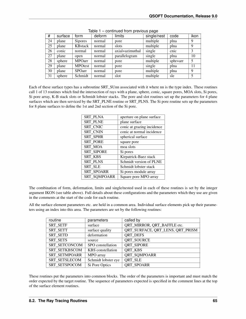
QSOFT Documentation, Release 9.0
Table 1 – continued from previous page# surface form deform limits single/nest code ikon24 plane Sipores normal pore multiple plna 925 plane KBstack normal slots multiple plna 926 conic normal normal axial+azimuthal single cnic 327 plane open normal parallelogram single plna 1028 sphere MPOarr normal pore multiple sphr+arr 529 plane MPOtest normal pore single plna 1130 plane SPOarr normal pore multiple plna 931 sphere Schmidt normal slot multiple sle 5
Each of these surface types has a subroutine SRT_SUnn associated with it where nn is the type index. These routinescall 1 of 13 routines which find the intersection of rays with a plane, sphere, conic, square pores, MOA slots, Si pores,Si pore array, K-B stack slots or Schmidt lobster stacks. The pore and slot routines set up the parameters for 4 planesurfaces which are then serviced by the SRT_PLNE routine or SRT_PLNS. The Si pore routine sets up the parametersfor 8 plane surfaces to define the 1st and 2nd section of the Si pore.
SRT_PLNA aperture on plane surfaceSRT_PLNE plane surfaceSRT_CNIC conic at grazing incidenceSRT_CNIN conic at normal incidenceSRT_SPHR spherical surfaceSRT_PORE square poreSRT_MOA moa slotsSRT_SIPORE Si poresSRT_KBS Kirpatrick-Baez stackSRT_PLNS Schmidt version of PLNESRT_SLE Schmidt lobster stackSRT_SPOARR Si pores module arraySRT_SQMPOARR Square pore MPO array
The combination of form, deformation, limits and single/nested used in each of these routines is set by the integerargument IKON (see table above). Full details about these configurations and the parameters which they use are givenin the comments at the start of the code for each routine.
All the surface element parameters etc. are held in a common area. Individual surface elements pick up their parame-ters using an index into this area. The parameters are set by the following routines:
routine parameters called bySRT_SETF surface QRT_MIRROR, QRT_BAFFLE etc.SRT_SETT surface quality QRT_SURFACE, QRT_LENS, QRT_PRISMSRT_SETD deformation QRT_DEFSSRT_SETS source QRT_SOURCESRT_SETCONCOM SPO constellation QRT_SIPORESRT_SETKBSCOM KBS constellation QRT_KBSSRT_SETMPOARR MPO array QRT_SQMPOARRSRT_SETSLECOM Schmidt lobster eye QRT_SLESRT_SETSPOCOM Si Pore Optics QRT_SPOARR
These routines put the parameters into common blocks. The order of the parameters is important and must match theorder expected by the target routine. The sequence of parameters expected is specified in the comment lines at the topof the surface element routines.
8.2. The Ray Tracing Routines 65
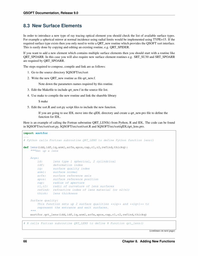
QSOFT Documentation, Release 9.0
8.3 New Surface Elements
In order to introduce a new type of ray tracing optical element you should check the list of available surface types.For example a spherical mirror at normal incidence using radial limits would be implemented using TYPE=15. If therequired surface type exists then you only need to write a QRT_new routine which provides the QSOFT xsrt interface.This is easily done by copying and editing an existing routine, e.g. QRT_SPIDER.
If you want to add a new element which contains multiple surface elements then you should start with a routine likeQRT_SPOARR. In this case you will also require new surface element routines e.g. SRT_SU30 and SRT_SPOARRare required by QRT_SPOARR.
The steps required to compose, compile and link are as follows:
1. Go to the source directory $QSOFT/src/xsrt
2. Write the new QRT_new routine as file qrt_new.f.
Note down the parameters names required by this routine.
3. Edit the Makefile to include qrt_new.f in the source file list.
4. Use make to compile the new routine and link the shareble library
$ make
5. Edit the xsrt.R and xsrt.py script files to include the new function.
If you are going to use IDL move into the qIDL directory and create a qrt_new.pro file to define thefunction for IDL.
Here is an example of calling the Fortran subroutine QRT_LENS() from Python, R and IDL. The code can be foundin $QSOFT/src/xsrt/xsrt.py, $QSOFT/src/xsrt/xsrt.R and $QSOFT/src/xsrt/qIDL/qrt_lens.pro.
import xsrtfor...# Python calls Fortran subroutine QRT_LENS to define Python function lens()
def lens(idd,idf,iq,anml,arfx,apos,rap,r1,r2,refind,thickq):"""Set up a lens
Args:id: lens type 1 spherical, 2 cylindricalidf: deformation indexiq: surface quality indexanml: surface normalarfx: surface reference axisapos: surface reference positionrap: radius of aperturer1,r2: radii of curvature of lens surfacesrefind: refractive index of lens material (or n2/n1)thick: lens thickness
Surface quality:This function sets up 2 surface qualities **iq** and **iq+1** torepresent the entrance and exit surfaces.
"""xsrtfor.qrt_lens(idd,idf,iq,anml,arfx,apos,rap,r1,r2,refind,thickq)
# R calls Fortran subroutine QRT_LENS to define R Function qrt_lens()
(continues on next page)
66 Chapter 8. Adding New Functions
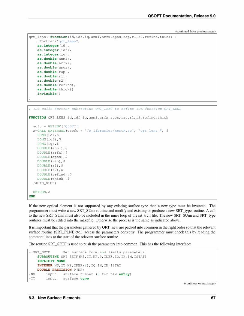
QSOFT Documentation, Release 9.0
(continued from previous page)
qrt_lens<-function(id,idf,iq,anml,arfx,apos,rap,r1,r2,refind,thick) {.Fortran("qrt_lens",as.integer(id),as.integer(idf),as.integer(iq),as.double(anml),as.double(arfx),as.double(apos),as.double(rap),as.double(r1),as.double(r2),as.double(refind),as.double(thick))invisible()
}
; IDL calls Fortran subroutine QRT_LENS to define IDL function QRT_LENS
FUNCTION QRT_LENS,id,idf,iq,anml,arfx,apos,rap,r1,r2,refind,thick
soft = GETENV('QSOFT')A=CALL_EXTERNAL(qsoft + '/R_libraries/xsrtR.so', "qrt_lens_", $LONG(id),$LONG(idf),$LONG(iq),$DOUBLE(anml),$DOUBLE(arfx),$DOUBLE(apos),$DOUBLE(rap),$DOUBLE(r1),$DOUBLE(r2),$DOUBLE(refind),$DOUBLE(thick),$
/AUTO_GLUE)
RETURN,AEND
If the new optical element is not supported by any existing surface type then a new type must be invented. Theprogrammer must write a new SRT_SUnn routine and modify and existing or produce a new SRT_type routine. A callto the new SRT_SUnn must also be included in the inner loop of the srt_trc.f file. The new SRT_SUnn and SRT_typeroutines must be edited into the makefile. Otherwise the process is the same as indicated above.
It is important that the parameters gathered by QRT_new are packed into common in the right order so that the relevantsurface routine (SRT_PLNE etc.) access the parameters correctly. The programmer must check this by reading thecomment lines at the start of the relevant surface routine.
The routine SRT_SETF is used to push the parameters into common. This has the following interface:
*+SRT_SETF Set surface form and limits parametersSUBROUTINE SRT_SETF(NS,IT,NP,P,IDEF,IQ,IH,IM,ISTAT)IMPLICIT NONEINTEGER NS,IT,NP,IDEF(2),IQ,IH,IM,ISTATDOUBLE PRECISION P(NP)
*NS input surface number (0 for new entry)
*IT input surface type(continues on next page)
8.3. New Surface Elements 67
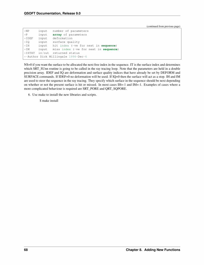
QSOFT Documentation, Release 9.0
(continued from previous page)
*NP input number of parameters
*P input array of parameters
*IDEF input deformation
*IQ input surface quality
*IH input hit index (-ve for next in sequence)
*IM input miss index (-ve for next in sequence)
*ISTAT in/out returned status
*-Author Dick Willingale 1996-Dec-6
NS=0 if you want the surface to be allocated the next free index in the sequence. IT is the surface index and determineswhich SRT_SUnn routine is going to be called in the ray tracing loop. Note that the parameters are held in a doubleprecision array. IDEF and IQ are deformation and surface quality indices that have already be set by DEFORM andSURFACE commands. If IDEF=0 no deformation will be used. If IQ=0 then the surface will act as a stop. IH and IMare used to steer the sequence in the ray tracing. They specify which surface in the sequence should be next dependingon whether or not the present surface is hit or missed. In most cases IH=-1 and IM=-1. Examples of cases where amore complicated behaviour is required are SRT_PORE and QRT_SQPORE.
6. Use make to install the new libraries and scripts.
$ make install
68 Chapter 8. Adding New Functions

CHAPTER
NINE
AUTHORS
QSOFT was written by Dick Willingale mailto:[email protected] with contributions from Vladimir Tichy mailto:[email protected] and Adrian Martindale mailto:[email protected]
69

QSOFT Documentation, Release 9.0
70 Chapter 9. Authors
PYTHON MODULE INDEX
aastro, 25
iimages, 16
qqfits, 10
xxscat, 31xsrt, 45
71

QSOFT Documentation, Release 9.0
72 Python Module Index
INDEX
Symbols__init__() (qfits.fitsfile method), 12__init__() (qfits.fitshdu method), 12
Aaperture() (in module xsrt), 45astro (module), 25
Bbaffle() (in module xsrt), 45beam() (in module images), 16bfield() (in module xsrt), 46binxy() (in module images), 17brems() (in module astro), 25btoc() (in module astro), 25
Cc1nest() (in module xsrt), 46cosmo() (in module astro), 26ctob() (in module astro), 26
Ddefmat() (in module xsrt), 47deform() (in module xsrt), 47defparxy() (in module xsrt), 47detector() (in module xsrt), 48display() (qfits.fitsfile method), 12display() (qfits.fitshdu method), 13dustrings() (in module xscat), 31duststat (class in xscat), 32dustthetascat() (in module xscat), 32
Eelips() (in module xsrt), 48eltmxt() (in module xsrt), 48
Ffitscolnam() (in module qfits), 10fitsfile (class in qfits), 12fitsgcol() (in module qfits), 10fitsgcolv() (in module qfits), 10
fitsgetkey() (in module qfits), 11fitshdu (class in qfits), 12fitshduinfo() (in module qfits), 11fitsparr() (in module qfits), 12fitsptab() (in module qfits), 12fitstypes() (in module qfits), 12fitsupdate() (in module qfits), 12fresnel() (in module xsrt), 49
Ggaussian() (in module images), 17getpos() (in module images), 17
Hhabs() (in module astro), 26hamgrid() (in module images), 18
Iigmtau() (in module astro), 26iigmtau() (in module astro), 27iigmtauvz() (in module astro), 27iismtau() (in module astro), 28images (module), 16init() (in module astro), 28init() (in module images), 18init() (in module qfits), 12init() (in module xsrt), 50ismtau() (in module astro), 28
Kkbs() (in module xsrt), 50kcorrb() (in module astro), 28king_profile() (in module images), 18
Llamgrid() (in module images), 18lebin() (in module images), 18lecbeam() (in module images), 19lecimage() (in module images), 19lens() (in module xsrt), 51lepsf() (in module images), 20list() (xscat.mievs method), 35
73
QSOFT Documentation, Release 9.0
lorentzian() (in module images), 20lyftau() (in module astro), 28lyftauvz() (in module astro), 29
Mmiev0() (in module xscat), 32mievs (class in xscat), 35mirror() (in module xsrt), 51moa() (in module xsrt), 51
Oopgrat() (in module xsrt), 52
Ppeakchisq() (in module images), 21plt_show_locator() (in module images), 21prism() (in module xsrt), 52prtathena() (in module xsrt), 53
Qqfits (module), 10quaderr() (in module images), 21
Rrectangles() (in module images), 21reset() (in module astro), 29reset() (in module images), 22reset() (in module xsrt), 54rotate() (in module xsrt), 54rseed() (in module xsrt), 54
Ssave() (qfits.fitsfile method), 12setabund() (in module astro), 29setfield() (in module images), 22setpos() (in module images), 22setsky() (in module images), 22shift() (in module xsrt), 54sipore() (in module xsrt), 54sle() (in module xsrt), 55source() (in module xsrt), 55spider() (in module xsrt), 56spoarr() (in module xsrt), 56sqbeam() (in module images), 23sqmpoarr() (in module xsrt), 57sqpore() (in module xsrt), 58srchmin() (in module images), 24srtlist() (in module xsrt), 59srtreset() (in module xsrt), 59surface() (in module xsrt), 59
Ttoxy() (in module images), 24
trace() (in module xsrt), 59
Ww1nest() (in module xsrt), 60wolter2() (in module xsrt), 61
Xxfresnel() (in module xscat), 35xopt() (in module xscat), 35xscat (module), 31xsrt (module), 45
74 Index