Image segmentation through operators based upon topologyGilles Bertrand, Jean-Christophe Everat and Michel CouprieLaboratoire PSI, ESIEE Cit�e Descartes B.P. 9993162 Noisy-Le-Grand Cedex France, e-mail: fbertrang,everatj,coupriemg@esiee.frAbstract: We consider a cross-section topology which is de�ned on grayscale images. The maininterest of this topology is that it keeps track of the grayscale informations of an image. We de�ne somebasic notions relative to that topology. Furthermore, we indicate how to get an homotopic kernel anda leveling kernel. Such kernels may be seen as \ultimate" topological simpli�cations of an image. Akernel of a real image, though simpli�ed, is still an intricated image from a topological point of view. Weintroduce the notion of irregular region. The iterative removal of irregular regions in a kernel allows toselectively simplify the topology of the image. Through an example, we show that this notion leads to amethod for segmenting some grayscale images without the need of de�ning and tuning parameters.Keywords: discrete topology, cross-section topology, topological numbers, regularization, segmenta-tion.1

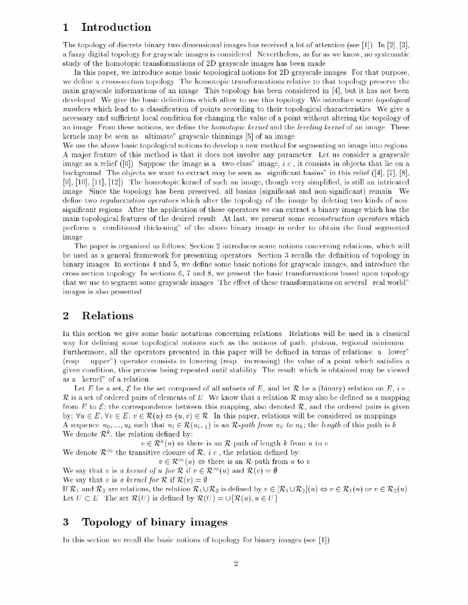
1 IntroductionThe topology of discrete binary two-dimensional images has received a lot of attention (see [1]). In [2], [3],a fuzzy digital topology for grayscale images is considered. Nevertheless, as far as we know, no systematicstudy of the homotopic transformations of 2D grayscale images has been made.In this paper, we introduce some basic topological notions for 2D grayscale images. For that purpose,we de�ne a cross-section topology. The homotopic transformations relative to that topology preserve themain grayscale informations of an image. This topology has been considered in [4], but it has not beendeveloped. We give the basic de�nitions which allow to use this topology. We introduce some topologicalnumbers which lead to a classi�cation of points according to their topological characteristics. We give anecessary and su�cient local condition for changing the value of a point without altering the topology ofan image. From these notions, we de�ne the homotopic kernel and the leveling kernel of an image. Thesekernels may be seen as \ultimate" grayscale thinnings [5] of an image.We use the above basic topological notions to develop a new method for segmenting an image into regions.A major feature of this method is that it does not involve any parameter. Let us consider a grayscaleimage as a relief ([6]). Suppose the image is a \two-class" image, i.e., it consists in objects that lie on abackground. The objects we want to extract may be seen as \signi�cant basins" in this relief ([4], [7], [8],[9], [10], [11], [12]). The homotopic kernel of such an image, though very simpli�ed, is still an intricatedimage. Since the topology has been preserved, all basins (signi�cant and non-signi�cant) remain. Wede�ne two regularization operators which alter the topology of the image by deleting two kinds of non-signi�cant regions. After the application of these operators we can extract a binary image which has themain topological features of the desired result. At last, we present some reconstruction operators whichperform a \conditional thickening" of the above binary image in order to obtain the �nal segmentedimage.The paper is organized as follows: Section 2 introduces some notions concerning relations, which willbe used as a general framework for presenting operators. Section 3 recalls the de�nition of topology inbinary images. In sections 4 and 5, we de�ne some basic notions for grayscale images, and introduce thecross-section topology. In sections 6, 7 and 8, we present the basic transformations based upon topologythat we use to segment some grayscale images. The e�ect of these transformations on several \real world"images is also presented.2 RelationsIn this section we give some basic notations concerning relations. Relations will be used in a classicalway for de�ning some topological notions such as the notions of path, plateau, regional minimum...Furthermore, all the operators presented in this paper will be de�ned in terms of relations: a \lower"(resp. \upper") operator consists in lowering (resp. increasing) the value of a point which satis�es agiven condition, this process being repeated until stability. The result which is obtained may be viewedas a \kernel" of a relation.Let E be a set, E be the set composed of all subsets of E, and let R be a (binary) relation on E, i.e.,R is a set of ordered pairs of elements of E. We know that a relation R may also be de�ned as a mappingfrom E to E ; the correspondence between this mapping, also denoted R, and the ordered pairs is givenby: 8u 2 E, 8v 2 E, v 2 R(u), (u; v) 2 R. In this paper, relations will be considered as mappings.A sequence u0; :::; uk such that ui 2 R(ui�1) is an R-path from u0 to uk; the length of this path is k.We denote Rk, the relation de�ned by:v 2 Rk(u), there is an R-path of length k from u to v.We denote R1 the transitive closure of R, i.e., the relation de�ned by:v 2 R1(u) , there is an R-path from u to v.We say that v is a kernel of u for R if v 2 R1(u) and R(v) = ;.We say that v is a kernel for R if R(v) = ;.IfR1 and R2 are relations, the relation R1[R2 is de�ned by v 2 [R1[R2](u), v 2 R1(u) or v 2 R2(u).Let U � E. The set R(U ) is de�ned by R(U ) = [fR(u); u 2 Ug.3 Topology of binary imagesIn this section we recall the basic notions of topology for binary images (see [1]).2

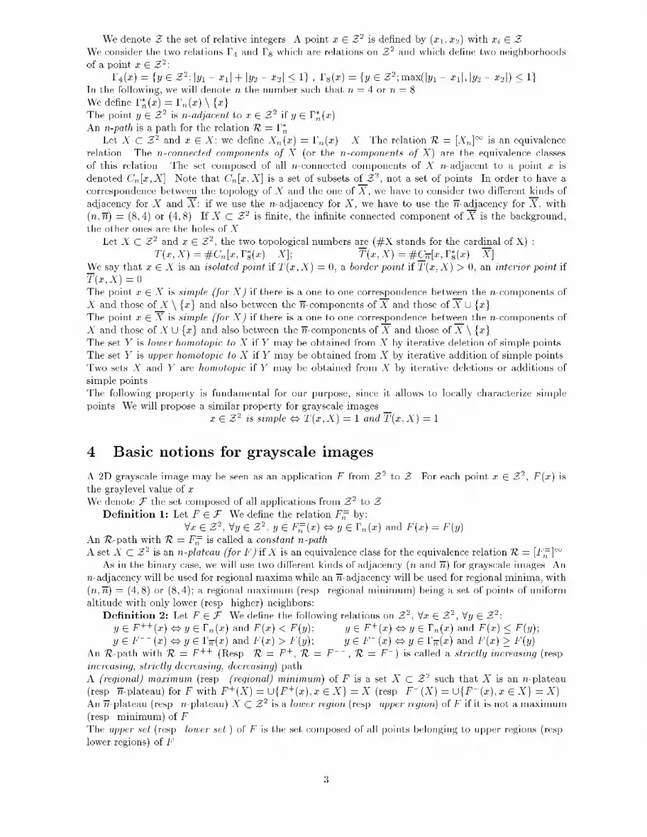
We denote Z the set of relative integers. A point x 2 Z2 is de�ned by (x1; x2) with xi 2 Z.We consider the two relations �4 and �8 which are relations on Z2 and which de�ne two neighborhoodsof a point x 2 Z2:�4(x) = fy 2 Z2; jy1 � x1j+ jy2 � x2j � 1g ; �8(x) = fy 2 Z2;max(jy1 � x1j; jy2 � x2j) � 1g.In the following, we will denote n the number such that n = 4 or n = 8.We de�ne ��n(x) = �n(x) n fxg.The point y 2 Z2 is n-adjacent to x 2 Z2 if y 2 ��n(x).An n-path is a path for the relation R = ��n.Let X � Z2 and x 2 X; we de�ne Xn(x) = �n(x) \X. The relation R = [Xn]1 is an equivalencerelation. The n-connected components of X (or the n-components of X) are the equivalence classesof this relation. The set composed of all n-connected components of X n-adjacent to a point x isdenoted Cn[x;X]. Note that Cn[x;X] is a set of subsets of Z2, not a set of points. In order to have acorrespondence between the topology of X and the one of X , we have to consider two di�erent kinds ofadjacency for X and X: if we use the n-adjacency for X, we have to use the n-adjacency for X, with(n; n) = (8; 4) or (4; 8). If X � Z2 is �nite, the in�nite connected component of X is the background,the other ones are the holes of X.Let X � Z2 and x 2 Z2, the two topological numbers are (#X stands for the cardinal of X) :T (x;X) = #Cn[x;��8(x) \X]; T (x;X) = #Cn[x;��8(x) \X ].We say that x 2 X is an isolated point if T (x;X) = 0, a border point if T (x;X) > 0, an interior point ifT (x;X) = 0.The point x 2 X is simple (for X) if there is a one to one correspondence between the n-components ofX and those of X n fxg and also between the n-components of X and those of X [ fxg.The point x 2 X is simple (for X) if there is a one to one correspondence between the n-components ofX and those of X [ fxg and also between the n-components of X and those of X n fxg.The set Y is lower homotopic to X if Y may be obtained from X by iterative deletion of simple points.The set Y is upper homotopic to X if Y may be obtained from X by iterative addition of simple points.Two sets X and Y are homotopic if Y may be obtained from X by iterative deletions or additions ofsimple points.The following property is fundamental for our purpose, since it allows to locally characterize simplepoints. We will propose a similar property for grayscale images.x 2 Z2 is simple , T (x;X) = 1 and T (x;X) = 1.4 Basic notions for grayscale imagesA 2D grayscale image may be seen as an application F from Z2 to Z. For each point x 2 Z2, F (x) isthe graylevel value of x.We denote F the set composed of all applications from Z2 to Z.De�nition 1: Let F 2 F . We de�ne the relation F=n by:8x 2 Z2, 8y 2 Z2, y 2 F=n (x), y 2 �n(x) and F (x) = F (y).An R-path with R = F=n is called a constant n-path.A set X � Z2 is an n-plateau (for F ) if X is an equivalence class for the equivalence relation R = [F=n ]1.As in the binary case, we will use two di�erent kinds of adjacency (n and n) for grayscale images. Ann-adjacency will be used for regional maximawhile an n-adjacency will be used for regional minima, with(n; n) = (4; 8) or (8; 4); a regional maximum (resp. regional minimum) being a set of points of uniformaltitude with only lower (resp. higher) neighbors:De�nition 2: Let F 2 F . We de�ne the following relations on Z2, 8x 2 Z2, 8y 2 Z2:y 2 F++(x), y 2 �n(x) and F (x) < F (y); y 2 F+(x), y 2 �n(x) and F (x) � F (y);y 2 F��(x), y 2 �n(x) and F (x) > F (y); y 2 F�(x), y 2 �n(x) and F (x) � F (y).An R-path with R = F++ (Resp. R = F+, R = F��, R = F�) is called a strictly increasing (resp.increasing, strictly decreasing, decreasing) path.A (regional) maximum (resp. (regional) minimum) of F is a set X � Z2 such that X is an n-plateau(resp. n-plateau) for F with F+(X) = [fF+(x); x 2 Xg = X (resp. F�(X) = [fF�(x); x 2 Xg = X).An n-plateau (resp. n-plateau) X � Z2 is a lower region (resp. upper region) of F if it is not a maximum(resp. minimum) of F .The upper set (resp. lower set ) of F is the set composed of all points belonging to upper regions (resp.lower regions) of F . 3

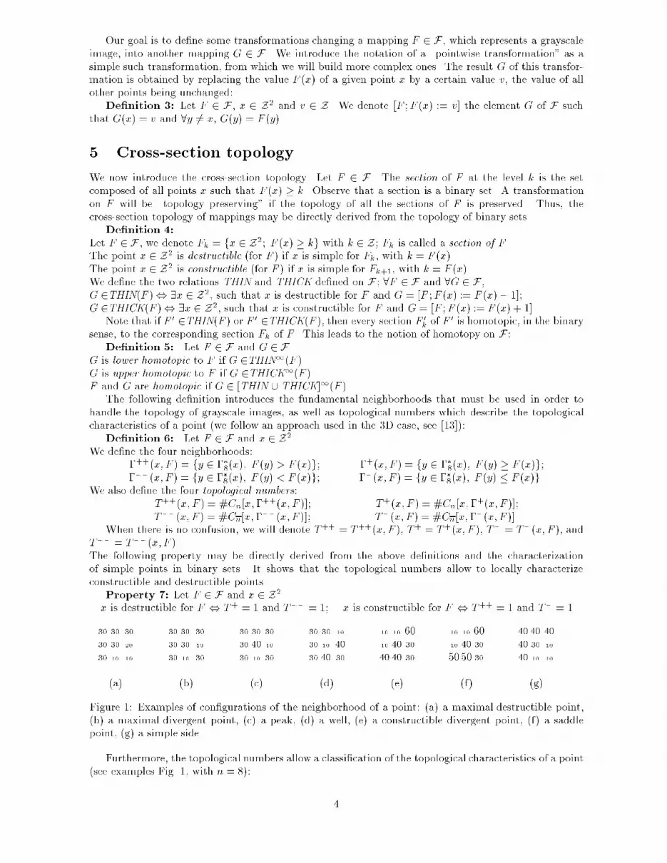
Our goal is to de�ne some transformations changing a mapping F 2 F , which represents a grayscaleimage, into another mapping G 2 F . We introduce the notation of a \pointwise transformation" as asimple such transformation, from which we will build more complex ones. The result G of this transfor-mation is obtained by replacing the value F (x) of a given point x by a certain value v, the value of allother points being unchanged:De�nition 3: Let F 2 F , x 2 Z2 and v 2 Z. We denote [F ;F (x) := v] the element G of F suchthat G(x) = v and 8y 6= x, G(y) = F (y).5 Cross-section topologyWe now introduce the cross-section topology. Let F 2 F . The section of F at the level k is the setcomposed of all points x such that F (x) � k. Observe that a section is a binary set. A transformationon F will be \topology preserving" if the topology of all the sections of F is preserved. Thus, thecross-section topology of mappings may be directly derived from the topology of binary sets.De�nition 4:Let F 2 F , we denote Fk = fx 2 Z2; F (x) � kg with k 2 Z; Fk is called a section of F .The point x 2 Z2 is destructible (for F ) if x is simple for Fk, with k = F (x).The point x 2 Z2 is constructible (for F ) if x is simple for Fk+1, with k = F (x).We de�ne the two relations THIN and THICK de�ned on F ; 8F 2 F and 8G 2 F ,G 2THIN(F ), 9x 2 Z2, such that x is destructible for F and G = [F ;F (x) := F (x)� 1];G 2THICK(F ), 9x 2 Z2, such that x is constructible for F and G = [F ;F (x) := F (x) + 1].Note that if F 0 2THIN(F ) or F 0 2THICK(F ), then every section F 0k of F 0 is homotopic, in the binarysense, to the corresponding section Fk of F . This leads to the notion of homotopy on F :De�nition 5: Let F 2 F and G 2 F .G is lower homotopic to F if G 2THIN1(F ).G is upper homotopic to F if G 2THICK1(F ).F and G are homotopic if G 2 [THIN [ THICK]1(F ).The following de�nition introduces the fundamental neighborhoods that must be used in order tohandle the topology of grayscale images, as well as topological numbers which describe the topologicalcharacteristics of a point (we follow an approach used in the 3D case, see [13]):De�nition 6: Let F 2 F and x 2 Z2.We de�ne the four neighborhoods:�++(x; F ) = fy 2 ��8(x); F (y) > F (x)g; �+(x; F ) = fy 2 ��8(x); F (y) � F (x)g;���(x; F ) = fy 2 ��8(x); F (y) < F (x)g; ��(x; F ) = fy 2 ��8(x); F (y) � F (x)g.We also de�ne the four topological numbers:T++(x; F ) = #Cn[x;�++(x; F )]; T+(x; F ) = #Cn[x;�+(x; F )];T��(x; F ) = #Cn[x;���(x; F )]; T�(x; F ) = #Cn[x;��(x; F )].When there is no confusion, we will denote T++ = T++(x; F ), T+ = T+(x; F ), T� = T�(x; F ), andT�� = T��(x; F ).The following property may be directly derived from the above de�nitions and the characterizationof simple points in binary sets. It shows that the topological numbers allow to locally characterizeconstructible and destructible points.Property 7: Let F 2 F and x 2 Z2.x is destructible for F , T+ = 1 and T�� = 1; x is constructible for F , T++ = 1 and T� = 1.30 30 3030 30 2030 10 10(a) 30 30 3030 30 1030 10 30(b) 30 30 3030 40 1030 10 30(c) 30 30 1030 10 4030 40 30(d) 10 10 6010 40 3040 40 30(e) 10 10 6010 40 305050 30(f) 40 40 4040 30 1040 10 10(g)Figure 1: Examples of con�gurations of the neighborhood of a point: (a) a maximal destructible point,(b) a maximal divergent point, (c) a peak, (d) a well, (e) a constructible divergent point, (f) a saddlepoint, (g) a simple side.Furthermore, the topological numbers allow a classi�cation of the topological characteristics of a point(see examples Fig. 1, with n = 8): 4

De�nition 8: Let F 2 F and x 2 Z2:x is a peak if T+ = 0; x is minimal if T�� = 0; x is divergent if T�� > 1;x is a well if T� = 0; x is maximal if T++ = 0; x is convergent if T++ > 1;x is a lower point if it is not maximal; x is an upper point if it is not minimal;x is an interior point if it is minimal and maximal;x is a simple side if it is destructible and constructible;x is a saddle point if it is divergent and convergent.By considering all the possible values of the four topological numbers it may be seen that:Property 9: Let F 2 F and x 2 Z2, x corresponds necessarily to one and only one of the followingtypes:1) A peak; 2) A well; 3) An interior point; 4) A minimal constructible point;5) A maximal destructible point; 6) A minimal convergent point; 7) A maximal divergent point;8) A simple side; 9) A destructible convergent point; 10) A constructible divergent point; 11) Asaddle point.6 Homotopic transformations and leveling transformationsWe introduce two basic transformations relative to the cross-section topology:De�nition 10: Let F 2 F .A kernel of F for the relation THIN is called a lower homotopic kernel of F .A kernel of F for the relation THICK is called an upper homotopic kernel of F .The lower (resp. upper) homotopic kernel of F may be seen as an \ultimate" topological simpli�cationof F , in the sense that no destructible (resp. constructible) point remains in the kernel.We can compute a lower homotopic kernel of F by using iteratively the de�nition of THIN(F ) (Def. 4).At each step of the procedure, we lower the value of a destructible point by 1. In fact, it is possible tohave a faster procedure based on the following properties:Let F 2 F and x 2 Z2. We de�ne:�++(x; F ) =MINfF (y); y 2 �++(x; F )g if �++(x; F ) 6= ;, �++(x; F ) = F (x) otherwise;���(x; F ) =MAXfF (y); y 2 ���(x; F )g if ���(x; F ) 6= ;, ���(x; F ) = F (x) otherwise.If x is constructible for F , then F and [F ;F (x) := �++(x; F )] are homotopic.If x is destructible for F , then F and [F ;F (x) := ���(x; F )] are homotopic.The computation of lower and upper kernels may be e�ciently done by using a \breadth-�rst" strategy.A classical technique for implementing such a strategy is based on two lists of points. The �rst list isinitialized with all constructible (resp. destructible) points of the original image. If the �rst list is notempty, we extract the �rst point of the list. If this point is constructible (resp. destructible), its value ischanged in the image, and the neighbors of this point are inserted in the second list. After the scanningof the �rst list, we exchange the roles of the �rst and the second list. We repeat the procedure until thesecond list is empty. All kernels presented in this paper have been computed using this technique.5

20 20 20 20 20 20 20 20 20 20 20 20 2020 25 25 45 50 55 60 50 45 45 25 25 2020 25 50 20 20 20 20 35 20 20 45 25 2020 45 20 20 35 20 20 60 55 20 20 45 2020 45 20 35 20 35 20 45 50 20 20 50 2020 45 20 20 35 20 20 45 20 20 20 45 2020 60 20 20 20 20 20 20 35 50 35 45 2020 45 20 20 20 70 20 20 20 20 20 50 2020 45 20 20 60 50 60 20 25 30 30 45 2020 25 45 20 20 60 20 20 35 35 45 25 2020 25 25 45 45 50 50 60 50 45 25 25 2020 20 20 20 20 20 20 20 20 20 20 20 2020 20 20 20 20 20 20 20 20 20 20 20 2020 50 50 45 60 60 60 60 60 60 45 50 2020 50 50 20 20 20 35 35 35 35 45 50 2020 50 20 20 35 20 20 60 60 35 50 50 2020 45 20 35 20 35 20 60 60 20 50 50 2020 60 20 20 35 35 20 60 35 35 35 45 2020 60 60 20 20 20 20 35 35 50 35 50 2020 60 60 45 70 70 70 50 35 35 35 50 2020 60 45 45 70 50 70 50 60 45 50 50 2020 60 45 70 70 60 50 50 60 45 50 50 2020 60 45 70 70 70 50 60 60 45 50 50 2020 20 20 20 20 20 20 20 20 20 20 20 20

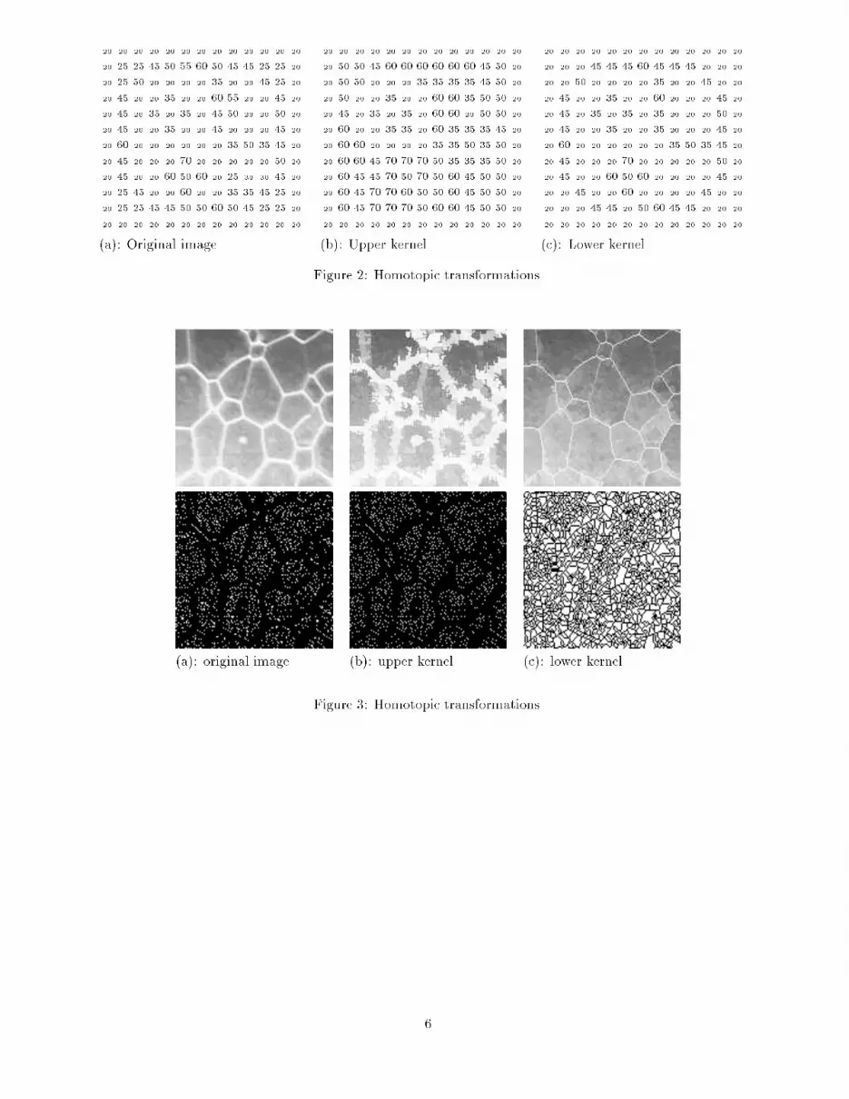
20 20 20 20 20 20 20 20 20 20 20 20 2020 20 20 45 45 45 60 45 45 45 20 20 2020 20 50 20 20 20 20 35 20 20 45 20 2020 45 20 20 35 20 20 60 20 20 20 45 2020 45 20 35 20 35 20 35 20 20 20 50 2020 45 20 20 35 20 20 35 20 20 20 45 2020 60 20 20 20 20 20 20 35 50 35 45 2020 45 20 20 20 70 20 20 20 20 20 50 2020 45 20 20 60 50 60 20 20 20 20 45 2020 20 45 20 20 60 20 20 20 20 45 20 2020 20 20 45 45 20 50 60 45 45 20 20 2020 20 20 20 20 20 20 20 20 20 20 20 20(a): Original image. (b): Upper kernel. (c): Lower kernel.Figure 2: Homotopic transformations.(a): original image. (b): upper kernel. (c): lower kernel.Figure 3: Homotopic transformations.

6

(a) 30 30 30 30 30 30 30 30 30 30 30 30 3030 10 10 30 10 10 30 10 10 30 10 10 3030 10 10 10 30 10 30 10 30 10 10 10 3030 10 10 10 10 30 30 30 10 10 10 10 3030 30 30 30 30 30 30 30 30 30 30 30 3030 10 10 10 10 30 30 30 10 10 10 10 3030 10 10 10 30 10 30 10 30 10 10 10 3030 10 10 30 10 10 30 10 10 30 10 10 3030 30 30 30 30 30 30 30 30 30 30 30 30 (b) 40 40 40 40 40 40 40 40 40 40 40 40 4040 10 10 10 10 10 10 10 10 10 10 10 4040 10 10 10 10 10 10 10 10 10 10 10 4040 10 10 10 10 10 40 10 10 10 10 10 4040 40 40 40 40 40 30 40 40 40 40 40 4040 10 10 10 10 10 30 10 10 10 10 10 4040 10 10 10 10 10 30 10 10 10 10 10 4040 10 10 10 10 10 30 10 10 10 10 10 4040 40 40 40 40 40 40 40 40 40 40 40 40(c) 40 40 40 40 40 4040 30 30 30 10 4040 30 30 10 30 4040 30 10 30 30 4040 10 30 30 30 4040 40 40 40 40 40 (d) 30 30 30 30 30 30 30 30 30 30 30 30 3030 10 10 10 10 10 10 10 10 10 10 10 3030 10 10 10 10 10 10 10 10 10 10 10 3030 10 10 10 10 40 40 40 10 10 10 10 3030 10 10 10 40 30 30 30 40 10 10 10 3030 10 10 10 40 30 30 30 40 10 10 10 3030 10 10 10 40 30 30 30 40 10 10 10 3030 10 10 40 20 40 30 40 20 40 10 10 3030 10 10 10 40 10 30 10 40 10 10 10 3030 10 10 10 10 10 30 10 10 10 10 10 3030 10 10 10 10 10 30 10 10 10 10 10 3030 30 30 30 30 30 30 30 30 30 30 30 30Figure 4: Four basic con�gurations of thick lower kernels: (a) the at junction, (b) The grayscale junction,(c) the network of minima, (d) the forti�ed castle.7

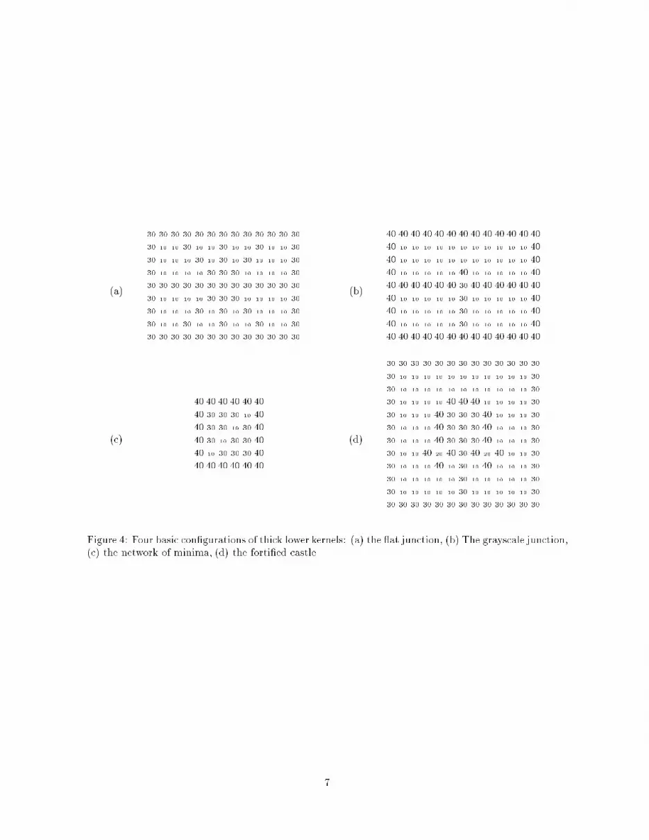
In Fig. 2, an upper and a lower homotopic kernel are represented (with n = 8). Two kernels cor-responding to a real image are also represented Fig. 3. The Fig. 3 (a) shows an original image (256graylevels); the lower levels are in black and the higher levels are in white. Below each grayscale imageof Fig. 3 (and subsequent �gures), the corresponding regional minima are given : they appear in white.We can see that, for a real image, there is a lot of minima, each of these regions being composed ofonly few points. Since their size, only few points of the minima have been \deleted" by the upper kerneltransformation (Fig. 3 (b)). On the other hand, the lower kernel transformation expands as much aspossible the minima. Nevertheless, if we examine the upper set (non-minimal plateaus) of Fig. 3 (c), wenotice that it is not thin. In fact, an homotopic lower kernel cannot be viewed as a \network of thinlines" : due to the discrete nature of the image representation, it may contain thick parts. Four basiccon�gurations, depicted Fig. 4, may explain this phenomenon:a) The at junction; we retrieve this con�guration in homotopic kernels of binary images;b) The grayscale junction; this con�guration is thicker than a binary kernel, in the sense that there aresome points which are simple for the (binary) upper set;c) The network of minima; the points adjacent to some very close regional minima (often one pointminima) may be non-destructible. Thus, we can generate a thick plateau which is not minimal (the 30'sof Fig. 4 (c)). It can be seen that networks of minima may generate thick regions of arbitrary size.d) The forti�ed castle; the entrance of the castle consists in a thin line which comes out onto the insideof the castle (the 3� 3 block of 30's in Fig. 4 (d)). The inside of a castle is not a subset of a minimumand it can be seen that we can build castles the insides of which have an arbitrary size.We introduce now the leveling kernels which may be viewed as �ltered homotopic kernels:De�nition 11:We de�ne the lower leveling relation LLE and the upper leveling relation ULE; 8F 2 F , 8G 2 F :G 2LLE(F ) , 9x 2 Z2, such that x is destructible or a peak for F , and G = [F ;F (x) := F (x)� 1];G 2ULE(F ) , 9x 2 Z2, such that x is constructible or a well for F , and G = [F ;F (x) := F (x) + 1].A lower leveling kernel is a kernel for LLE. An upper leveling kernel is a kernel for ULE.As for homotopic kernels, it is possible to increase (resp. decrease) the value of a point up to �++(x; F )(resp. down to ���(x; F )) for a faster procedure. Here again, we use the above-mentioned breadth-�rststrategy for computing lower and upper leveling kernels.Let us compare the lower homotopic kernel (Fig. 2 (c)) of an original image (Fig. 2 (a)) with the lowerleveling kernel (Fig. 5 (a)) of the same image. It may be seen that the set composed of upper regions hasbeen attened down. A lower leveling kernel of the real image of Fig. 3 (a) is depicted Fig. 6 (a). Despitethe appearance, this kernel is very di�erent from the homotopic kernel of Fig. 3 (c): as mentioned abovethe values of the points belonging to upper regions have been smoothed. This characteristic of levelingkernels will be used in the next section for regularization operators.20 20 20 20 20 20 20 20 20 20 20 20 2020 20 20 45 45 45 45 45 45 45 20 20 2020 20 45 20 20 20 20 35 20 20 45 20 2020 45 20 20 35 20 20 35 20 20 20 45 2020 45 20 35 20 35 20 35 20 20 20 45 2020 45 20 20 35 20 20 35 20 20 20 45 2020 45 20 20 20 20 20 20 35 35 35 45 2020 45 20 20 20 60 20 20 20 20 20 45 2020 45 20 20 60 50 60 20 20 20 20 45 2020 20 45 20 20 60 20 20 20 20 45 20 2020 20 20 45 45 20 45 45 45 45 20 20 2020 20 20 20 20 20 20 20 20 20 20 20 2020 20 20 20 20 20 20 20 20 20 20 20 2020 20 20 45 45 45 45 45 45 45 20 20 2020 20 45 20 20 20 20 20 20 20 45 20 2020 45 20 20 20 20 20 20 20 20 20 45 2020 45 20 20 20 20 20 20 20 20 20 45 2020 45 20 20 20 20 20 20 20 20 20 45 2020 45 20 20 20 20 20 20 20 20 20 45 2020 45 20 20 20 60 20 20 20 20 20 45 2020 45 20 20 60 50 60 20 20 20 20 45 2020 20 45 20 20 60 20 20 20 20 45 20 2020 20 20 45 45 20 45 45 45 45 20 20 2020 20 20 20 20 20 20 20 20 20 20 20 20

20 20 20 20 20 20 20 20 20 20 20 20 2020 20 20 45 45 45 45 45 45 45 20 20 2020 20 45 20 20 20 20 20 20 20 45 20 2020 45 20 20 20 20 20 20 20 20 20 45 2020 45 20 20 20 20 20 20 20 20 20 45 2020 45 20 20 20 20 20 20 20 20 20 45 2020 45 20 20 20 20 20 20 20 20 20 45 2020 45 20 20 20 20 20 20 20 20 20 45 2020 45 20 20 20 20 20 20 20 20 20 45 2020 20 45 20 20 45 20 20 20 20 45 20 2020 20 20 45 45 20 45 45 45 45 20 20 2020 20 20 20 20 20 20 20 20 20 20 20 20(a): Lower leveling. (b): Lower regularization. (c): Upper regularization.Figure 5: Leveling and regularization.7 Regularization transformationsWe have seen, through an example, that the minima of a real image do not correspond to the signi�cantbasins. In Fig. 2 (a), the signi�cant basins which are perceived, correspond to the cells of the image.8

(a): lower leveling. (b): lower regularization. (c): upper regularization.Figure 6: Leveling transformation and regularization.Nevertheless, each cell contains a lot of minima. The homotopic and leveling kernels of an image, thoughsimpli�ed, keep all these minima. This over-segmentation problem is also crucial when using methodsbased upon the watershed transformation ([7], [9], [14], [15]).In this section, we propose a method for detecting signi�cant basins. In a lower kernel, the minimaare coming into contact through upper points. We will take advantage of this feature to characterizesome non-signi�cant regions. Since its upper values have been attened down, we will consider the lowerleveling kernel rather than the lower homotopic kernel:De�nition 12: Let K 2 F be a lower leveling kernel.Let R1 and R2 be two minima of K. We say that a point x is a separating point for R1 and R2, ifx is adjacent to both R1 and R2. If R1 and R2 are separated by a point, we say that R1 and R2 areneighboring minima.If R is a minimum, we de�ne the upper value (R) of R as:(R) =MAXfK(x); for each point x adjacent to R g.K

(R)Ψ

x

R R’

K x

RFigure 7: Regularization: an example of upper irregular point and irregular minimum.We now introduce the notion of regularization (see Fig. 7):De�nition 13: Let K 2 F be a lower leveling kernel.9

�������������������������������������������������������������������������������������������������������������������������������������������������������������������������������������������������������������������������������������������������������������������������������������������������������������������������������������������������������������������������������������������������������������������������������������������������������������������������������������������������������������������� �������������������������������������������������������������������������������������������������������������������������������������������������������������������������������������������������������������������������������������������������������������������������������������������������������������������������������������������������������������������������������������������������������������������������������������������������������������������������������������������������������������������� ��������������������������������������������������������������������������������������������������������������������������������������������������������������������������������������������������������������������������������������������������������������������������������������������������������������������������������������������������������������������������������������������������������������������������������������������������������������������������������������������������������������������

�������������������������������������������������������������������������������������������������������������������������������������������������������������������������������������������������������������������������������������������������������������������������������������������������������������������������������������������������������������������������������������������������������������������������������������������������������������������������������������������������������������������� �������������������������������������������������������������������������������������������������������������������������������������������������������������������������������������������������������������������������������������������������������������������������������������������������������������������������������������������������������������������������������������������������������������������������������������������������������������������������������������������������������������������� ��������������������������������������������������������������������������������������������������������������������������������������������������������������������������������������������������������������������������������������������������������������������������������������������������������������������������������������������������������������������������������������������������������������������������������������������������������������������������������������������������������������������

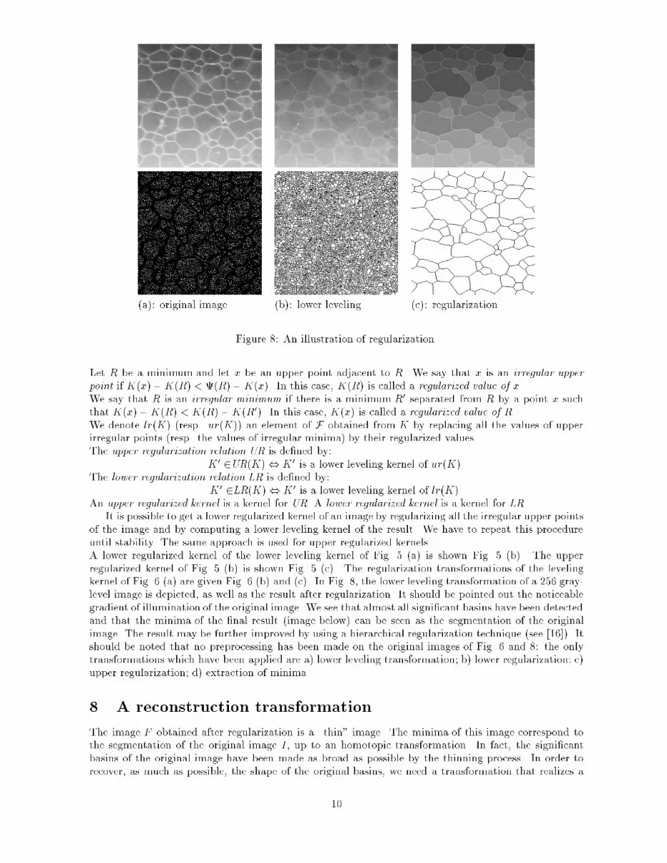
(a): original image. (b): lower leveling. (c): regularization.Figure 8: An illustration of regularization.Let R be a minimum and let x be an upper point adjacent to R. We say that x is an irregular upperpoint if K(x)�K(R) < (R) �K(x). In this case, K(R) is called a regularized value of x.We say that R is an irregular minimum if there is a minimum R0 separated from R by a point x suchthat K(x) �K(R) < K(R) �K(R0). In this case, K(x) is called a regularized value of R.We denote lr(K) (resp. ur(K)) an element of F obtained from K by replacing all the values of upperirregular points (resp. the values of irregular minima) by their regularized values.The upper regularization relation UR is de�ned by:K 0 2UR(K), K 0 is a lower leveling kernel of ur(K).The lower regularization relation LR is de�ned by:K0 2LR(K), K 0 is a lower leveling kernel of lr(K).An upper regularized kernel is a kernel for UR. A lower regularized kernel is a kernel for LR.It is possible to get a lower regularized kernel of an image by regularizing all the irregular upper pointsof the image and by computing a lower leveling kernel of the result. We have to repeat this procedureuntil stability. The same approach is used for upper regularized kernels.A lower regularized kernel of the lower leveling kernel of Fig. 5 (a) is shown Fig. 5 (b). The upperregularized kernel of Fig. 5 (b) is shown Fig. 5 (c). The regularization transformations of the levelingkernel of Fig. 6 (a) are given Fig. 6 (b) and (c). In Fig. 8, the lower leveling transformation of a 256 gray-level image is depicted, as well as the result after regularization. It should be pointed out the noticeablegradient of illumination of the original image. We see that almost all signi�cant basins have been detectedand that the minima of the �nal result (image below) can be seen as the segmentation of the originalimage. The result may be further improved by using a hierarchical regularization technique (see [16]). Itshould be noted that no preprocessing has been made on the original images of Fig. 6 and 8: the onlytransformations which have been applied are a) lower leveling transformation; b) lower regularization; c)upper regularization; d) extraction of minima.8 A reconstruction transformationThe image F obtained after regularization is a \thin" image. The minima of this image correspond tothe segmentation of the original image I, up to an homotopic transformation. In fact, the signi�cantbasins of the original image have been made as broad as possible by the thinning process. In order torecover, as much as possible, the shape of the original basins, we need a transformation that realizes a10

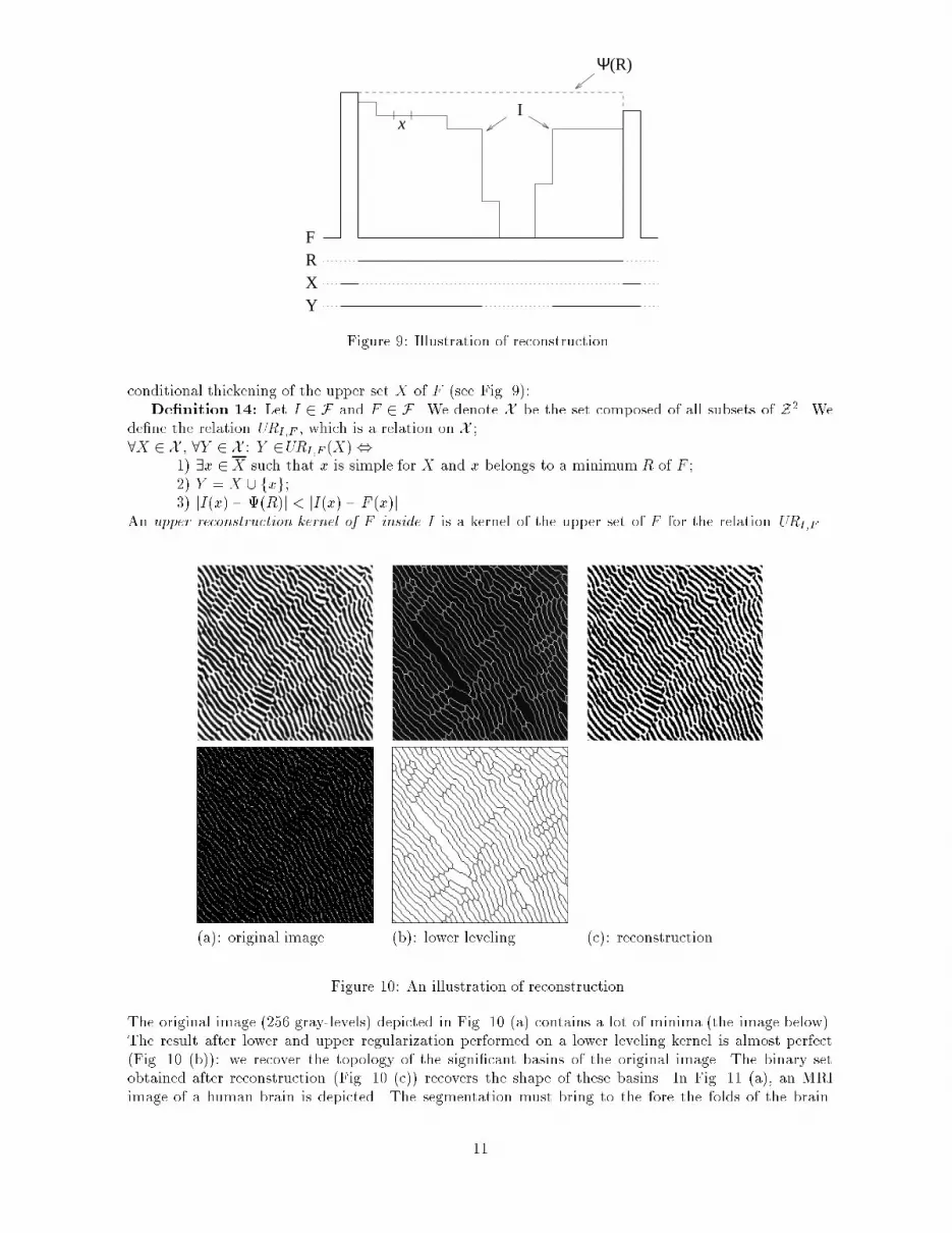
x

RXY

F

I

Ψ(R)

Figure 9: Illustration of reconstruction.conditional thickening of the upper set X of F (see Fig. 9):De�nition 14: Let I 2 F and F 2 F . We denote X be the set composed of all subsets of Z2. Wede�ne the relation URI;F , which is a relation on X ;8X 2 X , 8Y 2 X : Y 2URI;F (X),1) 9x 2 X such that x is simple for X and x belongs to a minimum R of F ;2) Y = X [ fxg;3) jI(x)� (R)j < jI(x) � F (x)j.An upper reconstruction kernel of F inside I is a kernel of the upper set of F for the relation URI;F .(a): original image. (b): lower leveling. (c): reconstruction.Figure 10: An illustration of reconstruction.The original image (256 gray-levels) depicted in Fig. 10 (a) contains a lot of minima (the image below).The result after lower and upper regularization performed on a lower leveling kernel is almost perfect(Fig. 10 (b)): we recover the topology of the signi�cant basins of the original image. The binary setobtained after reconstruction (Fig. 10 (c)) recovers the shape of these basins. In Fig. 11 (a), an MRIimage of a human brain is depicted. The segmentation must bring to the fore the folds of the brain.11

(a): original image. (b): regularization. (c): upper set.(d): hom. reconstruction. (e): hierarchical reconstruc-tion. (f): non-hom. reconstruction.Figure 11: An illustration of reconstruction.The Fig. 11 (a) is a picture of an electrophoresis gel. The images obtained after regularization areshown Fig. 11 (b) and 11 (b). The Fig. 10 (d) and 11 (d) show the result after reconstruction. We canobserve some ill-shaped lines which alter the quality of the result. They are due to the fact that a largeminimum of a regularized image may contain, in the original image, several reconstructible zones. Sincethe reconstruction operator preserves the homotopy, some paths must be preserved between these zones.The location of these paths depends on the scanning order of the points and thus does not take intoaccount the relief of the original image.A solution to this problem is to consider a hierarchical reconstruction operator which processes thepoints according to their increasing gray-levels. The result of this operator is represented Fig. 11 (e) and12 (e). The paths which are generated for the preservation of homotopy are made of points of lowestpossible values. Thus the segmented image \�ts" the original image.In homotopic reconstructions, some reconstructible zones surrounded by non-reconstructible ones maynever been reached. These zones correspond to holes in the object. If these holes are to be recovered,a non-homotopic reconstruction operator must be used. The de�nition of this operator is the same asthe de�nition of the reconstruction operator, except that we do not impose that the point x be simple(see Def. 14). The results given by this operator are represented Fig. 11 (f) and 12 (f): some light anddisconnected areas are recovered.9 ConclusionWe have introduced a cross-section topology and some basic transformations relative to that topology,the homotopic and leveling transformations. Based on these notions, we have proposed a segmentationchain for grayscale images which consists in the three following steps:1) The leveling transformation. It preserves some basic topological characteristics of the regionsto be segmented. For example, it preserves the connectedness of minima. It also gives informations aboutthe minima which may be considered as neighbors as well as the altitude of the pass which separates twoneighboring minima.2) Two regularization transformations. They break the topology in order to eliminate non-signi�cant regions. The upper regularization eliminates non-signi�cant minima, while the lower regular-12

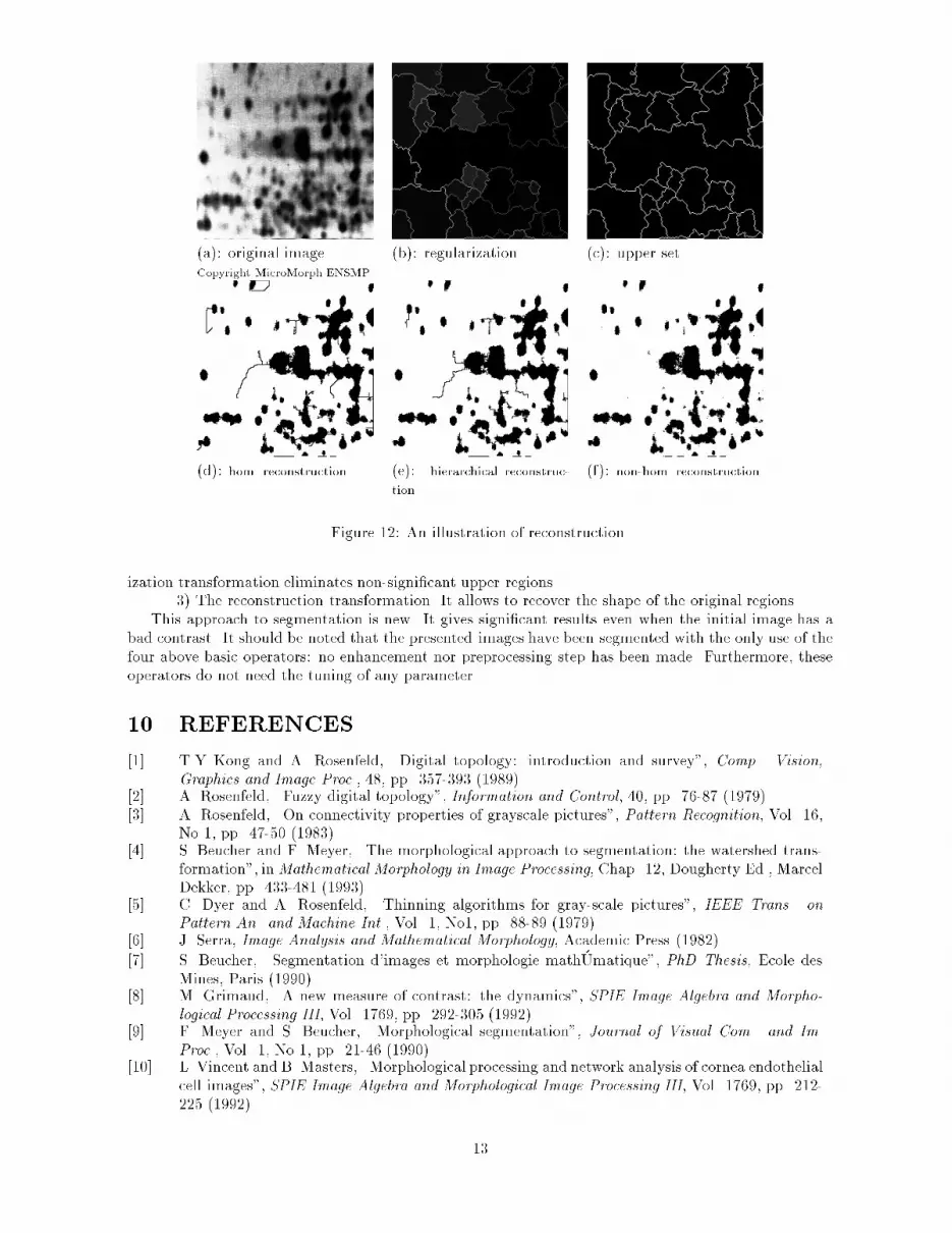
(a): original image.Copyright MicroMorph ENSMP (b): regularization. (c): upper set.(d): hom. reconstruction. (e): hierarchical reconstruc-tion. (f): non-hom. reconstruction.Figure 12: An illustration of reconstruction.ization transformation eliminates non-signi�cant upper regions.3) The reconstruction transformation. It allows to recover the shape of the original regions.This approach to segmentation is new. It gives signi�cant results even when the initial image has abad contrast. It should be noted that the presented images have been segmented with the only use of thefour above basic operators: no enhancement nor preprocessing step has been made. Furthermore, theseoperators do not need the tuning of any parameter.10 REFERENCES[1] T.Y Kong and A. Rosenfeld, \Digital topology: introduction and survey", Comp. Vision,Graphics and Image Proc., 48, pp. 357-393 (1989).[2] A. Rosenfeld, \Fuzzy digital topology", Information and Control, 40, pp. 76-87 (1979).[3] A. Rosenfeld, \On connectivity properties of grayscale pictures", Pattern Recognition, Vol. 16,No 1, pp. 47-50 (1983).[4] S. Beucher and F. Meyer, \The morphological approach to segmentation: the watershed trans-formation", inMathematical Morphology in Image Processing, Chap. 12, Dougherty Ed., MarcelDekker, pp. 433-481 (1993).[5] C. Dyer and A. Rosenfeld, \Thinning algorithms for gray-scale pictures", IEEE Trans. onPattern An. and Machine Int., Vol. 1, No1, pp. 88-89 (1979).[6] J. Serra, Image Analysis and Mathematical Morphology, Academic Press (1982).[7] S. Beucher, \Segmentation d'images et morphologie math�Umatique", PhD Thesis, Ecole desMines, Paris (1990).[8] M. Grimaud, \A new measure of contrast: the dynamics", SPIE Image Algebra and Morpho-logical Processing III, Vol. 1769, pp. 292-305 (1992).[9] F. Meyer and S. Beucher, \Morphological segmentation", Journal of Visual Com. and Im.Proc., Vol. 1, No 1, pp. 21-46 (1990).[10] L. Vincent and B. Masters, \Morphological processing and network analysis of cornea endothelialcell images", SPIE Image Algebra and Morphological Image Processing III, Vol. 1769, pp. 212-225 (1992). 13

[11] L. Vincent, \Algorithmes morphologiques �a base de �les d'attente et de lacets. Extension auxgraphes", PhD Thesis, Ecole des Mines, Paris (1990).[12] J.P. Cocquerez and S. Philipp, Analyse d'images: �ltrage et segmentation, Masson Ed., Paris(1995).[13] G. Bertrand, \Simple points, topological numbers and geodesic neighborhoods in cubic grids",Pattern Rec. Letters, Vol. 15, pp. 1003-1011 (1994).[14] F. Meyer, \Skeletons and perceptual graphs", Signal Processing, Vol. 16, pp. 335-363 (1989).[15] F. Meyer, \Un algorithme optimal de ligne de partage des eaux", 8th Conf. Rec. des Formes etInt. Art., Vol. 2, AFCET Ed., Lyon, pp. 847-859 (1992).[16] J.C. Everat and G. Bertrand, \New topological operators for segmentation", IEEE Int. Conf.on Image Processing, Vol. III/III, pp. 45-48 (1996).AcknowledgmentsThe authors gratefully acknowledge M. C. de Andrade for providing the image of ceramic material(Fig. 3 (a) and 8 (a)).

14